NASA Contractor Report 177988

lCASE REPORT NO. 85-43

ICASE ACCURACY OF SCHEMES WITH NONUNIFORM MESHES FOR COMPRESSIBLE FLUID FLOWS

Eli Turkel

NASA Contract No. NAS1-17070

September 1985

NASA-CR-177988 19860004485

NOV 1 4 1985 LAIJGLi:Y r,'ES",\i"lCH CE"fm

lIGi1,;RY, NIl,S,\

't.'~~1~WtJ,. VIRGIN':\

INSTITl,1TE FOR CO~lPUTER APPLICATIONS IN SCIENCE AND ENGInEERING NASA Langley Research Center, Hampton, Virginia 23665

Operated by the Universities Space Research Association

NJ\SI\ National Aeronautics and Space Administration

Langley Research Center Hampton, Virginia 23665

1111111111111 1111 11111 11111 11111 11111 11111111 NF01014

ACCURACY OF SCHEMES WITH NONUNIFORM MESHES

FOR COMPRESSIBLE FLUID FLOWS

Eli Turkel

Tel-Aviv University

and

Institute for Computer Applications in Science and Engineering

Abstract

We consider the accuracy of the space discretization for time-dependent

problems when a nonuniform mesh is used. We show that many schemes reduce to

first-order accuracy while a popular finite volume scheme is even inconsistent

for general grids. This accuracy is based on physical variables. However,

when accuracy is measured in computational variables then second-order

accuracy can be obtained. This is meaningful only if the mesh accurately

reflects the properties of the solution. In addition we analyze the stability

properties of some improved accurate schemes and show that they also allow for

larger time steps when Runge-Kutta type methods are used to advance in time.

Research was supported in part by the National Aeronautics and Space Administration under NASA Contract No. NASl-17070 while the author was in residence at ICASE, NASA Langley Reserach Center, Hampton, VA 23665.

i

I. INTRODUCTION

With the latest class of computers it is now possible to routinely perform

two-dimensional calculations for both the Euler and the compressible Navier-

Stokes equations. Three-dimensional Euler calculations about simple shapes

are feasible if a relatively coarse grid is used. Three-dimensional

calculations based on the thin layer compressible Navier-Stokes calculations

are just becoming available. The current trend is to use coordinates

constructed so that the solid surfaces are coordinate lines while the other

coordinate directions are close to orthogonal (see however [4]). This

approach simplifies the boundary conditions at the solid surfaces. Moreover,

whenever boundary layers exist, this approach allows one to refine the mesh

across the boundary layer while having a relatively coarse mesh parallel to

the boundary layer.

The construction of a general curvilinear grid is still not easily

accomplished. Difficulties occur when one wishes the grids to vary smoothly

while also being able to concentrate points in certain regions. Since many

bodies have cusped regions, the meshes frequently are far from regular in

these regions. In three dimensions these difficulties are compounded. First,

on present day machines one is still restricted to relatively coarse grids.

In addition the shape of the bodies can be more complicated in three

dimensions. One frequently uses a quasi two-dimensional approach which has

difficulties when the body no longer appears in some two-dimensional slice.

The result of all these difficulties is that the meshes that are constructed

are highly distorted in some regions. These distortions appear as high aspect

ratios and angles quite far from 900 for quadrilateral elements. Even more

disturbing is the change of these quantities from a cell to its neighboring

cells (see, for example, Figure 2).

-2-

In this paper we consider two aspects of the calculations for compressible

flow. The first is the accuracy of various schemes when used on grids which

have distorted meshes. In addition we shall also consider some explicit time

marching techniques that utilize improved space discretizations. We shall

also discuss finite volume approaches and show that some of the improvements

also allow larger time steps.

The effect of nonuniform grids on accuracy has previously been discussed

by several authors, e.g., Hoffman [7], Mastin [9], Steger [14], and Vinokur

[22] • Rai et. al. [12] have performed calculations on discontinuous grids

using a first-order upwind scheme. Pike [10] has also considered upwind

schemes on general (one-dimensional) meshes and has examined conservation and

TVD properties.

II. SPACE DISCRETIZATION

We shall consider time dependent problems. This also applies to steady

state problems if we use pseudo time-dependent methods. Thus we shall march a

time-dependent equation which need not be consistent with the time-dependent

physics of the process but has the same steady state equation.

We consider the conservation equations

wt

+ f + g + h x Y z

o. ( 2.1)

We decouple the time integration from the space discretization. Hence we

will, for now, keep the time variable continuous and only consider the

approximation in space. Using a finite volume approach we integrate (2.1) in

a cell n and assuming that n is independent of time we obtain

-3-

o (2.2)

Using the divergence theorem this becomes

~t f wdV + f F.ridS n an

o (2.3)

where F (f, g, h)t and n is the unit outward normal. Equivalently,

o.

Let w be the average of w in a cell. Then we have

and

w = .!. f wdv V n

dw + .!. f F.~dS dt V n o.

(2.4)

(2.5a)

(2.5b)

We stress that (2.5) is exact and that no approximations have been made to

this point.

To illustrate the situation we consider the two-dimensional case shown in

Figure 1.

-4-

F

(i + 1,j)

B

Figure 1

In this case (2.5) becomes

1 J" w - - wdxdy V n

V dw + J +.r + J + J (fdy - gdx) dt AB BC CD DA

Consider, for example, the integral

.r fdy - gdx. BC

o.

E

(2.6a)

(2.6b)

(2.7)

At this stage we replace (2.7) with an integration rule. We would prefer that

our formulas be at least second-order accurate for uniform meshes and so we

consider two integration rules. The first is the midpoint rule. Thus we have

(see Figure 1)

J (fdy - gdx) BC

-5-

(2.8)

We have replaced the line integral by values of the fluxes at the point G,

where G is the midpoint measured in terms of x and y. ~x, ~y are the

changes in x and y respectively between the points B

alternative is to use the trapezoidal rule. We then have

J fdy - gdx = 1J2 [~y(f(B) - f(C» - ~x(g(B) + g(C»] BC

3 3 + O(~x) + (~y) ).

and C. An

(2.9)

To proceed further we must know the fluxes at the point G (for (2.8»

or Band C (for (2.9». The fluxes f, g are functions of the dependent

variable wand sometimes also the independent variables. However, w is

defined in (2. 6a) as a cell averaged quantity and is not known at specific

points. To overcome this difficulty we shall replace w by w •• ~,J

where

w.. is a point value of w at some point wi thin the cell. An appropriate ~,J

choice is to use the centroid of the cell and then

1 2 w .. = v.r wdv + O(V ) ~,] n

(2.10)

and we retain second-order accuracy.

Having defined w· . ~,J

we can then find w at the point G or at B

and C by averaging. One possibility (e.g., [8]) is to use simple arithmetic

averaging so that

w(G) = 1J2 (w .. + w.+1 .). ~,J ~ ,]

(2.11a)

-6-

Similarly if one uses (2.9) then we have

w(C) =1/4 (w .. +w·+1 · +w. ·1 +w. 1.1)· 1.,J 1.,J 1.,]+ 1.+ ,J+ (2.l1b)

We note that we have averaged the quantity w. Since f and g are

nonlinear functions of w we can instead average f and g or else other

quantities. The disadvantage of averaging f and g is that this decouples

the even and odd points when (2.IIa) is used. The advantage of averaging f

and g is that in the steady state the fluxes are continuous across shocks if

the shock is aligned with a mesh line.

Having made the choice (2.lIa) or (2.1Ib) this completes the space

discretization of (2.1). Assuming we average the fluxes the choice of (2.IIa)

leads to the two-dimensional scheme

dw .. V(n) dt1.,J +1/zr(f.+l . + f .. )/::'Xi+I/ . - (f .. + f. 1 .)/::'x. 1/ . 1 oJ 1,J 2 ,] 1,] 1.-,J 1.- 2,J

+ (f .. +1 + f .. )/::'x. ·+1/ - (f .. + f .. 1)/::'x .. 1/ 1.,J 1.,J 1.,] 2 1.,J 1.,J- 1.,]- 2

(2.12)

+ (g·+1 . + g .. )/::'Y.+l/ . - (g .. + g. 1 .)15.y. 1/ . 1.,J 1.,J 1. 2,J 1.,J 1.-,] 1.- 2,J

+ (g1.. ·+1 + g1. .. )/::'Y1.. ·+1/ - (g .. + g. ·_I)l5.y· ._1/] 0 ,J ,J,J 2 1.,J 1.,] 1.,J 2

where v(n) =1/2 1(yc - YA)(xB - x....) - (x - x )(y - Y )1 u CAB D (see Figure 1).

Assuming that the positions (x, y) are given at the mesh nodes

(I5.X).+I/ . = x(C) - x(B), etc. 1. 2,J

For a uniform mesh I5.x, l5.y constant this

reduces to a centered difference formula

-7-

dw" f'+1' - f, l' gi,J'+1 - g1',J'-1 1, J + 1 , J 1-, J + ~~_>L_""':;'-::-_~ _ _ "'--~ dt Z~x 2~y

o. (Z.13)

The trapezoidal rule (Z.11b) reduces, in the case of a uniform mesh, to

dWi,j +1;. [fi+1,j+1 - fi-1,j+l + 2 (fi+l,j - fi-1,j) + fi+l,j-l - f i - 1,j-l dt 4 2~x 2~x Z~x

gi+l,J'+1 - gi+l,J'-1 (g, '+1 - g, , 1) + + Z 1, J 1,J - + __ ...:..:<_-::-__ ---'~_ Z~y Z~y

(2.14)

gi-1,j+l - gi-L,j-l] = o. Z~y

We shall see later that (2.14) has advantages in terms of the allowable time

step and in terms of accuracy, while (Z.13) has fewer operations and does not

require any special treatment for the tangential components near boundaries.

We will discuss the time integration of these systems later in Section

v. For later purposes we note that there is another possibility besides

(Z.13) and (Z.14). This is given by (for uniform meshes)

dWi,j + 1/ [fi+l,j+l - f i - 1,j+l + fi+l,j-1 - f i - 1,j-1 dt 2 Z~x 2~x

(2.15)

+ gi+l,j+l - gi+1,j-l + gi-l,j+l - gi-l,j-l] o. Z~y Z~y

We shall see that the stability properties of (2.15) are even better than

(2.14) and allow an optimal time step. Now, however the even and odd points

are decoupled. In the next section we discuss the accuracy of these schemes.

-8-

III. ACCRUACY - ONE DIMENSION

We now consider the accuracy of schemes for nonuniform meshes. To

simplify matters we first consider one-dimensional schemes. We consider the

equation

O. (3.1 )

We shall also consider the change of variables ';(x) and then (3.1)

becomes

or in conservation form

f w +-1.= 0

t Xl; (3.2a)

O • (3.2b)

.;(x) will be chosen so that the nonuniform mesh in X becomes a uniform mesh

in .;. We will usually scale .; so that ~.; = 1. Frequently ';(x) is never

constructed but the variable .; determines the location of In one

dimension.; has the property that l;(xj

) = j at all the nodes, j = O, ••• ,N.

To construct ';(x) is now a standard problem in interpolation theory.

However, we must have that ';'(x.) :# 0 and would prefer that .;(x) be ]

monotone, i.e. , if x. < x ~ xj +1 then j ~ ';(x) ~j + 1. This guarantees

]

that intervals get mapped onto corresponding intervals. In multidimensions we

would like to map each cell onto a standard rectangle or cube. If the

geometry is so distorted that this cannot be done then this approach is not

viable. We stress that there is no need to actually construct .; and hence

there is no need for .; to be defined globally. Since all accuracy

requirements are local, it is sufficient that .;(x) can be constructed

locally at each mesh cell but with sufficient smoothness.

-9-

Figure 2

Before discussing accuracy we first mention how nonuniform meshes may be

constructed. One difficulty with the analysis is that the theory of accuracy

is an asymptotic theory as the mesh is refined. In practice one usually deals

with a finite grid which is not extremely fine, especially in three

-10-

dimensions. Multidimensional grid generation about general configurations is

difficult [16, 17]. Not only is the mesh nonuniform but singularities can

appear at which quadrilaterals collapse into triangles. One advantage of a

finite volume approach is that the formulas are still valid in this limit.

However, it is not clear what happens to the accuracy of the scheme in this

degenerate limit. In Figure 2 we show a two-dimensional section of a three-

dimensional grid showing a few cells near the leading edge. In the next plane

triangular elements appear. This grid was generated using FL057.

Given a mesh there are two ways of constructing a finer mesh. One method

is to subdivide each cell into smaller cells. This process usually leads to a

smooth distribution but is difficult to implement using general

quadrilaterals. An alternative is to grid the entire region anew using more

nodes and ignoring the coarser mesh. This is equivalent to refining the mesh

in the computational ~ variables. With this method the mesh is less likely

to be smooth in the physical space.

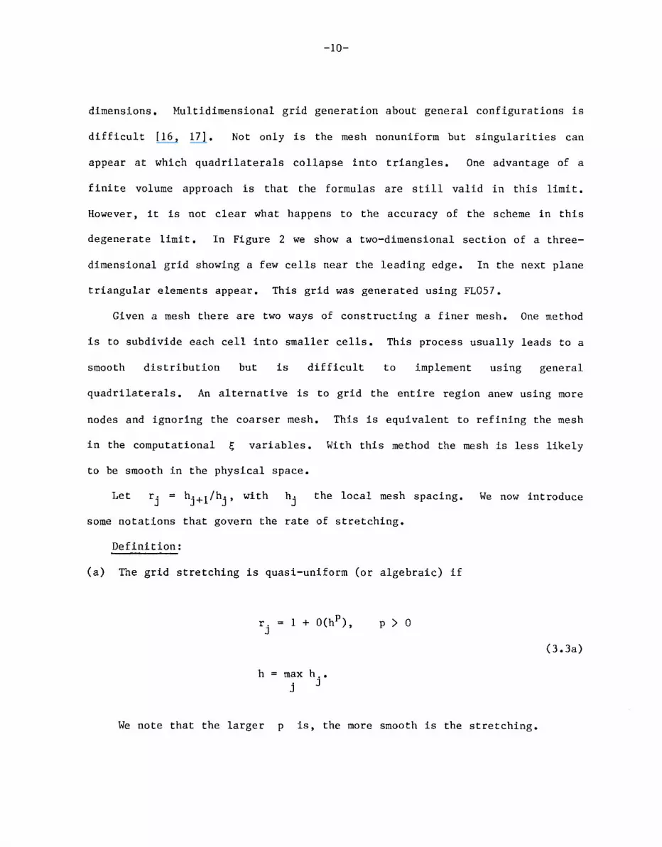
Let the local mesh spacing. We now introduce

some notations that govern the rate of stretching.

Definition:

(a) The grid stretching is quasi-uniform (or algebraic) if

r. J

p > 0

(3.3a)

h max h .• j J

We note that the larger p is, the more smooth is the stretching.

-11-

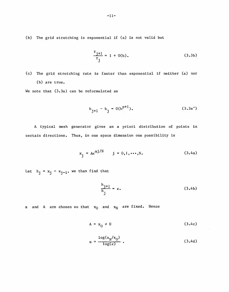
(b) The grid stretching is exponential if (a) is not valid but

r'+ l ~ = 1 + O(h). r.

J

(3.3b)

(c) The grid stretching rate is faster than exponential if neither (a) nor

(b) are true.

We note that (3.3a) can be reformulated as

O(hP+1). (3.3a')

A typical mesh generator gives an a priori distribution of points in

certain directions. Thus, in one space dimension one possibility is

x. J

j

Xj - Xj-l' we than find that

and A are chosen so that

A

a

h'+l ~= K. h.

J

and

10g(xN/XO)

10g(K)

O,l, ••• ,N.

are fixed. Hence

(3.4a)

(3.4b)

(3.4c)

(3.4d)

-12-

Thus, for fixed K * 1 + O(h) we have a fixed ratio between the areas of the

cells and so the stretching is exponential. Furthermore, it is shown in [8,

20] that exponential stretchings can accelerate the convergence to a steady

state. On the other hand it is shown in [6] that nonuniform meshes may

introduce false reflections from the gradients of the stretching. Exponential

stretchings are common in many exterior calculations. When K = 1 + O(h)

then the stretching is algebraic.

We shall only consider the case that the metric coefficients are evaluated

numerically. Hof fman [7] has conside red some examples whe re l; is a known

function of x and all metric derivatives are calculated analytically. He

has shown that if is refined so that lll; is halved then quadratic

convergence is retained. This is equivalent to having an algebraic grid

stretching.

We wish our formulas to be in conservation form. Again considering the

integral form the equation we wish to solve is

dW + _1 f ;I: + .l'".ndS dt V n

o (3. Sa)

where w is the volume weighted average of w. We say that the scheme is in

conservation form if we replace the integral by any consistent

approximation. Hence, we replace (2.5) by

o (3.5b)

where are weights that depend on the nonuniform spacing. In general

will depend on several hj • We must however use the same summation formula in

each cell.

-13-

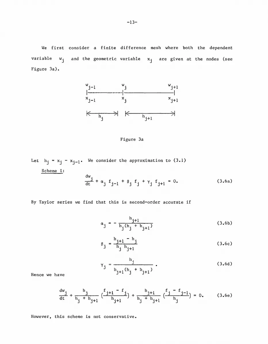
We first consider a finite difference mesh where both the dependent

variable Wj and the geometric variable Xj are given

Figure 3a).

w. 1 w. wj +1 J- J 1 1 1 x. 1 J-

x. xj +1 J

k >1 ~ ~ h. hj+l J

Figure 3a

Let hj = Xj - Xj-l' We consider the approximation to (3.1)

Scheme I: dw. -1.+ f +0 f + f dt Cl j j-l ~j j Yj j+l o.

at

By Taylor series we find that this is second-order accurate if

Cl. J

Hence we have

h.(h. + h.+1 ) J J J

h j +1 - h j

h j hj +1

h. J

dw. h. (fJ'+1 - f. h

J'+1 f. - f

J._1)

_J + J J) + (-'J:!.....:----"'~ dt hj + hj +1 hj +1 hj + hj +1 hj

However, this scheme is not conservative.

the nodes (see

(3.6a)

(3.6b)

(3.6c)

(3.6d)

o. (3.6e)

-14-

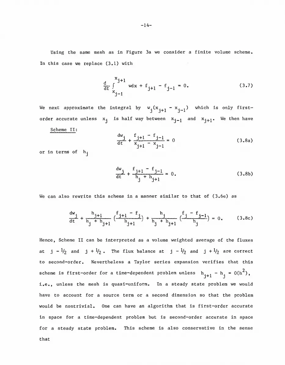
Using the same mesh as in Figure 3a we consider a finite volume scheme.

In this case we replace (3.1) with

d x j +1 dt f wdx + f j +1 - f j _ 1 = O.

x. 1 ]-

(3.7)

We next approximate the integral by Wj (xj+

1 - x

j_

1) which is only first-

order accurate unless is half way between x j -1 and We then have

Scheme II:

o (3.8a)

or in terms of h j

(3.8b)

We can also rewrite this scheme in a manner similar to that of (3.6e) as

O. (3. 8c)

Hence, Scheme II can be interpreted as a volume weighted average of the fluxes

at j - 1;2 and j + 1J2 • The flux balance at j - liz and j + 1/2 are correct

to second-order. Nevertheless a Taylor series expansion verifies that this

scheme is first-order for a time-dependent problem unless hj+

1 - h

j = O(h 2),

i.e., unless the mesh is quasi-uniform. In a steady state problem we would

have to account for a source term or a second dimension so that the problem

would be nontrivial. One can have an algorithm that is first-order accurate

in space for a time-dependent problem but is second-order accurate in space

for a steady state problem. This scheme is also conservative in the sense

that

-15-

h. + h \' (J j+1) L 2 Wj j

is constant except for boundary effects. Thus the conservation takes place

if Wj is associated with part of the cell to the left and an appropriate

part of the cell to the right of wj"

We next consider the mapping ~ = ~(x). A straightforward central

differencing to (3.2a) leads to (3.8). We thus conclude that Scheme II is

first-order (for nonuniform meshes) in x but is second-order in ~. In

other words, if w is quadratic in ~ then (3.8) is exact but if w is

quadratic in x then we have a discretization error. In theory we use a

nonuniform mesh because it reflects the gradients of the solution. Hence, it

would be natural to assume that w behaves quadratically in ~ rather than

in x. In practice the mesh is determined more by geometrical considerations

than the behavior of the solution. Furthermore, for a system of equations not

all the quantities grow at the same rate. When we are interested in global

quantities, e.g., lift and drag, it is not clear if the approximations will be

first- or second-order accurate.

We next consider a modification of Scheme II.

Scheme IIa:

where

Cl. J

K. J

h~ J

2 2 ' hJ. h. + h J j+1

o

x. - x. 1 J r

(3.9a)

(3.9b)

(3.9c)

(3.9d)

-16-

This scheme uses dependent variables at j - 1, j, j + 1 but geometrical data

at j - 2, j - 1, j, j + 1. A symmetric variant is obtained if (3.9c) is used

to define rather than One can also obtain a similar formula that

depends on the geometrical data at j - 2 through j + 2. This scheme is

second-order in physical space as long as the mesh stretching is no worse than

exponential. The scheme is conservative in that I K j Wj is conserved.

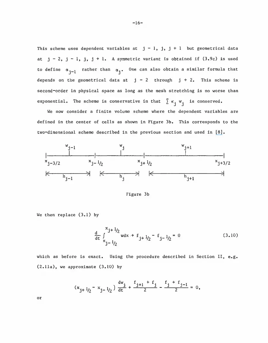
We now consider a finite volume scheme where the dependent variables are

defined in the center of cells as shown in Figure 3b. This corresponds to the

two-dimensional scheme described in the previous section and used in [8].

w. 1 w. wj+l J- J

I I I x j - 3/ 2 xj _ 1/2 xj + 1/2 xj +3/ 2

k ~ /< >l /< ~ h. 1 h. h j +1 J- J

Figure 3b

We then replace (3.1) by

(3.10)

which as before is exact. Using the procedure described in Section II, e.g.

(2.11a), we approximate (3.10) by

dw. fJ.+1 + f.

( )_J_+ J xj + 1/2 - xj _ 1/2 dt 2

f.+f. 1 J J-2

0,

or

-17-

Scheme III:

dw. fJ'+1 - f

J'-1 __ J_ + ~~ ____ ~~ __ ~

dt 2(x.+ 1/ - x. 1/) J 2 J- 2

O. (3.11)

Assuming that is evaluated half way between x. 1/ and J- 2 xj + 1/2

, a Taylor

series expansion verifies that this scheme is inconsistent unless

O(h), (3.12)

i.e., unless the mesh is quasi-uniform (algebraic) (3.3a). Note that (3.11)

is second-order accurate only if the left-hand side of (3.12) is 0(h2), i.e.,

rj 1 + 0(h2) which requires an even smoother grid, i.e., (3.3a) with

p = 2. Introducing a mapping ~ = ~(x) we again verify that (3.11) is

second-order in ~~. Hence, we conclude that for an irregular mesh (3.11) is

inconsistent in x but is second-order in ~. However, now the location of

Wj is different in the two interpretations. Considering (3.11) in physical

space Wj is evaluated half way between xj - 1/2 and xj + 1/

2, i.e.,

x. = 1J2 (x. If + x. If ) • J J- 2 J+ 2

However, in ~ space we have x. = x(j) where J

x = x(~) is the inverse map of ~ = ~(x) j -lf2= I:"(x. 1 ) , ., J- /2 '

j + 1/2 = I; (xj+ 1/]. Hence, we assume that I;(x) is invertible and that if

j - 1/2 ~ I; ~ j + 1/2 then x. If < x(1;) < x.+ 1/ • J- 2- - J 2 Since does not enter into

the scheme we only need know that such a ~(x) exists. The final scheme does

not depend on the derivation of (3.11) as coming from a physical or

computational space. However, the final interpretation of the numerical

solution, e.g., graphics, does depend on how one defines Xj. Furthermore, if

the fluxes depend explicitly on the geometry, e.g., cylindrical coordinates,

then the two interpretations of (3.11) will result in different schemes.

-18-

In order to remove the inconsistency of (3.11) for an exponential mesh we

consider another approach previously used by Collela and Woodward to construct

upwind differences [5]. Let

x f w(x,t)dx.

xj + 1/2 - x j _ 1/2 xj

_ 1/2 W(x,t) 1 (3.13)

Then

w. J

(3.14a)

is the volume average of w used in the finite volume scheme (3.10). We also

have that

W(Xj +3/2 )

W(x. If ) r 2 o (3.14b)

(3.14c)

The local value of w(x) is then given by aw w(x) = ax' We now fit W(x) with

a quadratic, interpolating at xj

_ 1/2' xj+ 1/2' x j +3/2 using (3.14).

differentiate W(x) and evaluate at Xj+~2 to find

Then (3.9) becomes

Scheme IlIa: dW. f (W .+ If ) - f (W. 1/ ) ........J.. + J 2 J- 2 dt x.+ If - x. 1/

J 2 J- 2 o.

Interpreting as w at the midpoint between

expanding in a Taylor series we find that (3.16) has a truncation error

We then

(3.15)

(3.16)

and

-19-

Hence, (3.15), (3.16) is second-order accurate for an algebraic mesh and

first-order accurate when used with an exponential mesh. Thus f j+ liz is

simply given by linear interpolation in W accounting for the nonuniform

mesh. We note that if we wish (3.10) to be fourth-order in space we do not

wish to find fj+llz using cubic interpolation. This occurs since

Of - f j -V2 is only a second-order approximation to ax. Hence, to get fourth-

af order accuracy we must find ax directly using Xj-2 through Xj+2. This

has been previously observed by Zalesak [23]. We also note that the scheme is

conservative since (3.10) is derived from the integral form. In particular

I (x.+ If - x. If )w. j J 2 J- 2 J

is constant in time excluding boundary effects. The use of (3.16) gives

first-order accuracy if is almost constant, i.e., the mesh is

exponential, and gives second-order accuracy if the mesh is algebraic, i.e.,

rj = 1 + O(h).

We wish to stress that the difficulties with the cell centered quantities

arises because of the finite volume approach. If we define the dependent

variables in the center of the cell but use a finite difference approach then

we can achieve higher accuracy as was done for the case of nodal variables in

Schemes II and IIa. In particular we consider the following generalization of

Scheme IIa.

-20-

Expanding

(3.17)

in a Taylor Series we find that

(3.18)

Hence, Q is a first-order approximation to f' if

(3.19)

Furthermore, Q is a second-order approximation if (3.19) holds with p 3

and in addition

or letting r. J

2 3 (1 - a. l)(h. + h. 1) + O(h ) J- J J-

(1 - a._1)(1 + ___ 1 __ )2 + O(h).

Jr. 1 J-

For a finite volume scheme K. = h. and so (3.19) determines J J

(3.20 )

(3.20a)

and we have

Scheme IlIa which is first-order. For a finite difference scheme we can

choose both aj

and K .• We thus have J

-21-

Scheme IIIb:

dw. f.+l/ - f. 1/ ---1.+ J 2 r 2 dt K.

o (3.21a) J

f j+ 1/2 = a. f j +1 + (1- a.)f.

J J J (3.21b)

2 (h. +h. 1)

a. J J- h. xj + Ih - xj _ 1/2 2 2 ,

J (h. + h. 1) + (h. + hj +1 ) J

J J- J

(3.21c)

(hj

+ h j +1 ) (hj + h. 1)

K. a. + (1 - a. 1) J-J J 2 J- 2

(3.2ld)

This scheme is now second-order in physical space as long as the mesh spacing

is no worse than exponential. However, viewed as a finite volume scheme

(3.2la) implies that

(3.22 )

which is not within the spirit of a finite volume approach especially for

multidimensions.

We now summarize the conclusions of this section. In general both central

finite difference formulas and finite volume formulas will be only first-order

accurate in the physical variables when nonuniform meshes are used unless the

weighted formulas (3.6) are used. When the dependent variables are defined in

the middle of the cell then the formulas are not even consistent unless the

mesh is quasi-uniform. In most cases the scheme is second-order measured in

terms of some computational variables ~(x). If this variable is

carefully chosen to match properties of all components of the solution, then

this second-order accuracy is meaningful. However, if the stretching is

-22-

utilized simply to put the outer boundary far away then the stretching can

reduce the order of accuracy. Numerical experiments verify that the

computational solution can be very inaccurate although formally the solution

is second-order in s. One could possibly post-process the solution, but this

would be very difficult to do on general multidimensional meshes.

In this section we have only discussed semidiscrete formulations where the

time discretization is not included. It is easy to see that the extensions to

fully discrete algorithms using Runge-Kutta type formulas in time, e.g., [8,

20] or else implicit formulas, e.g., [2,3,11]' are straightforward. When a

MacCormack type formula is used then one can again verify that one loses

accuracy on a nonuniform grid. In this case to achieve second-order accuracy

in x one should let h. x. - x. 1 and then J J J-

2h. (+1 -f~) n J tot. J J w. w. - h. + hj +1 J J J hj+l

and (3.23)

n+l ~I/+; 2hj +1 ~. :jfj_

l) J. w. + w. -

hj + hj +1 tot J

J J

IV. ACCURACY - TWO DIMENSIONS

In one dimension we have seen that when the geometrical data and the

variables are defined at the same point then a simple averaging of the fluxes

gives first-order accuracy in x and second-order accuracy in the

computational space variable, s. When using nonuniform meshes the accuracy in

the physical space can be improved by using the weighted formula (3.6). When

the dependent variable is defined in the middle of a cell then simple

-23-

averaging of the fluxes can give an inconsistent scheme for an exponentially

stretched mesh. Instead a weighted average (3.14), (3.15) should be used.

In extending these results to two space dimensions we encounter several

new difficulties. First a x difference at given point i can be given by

evaluating it at (i, j) or averaging over several j lines, e.g., (2.13),

(2.14), (2.15). In addition weighting formulas, e.g., (3.14), (3.15) must now

be replaced by two-dimensional interpolations. By considering cells with

equal volume but different shapes it is easy to see that volume weighting can

decrease the accuracy of the algorithm. It is necessary to include more

information than just the volume of neighboring cells.

In one

for which

space dimension we defined a smooth (or quasi-uniform) grid as one

h.+l r = _J_ = 1 + O(h). In two space dimensions we need to consider

j h. J

two-dimensional effects and not just demand that the volumes vary smoothly.

Consider the situation shown in Figure 4. All the cells have the same area

but it is obvious that one should not define the flux at G as the average of

those at the cell centers E and F. Rather the flux at G must be found by

a two-dimensional interpolation.

F •

A B

Figure 4

-24-

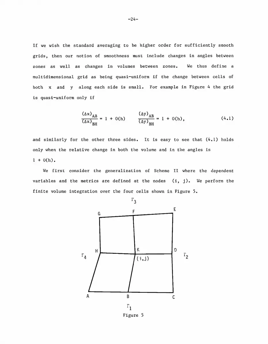
If we wish the standard averaging to be higher order for sufficiently smooth

grids, then our notion of smoothness must include changes in angles between

zones as well as changes in volumes between zones. We thus define a

multidimensional grid as being quasi-uniform if the change between cells of

both x and y along each side is small. For example in Figure 4 the grid

is quasi-uniform only if

1 + O(h) 1 + O(h), (4.1)

and similarly for the other three sides. It is easy to see that (4.1) holds

only when the relative change in both the volume and in the angles is

1 + O(h).

We first consider the generalization of Scheme II where the dependent

variables and the metrics are defined at the nodes (i, j). We perform the

finite volume integration over the four cells shown in Figure S.

A

G F E

K D r---------~--------~

( i ,j )

B

f1

Figure 5

c

-25-

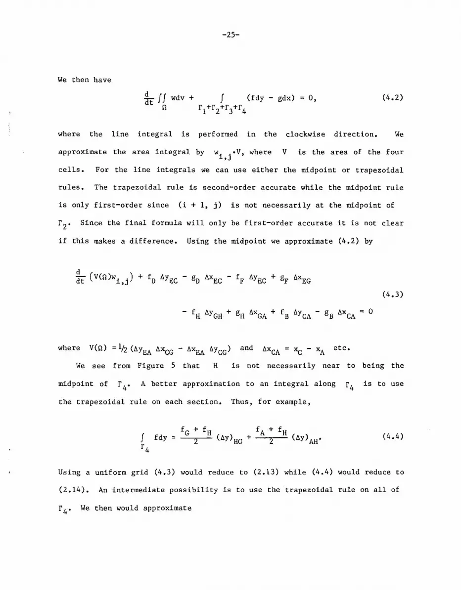
We then have

0, (4.2)

where the line integral is performed in the clockwise direction. We

approximate the area integral by w ..• V, where 1.,]

v is the area of the four

cells. For the line integrals we can use either the midpoint or trapezoidal

rules. The trapezoidal rule is second-order accurate while the midpoint rule

is only first-order since (i + 1, j) is not necessarily at the midpoint of

r 2• Since the final formula will only be first-order accurate it is not clear

if this makes a difference. Using the midpoint we approximate (4.2) by

(4.3)

where and etc.

We see from Figure 5 that H is not necessarily near to being the

midpoint of A better approximation to an integral along is to use

the trapezoidal rule on each section. Thus, for example,

(4.4)

Using a uniform grid (4.3) would reduce to (2.13) while (4.4) would reduce to

(2.14). An intermediate possibility is to use the trapezoidal rule on all of

r 4 • We then would approximate

-26-

fdy '" (4.5)

For a uniform mesh (4.5) would reduce to (2.15). We refer the reader to the

appendix for the full two-dimensional formulas.

In this discussion we have not considered the effects caused by the

differencing of metrics. In the far field exterior to a body the flow is

almost uniform but the mesh is frequently highly stretched. It is desirable

that the derivatives be small independent of the mesh stretching. Steger [14]

discusses various techniques to accomplish this. It is obvious that finite

volume schemes automatically satisfy this grid conservation property, see,

e.g., (A2), (A4). In addition Steger also presents numerous examples that

demonstrate the effect of nonuniform or highly skewed grids on the accuracy of

the solution. For some schemes highly stretched meshes can also affect the

rate of convergence to a steady state.

V. TIME INTEGRATION

All the formulas discussed until this point have -used a semidiscrete

formulation and have concentrated on the space discretization. One possible

way of integrating these equations in time is to use an implicit method with

A.D. I. splitting for multidimensional problems (see [2], [3]). In the rest of

this section we shall describe and analyze the use of Runge-Kutta type

formulas [8].

Let Lu represent the space discretization of a method. Then a K stage

Runge-Kutta method has the form

u(l) n u

(k) n u u

where n+l (K) u = u •

-27-

+ al

i\tLun

+ II L (k-l) ak

t u k 1,2, ••• ,K

are given parameters with a = 1 K

(5.1)

for at

least first-order accuracy in time. When L has constant coefficients we can

Fourier transform (5.1). Let Q(e,.) be the Fourier transform of the space

discretization operator L and let u be the Fourier transform of u. We

then find that (5.1) becomes

~n+l = G~n (5.2a)

where

G (5.2b)

and PK is a polynomial

(5.2c)

where

(5.2d)

(5.2c) generates a stability region, i.e., a domain in the complex plane

where IPK(z) I .s. 1. We shall now consider the hyperbolic (inviscid) case.

All the formulas introduced have central differences and so Q lies on the

imaginary axis. In this case (5.1) is stable if

where K depends on the sequence

llt < K - A

and

(5.3)

A

-28-

A

max p(Q(e,1jJ» -1T~e, 1jJ~1T

(5.4)

where p(Q) is the spectral radius of Q. Hence, given a sequence al""'~

the allowable time step depends on the eigenvalues of Q, i.e., on properties

of the scheme.

Specifically we consider the Euler equations in general curvilinear

coordinates. This system can be written as

wt + Aw + Bw = 0 (5.5) x y

(x, y) (p, t and where are general coordinates w = pUt pv, E)

0 Y -x 0 Y Y

Y 2 q - (y-2)Y u -x u - (y-l)Y v (y-l )Y s - uq y y y y Y

A

-X 2 Y v + (y-l)X u q + (y-l)X v -(y-l)X s - vq x y x x x

1 h - (y-l)qu h - (y-l)qv -q(h-s ) Y -x yq Y y

(5.6)

0 -Y x 0 x x

-Y 2 r + (y-2)Y u x u + (y-l)Y v -(y-l)Y s - ur x x x x x

B=

X 2 -Y v - (y-l)X u r - (y-2)X v (y-l)X s - vr x x x x x

2 h - (y-l)ru h - (y-l)rv -r(h-s ) -Y X yr x x

-29-

Here X, Yare the Cartesian coordinates and (x, y) are the generalized

coordinates. Also

q Y u - X v y y

r = X v - Y u x x

2 (y - 1) (u2 + v2 ) s 2

h c2

y -

We first consider the case that

f '" x

f. +1 . - f. 1 . 1,J 1- ,]

2~x

2 2 u + v

1 + 2

(5.7)

(5.8)

This scheme (2.11a) is used in FL052, [8] and reduces to (2.13) for a uniform

mesh. In this case the stability criterion becomes [20]

M < K (5.9)

Iql + Irl + /X2 + y2 + X2 + y2 + 21x X + Y Y Ic x x y y xy xy

We next consider the case where the flux integrals are approximated by the

trapezoidal rule. This scheme is given in (2.11b) and reduces to (2.14) for a

uniform mesh. The schemes given in the appendix, which account for

nonunifo'rmities in the mesh while averaging, are also included in this case.

We thus consider

-30-

f H1 ,j+l - f i - 1 ,j+l + 2(f"+1 " - f" 1 ") + f - f f '"

1. ,J 1.- ,J Hl,j-1 i-l,j-l x 8t.x

(5.10)

gH1,j+1 - gHl,j-1 + 2(gi "+1 - g" " 1) + gi-1,j+l - gi-1,j-l ,J 1., J-gy '" 8t.y

For this case the stability limit is given by [19]

i'!t < K (5.11)

Iwl + la2 + b

2 c

with Y + Y + max(Y , Y )

x Y x Y a = 2

X + X + max (Xx' Xy) b

x y (5.12)

2

w q + r + max(q, r)

2

We note that this is a larger time step than allowed by (5.9) but at the

expense of a more complicated algorithm. In FL052 the calculation of the

fluxes and the artificial viscosity accounts for most of the running time.

Hence, complicating the averaging procedure for the fluxes does not require

much extra computer time.

Finally we consider the averaging

(fH1,j+1 - f i - 1 ,j+l) + (f H1 ,j-l -f"I"I) f '"

1.- ,J-

x 4t.x

(5.13)

(gHl,j+l - gi+1 ,j-l) + (gi-1,j+1 - gi-l,j-l) gy '" 4t.y

-31-

In this case we can give two criteria that are sufficient for stability (see

also [1]). One is that

[ !Jox !Joy] !Jot ~ K max p(A)' P<BT (5.14)

or equivalently

K (5.15)

Irl + /~2 + y2 c] x x

This is the same condition one would obtain using time splitting. A second

possible criterion is that

(5.16)

Both these criteria provide sufficient conditions for stability. In both

cases these allow larger time steps than (5.11) which in turn allow larger

time steps than (5.9).

VI. STABILITY

We next consider the effect of a nonuniform grid on the stability of an

explicit scheme. To be specific we will compare the Schemes III and IlIa for

the one-dimensional problem. For an equation with constant coefficients

wt + aw 0 x

Scheme III (3.10) becomes dw. --1. + dt

Qw 0 (6.1a)

with

Qw. J

-32-

a(wj+l - wj _1)

2(x.+ 1/ - x. If ) J 2 r 2

(6.lb)

Formally replacing by e ij~ (i.e., forming the pseudodifference

operator) we find that

Q (6.2)

We thus see that the symbol is purely imaginary. Using a Runge-Kutta type

scheme [8] (see also (5.1)-(5.4», this leads to a stability limit of the form

(6.3)

where K is given by the intersection of the stability curve of the Runge-

Kutta scheme with the imaginary axis.

We next consider the Scheme IlIa (3.14)-(3.15) with constant coefficients,

dw. ---1.+Q w=O dt a

(6.4a)

where

(6.4b)

In this case

f h,(h,+! - h, 1) Q

a _ a J J J-

(1 - cos ~) - 'h:"" (h. + hj +1 )(hj _1 + h.) J J J

(6.5)

i(1 +

2

h)Sin]. h. - h. 1 h.+l + J J- J

(hj + hj +1 )(hj _1 +

-33-

Note: Qa

has a nonzero real part. Qa

is dissipative if and only if

a(h·+1 - h. 1) > o. J J--(6.6)

In other words, if the mesh expands in the direction of the wave then the wave

is dissipated. If the mesh contracts in the direction of the wave motion then

the wave is amplified. Alternatively, consider an 0 mesh where the spacing

between nodes increases as the mesh goes to the outer boundary. Then outgoing

waves are dissipated while incoming waves are amplified. Thus absorbing

boundary conditions are important. We point out that the above statement is

not completely accurate. The stability region of many Runge-Kutta schemes

include a portion of the positive complex plane. Hence, even though the real

part of -Q is positive, nevertheless, the total Runge-Kutta scheme can be

dissipative. Usually this intrusion of the stability region into the right

half plane is largest near the imaginary stability limit. Hence, the

amplification of incoming waves is least pernicious when the time step is near

the stability limit. This is an additional motivation to use a local time

step.

The time step restriction for (6.5) is much more difficult to analyze than

for (6.2) since Q contains real and imaginary parts that depend on the

Fourier variable ~. As before we let r. J

h.+l/h ' then J j

a J J-

[

r. r. 1 - 1 Qa = h

j 7("!"'"1-+---"r:""'

j""<")""7("!"'"1-+-r-

j-_-

1"<"") (1 - cos ~)

(

r. 1 - r. ) J- J . + i 1 + (1 + r.)(l + r. 1) S1n

J J-

(6.7)

-34-

'" Hence, if the mesh is algebraic then Q a

Q + O(h) and so the stability

limit is given by (6.3). When the mesh ratio is exponential then the

imaginary part of Q (i.e., the wave speed) is changed by 0(1) terms.

Hence, for an exponentially stretched mesh the stability properties of the

scheme are different than that for a uniform mesh.

In this entire analysis we have assumed that the coarsest mesh is still

sufficiently fine to resolve the waves. Hence, stability analysis,. which is

an asymptotic theory, is still valid. In many cases the outer meshes are

large compared with the relevant wave lengths. In this case other phenomena,

e.g., wave reflections, may also be present, see [6].

We next consider the effect of using a local time step for the fully

discrete algorithm. (6.1) can then be approximated by

choosing lit, J

wn,+l _ Wn alltj ( n n) J J' + 2( ) wJ'+1 - wJ'-1 x,+11 - x, I;

J 2 r 2

o

K(x '+ 11 - x, I; ) J 2 J- 2 as the local time step (6.8) becomes

wn+1 _ W~ + ! (wn wn ) j J 2 j+l - j-l o

(6.8)

(6.9)

which is stable when used in a Runge-Kutta type mode for the appropriate K.

However, now all effects of the nonuniform mesh disappear. Hence, in one

dimension we have recovered the standard analysis. Thus using a local time

step removes the dissipation or growth previously discussed. It also removes

the false reflection found by Giles and Thompson [6]. Using the finite volume

scheme with linear interpolation, (6.4), the use of a local time step cannot

remove the real part of the eigenvalues and so we cannot recover the

properties of a uniform grid.

-35-

VII. COMPUTATIONAL RESULTS

In order to show the value of accounting for the nonuniform mesh we

present one sample case. We consider the Runge-Kutta scheme for the Euler

equations, FL052T described in [8]. This is a finite volume method wi~ the

unknowns given at the cell centers. As a specific case we consider the I two-

dimensional flow about a NACA0012. The inflow conditions are • M = 0.3, co

a = 10 0• Since this is a subsonic flow the numerical solution can be compared

with the solution to a potential code with a very fine mesh. In Table I we

present the lift and drag for a coarse 64 x 16 0 mesh. The original code is

based on a two-dimensional version of (3.9)-(3.10) while the new version is

based on (3.14)-(3.15). Though this correction only accounts for one-

dimensional effects we note a marked improvement in the results.

Table I

Code CL CD

Potential code with fine mesh 1.274 0.0000

Original FL052T 64 x 16 0 mesh 1.227 0.0087

Improved version 1.264 0.0025

Comparison of new and original code for flow about NACA0012 with

o a = 10 •

M co

0.3,

-36-

VIII. CONCLUSION

In (3.3) we defined algebraic and exponential rates of grid stretching.

With an algebraic stretching, the grid metrics are sufficiently smooth that

all second-order techniques retain their formal accuracy. When exponential or

faster stretching is used then the accuracy of a central difference scheme or

finite volume method will deteriorate to first-order accuracy unless special

weighting formulas are used, e.g., (3.6). When the dependent variables are

defined at the center of the cells, then the finite volume approach can yield

an inconsistent scheme unless the weighting (3.14) is used. With this

weighting the scheme is second-order for an algebraic stretching and is first­

order when the stretching is faster than algebraic.

In all cases the algorithm is second-order measured in terms of a

computational variable E; rather than in terms of the physical coordinate

x. If this E; corresponds to the behavior of all components of the solution,

then this measure of accuracy is reasonable. I t is clear that E; should

always be chosen so that the solut.ion is smooth in the E; variable. However,

in many cases E; is chosen simply to put the outer boundary sufficiently far

away. Thus, for example, if the solution has a boundary layer then one would

want the grid to be almost uniform within the boundary layer. One could use

an exponential mesh in the outer region only if the solution decays

exponentially in the far field. Furthermore, if E; = E;(x) is not given

analytically but rather Xj is given then there may not exist a sufficiently

smooth and monotone E;(x).

In multidimensions these difficulties are compounded. First the grid is

quasi-uniform only if both the volumes and all angles vary sufficiently

slowly. Difficulties in constructing multidimensional grids leads to

-37-

nonuniform grids that are due to geometrical effects that have nothing to do

with the behavior of the solution, e.g, Figure 2. Hence, in this case, it

becomes more important to introduce weights that compensate for the nonuniform

grid. Unfortunately the weighting formulas must now account for the

multidimensional geometrical behavior. One possibility is to use bilinear

interpolation within a cell as is done in finite element codes, see formulas

in the appendix.

In several dimensions the line integrals of the fluxes can be approximated

by either a midpoint or a trapezoidal rule. For a uniform mesh with cell

centered variables the midpoint rule yields a simpler formula and one that

gives no difficulty for the tangential flux near a boundary. However, when

the mesh is distorted the midpoint rule may be more inaccurate due to

difficulties in locating the actual midpoint. Furthermore, if a two-

dimensional interpolation is used then the simplicity of the midpoint rule is

lost. The trapezoidal rule requires more work but allows a larger time

step. In addition it is now easier to use either volume weighting or bilinear

interpolation to calculate the value of the fluxes at the nodes. Weighting

formulas similar to (3.14) can now be used; see the appendix for full two­

dimensional formulas. Alternatively one can use a finite difference or finite

volume scheme where all variables are defined at the nodes. This guarantees

first-order accuracy in x even when the mesh is exponential. For two-

dimensional problems, grids can be constructed which are fairly quasi-

uniform. In this case both approaches give similar accuracy, see, e.g.,

[17] • For three-dimensional problems about complex bodies it is much more

difficult to construct a quasi-uniform grid.

patching of grids may be necessary.

In this case some sort of

-38-

The use of a trapezoidal integration rule instead of the midpoint rule

allows a larger time step but at the expense of a slightly more complicated

formula and additional difficulties near the boundaries. The use of weighted

formulas can change the dissipation and stability properties of the scheme.

We also show that nonuniform meshes may change the dissipation properties

of the time integration scheme. These dissipation terms are further changed

if a local time step is used.

-39-

APPENDIX

In this appendix we give the details for two separate two-dimensional

schemes. The extension to three dimensions is immediate. We only consider

the semidiscrete problem with the time integration to be explicit Runge-Kutta

or else some implicit scheme.

In the first algorithm we assume that both the coordinates and variables

are given at the nodes (see Figure Ai). We use a finite volume approach and

evaluate the line integrals using a trapezoidal rule.

G~ __________ ~F __________ --,E

H~ __________ ~K __________ -1D

(i,j)

A B C

Figure Ai

Consider the equation

w + f + g = O. t x y

(Ai)

We convert this to an integral relationship as in (2.6). Let fA denote f

at the point A and let l'lXB+l = xB - xH etc. for all the possibilities.

Note that the order of the indices is important. We then have

-40-

Scheme AI:

(A2)

where

For a uniform Cartesian mesh this reduces to

dWi . f - fA + 2(fO

- fH

) + fE - fG ,J + C dt 4flx

(A3) g - g + 2(gF - gB) + g -"g

+ G A E C o. 4fly

The second scheme that we consider has the geometrical quantities at the

nodes but the dependent variables are given at the cell centers (see Figure

A2) this extends the scheme used in FL052 [8]. However, we use the

trapezoidal rule to evaluate the integrals rather than the midpoint rule used

in [8].

-41-

H r---- I- ___ ,G I I I I

D I I I C I

I I I I I I

(i,j) I I

E~---- ----..IF

A B

Figure A2

The results in

Scheme A2:

(A4)

In order to evaluate the' fluxes at the nodes we could use volume weighted

averages. An alternative is to use bilinear interpolation using the cell

centers. We first must locate the cell centers. Using simple averaging we

find that

(AS)

-42-

As an example of using bilinear interpolation we give the formulas for

calculating f at the point C given the values of f at the points E, F,

G, and H and given the locations of all the nodes and cell centers. Let

(f.+1 ,- f, ,)l1X.-E - (f i '+1 - f, ,)l1XF'E 1 ,J 1,J Ii ,J 1,J

8

y

We then define

C D =

B = f i +1,j - fi,j - Cl1YFE - D(xi +1,j Yi +1,j - Xi,j Yi,j) l1xFE

A = f, , - Bx, , - Cy, , - Dx, , y, ,. 1,] 1,J 1,J 1,J 1,J

Finally we have

(A6)

(A7)

(AB)

-43-

For a uniform mesh 6x = 6y this gives

fC =1/4 (f, ,+ f'+l ,+ f, '+1 + f'+l '+1)· 1.,] 1.,] 1.,] 1.,J

(A9)

For both Scheme Ai and Scheme A2 the stability condition is given by (5.11).

This allows a larger time step than the stability criterion (5.9) for the

scheme used in FL052.

Acknowledgement

The author would like to thank A. Bayliss and S. Yaniv for many fruitful

discussions.

-44-

REFERENCES

[1] Abarbanel, S. and D. Gottlieb, A note on the leap-frog scheme in two and

three dimensions, J. Comput. Phys., 21 (1976), pp. 351-355.

[2] Beam, R. W. and R. F. Warming, An implicit finite difference algorithm

for hyperbolic systems in conservation law form, J. Compute ·Phys., 22

(1976), pp. 87-110.

[3] Briley, W. R. and H. McDonald, Solution of the multidimensional

compressible Navier-Stokes equations by a generalized implicit method,

J. Comput. Phys., 24 (1977), pp. 372-397.

[4] Clarke, D. K., M. D. Salas, and H. A. Hassan, Euler calculations for

multi-element airfoils using Cartesian grids, AlAA 85-0291.

[5] Colella, P. and P. R. Woodward, The piecewise~parabolic method (PPM) for

gas dynamical calculations, J. Comput. Phys., 54 (1984) pp. 174-201.

[6] Giles, M. and W. T. Thompkins, Jr., Interval reflection due to a

nonuniform grid, Advances in Computer Methods for Partial Differential

Equations V (IMACS), (R. Vichnevetsky and R. S. Stepleman, eds.), 1984,

pp. 322-328.

[7] Hoffman, J. D., Relationship between the truncation errors of centered

finite difference approximation on uniform and nonuniform meshes, J.

Comput. Phys., 46 (1982), pp. 469-474.

-45-

[8] Jameson, A., W. Schmidt, and E. Turkel, Numerical solutions of the Euler

equations by finite volume methods using Runge-Kutta time-stepping

schemes, AlAA 81-1259.

[9] Mastin, C. W., Error induced by coordinate systems, Numerical Grid

Generation, (J. F. Thompson, ed.), Elseiver-North Holland, Amsterdam,

1982, pp. 31-40.

[10] Pike, T., Grid adaptive algorithms for the solution of the Euler

equations on irregular grids, J. Comput. Phys., to appear, 1985.

[11] Pullman, T. H. and J. L. Steger, Recent improvements in efficiency,

accuracy, and convergence for implicit approximate factorization

algorithms, AlAA 85-0360.

[12] Rai, M. M., K. A. Hessenius, and S. R. Chakravarthy, Metric

discontinuous zonal grid calculations using the Osher scheme, Comput. &

Fluids, 12 (1984), pp. 161-176.

[13] South, J. C., Recent advances in computational transonic aerodynamics,

AlAA 85-0366.

[14] Steger, J. L., On application of body conforming curvilinear grids for

finite difference solution of external flow, Numerical Grid Generation

(J. F. Thompson, ed.) Elsevier-North Holland, Amsterdan, 1982, pp. 295-

316.

-46-

[15] Swanson, R. C. and E. Turkel, A multistage time-stepping scheme for the

Navier-Stokes equations, AlAA 85-0035.

[16] Thompson, J. F., U. A. Warsi, and C. W. Mastin, Boundary-fitted

coordinate systems for numerical solution of partial differential

equations - a review, J. Comput. Phys., 47 (1982), pp. 1-108.

[17] Thompson, J. F., A survey of grid generation tehcniques in computational

fluid dynamics, AlAA 83-0447.

[18] Thompson, J. F., A survey of dynamically adaptive grids in the numerical

solution of partial differential equations, Appl. Numer. Math., 1

(19~4), pp. 3-27.

[19] Turkel, E., Composite methods for hyperbolic equations, SIAM J. Numer.

Anal., 14 (1977), pp. 744-759.

[20] Turkel, E., Acceleration to a steady state for the Euler equations,

Proc. INRIA Euler Workshop, (SIAM), 1983.

[21] Turkel, E., Algorithms for the Euler and Navier-Stokes equations for

supercomputers, The Impact of Supercomputers in the Next Decade of CFD,

Birkhauser, Boston, 1984.

[22] Vinokur, M., On one-dimensional stretching functions for finite

difference calculations, J. Comput. Phys., 50, (1983), pp. 215-234.

-47-

[23] Zalesak, S. T. , Fully multidimensional flux-corrected transport

algorithms for fluids, J. Comput. Phys., 31 (1979), pp. 335-362.

1. Report No. NASA CR-177988 I 2. Government Accession No. 3. Recipient's Catalog No.

ICASE Report No. 85-43 4. Title and Subtitle 5. Report Da te

ACCURACY OF SCHEMES WITH NONUNIFORM MESHES FOR C:;:"nt-"",h"r IQA"

COMPRESSIBLE FLUID FLOWS 6. Performing Organization Code

7. Author(sl B. Performing Organization Report No.

Eli Turkel 85-43 10. Work Unit No.

9. Performing Organization Name and Address

Institute for Computer Applications in Science and Engineering 11. Contract or Grant No.

Mail Stop 132C, NASA Langley Research Center NASl-17070 Hampton, VA 23665 13. Type of Report and Period Covered

12. Sponsoring Agency Name and Address

National Aeronautics and Space Administration ro n

Washington, D.C. 20546 14. Sponsoring A~ncy'~o;de

505-31-83-01 15. Supplementary Notes

Langley Technical Monitor: J. C. South Jr. Submitted to Appl. Numer. Math.

Final Report 16. Abstract

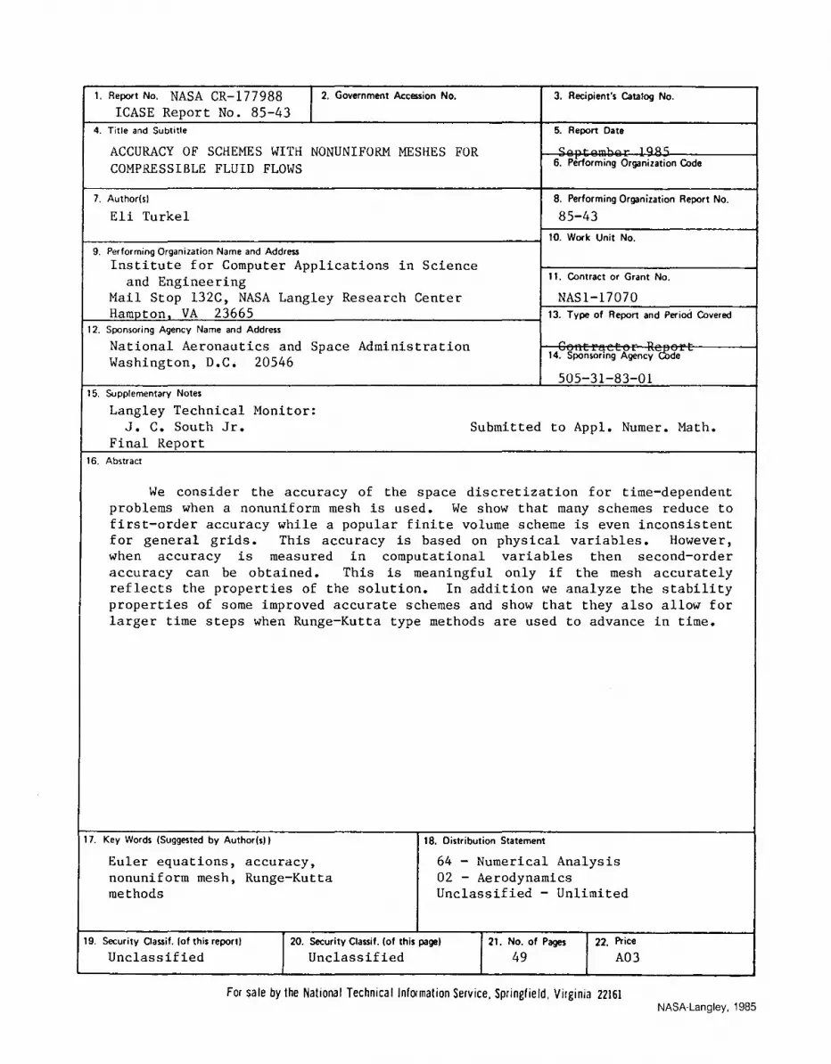
We consider the accuracy of the space discretization for time-dependent problems when a nonuniform mesh is used. We show that many schemes reduce to first-order accuracy while a popular finite volume scheme is even inconsistent for general grids. This accuracy is based on physical variables. However, when accuracy is measured in computational variables then second-order accuracy can be obtained. This is meaningful only if the mesh accurately reflects the properties of the solution. In addition we analyze the stability properties of some improved accurate schemes and show that they also allow for larger time steps when Runge-Kutta type methods are used to advance in time.

17. Key Words (Suggested by Author(s) I lB. Distribution Statement

Euler equations, accuracy, 64 - Numerical Analysis nonuniform mesh, Runge-Kutta 02 - Aerodynamics methods Unclassified - Unlimited

19. Security Classif. (of this report) 20. Security Classif. (of this pagel 21. No. of Pages 22. Price

Unclassified Unclassified 49 A03

For sale by the National Technical Information Service, Springfield, Virginia 22161 NASA-Langley, 1985

End of Document