Embed Size (px)
Citation preview
Mathl. Cornput. Modelling Vol. 17, No. 7, pp. 37-55, 1993 Printed in Great Britain
0895-7177193 $6.00 + 0.00 Pergamon Press Ltd
ABEL-GONTSCHAROFF BOUNDARY VALUE PROBLEMS
RAVI P. AGARWAL AND QIN SHENG
Department of Mathematics, National University of Singapore
Kent Ridge, Singapore 0511
PATRICIA J. Y. WONG
Division of Mathematics, Nanyang Technological University
Bukit Timah Road, Singapore 1025
(Received May 1992; accepted June 1992)
Abstract-In this paper, we shall provide necessary and sufficient conditions for the existence and uniqueness of solutions of general nth order nonlinear differential equations satisfying Abel- Gontscharoff boundary conditions. Sufficient conditions which guarantee the convergence of a general class of iterative methods are provided. Computational aspects of these iterative methods are also discussed. An example which dwells upon the importance of the obtained results is also included.
1. INTRODUCTION
In this paper, we shall consider the differential equation
y(n) = f(z, y, y’, . . . ,y+q U-1)
together with the Abel-Gontscharoff boundary conditions [1,2]
~%i+d = -%+I, O<i<n-1, (1.2)
where -co < a 5 al I a2 I .. . 5 a, 5 b < 00. Throughout, it will be assumed that the
function f in (1.1) is continuous at least in the interior of the domain of its definition. Boundary conditions (1.2), in particular, include the
(i) (kl,... , k,) right focal point conditions
yci)(aj) = Ai,j Sj-1 I i 5 Sj - 1, SO = 0, sj = 2 ki,
a 5 al < a2 < . . . < a, 5 b
(ii) two-point right focal conditions
yti)(al) = Ai, Olil(Y,
yli)(a2) = Ai, cr+l<i<n-1,
a 2 al < a2 5 b.
(1.3)
(1.4)
HCM 17:7-0 37
38 R.P. AGARWAL et al.
The qualitative theory of these boundary value problems is in a process of continuous develop- ment, as it is apparent from the large number of research papers dedicated to it [3-181. Most of these investigations provide necessary and sufficient conditions which ensure the existence and/or uniqueness of the solutions. While the quantitative results for the two point right focal boundary value problems with ai = a, u2 = b are available in [19-221, the general problem (l.l), (1.2) re- mains untouched. In this paper, we shall employ recently obtained best possible inequalities [23) to obtain easily verifiable necessary and sufficient conditions which ensure the existence and/or uniqueness of the solutions of (l.l), (1.2). These inequalities are further used to obtain sufficient conditions which guarantee the convergence of a general class of iterative methods for the prob- lem (l.l), (1.2). The linear convergence of the Picard method and the quadratic convergence of the Newton method (Quasilinearization) are deduced from the general result. A priori necessary and sufficient conditions for the convergence of approximate iterative methods to the unique so- lution of (l.l), (1.2) are also provided. Finally, an example which dwells upon the importance of the obtained results is illustrated.
2. PRELIMINARIES
Throughout, in what follows, we shall assume that the function y(z) E C(n)[a, 61, although this restriction is not necessary.
LEMMA 2.1. The Abel-Gontscharoff interpolating polynomial P,_ 1 (x) of the function y(z), i.e., satisfying
P:‘,(ui+i) = Y%i+i), O<i<n--1, (2.1)
can be expressed as n-1
P,_I(z) = c Z(z) y%i+d, (2.2) i=o
where TO(Z) = 1, and Ti(z), 1 I i I n - 1 is the unique polynomial of degree i satisfying
T,!~)(u~+~) = 0, o<j<i-1,
T,(i’(ui) = 1,
and it can be written as
Ti(Z) = lr2,1 ., . . ...2.
/= fXl
1 a1 u; i-l . . . a1 (42 0 1 2uz . . . (i - l)u;-2 iu;-l
0 0 0 ::: (2.4)
i!u, (i-1)l Xi2 zi-l
= Ja, J,, . . .~~ld:‘,,,:, . . .&cl, (20 = z). (2.5)
(2.3)
PROOF. It is clear that Ti(zc) is a polynomial of degree i. Further, Ti(Z) defined in (2.4) sat- isfies (2.3) and follows from the usual properties of the determinants. Similarly, Ti(z) defined in (2.5) satisfies (2.3) and follows by the successive differentiation.
In particular, we have
COROLLARY 2.2. [4]
y(z), i.e., satisfying
To(x) = 1, Tl(z) = 2 - al,
T2(z) = ; [z2 - 2uzx + ui(2uz - al)] . I
The two point right focal interpolating polynomial Qn_ i (x) of the function
Q::&I> = Y%), Olila,
Q:i,(a2> = ~%2), (2.6)
cy+lliln-1,

Boundary value problems 39
can be written as
&n-l(z) = c a (x ;!al)* y(Q1) + n-g2 y(a+1+j)(,2). (2.7) i=O j=O
PROOF. Since al = a2 = . - - = a,+1 from (2.5), it is clear that Ti(x) = (x-a~)~/i!, 0 I i I cy+l. Further, since (a2 =)ua+2 = ua+3 = . . . = a, once again from (2.5), we have
gl;...l; (~“+j;a2)jdxctl...dxl
=~yy...~:_ (~(~~+~-~~~~~~)~~~~~-~)dx.,l...dxl
2 (x - al) a+l+yal _ a2)j-i =
((Y + 1 + i)! (j - i)! ’ l<j<n-a-2.
i=. I
LEMMA 2.3. In terms of repeated integrals the error function e(x) = y(x) - P,_l(x) can be written as
e(x) =~:~~...~:_-‘y(~)(x~)dx~...d~~. (2.8)
PROOF. It suffices to note that
Oljln-1. (2.9)
LEMMA 2.4. The error function e(x) = y(x) - P,+I(x) can be written as
e(x) = J b
!dx, t> y’“‘(t) dt, (2.10) la
where g(x, t) is the Green’s function of the boundary value problem
,(n) = 0,
Z(i)(Odj+l) = 0, OSiSn-1,
and appears as
dx,t) = ak 5 t 5 xv
-c;:; &[ (&+I - ty-1, x 5 t 5 ak+l,
k=O,l,..., n (a0 = a, a,+1 = b).
PROOF. It is clear that e(“)(x) = YCn)(x),
e(‘)(ai+l) = 0, OSiSn-1,
and, therefore, n-1
e(x) = c ~i(x>ai+l+ & Jz(x - t)+l y(“)(t) dt, i=o * a
(2.11)
(2.12)

40 R.P. ACARWAL et al.
where
oi+r = -
Thus, it follows that
n-1 e(z) = - C Ti(s) /ai+l(fp+l _ t)n-i-ly(n)(t)&
i=. (n-i - l)! 0
+(A)! 4x - J (x - t)“-ly(yt) dt
(2.13) =
However, from (2.8) it is obvious that
(x - t)n-1 n-l (n _ 1), = c 2xX) ‘“;‘nl_-i~;)i;’
i=o (2.14)
and hence, (2.13) is the same as (2.10) which follows from the definition of g(x, t) in (2.12). fl
COROLLARY 2.5. [4] Corresponding to the two point right focal conditions (1.4) the Green’s function h(z, t) of the boundary value problem
,(n) = 0 ,
“qzl) = 0, O<i<Cr,
Ji)(az) = 0, a+lli<n-1
(2.15)
is given by
(x - a# (a1 - tp-i-1, a<tIx,
(2.16) (z - al)” (a1 - ty-i-l, xltlb.
tither, for al 5 t, x 5 a2 the following inequalities hold
O<il(Y, (2.17)
(-1Y &i - , aw&t) > o
o+l<i<n-1. (2.18)
COROLLARY 2.6. Corresponding to the two point right focal conditions (1.4) the error function E(x) = y(x) - &-l(x) in the interval (al, 4 can be written as
where < E (ul,uz), and
a(x) = zl(4YW) , (2.19)
T,(4=-& n
.c(> 1 (x - a# (a1 - az)? r=a+1
(2.20)

Boundary value problems 41
PROOF. In view of (2.17), (-l)“-“-lh(x, t) 2 0, al < t, x 5 ~2; also since
J aah(x,t)dt= f ,g (y) (x - U#(Ul - u2y, a1 t=a+l
equality (2.19) follows on applying the mean value theorem in
J aa
a(x) = h(x, t)y’“‘(t) di!. 01
LEMMA 2.7. [4,24,25] For each 0 5 j 5 n - 1, the following holds
I I e(j)(x) I - (n ~ j)! ( r(nn_~‘_i;,2] > (b - u)n--3 M’
(2.21)
(2.22)
I
(2.23)
where A4 = max [Al. a<x<b
REMARK 2.1. For each 0 5 j 2 n - 1, the inequality (2.23) is the best possible, in the sense that equality holds if and only if y cn) = M. However, if al = a and a, = b, then (2.23) can be improved.
LEMMA 2.8. [23] Let (;Y and /3 be nonnegative integers such that
a=al = . . . = a,+1 < ua+2 5 f * * I u,_p < an-o+1 = . *. = a, = b.
Then, for each 0 I j I n - 1, the following holds
’ ifOLjln-P-1 (2.24) ifn-p<j<n-1
where T* = max{cr - j, p, [(n - j - 1)/2]}.
Inequalities (2.24) are the best possible.
COROLLARY 2.9. [4] Corresponding to the two point right focal conditions (1.4) let al = a and u2 = b. Then, for each 0 < j 5 n - 1 the following holds
if05 j<(r (b - u)“+M. (2.25)
ifa+llj<n-1
In view of Lemmas 2.7 and 2.8, hereafter, we shall assume that Cn,j are the best ‘available’ constants in the inequalities
I@(x)1 I Cn,j(b - a)“-j ,FJb Iy(“)(X)I , 0 5 j 5 n - 1. --
(2.26)
3. EXISTENCE AND UNIQUENESS
THEOREM 3.1. Suppose that
(i) K3 > 0, 0 5 j 5 n - 1 are given real numbers and let Q be the maximum of If(x, ‘yo,
Yl,..., Yn_l)l on the compact set [a, b] x DO, where Do = {(yo,yl,...,yn_l) :
j~jlS2Kj, OSj<n--1)
(ii) (b - u) 5 (&) 1’(n-j) , 0 5 j 5 n - 1
(iii) lAj+ll + Cyii-j $ ( [(i Zf,2])
(b -~~)~(Ai+j+ll = Sj 5 Kj, 0 5 j 5 n - 1.
Then, the boundary value problem (l.l), (1.2) has a solution in Do.

42 R.P. AGARWAL et al.
PROOF. The set
B[a,b] = Y(Z) E c (
(+I) [a, b] : Ily(j) 11 <2Kj, O<jln-1 >
,
where /[Y(j)]] = ,msnsb [y(j)(z)] is a closed convex subset of the Banach space C(+‘) [a, b]. Consider
an operator T : E(ntl) [a, b] + Cl”) [a, b] a~ follows
(Ty)(z) = I’,-I(Z) + /bg(~,t)f(t,~(t),...,~‘“-l’(t))dt. Ja
Obviously, any fixed point of (3.1) is a solution of (l.l), (1.2).
We note that (Ty)(x)-P,-I(Z) E C(“)[a,b], (Ty)‘j’(aj+l)-P~j_)l(aj+l) = 0, 0 5 j 5 n-l and
(Ty)tn)(z) - Ppl(z) = (TY)(~)(z) = f(z, y(z), . . . ,y(+‘)(z)), and hence, for all y(z) E B[a,b], it follows that
I((Ty)‘j’ - P~J,(I 5 Cn,j(b - a)“-jQ, 0 5 j < n - 1,
which in view of (ii) gives
I((Ty)‘j’I(~(l~~1/I+Kj, Olj<n-1. (3.2)
However, since n-1
I’:&) = c T,!j’(z) Ai+l, O<jln-1, i=j
from Lemma 2.7, we find
Thus, the hypothesis (iii) in (3.2) leads to
Il(~y)(j)ll <2Kj, Osj<n-1. (3.4)
Thus, T maps B[u,b] into itself. Further, the inequalities (3.4) imply that the sets {(Ty)(j)(z) : y(z) E B[u,b]}, 0 5 j 5 n - 1 are uniformly bounded and equicontinuous on [a, b]. Hence, m[u, b] is compact follows from the Ascoli-Arzela theorem. Therefore, the Schauder fixed point theorem is applicable and a fixed point of (3.1) in Ds exists. I
COROLLARY 3.2. Suppose that the function f(z,yO,yl,. . . , y,,_l) on [u, b] x Rn satisfies the following condition
n-1
If(z, YO, Yl, . . .7 Yn-1)l 5 L + C Li IYila’7 (3.5) i=o
where L, Li, 0 5 i 6 n - 1 are nonnegative constants, and 0 < Cri < 1, 0 5 i 5 n - 1. Then, the boundary value problem (3.1), (3.2) has a solution.
PROOF. For y(t) E B[u, b] the condition (3.5) implies that
n-l
1% Y(Z), . . . ) Y(~-‘)(cE))~ 5 L + C Li(2Ki)Q* = &I, i=O
say. Now Corollary 3.2 follows immediately by observing that the hypotheses of Theorem 3.1 are satisfied with Q replaced by Qr provided Kj, 0 5 j 5 n - 1 are sufficiently large. a

Boundary value problems 43
COROLLARY 3.3. Suppose that the conditions of Theorem 3.1 are satisfied. Then, for any E > 0
there is a solution Y(s) of the boundary value problem (3.1), (3.2) such that lY(j)(z) - Ptj-‘,(z)l < E, 0 5 j 5 n - 1 provided (b - a) is sufficiently small.
COROLLARY 3.4. Suppose that the conditions (i), (ii) of Theorem 3.1 are satisfied. Then, for
any dxc> E C (“-‘)[a, b] the differential equation (1.1) together with
y@(ai+l) = g(i)(ai+l) 7 O<i<n-1 (3.6)
has a solution provided
where Mj = JIIF~ [g(j)(x)1 , 0 5 j 5 n - 1. --
THEOREM 3.5. Suppose that the function f(z, 2/o, ~1,. . . ,yn_l) on [a, b] x D1 satisfies the fol- lowing condition
n-1
If(&YO,Yl,... ,Yn-1)l 5 L + C J% IYil, (3.7) i-0
where
Dl = { (YO,Yl,...
L+c ,Yn-1): lyjl 5 Sj +Cn,j(b-a)n-j- 1_o, OLjln-1
I
and n-1
c = c LiSi i=o n-l
8 = c c*,i Li(b - ay < 1. i=o
Then, the boundary value problem (l.l), (1.2) has a solution in D1.
PROOF. It is clear that the boundary value problem (l.l), (1.2) is equivalent to the problem
W’“‘(Z) = f(z,?.u(z) + P,_l(Z), . . . ,w+l)(z) + P~;Q(z)), (3.8)
&)(ai+l) = 0, Oliln-1, (3.9)
where UJ(X) = y(z) - P,_l(x). We define M as the set of functions n times continuously dif- ferentiable on [a, b] satisfying the boundary conditions (3.9). If we introduce in M the norm llwll = ,~~x~ 1 d”)(z)l, then M becomes a Banach space. We shall show that the mapping
-- T : M --) M defined by
(Tw)(z) = fg(qt) f&w(t) + P,_l(t), . . . ,w@-l)(t) + P;;‘)(t))& (3.10)
maps the ball S = {W(X) L M : llwll 5 s} ’ into itself. For this, let ~(5) E S then from (2.26),
we have
I I
L+c w(j)(,) 5 Cn,j(b - q-j 1_, O<j<n-1
and hence, in view of (3.3), it follows that
5 sj + cn,) (b - a)+j 1-8, Oljln-1,
which implies that (
u)(z) + P,_~(x), . . . , d”-‘)(z) + F’~:;‘)(z)) E D1.
44 R.P. AGARWAL et al.
Further, from (3.10) we have
Thus, it follows from Schauder’s fixed point theorem that T has a fixed point in 5’. This fixed point w(z) is a solution of (3.8), (3.9) and hence the boundary value problem (l.l), (1.2) has a solution y(z) = W(X) + P,_r(s). I
THEOREM 3.6. Suppose that the differential equation (1.1) together with the boundary condi- tions
Y(i$&+r) = 0, Oli<n-1 (3.11)
has a nontrivial solution y(x) and the condition (3.7) with L = 0 is satisfied for all
(z,Yo,Y1,. * . ,Y,+~) E (a,b] x Dz, where
Dz = {(Yo,YI,-. ,yn_l):Iy~ljlIC*,j(b-u)n-jm, Olj<n-1)
and m = ,r_-nZyb 1 Y(~)(X) I. Then, it is necessary that B 2 1. - -
PROOF. Since y(z) is a nontrivial solution of (l.l), (3.11) it is necessary that m # 0. Thus, in view of (2.26), it follows that (z, y(z), . . . , y(“-‘l(z)) E [a, b] x D2. Thus, we have
=
C Li C,,i (b - u)~-~ m i=O
8m
and hence 8 2 1. Conditions of Theorem 3.6 ensure that in (3.7) at least one of the Li, 0 5 i 5 71 - 1 will not
be zero, otherwise on [a, b] the solution y(r) will be a polynomial of degree at most (n - 1) and will not be a nontrivial solution of (l.l), (3.11). Further, y(z) E 0 is obviously a solution of (l.l), (3.11) and, if 8 < 1, then it is also unique. I
n-1
THEOREM 3.7. Suppose that for all (z,ys, ~1,. . . ,Y,+~), (2, go, yl,. . . ,j~.~) E [u,b] x D1 the function f satisfies the Lipschitz condition
n-1
If (2, YO? Yl? . . ..Yn-l)-f(2.~O,~l,...,&n-1)1 I ~LilYi-~il~ , (3.12) i=o
where L = ~ng~$f(x,O,O,. . . , O)l. Then, the boundary value problem (l.l), (1.2) has a unique
solution in rS;.-

Boundary Mlue problems 45
PROOF. Lipschitz condition (3.12) implies (3.7) and hence the existence of a solution in D1 follows from Theorem 3.5. To show the uniqueness, we let ‘~1 (x) and We be two solu-
tions of (3.8), (3.9) in Dl. Then, (z, WI(Z) + P,_l(z), . . . , we-‘) + P:_<‘)(z)), (5, w2(z) +
P,_l(Z), . . . ,wp (z)+Py(z)) E [a$] XD 1, and hence, in view of (3.8) and (3.12) it follows that
Since 6 < 1, we find that W?‘(Z) = W?‘(X) for all 2 E [a, b]. Thus, yl(z) = yz(z) follows from the boundary conditions (3.9). I
4. CONVERGENCE OF ITERATIVE METHODS
DEFINITION 4.1. A function g(z) E C(“)(a, b] called an approximate solution of (1.1), (1.2) if there exist nonnegative constants 6 and e such that
max a<x<b
g(“)(z) - f(z, Q(Z), . . . , (4.1)
and
IAj+l - g(j)(q+~)( + n$;J; ( I(ii-i;i21) (b - ali (Ai+j+~ - gci+j) (ai+j+~)(
5 c Cn,j(b - uy--j, 0 5 j < TI - 1. (4.2)
The inequality (4.1) means that there exists a continuous function v(x) such that
jji’“‘(Z) = f@,&(X), . . . ,jj’“-“(z)) + q(2)
and
aFZ!b 177(x)1 I 6. --
(4.3)
(4.4)
Thus, the approximate solution y(z) can be written as
?-j(X) = &1(X) + I” [
s(z, t) f(& g(t), . . > 5’“-w + v(t)] dt,
where p,_l(z) is the (n - l)th degree polynomial expressed as
n-l
(4.5)
Pn_1(5) = c T&)g(qui+l). (4.6) i=o
In what follows, we shall consider the Banach space dn-‘)[u, 61 and for y(z) E C(n-‘)ju, b]
(4.7)
THEOREM 4.1. With respect to the boundary value problem (1.1), (1.2), we ILssume that there exists an approximate solution 5 (x) and
(i) the function f(z, ye,, yl, . . . , y,-1) is continuously differentiable with respect to all yi, 0 < i 5 n - 1 on [a, b] x &, where
D3 = 1 (YO,Yl,... rYn-I) : IYj - Q'%jj IN. Cnoy+ OIj<?z-1 ,
>

46
(ii)
(iii)
(iv) Then,
(1)
(2)
(3)
R.P. AGARWAL et al.
there exist nonnegative constants Li, 0 5 i 5 n - 1 such that for al‘1 (CC, yo, ~1,. . . ,y,.,-1) E
[a, bl x D3
&~9Yo7Y17...7 YA)i I&, O<i<n-1
the function P(z) iicontinuous on [a,b], P = ma~b~~(z)~, and 80 = (1 + 2/3)0 c 1, --
ivr = (1 - @)-‘(e + S) c,,s (b - a>n I N.
the sequence {ym(z)} generated by the process
Y$l(4 = m, Ym(Z), * * * 1 Y2%)) n-l
+ P(x) c (Yz+l i=o (4.8)
y$_l(ai+l) = Ai+13 Oli<n-1, m=O,l,..., (4.9)
with ys(z) = y(x) remains in S(Z, NI), the sequence {ym(z)} converges to the unique solution y*(x) of the boundary value prob lem (l.l), (1.2), a bound on the error is given by
IIYm-Y*Il 5 (‘:‘;~)“(~)-‘IIY1-Yoll
5 (‘:‘;r)” (1 - e,>-’ (e + a> c,,o (b - a)n.
(4.10)
(4.11)
PROOF. First, we shall show that {y,(x)} C S(y, Nr). For this, we define an implicit operator T as follows
(TY)(x) = J’,-I(Z) + Jbs(x, t) [f(t, y(t), . . . , y’“-‘)(t)) a
n-1
+ P(t) c ((TY)?~) - y’“‘(t)) i=O
& f(t,y(r), * f * ,r’“-l’(t))]&
(4.12)
whose form is patterned on the integral equation representatio-n of (4.8), (4.9). Since y(x) E S(y, Nr), it is sufficient to show that if y(x) E S(g, Nr), then (Ty)(x) E s(g, NI).
Let y(x) E S(&, Nr), then from the definition of norm (4.7), we have
which implies that
and hence, (y(z), . . . ,~J(~-~)(z)) E Ds. Thus, from (4.12) and (4.5), we have
(Ty)(x) - y(x) = P,-l(X) - K-l(X) + JbsW) [f(CY(t). . . .9Y+l)(t)) 0
n-1
+ P(t) c ((Td(“)(t) - d”‘(t))
i=O
& fk y(t), * * * 9 y’“-“(t))
- f(C x7(t), . f . 7 Y -‘“-l’(t)) -q(t) I dt.

Boundary value problems
Therefore, in view of (2.26), (4.2) and (4.4), we obtain
I(Ty)‘qz) - &(j)(z)1 I ECn,j(b - a)“+ + cn,j(b - q-j
x max a<x<b [ 1
- f(? Y(Z), * * * 7 Y’“--l)(d) - f(G G(z), . . .
+ an& py)(“)(s) - yo(z)( + 61, O<jln-1,
i=o
which gives
G,o (b - a)j Gj
((TY)‘-” - LP’(s)( 5 (E + 6)C*,o (b - ay n-1
+ c G&i@ - 4qY - &II i=O
n-1
+ PC Cn,iJ%(b - a>n-i{II(TY> - &II + IIY - LVIII7 O<j<n-I i=O
and hence,
jl(Ty) - gjl 5 (E + b)Cn,o (b - ajn + (1 + PMIY - all + Pell(TY) - ?7lI
Ol-
II - 011 I (1 - PW’[(c + v&,0 (b - ay + (1 + Lw~ll.
Thus, II - jj)) 5 IV1 follows from the definition of NI. Next, we shall show the convergence of the sequence {ym(z)}. From (4.8), (4.9), we have
Ym+lb) - Y?n(~) = f(h YvL($. . * ,Yp?)W - f(k Ym-l(t), . *. 7 Y$L%))
+ Pdg{ ( y$\&) - y;)(t)) --$---f(t,Ym@). . . .7YiF(tN (4.13) i==o m
- (y::‘(t) - y;L,(t)) ay’“;,(t) f(t,Ym-l(t),. . . ,Yk,‘) w }] f&k m
Thus, from (2.26) and the fact that {ym(z)} C s(g, Nl), we get
and hence,
CT&,0 @ - 4j ( ‘)
Gj IY;+&g - Ygi’(r)l L (1 + PP IlYm - Ym-111 + P4IYm+l - Ymll7 Oljln-1,
which provides
IlYmfl - Ymll I s IlYm - Ym-111.
48 R.P. AGARWAL et al.
The above inequality by an easy induction gives
IlYm+l -Ymll L: (‘:‘;~)“llY1-Yoll. (4.14)
Since (1 + a/3)0 < 1, inequality (4.14) implies that {ym(z)} is a Cauchy sequence and hence converges to some y*(z) E S(Y,IVr). This y*(z) is the unique solution of (l.l), (1.2) and can be easily verified.
The error bound (4.10) follows from (4.14) and the triangle inequality
IlYm+* - Ymll I lIYm+p - Ym+p-ill + ... + IIYm+l - Ymll
< P+PP m+p-l+**_ K ) + ((:i_;f)‘“] llYl -Yell
z (r;;;;+ @j-l llyI -yell
and now taking p -+ 00. Next, from (4.5), (4.8), (4.9), we have
y1(5) -Ye(Z) = P,-l(2) - K-l(~) + J
6L+,t) a
[
n-1 x p(t) 5 (yp’(t) - Yp(t)) ---&-p Yo(t)>.~. 7 Yr”w - v(t) 1 dt
and hence, as earlier, we find
which is the same as
llY1 - Yoll I (E + 6) cl,0 (b - aJn + PqYl - yoJ(,
IlYl - Yell < (1 - @WE + 6) cn,o (b - ay. (4.15)
Using (4.15) in (4.10), we obtain the required inequality (4.11). I
COROLLARY 4.2. With respect to the boundary value problem (1.1), (1.2), we assume that there exists an approximate solution Y(x) and
(i) the function f(x, yc, yr,. . . (ii) 8 < 1,
, y,_r) satisfies the Lipschitz condition (3.12) on [a, b] x Da,
(iii) IV2 = (1 - e)-lcE + 6) C,,O (b - a)n < N.
Then,
(1) the sequence {ym(x)} generated by the process
I 6
Ym+l(X) = pn-l(X) + dx, t>f(t, ym(t), . . ., Y!,?(Q) dt, m=O,l,..., (4.16) a
with ys(x) = Y(z) remains in S(Z, Nz), (2) the sequence {y,(x)} converges to the unique solution y*(x) of the boundary value prob-
lem (1.11, (1.2),
(3) a bound on the error is given by
11~~ - Y*H 5 ml - WilYl - ~~11
5 eyi - e)-l(c + 6) Cn,o (b - a)“.
(4.17)
(4.18)

Boundary value problems 49
THEOREM 4.3. Let in Theorem 4.1 the function p(z) E 1. Further, let f(z, 90, yl,. . . , Y,-~) be continuously twice differentiable with respect to all yi, 0 5 i 5 n - 1 on [a, b] x D3 and
&~(~vYo,YIY-..TY~-I) I LiLjK, 0 5 i,j 5 n - 1. s 3
Then,
(4.19)
(4.20)
where cy = K02/(2(1-e)C,,o (b-a)n). Th us, the convergence is quadratic if f K(E + 6) x (A) 2
< 1.
PROOF. From {y,(x)} C s(Z, Nl) with /? = 1, it follows that for all m, (ym(z), . . . , y?-“(z)) E D3. Further, since f is twice continuously differentiable, we have
f(s, y&z), . . . , y$y’(z)) = f(G Ym-l(Z), . . * 7 Yi?z’(~))
(4.21)
where pi(z) lies between Y;_~(E) and y$)(z), 0 I i 5 n - 1. Using (4.21) in (4 13) ke’, * ,
Ym+l(~) - Yn&) = ~~(r.i)(~(Y~~~(t)-Y~)(t))~~(t,Ym(t)....,Y~-Li(t))
+ ; [ ng (YW - Yi)4W) & a=0 1
2 f(C Po(4, . . . ,Pn-l(t)) &.
1
Thus, (2.26) provides
IY$$l(5) - Y$$‘(z)l = Cn,j (b - a)“-j i
n-1 c. C Lic(b - ~)-illYm+l - Ynll i=O
and hence,
IlYm+l - Ymll 5 ~llYm+l - hll + 2cn o;;2_ a>n IlYm - Ym-1 II23
which is the same as the first part of the inequality (4.20). The second part of (4.20) follows by an easy induction. Finally, the last part is an application of (4.15) with p = 1. I
In Theorem 4.1, the conclusion (3) ensures that the sequence {y,(z)}, generated from (4.8), (4.9), converges linearly to the unique solution of the boundary value problem (l.l), (1.2). For /3(z) E 1, Theorem 4.3 provides its quadratic convergence. However, in practical evaluation this

50 R.P. AGARWAL et al.
sequence is approximated by the computed sequence, say, {z~(x)} which satisfies the recurrence relation
&&i+d = -%+I, O<i<n-1, m=O,l,...,
with .zo(x) = ye(x) = y(x). With respect to fm, we shall assume the following condition.
CONDITION C1.
(4.23)
(i) The function fm(z, yo,y~, . . . , y,_l) is continuously differentiable with respect to all Yi,
O<i<n-lon[a,b]xDsand
$f&,Yo,Y1,. . . ,Yn-1) 5 Li, O<i<n-1. 2
(ii) For z,(z), . . . , z2-l) (x) obtained from (4.22), (4.23), the following inequality is satisfied
where A > 0 is a constant. The above inequality corresponds to the relative error in approximating f by fm for the
(m + l)th iteration.
THEOREM 4.4. With respect to the boundary value problem (l.l), (1.2), we assume that there exists an approximate solution g(z) and Condition Cl is satisfied. Further, we assume
(9 (ii)
(iii)
Then,
(1)
;:;
(4)
IV*
Conditions (i) and (ii) of Theorem 4.1, +,A = (1 + 2/3 + A)0 < 1, Ns = (1 - 8g,A)-‘(c + 6 + AF)C,,o(b - a)n 5 N, where F = ,ma& If(xcg(x), . . . ,
-- g’“-l’(x))\.
all the conclusions (l)-(3) of Theorem 4.1 are valid, the sequence {zm(z)} obtained from (4.22), (4.23) remains in s(&, N3), the sequence {Ed} converges to y*(x), the solution of (1.11, (1.2), if and only if lim a, = 0, where
Tn’M
b a m= II GTz+1(~) - PtI-1(x> - I g(x, qf(c k($. . .Y
a &y’(t)) q,
a bound on the error is given by
- Z,+~II 5 (1 - erl [(I + mwm+l - 41
+ AGo@ - a)” ,‘=yb If(x, z&x>, . . . , z:-“(x))/]. (4.24) - -
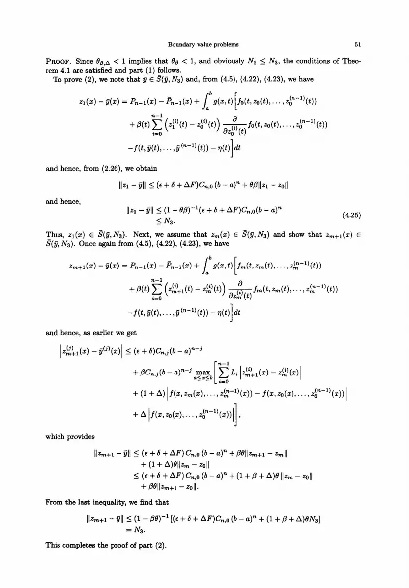
Boundary value problems 51
PROOF. Since 00,~ < 1 implies that 0~ < 1, and obviously Nr 5 Na, the conditions of Theo- rem 4.1 are satisfied and part (1) follows.
To prove (2), we note that jj E s(g,Ns) and, from (4.5), (4.22), (4.23), we have
q(z) -g(z) = P,_l(Z) - L(z) + JLS(L-J) [fo(t.lo(t), . . . ,$%) a
n-l
+ /3(t) 5 (zf’(t) - g(t)) ---&Joct, .zo(t>, . * * 9 4+“(t))
-f(C s(t), . . . 7 Y -‘“-l’(t)) - 7)(t) fit 1
and hence, from (2.26), we obtain
11~1 - 811 I (c + 6 + WG,o @ - a>” + Wlla - -zolI
and llzl - gl( I (1 - e/3)-‘(e + 6 + AF)G,,o@ - aIn
I N3. (4.25)
Thus, zl(z) E s(g, Na). Next, we assume that zm(z) E s(g, Ns) and show that z~+I(z) E @, N3). Once again from (4.5), (4.22), (4.23), we have
z,+1(z) - g(z) = Pn-l(2) - Pn_l(Z) + JLS(Zd) [f&Gn(% . *. 9 4rY”(w a
n-1
+ B(t) c (&(t) - 4w) &-p,lm(t), . * * 7 4pw i=o
-f(C s(t), . * * 2 Y -‘“-l’(t)) - q(t) 1
tit
and hence, as earlier we get
+ (1 + A) If(z,z,(z), . . . &-l)(z)) - f(z,z,,(z), . . . ,$-“(+))I
+ A f(z, zo(z), . . . , $--l) z ( ))I]
,
which provides
II~m+l - dl 5 (e + 6 + 4 Go (b - aY + Pellz,+l - tmll + (1 + ~MlG?l - zoll
5 (e + 6 + AF) Cn,o (b - aY + (I + /3 + A)e ll.zm - z,,ll
+ peiizm+l - ~~11.
F’rom the last inequality, we find that
IlGn+1 - &ll I (1 - pe)-’ [(c + 5 + AF)C,,O (b - ay + (1 + p + A)eNs]
= N3.
This completes the proof of part (2).
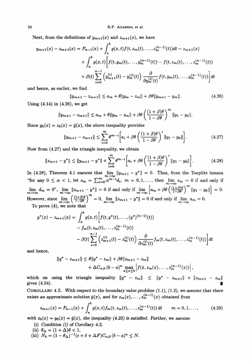
52 R.P. AGARWAL et al.
Next, from the definitions of ym+r(z) and zm+r(z), we have
I
b
Ym+l(Z) - G&+1(~) = pn-lb> + g(&t)f(t, Gn(q, * * * , &+(q)dt - %.+1(~) a
b + J [ g(a,t) f(k ym(t), *. .7 Y2-"W) - f(h &b(t), . . .Y &-“(w a
n-1
+ P(t) c (Y:!&) - Yim) &-pYm@)3.. . ) Ym] dt i=O
and hence, as earlier, we find
IIYm+l - Gn+111 I Gn + ~IlYm - Gnll + PqIYm+l - Ymll.
Using (4.14) in (4.26), we get
(4.26)
IIYm+l - Gn+1 II 2 hn + qynz - z,ll + pe (‘:‘;~)mllyl-Yoll.
Since ye(z) = Q(Z) = y(z), the above inequality provides
IIYm+l - z,+~ ll 2 2 e”-i i=. [~i+U~((:~~~)illyl-yOll].
Now from (4.27) and the triangle inequality, we obtain
IIz~+~ - Y* ii I IIY~+~ - Y*II + 2 em-i [ui + pe (e)’ IIY~ - yoke]. i=O
(4.27)
(4.28)
In (4.28), Theorem 4.1 ensures that ,liliW llyn+i - y*II = 0. Thus, from the Toeplitz lemma
“for any 0 5 CY < 1, let s,,, = CEO C-P-~&, m = 0, 1, . . . , then ,li*“, s, = 0 if and only if
lim d, = 0”, lim Ilz,+i - y*ll = 0 if and only if lim m--W0 m--rm m~oo [em + 00 (w)” llyl - y. tl] = 0.
However, since ,llr (w) m = 0, lim IIz,+i - y*ll = 0 if and only if lim a, = 0. m-C0 m+cc
To prove (4), we note that
and hence,
ll~* - ~~+~ll I oily* - hll + mlh+l - hll
+ AC,,, (b - “,“a~z~b If@, G(Z), . . . , d,?(d)/ , - -
which on using the triangle inequality lly* - z,II 5 lly* - z,+lll + IIzm+i - zmll gives (4.24). I
COROLLARY 4.5. With respect to the boundary value problem (1.1), (1.2), we assume that there
exists an approximate solution g(z), and for zm(z), . . . , z~-~)(z) obtained from b
Zm+1(~) = pn-l(Z) + J
g(t, Wn(t, &n(t), . . . , z$-“(Q) c-it m=O,l,..., (4.29) a
with ZO(Z) = ye(z) = g(z), the inequality (4.23) is satisfied. Further, we assume
(i) Condition (i) of Corollary 4.2, (ii) eA = (1 + A)6 < 1,
(iii) N4 = (I - e&‘(e + 6 + AF)C,,e (b - a)* 5 N.

Boundary value problems 53
Then,
(1) all the conclusions (l)-(3) of Corollary 4.2 are valid, (2) the sequence {z,(x)} obtained from (4.29) remains in s(p, Na), (3) the sequence {zm(x)} converges to y*(x), the solution of (1.1), (1.2) if and only if
flm a, = 0,
(4) a bound on the error is given by
5. AN EXAMPLE
Consider the boundary value problem
y(v) = ._A____ 10 + x2
ey + cos x2 + e-”
Y(O) = 1, y’ ($) =O, y”(;) =f, y$) =O, ~(‘~)(1)=0.
(5.1)
(5.2)
For this problem, we note that
(5.3)
and cs,o = &. Further, for the differential eqnation (5.1), it is sufficient to consider the set
Do = (90 : lyol I ‘.%}. Thus, it follows that Q = i e2Ko + 2. Hence, the conditions of
Theorem 3.1 are satisfied provided
l< ( L$Y+2)1’5 (5.4)
and
(5.5)
Inequality (5.4) implies that 0.1062 I Ko I 3.2177. Therefore, both the inequalities (5.4), (5.5) are satisfied provided 1.25 I KO I 3.2177. In conclusion, the problem (5.1), (5.2) has a solution y(x) such that [y(z)1 I 1.25.
Next, to apply Theorem 4.1 we assume that a(x) = Pd(x) so that the boundary conditions (5.2) are exactly satisfied, and hence E = 0. Further, the inequality (4.1) reduces to
1 max O--e P4(z) - cosx2 - e-” eg/’ + 2 = 6.
O<z<l 10 + 5
-- x2 $ (5.6)
Also, since for the problem (5.1), (5.2), the set D3 = {yo : Iyo - P4(x)I < IV}, 8 can be taken as
0 = -& x $ x eN+‘/’ < 1 (5.7)
and hence, N < 4.173317. (5.8)
Thus, the condition of Theorem 4.1 with p = 0 (or of Corollary 4.2) are satisfied provided
(1 - e)-’ ($eg/8+2).$<N, (5.9)

54 R.P. AGARWAL et al.
i.e., 0.117435 5 N < 4.145082. (5.10)
Clearly, (5.7) as well as (5.9) holds if (5.10) holds. Thus, in conclusion:
(i) the problem (5.1), (5.2) h as a solusion y*(z) in 0s = {ye :I yc - P4(2)1 5 0.117435}, (ii) this solution y*(z) is unique in Ds = {ye :) ys - Pd(z)[ 5 4.145082},
(iii) the sequence {y,(z)} generated by
y$$ (x) = & eymlx) + cos x2 + e-”
Ym+l(O) = 17 Yk+1 ; 0 =o, y;+1 ; =;, 0 Yii+1 a 0 =o, ?/g,“!(l)=0 m=0,1,...,
(5.11)
with ys(z) = Pd(z), converges to y*(s), moreover, if we choose N = 0.117435 then 8 = 0.01732019, and the following error estimate holds:
Iy,&) - y*(z)1 5 (0.01732019)m (0.117435082). (5.12)
The iterates ym+i(z) from (5.11) can be computed by using simple quadrature formulae. First eight iterates by employing the Trapezoidal rule with h = l/80 are presented in the following:
number of iterations
Table 1
computational error
3.26635247 x 1O-3
4.89861821 x lo-’
9.96934757 x lo-”
1.80966353 x lo-l4
2.22044605 x lo-l6
0.0
0.0
0.0
estimated error bound
1.17435082 x 10-l
2.03399790 x 10-s
3.52292293 x 10-S
6.10176933 x 1O-7
1.05683802 x 10-s
1.83046348 x lo-”
3.17039747 x 10⁻¹²
5.49118854 x lo-l4
Finally, we shall apply Theorem 4.3 to our problem (5.1), (5.2). For this, it is necessary that
81 = 38 < 1 (5.13)
and
(1 - 38)-i ($egjs+2) .h 2 N. (5.14)
Inequality (5.13) holds if and only if
N < 3.074705078 (5.15)
and (5.14) implies that 0.1540108 2 N 5 3.0359523. (5.16)
Obviously, both inequalities (5.15) and (5.16) hold if N satisfies (5.16). Thus, if we choose N = 0.1540108, then B = 0.0179655, LO = 0.35931 and it follows that K = 2.7831121. Therefore,
= 1.098779 x 1O-3 < 1.
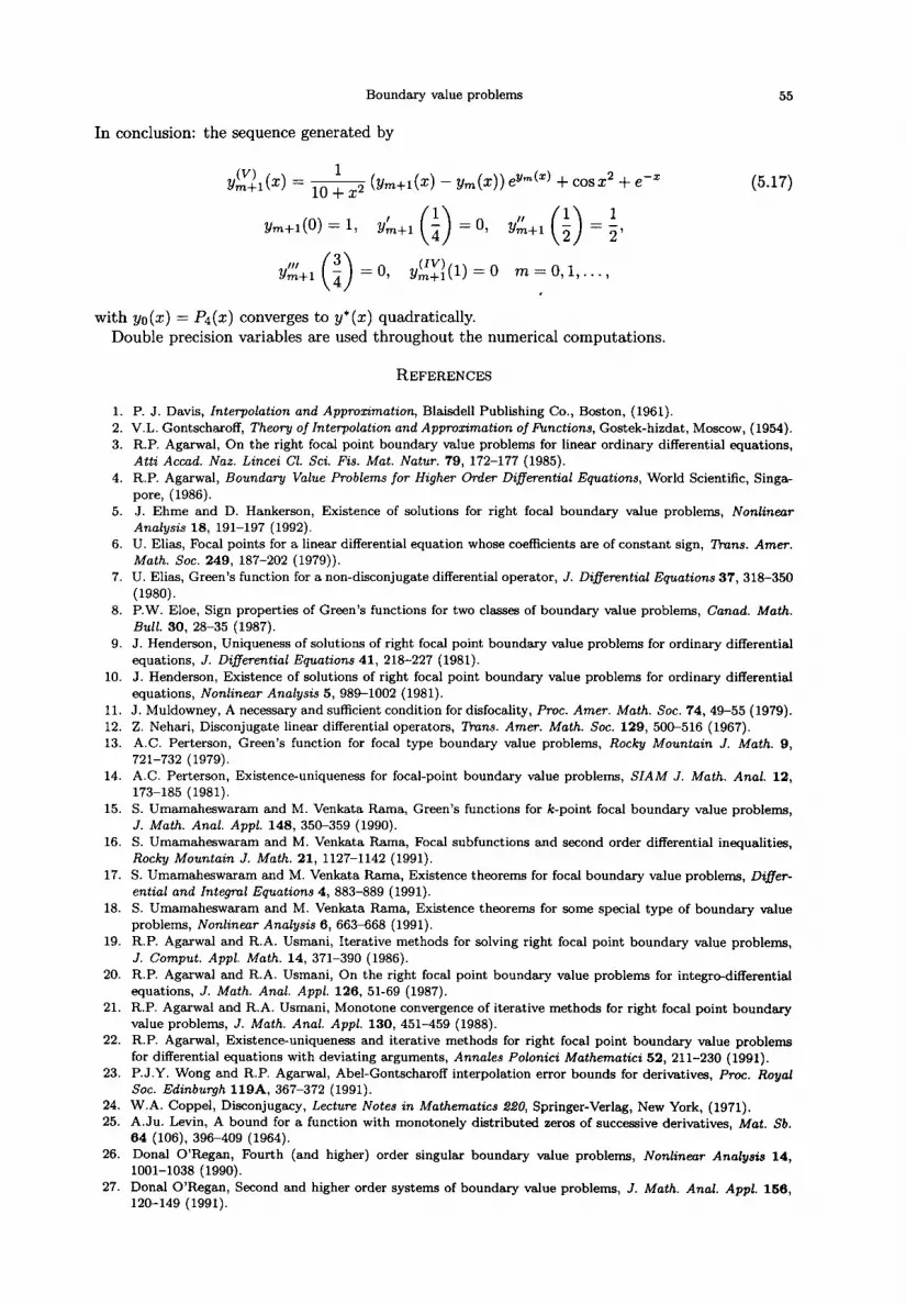
Boundary value problems
In conclusion: the sequence generated by
55
y(V)&) = m+ & (ym+l(2) - ym(x)) eymcs) + cosz2 + e-” (5.17)
Ym+lP) = 1, Yin+1 ; 0 =o, y;+l ; =;, 0 YX+1 ; 0 =o, y;;!(l)=0 m=O,l,...,
with ye(z) = Pi converges to y*(z) quadratically. Double precision variables are used throughout the numerical computations.
1. 2. 3.
4.
5
6
7.
8.
9.
10.
11. 12. 13.
14.
15.
16.
17.
18.
19.
20.
21.
22.
23.
24. 25.
26.
27.
REFERENCES
P. J. Davis, Interpolation and Approximation, Blaisdell Publishing Co., Boston, (1961). V.L. Gontscharoff, Theory of Interpolation and Approximation of finctions, Gostek-hizdat, Moscow, (1954). R.P. Agarwal, On the right focal point boundary value problems for linear ordinary differential equations, Atti Accad. Naz. Lincei Cl. Sci. Fis. Mat. Natur. 79, 172-177 (1985). R.P. Agarwal, Boundary Value Problems for Higher Order Differential Equations, World Scientific, Sings
pore, (1986). J. Ehme and D. Hankerson, Existence of solutions for right focal boundary value problems, Nonlinear Analysis 18, 191-197 (1992). U. Eliss, Focal points for a linear differential equation whose coefficients are of constant sign, Tmns. Amer. Math. Sot. 249, 187-202 (1979)). U. Elias, Green’s function for a non-disconjugate differential operator, J. Diflerential Equations 37, 318-350
(1980). P.W. Eloe, Sign properties of Green’s functions for two classes of boundary value problems, Canad. Math.
Bull. 30, 28-35 (1987). J. Henderson, Uniqueness of solutions of right focal point boundary value problems for ordinary differential equations, J. Dierential Equations 41, 218-227 (1981). J. Henderson, Existence of solutions of right focal point boundary value problems for ordinary differential equations, Nonlinear Analysis 5, 989-1002 (1981). J. Muldowney, A necessary and sufficient condition for disfocality, Proc. Amer. Math. Sot. 74, 49-55 (1979). Z. Nehari, Disconjugate linear differential operators, Trans. Amer. Math. Sot. 129, 500-516 (1967). A.C. Perterson, Green’s function for focal type boundary value problems, Rocky Mountain J. Math. 9, 721-732 (1979). A.C. Perterson, Existence-uniqueness for focal-point boundary value problems, SIAM J. Math. Anal. 12, 173-185 (1981). S. Umamaheswaram and M. Venkata Rama, Green’s functions for k-point focal boundary value problems, J. Math. Anal. Appl. 148, 35&359 (1990). S. Umamaheswaram and M. Venkata Rama, Focal subfunctions and second order differential inequalities, Rocky Mountain J. Math. 21, 1127-1142 (1991). S. Umamaheswaram and M. Venkata Rama, Existence theorems for focal boundary value problems, Difler- ential and Integral Equations 4, 883-889 (1991). S. Umamaheswaram and M. Venkata Rama, Existence theorems for some special type of boundary value problems, Nonlinear Analysis 6, 663-668 (1991). R.P. Agarwal and R.A. Usmani, Iterative methods for solving right focal point boundary value problems, J. Comput. Appl. Math. 14, 371-390 (1986). R.P. Agarwal and R.A. Usmani, On the right focal point boundary value problems for integredifferential equations, J. Math. Anal. Appl. 126, 51-69 (1987). R.P. Agarwal and R.A. Usmani, Monotone convergence of iterative methods for right focal point boundary value problems, J. Math. Anal. Appl. 130, 451-459 (1988). R.P. Agarwal, Existence-uniqueness and iterative methods for right focal point boundary value problems for differential equations with deviating arguments, Annales Polonici Mathematici 52, 211-230 (1991). P.J.Y. Wong and R.P. Agarwal, Abel-Gontscharoff interpolation error bounds for derivatives, Proc. Royal Sot. Edinburgh 119A, 367-372 (1991). W.A. Coppel, Disconjugacy, Lecture Notes in Mathematics 220, Springer-Verlag, New York, (1971). A.Ju. Levin, A bound for a function with monotonely distributed zeros of successive derivatives, Mat. Sb. 64 (106), 396-409 (1964). Donal O’Regan, Fourth (and higher) order singular boundary value problems, Nonlineur Analysis 14, 1001-1038 (1990). Donal O’Regan, Second and higher order systems of boundary value problems, J. Math. Anal. Appl. 156, 120-149 (1991).


