A timber harvesting model for Austria

Computers and Electronics in Agriculture

28 (228) 133–149

A timber harvesting model for Austria

Hubert Sterba a,*, Michael Golser a, Martin Moser a,Klemens Schadauer b

a Institute for Forest Growth and Yield, Uni6ersitat fur Bodenkultur Wien, Peter Jordanstraße 82,A-1190 Vienna, Austria

b Federal Forest Research Center, Seckendorff-Gudent-Weg 8, A-1131 Vienna, Austria

Abstract

Between 1981 and 1985 the Austrian National Forest Inventory (ANF) established a set of5500 clusters, each with four permanent plots covering all Austrian forests. After the firstremeasurement between 1986 and 1990 models were developed to predict tree growth,mortality and the behavior of forest owners in harvesting timber. A set of logistic equationsdescribes the probability for a given stand to exhibit intermediate harvesting, single-treeselection or final clear cutting. Independent variables were either continuous or categorical,describing: (i) regional units such as provinces, (ii) types of ownership (groups of ownershipsizes), (iii) site factors (elevation and slope), and (iv) stand characteristics (species mixture,density, mean diameter). Timber removals on the plots are recorded by five relative diameterat breast height (dbh)-classes. Removal percentages differ by elevation, harvesting categories,and tree species groups. Timber harvest forecasts and their spatial arrangement over Austriain the following four 5-year periods were made available to the public using computersoftware. In 1997 data of the second inventory remeasurements were available and thus theforecasts for this period could be evaluated. When forecast units are large enough, deviationsfrom the model are either small or can be explained by a different timber market scenarioand/or a general socio-economical scenario. © 2000 Elsevier Science B.V. All rights reserved.

Keywords: Growth model; Timber harvest forcast; Validation; Forest inventory

www.elsevier.com/locate/compag

* Corresponding author.

0168-1699/00/$ - see front matter © 2000 Elsevier Science B.V. All rights reserved.

PII: S0168-1699(00)00121-6

H. Sterba et al. / Computers and Electronics in Agriculture 28 (2000) 133–149134

1. Introduction — why forecasts of timber harvests in Austria

Austrian forests cover about 3.9 million ha or 47% of the country’s total area,and 85% of these forests are exploitable forests. Forest owners are typicallynonindustrial, and sell their timber to wood processors. Ownerships are usuallysmall (15 ha average), only 20% of the forest area are public forests. In terms offorest owners, 2/3 of the owners own less than 2 ha, and approximately 50% ofthe forest area belongs to owners with less than 200 ha (Bundesministerium furLand- und Forstwirtschaft, 1995). The forest industry, especially the sawmills,typically (with few exceptions) do not own forest lands. They are structuredsimilarly to forest owners, 50% of the yearly roundwood is processed bysawmills processing less than 100 000 m3 per year, thus the small sawmills out-number the big ones. In 1996, therefore, the Association of the AustrianSawmilling Industries ordered the development of software which would enable asingle sawmill or any other user to get forecasts of timber harvests for aninteractively definable region within Austria by tree species, and a number ofother categories for four 5-year periods (Fig. 1). This software is written inDelphi and runs under Windows 3.1, Windows 95 and Windows NT, and is alsonetwork compatible. The minimum hardware requirements are a 386 processorwith 2 MB RAM and a VGA graphics card.

2. Data

In order to mimic the behavior of Austrian forest owners, a harvesting modelwas built, based on the data from the Austrian National Forest Inventory(ANF) for the two observation periods 1981–1985 and 1986–1990. This inven-tory consists of permanent sample plots covering all of Austria. Sample plots areclustered at the four corners of a 200×200 m square. The clusters themselvesare systematically distributed over Austria at a distance of 3.89 km. In any givenyear every fifth cluster is measured, ensuring a representative sample of allAustrian forests each year. The total inventory comprises 5500 clusters and22 000 sample plots. Plot centers have been marked by a hidden iron stakeburied underground. Trees with a diameter at breast height (dbh) larger than10.4 cm were selected by angle count sampling (Bitterlich, 1948) with basal areafactor 4 m2 ha−1. Trees with dbh between 5 and 10.4 cm were only measuredwithin a circle of 2.6 m radius. Sample trees were recorded by their polarcoordinates and marked by a nail at the base of the tree. Remeasurement onthese plots was done in five overlapping 5-year intervals, thus covering theperiod from 1981 to 1990. For the objective of this paper, i.e. the evaluation ofthe harvest model, data from the second remeasurement of the plots from 1992to 1996 were used.

H. Sterba et al. / Computers and Electronics in Agriculture 28 (2000) 133–149 135

Fig

.1.I

nter

acti

vese

lect

ion

ofre

gion

s,tr

eesp

ecie

s,ow

ners

hip

clas

ses

and

othe

rca

tego

ries

for

tim

ber

harv

est

fore

cast

sw

ith

PR

OG

NA

US.


3. The models

An individual tree growth simulator of the FVS-type, PROGNAUS, (Monserudet al., 1997) was built from the first remeasurement of the forest inventory.PROGNAUS consists of a basal area growth model (Monserud and Sterba, 1996),a height growth model (Knieling, 1994), a crown ratio model (Hasenauer andMonserud, 1996) and a mortality model (Monserud and Sterba, 1999). For thesoftware to forecast timber harvests, Moser (1996) added a harvest model, simulat-ing how forest owners harvest trees in their forests. Since all the above mentionedmodels were developed for a 5 year period (according to the data base) and theforecasts had to be made for 20 years, some additional models, e.g. to establishingrowth, and to describe the change of the forest development type (youth, thicket,pole stage, mature, uneven-aged) were built in order to update the data after each5-year forecast.

For the harvest model a stochastic approach was used, distinguishing betweenfour kinds of harvests on each plot, namely:1. regular final harvests

1.1. in clear cuts (defined by the ANF, as removing all trees on an area largerthan 500 m2),

1.2. as single-tree harvests2. regular intermediate thinnings, and3. salvage cuts, i.e. harvests necessitated by snow damage, windthrows, insect

and/or fungi damage.The probability for any of the above harvests to take place on a given inventory

plot was depicted by LOGIT-functions of the general form:

P(harvest)=LOGIT(X)=1

1+eb%X

with X the vector of independent variables and b the associated coefficients. TheCATMOD-procedure (SAS Institute, 1987) was used to estimate the parameters ofthe logistic equation using maximum likelihood methods. The harvest model (Fig.2) consists of four equations that compute the probabilities for the outcome of thefour dichotomous decisions outlined below.

(i) Probability of any regular harvest on a plot:P(regular harvest)

=LOGIT(dg, hL, BA, CV, ELEV, PF, HC1, HC2, DIST, PROV1, CON, MIX)where dg is the dbh of the mean basal area stem, hL is Lorey’s mean height, i.e. thebasal area weighted mean of the tree heights (Prodan (1965), p. 181), BA is thebasal area per hectare, CV is the coefficient of variation of the dbh-distribution,ELEV is the elevation. All the other parameters are dummy variables (Draper andSmith, 1981) assuming a value of zero unless meeting the described condition: MC1equals 1 if the plot is situated in a protection forest, MC2 equals 1 if it is in acommercial forest, HC1 is equal 1 if the slope is less than 30%, HC2 is 1 if thesurface at the plot was classified as difficult for harvesting operations (through soil


Fig. 2. Decision tree for simulating harvest on the plot level. The decision model consists of fourequations that estimate the probability of each of the outcomes for the four underlined dichotomousdecisions.

groups), DIST is 1 if the distance to the next rack or forest road is less than 100 m,PROV1 is 1 in the province of Tyrol, CON is 1 if the proportion of conifers (bybasal area) is larger than 25%, and MIX is 1 if the proportion of conifers is between25 and 75%, all otherwise 0.

(ii) Probability of salvage cuts, conditional on no regular harvest:

P(salvage�¬regular harvest)

=LOGIT(dg, hL, BA, CV, OW, HC1, PROV1, PROV2, CON)

where OW is 1 if the plot is situated in a forest ownership of less than 200 ha,PROV2 is 1 in the province of Salzburg and the other variables are as given above;

(iii) Probability of final harvest, conditional on regular harvest:

P(final�regular)=LOGIT(dg, hL, BA, CV, OW, MC1, CON)

(iv) Probability of clear cut, conditional on final harvest:

P(clear–cut�final)=LOGIT(dg, BA, ELEV, MC1, MC2)

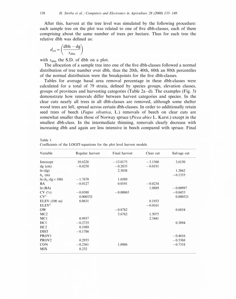
The coefficients of these four models are given in Table 1.The forecasts (made available on a CD) were the average results of 500 runs for

each period. In each run the type of harvest allocated to a plot, if any, wasdetermined by comparing random numbers (uniform (0, 1)) to probabilities calcu-lated for the plot.


After this, harvest at the tree level was simulated by the following procedure:each sample tree on the plot was related to one of five dbh-classes, each of themcomprising about the same number of trees per hectare. Thus for each tree therelative dbh was defined as:

drel=�dbh−dg

sdbh

�with sdbh the S.D. of dbh on a plot.

The allocation of a sample tree into one of the five dbh-classes followed a normaldistribution of tree number over dbh, thus the 20th, 40th, 60th an 80th percentilesof the normal distribution were the breakpoints for the five dbh-classes.

Tables for average basal area removal percentage in these dbh-classes werecalculated for a total of 79 strata, defined by species groups, elevation classes,groups of provinces and harvesting categories (Table 2a–d). The examples (Fig. 3)demonstrate how removals differ between harvest categories and species. In theclear cuts nearly all trees in all dbh-classes are removed, although some shelterwood trees are left, spread across certain dbh-classes. In order to additionally retainseed trees of beech (Fagus sil6atica, L.) removals of beech on clear cuts aresomewhat smaller than those of Norway spruce (Picea abies L. Karst.) except in thesmallest dbh-class. In the intermediate thinning, removals clearly decrease withincreasing dbh and again are less intensive in beech compared with spruce. Final

Table 1Coefficients of the LOGIT-equations for the plot level harvest models

Regular harvest Salvage cutVariable Clear cutFinal harvest

Intercept 10.6226 −13.0175 −3.1560 3.6150−0.0191dg (cm) −0.2835−0.0258

ln (dg) 2.3038 1.2862hL (m) −0.1353

1.6589−1.7678ln (hL/dg×100)BA −0.0127 0.0191 −0.0234ln (BA) 1.0889 −0.00997CV (%) −0.0388 −0.00065 −0.0453

0.000521CV2 0.0005320.0631ELEV (100 m) 0.1933

−0.0161ELEV2

0.6854OW −0.87823.6762MC2 1.5075

MC1 0.9937 2.3441HC1 0.3894−0.2725HC2 0.1989DIST −0.1786PROV1 −0.4616

0.2955 −0.5368PROV2−0.7318−0.2361 1.0986CON

0.232MIX


single-tree harvests in spruce seem to increase with increasing dbh (target diameterharvest according to Reininger (1989)), while in beech, single-tree harvests as wellas salvage cuts are about uniformly distributed over the dbh-classes. Salvage cuts inspruce are concentrated around the average dbh. In the final tree harvest model thebasal area, represented by every tree in the plot is reduced by the percentages givenin the appropriate Table.

4. Evaluation of the harvest model

Actual harvests were calculated from the repeated forest inventory 1992–1996,thus the plots last measured in 1986 were measured again in 1992, those measuredin 1987 in 1993, etc. Because this inventory period covered 6 years, while thesimulator PROGNAUS was built for 5 year periods, the harvests, reported by theinventory were multiplied by 5/6 in order to compare with the forecasts ofPROGNAUS.

Several comparisons were made for two different cases, first for the whole ofAustria, and second for a specific region that might be selected by a sawmill owner.For this latter case, the mill is situated in eastern Carinthia and the owner wants toknow the probable timber yield within a circle of approximately 60 km around thesawmill. The average elevation of this region is somewhat above the Austrianaverage; there are more spruce and fewer broadleaves compared to the average forAustria. Protection forests are less frequent and small forest ownerships are morefrequent in this region (Table 3). For both cases, Austria and the selected region,harvests were compared in terms of fellings in m3 outside bark. The proportions oftotal harvested volume with respect to management types (protection forest,commercial forests), elevation, harvest categories (intermediate thinning, single-treeselection, final clear cuts), dbh-classes, and tree species were also compared. Due tothe large number of plots and sample trees, practically any deviation from theforecasts will be statistically significant. Thus the magnitude of the deviations ofpredicted volume proportions by categories are of greater interest. Therefore asimple distance measure (Dirk, 1995) for this deviation was defined as:

Distance(%)= %Categories

� f%observed− f%PROGNAUS�

with f% the observed and predicted proportion of harvested volume in the givencategory, and Distance (%) covering a range between 0 (no deviation, full fit) and200% (maximum deviation).

5. Results

The comparison between actual and projected harvests by ownership size andharvest categories indicate large interactions for both the whole of Austria and theselected region (Table 4). Generally, total harvests were overestimated, this


Table 2Intermediate thinning model on tree level (a), clear cut model on tree level (b), single-tree selectionmodel on tree level (c), and salvage cut model on tree level (d)a

Province Elevation (m) Dbh-classTree species group

1 2 3 4 5

a37 13Spruce and fir 0Burgenland 0 0\200

Spruce and fir B500 54 20 40 6 4CarinthiaSpruce and fir 61Carinthia 41 27 17 9500–1000

59 52 10\1000 19Spruce and fir 10CarinthiaB500Lower Austria 64 34 19 19 7Spruce and fir

67 47 25Spruce and fir 7Lower Austria 7\50058 39 11B500 3Upper Austria 4Spruce and fir

\500Upper Austria 65 43 25 12 2Spruce and firSpruce and fir 52Salzburg 37 21 9 5B1000

74 33 361000–1500 21Salzburg 9Spruce and fir\1500Salzburg 70 75 38 48 0Spruce and fir

74 58 7Spruce and fir 9Styria 5B50068 47 25500–1000 10Styria 5Spruce and fir

1000–1500Styria 69 54 35 14 12Spruce and fir75 60 29Spruce and fir 7Styria 0\150056 32 38B1000 9Spruce and fir 11Tyrol and Vorb.

\1000Tyrol and Vorb. 89 20 21 0 0Spruce and fir55 27 18Larch 8Austria 5\20058 49 36\200 25Austria 9Pine and other conif.

\200Austria 39 33 20 9 11BeechOak and other hardw. 55Austria 37 28 26 8\200

60 51 62 48 48\200Other broadl. Austria

bBurgenland \200 26 31 11 20 19Spruce and fir

23 26Spruce and fir 17Carinthia 33 33B100033 25 28\1000 19Carinthia 31Spruce and fir

B500Lower Austria 36 23 22 6 18Spruce and fir45 27Spruce and fir 15Lower Austria 24 24500–100066 30 17\1000 23Spruce and fir 21Lower Austria

B500Upper Austria 39 22 24 12 19Spruce and fir44 33 24Spruce and fir 21Upper Austria 20\50035 14 14B1000 26Salzburg 18Spruce and fir

\1000Salzburg 45 39 28 21 35Spruce and firSpruce and fir 24Styria 6 29 2 17B500

40 27 31500–1000 20Styria 35Spruce and fir\1000Styria 42 40 39 20 25Spruce and fir

12 24 23Spruce and fir 18Tyrol and Vorb. 29B100026 21 361000–1500 37Tyrol and Vorb. 40Spruce and fir

\1500Tyrol and Vorb. 25 0 19 25 49Spruce and fir22 24Larch 21Austria 21 21\20044 32 28\200 20Pine and other conif. 19Austria

\200Austria 34 26 24 16 21Beech43 35Oak and other hardw. 36Austria 23 21\20053 54 58\200 48Austria 51Other broadl.


Table 2 (Continued)

Tree species group Elevation (m) Dbh-classProvince

1 2 3 4 5

c74 100Spruce and fir 73Carinthia 87 77B1000

Spruce and fir 72Carinthia 56 66 80 83\100092 81 94B500 86Spruce and fir 85Lower Austria

\500Lower Austria 64 63 71 100 82Spruce and firB500Upper Austria 90 68 91 88 81Spruce and fir

81 85 75\500 100Spruce and fir 96Upper AustriaSpruce and fir 100Salzburg 81 79 100 78B1000

91 100 100\1000 100Salzburg 94Spruce and firB1000Burgenl. and Styria 94 90 81 79 85Spruce and fir

1000–1500Burgenl. and Styria 88 78 86 86 81Spruce and fir94 81 100\1500 67Spruce and fir 49Burgenl. and Styria56 100 88Spruce and fir 100Tyrol and Vorb. 85B150066 11 55\1500 74Spruce and fir 83Tyrol and Vorb.

\200Austria 92 87 79 82 74Larch\200Austria 100 98 83 88 92Pine and other conif.

93 63 69\200 76Beech 73Austria83 79 93 69 65Oak and other hardw. Austria \20091 84 84 63 85\200Other broadl. Austria

dCarinthia B1000 21 29 38 12 40Spruce and firCarinthia \1000 51 37 26 20 10Spruce and fir

41 22 25B500 25Spruce and fir 42Lower Austria56 29Spruce and fir 62Lower Austria 22 30\50052 18 60B500 19Spruce and fir 22Upper Austria

\500Upper Austria 30 30 46 9 14Spruce and firB1000Salzburg 28 45 24 28 17Spruce and fir

35 31 24\1000 37Spruce and fir 39Salzburg37 51 27 41 33Spruce and fir Burgenl. and Styria B100028 34 38\1000 14Burgenl. and Styria 32Spruce and fir

B1000Tyrol and Vorb. 40 11 21 12 16Spruce and fir16 26 19Spruce and fir 18Tyrol and Vorb. 101000–150034 26 34\1500 32Tyrol and Vorb. 37Spruce and fir

\200Austria 29 17 21 5 16LarchPine and other conif. \200 49 36 34 28 49Austria

27 20 29\200 18Beech 30Austria\200Austria 0 12 0 41 22Oak and other hardw.

Other broadl. \200 68 64 45 14 36Austria

a Percent basal area removal by species group, province, elevation and dbh-class.


overestimation being larger for the whole of Austria than for the selected region,and larger for small landowners than for larger ones. Salvage cuts, which are onlyabout 10% of total harvests, were overestimated in large ownerships and underesti-mated in small ownerships. While small landowners reduced both categories of finalharvest in favor of thinnings, larger landowners reduced only clear cuts. In theselected region both types of landowners reduced only single-tree selection, thepreferred final harvesting category in small forest ownerships.

These facts can also be seen from the distances between actual and projectedvolume distribution of harvests (Table 5). Given that distances above 10 indicateimportant deviations from the predicted distribution, the distribution for harvestcategories and for most of the categories within salvage cuts differ notably from thepredictions. Distributions for elevation and for dbh-classes in regular harvests, aswell as the distribution for species in clear cuts and intermediate thinnings, were

Fig. 3. Example for the harvest model on tree level. Norway spruce and common beech in one out of79 strata. Percent basal area removal in the five relative dbh-classes.

Table 3Characteristics of the selected region in comparison with the average of Austria

Selected regionAustria

905Elevation (m) 10625.17.4Protection forest area (%)

53Small forest ownership area (%) 7061 72Norway spruce volume (%)

916Broadleaf tree volume (%)


Fig

.4.

Har

vest

edvo

lum

edi

stri

buti

onby

dbh

aspr

edic

ted

(PR

OG

NA

US)

and

obse

rved

byth

eA

ustr

ian

Nat

iona

lIn

vent

ory

(AN

F92

/96)

.


Fig

.5.

Har

vest

edvo

lum

edi

stri

buti

onby

elev

atio

nas

pred

icte

d(P

RO

GN

AU

S)an

dob

serv

edby

the

Aus

tria

nN

atio

nal

Inve

ntor

y(A

NF

92/9

6).


Table 4Fellings by ownerships and harvest categories as observed by the Austrian Forest Inventory (ANF92/96) and predicted by PROGNAUS in 1000 m3 outside bark

Austria Selected region

D%a ActualActual PROGNAUS D%aPROGNAUS

Small landowners (B200 ha)−14.1 2296Total Harvest 23649360 −3.010718

3.4 352Thinning 3071402 12.81354−24.4 783 9414319 −20.2Selection 3471−22.7Clearcut 9703552 967 0.44358

26.5 191 149 22.0687Salvage 935

Large landowners (\200 ha)−7.4Total Harvest 10158566 984 3.19202

32.6 221 1481096 33.0Thinning 162727732893 4.1 264 304 −15.2Selection

−30.3 425 4083968 4.03045ClearcutSalvage −35.31007 105 124 −18.11362

All landownersTotal harvest 19920 −11.1 3311 3348 −1.117926

19.1 573 4552450 20.63029Thinning−11.4 1046 1245Selection −19.06364 7092−26.4 1394 13768326 1.3Clear cut 6597−5.6Salvage 2961941 273 7.82050

a D% Is the over- or underestimation of the actual harvests by the model (in percent).

Table 5Distance (%) between harvest volume distributions

Grouping Selected regionAustria

Regular harvest Salvage cutSalvage cutRegular harvest

Elevation 9.477.28 39.9441.170.98 2.523.400.90Management type

–10.71 11.56 –Harvest category13.337.26 8.75 25.98Dbh-class

8.1910.88 ––Tree intermediate thinning–12.88 21.45 –Species single-tree selection

5.18 ––9.60Within clear cut

8.77Total 7.656.40 10.89


predicted well. Fig. 4 indicates that the distribution for dbh-classes was predicted wellfor regular harvests, but not as well for salvage cuts. Fig. 5 shows that the same istrue for elevation. The distribution for tree species exhibit interesting deviationsespecially in single-tree selections (Table 6).

6. Discussion

6.1. Total har6est

The first, and most important result is the overestimation of the total harvests.Nearly all of these 2 million m3 overestimates are located in regular harvests ofsmall forest ownerships (Table 4). Severe storm damage, mainly in neighboringGerman (Bavarian) forests in 1990 led to a bark beetle outbreak, lasting until about1996 (Forstliche Bundesversuchsanstalt, 1996). Partly for this reason and partlybecause of low world sawn-wood prices, timber prices decreased seriously, and havenot yet recovered fully (Fig. 6). Only small forest owners, who do not depend

Table 6Distribution of observed (ANF 92/96) and predicted (PROGNAUS) harvested volume by species inpercent of final single-tree selections

AustriaSpecies Selected region

ANF 92/96 PROGNAUSANF 92/96 PROGNAUS

58.2 72.159.8Norway spruce (Picea abies L.) 64.8White fir (Abies alba L.) 2.32.45.46.7

9.94.4 7.54.8European larch (Larix europaea L.)12.5 7.2Scots pine (Pinus sil6estris L.) 8.312.1

6.9 8.8Common beech (Fagus sil6atica L.) 1.1 4.33.7 0.6Oak (Quercus sp.) 1.42.8

7.99.87.1 5.8Other deciduous

Fig. 6. Conifer round-wood price development. Index reference is January 1998. Note that the figurestarts 1998 midyear. Source: WIFO (1998).


significantly on income from forestry, are able to, and do, react to fluctuations intimber market prices (Schwarzbauer, 1997). So, the storm damage of 1990, togetherwith the following timber market situation, seem to have resulted in a decrease inharvest that was more pronounced in owners of small forest properties.

6.2. Distribution by different categories

As indicated by the average distances (Table 5) the relative distribution ofharvested volume to many of the different categories has been predicted quite wellby PROGNAUS. Those predicted less well are discussed as follows:

6.2.1. Sal6age cuts by ele6ation and dbh-classesThe bark beetle outbreak may again be the reason why salvage cuts shifted to

lower elevations (Fig. 5) and to smaller dbh-classes than experienced in theinventory period 1981–1990 and thus incorporated in the model (Fig. 4). Due tothe biology of Ips typographus and Ips chalcographus, smaller trees in forests atlower elevations are more susceptible to bark beetle attacks. Because Austrian lawdictates that dead trees have to be removed from the forest, the concentration ofsalvage cuts in these strata after 1990 are explained.

6.2.2. Har6esting categoriesThe smaller reduction of total harvests for larger landowners was allocated to

clear cuts and partly compensated for by increased thinnings. The larger totalharvest reduction for small forest owners occurred in both categories of finalharvests, single-tree selection and clear cuts. In the selected region a shift from finalsingle-tree selection to thinnings took place in both ownership categories. Thus, thedecrease in total harvest, mainly caused by storm damages followed by bark beetleoutbreaks and market price changes, and the unexpected location of salvage cuts,led to a shift between harvest categories, depending on the size of ownership. Thiseffect probably also differed by region.

6.2.3. Tree species in final single-tree selectionIn the course of ‘regular’ harvesting, single trees in old stands are often harvested

when their crown condition seems to indicate poor vigor and probably approachingdeath. If they already had died they would have been counted as ‘salvage cuts’ inthe forest inventory. From recent monitoring of crown conditions in Austria weknow that white fir, Scots pine and oaks are the species with the worst crownconditions (Kristofel and Neumann, 1997). While the vigor of white fir hasimproved significantly since 1990, average needle loss for Scots pine and oak variedsubstantially, with peaks in 1992 and 1994 (Kristofel and Neumann, 1997). There-fore, these species may have been removed more frequently during these periodsthan predicted by PROGNAUS.


7. Conclusions

For several categories, predicted harvests reflected actual harvests quite well.Nevertheless, some serious deviations from the predictions were noticed. Thesedeviations can be explained through windthrows, bark beetle outbreaks, and asingular market anomaly. Not unexpectedly, larger catastrophic-like events andeconomic developments cannot be foreseen by PROGNAUS. Nevertheless, weexpect the model to work quite well under normal conditions. Using individual treecrown condition and roundwood prices as predictors in the model will not improvepredictions as long as they themselves cannot be foreseen. However, these variableswould permit the model to be used for projections under different scenarios oftimber market and ‘forest dieback’ and thus help answer ‘what–if’ questions.

Acknowledgements

The authors want to thank the Association of the Austrian Sawmilling Industriesfor promoting and sponsoring this work; the Austrian Science Foundation foradditional funding within the Special Research Program SRP008; the AustrianMinistry of Agriculture and Forestry and the Federal Forest Research Center inVienna for making the data of the ANF available; and last but not least, KarlSchieler, head of the ANF and Peter Schwarzbauer, Professor for Forest ProductsMarket Research at the Universitat fur Bodenkultur Wien and Bill Wykoff,Moscow Forestry Science Laboratory, Idaho, for valuable review comments.

References

Bitterlich, W., 1948. Die Winkelzahlprobe. Allg. Forst- u. Holzwirtsch. Ztg. Wien 59, 4–5.Bundesministerium fur Land- und Forstwirtschaft 1995. O8 sterreichischer Waldbericht 1994. Bundesmin-

isterium fur Land- und Forstwirtschaft Wien.Dirk, W., 1995. Funktionalanalysis. Springer, Berlin.Draper, N.R., Smith, H., 1981. Applied Regression Analysis, 2nd edn. Wiley, New York.Forstliche Bundesversuchsanstalt, 1996. Borkenkaferschaden in O8 sterreich. Forstsch. Aktuell 17/18,

3–4.Hasenauer, H., Monserud, R.A., 1996. A crown ratio model for Austrian forests. For. Ecol. Manag. 84,

49–60.Knieling, A., 1994. Methodische Beitrage zur Auswertung der O8 sterreichischen Forstinventur nach 1980.

PhD Thesis, Universitat fur Bodenkultur Wien.Kristofel, F., Neumann, M., 1997. Ergebnisse der Kronenzustandserhebungen 1996. O8 sterr. Forstztg.

107 (3), 39–40.Monserud, R.A., Sterba, H., Hasenauer, H., 1997. PROGNAUS. In: Teck, R., Moer, M., Adams, J.

(Eds.), Proceedings: Forest Vegetation Simulator Conference, 3–7 February 1997, Fort Collins, CO.General Technical Report INT-GTR-373. Ogden, UT: USDA Forestry Service, InternationalResearch Station, pp. 50–56.


Monserud, R.A., Sterba, H., 1996. A basal area increment model for even- and uneven-aged foreststands in Austria. For. Ecol. Manag. 80, 57–80.

Monserud, R.A., Sterba, H., 1999. Modeling individual tree mortality for Austrian forest species. For.Ecol. Manag. 113, 109–123.

Moser, M. 1996. PROGNAUS — Simulation des Holzaufkommens fur O8 sterreich. Unpublishedprogram description.

Prodan, M., 1965. Holzmesslehre. J.D. Sauerlander, Frankfurt/M.Reininger, H., 1989. Zielstarken-Nutzung, 3rd edn. O8 sterr. Agrarverlag, Wien.SAS Institute, 1987. SAS/STAT Guide for Personal Computers, Version 6 edition, Cary, NC.Schwarzbauer, P., 1997. Demand and supply analysis of roundwood and forest products markets in

Europe. EFI Proc. 17, 7–44.WIFO 1998. WIFO-Volkswirtschaftliche Datenbank, KGEN. http://www.wifo.ac.at, Wien.

.

Documents

A timber harvesting model for Austria