A threshold finite cellular automata NP-complete problem

Oscar Borrego-Hernandez, Mario Miguel Ojeda-RamırezDepartment of Mathematics, Universidad Veracruzana

Abstract

Cellular automata are discrete dynamical systemsthat provide simple models for a wide range of com-plex phenomena. We introduce a constrained opti-mization problem related to a binary spatio-temporalprocess. This process is modeled as a finite cellularautomaton with a threshold-based transition functionthat depends not only on the neighborhood of thecell, but also on its spatial location and time. Weanalyze the computational complexity of this prob-lem and prove that it is NP-complete by means of areduction of the well-known 3-SAT problem. Sincean efficient (polynomial time) solution for an NP-complete problem has, as yet, not been found, andan exhaustive enumeration is not viable, a geneticalgorithm for addressing this problem is proposed.The performance of the algorithm is evaluated for 50simulated instances, showing that, although it doesnot yield accurate enough results for every instancetested, it is a reasonable starting point that may beimproved by modifying some of its component parts.Keywords: NP-completeness, spatio-temporal

process, 3-SAT, cellular automata, genetic algorithm

1 Introduction

Cellular automata (CA) are lattice dynamical sys-tems where time is discrete, the lattice is in a finitenumber of dimensions, and each unit, called cell, ischaracterized by an internal state that takes on a fi-nite set of values. CA were originally introduced byJohn von Neumann and Stanislaw Ulam in the late1940s under the name of cellular spaces, as possibleidealization of biological systems (see [13, 1]).

Von Neumann was interested in finding a logical

abstraction of self-replicating systems when Ulam,his colleague at the Los Alamos National Labora-tory, suggested him using a discrete system for de-signing a reductionist model of self-replication. Fol-lowing Ulam’s suggestions, von Neumann addressedthe problem in the framework of a discrete universemade up of cells, where each cell is characterized byan internal state represented by a finite number ofbits. This system of cells evolves, in discrete timesteps, according to a simple rule, and the new inter-nal state depends on the current state of the neighborcells. [1]

At the beginning of the 1980s Wolfram [13, 14, 15]studied in detail a family of simple one-dimensionalCA rules, he noticed that a cellular automaton isa discrete dynamical system and, as such, exhibitsmany of the behaviors encountered in a continuoussystem.

According to Wolfram [13] CA are of sufficientgenerality to provide simple models for a very widevariety of physical, chemical, biological and othersystems. They exhibit complicated behavior anal-ogous to that found with differential equations, butby virtue of their simpler construction are potentiallyamenable to a more detailed and complete analysis.Any physical system satisfying differential equationsmay be approximated as a cellular automaton by in-troducing finite differences and discrete variables [13].Furthermore, sufficiently complicated CA are knownto be universal computers, capable of computing anycomputable function given appropriate input [13, 1].

Wolfram [14] also noticed that different initialstates with a particular cellular automaton rule yieldpatterns that differ in detail, but are similar in formand statistical properties, while different cellular au-tomaton rules yield very different patterns.

1

Since CA models are very flexible, they can be con-veniently modified or adapted for addressing differentkind of problems for spatio-temporal systems, for ex-ample: Li and Yeh [9] built a CA model integratedwith a Geographical Information System for planningof sustainable urban development. They embeddedsome constraints in evolution rules of CA so that ur-ban growth can be rationalized according to a set oflocal, regional and global sustainable criteria, undercomplicated and changeable environmental factors.Another example is found in the work of Hooten andWikle [7], where CA are formulated probabilistically,the state of a cell is defined by parametric probabil-ity distributions and the behavior of the system as awhole is expressed in terms of likelihood.

In section 2 we formulate the constrained optimiza-tion problem we are interested in and specify the CAmodel it is based on. In section 3 we prove thatthis problem is NP-complete using a reduction of the3-SAT problem. In section 4 we propose a geneticalgorithm for addressing the problem from a meta-heuristic approach, we also present and discuss theresults for 50 simulated instances.

2 Problem formulation

2.1 Cellular automata definition

This work concentrates on two-dimensional CA. Al-though there is not a generally established or ac-cepted definition of cellular automaton in the liter-ature, a standard two-dimensional cellular automa-ton can be formally defined as a triple (Q,N , δ),where Q 6= ∅ is a finite set of possible states for acell, N : Z2 → (Z2)p is the neighborhood function,δ : Qp → Q is the evolution function and p ∈ Z+

is the cardinal of any cell neighborhood (all of themhave the same number of items). The cells are in-dexed horizontal and vertically in a discrete coordi-nate system, thus, the set of cells is isomorphic to Z2

and each cell is identified by its position (i, j) ∈ Z2.The neighborhood function is such that

N (i, j) =(N (1)

ij , . . . ,N (p)ij

)

is a p-tuple where N (k)ij is the k-th neighbor of cell

(i, j). Thus, given the initial state (at time zero) for

each cell: q(0)ij , the automaton evolves according to:

q(t+1)ij = δ

(q(t)

N (1)ij

, . . . , q(t)

N (p)ij

),

where q(t)ij is the state of cell (i, j) at time t.

For a detailed discussion on properties, classifica-tion and general theory of CA see [1],[13],[14] or [15].

Before introducing the particular family of CA andthe problem we are interested in, we present a moti-vating example related to air pollution, that will helpto justify the approach that follows.

2.2 Motivating example: air pollu-tants concentration

Urban air pollution is a very important environmen-tal issue. Many cities around the world have airquality monitoring networks. Usually, the monitor-ing stations that make up the network, report pollu-tants concentration with certain temporal frequency.Nevertheless, for assessing the potential health riskpopulation is been exposed to, it is not enough con-sidering the stations records, but considering pollu-tion on other locations, e.g. on a regular grid withthe required resolution, is also necessary. This is whythe pollutants concentration should be estimated forsuch locations.

Focusing on a particular air pollutant, rather thanconsidering its concentration as a continuous quan-tity, we can divide the spatial domain into a regulargrid of size n×m cells, and consider the binary spatio-

temporal process {Y (t)i,j : i = 1 . . . n, j = 1 . . .m, t =

0, 1, . . .} where the variable Y(t)i,j has value 1 if the pol-

lutant concentration is greater than certain thresholdτ on cell (i, j) at time t, and 0 otherwise. This processis particularly interesting if the threshold τ coincideswith the value of certain ambient air quality standardassociated with the pollutant.

The process {Y (t)i,j } can be modeled as a finite

two-dimensional cellular automaton, this is a two-dimensional cellular automaton where the lattice isfinite in both dimensions. In this case the set of

2

cells can be seen as isomorphic to G ≡ {1, . . . , n} ×{1, . . . ,m} in stead of Z2, but some neighbors can stilllie out of this spatial domain. Thus, some boundaryconditions should be specified, these are conditionsrelated to the cells near the boundaries of the spatialgrid.

We assume that the data from monitoring sta-tions is available for time t = 1, . . . , T , such thatthe process is completely unknown for t = 0 and par-tially specified for t > 0. Let Dt ≡ {(i, j) ∈ G :(i, j) observed at time t} be the set of locations ob-

served at time t, with t = 1 . . . T , and let Z(t)i,j ∈ {0, 1}

with (i, j) ∈ Dt be the observed state of cell (i, j)at time t. Alternatively, we can specify the sets

D+t ≡ {(i, j) ∈ G : Z

(t)i,j = 1} and D−t ≡ {(i, j) ∈

G : Z(t)i,j = 0} for t = 1 . . . T .

The goal is to assign states to each cell at time

t = 0, i.e. find values for the Y(0)i,j with (i, j) ∈ G, such

that the evolution of the automaton is as coherent aspossible with the data Z

(t)i,j . This notion of coherence

optimization will be formalized in the next section.Furthermore, a city may have different zones with

similar patterns of air pollution determined by fac-tors such as traffic, emissions, weather conditions,proximity and many others. In this regard, we alsoconsider that certain correlation structure among lo-cations for time t = 0 is previously known. Thiscorrelation structure is expressed by means of a setC+ ⊆ G2 and the following constraints:

Y(0)i,j = Y

(0)k,l for ((i, j), (k, l)) ∈ C+.

Moreover, the constraints can be partially specifiedby a subset A+ ⊆ C+.

In general, solving this problem seems to be com-putationally expensive since the number of candi-dates for the solution is 2nm, although the correlationconstraints can reduce this number.

In the next subsection we completely specify thecellular automaton by defining the neighborhood andevolution functions.

2.3 A threshold finite CA

Once the motivating ideas have been presented, wecan introduce the cellular automaton we are inter-

ested in and the associated problem we are address-ing.

We propose using a simple neighborhood structure:the Queen neighborhood, which is known in literatureas Moore neighborhood, i.e., the neighbors of a cellare the proper cell and the eight cells surroundingit, nine in total. Formally, the neighbors are definedaccording to the following table:

k N (k)ij

1 (i− 1, j − 1)2 (i− 1, j)3 (i− 1, j + 1)4 (i, j − 1)5 (i, j)6 (i, j + 1)7 (i+ 1, j − 1)8 (i+ 1, j)9 (i+ 1, j + 1)

For specifying the evolution function we considera threshold structure and extend the standard defi-nition allowing the evolution function to depend alsoon time and spatial location. The evolution functionis defined as

δ(x1, . . . , x9, i, j, t) =

{1 if

∑9k=1 β

(k)ij xk > θt

0 otherwise,

(1)

where β(k)ij is a weight coefficient associated to the

k-th neighbor of cell (i, j), we also use the vectorial

notation βij =(β(1)ij , . . . , β

(9)ij

)T, and θt is a thresh-

old parameter that depends on time.

In the air pollution example, the parameters β(k)ij

can express an increment or decrement in concentra-tion because of diffusion or transportation (caused bythe wind, for example) either from or to the neigh-boring cells. While the parameters θt can express theeffects of atmospheric convection or deposition.

Since the cellular automaton is finite, boundaryconditions should be specified. We consider constantboundaries with all cells set to state 0 for every timestep, this is

Y(t)0,j = Y

(t)(n+1),j = 0 for j = 0, . . . ,m+ 1

Y(t)i,0 = Y

(t)i,(m+1) = 0 for i = 1, . . . , n

3

for t = 0, 1, . . ..

2.4 Constrained optimization formu-lation

We are now in conditions to formulate the problemfrom a constrained optimization perspective.

Problem 1. Optimization problem. Given the valuesof the parameters βij ∈ R9 for i = 1 . . . n, j = 1 . . .mand θt ∈ R for t = 1 . . . T , as well as the sets A+ ⊆G2 and D+

t , D−t ⊆ G for t = 1 . . . T , the problem isstated as

min(Y

(0)1,1 ,...,Y

(0)n,m

)T∑

t=1

∑(i,j)∈D+

t

(1− Y (t)

i,j

)+

∑(i,j)∈D−t

Y(t)i,j

subject to

Y(0)i,j = Y

(0)k,l for ((i, j), (k, l)) ∈ A+

where the Y(t)i,j are given by the recurrence relation

Y(t)i,j = δ

(Y

(t−1)N (1)

ij

, . . . , Y(t−1)N (9)

ij

, i, j, t

)for t = 1 . . . T , and the function δ(. . .) is defined inequation (1).

The objective function of Problem 1 yields thenumber of cells for which the data value and the au-tomaton value are different. While the set A+ is usedto express the correlation structure.

In the next section, we analyze the computationalcomplexity of Problem 1.

3 NP-completeness

The class of problems P consists of those problemsthat are solvable in polynomial time. More specifi-cally, they are problems that can be solved in timeO(nk) for some constant k, where n is the size of theinput to the problem. On the other hand, the classNP consists of those problems that are verifiable inpolynomial time. This means that given a certificate

of a solution, the correctness of this certificate can beverified in time polynomial in the size of the input tothe problem. [2]

Any problem in P is also in NP, since if a problem isin P then it can be solved in polynomial time withouteven being given a certificate, thus we have P ⊆ NP.The open question is whether or not P is a propersubset of NP.

For addressing such question, a special class of NPproblems has been identified: the NP-complete prob-lems. A problem is said to be NP-complete if it isin NP, and any problem in NP can be reduced toit in polynomial time. Reductions are operationsthat convert one problem into another. Since poly-nomial reductions are transitive, for proving the NP-completeness of a problem in NP, we only need tofind an NP-complete problem that reduces to it inpolynomial time.

NP-completeness applies directly not to optimiza-tion problems, however, but to decision problems,these are problems with answers restricted to YESor NO (or, more formally, 1 or 0) [2]. Therefore,for studying the computational complexity of an op-timization problem it is convenient to reformulate itas an equivalent or similar decision problem.

We say that a decision problem A reduces to adecision problem B, and denote it as A ∝ B, if thereexists a transformation from the input of A to theinput of B, such that A answers YES if and onlyif B answers YES to the transformed input of A. Inother words, this means that problem A can be solvedindirectly by means of B.

We transform Problem 1 into the following decisionproblem:

Problem 2. Decision problem.Input:

• The grid dimensions: integers n and m

• The number of time steps: T

• The parameters βij ∈ R9 for i = 1 . . . n, j =1 . . .m

• The parameters θt ∈ R for t = 1 . . . T

• The set A+ ⊆ G2

4

• The sets D+t , D−t ⊆ G for t = 1 . . . T

• An integer K ≥ 0

Output: Whether there is an assignment of states

Y(0)1,1 , Y

(0)1,2 , . . . , Y

(0)n,m for the corresponding cells in the

automaton such that the following relations are ful-filled:

T∑t=1

∑(i,j)∈D+

t

(1− Y (t)

i,j

)+

∑(i,j)∈D−t

Y(t)i,j

≤ K (2)

Y(0)i,j = Y

(0)k,l for ((i, j), (k, l)) ∈ A+ (3)

where the Y(t)i,j are given by the recurrence relation

Y(t)i,j = δ

(Y

(t−1)N (1)

ij

, . . . , Y(t−1)N (9)

ij

, i, j, t

)(4)

for t = 1 . . . T .

In order to prove the NP-completeness of Prob-lem 2 we use a reduction of the 3-Satisfiability (3-SAT) problem [2, 12, 5]. The 3-SAT problem isstated as follows:

Problem 3. 3-Satisfiability (3-SAT). Input: A setof p Boolean variables V = {v1, . . . , vp} and a collec-tion of clauses C1, . . . Cq where each clause containsexactly 3 literals, over the set V . Output: Is there atruth assignment to V such that each clause is satis-fied?

The output of 3-SAT is equivalent to decidingwhether or not the propositional formula C1 ∧ C2 ∧. . .∧Cq is satisfiable, i.e., if there is an assignment tothe variables such that this formula evaluates to true.This formula is in conjunctive normal form (CNF),that is why this problem is also referred to as 3-CNF-SAT. For a detailed discussion about this problem see[12] (pp. 328-330), [2] (pp. 869 - 872) or [5] (pp. 39- 50).

Lets prove that Problem 2 is NP.

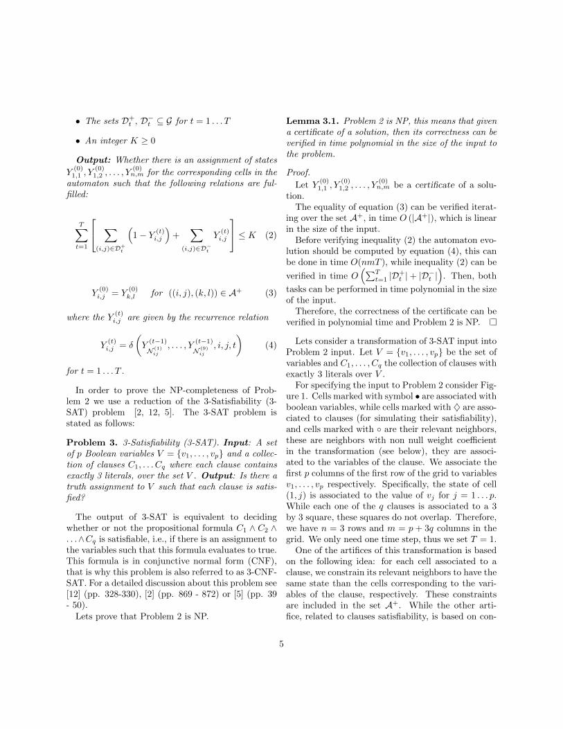
Lemma 3.1. Problem 2 is NP, this means that givena certificate of a solution, then its correctness can beverified in time polynomial in the size of the input tothe problem.

Proof.

Let Y(0)1,1 , Y

(0)1,2 , . . . , Y

(0)n,m be a certificate of a solu-

tion.The equality of equation (3) can be verified iterat-

ing over the set A+, in time O (|A+|), which is linearin the size of the input.

Before verifying inequality (2) the automaton evo-lution should be computed by equation (4), this canbe done in time O(nmT ), while inequality (2) can be

verified in time O(∑T

t=1 |D+t |+ |D−t |

). Then, both

tasks can be performed in time polynomial in the sizeof the input.

Therefore, the correctness of the certificate can beverified in polynomial time and Problem 2 is NP.

Lets consider a transformation of 3-SAT input intoProblem 2 input. Let V = {v1, . . . , vp} be the set ofvariables and C1, . . . , Cq the collection of clauses withexactly 3 literals over V .

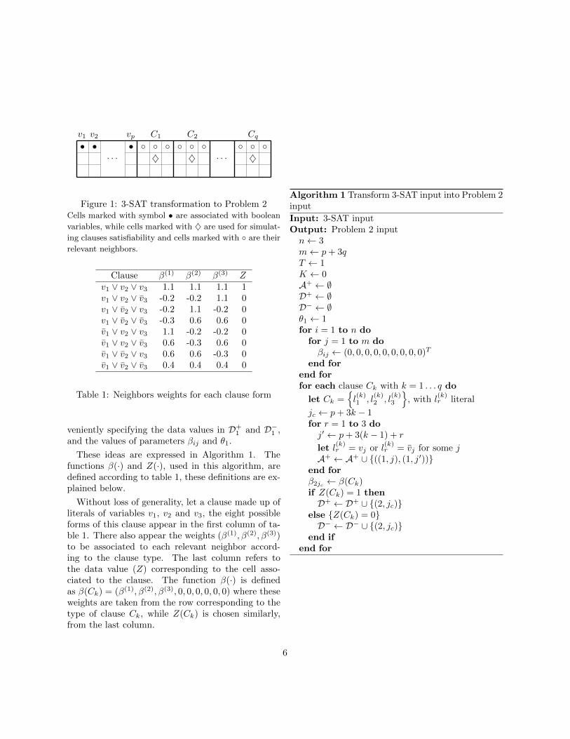
For specifying the input to Problem 2 consider Fig-ure 1. Cells marked with symbol • are associated withboolean variables, while cells marked with ♦ are asso-ciated to clauses (for simulating their satisfiability),and cells marked with ◦ are their relevant neighbors,these are neighbors with non null weight coefficientin the transformation (see below), they are associ-ated to the variables of the clause. We associate thefirst p columns of the first row of the grid to variablesv1, . . . , vp respectively. Specifically, the state of cell(1, j) is associated to the value of vj for j = 1 . . . p.While each one of the q clauses is associated to a 3by 3 square, these squares do not overlap. Therefore,we have n = 3 rows and m = p + 3q columns in thegrid. We only need one time step, thus we set T = 1.

One of the artifices of this transformation is basedon the following idea: for each cell associated to aclause, we constrain its relevant neighbors to have thesame state than the cells corresponding to the vari-ables of the clause, respectively. These constraintsare included in the set A+. While the other arti-fice, related to clauses satisfiability, is based on con-

5

. . . . . .

v1 v2 vp C1 C2 Cq

• • • ◦ ◦ ◦ ◦ ◦ ◦ ◦ ◦ ◦♦ ♦ ♦

Figure 1: 3-SAT transformation to Problem 2Cells marked with symbol • are associated with boolean

variables, while cells marked with ♦ are used for simulat-

ing clauses satisfiability and cells marked with ◦ are their

relevant neighbors.

Clause β(1) β(2) β(3) Zv1 ∨ v2 ∨ v3 1.1 1.1 1.1 1v1 ∨ v2 ∨ v3 -0.2 -0.2 1.1 0v1 ∨ v2 ∨ v3 -0.2 1.1 -0.2 0v1 ∨ v2 ∨ v3 -0.3 0.6 0.6 0v1 ∨ v2 ∨ v3 1.1 -0.2 -0.2 0v1 ∨ v2 ∨ v3 0.6 -0.3 0.6 0v1 ∨ v2 ∨ v3 0.6 0.6 -0.3 0v1 ∨ v2 ∨ v3 0.4 0.4 0.4 0

Table 1: Neighbors weights for each clause form

veniently specifying the data values in D+1 and D−1 ,

and the values of parameters βij and θ1.

These ideas are expressed in Algorithm 1. Thefunctions β(·) and Z(·), used in this algorithm, aredefined according to table 1, these definitions are ex-plained below.

Without loss of generality, let a clause made up ofliterals of variables v1, v2 and v3, the eight possibleforms of this clause appear in the first column of ta-ble 1. There also appear the weights (β(1), β(2), β(3))to be associated to each relevant neighbor accord-ing to the clause type. The last column refers tothe data value (Z) corresponding to the cell asso-ciated to the clause. The function β(·) is definedas β(Ck) = (β(1), β(2), β(3), 0, 0, 0, 0, 0, 0) where theseweights are taken from the row corresponding to thetype of clause Ck, while Z(Ck) is chosen similarly,from the last column.

Algorithm 1 Transform 3-SAT input into Problem 2input

Input: 3-SAT inputOutput: Problem 2 inputn← 3m← p+ 3qT ← 1K ← 0A+ ← ∅D+ ← ∅D− ← ∅θ1 ← 1for i = 1 to n do

for j = 1 to m doβij ← (0, 0, 0, 0, 0, 0, 0, 0, 0)T

end forend forfor each clause Ck with k = 1 . . . q do

let Ck ={l(k)1 , l

(k)2 , l

(k)3

}, with l

(k)r literal

jc ← p+ 3k − 1for r = 1 to 3 doj′ ← p+ 3(k − 1) + r

let l(k)r = vj or l

(k)r = vj for some j

A+ ← A+ ∪ {((1, j), (1, j′))}end forβ2jc ← β(Ck)if Z(Ck) = 1 thenD+ ← D+ ∪ {(2, jc)}

else {Z(Ck) = 0}D− ← D− ∪ {(2, jc)}

end ifend for

6

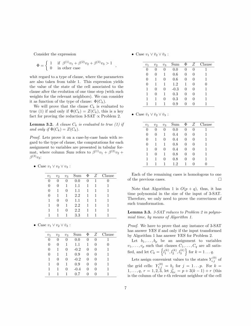
Consider the expression

Φ =

{1 if β(1)v1 + β(2)v2 + β(3)v3 > 10 in other case

,

whit regard to a type of clause, where the parametersare also taken from table 1. This expression yieldsthe value of the state of the cell associated to theclause after the evolution of one time step (with suchweights for the relevant neighbors). We can considerit as function of the type of clause: Φ(Ck).

We will prove that the clause Ck is evaluated totrue (1) if and only if Φ(Ck) = Z(Ck), this is a keyfact for proving the reduction 3-SAT ∝ Problem 2.

Lemma 3.2. A clause Ck is evaluated to true (1) ifand only if Φ(Ck) = Z(Ck).

Proof. Lets prove it on a case-by-case basis with re-gard to the type of clause, the computations for eachassignment to variables are presented in tabular for-mat, where column Sum refers to β(1)v1 + β(2)v2 +β(3)v3:

• Case v1 ∨ v2 ∨ v3 :

v1 v2 v3 Sum Φ Z Clause0 0 0 0.0 0 1 00 0 1 1.1 1 1 10 1 0 1.1 1 1 10 1 1 2.2 1 1 11 0 0 1.1 1 1 11 0 1 2.2 1 1 11 1 0 2.2 1 1 11 1 1 3.3 1 1 1

• Case v1 ∨ v2 ∨ v3 :

v1 v2 v3 Sum Φ Z Clause0 0 0 0.0 0 0 10 0 1 1.1 1 0 00 1 0 -0.2 0 0 10 1 1 0.9 0 0 11 0 0 -0.2 0 0 11 0 1 0.9 0 0 11 1 0 -0.4 0 0 11 1 1 0.7 0 0 1

• Case v1 ∨ v2 ∨ v3 :

v1 v2 v3 Sum Φ Z Clause0 0 0 0.0 0 0 10 0 1 0.6 0 0 10 1 0 0.6 0 0 10 1 1 1.2 1 0 01 0 0 -0.3 0 0 11 0 1 0.3 0 0 11 1 0 0.3 0 0 11 1 1 0.9 0 0 1

• Case v1 ∨ v2 ∨ v3 :

v1 v2 v3 Sum Φ Z Clause0 0 0 0.0 0 0 10 0 1 0.4 0 0 10 1 0 0.4 0 0 10 1 1 0.8 0 0 11 0 0 0.4 0 0 11 0 1 0.8 0 0 11 1 0 0.8 0 0 11 1 1 1.2 1 0 0

Each of the remaining cases is homologous to oneof the previous cases.

Note that Algorithm 1 is O(p + q), thus, it hastime polynomial in the size of the input of 3-SAT.Therefore, we only need to prove the correctness ofsuch transformation.

Lemma 3.3. 3-SAT reduces to Problem 2 in polyno-mial time, by means of Algorithm 1.

Proof. We have to prove that any instance of 3-SAThas answer YES if and only if the input transformedby Algorithm 1 has answer YES for Problem 2.

Let b1, . . . , bp be an assignment to variablesv1, . . . , vp such that clauses C1, . . . , Cq are all satis-

fied, and let Ck ={l(k)1 , l

(k)2 , l

(k)3

}for k = 1 . . . q.

Lets assign convenient values to the states Y(0)i,j of

the grid cells: Y(0)1,j = bj for j = 1 . . . p. For k =

1, . . . , q, r = 1, 2, 3, let j′kr = p + 3(k − 1) + r (thisis the column of the r-th relevant neighbor of the cell

7

associated to clause Ck), we set Y(0)1,j′kr

= bj where

either l(k)r = vj or l

(k)r = vj for some j, 1 ≤ j ≤ p.

The remaining states that have not been assigneda value are not relevant for this proof, thus, they canbe assigned any value.

From the construction of the set A+ in Algorithm

1 and the election of the Y(0)i,j , the constraints from

equation (3) are fulfilled.Let Ck be one of the clauses, in Algorithm 1 it was

associated to the cell(

2, j(k)c

)where j

(k)c = p+3k−1,

and the weight coefficients β2j

(k)c

were setted as β(Ck)

according to table 1. Since Ck evaluates to true, from

lemma 3.2 and the election of Y(0)i,j , we have Y

(1)

2,j(k)c

=

Z(Ck), thus its contribution to the sum from equation(2) is zero. We can say this for any k = 1, . . . , q,hence, the inequality of equation (2) is fulfilled andthere is a YES answer for the transformed input of3-SAT.

Lets consider the opposite direction, i.e., lets sup-pose that the answer for the transformed input is

YES. We want to prove that if we set bj = Y(0)1j for

j = 1, . . . , p, this assignment to variables satisfies ev-ery clause.

Lets concentrate on clause Ck. Since the con-straints in the set A+ are satisfied, the neighbors

of cell(

2, j(k)c

)are assigned states corresponding to

the values of the variables of Ck. Furthermore, the

inequality of equation (2) is satisfied, then Y(1)

2j(k) =

Z(Ck), and from lemma 3.2 we have that Ck is eval-uated to true. Since this can be generalized for everyclause, there is also a YES answer for 3-SAT.

Therefore, we conclude that 3-SAT ∝ Problem 2.

Theorem 3.4. NP-completeness. Problem 2 is NP-complete.

Proof. The proof is direct from lemmas 3.1 and 3.3.

4 Genetic Algorithm

Since Problem 2 is NP-complete, it does not seem tohave an efficient (polynomial) solution, and an ex-

haustive enumeration is not viable. That is why wepropose a genetic algorithm approach for addressingProblem 1.

Genetic algorithms (GAs) are a family of domain-independent adaptive meta-heuristics routinely usedin search and optimization problems, both for con-tinuous and discrete functions.

Much of the interest in GAs is due to the fact thatthey are a significant improvement over traditionalmethods without the need for incorporating highlydomain-specific knowledge. There is considerable ev-idence that genetic algorithms are useful for globalfunction optimization and NP-hard problems. [8]

GAs mimic the genetic change in the evolution pro-cess of a population of individuals. According to Dar-win’s theory of evolution, in an environment that canhost only a limited number of individuals, given thebasic instinct of individuals to reproduce, selectionbecomes inevitable if the population size is not togrow exponentially. Natural selection favours thoseindividuals that compete for the given resources mosteffectively, in other words, those that are adapted orfit to the environmental conditions best. This phe-nomenon is known as survival of the fittest. [3]

The other primary force identified by Darwin re-sults from phenotypic variations among members ofthe population. Each individual represents an uniquecombination of phenotypic traits that is evaluated bythe environment. If it evaluates favourably, then itis propagated via the individual’s offspring, other-wise it is discarded by dying without offspring. Dar-win’s insight was that small, random variations (mu-tations) in phenotypic traits occur during reproduc-tion from generation to generation. Through thesevariations, new combinations of traits occur and getevaluated. [3]

In a GA, individuals, also called strings or chro-mosomes, are made of units (genes, features, charac-ters) which control the inheritance of one or severalcharacters [11]. Individuals are computationally rep-resented by means of a domain or problem specificencoding function.

Designing a GA involves specifying the followingelements:

1. an encoding: for computationally representing

8

individuals;

2. a notion of fitness: expresses the extent to whichan individual is adapted to its environment;

3. a selection operator: controls which individualssurvive and have the opportunity of reproducing;

4. a crossover operator: forms offspring by com-bining the genetic information from the parents;and

5. a mutation operator: randomly alters the valuesof some genes in a chromosome.

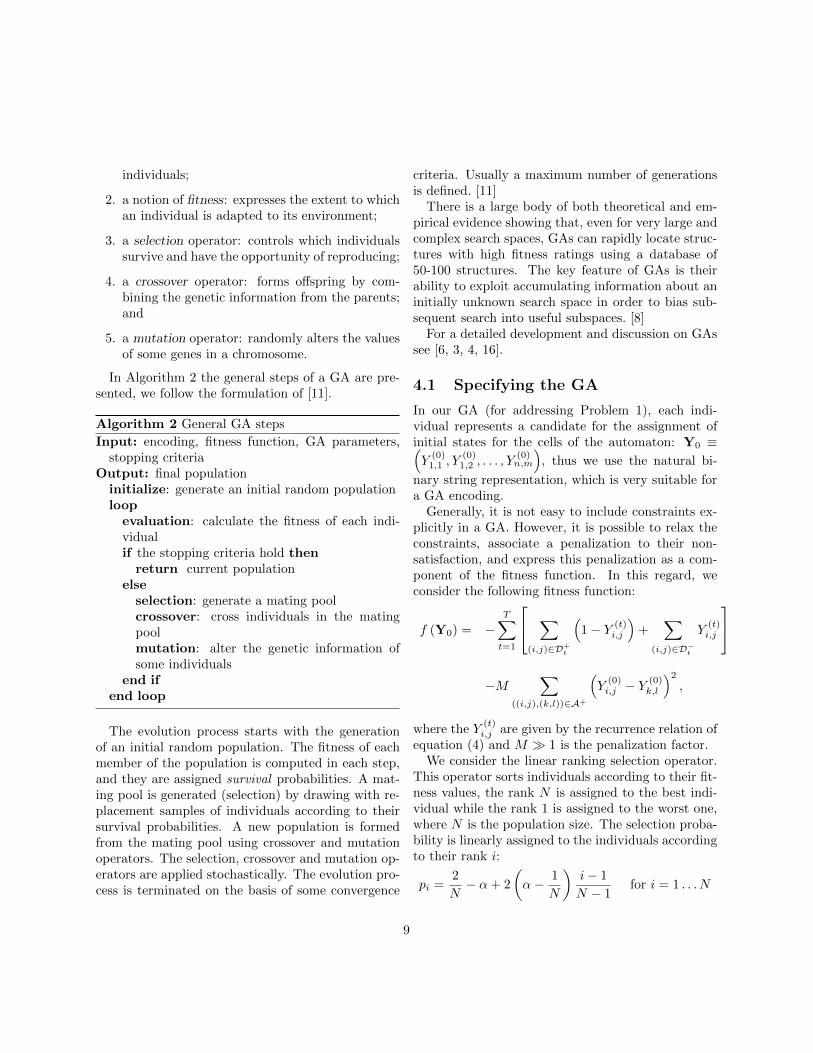
In Algorithm 2 the general steps of a GA are pre-sented, we follow the formulation of [11].

Algorithm 2 General GA steps

Input: encoding, fitness function, GA parameters,stopping criteria

Output: final populationinitialize: generate an initial random populationloopevaluation: calculate the fitness of each indi-vidualif the stopping criteria hold then

return current populationelseselection: generate a mating poolcrossover: cross individuals in the matingpoolmutation: alter the genetic information ofsome individuals

end ifend loop

The evolution process starts with the generationof an initial random population. The fitness of eachmember of the population is computed in each step,and they are assigned survival probabilities. A mat-ing pool is generated (selection) by drawing with re-placement samples of individuals according to theirsurvival probabilities. A new population is formedfrom the mating pool using crossover and mutationoperators. The selection, crossover and mutation op-erators are applied stochastically. The evolution pro-cess is terminated on the basis of some convergence

criteria. Usually a maximum number of generationsis defined. [11]

There is a large body of both theoretical and em-pirical evidence showing that, even for very large andcomplex search spaces, GAs can rapidly locate struc-tures with high fitness ratings using a database of50-100 structures. The key feature of GAs is theirability to exploit accumulating information about aninitially unknown search space in order to bias sub-sequent search into useful subspaces. [8]

For a detailed development and discussion on GAssee [6, 3, 4, 16].

4.1 Specifying the GA

In our GA (for addressing Problem 1), each indi-vidual represents a candidate for the assignment ofinitial states for the cells of the automaton: Y0 ≡(Y

(0)1,1 , Y

(0)1,2 , . . . , Y

(0)n,m

), thus we use the natural bi-

nary string representation, which is very suitable fora GA encoding.

Generally, it is not easy to include constraints ex-plicitly in a GA. However, it is possible to relax theconstraints, associate a penalization to their non-satisfaction, and express this penalization as a com-ponent of the fitness function. In this regard, weconsider the following fitness function:

f (Y0) = −T∑

t=1

∑(i,j)∈D+

t

(1− Y (t)

i,j

)+

∑(i,j)∈D−t

Y(t)i,j

−M

∑((i,j),(k,l))∈A+

(Y

(0)i,j − Y

(0)k,l

)2,

where the Y(t)i,j are given by the recurrence relation of

equation (4) and M � 1 is the penalization factor.We consider the linear ranking selection operator.

This operator sorts individuals according to their fit-ness values, the rank N is assigned to the best indi-vidual while the rank 1 is assigned to the worst one,where N is the population size. The selection proba-bility is linearly assigned to the individuals accordingto their rank i:

pi =2

N− α+ 2

(α− 1

N

)i− 1

N − 1for i = 1 . . . N

9

where α ∈(

1N ,

2N

)is the selection probability for

the best individual. Note that the selection probabil-ity for the worst individual p1 is 2

N − α. We choose

α = 2(N−2)N(N−1) , this yields p1 = 2

N(N−1) , and the rate

best/worst selection probability is α/p1 = N − 2.

We consider the single point crossover operator andthe uniform random mutation operator. The singlepoint crossover operator selects an (admissible) ran-dom index for splitting up the parent strings, and thedata beyond that index in either individual strings isswapped between them. While the uniform randommutation operator alters a chromosome by flippingone of its bits, chosen random and uniformly. Theprobabilities of crossover between a pair of chromo-somes and mutation of a chromosome are controlledby the parameters ρc and ρm respectively.

4.2 Software

In this work, all the computations have been per-formed using the platform R [10]. R is a free softwareproject that provides a framework for computationalstatistics and graphics generation, over a program-ming language of the same name. It is widely usedby researchers from diverse disciplines, due to thecomputation facilities it offers, its availability for sev-eral operating systems, as well as the large numberof packages of specific purpose available in its repos-itories.

In particular, we used the R package GA [11]. Thispackage is a collection of general purpose functionsthat provide a flexible set of tools for applying a widerange of genetic algorithm methods.

4.3 Simulated instances

In order to test our GA we generate 50 random in-stances of Problem 1. Every instance has the samesize, with n = m = T = 10.

Since we want to assess the algorithm precision,we need to know the true optima. Hence, for eachinstance we randomly generate an initial configura-tion of states for the automaton Y0, by drawing cellstates independently from a Bernoulli distributionBern(0.5).

For each instance, the parameters β(k)ij and θt

are drawn from Gaussian distributions: N (0, 1) andN (0, 4.5), respectively.

Note that with such scheme of distributions weguarantee that θ1 has the same distribution as thesum

9∑k=1

β(k)ij Y

(0)

N (k)ij

,

for each cell (i, j) with i = 1 . . . n and j = 1 . . .m,

then the Y(1)i,j also have a Bernoulli distribution

Bern(0.5) (but they are not necessarily independent).

We perform the automaton evolution according to(4) for T time steps. We build the constraints set A+,by choosing a simple random sample, with replace-ment, of nm/2 pairs of cells, if the cells in a pair havedifferent states for time 0 (given by the assignmentY0) the pair is discarded. In consequence, |A+| hasa expected value of nm/4.

In order to build the data sets we choose a simplerandom sample of size nmT/4 over the states of cellsat any time, i.e., for i = 1 . . . n, j = 1 . . .m and

t = 1 . . . T . If a state Y(t)i,j from the sample has value

1 the pair (i, j) is inserted inD+t , otherwise (Y

(t)i,j = 0)

(i, j) is inserted in D−t . Hence, we have |D+t |+|D−t | =

nmT/4.

The constraints penalization M is set to nm.

Given this selection of the instances of the problem,we ensure that all of them have optimum value of 0 forthe fitness function, and we can compare this valuewith the results obtained with the GA.

4.4 Results

The GA parameters are set as follows:

Parameter Valuepopulation size N 50number of generations 100crossover probability ρc 0.8mutation probability ρm 0.8

Then the selection probability for the best individ-ual is α = 0.03918367 and the homologous for theworst individual is p1 = 0.00081632.

10

Histogram of maximum fitness

Maximum fitness

Fre

quen

cy

−200 −150 −100 −50 0

02

46

810

1214

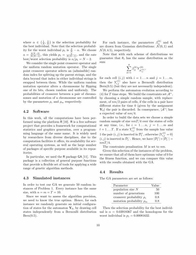
Figure 2: Histogram of the fitness of the best indi-vidual for each instance

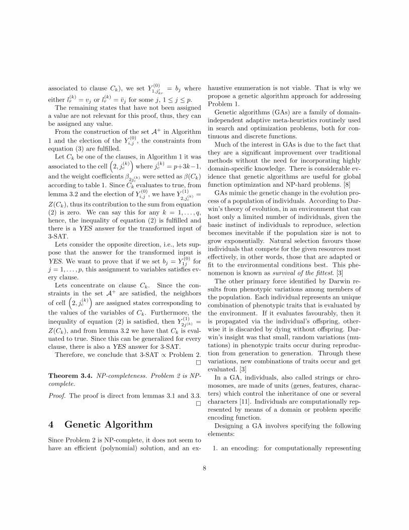
We consider as solution of an instance, the indi-vidual of maximum fitness (any of them if it is notunique) yielded by the GA when the instance is spec-ified as input, regardless whether it is feasible (in thesense of satisfying the constraints) or not.

After running the GA for the 50 instances, 39 ofthem (78%) yielded feasible solutions. While forthe remaining 11 (non-feasible) solutions, at mosttwo constraints were not satisfied. For the feasi-ble solutions the maximum fitness was at least -12,this means that the maximum number of state mis-matches with regard to the data was 12 (4.8% of thedata size: 250). Furthermore, the GA found optimalsolutions for 6 instances.

In Figure 2 a histogram of the maximum fitnessyielded by the GA for each instance is presented. Thegaps observed are due to the constraints penalizationfactor. A concentration pattern can be observed nearthe optimum.

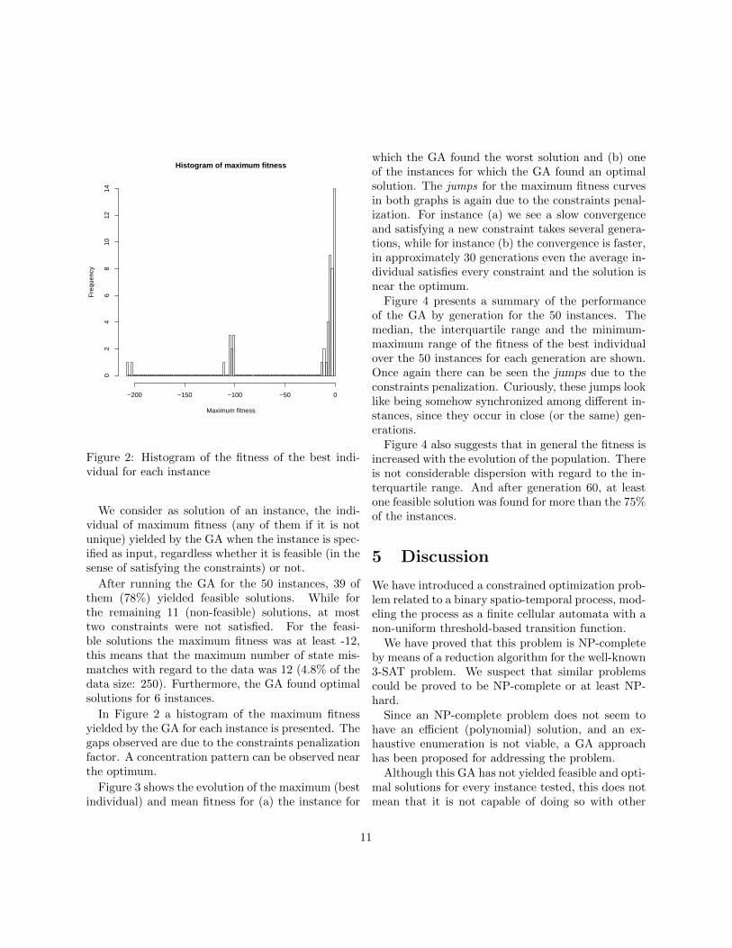
Figure 3 shows the evolution of the maximum (bestindividual) and mean fitness for (a) the instance for

which the GA found the worst solution and (b) oneof the instances for which the GA found an optimalsolution. The jumps for the maximum fitness curvesin both graphs is again due to the constraints penal-ization. For instance (a) we see a slow convergenceand satisfying a new constraint takes several genera-tions, while for instance (b) the convergence is faster,in approximately 30 generations even the average in-dividual satisfies every constraint and the solution isnear the optimum.

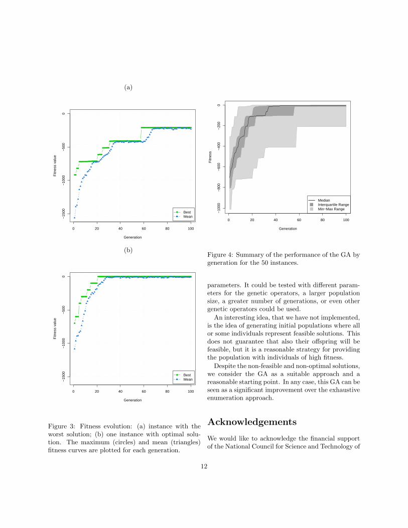
Figure 4 presents a summary of the performanceof the GA by generation for the 50 instances. Themedian, the interquartile range and the minimum-maximum range of the fitness of the best individualover the 50 instances for each generation are shown.Once again there can be seen the jumps due to theconstraints penalization. Curiously, these jumps looklike being somehow synchronized among different in-stances, since they occur in close (or the same) gen-erations.

Figure 4 also suggests that in general the fitness isincreased with the evolution of the population. Thereis not considerable dispersion with regard to the in-terquartile range. And after generation 60, at leastone feasible solution was found for more than the 75%of the instances.

5 Discussion

We have introduced a constrained optimization prob-lem related to a binary spatio-temporal process, mod-eling the process as a finite cellular automata with anon-uniform threshold-based transition function.

We have proved that this problem is NP-completeby means of a reduction algorithm for the well-known3-SAT problem. We suspect that similar problemscould be proved to be NP-complete or at least NP-hard.

Since an NP-complete problem does not seem tohave an efficient (polynomial) solution, and an ex-haustive enumeration is not viable, a GA approachhas been proposed for addressing the problem.

Although this GA has not yielded feasible and opti-mal solutions for every instance tested, this does notmean that it is not capable of doing so with other

11

(a)

0 20 40 60 80 100

−15

00−

1000

−50

00

Generation

Fitn

ess

valu

e

● ●

● ●

● ● ● ● ● ● ● ● ● ● ● ● ● ● ● ●

● ● ● ●

● ● ● ● ● ●

● ● ● ● ● ● ● ● ● ● ● ● ● ● ● ● ● ● ● ● ● ● ● ● ● ● ●

● ● ● ● ● ● ● ● ● ● ● ● ● ● ● ● ● ● ● ● ● ● ● ● ● ● ● ● ● ● ● ● ● ● ● ● ● ● ● ● ● ● ●

● BestMean

(b)

0 20 40 60 80 100

−15

00−

1000

−50

00

Generation

Fitn

ess

valu

e

●

● ● ●

● ●

● ● ● ● ●

● ● ●

● ● ● ● ● ●

● ● ● ● ● ● ● ● ● ● ● ● ● ● ● ● ● ● ● ● ● ● ● ● ● ● ● ● ● ● ● ● ● ● ● ● ● ● ● ● ● ● ● ● ● ● ● ● ● ● ● ● ● ● ● ● ● ● ● ● ● ● ● ● ● ● ● ● ● ● ● ● ● ● ● ● ● ● ● ●

● BestMean

Figure 3: Fitness evolution: (a) instance with theworst solution; (b) one instance with optimal solu-tion. The maximum (circles) and mean (triangles)fitness curves are plotted for each generation.

0 20 40 60 80 100−

1000

−80

0−

600

−40

0−

200

0

Generation

Fitn

ess

MedianInterquartile RangeMin−Max Range

Figure 4: Summary of the performance of the GA bygeneration for the 50 instances.

parameters. It could be tested with different param-eters for the genetic operators, a larger populationsize, a greater number of generations, or even othergenetic operators could be used.

An interesting idea, that we have not implemented,is the idea of generating initial populations where allor some individuals represent feasible solutions. Thisdoes not guarantee that also their offspring will befeasible, but it is a reasonable strategy for providingthe population with individuals of high fitness.

Despite the non-feasible and non-optimal solutions,we consider the GA as a suitable approach and areasonable starting point. In any case, this GA can beseen as a significant improvement over the exhaustiveenumeration approach.

Acknowledgements

We would like to acknowledge the financial supportof the National Council for Science and Technology of

12

Mexico (CONACyT) for the fulfillment of this work.

References

[1] Bastien Chopard and Michel Droz. Cellular Au-tomata Modeling of Physical Systems. Cam-bridge University Press, Cambridge, UnitedKingdom, 1998.

[2] Thomas H. Cormen, Charles E. Leiserson,Ronald L. Rivest, and Clifford Stein. Introduc-tion to Algorithms, Second Edition. The MITPress, Cambridge, Massachusetts London, Eng-land, 2001.

[3] Smith J.E. Eiben Agoston E. Introductionto Evolutionary Computing. Springer-Verlag,Berlin, 2003.

[4] David B. Fogel. Evolutionary computation: to-ward a new philosophy of machine intelligence.Third edition. Jhon Wiley & Sons Inc., Hoboken,New Jersey, 2006.

[5] Michael R. Garey and David S. Johnson. Com-puters and Intractability: A Guide to the Theoryof NP-Completeness. W. H. Freeman, New York,USA, 1979.

[6] Randy L. Haupt and Sue Ellen Haupt. PracticalGenetic Algorithms. 2nd edition. John Wiley &Sons, New York, 2004.

[7] Mevin B. Hooten and Christopher K. Wikle.Statistical agent-based models for discretespatio-temporal systems. Journal of the Amer-ican Statistical Association, 105(489):236–248,March 2010.

[8] Kenneth De Jong. Learning with genetic algo-rithms: An overview. Machine Learning, 3:121–138, 1988.

[9] Xia Li and Anthony G. Yeh. Modelling sus-tainable urban development by the integrationof constrained cellular automata and gis. Int.J. Geographical Information Science, 14(2):131–152, 2000.

[10] R Development Core Team. R: A Language andEnvironment for Statistical Computing. R Foun-dation for Statistical Computing, Vienna, Aus-tria, 2013. ISBN 3-900051-07-0.

[11] Luca Scrucca. GA: A package for genetic al-gorithms in R. Journal of Statistical Software,53(4):1–37, 2013.

[12] Steven S. Skiena. The Algorithm Design Man-ual, Second Edition. Springer-Verlag, New York,2008.

[13] Stephen Wolfram. Statistical mechanics of cel-lular automata. Reviews of Modern Physics,55(3):601–644, July 1983.

[14] Stephen Wolfram. Cellular automata as modelsof complexity. Nature, 311(4):419–424, October1984.

[15] Stephen Wolfram. Cellular automaton fluids1: Basic theory. Journal of Statistical Physics,45(3/4):471–526, November 1986.

[16] Xinjie Yu and Mitsuo Gen. Introduction to Evo-lutionary Algorithms. Springer-Verlag, Heidel-berg, Berlin, 2010.

13