Embed Size (px)
Citation preview

arX
iv:c
s/03
0705
0v1
[cs
.AI]
21
Jul 2
003
A ternary Relation Algebra of directed lines
Amar Isli
Fachbereich Informatik, Universitat Hamburg,Vogt-Kolln-Strasse 30, D-22527 Hamburg, Germany
Abstract
We define a ternary Relation Algebra (RA) of relative position relations on two-dimensional directed lines (d-lines for short). A d-line has two degrees of freedom(DFs): a rotational DF (RDF), and a translational DF (TDF). The representationof the RDF of a d-line will be handled by an RA of 2D orientations, CYCt, knownin the literature. A second algebra, T At, which will handle the TDF of a d-line,will be defined. The two algebras, T At and CYCt, will constitute, respectively, thetranslational and the rotational components of the RA, PAt, of relative positionrelations on d-lines: the PAt atoms will consist of those pairs 〈t, r〉 of a T At atomand a CYCt atom that are compatible. We present in detail the RA PAt, with itsconverse table, its rotation table and its composition tables. We show that a (poly-nomial) constraint propagation algorithm, known in the literature, is complete for asubset of PAt relations including almost all of the atomic relations. We will discussthe application scope of the RA, which includes incidence geometry, GIS (Geo-graphic Information Systems), shape representation, localisation in (multi-)robotnavigation, and the representation of motion prepositions in NLP (Natural Lan-guage Processing). We then compare the RA to existing ones, such as an algebrafor reasoning about rectangles parallel to the axes of an (orthogonal) coordinate sys-tem, a “spatial Odyssey” of Allen’s interval algebra, and an algebra for reasoningabout 2D segments.
Key words: Relation algebra, Spatial reasoning, Qualitative reasoning, Geometricreasoning, Constraint satisfaction, Knowledge representation.
⋆ This work was supported partly by the DFG project “Description Logics andSpatial reasoning” (DLS), under grant NE 279/8-1, and partly by the EU project“Cognitive Vision systems” (CogVis), under grant CogVis IST 2000-29375.
Preprint submitted to Elsevier Preprint 1 February 2008

1 Introduction
Qualitative Spatial Reasoning (QSR), and more generally Qualitative Rea-soning (QR), distinguishes from quantitative reasoning by its particularity ofremaining at a description level as high as possible. In other words, QSR sticksat the idea of “making only as many distinctions as necessary” [11,20], ideaborrowed to naıve physics [27]. The core motivation behind this is that, when-ever the number of distinctions that need to be made is finite, the reasoningissue can get rid of the calculations details of quantitative models, and betransformed into a simple matter of symbols manipulation; in the particularcase of constraint-based spatial and temporal reasoning, this means a finiterelation algebra (finite RA), with tables recording the results of applying thedifferent operations to the different atoms, and the reasoning issue reduced toa matter of table look-ups: the best illustration to this is certainly Allen’s [1]algebra of time intervals.
The main problem in designing a QSR language is certainly to come up withthe right, cognitively adequate, distinctions that need to be made; this prob-lem is often referred to as the qualitative/quantitative dilemma, or the finite-ness/density dilemma [25] (how to distinguish between the infinite numberof elements of an —infinite— universe using only a finite number of distinc-tions?): to say it another way, because such a language can make only a finitenumber of distinctions, it should reflect as good as possible the real world;ideally, such a language would be such that it distinguishes between two situ-ations if and only if Humans, or the agents expected to use the language, dodistinguish between the two situations. Qualitative reasoning had to face criti-cism —examples include Forbus, Nielsen and Faltings’ [18] poverty conjecture,or Habel’s [25] argument that such a language, even when built according tocognitive adequacy criteria, still suffers from not having “the ability to refinediscrete structures if necessary”. The tendency has since then changed, duecertainly to the success gained by QSR in real applications, such as GIS, robotnavigation, or shape description.
QSR has now its place in AI. Its research has focussed for about a decade onaspects such as topology, orientation and distance. The aspect the most devel-oped so far is topology, illustrated by the well-known RCC theory [51], fromwhich derives the RCC-8 calculus [51,16]. The RCC theory, on the other hand,stems from Clarke’s “calculus of individuals” [9], based on a binary “connectedwith” relation —sharing of a point of the arguments. Clarke’s work, in turn,was developed from classical mereology [42,43] and Whitehead’s “extension-ally connected with” relation [60]. The huge interest, the last couple of years,in applications such as robot navigation, illustrated by active and promisingRoboCup soccer meetings at the main AI conferences (IJCAI, AAAI: see,for instance, [54] for RoboCup’99), had and still have as a consequence that
2

relative orientation, and, more generally, relative position, considered as ex-pressing more specific knowledge, are gaining increasing interest from the QSRcommunity.
The research in QSR has reached a point where the integration of different as-pects of knowledge, such as relative orientation and relative distance, topologyand orientation, or, as in the present work, relative orientation and relativetranslation, is more than needed, in order to face the new demand of realapplications. Such an integration of different aspects of knowledge is seen asposition, because a calculus coming from such a combination, if it cannot rep-resent the position of an object as precisely as do quantitative models, yetprovides a representation more specific than the ones of the combined calculi.It seems to be the case that all researchers in the area are aware of the prob-lem [11,17,19,20]. When looking at what has really been achieved so far in thisdirection, apart from the work in [10], and, more recently, the one in [23], notmuch can be said.
In this work, we consider the geometric element consisting of a (2-dimensional)directed line (d-line for short). Such an element has two degrees of freedom(DFs) [26,38]: a rotational DF (RDF) and a translational DF (TDF). TheRDF, on the one hand, constrains the way a d-line can rotate relative toanother d-line (relative orientation); the TDF, on the other hand, constrainsthe way a d-line can translate relative to another, or other, d-lines, so that oncethe RDF of a d-line, say ℓ1, has been “absorbed” (i.e., its orientation has beenfixed), we know how to translate ℓ1 (a move parallel to the orientation), sothat its desired position gets fixed, and its TDF absorbed (e.g., translate ℓ1 sothat its intersecting point with a second d-line ℓ2 comes before the intersectingpoint of a third d-line ℓ3 with ℓ2, when we walk along ℓ2 heading the positivedirection; or so that ℓ1 is parallel to both, and does not lie between, ℓ2 and ℓ3).We can right now notice a point of high importance for the TDF of d-lines,which is that their oriented-ness makes them much richer than undirectedlines, or u-lines: contrary to u-lines:
(1) when walking along a d-line, we know whether we are heading the positiveor the negative direction; and
(2) when walking perpendicularly to a d-line, we know whether we are head-ing towards the right half-plane or towards the left half-plane boundedby the d-line.
We provide a ternary Relation Algebra (RA), PAt, of relative position rela-tions on d-lines; the way we proceed is, somehow, imposed by the two DFs ofa d-line:
(1) a ternary RA of 2D orientations, CYCt, recently known in the literature[35,36], will be the rotational component of PAt; and
3
(2) a second ternary algebra, T At, which will constitute the translationalcomponent of PAt, will be defined.
The PAt atoms will consist of those pairs 〈t, r〉 of a T At atom and a CYCt
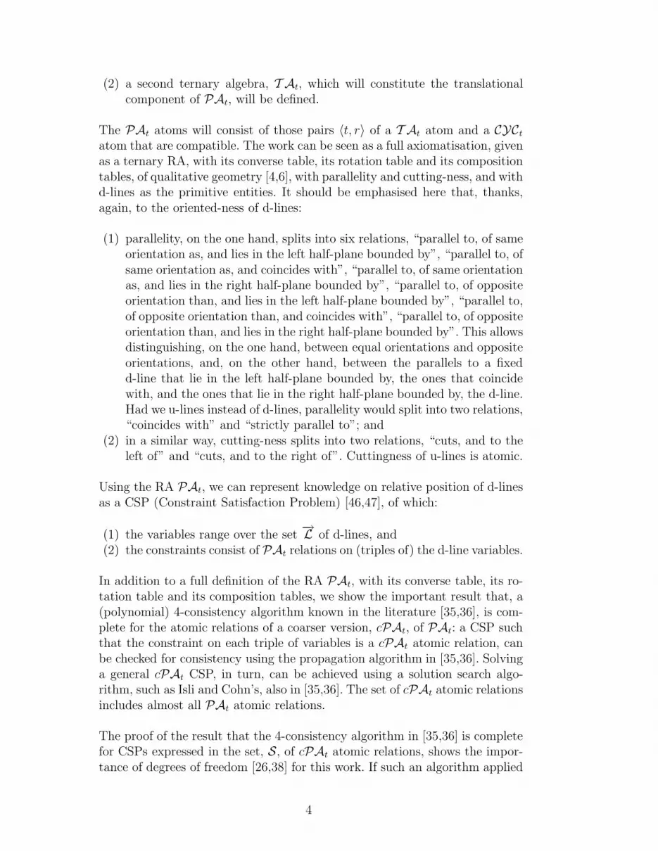
atom that are compatible. The work can be seen as a full axiomatisation, givenas a ternary RA, with its converse table, its rotation table and its compositiontables, of qualitative geometry [4,6], with parallelity and cutting-ness, and withd-lines as the primitive entities. It should be emphasised here that, thanks,again, to the oriented-ness of d-lines:
(1) parallelity, on the one hand, splits into six relations, “parallel to, of sameorientation as, and lies in the left half-plane bounded by”, “parallel to, ofsame orientation as, and coincides with”, “parallel to, of same orientationas, and lies in the right half-plane bounded by”, “parallel to, of oppositeorientation than, and lies in the left half-plane bounded by”, “parallel to,of opposite orientation than, and coincides with”, “parallel to, of oppositeorientation than, and lies in the right half-plane bounded by”. This allowsdistinguishing, on the one hand, between equal orientations and oppositeorientations, and, on the other hand, between the parallels to a fixedd-line that lie in the left half-plane bounded by, the ones that coincidewith, and the ones that lie in the right half-plane bounded by, the d-line.Had we u-lines instead of d-lines, parallelity would split into two relations,“coincides with” and “strictly parallel to”; and
(2) in a similar way, cutting-ness splits into two relations, “cuts, and to theleft of” and “cuts, and to the right of”. Cuttingness of u-lines is atomic.
Using the RA PAt, we can represent knowledge on relative position of d-linesas a CSP (Constraint Satisfaction Problem) [46,47], of which:
(1) the variables range over the set−→L of d-lines, and
(2) the constraints consist of PAt relations on (triples of) the d-line variables.
In addition to a full definition of the RA PAt, with its converse table, its ro-tation table and its composition tables, we show the important result that, a(polynomial) 4-consistency algorithm known in the literature [35,36], is com-plete for the atomic relations of a coarser version, cPAt, of PAt: a CSP suchthat the constraint on each triple of variables is a cPAt atomic relation, canbe checked for consistency using the propagation algorithm in [35,36]. Solvinga general cPAt CSP, in turn, can be achieved using a solution search algo-rithm, such as Isli and Cohn’s, also in [35,36]. The set of cPAt atomic relationsincludes almost all PAt atomic relations.
The proof of the result that the 4-consistency algorithm in [35,36] is completefor CSPs expressed in the set, S, of cPAt atomic relations, shows the impor-tance of degrees of freedom [26,38] for this work. If such an algorithm applied
4

to such a CSP does not derive the empty relation —in which case, the resultsays that the CSP is consistent— then, in order to find a spatial scene that isa model of the CSP, we can proceed as follows:
(1) Start by getting the RDF absorbed for each of the d-line variables in-volved in the CSP. In other words, start by fixing the orientation for eachof the variables. This can be done using a result in [35,36], stating thata 4-consistent atomic CSP of 2D orientations is (globally) consistent: theproof of this result gives a backtrack-free method for the construction ofa solution to such a CSP; the solution can be seen as a set of d-lines allof which are incident with a fixed point —concurrent d-lines.
(2) Once the RDF has been fixed for each of the d-line variables, the problemhas been brought down to a 1D problem: a simple translational problem.The TDF, for each of the d-line variables, has to be fixed: how to translatethe d-lines relative to one another, so that the TDF of each of the d-linevariables gets absorbed (i.e., so that all the T At constraints get satisfied)—see the proof of Theorem 2 for details.
In the light of the preceding lines, we can provide a plausible explanation tothe question of why QSR researchers have not, so far, sufficiently tackled theemerging challenge of integrating different spatial aspects. Combining, for in-stance, an algebra of relative orientation with an algebra of relative distance,may lead to an algebra with a high number of atoms (a number that cango up to the product of the numbers of atoms of the combined algebras). Ahigh number of atoms, in turn, means, among other things, a big composi-tion table (which is generally hard to build, sometimes even with the help ofa computer —see the challenge in [52]!). QSR languages known so far, par-ticularly the constraint-based ones, could be described as all-aspects-at-oncelanguages, in the sense that the way the different spatial aspects, such as,for the present work, relative orientation and relative translation, correspond-ing to the different DFs of the objects —here d-lines— in consideration, aretreated as undecomposable: as a consequence, the composition table is simplyan 2-dimensional table, with d2 entries, d being the number of atoms of thelanguage. The present work is expected to help changing the tendency, sincethe composition of the PAt relations is brought down to a matter of a crossproduct of the composition of the relations of the translational projection, onthe one hand, and the composition of the relations of the rotational projec-tion, on the other hand. The method could thus be described as a “divide andconquer” one:
(1) project the knowledge onto the different DFs;(2) process (compose) the knowledge at the level of each of the projections;
and(3) perform the cross product of the different results in order to get the
composition of the initial knowledge.
5

As such, the work can be looked at as answering, at least partly, the challengesin [52] for the particular case of QSR: combining different spatial aspects, inthe way it is done in the present work, does not necessarily increase the difficul-ties related to composition, because each of the combined aspects correspondsto one of the DFs [26,38] of the objects in consideration; the different DFs ofan object, in turn, are, in some sense, independent from each other, so thatthe composition issue can be tackled using the “divide and conquer” methodreferred to above.
Another point worth mentioning is that the current work illustrates the im-portantce of the work in [35,36], since, as illustrated by the previous lines,the RA CYCt in [35,36] is one of the main two components, specifically therotational component, of the main RA, PAt, investigated here.
The application scope of the RA is large: we discuss the issue for four applica-tion domains, Geographical Information Systems (GIS), shape representation,robot’s panorama description, and the representation of motion prepositions.We also consider incidence geometry and show how to represent with the RAthe incidence of a point with a (directed) line, betweenness of three points,and non-collinearity of three points.
We then turn to related work met in the literature, consisting mainly of(relation) algebras for representing and reasoning about polygonally shapedobjects: a dipole algebra [48], important for applications such as cognitiverobotics [50] and spatial information systems [29]; an algebra of directed inter-vals [53]; and an algebra of rectangles whose sides are parallel to the axes of anorthogonal coordinate system of the 2-dimensional Euclidean space [3,24,49].We show that in each case the atomic relations can be expressed in the RA.
Section 2 provides some background on constraint-based, or relational, reason-ing; an emphasis is given to relation algebras (RAs). Section 3 is devoted to aquick overview of the ternary RA of 2D orientations in [36]. Section 4 presentsin detail the ternary RA of relative position relations on d-lines. Section 5deals with ternary CSPs of relative position relations on d-lines, expressed inthe new RA; and shows the result that, if such a CSP is expressed in theset, S, of atomic relations of a coarser version of the new RA, then a known4-consistency algorihm [35,36] either detects its inconsistency, or, if the CSP isconsistent, makes it globally consistent. Section 6 describes the use of the newRA in incidence geometry, and its applications in domains such as GIS, polyg-onal shape representation, (self)localisation of a robot, and the representationof motion prepositions in natural language. Section 7 relates the new RA tosimilar work in the literature: Scivos and Nebel’s work [55] on NP-hardnessof Freksa’s calculus [20,61]; Moratz et al.’s dipole algebra [48]; Renz’s spatialOdyssey [53] of Allen’s interval algebra [1]; and the rectangle algebra [3,24,49].Section 8 summarises the work.
6

Degrees of freedom analysis: the metaphor assembly plan
The work to be presented has been inspired by the approach to solving ge-ometric constraint systems, known as Degrees of Freedom Analysis, or DFAfor short. For more details on DFA, the reader is referred to [38] (see also[37,39]). For the purpose of this work, we just mention quickly how the inspi-ration came. “Degrees of freedom analysis employs the notion of incrementalassembly as a metaphor for solving geometric constraint systems ...” ([39],page 34). The term incremental refers to the way the method, knowm as theMetaphor Assembly Plan (MAP) [39], proceeds, by fixing step by step thedifferent degrees of freedom of the object variables involved in the geometricconstraint problem, until all of them have been fixed, or absorbed, at whichstage all objects have been assigned their right positions, and the problemsolved. This inspiration led to the ternary relation algebra of d-lines to bepresented, which decomposes into two components, a translational compo-nent, handling the translational degrees of freedom of d-lines, and a rotationalcomponent, handling the rotational degrees of freedom of d-lines. The atomsof the RA consist of pairs of atoms —an atom of the translational componentand an atom of the rotational component. More importantly, the different op-erations on ternary relations —converse, rotation and composition— appliedto the RA’s atoms, reduce to cross products of the operations applied to theatoms of the translational component, on the one hand, and to the atoms ofthe rotational component, on the other hand. The operations, of which themost important is composition, could thus be parallelised. Furthermore, aswill be seen in the proof of Theorem 2, searching for a solution of a problemexpressed in the RA can be done in a way which has some similar side withthe MAP method used in DFA: we first fix the rotational degrees of freedomof the d-line variables, by searching for a solution of the rotational component;we then fix the translational degrees of freedom by translating, relative to oneanother, the d-lines of the rotational solution.
2 Constraint satisfaction problems
The aim of this section is to introduce some background on constraint-basedreasoning.
A constraint satisfaction problem (CSP) of order n consists of:
(1) a finite set of n variables, x1, . . . , xn;(2) a set U (called the universe of the problem); and(3) a set of constraints on values from U which may be assigned to the
variables.
7

Anm-ary constraint is of the formR(xi1 , · · · , xim), and asserts that them-tupleof values assigned to the variables xi1 , · · · , xim must lie in the m-ary relationR (an m-ary relation over the universe U is any subset of Um). An m-ary CSPis one of which the constraints are m-ary constraints.
Composition and converse for binary relations were introduced by De Morgan[12]. Isli and Cohn [35,36] extended the operations of composition and converseto ternary relations, and introduced for ternary relations the operation ofrotation, which is not needed for binary relations. For any two ternary relationsR and S, R∩S is the intersection of R and S, R∪S is the union of R and S,R ◦ S is the composition of R and S, R⌣ is the converse of R, and R⌢ is therotation of R:
R ∩ S= {(a, b, c) : (a, b, c) ∈ R and (a, b, c) ∈ S} (1)
R ∪ S= {(a, b, c) : (a, b, c) ∈ R or (a, b, c) ∈ S} (2)
R ◦ S= {(a, b, c) : for some d, (a, b, d) ∈ R and (a, d, c) ∈ S} (3)
R⌣ = {(a, b, c) : (a, c, b) ∈ R} (4)
R⌢ = {(a, b, c) : (c, a, b) ∈ R} (5)
Three special ternary relations over a universe U are the empty relation ∅which contains no triples at all, the identity relation It
U = {(a, a, a) : a ∈ U},and the universal relation ⊤t
U = U × U × U .
2.1 Constraint matrices
A ternary constraint matrix of order n over U is an n× n× n-matrix, say T ,of ternary relations over U verifying the following:
(∀i ≤ n) (Tiii ⊆ ItU) (the identity property)
(∀i, j, k ≤ n) (Tijk = (Tikj)⌣) (the converse property)
(∀i, j, k ≤ n) (Tijk = (Tkij)⌢) (the rotation property)
Let P be a ternary CSP of order n over a universe U . Without loss of generality,we can make the assumption that for any three variables xi, xj, xk, there is atmost one constraint involving them. P can be associated with the followingternary constraint matrix, denoted T P :
(1) initialise all entries to the universal relation: (∀i, j, k ≤ n)((T P )ijk ←⊤t
U);
8

(2) initialise the diagonal elements to the identity relation: (∀i ≤ n)((T P )iii ←It
U); and(3) for all triples (xi, xj , xk) of variables on which a constraint (xi, xj , xk) ∈ R
is specified:
(T P )ijk ← (T P )ijk ∩ R, (T P )ikj ← ((T P )ijk)⌣, (T P )jki ← ((T P )ijk)
⌢,
(T P )jik ← ((T P )jki)⌣, (T P )kij ← ((T P )jki)
⌢, (T P )kji ← ((T P )kij)⌣.
We make the assumption that, unless explicitly specified otherwise, a CSP isgiven as a constraint matrix.
2.2 (Strong) k-consistency, refinement
Let P be a ternary CSP of order n, V its set of variables and U its universe.An instantiation of P is any n-tuple (a1, a2, . . . , an) of Un, representing anassignment of a value to each variable. A consistent instantiation, or solution,of P is an instantiation satisfying all the constraints. P is consistent if it hasat least one solution; it is inconsistent otherwise. The consistency problem ofP is the problem of verifying whether P is consistent.
Let V ′ = {xi1 , . . . , xij} be a subset of V . The sub-CSP of P generated by V ′,denoted P|V ′, is the CSP with set of variables V ′ and whose constraint matrixis obtained by projecting the constraint matrix of P onto V ′. P is k-consistent[21] if for any subset V ′ of V containing k − 1 variables, and for any vari-able X ∈ V , every solution to P|V ′ can be extended to a solution to P|V ′∪{X}.P is strongly k-consistent if it is j-consistent, for all j ≤ k. 1-consistency, 2-consistency and 3-consistency correspond to node-consistency, arc-consistencyand path-consistency, respectively [46,47]. Strong n-consistency of P corre-sponds to what is called global consistency in [13]. Global consistency facili-tates the important task of searching for a solution, which can be done, whenthe property is met, without backtracking [21].
A refinement of P is a CSP P ′ with the same set of variables, and such that(∀i, j, k)((T P ′
)ijk ⊆ (T P )ijk).
2.3 Relation algebras
We recall some basic notions on relation algebras (RAs). For more details,the reader is referred to [57,14,15,40] for binary RAs, as first introduced byTarski [57], who was mainly interested in formalising the theory of binaryrelations; and to [36] for ternary RAs, motivated by the authors with the factthat binary RAs are not sufficient for the representation of spatial knowledge,
9

such as cyclic ordering of three points of the plane, known to be of primaryimportance for applications such as robot localisation (how to represent thekonwledge that, seen from the robot’s position, three landmarks, say L1, L2
and L3, are met in that order, when we scan, say in the anticlockwise direction,a circle centred at the robot’s position, starting from L1) —cyclic ordering canbe looked at as the cyclic time counterpart of linear time betweenness. 1
A Boolean algebra (BA) with universeA is an algebra of the form 〈A,⊕,⊙,− ,⊥,⊤〉which satisfies the following properties, for all R, S, T ∈ A:
R⊕ (S ⊕ T ) = (R⊕ S)⊕ T (6)
R⊕ S =S ⊕ R (7)
R⊙ S ⊕ R=R (8)
R⊙ S ⊕ T =(R⊕ T )⊙ (S ⊕ T ) (9)
R⊕ R=⊤ (10)
R is a binary RA with universe A [57,40] if:
(1) A is a set of binary relations; and(2) R = 〈A,⊕,⊙,− ,⊥,⊤, ◦,⌣ , I〉, where 〈A,⊕,⊙,− ,⊥,⊤〉 is a BA (called
the Boolean part, or reduct, of R), ◦ is a binary operation, ⌣ is a unaryoperation, I ∈ A, and the following identities hold for all R, S, T ∈ A:
(R ◦ S) ◦ T =R ◦ (S ◦ T ) (11)
(R⊕ S) ◦ T =R ◦ T ⊕ S ◦ T (12)
R ◦ I = I ◦R = R (13)
(R⌣)⌣ =R (14)
(R⊕ S)⌣ =R⌣ ⊕ S⌣ (15)
(R ◦ S)⌣ =S⌣ ◦R⌣ (16)
R⌣ ◦R ◦ S ⊙ S=⊥ (17)
Ternary RAs [36] need a (unary) operation called rotation, in addition to anadaptation to the ternary case of the operations of composition and converse,first introduced by De Morgan for binary relations [12]. R is a ternary RAwith universe A [36] if:
(1) A is a set of ternary relations; and(2) R = 〈A,⊕,⊙,− ,⊥,⊤, ◦,⌣ ,⌢ , I〉 where 〈A,⊕,⊙,− ,⊥,⊤〉 is a BA (called
the Boolean part, or reduct, of R), ◦ is a binary operation, ⌣ and ⌢
are unary operations, I ∈ A, and the following identities hold for allR, S, T ∈ A:
1 The work in [32] shows how to solve a CSP of cyclic time intervals [5,30] us-ing results on cyclic ordering of 2D orientations [35,36], which emphasises the linkbetween cyclic time and cyclic ordering of 2D orientations.
10

(R ◦ S) ◦ T =R ◦ (S ◦ T ) (18)
(R⊕ S) ◦ T =R ◦ T ⊕ S ◦ T (19)
R ◦ I = I ◦R = R (20)
(R⌣)⌣ =R (21)
(R⊕ S)⌣ =R⌣ ⊕ S⌣ (22)
(R ◦ S)⌣ =S⌣ ◦R⌣ (23)
R⌣ ◦R ◦ S ⊙ S=⊥ (24)
((R⌢)⌢)⌢ =R (25)
(R⊕ S)⌢ =R⌢ ⊕ S⌢ (26)
Let R be an RA. The elements of R are just the relations in its universe. Anatom of R is a minimal nonzero element, i.e., R is an atom if R 6= ⊥ and forevery S ∈ A, either R ⊙ S = ⊥ or R ⊙ S = ⊥. R is atomic if every nonzeroelement has an atom below it; i.e., if for all nonzero elements R, there existsan atom A such that A⊙ R = A. R is finite if its universe has finitely manyelements. A finite RA is atomic, and its Boolean part is completely determinedby its atoms. Furthermore, in an atomic RA, the result of applying any ofthe operations of the RA to any elements can be obtained from the resultsof applying the different operations to the atoms. Specifying a finite, thusatomic, RA reduces thus to specifying the identity element and the results ofapplying the different operations to the different atoms.
The full binary (resp. ternary) RA over a set U is the RAFBU = 〈binRel(U),∪,∩,−, ∅,⊤b
U , ◦,⌣ , Ib
U〉 (resp. FT U = 〈terRel(U),∪,∩,− , ∅,⊤tU , ◦,
⌣ ,⌢ , ItU〉), where:
(1) the universe binRel(U) (resp. terRel(U)) is the set of all binary (resp.ternary) relations over U ;
(2) ∪, ∩ and − are, respectively, the usual set-theoretic operations of union,intersection and complement;
(3) ∅ is the empty relation;(4) ⊤b
U (resp. ⊤tU ) is the universal binary (resp. ternary) relation over U :
⊤bU = U × U (resp. ⊤t
U = U × U × U);(5) ◦ and ⌣ are, respectively, the operations of composition and converse of
binary (resp. ternary) relations;(6) ⌢ is the operation of rotation of ternary relations; and(7) Ib
U (resp. ItU) is the binary (resp. ternary) identity relation over U : Ib
U ={(a, a)|a ∈ U} (resp. It
U = {(a, a, a)|a ∈ U}).
A binary (resp. ternary) RA over a set U is an RAR = 〈A,∪,∩,− , ∅,⊤bU , ◦,
⌣ , IbU〉
(resp.R = 〈A,∪,∩,− , ∅,⊤tU , ◦,
⌣ ,⌢ , ItU〉), with universe A ⊆ binRel(U) (resp.
A ⊆ terRel(U)), such that:
(1) A is closed under the distinguished operations of binRel(U) (resp. terRel(U)),namely, under the operations ∪, ∩, −, ◦ and ⌣ (resp. the operations ∪,∩, −, ◦, ⌣ and ⌢); and
11

(2) A contains the distinguished constants, namely, the relations ∅, ⊤bU and
IbU (resp. the relations ∅, ⊤t
U and ItU ).
Such a binary (resp. ternary) RA is a subalgebra of the full RA FBU (resp.FT U).
Let {Ri : i ∈ I} ⊆ binRel(U) (resp. {Ri : i ∈ I} ⊆ terRel(U)). The binary(resp. ternary) RA generated by {Ri : i ∈ I}, denoted by 〈Ri : i ∈ I〉, isthe RA 〈A,∪,∩,− , ∅,⊤b
U , ◦,⌣ , Ib
U〉 (resp. 〈A,∪,∩,− , ∅,⊤tU , ◦,
⌣ ,⌢ , ItU〉), such
that A is the smallest subset of binRel(U) (resp. terRel(U)) closed under thedistinguished operations of binRel(U) (resp. terRel(U)). We refer to {Ri : i ∈I} as a base of 〈Ri : i ∈ I〉.
Of particular interest to this work are atomic, finite ternary RAs over a setU , of the form 〈2A,∪,∩,− , ∅,⊤t
U , ◦,⌣ ,⌢ , It
U〉, where A is a nonempty finiteset of atoms that are Jointly Exhaustive and Pairwise Disjoint (JEPD): for alltriples (x, y, z) ∈ U3, there exists one and only one atom t from A such thatt(x, y, z). Such a set A of atoms correponds to the finite partitioning,
⋃
t∈A
t, of
the universal ternary relation over U , ⊤tU . Such an RA is nothing else than
the RA 〈t : t ∈ A〉 generated by A. The universe U will be, unless otherwise
specified, the set−→L of 2D directed lines.
Throughout the rest of the paper, given an n-ary algebra R, with atomsr1, . . . , rm, and universe U , we shall use the notation U-at to refer to theset {r1, . . . , rm} of all atoms; an R relation, say R, is any subset of U-at,interpreted as follows:
(∀x1, . . . , xn ∈ U)(R(x1, . . . , xn)⇔∨
r∈R
r(x1, . . . , xn))
An R atomic relation is an R relation consisting of one single atom (singletonset).
3 Isli and Cohn’s ternary RA of 2D orientations
We use IR2 as a model of the plane, and assume that IR2 is associated with aCartesian coordinate system (x,O, y). We refer to the set of 2D orientationsas 2DO; to the circle centred at O and of unit radius, as CO,1; to the set of
directed lines of the plane as−→L ; to the set of undirected lines of the plane
as L; to the union−→L ∪ L as L; and to the set, subset of
−→L , of directed lines
of the plane containing (incident with) O, as−→LO. Throughout the rest of
the paper, we use d-line and u-line as abbreviations for “directed line” and
12

“undirected line”, respectively. Given two distinct points x and y of the planeIR2, we denote by −→xy the d-line containing x and y and oriented from x to y;given a set A, |A| denotes the cardinality (i.e., the number of elements) of A;
given ℓ ∈−→L , O(ℓ) refers to the orientation of ℓ; given ℓ ∈ L, pts(ℓ) refers to
the set of points of the plane belonging to ℓ.
It is common in geometry to consider a line as a set of points, so that one canwrite, for a line ℓ, that ℓ = pts(ℓ); this is possible as long as we are concerned
only with u-lines, i.e., with the set L; when the space in consideration is−→L ,
or its superset L, this is not possible any longer, for pts(ℓ) does not containthe information of whether ℓ is a d-line or a u-line.
Definition 1 The isomorphisms I1 and I2 are defined as follows:
(1) I1 : 2DO → CO,1; I1(z) is the point Pz ∈ CO,1 such that the orientation
of the d-line−−→OPz is z.
(2) I2 : 2DO →−→LO; I2(z) is the line ℓO,z ∈
−→LO of orientation z.
Definition 2 The angle determined by two d-lines D1 and D2, denoted ≺D1, D2 ≻, is the one corresponding to the move in an anticlockwise directionfrom D1 to D2. The angle ≺ z1, z2 ≻ determined by orientations z1 and z2 isthe angle ≺ I2(z1), I2(z2) ≻.
The set 2DO can thus be viewed as the set of points of CO,1 (or of any fixedcircle), or as the set of d-lines containing O (or any fixed point). Isli and Cohn[35,36] have defined a binary RA of 2D orientations, CYCb, that contains fouratoms: e (equal), l (left), o (opposite) and r (right). For all x, y ∈ 2DO:
e(y, x)⇔≺ x, y ≻= 0
l(y, x)⇔≺ x, y ≻∈ (0, π)
o(y, x)⇔≺ x, y ≻= π
r(y, x)⇔≺ x, y ≻∈ (π, 2π)
Based on CYCb, Isli and Cohn [35,36] have built a ternary RA, CYCt, for cyclicordering of 2D orientations: CYCt has 24 atoms, thus 224 relations. The atomsof CYCt are written as b1b2b3, where b1, b2, b3 are atoms of CYCb, and such anatom is interpreted as follows: (∀x, y, z ∈ 2DO)(b1b2b3(x, y, z) ⇔ b1(y, x) ∧b2(z, y)∧ b3(z, x)). Figure 1 reproduces the CYCt converse and rotation table.Figure 2 illustrates the 24 CYCt atoms, and the angle determined by twod-lines. The reader is referred to [35,36] for the CYCt composition tables.
13

t t⌣ t⌢
eee eee eee
ell lre lre
eoo ooe ooe
err rle rle
lel lel err
lll lrl lrr
llo orl lor
llr rrl llr
t t⌣ t⌢
lor rol olr
lre ell rer
lrl lll rrr
lrr rll rlr
oeo oeo eoo
olr rro llo
ooe eoo oeo
orl llo rro
t t⌣ t⌢
rer rer ell
rle err lel
rll lrr lrl
rlr rrr lll
rol lor orl
rrl llr rrl
rro olr rol
rrr rlr rll
Fig. 1. The converse t⌣ and the rotation t⌢ of a CYCt atom t.
4 The algebra of d-lines
We define in this section our algebra of ternary relations on d-lines. Theknowlege the algebra can express, consists of a combination of translationalknowledge and rotational knowledge. The translational component records asternary relations knowledge such as, the order in which two d-lines cut a thirdone, or the order in which come three parallel d-lines, when we move from theleft half-plane towards the right half-plane bounded by one of the d-lines.
The rotational component, on the other hand, records, also as ternary rela-tions, knowledge on the relative angles of the three d-line arguments; specifi-cally, on the angles determined by pairs of the three arguments.
4.1 The translational component
We start by defining three binary relations, cuts, coinc-with (coincides with)
and s-par-to (strictly parallel to), over the set−→L of d-lines, and the derived
relation par-to (parallel to) of parallelity. For all x, y ∈−→L :
cuts(x, y)⇔|pts(x) ∩ pts(y)| = 1 (27)
coinc-with(x, y)⇔ pts(x) = pts(y) (28)
s-par-to(x, y)⇔ pts(x) ∩ pts(y) = ∅ (29)
par-to(x, y)⇔ coinc-with(x, y) ∨ s-par-to(x, y) (30)
The first three relations are symmetric, in the sense that for all r ∈ {cuts, coinc-with,
s-par-to}, and for all x, y ∈−→L , if r(x, y) then r(y, x). They define a partition
14

(a)
D1
D2
D2D1
(b)
X
Z
Y
X=Z
Y
X
Z
Y
X
Y
Z
X
Y
Z
X=Y
Z
X
Y=Z
X=Z
YZ
X=Y
Z
X=Y
X=Y=Z
Y
Z
X
Y
X
Z
X
Z
Y
X
Y=Z
Z
Y
X
Y
X
Z
X
Z
YYZ
X
X=Z
Y
X
Y=Z Y
X
ZY
Z
X X
Z
Y
Fig. 2. (a) Graphical illustration of the 24 CYCt atoms: from top to bottom,left to right, the atoms are lrl, lel, lll, llr, lor, lrr, rll, rol, rrl, rrr, rer, rlr, lre, llo, rle, rro,ell, err, orl, olr, eee, eoo, ooe, oeo; (b) The angle 〈D1,D2〉 determined by two d-linesD1 and D2 is the one corresponding to the move in an anticlockwise direction fromD1 to D2.
of−→L ×
−→L ; in other words, using a terminology now common in Qualitative
Spatial Reasoning (QSR), the three relations cuts, coinc-with and s-par-to areJointly Exhaustive and Pairwise Disjoint (JEPD).
We use the relations cuts and par-to to define four ternary relations, cc, cp, pcand pp, over
−→L . For all x, y, z ∈
−→L :
cc(x, y, z)⇔ cuts(y, x) ∧ cuts(z, x)
cp(x, y, z)⇔ cuts(y, x) ∧ par-to(z, x)
pc(x, y, z)⇔ par-to(y, x) ∧ cuts(z, x)
pp(x, y, z)⇔ par-to(y, x) ∧ par-to(z, x)
The relations cp and pc are the converses of each other: cp⌣ = pc and pc⌣ =cp; each of the other two relations, cc and pp, is its own converse: cc⌣ = ccand pp⌣ = pp. The relations cc, cp, pc and pp provide for each of their lasttwo arguments the knowledge of whether it cuts, or is parallel to, the firstargument.
15

In order for the translational component of our algebra to be expressivelyinteresting, we want it to express as well knowledge such as the following:
(1) when the last two arguments both cut the first, which of them comes firstwhen we walk along the first argument heading the positive direction;
(2) when one of the last two arguments is parallel to the first, which sideof the first argument (the left half-plane, the d-line itself, or the righthalf-plane) it belongs to; and
(3) when all three arguments are parallel to each other, in what order dothey appear when we walk perpendicularly to, from the left half-planeand heading towards the right half-plane bounded by, the first argument.
Definition 3 Let ℓ ∈−→L . The relations <ℓ, =ℓ and >ℓ are defined as follows.
For all x, y ∈ IR2:
x <ℓ y⇔x ∈ pts(ℓ) ∧ y ∈ pts(ℓ) ∧ x 6= y∧ ≺ ℓ,−→xy ≻= 0
x =ℓ y⇔x ∈ pts(ℓ) ∧ y ∈ pts(ℓ) ∧ x = y
x >ℓ y⇔ y <ℓ x
Readers familiar with Vilain and Kautz’s [59] linear time point algebra, PA,can easily notice a similarity between the relations in Definition 3, <ℓ, =ℓ
and >ℓ, and the PA atoms, <, = and >; the latter uses the time line as thereference directed line, which, because it is a global reference line, does notneed to appear as a subscript in the relations. As argued in Appendix A, thefact that PAt is an RA is a direct consequence of the conjunction of the twofacts that (1) PA is an RA [40], and (2) CYCt is an RA [36].
We make use of the relations <ℓ, =ℓ and >ℓ of Definition 3 to refine the relationcc into three relations cc<, cc= and cc>, which add to the knowledge alreadycontained in cc, the order in which the last two arguments are met in the walkalong the first argument heading the positive direction. For all ℓ1, ℓ2, ℓ3 ∈
−→L :
cc<(ℓ1, ℓ2, ℓ3)⇔ cc(ℓ1, ℓ2, ℓ3) ∧
(∀x ∈ pts(ℓ2) ∩ pts(ℓ1))(∀y ∈ pts(ℓ3) ∩ pts(ℓ1))(x <ℓ1 y)
cc=(ℓ1, ℓ2, ℓ3)⇔ cc(ℓ1, ℓ2, ℓ3) ∧ (pts(ℓ2) ∩ pts(ℓ1) = pts(ℓ3) ∩ pts(ℓ1))
cc>(ℓ1, ℓ2, ℓ3)⇔ cc<(ℓ1, ℓ3, ℓ2)
Definition 4 (plane partition determined by a d-line) A d-line ℓ definesthe obvious partition of the plane illustrated in Figure 3(a). We refer to theset of all regions of the partition as p-partition(ℓ), and to each region inp-partition(ℓ) as pp-regionx(ℓ), where x is the label associated with the regionin Figure 3(a).
16

Given a d-line ℓ, we will also refer to pp-regionl(ℓ), pp-regionc(ℓ) and pp-regionr(ℓ)as lhp(ℓ) (the open left half-plane bounded by ℓ), pts(ℓ) (the set of points ofℓ) and rhp(ℓ) (the open right half-plane bounded by ℓ), respectively.
We now split the relation s-par-to into two obvious (finer) relations, l-par-to
(l for left) and r-par-to (r for right). For all ℓ, ℓ′ ∈−→L :
l-par-to(ℓ′, ℓ)⇔ s-par-to(ℓ′, ℓ) ∧ (∀x ∈ pts(ℓ′))(x ∈ lhp(ℓ))
r-par-to(ℓ′, ℓ)⇔ s-par-to(ℓ′, ℓ) ∧ ¬l-par-to(ℓ′, ℓ)
In other words, we have the following, for all d-lines ℓ and ℓ′:
l-par-to(ℓ′, ℓ)⇔ pts(ℓ′) ⊂ lhp(ℓ)
coinc-with(ℓ′, ℓ)⇔ pts(ℓ′) = pts(ℓ)
r-par-to(ℓ′, ℓ)⇔ pts(ℓ′) ⊂ rhp(ℓ)
Readers familiar with Vilain and Kautz’s point algebra PA [59] can, again,easily notice a similarity between the relations l-par-to, coinc-with and r-par-to,on the one hand, and the PA atoms <, = and >, on the other hand.
We make use of the relations l-par-to, coinc-with and r-par-to to refine therelation cp into three relations, cpl, cpc and cpr; the relation pc into threerelations, pcl, pcc and pcr; and the relation pp into three relations, ppl, ppc andppr. For all ℓ1, ℓ2, ℓ3 ∈
−→L :
cpl(ℓ1, ℓ2, ℓ3)⇔ cp(ℓ1, ℓ2, ℓ3) ∧ l-par-to(ℓ3, ℓ1)
cpc(ℓ1, ℓ2, ℓ3)⇔ cp(ℓ1, ℓ2, ℓ3) ∧ coinc-with(ℓ3, ℓ1)
cpr(ℓ1, ℓ2, ℓ3)⇔ cp(ℓ1, ℓ2, ℓ3) ∧ r-par-to(ℓ3, ℓ1)
pcl(ℓ1, ℓ2, ℓ3)⇔ pc(ℓ1, ℓ2, ℓ3) ∧ l-par-to(ℓ2, ℓ1)
pcc(ℓ1, ℓ2, ℓ3)⇔ pc(ℓ1, ℓ2, ℓ3) ∧ coinc-with(ℓ2, ℓ1)
pcr(ℓ1, ℓ2, ℓ3)⇔ pc(ℓ1, ℓ2, ℓ3) ∧ r-par-to(ℓ2, ℓ1)
ppl(ℓ1, ℓ2, ℓ3)⇔ pp(ℓ1, ℓ2, ℓ3) ∧ l-par-to(ℓ2, ℓ1)
ppc(ℓ1, ℓ2, ℓ3)⇔ pp(ℓ1, ℓ2, ℓ3) ∧ coinc-with(ℓ2, ℓ1)
ppr(ℓ1, ℓ2, ℓ3)⇔ pp(ℓ1, ℓ2, ℓ3) ∧ r-par-to(ℓ2, ℓ1)
Again, readers familiar with Vilain and Kautz’s algebra PA [59] can easilynotice a similarity between the relations cpl, cpc and cpr and the PA atoms,<, = and >; between the relations pcl, pcc and pcr and the PA atoms; andbetween the relations ppl, ppc and ppr and the PA atoms.
Definition 5 (line partition) Let ℓ1 and ℓ2 be two cutting d-lines —i.e.,such that cuts(ℓ1, ℓ2). ℓ2 defines a partition of ℓ1 as illustrated in Figure 3(b).
17

The three regions of the partition, labelled <, = and > in Figure 3(b), cor-respond, respectively, to the open left half-line bounded by the intersectingpoint of ℓ1 and ℓ2, the intersecting point of ℓ1 and ℓ2, and the open righthalf-line bounded by the intersecting point of ℓ1 and ℓ2. We refer to the setof all regions of the partition as line-partition(ℓ1, ℓ2), and to each region inline-partition(ℓ1, ℓ2) as lp-regionx(ℓ1, ℓ2), where x is the label associated withthe region in Figure 3(b).
Using the line partition of Definition 5, we have the following, for all d-lines ℓ1,ℓ2 and ℓ3 verifying cc(ℓ1, ℓ2, ℓ3): cc<(ℓ1, ℓ2, ℓ3) iff pts(ℓ2)∩pts(ℓ1) ⊂ lp-region<(ℓ1, ℓ3);cc=(ℓ1, ℓ2, ℓ3) iff pts(ℓ2) ∩ pts(ℓ1) = lp-region=(ℓ1, ℓ3); and cc>(ℓ1, ℓ2, ℓ3) iffpts(ℓ2) ∩ pts(ℓ1) ⊂ lp-region>(ℓ1, ℓ3).
Definition 6 (plane partition determined by two parallel d-lines) Twoparallel d-lines ℓ1 and ℓ2 define a partition of the plane as illustrated in Figure3(c) for the case l-par-to(ℓ2, ℓ1), in Figure 3(d) for the case coinc-with(ℓ2, ℓ1),and in Figure 3(e) for the case r-par-to(ℓ2, ℓ1). Each region of the partitionis an open half-plane bounded by either ℓ1 or ℓ2, a line (ℓ1 or ℓ2), or theintersection of two open half-planes bounded by ℓ1 and ℓ2. We refer to theset of all regions of the partition as p-partition(ℓ1, ℓ2), and to each region inp-partition(ℓ1, ℓ2) as pp-regionx(ℓ1, ℓ2), where x is the label associated with theregion in Figures 3(c-d-e).
The partition of the plane determined by two parallel d-lines —Definition 6—is now used to refine the relation ppl into ppl0, ppl1, ppl2, ppl3 and ppl4; therelation ppc into ppc0, ppc1 and ppc2; and the relation ppr into ppr0, ppr1, ppr2,ppr3 and ppr4. For all ℓ1, ℓ2, ℓ3 ∈
−→L :
(∀i ≤ 4)(ppli(ℓ1, ℓ2, ℓ3)⇔ ppl(ℓ1, ℓ2, ℓ3) ∧ pts(ℓ3) ⊆ pp-regioni(ℓ1, ℓ2))
(∀i ≤ 2)(ppci(ℓ1, ℓ2, ℓ3)⇔ ppc(ℓ1, ℓ2, ℓ3) ∧ pts(ℓ3) ⊆ pp-regioni(ℓ1, ℓ2))
(∀i ≤ 4)(ppri(ℓ1, ℓ2, ℓ3)⇔ ppr(ℓ1, ℓ2, ℓ3) ∧ pts(ℓ3) ⊆ pp-regioni(ℓ1, ℓ2))
Readers familiar with Ligozat’s (p, q)-relations [44] can easily notice a sim-ilarity between (1, 2)-relations and the relations ppli, i ∈ {0, . . . , 4}, on theone hand, and between (1, 2)-relations and the relations ppri, i ∈ {0, . . . , 4},on the other hand. Ligozat’s (1, 2)-relations are called point-interval relationsin [58]. Again, readers familiar with Vilain and Kautz’s algebra PA [59] caneasily notice a similarity between the relations ppc0, ppc1 and ppc2 and the PAatoms, <, = and >.
From now on, we refer to the translational component as T At (Translational
Algebra of ternary relations —over−→L ); to the set of all T At atoms as T At-at:
cc = {cc<, cc=, cc>}
18

666
0 1 2 3 4
ℓ1 ℓ2
(e)
0 1 2
ℓ1ℓ2
(d)
0 2 3 41
ℓ2 ℓ1
(c)
TT
TT
TT
TT
TT 6
ℓ1
(b)
ℓ2
=
<
>
6
c r
ℓ
(a)
l
Fig. 3. (a) The plane partition determined by a d-line; (b) the line partition de-termined by a d-line ℓ2 on a d-line ℓ1; (c) the plane partition determined by twod-lines ℓ1 and ℓ2 verifying l-par-to(ℓ2, ℓ1); (d) the plane partition determined by twod-lines ℓ1 and ℓ2 verifying coinc-with(ℓ2, ℓ1); (e) the plane partition determined bytwo d-lines ℓ1 and ℓ2 verifying r-par-to(ℓ2, ℓ1).
cp = {cpl, cpc, cpr}
pc = {pcl, pcc, pcr}
ppl = {ppl0, ppl1, ppl2, ppl3, ppl4}
ppc = {ppc0, ppc1, ppc2}
ppr = {ppr0, ppr1, ppr2, ppr3, ppr4}
pp = ppl ∪ ppc ∪ ppr
T At-at= cc ∪ cp ∪ pc ∪ pp
The T At composition tables. Given four d-lines x, y, z, t and two T At
atoms r and s, the conjunction r(x, y, z)∧ s(x, z, t) is inconsistent if the mostspecific binary relation, r31(z, x), implied by r(x, y, z) on the pair (z, x), is dif-ferent from the most specific binary relation, s21(z, x), on the same pair (z, x),implied by s(x, z, t) (see Figure 4 for illustration). Each of r31 and s21 can be
19

}
I
6�
.
@@
@@
@@
@@�
���
��
��
r23s23
z
x
r21
s21 r31
yt
s31
Fig. 4. The conjunction r(x, y, z) ∧ s(x, z, t) is inconsistent if r31 6= s21.
either of the four binary relations cuts, l-par-to, coinc-with or r-par-to; thesefour binary relations are Jointly Exhaustive and Pairwise Disjoint (JEPD),which means that any two d-lines are related by one and only one of the fourrelations. Stated otherwise, when r31 6= s21, we have r ◦ s = ∅. Thus compo-sition splits into four composition tables, corresponding to the following fourcases:
(1) Case 1: r31 = s21 = cuts. This corresponds to r ∈ cuts31 and s ∈ cuts21,with cuts31 = {cc<, cc=, cc>, pcl, pcc, pcr} and cuts21 = {cc<, cc=, cc>, cpl, cpc, cpr};
(2) Case 2: r31 = s21 = l-par-to. This corresponds to r ∈ l-par-to31 and s ∈l-par-to21, with l-par-to31 = {cpl, ppl0, ppl1, ppl2, ppc0, ppr0} and l-par-to21 ={pcl, ppl0, ppl1, ppl2, ppl3, ppl4};
(3) Case 3: r31 = s21 = coinc-with. This corresponds to r ∈ coinc-with31 ands ∈ coinc-with21, with coinc-with31 = {cpc, ppl3, ppc1, ppr1} and coinc-with21 ={pcc, ppc0, ppc1, ppc2}; and
(4) Case 4: r31 = s21 = r-par-to. This corresponds to r ∈ r-par-to31 and s ∈r-par-to21, with r-par-to31 = {cpr, ppl4, ppc2, ppr2, ppr3, ppr4} and r-par-to21 ={pcr, ppr0, ppr1, ppr2, ppr3, ppr4}.
Figure 5 presents the four composition tables. 2
4.2 The rotational component
It is important to insist at this point on the importance, for the translationalcomponent T At, of the oriented-ness of d-lines: if the objects we are dealingwith were simple u-lines, we would not be able, when two lines both cut a thirdline, to say more than whether they cut it at the same point or at distinctpoints (specifically, when the cutting points are distinct, saying that one ofthe lines comes before the other would make no sense); similarly, we wouldonly be able to say, when two lines are parallel, whether they coincide or not.
If we consider the rotational knowledge present in the T At relations, i.e., the
2 Alternatively, one could define one single composition table for T At. Such a tablewould have 22×22 entries, most of which (i.e., 22×22−(6×6+6×6+4×4+6×6))would be the empty relation.
20

t t⌣ t⌢
cc< cc> {cc<, cc>, pcl, pcr}
cc= cc= {cc=, pcc}
cc> cc< {cc<, cc>, pcl, pcr}
cpl pcl {cc<, cc>}
cpc pcc {cc=}
cpr pcr {cc<, cc>}
pcl cpl {cpl, cpr}
pcc cpc {cpc}
pcr cpr {cpl, cpr}
ppl0 ppl2 {ppl4, ppr0}
ppl1 ppl1 {ppc0, ppc2}
t t⌣ t⌢
ppl2 ppl0 {ppl0, ppr4}
ppl3 ppc0 {ppl1, ppr3}
ppl4 ppr0 {ppl2, ppr2}
ppc0 ppl3 {ppl3, ppr1}
ppc1 ppc1 {ppc1}
ppc2 ppr1 {ppl3, ppr1}
ppr0 ppl4 {ppl2, ppr2}
ppr1 ppc2 {ppl1, ppr3}
ppr2 ppr4 {ppl0, ppr4}
ppr3 ppr3 {ppc0, ppc2}
ppr4 ppr2 {ppl4, ppr0}
◦ cc< cc= cc> cpl cpc cpr
cc< cc< cc< cc cpl cpc cpr
cc= cc< cc= cc> cpl cpc cpr
cc> cc cc< cc> cpl cpc cpr
pcl pcl pcl pcl ppll ppl3 ppl4
pcc pcc pcc pcc ppc0 ppc1 ppc2
pcr pcr pcr pcr ppr0 ppr1 pprr
◦ pcl ppl0 ppl1 ppl2 ppl3 ppl4
cpl cc cpl cpl cpl cpc cpr
ppl0 pcl ppl0 ppl0 ppll ppl3 ppl4
ppl1 pcl ppl0 ppl1 ppl2 ppl3 ppl4
ppl2 pcl ppll ppl2 ppl2 ppl3 ppl4
ppc0 pcc ppc0 ppc0 ppc0 ppc1 ppc2
ppr0 pcr ppr0 ppr0 ppr0 ppr1 pprr
◦ pcc ppc0 ppc1 ppc2
cpc cc cpl cpc cpr
ppl3 pcl ppll ppl3 ppl4
ppc1 pcc ppc0 ppc1 ppc2
ppr1 pcr ppr0 ppr1 pprr
◦ pcr ppr0 ppr1 ppr2 ppr3 ppr4
cpr cc cpl cpc cpr cpr cpr
ppl4 pcl ppll ppl3 ppl4 ppl4 ppl4
ppc2 pcc ppc0 ppc1 ppc2 ppc2 ppc2
ppr2 pcr ppr0 ppr1 ppr2 ppr2 pprr
ppr3 pcr ppr0 ppr1 ppr2 ppr3 ppr4
ppr4 pcr ppr0 ppr1 pprr ppr4 ppr4
Fig. 5. (Top) the converse t⌣ and the rotation t⌢ for each T At atom t; (Middle andBottom) the T At composition tables (case 1, case 2, case 3 and case 4, respectively).ppll and pprr stand, respectively, for {ppl0, ppl1, ppl2} and {ppr2, ppr3, ppr4}.
21

knowledge on the relative angles of the three arguments, we realise that thisconsists, for pairs (x, y) of the three arguments, of knowledge of the form〈x, y〉 ∈ (0, π)∪ (π, 2π), inferrable from x and y being cutting d-lines, or of theform 〈x, y〉 ∈ {π, 2π}, inferrable from x and y being parallel d-lines. However,so restricting the rotational expressiveness would mean that we are not ex-ploiting the oriented-ness of the d-line arguments. In other words, this wouldmean that we are using d-lines as if they were simple u-lines. The oriented-ness of d-lines, again, makes them much richer than u-lines, so that we can,for instance, say that a d-line is to the left of, or opposite to, another d-line;a level of relation granularity which cannot be reached using the universe ofu-lines.
It should be clear that the relations cuts and par-to relate to the CYCb relationsin the following way. For all x, y ∈
−→L :
cuts(x, y)⇔{l, r}(O(x),O(y))
par-to(x, y)⇔{e, o}(O(x),O(y))
On the other hand, it is easy to see that the rotational information recordedby the four relations cc, cp, pc and pp can be expressed using the RA CYCt.Namely, for all x, y, z ∈
−→L :
cc(x, y, z)⇔φ1(O(x),O(y),O(z))
cp(x, y, z)⇔φ2(O(x),O(y),O(z))
pc(x, y, z)⇔φ3(O(x),O(y),O(z))
pp(x, y, z)⇔φ4(O(x),O(y),O(z))
where φ1, φ2, φ3 and φ4 are the following CYCt relations, defining a partitionof the set CYCt-at of all CYCt atoms:
φ1 = {lrl, lel, lll, llr, lor, lrr, rll, rol, rrl, rrr, rer, rlr}
φ2 = {lre, llo, rle, rro}
φ3 = {ell, err, orl, olr}
φ4 = {eee, eoo, ooe, oeo}
The first two rows in Figure 2(a) illustrate the CYCt atoms in φ1, the thirdrow illustrates the atoms in φ2, the fourth row illustrates the atoms in φ3, andthe bottom row illustrates the atoms in φ4.
In other words, the rotational expressiveness of what we have defined so farreduces to the four CYCt relations φ1, φ2, φ3 and φ4 above. We augment therotational component by using the whole RA CYCt. From now on, given aCYCt relation R and three d-lines x, y and z, we use the notation R(x, y, z)as a synonym to R(O(x),O(y),O(z)):
22

(∀R ∈ CYCt)(∀x, y, z ∈−→L )(R(x, y, z)⇔R(O(x),O(y),O(z)))
4.3 The final algebra
From now on, we refer to the final algebra as PAt (Positional Algebra of
ternary relations —over−→L ).
Definition 7 (the PAt atoms) (1) A T At atom t is compatible with a CYCt
atom r, denoted by comp(t, r), if and only if there exists a configuration of threed-lines x, y and z such that both t(x, y, z) and r(x, y, z) hold; (2) a T At atomt and a CYCt atom r such that comp(t, r) define a PAt atom, which we referto as 〈t, r〉.
Figure 6 considers one atom r for each of the four CYCt disjunctive relationsφ1, φ2, φ3 and φ4, and illustrates all PAt atoms 〈t, r〉 by considering all T At
atoms t that are compatible with r. For each such r:
(1) the figure provides a spatial scene of three d-lines x, y and z satisfying r;i.e., such that r(x, y, z); and
(2) for each T At atom t that is compatible with r —〈t, r〉 being therefore aPAt atom— the figure provides a spatial scene of three d-lines x, y andz satifying 〈t, r〉; i.e., such that 〈t, r〉(x, y, z).
More generally, each T At atom in cc = {cc<, cc=, cc>} (resp. cp = {cpl, cpc, cpr},pc = {pcl, pcc, pcr}, pp = {ppl0, ppl1, ppl2, ppl3, ppl4, ppc0, ppc1, ppc2, ppr0, ppr1, ppr2,ppr3, ppr4}) is compatible with each CYCt atom in φ1 (resp. φ2, φ3, φ4). Thusthe set of all PAt atoms is
PAt-at = {〈t, r〉|(t ∈ cc ∧ r ∈ φ1) ∨ (t ∈ cp ∧ r ∈ φ2) ∨ (t ∈ pc ∧ r ∈ φ3) ∨ (t ∈ pp ∧ r ∈ φ4)}
The total number of PAt atoms is 3× 12 + 3× 4 + 3× 4 + 13× 4 = 112.
Definition 8 (projection and cross product) Let T be a T At relation, Ra CYCt relation, and S a PAt relation:
(1) The translational projection,▽t(S), and the rotational projection,▽r(S),of S are the T At relation and the CYCt relation, respectively, defined asfollows:
▽t(S)= {t ∈ T At-at|(∃r ∈ CYCt-at)(〈t, r〉 ∈ S)}
▽r(S)= {r ∈ CYCt-at|(∃t ∈ T At-at)(〈t, r〉 ∈ S)}
(2) The cross product, Π(T,R), of T and R is the PAt relation defined asfollows:
23

?
6
? ??
6
llo 〈cpl, llo〉 〈cpc, llo〉 〈cpr, llo〉
ell 〈pcl, ell〉 〈pcc, ell〉 〈pcr , ell〉
?
6
?
6
? ???
6
〈ppl4, eoo〉〈ppl3, eoo〉〈ppl2, eoo〉〈ppl1, eoo〉eoo 〈ppl0, eoo〉
? ??
6
〈ppc0, eoo〉 〈ppc1, eoo〉 〈ppc2, eoo〉
?
6
?
6
? ? ?
〈ppr0, eoo〉 〈ppr1
, eoo〉 〈ppr2, eoo〉 〈ppr3
, eoo〉 〈ppr4, eoo〉
lrl 〈cc<, lrl〉 〈cc=, lrl〉 〈cc>, lrl〉
ZZ
Z}Z
ZZ}
6
ZZ
Z}6
ZZ
Z}Y
Z
X X
Y
X
YY
Z ZZ
X
6
ZZ
Z}6
ZZ
Z}6
ZZ
Z}66
ZZ
Z}6
X=Y
Z
Y
Z
YXX=Y
ZZ
X
66 6 66 6 66
Z
X=Y
Z Z Z Z Z
XYXYXYXYXY
6 6Y=X Y=X
Z Z Z
Y=X
66 6 66 6 66YX Y YX X YX
ZZZ Z
X
Z
Y
ZZ
Z}6�
���= Z
ZZ}
6
ZZ
Z}6�
���= Z
ZZ}
6
��
��=
��
��=Y
Z
X
Z
X
Y
Z
X
Z
X
Y
Y
Fig. 6. Each T At atom in cc = {cc<, cc=, cc>} is compatible with each CYCt
atom r in φ1 = {lrl, lel, lll, llr, lor, lrr, rll, rol, rrl, rrr, rer, rlr} (see the top row forr = lrl); each T At atom in cp = {cpl, cpc, cpr} is compatible with each CYCt
atom r in φ2 = {lre, llo, rle, rro} (see the second row from the top for r = llo);each T At atom in pc = {pcl, pcc, pcr} is compatible with each CYCt atom r inφ3 = {ell, err, orl, olr} (see the third row from the top for r = ell); and each T At
atom in pp = {ppl0, ppl1, ppl2, ppl3, ppl4, ppc0, ppc1, ppc2, ppr0, ppr1, ppr2, ppr3, ppr4} iscompatible with each CYCt atom r in φ4 = {eee, eoo, ooe, oeo} (see the last threerows from the top for r = eoo).
24

6 6
XXXXXXy
JJ
JJ
JJ]66
XXXXXXyXXXXXXy
XXXXXXz
�
6 6JJ
JJJJ
�
66XXXXXXz
�
XXXXXXzXXXXXXz
XXXXXXzXXXXXXz
XXXXXXzXXXXXXz
6
XXXXXX
JJJJ
JJ
XXXXXXyXXXXXXy
6 6
XXXXXXy
JJ
JJ
JJ]
XXXXXXy
6 6
XXXXXXy
JJJJ
JJ
�
6
XXXXXXXXXXXXy
XXXXXXy
6
? ?
XXXXXXzXXXXXXz
6 66 6 6
6
XXXXXXXXXXXXy
?
XXXXXXz
6 6 6
XXXXXXz
6 6
XXXXXXy
?
6
?
6 6 66 6
?
66 6
? ?
6
〈cc<, lor〉 〈cc<, lrr〉 〈cc<, rll〉 〈cc<, rol〉
〈cc<, rrl〉 〈cc<, rrr〉 〈cc<, rer〉 〈cc<, rlr〉
X
Z
X Z
Y
XZ
Y
X
Z
Y
X
Y
X
Y
Z
X
Z
Y
X Z
Y
〈cc<, lrl〉 〈cc<, lel〉 〈cc<, lll〉 〈cc<, llr〉cc<
XZ
Y
Z X
Z
Y
X
Y
Z
X X
Z
YY
Y
Z
〈cpl, lre〉 〈cpl, llo〉 〈cpl, rle〉 〈cpl, rro〉cpl
XZ
Y
X
Y
X X X
Y YZ
ZZ
Z
Y
〈pcl, ell〉 〈pcl, olr〉pcl
XY
Z
X X
ZY
Y
〈pcl, err〉
X
Z
Y
〈pcl, orl〉
Z
X
Y
Z
〈ppl0, eee〉 〈ppl0, oeo〉ppl0
X X X
Y〈ppl0, eoo〉
XY
〈ppl0, ooe〉
X
YZ
Z
Z
YZ Z Y
Fig. 7. Each T At atom in cc is compatible with each CYCt atom r in φ1 (see thetop pair of boxes for t = cc<); each T At atom in cp is compatible with each CYCt
atom r in φ2 (see the second pair of boxes from the top for t = cpl); each T At atomin pc is compatible with each CYCt atom r in φ3 (see the third pair of boxes fromthe top for t = pcl); and each T At atom in pp is compatible with each CYCt atomr in φ4 (see the last pair of boxes from the top for t = ppl0).
Π(T, S)= {〈t, r〉 ∈ PAt-at|(t ∈ T ) ∧ (r ∈ R)}
The notation 〈T, S〉 will be used synonymously to Π(T, S).(3) S is projectable if it is equal to the cross product of its translational pro-
jection and its rotational projection; i.e., if S = Π(▽t(S),▽r(S)).
25

4.4 RDFs and TDFs of d-lines: their independance
Consider a CYCt atom, say r, and three d-linesX, Y and Z such that r(X, Y, Y ).For all T At atoms t that are compatible with r, one can find d-lines X ′,Y ′ and Z ′ that are translations of X, Y and Z, respectively, thus verifyingr(X ′, Y ′, Y ′), such that t(X ′, Y ′, Y ′):
r(X ′, Y ′, Y ′) ∧ t(X ′, Y ′, Y ′)
This is illustrated in Figure 6 for each CYCt atom r in {lrl, llo, ell, eoo}.
In a similar way, consider a T At atom, say t, and three d-linesX, Y and Z suchthat t(X, Y, Y ). For all CYCt atoms r that are compatible with t, one can findd-lines Y ′ and Z ′ that are rotations of Y and Z, respectively, each about itsintersecting point with X thus verifying r(X ′, Y ′, Y ′), such that t(X ′, Y ′, Y ′):
r(X ′, Y ′, Y ′) ∧ t(X ′, Y ′, Y ′)
This is illustrated in Figure 7 for each CYCt atom t in {cc<, cpl, pcl, ppl0}.
4.5 The operations applied to the PAt atoms
The converse table, the rotation table and the composition tables of CYCt canbe found in [35,36] (the converse table and the rotation table are reproducedin Figre 1). For T At, Figure 5 provides the converse table and the compositiontables. Thus, thanks to the independence property discussed above, the con-verse and the composition of PAt atoms can be obtained from the converseand the composition of the atoms of the translational component, T At, andthe converse and the composition of the rotational component, CYCt. Namely,if s1 = 〈t1, r1〉 and s2 = 〈t2, r2〉 are two PAt atoms, then:
(s1)⌣ =Π((t1)
⌣, (r1)⌣) = 〈(t1)
⌣, (r1)⌣〉
s1 ◦ s2 =Π(t1 ◦ t2, r1 ◦ r2) = 〈t1 ◦ t2, r1 ◦ r2〉
As an example:
(1) from (ppl0)⌣ = ppl2 and (ooe)⌣ = eoo, we get 〈ppl0, ooe〉
⌣ = 〈ppl2, eoo〉;(2) from cc< ◦ cc= = cc< and rrl ◦ lrr = rlr, we get 〈cc<, rrl〉 ◦ 〈cc=, lrr〉 =〈cc<, rlr〉; and
(3) from cc< ◦ cpl = cpl and rrl ◦ llo = rro, we get 〈cc<, rrl〉 ◦ 〈cpl, llo〉 =〈cpl, rro〉.
26

The T At relations take into account only the orientation of the first argument,which is sufficient, given the knowledge, summarised below, the algebra issupposed to represent:
(1) If the last two arguments both cut the first, the algebra is supposedto represent the order of the cutting points, in the walk along the firstargument heading the positive direction.
(2) If one of the last two arguments is parallel to the first, the algebra issupposed to represent the side of the first argument (the left half-plane,the argument itself, or the right half-plane) the parallel d-line lies in.
(3) If the last two arguments are both parallel to the first, the algebra issupposed to represent the order in which the three arguments are en-countered, when we walk perpendicularly to, from the left half-plane andheading towards the right half-plane bounded by, the first argument.
The orientations of the last two arguments are ignored by the T At relations.This has an effect on the computation of the rotations of the T At atoms, asexplained below.
Composition records the relation one can infer on the triple (x, y, t), givena relation r1 on a triple (x, y, z) and a relation r2 on a triple (x, z, t). Forthe particular case of T At, since r1 and r2 hold on the triples (x, y, z) and(x, z, t), respectively, this means that the only orientation that is taken intoconsideration in the two relations is that of the common first argument, x;and since the relation R we want to infer is on the triple (x, y, t), which alsohas x as the first argument, we can, just from the way y and z, on the onehand, and z and t, on the other hand, compare relative to x, easily inferhow the extreme variables, y and t, compare relative to the same variable x(again, this is very similar to work done so far on temporal relations, such aspoint-point relations [59], interval-interval relations [1], and point-interval andinterval-point relations [44,58]).
Similarly to composition, from a T At atom r on a triple (x, y, z), which,again, takes into consideration only the orientation of the first argument, x,the converse operation needs to find a relation r⌣ on the triple (x, z, y), whichneeds to take into consideration only the orientation of the first argument,which happens to be also x (i.e., the same argument as the one r takes intoconsideration).
Computing the composition and the converse for the T At atoms poses thus noproblem. This is however not the case when considering the rotation operation.From a T At atom r on (x, y, z), which takes the orientation of x into account,the operation needs to infer the relation r⌢ on (y, z, x), which needs, butcannot get from what is known, the orientation of the first argument, y. Insteadof showing how to get the rotation of the PAt atoms from the rotation of the
27

lrl lel lll llr lor lrr
cc< 〈cc<, rrr〉 〈pcr , err〉 〈cc>, lrr〉 〈cc<, llr〉 〈pcr , olr〉 〈cc>, rlr〉
cc= 〈cc=, rrr〉 〈pcc, err〉 〈cc=, lrr〉 〈cc=, llr〉 〈pcc, olr〉 〈cc=, rlr〉
cc> 〈cc>, rrr〉 〈pcl, err〉 〈cc<, lrr〉 〈cc>, llr〉 〈pcl, olr〉 〈cc<, rlr〉
rll rol rrl rrr rer rlr
cc< 〈cc>, lrl〉 〈pcl, orl〉 〈cc<, rrl〉 〈cc>, rll〉 〈pcl, ell〉 〈cc<, lll〉
cc= 〈cc=, lrl〉 〈pcc, orl〉 〈cc=, rrl〉 〈cc=, rll〉 〈pcc, ell〉 〈cc=, lll〉
cc> 〈cc<, lrl〉 〈pcr , orl〉 〈cc<, rrl〉 〈cc<, rll〉 〈pcr , ell〉 〈cc>, lll〉
lre llo rle rro
cpl 〈cc>, rer〉 〈cc>, lor〉 〈cc<, lel〉 〈cc<, rol〉
cpc 〈cc=, rer〉 〈cc=, lor〉 〈cc=, lel〉 〈cc=, rol〉
cpr 〈cc<, rer〉 〈cc<, lor〉 〈cc>, lel〉 〈cc>, rol〉
ell err orl olr
pcl 〈cpr, lre〉 〈cpr , rle〉 〈cpl, rro〉 〈cpl, llo〉
pcc 〈cpc, lre〉 〈cpc, rle〉 〈cpc, rro〉 〈cpc, llo〉
pcr 〈cpl, lre〉 〈cpl, rle〉 〈cpr, rro〉 〈cpr , llo〉
eee eoo ooe oeo
ppl0 〈ppl4, eee〉 〈ppl4, ooe〉 〈ppr0, oeo〉 〈ppr0, eoo〉
ppl1 〈ppc2, eee〉 〈ppc2, ooe〉 〈ppc0, oeo〉 〈ppc0, eoo〉
ppl2 〈ppr4, eee〉 〈ppr4, ooe〉 〈ppl0, oeo〉 〈ppl0, eoo〉
ppl3 〈ppr3, eee〉 〈ppr3, ooe〉 〈ppl1, oeo〉 〈ppl1, eoo〉
ppl4 〈ppr2, eee〉 〈ppr2, ooe〉 〈ppl2, oeo〉 〈ppl2, eoo〉
ppc0 〈ppl3, eee〉 〈ppl3, ooe〉 〈ppr1, oeo〉 〈ppr1, eoo〉
ppc1 〈ppc1, eee〉 〈ppc1, ooe〉 〈ppc1, oeo〉 〈ppc1, eoo〉
ppc2 〈ppr1, eee〉 〈ppr1, ooe〉 〈ppl3, oeo〉 〈ppl3, eoo〉
ppr0 〈ppl2, eee〉 〈ppl2, ooe〉 〈ppr2, oeo〉 〈ppr2, eoo〉
ppr1 〈ppl1, eee〉 〈ppl1, ooe〉 〈ppr3, oeo〉 〈ppr3, eoo〉
ppr2 〈ppl0, eee〉 〈ppl0, ooe〉 〈ppr4, oeo〉 〈ppr4, eoo〉
ppr3 〈ppc0, eee〉 〈ppc0, ooe〉 〈ppc2, oeo〉 〈ppc2, eoo〉
ppr4 〈ppr0, eee〉 〈ppr0, ooe〉 〈ppl4, oeo〉 〈ppl4, eoo〉
Fig. 8. The rotations of the PAt atoms: for each of the five tables, the leftmostelement of a line is a T At atom, t, and the top element of a column is a CYCt atom,r, and the entry at the intersection of the line and the column records the rotationof the PAt atom 〈t, r〉.
T At atoms and the rotation of the CYCt atoms, which is possible but not asstraightforward as for composition and converse, we preferred to dress a 112-element rotation table recording for each PAt atom 〈t, r〉 its rotation 〈t, r〉⌢
(see Figure 8).
Remark 1 A CYCt relation R is equivalent to the PAt relation consisting ofall PAt atoms 〈r, t〉 verifying r ∈ R:
R≡{〈r, t〉 ∈ PAt-at|r ∈ R}
In a similar way, a T At relation T is equivalent to the PAt relation consisting
28

of all PAt atoms 〈r, t〉 verifying t ∈ T :
T ≡{〈r, t〉 ∈ PAt-at|t ∈ T}
5 Reasoning about PAt relations: PAt-CSPs
A PAt-CSP (resp. CYCt-CSP, T At-CSP) is a CSP [46,47] of ternary con-straints (ternary CSP), of which
(1) the variables range over the set−→L of d-lines; and
(2) the constraints consist of PAt (resp. CYCt, T At) relations on (triples of)the variables.
A CSP of either of the three forms is said to be atomic if the entries of itsconstraint matrix all consist of atomic relations. A scenario is a refinementwhich is atomic. The translational (resp. rotational) projection, ▽t(P ) (resp.▽r(P )), of a PAt-CSP P is the T At-CSP (resp. CYCt-CSP) defined as follows:
(1) the variables are the same as the ones of P ; and(2) the constraint matrix of the projection is obtained by projecting the
constraint matrix of P onto T At (resp. CYCt):
(∀i, j, k)[(T ▽t(P ))ijk = ▽t([TP ]ijk)]
(resp. (∀i, j, k)([T ▽r(P )]ijk = ▽r([TP ]ijk)))
The solution search algorithm in [35,36] for CYCt-CSPs, which we refer to asIC-sa algorithm, can be easily adapted so that it searches for a 4-consistentscenario of a PAt-CSP, if any, or otherwise reports inconsistency. The IC-saalgorithm differs from Ladkin and Reinefeld’s [41] in that:
(1) it refines the relation on a triple of variables at each node of the searchtree, instead of the relation on a pair of variables; and
(2) it makes use of a procedure achieving 4-consistency, in the preprocessingstep and as the filtering method during the search, instead of a pathconsistency procedure.
On the other hand, the 4-consistency procedure in [35,36] for CYCt-CSPs,which we refer to as IC-pa algorithm, can be adapted so that it achieves 4-consistency for a PAt-CSP. Such an adaptation would repeat the followingsteps until either the empty relation is detected (indicating inconsistency), ora fixed point is reached, indicating that the CSP has been made 4-consistent:
29

(1) consider a quadruple (Xi, Xj, Xk, Xl) of variables verifying (T P )ijl 6⊆((T P )ijk ◦ (T P )ikl);
(2) (T P )ijl ← (T P )ijl ∩ (T P )ijk ◦ (BP )ikl;(3) if ((T P )ijl = ∅) then exit (the CSP is inconsistent).
The reader is referred to [35,36] for more details on the IC-sa and IC-paalgorithms. IC-pa achieves 4-consistency for PAt-CSPs.
Theorem 1 Let P be a PAt-CSP. Applied to P , the IC-pa algorithm eitherdetects that P is inconsistent, or achieves strong 4-consistency for P .
Proof. Suppose that IC-pa [35,36] applied to P does not detect any incon-sistency: we show that P has then been made strongly 4-consistent. The def-inition of composition for ternary relations implies that, if P is closed underthe 4-consistency operation, (T P )ijl ← (T P )ijl∩ (T P )ijk ◦ (B
P )ikl, which is thecase if P is 4-consistent, then any solution to any 3-variable sub-CSP extendsto any fourth variable, as long as the composition computed from the com-position tables matches the exact composition; i.e., as long as, given any twoPAt atoms, say r and s, it is the case that r ◦ s = T [r, s], where T [r, s] is thecomputed composition of r and s (computed, as we have seen, as the crossproduct of the composition of the translational projections of r and s, on theone hand, and the composition of the rotational projections of r and s, on theother hand). But this is the case since PAt is an RA —see Appendix A.
The important question now is whether the IC-pa algorithm in [35,36] is com-plete for atomic PAt-CSPs. A positive answer would imply, on the one hand,that we can check complete knowledge, expressed in PAt as an atomic CSP,in polynomial time; and, on the other hand, that a general CSP expressed inPAt can be checked for consistency using the IC-sa solution search algorithmin [35,36]. We show that the answer is almost in the affirmative: completenessholds for a set S, defined below, of PAt JEPD relations including almost allof the PAt atomic relations.
Definition 9 (S = S1 ∪ S2) The set S of PAt relations is defined as S =S1 ∪ S2, with the subsets S1 and S2 defined as follows:
(1) S1 is the set of all PAt atomic relations {〈t, s〉} holding on triples ofd-lines involving at least two arguments that are parallel to each other—strictly parallel or coincide.
(2) S2 is the set of all PAt relations of the form {〈cc<, s〉, 〈cc=, s〉, 〈cc>, s〉},where s is any CYCt atom from the set PairwiseCutting = {lll, llr, lrl, lrr, rll, rlr, rrl, rrr}.Each element of PairwiseCutting has the property that it is compatiblewith and only with each T At atom from the set 2and3cut1 = {cc<, cc=, cc>}.Therefore the set S2 can be written either as {{〈cc<, s〉, 〈cc=, s〉, 〈cc>, s〉}|s ∈PairwiseCutting}, or as a set of CYCt atomic relations, {{s}|s ∈ PairwiseCutting}.
30

The relations in S are JEPD; their particularity is that they can representthe knowledge consisting of the order in which two d-lines cut a third d-lineonly if the first two d-lines are parallel to each other. For triples of d-linesthat are pairwise cutting (no two arguments are parallel to each other), therelations in S can represent only their rotational knowledge —namely, theycannot represent the order in which any two of the three arguments cut thethird. To summarise, we have S = S1 ∪ S2, with S1 = {{〈t, s〉}|〈t, s〉 ∈PAt-at ∧ s /∈ PairwiseCutting} and S2 = {{〈cc<, s〉, 〈cc=, s〉, 〈cc>, s〉}|s ∈PairwiseCutting}.
We refer to the subalgebra of PAt generated by S as cPAt (coarse PAt).Each PAt atomic relation {〈t, s〉} from the set S1 gives rise to an atom of theRA cPAt: the atom 〈t, s〉, which is also an atom of PAt. Each PAt relation{〈cc<, s〉, 〈cc=, s〉, 〈cc>, s〉} from the set S2 (s ∈ PairwiseCutting) gives rise toan atom of the RA cPAt: the atom 〈∗, s〉, which is semantically the same asthe CYCt atom s (intuitively, the * symbol in the translational part of the atomsays that the atom records no translational information —to say it differently,the information recorded by the atom is the same as that recorded by theCYCt atom appearing in the rotational part). The set cPAt-at of cPAt atomsis thus cPAt-at = {〈t, s〉|〈t, s〉 ∈ PAt-at ∧ s /∈ PairwiseCutting} ∪ {〈∗, s〉|s ∈PairwiseCutting}.
The next theorem states tractability of the set cPAt-ar = {{r}|r ∈ cPAt-at}of cPAt atomic relations.
Theorem 2 Let P be a cPAt-CSP expressed in the set cPAt-ar of atomicrelations. If P is 4-consistent then it is globally consistent.
The proof uses Helly’s convexity theorem [8].
Theorem 3 (Helly’s theorem [8]) Let Γ be a set of convex regions of them-dimensional space IRm. If every m + 1 elements of Γ have a non emptyintersection then the intersection of all elements of Γ is non empty.
We now prove Theorem 2.
Proof. Let P be a 4-consistent atomic cPAt-CSP, P ′ = ▽t(P ) and P ′′ =▽r(P ). From Theorem 1, we get strong 4-consistency of P . From strong 4-consistency of P , we get strong 4-consistency of P ′ and strong 4-consistencyof P ′′. P ′′ being atomic and strongly 4-consistent, it is globally consistent[35,36]. Let S = (d1, . . . , di, . . . , dn) be an instantiation of the variable n-tuple(X1, . . . , Xi, . . . , Xn) that is solution to P ′′. We can, and do, suppose that thedi’s are d-lines through O (see Definition 1). We now show that we can movethe di’s around, so that the new instantiation of the variables is still solutionto P ′′, and is solution to P ′ (thus to P ): one way, which is the way followed, tomake the solution to P ′′ remain solution to P ′′ is to use only d-lines translation:
31

translating a d-line does not modify its orientation. So all that is needed, isto find the right translation, one that makes the solution to P ′′ also solutionto P ′, thus to P . Thanks to the property of independance of the translationalcomponent and the rotational component of a PAt atom (see Subsection 4.4),〈t, r〉, it is the case that for all configurations (ℓ1, ℓ2, ℓ3) of three d-lines, suchthat r(ℓ1, ℓ2, ℓ3) holds, we can translate the ℓi’s, i = 1 . . . 3, relative to oneanother (again, a translation does not alter the rotational knowledge on thetriple), so that the T At atom t holds on the triple (ℓ′1, ℓ
′2, ℓ
′3), where ℓ′1, ℓ
′2 and
ℓ′3 are, respectively, the translations of ℓ1, ℓ2 and ℓ3.
We go back to our rotational solution S = (d1, . . . , di, . . . , dn). We suppose thatwe have successfully translated d1, . . . , di (i ≥ 3), so that the new instantiation(d′1, . . . , d
′i) of the variable i-tuple (X1, . . . , Xi) is solution to the sub-CSP
P ′|{X1,...,Xi}
, thus to P|{X1,...,Xi}. We show that we can translate di+1, so that
(d′1, . . . , d′i, d
′i+1), where d′i+1 is the new instantiation of Xi+1 resulting from
the translation of di+1, is solution to P ′|{X1,...,Xi,Xi+1}
, thus to P|{X1,...,Xi,Xi+1}.For this purpose, we suppose that the 2D space is associated with a system(x,O, y) of coordinates. Without loss of generality, we assume that the x-
axis,−→Ox, (is parallel to, and) has the same orientation as the d-line di+1.
As a consequence, all d-lines d′j, j ∈ {1, · · · , i}, that are parallel to di+1, arecurves of equation of the form y = qj , where qj is a constant; furthermore, theequation of the d-line d′i+1 we are looking for, should be of the form y = qi+1,where qi+1 is a constant. The problem thus is to show that such a constantqi+1 can be found.
Given this, we can write as follows the constraints relating the d-line d′i+1 weare looking for, to the d-lines d′1, . . . , d
′i, constituting the assignments of the
variables already consistently instantiated, both rotationally and translation-ally. Initialise S to the empty set; then for all j, k ∈ {1, . . . , i}, with j ≤ k:
(1) if (T P )(i+1)jk = {〈∗, s〉} (with s ∈ PairwiseCutting). According to thedefinition of the cPAt atoms, the * symbol refers to the T At relationcc = {cc<, cc=, cc>}, consisting of all T At atoms that are compatible witheach of the CYCt atoms from the set PairwiseCutting: cc(d′i+1, d
′j, d
′k) (see
the illustration of Figure 9(a)). All translations d+i+1 of di+1 satisfy the
constraint cc(d+i+1, d
′j, d
′k), thus (T P )(i+1)jk(d
+i+1, d
′j, d
′k), since they already
satisfy the rotational constraint s(d+i+1, d
′j, d
′k) —nothing is added to S;
(2) if (T P )(i+1)jk = {〈cpm, s〉}, with m ∈ {l, c, r}, s /∈ PairwiseCutting (seethe illustration of Figure 9(b) for m = l), then the d-line d+
i+1 we arelooking for, should be so that d′k is parallel to d+
i+1, and lies within theleft open half-plane bounded by d+
i+1 if m = l, coincides with d+i+1 if
m = c, or lies within the right open half-plane bounded by d+i+1 if m =
r. The translational sub-constraint cpm(d+i+1, d
′j, d
′k) is equivalent to the
constraint that the equation of d+i+1 should be of the form y = qi+1, with
32

-
6
-
��
��
��
��
@@
@@
@@
-
��
��
��
��
-
6
-
6
-
-
6
-
-
6
-
y
O
(a)
d′j
d′k
d+
i+1
x
y
O
(b)
d+
i+1
d′j
x
y = qk
y
O
(c)
x
d+
i+1
d′j
d′ky = qk
y = qj
y
O
(d)
x
y = qj d′j d+
i+1
(e)
y
Ox
y = qk
y = qj
d+
i+1
d′k
d′j
d′k
d′k
y = qk
Fig. 9. Illustration of the proof of Theorem 2: (a) all translations d+i+1 of di+1 satisfy
the constraint cc(d+i+1, d
′j , d
′k); (b) the constraint cpl(d
+i+1, d
′j , d
′k) is equivalent to the
constraint that the equation of d+i+1 should be of the form y < qk, y = qk or y > qk,
depending on whether m = l, m = c or m = r, respectively.
qi+1 being a constant, and qi+1 < qk, qi+1 = qk or qi+1 > qk, depending onwhether m = l, m = c or m = r, respectively. Add to S the correspondingequivalent linear inequality:
S ←
S ∪ {qi+1 ∈ (−∞, qk)} if m = l,
S ∪ {qi+1 ∈ {qk}} if m = c,
S ∪ {qi+1 ∈ (qk,+∞)} if m = r.
(3) if (T P )(i+1)jk = {〈pcm, s〉}, with m ∈ {l, c, r}, s /∈ PairwiseCutting. Thetranslational sub-constraint pcm(d′i+1, d
′j, d
′k) is equivalent to cpm(d′i+1, d
′k, d
′j),
obtained by swapping d′j and d′k and replacing the atom pcm by its con-verse, cpm. In a similar way as in the previous point, we add to S theequivalent linear inequality:
33

S ←
S ∪ {qi+1 ∈ (−∞, qj)} if m = l,
S ∪ {qi+1 ∈ {qj}} if m = c,
S ∪ {qi+1 ∈ (qj ,+∞)} if m = r.
(4) if (T P )(i+1)jk = {〈ppmn, s〉}, with m = l and n ∈ {0, . . . , 4} (see theillustration of Figure 9(c) for m = l and n = 0), m = c and n ∈ {0, 1, 2}(see the illustration of Figure 9(d) for m = c and n = 0), or m = rand n ∈ {0, . . . , 4} (see the illustration of Figure 9(e) for m = r andn = 0), then the d-line d′i+1 we are looking for, should be such that d′jand d′k are both parallel to it. d′j and d′k are thus curves of equations ofthe form y = qj and y = qk, respectively, qj and qk being constants. Thetranslational constraint ppmn(d+
i+1, d′j, d
′k), which has to be satisfied, can
be equivalently replaced by either of the two linear inequalities qi+1αqj orqi+1βqk, or by their conjunction qi+1αqj ∧ qi+1βqk, with α, β ∈ {<,=, >}.Add to S the corresponding equivalent linear inequality or conjunctionof linear inequalities, in the following way:
S ←
S ∪ {qi+1 ∈ (−∞, qj)} if m = l and n ∈ {0, 1},
S ∪ {qi+1 ∈ (−∞, qk)} if m = l and n = 2,
S ∪ {qi+1 ∈ {qk}} if m = l and n = 3,
S ∪ {qi+1 ∈ (−∞, qj), qi+1 ∈ (qk,+∞)} if m = l and n = 4,
S ∪ {qi+1 ∈ {qj}} if m = c,
S ∪ {qi+1 ∈ (qj,+∞), qi+1 ∈ (−∞, qk)} if m = r and n = 0,
S ∪ {qi+1 ∈ {qk}} if m = r and n = 1,
S ∪ {qi+1 ∈ (qk,+∞)} if m = r and n{2, 3},
S ∪ {qi+1 ∈ (qj,+∞)} if m = r and n = 4
Consider now two elements qi+1 ∈ S1 and qi+1 ∈ S2 of S, and suppose thatthe sets S1 and S2 have an empty intersection. There would then exist j, k ∈{1, . . . , i} such that S1 ∈ {(−∞, qj), {qj}, (qj ,+∞)}, S2 ∈ {(−∞, qk), {qk}, (qk,+∞)}and S1 ∩ S2 = ∅. From the construction of S, we get that there exist j1, k1 ∈{1, . . . , i} such that (T P ′
)(i+1)jj1(d+i+1, d
′j, d
′j1
)⇒ qi+1 ∈ S1 and (T P ′
)(i+1)kk1(d+
i+1, d′k, d
′k1
)⇒qi+1 ∈ S2. Because the elements of {(−∞, qj), {qj}, (qj,+∞)}, on the onehand, and the elements of {(−∞, qk), {qk}, (qk,+∞)}, on the other hand, arejointly exhaustive (their union gives the whole set of real numbers) and pair-wise disjoint, and the CSP P ′ strongly 4-consistent, it must be the case that forall l ∈ {1, . . . , i}, (T P ′
)(i+1)jl(d+i+1, d
′j, d
′l)⇒ qi+1 ∈ S1 and (T P ′
)(i+1)kl(d+i+1, d
′k, d
′l)⇒
qi+1 ∈ S2. Strong 4-consistency of the CSP implies that it must be the casethat S1 and S2 have a nonempty intersection.
34

Let S ′ be the set of all elements of the form A such that qi+1 ∈ A is elementof S:
S ′ = {A|{qi+1 ∈ A} ⊆ S}
The point now is that the elements of S ′ are convex subsets of the set IR ofreal numbers. The elements of S ′ being pairwise intersecting, Helly’s theorem[8] specialised to m = 2 (see Theorem 3) implies that the intersection of allelements in S ′ is non empty. Any translation d′i+1 of di+1 of equation y = qi+1,with qi+1 being a constant from S ′, would make the tuple (x′1, . . . , x
′i, x
′i+1)
solution to P ′|{X1,...,Xi,Xi+1}
, thus to P|{X1,...,Xi,Xi+1}.
Given that the cPAt atomic relations are tractable, and that an atomic cPAt-CSP can be be solved using the IC-pa propagation algorithm in [35,36], it fol-lows that a general cPAt-CSP can be solved using the IC-sa search algorithmalso in [35,36], alluded to before.
Corollary 1 Let P be a cPAt-CSP. The consistency problem of P can besolved using the IC-sa search algorithm in [35,36].
6 Use of the RA PAt
The RA PAt is clearly well suited for applications such as robot localisationand navigation, Geographical Information Systems (GIS), and shape descrip-tion. First, thanks to the objects the RA deals with, namely, d-lines: suchan object is much richer than a simple u-line, because it does not consistonly of a support (e.g., “the support of the current robot’s motion is the lineUniversity-TrainStation”), but also of the important feature of orientation,which allows, in the particular case of robot navigation, of representing, inaddition of the motion’s support, the motion’s direction (e.g., “the currentrobot’s motion is supported by, and is of the same orientation as, the d-lineUniversity-TrainStation”). Then, thanks to the kind of relations on the han-dled objects; the strength of the relations comes from their two features, arotational feature and a translational feature: the former handles the RDFs ofthe represented objects, the latter their TDFs:
(1) The rotational feature allows for the representation of statements suchas “parallel to, and of same/opposite orientation as”, or “cuts, and tothe left/right of”. As we saw, this feature corresponds to what Isli andCohn’s RA CYCt [35,36] can express.
(2) The translational feature allows for the representation of statements suchas “ℓ1 is parallel to, and lies strictly to the left of”, or “ℓ2 cuts ℓ1 beforeℓ3 does”, or (and this is an important disjunctive relation!) “ℓ3 is parallel
35

to both, and does not lie between, ℓ1 and ℓ2”. This last statement isrepresented as follows: 3 , 4
{ppl0, ppl4, ppc0, ppc2, ppr0, ppr4}(ℓ1, ℓ2, ℓ3)
We discuss below some of the potential application areas of the presentedwork.
��
��
��
���
SS
SS
SS
SSo
��������������������
��
��
��
��
��
��
��
@@
@@
@@
@@
@@
(a)
(b) (c)
ℓ1ℓ2
P
ℓc
P3
P2
ℓb ℓaℓd ℓc
ℓb
P3
P1 P2 ℓa
P1
Fig. 10. Illustration of the use of the RA PAt —incidence geometry.
6.1 Incidence geometry
2D incidence geometry [4] deals with the universe of points and (directed)lines. Incidence (of a point with a line), betweenness (of three points, but alsobetweenness of three parallel d-lines 5 ), and non-collinearity (of three points)are easily representable in the RA PAt:
(1) A point P will be considered as the intersection of two d-lines ℓ1 andℓ2, such that cuts(ℓ2, ℓ1) and l(ℓ2, ℓ1) —ℓ1 and ℓ2 are cutting d-lines andℓ2 is to the left of ℓ1 (see Figure 10(a)). Transforming the conjunction
3 The representation of the other statements is left to the reader.4 ℓ1 and ℓ2 may coincide, in which case the statement “ℓ3 is parallel to both, anddoes not lie between, ℓ1 and ℓ2” is synonymous of “ℓ3 is parallel to both, and doesnot coincide with, ℓ1 and ℓ2”, represented by the subformula {ppc0, ppc2}(ℓ1, ℓ2, ℓ3).5 A d-line ℓ2 is between d-lines ℓ1 and ℓ3 if and only if ℓ2 is parallel to both, andlies between, ℓ1 and ℓ3.
36

cuts(ℓ2, ℓ1) ∧ l(ℓ2, ℓ1) into the RA PAt, we get 〈cpc, lre〉(ℓ1, ℓ2, ℓ1). Werefer to the pair (ℓ1, ℓ2) as the PAt representation of P , and denote it byψ(P ): ψ(P ) = (ℓ1, ℓ2).
(2) Let P be a point such that ψ(P ) = (ℓ1, ℓ2), and ℓ a d-line. Incidence ofP with ℓ, inc-with(P, ℓ), is represented in PAt as {cc=, cpc, pcc}(ℓ, ℓ1, ℓ2),saying that the three d-lines ℓ, ℓ1 and ℓ2 are concurrent.
(3) Let P1, P2 and P3 be three points such that ψ(P1) = (ℓ1, ℓ2), ψ(P2) =(ℓ3, ℓ4) and ψ(P3) = (ℓ5, ℓ6). P2 is between P1 and P3 can be representedusing four d-lines ℓa, ℓb, ℓc, ℓd on which we impose the constraints that(see Figure 10(b) for illustration): 6
(a) ℓb is parallel to both, and lies between, ℓa and ℓc; and(b) ℓd cuts ℓa at P1, ℓb at P2 and ℓc at P3.Statement 3a defines betweenness of parallel d-lines, and is represented asbtw dl(ℓa, ℓb, ℓc) ≡ {ppl0, ppl1, ppc0, ppc1, ppc2, ppr3, ppr4}(ℓa, ℓb, ℓc), whichsplits into:• {ppl0, ppl1}(ℓa, ℓb, ℓc), corresponding to ℓb being strictly to the left ofℓa;• {ppc0, ppc1, ppc2}(ℓa, ℓb, ℓc), corresponding to ℓb coinciding with ℓa;
and• {ppr3, ppr4}(ℓa, ℓb, ℓc), corresponding to ℓb being strictly to the right
of ℓa.Statement 3b is represented using the previous point on incidence of apoint with a line. Namely:• the substatement “ℓd cuts ℓa at P1” is represented as
inc-with(P1, ℓa) ∧ inc-with(P1, ℓd)≡{cc=, cpc, pcc}(ℓa, ℓ1, ℓ2) ∧
{cc=, cpc, pcc}(ℓd, ℓ1, ℓ2);
• the substatement “ℓd cuts ℓb at P2” as
inc-with(P2, ℓb) ∧ inc-with(P2, ℓd)≡{cc=, cpc, pcc}(ℓb, ℓ3, ℓ4) ∧
{cc=, cpc, pcc}(ℓd, ℓ3, ℓ4);
and• the substatement “ℓd cuts ℓc at P3” as
inc-with(P3, ℓc) ∧ inc-with(P3, ℓd)≡{cc=, cpc, pcc}(ℓc, ℓ5, ℓ6) ∧
{cc=, cpc, pcc}(ℓd, ℓ5, ℓ6).
Putting everything together, betweenness of P1, P2 and P3, btw p(P1, P2, P3),is represented as follows:
btw p(P1, P2, P3)≡{ppl0, ppl1, ppc0, ppc1, ppc2, ppr3, ppr4}(ℓa, ℓb, ℓc) ∧
6 We represent here large betweenness of P1, P2 and P3, in the sense that P2
coincides with P1, lies strictly between P1 and P3, or coincides with P3.
37

{cc=, cpc, pcc}(ℓa, ℓ1, ℓ2) ∧ {cc=, cpc, pcc}(ℓd, ℓ1, ℓ2) ∧
{cc=, cpc, pcc}(ℓb, ℓ3, ℓ4) ∧ {cc=, cpc, pcc}(ℓd, ℓ3, ℓ4) ∧
{cc=, cpc, pcc}(ℓc, ℓ5, ℓ6) ∧ {cc=, cpc, pcc}(ℓd, ℓ5, ℓ6)
(4) Let P1, P2 and P3 as in the previous point: ψ(P1) = (ℓ1, ℓ2), ψ(P2) =(ℓ3, ℓ4) and ψ(P3) = (ℓ5, ℓ6). Non-collinearity of the three points, non coll(P1, P2, P3),can be represented using three d-lines ℓa, ℓb, ℓc on which we impose theconstraints that (see Figure 10(c) for illustration):(a) ℓb and ℓc both cut ℓa, but at distinct points;(b) P1 is incident with each of ℓa and ℓb, P2 with each of ℓa and ℓc, and
P3 with each of ℓb and ℓc.We get:
non coll(P1, P2, P3)≡{cc<, cc>}(ℓa, ℓb, ℓc) ∧
inc-with(P1, ℓa) ∧ inc-with(P1, ℓb) ∧
inc-with(P2, ℓa) ∧ inc-with(P2, ℓc) ∧
inc-with(P3, ℓb) ∧ inc-with(P3, ℓc)
Translating the incidence relation into the RA PAt, we get:
non coll(P1, P2, P3)≡{cc<, cc>}(ℓa, ℓb, ℓc) ∧
{cc=, cpc, pcc}(ℓa, ℓ1, ℓ2) ∧ {cc=, cpc, pcc}(ℓb, ℓ1, ℓ2) ∧
{cc=, cpc, pcc}(ℓa, ℓ3, ℓ4) ∧ {cc=, cpc, pcc}(ℓc, ℓ3, ℓ4) ∧
{cc=, cpc, pcc}(ℓb, ℓ5, ℓ6) ∧ {cc=, cpc, pcc}(ℓc, ℓ5, ℓ6)
6.2 Geographical Information Systems
The objects manipulated by GIS applications are mainly points, segments andproper polygons (more than two sides) of the 2-dimensional space. A general(for instance, concave) polygon can always be decomposed into a union ofconex polygons —see, for instance, the work in [7], where a system answeringqueries on the RCC-8 [51] relation between two input (polygonal) regions ofa geographical database is defined.
In order to use the RA PAt to reason about polygons, we need to provide arepresentation of convex polygons, not in terms of an ordered, say anticlock-wise, list of vertices, of the form (X1, . . . , Xn), n ≥ 1, but in terms of anordered, anticlockwise, list of d-lines, of the form (ℓ1, . . . , ℓn), n ≥ 1. 7 Rea-
7 A ordered, anticlockwise, list of d-lines is a list (ℓ1, . . . , ℓn), n ≥ 1, of d-lines, suchthat the list (ℓ′1, . . . , ℓ
′n), obtained by translating each of the ℓi’s so that it contains
a fixed point O, verifies the following: the positive half-lines of ℓ′1, . . . , ℓ′n bounded
by O are met in that order when scanning a circle, say C, centered at O, startingfrom the intersecting point of C with the positive half-line of ℓ′1 bounded by O.
38

soning about a collection of convex polygons transfoms then into reasoningabout the d-lines in the representations of the different convex polygons inthe collection.
Points and (directed) line segments are special cases of convex polygons:
(1) We have already seen how to represent a point P as the intersection oftwo d-lines ℓ1 and ℓ2, such that cuts(ℓ2, ℓ1) and l(ℓ2, ℓ1), which transformsinto the RA PAt as {〈cpc, lre〉}(ℓ1, ℓ2, ℓ1). The pair (ℓ1, ℓ2) is referred to asthe PAt representation of P , denoted ψ(P ): ψ(P ) = (ℓ1, ℓ2) —see Figure10(a).
(2) A segment S = (X1, X2) will be represented using three d-lines ℓ1, ℓ2and ℓ3, such that ℓ2 and ℓ3 are parallel to each other; ℓ3 lies within theleft half-plane bounded by ℓ2; and ℓ2 is to the left of, and ℓ3 to the rightof, ℓ1 (the segment is then the part of ℓ1 between the intersecting pointswith the other two d-lines, oriented from the intersecting point with ℓ3to the intersecting point with ℓ2). An illustration is provided in Figure11(a). We get the following: {〈cc>, lor〉}(ℓ1, ℓ2, ℓ3). We refer to the triple(ℓ1, ℓ2, ℓ3) as the PAt representation of S, which we denote by ψ(S):ψ(S) = (ℓ1, ℓ2, ℓ3).
A convex polygon with p vertices, with p ≥ 3, will be represented as the p-tuple (ℓ1, ℓ2, . . . , ℓp) of d-lines, such that, for all i = 1 . . . p, the d-lines ℓi, ℓi+p1
and ℓi+p2 verify the following:
(1) ℓi and ℓi+p2 both cut ℓi+p1, but ℓi does it before ℓi+p2;(2) ℓi+p1 is to the left of ℓi; and(3) ℓi+p2 is to the left of ℓi+p1,
where +p is cyclic addition over the set {1, . . . , p}; i.e.
i+p 1 =
i+ 1 if i ≤ p− 1,
1 if i = pi+p 2 =
i+ 2 if i ≤ p− 2,
1 if i = p− 1,
2 if i = p
The polygon is then the contour of the surface consisting of the intersectionof the p left half-planes delimited by the d-lines ℓ1, . . . , ℓp. The conjunction ofthe three points 1, 2 and 3 just above translates into the RA PAt as follows:
{〈cc<, rll〉, 〈cc<, rol〉, 〈cc<, rrl〉}(ℓi+p1, ℓi, ℓi+p2)
—see the illustration of Figure 11(b-c-d).
39

S
l1
l1
l2
l3
l1
l2
(a)
(b)
(c)
(d)
X2
X2X3
X3
l2
X1
X5 Xp
X4 X1
X4
X5l3 Xp
l1
l2
l3
X2X3
X4
X5 Xp
X1
l3
X1
X2
Fig. 11. (Left) a (directed) line segment S = (X1,X2) is represented in the RAPAt using three d-lines ℓ1, ℓ2 and ℓ3, such that ℓ2 is to the left of, and ℓ3 tothe right of, ℓ1; and ℓ3 is parallel to, and lies within the left half-plane boundedby, ℓ2 (X1 is then the intersecting point of ℓ1 with ℓ3; and X2 the intersectingpoint of ℓ1 with ℓ2): {〈cc>, lor〉}(ℓ1, ℓ2, ℓ3). (Right) a p-vertex convex polygon,given as an ordered, anticlockwise, list (X1,X2,X3, . . . ,Xp) of p vertices, p ≥ 3,is represented in the RA PAt as an ordered, anticlockwise, list (ℓ1, ℓ2, ℓ3, . . . , ℓp)of p d-lines, such that every three consecutive d-lines ℓi, ℓi+p1 and ℓi+p2 verify{〈cc<, rll〉(ℓi+p1, ℓi, ℓi+p2) (see illustration (b) for i = 1), 〈cc<, rol〉(ℓi+p1, ℓi, ℓi+p2)(see illustration (c) for i = 1) or 〈cc<, rrl〉(ℓi+p1, ℓi, ℓi+p2) (see illustration (d) fori = 1): {〈cc<, rll〉, 〈cc<, rol〉, 〈cc<, rrl〉}(ℓi+p1, ℓi, ℓi+p2).
6.3 (Polygonal) shape representation
In shape representation, the shapes dealt with are mostly polygonal; whenthey are not, they are generally given polygonal approximations (a circle, forinstance, can be so approximated).
Example 1
To illustrate the use of the RA PAt for polygonal shape representation, weconsider a first example illustrated by the shape of Figure 12(top), representinga table composed of three parallelogram-like parts, P1, P2 and P3. The partsP2 and P3 constitute the base of the table, i.e., the part reposing on the ground,and holding the top part, represented by P1. The side AB of the upper part
40

��
��
��
��
��
��
��
��
ee
ee
\\
\\
I
A D
CB
P1
E H
G
P2 P3
F J K
L
SS
SS
SSo
-�
-
��
��
��
�
-
�
�
��
��
���
SS
SS
SS
SS
SSSw
��
��
��
�
��
��
���
Lda
Lhe
Lgh
Lfg
Lij
Lli
Lcd
Lkl
Lbc
Ljk
LabLef
Fig. 12. Shape representation —example 1.
is collinear with the diagonal EG of part P2. The vertex C of part P1 comesstrictly inside the side IL of part P3. Finally, the non-horizontal sides of partsP2 and P3 are pairwise parallel.
With each side XY of the three table parts we associate a d-line Lxy, as indi-cated in Figure 12(bottom). Part P1 of the table is then the surface consistingof the intersection of the left half-planes bounded by the d-lines ℓab, ℓbc, ℓcdand ℓda; Part P2 is the surface consisting of the intersection of the left half-planes bounded by the d-lines ℓef , ℓfg, ℓgh and ℓhe; and Part P3 is the surfaceconsisting of the intersection of the left half-planes bounded by the d-lines ℓij ,ℓjk, ℓkl and ℓli.
(1) Part P1 reposes on parts P2 and P3, which means that (the supports of)the three d-lines Lbc, Lhe and Lli coincide:
{〈ppc1, oeo〉}(Lbc, Lhe, Lli)
(2) The d-lines Lfg and Ljk, which constitute the base of the table, coincide;and are both parallel to, and lie within the right open half-plane boundedby, Lbc:
{〈ppr3, eee〉}(Lbc, Lfg, Ljk)
(3) The d-line Lda is parallel to, lies within the left open half-plane boundedby, and is of opposite orientation than, the d-line Lbc:
{〈ppl1, oeo〉}(Lbc, Lda, Lda)
41

��������������������������������������������������������
��������������������������������������������������������
��������������������������������������������������������
��������������������������������������������������������
����������������������������������������������������������������������
���������������������������������������������������������������������� E
F A
B
C
E
F A
B
C
DE
F A
B
C
(a) (b) (c)
DD
Fig. 13. Shape representation —example 2.
(4) Parallelity of the non-horizontal sides of part P1 can be expressed thus:
{〈ppl1, oeo〉}(Lab, Lcd, Lcd)
(5) Pairwise parallelity of the non-horizontal sides of parts P2 and P3 can beexpressed thus:
{〈ppl0, ooe〉}(Lef , Lgh, Lij) ∧ {〈ppr4, ooe〉}(Lgh, Lij , Lkl)
(6) Collinearity of side AB with diagonal EG of part P2 can be expressed byconcurrency of d-lines Lab, Lbc and Lef , on the one hand, and concurrencyof d-lines Lab, Lfg and Lgh, on the other hand:
{〈cc=, lrr〉}(Lab, Lbc, Lef) ∧ {〈cc=, lll〉}(Lab, Lfg, Lgh)
(7) Finally, strict betweenness of vertices I, C and L (C strictly between Iand L) is expressed by the conjuction of “Lcd cuts Lli before Lij does”and “Lcd cuts Lli after Lkl does”. This translates into the RA PAt asfollows:
{〈cc<, rll〉}(Lli, Lcd, Lij) ∧ {〈cc>, rrr〉}(Lli, Lcd, Lkl)
Example 2
As a second example, we consider the three polygonal shapes of Figure 13.Similarly to the previous example, we associate with each side, say XY, a d-lineLxy. The PAt algebra is able to distinguish between the three shapes: for alltriples (ℓ1, ℓ2, ℓ3) of d-lines not involving the d-line LCD, the PAt relation on(ℓ1, ℓ2, ℓ3) is the same for all three shapes; the relation on any of the triplesinvolving the d-line LCD, however, differs from any of the three shapes to anyof the other two. For instance, if we consider the triple (Lab, Lbc, Lcd), we getthe relation {〈cc>, rlr〉} for the shape of Figure 13(a); the relation {〈cpr, rle〉}for the shape of Figure 13(b); and the relation {〈cc<, rll〉} for the shape ofFigure 13(c).
42

gg
w
w
g
���������������
ZZ
ZZ
ZZ
ZZ
ZZ
ZZ~
?
�������������������1
]JJJ
JJJ
JJJ
JJJ
JJJ
JJJ
JJJ
�
�
Ra
L1L2
Rb
ℓba
ℓab
ℓa2
ℓb2
ℓb1
ℓa1
ℓb3
ℓa3
L3
Fig. 14. A two-robots panorama example.
6.4 Localisation in multi-robot navigation
Self-localisation of a robot, embedded in an environment with n landmarks,consists of describing the panorama of the robot w.r.t. the landmarks; i.e., howthe different landmarks are situated relative to one another, as viewed from thecurrent robot’s position (the robot is supposed equipped with a camera). Thestandard way of representing such a panorama is to give the (cyclic) order inwhich the landmarks appear in a 360-degrees anticlockwise turn, starting, say,from landmark 1 (the landmarks are supposed numbered from 1 to n). If we usethe d-lines relating the robot to the different landmarks, then the problem canbe represented using the RA CYCt [36], by providing for each triple (ℓ1, ℓ2, ℓ3)of the d-lines the CYCt relation it satisfies. For instance, if the three d-linesℓ1, ℓ2 and ℓ3 appear in that order in a 360-degrees anticlockwise turn aboutthe robot’s location, the situation can be described using the CYCt relationcyc = {lrl, orl, rll, rol, rrl, rro, rrr}, expressing anticlockwise betweenness:cyc(ℓ1, ℓ2, ℓ3).
8
Consider now the situation depicted in Figure 14, with two robots, Ra and Rb,embedded in a three-landmark environment. As long as we are only concernedwith the panorama of one of the two robots, say Ra, we can use the RA CYCt
8 This can be easily checked using the illustrations of the different CYCt atoms,given in Figure 2(a).
43

to represent it, by providing for each triple of the four d-lines ℓa1, ℓa2, ℓa3
and ℓab, connecting, respectively, the robot Ra to the three landmarks L1, L2
and L3 and to the robot Rb, the order in which they appear in a 360-degreesanticlockwise turn about Ra’s location. Because the two robots are embeddedin a same environment, it is clearly unrealistic to consider only the panoramaof one of them. The knowledge should thus consist of the conjuction of thepanoramas of both robots, providing thus the way each of the two robots sees“its environment” (which includes the other robot). We thus need to considerthe d-lines connecting each of the two robots to each of the three landmarks,and to the other robot. The involved d-lines are thus not concurrent, as isthe case with a one-robot panorama. The RA CYCt, which handles 2D orien-tations, which can be viewed as d-lines through a fixed point (see Definition1, isomorphism I2), is therefore not sufficient to represent the knowledge athand: the RA PAt is, however, well-suited for the purpose, as we show below.
(1) The panorama of robot Ra, which provides the CYCt relation on eachtriple of the d-lines joining Ra’s position to the different landmarks and tothe other robot, is given by the conjunction rlr(la1, la2, la3)∧rlr(la1, la2, lab)∧rrr(la1, la3, lab). The CYCt relation on the triple (la2, la3, lab) is not pro-vided explicitly, but it is implicitly present in the knowledge, and can beinferred by propagation as follows:(a) Using the rotation operation, we get from rlr(la1, la2, la3) and rlr(la1, la2, lab)
the relations lll(la2, la3, la1) and lll(la2, lab, la1), respectively. From lll(la2, lab, la1),we get, using the converse operation, the relation lrl(la2, la1, lab). Fi-nally, from the conjunction lll(la2, la3, la1)∧ lrl(la2, la1, lab), we get, us-ing the composition operation, a first relation on the triple (la2, la3, lab):{lel, lll, lrl}(la2, la3, lab).
(b) Using rotation and then converse, we get from lll(la2, la3, la1) the rela-tion rll(la3, la2, la1), and from rrr(la1, la3, lab) the relation lrr(la3, la1, lab).Using composition, we infer from the conjunction rll(la3, la2, la1) ∧lrr(la3, la1, lab) the relation {lre, lrl, lrr} on the triple (la3, la2, lab):{rer, rlr, rrr}(la3, la2, lab). Using, again, rotation and then converse, weget a second relation on the triple (la2, la3, lab): {lre, lrl, lrr}(la2, la3, lab).
(c) Intersecting the results of the last two points, we get the final relationon the triple (la2, la3, lab): {lrl}(la2, la3, lab).
(2) Similarly, the panorama of robotRb is given by the conjunction {lor}(lb1, lb2, lb3)∧{lrl}(lb1, lb2, lba). The CYCt relation on the triple (lb1, lb3, lba) as well as theone on the triple (lb2, lb3, lba) are not provided explicitly, but they are im-plicitly present in the knowledge.
It is important to note that, if we want to combine the knowledge consistingof Ra’s panorama, on the one hand, and Rb’s panorama, on the other hand,we cannot any longer use orientations, but d-lines: simply because the d-linevariables involved in Ra’s panorama and the ones involved in Rb’s panoramaare not all concurrent. As a consequence, we have to leave the realm of 2D
44

orientations and enter the one of d-lines: we transform the above knowledgeinto the RA PAt. Basically, we need to add to the relations in the previousenumeration the fact that the arguments of each triple consist of concurrentd-lines: we need to use the T At relation cc=. The main two conjunctionsin Items 1 and 2 become, respectively, as follows: {〈cc=, rlr〉}(la1, la2, la3) ∧{〈cc=, rlr〉}(la1, la2, lab) ∧ {〈cc=, rrr〉}(la1, la3, lab) and {〈cc=, lor〉}(lb1, lb2, lb3) ∧{〈cc=, lrl〉}(lb1, lb2, lba).
What has been done so far expresses only relations whose arguments consistof d-lines that are (1) all incident with Ra’s position, or (2) all incident withRb’s position. Konowledge combining the two kinds of d-lines needs also to beexpressed; examples include the following:
(1) The d-lines lab and lba coincide and are of opposite orientations; this canbe expressed thus: {〈ppc1, oeo〉}(lab, lba, lba).
(2) the d-line la3 cuts the d-line lab before lb3 does: {cc<}(lab, la3, lb3); the ori-entational knowledge on the same triple is {lll}(lab, la3, lb3); the positionalknowledge is thus the PAt relation {〈cc<, lll〉}(lab, la3, lb3).
6.5 Natural language processing: representation of motion prepositions
According to Herskovits [28], every motion preposition fits in a syntactic frame
NP [activity verb] Preposition NP
Examples include:
(1) The ball rolled across the street.(2) The ball rolled along the street.(3) The ball rolled toward the boy.
The moving object is referred to as the Figure; the referent of the object ofthe preposition (the reference object) is referred to as the Ground [56]. Thepreposition constrains the trajectory, or path of the Figure.
“In conclusion, a motion preposition defines a field of directed lines w.r.t. theGround” [28].
The examples above on the use of motion prepositions concern perception.Herskovits [28] also discusses the use of motion prepositions in motion plan-ning, as well as in navigation and cognitive maps:
(1) “The linguistic representation of objects’ paths as lines is fundamentalto motion planning” ([28], page 174).
45
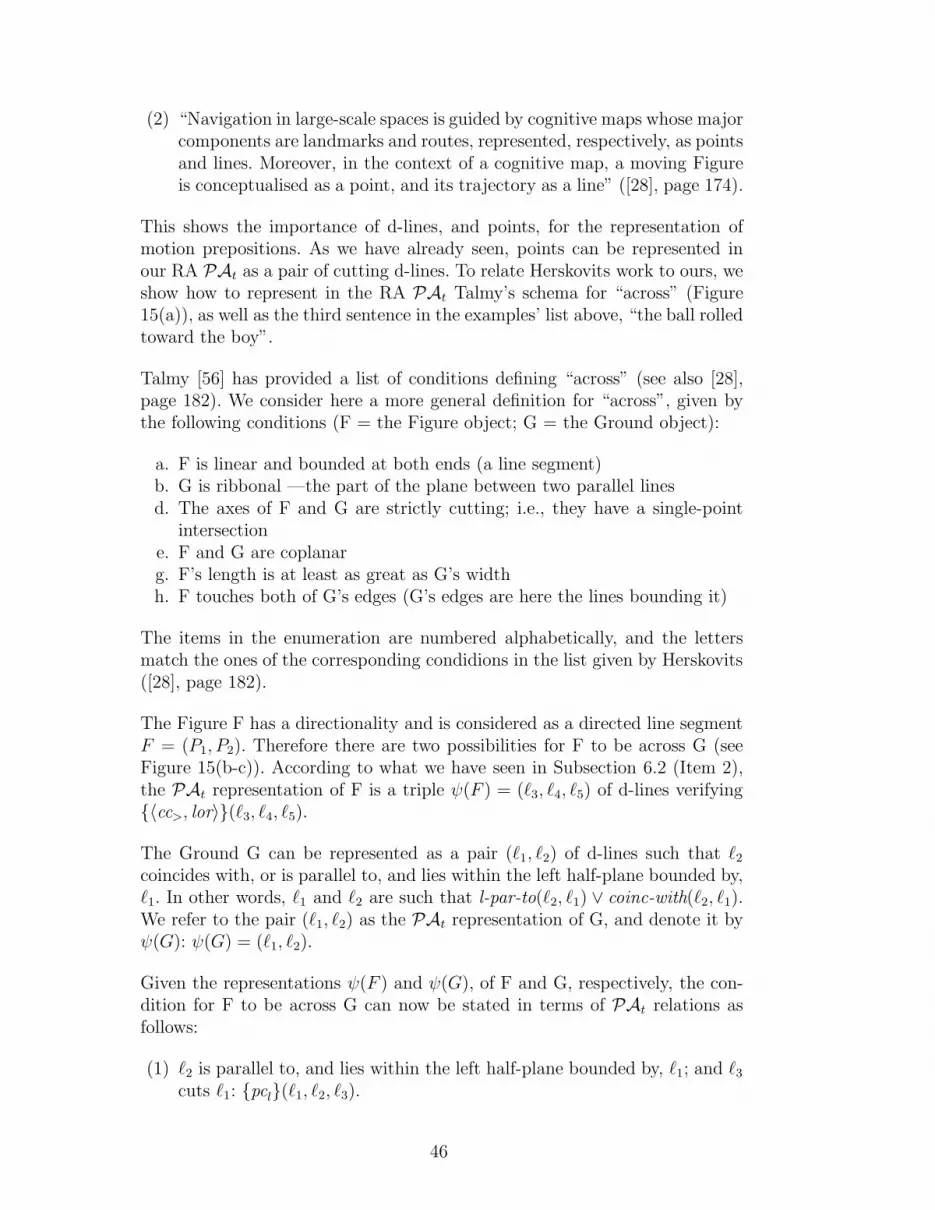
(2) “Navigation in large-scale spaces is guided by cognitive maps whose majorcomponents are landmarks and routes, represented, respectively, as pointsand lines. Moreover, in the context of a cognitive map, a moving Figureis conceptualised as a point, and its trajectory as a line” ([28], page 174).
This shows the importance of d-lines, and points, for the representation ofmotion prepositions. As we have already seen, points can be represented inour RA PAt as a pair of cutting d-lines. To relate Herskovits work to ours, weshow how to represent in the RA PAt Talmy’s schema for “across” (Figure15(a)), as well as the third sentence in the examples’ list above, “the ball rolledtoward the boy”.
Talmy [56] has provided a list of conditions defining “across” (see also [28],page 182). We consider here a more general definition for “across”, given bythe following conditions (F = the Figure object; G = the Ground object):
a. F is linear and bounded at both ends (a line segment)b. G is ribbonal —the part of the plane between two parallel linesd. The axes of F and G are strictly cutting; i.e., they have a single-point
intersectione. F and G are coplanarg. F’s length is at least as great as G’s widthh. F touches both of G’s edges (G’s edges are here the lines bounding it)
The items in the enumeration are numbered alphabetically, and the lettersmatch the ones of the corresponding condidions in the list given by Herskovits([28], page 182).
The Figure F has a directionality and is considered as a directed line segmentF = (P1, P2). Therefore there are two possibilities for F to be across G (seeFigure 15(b-c)). According to what we have seen in Subsection 6.2 (Item 2),the PAt representation of F is a triple ψ(F ) = (ℓ3, ℓ4, ℓ5) of d-lines verifying{〈cc>, lor〉}(ℓ3, ℓ4, ℓ5).
The Ground G can be represented as a pair (ℓ1, ℓ2) of d-lines such that ℓ2coincides with, or is parallel to, and lies within the left half-plane bounded by,ℓ1. In other words, ℓ1 and ℓ2 are such that l-par-to(ℓ2, ℓ1) ∨ coinc-with(ℓ2, ℓ1).We refer to the pair (ℓ1, ℓ2) as the PAt representation of G, and denote it byψ(G): ψ(G) = (ℓ1, ℓ2).
Given the representations ψ(F ) and ψ(G), of F and G, respectively, the con-dition for F to be across G can now be stated in terms of PAt relations asfollows:
(1) ℓ2 is parallel to, and lies within the left half-plane bounded by, ℓ1; and ℓ3cuts ℓ1: {pcl}(ℓ1, ℓ2, ℓ3).
46

- -
6
?ℓ1
ℓ2
ℓ1
ℓ2P2
(b) (c)
P1
P1 P2
- -
���������HHHHY
AAAAAAAAU
XXXXXz
XXXXy
HHHHHj(b’) (c’)
ℓ1ℓ1
ℓ2
P1P2
P1P2
ℓ4 ℓ3
ℓ5
ℓ5
ℓ2
ℓ4ℓ3
XXXy
(a)
Ground
Figure
Fig. 15. Diagrammatic representation of Talmy’s schema for “across”.
frontneutralback
(a) (b)
backneutral
(c)
1
12
155 10
94
3 138
6
(d)
2
11
7A
B
A
B B
AA
Bfront14
rightleft
straight
Fig. 16. The partition of the plane on which is based the relative orientation calculusin [20,61].
(2) ℓ5 cuts ℓ3 before ℓ1 does; ℓ5 cuts ℓ3 before ℓ2 does; ℓ1 cuts ℓ3 before ℓ4does; and ℓ2 cuts ℓ3 before ℓ4 does: {cc<}(ℓ3, ℓ5, ℓ1) ∧ {cc<}(ℓ3, ℓ5, ℓ2) ∧{cc<}(ℓ3, ℓ1, ℓ4) ∧ {cc<}(ℓ3, ℓ2, ℓ4).
7 Related work
We now discuss the most related work in the literature.
47

7.1 Scivos and Nebel’s NP-hardness result of Freksa’s calculus
A well-known model of relative orientation of 2D points is the calculus, oftenreferred to as the Double-Cross Calculus, defined in [20], and developed furtherin [61]. The calculus corresponds to a specific partition, into 15 regions, of theplane, determined by a parent object, say A, and a reference object, say B(Figure 16(d)). The partition is based on the following:
(1) the left/straight/right partition of the plane determined by an observerplaced at the parent object and looking in the direction of the referenceobject (Figure 16(a));
(2) the front/neutral/back partition of the plane determined by the sameobserver (Figure 16(b)); and
(3) the similar front/neutral/back partition of the plane obtained when weswap the roles of the parent object and the reference object (Figure 16(c)).
Combining the three partitions (a), (b) and (c) of Figure 16 leads to thepartition of the plane on which is based the calculus in [20,61] (Figure 16(d)).The region numbered n, n ∈ {1, . . . , 15}, in the partition is referred to asreg(A,B, n), and gives rise to a basic relation, or atom, of the calculus, whichwe refer to as fn:
(∀n ∈ {1, . . . , 15})(∀C)(fn(A,B,C)⇔ C ∈ reg(A,B, n))
Scivos and Nebel [55] have shown that the subset {{f10}, T}, where T is theuniversal relation, is NP-hard; the proof uses a reduction of the betweennessproblem ([22], page 279). We consider here a coarser version of Freksa’s cal-culus, which does not distinguish between f1, f2, f3, f4 and f5, on the onehand, and between f11, f12, f13, f14 and f15, on the other hand. We show thata CSP, P , expressed in FC = {fℓ, {f6}, {f7}, {f8}, {f9}, {f10}, fr, T}, wherefℓ = {f1, f2, f3, f4, f5} and fr = {f11, f12, f13, f14, f15}, can be translated intoan equivalent PAt-CSP, P ′. The idea is to first eliminate the relations {f7}and {f9} from P , which involve necessarily equal variables (see Definition 10below). We then show how to translate each constraint of the resulting prob-lem, expressed in FC \ {{f7}, {f9}} = {fℓ, {f6}, {f8}, {f10}, fr, T}, into theRA PAt.
Definition 10 Two variables of a CSP are necessarily equal if they receivethe same instantiation in all models of the CSP.
(1) Let Xi, Xj and Xk be three variables such that {f7}(Xi, Xj, Xk). ThenXi and Xk are necessarily equal. In such a case, we perform the following,for all variables Xl and Xm:(a) (T P )lmi ← (T P )lmi ∩ (T P )lmk
48

(b) (T P )lim ← (T P )lim ∩ (T P )lkm
(c) (T P )ilm ← (T P )ilm ∩ (T P )klm
If in any of the above replacement operations, the empty relation is de-tected then the CSP is clearly inconsistent. Otherwise, the variable Xk
can be removed from the CSP: replacement the CSP by the sub-CSPP|V \{Xk}, where V is the set of all variables.
(2) If there exist variables Xi, Xj and Xk such that {f7}(Xi, Xj, Xk) thenrepeat the process from 1.
(3) If there exist three variables Xi, Xj and Xk such that {f9}(Xi, Xj, Xk)then Xj and Xk are necessarily equal. The constraint {f9}(Xi, Xj, Xk) isequivalent to the constraint {f7}(Xj , Xi, Xk):(a) (T P )jik ← (T P )jik ∩ {f7}(b) If (T P )jik = ∅ then exit (the CSP is inconsistent)(c) Repeat the process from Item 1
(4) If there exist no three variables Xi, Xj and Xk such that {f9}(Xi, Xj, Xk)then the process has been achieved: the resulting CSP has no two vari-ables that are necessarily equal; in other words, it is expressed in FC \{{f7}, {f9}}.
The second step is to show how to translate a CSP, P , expressed in FC \{{f7}, {f9}} into a CSP P ′ expressed in the RA PAt.
(1) Initialise the set V ′ of variables and the set C ′ of constraints of P ′ to theempty set:V ′ ← ∅, C ′ ← ∅
(2) For each pair (Xi, Xj), i < j, of variables from V , the set of variables ofP , we create a d-line variable Xij:V ′ ← V ′ ∪ {Xij}
(3) For each variable Xi from V , we create two d-line variables Xi1 and Xi2
such that ψ(Xi) = (Xi1 , Xi2); i.e., such that {< cpc, lre >}(Xi1 , Xi2, Xi1):V ′ ← V ′ ∪ {Xi1 , Xi2}, C
′ ← C ′ ∪ {{< cpc, lre >}(Xi1, Xi2, Xi1)}.(4) For all distinct variables Xi and Xj of P , we have Xi ∈ Xij and Xj ∈ Xij :
C ′ ← C ′ ∪ {{cc=, cpc, pcc}(Xij, Xi1, Xi2), {cc=, cpc, pcc}(Xij, Xj1, Xj2)}(5) Xij is oriented from Xi to Xj ; i.e., Xi is met before Xj in the positive
walk along Xij:9
C ′ ← C ′∪{{cc<, cpc, pcc, ppc1}(Xij, Xi1, Xj1), {cc<, cpc, pcc, ppc1}(Xij, Xi2 , Xj2)}(6) For each constraint of P of the form {fℓ}(Xi, Xj, Xk), we add the con-
straint {lel}(Xij, Xik, Xik) to P ′:C ′ ← C ′ ∪ {{lel}(Xij , Xik, Xik)}
9 The conditions ψ(Xi) = (Xi1 ,Xi2) and ψ(Xj) = (Xj1 ,Xj2) imply that in all solu-tions to the CSP P ′ in construction, the instantiations {Xij = ℓij ,Xi1 = ℓi1,Xi2 =ℓi2 ,Xj1 = ℓj1,Xj2 = ℓj2} of the variables in {Xij ,Xi1 ,Xi2 ,Xj1 ,Xj2} are such thatℓi1 and ℓi2, on the one hand, and ℓj1 and ℓj2, on the other hand, cannot be bothparallel to ℓij.
49

(7) For each constraint of P of the form {f6}(Xi, Xj, Xk), we add the con-straint {oeo}(Xij , Xik, Xik) to P ′:C ′ ← C ′ ∪ {{oeo}(Xij , Xik, Xik)}
(8) For each constraint of P of the form {f8}(Xi, Xj, Xk), we add the con-straints {eee}(Xij, Xik, Xik) and {oeo}(Xij , Xjk, Xjk) to P ′:C ′ ← C ′ ∪ {{eee}(Xij , Xik, Xik), {oeo}(Xij, Xjk, Xjk)}
(9) For each constraint of P of the form {f10}(Xi, Xj, Xk), transform it intothe equivalent constraint {f6}(Xj, Xi, Xk) and apply Step 7
(10) For each constraint of P of the form {fr}(Xi, Xj, Xk), transform it intothe equivalent constraint {fℓ}(Xj, Xi, Xk) and apply Step 6
7.2 Moratz et al.’s dipole algebra and Renz’s spatial Odyssey of Allen’s in-terval algebra
A dipole is an oriented line segment. We follow here the notation in [48], anddenote dipoles by the letters A, B, C, ..., the starting endpoint and the endingendpoint of a dipole A by sA and eA, respectively. The simple version of thedipole algebra, denoted D24, presents 24 atoms, which are characterised bythe fact that they cannot represent a configuration of two dipoles with atleast three of the four endpoints collinear and pairwise distinct. The reasonfor presenting a simple version of the algebra is that it has the advantageof being a relation algebra 10 [57,40,36], and of presenting a relatively smallnumber of atoms, offering thus a manageable composition table, and a wideapplication domain. The complete version, denoted D69, contains 69 atomsthat are Jointly Exhaustive and Pairwise Disjoint: any spatial configurationof two dipoles is described by one and only one of the 69 atoms. We focuson the more general version, D69. The description of D69 atoms is based onseven dipole-point relations, l (left), b (behind), s (starts), i (inside), e (ends),f (front) and r (right): given a dipole A = (sA, eA), a point P and a dipole-point relation R ∈ {l, b, s, i, e, f, r}, we have A R P if and only if the point Pbelongs to the region labelled R in the partition of the plane determined byA, illustrated in Figure 17 (see [48] for details).
A dipole-dipole relation is denoted in [48] by a word of length 4 over the al-phabet {l, b, s, i, e, f, r}, of the form R1R2R3R4. Such a relation on two dipolesA and B, denoted by A R1R2R3R4 B, is interpreted as follows:
A R1R2R3R4 B ⇔ (A R1 sB) ∧ (A R2 eB) ∧ (B R3 sA) ∧ (B R4 eA)(31)
10 As far as we can say, the authors did not check, for instance, that the entriesof the composition table record the exact composition of the corresponding atoms;i.e., whether, given any two atoms, say r and s, it is the case that r ◦ s = T [r, s],where T [r, s] is the entry at row r and column s of the composition table. If this isnot the case, the calculus would not be an RA.
50

l
b
s
i
e
f
r
sA
eA
Fig. 17. Partition of plane determined by a dipole A = (sA, eA) [48].
In order to get a PAt representation for each of the 69 dipole relations in [48],we need to provide a PAt representation for each of the seven dipole-pointrelations l, b, s, i, e, f, r. For this purpose, we consider a dipole A = (sA, eA)and a point P :
(1) Each of the three points P , sA and eA is associated with a pair of d-linesconsisting of its PAt representations (see Subsection 6.1 Item 1): ψ(P ) =(ℓ1P , ℓ
2P ), ψ(sA) = (ℓ1sA
, ℓ2sA) and ψ(eA) = (ℓ1eA
, ℓ2eA). The corresponding
set of PAt constraints is {{〈cpc, lre〉}(ℓ1P , ℓ
2P , ℓ
1P ), {〈cpc, lre〉}(ℓ
1sA, ℓ2sA
, ℓ1sA),
{〈cpc, lre〉}(ℓ1eA, ℓ2eA
, ℓ1eA)}
(2) We associate with A a d-line ℓA oriented from sA to eA:(a) From sA ∈ ℓA and eA ∈ ℓA, we get the following set of constraints
(see Subsection 7.1, third enumeration, Item 4):{{cc=, cpc, pcc}(ℓA, ℓ
1sA, ℓ2sA
), {cc=, cpc, pcc}(ℓA, ℓ1eA, ℓ2eA
)}(b) From ℓA oriented from sA to eA, we get the following set of constraints
(see Subsection 7.1, third enumeration, Item 5):{{cc<, cpc, pcc, ppc1}(ℓA, ℓ
1sA, ℓ1eA
), {cc<, cpc, pcc, ppc1}(ℓA, ℓ2sA, ℓ2eA
)}(3) The relations l, b, i, f and r are translated into PAt in a similar way
as the relations fl, f6, f8, f10 and fr of Freksa’s calculus (see Subsection7.1, third enumeration, Items 6-10), thanks to the following equivalences:(A l P ) iff fl(sA, eA, P ); (A b P ) iff f6(sA, eA, P ); (A i P ) iff f8(sA, eA, P );(A f P ) iff f10(sA, eA, P ); and (A r P ) iff fr(sA, eA, P ).
(4) A s P (P coincides with sA) is expressed by concurrency of ℓ1P , ℓ2P andℓ1sA
, on the one hand, and concurrency of ℓ1P , ℓ2P and ℓ2sA, on the other
hand:{{cc=, cpc, pcc}(ℓ
1P , ℓ
2P , ℓ
1sA
), {cc=, cpc, pcc}(ℓ1P , ℓ
2P , ℓ
2sA
)}(5) In a similar way, we translate A e P (P coincides with eA) using a double
concurrency:{{cc=, cpc, pcc}(ℓ
1P , ℓ
2P , ℓ
1eA
), {cc=, cpc, pcc}(ℓ1P , ℓ
2P , ℓ
2eA
)}
51

Renz’s work [53] was motivated by applications such as traffic scenarios, wherecars and their regions of influence can be represented as directed intervals ofan underlying line representing the road. We refer to the underlying line asℓRenz. The 26 atomic relations of Renz’s algebra of directed intervals [53] canbe seen as particular relations of Moratz et al.’s D69 algebra [48], as long aswe have a mean of constraining all involved directed intervals to belong to theunderlying line ℓRenz.
Consider two directed intervals x and y. x and y are particular oriented seg-ments x = (sx, ex) and y = (sy, ey). As in the above discussion of Moratz etal.’s D69 algebra, we associate with each point P in {sx, ex, sy, ey} its PAt
representation ψ(P ) = (ℓ1P , ℓ2P ), and with each oriented segments S in {x, y} a
d-line ℓS oriented from the left endpoint to the right endpoint of the segment.
(1) Constraining a directed interval, for instance x, to be part of the under-lying line ℓRenz can be easily done with the RA PAt, by saying that theline ℓx coincides with ℓRenz:{〈ppc1, eee〉, 〈ppc1, oeo〉}(ℓRenz, ℓx, ℓx)
(2) Once each of the directed intervals is constrained to be part of ℓRenz, theatomic relations can be translated into PAt using what has been doneabove for Moratz et al.’s D69 dipole algebra, thanks to the equivalences ofFigure 18 between directed intervals base relations andD69 base relations.
7.3 Reasoning about parallel-to-the-axes parallelograms
Approaches to reasoning about parallelograms of the 2D space, whose sidesare parallel to the axes of some system (x,O, y) of coordinates, can be foundin the literature [3,24,49]. These approaches are straighforward extensions ofAllen’s algebra of temporal intervals [1]. Given such a parallelogram, say P ,we denote by P x and P y the intervals consisting of the projections of P on thex- and y-axes, respectively. The atoms of the corresponding rectangle algebra,RgA, are of the form (r1, r2), where r1 and r2 are Allen’s atoms [1] (theAllen’s atoms are < (before), m (meets), o (overlaps), s (starts), d (during),f (finishes); their respective converses > (after), mi (met-by), oi (overlapped-by, si (started-by), di (contains), fi (finished-by); and eq (equals), which is itsproper converse). If P1 and P2 are two parallelograms as described, then:
(r1, r2)(P1, P2)⇔ r1(Px1 , P
x2 ) ∧ r2(P
y1 , P
y2 ) (32)
The translation of the atoms of the rectangle algebra into the RA PAt canthus be obtained from the procedure already described on translating intoPAt Moratz et al.’s relations [48], on the one hand, and Renz’s relations [53],on the other hand (see Figure 18).
52

Directed Intervals Sym- Pictorial D69 Base
Base Relation bol Example Relation
x behind= y b= −x− > x ffbb y
................................................ ..........
y in-front-of= x f= −y− > y bbff x
x behind 6= y b6= < −x− x bbbb y
−y− >
x in-front-of6= y f6= −x− > x ffff y
< −y−
x meets-from-behind= y mb= −x− > x efbs y
................................................ ..........
y meets-in-the-front= x mf= −y− > y bsef x
x meets-from-behind 6= y mb6= < −x− x sbsb y
−y− >
x meets-in-the-front6= y mf6= −x− > x fefe y
< −y−
x overlaps-from-behind= y ob= −x− > x ifbi y
................................................ ..........
y overlaps-in-the-front= x of= −y− > y biif x
x overlaps-from-behind6= y ob6= < −x− x ibib y
−y− >
x overlaps-in-the-front6= y of 6= −x− > x fifi y
< −y−
x contained-in= y c= −x− > x bfii y
................................................ ..........
y extends= x e= — y — > y iibf x
x contained-in 6= y c6= < −x− x fbii y
................................................ ..........
y extends 6= x e6= — y — > y iifb x
x contained-in-the-back-of= y cb= −x− > x sfsi y
................................................ ..........
y extends-the-front-of= x ef= — y — > y sisf x
x contained-in-the-back-of 6= y cb6= < −x− x ebis y
................................................ ..........
y extends-the-back-of 6= x eb6= — y — > y iseb x
x contained-in-the-front-of= y cf= −x− > x beie y
................................................ ..........
y extends-the-back-of= x eb= — y — > y iebe x
x contained-in-the-front-of 6= y cf 6= < −x− x fsei y
................................................ ..........
y extends-the-front-of 6= x ef 6= — y — > y eifs x
x equals= y eq= −x− > x sese y
−y− >
x equals 6= y eq6= −x− > x eses y
< −y−
Fig. 18. The 26 base relations of the directed intervals algebra, and their translationinto the RA PAt. 53

8 Conclusion and further work
We have presented a Relation Algebra (RA) [57,40,36] of relative position rela-tions on 2-dimensional directed lines (d-lines). The converse table, the rotationtable and the composition tables of the RA have been provided. Furthermore,thanks to its inspiration from the theory of degrees of freedom analysis [26,38],the work can be seen as answering, at least partly, the challenges in [52] forthe particular case of qualitative spatial reasoning: computing, for instance,the composition of two relations is derived from:
(1) the composition of the rotational projections of the two relations, on theone hand; and
(2) the composition of the translational projections, on the other hand.
More importantly, current research shows clearly the importance of developingspatial RAs: specialising an ALC(D)-like Description Logic (DL) [2], so thatthe roles are temporal immediate-successor (accessibility) relations, and theconcrete domain is generated by a decidable spatial RA in the style of the well-known Region-Connection Calculus RCC-8 [51], such as the RA cPAt definedin this paper, leads to a computationally well-behaving family of languagesfor spatial change in general, and for motion of spatial scenes in particular:
(1) Deciding satisfiability of an ALC(D) concept w.r.t. to a cyclic TBox is,in general, undecidable (see, for instance, [45]).
(2) In the case of the spatio-temporalisation, however, if we use what is calledweakly cyclic TBoxes in [31] (see also the related work [34]), then sat-isfiability of a concept w.r.t. such a TBox is decidable. The axioms of aweakly cyclic TBox capture the properties of modal temporal operators.The reader is referred to [31] for details. 11
Extending the presented RA to 3D would allow, for instance, for the repre-sentation of 3D shapes, such as polyhedra, which are the 3D counterpart ofpolygons in the 2D space, which are themselves the 2D counterpart of (convex)intervals in the 1D space. This could be achieved thus:
(1) extend Isli and Cohn’s RA CYCt [35,36] to orientations of the 3D space;(2) extend the T At algebra to directed lines of the 3D space; and(3) combine the two calculi, as done in this work for the 2D counterparts,
to get a calculus for reasoning about relative position of directed lines ofthe 3D space.
11 A full version of [31], including the decidability proof, will be made downloadablesoon [33].
54

References
[1] J F Allen. Maintaining knowledge about temporal intervals. Communicationsof the Association for Computing Machinery, 26(11):832–843, 1983.
[2] F Baader and P Hanschke. A scheme for integrating concrete domains intoconcept languages. In Proceedings of the 12th International Joint Conferenceon Artificial Intelligence (IJCAI), pages 452–457, Sydney, 1991. MorganKaufmann.
[3] P Balbiani, J-F Condotta, and L F del Cerro. A model for reasoning aboutbidimensional temporal relations. In Proceedings of Principles of KnowledgeRepresentation and Reasoning (KR), pages 124–130, Trento, Italy, 1998.Morgan Kaufmann.
[4] P Balbiani, V Dugat, L F del Cerro, and A Lopez. Elements de geometriemecanique. Editions Hermes, 1994.
[5] P Balbiani and A Osmani. A model for reasoning about topologic relationsbetween cyclic intervals. In A G Cohn, F Giunchiglia, and B Selman, editors,Proceedings of Principles of Knowledge Representation and Reasoning (KR),pages 378–385, 2000.
[6] B Bennett, A G Cohn, P Torrini, and S M Hazarika. A foundation for region-based qualitative geometry. In W Horn, editor, Proceedings ECAI, Berlin, 2000.IOS Press.
[7] B Bennett, A Isli, and A G Cohn. A system handling RCC-8 Queries on 2DRegions representable in the Closure Algebra of Half-Planes. In D Abel andB C Ooi, editors, Proceedings of the 11th International Conference on Industrial& Engineering Applications of Artificial Intelligence & Expert Systems (IEA-AIE), Lecture Notes in Artificial Intelligence, pages 281–290, Castellon, Spain,1998. Springer-Verlag.
[8] V Chvatal. Linear Programming. W.H. Freeman and Company, New York,1983.
[9] B L Clarke. A Calculus of Individuals based on ‘Connection’. Notre DameJournal of Formal Logic, 23(3):204–218, July 1981.
[10] E Clementini, P Di Felice, and D Hernandez. Qualitative representation ofpositional information. Artificial Intelligence, 95:317–356, 1997.
[11] A G Cohn. Qualitative spatial representation and reasoning techniques. InProceedings KI: German Annual Conference on Artificial Intelligence, volume1303 of Lecture Notes in Artificial Intelligence, pages 1–30, Freiburg, Germany,1997. Springer-Verlag.
[12] A De Morgan. On the Syllogism and other Logical Writings. Yale UniversityPress, New Haven, 1966.
55

[13] R Dechter. From local to global consistency. Artificial Intelligence, 55:87–107,1992.
[14] I Duntsch, H Wang, and S McCloskey. Relation algebras in qualitative spatialreasoning. Fundamenta Informatica, 39:229–248, 1999.
[15] I Duntsch, H Wang, and S McCloskey. A relation-algebraic approach to theregion connection calculus. Theoretical Computer Science, 255:229–248, 2001.
[16] M Egenhofer and R Franzosa. Point-set topological spatial relations.International Journal of Geographical Information Systems, 5(2):161–174, 1991.
[17] M T Escrig and F Toledo. The integration of Qualitative Orientationand Named Distances: Application to a Qualitative Navigation Simulator.International Journal on Artificial Intelligence Tools, Issue on the best papersof ICTAI’96, 1997.
[18] K D Forbus, P Nielsen, and B Faltings. Qualitative spatial reasoning: The clockproject. Artificial Intelligence, 51:417–471, 1991.
[19] A U Frank. Qualitative spatial reasoning about distances and directions ingeographic space. Journal of Visual Languages and Computing, 3:343–371,1992.
[20] C Freksa. Using Orientation Information for Qualitative Spatial Reasoning.In A U Frank, I Campari, and U Formentini, editors, Proceedings of GIS —from Space to Territory: Theories and Methods of Spatio-Temporal Reasoning,Berlin, 1992. Springer.
[21] E C Freuder. A sufficient condition for backtrack-free search. Journal of theAssociation for Computing Machinery, 29:24–32, 1982.
[22] M R Garey and D S Johnson. Computers and intractability. Freeman, NewYork, 1979.
[23] A Gerevini and J Renz. Combining topological and qualitative size constraintsfor spatial reasoning. In M J Maher and J-F Puget, editors, Proceedings ofthe Fourth International Conference on Principles and Practice of ConstraintProgramming (CP), volume 1520 of Lecture Notes in Computer Science, pages220–234. Springer, 1998.
[24] H Gusgen. Spatial reasoning based on Allen’s temporal logic. Technical ReportTR-89-049, ICSI, Berkley, CA, 1989.
[25] C Habel. Representing space and time: Discrete, dense or continuous? is thatthe question? In C Eschenbach and W Heydrich, editors, Parts and Wholes —Integrity and Granularity, pages 97–107. 1995.
[26] R S Hartenberg and J Denavit. Kinematic synthesis of linkages. McGraw-Hill,New York, 1964.
[27] P J Hayes. The second naive physics manifesto. In J R Hobbs and R C Moore,editors, Formal Theories of the Commonsense World, pages 1–36. Ablex, 1985.
56

[28] A Herskovits. Language, spatial cognition, and vision. In O Stock, editor,Spatial and Temporal Reasoning, chapter 6, pages 155–202. Kluwer AcademicPublishers, Dordrecht/Boston/London, 1997.
[29] E G Hoel and H Samet. Efficient processing of spatial queries in line segmentdatabases. In Proceedings 2nd International Symposium on Large SpatialDatabases (SSD), pages 237–255, 1991.
[30] K Hornsby, M J Egenhofer, and P Hayes. Modeling cyclic change. In P Chen,D Embley, J Kouloumdjian, S Liddle, and J Roddick, editors, Advances inconceptual modeling, Proceedings of the ER Workshops, volume 1727 of Lecturenotes in Artificial Intelligence, pages 98–109, Berlin, 1999. Springer-Verlag.
[31] A Isli. A family of spatio-temporal languagesas an ALC(D) spatio-temporalisation with weakly cyclic TBoxes. Submitted(downloadable from http://kogs-www.informatik.uni-hamburg.de/ isli/home-Publications-Submitted.html).
[32] A Isli. On deciding consistency for CSPs of cyclic time intervals. In Proceedings14th International FLAIRS Conference, Special Track on SpatiotemporalReasoning, pages 547–551, Key West, FL, 2001. AAAI Press.
[33] A Isli. Bridging the gap between modal temporal logic and constraint-based QSR as a spatio-temporalisation of ALC(D) with weakly cyclictboxes. Technical Report FBI-HH-M-311/02, Fachbereich Informatik,Universitat Hamburg, 2002. To appear (downloadable soon from http://kogs-www.informatik.uni-hamburg.de/ isli/home-Publications-TR.html).
[34] A Isli. A family of qualitative theories for continuous spatio-temporal change asa spatio-temporalisation of ALC(D) —first results. In R V Rodrıguez, editor,Proceedings of the ECAI Workshop on Spatial and Temporal Reasoning, pages81–86, Lyon, France, 2002.
[35] A Isli and A G Cohn. An Algebra for cyclic Ordering of 2D Orientations. InProceedings AAAI, pages 643–649, Madison, WI, 1998. AAAI Press.
[36] A Isli and A G Cohn. A new Approach to cyclic Ordering of 2D Orientationsusing ternary Relation Algebras. Artificial Intelligence, 122(1-2):137–187, 2000.
[37] G A Kramer. Solving geometric constraint systems. In Proceedings AAAI-90,1990.
[38] G A Kramer. A geometric constraint engine. Artificial Intelligence, 58:327–360,1992.
[39] G A Kramer. Solving Geometric Constraint Systems: A Case Study inKinematics. Artificial Intelligence. MIT Press, 1992.
[40] P Ladkin and R Maddux. On binary Constraint Problems. Journal of theAssociation for Computing Machinery, 41(3):435–469, 1994.
[41] P Ladkin and A Reinefeld. Effective Solution of qualitative ConstraintProblems. Artificial Intelligence, 57:105–124, 1992.
57

[42] H S Leonard and N Goodman. The Calculus of Individuals and its Uses. Journalof Symbolic Logic, 5:45–55, 1940.
[43] S Lesniewski. O Podstawach Ogolnej Teoryi Mnogosci. Przeglad Filozoficzny,31:261–291, 1928.
[44] G Ligozat. On generalized interval calculii. In Proceedings AAAI-91, pages234–240, Anaheim, California, 1991.
[45] C Lutz. The Complexity of Description Logics with Concrete Domains. PhDthesis, LuFG Theoretical Computer Science, RWTH, Aachen, 2001.
[46] A K Mackworth. Consistency in Networks of Relations. Artificial Intelligence,8:99–118, 1977.
[47] U Montanari. Networks of Constraints: fundamental Properties andApplications to Picture Processing. Information Sciences, 7:95–132, 1974.
[48] R Moratz, J Renz, and D Wolter. Qualitative spatial reasoning about linesegments. In W Horn, editor, Proceedings ECAI, Berlin, 2000. IOS Press.
[49] A Mukerjee and G Joe. A qualitative Model for Space. In Proceedings AAAI-90,pages 721–727, Los Altos, 1990. Morgan Kaufmann.
[50] A Musto, K Stein, A Eisenkolb, and T Rofer. Qualitative and quantitativerepresentations of locomotion and their application in robot navigation. InProceedings IJCAI-99, pages 1067–1072, 1999.
[51] D Randell, Z Cui, and A Cohn. A spatial Logic based on Regions andConnection. In Proceedings KR-92, pages 165–176, San Mateo, 1992. MorganKaufmann.
[52] D A Randell, A G Cohn, and Z Cui. Computing transitivity tables: A challengefor automated theorem provers. In Proceedings CADE 11, Berlin, 1992. SpringerVerlag.
[53] J Renz. A Spatial Odyssey of the Interval Algebra: 1. Directed Intervals. InProceedings IJCAI-01, pages 51–56, 2001.
[54] RoboCup-99. Robocup. AI Magazine, 21(3), 2000.
[55] A Scivos and B Nebel. Double-Crossing: Decidability and ComputationalComplexity of a Qualitative Calculus for Navigation. In D R Montello, editor,Spatial Information Theory: Foundations of GIS, number 2205 in LNCS, pages431–446, Morro Bay, CA, 2001. Springer.
[56] L Talmy. How language structures space. In H Pick and L Acredolo, editors,Spatial Orientation: Theory, Research, and Application, pages 255–282. PlenumPress, New York, 1983.
[57] A Tarski. On the Calculus of Relations. Journal of Symbolic Logic, 6:73–89,1941.
58

[58] M Vilain. A system for reasoning about time. In Proceedings of the AAAI-82,pages 197–201, Pittsburg, Pennsylvania, 1982.
[59] M B Vilain and H Kautz. Constraint Propagation Algorithms for TemporalReasoning. In Proceedings AAAI-86, pages 377–382, Philadelphia, August 1986.Morgan Kaufmann.
[60] A N Whitehead. Process and Reality. The MacMillan Company, New York,1929.
[61] K Zimmermann and C Freksa. Qualitative Spatial Reasoning using Orientation,Distance, and Path Knowledge. Applied Intelligence, 6:49–58, 1996.
59

A Checking that PAt satisfies the ternary RA properties
PAt is the structure PAt = 〈2PAt-at,∪,∩,− , ∅,PAt-at, ◦,⌣ ,⌢ , I23
−→L〉, where:
(1) the set 2PAt-at of subsets of PAt-at is the set of elements, or relations,of PAt;
(2) the Boolean operations of addition, product and complement are givenby the set-theoretic operations of union (∪), intersection (∩) and com-plement (−);
(3) the empty set provides the empty, or bottom, element of PAt;(4) the set PAt-at of atoms provides the universal, or top, element of PAt;(5) the composition, converse and rotation of elements of PAt are, respec-
tively, the operations ◦, ⌣ and ⌢, as defined in [36] —see also Section 2,Equations (3)-(4)-(5); and
(6) the identity element is given by I23−→L
= {(a, b, b) : a, b ∈−→L}.
The verification that PAt satisfies the nine ternary RA properties (18)− · · ·−(26)is done in a similar way as for CYCt -see [36], Appendix B. The only thingthat remains to be checked is that the converse table, the rotation table andthe composition tables record, respectively, the exact converses, the exact ro-tations and the exact compositions. But this follows straighforwardly from thefacts:
(1) that CYCt is an RA [36], and(2) that Vilain and Kautz’s calculus of time points [59] is an RA [40].
60