Embed Size (px)
Citation preview

1
A set-membership approach for high integrity height-aided satellite positioning
Vincent Drevelle, Philippe Bonnifait
Heudiasyc
CNRS: UMR 6599 – Université de Technologie de Compiègne
Centre de Recherche de Royallieu, BP 20529, 60205 Compiègne, France
Tel. +33 3 44 23 46 45
Fax. +33 3 44 23 44 77
Email: [email protected]
The final publication is available at www.springerlink.com:
http://dx.doi.org/10.1007/s10291-010-0195-3
Abstract A Robust Set Inversion via Interval Analysis method in a bounded error
framework is used to compute three-dimensional location zones in real time, at a given
confidence level. This approach differs significantly from the usual Gaussian error model
paradigm, since the satellite positions and the pseudorange measurements are represented
by intervals encompassing the true value with a particular level of confidence. The
method computes a location zone recursively, using contractions and bisections of an
arbitrarily large initial location box. Such an approach can also handle an arbitrary
number of erroneous measurements using a q-relaxed solver, and allows the integration of
geographic and cartographic information such as digital elevation models or 3-
dimensional maps. With enough data redundancy, inconsistent measurements can be
detected and even rejected. The integrity risk of the location zone comes only from the
measurement bounds settings, since the solver is guaranteed. A method for setting these
bounds for a particular location zone confidence level is proposed. An experimental
validation using real L1 code measurements and a digital elevation model is also reported
in order to illustrate the performance of the method on real data.
Keywords: GPS; Interval Analysis; Robust positioning; Elevation model; Land
vehicles
hal-0
0608
133,
ver
sion
1 -
12 J
ul 2
011
Author manuscript, published in "GPS Solutions 15, 4 (2011) 357-368" DOI : 10.1007/s10291-010-0195-3

2
Introduction
Positioning services are becoming more frequently used in safety- and reliability-
critical applications for land vehicles, where not only an estimate of a user's
location is required, but also confidence indicators and means of ensuring
integrity.
Fig. 1 Experimental intelligent vehicles: Carmen and Strada
In the context of urban navigation with Global Navigation Satellite Systems
(GNSS), the main source of erroneous measurements is multipath propagation and
more specifically non-line-of-sight propagation, when the direct signal is blocked
by buildings and only reflected signals are observed. Furthermore, several
multipath altered measurements can be observed at the same epoch (Le Marchand
et al. 2009). Satellite-Based Augmentation Systems (SBAS) have little effect in
these conditions since they provide integrity information to protect the user
against signal-in-space malfunction, but not against local effects of multipath.
Moreover, satellite outages due to signal blocking by surrounding buildings have
other significant effects such as reducing data redundancy, degrading the
geometrical configuration, and decreasing SBAS availability. Other sources of
information are necessary to increase information redundancy and improve
localization in such difficult environment. The usual approach is to use
proprioceptive sensors that enable dead reckoning, the drift of which is
compensated by the available GNSS measurements. For land vehicles, an
alternative approach is to make use of geographical information to constrain the
location on mapped roads (Fouque and Bonnifait 2008). Another source of
information can be a Digital Elevation Model (DEM), which is very useful for
constraining the altitude (Li et al. 2005).
In practice, the knowledge of positioning accuracy is crucial. Localization can
thus be directly addressed as a set-membership problem that consists in finding
the zone in which the user is located, with a given level of confidence. Set-
theoretical methods have successfully been employed in robotics to address
localization problems (Jaulin et al. 2002; Meizel et al. 2002). These methods have
interesting properties, such as the ability to handle several hypotheses in cases of
ambiguous solutions simply by computing disconnected solution sets. Moreover,
when measurement errors are bounded, guaranteed solutions can be computed —
i.e. location zones in which the user is guaranteed to be located. In practice,
hal-0
0608
133,
ver
sion
1 -
12 J
ul 2
011

3
finding absolute bounds for the error is not always possible, and is often an
excessively conservative approach that fails to yield informative solutions. We
use a relaxed set-membership approach, which allows a given number of
measurements to be treated as outliers without affecting the consistency of the
solution set. This enables dealing with erroneous measurements, while avoiding
empty solutions. The solution-set integrity risk is bounded by the risk taken when
setting measurement error bounds and the number of tolerated outliers. No risk is
added by the employed set inversion algorithm, which solves the problem in a
guaranteed way. This makes the method particularly attractive in comparison with
existing solvers. Another advantage of a set-membership approach is that it allows
geographical information to be incorporated easily. Spatial inequality constraints
can be introduced into the computation without biasing the estimation process.
After a brief overview of current GPS integrity approaches, we introduce the
concept of set-membership positioning with a simple two-dimensional
pedagogical example. Guaranteed solvers for set-inversion based on interval
analysis and constraint propagation are then presented. A robust solver is also
introduced, and a method for setting measurement error bounds in relation to a
specified risk is explained. Finally, experimental results using real L1 GPS
pseudorange measurements and a DEM are presented and analyzed.
Current approaches
Punctual GNSS positioning using pseudoranges is typically handled as a nonlinear
Least-Squares problem using a Gauss-like method (Leick 2004; Kaplan and
Hegarty 2006). Other methods have been proposed to provide a non-iterative
computation (Bancroft 1985) or to allow positioning in situations with fewer than
four good measurements (Chang et al. 2009). In practice, some means of
computing an upper bound of the positioning error, linked to an integrity risk, is
required to determine whether the navigation system is usable for a given task.
When dealing with safety applications, the system should be able to handle
erroneous measurements. The concepts of internal and external reliability (Baarda
1968) enable to quantify the system‘s response in the presence of an unmodeled
error.
Internal reliability is characterized by the Minimal Detectable Bias (MDB), which
represents the size of the errors that can be detected by a given test statistics
(Salzmann 1991). The null hypothesis H0 represents the fault free case, where
model errors are absent. The alternative hypothesis Ha considers the existence of a
bias in one of the measurements. The MDB depends not only on the level of
confidence and on the detection power of the test statistics, but also on the
geometry of the problem, the noise model and the alternate hypothesis considered.
External reliability characterizes the effect in the position domain of an undetected
error model. Several external reliability metrics have been defined, such as the
Bias to Noise Ratio, which represents the significance of such an unobserved error
in a normalized way, and the Horizontal and Vertical Protection Levels
(HPL/VPL).
The Detection, Identification and Adaptation (DIA) scheme proposed in
Teunissen (1990) enables quality control of the position solution, in parallel to a
hal-0
0608
133,
ver
sion
1 -
12 J
ul 2
011

4
Kalman filter. Error detection is first performed by testing H0 against Ha. Then, if
a fault is detected, a second test statistics is used to identify the alternate
hypothesis, if possible. Upon success, an adaptation procedure is done to take into
account the detection. The chosen alternative hypotheses Ha are often limited to
errors on single measurements. The processing of simultaneous faults is
performed by iteratively applying DIA until H0 is validated.
Aviation receivers need to provide HPL and VPL that define, within an integrity
risk, the statistical upper bounds of position errors that will not be exceeded
without being detected in a given time to alert. This is achieved by Receiver
Autonomous Integrity Monitoring (RAIM) (Brown 1992; Walter and Enge 1995;
Feng et al. 2006), which implements a local version of the DIA scheme on single
epochs, called Fault Detection and Exclusion (FDE). The thresholds of the test
statistics used are set to meet the required navigation performance specifications
on integrity and availability. RAIM can be improved by the use of a dynamic
model (Hewitson 2007).
Other methods to compute navigation solutions in the presence of erroneous
measurements are based on robust estimation, like Huber‘s robust M-estimator
(Huber 1964). Range Consensus (Schroth et al. 2008) is an approach which
computes solutions on random four-satellite subsets and retains the solution which
is compatible with the most measurements, while rejecting the other
measurements as outliers. Solution separation is another method, which consists
in computing a solution with all available measurements, and all the sub-solutions
excluding one measurement (Schubert 2006).
A way to reduce the Minimal Detectable Biases, and as a consequence improving
integrity, is to add external information like a barometric pressure sensor for
instance (Gutmann et al. 2009). For ground vehicles, altitude information can be
provided to the system by using a DEM. This information is often added as a
virtual range from the center of the earth. In our approach, the altitude information
is easily introduced as a constraint coming from a DEM.
Set-membership positioning
In a bounded-error context, determining the user location zone consists in finding
the set of positions compatible with the measurements and their associated error
bounds. Positioning as a set-membership problem is introduced here with a simple
2D localization example, also showing the effects of wrong measurements on the
solution-set. In the presence of outliers, a relaxed approach enables robust set-
membership positioning.
Motivation
Algorithms that compute position from measurements for snapshot problems are
often based on punctual iterative methods that can be made robust to erroneous
measurements. Their main drawback is the risk to fall into a local minimum if the
initial guess is too far from the solution, or if erroneous measurements are not
properly handled.
hal-0
0608
133,
ver
sion
1 -
12 J
ul 2
011

5
Set-inversion methods guarantee that no solution will be missed inside an
arbitrarily big initial box, even if the equations are nonlinear. Relaxed-set
inversion is an extension that can also compute a guaranteed solution in the
presence of several outliers. When considering single faults, 1-relaxed set-
inversion provides external reliability information by computing the solution set
assuming the hypothesis of at most one erroneous measurement. In other words,
the solution set computed with the 1-relaxed solver covers the hypotheses H0 and
Ha.
For the DIA method, H0 is tested by a statistical test on the residuals.
Identification is then done using individual tests on each Ha. Transition from
internal integrity to external reliability assumes a linear(ized) model and usually
one fault at a time. A set-inversion method can handle nonlinear models without
adding any risk of invalid linearization. Such an approach can also be robust to an
arbitrary number of outliers, under the hypothesis that there is enough
redundancy. Therefore, robust set-inversion allows specifying alternate
hypotheses Ha with several simultaneous faults without explicitly testing every
fault combination.
Finally, when the problem is under-constrained, a set-inversion method can
compute all the location sets, even if there is a manifold of solutions. This is
particularly difficult to achieve using the approaches mentioned above. For
instance, with only 4 satellites in view, a location zone robust to one erroneous
measurement can still be computed.
Illustrative example with static beacons
Let us consider a time-of-flight positioning example having similarities with
GNSS even if, thanks to the longer ranges involved, nonlinearity is not a difficult
problem for GNSS positioning. One robot and three beacons communicate via a
radio link, as in Röhrig and Müller (2009). This radio link not only allows
communication, but also precision ranging with 1m accuracy.
To perform set-membership positioning, each measurement has to be represented
as the set of possible values given uncertainty. Intervals are commonly used to
express measurement inaccuracy. The maximum expected ranging error is added
to the measured value to represent measurements as intervals
],[=][ max
i
max
ii ededd (1)
Each measurement acts as a constraint on the robot's location, setting bounds on
the distance between the robot and the beacon. Since the robot and the beacons lie
on the same horizontal plane, we have the membership relation:
][)()( 22 i
iBRiBR dyyxx (2)
Given (2), each measurement constrains the robot location inside a ring, whose
inner and outer radii are respectively the lower and upper bounds of the
measurement interval ][ id .
hal-0
0608
133,
ver
sion
1 -
12 J
ul 2
011

6
Fig. 2 Localization using 3 beacons. Solution set in black. 1-relaxed solution set in black and grey.
The actual solution is shown as a red cross.
As there are three beacons, the measurement equation must be satisfied for the
three measurements. The robot is thus located within the intersection of the three
rings (the black area in Fig. 2a).
It is important to bear in mind that as long as the measurements are consistent
with the chosen bounded error model, the solution set will include the true user
location.
Effect of wrong measurements
Beacon ranging can be affected by multipath propagation or faulty beacons, so
that a measured range may be inconsistent with the error bounds. This kind of
measurement is often referred to as an ―outlier‖ or a ―fault‖. When using standard
set inversion, there are two possible consequences:
The solution is the empty set (Fig. 2b). This occurs when the erroneous
measurement is inconsistent with the other measurements, so that there is
no common intersection. One may therefore immediately conclude that
there is something wrong with the measurements or with the model.
The solution is not empty, but does not contain the actual robot location
(Fig. 2c and 2d). The set-membership method is then unable to detect the
presence of an erroneous measurement, and the solution set is inconsistent
with the truth.
To deal with erroneous measurements, a robust set-membership method must be
used. This is done by relaxing the number of constraints to be satisfied. In this
example, allowing at most one erroneous measurement is achieved by considering
hal-0
0608
133,
ver
sion
1 -
12 J
ul 2
011

7
the set of solutions compatible with at least two measurements (the gray and black
surfaces in Fig. 2). In the general case, an arbitrary number q of erroneous
measurements can be tolerated, using the q -relaxed intersection of the constraints
(Jaulin 2009).
Set inversion via interval analysis
In the previous example, the solution sets for each constraint were easy to
represent as rings, and we assumed that any set could be computed with an exact
representation. In real localization problems, the constraints are given by the
measurements and an observation function, but they may also reflect prior
information like the terrain profile, which can lead to arbitrary sets of solutions.
We therefore use interval analysis (Moore 1966) to perform a guaranteed set
inversion.
Interval analysis
Since an exact representation of sets is not tractable in the general case, an
efficient and easily implemented representation is to consider intervals, and their
multidimensional extension: interval vectors, also called boxes. Let IR be the set
of real intervals, and nIR the set of n-dimensional boxes.
Computations can easily be performed on intervals, thanks to interval arithmetic.
Inclusion functions ][f are defined such that the image of ][x by ][f includes the
image of ][x by f :
]).]([[])([,][ xfxfIRxn
To approximate compact sets in a guaranteed way, subpavings are used. A
subpaving of a box ][x is the union of nonempty and non-overlapping subboxes
of ][x . A guaranteed approximation of a compact set X can be made by
bracketing it between an inner subpaving X and an outer subpaving X such as
XXX (Fig. 3).
Fig. 3 Bracketing of the hatched set between two subpavings. Red boxes: inner subpaving X , Red
and yellow: outer subpaving ΔXXX =
hal-0
0608
133,
ver
sion
1 -
12 J
ul 2
011

8
Set inversion
The set inversion problem consists in determining the set X such as YXf =)(
when Y is known. A box ][x of nIR is said to be feasible if Xx][ (all
elements of the box are solutions of the problem) and unfeasible if =][ Xx
(none of the elements of the box is a solution of the problem), otherwise ][x is
ambiguous. We can characterize the feasibility of boxes by using an inclusion
function ][f of the function f to be inverted,
If Yxf ])]([[ then ][x is feasible
If =])]([[ Yxf then ][x is unfeasible
Else ][x is indeterminate, meaning it can be feasible, unfeasible or
ambiguous.
Starting from an arbitrarily large prior searching box ][ 0x , the Set Inversion Via
Interval Analysis (SIVIA) algorithm (Jaulin and Walter 1993) works by testing
the feasibility of boxes. Feasible boxes are added to the inner subpaving X of
solutions. Unfeasible boxes are discarded, since they contain no solution. Finally,
indeterminate boxes are bisected into two subboxes, which are enqueued in the
list L of boxes waiting to be examined. Algorithm termination is ensured by
adding indeterminate boxes whose width is less than to the subpaving of
indeterminate boxes ΔX . Thus the outer subpaving is ΔXXX = .
The number of bisections required gets exponentially larger as the dimension of
the problem increases, and the computational burden quickly becomes intractable.
To counteract the curse of dimensionality, contractors have to be used (Jaulin et
al. 2001b). A contractor is a function that shrinks a box without losing any
solutions. It can speed up computation without sacrificing the guarantee of a
solution. A simple way to build a contractor is to use a constraint propagation
algorithm (Jaulin et al. 2001b).
q-relaxed set inversion
Robustness can be implemented by relaxing a given number q of constraints
involving outliers. The solver will then compute a subpaving of the state space
consistent with at least qm measurements, where m is the length of the
observation vector. This is done using the so called q -relaxed intersection.
Considering m sets m1 ,, XX of nR , the q -relaxed intersection
}{q
iX is the set
of nRx which belong to at least qm of the iX 's. The Robust Set Inverter via
Interval Analysis (RSIVIA) solver (Jaulin et al. 2001b) guarantees the
computation of a q -relaxed solution set (see Algorithm 1).
hal-0
0608
133,
ver
sion
1 -
12 J
ul 2
011

9
Algorithm 1 RSIVIA (in: ][ 0x , f , Y , q )
Robust Set Inverter via Interval Analysis
)],([push L0x
while L do
)(pull=][ Lx
repeat
for mi 1= do
)]([ ix = contract ][x with if and ][ iy
end for
}{
},{1,
)]([=][q
mi
ixx
// hull of the q -relaxed intersection of m boxes
until no more contraction can be done on ][x
if ][x then
])([bisect=])[],([ xxx 21
)],([push);],([push LL 21 xx
end if
end while
return L
Fig. 4 Steps of RSIVIA on a 3 beacon localization problem
Fig. 4 shows the main steps of RSIVIA, applied to a fixed beacon localization
problem. The prior box is first contracted independently with each measurement
to get three boxes approximating the intersection of each constraint with the prior
box (Fig. 4a). The grayed zones in Fig. 4b represent the 1-relaxed intersections of
hal-0
0608
133,
ver
sion
1 -
12 J
ul 2
011

10
the three boxes. The hatched box, which is the box union of the grayed boxes,
becomes a new initial box. We have thus contracted the initial box without losing
any solutions. Contraction with each measurement is repeated, starting with the
new box (Fig. 4c), following which the initial box is reduced again so as to
enclose the q -relaxed intersection of contracted boxes. These steps are repeated
(Fig. 4d and 4e) until no further contractions can be performed (Fig. 4f). A
bisection is then carried out, and the contraction process is applied to the two
subboxes (Fig. 4g).
Setting measurement error bounds as a function of a given level of confidence
When using a q-relaxed guaranteed solver such as RSIVIA, the probability of the
true solution being inside the computed solution set can be computed, given a
prior measurement error distribution and a maximum number of outliers (denoted
q ) (Drevelle and Bonnifait 2009b). The risk is taken when setting measurement
error bounds and the maximum number of outliers. The bounds are then
propagated in a guaranteed way, such that no risk is added by the solver when set-
inversion is performed.
Knowing the probability density function y
ef of the measurement error ye and
the error bounds ],[ ba , a measurement measy is represented by the interval
],[=][ byayy measmeasmeas . The probability ])[(= measyyPp of the true y
being inside ][ measy can be computed.
dfyyPpy
e
b
ameas )(=])[(= (3)
Let okn be the number of measurements that respect the error bounds. Given the
assumption of independence, the probability of having exactly k correct
measurements out of m is given by the binomial law:
kmk
ok ppkmk
mknP )(1
)!(!
!=)=( (4)
Thus, by summing (4) over successive k values, the probability of having at least
qm correct measurements is
kmkm
qmk
ok ppkmk
mqmnP )(1
)!(!
!=)(
=
(5)
A guaranteed algorithm like RSIVIA computes a conservative approximation X
of the solution set X . Moreover, if the hypotheses made on the measurements are
confirmed, the solution set is consistent with the truth. Thus,
XX xxqmnok
which leads to
hal-0
0608
133,
ver
sion
1 -
12 J
ul 2
011

11
)()()( qmnPxPxP okXX (6)
Setting )( qmnP ok to a confidence level confP will ensure at least this
confidence level for the computed solution. Since the number of measurements m
and the number of tolerated outliers q are known, p can be determined from (5)
for a given )( qmnP ok . Measurement bounds can then be chosen to satisfy (3).
There is one degree of freedom left for choosing the lower and upper bounds a
and b of the measurement error interval. Consequently, they may be chosen to
minimize the width of ],[ ba , i.e. minimize ab .
Fig. 5 Setting bounds on a Gaussian measurement error
In the case of a centered Gaussian measurement error )(0,~ yy Ne , which is the
usual model in GPS positioning, with representing the cumulative distribution
function of the standard normal distribution, the measurement interval should be
set to
],[=][ ymeasymeasmeas KyKyy (7)
In this case, K is simply given by
2
1= 1 p
K (8)
This way, the same amount of risk is taken on each tail of the Gaussian
distribution of error (Fig. 5).
Computation of GPS location zones
The set-inversion methods presented above are applied to GPS pseudorange
measurements in this section. It enables computing location zones in real time,
and performing fault detection and identification.
Set-membership GPS localization
GPS positioning with pseudoranges is a four-dimensional problem: along with the
Cartesian coordinates ),,( zyx of the user, the user's clock offset udt has to be
hal-0
0608
133,
ver
sion
1 -
12 J
ul 2
011

12
estimated. With i being the corrected pseudoranges, the GPS code observation
model in Earth Centered Earth Fixed (ECEF) coordinates is (for simplification,
the time index is omitted in the following equations):
ummm
u
u
m cdtzzyyxx
cdtzzyyxx
cdtzzyyxx
2s2s2s
2s
2
2s
2
2s
2
2s
1
2s
1
2s
1
2
1
)()()(
)()()(
)()()(
=
Satellite positions at the emission time ),,( sss
iii zyx are known only with
uncertainty, owing to the inaccuracy of the broadcast ephemeris information.
Using interval analysis, it is easy to take this inaccuracy into account. For each
satellite, we consider a box ])[],[],([=][ ssss
iiii zyxx whose bounds are chosen to
contain the true satellite position at a given confidence level.
Pseudorange corrections are imprecise because of model and parameter errors.
Moreover, the receiver is also subject to measurement errors. We therefore model
the corrected pseudorange measurements as intervals ][ i whose bounds are
determined given an integrity risk.
The location zone computation consists in characterizing the set X of all
locations compatible with the measurements and the satellite position intervals:
})()()(=
],[),,(],[
,1=|),,,{(=
2s2s2s
ssss
4
uiiii
iiiiii
u
cdtyxyyxx
zyx
micdtzyx
x
RX
The solution set is the set of locations for which a pseudorange and a satellite
position can be found inside the measurement and satellite position intervals for
every satellite.
To add robustness, the location zone is computed assuming at least 1m good
measurements. RSIVIA is used to solve the relaxed set inversion problem. By
recursively contracting and bisecting an arbitrarily large initial box, this algorithm
returns a subpaving of the state-space (user position and clock offset) guaranteed
to include the solution set, i.e. an outer approximation of the solution set by a set
of boxes. As long as the initial hypothesis is valid, i.e. as long as only at most one
measurement exceeds the error bounds, the true receiver position is guaranteed to
be inside the computed localization zone. The bounds are chosen so that the risk
of more than one wrong measurement, i.e. the risk that at least two measurements
do not respect the error bounds, is 10-7
.
The constraint induced by the thi pseudorange measurement is represented by the
natural inclusion function of the observation function:
][])[]([])[]([])[]([=])]([[ 2s2s2s
uiiii dtczzyyxxf x (9)
hal-0
0608
133,
ver
sion
1 -
12 J
ul 2
011

13
A constraint propagation contractor for (9) is built using the Fall-Climb algorithm
(Jaulin et al. 2001a), which allows constraints to be propagated in an optimal
order.
GPS-only location zone computation
Fig. 6 Experimental setup. Left: Septentrio PolaRx GPS Receiver. Right: Experimental vehicle
running the real-time set-membership positioning application, GPS antenna on the roof.
Test data were recorded using a Septentrio PolaRx receiver and the experimental
vehicle shown in Fig. 6. The ground truth solution is provided by a post-processed
Trimble 5700 receiver with a local base. The sequence covers 1800 m of road
network near the lab in Compiègne, and lasts about 170 seconds. During this test,
the number of used L1-pseudoranges was between 4 and 6. Figure 7 shows the
bounding boxes of solutions for each measurement epoch. These solutions are
computed using a nonrobust SIVIA.
The EGNOS augmentation system has been used to get corrected pseudoranges
with associated measurement error variances, assuming an overbounding
Gaussian distribution.
hal-0
0608
133,
ver
sion
1 -
12 J
ul 2
011

14
Fig. 7 Bird's eye view of the trajectory. Boxes are bounding boxes of nonrobust solution sets.
Reference trajectory is in black.
Fig. 8 Location zone bounds with respect to ground truth. An increasing bias is applied to the first
pseudorange. Ground truth is at zero ordinate. Non-robust set inversion in thick blue, robust set
inversion in red
When using a nonrobust solver, inconsistencies between measurements can be
detected when the solution set is empty. However, the measurement error may be
too small to be detected, while nevertheless being large enough to make the
hal-0
0608
133,
ver
sion
1 -
12 J
ul 2
011

15
computed location zone inconsistent with ground truth. This will be illustrated
below.
In Fig. 8, a bias ramp is added to the first pseudorange of the set of six available
pseudoranges. The nonrobust solution set (thick blue lines) remains consistent
with ground truth until the bias reaches 18 m (a). With a measurement bias
ranging from 18 to 23 m (b), ground truth is no longer consistent with the solution
set, but there is no way of detecting this. This is the weakness of the nonrobust
solver. Starting from a 24m bias, the solution set becomes empty (c), which
proves that there is inconsistency between the measurements and the model.
Fig. 9 Horizontal projection of the 1-relaxed solution with one biased measurement. Red dot is
ground truth.
Using a robust 1-relaxed solver, the presence of one wrong measurement does not
compromise the integrity of the computed location zone. Changes in location zone
bounds with respect to the pseudorange bias in Fig. 8 (thin red lines) can be
explained in three phases. Up to a 19 m bias, a nonempty six-satellite solution can
be computed. Since the solver is robust to one faulty measurement, all the five-
satellite solutions are also included (Fig. 9a). The location zone gets tighter as the
inconsistency grows. Starting from a 19 m bias, the presence of an erroneous
measurement can be detected, as the six-satellite solution is the empty set. The
solution set is thus composed only of five-satellite solutions. Figure 9b shows two
nonempty five-satellite solutions. Finally, when the bias exceeds 50 m, only one
five-satellite solution is nonempty, thus excluding the faulty measurement from
the location zone computation (Fig. 9c). If necessary, the wrong measurement can
be identified by testing the compatibility of the solution set with each
measurement.
Fig. 10 MDB and fault detection and identification performance of the set-inversion method for
each satellite at t=10s. Values for satellite 23 have been truncated.
hal-0
0608
133,
ver
sion
1 -
12 J
ul 2
011
16
The faults detected with the set-inversion method are consistent with minimal
detectable biases. Results at a particular epoch are shown in Fig. 10. To allow
comparison, we matched the error bounds choice with a 5·10-5
false alarm
probability and 10-3
probability of misdetection. MDB computations were done
with standard analytical expression presented in Teunissen (1998).
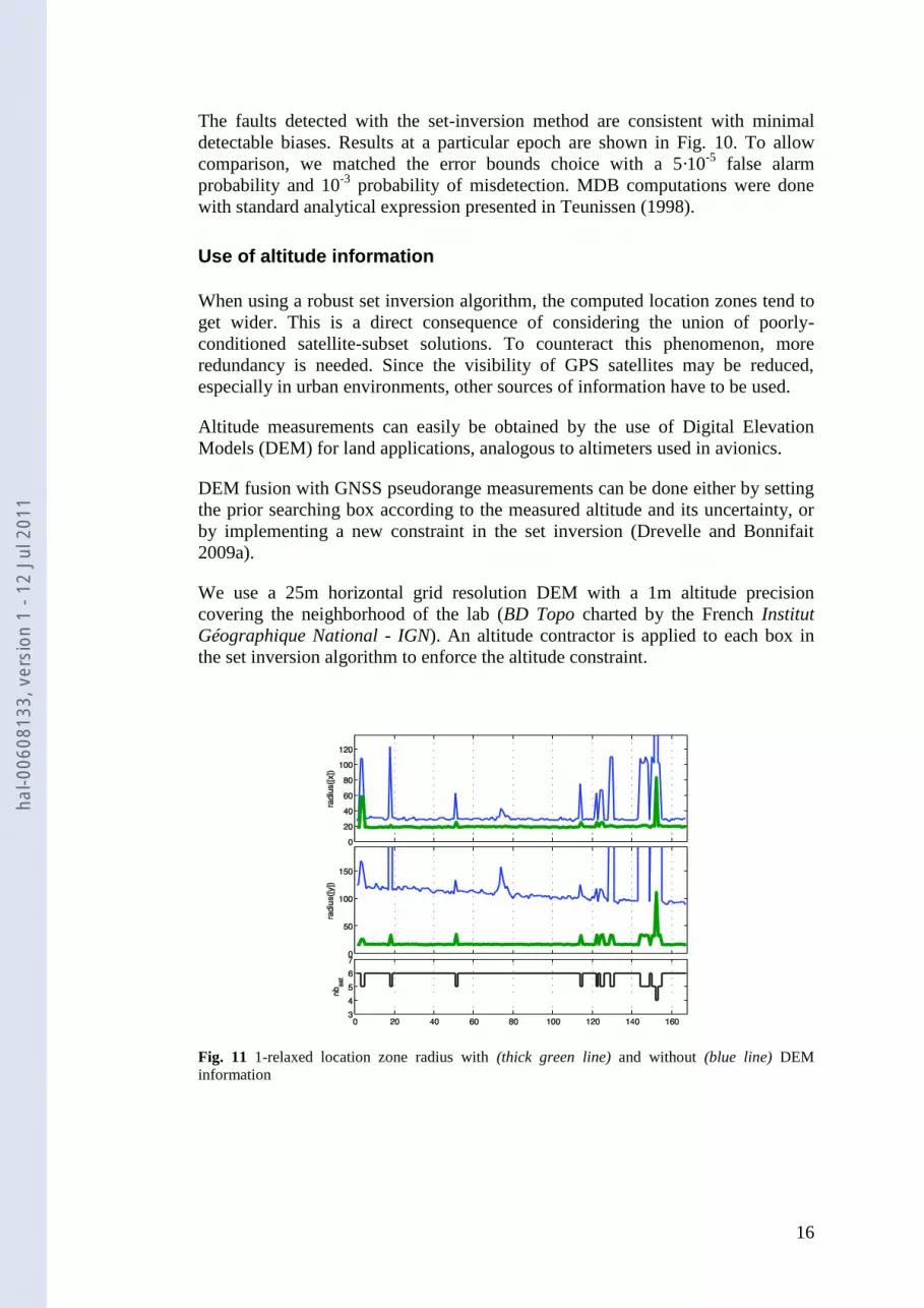
Use of altitude information
When using a robust set inversion algorithm, the computed location zones tend to
get wider. This is a direct consequence of considering the union of poorly-
conditioned satellite-subset solutions. To counteract this phenomenon, more
redundancy is needed. Since the visibility of GPS satellites may be reduced,
especially in urban environments, other sources of information have to be used.
Altitude measurements can easily be obtained by the use of Digital Elevation
Models (DEM) for land applications, analogous to altimeters used in avionics.
DEM fusion with GNSS pseudorange measurements can be done either by setting
the prior searching box according to the measured altitude and its uncertainty, or
by implementing a new constraint in the set inversion (Drevelle and Bonnifait
2009a).
We use a 25m horizontal grid resolution DEM with a 1m altitude precision
covering the neighborhood of the lab (BD Topo charted by the French Institut
Géographique National - IGN). An altitude contractor is applied to each box in
the set inversion algorithm to enforce the altitude constraint.
Fig. 11 1-relaxed location zone radius with (thick green line) and without (blue line) DEM
information
hal-0
0608
133,
ver
sion
1 -
12 J
ul 2
011

17
In this trial. with the immunity to one erroneous measurement (RSIVIA with
1=q ), the altitude information from the DEM reduces the horizontal location
zone radius by a factor 5 on the y axis (Fig. 11).
The benefits of altitude information in reducing horizontal uncertainty are
especially noticeable when few satellites are visible, or when robustness to a large
number of faulty measurements is required. The altitude constraint provided by
the DEM enables robust snapshot localization with as few as four satellites.
Fig. 12 Location zone bounds with respect to ground truth, using DEM information. An increasing
bias is applied on the first pseudorange.
Figure 12 shows the influence of a biased measurement on the horizontal position
bounds, when merging DEM information with GPS pseudorange measurements.
It is the same six-satellite dataset as in Fig. 10, allowing us to compare results
with and without the use of a DEM. The nonrobust approach is little improved by
the use of a DEM: Integrity is lost between 17 m and 21 m bias, while it was lost
between 18 m and 23 m without the DEM information. Location zone is also a
few meters tighter. A great improvement can be seen in the 1-relaxed solver
behavior. The location zone always remains consistent with ground truth, since
there is only one erroneous measurement, but it is tighter thanks to the added
constraint, especially on the y-axis. The presence of an outlier is detected earlier,
starting from a 16 m bias (19 meters without DEM). Moreover, the erroneous
hal-0
0608
133,
ver
sion
1 -
12 J
ul 2
011

18
measurement is totally excluded from the solution after a 25m bias, where 50 m
were necessary without DEM altitude information.
An experiment has also been conducted to compare the 1m resolution IGN DEM
with a coarser DEM from the NASA‘s Shuttle Radar Topography Mission, with a
14m vertical accuracy. A ramp error was successively applied to each satellite in
view, and the bias values for which error detection and identification occurred
were recorded. Higher precision DEM not only allows detection of smaller biases
(Fig. 13a), but it also significantly reduces the size of error needed to identify the
faulty measurement (Fig. 13b).
Fig. 13 Influence of DEM precision on fault detection and identification
Maximum number of tolerated outliers
The maximum number of tolerated outliers has to be set before set-inversion.
Several choices are available. If only satellite failures are considered, a reasonable
approach is to set the maximum number of outliers to one. This approach can be
used in an open sky environment, and it corresponds to the ‗one fault at a time‘
hypothesis.
In urban areas, the risk of receiving simultaneous non-line-of-sight measurements
is not negligible. Moreover, the number of visible satellites can be low. In this
case, the number q of tolerated outliers can be set as a tradeoff between precision
and integrity. The quality of the receiver and the antenna and their ability to reject
reflected signals play a prominent part in the setting of q. For the Septentrio
PolaRx and its polarized antenna, setting q=1 is a reasonable choice. With a low-
end receiver with a patch antenna, it is common to receive three simultaneous
wrong measurements in urban areas (Le Marchand et al. 2009). Setting q=3
ensures that a nonempty solution will exist most of the time.
Another approach can be based on the Guaranteed Outlier Minimal Number
Estimator (Kieffer et al. 2000). The idea is to compute q-relaxed solutions with
increasing values of q, until a nonempty solution is found. Robustness to
undetectable errors can then be provided by adding a number of tolerated
undetected errors to the value of q previously found.
hal-0
0608
133,
ver
sion
1 -
12 J
ul 2
011
19
Conclusion
A new method to characterize a location zone has been presented. It is based on
robust set inversion using interval analysis. Bounds are set on measurements,
taking error and risk into account. These bounded-error measurements translate
into constraints in the location domain. Using interval analysis, the constraint
satisfaction problem can then be solved, and a defined number of constraints can
be relaxed in order to maintain solution integrity in the presence of outliers.
An experimental validation to compute location zones was carried out, using GPS
pseudorange measurements corrected with EGNOS, and a Digital Elevation
Model. It was implemented in real time as a parallelized C++ program. Results
show that additional altitude information from the DEM enabled more precise
positioning while tolerating GPS outliers, especially with a small number of
visible satellites. Since each box in a subpaving can be processed independently
of the others, the interval methods employed can be easily and efficiently
parallelized to take advantage of the additional power of multi-core processors.
The presented snapshot GPS-DEM robust location zone computation algorithm
fails to provide a useful location zone when the number of pseudorange
measurements becomes too low (with respect to the number of tolerated outliers).
Future work will be focused on dynamic car positioning, using a kinematic
vehicle model and embedded proprioceptive sensors. This will constrain the
location zone, especially during GPS outages in difficult environments like urban
canyons.
Aknowledgements The dataset and the reference trajectory used in this work were provided by
Clément Fouque (Heudiasyc UMR 6599, Université de Technologie de Compiègne).
References
Baarda W (1968) A Testing Procedure for use in Geodetic Networks. Ned Geod Comm Publ on
Geodesy, New series 2(5)
Bancroft S (1985) An algebraic solution of the GPS equations. IEEE T Aero Elec Sys 21(1):56–59
Brown RG (1992) A baseline GPS RAIM scheme and a note on the equivalence of three RAIM
methods. Navigation
Chang TH, Wang LS, Chang FR (2009) A Solution to the Ill-Conditioned GPS Positioning
Problem in an Urban Environment. IEEE T Intell Transp 10(1):135–145
Drevelle V, Bonnifait P (2009a) High integrity GNSS location zone characterization using interval
analysis. In: Proceedings of ION GNSS 2009, pp 2178–2187
Drevelle V, Bonnifait P (2009b) Integrity Zone Computation using Interval Analysis. In:
Proceedings of the European Navigation Conference (GNSS 2009)
Feng S, Ochieng W, Walsh D, Ioannides R (2006) A measurement domain receiver autonomous
integrity monitoring algorithm. GPS Solut 10(2):85–96
Fouque C, Bonnifait P (2008) Tightly-coupled GIS data in GNSS fix computations with integrity
testing. Int J Intell Inf Database Syst 2(2):167–186
Gutmann J, Marti L, Lammel G (2009) Multipath Detection and Mitigation by Means of a MEMS
Based Pressure Sensor for Low-Cost Systems. In: Proceedings of the 22nd International
Meeting of the Satellite Division of The Institute of Navigation, pp 2077–2087
Hewitson S, Wang J (2007) GNSS Receiver Autonomous Integrity Monitoring with a Dynamic
Model. J Navig 60(2):247–263
Huber PJ (1964) Robust estimation of a location parameter. Ann Math Stat 35(1):73–101
Jaulin L (2009) Robust set-membership state estimation; application to underwater robotics.
Automatica 45(1):202–206
Jaulin L, Walter E (1993) Set inversion via interval analysis for nonlinear bounded-error
estimation. Automatica 29(4):1053–1064
hal-0
0608
133,
ver
sion
1 -
12 J
ul 2
011

20
Jaulin L, Kieffer M, Braems I, Walter E (2001a) Guaranteed Nonlinear Estimation Using
Constraint Propagation on Sets. Int J Control 74(18):1772–1782
Jaulin L, Kieffer M, Didrit O, Walter E (2001b) Applied Interval Analysis. Springer-Verlag
Jaulin L, Kieffer M, Walter E, Meizel D (2002) Guaranteed Robust Nonlinear Estimation with
Application to Robot Localization. IEEE T Syst Man Cy C 32(4):374–382
Kaplan E, Hegarty C (2006) Understanding GPS: Principles and Applications Second Edition.
Artech House Publishers
Kieffer M, Jaulin L, Walter E, Meizel D (2000) Robust Autonomous Robot Localization Using
Interval Analysis. Reliable Computing 6(3):337–362
Le Marchand O, Bonnifait P, Ibanez-Guzmán J, Bétaille D, Peyret F (2009) Characterization of
GPS multipath for passenger vehicles across urban environments. ATTI dell'Istituto Italiano di
Navigazione 189:77–88
Leick A (2004) GPS satellite surveying, Third edition.Wiley
Li J, Taylor G, Kidner DB (2005) Accuracy and reliability of map-matched GPS coordinates: The
dependence on terrain model resolution and interpolation algorithm. Comput Geosci
31(2):241–251
Meizel D, Leveque O, Jaulin L, Walter E (2002) Initial localization by set inversion. IEEE T
Robotic Autom 18(6):966–971
Moore RE (1966) Interval analysis. Prentice Hall
Röhrig C, Müller M (2009) Indoor location tracking in non-line-of-sight environments using
IEEE 802.15.4a wireless network. In: Conference Proceedings of IROS09, pp 552–557
Salzmann M (1991) MDB: a design tool for integrated navigation systems. Journal of Geodesy
65(2):109–115
Schroth G, Ene A, Blanch J, Walter T, Enge P (2008) Failure Detection and Exclusion via Range
Consensus. In: Proceedings of the European Navigation Conference
Schubert A (2006) Comparison of Solution Separation Method with Parity Space Methods. In:
Proceedings of ENC-GNSS 2006
Teunissen PJG (1990) Quality Control in Integrated Navigation Systems. IEEE Aerosp Electron
Syst Mag 5(7):35–41
Teunissen PJG (1998) Minimal Detectable Biases of GPS Data. Journal of Geodesy, 72:236–244
Walter T, Enge P (1995) Weighted RAIM for precision approach. In: Proceedings of ION GPS,
Institute of Navigation, pp 1995–2004
hal-0
0608
133,
ver
sion
1 -
12 J
ul 2
011