Samuel Clark

Department of Sociology, University of WashingtonInstitute of Behavioral Science, University of Colorado at Boulder

Agincourt Health and Population Unit, University of the Witwatersrand

Age-Standardization & Decomposition

2

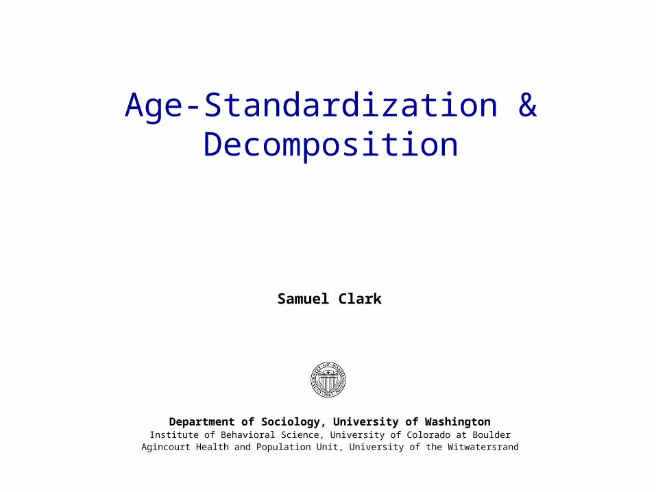
Period Age-Specific Death Rate

Death Rate for ages x to x+n during the period spanning 0 to T:

0,0, 0,n x

n xn x

D TM T

N T

M is the death rateD is the number of deathsN is the population

3

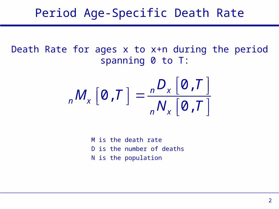
Lexis Diagram

0

5

10

15

20

25

30

35

40

0 5 10 15 20 25 30 35 40Tim e (years)

Age (years)

C1 C2 C3

4

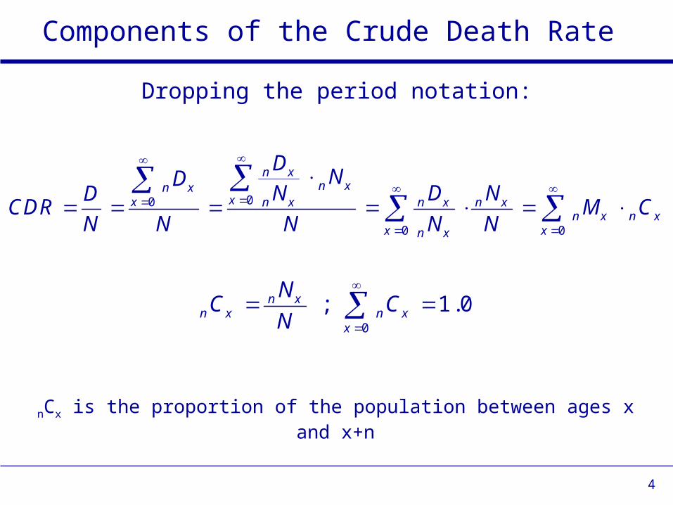
Components of the Crude Death Rate

Dropping the period notation:

00

0 0

n xn xn x

xx n x n x n xn x n x

x xn x

D ND N D NDCDR M CN N N N N

nCx is the proportion of the population between ages x and x+n

0; 1.0n x

n x n xx

NC CN

5

Standardization CDR is a function of the mortality schedule AND the age distribution

Changes in either or both affect the level of the CDR

When comparing CDRs, it is important to isolate the source of the differences:– Differences in age-specific mortality rates?– Differences in age distributions?

Age standardization holds the age structure constant so that the only source of difference is the mortality schedule

Same applies to any division of the population that produces differing rates (or proportions)

6

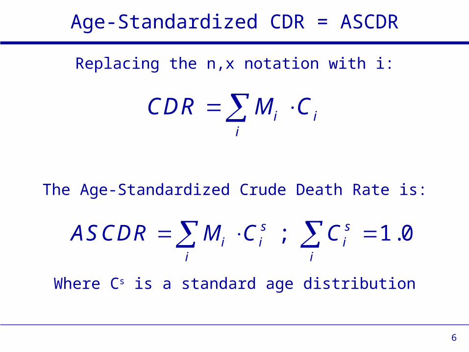
Age-Standardized CDR = ASCDR

i ii

CDR M C Replacing the n,x notation with i:

; 1.0s si i i

i iAS CDR M C C

The Age-Standardized Crude Death Rate is:

Where Cs is a standard age distribution

7

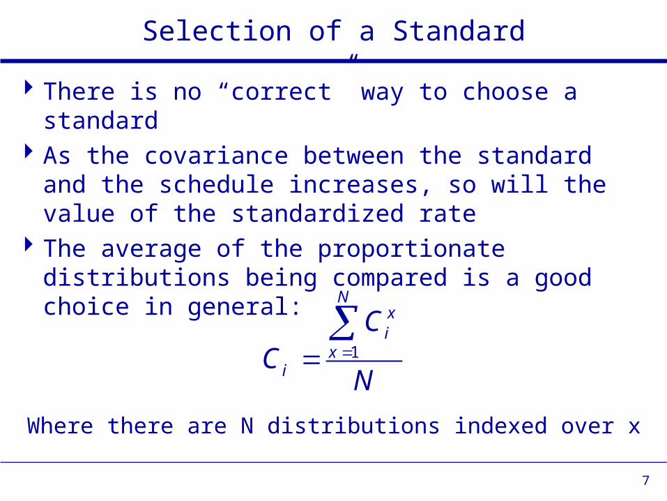
Selection of a Standard There is no “correct” way to choose a standard

As the covariance between the standard and the schedule increases, so will the value of the standardized rate

The average of the proportionate distributions being compared is a good choice in general:

1

Nxi

xi

CC

N

Where there are N distributions indexed over x

8

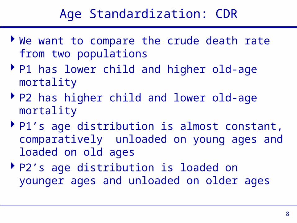
Age Standardization: CDR We want to compare the crude death rate from two populations

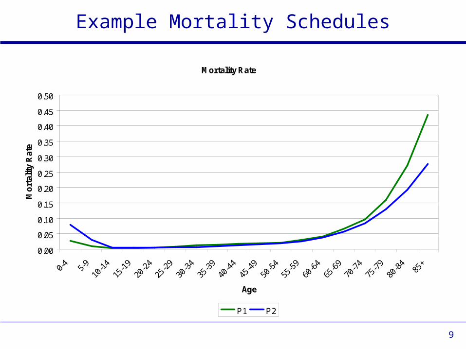
P1 has lower child and higher old-age mortality

P2 has higher child and lower old-age mortality

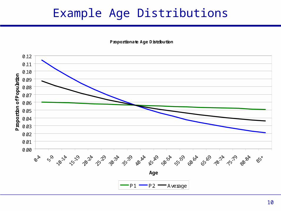
P1’s age distribution is almost constant, comparatively unloaded on young ages and loaded on old ages

P2’s age distribution is loaded on younger ages and unloaded on older ages

9

Example Mortality Schedules

M ortality Rate

0.000.050.100.150.200.250.300.350.400.450.50

0-4 5-9 10-14

15-19

20-24

25-29

30-34

35-39

40-44

45-49

50-54

55-59

60-64

65-69

70-74

75-79

80-84 85+

Age

Mortality R

ate

P1 P2

10

Example Age Distributions

Proportionate Age Distribution

0.000.010.020.030.040.050.060.070.080.090.100.110.12

0-4 5-9 10-14

15-19

20-24

25-29

30-34

35-39

40-44

45-49

50-54

55-59

60-64

65-69

70-74

75-79

80-84 85+

Age

Proportion of Population

P1 P2 Average

11

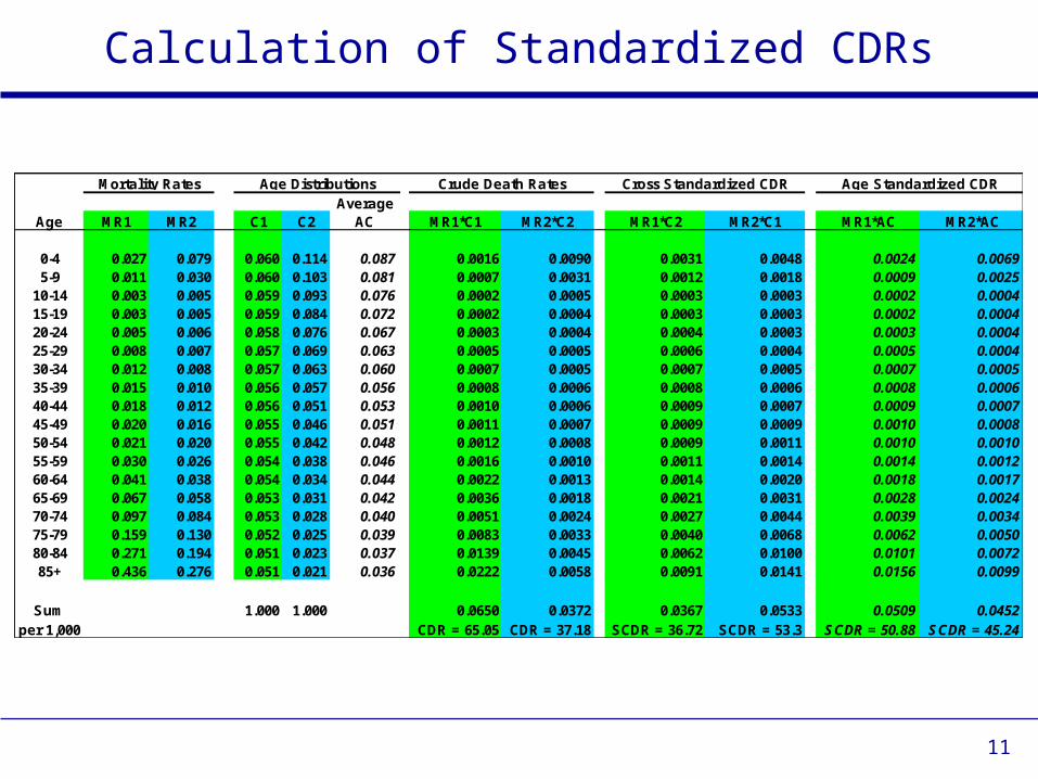
Calculation of Standardized CDRs

AverageAge M R1 M R2 C1 C2 AC M R1*C1 M R2*C2 M R1*C2 M R2*C1 M R1*AC M R2*AC

0-4 0.027 0.079 0.060 0.114 0.087 0.0016 0.0090 0.0031 0.0048 0.0024 0.00695-9 0.011 0.030 0.060 0.103 0.081 0.0007 0.0031 0.0012 0.0018 0.0009 0.002510-14 0.003 0.005 0.059 0.093 0.076 0.0002 0.0005 0.0003 0.0003 0.0002 0.000415-19 0.003 0.005 0.059 0.084 0.072 0.0002 0.0004 0.0003 0.0003 0.0002 0.000420-24 0.005 0.006 0.058 0.076 0.067 0.0003 0.0004 0.0004 0.0003 0.0003 0.000425-29 0.008 0.007 0.057 0.069 0.063 0.0005 0.0005 0.0006 0.0004 0.0005 0.000430-34 0.012 0.008 0.057 0.063 0.060 0.0007 0.0005 0.0007 0.0005 0.0007 0.000535-39 0.015 0.010 0.056 0.057 0.056 0.0008 0.0006 0.0008 0.0006 0.0008 0.000640-44 0.018 0.012 0.056 0.051 0.053 0.0010 0.0006 0.0009 0.0007 0.0009 0.000745-49 0.020 0.016 0.055 0.046 0.051 0.0011 0.0007 0.0009 0.0009 0.0010 0.000850-54 0.021 0.020 0.055 0.042 0.048 0.0012 0.0008 0.0009 0.0011 0.0010 0.001055-59 0.030 0.026 0.054 0.038 0.046 0.0016 0.0010 0.0011 0.0014 0.0014 0.001260-64 0.041 0.038 0.054 0.034 0.044 0.0022 0.0013 0.0014 0.0020 0.0018 0.001765-69 0.067 0.058 0.053 0.031 0.042 0.0036 0.0018 0.0021 0.0031 0.0028 0.002470-74 0.097 0.084 0.053 0.028 0.040 0.0051 0.0024 0.0027 0.0044 0.0039 0.003475-79 0.159 0.130 0.052 0.025 0.039 0.0083 0.0033 0.0040 0.0068 0.0062 0.005080-84 0.271 0.194 0.051 0.023 0.037 0.0139 0.0045 0.0062 0.0100 0.0101 0.007285+ 0.436 0.276 0.051 0.021 0.036 0.0222 0.0058 0.0091 0.0141 0.0156 0.0099

Sum 1.000 1.000 0.0650 0.0372 0.0367 0.0533 0.0509 0.0452per 1,000 CDR = 65.05 CDR = 37.18 SCDR = 36.72 SCDR = 53.3 S CDR = 50.88 S CDR = 45.24

Age Standardized CDRM ortality Rates Age Distributions Crude Death Rates Cross Standardized CDR

12

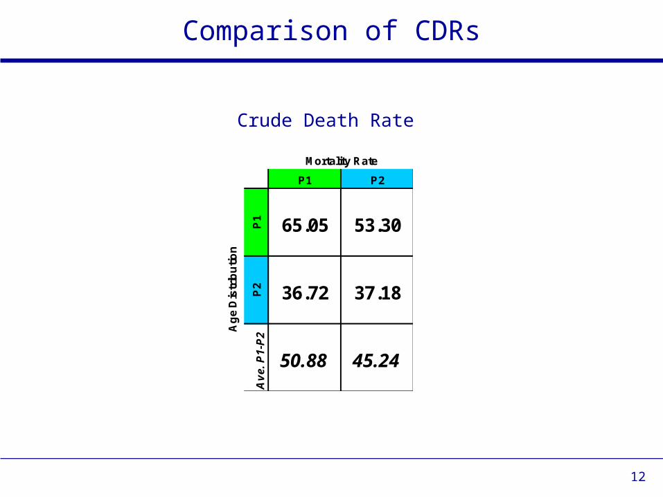
Comparison of CDRs

Crude Death Rate

P1 P2

P1 65.05 53.30P2 36.72 37.18

Ave

. P1-

P2

50.88 45.24

M ortality Rate

Age Distrib

ution

13

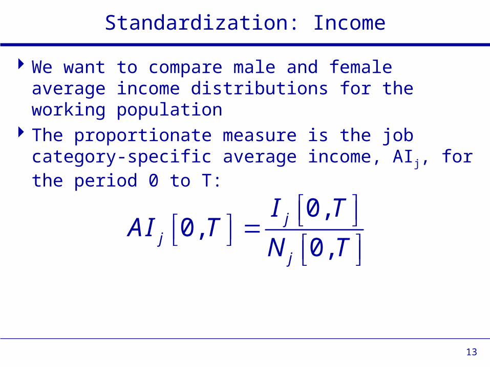
Standardization: Income We want to compare male and female average income distributions for the working population

The proportionate measure is the job category-specific average income, AIj, for the period 0 to T:

0,0, 0,j

jj

I TA I T

N T

14

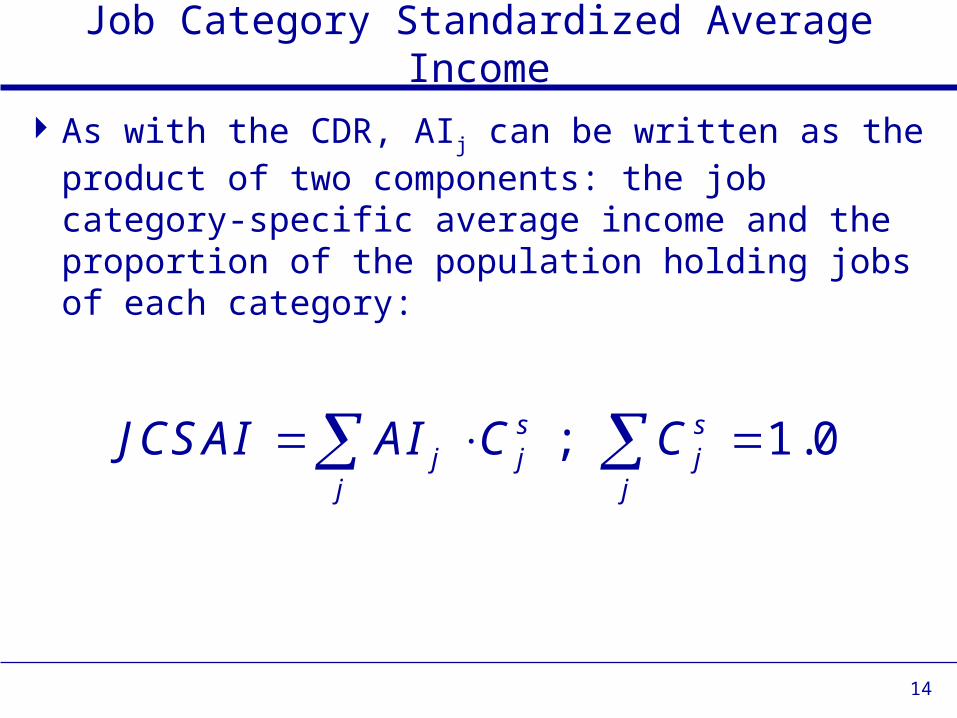
Job Category Standardized Average Income

As with the CDR, AIj can be written as the product of two components: the job category-specific average income and the proportion of the population holding jobs of each category:

; 1.0s sj j j

j jJ CS AI A I C C

15

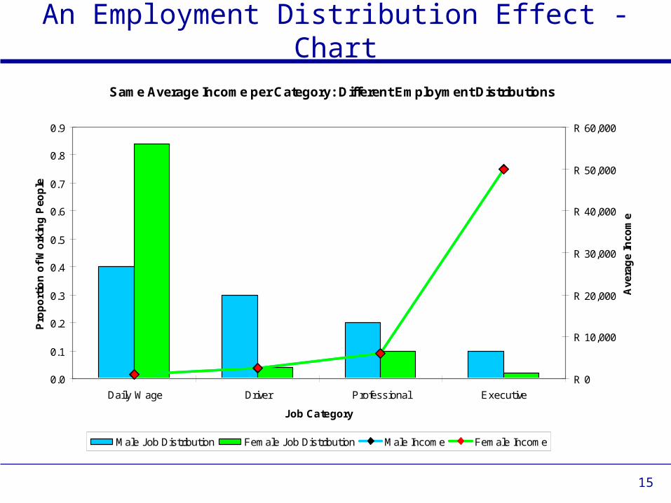
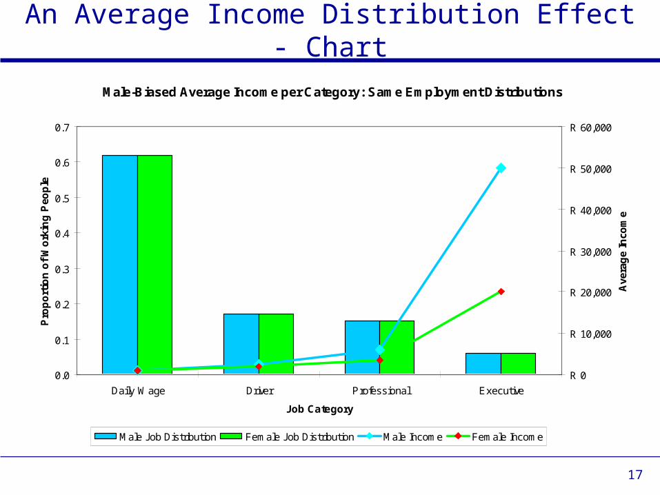
An Employment Distribution Effect - Chart

Sam e Average Incom e per Category: Different Em ploym ent Distributions

0.0

0.1

0.2

0.3

0.4

0.5

0.6

0.7

0.8

0.9

Daily W age Driver Professional ExecutiveJob Category

Prop

ortio

n of W

orking

People

R 0

R 10,000

R 20,000

R 30,000

R 40,000

R 50,000

R 60,000

Average Income

M ale Job Distribution Fem ale Job Distribution M ale Incom e Fem ale Incom e

16

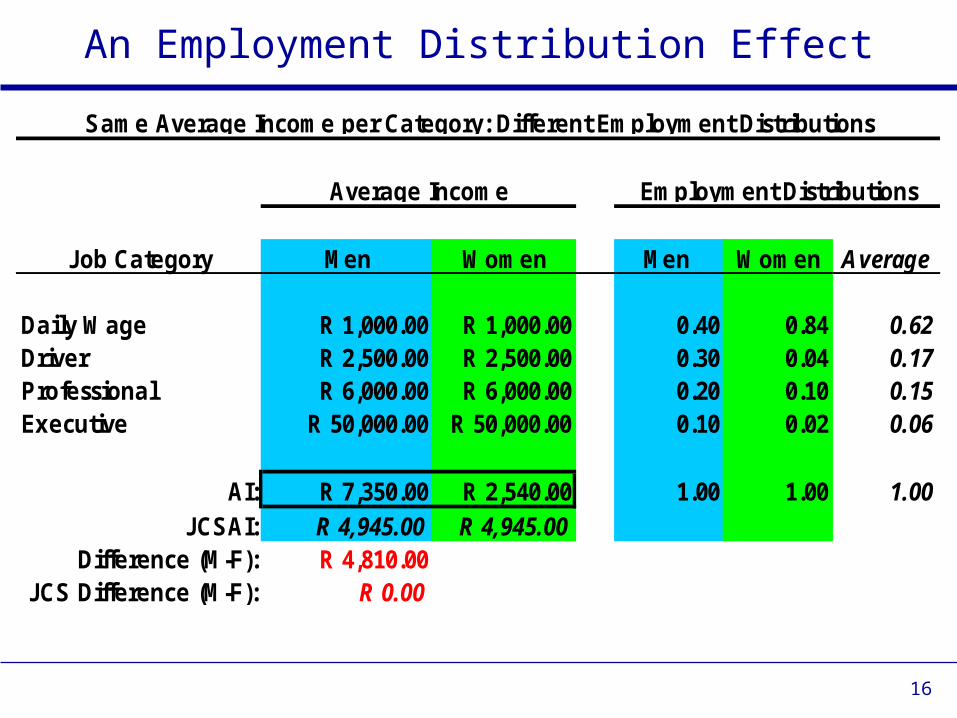
An Employment Distribution Effect

Job Category M en W om en M en W om en A verage

Daily W age R 1,000.00 R 1,000.00 0.40 0.84 0.62Driver R 2,500.00 R 2,500.00 0.30 0.04 0.17Professional R 6,000.00 R 6,000.00 0.20 0.10 0.15Executive R 50,000.00 R 50,000.00 0.10 0.02 0.06

AI: R 7,350.00 R 2,540.00 1.00 1.00 1.00JCSAI: R 4,945.00 R 4,945.00

Difference (M -F): R 4,810.00JCS Difference (M -F): R 0.00

Sam e Average Incom e per Category: Different Em ploym ent Distributions

Average Incom e Em ploym ent Distributions

17

M ale-Biased Average Incom e per Category: Sam e Em ploym ent Distributions

0.0

0.1

0.2

0.3

0.4

0.5

0.6

0.7

Daily W age Driver Professional ExecutiveJob Category

Prop

ortio

n of W

orking

People

R 0

R 10,000

R 20,000

R 30,000

R 40,000

R 50,000

R 60,000

Average Income

M ale Job Distribution Fem ale Job Distribution M ale Incom e Fem ale Incom e

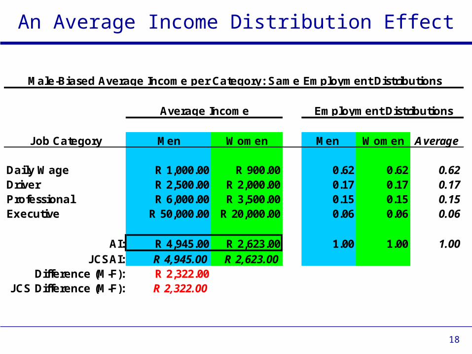
An Average Income Distribution Effect - Chart

18

An Average Income Distribution Effect

Job Category M en W om en M en W om en A verage

Daily W age R 1,000.00 R 900.00 0.62 0.62 0.62Driver R 2,500.00 R 2,000.00 0.17 0.17 0.17Professional R 6,000.00 R 3,500.00 0.15 0.15 0.15Executive R 50,000.00 R 20,000.00 0.06 0.06 0.06

AI: R 4,945.00 R 2,623.00 1.00 1.00 1.00JCSAI: R 4,945.00 R 2,623.00

Difference (M -F): R 2,322.00JCS Difference (M -F): R 2,322.00

M ale-Biased Average Incom e per Category: Sam e Em ploym ent Distributions

Average Incom e Em ploym ent Distributions

19

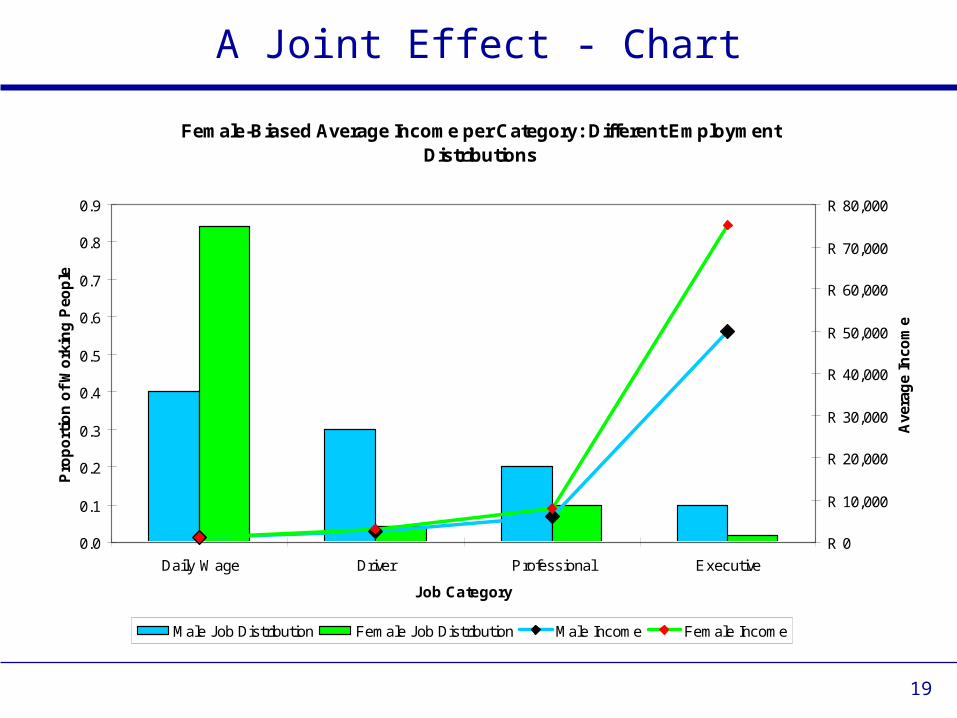
A Joint Effect - ChartFem ale-Biased Average Incom e per Category: Different Em ploym ent

Distributions

0.0

0.1

0.2

0.3

0.4

0.5

0.6

0.7

0.8

0.9

Daily W age Driver Professional ExecutiveJob Category

Prop

ortio

n of W

orking

People

R 0

R 10,000

R 20,000

R 30,000

R 40,000

R 50,000

R 60,000

R 70,000

R 80,000

Average Income

M ale Job Distribution Fem ale Job Distribution M ale Incom e Fem ale Incom e

20

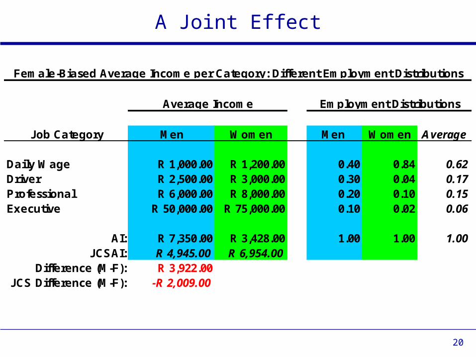
A Joint Effect

Job Category M en W om en M en W om en A verage

Daily W age R 1,000.00 R 1,200.00 0.40 0.84 0.62Driver R 2,500.00 R 3,000.00 0.30 0.04 0.17Professional R 6,000.00 R 8,000.00 0.20 0.10 0.15Executive R 50,000.00 R 75,000.00 0.10 0.02 0.06

AI: R 7,350.00 R 3,428.00 1.00 1.00 1.00JCSAI: R 4,945.00 R 6,954.00

Difference (M -F): R 3,922.00JCS Difference (M -F): -R 2,009.00

Fem ale-Biased Average Incom e per Category: Different Em ploym ent Distributions

Average Incom e Em ploym ent Distributions

21

Decomposition Decomposition refers to a technique that identifies the proportion of the difference between two crude death rates that results from the differences in the mortality schedules and the differences in the age distributions

As with the standardization technique described earlier, this is a general technique that can be used with any crude proportion formed as the sum of proportionate distribution and a proportional measure

22

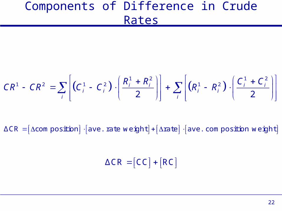
Components of Difference in Crude Rates

1 2 1 21 2 1 2 1 2

2 2i i i i

i i i ii i

R R C CCR CR C C R R

ΔCR com position ave. rate w eight rate ave. com position w eight

ΔCR CC RC

23

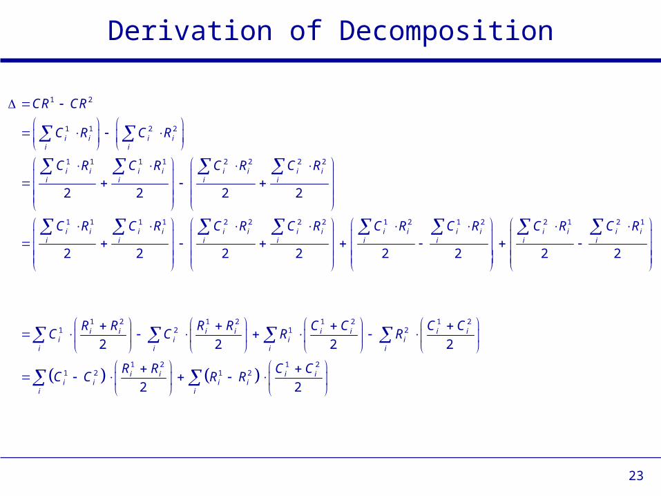
Derivation of Decomposition

1 2

1 1 2 2

1 1 1 1 2 2 2 2

1 1 1 1 2 2 2 2 1 2 1 2

2 2 2 2

2 2 2 2 2 2

i i i ii i

i i i i i i i ii i i i

i i i i i i i i i i i ii i i i i i

CR CR

C R C R

C R C R C R C R

C R C R C R C R C R C R

2 1 2 1

1 2 1 2 1 2 1 21 2 1 2

1 2 1 21 2 1 2

2 2

2 2 2 2

2 2

i i i ii i

i i i i i i i ii i i i

i i i i

i i i ii i i i

i i

C R C R

R R R R C C C CC C R R

R R C CC C R R

24

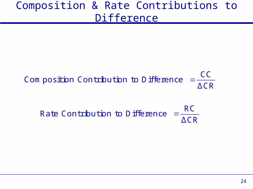
Composition & Rate Contributions to Difference

CCCom position Contribution to Difference ΔCR

RCRate Contribution to Difference ΔCR

25

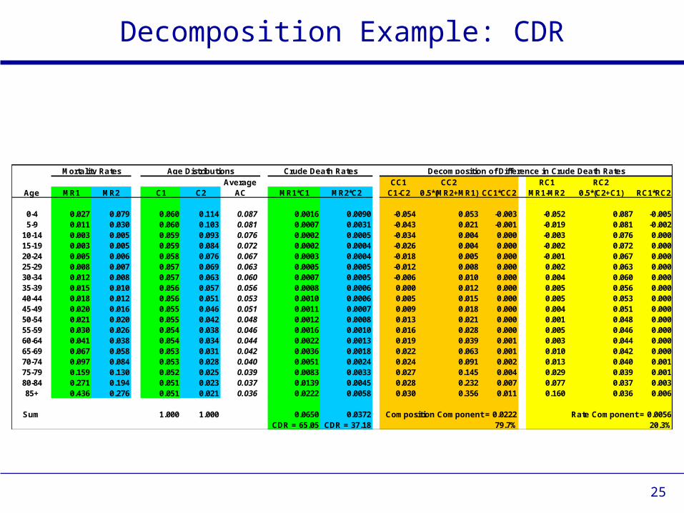
Decomposition Example: CDR

Average CC1 CC2 RC1 RC2Age M R1 M R2 C1 C2 AC M R1*C1 M R2*C2 C1-C2 0.5*(M R2+M R1) CC1*CC2 M R1-M R2 0.5*(C2+C1) RC1*RC2

0-4 0.027 0.079 0.060 0.114 0.087 0.0016 0.0090 -0.054 0.053 -0.003 -0.052 0.087 -0.0055-9 0.011 0.030 0.060 0.103 0.081 0.0007 0.0031 -0.043 0.021 -0.001 -0.019 0.081 -0.00210-14 0.003 0.005 0.059 0.093 0.076 0.0002 0.0005 -0.034 0.004 0.000 -0.003 0.076 0.00015-19 0.003 0.005 0.059 0.084 0.072 0.0002 0.0004 -0.026 0.004 0.000 -0.002 0.072 0.00020-24 0.005 0.006 0.058 0.076 0.067 0.0003 0.0004 -0.018 0.005 0.000 -0.001 0.067 0.00025-29 0.008 0.007 0.057 0.069 0.063 0.0005 0.0005 -0.012 0.008 0.000 0.002 0.063 0.00030-34 0.012 0.008 0.057 0.063 0.060 0.0007 0.0005 -0.006 0.010 0.000 0.004 0.060 0.00035-39 0.015 0.010 0.056 0.057 0.056 0.0008 0.0006 0.000 0.012 0.000 0.005 0.056 0.00040-44 0.018 0.012 0.056 0.051 0.053 0.0010 0.0006 0.005 0.015 0.000 0.005 0.053 0.00045-49 0.020 0.016 0.055 0.046 0.051 0.0011 0.0007 0.009 0.018 0.000 0.004 0.051 0.00050-54 0.021 0.020 0.055 0.042 0.048 0.0012 0.0008 0.013 0.021 0.000 0.001 0.048 0.00055-59 0.030 0.026 0.054 0.038 0.046 0.0016 0.0010 0.016 0.028 0.000 0.005 0.046 0.00060-64 0.041 0.038 0.054 0.034 0.044 0.0022 0.0013 0.019 0.039 0.001 0.003 0.044 0.00065-69 0.067 0.058 0.053 0.031 0.042 0.0036 0.0018 0.022 0.063 0.001 0.010 0.042 0.00070-74 0.097 0.084 0.053 0.028 0.040 0.0051 0.0024 0.024 0.091 0.002 0.013 0.040 0.00175-79 0.159 0.130 0.052 0.025 0.039 0.0083 0.0033 0.027 0.145 0.004 0.029 0.039 0.00180-84 0.271 0.194 0.051 0.023 0.037 0.0139 0.0045 0.028 0.232 0.007 0.077 0.037 0.00385+ 0.436 0.276 0.051 0.021 0.036 0.0222 0.0058 0.030 0.356 0.011 0.160 0.036 0.006

Sum 1.000 1.000 0.0650 0.0372 Com position Com ponent = 0.0222 Rate Com ponent = 0.0056CDR = 65.05 CDR = 37.18 79.7% 20.3%

Decom position of Difference in Crude Death RatesM ortality Rates Age Distributions Crude Death Rates

26

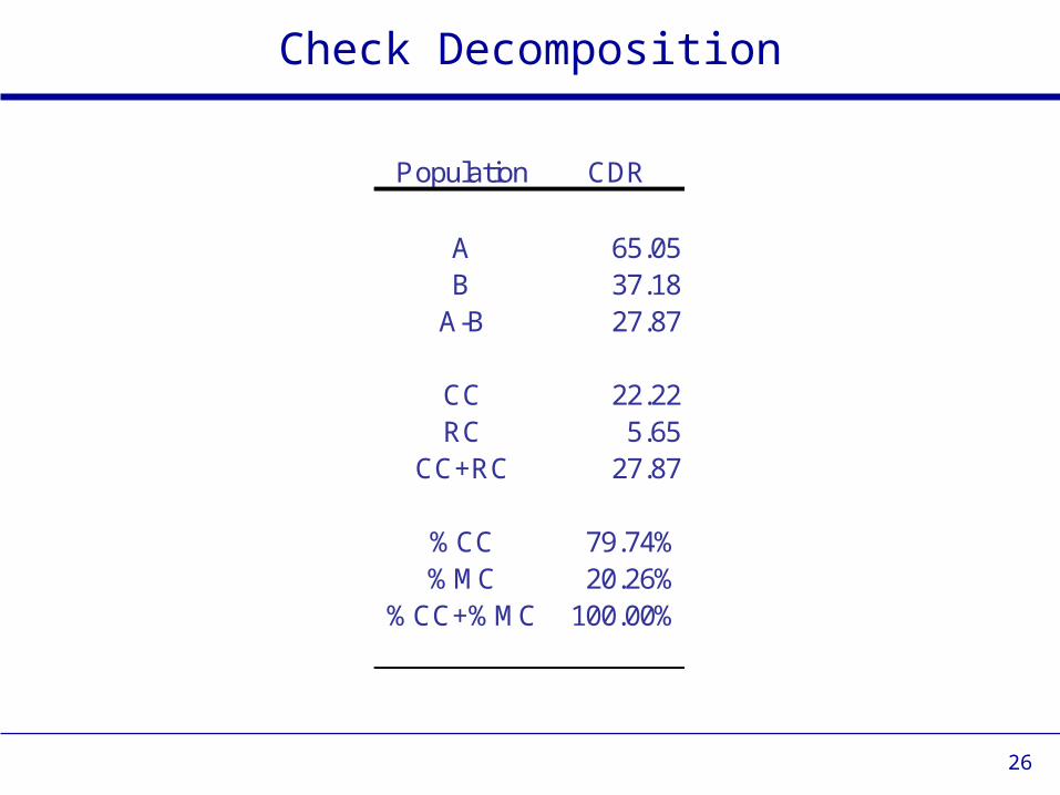
Check Decomposition

Population CDR

A 65.05B 37.18A-B 27.87

CC 22.22RC 5.65

CC+RC 27.87

% CC 79.74%% M C 20.26%

% CC+% M C 100.00%