A Recourse Certainty Equivalent for Decisions UnderUncertainty∗†

Aharon Ben-Tal‡ Adi Ben-Israel§

August 1, 1989Revised May 25, 1990

AbstractWe propose a new criterion for decision-making under uncertainty. The crite-

rion is based on a certainty equivalent (CE) of a (monetary valued) random variableZ,

Sv(Z) = supz{z + E

Zv(Z − z)}

where v(·) is the decision maker’s value-risk function. This CE is derived fromconsiderations of stochastic optimization with recourse, and is called recoursecertainty equivalent (RCE). We study (i) the properties of the RCE, (ii) the recov-erability of v(·) from Sv(·) (in terms of the rate of change in risk), (iii) comparisonwith the “classical CE” u−1Eu(·) in expected utility (EU) theory, (iv) relation torisk-aversion, (v) connection with Machina’s generalized expected utility theory,and its use to explain the Allais paradox and other decision theoretic paradoxes, and(vi) applications to models of production under price uncertainty, investmentin risky and safe assets and insurance. In these models the RCE gives intuitivelyappealing answers for all risk-averse decision makers, unlike the EU model which givesonly partial answers, and requires, in addition to risk-aversion, also assumptions onthe so-called Arrow-Pratt indices.

Key words: Stochastic optimization with recourse. Decision-making under uncertainty.Expected utility. Certainty equivalents. The Allais paradox and other decision the-oretic paradoxes. Risk aversion. Production under price uncertainty. Investment inrisky and safe assets. Insurance.

∗Supported by National Science Foundation Grant DDM-8996112.†Helpful comments by the referees are gratefully acknowledged.‡Faculty of Industrial Engineering and Management, Technion-Israel Institute of Technology, Haifa, Israel.§RUTCOR-Rutgers Center for Operations Research, School of Business and Department of Mathematics,

Rutgers University, New Brunswick, NJ 08903-5062.

0

1 Introduction

We propose a new criterion for decision-making under uncertainty using one of the funda-mental concepts of stochastic programming, namely that of recourse, [5], [14], [15] and [47].Recourse refers to corrective action, after realization of the random variables, which is takeninto account when making the actual decision (before realization). For the role of recoursein stochastic programming see [16], [25] and [49].

Decision making under uncertainty presupposes the ability to rank random vari-ables, i.e. a complete order � on the space of RV’s, with X � Y denotes X preferredto Y . If the preference order � is given in terms of a real valued function CE(·) on thespace of RV’s,

X � Y ⇐⇒ CE(X) ≥ CE(Y ) for all RV’s X, Y

we call CE(Z) a certainty equivalent (CE) of Z, corresponding to the preference � . Inparticular, a decision maker (DM for short) is indifferent between a RV Z and a constant1

z iff z = CE(Z).In the expected utility (EU) model, the DM is assumed to have a utility function u(·)

which typically is strictly increasing (more is better) and concave. The DM’s preferenceis then given by

X � Y ⇐⇒ E u(X) ≥ E u(Y ) (1.1)

⇐⇒ u−1E u(X) ≥ u−1E u(Y ),

Accordingly we define the classical certainty equivalent (CCE) by

Cu(Z) = u−1Eu(Z) (1.2)

Another CE, suggested by expected utility, is the u-mean CE Mu(·) defined, for any RV Z,by

E u(Z −Mu(Z)) = 0 (1.3)

see e.g. [11, p. 86], under “principle of zero utility”.Still another CE is based on the “dual theory” of Yaari, [50]. Given a monotone function

f : [0, 1] → [0, 1] with f(0) = 0 and f(1) = 1, Yaari’s certainty equivalent Yf (·) is

Yf (Z) =∫

f(1− FZ

(t))dt (1.4)

where FZ

is the cumulative distribution function of the RV Z. Unlike the CCE (1.2), both

Yaari’s CE (1.4) and the u-mean CE (1.3) are shift additive in the sense that

CE(Z + c) = CE(Z) + c for all RV Z and constant c (1.5)

1Regarded as a degenerate RV.

1

In the EU model a risk-averse decision maker, i.e. one for whom a RV X is less desirablethan a sure reward of EX, is characterized by a concave utility function u. The concavity ofu also expresses the attitude towards wealth (decreasing marginal utility). Thus the DM’sattitude towards wealth and his attitude towards risk are “forever bonded together”,[50, p. 95]. Certain difficulties with the EU model are due to this fact. In Yaari’s dual theory[50], and in the RCE model proposed below, the attitude towards wealth and the attitudetowards risk are effectively separated. In particular, Yaari’s risk aversion is compatible withlinearity in payments2.

The CE advocated here is the recourse certainty equivalent (RCE)

Sv(Z) := supz{z + E

Zv(Z − z)} (1.6)

where v(·) is the value-risk function of the DM. The RCE was first introduced in [9]. Wepropose here the RCE Sv as a criterion for decision making under uncertainty i.e. for rankingmonetary valued RV’s. The given value-risk function v induces a complete order � on RV’s,

X � Y ⇐⇒ Sv(X) ≥ Sv(Y ) (1.7)

in which case X is preferred over Y by a DM with a value-risk function v.To place the RCE in the framework of stochastic programming with recourse, consider a

mathematical program with stochastic RHS,

max {f(z) : g(z) ≤ Z } (1.8)

Here:z - decision variable,Z - budget ($),g(z) - the budget consumed by z,f(z) - the profit resulting from z.

In Stochastic Programming with Recourse (SPwR), the optimal decision z∗ is deter-mined by considering for each realization of Z a second stage decision y, consuming h(y)budget units and contributing v(y) to the profit. Thus z∗ is the optimal solution of

maxz

{f(z) + EZ

(max

y{v(y) : g(z) + h(y) ≤ Z}

)} (1.9)

The success of SPwR stems from the fact that it takes into account the trade off betweengreed (profit maximization) and caution (aversion to insolvency).

2“In studying the behavior of firms, linearity in payments may in fact be an appealing feature”, [50, p.96]. Indeed, a firm which divides the last dollar of its income as dividends, cannot be equated with theproverbial rich who value the marginal dollar at less than that. Yet both the firm, and the rich, can be riskaverse.

2

In those cases where z, y are scalars (e.g. levels of production), h(·) is monotone increas-ing (“more costs more”) and v(·) is monotone increasing (“more is better”), we can rewrite(1.9) as

maxz

{f(z) + EZ

(max

y{v(y) : g(z) + y ≤ Z}

)} (1.10)

where y, v correspond in (1.9) to h(y), v ◦ h−1 respectively. If v is monotonely increasingthen (1.10) is equivalent to:

maxz

{f(z) + EZ

v(Z − g(z))} (1.11)

in which y has been eliminated. The optimal value in (1.11) is the “SPwR value” of the SP(1.8).

In this paper we use the SPwR paradigm to “evaluate” RV’s. Our thesis is that assigninga value to a RV is in itself a decision problem. Thus, the “value” of a RV Z to a DMis the “most that he can make of it”, i.e.

value of Z = max {z : z ≤ Z} (1.12)

and we interpret (1.12) as the “SPwR value” which, by analogy with (1.11), is the RCE (1.6)

supz{z + E

Zv(Z − z)}

We call v(·) the value-risk function. Its meaning is explained in § 3.We apply the RCE to study three classical models of economic decisions under uncertainty

• competitive firm under price uncertainty, [41],[29]

• investment in safe and in risky assets, [3],[12],[22]

• optimal insurance coverage, [18]

In these models the classical EU theory usually requires conditions on the risk-aversionindices associated with the utility u: the Arrow-Pratt absolute risk-aversion index

r(z) = −u′′(z)

u′(z)(1.13)

and the Arrow-Pratt relative risk-aversion index

R(z) = zr(z) (1.14)

In contrast, the RCE theory gives unambigious predictions for all risk-averse DM’s, with-out further restrictive assumptions. Moreover, the RCE is mathematically tractable, com-parable in simplicity and elegance to the EU model.

3

2 Properties of the Recourse Certainty Equivalent

We begin by listing several reasonable assumptions on v(·). Important properties of the RCEfollow from combinations of these assumptions.

Assumption 2.1(v1) v(0) = 0(v2) v(·) is strictly increasing(v3) v(x) ≤ x for all x(v4) v(·) is strictly concave(v5) v is continuously differentiable

Remark 2.1 By Assumptions 2.1(v1),(v2)

v(x) < 0 for x < 0

thus v(·) can also be viewed as a penalty function, penalizing violations of the constraint

z ≤ Z

We can think of the variable z in (1.6) as a sure amount diverted from (or a loan takenagainst) a RV Z before realization, where insolvency (resulting from negative realizations ofZ − z) is penalized by the function v(·). The RCE (1.6) thus represents maximization ofpresent value of a lottery subject to strong aversion to insolvency.

Of particular interest is the following class of value-risk functions

U =

{v :

v strictly increasing, strictly concave, continuouslydifferentiable, v(0) = 0, v′(0) = 1

}(2.1)

which, for the purpose of comparison with the EU model, can be thought of as normalizedutility functions 3.

The attainment of supremum in (1.6) is settled, for any v ∈ U , as follows.

3For concave v the gradient inequality

v(x) ≤ v(0) + v′(0)x

shows that all v ∈ U satisfy (v3) of Assumption 2.1.

4

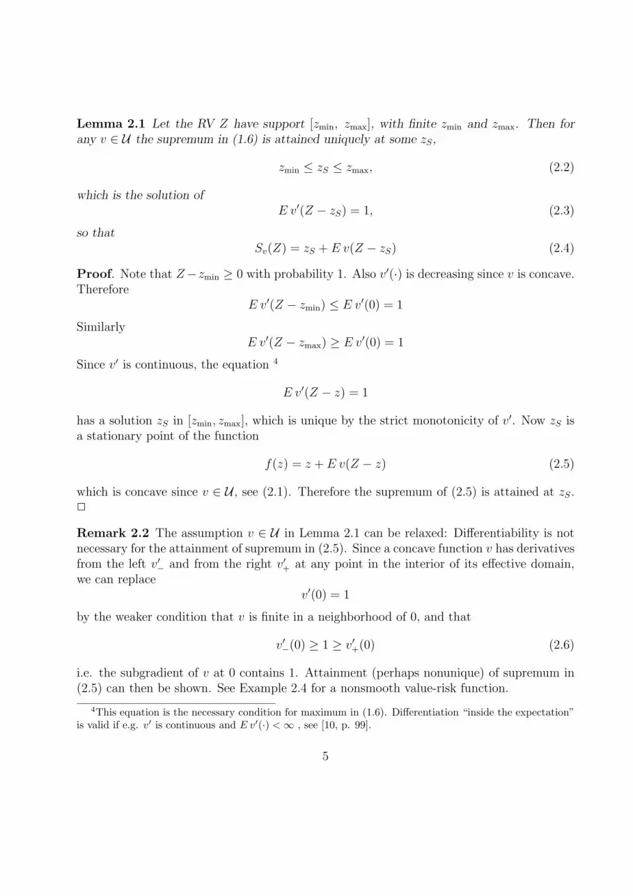
Lemma 2.1 Let the RV Z have support [zmin, zmax], with finite zmin and zmax. Then forany v ∈ U the supremum in (1.6) is attained uniquely at some zS,

zmin ≤ zS ≤ zmax, (2.2)

which is the solution ofE v′(Z − zS) = 1, (2.3)

so thatSv(Z) = zS + E v(Z − zS) (2.4)

Proof. Note that Z−zmin ≥ 0 with probability 1. Also v′(·) is decreasing since v is concave.Therefore

E v′(Z − zmin) ≤ E v′(0) = 1

SimilarlyE v′(Z − zmax) ≥ E v′(0) = 1

Since v′ is continuous, the equation 4

E v′(Z − z) = 1

has a solution zS in [zmin, zmax], which is unique by the strict monotonicity of v′. Now zS isa stationary point of the function

f(z) = z + E v(Z − z) (2.5)

which is concave since v ∈ U , see (2.1). Therefore the supremum of (2.5) is attained at zS.2

Remark 2.2 The assumption v ∈ U in Lemma 2.1 can be relaxed: Differentiability is notnecessary for the attainment of supremum in (2.5). Since a concave function v has derivativesfrom the left v′− and from the right v′+ at any point in the interior of its effective domain,we can replace

v′(0) = 1

by the weaker condition that v is finite in a neighborhood of 0, and that

v′−(0) ≥ 1 ≥ v′+(0) (2.6)

i.e. the subgradient of v at 0 contains 1. Attainment (perhaps nonunique) of supremum in(2.5) can then be shown. See Example 2.4 for a nonsmooth value-risk function.

4This equation is the necessary condition for maximum in (1.6). Differentiation “inside the expectation”is valid if e.g. v′ is continuous and E v′(·) < ∞ , see [10, p. 99].

5

Theorem 2.1 (Properties of the RCE)

(a) Shift additivity. For any v : IR → IR, any RV Z and any constant c

Sv(Z + c) = Sv(Z) + c (2.7)

(b) Consistency. If v satisfies (v1), (v3) then, for any constant c 5,

Sv(c) = c (2.8)

(c) Subhomogeneity. If v satisfies (v1) and (v4) then, for any RV Z,

1

λSv(λZ) is decreasing in λ, λ > 0

(d) Monotonicity. If v satisfies (v2) then, for any RV X and any nonnegative RV Y ,

Sv(X + Y ) ≥ Sv(X)

(e) Risk aversion. v satisfies (v3) if and only if

Sv(Z) ≤ EZ for all RV’s Z (2.9)

(f) Concavity. If v ∈ U then for any RV’s X0 , X1 and 0 < α < 1,

Sv(αX1 + (1− α)X0) ≥ αSv(X1) + (1− α)Sv(X0) (2.10)

(g) 2nd order stochastic dominance. Let X, Y be RV’s with compact supports. Then

Sv(X) ≥ Sv(Y ) for all v ∈ U (2.11)

if and only ifE v(X) ≥ E v(Y ) for all v ∈ U (2.12)

Proof. (a) For any function v : IR → IR,

Sv(Z + c) = supz{z + E v(Z + c− z)}

= c + supz{(z − c) + E v(Z − (z − c))} = c + Sv(Z)

(b) For any constant c,

Sv(c) = supz{z + v(c− z)}

≤ supz{z + (c− z)} by (v3)

= c5Considered as a degenerate RV.

6

Conversely,

Sv(c) ≥ {c + v(c− c)}= c by (v1)

(c) For any v : IR → IR and λ > 0 define vλ by

vλ(x) :=1

λv(λx), ∀ x (2.13)

Then

Svλ(Z) =

1

λSv(λZ), for all RV Z, (2.14)

as follows from,

Svλ(Z) = sup

z{z +

1

λE

Zv(λ(Z − z)}

=1

λsup

z{z + E

Zv(λZ − z)} (z = λz)

=1

λSv(λZ)

It therefore suffices to show that

vλ(z) is decreasing in λ, λ > 0

Indeed, let0 < λ1 < λ2

By the concavity of v it follows, for all z,

v(λ2z)− v(λ1z)

λ2 − λ1

≤ v(λ1z)− v(0)

λ1

and by (v1)v(λ2z)

λ2

≤ v(λ1z)

λ1

(d)

Sv(X + Y ) = supz{z + Ev(X + Y − z)}

≥ supz{z + Ev(X − z)} by (v2)

7

(e) If v satisfies (v3) then for any RV Z,

Sv(Z) = supz{z + Ev(Z − z)}

≤ supz{z + E(Z − z)} = EZ

Conversely, if for all RV’s ZSv(Z) ≤ EZ

then, for any RV Z and any constant z,

z + Ev(Z − z) ≤ EZ

. .. Ev(Z − z) ≤ E(Z − z)

. .. Ev(Z) ≤ EZ

proving (v3).(f) Let 0 < α < 1, and Xα = αX1 + (1− α)X0. Then by the concavity of v, for all z0, z1,

Ev(Xα − αz1 − (1− α)z0) ≥ αEv(X1 − z1) + (1− α)Ev(X0 − z0)

Adding αz1 + (1−α)z0 to both sides, and supremizing jointly with respect to z1, z0, we get

Sv(Xα) ≥ supz1, z0

{α [z1 + Ev(X1 − z1)] + (1− α) [z0 + Ev(X0 − z0)]}

= αSv(X1) + (1− α)Sv(X0)

(g) (2.12) =⇒ (2.11). Since each v ∈ U is increasing, (2.12) implies

z + Ev(X − z) ≥ z + Ev(Y − z) ∀ z, and ∀ v ∈ U

and (2.11) follows by taking suprema.(2.11) =⇒ (2.12). Let zX , zY be points where the suprema defining Sv(X) and Sv(Y ) areattained, see Lemma 2.1. Then, for any v ∈ U ,

Sv(X) = zX + Ev(X − zX) ≥ zY + Ev(Y − zY ), by (2.11)

≥ zX + Ev(Y − zX)

Therefore

Ev(X − zX) ≥ Ev(Y − zX) for all v ∈ U , implying (2.12). 2

8

Remark 2.3 Theorem 2.1 lists properties which seem reasonable for any certainty equiv-alent. Property (b) is natural and requires no justification. The remaining properties willnow be discussed one by one.(a) Note that shift additivity holds for all functions v, i.e. it is a generic property of theRCE. To explain shift additivity consider a decision-maker indifferent between a lottery Zand a sure amount S. If 1 Dollar is added to all the possible outcomes of the lottery, then anaddition of 1 Dollar to S will keep the decision maker indifferent. Recall that shift additivityholds also for the Yaari CE (1.4), and for the u-mean (1.3). For the classical CE (1.2), shiftadditivity holds iff the utility u is linear or exponential, see Example 2.1 below.(c) An important consequence (and the reason for the name “subhomogeneity”) is

Sv(λZ) ≤ λSv(Z), for all RV Z and λ > 1

Thus indifference between the RV Z and its CE Sv(Z) goes together with preference forλSv(Z) over the RV λZ, for λ > 1. This is explained by

E(λZ) = λEZ

Var (λZ) = λ2Var (Z) > λVar (Z) if λ > 1

An interesting result, in view of (c) and (e), is that for v ∈ U ,

limλ→0+

1

λSv(λZ) = EZ

(d) If v satisfies (v1) and (v2), and if the RV Z satisfies Z ≥ zmin with probability 1, then

Sv(Z) ≥ zmin (2.15)

This follows from part (d) by taking X = zmin (degenerate RV) and Y = Z − zmin.(e) In the EU model, risk aversion is characterized by the concavity of the utility function.In the RCE model risk aversion is carried by the weaker property v(x) ≤ x, ∀x. We showin § 4 that concavity of v corresponds to strong risk aversion in the sense of Rothschild andStiglitz, [38].(f) The concavity of Su(·), for all u ∈ U , expresses risk-aversion as aversion to variability.To gain insight consider the case of two independent RV’s X1 and X0 with the same meanand variance. The mixed RV Xα = αX1 + (1 − α)X0 has the same mean, but a smallervariance. Concavity of Su means that the more centered RV Xα is preferred.

The risk-aversion inequality (2.9) is implied by (f): Let Z, Z1, Z2, . . . be independent,identically distributed RV’s. Then by (f),

Su(1

n

n∑i=1

Zi ) ≥ 1

n

n∑i=1

Su(Zi)

= Su(Z)

9

As n →∞, (2.9) follows by the strong law of large numbers.In contrast, the classical CE u−1Eu(·) is not necessarily concave for all concave u.

(g) In general, for a given u ∈ U ,

E u(X) ≥ E u(Y ) (2.16)

does not implySu(X) ≥ Su(Y ) (2.17)

i.e. (2.16) and (2.17) may induce different orders on RV’s, see [9]. Note however that in(2.11) and (2.12) the inequality holds for all u ∈ U 6. This defines a partial order on RV’s,the (2nd order) stochastic dominance, [23].

Example 2.1 (Exponential value-risk function) Here

u(z) = 1− e−z , ∀ z, (2.18)

and equation (2.3) becomes Ee−Z+z = 1, giving zS = − log Ee−Z and the same value forthe RCE

Su(Z) = − log Ee−Z (2.19)

A special feature of the exponential utility function (2.18) is that the classical CE (1.2)becomes

u−1Eu(Z) = − log Ee−Z

showing that for the exponential function, the certainty equivalents (1.6) and (1.2) coincide.

Example 2.2 (Quadratic value-risk function) Here7

u(z) = z − 1

2z2 , z ≤ 1 (2.20)

and for a RV Z with zmax ≤ 1, EZ = µ and variance σ2, equation (2.3) gives zS = µ, andby (2.4)

Su(Z) = µ− 1

2σ2 (2.21)

Corollary 2.1 In both the exponential and quadratic value-risk functions

Su(n∑

i=1

Zi) =n∑

i=1

Su(Zi) (2.22)

for independent RV’s { Z1, Z2, . . . , Zn} 8 2

6In which case Y is called riskier than X.7The restriction z ≤ 1 in (2.20) guarantees that u is increasing throughout its domain.8The classical CE (1.2) is additive, for independent RV‘s, if u is exponential but not if u is quadratic.

10

Example 2.3 For the so-called hybrid model ([4],[42]) with exponential utility u and anormally distributed RV Z ∼ N(µ, σ2),

Su(Z) = µ− 1

2σ2

Example 2.4 (Piecewise linear value-risk function) Let

v(t) =

{βt, t ≤ 0αt, t > 0

0 < α < 1 < β (2.23)

If F is the cumulative distribution function of the RV Z, then the maximizing z in (1.6) isthe 1−α

β−α-percentile of the distribution F of Z:

z∗ = F−1(1− α

β − α)

and the RCE associated with (2.23) is

Sv(Z) = β∫ z∗

t dF (t) + α∫

z∗t dF (t).

The following result is stated for discrete RV’s. Let X be a RV assuming finitely manyvalues,

Prob {X = xi} = pi (2.24)

We denote X by

X = [x,p] , x = (x1, x2, . . . , xn), p = (p1, p2, . . . , pn) (2.25)

The RCE of [x,p] is

Sv([x,p]) = maxz

{z +n∑

i=1

pi v(xi − z)} (2.26)

We consider Sv([x,p]) as a function of the arguments x and p.

Theorem 2.2

(a) For any function v : IR → IR, and any x = (x1, x2, . . . , xn), the RCE Sv([x,p]) isconvex in p.(b) For v concave, and any probability vector p, the RCE Sv([x,p]) is concave in x.

11

Proof. (a) A pointwise supremum of affine functions, see (2.26), is convex.(b) The supremand

z +n∑

i=1

pi v(xi − z)

is jointly concave in z and x. The supremum over z is concave in x, [37]. 2

We summarize, for a RV [x,p], the dependence on p and x, of the expected utility Eu(·)and 3 certainty equivalents.

As a function As a functionof p of x

Eu, u concave linear concaveu−1Eu, u concave convex ?Yf (1.4) convex linearSv convex concave (if v is concave)

3 Recoverability and the Meaning of v(·)In § 2 we studied properties of Sv induced by v. This section is devoted to the inverseproblem, of recovering v from a given Sv.

The discussion is restricted to RCE’s Sv defined by v ∈ U . For these RCE’s, we findv ∈ U satisfying (1.6).

Our results are stated in terms of an elementary RV X

X =

{x, with probability p0, with probability p = 1− p

(3.1)

which we denote (x, p). For this RV,

Sv((x, p)) = supz{z + p v(x− z) + p v(−z)} (3.2)

which we abbreviate Sv(x, p).

Theorem 3.1 If v ∈ U then

v(x) =∂

∂pSv(x, p) |p=0 (3.3)

Proof. For v ∈ U the supremum in (3.2) is attained at z = z(x, p) satisfying the optimalitycondition (2.3)

p v′(x− z(x, p)) + p v′(−z(x, p)) = 1 (3.4)

12

-

6

p0 1

..

..

..

..

..

..

..

..

..

..

..

..

.

��

��

��

��

��

��

��

��

�

E{(x, p)} = p x

.....................................x

�����������������v(x).....................................Sv(x, p) p v(x)

tangent to Sv(x, ·) at p = 0slope = v(x) = ∂Sv(x,0)

∂p

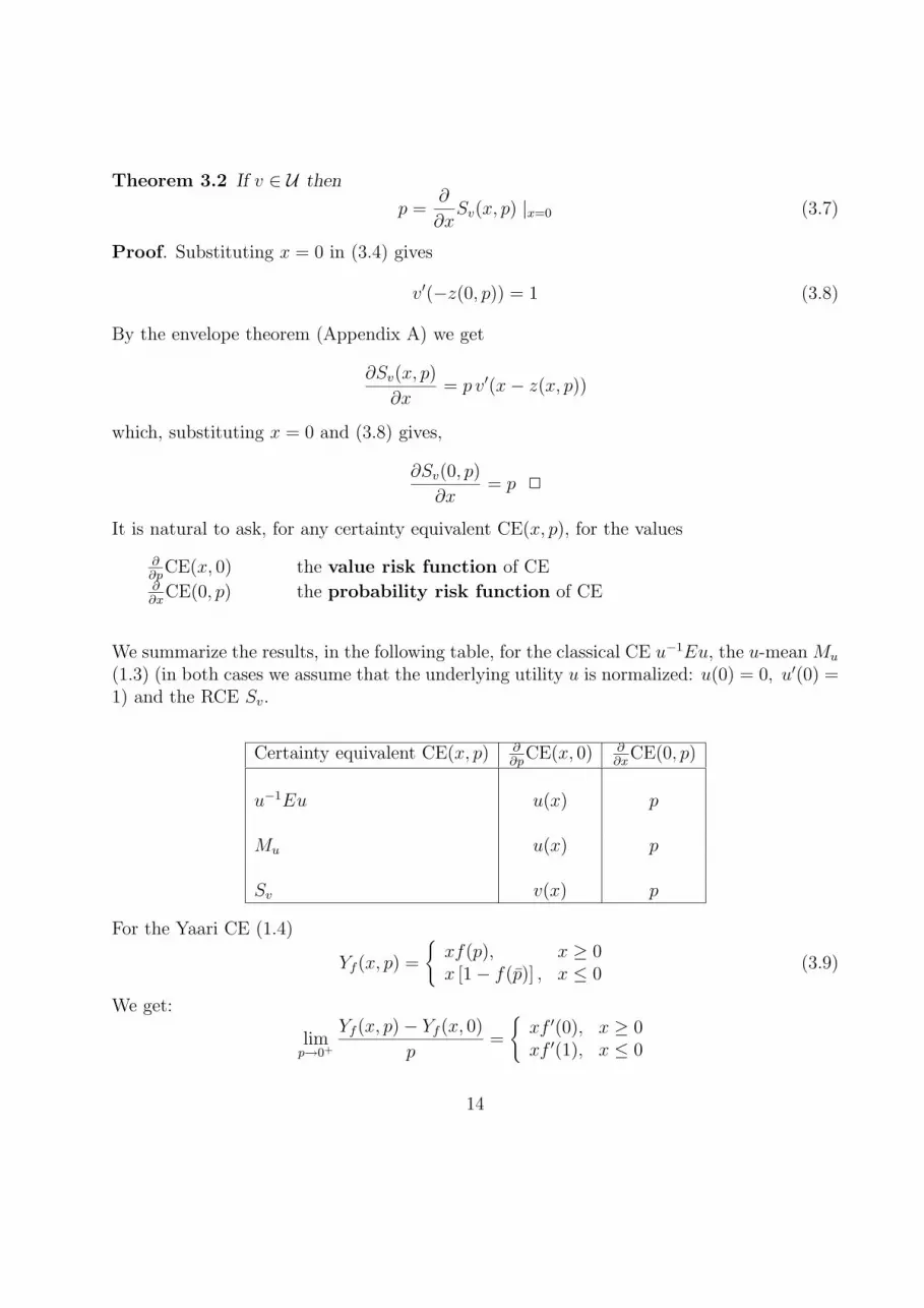
Figure 3.1: Recovering v(x) from Sv(x, p)

which, for p = 0 givesv′(−z(x, 0)) = 1

and since v ∈ U ,z(x, 0) = 0 (3.5)

Now, by the envelope theorem (appendix A),

∂Sv(x, p)

∂p= v(x− z(x, p))− v(−z(x, p)) (3.6)

and (3.3) follows by substituting (3.5) and v(0) = 0 in (3.6). 2

To interpret this result consider an RCE maximizing individual who currently owns 0 $,and is offered the sum x with probability p. The resulting change in his RCE is

∆(x, p) = Sv(x, p)− Sv(x, 0)

and the rate of change is ∆(x,p)p

. Theorem 3.1 says that this rate of change, for an infinitesimal

change in risk (p → 0) is precisely v(x), the value-risk function evaluated at x.Note that for a risk-neutral DM the added value ∆ is E{(x, p)} = px. We illustrate this,

for fixed x, in Fig. 3.1.The following theorem is a companion of Theorem 3.1. It says that the limiting rate of

change ∆(x,p)x

is exactly the probability p of obtaining x.

13

Theorem 3.2 If v ∈ U then

p =∂

∂xSv(x, p) |x=0 (3.7)

Proof. Substituting x = 0 in (3.4) gives

v′(−z(0, p)) = 1 (3.8)

By the envelope theorem (Appendix A) we get

∂Sv(x, p)

∂x= p v′(x− z(x, p))

which, substituting x = 0 and (3.8) gives,

∂Sv(0, p)

∂x= p 2

It is natural to ask, for any certainty equivalent CE(x, p), for the values

∂∂p

CE(x, 0) the value risk function of CE∂∂x

CE(0, p) the probability risk function of CE

We summarize the results, in the following table, for the classical CE u−1Eu, the u-mean Mu

(1.3) (in both cases we assume that the underlying utility u is normalized: u(0) = 0, u′(0) =1) and the RCE Sv.

Certainty equivalent CE(x, p) ∂∂p

CE(x, 0) ∂∂x

CE(0, p)

u−1Eu u(x) p

Mu u(x) p

Sv v(x) p

For the Yaari CE (1.4)

Yf (x, p) =

{xf(p), x ≥ 0x [1− f(p)] , x ≤ 0

(3.9)

We get:

limp→0+

Yf (x, p)− Yf (x, 0)

p=

{xf ′(0), x ≥ 0xf ′(1), x ≤ 0

14

and the two-sided derivatives

limx→0+

Yf (x, p)− Yf (0, p)

x= f(p)

limx→0−

Yf (x, p)− Yf (0, p)

x= 1− f(p)

Remark 3.1

(a) The value-risk function for the EU model is thus precisely the (normalized) utility u(x).This suggests a new way to recover the utility function in the EU theory.(b) The probability-risk function (for a nonnegative RV) in Yaari’s theory is thus preciselythe function f(p) in terms of which Yf is uniquely defined. This is a new interpretation off .(c) Note that the value-risk function corresponding to Yaari’s CE is of the form

v(x) =

{αx, x ≤ 0βx, x ≥ 0

(3.10)

with α = f ′(0), β = f ′(1). The convexity of f plus its normalization f(0) = 0, f(1) = 1imply

α < 1 < β

The function v in(3.10) is the source of the piecewise linear value-risk function inExmaple 2.4.

4 Strong Risk Aversion

In the EU model risk aversion is characterized by the concavity of the utility function, whilein the RCE model it is equivalent to the weaker property (Theorem 2.1(e))

v(x) ≤ x, ∀ x. (4.1)

It is natural to ask what corresponds, in the RCE model, to the concavity of v, i.e.

v ∈ U (4.2)

The answer is given here in terms of a classical notion of risk-aversion due to Rothschild andStiglitz [38], see also [17].

15

Definition 4.1 Let FX

, FY

be the c.d.f. of the RV’s X, Y with support [a, b] and equal

expected values.(a) If there is a c ∈ [a, b] such that

FY

(t) ≥ FX

(t), a ≤ t ≤ c

FX

(t) ≥ FY

(t), c ≤ t ≤ b

then FY

is said to differ from FX

by a mean preserving simple increase in risk

(MPSIR).(b) F

Yis said to differ from F

Xby a mean preserving increase in risk (MPIR) if it

differs from FX

by a sequence of MPSIR’s.

Definition 4.2 An RCE maximizing DM with a value-risk function v exhibits strong risk-aversion if {

FY

differs from FX

by a MPIR

}=⇒ Sv(Y ) ≤ Sv(X)

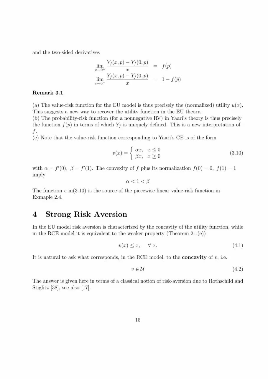
This concept is best illustrated graphically as in [33]. Let

x1 < x2 < x3

be fixed, and let D{x1, x2, x3} denote the probability distributions over the values x1, x2, x3.Each p = (p1, p2, p3) ∈ D{x1, x2, x3} can be represented by a point in the unit triangle in the(p1, p3)-plane as in Fig. 4.1, where p2 is determined by p2 = 1−p1−p3. The dotted lines areloci of distributions with same expectation (iso-mean lines) i.e. points (p1, p3) such that

p1 x1 + (1− p1 − p3) x2 + p3 x3 = constant (4.3)

As one moves in the unit triangle across the iso-mean lines, from the southeast (SE) cornerto the northwest (NW) corner, the values of the mean (4.3) increase. Thus movement fromthe SE to the NW is in the preferred direction.

The iso-mean lines are parallel with slope (i.e. ∆p3/∆p1)

slope of iso-mean lines =x2 − x1

x3 − x2

> 0 (4.4)

A movement along the iso-mean lines, in the NE direction corresponds to an MPIR as inDefinition 4.1(b).

Similarly, the solid lines in Fig. 4.1 represent iso expected utility curves which areparallel straight lines (due to the “linearity in probabilities” of the EU functional) with

slope of iso-EU lines =u(x2)− u(x1)

u(x3)− u(x2)> 0 (4.5)

16

@@

@@

@@

@@

@@

@@

@@

@0 p1 1

0

p3

1

@@

@I increasing preference

........

........

........

.

........

.......

.....

........

........

............

...........

......

.....

����������

��������

������

����

��

������

��

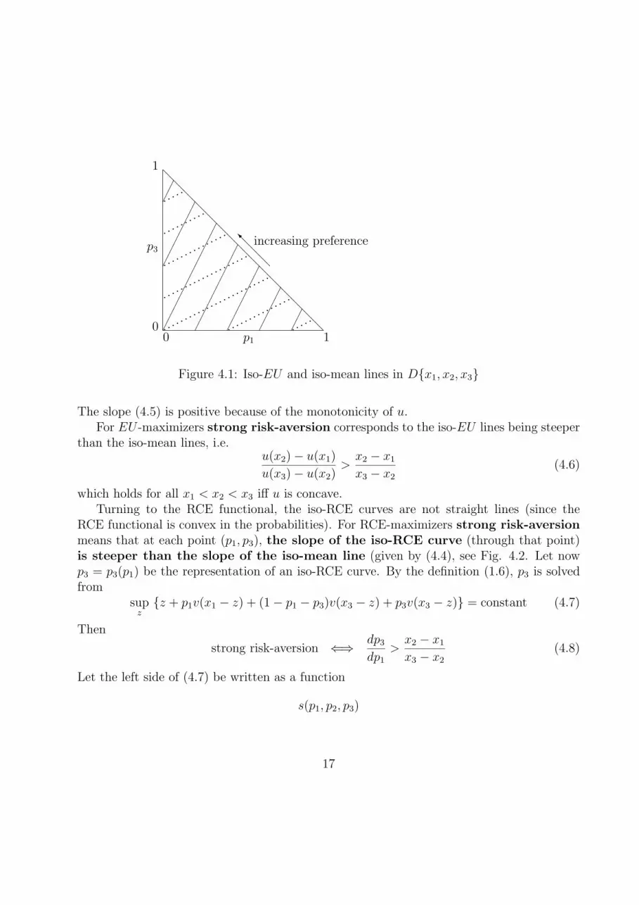
Figure 4.1: Iso-EU and iso-mean lines in D{x1, x2, x3}

The slope (4.5) is positive because of the monotonicity of u.For EU -maximizers strong risk-aversion corresponds to the iso-EU lines being steeper

than the iso-mean lines, i.e.u(x2)− u(x1)

u(x3)− u(x2)>

x2 − x1

x3 − x2

(4.6)

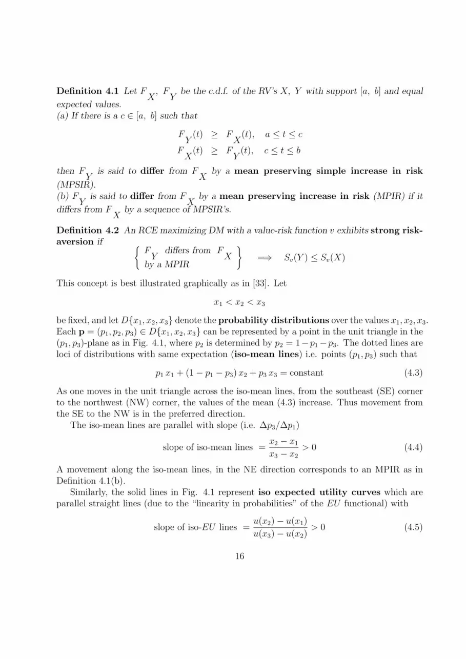
which holds for all x1 < x2 < x3 iff u is concave.Turning to the RCE functional, the iso-RCE curves are not straight lines (since the

RCE functional is convex in the probabilities). For RCE-maximizers strong risk-aversionmeans that at each point (p1, p3), the slope of the iso-RCE curve (through that point)is steeper than the slope of the iso-mean line (given by (4.4), see Fig. 4.2. Let nowp3 = p3(p1) be the representation of an iso-RCE curve. By the definition (1.6), p3 is solvedfrom

supz{z + p1v(x1 − z) + (1− p1 − p3)v(x3 − z) + p3v(x3 − z)} = constant (4.7)

Then

strong risk-aversion ⇐⇒ dp3

dp1

>x2 − x1

x3 − x2

(4.8)

Let the left side of (4.7) be written as a function

s(p1, p2, p3)

17

@@

@@

@@

@@

@@

@@

@@

@0 p1 1

0

p3

1

........

........

........

.

........

.......

.....

........

........

............

...........

......

.....

Figure 4.2: Iso-RCE curves and iso-mean lines in D{x1, x2, x3}

of the probabilities pi. Differentiating (4.7) with respect to p1 we get

s1 − s2 − (s2 − s3)p′3 = 0, where si =

∂s

∂pi

(4.9)

By the envelope theorem (Appendix A)

si =∂s

∂pi

= u(xi − z∗) (4.10)

where z∗ = z∗(p1, p3) is uniquely determined by (2.3)

p1 v′(x1 − z∗) + (1− p1 − p3) v′(x2 − z∗) + p3 v′(x3 − z∗) = 1

Combining (4.9) and (4.10) we thus get

p′3(p1) =v(x2 − z∗)− v(x1 − z∗)

v(x3 − z∗)− v(x2 − z∗)

and the Diamond-Stiglitz risk-aversion is, by (4.8)

v(x2 − z∗)− v(x1 − z∗)

v(x3 − z∗)− v(x2 − z∗)>

x2 − x1

x3 − x2

=(x2 − z∗)− (x1 − z∗)

(x3 − z∗)− (x2 − z∗)(4.11)

which holds for all x1 < x2 < x3 iff v is concave.

18

The above discussion can be generalized to a general RV X with distribution functionF ∈ D(T ), where

D(T ) := {distribution functions with compact support T} (4.12)

We note that the RCE Sv(X) can be written as

Sv(X) =∫

U(x, F ) dF (x) (4.13)

whereU(x, F ) = z(F ) + v(x− z(F )) (4.14)

and the maximizing z(F ) is obtained implicitly from (2.3)∫v′(x− z(F )) dF (x) = 1 (4.15)

Thus Sv, regarded as a function of F ,

Sv(X) = V (F ) (4.16)

is a generalized expected utility preference functional in the sense of Machina, [30].By (4.13), U(x, F ) is then the local utility function of Machina. We recall [30, Theorem 2]that for V (F ) Frechet differentiable on D(T ), the preference order induced by V is stronglyrisk-averse iff U(x, F ) is concave in x for all F ∈ D(T ). Finally, by (4.14), the local utilityU(·, F ) is concave for all F iff the risk-value function v(·) is concave.

Remark 4.1 In the EU theory concavity of the utility u characterizes both risk aversion(CE(X) ≤ E X) and strong risk aversion, hence the two are equivalent in EU theory. Inthe RCE theory, risk aversion requires that v(x) ≤ x while strong risk aversion requires thestronger property that v is concave.

For non-EU theories this divergence between the two notions of risk-aversion is not sur-prising. We note that in Yaari’s dual theory

Yf (X) ≤ E X requires f(t) ≤ t, ∀t

whereas strong risk-aversion requires the convexity of f , [50, Theorem 2]9.

9The convexity of f , plus Yaari’s normalization f(0) = 0, f(1) = 1 implies f(t) ≤ t.

19

5 The RCE and Decision Theoretic Paradoxes

The recent interest in “non-EU” theories 10 is motivated mainly by empirical evidence ofsystematic violations of the EU axioms, notably the Independence Axiom underlying the“linearity in probabilities”, [46]. Deviations from the behavior prescribed by EU Theory havebecome known as (“decision theoretic”) paradoxes, in particular, the Allais paradox ([1],[2]), the common consequence effect, the common ratio effect, over sensitivity tosmall probabilities and the utility evaluation effect, e.g. [26], [34] and [31].

The RCE is nonlinear (in fact convex, see § 2) in probabilities. Also, equations (4.13,4.14)show the RCE Sv to be a Machina’s generalized expected utility preference functional, if thevalue-risk function v belongs to the special class (2.1) of normalized utility functions U .We show now that a further restriction of v to a subclass UAP ∈ U “immunizes” the RCESv against the above-mentioned decision theoretic paradoxes.

The subclass UAP is defined in terms of a construct similar to the Arrow-Pratt abso-lute risk-aversion index. Let v ∈ U be twice continuously differentiable. Then its riskindex rv is defined as

rv(x) = −v′′(x)

v′(x)(5.1)

For Machina’s local utility function U(x, F ) we similarly define

rU,F (x) = −Uxx(x, F )

Ux(x, F )(5.2)

The class UAP is then

UAP =

{v ∈ U of (2.1) :

v twice continuously differentiablerv(x) is nonincreasing

}(5.3)

In Machina’s Generalized Expected Utility (GEU) Theory, the preference order V (F )(over distributions F ) is an integral of the local utility function U(x, F )

V (F ) =∫

U(x, F ) dF (x) (5.4)

and the decision theoretic paradoxes can be explained if U(x, F ) satisfies two hypotheses onthe risk index (5.2), see [30, § 4.1]Hypothesis I: For any distribution F ∈ D(T ), the risk index rU,F (x) is nonincreasing inx ∈ T .Hypothesis II: If F1, F2 ∈ D(T ), and if F1 stochastically dominates F2 (1st order), then

rU,F1(x) ≥ rU,F2(x),∀ x ∈ T (5.5)

10In particular [6], [7], [8], [13], [20], [21], [24], [26], [27], [30], [36], [48], [50].

20

Since, for v ∈ U , the RCE Sv is a GEU preference functional (see (4.13,4.14)), we mayuse Machina’s results of [30]. For the local utility function U(x, F ) of (4.14), Hypothesis Ireduces to the following statement: For every F ∈ D(T ),

−v′′(x− z(F ))

v′(x− z(F ))is nonincreasing in x

which clearly holds for v ∈ UAP. We show now that Hypothesis II also holds in UAP.

Proposition 5.1 Let v ∈ UAP, and let

U(x, F ) = z(F ) + v(x− z(F ))

be the underlying local utility (in the sense of (4.13, 4.14)). Then Hypothesis II holds.

Proof. Let F1 dominate F2 stochastically (1st order), i.e.

EF1 (h(X)) ≥ EF2 (h(X)) ∀ nondecreasing functions h (5.6)

For the above u(x, F ), Hypothesis II reduces to

rv(x− z(F1)) ≥ rv(x− z(F2)) ∀ x

which holds, for v ∈ UAP, if and only if,

z(F1) ≥ z(F2) (5.7)

We have to show that (5.6) implies (5.7). Suppose (5.6) holds, but

z(F1) < z(F2) (5.8)

Then, from the definition (4.15) of z(F ), the fact that −v′ is strictly increasing (since v ∈UAP ⊂ U) and the assumed inequality (5.8),

−1 = −EF1 v′(x− z(F1)) > −EF1 v′(x− z(F2))

≥ −EF2 v′(x− z(F2)) by (5.6) with h = −v′

= −1 by (4.15), contradicting (5.8). 2

To summarize: When confined to risk-value functions in the class UAP (5.3) (in particular,strictly concave and nonincreasing risk indices), the RCE theory is compatible with theobserved behavior (e.g. Allais paradox, common consequence effect, common ratio effect)which violates the Independence Axiom of EU theory.

21

6 Functionals and Approximations

Let Z = (Zi) be a RV in IRn, with expectation µµµ(vector) and covariance matrix Σ (if n = 1then as above Σ = σ2 ). For any vector y ∈ IRn , the inner product,

y · Z =n∑

i=1

yiZi

is a scalar RV. Given u ∈ U , the corresponding RCE of y · Z are taken as functionals in y,the RCE functional

su(y) := Su(y · Z), (6.1)

We collect properties of the RCE functional in the following theorem, whose proof appearsin Appendix B.

Theorem 6.1 Let u ∈ U be twice continuously differentiable, and let Z and su(·) be asabove. Then:(a) The functional su is concave, and given by

su(y) = zS(y) + Eu(y · Z− zS(y)) (6.2)

where zS(y) is the unique solution z of

E u′(y · Z− z) = 1 (6.3)

(b) Moreover,

su(0) = 0, ∇su(0) = µµµ, ∇2su(0) = u′′(0)Σ (6.4)

zS(0) = 0, ∇zS(0) = µµµ (6.5)

and if u is three times continuously differentiable,

∇2zS(0) =u′′′(0)

u′′(0)Σ 2 (6.6)

Theorem 6.1 can be used to obtain the following approximation of the functional su(·) basedon its Taylor expansion around y = 0.

Corollary 6.1 If u is three times continuously differentiable then

su(y) = µµµ · y +1

2u′′(0)y · Σy + ◦(‖ y ‖2) 2 (6.7)

Remark 6.1

22

(a) In particular, for n = 1 and y = 1, it follows from (6.7) that the RCE has the followingsecond-order approximation

Su(Z) ≈ µ +1

2u′′(0)σ2 (6.8)

= µ− 1

2r(0)σ2

where r(·) is the Arrow-Pratt risk-aversion index (1.13).(b) We also note that the approximation (6.7) is exact if

(i) u is quadratic, or(ii) u is exponential, Z is normal.

(c) By differentiating, and calculating the Taylor expansion of the classical CE (1.2) of y ·Z,

cu(y) = u−1Eu(y · Z) (6.9)

it follows that cu(y) is approximated by the right-hand side of (6.7). Thus we have

cu(y)− su(y) = ◦(‖ y ‖2) (6.10)

showing that the CE functionals (6.1) and (6.9) are close for small y.

7 Competitive Firm under Uncertainty

The first application of the RCE is to the classical model studied by Sandmo [41], see also[29, §5.2]. A firm sells its output q at a price P , which is a RV with a known distributionfunction and expected value EP = µ. Let C(q) be the total cost of producing q, whichconsists of a fixed cost B and a variable cost c(q),

C(q) = c(q) + B

The function c(·) is assumed normalized, increasing and strictly convex,

c(0) = 0, c′(q) > 0, c′′(q) > 0 ∀q ≥ 0 (7.1)

The firm has a strictly concave utility function u, i.e.

u′ > 0, u′′ < 0

which is normalized so that u(0) = 0, u′(0) = 1. The objective is to maximize profit

π(q) = qP − c(q)−B

23

which is a RV. The classical CE (1.2) is used is Sandmo’s analysis, so that the model studiedis

maxq≥0

u−1Eu(π(q))

or equivalently,maxq≥0

Eu(π(q)) (7.2)

Here we analyze the same model using the RCE. For the sake of comparison with the EUmodel, we assume that the firm’s value-risk function is u ∈ U , i.e. is a utility. The objectiveof the firm is therefore

maxq≥0

Su(π(q)) (7.3)

Now

maxq≥0

Su(π(q)) = maxq≥0

Su(qP − c(q)−B)

= maxq≥0

{Su(qP )− c(q)} −B

by (2.7). We conclude:

Proposition 7.1 The optimal production output q∗ is independent of the fixed cost B. 2

This result is in sharp contrast to the expected utility model (7.2) where the optimal outputq depends on the fixed cost B: q increases [decreases] with B if the Arrow-Pratt index r(·)is an increasing [decreasing] function; the dependence is ambigious for utilities for which r(·)is not monotone.

Note that the objective function in (7.3) is

f(q) = su(q)− c(q) (7.4)

where su(·) is the RCE functional (6.1). The function f is concave by Theorem 6.1 andthe assumptions on c. Therefore, the optimal solution q∗ of (7.3) is positive if and only iff ′(0) > 0. By (6.4) s′(0) = µ, so

q∗ > 0 if and only if µ > c′(0) (7.5)

in agreement with the expected utility model (7.2). We assume from now on that

µ > c′(0)

A central result in the theory of production under uncertainty is that, for the risk-aversefirm (i.e. concave utility function), the optimal production under uncertainty is less thanthe corresponding optimal production qcer under certainty, that is for P a degenerate RVwith value µ. We will prove now that the same result holds for the model (7.3). First recallthat the optimality condition for qcer is that marginal cost equals marginal revenue

c′(qcer) = µ (7.6)

24

Proposition 7.2 q∗ < qcer for all u ∈ U .

Proof. The optimality condition for q∗ is

0 = f ′(q∗) = s′u(q∗)− c′(q∗) (7.7)

By Theorem 6.1su(q) = z(q) + Eu(qP − z(q)) (7.8)

where z(q) is a differentiable function, uniquely determined by the equation

Eu′(qP − z(q)) = 1 (7.9)

By the envelope theorem (Appendix A),

s′u(q) = E{Pu′(qP − z(q))} (7.10)

and the optimality condition (7.7) becomes

EPu′(q∗P − z(q∗)) = c′(q∗) (7.11)

Multiplying (7.9) by µ and subtracting from (7.11) we get

E(P − µ)u′(q∗P − z(q∗)) = c′(q∗)− µ (7.12)

orE{Zh(Z)} = c′(q∗)− µ (7.13)

where we denoteZ := P − µ , h(Z) := u′(q∗Z + q∗µ− z(q∗))

Since u ∈ U , it follows that h is positive and decreasing, and it can then be shown (see e.g.[29, p. 249]) that

E{Zh(Z)} < h(0)EZ

but EZ = E{P − µ} = 0, and so, by (7.13),

c′(q∗) < µ

and by using (7.6)c′(q∗) < c′(qcer)

and since c′ is increasing,q∗ < qcer 2

25

7.1 Effect of Profits Tax

Suppose there is a proportional profits tax at rate 0 < t < 1, so that the profit after tax is

π(q) = (1− t)(qP − C(q))

As before, the firm seeks the optimal solution q∗ of (7.3), which here becomes

maxq≥0

Su(π(q)) = maxq≥0

Su((1− t)(qP − c(q)−B))

= maxq≥0

{Su((1− t)qP )− (1− t)c(q)} − (1− t)B

which can be rewritten, using the RCE functional su(·) and omitting the constant (1− t)B,

maxq≥0

su((1− t)q)− (1− t)c(q)

Let the optimal solution be q = q(t). The optimality condition here is

(1− t)s′u((1− t)q)− (1− t)c′(q) = 0

giving the identity (in t),s′u((1− t)q(t)) ≡ c′(q(t))

which, after differentiating (with respect to t),

[(1− t)q′(t)− q(t)] s′′((1− t)q) = q′(t)c′′(q)

and rearranging terms, gives

q′(t){c′′(q)− (1− t)s′′u((1− t)q)} = −q(t)s′′u((1− t)q) (7.14)

The coefficient of q′(t) is positive since c′′ > 0 and su(·) is concave (Theorem 6.1(a)). Theright-hand side of (7.14) is positive since q > 0, s′′ < 0. Therefore, by (7.14),

q′(t) > 0

and we proved:

Proposition 7.3 A marginal increase in profit tax causes the firm to increase production.2

In the classical expected utility case the effect of taxation depends on third-derivativeassumptions; it can be predicted unambigiously 11 only in one of the following cases:

(a) r constant and R increasing,(b) r decreasing and R increasing,(c) r decreasing and R constant.

In all these cases, the EU prediction agrees with our prediction in Proposition 7.3.

11See Katz’s correction [28] to [41].

26

7.2 Effect of Price Increase

If price were to increase from P to P + ε (ε fixed), then the corresponding optimal outputq(ε) is the solution of

maxq≥0

{ Su((P + ε)q)− c(q)} = maxq≥0

{ su(q) + εq − c(q)}

The optimality condition for q(ε) is

s′u(q(ε)) + ε = c′(q(ε))

Differentiating with respect to ε we get

q′(ε)s′′u(q(ε)) + 1 = q′(ε)c′′(q(ε))

hence

q′(ε) =1

c′′(q)− s′′(q)> 0

by the convexity of c and the concavity of su. We have so proved:

Proposition 7.4 A marginal increase in selling price causes the firm to increase production.2

This highly intuitive result is proved in the expected utility case only under the assumptionthat r(·) is non-increasing.

7.3 Effect of Futures Price Increase

The RCE criterion was also applied to an extension [19] of Sandmo’s model [41], dealingwith a firm under price uncertainty and where a futures market exists for the firm’s product.In [19, Proposition 5] it is shown that an increase in the current futures price causes aspeculator or a hedger to increase sales, but not so for a partial hedger, unless constantabsolute risk-aversion is assumed. This pathology is avoided in the RCE model, where theabove three types of producers will all increase sales, [43].

8 Investment in One Risky and in One Safe Assets:

The Arrow Model

Recall the classical model [3] of investment in a risky/safe pair of assets, concerning anindividual with utility u ∈ U and initial wealth A. The decision variable is the amount

27

a to be invested in the risky asset, so that m = A − a is the amount invested in the safeasset (cash).

The rate of return in the risky asset is a RV X.The final wealth of the individual is then

Y = A− a + (1 + X)a = A + aX

In [3] the model is analyzed via the maximal EU principle, so the optimal investment a∗ isthe solution of

max0≤a≤A

Eu(A + aX) (8.1)

or equivalentlymax

0≤a≤Au−1Eu(A + aX)

Some of the important results in [3] are:

(I1) a∗ > 0 if and only if EX > 0.

(I2) a∗ increases with wealth (i.e. da∗

dA≥ 0) if the absolute risk aversion index r(·) is

decreasing.

(I3) The wealth elasticity of the demand for cash balance (investment in the safe asset)

Em

EA:=

dm/dA

m/Ais at least one (8.2)

if the relative risk-aversion index

R(z) = −zu′′(z)

u′(z)is increasing (8.3)

Arrow [3] postulated that reasonable utility functions should satisfy (8.3), since the empir-ical evidence for (8.2) is strong, see the references in [3, p. 103].

We analyze this investment problem using the RCE criterion, i.e.

max0≤a≤A

Su(A + aX) (8.4)

where again we assume that the investor’s value-risk function is u ∈ U . The optimizationproblem (8.4) is, by (2.7), equivalent to

max0≤a≤A

Su(aX) + A

28

Let a∗ be the optimal solution. Using the RCE functional su(·), a∗ is in fact the solution of

max0≤a≤A

su(a) (8.5)

Now, since su(·) is concave

a∗ > 0 if and only if s′u(0) > 0

but by (6.4) s′(0) = EX, and we recover the result (I1).Assuming (as in [3]) an inner optimal solution (diversification)

0 < a∗ < A (8.6)

we conclude here, in contrast to (I2), that

da∗

dA= 0 (8.7)

i.e. the optimal investment is independent of wealth 12.An immediate consequence of (8.7) is

Em

EA> 1 ∀ u ∈ U

indeedEm

EA=

A

m

dm

dA=

A

A− a∗d(A− a∗)

dA=

A

A− a∗(1− da∗

dA) =

A

A− a∗> 1

proving (8.2) for all risk-averse investors. Thus, in the RCE model, there is no need for thecontroversial postulate (8.3).

The quadratic utility (2.33)

u(z) = z − 1

2z2 z ≤ 1

violates both of Arrow’s postulates (r decreasing, R increasing), and is consequently ”banned”from the EU model. In the RCE model, on the other hand, a quadratic value-risk functionis acceptable13. For this function the optimal investment a∗ is the optimal solution of

max0≤a≤A

{su(a) = µa− 1

2σ2a2}

12However, initial wealth will in general determine when divesification will be optimal, i.e. when (8.6) willhold.

13Assuming 0 ≤ X ≤ 1.

29

where µ = EX, σ2 = Var(X). Therefore

a∗ =

{µ/σ2 if 0 < µ/σ2 < AA if µ/σ2 ≥ A

showing that, for the full range of A values, a∗(A) is non-decreasing, in agreement with (I2).Moreover, if diversification is optimal, then

Em

EA=

A

A− µ/σ2> 1

Following [3] we consider the effects on optimal investment, of shifts in the RV X. Let h bethe shift parameter, and assume that the shifted RV X(h) is a differentiable function ofh, with X(0) = X. Examples are:

X(h) = X + h (additive shift),X(h) = (1 + h)X (multiplicative shift).

For the shifted problem, the objective is

max0≤a≤A

Su(aX(h)) (8.8)

Let a(h) be the optimal solution of (8.8), in particular a(0) = a∗. Now

Su(aX(h)) = ξ(a) + Eu(aX(h)− ξ(a)) (8.9)

where ξ(a) is the unique solution of

Eu′(aX(h)− ξ(a)) = 1 (8.10)

The optimality condition for a(h) is

d

da{ξ(a) + Eu(aX(h)− ξ(a))} = 0

which gives (using (8.10)) the following identities in h

E{X(h)u′(a(h)X(h)− ξ(a(h)))} ≡ 0 (8.11)

E{u′(a(h)X(h)− ξ(a(h)))} ≡ 1 (8.12)

Differentiating (8.11) with respect to h we get, denoting Z = aX(h)− ξ(a(h)),

a(h)E{u′′(Z)X(X − ξ′(a(h))} = E{X(h) [u′(Z) + a(h)X(h)u′′(Z)]} (8.13)

30

where a(h) = ddh

a(h) and similarly for X(h).

The second order optimality condition for a(h), d2

da2 Su(aX(h)) ≤ 0, is here

Eu′′(Z)X(X − ξ′(a(h))) ≥ 0

hence, by (8.13),

sign of a(h) = sign of E{X(h) [u′(Z) + aXu′′(Z)]}

exactly the same condition for the sign of ddh

a(h) as in [3, p. 105, eq. (18)]. Therefore, theconclusions of the EU model are also valid for the RCE model. In particular:

Proposition 8.1 As a function of the shift parameter h,a(h) increases for additive shift,a(h) decreases for multiplicative shift.

These results are illustrated for the quadratic value-risk function. There

a∗ =EX

Var(X)

and

a(h) = a∗ +h

Var(X)for an additive shift

a(h) =1

1 + ha∗ for a multiplicative shift (8.14)

In fact, (8.14) holds for arbitrary u ∈ U , a result proved in [45] for the EU model.

Proposition 8.2 If a∗ is the demand for the risky asset when the return is the RV X, thena(h) = a∗/1 + h is the demand when the return is (1 + h)X.

Proof. The optimality condition for a∗ is

E{u′(a∗X − ξ∗)X} = 0 (8.15)

where ξ∗ is the unique solution of

Eu′(a∗X − ξ∗) = 1 (8.16)

The optimality conditions for a(h) are given by (8.11), (8.12). Now, for a(h) = 11+h

a∗,

a(h)X(h) = a∗X (8.17)

and it follows, by comparing (8.12) with (8.16), that

ξ(a(h)) = ξ∗

Substituting this in (8.11) and using (8.17), we see that (8.11) is equivalent to (8.16), andthat a(h) = a∗/1 + h indeed satisfies the optimality conditions (8.11), (8.12). 2

31

9 Investment in a Risky/Safe Pair of Assets: An Ex-

tension

We study the model discussed in [12] and [22], which is an extension of the model in Section 8.The analysis applies to a fixed time interval, say a year. An investor allocates a proportion0 ≤ k ≤ 1 of his investment capital W0 to a risky asset, and proportion 1− k of W0 to a safeasset where the total annual return per dollar invested is τ ≥ 1. The total annual returnt per dollar invested in the risky asset, is a nonnegative RV. The investor’s total annualreturn is

kW0t + (1− k)W0τ

and for a utility function u, the optimal allocation k∗ is the solution of

max0≤k≤1

Eu(kW0t + (1− k)W0τ) (9.1)

The model of §5, is a special case with W0 = A, t = 1 + X, kW0 = a, τ = 1.It is assumed in [12], [22] that u′ > 0 and u′′ < 0, thus we assume without loss of

generality that u ∈ U .One of the main issues in [22] is the effect of an increase in the safe asset return τ on the

optimal allocation. The following are proved:

(F1) An investor maximizing expected utility will diversify (invest a positive amount ineach of the assets) if and only if

Etu′(W0t)

Eu′(W0t)< τ < E(t) (9.2)

(F2) Given (9.2) he will increase the proportion invested in the safe asset when τ increasesif either

(a) the absolute risk aversion index r(·) is non-decreasing, or(b) the relative risk aversion index R(·) is at most 1.

The same model is now analyzed using the RCE approach, i.e. with the objective

max0≤k≤1

Su(kW0t + (1− k)W0τ)

where u denotes the investor’s value risk function, assumed in U . Using (2.7) and thedefinition (6.1), the objective becomes

max0≤k≤1

{(1− k)W0τ + su(W0k)}) (9.3)

The following proposition, proved in Appendix C, gives the analogs of results (F1, (F2) inthe RCE model.

32

Proposition 9.1 (a) The RCE maximizing investor will diversify if and only if

Etu′(W0t− η) < τ < E(t) (9.4)

where η is the unique solution of

Eu′(W0t− η) = 1 (9.5)

(b) Given (9.4), he will increase the proportion invested in the safe asset when τ increases.2

Comparing part (b) with (F2), we see that plausible behavior (k∗ increases with τ) holdsin the RCE model for all u ∈ U , but in the EU model only for a restricted class of utilities.

We illustrate Proposition 9.1 in the case of the quadratic value-risk function (2.20). Herethe optimal proportion invested in the risky asset is:

k∗ =

0 if τ > E(t)E(t)−τW0σ2 if E(t)−W0σ

2 ≤ τ ≤ E(t)

1 if E(t)−W0σ2 > τ

(9.6)

where σ2 is the variance of t. Thus k∗ is increasing in E(t), decreasing with σ2 and decreasingwith τ (so that, the proportion 1− k∗ invested in the safe asset is increasing with safe assetreturn τ). These are reasonable reactions of a risk-averse investor.

We also see from (9.6) that k∗ decreases when the investment capital W0 increases.This result holds for arbitrary u ∈ U , see the next proposition (proved in Appendix B). Inthe EU model, the effect of W0 on k∗ depends on the relative risk-aversion index, see [12].

Proposition 9.2 If the investment capital increases, then the RCE-maximizing investorwill increase the proportion invested in the safe asset. 2.

Following the analysis in [3] and § 8, we consider now the elasticity of cash-balance (withrespect to W0). Here the cash balance (the amount invested in the safe asset) is

m = (1− k∗)W0

and the elasticity in question is EmEW0

.

Proposition 9.3 For every RCE-maximizing investor with u ∈ U ,

Em

EW0

≥ 1

33

Proof.Em

EW0

=dm/dW0

m/W0

=1− k∗(W0)−W0

dk∗(W0)dW0

1− k∗(W0)

henceEm

EW0

≥ 1 if and only ifdk∗(W0)

dW0

≤ 0 (9.7)

and the proof is completed by Proposition 9.2. 2

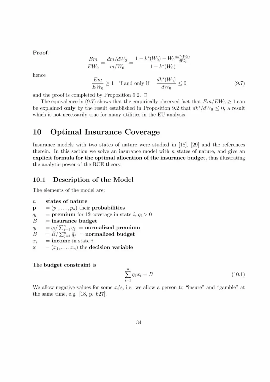
The equivalence in (9.7) shows that the empirically observed fact that Em/EW0 ≥ 1 canbe explained only by the result established in Proposition 9.2 that dk∗/dW0 ≤ 0, a resultwhich is not necessarily true for many utilities in the EU analysis.

10 Optimal Insurance Coverage

Insurance models with two states of nature were studied in [18], [29] and the referencestherein. In this section we solve an insurance model with n states of nature, and give anexplicit formula for the optimal allocation of the insurance budget, thus illustratingthe analytic power of the RCE theory.

10.1 Description of the Model

The elements of the model are:

n states of naturep = (p1, . . . , pn) their probabilitiesqi = premium for 1$ coverage in state i, qi > 0B = insurance budgetqi = qi/

∑nj=1 qj = normalized premium

B = B/∑n

j=1 qj = normalized budgetxi = income in state ix = (x1, . . . , xn) the decision variable

The budget constraint isn∑

i=1

qi xi = B (10.1)

We allow negative values for some xi’s, i.e. we allow a person to “insure” and “gamble” atthe same time, e.g. [18, p. 627].

34

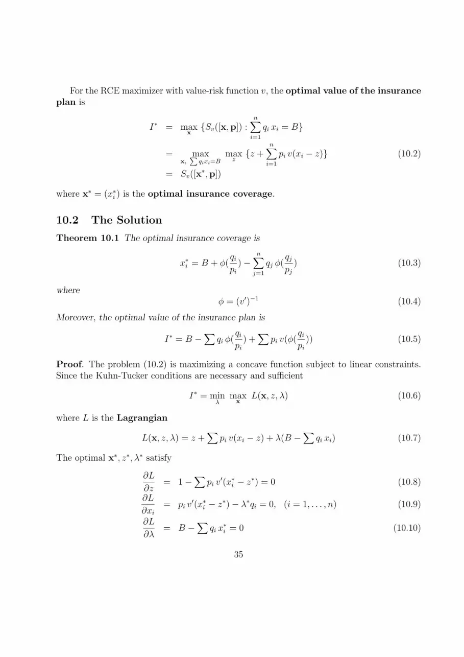
For the RCE maximizer with value-risk function v, the optimal value of the insuranceplan is

I∗ = maxx

{Sv([x,p]) :n∑

i=1

qi xi = B}

= maxx,∑

qixi=Bmax

z{z +

n∑i=1

pi v(xi − z)} (10.2)

= Sv([x∗,p])

where x∗ = (x∗i ) is the optimal insurance coverage.

10.2 The Solution

Theorem 10.1 The optimal insurance coverage is

x∗i = B + φ(qi

pi

)−n∑

j=1

qj φ(qj

pj

) (10.3)

whereφ = (v′)−1 (10.4)

Moreover, the optimal value of the insurance plan is

I∗ = B −∑

qi φ(qi

pi

) +∑

pi v(φ(qi

pi

)) (10.5)

Proof. The problem (10.2) is maximizing a concave function subject to linear constraints.Since the Kuhn-Tucker conditions are necessary and sufficient

I∗ = minλ

maxx

L(x, z, λ) (10.6)

where L is the Lagrangian

L(x, z, λ) = z +∑

pi v(xi − z) + λ(B −∑

qi xi) (10.7)

The optimal x∗, z∗, λ∗ satisfy

∂L

∂z= 1−

∑pi v

′(x∗i − z∗) = 0 (10.8)

∂L

∂xi

= pi v′(x∗i − z∗)− λ∗qi = 0, (i = 1, . . . , n) (10.9)

∂L

∂λ= B −

∑qi x

∗i = 0 (10.10)

35

From (10.9) and (10.8) we get

λ∗ =1∑qi

= 1

and consequently

v′(x∗i − z∗) =qi

pi

Since v′ is monotone decreasing (v is strictly concave) we write, using (10.4)

x∗i − z∗ = φ(qi

pi

), (i = 1, . . . , n) (10.11)

Multiplying (10.11) by qi and summing we get∑qi (x

∗i − z∗) =

∑qi φ(

qi

pi

)

. .. B − z∗ =∑

qi φ(qi

pi

)

. .. z∗ = B −∑

qi φ(qi

pi

)) (10.12)

which is compared with (10.11) to give (10.3). Finally,

I∗ = z∗ +∑

pi v(x∗i − z∗)

and (10.5) follows by (10.11) and (10.12). 2 In the above model, the price of insurance isactuarially fair if

qi = pi (i = 1, . . . , n)

i.e. if the normalized premiums agree with the probabilities.For actuarially fair premiums we get from (10.3), using that v′(0) = 1 implies φ(1) = 0,

x∗i = B (i = 1, . . . , n)

i.e. the individual is indifferent between the occurrence of states i = 1, . . . , n.

10.3 Special Case: Two States of Nature

We translate the results of Theorem 10.1 to the special case of two states, as given in [18],[29, §3].

Consider insurance against a single disaster. Specifically, let there be two states of nature:

State Disaster Probability1 occurs p2 does not occur 1− p

36

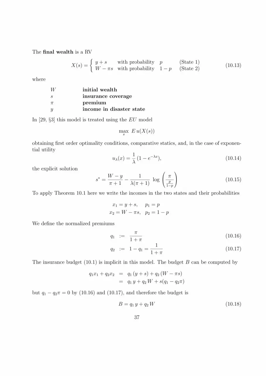
The final wealth is a RV

X(s) =

{y + s with probability p (State 1)W − πs with probability 1− p (State 2)

(10.13)

where

W initial wealths insurance coverageπ premiumy income in disaster state

In [29, §3] this model is treated using the EU model

maxs

E u(X(s))

obtaining first order optimality conditions, comparative statics, and, in the case of exponen-tial utility

uλ(x) =1

λ(1− e−λx), (10.14)

the explicit solution

s∗ =W − y

π + 1− 1

λ(π + 1)log

πp

1−p

(10.15)

To apply Theorem 10.1 here we write the incomes in the two states and their probabilities

x1 = y + s, p1 = p

x2 = W − πs, p2 = 1− p

We define the normalized premiums

q1 :=π

1 + π(10.16)

q2 := 1− q1 =1

1 + π(10.17)

The insurance budget (10.1) is implicit in this model. The budget B can be computed by

q1x1 + q2x2 = q1 (y + s) + q2 (W − πs)

= q1 y + q2 W + s(q1 − q2π)

but q1 − q2π = 0 by (10.16) and (10.17), and therefore the budget is

B = q1 y + q2 W (10.18)

37

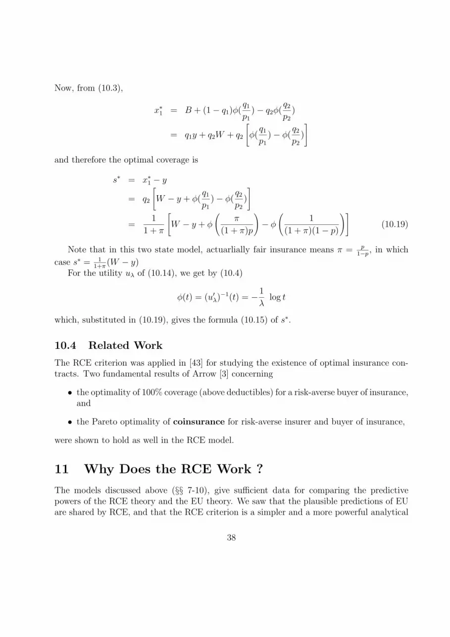
Now, from (10.3),

x∗1 = B + (1− q1)φ(q1

p1

)− q2φ(q2

p2

)

= q1y + q2W + q2

[φ(

q1

p1

)− φ(q2

p2

)

]

and therefore the optimal coverage is

s∗ = x∗1 − y

= q2

[W − y + φ(

q1

p1

)− φ(q2

p2

)

]

=1

1 + π

[W − y + φ

(π

(1 + π)p

)− φ

(1

(1 + π)(1− p)

)](10.19)

Note that in this two state model, actuarlially fair insurance means π = p1−p

, in which

case s∗ = 11+π

(W − y)For the utility uλ of (10.14), we get by (10.4)

φ(t) = (u′λ)−1(t) = −1

λlog t

which, substituted in (10.19), gives the formula (10.15) of s∗.

10.4 Related Work

The RCE criterion was applied in [43] for studying the existence of optimal insurance con-tracts. Two fundamental results of Arrow [3] concerning

• the optimality of 100% coverage (above deductibles) for a risk-averse buyer of insurance,and

• the Pareto optimality of coinsurance for risk-averse insurer and buyer of insurance,

were shown to hold as well in the RCE model.

11 Why Does the RCE Work ?

The models discussed above (§§ 7-10), give sufficient data for comparing the predictivepowers of the RCE theory and the EU theory. We saw that the plausible predictions of EUare shared by RCE, and that the RCE criterion is a simpler and a more powerful analytical

38

tool, e.g. § 10.2 where it gives an explicit solution for all risk-averse DM’s, while in generalthe EU model can only provide comparative statics. Also the RCE predictions hold for allrisk-averse DM’s, while in the EU model risk-aversion does not suffice and, in order to avoidimplausible predictions, restrictions (occassionally severe) must be imposed on the DM’ssubjective preference.

The simplicity of the RCE criterion can be explained at the technical level. Shift addi-tivity makes risky choices independent of constant factors (fixed costs, initial wealth), andby using the envelope theorem, comparative statics are free of certain ungainly derivatives.Such conveniences are in general unavailable to the EU maximizer.

This however is not the whole story. The main advantage of the RCE theory, at thefundamental level of modelling choice under risk, is that its risk aversion is of the “rightkind” from the start, without a need for qualifiers such as the Arrow-Pratt indices. Indeed,in the EU theory, behavior under uncertainty is analyzed in terms of the Arrow-Pratt indicesr(·) and R(·). The typical postulates are

(A1) r(w) = −u′′(w)u′(w)

is a non-increasing function of w

(A2) R(w) = −w u′′(w)u′(w)

is a non-decreasing function of w

The economic literature contains several alternative formulations. In particular ([17, pp.352-354] and [32, pp. 20-21]) (A1) is equivalent to

(B1) If u(w1 + c1) = E u(w1 + X) and u(w2 + c2) = E u(w2 + X) for w1 < w2, then c1 ≤ c2

and (A2) is equivalent to

(B2) If u(w1c1) = E u(w1X) and u(w2c2) = E u(w2X) for w1 < w2, then c1 ≥ c2

Properties (B1), (B2) can be expressed directly in terms of the classical CE

Cu(X) = u−1E u(X)

Indeed, (B1) is equivalent to

(C1) Cu(X + w)− w is a non-decreasing function of w

and (B2) is equivalent to

(C2) 1w

Cu(wX) is a non-increasing function of w

Consider now the RCE Sv(X). The properties corresponding to (C1), (C2) are

(S1) Sv(X + w)− w is a non-decreasing function of w

39

(S2) 1wSv(wX) is a non-increasing function of w

Now (S1) holds trivially, for any function v : IR → IR, by the shift additivity of the RCE,Theorem 2.1(a). In fact, Sv(X + w) − w is Sv(X), a constant in w. Moreover, (S2) is thesubhomogeneity property, proved in Theorem 2.1(c) for all v ∈ U 14.

Therefore, in the RCE theory the properties (S1) and (S2) hold for all value-risk functionv ∈ U , i.e. for all strongly risk-averse DM’s. In the EU theory, risk-aversion coincides withstrong risk-aversion (see § 4), but the properties (A1) and (A2) (which correspond to (S1)and (S2)) hold only for a restricted class of utilities.

References

[1] M. Allais, “Le Comportement de l’Homme Rational devant le Risque. Critique desPostulates et Axiomes de l’Ecole Americaine”, Econometrica 21(1953), 503-546.

[2] M. Allais and O. Hagen (Editors), Expected Utility Hypotheses and the Allais Paradox,D. Reidel, Dordrecht, 1979.

[3] K.J. Arrow, Essays on the Theory of Risk-Bearing, Markham, Chicago, 1971.

[4] G. Bamberg and K. Spremann, “Implications of Constant Risk Aversion”, Zeit. f. Oper.Res. 25(1981), 205-224.

[5] E.M. Beale, “On Minimizing a Convex Function subject to Linear Inequalities”, J. RoyalStatist. Soc. 17B(1955), 173-184.

[6] J.L. Becker and R.K. Sarin, “Lottery Dependent Utility”, Manag. sci. 33(1987), 1367-1382.

[7] D.E. Bell, “Regret in Decision Making under Uncertainty”, Oper. Res. 30(1982), 961-981.

[8] D.E. Bell, “Disappointment in Decision Making under Uncertainty”, Oper. Res.33(1982), 1-27.

[9] A. Ben-Tal and M. Teboulle, “Expected Utility, Penalty Functions, and Duality inStochastic Nonlinear Programming”, Management Sci. 32(1986), 1445-1466.

14The referee noted that for a strictly concave utility function u, the u-mean CE Mu (1.3) also satisfies(S1) and (S2). However, the u-mean and the RCE are not comparable; in particular, Mu is neither concave(in the sense of Theorem 2.1(f)) nor is it distributive (in the sense of Corollary 2.1 for quadratic u andindependent RV’s). A general theory of shift-additive, monotonic and subhomogeneous CE’s, including theRCE and the u-mean, deserves further study.

40

[10] N. Bourbaki, Elements de Mathematique. Fonctions d’une Variable Reelle, Vol. IX,Livre IV, Herman & Cie, Paris, 1958.

[11] H. Buhlmann, Mathematical Methods in Risk Theory, Springer-Verlag, Berlin, 1970.

[12] D. Cass and J.E. Stiglitz, “Risk Aversion and Wealth Effects on Portfolios with ManyAssets”, Rev. Econ. Stud. 39(1972), 331-354.

[13] S.H. Chew, “A Generalization of the Quasilinear Mean with Applications to the Mea-surement of Income Inequality and Decision Theory Resolving the Allais Paradox”,Econometrica 51(1983), 1065-1092.

[14] G.B. Dantzig, “Linear Programming under Uncertainty”, Manag. Sci. 1(1955), 197-206.

[15] G.B. Dantzig and A. Madansky, “On the Solution of Two-Stage Linear Programs un-der Uncertainty”, Proc. Fourth Berkeley Symposium on Mathematical Statistics andProbability, Vol. 1, pp. 165-176, University of California, Berkeley, 1961.

[16] M. Dempster, Stochasic Programming, Academic Press, London, 1980.

[17] P.A. Diamond and J.E. Stiglitz, “Increases in Risk and Risk Aversion”, J. Econ. Th.8(1974), 337-360.

[18] I. Ehrlich and G.S. Becker, “Market Insurance, Self-Insurance, and Self-Protection”, J.Polit. Econ. 80(1972), 623-648.

[19] G. Feder, R. Just and A. Schmitz, “Future Markets and the Theory of the Firm underPrice Uncertainty”, Quart. J. Econ. 86(1978), 317-328.

[20] P.C. Fishburn, “A New Model for Decisions under Uncertainty”, Econ. Lett. 21(1986),127-130.

[21] P.C. Fishburn, Nonlinear Preference and Utility Theory, J. Hopkins University Press,Baltimore, 1987.

[22] P.C. Fishburn and R.B. Porter, “Optimal Portfolios with One Safe and One Risky Asset;Effects of Change in rate of Return and Risk”, Management Sci. 22(1976), 1064-1073.

[23] J. Hadar and W. Russell, “Rules for Ordering Uncertain Prospects”, Amer. Econ. Rev.59(1969), 25-34.

[24] J. Handa, “Risk, Probabilities and a New Theory of Cardinal Utilities”, J. Polit.Econ.85(1977), 97-122.

[25] P. Kall, “Stochastic Programming”, Euro. J. O.R. 10(1982), 125-130.

41

[26] D. Kahneman and A. Tversky, “Prospect Theory: An Analysis of Decision under Risk”,Econometrica 47(1979), 263-291.

[27] U.S. Karmarkar, “Subjectively Weighted utility: A Descriptive Extension of the Ex-pected Utility Model”, Organization Behavior and Human Performance 21(1978), 61-72.

[28] E. Katz, “Relative Risk Aversion in Comparative Statics”, Amer. Econ. Rev. 73(1983),452-453.

[29] S.A. Lippman and J.J. McCall, “The Economics of Uncertainty: Selected Topics andProbabilistic Methods”, Chapter 6 in Volume 1 of Handbook of Mathematical Economics(K.J. Arrow and M.D. Intriligator, Editors), North-Holland, Amsterdam, 1981.

[30] M.J. Machina, “ ‘Expected Utility’ Analysis without the Independence Axiom”, Econo-metrica 50(1982), 277-323.

[31] M.J. Machina, “Generalized Expected Utility Analysis and the Nature of ObservedViolations of the Independence Axiom”, pp. 263-293 in Foundations of Utility and RiskTheory with Applications (B.P. Stigum and F. Wenstøp, Editors), D. Reidel, Dordrecht,1983.

[32] M.J. Machina, “The Economic Theory of Individual Behavior Towards Risk: Theory,Evidence and New Directions”, Economic Series Tech. Report No. 433 (October 1973),Institute of Mathematical studies in the Social Sciences, Stanford University.

[33] M.J. Machina, “Choice under Uncertainty: Problems Solved and Unsolved”, Econ.Perspectives 1(1987), 121-154.

[34] K.R. MacCrimmon and S. Larsson, “Utility Theory: Axioms vesus ‘Paradoxes’ ”, in[2].

[35] J.W. Pratt, “Risk Aversion in the Small and in the Large”, Econometrica 32(1964),122-136.

[36] J. Quiggin, “A Theory of Anticipated Utility”, J. Econ. Behavior and Organiz. 3(1982),323-343.

[37] R.T. Rockafellar, Convex Analysis, Princeton University Press, Princeton, 1970.

[38] M. Rothschild and J.E. Stiglitz, “Increasing Risk: I. A Definition”, J. Econ. Th. 2(1970),225-243.

42

[39] M. Rothschild and J.E. Stiglitz, “Increasing Risk: II. Its Economic Consequences”, J.Econ. Th. 3(1971), 66-84.

[40] P.A. Samuelson, Foundations of Economic Analysis, Harvard University Press, Cam-bridge, Mass. 1947.

[41] A. Sandmo, “On the Theory of the Competitive Firm under Price Uncertainty”, Amer.Econ. Rev. 61(1971), 65-73.

[42] J.K. Sengupta, Decision Models in Stochastic Programming, North-Holland, Amster-dam, 1982.

[43] S. Sharabany, Optimized Certainty Equivalent Criterion and its Applications to Eco-nomics under Uncertainty, M.Sc. thesis in Economics, Technion-Israel Institute of Tech-nology, Haifa, Israel, June 1987 (Hebrew).

[44] E. Silberberg, The Structure of Economics. A Mathematical Analysis, McGraw-Hill,New York, 1978.

[45] J. Tobin, “Liquidity Preference as Behavior towards Risk”, Rev. Econ. Stud. 25(1958),65-86.

[46] J. von Neumann and O. Morgenstern, Theory of Games and Economic Behavior, Prince-ton University Press, Princeton, 1947.

[47] D. Walkup and R. Wets, “Stochastic Programming with Recourse”, SIAM J. Appl.Math. 15(1967), 316-339.

[48] M. Weber and C. Camerer, “Recent Develpoments in Modelling Preferences underRisk”, OR Spektrum 9(1987), 129-151.

[49] R. Wets, “Stochasic Programming: Solution Techniques and Approximation Schemes”,pp. 566-603 in Mathematical Programming: The State of the Art, Bonn 1982 (A.Bachem, M. Grotschel and B. Korte, Editors), Springer-Verlag, Berlin, 1983.

[50] M.E. Yaari, “The Dual Theory of Choice under Risk”, Econometrica 55(1987), 95-115.

Appendix A. The Envelope Theorem

This result is used repeatedly in this paper. For convenience we cite an elementary versionhere. See [44] and [40] for details and examples.

43

Theorem A.1 (The Envelope Theorem). Consider the unconstrained maximization

maximizez y = f(z, q)

Let z∗(q) be the maximizer, for given q, and let

y∗ = f(z∗(q), q) = φ(q)

Then

φ′(q) =∂f(z∗(q), q)

∂q2

Appendix B. Proof of Theorem 6.1

(a) By (6.1) and (1.6), su(·) is the pointwise supremum of concave functionals, hence concave.The rest of (a) is proved as in Lemma 2.1.

(b) For y = 0, (6.3) givesEu′(−zS(0)) = 1

or u′(−zS(0)) = 1, proving that zS(0) = 0. From (6.2) it follows then that su(0) = 0.Differentiating (6.3) with respect to y gives

Eu′′(y · Z− zS(y))(Z−∇zS(y)) = 0

which at y = 0 becomesu′′(0)(EZ−∇zS(0)) = 0

proving that ∇zS(0) = µ. Then, by differentiating (6.2) at y = 0 we get ∇su(0) = 0.The expressions for ∇2zS(0) and ∇2su(0) follow similarly by differentiating (6.3) and

(6.2) twice at y = 0. 2

Appendix C. Results from Section 9

Proof of Proposition 9.1.(a) The objective function in (9.3)

h(k) = (1− k)W0τ + su(W0k)

is concave, by Theorem 6.1(a). Hence, the optimal solution x∗ is an inner solution, i.e.0 < k∗ < 1 if and only if

h′(0) > 0 and h′(1) < 0 (C.1)

44

Nowh′(k) = −W0τ + W0s

′u(W0k) (C.2)

which becomes, upon substitution of the computed expression for s′u(·),

h′(k) = −W0τ + W0Etu′(W0kt− η(W0k)) (C.3)

where η(q) is the unique solution of

Eu′(qt− η) = 1 (C.4)

Therefore

h′(0) = −W0τ + W0E(t)

h′(1) = −W0τ + W0Etu′(W0 − η(W0))

and (C.1) is equivalent to (9.4).(b) Let k(τ) be the optimal solution of (9.3) for given τ , i.e. h′(k(τ)) = 0, or using (C.3),

−τ + E{tu′(W0k(τ)t− η(W0k(τ))} ≡ 0

Differentiating this identity (in τ) with respect to τ , we obtain

−1 + E{tW0(k′(τ)t− k′(τ)η′(W0k(τ))u′′} = 0

ork′(τ)W0Et(t− η′)u′′ = 1 (C.5)

Now, the second order condition for the maximality of k(τ) is

0 > h′′(k) = W0E{tW0(t− η′)u′′} (C.6)

Therefore, k′(τ) is multiplied in (C.5) by a negative number, and consequently

k′(τ) < 0

proving that k(τ) [1− k(τ)], the proportion invested in the risky [safe] asset, is a decreasing[increasing] function of τ , the safe asset return. 2

Proof of Proposition 9.2. Let k = k(W0) be the optimal solution of (9.3), i.e.h′(k(W0)) = 0, or using (C.3)

−τ + E{tu′(W0k(W0)t− η(W0k(W0))} ≡ 0 (C.7)

45

Differentiating this identity (in W0) we get

Et [k(W0) + W0k′(W0)] [t− η′(W0k(W0))] u

′′ = 0

ork′W0Et(t− η′)u′′ = −EtkU ′′ (C.8)

By the second order optimality condition (C.6) it follows that, in (C.8), k′ is multiplied by anegative number. Since the right hand side of (C.8) is positive (t, k > 0, u′′ < 0), it followsthat

k′(W0) < 0 2

46