processes

Article

A Parallel Processing Approach to Dynamic Simulation ofEthylbenzene Process

Junkai Zhang , Zhongqi Liu, Zengzhi Du * and Jianhong Wang

�����������������

Citation: Zhang, J.; Liu, Z.; Du, Z.;

Wang, J. A Parallel Processing

Approach to Dynamic Simulation of

Ethylbenzene Process. Processes 2021,

9, 1386. https://doi.org/10.3390/

pr9081386

Academic Editor: Mohd Azlan

Hussain

Received: 14 July 2021

Accepted: 6 August 2021

Published: 10 August 2021

Publisher’s Note: MDPI stays neutral

with regard to jurisdictional claims in

published maps and institutional affil-

iations.

Copyright: © 2021 by the authors.

Licensee MDPI, Basel, Switzerland.

This article is an open access article

distributed under the terms and

conditions of the Creative Commons

Attribution (CC BY) license (https://

creativecommons.org/licenses/by/

4.0/).

Center for Process Simulation & Optimization, College of Chemical Engineering, Beijing University of ChemicalTechnology, Beijing 100029, China; jkzhang3@mail.buct.edu.cn (J.Z.); 2019200186@mail.buct.edu.cn (Z.L.);wjhmaster@263.net (J.W.)* Correspondence: duzz@mail.buct.edu.cn

Abstract: Parallel computing has been developed for many years in chemical process simulation.However, existing research on parallel computing in dynamic simulation cannot take full advantageof computer performance. More and more applications of data-driven methods and increasingcomplexity in chemical processes need faster dynamic simulators. In this research, we discussthe upper limit of speed-up for dynamic simulation of the chemical process. Then we design aparallel program considering the process model solving sequence and rewrite the General dynamicsimulation & optimization system (DSO) with two levels of parallelism, multithreading parallelismand vectorized parallelism. The dependency between subtasks and the characteristic of the hottestsubroutines are analyzed. Finally, the accelerating effect of the parallel simulator is tested based on a500 kt · a−1 ethylbenzene process simulation. A 5-hour process simulation shows that the highestspeed-up ratio to the original program is 261%, and the simulation finished in 70.98 s wall clock time.

Keywords: chemical process simulation; dynamic simulation; parallel computing; multithreading;vectorization

1. Introduction

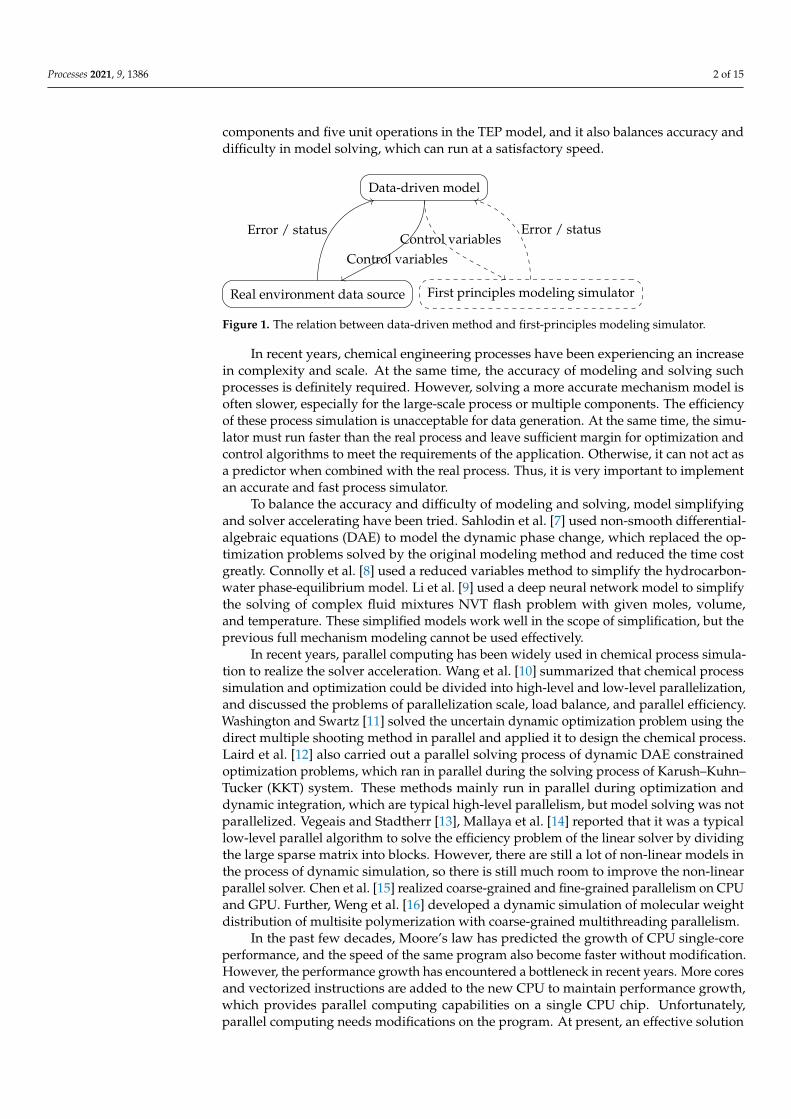
Dynamic simulation is widely used by chemical engineers to better understand theprocess [1]. The simulator based on the first principles model has a wide range of applica-tions on existing processes, and can also have certain predictions for some new processes,which has been proved to be effective in the past few decades. With the development ofthe fourth industrial revolution and the maturity of the big data environment, data-drivenmodeling becomes more widely accepted [2]. However, the corner case cannot be wellmodeled, such as start-up, shutdown, and fault if the data-driven elements are used onlyin modeling. In addition, the application of typical data-driven methods, such as modelpredictive control, optimal control, and reinforcement learning in the complex chemicalprocess may be infeasible without the initial data provided by the first-principles modelingsimulator in the way shown in Figure 1 [3]. Thus, the development of data-driven methodshighly depends on the accuracy and speed of solving the first-principles modeling simula-tor. Modeling combining mechanistic and data-driven elements can reveal the character ofthe chemical process better.

For a single unit operation or small-scale process, Luyben [4] reported that the defaultmodel exported by Aspen plus cannot accurately predict the corner case because “the de-fault heat-exchanger models do not account for heat-exchanger dynamics”. Hecht et al. [5]further reported a similar problem in the reactor. For the plantwide scale, one of themost commonly used and discussed process simulators is the Tennessee Eastman process(TEP) simulator which is carried out by Downs and Vogel [6] based on the simulationmodel by the Eastman company. The model was built according to the real process but thecomponents, kinetics, process, and operating conditions were modified. There are seven

Processes 2021, 9, 1386. https://doi.org/10.3390/pr9081386 https://www.mdpi.com/journal/processes

Processes 2021, 9, 1386 2 of 15

components and five unit operations in the TEP model, and it also balances accuracy anddifficulty in model solving, which can run at a satisfactory speed.

Data-driven model

Real environment data source First principles modeling simulator

Control variables

Error / statusControl variables

Error / status

Figure 1. The relation between data-driven method and first-principles modeling simulator.

In recent years, chemical engineering processes have been experiencing an increasein complexity and scale. At the same time, the accuracy of modeling and solving suchprocesses is definitely required. However, solving a more accurate mechanism model isoften slower, especially for the large-scale process or multiple components. The efficiencyof these process simulation is unacceptable for data generation. At the same time, the simu-lator must run faster than the real process and leave sufficient margin for optimization andcontrol algorithms to meet the requirements of the application. Otherwise, it can not act asa predictor when combined with the real process. Thus, it is very important to implementan accurate and fast process simulator.

To balance the accuracy and difficulty of modeling and solving, model simplifyingand solver accelerating have been tried. Sahlodin et al. [7] used non-smooth differential-algebraic equations (DAE) to model the dynamic phase change, which replaced the op-timization problems solved by the original modeling method and reduced the time costgreatly. Connolly et al. [8] used a reduced variables method to simplify the hydrocarbon-water phase-equilibrium model. Li et al. [9] used a deep neural network model to simplifythe solving of complex fluid mixtures NVT flash problem with given moles, volume,and temperature. These simplified models work well in the scope of simplification, but theprevious full mechanism modeling cannot be used effectively.

In recent years, parallel computing has been widely used in chemical process simula-tion to realize the solver acceleration. Wang et al. [10] summarized that chemical processsimulation and optimization could be divided into high-level and low-level parallelization,and discussed the problems of parallelization scale, load balance, and parallel efficiency.Washington and Swartz [11] solved the uncertain dynamic optimization problem using thedirect multiple shooting method in parallel and applied it to design the chemical process.Laird et al. [12] also carried out a parallel solving process of dynamic DAE constrainedoptimization problems, which ran in parallel during the solving process of Karush–Kuhn–Tucker (KKT) system. These methods mainly run in parallel during optimization anddynamic integration, which are typical high-level parallelism, but model solving was notparallelized. Vegeais and Stadtherr [13], Mallaya et al. [14] reported that it was a typicallow-level parallel algorithm to solve the efficiency problem of the linear solver by dividingthe large sparse matrix into blocks. However, there are still a lot of non-linear models inthe process of dynamic simulation, so there is still much room to improve the non-linearparallel solver. Chen et al. [15] realized coarse-grained and fine-grained parallelism on CPUand GPU. Further, Weng et al. [16] developed a dynamic simulation of molecular weightdistribution of multisite polymerization with coarse-grained multithreading parallelism.

In the past few decades, Moore’s law has predicted the growth of CPU single-coreperformance, and the speed of the same program also become faster without modification.However, the performance growth has encountered a bottleneck in recent years. More coresand vectorized instructions are added to the new CPU to maintain performance growth,which provides parallel computing capabilities on a single CPU chip. Unfortunately,parallel computing needs modifications on the program. At present, an effective solution

Processes 2021, 9, 1386 3 of 15

of increasing solving speed is to convert the problem into multiple sub-problems withoutdependence on each other and solve these sub-problems in parallel with the new CPU.

In this paper, we design a parallel dynamic simulation taking into account the char-acter of process and the development of computer. Multithreading and vectorizationparallel computing modifications are carried out based on General dynamic simulation &optimization system (DSO), which make full use of the features of modern CPU. Comparedto the previous research, we use high-level multithreading parallelism and assign tasksaccording to unit operations which brings clearer task allocation and lower communicationcosts. The effect of parallel computing modifications is tested on a 500 kt · a−1 ethylbenzeneprocess simulator.

2. Process Dynamic Simulation2.1. Current Program

For dynamic simulation, the solving of temperature, pressure, liquid level, concentra-tion, and other parameters changing with time is an initial value problem of DAE with theconstraints of the pipeline network. The form is given by Equation (1), where τ is time andy are process variables.

dydτ

= f (τ, y)

g(τ, y) = 0

y(τ0) = y0

(1)

For the chemical process, the improved Euler method is used to solve the problem.The iterative form is given by Equation (2), where h is the integral step [17].

yi+1 = yi + h f (τi+1, yi+1)

τi+1 = τi + h

y0 = y(τ0)

(2)

Due to the input of intermediate control variables during the dynamic simulation,the actual model form to be solved is given by Equation (3), where c are input con-trol variables.

dydτ

= f (τ, y, c)

g(τ, y) = 0

φ(y, c) = 0

c = c(τ)

(3)

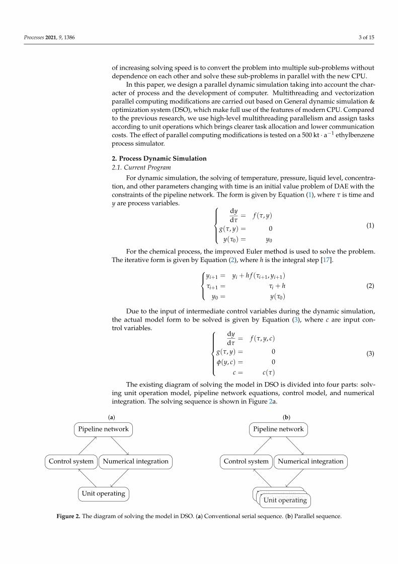
The existing diagram of solving the model in DSO is divided into four parts: solv-ing unit operation model, pipeline network equations, control model, and numericalintegration. The solving sequence is shown in Figure 2a.

(a)

Numerical integration

Unit operating

Control system

Pipeline network

(b)

Numerical integration

Unit operatingUnit operatingUnit operating

Control system

Pipeline network

Figure 2. The diagram of solving the model in DSO. (a) Conventional serial sequence. (b) Parallel sequence.

Processes 2021, 9, 1386 4 of 15

2.2. The Choice of Parallel Level

Parallel processing means that the process of solving the problem is divided intoseveral smaller parts and run on multiple processors at the same time to reduce therunning time, and then the parts are combined to produce the final result. When thereare dependencies in the problem pieces, the calculation process has to be carried out inserial. Partitioning, communication, synchronization, and load balancing are four typicalconsiderations in the design of parallel programs [18].

The parallel part is designed according to the character of dynamic simulation. The nu-merical integration cannot be parallelized because it is mostly iterative and changes basedon past iteration. During solving the unit operation model, the mass balance equation, heatbalance equation, physical property, thermodynamic parameters method, and reactionsare under consideration. As the short step size is selected, the calculation of a single unitoperation in a one-step integral iteration can be seen as independent of other unit opera-tions, and the numerical integration inside the unit operation is independent of other unitoperations. During solving the control system model, there is dependence in the cascadecontroller in one-step iteration. The pipeline network model is dependent because it needsto be solved iteratively in the field of directly connected pipes.

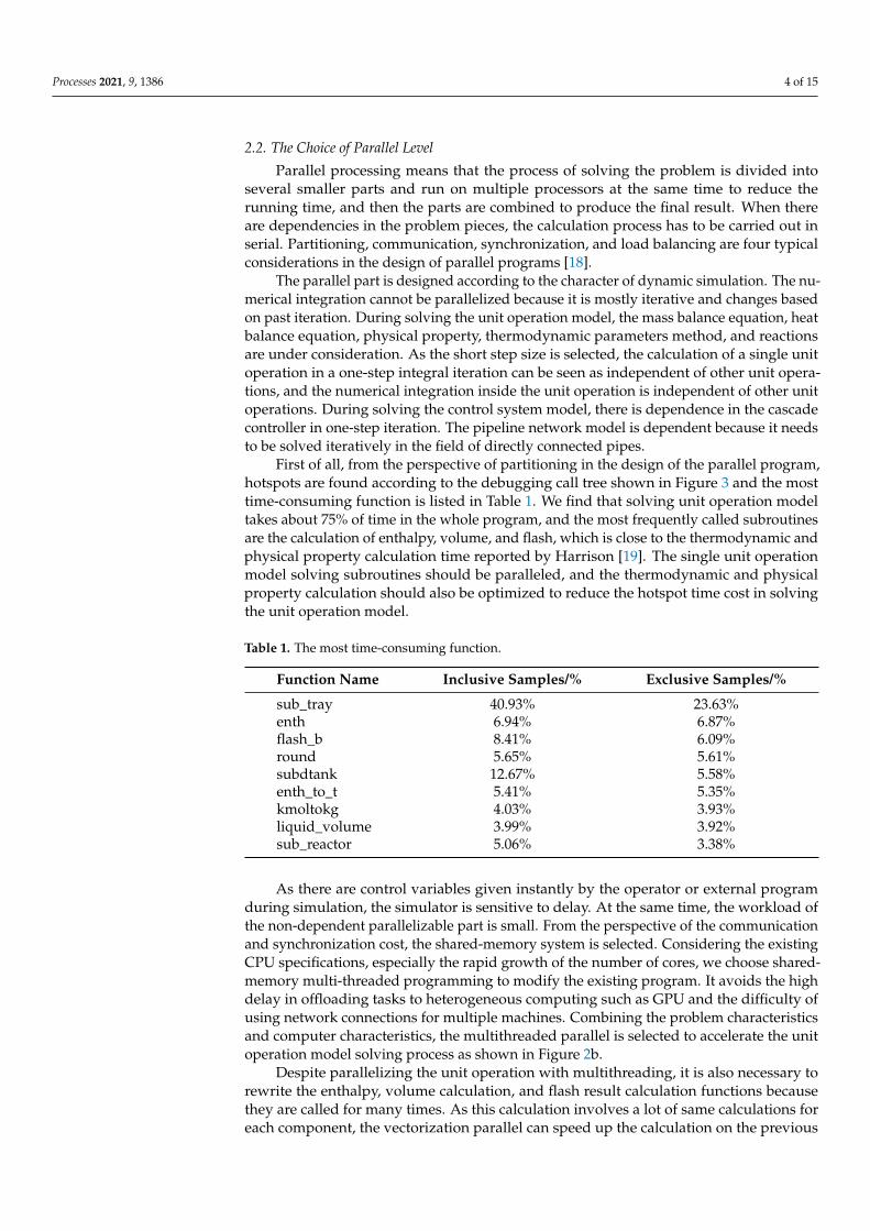
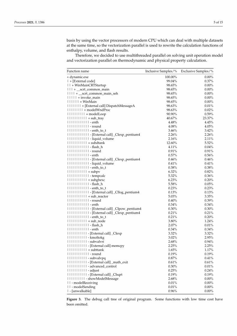
First of all, from the perspective of partitioning in the design of the parallel program,hotspots are found according to the debugging call tree shown in Figure 3 and the mosttime-consuming function is listed in Table 1. We find that solving unit operation modeltakes about 75% of time in the whole program, and the most frequently called subroutinesare the calculation of enthalpy, volume, and flash, which is close to the thermodynamic andphysical property calculation time reported by Harrison [19]. The single unit operationmodel solving subroutines should be paralleled, and the thermodynamic and physicalproperty calculation should also be optimized to reduce the hotspot time cost in solvingthe unit operation model.

Table 1. The most time-consuming function.

Function Name Inclusive Samples/% Exclusive Samples/%

sub_tray 40.93% 23.63%enth 6.94% 6.87%flash_b 8.41% 6.09%round 5.65% 5.61%subdtank 12.67% 5.58%enth_to_t 5.41% 5.35%kmoltokg 4.03% 3.93%liquid_volume 3.99% 3.92%sub_reactor 5.06% 3.38%

As there are control variables given instantly by the operator or external programduring simulation, the simulator is sensitive to delay. At the same time, the workload ofthe non-dependent parallelizable part is small. From the perspective of the communicationand synchronization cost, the shared-memory system is selected. Considering the existingCPU specifications, especially the rapid growth of the number of cores, we choose shared-memory multi-threaded programming to modify the existing program. It avoids the highdelay in offloading tasks to heterogeneous computing such as GPU and the difficulty ofusing network connections for multiple machines. Combining the problem characteristicsand computer characteristics, the multithreaded parallel is selected to accelerate the unitoperation model solving process as shown in Figure 2b.

Despite parallelizing the unit operation with multithreading, it is also necessary torewrite the enthalpy, volume calculation, and flash result calculation functions becausethey are called for many times. As this calculation involves a lot of same calculations foreach component, the vectorization parallel can speed up the calculation on the previous

Processes 2021, 9, 1386 5 of 15

basis by using the vector processors of modern CPU which can deal with multiple datasetsat the same time, so the vectorization parallel is used to rewrite the calculation functions ofenthalpy, volume, and flash results.

Therefore, we decided to use multithreaded parallel on solving unit operation modeland vectorization parallel on thermodynamic and physical property calculation.

Function name Inclusive Samples/% Exclusive Samples/%

+ dynamic.exe 100.00% 0.00%| + [External code] 99.04% 0.37%|| + WinMainCRTStartup 98.65% 0.00%||| + __scrt_common_main 98.65% 0.00%|||| + __scrt_common_main_seh 98.65% 0.00%||||| + invoke_main 98.65% 0.00%|||||| + WinMain 98.65% 0.00%||||||| + [External call] DispatchMessageA 98.63% 0.01%|||||||| + modelWndProc 98.63% 0.02%||||||||| + modelLoop 90.90% 0.59%|||||||||| + sub_tray 40.67% 23.37%||||||||||| - enth 4.48% 4.45%||||||||||| - round 4.08% 4.05%||||||||||| - enth_to_t 3.46% 3.42%||||||||||| - [External call] _CIexp_pentium4 2.26% 2.26%||||||||||| - liquid_volume 2.16% 2.11%|||||||||| + subdtank 12.60% 5.52%||||||||||| - flash_h 4.11% 0.04%||||||||||| - round 0.91% 0.91%||||||||||| - enth 0.57% 0.56%||||||||||| - [External call] _CIexp_pentium4 0.46% 0.46%||||||||||| - liquid_volume 0.41% 0.41%||||||||||| - enth_to_t 0.38% 0.38%|||||||||| + subpv 6.32% 0.82%||||||||||| - tempcalc 5.32% 0.36%|||||||||| + subghexc 6.23% 0.20%||||||||||| - flash_h 5.58% 0.05%||||||||||| - enth_to_t 0.23% 0.23%||||||||||| - [External call] _CIlog_pentium4 0.13% 0.13%|||||||||| + sub_reactor 5.03% 3.35%||||||||||| - round 0.40% 0.39%||||||||||| - enth 0.34% 0.34%||||||||||| - [External call] _CIpow_pentium4 0.30% 0.30%||||||||||| - [External call] _CIexp_pentium4 0.21% 0.21%||||||||||| - enth_to_t 0.21% 0.20%|||||||||| + sub_node 3.80% 1.24%||||||||||| - flash_h 2.07% 0.01%||||||||||| - enth 0.34% 0.34%|||||||||| - [External call] _CIexp 3.32% 3.32%|||||||||| - kmoltokg 3.02% 2.95%|||||||||| - subvalvri 2.68% 0.94%|||||||||| - [External call] memcpy 2.25% 2.25%|||||||||| + subttank 1.65% 1.17%||||||||||| - round 0.19% 0.19%|||||||||| - subvalvpq 0.87% 0.41%|||||||||| - [External call] _math_exit 0.61% 0.61%|||||||||| - advanced_control 0.30% 0.01%|||||||||| - adjust 0.25% 0.24%|||||||||| - [External call] _CIsqrt 0.19% 0.19%||||||||| - showModelMessage 2.68% 0.00%|| - modelReceiving 0.01% 0.00%|| - modelSending 0.01% 0.00%| - [unwalkable] 0.96% 0.00%

Figure 3. The debug call tree of original program. Some functions with low time cost havebeen omitted.

Processes 2021, 9, 1386 6 of 15

2.3. The Limit of Parallel Speedup

The speed-up (S) shown in Equation (4) is usually used to measure the effect ofparallel acceleration, where T(1) is the time used in serial and T(p) is time used in parallel.According to Amdahl’s law [20] as Equation (5), the upper limit of speed-up with thefixed workload is determined depending on the proportion p of parallelizable parts andthe number n of parallelizable parts. The proportion p of parallelizable parts is about75% according to the previous analysis so the upper limit of speed-up is 4 as shown inEquation (6).

S =T(1)T(p)

(4)

S =1

1− p + pn

(5)

limn→+∞

S =1

1− p=

11− 0.75

= 4 (6)

2.4. Test Case

The program performance test in the following sections is carried out on a computerwith AMD Ryzen™ 9 3900X with 12 cores and 64 GB RAM. As the CPU has precision boosttechnology, which can raise clock speed automatically, the clock speed is manually set to2.16 GHz to prevent the clock speed change during the performance test. The compilertoolchain used is MSVC 14.28, and compilation options are the same without specified ineach test. The iteration times and inter-process communication times of single system timercalls are modified to reduce the influence of system call time fluctuation. The simulationproject used in the test is a nearly stable state of the ethylbenzene process and the integrationtime step is set to 0.125 s. The simulation time in the test is five hours, and the wall clockrunning time is recorded. The effect of parallel computing modification is tested on a500 kt · a−1 ethylbenzene process simulator.

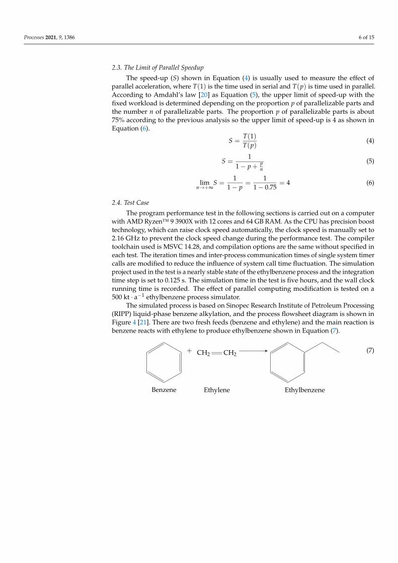
The simulated process is based on Sinopec Research Institute of Petroleum Processing(RIPP) liquid-phase benzene alkylation, and the process flowsheet diagram is shown inFigure 4 [21]. There are two fresh feeds (benzene and ethylene) and the main reaction isbenzene reacts with ethylene to produce ethylbenzene shown in Equation (7).

Benzene

+ CH2 CH2

Ethylene Ethylbenzene

(7)

Processes 2021, 9, 1386 7 of 15

C-1

C-2

C-3

C-4

D-1

D-2

D-3

D-4

R-1

R-2

D-5

D-6

E-1

R-3

R-4

R-5

E-2

E-3

E-4

E-5

E-6

E-7E-8

E-9

E-10

E-11

E-12

PC01

FC01

FC02

FC03

FC04

FC05

FC06

FC08

FC07

TC03

TC04

TC02

TC01

TC05

PC02

PC03

LC01

FC09

FC10

LC03

FC13

LC02 FC12

LC04

FC14 FC15

TC06

LC06 FC17

LC05

FC16

TC07

TC08

LC07

FC18

LC08

FC19

FFC01

Figure 4. The 500 kt · a−1 ethylbenzene process flowsheet diagram.

3. Multithreading Parallelism3.1. Overview of Multithreading Parallelism

Multithreading technology can execute more than one thread at the same time toimprove the throughput of the program. In this study, OpenMP is used to realize paral-lelize multithreading.

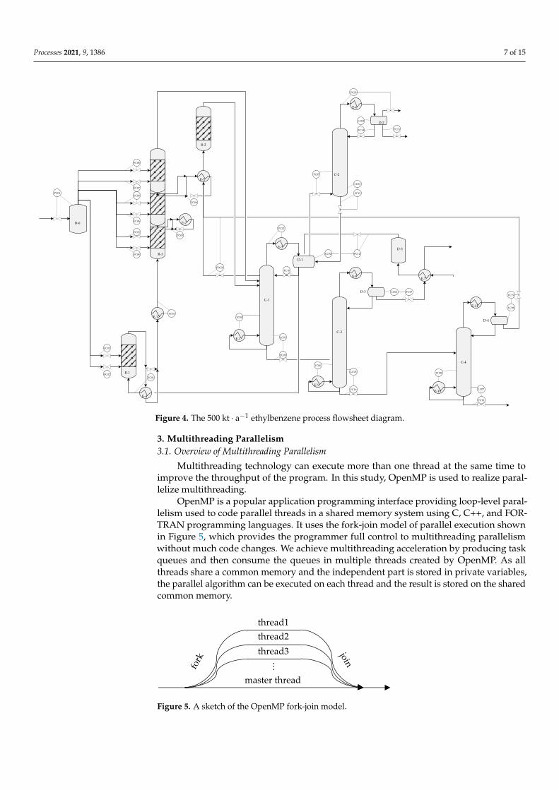
OpenMP is a popular application programming interface providing loop-level paral-lelism used to code parallel threads in a shared memory system using C, C++, and FOR-TRAN programming languages. It uses the fork-join model of parallel execution shownin Figure 5, which provides the programmer full control to multithreading parallelismwithout much code changes. We achieve multithreading acceleration by producing taskqueues and then consume the queues in multiple threads created by OpenMP. As allthreads share a common memory and the independent part is stored in private variables,the parallel algorithm can be executed on each thread and the result is stored on the sharedcommon memory.

thread3

thread2

thread1

…

master thread

fork

join

Figure 5. A sketch of the OpenMP fork-join model.

Processes 2021, 9, 1386 8 of 15

3.2. Task Allocation

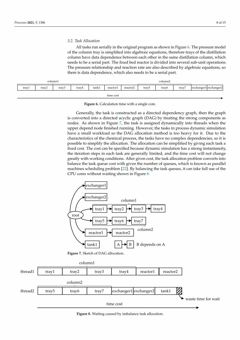
All tasks run serially in the original program as shown in Figure 6. The pressure modelof the column tray is simplified into algebraic equations, therefore trays of the distillationcolumn have data dependence between each other in the same distillation column, whichneeds to be a serial part. The fixed bed reactor is divided into several sub-unit operations.The pressure relationship and reaction rate are also described by algebraic equations, sothere is data dependence, which also needs to be a serial part.

tray1 tray2 tray3 tray4 tank1 reactor1 reactor2 tray5 tray6 tray7 exchanger1 exchanger2

time cost

column1 column2

Figure 6. Calculation time with a single core.

Generally, the task is constructed as a directed dependency graph, then the graphis converted into a directed acyclic graph (DAG) by treating the strong components asnodes. As shown in Figure 7, the task is assigned dynamically into threads when theupper depend node finished running. However, the tasks in process dynamic simulationhave a small workload so the DAG allocation method is too heavy for it. Due to thecharacteristics of the chemical process, the tasks have no complex dependencies, so it ispossible to simplify the allocation. The allocation can be simplified by giving each task afixed cost. The cost can be specified because dynamic simulation has a strong instantaneity,the iteration steps in each task are generally limited, and the time cost will not changegreatly with working conditions. After given cost, the task allocation problem converts intobalance the task queue cost with given the number of queues, which is known as parallelmachines scheduling problem [22]. By balancing the task queues, it can take full use of theCPU cores without waiting shown in Figure 8.

root

tray1 tray2 tray3 tray4

tray5 tray6 tray7

exchanger2

exchanger1

tank1

reactor1 reactor2column2

column1

BA B depends on A

Figure 7. Sketch of DAG allocation.

tray1 tray2 tray3 tray4

tank1

reactor1 reactor2

tray5 tray6 tray7 exchanger1 exchanger2

waste time for waittime cost

thread2

thread1

column1

column2

Figure 8. Waiting caused by imbalance task allocation.

Processes 2021, 9, 1386 9 of 15

As parallel machines scheduling problem is a non-deterministic polynomial-timehardness (NP-hard) problem, it is difficult to get the optimal solution. In order to reducethe initialization and start-up time of the whole program, we use a greedy algorithm toget a high-quality approach optimal solution to balance the task queues. The suboptimalsolution is acceptable because there are often a small number of heavy tasks (like columns)and a large number of light tasks (like tanks and heat exchangers) in the chemical process,so the task allocation is generally balanced enough even if the solution is not optimal.The steps of task allocation are listed as follows:

1. Treat the tasks with dependence as a single task;2. Sort all tasks into a list according to the time cost;3. Pop the first task from the list and put it on the shortest task queue;4. Sort all tasks queues according to the time cost;5. If there is any remaining task in the list, return to Step 3. Otherwise, end of the task

allocation.

Because the compiler only supports OpenMP 2.0 [23], the task queue is consumed inthe loop. The principle of multithreading rewriting is shown in Algorithm 1.

Algorithm 1 Pseudocode for task queue consuming

#pragma omp parallel for num_threads(n) schedule(static)for i = 0 to n do

consume(task queue[i])end for

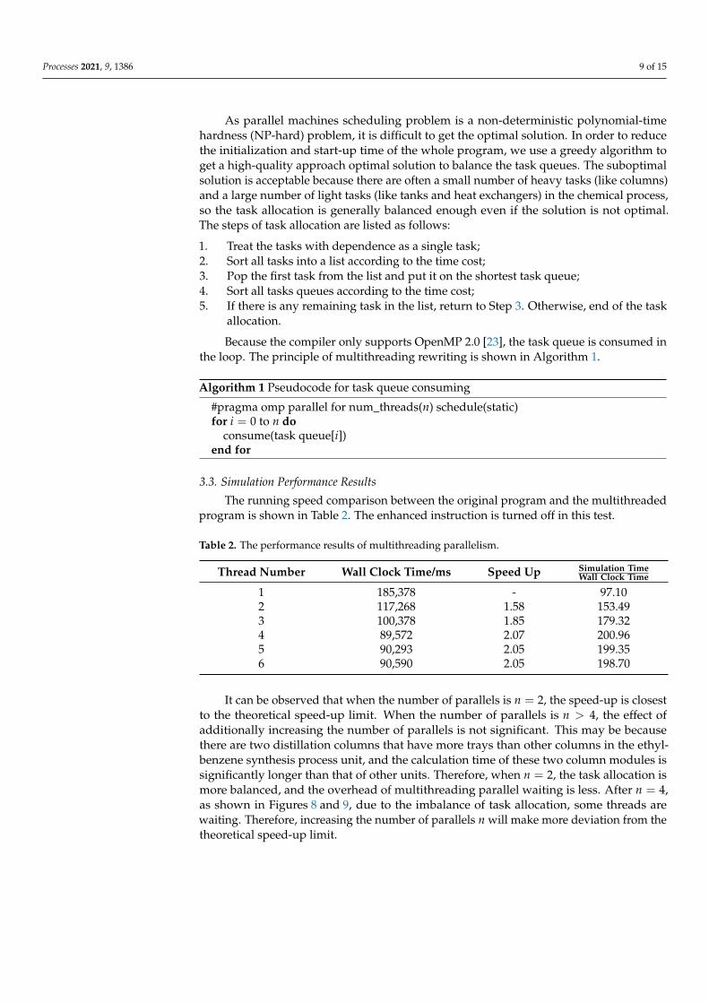
3.3. Simulation Performance Results

The running speed comparison between the original program and the multithreadedprogram is shown in Table 2. The enhanced instruction is turned off in this test.

Table 2. The performance results of multithreading parallelism.

Thread Number Wall Clock Time/ms Speed Up Simulation TimeWall Clock Time

1 185,378 - 97.102 117,268 1.58 153.493 100,378 1.85 179.324 89,572 2.07 200.965 90,293 2.05 199.356 90,590 2.05 198.70

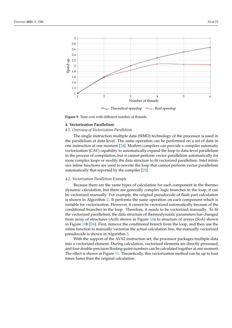
It can be observed that when the number of parallels is n = 2, the speed-up is closestto the theoretical speed-up limit. When the number of parallels is n > 4, the effect ofadditionally increasing the number of parallels is not significant. This may be becausethere are two distillation columns that have more trays than other columns in the ethyl-benzene synthesis process unit, and the calculation time of these two column modules issignificantly longer than that of other units. Therefore, when n = 2, the task allocation ismore balanced, and the overhead of multithreading parallel waiting is less. After n = 4,as shown in Figures 8 and 9, due to the imbalance of task allocation, some threads arewaiting. Therefore, increasing the number of parallels n will make more deviation from thetheoretical speed-up limit.

Processes 2021, 9, 1386 10 of 15

1 2 3 4 5 61

1.2

1.4

1.6

1.8

2

2.2

2.4

2.6

2.8

3

Number of threads

Spee

dup

Theoretical speedup Real speedup

Figure 9. Time cost with different number of threads.

4. Vectorization Parallelism4.1. Overview of Vectorization Parallelism

The single instruction multiple data (SIMD) technology of the processor is used inthe parallelism at data-level. The same operation can be performed on a set of data inone instruction at one moment [24]. Modern compilers can provide a compiler automaticvectorization (CAV) capability to automatically expand the loop to data-level parallelismin the process of compilation, but it cannot perform vector parallelism automatically formore complex loops or modify the data structure to fit vectorized parallelism. Intel intrin-sics inline functions are used to rewrite the loop that cannot perform vector parallelismautomatically that reported by the compiler [25].

4.2. Vectorization Parallelism Example

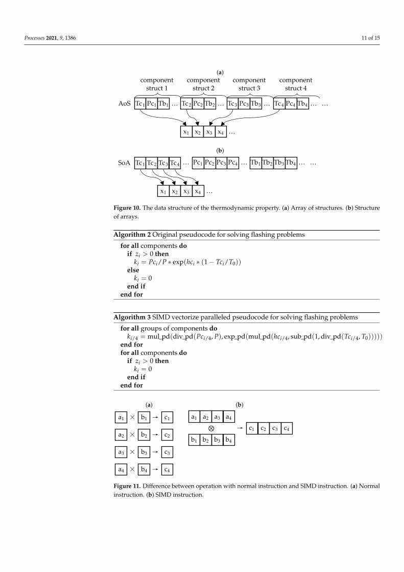
Because there are the same types of calculation for each component in the thermo-dynamic calculation, but there are generally complex logic branches in the loop, it canbe vectorized manually. For example, the original pseudocode of flash part calculationis shown in Algorithm 2. It performs the same operation on each component which issuitable for vectorization. However, it cannot be vectorized automatically because of theconditional branches in the loop. Therefore, it needs to be vectorized manually. To fitthe vectorized parallelism, the data structure of thermodynamic parameters has changedfrom array of structures (AoS) shown in Figure 10a to structure of arrays (SoA) shownin Figure 10b [26]. First, remove the conditional branch from the loop, and then use theinline function to manually vectorize the actual calculation line, the manually vectorizedpseudocode is shown in Algorithm 3.

With the support of the AVX2 instruction set, the processor packages multiple datainto a vectorized element. During calculation, vectorized elements are directly processed,and four double-precision floating-point numbers can be calculated together at one moment.The effect is shown in Figure 11. Theoretically, this vectorization method can be up to fourtimes faster than the original calculation.

Processes 2021, 9, 1386 11 of 15

(a)

Tc1 Pc1 Tb1 … Tc2 Pc2 Tb2 …

x1 x2 …

Tc3 Pc3 Tb3 …

x3

component struct 1

AoS

componentstruct 2

componentstruct 3

Tc4 Pc4 Tb4 …

component struct 4

…

x4

(b)

Tc1 Pc1 Tb1…Tc2 Pc2 Tb2…

x1 x2 …

Tc3 Pc3 Tb3 … …

x3

SoA Tc4 Pc4 Tb4

x4

Figure 10. The data structure of the thermodynamic property. (a) Array of structures. (b) Structureof arrays.

Algorithm 2 Original pseudocode for solving flashing problems

for all components doif zi > 0 then

ki = Pci/P ∗ exp(hci ∗ (1− Tci/T0))else

ki = 0end if

end for

Algorithm 3 SIMD vectorize paralleled pseudocode for solving flashing problems

for all groups of components doki/4 = mul_pd(div_pd(Pci/4, P), exp_pd(mul_pd(hci/4, sub_pd(1, div_pd(Tci/4, T0)))))

end forfor all components do

if zi > 0 thenki = 0

end ifend for

(a)

a1 c1

a2 c2

b1

b2

a3 c3b3

a4 c4b4

× →

× →

× →

× →

(b)

a1

c1

a2

c2

b1 b2

a3

c3

b3

a4

c4

b4

⊗ →

Figure 11. Difference between operation with normal instruction and SIMD instruction. (a) Normalinstruction. (b) SIMD instruction.

Processes 2021, 9, 1386 12 of 15

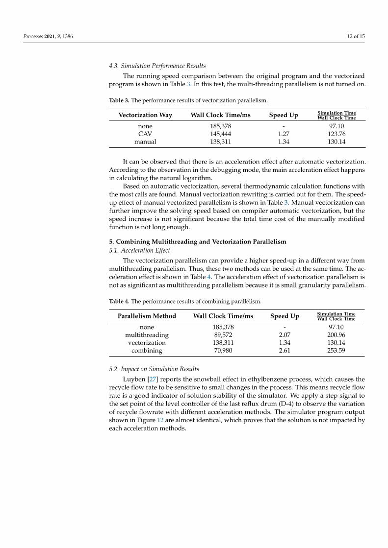
4.3. Simulation Performance Results

The running speed comparison between the original program and the vectorizedprogram is shown in Table 3. In this test, the multi-threading parallelism is not turned on.

Table 3. The performance results of vectorization parallelism.

Vectorization Way Wall Clock Time/ms Speed Up Simulation TimeWall Clock Time

none 185,378 - 97.10CAV 145,444 1.27 123.76

manual 138,311 1.34 130.14

It can be observed that there is an acceleration effect after automatic vectorization.According to the observation in the debugging mode, the main acceleration effect happensin calculating the natural logarithm.

Based on automatic vectorization, several thermodynamic calculation functions withthe most calls are found. Manual vectorization rewriting is carried out for them. The speed-up effect of manual vectorized parallelism is shown in Table 3. Manual vectorization canfurther improve the solving speed based on compiler automatic vectorization, but thespeed increase is not significant because the total time cost of the manually modifiedfunction is not long enough.

5. Combining Multithreading and Vectorization Parallelism5.1. Acceleration Effect

The vectorization parallelism can provide a higher speed-up in a different way frommultithreading parallelism. Thus, these two methods can be used at the same time. The ac-celeration effect is shown in Table 4. The acceleration effect of vectorization parallelism isnot as significant as multithreading parallelism because it is small granularity parallelism.

Table 4. The performance results of combining parallelism.

Parallelism Method Wall Clock Time/ms Speed Up Simulation TimeWall Clock Time

none 185,378 - 97.10multithreading 89,572 2.07 200.96vectorization 138,311 1.34 130.14

combining 70,980 2.61 253.59

5.2. Impact on Simulation Results

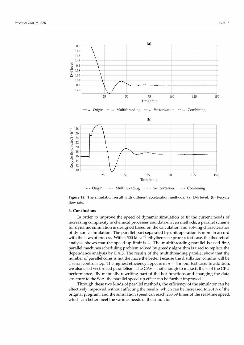
Luyben [27] reports the snowball effect in ethylbenzene process, which causes therecycle flow rate to be sensitive to small changes in the process. This means recycle flowrate is a good indicator of solution stability of the simulator. We apply a step signal tothe set point of the level controller of the last reflux drum (D-4) to observe the variationof recycle flowrate with different acceleration methods. The simulator program outputshown in Figure 12 are almost identical, which proves that the solution is not impacted byeach acceleration methods.

Processes 2021, 9, 1386 13 of 15

(a)

25 50 75 100 125 150

0.280.3

0.330.350.380.4

0.430.450.480.5

Time/min

D-4

leve

l

Origin Multithreading Vectorization Combining

(b)

Version August 1, 2021 submitted to Processes 13 of 15

the set point of the level controller of the last reflux drum (D-4) to observe the variation291

of recycle flowrate with different acceleration methods. The simulator program output292

shown in Figure 12 are almost identical, which proves that the solution is not impacted293

by each acceleration methods.294

25 50 75 100 125 150

0.280.3

0.330.350.38

0.40.430.450.48

0.5

Time/min

D-4

leve

l/%

Origin Multithreading Vectorization Combining

25 50 75 100 125 150

10121416182022242628

Time/min

Rec

ycle

flow

rate

/t·

h−

1

Origin Multithreading Vectorization Combining

Figure 12. The simulation result with different acceleration methods. (a) D-4 level. (b) Recycleflow rate.

6. Conclusions295

In order to improve the speed of dynamic simulation to fit the current needs of296

increasing complexity in chemical processes and data-driven methods, a parallel scheme297

for dynamic simulation is designed based on the calculation and solving characteristics298

of dynamic simulation. The parallel part separated by unit operation is more in accord299

with the laws of process. With a 500kt · a−1 ethylbenzene process test case, the theoretical300

analysis shows that the speedup limit is 4. The multithreading parallel is used first,301

parallel machines scheduling problem solved by greedy algorithm is used to replace302

the dependence analysis by DAG. The results of the multithreading parallel show that303

the number of parallel cores is not the more the better because the distillation column304

will be a serial control step. The highest efficiency appears in n = 4 in our test case. In305

addition, we also used vectorized parallelism. The CAV is not enough to make full use306

of the CPU performance. By manually rewriting part of the hot functions and changing307

the data structure to the SoA, the parallel speed-up effect can be further improved.308

Through these two kinds of parallel methods, the efficiency of the simulator can be309

effectively improved without affecting the results, which can be increased to 261% of310

the original program, and the simulation speed can reach 253.59 times of the real-time311

speed, which can better meet the various needs of the simulator.312

Figure 12. The simulation result with different acceleration methods. (a) D-4 level. (b) Recycleflow rate.

6. Conclusions

In order to improve the speed of dynamic simulation to fit the current needs ofincreasing complexity in chemical processes and data-driven methods, a parallel schemefor dynamic simulation is designed based on the calculation and solving characteristicsof dynamic simulation. The parallel part separated by unit operation is more in accordwith the laws of process. With a 500 kt · a−1 ethylbenzene process test case, the theoreticalanalysis shows that the speed-up limit is 4. The multithreading parallel is used first,parallel machines scheduling problem solved by greedy algorithm is used to replace thedependence analysis by DAG. The results of the multithreading parallel show that thenumber of parallel cores is not the more the better because the distillation column will bea serial control step. The highest efficiency appears in n = 4 in our test case. In addition,we also used vectorized parallelism. The CAV is not enough to make full use of the CPUperformance. By manually rewriting part of the hot functions and changing the datastructure to the SoA, the parallel speed-up effect can be further improved.

Through these two kinds of parallel methods, the efficiency of the simulator can beeffectively improved without affecting the results, which can be increased to 261% of theoriginal program, and the simulation speed can reach 253.59 times of the real-time speed,which can better meet the various needs of the simulator.

Processes 2021, 9, 1386 14 of 15

Author Contributions: Conceptualization, J.Z.; Investigation, Z.L.; Methodology, J.Z.; Project ad-ministration, Z.D.; Resources, Z.D. and J.W.; Software, J.Z.; Supervision, Z.D.; Validation, Z.L.;Writing—original draft, J.Z. and Z.D. All authors have read and agreed to the published version ofthe manuscript.

Funding: This research received no external funding.

Institutional Review Board Statement: Not applicable.

Informed Consent Statement: Not applicable.

Data Availability Statement: Data sharing not applicable.

Acknowledgments: Thanks Chao Song for giving us help in writing and Peiran Yao from Universityof Alberta giving us a lot of help in computer programming.

Conflicts of Interest: The authors declare no conflicts of interest.

Abbreviations

The following abbreviations are used in this manuscript:AVX2 Advanced vector extensions 2CAV Compiler automatic vectorizationDAE Differential-algebraic equationsDAG Directed acyclic graphDSO General dynamic simulation & optimization systemKKT Karush–Kuhn–TuckerNP-hard Non-deterministic polynomial-time hardnessSIMD Single instruction multiple dataTEP Tennessee Eastman process

References1. Luyben, W.L. Principles and Case Studies of Simultaneous Design; John Wiley & Sons, Ltd.: Hoboken, NJ, USA, 2011;

doi:10.1002/9781118001653.ch1. [CrossRef]2. Sansana, J.; Joswiak, M.N.; Castillo, I.; Wang, Z.; Rendall, R.; Chiang, L.H.; Reis, M.S. Recent trends on hybrid modeling for

Industry 4.0. Comput. Chem. Eng. 2021, 151, 107365. [CrossRef]3. Nian, R.; Liu, J.; Huang, B. A review On reinforcement learning: Introduction and applications in industrial process control.

Comput. Chem. Eng. 2020, 139, 106886. [CrossRef]4. Luyben, W.L. Rigorous dynamic models for distillation safety analysis. Comput. Chem. Eng. 2012, 40, 110–116. [CrossRef]5. Hecht, C.; Rix, A.; Paul, N.; Zitzewitz, P. Dynamische Prozesssimulation als Werkzeug in der Sicherheitsanalyse. Chem. Ing. Tech.

2020, 92, 2028–2034. [CrossRef]6. Downs, J.; Vogel, E. A plant-wide industrial process control problem. Comput. Chem. Eng. 1993, 17, 245–255. [CrossRef]7. Sahlodin, A.M.; Watson, H.A.J.; Barton, P.I. Nonsmooth model for dynamic simulation of phase changes. AIChE J. 2016,

62, 3334–3351. [CrossRef]8. Connolly, M.; Pan, H.; Tchelepi, H. Three-Phase Equilibrium Computations for Hydrocarbon–Water Mixtures Using a Reduced

Variables Method. Ind. Eng. Chem. Res. 2019, 58, 14954–14974. [CrossRef]9. Li, Y.; Zhang, T.; Sun, S. Acceleration of the NVT Flash Calculation for Multicomponent Mixtures Using Deep Neural Network

Models. Ind. Eng. Chem. Res. 2019, 58, 12312–12322. [CrossRef]10. Wang, J.; Chen, B.; He, X. Parallel computing applied in chemical process simulation and optimization: A review. CIESC J. 2002,

53, 441–446.:0438-1157.2002.05.001. [CrossRef]11. Washington, I.D.; Swartz, C.L.E. Design under uncertainty using parallel multiperiod dynamic optimization. AIChE J. 2014,

60, 3151–3168. [CrossRef]12. Laird, C.D.; Wong, A.V.; Akesson, J. Parallel Solution of Large-Scale Dynamic Optimization Problems. In 21st European

Symposium on Computer Aided Process Engineering; Computer Aided Chemical Engineering; Pistikopoulos, E., Georgiadis,M., Kokossis, A., Eds.; Elsevier: Amsterdam, The Netherlands, 2011; Volume 29, pp. 813–817. [CrossRef]

13. Vegeais, J.A.; Stadtherr, M.A. Parallel processing strategies for chemical process flowsheeting. AIChE J. 1992, 38, 1399–1407.[CrossRef]

14. Mallaya, J.U.; Zitney, S.E.; Choudhary, S.; Stadtherr, M.A. Parallel frontal solver for large-scale process simulation and optimization.AIChE J. 1997, 43, 1032–1040. [CrossRef]

15. Chen, Z.; Chen, X.; Shao, Z.; Yao, Z.; Biegler, L.T. Parallel calculation methods for molecular weight distribution of batch freeradical polymerization. Comput. Chem. Eng. 2013, 48, 175–186. [CrossRef]

Processes 2021, 9, 1386 15 of 15

16. Weng, J.; Chen, X.; Biegler, L.T. A multi-thread parallel computation method for dynamic simulation of molecular weightdistribution of multisite polymerization. Comput. Chem. Eng. 2015, 82, 55–67. [CrossRef]

17. Du, Z. Research and Application on General Dynamic Process Simulation System and Its Core Technologies. Ph.D. Thesis ,Beijing University of Chemical Technology, Beijing, China, 2014.

18. Schmidt, B.; Gonzalez-Dominguez, J.; Hundt, C.; Schlarb, M. Parallel Programming: Concepts and Practice; Morgan Kaufmann:Cambridge, MA, USA, 2017.

19. Harrison, B.K. Exploiting parallelism in chemical engineering computations. AIChE J. 1990, 36, 291–292. [CrossRef]20. Amdahl, G.M. Validity of the Single Processor Approach to Achieving Large Scale Computing Capabilities. In Proceedings of the

Spring Joint Computer Conference (AFIPS ’67), Atlantic City, NJ, USA, 18–20 April 1967; Association for Computing Machinery:New York, NY, USA, 1967; pp. 483–485. [CrossRef]

21. Dai, H. Aromatics Technology; China Petrochemical Press: Beijing, China, 2014.22. Rodriguez, F.J.; Lozano, M.; Blum, C.; García-Martínez, C. An iterated greedy algorithm for the large-scale unrelated parallel

machines scheduling problem. Comput. Oper. Res. 2013, 40, 1829–1841. [CrossRef]23. OpenMP in Visual C++. Available online: https://docs.microsoft.com/en-us/cpp/parallel/openmp/openmp-in-visual-cpp

(accessed on 30 June 2021).24. Intel® 64 and IA-32 Architectures Optimization Reference Manual. 2020. Available online: https://software.intel.com/

content/www/us/en/develop/download/intel-64-and-ia-32-architectures-optimization-reference-manual.html (accessed on30 June 2021).

25. Amiri, H.; Shahbahrami, A. SIMD programming using Intel vector extensions. J. Parallel Distrib. Comput. 2020, 135, 83–100.[CrossRef]

26. Pohl, A.; Cosenza, B.; Mesa, M.A.; Chi, C.C.; Juurlink, B. An Evaluation of Current SIMD Programming Models for C++. InProceedings of the 3rd Workshop on Programming Models for SIMD/Vector Processing (WPMVP ’16), Barcelona, Spain, 13March 2016; Association for Computing Machinery: New York, NY, USA, 2016; doi:10.1145/2870650.2870653. [CrossRef]

27. Luyben, W.L. Design and control of the ethyl benzene process. AIChE J. 2011, 57, 655–670. [CrossRef]