Mapping Computer-Vision-Related Tasks onto Reconfigurable Parallel-Processing Systems

Mapping Computer- Vision-Related Tasks onto Reconfigurable Parallel- Processing Systems

Howard Jay Siegel, James B. Armstrong, and Daniel W. Watson Purdue University

The authors demonstrate how

reconfigurability can be used by reviewing and

examining five computer-vision-

related algorithms. Each one emphasizes

different aspect of reconfigurability.

a

he “need for speed” has been the single most influential factor in super- computer design. In the past, technology fueled the development of faster computers through better semiconductor devices and very large scale

integration (VLSI). Technology, as a source of speed for a single processor, is bounded by the speed of light and physical limitations on miniaturization. Conse- quently, it has become necessary to replicate hardware to allow concurrent execution to achieve the performance requirements of many of today’s scientific and industrial applications. This concurrent execution, or parallel processing, has forced the reformulation of the most well-accepted sequential programs and even the mathematical rethinking of some problems. The parallel programmer needs to “think parallel.”

Many parallel-processing systems of different sizes and configurations have been developed (see the “Models of parallelism” sidebar). The feasibility of systems with thousands of processors has become evident with the introduction of several types of massively parallel systems. As the size, hardware complexity, and programming diversity of parallel systems continue to evolve, the range of alternatives for implementing a parallel task on these systems grows. Choosing the proper parallel algorithm and implementation becomes an important decision and has a significant impact on the performance of the application (see the “SIMD versus MIMD” sidebar). This article is a tutorial overview of how selected computer-vision-related algorithms can be mapped onto reconfigurable parallel- processing systems.

The reconfigurable parallel-processing system assumed for the discussions here is a multiprocessor system capable of mixed-mode parallelism; that is, it can operate in either the SIMD (single instruction, multiple data) or MIMD (multiple instruction, multiple data) mode of parallelism (see the sidebars) and can dynam- ically switch between modes at instruction-level granularity with generally negli- gible overhead. In addition, it can be partitioned into independent or communicat- ing submachines, each having the same characteristics as the original machine. Furthermore, this reconfigurable system model uses a flexible multistage cube

54 0018-9162/92/0200-0054$03.00 Q 1992 IEEE COMPUTER

interconnection network,’ which allows the connection patterns among the processors to be varied.

Thus, the system is reconfigurable along three dimensions:

mode of parallelism (SIMD/MIMD), partitionability, and interprocessor connectivity.

Designed at Purdue University, the PASM (partitionable SIMDIMIMD) parallel-processing system is one such machine, and its 30-processor small-scale prototype (16 processors in its compu- tational engine) is supporting active experimentation.2 Other machines capable of some form of mixed-mode operation include TRAC (Texas Recon- figurable Array C o m p ~ t e r ) ~ and O p ~ i l a . ~

The main goal here is to demonstrate how reconfigurability can be used by reviewing and examining five computer-vision-related algorithms. Each algorithm has been chosen to make a different point:

The image-smoothing algorithm, used for noise reduction, shows how

Models of parallelism

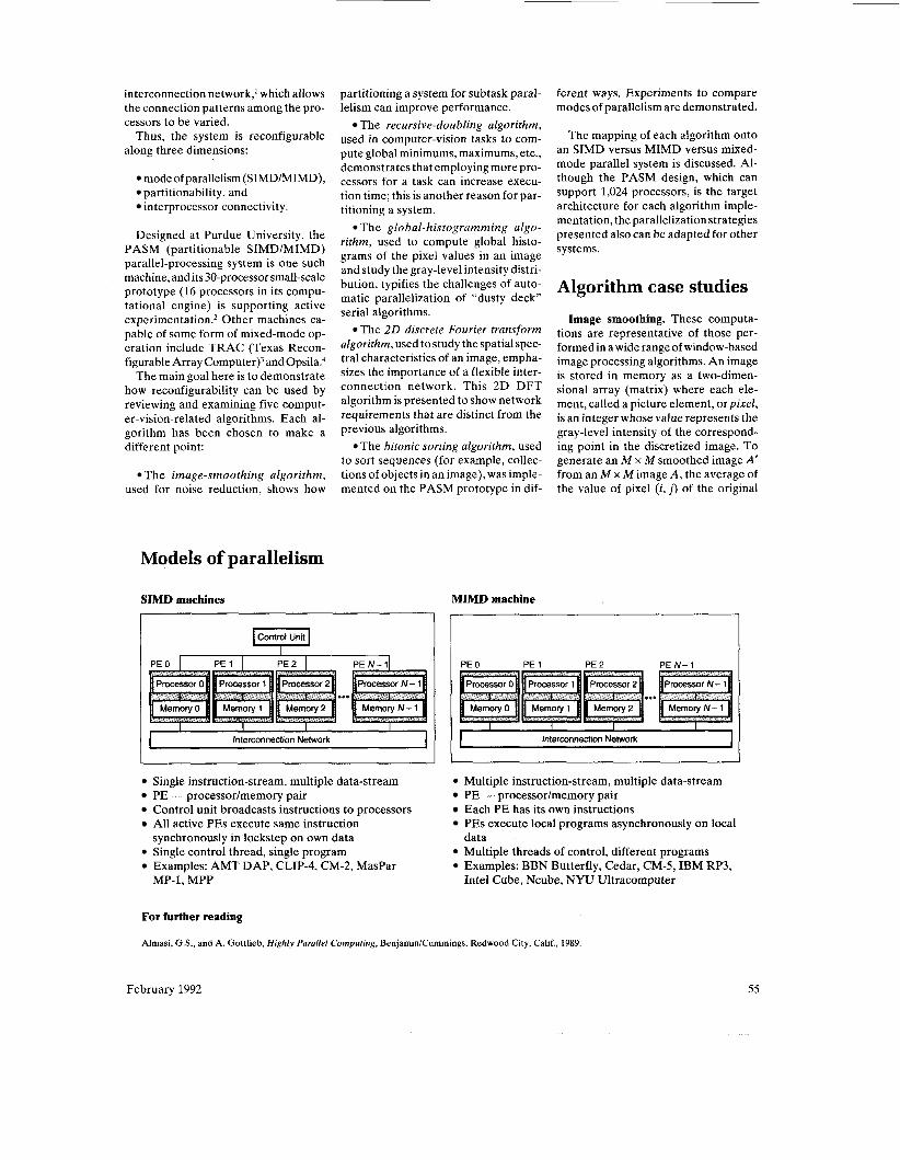
SIMD machines

partitioning a system for subtask parallelism can improve performance.

The recursive-doubling algorithm, used in computer-vision tasks to compute global minimums, maximums, etc., demonstrates that employing more processors for a task can increase execution time; this is another reason for partitioning a system.

The global-his togramming a lgo- rithm, used to compute global histograms of the pixel values in an image and study the gray-level intensity distri- bution, typifies the challenges of automatic parallelization of “dusty deck” serial algorithms.

The 2 0 discrete Fourier transform algorithm, used to study the spatial spec- tral characteristics of an image, emphasizes the importance of a flexible interconnection network. This 2D DFT algorithm is presented to show network requirements that are distinct from the previous algorithms.

The bitonic sorting algorithm, used to sort sequences (for example, collec- tions of objects in an image), was implemented on the PASM prototype in dif-

ferent ways. Experiments to compare modes of parallelism are demonstrated.

The mapping of each algorithm onto an SIMD versus MIMD versus mixed- mode parallel system is discussed. Al- though the PASM design, which can support 1,024 processors, is the target architecture for each algorithm implementation, the parallelization strategies presented also can be adapted for other systems.

Algorithm case studies

Image smoothing. These computations are representative of those performed in a wide range of window-based image processing algorithms. An image is stored in memory as a two-dimensional array (matrix) where each element, called a picture element, or pixel, is an integer whose value represents the gray-level intensity of the corresponding point in the discretized image. To generate an M x M smoothed image A’ from an M x M image A , the average of the value of pixel ( i , j ) of the original

... I I I I

Interconnection Network I 1

MIMD machine

I I I I Interconnection Network I

I I I

Single instruction-stream, multiple data-stream PE - processorlmemory pair Control unit broadcasts instructions to processors All active PES execute same instruction synchronously in lockstep on own data Single control thread, single program Examples: AMT DAP, CLIP-4, CM-2, MasPar MP-1, MPP

Multiple instruction-stream, multiple data-stream PE - processor/memory pair Each PE has its own instructions PES execute local programs asynchronously on local data Multiple threads of control, different programs Examples: BBN Butterfly, Cedar, CM-5, IBM RP3, Intel Cube, Ncube, NYU Ultracomputer

For further reading

Almasi, G.S., and A. Gottlieb, Highly Parallel Computing, Benjamin/Cummings, Redwood City, Calif., 1989.

February 1992 55

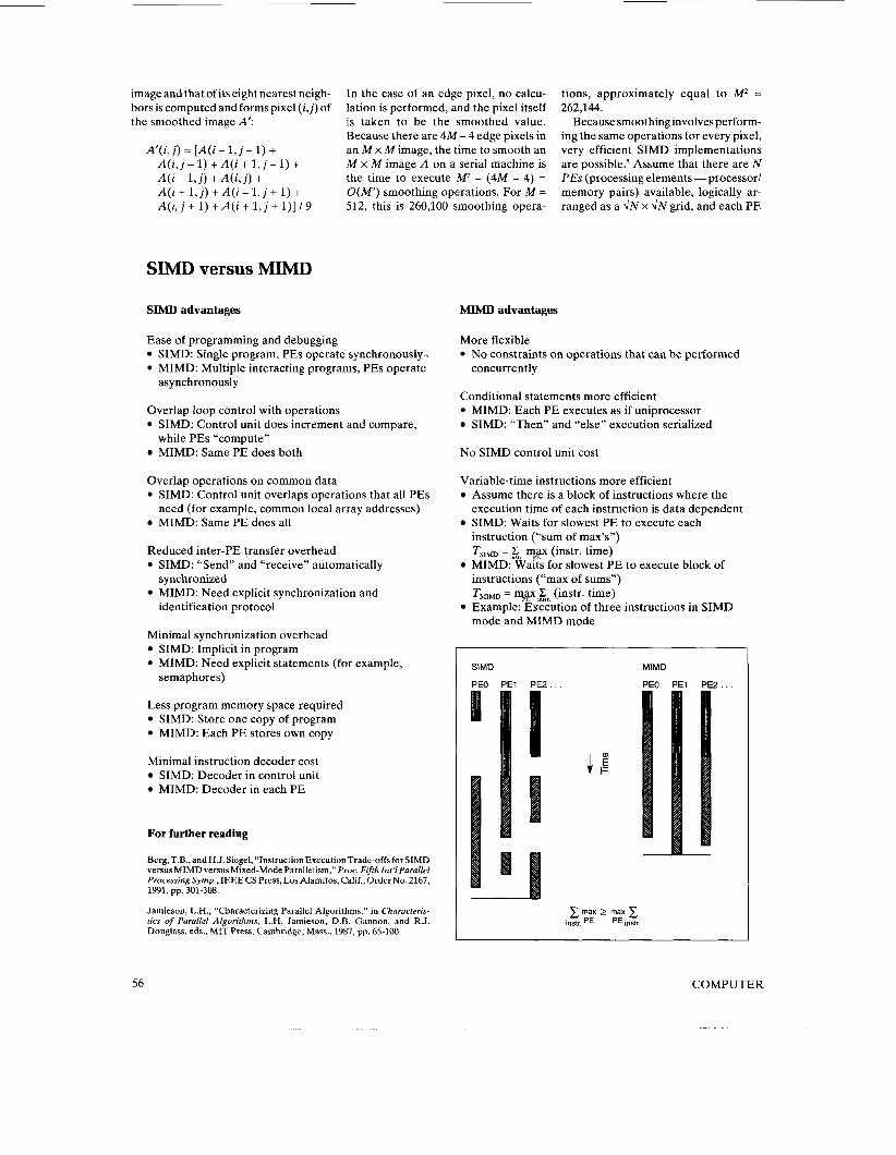
image and that of its eight nearest neigh- bors is computed and forms pixel ( i , j ) of the smoothed image A’:

A’(i, j ) = [A(i - 1, j - 1) +

A(i - 1, j ) + A(i, j ) + A(i + 1, j ) + A(z- 1, j + 1) + A(i, j + l ) + A ( i + l , j + 1 ) ] / 9

A(i, j - 1) + A(i + 1, j - 1) +

SIMD versus MIMD

SIMD advantages

In the case of an edge pixel, no calculation is performed, and the pixel itself is taken to be the smoothed value. Because there are 4M - 4 edge pixels in an M x M image, the time to smooth an M x M image A on a serial machine is the time to execute Mz - (4M - 4) = O ( M 2 ) smoothing operations. For M = 512, this is 260,100 smoothing opera-

Ease of programming and debugging SIMD: Single program, PES operate synchronously.. MIMD: Multiple interacting programs, PES operate asynchronously

Overlap loop control with operations SIMD: Control unit does increment and compare, while PES “compute” MIMD: Same PE does both

Overlap operations on common data SIMD: Control unit overlaps operations that all PES need (for example, common local array addresses) MIMD: Same PE does all

Reduced inter-PE transfer overhead SIMD: “Send” and “receive” automatically

MIMD: Need explicit synchronization and synchronized

identification protocol

Minimal synchronization overhead SIMD: Implicit in program MIMD: Need explicit statements (for example, semaphores)

Less program memory space required SIMD: Store one copy of program MIMD: Each PE stores own copy

Minimal instruction decoder cost SIMD: Decoder in control unit MIMD: Decoder in each PE

For further reading

Berg, T.B., and H.J. Siegel, “Instruction Execution Trade-offs for SIMD versus MIMD versus Mixed-Mode Parallelism,” Proc. Fifth Int’lParallel Processing Symp., IEEE CS Press, Los Alamitos, Calif., Order No. 2167, 1991, pp. 301-308.

Jamieson, L.H., “Characterizing Parallel Algorithms,” in Characteris- tics of Parallel Algorithms, L.H. Jamieson, D.B. Gannon, and R.J. Douglass, eds., MIT Press, Cambridge, Mass., 1987, pp. 65-100.

MIMD advantages

tions, approximately equal to M 2 = 262,144.

Because smoothing involves performing the same operations for every pixel, very efficient SIMD implementations are pos~ible .~ Assume that there are N PES (processing elements -processor/ memory pairs) available, logically ar- ranged as a d N x d N grid, and each PE

More flexible No constraints on operations that can be performed concurrently

Conditional statements more efficient MIMD: Each PE executes as if uniprocessor SIMD: “Then” and “else” execution serialized

No SIMD control unit cost

Variable-time instructions more efficient Assume there is a block of instructions where the execution time of each instruction is data dependent SIMD: Waits for slowest PE to execute each instruction (“sum of max’s”) TSIMD =;, rngx (instr. time) MIMD: Waits for slowest PE to execute block of instructions (“max of sums”) TMIMD = mgx;, (instr. time)

mode and MIMD mode Example: Execution of three instructions in SIMD

1 SIMD I

. . . PE0 PE1 PE2

MIMD

I max 2 max

instr. PE PE instr.

56 COMPUTER

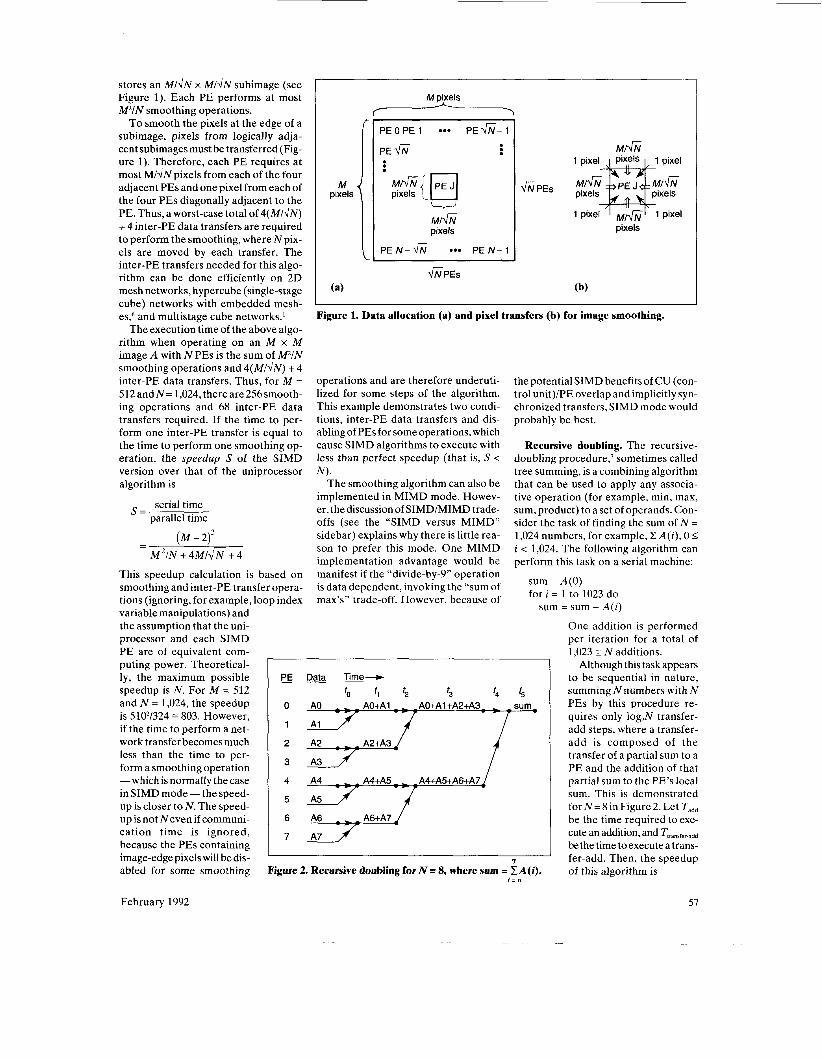
stores an MIdN x MIdN subimage (see Figure 1). Each PE performs at most M2/N smoothing operations.

To smooth the pixels at the edge of a subimage, pixels from logically adjacent subimages must be transferred (Fig- ure 1). Therefore, each PE requires at most MIdN pixels from each of the four adjacent PES and one pixel from each of the four PES diagonally adjacent to the PE. Thus, a worst-case total of 4(MldN) + 4 inter-PE data transfers are required to perform the smoothing, where N pixels are moved by each transfer. The inter-PE transfers needed for this algorithm can be done efficiently on 2D mesh networks, hypercube (single-stage cube) networks with embedded mesh- es: and multistage cube networks.’

The execution time of the above algorithm when operating on an M x M image A with N PES is the sum of M2/N smoothing operations and 4(MIdN) + 4 inter-PE data transfers. Thus, for M = 512andN= 1,024, thereare256smooth- ing operations and 68 inter-PE data transfers required. If the time to perform one inter-PE transfer is equal to the time to perform one smoothing operation, the speedup S of the SIMD version over that of the uniprocessor algorithm is

serial time parallel time

- (M-2)2

M2/N + 4 M l f i + 4

S =

This speedup calculation is based on smoothing and inter-PE transfer operations (ignoring, for example, loop index variable manipulations) and the assumption that the uniprocessor and each SIMD PE are of equivalent computing power. Theoretical- ly, the maximum possible speedup is N. For M = 512 and N = 1,024, the speedup is 5102/324 E 803. However, if the time to perform a network transfer becomes much less than the time to perform a smoothing operation -which is normally the case in SIMD mode - the speedup is closer to N. The speedup is not Neven if communi- cation time is ignored, because the PES containing image-edge pixels will be dis-

M pixels

M pixels - PEOPE1 e** P E G - 1

PE fi . . . pixels

i--J MI& pixels

f i P E s

M l f i

pixels

pixels

Figure 1. Data allocation (a) and pixel transfers (b) for image smoothing.

operations and are therefore underuti- lized for some steps of the algorithm. This example demonstrates two condi- tions, inter-PE data transfers and dis- abling of PES for some operations, which cause SIMD algorithms to execute with less than perfect speedup (that is, S <

The smoothing algorithm can also be implemented in MIMD mode. Howev- er, the discussion of SIMDIMIMD trade- offs (see the “SIMD versus MIMD” sidebar) explains why there is little reason to prefer this mode. One MIMD implementation advantage would be manifest if the “divide-by-9” operation is data dependent, invoking the “sum of max’s” trade-off. However, because of

NI.

the potential SIMD benefits of CU (control unit)/PE overlap and implicitly synchronized transfers, SIMD mode would probably be best.

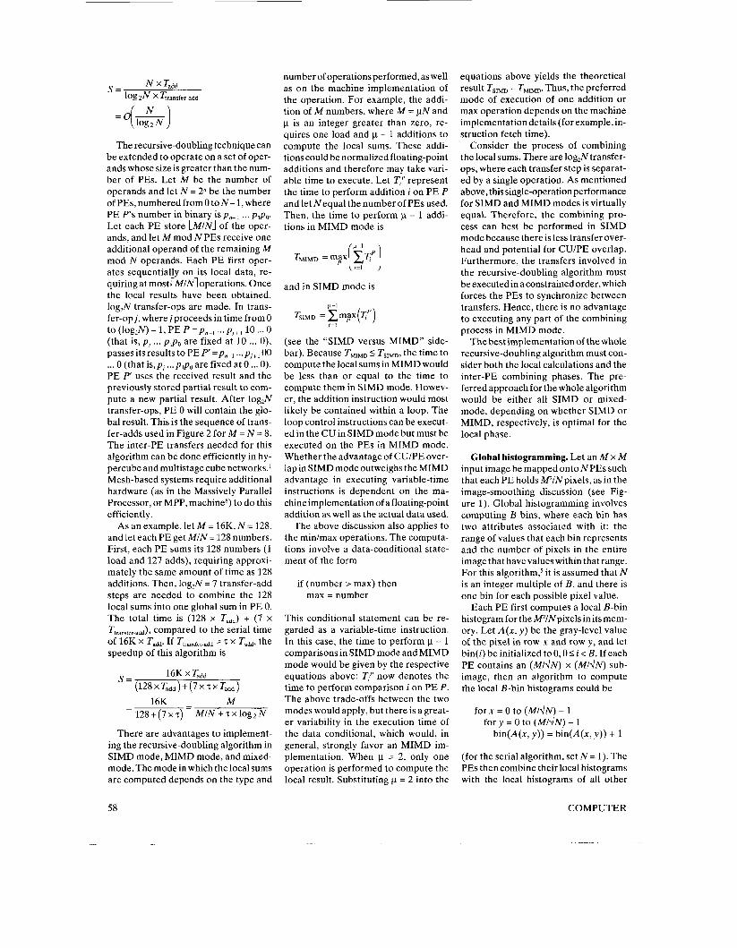
Recursive doubling. The recursive- doubling procedure,’ sometimes called tree summing, is a combining algorithm that can be used to apply any associa- tive operation (for example, min, max, sum, product) to a set of operands. Con- sider the task of finding the sum of N = 1,024 numbers, for example, CA(i) , 0 2 i < 1,024. The following algorithm can perform this task on a serial machine:

sum = A(0) for i = 1 to 1023 do

sum = sum + A(i )

p_E Data Time-

10 fl t t3 t4 t5

2 A2 _ _ _ 3 A3

4 A4 _ _ _ A4+A5 _ - _ A4+A5iA6+A7

5 A5

6 A6 _ _ _ A&A7

7 A7

7 abled for some smoothing

February 1992

Figure 2. Recursive doubling for N = 8, where sum =.CA(i). 1 = 0

One addition is performed per iteration for a total of 1,023 E N additions.

Although this task appears to be sequential in nature, summing N numbers with N PES by this procedure requires only log,N transfer- add steps, where a transfer- add is composed of the transfer of a partial sum to a PE and the addition of that partial sum to the PE’s local sum. This is demonstrated for N = 8 in Figure 2. Let Tadd be the time required to execute an addition, and T,ranrfer.add be the time to execute a transfer-add. Then, the speedup of this algorithm is

57

Tadd S = 1% 2N Transfer-add

number of operations performed, as well as on the machine implementation of the operation. For example, the addition of M numbers, where M = pN and p is an integer greater than zero, re-

equations above yields the theoretical result TSIMD = TMIMD. Thus, the preferred mode of execution of one addition or max operation depends on the machine implementationdetails (for example, in-

quires one load and p - 1 additions to compute the local sums. These additions could be normalized floating-point additions and therefore may take variable time to execute. Let TtP represent the time to perform addition i on PE P and let N equal the number of PEs used. Then, the time to perform - 1 additions in MIMD mode is

struction fetch time). Consider the process of combining

the local sums. There are log,N transfer- ops, where each transfer step is separat- ed by a single operation. As mentioned above,thissingle-operationperformance for SIMD and MIMD modes is virtually equal. Therefore, the combining process can best be performed in SIMD

The recursive-doubling technique can be extended to operate on a set of operands whose size is greater than the number of PES. Let M be the number of operands and let N = 2“ be the number of PES, numbered from 0 to N- 1, where PE P’s number in binary is p,- ... ~ 9 ~ . Let each PE store LMINJ of the operands, and let M mod N PES receive one additional operand of the remaining M mod N operands. Each PE first oper- ates sequentially on its local data, requiring at most rMIN1 operations. Once the local results have been obtained, log,N transfer-ops are made. In transfer-op j, where jproceeds in time from 0

(that is, p, ... p g , are fixed at 10 ... 0), to(log,N)-l ,PEP=p,-1 ...p,+, 10 ... 0

mode because there is less transfer overhead and potential for CU/PE overlap. Furthermore, the transfers involved in the recursive-doubling algorithm must be executed in a constrained order, which forces the PES to synchronize between transfers. Hence, there is no advantage to executing any part of the combining process in MIMD mode.

The best implementation of the whole

P-1

TMIMD = [ f ) i=l

and in SIMD mode is

P-1

GMD = zmpax(~‘) i=l

(see the “SIMD versus MIMD” side- passesits results to PE P’=p,_l ...pi+l 00 ... 0 (that is,p, . . .p ,po are fixed at 0 ... 0). PE P’ uses the received result and the previously stored partial result to compute a new partial result. After log,N transfer-ops, PE 0 will contain the global result. This is the sequence of transfer-adds used in Figure 2 for M = N = 8. The inter-PE transfers needed for this algorithm can be done efficiently in hypercube and multistage cube networks.’ Mesh-based systems require additional hardware (as in the Massively Parallel Processor, or MPP, machine8) to do this efficiently.

As an example, let M = 16K, N = 128, and let each PE get MIN = 128 numbers. First, each PE sums its 128 numbers (1 load and 127 adds), requiring approximately the same amount of time as 128 additions. Then, log,N = 7 transfer-add steps are needed to combine the 128 local sums into one global sum in PE 0. The total time is (128 x Tadd) + (7 x

bar). Because TMIMD I TSIMD, the time to compute thelocal sumsinMIMDwould be less than or equal to the time to compute them in SIMD mode. Howev- er, the addition instruction would most likely be contained within a loop. The loop control instructions can be executed in the CU in SIMD mode but must be executed on the PES in MIMD mode. Whether the advantage of CUIPE overlap in SIMD mode outweighs the MIMD advantage in executing variable-time instructions is dependent on the machine implementation of a floating-point addition as well as the actual data used.

The above discussion also applies to the minhax operations. The computations involve a data-conditional statement of the form

recursive-doubling algorithm must consider both the local calculations and the inter-PE combining phases. The preferred approach for the whole algorithm would be either all SIMD or mixed- mode, depending on whether SIMD or MIMD, respectively, is optimal for the local phase.

Global histogramming. Let an M x M input image be mapped onto N PEs such that each PE holds WIN pixels, as in the image-smoothing discussion (see Fig- ure 1). Global histogramming involves computing B bins, where each bin has two attributes associated with it: the range of values that each bin represents and the number of pixels in the entire image that have values within that range. For this algorithm? it is assumed that N is an integer multiple of B , and there is one bin for each possible pixel value.

Each PE first computes a local B-bin histogramfortheWINpixelsinitsmem-

if (number > max) then max = number

This conditional statement can be re- Ttransfer.add), compared to the serial time of 16K x Tad& If Ttransfer.add = z x Tad& the speedup of this algorithm is

garded as a variable-time instruction. In this case, the time to perform p - 1 comparisons in SIMD mode and MIMD mode would be given by the respective equations above: T,P now denotes the time to perform comparison i on PE P.

16K M The above trade-offs between the two modes would apply, but there is a greater variability in the execution time of the data conditional, which would, in

16K x &dd

(128 XTadd) + (7 x z x K d d ) s=

- 128 + (7 z) = M/N + log2 N

There are advantages to implement-

ory. Let A(x, y ) be thegray-level value of the pixel in row x and row y , and let bin(i) be initialized to 0,O 5 i < B. If each PE contains an (MIdN) x (MIdN) subimage, then an algorithm to compute the local B-bin histograms could be

for x = 0 to (MIdN) - 1 for y = 0 to ( M I ~ N ) - 1

bin(A(x, y ) ) = bin(A(x, y ) ) + 1 ing the recursive-doubling algorithm in SIMD mode, MlMD mode, and mixed- mode. The mode in which the local sums are computed depends on the type and

general, strongly favor an MIMD implementation. When p = 2, only one operation is performed to compute the local result. Substituting p = 2 into the

(for the serial algorithm, set N = 1). The PES then combine their local histograms with the local histograms of all other

58 COMPUTER

PES. The straightforward approach to combining the local histograms is to combine one bin at a time using recursive doubling, requiring Blog,N transfer-add steps.

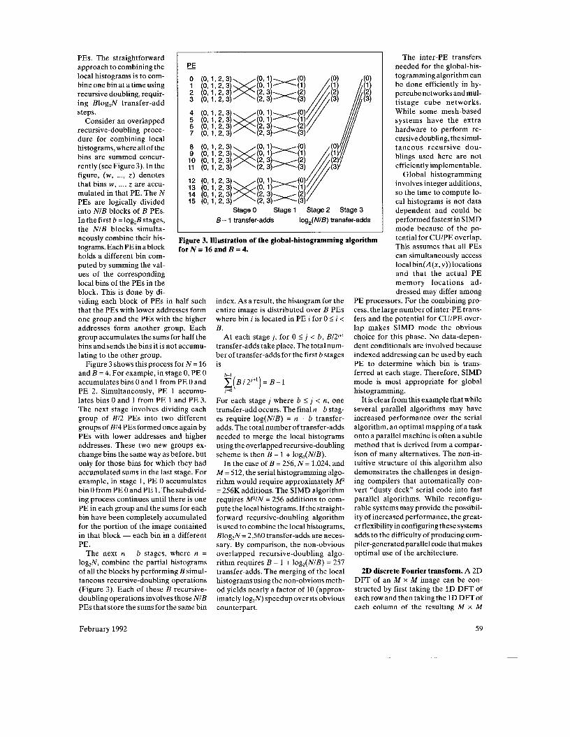
Consider an overlapped recursive-doubling procedure for combining local histograms, where all of the bins are summed concurrently (see Figure3). In the figure, (w, ..., z ) denotes that bins w, ..., z are accumulated in that PE. The N PES are logically divided into NIB blocks of B PES. In the first b = log,B stages, the NIB blocks simultaneously combine their histograms. Each PE in a block holds a different bin computed by summing the values of the corresponding local bins of the PES in the block. This is done by di-

E 0 1 2 3

4 5 6 7

Stage 0 Stage 1 Stage 2 Stage 3 B - 1 transfer-adds log,( NIB) transfer-adds

Figure 3. Illustration of the global-histogramming algorithm for N = 16 and B = 4.

viding each block of PES in half such that the PES with lower addresses form one group and the PES with the higher addresses form another group. Each group accumulates the sums for half the bins and sends the bins it is not accumu- lating to the other group.

Figure 3 shows this process for N = 16 and B = 4. For example, in stage 0, PE 0 accumulates bins 0 and 1 from PE 0 and PE 2. Simultaneously, PE 1 accumulates bins 0 and 1 from PE 1 and PE 3. The next stage involves dividing each group of B/2 PES into two different groups of Bl4 PES formed once again by PES with lower addresses and higher addresses. These two new groups ex- change bins the same way as before, but only for those bins for which they had accumulated sums in the last stage. For example, in stage 1, PE 0 accumulates bin 0 from PE 0 and PE 1. The subdivid- ing process continues until there is one PE in each group and the sums for each bin have been completely accumulated for the portion of the image contained in that block - each bin in a different PE.

The next n - b stages, where n = log,N, combine the partial histograms of all the blocks by performing B simul- taneous recursive-doubling operations (Figure 3). Each of these B recursive- doubling operations involves those NIB PES that store the sums for the same bin

index. As a result, the histogram for the entire image is distributed over B PES where bin i is located in PE i for 0 < i < B.

At each stage j , for 0 5 j < b, B12if1 transfer-adds take place. The total number of transfer-adds for the first b stages is

b-l

x(B/2 ’+’ )= B-1 1=0

For each stage j where b < j < n, one transfer-add occurs. The finaln- b stages require log(N1B) = n - b transfer- adds. The total number of transfer-adds needed to merge the local histograms using the overlapped recursive-doubling scheme is then B - 1 + log,(N/B).

In the case of B = 256, N = 1,024, and M = 512, the serial histogramming algorithm would require approximately M Z = 256K additions. The SIMD algorithm requires WIN = 256 additions to compute the local histograms. If the straightforward recursive-doubling algorithm is used to combine the local histograms, Blog,N = 2,560 transfer-adds are necessary. By comparison, the non-obvious overlapped recursive-doubling algorithm requires B - 1 + log,(NlB) = 257 transfer-adds. The merging of the local histograms using the non-obvious method yields nearly a factor of 10 (approximately log,N) speedup over its obvious counterpart.

The inter-PE transfers needed for the global-histogramming algorithm can be done efficiently in hypercube networks and multistage cube networks. While some mesh-based systems have the extra hardware to perform recursive doubling, the simul- taneous recursive dou- blings used here are not efficiently implementable.

Global histogramming involves integer additions, so the time to compute local histograms is not data dependent and could be performed fastest in SIMD mode because of the potential for CUIPE overlap. This assumes that all PES can simultaneously access local bin(A(x, y ) ) locations and that the actual PE memory locations ad- dressed may differ among

PE processors. For the combining process, the large number of inter-PE transfers and the potential for CUIPE overlap makes SIMD mode the obvious choice for this phase. No data-dependent conditionals are involved because indexed addressing can be used by each PE to determine which bin is transferred at each stage. Therefore, SIMD mode is most appropriate for global histogramming.

It is clear from this example that while several parallel algorithms may have increased performance over the serial algorithm, an optimal mapping of a task onto a parallel machine is often a subtle method that is derived from a comparison of many alternatives. The non-in- tuitive structure of this algorithm also demonstrates the challenges in design- ing compilers that automatically con- vert “dusty deck” serial code into fast parallel algorithms. While reconfigurable systems may provide the possibil- ity of increased performance, the greater flexibility in configuring these systems adds to the difficulty of producing com- piler-generated parallel code that makes optimal use of the architecture.

2D discrete Fourier transform. A 2D DFT of an M x M image can be con- structed by first taking the 1D DFT of each row and then taking the 1D DFT of each column of the resulting M x M

February 1992 59

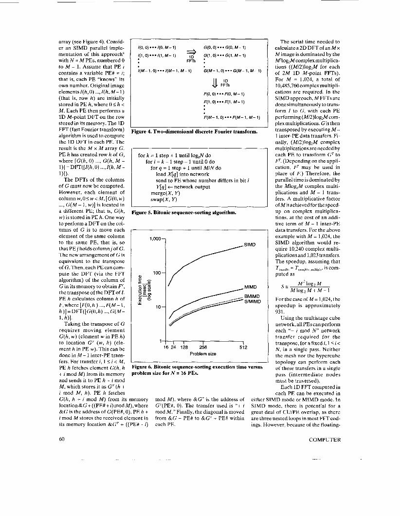
array (see Figure 4). Consid- er an SIMD parallel implementation of this approach9 with N = M PES, numbered 0 to M - 1. Assume that PE i contains a variable PE# = i; that is, each PE “knows” its own number. Original image elementsZ(h,O) ..., Z(h,M-1) (that is, row h) are initially stored in PE h, where 0 I h < M. Each PE then performs a 1D M-point DFT on the row stored in its memory. The 1D FFT (fast Fourier transform) algorithm is used to compute the 1D DFT in each PE. The result is the M x M array G. PE h has created row h of G, where [G(h, 0) ..., G(h, M - l)]=DFT([Z(h,O) ..., Z(h, M- I)]).

The DFTs of the columns of G must now be computed. However, each element of column w, 0 5 w < M, [G(O, w) ..., G(M - 1, w)] is located in a different PE; that is, G(h, w) is stored in PE h. One way to perform a DFT on the columns of G is to move each element of the same column to the same PE, that is, so that PE j holds column j of G. The new arrangement of G is equivalent to the transpose of G.Then,eachPEcancom- pute the DFT (via the FFT algorithm) of the column of G in its memory to obtain F, the transpose of the DFT of Z. PE h calculates column h of F, where [F(O, h ) ..., F(M - 1, h)]=DFT([G(O,h) ..., G(M- 1, h)].

Taking the transpose of G requires moving element G(h, w) (element w in PE h) to location GT (w, h) (element h in PE w). This can be done in M - 1 inter-PE transfers. For transfer i, 1 < i < M , PE h fetches element G(h, h + i mod M ) from its memory and sends it to PE h + i mod M , which stores it as Gr (h + i mod M , h ) . PE h fetches G(h, h + i mod M) from its

I ( O , O ) * * * I(0, M- 1)

I(1,O) I( 1, M- 1 )

G(0,O) * * * G(0, M- 1)

ID G ( 1 , 0 ) * * * G(1, M- 1) * . FFTs : . I (M-I ,O)***I (M- l , M-1) G ( M - I , O ) * * * G ( M - l , M - l )

F(O,O)*** F(0, M- I )

F(1,O) F( 1, M- 1)

. F(M - 1,O) F(M - 1 , M - 1 )

Ggure 4. Two-dimensional discrete Fourier transform.

for k = 1 step + 1 until log,N do for i = k - 1 step - 1 until 0 do

for q = 1 step + 1 until MIN do load X[q] into network send to PE whose number differs in bit i y[q] t network output

merge(X, r> swap(X Y)

Figure 5. Bitonic sequence-sorting algorithm.

I I I I 5 24 128 256 512

Problem size

Figure 6. Bitonic sequence-sorting execution time versus problem size for N = 16 PES.

The serial time needed to calculate a 2D DFT of an M x M image is dominated by the Wlog,M complex multiplications ((M/2)log2M for each of 2M 1D M-point FFTs). For M = 1,024, a total of 10,485,760 complex multiplications are required. In the SIMD approach, M FFTs are done simultaneously to transform Z to G, with each PE performing (M/2)log2M complex multiplications. G is then transposed by executing M - 1 inter-PE data transfers. Fi- nally, (M/2)log2M complex multiplications are needed by each PE to transform GT to F. (Depending on the application, F may be used in place of F.) Therefore, the parallel time is dominated by the Mlog2M complex multiplications and M - 1 transfers. A multiplicative factor of M is achieved for the speedup on complex multiplications, at the cost of an addi- tive term of M - 1 inter-PE data transfers. For the above example with M = 1,024, the SIMD algorithm would require 10,240 complex multiplications and 1,023 transfers. The speedup, assuming that

puted as Ttransfer = Tcomplex-multiply 3 is corn-

M 2 log, M S E M log2 M + M -1

For the case of M = 1,024, the speedup is approximately 931.

Using the multistage cube network, all PES can perform each “+ i mod N ’ network transfer required for the transpose, for a fixed i, 1 5 i < N, in a single pass. Neither the mesh nor the hypercube topology can perform each of these transfers in a single pass (intermediate nodes must be traversed).

Each 1D FFT computed in each PE can be executed in

, memory location&G+((PE#+i)modM),where &G is the address of G(PE#, 0). PE h + i mod M stores the received element in its memory location &Gr + ((PE# - i)

mod M), where &GT is the address of GT(PE#, 0). The transfer used is “+ i mod M.” Finally, the diagonal is moved from &G + PE# to &GT + PE# within each PE.

either SIMD mode or MIMD mode. In SIMD mode, there is potential for a great deal of CU/PE overlap, as there are three nested loops in most FFT cod- ings. However, because of the floating-

60 COMPUTER

point computations involved, the time to execute many of the instructions may be data dependent, invoking the “max of the sums” versus “sum of the max’s” advantage for MIMD. In addition, some highly efficient FFT implementations contain several conditional statements that are used to detect special cases where a simplified approach can be employed, and conditionals are performed more effectively in MIMD mode. The final choice of mode depends on details of the actual FFT implementation and machine architecture used. The transpose can be done more efficiently in SIMD mode because of the CUIPE overlap and the reduced inter-PE transfer overhead advantages. Thus, either a mixed-mode version, with the 1D FFTs done in MIMD mode and the transpose done in SIMD mode, or a pure SIMD-mode version should be employed, depending on specifics of the algorithm and machine.

Bitonic sequence sorting. Consider the bitonic sorting of sequences on the PASM prototype.2 Assume there are M numbers and N = 2” PES, where M is an integer multiple of N , and that MIN numbers are stored in each PE - initially sorted. The goal is to have each PE contain a sorted list of MIN elements, where the elements in PE i are less than or equal to the elements in PE k, for i < k . The regular bitonic sorting algorithm,1° where M = N , is modified in Figure 5 to accommodate the MIN sequences in each PE.2 Instead of performing a comparison at each step, an ordered merge is done between the local PE sequence X and the transferred sequence Y using local data- conditional statements (“merge(X, Y)”). The lesser half of the merged sequence is assigned the pointer Xand the greater half is assigned the pointer Y . The pointers to the two lists are then swapped, based on a precomputed data- independent mask (“swap(X, Y)”) .

When choosing the mode of parallelism, the programmer must consider two salient characteristics of the algorithm. First, the ordered merge involves many comparisons that can be more efficiently computed in MIMD mode. Second, the algorithm requires many network transfers, which are better performed in SIMD mode. To evalu- ate different approaches to this algorithm, a pure SIMD, a pure MIMD,

and two mixed-mode implementations have been executed on the prototype.

In the SlMIMD (SIMDIMIMD) mixed-mode implementation, the ordered merge and swap routines were executed in MIMD mode, while the rest of the operations, including network transfers, were performed in SIMD mode. This algorithm has an advantage over pure SIMD and pure MIMD implementations because all comparisons are done in MIMD mode and all network transfers are done in SIMD mode. Additionally, there is potential for significant CUIPE overlap in the SIMD instructions.

The BMIMD (barrier MIMD) mixed- mode implementation uses MIMD mode but uses barrier synchronization” to synchronize all inter-PE transfers. This is typically performed in three steps. First, each PE arrives at a synchronization point in an algorithm called the barrier. Next, each PE will wait at the barrier until all the PES have “an- nounced” that they are at the barrier. On PASM, this is accomplished byfetch- ing a word from the SIMD address space, thus using the SIMD instruction fetch synchronization hardware to implement the barrier. Finally, all PES continue execution simultaneously. During the bitonic sorting algorithm, the PES barrier synchronize before each inter-PE transfer. Consequently, the PES can perform the transfer without the overhead normally involved with MIMD network transfers. Thus, the BMIMD implementation has the advantage of performing data-dependent conditionals in MIMD mode but performs barrier synchronization to reduce inter-PE data transfer overhead. Therefore, its performance would be expected to be better than pure SIMD or pure MIMD.

Figure 6 shows the resultsof the SIMD, MIMD, SIMIMD, and BMIMD algorithms for the bitonic sorting problem with N = 16 PES. There is a significant improvement in execution time for both mixed-mode algorithms. SIMIMD performed better than BMIMD, with the difference increasing with M , mainly because of the CU/PE overlap. The mixed-mode results are the product of properties inherent to the modes of parallelism and not artifacts of the prototype construction, as discussed by Fineberg et aL2 The PASM prototype is a constantly evolving tool for under- standing the programming and design of parallel-processing systems.

Mapping algorithms onto partitionable systems

Two potential advantages of a partitionable parallel-processing system are demonstrated - the first involving subtask parallelism and the second consid- ering the number of PES assigned to a task.

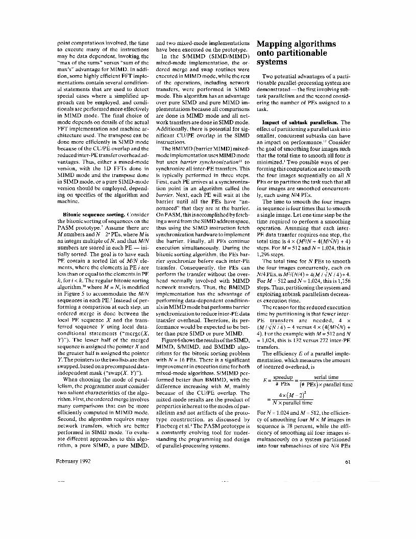
Impact of subtask parallelism. The effect of partitioning a parallel task into smaller, concurrent subtasks can have an impact on performance.I2 Consider the goal of smoothing four images such that the total time to smooth all four is minimized.’ Two possible ways of performing this computation are to smooth the four images sequentially on all N PES or to partition the task such that all four images are smoothed concurrently, each using NI4 PES.

The time to smooth the four images in sequence is four times that to smooth a single image. Let one time step be the time required to perform a smoothing operation. Assuming that each inter- PE data transfer requires one step, the total time is 4 x ( M 2 / N + 4 ( M / . / N ) + 4 ) steps. For M = 512 and N = 1,024, this is 1,296 steps.

The total time for N PES to smooth the four images concurrently, each on NI4 PES, is W l ( N l 4 ) + 4(M I I/N/4)+ 4 . For M = 512 and N = 1,024, this is 1,156 steps. Thus, partitioning the system and exploiting subtask parallelism decreases execution time.

The reason for the reduced execution time by partitioning is that fewer inter- PE transfers are needed, 4 x ( M I JN/4) + 4 versus 4 x ( 4 ( M l d N ) + 4 ) . For the example with M = 512 and N = 1,024, this is 132 versus 272 inter-PE transfers.

The efficiency E of a parallel implementation, which measures the amount of incurred overhead, is

speedup - serial time E=- # PES (# PES) x parallel time

- 4 x ( M - 2 ) 2 N x parallel time

For hi= 1,024 and M = 512, the efficiency of smoothing four M x M images in sequence is 78 percent, while the efficiency of smoothing all four images simultaneously on a system partitioned into four submachines of size NI4 PES

February 1992 61

each is 88 percent. The efficiency improved because the larger subimage size (32 by 32 versus 16 by 16) reduces the percentage of the total execution time spent doing inter-PE data transfers (132I (322 + 132) = 11 percent versus 68/(16* + 68) = 21 percent).

This example illustrates

N

Timeunits

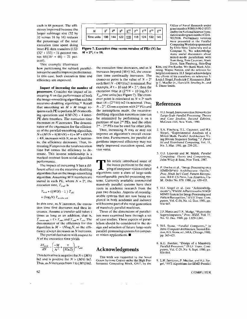
27 28 29 2’0 211 212 213 214

198 144 122 116 118 124 132 141

1

Figure 7. Execution time versus number of PES ( N ) for M = 214, z = io.

how partitioning for subtask parallelism can be used to improve performance. In this case, both execution time and efficiency are improved.

Impact of increasing the number of processors. Consider the impact of increasing N on the performance of both the image-smoothing algorithm and the recursive-doubling algorithm.’* Recall that smoothing an M x M image requires each PE to perform WINsmooth- ing operations and 4(MIdN) + 4 inter- PE data transfers. The execution time decreases as N increases. The denominator of the expression for the efficiency of the parallel smoothing algorithm, N x (WIN + 4(MIdN) + 4) = W + 4MdN + 4N, increases with N , so as N increases, the efficiency decreases. Thus, increasing Nimproves the total execution time but causes the efficiency to de- crease. This inverse relationship is a marked contrast from serial-algorithm performance.

The impact of increasing N has a different effect on the recursive-doubling algorithm than on the image-smoothing algorithm. Assuming MIN numbers are stored in each PE, where N = 2”, the execution time, T,,,,,, is

In this case, as N increases, the execution time first decreases and then increases. Assume a transfer-add takes z times as long as an addition; that is,

denominator of the efficiency for this algorithm is M + zMog,N, so the efficiency always decreases as N increases.

The partial derivative with respect to N of the execution time yields

Ttransier-add = ‘add, and = Tadd‘ The

This derivative is negative for N < (MIz) In2 and is positive for N > (MIz) ln2. Thus, as N increases from 1 to ( M l z ) ln2,

the execution time decreases, and as N increases beyond ( M l z ) ln2, the execution time continually increases. The crossover point is the value of N = 2” such that I N - (MIz) ln2 I is minimal. For example, if z = 10 and M = 214, then the execution time is (2I4/N + 10 log,N) x Tadd time units (see Figure 7). The crossover point is calculated as N = 2” such that I N - (214/10) ln2 I is minimal. Thus, N = 21°. Given a system with 214 PES and the assumptions made, the recursive- doubling-algorithm execution time can be minimized by performing it on a partition of size 21° PES, and the other 214 - 21° PES can be used for other jobs.

Thus, increasing N may or may not improve an algorithm’s overall execution time. Furthermore, for parallel algorithms improved efficiency may not imply improved execution speed, and vice versa.

his article introduced some of the issues pertinent to the mapping of computer-vision-related

algorithms onto a class of large-scale reconfigurable parallel-processing systems. Currently available commercial massively parallel systems have their roots in academic research from the past two decades. Aspects of reconfigurable systems that are now being ex- plored in both academia and industry will become part of the next generation of massively parallel machines.

Three of the dimensions of parallelism were examined here through a set of case studies. These aspects of parallelism should be considered in the design and selection of future large-scale parallel-processing systems for computer-vision applications.

Acknowledgments This work was supported by the Naval

Ocean Systems Center under the High Per- formance Computing Block, ONT; by the

Office of Naval Research under grant number N00014-90-J-1937; and by the National Science Foun- dation under grant number CDA- 9015696. Preliminary versions were presented at the Parallel Computing Workshop sponsored by Ohio State University and at Compsac 91. We acknowledge man; useful discussions about mixed-mode parallelism with Tom Berg, Tom Casavant, Hank Dietz, Sam Fineberg, Shin-Dug

Kim, and Jim Kuehn. We thank Mark Alle- mang, Wayne Nation, and the referees for helpful comments. H.J. Siegel acknowledges the efforts of his coauthors on reference 5: Leah J. Siegel, Frederick C . Kemmerer, Phil- ip T. Mueller Jr., Harold E. Smalley Jr., and S. Diane Smith.

References 1.

2.

3.

4.

5 .

6.

7.

8.

9.

H.J. Siegel, Interconnection Networks for Large-scale Parallel Processing: Theory and Case Studies, Second Edition, McGraw-Hill, New York, 1990.

S.A. Fineberg, T.L. Casavant, and H.J. Siegel, “Experimental Analysis of a Mixed-Mode Parallel Architecture Us- ing Bitonic Sequence Sorting,” J. Paral- lel and Distributed Computing, Vol. 11, No. 3, Mar. 1991, pp. 239-251.

G.J. Lipovski and M. Malek, Parallel Computing: Theory and Comparisons, John Wiley & Sons, New York, 1987.

P. Duclos et al., “Image Processing on a SIMD/SPMD Architecture: Opsila,” Proc. Ninth Int’l Con$ Pattern Recogni- tion, IEEE CS Press, Los Alamitos, Ca- lif., Order No. 878,1988, pp. 430-433.

H.J. Siegel et al. (see “Acknowledg- ments”), “PASM: Apartitionable SIMD/ MIMD System for Image Processing and Pattern Recognition,”IEEE Trans. Com- puters, Vol. C-30, No. 12, Dec. 1981, pp. 934-947.

J.P. Hayes and T.N. Mudge, “Hypercube Supercomputers,” Proc. IEEE, Vol. 77, No. 12, Dec. 1989, pp. 1,829-1,841.

H.S. Stone, “Parallel Computers,” in Intro. Computer Architecture, Second Edi- tion,H.S. Stone,ed.,SRA, Chicago, 1980, pp. 363-425.

K.E. Batcher, “Design of a Massively Parallel Processor,” IEEE Trans. Com- puters, Vol. C-29, No. 9, Sept. 1980, pp. 836-844.

L.H. Jamieson, P. Mueller, and H.J. Sie- gel, “FFT Algorithms for SIMD Parallel

62 COMPUTER

Processing Systems,” J . Parallel and Dts- rribuird C u r n p u r i r c t ; , Vol. 3 , No. I , Mar. 1986, pp. 48-71.

10. K.E. Batcher, “Sorting Networks and their Applications,” Proc. A FIPS Spring Joint Computer Conf, 1968, pp. 307-314.

11. H.F. Jordan, “A Special-Purpose Archi- tecture for Finite-Element Analysis,” Proc. Int’l Cont Parallel Processing, IEEE CS Press, Los Alamitos, Calif., Order No. 175 (microfiche only), 1978, pp. 263- 266.

12. R. Krishnamurti and E. Ma, “The Pro- cessor Partitioning Problem in Special- Purpose Partitionable Systems,” Proc. Int’l Con$ Parallel Processing, Vol. I, IEEE CS Press, Los Alamitos, Calif., Order No. 889 (microfiche only), 1988, pp. 434-443.

Howard Jay Siegel is a professor and the coordinator of the Parallel Processing Labo- ratory in the School of Electrical Engineer- ing at Purdue University, West Lafayette, Indiana. His current research focuses on interconnection networks and the use and design of the PASM reconfigurable parallel computer system. H e is coeditor-in-chief of The Journal of Parallel and Distributed Com- puting and program chair of Frontiers 92, the Fourth Symposium on the Frontiers of Mas- sively Parallel Computation.

Siegel received two BS degrees from MIT and the MA, MSE, and PhD degrees from Princeton University. H e is a fellow of the IEEE and a member of the IEEE Com- puter Society, the ACM, Eta Kappa Nu, and Sigma Xi.

James B. Armstrong is a PhD candidate in the School of Electrical Engineering at Pur- due University, West Lafayette, Indiana. His research interests are in operating system considerations for reconfigurable parallel computing systems, and he uses the PASM prototype as a testbed for his theoretical work. He is the student manager of the E E School’s Parallel Processing Laboratory and a codeveloper of a graduate-level course on programming parallel machines.

Armstrong received a BS degree in electrical engineering and computer science and a management systems certificate from Prin- ceton University in 1988, and an MSEE degree from Purdue in 1989. He is a member of Eta Kappa Nu, the IEEE Computer Society, Sigma Xi, and Tau Beta Pi.

Daniel W. Watson is a PhD candidate in the School of Electrical Engineering at Purdue University, West Lafayette, Indiana. His research interests include automatic parallel- mode selection techniques and distributed- memory management. H e is a codeveloper of a graduate-level course on programming parallel machines.

Watson received a BSEE degree from Tennessee Technological University in 1985 and an MSEE degree from Purdue in 1990. From 1985 to 1987, he developed software simulations for the Naval Surface Weapons Center in Dahlgren, Virginia. He is a member of the IEEE, the IEEE Computer Soci- ety, Gamma Beta Phi, Tau Beta Pi, and Eta Kappa Nu.

1951 -1991

4m 3RD ANNUAL

CONFERENCEON INTEUIGEM ROBOTlC

SYSTEMS FOR SPACE MPLORATlON

NASA Center for Intelligent Robotic Systems for Space Explora- tion Conference is the third annual conference on engineering in space. The 14 papers in this first bound edition discusses intelligent robotic systems for future space exploration missions.

Sectiom: Planning and Represen- tation, Coordination and Integration, Motion Control, Vision and Sensing, Robotics for Space Applications.

144 PAGES 1991 SOFTBOUND lSBN 08186-2595-3 CATALOG NO. 2595

$40 00 MEMBERS $20 00

This book explores AI theory and AI applications through its investigation of AI tools and their manipulation of old and new forms of knowledge. This volume contains 84 papers covering AI algorithms and tools for software engineering, knowledge-based systems, reasoning and problem- solving, and machine learning.

Sections Include: Machine Learn- ing, Knowledge Acquisition and Validation, Parallel Implementa- tions, Software Development and Maintenance, Genetic Algorithms, Knowledge Representation Schemes, Geometric Constraint Satisfaction, Constraint Satisfac- tion Algorithms, Efficient Inference Techniques, Knowl- edge-Based Applications, Applications of AI Techniques.

568 PAGES. 1991. SOFTBOUND. lSBN 0-8186-2300-4. CATALOG NO. 2300

$100.00 MEMBERS $50.00

Call toll-free 1-800-CS-BOOKS

Readers can contact the authors at the Parallel Processing Laboratory, Purdue University, School of Electrical Engineering, Electrical Engineering Building, West Lafayette, IN 47907- 1285.

February 1992

Documents

Mapping Computer-Vision-Related Tasks onto Reconfigurable Parallel-Processing Systems