Embed Size (px)
Citation preview

- Bogotá - Colombia - Bogotá - Colombia - Bogotá - Colombia - Bogotá - Colombia - Bogotá - Colombia - Bogotá - Colombia - Bogotá - Colombia - Bogotá - Colombia - B
A Macro CGE Model for the Colombian Economy
Por: Andrés M. Velasco, Camilo A. Cárdenas Hurtado
Núm. 863 2015
A Macro CGE Modelfor the Colombian Economy∗
Andres M. Velasco†
Camilo A. Cardenas Hurtado‡
2015
Abstract
This paper presents the construction of a tailor-made Macro Computable GeneralEquilibrium Model for the Colombian economy that satisfies Banco de la Republica’smacroeconomic programming and forecasting interests. Using information on the na-tional accounts divulged by the National Statistics Department (DANE), we set an easilyupdatable Macro Social Accounting Matrix that serves as a starting point for the modelparameters calibration and estimation.
Keywords: Social Accounting Matrix, Computable General Equilibrium Models,
Colombian Economy, Macroeconomic Programming.
JEL: C67, C68, D57, D58
1. Introduction
Applied economic policy analyses need both a theoretically consistent framework and a soliddataset that represents the current state of an economy. Applied Computable General Equi-librium Models (CGEM) provide the tools to achieve such goals. These models have beenfound useful in a wide range of policy-assessment oriented applications, including, tradingpolicies, environmental impacts, taxation and fiscal effects, productivity shocks and economicgrowth, income distribution, among other important topics (Dixon and Jorgenson, 2013).
Any CGEM consists of two main parts: The first one, a square table known as the SocialAccounting Matrix (SAM), which is a detailed and coherent summary of the transactions
∗The authors are grateful to the Fiscal, Financial accounts, and External sections and the Research Depart-ment at Banco de la Republica. In special we thank Oscar Bautista, Nestor Espinoza, Celina Gaitan, AaronGaravito, Ana Marıa Iregui, D. Camilo Lopez, Johanna Lopez, Enrique Montes, Jorge Ramos, Jose Morenoand the attendants to the Economics Weekly Seminar at Banco de la Republica for their help and comments.They also thank Juliana Avila, Camilo Porras and Marcela Rey for their research assistance. Opinions andresults expressed here do not necessarily reflect those of Banco de la Republica’s Board of Directors nor theMinistry of Public Finance.†Ministry of Finance and Public Credit. e-mail: [email protected].‡Banco de la Republica. e-mail: [email protected]. Corresponding author.
1
and flows of goods and services and the cost structure of a given economy in a certain (fixed)period of time. The second one, a whole set of equations that analytically model thesetransactions and flows, consistent in a microeconomic sense and in accordance to a (oftencompetitive) general equilibrium framework. Some examples of CGEM for Colombia arethose in Bussolo et al. (1998) and Rutherford and Light (2002). A much broader compilationof pioneering works on CGE modeling for the Colombian economy can be found in Lopezet al. (1994). Although possible, a deeper literature review on this topic is beyond the scopeof this paper.
This paper is intended to present a tailor-made Macro-CGEM that meets the needs atthe Central Bank of Colombia for incorporating the Balance of Payments macroeconomicprogramming results alongside with other projections made for relevant macroeconomic vari-ables for a small and open economy. The Macro-SAM built for this model is presented insection 2, whilst the key equations for this model are presented in section 3. Parametercalibration is explained in section 4, while section 5 and 6 document a sensibility analysisrelated to the choice of the elasticities in the model. Section 7 concludes and poses furtherrelevant extensions to this model.
2. A Macro Social Accounting Matrix for Colombia
A Social Accounting Matrix (SAM) is a compact representation of the economic structureof a country. Although summarized, a SAM contains the relevant transactions that occurbetween agents in the economy, the existing flows of goods and services and the cost structureof the production (supply) side of the economy. More detailed SAMs often include a descrip-tion of the taxation structure, welfare distribution by quantiles of income, international tradepartners, etc. Its size and details depend largely on the available information and its finalpurpose. A very comprehensive manual for SAMs construction and their applications is thatof Pyatt and Round (1985). Some examples of detailed SAMs built for the Colombian econ-omy are those in Valderrama and Gutierrez (1995), Bussolo and Correa (1998), Prada andGuzman (2002), Ramırez and Prada (2000), Karl (2004), Jensen and Karl (2004), Hernandez(2003), Corredor and Pardo (2008) and Cespedes (2011). These SAMs served as basis forthe implementation of specialized CGE models with financial, health policies and taxationimpact aims.
The construction of the SAM supporting the Macro-CGE model presented in this paperdoes not involve the detail available for the other matrices mentioned above, since the mainobjectives of this model do not require it. In this section we describe in detail the construc-tion of a tailor-made Macro Social Accounting Matrix (Macro-SAM), benchmark year 2011(extended to 2012 as well). This Macro-SAM is an aggregation of an actual SAM and isalso largely based on the guidelines presented in Lora (2008, chapter 13). We recall thatthe main advantage of this Macro-SAM structure is that it can be updated every year whenDANE publishes the annual national account results (i.e. the Supply-Demand Balance andthe Integrated Economic Accounts matrices). Therefore, the counterfactual results derivedfrom the model’s application are compared to a up-to-date baseline scenario.
2
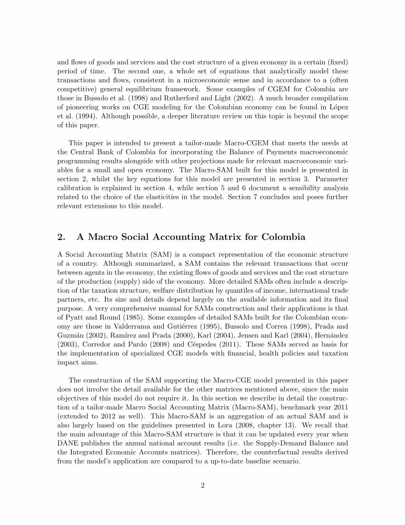
The Macro-SAM we present in this section aggregates the economy over six differentdimensions, as seen in Figure 1:
1. Factors (F),
2. Production and Products (P),
3. Distribution (D),
4. Agents (A),
5. Rents, Taxes and Transfers (T), and
6. Savings-Investment Balance (B).
The Macro-SAM is read as it follows: every non-empty sub-matrix arising from the in-tersection of each of the dimensions above represents a set of transactions in the economy.Columns represent purchases or payments and rows represent sales or recipients, e.g, thecell FAC (in P, column) - L (in F, row) represents the total payment from the account fac-tor aggregation (FAC) to labor supply (L) for its marginal product in the aggregate valueproduction process. The sub-matrix P-FAC accounts for the marginal product paid to eachproduction factor (labor, capital and mixed income).
Every non-empty slot in the Macro-SAM shown in Figure 1 represents a transactionbetween agents in a certain stage of the production or income distribution or demand blocksof the economy, as explained in section 3.1. These transactions are also modeled explicitlythrough equations that are presented in section 3.2.
3. A Macro CGE Model
3.1. The Economy
The structure of the economy, which is based on the National Accounts and the SAM resultsis summarized in the scheme shown in Figure 2. In this economy there is an aggregatedgood produced by a representative activity in the supply block that demands three differentproduction factors: Capital (K), Labor (L), and Mixed Income (Z), the latter arising fromthe impossibility of successfully classifying this factor’s remuneration into either Capital orLabor. These three factors are aggregated into a single production factor, FAC, which isthe base for added value (AV) formation. Jointly with indirect taxes net of subsidies, AVforms Gross Domestic Products (Y), which added to intermediate consumption (IC) yieldsdomestic supply (OUT). Total supply (ACT) results from adding up OUT and imports, M.
Total supply is then distributed between IC (meeting the former IC demand) and finalconsumption (FC), which in turn is further divided into household’s Consumption (C), Invest-ment (I), Government’s expenditure (G), and Traditional (XT) and Non-traditional Exports(XNT). These types of FC are demanded by four institutional agents, namely: Households(HH), Firms (FR), the Government (GV) and the Rest of the World (RW). Transactions that
3
Bal.
B
L
KZ
FAC
AV
YIC
DO
UT
MA
CT
ICS
FCC
IIh
hIf
rIg
vIp
rG
XX
tX
nH
HFR
GV
RW
RT
Xv
TX
yyT
Rf
Th
hT
ac
SC
SB
CT
PT
SI
LAB
OU
RL
196
196
CA
PIT
AL
K223
223
MIX
ED
Z135
135
PR
OD
UC
TIO
NFA
C554
554
AD
DED
VA
LUE
AV
567
567
GR
OSS D
OM
EST
IC P
RO
DU
CT
Y622
622
DEM
AN
D O
F IN
T. C
ON
SU
MP.
ICD
479
479
OU
TPU
TO
UT
1100
1100
IMPO
RT
SM
123
123
AC
TIV
ITY
AC
T479
745
1223
SU
PPLY
OF
INT
. C
ON
SU
MP.
ICS
479
479
FIN
AL
CO
NSU
MPT
ION
FC423
148
56
81
37
745
PR
IVA
TE C
ON
SU
MPT
ION
C423
423
INV
EST
MEN
TI
35
92
21
148
HO
USEH
OLD
S I
NV
EST
MEN
TIh
h35
35
FIR
MS I
NV
EST
MEN
TIf
r92
92
GO
VER
NM
EN
T I
NV
EST
MEN
TIg
v21
21
PR
IVA
TE I
NV
EST
MEN
TIp
r126
126
GO
VER
NM
EN
T E
XPEN
DIT
UR
EG
56
56
EX
PO
RT
SX
118
118
TR
AD
ITIO
NA
L EX
PO
RT
SX
t81
81
NO
N-T
RA
DIT
ION
AL
EX
PO
RT
SX
n37
37
HO
USEH
OLD
SH
H198
26
135
59
51
25
43
538
FIR
MS
FR191
46
18
254
GO
VER
NM
EN
TG
V6
25
13
49
57
31
36
3176
REST
OF
TH
E W
OR
LDR
W-2
123
27
148
REN
TS
R11
130
16
157
PR
OD
UC
TIO
N T
AX
ES
TX
va13
13
PR
OD
UC
T T
AX
ES
TX
yy49
49
IMPO
RT
TA
RIF
FST
Rff
55
DIR
EC
T T
AX
ES T
O H
HT
hh
77
DIR
TA
XES T
O F
R &
GV
Tac
31
031
SO
CIA
L C
ON
TR
IBU
TIO
NS
SC
53
53
SO
CIA
L B
EN
EFI
TS
SB
546
51
CU
RR
EN
T T
RA
NSFE
RS
CT
18
11
28
PR
OD
UC
T T
RA
NSFE
RS
PT
43
43
BSA
VIN
GS-I
NV
EST
MEN
T B
AL.
SI
43
70
15
20
148
196
223
135
554
567
622
479
1100
123
1223
479
745
423
148
35
92
21
126
56
118
81
37
538
254
176
148
157
13
49
57
31
53
51
28
43
148
TO
TA
L
Pro
du
ctio
n a
nd
pro
du
cts
FP
D
P D A T
Dis
trib
uti
on
Fact
ors
F
Agen
ts
TO
T.
AT
Ren
ts t
axe
s an
d t
ran
sfers
Fig
ure
1:M
acr
oS
oci
al
Acc
ounti
ng
Matr
ix,
2011
.S
ou
rce:
Au
thor’
sca
lcu
lati
ons
usi
ng
nati
onal
acco
unts
info
rmat
ion
pu
bli
shed
by
DA
NE
.
4
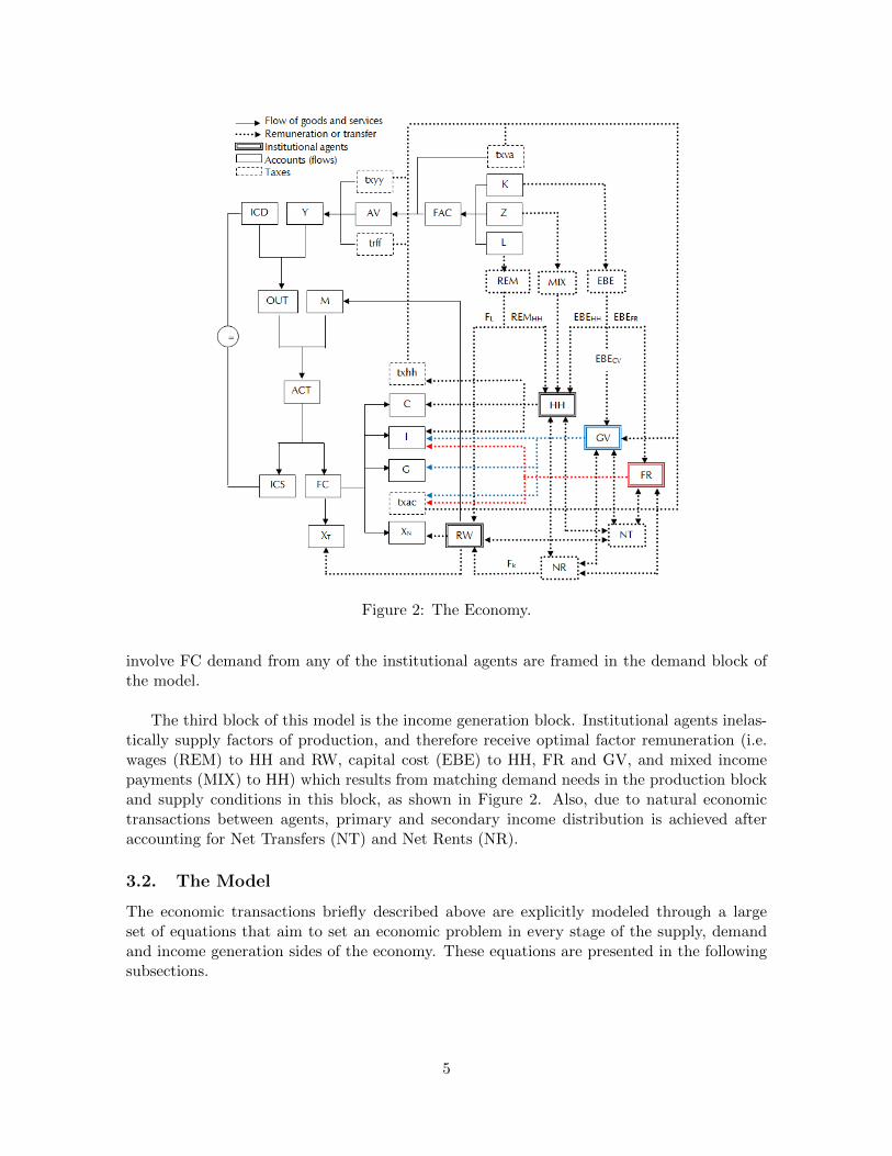
Figure 2: The Economy.
involve FC demand from any of the institutional agents are framed in the demand block ofthe model.
The third block of this model is the income generation block. Institutional agents inelas-tically supply factors of production, and therefore receive optimal factor remuneration (i.e.wages (REM) to HH and RW, capital cost (EBE) to HH, FR and GV, and mixed incomepayments (MIX) to HH) which results from matching demand needs in the production blockand supply conditions in this block, as shown in Figure 2. Also, due to natural economictransactions between agents, primary and secondary income distribution is achieved afteraccounting for Net Transfers (NT) and Net Rents (NR).
3.2. The Model
The economic transactions briefly described above are explicitly modeled through a largeset of equations that aim to set an economic problem in every stage of the supply, demandand income generation sides of the economy. These equations are presented in the followingsubsections.
5
3.2.1. The Supply Side
In the supply side of the economy production factors, indirect taxes, intermediate consump-tion and imports are combined to create total supply of a single representative (aggregated)good. This process involves solving three different cost minimization problems: First, the firmsolves for factor demands in a third-level-nested cost minimization problem. Second, it solvesfor combination of GDP and intermediate consumption in a second-level cost minimizationproblem. Lastly, the firm solves for combination of domestic output (supply) and imports inthe first-level minimization cost problem. As a result, total supply, ACT, is obtained.
On the second stage of the supply side, firm maximizes its revenue by optimally solvinga second-level-nested profit maximization problem which involves solving for the FC and ICdistribution problem on the first part and then the FC distribution problem, which is theactual link to demand side of the economy.
Factor Demand Problem, Added Value and Gross Domestic Product
Suppose the firm is able to merge the three production factors in our economy into a singlefactor (FAC). The latter, along with production taxes, yields added value. Therefore, firmoptimally minimizes its expenditure in production factors (1), subject to a Constant Elasticityof Substitution (CES from now on) technology for factor aggregation (2), as in:
min{L,K,Z}
pLL+ pKK + pZZ, (1)
FAC = θF
(πLL
σF−1
σF + πKKσF−1
σF + πZZσF−1
σF
) σFσF−1
(2)
Recall that elasticity of substitution among factors satisfies σF > 0. From the first orderconditions (FOC) we derive the optimal demand of factors:
L =
(θFπL
pFpL
)σF FACθF
(3)
K =
(θFπK
pFpK
)σF FACθF
(4)
Z =
(θFπZ
pFpZ
)σF FACθF
(5)
where the aggregated price of factors pF is expressed as
pF =1
θF
(πσFL p1−σF
L + πσFK p1−σFK + πσFZ p1−σF
Z
) 11−σF (6)
Added Value (in nominal terms), AV , is completed once indirect production taxes areacknowledged, therefore we have that:
pAVAV = pFFAC + TXva (7)
where tax revenue in production is given by:
TXva = txvapFFAC (8)
6
Note that in the base year prices are all set equal to one, therefore combination of Equations(7) and Equation (8) yields
AV = FAC (1 + txva) (9)
GDP (Y ) supply is obtained by adding up nominal AV, indirect taxes and import tariffs, asit follows:
pY Y = pAVAV + TXyy + TRff (10)
where indirect (net) taxes over products (TXyy) and import tariffs (TRff ) are given by ashare of nominal AV and imports:
TXyy = txyypAVAV , and TRff = trffpMM (11)
Domestic Supply Problem
GDP and IC combined yield total domestic supply of the representative good., thereforethe firm chooses optimal combination of GDP and intermediate consumption in the domesticoutput’s second-level cost minimization problem, which involves solving for the following opti-mization problem, subject to a CES technology of aggregation, with elasticity of substitutionbetween GDP and intermediate consumption satisfying σO > 0,
min{Y,IC}
pY Y + pICICD (12)
OUT = θO
(πY Y
σO−1
σO + πICDICDσO−1
σO
) σOσO−1
(13)
As above, from the FOC of this problem optimal GDP and Intermediate Consumptiondemands are derived and expressed as
Y =
(θOπY
pOpY
)σo OUTθO
(14)
ICD =
(θOπICD
pOpIC
)σO OUTθO
(15)
where the aggregated price of domestic output pO is given by
pO =1
θO
(πσOY p1−σO
Y + πσOICDp1−σOIC
) 11−σO . (16)
Recall that with GDP supply in Equation (10) and demand in Equation (14) one can easilyderive the price at which the market clears, pY , as:
pY =
[pAVAV + TXyy + TRff
(θOπY pO)σO OUTθO
] 11−σO
(17)
7
Aggregated Supply Problem
Total supply is the result of the sum of domestic output, Y, and imports, M. Optimal demandsfrom both inputs are estimated from the first-level cost minimization problem given by
min{OUT,M}
pOOUT + pMM (18)
subject to a CES technology of aggregation, with elasticity of substitution between outputand imports of σA > 0,
ACT = θA
(πOOUT
σA−1
σA + πMMσA−1
σA
) σAσA−1
(19)
From FOC derived from the latter, optimal domestic output and imports demands are,respectively
OUT =
(θAπO
pApO
)σA ACTθA
(20)
M =
(θAπM
pApM
)σA ACTθA
(21)
with aggregated price of the activity, ACT, pA given by
pA =1
θA
(πσAO p1−σA
O + πσAM p1−σAM
) 11−σA . (22)
Again, from OUT supply determined in Equation (13) and OUT demand in Equation(20) we solve for the price pO that fulfills the market clearing condition:
pO = θAπO
ACTθA
θO
(πY Y
σO−1
σO + πICDICDσO−1
σO
) σOσO−1
1σA
pA (23)
Additional considerations are imposed upon ACT formation. First one follows from theclearing market condition, which assures that total supply ACT in nominal terms equals thesum of total nominal domestic supply and total external nominal supply:
pAACT = pOOUT + pMM
ACT =pOOUT + pMM
pA(24)
Also, we assume that RW elastically supplies imports at an international price p∗M . There-fore, domestic import price is given by the expression
pM = e · p∗M , (25)
where e is the nominal exchange rate.
8
Supply Distribution Problem: First Stage
On a first stage of supply distribution, ACT is distributed between intermediate (IC) andfinal consumption (FC). The firm determines optimal amounts of IC and FC by maximizingrevenue from sales:
max{IC,FC}
pICICS + pFCFC (26)
subject to a CET technology of distribution with elasticity of transformation between inter-mediate and final consumption is τA < 0,
ACT = θAD
(πICSICS
τA−1
τA + πFCFCτA−1
τA
) τAτA−1
(27)
Yet again, from the FOC derived for this problem, optimal supply of intermediate andfinal consumption are, respectively:
ICS =
(θADπICS
pApIC
)τA ACTθAD
(28)
FC =
(θADπFC
pApFC
)τA ACTθAD
(29)
where activity price, pA, is given by the expression
pA =1
θAD
(πτAICSp
1−τAIC + πτAFCp
1−τAFC
) 11−τA (30)
Nevertheless, pA is determined through the market clearing condition in the distributionof ACT between ICS and FC:
pAACT = pICICS + pFCFC
pA =pICICS + pFCFC
ACT(31)
With ICD in (15) and ICS (28) we solve for the intermediate consumption price, pIC , as:
pIC =
[(θOπICDpO)σo OUTθO
(θADπICSpA)τA ACTθAD
] 1σo−τA
(32)
Supply Distribution Problem: Second Stage
The firm determines distribution of FC supply between Consumption (C), Investment (I),Government Expenditure (G) and Exports (X). X are classified between traditional, XT
(which are assumed as exogenous); and non-traditional, XNT, which in turn are consideredas endogenous. The firm maximizes its revenue for selling final consumption by optimallysolving for the following problem:
max{C,I,G,XN}
pCC + pII + pGG+ pXT XT + pXNTXNT (33)
9
subject to a linear-CET technology for distribution, with an elasticity of transformationbetween different types of FC that satisfies τFC < 0 :
FC = XT + θFC
(πCC
τFC−1
τFC + πIIτFC−1
τFC + πGGτFC−1
τFC + πXNTXτFC−1
τFCNT
) τFCτFC−1
(34)
After solving for the optimal quantities of C, G, I and XNT, from the FOC we have thatthe firm distributes FC according to the following expressions:
C =
[θFCπC
pFCFC − pXT XT
pC(FC − XT
) ]τFC FC − XT
θFC(35)
I =
[θFCπI
pFCFC − pXT XT
pI(FC − XT
) ]τFCFC − XT
θFC(36)
G =
[θFCπG
pFCFC − pXT XT
pG(FC − XT
) ]τFC FC − XT
θFC(37)
XNT =
[θFCπXNT
pFCFC − pXT XT
pXNT(FC − XT
)]τFC FC − XT
θFC(38)
where the nominal value of FC, pFCFC, is given by:
pFCFC =1
θFC
∑i∈{C,G,I,XNT }
πτFCi p1−τFCi
11−τFC (
FC − XT
)+ pXT XT (39)
From optimal supply of FC in (29) and its distribution technology (demand) in (34) wecan solve for the optimal price of FC, pFC as
pFC =
(θADπFCpA)τA ACTθAD
XT + θFC
(∑πii
τFC−1
τFC
) τFCτFC−1
1τA
for i ∈ {C,G, I,XNT } (40)
3.2.2. Income Distribution
We now describe the second block of the model: the income distribution block. In this MacroCGE model, three out of four institutional agents take part in the production process and inconsequence, receive factor remuneration. Households, firms and the Government are paidtheir marginal product from labor (REM), capital (EBE) and mixed income factors (MIX).Also, institutional agents exchange net transfers and rents between themselves (NT and NR).Taxes caused during production and product formation are transfered to the Government,as well as direct taxes paid by households, firms, and Government-owned firms (txva, txyy,trff, txhh and txac).
10
Factor supply, remuneration and distribution
We recall that this model assumes inelastic supply of all three production factors, L, Kand Z. Hence, factor remuneration prices are entirely determined by endogenous demandconditions: Given the optimal demands of factors in (3) to (5), and the inelastic supplies, wederive the factor prices:
pL = θFπL
(FAC
θF L
) 1σF
pF (41)
pK = θFπK
(FAC
θF K
) 1σF
pF (42)
pZ = θFπZ
(FAC
θF Z
) 1σF
pF (43)
Therefore the following equalities must hold:
pLL = REM = REMHH + FL (44)
pKK = EBE = EBEHH + EBEFR + EBEGV (45)
pZZ = MIX = MIXHH (46)
where, in (44), REM stands for labor remuneration and sub-index HH implies that thehouseholds are the recipient; FL are net labor remuneration to RW; in (45), EBE stands forcapital remuneration and sub-indexes FR and GV imply firms and the Government are therecipients, respectively; and in (46), MIX stands for mixed income rents, a third factor paidonly to HH.
Distribution of factors remuneration and rents among institutional agents (RHS parts ofequations (44) to (46)) are paid according to fixed coefficients:
REMHH = πREMHH REM and FL = πREMRW REM (47)
EBEHH = πEBEHH EBE , EBEFR = πEBEFR EBE and EBEGV = πEBEGV EBE (48)
where upper-indexes indicate the account (or institutional agent) from which flows of re-sources are coming and, as before, sub-indexes denote which agent is the recipient, e.g.πREMHH is the share of REM (account) that is paid to HH (recipient).
Rents
Institutional agents pay rents, R, according to a fixed share of their capital remunerationincome, EBE.
RHH = πHHR EBEHH , RFR = πFRR EBEFR, and RGV = πGVR EBEGV (49)
Likewise, rents are distributed amongst institutional agents according to constant coeffi-cients:
RHH = πRHHR, RFR = πRFRR, RGV = πRGVR , and FK = πRRWR (50)
From (49) and (50), we have that
R ≡ RHH +RFR +RGV ≡ RHH +RFR +RGV + FK (51)
11
Direct Taxes
Domestic institutional agents pay direct taxes according to a fixed portion of their income,defined for each one as
YHH = REMHH + EBEHH +MIXHH +(RHH −RHH
)(52)
YFR = EBEFR +(RFR −RFR
)(53)
YGV = EBEGV +(RGV −RGV
)(54)
which are the equations for household’s income, YHH , firm’s income, YFR, and Govern-ment’s income, YGV , respectively. Net rents (NR) are in parenthesis for each institutionalagent. Assuming no tax evasion and perfect fiscal compliance, institutional agents pay directas it follows:
TXhh = txhh · YHH (55)
TXacFR = txacFR · YFR (56)
TXacGV = txacGV · YGV (57)
As in (51), from equations (55) to (56), we have that total direct taxes are given by
T = TXhh+ TXacFR + TXacGV (58)
Transfers
There are four types of transfers: social contributions (SC), social benefits (SB), other cur-rent transfers (CT), and product transfers (PT). We assume exogenous payments of social
contributions from households, SCHH
, which are distributed among FR and GV accordingto fixed coefficients:
SCHHFR = πSCFRSCHH
(59)
SCHHGV = πSCGV SCHH
(60)
Also, households receive exogenously assumed social benefits, SBHH , paid by firms andthe Government, according to a fixed share:
SBFRHH = πSBFRSBHH (61)
SBGVHH = πSBGV SBHH (62)
Other current transfers (CT) are exogenously transfered from RW and FR
CTRW
+ CTFR
= CT (63)
and distributed to HH and GV according to fixed coefficients:
CTHH = πCTHHCT (64)
CTGV = πCTGV CT (65)
12

We also assume exogenous product transfers, P T , paid by GV to HH,
P TGV
= P THH (66)
Given equations (59) to (66), net transfers, NT, for each institutional agent are summa-rized by the following equations:
NTHH = −SCHH + SBHH + CTHH + P THH (67)
NTFR = SCHHFR − SBFRHH − CT
FR(68)
NTGV = SCHHGV − SBGVHH + CTGV − P T
GV(69)
NTRW = −CTRW (70)
for net transfers for HH, FR, GV and RW, respectively.
3.2.3. The Demand Side
We now describe the third and final block of this model: the demand side. Given the supply ofdifferent types of FC, as developed in the first block, and subject to the budget restrictions foreach agent that arise from income distribution described in the second block, institutionalagents demand a representative good labeled generically as Consumption (C), Investment(I), Public Consumption (G) and non-traditional Exports (XNT). The demand block can bedivided into domestic (from HH, FR and GV) and external (from RW) sub-blocks, which wereadily describe:
Domestic Demand
We assume that households face Cobb-Douglas preferences with savings in the utility function,which produces consumption demand (C) and HH’s savings, SHH, of the form
C = αDYHHpC
(71)
SHH = DYHH − pCC (72)
where DYHH stands for HH’s disposable income, defined using (52), (55) and (67) as:
DYHH = YHH +NTHH − TXhh (73)
Both households’ and firms’ investment, IHH and IFR respectively, are defined by privateinvestment, IPR. In this model, IHH and IFR are determined as a fixed share β of IPR:
IHH = β · IPR (74)
IFR = (1− β) · IPR (75)
Using (53), (56) and (68) we define firms’ savings, SFR as
SFR = YFR +NTFR − TXacFR (76)
13

We assume the Government expenditure and investment to be exogenous:
G = G (77)
IGV = IGV (78)
With public investment given in (78) and private investment resulting from the sum of(74) and (75), total demand for investment, I, is defined as the aggregate
I = IPR + IGV (79)
Given Investment demand in (79), and bearing in mind that Investment supply is givenby (36), we solve for the optimal price for investment:
pI = θFCπIpFCFC − pXT XT(
FC − XT
) [FC − XT
θFC(IPR + IGV
)] 1τFC
(80)
Following the same fashion, Government expenditure supply in (37) and exogenous as-sumed demand in (77), jointly determine the optimal price for Government expenditure:
pG = θFCπGpFCFC − pXT XT(
FC − XT
) (FC − XT
θFCG
) 1τFC
(81)
Again, using definitions in (8), (11), (54), (58) and (69), we obtain an expression forpublic (Government) savings:
SGV = YGV +NTGV + Tx+ T − TXacGV − pGG (82)
where Tx groups indirect taxes, i.e.
Tx = TXva + TXyy + TRff (83)
External demand
Optimal RW demand for non-traditional exports coming from Colombian markets is obtainedfrom the FOC derived from the RW’s imports (exports for their trading counterparts) demandfunction. We assume a CES-type function that aggregates imports from all possible origins.Therefore, demand for Colombian XNT is given by
XNT =
(θM∗ · πCOL
e · p∗M∗
pXNT
)σ∗M M∗
θM∗(84)
where θM∗ an πCOL are scale and Colombia’s share parameter in the aggregation of RWimports. Note since we assumed a CES-type function, σ∗
M> 0 is supposed to hold. RW
imports, M∗, and their price, p∗M∗
, are assumed to follow exogenous dynamics.
Given the exogenous demand for traditional exports XT and the endogenous demand fornon-traditional exports XNT in (84), total exports are computed as the sum of the traditionaland non-traditional components
X = XNT + XT (85)
14
In addition, price of total exports must satisfy
pX =pXT XT + pXNTXNT
X(86)
and price of non-traditional exports is determined jointly by their supply in (38) and theirdemand in (84)
pXNT =
(θM∗ · πCOL · e · p∗M∗
)σ∗M M∗
θM∗(θFC · πXNT ·
pFCFC−pXT XT(FC−XT )
)τFCFC−XTθFC
1
σ∗M−τFC
(87)
Finally, we assume that RW demands traditional exports at an exogenous internationalprice p∗XT , which implies that internal price for XT is given by
pXT = e · p∗XT (88)
3.2.4. Closure of the Model
The closure of a CGE model is defined as a set of equations (exogenous variables) that assurethat markets equilibrium is achieved in a Walrasian sense. In other words, a model is de-termined (closed) when the number of endogenous variables equals the number of equations,and therefore, there exists a unique solution to the system of equations. Closing a model isakin to drop a specific assumption from the original model (Sen, 1963). Several alternativesof closure equations have been explored over the past few decades, each one depending onthe particular way the researcher understands the macroeconomic mechanisms that rule themodeled economy. In this paper we present two alternative closures: a Kaldorian-type one,called the investment closure; and a Classic-type one, known as the external savings closure(Decaluwe et al., 1987)1.
In the former, total investment is assumed to be fixed at a certain level, and total savingsadjust to satisfy such demand for investment requirements; whilst in the latter, total savingslevels are assumed to be fixed and investment adjusts itself given the available amount ofresources in the economy. In this CGEM we have four variables that are not yet determined:two nominal prices, the nominal exchange rate, e, and the price of consumption, pC ; and twoflows: external savings, SRW, and private investment, IPR. Each closure assumes fixed valuesfor a nominal price and a flow, as we shall see promptly.
Also, from equations (47), (50) and (70), we set RW bilateral income as
YRW = FL + FK − CTRW
(89)
1Authors recall that names are not necessarily related to the author’s main ideas, e.g. Kaldor, Keynes, etc.
15
Investment Closure
This closure assumes exogenous nominal exchange rate and fixed private investment levels:
e = e (90)
IPR = IPR (91)
Given (90) and (91), RW savings in the country, SRW, is left to be an endogenous variable,given by:
SRW = YRW + pMM − pXX (92)
Also, given SRW in (92), we complete aggregate savings S = SHH + SFR + SGV + SRW.This leaves the Savings-Investment (S-I) balance depending on the price of consumption, byreplacing (72) in the latter expression and solving for pC . Therefore we obtain
pC =DYHH + SFR + SGV + SRW − pI I
C(93)
External Savings Closure
This closure assumes exogenous consumption price and RW savings:
pC = pC (94)
SRW = SRW (95)
We use the definition of external savings proposed in (92) to solve for the nominal exchangerate, e:
SRW = YRW + pM (e)M(e)− pX(e)X(e) (96)
where (e) denotes a non-linear function of the nominal exchange rate, e. Once determined e,private investment IPR adjusts its levels to match the S-I balance, and therefore, is given by:
IPR =S
pI− IGV =
SHH + SFR + SGV + SRWpI
− IGV (97)
4. Parameter calibration
The scale and share parameters in each one of the CES and CET structures used throughoutthe three blocks of the model discussed in section 3 can be calibrated using information fromthe tailor made Macro-SAM constructed for this model, presented in section 2. In this sectionwe present an example of how share and scale parameters in a CES function are calibratedin this model. All other scale and share parameters can be calibrated analogously.
Share parameters
From (3) we have that share parameters πi can be expressed as:
πK = πLpKpL
(K
L
) 1σF
πZ = πLpZpL
(Z
L
) 1σF
16
Using the fact that share parameters sum up to unity:
πL + πK + πZ = 1 ,
we obtain:
πL =pLL
1σF
pLL1σF + pKK
1σF + pZZ
1σF
Following the same steps for K and Z we have that their share parameters are given by
πK =pKK
1σF
pLL1σF + pKK
1σF + pZZ
1σF
πZ =pZZ
1σF
pLL1σF + pKK
1σF + pZZ
1σF
Scale parameter
Scale parameter θF is calibrated using the previously calibrated share parameters and (2):
θF = FAC
(pLL
1σF + pKK
1σF + pZZ
1σF
pLL+ pKK + pZZ
) σFσF−1
All other scale parameters in the model are calibrated analogously.
Scale Parameters for RW imports
In order to calibrate the scale parameter in RW demand for imports function, θM∗ , all(domestic and foreign) prices equal are set to equal unity in the baseline scenario. Aftercontrolling for that, from equation (87), it must hold that:
θM∗ =
[πτFCXNT
(FC − XT
)θ1−τFCFC · πσ
∗MCOL · M∗
] 1σ∗M−1
5. Elasticities: A Sensibility Analysis
As stated before, scale and share parameters are calibrated using observed data on the Macro-SAM built for the benchmark year presented in section 2. However, elasticities are not easilycalibrated and are either taken as given from the relevant existing literature or usually esti-mated through econometric methods (as in Hillberry and Hummels, 2013). In this paper weadopt the first approach and we do not present an econometric estimation of the elasticitiesin the model. However, we do present sensibility analyses for each elasticity to be considered.
One advantage of the CES and CET functional forms is that they can be considered as ageneral case of a linear, a Cobb-Douglas, or a Leontieff type of isoquant curves (both on theconsumer’s and producer’s optimization problem), depending on the value of the parameterσ or τ . We have three cases:
17
1.00468
1.00470
1.00472
1.00474
1.00476
1.00478
1.00480
1.00482
0.5
0.5
5
0.6
0.6
5
0.7
0.7
5
0.8
0.8
5
0.9
0.9
5 1
1.0
5
1.1
1.1
5
1.2
1.2
5
1.3
1.3
5
1.4
1.4
5
1.5
Consumption Good's Price Response to 0.2% Increase in Productivity
(deviation from equilibrium level, PCONS = 1)
𝜎F
(a) PCONS response. Savings Closure.
𝜎F
1.00689
1.00690
1.00691
1.00692
1.00693
1.00694
1.00695
1.00696
1.00697
1.00698
1.00699
0.5
0.5
5
0.6
0.6
5
0.7
0.7
5
0.8
0.8
5
0.9
0.9
5 1
1.0
5
1.1
1.1
5
1.2
1.2
5
1.3
1.3
5
1.4
1.4
5
1.5
Exchange Rate Response to 0.2% Increase in Productivity
(deviation from equilibrium level, e = 1)
(b) e response. Investment Closure.
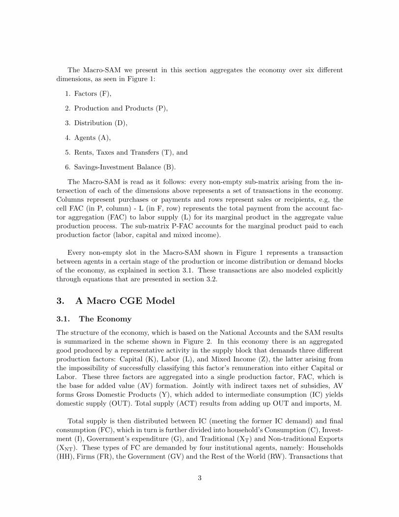
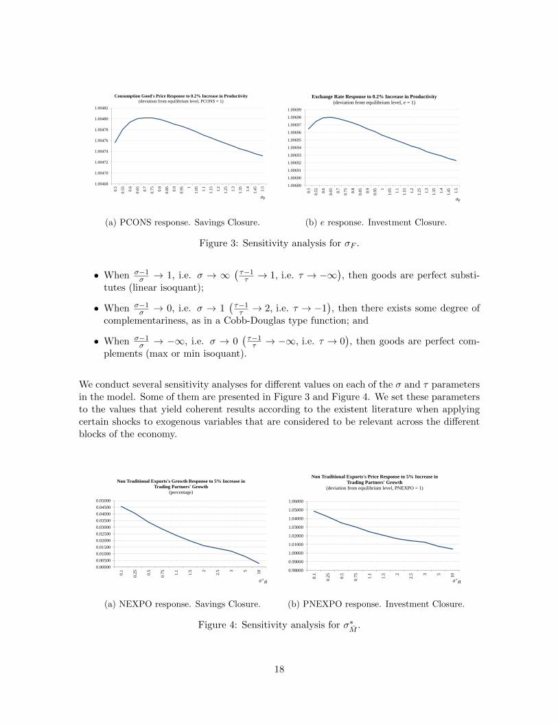
Figure 3: Sensitivity analysis for σF .
• When σ−1σ → 1, i.e. σ → ∞
(τ−1τ → 1, i.e. τ → −∞
), then goods are perfect substi-
tutes (linear isoquant);
• When σ−1σ → 0, i.e. σ → 1
(τ−1τ → 2, i.e. τ → −1
), then there exists some degree of
complementariness, as in a Cobb-Douglas type function; and
• When σ−1σ → −∞, i.e. σ → 0
(τ−1τ → −∞, i.e. τ → 0
), then goods are perfect com-
plements (max or min isoquant).
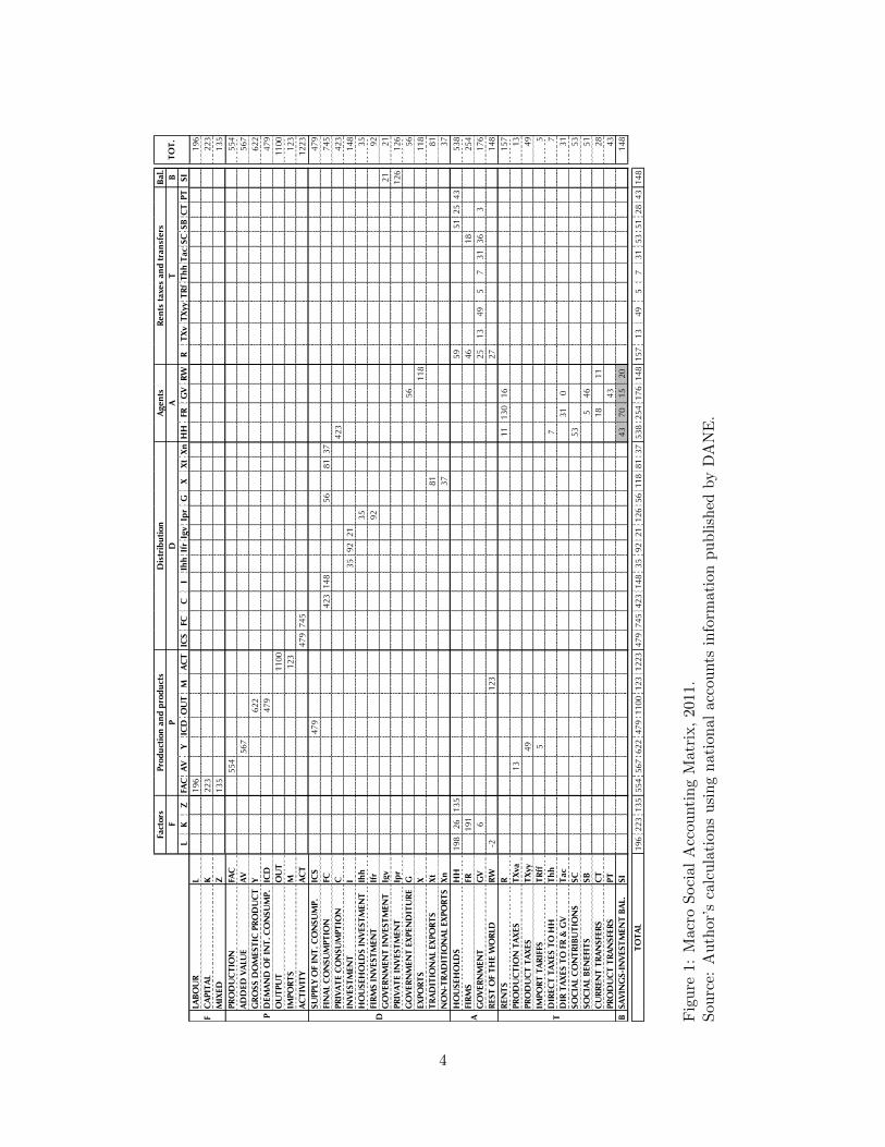
We conduct several sensitivity analyses for different values on each of the σ and τ parametersin the model. Some of them are presented in Figure 3 and Figure 4. We set these parametersto the values that yield coherent results according to the existent literature when applyingcertain shocks to exogenous variables that are considered to be relevant across the differentblocks of the economy.
𝜎∗𝑀
0.00000
0.00500
0.01000
0.01500
0.02000
0.02500
0.03000
0.03500
0.04000
0.04500
0.05000
0.1
0.2
5
0.5
0.7
5
1.1
1.5 2
2.5 3 5
10
Non Traditional Exports's Growth Response to 5% Increase in
Trading Partners' Growth
(percentage)
(a) NEXPO response. Savings Closure.
𝜎∗𝑀
0.98000
0.99000
1.00000
1.01000
1.02000
1.03000
1.04000
1.05000
1.06000
0.1
0.2
5
0.5
0.7
5
1.1
1.5 2
2.5 3 5
10
Non Traditional Exports's Price Response to 5% Increase in
Trading Partners' Growth
(deviation from equilibrium level, PNEXPO = 1)
(b) PNEXPO response. Investment Closure.
Figure 4: Sensitivity analysis for σ∗M
.
18
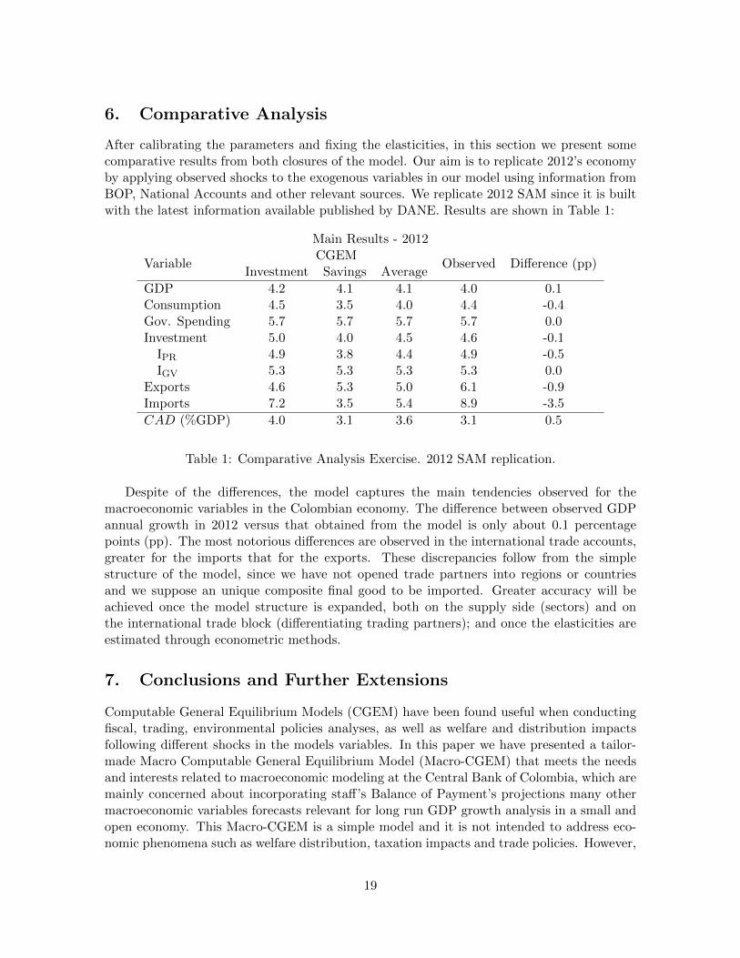
6. Comparative Analysis
After calibrating the parameters and fixing the elasticities, in this section we present somecomparative results from both closures of the model. Our aim is to replicate 2012’s economyby applying observed shocks to the exogenous variables in our model using information fromBOP, National Accounts and other relevant sources. We replicate 2012 SAM since it is builtwith the latest information available published by DANE. Results are shown in Table 1:
Main Results - 2012
VariableCGEM
Observed Difference (pp)Investment Savings Average
GDP 4.2 4.1 4.1 4.0 0.1Consumption 4.5 3.5 4.0 4.4 -0.4Gov. Spending 5.7 5.7 5.7 5.7 0.0Investment 5.0 4.0 4.5 4.6 -0.1
IPR 4.9 3.8 4.4 4.9 -0.5IGV 5.3 5.3 5.3 5.3 0.0
Exports 4.6 5.3 5.0 6.1 -0.9Imports 7.2 3.5 5.4 8.9 -3.5
CAD (%GDP) 4.0 3.1 3.6 3.1 0.5
Table 1: Comparative Analysis Exercise. 2012 SAM replication.
Despite of the differences, the model captures the main tendencies observed for themacroeconomic variables in the Colombian economy. The difference between observed GDPannual growth in 2012 versus that obtained from the model is only about 0.1 percentagepoints (pp). The most notorious differences are observed in the international trade accounts,greater for the imports that for the exports. These discrepancies follow from the simplestructure of the model, since we have not opened trade partners into regions or countriesand we suppose an unique composite final good to be imported. Greater accuracy will beachieved once the model structure is expanded, both on the supply side (sectors) and onthe international trade block (differentiating trading partners); and once the elasticities areestimated through econometric methods.
7. Conclusions and Further Extensions
Computable General Equilibrium Models (CGEM) have been found useful when conductingfiscal, trading, environmental policies analyses, as well as welfare and distribution impactsfollowing different shocks in the models variables. In this paper we have presented a tailor-made Macro Computable General Equilibrium Model (Macro-CGEM) that meets the needsand interests related to macroeconomic modeling at the Central Bank of Colombia, which aremainly concerned about incorporating staff’s Balance of Payment’s projections many othermacroeconomic variables forecasts relevant for long run GDP growth analysis in a small andopen economy. This Macro-CGEM is a simple model and it is not intended to address eco-nomic phenomena such as welfare distribution, taxation impacts and trade policies. However,
19

once the SAM is configured properly, it will serve as a starting point for conducting fiscaland trading policies analyses.
This model consists of three main blocks: production (supply), distribution and demandblocks. In each one the agents face optimization problems concerning maximizing certainquantity subject to a technology of aggregation or transformation (CES and CET, respec-tively). Two alternative closures are presented: i) one in which private investment is assumedto be exogenous, as well as exchange rate. This leaves external savings (current accountdeficit) and the composite good price as endogenous variables; and ii) a closure in whichexternal savings and the composite good price are exogenous, therefore leaving private in-vestment and the exchange rate as endogenous variables. In this paper, the main interest ofthis Macro-CGEM users is to build counterfactual scenarios related to commodities pricesshocks, external demand growth, public and private investment shocks, and current accountdeficit levels shifts.
The sensitivity analyses exercises suggested that the elasticities used in the model arecoherent with economic theory and similar to those used in previous models. However, theseelasticities shall be estimated through econometric methods in posterior updates of the model.A comparative analysis is carried using 2012 national accounts information. Results showthat this model captures the main characteristics of the Colombian economy, and althoughgreater accuracy could be achieved for the international trade accounts, once the structureof the model is expanded we expect to obtain more detailed results.
Lastly, we recall that this model admits further extensions. Firstly, an extended versionof the production block of the model which includes different sectors is currently being de-veloped. Secondly, a more detailed taxation structure shall be explored, as well as a broadermodeling of the Colombian trading partners and conditions. Also, econometric estimationof the model elasticities shall be conducted, as it has been already stated. GAMS codes andSAMs are available upon request from the corresponding author.
20
References
Bussolo, M. and Correa, R. (1998). A 1994 Detailed Social Accouting Matrix for Colombia.Fedesarrollo - Working Papers Series, 10.
Bussolo, M., Roland-Host, D., and van der Mensbrugghe, D. (1998). The Technical Specifica-tion of FEDESARROLLO’s Long Run General Equilibrium Model. Fedesarrollo - WorkingPapers Series, 4.
Cespedes, E. (2011). Una matriz de contabilidad social con informalidad 2007: documentaciontecnica. DNP - Archivos de Economıa, 377.
Corredor, D. and Pardo, O. (2008). Matrices de Contabilidad Social 2003, 2004, y 2005 paraColombia. DNP - Archivos de Economıa, 339.
Decaluwe, B., Martens, A., and Monette, M. (1987). Macroclosures in Open Economy CGEModels: A Numerical Reappraisal. Universite Laval, Universite de Montreal & C.R.D.RWorking papers, 8704.
Dixon, P. and Jorgenson, D., editors (2013). Handbook of Computable General EquilibriumModeling, volume 1A and 1B. ElSevier.
Hernandez, G. (2003). Construccion de una Matriz de Contabilidad Social Financiera paraColombia. DNP - Archivos de Economıa, 223.
Hillberry, R. and Hummels, D. (2013). Trade elasticity parameters for a computable generalequilibrium model. In Dixon, P. and Jorgenson, D., editors, Handbook of ComputableGeneral Equilibrium Modeling, volume 1A and 1B, chapter 18, pages 1213–1269. ElSevier.
Jensen, H. T. and Karl, C. (2004). A “Real ” Financial Social Accouting Matrix for Colombia.DNP - Archivos de Economıa, 264.
Karl, C. (2004). 2000 Social Accounting Matrix for Colombia. DNP - Archivos de Economıa,256.
Lopez, E., Ripoll, M., and Cepeda, F. (1994). Cronica de los Modelos de Equilibrio Generalen Colombia. Borradores de Economıa - Banco de la Republica, 13.
Lora, E. (2008). Tecnicas de Medicion Economica. Alfaomega, 4th edition.
Prada, S. and Guzman, O. (2002). Matriz de Contabilidad Social Tributaria para 1997.Ministerio de Hacienda y Credito Publico, mimeo.
Pyatt, G. and Round, J. (1985). Social Accouting Matrices. A Basis for Planning. The WorldBank, 1st edition.
Ramırez, J. M. and Prada, S. (2000). Matriz de Contabilidad Social 1996 para Colombia.Documentos de trabajo CEGA, 1.
Rutherford, T. and Light, M. (2002). A General Equilibrium Model for Tax Policy Analysisin Colombia: The MEGATAX Model. DNP - Archivos de Economıa, 188.
21
Sen, A. (1963). Neoclassical and Neokeynesian Theories of Distribution. Economic Record,39(85):53–64.
Valderrama, F. M. and Gutierrez, J. A. (1995). Matriz de Contabilidad Social 1992. DNP -Archivos de Economıa, 40.
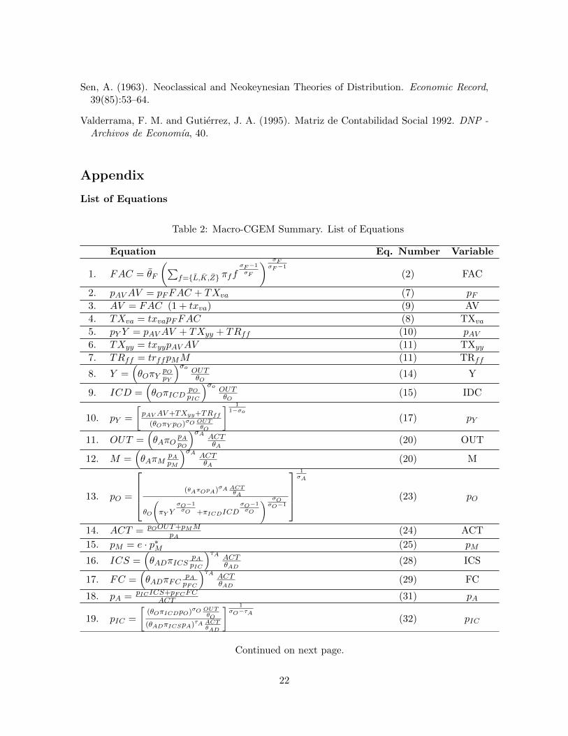
Appendix
List of Equations
Table 2: Macro-CGEM Summary. List of Equations
Equation Eq. Number Variable
1. FAC = θF
(∑f={L,K,Z} πff
σF−1
σF
) σFσF−1
(2) FAC
2. pAVAV = pFFAC + TXva (7) pF3. AV = FAC (1 + txva) (9) AV
4. TXva = txvapFFAC (8) TXva
5. pY Y = pAVAV + TXyy + TRff (10) pAV6. TXyy = txyypAVAV (11) TXyy
7. TRff = trffpMM (11) TRff
8. Y =(θOπY
pOpY
)σoOUTθO
(14) Y
9. ICD =(θOπICD
pOpIC
)σoOUTθO
(15) IDC
10. pY =
[pAV AV+TXyy+TRff
(θOπY pO)σO OUTθO
] 11−σo
(17) pY
11. OUT =(θAπO
pApO
)σA ACTθA
(20) OUT
12. M =(θAπM
pApM
)σA ACTθA
(20) M
13. pO =
(θAπOpA)σA ACTθA
θO
(πY Y
σO−1σO +πICDICD
σO−1σO
) σOσO−1
1σA
(23) pO
14. ACT = pOOUT+pMMpA
(24) ACT
15. pM = e · p∗M (25) pM
16. ICS =(θADπICS
pApIC
)τA ACTθAD
(28) ICS
17. FC =(θADπFC
pApFC
)τA ACTθAD
(29) FC
18. pA = pICICS+pFCFCACT (31) pA
19. pIC =
[(θOπICDpO)σO OUT
θO
(θADπICSpA)τA ACTθAD
] 1σO−τA
(32) pIC
Continued on next page.
22
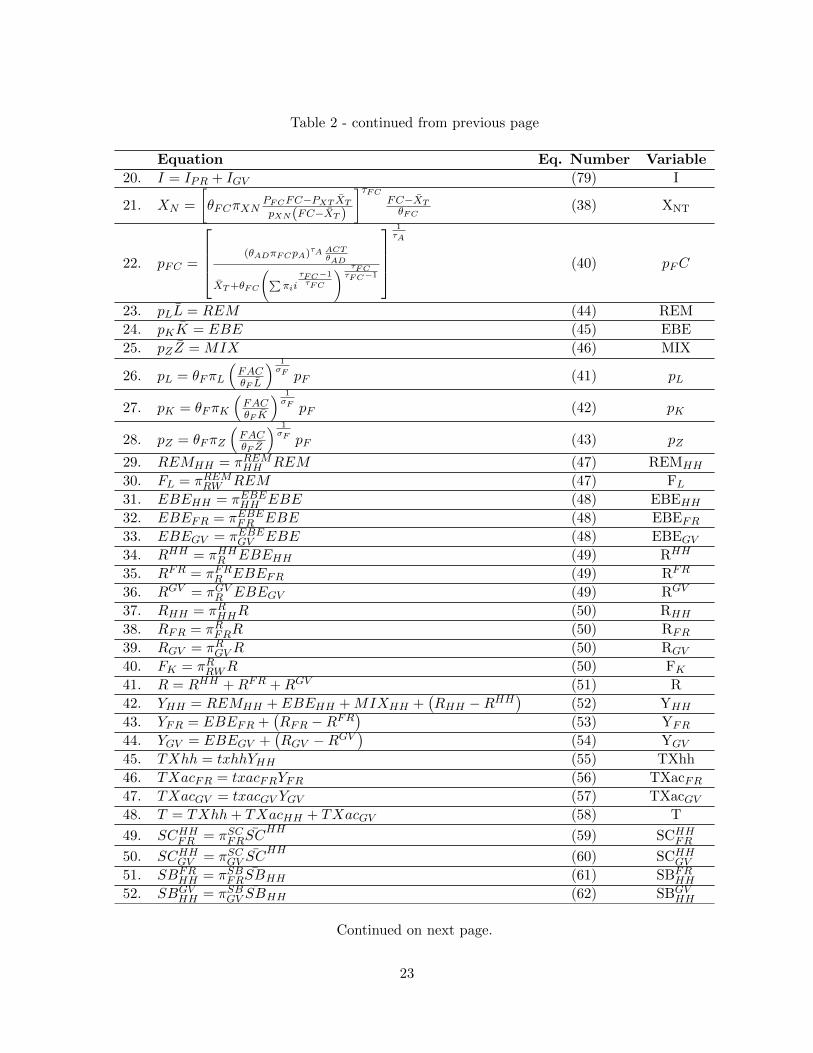
Table 2 - continued from previous page
Equation Eq. Number Variable
20. I = IPR + IGV (79) I
21. XN =
[θFCπXN
PFCFC−PXT XTpXN(FC−XT )
]τFCFC−XTθFC
(38) XNT
22. pFC =
(θADπFCpA)τA ACTθAD
XT+θFC
(∑πii
τFC−1τFC
) τFCτFC−1
1τA
(40) pFC
23. pLL = REM (44) REM
24. pKK = EBE (45) EBE
25. pZZ = MIX (46) MIX
26. pL = θFπL
(FACθF L
) 1σF pF (41) pL
27. pK = θFπK
(FACθF K
) 1σF pF (42) pK
28. pZ = θFπZ
(FACθF Z
) 1σF pF (43) pZ
29. REMHH = πREMHH REM (47) REMHH
30. FL = πREMRW REM (47) FL31. EBEHH = πEBEHH EBE (48) EBEHH32. EBEFR = πEBEFR EBE (48) EBEFR33. EBEGV = πEBEGV EBE (48) EBEGV34. RHH = πHHR EBEHH (49) RHH
35. RFR = πFRR EBEFR (49) RFR
36. RGV = πGVR EBEGV (49) RGV
37. RHH = πRHHR (50) RHH
38. RFR = πRFRR (50) RFR
39. RGV = πRGVR (50) RGV
40. FK = πRRWR (50) FK41. R = RHH +RFR +RGV (51) R
42. YHH = REMHH + EBEHH +MIXHH +(RHH −RHH
)(52) YHH
43. YFR = EBEFR +(RFR −RFR
)(53) YFR
44. YGV = EBEGV +(RGV −RGV
)(54) YGV
45. TXhh = txhhYHH (55) TXhh
46. TXacFR = txacFRYFR (56) TXacFR47. TXacGV = txacGV YGV (57) TXacGV48. T = TXhh+ TXacHH + TXacGV (58) T
49. SCHHFR = πSCFRSCHH
(59) SCHHFR
50. SCHHGV = πSCGV SCHH
(60) SCHHGV
51. SBFRHH = πSBFRSBHH (61) SBFR
HH
52. SBGVHH = πSBGV SBHH (62) SBGV
HH
Continued on next page.
23
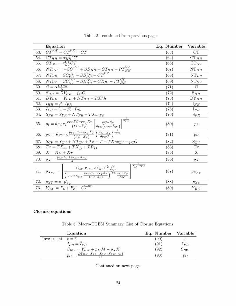
Table 2 - continued from previous page
Equation Eq. Number Variable
53. CTRW
+ CTFR
= CT (63) CT
54. CTHH = πCTHHCT (64) CTHH
55. CTGV = πCTGV CT (65) CTGV
56. NTHH = −SCHH + SBHH + CTHH + P TGVHH (67) NTHH
57. NTFR = SCHHFR − SBFRHH − CT
FR(68) NTFR
58. NTGV = SCHHGV − SBGVHH + CTGV − P T
GVHH (69) NTGV
59. C = αDYHHpC(71) C
60. SHH = DYHH − pCC (72) SHH61. DYHH = YHH +NTHH − TXhh (73) DYHH
62. IHH = β · IPR (74) IHH63. IFR = (1− β) · IPR (75) IPR64. SFR = YFR +NTFR − TXacFR (76) SFR
65. pI = θFCπIpFCFC−pXT XT
(FC−XT )
[FC−XT
θFC(IPR+IGV )
] 1τFC
(80) pI
66. pG = θFCπGpFCFC−pXT XT
(FC−XT )
(FC−XTθFCG
) 1τFC (81) pG
67. SGV = YGV +NTGV + Tx+ T − TXacGV − pGG (82) SGV68. Tx = TXva + TXyy + TRff (83) Tx
69. X = XN + XT (85) X
70. pX =pXT XT+pXNTXNT
X (86) pX
71. pXNT =
(θM∗ ·πCOL·e·p∗M∗)σ∗M M∗θM∗(
θFC ·πXNT ·pFCFC−pXT XT
(FC−XT )
)τFC FC−XTθFC
1σ∗M−τFC
(87) pXNT
72. pXT = e · p∗XT (88) pXT73. YRW = FL + FK − CT
RW(89) YRW
Closure equations
Table 3: Macro-CGEM Summary. List of Closure Equations
Equation Eq. Number Variable
Investment e = e (90) eIPR = IPR (91) IPRSRW = YRW + pMM − pXX (92) SRW
pC = DYHH+SFR+SGV +SRW−pI IC (93) pC
Continued on next page.
24
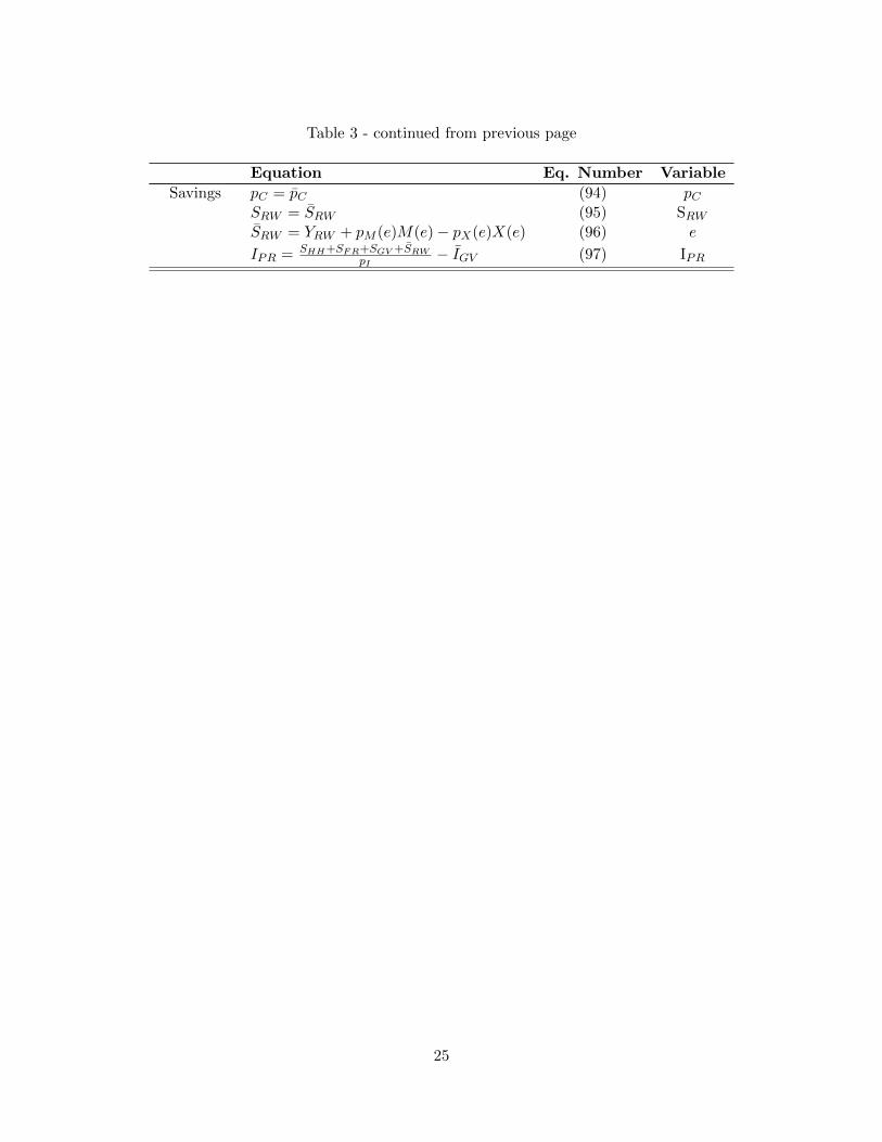
Table 3 - continued from previous page
Equation Eq. Number Variable
Savings pC = pC (94) pCSRW = SRW (95) SRWSRW = YRW + pM (e)M(e)− pX(e)X(e) (96) e
IPR = SHH+SFR+SGV +SRWpI
− IGV (97) IPR
25

ogotá -


