A high-resolution hydrodynamic investigation of brown trout (Salmo trutta) and rainbow trout (Oncorhynchus mykiss) redds

A HIGH-RESOLUTION HYDRODYNAMIC INVESTIGATION OF BROWN TROUT(SALMO TRUTTA) AND RAINBOW TROUT (ONCORHYNCHUS MYKISS) REDDS

M. A. MARCHILDON,a W. K. ANNABLE,a* J. G. IMHOFb and M. POWERc

a Department of Civil and Environmental Engineering, University of Waterloo, Waterloo, Ontario, N2L 3G1 Canadab Trout Unlimited Canada c/o Rm. 270, Axelrod Building, University of Guelph, Guelph, Ontario, N1G 2W1 Canada

c Department of Biology, University of Waterloo, Waterloo, Ontario, N2L 3G1 Canada

ABSTRACT

High-resolution velocity measurements were taken over a series of redds on a gravel-bed stream using a Pulse Coherent AcousticDoppler Profiler (PCADP) to quantify the hydrodynamics of brown trout (Salmo trutta) and rainbow trout (Oncorhynchus mykiss)redds. On redds studied, over 4500 velocity measurements per redd were acquired per day to quantify the flow velocity, flow depth andrelated fluid mechanics metrics of Reynolds numbers, Froude numbers and turbulent kinetic energy per unit area. Results showed thatvelocity and Froude numbers varied widely at the redd scale, but consistently showed higher velocities and Froude numbers over thetailspill regions relative to the surrounding study limits. Results of Reynolds numbers calculations showed no apparent correlations tospawning location preference and redd structure. Turbulent kinetic energy per unit area consistently demonstrated a strong correlationwith redd locations. The metric maintained low values (i.e. unidirectional flow with little turbulence) where all redds and attemptedredds were observed. The study also demonstrates that a number of hydraulic metrics and several spatial scales will likely be necessaryto understand any inherent relationship between river hydraulics and redd placement. Copyright # 2010 John Wiley & Sons, Ltd.

key words: fish habitat; hydraulics; fluvial geomorphology; redd selection

Received 22 August 2009; Revised 9 December 2009; Accepted 18 December 2009

INTRODUCTION

As both biotic and abiotic research has progressed in the

study of water courses, it has becomewidely recognized that

a collaborative effort amongst scientific, engineering and

social disciplines must be incorporated into lotic system

research to provide effective management and rehabilitation

strategies (Maddock, 1999; Schwartz and Herricks, 2007).

Imhof et al. (1996) stressed the need to evaluate lotic

systems at multiple nested spatial and temporal scales to

characterize channel form and function. They identified that

stream health potential is determined by the characteristics

of the watershed and channel geomorphological function at

large scales (from the basin and sub-basin scales) down to

the river-reach scale. Conversely, the investigation of

potential stream health is realized through river function

as it pertains to small-scale or micro-scale level processes

such as channel shear, sediment transport and biodiversity.

With increasing scale, and thus watershed complexity,

micro-scale processes are commonly simplified or hom-

ogenized to address scalability in observations. Examples of

such simplifications include the velocity-area method

(Buchanan and Somers, 1969) used to quantify discharge,

Manning’s equation used to estimate average cross-sectional

channel velocity, Wolman’s (1954) pebble count used to

represent substrate surface roughness distribution, indicator

species used to represent aquatic diversity and health

(Statzner et al., 1988; Champoux et al., 2003) and habitat

suitability indices used to evaluate instream flow require-

ments at various discharge events (Raleigh et al., 1984,

1986).

Another common problem related to the physical metrics

used in the study of rivers is the disparity between the data

collected to characterize fine-scale physical habitat features

and the data collected at flood flow conditions that define

channel morphology and physical habitat forms. Biological

data are typically collected during low flow seasons when

rivers are wadable and aquatic life is observable (Smith,

1973; Shirvell and Dungey, 1983; Witzel and MacCrimmon,

1983a; Kondolf et al., 1993). In these conditions, the

hydraulic, sedimentological and geomorphological pro-

cesses dictating river form, function and hence physical

habitat features are nominal. Conversely, measurements

related to channel form and function are primarily measured

during flood stages (i.e. bankfull discharge and larger) when

the hydraulic and sedimentological processes are actively

defining channel geomorphology (Leopold et al., 1964). The

disparity in temporal sampling strategies between biological

and physical scientists inevitably results in distinctly

different descriptions of the same physical system where

a continuum of spatial and temporal states should exist.

RIVER RESEARCH AND APPLICATIONS

River Res. Applic. 27: 345–359 (2011)

Published online 31 January 2010 in Wiley Online Library(wileyonlinelibrary.com) DOI: 10.1002/rra.1362

*Correspondence to: W. K. Annable, Department of Civil and Environ-mental Engineering, University of Waterloo, Waterloo, Ontario, N2L 3G1Canada. E-mail: [email protected]

Copyright # 2010 John Wiley & Sons, Ltd.

The tendency of many river spawning fishes to construct

redds in the stream bed substrate results in a biophysical

junction between small-scale processes and large-scale river

form and function. Construction and release of fertilized ova

into porous substrates is one strategy to protect vulnerable

embryos from predation and physical disruption or damage.

The site-specific selection process of a spawning fish is

believed to be based upon the small-scale physical and

chemical conditions (Burner, 1951) moderated somewhat by

the size of the female (Kondolf and Wolman, 1993). Thus

the majority of redd placement studies have concentrated on

fine-scale habitat measurement (e.g. Ottaway et al., 1981;

Shirvell and Dungey, 1983; Grost et al., 1990; Essington

et al., 1998). However, one cannot neglect that the micro-

habitats that fish select for spawning are influenced by larger

morphological features (such as a run or a riffle) formed by

hydraulic and sediment transport processes that occur during

larger and less frequent discharge events. Thus, little work

has been done to examine differences in redd placement

characteristics as a function of macro-habitat units (but see

Zimmer and Power, 2006). Recent advances in high-

resolution three-dimensional flow measurement technology,

however, provides an opportunity to study the hydrodynamic

characteristics of redds and surrounding fluvial features in

unprecedented detail. To that end, the spawning habitat of

brown trout (Salmo trutta) and rainbow trout (Oncorhynchus

mykiss) redds were measured and evaluated to determine if

identifiable hydrodynamic properties existed that would aid

in the definition of spawning habitat and description of its

complexity.

BACKGROUND

Spawning begins with a female fish scanning the stream bed

for a suitable spawning location, a process referred to as the

pre-spawning stage (Burner, 1951). The female may carry

out exploratory cutting (Jones and Ball, 1954; Grost et al.,

1991), whereby the female, through vigorous movements of

her tail, induces a negative pressure on the stream bed

surface (Kondolf et al., 1993), subsequently releasing

sediment into the current for transport downstream. If the

female considers the site suitable, she continues cutting into

the stream bed, leaving behind a semi-spherical depression

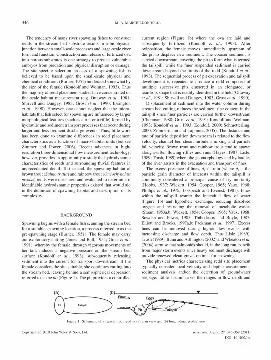
referred to as the pit (Figure 1). The pit provides a controlled

current region (Figure 1b) where the ova are laid and

subsequently fertilized (Kondolf et al., 1993). After

oviposition, the female moves immediately upstream of

the pit to displace new sediment. The coarser sediment is

carried downstream, covering the pit to form what is termed

the tailspill, while the finer suspended sediment is carried

downstream beyond the limits of the redd (Kondolf et al.,

1993). The sequential process of pit excavation and tailspill

development is repeated to produce a redd composed of

multiple successive pits clustered in an elongated, or

teardrop, shape that is readily identified in the field (Ottaway

et al., 1981; Shirvell and Dungey, 1983; Grost et al., 1990).

Displacement of sediment into the water column during

stream bed cutting reduces the sediment fine content in the

tailspill since finer particles are carried further downstream

(Chapman, 1988; Grost et al., 1991; Kondolf and Wolman,

1993; Kondolf et al., 1993; Kondolf, 2000; Schmetterling,

2000; Zimmermann and Lapointe, 2005). The distance and

rate of particle deposition downstream is related to the flow

velocity, channel bed shear, turbulent mixing and particle

fall velocity. Brown trout and rainbow trout tend to spawn

along swifter flowing riffles and runs (Hayes, 1987; Lisle,

1989; Trush, 1989) where the geomorphology and hydraulics

of the river assists in the evacuation and transport of fines.

The excess presence of fines, di< 1mm (where di is the

particle grain diameter of interest) within the tailspill is

commonly considered a principal cause of fry mortality

(Hobbs, 1937; Wickett, 1954; Cooper, 1965; Vaux, 1968;

Phillips et al., 1975; Lotspeich and Everest, 1981). Fines

within the tailspill restrict the interstitial flow of water

(Figure 1b) and hyporheic exchange, reducing dissolved

oxygen and restricting the removal of metabolic wastes

(Stuart, 1953a,b; Wickett, 1954; Cooper, 1965; Vaux, 1968;

Sowden and Power, 1985; Thibodeaux and Boyle, 1987;

Elliott and Brooks, 1997a,b; Packman et al., 1997). Excess

fines can be removed during higher flow events with

increasing discharge and flow depth. Thus Lisle (1989),

Trush (1989), Bunn and Arthington (2002) andWheaton et al.

(2004) surmise that salmonids should, in the long run, benefit

from major storm events since heavy sediment discharge will

provide renewed clean gravel optimal for spawning.

The physical metrics characterizing redd site placement

typically consider local velocity and depth measurements,

sediment analysis and/or the detection of groundwater

seepage. Table I summarizes the ranges in flow depth and

Figure 1. Schematic of a typical trout redd in (a) plan view and (b) longitudinal profile view

Copyright # 2010 John Wiley & Sons, Ltd. River Res. Applic. 27: 345–359 (2011)

DOI: 10.1002/rra

346 M. A. MARCHILDON ET AL.

Table

I.A

summaryofliterature

reported

ofvelocities

anddepthsrecorded

proxim

alto

browntroutandrainbow

troutredds

Species

Velocity

(cms�

1)

Depth

(cm)Depth

ofpit

(cm)

Tailspill

length

(cm)

NMeasurementlocations

Methodofvelocity

determination

Currentmeter

used

Source

Brown

40(37–43)a

ND

28(27–30)a

ND

90

Deepestpartofpit

0.6

Depth,3cm

abovesurface

Marsh-M

cBirney

model

201

Beard

andCarline

(1991)(1987study)

Brown

33(31–36)a

ND

27(25–30)a

ND

113

Deepestpartofpit

0.6

Depth,3cm

abovesurface

Marsh-M

cBirney

model

201

Beard

andCarline

(1991)(1988study)

Rainbow

20–100

5–50

ND

50–350

61

Threelocationsin

frontofredd

0.6

Depth

Ottcurrentmeter

Crisp

andCarling(1989)

Brown

26.8

(3.4)

30.4

(3.5)

ND

ND

ND

ND

0.6

Depth,3cm

abovesurface

Marsh-M

cBirney

model

201

Essingtonet

al.(1998)b

Brown

34(15)

17(5)

20(5)

147(42)

80

Infrontofredd,in

reddpitandcrestof

tailspill

0.6

Depth

Marsh-M

cBirney

model

201

Grostet

al.(1990)

Brown

27.4

(13.6)

50.0

(15.5)

ND

ND

125

ND

ND

ND

Heggberget

(1991)

Brownand

rainbow

36.4

(15.7)

15.0

(5.0)

ND

ND

25

‘Several

points

around

theredd’

0.6

Depth

Pygmyorprice

currentmeter

Kondolfet

al.(1993)

Brown

37.1

(0.9)

7.2

(0.2)

ND

ND

264

Crest

oftailspill

4.5cm

Abovesurface,

theaverageheightof

amature

trout

Ottcurrentmeter

Ottaw

ayet

al.(1981)c

Brown

30.8

(13.7–45.7)d

16.2

(3–39.6)d

19.5

(7.6–39.6)d

ND

121

Infrontofreddpitand

crestoftailspill

0.6

Depth

Price

currentmeter

ReiserandWesche,

1977

Brown

39.4

(11.2)

31.7

(15.3)

ND

ND

118

Crest

oftailspill

2cm

Above

completedredd

Ottcurrentmeter,

Leopold-Stevens

currentmeter

ShirvellandDungey

(1983)

Brown

44.5

(54.1)

42.6

(54.4)

ND

ND

115

Infrontofredd

12cm

Abovesurface

No.22Gurley

currentmeter

Smith(1973)

Rainbow

69.8

(44.2)

34.2

(42.3)

ND

ND

51

Infrontofredd

12cm

Abovesurface

No.22Gurley

currentmeter

Smith(1973)

Brown

43(16.1)

20(5)

ND

ND

12

Centreoftheredd

5cm

Abovesurface

Marsh-M

cBirney

model

201

Sorensenet

al.(1995)

Brown

46.5

(14.9)

25.5

(8)

ND

ND

110

‘Atoneto

threepositions

aboveredd’

10cm

Abovesurface

Ottcurrentmeter

WitzelandMacCrimmon

(1983a)

Brown

30.3

(9.2)

35.3

(12.9)

37.9

(0.4)

189.2

(6.7)159

‘Velocity

isreferenced

withrespectto

thestream

bed

immediately

upstream

oftheredd’

Manning’s

uniform

flow

equation

None;

seemethodof

velocity

determination

Zim

mer

andPower

(2006)e;M.Power,

pers.comm.

a95%

Confidence

interval

within

parentheses.

bWeightedmean(BevingtonandRobinson,1992)usedto

combinethedataoffourreaches

from

Essingtonet

al.(1998).

cWeightedmean(BevingtonandRobinson,1992)usedto

combinethedataofeightreaches

from

Ottaw

ayet

al.(1981).Depth¼(depth

over

tailspill)þ(4cm

averagetailspillweight).

dValues

inbracketsare90%

confidence

interval

forvelocities

andminim

um–maxim

um

values

fordepths.

eWeightedmeanusedonBrowntroutreddslocatedonriffles

ofboth

channel

types

usingmethodsfrom

BevingtonandRobinson(1992),59of268reddsincluded

from

Zim

mer

andPower

(2005).


DOI: 10.1002/rra

HIGH-RESOLUTION INVESTIGATION OF REDDS 347

velocities from several studies where the hydraulic

characteristics of brown trout and rainbow trout redds have

been investigated. As evidenced in the table, there is a broad

range in observed velocities and pit depths. Table I also lists

the velocity measurement methods that varied within and

among studies. Most studies determined mean velocities

using the four-tenths/six-tenths method (Henderson, 1966)

such that the velocity observation depth (z – relative to the

stream bed) is at z¼ 0.4h (or 60% below the water surface)

where h is the observed flow depth. Others measured nose-

level velocities at z¼ 10 cm (Smith, 1973; Witzel and

MacCrimmon, 1983a) or at z¼ 5 cm (Ottaway et al., 1981),

which is considered to coincide with the depth at which the

velocity most influences the fish’s ability to hold station

(Ottaway et al., 1981). Zimmer and Power (2006) calculated

the velocity at a series of redds using Manning’s equation

(Henderson, 1966) which is representative of the average

cross-sectional flow velocity. Grost et al. (1990) stated that

no matter what method was used to measure velocities,

spawning salmon and trout consistently avoided low

velocity regions and have a minimum spawning velocity

(Umin) threshold of 20 cm s�1.

METHODOLOGY

A SonTekTM Pulse Coherent Acoustic Doppler Profiler

(PCADP) was employed to measure three-dimensional

velocities on a highly discretized planometric spatial scale.

The PCADP is a downward looking velocity profiler capable

of obtaining three-dimensional velocity measurements at

1.6 cm vertical increments, ranging from 5 cm below the

PCADP to the channel bed. The operation of the PCADP

implicitly assumes flow homogeneity between the three

beams at every depth, where the distance between each beam

is 40% of the depth of measurement. The relative error

associated with the PCADP, therefore, is dependent on

measurement depth, water velocity and temperature, and the

length of the averaging interval. In this study a 30 s

averaging interval was used over a flow depth no greater than

1m (typical maximum wading flow depth) such that 104

beam pairs per sample with a maximum error of

�0.03 cm s�1 were obtained.

Application of the PCADP requires a fixed position to

accurately obtain velocity profiles. The PCADP is com-

monly employed in laboratory flumes or at fixed stations in

larger rivers, estuaries or other bodies of water to sample

velocity changes over extended periods of time. For the

intended study application, two-dimensional spatial data

gathered at short sampling periods were of particular interest

such that discharge could be assumed to be relatively

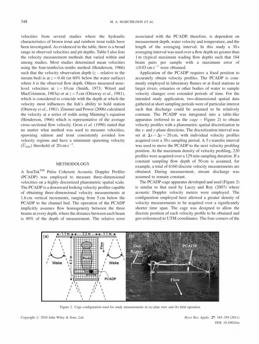
constant. The PCADP was integrated into a table-like

apparatus (referred to as the cage – Figure 2) to obtain

velocity profiles with a planometric spatial discretization in

the x- and y-plane directions. The discretization interval was

set at Dx¼Dy¼ 20 cm, with individual velocity profiles

acquired over a 30 s sampling period. A 5 s transfer interval

was used to move the PCADP to the next velocity profiling

position. At the maximum density of velocity profiling, 220

profiles were acquired over a 129min sampling duration. If a

constant sampling flow depth of 50 cm is assumed, for

example, a total of 6160 discrete velocity measurements are

obtained. During measurement, stream discharge was

assumed to remain constant.

The PCADP-cage apparatus developed and used (Figure 2)

is similar to that used by Lacey and Roy (2007) where

acoustic Doppler velocity meters were employed. The

configuration employed here allowed a greater density of

velocity measurements to be acquired over a significantly

shorter time span. The cage was designed to allow the

discrete position of each velocity profile to be obtained and

geo-referenced to UTM coordinates. The four corners of the

Figure 2. Cage configuration used for study measurements in (a) plan view and (b) field operation


DOI: 10.1002/rra


cage were outfitted with total station prism mounts so that

the corners could be surveyed and referenced to established

geodetic coordinates on land, thus creating a three-

dimensional Cartesian coordinate system of velocity

measurements. Outriggers were integrated into the cage

design to minimize wake turbulence induced by the

upstream legs (Figure 2) and minimize disturbances within

the sampling area. As illustrated in Figure 2b, the user

maintains a constant 2.5m distance from the PCADP at all

times and retreats backward beyond the limits of the cage

and outriggers as measurements progressed across the cage.

A number of metrics were derived from the data. Dimen-

sionless fluid ratios have been used elsewhere to characterize

lotic flow conditions important for micro-habitat selection,

population density and the evolved adaptations of aquatic

organisms (e.g. Leopold and Maddock, 1953; Statzner et al.,

1988; Davis and Barmuta, 1989; Jowett, 1993; Newbury and

Gaboury, 1993; Vogel, 1994; Allan, 1995; Giller and

Malmqvist, 1998; Wadeson and Rowntree, 1998; Rempel

et al., 2000; Lamouroux and Capra, 2002). The Reynolds

number (Re) is the ratio of inertial to viscous forces and is

defined as

Re ¼ ul

v(1a)

where u is the flow velocity at a given location, l is the

characteristic length and n is the kinematic viscosity. For

high width/depth ratio channels, u is often assumed to be the

depth-averaged velocity, U, and l is equal to the flow depth,

h, such that the Reynolds number is expressed as

Re ¼ Uh

v(1b)

for assumed flow under fully turbulent flow conditions (i.e.

Re> 2500, Knighton, 1998).

The Froude number (Fr) defines the ratio of a fluids

inertial forces to gravitational forces and has frequently been

used to describe the tranquility of flow when characterizing

physical habitat (Statzner et al., 1988). The Froude number

is defined as

Fr ¼ Uffiffiffiffiffigh

p (2)

where g is the gravitational constant. Flow is characterized

as sub-critical (or tranquil) when Fr< 1 and super-critical

when Fr> 1. The majority of natural rivers across the world

are typified by Froude numbers <1 at the reach scale. The

most common exceptions are rivers located in steep

mountainous regions, where channel bed slopes typically

exceed 5%. However, at the sub-reach scale, multiple meso-

scale fluid transitions between sub- and super-critical flow

are readily observable (even at low-flow conditions) as water

passes over individual rocks along the stream bed creating a

series of micro-scale hydraulic jumps (Newbury and

Gaboury, 1993).

Methods used to define physical habitat are mostly two-

dimensional (planform) metrics that implicitly assume

depth-wise homogeneity. To illustrate depth-wise trends, a

modification of turbulent kinetic energy per unit mass

equation was developed as an alternative to the Reynolds

number to describe the turbulence state of the observed flow

conditions. The mean turbulent kinetic energy per unit mass

(e) was used to assess the consistency of time-averaged

velocity measurements (Moody and Smith, 2004; Stone

et al., 2006; Smith and Brannon, 2007) and was defined as

e ¼ 1

2ðs2

x þ s2y þ s2

z Þ (3a)

where s2x ; s

2y ; s

2z are the velocity variances in the x-, y-, z-

directions, respectively. In place of a point velocity

observation as described by Equation (3a), a series of

vertical velocities were obtained in this study at a given

planometric location to estimate a vertical velocity profile

that is a depth integrated measure of turbulent kinetic energy

per unit area (ea). Summing the principal velocity

components of each vertical velocity profiles yields

ea¼ rh

2ðn� 1ÞXn

i¼0

½ðux;i�UxÞ2 þ ðuy;i � UyÞ2 þ ðuz;i � UzÞ2�

(3b)

for a discrete velocity profile where r is the density of water

and n is the number of velocity observations in each vertical

profile. Low values of ea ! 0:0 depict parallel flow lines

where flow tends towards unidirectional behaviour in the

downstream direction. As values of ea increase, flow

becomes more turbulent.

The existence of interstitial flow can be estimated by the

difference in average velocities between the pit and tailspill

region and the resulting kinetic energy heads (u2/2g). The

vertical transition from the pit to the top of the tailspill can be

simplified as a small bed rise (DZ) observed in a channel whichcan be evaluated using the Bernoulli equation such that

h1 þ u212g

¼ h2 þ u222g

þ DZ (4)

where 1 represents the hydraulic metrics of the pit and 2

represents the hydraulic metrics above the tailspill.

STUDY SITE

Whiteman’s Creek, located near Paris, Ontario, Canada

(Figure 3a) was selected to investigate the hydrodynamic

characteristics of sites selected by spawning rainbow and


DOI: 10.1002/rra


brown trout. The study reach is characterized as a low bed

slope (Figure 3b), flood plain dominated, gravel-bed river.

Summary of reach characteristics (Table II) are from Hartley

(1999).

Research by Hartley (1999) suggested that the selected

reach supported diverse aquatic niches. Thus both spring-

spawning rainbow trout and fall-spawning brown trout use

the reach for spawning. Redd identification was undertaken

within a week of spawning, when strong visual contrasts

could be identified in bed material prior to periphytic

regrowth (Witzel and MacCrimmon, 1983a,b; Grost et al.,

1990; Beard and Carline, 1991; Schmetterling, 2000). A

subset of riffles identified with redds were selected for

detailed hydrodynamic analysis. Rainbow trout redds were

identified in only two riffles (R1 and R3) within the study

reach (Figure 3). A similar survey of the study reach in the

autumn noted the presence of brown trout redds in five

separate riffles. Only two of the five riffles, R1 and R2, were

selected for use in the study (Figure 3). Choice of study

riffles was random and within the constraint of equipment

accessibility. All selected riffles demonstrated high spawn-

ing activity over the course of the respective spring and

autumn spawning periods based on the presence of multiple

redds and evidence of redd superimposition and/or

abandoned/incomplete redd construction.

Habitat variables for both brown trout and rainbow trout

study redds are presented in Table III. For brown trout,

velocity profile suites were measured between 6th and 15th

November 2006 in a window between two larger flow events

that exceeded wadable conditions. During the study period,

a relatively constant discharge of 5.5m3 s�1 was measured at

the gauge station at the upper limit of the study reach

(Figure 3).

For rainbow trout redds in riffles R1 and R3, velocity

profiles were obtained between 9th and 11th May 2007, when

a relatively constant discharge of 2.33m3 s�1 was observed.

RESULTS

A total 2683 velocity profiles were acquired from the brown

trout and rainbow trout study redds. Data are compared to

previous literature studies in Figure 4. Mean velocities

Figure 3. Whiteman’s Creek study reach (a) site location map and (b) longitudinal profile of riffle study locations (R1, R2 and R3)

Table II. A summary of study reach parameters from Hartley(1999)

Parameter Metric

Bed slope (S0) 0.27%Sinuosity (V) 1.6Effective catchment area (Ad) 383 km2

Bankfull discharge (Qbf) 42m3 s�1

Average bankfull width (Wbf) 23.2mAverage bankfull depth (hbf) 1.1mParticle size of riffles d16¼ 11.8mm, d50¼ 42.8mm,

d84¼ 90.9mmParticle size of reach d16¼ 8.1mm, d50¼ 33.4mm,

d84¼ 72.8mm

Table III. Summary of habitat variables measured at brown trout and rainbow trout study redds

Variables Brown trout redds Rainbow trout redds

Data collection period 6–15 November 2006 9–11 May 2007Study discharge (Q) 5.5m3 s�1 2.33m3 s�1

Temperature (oC) 68C� T� 98C 158C� T� 198CBed slope (S0) BR1¼ 0.0061mm�1 R1¼ 0.0061mm�1

BR2¼ 0.0007mm�1 R3¼ 0.0075mm�1

Bed friction slope (Sf) BR1¼ 0.0028mm�1 R1¼ 0.0028mm�1

BR2¼ 0.0027mm�1 R3¼ 0.0004mm�1


DOI: 10.1002/rra


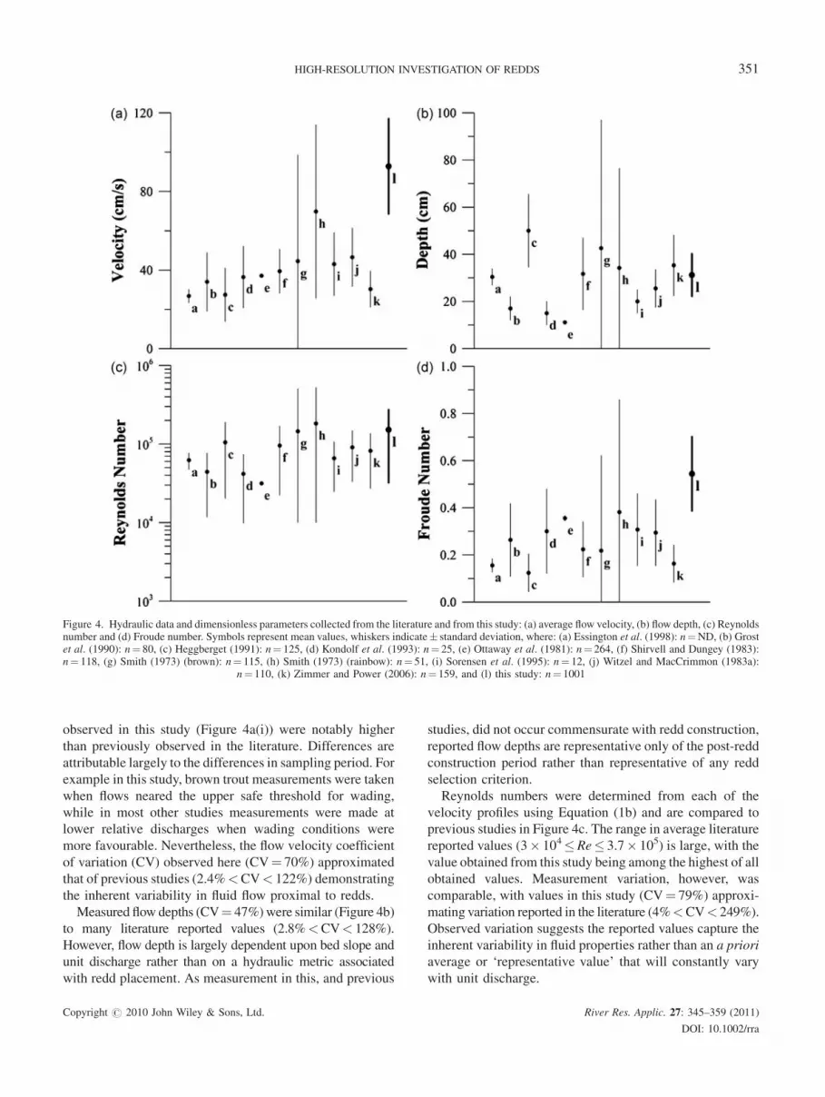
observed in this study (Figure 4a(i)) were notably higher

than previously observed in the literature. Differences are

attributable largely to the differences in sampling period. For

example in this study, brown trout measurements were taken

when flows neared the upper safe threshold for wading,

while in most other studies measurements were made at

lower relative discharges when wading conditions were

more favourable. Nevertheless, the flow velocity coefficient

of variation (CV) observed here (CV¼ 70%) approximated

that of previous studies (2.4%<CV< 122%) demonstrating

the inherent variability in fluid flow proximal to redds.

Measured flow depths (CV¼ 47%)were similar (Figure 4b)

to many literature reported values (2.8%<CV< 128%).

However, flow depth is largely dependent upon bed slope and

unit discharge rather than on a hydraulic metric associated

with redd placement. As measurement in this, and previous

studies, did not occur commensurate with redd construction,

reported flow depths are representative only of the post-redd

construction period rather than representative of any redd

selection criterion.

Reynolds numbers were determined from each of the

velocity profiles using Equation (1b) and are compared to

previous studies in Figure 4c. The range in average literature

reported values (3� 104�Re� 3.7� 105) is large, with the

value obtained from this study being among the highest of all

obtained values. Measurement variation, however, was

comparable, with values in this study (CV¼ 79%) approxi-

mating variation reported in the literature (4%<CV< 249%).

Observed variation suggests the reported values capture the

inherent variability in fluid properties rather than an a priori

average or ‘representative value’ that will constantly vary

with unit discharge.

Figure 4. Hydraulic data and dimensionless parameters collected from the literature and from this study: (a) average flow velocity, (b) flow depth, (c) Reynoldsnumber and (d) Froude number. Symbols represent mean values, whiskers indicate� standard deviation, where: (a) Essington et al. (1998): n¼ND, (b) Grostet al. (1990): n¼ 80, (c) Heggberget (1991): n¼ 125, (d) Kondolf et al. (1993): n¼ 25, (e) Ottaway et al. (1981): n¼ 264, (f) Shirvell and Dungey (1983):n¼ 118, (g) Smith (1973) (brown): n¼ 115, (h) Smith (1973) (rainbow): n¼ 51, (i) Sorensen et al. (1995): n¼ 12, (j) Witzel and MacCrimmon (1983a):

n¼ 110, (k) Zimmer and Power (2006): n¼ 159, and (l) this study: n¼ 1001


DOI: 10.1002/rra


Froude numbers calculated using Equation (2) were also

compared to previous studies (Figure 4d) and were, on

average, higher than in previous literature studies. Measure-

ment variation (CV¼ 29%), however, compared favourably

to variation reported in the literature (3%<CV< 185%).

The Froude number is linearly proportional to the velocity

(Figure 4a) and as a result of the higher velocities measured,

particularly in brown trout redds, higher Froude numbers

were obtained.

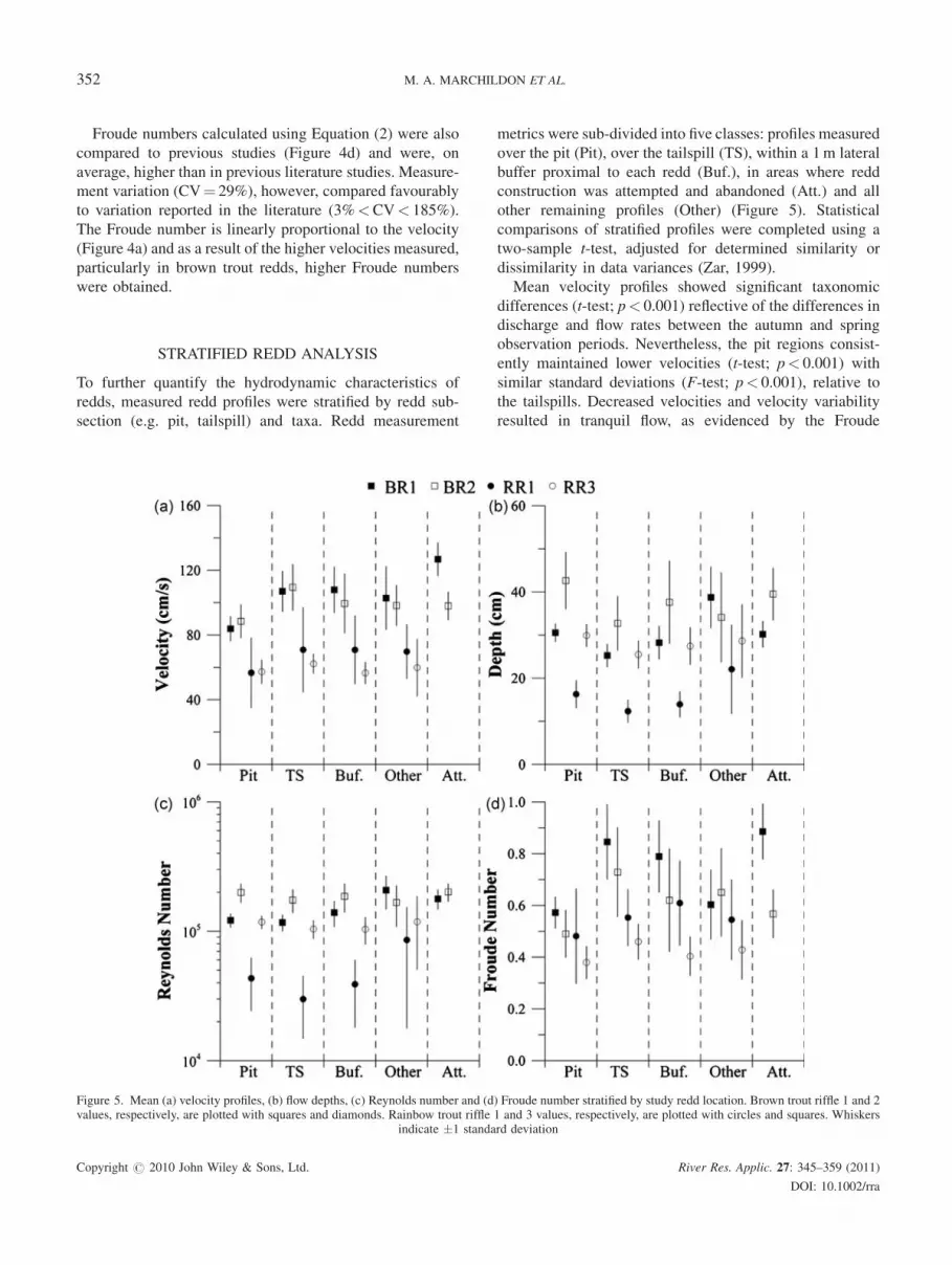
STRATIFIED REDD ANALYSIS

To further quantify the hydrodynamic characteristics of

redds, measured redd profiles were stratified by redd sub-

section (e.g. pit, tailspill) and taxa. Redd measurement

metrics were sub-divided into five classes: profiles measured

over the pit (Pit), over the tailspill (TS), within a 1m lateral

buffer proximal to each redd (Buf.), in areas where redd

construction was attempted and abandoned (Att.) and all

other remaining profiles (Other) (Figure 5). Statistical

comparisons of stratified profiles were completed using a

two-sample t-test, adjusted for determined similarity or

dissimilarity in data variances (Zar, 1999).

Mean velocity profiles showed significant taxonomic

differences (t-test; p< 0.001) reflective of the differences in

discharge and flow rates between the autumn and spring

observation periods. Nevertheless, the pit regions consist-

ently maintained lower velocities (t-test; p< 0.001) with

similar standard deviations (F-test; p< 0.001), relative to

the tailspills. Decreased velocities and velocity variability

resulted in tranquil flow, as evidenced by the Froude

Figure 5. Mean (a) velocity profiles, (b) flow depths, (c) Reynolds number and (d) Froude number stratified by study redd location. Brown trout riffle 1 and 2values, respectively, are plotted with squares and diamonds. Rainbow trout riffle 1 and 3 values, respectively, are plotted with circles and squares. Whiskers

indicate �1 standard deviation


DOI: 10.1002/rra


numbers in Figure 5d, describe a controlled region in the pit

for ova placement and fertilization experiencing minimal

disturbance relative to the remainder of the redd and

surrounding redd region.

The Reynolds numbers when stratified by redd location

and taxa indicated similar means (all pairwise t-test;

p> 0.05) and all pairwise variances (F-test; p> 0.05) with

the exception of the rainbow trout redd on riffle 1 (R1).

Lower Reynolds numbers were related to the lower

velocities (Figure 5a) and flow depths (Figure 5b) at the

time of measurement. These results continue to demonstrate

the inherent variability of flow over the redd that can occur

over a relatively short period of sampling. Given the high

resolution of measurement, the large range in observed

values effectively demonstrates temporal variability in

hydraulic metrics and challenges the appropriateness of

using a single or representative value to represent redd

hydraulic or habitat condition.

In addition to the higher Froude number in the tailspill

regions relative to other areas of the redd (t-test; p for all red

class comparisons <0.01, Figure 5d), it is important to

consider occurrences of flow conditions nearing super-

critical flow conditions (Fr! 1.0) over the tailspill and

some of the surrounding buffer regions of the studied

rainbow trout redd from riffle 1. Close inspection of the data

identifies a number of outlier locations where super-critical

flow occurred. These are micro-scale hydraulic jumps

created by the combined hydraulic conditions of shallow

flow depths (Figure 5b) and higher velocities lf flow lines

around individual. The hydraulic jumps occur over

individual clasts, transitioning from sub-critical over the

rock and returning to sub-critical flow through a hydraulic

jump on the micro-hydraulic scale. Micro-scale hydraulic

jumps entrain dissolved oxygen in the water column, which

may enter the tailspill substrate and provide additional

benefits to the ova during low-flow conditions.

Figure 6 presents the plots of turbulent kinetic energy per

unit area by stratifying the data into redd sub-regions

(similar to Figure 5). For both brown and rainbow

trout, there was a considerable decrease in secondary flow

above and surrounding the tailspill (TS) and buffer (Buf.)

regions (all comparisons p< 0.01). These are the regions

where the flow is mostly parallel and unidirectional in the

downstream direction. Flow principally focussed in one

direction over the tailspills may benefit the region by

maintaining smaller secondary flow patterns that enhance

the deposition of fine-grained material to the detriment of the

developing ova. Furthermore, the high variation of the

profiles categorized as ‘other’ in Figure 6 illustrates two

important characteristics of the measured flow regimes.

First, it shows that assuming depth-wise homogeneity when

employing the use of two-dimensional planform hydraulic

models is a major simplification. Second, there is a high

degree of spatial depth-wise heterogeneity in the planform

perspective.

Early workers noted fertilized eggs in tailspill interstitial

spaces (Hobbs, 1937; Burner, 1951). Dye experiments

further noted that flow entered the redd at the upstream end

of the tailspill, exiting downstream of the redd’s crest

(Figure 1b), and affected regions occupied by fertilized eggs.

Wu (2000) noted that bedforns reportedly experiencing

substantial interstitial flow had a form analogous to salmonid

redds, as illustrated in Figure 1b. Interstitial flow within the

bedform is attributed to flux variations at the sediment–water

interface, consistent with Bernoulli’s principle.

Although dye-tracing experiments were not conducted

through the tailspills in this study, the hydraulic data

collected provides a means of interpreting the existence of

interstitial flow. Velocity measurements were extracted from

the profiles at 1.6 cm above the stream bed that represent the

velocities closest to the sediment–water interface. The

velocities were stratified by redd sub-regions, as previously

described, and plotted in Figure 7a. The results show a

considerable increase in flow velocities immediately over

the tailspill regions relative to the redd pit regions (t-test;

p< 0.01). The difference in average velocities between the

pit and tailspill regions, and resulting kinetic energy heads

(u2/2g), corroborates the existence of interstitial flow. Using

the maximum depth of each pit, the associated shallowest

depth over each tailspill and the velocities observed at a

Figure 6. Mean turbulent kinetic energy per unit area of stream bedstratified by riffle location. Brown trout riffle 1 and 2 values, respectively,are plotted with squares and diamonds. Rainbow trout riffle 1 and 3 values,respectively, are plotted with circles and squares. Whiskers indicate �1

standard deviation


DOI: 10.1002/rra


depth of 1.6 cm above the stream bed in each pit and tailspill,

an energy balance between the pits and tailspills can be

calculated using Equation (4). The analysis results in an

average difference in total energy between the pits and

tailspills of 6.8% and an entire range between 1.75 and

11.2%. Results are well within the error measurement range

of the calculation (given the scale and relative roughness of

the substrate) and, therefore, conservation of energy can be

assumed. Given that the bed rise (DZ) in all cases is

permeable, interstitial flow must be occurring within the

tailspill regions.

Although internal circular flow within redd pits have been

suggested in the literature (e.g. Hobbs, 1937; Burner, 1951 –

Figure 1b) data collected here do not substantiate such

conclusions. For flow profiles collected in this study the

average of the collected z-direction velocity standard

deviations (sz) is presented in Figure 7b. If a circular flow

pattern were present, a notable increase in sz for profiles

measured in the pit regions relative to the surrounding

regions should be observed. Results of the analysis here

show no distinct difference in the standard deviations of the

flow directions in the vertical (z) direction (F-test; p> 0.05),

thereby demonstrating that dominant circulation patterns in

the pit region do not exist. Although the analysis does not

exclude the possibility of weak circulation patterns

occurring within the pit, associated flows would be below

the detectable limits of the PCADP. Other circulation

patterns may also arise in the pit regions that cannot be

identified by characterizing the standard deviations of the

vertical velocity component. Mean turbulent kinetic energy

per unit area (Figure 6) in the pit regions of the redd show

higher values than the tail regions. These more complex

patterns may represent planometric circulation patterns

within the pit regions.

PLANOMETRIC DISTRIBUTION OF HYDRAULIC

PARAMETERS

The hydraulic metrics used in the analysis above were also

used to plot depth-average velocity profiles, with the

exception of the velocity observed 10 cm above the stream

bed (U10). Figures 8 and 9 illustrate the two-dimensional

plan form spatial distribution patterns of hydraulic metrics

studied for a sub-set of measured redds. The hydraulic

metrics shown are of two brown trout redds (Figure 8)

located on riffle 2 (BR2-1 and BR2-2) and two rainbow trout

redds (Figure 9) located on riffle 1 (RR1) and riffle 3 (RR2).

Examination of the metric spatial trends for redds and/or

taxa showed no clear trends in any of the metrics, with the

exception of the mean turbulent kinetic energy per unit area

which consistently identified the redd tailspills with very

unidirectional parallel flow conditions (p< 0.001). Metrics

were consistently higher for the brown trout redds illustrated

relative to rainbow trout redds (t-test; p for taxonomic

comparisons <0.05). Similar results were obtained with the

analysis of the other brown and rainbow trout redds (t-test; p

for taxonomic comparisons <0.01). The differences in

metric magnitude (Figures 8 and 9) is largely attributable to

the differences in flow rates between the two study periods,

with flows of 5.5 and 2.33m3 s�1, respectively, prevailing

during the completion of the brown trout and rainbow trout

redd studies. The temporal pattern of study results further

reinforces the importance of identifying a range in metrics,

Figure 7. (a) Average velocity at 1.6 cm above stream bed (u1.6) and (b) averages of profile vertical velocity standard deviation (sz) stratified by redd location.Brown trout riffle 1 and 2 values, respectively, are plotted with squares and diamonds. Rainbow trout riffle 1 and 3 values, respectively, are plotted with circles

and squares. Whiskers indicate �1 standard deviation


DOI: 10.1002/rra


Figure 8. Two-dimensional hydraulic parameter distributions of two brown trout redds on riffle 2 (BR2-1) and (BR2-2) of Reynolds number (Re), Froudenumber (Fr), average flow velocity (U, flow velocity 10 cm above stream bed (U10), and mean turbulent kinetic energy per unit area (ea)). Mean flow direction is

indicated by arrows and the ellipses indicates the extent of the redd. This figure is available in colour online at wileyonlinelibrary.com/journal/rra


DOI: 10.1002/rra


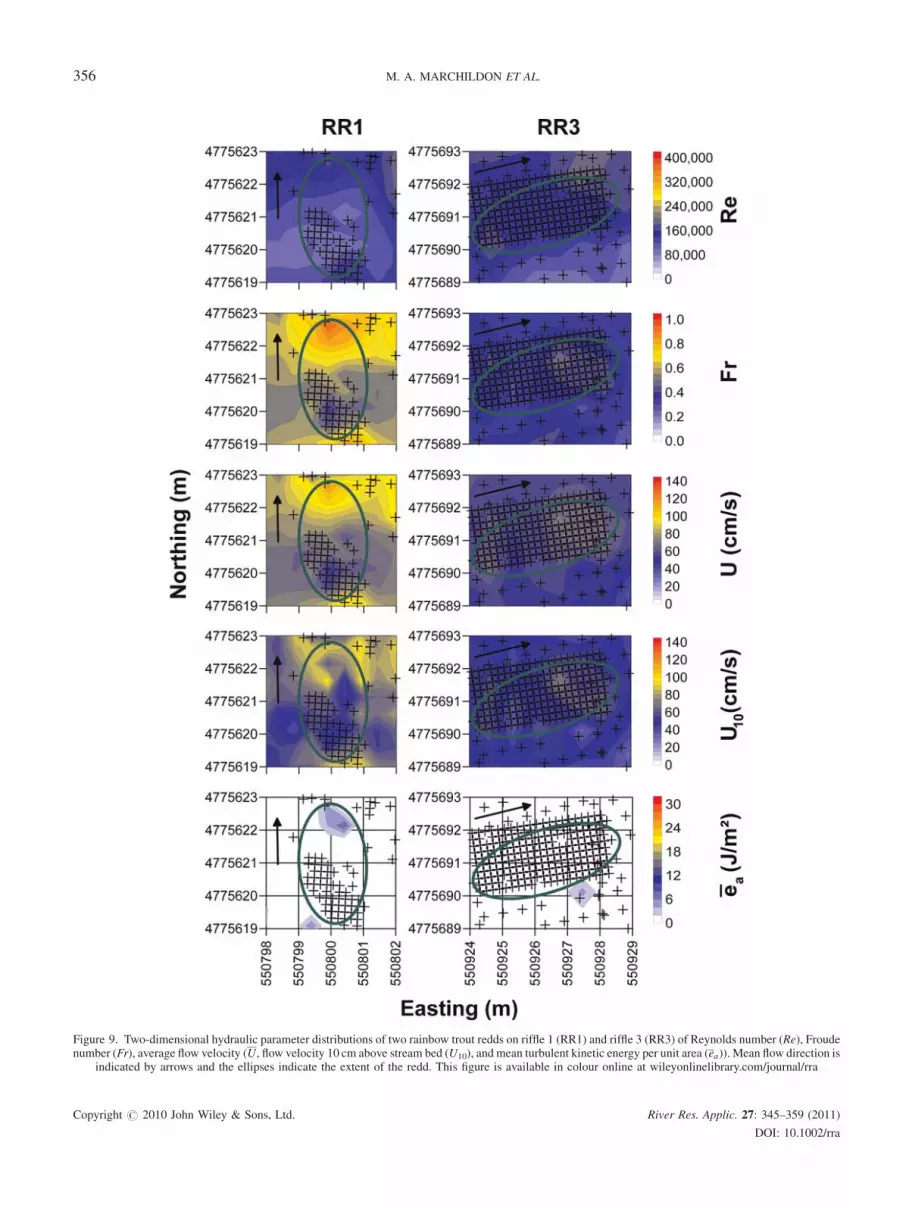
Figure 9. Two-dimensional hydraulic parameter distributions of two rainbow trout redds on riffle 1 (RR1) and riffle 3 (RR3) of Reynolds number (Re), Froudenumber (Fr), average flow velocity (U, flow velocity 10 cm above stream bed (U10), and mean turbulent kinetic energy per unit area (ea)). Mean flow direction is

indicated by arrows and the ellipses indicate the extent of the redd. This figure is available in colour online at wileyonlinelibrary.com/journal/rra


DOI: 10.1002/rra


rather than specific representative values to characterize the

redd suitability characteristics of a specific river reach.

Similar to the previous discussions, Froude numbers were

consistently observed to increase over the tailspills relative

to other parts of the redd (t-test; p for all red class

comparisons<0.01), a fact attributable to the shallower flow

depths and higher velocities as expressed in Equation (2).

Lower velocities were observed at 10 cm above the stream

bed (U10) in most cases relative to the depth-average

velocities (U) which will further trend towards 0 cm s�1 at

the sediment–water interface. The velocities 10 cm above

the stream bed also spatially show a lower velocity in the pit

region relative to the tailspill region (t-tets; p< 0.01). No

clear discernable trends were observed in using Reynolds

number to characterize the redds and surrounding regions

other than to note that the spatial range in values was large

(3� 104�Re� 3.7� 105).

CONCLUSIONS

Results of this study have demonstrated high spatial varia-

bility in the physical metrics typically used to characterize

lotic flow regimes. The only parameter that consistently

spatially correlated with redd location was turbulent kinetic

energy per unit area of stream bed. Low turbulent kinetic

energy per unit area is related to flow regimes with little

turbulence where flow is essentially unidirectional.

At the redd scale, the lowest turbulent kinetic energy per

unit area existed atop the tailspills, where the flow passing

over the elongated teardrop form showed an increase in the

linearity of flow. From a fluid dynamics perspective, the

teardrop form is known to produce the lowest amount of drag

per unit volume, as long as the fluid flow is moving along the

teardrop’s principal axis (Vogel, 1994). This would be

complementary to the development of interstitial flow

through the tailspill in order to aerate the ova.

Results of Froude number analysis demonstrated high

spatial variability and no particular spatial consistency with

redd site location. Froude numbers were the highest over the

tailspill areas where higher velocities and shallower flow

depths consistently exist. However, beyond the limits of the

pit and tailspill, no spatial trends in the measured hydraulic

parameters were identified relating to redd location

placement. Of particular note was the fact there were no

spatial correlations were identified between red locations

and the Reynolds number.

The spatial variability observed in the fluid properties of

flow velocity and flow depth and the resulting metrics of the

Reynolds number, the Froude number and turbulent kinetic

energy per unit area were not surprising considering the high

resolution of the measurements and the decrease in

measurement scale towards the micro-scale relative to

previous studies. In particular, the differences in average

reported values and the ranges of variability in the metrics

measured and calculated between the study periods for the

spring and fall redd surveys demonstrates the inherent

natural variability of aquatic systems that strongly suggests

they cannot be accurately described by single ‘representa-

tive’ hydraulic metric values.

NOMENCLATURE

Ad effective catchment area (L2)

di grain size diameter (where i¼ 5,16, 25, . . . 95thpercentile) (L)

e mean turbulent kinetic energy per unit mass (L2T �2)

ea mean turbulent kinetic energy per unit area (MT �2)

Fr Froude number

g gravitational acceleration (LT �2)

h flow depth (L)

hbf bankfull depth (L)

l characteristic length (L)

n number of observations in vertical velocity profile

Q bankfull discharge (L3T �1)

Qbf bankfull discharge (L3T �1)

Re Reynolds number

Sf friction slope

S0 bed slope

T temperature (8C)u velocity (LT�1)

u1.6 skin velocity 1.6 cm above stream bed (LT�1)

u10 flow velocity 10 cm above stream bed (LT�1)

U depth-averaged velocity (LT �1)

Umin average minimum spawning velocity threshold

(LT�1)

Wbf bankfull width (L)

z height above stream bed (L)

Dx spatial discretization of PCADP in the x-direction

(L)

Dy spatial discretization of PCADP in the x-direction

(L)

DZ bed rise (L)

n kinematic viscosity of water, where n¼m/r (L2T �1)

r mass density of water �1000 kgm�3 (ML�3)

sx,y,z standard deviation of velocity in the x-, y-, z-

directions (LT �1)

V sinuosity

ACKNOWLEDGEMENTS

Funding for this project was provided by the National

Science and Engineering Research Council of Canada

(NSERC) Discovery Grant programme, Trout Unlimited

Canada – Cold Water Conservation Fund, Canada Founda-


DOI: 10.1002/rra


tion for Innovation – Leaders Opportunity Fund and the

Grand River Conservation Authority – Apps Mill Nature

Centre.

REFERENCES

Allan JD. 1995. Stream Ecology: Structure and Function of Running

Waters. Chapman & Hall: London.

Beard TD Jr, Carline RF. 1991. Influence of spawning and other stream

habitat features on spatial variability of wild brown trout. Transactions of

the American Fisheries Society 120: 711–722.

Bevington PR, Robinson DK. 1992. Data Reduction and Error Analysis for

the Physical Sciences, 2nd edn. McGraw-Hill: Boston, New York.

Buchanan TJ, Somers WP. 1969. Discharge measurements at gaging

stations, US Geological Survey Techniques of Water-Resources Inves-

tigation, Book 3, Chapter A8, 73.

Bunn SE, Arthington AH. 2002. Basic principles and ecological con-

sequences of altered flow regimes for aquatic biodiversity. Environmental

Management 30(4): 492–507.

Burner CJ. 1951. Characteristics of spawning nests of Columbia River

salmon. U.S. Fish and Wildlife Service: Fishery Bulletin 61: 97–110.

Champoux O, Biron PM, Roy AG. 2003. The long-term effectiveness of fish

habitat restoration practices: Lawrence Creek, Wisconsin. Annals of the

Association of American Geographers 93(1): 42–54.

Chapman DW. 1988. Critical review of variables used to define effects of

fines in redds of large salmonids. Transactions of the American Fisheries

Society 117(1): 1–21.

Cooper AC. 1965. The Effect of Transported Stream Sediments on the

Survival of Sockeye and Pink Salmon Eggs and Alevin. International

Pacific Salmon Committee Bulletin 1: New Westminster, B.C.

Crisp DT, Carling PA. 1989. Observation on siting, dimensions and

structure of salmonid redds. Journal of Fish Biology 34: 119–134.

Davis JA, Barmuta LA. 1989. An ecologically useful classification of mean

and near-bed flows in streams and rivers. Freshwater Biology 21: 271–

282.

Elliott AH, Brooks NH. 1997a. Transfer of nonsorbing solutes to a

streambed with bed forms: theory. Water Resources Research 33:

123–136.

Elliott AH, Brooks NH. 1997b. Transfer of nonsorbing solutes to a

streambed with bed forms: laboratory experiments. Water Resources

Research 33: 137–151.

Essington TE, Sorensen PW, Paron DG. 1998. High rate of redd super-

imposition by brook trout (Salvelinus fontinalis) and brown trout (Salmo

trutta) in a Minnesota stream cannot be explained by habitat availability

alone. Canadian Journal of Fisheries and Aquatic Sciences 55: 2310–

2316.

Giller PS, Malmqvist B. 1998. The Biology of Streams and Rivers, 3rd edn.

Oxford University Press: Oxford.

Grost RT, Hubert WA, Wesche TA. 1990. Redd site selection by brown trout

in Douglas creek, Wyoming. Journal of Freshwater Ecology 5(3): 365–

371.

Grost RT, Hubert WA, Wesche TA. 1991. Description of brown trout in a

mountain stream. Transactions of the American Fisheries Society 120:

582–588.

Hartley AM. 1999. The pool-riffle sequence as the principal design com-

ponent of low-gradient, meandering, gravel-bed channels, M.Sc. Thesis,

School of Engineering, University of Guelph, Guelph, Ontario, Canada,

158.

Hayes JW. 1987. Competition for spawning space between brown (Salmo

trutta) and rainbow trout (S. gairdneri) in a lake inlet tributary, New

Zealand. Canadian Journal of Fisheries and Aquatic Sciences 44: 40–47.

Heggberget TG. 1991. Some environmental requirements of Atlantic

salmon. American Fisheries Society Symposium 10: 132–135.

Henderson FM. 1966. Open Channel Flow. MacMillan Publishing Com-

pany: New York; 522.

Hobbs DF. 1937. Natural reproduction of quinnat salmon, brown and

rainbow trout in certain New Zealand waters. New Zealand Marine

Department Fisheries Bulletin 6: 104.

Imhof JG, Fitzgibbon J, Annable WK. 1996. A hierarchical evaluation

system for characterizing watershed ecosystems for fish habitat. Cana-

dian Journal of Fisheries and Aquatic Sciences 53: 312–326.

Jones JW, Ball JN. 1954. The spawning behaviour of brown trout and

salmon. British Journal of Animal Behaviour 2: 103–114.

Jowett IG. 1993. A method for objectively identifying pool, run, and riffle

habitats from physical measures. New Zealand Journal of Marine and

Freshwater Research 27: 241–248.

Knighton D. 1998. Fluvial Forms and Processes: A New Perspective.

Oxford University Press, Inc.: New York.

Kondolf GM. 2000. Assessing salmonid spawning gravel quality. Trans-

actions of the American Fisheries Society 129: 262–281.

Kondolf GM, Wolman MG. 1993. The size of salmonid spawning gravels.

Water Resources Research 29(7): 2275–2285.

Kondolf GM, Sale MJ, Wolman MG. 1993. Modification of fluvial gravel

size by spawning salmonids. Water Resources Research 29(7): 2265–

2274.

Lacey RW, Roy AG. 2007. A comparative study of the turbulent flow field

with and without a pebble cluster in a gravel bed river. Water Resources

Research 43(W05502): 1–7.

Lamouroux N, Capra H. 2002. Simple predictions of instream habitat model

outputs for target fish populations. Freshwater biology 47(8): 1543–1556.

Leopold LB, Maddock T Jr. 1953. The hydraulic geometry of stream

channels and some physiographic implications. U.S.G.S Professional

Paper 252, 57.

Leopold LB, Wolman MG, Miller JP. 1964. Fluvial Processes in Geo-

morphology. W. H. Freeman: San Francisco; 522.

Lisle TE. 1989. Sediment transport and resulting deposition in spawning

gravels, north Coastal California. Water Resources Research 25(6):

1303–1319.

Lotspeich FB, Everest FH. 1981. A new approach for reporting and

interpreting textural composition of spawning gravel. U.S.D.A. Forestry

Service Research note PNW-369, 11.

Maddock I. 1999. The importance of physical habitat assessment for

evaluating river health. Freshwater biology 41: 373–391.

Moody JA, Smith JD. 2004. Field measurements of Reynolds stress near a

riverbank. Hydraulic Measurements and Experimental Methods Con-

ference 2002, 1–12.

Newbury RW, Gaboury M. 1993. Stream Analysis and Fish Habitat Design:

A Field Manual. Newbury Hydraulics: Gibsons.

Ottaway EM, Carling PA, Clark A, Reader NA. 1981. Observations on the

structure of brown trout, Salmo trutta Linnaeus, redds. Journal of Fish

Biology 19: 593–607.

Packman AI, Brooks NH, Morgan JJ. 1997. Experimental techniques for

laboratory investigation of clay colloid transport and filtration in a stream

with a sand seal. Water, Air and Soil Pollution 99: 113–122.

Phillips RW, Lantz RL, Claire EW,Moring JR. 1975. Some effects of gravel

mixtures on emergence of coho salmon and steelhead trout fry. Trans-

actions of the American Fisheries Society 3: 461–466.

Raleigh RF, Hickman T, Solomon RC. 1984. Habitat suitability infor-

mation: rainbow trout. U.S. Department of the Interior. Fish and Wildlife

Service FWS/OBS-82/10.60, 74.

Raleigh RF, Zuckerman LD, Nelson PC. 1986. Habitat suitability index

models and instream flow suitability curves: brown trout. U.S. Depart-

ment of the Interior. Fish and Wildlife Service: Biological report

82(10.24).


DOI: 10.1002/rra


Reiser DW, Wesche TA. 1977. Determination of physical and hydraulic

preferences of brown and brook trout in the selection of spawning

locations. Water Resources Series No. 64. Water Resources Research

Institute, University of Wyoming, Laramie, Wyoming, 100.

Rempel LL, Richardson JS, Healey MC. 2000. Macroinvertebrate com-

munity structure along gradients of hydraulic and sedimentary conditions

in a gravel-bed river. Freshwater biology 45: 57–73.

Schmetterling DA. 2000. Redd characteristics of fluvial westslope cutthroat

trout in four tributaries to the Black river, Montana. North American

Journal of Fisheries Management 20: 776–783.

Schwartz JS, Herricks EE. 2007. Evaluation of pool-riffle naturalization

structures on habitat complexity and the fish community in an urban

Illinois stream. River Research and Applications 23: 451–466.

Shirvell CS, Dungey RG. 1983. Microhabitats chosen by brown trout for

feeding and spawning in rivers. Transactions of the American Fisheries

Society 112: 355–367.

Smith AK. 1973. Development and application of spawning velocity and

depth criteria for Oregon salmonids. Transactions of the American

Fisheries Society 2: 312–316.

Smith DL, Brannon EL. 2007. Influence of cover on mean column hydraulic

characteristics in small pool riffle morphology streams. River Research

and Applications 23: 125–139.

Sorensen PW, Cardwell JR, Essington T, Weigel DE. 1995. Reproductive

interactions between sympatric brook and brown trout in a small Min-

nesota stream. Canadian Journal of Fisheries and Aquatic Sciences 52:

1958–1965.

Sowden TK, Power G. 1985. Prediction of rainbow trout embryo survival in

relation to groundwater seepage and particle size of spawning substrates.

Transactions of the American Fisheries Society 114: 804–812.

Statzner B, Gore JA, Resh VH. 1988. Hydraulic stream ecology: observed

patterns and potential applications. Journal of the North American

Benthological Society 7(4): 307–360.

Stone MC, Hotchkiss RH, Morrison RR. 2006. Turbulence observations in

cobble-bed rivers. World Environmental and Water Resource Congress

2006 Examining the Confluence of Environmental and Water Concerns.

Stuart TA. 1953a. Spawning migration, reproduction, and young stages of

loch trout (Salmo trutta L.). Scottish Home Department, Freshwater and

Salmon Fisheries Research 5, Edinburgh, 39.

Stuart TA. 1953b. Water currents through permeable gravels and their

significance to spawning salmons, etc. Nature 172: 407–408.

Thibodeaux LJ, Boyle JD. 1987. Bedform-generated convective transport in

bottom sediment. Nature 325: 341–343.

Trush WJ. 1989. Salmonid geomorphology. Proceedings of the Wild Trout

IV Symposium, Yellowstone National Park, Wyoming, September 18–19,

163–169.

Vaux WG. 1968. Intergravel flow and interchange of water in a

streambed U.S. Fish and Wildlife Service: Fishery Bulletin 66: 479–489.

Vogel S. 1994. Life in Moving Fluids: The Physical Biology of Flow. W.

Grant Press: Boston; 467.

Wadeson RA, Rowntree KM. 1998. Application of the hydraulic biotope

concept to the classification of instream habitats. Aquatic Ecosystems

Health and Management 1: 143–157.

Wheaton JM, Pasternack GB, Merz JE. 2004. Spawning habitat rehabilita-

tion – I. Conceptual approach and methods. International Journal of

River Basin Management 2(1): 3–20.

Wickett WP. 1954. The oxygen supply to salmon eggs in spawning beds.

Journal of the Fisheries Research Board of Canada 11(6): 933–953.

Witzel LD, MacCrimmon HR. 1983a. Redd-site selection by brook trout

and brown trout in southwestern Ontario streams. Transactions of the

American Fisheries Society 112: 760–771.

Witzel LD, MacCrimmon HR. 1983b. Embryo survival and alevin emergence

of brook charr, Salvelinus fontinalis, and brown trout, Salmo trutta, relative

to redd gravel composition. Canadian Journal of Zoology 61: 1783–1792.

Wolman MG. 1954. A method of sampling coarse river-bed material.

Transactions of the American Geophysical Union 35(6): 951–956.

Wu F.-C. 2000. Modeling embryo survival affected by sediment deposition

into salmonid spawning gravels: application to flushing flow prescrip-

tions. Water Resources Research 36(6): 1595–1603.

Zar JH. 1999. Biostatistical Analysis, 2nd edn. Prentice Halll, Upper Saddle

River: New Jersey; 663.

Zimmer MP, Power M. 2006. Brown trout habitat selection preferences and

redd characteristics in the Credit river, Ontario. Journal of Fish Biology

68: 1–14.

Zimmermann AE, Lapointe M. 2005. Intergranular flow velocity through

salmonid redds: sensitivity to fines infiltration from low intensity sedi-

ment transport events. River Research and Applications 21: 865–881.


DOI: 10.1002/rra


Documents

A high-resolution hydrodynamic investigation of brown trout (Salmo trutta) and rainbow trout (Oncorhynchus mykiss) redds