A Generalized Simulation Model of Chillers and Heat Pumps

GRE156, 1

International Symposium on Refrigeration Technology 2010, Zhuhai, China

A Generalized Simulation Model of Chillers and Heat Pumps to

Be Calibrated on Published Manufacturer’s Data

Vincent LEMORT

1* and Stéphane BERTAGNOLIO

2

1,2

Thermodynamics Laboratory

University of Liège

Campus du Sart Tilman, B49

B-4000 Liège, Belgium

E-mail: [email protected]

*Corresponding Author

ABSTRACT

This paper shows how semi-empirical models of chillers and heat pumps can be calibrated on the basis of

manufacturer’s published data, which is most of the time the only available source of information. A calibration

methodology is proposed and illustrated for different technologies of vapor-compression machines, pointing out

tips and tricks. Whatever the size and technology (e.g. scroll, screw or reciprocating compressors), the semi-

empirical model is found to predict both full load and part load performance with a very good accuracy. This is

partially due to the tailor-made formalism of the model, which allows describing the main features of the

machine.

1. INTRODUCTION

Accurate simulation of chillers and heat pump systems is welcome at different stages of HVAC system life

cycle, such as design, evaluation, commissioning and control. Different simulation models can be considered and

are generally classified between empirical (Hydeman et al., 2002; Morisot and Marchio, 2002), semi-empirical

(Bourdhouxe, 1994) and deterministic models. Semi-empirical models, which are based on a physical

description of the machine, allow extrapolating the performance for different operating conditions or

modification of the design, the control, the refrigerant or the size of the machine. Moreover, they require a

limited number of parameters that can be identified on the basis of information published by the manufacturers,

when expensive and time-consuming experimental approach cannot be implemented. The objective of this paper

is to show how this information can be used to calibrate a simulation model of a chiller/heat pump. A

methodology will be defined and illustrated for different technologies of machines.

2. MODELING A VAPOR-COMPRESSION CHILLER/HEAT PUMP

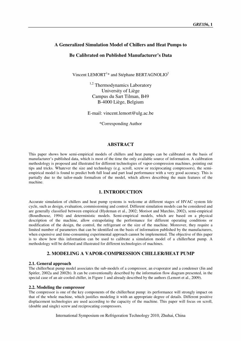
2.1. General approach The chiller/heat pump model associates the sub-models of a compressor, an evaporator and a condenser (Jin and

Spitler, 2002a and 2002b). It can be conventionally described by the information flow diagram presented, in the

special case of an air-cooled chiller, in Figure 1 and already described by the authors (Lemort et al., 2009).

2.2. Modeling the compressor The compressor is one of the key components of the chiller/heat pump: its performance will strongly impact on

that of the whole machine, which justifies modeling it with an appropriate degree of details. Different positive

displacement technologies are used according to the capacity of the machine. This paper will focus on scroll,

(double and single) screw and reciprocating compressors.

GRE156, 2


Co

mp

ress

orNcp

Co

nd

ense

r

Ev

ap

ora

tor

Ex

pa

nsi

on

va

lve

Tr,ex,cp

∆Tr,ex,cd

cpW&

rM&

Tr,ex,cd

rM& rM&

evQ&

Tr,ex,ev

Pr,ex,cd

Tr,su,cp

Pr,su,cp

Pr,ex,cp

Pr,su,ev

cdQ&a,cdM&

w,evM&

Ta,su,cd Tw,su,ev

hr,su,ev

Ta,ex,cd Tw,ex,ev

Pr,su,ev

Pr,ex,ev

Pr,su,cd

∆Tr,ex,ev

Figure 1: Schematic representation of an air-cooled chiller model

Scroll and screw compressors

Scroll and screw compressors are described in a very similar way, on the basis of the simulation model proposed

by Winandy (2002). The modeling accounts for the built-in volume ratio (parameter rv,in) and the internal

leakages (lumped into one unique flow computed by introducing a fictitious leakage area Aleak). Suction and

discharge heat transfers, as well as the heat transfer between the compressor and the ambient, are described on

the basis of three heat transfer coefficients (AUsu, AUex and AUamb). Electro-mechanical losses are split into

constant losses ( 0,lossW& ) and losses proportional to the internal compression power (factor α). If not negligible,

suction and discharge pressure losses can be introduced in the modeling, which requires two additional

parameters (dsu and dex). The modeling assumes that the fluid undergoes the following consecutive steps: supply

heating-up (su → su,1); mixing with the internal leakage (su,1 → su,2); adiabatic and reversible compression

(su,2 → in); adiabatic compression at a constant machine volume (in → ex,1); exhaust cooling-down (ex,1 →

ex)

Reciprocating compressors

Reciprocating compressors do not present a built-in volume ratio, so that the entire compression process (su,2 →

ex,1) can be considered as fully isentropic. Another difference with the two previous machines is the presence of

a clearance volume, whose re-expansion will limit the refrigerant volume flow rate swept by the machine. The

internal mass flow rate can be calculated by:

−⋅⋅−=⋅ 1

,2,

,3,

,,,3,,

cpexr

cpsur

cpscpcpscpsurcpinv

vVCVvM &&& (1)

2.3. Modeling the heat exchangers The basic modeling of the evaporator and the condenser consists in assuming that the heat exchanger is semi-

isothermal, with the constant temperature equal to the saturation temperature. The single-phase zones of the heat

exchanger are neglected and the model reduces to a one-zone heat exchanger. This assumption is acceptable for

the evaporator of a chiller, since it presents a large two-phase zone and a small single-phase (superheating) zone.

In order to be more accurate in the condenser modeling, an average condensing temperature cdT can be defined

as the weighted average of the actual temperatures occurring in the three zones (single-phase desuperheating,

two-phase condensation and single-phase undercooling) (Lemort et al., 2009).

For both heat exchangers, the overall heat transfer coefficient AU is computed by associating 2 convective heat

transfer resistances in series: Rsf, and Rr. The evaporating and condensing powers are computed by using the ε-

NTU method. For the condenser, it gives:

( )cdsusfcdcdsf

cdsf

cd

cd TTCC

AUQ ,,,

,

exp1 −

−−= &

&& (2)

3. CALIBRATION OF THE MODEL BASED ON

PUBLISHED MANUFACTURER DATA

GRE156, 3


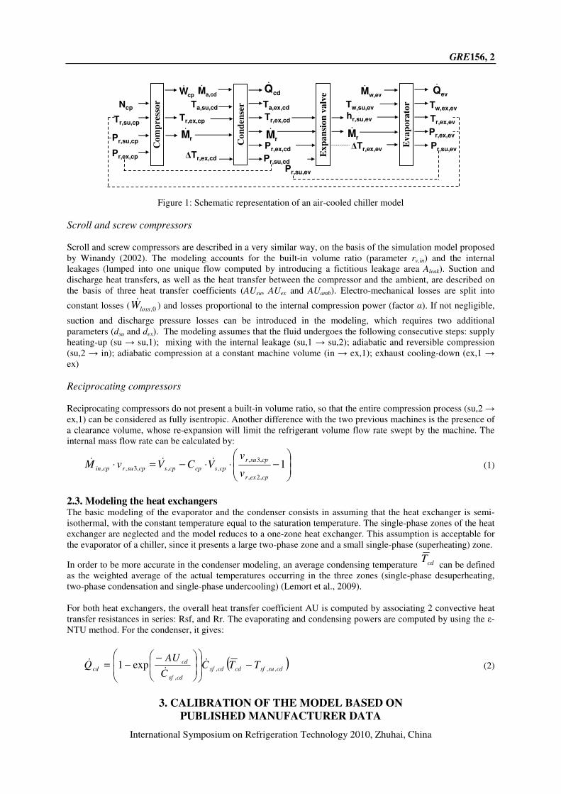
3.1. Calibration methodology Calibration of the chiller/heat pump simulation model is carried out in 2 steps (Figure 2). First, the parameters of

the compressor model are identified based on the information provided by the compressor manufacturer. Then,

the parameters of the other components are identified based on chiller/heat pump manufacturer data. The

chiller/heat pump manufacturer only seldom gives precise information regarding the brand of compressor used in

the machine. Hence, it is rather difficult to associate data published by both the compressor and the chiller

manufacturers for a given chiller/heat pump. In that case, it is recommended to select a similar compressor “off-

the-shelf”, of which performance is published, in order to estimate first guesses of the parameters of the

compressor model. These parameters can be updated afterwards in order to best predict the performance of the

entire machine.

Figure 2: Chiller/heat pump calibration flow chart

The calibration methodology can be achieved in 4 steps:

1) Analysis of manufacturer’s submittal. The main physical features of the machine are collected (type of

condenser cooling, number and types of compressors,…). Performance points of the chiller/heat pump are

retrieved. If it is possible, the brand and model of compressor are identified and performance points are

retrieved. The major peculiarities of the machine are identified. The simulation model must be adapted in

consequence.

2) Generation of default guesses for the parameters. The model is first “tested” with default guesses. The latter

are determined on the basis of the modeler’s experience. They could also be easily assessed with rational

assumptions (such as a 65% efficiency for a heat exchanger). Extrapolation for different sizes/capacities

could also be considered.

3) Manual calibration. This calibration consists in carrying out a sensitivity analysis on each parameters,

which quickly allows identifying the most influencing parameters and largely improve the model’s quality.

4) Automatic calibration. This step consists in implementing an algorithm optimizing an objective function

This step allows refining the parameters of the simulation model. The lower and upper bounds for the search

of parameters are determined through the 3rd

step, which guarantees realism in the choice of bounds.

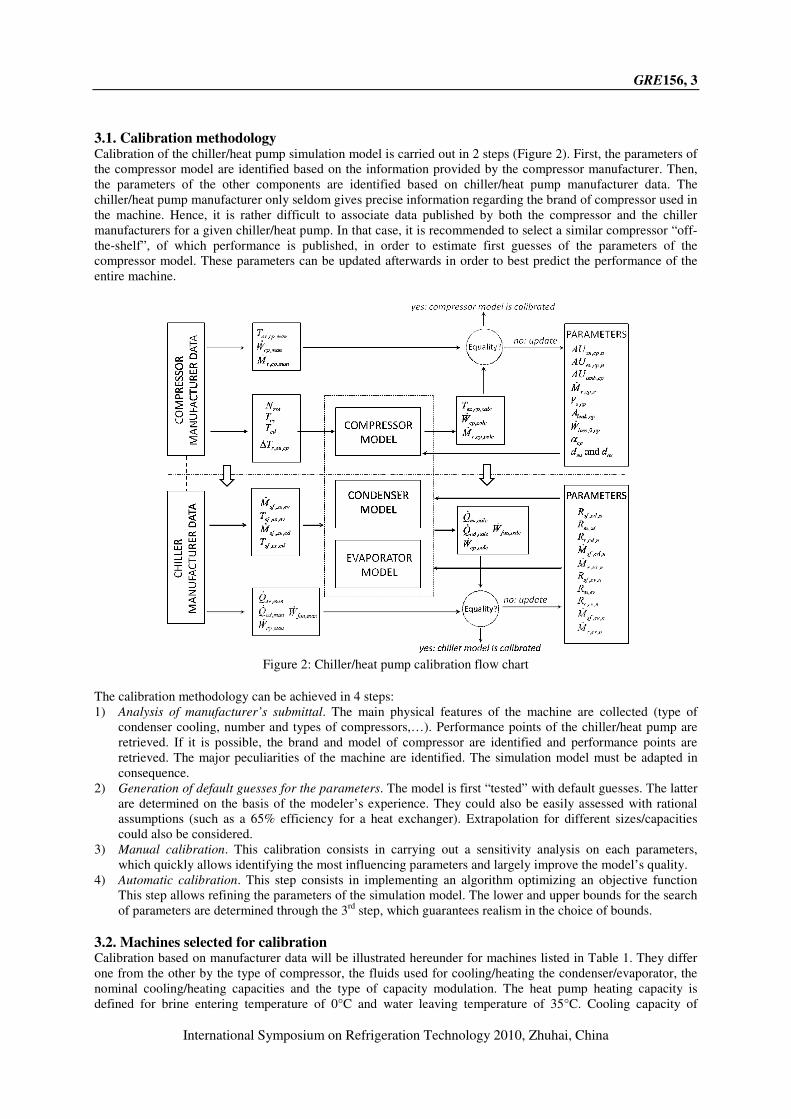
3.2. Machines selected for calibration Calibration based on manufacturer data will be illustrated hereunder for machines listed in Table 1. They differ

one from the other by the type of compressor, the fluids used for cooling/heating the condenser/evaporator, the

nominal cooling/heating capacities and the type of capacity modulation. The heat pump heating capacity is

defined for brine entering temperature of 0°C and water leaving temperature of 35°C. Cooling capacity of

GRE156, 4


chillers is rated for a chilled water leaving temperature of 7°C and a cooling air/water entering temperature of

35/30°C.

Table 1: Series of vapor compression machines considered in this study

Compressor Condenser Evaporator Cooling/heating

capacity

Regulation Refrigerant

PAC-

SCRO-

BRI-

WAT

Scroll Water-

cooled Brine-heated 10.2

1

compressor

ON/OFF

R407C

CH-

SCRO-

AIR Scroll

Air-cooled

micro-

channel

Direct

expansion

Water-heated

shell and tubes

346

4 to 6

compressors

ON/OFF

R410a

CH-

SCRO-

WAT Scroll

Water-

cooled

shell and

tubes

Direct

expansion

Water-heated

shell and tubes

286

4 to 6

compressors

ON/OFF

R410a

CH-

SCRE-

AIR

Twin-screw

Air-cooled

micro-

channel

Flooded water

heated shell

and tube

293

2

compressors

Slide valve

R134a

CH-

SCRE-

WAT Single-screw

Water-

cooled

shell and

tubes

Direct

expansion

water-heated

shell and tubes

160-480

2

compressors

Slide valve

R134a

CH-

RECI-

AIR Reciprocating

Air-cooled

Tubes and

fins

Direct

expansion

water- heated

shell and tubes

486

5

compressors

ON/OFF

R22

Information provided by the chiller/heat pump’s manufacturer consists of full load performance points

(heating/cooling capacity, compressor and fan electrical consumption) as function of secondary fluid

temperatures. Part load performance points are seldom provided. As far as possible, chiller/heat pump

manufacturers were asked to provide information allowing identifying the compressor brand and model.

Information published by the compressor manufacturer consists of the machine displacement, the displaced

refrigerant mass flow rate (or the cooling capacity for a liquid subcooling at the condenser exhaust and vapor

superheating at the evaporator exhaust) and the compressor electrical consumption as function of the evaporating

and condensing temperatures. In some cases, the heat rejection at the condenser is provided, which allows

estimating the compressor discharge temperature.

3.3. Validation of the models

Brine-to-water heat pump with a scroll compressor

In the case of the heat pump, it was possible to retrieve the brand and the model of scroll compressor. The

classical model of compressor was not able to predict correctly the performance of the compressor for high

pressure ratios. It might be due to the presence of a discharge reed valve. The discharge valve is particularly

important for systems working with pressure ratios of 6-8 or higher. In this case, the internal pressure ratio is

significantly below the compressor operating pressure ratio, resulting in an excessive compression work due to

gas back flow and recompression (Elson et al., 2008). The scroll compressor model proposed by Winandy et al.

(2002) has been adapted to account for the presence of the valve by modifying the description of the internal

compression process. In the case of under-compression (Figure 3 (b)), the internal compression is now described

by an adiabatic and reversible compression (su,2 → in), followed by an adiabatic compression at a constant

machine volume (in → in*) and an adiabatic and reversible compression (in* → ex,2). The distinction between

the two later compression processes is due to the presence of a residual clearance volume (C.Vs,cp) underneath the

reed valve and in which compressed gas is discharged when the compression chambers open.

GRE156, 5


P P

Pex,2

Psu,2

Pex,2

Pin Pin

V

inV cp,sVV

Psu,2

*

inP

inV cp,sV

(a) over compression (b) under-compression

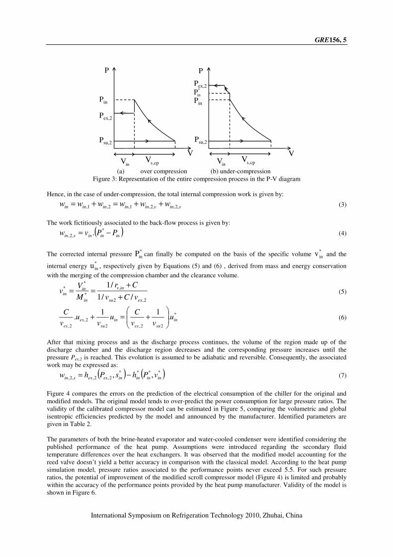
Figure 3: Representation of the entire compression process in the P-V diagram

Hence, in the case of under-compression, the total internal compression work is given by:

sinvininininin wwwwww ,2,,2,1,2,1, ++=+= (3)

The work fictitiously associated to the back-flow process is given by:

( )inininvin PPvw −=*

,2, . (4)

The corrected internal pressure *

inP can finally be computed on the basis of the specific volume *

inv and the

internal energy *

inu , respectively given by Equations (5) and (6) , derived from mass and energy conservation

with the merging of the compression chamber and the clearance volume.

2,2

,

*

**

//1

/1

exsu

inv

in

inin

vCv

Cr

M

Vv

+

+== (5)

*

22,2

2,

2,

.11

. in

suex

in

su

ex

ex

uvv

Cu

vu

v

C

+=+ (6)

After that mixing process and as the discharge process continues, the volume of the region made up of the

discharge chamber and the discharge region decreases and the corresponding pressure increases until the

pressure Pex,2 is reached. This evolution is assumed to be adiabatic and reversible. Consequently, the associated

work may be expressed as:

( ) ( )****

2,2,,2, ,, ininininexexsin vPhsPhw −= (7)

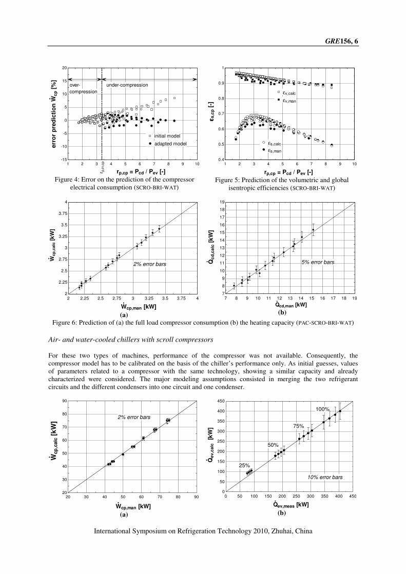
Figure 4 compares the errors on the prediction of the electrical consumption of the chiller for the original and

modified models. The original model tends to over-predict the power consumption for large pressure ratios. The

validity of the calibrated compressor model can be estimated in Figure 5, comparing the volumetric and global

isentropic efficiencies predicted by the model and announced by the manufacturer. Identified parameters are

given in Table 2.

The parameters of both the brine-heated evaporator and water-cooled condenser were identified considering the

published performance of the heat pump. Assumptions were introduced regarding the secondary fluid

temperature differences over the heat exchangers. It was observed that the modified model accounting for the

reed valve doesn’t yield a better accuracy in comparison with the classical model. According to the heat pump

simulation model, pressure ratios associated to the performance points never exceed 5.5. For such pressure

ratios, the potential of improvement of the modified scroll compressor model (Figure 4) is limited and probably

within the accuracy of the performance points provided by the heat pump manufacturer. Validity of the model is

shown in Figure 6.

GRE156, 6


1 2 3 4 5 6 7 8 9 10-15

-10

-5

0

5

10

15

20

rp,cp = Pcd / Pev [-]

err

or

pre

dic

tio

n W

cp [

%]

over-

compression

under-compression

r p,in

,cp

initial modelinitial model

adapted modeladapted model

Figure 4: Error on the prediction of the compressor

electrical consumption (SCRO-BRI-WAT)

1 2 3 4 5 6 7 8 9 100.4

0.5

0.6

0.7

0.8

0.9

1

rp,cp = Pcd / Pev [-]

εε εεs

,cp [

-]

εv,manεv,man

εs,calcεs,calc

εs,manεs,man

εv,calcεv,calc

Figure 5: Prediction of the volumetric and global

isentropic efficiencies (SCRO-BRI-WAT)

2 2.25 2.5 2.75 3 3.25 3.5 3.75 42

2.25

2.5

2.75

3

3.25

3.5

3.75

4

Wcp,man [kW]

Wcp

,calc

[k

W]

2% error bars

(a)

7 8 9 10 11 12 13 14 15 16 17 18 197

8

9

10

11

12

13

14

15

16

17

18

19

Qcd,man [kW]

Qc

d,c

alc

[kW

]

5% error bars

(b)

Figure 6: Prediction of (a) the full load compressor consumption (b) the heating capacity (PAC-SCRO-BRI-WAT)

Air- and water-cooled chillers with scroll compressors

For these two types of machines, performance of the compressor was not available. Consequently, the

compressor model has to be calibrated on the basis of the chiller’s performance only. As initial guesses, values

of parameters related to a compressor with the same technology, showing a similar capacity and already

characterized were considered. The major modeling assumptions consisted in merging the two refrigerant

circuits and the different condensers into one circuit and one condenser.

20 30 40 50 60 70 80 9020

30

40

50

60

70

80

90

Wcp,man [kW]

Wcp

,calc

[k

W]

2% error bars

(a)

0 50 100 150 200 250 300 350 400 4500

50

100

150

200

250

300

350

400

450

Qev,meas [kW]

Qe

v,c

alc

[k

W]

10% error bars

100%

75%

50%

25%

(b)

GRE156, 7


Figure 7: Prediction of (a) the full load compressor consumption (b) the part load cooling power (CH-SCRO-WAT)

Figure 7(a) compares the valued predicted by the model and announced by the manufacturer for the compressor

consumption. Figure 7(b) shows the capacity of the air-cooled scroll-compressor chiller model to predict the part

load performance points. Except for the lowest capacity stage, the model appears to predict the performance with

a very good accuracy. For the chiller electrical consumption, the best agreement was found when varying the fan

power consumption in proportion with the number of compressors in use.

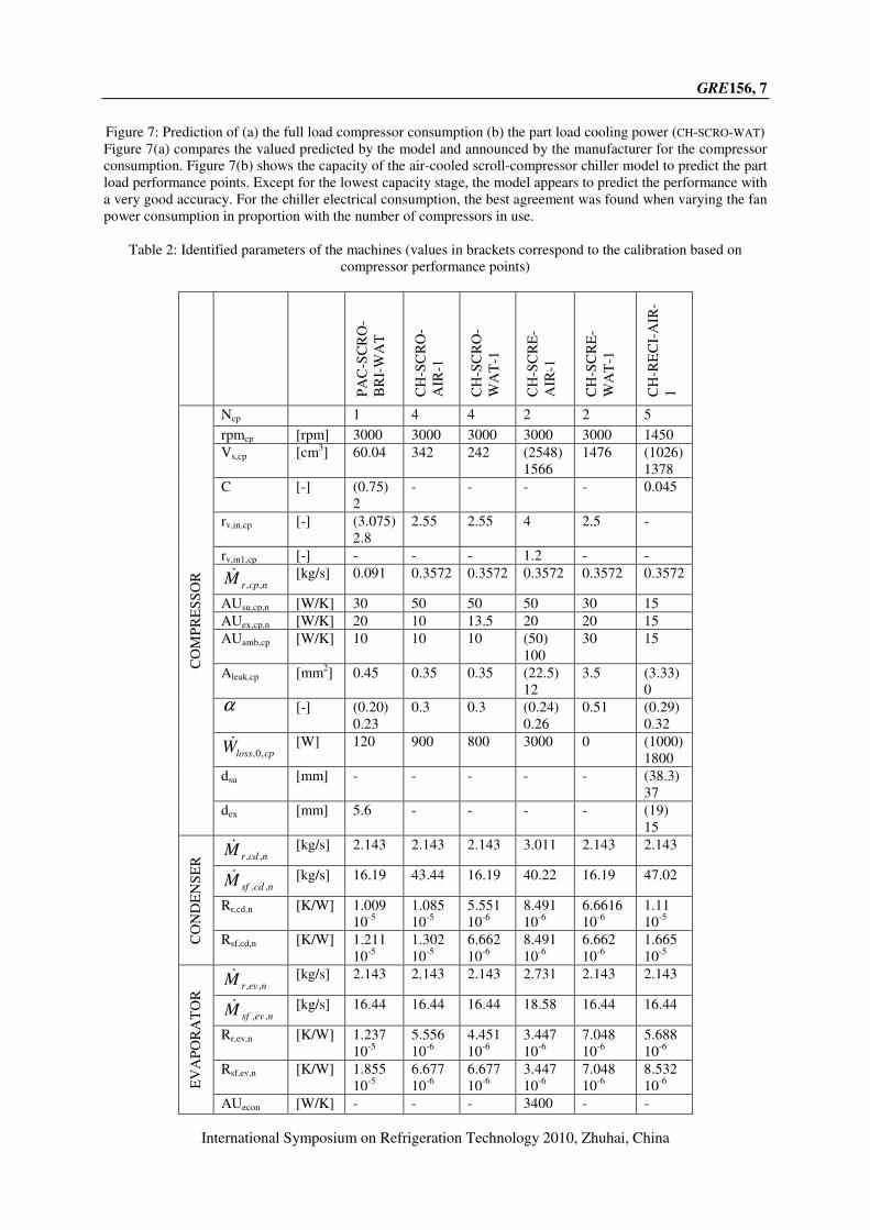
Table 2: Identified parameters of the machines (values in brackets correspond to the calibration based on

compressor performance points)

P

AC

-SC

RO

-

BR

I-W

AT

CH

-SC

RO

-

AIR

-1

CH

-SC

RO

-

WA

T-1

CH

-SC

RE

-

AIR

-1

CH

-SC

RE

-

WA

T-1

CH

-RE

CI-

AIR

-

1

CO

MP

RE

SS

OR

Ncp 1 4 4 2 2 5

rpmcp [rpm] 3000 3000 3000 3000 3000 1450

Vs,cp [cm3] 60.04 342 242 (2548)

1566

1476 (1026)

1378

C [-] (0.75)

2

- - - - 0.045

rv,in,cp [-] (3.075)

2.8

2.55 2.55 4 2.5 -

rv,in1,cp [-] - - - 1.2 - -

ncprM ,,&

[kg/s]

0.091 0.3572 0.3572 0.3572 0.3572 0.3572

AUsu,cp,n [W/K] 30 50 50 50 30 15

AUex,cp,n [W/K] 20 10 13.5 20 20 15

AUamb,cp [W/K] 10 10 10 (50)

100

30 15

Aleak,cp [mm2] 0.45 0.35 0.35 (22.5)

12

3.5 (3.33)

0 α [-] (0.20)

0.23

0.3 0.3 (0.24)

0.26

0.51 (0.29)

0.32

cplossW ,0,& [W] 120 900 800 3000 0 (1000)

1800

dsu [mm] - - - - - (38.3)

37

dex [mm] 5.6 - - - - (19)

15

CO

ND

EN

SE

R ncdrM ,,

& [kg/s] 2.143 2.143 2.143 3.011 2.143 2.143

ncdsfM ,,& [kg/s] 16.19 43.44 16.19 40.22 16.19 47.02

Rr,cd,n [K/W] 1.009

10-5

1.085

10-5

5.551

10-6

8.491

10-6

6.6616

10-6

1.11

10-5

Rsf,cd,n [K/W] 1.211

10-5

1.302

10-5

6.662

10-6

8.491

10-6

6.662

10-6

1.665

10-5

EV

AP

OR

AT

OR

nevrM ,,& [kg/s] 2.143 2.143 2.143 2.731 2.143 2.143

nevsfM ,,& [kg/s] 16.44 16.44 16.44 18.58 16.44 16.44

Rr,ev,n [K/W] 1.237

10-5

5.556

10-6

4.451

10-6

3.447

10-6

7.048

10-6

5.688

10-6

Rsf,ev,n [K/W] 1.855

10-5

6.677

10-6

6.677

10-6

3.447

10-6

7.048

10-6

8.532

10-6

AUecon [W/K] - - - 3400 - -

GRE156, 8


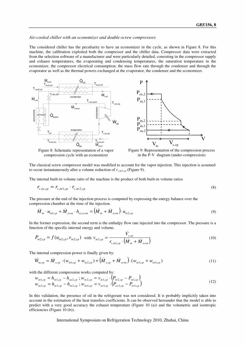
Air-cooled chiller with an economizer and double-screw compressors

The considered chiller has the peculiarity to have an economizer in the cycle, as shown in Figure 8. For this

machine, the calibration exploited both the compressor and the chiller data. Compressor data were extracted

from the selection software of a manufacturer and were particularly detailed, consisting in the compressor supply

and exhaust temperatures, the evaporating and condensing temperatures, the saturation temperature in the

economizer, the compressor electrical consumption, the mass flow rate through the condenser and through the

evaporator as well as the thermal powers exchanged at the evaporator, the condenser and the economizer.

Tr,ex,cp

Tr,ex2,cd

Tr,su,cpTev

evaporator

condensercom

pre

sso

r

eco

nom

izer

cdQ&

evQ&

cpW&econQ&

Ta,ex,cdTa,su,cd

Tw,ex,ev Tw,su,ev

cd,aM&

ev,rM&

ev,wM&

cd,rM&

econ,rM&

Tr,ex,cd

Tr,ex,econ

Figure 8: Schematic representation of a vapor

compression cycle with an economizer

P

Pex,2

Pin,3

V

Psu,2

inV cp,sV

Pin,2Pin,1

Figure 9: Representation of the compression process

in the P-V diagram (under-compression)

The classical screw compressor model was modified to account for the vapor injection. This injection is assumed

to occur instantaneously after a volume reduction of rv,in1,cp (Figure 9).

The internal built-in volume ratio of the machine is the product of both built-in volume ratios

cpinvcpinvcpinv rrr ,2,,1,,, ⋅= (8)

The pressure at the end of the injection process is computed by expressing the energy balance over the

compression chamber at the time of the injection.

( ) cpineconineconexeconcpinin uMMhMuM ,2,,1 ⋅+=⋅+⋅ &&&& (9)

In the former expression, the second term is the enthalpy flow rate injected into the compressor. The pressure is a

function of the specific internal energy and volume.

),( ,2,2,2 cpincpincpin vufP = with ( )econincpinv

cps

cpinMMr

Vv

&&

&

+⋅=

,1,

,

,2 (10)

The internal compression power is finally given by:

( ) )()( ,4,3,,2,1,, cpincpineconcpscpincpincpscpin wwMMwwMW +⋅+++⋅= &&&& (11)

with the different compression works computed by:

( )( )

cpincpexcpincpincpincpincpin

cpincpincpincpincpsucpincpin

PPvwhhw

PPvwhhw

,3,2,3,4,2,3,3

,1,2,1,2,2,1,1

;

;

−⋅=−=

−⋅=−= (12)

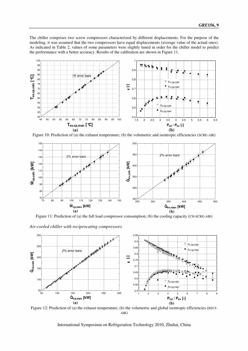
In this validation, the presence of oil in the refrigerant was not considered. It is probably implicitly taken into

account in the estimation of the heat transfers coefficients. It can be observed hereunder that the model is able to

predict with a very good accuracy the exhaust temperature (Figure 10 (a)) and the volumetric and isentropic

efficiencies (Figure 10 (b)).

GRE156, 9


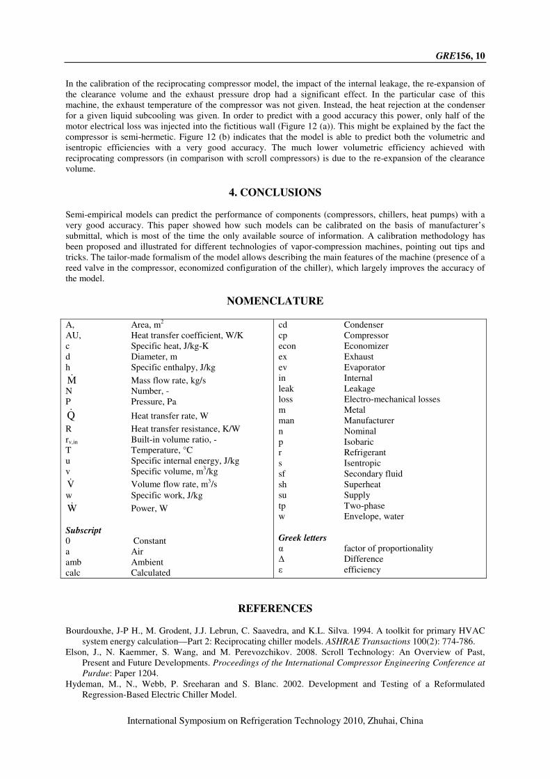
The chiller comprises two screw compressors characterized by different displacements. For the purpose of the

modeling, it was assumed that the two compressors have equal displacements (average value of the actual ones).

As indicated in Table 2, values of some parameters were slightly tuned in order for the chiller model to predict

the performance with a better accuracy. Results of the calibration are shown in Figure 11.

40 45 50 55 60 65 70 75 80 85 90 95 10040

45

50

55

60

65

70

75

80

85

90

95

100

Tex,cp,man [°C]

Tex,c

p,c

alc

[°C

] 1K error bars

(a)

1.5 2 2.5 3 3.5 4 4.5 5 5.5 6 6.50.4

0.5

0.6

0.7

0.8

0.9

1

Pcd / Pev [-] εε εε [

-]

εs,cp,calcεs,cp,calc

εs,cp,manεs,cp,man

εv,cp,calcεv,cp,calc

εv,cp,manεv,cp,man

(b)

Figure 10: Prediction of (a) the exhaust temperature; (b) the volumetric and isentropic efficiencies (SCRE-AIR)

70 80 90 100 110 120 130 140 15070

80

90

100

110

120

130

140

150

Wcp,man [kW]

Wcp

,calc

[k

W]

2% error bars

(a)

250 300 350 400 450 500250

300

350

400

450

500

Qev,man [kW]

Qe

v,c

alc

[kW

]

2% error bars

(b)

Figure 11: Prediction of (a) the full load compressor consumption; (b) the cooling capacity (CH-SCRE-AIR)

Air-cooled chiller with reciprocating compressors

50 100 150 200 250 30050

100

150

200

250

300

Qcd,man [kW]

Qc

d,c

alc

[kW

] 2% error bars

(a)

1 2 3 4 5 6 7 8 90.5

0.55

0.6

0.65

0.7

0.75

0.8

0.85

0.9

0.95

Pcd / Pev [-]

εε εε

[-]

εs,cp,calcεs,cp,calc

εs,cp,manεs,cp,man

εv,cp,calcεv,cp,calc

εv,cp,manεv,cp,man

(b)

Figure 12: Prediction of (a) the exhaust temperature; (b) the volumetric and global isentropic efficiencies (RECI-

AIR)

GRE156, 10


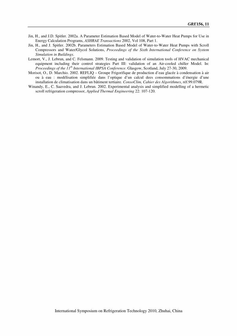
In the calibration of the reciprocating compressor model, the impact of the internal leakage, the re-expansion of

the clearance volume and the exhaust pressure drop had a significant effect. In the particular case of this

machine, the exhaust temperature of the compressor was not given. Instead, the heat rejection at the condenser

for a given liquid subcooling was given. In order to predict with a good accuracy this power, only half of the

motor electrical loss was injected into the fictitious wall (Figure 12 (a)). This might be explained by the fact the

compressor is semi-hermetic. Figure 12 (b) indicates that the model is able to predict both the volumetric and

isentropic efficiencies with a very good accuracy. The much lower volumetric efficiency achieved with

reciprocating compressors (in comparison with scroll compressors) is due to the re-expansion of the clearance

volume.

4. CONCLUSIONS

Semi-empirical models can predict the performance of components (compressors, chillers, heat pumps) with a

very good accuracy. This paper showed how such models can be calibrated on the basis of manufacturer’s

submittal, which is most of the time the only available source of information. A calibration methodology has

been proposed and illustrated for different technologies of vapor-compression machines, pointing out tips and

tricks. The tailor-made formalism of the model allows describing the main features of the machine (presence of a

reed valve in the compressor, economized configuration of the chiller), which largely improves the accuracy of

the model.

NOMENCLATURE A, Area, m

2

AU, Heat transfer coefficient, W/K

c Specific heat, J/kg-K

d Diameter, m

h Specific enthalpy, J/kg

M& Mass flow rate, kg/s

N Number, -

P Pressure, Pa

Q& Heat transfer rate, W

R Heat transfer resistance, K/W

rv,in Built-in volume ratio, -

T Temperature, °C

u Specific internal energy, J/kg

v Specific volume, m3/kg

V& Volume flow rate, m3/s

w Specific work, J/kg

W& Power, W

Subscript

0 Constant

a Air

amb Ambient

calc Calculated

cd Condenser

cp Compressor

econ Economizer

ex Exhaust

ev Evaporator

in Internal

leak Leakage

loss Electro-mechanical losses

m Metal

man Manufacturer

n Nominal

p Isobaric

r Refrigerant

s Isentropic

sf Secondary fluid

sh Superheat

su Supply

tp Two-phase

w Envelope, water

Greek letters

α factor of proportionality

∆ Difference

ε efficiency

REFERENCES

Bourdouxhe, J-P H., M. Grodent, J.J. Lebrun, C. Saavedra, and K.L. Silva. 1994. A toolkit for primary HVAC

system energy calculation—Part 2: Reciprocating chiller models. ASHRAE Transactions 100(2): 774-786.

Elson, J., N. Kaemmer, S. Wang, and M. Perevozchikov. 2008. Scroll Technology: An Overview of Past,

Present and Future Developments. Proceedings of the International Compressor Engineering Conference at

Purdue: Paper 1204.

Hydeman, M., N., Webb, P. Sreeharan and S. Blanc. 2002. Development and Testing of a Reformulated

Regression-Based Electric Chiller Model.

GRE156, 11


Jin, H., and J.D. Spitler. 2002a. A Parameter Estimation Based Model of Water-to-Water Heat Pumps for Use in

Energy Calculation Programs, ASHRAE Transactions 2002, Vol 108, Part 1.

Jin, H., and J. Spitler. 2002b. Parameters Estimation Based Model of Water-to-Water Heat Pumps with Scroll

Compressors and Water/Glycol Solutions, Proceedings of the Sixth International Conference on System

Simulation in Buildings.

Lemort, V., J. Lebrun, and C. Felsmann. 2009. Testing and validation of simulation tools of HVAC mechanical

equipment including their control strategies Part III: validation of an Air-cooled chiller Model. In:

Proceedings of the 11th

International IBPSA Conference. Glasgow, Scotland, July 27-30, 2009.

Morisot, O., D. Marchio. 2002. REFLIQ – Groupe Frigorifique de production d’eau glacée à condensation à air

ou à eau : modélisation simplifiée dans l’optique d’un calcul dees consommations d’énergie d’une

installation de climatisation dans un bâtiment tertiaire. ConsoClim, Cahier des Algorithmes, réf.99.079R.

Winandy, E., C. Saavedra, and J. Lebrun. 2002. Experimental analysis and simplified modelling of a hermetic

scroll refrigeration compressor, Applied Thermal Engineering 22: 107-120.

Documents

A Generalized Simulation Model of Chillers and Heat Pumps