Embed Size (px)
Citation preview
1
RH: General framework for animal movement 1
A general discrete-time modeling framework for animal movement 2
using multi-state random walks 3
Brett T. McClintock1, Centre for Research into Ecological and Environmental 4
Modelling and School of Mathematics and Statistics, University of St Andrews, St 5
Andrews, Fife, Scotland, UK, KY16 9LZ. 6
Ruth King, Centre for Research into Ecological and Environmental Modelling and 7
School of Mathematics and Statistics, University of St Andrews, St Andrews, Fife, 8
Scotland, UK, KY16 9LZ, [email protected]. 9
Len Thomas, Centre for Research into Ecological and Environmental Modelling 10
and School of Mathematics and Statistics, University of St Andrews, St Andrews, 11
Fife, Scotland, UK, KY16 9LZ, [email protected]. 12
Jason Matthiopoulos, Scottish Oceans Institute, School of Biology, University of St 13
Andrews, St Andrews, Fife, Scotland, UK, KY16 8LB, [email protected]. 14
Bernie J. McConnell, Scottish Oceans Institute, School of Biology, University of St 15
Andrews, St Andrews, Fife, Scotland, UK, KY16 8LB, [email protected]. 16
Juan M. Morales, Ecotono, INIBIOMA–CONICET , Universidad Nacional del 17
Comahue, Quintral 1250, 8400 Bariloche, Argentina, [email protected]. 18
Manuscript type: Article 19
Submitted to: Ecological Monographs 20
15 March 2012 21
1Current address: National Marine Mammal Laboratory, Alaska Fisheries Science 22
Center, National Marine Fisheries Service, NOAA, 7600 Sand Point Way NE, Seattle, 23
WA 98115 USA (E-mail: [email protected]). 24
2
Abstract. Recent developments in animal tracking technology have permitted the 25
collection of detailed data on the movement paths of individuals from many species. 26
However, analysis methods for these data have not developed at a similar pace, largely 27
due to a lack of suitable candidate models, coupled with the technical difficulties of 28
fitting such models to data. To facilitate a general modeling framework, we propose 29
that complex movement paths can be conceived as a series of movement strategies 30
among which animals transition as they are affected by changes in their internal and 31
external environment. We synthesize previously existing and novel methodologies to 32
develop a general suite of mechanistic models based on biased and correlated random 33
walks that allow different behavioral states for directed (e.g., migration), exploratory 34
(e.g., dispersal), area-restricted (e.g., foraging), and other types of movement. Using 35
this “tool-box” of nested model components, multi-state movement models may be 36
custom-built for a wide variety of species and applications. As a unified state-space 37
modeling framework, it allows the simultaneous investigation of numerous hypotheses 38
about animal movement from imperfectly observed data, including time allocations to 39
different movement behavior states, transitions between states, the use of memory or 40
navigation, and strengths of attraction (or repulsion) to specific locations. The inclusion 41
of covariate information permits further investigation of specific hypotheses related to 42
factors driving different types of movement behavior. Using reversible jump Markov 43
chain Monte Carlo methods to facilitate Bayesian model selection and multi-model 44
inference, we apply the proposed methodology to real data by adapting it to the natural 45
history of the grey seal (Halichoerus grypus) in the North Sea. Although previous grey 46
seal studies tended to focus on correlated movements, we found overwhelming evidence 47
that bias towards haul-out or foraging locations better explained seal movement than 48
simple or correlated random walks. Posterior model probabilities also provided 49

3
evidence that seals transition among directed, area-restricted, and exploratory 50
movements associated with haul-out, foraging, and other behaviors. With this intuitive 51
framework for modeling and interpreting animal movement, we believe the 52
development and application of bespoke movement models will become more 53
accessible to ecologists and non-statisticians. 54
Key words: animal location data, biased correlated random walk, movement 55
model, state-space model, switching behavior, telemetry. 56
INTRODUCTION 57
Our ability to track and monitor wildlife populations has greatly improved with recent 58
technological advancements. These include animal-borne devices that allow the 59
collection of accurate time-series of individual location data (McConnell et al. 2010, 60
Tomkiewicz et al. 2010), biotelemetry devices providing physiological information 61
(Cooke et al. 2004, Payne et al. 2010), and remote sensing and geographic information 62
system (GIS) technologies for the acquisition of detailed landscape data at multiple 63
spatial scales (Gao 2002). Along with these developments, new challenges have arisen 64
in the collection, management, and analysis of geo-referenced animal location data 65
(Cagnacci et al. 2010, Urbano et al. 2010). 66
Although Global Positioning System (GPS) and other relocation technologies 67
have enabled the collection of large amounts of animal location data from diverse 68
terrestrial and aquatic taxa (Tomkiewicz et al. 2010), model development for the 69
analysis of these data has lagged behind. This is beginning to change as new methods 70
continue to appear in the ecological literature (Holyoak et al. 2008, Schick et al. 2008), 71
but unlike many other areas of ecology, no general estimation framework has been 72
developed for the analysis of movement trajectories that is widely accepted by the 73
practitioners collecting the majority of these data sets. For example, there are well-74

4
established inferential methods in population and community ecology for examining 75
patterns of abundance (e.g., Otis et al. 1978, Buckland et al. 2001, Borchers et al. 2002), 76
species occurrence (e.g., MacKenzie et al. 2006), and related vital rates that address 77
uncertainties (e.g., imperfect detection) associated with the process by which the data 78
were obtained (Williams et al. 2002, King et al. 2009). There also exists readily 79
accessible software for the analysis of these data by wildlife professionals (e.g., White 80
and Burnham 1999, Thomas et al. 2010). There remains a similar need (and desire) to 81
develop accessible, inferential data analysis methods in movement ecology (Schwarz 82
2009, Morales et al. 2010). 83
As animals respond to physiological and environmental stimuli, they often 84
exhibit different movement behavior states (or modes). Simple examples include 85
“exploratory” and “encamped” states in elk (Morales et al. 2004) or, equivalently, 86
“traveling” and “foraging” states in grey seals (Breed et al. 2009), where "exploratory" 87
or "traveling" describe movement states associated with greater directional persistence 88
and velocity relative to the "encamped" or "foraging" states. Inferring patterns and 89
dynamics of movement from time-series of animal location data often involves the 90
estimation of movement parameters associated with different types of movement 91
behavior states. However, because these states often cannot be observed directly, they 92
must be inferred based on trajectories alone in the absence of ancillary information (but 93
see Discussion). Estimation is complicated further by the fact that animal location data 94
often contain considerable observation error in both time and space, as well as missing 95
(or intermittent) observations. Sophisticated statistical models of the underlying 96
movement and observation process are therefore required to facilitate reliable inference 97
(Jonsen et al. 2005, Patterson et al. 2008, Schick et al. 2008). 98
5
A variety of approaches for analyzing animal location data have been proposed 99
in recent years, and these primarily differ in the spatio-temporal conceptualization of the 100
movement process. These include discrete-time and discrete-space (Schwarz et al. 101
1993, Brownie et al 1993, Dupuis 1995, King and Brooks 2002), discrete-time and 102
continuous-space (Morales et al. 2004, Jonsen et al. 2005), continuous-time and 103
discrete-space (Ovaskainen et al. 2008), or continuous-time and continuous-space 104
(Blackwell 2003, Johnson et al. 2008) movement process models. Similarly, latent 105
behaviors associated with different types of movement can be treated as continuous 106
(Forester et al. 2007) or discrete (Morales et al. 2004, Jonsen et al. 2005) states among 107
which animals transition in response to changes in their internal and external 108
environment. The representation of movement also differs among these approaches, by 109
specifying the movement process on the positions themselves (Blackwell 2003, Jonsen 110
et al. 2006) or derived quantities, such as the differences between consecutive 111
coordinates (Jonsen et al. 2005, Johnson et al. 2008), step lengths (Forester et al. 2007), 112
or both step lengths and turning angles (Morales et al. 2004). Although earlier methods 113
ignored error in the timing and location of observations (Blackwell 2003, Morales et al. 114
2004), most recent approaches simultaneously model both the movement process and 115
observation process using state-space methods (Anderson-Sprecher and Ledolter 1991, 116
Jonsen et al. 2005, Johnson et al. 2008, Patterson et al. 2008). 117
The myriad of proposed methodologies for analyzing movement data makes 118
selection of any particular method (or model) a difficult task. The most sophisticated 119
continuous-time approaches, although appealing from a theoretical perspective, are 120
prohibitively technical for many non-statisticians. Further, continuous-time and 121
continuous-behavior models are less appealing to practitioners because the parameters 122
(e.g., instantaneous diffusion process parameters) can be difficult to interpret 123

6
biologically. Discrete-space models often necessitate spatial resolutions requiring high-124
dimensional matrices or integrals that can lead to computational difficulties. Perhaps 125
most inhibiting to general use by ecologists is the fact that the majority of movement 126
models developed to date have focused on species-specific applications and relatively 127
few behavioral states, with little scope for generalization. Given these challenges, it is 128
certainly not surprising that even less attention has been given to strategies for model 129
selection and multi-model inference (Hoeting et al. 1999, Burnham and Anderson 2002, 130
King et al. 2009) in the analysis of movement data (but see Morales et al. 2004, King 131
and Brooks 2002; 2004). 132
We synthesize many of the appealing elements of previous approaches (e.g., 133
Dunn and Gipson 1977, Blackwell 1997, King and Brooks 2002, Blackwell et al. 2003, 134
Morales et al. 2004, Jonsen et al. 2005, Johnson et al. 2008) in combination with novel 135
methodologies to formulate a general modeling strategy for individual animal 136
movement in discrete-time and continuous-space that can be readily adapted to 137
accommodate many different types of movement and behavioral states. With an 138
increased emphasis on ecological inference from animal location data, these states can 139
be associated with directed (e.g., migratory or evasive), area-restricted (e.g., foraging or 140
nesting), exploratory (e.g., dispersal or searching), and correlated movements as 141
dictated by the species and application of interest. Using Bayesian analysis methods, 142
we also propose a model selection and multi-model inference procedure based on 143
weights of evidence for these different types of movement behaviors. We demonstrate 144
the use of this mechanistic, inferential modeling framework by adapting it to the natural 145
history of the grey seal (Halichoerus grypus) in the North Sea, an apex marine predator 146
often demonstrating characteristically complex movement patterns among haul-out 147
colonies and foraging patches. 148
7
METHODS 149
A general model for individual movement in discrete time 150
We first formulate a general model for animal movement as a mixture of discrete-time 151
random walks. An individual may switch among a set of discrete movement behavior 152
states 1, ,z Z= , where each state is characterized by distributions for the step length 153
and direction (or bearing) of movement between consecutive positions ( )1 1,t tX Y− − and 154
( ),t tX Y for each time step 1, , .t T= We assume the T time steps are of equal length 155
(but see State-space formulation). The set of Z movement behavior states can include 156
directed movements towards particular locations or "exploratory" movements that are 157
not associated with any particular location. When these movement behavior states are 158
not directly observable, this can be viewed as a hidden Markov model (Zucchini and 159
MacDonald 2009, Langrock et al. 2012). 160
For flexibility and mathematical convenience, we follow Morales et al. (2004) 161
by selecting a Weibull distribution for the step length ( )ts and a wrapped Cauchy 162
distribution for the direction ( )tφ of movement, but other distributions for step length 163
(e.g., gamma) or direction (e.g., von Mises) could also be used (Codling et al. 2010). 164
The movement process model is therefore a discrete-time, continuous-space, multi-state 165
random walk with step length [ ]| ~ Weibull( , )t t i is z i a b= and direction 166
[ ] ( )| ~ wCauchy ,t t i iz iφ µ ρ= . Specifically, we have the probability density functions 167
( ) ( )1
| exp /i
i
bbi t
t t t ii i
b sf s z i s aa a
− = = −
168
and 169
( ) ( )2
2
11|2 1 2 cos
it t
i i t i
f z i ρφπ ρ ρ φ µ
−= =
+ − − 170

8
for 0,za > 0,zb > 0 2 ,tφ π≤ < 0 2 ,zµ π≤ < 1 1,zρ− < < and 1, , .z Z= Assuming 171
independence between step length and direction within each movement behavior state 172
(see Discussion), the joint likelihood for ts and tφ (conditional on the latent state 173
variable tz ) is: 174
( ) ( ) ( )1
, | |T
t t t tt
f f s z f zφ=
=∏s zφ . 175
For switches between movement behavior states, we assign a categorical 176
distribution to the latent state variable .tz The simplest approach assigns every time 177
step to a movement behavior state independent of previous states or ancillary 178
information: 179
1~ Categorical( ,..., )t Zz ψ ψ , 180
such that 181
Pr( ),i tz iψ = = 182
where iψ is the (fixed) probability of being in state i at time t, and 1
1.Zii
ψ=
=∑ This 183
assumption is generally unrealistic for animal movements. Alternatively (and more 184
realistically), one could incorporate memory into the state transition probabilities using 185
a jth-order Markov process. Assuming movement behavior states were known, 186
Blackwell (1997; 2003) used a first-order Markov transition matrix to characterize 187
switches between states in continuous time. For a first-order Markov process in discrete 188
time, 189
[ ]1 ,1 ,| ~ Categorical( ,..., )t t k k Zz z k ψ ψ− = 190
and 191
, 1Pr( | ),k i t tz i z kψ −= = = 192

9
for 1, ,k Z= where ,k iψ is the probability of switching from state k at time t – 1 to 193
state i at time t, and ,11.Z
k iiψ
==∑ We note that this Markovian structure is analogous 194
to the state transition probabilities for multi-state capture-recapture models (e.g., 195
Brownie et al. 1993, Schwarz et al. 1993). 196
The multi-state movement model is specified according to the particular species 197
and ecological conditions of interest. The various movement behavior states may be 198
solely characterized by biased, correlated, or exploratory types of movement, but 199
environmental covariates and alternative parameterizations may also be utilized to 200
describe the movement process. Below we present a suite of models for different 201
movement characteristics that can be combined to form complex movement behavior 202
states. We emphasize that the proposed models fall under the same general modeling 203
framework, with the more basic models remaining nested within the more complex 204
models. These, and other extensions (see Discussion), may therefore be thought of as 205
contributions to a “tool-box”, from which a wide range of bespoke multi-state 206
movement models in discrete time can be assembled. By adding or removing 207
components from the tool-box, one may compare the different models nested within the 208
most general model (see Example: grey seal movement in the North Sea). This allows 209
simultaneous investigation of numerous hypotheses about animal movement, including 210
those involving: 1) time allocations to different movement behavior states (i.e., “activity 211
budgets”); 2) the use of navigation for directed movement towards specific locations; 3) 212
the relative strength of bias towards (or away from) specific locations; 4) the existence 213
of spatially-unassociated (but potentially correlated) exploratory movement states; and 214
5) factors affecting transition probabilities between movement behavior states. 215
Biased movements 216
10
Biased movement behavior states exhibiting attraction (or aversion) to particular 217
locations can be incorporated within the proposed framework. Suppose the set of Z 218
movement behavior states is composed entirely of attractions to one of c different 219
"centers of attraction" (i.e., Z = c). Assuming movement at time t is biased towards 220
center of attraction i ( )i.e., tz i= , we calculate the expected movement direction 221
( ),i tµ as the direction between the individual's previous location ( )1 1,t tX Y− − and the 222
location of the center of attraction ( )* *,i iX Y at time t. We note that the coordinates of 223
each center of attraction ( )* *,z zX Y , 1, ,z c= , are not necessarily assumed to be known 224
(see Example: grey seal movement in the North Sea). 225
The strength of bias to each center of attraction is determined by the mean vector 226
length of the wrapped Cauchy distribution ( )0 1zρ≤ < . This strength of bias need not 227
be constant. For example, in some instances one may expect less directed movement 228
once an individual has reached the vicinity of the current center of attraction, so that we 229
may specify: 230
( ), tanhz t z trρ δ= 231
where tδ is some metric of the distance (e.g., Euclidean) to the current center of 232
attraction, and 0zr ≥ is a (state-dependent) scaling parameter (see Appendix A). As an 233
individual is located closer to the current center of attraction, , 0,z tρ → and the 234
movement direction is uniformly distributed on the unit circle. This allows for unbiased 235
area-restricted searches (e.g., “encamped” or “foraging” types of movement, sensu 236
Morales et al. 2004 and Breed et al. 2009) once in the vicinity of the current center of 237
attraction. As an individual is located further from the current center of attraction, 238

11
, 1,z tρ → and tφ is not allowed to deviate from ,z tµ (Figure 1a). We note that this 239
formulation also permits bias away from a “center of repulsion” when 1 0.zρ− < ≤ 240
More complicated structural forms may be utilized for .zρ For example, when 241
far away, an animal may have only a general sense of the location of a center of 242
attraction, but the movement direction draws closer to ,z tµ as the distance to the center 243
of attraction decreases (i.e., the individual "hones in" on its target). An additional 244
quadratic term ( )zq allows this type of behavior to be included in the model: 245
( )2, tanhz t z t z tr qρ δ δ= + , 246
where zr and zq are constrained such that , 0z tρ ≥ for all reasonable tδ within the study 247
area. We note that alternative link functions, such as the logit link, may be utilized 248
when specifying zρ as a function of covariates (see Example: grey seal movement in the 249
North Sea). 250
Biased, correlated movements 251
Additional structure can describe biased movement behavior states that exhibit 252
correlations between successive movement directions (Figure 1b): 253
[ ] ( )1 ,| , ~ wCauchy ,t t t i t iz iφ φ λ ρ− = 254
with expected movement direction 255
( ), 1 ,1z t z t z z tλ η φ η µ−= + − 256
where 0φ is the (latent) movement direction prior to time step t = 1. Now the expected 257
movement direction ( ),z tλ is a weighted average of the strength of bias in the direction 258
of the current center of attraction ( ),z tµ and the previous movement direction ( )1tφ − for 259
0 1.zη≤ ≤ If 0,zη = then movement reverts to a standard biased random walk. If 260
12
1zη = , then movement becomes an unbiased correlated random walk. If 0,zρ = then 261
movement is a simple (i.e., unbiased and uncorrelated) random walk. If 1,zρ = then 262
movement is biased and deterministic (Barton et al. 2009). Because ,z tλ is wrapped on 263
the unit circle, we note that care must be taken in calculating ,z tλ whenever 264
1 ,t z tφ µ π− − > . 265
Exploratory movement states 266
By specifying zρ as a function of distance, the model allows unbiased movements when 267
an individual is in close proximity to a center of attraction. However, “exploratory” 268
states may include unbiased movements that are not associated with any center of 269
attraction. The set of Z movement behavior states can therefore be extended to include 270
c center of attraction and h exploratory movement states, such that Z = c + h. Such 271
exploratory states can be easily added within the above framework: 272
( ),
0 if is an exploratory statetanh otherwisez t
z t
zr
ρδ
=
273
Exploratory movements may be unbiased, but they can often exhibit directional 274
persistence (i.e., autocorrelation in movement direction). To include correlated 275
exploratory states within the biased random walk model, 276
[ ] ( )1 , ,| , ~ wCauchy ,t t t i t i tz iφ φ λ ρ− = 277
1,
,
if is an exploratory state otherwise
tz t
z t
zφλ
µ−
=
278
( ),
if is an exploratory statetanh otherwise
zz t
z t
zr
υρ
δ=
279
where 0 1zυ≤ < is the strength of directional persistence. For a biased correlated 280
random walk with correlated exploratory states (Figure 1c): 281

13
[ ] ( )1 , ,| , ~ wCauchy ,t t t i t i tz iφ φ λ ρ− = 282
( )1
,1 ,
if is an exploratory state1 otherwise
tz t
z t z z t
zφλ
η φ η µ−
−
= + − 283
and 284
( ),
if is an exploratory statetanh otherwise
zz t
z t
zr
υρ
δ=
285
Environmental covariates and alternative parameterizations 286
Animal movement is often heavily influenced by environmental factors, such as 287
landscape (e.g., slope or vegetation cover) or seascape (e.g., currents or temperature) 288
conditions. These factors may be incorporated within the parameters above using 289
standard link functions. For example, if a set of k covariates was identified as potential 290
predictors for step length, then one could assume: 291
[ ] ( ), ,| ~ Weibull ,t t i t i ts z i a b= 292
, ,0 , ,1
log( )k
z t z z j t jj
a α α ω=
= +∑ 293
, ,0 , ,1
log( )k
z t z z j t jj
b β β ω=
= +∑ 294
where ,t jω is the value for linear predictor j at time step t. Similarly, covariates could 295
also be incorporated into strengths of attraction ( ) and ,r q state transition probabilities 296
( ) ,ψ or any other parameters in the model. This includes the use of habitat-level 297
covariates on ( ),t tX Y for predicting movements during missing or unobserved time 298
steps (see Example: grey seal movement in the North Sea). Such predicted coordinates 299
allow the overall movement path to reflect specific spatial features (e.g., lakes or 300
mountains) of relevance to the species of interest. 301

14
Step length may also be a function of distance to the current center of attraction. 302
One could envisage longer step lengths (e.g., due to increased velocity or strength of 303
bias) when far away from the current center of attraction. Such effects could be 304
incorporated by specifying 305
( ), tanh ,z t z z ta γ κ δ= 306
where the scale parameter of the Weibull distribution ( ),z ta is now a function of tδ and 307
a (state-dependent) scaling parameter ( )zκ . When the animal is near the center of 308
attraction, ,z ta is closer to zero, and the step lengths are shorter. If the animal is far 309
from the current center of attraction, ,z ta will approach the (state-dependent) scale 310
parameter asymptote zγ . Alternative approaches could include change-points on the 311
step length parameters: 312
))
)
,1 ,1
,2 ,1 ,2,
, , 1 ,
if 0,
if ,
if ,
z t z
z t z zz t
z k t z k z k
a d
a d da
a d d
δ
δ
δ −
∈ ∈ = ∈
, 313
where ,z ld is the threshold distance for change-point l of center of attraction state z (see 314
Example: grey seal movement in the North Sea) . 315
Much of the biological interest in multi-state movement models lies in the 316
specification of behavioral state transition probabilities. Depending on the biological 317
questions of interest, it may often be advantageous to reparameterize the state transition 318
probability matrix. For example, with a migratory species it may be desirable to restrict 319
state transitions until the individual is in the vicinity of the current center of attraction 320
(i.e., so that "en-route" switches are avoided). A simple reparameterization allows such 321
behaviors to be more easily investigated: 322

15
( ) ( )( ) ( )
( ) ( )
1 1 1,2 1 1,
2 2,1 2 2 2,
,1 ,2
1 11 1
1 1
c
c
c c c c c
α α β α βα β α α β
α β α β α
− − − − =
− −
ψ 323
where ( )1Pr | ,i t tz i z iα −= = = ( ), 1Pr | , ,k i t tz i z k k iβ −= = = ≠ and , 1ck ii k
β≠
=∑ for k = 324
1,2,…,c. Using logit-linear intercept ( )zζ and slope ( )zξ parameters, state transitions 325
could incorporate the effects of distance: 326
,logit( )z t z z tα ζ ξ δ= + 327
whereby individuals could be more likely to remain in the current movement state until 328
they are in close proximity to the associated center of attraction. More complicated 329
covariate structures (e.g., the amount of time in the current state) or other 330
reparameterizations could be incorporated in a similar fashion. 331
State-space formulation 332
Even in well-designed studies, there will typically be some degree of measurement error 333
in spatio-temporal animal location data. Environmental conditions may affect the 334
timing and location of fixes, as may animal behavior (e.g., diving or burrowing species). 335
For reliable inference, these irregularities must be accounted for when applying the 336
mechanistic movement models described above. To account for spatial error and 337
temporal irregularity, we propose a continuous-time observation model to accompany 338
our discrete-time movement process model in a state-space formulation. 339
In the movement process model, we assume switches between behavioral states 340
can occur at regular time intervals of equal length. The switching interval length must 341
therefore be chosen at a temporal resolution of relevance to the species and conditions 342
of interest. Similar to Jonsen et al. (2005), we assume that individuals travel in a 343
straight line between times 1t − and t. The observed locations are labeled according to 344

16
the regular time interval into which they fall: we write ( ), ,,t i t ix y for the ith observation 345
between time 1t − and t, for 1, , ti n= . These are related to the regular locations 346
( ),t tX Y via: 347
( ),, , 1 ,1
t it i t i t t i t xx j X j X ε−= − + + 348
( ),, , 1 ,1
t it i t i t t i t yy j Y j Y ε−= − + + 349
with error terms 350
2, ~ (0, )x i xNε σ 351
2, ~ (0, )y i yNε σ 352
where [ ), 0,1t ij ∈ is the proportion of the time interval between locations ( )1 1,t tX Y− − and 353
( ),t tX Y at which the ith observation between times 1t − and t was obtained. Time 354
intervals with no observations (i.e., 0tn = ) do not contribute to the observation model 355
likelihood. In some applications (e.g., radio-telemetry triangulation or Argos satellite 356
locations), the measurement errors are known to have more frequent large outliers than 357
would occur under a normal distribution; in this case, a heavier-tailed error distribution 358
could be employed (e.g., t-distribution) that allows additional non-central or scale 359
parameters (e.g., Jonsen et al. 2005). 360
EXAMPLE: GREY SEAL MOVEMENT IN THE NORTH SEA 361
Background 362
We demonstrate the application of our model using hybrid-GPS transmitter data 363
collected from grey seals (Halichoerus grypus) in the North Sea. FastlocTM GPS 364
transmitter (Wildtrack Telemetry Systems, Leeds, UK) tags were deployed in April 365
2008 and attempted to obtain a location every 30 minutes until battery failure in August 366
or September 2008. Our multi-state random walk model was initially deemed 367

17
appropriate for grey seals because we suspected they could display oriented movements 368
among haul-out colonies and foraging patches. However, a combination of biological 369
and technological issues necessitated use of the state-space model described above: 1) 370
positions are only attainable when an individual surfaces, hence observations were 371
obtained at irregular time intervals; and 2) following any “dry” period where a 372
transmitter remained out of water for more than 10 minutes, no new fixes could be 373
obtained until the transmitter returned to water continuously for 40 seconds. In other 374
words, there were frequent missing data due to an inability to obtain locations while an 375
individual was either hauled out or underwater. 376
We fitted a multi-state random walk movement model to locations from a single 377
grey seal (Figure 2). The observed data consisted of 1045 locations irregularly spaced 378
in time between 9 April and 13 August 2008. Based on the scale of movements of grey 379
seals (McConnell et al. 1999) and the frequency of observations, we specified 380
1515T = regular switching intervals of 120min between times 1t − and time t for 381
1, , .t T= Our selection of 120min intervals reflects a trade-off between 382
computational efficiency, the temporal resolution of the data, and an acceptable 383
temporal resolution for inference about grey seal movement behavior. The first of these 384
120min intervals began at deployment on 9 April, and the last interval ended 385
immediately after the final observed location on 13 August. 386
Movement model specification 387
For demonstrative purposes, we specify a simplified model of grey seal movement by 388
limiting the number of center of attraction (c = 3) and exploratory (h = 2) states . Our 389
most general first-order Markov movement process model therefore consisted of Z = 5 390
potential states, including state-dependence on both movement direction and step length 391
parameters: 392
18
[ ] ( )1 , ,| , ~ wCauchy ,t t t i t i tz iφ φ λ ρ− = 393
( )1 ,,
1
1 if if
z t z z tz t
t
z cz c
η φ η µλ
φ−
−
+ − ≤= >
394
( )1 2
,
logit if c
if cz z t z t
z t
z
m r q z
z
δ δρ
υ
− + + ≤= >
395
[ ] , ,| ~ Weibull( , )t t i t i ts z i a b= 396
[ ) ( ) [ ) ( ),1 ,20, 0,,
1 + if
if z zz t z td d
z t
z
a a z ca
a z c
δ δ − ≤ = >
I I 397
[ ) ( ) [ ) ( ),1 ,20, 0,,
1 + if
if z zz t z td d
z t
z
b b z cb
b z c
δ δ − ≤ = >
I I 398
[ ]1 ,1 ,5| ~ Categorical( ,..., )t t k kz z k ψ ψ− = 399
where 1,2,3,4,5k = , zm is an intercept term on the logit scale, ,0 1,z tρ≤ < tδ is the 400
(scaled) Euclidean distance between the predicted location ( )1 1,t tX Y− − and center of 401
attraction ( )* *,z zX X at time t, and [ ) ( )0, z td δI is an indicator function for [ )0, .t zdδ ∈ We 402
chose to fit our state-space model using Bayesian analysis methods because of the 403
general complexity of the model and the ease by which these methods can 404
accommodate prior information, latent state variables, and missing data (Ellison 2004, 405
King et al. 2009). Posterior model probabilities also provide a straightforward means 406
for addressing model selection uncertainty (see Model selection and multi-model 407
inference). 408
For our Bayesian analysis, we specified uninformative prior distributions for 409
most of the parameters (Table 1). Based on previous studies of grey seal movements 410
(McConnell et al.1999), we specified a (conservative) maximum sustainable speed of 2 411

19
meters per second (such that 14.4ts ≤ km). For the UTM coordinates of the centers of 412
attraction ( )* *, ,z zX Y we specified joint discrete uniform priors over the coordinates of 413
the predicted locations ( ),t tX Y . This prior specification therefore assumes the centers 414
of attraction are located on the predicted movement path. We constrained state 415
assignments for time steps corresponding to ( )* *,z zX Y for each center of attraction, such 416
that tz k= if ( ) ( )* *, ,k k t tX Y X Y= for 1, , .k c= For the coordinates of the initial 417
location ( )0 0, ,X Y we specified a joint uniform prior over the region (A) defined by the 418
North Sea and coastline of Great Britain. We also constrained predicted locations 419
( ),t tX Y to be within A for 1, ,t T= (i.e., inland grey seal locations were prohibited a 420
priori). 421
Model selection and multi-model inference 422
We used a reversible jump Markov chain Monte Carlo (RJMCMC) algorithm (Green 423
1995) to fit the model and simultaneously investigate various (state-specific) 424
parameterizations for the strength of bias towards any centers of attraction and the 425
correlations between successive movements (see Appendix B). These parameterizations 426
included models with linear bias ( )1, logitz t z z tm rρ δ− = + and quadratic bias 427
( )1 2, logitz t z z t z tm r qρ δ δ− = + + towards centers of attraction for z = 1,2,3. We also 428
investigated models with no correlation in movement direction between successive time 429
steps when in a center of attraction state ( 0 for 1, 2,3z zη = = ) or an exploratory state 430
( 0 for 4,5z zυ = = ). 431
These different parameterizations yielded 256 potential models for evaluation 432
via posterior model probabilities. For all models, we assumed equal prior model 433
probabilities. For all parameters without standard full conditional posterior 434

20
distributions, random walk Metropolis-Hastings updates were used (e.g., Brooks 1998, 435
Givens and Hoeting 2005). After initial pilot tuning and burn-in, we produced a single 436
MCMC chain of five million iterations for calculating posterior summaries and model 437
probabilities. After thinning by 100 iterations to reduce memory requirements, Monte 438
Carlo estimates (including model-averaged estimates) were obtained for each of the 439
parameters from this single Markov chain. The RJMCMC algorithm was written in the 440
C programming language (Kernighan and Ritchie 1988), with pre- and post-processing 441
performed in R via the .C Interface (R Development Core Team 2009). 442
Example results and discussion 443
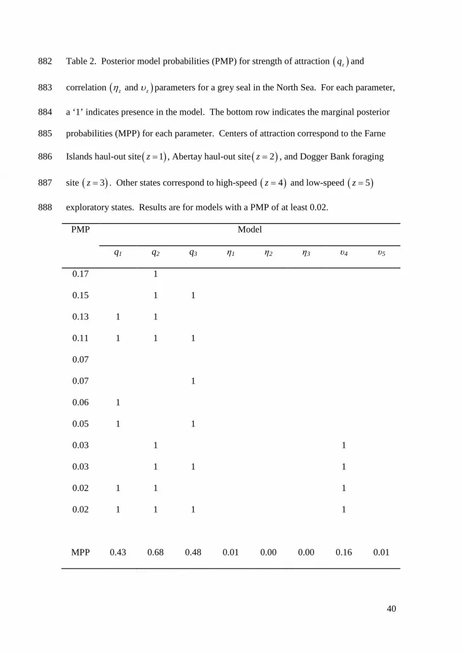
Posterior model probabilities (Table 2) and model-averaged parameter summaries 444
(Table 3) indicate biased movements towards all three centers of attraction. The 445
estimated coordinates of the centers of attraction correspond to the Farne Islands haul-446
out site, the Abertay haul-out site, and the Dogger Bank foraging site (Figure 3, 447
Appendix C), and the strengths of bias to these three sites differed as a function of 448
distance (Figure 4). The Abertay haul-out site maintained a strong and consistent bias 449
up to 350km. Both the Farne Islands haul-out and Dogger Bank foraging sites exhibited 450
a decreasing strength of bias curve, but we found little evidence of a quadratic effect of 451
distance (Tables 2, 3). Biased movements continued at greater distances (> 350km) and 452
declined less rapidly from the Dogger Bank foraging site than from the Farne Islands 453
haul-out site. These patterns of directed movement as a function of distance could be 454
indicative of the seal “honing in” on these targets, but ocean currents are also likely to 455
be influencing the timing and direction of these movements (see Gaspar et al. 2006). 456
Model-averaged posterior summaries indicated a strong tendency for the seal to 457
remain in its current movement state (Table 3), with switches between center of 458
attraction states rarely occurring until the seal had reached the vicinity of the current 459
21
center of attraction (Figure 3). We found very little evidence of correlated movements 460
when in a center of attraction state, with marginal posterior parameter probabilities of 461
0.01, 0.00, and 0.00 for 1η , 2η , and 3η , respectively. We found little evidence for 462
directional persistence during the exploratory states not associated with any center of 463
attraction (Table 3), with marginal posterior parameter probabilities of 0.16 for 4υ and 464
0.01 for 5υ . As expected, uncertainty in the coordinates of predicted locations 465
( ),t tX Y was greatest during time steps with missing data, most notably during extended 466
“dry” haul-out periods and foraging at Dogger Bank (Figure 3b). 467
Based on posterior summaries for the step length and change-point parameters, 468
we found strong evidence of shorter step lengths within 5km of the three centers of 469
attraction (Table 3). For the Farne Islands and Abertay sites, the predicted locations in 470
close proximity to these centers of attraction suggest restricted movement in the vicinity 471
of the haul-out colonies. For the Dogger Bank site, the predicted locations in the 472
vicinity suggest area-restricted searches during foraging (Figure 3). These findings are 473
consistent with expected haul-out and foraging movement behaviors of grey seals 474
(McConnell et al. 1999). Although neither of the exploratory states exhibited strong 475
directional persistence, parameter estimates indicated relatively longer step lengths (i.e., 476
higher speed) for one of these exploratory states (Table 3). This suggests transitory or 477
searching movements during the “high-speed” exploratory state (z = 4), but the “low-478
speed” exploratory state (z = 5) could be indicative of foraging or resting at sea. 479
Based on posterior state assignments, the mean proportion of time (95% highest 480
posterior density interval) between 9 April and 13 August 2008 that the seal spent in 481
each state was 0.39 (0.37, 0.41) for the Dogger Bank foraging state, 0.27 (0.26, 0.29) 482
for the Abertay haul-out state, 0.17 (0.16, 0.19) for the Farne Islands haul-out state, 0.12 483
(0.10, 0.13) for the low-speed exploratory state, and 0.05 (0.03, 0.06) for the high-speed 484
22
exploratory state. Due to tortuosity in the movement path, there was some uncertainty 485
in state assignments for transitory movements among centers of attraction. We suspect 486
these indirect paths are related to environmental cues or ocean currents. There was also 487
some state assignment uncertainty for movements in the vicinity of the Abertay and 488
Dogger Bank centers of attraction. This could be attributable to a potential foraging 489
area in the offshore sandbanks near the Abertay haul-out site, responses to prey 490
movement in the Dogger Bank foraging area, and missing location data during “dry” or 491
prolonged diving periods. Further model structure, including additional movement 492
behavior states or environmental covariates, may be required to better explain these 493
movements. 494
Given the reliability of locations using hybrid-GPS transmitters, we were not 495
particularly concerned about spatio-temporal measurement error for these data. We 496
were far more concerned about irregularly-observed and missing data because we were 497
unable to obtain locations while the seal was hauled out or underwater. Error terms (in 498
meters) were relatively small, with posterior medians for ˆ 562xσ = (95% HPDI: 511 - 499
620) and for ˆ 255yσ = (95% HPDI: 233 - 276). Similar to Patterson et al. (2010), the 500
larger value for xσ reflects the prevalence of east-west movements between haul-out 501
and foraging sites. There were several instances where small, but non-negligible, 502
differences were found between observed and predicted locations (Figure 3a), but we 503
believe these instances are more likely attributable to some deficiencies in the model 504
than to location measurement error. 505
Previous studies on individual seal movement (Jonsen et al. 2005, Johnson et al. 506
2008, Breed et al. 2009, Patterson et al. 2010) limited models to simple and correlated 507
random walks among haul-out and foraging areas. Based on posterior estimates and 508
probabilities for simple (0% of posterior model probabilities), correlated (0%), biased 509
23
(82%), and both biased and correlated (18%) random walk mixture models, we found 510
overwhelming evidence that including bias (or drift) towards centers of attraction better 511
explained seal movement than simple or correlated random walks. This result strongly 512
supports the recognized ability of grey seals to rely on navigational capabilities for 513
directed (and not simply correlated) movement among haul-out colonies and foraging 514
patches. 515
Correlations among parameters and the large number of latent variables made 516
the development of a model fitting algorithm a computational challenge. To help 517
diagnose convergence, we examined a series of additional chains with overdispersed 518
initial values. With poor starting values for ( )* *,z zX Y and ( ),t tX Y , we found the 519
algorithm could diverge or get caught in local maxima. However, we achieved similar 520
results for chains covering a range of reasonable starting values. Even with reasonable 521
starting values, it required about five million iterations before chains appeared to 522
converge. The centers of attraction do not necessarily need to be located on the 523
predicted movement path, but we found mixing and performance were greatly improved 524
by this prior specification for the coordinates of the centers of attraction ( )* *,z zX Y . We 525
also believe it is reasonable to assume that centers of attraction are visited (and hence 526
located along the predicted path). 527
At the expense of some biological realism, we chose to keep this example 528
relatively simple to demonstrate the application of this methodology to a general 529
audience. If our intended audience were limited to marine mammalogists, we would 530
have incorporated additional model complexity and prior information to better reflect 531
the biology of grey seals. Similar to Johnson et al. (2008), we could have included an 532
additional “dry” state for movement during periods when the seal was (presumably) out 533
of water (e.g., smaller step lengths). Alternatively, landscape covariates could have 534

24
been used for specifying "haul-out" movement states when the seal was located on land. 535
We also could have constrained transition probabilities to make switches between states 536
less likely until the seal reached the vicinity of the current center of attraction. Not only 537
would refinements such as these add biological realism, but they would likely improve 538
mixing and convergence of the RJMCMC algorithm. 539
DISCUSSION 540
With the development of an intuitive framework for modeling animal movement, 541
ecologists may better appreciate the applicability of mechanistic, inferential movement 542
models to a wide variety of species and conditions. We have proposed a discrete-time, 543
continuous-space, and discrete-state conceptualization of the individual animal 544
movement process to facilitate the biological interpretation of distinct movement 545
behaviors and associated parameters. We believe its mathematical simplicity and focus 546
on ecology can make the application of bespoke movement models more 547
straightforward for non-statisticians. This “tool-box” of model components allows 548
researchers to construct custom-built mechanistic movement models for the species of 549
interest, while providing a means to compare weights of evidence in support of specific 550
hypotheses about different movement behaviors. 551
Perhaps most appealing is the ease with which new components can be added 552
to the nested model-building tool-box. While more components can lead to a large 553
number of potential models to choose from, the framework can accommodate the 554
additional model selection uncertainty in a straightforward quantitative manner. As 555
demonstrated in our grey seal example, this approach enabled the simultaneous 556
investigation of numerous hypotheses about seal movement, including the use of 557
navigation and time allocations to different movement behavior states. To our 558

25
knowledge, this is the first methodology utilizing model weights for selection and multi-559
model inference in the mechanistic movement model literature. 560
Although our main goal has been to present this suite of model-building tools, 561
a serious study of animal movement should include some additional assessments of 562
goodness of fit. Morales et al. (2004) and Dalziel et al. (2010) briefly explore this topic, 563
including the use of posterior predictive checks and probes to test whether the fitted 564
models are consistent with emergent properties of the movement process (e.g., 565
autocorrelation patterns in displacements and habitat use). However, an assessment of 566
absolute goodness of fit remains a daunting task for mechanistic movement models. In 567
the absence of classical tests of goodness of fit, it is particularly important that the 568
model set be selected with care utilizing the best biological information available for 569
reliable inference. Conditional on this candidate model set, model comparisons (e.g., 570
based on posterior model probabilities or other model selection criteria) can provide 571
some assessment of the relative goodness of fit. 572
There remain many potential extensions to the modeling framework beyond 573
those already identified. In the grey seal example, we included two exploratory 574
movement states not associated with any center of attraction, but additional spatially-575
unassociated states that differ in their movement properties (and associated state 576
parameters) may be incorporated (sensu Morales et al. 2004, Jonsen et al. 2005, Breed 577
et al. 2009). These additional states could be used to further differentiate among 578
exploratory movements (e.g., dispersal or search strategies) that have unique 579
distributions for step length and the degree of correlation between successive 580
movements. 581
We reiterate that centers of attraction do not necessarily refer to a single location 582
in space. Rather, they can refer to any entity to which animals move in response to. 583

26
This includes immobile entities such as habitat patches, but also mobile entities such as 584
conspecifics or prey. Any given entity (or group of entities) could therefore be used to 585
define a different behavior state for movement towards, away from, or within each 586
entity. Potential centers of attraction can also be dynamically incorporated within an 587
individual’s portfolio as its habitat is explored, thus allowing for explicit modeling of 588
the effects of past experience on movement. Instead of centers of attraction, centers of 589
repulsion (where 1 0zρ− < ≤ ) may be particularly useful for demonstrating avoidance 590
behaviors related to encounters with conspecifics, predators, or undesirable habitats. 591
From a behavioral ecology perspective, perhaps most promising is the potential 592
for modeling movement state transition probabilities. By incorporating physiological or 593
environmental covariate information into the framework, one can investigate hypotheses 594
about the timing and motivations behind various movement behaviors as individuals 595
respond to changes in the internal and external environment (Morales et al. 2010). 596
Biotelemetry data (e.g., metabolic rate) or time of year (e.g., breeding season) are 597
among many factors that may help explain changes in movement behavior. Instead of 598
relying solely on trajectories, ancillary data may also be helpful in the assignment of 599
movement states. For example, additional landscape or seascape information may have 600
better explained the indirect movements between the two haul-out colonies in our grey 601
seal analysis. Recent advances, such as animal-borne accelerometers (Wilson et al. 602
2008, Holland et al. 2009, Payne et al. 2010), will likely provide additional ways to 603
distinguish among different types of movement (e.g., predator hunting and feeding). 604
There are also many ways by which memory can be incorporated into movements and 605
state transitions. Here we only explored two such mechanisms for memory, including 606
Markov processes for state transitions and the existence of spatial locations that are 607
committed to memory because they are (presumably) associated with specific goals. 608

27
The locations of centers of attraction are typically assumed to be known based 609
on prior knowledge or qualitative assessments of the data. Indeed, one could relatively 610
easily predict the coordinates of the three centers of attraction in our grey seal example 611
using only the naked eye or previous studies. However, we envision more complicated 612
movement paths where it is very difficult to identify or differentiate between potential 613
centers. We believe a quantitative means for estimating the location of centers and their 614
associated strengths of attraction (or repulsion), such as that proposed here, improves 615
our ability to extract reliable information from novel or more complex movement paths. 616
For simplicity, we chose to specify three centers of attraction in our grey seal 617
example. Although we found strong evidence of bias towards all three of these centers, 618
if any center z receives little support for bias (e.g., , 0z tρ ≈ for all tδ ), alternative models 619
removing such centers should be explored because state z essentially becomes an 620
uncorrelated exploratory state. This may have undesirable consequences, including 621
confounded exploratory states and poor MCMC mixing. Ideally, the model could be 622
extended to accommodate an unknown number of centers and reduce any need for ad-623
hoc assessments of the appropriate number of centers. This would require an additional 624
parameter for the number of centers and (state-specific) movement parameters for each 625
potential center. Similar to the multi-model inference procedure used here, a reversible 626
jump MCMC algorithm could be utilized to estimate the number of centers of attraction. 627
This potential extension constitutes the focus of current research. 628
Additional information or structural complexity could also be specified in the 629
observation process of the state-space model. For example, Jonsen et al. (2005) 630
specified informative priors for measurement error parameters based on previously 631
published records of location estimation error for Argos-tagged grey seals. State-632
dependent error or correlation terms (e.g., utilizing a multivariate normal error 633

28
distribution) could also be incorporated. Although a great deal of previous effort in the 634
analysis of animal location data has focused on the observation process, we expect 635
greater emphasis on the movement process as the quality of location data continue to 636
improve (e.g., with advances in GPS technology). 637
Although other approaches (e.g., Blackwell 2003, Jonsen et al. 2005, Johnson et 638
al. 2008) could potentially be extended to include the various types of movement 639
accommodated by our multi-state model, we chose to extend the basic methodology of 640
Morales et al. (2004) because of its intuitive appeal to ecologists and wildlife 641
professionals. The discrete-time, continuous-space approach of Jonsen et al. (2005) can 642
accommodate correlated and uncorrelated exploratory movements, but it does not 643
include biased or area-restricted movements related to specific locations or habitats. An 644
additional limitation of the correlated random walk approach of Jonsen et al. (2005) is a 645
lack of independence between direction and step length, resulting in higher-order auto-646
correlations than found in standard correlated random walks. Our approach assumes 647
independence between direction and step length for each movement behavior state, but 648
a joint distribution including correlations could potentially be incorporated if deemed 649
appropriate (e.g., specifying shorter step lengths when movement is away from the 650
current center of attraction). 651
The continuous-time, continuous-space approaches of Blackwell (2003) and 652
Johnson et al. (2008) do allow correlated movements and “drift” that can (potentially) 653
be related to specific locations (sensu Kendall 1974, Dunn and Gipson 1977). 654
However, Blackwell (2003) assumes movement behavior states are known and Johnson 655
et al. (2008) only include a single state with known covariates, hence neither approach 656
includes an estimation framework for both movement state and switching behavior. 657
Although satisfying from a mathematical and theoretical perspective, we believe the 658

29
often difficult interpretation of continuous-time movement parameters (e.g., those 659
related to Ornstein-Uhlenbeck and other diffusion processes) can in practice be 660
discouraging to applied ecologists wishing to use or extend these methods. This may 661
change as ecologists become more familiar with the principles of mechanistic 662
movement models and computer software makes these approaches more accessible. 663
Unlike continuous-time movement process models, the primary disadvantage of 664
a discrete-time approach is that the time scale between state transitions must be chosen 665
based on the biology of the species and the frequency of observations. For any 666
continuous- or discrete-time approach to be useful, the temporal resolution of the 667
observed data must be relevant to the specific movement behaviors of interest. The 668
timing and frequency of observations must therefore be carefully considered when 669
designing telemetry devices and data collection schemes. 670
To encourage the broader application of movement models in ecology, user-671
friendly software for the analysis of animal location data is needed. Ovaskainen et al 672
(2008) and Johnson et al. (2008) provided important first steps in accessible software by 673
creating DISPERSE and the R package CRAWL to perform the complicated 674
computations the models respectively require. Despite its relative mathematical 675
simplicity, the large number of parameters and latent variables inherent to our modeling 676
framework also makes implementation a computational challenge. We therefore 677
provide code for the full state-space formulation of our model (see Supplement) and are 678
currently developing a software package for general use by practitioners (Milazzo et al. 679
in prep.). 680
By making individual movement models more accessible and readily 681
interpretable to ecologists, we ultimately hope progress can be made towards linking 682
animal movement and population dynamics at the interface of behavioral, population, 683

30
and landscape ecology (Morales et al. 2010). Although the mechanistic links between 684
animal movement and population dynamics are theoretically understood, fitting 685
population-level models to data from many individuals will pose considerable 686
mathematical and computational challenges. Scaling individual movement models up 687
to population-level processes therefore remains a very promising avenue for future 688
research. 689
ACKNOWLEDGMENTS 690
Funding for this research was provided by the Engineering and Physical Sciences 691
Research Council (EPSRC reference EP/F069766/1). Hawthorne Beyer, Roland 692
Langrock, Tiago Marques, Lorenzo Milazzo, two anonymous referees, and the associate 693
editor Ken Newman provided helpful comments on the manuscript. 694
LITERATURE CITED 695
Anderson-Sprecher, R., and J. Ledolter. 1991. State-space analysis of wildlife telemetry 696
data. Journal of the American Statistical Association 86: 596-602. 697
Barton, K. A., B. L. Phillips, J. M. Morales, and J. M. J. Travis. 2009. The evolution of 698
an 'intelligent' dispersal strategy: biased, correlated random walks in patchy landscapes. 699
Oikos 118: 309-319. 700
Blackwell, P. G. 1997. Random diffusion models for animal movement. Ecological 701
Modelling 100: 87-102. 702
Blackwell, P. G. 2003. Bayesian inference for Markov processes with diffusion and 703
discrete components. Biometrika 90: 613-627. 704
Borchers, D. L., S. T. Buckland, and W. Zucchini. 2002. Estimating Animal 705
Abundance: Closed Populations. Springer-Verlag. 706

31
Breed, G. A., I. D. Jonsen, R. A. Myers, W. D. Bowen, and M. L. Leonard. 2009. Sex-707
specific, seasonal foraging tactics of adult grey seals (Halichoerus grypus) revealed by 708
state-space analysis. Ecology 90: 3209-3221. 709
Brooks, S. P. 1998. Markov chain Monte Carlo and its applications. The Statistician 47: 710
69-100. 711
Brownie, C., J. E. Hines, J. D. Nichols, K. H. Pollock, and J. B. Hestbeck. 1993. 712
Capture-recapture studies for multiple strata including non-Markovian transitions. 713
Biometrics 49: 1173-1187. 714
Buckland, S. T., D. R. Anderson, K. P. Burnham, J. L. Laake, D. L. Borchers, and L. 715
Thomas. 2001. Introduction to Distance Sampling: Estimating Abundance of Biological 716
Populations. Oxford University Press. 717
Burnham, K. P., and D. R. Anderson. 2002. Model Selection and Multi-model 718
Inference: A Practical Information-Theoretic Approach. 2nd Edition. Springer. 719
Cagnacci, F., L. Boitani, R. A. Powell, and M. S. Boyce. 2010. Animal ecology meets 720
GPS-based radiotelemetry: a perfect storm of opportunities and challenges. 721
Philosophical Transactions of the Royal Society B 27: 2157-2162. 722
Codling, E. A., R. N. Bearon, and G. J. Thorn. 2010. Diffusion about the mean drift 723
location in a biased random walk. Ecology 91: 3106-3113. 724
Cooke, S. J., S. G. Hinch, M. Wikelski, R. D. Andrews, L. J. Kuchel, T. G. Wolcott, and 725
P. J. Butler. 2004. Biotelemetry: a mechanistic approach to ecology. Trends in Ecology 726
and Evolution 19: 334-343. 727
Dalziel, B. D., J. M. Morales, and J. M. Fryxell. 2010. Fitting dynamic models to 728
animal movement data: the importance of probes for model selection, a reply to Franz 729
and Caillaud. American Naturalist 175: 762-764. 730
32
Dunn, J. E., and P. S. Gipson. 1977. Analysis of radio telemetry data in studies of home 731
range. Biometrics 33: 85-101. 732
Dupuis, J. A. 1995. Bayesian estimation of movement and survival probabilities from 733
capture-recapture data. Biometrika 82: 761-772. 734
Ellison, A. M. 2004. Bayesian inference in ecology. Ecology Letters 7: 509-520. 735
Forester, J. D., A. R. Ives, M. G. Turner, D. P. Anderson, D. Fortin, H. L. Beyer, D. W. 736
Smith, and M. S. Boyce. 2007. State-space models link elk movement patterns to 737
landscape characteristics in Yellowstone National Park. Ecological Monographs 77: 738
285-299. 739
Gao, J. 2002. Integration of GPS with remote sensing and GIS: reality and prospect. 740
Photogrammetric Engineering and Remote Sensing 68: 447-453. 741
Gaspar, P., J. -Y. Georges, S. Fossette, A. Lenoble, S. Ferraroli, and Y. Le Maho. 2006. 742
Marine animal behaviour: neglecting ocean currents can lead us up the wrong track. 743
Proceedings of the Royal Society B 273: 2697-2702. 744
Givens, G. H., and J. A. Hoeting. 2005. Computational Statistics. Wiley. 745
Green, P. J. 1995. Reversible jump Markov chain Monte Carlo computation and 746
Bayesian model determination. Biometrika 82: 711-732. 747
Hoeting, J. A., D. Madigan, A. E. Raftery, and C. T. Volinsky. 1999. Bayesian model 748
averaging: a tutorial. Statistical Science 14: 382-401. 749
Holland, R. A., M. Wikelski, F. Kümmeth F, and C. Bosque. 2009. The secret life of 750
oilbirds: new insights into the movement ecology of a unique avian frugivore. PLoS 751
ONE 4: e8264. doi:10.1371/journal.pone.0008264. 752
Holyoak, M., R. Casagrandi, R. Nathan, E. Revilla, and O. Spiegel. 2008. Trends and 753
missing parts in the study of movement ecology. Proceedings of the National Academy 754
of Sciences 105: 10960-19065. 755
33
Johnson, D. S., J. M. London, M.-A. Lea, and J. W. Durban. 2008. Continuous-time 756
correlated random walk model for animal telemetry data. Ecology 89: 1208-1215. 757
Jonsen, I. D., J. M. Flemming, and R. A. Myers. 2005. Robust state-space modeling of 758
animal movement data. Ecology 86: 2874-2880. 759
Jonsen, I. D., R. A. Myers, and M. C. James. 2006. Robust hierarchical state-space 760
models reveal diel variation in travel rates of migrating leatherback turtles. Journal of 761
Animal Ecology 75: 1046-1057. 762
Kendall, D. G. 1974. Pole-seeking Brownian motion and bird navigation. Journal of the 763
Royal Society B 36: 365-417. 764
Kernigham, B. W., and D. M. Ritchie. 1988. The C Programming Language. 2nd 765
Edition. Prentice Hall. 766
King, R., and S. P. Brooks. 2002. Bayesian model discrimination for multiple strata 767
capture-recapture data. Biometrika 89: 785-806. 768
King, R., and S. P. Brooks. 2004. A classical study of catch-effort models for Hector's 769
dolphins. Journal of the American Statistical Association 99: 325-333. 770
King, R., B. J. T. Morgan, O. Gimenez, and S. P. Brooks. 2009. Bayesian Analysis for 771
Population Ecology. Chapman and Hall/CRC. 772
Langrock, R., R. King, J. Matthiopoulos, L. Thomas, D. Fortin, and J. M. Morales. 773
2012. Flexible and practical modeling of animal telemetry data: hidden Markov models 774
and extensions. Technical Report, University of St Andrews. 775
MacKenzie, D. I., J. D. Nichols, J. A. Royle, K. H. Pollock, L. L. Bailey, and J. E. 776
Hines. 2006. Occupancy Estimation and Modeling: Inferring Patterns and Dynamics of 777
Species Occurrence. Academic Press. 778
McConnell, B. J., M. A. Fedak, P. Lovell, and P. S. Hammond. 1999. Movements and 779
foraging areas of grey seals in the North Sea. Journal of Applied Ecology 36: 573-590. 780

34
McConnell, B, J., M. A. Fedak, S. K. Hooker, and T. A. Patterson. 2010. Telemetry. 781
Pages 222- 262 in I. L. Boyd, W. D. Bowen, and S. J. Iverson, eds. Marine Mammal 782
Ecology and Conservation. Oxford University Press. 783
Milazzo, L., B. T. McClintock, R. King, L. Thomas, J. Matthiopoulos, and J. M. 784
Morales. In prep. MOMENTUM: Models Of animal MoveENT Using Multi-state 785
random walks. 786
Morales, J. M., D. T. Haydon, J. Frair, K E. Holsinger, and J. M. Fryxell. 2004. 787
Extracting more out of relocation data: building movement models as mixtures of 788
random walks. Ecology 85: 2436-2445. 789
Morales, J. M., P. R. Moorcroft, J. Matthiopoulos, J. L. Frair, J. G. Kie, R. A. Powell, E. 790
H. Merrill, and D. T. Haydon. 2010. Building the bridge between animal movement and 791
population dynamics. Philosophical Transactions of the Royal Society B 365: 2289-792
2301. 793
Otis. D. L., K. P. Burnham, G. C. White, and D. R. Anderson. 1978. Statistical 794
inference from capture data on closed animal populations. Wildlife Monographs 62: 3-795
135. 796
Ovaskainen, O., H. Rekola, E. Meyke, and E. Arjas. 2008. Bayesian methods for 797
analyzing movements in heterogeneous landscapes from mark-recapture data. Ecology 798
89: 542-554. 799
Patterson, T. A., L. Thomas, C. Wilcox, O. Ovaskainen, and J. Matthiopoulos. 2008. 800
State-space models of individual animal movement. Trends in Ecology and Evolution 801
23: 87-94. 802
Patterson, T. A., B. J. McConnell, M. A. Fedak, M. V. Bravington, and M. A. Hindell. 803
2010. Using GPS data to evaluate the accuracy of state-space methods for correction of 804
Argos satellite telemetry error. Ecology 91: 273-285. 805

35
Payne, N. L., B. M. Gillanders, R. S. Seymour, D. M. Webber, E. P. Snelling, and J. M. 806
Semmens. 2010. Accelerometry estimates field metabolic rate in giant Australian 807
cuttlefish Sepia apama during breeding. Journal of Animal Ecology doi: 808
10.1111/j.1365-2656.2010.01758.x. 809
R Development Core Team. 2009. R: A language and environment for statistical 810
computing. R Foundation for Statistical Computing, Vienna, Austria. ISBN 3-900051-811
07-0, URL http://www.R-project.org. 812
Schick, R. S., S. R. Loarie, F.Colchero, B. D. Best, A. Boustany, D. A. Conde, P. N. 813
Halpin, L. N. Joppa, C. M. McClellan, and J. S. Clark. 2008. Understanding movement 814
data and movement processes: current and emerging directions. Ecology Letters 11: 815
1338-1350. 816
Schwarz, C. J. 2009. Migration and movement – the next stage. Pages 323 – 348 in D. 817
L. Thomson, E. G. Cooch, and M. J. Conroy, eds. Modeling Demographic Processes in 818
Marked Populations. Springer. 819
Schwarz, C. J., J. F. Schweigert, and A. N. Arnason. 1993. Estimating migration rates 820
using tag-recovery data. Biometrics 49: 177-193. 821
Thomas, L., S. T. Buckland, E. A. Rexstad, J. L. Laake, S. Strindberg, S. L. Hedley, J. 822
R. B. Bishop, T. A. Marques, and K. P. Burnham. 2010. Distance software: design and 823
analysis of distance sampling surveys for estimating population size. Journal of Applied 824
Ecology 47: 5-14. 825
Tomkiewicz, S. M., M. R. Fuller, J. G. Kie, and K. K. Bates. 2010. Global positioning 826
system and associated technologies in animal behavior and ecological research. 827
Philosophical Transactions of the Royal Society B 365: 2163-2176. 828
36
Urbano, F., F. Cagnacci, C. Calenge, H. Dettki, A. Cameron, and M. Neteler. 2010. 829
Wildlife tracking data management: a new vision. Philosophical Transactions of the 830
Royal Society B 365: 2177-2185. 831
White, G. C., and K. P. Burnham. 1999. Program MARK: survival estimation from 832
populations of marked animals. Bird Study 46: S120-S139. 833
Williams, B. K., J. D. Nichols, and M. J. Conroy. 2002. Analysis and Management of 834
Animal Populations. Academic Press. 835
Wilson, R. P., E. L. C. Shepard, and N. Liebsch. 2008. Prying into the intimate details 836
of animal lives: use of a daily diary on animals. Endangered Species Research 4:123-837
137. 838
Zucchini, W. Z., and I. L. MacDonald. 2009. Hidden Markov Models for Time Series: 839
An Introduction Using R. Chapman and Hall/CRC. 840
841
842
843
844
845
846
847
848
849
850
851
852
853
37
APPENDIX A 854
Strength of bias for the wrapped Cauchy distribution as a function of distance to a 855
center of attraction (Ecological Archives XXXX-XXX-A1). 856
APPENDIX B 857
Reversible jump Markov chain Monte Carlo algorithm for the multi-state random walk 858
model (Ecological Archives XXXX-XXX-A2). 859
APPENDIX C 860
HTML animation of Figure 3 (Ecological Archives XXXX-XXX-A3). 861
SUPPLEMENT 862
Computer code and data for implementing the reversible jump Markov chain Monte 863
Carlo algorithm for the multi-state random walk model (Ecological Archives XXXX-864
XXX-A4). 865
866
867
868
869
870
871
872
873
874
875
876
877
38
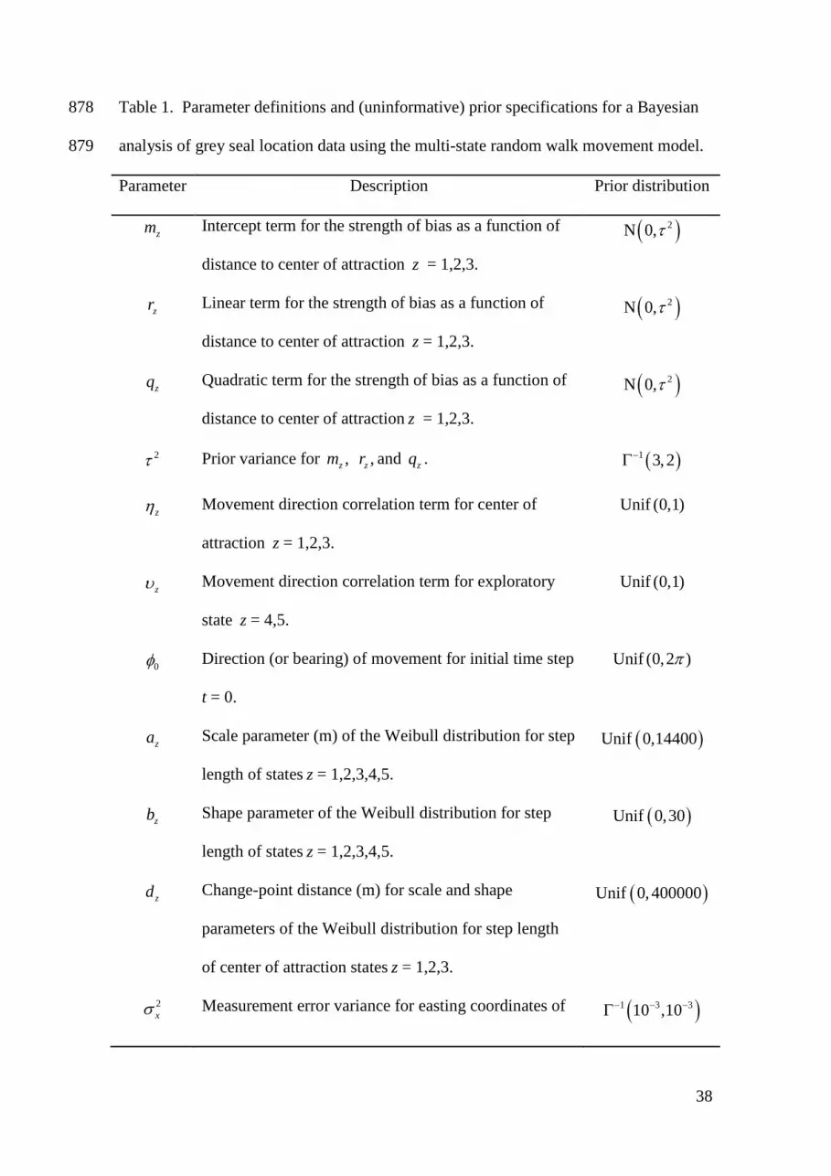
Table 1. Parameter definitions and (uninformative) prior specifications for a Bayesian 878
analysis of grey seal location data using the multi-state random walk movement model. 879
Parameter Description Prior distribution
zm Intercept term for the strength of bias as a function of
distance to center of attraction z = 1,2,3.
( )2N 0,τ
zr Linear term for the strength of bias as a function of
distance to center of attraction z = 1,2,3.
( )2N 0,τ
zq Quadratic term for the strength of bias as a function of
distance to center of attraction z = 1,2,3.
( )2N 0,τ
2τ Prior variance for ,zm ,zr and zq . ( )1 3, 2−Γ
zη Movement direction correlation term for center of
attraction z = 1,2,3.
Unif (0,1)
zυ Movement direction correlation term for exploratory
state z = 4,5.
Unif (0,1)
0φ Direction (or bearing) of movement for initial time step
t = 0.
Unif (0,2 )π
za Scale parameter (m) of the Weibull distribution for step
length of states z = 1,2,3,4,5.
( )Unif 0,14400
zb Shape parameter of the Weibull distribution for step
length of states z = 1,2,3,4,5.
( )Unif 0,30
zd Change-point distance (m) for scale and shape
parameters of the Weibull distribution for step length
of center of attraction states z = 1,2,3.
( )Unif 0,400000
2xσ Measurement error variance for easting coordinates of ( )1 3 310 ,10− − −Γ
39
observed locations ( ), ,,t i t ix y .
2yσ Measurement error variance for northing coordinates of
observed locations ( ), ,,t i t ix y .
( )1 3 310 ,10− − −Γ
[ ],k ⋅ψ The kth row vector of the state transition probability
matrix, with each element ( ),k iψ corresponding to the
switching probability from state k at time t - 1 to state i
= 1,2,3,4,5 at time t.
Dirichlet(1,1,1,1,1)
880
881
40
Table 2. Posterior model probabilities (PMP) for strength of attraction ( )zq and 882
correlation ( ) and z zη υ parameters for a grey seal in the North Sea. For each parameter, 883
a ‘1’ indicates presence in the model. The bottom row indicates the marginal posterior 884
probabilities (MPP) for each parameter. Centers of attraction correspond to the Farne 885
Islands haul-out site ( )1z = , Abertay haul-out site ( )2z = , and Dogger Bank foraging 886
site ( )3z = . Other states correspond to high-speed ( )4z = and low-speed ( )5z = 887
exploratory states. Results are for models with a PMP of at least 0.02. 888
PMP Model
q1 q2 q3 η1 η2 η3 υ4 υ5
0.17 1
0.15 1 1
0.13 1 1
0.11 1 1 1
0.07
0.07 1
0.06 1
0.05 1 1
0.03 1 1
0.03 1 1 1
0.02 1 1 1
0.02 1 1 1 1
MPP 0.43 0.68 0.48 0.01 0.00 0.00 0.16 0.01

41
Table 3. Model-averaged posterior summaries for strength of attraction 889
( ), , , and z z zr q m τ , correlation ( )0, , and z zη υ φ , step length ( ), , and z z za b d , 890
observation error ( ) and x yσ σ , and state transition probability ( ),k iψ parameters. 891
Summaries include posterior medians and 95% highest posterior density intervals 892
(HPDI), conditional on the parameter being present in the model. Posterior means are 893
reported for state transition probabilities. Center of attraction states correspond to the 894
Farne Islands haul-out site ( )1z = , Abertay haul-out site ( )2z = , and Dogger Bank 895
foraging site ( )3z = . The high-speed ( )4z = and low-speed ( )5z = exploratory states 896
are not associated with a center of attraction. 897
95% HPDI
Parameter Estimate Lower Upper
Strength of attraction parameters
1m 3.08 2.31 3.91
2m 4.54 3.85 5.37
3m 3.49 2.86 4.21
1r -5.47 -8.35 -2.40
2r -0.70 -9.84 4.47
3r -3.41 -7.10 -1.77
1q -0.53 -4.90 4.13
2q 3.40 -2.27 14.94
3q 1.63 -1.39 5.01
τ 3.00 1.68 5.63

42
Correlation parameters
1η 0.00 0.00 0.01
2η 0.00 0.00 0.00
3η 0.00 0.00 0.01
4υ 0.16 0.00 0.63
5υ 0.01 0.00 0.04
0φ 0.06 3.47 3.13
Step length parameters
1,1a 10497.04 10026.35 10990.62
2,1a 11052.65 10631.82 11524.23
3,1a 10859.38 10503.77 11194.52
4a 5188.94 4755.68 5644.98
5a 1902.68 1601.28 2230.24
1,1b 6.12 4.78 7.73
2,1b 6.17 5.33 7.43
3,1b 6.16 5.38 7.04
4b 19.96 8.51 30.00
5b 4.40 2.09 11.85
1d 1576.19 1152.39 2077.87
2d 5583.09 3694.29 6552.00
3d 1425.98 1016.81 2722.62
1,2a 1908.44 1369.26 2529.56
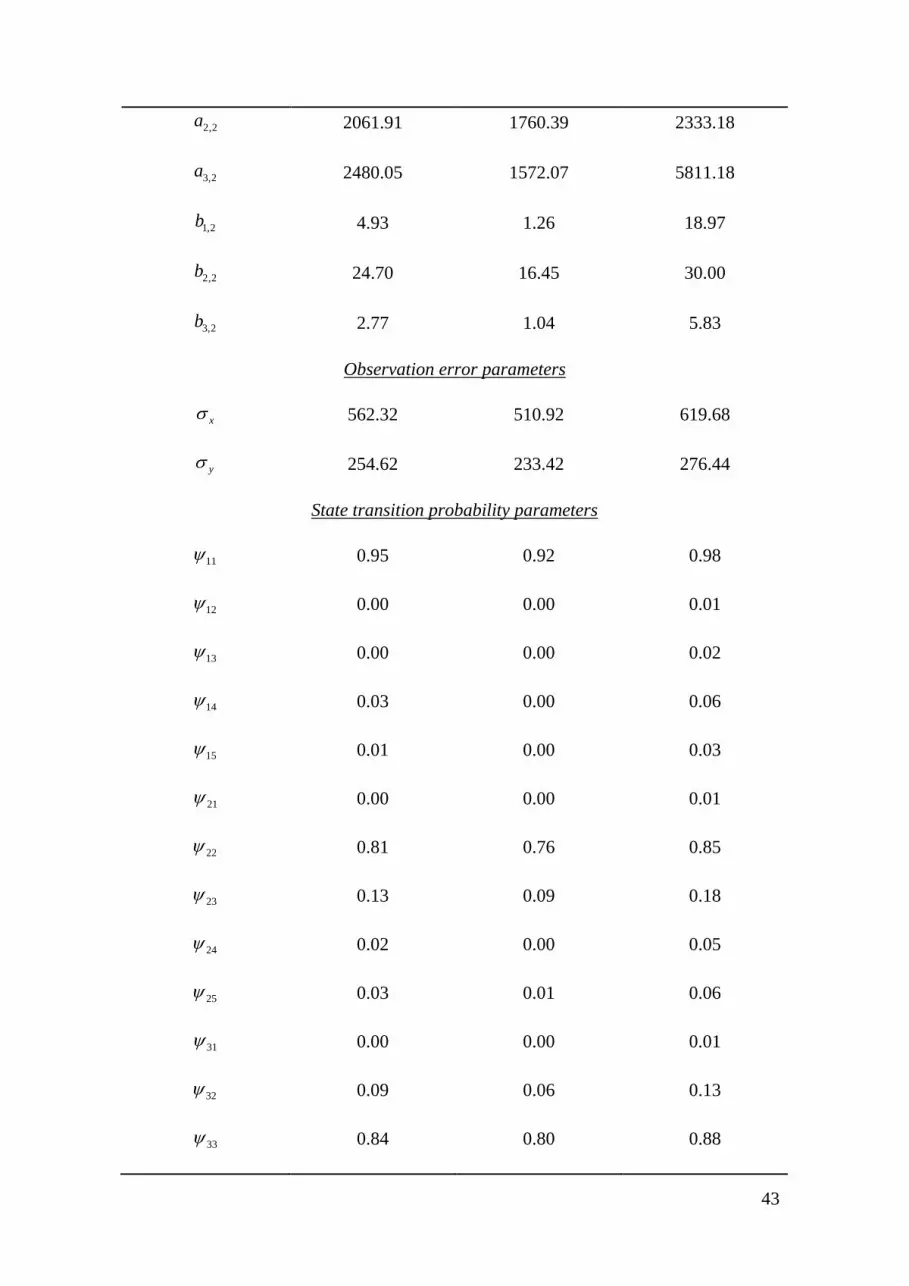
43
2,2a 2061.91 1760.39 2333.18
3,2a 2480.05 1572.07 5811.18
1,2b 4.93 1.26 18.97
2,2b 24.70 16.45 30.00
3,2b 2.77 1.04 5.83
Observation error parameters
xσ 562.32 510.92 619.68
yσ 254.62 233.42 276.44
State transition probability parameters
11ψ 0.95 0.92 0.98
12ψ 0.00 0.00 0.01
13ψ 0.00 0.00 0.02
14ψ 0.03 0.00 0.06
15ψ 0.01 0.00 0.03
21ψ 0.00 0.00 0.01
22ψ 0.81 0.76 0.85
23ψ 0.13 0.09 0.18
24ψ 0.02 0.00 0.05
25ψ 0.03 0.01 0.06
31ψ 0.00 0.00 0.01
32ψ 0.09 0.06 0.13
33ψ 0.84 0.80 0.88
44
34ψ 0.02 0.00 0.04
35ψ 0.04 0.02 0.06
41ψ 0.10 0.02 0.23
42ψ 0.16 0.01 0.33
43ψ 0.09 0.01 0.21
44ψ 0.41 0.20 0.62
45ψ 0.19 0.04 0.36
51ψ 0.01 0.00 0.03
52ψ 0.05 0.00 0.12
53ψ 0.15 0.07 0.24
54ψ 0.09 0.01 0.17
55ψ 0.69 0.59 0.78
898 899
900
901
902
903
904
905
906
907
908
909

45
Figure 1. Simulated time-series of animal location data using three centers of attraction 910
from multi-state (a) biased random walk; (b) biased correlated random walk; and (c) 911
biased correlated random walk with an exploratory state. The strength of bias towards 912
the corresponding center of attraction at each time step t, tz = 1,2,3, is a function of the 913
Euclidean distance between the current location and the center of attraction. 914
915
Figure 2. Observed locations for a grey seal as it traveled clockwise among a foraging 916
area in the North Sea and haul-out sites on the eastern coast of Great Britain. 917
918
Figure 3. Predicted locations, movement behavior states, and coordinates of three 919
centers of attraction for a grey seal in the North Sea and eastern coast of Great Britain. 920
Estimated movement states for the predicted locations (solid colored circles) correspond 921
to the Farne Islands haul-out site (red), Abertay haul-out site (green), Dogger Bank 922
foraging site (blue), or spatially-unassociated high-speed (light blue) and low-speed 923
(magenta) exploratory states. Solid yellow circles indicate the estimated coordinates of 924
the three centers of attraction, and solid black circles indicate observed locations in (a). 925
Uncertainty in the estimated state (< 95% posterior probability) is indicated by smaller 926
hollow circles within predicted locations in (a). Uncertainty in estimated coordinates 927
are indicated by symmetric 95% credible intervals for predicted locations in (b). An 928
animated version of this figure is available online (see Appendix C). 929
930
Figure 4. Model-averaged strength of bias ( )zρ to three centers of attraction as a 931
function of distance from a grey seal in the North Sea. Center of attraction states 932
correspond to the Farne Islands haul-out site (red), Abertay haul-out site (green), and 933
Dogger Bank foraging site (blue). Dashed lines indicate symmetric 95% credible 934

46
intervals. Lines terminate at the maximum distance at which the seal was assigned to 935
each respective center of attraction state. 936
937
938
939
940
941
942
943
944
945
946
947
948
949
950
951
952
953
954
955
956
957
958
959
47
Figure 1. 960
(a) 961
962
963
964
965
966
967
968
969

48
(b) 970
971
972
973
974
975
976
977
978
979
49
(c) 980
981
982
983
984
985
986
987
988
989

50
Figure 2. 990
991
992
993
994
995
996
997
998
999
1000
1001
1002
1003
1004

51
Figure 3. 1005
(a) 1006
1007
(b) 1008
1009

52
Figure 4. 1010
1011
1012