Centro de Investigación Operativa

I-2007-10

A first approximation of concatened convolutional codes from linear systems theory viewpoint

Joan Joseph Climent, Victoria Herranz, and

Carmen Perea

March 2007

ISSN 1576-7264 Depósito legal A-646-2000

Centro de Investigación Operativa Universidad Miguel Hernández de Elche Avda. de la Universidad s/n

03202 Elche (Alicante)

A first approximation of concatenated convolutional

codes from linear systems theory viewpoint∗

Joan-Josep ClimentInstitut Universitari d’Investigacio Informatica

Departament de Ciencia de la Computacio i Intel·ligencia Artificial,Universitat d’Alacant,

Ap. Correus 99, E-03080 Alacant, Spain.

Victoria Herranz Carmen PereaCentro de Investigacion Operativa,

Departamento de Estadıstica, Matematicas e Informatica,Universidad Miguel Hernandez,

Avenida del Ferrocarril, s/n. E-03202 Elche, Spain.

March 28, 2007

Abstract

This article focuses on the characterization of two models of concatenated convo-

lutional codes from the perspective of linear systems theory. We present an input-

state-output representation of these models and study the conditions for obtaining a

minimal input-state-output representation and non-catastrophic concatenated convolu-

tional code. We also establish conditions so that the concatenated codes are observable

and give a lower bound for their free distances.

Key words: Concatenated convolutional code, input-state-output representation, min-

imal representation, transfer function, observable convolutional code, controllable convolu-

tional code, observable pair, controllable pair, free distance.

1 Introduction

Coding theory has arisen from the need for better communication and better computer data

storage. Convolutional codes, a class of error correcting codes, are used in many wireless

∗This work was partially supported by Spanish grant MTM2005-05759

1

transmissions systems such as transmitting information in deep space with remarkable clarity.

A mathematical theory has been developed which has a strong relationship with algebra,

combinatorics and algebraic geometry. A key problem in convolutional coding theory was to

find a method for constructing codes of a given rate and complexity with good free distance.

Several methods have been introduced for this task. Perhaps the most popular technique is to

relate generator matrices of a convolutional code to generator matrices of some corresponding

cyclic or quasi-cyclic code (see for example [14, 18, 19, 29]). Abdel-Ghaffar [1] and Justesen

[15] limit their study to convolutional codes of rate 1/n and develop very effective techniques

for code constructions in this setting. Following this technique, Smarandache, Gluesing-

Luerssen and Rosenthal [27] give a construction of maximum distance separable convolutional

codes for each rate k/n and each degree δ.

It is common knowledge that there is a close connection between linear systems over finite

fields and convolutional codes. Rosenthal [22] provides a survey of the different points of view

about convolutional codes. Rosenthal, along with York and Schumacher ([25, 26]), intro-

duces the input-state-output representation and give a construction of a convolutional code

with free distance lower-bounded by the complexity of the code, using this representation.

Smarandache and Rosenthal [28], make a small adaptation to the construction presented in

[25] and introduce a construction of MDS convolutional codes of rate 1/n.

Another procedure for constructing new high rate convolutional codes from old ones is

via puncturing (see for example [21]). This method had widespread success because the

best codes constructed by puncturing are typically as powerful as other codes with the same

parameters, but are considerably easier to implement than “nonpunctured” codes.

In order to find a class of codes whose probability of error decreased exponentially with

code length, while decoding complexity increased only polynomially, Forney [3] came to

a solution consisting of the multilevel coding structure known as concatenated code. It

consists of a cascade of an inner and an outer code. Berrou, Glavieux and Thitimajshima

[2] introduce an interleaver between the two codes of the concatenation, which provides the

correction of error burst from the inner code by the outer code. The result was called “Turbo

Codes”.

Host, Johannesson, Sidorenko, Zigangirov, and Zyablov [7, 9], Host, Johannesson, Sidorenko,

Zigangirov, Zyablov, and Skopintsev [10] have developed a new construction of convolutional

codes based on code concatenation. This construction consists in a serial concatenation or

cascade of convolutional codes, but instead of letting one inner code follow one single outer

code, they put a set of parallel codes in place of the outer or the inner code, or both. Since

this construction resembles the structure of a fabric, they call these codes woven convolu-

tional codes.

Concatenated convolutional codes have always been studied from the generator matrix.

In this paper, we introduce a characterization of two kinds of concatenated convolutional

2

codes using linear systems theory. Host, Johannesson, Sidorenko, Zigangirov, and Zyablov

[8] show that the cascade of two canonical generator matrices is not necessarily canonical,

and therefore the degree of the convolutional code obtained from the cascade is unknown. In

this paper, we achieve conditions for the minimality of an input-state-output representation

of the concatenated code, so the degree of the cascade convolutional code can be obtained.

Furthermore, these authors give properties of the generator matrix and not for the codes,

as we give in this paper. Freudenberger, Jordan, Bossert and Shavgulidze [5], obtain a

concatenated code in a binary field with a free distance greater or equal to the product

of the free distances of the component codes under additional conditions in terms of the

interleavers between the codes. In contrast, working over an arbitrary field (not necessarily

binary), we do not only get a lower bound on the free distance of the models of concatenation

in terms of the free distance of the outer and inner codes, but also we obtain the degree of

the concatenated code. Therefore, we can compare this lower bound with the upper bound

given by the generalized Singleton bound.

This paper is structured as follows. In Section 2 we review the way convolutional codes

have often been defined in the coding literature. We also explain some recent advances in

systems theory in the context of convolutional codes defined over a Galois field. In Section 3

we study a first model of concatenated codes from the point of view of linear systems. We

also provide conditions in order to get a minimal input-state-output representation. We give

a lower bound of the free distance for these codes. A second model of concatenated codes

is developed in Section 4. These models of concatenation do not correspond to the classical

series connection in control theory (see for example [16]).

2 Preliminaries

Let F = GF (q) be the Galois field of q elements, F[z] the polynomial ring in the variable z

with coefficients in F, F(z) the field of rational functions over F, F((z)) the field of Laurent

series and F the algebraic closure of F.

Consider the matrices A ∈ Fδ×δ, B ∈ Fδ×k, C ∈ F(n−k)×δ and D ∈ F(n−k)×k. Following

[22] and [25], a rate k/n convolutional code C of degree of complexity δ can be described by

the linear system governed by the equations

xt+1 = Axt + But,

yt = Cxt + Dut,

vt =

(yt

ut

), x0 = 0,

(1)

where for each time instant t, xt ∈ Fδ is the state vector, ut ∈ Fk is the information vector,

and yt ∈ Fn−k is the parity vector. In linear systems theory, this representation is known

3

as the input-state-output representation. The integer δ describes the McMillan degree of the

linear system (1).

Remark 1: The input-state-output representation (1) is different from a realization often

found in the coding literature, where convolutional codes are usually represented by a driving

variable representation (see [21]),

xt+1 = Axt + Bmt,

vt = Cxt +Dmt.(2)

Here mt ∈ Fk is the message vector and vt ∈ Fn, xt ∈ Fδ as above. This representation

was introduced by Massey and Sain [20] and became the standard way in which convo-

lutional codes were represented in linear systems. Rosenthal and York [26] give us good

reasons for considering an input-state-output representation for the purpose of constructing

convolutional codes.

In terms of an input-state-output representation (1), the free distance of a convolutional

code C can be characterized (see [11]) as

dfree(C) = min

(∞∑

t=0

wt(ut) +∞∑

t=0

wt(yt)

)(3)

where the minimum has to be taken over all possible nonzero codewords and where wt

denotes the Hamming weight.

For algebraic reasons we assume that {vt ∈ Fn | t = 0, 1, 2, . . .} in Equation (1) is a finite-

weight codeword (see [26]), i.e., equation (1) is satisfied for all t = 0, 1, 2, . . . and there is an

integer γ such that xγ+1 = 0, ut = 0, for t ≥ γ+1, and therefore, yt = 0 for t ≥ γ+1, and the

code sequence has finite weight. Then, for a finite-weight codeword both the input sequence

and the state sequence (and hence the output sequence) need to have finite support. The set

of finite-weight codewords has a module structure over the polynomial ring F[z] (see [26]).

By abuse of notation, we will denote this module by C(A, B, C,D) and we refer it as the

finite-weight convolutional code generated by the matrices A, B, C, D.

Since F[z] is a principal ideal domain, C(A, B, C,D) is a free module of rank k and there

is an n× k polynomial matrix G(z) such that

C(A, B, C,D) = {v(z) ∈ Fn[z] | v(z) = G(z)m(z) for some m(z) ∈ Fk[z]}.

We call G(z) a polynomial generator matrix of the finite-weight convolutional code C(A, B, C,D).

In the sequel, we will study the properties of finite-weight convolutional codes of the

form C(A, B, C,D). It is customary to define a convolutional code as a F -linear subspace of

Fn, where F is either the field of rational functions F(z) or the field of Laurent series F((z))

4

[4, 12, 13, 21]. If G(z) is a polynomial generator matrix of C(A, B, C,D), then G(z) induces a

convolutional code C = C(A, B, C,D) ⊂ Fn by defining C as the F -linear span of the columns

of G(z) (see [26]). Observe that this definition is independent of the particular generator

matrix G(z) of C(A, B, C,D). The free distance of the convolutional code C is then defined

by expression (3), where the minimization is taken over all possible nonzero codewords in

C. By Lemma 2.13 of [26], if the pair (A, C) is observable, the free distance is attained in a

finite-weight codeword, that is, in a codeword of C(A, B, C,D). In fact, McElliece [21] shows

that finite-weight codewords are the only ones that can occur in engineering practice. So, in

this paper, we will consider

dfree(C) = limj→∞

dcj(C) (4)

where

dcj(C) = min

u0 6=0

{j∑

t=0

wt(ut) +

j∑t=0

wt(yt)

}(5)

is the jth column distance of the convolutional code C for j = 0, 1, 2, . . .

In the following, we adopt the notation used by McElliece [21] and we call a convolutional

code of rate k/n and degree δ an (n, k, δ)-code.

The free distance of an (n, k, δ)-code C is always upper-bounded (see [24]) by the gener-

alized Singleton bound

dfree(C) ≤ (n− k)

(⌊δ

k

⌋+ 1

)+ δ + 1.

In addition, the convolutional code C is called maximum-distance separable (MDS) if its free

distance is equal to the generalized Singleton bound.

We define a convolutional code to be observable if one, and therefore any, generator

matrix G(z) is right prime (see [23]). Furthermore, if G(z) is a generator matrix of an

observable convolutional code, then G(z) is a non-catastrophic generator matrix (see [23]).

Rosenthal and York [26] showed that expression (1) describes the state-space realization

of a rational and systematic convolutional encoder.

Theorem 1 (Lemma 2.14 of [26]): Let C(A, B, C,D) be a convolutional code. Then there

are polynomial matrices Y (z), and U(z) of sizes (n−k)×k and k×k, respectively, such that

the matrices A, B, C, and D appearing in (1) form a state-space realization of the transfer

function Y (z)U(z)−1, i.e., one has the relation

C(zI − A)−1B + D = Y (z)U(z)−1.

In particular, T (z) = Y (z)U(z)−1 describes a proper transfer function.

Furthermore, as a generator matrix over Fn[z], G(z) is equivalent to the systematic

generator matrix

Gsys(z) =

(Y (z)U(z)−1

Ik

).

5

Note that the description given by system (1) is generally not unique. Sometimes it is

possible to describe the code C(A, B, C,D) using matrices A1, B1, C1, D1 which are smaller

in size than the matrices A, B, C, D. But if C has degree δ, then it is possible (see [17]) to

choose matrices A, B, C, and D of sizes δ×δ, δ×k, (n−k)×δ and (n−k)×k, respectively.

In convolutional coding theory, an input-state-output representation (A, B, C,D) having the

above sizes is called a minimal representation and it is characterized through the condition

that the pair (A, B) is controllable, that is (see [26]),

rank(B AB · · · Aδ−1B

)= δ

or equivalently (see [6]),

rank(zI − A B

)= δ, for all z ∈ F.

On the other hand, we say that (A, C) is an observable pair if (AT , CT ) is a controllable

pair, that is (see [26]),

rank

C

CA...

CAδ−1

= δ

which is equivalent to (see [6]),

rank

(zI − A

C

)= δ, for all z ∈ F.

Notice that the concept of minimality of an input-state-output representation is different

from the concept of minimality of a representation in classical linear systems theory. A

representation (A, B, C,D) in linear systems literature is minimal if and only if (A, B) is

controllable and (A, C) is observable. In fact, if (A, B) is controllable, then the observabil-

ity of (A, C) ensures that the linear system (1) describes a noncatastrophic convolutional

encoder, as we can see in the following result.

Lemma 1 (Lemma 2.11 of [26]): Assume that the matrices (A, B) form a controllable

pair. The convolutional code C(A, B, C,D) defined through (1) represents an observable

convolutional code if and only if (A, C) forms an observable pair.

3 The first model of concatenated convolutional code

In this section, we introduce our first model of concatenated codes. Let Co and Ci be two

convolutional codes that we call outer code and inner code respectively. In this model, Co

6

Co

(m, k, δ1)

Ci

(n,m, δ2)- - -

-

-

-

u(1)t y

(1)t y

(2)t

y(1)t

u(1)t

Figure 1: Concatenated code CC(1)

is an (m, k, δ1)-code and Ci is an (n, m, δ2)-code. Let x(1)t , u

(1)t and y

(1)t be the state vector,

the information vector, and the parity vector of Co, respectively, and let x2t , u

(2)t , and y

(2)t be

the state vector, the information vector and the parity vector of Ci, respectively. Here the

codewords v(1)t and v

(2)t of Co and Ci respectively, are given by

v(1)t =

(y

(1)t

u(1)t

)and v

(2)t =

(y

(2)t

u(2)t

). (6)

In this model, the outer code Co and the inner code Ci are serialized, one after the other

(see Figure 1), so that the input information u(1)t is fed to Co and the obtained codeword v1

t

is then encoded by Ci in a way that

u(2)t = v

(1)t . (7)

We denote by CC(1) the corresponding concatenated convolutional code. Note that the vector

state xt, the information vector ut and the parity vector yt of CC(1) are given by

xt =

(x

(2)t

x(1)t

), ut = u

(1)t , and yt =

(y

(2)t

y(1)t

). (8)

So, the codewords vt of CC(1) are given by

vt =

(yt

ut

)=

y(2)t

y(1)t

u(1)t

=

(y

(2)t

v(1)t

)=

(y

(2)t

u(2)t

)= v

(2)t . (9)

Observe that a codeword of CC(1) is a codeword of Ci. Nevertheless, a codeword of Ci is

not necessarily a codeword of CC(1) (see Figure 1).

The next theorem introduces an input-state-output representation of the concatenated

convolutional code CC(1) from an input-state-output representation of the outer and inner

codes. In this paper we denote by O the zero matrix of the appropriate size.

7

Theorem 2: Let Co(A1, B1, C1, D1) be an (m, k, δ1)-code and let Ci(A2, B2, C2, D2) be an

(n, m, δ2)-code. Then an input-state-output representation for the rate k/n concatenated

code CC(1) is given by system (1), where

A =

(A2 B21C1

O A1

), B =

(B21D1 + B22

B1

),

C =

(C2 D21C1

O C1

), D =

(D21D1 + D22

D1

),

(10)

where B2 =(B21 B22

)and D2 =

(D21 D22

), with B21,B22, D21 and D22 matrices of sizes

δ2 × (m− k), δ2 × k, (n−m)× (m− k) and (n−m)× k, respectively.

Proof: ¿From expression (1) we have, for the code Co,

x(1)t+1 = A1x

(1)t + B1u

(1)t ,

y(1)t = C1x

(1)t + D1u

(1)t ,

and for the code Ci,

x(2)t+1 = A2x

(2)t + B2u

(2)t ,

y(2)t = C2x

(2)t + D2u

(2)t .

Now, taking into account that u(2)t = v

(1)t , if we consider the block partition of B2 =(

B21 B22

)and D2 =

(D21 D22

), in accordance with the block partition of u

(2)t =

(u(2)t,1 , u

(2)t,2 ), where u

(2)t,1 ∈ Fm−k and u

(2)t,2 ∈ Fk, then an input-state-output representation

of the concatenated code CC(1) is given by

xt+1 =

(A2 B21C1

O A1

)xt +

(B21D1 + B22

B1

)ut,

yt =

(C2 D21C1

O C1

)xt +

(D21D1 + D22

D1

)ut. �

By Theorems 1 and 2, it follows that the transfer function T (z) associated to the con-

catenated code CC(1) has the form given by Equation (11) in terms of the transfer functions

T1(z) and T2(z) associated to the outer code Co and the inner code Ci, respectively.

Theorem 3: Let T1(z) be the transfer function of the outer code Co and let T2(z) be the

transfer function of the inner code Ci. Then the transfer function T (z) associated to the

concatenated code CC(1) is

T (z) =

(T21(z)T1(z) + T22(z)

T1(z)

)(11)

where T2(z) =(T21(z) T22(z)

)with T21(z) and T22(z) matrices of sizes (n−m)× (m− k)

and (n−m)× k, respectively.

8

Now, we are interested in the conditions of the matrices Al, Bl, Cl, and Dl, for l = 1, 2, of

the outer and inner codes so that the concatenated code has a “good” representation. The

next example shows that it is not enough for the pair (Al, Bl) to be controllable, for l = 1, 2,

in order to get a controllable pair (A, B) of the concatenated code.

Example 1: Let α be a primitive element of the Galois field F = GF (8) with α3+α+1 = 0,

and consider the (2, 1, 2)-outer code Co(A1, B1, C1, D1), where

A1 =

(α 0

0 α2

), B1 =

(1 0

0 α6

), C1 =

(α4 α3

), D1 =

(1 α4

),

and a (3, 2, 2)-inner code Ci(A2, B2, C2, D2), where

A2 =

(α4 1

α3 0

), B2 =

(1 0 1

α 1 α

),

and C2 and D2 are arbitrary matrices.

For all z ∈ F we have that

rank(zIδ1 − A1 B1

)= rank

(z + α 0 1 0

0 z + α2 0 α6

)= 2,

rank(zIδ2 − A2 B2

)= rank

(z + α4 1 1 0 1

α3 z α 1 α

), = 2

and therefore, the pairs (A1, B1) and (A2, B2) are controllable.

Now, from Theorem 2, the matrices A and B for an input-state-output representation of

the concatenated code CC(1) are

A =

α4 1 α4 α3

α3 0 α5 α4

0 0 α 0

0 0 0 α2

and B =

1 α5

α3 α6

1 0

0 α6

.

Then, the pair (A, B) is not controllable because

rank(αI − A B

)= rank

α2 1 α4 α3 1 α5

α3 α α5 α4 α3 α6

0 0 0 0 1 0

0 0 0 α4 0 α6

= 3 6= 4.

The next theorem gives conditions which ensure both the controllability of the pair (A, B)

and the observability of the pair (A, C).

9

Theorem 4: Let Co(A1, B1, C1, D1) be an (m, k, δ1)-code and let Ci(A2, B2, C2, D2) be an

(n, m, δ2)-code. Let CC(1)(A, B, C,D) be the concatenated code described by the matrices in

expression (10).

(a) If rank(B) = δ1 + δ2, then (A, B, C,D) is a minimal representation of CC(1) with

complexity δ1 + δ2.

(b) If the pair (Al, Cl) is observable for l = 1, 2, then the pair (A, C) is observable.

Proof: (a) Since rank(B) = δ1 + δ2, it is clear that

rank(zI − A B

)= δ1 + δ2 for all z ∈ F.

So, the pair (A, B) is controllable and, consequently, (A, B, C,D) is a minimal representation

of CC(1).

(b) For all z ∈ F, we have, from the size of the matrix

(zI − A

C

), that

rank

(zI − A

C

)≤ δ1 + δ2.

Furthermore,

rank

(zI − A

C

)= rank

zIδ2 − A2 −B21C1

C2 D21C1

O zIδ1 − A1

O C1

≥ rank

(zIδ2 − A2

C2

)+ rank

(zIδ1 − A1

C1

)= δ2 + δ1.

So the rank

(zI − A

C

)= δ1 + δ2, and the pair (A, C) is observable. �

Now, as a consequence of Theorem 4 and Lemma 1, we have the following result.

Corollary 1: Let Co(A1, B1, C1, D1) be an (m, k, δ1)-code and let Ci(A2, B2, C2, D2) be an

(n, m, δ2)-code. Let CC(1)(A, B, C,D) be the concatenated code described by the matrices in

expression (10). Assume the following two conditions hold.

(a) rank(B) = δ1 + δ2,

(b) The matrices (Al, Cl) form an observable pair, for l = 1, 2.

10

Then (A, B, C,D) is a minimal representation of the observable convolutional code CC(1) with

complexity δ1 + δ2.

Remark 2: Note that the condition (a) of Theorem 4 implies that the pair (Al, Bl) is

controllable, for l = 1, 2.

Firstly, from (a) and the sizes of B1 and B2, it follows that

rank(B21D1 + B22) = δ2, (12)

rank(B1) = δ1. (13)

Now, from expression (13), we obtain that B1 has full row rank. So the matrices (A1, B1)

form a controllable pair.

On the other hand, if (A2, B2) is not a controllable pair, then, from relation (2.14) of

[26], the matrix B2 can be expressed as B2 =(B21 B22

)= S−1

(B2

O

), so it is not fullrank.

Furthermore, if rank(B2) = r2 < δ2, then we obtain that

rank(B2D1 + B22) ≤ r2 < δ2,

which contradicts (12).

Remark 3: Example 1 also shows that the converse of Remark 2 is not true in general

because the pair (Al, Bl) is controllable, for l = 1, 2, but rank(B) = 2 6= 2 + 2.

The next result gives conditions in order to achieve the controllability of the pair (A, B)

of the concatenated code CC(1), for the particular case where the outer code has rate 1/2

and complexity δ1 = 1 and the matrix A2 is a diagonal matrix.

Theorem 5: Let Co(A1, B1, C1, D1) be a (2, 1, 1)-code and let Ci(A2, B2, C2, D2) be an (n, 2, δ2)-

code. Let CC(1)(A, B, C,D) the concatenated code described by the matrices in expression

(10). Assume the following conditions hold.

(a) A2 is a diagonal matrix.

(b) The matrices (A1, B1) form a controllable pair and the matrices (A2, B21) form a con-

trollable pair.

(c) All the elements of vector B21 are nonzero and B22 is a zero vector.

(d) rank

(−C1 D1

λI − A1 B1

)= 2 for all λ eigenvalue of A.

Then, (A, B, C,D) is a minimal representation of the concatenated code CC(1) with complexity

δ1 + δ2 = 1 + δ2.

11

Proof: Taking into account that the outer code Co(A1, B1, C1, D1) is a (2, 1, 1)-code, the

matrices A1 =(a1

), B1 =

(b1

), C1 =

(c1

), and D1 =

(d1

)are scalar matrices. Now,

since B21 is a (δ2 × 1)-vector and the matrices (A2, B21) form a controllable pair, then all

the eigenvalues of A2 are different. Let

A2 = diag[λ1, λ2, . . . , λδ2 ] and B21 =

b12

b22

...

bδ22

.

First, assume that λ is an eigenvalue of A with λ 6= a1. We can assume, without loss of

generality, that λ = λ1. Then,

(λ1I − A B

)=

0 0 · · · 0 −b12c1 b12d1

0 λ1 − λ2 · · · 0 −b22c1 b22d1

......

......

...

0 0 · · · λ1 − λδ2 −bδ22c1 bδ22d1

0 0 · · · 0 λ1 − a1 b1

,

and taking into account that all the eigenvalues of A2 are different and conditions (c) and

(d), we get

rank(diag[λ1 − λ2, λ1 − λ3, . . . , λ1 − λδ2 ]) = δ2 − 1

and

rank

(−b12c1 b12d1

λ1 − a1 b1

)= rank

(−C1 D1

λ1I − A1 B1

)= 2.

Then,

rank(λ1I − A B

)= 2 + δ2 − 1 = 1 + δ2 = δ1 + δ2.

Let λ an eigenvalue of A with λ = a1. If λ is not an eigenvalue of A2, and we denote

A2 = diag[λ− λ1, λ− λ2 . . . , λ− λδ2 ] = diag[a1 − λ1, a1 − λ2, . . . , a1 − λδ2 ]

then, rank(A2) = δ2, so

rank(λI − A B

)= rank

(a1I − A B

)= rank

(A2 −B2C1 B2D1

O O B1

)= δ2 + 1,

since from condition (b), the pair (A1, B1) is controllable and, in particular, b1 6= 0, because

δ1 = 1.

12

Finally, if λ = a1 is also an eigenvalue of A2, then we can assume, without loss of

generality, that λ = λ1. Then, taking into account that all the eigenvalues of A2 are different,

rank(λI − A B

)= rank

0 0 · · · 0 −b12c1 b12d1

0 λ1 − λ2 · · · 0 −b22c1 b22d1

......

......

...

0 0 · · · λ1 − λδ2 −bδ22c1 bδ22d1

0 0 · · · 0 0 b1

= δ2 + 1.

since from conditions (c) and (d),

rank

(−b12c1 b12d1

0 b1

)= rank

(−b12c1 b12d1

λ− a1 b1

)= rank

(−C1 D1

λI − A1 B1

)= 2.

We conclude then,

rank(zI − A B

)= δ1 + δ2 for all z ∈ F,

that is, the matrices (A, B) form a controllable pair. �

Remark 4: Using the conditions of the above theorem, λ = a1 is an eigenvalue of matrix

A, so condition (d) is simplified to

rank

(−C1 D1

λI − A1 B1

)= rank

(−C1 D1

O B1

)= 2,

and consequently the matrices (A1, C1) form an observable pair, since δ1 = 1.

For the particular case where the complexity of the outer code and the inner code is

δ1 = δ2 = 1, we get the following result.

Theorem 6: Let Co(A1, B1, C1, D1) be an (m, k, 1)-code and let Ci(A2, B2, C2, D2) be an

(n, m, 1)-code. Let CC(1)(A, B, C,D) be the concatenated code described by matrices in ex-

pression (10). Assume the following conditions hold.

(a) The matrices (A1, B1) form a controllable pair.

(b) The matrix

(−B21C1 B21D1 + B22

A2 − A1 B1

), of size 2× (k + 1), has rank equal to 2.

Then, (A, B, C,D) is a minimal representation of the concatenated code CC(1)(A, B, C,D)

with complexity δ1 + δ2 = 2.

13

Proof: First, note that since δ1 = δ2 = 1, we have that A1 =(a1

)and A2 =

(a2

). So,

the eigenvalues of the matrix A of the code CC(1)(A, B, C,D) are a1 and a2. Supposing that

a1 = a2 = λ, then, from condition (b), we get

rank(λI − A B

)= rank

(O −B21C1 B21D1 + B22

O O B1

)= 2.

So rank(zI − A B

)= 2 = δ1 + δ2 for all z ∈ F, that is, the pair (A, B) is controllable.

Now, suppose that a1 6= a2. Then,

2 ≥ rank(a1I − A B

)= rank

(a1 − a2 −B21C1 B21D1 + B22

0 0 B1

)

≥ rank

(a1 − a2 B2D1

0 B1

)= 2

since from condition (a), we get B1 6= 0. Furthermore, from condition (b),

rank(a2I − A B

)= rank

(0 −B21C1 B21D1 + B22

0 a2 − a1 B1

)= 2.

Then, rank(zI − A B

)= 2 = δ1 +δ2 for all z ∈ F, that is, the pair (A, B) is controllable.�

Observe that the condition

rank

(−B21C1 B21D1 + B22

A2 − A1 B1

)= 2

of Theorem 6, does not imply necessarily that (A2, B21) is controllable. In fact, only if the

matrix B22 is the zero matrix, the previous condition implies the controllability of (A2, B21).

In the rest of the cases, we do not have this result, as we can see in the next example.

Example 2: As in Example 1, let α be a primitive element of F = GF (8). Let Co(A1, B1, C1, D1)

be a (4, 2, 1)-code, where C1 and D1 are arbitrary matrices of sizes 2×1 and 2×2, respectively,

and

A1 =(α)

, B1 =(1 1

).

Let Ci(A2, B2, C2, D2) be a (5, 4, 1)-code, where C2 and D2 are arbitrary matrices of sizes

1× 1 and 1× 4, respectively, and

A2 =(α3)

, B2 =(B21 B22

)=(0 0 α α

).

Observe that the pair (A2, B21) is not controllable, since B21 =(0 0

). Nevertheless,

rank

(−B21C1 B21D1 + B22

A2 − A1 B1

)= rank

(0 α α

1 1 1

)= 2,

14

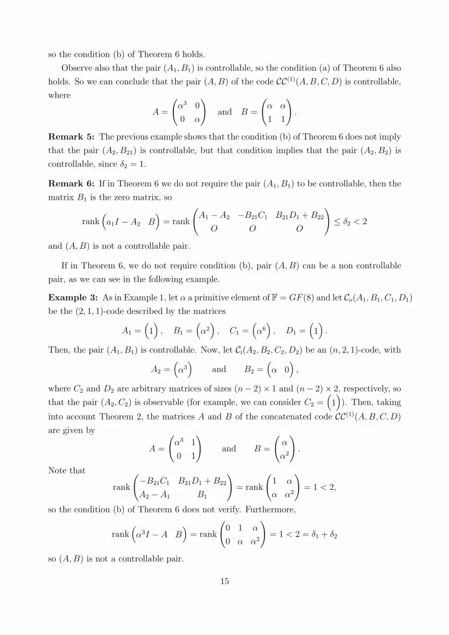
so the condition (b) of Theorem 6 holds.

Observe also that the pair (A1, B1) is controllable, so the condition (a) of Theorem 6 also

holds. So we can conclude that the pair (A, B) of the code CC(1)(A, B, C,D) is controllable,

where

A =

(α3 0

0 α

)and B =

(α α

1 1

).

Remark 5: The previous example shows that the condition (b) of Theorem 6 does not imply

that the pair (A2, B21) is controllable, but that condition implies that the pair (A2, B2) is

controllable, since δ2 = 1.

Remark 6: If in Theorem 6 we do not require the pair (A1, B1) to be controllable, then the

matrix B1 is the zero matrix, so

rank(a1I − A2 B

)= rank

(A1 − A2 −B21C1 B21D1 + B22

O O O

)≤ δ2 < 2

and (A, B) is not a controllable pair.

If in Theorem 6, we do not require condition (b), pair (A, B) can be a non controllable

pair, as we can see in the following example.

Example 3: As in Example 1, let α a primitive element of F = GF (8) and let Co(A1, B1, C1, D1)

be the (2, 1, 1)-code described by the matrices

A1 =(1)

, B1 =(α2)

, C1 =(α6)

, D1 =(1)

.

Then, the pair (A1, B1) is controllable. Now, let Ci(A2, B2, C2, D2) be an (n, 2, 1)-code, with

A2 =(α3)

and B2 =(α 0

),

where C2 and D2 are arbitrary matrices of sizes (n− 2)× 1 and (n− 2)× 2, respectively, so

that the pair (A2, C2) is observable (for example, we can consider C2 =(1)). Then, taking

into account Theorem 2, the matrices A and B of the concatenated code CC(1)(A, B, C,D)

are given by

A =

(α3 1

0 1

)and B =

(α

α2

).

Note that

rank

(−B21C1 B21D1 + B22

A2 − A1 B1

)= rank

(1 α

α α2

)= 1 < 2,

so the condition (b) of Theorem 6 does not verify. Furthermore,

rank(α3I − A B

)= rank

(0 1 α

0 α α2

)= 1 < 2 = δ1 + δ2

so (A, B) is not a controllable pair.

15

As a consequence of Theorem 6, we get the following result for the particular case where

the matrices A1 and A2 are equal.

Corollary 2: Let Co(A1, B1, C1, D1) be an (m, k, 1)-code, and let Ci(A2, B2, C2, D2) be an

(n, m, 1)-code. Let CC(1)(A, B, C,D) be the concatenated code described by the matrices in

expression (10). Assume that the following conditions hold.

(a) A1 = A2.

(b) The matrices (A1, B1) form a controllable pair.

(c) The vectors B21 and C1 are not orthogonal vectors.

Then, (A, B, C,D) is a minimal representation for the concatenated code CC(1) with com-

plexity δ1 + δ2 = 2.

Remark 7: Note that condition (c) of Corollary 2 implies in particular that the matrices

(A2, B21) form a controllable pair (and then, the matrices (A2, B2) form a controllable pair,

since δ2 = 1) and the matrices (A1, C1) form an observable pair.

If the outer code has rate k/(k+1), then the matrices B21 and C1 are of size 1×1. Then,

the vectors B21 and C1 are orthogonal if and only if one of them is the zero vector; so it is

sufficient to have controllability of pair (A2, B21) and observability of (A1, C1) so that the

condition (c) of Corollary 2 holds. Then, we get the following result.

Corollary 3: Let Co(A1, B1, C1, D1) be a (k + 1, k, 1)-code and let Ci(A2, B2, C2, D2) be an

(n, k + 1, 1)-code. Let CC(1)(A, B, C,D) be the concatenated code described by matrices in

expression (10). Assume the following conditions hold.

(a) A1 = A2.

(b) The matrices (A1, B1) form a controllable pair.

(c) The matrices (A2, B21) form a controllable pair.

(d) The matrices (A1, C1) form an observable pair.

Then, (A, B, C,D) is a minimal representation of the concatenated code CC(1) with complexity

δ1 + δ2 = 2.

Example 1 shows that it is not enough for the pair (Al, Bl) to be controllable, for l = 1, 2,

in order to get a controllable pair (A, B) of the concatenated code. For the particular case

where the outer code has rate 1/2 and all eigenvalues of A2 are eigenvalues of A1, that is,

σ(A2) ⊆ σ(A1), where σ(Ai) is the spectrum of Ai, we have the following result.

16

Theorem 7: Let Co(A1, B1, C1, D1) be a (2, 1, δ1)-code and let Ci(A2, B2, C2, D2) be an (n, 2, δ2)-

code. Let CC(1)(A, B, C,D) be the concatenated code described by the matrices in expression

(10). Assume the following conditions hold.

(a) σ(A2) ⊆ σ(A1).

(b) The matrices (A1, B1) form a controllable pair.

(c) The matrices (A2, B21) form a controllable pair.

(d) All the elements of matrix B21 are nonzero.

(e) The matrices (Al, Cl) form an observable pair, for l = 1, 2.

Then, (A, B, C,D) is a minimal representation of the concatenated code CC(1) with complexity

δ1 + δ2. Furthermore, CC(1) is an observable convolutional code.

Proof: Firstly, assume that δ1 = 1, then from condition (e), the pair (A1, C1) is observable,

so the (1× 1)-matrix C1 must be nonzero. Now, taking into account conditions (a) and (c),

rank(zI − A B

)= 1 + δ2 = δ1 + δ2

for all z ∈ F.

Now, assume that δ1 > 1 and suppose that for some z ∈ F, we have

rank(zI − A B

)< δ1 + δ2, (14)

so from condition (a), z ∈ σ(A) = σ(A1). By condition (b),

δ1 = rank(zIδ1 − A1 B1

)= rank

(O zIδ1 − A1 B1

)(15)

and, by conditions (c), (d) and (e), it follows that

δ2 = rank(zIδ2 − A2 B21

)=(zIδ2 − A2 −B21C1

). (16)

Now, taking into account the relations (14), (15) and (16), we have that one row of the

matrix(zIδ2 − A2 −B21C1 B21D1 + B22

)is a linear combination of the rows of the matrix(

O zIδ1 − A1 B1

)or one row of the matrix

(O zIδ1 − A1 B1

)is a linear combination

of the rows of the matrix(zIδ2 − A2 −B21C1 B21D1 + B22

). But then, from condition

(d), rank

(zIδ1 − A1

C1

)< δ1, which contradicts condition (e) for l = 1.

The observability condition for (A, C) follows from condition (e) using a similar argument

to Theorem 4. Finally, we get the observability condition of CC(1) by using Lemma 1. �

17

If in Theorem 7 we do not require the controllability condition of (A2, B21) then, the

representation of the concatenated code CC(1) may be nonminimal, as we can see in the

following example.

Example 4: For matrices in Example 1, the pair (A2, B2) is controllable. Nevertheless, the

pair (A2, B21) =

((α4 1

α3 0

),

(1

α

))is not controllable because

rank(αI − A2 B21

)= rank

(α2 1 1

α3 α α

)= 1 6= 2.

Furthermore, σ(A2) = {α, α2} = σ(A1), the matrices (A1, B1) and (A1, C1) form a con-

trollable and an observable pair, respectively, and all the elements of B21 are nonzero. So all

the conditions but condition (c) are verified. Now, since the pair (A, B) is not controllable

(see Example 1), the representation (A, B, C,D) is non-minimal.

Theorem 7 does not verify if σ(A2) 6⊆ σ(A1), as we can see in the following example.

Example 5: Let α be a primitive element of F = GF (8), as in Example 1. Let Co(A1, B1, C1, D1)

be the (2, 1, 1)-code described by matrices

A1 =(α2)

, B1 =(α)

, C1 =(1)

, D1 =(α)

and let Ci(A2, B2, C2, D2) be a (3, 2, 1)-code described by matrices

A2 =

(α2 0

1 α6

), B2 =

(B21 B22

)=

(α 0

1 0

),

where C2 and D2 are arbitrary matrices of sizes 1×2 and 1×1, respectively, so that (A2, C2) is

observable. Observe that (A1, B1) and (A2, B21) are controllable pairs, (Al, Cl) is observable,

for l = 1, 2 and all the elements of B21 are nonzero. Nevertheless,

σ(A2) = {α2, α6} 6⊆ {α2} = σ(A1).

Taking into account Theorem 2, the matrices A and B of an input-state-output repre-

sentation of the code CC(1) are given by

A =

α2 0 α

1 α6 1

0 0 α2

and B =

α2

α

α

.

Now,

rank(α6I − A B

)= rank

1 0 α α2

1 0 1 α

0 0 1 α

= 2 6= 3,

so (A, B) is not a controllable pair.

18

Once we have seen that we can obtain “good” representations for the concatenated code

CC(1), we provide, in the next theorem, a lower bound for the free distance of CC(1) in terms

of the free distances of Co and Ci. Firstly, we obtain a lower bound for the column distances

of CC(1), also in terms of the column distances of Co and Ci.

Lemma 2: Let CC(1) be the concatenated code given by Theorem 2 from the outer code Co

and the inner code Ci. Then

dcj(CC(1)) ≥ max

{dc

j(Co), dcj(Ci)

}for j = 0, 1, 2, . . . (17)

Proof: Taking into account expression (5), the relations between yt, y(1)t , y

(2)t ; ut, u

(1)t , u

(2)t ,

and vt, v(1)t , v

(2)t given by expressions (6)–(9), and that the condition u0 6= 0 implies u

(1)0 6= 0

and u(2)0 6= 0, we have

dcj(CC(1)) = min

u0 6=0

{j∑

t=0

wt(vt)

}≥ min

u(1)0 6=0

{j∑

t=0

wt(v(1)t )

}= dc

j(Co), (18)

dcj(CC(1)) = min

u0 6=0

{j∑

t=0

wt(vt)

}≥ min

u(2)0 6=0

{j∑

t=0

wt(v(2)t )

}= dc

j(Ci). (19)

Now, inequality (17) follows from inequalities (18) and (19). �

Now, as an immediate consequence of expression (4) and the above lemma we obtain the

following result.

Theorem 8: Let CC(1) be the concatenated code given by Theorem 2 from the outer code Co

and the inner code Ci. Then,

dfree(CC(1)) ≥ max {dfree(Co), dfree(Ci)} . (20)

We finish this section with an example. We use the construction proposed by Smaran-

dache and Rosenthal [28] in order to consider an outer MDS convolutional code. In this

case, we obtain a concatenated code CC(1) with free distance close to the Singleton bound.

We use a computer algebra program to obtain the free distances.

Example 6: Let α be a primitive element of F = GF (8), as in Example 1. Let Co(A1, B1, C1, D1)

be the (2, 1, 2)-code, where

A1 =

(α 0

0 α2

), B1 =

(1

1

), C1 =

(α5 α2

), D1 =

(1)

.

It follows that Co is an MDS convolutional code (see [28]), so dfree(Co) = 6. In addition, Co

in an observable convolutional code and the pair (A1, B1) is controllable.

19

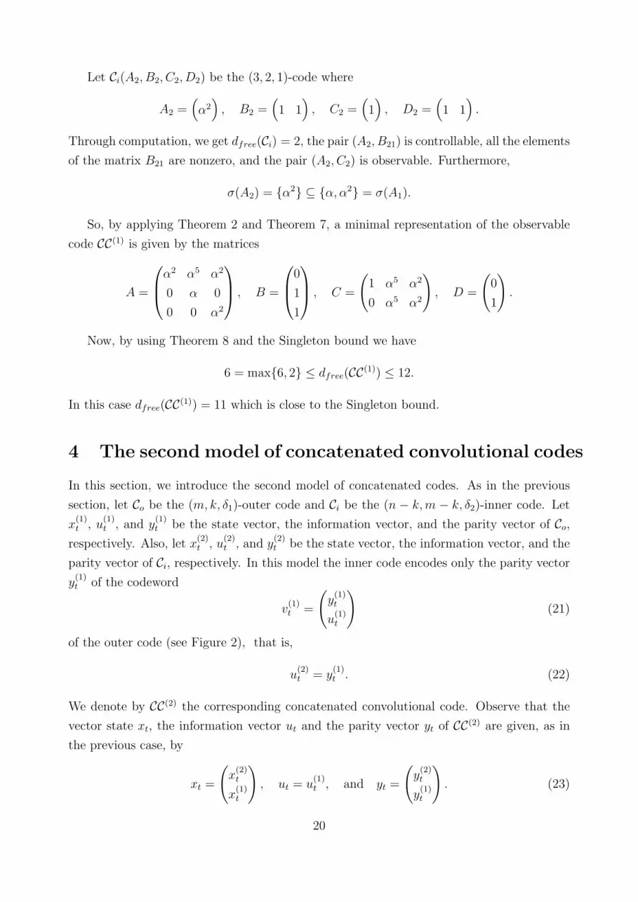
Let Ci(A2, B2, C2, D2) be the (3, 2, 1)-code where

A2 =(α2)

, B2 =(1 1

), C2 =

(1)

, D2 =(1 1

).

Through computation, we get dfree(Ci) = 2, the pair (A2, B21) is controllable, all the elements

of the matrix B21 are nonzero, and the pair (A2, C2) is observable. Furthermore,

σ(A2) = {α2} ⊆ {α, α2} = σ(A1).

So, by applying Theorem 2 and Theorem 7, a minimal representation of the observable

code CC(1) is given by the matrices

A =

α2 α5 α2

0 α 0

0 0 α2

, B =

0

1

1

, C =

(1 α5 α2

0 α5 α2

), D =

(0

1

).

Now, by using Theorem 8 and the Singleton bound we have

6 = max{6, 2} ≤ dfree(CC(1)) ≤ 12.

In this case dfree(CC(1)) = 11 which is close to the Singleton bound.

4 The second model of concatenated convolutional codes

In this section, we introduce the second model of concatenated codes. As in the previous

section, let Co be the (m, k, δ1)-outer code and Ci be the (n − k,m − k, δ2)-inner code. Let

x(1)t , u

(1)t , and y

(1)t be the state vector, the information vector, and the parity vector of Co,

respectively. Also, let x(2)t , u

(2)t , and y

(2)t be the state vector, the information vector, and the

parity vector of Ci, respectively. In this model the inner code encodes only the parity vector

y(1)t of the codeword

v(1)t =

(y

(1)t

u(1)t

)(21)

of the outer code (see Figure 2), that is,

u(2)t = y

(1)t . (22)

We denote by CC(2) the corresponding concatenated convolutional code. Observe that the

vector state xt, the information vector ut and the parity vector yt of CC(2) are given, as in

the previous case, by

xt =

(x

(2)t

x(1)t

), ut = u

(1)t , and yt =

(y

(2)t

y(1)t

). (23)

20

Co

(m, k)

Ci

(n− k,m− k)- - -

-

-

u(1)t y

(1)t y

(2)t

y(1)t

u(1)t

Figure 2: Concatenated Code CC(2)

But in this case, the codewords vt of CC(2) are given by

vt =

(yt

ut

)=

y(2)t

y(1)t

u(1)t

=

(y

(2)t

v(1)t

). (24)

Nevertheless, since the codewords of Ci are given by

v(2)t =

(y

(2)t

u(2)t

)=

(y

(2)t

y(1)t

)(25)

we have that vt 6= v(2)t .

Note that the form of the concatenated code CC(2) just introduced is different from the

form CC(1) proposed in Section 3. For the concatenated code CC(1) the information vector

u(2)t of the inner code Ci is the whole codeword v

(1)t of the outer code Co; there, u

(2)t = v

(1)t

has m components. In contrast, for the concatenated code CC(2), the information vector u(2)t

of the inner code Ci is only the parity vector y(1)t of the codeword v

(1)t of the outer code Co;

in this case u(2)t = y

(1)t has m− k components. So the parameters of the inner code of CC(2)

are different from the parameters of the inner code of CC(1).

The next theorem introduces an input-state-output representation of the concatenated

convolutional code CC(2) from an input-state-output representation of the outer and inner

codes.

Theorem 9: Let Co(A1, B1, C1, D1) be an (m, k, δ1)-code and let Ci(A2, B2, C2, D2) be an

(n− k,m− k, δ2)-code. Then an input-state-output representation for the concatenated code

CC(2) of rate k/n is given by system (1), where

A =

(A2 B2C1

O A1

), B =

(B2D1

B1

),

C =

(C2 D2C1

O C1

), D =

(D2D1

D1

).

(26)

21

Proof: By proceeding as in the proof of Theorem 2 we have

x(1)t+1 = A1x

(1)t + B1u

(1)t ,

y(1)t = C1x

(1)t + D1u

(1)t ,

x(2)t+1 = A2x

(2)t + B2u

(2)t ,

y(2)t = C2x

(2)t + D2u

(2)t .

Now, taking into account that u(2)t = y

(1)t and the comments at beginning of the section,

an input-state-output representation of the concatenated code CC(2) is given by

xt+1 =

(A2 B2C1

O A1

)xt +

(B2D1

B1

)ut,

yt =

(C2 D2C1

O C1

)xt +

(D2D1

D1

)ut.

�

Using Theorems 1 and 9, the next theorem allows us to obtain the transfer function T (z)

associated to the concatenated code CC(2) in terms of the transfer functions T1(z) and T2(z)

associated to the outer code C0 and the inner code Ci, respectively.

Theorem 10: Let T1(z) be the transfer function of the outer code Co and let T2(z) be the

transfer function of the inner code Ci. Then the transfer function T (z) associated to the

concatenated code CC(2) is

T (z) =

(T2(z)T1(z)

T1(z)

).

The next example shows that if pair (A1, B1) of the inner code and pair (A2, B2) of the

outer code are controllable, then pair (A, B) of the concatenated code CC(2) is not necessarily

a controllable pair.

Example 7: As in Example 1, let α be a primitive element of the Galois field F = GF (8).

Consider the (2, 1, 1)-outer code Co(A1, B1, C1, D1), where

A1 =(0)

, B1 =(1)

, C1 =(α4)

, D1 =(α3)

and the (2, 1, 1)-inner code Ci(A2, B2, C2, D2), where

A2 =(α)

, B2 =(1)

, C2 =(α4)

, D2 =(1)

.

It follows then that the matrices (Al, Bl) form a controllable pair, for l = 1, 2.

Now, from Theorem 9, the matrices A and B of an input-state-output representation of

the concatenated code CC(2) are

A =

(α α4

0 0

)and B =

(α3

1

).

But (A, B) is not a controllable pair because rank(αI − A B

)= 1 6= 2.

22

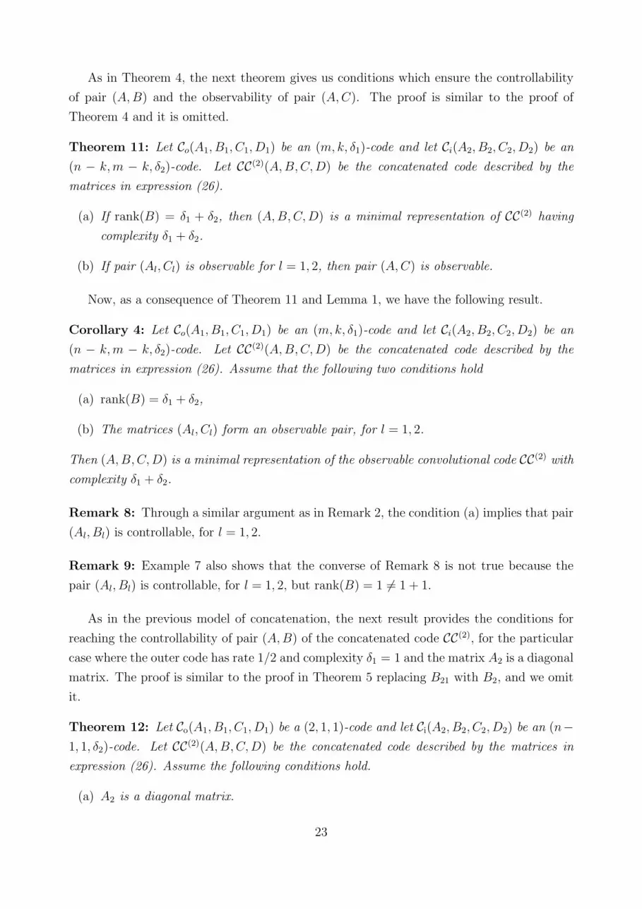
As in Theorem 4, the next theorem gives us conditions which ensure the controllability

of pair (A, B) and the observability of pair (A, C). The proof is similar to the proof of

Theorem 4 and it is omitted.

Theorem 11: Let Co(A1, B1, C1, D1) be an (m, k, δ1)-code and let Ci(A2, B2, C2, D2) be an

(n − k,m − k, δ2)-code. Let CC(2)(A, B, C,D) be the concatenated code described by the

matrices in expression (26).

(a) If rank(B) = δ1 + δ2, then (A, B, C,D) is a minimal representation of CC(2) having

complexity δ1 + δ2.

(b) If pair (Al, Cl) is observable for l = 1, 2, then pair (A, C) is observable.

Now, as a consequence of Theorem 11 and Lemma 1, we have the following result.

Corollary 4: Let Co(A1, B1, C1, D1) be an (m, k, δ1)-code and let Ci(A2, B2, C2, D2) be an

(n − k,m − k, δ2)-code. Let CC(2)(A, B, C,D) be the concatenated code described by the

matrices in expression (26). Assume that the following two conditions hold

(a) rank(B) = δ1 + δ2,

(b) The matrices (Al, Cl) form an observable pair, for l = 1, 2.

Then (A, B, C,D) is a minimal representation of the observable convolutional code CC(2) with

complexity δ1 + δ2.

Remark 8: Through a similar argument as in Remark 2, the condition (a) implies that pair

(Al, Bl) is controllable, for l = 1, 2.

Remark 9: Example 7 also shows that the converse of Remark 8 is not true because the

pair (Al, Bl) is controllable, for l = 1, 2, but rank(B) = 1 6= 1 + 1.

As in the previous model of concatenation, the next result provides the conditions for

reaching the controllability of pair (A, B) of the concatenated code CC(2), for the particular

case where the outer code has rate 1/2 and complexity δ1 = 1 and the matrix A2 is a diagonal

matrix. The proof is similar to the proof in Theorem 5 replacing B21 with B2, and we omit

it.

Theorem 12: Let Co(A1, B1, C1, D1) be a (2, 1, 1)-code and let Ci(A2, B2, C2, D2) be an (n−1, 1, δ2)-code. Let CC(2)(A, B, C,D) be the concatenated code described by the matrices in

expression (26). Assume the following conditions hold.

(a) A2 is a diagonal matrix.

23

(b) The matrices (Al, Bl) form a controllable pair.

(c) All the elements of the vector B2 are nonzero.

(d) rank

(−C1 D1

λI − A1 B1

)= 2 for all λ eigenvalue of A.

Then, (A, B, C,D) is a minimal representation of the concatenated code CC(2) with complexity

δ1 + δ2 = 1 + δ2.

Remark 10: Note that condition (d) of the previous theorem implies that the pair (A1, C1)

is observable, since δ1 = 1 (see Remark 4).

For the particular case where the complexity of the outer code and the inner code is

δ1 = δ2 = 1, we get a similar result to Theorem 6.

Theorem 13: Let Co(A1, B1, C1, D1) be an (m, k, 1)-code and let Ci(A2, B2, C2, D2) be an

(n−k,m−k, 1)-code. Let CC(2)(A, B, C,D) be the concatenated code described by the matrices

in expression (26). Assume the following conditions hold.

(a) The matrices (A1, B1) form a controllable pair.

(b) The matrix

(−B2C1 B2D1

A2 − A1 B1

), of size 2× (k + 1), has rank equal to 2.

Then, (A, B, C,D) is a minimal representation of the concatenated code CC(2)(A, B, C,D)

with complexity δ1 + δ2 = 2.

As a consequence of Theorem 13, we get the following result for the particular case where

the matrices A1 and A2 are equal.

Corollary 5: Let Co(A1, B1, C1, D1) be an (m, k, 1)-code, and let Ci(A2, B2, C2, D2) be an

(n−k, m−k, 1)-code. Let CC(2)(A, B, C,D) be the concatenated code described by the matrices

in expression (26). Assume the following conditions hold.

(a) A1 = A2.

(b) The matrices (A1, B1) form a controllable pair.

(c) The vectors B2 and C1 are not orthogonal vectors.

Then, (A, B, C,D) is a minimal representation for the concatenated code CC(2) with com-

plexity δ1 + δ2 = 2.

24

Remark 11: Note that condition (c) of Corollary 5 implies in particular that the pair

(A2, B2) is controllable and the pair (A1, C1) is observable, since taking into account that

δ1 = δ2 = 1, the condition B2C1 6= O implies that B2 6= 0 and C1 6= O.

If the outer code has rate k/(k +1), then the matrices B2 and C1 are of size 1× 1. Then,

the vectors B2 and C1 are orthogonal if and only if one of them is the zero vector; so it is

sufficient to have the controllability of the pair (A2, B2) and the observability of (A1, C1) so

that condition (c) of Corollary 5 holds. Then, we get the following result.

Corollary 6: Let Co(A1, B1, C1, D1) be a (k + 1, k, 1)-code and let Ci(A2, B2, C2, D2) be an

(n − k, 1, 1)-code. Let CC(2)(A, B, C,D) be the concatenated code described by the matrices

in expression (26). Assume the following conditions hold.

(a) A1 = A2.

(b) The matrices (Al, Bl) form a controllable pair, for l = 1, 2.

(c) The matrices (A1, C1) form an observable pair.

Then, (A, B, C,D) is a minimal representation of the concatenated code CC(2) with complexity

δ1 + δ2 = 2.

The proof of the following theorem is similar to the proof of Theorem 7 and we omit it.

Theorem 14: Let Co(A1, B1, C1, D1) be a (2, 1, δ1)-code and let Ci(A2, B2, C2, D2) be an

(n − 1, 1, δ2)-code. Let CC(2)(A, B, C,D) be the concatenated code described by the matri-

ces in expression (26). Assume the following conditions hold.

(a) σ(A2) ⊆ σ(A1).

(b) The matrices (Al, Bl) form a controllable pair, for l = 1, 2.

(c) All the elements of matrix B2 are nonzero.

(d) The matrices (Al, Cl) form an observable pair, for l = 1, 2.

Then (A, B, C,D) is a minimal representation of the concatenated code CC(2) with complexity

δ1 + δ2. Furthermore, CC(2) is an observable convolutional code.

If in Theorem 14 we do not require the controllability condition of one of the pairs (Al, Bl),

for l = 1, 2, then the representation of the concatenated code CC(2) may be nonminimal, as

we can see in the following example.

25

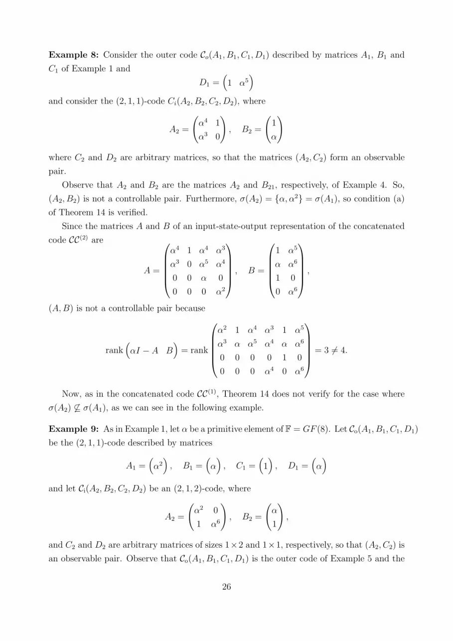
Example 8: Consider the outer code Co(A1, B1, C1, D1) described by matrices A1, B1 and

C1 of Example 1 and

D1 =(1 α5

)and consider the (2, 1, 1)-code Ci(A2, B2, C2, D2), where

A2 =

(α4 1

α3 0

), B2 =

(1

α

)

where C2 and D2 are arbitrary matrices, so that the matrices (A2, C2) form an observable

pair.

Observe that A2 and B2 are the matrices A2 and B21, respectively, of Example 4. So,

(A2, B2) is not a controllable pair. Furthermore, σ(A2) = {α, α2} = σ(A1), so condition (a)

of Theorem 14 is verified.

Since the matrices A and B of an input-state-output representation of the concatenated

code CC(2) are

A =

α4 1 α4 α3

α3 0 α5 α4

0 0 α 0

0 0 0 α2

, B =

1 α5

α α6

1 0

0 α6

,

(A, B) is not a controllable pair because

rank(αI − A B

)= rank

α2 1 α4 α3 1 α5

α3 α α5 α4 α α6

0 0 0 0 1 0

0 0 0 α4 0 α6

= 3 6= 4.

Now, as in the concatenated code CC(1), Theorem 14 does not verify for the case where

σ(A2) 6⊆ σ(A1), as we can see in the following example.

Example 9: As in Example 1, let α be a primitive element of F = GF (8). Let Co(A1, B1, C1, D1)

be the (2, 1, 1)-code described by matrices

A1 =(α2)

, B1 =(α)

, C1 =(1)

, D1 =(α)

and let Ci(A2, B2, C2, D2) be an (2, 1, 2)-code, where

A2 =

(α2 0

1 α6

), B2 =

(α

1

),

and C2 and D2 are arbitrary matrices of sizes 1×2 and 1×1, respectively, so that (A2, C2) is

an observable pair. Observe that Co(A1, B1, C1, D1) is the outer code of Example 5 and the

26

matrices A2 and B2 are the matrices A2 and B21 of Example 5. So (Al, Bl) is a controllable

pair, for l = 1, 2, (A1, C1) is an observable pair and σ(A2) 6⊆ σ(A1).

Now, taking into account Theorem 9, the matrices A and B of an input-state-output

representation of CC(2), are given by

A =

α2 0 α

1 α6 1

0 0 α2

and B =

α2

α

α

These matrices are the matrices A and B of Example 5, and then (A, B) is not a controllable

pair.

The next example shows that we cannot obtain a lower bound in terms of dfree(Ci) as in

expression (20) for the concatenated code CC(2).

Example 10: As in Example 1, let α be a primitive element of the field F = GF (8). Con-

sider the (3, 2, 1)-outer code Co(A1, B1, C1, D1) and the (2, 1, 1)-inner code Ci(A2, B2, C2, D2)

where

A1 =(α2)

, B1 =(1 1

), C1 =

(1)

, D1 =(1 1

),

A2 =(α)

, B2 =(1)

, C2 =(α4)

, D2 =(1)

.

Observe that, for l = 1, 2, the pairs (Al, Bl) and (Al, Cl) are controllable and observable,

respectively.

So, by applying Theorem 9, Theorem 13 and part (b) of Theorem 11, the matrices

A =

(α 1

0 α2

), B =

(1 1

1 1

), C =

(α4 1

0 1

), D =

(1 1

1 1

)

are a minimal representation of the (4, 2, 2)-observable code CC(2).

In addition dfree(Co) = 2 and dfree(Ci) = 4. Therefore

max{dfree(Co), dfree(Ci)} = 4.

Nevertheless,

dfree(CC(2)) = 2.

Observe that, in this case, rank(D1) = rank(1 1

)= 1 = m− k and k = 2.

As a consequence of the previous example, we can only obtain a lower bound for the free

distance of CC(2) in terms of dfree(Co). Nevertheless, if we require rank(D1) = k, then we can

obtain a refinement of this bound as we prove in the following theorem. Firstly, we obtain a

lower bound for the column distances of CC(2) in terms of the column distances of Co and Ci.

27

Lemma 3: Let CC(2) be the concatenated code given by Theorem 9 from the outer code Co

and the inner code Ci. Then

(a) dcj(CC(2)) ≥ dc

j(Co) for j = 0, 1, 2, . . .

(b) If rank(D1) = k, then dcj(CC(2)) ≥ dc

j(Ci) + 1.

Proof: Taking into account the relations between yt, y(1)t , y

(2)t ; ut, u

(1)t , u

(2)t , and vt, v

(1)t , v

(2)t

given by expressions (21)–(25) and using the same argument used to obtain inequality (18)

in the proof of Lemma 2, we obtain inequality of part (a).

Now, since y(1)0 = D1u

(1)0 and rank(D1) = k, we get that u0 = u

(1)0 6= 0 if and only if

u(2)0 = y

(1)0 6= 0. So, from expressions (5) and (21)–(25), we have

dcj(CC(2)) = min

u0 6=0

{j∑

t=0

wt(vt)

}= min

u(1)0 6=0

{j∑

t=0

wt(u(1)t )

}

+ minu(2)0 6=0

{j∑

t=0

wt(v(2)t )

}≥ 1 + dc

j(Ci) �

Now, as an immediate consequence of expression (4) and the above lemma we obtain the

following result.

Theorem 15: Let CC(2) be the concatenated code given by Theorem 9 from the outer code

Co and the inner code Ci. Then

(a) dfree(CC(2)) ≥ dfree(Co).

(b) If rank(D1) = k, then dfree(CC(2)) ≥ dfree(Ci) + 1.

As in the previous section, we finish this section with an example, in which we use the

construction proposed by Smarandache and Rosenthal [28] to obtain an MDS convolutional

code.

Example 11: As in Example 1, let α be a primitive element of F = GF (8). Let Co(A1, B1, C1, D1)

be the MDS convolutional code of rate 1/2 and degree δ1 = 2, where

A1 =

(α 0

0 α2

), B1 =

(1

α

), C1 =

(α3 α4

), D1 =

(1)

.

In this case, Co is an MDS convolutional code, so dfree(Co) = 6.

Let Ci(A2, B2, C2, D2) be the MDS convolutional code of rate 1/2 and degree δ2 = 1,

where

A2 =(α)

, B2 =(1)

, C2 =(α2)

, D2 =(α3)

.

28

It follows then that the matrices (Al, Bl) form a controllable pair, for l = 1, 2 and the

matrices (Al, Cl) form an observable pair, for l = 1, 2. Furthermore, σ(A2) ⊆ σ(A1). So, by

applying Theorem 9, Theorem 14 and part (b) of Theorem 11, the matrices

A =

α α3 α4

0 α 0

0 0 α2

, B =

1

1

α

, C =

(α2 α6 1

0 α3 α4

), D =

(α3

1

)

are a minimal representation of the observable code CC(2).

Now, since rank(D1) = 1, by Theorem 15 and the Singleton bound, we have

6 = max{6, 4 + 1} ≤ dfree(CC(2)) ≤ 12.

But in fact, dfree(CC(2)) = 11.

Now, if we permute the outer and the inner code, then applying Theorem 9 and Theo-

rem 12 we obtain a minimal representation of the new concatenated code CC(2) given by

A =

α 0 α2

0 α2 α3

0 0 α

, B =

α3

α4

1

, C =

(α3 α4 α2

0 0 α2

), D =

(α3

α3

)

which is observable by using part (b) of Theorem 11.

Now, since rank(D1) = 1, through Theorem 15 and the Singleton bound, we have

7 = max{4, 6 + 1} ≤ dfree(CC(2)) ≤ 12.

But in fact, dfree(CC(2)) = 12. So we get an MDS convolutional code.

References

[1] K. A. S. Abdel-Ghaffar. Some convolutional codes whose free distances are maximal.

IEEE Transactions on Information Theory, 35(1): 188–191, 1989.

[2] C. Berrou, A. Glavieux, and P. Thitimajshima. Near Shannon limit error-correcting

coding and decoding: turbo codes (1). In Proceedings of the International Conference

on Communication (Geneva, Switzerland), pages 1064–1070. IEEE, 1993.

[3] G. D. Forney, Jr. Concatenated Codes. MIT Press, Cambridge, MA, 1966.

[4] G. D. Forney, Jr. Convolutional codes I: Algebraic structure. IEEE Transactions on

Information Theory, 16: 720–738, 1970.

29

[5] J. Freudenberger, R. Jordan, M. Bossert, and S. Shavgulidze. Serially Concatenated

Convolutional Codes with Product Distance. 2nd International Symposium on Turbo

Codes and Related Topics, pages: 81–84 (2000).

[6] M. L. J. Hautus. Controllability and observability condition for linear autonomous sys-

tems. Proceedings of Nederlandse Akademie voor Wetenschappen, Series A, 72: 443–448

(1969).

[7] S. Host, R. Johannesson, V. Sidorenko, K. S. Zigangirov, and V. Zyablov. A first en-

counter with binary woven convolutional codes. In Proceedings of the 4th International

Symposium on Communication Theory and Applications, pages 13–18. Lake Districts,

UK, 1997.

[8] S. Host, R. Johannesson, V. R. Sidorenko, K. Sh. Zigangirov, and V. Zyablov. Cascaded

convolutional codes. In Communication and Coding, M. darnell and B. Honary, Eds.

London, U.K.: Research Studies/Wiley, 1998, pages 10–29.

[9] S. Host, R. Johannesson, V. Sidorenko, K. S. Zigangirov, and V. Zyablov. Woven

convolutional codes I: Encoder properties. IEEE Transactions on Information Theory,

48(4): 149–161, 2002.

[10] S. Host, R. Johannesson, V. Sidorenko, K. S. Zigangirov, V. Zyablov, and O. Skopintsev.

Generator matrices for binary woven convolutional codes. In Proceedings of the 6th

International Workshop on Algebraic and Comb. Coding Theory, pages 142–146. Pskov,

Russia, 1998.

[11] R. Hutchinson, J. Rosenthal, and R.Smarandache. Convolutional codes with maximum

distance profile. Systems and Control Letters, 54(1): 53-63 (2005).

[12] R. Johannesson and Z. Wan. A linear algebra approach to minimal convolutional en-

coders. IEEE Transactions on Information Theory, 39: 1219–1233, 1993.

[13] R. Johannesson and k. Sh. Zigangirov. Fundamentals of Convolutional Coding. IEEE

Press, New York, 1999.

[14] J. Justesen. New convolutional code constructions and a class of asymptotically good

time-varying codes. IEEE Transactions on Information Theory, 19(2): 220–225, 1973.

[15] J. Justesen. An algebraic construction of rate 1/ν convolutional codes. IEEE Transac-

tions on Information Theory, 21(1): 577–580, 1975.

[16] T. Kailath, Linear Systems. Prentice-Hall, 1980.

30

[17] R. E. Kalman, P. L. Falb, and M. A Arbib. Topics in mathematical system theory. Mc

Graw-Hill, New York, 1969.

[18] Y. Levy and D. J. Costello, Jr. An algebraic approach to constructing convolutional

codes from quasicyclic codes. DIMACS Series in Discrete Mathematics and Theoretical

Computer Science, 14: 189–198, 1993.

[19] L. Massey, J, D. J. Costello, and J. Justesen. Polynomial weights and code constructions.

IEEE Transactions on Information Theory, 19(1): 101–110, 1973.

[20] J. L. Massey and M. K. Sain. Codes, automata and continuous systems: Explicit inter-

connections. IEEE Transactions on Automatic Control, AC-12(6): 644–650, 1967.

[21] R. J. McEliece. The algebraic theory of convolutional codes. In V. Pless and

W.C.Huffman, editors, Handbook of Coding Theory, volume I, pages 1065-1138. El-

sevier, Amsterdam, 1998.

[22] J. Rosenthal. Connections between linear systems and convolutional codes. In B. Marcus

and J. Rosenthal editors, Codes, Systems and Graphical Models, IMA Vol. 123, pages

39-66, Sprinegr Verlag, 2001.

[23] J. Rosenthal, and R. Smarandache. Construction of convolutional codes from linear

systems theory. In Proceedings of the 35th Allerton Conference on Communication,

Control and Computing, pages 953–960, Allerton House, Monticello, IL, September

1997.

[24] J. Rosenthal, and R. Smarandache. Maximum distance separable convolutional codes.

Applicable Algebra in Engineering, Communication and Computing, 10: 15–32 (1999).

[25] J. Rosenthal, J. M. Schumacher, and E. V. York. On behaviors and convolutional codes.

IEEE Transactions on Information Theory, 42(6): 1881–1891, 1996.

[26] J. Rosenthal and E. V. York. BCH convolutional codes. IEEE Transactions on Infor-

mation Theory, 45(6): 1833–1844, 1999.

[27] R. Smarandache, H. Gluesing-Luerssen, and J. Rosenthal. Constructions of MDS-

convolutional codes. IEEE Transactions on Information Theory, 47(5): 2045–2049, 2001.

[28] R. Smarandache and J. Rosenthal. A state space approach for constructing MDS rate

1/n convolutional codes. In Proceedings of the 1998 IEEE Information Theory Workshop

on Information Theory, pages 116–117, Killarney, Kerry, Ireland, June 1998.

[29] R. M. Tanner. Convolutional codes from quasicyclic codes: A link between the theories

of block and convolutional codes. Technical Report USC-CRL-87-21, November 1987.

31