A componential analysis of pacemaker-counter timing systems

Journal of Experimental Psychology:Human Perception and Performance1990, Vol. 16, No. 4, 766-780

Copyright 1990 by the American Psychological Association, Inc.0096-1523/90/S00.75

A Componential Analysis of Pacemaker-Counter Timing Systems

J. Gregor FettermanIndiana University-Purdue University at Indianapolis

Peter R. KilleenArizona State University

Why does counting improve the accuracy of temporal judgments? Killeen and Weiss (1987)provided a formal answer to this question, and this article provides tests of their analysis. InExperiments 1 and 2, subjects responded on a telegraph key as they reproduced different intervals.Individual response rates remained constant for different target times, as predicted. The varianceof reproductions was recovered from the weighted sum of the first and second moments of thecomponent timing and counting processes. Variance in timing long intervals was mainly due tocounting error, as predicted. In Experiments 3-5, unconstrained response rate was measured andsubjects responded at (a) their unconstrained rate, (b) faster, or (c) slower. When subjectsresponded at the preferred rate, the accuracy of time judgment improved. Deviations in ratestended to increase the variability of temporal estimates. Implications for pacemaker-countermodels of timing are discussed.

When asked to estimate the duration of some event withoutthe aid of a time piece, most people mediate the estimationby counting (e.g., "one thousand one, one thousand two,"etc.), and balk if asked to time without counting. That thisstrategy is so readily adopted suggests that people intuitivelyrecognize that counting improves the accuracy of time judg-ments, an intuition supported by long-standing experimentalevidence (e.g., Gilliland & Martin, 1940). The ubiquity of thepractice calls into question experimental psychologists' at-tempts to prevent or interfere with subjects' counting strate-gies as a means of eliciting "uncontaminated" temporal judg-ments.

Although it is evident that subdividing a long interval intosubintervals (i.e., counting) improves temporal estimates, it isnot immediately obvious why this should be so. Killeen andWeiss (1987) recently provided an analysis of the timingprocess that rationalizes what intuition and data tell us. Inthis article, we briefly review the "optimal timing" analysis ofKilleen and Weiss, and then present the results of five exper-iments that confirm some of the predictions that follow fromtheir analysis.

We represent the timing process as a pacemaker-countersystem (elsewhere referred to as a clock-counter system orpacemaker-accumulator system). In these systems, one com-ponent (the pacemaker) generates pulses, and another (thecounter) accumulates them and signals when the number ofpulses equals or exceeds a criterion value. Pacemaker-countersystems will improve timing only if the sum of the variancesof the subintervals is less than the variance in estimating the

This research was supported in part by a National Research ServiceAward Postdoctoral Fellowship (1 F32 MH09306) from the NationalInstitute of Mental Health to J. Gregor Fetterman, and in part byNational Institute of Mental Health Grant 1 RO1 MH43233 to PeterR. Killeen.

Correspondence concerning this article should be addressed to J.Gregor Fetterman, Department of Psychology, Indiana University-Purdue University at Indianapolis, 1125 East 38th Street, Indianap-olis, Indiana 46205-2810, or to Peter R. Killeen, Department ofPsychology, Arizona State University, Tempe, Arizona 85287-1104.

interval as a whole and the counting process does not itselfadd too much variance to the estimate. Traditional treatmentsof such systems (e.g., Creelman, 1962; Treisman, 1963) holdthat most of the variance in the timing process results fromvariance in the timing of the subintervals, with zero variancein the counter. This assumption may not generally be correct.People make mistakes even with simple counting tasks. Thus,it seems plausible to assume nonzero error in counting, es-pecially under conditions where attention is focused on keep-ing the subintervals constant, and even more so when subjectsare distracted or discouraged from counting, as is commonpractice in timing experiments. We shall assume, therefore,that variance in timing an interval results from both variancein timing the subintervals and variance in counting the sub-intervals. We develop and test this notion and its implicationsmore formally here.

Let \ID equal the average duration of a subinterval, \IN theaverage number of subintervals, and \J.T the average durationof the interval generated. Then,

Mr =

and

"T f-o "N •

(1)

(2)

Equation 1 states that the estimated duration of an intervalequals the product of the average subinterval and the averagenumber of subintervals (M«). Equation 2 states that the vari-ance of temporal estimates equals the weighted sum of thevariances of the constituent timing and counting processes(Killeen & Weiss, 1987, p. 456). Equation 2 is not a "theory"of timing, but a standard model for random sums (see, e.g.,Luce, 1986). It requires that the subintervals by independentand identically distributed, and that error in the counter isindependent of error in the pacemaker. For notational con-venience, we hereafter write tiT as /, HN as n, and /J.D as d.

Equations 1 and 2 assert that the mean and variance oftemporal estimates reflect the joint contribution of the com-ponent process: the means and variances of the pacemakerand counter. From Equation 2, we may infer that optimalperformance might involve a trade-off between error in count-

766

PACEMAKER-COUNTER TIMING SYSTEMS 767

ing and error in timing. For example, as the error involved in

counting increases, it will be to the subjects' advantage to

count more slowly, dividing the interval into fewer and longer

subintervals. This trade-off will determine the optimal dura-

tion and number of the subintervals (Killeen & Weiss, 1987,

p. 456). 'To implement this analysis and identify the optimal trade-

off, we must specify the functional form that governs the

growth of variance in the component processes. We assume

that the growth of these variances corresponds to the following

equations:

an2 = at2d

2 + a,d + QO (3)

for the variance of the subintervals, and

for the variance of their number. In these equations, all a,

and ft, > 0. These fundamental error equations should not be

taken to imply that quadratic equations with all constants

greater than zero are needed to describe the constituent vari-

ances under all circumstances. On the contrary, these equa-

tions were selected for their generality; any of the coefficients

may be set to zero as appropriate to the model of counting or

timing under consideration.

We assume that a suitably motivated subject will select

values of n and d that yield estimates close to the target time,t, and that minimize a2 in Equation 2. Note that given a

mean estimate, t, we need only specify the value of « or d,

and the other follows; the two are interdependent. Our analy-

sis proceeds on the assumption that subjects attempt to min-

imize error by optimizing d, because in temporal estimations

and reproductions that is more directly and immediately

under their control than is n.

What value of d should an observer select to minimize <r,27

The answer depends upon the parameter values of the fun-

damental error equations. Consider first the case where there

is a fixed component of variability involved in generating the

subintervals, even when the duration of those subintervals

approaches zero («o > 0). This would be the case if there were

intrinsic variability associated with resetting the pacemaker

for the next subinterval. Then, assume (80 = 0 (which will be

the case if the subject can report when no counts occurred,

with perfect accuracy'). Then the optimal duration of the

subintervals is

• [00/02 d* < t . (5)

If ft > 0, then Equation 5 will still hold in the limit as t -^

oo, (with one exception, «2 = 0 and 0i > 0, in which case d*

= kt>n). Because I does not appear in Equation 5, in those

cases where it holds exactly the optimal rate of counting (I/

d*) should be constant and independent of the interval to be

timed. We shall return to this prediction when we present thedata.

What of the case where «„ = 0 (as the durations of the

subintervals approach 0, the variance of the subintervals also

approaches zero)? This obtains if the pacemaker is a Poisson

emitter (in which case ct2 = 0 also). Killeen and Weiss showed

that unless all other relevant parameters were zero (in which

case it did not matter what the subject did), then the subject

should count as fast as possible. In this case, there would be

other constraints on accuracy not represented by the funda-

mental error equations (i.e., as rates increase beyond some

limit, accuracy of counting would be impaired so that the

constants in Equation 4 would not stay constant). We subse-

quently describe some evidence that this may actually happen.

Inserting Equation 5 into Equation 2, we obtain

where

and

<T,2 = At + Bt + c,

B = at + 2[«o(a2 +

(6)

(7)

(8)

(9)

Equation 6 states that the variance of temporal estimates will

be a quadratic function of their duration. It allows us to

predict the accuracy of performance on an experimental task

as a function of t. Equation 6 shows that the relative contri-

butions of error in the timing and counting processes should

vary as a function of t. Even if subjects do not choose the

optimal value of d, Equation 6 remains appropriate, provided

that the value of d remains constant. (The constituents of the

coefficients A, B, and C would in that case differ from those

given by Equations 2-9).

Killeen and Weiss were not the first to formally assess the

contribution of counting to the timing process. Getty (1976)

suggested that the advantage of subdividing a long duration

into subintervals derived from the fact that the sum of the

variances of the subintervals was less than the variance that

results when the interval is estimated without such segmen-

tation. Getty had subjects count silently at different rates

established during a synchronization interval, and had them

signal when they had made 5 or (in another condition) 10

counts. He found that the variance of the times taken to reach

the criterion count was less in the 10-count condition. Getty

represented the variance of temporal estimates as

<r,2 = naf + a.,2, (10)

where a2 is a constant synchronization error, and af was

held to be proportional to d2 (i.e., a/ = kd1}. Although Getty's

analysis allows that the rate of counting affects timing, it

suggests that subjects should count as fast as possible because

timing error is held to decrease uniformly as a function of the

number of subdivisions of the major interval. This prediction,

which is counterfactual, results because no provision was

made for the contribution of counting error to the timing

1 Although this seems a given for typical subjects, there is animportant scenario in which it may fail. If the pacemaker is freerunning rather than synchronized with the onset of the timing process(see, e.g., Kristofierson, 1984), then there will be a synchronizationerror representable as jS0 that is proportional to d. It is likely that sosmall an error will only be apparent in well-practiced subjects, whereother sources of variability have been reduced to their minimum. Asimilar error may occur at the end of the interval unless the intervalbeing estimated or produced coincides with the last pulse.

768 J. GREGOR FETTERMAN AND PETER R. KILLEEN

process. If such allowances are made, we find that it is to thesubjects' advantage to count at a moderate pace to achieve abalance of timing and counting error.

The Killeen and Weiss formalism provides a framework fortheories of timing that use pacemaker-counter systems, and itcontains testable predictions about the contributions of theconstituents of such systems to the timing process. We shallattempt to test these predictions by measuring changes in themeans and variances of the component processes (the timingand counting of subintervals dand «), in addition to standardmeasures of time estimation. In the literature, these valuesare typically inferred from the data as free parameters forquantitative models of the timing process. For example, thedecrease in mean temporal estimates (corresponding to alengthening of subjective time) that accompanies the admin-istration of stimulant drugs (e.g., Doob, 1971) is taken toimply a decrease in the period (d) of a hypothetical pacemaker(i.e., an increase in the rate of the clock); but the evidence isindirect, supported by changes in parameter values recoveredfrom models fit to overall time estimates.

In the following experiments, we attempted direct measure-ment of the component processes. Subjects performed a tem-poral reproduction task in which they were instructed torespond on a telegraph key throughout the reproduction. Themean and variance of the successive interresponse intervalswere taken to represent the corresponding statistics on d, andthe number and variance of responses were used as thestatistics on n. Thus, subjects engaged in what could beconstrued as a mediative counting task as they reproducedtemporal intervals (Getty, 1976), but we did not label it assuch, nor did we provide guidance concerning the rate ofresponding during the reproduction (i.e., the rate of counting).The obtained values of d and « were incorporated in theequations of the optimal timing model, and predictions wereevaluated against the data.

Experiment 1

Method

Subjects. The participants were 16 undergraduates enrolled in anintroductory psychology course at Arizona State University. All wereright-handed. Participation served to partially fulfill course require-ments.

Apparatus. Two telegraph keys were located on the right side ofan Apple He computer and MED Associates interface adjacent to oneanother and within easy reach for the subject. The durations of events(stimuli and responses) were recorded to the nearest millisecond.

Procedure. Participants were seated in front of the computer, andthe task was explained according to a standardized set of instructions.The experimenter left the room after ensuring that the subject under-stood the task.

Each subject made 20 reproductions each of intervals of 4, 10, and20 s for a total of 60 trials; order of the intervals was counterbalancedover subjects. The intervals were tone durations presented throughthe computer; each auditory stimulus was presented just once, on thefirst trial of a 20-trial block. Subsequent reproductions were guidedby feedback (described later) provided after each estimate. Approxi-mately 3 s elapsed between the presentation of feedback and thebeginning of the next trial, which was signaled by the appearance of

a prompt on the computer monitor. Subjects were instructed to begintheir reproductions on the appearance of the prompt "GO." Timingof the reproduction commenced with the subjects' first response onthe left telegraph key, and ended with a single response on the righttelegraph key.

Participants were instructed to tap the left telegraph key for aperiod equal to the duration of the tone signal. No guidance wasprovided concerning the rate of tapping, except that subjects weretold to tap at whatever rate felt "comfortable." It was emphasized,however, that tapping should continue throughout the reproductionuntil the subject estimated that a period of time equal to the durationof the tone signal had elapsed, at which point a single tap on the righttelegraph key signified the end of the reproduction. All subjectsresponded throughout the reproduction task, although the rates oftapping varied widely across individuals.

Feedback was provided after each reproduction in the form of agraphic display on the computer screen; the display appeared about300 ms after subjects signaled the end of their estimate, and remainedon for approximately 3 s. The display contained a vertical line downthe center of the screen and a horizontal bar, originating at the leftedge of the screen. The distance of the vertical line from the left edgeof the screen represented the duration of the target interval; the lengthof the horizontal bar represented the duration of the subject's repro-duction relative to the duration of the target interval. The position ofthe right edge of the bar relative to the vertical line indicated thedirection (underestimate or overestimate) and magnitude of the sub-ject's error of estimation. This distance was directly proportional tothe percentage error of estimate. Reproductions within ±5% of thetarget time resulted in additional feedback; the words "RIGHT ON"appeared briefly on the screen, immediately following the offset ofthe graphic display. The experimenter ensured that all subjects under-stood the feedback display.

The data from each trial included the times between successiveresponses to the telegraph key (d), the total number of responses (ri),and the duration of the reproduction (t). The reproduction data foreach target time were partitioned into blocks of five trials and standarddeviations of t were calculated for each trial block; we inspected thestandard deviations over trial blocks as a measure of stability. Theanalyses that follow are based upon performances averaged over thelast five trials at each target time, by which point there were no visiblechanges in variability. All descriptive statistics (over trials and sub-jects) are bimeans (Killeen, 1985). Bimeans are weighted arithmeticmeans in which the data farthest from the mean are given reducedweights (Mosteller & Tukey, 1977).

Results and Discussion

Subjects were on the average very accurate in reproducingtemporal intervals; the best fitting line through the meanestimates had a unit slope and accounted for virtually all ofthe data variance, and the average data were quite represen-tative of individuals. The standard deviation of the estimatedduration was an increasing linear function of the requiredduration (VT = 0.10671 — 0.14), a result known as Weber'slaw. Whereas many different functions may be drawn throughthese points, the linear function provides an accurate andparsimonious summary of the data. The coefficient of varia-tion (standard deviation divided by the mean) provides anindex of the relative acuity of subjects' temporal judgments;for our average data, this measure was 0.106, ranging from0.028 to 0.212 for individual subjects.

Our subjects were instructed to tap as they reproducedtemporal intervals, but no directions were given concerning


the rate of tapping. The mean tap rate over all intervals was3.3 Hz, but there were substantial between-subjects differencesin rate (range: 0.8 to 6 Hz). Most important, however, themajority of subjects (13 of 16) maintained a constant rate oftapping as they reproduced different intervals in accord withthe predictions of Killeen and Weiss. Regressions of tap rateagainst T for those individuals indicated that their slopes didnot deviate systematically from zero. The mean of all individ-ual slopes was 0.044, not significantly different from zero,;(15) = 1.76, p > .05; two-tailed. The three exceptions to thisgeneralization showed monotonic increases in rate with in-creasing T. Most subjects, therefore, behaved in a mannerconsistent with predictions from the Killeen and Weiss analy-sis, which established that the optimal rate of counting shouldbe independent of T. There was no evidence to suggest thatsubjects might go slower for long intervals, as some intuitions(and one possible model of Killeen and Weiss) might suggest.

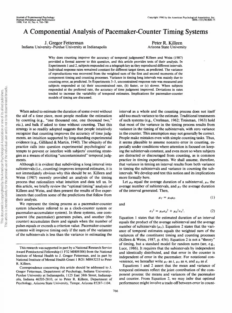
The wide variety of rates indicates that, if the subjects didselect optimal rates of counting, those rates must have beenidiosyncratic. Figure 1 expands upon this point by showingthe relation between standard deviations of t and tap rate forindividual subjects at each value of T. The standard deviationsin Figure 1 have been normalized to facilitate comparisonsacross the different intervals. The distribution of points inFigure 1 indicates little or no relation between tap rate andaccuracy (although there may be a slight tendency for fastercounting to result in lower accuracy). The implication is thatrate of counting either does not matter or that it is optimizedidiosyncratically by each subject. We return to this issue insubsequent experiments.

Assume (as before) that the variability of subjects' timejudgments (a,2) reflects the additive contributions of variabil-ity in the timing of subintervals (o-/) and variability in thenumber of subintervals (<?n

2). If this assumption is correct,then we may predict the variability of subjects' reproductions

b«wN

« -

2-

1 -

0-

A Z(CT4)* ztrjio)• Z(U20)

*A A

A M

A

•A

-1 -

-2-0 1 2 3 4 5 6 7

Response rate (taps/sec)Figure 1. Normalized (Z-score transforms) standard deviations oftemporal reproductions as a function of response rate (taps persecond) for individual subjects. (Negative values indicate less thanaverage variability, and positive values indicate greater than averagevariability.)

by taking the appropriately weighted sum of the constituentvariances. Combining these variances according to standardtechniques, we arrive at Equation 2. Equation 2 states thatvariance in estimating a time interval (a,2) may be predictedfrom the first and second moments of the component pro-cesses: the period of the pacemaker (d) and its variance, andthe number of counts (ri) and its variance. Equation 2 is nota particular model of timing; it is a standard relation thatmust hold if we are to proceed with any models that treattiming as a pacemaker-counter system involving the randomsum of independent random variables. Where the componentprocesses are independent, this includes standard models oftiming, where the variance of one of the components (typicallythe counter) is assumed to be zero.

Taking the mean intertap interval for each subject as ourmeasure of d, and the mean number of subintervals as ourmeasure of n, and inserting them and the appropriate vari-ances into Equation 2, we obtain the predictions shown inFigure 2, which shows predicted versus obtained variances oft for each subject. It appears that Equation 2 affords a goodapproximation for the 20-s interval, a mediocre approxima-tion for the 10-s interval, and a poor approximation of per-formance for the 4-s interval. Linear regressions of predictedversus obtained variance generally confirm the visual displayof Figure 2, but suggest several qualifications. The correspon-dence between predicted and obtained variances, as measuredby r2, is better at 4 s and worse at 20 s than suggested byFigure 2; linear regression gives r2 of .64 for the 4-s condition,.16 for the 10-s condition (which increases to .92 when thedata for two aberrant subjects are dropped), and .92 for the20-s condition. The absolute errors of prediction for the 4-scondition are exaggerated by the logarithmic axes (introducedto accommodate the large range of data). The slopes of thebest fitting lines were close to 1.0 (0.96, 1.1, and 1.1).

Figure 2 showed that variance in the sum of individualintertap intervals (nd) could be approximated from the meansand variances of the number and duration of those intervals.That approximation was best for the 20-s interval, where thebenefits of count-mediated timing would be greatest, andpoorest at the 4-s interval. Next, we address the relativecontributions of the constituents to overall variance in timing.Equation 6 tells us that the contribution of variability incounting (O to total variability (a2) will increase with T,and will dominate at moderate to long values of T. This isbecause At2 dominates the right-hand side for large T, and Adepends solely on counting error (A = /32). Table 1 presentsdata that bear on this point. The table shows the weightedvariances of the component processes (averaged across sub-jects) for each value of T, as expressed in Equation 2. Table1 confirms that the increase in a2 with Twas due to increasesin the variance in number of subintervals; there was very littlechange in the variance of d, because the rate of tapping (andhence the duration and variance of the subintervals) remainedconstant over T.

Figure 3 shows the relation between counting error (an) andthe total number of subintervals (n). The linear relationportrayed in Figure 3 indicates a Weber-like result for count-ing; the standard deviation is proportional to the mean num-ber of subintervals.


e

10

io

,5,

w2 10'

1 /\U 1 A 1 t l\A \ /\O * /\**1 1 AO

Obtained Variance

Figure 2. Obtained variances of temporal reproductions (abscissa)against predicted (synthesized) variances where the predictions arebased upon Equation 2. (The units are ms2. See text for details.)

Let us review the major findings of this experiment inwhich we asked subjects to respond repetitively while repro-ducing temporal intervals. The rate of responding variedconsiderably among subjects, but tended to remain constantfor the same subject estimating different intervals. Rates ofresponding and the standard deviations of temporal repro-ductions were unrelated; insofar as subjects selected an opti-mal rate of counting it appeared to be idiosyncratic. Variabil-ity in estimating intervals of time was predicted from acombination of error in the duration of the subintervals (d)and error in their number (n); total variability resulted pri-marily from variability in counting.

Experiment 2

The two-process framework of Killeen and Weiss provideda first approximation of subjects' performance on a temporalreproduction task in which the reproduction was accom-panied by repetitive tapping. However, as noted previously,there were substantial individual differences in tapping; somesubjects tapped rapidly, others slowly, and some at an inter-mediate pace. The large individual differences in tap ratesmight indicate that subjects were not performing the task inthe same way. A basic question is whether the tapping task,which we took to represent the constituents of the timingprocess, served to mediate temporal reproductions. Subjectswere not explicitly instructed to use their tapping to regulatetheir time judgments, but only to continue tapping through-out the reproduction. In some cases then, tapping may simply

Table 1Average Weighted Variances of the Duration (d) andNumber (n) of Subintervals, as Expressed in Equation 2

41020

0.00680.00610.0066

0.1520.8435.039

have been a "filler" activity having nothing to do with subjects'overall estimates of time. Experiment 2 was motivated by thisbasic question about the procedure.

Method

Subjects and apparatus. Four Arizona State University studentsparticipated in the experiment. Each was paid $10 for their partici-pation. The apparatus was the same as described in Experiment 1.

Procedure. The basic task was the same as described in Experi-ment 1. Subjects were instructed to tap on one telegraph key duringa temporal reproduction task and to signal the end of their estimatewith a single tap on a second key. The intervals were tone durations;each interval was presented directly just once. Subsequent reproduc-tions were guided by the graphic feedback display described in Ex-periment 1.

Subjects reproduced intervals of 2, 4, 7, 11, and 16 s. Subjectsmade 50 estimates of the 2- and 4-s intervals, and 40 estimates of theremaining intervals. The intervals were presented in a different ran-dom order to each subject. The instructions were modified such thateach subject was told to "use your tapping to help you judge thepassage of time in whatever way seems appropriate to you." In allother respects, the instructions were unchanged from Experiment 1.


Figure 4 shows the mean accuracy of temporal reproduc-tions for each subject; the data are averaged over the last 10trials at each interval value. As in Experiment 1, subjects werevery accurate in reproducing temporal intervals, althoughthere was a slight tendency toward underestimation at longerintervals.

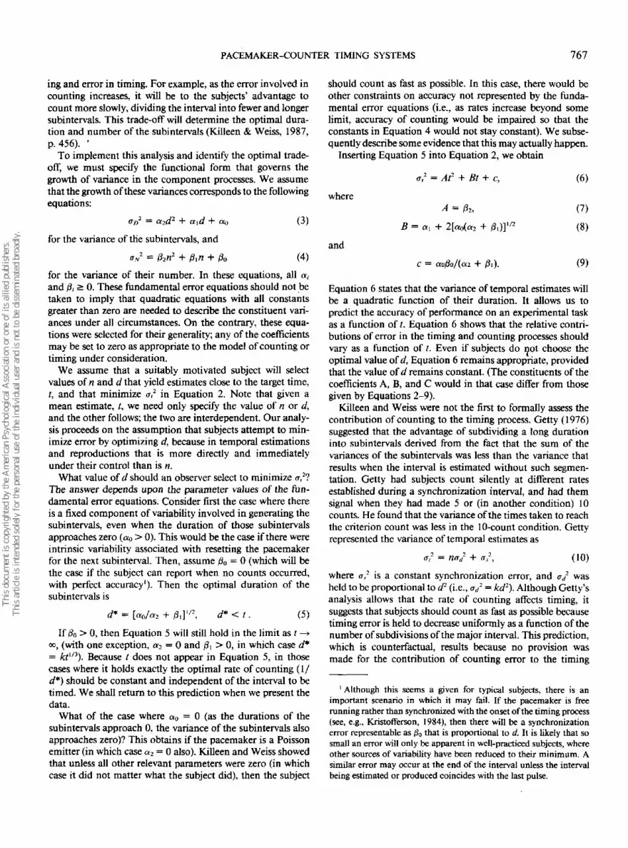
Figure 5 shows the variances of t for all subjects as afunction of t2. The lines through the points are best fittinglines based upon Equation 6 with B = 0 (a,2 = At2 + C). Foronly 1 subject (Subject 4) was the goodness of fit to the dataslightly improved by the addition of a linear component. Thenumbers in each panel are the coefficients of variation (CV= ajt) that provide an index of the relative acuity of subjects'temporal judgments akin to a Weber fraction. The values areimpressively low, and considerably less than the average valuefor Experiment 1 (.106).

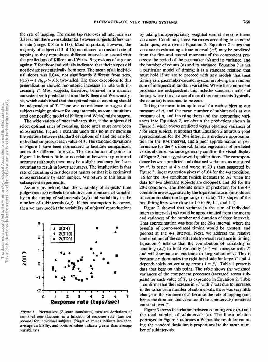
Figure 6 shows the average values of d (intertap intervals)for each subject as a function of t. All subjects maintained afairly constant rate of tapping (l/d) as they reproduced dif-ferent intervals, as predicted by Killeen and Weiss and ob-served in Experiment 1. As before, there were individualdifferences in tap rate.

Figure 7 shows obtained versus synthesized variances of /,where the synthesized variances are based on a modifiedversion of Equation 2. Inspection of the individual dataindicated that the mean of the final intertap interval (whenthe subject switched from the left to the right key) was, insome cases, quite discrepant from intertap intervals producedon the left key. Accordingly, the data were fit to a modifiedversion of Equation 2:

= (n - + + d2(11)

where n represents the total number of subintervals (includingthe final subinterval), (^represents the mean of all subintervals,


6-

4 -

2-

0

ff = 0.118n-0.21n

0 1 0 2 0 3 0 4 0 5 0 6 0 7 0n

Figure 3. Standard deviations of n (number of taps) as a functionof number of taps emitted.

<jd represents the variance of subintervals on the left key, andasw

2 represents the variance of the final subinterval, whichincorporates the time between the last response on the leftkey and the terminal response on the right key. The corre-spondence between the parameter-free predicted variancesand obtained variances for individual performances is reason-able. The deviations from predicted performance could haveresulted from drifts in response rates over trials or sequentialdependencies between successive intertap intervals.

In Experiment 1, we observed that average variability (<rn)of n was a linear function of the number of subintervals. InExperiment 2, there was little or no variability in «. Subjectsmade about the same number of taps for each reproductionof a given interval, a result that indicates a strategy of explicitcounting. For the case where variability in n is zero, Equation2 reduces to

<r,2 = n<rd2. (12)

The data of Subject 4 (for whom within-interval variance in

20-1

0(0

t = 0.92T + 0.45

10

T(sec)

20

Figure 4. Mean temporal reproductions as a function of intervalvalue ( T ) for each subject in Experiment 2.

n over the last 10 trials was zero) in Figure 7 indicate that thefit of the model equation to this special case was quite good.

To what extent were subjects' reproductions mediated bythe tapping task? Experiment 2 was motivated by this basicquestion about the procedure. Conceivably, subjects mighthave performed two tasks that were independent of oneanother except that the end of the interval caused tapping tostop. We believe this to be an unlikely scenario for tworeasons. First, when debriefed after the experiment, all sub-jects reported that they "counted" their taps as a means ofestimating elapsed time, and that they "adjusted" their esti-mates through changes in the duration and number of tapsmade.

Second, suppose t is timed separately and independently ofthe mechanism that controls tapping, except that the end of tstops the tapping. This scenario would result in a positivecorrelation between n and t; more important, however, thereshould be little or no correlation between d and t becauseunder the hypothesis the estimate of t is held to be indepen-dent of the speed of tapping ( l / d ) . If, on the other hand, t ismediated by the duration (d) and number (n) of the subinter-vals, we would expect a positive correlation between d and t.Table 2 presents the relevant correlational data for all subjectsat all values of T. The correlations are based on performancefor the last 10 trials at each interval. The pattern of correla-tions is generally supportive of the conclusion that subjects'overall estimates (t) were mediated by the duration andnumber of the subintervals; it provides little or no support forthe independent timer scenario. Significant positive correla-tions between d and t were observed in 60% of the cases, aspredicted by the mediation hypothesis but not the indepen-dent hypothesis; n and t were significantly positively correlatedin only 15% of the cases, further undermining the independ-ent process hypothesis.

The results of Experiment 2 corroborate those of Experi-ment 1: Subjects maintained a constant rate of tapping asthey reproduced different intervals; the rate of tapping variedamong individuals; and here the parameter-free syntheticequation (Equation 2), augmented by the addition of thevariance for switching to the second key, more accuratelyrepresented the individual obtained variances of subjects'temporal reproductions. Counting error was lower in Experi-ment 2, perhaps because all subjects adopted explicit countingstrategies; such strategies probably account for the impres-sively low Weber fractions.

Experiment 3

Tapping rate varied across subjects in Experiments 1 and2. We may infer either that subjects did not strive to minimizeerror by optimizing d, or that each subject selected what wasfor him or her the optimal value of d, with large intersubjectdifferences in the optimum. It would seem easy to decidebetween these alternatives by merely evaluating Equation 5for each subject, and seeing whether their preferred value ofd was well predicted by that equation. However, rememberthat the model predicted that rate of tapping should beconstant over intervals; the general success of that predictionwithin individuals precluded a test of Equation 5. This catch-


200 300

Figure 5. Variances of temporal reproductions for individual sub-jects of Experiment 2 as a function of average estimate squared (?).(The lines through the data points are best fitting lines based uponEquation 6 with B = 0.)

22 occurs because Equation 5 requires that we know thevalues of the parameters, a0 and a2, of the fundamental errorequation for the duration of the subintervals; but becausethere was little within-subject variability in d and thus a highlyrestricted range of the predictor, those could not be estab-lished. To establish such a function, in Experiments 3,4, and5 we forced subjects to count at different rates. Furthermore,by forcing subjects off their preferred rate of counting, wecould potentially assess the extent to which individuals se-lected optimal rates. If subjects chose an optimal rate, thenforced deviations from it should increase the variability oftemporal judgments. If, on the other hand, subjects' rates ofcounting were arbitrarily selected, forced deviations might beexpected to produce little systematic change in the accuracyof temporal judgments, increasing it in some cases and de-creasing it in others.

1200-

1000-

^ 800-u

S 600-

TS 400-

200-

010t(sec)

20

Figure 6. Mean intertap intervals (d) for each subject as a functionof mean reproduction (t).

Method

Subjects and apparatus. The subjects were 12 undergraduatesenrolled in an introductory psychology course at Arizona State Uni-versity. Participation served to partially fulfill course requirements.The apparatus was the same as described in Experiment 1.

Procedure. The basic task was unchanged from Experiment 1.Subjects were instructed to tap on one telegraph key during a temporalreproduction task. The intervals were tone durations; each intervalwas presented directly just once. Subsequent reproductions wereguided by the graphic feedback display described in Experiment 1.

The experiment included four phases conducted in two 1-hr ses-sions, with each subject participating in all phases. Phases 1 and 2were scheduled during the first session, and Phases 3 and 4 duringthe second session, approximately one week later. During Phase 1(free count), subjects made 20 reproductions of a 6-s interval underthe instructions that they were to tap during the reproduction atwhatever rate felt "comfortable," as in Experiment 1. As before, theexperimenter emphasized that the subject should continue tappingthroughout the reproduction, and all subjects complied with theinstructions. During Phase 2 (forced-count control), subjects made15 reproductions of the intervals 3, 6,12, and 24 s; presentation orderwas counterbalanced over subjects. Subjects were instructed to repro-duce the target time, but also to tap a specified number of timesduring the course of the reproduction. The required number of tapsdepended upon the subject's rate of counting during Phase 1, suchthat insofar as the subjects successfully approximated the requirednumber and target time, the rate of tapping would equal that of Phase1. The key difference in the two conditions was that, in Phase 2,subjects were given explicit instructions concerning the number oftaps to make during the reproduction. Feedback was provided onlywith respect to the total duration of the reproduction, not with respectto the number of taps made.

During Phases 3 and 4, subjects were required to tap at one half(slow condition) or twice (fast condition) their preferred rate. As inPhase 2, subjects made 15 reproductions of the intervals 3, 6, 12, and24 s in each phase; order of the intervals was counterbalanced oversubjects. Tapping rate was manipulated through changes in the re-quired number of taps for the different intervals and conditions (fastvs. slow). As in Phase 2, feedback was provided for the temporalreproduction, but not for the number of responses made. The se-quencing of fast and slow conditions was counterbalanced oversubjects.

Data from the last five trials for each target time in Phases 2, 3,and 4 were used in the analyses that follow. These data included theintertap intervals (d), the total number of responses (n), and theduration of the reproduction (t). All averages (over trials and subjects)are bhneans.


The top panel of Figure 8 shows mean accuracy of temporalreproductions over TTor the control, slow, and fast conditions(Phases 2, 3, and 4). As in Experiments 1 and 2, subjects werevery accurate in reproducing temporal intervals, and therewere no differences in the central tendency of temporal esti-mations for the different experimental conditions.

The bottom panel of Figure 8 shows standard deviations of/ for the control condition, where subjects were asked to countat their preferred rate, and the comparable data set fromExperiment 1. Standard deviations increased as a function ofT, as in Experiment 1, but the rate of change was not nearlyas great as in the first experiment. The slope of the best fitting


ot>

5 106:

e

aN 4

(0

«•* m3

9(A

10°

10° lO'1 10" 106 10'

Obtained Variance

Figure 7. Obtained variances of temporal reproductions (abscissa)against predicted (synthesized) variances where the predictions arebased upon Equation 11. (The units are ms2. See text for details.)

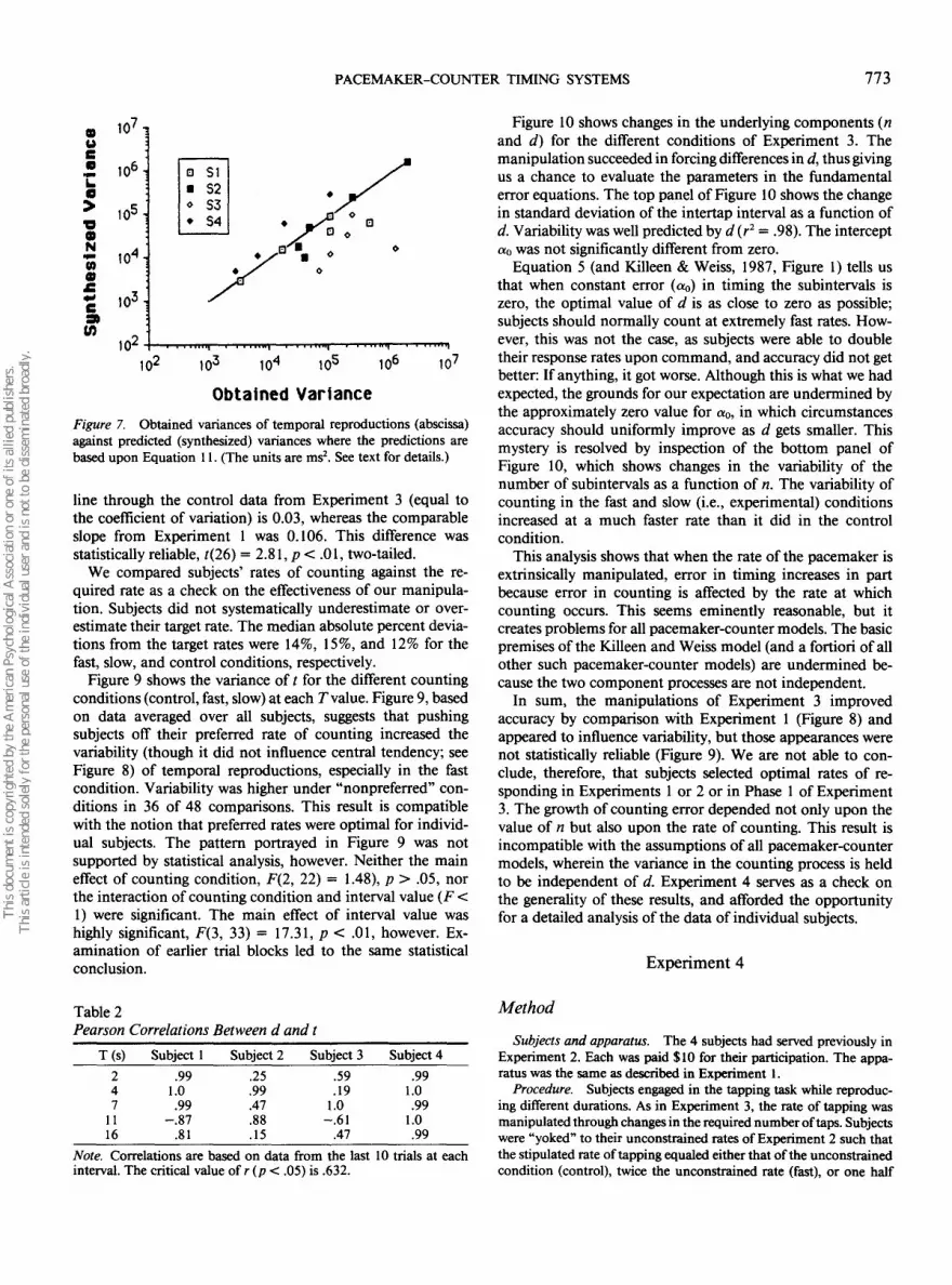
line through the control data from Experiment 3 (equal tothe coefficient of variation) is 0.03, whereas the comparableslope from Experiment 1 was 0.106. This difference wasstatistically reliable, t(26) = 2.81, p < .01, two-tailed.

We compared subjects' rates of counting against the re-quired rate as a check on the effectiveness of our manipula-tion. Subjects did not systematically underestimate or over-estimate their target rate. The median absolute percent devia-tions from the target rates were 14%, 15%, and 12% for thefast, slow, and control conditions, respectively.

Figure 9 shows the variance of t for the different countingconditions (control, fast, slow) at each rvalue. Figure 9, basedon data averaged over all subjects, suggests that pushingsubjects off their preferred rate of counting increased thevariability (though it did not influence central tendency; seeFigure 8) of temporal reproductions, especially in the fastcondition. Variability was higher under "nonpreferred" con-ditions in 36 of 48 comparisons. This result is compatiblewith the notion that preferred rates were optimal for individ-ual subjects. The pattern portrayed in Figure 9 was notsupported by statistical analysis, however. Neither the maineffect of counting condition, F(2, 22) = 1.48), p > .05, northe interaction of counting condition and interval value (F <1) were significant. The main effect of interval value washighly significant, F(3, 33) = 17.31, p < .01, however. Ex-amination of earlier trial blocks led to the same statisticalconclusion.

Figure 10 shows changes in the underlying components (nand d) for the different conditions of Experiment 3. Themanipulation succeeded in forcing differences in d, thus givingus a chance to evaluate the parameters in the fundamentalerror equations. The top panel of Figure 10 shows the changein standard deviation of the intertap interval as a function ofd. Variability was well predicted by d (r2 = .98). The intercepta0 was not significantly different from zero.

Equation 5 (and Killeen & Weiss, 1987, Figure 1) tells usthat when constant error (oo) in timing the subintervals iszero, the optimal value of d is as close to zero as possible;subjects should normally count at extremely fast rates. How-ever, this was not the case, as subjects were able to doubletheir response rates upon command, and accuracy did not getbetter: If anything, it got worse. Although this is what we hadexpected, the grounds for our expectation are undermined bythe approximately zero value for a0, in which circumstancesaccuracy should uniformly improve as d gets smaller. Thismystery is resolved by inspection of the bottom panel ofFigure 10, which shows changes in the variability of thenumber of subintervals as a function of n. The variability ofcounting in the fast and slow (i.e., experimental) conditionsincreased at a much faster rate than it did in the controlcondition.

This analysis shows that when the rate of the pacemaker isextrinsically manipulated, error in timing increases in partbecause error in counting is affected by the rate at whichcounting occurs. This seems eminently reasonable, but itcreates problems for all pacemaker-counter models. The basicpremises of the Killeen and Weiss model (and a fortiori of allother such pacemaker-counter models) are undermined be-cause the two component processes are not independent.

In sum, the manipulations of Experiment 3 improvedaccuracy by comparison with Experiment 1 (Figure 8) andappeared to influence variability, but those appearances werenot statistically reliable (Figure 9). We are not able to con-clude, therefore, that subjects selected optimal rates of re-sponding in Experiments 1 or 2 or in Phase 1 of Experiment3. The growth of counting error depended not only upon thevalue of n but also upon the rate of counting. This result isincompatible with the assumptions of all pacemaker-countermodels, wherein the variance in the counting process is heldto be independent of d. Experiment 4 serves as a check onthe generality of these results, and afforded the opportunityfor a detailed analysis of the data of individual subjects.

Experiment 4

Table 2Pearson Correlations Between d and t

T(s)247

1116

Subject 1.99

1.0.99

-.87.81

Subject 2.25.99.47.88.15

Subject 3.59.19

1.0-.61

.47

Subject 4.99

1.0.99

1.0.99

Note. Correlations are based on data from the last 10 trials at eachinterval. The critical value o f r ( p < .05) is .632.

Method

Subjects and apparatus. The 4 subjects had served previously inExperiment 2. Each was paid $10 for their participation. The appa-ratus was the same as described in Experiment 1.

Procedure. Subjects engaged in the tapping task while reproduc-ing different durations. As in Experiment 3, the rate of tapping wasmanipulated through changes in the required number of taps. Subjectswere "yoked" to their unconstrained rates of Experiment 2 such thatthe stipulated rate of tapping equaled either that of the unconstrainedcondition (control), twice the unconstrained rate (fast), or one half


20

o9

10

t = 1.0 IT +0.29

10 20T (sec)

u•i»

2 -fft a 0.1061 - 0.14

01 = 0.032 t + 0.11

0 10 20 SO

t (sec)

Figure 8. Means (top panel) and standard deviations (bottom panel)of temporal reproductions as a function of target interval ( T ) forExperiment 3. (Mean estimates [top panel] are shown for all condi-tions of Experiment 3. Standard deviations are shown for the controlcondition of Experiment 3 [filled symbols] and for Experiment 1[unfilled symbols]. The lines through the points are regressions withparameters as noted.)

the unconstrained rate (slow). Subjects made 40 reproductions of 4-and 11-s intervals under each tap rate condition (control, fast, andslow), and the conditions were presented in a different random orderto each subject. Feedback was provided after each estimate, but onlywith respect to the duration of the reproduction. The instructionswere as described in Experiment 3, except that the subjects were told

Figure 9. Variances of temporal reproductions as a function ofinterval value for the different conditions of Experiment 3.

to "use your tapping to help you judge the passage of time in whateverway seems appropriate to you."

Results and Discusson

The mean accuracy of subjects' estimates was not influ-enced by the experimental manipulations; in all cases subjectswere quite accurate in reproducing the target durations, as inExperiment 3.

Figure 11 shows the standard deviations of subjects' repro-ductions for the different intervals and counting conditions.The different counting conditions are represented as a func-tion of the average intertap interval (d), which varied accord-ing to the individualized required rate of tapping. It is clearthat variations in the rate of tapping affected the variabilityof temporal judgments. The pattern in this figure suggests anoptimum value of d(in the sense of minimizing variability of/) in the range of 300 to 400 ms. Values above or below thisrange (but especially above) increased the variability of timing.

As in Experiment 3, changes in the pacing requirementinfluenced the variability of subjects' temporal reproductions.Figure 11 suggests, however, that the optimal rate of tappingwas not idiosyncratic as suggested by Experiment 3. Ratherthe results of Experiment 4 indicate an absolute optimum ford in the vicinity of 1/3 s.

Experiment 5

In Experiments 3 and 4, we manipulated d through changesin the required number of taps. This approach forced subjectsto attend to the number of taps made, and perhaps facilitatedtiming for subjects not already predisposed to use countingstrategies. Almost certainly it served to minimize observederror in counting. In Experiment 5, we used a differenttechnique to force changes in d. Subjects were given a "sam-ple" target rate and asked to match the tempo of their tappingto the sample. The target rate was manipulated over condi-tions, and the effects of variations in the required rate wereassessed with respect to the accuracy and variability of sub-jects' reproductions.

Method

Subjects and apparatus. The 4 subjects had served previously inExperiments 2 and 4. They were paid $5 for their participation. Theapparatus was as described in Experiment 1.

Procedure. Subjects made 30 reproductions of an l l -s targetinterval by responding on a telegraph key for a period that matchedthe duration of a tone signal; the signal was presented just once;subsequent reproductions were guided by the feedback described inExperiment 1. Subjects' rate of tapping was manipulated over con-ditions through instructions to match a "sample" rate. Before eachblock of estimates, subjects heard a "sample" consisting of a series ofperiodic 1000-Hz tones; each tone lasted 15 ms, and the tone serieslasted 10 s. Under different conditions, the intertone intervals were150 ms (fast), 350 ms (medium), or 1200 ms (stow); subjects wereinstructed to practice the sample rate by synchronizing their tappingwith the tone and to maintain the sample tempo while reproducingthe target interval. A reminder of the sample rate was presented afterthe fifth trial of each block of estimates; the remaining reproductions


0.20 n

0.13-

uin o.io-

0.05-

0.00

10-

3-

Jd=0.24d- 0.01

.0 0.2 0.4

d (sec)

0.6 0.8

•X an = 0.065n + 0.682

ffn= 0.016n + 0.55

0 50 100 ISOn

Figure 10. Standard deviations of the duration of intertap intervals(d; top panel) and number of taps (n; bottom panel) as a function ofd and n, respectively. (For the bottom panel, the filled symbols[experimental] represent performance for the fast and slow condi-tions, and the unfilled symbols represent performance for the controlcondition.)

1000 2000

d (msec)

3000

Figure 11. Standard deviations of temporal reproductions for thedifferent conditions of Experiment 4. (Data are for each subject as afunction of d, with target interval as the parameter.)

were made without further exposure to the sample rate. The samplerates were presented in a different random order to each subject. Asin Experiments 3 and 4, subjects were told to "use your tapping tohelp you judge the passage of time in whatever way seems appropriateto you."


Manipulation of the rate of tapping did not affect theaccuracy of subjects' mean temporal reproductions, but themanipulation did produce changes in variability. Figure 12shows the standard deviations of reproductions for individualsfor each tap rate condition. The patterns are different fordifferent individuals. Variability for Subject 1 decreased mon-otonically with increases in the rate of tapping (i.e., decreasedin d), whereas for Subject 4 variability increased monotoni-cally with increases in the rate of tapping. For Subjects 2 and3 variability was lowest for the medium rate of tapping andhigher for faster or slower rates; this result is similar to thepattern portrayed in Figure 1 1 of Experiment 4.

The line through the data points shows the predicted vari-ances of t as a function of d, where the predictions are basedon Equation 2 rewritten with respect to d (Killeen & Weiss,1987, p. 457):

+ («2 + + (a,t + /32t2) + (13)

Estimates of the relevant coefficients of the fundamental errorequations were obtained as bimeans of individual subjectparameters in regressions corresponding to Equation 3 (datafrom this experiment: a0 = 700 ms, a, = 0, a2 = 0.0025) andEquation 4 (data from Experiment 2: |80 = 0.1, 0, = 0, ft =0.0005). The predicted variances remain constant over asubstantial range of d with upturns at extremely small (fastrate of counting) and large (slow rate of counting) values ofd. The upturn for large values of d is due primarily to /30,which we interpret as variability resulting from truncation orrounding error. Over a substantial range (250 < d < 500 ms),changes in the rate of counting have little impact on thevariability of timing; this could account for the weak effectsof our manipulations that forced subjects to deviate from theirpreferred rate of counting. Note that these predictions do nottake into account the increased variance resulting from coun-ter error at high rates of counting.

Figure 1 3 shows the changes in the standard deviation of das a function of d for each subject. As in Experiment 3, <rrf

appears to grow as a linear function of d, and the rate ofchange was similar for 3 of the 4 subjects.

General Discussion

We asked subjects to tap repeatedly on a telegraph key asthey reproduced temporal intervals, and took the durationand number of intertap intervals as measures of the compo-nents of a pacemaker-counter system. In Experiments 1 and2, most subjects did not vary their rate of responding as theyreproduced different durations; we interpreted this result assupportive of a fundamental prediction of the optimal timinganalysis that, to minimize variability in timing, the rate ofcounting should remain constant and independent of the


1200

1000-

U 800-

£ 600-*ta*w

b 400-

200-

500 1000

d (msec)1500

Figure 12. Standard deviations of temporal reproductions for thedifferent conditions of Experiment 5. (Variability measures are shownfor each subject as a function of d. The line through the data pointsrepresents predictions based upon Equation 14 [see text].)

duration of the interval to be timed (Equation 5). Rates ofresponding differed widely among subjects, but these differ-ences were not correlated with the variability of temporalreproductions (Figure 1). Equation 2, which relates the vari-ances of the component timing and counting processes to thevariance of temporal estimates, provided an approximateaccount of the data (Figures 2 and 7). The relative contribu-tions of the two components varied as a function of T, aspredicted (Table 1).

In Experiments 3, 4, and 5, subjects were required torespond faster or slower than their preferred response rate asthey reproduced temporal intervals. If subjects selected anoptimal rate of counting, we expected that forcing them off itwould impair timing (i.e., increase variability). In the controlcondition of Experiment 3, where subjects were constrained

0 200 400 600 800 1000 1200 1400

d (msec)

Figure 13. Standard deviations of d as a function of the mean valueof d for the 4 subjects in Experiment 5.

to regulate their tapping more carefully but at their preferredrate, their temporal judgments were more accurate than thoseof the subjects in the first experiment. The average data(Figure 9) indicated greater variability under the nonpreferredconditions, but the trends did not achieve statistical signifi-cance. The different pacing requirements imposed in Experi-ments 4 and 5 influenced variability, and suggested an opti-mum for d in the range of 250 to 500 ms.

Models of Pacemaker-Counter Systems

We have assumed throughout this article that the timingprocess may be represented as a pacemaker-counter system.Let us briefly review major theoretical accounts of suchsystems before evaluating our results in the context of Killeenand Weiss's generalized clock-counter model. The most im-portant early model was that of Creelman (1962) where thecounts were pulses emitted at random times by a stochasticsource and accumulated by a precise counter. This model,which (like most other models) holds that counting is error-less, has not been supported by the data (e.g., Allan & Kris-tofferson, 1974; Getty, 1975); these simple Poisson modelspredict that variance in estimates should increase as /, not ast2, which is counterfactual. To account for extant data, Creel-man had to add other sources of variance, such as an individ-ual forgetting parameter and a parameter that representedinstances where the subject's clock was not precisely synchro-nized with the onset of the signal. Treisman (1963) developeda model in which the counter is assumed to be error-free, butthe comparator (which compares information received froma memory store with inputs from the counter) is not. Treismanfurther assumed that the subintervals generated by the "clock"were constant within trials, but varied between trials. Thisassumption yields the experimental relation between T anda, known as Weber's law, and embodies a relationship be-tween the mean and variance of the pacemaker known asscalar timing (Gibbon, 1977).

Gibbon and Church (1984) developed a sophisticated clock-counter theory of timing by animals, one whose schematicform is very similar to Treisman's. Their information-processing model (and all other models of animal timing) hasbeen strongly constrained by the fact that Weber's law pro-vides a good description of most animal timing data (e.g., seeGibbon, 1977). Gibbon and Church took this result as evi-dence for a scalar timing process by which variance increaseswith the square of the mean, not linearly with it, as is the casefor a constant-rate Poisson process. The scalar timing propertyarises from variability in the pacemaker whose rate remainsconstant within trials but varies normally around a meanvalue between trials (Gibbon, Church, & Meek, 1984), pre-cisely as Treisman had previously postulated. The output ofthis system produces estimates whose mean and standarddeviation grow linearly with real time.

Elsewhere, we have suggested an alternative pacemaker-counter model of animal timing behavior (Killeen & Fetter-man, 1988). This behavioral theory of timing holds thatanimals base temporal judgments upon reinforcement-elicitedadjunctive behaviors. The behaviors serve as conditional cuesfor the passage of time; transitions between them are caused


by pulses from a pacemaker, which in many cases we mayassume to be a Poisson process. Killeen and Fetterman as-sumed that the rate of the pacemaker is proportional to therate of reinforcement (which varies inversely with T) in theexperimental context, and so their predictions also oftenconform to the relationship described as scalar timing (seeRousseau, Picard, & Pitre, 1984, for a similar model).

Pacemaker variance, whether within or between trials, sca-lar, or Poisson, is typically presumed to be the main contrib-utor to variability in timing. However, Kristofferson (1984)developed a "real-time criterion" theory of timing, whichassumes zero variance in the pacemaker. His account holdsthat the pacemaker is free running rather than synchronizedwith the onset of the stimulus to be timed. Variance in thistiming system is introduced through truncation errors in-curred at the onset and offset of the internally timed interval.As with other models, counting is assumed to be error free.

The available models of timing thus suggest different waysin which the pacemaker contributes to error in the timingprocess. The pacemaker has long been regarded as the sourceof variance in timing. It has been represented as generallyunreliable (Creelman, 1962; Killeen & Fetterman, 1988),unreliable only between trials (Gibbon & Church, 1984; Treis-man, 1963), or perfectly reliable (Kristofferson, 1984, forwhom error results from asynchronies between pulses of thepacemaker and the presentation of experimental stimuli).None of the models reviewed here, however, posit error incounting or allow for error in both timing and counting, aspermitted by Killeen and Weiss's generalization, and con-firmed by our results.

Models of Variance in the Pacemaker and Counter

The allocation of error to the component processes requiresseparate and distinct models for error in the counter and errorin the timer, and Equations 3 and 4 provided obvious candi-date models for these components. These models are flexiblebecause the coefficients in these equations may take on dif-ferent values depending upon the theory under consideration,including values of zero. We use the term model to denote aset of assumptions about the component processes (e.g., aPoisson model); when specific model types are used as descrip-tors of the overall liming process (e.g., Poisson timing), werefer to an observed relation between the mean and varianceof temporal estimates. Poisson models of the pacemaker donot necessarily imply Poisson timing of the whole interval,because the contribution of counter error must also be con-sidered. In this section, we evaluate what existing theory anddata tell us about plausible models for the component pro-cesses.

Pacemaker variance. Most theories of timing assume thatthe mean rate of the pacemaker remains constant (see Killeen& Fetterman, 1988, for an exception to this generalization);some have it varying around that mean value from one trialto the next. It is difficult to empirically evaluate differentmodels of the pacemaker because data are seldom reportedthat permit us to establish the relation between changes in itsperiod and variance. Getty (1976) simply assumed a scalarmodel for the pacemaker in which variance in the subintervals

increased as the square of the period («2 > 0; a, = 0), andCreelman (1962) assumed a Poisson model in which varianceis proportional to the period («2 = 0; a, > 0). Gibbon andChurch (1984) arrived at scalar timing because variance intime estimation is isomorphic with variance in the numberof pulses from the pacemaker source, whose rate is assumedto vary normally between trials yielding the scalar property.Our results, along with those of Wing and associates (e.g.,Wing, 1980; Wing & Kristofferson, 1973) and Wearden (inpress) provided more direct evidence about the characteristicsof the pacemaker mechanism, and hence about the appropri-ate form of Equation 3.

Wing and associates studied the timing process embodiedin the temporal spacing of repetitive motor responses, such asthe tapping of a telegraph key and the "counting" task usedin the present experiments. They used a technique in whichsubjects synchronized key-tap responses with the fixed-inter-val clicks of a metronome, and then attempted to continuetapping at the preestablished rate without the aid of themetronome. The variability of the temporal spacing of re-sponses following the synchronization period provides a mea-sure of the variance (or/) of the hypothetical pacemaker, andchanges in variability with different pacing requirements (i.e.,with changes in d) permit us to assess different versions ofEquation 3. In proceeding with this discussion, we assumethat the system that controls the timing of responses in motorproduction tasks also mediates the perceptual judgment ofduration, Keele and associates (e.g., Keele & Ivry, 1987; Keele,Pokorny, Corcos, & Ivry, 1985) conducted numerous timingexperiments whose results support this assumption.

The analysis of Wing and Kristofferson (1973; see Wing,1980, for a review) proceeds on the assumption that observedvariability in the timing of responses reflects the additivecontributions of two independent component processes.Timekeeper variance represents variability of the times be-tween successive pulses from the hypothetical pacemakersource; motor delay variance represents variability resultingfrom delays between pulses emitted by the pacemaker andthe ensuing motor response (i.e., the key tap). In the modelof Wing and Kristofferson, total variance is partitioned intothese underlying constituents through autocorrelationalanalysis. Wing and Kristofferson (1973) applied this model tosynchronized key-tapping data, and found that motor delayvariance remained approximately constant across differentpacing requirements, whereas pacemaker variance grew as alinear function of the required intertap interval. This result isconsistent with a Poisson model of the pacemaker. However,variance was predicted equally well by d or d2 (i.e., by Poissonor scalar models). There were large individual differences inthe slope (a,) with a median value of 0.4. Wing (1980) alsoreported data that supported a Poisson model for the genera-tion of subintervals, with an average value for at of 1.2.Rosenbaum and Patashnik (1980) had subjects produce asingle interval of time. Again the data were consistent with aPoisson model, with a typical value for al of 6.0.

Wearden (in press) used a task similar to ours wherebysubjects repeatedly pressed a button as they produced a 6-starget interval. The required number of presses was variedover five conditions (6, 7, 9, 11, and 13) while the target


interval remained constant. The standard deviations of theintercount intervals increased linearly with increases in themean intercount interval (slope of 0.105), a result that sup-ports a scalar model.

In Experiments 3 and 4, we manipulated d through changesin the required number of responses during intervals of fixedlength; in Experiment 5 subjects were asked to match a sampletempo as they reproduced different durations. In all threeexperiments, subjects responded at a steady pace throughoutthe reproduction, and the mean and variance of intertapintervals covaried in an orderly manner. Variance in d wasproportional to d2 (scalar model), although a linear functionbetween of and d (Poisson model) also provided a gooddescription of the data. Remember that our data indicated ascalar relation between the first and second moments of theestimates of the interval as a whole (variance increased as thesquare of the mean), a relation that has been held to beincompatible with a Poisson pacemaker (e.g., Creelman,1962). How can we have scalar timing if, as many studiesindicate, the pacemaker may be Poisson? This is possiblebecause the total variability reflects the additive contributionsof error in the timer and the counter (Equation 2). In the nextsection, we see that the counter has scalar properties (i.e., a2

= 02n2), and that these dominate overall timer variance for

moderate to long values of T.Counter variance. How might counter error affect timing?

Subjects might skip or fail to register a pulse ("count"), mightlose track and repeat a pulse, or might fail to increment adecade marker (e.g., "68, 69, 60, 61," etc). Variability incounting will result in any of these scenarios, and may besubstantial especially when attention is concurrently focusedon keeping the subintervals constant.

Each of the parameters of the fundamental error equationfor counting (Equation 4) represents a different type of error.i90 is the variance that is independent of the number of pulses,and as such represents synchronization error (an intervalstarting between two pulses) and truncation error (an intervalending between two counts). In reproduction, synchroniza-tion error should be minimal (unless the pacemaker is freerunning), but truncation error is inevitable. Its variance willequal the variance of a rectangular distribution ranging fromn - 0.5 to n + 0.5, which is 0.083. The contribution oftruncation error to total variance is proportional to d2 (seeEquation 13). /?, represents variance that is proportional to «,such as that resulting from the random failure to register acount. & represents variance that is proportional to n2. Forlarge counts, it is the major source of variance. When ft '»/8i, error is Weber-like; that is, Weber's law holds with aWeber fraction of Vft.

By comparison with timing, little is known about countingas it relates to the models under consideration. Indeed, count-ing may refer to several separate and distinct processes. Davisand Perusse (1988) suggested the term numerical competenceas a framework that subsumes a variety of numerical abilities,of which counting is one. By their definition, counting in-volves an enumerative process that provides an indication ofthe absolute numerosity of simultaneous or sequential events.This definition may be relevant to a subset of timing studiesin which explicit counting is involved (e.g., Getty, 1976).

Results from studies of memory for event frequency arerelevant (e.g., Greene, 1986; Jonides & Naveh-Benjamin,1987), and tell us that subjects are very accurate on thesetasks, and that performance improves when subjects are giveninstructions to attend to the frequency of events (Greene,1986). However, the number of events involved is typicallyquite small (often fewer than 10), and there is little informa-tion available about the variability of frequency estimates inrelation to the number of events counted. What we do knowindicates that counting error grows very slowly as a functionof number. Logie and Baddeley (1987) found Weber-likerelations in both estimates of n and counts of n. In the formercase, the Weber fraction was approximately 0.60, and in thelatter, 0.02, comparable to that found in our control conditionand in Experiment 2. Explicit enumeration clearly improvestiming (e.g., Hicks & Allen, 1979), and the improvement isgreater when subjects count out loud instead of to themselves(Goldstone, Boardman, & Leahmon, 1958).

In the schema of Davis and Perusse, estimation probablycomes closest to our construction of counting as it relates tohuman timing. Estimation involves an educated guess aboutthe number of events, without the aid of formal enumeration,and it does not require focused attention to the numericalproperties of stimuli. The unconstrained counting task ofExperiment 1 may well have involved estimation, whereasthe constraints of Experiment 3 came closer to enumerativecounting and resulted in substantially reduced variability oftemporal judgments.

Studies of numerosity judgments (i.e., estimation) withhumans (e.g., Burgess & Barlow, 1983; Cheatham & White,1952, 1954; Forsyth & Chapanis, 1958; Pollack, 1968; White,1963) suggest that counting error varies with number in a waythat is consistent with one version of Equation 4. For example,Pollack (1968) asked subjects to discriminate between trainsof auditory pulses that varied in number. He determineddifference thresholds for number, and his results, like ours(Figure 3), suggest that variance in counting grows as thesquare of number. For the lowest rate of stimulus repetition(10 Hz), the slope of the function was 0.082, close to what wefound when subjects counted at the fastest rate (about 6 Hz).

Data from studies of animal "counting" (e.g., Davis &Memmott, 1982; Fetterman, Dreyfus, & Stubbs, 1985; Hob-son & Newman, 1981; Meek & Church, 1983) provide addi-tional information about the nature of counting error. Al-though there is considerable methodological and conceptualconfusion regarding the status of animals' counting abilities(see Davis & Perusse, 1988) we can, at a minimum, allowthat animals possess the ability to discriminate the relativenumerosity of events ("many" versus "few"), and perhapsthey can estimate number, as we have used that term. As withhuman counting, the literature with animals indicates thatvariance grows with the square of number (e.g., Fetterman etal., 1985; Hobson, 1975).

Summary and Conclusions

Let us summarize what our data and related findings tellus about the components of pacemaker-counter systems. Thedata appear to favor a Poisson generator for the subintervals


(Rosenbaum & Patashnik, 1980; Wing, 1980; Wing & Kris-tofferson, 1973), although our results (Figure 9) are equallywell described by the Poisson and scalar models; this issue isnot settled. As for the counter, in cases involving estimation,variance increases as the square of number (e.g., Fettermanet al., 1985; Pollack, 1968; see also our Figure 5), a relationthat gives Weber's law for number. In cases of explicit count-ing, variance grows more slowly and may be a linear functionof number, as indicated by the data from the fast conditionof Experiment 3 (Figure 10). Such a relation could result frombinomial variability in the registration of pulses by the counter(e.g., there could be a constant probability of dropping indi-vidual pulses).

The available data suggest sensible models for the compo-nents of pacemaker-counter systems. Unfortunately, some ofthese same data suggest that the pacemaker and the countermay not be completely independent component processes, aswe had assumed. Hicks and Allen (1979) found that explicitcounting led to underestimation of time, suggesting thatcounting may decrease the rate of the pacemaker. Cheathamand White (1952, 1954) had subjects estimate the number ofvisual or auditory events, and found that numerical estimatesdepended on the rate of stimulus presentation, such thatsubjects systematically underestimated at faster rates. In Ex-periment 3, counting error (<rn

2) depended upon the subject'srate of responding (Figure 10). Such results, where countererror depends upon counting rate (although intuitively rea-sonable), are inconsistent with the presumptions of extantpacemaker-counter models.

There are models that can accommodate such interactionsof pacemaker and counter. For instance, blocked countermodels (Cox, 1962) describe systems in which pulses emittedby a Poisson source must be processed by the counter beforeanother pulse can be registered. Pulses that arrive during thisprocessing period are lost, or "missed." It is obvious that thenumber of pulses lost will depend upon their arrival rate andon the processing time. In the context of models for countererror, this model predicts that j3, will vary with the rate of thepacemaker, as the data suggest. For the data of Cheatham andWhite (1954), if we assume a blockage of 50 ms for eachpulse, the blocked counter model predicts the obtained in-creases in underestimation with increases in stimulus presen-tation rate. The duration of the hypothetical blockage periodis not unreasonable, and it is close to the 80-ms processingperiod assumed by one theory of time perception (Nakajima,1987). Whereas this model reconciles an interaction betweenrate of the pacemaker and variability in the counter, it permitsonly a linear growth of variance with number, not a quadratic(Weber-like) relation. Although it may subserve timing withexplicit counting (enumeration) where the data are not suffi-cient to rule out Poisson timing, it is inadequate as a generalmodel of counting and timing, where the counting may beaccomplished as estimation, and the timing is usually Weber-like (i.e., scalar), not Poisson-like.

Although the generalized model of Killeen and Weiss pro-vides a framework for these effects, the interdependence ofthe component processes undermines a basic assumption ofthe model. Counting error increases more rapidly when sub-jects estimate than when they explicitly enumerate events. By

itself, this merely limits the application of the model tocoherent performances, wherein the subject does not shiftmodes of counting. However, a continual interaction betweenrate of explicit counting and variance of the counter is notcaptured by the Killeen and Weiss (1987) formulation. Thisinterdependence could explain why subjects do best at mod-erate rates, even when aa is close to zero, under whichcircumstance optimal timing theory tells us that they shouldcount as fast as possible. Such results require a differentversion of Equation 4, the fundamental error equation forcounting variance. They also call into question Equation 2,which assumed independence of the component processes,although that equation may be relatively robust over this typeof deviation.

These data set a program for future research: clarificationof the appropriate fundamental error equations for variousconditions and subjects and their incorporation into a syn-thetic model for pacemaker-counter systems. Models that donot recognize error in both processes must be recognized asboundary conditions. Newer, generalized models must bemodified to respect the type of interdependence of compo-nents that we have demonstrated here.

References

Allan, L. G., & Kristofferson, A. B. (1974). Psychophysical theoriesof duration discrimination. Perception & Psychophysics, 16, 26-34.

Burgess, A. C., & Barlow, H. B. (1983). The precision of numerositydiscrimination in arrays of random dots. Vision Research, 23, 811 -820.

Cheatham, P. G., & White, C. T. (1952). Temporal numerosity: I.Perceived number as a function of flash number and flash rate.Journal of Experimental Psychology, 44, 447-451.

Cheatham, P. G., & White, C. T. (1954). Temporal numerosity: III.Auditory perception of number. Journal of Experimental Psychol-ogy, 47, 425-428.

Cox, D. R. (1962). Renewal theory. London: Methuen.Creelman, C. D. (1962). Human discrimination of auditory duration.

Journal of the Acoustical Society of America, 34, 582-593.Davis, H., & Memmott, H. (1982). Counting behavior in animals: A

critical evaluation. Psychological Bulletin, 92, 547-571.Davis, H., & Perusse, R. (1988). Numerical competence in animals:

Definitional issues, current evidence, and a new research agenda.Behavioral and Brain Sciences, 11, 561-615.

Doob, L. W. (1971). Patterning of time. New Haven, CT: YaleUniversity Press.

Fetterman, J. G., Dreyfus, L. R., & Stubbs, D. A. (1985). Scaling ofresponse-based events. Journal of Experimental Psychology: Ani-mal Behavior Processes, 11, 388-404.

Forsyth, D. M., & Chapanis, A. (1958). Counting repeated lightflashes as a function of their number, their rate of presentation,and retinal location stimulated. Journal of Experimental Psychol-ogy, 56,385-391.

Getty, D. J. (1975). Discrimination of short temporal intervals: Acomparison of two models. Perception & Psychophysics, 18, 1-8.

Getty, D. J. (1976). Counting processes in human timing. Perception& Psychophysics, 20, 191-197.

Gibbon, J. (1977). Scalar expectancy theory and Weber's law inanimal timing. Psychological Review, 84, 279-325.

Gibbon, J., & Church, R. M. (1984). Sources of variance in aninformation processing model of timing. In H. L. Roitblat, T. G.Sever, & H. S. Terrace (Eds.), Animal cognition (pp. 465-488).


Hillsdale, NJ: Erlbaum.Gibbon, J., Church, R. M, & Meek, W. H. (1984). Scalar timing in

memory. In J. Gibbon & L. Allan (Eds.), Annals of the New YorkAcademy of Sciences: Vol. 423. Timing and time perception (pp.52-77). New York: New York Academy of Sciences.

Gilliland, A. R., & Martin, R. (1940). Some factors in estimatingshort time intervals. Journal of Experimental Psychology, 27, 243-255.

Goldstone, S., Boardman, W. K., & Leahmon, W. T. (1958). Kines-thetic cues in the development of time concepts. Journal of GeneticPsychology, 93, 185-190.

Greene, R. L. (1986). Effects of intentionality and strategy on memoryfor frequency. Journal of Experimental Psychology: Learning,Memory, and Cognition, 12, 489-495.

Hicks, R. E., & Allen, D. A. (1979). Counting eliminates the repetitioneffect in judgments of temporal duration. Acta Psychologica, 43,361-366.

Hobson, S. L. (1975). Discriminability of fixed-ratio schedules forpigeons: Effects of absolute ratio size. Journal of the ExperimentalAnalysis of Behavior, 23, 25-35.

Hobson, S. L., & Newman, F. (1981). Fixed-ratio counting schedules:Response and time measures considered. In M. L. Commons & J.A. Nevin (Eds.), Quantitative analyses of behavior: Vol. 1. Discrim-inative properties of reinforcement schedules (pp. 193-224). Cam-bridge, MA: Ballinger.

Jonides, J., & Naveh-Benjamin, M. (1987). Estimating frequency ofoccurrence. Journal of Experimental Psychology: Learning, Mem-ory, and Cognition, 13, 230-240.

Keele, S. W., & Ivry, R. I. (1987). Modular analysis of timing skill.In G. H. Bower (Ed.), The psychology of learning and motivation(Vol. 21, pp. 183-228). New York: Academic.

Keele, S. W., Pokorny, R. A., Corcos, D. M., & Ivry, R. (1985). Doperception and motor production share common timing mecha-nisms: A correlation analysis. Acta Psychologica, 60, 173-191.

Killeen, P. R. (1985). The bimean: A measure of central tendencythat accomodates outliers. Behavior Research Methods, Instru-ments, and Computers, 17, 526-528.

Killeen, P. R., & Fetterman, J. G. (1988). A behavioral theory oftiming. Psychological Review, 95, 274-295.

Killeen, P. R., & Weiss, N. A. (1987). Optimal timing and the Weberfunction. Psychological Review, 94, 455-468.

Kristofferson, A. B. (1984). Quantal and deterministic timing inhuman duration discrimination. In J. Gibbon & L. Allan (Eds.),

Annals of the New York Academy of Sciences: Vol. 423. Timingand time perception (pp. 3-15). New York: New York Academy ofSciences.

Logic, R. H., & Baddeley, A. D. (1987). Cognitive processes incounting. Journal of Experimental Psychology: Learning, Memory,and Cognition, 13, 310-326.

Luce, R. D. (1986). Response times: Their role in inferring elementarymental organization. New York: Oxford University Press.

Meek, W. H., & Church, R. M. (1983). A mode control model ofcounting and timing processes. Journal of Experimental Psychol-ogy: Animal Behavior Processes, 9, 320-324.

Mosteller, F., & Tukey, J. W. (1977). Data analysis and regression:A second course in statistics. Reading, MA: Addison-Wesley.

Nakajima, Y. (1987). A model of empty duration perception. Percep-tion, 16, 485-520.

Pollack, I. (1968). Number or duration discrimination for auditorypulse trains. Journal of Experimental Psychology, 78, 660-665.

Rosenbaum, D. A., & Patashnik, O. (1980). A mental clock settingprocess revealed by reaction times. In G. E. Stelmach & J. Requin(Eds.), Tutorials in motor behavior (pp. 1-14), Amsterdam: NorthHolland.

Rousseau, R., Picard, D., & Pitre, E. (1984). An adaptive countermodel for time estimation. In J. Gibbon & L. Allan (Eds.), Annalsof the New York Academy of Sciences: Vol. 423. Timing and limeperception (pp. 639-642). New York: New York Academy ofSciences.

Treisman, M. (1963). Temporal discrimination and the indifferenceinterval: Implications for a model of the "internal clock." Psycho-logical Monographs, 77 (Whole No. 756).

Wearden, J. H. (in press). Do humans possess an internal clock withscalar timing properties? Learning and Motivation.

White, C. T. (1963). Temporal numerosity and the psychological unitof duration. Psychological Monographs, 77, 1-37.

Wing, A. M. (1980). The long and short of timing in responsesequences. In G. E. Stelmach & J. Requin (Eds.), Tutorials in motorbehavior (pp. 469-486). Amsterdam: North Holland.

Wing, A. M., & Kristofferson, A. B. (1973). The timing of interre-sponse intervals. Perception & Psychophysics, 20, 191-197.

Received September 27, 1988Revision received October 26, 1989

Accepted October 30, 1989

Documents

A componential analysis of pacemaker-counter timing systems