Journal of Dynamics and Differential Equations, Vol. 5, No. 1, 1993

A C l a s s o f N o n l i n e a r , C o m p l e t e l y I n t e g r a b l e

A b s t r a c t W a v e E q u a t i o n s

Thierry Cazenave, 1 Alain Haraux, 1 and Fred B. Weissler 2

Received December 12, 1991

If L is a positive self-adjoint operator on a Hilbert space H, with compact inverse, the second-order evolution equation in t, u '+ Lu + ][ull2nu= 0 has an infinite number of first integrals, pairwise in involution. It follows from this that no nontrivial solution tends weakly to 0 in H as t --, or. Under an additional separation assumption on the eigenvalues of L, all trajectories (u, u') are relatively compact in D(L 1/2) x H. Finally, if all the eigenvalues are simple, the set of initial values of quasi-periodic solutions is dense in the ball B~ = {(u 0, U'o)C:D(L1/Z)xH; IlLa/2uol]2+ [tu;ll2<e} for s sufficiently small.

KEY WORDS: Wave equations; quasi-periodic solutions; completely integrable Hamiltonian systems.

AMS CLASSIFICATIONS: Primary--58F07, 35L70; Secondary--35B40, 35B15.

1. I N T R O D U C T I O N A N D F U N C T I O N A L S E T T I N G

Le t H be a separab le , rea l H i l b e r t space a n d let L be a (poss ib ly

u n b o u n d e d ) se l f -adjoint , pos i t ive def in i te o p e r a t o r in H. T h e s e c o n d - o r d e r

e v o l u t i o n e q u a t i o n

u" + L u + c llull 2u -- 0 (1)

where II 1] is the norm in H and c > 0, is a Hamiltonian system that should combine certain properties of the abstract wave equation u '+ Lu = 0 and of the cen t ra l force m o t i o n u" +cllull2u=O. F o r the w a v e e q u a t i o n , the

1Analyse Num6rique, Universit6 Pierre et Marie Curie, 4 place Jussieu, F-75252 Paris Cedex 05, France.

2 Laboratoire Analyse G6om6trie et Applications, Institut Galil6e, Universit6 Paris XIII, Avenue J-B Cl6ment, F-93430 Villetanneuse, France.

129

1040-7294/93/0100-0129507.00/0 �9 1993 Plenum Publishing Corporation

130 Cazenave, Haraux, and Weissler

general solution is almost periodic if L has a complete set of eigenvectors, while the trajectories of the central force motion lie in the plane spanned by the initial values u(0) and u'(0) and are quasi-periodic with at most two basic frequencies (see, e.g., Ref. 9). It is therefore natural to ask whether or not the superposition of the two operators preserves the almost periodic character of the trajectories. Problem (1) includes as a special case the modified cubic wave equation

uloa = 0

(2)

with O a bounded domain of R N, which (with c = 1/10] ) can be considered as an approximation of the cubic wave equation

u . - A u + u 3 = 0

ulo~ = 0 (3)

Equation (3) was studied in Refs. 2, 4, 5, and 11, and the asymptotic behavior of an arbitrary solution is essentially unknown. Finally, when H = R 2, the system of two differential equations

u" + u(1 + u 2 + 1) 2) .~- 0

V" + v(k + u 2 + v 2) = 0 (4)

is an interesting special case of (2) for which many of the difficulties of the general equation are already manifest. The asymptotic behavior of the solu- tions to (4) is the object of the following paper [8], while in the present paper we look for general results concerning Eq. (1). Most of these were announced in our preliminary report [-7].

Throughout this paper, we assume that the setf-adjoint operator L has a complete set of eigenvectors. More precisely, H is the orthogonal (Hilbert) direct sum of the eigenspaces

Hj = ker(L - 2 / )

where the eigenvalues 2j, j t> 1, from a finite or infinite increasing sequence of positive real numbers. In other words,

N

/4= | H~ j=l

Nonlinear Integrable Abstract Wave Equations 131

where N is either a positive integer or oo. We set

mj = dim(Hi)

and so 1 ~ mj ~< oo. For convenience, we denote by J the set of allowable indices for the

eigenvalues. In other words,

({1 ..... N} if N < o o

J = ( N if N = o o

Similarly, for each j e J, we define

Kj = {;1 . . . . . mj} if if rnj < oo

m j = oo

Note that in the case N = oe we do not explicitly assume that )v ~ ~ as j ~ co, though this is the case if L is an elliptic differential operator. See the final remark for a discussion of more general conditions on the eigenvalues.

As we will see in Section 2, Eq. (1) admits an infinite family of conser- vation laws if N = oo. The conserved quantities are defined in terms of the components of the solution with respect to the above spectral decomposi- tion of L. It is therefore necessary to regard Eq. (1) as a (possibly infinite) system of ordinary differential equations for the components. We formulate this as follows. For each eigenvalue 2j we set

and then

x j = / = ( x j )

N

x = | j = l

Once we fix an orthonormal basis in each eigenspace Hi, j e J, the mapping H ~ ~ given by

u ~ U = (uj,~)j~j,k~ Kj

where uj, k is the k th component of the orthogonal projection of u onto Xj, is an isometric isomorphism. In particular,

N my

Ilull~ = II gll ~ u 2 j = l k = l

132 Cazenave, Haraux, and Weissler

Furthermore, the image of D(L 1/2) under this isometry is the space

j = l k = l

which itself is a Hilbert space equipped with the norm

N mj

llLi/ ull =llUll = Z Z j = l k = l

The isometry u ~-+ U can be extended to D(L-1/2), in which case the image is the larger space

{ ~J, kEKj;j N mj u2 } u= (uj, k)j E E k=l "~J

which, again, is a Hi]bert space equipped with the norm

mj 2 IIL-~/2ull~= IlSll~, = ~

j = l k = l /~J

We recall that ~ ' is the topological dual of ~ with ~r as pivot space, that is, ~ ~ 5f = ~ ' ~ ~ ' where the embeddings are dense.

We emphasize that the isometry u ~ U depends on the choice of bases for the eigenspaces Hi. We will see (Remark 3.6 and Theorem 6.8) that a judicious choice can be helpful.

Under the isometry between H and ~r described above, Eq. (1) with c = 1 is equivalent to the following system of second-order ordinary differential equations:

uS'k + ,~juj, k + II UIl~uj.k = 0 (5)

where j e J and k ~ Kj. Note that the constant c in Eq. (1) can always be reduced to 1 by setting une w = xfcu. System (5) is a Hamiltonian system associated with the energy E defined by

N mj 2 2

j = l k = l j = l k = l j 1 k = l

= �89 I1 vii 2 + �89 II UII ~- + 1 II Ul[ 4 (6 )

It is clear that E e C~(V x ~ r, R), and so the energy is conserved along trajectories (U(t), U ' ( t ) ) ~ x Sf of (5). In particular, the initial value problem for (1) [or (5)] is globally well posed in D(L m) x H.

Nonlinear Integrable Abstract Wave Equations 133

In Section 2 we introduce three families of conservation laws for system (5) and discuss some of their properties. In Section 3 we prove the existence of global, bounded solutions to (5) in a family of Hilbert spaces depending on a real parameter 0~>-1 . These spaces are simply the abstract Sobolov spaces built on ~U x X, which corresponds to 0 = 0, with Df x ~ ' corresponding to 0 = -1 . Our main results are stated and proved in Sections 4 and 6. In particular, we show that any solution such that U(t ) tends weakly to 0 in 5~ as t-~ oo must be identically zero (Theorem 4.1) and, under an additional assumption on the eigenvalues 2j, that the trajec- tory of a solution {(U(t), U'(t)); t e ~ } is relatively compact in any space in which it exists, such as ~t ~ x f or ~r x ~ ' (Theorem 4.5). In Section 5 we give some background concerning recurrent solutions. Finally, in Section 6 we give some sufficient conditions for the solution to be quasi-periodic (Theorems 6.2, 6.3, 6.8, and 6.9). These results provide a natural continua- tion of the previous work of Lax [10] and of Cabannes and Haraux [3] concerning similar problems.

2. THE CONSERVATION LAWS AND RELATED TOPICS

In addition to the Hilbert space ~Y, which plays a basic role with respect to the nonlinear term of (5), it is convenient here to consider also the space

= { (uj,~)j~ s,k ~ Kj; all but finitely many components are zero }

containing only finite linear combinations of the eigenvectors of L (i.e., their images in ~f). Indeed, it follows immediately from the special structure of (1) that this system generates a global flow on ~ and that each subspace of

fr,,, = { ( Uj.k )j~ s,k ~ KS; Uj, k V a 0 only i f j ~< m and k ~< m }

is invariant. On each ~m, the energy conservation yields global solutions in the regularity class C2(R, :~m) in which differential calculations can be made in the classical sense. With this in mind, we define for j ~ J the quantity

Ej(g, V)= Y~ v~+,~ju~,k, +~U),N Ilgl[ 2~ +~ Z 2i--'~j J k = 1 i C j l 1

(7)

Furthermore, given j e J and k, I e Kj, we set

Fff ' t (U, V) = UZkVjd-- Vj, kU+,s (8)

134 Cazenave, Haraux, and Weissler

It is clear enough that Ej and F f '~ are well defined on 5f x 5f and even on Y" x ~ ' . However, for the moment we restrict our attention to the trajectories on 0~ x ~ , where we have the following result.

Proposition 2.1. Ej(U, U') and Ff'I(U, U') are first integrals o f system (5). More precisely, for every trajectory in f ; x .~ we have

Ej(U(t), U' ( t ) )=Ej(U(O) , U'(0)), Ff"(U(t) , U'( t ) )=F~"(U(O), U'(0))

for all t E R and all j ~ J and k, l ~ Kj.

Proof. It follows from (5) that

l d 2 dt (ui'tuJ'k' - Ui'lUj'k)' 2 . . . . . . . - - (Idi, lUj, k __ Ui, lUj, k ) (Ui , lUj, k - - idi, lb!j,k )

= ( ~ i - ; ' j ) Ui, lUj, k(Ui, l ~ , k - - US, lUj, k )

Therefore,

1 d ~_ (ui, tuj, k ' w '2 , _ u~,t,,,k ~ m~

2 dt s 2 , - 2j - s s u~,,uj,~(u,,,u~,k - ui,,uj, k) i ~ j l 1 i ~ j l = 1

As well, we find

d{,2 21 } a; u',"+'tJuJ,*+$ "2" ell~

= 2uj, kuj, k + 22jUj, NUj, k + Uj, kUj, k II Nil 2 i i

N mi

= - Z Y~ u , , , . j , ~ ( u , , , u ; . ~ - u;,,u+,.) i = 1 l = 1

It follows that

m, )

2 ' gi, lUi, l l = 1

d f ,2 1 umkl U[12 + 1 (U,,,US, k--U~,,Uj, k)= ~ i # j l = 1

mj = - Z uj,,uj, k(uj , ,u; ,k-- u;,,u,O

l = 1

Summing the above identity over k ~ Kj, we obtain that Ej is a first integral of (5). Conservation of F~, t is immediate, since the equations for Uj, k and uj, t are the same. []

Nonlinear Integrable Abstract Wave Equations 135

We now derive some estimates on the first integrals Ej. To this end, we define the space Y'o, for - 1 ~< 0 < ~ by

j blj, k <. O0 j = l k = l

which is a Hilbert space when equipped with the norm

N rnj

IIulig E E o = ~ u;,~ j = l k = l

In particular, ~ = f i , 5Y = fo , and ~ ' = X_I. On the other hand, it is clear that Xo ~ ~ if - 1 ~< p ~< 0. We begin with with the following estimate.

Lemma 2.2. I f - - 1 ~ 00 < 01, then for every ~ > 0 there exists C(e) such that

II uII ~o < e 11 uII ~, + c(e)II uII =_~

for every U e YCo,.

Proof. First observe that if ()v)J~J is bounded, then all the norms [[ "[to are equivalent, in which case the result trivially holds (even with

= 0). Suppose now that N = ~ and 2j-~ ~ as j ~ ~ , and let Jo be large enough so that MOo ~ - oo/> 1. Then

JO mj ~ mj 1 0 2 I/uIl o<Y E oo+1 _1 2jo 2j u),k + ~ ~ 2 f uj, k

j = l k = l j = j o + l k = l / ~ j o

•]0o+1 "vo II utl ~_~ + 8 II uIJ ~, from which the result follows. []

Lemma 2.3. I f 0 >>. - 1 and every ( U, V) ~ Y'o + 1 x 3s then

Ej(U, V)~(1 -~l#,o([[U]]~+~ + UVll~)) ~ (2ju~,k+V~,k) k = l

(9)

and

mj rnj

Ej(v, v)<(1 +#j,o(tluIl~+,+ llvll~)) E (2ju~,~+vj~)+ �89 Ilvll~ E u~ j ,k k = l k = l

( lo )

136 Cazenave, Haraux, and Weissler

where

0, /f j = l

qj, o = 1 if j > 2 min{Alo+ l(~.j_ ~.1), 2o+,[] - - ~ j - - 1 ) } '

and

1 IAJ--]O+I[] --~j)

Proof. Observe first that

(Ui, IVj, k -- 1)i,,Uj, k) 2 ,~ 2 ( ~i ~jU~kl)2"~ +

~< 2 (2'u/2" + v'~')(2JuJ{k + v){k) min{2,, 2j}

(11)

Estimate (9) for j = l is immediate, since all the terms in E~ are nonnegative. For j >/2, we have

mj

k = l

2 1 ~ i ~ ~_ (U~,tVJ, k--V~,tUj, k) 2 (~'jU2k nt- UJ'k)--2 k=lE l 1 ~ J ~

and so it follows from (11) that

mj

k = l

=E k = ,

( i i (2jU~k+V)2k) 1 - E ~ 2'u2'+v~'~

2, u~,l~-'~i~,,q (~ju},,+v},k) l - J - ' m, 0+1.2 --~0.2

i=1 1=1

(9) follows, since )0+1()~i , j -2i)>~(1/qj , o). [Note that the function t~-+ t o+ 1(2j-t) is increasing on (0, (0 + 1)2j/(0 + 2)) and decreasing on ( (0+ 1)2j / (0+2), 21-).] We now prove (I0). Note that

) Ej<~ ~ 2jU2k+Vj, k j, kllgll~ k = l

71-21mJ ~ (ui'll3j'k - ~j k = l i = j + l l 1

Nonlinear Integrable Abstract Wave Equations 137

By applying (1 1), we get

P_Tj<~ E (s 1+ k = 1 i = j + l

( = Z + 4 0 1 + k = l i = j + l

1 "J + i II Ull ~ E ,~ju~,k

k=l

(10) follows, since 2~ o) for all i>j.

We now define, for - 1 ~< 0 < o%

m, ;,ub + ,

/ = 1

0 + 1 . 2 - - ~ 0 . 2 \ mi 2i Ui'l'T'l~iUi'l~

I=I

1 E~ V)= IIUII~+~ + II Vl102+~ IIUI}211UII 2

1 N mj

E E -~ 4 j = 1 k = l

We have the following result.

rnj u 2

j,k k = l

[]

,~J t=l 2i-2J (Ue':J'k--Vi'tU;'k)2 (12)

Lemma 2.4. For every - 1 <<. 0 < oo, the following properties hold.

(i) E~ ).

(ii) I f 0 > O, then there exists C(O) >~ 0 such that

E~ V) >~ [[ uII ~ +, + II vii ~ - c(o)(ll uIl~ + I1 Vll~_,)(ll uII ~- + II vii ~)

E~ V)<~ HUIl~+l + IlVll~ + �89 2

for all (U, V)~&+, x~;o. (iii) I f 0 < O, then there exists C(O) >1 0 such that

E~ V)>~ ]lUll~+l + II Vll~

g~ U, V) <<. (11Ullo 2 +1 + II vii ~)(1 + c(o)( II Ull 2o +x + tl vii ~)) + �89 ~ HuII

for all (U, V) aY'O+l xWo. (iv) E~ V) = 2E(U, V).

N

(v) I f U, V ~ , then E~ V)= ~ 2~ V). j = l

1 N (vi) I f U, V ~ , then E(U, V)=~j~I.= Ej(U, V).

138 Cazenave, Haraux, and Weissler

Proof. Suppose first that 0 > 0 . Then (2~176 and so the upper estimate of (ii) is immediate. To prove the lower estimate, note that

"~/0 --/k, ~ 1) ~,- ,~J ~ o(~o_1 + ;y_

and so, by (11),

20 - 2.~. (u, ,zv, ,k - u; ,evi , , ) 2 ~ 20(27-1 _{._ ~ : - -1) ( ; i hI2 , "~- D2l)(*~jbl2k "~- DJ2, k) 2 i - - I~ j 21 ' , �9

2 0 0 2 0 - 1 2 2 2 0 0 2 1 2 2 "<,h-- (~' u,,, + ;~. ~,,,)(;;uj,~ + ~2), + ~ (;j u;,~ + ,t ~ ~j,O(,~;u,,, + ~,~,)

Property (ii) follows easily. Suppose now that 0 < 0. Then (2 ~ - 2~ i - 2;) >0; and so the lower estimate of (iii) is immediate. To prove the upper estimate, note that

;o; 9 12~176 = 2~ IL-~176 ~< 101 min{2i, 2;} '+~ I,~,- 2;l

and so,

;9-; 0 ;0; 9 ;~i- ; ; ~< 101 2~+0

By applying (11), we get

2 f f - 2 ~ 2101 i, lAV l~il)i,i)(2 j Uj, k.~_/~jl)j,k) l~,--~j (lgi"UJ'k--blj'kbli'l)2~l+8(*~+Obl2 0 2 1 + 0 2 "0 2

and property (iii) follows easily. Property (i) is proved by similar estimates. Property (iv) is immediate from the definitions (6) and (12). Finally, to prove property (v), observe that if U, V e ~ , then also E j = 0 for all but a finite number of j. Therefore, the series makes sense. Now

~0 Ej( U, V)~- E 1~0 + l u 2 ' ~0 V2k ,=]_ I o 2 2 j,k + , ~ ,~; u),k II Ull j = l j = l k = i

1 N mj ~ (Ui, lUj, k __ ldj, kVi, l)2

' =1 k = l i~j l 1

Nonlinear Integrable Abstract Wave Equations 139

By symmetry,

N mj mi E E E E

j = l k = l i#j l = 1 2 i - 2 s 1 ~--~ mj mi

-~-~ 2 E E E ~ff--~Oi (Ui, lVj, k--Uj, kVi, l) 2 j = l k = l i*j l=l :~i--2J

Hence property (v), and property (vi) is a special case of (v). This completes the proof. []

These general properties of the conservation laws F: and E ~ will be useful throughout the paper. More specific properties, restricted to the case where the eigenvalues )~j are simple, will be established when needed in Section 6.

3. THE INITIAL V A L U E PROBLEM: EXISTENCE, R E G U L A R I T Y A N D RELATED Q U E S T I O N S

As already mentioned in Sections 1 and 2, our system (5) can be easily solved (existence and uniqueness of bounded, global solutions) in both spaces ~ x X and X x X. Since the nonlinear operator Y ~ It U[I ~ U is well defined and Lipschitz continuous on bounded sets of X, it is natural to look also at the Cauchy problem i n X x ~ ' and in the intermediate spaces Xo + 1 x Xo for - 1 < 0 < 0. The study of existence in Xo + 1 x Xo for 0 > 0 will yield regularity properties. In this direction, we have the following results.

Proposition 3.1. Let - 1 ~ < 0 < ~ . For every (Uo, Vo)eXo+l xXo, there exist T . , T* > O and a unique, maximal (mild) solution U ~ C ( ( - T . , T*), 3 f O + l ) n C l ( ( - T . , T*),Xo) of system (5). U is maxi- mal in the sense that i f T * < ~ (respectively, i f T . < ~ ) , then II u ( t ) l l o + 1 + [1 u ' ( t ) l l o - " o0 when t Y T* (respectively, when t ~ - T . ) . Moreover, U depends continuuouly on (Uo, Vo) in the sense that i f (U~, V ~ ) ~ (Uo, Vo) and if U n denote the corresponding solutions of (5), then for every compact interval I c ( - T , , T*), U n exists on I for n large enough and Un ~ U in C(I, Xo+ I) n CI(I, Xo).

Proof. We write (5) as a system of first-order equations by setting U ' = V. In other words,

~,k = - ~ , k - I l U l r ~ ~,k

140 Cazenave, Haraux, and Weissler

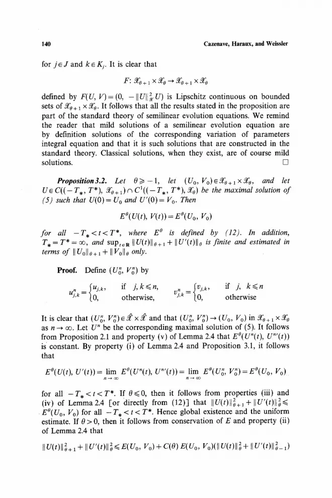
for j e J and k e Kj. It is clear that

F : f iO+l X f io "'-~"l" fiO + 1 X f io

defined by F(U, V)= (0, - I IUl[~U) is Lipschitz continuous on bounded sets of fi0 + 1 x fi0. It follows that all the results stated in the proposition are part of the standard theory of semilinear evolution equations. We remind the reader that mild solutions of a semilinear evolution equation are by definition solutions of the corresponding variation of parameters integral equation and that it is such solutions that are constructed in the standard theory. Classical solutions, when they exist, are of course mild solutions. []

Proposition3.2. Let 0>~-1, let (Uo, Vo)efio+lXfio, and let U e C ( ( - T , , T*), fi0+ 1)c~ C](( - T , , T*), fi0) be the maximal solution of (5) such that U(O)= Uo and U'(O)= Vo. Then

E~ V(t))=F-~ Vo)

for all - T , < t < T * , where E ~ is defined by (12). In addition, T , = T* = c~, and supt~R I[ U(t)[[O+l + [[ U'(t)l[o is finite and estimated in terms of ]] U0[]0+l + [[ V0[]0 only.

Proof. Define (Ug, Vg) by

n ~UJ, k' if j,k<~n, n =~vj, k, if j, k<~n u)'k = (0, otherwise, vJ'k ~0, otherwise

It is clear that ( U~', V o) e 2~ x 5~ and that ( Ug, Vg) ~ ( Uo, Vo) in fi0 + 1 x fifo as n ~ m. Let U n be the corresponding maximal solution of (5). It follows from Proposition 2.1 and property (v) of Lemma 2.4 that E~ U"(t ) ) is constant. By property (i) of Lemma 2.4 and Proposition 3.1, it follows that

E~ U'(t))= lim E~ U"'(t))= lim E~ V~)=E~ Vo) /~ ---+ o o n ---~ o o

for all - T , < t < T*. If 0~<0, then it follows from properties (iii) and (iv) of Lemma2.4 [-or directly from (12)] that [[U(t)l[~+l+ [ [U ' ( t ) ] t~ < E~ Vo) for all - T , < t < T*. Hence global existence and the uniform estimate. If 0 > 0, then it follows from conservation of E and property (ii) of Lemma 2.4 that

[] U(t)[[ ~+1 + [] U'(t)[[ ~ ~ E(Uo, Vo) + C(O) E(Uo, Vo)(ll U(t)[[ ~ + I[ U'(t)[[ ~_ 1)

Nonlinear Integrable Abstract Wave Equations 141

Lemma 2.2 now yields

il U(t) l l 2+1 --~ tl Ut( t )H o 2

<~ g ~ Vo) + �89 e(t)ll ~+ ~ + II u'(t)ll 2)

+ C1(0) g(Uo, Vo)(lt e(t)H 2_1 + II e'(t)l121)

<. g~ Vo) + �89 U(t)ll 2+~ + II u'(t)ll ~) + Cl(O) g(Uo, Vo) 2

Global existence and the uniform estimate follow easily. []

Remark 3.3. When 0 = 1, one verifies easily that E ~ can be written in the form

El( U, V) = ]lZl/2Vll ~ + HLUII ], + �89 II Ull 2 HZ~/2Uli 2 5s

N mj

+1( U, V)~-�89 IIVII 2 + 1 Z E (F)") 2 j = l k , l = l

Therefore, it follows from Propositions 2.1 and 3.2 that the following quantity is a first integral of (5).

/ ~ I ( u ' V) = tLL~/2VII 2 1/2 2 ~ + IlZUIl~ + �89 ~ ~,IIL UII~. 1 U 2 1 2 2

In particular, in the special case of the wave equation (2),

( o)2 J~l( u, h~t) IlVu'll~2+ ItAull~2+' ,2 �89 u ~ l lVu l l~+ �89 uu' 2 , 2 = - IlullL21lu IlL2

Therefore, the result of Proposition 3.2 for 0 = 1 means that any trajectory such that (u(0), u'(0)) ~ (H2(f2) c~ Ho1(s • H~(f2) remains bounded in that space for all t E R, assuming, for instance, that f2 has a C 2 boundary. This type of result is unknown for the "real" cubic equation (3), even when o = (0, ~).

Remark 3.4. When the eigenvalues 2j are multiple, the conservation of the quantities F f 't for k, l eKj is reminescent of the properties of the central force motion (case N = 1). Connected with this, the following simple lemma will allow us to reduce the multiplicities mj when we are dealing with a given trajectory U.

Lemraa 3.5. Let X be a real Banch space, let T > 0 , and let a t C([0, T], R). If uE C2([0, T], X) solves equation

u" +a(t)u=O

865/5/1-1o

142 Cazenave, Haraux, and Weissler

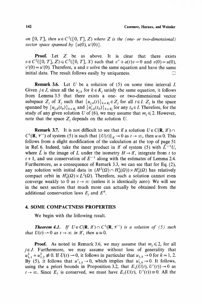
on [0, T], then u E C2([0, T], Z) where Z is the (one- or two-dimensional) vector space spanned by {u(0), u'(0)}.

Proof. Let Z be as above. It is clear that there exists v ~ C2([0, T], Z) ~ C2([-0, T], X) such that v" + a(t)v = 0 and v(0) = u(0), v'(0) = u'(0). Therefore, u and v solve the same equation and have the same initial data. The result follows easily by uniqueness. []

Remark 3.6. Let U be a solution of (5) on some time interval L Given j ~ J , since all the uj, k for k ~ K j satisfy the same equation, it follows from Lemma3.5 that there exists a one- or two-dimensional vector subspace Zj of Jfj such that {Uj, k ( t ) } k ~ Z j for all t e l Zj is the space spanned by {Uj, k ( t 0 )}k~ and {Uj, k ( t 0 )}k~ for any t0 ~ I. Therefore, for the study of any given solution U of (6), we may assume that mj ~< 2. However, note that the space Zj depends on the solution U.

Remark 3.7. It is not difficult to see that if a solution UE C(R, ~g) c~ CI(R, ~ ' ) of system (5) is such that II U(t)ll ~r--' 0 as t--, ~ , then u - 0. This follows from a slight modification of the calculation at the top of page 51 in Ref. 6. Indeed, take the inner product in X of system (5) with s where/2 is the image of L under the isometry H ~ Y', integrate from t to t + 1, and use conservation of E - 1 along with the estimates of Lemma 2.4. Furthermore, as a consequence of Remark 3.3, we can see that for Eq. (2), any solution with initial data in (H2(f2)~ H~o(O))• Ho~(12) has relatively compact orbit in Hlo(f2)x L2(s Therefore, such a solution cannot even converge weakly to 0 as t ~ oe (unless it is identically zero). We will see in the next section that much more can actually be obtained from the additional conservation laws Ej and E ~

4. SOME COMPACTNESS PROPERTIES

We begin with the following result.

Theorem 4.1. I f U~ C(R, Y')c~ CI(R, ~//~') is a solution of (5) such that U(t) --~ 0 as t ~ ~ in f , then u =- O.

Proofi As noted in Remark 3.6, we may assume that mj~<2, for all j ~ J . Furthermore, we may assume without loss of generality that U 2 1,1 + u~.2 ~ O. If U(t) --~ O, it follows in particular that Ul,~ ~ 0 for k = 1, 2. By (5), it follows that U"l.k~O, which implies that u'l.k~O. It follows, using the a priori hounds in Proposition 3.2, that EI(U(t), U ' ( t ) ) ~ 0 as t ~ o9. Since E1 is conserved, we must have E~(U(t), U ' ( t ) ) -O. All the

Nonlinear Integrable Abstract Wave Equations 143

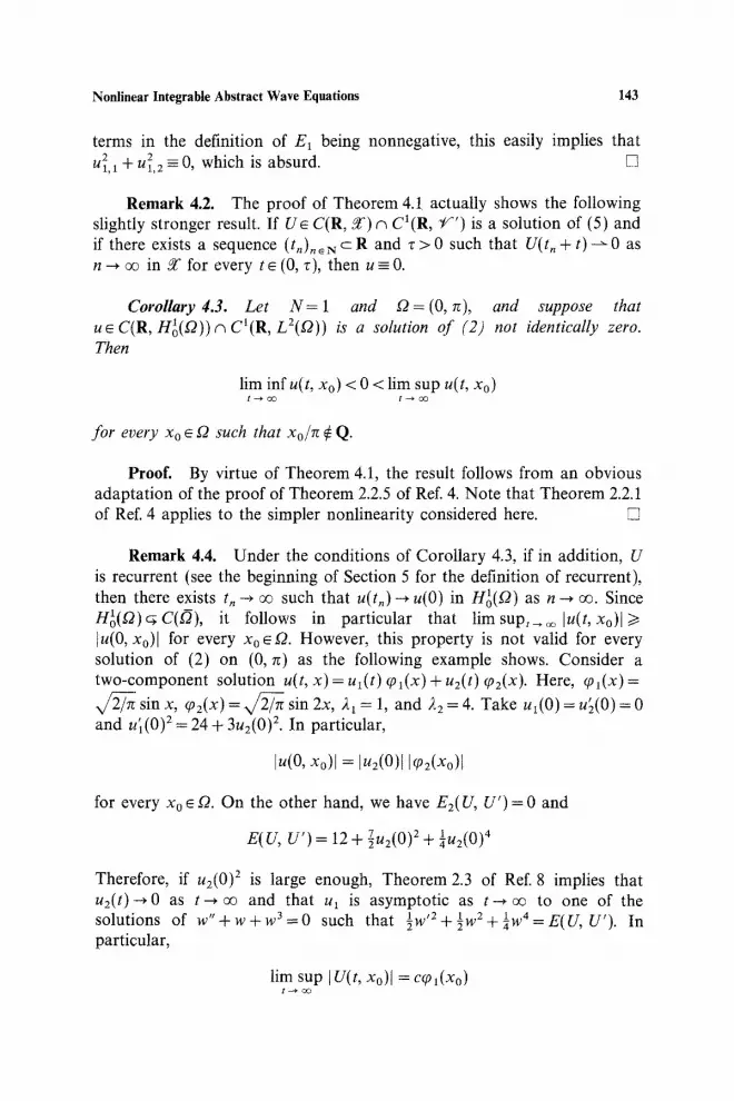
terms in the definition of E~ being nonnegative, this easily implies that U21,1 "t- U2,2 ~ 0, which is absurd. []

Remark 4.2. The proof of Theorem 4.1 actually shows the following slightly stronger result. If Ue C(R, ~r )~ CI(R, V ' ) is a solution of (5) and if there exists a sequence ( t n ) , ~ N c R and r > 0 such that U(t~ + t)---O as n ~ oo in Y" for every t s (0, ~), then u - 0.

Corollary 4.3. Let N= 1 and Y2 = (O, n), and suppose that u~ C(R, Hol(Q)) ~ CI(R, L2(f2)) is a solution of (2) not identically zero. Then

lim inf u(t, Xo) < 0 < lim sup u(t, Xo)

for every Xo e g2 such that Xo/n (! Q.

Proof. By virtue of Theorem 4.1, the result follows from an obvious adaptation of the proof of Theorem 2.2.5 of Ref. 4. Note that Theorem 2.2.1 of Ref. 4 applies to the simpler nonlinearity considered here. []

Remark 4.4. Under the conditions of Corollary 4.3, if in addition, U is recurrent (see the beginning of Section 5 for the definition of recurrent), then there exists tn ~ oo such that u(tn)~ u(O) in Hi(g?) as n ~ or. Since H~(g2)~C(O), it follows in particular that tim supt~oo lu(t, Xo)l>~ tu(0, Xo)l for every xoef2. However, this property is not valid for every solution of (2) on (0, ~) as the following example shows. Consider a two-component solution u(t, x) = ul(t) ~Ol(X) + u2(t) ~02(x). Here, ~ol(x) =

x / ~ sin x, ~o2(x) = x / ~ sin 2x, 21 -- 1, and 22 = 4. Take ui(0) = ui(0) = 0 and #1(0) 2 = 24 + 3u2(0) 2. In particular,

[u(0, Xo)l = lu2(0)l 1~o2(Xo)l

for every XoeO. On the other hand, we have E z ( U , U')=0 and

E(U, g ' )= 12-t- 7U2(0)2 "~ 1U2(0)4

Therefore, if u2(0) 2 is large enough, Theorem 2.3 of Ref. 8 implies that u2(t)-~O as t ~ oo and that ul is asymptotic as t ~ oo to one of the

1 , 2 �89 2 �88 4 solutions of w"+w+w3=O such that 5w + + =E(U,U'). In particular,

lim sup ]U(t, x0)[ = e(Dl(xo) t-+o9

144 Cazenave, Haraux, and Weissler

for every Xo ~ (2, where c > 0 is such that

lc2-~-lc4=E(U, U t)

In particular, if we assume that [U(0, Xo){ ~<lim s u p ~ ]U(t, Xo)], then lud0)l 1~o2(Xo)l ~ eq~l(xo). This implies that

q) 2(Xo) 2 u2(O) 2 "q- ~02(X0) 4 U2~) 4 ~ 1 6' 2 1 c4 = E(U, U') r 2 2 (p I(X0) 4 ~ "Ji-~

7 + 4 u2(O) 4 = 12 + ~ udO) 2

e4 and so

( ~02(x0)4 1 ) ~ - (q)2(x0)2 7) ~ 12

This is obviously impossible if u2(0) 2 is large enough, as soon as I~odxo)l > ~ol(Xo), which holds, for example, when Xo is in a small neighborhood of re/4.

Using sin mx instead of sin 2x, one can show in fact that even a weaker inequality l i m s u p , _ ~ [u(t, xo)l >~[u(0, xo)l is not valid for the general solution of Eq. (2).

Under separation assumptions on the 2is, Theorem 4.1 can also be recovered as a consequence of the following compactness result.

Theorem 4.5. Let - 1 <~ 0 < ~ . I f N = ~ , assume that 2) + ~ 1 -- ~j) ~ as j ~ . I f U ~ C ( R , YCo+,X97o) is a solution o f (5), then (Jt~i~ (U(t), U'( t)) is relatively compact in Y'o+ l •163

Proof. As noted in Remark 3.6, we may assume that mj ~< 2, for all j ~ J. We need only prove the result when N = ~ . In this case, it follows from the separation assumption that r/j,o ~ 0 as j ~ ~ , where qj, o is as in Lemma 2.3. Since, furthermore, there exists C such that

II U(t)ll~ +1 + II U'(t)[I ~ <~ C (13)

by Proposition 3.2, it follows from (9) that there exists Jo such that

mj E ()~O+luj, k(t)2+~'oVj, k(t)2)<'2~yEJ (U' U')

k=l

for J>~Jo. Define (aj)j~>l by

~'22~ U'), if J<Jo a j= ~2zoe j (v ' v ' ) , if J > J o

Nonlinear Integrable Abstract Wave Equations 145

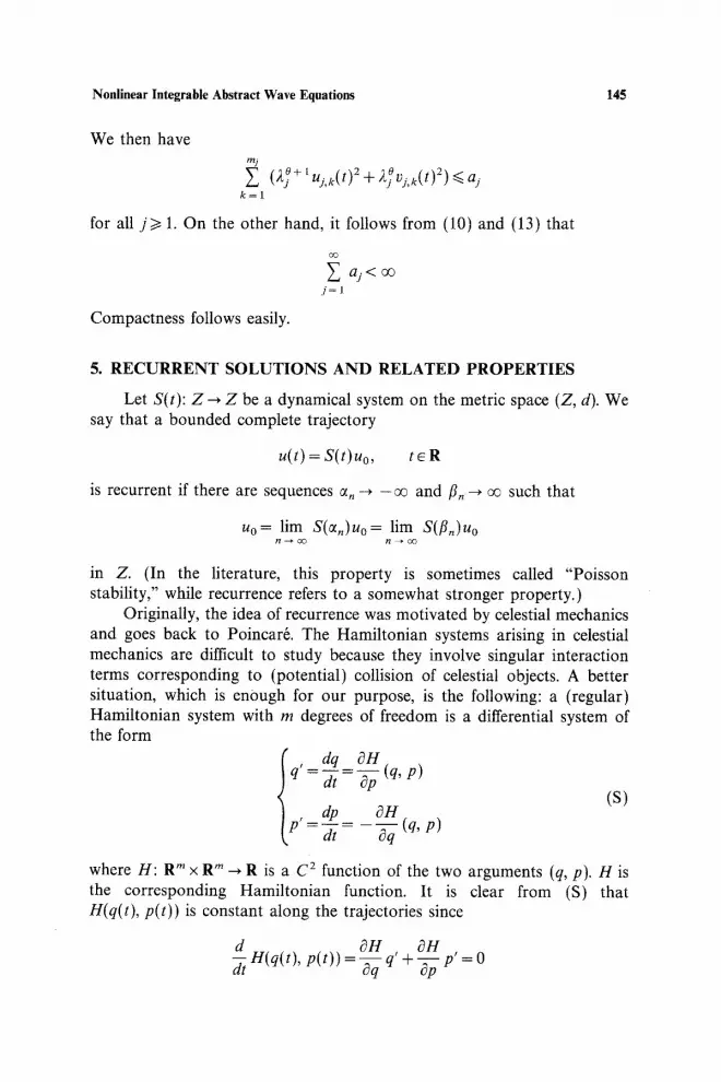
We then have mj

Z (2~ +~Uj, k(t) z + 2~ k(t) 2) ~< aj k = l

for all j~> 1. On the other hand, it follows from (10) and (13) that

~ a j<c~ j = l

Compactness follows easily.

5. R E C U R R E N T S O L U T I O N S A N D RELATED PROPERTIES

Let S(t): Z ~ Z be a dynamical system on the metric space (Z, d). We say that a bounded complete trajectory

u(t)=S(t)Uo, t e R

is recurrent if there are sequences an ~ - o e and fin ---' oe such that

Uo= lim S(an)Uo= lim S(fln)Uo n ~ o ~ n ~ o o

in Z. (In the literature, this property is sometimes called "Poisson stability," while recurrence refers to a somewhat stronger property.)

Originally, the idea of recurrence was motivated by celestial mechanics and goes back to Poincar& The Hamiltonian systems arising in celestial mechanics are difficult to study because they involve singular interaction terms corresponding to (potential) collision of celestial objects. A better situation, which is enough for our purpose, is the following: a (regular) Hamiltonian system with m degrees of freedom is a differential system of the form

, dq OH q = ~ - = (?p (q' P)

, dp OH (S) P =~ ~q (q, P)

where H: R m x R m ~ R is a C 2 function of the two arguments (q, p). H is the corresponding Hamiltonian function. It is clear from (S) that H(q(t), p(t)) is constant along the trajectories since

d OH , OHp, dt H(q(t), p(t)) = ~q q + -~p = 0

146 Cazenave, Haraux, and Weissler

by the equation. In particular, if H(q ,p ) tends to infinity when [ql + JPl ~ 0% then all trajectories of (S) are global and bounded on R: it is then natural to ask about their asymptotic behavior. At this level, the well-known Poincar6's recurrence theorem 1-12-1 asserts that there is a set 8 negligible for Lebesgue measure on Rm• R m such that for any (qo, Po) outside g, the trajectory (q, p) of (S) with initial values q(0)=q0 and p(0) = P0 is recurrent. Simple examples when m = 1 show that nonrecurrent trajectories may indeed exist in general. Poincar6's recurrence theorem is, in particular, applicable to second-order equations of the form

q" + A(q) = 0

where A: R m ~ R m is the gradient of a coercive, convex function. Applying this theorem to trajectories of (5) lying in some finite-dimensional subspace Xm, and taking into account Remark 3.6, it can be shown that "many" trajectories of (5) are in fact recurrent in X • ~ ' , for instance. More precisely, we have the following result.

Proposition 5.1. For all positive integers m the Lebesgue measure in YCm • Xm of the set of initial data yielding a nonrecurrent solution of (5) isO.

Corollary 5.2. There is a dense set of initial data giving rise to a solution U of (5) such that (U(t), U'(t)) is recurrent. Here, density and recurrence hold in the space X • ~/~' and, more generally, in Xo + 1• Xo for any 0 9 -1 .

Remark 5.3. Since (5) is a particular system, it is natural to ask whether nonrecurrent solutions of (5) do exist. Actually, in Ref. 8 we construct nonrecurrent trajectories of system (4), thereby showing that there always exist nonrecurrent solutions of (5) as soon as L is not of the form 21L

Remark 5.4. For the cubic wave equation (3), very little is known concerning the existence of recurrent solutions. When (2 = (0, n), a theorem of Rabinowitz [ 11 ] establishes the existence of nontrivial periodic (hence recurrent) solutions of (3). In Ref. 6 we computed some other types of solutions that seem to be recurrent (and possibly almost periodic), but theoretically the problem remains essentially open. The counterexamples of Ref. 8 suggest that nonrecurrent solutions of (3) might also exist.

Remark 5.5. Since small energy implies that the nonlinear terms of (5) are small compared to the linear terms, it is natural to expect that the

Nonlinear Integrable Abstract Wave Equations 147

solutions of (5) with a sufficiently small energy are recurrent and even almost periodic. At the present time we are unable to prove such a property. However, we have two partial results in this direction. First, as a consequence of Lemma 2.3, it can easily be seen that if, for instance, (U0, 1/o) is small enough in 5~ x ~ ' and if the expressions 2 j + ~ - 2 j , j e J are bounded away from zero, then no component uj.k can tend to 0 as t--+ oo (respectively, as t - - + - o o ) . Indeed, it then follows from (9) that there exists t /such that

m~

Ej(U, V)>(1-~I(IIUIIZ-+- IIVtl2,)) ~ (~jUZk +vZk) k = l

2 ~ 1 Assuming, for instance, that t/(ll U(0)ll ~, + H V(0){I v,~ "-~ ~, the result follows by the argument in the proof of Theorem 4.1. Therefore, the conclusion of Proposition 5.1 can be substantially reinforced for "small" solutions (but not for large energies since we may have v(t) --+ 0 for solutions of (4); see Ref. 8).

Our second partial result concerns small solutions in ~ x f and is proved in Section 6. At the present time the result is limited to the case where all eigenvalues 2j are simple. On the other hand, we will see that initial data of the form (~0, 0) or (0, ~o) with q~ ~ ~ always given rise to quasi-periodic solutions without smallness conditions on ~o and even if L has multiple eigenvalues.

6. QUASI-PERIODIC SOLUTIONS IN ~ x ~"

In this section, we will have occasion to impose the following addi- tional condition on the operator L, namely,

m j = l , for all j 6 J (14)

In order to state properly our results we need to recall some well-known facts from the theory of almost periodic functions. First, if X is a real Banach space and o~,...,~% are k positive real numbers, a function f : R ~ X is quasi-periodic with basic frequencies co~,...,co k is there exist Banach spaces X1 ..... Xk and a continuous function f : X~ x .. . x Xk--+ X such that

f(t)=f(q~l(t) ..... r for all t e R

with q~j a (2~/~@-periodic function R ~ Xj for all 1 ~<j ~< k. It is readily verified that any quasi-periodic function f : R --+ X is, in particular, almost periodic R --+ X.

148 Cazenave, Haraux, and Weissler

Also, we recall a well-known classical result whose proof can be found, for instance, in Chapter 10 of Ref. 1.

Theorem 6.1 (Liouville). Let (S) be a Hamiltonian system with m degrees of freedom and assume that there exists a set of m conserved quantities {Fi}l~i<.m such that

EFi, Fj] := E (OFi•Fj ori~Fj~ 1 <~l<<.m k O P t Oql dqz OPzJ = 0

for all 1 <<.i, j<~m. Let f = {fi}l<~i<~mGR m and assume that the gradients {VFi}I <<.i<~m are linearly independent at each point of the set

M = {x~ R2m; F~(x)=f~, Vie { 1,..., m}}

I f in addition, the set M is bounded, then all trajectories of (S) on M are quasi-periodic with at most m basic frequencies.

The main result of this section is the following.

Theorem 6.2. Under assumption (14), if (U o, Vo) ~ ~ x &r is such that Ej(Uo, Vo) > 0 for all j ~ J for which u~ + v 2 ~ O, then the solution U of (5) with initial data U(O)= Uo and U'(O)= Vo is quasi-periodic.

Theorem 6.2 and Lemma 2.3 immediately imply the following.

Theorem 6.3. In addition to (14), assume that there exists K > 0 such that

min{21(~.:+ 1 - 21), 2j(2j+ 1 - 2j)} ~> 1/K for all j ~ J

I f ( Uo, Vo) ~ ~ x f f is such that 2KE(Uo, I7o) < 1, then the solution U of (5) with initial data U(O)= Uo and U'(O)= Vo is quasi-periodic.

Proof. It follows from (9) and the hypothesis on the eigenvalues 2 i that

Ej( U, V)>~(1 - K( II UII ~ + II VI[ 2X ) )( ,~su )2 + v~ )

Therefore,

&(U, V) ~> (1 - 2KE(U, Z))(~ju~ + v})

In particular, if 2KE(Uo, Vo)<I, then either Ej(Uo, Vo)>O or U2o, j + v~,j = 0. The result now follows from Theorem 6.2. []

In order to prove Theorem 6.2, we need two technical lemmas. First, in view of the assumption (14), we may simplify the notation as follows:

u = (uj)j~

Nonlinear Integrable Abstract Wave Equations 149

and we observe that E~ now has the form

E j ( U , v ) = l _ z ( v i u j - u i v j ) 2 2 1 ( ) - - - + v, + ~ u ~ + 5 . ~ .~ 2 i ~ 2 i - ) v i t

We have the following result.

Lemma 6.4. Under assumption (14), the first integrals E~ are pairwise in involution. In other words, Ak, z=O for all k, l~J, where

j=l

for k, l>~ l.

Proof. (We will need only the result in 3~ • 5~. However, the reader can verify that the calculations below are valid in f x ~ ' . ) One verifies easily the following identities.

VjUk--UjOk 2 0Ek_ 2 j - 2 k Vk+UkUj' if j # k ~uj (15)

( ) i ck i=1

and (vju~-ujvk l - - Uk, OEk ~ 2 j _ 2 k if j r

= (16) Ol.)j ] ,r~ l)iU k -- UiV k

( - , ~ ~ i - ~ ui+2ve, if j = k

It follows that if k # l, then

~ OEk c3El

j= 10Uj ~Vj

=-- j#k , t

+ 2 j~k,l ( 2 j - 2k)(2k-- 2l)

+ ~ (v~uk- utv~)(vju~- ujv3 j~,~ (2 t - 2k)(2j- 2t)

(v;uk - u;vk)(v;ul- ujv3 vku~ + X (q-&)(q-~,) j~k , l

(vjuk - ujvk)(vkut-- ukvt) vju~

vjut-- ujvt 2 ,~j ;t~ u~uju~

+

vJu~- uJV~ u~u~uj j~k , l

ku, uk , ( 2 u,v. 2 k _ 2 t ukut 22k+u~+ u i + 2ugutvt- 2 2 t _ 2 k vkv l

i = l

(UlUk--UlVk)2 (VkUl--UkVl)2 VkUl--UkVl 3 ()~/__ 2k)2 UlVl"~ (~k __ ~/)2 UkVk l~ZZ2-~l IAkUl

+

150 Cazenave, Haraux, and Weissler

After simplication, we get

~ t~E k OEt j= 10u~ ~v s

= y~ { - (vsuk - usv,)(v~u l - usv,)

(1)kUl - Ukl)I)(VjUl__ Ujl)l) ] -- V k U l - Ukl) 1 ( N ~- l)kU.~ ..-[- - - - - - - UkU l ( ~ - 41)(4j- ,~,) ~j 4 ~ - ,~, 2,~ + Y,

i = = 1

+ 2u~utvl- 2 v~u~- u~v~ (v~u~- u~v~) 2 4~-2~ vkv~+ (4~_2~)~ (u~vk+ulvl)

(vju~- ujv~)(v~ut- ukvt) VjUl

By exchanging the roles of k and l, we have as well

~ ~E~ dE~ j=, Ovj duj

(vsu~- ujvk)(vjul- ujvl) = E - ( ~ j - ~ k ) ( 4 j - ~1) j~k , I

UkVl+ ( v j u , - ujvk)(v ,ul- u~vl)

(;tj - 4~)(,~ - "b)

(VkUl--UkVl)(VjUl--UjVl)UkVj + ukul 22l+ u~ + (4k - 4 i ) @ - 4l) 4~ - 4t i= t

+ 2U~UkVk -- 2 VkUt-- UkVl (VkUl-- UkVt) 2 4k__41 l)kl)lq (•k__ 4l)2 (Ukl)k"~Ull)l)

and so,

ujvl

(v juk- ujvk)(vjul- ujvi)(v~ul- ukvl) A~,, = Y~ - (4+- 4~)(4+- 41)

j~Sk, l

+ (vjuk - UjVk)(VkUt-- UkV3(VjUl-- UjVl) (,~j-,~k)(4~--,b)

+ ( v k u l - ukvl)(vjul- ujv3(vkuj- ukvj)~ ( ,~,- 43(4j-- 4/) J

{ 1 = 2 - (4j - 4 , ) (4 j - 41) ~ (,~j - ,~)(4~ - 41) j r

x (v juk- ujv , ) (vjut- ujvl)(vkul- ut, vl) = 0 I

1

(4k- 4,)(,~j- 4,)}

To study the linear independence of the first integrals Ej, we will use the following lemma.

Nc~linear Integrable Abstract Wave Equations 151

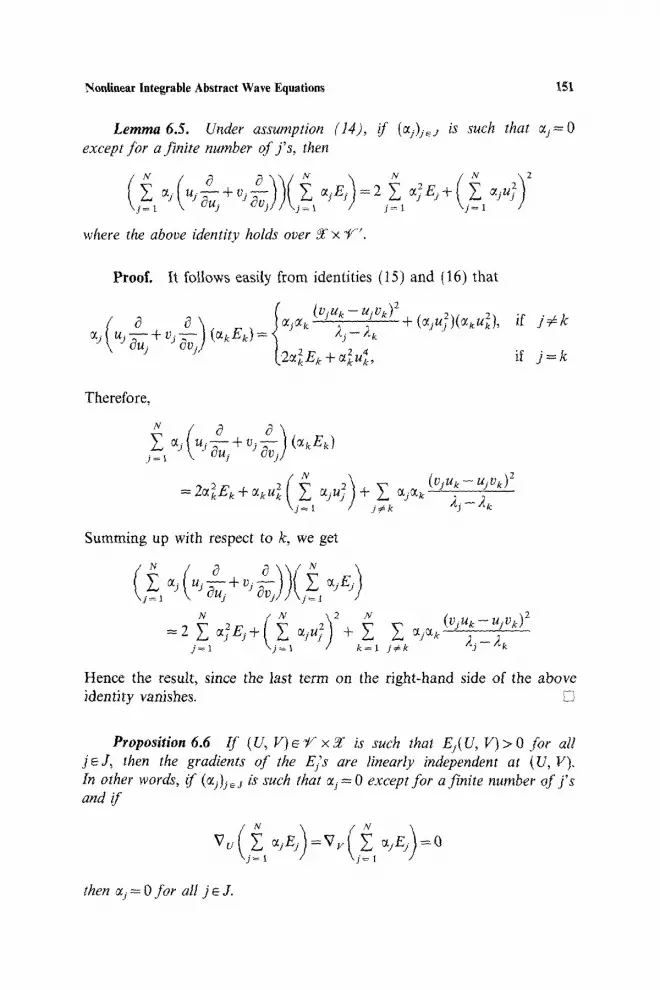
Lemma 6.5. Under assumption (14), if (~j)j~j is such that ~i=0 except for a finite number of j's, then

t j ~ j~l

where the above identity holds' over YC x ~U'.

Proof. It follows easily from identities (15) and (16) that

( (v/u~ - u:v~) ~

Therefore,

= 2e~Ek + ekU k ~j ,/ 1

(vjuk - ujv~) 2 + ~ % ~

j ~ ~ - &

Summing up with respect to k, we get

2j + E ~]U ~]~ + Z E ~ (v j~- u~v~) ~

=1 j~x k=~ j#k 2~--2r

Hence the result, since the last term on the right-hand side of the above identity vanishes.

Proposition 6.6 I f ( U, V) ~ ~/" • X is such that Ej( U, V) > 0 for all j e J , then the gradients of the Efs are linearly independent at (U, V), In other words, if (~j)j~j is such that ~j = 0 except for a finite number of j's and if

then ~j=O for all j~J .

152 Cazenave, Haraux, and Weissler

Proof. We have, in particular,

I 0 U j ~Vj j l

and it follows from Lemma 6.5 that ~7=i ~}Ej = 0. Therefore, c~j = 0 for all je J. []

We are now in a position to prove Theorem 6.2.

Proof of Theorem 6.2. Assume for simplicity that u] + v~ ~ 0 for I~<j~<M~<N, w h e r e M < o e and that u 2 + v ~ = 0 f o r j ~ > M + l . I t i s n o w sufficient to study the problem

uj'+2yUj+Us( ~ u ~ ) = 0 , for I~j<<.M 1

The above 2M-dimensional Hamiltonian system obviously has the same properties as system (5). In particular, it possesses M first integrals, that are pairwise in involution by Lemma 6.4. Furthermore, the first integrals are linearly independent on the set 01<.j<.M{Ej=Ej(Uo, Vo)} (by Proposition 6.6). The result now follows from Liouville's theorem cited above.

Remark 6.7. Note that if infj>~22s_1(2s-2s_l)=O, then smallness of the energy does not even imply that all the Ej's are nonnegative. To see this, assume that there exists a subsequence ( J , )~N such that 2 j _ l ( A j - A s _ l ) ~ 0 as n ~ oe and let (U n, V ~) satisfy

0, if jCjn, {0, j r u~= a . r if j=j~, v~.= b.r if j = j . - i

One verifies easily that E( U ., V . )= , 2 1 2 1 4 za. and Ej~ U", vn)= 5bn +-~2s~ + that 1 2 2 1 4 5[a.bJ()v~ It is clear that Ej.(U", V") has the same sign as

-�89 --~j,~_l)2 + ~jn--1(,~j,~--~jn--1)+ l(~jn--~jn--l)a2

Fix any sequence (an)n>~l such that 2jna ] --+ 0. One can then clearly choose the sequence (bn)n~>l such that b] - - ,0 [and so E(U ~, V") converges to zero], but Ej~ ~, r ) < 0 for all n>~l.

Theorem 6.2 also yields quasi-periodicity of solutions that do not have small energy. In particular, we have the following result.

Nonlinear Integrable Abstract Wave Equations 153

Theorem 6.8. Under the conditions of Section 1 [in particular, we do not assume that (14) holds], if (U o, Vo)~ ~ • ~ is such that Uo and Vo are linearly dependent, then the solution U of (5) with initial data U(O) = Uo and U'(O) = Vo is quasi-periodic.

Proof. Let U be as in the statement. By applying Lemma 3.5 in each of the spaces Hi, one is reduced to the case where (14) holds (see Remark 3.6). In addition, it follows from the linear dependence of Uo and Vo that

Ej(Uo, Vo) = (Vo) 2 + 2j(Uo)~ + �89 11Uo]l ~ (17)

In particular, either (Vo) } + (Uo) 2 = 0 [hence uj(t) - O] or Ej(Uo, Vo) > O; and so the result follows from Theorem 6.2. []

Theorem 6.9. Under the conditions of Section 1 [& particular, we do not assume that (14) holds], for every Uo ~ ~c the solution U of (5) with initial data U(O)= Uo and U'(O)= 0 and the solution Z of (5) with initial data Z(O) = 0 and Z'(O) = Uo are quasi-periodic.

Remark 6.10. Under the assumptions of Theorem 6.8, one can improve the conclusion of Theorem 4.1. Indeed, if U0 and Vo are linearly dependent, then it folows easily from (17) that no component uj, k can converge to 0 as t ~ oe (cf. Remark 5.5).

Final Remark. Throughout this paper, we have assumed that 2~ > 0 only in order to make the calculations simpler. All the results of the paper hold if 21 = 0 with straightforward modifications. In particular, the spaces Y'0 must be defined by

with the norm

f ml N mj t Co= u; Z 2 ul,k+ Z Z o 2j u),k <

t . k = l j = 2 k = l

ml N

IIull = E E E k = l j = 2 k = l

and the estimates of Lemma 2.4 take a more complicated form. Also, the results of Section 2 and 3 are still valid, with straightforward

modifications, if we allow the eigenvalues of L to form an arbitrary discrete set of positive real numbers, bounded away from zero. On the other hand, the proof of Theorem 4.1 still works only if we suppose that the eigenvalues

154 Cazenave, Haraux, and Weissler

of L f o r m a w e l l - o r d e r e d set, i.e., t ha t every n o n e m p t y subse t c o n t a i n e s a

smal les t e lement . F u r t h e r m o r e , the p roo f s of T h e o r e m s 4.5 a n d 6.3, as well

as R e m a r k 5.5, use s e p a r a t i o n c o n d i t i o n s on the e igenva lues wh ich cou ld

n o t h o l d were the re a f ini te a c c u m u l a t i o n po in t ; a n d R e m a r k 6.7 suggests

t ha t such s e p a r a t i o n p rope r t i e s a re essent ia l to the results.

R E F E R E N C E S

1. Arnold, V. (1989). Mathematical Methods of Classical Mechanics, Graduate Texts in Mathematics 60, 2nd ed., Springer, New York.

2. Brezis, H., Coron, J.-.M., and Nirenberg, L (1980). Free vibration for a nonlinear wave equation and a theorem of P. Rabinowitz. Commun. Pure Appl. Math. 33, 667-689.

3. Cabannes, H., and Haraux, A. (1981). Mouvements presque-p6riodiques d'une corde vibrante en pr6sence d'un obstacle fixe, rectiligne ou ponctuel. Int. J. Nonlin. Mech. 16, 449-458.

4. Cazenave, T., and Haraux, A. (1987). Oscillatory phenomena associated to semilinear wave equations in one spatial dimension. Trans. Am. Math. Soc. 300, 207-233.

5. Cazenave, %, and Haraux, A. (1988). Some oscillation properties of the wave equation in several space dimensions. J. Funct. Anal, 76, 87-109.

6. Cazenave, T., Haraux, A., Vfizquez, L., and Weissler, F. B. (1989). Nonlinear effects in the wave equation with a cubic restoring force. Comp. Mech. 5, 49-72.

7. Cazenave, T., Haraux, A., and Weissler, F. B. (1991). Une 6quation des ondes compl+te- ment int6grable avec non-lin6arit6 homog6ne de degr6 trois. C.R. Acad. Sci. Paris 313, 237-241.

8. Cazenave, T., Haraux, A., and Weissler, F. B. (1993). Detailed asymptotics for a convex Hamiltonian system with two degrees of freedom. J. Dynam. Diff. Eq. 5, 155-187.

9. Haraux, A. (1983). Remarks on Hamiltonian systems. Chinese J. Math. 11, 5-32. 10. Lax, P. D. (1975). Periodic solutions of the Korteweg-De Vries equation. Commun. Pure

Appl. Math. 28, 141-188. 11. Rabinowitz, P. H. (1978). Free vibrations for a semi-linear wave equation. Commun. Pure

Appl. Math. 31, 31-68. 12. Siegel, C. L., and Moser, J. K. (1971). Lectures on Celestial Mechanics, Springer,

New York.