MATHEMATICS

A CERTAIN METHOD OF OBTAINING BILATERAL GENERATING FUNCTIONS

BY

H. M. SRIVASTAVA AND J.-L. LAVOIE 1)

(Communicated by Prof. C. J. BOUWXAMP at the meeting of September 28, 1974)

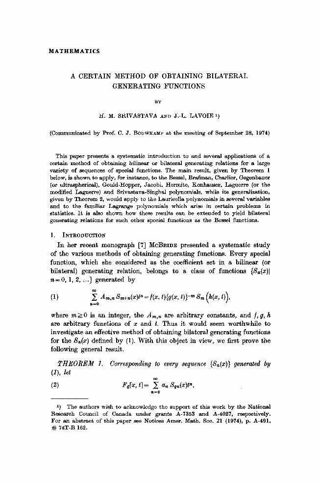
This paper presents a systematic introduction to and several applications of a certain method of obtaining bilinear or bilateral generating relations for a large variety of sequences of special functions. The main result, given by Theorem 1 below, is shown to apply, for instance, to the Bessel, Brafman, Charlier, Gegenbauer (or ultraspherical), Gould-Hopper, Jacobi, Hermite, Konhauser, Laguerre (or the modified Laguerre) and Srivastava-Singhal polynomials, while its generalization, given by Theorem 2, would apply to the Lauricella polynomials in several variables and to the familiar Lagrange polynomials which arise in certain problems in statistics. It is also shown how these results can be extended to yield bilateral generating relations for such other special fun&ions as the Bessel functions.

1. INTRODUCTION

In her recent monograph [7] MCBRIDE presented a systematic study of the various methods of obtaining generating functions. Every special function, which she considered as the coefficient set in a bilinear (or bilateral) generating relation, belongs to a class of functions {&(x)l n=O, 1, 2, . . . } generated by

where rn~ 0 is an integer, the Am,a are arbitrary constants, and f, g, h are arbitrary functions of x and t. Thus it would seem worthwhile to investigate an effective method of obtaining bilateral generating functions for the S,(z) defined by (1). With this object in view, we first prove the following general result.

THEOREM 1. Corresponding to every sequence {Sri(x)} generated by (4, let

(2)

1) The authors wish to acknowledge the support of this work by the National Research Council of Canada under grants A-7353 and A-4027, respeotively. For an abstract of this paper see Notices Amer. Math. Sot. 21 (1974), p. A-491, # 74T-B 162.

305

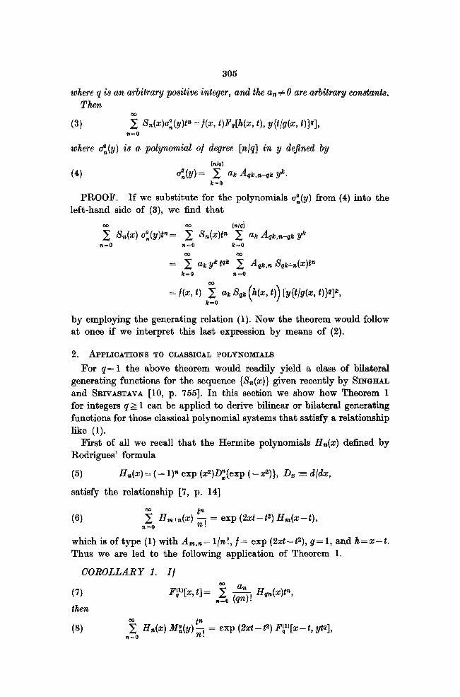
where q is an arbitrary positive integer, and the a, # 0 are arbitrary constants. Then

(3)

where a”,(y) is a polynomial of degree [n/q] in y defined by

(4) o:(y)= 2 ak Aqk,n-qk yk. k-0

PROOF. If we substitute for the polynomials a:(y) from (4) into the left-hand side of (3), we find that

5 S,(X) a”,(y)t”= g S,(x)tn ‘y ak Aqk,n-qk yk n-o V&=0 k-0

= 2 ak yk tqk 2 Aqk,n fiqk+n@)tn

k-0 n-0

= f(x, t) i k-0

ak ‘%k (h t)) b{#b, t)jqlk,

by employing the generating relation (1). Now the theorem would follow at once if we interpret this last expression by means of (2).

2. i%PPLICATIONS TO CLASSICAL POLYNOMIALS

For q= 1 the above theorem would readily yield a class of bilateral generating functions for the sequence (L!&(X)} given recently by SING+HAL and SRI~ASTAVA [lo, p. 7651. In this section we show how Theorem 1 for integers qk 1 can be applied to derive bilinear or bilateral generating functions for those classical polynomial systems that satisfy a relationship like (1).

First of all we recall that the Hermite polynomials a,(x) defined by Rodrigues’ formula

(5) Hn(x) = ( - l)n exp (+Di{exp ( -x2)), D, f @lx,

satisfy the relationship [7, p. 141

(6) n:. fJ?n+n(x) f = exp (26 - t2) Hm(x - t) ,

which is of type (1) with A,,,, = l/n!, f= exp (2&-P), g= 1, and h=x-t. Thus we are led to the following application of Theorem 1.

COROLLARY 1. If

(7) then

(8) ntio w4 xi(Y) 5 = exp (Zxt - t2) F;l)[x- t, ytq],

306

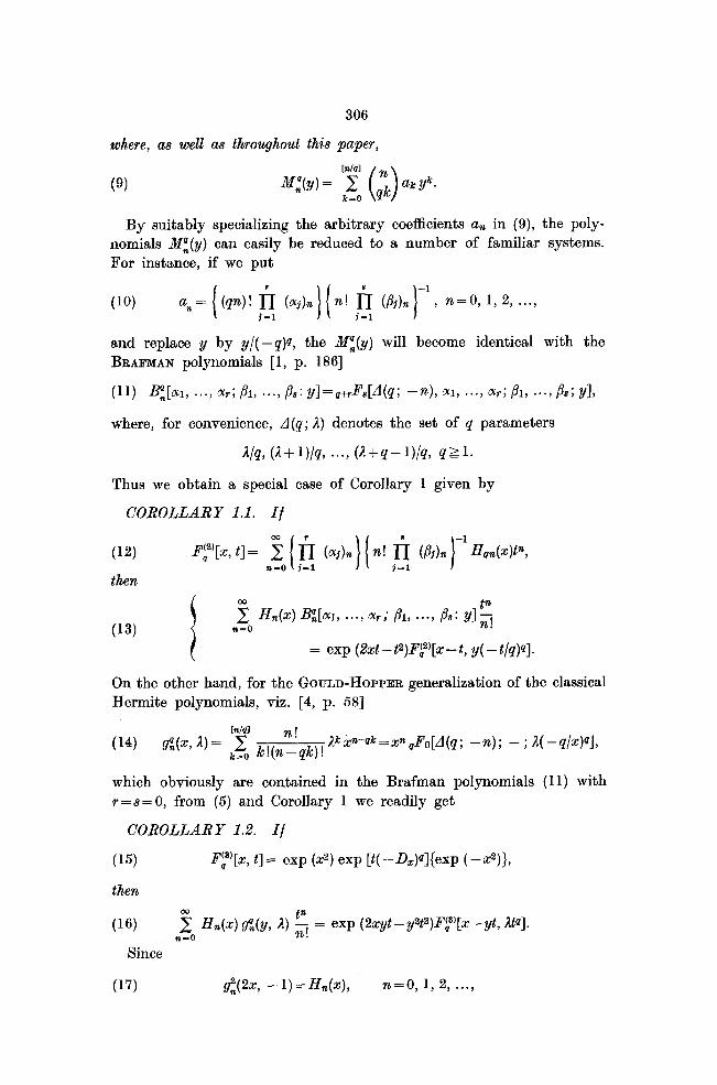
where, as well as throughout this paper,

(9)

By suitably specializing the arbitrary coefficients a, in (9), the poly- nomials M:(y) can easily be reduced to a number of familiar systems. For instance, if we put

(10) a, = (cd! Ii (4 ( i=l I( n! Ii cab i=l I

-1 ) n=o, 1, 2, . . . .

and replace y by y/( -q)p, the NE(y) will become identical with the BRAFMAN polynomials [l, p. 1861

(11) BQ,[oIl, . . . . ar; /%, . . . . /38: Y]=*+rFs[d(P; -n), 0119 .*a~ &; Bl, ***J /%i 91,

where, for convenience, A(q; A) denotes the set of q parameters

qq, (Ai- 1)/q, ***, (iz+q- 1)/q, (I& 1.

Thus we obtain a special case of Corollary 1 given by

COROLLARY 1.1. If

(12)

then

On the other hand, for the GOULD-HOPPER generalization of the classical Hermite polynomials, viz. [4, p. 581

Pzm”=xn&[A(q; -n); - ; A(-q/z)@],

which obviously are contained in the Brafman polynomials (11) with r = s = 0, from (5) and Corollary 1 we readily get

COROLLARY 1.2. If

(15) Fr’[x, t] = exp (x2) exp [t( -D,)q](exp ( --X2)},

then

(16) 2 SW gQ,(Y, 4 5 = exp (2xyt - y%2)F$‘[x - yt, AM] a n-o

Since

(17) s”,P& - 1) = fM4, n=O, 1, 2, . . . .

307

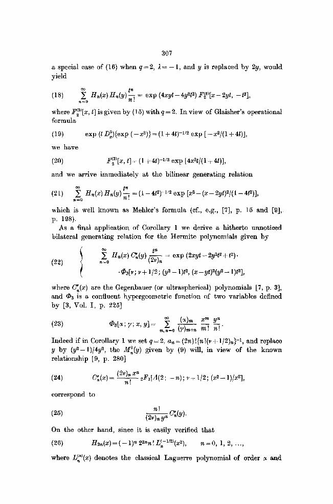
a special case of (16) when q= 2, 3, = - 1, and y is replaced by 2y, would yield

(18) %zo II&) H%(y) 5 = exp (4x$- 4yW) Pf)[x - 2yt, -@I,

where FF’[x, t] is given by (15) with q = 2. In view of Glaisher’s operational formula

(19) exp (t DE)(exp ( -x2)} = (1 + 4t)-i12 exp [ -X2/( 1 + 4t)],

we have

(20) FF’[x, t] = (1 + 4t)-112 exp [4z2t/( 1 + 4t)],

and we arrive immediately at the bilinear generating relation

(21) ngO H%(z) H&j) 5 = (1 - 4t2)-l12 exp [x2 - (x- 2yQ2/( 1 - 4t2)],

which is well known as Mehler’s formula (cf., e.g., [7], p. 15 and [9], p. 198).

As a final application of Corollary 1 we derive a hitherto unnoticed bilateral generating relation for the Hermite polynomials given by

(22)

:

j. K&) G(Y) (& = exp (2zyt - 2y2t2 + t2) .

* @[v; Y + l/2; (y2 - l)@, (z - yt)2(y2 - l)PJ,

where Cn(x) are the Gegenbauer (or ultraspherical) polynomials [7, p. 31, and @a is a confluent hypergeometric function of two variables defined by [3, Vol. I, p. 2251

(23)

Indeed if in Corollary 1 we set q = 2, a, = (2n) ! {n ! (IJ + 1/2),)-l, and replace y by (ya-1)/4y2, the W,(y) given by (9) will, in view of the known relationship [9, p. 2801

(24) C(2)= 9$2F1[Ll(2; -n); v+ l/S; (x2-- 1)/&q,

correspond to

On the other hand, since it is easily verified that

(26) Hz&)= (- l)R 2%l L’-l’2’(x2), . n n=O, 1, 2, . . . .

where L:‘(x) denotes the classical Laguerre polynomial of order a and

308

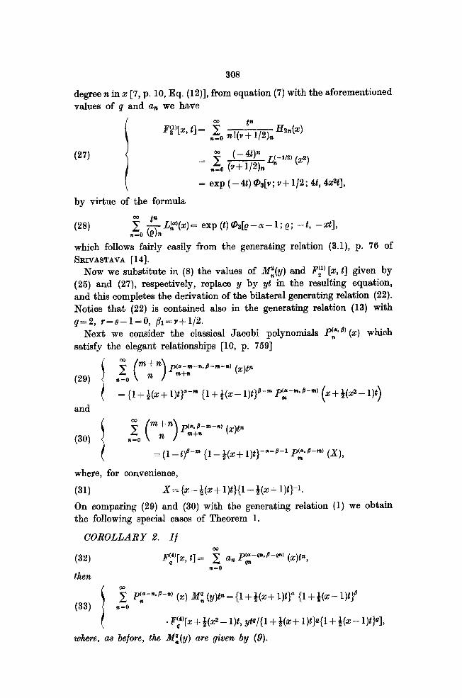
degree n in z [7, p. 10, Eq. (12)], from equation (7) with the aforementioned values of q and a, we have

FS”[x, t] =

by virtue of the formula

exp (-N@s[Y; Y+ l/2; 4t, 4291,

(28) nlo (e)n ls Q) t” p’(z) c exp (t)@s[e-a-- 1; e; --t, -a],

which follows fairly easily from the generating relation (3.1), p. 76 of SRIVASTAVA [ 141.

Now we substitute in (8) the values of M:(y) and Ii’:’ [x, t] given by (25) and (27), respectively, replace y by yt in the resulting equation, and this completes the derivation of the bilateral generating relation (22). Notice that (22) is contained also in the generating relation (13) with q=2, r=s-l=O, /!Ir=Y+1/2.

Next we consider the classical Jacobi polynomials PF8’ (2) which satisfy the elegant relationships [lo, p. 7591

(2g)

and = (1 +gx+ l)ty-” (1 +*(x- l)t}B-” Pp*b-m’ (z+gs- l)t>

(30) -

I

?. (“n’“) Ptp-.’ (2$”

=(l-t)b-m (1 -Q(z+ l)t)-“-8-1 Py+ (X),

where, for convenience,

(31) x=(27-g@+ l)t}{l -j&+ l)t}-1.

On comparing (29) and (30) with the generating relation (1) we obtain the following special cases of

COROLLARY 2. If

(32) Ph”[Z, t] =

then / m

Theorem 1.

I z1 P:-n+n) (33) n-o (22) M~(y)tn={l+*(X+l)t)n {l+j&r-l)t)B

t .~d”[~+~(2~-l)t,yt4/{1+~(z+l)t}*{1+8(2--)t}*l:

where, aa before, the HI(y) are given by (9).

309

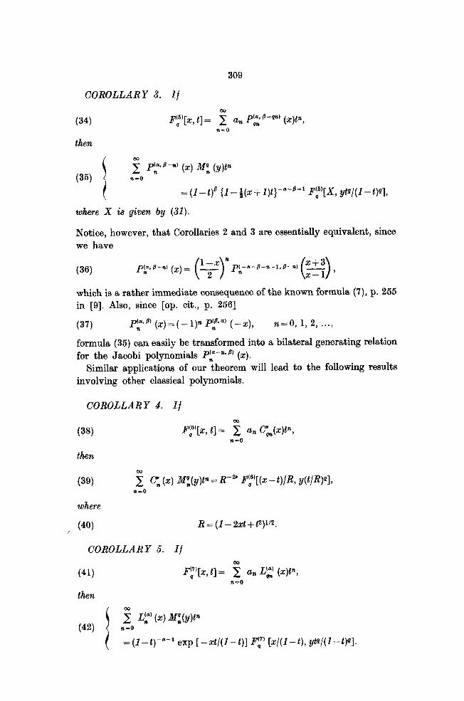
COROLLARY 3. If

(34)

then

P;‘[z, t]= 5 u1, PkB--pn) (x)t”, T&-=0

$ P;@-” (x) M; (y)t” n-o

= (1- ty {I- gx + l)t}-“-8-l F%‘[X, ytq(1 - ly],

where X is given. by (31).

Notice, however, that Corollaries 2 and 3 are essentially equivalent, since we have

(36) p($.@-d @)= 9 pt;a-8-n-l.~-n’

( )

n x+3 ( ) x--1 ’

which is a rather immediate consequence of the known formula (‘I), p. 255 in [9]. Also, since [op. cit., p. 2561

(3’) P($?’ (x)=(-l)* PF@ (-x), n=O, 1, 2, . . . .

formula (35) can easily be transformed into a bilateral generating relation for the Jacobi polynomials Pr-“* B, (x).

Similar applicstions of our theorem will lead to the following results involving other classical polynomials.

COROLLARY 4. If

(38)

then

PF’[X, t]= 2 CZn Cm(X)t”, n-0

(39)

where

2 q (x) M;(y)t”= R-* J’;‘[(x-q/R, y(t/R)@l, n=O

, (40) R = (I - 2xt f t2)1’2

COROLLARY 5. If

(41)

then

Pf’[X, t]= $ an Lz (X)t”, n-0

( = (1- t)-@-l exp [-xt/(l- t)] FC’ [z/(1 -t), @/(I - t)Q].

310

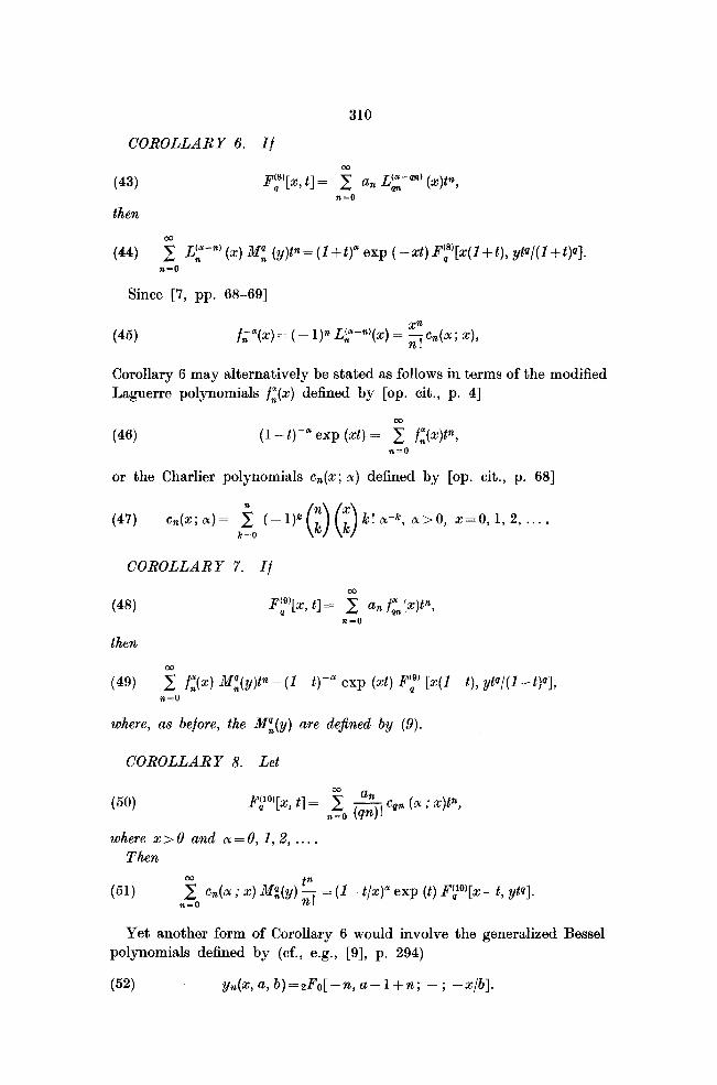
COROLLARY 6. If 00

(43) Fr)[x, t] = 2 a, LK-“’ (z)t’a, n=o

then

(44) 2 Lf-‘) (2) Mz (y)t” = (1 + t)” exp ( -33) Fr’[x(I + t), ytp/(I + VI. n-0

Since [7, pp. 68-691

(45) f;*(x) = (- l)n q-“‘(x) = $(a; X),

Corollary 6 may alternatively be stated as follows in terms of the modified Laguerre polynomials f;(x) defined by [op. cit., p. 41

(46) (1 -t)-” exp (xt) = f fz(z)t”, ?a=0

or the Charlier polynomials c,(x; LX) defined by [op. cit., p. 681

(47) k! ‘2-k, 01>0, x=0,1, 2, *.. .

COROLLARY 7. If

(48) Frl[x, t] = $ a, f&‘x)t”, T&=0

then

(49) nzo f,“(x) Mz(y)tn = (I-t)-” exp (A) FF’ [x(1-t), yP/(l- t)Q],

where, as before, the M:(y) are defined by (9).

COROLLARY 8. Let

(50) Fpyx, t] = n!. g, Cgn (a ; W”,

where x> 0 and L)I = 0, 1, 2, . . . . Then

(51) nzo cn(oc ; x) M;(y) 5 = (1 -t/x)” exp (t) FFO)[x - t, ytg].

Yet another form of Corollary 6 would involve the generalized Bessel polynomials defined by (cf., e.g., [9], p. 294)

(52) yn(z, a, b)=zFo[-n, a-l+n; - ; -x/b].

311

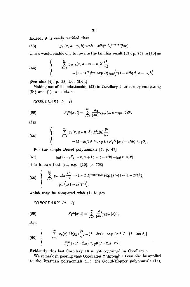
Indeed, it is easily verified that

(53) yn (L-C, a-n, b)=n!( --x/b)* Lt-“-“‘(b/z),

which would enable one to rewrite the familiar result (13), p. 757 in [lo] as

(54) nzo ym+&, a-m - n, b) 5

= (1 -xt/b)l-” exp (t) y,(r(l -xt/b)-1, a--m, b).

{See also [4], p. 58, Eq. (5.6).} Making use of the relationship (53) in Corollary 6, or else by comparing

(54) and (l), we obtain

COROLLARY 9. If

(55)

then

(56) %zo Y&G a - 12, b) Xi(y) 5

= (1 - xt/b)l-” exp (t) Fbll) [z(I - d/b)-1, ytq].

For the simple Bessel polynomials [7, p. 471

(57) yn(")=2J70[-%n+1; -;-+q=y&,2,2), it is known that (cf., e.g., [lo], p. 758)

m+1)/2 exp [x-1(1 - (1 - 2&)t}]

.ym (X(1 - 2st)-9,

which may be compared with (1) to get

COROLLARY 10. If

then

B!. yn(x) M:(y) F, = (1 - 2zt)-* exp [z-l{1 - (I- 24+}]

*Iy2’[2(1 - 2x$)-$ ytq1- 2%!)-‘1’21.

Evidently this last Corollary 10 is not contained in Corollary 9. We remark in passing that Corollaries 2 through 10 can also be applied

to the Brafman polynomials (II), the Gould-Hopper polynomials (14),

312

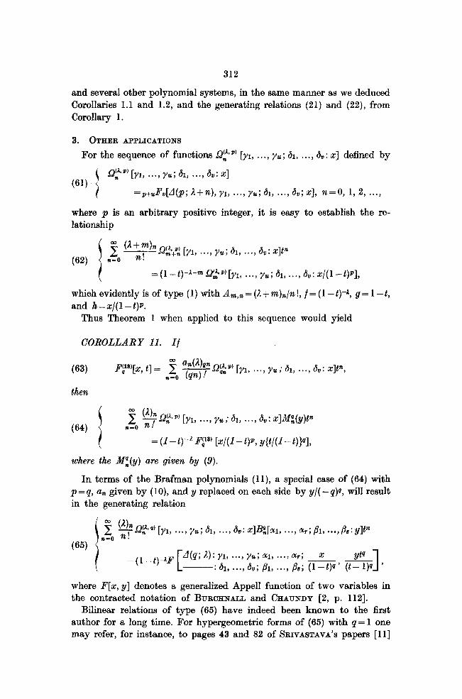
and several other polynomial systems, in the same manner as we deduced Corollaries 1.1 and 1.2, and the generating relations (21) and (22)) from Corollary 1.

3. OTHER APPLICATIONS

For the sequence of functions QFp) [JQ, . . . , yU ; 61, . . ., 8, : x] defined by

(61) \

QP”’ [y1, . . . . yu; 61, . . . . 6,: xl

1 =p+uF&4(p; R+n), y1, . ..) yu; 61, a**, 6,; xl:], n=% 1, 2, ***3

where p is an arbitrary positive integer, it is easy to establish the re- lationship

. -- yu, 6 1, . . . 9 ‘..9 6, : x]tn

=(l-t)-“-yjqyl, . ..) yu; 61, . . . . 6,: x/(1-t)r],

which evidently is of type (1) with Am,%= @+m),/n!, /=(1-t)-“, g=l-t, and n=z/(l-t)r.

Thus Theorem 1 when applied to this sequence would yield

COROLLARY 11. If

a7 (63) e3’[xY t1= z. m an(lZ)qn 52% 9) [?I, . . . ) yu ; 61, . . .) 6v: x]t”,

then

(64) 2 wn

f&*0 7 Ly*P) [y1, . . . , yu ; 61, . . . , 6,: x]dq(y)tfl

= (1 - t)-” Iy [x/(1 - tp, y{t/(l - t)}Q],

where the M:(y) are given by (9).

In terms of the Brafman polynomials (1 1 ), a special case of (64) with p =q, a,, given by (lo), and y replaced on each side by y/( -q)g, will result in the generating relation

where P[x, y] denotes a generalized Appell function of two variables in the contracted notation of BURCHNALL and CHAUNDY [2, p. 1123.

Bilinear relations of type (65) have indeed been known to the first author for a long time. For hypergeometric forms of (65) with q= 1 one may refer, for instance, to pages 43 and 82 of SRIVASTAVA’S papers [l I]

313

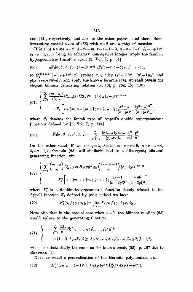
and [14], respectively, and also to the other papers cited there. Some interesting special cases of (66) with q= 2 are worthy of mention.

If in (65) we set q=2, il=2v+m, r=s-1=0, U=V-l=O, Bi=,9+1/2, 61 = Y + l/2, M being an arbitrary nonnegative integer, apply the familiar hypergeometric transformation [3, Vol. I, p. 641

(66) 2Fl[U, b; c; z]=(l -q-a-* zPr[c-a, c-b; c; x], IzI< 1, to Qer+m. 2) [-- ; Y-I- l/2: x], replace x, y, t by (x2-- 1)/x2, (yz- l)/yz and yt/s, nrespectively, and apply the known formula (24), we shall obtain the elegant bilinear generating relation (cf. [6], p. 254, Eq. (10))

aJ (m+n)! ?O (2eh

-- @m+*(x) cgyp = (2Y)m (x - yt) -‘B-m

(67)

*F4

x2 - 1 (y2 - l)P y+ih v+h+B;y+i, e+$;w, (x-Yt)2 , 1

where F4 denotes the fourth type of Appell’s double hypergeometric functions defined by [3, Vol. I, p. 2241

(68) F~[~,B;Y,Y’;~GYI= 5 (ol)rn+n (&hta Xrn yn - -. m.n-0 (y)m(Y’h m! n!

On the other hand, if we set q=2, A=2v+m, r=s=O, u=v-1=0, &=Y+ l/2, formula (65) will similarly lead to a (divergent) bilateral generating function, viz.

1 nFo (mr) %+ntx) Hn(YP GZ

(69) *

(2r+3(z~2yt)-2v-”

.p: [

Y+h, v+&+&; v+t;&@’ (x$)2 1 ,

where F: is a double hypergeometric function closely related to the Appell function F4 deflned by (68) ; indeed we have

(70) FZ[a,/l;y;x,yl= lim Fdar,8;7~,d;~dyl. d-+.x

Note also that in the special case when 2 = 0, the bilinear relation (65) would reduce to the generating function

(71) 5 &?;[a1

’ ***’ n-O n! @r; /%7 an.9 /X9: YP

=(1--t)-” ,,F&i(q; A), CR, . . . . a,; ,&, . . . . BR; YW---~)~I,

which is substantially the same as the known result (LX), p. 187 due to BRAIMAN [ 11.

Next we recall a generalization of the Hermite polynomials, viz.

(72) HL(x, a,~) = ( - l)n x-a exp (pxr)D:{@ exp ( -j33.?)},

314

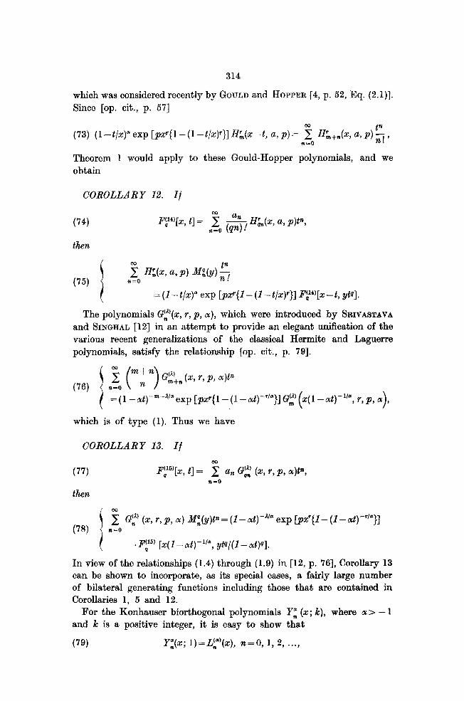
which was considered recently by GOULD and HOPPER [4, p. 52, Eq. (2.1)]. Since [op. cit., p. 571

(73) (l-t/~)“exp[~~rjl-(l--tlz)‘)l~~,(zt,a,p)=~~~~~+,(z,a,p)~,

Theorem 1 would apply to these Gould-Hopper polynomials, and we obtain

COROLLARY 12. If

(74)

then

(75)

: = (1 -t/x)” exp /-JM{I - (1 -t/z)‘}] Fi”)[z- t, ytQ].

The polynomials G:(x, r, p, LY), which were introduced by SRIYA~TAVA and SINCJHAL [12] in an attempt to provide an elegant unification of the various recent generalizations of the classical Hermite and Laguerre polynomials, satisfy the relationship [op. cit., p. 791.

exp [pz?{ 1 - (1 -cd)-““}] G2 (z( 1 - at)-1’a, r, p, a),

which is of type (1). Thus we have

COROLLARY 13. If

(77)

then

Fy’[x, t] = g a, Gz (x, r, p, b~)tn, n-0

Gp (x, r, p, a) Mz(y)tn = (I - d)-A’a exp [pS{l- (I- act)-“@>]

.Iirf’) [x(&at)-“=, @/(I-at)Q].

In view of the relationships (1.4) through (1.9) in [12, p. 761, Corollary 13 can be shown to incorporate, as its special cases, a fairly large number of bilateral generating functions including those that are contained in Corollaries 1, 5 and 12.

For the Konhauser biorthogonal polynomials Yz (2; k), where OL > - 1 and k is a positive integer, it is easy to show that

(79) YZ(x; l)=Ly’(z), n=O, 1,2, . ..)

315

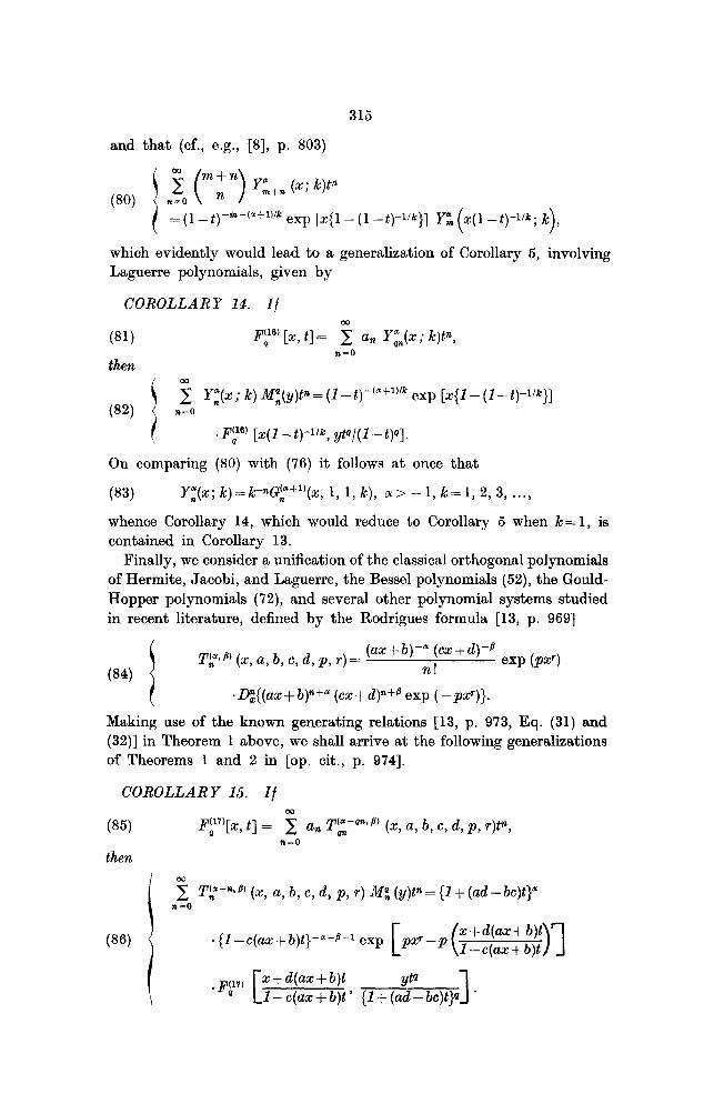
and that (cf., e.g., [8], p, 803)

(80) exp [x{ 1 - (1 - t)-l/k}] YE (x( 1 - t)-l’k ; k),

which evidently would lead to a generalization of Corollary 5, involving Laguerre polynomials, given by

COROLLARY 14. If

(81) then

Fy’ [x, t] = 5 a, YIn(x ; k)t”, n-0

(82) i 5 Y,“(x; k) Mt(y)tn = (1 -t)-‘“+‘“” exp [x(1 - (I- t)-l/k}]

n=O

Fh’s) [x(1 -t)-l’k, yt@/(l- t)~].

On comparing (80) with (76) it follows at once that

(83) Y;(x; k)=k-nG;+“(x, 1, 1; k), a> -1, k=l, 2, 3, . . . .

whence Corollary 14, which would reduce to Corollary 5 when k= 1, is contained in Corollary 13.

Finally, we consider a unification of the classical orthogonal polynomials of Hermite, Jacobi, and Laguerre, the Bessel polynomials (52), the Gould- Hopper polynomials (72), and several other polynomial systems studied in recent literature, defined by the Rodrigues formula [13, p. 9691

i Tp p) (x, a, b, c, d, p, r) =

(ax+b)-” (cx+d)-s

(84) n! exp WV

f -Q${(ax+b)“+a (cx+~)“+~ exp (-pi?)}.

Making use of the known generating relations [13, p. 973, Eq. (31) and (32)] in Theorem 1 above, we shall arrive at the following generalizations of Theorems 1 and 2 in [op. cit., p. 9741.

COROLLARY 15. If 00

(85) FT)[x, t] = 1 a, Tz-wn.p’ (x, a, b, c, d, p, r)P,

R=O

then

i

nzo Tt-“*@, ( x, a, b, c, d, p, r) M; (y)tn = (1 + (ad - bc)t}

(86) .{I-c(ax+b)t}-“-8-l exp [pxr-p(~‘~~~~~~))tttr]

316

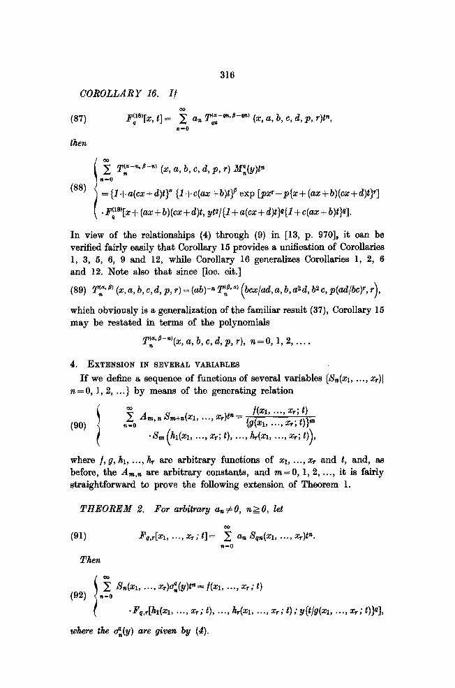
COROLLARY 16. If

VW FY[~, t] = 2 a, T~-rm*B-m’ (x, a, b, C, d, P, r)tRj 98-O

then

Cc a, b, c, 4 P, 4 Mz(yP

=(l+a(cx+d)t)” (I+c(az+b)t}@exp [PH-p(z+(ax+b)(cz+d)t~]

. Fy[x+ (ax+b)(cx+d)t, ytq/(l+a(cx+d)t}Q{l +c(ax+b)t}g].

In view of the relationships (4) through (9) in [13, p. 9701, it can be verified fairly easily that Corollary 15 provides a unification of Corollaries 1, 3, 5, 6, 9 and 12, while Corollary 16 generalizes Corollaries 1, 2, 6 and 12. Note also that since [lot. cit.]

(89) TF 8, (x, a, b, c, d, p, r) = (ab)-* T,, (8m a) (bcx/ad, a, b, azd, b2 c, p(ad/bc)r, r),

which obviously is a generalization of the familiar result (37), Corollary 15 may be restated in terms of the polynomials

T(“*p-“)(x, a, b, c, d, p, r), n= 0, 1, 2, . . . . n

4. EXTENSION IN SEVERAL VARIABLES

If we define a sequence of functions of several variables {S&i, . .., zr)] n=O, 1, 2, . ..} by means of the generating relation

A,,,, n &a+&~ . . . , x4” = {A;’ .;;;‘x;;;;m -8,

( h&l, . . . . xy; t), . . . . h&l, a*., xr; q

> ,

where f, g, h, . .., hr are arbitrary functions of xi, . . . . zr and t, and, as before, the A,,,,,, are arbitrary constants, and m=O, 1,2, . . . . it is fairly straightforward to prove the following extension of Theorem 1.

THEOREM 2. For arbitrary a,# 0, nl0, let

(91)

ThfX

Fq,r[xl, -a., xr ; tl = 5 a, &(xI, . . . , xr)tn. n-0

where the a”,(y) are given by (4).

317

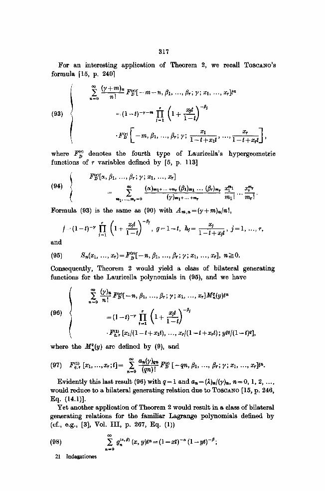
For an interesting application of Theorem 2, we recall TOSCANO’S formula [15, p. 2401

2 (Y+m)n --J--- Fa -m-n, /h, . . . . &; y; a, . . . . xrltn n-o

(93) =(1-p- fJ (l+ 29.J I-1

where FX’ denotes the fourth type of Lauricella’s hypergeometrio functions of r variables defined by [5, p. 1131

i Fl?[a, ,&, . . . . ,%; y; xl, . . . . xrl

(94) i

Formula (93) is the same as (90) with &,,,=(y+m),/n!,

/=(1-t)-? fJ l+ $t +, ( >’

g=l-t, 7&f= q lBt+,@’ j=l , --.,r, i-1

and

(96) &(x1, * * . , x,)=Pg)[-n, 81, . . . . pr; y; XI, . . . . ICY], n20.

Consequently, Theorem 2 would yield a class of bilateral generating functions for the Lauricella polynomials in (96), and we have

n-o q+[-", Bl, .--,a; Y;"l, ***, *lJckP % (?+I

(96) =(1-q-y fJ (1+ $-, I-1

-Fit; [q/(1 --txlt), . . . . G/(1--t+ti); y@/(l--t)*l, where the Hz(y) are defined by (Q), and

(97) Pa’, [ZI, . . ..z.;t]= 2 I, s F$) [--pa, /h, . . . . Br; y; ~1, . . . . d@.

Evidently this last result (96) with Q = 1 and a, = (A),/(r)R, n = 0, 1, 2, . . . , would reduoe to a bilateral generating relation due to TOSCANO [16, p. 246, Eq. (14.1)].

Yet another application of Theorem 2 would result in a olass of bilateral generating relations for the familiar Lagrange polynomials defined by (cf., e.g., [3], Vol. III, p. 267, Eq. (1))

(98) *F. g?fl) (2, y)P=(l-&)--&(l-?&yt)-@;

21 Indagationes

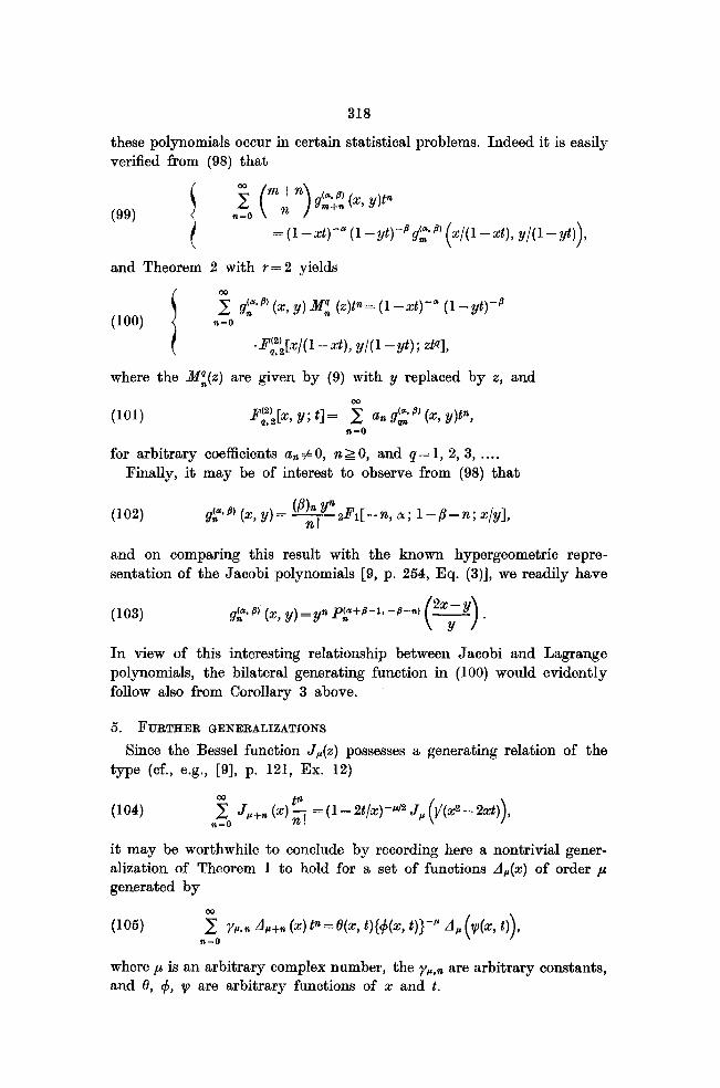
318

these polynomials occur in certain statistical problems. Indeed it is easily verified from (98) that

and Theorem 2 with r = 2 yields

(100) 5 g:yx,ypw; (.+“=(l-Xzt)--” (l-?&)-B

n=o

where the N:(Z) are given by (9) with y replaced by z, and

(101) Jy)2[x, y ; 4 = ngo an gg- B’ (2, yp,

for arbitrary coefficients a, # 0, nr 0, and q= 1, 2, 3, . . . . Finally, it may be of interest to observe from (98) that

(102) gp% (z, y)= i!2$ aF1[-n, or; 1-p-n; x/$/l,

and on comparing this result with the known hypergeometric repre- sentation of the Jacobi polynomials [9, p. 254, Eq. (3)], we readily have

SF p, (x, y) ‘yn p:+w. -P-N y . ( )

In view of this interesting relationship between Jacobi and Lagrange polynomials, the bilateral generating function in (100) would evidently follow also from Corollary 3 above.

5. FURTHER GENERALIZATIONS

Since the Bessel function J,(Z) possesses a generating relation of the type (cf., e.g., [9], p. 121, Ex. 12)

(104)

it may be worthwhile to conclude by recording here a nontrivial gener- alization of Theorem 1 to hold for a set of functions A,,(x) of order p generated by

(105) 5 Y&n n=0

&+n I4 t”=W, t){$(x, t,>-” A, (yb, t,),

where ,u is an arbitrary complex number, the yP,,, are arbitrary constants, and 8, 4, ‘y are arbitrary functions of x and t.

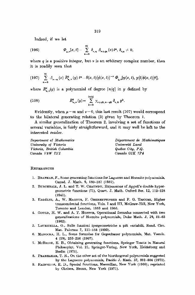
319

Indeed, if we let

006) cp,.&, t1= 2 dysn A,+, (4 t”, &,, + 0, n=O where q is a positive integer, but v is an arbitrary complex number, then it is readily seen that

(107) 5 dy+n (4 q y (Y) tn = w5 W(T WV @g,.,bc~? 0, Y{v&, q*1, 9I=O

where Bi,Jy) is a polynomial of degree [n/q] in y defined by

Rk’ (y) = 2 Yv+Q.n-gk %.k Yk’ k-0

Evidently, when p= m and v = 0, this last result (107) would correspond to the bilateral generating relation (3) given by Theorem 1.

A similar generalization of Theorem 2, involving a set of functions of several variables, is fairly straightforward, and it may well be left to the interested reader.

Department of Mathematics Ddpartement de Mathkmatiquea University of Victoria UniversiM Laval Victoria, B&ah Columbia Qudbec City, P.Q. Canada V&W 2Y2 Canudu BlK 7P4

REFERENCES

1. BRAFMAN, F., Some generating functions for Laguerre and Hermite polynomials, Canad. J. Math. 9, 189-187 (1957).

2. BURCHNALL, J. L. and T. W. CHAUNDY, Expansions of Appell’s double hyper- geometric functions (II), Quart. J. Math. Oxford Ser. 12, 112-128 (1941).

3. ERD~LYI, A., W. MAUNUS, F. OBERHETTIN~ER and F. G. TRICOMI, Higher transcendental functions, Vols. I and III, McGraw-Hill, New York, Toronto and London, 1953 and 1955.

4. GOULD, H. W. and A. T. HOPPER, Operational formulas connected with two generalizations of Hermite polynomials, Duke Math. J. 29, 51-63 (1962).

5. LATJRICELLA, G., Sulle funzioni ipergeometriche a piti variabili, Rend. Circ. Mat. Palermo 7, 111-158 (1893).

6. MANOCHA, H. L., Some formulae for Gegenbauer polynomials, Mat. Vesnik. 4 (19), 253-256 (1967).

7. MCBRIDE, E. B., Obtaining generating functions, Springer Tracts in Natural Philosophy, Vol. 21, Springer-Verlag, New York, Heidelberg and Berlin (1971).

8. PRABHAKAR, T. R., On the other set of the biorthogonal polynomials suggested by the Laguerre polynomials, Pacific J. Math. 37, 801-804 (1971).

9. RAINVILLE, E. D., Special functions, Macmillan, New York (1960); reprinted by Chelsea, Bronx, New York (1971).

320

10. SINOEAL, J. P. and H. M. SRIVASTAVA, A class of bilaterel generating functions for certain classical polynomials, Pacific J. Math. 42, 755-762 (1972).

11. SRIVASTAVA, H. M., A formal extension of certain generating functions-II, Glasnik Mat. Ser. III 6 (26), 3544 (1971).

12. and J. P. SINQHAL, A class of polynomials defined by generalized Rodrigues’ formula, Ann. Mat. Pura Appl. Ser. IV 90, 75-85 (1971).

13. and , A unified presentation of certain classical polynomi8ls. Math. Comp. 26, 969-975 (1972).

14. , Certain formulas associated with generalized Rice polynomials, II, Ann. Polon. Math. 27, 73-83 (1972).

15. TOS~ANO, L., Sui polinomi ipergeometrici a piti variabili de1 tipo FD di Lauricella, Matematiche (Catania) 27, 219-260 (1972).