A Block-Diagonal Algebraic Multigrid Preconditioner for the Brinkman Problem

Technical Report

TR-2012-015

A Block-Diagonal Algebraic Multigrid Preconditioner for the BrinkmanProblem

by

P.S. Vassilevski, U. Villa

Mathematics and Computer Science

EMORY UNIVERSITY

LLNL-JRNL-563431

A Block-Diagonal AlgebraicMultigrid Preconditioner for theBrinkman Problem

P. S. Vassilevski, U. Villa

July 6, 2012

Siam Journal on Scientific Computing

Disclaimer

This document was prepared as an account of work sponsored by an agency of the United States government. Neither the United States government nor Lawrence Livermore National Security, LLC, nor any of their employees makes any warranty, expressed or implied, or assumes any legal liability or responsibility for the accuracy, completeness, or usefulness of any information, apparatus, product, or process disclosed, or represents that its use would not infringe privately owned rights. Reference herein to any specific commercial product, process, or service by trade name, trademark, manufacturer, or otherwise does not necessarily constitute or imply its endorsement, recommendation, or favoring by the United States government or Lawrence Livermore National Security, LLC. The views and opinions of authors expressed herein do not necessarily state or reflect those of the United States government or Lawrence Livermore National Security, LLC, and shall not be used for advertising or product endorsement purposes.

A BLOCK-DIAGONAL ALGEBRAIC MULTIGRIDPRECONDITIONER FOR THE BRINKMAN PROBLEM ∗

PANAYOT S. VASSILEVSKI† AND UMBERTO VILLA ‡

Abstract. The Brinkman model is a unified law governing the flow of a viscous fluid in cav-ity (Stokes equations) and in porous media (Darcy equations). In this work, we explore a novelmixed formulation of the Brinkman problem by introducing the flow’s vorticity as an additionalunknown. This formulation allows for a uniformly stable and conforming discretization by standardfinite element (Nedelec, Raviart-Thomas, discontinuous piecewise polynomials). Based on the sta-bility analysis of the problem in the H(curl)−H(div)− L2 norms ([24]), we study a scalable blockdiagonal preconditioner which is provably optimal in the constant coefficient case. Such precondi-tioner takes advantage of the parallel auxiliary space AMG solvers for H(curl) and H(div) problemsavailable in hypre ([11]). The theoretical results are illustrated by numerical experiments.

Key words. Brinkman problem; Stokes-Darcy coupling; saddle-point problems; block precon-ditioners; algebraic multigrid.

Introduction. The Brinkman equations describe the flow of a viscous fluid incavity and porous media. It was initially proposed in [1], [2] as a homogenizationtechnique for the Navier-Stokes equations. Typical applications of this model are inunderground water hydrology, petroleum industry, automotive industry, biomedicalengineering, and heat pipes modeling.

Mathematically speaking the Brinkman model is a parameter-dependent combi-nation of the Darcy and Stokes models. Since in real applications the number andthe locations of the Stokes-Darcy interfaces might not be known a priori, the unifiedequations in the Brinkman model represent an advantage over the domain decom-position methods coupling the Darcy and the Stokes equations. However, the highvariability in the PDE coefficients, that may take extremely large or small values,negatively affects the conditioning of the discrete problem which poses a substantialchallenge for developing efficient preconditioners for this problem.

Another challenging aspect of the Brinkman model is the construction of a stablefinite element discretization ([17], [25]). As a matter of fact, standard inf-sup com-patible finite elements for both Stokes (Taylor Hood, P2-P0, Crouzeix-Raviart – P0,mini elements) or Darcy (Raviart-Thomas – P0 elements) lead to non-convergent dis-cretizations: the first group suffers of stability issues in the limit Darcy case, whereasthe second ones are not conforming in presence of viscosity. Numerous different ap-proaches have been proposed in the literature to address the numerical stability of thediscretization. Among those, penalization methods ([6], [7]), augmented Lagrangianand least squares stabilization approaches ([8]), or special high order non-conformingelements ([17], [9]) are some examples.

In the present paper, we consider the mixed formulation of the Brinkman problemproposed by the authors in [24]. Following what has already been done for the Stokesproblem ([5], [3]), the authors introduced the (scaled) vorticity as additional unknown.The well-posedness analysis of the mixed formulation was based on the Hilbert com-plex structure for the Hodge Laplacian, and the numerical stability of the method

∗This work was performed under the auspices of the U.S. Department of Energy by LawrenceLivermore National Laboratory under Contract DE-AC52-07NA27344.

† [email protected], Center for Applied Scientific Computing, Lawrence Livermore National Lab-oratory, P.O. Box 808, L-561, Livermore, CA 94551, U.S.A.

‡[email protected], Department of Mathematics and Computer Science, Emory University, At-lanta, GA 30322, U.S.A.

1

2 P. S. Vassilevski, U. Villa

was guaranteed by an analogous result on the discrete level. The particular choice ofNedelec, Raviart-Thomas and piecewise discontinuous elements, in fact, reproducesthe same embedding and mapping properties of the continuous spaces in the finiteelements spaces. In contrast to the penalization methods for the Brinkman problem([6], [7]), this approach allows for a conforming discretization by standard finite ele-ments. Discretization errors in the H(div)-norm of the velocity and in the L2-normof the pressure exhibit uniform decay rates with respect to the inverse permeabilitycoefficient k(x). Only the (scaled) vorticity is approximated with less accuracy as theequations approach the Darcy limit ([24]).A disadvantage of the mixed formulation approach is that the Hodge decompositionholds only for particular sets of boundary conditions ([3]).

In this work, we focus on the development of effective preconditioning techniquesfor the discrete saddle-point problem obtained after finite element discretization ofthe mixed formulation. Following the approach in [18], we construct a block diagonalpreconditioner with optimal convergence properties based on the stability analysisof the continuous problem. Such preconditioner has on its main diagonal the finiteelement matrices corresponding to the H(curl), H(div), and L2 norms involved in thestability estimates. To improve the efficiency of the preconditioner, we resort to theauxiliary space multigrid preconditioners for H(div) and H(curl) problems analyzedin [10] and further developed in [14], [15].

The remainder of the present paper is structured as follows. In Section 1, webriefly derive the mixed formulation of the Brinkman problem based on the HodgeLaplacian, and we provide a stability estimate. In Section 2, we address the numericaldiscretization of the mixed formulation with Nedelec, Raviart-Thomas and piecewisepolynomial discontinuous finite element which leads to a large sparse saddle-pointlinear system. In Section 3, we derive an optimal preconditioner with respect to themesh size. We also investigate an augmented Lagrangian approach in order to improvethe robustness of the preconditioner with respect to the PDE coefficients. Finally, inSection 4 we present numerical results, including some parallel scalability tests, forthe case of constant and space-dependent inverse permeability coefficient.

1. Mixed formulation of the Brinkman Problem. We assume that Ω is abounded simply connected domain in Rd with a Lipschitz continuous simply connectedboundary ∂Ω that has well-defined (almost everywhere) unit outward normal vectorn ∈ Rd. The generalized Brinkman problem reads

−ν ∆u + k(x) u +∇p = f(x), ∀ x ∈ Ωdiv u = g(x), ∀ x ∈ Ωu× n = g, on ∂Ω−p + ν div u = h, on ∂Ω,

(1.1)

where ν ≥ 0 is the fluid viscosity and k(x) is the inverse permeability of the medium.The challenge of this problems is when the coefficient k = k(x) takes two extremevalues O(1) and O(1/ε) in different parts of Ω. In the part of the domain withk = O(1), the PDE behaves like a Stokes problem, whereas in the rest of the domain,it behaves like Darcy equations.

In the present work, for simplicity, we assume natural boundary conditions on ∂Ω.However, other set of boundary conditions, like the essential boundary conditions(u · n = un, σ × n = στ ), can also be treated in a similar way. For the HodgeLaplacian, natural boundary conditions are also known in the literature as electricboundary conditions while the essential ones as magnetic boundary conditions due to

A Block-Diagonal Algebraic Multigrid Preconditioner for the Brinkman Problem 3

the close relation with Maxwell’s equations. In our work, we do not consider the caseof full Dirichlet boundary condition, as the mixed formulation is harder to analyze; itleads to suboptimal discretization error behavior ([3]).

To obtain a mixed formulation of the Brinkman problem (1.1), we exploit thevector calculus identity

∆u = ∇ div u− curl curl u,

and we define the (scaled) vorticity variable

σ = ε curl u, ε =√

ν.

After some straightforward manipulations, the mixed formulation reads

σ − ε curl u = 0, ∀ x ∈ Ωε curl σ − ε2 ∇(div u) + k(x) u +∇p = f(x), ∀ x ∈ Ωdiv u = g(x), ∀ x ∈ Ωu× n = g, on ∂Ω−p + ε2 div u = h, on ∂Ω.

(1.2)

In what follows, we assume that the inverse permeability coefficient k(x) belongsto L∞(Ω) ∩ L2(Ω), and that the inverse permeability k(x) and the viscosity ε2 cannot both vanish at the same time. Such assumptions imply that there exist constantsκmin > 0 and κmax < +∞, such that

0 < κmin ≤ k(x) + ε2 ≤ κmax. (1.3)

1.1. Functional spaces and mixed variational formulation. We now in-troduce some notation used throughout the paper. In what follows, sometimes weborrow some terminology from the finite element exterior calculus, e.g. from [4, 5],without explicitly referring to these (or other) sources. However, we keep this to aminimum to ensure that the presentation is self-contained.For vectorial functions u,v ∈ L2(Ω) = [L2(Ω)]d and scalar functions p, q ∈ L2(Ω), wewrite the inner products (u,v) =

∫Ω

u · v dΩ and (p, q) =∫Ω

p q dΩ. Similarly, wedenote by ‖v‖ and ‖p‖ the norms induced by the respective inner products.To come up with the weak formulation of the system (1.2), we introduce the functionalspaces Q, R and W , defined as

- Q ≡ H(curl,Ω) :=σ ∈ L2(Ω)| curl σ ∈ L2(Ω)

, equipped with the norm

‖τ‖2Q = ‖τ‖2 + ‖curl τ‖2;

- R ≡ H(div,Ω) :=u ∈ L2(Ω)| div u ∈ L2(Ω)

, equipped with the norm

‖v‖2R = ‖v‖2 + ‖div v‖2;

- W ≡ L2(Ω), equipped with the norm

‖q‖2W = ‖q‖2.

We denote with Q∗, R∗, and W ∗ the dual spaces of Q, R, and W , respectively. Itis clear that in the case of essential (magnetic) boundary conditions, the respective


spaces Q, R are proper subsets of H(curl), H(div); Q, R then consist of functionswith vanishing tangential or normal boundary traces.

The mixed variational formulation of the Brinkman problem (1.2), which is of ourmain interest, reads as follows.

Problem 1.1. Find (σ,u, p) ∈ Q×R×W such that m(σ, τ ) −c∗(u, τ ) = F (τ ) ∀ τ ∈ Q−c(σ,v) −a(u,v)− d(u,v) +b∗(p,v) = G(v) ∀ v ∈ R

b(u, q) = H(q) ∀ q ∈ W(1.4)

where

m(σ, τ ) = (σ, τ ), σ, τ ∈ Qc(σ, v) = ε (curl σ, v), σ ∈ Q, v ∈ R,a(u, v) = ε2(div u, div v), u, v ∈ R,d(u,v) = (k(x) u, v), u, v ∈ R,b(u, q) = (div u, q), u ∈ R, q ∈ W.

(1.5)

F ∈ Q∗, G ∈ R∗, H ∈ W ∗ are bounded functionals that take into account volumeforces and boundary conditions.

The stability analysis of the mixed formulation was carried out by the authors in[24], following the analysis of the Hodge Laplacian in [5], [3]. Here, we summarize themain results.

Let ε ≥ 0 and k(x) ∈ L∞(Ω) ∩ L2(Ω), 0 < κmin ≤ k(x) + ε2 ≤ κmax almosteverywhere in Ω, and introduce the weighted norms in the spaces Qw, Rw, Ww

defined by

‖τ‖2Qw= ‖τ‖2 +

ε2

κmax‖Cτ‖2, ‖v‖2Rw

= κmin‖v‖2R, ‖q‖2Ww=

1κmax

‖q‖2. (1.6)

Theorem 1.1. The bilinear form corresponding to the mixed problem, Problem1.1,

B(σ,u, p; τ ,v, q) == m(σ, τ )− c∗(u, τ )− c(σ,v)− a(u,v)− d(u,v) + b∗(p,v) + b(u, q), (1.7)

is bounded and satisfies an inf-sup condition. More specifically, there exist two con-stants M and α depending only on the domain Ω such that

|B(σ,u, p; τ ,v, q)| ≤ Mκmax

κmin‖(σ,u, p)‖Qw×Rw×Ww

‖(τ ,v, q)‖Qw×Rw×Ww(1.8)

and

inf(τ ,v,q)∈Q×R×W

sup(σ,u,p)∈Q×R×W

B(σ,u, p; τ ,v, q)‖(τ ,v, q)‖Qw×Rw×Ww ‖(σ,u, p)‖Qw×Rw×Ww

≥ α.

(1.9)The proof of the inf-sup condition is based on certain orthogonal decomposition ofQ and R and respective Poincare inequalities holding for one of the components inthese orthogonal decompositions. We refer to [24] for the details.

As an immediate consequence of the above theorem, the following well–posednessresult is obtained in [24].


Theorem 1.2. The generalized Brinkman problem, Problem 1.1, admits a uniquesolution and the following a priori estimate holds:

‖σ‖2Qw+ ‖u‖2Rw

+ ‖p‖2Ww≤ C(Ω)(‖F‖2Q∗

w+ ‖G‖2R∗

w+ ‖H‖2W∗

w).

Here C(Ω) is a constant depending only on the domain, and the weighted norms inthe spaces Qw, Rw, Ww are defined in (1.6).

2. Discretization. For a given integer r ≥ 0, we let Qh be the (r + 1)-thorder Nedelec finite elements ([20]), Rh the r-th order Raviart-Thomas finite elements([23, 20]), and Wh the discontinuous piecewise polynomials finite element of degree atmost r.

It is well-known ([19]) that the canonical interpolation operators ΠVh : V 7→ Vh

(V := Q, R, W ) commute with the curl and div differential operators, that is

curl ΠQh = ΠR

h curl, and div ΠRh = ΠW

h div.

Indeed such spaces form a finite dimensional subcomplex of the continuous deRham complex and give raise to the following commuting diagram ([4, 5]):

H1\R ∇−−−→ Q curl−−−−→ R div−−−→ Wy y y ySh\R

∇−−−→ Qhcurl−−−−→ Rh

div−−−→ Wh

.

Here we also introduced the space Sh of continuous piecewise polynomial of degree atmost r + 1. Even though such space is not directly involved in the discretization ofthe Brinkman problem, it plays an important role in the construction of the auxiliaryspace multigrid preconditioner for H(curl) and H(div) problems ([10],[14, 15]).

Of our main interest is the Galerkin problemProblem 2.1. Find (σh,uh, ph) ∈ Qh ×Rh ×Wh such that m(σh, τh) −c∗(uh, τh) = F (τh) ∀ τh ∈ Qh

−c(σh,vh) −a(uh,vh)− d(uh,vh) +b∗(ph,vh) = G(vh) ∀ vh ∈ Rh

b(uh, qh) = H(qh) ∀ qh ∈ Wh

(2.1)

Since the discrete finite element spaces Qh,Rh,Wh preserve all the properties ofthe continuous spaces, the bilinear form B restricted to the discrete spaces satisfies theinf-sup condition (1.9) with a constant αh bounded independently of h, and thereforethe Galerkin problem is well-posed ([24]).

To come up with an algebraic form of Problem 2.1, we let Nσ = dim(Qh), Nu =dim(Rh), Np = dim(Wh) be the dimensions of the finite element spaces Qh, Rh,Wh, and we introduce the vectors Σ ∈ RNσ , U ∈ RNu , P ∈ RNp collecting thefinite element degrees of freedom σi

h, i = 1, . . . , Nσ, uih, i = 1, . . . , Nu and pi

h, i =1, . . . , Np. We also introduce the finite element matrices M ∈ RNσ×Nσ , C ∈ RNu×Nσ ,A ∈ RNu×Nu , D ∈ RNu×Nu , B ∈ RNp×Nu whose entries are given by

Mi,j = m(σjh, τ i

h) = (σjh, τ i

h) i, j = 1, . . . , Nσ

Ci,j = c(σjh, vi

h) = ε (curl σjh, vi

h) i = 1, . . . , Nu, j = 1, . . . , Nσ

Ai,j = a(ujh, vi

h) = ε2(div ujh, div vi

h) i, j = 1, . . . , Nu

Di,j = d(ujh, vi

h) = (k(x) ujh, vi

h) i, j = 1, . . . , Nu

Bi,j = b(ujh, qi

h) = (div ujh, qi

h) i = 1, . . . , Np, j = 1, . . . , Nu.

(2.2)


Letting N = Nσ +Nu +Np be the total number of unknowns, we write the linearsystem corresponding to the Brinkman problem as

BX = B (2.3)

where the block matrix B ∈ RN×N and the block vectors X ∈ RN and B ∈ RN read

B =

M −CT 0−C −A−D BT

0 B 0

, X =

ΣUP

, B =

FGH

. (2.4)

We also introduce the augmented formulation of the Brinkman problem that willbe used in the numerical tests. Letting MW ∈ RNp×Np be the pressure mass matrixand γ ∈ R a positive number, the augmented matrix and right-hand-side have theform

Bγ =

M −CT 0−C −A−D − γBT M−1

W B BT

0 B 0

, Bγ =

FG− γBM−1

W HH

. (2.5)

The advantage of the augmented formulation is that it improves the inf-sup constantα, and therefore, it leads to the solution of better conditioned problems, provided thatthe augmentation parameter γ is not too large. In the numerical result presented inthe following we take γ of the order of the inverse permeability coefficient k.

3. Preconditioning. The discretized linear system (2.3) has the form of a sym-metric indefinite problem, having Nσ+Np positive eigenvalues and Nu negative eigen-values. An effective iterative method to solve linear system with symmetric indefinitematrices is MINRES ([21]) employing a symmetric positive definite preconditioner P.

To derive the preconditioner, we follow the approach presented in ([18]) for pre-conditioning symmetric saddle-point problems in a functional space setting. Accord-ing to the authors, the mapping properties of the differential operators of the con-tinuous problem suggest that block diagonal preconditioners are natural choices forsaddle-point problems. More specifically, given a stability estimate for the continuousproblem in some functional spaces, the block diagonal matrix, in which the blocksrepresent the discretization of the inner products in those spaces, leads to a uniformlybounded (in terms of h) preconditioner for the saddle-point discrete system of interest.

Recalling the weights in (1.6), wQ = ε2

κmax, wR = κmin, wW = 1

κmax, we introduce

the symmetric positive definite variational forms

q(σh, τh) = (σh, τh) + wQ(curl σh, curl τh), σh, τh ∈ Qh

r(uh,vh) = wR(uh,vh) + wR(div uh,div vh), uh,vh ∈ Rh

w(ph, qh) = wW (ph, qh), ph, qh ∈ Wh.(3.1)

The above forms define weighted inner products in Qw, Rw and Ww.Therefore (based on [18]), a uniform preconditioner for the saddle-point problem

(2.3) is given by

P =

Q 0 00 R 00 0 W

, (3.2)

where Q, R, W are the matrix representations of the weighted inner products q(σh, τh),r(uh,vh), and w(ph, qh).


We now proceed, for completeness, with the standard analysis of the spectralcondition number K(A) of the preconditioned saddle-point operator A = P− 1

2BP− 12 .

First of all, we remark that, if the vector Y ∈ RN collects the degrees of freedom ofthe finite element functions τh ∈ Qh, vh ∈ Rh, qh ∈ Wh, then the P norm of Y isequal to the norm of (τh,vh, qh) in Qw ×Rw ×Ww, that is

‖Y‖P =√

YTPY = ‖(τh,vh, qh)‖Qw×Rw×Ww .

Next, we recall the definition of the spectral condition number of an invertible(symmetric indefinite) operator A,

K(A) = supX∈RN

‖AX‖2‖X‖2

supY∈RN

‖A−1Y‖2‖Y‖2

=max |λ|min |λ|

, λ ∈ σ(A).

The aim now is to bound the two factors supX∈RN‖AX‖2‖X‖2 and supY∈RN

‖A−1Y‖2‖Y‖2 by

using the continuity and the inf-sup condition of the bilinear form B . For the firstterm, by letting X = P− 1

2 X and Y = P− 12 Y and by using (1.8), we have

supX∈RN

‖AX‖2‖X‖2

= supX∈RN

supY∈RN

YTAX‖Y‖2 ‖X‖2

= supX∈RN

supY∈RN

YTBX

‖Y‖P ‖X‖P≤ M

κmax

κmin.

Similarly, by using the discrete version of the inf-sup condition (1.9), for the secondterm we have

supY∈RN

‖A−1Y‖2‖Y‖2

=(

infX∈RN

‖AX‖2‖X‖2

)−1

=(

infX∈RN

supY∈RN

YTAX‖Y‖2 ‖X‖2

)−1

=(inf

X∈RN

supY∈RN

YTBX

‖Y‖P ‖X‖P

)−1

≤ 1αh

. (3.3)

In conclusion, combining the last two inequalities above, we obtain the followingresult.

Theorem 3.1. The relative condition number of B with respect the block–diagonalpreconditioner P satisfies the estimate

K(P− 12BP− 1

2 ) =max |λ|min |λ|

≤ M

αh

κmax

κmin.

The above estimate implies that in the particular case of constant inverse perme-ability k(x) = k0, the condition number of the preconditioned saddle-point problemis independent of both the mesh size and k0. The numerical experiments in the fol-lowing section confirm this claim. However, in the general case of variable coefficientk(x), the condition number increases proportionally to the ratio κmax

κmin. To alleviate

this issue, in the numerical results section, we introduce a special augmentation of theBrinkman problem and a modified version of the preconditioner, which gives optimalconvergence rates for smooth coefficients k(x).

Finally, we remark (as is well-known) that the operator A = P− 12BP− 1

2 above isintroduced only for the purpose of the analysis, and it does not explicitly appear in theimplementation of the preconditioned MINRES algorithm; indeed only applications ofP−1 to a vector are required. Moreover, to make it practical, we substitute P−1 with aspectrally equivalent operator P−1 that is easier to apply (in fact, with optimal cost).In the numerical results section, we demonstrate that letting P−1 be an auxiliaryspace AMG preconditioner can drastically reduce the computational effort.


4. Numerical Results. The numerical results presented in the following aimto study the performance of the proposed preconditioner both in terms of number ofiterations and wall time. Problems with increasing level of difficulty are considered:first the case when the inverse permeability coefficient k(x) is constant in the domain,then when it varies smoothly, and finally we illustrate the difficulties with the block–diagonal preconditioning approach when the coefficient k(x) admits large jumps.

Concerning the choice of the finite element spaces, we will restrict ourselves to thecase r = 0, i.e. first order Nedelec elements, lowest order Raviart-Thomas elements,and piecewise constant elements. This is not a limitation of the method since, inmany practical applications, only discretization error of first order can be achieveddue to non-smooth exact solutions and to discontinuities in the PDE coefficients.

Two different versions of the block-diagonal preconditioner in (3.2) are compared.In the exact (ideal) version the blocks Q, R are solved exactly by using the precondi-tioned conjugate gradient method; while in the AMG (practical) version the inverseof blocks Q, R are approximated by one V-cycle for the auxiliary space AMG forH(curl) and H(div) problem respectively.

In practice the AMG version of the preconditioner out-performs the exact one,but we remark the theoretical importance of the latter, since it allows us to confirmthe theoretical, uniform with respect to the mesh, performance of the preconditioner.

In both versions of the preconditioner, the block W is inverted exactly. Indeed,due to the choice of discontinuous pressure finite elements W has a block diagonalstructure, and it reduces to a diagonal matrix for piecewise constant elements.

Before discussing in detail the obtained numerical results, we describe briefly thesoftware, compilers and hardware that we have used.

Concerning the finite element discretization of the Brinkman problem, we usedthe parallel C++ library MFEM [http://code.google.com/p/mfem/], developed atLawrence Livermore National Laboratory (LLNL). This library supports a wide vari-ety of finite element spaces in 2D and 3D, as well as many bilinear and linear formsdefined on them. It includes classes for dealing with various types of triangular,quadrilateral, tetrahedral and hexahedral meshes and their global and local refine-ment. Parallelization in MFEM is based on MPI, and it leads to high scalability inthe finite element assembly procedure. It supports several solvers from the hyprelibrary (http://www.llnl.gov/CASC/hypre/). In particular, in our tests we used theauxiliary space algebraic multigrid solvers for H(curl) and H(div) ([14], [15]).

The initial meshes used in our simulation were generated with the unstructuredmesh generator Netgen [http://www.hpfem.jku.at/netgen/].

The numerical results presented in this section were obtained on hera, a high per-formance computer at LLNL. Hera has a total of 864 nodes connected by InfiniBandDDR (Mellanox). Each node has 16 AMD Quad-Core Opteron 2.3Ghz CPUs, and32GB of memory. Hera is running CHAOS 4.4, a Linux kernel developed at LLNL,specific for high performance computing.

Our code was compiled with the Intel mpiicc and mpiicpc compilers version11.1.046.

4.1. Constant coefficient weak scalability test. We study the performanceof the proposed preconditioner in the case of constant coefficient k(x) = k0. Inparticular, we present results relative to the augmented formulation (2.5) with γ = k0

and the block diagonal preconditioner P, where the weights wQ, wR, wW are given


by

wQ =ε2

k0 + ε2, wR = k0 + ε2, wW =

1k0 + ε2

. (4.1)

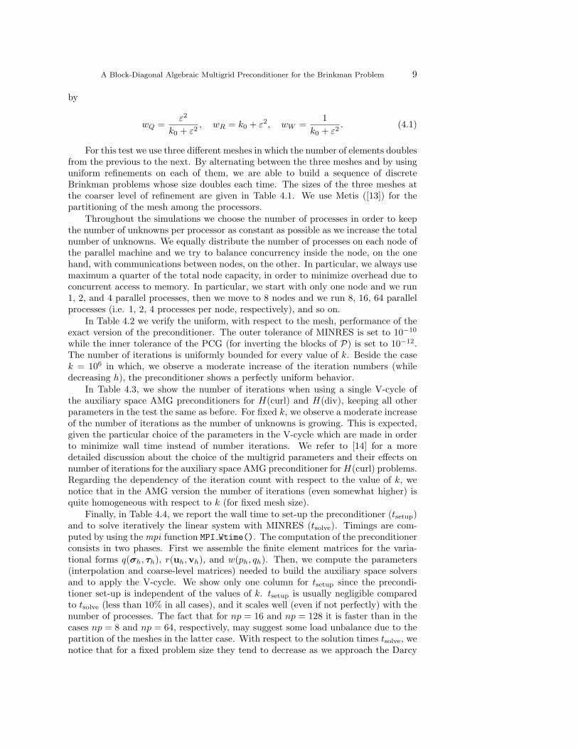
For this test we use three different meshes in which the number of elements doublesfrom the previous to the next. By alternating between the three meshes and by usinguniform refinements on each of them, we are able to build a sequence of discreteBrinkman problems whose size doubles each time. The sizes of the three meshes atthe coarser level of refinement are given in Table 4.1. We use Metis ([13]) for thepartitioning of the mesh among the processors.

Throughout the simulations we choose the number of processes in order to keepthe number of unknowns per processor as constant as possible as we increase the totalnumber of unknowns. We equally distribute the number of processes on each node ofthe parallel machine and we try to balance concurrency inside the node, on the onehand, with communications between nodes, on the other. In particular, we always usemaximum a quarter of the total node capacity, in order to minimize overhead due toconcurrent access to memory. In particular, we start with only one node and we run1, 2, and 4 parallel processes, then we move to 8 nodes and we run 8, 16, 64 parallelprocesses (i.e. 1, 2, 4 processes per node, respectively), and so on.

In Table 4.2 we verify the uniform, with respect to the mesh, performance of theexact version of the preconditioner. The outer tolerance of MINRES is set to 10−10

while the inner tolerance of the PCG (for inverting the blocks of P) is set to 10−12.The number of iterations is uniformly bounded for every value of k. Beside the casek = 106 in which, we observe a moderate increase of the iteration numbers (whiledecreasing h), the preconditioner shows a perfectly uniform behavior.

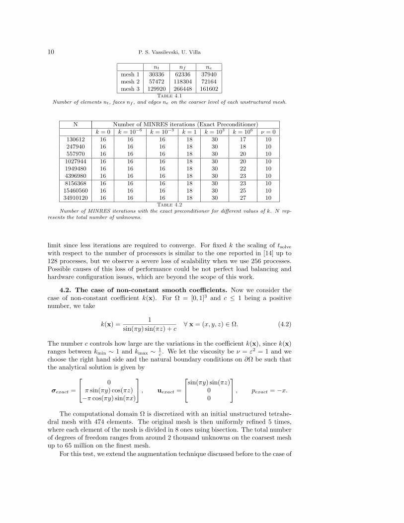
In Table 4.3, we show the number of iterations when using a single V-cycle ofthe auxiliary space AMG preconditioners for H(curl) and H(div), keeping all otherparameters in the test the same as before. For fixed k, we observe a moderate increaseof the number of iterations as the number of unknowns is growing. This is expected,given the particular choice of the parameters in the V-cycle which are made in orderto minimize wall time instead of number iterations. We refer to [14] for a moredetailed discussion about the choice of the multigrid parameters and their effects onnumber of iterations for the auxiliary space AMG preconditioner for H(curl) problems.Regarding the dependency of the iteration count with respect to the value of k, wenotice that in the AMG version the number of iterations (even somewhat higher) isquite homogeneous with respect to k (for fixed mesh size).

Finally, in Table 4.4, we report the wall time to set-up the preconditioner (tsetup)and to solve iteratively the linear system with MINRES (tsolve). Timings are com-puted by using the mpi function MPI Wtime(). The computation of the preconditionerconsists in two phases. First we assemble the finite element matrices for the varia-tional forms q(σh, τh), r(uh,vh), and w(ph, qh). Then, we compute the parameters(interpolation and coarse-level matrices) needed to build the auxiliary space solversand to apply the V-cycle. We show only one column for tsetup since the precondi-tioner set-up is independent of the values of k. tsetup is usually negligible comparedto tsolve (less than 10% in all cases), and it scales well (even if not perfectly) with thenumber of processes. The fact that for np = 16 and np = 128 it is faster than in thecases np = 8 and np = 64, respectively, may suggest some load unbalance due to thepartition of the meshes in the latter case. With respect to the solution times tsolve, wenotice that for a fixed problem size they tend to decrease as we approach the Darcy


nt nf ne

mesh 1 30336 62336 37940mesh 2 57472 118304 72164mesh 3 129920 266448 161602

Table 4.1Number of elements nt, faces nf , and edges ne on the coarser level of each unstructured mesh.

N Number of MINRES iterations (Exact Preconditioner)

k = 0 k = 10−6 k = 10−3 k = 1 k = 103 k = 106 ν = 0

130612 16 16 16 18 30 17 10247940 16 16 16 18 30 18 10557970 16 16 16 18 30 20 10

1027944 16 16 16 18 30 20 101949480 16 16 16 18 30 22 104396980 16 16 16 18 30 23 10

8156368 16 16 16 18 30 23 1015460560 16 16 16 18 30 25 1034910120 16 16 16 18 30 27 10

Table 4.2Number of MINRES iterations with the exact preconditioner for different values of k. N rep-

resents the total number of unknowns.

limit since less iterations are required to converge. For fixed k the scaling of tsolvewith respect to the number of processors is similar to the one reported in [14] up to128 processes, but we observe a severe loss of scalability when we use 256 processes.Possible causes of this loss of performance could be not perfect load balancing andhardware configuration issues, which are beyond the scope of this work.

4.2. The case of non-constant smooth coefficients. Now we consider thecase of non-constant coefficient k(x). For Ω = [0, 1]3 and c ≤ 1 being a positivenumber, we take

k(x) =1

sin(πy) sin(πz) + c∀ x = (x, y, z) ∈ Ω. (4.2)

The number c controls how large are the variations in the coefficient k(x), since k(x)ranges between kmin ∼ 1 and kmax ∼ 1

c . We let the viscosity be ν = ε2 = 1 and wechoose the right hand side and the natural boundary conditions on ∂Ω be such thatthe analytical solution is given by

σexact =

0π sin(πy) cos(πz)−π cos(πy) sin(πx)

, uexact =

sin(πy) sin(πz)00

, pexact = −x.

The computational domain Ω is discretized with an initial unstructured tetrahe-dral mesh with 474 elements. The original mesh is then uniformly refined 5 times,where each element of the mesh is divided in 8 ones using bisection. The total numberof degrees of freedom ranges from around 2 thousand unknowns on the coarsest meshup to 65 million on the finest mesh.

For this test, we extend the augmentation technique discussed before to the case of


Number of MINRES iterations (AMG Preconditioner)

N k = 0 k = 10−6 k = 10−3 k = 1 k = 103 k = 106 ν = 0

130612 44 44 44 36 37 32 21247940 48 48 48 40 39 34 23557970 51 51 51 46 43 37 24

1027944 57 57 57 48 49 39 261949480 60 60 60 51 50 40 274396980 61 61 61 52 52 42 28

8156368 68 69 68 61 55 43 2815460560 72 73 72 64 58 44 3034910120 72 72 72 65 59 45 30

Table 4.3Number of MINRES iterations with the AMG preconditioner for different values of k. N

represents the total number of unknowns.

tsolve (AMG Preconditioner) tsetup

nn np N k = 0 k = 10−6 k = 10−3 k = 1 k = 103 k = 106 ν = 0

1 1 130612 15.2 15.1 15.1 12.7 13.0 11.3 8.0 0.711 2 247940 17.7 17.7 17.7 15.1 14.7 13.0 9.5 0.961 4 557970 22.6 22.5 22.5 19.5 19.4 16.8 11.9 1.28

8 8 1027944 25.6 25.2 24.9 21.6 21.9 17.5 13.0 1.478 16 1949480 26.8 26.9 26.8 22.8 22.6 18.4 13.7 1.428 32 4396980 33.0 33.0 33.1 28.3 28.6 22.9 17.0 1.74

64 64 8156368 36.2 36.8 36.7 33.2 30.6 24.5 20.1 2.1564 128 15460560 45.3 44.8 44.9 41.5 35.7 28.3 22.0 1.7664 256 34910120 90.0 91.7 91.0 83.2 76.7 52.3 43.6 2.56

Table 4.4Computational cost of the AMG preconditioner. nn is the number of nodes used, np is the

number of processes, N the total number of degrees of freedom, tsolve and tsetup measures the timein seconds to solve the linear system and to assemble the preconditioner, respectively.

non constant coefficient. In particular, we solve the augmented saddle-point problem(σh, τh)− ε (uh, curl τh) = F (τh), ∀ τh ∈ Qh

−ε (curl σh,vh)− (k(x) uh,vh)− ((k(x) + ε2) div uh,div vh) + (ph,div uh) =G(vh) + H(k(x) div vh), ∀ vh ∈ Rh

(div uh, qh) = H(qh), ∀ qh ∈ Wh

(4.3)preconditioned by a block-diagonal preconditioner with blocks corresponding to thefollowing bilinear forms:

(σh, τh) + ε2

(1

k(x) + ε2curl σh, curl τh

)σh, τh ∈ Qh(

(k(x) + ε2) uh, vh

)+((k(x) + ε2) div uh, div vh

)uh,vh ∈ Rh(

1k(x) + ε2

ph, qh

)ph, qh ∈ Wh.

(4.4)

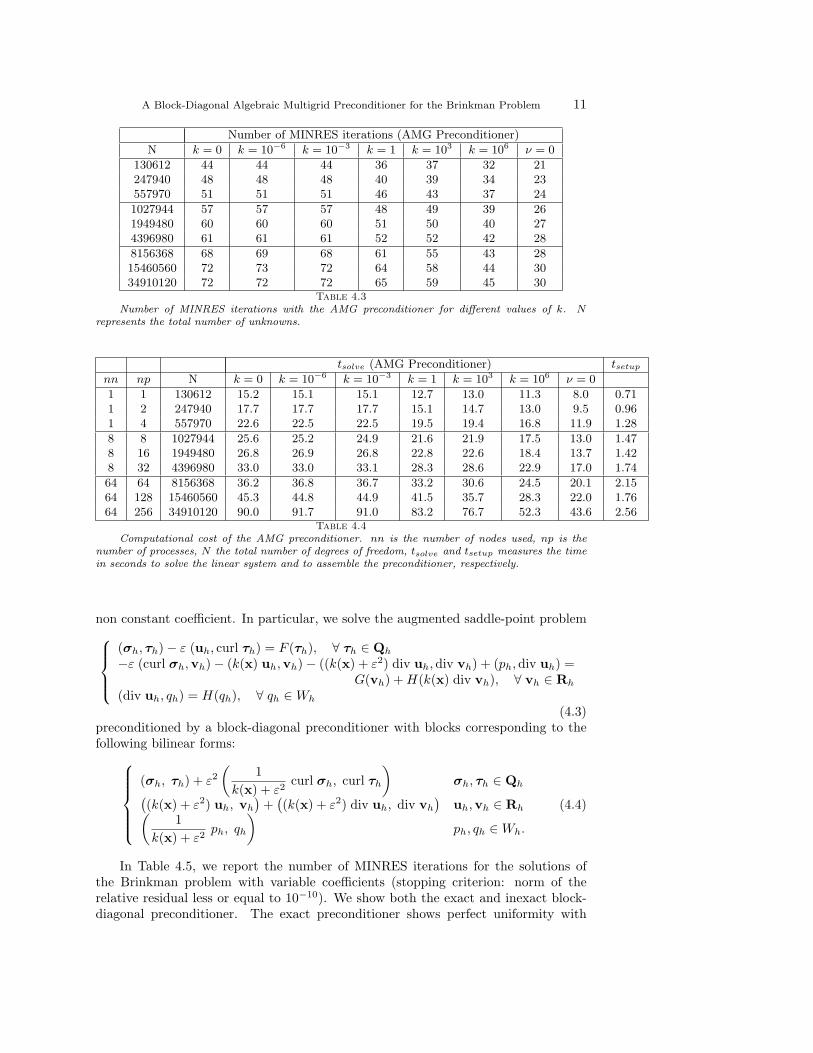
In Table 4.5, we report the number of MINRES iterations for the solutions ofthe Brinkman problem with variable coefficients (stopping criterion: norm of therelative residual less or equal to 10−10). We show both the exact and inexact block-diagonal preconditioner. The exact preconditioner shows perfect uniformity with


Exact nit AMG nit

N kmaxkmin

= 2 kmaxkmin

≈ 103 kmaxkmin

≈ 106 kmaxkmin

= 2 kmaxkmin

≈ 103 kmaxkmin

≈ 106

2.24K 19 30 30 26 35 3616.9K 19 29 30 32 37 38130K 19 29 32 46 45 481.03M 19 27 32 52 49 538.16M 19 27 32 63 61 6165M 19 27 32 74 70 70

Table 4.5Performances of the exact and AMG preconditioner for variable coefficient problem as a func-

tion of the ratio kmaxkmin

. N represents the total number of unknowns and nit the number of precon-

ditioned MINRES iterations to achieve a relative reduction of the residual norm up to 10−10.

respect to the mesh behavior, and a moderate dependence on the ratio kmaxkmin

. Theinexact preconditioner consists of one V-cycle of the auxiliary space AMG applied tothe weighted H(curl) and H(div) variational forms in (4.4). The number of iterationstends to grow as we refine the mesh, but it is more uniform respect to the ratio kmax

kmin.

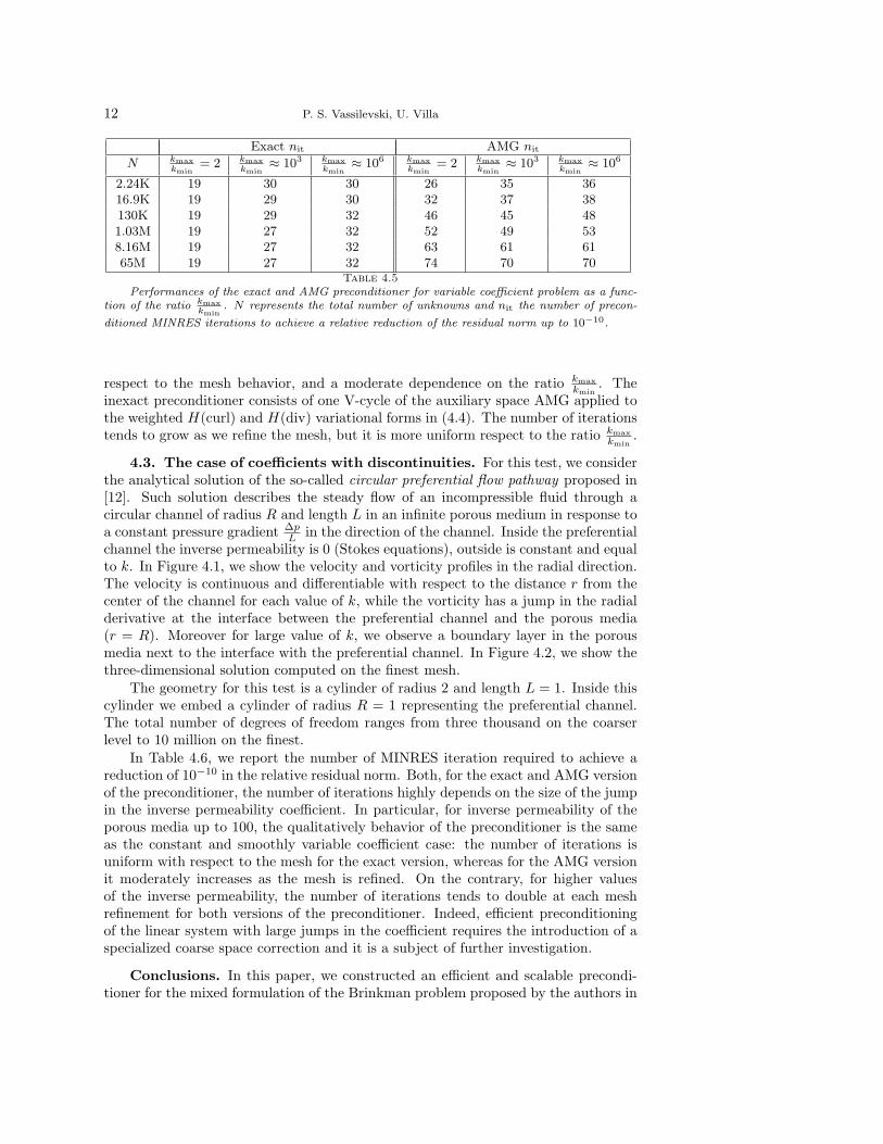
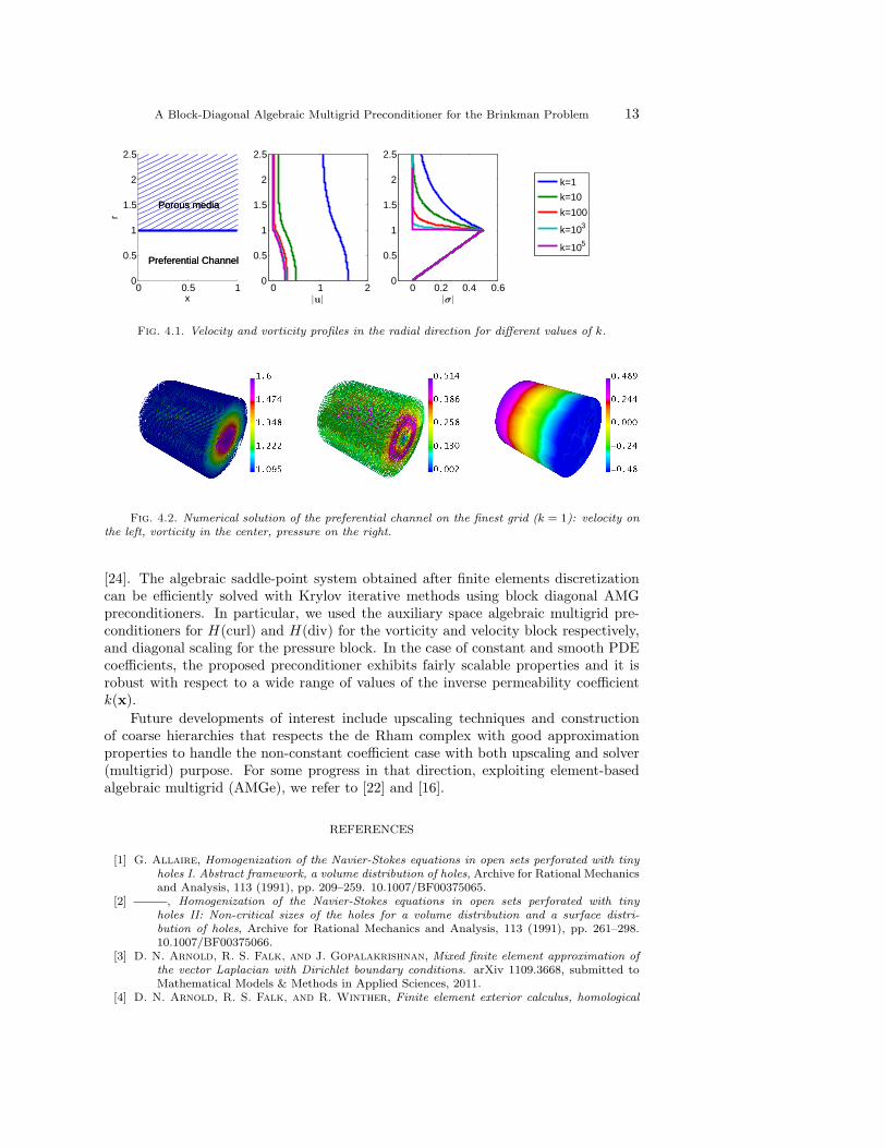
4.3. The case of coefficients with discontinuities. For this test, we considerthe analytical solution of the so-called circular preferential flow pathway proposed in[12]. Such solution describes the steady flow of an incompressible fluid through acircular channel of radius R and length L in an infinite porous medium in response toa constant pressure gradient ∆p

L in the direction of the channel. Inside the preferentialchannel the inverse permeability is 0 (Stokes equations), outside is constant and equalto k. In Figure 4.1, we show the velocity and vorticity profiles in the radial direction.The velocity is continuous and differentiable with respect to the distance r from thecenter of the channel for each value of k, while the vorticity has a jump in the radialderivative at the interface between the preferential channel and the porous media(r = R). Moreover for large value of k, we observe a boundary layer in the porousmedia next to the interface with the preferential channel. In Figure 4.2, we show thethree-dimensional solution computed on the finest mesh.

The geometry for this test is a cylinder of radius 2 and length L = 1. Inside thiscylinder we embed a cylinder of radius R = 1 representing the preferential channel.The total number of degrees of freedom ranges from three thousand on the coarserlevel to 10 million on the finest.

In Table 4.6, we report the number of MINRES iteration required to achieve areduction of 10−10 in the relative residual norm. Both, for the exact and AMG versionof the preconditioner, the number of iterations highly depends on the size of the jumpin the inverse permeability coefficient. In particular, for inverse permeability of theporous media up to 100, the qualitatively behavior of the preconditioner is the sameas the constant and smoothly variable coefficient case: the number of iterations isuniform with respect to the mesh for the exact version, whereas for the AMG versionit moderately increases as the mesh is refined. On the contrary, for higher valuesof the inverse permeability, the number of iterations tends to double at each meshrefinement for both versions of the preconditioner. Indeed, efficient preconditioningof the linear system with large jumps in the coefficient requires the introduction of aspecialized coarse space correction and it is a subject of further investigation.

Conclusions. In this paper, we constructed an efficient and scalable precondi-tioner for the mixed formulation of the Brinkman problem proposed by the authors in


0 0.5 10

0.5

1

1.5

2

2.5

Preferential Channel

Porous media

r

x

Preferential Channel

Porous media

0 1 20

0.5

1

1.5

2

2.5

|u|0 0.2 0.4 0.6

0

0.5

1

1.5

2

2.5

|σ|

k=1

k=10

k=100

k=103

k=105

Fig. 4.1. Velocity and vorticity profiles in the radial direction for different values of k.

Fig. 4.2. Numerical solution of the preferential channel on the finest grid (k = 1): velocity onthe left, vorticity in the center, pressure on the right.

[24]. The algebraic saddle-point system obtained after finite elements discretizationcan be efficiently solved with Krylov iterative methods using block diagonal AMGpreconditioners. In particular, we used the auxiliary space algebraic multigrid pre-conditioners for H(curl) and H(div) for the vorticity and velocity block respectively,and diagonal scaling for the pressure block. In the case of constant and smooth PDEcoefficients, the proposed preconditioner exhibits fairly scalable properties and it isrobust with respect to a wide range of values of the inverse permeability coefficientk(x).

Future developments of interest include upscaling techniques and constructionof coarse hierarchies that respects the de Rham complex with good approximationproperties to handle the non-constant coefficient case with both upscaling and solver(multigrid) purpose. For some progress in that direction, exploiting element-basedalgebraic multigrid (AMGe), we refer to [22] and [16].

REFERENCES

[1] G. Allaire, Homogenization of the Navier-Stokes equations in open sets perforated with tinyholes I. Abstract framework, a volume distribution of holes, Archive for Rational Mechanicsand Analysis, 113 (1991), pp. 209–259. 10.1007/BF00375065.

[2] , Homogenization of the Navier-Stokes equations in open sets perforated with tinyholes II: Non-critical sizes of the holes for a volume distribution and a surface distri-bution of holes, Archive for Rational Mechanics and Analysis, 113 (1991), pp. 261–298.10.1007/BF00375066.

[3] D. N. Arnold, R. S. Falk, and J. Gopalakrishnan, Mixed finite element approximation ofthe vector Laplacian with Dirichlet boundary conditions. arXiv 1109.3668, submitted toMathematical Models & Methods in Applied Sciences, 2011.

[4] D. N. Arnold, R. S. Falk, and R. Winther, Finite element exterior calculus, homological


Exact preconditioner nit

N k = 1 k = 10 k = 102 k = 103 k = 105

2.9K 28 40 92 129 12121K 27 38 94 189 221164K 25 36 90 202 3931.3M 23 34 83 199 64010M 23 31 79 186 868

AMG preconditioner nit

N k = 1 k = 10 k = 102 k = 103 k = 105

2.9K 30 43 93 133 13521K 30 43 100 199 271164K 31 44 105 235 5261.3M 34 48 112 264 92110M 40 57 128 293 > 999

Table 4.6Number of MINRES iterations to achieve a reduction of 10−10 for the relative residual norm

in the preferential channel test case.

techniques, and applications, Acta Numerica, 15 (2006), pp. 1–155.[5] , Finite element exterior calculus: from Hodge theory to numerical stability, Bull. Amer.

Math. Soc. (N.S.), 47 (2010), pp. 281–354. DOI: 10.1090/S0273-0979-10-01278-4.[6] E. Burman and P. Hansbo, Stabilized Crouzeix-Raviart element for the Darcy-Stokes problem,

Numerical Methods for Partial Differential Equations, 21 (2005), pp. 986–997.[7] , A unified stabilized method for Stokes’ and Darcy’s equations, Journal of Computational

and Applied Mathematics, 198 (2007), pp. 35 – 51.[8] M. R. Correa and A. F. D. Loula, A unified mixed formulation naturally coupling Stokes

and Darcy flows, Computer Methods in Applied Mechanics and Engineering, 198 (2009),pp. 2710 – 2722.

[9] J. Guzman and M. Neilan, A family of nonconforming elements for the Brinkman problem,IMA Journal of Numerical Analysis, (2012).

[10] R. Hiptmair and J. Xu, Nodal auxiliary space preconditioning in H(curl) and H(div) spaces,SIAM Journal on Numerical Analysis, 45 (2007), pp. 2483–2509.

[11] hypre : High performance preconditioners. http://www.llnl.gov/CASC/hypre/.[12] A. A. Jennings and R. Pisipati, The impact of Brinkman’s extension of Darcy’s law in the

neighborhood of a circular preferential flow pathway, Environmental Modelling and Soft-ware with Environment Data News, 14 (1999), pp. 427–435.

[13] G. Karypis and V. Kumar, MeTis: Unstructured Graph Partitioning and Sparse MatrixOrdering System, Version 4.0. http://www.cs.umn.edu/ metis, 2009.

[14] T. Kolev and P. S. Vassilevski, Parallel Auxiliary Space AMG for H(curl) Problems, J. ofComputational Mathematics, 27 (2009).

[15] , Parallel Auxiliary Space AMG Solver for H(div) Problems. Technical Report LLNL-JRNL-520391, December 15, 2011.

[16] I. V. Lashuk and P. S. Vassilevski, Element Agglomeration Coarse Raviart-Thomas SpacesWith Improved Approximation Properties, Numerical Linear Algebra with Applications,19 (2012), pp. 414–426.

[17] K. A. Mardal, X. C. Tai, and R. Winther, A Robust Finite Element Method for Darcy–Stokes Flow, SIAM J. Numer. Anal., 40 (2002), pp. 1605–1631.

[18] K. A. Mardal and R. Winther, Preconditioning discretizations of systems of partial differ-ential equations, Numerical Linear Algebra with Applications, 18 (2011), pp. 1–40.

[19] P. Monk, Finite Element Methods for Maxwell’s Equations, Numerical Mathematics and Sci-entific Computation, Oxford University Press, Oxford, UK, 2003.

[20] J. C. Nedelec, Mixed finite elements in R3, Numerische Mathematik, 35 (1980), pp. 315–341.10.1007/BF01396415.

[21] C. C. Paige and M. A. Saunders, Solution of sparse indefinite systems of linear equations,SIAM J. Numerical Analysis, (1975), pp. 617–629.

[22] J. E. Pasciak and P. S. Vassilevski, Exact de Rham Sequences of Spaces Defined on Macro-


elements in Two and Three Spatial Dimensions, SIAM J. on Scientific Computing, 30(2008), pp. 2427–2446.

[23] P. A. Raviart and J. M. Thomas, A mixed finite element method for 2nd order elliptic prob-lems, Mathematical Aspects of the Finite Element Method, Lecture Notes in Mathematics,606 (1977), pp. 292–315.

[24] P. S. Vassilevski and U. Villa, A mixed formulation for the Brinkman problem. in prepara-tion, 2012.

[25] X. P. Xie, J. C. Xu, and G. R Xue, Uniformly-stable finite element methods for Darcy-Stokes-Brinkman models , J. Comput. Math., (2008).

Documents

A Block-Diagonal Algebraic Multigrid Preconditioner for the Brinkman Problem