Embed Size (px)
Citation preview
Journal of Intelligent and Robotic Systems26: 353–388, 1999.© 1999Kluwer Academic Publishers. Printed in the Netherlands.
353
A Simple Robust Sliding-Mode Fuzzy-LogicController of the Diagonal Type
S. G. TZAFESTAS and G. G. RIGATOSIntelligent Robotics and Automation Laboratory, Department of Electrical and ComputerEngineering, National Technical University of Athens, Zografou , 15773, Athens, Greece; e-mail:[email protected]; [email protected]
(Received: 20 December 1999; accepted in final form: 10 June 1999)
Abstract. This paper derives and analyzes a new robust fuzzy-logic sliding-mode controller of thediagonal type, which does not need the prior design of the rule base. The basic objective of thecontroller is to keep the system on the sliding surface so as to ensure the asympotic stability of theclosed-loop system. The control law consists of two rules: (i) IF sign(e(t)e(t)) < 0 THEN maintainthe control action, and (ii) IF sign(e(t)e(t)) > 0 THEN change the control action, wheree(t) =x(t)− xd(t) is the system state error, and the control action can be either an increase or decrease ofthe control signal, which is realized through the use of fuzzy rules. The proposed controller, whichdoes not need the prior knowledge of the system model and the prior design of the membershipfunctions’ shape, was tested, by simulation, on linear and nonlinear systems. The performance wasin all cases excellent (very fast trajectory tracking, no chattering) . Of course, as in traditional control,there was a trade-off between the rise-time and the overshoot of the system response.
Key words: sliding-mode control, fuzzy logic control, sliding-mode fuzzy logic control, slidingsurface, iterative learning control, mobile robot motion control.
1. Introduction
For a large class of second-order systemsfuzzy logic controllers(FLCs) are de-signed using the fuzzy phase plane which is defined by the fuzzy values ofe
and e [14]. The fuzzy rules of an FLC of this type produce a fuzzy control sig-nal u employing the fuzzy values ofe and e. The usual heuristic approach forthe derivation of these control laws is to separate the fuzzy phase plane into twosemi-planes with a sliding line. This means that the FLC will have a “diagonal”form. Each semi-plane is used to define only positive or only negative values of thefuzzy control signalu. The magnitude of a specific positive/negative fuzzy valueof the control inputu is deduced from the distance of the fuzzy state vector[e, e]Tfrom the sliding line. This implies that the absolute value of the control signalu
increases/decreases with the increasing/decreasing distance of the state vector fromthe sliding line. This method of design is similar to the design of conventionalSliding-Mode Control(SMC) with Boundary Layer(BL) which is a technique ofrobust control [16].
354 S. G. TZAFESTAS AND G. G. RIGATOS
Because of the similarity between the diagonal FLC and SMC one can redefinethe diagonal FLC in terms of SMC with BL, and verify its stability and robust-ness. This is done in this paper. Furthermore, a modified approach to the design ofSliding-Mode Fuzzy-Logic Controllers (SMFLC) will be presented. The proposedcontroller, namedReduced Complexity-SMFLC(RC-SMFLC) is characterized byits simplicity, and can facilitate significantly the solution of control problems fornonlinear systems with model uncertainties, parameter fluctuations, and distur-bances. Comparing RC-SMFLC with already existing schemes of SMFLC, it willbe shown that the number of the required rules is drastically reduced. No previousknowledge about the system’s model is required. Finally, the similarity betweenRC-SMFLC and other heuristic control techniques, like the Iterative Learning Con-trol is investigated. The efficiency of RC-SMFLC was verified in several test sys-tems (linear and nonlinear). The results obtained by applying RC-SMFLC to anarc-welding and a mobile robot system are demonstrated.
2. Brief Review of Sliding-Mode Control
2.1. GENERAL PRINCIPLES
Consider the nonlinear and non-autonomous open-loop system:
x(n)(t) = f (x, t)+ b(x, t) · u+ d, x(n) = dnx
dtn, (1)
wherex(t) = (x, x, . . . , x(n−1))T is the state vector,d(x, t) is a time-dependent dis-turbance with known upper bound, andf (x, t) andb(x, t) are nonlinear functions.Assume also thatvu are the unmodelled frequencies of the system.
The tracking problem for (1) is:Find a control law for a desirable trajectoryxd(t) such that the tracking errorx(t) − xd(t) tends to zero independently of thesystem’s uncertainties.The tracking error of the state vector is
e(t) = x(t)− xd(t) = (e, e, . . . , e(n−1))T, with e(t) = x(t) − xd(t).
The sliding surfaces(x, t) = 0 is defined, where
s(x, t) =(
d
dt+ λ
)n−1
e =n−1∑k=0
(n− 1
k
)λke(n−1−k) (2)
with initial conditione(0) = 0.This means that, by settings(x, t) = 0, one has an homogenous differential
equation which has a unique solutione = 0. Consequently, an appropriate controlruleu has to be found, to keep the state vectore on the sliding surfaces(x, t) = 0.To this end, a Lyapunov function is defined
V = 1
2s2

SIMPLE FUZZY-LOGIC SLIDING-MODE CONTROLLER 355
Figure 1. Error state vector in the sliding mode.
Figure 2. SMC as a chain of lowpass filters.
with V (0) = 0 andV (s) > 0 for s > 0.An efficient condition for the stability of the system is (see [16]):
V = 1
2
d
dts2 6 −η|s|
which leads to the convergence condition:
ss 6 −η|s| ⇒ ss 6 −η sign(s)s ⇒ s · sign(s) 6 −η. (3)
If η > 0, then the system is driven to the sliding mode. This means that, if thestate trajectory[e, e]T has reached the sliding surfaces = 0, then it remains on itwhile at the same time it slides to the origine = 0 independently of the system’sparametric uncertainties and disturbances.
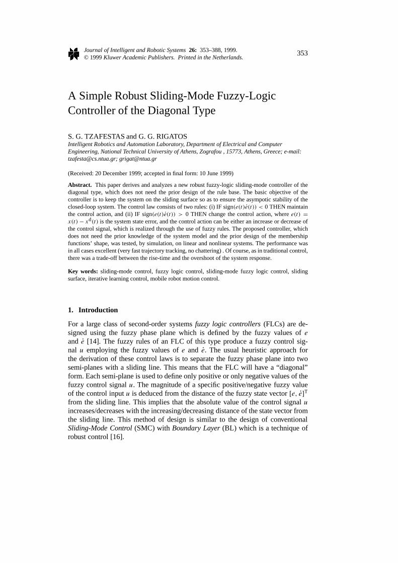
For a second-order system, convergence to the sliding mode is illustrated in the(e, e)-plane (Figure 1). The first step in the design of an SMC is the selection ofthe parameterλ. The linear differential Equation (2) can be considered as a chainof (n − 1)st-order low-pass filters, where the scalars plays the role of the input,λ is the break frequency (bandwidth) ande is the output (see Figure 2).
The parameterλ must be selected such that the unmodelled frequencies of thesystem to be rejected. From the elementary first-order filterH(p) = 1/(λ + p),wherep = d/dt , it can be observed that a sufficient condition for frequency re-jection isλ � p. Thus in order to reject all unmodeled frequencies one shouldselectλ � νumin, whereνumin is the lower bound of the system’s unmodelledfrequenciesνu.
356 S. G. TZAFESTAS AND G. G. RIGATOS
The next step is to find the control law that will keep the system in slidingmode. Equation (3) gives a sufficient condition for the asymptotic stability of theclosed-loop system. The first derivatives is calculated as follows:
s(x, t) =(
d
dt+ λ
)n−1
e =n−1∑k=0
(n− 1
k
)λken−1−k
= e(n−1) +(n− 1
1
)λe(n−2) +
(n− 1
2
)λ2e(n−3) + · · · + λ(n−1)e,
or
s(x, t) = e(n) +(n− 1
1
)λe(n−1) +
(n− 1
2
)λ2e(n−2) + · · · + λ(n−1)e,
or
s(x, t) = x(n) − x(n)d +n−1∑k=1
(n− 1
k
)λke(n−k). (4)
Substituting (4) in (3), and using (1), one gets([f (x, t)+ b(x, t)u + d]− x(n)d +
n−1∑k=1
(n− 1
k
)λke(n−k)
)sign(s) 6 −η. (5)
The sliding control law is now defined via the following equations:
u = b−1(u− f ),u = G(u−K(x, t) sign(s)
), (6)
u = x(n)d −n−1∑k=1
(n− 1
k
)λke(n−k),
whereK(x, t) > 0, andf and b are estimates of the functionsf andb, respec-tively. To choose the multiplicative coefficient (gain)G, the following bounds aredefined:
06 βmin 6 bb−1 6 βmax.
ThenG is defined asG = (βminβmax)−1/2, and the gain marginβ as
β =(βmax
βmin
)1/2
.
It now remains to findK(x, t) so as to satisfy Equation (3):s sign(s) 6 −η.Introducing (6) into (5) yields
sign(s)
(f + bb−1(u− f )+ d − x(n)d +
n−1∑k=1
(n− 1
k
)λke(n−k)
)6 −η,

SIMPLE FUZZY-LOGIC SLIDING-MODE CONTROLLER 357
i.e.,
sign(s)
(f − bb−1f + bb−1Gu− bb−1GK(x, t) sign(s)+ d − x(n)d
+n−1∑k=1
(n− 1
k
)λke(n−k)
)6 −η,
whence(1f + (bb−1G− 1
)u+ d) sign(s)− bb−1GK(x, t) 6 −η, (7)
where1f = f − bb−1f . The above inequality is satisfied if
bb−1GK(x, t) >∣∣1f + (bb−1G− 1
)u+ d∣∣+ η
or
bb−1GK(x, t) > |1f | + ∣∣(bb−1G− 1)∣∣∣∣u∣∣+ ∣∣d∣∣+ η.
Now, if bb−1 is replaced by its lower boundβmin, and the relationβminG = (βmin/
βmax)1/2 = β−1 is used, one gets
β−1K(x, t) > |1f | + ∣∣1− β−1∣∣∣∣u∣∣+ ∣∣d∣∣+ η,
whence
K(x, t) > β(|1f | + (1− β−1))∣∣u∣∣+ ∣∣d∣∣+ η. (8)
The upper boundsF, D andU
|1f | < F ,∣∣d∣∣ < D,
∣∣u∣∣ < Uare supposed to be known from the system’s analysis. Thus, a sufficient conditionfor the control law to make the sliding surfaces = 0 a domain of attraction, is
K(x, t) > β(F + (1− β−1
))U +D + η. (9)
2.2. SMC WITH BOUNDARY LAYER
An essential drawback of SMC is that, owing to the signum termK(x, t) sign(s),it causes abrupt changes (chattering) to the control signalu. However, this canbe avoided by introducing a Boundary Layer (BL) from both sides of the slidingsurfaces = 0. If the termK(x, t) sign(s) exceeds the width of the BL, then itbecomes saturated, and is assigned the maximum (minimum) permissible value.The width of BL is selected to be 28.
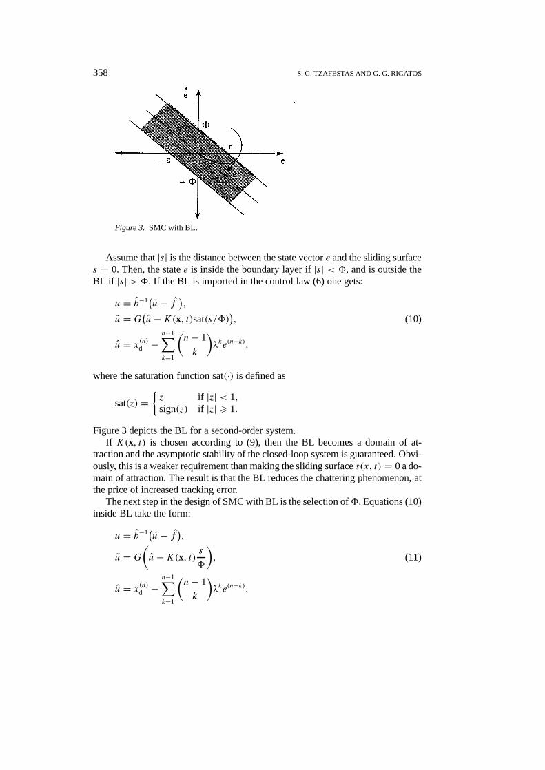
358 S. G. TZAFESTAS AND G. G. RIGATOS
Figure 3. SMC with BL.
Assume that|s| is the distance between the state vectore and the sliding surfaces = 0. Then, the statee is inside the boundary layer if|s| < 8, and is outside theBL if |s| > 8. If the BL is imported in the control law (6) one gets:
u = b−1(u− f ),
u = G(u−K(x, t)sat(s/8)), (10)
u = x(n)d −n−1∑k=1
(n− 1
k
)λke(n−k),
where the saturation function sat(·) is defined as
sat(z) ={z if |z| < 1,sign(z) if |z| > 1.
Figure 3 depicts the BL for a second-order system.If K(x, t) is chosen according to (9), then the BL becomes a domain of at-
traction and the asymptotic stability of the closed-loop system is guaranteed. Obvi-ously, this is a weaker requirement than making the sliding surfaces(x, t) = 0 a do-main of attraction. The result is that the BL reduces the chattering phenomenon, atthe price of increased tracking error.
The next step in the design of SMC with BL is the selection of8. Equations (10)inside BL take the form:
u = b−1(u− f ),u = G
(u−K(x, t) s
8
), (11)
u = x(n)d −n−1∑k=1
(n− 1
k
)λke(n−k).
SIMPLE FUZZY-LOGIC SLIDING-MODE CONTROLLER 359
Introducing (1) andu from (6) into (4) yields
s(x, t) = f (x, t) + b(x, t)u+ d − u= f (x, t) + b(x, t)(b−1
(u− f ))+ d − u,
or
s(x, t) = bb−1u+ (f − bb−1f)+ d − u,
or
s(x, t) = bb−1u+1f + d − u.Now, usingu from (11) yields
s(x, t) = bb−1G
(u−K s
8
)+1f + d − u,
whence
s(x, t)+ bb−1GK
8s = u(bb−1G− 1)+1f + d. (12)
Equation (12) represents a low-pass filter with inputu(bb−1G−1)+1f + d, out-puts, and break frequency(bb−1GK)/8. So far it has been shown how to computethe numerator of the break frequency expression. It only remains to determine thewidth8 of BL. There are two choices:
The first is to select8 in proportion to the desirable tracking accuracyε. Ac-cording to Slotine and Li [16],ε is selected as
ε = 8
λn−1. (13)
The second choice is to select the bandwidthbb−1GK/8 equal toλ. This choiceis known as “balanced condition”
bb−1GK
8= λ. (14)
From the above discussion one can see that the design of SMC with BL isidentical to the design of a simple SMC. The only additional step required is theselection of the width8 which can be done either by (13) or (14).
3. Similarity between FLC and SMC
3.1. THE DIAGONAL-TYPE FLC
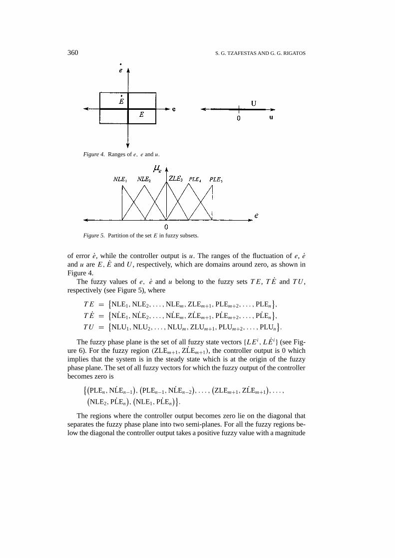
Consider a second-order SISO nonlinear and non-autonomous system. In the caseof a diagonal-type FLC the controller inputs are the errore and the rate of change
360 S. G. TZAFESTAS AND G. G. RIGATOS
Figure 4. Ranges ofe, e andu.
Figure 5. Partition of the setE in fuzzy subsets.
of error e, while the controller output isu. The ranges of the fluctuation ofe, eandu areE, E andU , respectively, which are domains around zero, as shown inFigure 4.
The fuzzy values ofe, e andu belong to the fuzzy setsTE, T E and TU ,respectively (see Figure 5), where
T E = {NLE1,NLE2, . . . ,NLEm,ZLEm+1,PLEm+2, . . . ,PLEn
},
T E = {NLE1,NLE2, . . . ,NLEm,ZLEm+1,PLEm+2, . . . ,PLEn
},
T U = {NLU1,NLU2, . . . ,NLUm,ZLUm+1,PLUm+2, . . . ,PLUn
}.
The fuzzy phase plane is the set of all fuzzy state vectors{LEi,LEi} (see Fig-ure 6). For the fuzzy region(ZLEm+1,ZLEm+1), the controller output is 0 whichimplies that the system is in the steady state which is at the origin of the fuzzyphase plane. The set of all fuzzy vectors for which the fuzzy output of the controllerbecomes zero is{(
PLEn,NLEn−1),(PLEn−1,NLEn−2
), . . . ,
(ZLEm+1,ZLEm+1
), . . . ,(
NLE2,PLEn),(NLE1,PLEn
)}.
The regions where the controller output becomes zero lie on the diagonal thatseparates the fuzzy phase plane into two semi-planes. For all the fuzzy regions be-low the diagonal the controller output takes a positive fuzzy value with a magnitude

SIMPLE FUZZY-LOGIC SLIDING-MODE CONTROLLER 361
Figure 6. Partition of the fuzzy phase plane in regions(LEi ,LEi ).
Figure 7. Fuzzy regions below the diagonal.
that depends on the distance between this fuzzy region and a particular zero-regionon the diagonal, below which the given fuzzy region is located. The set of all fuzzyregions below the diagonal is{(
NLE1,PLEn−1), . . . ,
(NLE1,NLE1
)},
i.e., the fuzzy regions below the zero region(NLE1,PLEn),{(NLE2,NLEn−2
), . . . ,
(NLE2,NLE1
)},
i.e., the fuzzy regions below the zero region(NLE2,PLEn−1),
(PLEn−1,NLE1),
i.e., the fuzzy region below the zero region(PLEn−1,NLE2).As distance between a “fuzzy region below the diagonal” and the “diagonal” is
defined the distance between the “center of this region” and the “center of the zeroregion below which the given fuzzy region is located”.
For all the fuzzy regions above the diagonal, the controller output is assignednegative values with magnitude depending on the distance between the fuzzy re-gion and the diagonal. The fuzzy regions that lie over the diagonal are:{(
PLEn,NLE2), . . . ,
(PLEn,PLEn
)},
362 S. G. TZAFESTAS AND G. G. RIGATOS
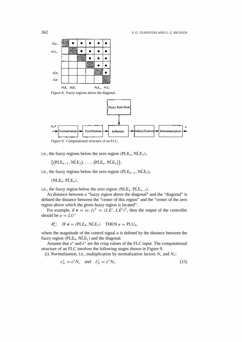
Figure 8. Fuzzy regions above the diagonal.
Figure 9. Computational structure of an FLC.
i.e., the fuzzy regions below the zero region(PLEn,NLE1),{(PLEn−1,NLE2
), . . . ,
(PLEn,PLEn
)},
i.e., the fuzzy regions below the zero region(PLEn−1,NLE2),
(NLE2,PLEn),
i.e., the fuzzy region below the zero region(NLE2,PLEn−1).As distance between a “fuzzy region above the diagonal” and the “diagonal” is
defined the distance between the “center of this region” and the “center of the zeroregion above which the given fuzzy region is located”.
For example, ife = (e, e)T = (LEi, LEi)T, then the output of the controllershould beu = LUi
Ric: IF e= (PLE4,NLE1) THEN u = PLU4,
where the magnitude of the control signalu is defined by the distance between thefuzzy region(PLE4,NLE1) and the diagonal.
Assume thate∗ ande∗ are the crisp values of the FLC input. The computationalstructure of an FLC involves the following stages shown in Figure 9.
(i) Normalization, i.e., multiplication by normalization factorsNe andNe:
e∗N = e∗Ne and e∗N = e∗Ne. (15)

SIMPLE FUZZY-LOGIC SLIDING-MODE CONTROLLER 363
(ii) Fuzzificationof the normalized inputse∗N ande∗N , i.e., calculation of the mem-bership valueµi(e∗) of the input vectore∗ = (e∗N, e∗N)T in the fuzzy region(
LEi,LEi), i = 1,2, . . . , n.
(iii) Inference, i.e., computation of the membership valueµCLUi (uN) of the con-troller output in the fuzzy setLUi, through the use ofµi(e∗) and the rulebase. For a multi-input/single-output FLC, theith fuzzy rule of the fuzzy rulebase has the form
Ric: IF e∗ = LEi THEN u = LUi. (16)
(iv) Defuzzification, i.e., a mapping of the membership valueµCLUi (uN) to a crisppoint of the setLUi.
(v) Denormalizationof the controller crisp outputuN , i.e., multiplication by de-normalization factorsN−1
u :
u = N−1u uN. (17)
3.2. PROPERTIES OF THE TRANSFER CHARACTERISTIC OF A DIAGONAL-TYPE
FLC
The transfer characteristic (control surface) of a diagonal FLC is a nonlinear map-ping u = h(e, e) which is defined by the operating points and the interpolationbetween them.
An operating pointP i(ei, ei )T is defined as follows:Assume thatei = (ei, ei )T is the FLC input andui is the corresponding output.
Assume also that the center of the fuzzy regionLEi is defined asei ∈ E2, whereei = (ei, ei )T are crisp values such thatµLEi (e) = 1 andµLEi (e) = 1. Then, anoperating pointP i(ei, ei )T is a point for whiche is located at the center of the fuzzyregionLEi, andui is the corresponding crisp output of the FLC. Thus, when the in-put of the FLC coincides with an operating point, only one rule should be activated.
The quality of interpolation between the operating points (activation and ag-gregation of more than one fuzzy IF–THEN rules) depends on the methods ofinferencing and defuzzification. A special feature of the control surfaceu = h(e, e)is the diagonalu = h(e, e) = 0, whereu changes its sign. The diagonal-type FLCis designed such that for an increasing Euclidean distance|s| between the statevectore and the diagonalu = 0, the absolute value|u| of the controller outputincreases monotonically, i.e.,
|s2| > |s1| implies∣∣u(s2)∣∣ > ∣∣u(s1)∣∣.
3.3. SMC WITH BL FOR A SECOND-ORDER SYSTEM
The diagonal-type FLC was derived and discussed in Sections 3.1 and 3.2 for asecond-order system. In order to show the similarity between the diagonal-type
364 S. G. TZAFESTAS AND G. G. RIGATOS
FLC and SMC with BL the latter control method is applied here to a second-ordersystem
x = f (x, t) + b(x, t)u + d, (18)
where the sliding line is
s = λe + e. (19)
The control law is (see (10)):
u = b−1(u− f ), u = G(u−K(x, t)sat(s/8)
), u = xd − λe,
i.e.,
u = b−1(− f +G(xd − λe
)−GK(x, t)sat(s/8)). (20)
This control law involves the following terms:
(a) Compensation term:ucomp= −b−1f , (21)
(b) Filtering term:ufilt = −b−1Gλe. (22)
This term rejects the unmodelled frequencies of the system
(c) Feedforward term:uff = b−1Gxd, (23)
(d) Feedback control term:uc = −b−1GK(x, t)sat(s/8)). (24)
This term prevents the state vectore from moving away from the sliding surfaces = 0. The negative sign indicates that the control action takes always place in thedirection of error’s decrease.
The part−K(x, t)sat(s/8) is of diagonal form, withs = 0 being the diagonalline. Examining the diagonal part ofuc one gets
udiag= −K(x, t)sat(s/8), (24′)
where
udiag > 0 for s < 0,
udiag = 0 for s = 0,
udiag < 0 for s > 0.
Assuming thatK is constant, and that the state error vectore lies inside the BL, then
udiag= −K s
8= K |s|
8sign(s). (25)
The relation (25) shows thatudiag is proportional to|s|. Consequently, the magni-tude ofudiag increases when the distance of the fuzzy region(e, e) from the slidingsurfaces = 0 increases, and vice versa.

SIMPLE FUZZY-LOGIC SLIDING-MODE CONTROLLER 365
3.4. ANALYTICAL DESCRIPTION OF A DIAGONAL-TYPE FLC
The diagonal-type FLC provides a mapping from the crisp state vector(e, e) to acrisp control output u, and the magnitude of the fuzzy control signal is proportionalto the distance of the fuzzy region(e, e) from the diagonal. The states that arelocated on the diagonal have a significant role because there the control outputchanges sign. The diagonal for a second-order system is described by the equation
s = λe + e = 0.
Here, the rules of the diagonal-type FLC are selected such that:(a) the statese ande are bounded as
−emax6 e 6 +emax and − emax6 e 6 emax, (26)
(b) the control signalu is bounded as
−umax6 u 6 umax, (27)
(c) the statese ande that are located on the diagonal produce zero control signals,(d) the statese ande that are located below the diagonal produce positive control
signals,(e) the statese ande that are located above the diagonal produce negative control
signals,(f) the magnitude of the control signal|u| increases when the distance from the
diagonal increases, and vice-versa.The properties (a) and (b) are inherent features of FLC. The properties (d) and
(e) ensure that the control action tries to keep the state vector on the sliding surface(diagonal) and take place in the direction of error decrease.
The analytical form of a diagonal-type FLC is
ufuzz = −Kfuzz(e, e, λ) sign(s) (28)
with the following conditions:1. −emax6 e 6 +emax,2. −emax6 e 6 emax,3. λ > 0,4. 06 Kfuzz < umax= Kfuzz|max,5. Kfuzz(e1, e1, λ) 6 Kfuzz(e2, e2, λ) for |λe1 + e1| 6 |λe2 + e2|, which means
that the greater the distance of(e, e) from the sliding surface is, the greater thecontrol signal becomes.
3.5. COMPARISON BETWEEN SMC WITH BL AND DIAGONAL-TYPE FLC
The diagonal control term in SMC with BL is (see (25))
udiag= −Ks8= −K|s|
8sign(s)

366 S. G. TZAFESTAS AND G. G. RIGATOS
Figure 10. Transfer characteristic of: (a) SMC, and (b) diagonal-type FLC.
Figure 11. Error state vector boundaries in: (a) SMC with BL, (b) diagonal-type FLC.
while the control term in the diagonal-type FLC is (see (28))
ufuzz = −Kfuzz(e, e, λ
)sign(s).
From the above two equations the similarity between SMC with BL, and FLC isobvious. Additionally, the vicinity of the diagonal in a diagonal-type FLC can beviewed as a BL. The main differences between the two controllers are:(a) The transfer characteristicufuzz = f (s) of a diagonal-type FLC is nonlinear
(due to the nonlinear nature of FLC), while the one of SMC with BL is linear(see Figure 10).
(b) In the diagonal-type FLC, the state vectore is bounded (it is an inherentstructural property of FLC) while this does not happen in SMC with BL (seeFigure 11).
3.6. THE BASIC PRINCIPLES OF SMFLC
As it has already been mentioned in the diagonal-type FLC the magnitude of thecontrol signal u changes in proportion to the distance of(e, e) from the diagonal.Thus the control rules can be modified as:
Ric: IF s = LSi THEN u = LUi,
SIMPLE FUZZY-LOGIC SLIDING-MODE CONTROLLER 367
in which case the corresponding control law becomes
ufuzz = −Kfuzz(|s|) sign(s). (29)
Equation (17) resembles even more to the control law of SMC with BL, and can benamed “Sliding Mode FLC” (SMFLC). The main advantage of SMFLC comparedto a typical diagonal-type FLC is that it reduces drastically the number of rulesin the rule base. This happens because the diagonal-type FLC uses as inputs thestate variablese and e, and so the number of the controller inputs is equal to theelements of the state vectore. On the contrary, the only input of the SMFLC is the“signed” distance s from the diagonal. For anth-order system the distances can becalculated by
s(x, t) =n−1∑k=0
(n− 1
k
)λke(n−1−k).
In Section 4 the Reduced-Complexity SMFLC (RC-SMFLC) will be designed,which requires even less rules and introduces a simpler perspective in the designof diagonal-type FLCs.
3.7. DESIGN OF AN SMFLC
As it has already been mentioned the control law of SMC is
u = b−1Gu− b−1f − b−1GK(x, t)sat(s/8),
u = x(n)d −n−1∑k=1
(n− 1
k
)λke(n−k).
After some modifications in the above control law SMFLC is derived:
u = b−1Gu− b−1f + b−1Gufuzz,
ufuzz = −K(|s| sign(s)
).
(30)
The design of SMFLC is concentrated on the fuzzy part:
ufuzz = −K(|s| sign(s)
)while the choice of the previous terms can be done as in SMC. The choice of thetransfer characteristic will be examined first.
3.8. DESIGN OF THE TRANSFER CHARACTERISTIC
The crucial point in the design of SMFLC is the choice of the number of the fuzzysubsets for the inputs and the outputs of the controller and consequently the shapeof the corresponding membership functions.
368 S. G. TZAFESTAS AND G. G. RIGATOS
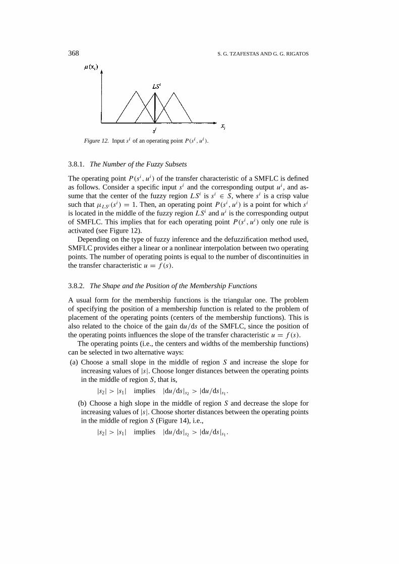
Figure 12. Input si of an operating pointP(si , ui ).
3.8.1. The Number of the Fuzzy Subsets
The operating pointP(si, ui) of the transfer characteristic of a SMFLC is definedas follows. Consider a specific inputsi and the corresponding outputui , and as-sume that the center of the fuzzy regionLSi is si ∈ S, wheresi is a crisp valuesuch thatµLSi (s
i) = 1. Then, an operating pointP(si, ui) is a point for whichsi
is located in the middle of the fuzzy regionLSi andui is the corresponding outputof SMFLC. This implies that for each operating pointP(si, ui) only one rule isactivated (see Figure 12).
Depending on the type of fuzzy inference and the defuzzification method used,SMFLC provides either a linear or a nonlinear interpolation between two operatingpoints. The number of operating points is equal to the number of discontinuities inthe transfer characteristicu = f (s).
3.8.2. The Shape and the Position of the Membership Functions
A usual form for the membership functions is the triangular one. The problemof specifying the position of a membership function is related to the problem ofplacement of the operating points (centers of the membership functions). This isalso related to the choice of the gain du/ds of the SMFLC, since the position ofthe operating points influences the slope of the transfer characteristicu = f (s).
The operating points (i.e., the centers and widths of the membership functions)can be selected in two alternative ways:(a) Choose a small slope in the middle of regionS and increase the slope for
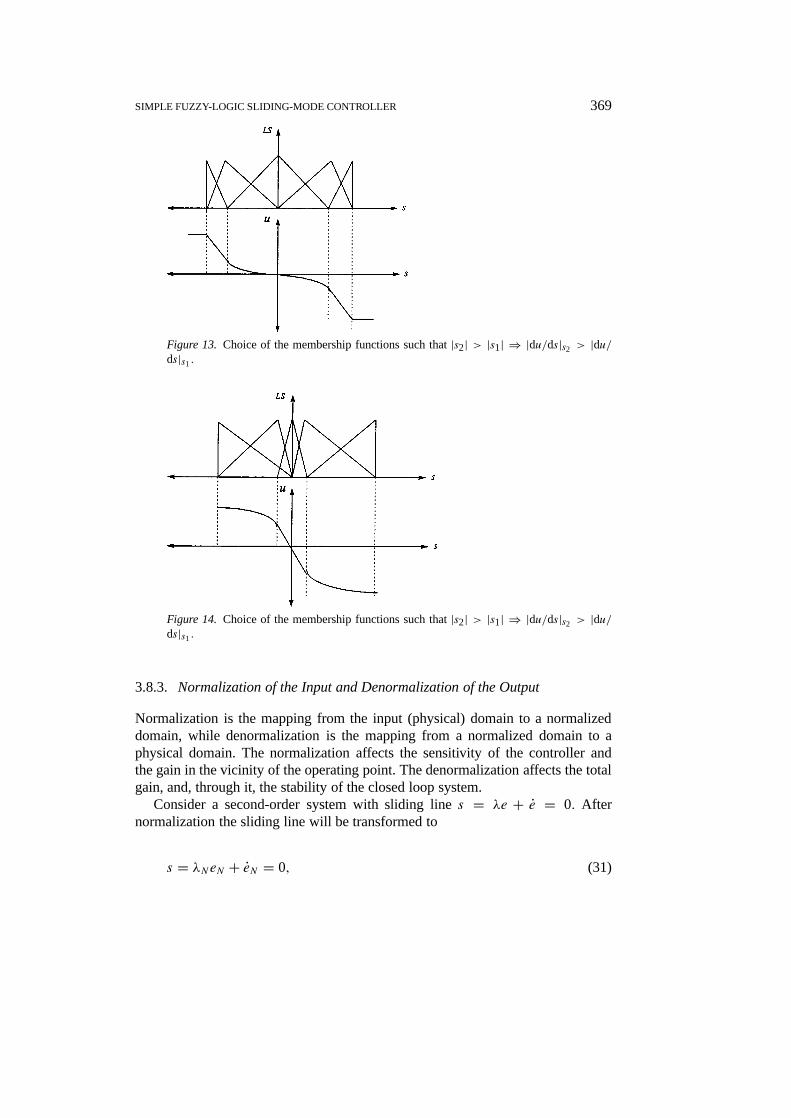
increasing values of|s|. Choose longer distances between the operating pointsin the middle of regionS, that is,
|s2| > |s1| implies |du/ds|s2 > |du/ds|s1.(b) Choose a high slope in the middle of regionS and decrease the slope forincreasing values of|s|. Choose shorter distances between the operating pointsin the middle of regionS (Figure 14), i.e.,
|s2| > |s1| implies |du/ds|s2 > |du/ds|s1.
SIMPLE FUZZY-LOGIC SLIDING-MODE CONTROLLER 369
Figure 13. Choice of the membership functions such that|s2| > |s1| ⇒ |du/ds|s2 > |du/ds|s1 .
Figure 14. Choice of the membership functions such that|s2| > |s1| ⇒ |du/ds|s2 > |du/ds|s1 .
3.8.3. Normalization of the Input and Denormalization of the Output
Normalization is the mapping from the input (physical) domain to a normalizeddomain, while denormalization is the mapping from a normalized domain to aphysical domain. The normalization affects the sensitivity of the controller andthe gain in the vicinity of the operating point. The denormalization affects the totalgain, and, through it, the stability of the closed loop system.
Consider a second-order system with sliding lines = λe + e = 0. Afternormalization the sliding line will be transformed to
s = λNeN + eN = 0, (31)

370 S. G. TZAFESTAS AND G. G. RIGATOS
where
eN = eNe, eN = eNe and λ = λN NeNe. (32)
The parameterλ plays the role of the rejection frequency for all unmodelled fre-quencies of the system and has to beλ 6 νsu. Thus the normalized parameterλNshould satisfy the condition
Ne
Ne6 νsu
λN. (33)
For the denormalization of the output in the same second-order system one has
uN = Nuu implies u = N−1u uN.
The choice ofNu is important for the stability of the closed-loop system, anddepends on the maximum value ofKfuzz. To achieve asymptotic stability of theclosed-loop system one has to choose
Kfuzz|max> β(F + (1− β−1
)U +D + η), (34)
where
Kfuzz|max= max(Kfuzz(|s|)
).
From the relationKfuzzN |max = NuKfuzz|max, one can calculate the normalizationcoefficientNu:
Nu = KfuzzN |max
Kfuzz|max. (35)
Another approach to normalization and denormalization of SMFLCs would be toleave the coefficients of the equations unchanged and inflate or deflate directly theinput or the output of the controller.
3.8.4. SMFLC as a State-dependent Filter
SMFLC, like SMC, can be regarded as a filter function [14]. If the transfer charac-teristic between two operating pointsi andi+1 is approximately considered to bea linear segment, then a gainki/φi can be attached to thisith segment. Since thegain changes take place from segment to segment, one obtains a state-dependentfilter function (see Figure 15).
For theith segment of the transfer characteristic, the resulting filter function issimilar to the one for SMC:
s + bb−1Gki
φis = bb−1Gui sign(s)+ u(bb−1G− 1
)+1f + d (36)
SIMPLE FUZZY-LOGIC SLIDING-MODE CONTROLLER 371
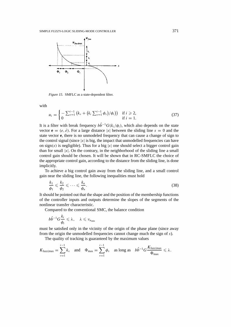
Figure 15. SMFLC as a state-dependent filter.
with
ui ={−∑i−1
ν=1
(kν +
(ki∑i−1
ν=1φν)/φi))
if i > 2,0 if i = 1.
(37)
It is a filter with break frequencybb−1G(ki/φi), which also depends on the statevectore = (e, e). For a large distance|s| between the sliding lines = 0 and thestate vectore, there is no unmodeled frequency that can cause a change of sign tothe control signal (since|s| is big, the impact that unmodelled frequencies can haveon sign(s) is negligible). Thus for a big|s| one should select a bigger control gainthan for small|s|. On the contrary, in the neighborhood of the sliding line a smallcontrol gain should be chosen. It will be shown that in RC-SMFLC the choice ofthe appropriate control gain, according to the distance from the sliding line, is doneimplicitly.
To achieve a big control gain away from the sliding line, and a small controlgain near the sliding line, the following inequalities must hold
k1
φ16 k2
φ26 · · · 6 kn
φn. (38)
It should be pointed out that the shape and the position of the membership functionsof the controller inputs and outputs determine the slopes of the segments of thenonlinear transfer characteristic.
Compared to the conventional SMC, the balance condition
bb−1Gki
φi6 λ, λ 6 νumin
must be satisfied only in the vicinity of the origin of the phase plane (since awayfrom the origin the unmodelled frequencies cannot change much the sign ofs).
The quality of tracking is guaranteed by the maximum values
Kfuzz|max=i−1∑ν=1
kν and 8max=i−1∑ν=1
φν as long as bb−1GKfuzz|max
8max6 λ.

372 S. G. TZAFESTAS AND G. G. RIGATOS
In RC-SMFLC tracking quality will not be of primary importance.
3.8.5. SMFLC for anth Order System
The design of an SMFLC for a second-order system can be extended to anth ordersystem [14]. The crucial point is to produce the normalization factorsNe,Ne, . . . ,
Ne(n−1) for each one of the statese, e, . . . , e(n−1). The unnormalized sliding surfaceis determined by(
d
dt+ λ
)(n−1)
e = e(n−1) +(n− 1
1
)λe(n−2) + · · · + λ(n−1)e = 0,
and the normalized one by(d
dt+ λ
)(n−1)
eN = e(n−1)N +
(n− 1
1
)λNe
(n−2)N + · · · + λ(n−1)
N eN = 0.
With the use of normalization factors, one gets(d
dt+ λ
)(n−1)
eN
= e(n−1) +(n− 1
1
)λNNe(n−2)
Ne(n−1)e(n−2) + · · · + λ(n−1)
N
Ne
Ne(n−1)e = 0.
Comparing the coefficients of the above two equations yields:
λ = λN Ne(n−2)
Ne(n−1), λ2 = λ2
N
Ne(n−3)
Ne(n−1), λn−1 = λn−1
N
Ne
Ne(n−1), (39)
Ne(n−2)
Ne(n−1)= · · · = Ne
Ne= λ
λN. (40)
This means that, ifλ, λN andNe are known, one can calculate all the normalizationfactors.
In RC-SMFLC one has just to normalize the scalar control input (i.e., to useonly one normalization factor) and proceed to the design of the SMFLC in thenormalized region of the input values.
4. Design of an RC-SMFLC
4.1. THE CONCEPT
To design aReduced-Complexity SMFLC,the basic conditions that assure the con-vergence of a system to the desirable set-point are taken into account. Considerthenth-order nonlinear non-autonomous system given by (1) with outputx(t) anddesirable set-pointxd(t).

SIMPLE FUZZY-LOGIC SLIDING-MODE CONTROLLER 373
Denoting the tracking error bye(t) = x(t)− xd(t), and the rate of error changeby e(t) = x(t)− xd(t), the convergence conditions are expressed as follows:
• IF e(t) > 0 ande(t) < 0 THENx(t)→ xd(t) impliese(t)→ 0.• IF e(t) > 0 ande(t) > 0 THENx(t) deviates fromxd(t).• IF e(t) < 0 ande(t) < 0 THENx(t) deviates fromxd(t).• IF e(t) < 0 ande(t) > 0 THENx(t)→ xd(t) impliese(t)→ 0.
The above four convergence conditions can be merged in two conditions, namely:
IF e(t)e(t) < 0 THENx(t) < xd(t), i.e.,e(t)→ 0. (41)
IF e(t)e(t) > 0 THENx(t) deviates fromxd(t). (42)
The same conditions could have been derived from the Lyapunov function
V = 1
2e2⇒ V = ee.
From (41) and (42) it is obvious that the greater part of the information, needed toachieve convergence to the desirable setpoint, is contained ine(t) ande(t).
Define now the sliding surfaces(x, t)
s(x, t) = e(t)e(t) < 0. (43)
Then, the control law can be expressed as follows:
• IF sign(e(t)e(t)) < 0, THEN the control action leads to convergence andshould be maintained.• IF sign(e(t)e(t)) > 0, THEN the control action leads to divergence andshould be altered.
Once the state vector[e(t), e(t)]T is found in the semi-planes(x, t) = e(t)e(t)< 0, it gradually approaches the null vector[0,0]T. Thus, the goal is to find acontrol lawu that will be able to keep the state vector in the semi-planes(x, t) =e(t)e(t) < 0.
4.2. THE RULE BASE OF RC-SMFLC
There are two possible control actions: increase or decrease the control signalu.Thus, the rule base of RC-SMFLC is:
R1: IF sign(e(t)e(t)) < 0 AND the previous control action was to increase thecontrol signal THEN keep on increasing.
R2: IF sign(e(t)e(t)) < 0 AND the previous control action was to decrease thecontrol signal THEN keep on decreasing.
R3: IF sign(e(t)e(t)) > 0 AND the previous control action was to increase thecontrol signal THEN now decrease it.

374 S. G. TZAFESTAS AND G. G. RIGATOS
R4: IF sign(e(t)e(t)) > 0 AND the previous control action was to decrease thecontrol signal THEN now increase it.
An equivalent formulation is the following:
R1: IF sign(e(t)e(t)
)< 0 AND 1uk > 0 THEN1uk+1 > 0,
R2: IF sign(e(t)e(t)
)< 0 AND 1uk < 0 THEN1uk+1 < 0,
R3: IF sign(e(t)e(t)
)> 0 AND 1uk > 0 THEN1uk+1 < 0,
R4: IF sign(e(t)e(t)
)> 0 AND 1uk < 0 THEN1uk+1 > 0,
where1uk is the change in the control signal at thekth iteration of the algorithm.To ensure that the control signal is increased with the use of the FLC, the
following rules are employed:
IF uk isU1 THEN uk+1 isU2,
IF uk isU2 THEN uk+1 isU3,...
IF uk isUn−1 THEN uk+1 isUn.
To ensure that the control signal is decreased with the use of the FLC the rules thatmust be used are:
IF uk isU2 THEN uk+1 isU1,
IF uk isU3 THEN uk+1 isU2,...
IF uk isUn THEN uk+1 isUn−1,
whereU1, U2, . . . , Un−1, Un are the fuzzy subsets in which the fuzzy phase planeU
of the control input is divided.If the fuzzy phase planeU is partitioned byn triangular membership functions
with equal widths and slopes, it can easily be verified that the above rule basecan lead the system to oscillations around the desirable set-point. Consequently,in order to achieve convergence, the nonlinear transfer characteristic of the fuzzycontroller should be such that the smaller the distance from the setpoint is thesmaller the change of the control signal becomes.
4.3. ANALYTICAL DESCRIPTION OF THE RC-SMFLC
In the diagonal-type FLC it was necessary to produce a fuzzy control signal thatwould be proportional to the distance from the diagonal, where the diagonal wasthe sliding surface
s(x, t) =n−1∑k=1
(n− 1
k
)λke(n−k).
SIMPLE FUZZY-LOGIC SLIDING-MODE CONTROLLER 375
In the RC-SMFLC it is necessary to produce a fuzzy control signal that will beproportional to the distance from the set-pointe = 0. Thus in this casee = 0 playsthe role of the diagonal.
Therefore, there are two requirements for the control law in RC-SMFLC:(a) To keep the error state vector[e(t), e(t)]T inside the sliding surfaces(x, t) =
e(t)e(t) < 0,(b) Its magnitude to be proportional to the distance from the diagonale = 0.
The RC-SMFLC has similar properties to the ones of a diagonal-type FLC asdescribed in the Section 3.4, i.e.,(a) the statese ande are bounded,(b) the control signalu is bounded,(c) the statese ande that are located on the diagonal produce zero control signals,(d) the statese ande that are located above the diagonal produce negative control
signals (because surpass of the diagonal is a result of an “increase” controlaction, which means that the next control action will be “decrease”),
(e) the statese ande that are located below the diagonal produce positive controlsignals.
It remains to show that RC-SMFLC also satisfies the property (f), i.e., themagnitude of the control signal|u| decreases when the distance from the diagonaldecreases. The desirable control law should be similar to the one of a diagonal-typeFLC:
ufuzz = −Kfuzz(e, e, λ) sign(s)
or to the control law of SMFLC:
ufuzz = −K(|s| sign(s)
), where|s| is the distance from the diagonal.
The use of membership functions with the same shape (e.g., triangular with thesame width and slopes) produces a control law of the form:
ufuzz = −K sign(s), whereK is static.
To overcome this problem, the width of the membership functions should be mod-ified at every crossing of the diagonale = 0. The last two control signalsuk−1 anduk are taken into account:
uk−1 is the last control signal below (above) the diagonal,uk is the last control signal above (below) the diagonal.
Recalling the bisection method, the control signalu∗ that will produce zero errorshould be searched in the range[uk−1, uk]. The new fuzzy subsetsU1, U2, . . . ,
Un−1, Un correspond to the division of the interval between these two controlsignals[uk−1, uk] in n equal segments. Thus the operating pointsP(si, ui) are inthis case moving, and the nonlinear transfer characteristicu = f (s) of the fuzzycontroller changes. As the diagonal is approached, the width of the membership
376 S. G. TZAFESTAS AND G. G. RIGATOS
functions is reduced, and consequently, the control gainK is reduced too. In thisway a control law of the form
ufuzz = −Kfuzz(
sign(
sign(ekek+1))
sign(s)), s = ee, (44)
whereek is the error at thekth step of the algorithm, andek+1 is the error at the(k + 1)th step of the algorithm, is derived, and the similarity between RC-SMFLCand the diagonal-type FLC or the conventional SMFLC becomes clear.
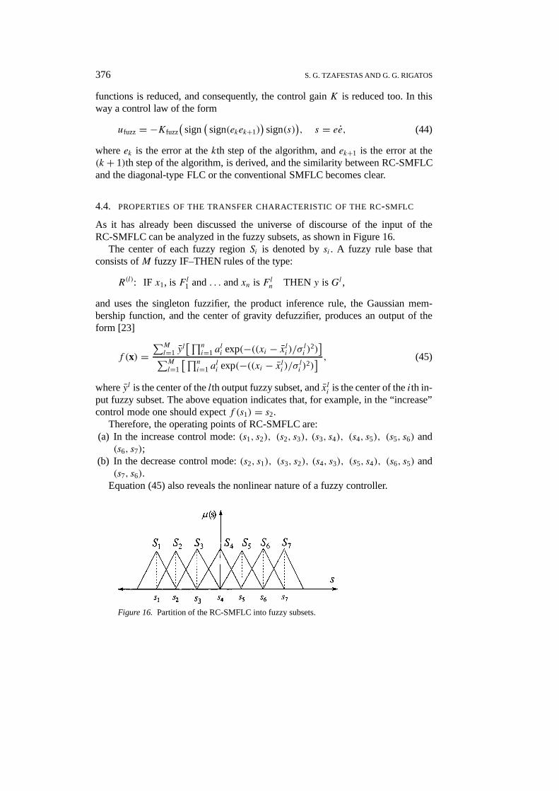
4.4. PROPERTIES OF THE TRANSFER CHARACTERISTIC OF THE RC-SMFLC
As it has already been discussed the universe of discourse of the input of theRC-SMFLC can be analyzed in the fuzzy subsets, as shown in Figure 16.
The center of each fuzzy regionSi is denoted bysi . A fuzzy rule base thatconsists ofM fuzzy IF–THEN rules of the type:
R(l): IF x1, isF l1 and. . . andxn is F ln THEN y isGl ,
and uses the singleton fuzzifier, the product inference rule, the Gaussian mem-bership function, and the center of gravity defuzzifier, produces an output of theform [23]
f (x) =∑M
l=1 yl[∏n
i=1 ali exp(−((xi − xli )/σ li )2)
]∑Ml=1
[∏ni=1 a
li exp(−((xi − xli )/σ li )2)
] , (45)
whereyl is the center of thelth output fuzzy subset, andxli is the center of theith in-put fuzzy subset. The above equation indicates that, for example, in the “increase”control mode one should expectf (s1) = s2.
Therefore, the operating points of RC-SMFLC are:(a) In the increase control mode:(s1, s2), (s2, s3), (s3, s4), (s4, s5), (s5, s6) and
(s6, s7);(b) In the decrease control mode:(s2, s1), (s3, s2), (s4, s3), (s5, s4), (s6, s5) and
(s7, s6).Equation (45) also reveals the nonlinear nature of a fuzzy controller.
Figure 16. Partition of the RC-SMFLC into fuzzy subsets.

SIMPLE FUZZY-LOGIC SLIDING-MODE CONTROLLER 377
Figure 17. Approximation of the transfer characteristic of RC-SMFLC: (a) increase controlaction, (b) decrease control action.
As it can be observed from Figure 16, at the beginning of the controller opera-tion, the fuzzy subsets have equal width and identical shape.
Therefore, a rough approximation of the transfer characteristicuk+1 = f (uk)
would have the form shown in Figure 17. Of course, the transfer characteristic be-tween two adjacent operating points is not described by a first order linear function,but what the above diagram tries to stress out is that the change of the magnitudeof the control signal does not tie directly to the size of the controller’s inputs:
|s2| > |s1| implies |du/ds|s2 = |du/ds|s1 or
|s2| < |s1| implies |du/ds|s2 = |du/ds|s1.While the algorithm evolves, each change of sign(ekek+1) clips the ranges of
fluctuation of the control signal. This causes a reduction of the parameterKfuzz,which is proportional to|du/ds|. However, between two successive changes ofsign(ekek+1), |du/ds| remains unaffected, and therefore,Kfuzz remains unchangedtoo.
Unlike SMFLC, the study of RC-SMFLC as a state-dependent filter shows thatno additional effort is needed in order to achieve different control gains in differentareas of the transfer characteristic. Between two successive changes of the sign ofekek+1, the local control gains satisfy the equality
k1
φ1= k2
φ2= · · · = kn
φn.
The transition from the one side of the diagonale = 0 to the other, results in anequal diminution of all the local gainski/φi . In SMFLC the reduction of the localcontrol gains, as the output approaches the diagonale = 0, is designed beforehand.On the contrary, in the RC-SMFLC this reduction occurs during the evolution ofthe algorithm.
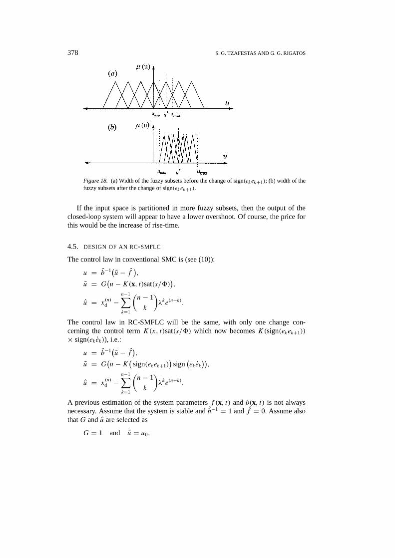
378 S. G. TZAFESTAS AND G. G. RIGATOS
Figure 18. (a) Width of the fuzzy subsets before the change of sign(ekek+1); (b) width of thefuzzy subsets after the change of sign(ekek+1).
If the input space is partitioned in more fuzzy subsets, then the output of theclosed-loop system will appear to have a lower overshoot. Of course, the price forthis would be the increase of rise-time.
4.5. DESIGN OF AN RC-SMFLC
The control law in conventional SMC is (see (10)):
u = b−1(u− f ),
u = G(u−K(x, t)sat(s/8)
),
u = x(n)d −
n−1∑k=1
(n− 1
k
)λke(n−k).
The control law in RC-SMFLC will be the same, with only one change con-cerning the control termK(x, t)sat(s/8) which now becomesK(sign(ekek+1))
× sign(ekek)), i.e.:
u = b−1(u− f ),u = G
(u−K( sign(ekek+1)
)sign
(ekek
)),
u = x(n)
d −n−1∑k=1
(n− 1
k
)λke(n−k).
A previous estimation of the system parametersf (x, t) andb(x, t) is not alwaysnecessary. Assume that the system is stable andb−1 = 1 andf = 0. Assume alsothatG andu are selected as
G = 1 and u = u0,
SIMPLE FUZZY-LOGIC SLIDING-MODE CONTROLLER 379
whereu0 is a randomly selected value in the interval of the permitted input values.Introducing this selection in the above RC-SMFLC equations yields
u = u
u = u−K( sign(ekek+1))
sign(ekek
), (46)
u = u0.
The absence of estimation of the system’s parametersf (x, t) andb(x, t) meansthat RC-SMFLC will have to handle additional parameter uncertainties. However,this additional uncertainty can be viewed as a perturbation that can be compensatedby the robustness property possessed by the fuzzy controller.
Neglecting the filtering term
ufilt = −b−1G
n−1∑k=1
(n− 1
k
)λke(n−k),
makes the system susceptible to unmodelled high frequencies and consequentlythis should be done with caution.
5. Similarity between RC-SMFLC and Iterative Learning Control
5.1. THE PROBLEM OF SELF-CONSTRUCTING RULE BASES
A great advantage of the RC-SMFLC method is that its rule base does not relatedirectly the error or the rate of error’s change to the output under control. Therefore,it does not contain rules of the form
IF e isE ande isE THEN1u isU .
This kind of rules are the core of other fuzzy controllers [6, 7], such as fuzzy PD,fuzzy PI or fuzzy PID ones [10, 11, 19], or of the SMFLC type [9, 15, 24].
A question arising from real implementation of rule-based control systems ishow a set of similar control rules can be derived. The success and performance ofrule-based control systems depend largely on the availability and the performanceof the rule-base. When there are no experts or skilled operators available to supplynecessary knowledge, it is necessary to construct the rule-base by directly oper-ating the process being controlled. It is also desirable to refine and improve therough rule-base derived from experts which may be incomplete, inconsistent oreven partly incorrect, especially when the operating condition is changed.
An approach to self-constructing rule-bases would be the implementation ofneuro-fuzzy techniques like training of the fuzzy logic controller using back-propag-ation, orthogonal least squares, nearest neighborhood clustering or genetic algo-rithms. These techniques consist of initializing the rule-base with low confidencelevel rules provided by experts. While the algorithm goes on, the rules are modifiedaccording to the deviation of the output from the desirable setpoint. Finally, the
380 S. G. TZAFESTAS AND G. G. RIGATOS
optimal widths and centers of the fuzzy subsets of the rules are selected. Anothermethodology that can be used to construct rule bases isiterative learning control.Since RC-SMFLC bares resemblance to iterative learning control the latter is goingto be discussed analytically.
5.2. ITERATIVE LEARNING CONTROL
As the name implies, the correct control action is progressively learned and hencedesired performance is progressively achieved by repeated trial. The modificationof the present control is based on the error information obtained during previoustrials. The concept and algorithm were formally proposed by Arimoto [1].
The objective of the learning control is to determine the control inputu byrepetitive trial such that the errore(t) = yd(t)− y(t) tends asymptotically to zero.The following algorithms have been proposed:(a) Error correction algorithm
uk+1(t) = uk(t)+ g1ek(t). (47)(b) Error and error-derivative correction algorithm
uk+1(t) = uk(t)+ p1ek(t)+ q1ek(t), (48)wherek denotes the number of iterations, andg1, p1, q1 are learning gains.The above algorithms may be represented compact matrix form as
uk+1(t) = uk(t)+ Pek(t)+Qek(t),whereP andQ are learning matrices.
The change of the control signalu takes place at each iterationk, and in theinterval between two successive iterationsk andk + 1 the controller tries to leadthe system to the desirable output using the same control signaluk(t). This remindsdirectly of the RC-SMFLC, where between two successive crossings of the diago-nale = 0 the slope of the transfer characteristicuk+1 = f (uk) remains unchanged,while in this interval,uk(t) is determined by the increase or decrease control mode.
Comparing iterative learning algorithm and RC-SMFLC to MRAC, one cannote that although at first look they seem to have some properties in common, theyalso have subtle differences. In MRAC the objects to be adjusted are some parame-ters, for instance feedforward or feedback gains, whereas in the Iterative LearningAlgorithm and in the RC-SMFLC the control input is directly updated. MRACis designed to force the error to go asymptotically to zero with increasing time,while the iterative learning algorithm and RC-SMFLC are intended to eliminatethis error uniformly in a time interval of interest and this objective is achieved withthe increase of the iteration number.
5.3. RULE-BASE FORMATION
It is very difficult to derive from numerical data a rule base in the form of IF–THENstatements which will be linguistically identical to the rule base acquired from

SIMPLE FUZZY-LOGIC SLIDING-MODE CONTROLLER 381
expert’s verbal description. However, parallel to iterative learning, a rule base for-mation mechanism can be implemented for extracting the rules from the recordedinput-output data pairs (Linkens [12]). At each trial, this mechanism creates a setof control rules for each input-output pair. Each rule, relating the measured controlerror e and the change-in-errore to the control actionu has the form IFe = E
and e = E THEN u = U . No linguistic label is attached on the THEN part(Sugeno-type rules [4]). It is worth noting that the rules are purely value-based inthe sense that there is no time variable embedded in the rule variables. The rule-base is memoryless, meaning that it is updated at each trial and relies only on thevalues ofe, e andu obtained at the present trial. The same technique for rule-baseformation could be applied in RC-SMFLC. Therefore if RC-SMLFC is followed,by a rule-base formation algorithm it can used to substitute the neurofuzzy controltechniques that construct rule bases by self-learning.
6. Simulation Results
The proposed adaptive fuzzy controller has been tested in many different casesamong which are:(i) the regulation of the thermal and geometrical characteristics of the arc-welding
process [3, 18], and(ii) the motion control of a mobile robot that moves in a partially unknown envi-
ronment [22].The simulation code was written in C++.
6.1. THE LINEARIZED MODEL OF ARC-WELDING
Arc-welding is a highly nonlinear process which is subject to many disturbancesand parametric changes due to the severe environmental conditions.
However, its model can be linearized in small regions around specific operationpoints and thus its geometrical and thermal characteristics can locally be describedby linear transfer functions [18].
As far as its thermal characteristics are concerned, the arc-welding thermalmodel considers as outputs theweld nugget cross-section NS, theheat affected zoneHZ and thecenterline cooling rate CR,and as inputs thethermal power of the torch.
The transfer function ofNSis of first order, while the transfer function ofHZ isgiven by a second-order one with relative degree one. Finally, the linearized modelof CR is of second order with relative degree two.
NS(s)
U(s)= Ka
τas + 1,
HZ(s)
U(s)= Kb(τbs + 1)
(τ1s + 1)(τ2s + 1)
and
CR(s)
U(s)= Kc
(τas + 1)(τbs + 1).
382 S. G. TZAFESTAS AND G. G. RIGATOS
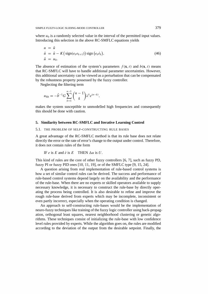
Figure 19. Control of the cooling rate of the arc-welding process.
Figure 20. Tracking of a ramp set-point with positive slope.
The following 2nd order linear system was tested (input: thermal power of thetorch,Q-output: CR)
Gm(z) = 0.11(z+ 1)2
(z− 0.96)(z − 0.63).
The system model is assumed to be unknown, and the fuzzy expert controller hadto operate under total parametric uncertainty.
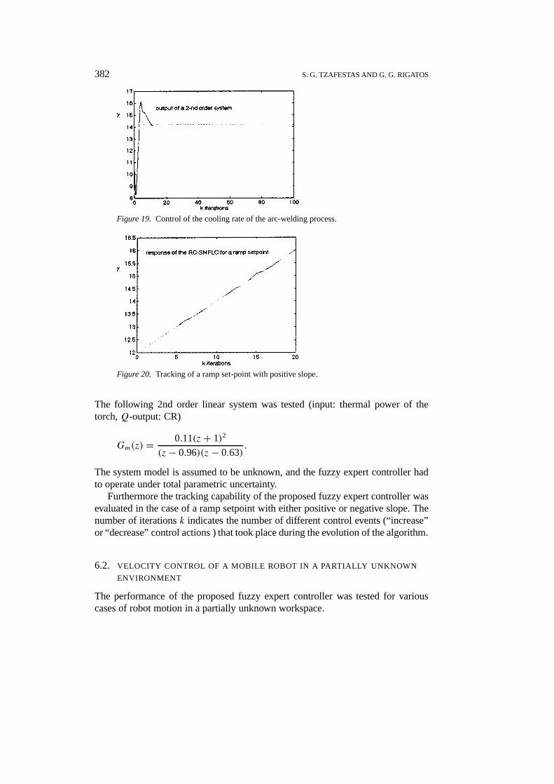
Furthermore the tracking capability of the proposed fuzzy expert controller wasevaluated in the case of a ramp setpoint with either positive or negative slope. Thenumber of iterationsk indicates the number of different control events (“increase”or “decrease” control actions ) that took place during the evolution of the algorithm.
6.2. VELOCITY CONTROL OF A MOBILE ROBOT IN A PARTIALLY UNKNOWN
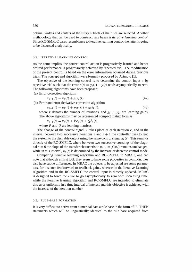
ENVIRONMENT
The performance of the proposed fuzzy expert controller was tested for variouscases of robot motion in a partially unknown workspace.
SIMPLE FUZZY-LOGIC SLIDING-MODE CONTROLLER 383
Figure 21. Tracking of a ramp set-point with negative slope.
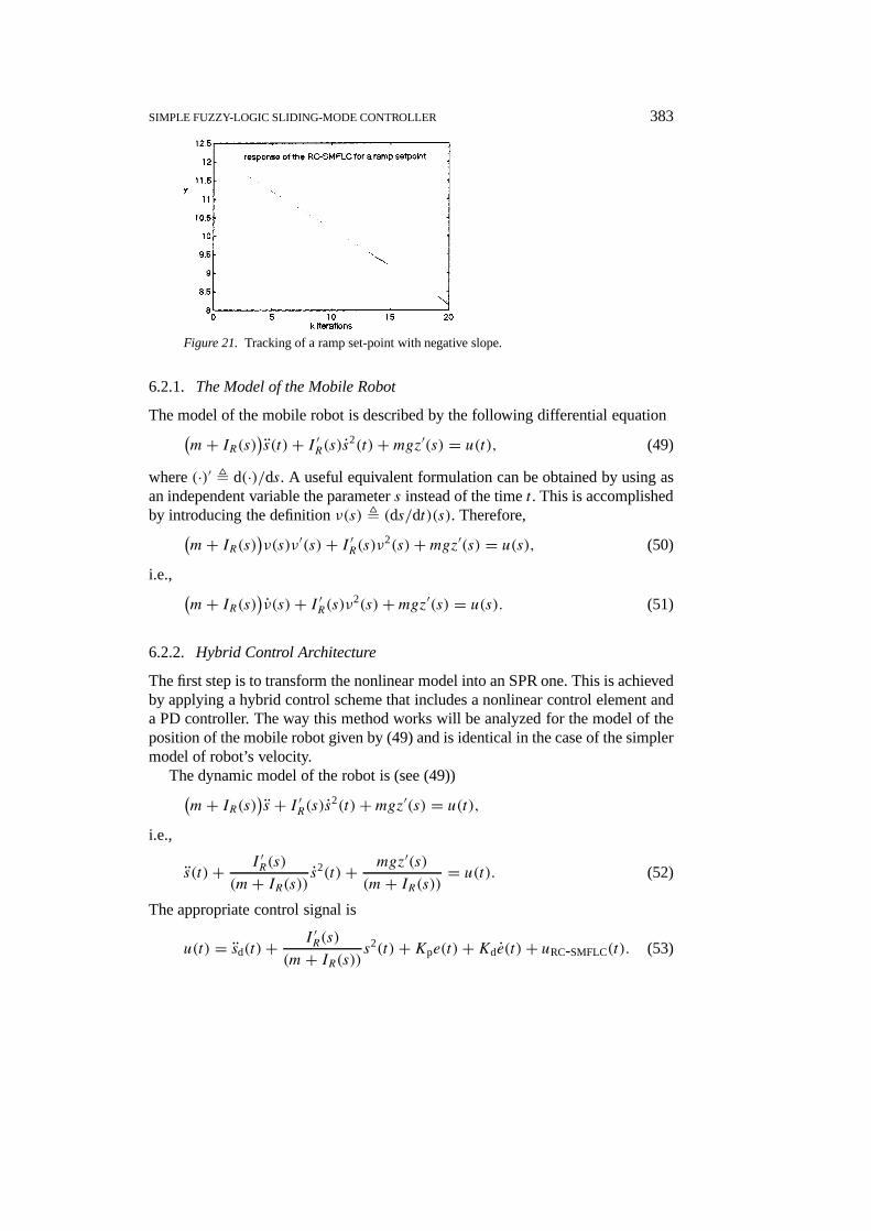
6.2.1. The Model of the Mobile Robot
The model of the mobile robot is described by the following differential equation(m+ IR(s)
)s(t)+ I ′R(s)s2(t)+mgz′(s) = u(t), (49)
where(·)′ , d(·)/ds. A useful equivalent formulation can be obtained by using asan independent variable the parameters instead of the timet . This is accomplishedby introducing the definitionν(s) , (ds/dt)(s). Therefore,(
m+ IR(s))ν(s)ν′(s)+ I ′R(s)ν2(s)+mgz′(s) = u(s), (50)
i.e., (m+ IR(s)
)ν(s)+ I ′R(s)ν2(s)+mgz′(s) = u(s). (51)
6.2.2. Hybrid Control Architecture
The first step is to transform the nonlinear model into an SPR one. This is achievedby applying a hybrid control scheme that includes a nonlinear control element anda PD controller. The way this method works will be analyzed for the model of theposition of the mobile robot given by (49) and is identical in the case of the simplermodel of robot’s velocity.
The dynamic model of the robot is (see (49))(m+ IR(s)
)s + I ′R(s)s2(t)+mgz′(s) = u(t),
i.e.,
s(t)+ I ′R(s)(m+ IR(s)) s
2(t)+ mgz′(s)(m+ IR(s)) = u(t). (52)
The appropriate control signal is
u(t) = sd(t)+ I ′R(s)(m+ IR(s)) s
2(t)+Kpe(t)+Kde(t)+ uRC-SMFLC(t). (53)

384 S. G. TZAFESTAS AND G. G. RIGATOS
Figure 22. Hybrid controller structure.
Indeed, introducing (35) into (36) one gets
s(t)+ I ′R(s)(m+ IR(s)) s
2(t)+ mgz′(s)(m+ IR(s))
= sd(t)+ I ′R(s)(m+ IR(s)) s
2(t)+Kpe(t)+Kde(t)+ uRC-SMFLC(t),
i.e.,
s(t)− sd(t)+Kpe(t)+Kde(t) = uRC-SMFLC(t)− mgz′(s)(m+ IR(s)) , (54)
wheree(t) = sd(t)− s(t). Thus,
e(t)+Kpe(t)+Kde(t) = mgz′(s)(m+ IR(s)) − uRC-SMFLC(t). (55)
The poles of the system described by (55) are determined by the gainsKp
andKd. Thus, if Kp andKd are appropriately selected, then the model of theposition of the mobile robot comes in an SPR form. RC-SMFLC is then goingto compensate the termmgz′(s)/(m+ IR(s)) and assures that limt→∞ e(t) = 0.
It was assumed that the massm, the moment of inertiaI and the “reflected” iner-tia IR of the robot were known, and the uncertainty of the robotic model concernedonly the existence of slopes∂z/∂s in the robot trajectory. The robot could mountan uphill slope(∂z/∂s > 0), or could go down a downhill slope(∂z/∂s < 0). Boththe magnitude and the sign of the slope were unknown and time varying.
At first the robot path was designed to lie on an uphill slope. The RC-SMFL con-troller imitates perfectly the behavior of a human driver. When the slope increasesthen the driver has to press more the accelerator pedal in order to compensate theaugmented impact of the gravitational term
mg
(m+ IR(s))∂z
∂s.
SIMPLE FUZZY-LOGIC SLIDING-MODE CONTROLLER 385
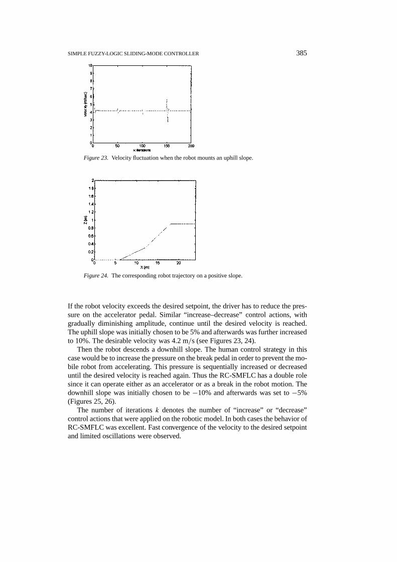
Figure 23. Velocity fluctuation when the robot mounts an uphill slope.
Figure 24. The corresponding robot trajectory on a positive slope.
If the robot velocity exceeds the desired setpoint, the driver has to reduce the pres-sure on the accelerator pedal. Similar “increase–decrease” control actions, withgradually diminishing amplitude, continue until the desired velocity is reached.The uphill slope was initially chosen to be 5% and afterwards was further increasedto 10%. The desirable velocity was 4.2 m/s (see Figures 23, 24).
Then the robot descends a downhill slope. The human control strategy in thiscase would be to increase the pressure on the break pedal in order to prevent the mo-bile robot from accelerating. This pressure is sequentially increased or decreaseduntil the desired velocity is reached again. Thus the RC-SMFLC has a double rolesince it can operate either as an accelerator or as a break in the robot motion. Thedownhill slope was initially chosen to be−10% and afterwards was set to−5%(Figures 25, 26).
The number of iterationsk denotes the number of “increase” or “decrease”control actions that were applied on the robotic model. In both cases the behavior ofRC-SMFLC was excellent. Fast convergence of the velocity to the desired setpointand limited oscillations were observed.

386 S. G. TZAFESTAS AND G. G. RIGATOS
Figure 25. Velocity fluctuations when the robot descends a downhill slope.
Figure 26. The corresponding robot trajectory on a downhill slope.
7. Conclusions
A new approach of sliding-mode fuzzy control was presented in this paper. Itcombines the basic principles of diagonal-type fuzzy controllers with sliding modetheory, and has the additional advantage that no prior design of the rule base isrequired.
Instead of trying to keep the system on a sliding surface of the form
s(x, t) =n−1∑k=0
(n− 1
k
)λke(n−k) = 0,
the goal now is to find a control lawu which will keep the system on the slidingsurfaces(x, t) = ee < 0. If the system remains on this sliding surface then zeroerror will be achieved and the asymptotic stability of the closed-loop system will

SIMPLE FUZZY-LOGIC SLIDING-MODE CONTROLLER 387
be guaranteed. The control law that satisfies the above requirements is describedby the rules:
IF sign(e(t)e(t)
)< 0 THEN maintain the control action,
IF sign(e(t)e(t)
)> 0 THEN change the control action,
where the control action can be either an increase or a decrease of the controlsignal. The increase or decrease of the control signal is realized via the use offuzzy linguistic rules.
The problem now is to determine changes in the control signal that will becomesmaller as the system’s output approaches the diagonale = 0. This is achievedby changing the widths of the fuzzy subsets in which the control signal can beanalyzed. The adaptation of the widths is performed each time the system’s outputcrosses the diagonale = 0, either in a positive or a negative direction.
In contrast to the conventional SMFLC, there is no need to design in advance theshape of the membership functions. All membership functions are identical trian-gular functions, and therefore the transfer characteristic of RC-SMFLC is roughlyapproximated by a first-order linear function. Unlike SMFLC, in RC-SMFLC noprevious existence of a rule base, connecting the error output to the control signal,is necessary. Thus the problem of unavailable expert’s knowledge is solved.
The RC-SMFLC algorithm bares a noticeable to other adaptive control tech-niques such as the iterative learning algorithm. The underlying affinity betweenRC-SMFLC and other robust or adaptive control schemes becomes clear.
The performance of the model-free controller RC-SMFLC has been tested forseveral systems, both linear and nonlinear. RC-SMFLC and proved to be satisfac-tory. No previous knowledge of the system’s model was required. The RC-SMFLCcontrol scheme proved to be robust for all kind of disturbances and parameterchanges of the system. Fast convergence was achieved. As it happens in con-ventional control techniques, there is a trade-off between the rise-time and theovershoot. RC-SMFLC can be viewed as a simple but efficient tool for handlingdifficult nonlinear control problems with strong parametric uncertainties and dis-turbances. Its application could cover a wide range of industrial processes such asarc-welding, deburring, robotic manipulators, etc.
The application of RC-SMFLC can be continued for multivariable systems.The main idea is to adopt a decentralized control strategy which will treat thesystem as a set of single input-single output subsystems. The interaction effectsbetween inputs and outputs can be removed by introducing a simple compensationprocedure based on the genetic algorithms (see [20]).
References
1. Arimoto, S.: Learning control theory for robotic motion,Internat. J. Adaptive Control SignalProcessing4 (1990), 543–564.
2. Cox, E.:The Fuzzy System Handbook, Academic Press, New York, 1994.
388 S. G. TZAFESTAS AND G. G. RIGATOS
3. Doumanidis, C. and Hardt, D. E.: A model for in-process control of thermal properties duringwelding,ASME J. Dyn. Systems Meas. Control111(1989), 40–50.
4. Jamshidi, M.:Large Scale Systems: Modelling, Control and Fuzzy Logic, Prentice-Hall,Englewood Cliffs, NJ, 1997.
5. Kosko, B.:Neural Networks and Fuzzy Systems: A Dynamical Systems Approach to MachineIntelligence, Prentice-Hall, Englewood Cliffs, NJ, 1992.
6. Li, W.: A method for design of a hybrid neuro-fuzzy control system based on behaviormodeling,IEEE Trans. Fuzzy Systems5(1) (1997), 128–137.
7. Liand, H. and Gatland, H. B.: Conventional fuzzy control and its enhancement,IEEE Trans.Systems Man Cybernet.26(5) (1996), 791–801.
8. Lin, C. T.: Neural Fuzzy Control Systems with Structure and Parameter Learning, WorldScientific, Singapore/London, 1994.
9. Lin, S. C. and Kung, C. C.: Linguistic fuzzy sliding mode controller, in:Proc. of 1992 Amer.Control Conf., Chicago, IL, pp. 1904–1905.
10. Malki, H. A., Li, H., and Chen, G.: New design and stability analysis of fuzzy propor-tional-derivative control systems,IEEE Trans. Fuzzy Systems4(4) (1994), 245–254.
11. Malki, H., Misir, D., Feigenspan, D., and Chen, G.: Fuzzy PID control of a flexible-joint robotarm with uncertainties from time-varying loads,IEEE Trans. Control Systems Technol.5(3)(1997), 371–378.
12. Nie, J. and Linkens, D.:Fuzzy-Neural Control: Principles, Algorithms and Applications,Prentice-Hall, Englewood Cliffs, NJ, 1995, pp. 69–86.
13. Nishar, D. V., Schiano, J. L., Perkins, W. R., and Weber, R. A.: Adaptive Control ofTemperature in Arc-Welding,IEEE Control Systems Magaz. (1994), 4–12.
14. Palm, R., Driankov, D., and Hellendoorn, H.:Model-Based Fuzzy Control, Springer, Berlin,1996, pp. 75–113.
15. Pieper, J. K. and Goheen, K. R.: Discrete–time sliding mode control via input–output models,in: Proc. of Amer. Control Conf., San Fransisco, CA, 1993, pp. 964–965.
16. Slotine, J. E. and Li, W.:Applied Nonlinear Control, Prentice-Hall, Englewood Cliffs, NJ, 1991.17. Tzafestas, S. G.: Digital PID and self-tuning control, in: S. G. Tzafestas (ed.),Applied Digital
Control, North-Holland, Amsterdam, 1985, pp. 1–49.18. Tzafestas, S. G., Kyriannakis, E., and Rigatos, G.: Adaptive, model-based predictive and
neural control of the welding process, in: S. G. Tzafestas (ed.),Methods and Applications ofIntelligent Control, Kluwer, Dordrecht/Boston, 1997, pp. 509–548.
19. Tzafestas, S. G. and Papanikolopoulos, N. P.: Incremental fuzzy expert PID control,IEEETrans. Industr. Electronics37(5) (1990), 365–371.
20. Tzafestas, S. G. and Rigatos, G. G.: Self-tuning multivariable fuzzy and neural control usinggenetic algorithms, in:Proc. of DSI ’99 Internat. Conf., Athens, Greece, 1999.
21. Tzafestas, S. G. and Tzafestas, C. S.: Fuzzy and neural control: Basic principles andarchitectures, in: S. G. Tzafestas (ed.),Methods and Applications of Intelligent Control,Kluwer, Dordrecht/Boston, 1997, pp. 25–60.
22. Tzafestas, S. G., Tzamtzi, M. P., and Rigatos, G. G.: Robust control and motion design formobile robots in a time-varying environment, in:CESA ’96 IMACS Multiconference Proc.,Lille, France, July 1996, pp. 706–712.
23. Wang, L. X.:Adaptive Fuzzy Systems and Control: Design and Stability Analysis, Prent-ice-Hall, Englewood Cliffs, NJ, 1994, pp. 9–28.
24. Wu, J. C. and Liu, T. S.: A sliding-mode approach to fuzzy control design,IEEE Trans.Control Systems Technol.4(2) (1996), 141–151.