Embed Size (px)
Citation preview
Kent Academic RepositoryFull text document (pdf)
Copyright & reuse
Content in the Kent Academic Repository is made available for research purposes. Unless otherwise stated all
content is protected by copyright and in the absence of an open licence (eg Creative Commons), permissions
for further reuse of content should be sought from the publisher, author or other copyright holder.
Versions of research
The version in the Kent Academic Repository may differ from the final published version.
Users are advised to check http://kar.kent.ac.uk for the status of the paper. Users should always cite the
published version of record.
Enquiries
For any further enquiries regarding the licence status of this document, please contact:
If you believe this document infringes copyright then please contact the KAR admin team with the take-down
information provided at http://kar.kent.ac.uk/contact.html
Citation for published version
Chin, Catherine Caroline (2018) Advancement in application of supercontinuum sources in biomedicalimaging and OCT. Master of Philosophy (MPhil) thesis, University of Kent,.
DOI
Link to record in KAR
https://kar.kent.ac.uk/70368/
Document Version
Publisher pdf

Advancement in application of supercontinuum sources in
biomedical imaging and OCT
Catherine Caroline Chin
School of Physical Sciences
University of Kent
Thesis submitted for Master of Philosophy degree
November 2018
The work presented in this thesis was performed:
• Between August 2014 and January 2016, within the Applied Optics Group, at the University of Kent, School Physical Sciences, Canterbury, CT2 7NH, United Kingdom, and
• Between February 2016 and July 2017, at NKT Photonics A/S, Blokken 84, Birkerød, 3460, Denmark
This work was supported by the Marie Curie ITN European grant number 607627 (FP7-PEOPLE-2013-ITN) under project UBAPHODESA (www.ubaphodesa.com)
Preface
Acknowledgement
Since the work in this thesis transcends multiple disciplines of science and technology, I am grateful for the assistance I received from personnel in the School of Physical Sciences, Jennison School of Computing, Medway School of Pharmacy, NKT Photonics A/S, DTU Fotonik at the Technical University of Denmark, and The Maidstone and Tunbridge Wells NHS Trust Hospital.
First, I would like to express my greatest gratitude towards Prof Adrian Podoleanu, for supervising this work, and revising the technical writings on published works. This research work was partly performed at NKT Photonics, I extend my appreciation towards Dr Lasse Leick, Dr Thomas Feuchter, Dr Peter Moselund and Prof Ole Bang for making this thesis possible. I’m thankful for the technical advice and support I received from the NKT team.
Many thanks to Dr Adrian Bradu, Dr Sylvian Rivet and Dr Manuel Marques for the good training in using the master/slave OCT system, without which the collaboration with external clinicians would not been able to run smoothly. I also extend my gratitude to Prof John Schofield, and Miss Mona Khandwala for their patience in teaching me the medical terminologies when we authored the imaging paper on skin cancer.
I sincerely appreciate the time and effort by Dr Gulprit Lall, for the wonderful research experience we had, at Charles River laboratory in Ramsgate and in Medway, Kent.
I also enjoyed the many discussions, outreaches and social outing events we had between the ESRs for the last three years. Michael Maria, Felix Fleischhauer, Sophie Caujolle and Magalie Bondu – thank you! Many thanks, to Rasmus Engelsholm, Laurant Huot and Patrick Bowen for your technical support in the lab.
Finally, I am indebted to the many support from my parents, Vincent Chin and Irene Lim, and for their tremendous encouragement throughout these years.
Preface ii
Abstract
This thesis describes the applications of supercontinuum (SC) sources in biomedical imaging and optical coherence tomography (OCT). Three applications of ultra-broadband imaging were identified, and performed. The first application involves clinical study of eyelid basal cell carcinoma (BCC), a very common type of skin cancer among people with light skin tone in developed countries. The aim was to develop a fast and accurate detection of BCC without first needing surgical intervention. The second application relates to photo receptors in mammalian eye. Retina decoding involving photoreceptor response was performed, using a dual-wavelength light source, tuned at different intensity and exposure duration. The study was conducted to assist diagnosis in age-related macular degeneration (AMD) and to detect symptoms in early-stage vision loss. The third application aims to enhance document security and reduce counterfeit. A novel broadband polarisation-sensitive (PS-) OCT prototype was developed. Powered by SC sources, this revolutionary spectrometer based OCT system scans for birefringent imprints in composite materials, such as cotton-fibre, polymer substrate and dichroic ink pigments in banknotes. Polarisation properties were evaluated and analysed.
To enable high-quality OCT application, measurements of dispersion, noise and polarisation extinction ratio (PER) were carried out. Noise was characterised to assist the development of low-noise SC sources. Dispersion was compensated so that high axial resolution (< 5µm) imaging can be achieved. The PER was studied to allow efficient selection and control of polarisation from the light source as well as that in the OCT system.
Finally, the works concluded further improvement in PS-OCT system was needed, by incorporating the master/slave technique and an automatic switch for sequential detection.
Preface iii
Publications and conference papers
1. C. Chin, F.Toadere, T. Feuchter, L. Leick, P. Moselund, A. Bradu, and A. Podoleanu, “Acousto-optic tunable filter for dispersion characterization of time-domain optical coherence tomography systems,” Applied Optics Vol. 55, Issue 21, 5707-5714 (2016).
2. C. Chin, A. Bradu, R. Lim, M. Khandwala, J. Schofield, L. Leick, and A. Podoleanu, “Master/slave optical coherence tomography imaging of eyelid basal cell carcinoma,” Applied Optics Vol. 55, Issue 25, 7378-7386 (2016). [featured on front page of issue 25]
3. C. Chin, R. D. Engelsholm, P. M. Moselund, T. Feuchter, L. Leick, A. Podoleanu, O. Bang, ”Polarization extinction ratio and polarization dependent intensity noise in long-pulse supercontinuum generation,” Proc. SPIE 10089, Real-time Measurements, Rogue Phenomena, and Single-Shot Applications II, 100890L (April 2017).
4. [awaiting publication] C. Chin, R. D. Engelsholm, P. M. Moselund, T. Feuchter, L. Leick, A. Podoleanu, O. Bang, ”Polarization extinction ratio and intensity noise in long-pulse supercontinuum generation,” Opt. Expr. (2017).

Preface iv
List of figures
1.1 Resolution versus penetration depth for different imaging technologies………................ 8
1.2 Therapeutic window with absorbance as function of wavelength for well-known tissue composites……………………………………………………..................... 9
1.3 Anatomy of a human eye ……………………………………………………………..... 10 1.4 Photoreceptors in a human eye ……………………………………………………….... 11 1.5 Sensitivity and light response of typical human photoreceptors ………………….......... 12 1.6 Different layers of human skin ……………………………………………………..….. 13 2.1 A simple Michelson interferometer in free space …………………………………........ 18 2.2 A simple fibre based interferometer with a 2x2 directional coupler ………………........ 22 2.3 A time-domain interferometer with output A-scan, sensitivity and axial range …........... 24 2.4 Spectrometer based Fourier domain interferometer in free-space ………………........... 26 2.5 A swept-source based interferometer in free space ………………………………......... 28 2.6 Experimental construction of master/slave interferometer based on a SS-OCT in fibre .. 30 2.7 Composition of an SLD diode …………………………………………………………. 34 2.8 Superlum BroadLighters series SLD at 1300 nm with 20 mW output ……………......... 35 2.9 Optical spectrum and coherence function at full output power for Superlum BroadLighters
series SLD model S1300-G-I-20 ……………………………………............................. 35 2.10 Optical spectrum of Axsun swept-source model SS1300-OCT at 1 µm ………........... 36 2.11 NKT Photonics SuperK Extreme supercontinuum source ………………………........ 39 2.12 NKT Photonics SuperK Compact supercontinuum source ………………………....... 39 2.13 Supercontinuum spectrum from SuperK Extreme and SuperK Compact ………......... 40 3.1.1 Illustration of a time-domain fibre-based interferometer for noise measurement ......... 47 3.1.2 Distribution of electric fields at input and output ports of a directional coupler…........ 49 3.1.3 In-house balance detector with two InGaAs photodiodes for noise and SNR measurements
in an OCT system …………………………………………………............................... 51 3.1.4 Oscilloscope readout of noise power (AC fluctuation) sampled over 100 kHz electrical
bandwidth and the linear DC component at balance detector ………............................ 63 3.1.5 Theoretical SNR for optical sources with different bandwidth at 1300 nm ……........... 64 3.1.6 Measured noise power relative to input power ……………………………………..... 65 3.1.7 Measured SNR in TD-OCT system for optical sources of 35 nm and 150 nm.............. 67 3.2.1 Experimental set-up for polarization extinction ratio measurements for a long pulse
supercontinuum system ……………………………………………………................. 71 3.2.2 Experimental results for full length nonlinear fibre of 8.5 m ……………………......... 74 3.2.3 Experimental results for three fibre lengths of 8.5 m, 4.5 m and 1.5 m at full pump power
(100%) ………………………………………………………………………............... 75 3.2.4 Experimental results for 4.5 m non-linear fibre length at high 100% and low 30% pump
power …………………………………………………………………………............. 77 3.2.5 Spectra, (bottom) PER for 1.5 m NLF length at low power levels (30%) for three
optimisations …………………………………………………………………………. 78 3.2.6 spectra, (bottom) PER for all three optimisations with NLF length at 1.5 m at full pump
power …………………………………………………………………………............. 79 3.2.7 Schematic diagram for birefringence measurement of nonlinear fibre …………........ 80
Preface v
3.2.8 Birefringence measurement with reference spectrum, and spectra of two fibre lengths with interference fringes ……………………………………….......................................... 82
3.2.9 Full wavelength birefringence measurement ……………………………………....... 83 3.2.10 Experimental setup for pulse-to-pulse RIN measurement using a high-speed GHz
oscilloscope, photo detectors and combination of band pass filters (BPF) …........... 84 3.2.11 Pulse-to-pulse RIN amplitude measured with an oscilloscope and band pass filters
…………………………………………………………………………………....... 84 3.2.12 RIN measured at two power levels (100% & 30%) for NLF length at 8.5 m............ 86 3.2.13 RIN measured at two power levels (100% & 30%) for NLF length at 4.5 m…........ 87 3.2.14 RIN measured at two power levels (100% & 30%) for NLF length at 1.5 m…........ 87 3.2.15 Near-Gaussian symmetric probability distribution for RIN measured at 1000 nm (BW 10
nm) on polarisation axis optimised to maximum total power (Pmax)......................... 89 3.2.16 Long-tailed probability distribution for RIN measured at 1500 nm (BW 12 nm) on
polarisation axis optimised to maximum total power (Pmax)...................................... 89 3.2.17 Long-tailed symmetric probability distribution for RIN measured at 1650 nm (BW 12 nm)
on polarisation axis optimised to maximum total power (Pmax)................................. 90 3.2.18 Pulse height histograms at selected wavelengths optimised for two polarisation
components (Pmax and Pmin) on full SC power (100%) …………………………..... 91 3.2.19 Skew and kurtosis calculated from intensity histogram for two polarisation directions at
full SC power (100%) ………………………………………………...................... 92 4.1 Illustration of broadening of FWHM of a pulse travelling through a dispersive medium
……………………………………………………………………………….............. 103 4.2 Dispersion slope as function of dispersion versus wavelength …………………....... 104 4.3 A Gaussian shaped pulse with FWHM indicated …………………………………... 105 4.4 Broadband supercontinuum source (NKT SuperK Extreme) with its output fed into two
spectral filtering accessories (either into the AOTF or SuperK Split) …….................. 108 4.5 Graphical control user interface for output wavelength selection at the AOTF........... 108 4.6 Output spectrum from SuperK Split splitter module ……………………………...... 109 4.7 System configuration for dispersion characterisation using a time-domain OCT system at
1300 nm …………………………………………………………………................... 110 4.8 Illustration of iterative glass addition method for dispersion compensation in the 1300 nm
system …………………………………………………………………….................. 111 4.9 ΔOPD versus wavelength λm for different DCG length …………………………....... 112 4.10 Interference strength versus wavelength λm selected by AOTF ………………........ 114 4.11 Autocorrelation function for 1300 nm system …………………………………...... 115 5.1 Illustration of linearly, circularly and elliptically polarised EM waves, and their Jones
vector directions …………………………………………………………………….... 124 5.2 Illustration of s- and p-polarisation states for incident, transmitted and reflected lights
interacting between air and glass interface …………………………………………… 125 5.3 Experimental set up of a broadband dual-spectrometer PS-OCT system powered by a
supercontinuum source ……………………………………………………................. 131 5.4 Pixel number to wavelength calibration curve for Wasatch Cobra-S model spectrometer
(650-950 nm) …………………………………………………………........................ 133 5.5 Sensitivity roll-off for Wasatch Cobra-S spectrometer …………………………........ 134 5.6 The “reference sample spectrum” recorded at the output of (top) Channel 1, using
spectrometer SP1 and (bottom) Channel 2, using spectrometer SP2 ……………….... 135
Preface vi
5.7 The sample with a crossed out section showing the scan area of 8 mm × 8 mm of specimen 1 ……………………………………………………………………………................. 136
5.8 The sample with a crossed out section showing the scan area of 8 mm × 8 mm of specimen 2 ……………………………………………………………………………................. 136
5.9 PS-OCT image output from (left) horizontal polarisation, and (right) vertical polarisation for Specimen 1 …………………………………………………………....................... 137
5.10 Post-processed PS-OCT images of Specimen 1 (left) intensity image showing reflectivity, (right) phase retardation ………………......................................................................... 137
5.11 PS-OCT image output from (left) horizontal polarisation, and (right) vertical polarisation for Specimen 2 ………………………………………………………........................ 138
5.12 Post-processed PS-OCT images of Specimen 2 (left) intensity image showing reflectivity, (right) phase retardation …………………………………………………………......... 138
6.1 MS-OCT system configuration ……………………………………………………...... 147 6.2 Illustration of Master/Slave raster made from 3 categories of images. (a) 40 en-face OCT
images separated axially by 5 µm (measured in air), (b) two cross-section OCT images acquired from two orthogonal orientations and (c) an average of the en-face images displayed for guidance. The horizontal size of all images and the vertical size of en-face OCT images: 3 mm × 3 mm. The vertical size of the two cross section images is 3 mm × 1.5 mm (measured in air). The en-face images have 200×200 pixels while the cross section images 200 × 300 pixel …………................................................................................. 150
6.3 Illustration of assembling cross-section scans from en-face images. En-face images are delivered by the MS-OCT technique …………………………………........................ 151
6.4 Histology images of nodular BCC corresponding to tissue sample of Case 1 ….......... 152 6.5 Results of Case 1. Cross section OCT images of eyelid BCC taken from three consecutive
transverse slices at the centre of the sample ……………………….............................. 152 6.6 Results of Case 1. En-face OCT images of eyelid BCC taken at different depths. The depth
was measured from the top of the sample in air ……………………............................ 153 6.7 Results for another region of Case 1. (left): histology image showing blocks of BCC
tumours. (right): En-face OCT image of corresponding region taken at a depth of 780 µm from top of sample (measured in air) …………………………………….................... 153
6.8 Histology images of superficial BCC from tissue sample of Case 2. The image on the left shows a tumour exhibiting nested and budding patterns. The lateral size × depth size of the left image is 4 mm × 3 mm ……………………………………................................... 154
6.9 Results of Case 2. Cross section OCT images of eyelid BCC taken from the centre of tumour. (1) sweat ducts. (2) blood capillary under the dermis layer. (3) suspected areas of BCC. The lateral size × depth size of image is 1.5 mm × 0.6 mm ……........................ 155
6.10 Results of Case 2. En-face OCT images of eyelid BCC taken at different depths between 450 to 950 µm. The depth was measured from the top of sample in air. The arrows show the areas of BCC correlated with histology data in Fig. 6.8. The size of each image is 1.5 mm × 1.5 mm …………………………………………........................................................... 155
6.11 Histology images of Case 3. Image in (b) shows an enlarged view of the white boxed region in image (a). Image (c) shows an enlarged view of the black box area of image (a). The image (d) shows an enlarged region of image (b) indicating presence of nodular pigmented type BCC tumour lobules beneath the epidermis. Magnification: (a) ×20, (b) ×50, (c) ×100, (d) ×200 ………………………………......................................................................... 156

Preface vii
6.12 Results of Case 3. Cross section OCT images of suspected BCC taken at three lateral positions from the centre of sample. The arrows show the areas with pigment correlated with histology images. The lateral size × depth size of each image is 1.5 mm × 0.6 mm …………………………………………………………................................................. 157
6.13 Results of Case 3. En-face OCT images of eyelid BCC taken at different depths in the range 425-650 µm. The depth was measured from the top of the sample in air. The arrows show the areas of BCC. The size of each image is 1.5 mm × 1.5 mm ……………..……….. 157
6.14 Orthogonal views of a pig embryo with cross-section diameter between 80-100 μm in ImageJ (top left: en-face slice XY, top right: YZ, bottom left: XZ). The cross-section yellow line indicates the centre of the image ……………………………................... 162
6.15 Illustration of Master/Slave raster scan for pig embryo made from 3 categories of images a) 40 en-face OCT images separated axially by 5 µm (measured in air), (b) two cross-section OCT images acquired from two orthogonal orientations and (c) an average of the en-face images displayed for guidance ..................................................................................... 163
6.16 Volumetric 3D views of a pig embryo with cross-section diameter of 100 μm in ImageJ ………………………………………........................................................................... 164
7.1 Spectral sensitivity profiles of the classic retinal photoreceptors …………………....... 171 7.2 Stimulus protocols for a Xenon arc consisting of: (a) a single 480 nm light pulse for 60s, and
through the SCWL and (b) a dual stimulus generated at 560 nm for 60 s and at 480nm signal for the last 45s ………………………………………………….................................... 172
7.3 Stimulus protocols for supercontinuum consisting of a dual stimulus generated at 560 nm for full 60 s and at 480nm signal for the last 45s (from t=15s onwards)…......................... 173
7.4 Stimulus protocols for a supercontinuum consisting of: a single 480 nm light pulse for 60s ……………………………………………………………………………………........ 173
7.5 Pupil area was measured by drawing ellipses around the circumference of the pupil in dark adapted, dilated (left) and constricted (right) eyes …………………………................. 174
7.6 Schematic of a single Xe Arc light source used to provide a stimulus ……………....... 175 7.7 Schematic of the dual stimulus SCWL light source ………………………………....... 176 7.8 Spectral line output of SuperK VARIA (NKT Photonics A/S, Denmark) …………...... 177 7.9 The pupillary light reflex of dark-adapted mice using a 480 nm light generated by a Xe arc
source …………………………………………………………………………............. 179 7.10 Irradiance responses using a 560 nm light (orange curve) and irradiance responses using a
560 nm+480 nm (light red curve) stimulus ……………………………….................. 179 7.11 Pupil images from dark adapted (t=-3s) through to 560 nm light (t=10s) and finally 480
nm+560nm (t=20s) ………………………………………………………………...... 180 7.12 The dark adapted pupillary response from a 480 nm Xe arc versus a dual 480 nm+560 nm
pulse, with same irradiance response profile (p>0.05) ……………............................. 181 7.13 Experimental setup used in Charles River laboratory …………………………........... 183 7.14 Multi-wavelength output of the NKT SuperK Varia module ………………………... 183
Preface viii
List of tables
2.1 Different phase condition for interference and output intensities ………....................... 21 2.2 Optical components and their abbreviations for an MSI ................................................ 29 3.1.1 Parameters of a basic PIN photo detector used for noise characterisation.................... 52 3.1.2 Signal variation vs input power for the EPN regime ................................................... 66 3.2.1 Measured total spectral power for three different pump power levels ......................... 73 3.2.2 Skew and kurtosis calculated for polarisation with highest power (Pmax)................... 92 4.1 Sellmeier coefficient constants for N-BK7 glass ............................................................ 113 4.2 Comparison between Experimental and Calculated FWHM of Autocorrelation Function for
Six Values of Dispersion for system at 1300 nm ............................................................ 116 5.1 Jones vectors for different polarisations ......................................................................... 125 5.2 Input and output polarisations with QWP and HWP ...................................................... 126 6.1 Four major statistical risk factors of BCC patients ......................................................... 143 6.2 Four major BCC subtypes and their associated histomorphology features ..................... 144 7.1 Effective quantal flux density calculated at different wavelengths and illuminating power
levels ............................................................................................................................... 178

Preface ix
Glossary of Abbreviations
°C Celsius (unit)
3D three-dimension
A Amperes (unit)
AC alternating current
ADC analogue to digital converter
AF audio frequency
Ag silver
AM amplitude modulation
AMD age-related macular degeneration
AOG Applied Optics Group
AOI angle of incidence
AOR angle of reflectance
AOTF acousto-optic tuneable filter
AR anti-reflection
ASE amplified spontaneous emission
Au gold
B birefringence
BAL balance
BCC basal cell carcinoma
BK7 borosilicate Krone (crown glass)
BN beat noise
BPD balance photo detector
BPF band pass filter
BS beam splitter
BW bandwidth
C Coulombs (unit)
CCD coupled charge device
CD chromatic dispersion
CDF cumulative distribution function
CF collimation fibre
CG coherence gate
CL coherence length
Preface x
CM confocal microscope
CNS central nervous systems
Cp capacitor
CR contrast ratio
CS channelled spectrum
CSLM confocal scanning laser microscopy
CT computed tomography
CUDA compute unified device architecture
CW continuous wave
DAC digital to analogue converter
DAQ data acquisition
dB decibel (unit)
dBm decibel-milliwatts (unit)
DC direct current
DCG dispersion compensation glass
DF dynamic focus
DG diffraction grating
DIFF differential
DR dynamic range
DM dichroic mirror
DNA deoxyribonucleic acid
DOF depth of focus
DSP digital signal processing
DU demodulation unit
ELEC electrical
EM electromagnetic
EPN excess photon noise
ESA electrical spectrum analyser
EU European Union
F farad (unit)
FC fibre coupler
FC/PC fibre-optic connector/ physical contact
FD Fourier domain
FL focal length
FFT fast Fourier transform

Preface xi
FLIM fluorescent lifetime imaging microscopy
FPGA field programmable gate arrays
FTIR Fourier transformed infrared spectroscopy
FWHM full width at half maximum
FWM four wave mixing
GDD group delay dispersion
Ge Germanium
GP general practitioner
GPU graphics processing unit
GS galvanometer scanner
GVD group velocity dispersion
HDR high dynamic range
HeNe helium neon
HFUS high frequency ultrasound
HOD higher order dispersion
HWP half wave plate
Hz hertz (unit)
I inductor
IEEE Institute of Electrical and Electronics Engineers
InGaAs Indium gallium arsenide
IF intermediate frequency
IM intermodulation
IR infrared
IRC irradiance response curve
INTS integrating sphere
J Joules (unit)
JPEG Joint Picture Experts Group
K Kelvin (unit)
L lens
LC inductor-capacitor (circuitry)
LCI low coherence interferometry
LCD liquid crystal display
LD light dark
LNA low noise amplifier
LO local oscillator
Preface xii
LP linear polarisation
LPF long pass filter
LT light tube
LTI linear time invariant
M mirror
MI modulation instability
MLS motorised linear (translation) stage
MMF multimode fibre
MO microscope objective
MPM multi-photon microscopy
MRI magnetic resonance imaging
MS master/slave
MSE mean-squared error
MSF mean-squared fluctuation
MSI master/slave interferometry
NA numerical aperture
ND neutral density
NEC noise equivalent current
NHS National Health Service (UK)
NI National Instruments
NIF non-image forming
NIH National Institute of Health (US)
NIR near infrared
NLF nonlinear fibre
OCT optical coherence tomography
OEM original equipment manufacturing
Op-amp operational amplifier
OPD optical path difference
OPL optical path length
OPT optical
OSA optical spectrum analyser
OSC oscilloscope
P polariser
PAM photo-acoustic microscopy
PBS polarisation beam splitter
Preface xiii
PC polarisation controller
PCB printed circuit board
PCF photonic crystal fibre
PDF probability density function (maths & stats)
portable document format (file)
PD photo diode
PER polarisation extinction ratio
PHH pulse height histogram
PLL phase locked loop
PLR pupillary light reflex
PM polarisation maintaining
PMD polarisation mode dispersion
PNG portable network graphics
PR photo receiver
PRF pulse repetition frequency
PSD power spectral density
PSF point spread function
PS-OCT polarisation sensitive optical coherence tomography
QWP quarter wave plate
R resistor
RCM reflectance confocal microscopy
RCG retinal ganglion cell
RIN relative intensity noise
RF radio frequency
S sensitivity
SC supercontinuum
SCWL supercontinuum white light
SD spectral domain
SEM scanning electron microscope
SHG second harmonic generation
Si Silicon
SLD super-luminescent diode
SLO scanning laser ophthalmoscopy
SMF single mode fibre
SN shot noise
Preface xiv
SNR signal to noise ratio
Sp-OCT spectrometer based optical coherence tomography
SPIE Society of photo-optical instrumentation engineers
SPM self-phase modulation
SRS stimulated Raman scattering
SS swept source
T temperature
TD time domain
TFT thin film transistor
TH threshold
TIA trans-impedance amplifier
TIFF tagged image file format
TIR total internal refraction
TOD third order dispersion
TN thermal noise
TS translation stage
TTL transistor to transistor logic
UBB ultra broadband
USAF United States Air Force
UWB ultra-wideband
USB universal serial bus
UV ultra violet
UVFS UV fused silica
V Volts (unit)
VIS visible spectrum
W Watts (unit)
WL wavelength (λ)
Xe Xenon
XPM cross-phase modulation
ZDF zero dispersion fibre
ZDW zero dispersion wavelength
ZO zeroth order

Table of contents
0 Preface
0.1 Acknowledgement .................................................................................................... i
0.2 Abstract ...................................................................................................................... ii
0.3 Publications & conference papers ............................................................................ iii
0.4 List of figures ............................................................................................................ iv
0.5 List of tables ............................................................................................................. viii
0.6 Glossary ..................................................................................................................... x
0.7 Table of contents ....................................................................................................... xv
1 Introduction .................................................................................................................... 1
1.1 Background .............................................................................................................. 2
1.2 Chapters summary ................................................................................................... 3
1.2.1 Technology limitation ................................................................................. 6
1.3 OCT in biomedical applications ................................................................................ 9
1.3.1 Optical properties in tissues ........................................................................ 9
1.3.2 The eye .......................................................................................................... 10
1.3.3 The skin ........................................................................................................ 12
1.3.4 Investigative methods .................................................................................... 14
2 OCT and sources ............................................................................................................ 17
2.1 Low coherence interferometry ................................................................................. 17
2.1.1 Free space coherence ................................................................................. 17
2.1.2 Interference ................................................................................................. 19
2.1.2.1 Conditions for interference .................................................................. 21
2.1.3 Fibre-based system ..................................................................................... 22
2.2 Time-domain OCT .................................................................................................... 23
2.3 Spectral domain OCT ............................................................................................... 25
2.3.1 Spectrometer based OCT .............................................................................. 27
2.3.2 Swept-source (SS) based OCT ..................................................................... 27
2.4 Master/slave OCT ..................................................................................................... 29

Table of contents xvi
2.4.1 Principles of operation ................................................................................. 29
2.5 Optical sources .......................................................................................................... 33
2.5.1 Narrowband sources .................................................................................... 33
2.5.2 Supercontinuum sources ............................................................................. 37
3 Noise and polarisation effects in ultra broadband OCT imaging ............................... 45
3.1 Noise in balanced OCT system ................................................................................. 47
3.1.1 Coupler theory ............................................................................................ 47
3.1.2 Photodiode detection ................................................................................... 51
3.1.2.1 Balance detection ................................................................................. 51
3.1.2.2 PIN diode ............................................................................................ 52
3.1.3 Noise theory ................................................................................................. 53
3.1.3.1 Shot noise ............................................................................................. 54
3.1.3.2 Excess photon noise ............................................................................. 55
3.1.3.3 Excess noise at low frequencies ............................................................ 57
(A) Frequency dependent limitation ............................................................ 57
(B) Optical beam limitation ........................................................................ 57
(C) Semiconductor limitation ..................................................................... 58
(D) Signal processing, filtering & rectification constraints ........................ 58
3.1.3.4 Thermal noise ....................................................................................... 59
3.1.3.5 Beat noise ............................................................................................ 59
3.1.3.6 Total noise power ................................................................................ 60
3.1.4 SNR and sensitivity ..................................................................................... 61
3.1.4.1 SNR ...................................................................................................... 61
3.1.4.2 Sensitivity ............................................................................................. 61
3.1.5 Noise measurement technique ...................................................................... 63
3.1.5.1 Theoretical modelling ........................................................................... 63
3.1.5.2 Experimental measurement ................................................................... 65
3.1.6 Summary of statistical noise ........................................................................ 69
3.2 Polarisation and noise in long pulse supercontinuum ................................................ 70
3.2.1 Polarisation extinction ratio characterisation ................................................ 71
3.2.1.1 Optimisation to total power ................................................................... 73
3.2.1.2 Optimisation to maximum pump wavelength (1064 nm) ...................... 76
3.2.1.3 Optimisation to maximum power at red edge (1950 nm) ...................... 77
3.2.2 Fibre birefringence ...................................................................................... 80

Table of contents xvii
3.2.3 Polarisation relative intensity noise ............................................................. 84
3.2.3.1 RIN ......................................................................................................... 86
3.2.3.2 Pulse height histogram ........................................................................... 88
3.3 Polarisation noise in OCT application ...................................................................... 94
4 Dispersion in ultra broadband OCT systems ................................................................ 101
4.1 Dispersion and coherence .......................................................................................... 102
4.1.1 Coherence .................................................................................................... 102
4.1.2 Dispersion .................................................................................................... 103
4.1.3 Autocorrelation of a pulse ........................................................................... 105
4.2 Methods to evaluate and reduce dispersion ............................................................... 107
4.3 Dispersion experiments ............................................................................................. 109
4.3.1 Dispersion measurement with time-domain OCT at 1300 nm ..................... 109
4.4 Dispersion analysis .................................................................................................... 111
4.4.1 Dispersion measurement with AOTF at 1300 nm ....................................... 111
4.4.2 Dispersion measurement with FWHM of autocorrelation at 1300 nm ....... 115
4.5 Comparison between AOTF and FWHM autocorrelation ........................................ 117
4.5.1 Superiority of AOTF method ...................................................................... 117
4.5.2 Minimising dispersion ................................................................................. 118
4.5.3 Application of AOTF in broadband OCT dispersion measurement ............. 120
5 Ultra broadband polarisation sensitive and Master/slave OCT .................................. 122
5.1 Proof of concept ........................................................................................................ 124
5.1.1 Polarisation of light ..................................................................................... 124
5.1.2 Slow and fast axes determination ................................................................ 126
5.1.3 Jones matrices ............................................................................................ 127
5.1.4 Bank notes .................................................................................................... 128
5.2 PS-OCT system set-up .............................................................................................. 129
5.2.1 Polarisation selection and switching ............................................................ 130
5.2.2 Polarisation detection .................................................................................. 132
5.2.3 Dispersion compensation and spectrometer calibration................................. 133
5.2.4 Technical challenges .................................................................................... 134
5.3 Imaging results ............................................................................................................ 135
5.3.1 Birefringence samples .................................................................................. 135
5.3.2 Cross-section images .................................................................................... 136

Table of contents xviii
5.3.3 Future work ................................................................................................. 138
6 Application of OCT in biomedical imaging .................................................................. 141
6.1 Clinical significance of BCC .................................................................................... 143
6.1.1 Clinical classifications of BCC ................................................................... 143
6.1.2 Histology tissue imaging ............................................................................ 145
6.1.3 Histology correlation ................................................................................. 146
6.2 En-face imaging ....................................................................................................... 146
6.2.1 Master/slave OCT machine ........................................................................ 146
6.2.2 BCC correlation techniques and results ..................................................... 151
6.2.3 Comments on technology ......................................................................... 158
6.3 Imaging of mammalian embryos .............................................................................. 161
7 Application of supercontinuum light sources in vision science .................................. 169
7.1 Pupillometry ............................................................................................................. 171
7.1.1 Pupil light reflexes in mammals ................................................................ 171
7.1.2 Animals and ethics ..................................................................................... 172
7.1.3 Image capture and analysis ......................................................................... 172
7.1.4 Dual laser and multi-wavelength setup ....................................................... 175
7.1.4.1 Xenon Arc ........................................................................................... 175
7.1.4.2 NKT supercontinuum white light source ............................................ 175
7.2 Pupil stimulus and results ........................................................................................... 177
7.2.1 Light stimulus .............................................................................................. 177
7.2.2 Advantages and significance ........................................................................ 181
7.2.3 Potential breakthrough in vision science ...................................................... 182
8 Conclusion ........................................................................................................................ 185
8.1 Future works ............................................................................................................. 189
Appendices ........................................................................................................................ 191
1
Introduction
High-resolution optical coherence tomography (OCT) is fast emerging as an
increasingly common non-invasive imaging of three-dimensional (3D) microstructures and
biological tissues. It is used extensively in dermatology and ophthalmology [1-2]. The
OCT technology was first reported by the research group of Professor James Fujimoto, at
the Massachusetts Institute of Technology (MIT) in 1991 [3-4]. It incorporates the basic
principle of low coherence interferometry (LCI) by improving multiple direction lateral
scanning capabilities to enhance penetration depth [5-6]. This technique enables simple
one dimensional (1D) axial scanning, and was later extended to two and three dimensional
(3D) tomography. According to its inventor, Fujimoto et al, that OCT has significant
advantages over is nearest comparable imaging modalities, such as confocal microscopy
(CF) and multiphoton microscopy (MPM) [7-8]. In comparison, OCT offers high
sensitivity imaging, high axial resolution, and long working distances [9]. OCT generally
has a much higher resolution but also lower penetration depth when comparing to
ultrasound, photo-acoustic microscopy (PAM), computed tomography (CT) and magnetic
resonance imaging (MRI) [10]. On the flip side, CF and MPM can provide comparable oe
better resolution to OCT, but with much lower sensitivity and therefore shallower
penetration depth. In recent years, specialists in this field have discovered ways to extend
axial imaging resolution of OCT with broadband optical sources. Many publications have
suggested that the supercontinuum (SC) sources, such as those manufactured by NKT
Photonics and Fianium, is the way forward. This idea of employing SC sources with OCT
resonated with among researchers at Applied Optics Group (AOG), particularly group
leader Prof. Adrian Podoleanu and Dr Adrian Bradu. Since 2013, a collaboration with
NKT Photonics was sought, to explore ways to improve SC sources for use in OCT
imaging. The outcome was the successful European Union (EU) grant for project
UBAPHODESA (Ultra-Wide Bandwidth Photonics Devices, Sources and Applications).
UBAPHODESA’s main objective was to develop ultra-broadband optical sources to
improve OCT imaging systems for biomedical applications. This thesis summarises the
three years research works carried out to achieve that goal.
Chapter 1 Introduction 2
1.1 Background
The UBAPHODESA project heavily emphasises on application related research and
product integration, such as: (a) assembly of high resolution, low noise OCT imaging
technology for the eye and OCT endoscopy; (b) assembly of systems to exploit the broad
bandwith of supercontinuum in spectroscopy and nonlinear optics applications, and; (c)
evaluate the potential of photo acoustics in adding diagnostic contrast, and be a suitable
light weight, compact and portable technology ready in the clinic. On the research part, the
main motivation is to establish a link between the source performance and the clinical
setting, in order to clarify how to improve diagnostic contrast and imaging quality up to the
level of clinical acceptance.
Since NKT Photonics is mainly an optical source manufacturer, they have no prior
experience in areas related to OCT. It is costly to acquire such knowledge in an industrial
setting and time-consuming to train new personnel. On the other hand, the University of
Kent already has expertise in OCT, but needs access to cutting-edge supercontinuum
sources. Therefore, as the world’s leader in supercontinuum source manufacturing, NKT
Photonics was the ideal industrial partner. Their experience has indicated the need for
specialised research in the area of noise. Characterisation of supercontinuum to understand
noise in a variety of broadband optical set-ups has been very important for them. These are
the knowledge NKT Photonics urgently need to design and produce low-noise sources for
their customers. There are a wide range of applications with supercontinuum lasers: OCT
imaging, material characterisation, metrology and remote sensing. The intent was that,
through this European collaboration, the early stage researchers (ESRs) should characterise
and optimise the supercontinuum sources at NKT, integrate them with high-resolution
OCT systems designed in Kent, and commercialise the final imaging solutions to
clinicians. However, as these systems are meant to be broadband, several technical
challenges persist. Issues such as chromatic aberrations, dispersion and wave front
distortion have to be resolved.
The UBAPHODESA project also has several other far-reaching objectives, such as
to establish long lasting collaboration links between the partners involved, to secure
Europe’s lead in terms of photonics, optical broadband sources and applications, as well as
by collaborating with the associated partners, to improve education of future specialists
and empower them to react to avenues not identified as yet, for future and yet to be
explored supercontinuum applications. That is why technical collaboration between NKT
Photonics and academia can yield exciting results. With the expertise in laser system
Chapter 1 Introduction 3
design and manufacturing, engineers at NKT Photonics were able to allocate necessary
resources to assist UBAPHODESA researchers during their work. The feedback from this
collaboration was positive. Several ambitious projects and researches that transcend
multiple scientific disciplines, such as the OCT clinical trials involving human subjects and
laboratory animals, were realised.
To facilitate technical expertise transfers between academic and industrial partners,
the works discussed in this thesis were performed at two sites: Applied Optics Group
(AOG) at the University of Kent in Canterbury, UK and NKT Photonics A/S in Birkerød,
Denmark. Equal amount of time were spent in both sites, amounting to 18 months each.
While at the University of Kent, two research projects, one involving clinicians from the
Maidstone Hospital, and another with the Medway School of Pharmacy, were conducted.
1.2 Chapters summary
This section provides a brief description on the contents of each chapter and their
relevance to the topic of research as a whole. The works presented in this thesis are
organised in the following order: one theoretical chapter (Chapter 2), one practical chapter
(Chapter 3), two experimental chapters (Chapters 4 and 5), and two application chapters
(Chapters 6 and 7).
Chapter two is a theoretical chapter reviewing past and current development of
OCT techniques as well as broadband light sources. We begin by presenting the brief
concept of coherence and interference, using a simple Michelson interferometer. We move
on to show how a basic interferometric imaging system has evolved into the modern OCT
technologies. We then continue into derivations of mathematical expressions for the OCT
signals in both spatial and temporal domains, while we look into fundamental origin of
lateral and axial scanning, before extending these concepts into producing a 3D
tomography. We also look into the applications used today in various biomedical hot-
topics such as dermatology and ophthalmology. This chapter also includes a description on
the different types of OCT techniques: time domain, spectral domain (including
spectrometer based and swept-source based operations) and finally our master/slave (MS)
system. We go further into the capabilities and drawbacks of several OCT techniques
explored, as are their various practical uses. Some of the practical details of
implementation are also discussed, particularly those which are of relevance to the
Chapter 1 Introduction 4
methods employed in the following chapters. We conclude this chapter by looking into
various optical sources for OCT systems, from narrowband to broadband.
Chapter three is the practical chapter assessing measurable parameters, such as
noise, polarisation extinction ratio (PER) and balance detection to improve OCT imaging
quality. We reviewed various types of noise sources, including ways of characterising
them. Some of the noise discussed are from the optical source, while others are added by
the interferometer. The classifications of noise with theoretical modelling form a large part
of our study. We also find ways to optimise the SNR on OCT imaging, in an attempt to
improve the axial resolution. Further in this chapter, we investigate the polarisation of
supercontinuum generated in nominally non-birefringent silica photonic crystal fibres
(PCF) over the entire spectrum of the source, from 450 nm to 2400 nm. We initially
showed the degree of polarisation varies but in some parts of the spectrum there is a stable
PER of over 10 dB. We later experimentally demonstrate how the spectrally resolved
polarization develops with increasing power and along the length of the nonlinear fibre.
The experimental results are compared to numerical simulations of coupled polarisation
states, mimicking the experimental conditions. Subsequently, we illustrate the principle to
correctly measure a single-shot pulse-to-pulse polarisation dependent relative intensity
noise (PD-RIN) in two polarisation directions, and how the noise are analysed using long-
tailed and rogue wave statistics. In this chapter, we used a range of narrow band pass filters
(BPF) between 550 nm to 2000 nm, and fast photo detectors, to record pulses from the
source. Peaks from these pulses are first extracted, and then the distribution of the pulse
height histogram (PHH) is constructed. Analysis using higher-order moments about the
mean (variance, skew and kurtosis) showed that: (1) around the pump wavelength of 1064
nm, the PD-RIN is lowest, PHH exhibits a Gaussian distribution, and higher order
moments are zero, (2) further away from pump, PD-RIN increases in parabolic fashion,
PHH follows a left-skewed long-tailed Gamma distribution, and higher-order moments
increase. Spectrally, the difference of the PD-RIN in the two orthogonal axes increases
with PER. We later show how birefringence increases with wavelength and how stimulated
Raman scattering (SRS) has a role in spectral broadening.
Chapter four is the experimental chapter that shows the use of a broadband
supercontinuum light source with an acousto-optic tuneable filter (AOTF) to characterise
dispersion in OCT systems. The filter mentioned here is designed to sweep across two
spectral ranges, from 800 to 900 nm and from 1200 to 1500 nm, respectively. In this
chapter, we introduce a fibre-based time-domain OCT system, operating at 1300 nm.
Dispersion compensation for 1300 nm was achieved using BK 7 glass rods in the reference
Chapter 1 Introduction 5
arm. The use of AOTF allows evaluation of dispersion in under and overcompensated
systems. Further in the chapter, we evaluate the AOTF method using the wavelength
dependence of the optical path difference (OPD) that corresponds to the maximum strength
of the interference signals recorded using a mirror as object. In addition, a thorough
comparison is made between the AOTF method and the more usual method based on
measurement of the full width at half-maximum (FWHM) of the autocorrelation peak. This
comparison shows that, based on our measured results, the AOTF method is more accurate
in terms of evaluation of the dispersion left uncompensated after each adjustment. The
AOTF method also provides information on the direction of dispersion compensation,
which cannot be easily obtained with FWHM of autocorrelation method.
Chapter five is another experimental chapter. This chapter goes in length to explain
the benefit of measuring polarisation properties in samples, and how a polarisation-
sensitive broadband OCT system is useful in histology, bio-security and archaeology. A
detailed theoretical discussion about PS-OCT begins from the very basic Jones
formulation, to electric field rotation, and further into birefringence calculation. We also
describe the construction of the PS-OCT setup, from initial polarisation selection, to how
we controlled polarisation state at every stage of the interferometer system. Finally, we
include a comprehensive discussion on polarisation receiver system that features a simple,
switchable dual-spectrometer design. The detection mechanism allows us to extract both
amplitude and phase information from two orthogonal polarisation directions.
Chapter six is the application chapter that incorporates functional OCT imaging and
dispersion free master/slave interferometer technique on basal cell carcinoma (BCC), a
common type of skin cancer. To illustrate the clinical application, we used a conventional
swept source at 1300 nm, with sweeping speed of 50 kHz. The imaging part involves a
three-step process. First, 384 channelled spectra using a mirror were stored for 384 optical
path differences at the master stage. Subsequently, the stored channelled spectra (masks)
were correlated with the channelled spectrum from the BCC tissue to produce 384 en-face
OCT images (200 × 200 pixels) for the optical path difference values used to acquire the
masks. Finally, these en-face slices were stacked to form a volume to cross-reference BCC
tumour margins in the orthogonal plane. Per each eyelid sample, several en face images of
200 × 200 lateral pixels are produced in the time to scan laterally a complete raster of 1.6 s.
Combination of the en-face views with the cross-sectioning views allow for better
discrimination of BCCs comparable to using cross-sectional imaging alone, as previously
reported using the conventional fast-Fourier-transform-based OCT techniques. As for the
Chapter 1 Introduction 6
optical source, we determined that it could be replaced with a broadband supercontinuum
source while maintaining dispersion free imaging with master/slave technique.
Chapter seven is another application chapter focuses on the use of broadband
supercontinuum light source to evaluate eye pupil response. In this chapter, we assessed
the spectral sensitivity of the pupillary light reflex in mice using a high power super
continuum white light (SCWL) source in a dual wavelength configuration. This novel
approach was compared to data collected from a more traditional setup using a Xenon arc
lamp fitted with monochromatic interference filters. Irradiance response curves were
constructed using both systems, with the added benefit of a two-wavelength, equivocal
power, and output using the SCWL. The variables applied to the light source were
intensity, wavelength and stimulus duration through which the physiological output
measured was the minimum pupil size attained under such conditions. We show that by
implementing the SCWL as our novel stimulus we were able to dramatically increase the
physiological usefulness of our pupillometry system.
Chapter eight sums up the work presented in this thesis, and the overall
achievements during the three years of this research work. Also proposed in this chapter
are area of interests that are worth further investigations.
1.2.1 Technology limitation
Similar to many imaging technologies, there are huge varieties of fundamentals and
practical limitations in both OCT and supercontinuum. Among the frequently cited
technical limitations, we have compiled a list of them here as the issues we will address in
subsequent chapters of this thesis.
(a) Axial and lateral resolution
Many commercial OCT systems in the market lack the resolution to resolve
sub-micron histology features, such as the retina layers in the eye or basal cell
carcinoma on the skin. Out of the box improvement to lateral resolution of an
existing OCT system can be relatively simple as this involves swapping the scanning
(or telocentric) lens by another interface optics with higher numerical aperture (NA).
The disadvantage, however, is that it reduces the depth of focus and hence the
imaging depth range and sensitivity. Therefore, some form of dynamic focusing is
then required, such as the methods described in [11-12] by Avanaki and Hughes. On
Chapter 1 Introduction 7
the other hand, improvements to axial resolution generally requires the replacement
of optical sources and spectrometers to broadband version. In this thesis, we
discussed extensively on the use of supercontinuum sources, and methods to
overcome noise, dispersion and polarisation, in Chapters 3, 4 and 5 respectively.
(b) Signal to noise
The ability of an imaging system to discriminate useful features relies on its
signal to noise ratio (SNR). Several parameters can degrade its SNR ratings, such as
a noisy optical source, poor coupling efficiency between free-space to fibre interface,
improper signal attenuation due to low power from the sample, and signal saturation
at detector.
(c) Chromatic aberrations
The use of refractive optics such as lenses for ultra-high bandwidth imaging is
particularly challenging. Since broadband spectrum can easily span across 300-500
nm wide, but very few use the full width, the ability to focus all wavelengths into one
spot is not without issue. In general beam propagation, all lenses will have some
chromatic aberrations. When focusing a beam, some parts of the will have its beam
waist (or focal point) at a different distance due to the chromatic aberration of the
lens. The focal length of each wavelength is different, resulting in different
wavelengths focused on different positions, along the optical axis.
(d) Polarisation dependency
The challenge to spatially resolve ex-vivo and also in-vivo images due to
polarisation changes in skeletal muscle, bone, skin and brain relies on the ability to
control polarisation correctly. This area involves complex coherent detection
technique to pick up the differential signal that contains two orthogonal polarization
states of the signal formed by interference of light reflected from the biological
sample and a mirror in the reference arm of a Michelson interferometer, polarization
capabilities can also extend the penetration depth, indirectly by measuring the change
in polarisation resolved depth structural changes in biological tissues, additional
birefringence properties not otherwise detectable with conventional intensity only
imaging technique, as example, any fibrous structure (organic or not) will influence
the polarization of light, as shown in Chapter 5.
Chapter 1 Introduction 8
(e) Penetration depth
OCT relies on interference and therefore requires stable and deterministic
phase relations between the interfering waves [9]. Due to scattering and absorption in
the examined object, the number of photons in the backscattered wave conserving
stable phase relations to the photons in the incident wave reduces with depth. The
maximum penetration depth, Δz is therefore determined by the depth layer where the
object wave exhibits sufficient strength to measurable interference, normally on a
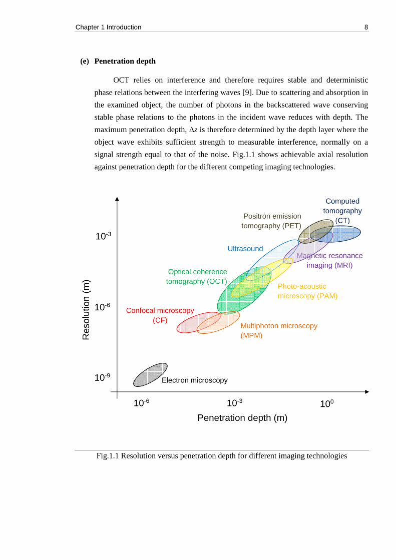
signal strength equal to that of the noise. Fig.1.1 shows achievable axial resolution
against penetration depth for the different competing imaging technologies.
Fig.1.1 Resolution versus penetration depth for different imaging technologies
10-3
10-6
10-9
10-3 10-6 100
Penetration depth (m)
Res
olut
ion
(m)
Optical coherence tomography (OCT)
Photo-acoustic microscopy (PAM)
Positron emission tomography (PET)
Ultrasound Magnetic resonance
imaging (MRI)
Computed tomography
(CT)
Electron microscopy
Confocal microscopy (CF)
Multiphoton microscopy (MPM)
Chapter 1 Introduction 9
1.3 OCT in biomedical applications
OCT has become increasingly popular for skin and eye diagnosis. Since 2010, there
are more than 100 peer reviewed papers published a year on the use of OCT in these areas.
OCT is currently the preferred way to image the retina for glaucoma, as evidenced in [13].
Many recent OCT systems has also incorporate the scanning laser ophthalmoscope (SLO)
technology in many hospitals and eye clinics in the UK, given the added benefits of better
axial resolutions [14]. The main use of OCT on skin is to diagnose tumour development,
such as the eyelid BCC. In this section, we introduce the basic anatomy of both eye and
skin, and the optical properties of their tissue made up.
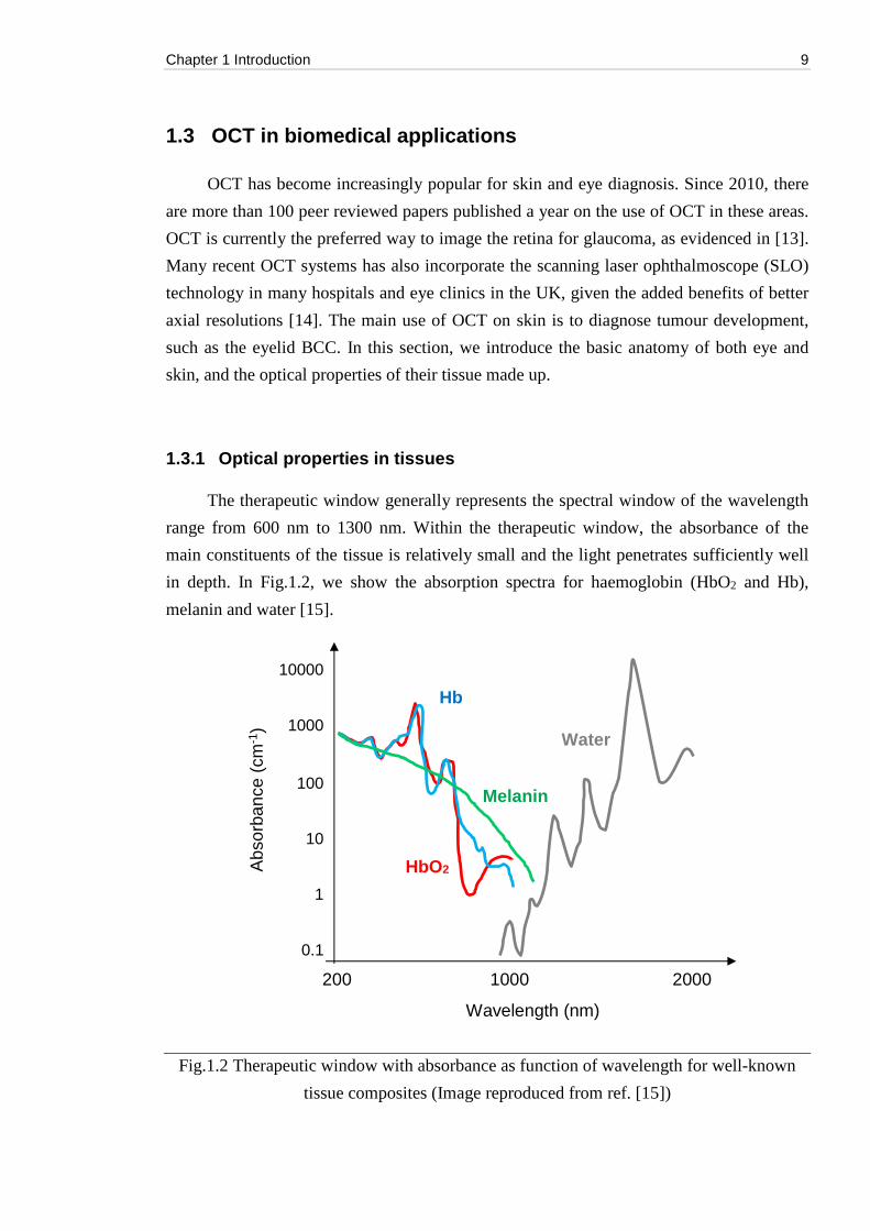
1.3.1 Optical properties in tissues
The therapeutic window generally represents the spectral window of the wavelength
range from 600 nm to 1300 nm. Within the therapeutic window, the absorbance of the
main constituents of the tissue is relatively small and the light penetrates sufficiently well
in depth. In Fig.1.2, we show the absorption spectra for haemoglobin (HbO2 and Hb),
melanin and water [15].
Fig.1.2 Therapeutic window with absorbance as function of wavelength for well-known
tissue composites (Image reproduced from ref. [15])
10000
1000
100
10
1
0.1
200 1000 2000
HbO2
Melanin
Hb
Water
Wavelength (nm)
Abs
orba
nce
(cm
-1)
Chapter 1 Introduction 10
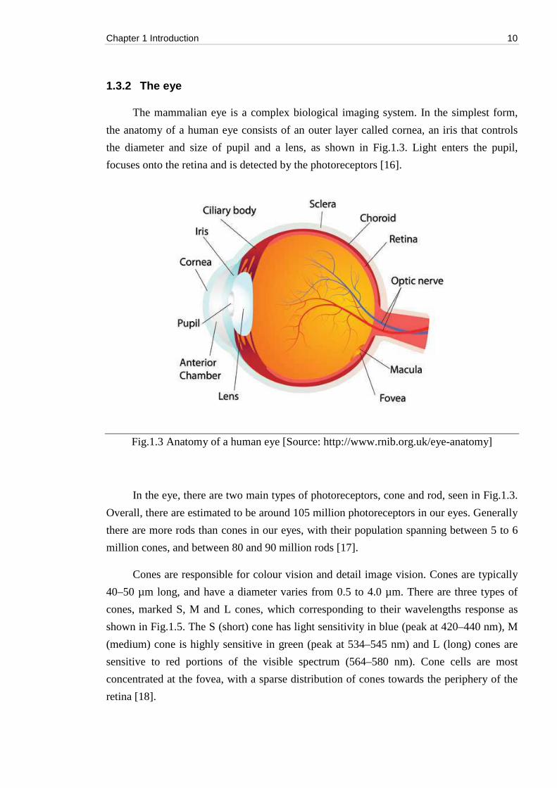
1.3.2 The eye
The mammalian eye is a complex biological imaging system. In the simplest form,
the anatomy of a human eye consists of an outer layer called cornea, an iris that controls
the diameter and size of pupil and a lens, as shown in Fig.1.3. Light enters the pupil,
focuses onto the retina and is detected by the photoreceptors [16].
Fig.1.3 Anatomy of a human eye [Source: http://www.rnib.org.uk/eye-anatomy]
In the eye, there are two main types of photoreceptors, cone and rod, seen in Fig.1.3.
Overall, there are estimated to be around 105 million photoreceptors in our eyes. Generally
there are more rods than cones in our eyes, with their population spanning between 5 to 6
million cones, and between 80 and 90 million rods [17].
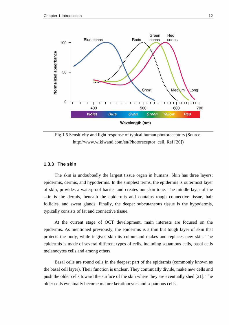
Cones are responsible for colour vision and detail image vision. Cones are typically
40–50 µm long, and have a diameter varies from 0.5 to 4.0 µm. There are three types of
cones, marked S, M and L cones, which corresponding to their wavelengths response as
shown in Fig.1.5. The S (short) cone has light sensitivity in blue (peak at 420–440 nm), M
(medium) cone is highly sensitive in green (peak at 534–545 nm) and L (long) cones are
sensitive to red portions of the visible spectrum (564–580 nm). Cone cells are most
concentrated at the fovea, with a sparse distribution of cones towards the periphery of the
retina [18].
Chapter 1 Introduction 11
Rods, on the other hand, are highly sensitive to light and can provide some grey scale
vision in low-light environments. Rods have peak response between 490-500 nm ranges
(Fig.1.5) [20]. Rods however cannot distinguish colour but provide only luminosity
information. Rod cells are approximately 2 μm in diameter and distributed across most of
the retina except the fovea and the optic disc, with a higher density in the peripheries of the
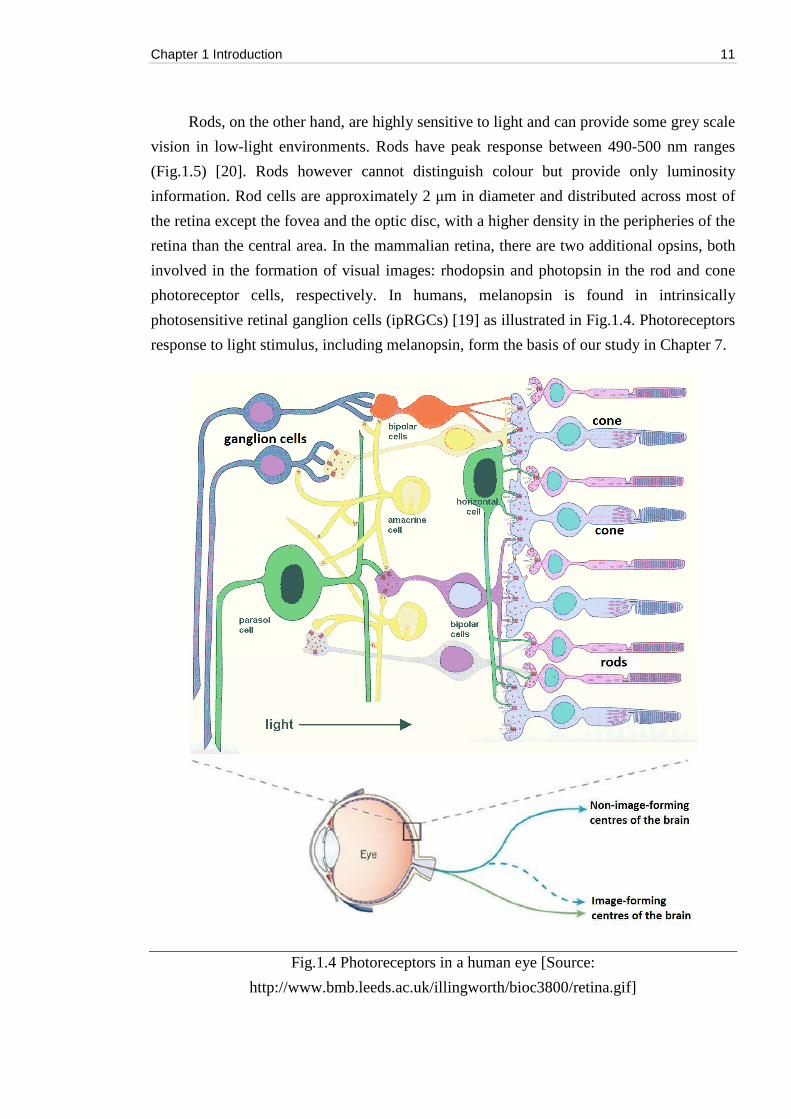
retina than the central area. In the mammalian retina, there are two additional opsins, both
involved in the formation of visual images: rhodopsin and photopsin in the rod and cone
photoreceptor cells, respectively. In humans, melanopsin is found in intrinsically
photosensitive retinal ganglion cells (ipRGCs) [19] as illustrated in Fig.1.4. Photoreceptors
response to light stimulus, including melanopsin, form the basis of our study in Chapter 7.
Fig.1.4 Photoreceptors in a human eye [Source:
http://www.bmb.leeds.ac.uk/illingworth/bioc3800/retina.gif]
Chapter 1 Introduction 12
Fig.1.5 Sensitivity and light response of typical human photoreceptors (Source:
http://www.wikiwand.com/en/Photoreceptor_cell, Ref [20])
1.3.3 The skin
The skin is undoubtedly the largest tissue organ in humans. Skin has three layers:
epidermis, dermis, and hypodermis. In the simplest terms, the epidermis is outermost layer
of skin, provides a waterproof barrier and creates our skin tone. The middle layer of the
skin is the dermis, beneath the epidermis and contains tough connective tissue, hair
follicles, and sweat glands. Finally, the deeper subcutaneous tissue is the hypodermis,
typically consists of fat and connective tissue.
At the current stage of OCT development, main interests are focused on the
epidermis. As mentioned previously, the epidermis is a thin but tough layer of skin that
protects the body, while it gives skin its colour and makes and replaces new skin. The
epidermis is made of several different types of cells, including squamous cells, basal cells
melanocytes cells and among others.
Basal cells are round cells in the deepest part of the epidermis (commonly known as
the basal cell layer). Their function is unclear. They continually divide, make new cells and
push the older cells toward the surface of the skin where they are eventually shed [21]. The
older cells eventually become mature keratinocytes and squamous cells.
Chapter 1 Introduction 13
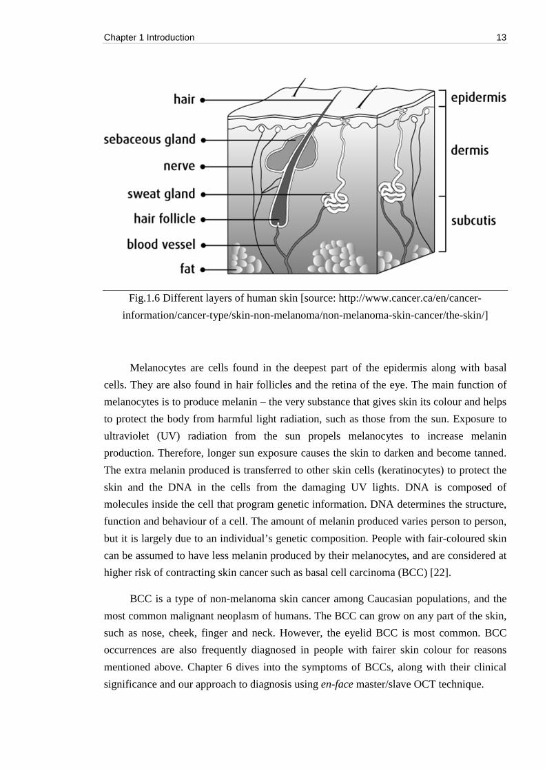
Fig.1.6 Different layers of human skin [source: http://www.cancer.ca/en/cancer-
information/cancer-type/skin-non-melanoma/non-melanoma-skin-cancer/the-skin/]
Melanocytes are cells found in the deepest part of the epidermis along with basal
cells. They are also found in hair follicles and the retina of the eye. The main function of
melanocytes is to produce melanin – the very substance that gives skin its colour and helps
to protect the body from harmful light radiation, such as those from the sun. Exposure to
ultraviolet (UV) radiation from the sun propels melanocytes to increase melanin
production. Therefore, longer sun exposure causes the skin to darken and become tanned.
The extra melanin produced is transferred to other skin cells (keratinocytes) to protect the
skin and the DNA in the cells from the damaging UV lights. DNA is composed of
molecules inside the cell that program genetic information. DNA determines the structure,
function and behaviour of a cell. The amount of melanin produced varies person to person,
but it is largely due to an individual’s genetic composition. People with fair-coloured skin
can be assumed to have less melanin produced by their melanocytes, and are considered at
higher risk of contracting skin cancer such as basal cell carcinoma (BCC) [22].
BCC is a type of non-melanoma skin cancer among Caucasian populations, and the
most common malignant neoplasm of humans. The BCC can grow on any part of the skin,
such as nose, cheek, finger and neck. However, the eyelid BCC is most common. BCC
occurrences are also frequently diagnosed in people with fairer skin colour for reasons
mentioned above. Chapter 6 dives into the symptoms of BCCs, along with their clinical
significance and our approach to diagnosis using en-face master/slave OCT technique.

Chapter 1 Introduction 14
1.3.4 Investigative methods
Imaging human tissues have a challenge. One of them is to be able to improve
penetration depth and maintain reasonable SNR. For the skin, OCT with proper
wavelength of 1300 nm. A quantitative study [23] has found that biological tissues can
allow an increase of the OCT imaging depth at 1600 nm compared to 1300 nm for samples
with high scattering power and low water content. Our earlier studies with swept source
[24] to compare 1300 nm to 850 nm also found the same conclusion on the use of longer
wavelength on skin tissue imaging. Our results were confirmed by study by Tearney et al.
in 1995 [25], which concluded that high numerical aperture OCT enhanced confocal
microscopy have potential for non-invasive in-vivo diagnosis.
According to a study conducted by [26-27] light attenuation including both
absorption and scattering in human skin reaches a minimum around 1300 nm wavelength
due to the combination of diminishing scattering cross-section with wavelength and
avoiding the resonant molecular absorption of common tissue constituents such as water,
melanin and haemoglobin (see Fig. 1.2). By moving the operating wavelength of optical
biopsy from 800 nm band, to 1200-1400 nm spectral range, not only can it increase the
penetration depth in skin, but also reduce multiphoton absorption in cross sections, thus
reduce the potential of photo damage and photo toxicity when imaging with higher optical
power.
For the eye, wavelengths in the region of 1300 nm have little usefulness for practical
ophthalmology applications, as they are absorbed by the water contents in the ocular
chamber. Therefore, the use of 1300 nm is limited to the anterior eye segment, where it is
used to image the sclera and iris (front section of the eye shown in Fig. 1.3) [28]. Other
wavelengths range in 700-850 nm are more common for imaging the retina. Nevertheless,
the complexity in wavelength selection to image the eye have prompted the industry to
explore broadband sources to overcome this situation. Here, we will demonstrate a recent
approach is to use the supercontinuum (SC) with multi-wavelength filtering and
programmable stimulus duration. We illustrate the principle of operation with SC sources
to evaluate retina photo receptors through pupil light reflex (PLR), all in Chapter 7.
En-face OCT on skin and SC with systematic retina decoding to detect and analyse
response from the eye form the basis of our functional (or physiological) imaging
application in this thesis.
Chapter 1 Introduction 15
References
1. J. Welzel, “Optical coherence tomography in dermatology: a review,” Skin Res Technol. 7(1), 1-9 (2001).
2. M. Adhim, J. S. Duker, “Optical coherence tomography – current and future applications,” Current opinion in ophthalmology, 24(3) 213-221 (2013).
3. D. Huang, E. A. Swanson, C. P. Lin, J. S. Schuman, W. G. Stinson, W. Chang, M. R. Hee, T. Flotte, K. Gregory, and C. A. Puliafito, "Optical coherence tomography " Science 254, 1178-1181 (1991).
4. J. G. Fujimoto, C. Pitris, S. A. Boppart, M. E. Brezinski, “Optical Coherence Tomography: An Emerging Technology for Biomedical Imaging and Optical Biopsy,” Neoplasia, 2(1), 9-25 (2000).
5. R. C. Youngquist, S. Carr, and D. E. N. Davies, "Optical coherence-domain reflectometry: a new optical evaluation technique," Opt. Lett. 12, 158-160 (1987).
6. O A. F. Fercher, C. K. Hitzenberger, G. Kamp, and S. Y. El-Zaiat, "Measurement of intraocular distances by backscattering spectral interferometry," Opt. Comm. 117, 43-48 (1995).
7. N. Bouheraoua, L. Jouve, M. E. Sanharawi, O. Sandali, C. Temstet, P. Loriaut, E. Basli, V. Borderie, L. Laroche, “Optical coherence tomography and confocal microscopy following three different protocols of corneal collagen-crosslinking in keratoconus,” Invest. Ophthalmol. Vis. Sci. 55(11), 7601-7609 (2014).
8. B. Jeong, B. Lee, M. S. Jang, H. Nam, S. J. Yoon, T. Wang, J. Doh, B. G. Yang, M. Ho Jang, K. H. Kim, "Combined two-photon microscopy and optical coherence tomography using individually optimized sources," Opt. Expr. 19, 13089-13096 (2011).
9. X. Zhang, H. F. Zhang, S. Jiao, “Optical coherence photoacoustic microscopy: accomplishing optical coherence tomography and photoacoustic microscopy with a single light source,” J. Biomedical Opt. 17(3), 030502 (2012).
10. J. P. Dunkers, D. P. Sanders, D. L. Hunston, M. J. Everett, W. H. Green, “Comparison of Optical Coherence Tomography, X-Ray Computed Tomography, and Confocal Microscopy Results from an Impact Damaged Epoxy/E-Glass Composite,” J. Adhesion 78, 129–154 (2002).
11. M. R. N. Avanaki, A. Aber, S. A. Hojjatoleslami, M. Sira, J. Schofield, C. Jones, A. Gh. Podoleanu, “Dynamic focus optical coherence tomography: feasibility for improved basal cell carcinoma investigation,” Proc. SPIE 8225X, 82252J (2012).
12. M. Hughes, A. Gh. Podoleanu, “Simplified dynamic focus method for time domain OCT,” Elec. Lett. 45(12), 623-624 (2009).
13. J. Kotowski, G. Wollstein, L. S. Folio, H. Ishikawa, J. S. Schuman, “Clinical Use of OCT in Assessing Glaucoma Progression,” Ophthalmic Sur. Lasers Imaging 42(0), S6-S14 (2011).
14. F. Felberer, M. Rechenmacher, R. Haindl, B. Baumann, C. K. Hitzenberger, M. Pircher, “ Imaging of retinal vasculature using adaptive optics SLO/OCT,” Biomed. Opt. Expr. 6(4), 1407-1418 (2015).
15. B. L. Horecker, “The Absorption Spectra of Hemoglobin and its derivatives in the visible and near infra-red spectra,” J. Biol. Chem. 148, 173-183 (1943).
16. A. Roorda, D. R. Williams, “The arrangement of the three cone classes in the living human eye,” Nature 397(6719), 520-2 (1999).
Chapter 1 Introduction 16
17. L. T. Sharpe, A. Stockman, D. I. MacLeod, “Rod flicker perception: scotopic duality, phase lags and destructive interference,” Vision Res. 29(11), 1539-59 (1989).
18. D. Mustafi, A. H. Engel, K. Palczewski, “Structure of Cone Photoreceptors,” Prog. Reti. Eye Res. 28(4), 289-302 (2009).
19. M. Hatori, S. Panda, “The emerging roles of melanopsin in behavioral adaptation to light,” J. Mol. Med. 16(1), 435-446 (2010).
20. J. K. Bowmaker and H. J. A. Dartnall, "Visual pigments of rods and cones in a human retina," J. Physiol. 298, 501–511 (1980).
21. National Health Institute (NIH) SEER Training Modules – Layers of the Skin, https://training.seer.cancer.gov/melanoma/anatomy/layers.html retrieved July 16, 2017.
22. Canadian Cancer Society – The Skin, “http://www.cancer.ca/en/cancer-information/cancer-type/skin-non-melanoma/non-melanoma-skin-cancer/the-skin/?region=on” retrieved July 16, 2017.
23. Kodach VM, Kalkman J, Faber DJ, van Leeuwen TG. Quantitative comparison of the OCT imaging depth at 1300 nm and 1600 nm. Biomedical Optics Expr. 1(1), 176-185 (2010).
24. M. Khandwala, B. R. Penmetsa, S. Dey, J. B. Schofield, C. A. Jones, A. Podoleanu, “Imaging of periocular basal cell carcinoma using en face optical coherence tomography: a pilot study,” Brit. J. Ophthal. 1136, 1-5 (2010).
25. Guillermo J. Tearney ; Mark E. Brezinski ; Michael R. Hee ; Brett E. Bouma ; Joseph A. Izatt, et al. "Optical coherence tomography in multiply scattering tissue", Proc. SPIE 2389X, 29 (1995).
26. R. R. Anderson and J. A. Parish, “The optics of human skin,” J. Invest. Dermatol. 77, 13-19 (1981).
27. P. C. Cheng, S. J. Pan, A. Shih, K.-S. Kim, W. S. Liou, and M. S. Park, “Highly efficient upconverters for multiphoton fluorescence microscopy,” Journal of Microscopy 189, 199-212 (1998).
28. S. Radhakrishnan, A. M. Rollins, J. E. Roth, S. Yazdanfar, V. Westphal, D. S. Bardenstein, J. A. Izatt, “Real-Time Optical Coherence Tomography of the Anterior Segment at 1310 nm,” Arch. Ophthalmol. 119(8), 1179-1185 (2001).
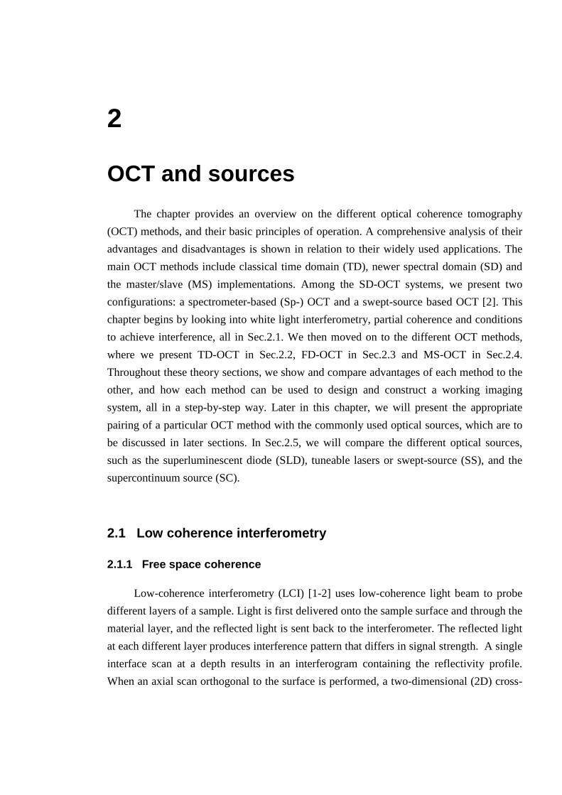
2
OCT and sources
The chapter provides an overview on the different optical coherence tomography
(OCT) methods, and their basic principles of operation. A comprehensive analysis of their
advantages and disadvantages is shown in relation to their widely used applications. The
main OCT methods include classical time domain (TD), newer spectral domain (SD) and
the master/slave (MS) implementations. Among the SD-OCT systems, we present two
configurations: a spectrometer-based (Sp-) OCT and a swept-source based OCT [2]. This
chapter begins by looking into white light interferometry, partial coherence and conditions
to achieve interference, all in Sec.2.1. We then moved on to the different OCT methods,
where we present TD-OCT in Sec.2.2, FD-OCT in Sec.2.3 and MS-OCT in Sec.2.4.
Throughout these theory sections, we show and compare advantages of each method to the
other, and how each method can be used to design and construct a working imaging
system, all in a step-by-step way. Later in this chapter, we will present the appropriate
pairing of a particular OCT method with the commonly used optical sources, which are to
be discussed in later sections. In Sec.2.5, we will compare the different optical sources,
such as the superluminescent diode (SLD), tuneable lasers or swept-source (SS), and the
supercontinuum source (SC).
2.1 Low coherence interferometry
2.1.1 Free space coherence
Low-coherence interferometry (LCI) [1-2] uses low-coherence light beam to probe
different layers of a sample. Light is first delivered onto the sample surface and through the
material layer, and the reflected light is sent back to the interferometer. The reflected light
at each different layer produces interference pattern that differs in signal strength. A single
interface scan at a depth results in an interferogram containing the reflectivity profile.
When an axial scan orthogonal to the surface is performed, a two-dimensional (2D) cross-
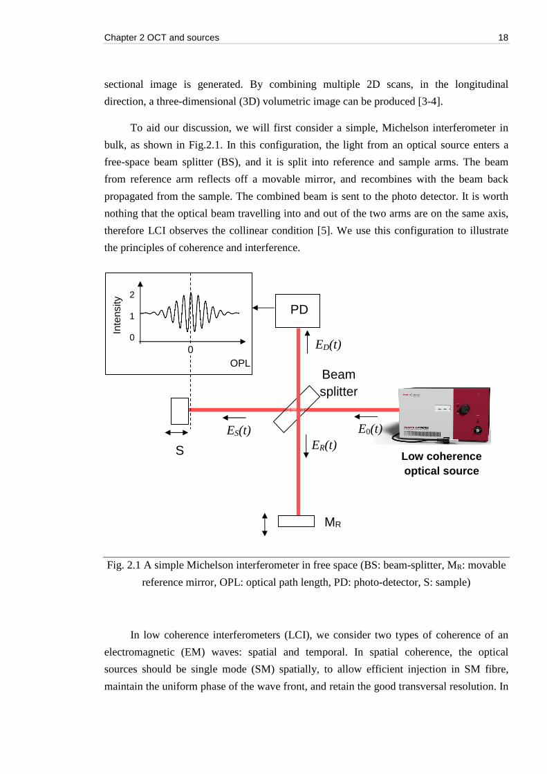
Chapter 2 OCT and sources 18
sectional image is generated. By combining multiple 2D scans, in the longitudinal
direction, a three-dimensional (3D) volumetric image can be produced [3-4].
To aid our discussion, we will first consider a simple, Michelson interferometer in
bulk, as shown in Fig.2.1. In this configuration, the light from an optical source enters a
free-space beam splitter (BS), and it is split into reference and sample arms. The beam
from reference arm reflects off a movable mirror, and recombines with the beam back
propagated from the sample. The combined beam is sent to the photo detector. It is worth
nothing that the optical beam travelling into and out of the two arms are on the same axis,
therefore LCI observes the collinear condition [5]. We use this configuration to illustrate
the principles of coherence and interference.
Fig. 2.1 A simple Michelson interferometer in free space (BS: beam-splitter, MR: movable
reference mirror, OPL: optical path length, PD: photo-detector, S: sample)
In low coherence interferometers (LCI), we consider two types of coherence of an
electromagnetic (EM) waves: spatial and temporal. In spatial coherence, the optical
sources should be single mode (SM) spatially, to allow efficient injection in SM fibre,
maintain the uniform phase of the wave front, and retain the good transversal resolution. In
Beam splitter
MR
S Low coherence optical source
PD
Inte
nsity
OPL
2
1
0 0
ER(t) ES(t) E0(t)
ED(t)
Chapter 2 OCT and sources 19
temporal coherence, the optical sources should be monochromatic, and exhibit high
correlation between phases of a light at different points in space along the direction of
propagation. The classical Michelson interferometer is based on amplitude division, and
therefore is widely used to measure the temporal coherence of a source. Interference
resulting from temporal coherence encodes the spectral content of the intensity
distribution. Light waves with wavelength λ and λ ± Δλ with constructively interfere at
some point in space until the propagation distance is equal to or longer than the coherence
length of the optical source.
The coherence length, CL, can be determined if the source central wavelength, and its
optical bandwidth are known. The actual coherence length can be calculated as in Eqn. 2.1.
λλ
π ∆≈
2)2ln(4LC (2.1)
where λ is the central wavelength and Δλ is the full-width at half maximum (FWHM)
bandwidth of the optical source.
The coherence length can be theoretically derived from the FWHM of the
autocorrelation function (AF) of the source’s electric field [6-7], denoted by the symbol
Γ(x), as shown in Eqn. 2.2.
( ) ( ) ( )∞
∞−
+=Γ ττ dxExEx (2.2)
where E(x) is the electric field, and E(x + τ) is the autocorrelation function of electric
field with time variable τ.
The autocorrelation function introduced here is related to the optical bandwidth of
light source used, by the Wiener-Khinchin theorem, which states that the Fourier transform
of the autocorrelation function was equal to the power spectral density S(v).
( ) ( ) ( )∞
∞−
Γ= τττ djkvS exp (2.3)
Our subsequent studies of noise in Chapter 3 and dispersion in Chapter 4 will involve
the relationship between Γ(x) and Δλ.
Chapter 2 OCT and sources 20
2.1.2 Interference
By referring to Fig.2.1, let us begin by writing the electric field of the light coming
out form the broadband source in Eqn.2.4. We can also write the backscattered field from
both reference and sample arms in Eqns.2.5 and 2.6, respectively.
( )tkzAE ω−= cos00 (2.4)
( ) ( )tkzARtzE RRRR ω−= cos, 0 (2.5)
( ) ( )tkzARtzE SSSS ω−= cos, 0 (2.6)
where A0 is the complex amplitude of the field, RR and RS are reflectivity of
reference and sample arms, k is the wavenumber (2π/λ), z is the propagation direction, zR
and zS are OPLs of reference and sample arms, ω is the angular frequency and t is time.
The fields and intensities detected at photodiode become Eqn.2.6 and Eqn.2.7 [6-8].
( ) ( ) ( )tzEtzEtzzE SSRRRSPD ,,,, += (2.6)
( ) ( )( )SR zzkEEEEOPDI −++= cos2 2122
21 (2.7)
After replacing OPD = zR – zS in Eqn.2.7, integrating the output intensities over the
detector bandwidth and performing an inverse FT, the photo-detected signal becomes
Eqn.2.8. The complete derivations of electric fields to photo-detected intensities can be
found in reference [4-8]. The noise and sensitivity discussions are found in Sec.3.1.3 and
Sec.3.1.5 in Chapter 3.
( ) ( )==
−++=N
nnn
N
nnnPD kzzzEEEEzI
1021
1
2,2
21 2 cos )(2 γ (2.8)
The first term in Eqn.2.8 is the DC component (21E ), which contains amplitude only
but no depth information from the sample. The second term =
N
nnE
1
2,2
is the cross
correlation, which contains the information about the sample reflectivity profile. The third
term ( )=
N
nnn kzzEE
121 2 cos )(2 γ is the autocorrelation function that contains both
interference and phase information of backscattered signals reflected off different depth
layers from the sample.
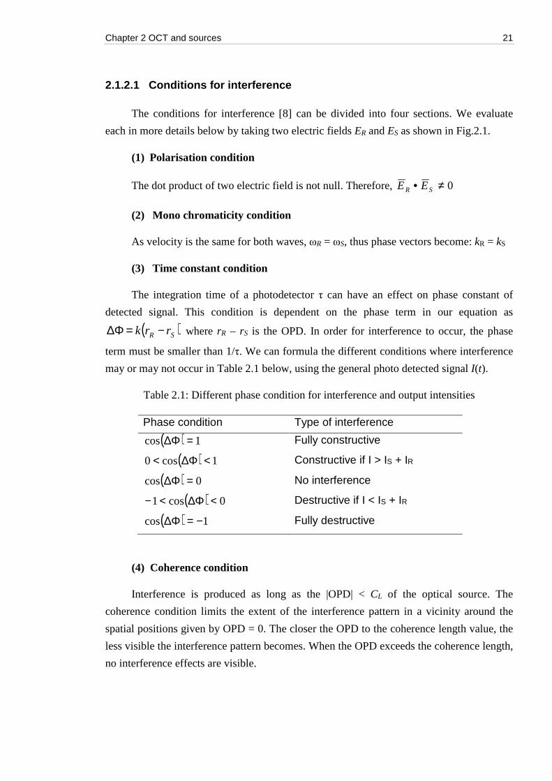
Chapter 2 OCT and sources 21
2.1.2.1 Conditions for interference
The conditions for interference [8] can be divided into four sections. We evaluate
each in more details below by taking two electric fields ER and ES as shown in Fig.2.1.
(1) Polarisation condition
The dot product of two electric field is not null. Therefore, 0≠• SR EE
(2) Mono chromaticity condition
As velocity is the same for both waves, ωR = ωS, thus phase vectors become: kR = kS
(3) Time constant condition
The integration time of a photodetector τ can have an effect on phase constant of
detected signal. This condition is dependent on the phase term in our equation as
( )SR rrk −=∆Φ where rR – rS is the OPD. In order for interference to occur, the phase
term must be smaller than 1/τ. We can formula the different conditions where interference
may or may not occur in Table 2.1 below, using the general photo detected signal I(t).
Table 2.1: Different phase condition for interference and output intensities
Phase condition Type of interference
( ) 1cos =∆Φ Fully constructive
( ) 1cos0 <∆Φ< Constructive if I > IS + IR
( ) 0cos =∆Φ No interference
( ) 0cos1 <∆Φ<− Destructive if I < IS + IR
( ) 1cos −=∆Φ Fully destructive
(4) Coherence condition
Interference is produced as long as the |OPD| < CL of the optical source. The
coherence condition limits the extent of the interference pattern in a vicinity around the
spatial positions given by OPD = 0. The closer the OPD to the coherence length value, the
less visible the interference pattern becomes. When the OPD exceeds the coherence length,
no interference effects are visible.
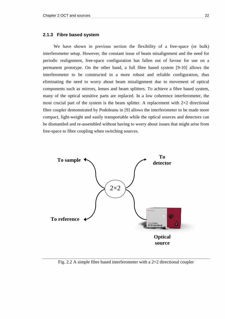
Chapter 2 OCT and sources 22
2.1.3 Fibre based system
We have shown in previous section the flexibility of a free-space (or bulk)
interferometer setup. However, the constant issue of beam misalignment and the need for
periodic realignment, free-space configuration has fallen out of favour for use on a
permanent prototype. On the other hand, a full fibre based system [9-10] allows the
interferometer to be constructed in a more robust and reliable configuration, thus
eliminating the need to worry about beam misalignment due to movement of optical
components such as mirrors, lenses and beam splitters. To achieve a fibre based system,
many of the optical sensitive parts are replaced. In a low coherence interferometer, the
most crucial part of the system is the beam splitter. A replacement with 2×2 directional
fibre coupler demonstrated by Podoleanu in [9] allows the interferometer to be made more
compact, light-weight and easily transportable while the optical sources and detectors can
be dismantled and re-assembled without having to worry about issues that might arise from
free-space to fibre coupling when switching sources.
Fig. 2.2 A simple fibre based interferometer with a 2×2 directional coupler
To detector
Optical source
To sample
To reference
2×2
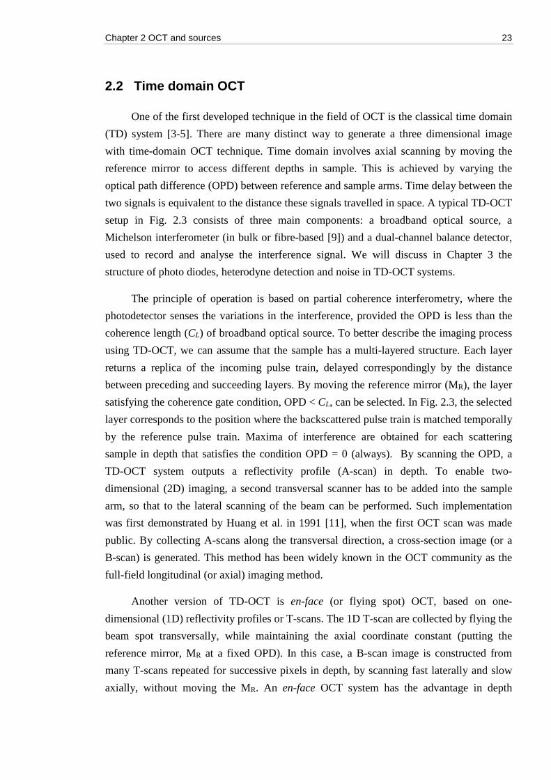
Chapter 2 OCT and sources 23
2.2 Time domain OCT
One of the first developed technique in the field of OCT is the classical time domain
(TD) system [3-5]. There are many distinct way to generate a three dimensional image
with time-domain OCT technique. Time domain involves axial scanning by moving the
reference mirror to access different depths in sample. This is achieved by varying the
optical path difference (OPD) between reference and sample arms. Time delay between the
two signals is equivalent to the distance these signals travelled in space. A typical TD-OCT
setup in Fig. 2.3 consists of three main components: a broadband optical source, a
Michelson interferometer (in bulk or fibre-based [9]) and a dual-channel balance detector,
used to record and analyse the interference signal. We will discuss in Chapter 3 the
structure of photo diodes, heterodyne detection and noise in TD-OCT systems.
The principle of operation is based on partial coherence interferometry, where the
photodetector senses the variations in the interference, provided the OPD is less than the
coherence length (CL) of broadband optical source. To better describe the imaging process
using TD-OCT, we can assume that the sample has a multi-layered structure. Each layer
returns a replica of the incoming pulse train, delayed correspondingly by the distance
between preceding and succeeding layers. By moving the reference mirror (MR), the layer
satisfying the coherence gate condition, OPD < CL, can be selected. In Fig. 2.3, the selected
layer corresponds to the position where the backscattered pulse train is matched temporally
by the reference pulse train. Maxima of interference are obtained for each scattering
sample in depth that satisfies the condition OPD = 0 (always). By scanning the OPD, a
TD-OCT system outputs a reflectivity profile (A-scan) in depth. To enable two-
dimensional (2D) imaging, a second transversal scanner has to be added into the sample
arm, so that to the lateral scanning of the beam can be performed. Such implementation
was first demonstrated by Huang et al. in 1991 [11], when the first OCT scan was made
public. By collecting A-scans along the transversal direction, a cross-section image (or a
B-scan) is generated. This method has been widely known in the OCT community as the
full-field longitudinal (or axial) imaging method.
Another version of TD-OCT is en-face (or flying spot) OCT, based on one-
dimensional (1D) reflectivity profiles or T-scans. The 1D T-scan are collected by flying the
beam spot transversally, while maintaining the axial coordinate constant (putting the
reference mirror, MR at a fixed OPD). In this case, a B-scan image is constructed from
many T-scans repeated for successive pixels in depth, by scanning fast laterally and slow
axially, without moving the MR. An en-face OCT system has the advantage in depth
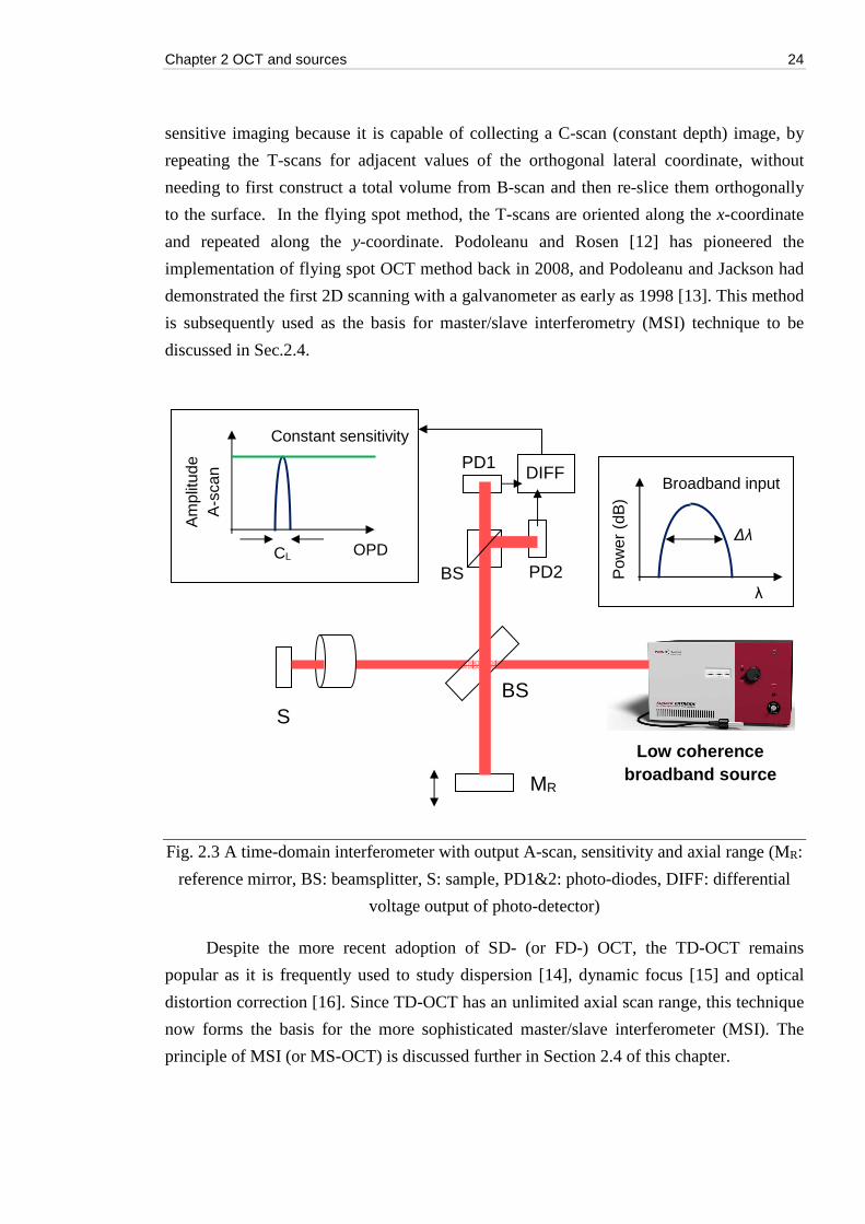
Chapter 2 OCT and sources 24
sensitive imaging because it is capable of collecting a C-scan (constant depth) image, by
repeating the T-scans for adjacent values of the orthogonal lateral coordinate, without
needing to first construct a total volume from B-scan and then re-slice them orthogonally
to the surface. In the flying spot method, the T-scans are oriented along the x-coordinate
and repeated along the y-coordinate. Podoleanu and Rosen [12] has pioneered the
implementation of flying spot OCT method back in 2008, and Podoleanu and Jackson had
demonstrated the first 2D scanning with a galvanometer as early as 1998 [13]. This method
is subsequently used as the basis for master/slave interferometry (MSI) technique to be
discussed in Sec.2.4.
Fig. 2.3 A time-domain interferometer with output A-scan, sensitivity and axial range (MR:
reference mirror, BS: beamsplitter, S: sample, PD1&2: photo-diodes, DIFF: differential
voltage output of photo-detector)
Despite the more recent adoption of SD- (or FD-) OCT, the TD-OCT remains
popular as it is frequently used to study dispersion [14], dynamic focus [15] and optical
distortion correction [16]. Since TD-OCT has an unlimited axial scan range, this technique
now forms the basis for the more sophisticated master/slave interferometer (MSI). The
principle of MSI (or MS-OCT) is discussed further in Section 2.4 of this chapter.
BS
MR
S
Constant sensitivity
Am
plitu
de
A-s
can
CL OPD
Broadband input
Pow
er (
dB)
Δλ
λ
Low coherence broadband source
PD1
PD2 BS
DIFF
Chapter 2 OCT and sources 25
2.3 Spectral domain OCT
The spectral domain (SD-) OCT is also known as Fourier domain (FD-) OCT. In this
section, we present the details of the two types of SD-OCT implementations: spectrometer
based (Sp-) and swept-source (SS-) OCT. The spectral domain method has shown beyond
doubt their capacity to produce reflectivity profiles (A-scans) from multiple depths with
very high accuracy. Therefore, the promises of high resolution, high sensitivity [17-18] and
faster measurement speed have resulted in SD-OCT becomes the de-facto method in the
industry, and has since replaced TD-OCT in many commercial systems [18].
As TD-OCT only achieves interference with backscattered lights from both arms of
the interferometer within the coherence gate of the source, SD-OCT is able to capture the
signals directly from the entire depth range. The principle of operation between the two
techniques is also different. SD-OCT detects spectrally resolved interference signals,
which are generated by the optical path difference (OPD) between the reference mirror and
the sample [17]. SD-OCT requires no depth scanning, and the acquisition speed is limited
by the read-out rate of the line-scan camera or the sweeping-rate of the laser [19]. Real-
time imaging is easily enabled because the data acquisition time in SD-OCT is much
shorter compared to TD-OCT. In addition, several papers have reported that the sensitivity
of SD-OCT to be at least 20 dB higher than that of TD-OCT [18].
The general difference between Sp-OCT and SS-OCT are (a) the light source used,
and (b) the type of detector used. In Sp-OCT, typically a broadband light source such the
supercontinuum (SC) is used to achieve better axial resolution. In the detection system Sp-
OCT, the interrogation of spectrum at the interferometer output is carried out by a
spectrometer, usually built using a prism or a diffraction grating employing a 2D linear
array or a line camera. In the case of the SS-OCT, a tuneable laser source is used to sweep
a narrowband output through a large optical bandwidth, allow the tuning the frequency of
the laser source. The detection mechanism of SS-OCT consists of photo-detectors, similar
to the one used in TD-OCT [17].
The similarities of Sp-OCT and SS-OCT are the techniques used to interrogate the
modulation of the interference spectrum to gather information about the axial reflectivity
profiles (A-scan). In both of these implementations, the A-scan is obtained by a fast
Fourier transform (FFT) of the electrical signal proportional to the shape of the channelled
spectrum at the interferometer output, hence called the SD- or FD-OCT.
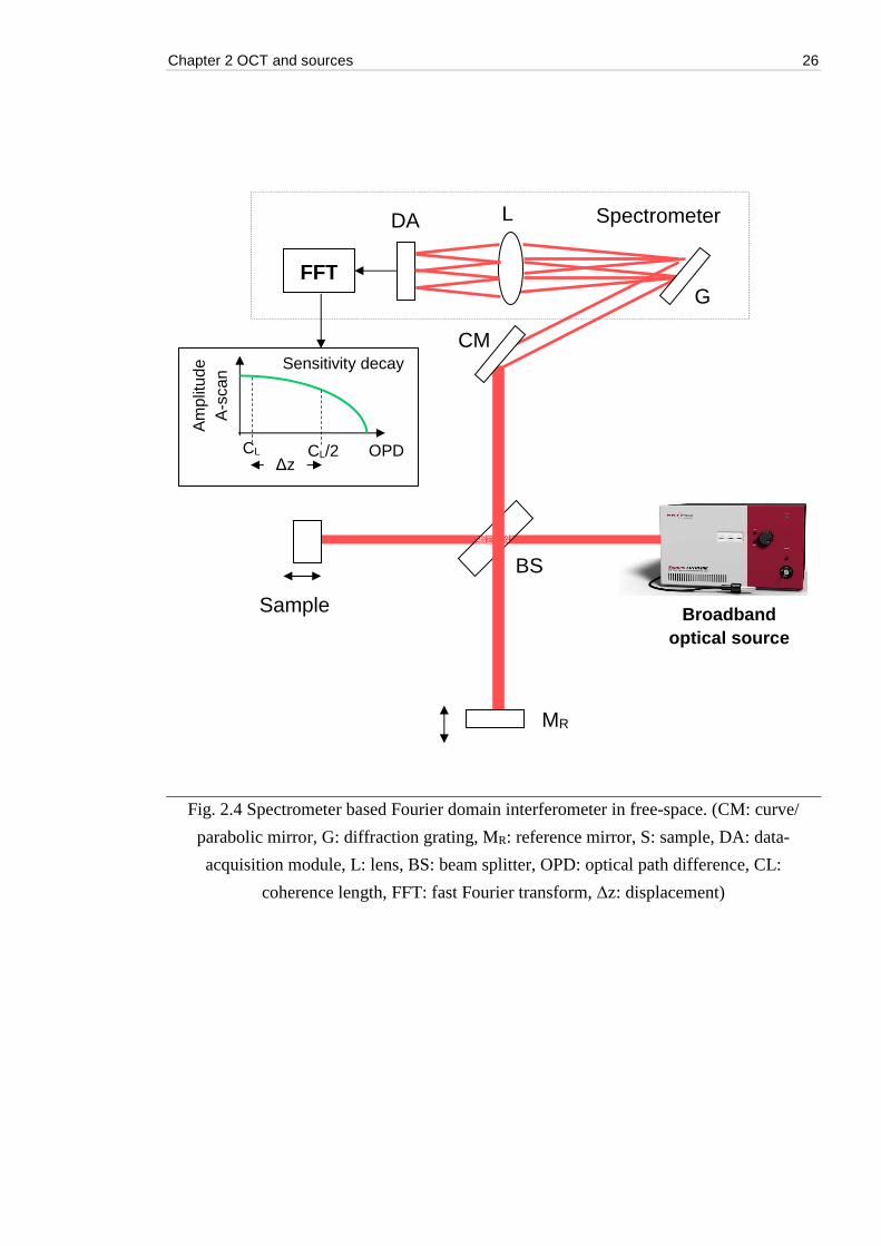
Chapter 2 OCT and sources 26
Fig. 2.4 Spectrometer based Fourier domain interferometer in free-space. (CM: curve/
parabolic mirror, G: diffraction grating, MR: reference mirror, S: sample, DA: data-
acquisition module, L: lens, BS: beam splitter, OPD: optical path difference, CL:
coherence length, FFT: fast Fourier transform, Δz: displacement)
Broadband optical source
Spectrometer
G
DA
FFT
L
OPD
Am
plitu
de
A-s
can
CL CL/2 Δz
Sensitivity decay
BS
MR
Sample
CM
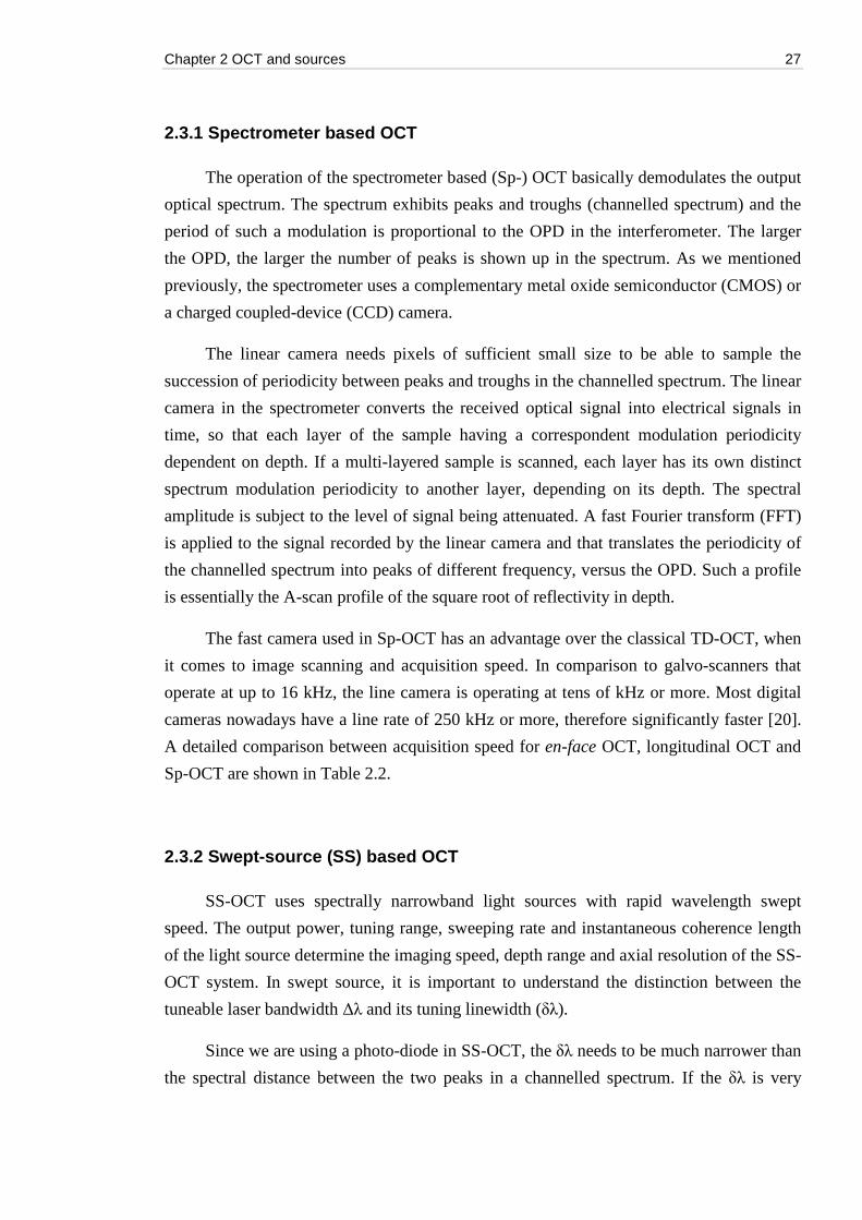
Chapter 2 OCT and sources 27
2.3.1 Spectrometer based OCT
The operation of the spectrometer based (Sp-) OCT basically demodulates the output
optical spectrum. The spectrum exhibits peaks and troughs (channelled spectrum) and the
period of such a modulation is proportional to the OPD in the interferometer. The larger
the OPD, the larger the number of peaks is shown up in the spectrum. As we mentioned
previously, the spectrometer uses a complementary metal oxide semiconductor (CMOS) or
a charged coupled-device (CCD) camera.
The linear camera needs pixels of sufficient small size to be able to sample the
succession of periodicity between peaks and troughs in the channelled spectrum. The linear
camera in the spectrometer converts the received optical signal into electrical signals in
time, so that each layer of the sample having a correspondent modulation periodicity
dependent on depth. If a multi-layered sample is scanned, each layer has its own distinct
spectrum modulation periodicity to another layer, depending on its depth. The spectral
amplitude is subject to the level of signal being attenuated. A fast Fourier transform (FFT)
is applied to the signal recorded by the linear camera and that translates the periodicity of
the channelled spectrum into peaks of different frequency, versus the OPD. Such a profile
is essentially the A-scan profile of the square root of reflectivity in depth.
The fast camera used in Sp-OCT has an advantage over the classical TD-OCT, when
it comes to image scanning and acquisition speed. In comparison to galvo-scanners that
operate at up to 16 kHz, the line camera is operating at tens of kHz or more. Most digital
cameras nowadays have a line rate of 250 kHz or more, therefore significantly faster [20].
A detailed comparison between acquisition speed for en-face OCT, longitudinal OCT and
Sp-OCT are shown in Table 2.2.
2.3.2 Swept-source (SS) based OCT
SS-OCT uses spectrally narrowband light sources with rapid wavelength swept
speed. The output power, tuning range, sweeping rate and instantaneous coherence length
of the light source determine the imaging speed, depth range and axial resolution of the SS-
OCT system. In swept source, it is important to understand the distinction between the
tuneable laser bandwidth Δλ and its tuning linewidth (δλ).
Since we are using a photo-diode in SS-OCT, the δλ needs to be much narrower than
the spectral distance between the two peaks in a channelled spectrum. If the δλ is very
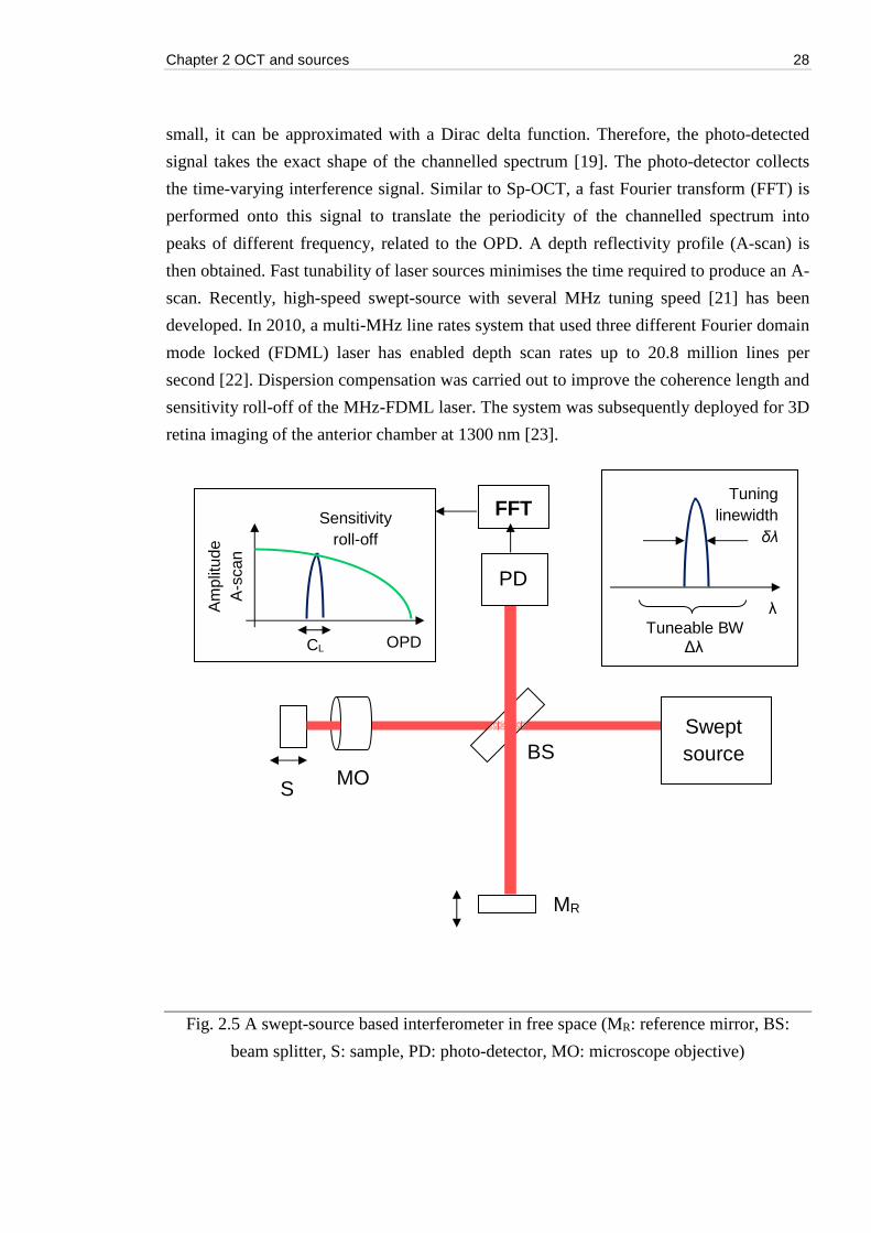
Chapter 2 OCT and sources 28
small, it can be approximated with a Dirac delta function. Therefore, the photo-detected
signal takes the exact shape of the channelled spectrum [19]. The photo-detector collects
the time-varying interference signal. Similar to Sp-OCT, a fast Fourier transform (FFT) is
performed onto this signal to translate the periodicity of the channelled spectrum into
peaks of different frequency, related to the OPD. A depth reflectivity profile (A-scan) is
then obtained. Fast tunability of laser sources minimises the time required to produce an A-
scan. Recently, high-speed swept-source with several MHz tuning speed [21] has been
developed. In 2010, a multi-MHz line rates system that used three different Fourier domain
mode locked (FDML) laser has enabled depth scan rates up to 20.8 million lines per
second [22]. Dispersion compensation was carried out to improve the coherence length and
sensitivity roll-off of the MHz-FDML laser. The system was subsequently deployed for 3D
retina imaging of the anterior chamber at 1300 nm [23].
Fig. 2.5 A swept-source based interferometer in free space (MR: reference mirror, BS:
beam splitter, S: sample, PD: photo-detector, MO: microscope objective)
Am
plitu
de
A-s
can
CL Tuneable BW
Tuning linewidth
δλ
λ
Sensitivity roll-off
Δλ
FFT
OPD
BS
MR
S MO
PD
Swept source

Chapter 2 OCT and sources 29
2.4 Master/slave OCT
2.4.1 Principles of operation
The master/slave (MS-) OCT is the most recent invention by Adrian Podoleanu and
Adrian Bradu in the Applied Optics Group (AOG). This MS-OCT technique incorporate
the advantages of time-domain, swept-source and spectrometer-based implementations,
while removing the need of better signal sampling and data linearization before the Fourier
transform (FT) processor. The MSI is based on comparing electrical signals proportional to
channelled spectrum (CS) shapes at the interferometer output. It uses correlation as
opposed to convolution in FFT. The higher the similarity of CS shapes, the larger the MSI
signal. Since no FT is required, the MSI method does not need to organize the channelled
spectrum data in equal frequency slots (or linearization). The dispersion was compensated
for by matching the lengths of fibre and placing similar lenses with those used in the object
arm, in the reference arm. With MSI, we can achieve the theoretical axial resolution
without any re-sampling or linearization. Therefore, MSI is tolerant to nonlinearities when
tuning the swept source [19, 25], and nonlinearities in the spectrometer grating [24].
The MS-OCT principle of operation involves the use of two interferometers, Master
and Slave. A Slave Interferometer (SI) first “listens” to the operation of a Master
Interferometer (MI). The SI and MI illustrated here are simple Michelson interferometers.
It consists of two sets of beam splitters (BS), reference mirrors and object mirrors, for each
interferometer. The terminology used is in Fig.2.6 are described in Table 2.2.
Table 2.2 Optical components and their abbreviations for an MSI.
Optical parts Slave interferometer (SI) Master interferometer (MI)
Beam splitter (BS) SBS MBS
Reference mirror (RM) SRM MRM
Object mirror (OM) - MOM
Object O -
More specifically, signal is acquired by the Slave Interferometer on the right, for an
OPD value determined by the Master Interferometer (MI). In the MI, the OPDM is
determined by the difference between the optical path lengths measured from the MBS to
the two mirrors, MRM and MOM. In the Slave Interferometer, the OPDS is determined by
Chapter 2 OCT and sources 30
the difference between the reference path length (measured from the SBS to the SRM) and
the object path length (measured from SBS to different scattering points in the object, O).
Fig. 2.6 A Experimental construction of master/slave interferometer based on a SS-OCT in
fibre (OS: swept source; SI: slave interferometer; DC1, 20/80 single mode directional
coupler; DC2: 50/50 single mode directional coupler; XYSH: two-dimensional lateral
scanning head; L1 to L6: lenses; O: object; MO: model object; SAB: slave acquisition
block; PhD1, PhD2: photo-detectors; DA: differential amplifier; CS(OPD): channelled
spectrum delivered by the SAB; C: multiple channel comparison block equipped with P
comparison blocks: C1, C2, …CP s; SoM: storage bank of P memories, M1, M2, …MP;
A1, A2,…AP: amplitudes of the interference signal from P scattering points inside the
object O from respective depths z1, z2, …zP; FFT: fast Fourier transformation block; PC:
personal computer implementing the blocks C, SoM, FFT and display of images) [Source:
https://www.osapublishing.org/oe/fulltext.cfm?uri=oe-21-16-19324&id=260019]
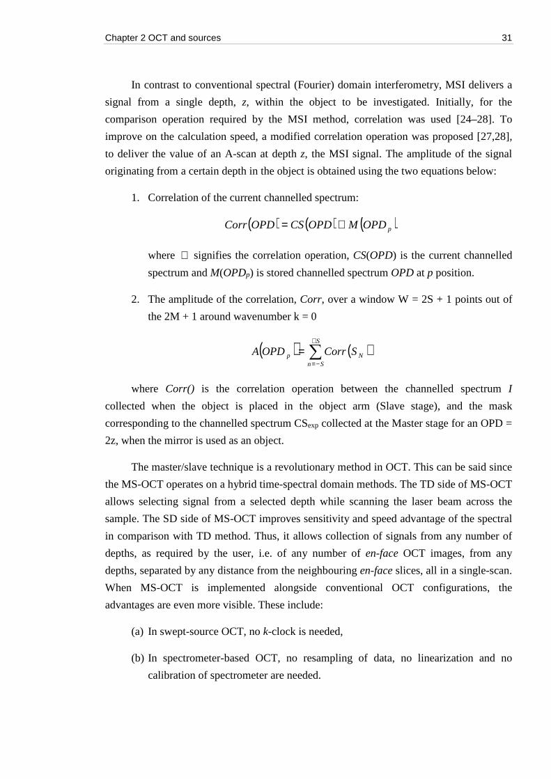
Chapter 2 OCT and sources 31
In contrast to conventional spectral (Fourier) domain interferometry, MSI delivers a
signal from a single depth, z, within the object to be investigated. Initially, for the
comparison operation required by the MSI method, correlation was used [24–28]. To
improve on the calculation speed, a modified correlation operation was proposed [27,28],
to deliver the value of an A-scan at depth z, the MSI signal. The amplitude of the signal
originating from a certain depth in the object is obtained using the two equations below:
1. Correlation of the current channelled spectrum:
( ) ( ) ( )pOPDMOPDCSOPDCorr ⊗=
where ⊗ signifies the correlation operation, CS(OPD) is the current channelled
spectrum and M(OPDp) is stored channelled spectrum OPD at p position.
2. The amplitude of the correlation, Corr, over a window W = 2S + 1 points out of
the 2M + 1 around wavenumber k = 0
( ) ( )+
−=
=S
SnNp SCorrOPDA
where Corr() is the correlation operation between the channelled spectrum I
collected when the object is placed in the object arm (Slave stage), and the mask
corresponding to the channelled spectrum CSexp collected at the Master stage for an OPD =
2z, when the mirror is used as an object.
The master/slave technique is a revolutionary method in OCT. This can be said since
the MS-OCT operates on a hybrid time-spectral domain methods. The TD side of MS-OCT
allows selecting signal from a selected depth while scanning the laser beam across the
sample. The SD side of MS-OCT improves sensitivity and speed advantage of the spectral
in comparison with TD method. Thus, it allows collection of signals from any number of
depths, as required by the user, i.e. of any number of en-face OCT images, from any
depths, separated by any distance from the neighbouring en-face slices, all in a single-scan.
When MS-OCT is implemented alongside conventional OCT configurations, the
advantages are even more visible. These include:
(a) In swept-source OCT, no k-clock is needed,
(b) In spectrometer-based OCT, no resampling of data, no linearization and no
calibration of spectrometer are needed.
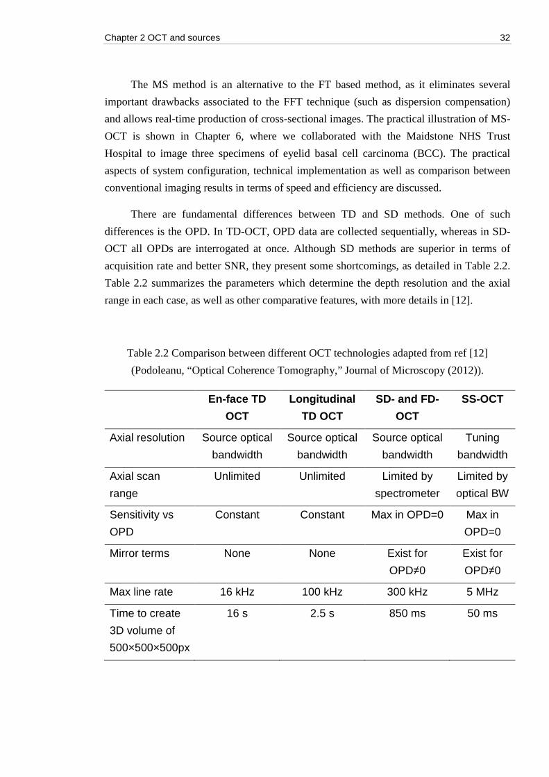
Chapter 2 OCT and sources 32
The MS method is an alternative to the FT based method, as it eliminates several
important drawbacks associated to the FFT technique (such as dispersion compensation)
and allows real-time production of cross-sectional images. The practical illustration of MS-
OCT is shown in Chapter 6, where we collaborated with the Maidstone NHS Trust
Hospital to image three specimens of eyelid basal cell carcinoma (BCC). The practical
aspects of system configuration, technical implementation as well as comparison between
conventional imaging results in terms of speed and efficiency are discussed.
There are fundamental differences between TD and SD methods. One of such
differences is the OPD. In TD-OCT, OPD data are collected sequentially, whereas in SD-
OCT all OPDs are interrogated at once. Although SD methods are superior in terms of
acquisition rate and better SNR, they present some shortcomings, as detailed in Table 2.2.
Table 2.2 summarizes the parameters which determine the depth resolution and the axial
range in each case, as well as other comparative features, with more details in [12].
Table 2.2 Comparison between different OCT technologies adapted from ref [12]
(Podoleanu, “Optical Coherence Tomography,” Journal of Microscopy (2012)).
En-face TD
OCT
Longitudinal
TD OCT
SD- and FD-
OCT
SS-OCT
Axial resolution Source optical
bandwidth
Source optical
bandwidth
Source optical
bandwidth
Tuning
bandwidth
Axial scan
range
Unlimited Unlimited Limited by
spectrometer
Limited by
optical BW
Sensitivity vs
OPD
Constant Constant Max in OPD=0 Max in
OPD=0
Mirror terms None None Exist for
OPD≠0
Exist for
OPD≠0
Max line rate 16 kHz 100 kHz 300 kHz 5 MHz
Time to create
3D volume of
500×500×500px
16 s 2.5 s 850 ms 50 ms
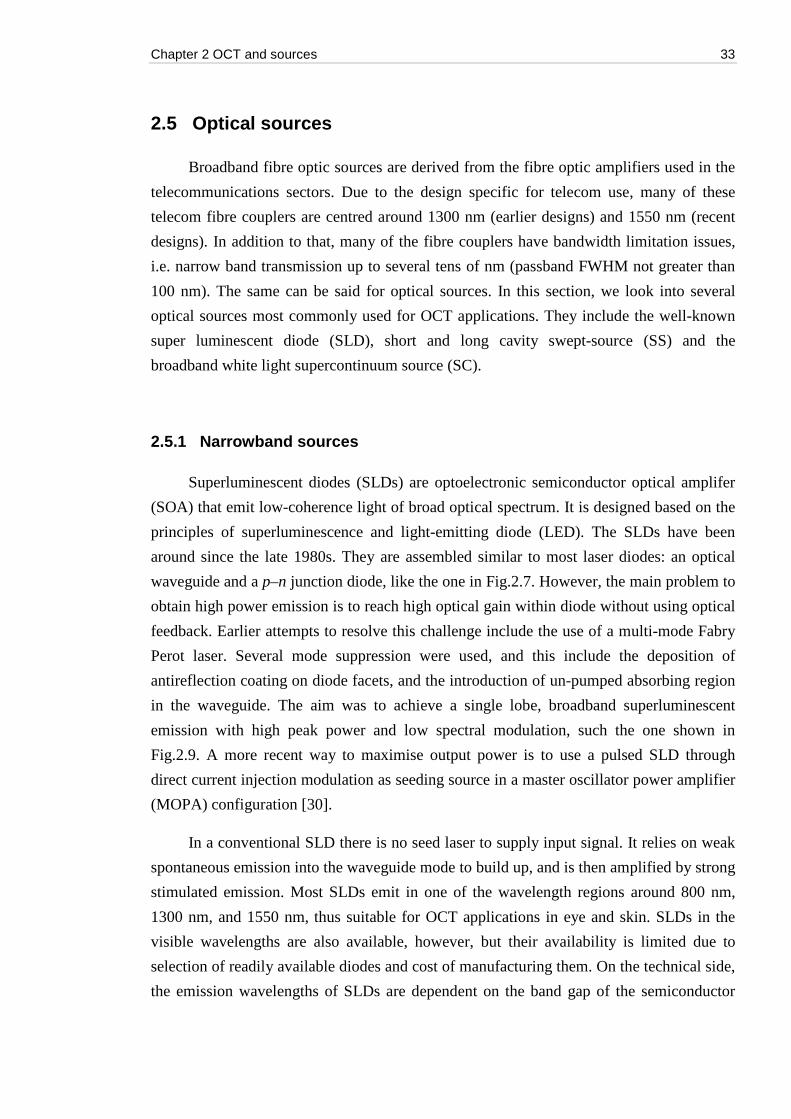
Chapter 2 OCT and sources 33
2.5 Optical sources
Broadband fibre optic sources are derived from the fibre optic amplifiers used in the
telecommunications sectors. Due to the design specific for telecom use, many of these
telecom fibre couplers are centred around 1300 nm (earlier designs) and 1550 nm (recent
designs). In addition to that, many of the fibre couplers have bandwidth limitation issues,
i.e. narrow band transmission up to several tens of nm (passband FWHM not greater than
100 nm). The same can be said for optical sources. In this section, we look into several
optical sources most commonly used for OCT applications. They include the well-known
super luminescent diode (SLD), short and long cavity swept-source (SS) and the
broadband white light supercontinuum source (SC).
2.5.1 Narrowband sources
Superluminescent diodes (SLDs) are optoelectronic semiconductor optical amplifer
(SOA) that emit low-coherence light of broad optical spectrum. It is designed based on the
principles of superluminescence and light-emitting diode (LED). The SLDs have been
around since the late 1980s. They are assembled similar to most laser diodes: an optical
waveguide and a p–n junction diode, like the one in Fig.2.7. However, the main problem to
obtain high power emission is to reach high optical gain within diode without using optical
feedback. Earlier attempts to resolve this challenge include the use of a multi-mode Fabry
Perot laser. Several mode suppression were used, and this include the deposition of
antireflection coating on diode facets, and the introduction of un-pumped absorbing region
in the waveguide. The aim was to achieve a single lobe, broadband superluminescent
emission with high peak power and low spectral modulation, such the one shown in
Fig.2.9. A more recent way to maximise output power is to use a pulsed SLD through
direct current injection modulation as seeding source in a master oscillator power amplifier
(MOPA) configuration [30].
In a conventional SLD there is no seed laser to supply input signal. It relies on weak
spontaneous emission into the waveguide mode to build up, and is then amplified by strong
stimulated emission. Most SLDs emit in one of the wavelength regions around 800 nm,
1300 nm, and 1550 nm, thus suitable for OCT applications in eye and skin. SLDs in the
visible wavelengths are also available, however, but their availability is limited due to
selection of readily available diodes and cost of manufacturing them. On the technical side,
the emission wavelengths of SLDs are dependent on the band gap of the semiconductor
Chapter 2 OCT and sources 34
diode used. A semiconductor with a larger band gap such as AlGaAs emits a shorter
wavelength, in the region of 800-900 nm. On the other hand, smaller band gap LEDs such
as the GaInAsP emits a longer wavelength, usually between 1.3 μm to 1.6 μm. When a
broader wavelength emission is necessary, the semiconductor composition can be varied to
shift the central wavelength and optical bandwidth.
Fig. 2.7 Composition of an SLD diode (source: https://www.fiberlabs-inc.com/about-sld/)
Typical output powers are in the range from a few mW to about 40 mW. Their
emission are spatially close to the diffraction-limit, therefore the spatial coherence and
beam quality are very high. The optical bandwidth of an SLD is usually in the region of
tens of nanometres, up to 150 nm for diodes emitting at 800 nm. This corresponds to a
coherence length of 1-30 μm. The bandwidths of SLDs operating at wavelengths above 1
μm are even smaller, between 30-60 nm, such as the one in Fig.2.9. Apart from that, due to
gain narrowing, there is a trade-off between higher output power and broader bandwidth.
The SLDs are notoriously known for wavelength stability and durability. Because of the
semiconductor gain medium, it is not susceptible to huge ambient temperature fluctuation
and have short intrinsic noise As such, we can expect very little wavelength drifts over
long hours of continuous operation (< 100 pm/K). Furthermore, these diodes are pretty
long-lasting, can they can have a lifetime that exceeds 20,000 hours, which are several
times more than the operational cycles of a swept-source (4000-5000 hours) or a
supercontinuum source (2000-3000 hours). The drawbacks of an SLD are bandwidth and
power limitations.
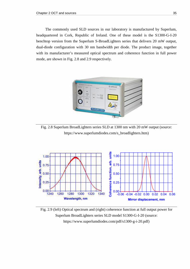
Chapter 2 OCT and sources 35
The commonly used SLD sources in our laboratory is manufactured by Superlum,
headquartered in Cork, Republic of Ireland. One of these model is the S1300-G-I-20
benchtop version from the Superlum S-BroadLighters series that delivers 20 mW output,
dual-diode configuration with 30 nm bandwidth per diode. The product image, together
with its manufacturer’s measured optical spectrum and coherence function in full power
mode, are shown in Fig. 2.8 and 2.9 respectively.
Fig. 2.8 Superlum BroadLighters series SLD at 1300 nm with 20 mW output (source:
https://www.superlumdiodes.com/s_broadlighters.htm)
Fig. 2.9 (left) Optical spectrum and (right) coherence function at full output power for
Superlum BroadLighters series SLD model S1300-G-I-20 (source:
https://www.superlumdiodes.com/pdf/s1300-g-i-20.pdf)
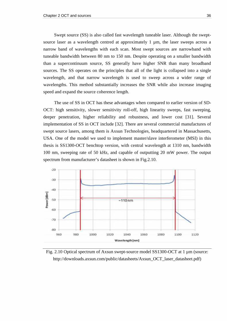
Chapter 2 OCT and sources 36
Swept source (SS) is also called fast wavelength tuneable laser. Although the swept-
source laser as a wavelength centred at approximately 1 µm, the laser sweeps across a
narrow band of wavelengths with each scan. Most swept sources are narrowband with
tuneable bandwidth between 80 nm to 150 nm. Despite operating on a smaller bandwidth
than a supercontinuum source, SS generally have higher SNR than many broadband
sources. The SS operates on the principles that all of the light is collapsed into a single
wavelength, and that narrow wavelength is used to sweep across a wider range of
wavelengths. This method substantially increases the SNR while also increase imaging
speed and expand the source coherence length.
The use of SS in OCT has these advantages when compared to earlier version of SD-
OCT: high sensitivity, slower sensitivity roll-off, high linearity sweeps, fast sweeping,
deeper penetration, higher reliability and robustness, and lower cost [31]. Several
implementation of SS in OCT include [32]. There are several commercial manufactures of
swept source lasers, among them is Axsun Technologies, headquartered in Massachusetts,
USA. One of the model we used to implement master/slave interferometer (MSI) in this
thesis is SS1300-OCT benchtop version, with central wavelength at 1310 nm, bandwidth
100 nm, sweeping rate of 50 kHz, and capable of outputting 20 mW power. The output
spectrum from manufacturer’s datasheet is shown in Fig.2.10.
Fig. 2.10 Optical spectrum of Axsun swept-source model SS1300-OCT at 1 µm (source:
http://downloads.axsun.com/public/datasheets/Axsun_OCT_laser_datasheet.pdf)
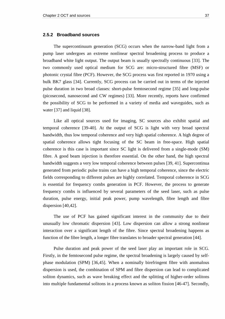
Chapter 2 OCT and sources 37
2.5.2 Broadband sources
The supercontinuum generation (SCG) occurs when the narrow-band light from a
pump laser undergoes an extreme nonlinear spectral broadening process to produce a
broadband white light output. The output beam is usually spectrally continuous [33]. The
two commonly used optical medium for SCG are: micro-structured fibre (MSF) or
photonic crystal fibre (PCF). However, the SCG process was first reported in 1970 using a
bulk BK7 glass [34]. Currently, SCG process can be carried out in terms of the injected
pulse duration in two broad classes: short-pulse femtosecond regime [35] and long-pulse
(picosecond, nanosecond and CW regimes) [33]. More recently, reports have confirmed
the possibility of SCG to be performed in a variety of media and waveguides, such as
water [37] and liquid [38].
Like all optical sources used for imaging, SC sources also exhibit spatial and
temporal coherence [39-40]. At the output of SCG is light with very broad spectral
bandwidth, thus low temporal coherence and very high spatial coherence. A high degree of
spatial coherence allows tight focusing of the SC beam in free-space. High spatial
coherence is this case is important since SC light is delivered from a single-mode (SM)
fibre. A good beam injection is therefore essential. On the other hand, the high spectral
bandwidth suggests a very low temporal coherence between pulses [39, 41]. Supercontinua
generated from periodic pulse trains can have a high temporal coherence, since the electric
fields corresponding to different pulses are highly correlated. Temporal coherence in SCG
is essential for frequency combs generation in PCF. However, the process to generate
frequency combs is influenced by several parameters of the seed laser, such as pulse
duration, pulse energy, initial peak power, pump wavelength, fibre length and fibre
dispersion [40,42].
The use of PCF has gained significant interest in the community due to their
unusually low chromatic dispersion [43]. Low dispersion can allow a strong nonlinear
interaction over a significant length of the fibre. Since spectral broadening happens as
function of the fibre length, a longer fibre translates to broader spectral generation [44].
Pulse duration and peak power of the seed laser play an important role in SCG.
Firstly, in the femtosecond pulse regime, the spectral broadening is largely caused by self-
phase modulation (SPM) [36,45]. When a nominally birefringent fibre with anomalous
dispersion is used, the combination of SPM and fibre dispersion can lead to complicated
soliton dynamics, such as wave breaking effect and the splitting of higher-order solitons
into multiple fundamental solitons in a process known as soliton fission [46-47]. Secondly,
Chapter 2 OCT and sources 38
when the SCG process involves pumping with pulses in the picosecond time regime,
stimulated Raman scattering (SRS) and four-wave mixing (FWM) can cause pulse-to-pulse
intensity fluctuation to increase [48-51], therefore producing higher relative intensity noise
(RIN) at the output. Finally, SCG using seed laser with CW and longer fibres (greater than
100 m) has also been explored previously [52-54]. However, this CW regime is not the
main area of research in NKT Photonics.
The noise properties of the generated continua are different in different parts of the
spectrum [52]. When pumped with short pulses of 5 ps or less, SPM is the major nonlinear
process. The phase coherence of the generated supercontinuum pulses can be very high,
even after these pulses experienced massive spectral broadening [56-57]. The noise is
time-invariant and deterministic, and can be modelled with NLSE (nonlinear nonlinear
Schrödinger equation). However, when higher-order soliton effects are involved, the SCG
process can be very sensitive to even the smallest intensity fluctuations from the seed laser,
resulting in huge differences in the properties of one pulse relative to another [58]. These
fluctuations (or commonly known as relative intensity noise, RIN) can affect the stability
of SCG process. It is therefore essential that we characterise the RIN and produce low-
noise SC for better OCT imaging [59-62]. We have dedicated Sec.3.2 in Chapter 3 to study
RIN, analyse the characteristics of pulses in generated supercontinua, and to find out the
different factors that influenced them.
Nevertheless, the strongly nonlinear interaction of pulses within the SCG process
makes it extremely complex to predict noise behaviours [51]. Thus, numerical simulation
and pulse propagation modelling is required. In this project, despite a thorough
experimental study on noise with SC sources were carried out [59], some of our results
remained difficult to explain until future modelling is done.
Since NKT Photonics is our industry partner, we have access to their commercial SC
sources, such as the SuperK Extreme and Fianium Whitelase. The SuperK Extreme models
features the EXR series shown in Fig. 2.11). The EXR9 is the low-noise version and
EXR20 is the high power version. In this thesis, we used the EXR9 for polarisation
sensitive OCT in Chapter 5, and EXR20 for retinal decoding in Chapter 7. Apart from that,
NKT Photonics also produces a compact version of SC source, the SuperK Compact
(Fig.2.12). We used SuperK Compact in Chapter 3 to characterise the birefringence of
nonlinear fibre (NLF) used in noise and polarisation measurements. The output spectra for
SuperK EXR and SuperK Compact are shown in Fig.2.13.
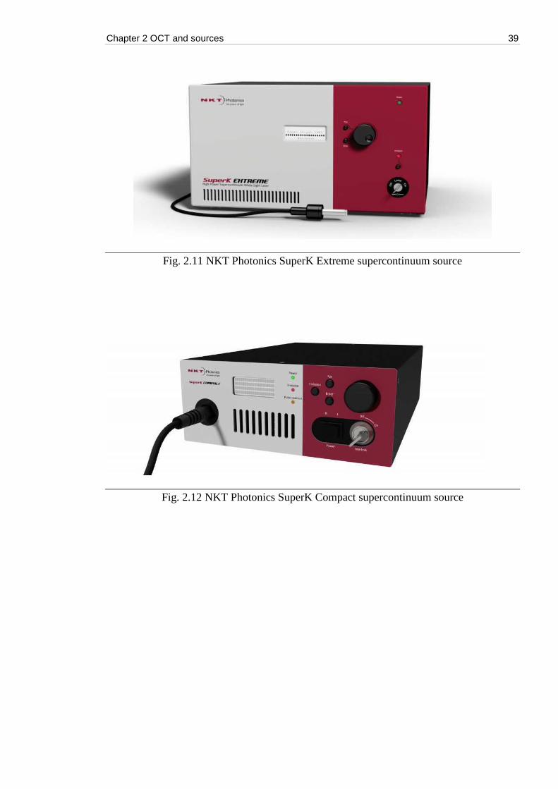
Chapter 2 OCT and sources 39
Fig. 2.11 NKT Photonics SuperK Extreme supercontinuum source
Fig. 2.12 NKT Photonics SuperK Compact supercontinuum source
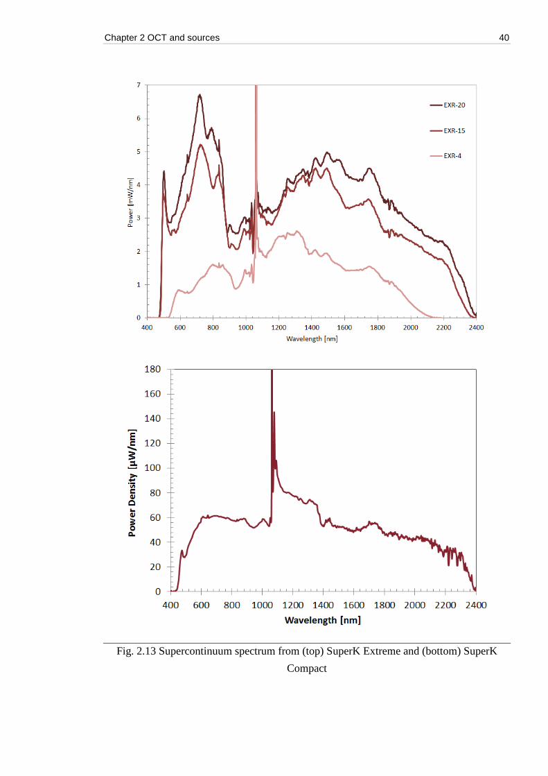
Chapter 2 OCT and sources 40
Fig. 2.13 Supercontinuum spectrum from (top) SuperK Extreme and (bottom) SuperK
Compact
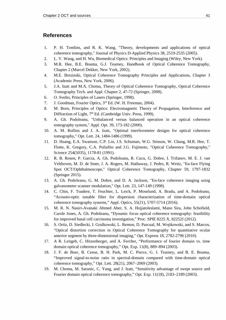
Chapter 2 OCT and sources 41
References
1. P. H. Tomlins, and R. K. Wang, "Theory, developments and applications of optical coherence tomography," Journal of Physics D-Applied Physics 38, 2519-2535 (2005).
2. L. V. Wang, and H. Wu, Biomedical Optics: Principles and Imaging (Wiley, New York). 3. M.R. Hee, B.E. Bouma, G.J. Tearney, Handbook of Optical Coherence Tomography,
Chapter 2 (Marcel Dekker, New York, 2002). 4. M.E. Brezinski, Optical Coherence Tomography Principles and Applications, Chapter 3
(Academic Press, New York, 2006). 5. J.A. Izatt and M.A. Choma, Theory of Optical Coherence Tomography, Optical Coherence
Tomography Tech. and Appl. Chapter 2, 47-72 (Springer, 2008). 6. O. Svelto, Principles of Lasers (Springer, 1998). 7. J. Goodman, Fourier Optics, 3rd Ed. (W. H. Freeman, 2004). 8. M. Born, Principles of Optics: Electromagnetic Theory of Propagation, Interference and
Diffraction of Light, 7th Ed. (Cambridge Univ. Press, 1999). 9. A. Gh. Podoleanu, "Unbalanced versus balanced operation in an optical coherence
tomography system," Appl. Opt. 39, 173-182 (2000). 10. A. M. Rollins and J. A. Izatt, "Optimal interferometer designs for optical coherence
tomography," Opt. Lett. 24, 1484-1486 (1999). 11. D. Huang, E.A. Swanson, C.P. Lin, J.S. Schuman, W.G. Stinson, W. Chang, M.R. Hee, T.
Flotte, K. Gregory, C.A. Puliafito and J.G. Fujimoto, "Optical Coherence Tomography," Science 254(5035), 1178-81 (1991).
12. R. B. Rosen, P. Garcia, A. Gh. Podoleanu, R. Cucu, G. Dobre, I. Trifanov, M. E. J. van Velthoven, M. D. de Smet, J. A. Rogers, M. Hathaway, J. Pedro, R. Weitz, "En-face Flying Spot OCT/Ophthalmoscope," Optical Coherence Tomography, Chapter 59, 1797-1832 (Springer 2015).
13. A. Gh. Podoleanu, G. M. Dobre, and D. A. Jackson, "En-face coherence imaging using galvanometer scanner modulation," Opt. Lett. 23, 147-149 (1998).
14. C. Chin, F. Toadere, T. Feuchter, L. Leick, P. Moselund, A. Bradu, and A. Podoleanu, “Acousto-optic tunable filter for dispersion characterization of time-domain optical coherence tomography systems,” Appl. Optics, 55(21), 5707-5714 (2016).
15. M. R. N. Nasiri-Avanaki Ahmed Aber, S. A. Hojjatoleslami, Mano Sira, John Schofield, Carole Jones, A. Gh. Podoleanu, “Dynamic focus optical coherence tomography: feasibility for improved basal cell carcinoma investigation,” Proc. SPIE 8225 X, 82252J (2012).
16. S. Ortiz, D. Siedlecki, I. Grulkowski, L. Remon, D. Pascual, M. Wojtkowski, and S. Marcos, "Optical distortion correction in Optical Coherence Tomography for quantitative ocular anterior segment by three-dimensional imaging," Opt. Express 18, 2782-2796 (2010).
17. A R. Leitgeb, C. Hitzenberger, and A. Fercher, “Performance of fourier domain vs. time domain optical coherence tomography,” Opt. Exp. 11(8), 889–894 (2003).
18. J. F. de Boer, B. Cense, B. H. Park, M. C. Pierce, G. J. Tearney, and B. E. Bouma, “Improved signal-to-noise ratio in spectral-domain compared with time-domain optical coherence tomography,” Opt. Lett. 28(21), 2067–2069 (2003).
19. M. Choma, M. Sarunic, C. Yang, and J. Izatt, “Sensitivity advantage of swept source and Fourier domain optical coherence tomography,” Opt. Exp. 11(18), 2183–2189 (2003).
Chapter 2 OCT and sources 42
20. L. An, P. Li, T. Shen and R. Wang, “High speed spectral domain optical coherence
tomography for retinal imaging at 500,000 A̻lines per second,” Biomed. Opt. Expr. 2(10),
2770–2783 (2011). 21. W. Wieser, B. R. Biedermann, T. Klein, C. M. Eigenwillig, and R. Huber, "Multi-Megahertz
OCT: High quality 3D imaging at 20 million A-scans and 4.5 GVoxels per second," Opt. Express 18, 14685-14704 (2010).
22. W. Wieser, T. Klein, D. C. Adler, F. Trépanier, C. M. Eigenwillig, S. Karpf, J. M. Schmitt and R. Huber, “Extended coherence length megahertz FDML and its application for anterior segment imaging,” Biomed. Opt. Expr. 3(10), 2647–2657 (2012).
23. B. Potsaid, B. Baumann, D. Huang, S. Barry, A. E. Cable, J. S. Schuman, J. S. Duker, J. G. Fujimoto, “Ultrahigh speed 1050nm swept source/Fourier domain OCT retinal and anterior segment imaging at 100,000 to 400,000 axial scans per second,” Opt. Express 18(19), 20029–20048 (2010).
24. Adrian Gh. Podoleanu and Adrian Bradu, “Master–slave interferometry for parallel spectral domain interferometry sensing and versatile 3D optical coherence tomography,” Opt. Express 21, 19324-19338 (2013).
25. Adrian Bradu and Adrian Gh. Podoleanu, “Calibration-free B-scan images produced by master/slave optical coherence tomography,” Opt. Lett. 39, 450-453 (2014).
26. Adrian Bradu, Michael Maria, and Adrian Gh. Podoleanu, “Demonstration of tolerance to dispersion of master/slave interferometry,” Opt. Express 23, 14148-14161 (2015).
27. Adrian Bradu, Sylvain Rivet, and Adrian Podoleanu, “Master/slave interferometry – ideal tool for coherence revival swept source optical coherence tomography,” Biomed. Opt. Express 7, 2453-2468 (2016).
28. Adrian Bradu and Adrian Gh. Podoleanu, “Imaging the eye fundus with real-time en-face spectral domain optical coherence tomography,” Biomed. Opt. Express 5, 1233-1249 (2014)
29. C. Chin, A. Bradu, R. Lim, M. Khandwala, J. Schofield, L. Leick, and A. Podoleanu, “Master/slave optical coherence tomography imaging of eyelid basal cell carcinoma,” Appl. Opt. 55, 7378-7386 (2016)
30. M. Melo, J. M. Sousa, J. R. Salcedo, “Superluminescent diode versus Fabry-Perot laser diode seeding in pulsed MOPA fiber laser systems for SBS suppression,” Proc. SPIE 9344XII, 93440I (2015).
31. S. Kishi, “Impact of swept source optical coherence tomography on ophthalmology,” Taiwan J. Ophthalmology, 6(2), 58-68 (2016).
32. M. Choma, K. Hsu, J. A. Izatt, “Swept source optical coherence tomography using an all-fiber 1300-nm ring laser source,” J. Biomedical Opt. 10(4), 044009 (2005).
33. J. M. Dudley, G. Genty, S. Coen, “Supercontinuum generation in photonic crystal fiber ,” Rev. Modern Phy. 78, 1135-117 (2006).
34. R. R. Alfano and S. L. Shapiro, “Emission in the Region 4000 to 7000 Å Via Four-Photon Coupling in Glass,” Phys. Rev. Lett. 24, 584 (1970).
35. F. Poletti and P. Horak, "Dynamics of femtosecond supercontinuum generation in multimode fibers," Opt. Express 17, 6134-6147 (2009).
36. S. Coen, A. H. L. Chau, R. Leonhardt, J. D. Harvey, J. C. Knight, W. J. Wadsworth, and P. St. J. Russell, "White-light supercontinuum generation with 60-ps pump pulses in a photonic crystal fiber," Opt. Lett. 26, 1356-1358 (2001).
Chapter 2 OCT and sources 43
37. J. A. Dharmadhikari, G. Steinmeyer, G. Gopakumar, D. Mathur, and A. K. Dharmadhikari, "Femtosecond supercontinuum generation in water in the vicinity of absorption bands," Opt. Lett. 41, 3475-3478 (2016)
38. L. Wang, Y.X. Fan, Z.D. Yan, H.T. Wang, and Z.L. Wang, "Flat-plateau supercontinuum generation in liquid absorptive medium by femtosecond filamentation," Opt. Lett. 35, 2925-2927 (2010).
39. I. Zeylikovich and R.R. Alfano, “Coherence properties of the supercontinuum source,” Appl. Phys. B, 77(2–3), 265–268 (2003).
40. V. A. Semenova, A. V. Tsypkin, S. E. Putilin and V. G. Bespalov, “A method for the coherence measurement of the supercontinuum source using Michelson interferometer,” J. Phys. Conf. S. 536, 012027 (2014).
41. I. Zeylikovich, V. Kartazaev and R. R. Alfano, "Spectral, temporal, and coherence properties of supercontinuum generation in microstructure fiber," J. Opt. Soc. Am. B 22, 1453-1460 (2005).
42. E. Baubeau, F. Salin, C. Le Blanc, “Spatio-temporal coherence properties of super-continuum single filament in bulk media,” Springer S. in Chem. Phys. Vol.63, Ultrafast Phenomena XI, 81-83 (1998).
43. K. Saitoh, M. Koshiba, T. Hasegawa, and E. Sasaoka, "Chromatic dispersion control in photonic crystal fibers: application to ultra-flattened dispersion," Opt. Express 11, 843-852 (2003)
44. A. Díez et al., "Control of the chromatic dispersion of photonic crystal fibers for supercontinuum and photon pairs generation," 11th Intl. Conf. LFNM, 1-2 (2011).
45. M. Suzuki, M. Baba, S. Yoneya and H. Kuroda, “Efficient spectral broadening of supercontinuum in photonic crystal fiber with self-phase modulation induced by femtosecond laser pulse,” Appl. Phys. Lett. 101(19), 1110 (2012).
46. S. W. Harun, R. Akbari, H. Arof, H. Ahmad, “Supercontinuum generation in photonic crystal fiber using femtosecond pulses,” Laser Physics, 21(7), 1215–1218 (2011).
47. G. Genty, M. Lehtonen, and H. Ludvigsen, “Spectral broadening of femtosecond pulses into continuum radiation in microstructured fibers,” Opt. Expr. 10 (20), 1083-1098 (2002).
48. M. Liao, W. Gao, T. Cheng, Z. Duan, X. Xue, T. Suzuki and Y. Ohishi, “Flat and broadband supercontinuum generation by four-wave mixing in a highly nonlinear tapered microstructured fiber,” Opt. Expr. 20(26), B574-580 (2012).
49. W. Yu, R. R. Alfano, C. L. Sam and R. J. Seymour, “Spectral broadening of picosecond 1.06 µm pulse in KBr,” Opt. Commun. 14, 344-347 (1975).
50. S. Coen, A. Hing Lun Chau, R. Leonhardt, J. D. Harvey, J. C. Knight, W. J. Wadsworth and P. St. J. Russell, “Supercontinuum generation by stimulated Raman scattering and parametric four-wave mixing in photonic crystal fibers,” J. Opt. Soc. Am. B 19, 753-764 (2002).
51. S. Pitois, G. Millot and P. Tchofo Dinda, “Influence of parametric four-wave mixing effects on stimulated Raman scattering in bimodal optical fibers,” Opt. Lett. 23, 1456-1458 (1998).
52. Y. Yu, S. Ruan, J. Zhao and C. Du, “Continuous-wave supercontinuum generation in a 100-m high nonlinear photonic crystal fiber,” Proc. of SPIE Vol. 6279, 62791B-1 (2007).
53. M. Prabhu, N. S. Kim and K. Ueda, “Ultra-Broadband CW Supercontinuum Generation Centered at 1483.4 nm from Brillouin/Raman Fiber Laser,” Japanese J. Appl. Physics, 39(2), 4A (2000).
Chapter 2 OCT and sources 44
54. W. Gao, M. Liao, X. Yan, T. Suzuki, Y. Ohishi, “Quasi-CW supercontinuum generation in a HNLF pumped by sub-microsecond pulse,” IEEE Xplore 17th Opto-Electron. Comm. Conf. 200-201 (2012).
55. B. Wetzel, A. Stefani, L. Larger, P. A. Lacourt, J. M. Merolla, T. Sylvestre, A. Kudlinski, A. Mussot, G. Genty, F. Dias, J. M. Dudley, “Real-time full bandwidth measurement of spectral noise in supercontinuum generation,” Sci. Rep. 2(882), 1-7 (2012).
56. A. Zaytsev, C.H. Lin, Y.J. You, C.C. Chung, C.L. Wang and C.L. Pan, “Supercontinuum generation by noise-like pulses transmitted through normally dispersive standard single-mode fibers,” Opt. Expr. 21(13), 16056-16062 (2013).
57. B. E. Olsson, P. Ohlen and D. I. Blumenthal, "Noise in sliced self-phase modulation broadened spectrum," CLEO Technical Digest. 39, 207-208 (2000).
58. T. Schreiber, J. Limpert, H. Zellmer and A. Tunnermann, "Radio frequency noise of femto- and picosecond pulse generated supercontinuum spectra," CLEO Conference vol.2, 2 (2004).
59. W. J. Brown, S. Kim and A. Wax, “Noise Characterization of Supercontinuum Sources for Low Coherence Interferometry Applications,” J. Opt. Society Amer. A, 31(12), 2703–2710 (2014).
60. N. R. Newbury, B. R. Washburn, and K. L. Corwin, “Noise amplification during supercontinuum generation in microstructure fiber,” Opt. Lett. 28(11), 944-946 (2003).
61. N. I. Nikolov, T. Sørensen, O. Bang, A. Bjarklev and J. J. Rasmussen, “Modelling of supercontinuum generation in highly nonlinear photonic crystal fibres,” J. Optical Fiber Comm. Rep. 5(1–6), 1–21 (2008).
62. C. Chin, R. D. Engelsholm, P. M. Moselund, T. Feuchter, L. Leick, A. Podoleanu, O. Bang, “Polarization extinction ratio and polarization dependent intensity noise in long-pulse supercontinuum generation,” SPIE Proceedings Vol. 10089, 100890L (2017).
3
Noise and polarisation in ultra-broadband OCT imaging
Noise measurement is an integral part of performance analysis in optical coherence
tomography (OCT) system. The ability to improve signal-to-noise (SNR) for imaging
relies on quantitative analysis of noise factors, both from the laser source, and those in the
system. Noise in these systems is mainly caused by non-optimised optical configurations
and sensitivity of the detection system. The detection mechanism used, such as homodyne
or heterodyne can largely influence the noise. The difference in noise level is contributed
by the difference in detector noise floor, photo-electrons dynamics of diodes, and the noise
current. In our analysis of noise in Section 3.1, we consider a low-coherence Michelson
interferometer applicable for different modalities of OCT techniques. This includes the
classical time-domain (TD) system, to more recent Fourier domain (FD); swept source
based spectral domain (SD) and the master-slave (MS) interferometer systems.
The signal-to-noise provides a relative measure of noise performance of the source.
This is largely caused by the waveguide reflectivity and optical components used to
construct the OCT system. At the source, optical power levels predominantly influence
how much noise power is generated. At this stage of the characterisation process, noise can
be classified into three broad categories: thermal noise (TN), shot noise (SN) and excess
photon noise (EPN). In the vast majority of publication, the emphasis is placed on thermal
and shot noises, while neglecting EPN.
The typical optical sources used are mainly the super luminescent diodes (SLD) and
tuneable lasers such as swept source (SS). These optical sources have limited spectral
bandwidth, usually between 70 nm to about 100 nm. However, with the advent of mode-
locked lasers that offer femtosecond pulses and very high peak power, to supercontinuum
(SC) sources with very broad optical bandwidth, additional noise power terms become
significant.
Chapter 3 Noise and polarisation in ultra-broadband OCT imaging 46
In terms of optical bandwidth, we look into various factors that can affect the SNR of
a fibre-coupled OCT system with balance detection. These factors typically include fibre-
end reflectivity, cross-coupling efficiency, optical power at the source, and the beatings
between various frequency components of a spectrum, in the case when a broadband
optical source is used. A detailed comparison between SLD and SC sources reveals the
influence of the optical source bandwidth on EPN power.
Various concepts of improving SNR using experiment of noise measurement in time
domain OCT system have been suggested since the last decade. Sorin & Barney (1992) [1]
proposed that by attenuating reference arm power deliberately while maintaining power in
object arm could suppress relative intensity noise (RIN) from the source. This method can
be achieved by using a fibre coupler with unequal splitting ratios. We will present in sub-
section 3.1.1 on how to allocate 20% incident power into the reference arm and 80% into
the sample arm. In another experiment published by Takada et al. (1998) [2], the team
illustrated that by employing a balance detection technique based on coherent heterodyne
principle, it is sufficient to overcome thermal and electrical noise caused by the instability
of receiver electronics circuitry. This method eliminates the need to manipulate reference
arm parameters. Subsequently, in a year later, Rollins et al. (1999) [3] showed that besides
relative intensity noise (RIN) and thermal noise, the power required in the OCT system to
achieve shot noise threshold can be lowered using a dual-balance interferometer design. As
a result, they managed to improve the overall SNR of a time domain OCT system by a
factor of 6, using only up to 1 mW of source power.
As recent as in 2006, Haskell and Yoshino et al. [4] reported that despite various
efforts in previous researches to eliminate different noise terms to improve SNR in OCT
systems, none of them have taken into account an extra noise term called beat noise,
despite being discovered by Mandel back in 1962 [5]. Beat noise (BN) is optical line width
dependent. However, Haskell et al. suggested that balance detection can suppress beat
noise, but only for source powers up to a few milliwatts. In addition, the effect of
broadening the spectra bandwidth of the source allows an improvement in axial resolution
and depth penetration of OCT system. When combined with low-noise high sensitivity
detection mechanism, the use of broadband sources could make sub-micron resolution in-
vivo imaging practical with the classical time domain OCT configuration.
In the second part of this chapter (Section 3.2), we’ll look into the effect of
polarisation extinction ratio (PER) and polarisation dependent RIN in SC sources.
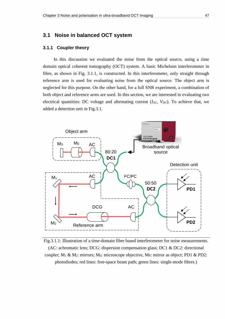
Chapter 3 Noise and polarisation in ultra-broadband OCT imaging 47
3.1 Noise in balanced OCT system
3.1.1 Coupler theory
In this discussion we evaluated the noise from the optical source, using a time
domain optical coherent tomography (OCT) system. A basic Michelson interferometer in
fibre, as shown in Fig. 3.1.1, is constructed. In this interferometer, only straight through
reference arm is used for evaluating noise from the optical source. The object arm is
neglected for this purpose. On the other hand, for a full SNR experiment, a combination of
both object and reference arms are used. In this section, we are interested in evaluating two
electrical quantities: DC voltage and alternating current (IAC, VDC). To achieve that, we
added a detection unit in Fig.3.1.
Fig.3.1.1: Illustration of a time-domain fibre based interferometer for noise measurements.
(AC: achromatic lens; DCG: dispersion compensation glass; DC1 & DC2: directional
coupler; M1 & M 2: mirrors; M0: microscope objective, Ms: mirror as object; PD1 & PD2:
photodiodes; red lines: free-space beam path; green lines: single-mode fibres.)
Reference arm
DC1
DC2 PD1
PD2
80:20
50:50
DCG AC
M1
M2
FC/PC AC
AC MS M0
Object arm
Broadband optical source
Detection unit
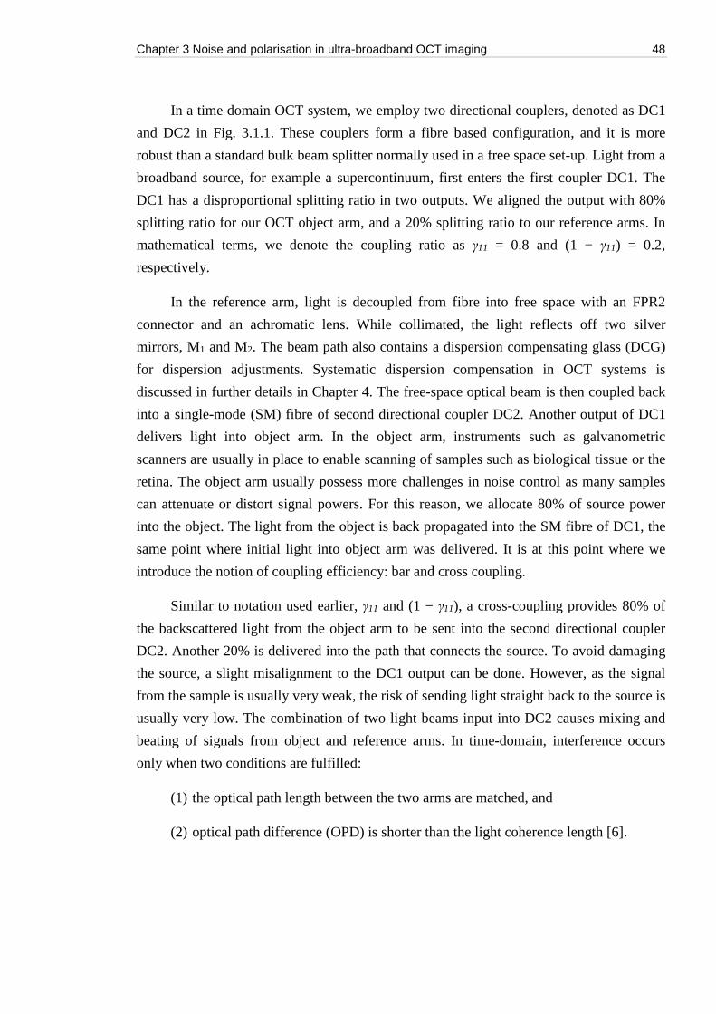
Chapter 3 Noise and polarisation in ultra-broadband OCT imaging 48
In a time domain OCT system, we employ two directional couplers, denoted as DC1
and DC2 in Fig. 3.1.1. These couplers form a fibre based configuration, and it is more
robust than a standard bulk beam splitter normally used in a free space set-up. Light from a
broadband source, for example a supercontinuum, first enters the first coupler DC1. The
DC1 has a disproportional splitting ratio in two outputs. We aligned the output with 80%
splitting ratio for our OCT object arm, and a 20% splitting ratio to our reference arms. In
mathematical terms, we denote the coupling ratio as γ11 = 0.8 and (1 − γ11) = 0.2,
respectively.
In the reference arm, light is decoupled from fibre into free space with an FPR2
connector and an achromatic lens. While collimated, the light reflects off two silver
mirrors, M1 and M2. The beam path also contains a dispersion compensating glass (DCG)
for dispersion adjustments. Systematic dispersion compensation in OCT systems is
discussed in further details in Chapter 4. The free-space optical beam is then coupled back
into a single-mode (SM) fibre of second directional coupler DC2. Another output of DC1
delivers light into object arm. In the object arm, instruments such as galvanometric
scanners are usually in place to enable scanning of samples such as biological tissue or the
retina. The object arm usually possess more challenges in noise control as many samples
can attenuate or distort signal powers. For this reason, we allocate 80% of source power
into the object. The light from the object is back propagated into the SM fibre of DC1, the
same point where initial light into object arm was delivered. It is at this point where we
introduce the notion of coupling efficiency: bar and cross coupling.
Similar to notation used earlier, γ11 and (1 − γ11), a cross-coupling provides 80% of
the backscattered light from the object arm to be sent into the second directional coupler
DC2. Another 20% is delivered into the path that connects the source. To avoid damaging
the source, a slight misalignment to the DC1 output can be done. However, as the signal
from the sample is usually very weak, the risk of sending light straight back to the source is
usually very low. The combination of two light beams input into DC2 causes mixing and
beating of signals from object and reference arms. In time-domain, interference occurs
only when two conditions are fulfilled:
(1) the optical path length between the two arms are matched, and
(2) optical path difference (OPD) is shorter than the light coherence length [6].
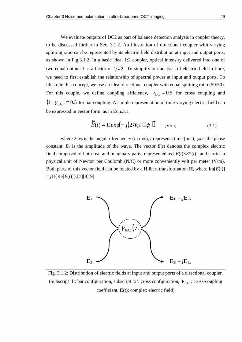
Chapter 3 Noise and polarisation in ultra-broadband OCT imaging 49
We evaluate outputs of DC2 as part of balance detection analysis in coupler theory,
to be discussed further in Sec. 3.1.2. An illustration of directional coupler with varying
splitting ratio can be represented by its electric field distribution at input and output ports,
as shown in Fig.3.1.2. In a basic ideal 1:2 coupler, optical intensity delivered into one of
two equal outputs has a factor of 21 . To simplify our analysis of electric field in fibre,
we need to first establish the relationship of spectral power at input and output ports. To
illustrate this concept, we use an ideal directional coupler with equal splitting ratio (50:50).
For this couple, we define coupling efficiency, 5.0=BALγ for cross coupling and
( ) 5.01 =− BALγ for bar coupling. A simple representation of time varying electric field can
be expressed in vector form, as in Eqn.3.1:
( )( )002exp)( ϕπ +−= tvjEtEρ
[V/m] (3.1)
where 2πv0 is the angular frequency (in m/s), t represents time (in s), φ0 is the phase
constant, E0 is the amplitude of the wave. The vector E(t) denotes the complex electric
field composed of both real and imaginary parts, represented as | E(t)×E*( t) | and carries a
physical unit of Newton per Coulomb (N/C) or more conveniently volt per meter (V/m).
Both parts of this vector field can be related by a Hilbert transformation H, where Im[E(t)]
= jH{Re[E(t)]}.[7][8][9]
Fig. 3.1.2: Distribution of electric fields at input and output ports of a directional coupler.
(Subscript ‘l’: bar configuration, subscript ‘x’: cross configuration, BALγ : cross-coupling
coefficient, E(t): complex electric field)
E1l – jE2x
E2l – jE1x
E1
E2
( )vBALγ
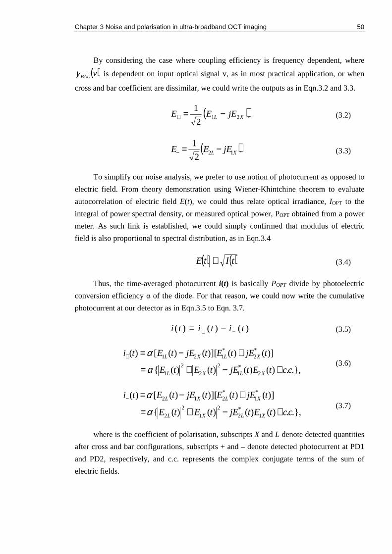
Chapter 3 Noise and polarisation in ultra-broadband OCT imaging 50
By considering the case where coupling efficiency is frequency dependent, where
( )vBALγ is dependent on input optical signal v, as in most practical application, or when
cross and bar coefficient are dissimilar, we could write the outputs as in Eqn.3.2 and 3.3.
( ),2
121 XL jEEE −=+ (3.2)
( ).2
112 XL jEEE −=− (3.3)
To simplify our noise analysis, we prefer to use notion of photocurrent as opposed to
electric field. From theory demonstration using Wiener-Khintchine theorem to evaluate
autocorrelation of electric field E(t), we could thus relate optical irradiance, IOPT to the
integral of power spectral density, or measured optical power, POPT obtained from a power
meter. As such link is established, we could simply confirmed that modulus of electric
field is also proportional to spectral distribution, as in Eqn.3.4
( ) ( )tItE ∝ (3.4)
Thus, the time-averaged photocurrent i(t) is basically POPT divide by photoelectric
conversion efficiency α of the diode. For that reason, we could now write the cumulative
photocurrent at our detector as in Eqn.3.5 to Eqn. 3.7.
)()()( tititi −+ −= (3.5)
.},.)()()()({
)]()()][()([ )(
2*1
2
2
2
1
*2
*121
cctEtjEtEtE
tjEtEtjEtEti
XLXL
XLXL
+−+=
+−=+
α
α (3.6)
.},.)()()()({
)]()()][()([ )(
1*2
2
1
2
2
*1
*212
cctEtjEtEtE
tjEtEtjEtEti
XLXL
XLXL
+−+=
+−=−
α
α (3.7)
where is the coefficient of polarisation, subscripts X and L denote detected quantities
after cross and bar configurations, subscripts + and – denote detected photocurrent at PD1
and PD2, respectively, and c.c. represents the complex conjugate terms of the sum of
electric fields.
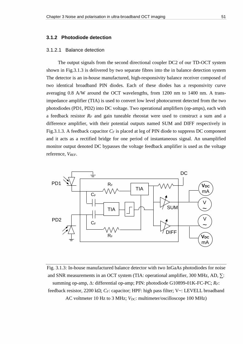
Chapter 3 Noise and polarisation in ultra-broadband OCT imaging 51
3.1.2 Photodiode detection
3.1.2.1 Balance detection
The output signals from the second directional coupler DC2 of our TD-OCT system
shown in Fig.3.1.3 is delivered by two separate fibres into the in balance detection system
The detector is an in-house manufactured, high-responsivity balance receiver composed of
two identical broadband PIN diodes. Each of these diodes has a responsivity curve
averaging 0.8 A/W around the OCT wavelengths, from 1200 nm to 1400 nm. A trans-
impedance amplifier (TIA) is used to convert low level photocurrent detected from the two
photodiodes (PD1, PD2) into DC voltage. Two operational amplifiers (op-amps), each with
a feedback resistor RF and gain tuneable rheostat were used to construct a sum and a
difference amplifier, with their potential outputs named SUM and DIFF respectively in
Fig.3.1.3. A feedback capacitor CF is placed at leg of PIN diode to suppress DC component
and it acts as a rectified bridge for one period of instantaneous signal. An unamplified
monitor output denoted DC bypasses the voltage feedback amplifier is used as the voltage
reference, VREF.
Fig. 3.1.3: In-house manufactured balance detector with two InGaAs photodiodes for noise
and SNR measurements in an OCT system (TIA: operational amplifier, 300 MHz, AD, ∑:
summing op-amp, Δ: differential op-amp; PIN: photodiode G10899-01K-FC-PC; RF:
feedback resistor, 2200 kΩ; CF: capacitor; HPF: high pass filter; V~: LEVELL broadband
AC voltmeter 10 Hz to 3 MHz; VDC: multimeter/oscilloscope 100 MHz)
TIA
TIA
DC
RF
V ~
VDC mA
CF
CF
SUM
DIFF RF
V ~
VDC mA
PD1
PD2
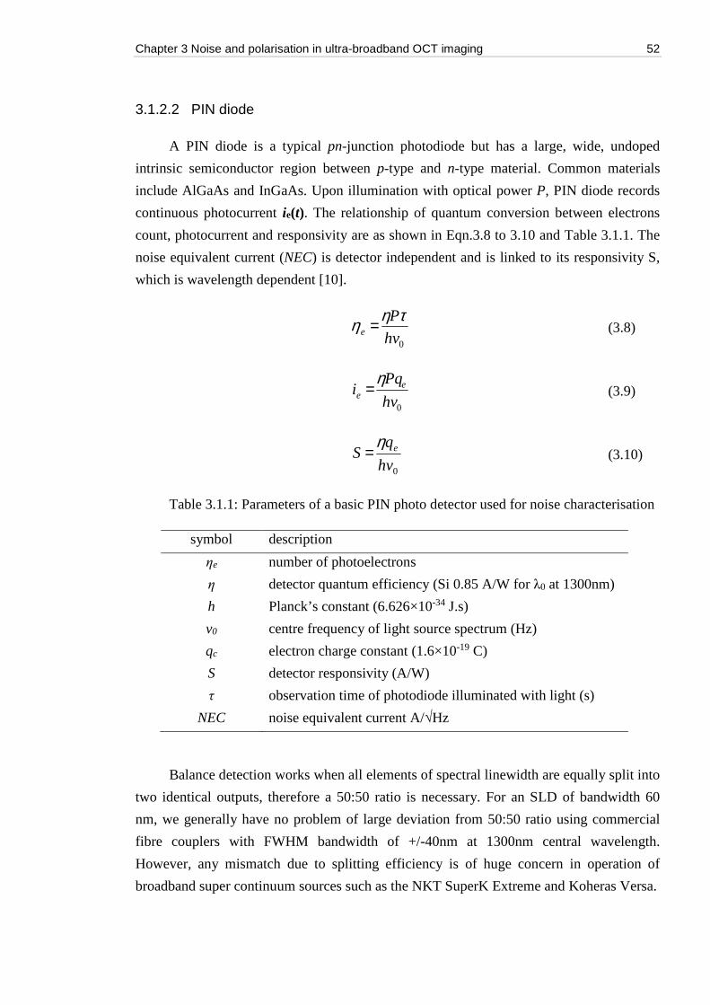
Chapter 3 Noise and polarisation in ultra-broadband OCT imaging 52
3.1.2.2 PIN diode
A PIN diode is a typical pn-junction photodiode but has a large, wide, undoped
intrinsic semiconductor region between p-type and n-type material. Common materials
include AlGaAs and InGaAs. Upon illumination with optical power P, PIN diode records
continuous photocurrent ie(t). The relationship of quantum conversion between electrons
count, photocurrent and responsivity are as shown in Eqn.3.8 to 3.10 and Table 3.1.1. The
noise equivalent current (NEC) is detector independent and is linked to its responsivity S,
which is wavelength dependent [10].
0hv
Pe
τηη = (3.8)
0hv
Pqi ee
η= (3.9)
0hv
qS eη
= (3.10)
Table 3.1.1: Parameters of a basic PIN photo detector used for noise characterisation
symbol description
ηe number of photoelectrons
η detector quantum efficiency (Si 0.85 A/W for λ0 at 1300nm)
h Planck’s constant (6.626×10⁻³⁴ J.s)
v0 centre frequency of light source spectrum (Hz)
qc electron charge constant (1.6×10⁻¹⁹ C)
S detector responsivity (A/W)
τ observation time of photodiode illuminated with light (s)
NEC noise equivalent current A/√Hz
Balance detection works when all elements of spectral linewidth are equally split into
two identical outputs, therefore a 50:50 ratio is necessary. For an SLD of bandwidth 60
nm, we generally have no problem of large deviation from 50:50 ratio using commercial
fibre couplers with FWHM bandwidth of +/-40nm at 1300nm central wavelength.
However, any mismatch due to splitting efficiency is of huge concern in operation of
broadband super continuum sources such as the NKT SuperK Extreme and Koheras Versa.
Chapter 3 Noise and polarisation in ultra-broadband OCT imaging 53
These sources have very large optical bandwidth. When used with an OCT system at
800 nm, typical bandwidth of 300 nm can be expected. Therefore, to make detection
compatible with all these broadband implementations, we need to take into account of
different noise power as some of them can negatively degrade our system SNR. The most
common occurrence is the huge photocurrent fluctuation in many narrowband detectors.
The choices of broadband detectors are limited, and even if they are available, can be
costly. One option is heterodyne detection. Heterodyne signal detection in time-domain
OCT system can suppress flicker noise (generally known as 1/f noise) for signal bandwidth
above audible frequency (AF) range, generally 20 kHz or higher. A heterodyne balanced
detection system can additionally suppress low frequencies excess noise (Sec.3.1.3.3) that
present in a non-balanced or homodyne configuration. Heterodyne detection can be
achieved by allowing short exposure time (< 10 µs) to PIN diode at measurement. Further
implementation is discussed in the noise measurement section.
3.1.3 Noise theory
Noise is defined as the mean square fluctuation (MSF, <Δn²>) of random number of
electrons on a photodiode over illuminated area A, over observation duration Δτ [11]. The
evaluation of noise takes into account of fluctuations of the envelope power of AC current
on the detector that resulted in a cross coupling efficiency (γBAL) of 0.5. As such, the
interference signal )(tiAC can then be written as in Eqn.3.11 based on derivation of electric
field in Eqns.3.6 and 3.7. Similarly, the DC current terms can be expressed as in Eqn.3.12.
.].)()(..)()([
)()()(*21
*12 cctEtjEcctEtjE
tititi
LxLX
acac
+++−+=
−= −+
α (3.11)
{ }{ })()(
)()()()(
)()()(
21
2121
tPtP
tPtPtPtP
tititi
LXXL
dc
+=
+−+=−= −+
αα (3.12)
where α is the coefficient of polarisation, c.c. indicates complex conjugates,
subscripts X and L denote detected quantities after cross and bar configurations, subscripts
+ and – denote detected photocurrent at PD1 and PD2, respectively.
Chapter 3 Noise and polarisation in ultra-broadband OCT imaging 54
Photocurrent response for OCT system at detector output can be expressed by taking
into account the cross-coupling terms of first directional coupler (DC1) and power from
both arms of interferometer (PREF and POBJ). Instantaneous photocurrents can be written as
sum of optical power multiplied by photodiode responsivity for an equal split output from
second directional coupler DC2, with 50% cross efficiency cancellation. Therefore, we
could express <i²(t)> the photo detected signal as in Eqn.3.13 [1].
( )00
22cos2)( ϕπα −= tvPPti OBJREF (3.13)
where α is the coefficient of polarisation, 2πv0 is the angular frequency of light
source (in Hz), φ0 is the phase constant of the interfering light.
To take a look into the different noise terms, let us now consider a light beam from a
single-mode non-polarised source. The root mean square (RMS) value of photocurrent
fluctuation measured across a resistor at photodiode output can be described in Eqn.3.14.
The equation combines two noise terms: shot noise (SN) and excess photon noise (EPN).
[ ]eff
ELECDCDCELECDCDC
eff
ELECdcelecdc
EPNshotrms
v
BIIBIIq
v
BIBIq
III
∆++=
∆+=
∆+∆=∆
,2,1,2,1
2
222
2 2
2 2 (3.14)
where BELEC is the electrical bandwidth (Hz), Δveff is the effective frequency of light
source (in Hz) and qe is the electron charge constant (1.6×10⁻¹⁹ C).
3.1.3.1 Shot noise
Shot noise is produced in OCT system by beating between signals from fibre-end end
reflection and reference arm, and is proportional to elementary electric charge qe. The
mean photocurrent 2(IDC) for shot noise can be further evaluated on contribution from
cumulated currents of <I1> + <I2> due to fibre-end reflection IFER, and that due to reference
arm signal IREF. As such, shot noise power can be written as in Eqn.3.15.
( )212 2 PPBqi ELECeSN +=∆ α (3.15)
where α is the coefficient of polarisation, BELEC is the electrical bandwidth (Hz) and
qe is the electron charge constant (1.6×10⁻¹⁹ C).
Chapter 3 Noise and polarisation in ultra-broadband OCT imaging 55
In a classical light analysis theory, shot noise is generated by a constant intensity
signal, from photon fluctuation in the same spin state falling onto the detector area, within
a coherence time of observation (τ). The distribution of these photon follow a probability
distribution in Eqn.3.15, and it obeys the Poisson’s statistical formulae with a mean square
fluctuation (MSF) of <Δn²> = <n>. By taking into account of PIN photodiode quantum
efficiency, α, we could write Eqn.3.16.
!)(
n
ennP
nn ><−
= (3.16)
nn α=∆ 2 (3.17)
3.1.3.2 Excess photon noise
Excess photon noise (EPN) is produced by the beating of Fourier components within
the broadband optical spectrum, and its resulting noise power is inversely proportional to
optical bandwidth Δveff of the source, as defined in Eqn.3.18. EPN is also technically called
wave interaction noise or photon-bunching effect for that matter. We can therefore analyse
EPN is the form of photon fluctuation in the particle nature of light.
[ ] =∆ dvvPdvvPveff )()( 22 (3.18)
By referring to Eqn.3.17, we could model this noise as <n>², effectively adding a
second noise term to make it becomes Eqn.3.19, subject to condition that coherence time
of an optical source τC is smaller than coherence time of our detector τE. By considering the
inverse proportionality between time and bandwidth, the linewidth of our source ought to
be much larger than our detector bandwidth.
22 nnn αα +=∆ with condition (τC << τE) (3.19)
By relating Eqn.3.19 to Eqn.3.15, we could re-write it such that it follows the Bose-
Einstein photon counting distribution. The resulting expression in Eqn.3.20 is the general
expression for MSF of random photon, which is both strict sense stationary and ergodic.
1)1()( ++=
n
n
n
nnP (3.20)
Chapter 3 Noise and polarisation in ultra-broadband OCT imaging 56
The mean square current fluctuation in Eqn.3.14 can therefore be obtained by
multiplying both sides of Eqn.3.19 with (qE/τ)² and grouping the term <n> qE/τ = IDC as the
time-varying photocurrent at detector output. Therefore, the final form of EPN as becomes
OPT
ELECDCEPN B
BII 22 )(2α=∆ (3.21)
with 2
2
2
1212 PPPPI DC ++= (3.22)
To demonstrate the existence of excess noise current in bandwidth dependent
broadband sources, as opposed to laser, we look into a comparison made by Morkel et al.
(Southampton, 1989) between a HeNe laser and a 2 nm SLD source. In their noise
characteristic measurement, a detection system employing a 500 kHz low-noise trans
impedance amplifier (TIA) was used to monitor signal fluctuation within a 100 kHz
electrical bandwidth to achieve signal-to-noise sensitivity over 600:1 and eliminate 1/f
noise from SLD source. They recorded a 10 dB/decade of signal for SLD vs 5 dB/decade
for HeNe. For this reason, they have shown in their experiment that, using noise curve
from SLD output, due to an additional EPN term, total detected power increased by the
power of two with respect to input signal IDC. The measurement was done against a linear
trend observed for HeNe laser. The HeNe laser is shot-noise-limited. Our interest to
broadband OCT imaging will likely involve optical sources with bandwidth greater than
300 nm. The use of a supercontinuum (SC) source, such as SuperK Extreme from NKT
Photonics A/S is a preferred choice. However, the issue of shot noise in a SC source will
have to be evaluated thoroughly. For this reason, a dedicated experimental section in this
chapter, Section 3.2.3 will discuss SN and EPN in SC in more details. The ratio, REPN/SN
of excess photon noise to shot noise for both coherent and incoherent sources can be
verified as in Eqn.3.23, subjecting to bandwidth of both optical source (BOPT) and detector
(BELEC), for incoherent light fluctuations the inequality in Eqn.3.24 holds.
6/ 10
2−<=
ELECe
DCSNEPN Bq
IR (3.23)
OPT
ELECDCDCELECe B
BIIBq 22 >> (3.24)
where BELEC is the electrical bandwidth (Hz), BOPT is the optical bandwidth (Hz) and
qe is the electron charge constant (1.6×10⁻¹⁹ C).
Chapter 3 Noise and polarisation in ultra-broadband OCT imaging 57
3.1.3.3 Excess noise at low frequencies
A. Frequency dependent limitation
As measurement of noise power spans across several decades of frequencies, the use
of a band pass filter to restrict measurement range is important. We can typically evaluate
noise suppression performance up to generally 100 kHz without considering contribution
of 1/f noise terms. However, in this case, effect of quantum noise suppression in audio
frequency (AF) band is difficult to quantify without resorting to expensive equipment such
as lock-in amplifier and high speed oscilloscope. In addition to EPN dependent on
linewidth of optical sources mentioned above, several articles had also identified causes of
excess noise at low frequency, in the audible range, up to 10 kHz, especially in the
detection mechanism, to be discussed further in detailed in the following sub-section.
In low frequency detection, such as the most commonly used balance detection
technique, the use passive electronic components like resistors, capacitors, inductors and
op-amps in detection circuitry cannot be avoided. Many of these semiconductor parts have
parasitic effect that is dependent on frequency. Detector sensitivity therefore has a
frequency roll off effect. Detector units operating at frequency at a few 100 kHz will
remain susceptible to a different IV response than analysis at audio frequencies.
B. Optical beam limitation
Another source of noise at low frequencies is beam jitter. Beam jitter occurs due to
backscattering from mainly biological tissue sample, or object with imperfect surface and
refractive indices. The primary concern in dealing with beam jitter is the distortion of beam
quality, mode of transmission in fibre. It has to be noted that not all Gaussian shaped beam
spot is re-injected back into single mode (SM) fibre core, and that can lead to fibre-end
reflectivity – another undesirable effect in a free space to fibre OCT system. On the
spectral side, independent to dispersion in the interferometer, this beam jittering issue often
resulted in non-overlapping of Fourier components in a bandwidth in the interferometer,
making spectral density of output beam non time invariant to the source beam. For
example, a full 300 nm broadband light in measured in free space section of the
interferometer, while at the detector, the measured optical bandwidth becomes
narrowband.
Chapter 3 Noise and polarisation in ultra-broadband OCT imaging 58
Parasite interference is predominantly caused by optical alignment imperfection and
non-optimisation of beam splitting ratios in a bulk beam splitter or within a directional
coupler. Without an ideal γBAL = 0.5 splitting efficiency, this often leads to unequal
photocurrents subtraction due to spectral shape distortion between light beams at two
photodiodes. In addition to parasitic effect at detector, stray reflections due to scattering of
light from original path beam in either sample arm due to surface imperfection or reference
arm due to dust also able to alter non-coherence beam at interference.
C. Semiconductor limitation
Photosensitive diodes with built-in p-n junction also contribute to dark current
production resulted from random generation of electrons and holes within the depletion
region of these devices. As a result, even at very low dark current magnitude of a few
pA/√Hz, evaluating non-linearity of noise terms differentiating shot and excess noise at
this current level is difficult.
D. Signal processing, filtering & rectification constraints
This phenomenon is due to signal amplification process. Ideally difference in
photocurrents between two outputs (LO–local oscillator and IF–intermediate frequency)
will result in subtraction to product differential value. However, non-subtracted
photocurrent with frequency component above AF range will continue to degrade amplifier
performance with increase in intensity noise ratio to amplified signal. In most practical
case, despite use of low-noise amplifiers (LNAs) in the detector system, quantum noise
remain to dominate noise power up to 10 kHz. Major disadvantage of using a non-balanced
configuration is to provide flexibility to cancel photocurrents that are differ from LO value.
As we select our electrical noise bandwidth for frequency analysis, we employ a
linear, time-invariant (LTI) filter for this process. When we pass a time varying, non-white
spectral response photocurrents into this electronic filter, we expect to have output signal
that is at least wide-sense stationary, where its 1st moment and auto covariance is invariant
with respect to time. Nevertheless, the frequency response of the filter and integrated
circuit does vary in time, resulting in non-white noise, signal whose power spectral density
is not constant but random, and its joint probability density function (JPDF), mean and
covariance changes with time.
Chapter 3 Noise and polarisation in ultra-broadband OCT imaging 59
3.1.3.4 Thermal noise
This form of noise is caused by the load resistor in a balance detector shown in
Fig.3.2 is time incoherent and independent to noise produced by optical sources. The
variance of thermal noise power due to circuit resistance and limitation of electrical
bandwidth on analogue-to-digital conversion (ADC) process can be written as in Eqn.3.25.
elecload
Belecthermal B
R
TkBNEPi
4)(2 =>=∆< (3.25)
where Belec is the electrical bandwidth of the detector, kB is the Boltzmann constant, T
is the ambient room temperature (300 K), Rload is the resistance value (in Ω), NEP is the
noise equivalent power (A.Hz-1/2) as defined in Table 3.1. Thermal noise usually has very
little effect to overall noise power, and therefore is negligible for most noise analysis.
3.1.3.5 Beat noise
Haskell et al. [4] disputed many findings by OCT researchers in area related to noise
performance analysis. They have further noted that many previous publications had
omitted an additional noise term – beat noise – in their Michelson interferometer system.
The concept of beat noise, or loosely defined as fourth order interference in signal
processing, can be obtained by correlating signals from two photodetectors that are
separated in both space and time. It was first discovered by Alford and Gold back in 1958,
when they showed a time delay produce by an interferometer with optical path difference
(OPD) that is much greater than the light source coherence length (LC). This effect has a
correlated intensity fluctuation, in the form of a spectral modulation that was observed as a
result of parametric down-conversion of correlated photon pairs in a superposition state.
According to Haskell et al. [4] and Mandel [5], the beat noise term is equal in
magnitude but distinct from the cross term in the usual Bose-Einstein photon-bunching
effect. The main cause of beat noise is not due to beatings between various frequency
components in a spectral bandwidth, but rather due to two partially coherent and
incoherent beams (PCOH and PINCOH) reflected off a multi-layered material with varying
refractive index. Independent of material dispersion, refractive index differences as a
function of depth and thickness in an object can cause the backscattered beam to attenuate
in signal strength, propagate at different speed, and lose spatial coherence at detector.
Chapter 3 Noise and polarisation in ultra-broadband OCT imaging 60
By referring to our Eqn.3.2, according to claims by Haskell et al. [4], this beat noise
current term can be written as in Eqn.3.26:
[ ]2122 2 PP
B
BI
opt
elecBeat α=∆ (3.26)
where α is the coefficient of polarisation, Belec is the electrical bandwidth, Bopt is the
optical bandwidth, P1 and P2 are received power at photodiodes 1 and 2.
A detailed analysis carried out by Yoshino et al. [12] and affirmed by Haskell has
demonstrated that beat noise, as similar to EPN term, is due to the changes in total optical
power spectrum incident upon the PIN photodiodes causing interference in two partially
coherent beams. The main reasoning could be laid upon wavelength dependent coupling
efficiency shown in section 3.1.1 of this thesis.
3.1.3.6 Total noise power
Total noise power at output of balance detector can be written as sum of thermal
noise, shot noise, excess photon noise and beat noise. As we assume an equal splitting ratio
of 50:50 for the second directional couple DC2 under balance condition, the spectra
response between its input and output is invariant, the contribution of frequency
component shift is null. We could theoretically rewrite the total noise power to become
Eqn.3.27, by combining Eqns. 3.14-3.15, 3.21, 3.25-3.26.
{ }
+
∆+++=∆
210
2
2
2
1221
2 21
22
PPv
PPPPq
R
TkBi e
L
Belec αα (3.27)
where α is the coefficient of polarisation, Belec is the electrical bandwidth, Bopt is the
optical bandwidth, P1 and P2 are received power at photodiodes PD1 and PD2, kB is the
Boltzmann constant, T is the ambient room temperature (300 K), RL is the load resistance
(in Ω), v0 is the central frequency of light source (in Hz), qe is the electron charge constant
(1.6×10⁻¹⁹ C).
Chapter 3 Noise and polarisation in ultra-broadband OCT imaging 61
3.1.4 SNR and sensitivity
3.1.4.1 SNR
Signal-to-noise ratio (SNR) is a relative measure of superiority of detectable signal
with respect to degradation in signal quality resulting from various events of photoelectron
fluctuation in both input and output of photodetector system at unity bandwidth. By
considering an optical source of different frequencies and random phases in a sinusoidal
wave field, with a Gaussian component of noise due to spontaneous emission, electrical,
thermal and mechanical instability in Eqn.3.1, we could derive a probability density
function of noise p(v) in the Gaussian form as a function of SNR in Eqns.3.28 and 3.29.
( ) cos)( 000 noiseVtVtv ++= ϕω (3.28)
2noiseV
VSNR= (3.29)
where ω0 is the angular frequency (in m/s), t represents time (in s), φ0 is the phase
constant, V0 is the amplitude of the signal and Vnoise is the noise voltage.
3.1.4.2 Sensitivity
Sensitivity (∑) of TD-OCT system in Eqn.3.30 can be achieved with minimal sample
arm reflectivity min(RS) and fibre-end reflectivity, min(RREF) [10]. The Advantage of using
TD-OCT is that the illuminated power is proportional to photodiode current, for each A-
scan. Therefore, DC current at detector is proportional to NEC. The NEC is much lower in
FD-OCT since Fourier transformation takes into account of receiver quantum noise.
( )200
20
2
)1(21
NECv
RPqRP
RP
B
eff
REFBALBJeREFBALBJ
REFBJBALbal
ELECOCTTD
+
∆+
−=Σ −
γγ
γγ (3.30)
where BALγ is the coupling efficiency of DC2, OBJP is the power from object, REFR
is the reflectivity of object, qe is the electron charge constant, BELEC is the electrical
bandwidth of the detector, NEC is the noise equivalent current and Δveff is the effective
frequency of light source.
Chapter 3 Noise and polarisation in ultra-broadband OCT imaging 62
As excess-noise in FD-OCT is significantly larger (scaled by pixel value to factor
power of √N), balance detection can’t effectively suppress coherent noise and thus has no
better sensitivity enhancement otherwise achievable in TD-OCT system. In an optimised
TD interferometer, the splitting efficiency of first directional coupler (DC1) was deemed
necessary to be indifferent to 50:50. As demonstrated by Rosa and Podoleanu [7], an
optimum efficiency of 80:20 was found. In this case, reference arm power PR is four times
as huge as PS, and therefore, the reflectivity in reference arm is much larger, at least 10×
the reflectivity in sample arm (ROBJ << RREF). The SNR notation in Eqn.3.29 becomes
22REFREFbalREFREF
REFREFOBJOBJ
RPRP
RPRPSNR
γ+∝ (3.31)
where BALγ is the coupling efficiency of DC2, REFP is the power from reference arm
and OBJP is the power from object arm.
In shot noise limited OCT system, we could work out SNR, where NEB ≈ 2Δf as in
Eqn.3.32.[13] Signal-to-noise ratio as function of detector current for this system using
incoherent sources of varying optical linewidth centred at 1300 nm is plotted in Fig.3.1.5.
opt
elecDCelece
DCSS
B
BIBq
I
NEB
R
hv
PSNR
+==
2
2
1
0
α (3.32)
where α is the coefficient of polarisation, Belec is the electrical bandwidth, Bopt is the
optical bandwidth, PS is power from the sample, RS is the sample arm reflectivity, IDC is the
noise power from detector, v0 is the central frequency of light source (in Hz), qe is the
electron charge constant (1.6×10⁻¹⁹ C) and h is Planck’s constant (6.626×10⁻³⁴ J.s).
By Nyquist sampling theorem, our optimum bandwidth for BPF ought to be equal to
or larger than 2Δf. It is noted that wider detection filter bandwidth decreases sensitivity,
and smaller bandwidth will decrease resolution. Incoherent light has no contribution to
increase interference fringes, i.e. due to phase mismatch of frequency components in
spectra bandwidth, and the auto covariance of them vary in time. Thus, no improvement
over sensitivity or dynamic range is attained for very large band source (Δλ>100 nm) in a
narrowband directional coupler (BW +/-40nm).
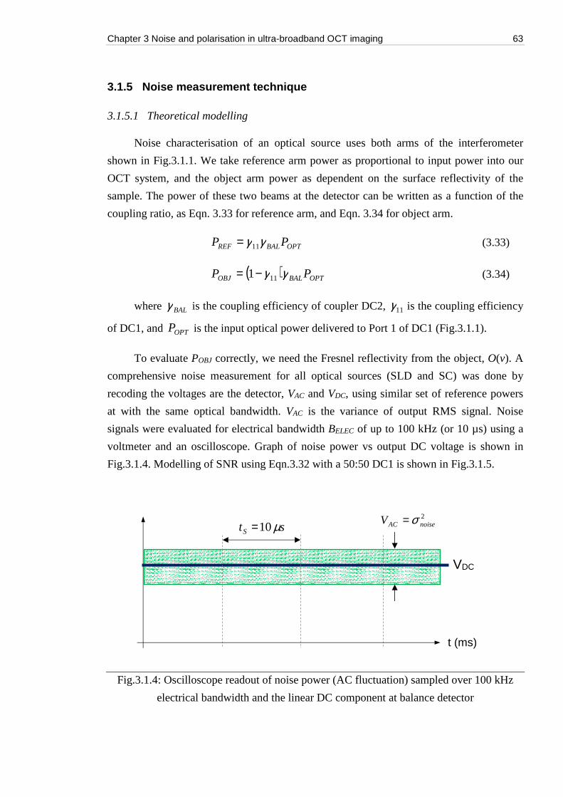
Chapter 3 Noise and polarisation in ultra-broadband OCT imaging 63
3.1.5 Noise measurement technique
3.1.5.1 Theoretical modelling
Noise characterisation of an optical source uses both arms of the interferometer
shown in Fig.3.1.1. We take reference arm power as proportional to input power into our
OCT system, and the object arm power as dependent on the surface reflectivity of the
sample. The power of these two beams at the detector can be written as a function of the
coupling ratio, as Eqn. 3.33 for reference arm, and Eqn. 3.34 for object arm.
OPTBALREF PP γγ11= (3.33)
( ) OPTBALOBJ PP γγ111−= (3.34)
where BALγ is the coupling efficiency of coupler DC2, 11γ is the coupling efficiency
of DC1, and OPTP is the input optical power delivered to Port 1 of DC1 (Fig.3.1.1).
To evaluate POBJ correctly, we need the Fresnel reflectivity from the object, O(v). A
comprehensive noise measurement for all optical sources (SLD and SC) was done by
recoding the voltages are the detector, VAC and VDC, using similar set of reference powers
at with the same optical bandwidth. VAC is the variance of output RMS signal. Noise
signals were evaluated for electrical bandwidth BELEC of up to 100 kHz (or 10 µs) using a
voltmeter and an oscilloscope. Graph of noise power vs output DC voltage is shown in
Fig.3.1.4. Modelling of SNR using Eqn.3.32 with a 50:50 DC1 is shown in Fig.3.1.5.
Fig.3.1.4: Oscilloscope readout of noise power (AC fluctuation) sampled over 100 kHz
electrical bandwidth and the linear DC component at balance detector
t (ms)
VDC
2noiseACV σ=
stS µ 10=
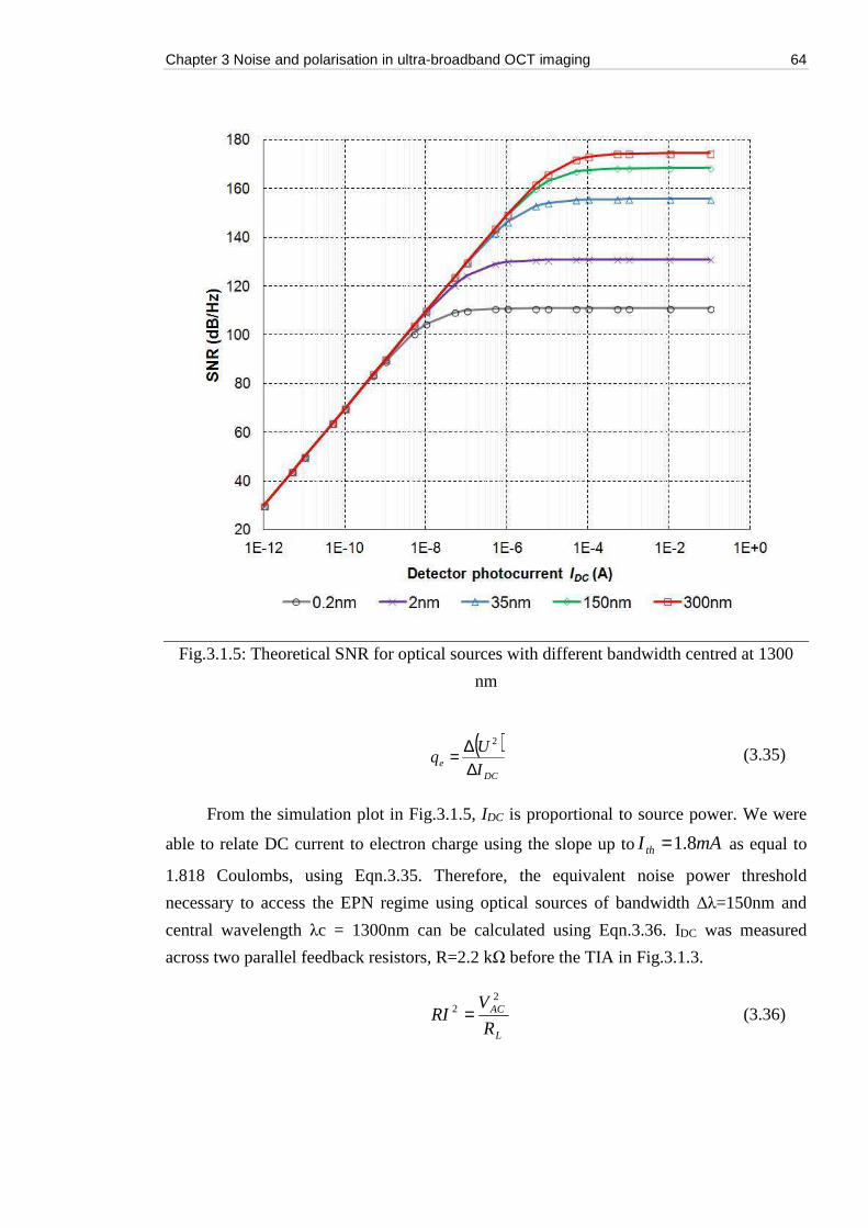
Chapter 3 Noise and polarisation in ultra-broadband OCT imaging 64
Fig.3.1.5: Theoretical SNR for optical sources with different bandwidth centred at 1300
nm
( )DC
e I
Uq
∆∆=
2
(3.35)
From the simulation plot in Fig.3.1.5, IDC is proportional to source power. We were
able to relate DC current to electron charge using the slope up to mAI th 8.1= as equal to
1.818 Coulombs, using Eqn.3.35. Therefore, the equivalent noise power threshold
necessary to access the EPN regime using optical sources of bandwidth Δλ=150nm and
central wavelength λc = 1300nm can be calculated using Eqn.3.36. IDC was measured
across two parallel feedback resistors, R=2.2 kΩ before the TIA in Fig.3.1.3.
L
AC
R
VRI
22 = (3.36)
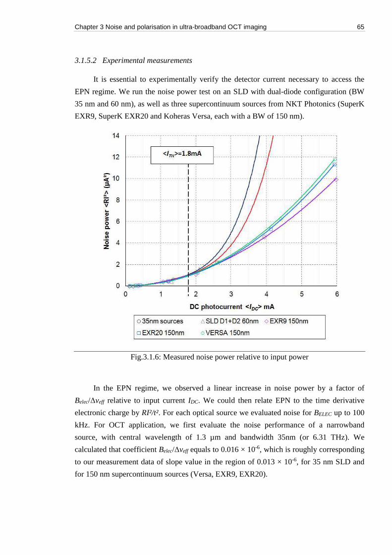
Chapter 3 Noise and polarisation in ultra-broadband OCT imaging 65
3.1.5.2 Experimental measurements
It is essential to experimentally verify the detector current necessary to access the
EPN regime. We run the noise power test on an SLD with dual-diode configuration (BW
35 nm and 60 nm), as well as three supercontinuum sources from NKT Photonics (SuperK
EXR9, SuperK EXR20 and Koheras Versa, each with a BW of 150 nm).
Fig.3.1.6: Measured noise power relative to input power
In the EPN regime, we observed a linear increase in noise power by a factor of
Belec/Δveff relative to input current IDC. We could then relate EPN to the time derivative
electronic charge by RI²/t². For each optical source we evaluated noise for BELEC up to 100
kHz. For OCT application, we first evaluate the noise performance of a narrowband
source, with central wavelength of 1.3 µm and bandwidth 35nm (or 6.31 THz). We
calculated that coefficient Belec/Δveff equals to 0.016 × 10⁻⁶, which is roughly corresponding
to our measurement data of slope value in the region of 0.013 × 10⁻⁶, for 35 nm SLD and
for 150 nm supercontinuum sources (Versa, EXR9, EXR20).
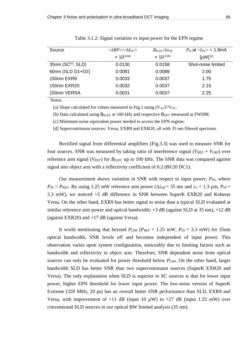
Chapter 3 Noise and polarisation in ultra-broadband OCT imaging 66
Table 3.1.2: Signal variation vs input power for the EPN regime
Source <ΔRI²>/<ΔIDC>
× 10-6 [a]
BELEC/Δveff
× 10-6 [b]
Pth at <IDC> = 1.8mA
[µW] [c]
35nm (SC[c], SLD) 0.0130 0.0158 Shot-noise limited
60nm (SLD D1+D2) 0.0081 0.0089 2.00
150nm EXR9 0.0033 0.0037 1.75
150nm EXR20 0.0032 0.0037 2.15
150nm VERSA 0.0031 0.0037 2.25
Notes:
[a] Slope calculated for values measured in Fig.1 using (VAC)2/VDC.
[b] Data calculated using BELEC at 100 kHz and respective BOPT measured at FWHM.
[c] Minimum noise equivalent power needed to access the EPN regime.
[d] Supercontinuum sources: Versa, EXR9 and EXR20, all with 35 nm filtered spectrum.
Rectified signal from differential amplifiers (Fig.3.3) was used to measure SNR for
four sources. SNR was measured by taking ratio of interference signal (VREF + VOBJ) over
reference arm signal (VREF) for BELEC up to 100 kHz. The SNR data was compared against
signal into object arm with a reflectivity coefficient of 0.2 (80:20 DC1).
Our measurement shows variation in SNR with respect to input power, PIN, where
PIN ≈ PREF. By using 1.25 mW reference arm power (Δλeff = 35 nm and λC = 1.3 µm, PIN =
3.3 mW), we noticed +5 dB difference in SNR between SuperK EXR20 and Koheras
Versa. On the other hand, EXR9 has better signal to noise than a typical SLD evaluated at
similar reference arm power and optical bandwidth: +3 dB (against SLD at 35 nm), +12 dB
(against EXR20) and +17 dB (against Versa).
It worth mentioning that beyond PLIM (PREF = 1.25 mW, PIN = 3.3 mW) for 35nm
optical bandwidth, SNR levels off and becomes independent of input power. This
observation varies upon system configuration, noticeably due to limiting factors such as
bandwidth and reflectivity in object arm. Therefore, SNR dependent noise from optical
sources can only be evaluated for power threshold below PLIM. On the other hand, larger
bandwidth SLD has better SNR than two supercontinuum sources (SuperK EXR20 and
Versa). The only explanation when SLD is superior to SC sources is that for lower input
power, higher EPN threshold for lower input power. The low-noise version of SuperK
Extreme (320 MHz, 20 ps) has an overall better SNR performance than SLD, EXR9 and
Versa, with improvement of +11 dB (input 10 µW) to +27 dB (input 1.25 mW) over
conventional SLD sources in our optical BW limited analysis (35 nm).
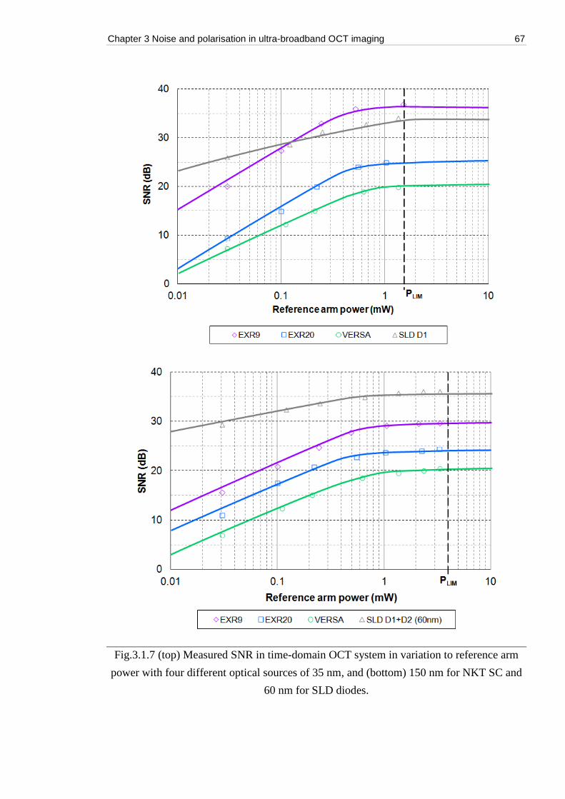
Chapter 3 Noise and polarisation in ultra-broadband OCT imaging 67
Fig.3.1.7 (top) Measured SNR in time-domain OCT system in variation to reference arm
power with four different optical sources of 35 nm, and (bottom) 150 nm for NKT SC and
60 nm for SLD diodes.
Chapter 3 Noise and polarisation in ultra-broadband OCT imaging 68
In comparison to noise data, our minimum power to operate the SuperK EXR9
beyond shot noise regime was 1.75 µW. However, we are not able to draw a conclusion if
increasing the optical bandwidth from SuperK EXR9 can make the imaging less noisy than
SLD of similar BW. Nevertheless, in terms of SNR ratings, comparison between two
supercontinuum sources has again proven that with a 150 nm bandwidth, SuperK EXR9 is
between +7 dB to +9 dB better than Versa. It has to be noted that our measured values of
Belec/Δveff for 150 nm case varied despite every effort to have exactly 150 nm filtered
optical spectrum going into and coming out from our OCT system by making ensuring we
have Δλeff = ΔλREF = ΔλP1 = ΔλP2. Spectrum at each of these positions were measured with
an OSA. Initial findings indicate that these small variations are due to dispersion of
wavelengths in SM fibre and transmission band of two directional couplers used. We
therefore able to conclude that:
(a) In total noise power measurement, we observe a linear trend in shot noise regime
for detector power up to 1.8 mA evaluated over an electrical bandwidth of 100 kHz.
Noise power is a measure of photocurrent fluctuation in photo detector due to noise
from the source.
(b) Shot noise power is independent of laser linewidth (Δveff), thus a narrowband
source (e.g. SLD) at 35nm and a broadband supercontinuum source (e.g. SuperK
Extreme) at 200 nm makes no difference to current fluctuation at PIN diodes. Shot
noise increases as we increased our amplifier bandwidth.
(c) Excess photon noise is inversely proportional to optical bandwidth. With a 150 nm
broadband source such as the EXR9, we can expect four times lower in total noise
power compare to a 35nm SLD. Our results proved this was the case.
(d) SNR measurement gives an in-sight into noise in OCT system. With a time domain
interferometer, we observed that at similar reference arm power (PREF > 150µW),
the low-noise supercontinuum SuperK EXR9 gives slightly better SNR than SLD
and two other supercontinuum sources, SuperK EXR9 and VERSA, when imaged
with a sample of surface reflectivity R > 0.3.
(e) Independent of optical bandwidth used, we showed that SuperK EXR9 gives better
SNR in OCT imaging than two other supercontinuum sources (Versa and EXR20).
We therefore verified the low-noise claims from NKT Photonics.
Chapter 3 Noise and polarisation in ultra-broadband OCT imaging 69
3.1.6 Summary of statistical noise
In the analysis of noise power, we provide an in-sight into basic physical quantities
that affect optimisation of an OCT system using both coherent and incoherent optical
sources and detection techniques. We began by analysing the photocurrent flow in
directional coupler, deriving the equations from electric field to optical power, to show
how noise power can evaluated from the AC current fluctuation with optical couplers with
different coupling efficiency. We have discussed thermal noise, shot noise and excess
photon noise. We demonstrated that thermal noise is generated by instability in electrical
circuitry of the photo detector and the resistor. Shot noise, on the other hand is due to
quantum fluctuation of electrons at detector input that follows the Poisson statistical
distribution of mean-square fluctuation (MSF) <Δn>=<n>. The third noise term, excess
photon noise (EPN), is caused by beatings of various Fourier components in an optical
spectrum. EPN follows the Bose-Einstein probability distribution of MSF <Δn>=<n²>. An
additional term called beat noise was introduced to include partially coherent light signal
and its reflectivity coefficient into the total noise calculation. A comparison of various
techniques employed to improve SNR were discussed. These techniques include
deliberately attenuating reference arm power with an iris to reduce saturation, and to
unbalance photo detector system.
We have also analytically shown that despite an increase in the bandwidth of optical
sources Δλ (or Δv in optical frequency), the upper limit of the SNR could not be extended
further due to some these main factors: (a) fibre-end stray reflections, (b) incoherent
spectral bandwidth of signals, and (c) non-overlapping in time of spectral powers deviation
from both arms of the interferometer that resulted in reduced interference fringes. It is also
evident that by employing ultra-broadband optical sources such as the white light
supercontinuum (SC) source from NKT Photonics can only marginally improved the SNR.
However, this approach requires the SC source to be operating at its full power (100%).
Nevertheless, we also discovered that by using a fibre-based OCT system, our ability to
manipulate the source optical bandwidth for a gain in SNR is dependent on transmission
band of fibre couplers in use. A narrow band coupler is not suitable for systems running on
SC sources, not only from the bandwidth perspective, but also due to various noise it
generates. A complete redesign of the broadband coupler is therefore necessary, and should
be priority for the next project.
Chapter 3 Noise and polarisation in ultra-broadband OCT imaging 70
3.2 Polarisation and noise in long pulse supercontinuum
Long pulse supercontinuum (SC) light sources have traditionally been ignored when
considered for optical coherence tomography (OCT) [16] owing to their poor noise
performance. In the last decade, SC sources have made inroads into other fields of study,
such as optical metrology [17], chemical sensing [18], fibre sensor technology [19] and
white light trapping [20]. During these periods, super luminescent diodes (SLD) and
tuneable lasers such as swept sources have been widely adopted by OCT developers [21].
However, many of these light sources struggled to provide sufficient optical bandwidth
needed to response to the increasing demand for high axial resolution imaging, especially
in the non-conventional wavelength range [22-23]. As recently, the use of SC sources have
made a comeback again on tomography imaging and high-resolution OCT with SC has
again been researched [24]. This time around, the main argument for SC wasn’t on RIN,
but the promising imaging results SC sources can deliver, based upon its wider optical
bandwidth and higher power [25] than any other light sources.
We believe that the future of OCT relies heavily on the successful development of a
low-noise version of the SC source, and ability to exploit the polarization effects delivered
by these high performance sources. Recently, a simulation model has shown polarization
dependent output power at longer wavelengths [26]. However, this was not experimentally
verified in their later tests and is yet to be observed [27]. Nevertheless, an earlier study
using direct time-domain measurements of the amplitude statistics has concluded that pulse
to pulse stability depends on the pump power and input polarization [28]. We also note
that, as early as 1995, polarization effects resulting in spectral broadening in weakly
birefringent micro-structured fibre (MSF) had been investigated [29], with these tests later
repeated for its highly birefringent counterpart [30]. For these reasons, we have initiated a
comprehensive study on SC in three areas of interest: polarization extinction ratio (PER),
polarization changes [31] in a nominally non-birefringent photonic crystal fibre (PCF), and
polarization dependent relative intensity noise (RIN). Birefringence is an important area to
investigate in SC generation as it provides important information on wave propagation in
fibre that could transform polarization states and polarization-mode coupling [32]. We
evaluated the birefringent profile of the output SC beam by using different nonlinear fibre
lengths (3m and 10m, model SC-5.0-1040, NKT Photonics).
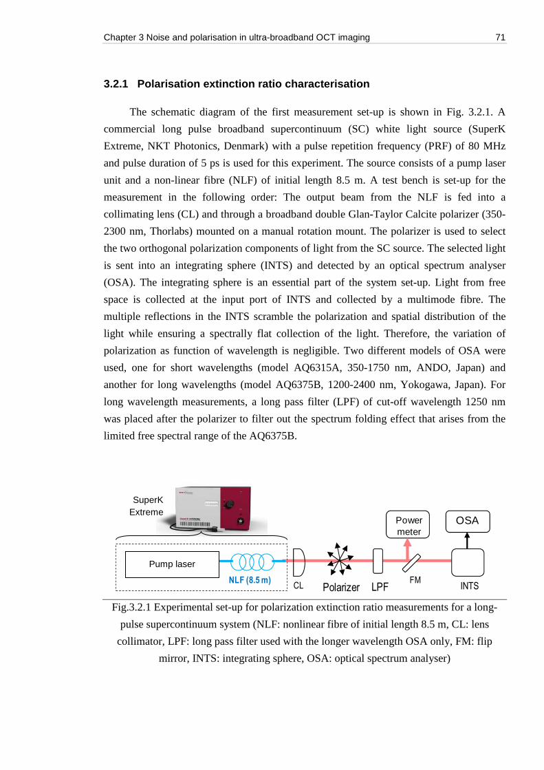
Chapter 3 Noise and polarisation in ultra-broadband OCT imaging 71
3.2.1 Polarisation extinction ratio characterisation
The schematic diagram of the first measurement set-up is shown in Fig. 3.2.1. A
commercial long pulse broadband supercontinuum (SC) white light source (SuperK
Extreme, NKT Photonics, Denmark) with a pulse repetition frequency (PRF) of 80 MHz
and pulse duration of 5 ps is used for this experiment. The source consists of a pump laser
unit and a non-linear fibre (NLF) of initial length 8.5 m. A test bench is set-up for the
measurement in the following order: The output beam from the NLF is fed into a
collimating lens (CL) and through a broadband double Glan-Taylor Calcite polarizer (350-
2300 nm, Thorlabs) mounted on a manual rotation mount. The polarizer is used to select
the two orthogonal polarization components of light from the SC source. The selected light
is sent into an integrating sphere (INTS) and detected by an optical spectrum analyser
(OSA). The integrating sphere is an essential part of the system set-up. Light from free
space is collected at the input port of INTS and collected by a multimode fibre. The
multiple reflections in the INTS scramble the polarization and spatial distribution of the
light while ensuring a spectrally flat collection of the light. Therefore, the variation of
polarization as function of wavelength is negligible. Two different models of OSA were
used, one for short wavelengths (model AQ6315A, 350-1750 nm, ANDO, Japan) and
another for long wavelengths (model AQ6375B, 1200-2400 nm, Yokogawa, Japan). For
long wavelength measurements, a long pass filter (LPF) of cut-off wavelength 1250 nm
was placed after the polarizer to filter out the spectrum folding effect that arises from the
limited free spectral range of the AQ6375B.
Fig.3.2.1 Experimental set-up for polarization extinction ratio measurements for a long-
pulse supercontinuum system (NLF: nonlinear fibre of initial length 8.5 m, CL: lens
collimator, LPF: long pass filter used with the longer wavelength OSA only, FM: flip
mirror, INTS: integrating sphere, OSA: optical spectrum analyser)
Power meter
NLF (8.5 m)INTSPolarizer
OSA
LPFCLFM
Pump laser
SuperK Extreme
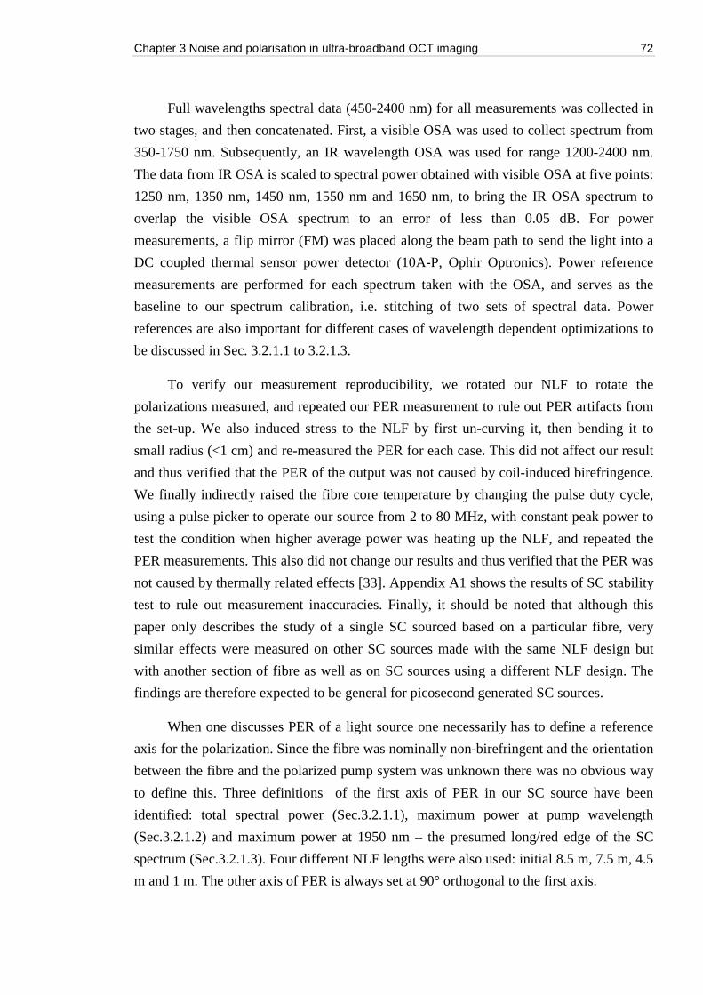
Chapter 3 Noise and polarisation in ultra-broadband OCT imaging 72
Full wavelengths spectral data (450-2400 nm) for all measurements was collected in
two stages, and then concatenated. First, a visible OSA was used to collect spectrum from
350-1750 nm. Subsequently, an IR wavelength OSA was used for range 1200-2400 nm.
The data from IR OSA is scaled to spectral power obtained with visible OSA at five points:
1250 nm, 1350 nm, 1450 nm, 1550 nm and 1650 nm, to bring the IR OSA spectrum to
overlap the visible OSA spectrum to an error of less than 0.05 dB. For power
measurements, a flip mirror (FM) was placed along the beam path to send the light into a
DC coupled thermal sensor power detector (10A-P, Ophir Optronics). Power reference
measurements are performed for each spectrum taken with the OSA, and serves as the
baseline to our spectrum calibration, i.e. stitching of two sets of spectral data. Power
references are also important for different cases of wavelength dependent optimizations to
be discussed in Sec. 3.2.1.1 to 3.2.1.3.
To verify our measurement reproducibility, we rotated our NLF to rotate the
polarizations measured, and repeated our PER measurement to rule out PER artifacts from
the set-up. We also induced stress to the NLF by first un-curving it, then bending it to
small radius (<1 cm) and re-measured the PER for each case. This did not affect our result
and thus verified that the PER of the output was not caused by coil-induced birefringence.
We finally indirectly raised the fibre core temperature by changing the pulse duty cycle,
using a pulse picker to operate our source from 2 to 80 MHz, with constant peak power to
test the condition when higher average power was heating up the NLF, and repeated the
PER measurements. This also did not change our results and thus verified that the PER was
not caused by thermally related effects [33]. Appendix A1 shows the results of SC stability
test to rule out measurement inaccuracies. Finally, it should be noted that although this
paper only describes the study of a single SC sourced based on a particular fibre, very
similar effects were measured on other SC sources made with the same NLF design but
with another section of fibre as well as on SC sources using a different NLF design. The
findings are therefore expected to be general for picosecond generated SC sources.
When one discusses PER of a light source one necessarily has to define a reference
axis for the polarization. Since the fibre was nominally non-birefringent and the orientation
between the fibre and the polarized pump system was unknown there was no obvious way
to define this. Three definitions of the first axis of PER in our SC source have been
identified: total spectral power (Sec.3.2.1.1), maximum power at pump wavelength
(Sec.3.2.1.2) and maximum power at 1950 nm – the presumed long/red edge of the SC
spectrum (Sec.3.2.1.3). Four different NLF lengths were also used: initial 8.5 m, 7.5 m, 4.5
m and 1 m. The other axis of PER is always set at 90° orthogonal to the first axis.
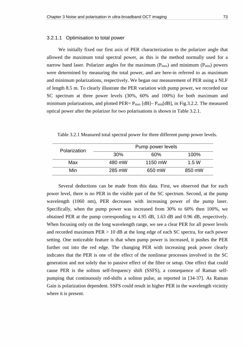
Chapter 3 Noise and polarisation in ultra-broadband OCT imaging 73
3.2.1.1 Optimisation to total power
We initially fixed our first axis of PER characterization to the polarizer angle that
allowed the maximum total spectral power, as this is the method normally used for a
narrow band laser. Polarizer angles for the maximum (Pmax) and minimum (Pmin) powers
were determined by measuring the total power, and are here-in referred to as maximum
and minimum polarizations, respectively. We began our measurement of PER using a NLF
of length 8.5 m. To clearly illustrate the PER variation with pump power, we recorded our
SC spectrum at three power levels (30%, 60% and 100%) for both maximum and
minimum polarizations, and plotted PER= Pmax [dB]– Pmin[dB], in Fig.3.2.2. The measured
optical power after the polarizer for two polarisations is shown in Table 3.2.1.
Table 3.2.1 Measured total spectral power for three different pump power levels.
Polarization Pump power levels
30% 60% 100%
Max 480 mW 1150 mW 1.5 W
Min 285 mW 650 mW 850 mW
Several deductions can be made from this data. First, we observed that for each
power level, there is no PER in the visible part of the SC spectrum. Second, at the pump
wavelength (1060 nm), PER decreases with increasing power of the pump laser.
Specifically, when the pump power was increased from 30% to 60% then 100%, we
obtained PER at the pump corresponding to 4.95 dB, 1.63 dB and 0.96 dB, respectively.
When focusing only on the long wavelength range, we see a clear PER for all power levels
and recorded maximum PER > 10 dB at the long edge of each SC spectra, for each power
setting. One noticeable feature is that when pump power is increased, it pushes the PER
further out into the red edge. The changing PER with increasing peak power clearly
indicates that the PER is one of the effect of the nonlinear processes involved in the SC
generation and not solely due to passive effect of the fibre or setup. One effect that could
cause PER is the soliton self-frequency shift (SSFS), a consequence of Raman self-
pumping that continuously red-shifts a soliton pulse, as reported in [34-37]. As Raman
Gain is polarization dependent. SSFS could result in higher PER in the wavelength vicinity
where it is present.
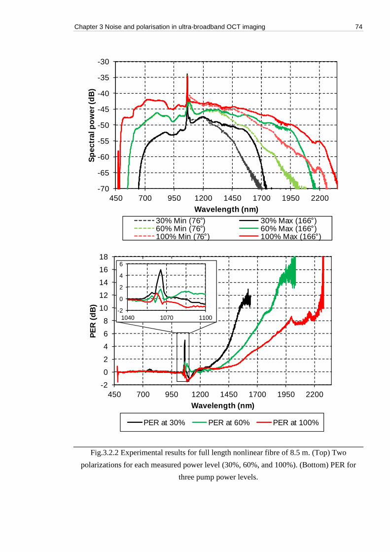
Chapter 3 Noise and polarisation in ultra-broadband OCT imaging 74
Fig.3.2.2 Experimental results for full length nonlinear fibre of 8.5 m. (Top) Two
polarizations for each measured power level (30%, 60%, and 100%). (Bottom) PER for
three pump power levels.
-70
-65
-60
-55
-50
-45
-40
-35
-30
450 700 950 1200 1450 1700 1950 2200
Sp
ectr
al p
ow
er (d
B)
Wavelength (nm)30% Min (76°) 30% Max (166°)60% Min (76°) 60% Max (166°)100% Min (76°) 100% Max (166°)
-2
0
2
4
6
8
10
12
14
16
18
450 700 950 1200 1450 1700 1950 2200
PE
R (
dB
)
Wavelength (nm)
PER at 30% PER at 60% PER at 100%
-2
0
2
4
6
1040 1070 1100
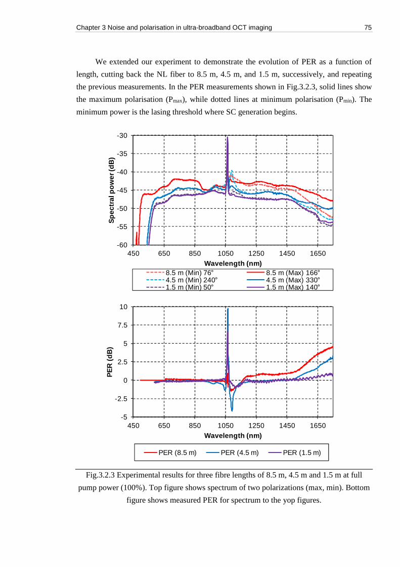
Chapter 3 Noise and polarisation in ultra-broadband OCT imaging 75
We extended our experiment to demonstrate the evolution of PER as a function of
length, cutting back the NL fiber to 8.5 m, 4.5 m, and 1.5 m, successively, and repeating
the previous measurements. In the PER measurements shown in Fig.3.2.3, solid lines show
the maximum polarisation (Pmax), while dotted lines at minimum polarisation (Pmin). The
minimum power is the lasing threshold where SC generation begins.
Fig.3.2.3 Experimental results for three fibre lengths of 8.5 m, 4.5 m and 1.5 m at full
pump power (100%). Top figure shows spectrum of two polarizations (max, min). Bottom
figure shows measured PER for spectrum to the yop figures.
-60
-55
-50
-45
-40
-35
-30
450 650 850 1050 1250 1450 1650
Sp
ectr
al p
ow
er (d
B)
Wavelength (nm)8.5 m (Min) 76° 8.5 m (Max) 166°4.5 m (Min) 240° 4.5 m (Max) 330°1.5 m (Min) 50° 1.5 m (Max) 140°
-5
-2.5
0
2.5
5
7.5
10
450 650 850 1050 1250 1450 1650
PE
R (
dB
)
Wavelength (nm)
PER (8.5 m) PER (4.5 m) PER (1.5 m)
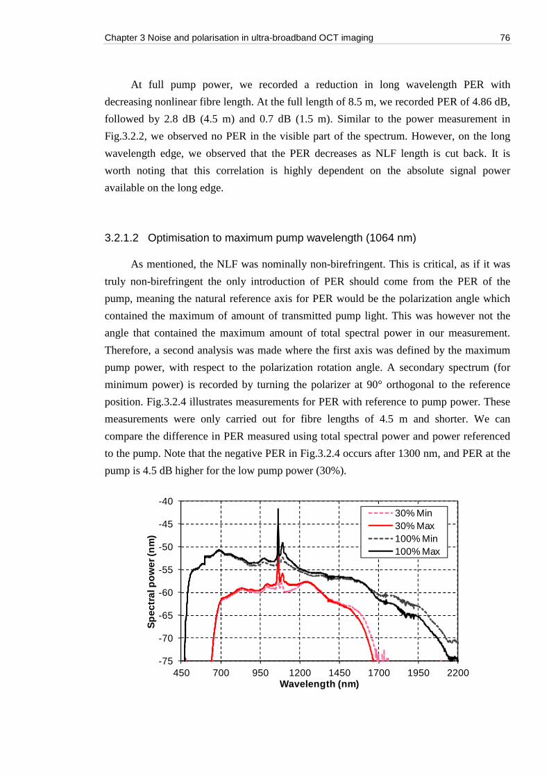
Chapter 3 Noise and polarisation in ultra-broadband OCT imaging 76
At full pump power, we recorded a reduction in long wavelength PER with
decreasing nonlinear fibre length. At the full length of 8.5 m, we recorded PER of 4.86 dB,
followed by 2.8 dB (4.5 m) and 0.7 dB (1.5 m). Similar to the power measurement in
Fig.3.2.2, we observed no PER in the visible part of the spectrum. However, on the long
wavelength edge, we observed that the PER decreases as NLF length is cut back. It is
worth noting that this correlation is highly dependent on the absolute signal power
available on the long edge.
3.2.1.2 Optimisation to maximum pump wavelength (1064 nm)
As mentioned, the NLF was nominally non-birefringent. This is critical, as if it was
truly non-birefringent the only introduction of PER should come from the PER of the
pump, meaning the natural reference axis for PER would be the polarization angle which
contained the maximum of amount of transmitted pump light. This was however not the
angle that contained the maximum amount of total spectral power in our measurement.
Therefore, a second analysis was made where the first axis was defined by the maximum
pump power, with respect to the polarization rotation angle. A secondary spectrum (for
minimum power) is recorded by turning the polarizer at 90° orthogonal to the reference
position. Fig.3.2.4 illustrates measurements for PER with reference to pump power. These
measurements were only carried out for fibre lengths of 4.5 m and shorter. We can
compare the difference in PER measured using total spectral power and power referenced
to the pump. Note that the negative PER in Fig.3.2.4 occurs after 1300 nm, and PER at the
pump is 4.5 dB higher for the low pump power (30%).
-75
-70
-65
-60
-55
-50
-45
-40
450 700 950 1200 1450 1700 1950 2200
Sp
ectr
al p
ow
er (n
m)
Wavelength (nm)
30% Min30% Max100% Min100% Max
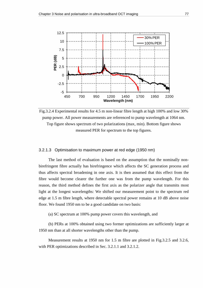
Chapter 3 Noise and polarisation in ultra-broadband OCT imaging 77
Fig.3.2.4 Experimental results for 4.5 m non-linear fibre length at high 100% and low 30%
pump power. All power measurements are referenced to pump wavelength at 1064 nm.
Top figure shows spectrum of two polarizations (max, min). Bottom figure shows
measured PER for spectrum to the top figures.
3.2.1.3 Optimisation to maximum power at red edge (1950 nm)
The last method of evaluation is based on the assumption that the nominally non-
birefringent fibre actually has birefringence which affects the SC generation process and
thus affects spectral broadening in one axis. It is then assumed that this effect from the
fibre would become clearer the further one was from the pump wavelength. For this
reason, the third method defines the first axis as the polarizer angle that transmits most
light at the longest wavelengths: We shifted our measurement point to the spectrum red
edge at 1.5 m fibre length, where detectable spectral power remains at 10 dB above noise
floor. We found 1950 nm to be a good candidate on two basis:
(a) SC spectrum at 100% pump power covers this wavelength, and
(b) PERs at 100% obtained using two former optimizations are sufficiently larger at
1950 nm than at all shorter wavelengths other than the pump.
Measurement results at 1950 nm for 1.5 m fibre are plotted in Fig.3.2.5 and 3.2.6,
with PER optimizations described in Sec. 3.2.1.1 and 3.2.1.2.
-5
-2.5
0
2.5
5
7.5
10
12.5
450 700 950 1200 1450 1700 1950 2200
PE
R (
dB
)
Wavelength (nm)
30% PER
100% PER
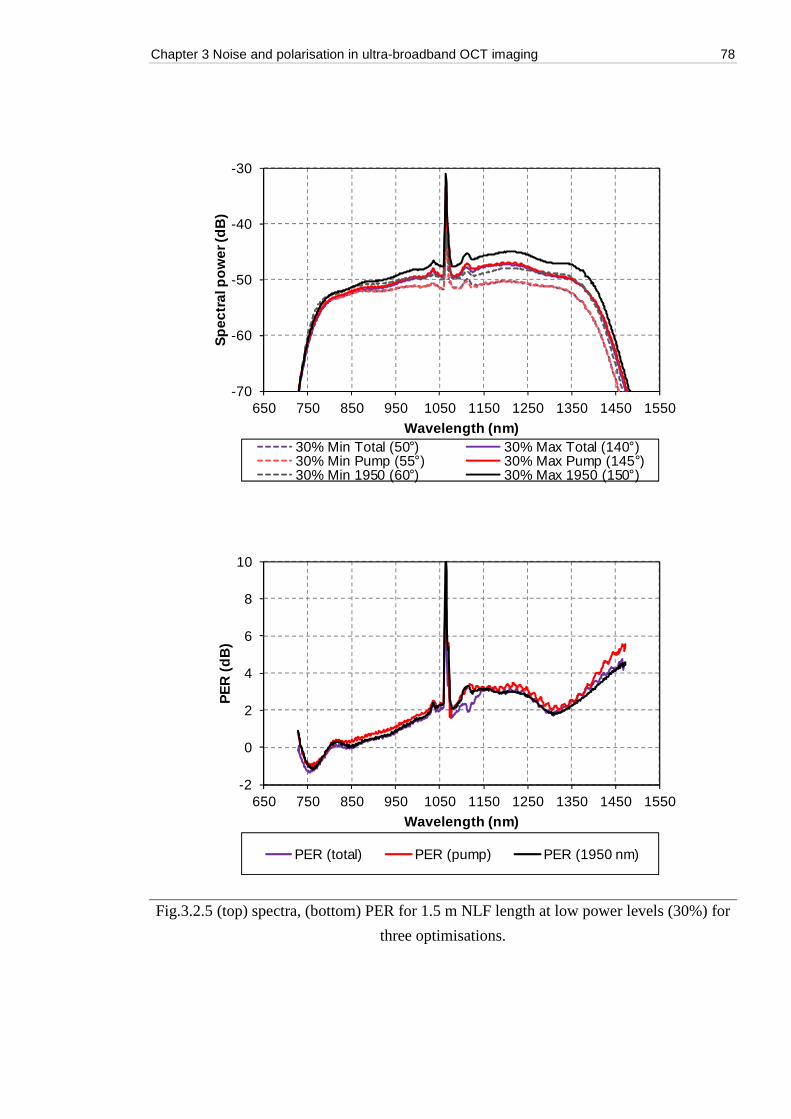
Chapter 3 Noise and polarisation in ultra-broadband OCT imaging 78
Fig.3.2.5 (top) spectra, (bottom) PER for 1.5 m NLF length at low power levels (30%) for
three optimisations.
-70
-60
-50
-40
-30
650 750 850 950 1050 1150 1250 1350 1450 1550
Sp
ectr
al p
ow
er (d
B)
Wavelength (nm)30% Min Total (50°) 30% Max Total (140°)30% Min Pump (55°) 30% Max Pump (145°)30% Min 1950 (60°) 30% Max 1950 (150°)
-2
0
2
4
6
8
10
650 750 850 950 1050 1150 1250 1350 1450 1550
PE
R (
dB
)
Wavelength (nm)
PER (total) PER (pump) PER (1950 nm)
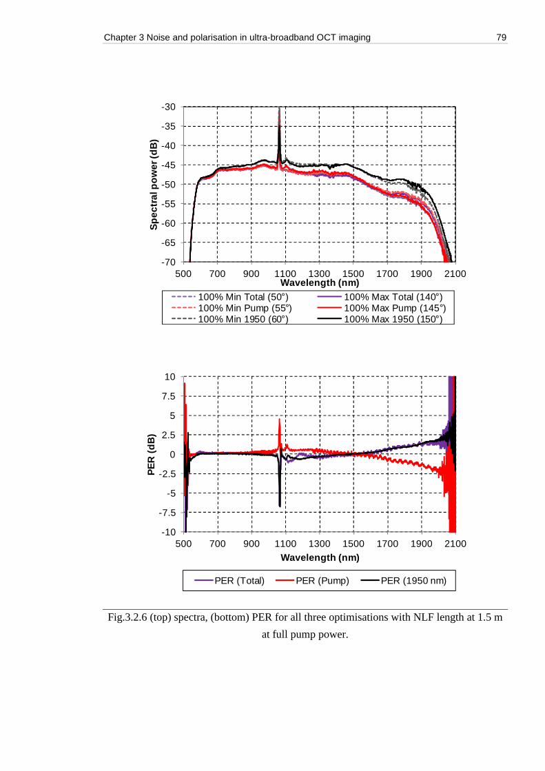
Chapter 3 Noise and polarisation in ultra-broadband OCT imaging 79
Fig.3.2.6 (top) spectra, (bottom) PER for all three optimisations with NLF length at 1.5 m
at full pump power.
-70
-65
-60
-55
-50
-45
-40
-35
-30
500 700 900 1100 1300 1500 1700 1900 2100
Sp
ectr
al p
ow
er (d
B)
Wavelength (nm)
100% Min Total (50°) 100% Max Total (140°)100% Min Pump (55°) 100% Max Pump (145°)100% Min 1950 (60°) 100% Max 1950 (150°)
-10
-7.5
-5
-2.5
0
2.5
5
7.5
10
500 700 900 1100 1300 1500 1700 1900 2100
PE
R (
dB
)
Wavelength (nm)
PER (Total) PER (Pump) PER (1950 nm)
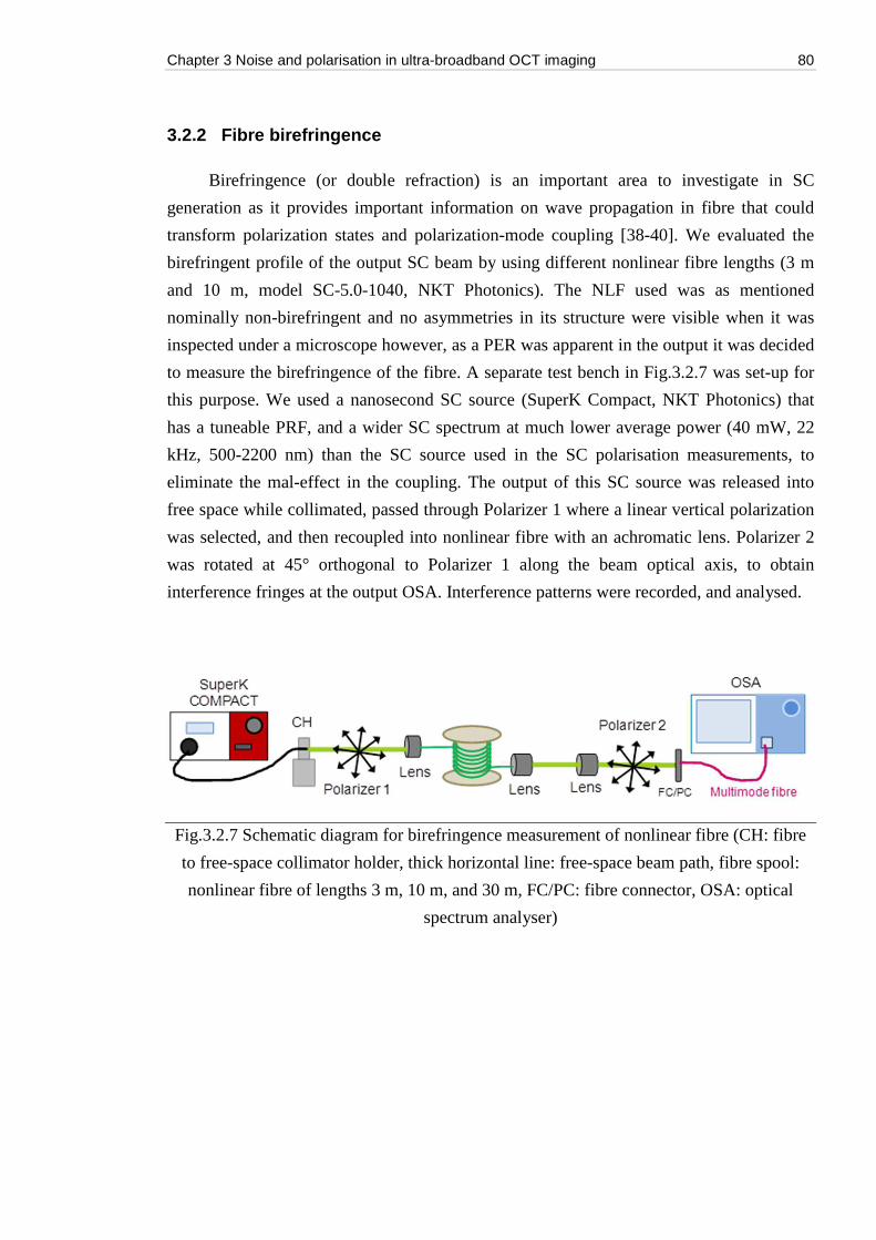
Chapter 3 Noise and polarisation in ultra-broadband OCT imaging 80
3.2.2 Fibre birefringence
Birefringence (or double refraction) is an important area to investigate in SC
generation as it provides important information on wave propagation in fibre that could
transform polarization states and polarization-mode coupling [38-40]. We evaluated the
birefringent profile of the output SC beam by using different nonlinear fibre lengths (3 m
and 10 m, model SC-5.0-1040, NKT Photonics). The NLF used was as mentioned
nominally non-birefringent and no asymmetries in its structure were visible when it was
inspected under a microscope however, as a PER was apparent in the output it was decided
to measure the birefringence of the fibre. A separate test bench in Fig.3.2.7 was set-up for
this purpose. We used a nanosecond SC source (SuperK Compact, NKT Photonics) that
has a tuneable PRF, and a wider SC spectrum at much lower average power (40 mW, 22
kHz, 500-2200 nm) than the SC source used in the SC polarisation measurements, to
eliminate the mal-effect in the coupling. The output of this SC source was released into
free space while collimated, passed through Polarizer 1 where a linear vertical polarization
was selected, and then recoupled into nonlinear fibre with an achromatic lens. Polarizer 2
was rotated at 45° orthogonal to Polarizer 1 along the beam optical axis, to obtain
interference fringes at the output OSA. Interference patterns were recorded, and analysed.
Fig.3.2.7 Schematic diagram for birefringence measurement of nonlinear fibre (CH: fibre
to free-space collimator holder, thick horizontal line: free-space beam path, fibre spool:
nonlinear fibre of lengths 3 m, 10 m, and 30 m, FC/PC: fibre connector, OSA: optical
spectrum analyser)
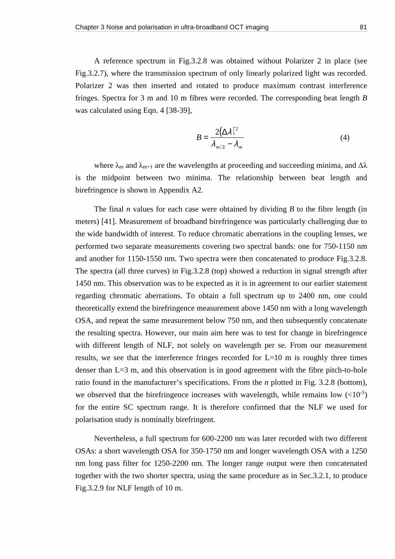
Chapter 3 Noise and polarisation in ultra-broadband OCT imaging 81
A reference spectrum in Fig.3.2.8 was obtained without Polarizer 2 in place (see
Fig.3.2.7), where the transmission spectrum of only linearly polarized light was recorded.
Polarizer 2 was then inserted and rotated to produce maximum contrast interference
fringes. Spectra for 3 m and 10 m fibres were recorded. The corresponding beat length B
was calculated using Eqn. 4 [38-39],
( )
mm
Bλλ
λ−
∆=+1
22 (4)
where λm and λm+1 are the wavelengths at proceeding and succeeding minima, and Δλ
is the midpoint between two minima. The relationship between beat length and
birefringence is shown in Appendix A2.
The final n values for each case were obtained by dividing B to the fibre length (in
meters) [41]. Measurement of broadband birefringence was particularly challenging due to
the wide bandwidth of interest. To reduce chromatic aberrations in the coupling lenses, we
performed two separate measurements covering two spectral bands: one for 750-1150 nm
and another for 1150-1550 nm. Two spectra were then concatenated to produce Fig.3.2.8.
The spectra (all three curves) in Fig.3.2.8 (top) showed a reduction in signal strength after
1450 nm. This observation was to be expected as it is in agreement to our earlier statement
regarding chromatic aberrations. To obtain a full spectrum up to 2400 nm, one could
theoretically extend the birefringence measurement above 1450 nm with a long wavelength
OSA, and repeat the same measurement below 750 nm, and then subsequently concatenate
the resulting spectra. However, our main aim here was to test for change in birefringence
with different length of NLF, not solely on wavelength per se. From our measurement
results, we see that the interference fringes recorded for L=10 m is roughly three times
denser than L=3 m, and this observation is in good agreement with the fibre pitch-to-hole
ratio found in the manufacturer’s specifications. From the n plotted in Fig. 3.2.8 (bottom),
we observed that the birefringence increases with wavelength, while remains low (<10-5)
for the entire SC spectrum range. It is therefore confirmed that the NLF we used for
polarisation study is nominally birefringent.
Nevertheless, a full spectrum for 600-2200 nm was later recorded with two different
OSAs: a short wavelength OSA for 350-1750 nm and longer wavelength OSA with a 1250
nm long pass filter for 1250-2200 nm. The longer range output were then concatenated
together with the two shorter spectra, using the same procedure as in Sec.3.2.1, to produce
Fig.3.2.9 for NLF length of 10 m.
Chapter 3 Noise and polarisation in ultra-broadband OCT imaging 82
Fig.3.2.8 Birefringence measurement. (Top) Reference spectrum, and spectra of two fibre
lengths with interference fringes. (Bottom) n values calculated using signal spectra in top
figure.
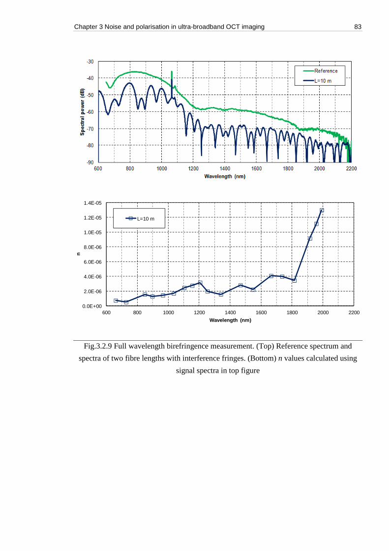
Chapter 3 Noise and polarisation in ultra-broadband OCT imaging 83
Fig.3.2.9 Full wavelength birefringence measurement. (Top) Reference spectrum and
spectra of two fibre lengths with interference fringes. (Bottom) n values calculated using
signal spectra in top figure
0.0E+00
2.0E-06
4.0E-06
6.0E-06
8.0E-06
1.0E-05
1.2E-05
1.4E-05
600 800 1000 1200 1400 1600 1800 2000 2200
n
Wavelength (nm)
L=10 m
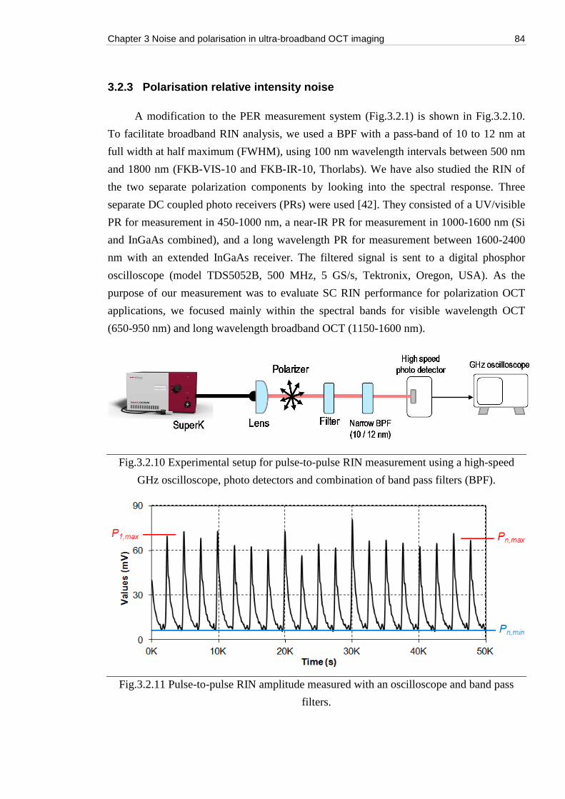
Chapter 3 Noise and polarisation in ultra-broadband OCT imaging 84
3.2.3 Polarisation relative intensity noise
A modification to the PER measurement system (Fig.3.2.1) is shown in Fig.3.2.10.
To facilitate broadband RIN analysis, we used a BPF with a pass-band of 10 to 12 nm at
full width at half maximum (FWHM), using 100 nm wavelength intervals between 500 nm
and 1800 nm (FKB-VIS-10 and FKB-IR-10, Thorlabs). We have also studied the RIN of
the two separate polarization components by looking into the spectral response. Three
separate DC coupled photo receivers (PRs) were used [42]. They consisted of a UV/visible
PR for measurement in 450-1000 nm, a near-IR PR for measurement in 1000-1600 nm (Si
and InGaAs combined), and a long wavelength PR for measurement between 1600-2400
nm with an extended InGaAs receiver. The filtered signal is sent to a digital phosphor
oscilloscope (model TDS5052B, 500 MHz, 5 GS/s, Tektronix, Oregon, USA). As the
purpose of our measurement was to evaluate SC RIN performance for polarization OCT
applications, we focused mainly within the spectral bands for visible wavelength OCT
(650-950 nm) and long wavelength broadband OCT (1150-1600 nm).
Fig.3.2.10 Experimental setup for pulse-to-pulse RIN measurement using a high-speed
GHz oscilloscope, photo detectors and combination of band pass filters (BPF).
Fig.3.2.11 Pulse-to-pulse RIN amplitude measured with an oscilloscope and band pass
filters.
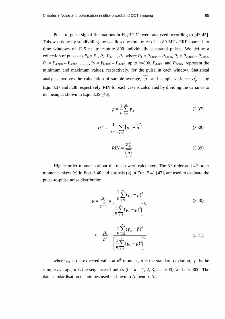
Chapter 3 Noise and polarisation in ultra-broadband OCT imaging 85
Pulse-to-pulse signal fluctuations in Fig.3.2.11 were analyzed according to [43-45].
This was done by subdividing the oscilloscope time trace of an 80 MHz PRF source into
time windows of 12.5 ns, to capture 800 individually separated pulses. We define a
collection of pulses as Pk = P1, P2, P3, ..., Pn, where P1 = P1,max – P1,min, P2 = P2,max – P2,min,
P3 = P3,max – P3,min, ……, Pn = Pn,max – Pn,min, up to n=800. Pn,min and Pn,max represent the
minimum and maximum values, respectively, for the pulse in each window. Statistical
analysis involves the calculation of sample average, p and sample variance 2pσ using
Eqn. 3.37 and 3.38 respectively. RIN for each case is calculated by dividing the variance to
its mean, as shown in Eqn. 3.39 [46].
=
=n
kkp
np
1
1 (3.37)
( )=
−−
=n
kkp pp
n 1
22
1
1σ (3.38)
pRIN
p2σ
= (3.39)
Higher order moments about the mean were calculated. The 3rd order and 4th order
moments, skew (γ) in Eqn. 3.40 and kurtosis (κ) in Eqn. 3.41 [47], are used to evaluate the
pulse-to-pulse noise distribution.
23
1
2
1
3
233
)(1
)(1
−
−==
=
=
n
kk
n
kk
ppn
ppn
σ
µγ (3.40)
2
1
2
1
4
44
)(1
)(1
−
−==
=
=
n
kk
n
kk
ppn
ppn
σµκ (3.41)
where μn is the expected value at nth moment, σ is the standard deviation, p is the
sample average, k is the sequence of pulses (i.e. k = 1, 2, 3, … , 800), and n is 800. The
data standardisation techniques used is shown in Appendix A4.
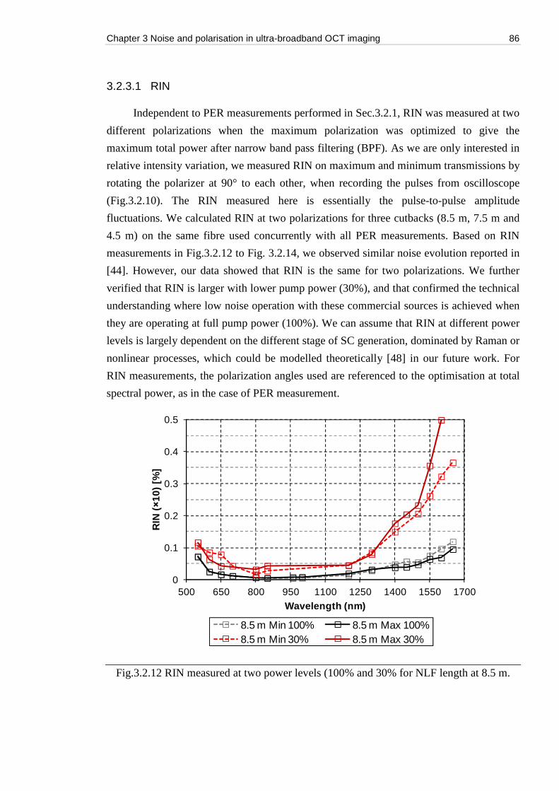
Chapter 3 Noise and polarisation in ultra-broadband OCT imaging 86
3.2.3.1 RIN
Independent to PER measurements performed in Sec.3.2.1, RIN was measured at two
different polarizations when the maximum polarization was optimized to give the
maximum total power after narrow band pass filtering (BPF). As we are only interested in
relative intensity variation, we measured RIN on maximum and minimum transmissions by
rotating the polarizer at 90° to each other, when recording the pulses from oscilloscope
(Fig.3.2.10). The RIN measured here is essentially the pulse-to-pulse amplitude
fluctuations. We calculated RIN at two polarizations for three cutbacks (8.5 m, 7.5 m and
4.5 m) on the same fibre used concurrently with all PER measurements. Based on RIN
measurements in Fig.3.2.12 to Fig. 3.2.14, we observed similar noise evolution reported in
[44]. However, our data showed that RIN is the same for two polarizations. We further
verified that RIN is larger with lower pump power (30%), and that confirmed the technical
understanding where low noise operation with these commercial sources is achieved when
they are operating at full pump power (100%). We can assume that RIN at different power
levels is largely dependent on the different stage of SC generation, dominated by Raman or
nonlinear processes, which could be modelled theoretically [48] in our future work. For
RIN measurements, the polarization angles used are referenced to the optimisation at total
spectral power, as in the case of PER measurement.
Fig.3.2.12 RIN measured at two power levels (100% and 30% for NLF length at 8.5 m.
0
0.1
0.2
0.3
0.4
0.5
500 650 800 950 1100 1250 1400 1550 1700
RIN
(×
10)
[%]
Wavelength (nm)
8.5 m Min 100% 8.5 m Max 100%8.5 m Min 30% 8.5 m Max 30%
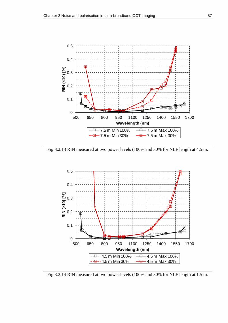
Chapter 3 Noise and polarisation in ultra-broadband OCT imaging 87
Fig.3.2.13 RIN measured at two power levels (100% and 30% for NLF length at 4.5 m.
Fig.3.2.14 RIN measured at two power levels (100% and 30% for NLF length at 1.5 m.
0
0.1
0.2
0.3
0.4
0.5
500 650 800 950 1100 1250 1400 1550 1700
RIN
(×
10)
[%]
Wavelength (nm)
7.5 m Min 100% 7.5 m Max 100%7.5 m Min 30% 7.5 m Max 30%
0
0.1
0.2
0.3
0.4
0.5
500 650 800 950 1100 1250 1400 1550 1700
RIN
(×
10)
[%]
Wavelength (nm)
4.5 m Min 100% 4.5 m Max 100%4.5 m Min 30% 4.5 m Max 30%
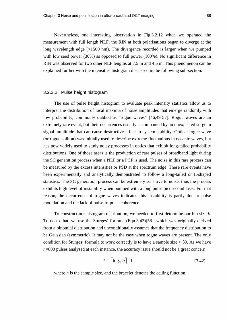
Chapter 3 Noise and polarisation in ultra-broadband OCT imaging 88
Nevertheless, one interesting observation in Fig.3.2.12 when we operated the
measurement with full length NLF, the RIN at both polarisations began to diverge at the
long wavelength edge (>1500 nm). The divergence recorded is larger when we pumped
with low seed power (30%) as opposed to full power (100%). No significant difference in
RIN was observed for two other NLF lengths at 7.5 m and 4.5 m. This phenomenon can be
explained further with the intensities histogram discussed in the following sub-section.
3.2.3.2 Pulse height histogram
The use of pulse height histogram to evaluate peak intensity statistics allow us to
interpret the distribution of local maxima of noise amplitudes that emerge randomly with
low probability, commonly dubbed as “rogue waves” [46,49-57]. Rogue waves are an
extremely rare event, but their occurrences usually accompanied by an unexpected surge in
signal amplitude that can cause destructive effect to system stability. Optical rogue wave
(or rogue soliton) was initially used to describe extreme fluctuations in oceanic waves, but
has now widely used to study noisy processes in optics that exhibit long-tailed probability
distributions. One of those areas is the production of rare pulses of broadband light during
the SC generation process when a NLF or a PCF is used. The noise in this rare process can
be measured by the excess intensities or PSD at the spectrum edge. These rare events have
been experimentally and analytically demonstrated to follow a long-tailed or L-shaped
statistics. The SC generation process can be extremely sensitive to noise, thus the process
exhibits high level of instability when pumped with a long pulse picosecond laser. For that
reason, the occurrence of rogue waves indicates this instability is partly due to pulse
modulation and the lack of pulse-to-pulse coherence.
To construct our histogram distribution, we needed to first determine our bin size k.
To do to that, we use the Sturges’ formula (Eqn.3.42)[58], which was originally derived
from a binomial distribution and unconditionally assumes that the frequency distribution to
be Gaussian (symmetric). It may not be the case when rogue waves are present. The only
condition for Sturges’ formula to work correctly is to have a sample size > 30. As we have
n=800 pulses analysed at each instance, the accuracy issue should not be a great concern.
1log2 += nk (3.42)
where n is the sample size, and the bracelet denotes the ceiling function.
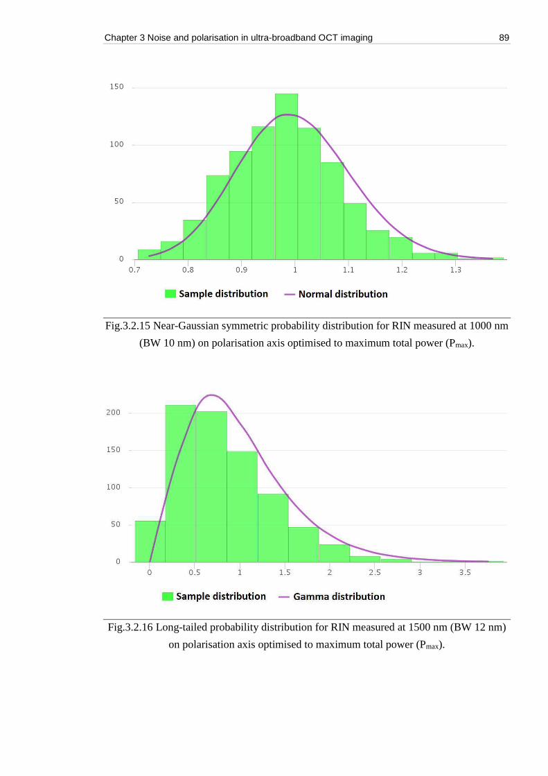
Chapter 3 Noise and polarisation in ultra-broadband OCT imaging 89
Fig.3.2.15 Near-Gaussian symmetric probability distribution for RIN measured at 1000 nm
(BW 10 nm) on polarisation axis optimised to maximum total power (Pmax).
Fig.3.2.16 Long-tailed probability distribution for RIN measured at 1500 nm (BW 12 nm)
on polarisation axis optimised to maximum total power (Pmax).
Chapter 3 Noise and polarisation in ultra-broadband OCT imaging 90
Fig.3.2.17 Long-tailed probability distribution for RIN measured at 1650 nm (BW 12 nm)
on polarisation axis optimised to maximum total power (Pmax).
Since we were mainly interested in studying the dynamics of solitons collisions at the
longer wavelengths, we plotted in Fig.3.2.15 to 3.2.17 show histograms of the pulse energy
fluctuations extracted over a 12 nm bandwidth at three wavelength ranges: 1000 nm, 1550
nm and 1650 nm. The use of histograms at specific wavelengths are useful to illustrate how
statistics of pulse amplitude fluctuations can vary from symmetric patterns (Gaussian
distribution overlay) near the pump (1000 nm) to long-tailed right-skewed (Gamma
distribution overlay) that decay exponentially near the red edge of the SC spectrum (1500
nm and 1650 nm). In the former case, we can safely assume that near the pump, the pulse
break up is dominated by modulation instability (MI). In the later case, around the long
wavelength edge, the pulse dynamics is dominated by Raman soliton self-frequency shift
(SFSS), as validated in our PER measurements in Sec. 3.2.1.1. The pulse intensity
histogram for the full SC spectrum (including visible wavelength and the blue edge) is
shown in Fig. 3.2.18.
Another way to analyse the extreme events in a spontaneous MI-driven SC
generation is to look at the higher-order statistical moments, such as skew and kurtosis.
Sorensen et al [46] has shown that the skew-kurtosis product (γ·κ) is a useful indicator of
the presence of rogue wave like dynamic behaviour.
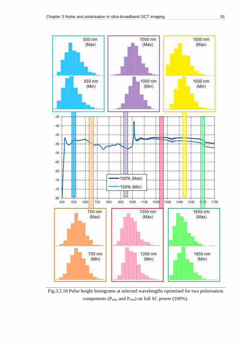
Chapter 3 Noise and polarisation in ultra-broadband OCT imaging 91
Fig.3.2.18 Pulse height histograms at selected wavelengths optimised for two polarisation
components (Pmax and Pmin) on full SC power (100%).
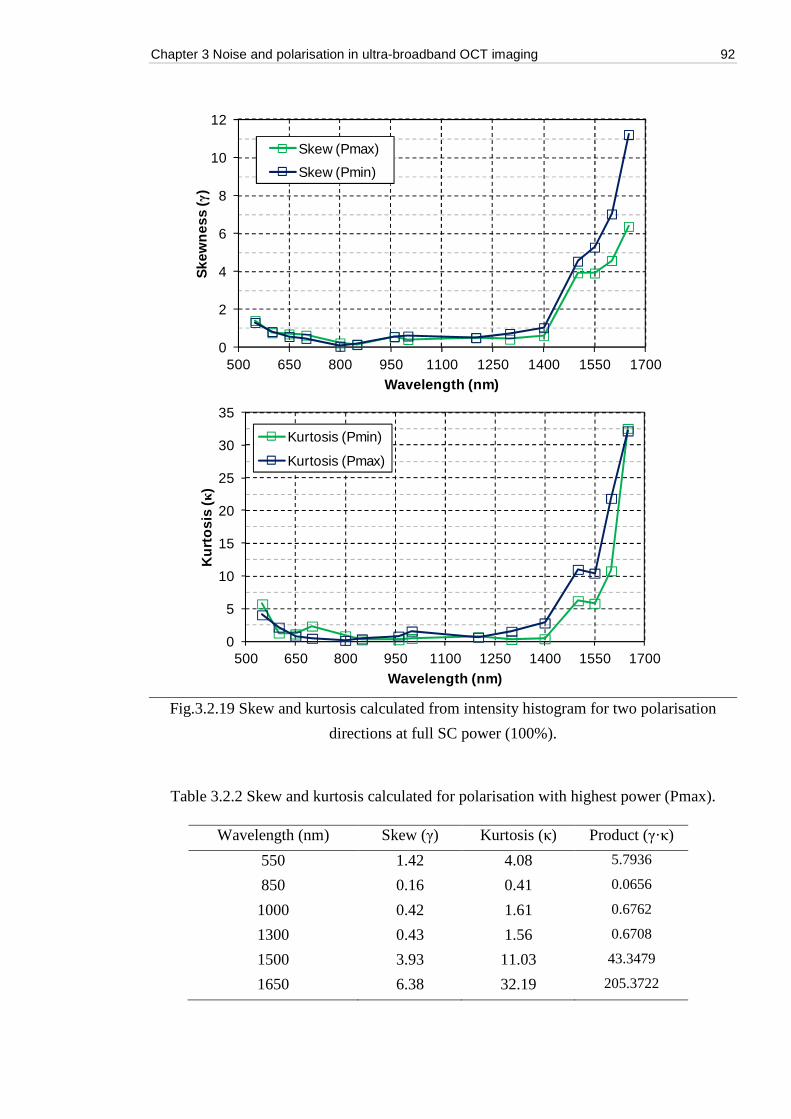
Chapter 3 Noise and polarisation in ultra-broadband OCT imaging 92
Fig.3.2.19 Skew and kurtosis calculated from intensity histogram for two polarisation
directions at full SC power (100%).
Table 3.2.2 Skew and kurtosis calculated for polarisation with highest power (Pmax).
Wavelength (nm) Skew (γ) Kurtosis (κ) Product (γ·κ)
550 1.42 4.08 5.7936
850 0.16 0.41 0.0656
1000 0.42 1.61 0.6762
1300 0.43 1.56 0.6708
1500 3.93 11.03 43.3479
1650 6.38 32.19 205.3722
0
2
4
6
8
10
12
500 650 800 950 1100 1250 1400 1550 1700
Ske
wn
ess
(γ)
Wavelength (nm)
Skew (Pmax)
Skew (Pmin)
0
5
10
15
20
25
30
35
500 650 800 950 1100 1250 1400 1550 1700
Ku
rto
sis
(κ)
Wavelength (nm)
Kurtosis (Pmin)
Kurtosis (Pmax)
Chapter 3 Noise and polarisation in ultra-broadband OCT imaging 93
We have chosen six wavelengths of interest, and tabulate the values of skew and
kurtosis in Fig.3.2.19 into Table 3.2.2. If the pulse intensity histogram exhibits a perfectly
Gaussian distribution function, we shall obtain zero for both skew and kurtosis [46,49].
However, our results have shown that it is not the case. For wavelengths in the vicinity of
the pump (between 850 nm and 1300 nm), we recorded the lowest values for both
parameters. Likewise from the histogram data, we observed that the pulse intensity
fluctuations are low. This is an indication that the noise characteristics in these wavelength
regions are dominated by low amplitude pulses generated through spontaneous MI [46,48].
However, at the spectral red edges, the pulse intensity fluctuations became significant as
evidenced from long-tailed (non-Gaussian) [59] histogram statistics, and this dynamics can
be attributed to stimulated Raman scattering (SRS), where red-shifted solitons were first
ejected from the pump pulse, and then underwent collisions in the Raman gain regime [46,
51-54]. Solitons collisions also caused dispersive waves to be generated in the blue edge of
the SC spectrum [49,51,56], and this event can be seen by the right-skewed histograms
extracted at 550 nm, while the increase in skew and kurtosis were recorded at this
wavelength. On the other hand, the rogue wave event had been observed at 1500 nm and
1650 nm, when the pulse dynamics become dominated by extreme sensitivity to peak
power variations, as evidenced in the excess value of skew-kurtosis product (γ·κ = 43.35 at
1500 nm and γ·κ = 205.37 at 1650 nm). These values are in good agreement to the
simulation data performed by [46], where they had previously shown that the skew-
kurtosis product > 10 yields rogue wave event during SC generation process.
Our measurement and analysis subsequently verified earlier findings on the long-
tailed statistical distribution that the optical rogue waves were originated from the
amplification of noise in the MI process, while the pump pulse experienced Raman
induced SSFS, wave-breaking process results in spectral broadening as these solitons
propagate down the long PCF, and as pulse-to-pulse fluctuations become significant, the
stability SC generation is subsequently affected. Several methods to control strong pulse
amplitude fluctuations and harness rogue waves have been proposed [60-63] in order to
improve the noise performance of a SC source.
Chapter 3 Noise and polarisation in ultra-broadband OCT imaging 94
3.3 Polarisation noise in OCT applications
In standard narrowband lasers PER is easy to quantify and its cause is generally
relatively simple to explain if one knows how the laser is constructed. However, due to the
complex nature of SC generation processes and the resulting wide spectrum, polarization
properties of produced SC are hard to quantify, characterize and explain. This is perhaps
the reason why this field has not previously been explored in detail. In all three
measurement optimizations in Sec.3.1, we observed significant PER around the pump.
This is expectable 1060-1070 nm as the fibre is short and the polarized pump is not
expected to be completely scrambled by the nonlinear fibre. It is however interesting that
the PER at the pump is reduced at higher pump powers. There are also some polarization
effects around 1100 nm which is the region where the Raman gain from the pump and the
modulation (MI) gain both have peaks [29,37,64-65]. As the Raman effect is polarization
sensitive it is not unexpected to see PER effects here. We would have expected to find the
majority of the light generated around 1100 nm is in the same axis as the majority of the
pump light as the Raman Gain is stronger to the same polarization that to the opposite
polarization. However while the measurements consistently show some PER in this region
there is no clear trend as to whether the majority of the light around 1100 nm in the same
axis as the pump or the opposite. Further from the pump i.e. >1200nm we see a PER which
consistently increase with wavelength but decreases or is pushed to longer wavelengths
with longer fibre and/or higher peak power. This region is the part of the spectrum which is
generated by solitons which red-shift from the MI region through the Raman caused
soliton self-frequency shift effect [35]. The reason the increasing PER with wavelength
could be that the polarization sensitivity of the Raman effect gradually “cleans up” the
polarization of the solitons polarization as they red-shift, however this would not explain
why PER then decrease with fibre length and increasing power. Another theory could be
that the highest power solitons for some reason is generated in one polarization axis of the
fibre and that the birefringence of the fibre is strong enough to keep them in that axis and
that the longest wavelengths which correspond to the strongest solitons are thus always
birefringent [66]. It is also worth noting that although clear PER effects are visible in the
long wavelength part of the spectrum there was little or no PER at wavelengths shorter
than the pump which is surprising as it is well known that the solitons at the long
wavelength edge of the continuum are responsible for the shifting of light to the shortest
wavelengths.
Chapter 3 Noise and polarisation in ultra-broadband OCT imaging 95
Our investigation concluded that there can be clear PER on the long wavelength edge
of picosecond generated SC from nominally non-birefringent silica PCF. We demonstrate
that some parts of the spectrum shows stable PER of over 10 dB, when measured with
reference to total spectra power. Specifically, wavelength of high PER occurred only in the
immediate vicinity of the pump wavelength, and for increasingly longer wavelengths. We
experimentally investigated how the spectrally resolved polarization develops with
increasing power, NLF length and wavelength, through the measurement of spectra and
RIN analysis. We found that there is no significant difference in the RIN of the two
polarizations and that at normal operating conditions i.e. long fibre and high power. The
source has negligible PER in the spectral bands typically used for OCT (650-950 nm and
1150-1550 nm). This report therefore validates the SC sources from NKT Photonics A/S
for use in polarization sensitive OCT applications within with optimal low-RIN
performance and some PER.
The other effect we have seen with our measurement is polarisation selection. Since
we are using a commercial light source, the NLF was assumed to be PM. Depending on
orientation of polarisation axis we assume the NLF to be non-birefringent. However,
results in Sec.3.2 showed the NLF to be nominally birefringent (<10-6). We also observed
the change of PER reduces as fibre length decreased, and is valid for all fibre lengths we
measured. This indicates it is not due to confinement loss or any polarising effect as both
axes lose power [48]. It is worth noting the change in PER at the pump wavelength. With
shorter fibre, there is a systematic trend that PER reduction is significant away from pump.
First, we showed that the same signed PER is obtained when total power measurement is
used. In this case, the pump doesn’t move, regardless of pump power. It appears that some
changes happen at longer wavelength. At low power, the maximum axis becomes
minimum axis, as evidenced in Fig.3.2.6. This can be consists of the superposition of the
supercontinua generated along each polarisation axis [66]. Second, the PER is fixed at the
pump. This is because everything measured around pump is a nonlinear process. Therefore
it is the principle fibre axis orientation that results in self-induced polarisation changes
[67], thus higher PER. Third, PER increases with pump power at longer wavelengths.
Higher power induces greater Raman self-frequency shift (SFS) on solitons, causing them
to experience greater red-shift. Forth, we observed the birefringence increases with
wavelength. This could be attributed to pulse walk-off that reduces the polarisation
interaction length, resulting in pulses in two polarisation axes stopped interacting [66].
Chapter 3 Noise and polarisation in ultra-broadband OCT imaging 96
We do not propose to explain the clear PER effects that we have measured SC
generation process are simply too complex to do so with any certainty. The general
understanding of how supercontinua are generated have emerged gradually over nearly a
decade of comparison of measurements and increasingly detailed simulations. However
measurements have generally focused on the visible wavelength of the supercontinua and
appear to have over looked these PER effect on the long wavelength edge. Meanwhile
most simulations have generally assumed ideal perfectly non-birefringent fibres and often
only modelled the evolution of a single evolution. It is therefore expected that considerable
effort will be needed before these PER effects can be fully explained.
On the noise studies, we are unable to make new conclusion on the polarisation
dependency. However, the use of higher order moments about the mean, such as skew and
kurtosis, allows us to at least quantify the noise at different regions of the spectrum. Our
results have preliminarily validated the earlier claims from Moller et al that RIN is low
around the pump, and increase in a parabolic way for wavelengths further out to the
spectral edges. Nevertheless, we can only observe a minor variation in noise from our
pulse height histogram (PHH) statistics, for the two polarizations. Our long tailed
probability distribution did show little difference in PD-RIN at different pump power.
Without these rigorous analysis, these variations are too little to be noticed experimentally,
and to our understanding, these effect will be insignificant to general SC operations or
when used in imaging applications such as OCT.
Our investigation concluded that the degree of polarisation varies at edge of the
spectrum in nominally non-birefringent silica PCF. We demonstrate that some parts of the
spectrum shows stable PER of over 10 dB, when measured with reference to total spectra
power. Specifically, wavelength of high PER occurred only in the immediate vicinity of
the pump wavelength, and for increasingly longer wavelengths. Region where PER
appears is dependent on power and fibre length. We experimentally verified how the
spectrally resolved polarisation develops with increasing power and along the length of the
NLF, through the measurement of birefringence and pulse to pulse RIN analysis. The
experimental results are compared to numerical simulations of coupled polarisation states
mimicking the experimental conditions. This report therefore validates the SC sources
from NKT Photonics A/S for use in polarisation-sensitive OCT applications within two
spectral bands (650-950 nm and 1150-1550 nm) with optimal low-RIN performance and
some PER. The results we published are to be used to assist in future simulation to explain
our findings.
Chapter 3 Noise and polarisation in ultra-broadband OCT imaging 97
References
1. W. V. Sorin and D. M. Baney, “A simple intensity noise reduction technique for optical low-coherence reflectometry,” IEEE Photonics Tech. Lett., vol. 4, no. 12, pp. 1404-1406, 1992.
2. K. Takada, “Noise in optical low-coherence reflectometry,” IEEE J. Quantum Elec., vol.34, pp. 1098-1108, 1998.
3. A. Rollins and J. Izatt, “Optimal interferometer designs for optical coherence tomography,” Opt. Lett., vol. 24, pp. 1484-1486, 1999.
4. R. C. Haskell, D. Liao, A. E. Pivonka, et al., “Role of beat noise in limiting the sensitivity of optical coherence tomography,” J. Opt. Soc. Am. A, vol. 23, no. 11, pp. 2747-2755, 2006.
5. L. Mendel, “Interference and the Alford and Gold effect,” J. Opt. Soc. Am. A, vol. 52, no. 12, pp. 1335-1339, 1962.
6. S. A. Dyer, Wiley survey of instrumentation and measurement, Wiley-IEEE Press, pp. 459-461, 2004.
7. C. C. Rosa and A. Gh. Podoleanu, “Limitation of the achievable signal-to-noise ratio in optical coherence tomography due to mismatch of the balanced receiver,” Appl. Opt., vol. 43, no.25, pp. 4802-4815, 2004.
8. A. Yariv, Optical Electronics, 4th ed., Saunders, Philadelphia, PA, pp. 520-529, 1991 9. M. Born and E. Wolf, Principles of Optics, 6th ed., Pergamon, Oxford, pp. 503-529, 1991. 10. R. Leitgeb, C. K. Hitzenberger, A. F. Fercher, “Performance of fourier domain vs. time
domain optical coherence tomography,” Opt. Expr., vol. 11, no. 8, pp.889-894, 2003. 11. H. Hodara, “Statistics of thermal and laser radiation,” Proceedings of the IEEE, pp. 696-704,
1964. 12. T. Yoshino, M. R. Ali, B. C. Sarker, "Performance analysis of low-coherence interferometry
taking into consideration of beat noise,” J. Opt. Soc. Am. A., vol. 22, pp. 328-335, 2005. 13. E. A. Swanson, D. Huang, M. R. Hee, et al, "High-speed optical coherence domain
reflectometry,” Opt. Lett., vol. 17, no. 2, 1992. 14. G. L. Abbas, V. W. S. Chan, T. K. Yee, "A dual-detector optical heterodyne receiver for
local oscillator noise suppression,” J. Lightwave Tech., vol. LT-3, no. 5, pp. 1110-1122, 1985.
15. H. P. Yuen, V. W. S. Chan, “Noise in homodyne and heterodyne detection,” Opt. Lett., vol. 8, no. 3, pp.177-179, 1983.
16. J. Brown, S. Kim, and A. Wax, “Noise characterization of supercontinuum sources for low-coherence interferometry applications,” J. Opt. Soc. Am. A 31, 2703-2710 (2014)
17. J. T. Woodward, A. W. Smith, C. A. Jenkins, C. Lin, S. W. Brown and K. R. Lykke, "Supercontinuum sources for metrology", Metrologia, 46(4) S277 (2009).
18. C. F. Kaminski, R. S. Watt, A. D. Elder, J. H. Frank, J. Hultm "Supercontinuum radiation for applications in chemical sensing and microscopy," Appl. Phys. B 92, 367–378 (2008).
19. S. Coen, J. D. Harvey, G. Genty, and J. M. Dudley, "Fiber Based Supercontinuum Sources for Optical Fibre Sensors," OSA Technical Digest (CD), paper TuA2 (2006).
20. P. Wang et al., "White Light Trapping Using Supercontinuum Generation Spectra in a Lead-Silicate Fibre Taper," in J. Lightwave Tech. 32(1), 40-45 (2014).
21. W. Drexler, M. Liu, A. Kumar, T, Kamali, A. Unterhuber, R. A. Leitgeb, “Optical coherence tomography today: speed, contrast, and multimodality,” J. Biomed. Opt. 19(7), 071412 (2014).
Chapter 3 Noise and polarisation in ultra-broadband OCT imaging 98
22. M. Yamanaka, T. Teranishi, H. Kawagoe, N. Nishizawa, "Optical coherence microscopy in 1700 nm spectral band for high-resolution label-free deep-tissue imaging," Sci. Rep. 6, 31715 (2016).
23. P. Bhatia, S. Choudhari, A. Rodrigues, M. Patil and R. Makkar, "High resolution imaging system using spectral domain Optical Coherence Tomography using NIR source," IEEE Xplore (WiSPNET), 2212-2216 (2016).
24. You, C. Wang, Y. Lin, A. Zaytsev, P. Xue and C. Pan, “Ultrahigh-resolution optical coherence tomography at 1.3 μm central wavelength by using a supercontinuum source pumped by noise-like pulses,” Laser Phys. Lett. 13, 025101 (2016).
25. W. J. Brown, S. Kim, A. Wax, "Noise Characterization of Supercontinuum Sources for Low Coherence Interferometry Applications," J. Opt. Soc. Amer. A. 31(12), 2703–2710 (2014).
26. Z. Zhu and T. G. Brown, "Polarization properties of supercontinuum spectra generated in birefringent photonic crystal fibers," J. Opt. Soc. Am. B 21(2), 249-257 (2004).
27. Z. Zhu and T. Brown, "Experimental studies of polarization properties of supercontinua generated in a birefringent photonic crystal fiber," Opt. Express 12(5), 791-796 (2004).
28. D. Solli and B. Jalali, "Direct Time-Domain Measurements of the Pulse Amplitude Statistics of a Fiber Supercontinuum Source," CLEO Conference, OSA Technical Digest Series (CD) CMB3 (2007).
29. S. G. Murdoch, R. Leonhardt, and J. D. Harvey, "Polarization modulation instability in weakly birefringent fibers," Opt. Lett. 20(8), 866-868 (1995).
30. M. Tianprateep, J. Tada, and F. Kannari, "Influence of polarization and pulse shape of femtosecond initial laser pulses on spectral broadening in microstructure fibers," Opt. Rev. 12(3), 179-189 (2005).
31. S. Wabnitz, E. M. Wright, and G. I. Stegeman, "Polarization instabilities of dark and bright coupled solitary waves in birefringent optical fibers," Phys. Rev. A 41, 6415 (1990).
32. N. Hanik, Modelling of nonlinear optical wave propagation including linear mode-coupling and birefringence, Opt. Comm. 214(1), 207-230 (2002).
33. S. R. Domingue and R. A. Bartels, "Overcoming temporal polarization instabilities from the latent birefringence in all-normal dispersion, wavebreaking-extended nonlinear fiber supercontinuum generation," Opt. Exp. 21, 13305-13321, (2013).
34. H. Tu, Y. Liu, X. Liu, D. Turchinovich, J. Lgsgaard, and S. Boppart, "Nonlinear polarization dynamics in a weakly birefringent all-normal dispersion photonic crystal fiber: toward a practical coherent fiber supercontinuum laser," Opt. Expr. 20, 1113-1128 (2012).
35. J. M. Dudley, G. Genty, S. Coen, "Supercontinuum generation is photonic crystal fiber", Rev. Mod. Phys(4). 78, 1135-1184 (2006).
36. V. L. Kalashnikov, P. Dombi, T. Fuji, W. J. Wadsworth, J. C. Knight, P. St. J. Russell, R. S. Windeler, and A.Apolonski, "Maximization of supercontinua in photonic crystal fibers by using double pulses and polarization effects," Appl. Phys. B 77(2-3), 319-324 (2003).
37. S. Coen, A. H. L. Chau, R. Leonhardt, J. D. Harvey, "Supercontinuum generation by stimulated Raman scattering and parametric four-wave mixing in photonic crystal fibers", J. Opt. Soc. Am. B 19(4) 753-764 (2002).
38. Y. Yang, W. Duan and M. Ye, "High precision measurement technology for beat length of birefringence optical fiber," Meas. Sci. Technol. 24, 025201 (2013)
39. P. Hlubina and D. Ciprian, "Spectral-domain measurement of phase modal birefringence in polarization-maintaining fiber," Opt. Express 15 (25), 17019-17024 (2007).
Chapter 3 Noise and polarisation in ultra-broadband OCT imaging 99
40. Y. Mizuno, Z. He and K. Hotate, "Polarization Beat Length Distribution Measurement in Single-Mode Optical Fibers with Brillouin Optical Correlation-Domain Reflectometry," Appl. Phys. Express 2 046502 (2009).
41. S. C. Rashleigh, "Measurement of fiber birefringence by wavelength scanning: effect of dispersion," Opt. Lett. 8, 336-338 (1983).
42. D. Derickson, ed., Fiber Optic Test and Measurement (Prentice Hall, 1998) 43. J. Ramsay, S. Dupont, and S. R. Keiding, "Pulse-to-pulse noise reduction in infrared
supercontinuum spectroscopy: Polarization and amplitude fluctuations," Laser Phys. Lett. 11, 095702 (2014).
44. Y. Liu, Y. Zhao, J. Lyngsø, S. You, W. L. Wilson, H. Tu, "Suppressing short-term polarization noise and related spectral decoherence in all-normal dispersion fiber supercontinuum generation," J. Light. Tech. 33(9), 1814-1820 (2015).
45. U. Møller, S. T. Sørensen, C. Jakobsen, J. Johansen, P. M. Moselund, C. L. Thomsen, and O. Bang, "Power dependence of supercontinuum noise in uniform and tapered PCFs," Opt. Express 20, 2851-2857 (2012).
46. S.T. Sørensen, O. Bang, B. Wetzel, J.M. Dudley, "Describing supercontinuum noise and rogue wave statistics using higher-order moments," Opt. Comm. 285, 2451-2455 (2012).
47. H. Cramér, “Mathematical methods and statistics,” Princeton Univ. Press (1999). 48. M. H. Frosz, "Validation of input-noise model for simulations of supercontinuum generation
and rogue waves," Opt. Express, 18(14), 14778-14787 (2010). 49. Shanti Toenger, Thomas Godin, Cyril Billet, Frédéric Dias, Miro Erkintalo, Goëry Genty &
John M. Dudley, "Emergent rogue wave structures and statistics in spontaneous modulation instability," Sci. Rep. 5, 10380 (2015).
50. C. Lafargue, J. Bolger, G. Genty, F. Dias, J. M. Dudley, and B. J. Eggleton, “Direct detection of optical rogue wave energy statistics in supercontinuum generation,” Electron. Lett. 45, 217–219 (2009).
51. D. R. Solli, C. Ropers, P. Koonath, and B. Jalali, “Optical rogue waves,” Nature 450, 1054–1057 (2007).
52. B. Wetzel, A. Stefani, L. Larger, P. A. Lacourt, J. M. Merolla, T. Sylvestre, A. Kudlinski, A. Mussot, G. Genty, F. Dias and J. M. Dudley, "Real-time full bandwidth measurement of spectral noise in supercontinuum generation," Sci. Rep. 2(882), 1-7 (2012)
53. C. Lafargue, J. Bolger, G. Genty, F. Dias, J. M. Dudley and B. J. Eggleton, "Direct detection of optical rogue wave energy statistics in supercontinuum generation," Electron. Lett. 45(4), 217-219 (2009).
54. A. Aalto, G. Genty, and J. Toivonen, "Extreme-value statistics in supercontinuum generation by cascaded stimulated Raman scattering," Opt. Express 18, 1234-1239 (2010).
55. K.L. Corwin, N.R. Newbury, J.M. Dudley, S. Coen, S.A. Diddams, B.R. Washburn, K. Weber, R.S. Windeler, "Fundamental amplitude noise limitations to supercontinuum spectra generated in a microstructured fiber," Appl. Phy. B 77(2-3), 269-277 (2003).
56. J. M. Dudley, F. Dias, M. Erkintalo, and G. Genty, “Instabilities, breathers, and rogue waves in optics,” Nature Photon. 8, 755–764 (2014).
57. M. Erkintalo, G. Genty, and J. M. Dudley, “Rogue wave like characteristics in femtosecond supercontinuum generation,” Opt. Lett. 34, 2468–2470 (2009).
58. H.O. Lancaster, “An Introduction to Medical Statistics,” John Wiley & Sons (1974). 59. Y. E. Monfared and S. A. Ponomarenko, "Non-Gaussian statistics and optical rogue waves in
stimulated Raman scattering," Opt. Express 25, 5941-5950 (2017)
Chapter 3 Noise and polarisation in ultra-broadband OCT imaging 100
60. D. R. Solli, C. Ropers, and B. Jalali, “Active Control of Rogue Waves for Stimulated Supercontinuum Generation,” Phys. Rev. Lett. 101 (23), 233902 (2008).
61. J. M. Dudley, G. Genty, and B. J. Eggleton, "Harnessing and control of optical rogue waves in supercontinuum generation," Opt. Express 16, 3644-3651 (2008).
62. G. Genty and J. M. Dudley, “Route to Coherent Supercontinuum Generation in the Long Pulse Regime,” IEEE J. Quantum Electron. 45(11), 1331-1335 (2009).
63. A. Kudlinski, B. Barviau, A. Leray, C. Spriet, L. Héliot, and A. Mussot, "Control of pulse-to-pulse fluctuations in visible supercontinuum," Opt. Express 18, 27445-27454 (2010).
64. S. Wabnitz, "Modulation polarization instability of light in a nonlinear birefringent dispersive medium," Phys. Rev. A 38, 2018-2021 (1988).
65. E. A. Golovchenko and A. N. Pilipetskii, "Unified analysis of four-photon mixing, modulational instability, and stimulated Raman scattering under various polarization conditions in fibers," J. Opt. Soc. Am. B 11(1), 92-101 (1994).
66. A. Proulx, J.-M. Ménard, N.Hô, J. Laniel, R. Vallée, and C. Paré, "Intensity and polarization dependences of the supercontinuum generation in birefringent and highly nonlinear microstructured fibers," Opt. Expr. 11(25), 3338-3345 (2003)
67. H. G. Winful, “Self-induced polarization changes in birefringent optical fiber,” Appl. Phys. Lett. 47, 213–215 (1986). .
4
Dispersion in OCT systems
High-resolution optical coherence tomography (OCT) has become increasingly
common for non invasive imaging of three-dimensional (3D) microstructures and
biological tissues, especially in ophthalmology [1]. The demand of commercial high-
resolution imaging has increased in the last decade owing to improved capability to track
sub-micron features and layered structures. The development of such systems requires the
use of optical components with different glass thickness and densities. However, the
presence of various glass materials of different refractive indices in an OCT configuration
makes the phase velocity dependent on the wavelength of the excitation signal.
To achieve the theoretical axial resolution determined by the bandwidth Δλ of the
source, compensation for dispersion in the interferometer is essential. Dispersion occurs
because the refractive index varies with the wavelength. Therefore, group velocity
mismatch between different wavelength components in the spectrum leads to deterioration
of the axial resolution, irrespective of the OCT method used: time domain, spectrometer-
based (spectral domain) [2] or swept source based (Fourier domain) OCT systems [3].
Despite the widespread use of spectrometer-based and swept source-based methods. In
recent times, time-domain OCT retains niche applications in microscopy, where high
transversal resolution is achievable using high numerical aperture (NA) objectives [4].
For a time-domain OCT system, a typical compensation method, referred to here as
the full-width at half-maximum (FWHM) method, is based on iterative adjustment of
dispersion inserted into the interferometer until the FWHM of the autocorrelation function
is minimised. This operation is time-consuming, as it requires repetitive procedures and
easily prone to measurement errors. After each adjustment, there is no way to know in
which direction to proceed, whether to add or reduce glass length to adjust the dispersion
introduced by the optical components in the system. The classical procedure only aims at
finding a minimum of the autocorrelation peak width.
We therefore present a better method to evaluate dispersion in time-domain
interferometers. This method involves using a tuneable optical source in a broadband
Chapter 4 Dispersion in OCT systems 102
range, a mirror placed in the object arm of the interferometer and measuring the relative
position of the autocorrelation peak in optical path difference (OPD) versus the central
wavelength of the tuneable source. The method is illustrated on a time-domain OCT
systems. It is also applicable for Sp-OCT, SS-OCT and conventional FD-OCT.
Previous reports have documented the utilization of rods of SF11 glass [5] and of
spectral delay lines for dispersion characterization [6–13]. Similar methods of dispersion
compensation are illustrated here. In this chapter, we present a novel approach to use
different BK 7 rod glasses to compensate for dispersion of a time-domain OCT system
operating at 1300 nm.
4.1 Dispersion and coherence
4.1.1 Coherence
In low coherence interferometers with negligible dispersion, the theoretical limit for
the axial resolution is determined by half of the source coherence length CL. For a
Gaussian spectral-shaped source spectrum, with λ the central wavelength and a FWHM
bandwidth of Δλ, CL is given by.
λλ
π ∆≈
2)2ln(4LC (4.1)
The inverse proportionality with Δλ makes broadband light sources essential for
achieving high axial resolution [1,5,6]. In recent years, broadband supercontinuum sources
have been used extensively in many OCT applications. The larger the optical bandwidth,
the shorter the coherence length. However, dispersion is manifest, as variation of index of
refraction with wavelength becomes significant.. If dispersion is left uncompensated in the
interferometer, the autocorrelation peak width of an A-scan measured using a mirror as
object becomes wider, resulting in degradation of imaging resolution.
To study dispersion in optics, let us first consider a Gaussian shaped pulse, with an
amplitude A0, angular frequency ω propagating along z-axis through a dispersive medium
with a wave constant β as shown in Fig. 4.1. The general expression for this pulse can be
written as in Eqn.4.2.
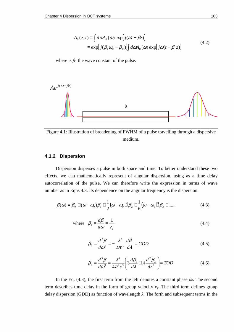
Chapter 4 Dispersion in OCT systems 103
[ ][ ] [ ]
−−=
−=
)(exp)()(exp
)(exp)(),(
10001
00
ztjAdj
ztjAdtzA
βωωωβωβ
βωωω (4.2)
where is β1 the wave constant of the pulse.
Figure 4.1: Illustration of broadening of FWHM of a pulse travelling through a dispersive
medium.
4.1.2 Dispersion
Dispersion disperses a pulse in both space and time. To better understand these two
effects, we can mathematically represent of angular dispersion, using as a time delay
autocorrelation of the pulse. We can therefore write the expression in terms of wave
number as in Eqns 4.3. Its dependence on the angular frequency is the dispersion.
( ) ( ) ......6
1
2
1)()( 3
302
20100 +−+−+−+= βωωβωωβωωβωβ (4.3)
where gvd
d 11 ==
ωββ (4.4)
GDDd
d
cd
d =−==λβ
πλ
ωββ 1
2
2
2
2
2 2 (4.5)
TODd
d
d
d
cd
d =
+==
22
21
32
4
3
3
3 34 λ
βλλβ
πλ
ωββ (4.6)
In the Eq. (4.3), the first term from the left denotes a constant phase β0. The second
term describes time delay in the form of group velocity vg. The third term defines group
delay dispersion (GDD) as function of wavelength λ. The forth and subsequent terms in the
)( ztjAe βω −
β
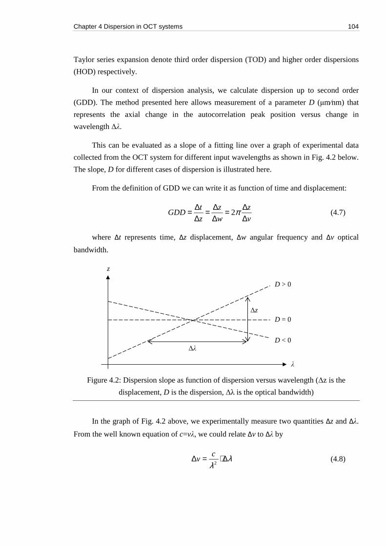
Chapter 4 Dispersion in OCT systems 104
Taylor series expansion denote third order dispersion (TOD) and higher order dispersions
(HOD) respectively.
In our context of dispersion analysis, we calculate dispersion up to second order
(GDD). The method presented here allows measurement of a parameter D (μm∕nm) that
represents the axial change in the autocorrelation peak position versus change in
wavelength Δλ.
This can be evaluated as a slope of a fitting line over a graph of experimental data
collected from the OCT system for different input wavelengths as shown in Fig. 4.2 below.
The slope, D for different cases of dispersion is illustrated here.
From the definition of GDD we can write it as function of time and displacement:
v
z
w
z
z
tGDD
∆∆=
∆∆=
∆∆= π2 (4.7)
where Δt represents time, Δz displacement, Δw angular frequency and Δv optical
bandwidth.
Figure 4.2: Dispersion slope as function of dispersion versus wavelength (Δz is the
displacement, D is the dispersion, Δλ is the optical bandwidth)
In the graph of Fig. 4.2 above, we experimentally measure two quantities Δz and Δλ.
From the well known equation of c=vλ, we could relate Δv to Δλ by
λλ
∆⋅=∆2
cv (4.8)
λ
D > 0
D = 0
D < 0
Δz
Δλ
z
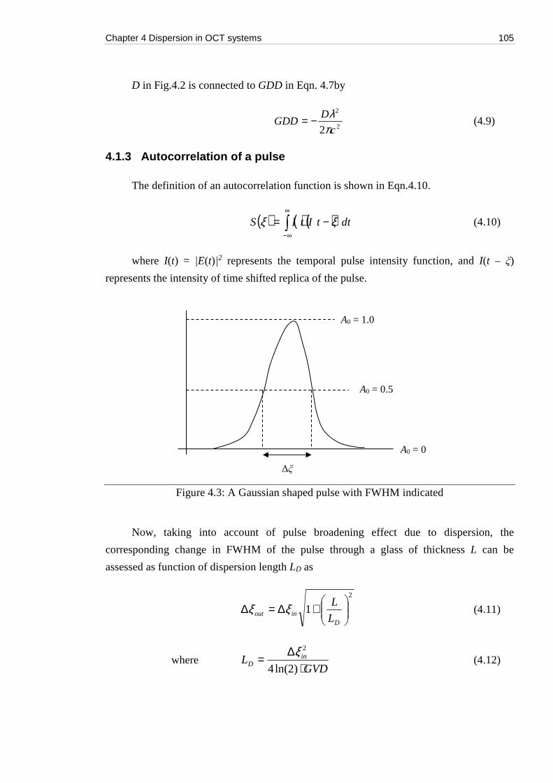
Chapter 4 Dispersion in OCT systems 105
D in Fig.4.2 is connected to GDD in Eqn. 4.7by
2
2
2 c
DGDD
πλ−= (4.9)
4.1.3 Autocorrelation of a pulse
The definition of an autocorrelation function is shown in Eqn.4.10.
( ) ( ) ( )∞
∞−
−= dttItIS ξξ (4.10)
where I(t) = |E(t)|2 represents the temporal pulse intensity function, and I(t – ξ)
represents the intensity of time shifted replica of the pulse.
Figure 4.3: A Gaussian shaped pulse with FWHM indicated
Now, taking into account of pulse broadening effect due to dispersion, the
corresponding change in FWHM of the pulse through a glass of thickness L can be
assessed as function of dispersion length LD as
2
1
+∆=∆
Dinout L
Lξξ (4.11)
where GVD
L inD ⋅
∆=
)2ln(4
2ξ (4.12)
A0 = 1.0
A0 = 0.5
A0 = 0
Δξ
Chapter 4 Dispersion in OCT systems 106
Dispersion length is defined as the propagation distance after a pulse travels, the
pulse width broadens by a factor of √2.
Therefore, the output temporal pulse autocorrelation function is:
2
2)2ln(41
∆+∆=∆
ininout
GDD
ξξξ (4.13)
where GVDLGDD ×= (4.14)
Finally, we have to relate the mathematical expression of acousto-optic tuneable
filter (AOTF) method to the formulas derived for the method of measuring FWHM of
autocorrelation function. To do that, we first need to evaluate n versus wavelength, and this
is the dispersion problem. Let us now consider c is the speed of light, the inverse
proportionality of coherence length ρ from CL in Eq. (4.1), we define
2)2ln(2
πc
λλρ ∆= (4.15)
The shape of the autocorrelation function S(ξ) [7,8] can be written as
( )
+−
+=
2
22
24 2
20
12
1exp
1 dcd
AS
ξρξ (4.16)
where ξ is measured along the depth coordinate, and d defines the dispersion
enlargement, related to the group delay dispersion (GDD) by.
GDDd 2ρ= (4.17)
The larger the GDD, the wider the A-scan peak. By expanding the terms for d we
obtain
LCDd
λ∆−= (4.18)
To obtain the FWHM of the autocorrelation peak, we set the exponential term in
Eqn.4.16 to 0.5, and solve for Eqns. 4.9, 4.16 and 4.17. The FWHM of the autocorrelation
becomes
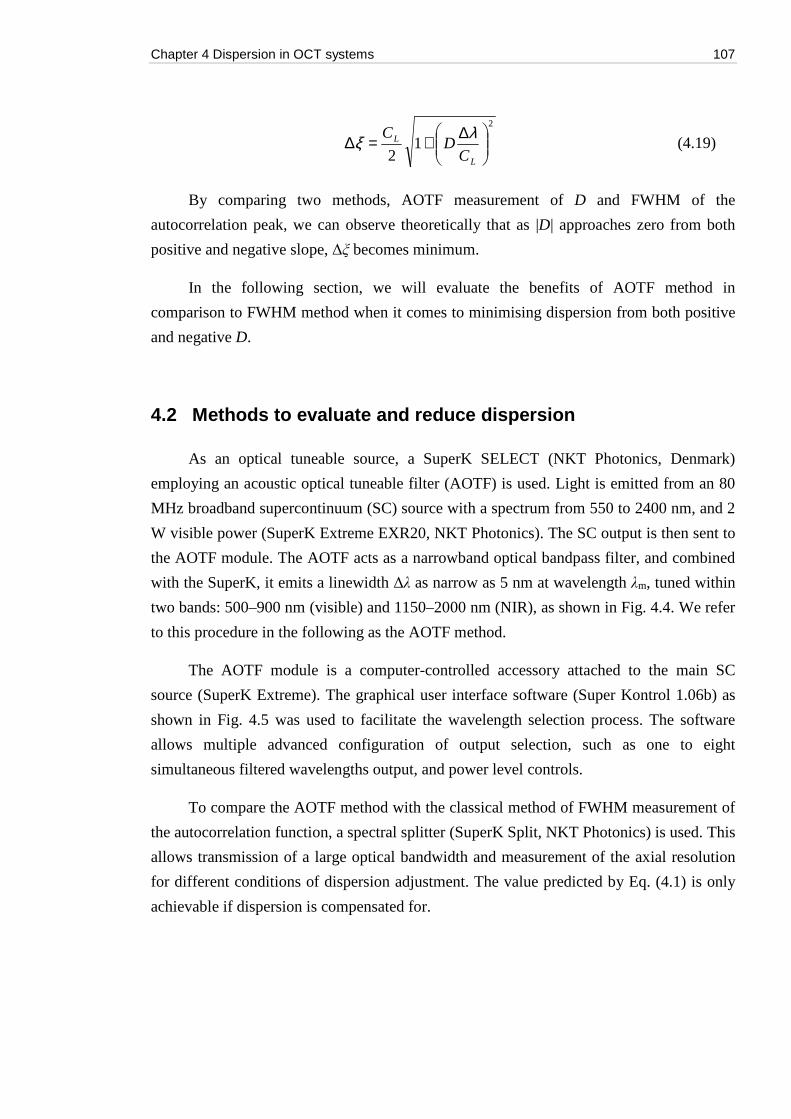
Chapter 4 Dispersion in OCT systems 107
2
12
∆+=∆L
L
CD
C λξ (4.19)
By comparing two methods, AOTF measurement of D and FWHM of the
autocorrelation peak, we can observe theoretically that as |D| approaches zero from both
positive and negative slope, Δξ becomes minimum.
In the following section, we will evaluate the benefits of AOTF method in
comparison to FWHM method when it comes to minimising dispersion from both positive
and negative D.
4.2 Methods to evaluate and reduce dispersion
As an optical tuneable source, a SuperK SELECT (NKT Photonics, Denmark)
employing an acoustic optical tuneable filter (AOTF) is used. Light is emitted from an 80
MHz broadband supercontinuum (SC) source with a spectrum from 550 to 2400 nm, and 2
W visible power (SuperK Extreme EXR20, NKT Photonics). The SC output is then sent to
the AOTF module. The AOTF acts as a narrowband optical bandpass filter, and combined
with the SuperK, it emits a linewidth Δλ as narrow as 5 nm at wavelength λm, tuned within
two bands: 500–900 nm (visible) and 1150–2000 nm (NIR), as shown in Fig. 4.4. We refer
to this procedure in the following as the AOTF method.
The AOTF module is a computer-controlled accessory attached to the main SC
source (SuperK Extreme). The graphical user interface software (Super Kontrol 1.06b) as
shown in Fig. 4.5 was used to facilitate the wavelength selection process. The software
allows multiple advanced configuration of output selection, such as one to eight
simultaneous filtered wavelengths output, and power level controls.
To compare the AOTF method with the classical method of FWHM measurement of
the autocorrelation function, a spectral splitter (SuperK Split, NKT Photonics) is used. This
allows transmission of a large optical bandwidth and measurement of the axial resolution
for different conditions of dispersion adjustment. The value predicted by Eq. (4.1) is only
achievable if dispersion is compensated for.
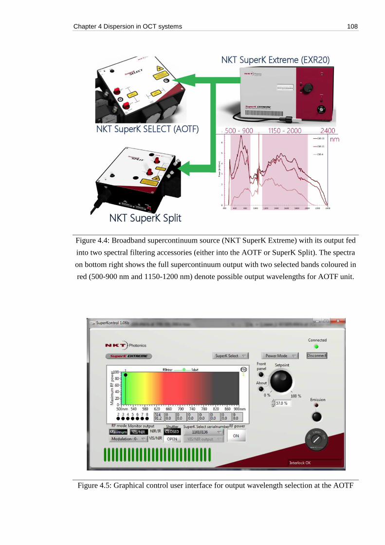
Chapter 4 Dispersion in OCT systems 108
Figure 4.4: Broadband supercontinuum source (NKT SuperK Extreme) with its output fed
into two spectral filtering accessories (either into the AOTF or SuperK Split). The spectra
on bottom right shows the full supercontinuum output with two selected bands coloured in
red (500-900 nm and 1150-1200 nm) denote possible output wavelengths for AOTF unit.
Figure 4.5: Graphical control user interface for output wavelength selection at the AOTF
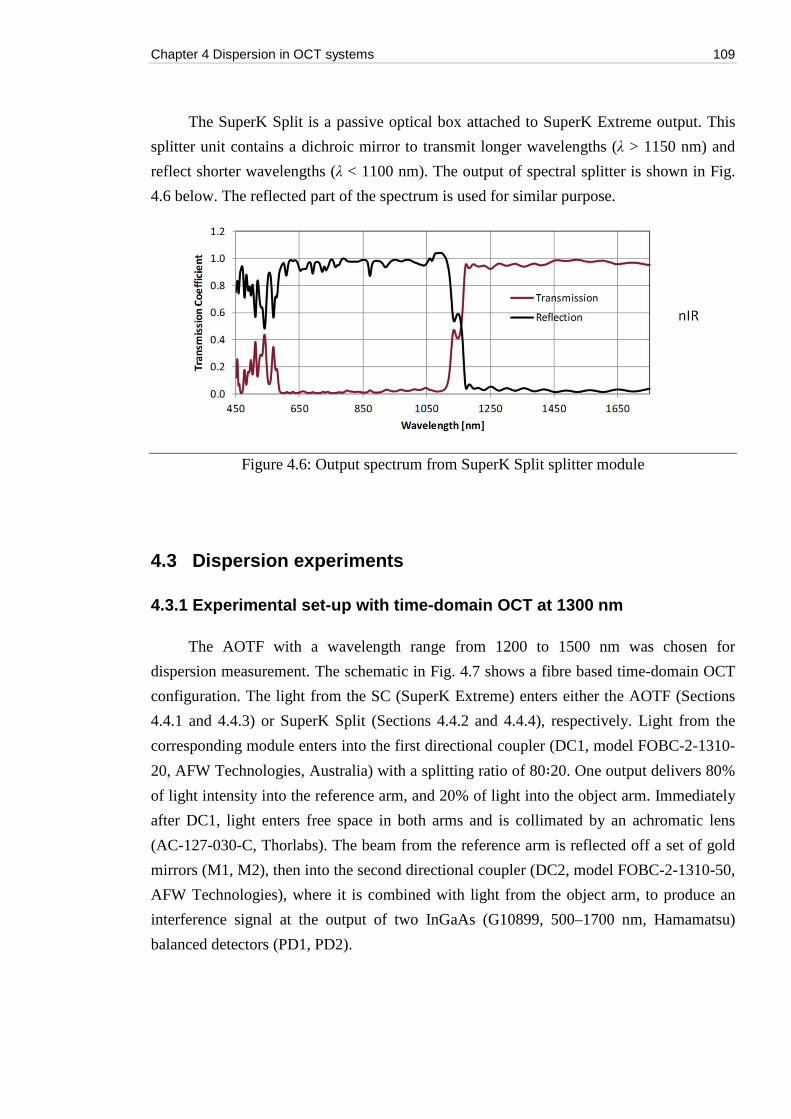
Chapter 4 Dispersion in OCT systems 109
The SuperK Split is a passive optical box attached to SuperK Extreme output. This
splitter unit contains a dichroic mirror to transmit longer wavelengths (λ > 1150 nm) and
reflect shorter wavelengths (λ < 1100 nm). The output of spectral splitter is shown in Fig.
4.6 below. The reflected part of the spectrum is used for similar purpose.
Figure 4.6: Output spectrum from SuperK Split splitter module
4.3 Dispersion experiments
4.3.1 Experimental set-up with time-domain OCT at 1300 nm
The AOTF with a wavelength range from 1200 to 1500 nm was chosen for
dispersion measurement. The schematic in Fig. 4.7 shows a fibre based time-domain OCT
configuration. The light from the SC (SuperK Extreme) enters either the AOTF (Sections
4.4.1 and 4.4.3) or SuperK Split (Sections 4.4.2 and 4.4.4), respectively. Light from the
corresponding module enters into the first directional coupler (DC1, model FOBC-2-1310-
20, AFW Technologies, Australia) with a splitting ratio of 80∶20. One output delivers 80%
of light intensity into the reference arm, and 20% of light into the object arm. Immediately
after DC1, light enters free space in both arms and is collimated by an achromatic lens
(AC-127-030-C, Thorlabs). The beam from the reference arm is reflected off a set of gold
mirrors (M1, M2), then into the second directional coupler (DC2, model FOBC-2-1310-50,
AFW Technologies), where it is combined with light from the object arm, to produce an
interference signal at the output of two InGaAs (G10899, 500–1700 nm, Hamamatsu)
balanced detectors (PD1, PD2).
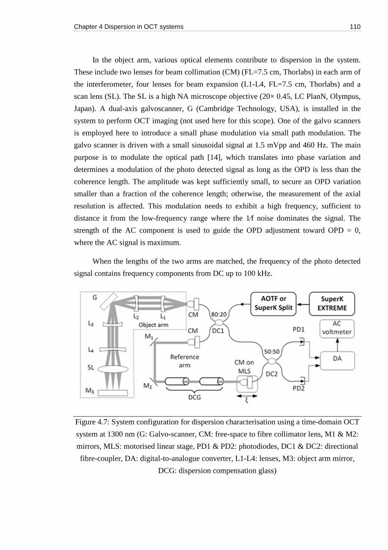
Chapter 4 Dispersion in OCT systems 110
In the object arm, various optical elements contribute to dispersion in the system.
These include two lenses for beam collimation (CM) (FL=7.5 cm, Thorlabs) in each arm of
the interferometer, four lenses for beam expansion (L1-L4, FL=7.5 cm, Thorlabs) and a
scan lens (SL). The SL is a high NA microscope objective (20× 0.45, LC PlanN, Olympus,
Japan). A dual-axis galvoscanner, G (Cambridge Technology, USA), is installed in the
system to perform OCT imaging (not used here for this scope). One of the galvo scanners
is employed here to introduce a small phase modulation via small path modulation. The
galvo scanner is driven with a small sinusoidal signal at 1.5 mVpp and 460 Hz. The main
purpose is to modulate the optical path [14], which translates into phase variation and
determines a modulation of the photo detected signal as long as the OPD is less than the
coherence length. The amplitude was kept sufficiently small, to secure an OPD variation
smaller than a fraction of the coherence length; otherwise, the measurement of the axial
resolution is affected. This modulation needs to exhibit a high frequency, sufficient to
distance it from the low-frequency range where the 1∕f noise dominates the signal. The
strength of the AC component is used to guide the OPD adjustment toward OPD = 0,
where the AC signal is maximum.
When the lengths of the two arms are matched, the frequency of the photo detected
signal contains frequency components from DC up to 100 kHz.
Figure 4.7: System configuration for dispersion characterisation using a time-domain OCT
system at 1300 nm (G: Galvo-scanner, CM: free-space to fibre collimator lens, M1 & M2:
mirrors, MLS: motorised linear stage, PD1 & PD2: photodiodes, DC1 & DC2: directional
fibre-coupler, DA: digital-to-analogue converter, L1-L4: lenses, M3: object arm mirror,
DCG: dispersion compensation glass)
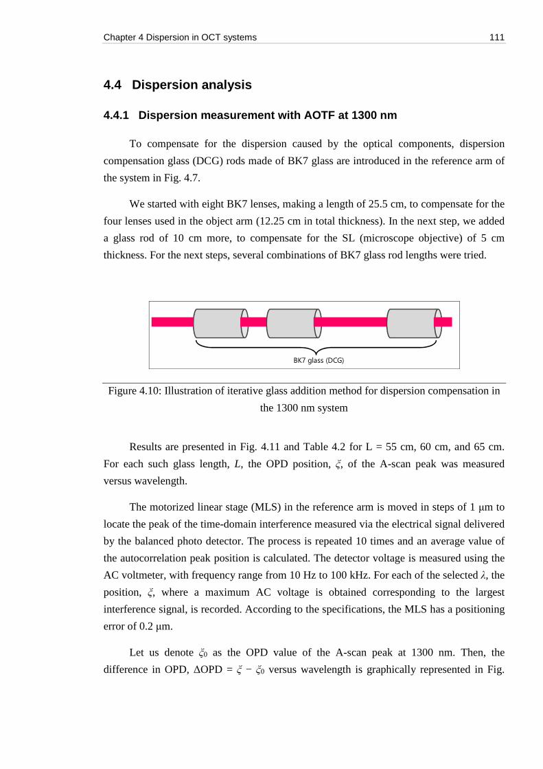
Chapter 4 Dispersion in OCT systems 111
4.4 Dispersion analysis
4.4.1 Dispersion measurement with AOTF at 1300 nm
To compensate for the dispersion caused by the optical components, dispersion
compensation glass (DCG) rods made of BK7 glass are introduced in the reference arm of
the system in Fig. 4.7.
We started with eight BK7 lenses, making a length of 25.5 cm, to compensate for the
four lenses used in the object arm (12.25 cm in total thickness). In the next step, we added
a glass rod of 10 cm more, to compensate for the SL (microscope objective) of 5 cm
thickness. For the next steps, several combinations of BK7 glass rod lengths were tried.
Figure 4.10: Illustration of iterative glass addition method for dispersion compensation in
the 1300 nm system
Results are presented in Fig. 4.11 and Table 4.2 for L = 55 cm, 60 cm, and 65 cm.
For each such glass length, L, the OPD position, ξ, of the A-scan peak was measured
versus wavelength.
The motorized linear stage (MLS) in the reference arm is moved in steps of 1 μm to
locate the peak of the time-domain interference measured via the electrical signal delivered
by the balanced photo detector. The process is repeated 10 times and an average value of
the autocorrelation peak position is calculated. The detector voltage is measured using the
AC voltmeter, with frequency range from 10 Hz to 100 kHz. For each of the selected λ, the
position, ξ, where a maximum AC voltage is obtained corresponding to the largest
interference signal, is recorded. According to the specifications, the MLS has a positioning
error of 0.2 μm.
Let us denote ξ0 as the OPD value of the A-scan peak at 1300 nm. Then, the
difference in OPD, ΔOPD = ξ − ξ0 versus wavelength is graphically represented in Fig.
BK7 glass (DCG)
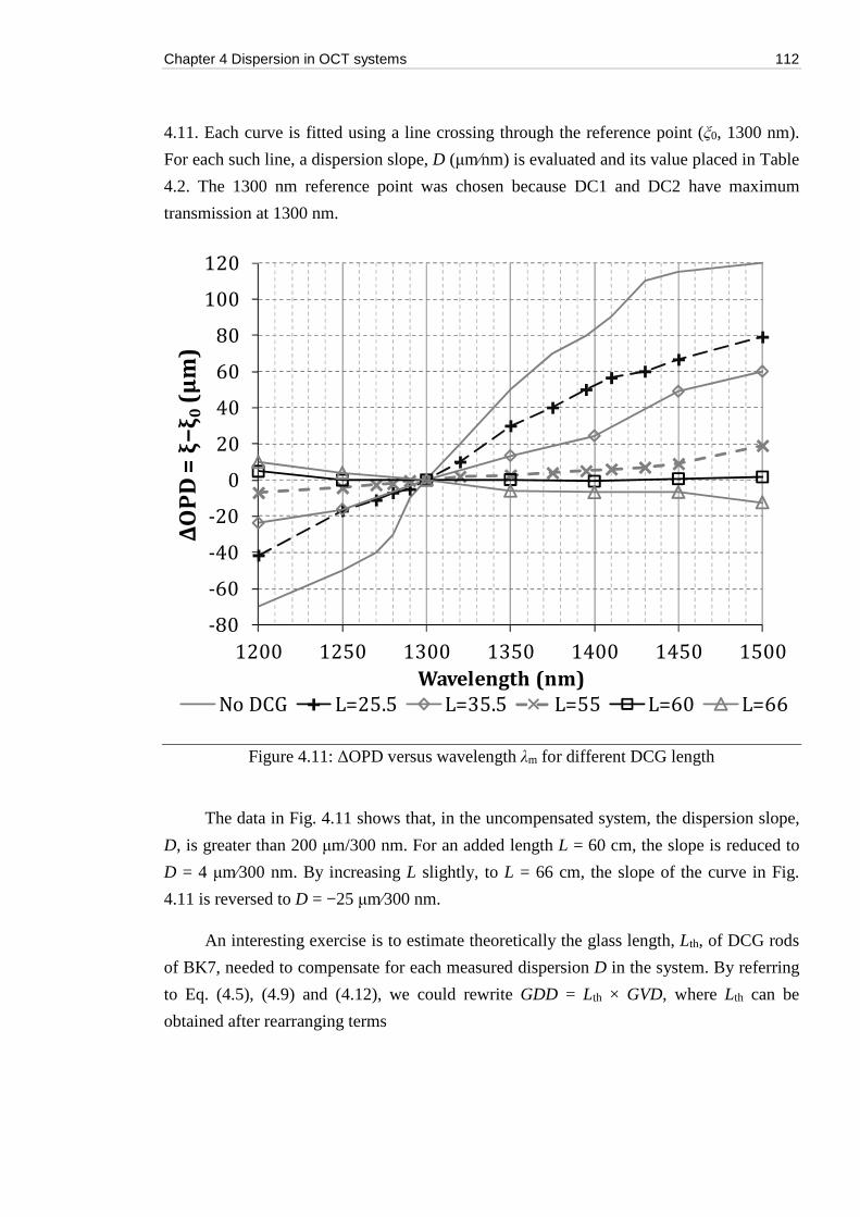
Chapter 4 Dispersion in OCT systems 112
4.11. Each curve is fitted using a line crossing through the reference point (ξ0, 1300 nm).
For each such line, a dispersion slope, D (μm∕nm) is evaluated and its value placed in Table
4.2. The 1300 nm reference point was chosen because DC1 and DC2 have maximum
transmission at 1300 nm.
Figure 4.11: ΔOPD versus wavelength λm for different DCG length
The data in Fig. 4.11 shows that, in the uncompensated system, the dispersion slope,
D, is greater than 200 μm/300 nm. For an added length L = 60 cm, the slope is reduced to
D = 4 μm∕300 nm. By increasing L slightly, to L = 66 cm, the slope of the curve in Fig.
4.11 is reversed to D = −25 μm∕300 nm.
An interesting exercise is to estimate theoretically the glass length, Lth, of DCG rods
of BK7, needed to compensate for each measured dispersion D in the system. By referring
to Eq. (4.5), (4.9) and (4.12), we could rewrite GDD = Lth × GVD, where Lth can be
obtained after rearranging terms
-80
-60
-40
-20
0
20
40
60
80
100
120
1200 1250 1300 1350 1400 1450 1500
ΔO
PD
= ξ
−ξ 0
(µm
)
Wavelength (nm)
No DCG L=25.5 L=35.5 L=55 L=60 L=66
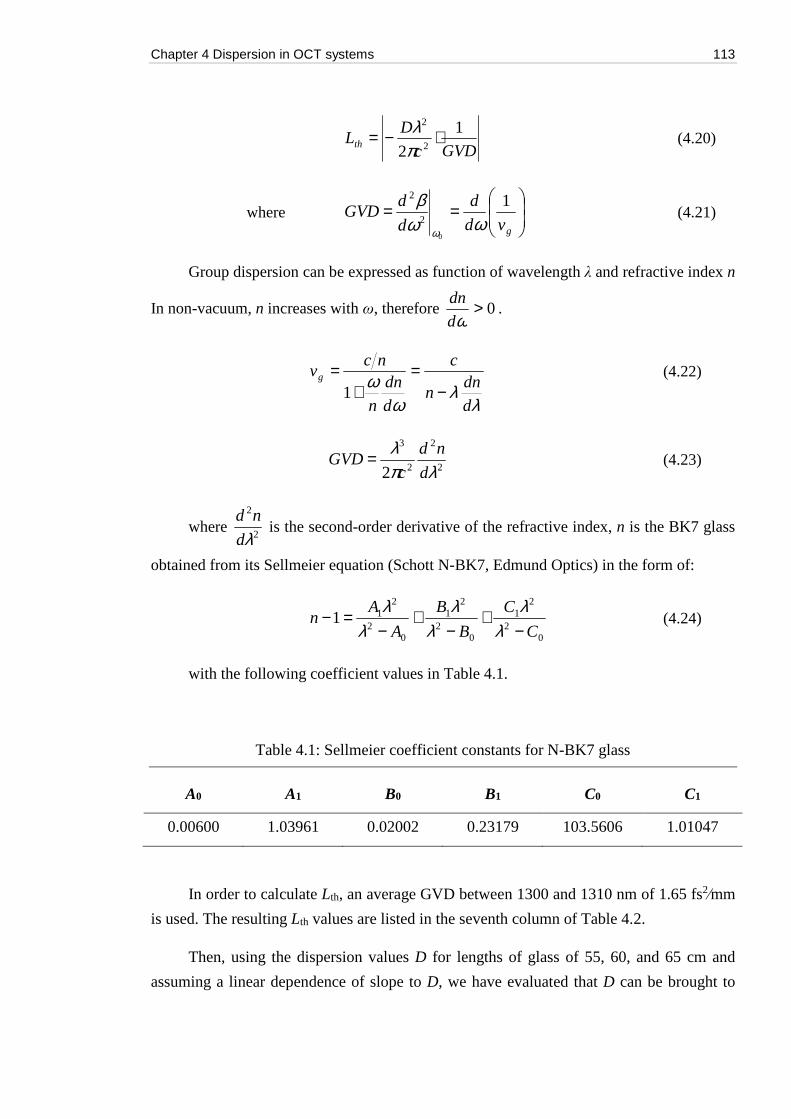
Chapter 4 Dispersion in OCT systems 113
GVDc
DLth
1
2 2
2
⋅−=πλ
(4.20)
where
==
gvd
d
d
dGVD
1
0
2
2
ωωβ
ω
(4.21)
Group dispersion can be expressed as function of wavelength λ and refractive index n
In non-vacuum, n increases with ω, therefore 0>ωd
dn.
λλ
ωω
d
dnn
c
d
dn
n
ncvg
−=
+=
1 (4.22)
2
2
2
3
2 λπλ
d
nd
cGVD= (4.23)
where 2
2
λd
nd is the second-order derivative of the refractive index, n is the BK7 glass
obtained from its Sellmeier equation (Schott N-BK7, Edmund Optics) in the form of:
02
21
02
21
02
211
C
C
B
B
A
An
−+
−+
−=−
λλ
λλ
λλ
(4.24)
with the following coefficient values in Table 4.1.
Table 4.1: Sellmeier coefficient constants for N-BK7 glass
A0 A1 B0 B1 C0 C1
0.00600 1.03961 0.02002 0.23179 103.5606 1.01047
In order to calculate Lth, an average GVD between 1300 and 1310 nm of 1.65 fs2∕mm
is used. The resulting Lth values are listed in the seventh column of Table 4.2.
Then, using the dispersion values D for lengths of glass of 55, 60, and 65 cm and
assuming a linear dependence of slope to D, we have evaluated that D can be brought to
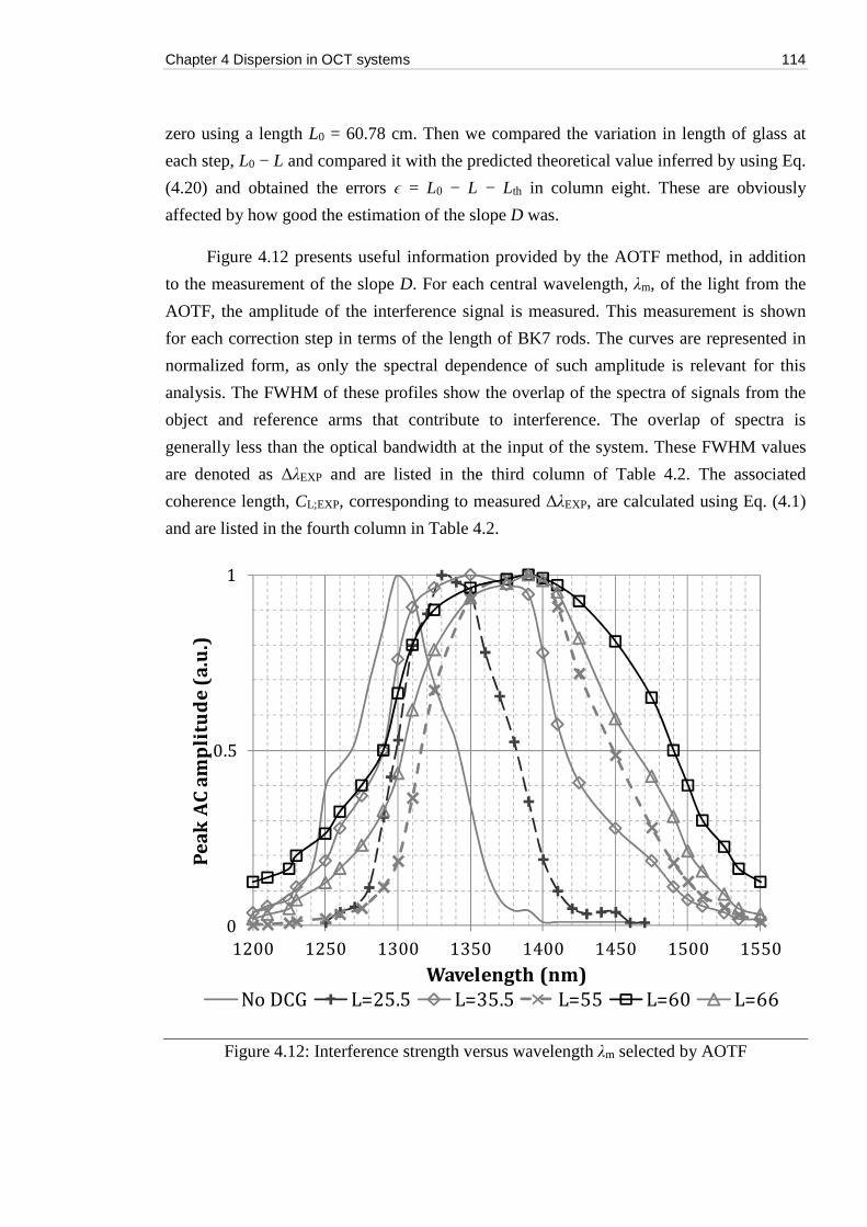
Chapter 4 Dispersion in OCT systems 114
zero using a length L0 = 60.78 cm. Then we compared the variation in length of glass at
each step, L0 − L and compared it with the predicted theoretical value inferred by using Eq.
(4.20) and obtained the errors ϵ = L0 − L − Lth in column eight. These are obviously
affected by how good the estimation of the slope D was.
Figure 4.12 presents useful information provided by the AOTF method, in addition
to the measurement of the slope D. For each central wavelength, λm, of the light from the
AOTF, the amplitude of the interference signal is measured. This measurement is shown
for each correction step in terms of the length of BK7 rods. The curves are represented in
normalized form, as only the spectral dependence of such amplitude is relevant for this
analysis. The FWHM of these profiles show the overlap of the spectra of signals from the
object and reference arms that contribute to interference. The overlap of spectra is
generally less than the optical bandwidth at the input of the system. These FWHM values
are denoted as ΔλEXP and are listed in the third column of Table 4.2. The associated
coherence length, CL;EXP, corresponding to measured ΔλEXP, are calculated using Eq. (4.1)
and are listed in the fourth column in Table 4.2.
Figure 4.12: Interference strength versus wavelength λm selected by AOTF
0
0.5
1
1200 1250 1300 1350 1400 1450 1500 1550
Pe
ak
AC
am
pli
tud
e (
a.u
.)
Wavelength (nm)
No DCG L=25.5 L=35.5 L=55 L=60 L=66
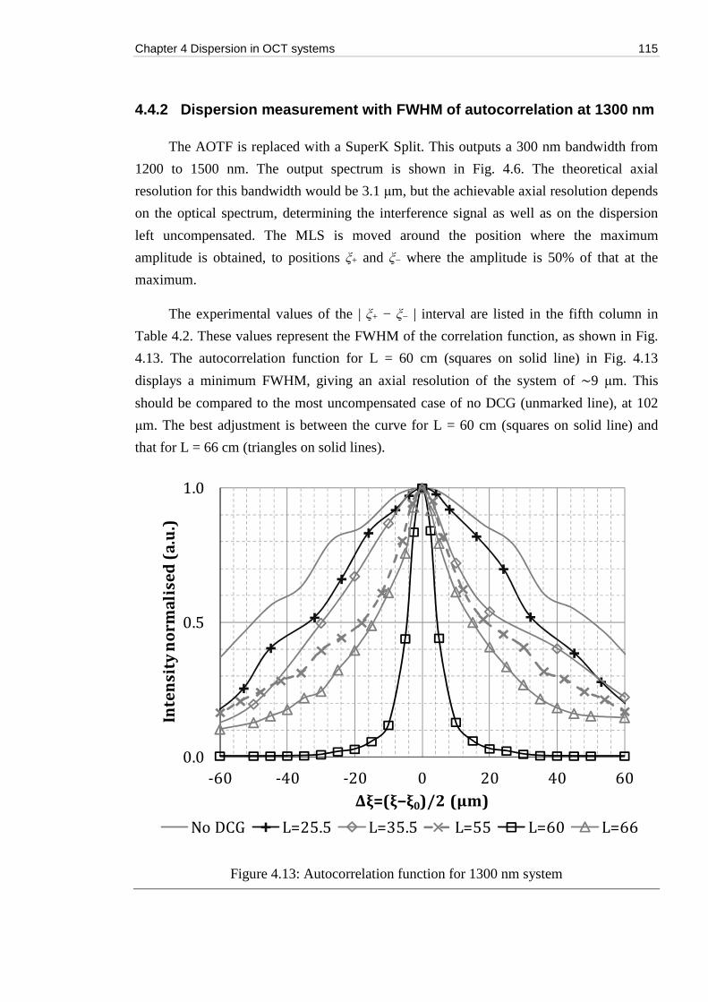
Chapter 4 Dispersion in OCT systems 115
4.4.2 Dispersion measurement with FWHM of autocorrelation at 1300 nm
The AOTF is replaced with a SuperK Split. This outputs a 300 nm bandwidth from
1200 to 1500 nm. The output spectrum is shown in Fig. 4.6. The theoretical axial
resolution for this bandwidth would be 3.1 μm, but the achievable axial resolution depends
on the optical spectrum, determining the interference signal as well as on the dispersion
left uncompensated. The MLS is moved around the position where the maximum
amplitude is obtained, to positions ξ+ and ξ− where the amplitude is 50% of that at the
maximum.
The experimental values of the | ξ+ − ξ− | interval are listed in the fifth column in
Table 4.2. These values represent the FWHM of the correlation function, as shown in Fig.
4.13. The autocorrelation function for L = 60 cm (squares on solid line) in Fig. 4.13
displays a minimum FWHM, giving an axial resolution of the system of ∼9 μm. This
should be compared to the most uncompensated case of no DCG (unmarked line), at 102
μm. The best adjustment is between the curve for L = 60 cm (squares on solid line) and
that for L = 66 cm (triangles on solid lines).
Figure 4.13: Autocorrelation function for 1300 nm system
0.0
0.5
1.0
-60 -40 -20 0 20 40 60
Inte
ns
ity
no
rm
ali
se
d (
a.u
.)
Δξ=(ξ−ξ0)/2 (µm)
No DCG L=25.5 L=35.5 L=55 L=60 L=66
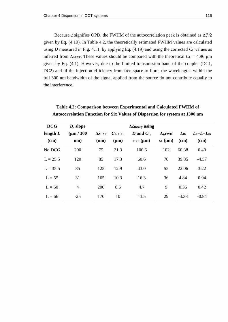
Chapter 4 Dispersion in OCT systems 116
Because ξ signifies OPD, the FWHM of the autocorrelation peak is obtained as Δξ ∕2
given by Eq. (4.19). In Table 4.2, the theoretically estimated FWHM values are calculated
using D measured in Fig. 4.11, by applying Eq. (4.19) and using the corrected CL values as
inferred from ΔλEXP. These values should be compared with the theoretical CL = 4.96 μm
given by Eq. (4.1). However, due to the limited transmission band of the coupler (DC1,
DC2) and of the injection efficiency from free space to fibre, the wavelengths within the
full 300 nm bandwidth of the signal applied from the source do not contribute equally to
the interference.
Table 4.2: Comparison between Experimental and Calculated FWHM of
Autocorrelation Function for Six Values of Dispersion for system at 1300 nm
DCG
length L
(cm)
D, slope
(μm / 300
nm)
ΔλEXP
(nm)
CL, EXP
(µm)
Δξtheory using
D and CL,
EXP (μm)
ΔξFWH
M (µm)
Lth
(cm)
L0−L−Lth
(cm)
No DCG 200 75 21.3 100.6 102 60.38 0.40
L = 25.5 120 85 17.3 60.6 70 39.85 -4.57
L = 35.5 85 125 12.9 43.0 55 22.06 3.22
L = 55 31 165 10.3 16.3 36 4.84 0.94
L = 60 4 200 8.5 4.7 9 0.36 0.42
L = 66 -25 170 10 13.5 29 -4.38 -0.84
Chapter 4 Dispersion in OCT systems 117
4.5 Comparison between AOTF and FWHM autocorrelation
Two methods of dispersion compensation have been presented and utilized on two
systems operating at two different wavelength bands. In a low-coherence interferometer,
driven by a broadband source, the simplest, yet time-consuming procedure to compensate
for the dispersion is based on the FWHM measurement of the autocorrelation peak. This is
performed iteratively by adjusting the dispersion up or down until FWHM minimum is
achieved. The method can reach a FWHM minimum, depending on the possibility to
proceed in sufficiently small steps. Adjusting the glass length in System 1 may be difficult,
depending on the availability of different lengths of glass.
The SDL used in System 2 allows continuous adjustment of the dispersion
compensation, in contrast to the stepped variation of the length of BK7 glass rods. Thus, it
is more likely to achieve the desired minimum dispersion compensation than using steps of
glass. Irrespective of the method, however, a single measurement of FWHM does not tell
which way to proceed, to increase or decrease the glass length of dispersion in the SDL,
while a single slope measurement using the AOTF method provides such information.
Therefore, the AOTF method appears more convenient for the task of dispersion
compensation.
4.5.1 Superiority of AOTF method
The biggest advantage of the AOTF method is that the minimum slope for the graphs
in Figs. 4.4 and 4.7 represent an absolute achievable condition, and this corresponds to a
zero value, which is known. The value toward which we tend to direct adjustments is not
known in the FWHM method. In an ideal situation, when the dispersion is fully
compensated for, the FWHM of autocorrelation theoretically becomes Δδ = CL∕2.
However, in reality, the value measured is typically larger, as the two interfering
waves may not have similar spectral shapes and may not be as wide as the original optical
source spectrum. Deviations of the source spectrum shape from Gaussian increase the
value in Eq. (4.1). Even if the spectral shape from the source is Gaussian, the injection into
the fibre may not be uniform over the spectrum, resulting in alteration of the spectral shape
of the interfering field. In other words, the value toward which we push the FWHM
measurement is not known.
Chapter 4 Dispersion in OCT systems 118
When using the AOTF method, a change of sign in the slope immediately suggests
the direction of the next step. In opposition to the AOTF method, the best adjustment when
using the FWHM method is reaching a minimum value for the FWHM. Therefore, when
using the FWHM method, it is necessary to apply dispersion correction until a minimum is
found, and this can only be established by continuing with the process until an increase of
the FWHM value is measured.
If the slope of the graph obtained with the AOTF approaches zero, this means that
the dispersion is compensated and further optimization is not required. Therefore,
measuring the slope with the AOTF method requires only a single iteration, because the
optimal DCG length can be
(i) calculated from the first measured slope, and
(ii) in principle, can be obtained from dispersion data of the material. This
procedure was illustrated in Section 4.4.1.
4.5.2 Minimising dispersion
On the other hand, even if a slope near zero μm/nm is achieved using the AOTF
method, this does not mean that the ΔξFWHM reaches the theoretical limit predicted by Eq.
(4.1) for reasons mentioned above, and as shown by values in Tables 4.2 and 4.3. Some
large differences between the FWHM ΔξFWHM measured and Δξtheory are observed in the
two tables. These differences may be explained based on the facts that:
(i) the spectra of the two interfering beams do not coincide, due to the spectral
dependence of fibre injection;
(ii) not all parts of the overlapping spectra contribute to interference due to
polarization mismatches; and
(iii) the theory presented above for the shape of the autocorrelation function
assumed a Gaussian profile of the spectrum, which is not the case in practice.
Chapter 4 Dispersion in OCT systems 119
Also, there are several different types of glass in the interferometer, with their own
dispersion. Additionally, the slopes of graphs in Figs. 4.11 and 4.14 are estimated based on
fitting straight lines to curves that exhibit clear nonlinear behaviour.
From a different perspective, let us consider the process of seeking minimum
dispersion that can be achieved by the two methods, based on guidance using FWHM
measurements and using the AOTF measurements. Using a derivative of the FWHM, Δξ in
Eq. (4.19) in respect to D,
( )( ) ( )
2
2
2
12L
LC
DC
D
Dd
d
λλξ
∆⋅+
∆⋅=∆ (4.25)
gives the dependence of the FWHM method on the dispersion coefficient D. Let us
consider that we are close to small values in D, in which case (4.25) becomes
( )( ) LC
D
Dd
d
2
λξ ∆⋅≈∆ (4.26)
In case of a good dispersion adjustment, the delay in OPD at the extreme values of
the AOTF bandwidth is δm, determining a minimum measurable dispersion coefficient:
λδ∆
= mD (4.27)
Considering that the minimum in D equals the error in D evaluation, i.e., d(D) ≈ D,
using (4.26) and (4.27), the error in FWHM measurement becomes
( ) ( ) ( )LL C
m
C
md
22
222 δλλ
δξ =∆
∆≈∆ (4.28)
Chapter 4 Dispersion in OCT systems 120
As long as δm < 2CL, then d(Δξ) < δm. This means that the error in FWHM of the
AOTF, as determined by d(Δξ), is less than the error in positioning the peak in the A-scan
δm. That is in fact the error in measuring the FWHM in the method relying on FWHM
measurement. Therefore, Eq. (4.28) demonstrates superiority of the AOTF method over the
FWHM measurement method in bringing the setup closer to minimum dispersion.
4.5.3 Application of AOTF in broadband OCT dispersion measurement
As shown by the measurement of the interference signal versus wavelength selected
by the AOTF in the setup at 1300 nm (Fig. 4.12), the accuracy of the FWHM measurement
of autocorrelation peak is limited to a bandwidth of signals contributing to interference.
This may be narrower than the bandwidth of the AOTF method. In other words, the AOTF
method allows measurements at a whole range of wavelengths, including and beyond the
overlapped part of the interference spectrum that determines the effective bandwidth.
Hence better accuracy in compensating for the dispersion is achievable with the AOTF
method.
The AOTF method presented is an alternative to the methods at hand in OCT
systems using spectrometers or swept sources, where spectral information can be used to
compensate for the dispersion. Although the method presented employs the time-domain
principle, it is equally applicable to swept source OCT configurations, where the swept
source is replaced with the AOTF module, dispersion is minimized, and then the swept
source is placed back into the system.
Chapter 4 Dispersion in OCT systems 121
References
1. R. Yadav, K. Lee, J. Rolland, J. Zavislan, J. Aquavella, and G. Yoon, “Micrometer axial OCT for corneal imaging,” Biomed. Opt. Express 2, 3037–3046 (2011).
2. Z. Yaqoob, J. Wu, and C. Yang, “Spectral domain optical coherence tomography: a better OCT imaging strategy,” BioTechniques 39, S6–S13 (2005).
3. M. Wojtkowski, R. Leitgeb, A. Kowalczyk, T. Bajraszewski, and A. F. Fercher, “In vivo human retinal imaging by Fourier domain optical coherence tomography,” J. Biomed. Opt. 7, 457–463 (2002).
4. A. Dubois, K. Grieve, G. Moneron, R. Lecaque, L. Vabre, and C. Boccara, “Ultrahigh-resolution full-field optical coherence tomography,” Appl. Opt. 43, 2874–2883 (2004).
5. B. Hofer, B. Považay, A. Unterhuber, L. Wang, B. Hermann, S. Rey, G. Matz, and W. Drexler, “Fast dispersion encoded full range optical coherence tomography for retinal imaging at 800 nm and 1060 nm,” Opt. Express 18, 4898–4919 (2010).
6. G. J. Tearney, B. E. Bouma, and J. G. Fujimoto, “High-speed phaseand group-delay scanning with a grating-based phase control delay line,” Opt. Lett. 22, 1811–1813 (1997).
7. A. V. Zvyagin, E. D. J. Smith, and D. D. Sampson, “Delay and dispersion characteristics of a frequency-domain optical delay line for scanning interferometry,” J. Opt. Soc. Am. A 20, 333–341 (2003).
8. A. Meadway, S. H. H. Darbrazi, G. Dobre, R. B. Rosen, and A. Gh. Podoleanu, “A rapid method of measuring dispersion in low coherence interferometry and optical coherence tomography systems,” J. Opt. 12, 015302 (2010).
9. C. C. Rosa, J. Rogers, and A. G. Podoleanu, “Fast scanning transmissive delay line for optical coherence tomography,” Opt. Lett. 30, 3263–3265 (2005).
10. F. Toadere, A. Bradu, W. Poon, D. Schultz, and A. Podoleanu, “Spectral delay line for display control in swept source OCT,” Proc. SPIE 9258, 92581X (2014).
11. K. S. Lee, A. C. Akcay, T. Delemos, E. Clarkson, and J. P. Rolland, “Dispersion control with a Fourier domain optical delay line in a fiber optic imaging interferometer,” Appl. Opt. 44, 4009–4022 (2005).
12. H. Ye, D. Ling, Y. Xu, and X. Huang, “Dispersion and compensation of optical coherence tomography using double path rapid scanning optical delay line,” Proc. SPIE 9656, 96560K (2015).
13. K. K. M. B. D. Silva, A. V. Zvyagin, and D. D. Sampson, “Extended range, rapid scanning optical delay line for biomedical interferometric imaging,” Electron. Lett. 35, 1404–1406 (1999).
14. A. Gh. Podoleanu, G. M. Dobre, and D. A. Jackson, “En-face coherence imaging using galvanometer scanner modulation,” Opt. Lett. 23, 147–149 (1998).
5
Ultra-broadband polarisation sensitive optical coherence tomography
Polarisation sensitive optical coherence tomography (PS-OCT) is a functional
extension to intensity based light imaging system by utilising additional information
carried by polarized light to provide enhance contrast. In traditional imaging, when only
backscattered intensity is collected and analyzed, information related to depth and layered
structure are neglected. In a typical microscopy system, researchers in the field worked to
improve axial resolution and penetration depth, hoping to pick up sub-micron features not
currently visible with most commercial OCT systems. Most research target at expanding
the broadband capabilities of such systems by using super continuum light sources. At the
same time, intense research has been going on to develop new techniques to extract
additional information otherwise not discoverable with intensity based imaging.
PS-OCT on the other hand measures depth-resolved phase retardation of incident
optical light and the altering state of light reflected from the target sample as a formed
birefringence. Birefringence is the optical property of a material having a refractive index
that depends on the polarisation state and propagation direction of light. When a light
enters a material of birefringence, the incident light can be decomposed into two
orthogonal components with varying refractive indices, commonly known as parallel (co-)
and perpendicular (cross-) optical axes, thus polarisation dependent phase velocity.
Birefringence occurs in many biological materials such as biological tissue structures,
polymers and organic fibres. These structures alter the polarisation state of the light and
show varying degree of birefringence. Therefore a light specific contrast not observable in
conventional OCT system can be seen clearly in PS-OCT images.
For that reason, many new developments in PS-OCT have been published. The
technique used to implement a PS-OCT system is rather similar to the normal OCT, as
previously described in Chapter 2. Broadly speaking, these techniques can be divided into
two main categories: (a) time-domain, and (b) spectral or Fourier domain. Within each of
these two methods, there exist a free-space (bulk) and a fibre-based implementation, all for
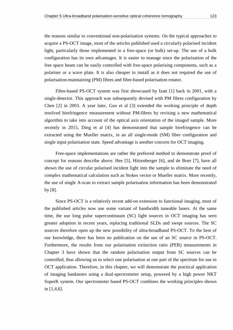
Chapter 5 Ultra-broadband polarisation-sensitive optical coherence tomography 123
the reasons similar to conventional non-polarisation systems. On the typical approaches to
acquire a PS-OCT image, most of the articles published used a circularly polarised incident
light, particularly those implemented in a free-space (or bulk) set-up. The use of a bulk
configuration has its own advantages. It is easier to manage since the polarisation of the
free space beam can be easily controlled with free-space polarising components, such as a
polariser or a wave plate. It is also cheaper to install as it does not required the use of
polarisation-maintaining (PM) fibres and fibre-based polarisation rotator.
Fibre-based PS-OCT system was first showcased by Izatt [1] back in 2001, with a
single-detector. This approach was subsequently devised with PM fibres configuration by
Chen [2] in 2003. A year later, Guo et al [3] extended the working principle of depth
resolved birefringence measurement without PM-fibres by revising a new mathematical
algorithm to take into account of the optical axis orientation of the imaged sample. More
recently in 2015, Ding et al [4] has demonstrated that sample birefringence can be
extracted using the Mueller matrix, in an all single-mode (SM) fibre configuration and
single input polarisation state. Speed advantage is another concern for OCT imaging.
Free-space implementations are rather the preferred method to demonstrate proof of
concept for reasons describe above. Hee [5], Hitzenberger [6], and de Boer [7], have all
shown the use of circular polarised incident light into the sample to eliminate the need of
complex mathematical calculation such as Stokes vector or Mueller matrix. More recently,
the use of single A-scan to extract sample polarisation information has been demonstrated
by [8].
Since PS-OCT is a relatively recent add-on extension to functional imaging, most of
the published articles now use some variant of bandwidth tuneable lasers. At the same
time, the use long pulse supercontinuum (SC) light sources in OCT imaging has seen
greater adoption in recent years, replacing traditional SLDs and swept sources. The SC
sources therefore open up the new possibility of ultra-broadband PS-OCT. To the best of
our knowledge, there has been no publication on the use of an SC source in PS-OCT.
Furthermore, the results from our polarisation extinction ratio (PER) measurements in
Chapter 3 have shown that the random polarisation output from SC sources can be
controlled, thus allowing us to select one polarisation at one part of the spectrum for use in
OCT application. Therefore, in this chapter, we will demonstrate the practical application
of imaging banknotes using a dual-spectrometer setup, powered by a high power NKT
SuperK system. Our spectrometer based PS-OCT combines the working principles shown
in [1,4,6].
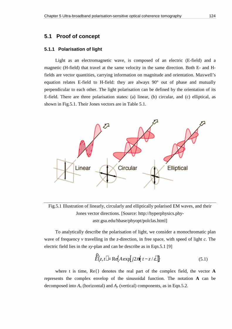
Chapter 5 Ultra-broadband polarisation-sensitive optical coherence tomography 124
5.1 Proof of concept
5.1.1 Polarisation of light
Light as an electromagnetic wave, is composed of an electric (E-field) and a
magnetic (H-field) that travel at the same velocity in the same direction. Both E- and H-
fields are vector quantities, carrying information on magnitude and orientation. Maxwell’s
equation relates E-field to H-field: they are always 90° out of phase and mutually
perpendicular to each other. The light polarisation can be defined by the orientation of its
E-field. There are three polarisation states: (a) linear, (b) circular, and (c) elliptical, as
shown in Fig.5.1. Their Jones vectors are in Table 5.1.
Fig.5.1 Illustration of linearly, circularly and elliptically polarised EM waves, and their
Jones vector directions. [Source: http://hyperphysics.phy-
astr.gsu.edu/hbase/phyopt/polclas.html]
To analytically describe the polarisation of light, we consider a monochromatic plan
wave of frequency v travelling in the z-direction, in free space, with speed of light c. The
electric field lies in the xy-plan and can be describe as in Eqn.5.1 [9]
( ) ( )[ ]{ }cztvjAtzE /2expRe, −= πρ
(5.1)
where t is time, Re{} denotes the real part of the complex field, the vector A
represents the complex envelop of the sinusoidal function. The notation A can be
decomposed into Ax (horizontal) and Ay (vertical) components, as in Eqn.5.2.
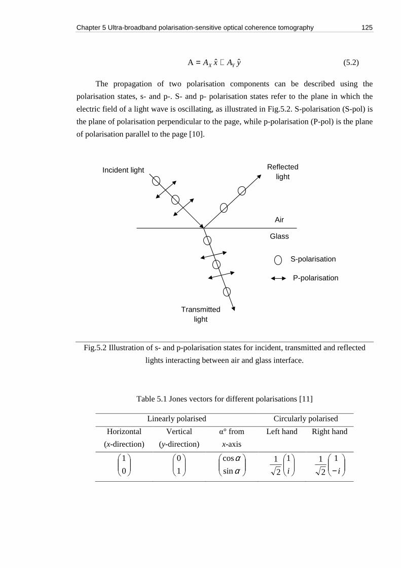
Chapter 5 Ultra-broadband polarisation-sensitive optical coherence tomography 125
yAxA YX ˆˆA += (5.2)
The propagation of two polarisation components can be described using the
polarisation states, s- and p-. S- and p- polarisation states refer to the plane in which the
electric field of a light wave is oscillating, as illustrated in Fig.5.2. S-polarisation (S-pol) is
the plane of polarisation perpendicular to the page, while p-polarisation (P-pol) is the plane
of polarisation parallel to the page [10].
Fig.5.2 Illustration of s- and p-polarisation states for incident, transmitted and reflected
lights interacting between air and glass interface.
Table 5.1 Jones vectors for different polarisations [11]
Linearly polarised Circularly polarised
Horizontal
(x-direction)
Vertical
(y-direction)
α° from
x-axis
Left hand Right hand
0
1
1
0
αα
sin
cos
i
1
2
1
− i
1
2
1
Incident light Reflected light
Transmitted light
S-polarisation
P-polarisation
Air
Glass
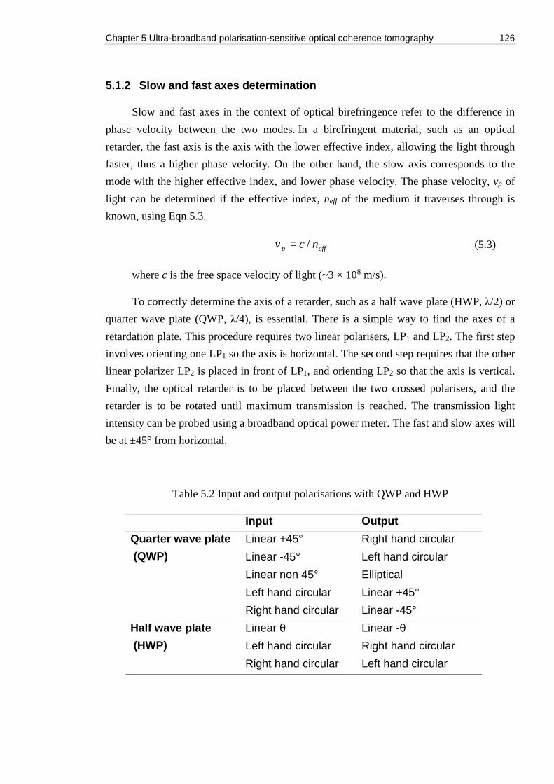
Chapter 5 Ultra-broadband polarisation-sensitive optical coherence tomography 126
5.1.2 Slow and fast axes determination
Slow and fast axes in the context of optical birefringence refer to the difference in
phase velocity between the two modes. In a birefringent material, such as an optical
retarder, the fast axis is the axis with the lower effective index, allowing the light through
faster, thus a higher phase velocity. On the other hand, the slow axis corresponds to the
mode with the higher effective index, and lower phase velocity. The phase velocity, vp of
light can be determined if the effective index, neff of the medium it traverses through is
known, using Eqn.5.3.
effp ncv /= (5.3)
where c is the free space velocity of light (~3 × 10⁸ m/s).
To correctly determine the axis of a retarder, such as a half wave plate (HWP, λ/2) or
quarter wave plate (QWP, λ/4), is essential. There is a simple way to find the axes of a
retardation plate. This procedure requires two linear polarisers, LP1 and LP2. The first step
involves orienting one LP1 so the axis is horizontal. The second step requires that the other
linear polarizer LP2 is placed in front of LP1, and orienting LP2 so that the axis is vertical.
Finally, the optical retarder is to be placed between the two crossed polarisers, and the
retarder is to be rotated until maximum transmission is reached. The transmission light
intensity can be probed using a broadband optical power meter. The fast and slow axes will
be at ±45° from horizontal.
Table 5.2 Input and output polarisations with QWP and HWP
Input Output
Quarter wave plate
(QWP)
Linear +45° Right hand circular
Linear -45° Left hand circular
Linear non 45° Elliptical
Left hand circular Linear +45°
Right hand circular Linear -45°
Half wave plate
(HWP)
Linear θ Linear -θ
Left hand circular Right hand circular
Right hand circular Left hand circular

Chapter 5 Ultra-broadband polarisation-sensitive optical coherence tomography 127
5.1.2 Jones matrices
The Jones matrix calculus is a matrix formulation of polarised light. It consists of
two forms: a 2×1 Jones vectors to describe only the field components, and a 2×2 Jones
matrix to describe the polarising components. The use of Jones formulation is only limited
to treating the completely polarised light. Therefore, unpolarised or partially polarised light
cannot be represented with Jones formulation. The Jones matrices are also used when
treating interference phenomena or when the electric field amplitudes are superposed. To
illustrate Jones formulation, we first introduce the Jones matrices for a general retarder in
Eqn.5.4, and then use it for different polarising elements, such as a retarder, a polariser, a
half wave plate and a quarter wave plate are represented in Eqn.5.5 to 5.8 [11].
( )
+⋅−⋅−⋅⋅+
= −−
−−
θθθθθθθθθδ δδ
δδ
22
22
sin)(cos)1(sincos
)1(sincos)(sincos,
jj
jj
ee
eeM (5.4)
Where δ is the phase retardation and θ is the fast-axis orientation.
If we now consider a retarder plate with y-axis as fast-axis and x-axis the slow axis,
the retarder’s Jones matrix becomes
= − δ
δ
δ j
j
e
eM
0
0
2
1 (5.5)
A polariser with polarising axis along x-axis can be written as
=
00
01)(xPM (5.6)
A QWP with the fast-axis along the x-axis is therefore
+−
=j
jM QWP 10
01
2
1 (5.7)
A HWP with slow-axis along the y-axis becomes
−=
0
0
j
jM HWP (5.8)
Chapter 5 Ultra-broadband polarisation-sensitive optical coherence tomography 128
We will use the Jones matrices discussed here to represent the polarized beam
propagating through different polarising elements in a PS-OCT system. We’ll describe our
polarisation sensitive interferometer in Sec.5.2, and the controlling polarisation in
Sec.5.2.1.
5.1.4 Bank notes
Bank notes or paper currency are secured instruments. These papers usually have
security identifiers such as micro embossed threads, watermarking, diffractive holograms,
and specialized inks, printed traditionally on cotton fibre or more recently on polymer
substrates. Common security features include variation of paper thickness and density to
create subtle variations in the light and dark areas, inks pigments that exhibit dichroic
properties that alter light polarisation at angles, as well as more sophisticated liquid crystal
holograms that are birefringent, as documented in [12].
Most recently, the introduction of polymer bank notes have transformed the industry.
The new polymer notes are more durable, cleaner, waster resistance and difficult to
counterfeit. The use of plastics in security documents extends beyond currency. More and
more previously paper based documents, such as driving license, identity cards and access
control credentials are now phased out in favour of the polymer version.
Since polymer substrate is made out of the synthetic composite material, its
composition has widely characterised in the chemistry laboratories using well-established
spectroscopy techniques, such as X-ray diffraction, FTIR, Raman and UV/visible
spectroscopy. Many of these analytical techniques are use to determine the molecular
structure of unknown organic compounds present in polymer. Many of these compounds
are birefringent. The use of optical coherence tomography (OCT) to perform meso-scale,
volumetric characterisation of polymer composites, polymer blends, biomaterials, and
ceramic coatings have been done by researchers in the National Institute of Science and
Technology (NIST) in USA [13-14].
Chapter 5 Ultra-broadband polarisation-sensitive optical coherence tomography 129
5.2 PS-OCT system set-up
An OCT system configuration with dual-spectrometer detection is constructed as in
Fig.5.2. A free-space in bulk concept of Michelson interferometer is used. To illustrate
wideband OCT capabilities, a commercial, low-noise supercontinuum source (SuperK
Extreme EXR 9, NKT Photonics, Denmark) that emits a broadband light from 480-2400
nm (visible power 900 mW), pulse repetition frequency (PRF) of 320 MHz, and pulse
duration of 5 ps is used in this experiment. The SuperK output is fed into a spectrum
splitter unit, SuperK Split (NKT Photonics). The SuperK Split is a passive optical
accessories attached to SuperK Extreme output. This splitter unit contains a dichroic mirror
to transmit longer wavelengths (λ > 1150 nm) and reflect shorter wavelengths (λ < 1100
nm). In this experiment, the visible band with usable bandwidth from 650-1100 nm is used.
The theoretical axial resolution for this bandwidth would be 1.2 μm, but the achievable
axial resolution depends on the polarisation of optical spectrum, determining the
interference signal as well as on the dispersion left uncompensated. A broadband double
Glan-Taylor Calcite polarizer (350-2300 nm, Thorlabs) is used to rotate the output beam
into linear vertical polarisation. This beam is split by a non-polarizing beam splitter (BS),
into the reference (reflected) and sample (transmitted) arms. Dispersion optimization was
performed using advanced method described in [4].
The reference beam transmits through a dispersion compensation glass (DCG,
LSM03DC, Thorlabs), and a quarter wave plate (QWPR), oriented with its fast axis rotated
to 22.5° to the horizontal polarisation, resulting in a right handed circular polarisation. The
reference beam is reflected at movable reference mirror (MR). The back propagating beam,
now left handed circularly polarized, passes through QWPR, and resulted in the reference
beam rotated at -45° to the linear horizontal. This beam provides reference intensity
equally in two components, horizontal and vertical, which will be decomposed with
polarizing beam splitter (PBS) at the interferometer output.
In the sample arm, a quarter wave plate (QWPS) is oriented at 45° to provide a
circular wave into the sample. The beam passes through a 2-axis galvanometric scanner
(XY), denoted respectively as GX (frame) and GY (line). Both GX and GY are driven with
sinusoidal signal. Since camera has a maximum line rate of 250 kHz, each of the 500
lateral pixels are acquired within 4 µs. To achieve an image of size 500×500, that requires
2 s per B-scan. The scanned beam goes through an OCT optimized microscope objective
lens (LSM02, 5x, Thorlabs) with focal length 7 mm. With a measured transversal
resolution of 10 µm, the lateral image size is limited to 1.8 cm × 1.8 cm. The maximum
Chapter 5 Ultra-broadband polarisation-sensitive optical coherence tomography 130
scan area is triggered when 5V TTL signal is supplied to both galvo-scanners. The
backscattered beam from the sample passes through QWPS, resulting in an elliptical
polarisation state containing birefringence information from the sample.
The interferometric signals from reference and sample arms are combined at BS, and
are sent through a PBS where two polarisation components are extracted, collimated into a
fibre using a free-space to fibre coupler (SCT, SuperK Select, NKT Photonics), and
delivered to separate spectrometers (SP1, SP2) for detection. The detection mechanism
consists of broadband visible range spectrometers (model Cobra-S C-650-950-S2K, 650-
950 nm, Wasatch Photonics), one for each polarisation component.
5.2.1 Polarisation selection and switching
At the output of SuperK Split, the light is polarised, as resulted from random nature
of supercontinuum generation. A broadband polarizer selects a vertical linear polarisation,
represented by its Jones vector as
=
1
00EE (5.9)
Where E0 = A0 exp (jωt), E denotes vector component of electric field, A0 is the
signal amplitude, Jones matrix of 0 and 1 represent horizontal and vertical polarisation
states. The backscattered sample signal detected before the PBS [5] can be written as
( )( ) ( )
= −−
−
θδπ
δ
δδ
20
sin
cos
2 j
j
Se
eR
EE (5.10)
The back propagated reference signal can equally be represented as
−=
1
1
2
1
20E
ER (5.11)
Another way to experimentally verify that a circular is sent to the sample is to put the
second polariser P2 at the position of sample (S). With the reference arm blocked, light
from the first polariser (P1) enters the QWPS, bouncing off the galvo-scanner mirrors XY,
and into P2. Polariser P2 is then rotated around 360°. If the polarisation coming out from
the QWPS is circular, power reading at the P2 output remains constant for all angles of P2.
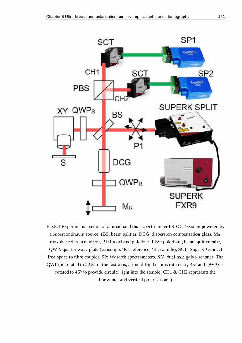
Chapter 5 Ultra-broadband polarisation-sensitive optical coherence tomography 131
Fig.5.3 Experimental set up of a broadband dual-spectrometer PS-OCT system powered by
a supercontinuum source. (BS: beam splitter, DCG: dispersion compensation glass, MR:
movable reference mirror, P1: broadband polarizer, PBS: polarizing beam splitter cube,
QWP: quarter wave plate (subscripts ‘R’: reference, ‘S’: sample), SCT: SuperK Connect
free-space to fibre coupler, SP: Wasatch spectrometers, XY: dual-axis galvo-scanner. The
QWPR is rotated to 22.5° of the fast-axis, a round-trip beam is rotated by 45° and QWPS is
rotated to 45° to provide circular light into the sample. CH1 & CH2 represents the
horizontal and vertical polarisations.)
Chapter 5 Ultra-broadband polarisation-sensitive optical coherence tomography 132
5.2.2 Polarisation detection
OCT interference signal recorded from the spectrometer can be written in Eqn.5.12
as the sum of amplitude modulation in both sample and reference arms
( ) ( ) ( )CHCHSCHRCHSCHRCH zzIIIIzI Φ−⋅++= cos2 0,,,, γ (5.12)
where ICH represents interfered signals for two channelled polarisation components,
horizontal and vertical (CH1, CH2), IR and IS each corresponds to signal intensities
recorded in reference and sample arms, z is the OPD position (where z0 is when OPD=0),
cos(ϕCH) is the phase term of the oscillating signal. The interference signal at different
OPD position is fast Fourier transformed (FFT) to produce A-scans. B-scan is produced by
transverse scanning the sample orthogonal to the surface, as discussed before in Sec.2.3 in
Chapter 2 on spectrometer-based OCT method.
At the interferometer exit, the OCT light beam is split up into its horizontal (H) and
vertical (V) component by the PBS, and are then detected by separate detection units,
spectrometers SP1 and SP2. By the respective signal amplitudes (ACH1, ACH2) and the
relative phase difference ΔΦCH, Jones vectors are detected for every image pixel. These
Jones vectors enable the calculation of the sample’s birefringent properties, namely of
phase retardation δ as well as sample reflectivity intensity RD [15]:
21
22 CHCHD AAR −= (5.13)
= −
1
21tanCH
CH
A
Aδ (5.14)
Since δ = Δn×L is dependent on sample birefringence, the value of δ accumulates as
a function of L, the distance light travelled in a birefringent material [15]. Therefore, the
measured phase retardation results are cumulative. The birefringence measured in this case
is similar to the one measured in nonlinear fibre (NLF) in Section 3.2.2, where the beat
length analogy in fibre is similar to the thickness of birefringent material imaged. In
nominally non-birefringent samples, the phase retardation however is small and limited. In
a strongly birefringent sample, the cumulative phase retardation can be huge.
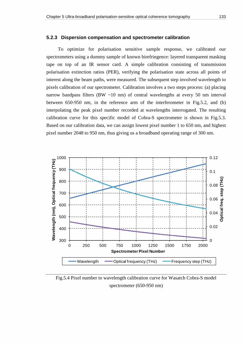
Chapter 5 Ultra-broadband polarisation-sensitive optical coherence tomography 133
5.2.3 Dispersion compensation and spectrometer calibration
To optimize for polarisation sensitive sample response, we calibrated our
spectrometers using a dummy sample of known birefringence: layered transparent masking
tape on top of an IR sensor card. A simple calibration consisting of transmission
polarisation extinction ratios (PER), verifying the polarisation state across all points of
interest along the beam paths, were measured. The subsequent step involved wavelength to
pixels calibration of our spectrometer. Calibration involves a two steps process: (a) placing
narrow bandpass filters (BW ~10 nm) of central wavelengths at every 50 nm interval
between 650-950 nm, in the reference arm of the interferometer in Fig.5.2, and (b)
interpolating the peak pixel number recorded at wavelengths interrogated. The resulting
calibration curve for this specific model of Cobra-S spectrometer is shown in Fig.5.3.
Based on our calibration data, we can assign lowest pixel number 1 to 650 nm, and highest
pixel number 2048 to 950 nm, thus giving us a broadband operating range of 300 nm.
Fig.5.4 Pixel number to wavelength calibration curve for Wasatch Cobra-S model
spectrometer (650-950 nm)
0
0.02
0.04
0.06
0.08
0.1
0.12
300
400
500
600
700
800
900
1000
0 250 500 750 1000 1250 1500 1750 2000
Op
tica
l fre
q. s
tep
(TH
z)
Wav
elen
gth
(nm
), O
pti
cal f
req
uen
cy (T
Hz)
Spectrometer Pixel Number
Wavelength Optical frequency (THz) Frequency step (THz)
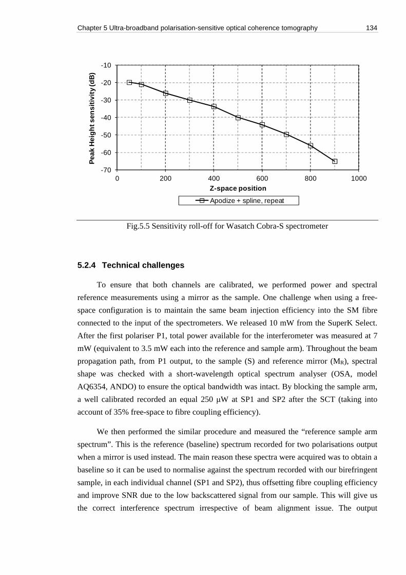
Chapter 5 Ultra-broadband polarisation-sensitive optical coherence tomography 134
Fig.5.5 Sensitivity roll-off for Wasatch Cobra-S spectrometer
5.2.4 Technical challenges
To ensure that both channels are calibrated, we performed power and spectral
reference measurements using a mirror as the sample. One challenge when using a free-
space configuration is to maintain the same beam injection efficiency into the SM fibre
connected to the input of the spectrometers. We released 10 mW from the SuperK Select.
After the first polariser P1, total power available for the interferometer was measured at 7
mW (equivalent to 3.5 mW each into the reference and sample arm). Throughout the beam
propagation path, from P1 output, to the sample (S) and reference mirror (MR), spectral
shape was checked with a short-wavelength optical spectrum analyser (OSA, model
AQ6354, ANDO) to ensure the optical bandwidth was intact. By blocking the sample arm,
a well calibrated recorded an equal 250 μW at SP1 and SP2 after the SCT (taking into
account of 35% free-space to fibre coupling efficiency).
We then performed the similar procedure and measured the “reference sample arm
spectrum”. This is the reference (baseline) spectrum recorded for two polarisations output
when a mirror is used instead. The main reason these spectra were acquired was to obtain a
baseline so it can be used to normalise against the spectrum recorded with our birefringent
sample, in each individual channel (SP1 and SP2), thus offsetting fibre coupling efficiency
and improve SNR due to the low backscattered signal from our sample. This will give us
the correct interference spectrum irrespective of beam alignment issue. The output
-70
-60
-50
-40
-30
-20
-10
0 200 400 600 800 1000
Pea
k H
eig
ht s
ensi
tivi
ty (d
B)
Z-space position
Apodize + spline, repeat
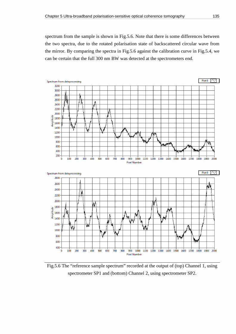
Chapter 5 Ultra-broadband polarisation-sensitive optical coherence tomography 135
spectrum from the sample is shown in Fig.5.6. Note that there is some differences between
the two spectra, due to the rotated polarisation state of backscattered circular wave from
the mirror. By comparing the spectra in Fig.5.6 against the calibration curve in Fig.5.4, we
can be certain that the full 300 nm BW was detected at the spectrometers end.
Fig.5.6 The “reference sample spectrum” recorded at the output of (top) Channel 1, using
spectrometer SP1 and (bottom) Channel 2, using spectrometer SP2.
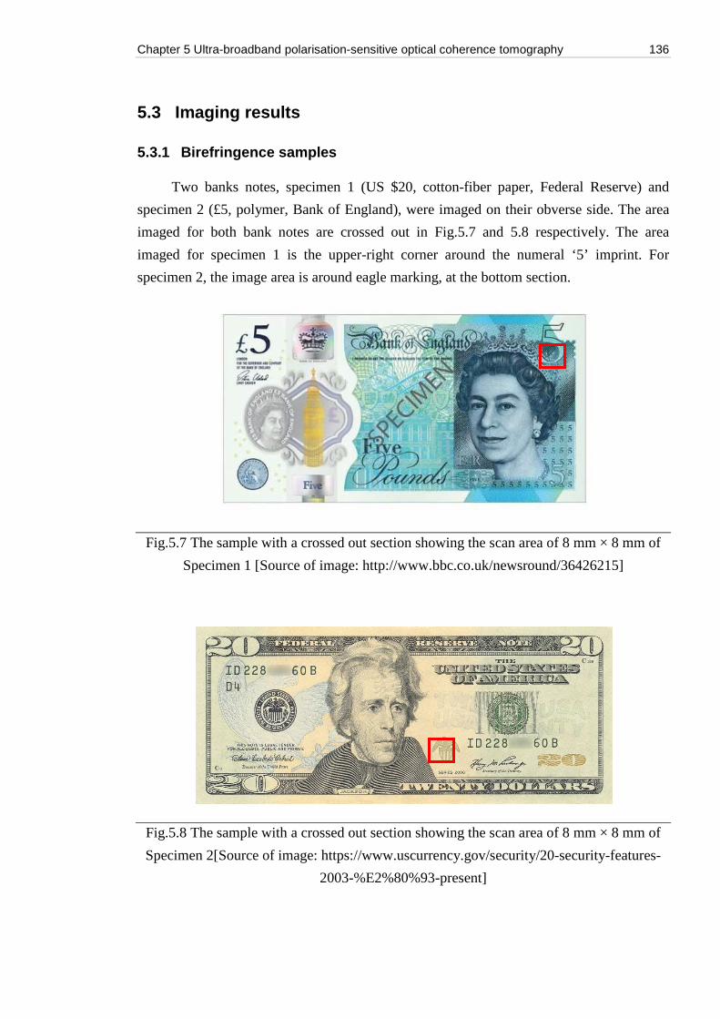
Chapter 5 Ultra-broadband polarisation-sensitive optical coherence tomography 136
5.3 Imaging results
5.3.1 Birefringence samples
Two banks notes, specimen 1 (US $20, cotton-fiber paper, Federal Reserve) and
specimen 2 (£5, polymer, Bank of England), were imaged on their obverse side. The area
imaged for both bank notes are crossed out in Fig.5.7 and 5.8 respectively. The area
imaged for specimen 1 is the upper-right corner around the numeral ‘5’ imprint. For
specimen 2, the image area is around eagle marking, at the bottom section.
Fig.5.7 The sample with a crossed out section showing the scan area of 8 mm × 8 mm of
Specimen 1 [Source of image: http://www.bbc.co.uk/newsround/36426215]
Fig.5.8 The sample with a crossed out section showing the scan area of 8 mm × 8 mm of
Specimen 2[Source of image: https://www.uscurrency.gov/security/20-security-features-
2003-%E2%80%93-present]
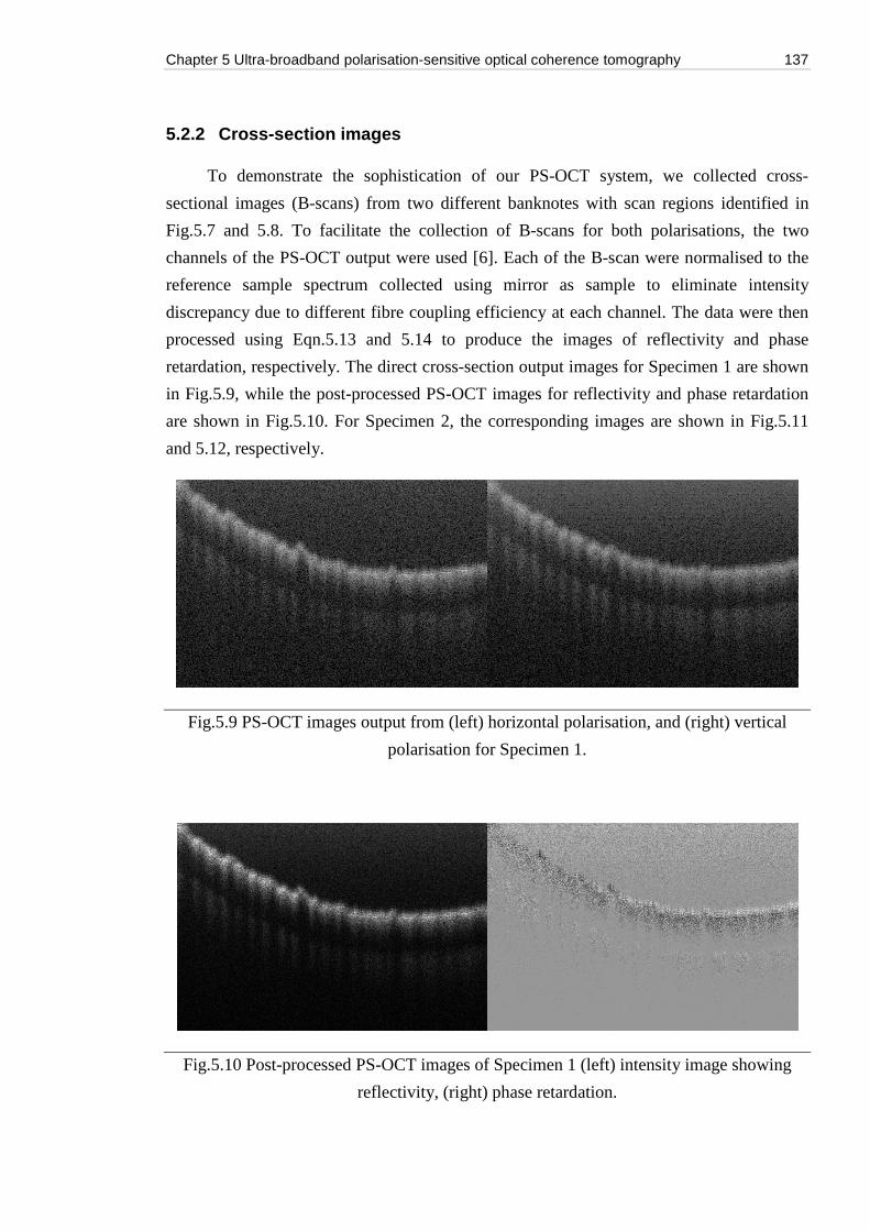
Chapter 5 Ultra-broadband polarisation-sensitive optical coherence tomography 137
5.2.2 Cross-section images
To demonstrate the sophistication of our PS-OCT system, we collected cross-
sectional images (B-scans) from two different banknotes with scan regions identified in
Fig.5.7 and 5.8. To facilitate the collection of B-scans for both polarisations, the two
channels of the PS-OCT output were used [6]. Each of the B-scan were normalised to the
reference sample spectrum collected using mirror as sample to eliminate intensity
discrepancy due to different fibre coupling efficiency at each channel. The data were then
processed using Eqn.5.13 and 5.14 to produce the images of reflectivity and phase
retardation, respectively. The direct cross-section output images for Specimen 1 are shown
in Fig.5.9, while the post-processed PS-OCT images for reflectivity and phase retardation
are shown in Fig.5.10. For Specimen 2, the corresponding images are shown in Fig.5.11
and 5.12, respectively.
Fig.5.9 PS-OCT images output from (left) horizontal polarisation, and (right) vertical
polarisation for Specimen 1.
Fig.5.10 Post-processed PS-OCT images of Specimen 1 (left) intensity image showing
reflectivity, (right) phase retardation.
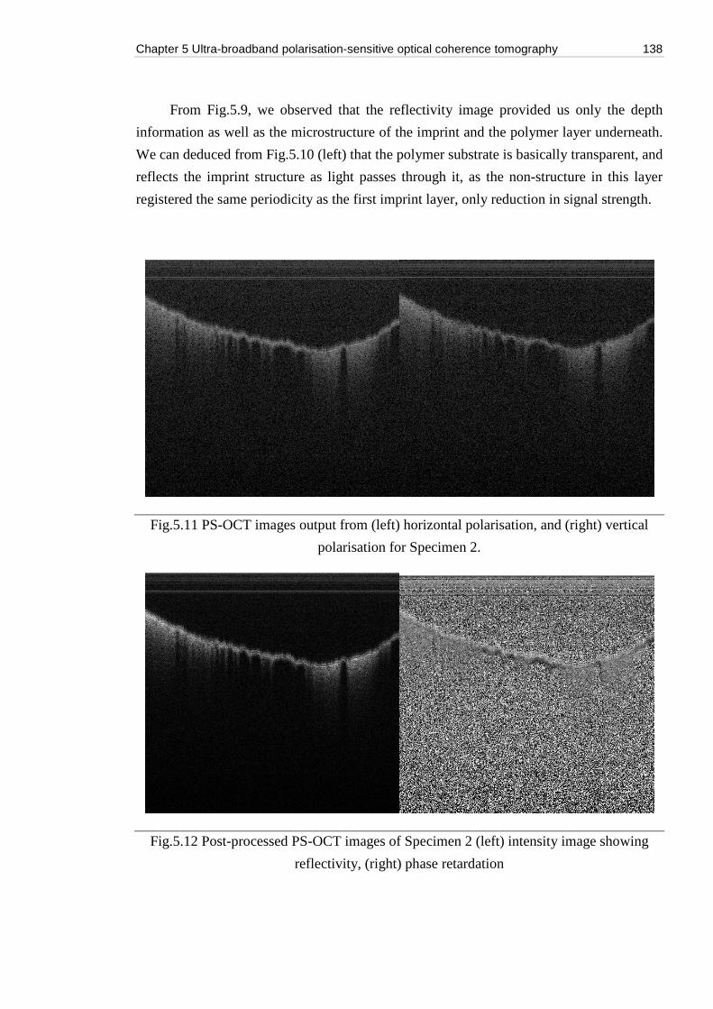
Chapter 5 Ultra-broadband polarisation-sensitive optical coherence tomography 138
From Fig.5.9, we observed that the reflectivity image provided us only the depth
information as well as the microstructure of the imprint and the polymer layer underneath.
We can deduced from Fig.5.10 (left) that the polymer substrate is basically transparent, and
reflects the imprint structure as light passes through it, as the non-structure in this layer
registered the same periodicity as the first imprint layer, only reduction in signal strength.
Fig.5.11 PS-OCT images output from (left) horizontal polarisation, and (right) vertical
polarisation for Specimen 2.
Fig.5.12 Post-processed PS-OCT images of Specimen 2 (left) intensity image showing
reflectivity, (right) phase retardation
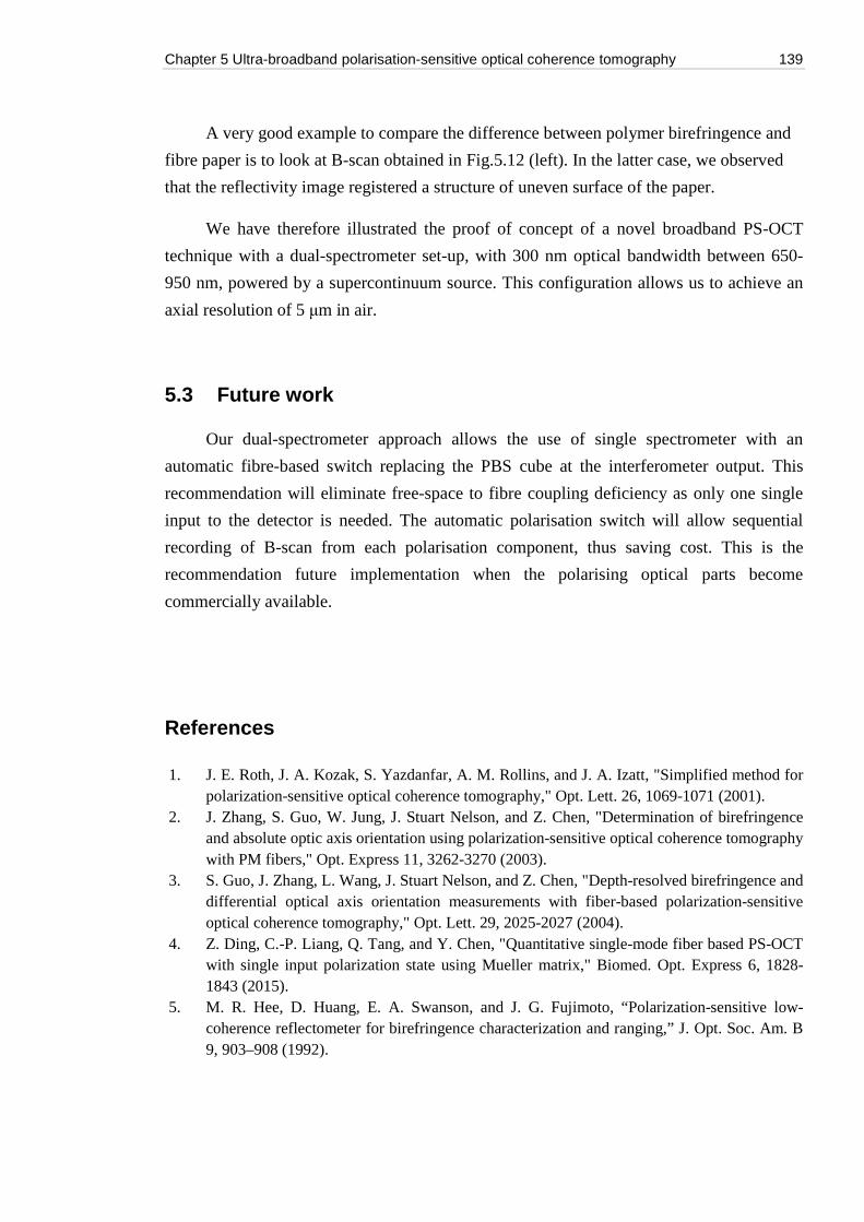
Chapter 5 Ultra-broadband polarisation-sensitive optical coherence tomography 139
A very good example to compare the difference between polymer birefringence and
fibre paper is to look at B-scan obtained in Fig.5.12 (left). In the latter case, we observed
that the reflectivity image registered a structure of uneven surface of the paper.
We have therefore illustrated the proof of concept of a novel broadband PS-OCT
technique with a dual-spectrometer set-up, with 300 nm optical bandwidth between 650-
950 nm, powered by a supercontinuum source. This configuration allows us to achieve an
axial resolution of 5 μm in air.
5.3 Future work
Our dual-spectrometer approach allows the use of single spectrometer with an
automatic fibre-based switch replacing the PBS cube at the interferometer output. This
recommendation will eliminate free-space to fibre coupling deficiency as only one single
input to the detector is needed. The automatic polarisation switch will allow sequential
recording of B-scan from each polarisation component, thus saving cost. This is the
recommendation future implementation when the polarising optical parts become
commercially available.
References
1. J. E. Roth, J. A. Kozak, S. Yazdanfar, A. M. Rollins, and J. A. Izatt, "Simplified method for polarization-sensitive optical coherence tomography," Opt. Lett. 26, 1069-1071 (2001).
2. J. Zhang, S. Guo, W. Jung, J. Stuart Nelson, and Z. Chen, "Determination of birefringence and absolute optic axis orientation using polarization-sensitive optical coherence tomography with PM fibers," Opt. Express 11, 3262-3270 (2003).
3. S. Guo, J. Zhang, L. Wang, J. Stuart Nelson, and Z. Chen, "Depth-resolved birefringence and differential optical axis orientation measurements with fiber-based polarization-sensitive optical coherence tomography," Opt. Lett. 29, 2025-2027 (2004).
4. Z. Ding, C.-P. Liang, Q. Tang, and Y. Chen, "Quantitative single-mode fiber based PS-OCT with single input polarization state using Mueller matrix," Biomed. Opt. Express 6, 1828-1843 (2015).
5. M. R. Hee, D. Huang, E. A. Swanson, and J. G. Fujimoto, “Polarization-sensitive low-coherence reflectometer for birefringence characterization and ranging,” J. Opt. Soc. Am. B 9, 903–908 (1992).
Chapter 5 Ultra-broadband polarisation-sensitive optical coherence tomography 140
6. C. K. Hitzenberger, E. Götzinger, M. Sticker, M. Pircher, and A. F. Fercher, "Measurement and imaging of birefringence and optic axis orientation by phase resolved polarization sensitive optical coherence tomography," Opt. Express 9, 780-790 (2001).
7. J. F. de Boer, T. E. Milner, M. J. C. van Gemert, and J. S. Nelson, “Two-dimensional birefringence imaging in biological tissue by polarization-sensitive optical coherence tomography,” Opt. Lett. 22, 934–936 (1997).
8. E. Götzinger, M. Pircher, and C. K. Hitzenberger, "High speed spectral domain polarization sensitive optical coherence tomography of the human retina," Opt. Express 13, 10217-10229 (2005).
9. B. E. A. Saleh and M. C. Teich: Fundamentals of Photonics, 2nd Ed. Wiley (2007). 10. P. N. Butcher and D. Cotter: The Elements of Nonlinear Optics, Cambridge Univ. Press
(1991). 11. E. Collett, Field Guide to Polarisation, SPIE Press, Bellingham, WA (2005). 12. M. E. Brezinski, Optical Coherence Tomography: Principles and Applications, Academic
Press, 197-236 (2006). 13. J. P. Dunkers, F. R. Phelan, D. S. Sanders, M. J. Everett, W. H. Green, D. L. Hunston, and R.
S. Parnas, "The Application of Optical Coherence Tomography in Problems in Polymer Matrix Composites", Journal of Optics and Lasers in Engineering.
14. J. P. Dunkers, M. J. Everett, D. P. Sanders, and D. L. Hunston, "Imaging of Composite Defects and Damage Using Optical Coherence Tomography", Proc. of PLAST, Advancing with Composites (2000).

6
Application of OCT in biomedical imaging
Optical imaging of skin malignancy has generated huge interest among the medical
community recently thanks to more recent development of contactless and non-invasive
imaging technique such as OCT. In this chapter, we teamed up with clinicians from the
Maidstone and Tunbridge Wells NHS Trust Hospital, Prof. Dr John Schofield, Dr Mona
Khandwala, and Miss Rongxuan Lim, to image basal cell carcinoma (BCC) using the en-
face OCT system we developed in Applied Optics Group, at the University of Kent.
BCC is the most common form of skin cancer in Caucasians [1] and accounts for 80-
90% of all eyelid malignancies [2,3]. It is estimated that there are 53,000 new BCC cases
diagnosed in UK yearly [4]. The gold standard for tumour diagnosis involves surgical
biopsy for histological analysis [5]. To reduce patient morbidity from surgery, non-
invasive methods of diagnosis and determining tumour margins have been investigated in
recent years. They include reflectance confocal microscopy (RCM) [6], high frequency
ultrasound (HFUS) [7], multispectral imaging [8], multiphoton microscopy [9], fluorescent
technique [10], confocal scanning laser microscopy (CSLM) [11] and optical coherence
tomography (OCT) [12,13]. Although these technologies provide valuable information,
they are not yet widely adopted by mainstream health care professionals to provide high
level of certainty essential for accurate treatment. None of these emerging techniques have
been used entirely independently, or proved to be superior to the gold standard. These new
techniques are often used to bridge the gap of limitation on established technologies,
demanding new imaging systems with better penetration depth and sensitivity.
Nevertheless, recent literature has suggested that OCT in en-face imaging mode presents
the potential of improved diagnostic specificity of BCC morphology compared with
clinical assessment and dermoscopy alone [14-15].
For this reason, we implemented an en-face optical coherence tomography (OCT)
system powered with our enhanced master-slave (MS) technique [16]. Compared to
conventional fast Fourier transform (FFT) based OCT, the MS technique is tolerant to the
Chapter 6 Application of OCT in biomedical imaging 142
non-uniformities in the modulation frequency of the spectra acquired as well as to
dispersion in the interferometer [17]. Therefore, the MS technique allows achieving the
theoretical expected parameters for the sensitivity and for the axial resolution, as
determined by the bandwidth of the system, and by the spectral domain principle. The MS
technique leads to attainment of such values with no need for resampling of data. In
conventional FFT based OCT, the axial resolution and sensitivity are as good as the
resampling and data linearization methods, which generally operate well at shallow depths
only. Additionally, the MS technique gives direct access to information from selected
depths, allowing real time display of one or more en-face OCT images from such depths
[18]. The MS method has been applied to OCT imaging of the eye fundus, and by
harnessing the power of graphic cards, real time production of en-face images was made
possible [19].
This is a pilot study aiming to correlate the histological features of periocular BCC to
features seen on the OCT scan using the MS technique. To the best of our knowledge, this
is the first pilot study using Master/Slave OCT technique for imaging periocular BCCs.
Prior to this thesis work, three other studies to image BCC were conducted by our group in
collaboration with clinicians from the Maidstone Hospital. These studies has explored the
use of dual wavelengths (840 nm and 1300 nm) time domain (TD)-OCT [20], FFT based
OCT [21] and dynamic focus (DF)-OCT [22]. Based on the experience we gathered from
these three tests, we identified that essential in performing accurate correlations with
histology data, is to acquire high resolution OCT images and correctly identify the margins
of any skin lesion precisely. On the wavelength selection, we identified that light at 1300
nm suffer less scattering in tissue, thus providing better signal strength compared to 850
nm when used for imaging BCC [19-23].
Independent to our group’s research, the use of 1300 nm for OCT imaging was
further documented by the study of BCC that employs a combined RCM/OCT system for
ex-vivo imaging [24]. The data processing of OCT signals is based on conventional FFT
based technique. In contrast to MS technique, dispersion compensation and interpolation
are employed. The resulting set of 512 OCT raster images using their method could be
acquired in 13 s. While the RCM channel delivers en-face images, the OCT is performed
in cross section. Single en-face images are inferred by software cut of volumes of A-scans
and placed in comparison with the RCM images. Another study employed a commercial 20
kHz tuneable laser to produce 120 stack OCT images of size 6 mm × 6 mm in between 10-
20s [25]. None of the OCT systems referenced above are capable of producing en-face
images in real time.
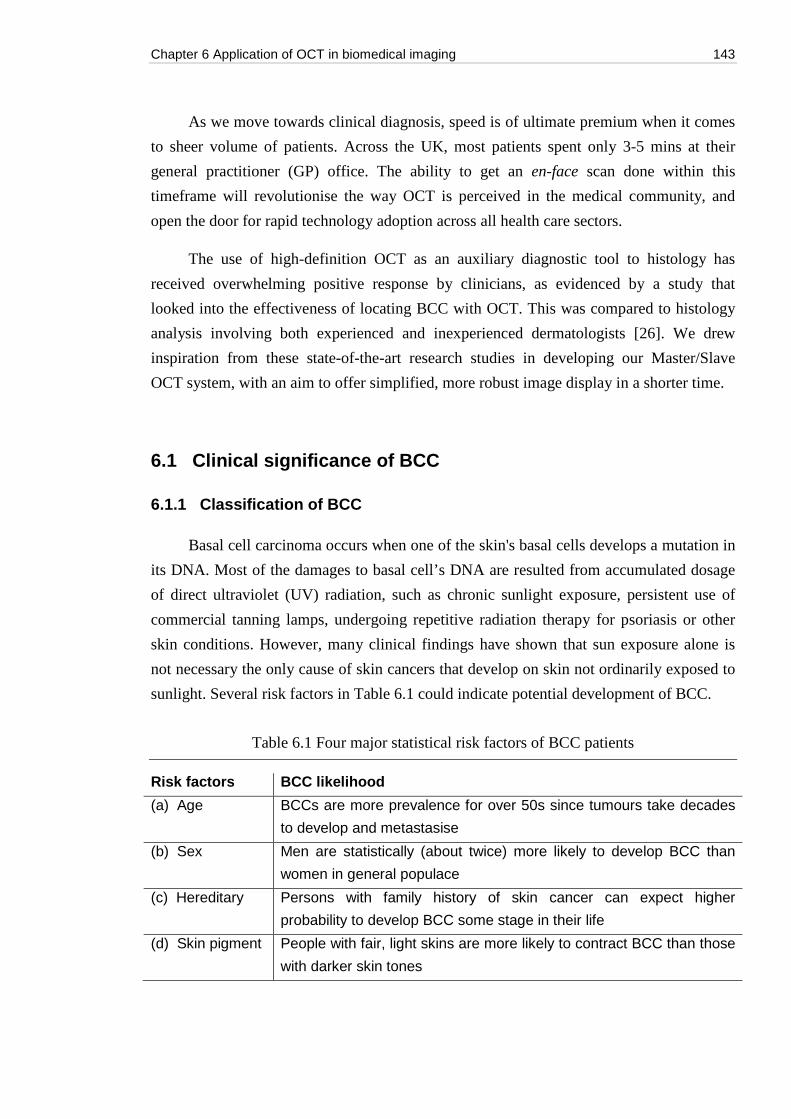
Chapter 6 Application of OCT in biomedical imaging 143
As we move towards clinical diagnosis, speed is of ultimate premium when it comes
to sheer volume of patients. Across the UK, most patients spent only 3-5 mins at their
general practitioner (GP) office. The ability to get an en-face scan done within this
timeframe will revolutionise the way OCT is perceived in the medical community, and
open the door for rapid technology adoption across all health care sectors.
The use of high-definition OCT as an auxiliary diagnostic tool to histology has
received overwhelming positive response by clinicians, as evidenced by a study that
looked into the effectiveness of locating BCC with OCT. This was compared to histology
analysis involving both experienced and inexperienced dermatologists [26]. We drew
inspiration from these state-of-the-art research studies in developing our Master/Slave
OCT system, with an aim to offer simplified, more robust image display in a shorter time.
6.1 Clinical significance of BCC
6.1.1 Classification of BCC
Basal cell carcinoma occurs when one of the skin's basal cells develops a mutation in
its DNA. Most of the damages to basal cell’s DNA are resulted from accumulated dosage
of direct ultraviolet (UV) radiation, such as chronic sunlight exposure, persistent use of
commercial tanning lamps, undergoing repetitive radiation therapy for psoriasis or other
skin conditions. However, many clinical findings have shown that sun exposure alone is
not necessary the only cause of skin cancers that develop on skin not ordinarily exposed to
sunlight. Several risk factors in Table 6.1 could indicate potential development of BCC.
Table 6.1 Four major statistical risk factors of BCC patients
Risk factors BCC likelihood
(a) Age BCCs are more prevalence for over 50s since tumours take decades
to develop and metastasise
(b) Sex Men are statistically (about twice) more likely to develop BCC than
women in general populace
(c) Hereditary Persons with family history of skin cancer can expect higher
probability to develop BCC some stage in their life
(d) Skin pigment People with fair, light skins are more likely to contract BCC than those
with darker skin tones
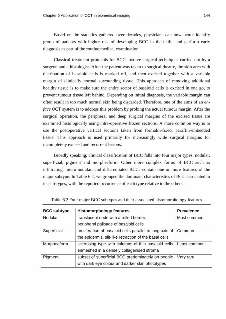
Chapter 6 Application of OCT in biomedical imaging 144
Based on the statistics gathered over decades, physicians can now better identify
group of patients with higher risk of developing BCC in their life, and perform early
diagnosis as part of the routine medical examination.
Classical treatment protocols for BCC involve surgical techniques carried out by a
surgeon and a histologist. After the patient was taken to surgical theatre, the skin area with
distribution of basaloid cells is marked off, and then excised together with a variable
margin of clinically normal surrounding tissue. This approach of removing additional
healthy tissue is to make sure the entire sector of basaloid cells is excised in one go, to
prevent tumour tissue left behind. Depending on initial diagnosis, the variable margin can
often result in too much normal skin being discarded. Therefore, one of the aims of an en-
face OCT system is to address this problem by probing the actual tumour margin. After the
surgical operation, the peripheral and deep surgical margins of the excised tissue are
examined histologically using intra-operative frozen sections. A more common way is to
use the postoperative vertical sections taken from formalin-fixed, paraffin-embedded
tissue. This approach is used primarily for increasingly wide surgical margins for
incompletely excised and recurrent lesions.
Broadly speaking, clinical classification of BCC falls into four major types: nodular,
superficial, pigment and morpheaform. Other more complex forms of BCC such as
infiltrating, micro-nodular, and differentiated BCCs contain one or more features of the
major subtype. In Table 6.2, we grouped the dominant characteristics of BCC associated to
its sub-types, with the reported occurrence of each type relative to the others.
Table 6.2 Four major BCC subtypes and their associated histomorphology features
BCC subtype Histomorphology features Prevalence
Nodular translucent node with a rolled border,
peripheral palisade of basaloid cells
Most common
Superficial proliferation of basaloid cells parallel to long axis of
the epidermis, slit-like retraction of the basal cells
Common
Morpheaform sclerosing type with columns of thin basaloid cells
enmeshed in a densely collagenised stroma
Least common
Pigment subset of superficial BCC predominately on people
with dark eye colour and darker skin phototypes
Very rare
Chapter 6 Application of OCT in biomedical imaging 145
The symptoms of an early stage BCC can be identified by the area of skin or lesions
that appears to change in texture, colour and structure. By relating these symptoms to
major BCC subtypes, we can design an OCT system to identify patients with these skin
characteristics. For the most common case, a nodular BCC exhibits a translucent lesion
with pearly white, skin-coloured or pink bump, allowing tiny blood vessels to be visible
from the lesion surface. An OCT system operating in the 1300 nm is best suited to probe
this kind of BCC. On the other hand, BCCs with a flat, scaly and reddish patch scattering
around the skin can be detected by naked eye. An OCT system can be used to aid the
validation of tumour, therefore eliminating false diagnosis. However, as the presence of
BCC on skin lesions can be random, an OCT technology capable of automatically
distinguishing one BCC subtypes from another is useful. In our application chapter, we
concentrate only on eyelid (periocular) BCC using our MS-OCT system.
6.1.2 Histology tissue imaging
Three consecutive patients over the age of 18 with a biopsy proven periocular
nodular BCC, without previous eyelid surgery, were enrolled into the study. The study
protocol (“Ethical Approval”) was approved by the Research and Development
Department of the Maidstone and Tunbridge Wells NHS Trust, and also by the Ethics
Committee at the School of Physical Sciences, University of Kent. Informed consent was
obtained from the participants. All procedures relating to removal, storage and transport
were carried out in accordance to Human Tissue Act 2004 (UK) under the licence acquired
by the NHS Trust from Human Tissue Authority (HTA).
All BCC lesions were surgically excised with predetermined 2 mm margins of
normal skin. The orientation of each specimen was specified by using 6/0 silk sutures of
various lengths to mark 3 of the margins of the lesion. The excised specimens were placed
in 10% neutral buffered formalin and transported from Maidstone Hospital to the
University of Kent within 3 hours of excision for OCT imaging. For purpose of image
acquisition, the BCC tissue was placed on a transparent microscope glass slice, with its
superior margin aligned to the horizontal direction of the optical beam axis at the
microscope focus of the OCT machine. After OCT imaging was completed, the specimens
were placed back into 10% neutral buffered formalin and transported to the Maidstone
Hospital Histology Department the same day.
Chapter 6 Application of OCT in biomedical imaging 146
6.1.3 Histology correlation
The specimens were allowed to fix in 10% neutral buffered formalin for 24 hours
and then "bread sliced" at 2 mm intervals at 90 degrees to the skin surface retaining
orientation as denoted by marking sutures. Each slice was processed and paraffin
embedded with serial sections cut at 2 µm intervals, then mounted on glass slides, stained
with haematoxylin and eosin and viewed in a conventional light microscope.
Photomicrographs were captured for comparison with OCT images and correlation
undertaken by identification of the matching features of the OCT and histology images
under supervision of Prof. Dr. John Schofield, at the Maidstone Hospital.
The procedures to correlation are described in details in Section 6.2.2. En-face OCT
images are matched side by side to histology image at different tissue depth, beginning
from slice 192 (denoted as middle point) and extend every 5 slice interval above and below
the middle. Probable BCC features on en-face images are searched by naked eye
comparison to description in Table 6.2, then correlate against confirmed BCCs in histology
image. To assist with large number of en-face images, ImageJ software was used to
facilitate image manipulation: slice stacking, transformation and 3D volume construction.
6.2 en-face imaging
The imaging of en-face BCC samples were performed using a custom built MS-OCT
system as discussed in Section 6.2.1. The post-analysis and step-by-step correlation of en-
face images to histology scans are demonstrated in Section 6.2.2. Finally, a technical
comparison has been made between our current results, image qualities and OCT system
performance in Section 6.2.3.
6.2.1 Master/Slave OCT machine
The schematic diagram of the MS-OCT system assembled is shown in Fig. 6.1. Light
is first emitted from a tuneable swept source (SS) operating at 1310 nm central wavelength
with a 100 nm sweeping range, 50 kHz sweeping speed and 15 mW max output power
(model SSOCT-1310, Axsun Technology, MA, USA). An interferometer, using two
directional fibre couplers, DC1 and DC2 was assembled. The light from the source enters
the first directional coupler (DC1, model FOBC-2-1310-20, AFW Technology, Australia)
with a splitting ratio of 80:20. One output delivers 80% of light intensity into the reference
arm, and 20% of light into the object arm.
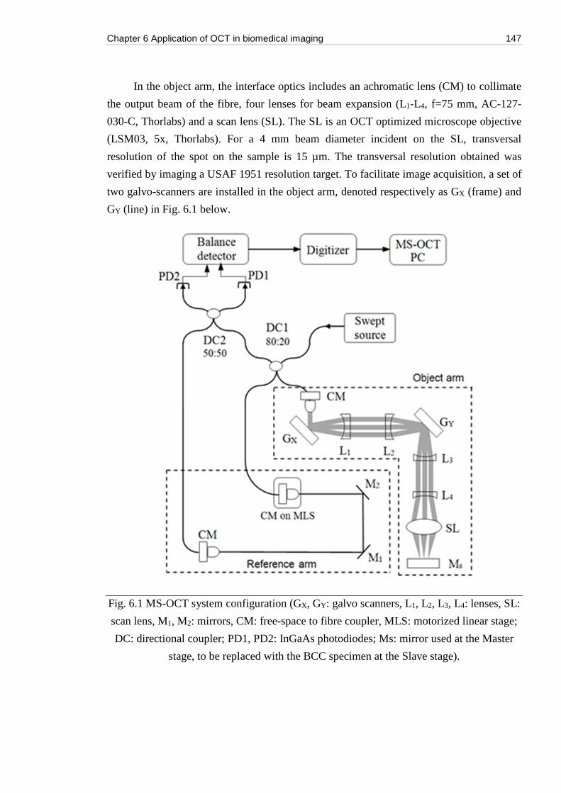
Chapter 6 Application of OCT in biomedical imaging 147
In the object arm, the interface optics includes an achromatic lens (CM) to collimate
the output beam of the fibre, four lenses for beam expansion (L1-L4, f=75 mm, AC-127-
030-C, Thorlabs) and a scan lens (SL). The SL is an OCT optimized microscope objective
(LSM03, 5x, Thorlabs). For a 4 mm beam diameter incident on the SL, transversal
resolution of the spot on the sample is 15 µm. The transversal resolution obtained was
verified by imaging a USAF 1951 resolution target. To facilitate image acquisition, a set of
two galvo-scanners are installed in the object arm, denoted respectively as GX (frame) and
GY (line) in Fig. 6.1 below.
Fig. 6.1 MS-OCT system configuration (GX, GY: galvo scanners, L1, L2, L3, L4: lenses, SL:
scan lens, M1, M2: mirrors, CM: free-space to fibre coupler, MLS: motorized linear stage;
DC: directional coupler; PD1, PD2: InGaAs photodiodes; Ms: mirror used at the Master
stage, to be replaced with the BCC specimen at the Slave stage).
Chapter 6 Application of OCT in biomedical imaging 148
Both GX and GY are driven with triangular ramps. Since SS has a tuning frequency of
50 kHz, each of the 200 lateral pixels are acquired within 20 µs. GX is driven with a
triangular signal, where each ramp duration is 20 µs/pixel × 200 pixels = 4 ms, with every
other ramp discarded, so at a frequency of 125 Hz. The frame scanner GY is driven with a
triangular signal, which for 200 lines, requires 1.6 s. With a measured transversal
resolution of 15 µm, the lateral image size is limited to 3 mm × 3 mm. A single ramp of the
frame signal is used for data acquisition while the other ramp is used for data transfer to
the GPU and data processing. As a result, the time needed to acquire each 2D en face
dataset of 200 × 200 = 40,000 channelled spectra is 1.6 s.
The light into the reference arm is reflected off a set of mirrors (M1, M2), then into
the second directional coupler (DC2, model FOBC-2-1310-50, AFW Technology,
Australia), where it is combined with signal from the object arm, to produce interference
patterns. The outputs of the DC2 are connected to the photo detectors PD1 and PD2 of a
balance photo-detector module (model BPD-200, Santec, Japan, 200 MHz). This signal is
sent to a digitizer (Alazartech, Canada, model ATS9350, 500 MB/s). This is embedded
into a PC with an Intel Xeon processor (model E5646, 2.4 GHz, 6 cores) and a GPU card
(GeForce GTX 780 Ti), loaded with a custom 64-bit LabVIEW 2014 program to display
simultaneously en-face images from 40 different depths [28-29].
The imaging process using the master-slave (MS) method is a two-step process.
First, at the Master stage, a mirror (MS) is placed in-lieu of the BCC specimen in the focal
plane of SL. A set of 384 channelled spectra (masks), are collected and stored. The masks
are acquired for MLS positions separated by 10 µm steps using a motorized translation
stage, MLS (model MFA-CC, repeatability 0.3 µm, speed 2.5 mm/s, Newport) driven by a
motion controller (ESP301, Newport). These masks represent the channelled spectra at the
OCT interferometer output for 384 values obtained by equivalently displacing the mirror
MS by 5 µm. Thus, with 384 masks, an axial depth range of 1.8 mm in air is achieved.
A special program was created to allow quick acquisition of masks by shifting the
MLS to a new incremented position by the chosen differential interval (10 µm) followed
by time to wait for mechanical vibrations to settle and then followed by the storage of
mask for that position, and then moved to the next position and so on. The whole process
takes less than 5 minutes and once masks are collected the process does not need to be
repeated. Collection of masks is performed with no voltage applied to the two galvo-
scanners, i.e. using the optical beam on axis.
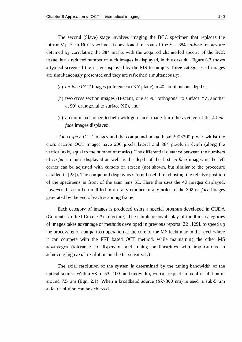
Chapter 6 Application of OCT in biomedical imaging 149
The second (Slave) stage involves imaging the BCC specimen that replaces the
mirror MS. Each BCC specimen is positioned in front of the SL. 384 en-face images are
obtained by correlating the 384 masks with the acquired channelled spectra of the BCC
tissue, but a reduced number of such images is displayed, in this case 40. Figure 6.2 shows
a typical screen of the raster displayed by the MS technique. Three categories of images
are simultaneously presented and they are refreshed simultaneously:
(a) en-face OCT images (reference to XY plane) at 40 simultaneous depths,
(b) two cross section images (B-scans, one at 90° orthogonal to surface YZ, another
at 90° orthogonal to surface XZ), and
(c) a compound image to help with guidance, made from the average of the 40 en-
face images displayed.
The en-face OCT images and the compound image have 200×200 pixels whilst the
cross section OCT images have 200 pixels lateral and 384 pixels in depth (along the
vertical axis, equal to the number of masks). The differential distance between the numbers
of en-face images displayed as well as the depth of the first en-face images in the left
corner can be adjusted with cursors on screen (not shown, but similar to the procedure
detailed in [28]). The compound display was found useful in adjusting the relative position
of the specimens in front of the scan lens SL. Here this uses the 40 images displayed,
however this can be modified to use any number in any order of the 398 en-face images
generated by the end of each scanning frame.
Each category of images is produced using a special program developed in CUDA
(Compute Unified Device Architecture). The simultaneous display of the three categories
of images takes advantage of methods developed in previous reports [22], [29], to speed up
the processing of comparison operation at the core of the MS technique to the level where
it can compete with the FFT based OCT method, while maintaining the other MS
advantages (tolerance to dispersion and tuning nonlinearities with implications in
achieving high axial resolution and better sensitivity).
The axial resolution of the system is determined by the tuning bandwidth of the
optical source. With a SS of Δλ=100 nm bandwidth, we can expect an axial resolution of
around 7.5 µm (Eqn. 2.1). When a broadband source (Δλ>300 nm) is used, a sub-5 µm
axial resolution can be achieved.
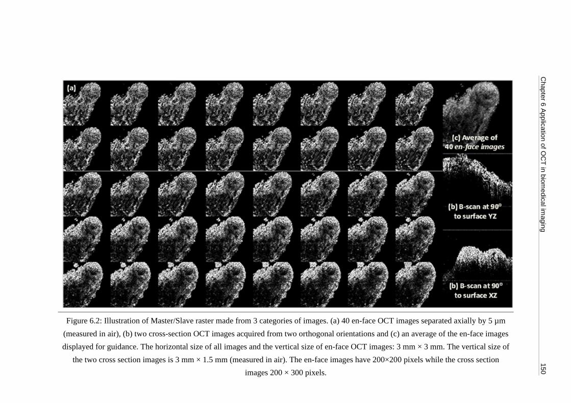
Chapter 6 A
pplication of OC
T in biom
edical imaging
150
Figure 6.2: Illustration of Master/Slave raster made from 3 categories of images. (a) 40 en-face OCT images separated axially by 5 µm
(measured in air), (b) two cross-section OCT images acquired from two orthogonal orientations and (c) an average of the en-face images
displayed for guidance. The horizontal size of all images and the vertical size of en-face OCT images: 3 mm × 3 mm. The vertical size of
the two cross section images is 3 mm × 1.5 mm (measured in air). The en-face images have 200×200 pixels while the cross section
images 200 × 300 pixels.
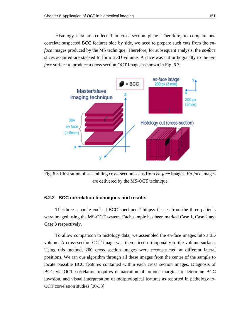
Chapter 6 Application of OCT in biomedical imaging 151
Histology data are collected in cross-section plane. Therefore, to compare and
correlate suspected BCC features side by side, we need to prepare such cuts from the en-
face images produced by the MS technique. Therefore, for subsequent analysis, the en-face
slices acquired are stacked to form a 3D volume. A slice was cut orthogonally to the en-
face surface to produce a cross section OCT image, as shown in Fig. 6.3.
Fig. 6.3 Illustration of assembling cross-section scans from en-face images. En-face images
are delivered by the MS-OCT technique
6.2.2 BCC correlation techniques and results
The three separate excised BCC specimens’ biopsy tissues from the three patients
were imaged using the MS-OCT system. Each sample has been marked Case 1, Case 2 and
Case 3 respectively.
To allow comparison to histology data, we assembled the en-face images into a 3D
volume. A cross section OCT image was then sliced orthogonally to the volume surface.
Using this method, 200 cross section images were reconstructed at different lateral
positions. We ran our algorithm through all these images from the centre of the sample to
locate possible BCC features contained within each cross section images. Diagnosis of
BCC via OCT correlation requires demarcation of tumour margins to determine BCC
invasion, and visual interpretation of morphological features as reported in pathology-to-
OCT correlation studies [30-33].
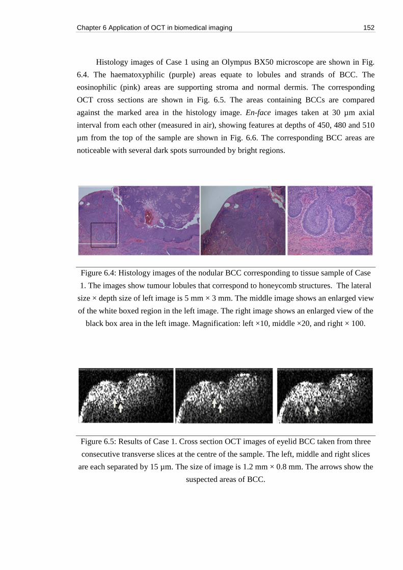
Chapter 6 Application of OCT in biomedical imaging 152
Histology images of Case 1 using an Olympus BX50 microscope are shown in Fig.
6.4. The haematoxyphilic (purple) areas equate to lobules and strands of BCC. The
eosinophilic (pink) areas are supporting stroma and normal dermis. The corresponding
OCT cross sections are shown in Fig. 6.5. The areas containing BCCs are compared
against the marked area in the histology image. En-face images taken at 30 µm axial
interval from each other (measured in air), showing features at depths of 450, 480 and 510
µm from the top of the sample are shown in Fig. 6.6. The corresponding BCC areas are
noticeable with several dark spots surrounded by bright regions.
Figure 6.4: Histology images of the nodular BCC corresponding to tissue sample of Case
1. The images show tumour lobules that correspond to honeycomb structures. The lateral
size × depth size of left image is 5 mm × 3 mm. The middle image shows an enlarged view
of the white boxed region in the left image. The right image shows an enlarged view of the
black box area in the left image. Magnification: left ×10, middle ×20, and right × 100.
Figure 6.5: Results of Case 1. Cross section OCT images of eyelid BCC taken from three
consecutive transverse slices at the centre of the sample. The left, middle and right slices
are each separated by 15 µm. The size of image is 1.2 mm × 0.8 mm. The arrows show the
suspected areas of BCC.
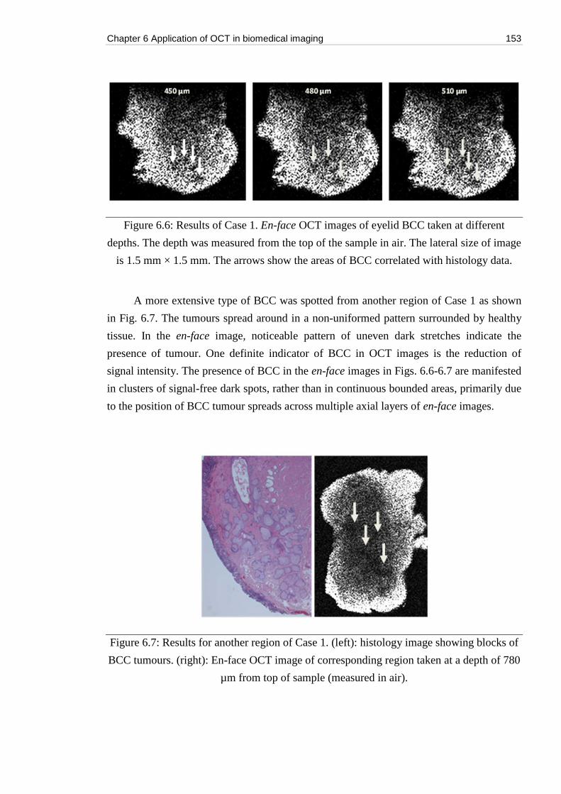
Chapter 6 Application of OCT in biomedical imaging 153
Figure 6.6: Results of Case 1. En-face OCT images of eyelid BCC taken at different
depths. The depth was measured from the top of the sample in air. The lateral size of image
is 1.5 mm × 1.5 mm. The arrows show the areas of BCC correlated with histology data.
A more extensive type of BCC was spotted from another region of Case 1 as shown
in Fig. 6.7. The tumours spread around in a non-uniformed pattern surrounded by healthy
tissue. In the en-face image, noticeable pattern of uneven dark stretches indicate the
presence of tumour. One definite indicator of BCC in OCT images is the reduction of
signal intensity. The presence of BCC in the en-face images in Figs. 6.6-6.7 are manifested
in clusters of signal-free dark spots, rather than in continuous bounded areas, primarily due
to the position of BCC tumour spreads across multiple axial layers of en-face images.
Figure 6.7: Results for another region of Case 1. (left): histology image showing blocks of
BCC tumours. (right): En-face OCT image of corresponding region taken at a depth of 780
µm from top of sample (measured in air).
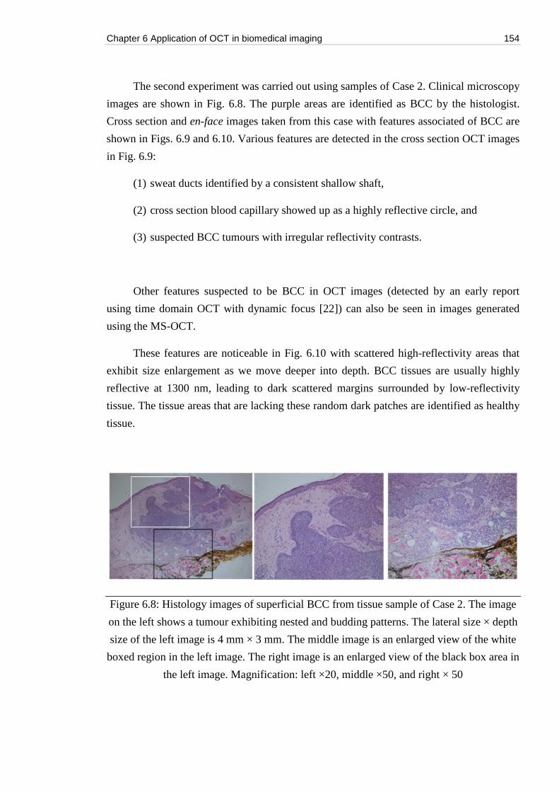
Chapter 6 Application of OCT in biomedical imaging 154
The second experiment was carried out using samples of Case 2. Clinical microscopy
images are shown in Fig. 6.8. The purple areas are identified as BCC by the histologist.
Cross section and en-face images taken from this case with features associated of BCC are
shown in Figs. 6.9 and 6.10. Various features are detected in the cross section OCT images
in Fig. 6.9:
(1) sweat ducts identified by a consistent shallow shaft,
(2) cross section blood capillary showed up as a highly reflective circle, and
(3) suspected BCC tumours with irregular reflectivity contrasts.
Other features suspected to be BCC in OCT images (detected by an early report
using time domain OCT with dynamic focus [22]) can also be seen in images generated
using the MS-OCT.
These features are noticeable in Fig. 6.10 with scattered high-reflectivity areas that
exhibit size enlargement as we move deeper into depth. BCC tissues are usually highly
reflective at 1300 nm, leading to dark scattered margins surrounded by low-reflectivity
tissue. The tissue areas that are lacking these random dark patches are identified as healthy
tissue.
Figure 6.8: Histology images of superficial BCC from tissue sample of Case 2. The image
on the left shows a tumour exhibiting nested and budding patterns. The lateral size × depth
size of the left image is 4 mm × 3 mm. The middle image is an enlarged view of the white
boxed region in the left image. The right image is an enlarged view of the black box area in
the left image. Magnification: left ×20, middle ×50, and right × 50
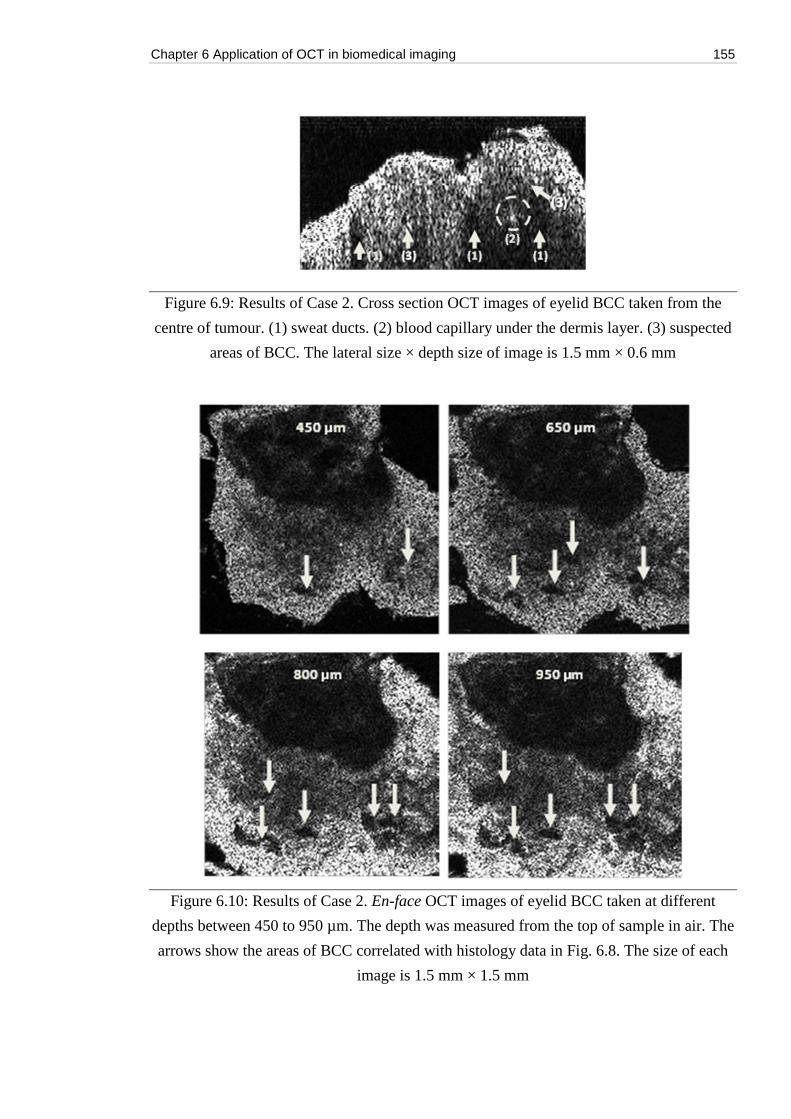
Chapter 6 Application of OCT in biomedical imaging 155
Figure 6.9: Results of Case 2. Cross section OCT images of eyelid BCC taken from the
centre of tumour. (1) sweat ducts. (2) blood capillary under the dermis layer. (3) suspected
areas of BCC. The lateral size × depth size of image is 1.5 mm × 0.6 mm
Figure 6.10: Results of Case 2. En-face OCT images of eyelid BCC taken at different
depths between 450 to 950 µm. The depth was measured from the top of sample in air. The
arrows show the areas of BCC correlated with histology data in Fig. 6.8. The size of each
image is 1.5 mm × 1.5 mm
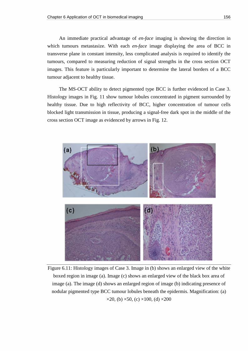
Chapter 6 Application of OCT in biomedical imaging 156
An immediate practical advantage of en-face imaging is showing the direction in
which tumours metastasize. With each en-face image displaying the area of BCC in
transverse plane in constant intensity, less complicated analysis is required to identify the
tumours, compared to measuring reduction of signal strengths in the cross section OCT
images. This feature is particularly important to determine the lateral borders of a BCC
tumour adjacent to healthy tissue.
The MS-OCT ability to detect pigmented type BCC is further evidenced in Case 3.
Histology images in Fig. 11 show tumour lobules concentrated in pigment surrounded by
healthy tissue. Due to high reflectivity of BCC, higher concentration of tumour cells
blocked light transmission in tissue, producing a signal-free dark spot in the middle of the
cross section OCT image as evidenced by arrows in Fig. 12.
Figure 6.11: Histology images of Case 3. Image in (b) shows an enlarged view of the white
boxed region in image (a). Image (c) shows an enlarged view of the black box area of
image (a). The image (d) shows an enlarged region of image (b) indicating presence of
nodular pigmented type BCC tumour lobules beneath the epidermis. Magnification: (a)
×20, (b) ×50, (c) ×100, (d) ×200
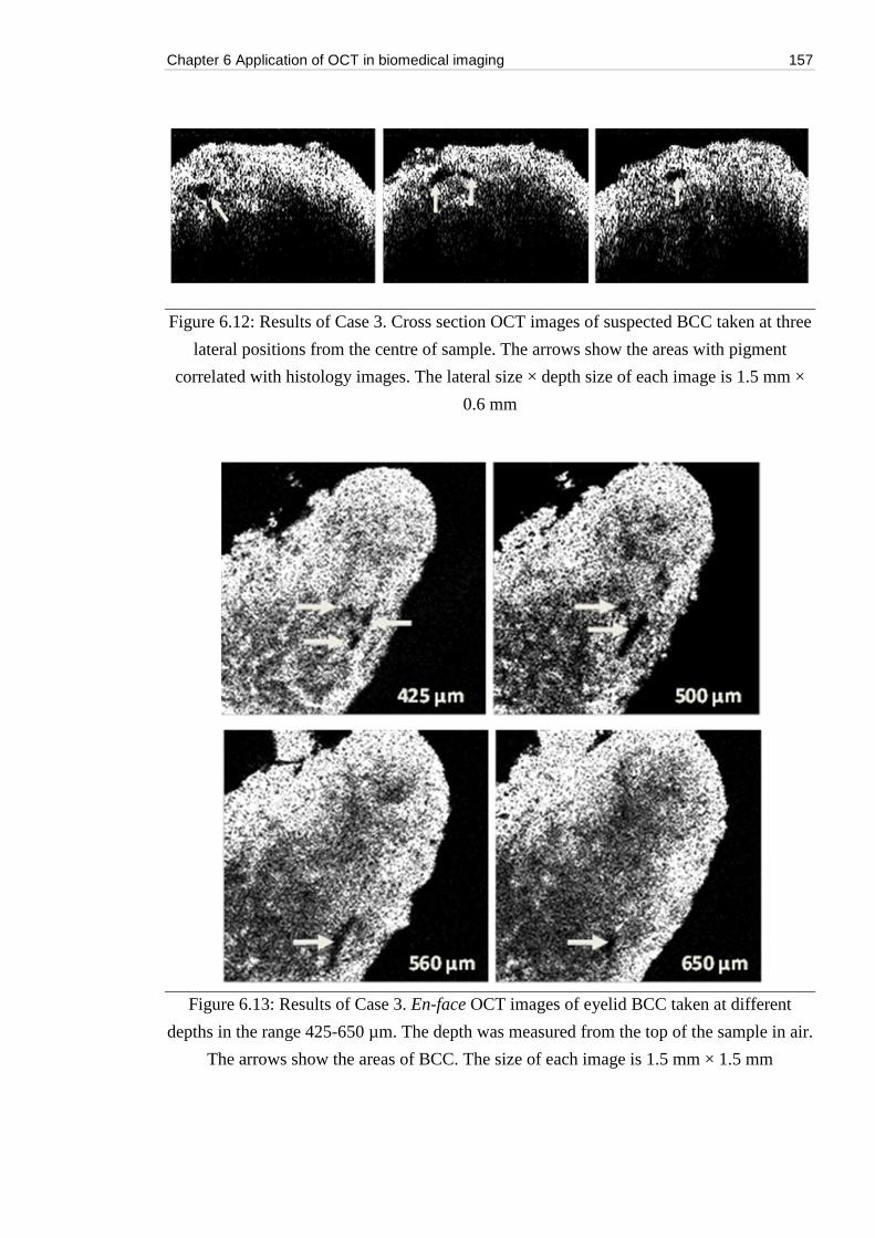
Chapter 6 Application of OCT in biomedical imaging 157
Figure 6.12: Results of Case 3. Cross section OCT images of suspected BCC taken at three
lateral positions from the centre of sample. The arrows show the areas with pigment
correlated with histology images. The lateral size × depth size of each image is 1.5 mm ×
0.6 mm
Figure 6.13: Results of Case 3. En-face OCT images of eyelid BCC taken at different
depths in the range 425-650 µm. The depth was measured from the top of the sample in air.
The arrows show the areas of BCC. The size of each image is 1.5 mm × 1.5 mm
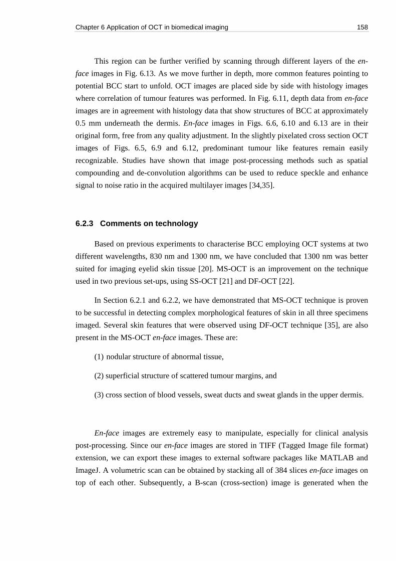
Chapter 6 Application of OCT in biomedical imaging 158
This region can be further verified by scanning through different layers of the en-
face images in Fig. 6.13. As we move further in depth, more common features pointing to
potential BCC start to unfold. OCT images are placed side by side with histology images
where correlation of tumour features was performed. In Fig. 6.11, depth data from en-face
images are in agreement with histology data that show structures of BCC at approximately
0.5 mm underneath the dermis. En-face images in Figs. 6.6, 6.10 and 6.13 are in their
original form, free from any quality adjustment. In the slightly pixelated cross section OCT
images of Figs. 6.5, 6.9 and 6.12, predominant tumour like features remain easily
recognizable. Studies have shown that image post-processing methods such as spatial
compounding and de-convolution algorithms can be used to reduce speckle and enhance
signal to noise ratio in the acquired multilayer images [34,35].
6.2.3 Comments on technology
Based on previous experiments to characterise BCC employing OCT systems at two
different wavelengths, 830 nm and 1300 nm, we have concluded that 1300 nm was better
suited for imaging eyelid skin tissue [20]. MS-OCT is an improvement on the technique
used in two previous set-ups, using SS-OCT [21] and DF-OCT [22].
In Section 6.2.1 and 6.2.2, we have demonstrated that MS-OCT technique is proven
to be successful in detecting complex morphological features of skin in all three specimens
imaged. Several skin features that were observed using DF-OCT technique [35], are also
present in the MS-OCT en-face images. These are:
(1) nodular structure of abnormal tissue,
(2) superficial structure of scattered tumour margins, and
(3) cross section of blood vessels, sweat ducts and sweat glands in the upper dermis.
En-face images are extremely easy to manipulate, especially for clinical analysis
post-processing. Since our en-face images are stored in TIFF (Tagged Image file format)
extension, we can export these images to external software packages like MATLAB and
ImageJ. A volumetric scan can be obtained by stacking all of 384 slices en-face images on
top of each other. Subsequently, a B-scan (cross-section) image is generated when the
Chapter 6 Application of OCT in biomedical imaging 159
volume is sliced at 90° orthogonal to the en-face surface. BCCs in cross section OCT
images can be identified by three main phenomena:
(a) abnormal reflectivity profile as we go in depth
(b) obscure regions with clear margins and
(c) repetitive inhomogeneous features different from the surrounding cells.
Similar morphological features are also used to identify potential BCC candidates in
the en-face images. A side-by-side comparison with histology images for all three cases
further validates the use of these criteria in OCT images with high certainty to locate and
detect various types of BCC.
In the first two BCC structures, nodal and superficial, the presence of BCC tissue in
en-face image can be determined from the absence of back reflected signal in a bounded
area with clear edges. The presence of some random, low-reflectivity black spots indicate
distribution of pigmented BCC structures. The lack of signal from BCC structures can be
explained by higher absorption due to their denser structure compared to normal tissue [20,
21]. This feature is predominately visible on OCT systems operating at 1300 nm than on
systems using shorter wavelengths.
Conventionally, averaging multiple en-face images usually improves the signal to
noise, allowing better location of BCCs otherwise unnoticeable in a cross section OCT
image, but this is done on the expense of axial resolution. Therefore, our approach to better
SNR is to improve the axial resolution by using a broadband optical source that can deliver
bandwidth of 300 nm or wider. Despite this chapter demonstrating MS-OCT with a swept
source, the Master/Slave method can equally be applied to an ultra broadband source, by
using a supercontinuum source and a spectrometer, in order to achieve better axial
resolution [37]. The fundamental work recorded in this thesis builds the foundation to
future exploration of such an option.
In this pilot study, en-face images of BCC samples taken from three patients were
produced using the novel Master/Slave method. In all cases, the suspected BCC regions
showed significant reduction in the signal strengths compared to uniform signal reflectivity
in neighbouring tissues. In some cases, the presence of potential BCC can be identified by
irregular scattering of high reflectivity dark spots (Fig. 6.6) and inconsistent light
distribution pattern (Fig. 6.7) in skin tomograms.

Chapter 6 Application of OCT in biomedical imaging 160
All features associated with BCC demonstrated in our three previous studies [20-22]
are also seen with en-face images obtained using MS-OCT. Three common types of BCC
were identified and fitted well with histology criteria. In particular, nodular BCC are noted
with their low reflectivity of light at 1310 nm, closely corresponding to BCC on correlation
by the histologist following standard laboratory processing. Other subtypes of BCC may
also be picked up by their irregular reflectivity profile in en-face images. High accuracy in
distinguishing uncertain tumour lesions from healthy skins was established [15].
A further study has been planned once a portable handheld probe incorporating
Master/Slave technique is manufactured. This will ease the transport of technology for
clinical trials at hospitals, allowing imaging to be carried out in real time, in three possible
scenarios, involving both in-vitro and in-vivo experiments:
(1) pre-surgery diagnosis,
(2) intra-operative assessment of precise tumour margins,
(3) post-surgical side by side histology assessment.
In-vivo OCT imaging would be preferred for its enhanced clinical value to
dermatologist and pathologist [37-39], as the water content and skin optical properties are
preserved. We acknowledge possible signal distortions due to in-vitro imaging. For this
reason, further work in axial resolution improvement and the development of polarisation-
sensitive capabilities will be required.
The use of MS-OCT technique has allowed en-face images to display noticeable
BCC features in real time. With no further image processing required, rapid assessment of
BCC extent and surgical margins in excised skin specimens can be carried out, allowing
for enhanced management of patients in the clinical setting. In addition to that, a quick
patient turnover also save time and eliminate diagnosis errors.
This is a preliminary study to assess the values of the en-face display in diagnosing
BCC. The MS technique is ideally suited to deliver such display as the image is assembled
directly while laterally scanning with no need to wait for a whole assembly of A-scans to
be subsequently cut.
Chapter 6 Application of OCT in biomedical imaging 161
6.3 Imaging of mammalian embryos
In recent years, ability to perform live tissue imaging has gained traction in the area
of fertility treatments. As demonstrated in previous section on the benefits of en-fact OCT
imaging for BCC, we teamed up with researchers from Dr Gary Robinson’s group at the
School of Biosciences, at the University of Kent, and carried out the pilot project to image
pig embryos using the our MS-OCT system.
Several new researches in this area were done to improve the field of reproductive
biology and medicine, the efficiency of in vitro fertilisation (IVF) to above 40% for
women [40]. Currently, the lack of non-invasive treatments procedures was cited as the
main cause for low fertilization efficiencies [41]. Without the use of high resolution,
functional in vivo tomography imaging, there is no way to accurately assess the quality and
development potential of embryos, prior to the IVF transfers. More recently, several
groups have started to employ OCT imaging to achieve this goal [41-44].
Our aim in this project was not to primarily evaluate the oocyte development
process, but rather to test our en-face OCT capability to achieve the axial and transversal
resolutions needed to discriminate the features of sub-cellular structures of the embryos.
To do that, we replaced the microscope objective (tele-centric lens) in Fig.6.1 of Sec.6.2 to
a high NA version from Olympus. The new MO allows us to image with a transversal
resolution of ~ 5 μm, as opposed to the previous ~12.5 μm used for BCC imaging. The
axial resolution remained as it was, since we used the same Axsun swept-source with a 100
nm optical bandwidth (model SS1300-OCT). The imaged pig embryos are shown in
orthogonal views (XY, YZ and XZ) Fig.6.14, all 40 simultaneous en-face OCT raster scans
in Fig.6.15 and 3D volume displays in Fig.6.16.
We have demonstrated how live embryonic imagings with en-face OCT can be used
to assess structural and functional birth defects, during the early stage development of
fertilisation process. Therefore, we have shown that our master/slave OCT technology can
be used for various biomedical applications, not limited to only BCC diagnosis.
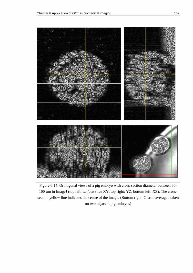
Chapter 6 Application of OCT in biomedical imaging 162
Figure 6.14: Orthogonal views of a pig embryo with cross-section diameter between 80-
100 μm in ImageJ (top left: en-face slice XY, top right: YZ, bottom left: XZ). The cross-
section yellow line indicates the centre of the image. (Bottom right: C-scan averaged taken
on two adjacent pig embryos)
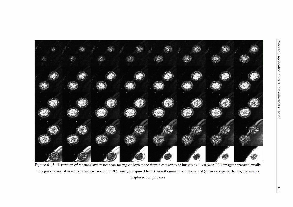
Chapter 6 A
pplication of OC
T in biom
edical imaging
163
Figure 6.15: Illustration of Master/Slave raster scan for pig embryo made from 3 categories of images a) 40 en-face OCT images separated axially
by 5 µm (measured in air), (b) two cross-section OCT images acquired from two orthogonal orientations and (c) an average of the en-face images
displayed for guidance
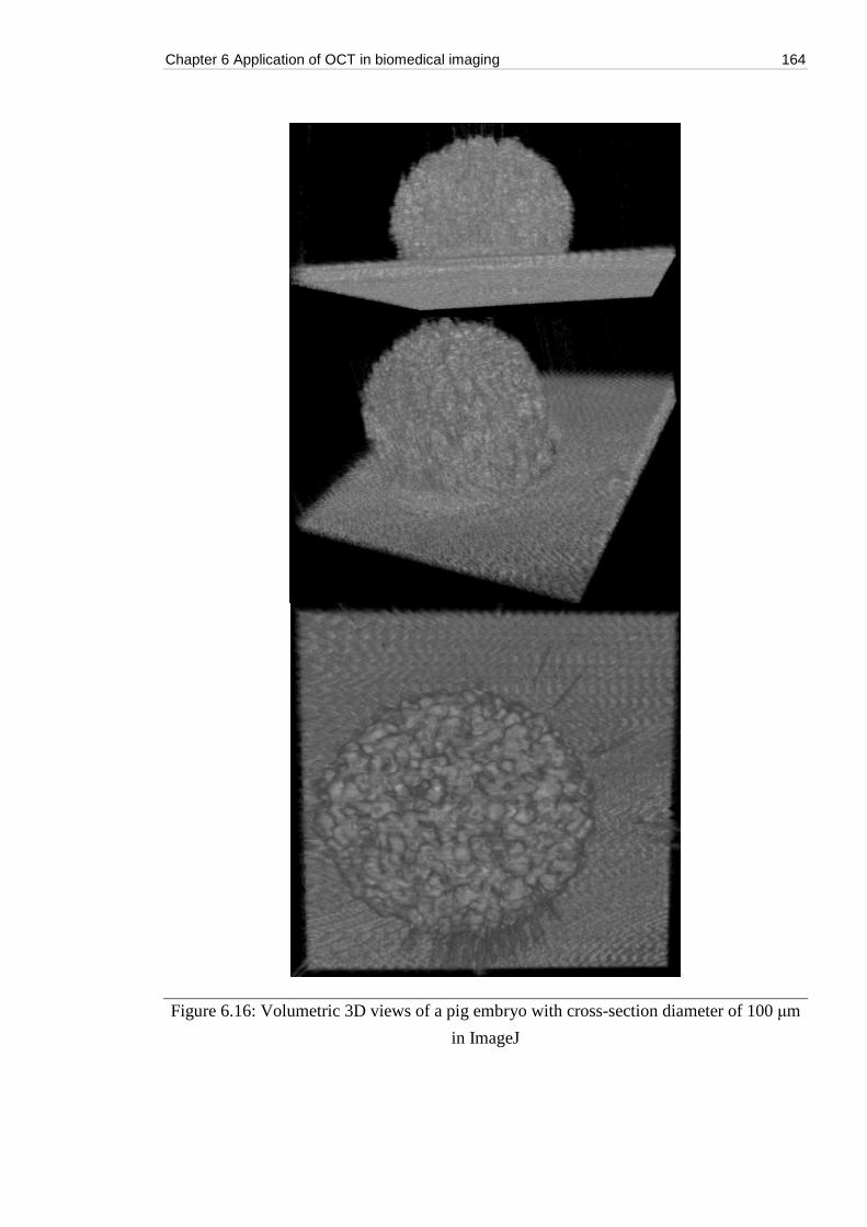
Chapter 6 Application of OCT in biomedical imaging 164
Figure 6.16: Volumetric 3D views of a pig embryo with cross-section diameter of 100 μm
in ImageJ
Chapter 6 Application of OCT in biomedical imaging 165
References
1. A. Lomas, J. Leonardi-Bee, F. Bath-Hextall, “A systematic review of worldwide incidence
of nonmelanoma skin cancer,” Br. J. Dermatol. 166 (5), 1069-80 (May 2012).
2. C. E. Margo, K. Waltz, “Basal cell carcinoma of the eyelid and periocular skin,” Surv.
Ophthalmol., 38(2), 169-92 (1993).
3. G. W. Jung, A. I. Metelitsa, D. C. Dover, and T. G. Salopek, “Trends in incidence of
nonmelanoma skin cancers in Alberta, Canada, 1988–2007,” Br. J. Dermatol. 163, 146–154
(2010).
4. F. Bath-Hextall, J. Leonardi-Bee, C. Smith, A. Meal, R. Hubbard, “Trends in incidence of
skin basal cell carcinoma. Additional evidence from a UK primary care database study,” Int.
J. Cancer, 121(9), 2105-8 (1993).
5. Improving outcomes for people with skin tumours including melanoma (update): the
management of low-risk basal cell carcinomas in the community. NICE Guidance on Cancer
Services. May (2010).
6. M. Venturini, G. Gualdi, A. Zanca, L. Lorenzi, G. Pellacani, P. G. Calzavara-Pinton, “A new
approach for presurgical margin assessment by reflectance confocal microscopy of basal cell
carcinoma,” Br. J. Dermatol., 174(2), 380-385 (Feb 2016).
7. M. Nassiri-Kashani, B. Sadr, F. Fanian, K. Kamyab, P. Noormohammadpour, M. M.
Shahshahani, H. Zartab, M. M. Naghizadeh, M. Sarraf-Yazdy, A. Firooz, “Pre-operative
assessment of basal cell carcinoma dimensions using high frequency ultrasonography and its
correlation with histopathology,” Skin Res. Technol., 19(1), 132-138 (2013).
8. I. Kopriva, A. Persin, N. Puizina-Ivic, L. Miric, “Robust demarcation of basal cell carcinoma
by dependent component analysis-based segmentation of multi-spectra fluorescence
images,” J. Photochem. Photobio. B. 100 (1), 10-18 (2010).
9. M. Balu, C. B. Zachary, R. M. Harris, T. B. Krasieva, K. Konig, B. J. Tromberg, K. M.
Kelly, “In vivo multiphoton microscopy of basal cell carcinoma,” JAMA Dermatol. 151
(10), 1068-1074 (2015).
10. R. Patalay, C. Talbot, Y. Alexandrov, M. O. Lenz, S. Kumar, S. Warren, I. Munro, M. A. A.
Neil, K. Konig, P. M. W. French, A. Chu, G. W. H. Stamp, C. Dunsby, “Multiphoton
multispectral fluorescence lifetime tomography for the evaluation of basal cell carcinomas,”
PLoS One 7 (9), e43460 (2012).
11. K. Busam, C. Charles, C. Lohmann, A. Marghoob, M. Goldgeier, A. Halpern, “Detection of
intraepidermal microscopy,” Melanoma Res. 12, 349-355 (2002).
12. M. A. Boone, M. Suppa, G. Pellacani, A. Marneffe, M. Miyamoto, I. Alarcon, C. Ruini, R.
Hofmann-Wellenhof, J. Malvehy, G. B. Jemec, V. Del Marmol, “High-definition optical
coherence tomography algorithm for discrimination of basal cell carcinoma from clinical
BCC imitators and differentiation between common subtypes,” J. Eur. Acad. Dermatol.
Venereol. 29(9), 1771-80 (2015).
Chapter 6 Application of OCT in biomedical imaging 166
13. M. A. L. M. Boone, S. Norrenberg, G. B. E. Jemec, V. Del Marmol, ”Imaging of basal cell
carcinoma by high-definition optical coherence tomography: histomorphological correlation.
A pilot study,” B. J. Dermatol., 167, 856-864 (2012).
14. T. Maier, M. Braun-Falco, T. Hinz, M. H. Schmid-Wendtner, T. Ruzicka, C. Berking,
“Morphology of basal cell carcinoma in high definition optical coherence tomography: en-
face and slice imaging mode, and comparison with histology,” J. Eur. Acad Dermatol
Venereol, 27 (1), 97-104 (2013).
15. M. Ulrich, T. von Braunmuehl, H. Kurzen, T. Dirschka, C. Kellner, E. Sattler, C. Berking, J.
Welzel, U. Reinhold, “The sensitivity and specificity of optical coherence tomography for
the assisted diagnosis of nonpigmented basal cell carcinoma: an observational study,” B. J.
Dermatol, 172(2), 428-435 (2015).
16. A. Gh. Podoleanu, A. Bradu, “Master–slave interferometry for parallel spectral domain
interferometry sensing and versatile 3D optical coherence tomography,” Opt. Exp. 21(16),
19324-19338 (2013).
17. A. Bradu, M. Maria, A. Gh. Podoleanu, “Demonstration of tolerance to dispersion of
master/slave interferometry,” Opt Exp. 5(11), 14148-14161 (2015).
18. J. Wang, A. Bradu, G. Dobre, A. Podoleanu, “Full-field swept source master-slave optical
coherence tomography,” IEEE Photonics J. 7(4) (2015)
19. A. Bradu, A. Gh. Podoleanu, “Imaging the eye fundus with real-time en-face spectral
domain optical coherence tomography,” Biomed Opt Exp. 5(4), 1233-1249 (2014).
20. B. R. Penmetsa, M. Khandwala, A. Bradu, M. Hughes, C. A. Jones, J. Schofield, A. G.
Podoleanu, “Imaging of basal cell carcinoma tissue using en-face OCT,” Proc. SPIE 7139,
71390J (2008).
21. M. Khandwala, B. R. Penmetsa, S. Dey, J. B. Schofield, C. A. Jones, A. Podoleanu,
“Imaging of periocular basal cell carcinoma using en face optical coherence tomography: a
pilot study,” Brit. J. Ophthal. 1136, 1-5 (2010).
22. M. R. N. Avanaki, A. Hojjatoleslami, M, Sira, J. Schofield, C. Jones, A. Gh. Podoleanu,
“Investigation of basal cell carcinoma using dynamic focus optical coherence tomography,”
Appl. Opt. 52(10), 2116-2124 (2013).
23. J. K. Patel, S. Konda, O. A. Perez, S. Amini, G. Elgart, B. Berman, ”Newer
technologies/techniques and tools in the diagnosis of melanoma,” E. J. Dermatol. 18, 617-
631 (2008).
24. N. Iftimia, G. Peterson, E. W. Chang, G. Maguluri, W. Fox, M. Rajadhyaksha, “Combined
reflectance confocal microscopy-optical coherence tomography for delineation of basal cell
carcinoma margins: an ex vivo study,” J. Bio. Opt. 21(1), 016006 (2016).
25. M. Ulrich, L. Themstrup, N. Carvalho, M. Manfredi, C. Grana, S. Ciardo, R. Kastle, J.
Holmes, R. Whitehead, G. B. E. Jemec, G. Pellacani, J. Welzel, “Dynamic optical coherence
tomography in dermatology,” J. Dermatol. 232, 298-311 (2016).
Chapter 6 Application of OCT in biomedical imaging 167
26. G. Li, J. K. Tietze, X. Tao, D. Kulichova, T. Ruzicka, C. Berking, T. Maier, “High-definition
optical coherence tomography in the diagnosis of basal cell carcinoma evaluated by an
experienced versus in experienced investigator,” J. Clin. Exp. Dermatol. Res. 5(4), 1000227
(2014).
27. A. Hojjatoleslami, M. R. N. Avanaki, “OCT skin imaging enhancement through attenuation
compensation,” Appl. Opt.51, 4927-4935 (2012).
28. A. Bradu, K. Kapinchev, F. Barnes, A. Podoleanu, “Master slave en-face OCT/SLO,”
Biomed. Opt. Exp. 6(9), 3655-3669 (2015).
29. A. Bradu, K. Kapinchev, F. Barnes, A. Podoleanu, ”On the possibility of producing true real-
time retinal cross-sectional images using a graphics processing unit enhanced master-slave
optical coherence tomography system,” J. Biomed. Opt. 20(7) (2015).
30. M. A. Boone, M. Suppa, G. Pellacani, A. Marneffe, M. Miyamoo, I. Alarcon, C. Ruini, R.
Hofmann-Wellenhof, J. Malvehy, G.B. Jemec, V. Del Marmol, “High-definition optical
coherence tomography algorithm for discrimination of basal cell carcinoma from clinical
BCC imitators and differentiation between common subtypes,” J. Eur. Acad. Dermatol.
Venereol. 29, 1771-1780 (2015).
31. T. Gambichler, I. Plura, P. Kampilafkos, K. Valavanis, M Sand, F. G. Bechara, M. Stucker,
“Histopathological correlates of basal cell carcinoma in the slice and en face imaging modes
of high-definition optical coherence tomography,” Br. J. Dermatol. 170, 1358-1361 (2014).
32. A. J. Coleman, T. J. Richardson, G. Orchard, et al., “Histological correlates of optical
coherence tomography in non-melanoma skin cancer,” Skin Res. Technol. 19, 10-19 (2013).
33. M. A. Boone, S. Norrenberg, G. B. Jemec, V. Del Marmol, “Imaging of basal cell carcinoma
by high-definition optical coherence tomography: histomorphological correlation. A pilot
study,” Br. J. Dermatol. 167, 856-864 (2012).
34. S. A. Hojjatoleslami, M. R. N. Avanaki, A. Gh. Podoleanu, “Image quality improvement in
optical coherence tomography using Lucy-Richardson deconvolution algorithm,” Appl. Opt.
54, 5663-5670 (2013).
35. M. R. N. Avanaki, R. Cernat, P. J. Tadrous, T. Tatla, A. Gh. Podoleanu, S. A.
Hojjatoleslami, “Spatial compounding algorithm for speckle reduction of dynamic focus
OCT images,” IEEE Photon. Tech. Lett. 25, 1439-1442 (2013).
36. M. Mogensen, T. Joergensen, L, Thrane, B. M. Nurnberg, G. B. E. Jemec, “Improved quality
of optical coherence tomography imaging of basal cell carcinomas using speckle reduction,”
Exp. Dermatol.,19(8), 293-295 (2009).
37. M. Maria, M. J. M. Marques, C. Costa, A. Bradu, T. Feuchter, L Leick, A. G. H. Podoleanu,
“Broadband master-slave interferometry using a super-continuum source,” Proc. SPIE, 9697,
96972R (2016).
38. M. Mogensen, T. M. Joergensen, B. M. Nurnberg, H. A. Morsy, J. B. Thomsen, L. Thrane,
G. B. Jemec,”Assessment of optical coherence tomography imaging in the diagnosis of non-
Chapter 6 Application of OCT in biomedical imaging 168
melanoma skin cancer and benign lesions versus normal skin: observer-blinded evaluation
by dermatologiss and pathologists,” Dermatol. Surg.,35,965-972 (2009).
39. J. M. Olmedo, K. E. Warschaw, J. M. Schmitt, D. L. Swanson, “Optical coherence
tomography for the characterization of basal cell carcinoma in vivo: a pilot study,” J. Am.
Acad. Dermatol.,55,408-412 (2006).
40. A. Ajduk, M. Zernicka-Goetz, “Quality control of embryo development,” Molecular Aspects
of Medicine, 34(5), 903-918 (2013).
41. K. Karnowski, A. Ajduk, B. Wieloch, S. Tamborski, K. Krawiec, M. Wojtkowski & M.
Szkulmowski, "Optical coherence microscopy as a novel, non-invasive method for the 4D
live imaging of early mammalian embryos," Sci. Rep. 7(4165) (2017).
42. L. Zarnescu, M.C. Leung, M. Abeyta, H. Sudkamp, T. Baer, B. Behr, A.K. Ellerbee, “Label-
free characterization of vitrification-induced morphology changes in single-cell embryos
with full-field optical coherence tomography,” J. Biomed. Opt. 20(9), 096004 (2015).
43. J. Y. Xiao, B. Wang, G. Y. Lu, Z. Q. Zhu and Y. J. Huang, “Imaging of oocyte development
using ultrahigh-resolution full-field optical coherence tomography,” Appl. Opt. 51, 3650–
3654 (2012).
44. J. Zheng, D. Lu, T. Chen, C. Wang, N. Tian, F. Zhao, T. Huo, N. Zhang, D. Chen, W. Ma, J.
Sun, P. Xue, “Label-free subcellular 3D live imaging of preimplantation mouse embryos
with full-field optical coherence tomography” J. Biomed. Opt. 17 (2012).
7
Application of supercontinuum light sources in vision science
Application of a broadband supercontinuum source goes beyond OCT imaging.
Today’s supercontinuum sources have ventured into the regime of complex light
manipulation and they have also taken advantage of full range power controls. This niche
opens up exciting new field of possibilities in medical imaging and also vision science
research. To demonstrate such capabilities, we collaborated with Dr Gurprit Lall of The
Medway School of Pharmacy in Kent, and used a supercontinuum white light (SCWL)
source from NKT Photonics A/S, to study the pupil light reflex in mammals upon multi-
colour light stimuli.
In this chapter, we assessed the spectral sensitivity of the pupillary light reflex in
wild type mice using a high power SCWL source in a dual wavelength configuration. This
novel approach was compared to data collected from a more traditional setup using a
Xenon arc (Xe Arc) lamp fitted with monochromatic interference filters. Irradiance
response curves (IRCs) were constructed using both systems, with the added benefit of a
two-wavelength, equivocal power, and output using the SCWL. The variables applied to
the light source were intensity, wavelength and stimulus duration through which the
physiological output measured was the minimum pupil size attained under such conditions.
We showed that by implementing the SCWL as our novel stimulus, we were able to
dramatically increase the physiological usefulness of our pupillometry system.
Our experiment focuses mainly on the papillary light response in the mammalian eye
that closely resembles that of humans. The mammalian eye is an essential component of
the central nervous systems’ (CNS) sensory complement. It is primarily, responsible for
generating a visual representation of our environment. This is possible through the
decoding of light by a structure termed the retina, which contains complex neuronal
structures capable of detecting the spectral composition of a light source and converting
this into an electrical impulse. The retina, itself, coats the back of the inner eyeball and
forms optic nerves that feed the brain; ultimately terminating at the occipital lobe. It's
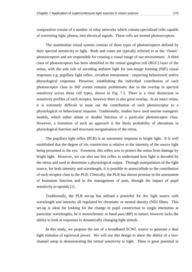
Chapter 7 Application of supercontinuum light sources in vision science 170
composition consist of a number of relay networks which contain specialised cells capable
of converting light, photos, into electrical signals. These cells are termed photoreceptors.
The mammalian visual system consists of three types of photoreceptors defined by
their spectral sensitivity to light. Rods and cones are typically referred to as the ‘classic’
photoreceptors and are responsible for creating a visual image of our environment. A third
class of photoreceptors has been identified in the retinal ganglion cell (RGC) layer of the
retina, with the sole role of encoding ambient light for non-image forming (NIF) visual
responses e.g. pupillary light reflex, circadian entrainment - impacting behavioural and/or
physiological responses. However, establishing the individual contribution of each
photoreceptor class to NIF events remains problematic due to the overlap in spectral
sensitivity across these cell types, shown in Fig. 7.1. There is a clear distinction in
sensitivity profiles of each receptor, however there is also great overlap. In an intact retina,
it is extremely difficult to tease out the contribution of each photoreceptor to a
physiological or behavioural response. Traditionally, studies have used murine transgenic
models, which either ablate or disable function of a particular photoreceptor class.
However, a limitation of such an approach is the likely probability of alterations in
physiological function and structural reorganisation of the retina.
The pupillary light reflex (PLR) is an autonomic response to bright light. It is well
established that the degree of iris constriction is relative to the intensity of the source light
being presented to the eye. Foremost, this reflex acts to protect the retina from damage by
bright light. However, we can also use this reflex to understand how light is decoded by
the retina and used to determine a physiological output. Through manipulation of the light
source, for both intensity and wavelength, it is possible to assess/allude to the contribution
of each receptor class to the PLR. Clinically, the PLR has shown promise in the assessment
of brainstem function and in the management of pain, through the impact of pupil
sensitivity to opioids [1].
Traditionally, the PLR set-up has utilised a powerful Xe Arc light source with
wavelength and intensity all regulated by chromatic or neutral density (ND) filters. This
set-up is ideal for looking for the change in pupil constriction to single intensities at
particular wavelengths, be it monochromic or band pass (BP) in nature; however lacks the
ability to look at responses to dynamically changing light stimuli.
In this study, we propose the use of a broadband SCWL source to generate a dual
light stimulus of equivocal power. We will use this design to show the ability of a two-
channel setup in demonstrating the retinal sensitivity to light. There is great potential in
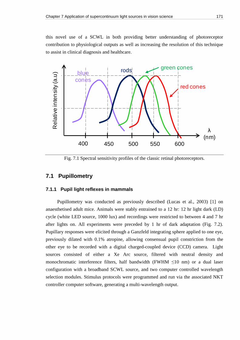
Chapter 7 Application of supercontinuum light sources in vision science 171
this novel use of a SCWL in both providing better understanding of photoreceptor
contribution to physiological outputs as well as increasing the resolution of this technique
to assist in clinical diagnosis and healthcare.
Fig. 7.1 Spectral sensitivity profiles of the classic retinal photoreceptors.
7.1 Pupillometry
7.1.1 Pupil light reflexes in mammals
Pupillometry was conducted as previously described (Lucas et al., 2003) [1] on
anaesthetised adult mice. Animals were stably entrained to a 12 hr: 12 hr light dark (LD)
cycle (white LED source, 1000 lux) and recordings were restricted to between 4 and 7 hr
after lights on. All experiments were preceded by 1 hr of dark adaptation (Fig. 7.2).
Pupillary responses were elicited through a Ganzfeld integrating sphere applied to one eye,
previously dilated with 0.1% atropine, allowing consensual pupil constriction from the
other eye to be recorded with a digital charged-coupled device (CCD) camera. Light
sources consisted of either a Xe Arc source, filtered with neutral density and
monochromatic interference filters, half bandwidth (FWHM ≤10 nm) or a dual laser
configuration with a broadband SCWL source, and two computer controlled wavelength
selection modules. Stimulus protocols were programmed and run via the associated NKT
controller computer software, generating a multi-wavelength output.
Rel
ativ
e in
ten
sity
(a.u
)
400 450 500 550 600
λ
(nm)
red cones
blue cones
rods green cones
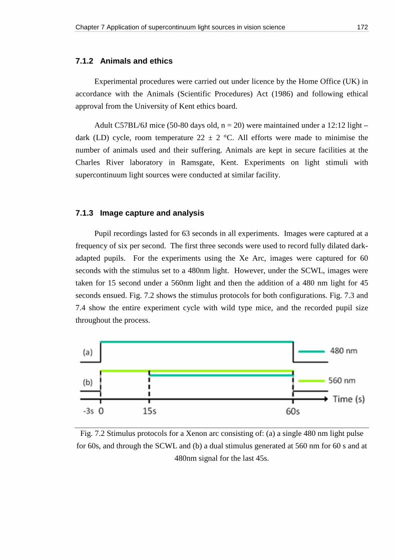
Chapter 7 Application of supercontinuum light sources in vision science 172
7.1.2 Animals and ethics
Experimental procedures were carried out under licence by the Home Office (UK) in
accordance with the Animals (Scientific Procedures) Act (1986) and following ethical
approval from the University of Kent ethics board.
Adult C57BL/6J mice (50-80 days old, n = 20) were maintained under a 12:12 light –
dark (LD) cycle, room temperature 22 ± 2 °C. All efforts were made to minimise the
number of animals used and their suffering. Animals are kept in secure facilities at the
Charles River laboratory in Ramsgate, Kent. Experiments on light stimuli with
supercontinuum light sources were conducted at similar facility.
7.1.3 Image capture and analysis
Pupil recordings lasted for 63 seconds in all experiments. Images were captured at a
frequency of six per second. The first three seconds were used to record fully dilated dark-
adapted pupils. For the experiments using the Xe Arc, images were captured for 60
seconds with the stimulus set to a 480nm light. However, under the SCWL, images were
taken for 15 second under a 560nm light and then the addition of a 480 nm light for 45
seconds ensued. Fig. 7.2 shows the stimulus protocols for both configurations. Fig. 7.3 and
7.4 show the entire experiment cycle with wild type mice, and the recorded pupil size
throughout the process.
Fig. 7.2 Stimulus protocols for a Xenon arc consisting of: (a) a single 480 nm light pulse
for 60s, and through the SCWL and (b) a dual stimulus generated at 560 nm for 60 s and at
480nm signal for the last 45s.
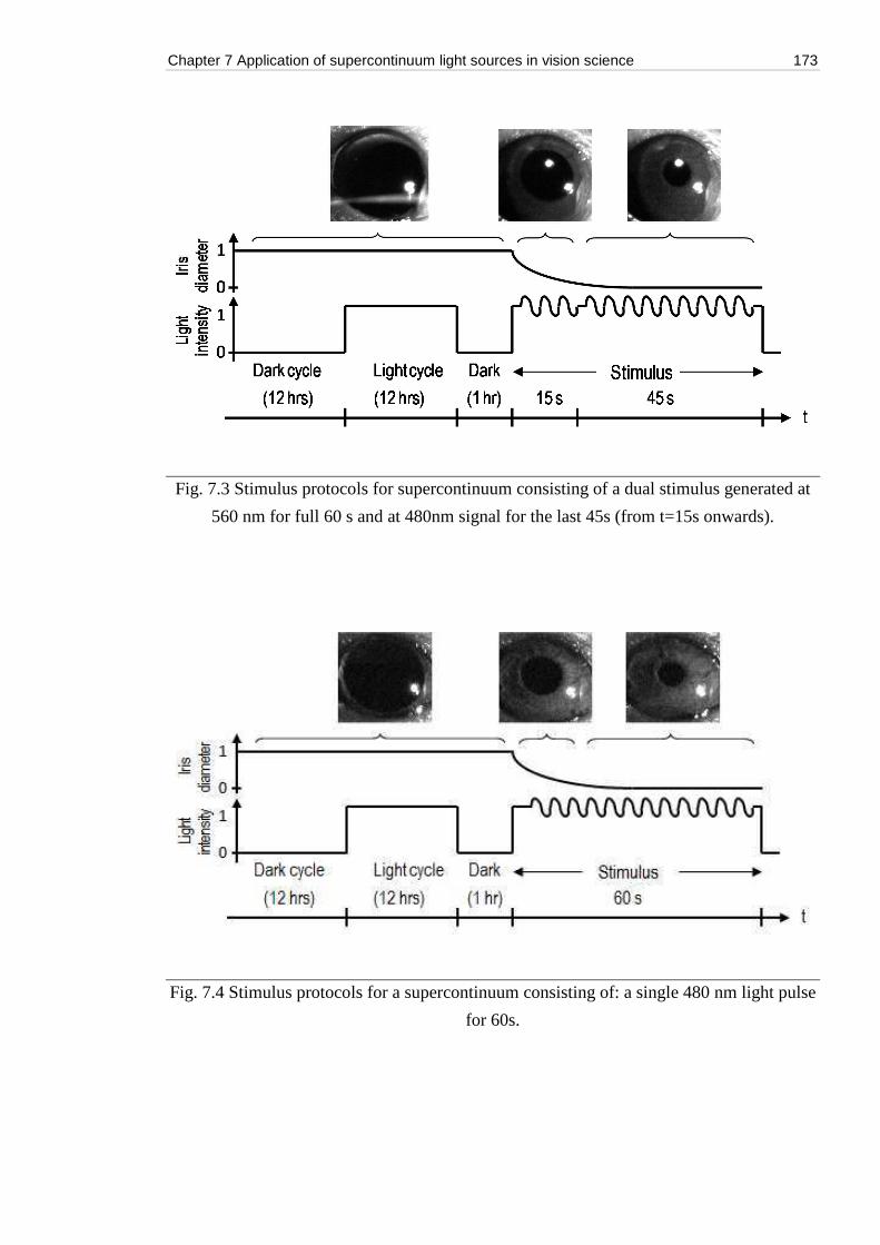
Chapter 7 Application of supercontinuum light sources in vision science 173
Fig. 7.3 Stimulus protocols for supercontinuum consisting of a dual stimulus generated at
560 nm for full 60 s and at 480nm signal for the last 45s (from t=15s onwards).
Fig. 7.4 Stimulus protocols for a supercontinuum consisting of: a single 480 nm light pulse
for 60s.
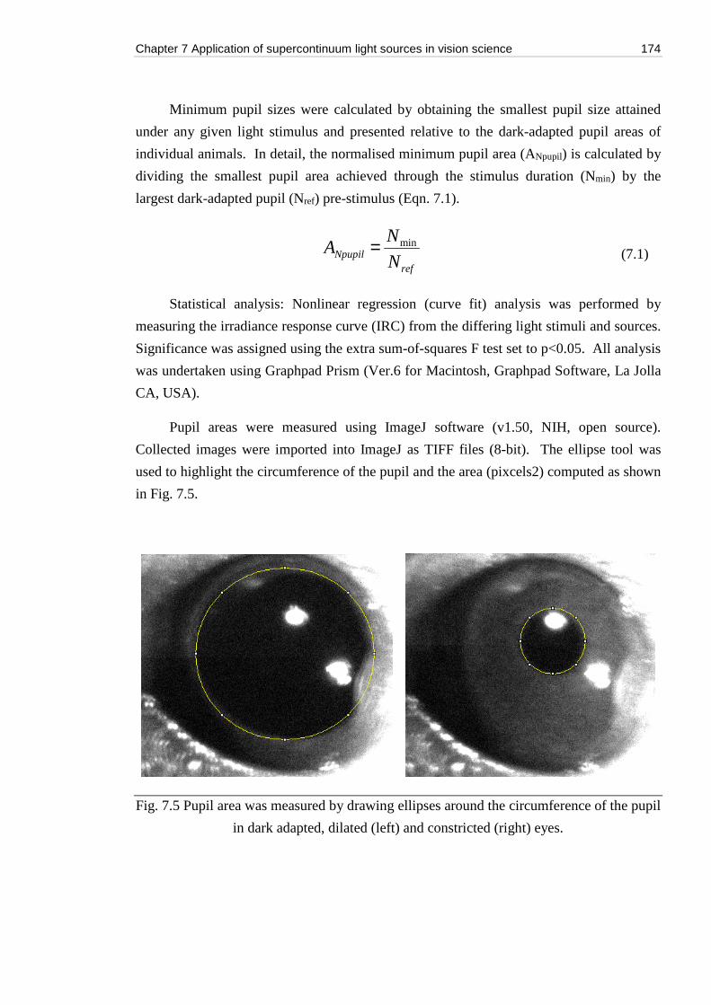
Chapter 7 Application of supercontinuum light sources in vision science 174
Minimum pupil sizes were calculated by obtaining the smallest pupil size attained
under any given light stimulus and presented relative to the dark-adapted pupil areas of
individual animals. In detail, the normalised minimum pupil area (ANpupil) is calculated by
dividing the smallest pupil area achieved through the stimulus duration (Nmin) by the
largest dark-adapted pupil (Nref) pre-stimulus (Eqn. 7.1).
refNpupil N
NA min= (7.1)
Statistical analysis: Nonlinear regression (curve fit) analysis was performed by
measuring the irradiance response curve (IRC) from the differing light stimuli and sources.
Significance was assigned using the extra sum-of-squares F test set to p<0.05. All analysis
was undertaken using Graphpad Prism (Ver.6 for Macintosh, Graphpad Software, La Jolla
CA, USA).
Pupil areas were measured using ImageJ software (v1.50, NIH, open source).
Collected images were imported into ImageJ as TIFF files (8-bit). The ellipse tool was
used to highlight the circumference of the pupil and the area (pixcels2) computed as shown
in Fig. 7.5.
Fig. 7.5 Pupil area was measured by drawing ellipses around the circumference of the pupil
in dark adapted, dilated (left) and constricted (right) eyes.
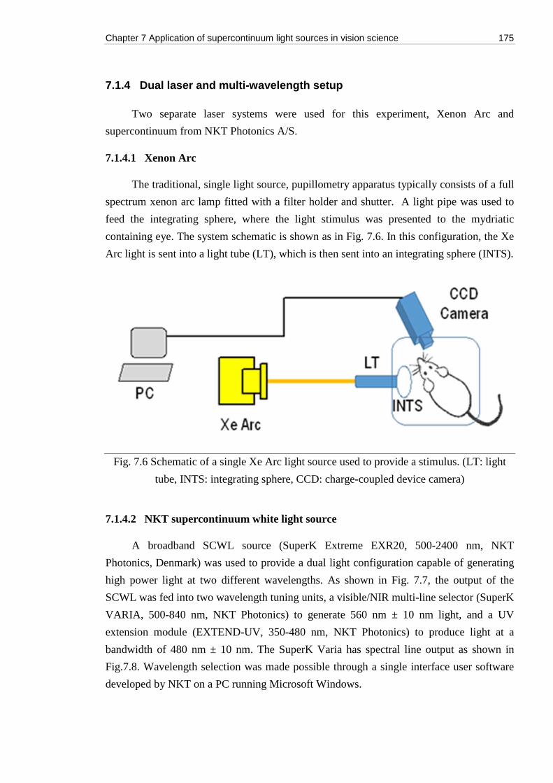
Chapter 7 Application of supercontinuum light sources in vision science 175
7.1.4 Dual laser and multi-wavelength setup
Two separate laser systems were used for this experiment, Xenon Arc and
supercontinuum from NKT Photonics A/S.
7.1.4.1 Xenon Arc
The traditional, single light source, pupillometry apparatus typically consists of a full
spectrum xenon arc lamp fitted with a filter holder and shutter. A light pipe was used to
feed the integrating sphere, where the light stimulus was presented to the mydriatic
containing eye. The system schematic is shown as in Fig. 7.6. In this configuration, the Xe
Arc light is sent into a light tube (LT), which is then sent into an integrating sphere (INTS).
Fig. 7.6 Schematic of a single Xe Arc light source used to provide a stimulus. (LT: light
tube, INTS: integrating sphere, CCD: charge-coupled device camera)
7.1.4.2 NKT supercontinuum white light source
A broadband SCWL source (SuperK Extreme EXR20, 500-2400 nm, NKT
Photonics, Denmark) was used to provide a dual light configuration capable of generating
high power light at two different wavelengths. As shown in Fig. 7.7, the output of the
SCWL was fed into two wavelength tuning units, a visible/NIR multi-line selector (SuperK
VARIA, 500-840 nm, NKT Photonics) to generate 560 nm ± 10 nm light, and a UV
extension module (EXTEND-UV, 350-480 nm, NKT Photonics) to produce light at a
bandwidth of 480 nm ± 10 nm. The SuperK Varia has spectral line output as shown in
Fig.7.8. Wavelength selection was made possible through a single interface user software
developed by NKT on a PC running Microsoft Windows.
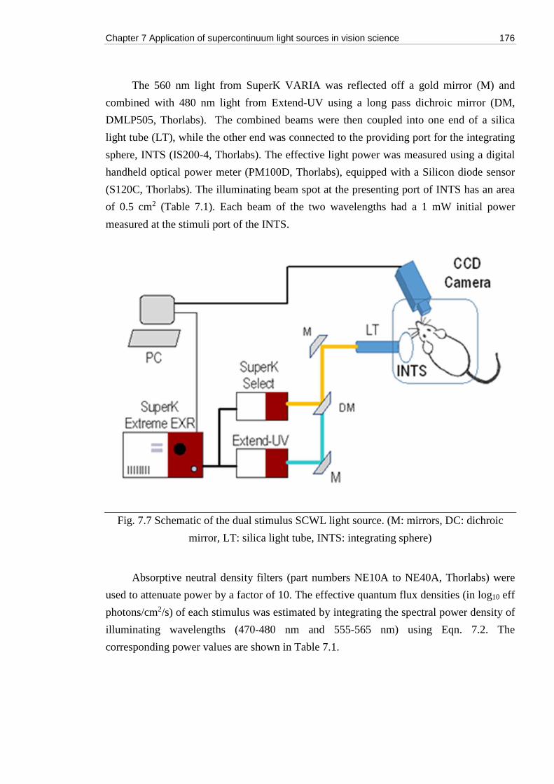
Chapter 7 Application of supercontinuum light sources in vision science 176
The 560 nm light from SuperK VARIA was reflected off a gold mirror (M) and
combined with 480 nm light from Extend-UV using a long pass dichroic mirror (DM,
DMLP505, Thorlabs). The combined beams were then coupled into one end of a silica
light tube (LT), while the other end was connected to the providing port for the integrating
sphere, INTS (IS200-4, Thorlabs). The effective light power was measured using a digital
handheld optical power meter (PM100D, Thorlabs), equipped with a Silicon diode sensor
(S120C, Thorlabs). The illuminating beam spot at the presenting port of INTS has an area
of 0.5 cm2 (Table 7.1). Each beam of the two wavelengths had a 1 mW initial power
measured at the stimuli port of the INTS.
Fig. 7.7 Schematic of the dual stimulus SCWL light source. (M: mirrors, DC: dichroic
mirror, LT: silica light tube, INTS: integrating sphere)
Absorptive neutral density filters (part numbers NE10A to NE40A, Thorlabs) were
used to attenuate power by a factor of 10. The effective quantum flux densities (in log10 eff
photons/cm2/s) of each stimulus was estimated by integrating the spectral power density of
illuminating wavelengths (470-480 nm and 555-565 nm) using Eqn. 7.2. The
corresponding power values are shown in Table 7.1.
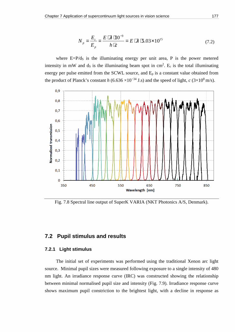
Chapter 7 Application of supercontinuum light sources in vision science 177
159
1003.510 ×⋅⋅=
⋅⋅⋅==
−
λλE
ch
E
E
EN
p
cp (7.2)
where E=P/dS is the illuminating energy per unit area, P is the power metered
intensity in mW and dS is the illuminating beam spot in cm2. Ec is the total illuminating
energy per pulse emitted from the SCWL source, and Ep is a constant value obtained from
the product of Planck’s constant h (6.636 ×10⁻³⁴ J.s) and the speed of light, c (3×10⁸ m/s).
Fig. 7.8 Spectral line output of SuperK VARIA (NKT Photonics A/S, Denmark).
7.2 Pupil stimulus and results
7.2.1 Light stimulus
The initial set of experiments was performed using the traditional Xenon arc light
source. Minimal pupil sizes were measured following exposure to a single intensity of 480
nm light. An irradiance response curve (IRC) was constructed showing the relationship
between minimal normalised pupil size and intensity (Fig. 7.9). Irradiance response curve
shows maximum pupil constriction to the brightest light, with a decline in response as
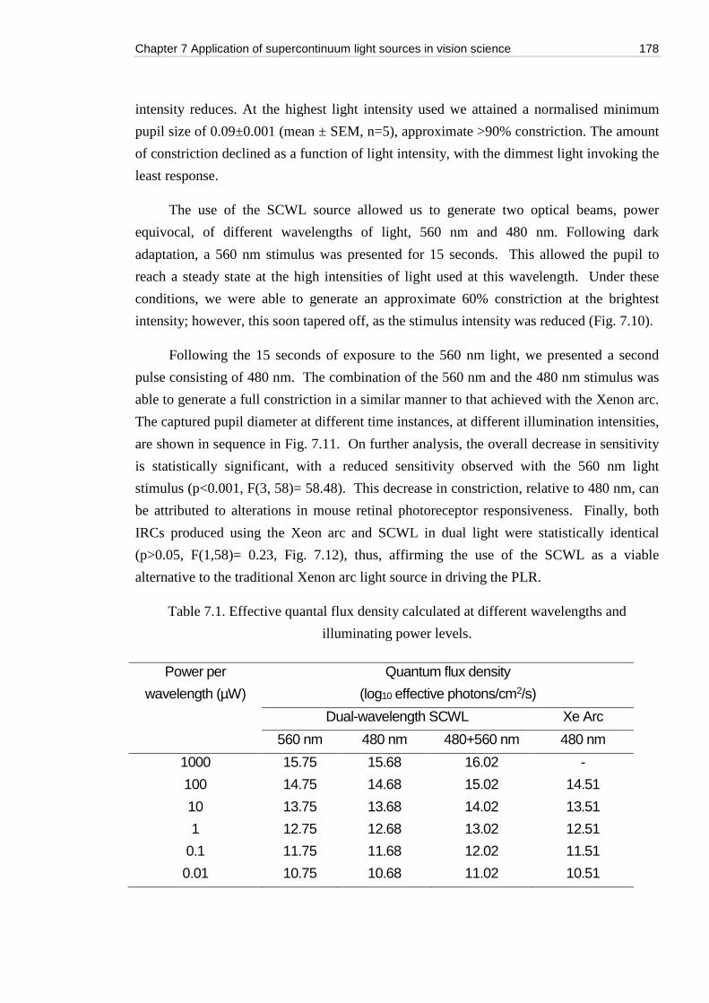
Chapter 7 Application of supercontinuum light sources in vision science 178
intensity reduces. At the highest light intensity used we attained a normalised minimum
pupil size of 0.09±0.001 (mean ± SEM, n=5), approximate >90% constriction. The amount
of constriction declined as a function of light intensity, with the dimmest light invoking the
least response.
The use of the SCWL source allowed us to generate two optical beams, power
equivocal, of different wavelengths of light, 560 nm and 480 nm. Following dark
adaptation, a 560 nm stimulus was presented for 15 seconds. This allowed the pupil to
reach a steady state at the high intensities of light used at this wavelength. Under these
conditions, we were able to generate an approximate 60% constriction at the brightest
intensity; however, this soon tapered off, as the stimulus intensity was reduced (Fig. 7.10).
Following the 15 seconds of exposure to the 560 nm light, we presented a second
pulse consisting of 480 nm. The combination of the 560 nm and the 480 nm stimulus was
able to generate a full constriction in a similar manner to that achieved with the Xenon arc.
The captured pupil diameter at different time instances, at different illumination intensities,
are shown in sequence in Fig. 7.11. On further analysis, the overall decrease in sensitivity
is statistically significant, with a reduced sensitivity observed with the 560 nm light
stimulus (p<0.001, F(3, 58)= 58.48). This decrease in constriction, relative to 480 nm, can
be attributed to alterations in mouse retinal photoreceptor responsiveness. Finally, both
IRCs produced using the Xeon arc and SCWL in dual light were statistically identical
(p>0.05, F(1,58)= 0.23, Fig. 7.12), thus, affirming the use of the SCWL as a viable
alternative to the traditional Xenon arc light source in driving the PLR.
Table 7.1. Effective quantal flux density calculated at different wavelengths and
illuminating power levels.
Power per
wavelength (µW)
Quantum flux density
(log10 effective photons/cm2/s)
Dual-wavelength SCWL Xe Arc
560 nm 480 nm 480+560 nm 480 nm
1000 15.75 15.68 16.02 -
100 14.75 14.68 15.02 14.51
10 13.75 13.68 14.02 13.51
1 12.75 12.68 13.02 12.51
0.1 11.75 11.68 12.02 11.51
0.01 10.75 10.68 11.02 10.51
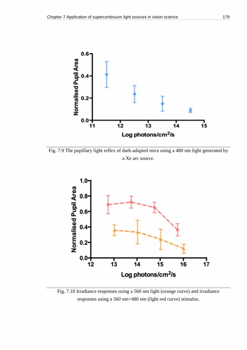
Chapter 7 Application of supercontinuum light sources in vision science 179
Fig. 7.9 The pupillary light reflex of dark-adapted mice using a 480 nm light generated by
a Xe arc source.
Fig. 7.10 Irradiance responses using a 560 nm light (orange curve) and irradiance
responses using a 560 nm+480 nm (light red curve) stimulus.
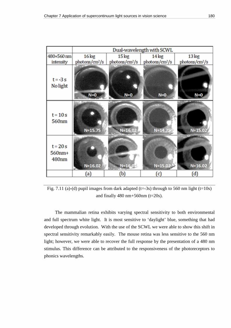
Chapter 7 Application of supercontinuum light sources in vision science 180
Fig. 7.11 (a)-(d) pupil images from dark adapted (t=-3s) through to 560 nm light (t=10s)
and finally 480 nm+560nm (t=20s).
The mammalian retina exhibits varying spectral sensitivity to both environmental
and full spectrum white light. It is most sensitive to ‘daylight’ blue, something that had
developed through evolution. With the use of the SCWL we were able to show this shift in
spectral sensitivity remarkably easily. The mouse retina was less sensitive to the 560 nm
light; however, we were able to recover the full response by the presentation of a 480 nm
stimulus. This difference can be attributed to the responsiveness of the photoreceptors to
phonics wavelengths.
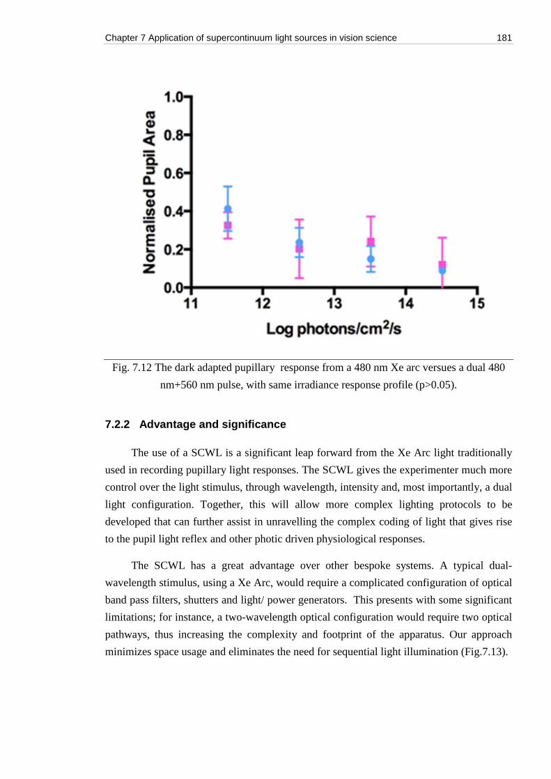
Chapter 7 Application of supercontinuum light sources in vision science 181
Fig. 7.12 The dark adapted pupillary response from a 480 nm Xe arc versues a dual 480
nm+560 nm pulse, with same irradiance response profile (p>0.05).
7.2.2 Advantage and significance
The use of a SCWL is a significant leap forward from the Xe Arc light traditionally
used in recording pupillary light responses. The SCWL gives the experimenter much more
control over the light stimulus, through wavelength, intensity and, most importantly, a dual
light configuration. Together, this will allow more complex lighting protocols to be
developed that can further assist in unravelling the complex coding of light that gives rise
to the pupil light reflex and other photic driven physiological responses.
The SCWL has a great advantage over other bespoke systems. A typical dual-
wavelength stimulus, using a Xe Arc, would require a complicated configuration of optical
band pass filters, shutters and light/ power generators. This presents with some significant
limitations; for instance, a two-wavelength optical configuration would require two optical
pathways, thus increasing the complexity and footprint of the apparatus. Our approach
minimizes space usage and eliminates the need for sequential light illumination (Fig.7.13).
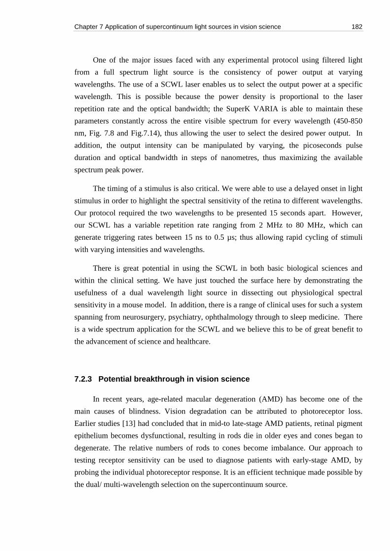
Chapter 7 Application of supercontinuum light sources in vision science 182
One of the major issues faced with any experimental protocol using filtered light
from a full spectrum light source is the consistency of power output at varying
wavelengths. The use of a SCWL laser enables us to select the output power at a specific
wavelength. This is possible because the power density is proportional to the laser
repetition rate and the optical bandwidth; the SuperK VARIA is able to maintain these
parameters constantly across the entire visible spectrum for every wavelength (450-850
nm, Fig. 7.8 and Fig.7.14), thus allowing the user to select the desired power output. In
addition, the output intensity can be manipulated by varying, the picoseconds pulse
duration and optical bandwidth in steps of nanometres, thus maximizing the available
spectrum peak power.
The timing of a stimulus is also critical. We were able to use a delayed onset in light
stimulus in order to highlight the spectral sensitivity of the retina to different wavelengths.
Our protocol required the two wavelengths to be presented 15 seconds apart. However,
our SCWL has a variable repetition rate ranging from 2 MHz to 80 MHz, which can
generate triggering rates between 15 ns to 0.5 µs; thus allowing rapid cycling of stimuli
with varying intensities and wavelengths.
There is great potential in using the SCWL in both basic biological sciences and
within the clinical setting. We have just touched the surface here by demonstrating the
usefulness of a dual wavelength light source in dissecting out physiological spectral
sensitivity in a mouse model. In addition, there is a range of clinical uses for such a system
spanning from neurosurgery, psychiatry, ophthalmology through to sleep medicine. There
is a wide spectrum application for the SCWL and we believe this to be of great benefit to
the advancement of science and healthcare.
7.2.3 Potential breakthrough in vision science
In recent years, age-related macular degeneration (AMD) has become one of the
main causes of blindness. Vision degradation can be attributed to photoreceptor loss.
Earlier studies [13] had concluded that in mid-to late-stage AMD patients, retinal pigment
epithelium becomes dysfunctional, resulting in rods die in older eyes and cones began to
degenerate. The relative numbers of rods to cones become imbalance. Our approach to
testing receptor sensitivity can be used to diagnose patients with early-stage AMD, by
probing the individual photoreceptor response. It is an efficient technique made possible by
the dual/ multi-wavelength selection on the supercontinuum source.
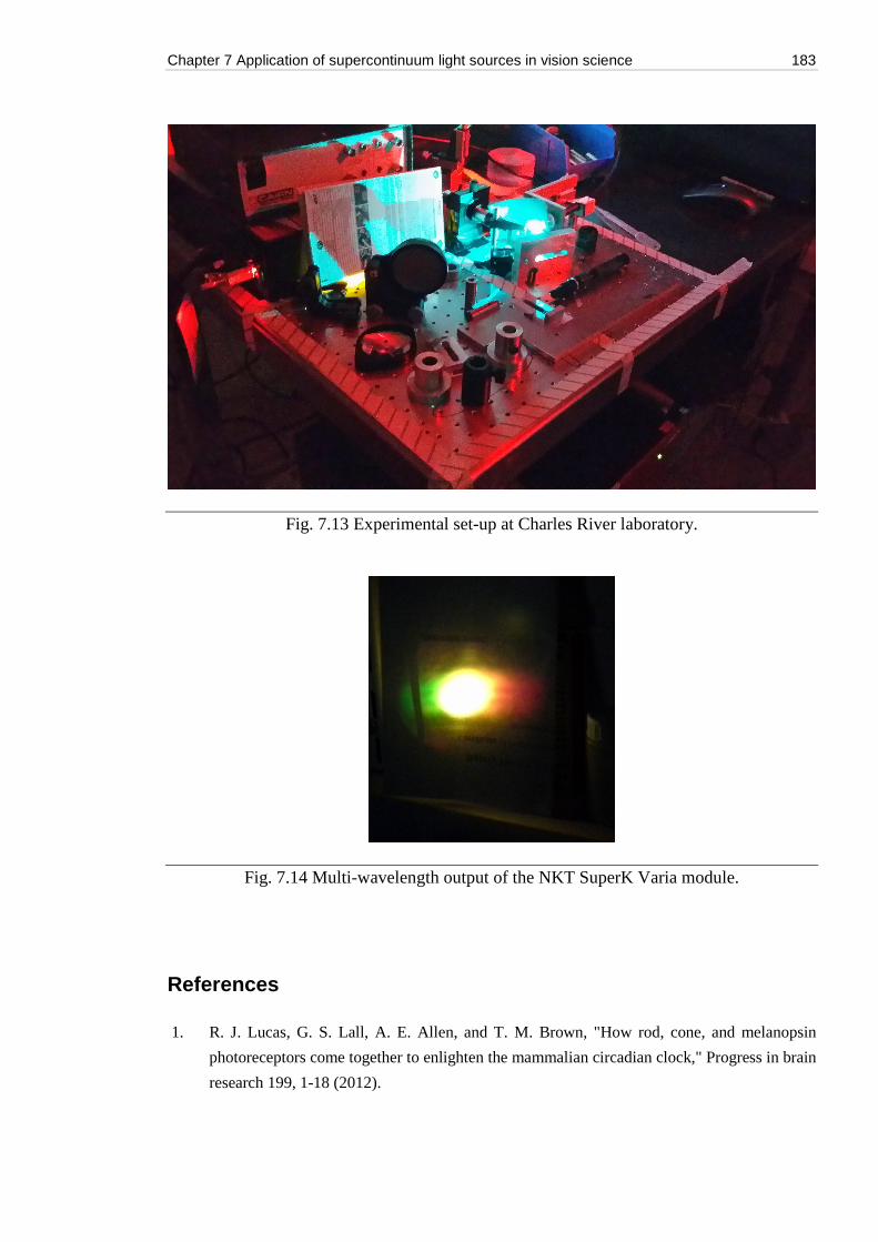
Chapter 7 Application of supercontinuum light sources in vision science 183
Fig. 7.13 Experimental set-up at Charles River laboratory.
Fig. 7.14 Multi-wavelength output of the NKT SuperK Varia module.
References
1. R. J. Lucas, G. S. Lall, A. E. Allen, and T. M. Brown, "How rod, cone, and melanopsin
photoreceptors come together to enlighten the mammalian circadian clock," Progress in brain
research 199, 1-18 (2012).
Chapter 7 Application of supercontinuum light sources in vision science 184
2. D. G. McMahon, P. M. Iuvone, and G. Tosini, "Circadian organization of the mammalian
retina: from gene regulation to physiology and diseases," Progress in retinal and eye research
39, 58-76 (2014).
3. C. M. Altimus, A. D. Guler, N. M. Alam, A. C. Arman, G. T. Prusky, A. P. Sampath, and S.
Hattar, "Rod photoreceptors drive circadian photoentrainment across a wide range of light
intensities," Nature neuroscience 13, 1107-1112 (2010).
4. G. S. Lall, V. L. Revell, H. Momiji, J. Al Enezi, C. M. Altimus, A. D. Guler, C. Aguilar, M.
A. Cameron, S. Allender, M. W. Hankins, and R. J. Lucas, "Distinct contributions of rod,
cone, and melanopsin photoreceptors to encoding irradiance," Neuron 66, 417-428 (2010).
5. R. J. Lucas, R. H. Douglas, and R. G. Foster, "Characterization of an ocular photopigment
capable of driving pupillary constriction in mice," Nature neuroscience 4, 621-626 (2001).
6. R. J. Lucas and R. G. Foster, "Neither functional rod photoreceptors nor rod or cone outer
segments are required for the photic inhibition of pineal melatonin," Endocrinology 140,
1520-1524 (1999).
7. D. Lupi, H. M. Cooper, A. Froehlich, L. Standford, M. A. McCall, and R. G. Foster,
"Transgenic ablation of rod photoreceptors alters the circadian phenotype of mice,"
Neuroscience 89, 363-374 (1999).
8. R. J. Lucas, S. Hattar, M. Takao, D. M. Berson, R. G. Foster, and K. W. Yau, "Diminished
pupillary light reflex at high irradiances in melanopsin-knockout mice," Science 299, 245-
247 (2003).
9. A. E. Neice, M. Behrends, M. P. Bokoch, K. M. Seligman, N. M. Conrad, and M. D. Larson,
"Prediction of Opioid Analgesic Efficacy by Measurement of Pupillary Unrest," Anesthesia
and analgesia (2016).
10. A. C. Lukaszewicz, D. Dereu, E. Gayat, and D. Payen, "The relevance of pupillometry for
evaluation of analgesia before noxious procedures in the intensive care unit," Anesthesia and
analgesia 120, 1297-1300 (2015).
11. T. M. Brown, "Using light to tell the time of day: sensory coding in the mammalian
circadian visual network," The Journal of experimental biology 219, 1779-1792 (2016).
12. B. Feigl and A. J. Zele, "Melanopsin-expressing intrinsically photosensitive retinal ganglion
cells in retinal disease," Optometry and vision science: official publication of the American
Academy of Optometry 91, 894-903 (2014).
13. C. A. Curcio, N. E. Medeiros, C. L. Millican, “Photoreceptor loss in age-related macular
degeneration,” Invest Ophthalmol Vis Sci. 37(7):1236-49 (1996).
8
Conclusion
The works in this thesis have shown that high-resolution OCT is now one of the
preferred method for non-invasive imaging by ophthalmologist and dermatologist. The
application of ultra-broadband OCT has seen significant demands from health industries
with promising results. Several commercial prototypes of portable and handheld OCT
devices have been manufactured in the last three years while this thesis was in progress. It
is now established that OCT is a mature technology, and can be independently deployed in
hospitals and surgical theatres. The general adoption of broadband OCT technology will
take time. However, there is still more catching up to do to enable real-time, reliable, in
vivo biomedical diagnosis with broadband OCT. It is therefore essential that further
development in this area is more commercial oriented, so that extension of OCT
capabilities can be used to attract industry interests.
Most parts of this thesis have focused on technological problems that hindered the
use of OCT in clinical environment. In Chapter 2, we reviewed scientific research and
technological development of OCT since its early inception in 1990. We showed how this
field had overcome technical hurdles in the earlier implementation, and progressed into the
robust imaging technology we know today. Chapters 3 and 4 went further into addressing
numbers of specialised limitations: noise, dispersion and polarisation. We viewed these
limitations as a two-sided challenge: manufacturing artefacts in the commercial light
sources as well as due to the imperfect construction of the interferometer systems. Not all
limitations are detrimental to our research. Some of these limitations, noise and dispersion,
for example, can have adverse effect to the imaging quality if they are left unresolved,
while polarisation can play a vital role in detecting additional image features, if they are
used to our advantage. The technical solutions to these limitation resulted in a simple,
broadband polarisation sensitive (PS-) OCT with master/slave interferometer (MSI)
technology. We have discussed in details this implementation in Chapter 5.
A large portion of this research was dedicated to characterising limitations, as we
researched and resolved them step-by-step. The first technical limitation addressed was
noise. In Chapter 3, we discussed extensively on methods used to quantify and minimise
Chapter 8 Conclusion 186
noise coming out from the light source, and likewise for noise added by the OCT setup.
This thesis emphasises on the use of supercontinuum sources to enhance imaging
capabilities: better signal to noise ratio, minimum dispersion and ultra-high imaging
resolution. We have incorporated light sources with increasing bandwidth in our noise
studies: from a dual diode SLD, to swept sources, and finally supercontinuum sources.
Based on the bandwidth argument, we have consistently stressed on the potential of
supercontinuum to be used to power OCT systems, while we dismissed the earlier
misconception of supercontinuum as being noisy as a thing of the past. We have evaluated
key parameters in supercontinuum generation, and performed optimisation on several of
these: pulse repetition frequency, energy emission per pulse, fibre birefringence and
polarisation. These studies aimed to make supercontinuum source the preferred light
source for ultra-broadband OCT imaging.
The second limitation we have overcome was dispersion. For an OCT system to
resolve image features of 5 µm or less axially, it is essential that we properly compensate
for dispersion. We proposed the state of the art acousto-optic tuneable filter (AOTF)
method. In Chapter 4, we have shown the principle of operation with an AOTF, used
together with a supercontinuum light source. This method allows us to select a narrow
band light from a broadband spectrum. The AOTF module from NKT Photonics came in
handy. It operates in two widely used spectral ranges for commercial imaging systems:
visible from 500 to 900 nm, and near infrared from 1150 to 2000 nm. A custom built
hardware-based dispersion compensation procedure was quantified using the AOTF,
employing addition of dispersive glass elements. BK7 glass rods were added in the
reference arm of the interferometer. Since the line width of the AOTF module can be as
narrow as 5 nm, it was useful to scan across the broadband spectrum for dispersion
irregularities. The AOTF method had one clear advantage: it allows us to speed up the
process to obtain the variation of autocorrelation peak position in OPD versus wavelength,
all in a single measurement. The slope obtained quickly determines the direction of
compensation needed. This is in contrast to the time-consuming full-width at half
maximum (FWHM) measurement of the autocorrelation function method, widely used in
the industry. The established method requires multiple FWHM measurements, and does
not provide direction of compensation needed. Our approach has established that, by
estimating errors in measuring the FWHM of the A-scan peak, the AOTF method is more
superior in reaching the minimum dispersion. It is also applicable for all OCT systems.
Simple dispersion compensation can make commercial ultra-broadband OCT
implementation easier and more attractive.
Chapter 8 Conclusion 187
The third limitation we encountered and now resolved is polarisation. In Chapters 3
and 5, we have shown that polarisation effect is a two-way sword: it can work against us as
well as in our favour. Conventional OCT imaging has been intensity based since the early
days. Many commercial systems had adopted similar approach and have remained so till
this day. However, we have demonstrated in Chapters 5 and 6 that there are increasing
number of applications where polarisation sensitive imaging can be an advantage. This is
particularly true in areas related to bio-security (explosive, narcotics), arts of historical
value (paintings, archaeological artefacts) and complex histology structures (skin cancers,
tooth decays, retina diseases), where these specimens have important multi-layer
birefringent features. The work in second half of Chapter 3 has experimentally and
theoretically verified that polarisation controlling elements can be added and manipulated
in the optical sources, particularly at different stages of the supercontinuum generation
process. Armed with the knowledge in polarisation selection, we can now enhance our
imaging capabilities further.
The forth limitation deals with application practicality. In an academia-only research,
we focused on build to order (BTO) imaging equipment. The popularity of customisable
system has become a mainstream niche in medical equipment industries. From the very
simpler original equipment manufacturing (OEM) devices, to more sophisticated designs
and production for application-specific equipment, the obstacles to incorporate latest
research into existing commercial products need to be overcome. These hurdles involve
technology integration and compatibility. UBAPHODESA researchers with academia and
industrial experience can now offer feasible solutions to bridge these challenges.
Chapter 5 is a good example of how research meets market. Equipped with the
knowledge and know-how from Chapters 2, 3 and 4, a bespoke PS-OCT system was
assembled. We aimed to devise a high-speed and low-cost commercial solution, by
developing a single, switchable spectrometer-based OCT system powered by a
supercontinuum source. All optical components are readily available, and such a system
can be constructed to be portable. In the past, PS-OCT was deemed too much of a
challenge, due to time required to design and to manufacture a two-channel polarisation
sensitive detection system, and the relatively high costs associated to acquire polarisation
sensitive optical parts. We have successfully demonstrate the ability of our broadband PS-
OCT system to pick up birefringent information from banknotes, and this opens up the
possibility of applying polarisation imaging in counterfeit detection of other security
sensitive documents.
Chapter 8 Conclusion 188
Chapters 6 and 7 focused on the application side of low noise supercontinuum and
OCT for biomedical specialists. To illustrate the practical aspect of a dispersion tolerant
OCT system, we teamed up with clinicians from Maidstone and Tunbridge Wells NHS
Trust Hospital to do a pilot study. In Chapter 6, we characterised different types of eyelid
basal cell carcinoma (BCC), using our sophisticated master/slave (MS-) OCT system. The
use of MS-OCT technique has allowed en-face images to detect noticeable BCC features in
real time. With no further image processing required, rapid assessment of BCC surgical
margins in excised skin specimens can be carried out, allowing for improved management
of patients in clinics. This preliminary study to assess the values of the en-face display has
evidenced that MSI technique is ideally suited to deliver such display, as the image is
assembled directly, while laterally scanning is performed. There is no need to wait for a
whole 3D volume assembly to obtain B-scans. We have illustrated the importance of
collaboration between an academia (University of Kent), an industry (NKT Photonics) and
a national health service (Maidstone Hospital), to explore innovative treatment options.
Industrial feedback from our collaborators in Chapter 6 was positive. They have expressed
interests for a clinical trial of en-face OCT. By combining our research in Chapter 5, we
had further strengthened the case for OCT in hospitals.
Further demonstration of supercontinuum capabilities in Chapter 7 has expanded our
research horizons to include a non-conventional imaging system to study vision response.
In this chapter, we assessed the spectral sensitivity of the pupillary light reflex in mice
using a high power super continuum source in a dual-wavelength configuration. This novel
approach was compared to data collected from a more traditional, clinical setup using a
Xenon arc lamp fitted with monochromatic bandpass filters. Irradiance response curves
were constructed using both systems, with the added benefit of a dual-wavelength,
equivocal power, and customisable output using the supercontinuum. The variables applied
to the light source were intensity, wavelength and stimulus duration through which the
physiological output measured was the minimum pupil size attained under such conditions.
We show that by implementing the supercontinuum source as our novel stimulus, these
variables can be tuned automatically and pre-programmed. Results from our tests showed
that we were able to dramatically increase the physiological usefulness of our pupillometry
system. We also demonstrate the efficiency and effectiveness of the supercontinuum
approach, allowing for multi-wavelength, multi-speed and multi-intensity adaptation, while
reducing mechanical complexity. Further works involving automation in data capture and
analysis have been proposed and revised.
Chapter 8 Conclusion 189
Most of the work described in this thesis is aimed at future applications. There is
always room for technological innovation. We have seen OCT system evolves for the last
25 years, and we believe challenges remain. OCT technology is now venturing into
applications in health care and pharmaceutical sectors, with great commercialisation
potential. That is why we believe in constant improvement in OCT technology in areas
related to signal processing, user friendliness, and equipment portability. Our approach to
polarisation sensitive OCT using MSI and supercontinuum source is the first step to
achieving this goal. To the best of our knowledge, there is currently no publication in this
hybrid area of research.
Research and innovation are all about improving quality of life. From biomedical
imaging to accelerating health care diagnosis, the results in this thesis have laid the
foundation for research of the future.
8.1 Future works
The author proposes the extension of the study involving BCC in an actual clinical
setting. It should be equipped with smaller optical source, and more sophisticated OCT
system, which is polarisation sensitive, broadband and dispersion tolerant (enabled by MSI
technique), it will become more convenient to transport such an imaging system into a
local hospital for clinical trials.
Apart from the commercial and medical side, the author also noticed a huge potential
in polarisation sensitive OCT applications. This thesis has demonstrated the use of high-
resolution PS-OCT in detecting highly birefringent features in banknotes. The author
proposes further investigation in detecting counterfeiting in valuable and secured
documents by incorporating the MSI technique, in future projects.
More work is also required in the area relating to polarisation noise study. Since the
author presented only the results from commercial supercontinuum sources, the author
anticipates it would be interesting to also theoretically optimise the different noise
parameters within the supercontinuum generation process, through simulation and
modelling. The author has collaborated in part with Prof. Ole Bang’s team at Danish
Technical University (DTU) in Denmark, to realise this project. Further research on
supercontinuum noise in general and polarisation noise in particular, will be continued by
Chapter 8 Conclusion 190
researchers at Prof. Bang’s laboratory, and further work will be carried out for the benefits
of the supercontinuum community.
In the final section of PS-OCT chapter, we mentioned the need to improve sequential
recording of B-scan from each polarisation component, with an automatic polarisation
switch at the output of the interferometer. This is our recommendation to improve
acquisition speed, reduce cost of having one instead of two identical spectrometers, as well
as eliminate beam injection issues. Such an implementation is only possible when the
polarising optical parts are commercially available in the future.
On the project to study light response on photo receptors, the author proposes a
multi-wavelength light stimulus on transgenic mice – mice with one or more
photoreceptors or melanopsin cells knocked out (or deactivated) genetically. This research
regime will unleash the full potential of supercontinuum light sources, and make use of the
advanced light control mechanics developed by engineers at NKT Photonics.
References
1. J. K. Lyngsø, C. Jakobsen, H. R. Simonsen, and J. Broeng, “Single-mode 7-cell core hollow
core photonic crystal fiber with increased bandwidth,” Proc. of SPIE 7753, 77533Q (2011).
2. S. Petersen, M. Chen, A. Shirakawa, C. Olausson, T. Alkeskjold, and J. Lægsgaard, "Large-
mode-area hybrid photonic crystal fiber amplifier at 1178 nm," Opt. Lett. 40, 1741-1744
(2015).
3. S. R. Petersen, T. T. Alkeskjold, F. Poli, E. Coscelli, M. M. Jørgensen, M. Laurila, J. Broeng,
“Hybrid Ytterbium-doped large-mode-area photonic crystal fiber amplifier for long
wavelengths,” Optics Express, 20(6), 6010-6020 (2012).
4. B. Sun et al., "Broadband Thermo-Optic Switching Effect Based on Liquid Crystal Infiltrated
Photonic Crystal Fibers," in IEEE Photonics Journal, vol. 7, no. 4, pp. 1-7, Aug. 2015
5. J. Lee, B. Zhen, S. Chua, O. Shapira, and M. Soljačić, "Fabricating centimeter-scale high
quality factor two-dimensional periodic photonic crystal slabs," Opt. Express 22, 3724-3731
(2014).
6. N. H. Wan, F. Meng, T. Schröder, R. J. Shiue, E. H. Chen & D. Englund, "High-resolution
optical spectroscopy using multimode interference in a compact tapered fibre," Nature Comm.
7762 (2015).
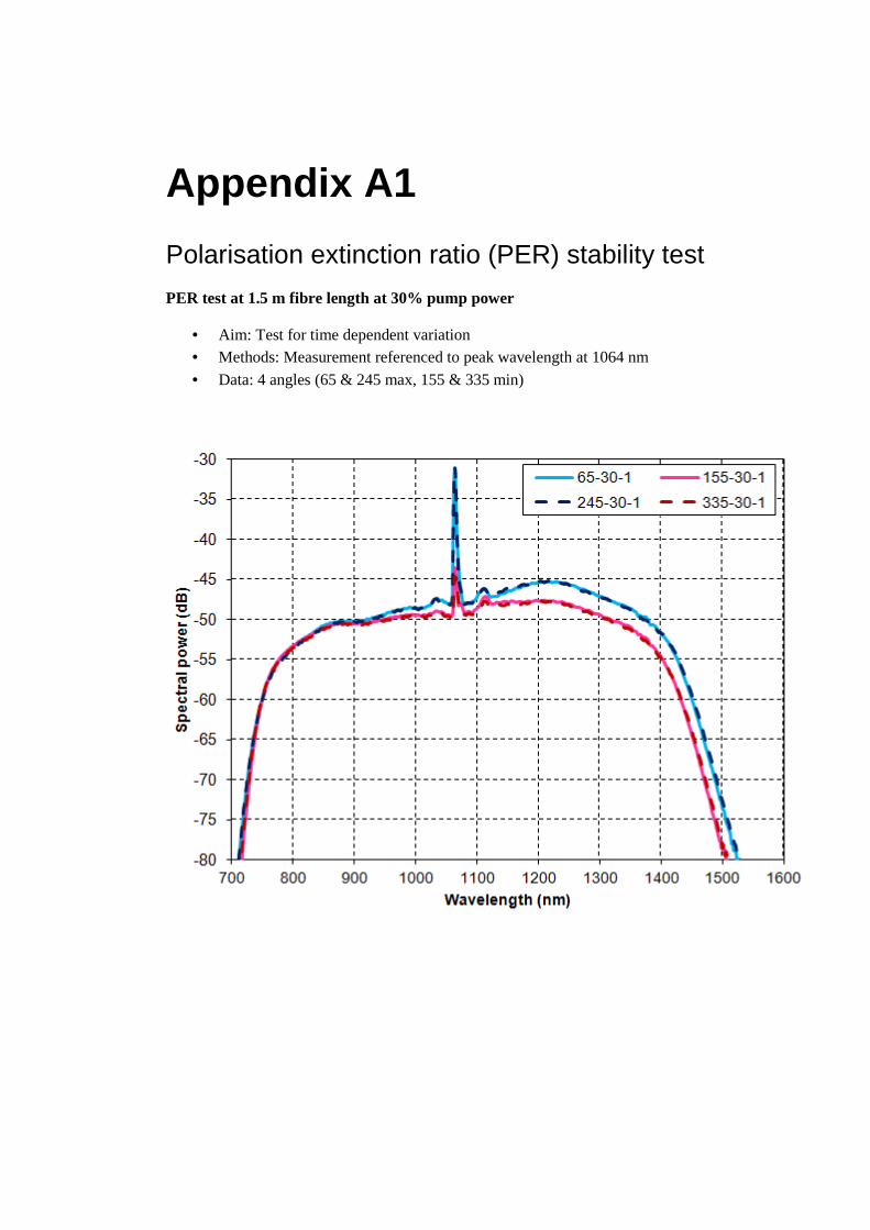
Appendix A1
Polarisation extinction ratio (PER) stability test
PER test at 1.5 m fibre length at 30% pump power
• Aim: Test for time dependent variation • Methods: Measurement referenced to peak wavelength at 1064 nm
• Data: 4 angles (65 & 245 max, 155 & 335 min)
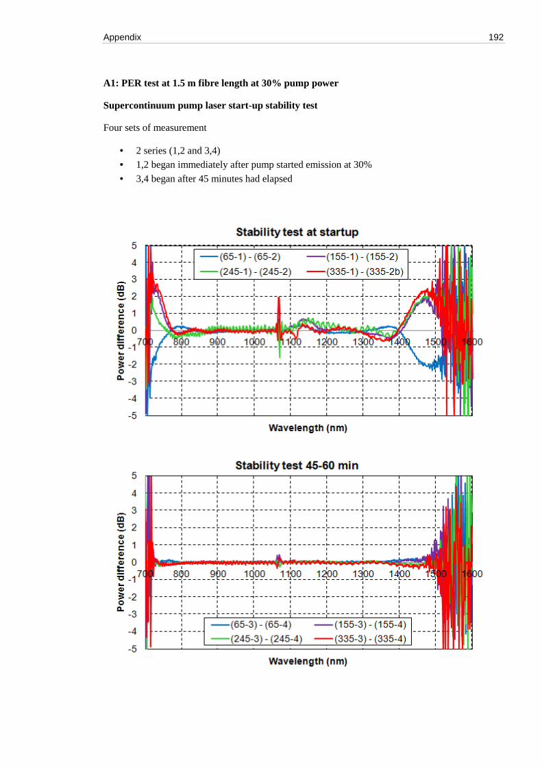
Appendix 192
A1: PER test at 1.5 m fibre length at 30% pump power
Supercontinuum pump laser start-up stability test
Four sets of measurement
• 2 series (1,2 and 3,4) • 1,2 began immediately after pump started emission at 30%
• 3,4 began after 45 minutes had elapsed
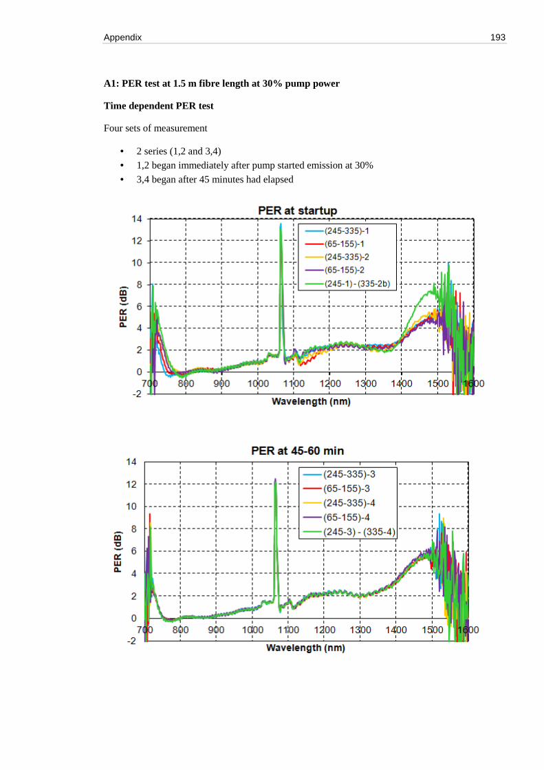
Appendix 193
A1: PER test at 1.5 m fibre length at 30% pump power
Time dependent PER test
Four sets of measurement
• 2 series (1,2 and 3,4) • 1,2 began immediately after pump started emission at 30%
• 3,4 began after 45 minutes had elapsed
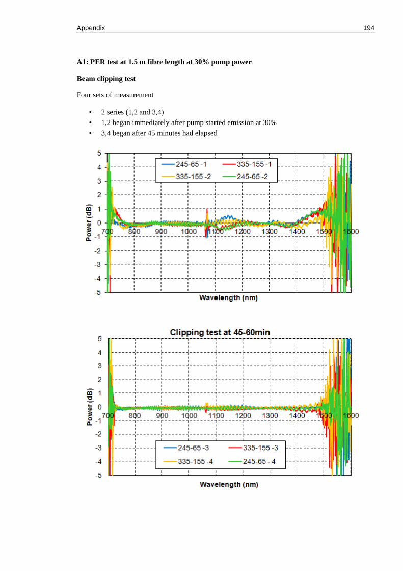
Appendix 194
A1: PER test at 1.5 m fibre length at 30% pump power
Beam clipping test
Four sets of measurement
• 2 series (1,2 and 3,4) • 1,2 began immediately after pump started emission at 30%
• 3,4 began after 45 minutes had elapsed
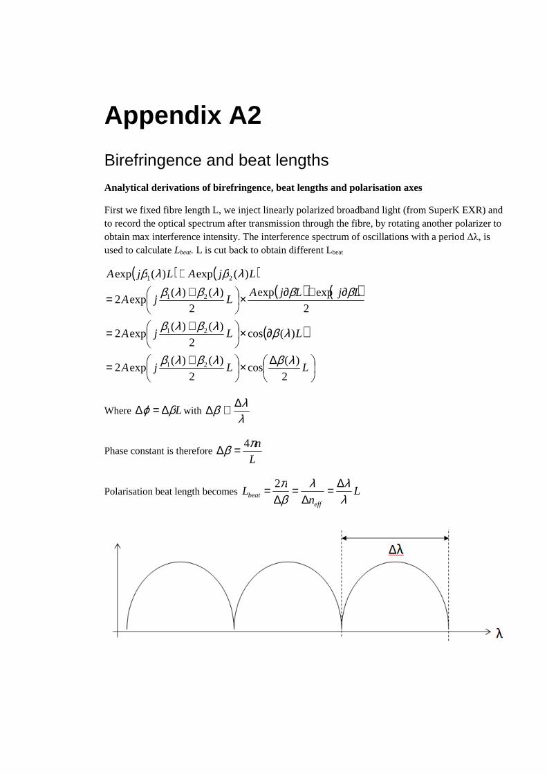
Appendix A2
Birefringence and beat lengths
Analytical derivations of birefringence, beat lengths and polarisation axes
First we fixed fibre length L, we inject linearly polarized broadband light (from SuperK EXR) and to record the optical spectrum after transmission through the fibre, by rotating another polarizer to obtain max interference intensity. The interference spectrum of oscillations with a period Δλ, is used to calculate Lbeat. L is cut back to obtain different Lbeat
( ) ( )( ) ( )
( )
∆×
+=
∂×
+=
∂+∂×
+=
+
LLjA
LLjA
LjLjALjA
LjALjA
2
)(cos
2
)()(exp2
)(cos2
)()(exp2
2
expexp
2
)()(exp2
)(exp)(exp
21
21
21
21
λβλβλβ
λβλβλβ
ββλβλβλβλβ
Where Lβϕ ∆=∆ with λλβ ∆∝∆
Phase constant is therefore L
nπβ 4=∆
Polarisation beat length becomes Ln
Leff
beat λλλ
βπ ∆=
∆=
∆= 2
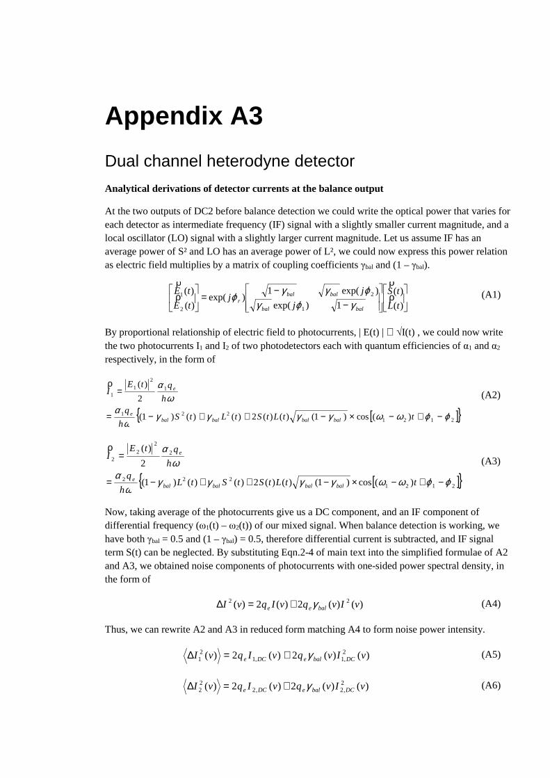
Appendix A3
Dual channel heterodyne detector
Analytical derivations of detector currents at the balance output
At the two outputs of DC2 before balance detection we could write the optical power that varies for each detector as intermediate frequency (IF) signal with a slightly smaller current magnitude, and a local oscillator (LO) signal with a slightly larger current magnitude. Let us assume IF has an average power of S² and LO has an average power of L², we could now express this power relation as electric field multiplies by a matrix of coupling coefficients γbal and (1 – γbal).
−−
=
)(
)(
1)exp(
)exp(1)exp(
)(
)(
1
2
2
1
tL
tS
j
jj
tE
tE
balbal
balbalr ρ
ρρρ
γϕγϕγγϕ (A1)
By proportional relationship of electric field to photocurrents, | E(t) | ∝ √I(t) , we could now write the two photocurrents I1 and I2 of two photodetectors each with quantum efficiencies of α1 and α2 respectively, in the form of
[ ]{ }2121221
1
2
11
)(cos)1()()(2)()()1(
2
)(
ϕϕωωγγγγω
αω
α
−+−×−++−=
=
ttLtStLtSh
qh
qtEI
balbalbalbale
eρ
(A2)
[ ]{ }2121222
2
2
22
)(cos)1()()(2)()()1(
2
)(
ϕϕωωγγγγω
αω
α
−+−×−++−=
=
ttLtStStLh
qh
qtEI
balbalbalbale
eρ
(A3)
Now, taking average of the photocurrents give us a DC component, and an IF component of differential frequency (ω1(t) – ω2(t)) of our mixed signal. When balance detection is working, we have both γbal = 0.5 and (1 – γbal) = 0.5, therefore differential current is subtracted, and IF signal term S(t) can be neglected. By substituting Eqn.2-4 of main text into the simplified formulae of A2 and A3, we obtained noise components of photocurrents with one-sided power spectral density, in the form of
)()(2)(2)( 22 vIvqvIqvI balee γ+=∆ (A4)
Thus, we can rewrite A2 and A3 in reduced form matching A4 to form noise power intensity.
)()(2)(2)( 2,1,1
21 vIvqvIqvI DCbaleDCe γ+=∆ (A5)
)()(2)(2)( 2,2,2
22 vIvqvIqvI DCbaleDCe γ+=∆ (A6)

Appendix A4
Data standardisation techniques
Statistical representation of expected value, variance and standard deviation
Data standardisation is essential for statistics. Several earlier articles have mentioned the process. These include:
1. Gaver (1985) 2. Johnson and Wichern (1992) 3. Everit (1993) 4. Van Tongeren (1995) 5. Milligan and Cooper (1988)
Techniques Mean Variance Std dev (1) 0-1 Scaling (end points scaling)
minmax
min
VV
VV
−−
Different Different Different
(2) Dividing each value by range
minmax VV
V
−
Different Different Different
(3) Z-score scaling
σVV −
0 1 1
(4) Dividing each value by standard deviation
σV
Different 1 1
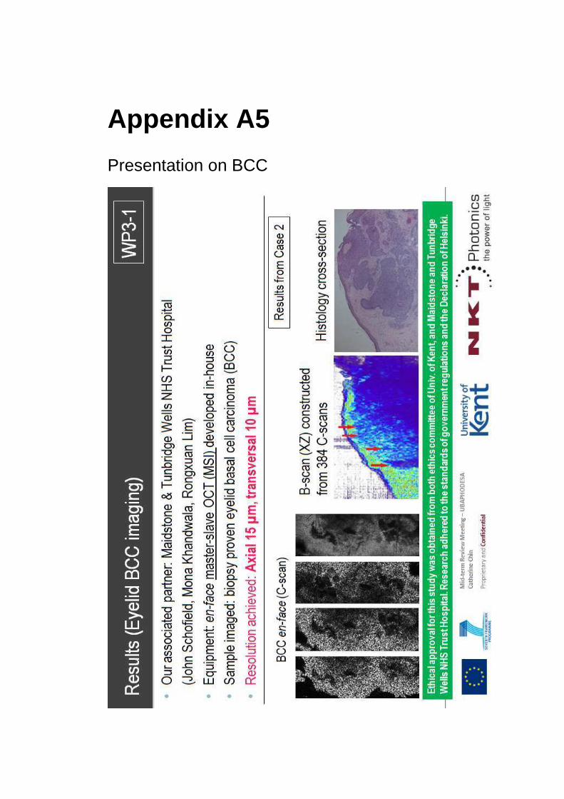
Appendix A5
Presentation on BCC


