Embed Size (px)
Citation preview
1 | Page
Clarifications sought by the EAC on EIA of Thermal Power Projects
Project: Proposed 2 x 660 MW Khurja Super Thermal Power Project
Clarifications of the observations of the 1stEAC (Thermal) meeting held on
28th December, 2016
1. The EIA prepared by Mantec Consultants (P) Ltd, is not comprehensive. PP
could not provide the quantity of fly ash generated and concrete disposal plan.
All the maps and layouts provided in the EIA are not legible.
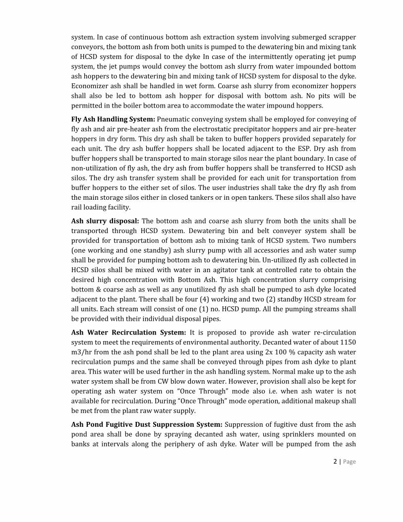
Reply: Mantec Consultants (P) Ltd., New Delhi has prepared the EIA Report as per TOR prescribed by MOEF&CC. However, the clarifications sought during the EAC meeting are submitted as follows. (a) The detail of fly ash generation is covered in Section 1.5, Chapter-1 of Annexure-XIII of the EIA Report. The details of Fly Ash generation and disposal plan are given below:
The proposed power plant will consume approx. 5.4 million TPA coal, with average ash
content less than 34%. Therefore, the maximum quantity of ash generation will be 1.836
million TPA. Out of this, the quantity of bottom ash will be approx. 0.3672 MTPA (@20%)
and the fly ash quantity will be approx.1.469 million TPA (@80%).
Annual coal consumption : 5.4 million TPA
Maximum ash content : 34%
Total ash generation, max. : 1.836 million TPA
Fly ash generation, max. (@80%) : 1.469 million TPA
Bottom ash generation, max. (@20%) : 0.367 million TPA
Ash Handling & Disposal system
Ash Handling System: The bottom ash shall be extracted and disposed-off with Wet
Disposal or High Concentration Slurry Disposal (HCSD) system. The fly ash along with air
pre-heater ash shall be conveyed in dry form from the ash collection hoppers. This dry fly as
ash shall be taken to buffer hoppers for its onward transportation in dry form to storage
silos near plant boundary for utilization. In case of non-utilization during first four years of
operation, fly ash shall be disposed-off as high concentration slurry in the Ash Dyke.
Bottom Ash Handling System: Bottom ash shall be extracted either by using a
continuously operating submerged scraper chain conveyor system or by using
intermittently operating jet pumps in conjunction with a water-impounded hopper. Dry
type bottom ash hoppers shall be used in case of the submerged scraper chain conveyor
2 | Page
system. In case of continuous bottom ash extraction system involving submerged scrapper
conveyors, the bottom ash from both units is pumped to the dewatering bin and mixing tank
of HCSD system for disposal to the dyke In case of the intermittently operating jet pump
system, the jet pumps would convey the bottom ash slurry from water impounded bottom
ash hoppers to the dewatering bin and mixing tank of HCSD system for disposal to the dyke.
Economizer ash shall be handled in wet form. Coarse ash slurry from economizer hoppers
shall also be led to bottom ash hopper for disposal with bottom ash. No pits will be
permitted in the boiler bottom area to accommodate the water impound hoppers.
Fly Ash Handling System: Pneumatic conveying system shall be employed for conveying of
fly ash and air pre-heater ash from the electrostatic precipitator hoppers and air pre-heater
hoppers in dry form. This dry ash shall be taken to buffer hoppers provided separately for
each unit. The dry ash buffer hoppers shall be located adjacent to the ESP. Dry ash from
buffer hoppers shall be transported to main storage silos near the plant boundary. In case of
non-utilization of fly ash, the dry ash from buffer hoppers shall be transferred to HCSD ash
silos. The dry ash transfer system shall be provided for each unit for transportation from
buffer hoppers to the either set of silos. The user industries shall take the dry fly ash from
the main storage silos either in closed tankers or in open tankers. These silos shall also have
rail loading facility.
Ash slurry disposal: The bottom ash and coarse ash slurry from both the units shall be
transported through HCSD system. Dewatering bin and belt conveyer system shall be
provided for transportation of bottom ash to mixing tank of HCSD system. Two numbers
(one working and one standby) ash slurry pump with all accessories and ash water sump
shall be provided for pumping bottom ash to dewatering bin. Un-utilized fly ash collected in
HCSD silos shall be mixed with water in an agitator tank at controlled rate to obtain the
desired high concentration with Bottom Ash. This high concentration slurry comprising
bottom & coarse ash as well as any unutilized fly ash shall be pumped to ash dyke located
adjacent to the plant. There shall be four (4) working and two (2) standby HCSD stream for
all units. Each stream will consist of one (1) no. HCSD pump. All the pumping streams shall
be provided with their individual disposal pipes.
Ash Water Recirculation System: It is proposed to provide ash water re-circulation
system to meet the requirements of environmental authority. Decanted water of about 1150
m3/hr from the ash pond shall be led to the plant area using 2x 100 % capacity ash water
recirculation pumps and the same shall be conveyed through pipes from ash dyke to plant
area. This water will be used further in the ash handling system. Normal make up to the ash
water system shall be from CW blow down water. However, provision shall also be kept for
operating ash water system on “Once Through” mode also i.e. when ash water is not
available for recirculation. During “Once Through” mode operation, additional makeup shall
be met from the plant raw water supply.
Ash Pond Fugitive Dust Suppression System: Suppression of fugitive dust from the ash
pond area shall be done by spraying decanted ash water, using sprinklers mounted on
banks at intervals along the periphery of ash dyke. Water will be pumped from the ash
3 | Page
water recirculation pump house through dust suppression water header to the sprinkler
nozzles. 2 x 100 % pumps are provided for this purpose to cater to the requirements of both
lagoons. The sprinklers shall be of swiveling type mounted at a height to ensure sufficient
coverage for mitigating the fugitive dust problem.
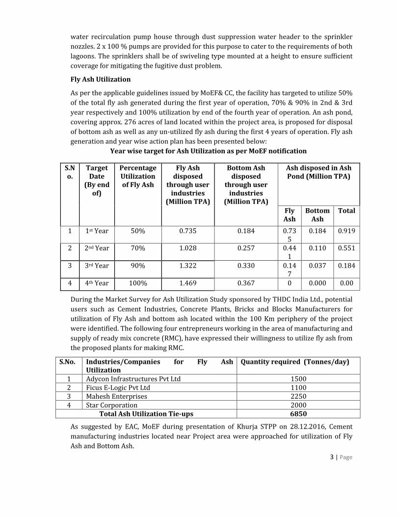
Fly Ash Utilization
As per the applicable guidelines issued by MoEF& CC, the facility has targeted to utilize 50%
of the total fly ash generated during the first year of operation, 70% & 90% in 2nd & 3rd
year respectively and 100% utilization by end of the fourth year of operation. An ash pond,
covering approx. 276 acres of land located within the project area, is proposed for disposal
of bottom ash as well as any un-utilized fly ash during the first 4 years of operation. Fly ash
generation and year wise action plan has been presented below:
Year wise target for Ash Utilization as per MoEF notification
S.No.
Target Date
(By end of)
Percentage Utilization of Fly Ash
Fly Ash disposed
through user industries
(Million TPA)
Bottom Ash disposed
through user industries
(Million TPA)
Ash disposed in Ash Pond (Million TPA)
Fly Ash
Bottom Ash
Total
1 1st Year 50% 0.735 0.184 0.735
0.184 0.919
2 2nd Year 70% 1.028 0.257 0.441
0.110 0.551
3 3rd Year 90% 1.322 0.330 0.147
0.037 0.184
4 4th Year 100% 1.469 0.367 0 0.000 0.00
During the Market Survey for Ash Utilization Study sponsored by THDC India Ltd., potential
users such as Cement Industries, Concrete Plants, Bricks and Blocks Manufacturers for
utilization of Fly Ash and bottom ash located within the 100 Km periphery of the project
were identified. The following four entrepreneurs working in the area of manufacturing and
supply of ready mix concrete (RMC), have expressed their willingness to utilize fly ash from
the proposed plants for making RMC.
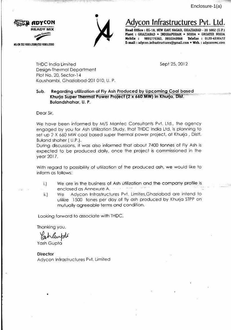
S.No. Industries/Companies for Fly Ash Utilization
Quantity required (Tonnes/day)
1 Adycon Infrastructures Pvt Ltd 1500 2 Ficus E-Logic Pvt Ltd 1100 3 Mahesh Enterprises 2250 4 Star Corporation 2000
Total Ash Utilization Tie-ups 6850
As suggested by EAC, MoEF during presentation of Khurja STPP on 28.12.2016, Cement
manufacturing industries located near Project area were approached for utilization of Fly
Ash and Bottom Ash.
4 | Page
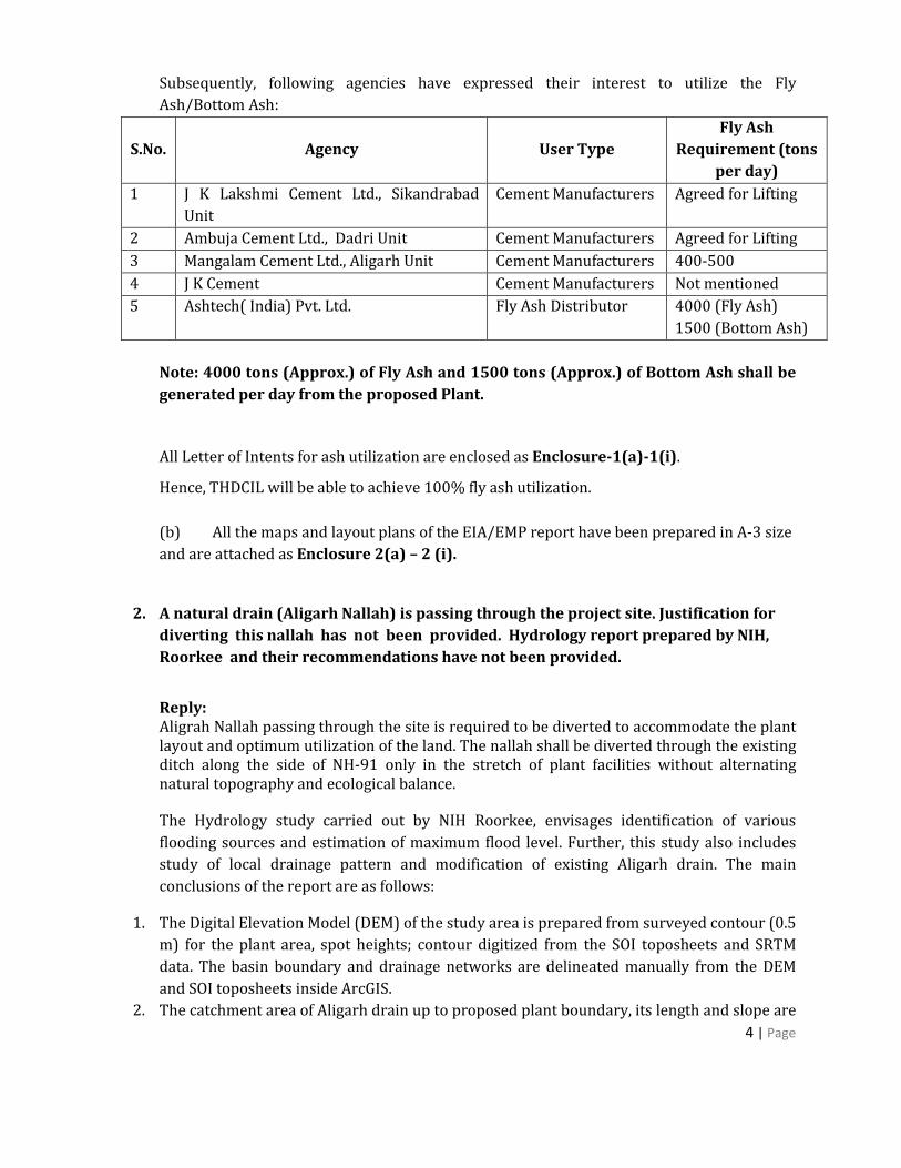
Subsequently, following agencies have expressed their interest to utilize the Fly
Ash/Bottom Ash:
S.No. Agency User Type
Fly Ash
Requirement (tons
per day)
1 J K Lakshmi Cement Ltd., Sikandrabad
Unit
Cement Manufacturers Agreed for Lifting
2 Ambuja Cement Ltd., Dadri Unit Cement Manufacturers Agreed for Lifting
3 Mangalam Cement Ltd., Aligarh Unit Cement Manufacturers 400-500
4 J K Cement Cement Manufacturers Not mentioned
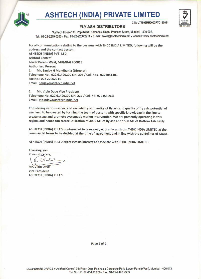
5 Ashtech( India) Pvt. Ltd. Fly Ash Distributor 4000 (Fly Ash)
1500 (Bottom Ash)
Note: 4000 tons (Approx.) of Fly Ash and 1500 tons (Approx.) of Bottom Ash shall be
generated per day from the proposed Plant.
All Letter of Intents for ash utilization are enclosed as Enclosure-1(a)-1(i).
Hence, THDCIL will be able to achieve 100% fly ash utilization.
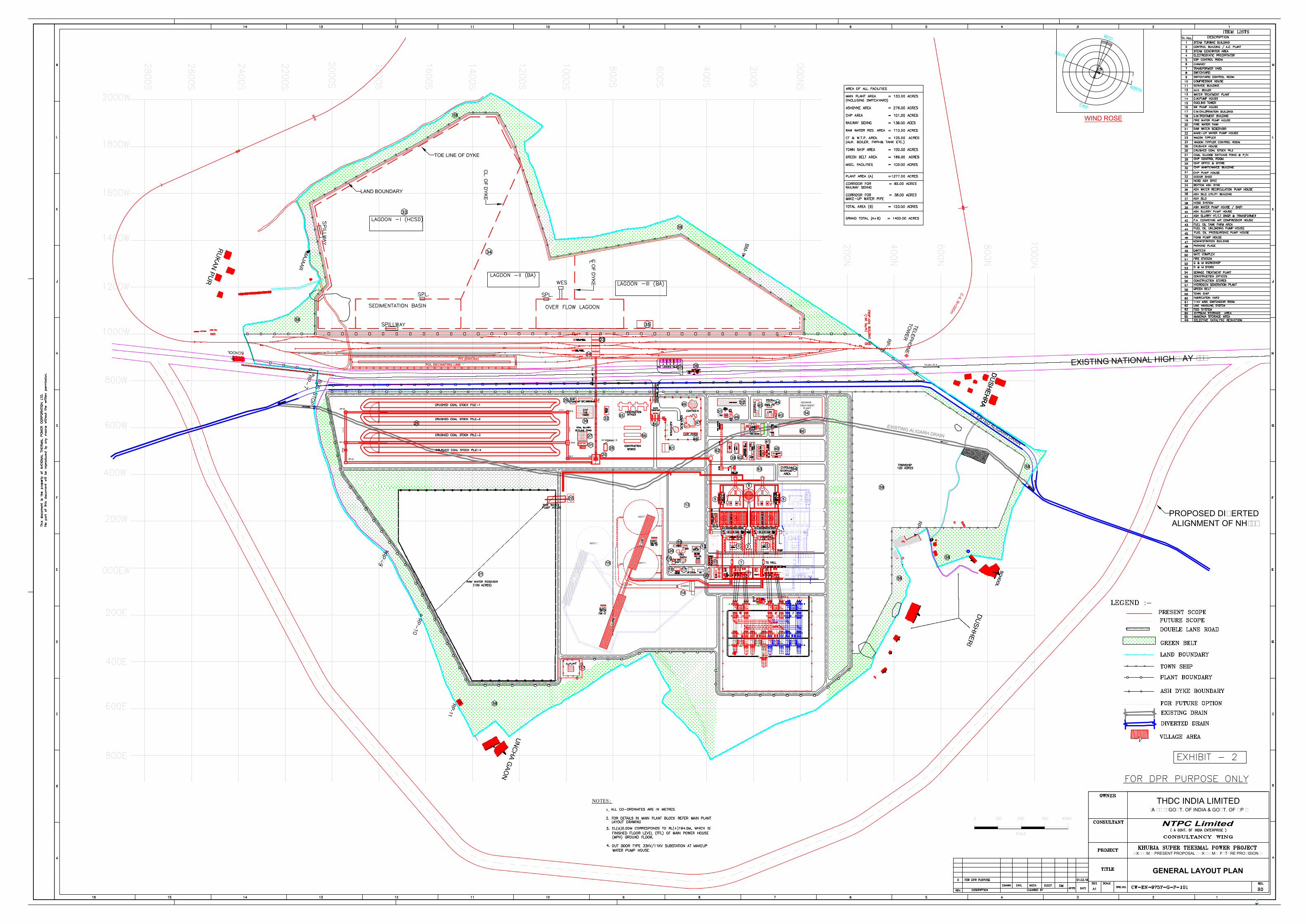
(b) All the maps and layout plans of the EIA/EMP report have been prepared in A-3 size
and are attached as Enclosure 2(a) – 2 (i).
2. A natural drain (Aligarh Nallah) is passing through the project site. Justification for
diverting this nallah has not been provided. Hydrology report prepared by NIH,
Roorkee and their recommendations have not been provided.
Reply: Aligrah Nallah passing through the site is required to be diverted to accommodate the plant layout and optimum utilization of the land. The nallah shall be diverted through the existing ditch along the side of NH-91 only in the stretch of plant facilities without alternating natural topography and ecological balance.
The Hydrology study carried out by NIH Roorkee, envisages identification of various
flooding sources and estimation of maximum flood level. Further, this study also includes
study of local drainage pattern and modification of existing Aligarh drain. The main
conclusions of the report are as follows:
1. The Digital Elevation Model (DEM) of the study area is prepared from surveyed contour (0.5
m) for the plant area, spot heights; contour digitized from the SOI toposheets and SRTM
data. The basin boundary and drainage networks are delineated manually from the DEM
and SOI toposheets inside ArcGIS.
2. The catchment area of Aligarh drain up to proposed plant boundary, its length and slope are
5 | Page
used to derive unit hydrograph using the guideline provided by CWC.
3. The 1-day annual maximum rainfall for various return periods are estimated for the site
Aligarh, Bulandshahr, Khurja by rainfall frequency analysis using L-moments approach.
Similarly the regional 1-day annual maximum rainfall for various return periods are also
estimated.
4. The regional L-moments based approach resulted in maximum rainfall value based on the
data of three stations for 100 year return period rainfall. Hence, regional 1-day annual
maximum rainfalls for 100 year return period is used for design flood estimation and drain
design. The regional rainfall estimated using the rainfall data of three rain gauge stations
are 20.71 cm, 24.65 cm and 28.99 cm respectively for 25, 50 and 100 year return periods
respectively.
5. The Peak discharge (m3/s) in Aligarh drain for 2, 10, 25, 50 and 100 year return periods are
found to be 20.13 m3/s, 44.06 m3/s, 59.1 m3/s, 71.59 m3/s and 85.88m3/s respectively
from its catchment area of 10.5 km2 .
6. It is observed that the existing cross-section of Aligarh drain is unable to carry design
discharge. Hence, modified lined trapezoidal cross-sections is proposed. Moreover, possible
re-alignment of Aligarh drain is also proposed. However, the width is limited to 10 m and
overflow has been allowed.
7. The potential source of flooding at the plant site is due to the local rainfall and overflow
from the Aligarh drain also.
8. The land formation level should be based on the computed maximum flood elevation for
severe most flooding scenario (100 year return period), model uncertainty and limitation of
data availability. Considering these aspects, it is suggested to have the safe grade level in the
plant area higher than RL 193.5 m and the plinth levels should be higher than 194.1 m or
194.4 m to avoid any drainage congestion due to highway alignment. The land development
work within the plant site should be carried out to maintain the natural slope to facilitate
the drainage in the area and divert any entry of excess water through plant boundary.
9. The peak flow for 25 and 50 year return period rainfall is estimated for various local and
periphery drain sections and the trapezoidal drains are designed using Manning’s formula
and free board is provided as per BIS standard IS 10430-2000.
10. The local and periphery drains are designed for trapezoidal section with a side slope of
1.5:1 (H:V) and longitudinal slope of 0.001 m/m (1.0 m/km) to carry the discharge
generated locally. Moreover, the drain sections are designed for velocity less than 2 m/s and
Manning's roughness coefficient (n) values of 0.015.
A copy of the report is attached as Enclosure-3.
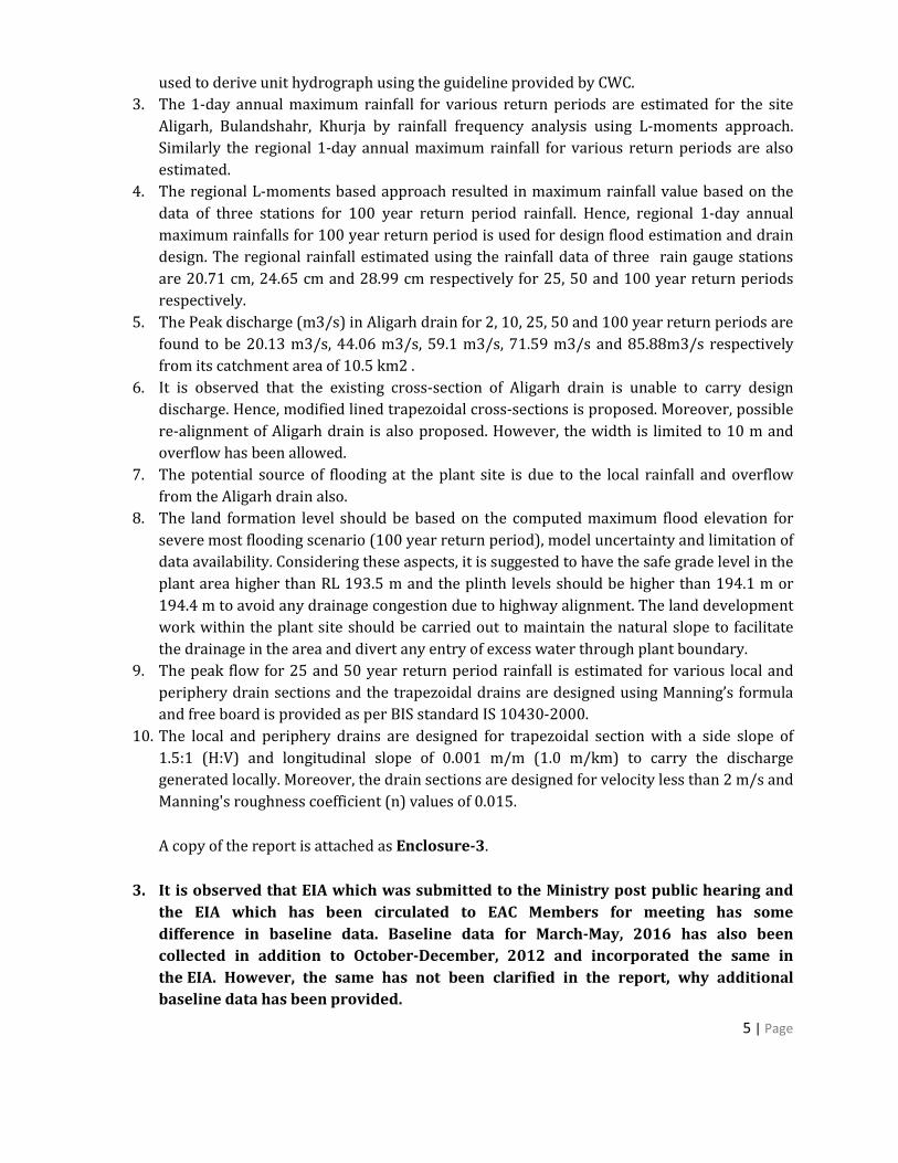
3. It is observed that EIA which was submitted to the Ministry post public hearing and
the EIA which has been circulated to EAC Members for meeting has some
difference in baseline data. Baseline data for March-May, 2016 has also been
collected in addition to October-December, 2012 and incorporated the same in
the EIA. However, the same has not been clarified in the report, why additional
baseline data has been provided.
6 | Page
Reply:
The EIA report, based on baseline data collected during October-December, 2012 and taking
care of the issues raised during public hearing held on 1st August 2012, was submitted to
MoEF&CC on 6th October, 2015. Appraisal of the project was held up due to non-availability
of firm coal linkage – which was finally received vide Ministry of Coal letter dated
29thAugust 2016. Meanwhile, with notification of Environment (Protection) Amendment
Rules, 2015 dated 7th December, 2015, water consumption and emission norms for thermal
power plants were changed significantly. These factors required some changes in the EIA
report. As a period of 3 years had elapsed since generation of baseline data in October –
December, 2012, it was considered worthwhile to revalidate the same by repeating it for 1
more season, i.e., March – May, 2016.
4. In the EIA, baseline data for NOx and SO2 results have been shown in the
Ozone values. The whole EIA report has been prepared in qualitative manner.
Reply:
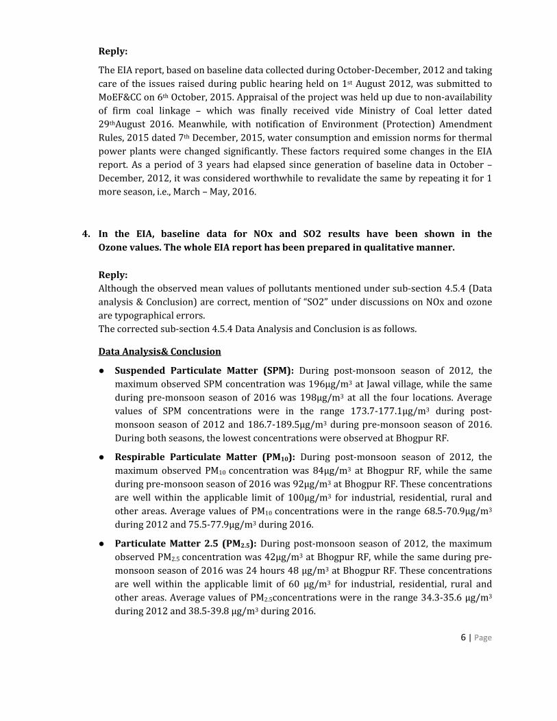
Although the observed mean values of pollutants mentioned under sub-section 4.5.4 (Data
analysis & Conclusion) are correct, mention of “SO2” under discussions on NOx and ozone
are typographical errors.
The corrected sub-section 4.5.4 Data Analysis and Conclusion is as follows.
Data Analysis& Conclusion
Suspended Particulate Matter (SPM): During post-monsoon season of 2012, the
maximum observed SPM concentration was 196µg/m3 at Jawal village, while the same
during pre-monsoon season of 2016 was 198µg/m3 at all the four locations. Average
values of SPM concentrations were in the range 173.7-177.1µg/m3 during post-
monsoon season of 2012 and 186.7-189.5µg/m3 during pre-monsoon season of 2016.
During both seasons, the lowest concentrations were observed at Bhogpur RF.
Respirable Particulate Matter (PM10): During post-monsoon season of 2012, the
maximum observed PM10 concentration was 84µg/m3 at Bhogpur RF, while the same
during pre-monsoon season of 2016 was 92µg/m3 at Bhogpur RF. These concentrations
are well within the applicable limit of 100µg/m3 for industrial, residential, rural and
other areas. Average values of PM10 concentrations were in the range 68.5-70.9µg/m3
during 2012 and 75.5-77.9µg/m3 during 2016.
Particulate Matter 2.5 (PM2.5): During post-monsoon season of 2012, the maximum
observed PM2.5 concentration was 42µg/m3 at Bhogpur RF, while the same during pre-
monsoon season of 2016 was 24 hours 48 µg/m3 at Bhogpur RF. These concentrations
are well within the applicable limit of 60 µg/m3 for industrial, residential, rural and
other areas. Average values of PM2.5concentrations were in the range 34.3-35.6 µg/m3
during 2012 and 38.5-39.8 µg/m3 during 2016.

7 | Page
Sulphur Dioxide (SO2): During post-monsoon season of 2012, the maximum observed
SO2 concentration was 17.2µg/m3 at Gwarauli village, while the same during pre-
monsoon season of 2016 was 19 µg/m3 at Gwarauli village. These concentrations are
well within the applicable limit of 80 µg/m3 for industrial, residential, rural and other
areas. Average values of SO2 concentrations were in the range 11.5 to 12.7 µg/m3 during
2012 and 12.8-13.9 µg/m3 during 2016.
Nitrogen Oxides (NOX): During post-monsoon season of 2012, the maximum observed
NOx concentration was 32 µg/m3 at Gwarauli village, while the same during pre-
monsoon season of 2016 was 35 µg/m3 at Bhogpur RF, Gwarauli & Jawal villages. These
concentrations are well within the applicable limit of 80 µg/m3 for industrial,
residential, rural and other areas. Average values of NO2 concentrations were in the
range 24.3 to 26.8 µg/m3 during 2012 and 26.8-29.4 µg/m3 during 2016.
Ozone (O3): During post-monsoon season of 2012, the maximum observed O3
concentration was 31.8µg/m3 at Jawal village, while the same during pre-monsoon
season of 2016 was 35µg/m3 at Jawal village. These concentrations are well within the
applicable limit of 100 µg/m3 for industrial, residential, rural and other areas. Average
values of O3concentrations were in the range of 25.8 to 26.7 µg/m3 during 2012 and
28.4 to 29.4 µg/m3 during 2016.
Mercury (Hg): The value of mercury was found to be below detectable limit (bdl) at all
4 monitoring locations during the two seasons of survey.
Conclusion: The existing levels of monitored air pollutants in the study area are well within
the prescribed limits and the area can accommodate further development with controlled
emissions.
5. Details of Quantitative Risk Assessment and credible failure scenarios for Hazardous Chemical containers such as Fuel Oil, Transformer Oil, Chlorine, etc have not been provided in the EIA
Reply: Separate Report for Quantitave Risk Assessment and credible failure scenarios for Hazardous Chemical containers such as Fuel Oil, Transformer Oil, Chlorine, etc for the proposed project is given as Enclosure- 4. Consequence analysis was carried out for identified selected failure cases given in the
report. Damage distances for the accidental release of hazardous materials have been
computed at 2F, 3D and 5D weather conditions. In these conditions, 2, 3 and 5 are wind
velocities in m/s and F and D are atmospheric stability classes. Credible Failure scenarios
considered are given below:
1. 25 mm, 50 mm Leak and Catastrophic rupture in LDO & Transformer Oil Storage
Tank
2. 10 mm leak & catastrophic rupture from Hydrogen Cylinder & compressor
3. 2mm leak from Flange of Chlorine tonner
8 | Page
4. 10mm leak & catastrophic rupture from Ammonia Bullet storage tank
Risk evaluation shows individual risk to be 8.274x 10⁻⁶/yr and societal risk to be 1.234x 10-
5/yr, which are both in the acceptable region as per HSE UK.
Hence, proposed project is safe to be operated as Impact distance due to failure scenario
and Overall risk calculated are well within the limits.
6. Native and indigenous species have not been proposed in the EIA which shall be
part of green belt development plan.
Reply: Native and indigenous species have been proposed for greenbelt development as
per guideline of CPCB 2000. 26 Trees, 5 small trees, and 14 shrub species were proposed.
Species for plantation were selected according to the agro climatic zone and subzones
mentioned in the guideline. Detailed Green Belt Development Plan including native and
indigenous species is given as Enclosure-5.
S.No. Description of Enclosure 1 Agreement letters for Ash Utilization
2
Maps and Layout plans of the EIA/EMP report
Maps/Layout Cross-referencing with EIA/EMP Report Page No.
Buffer Map of Study Area 36 Satellite Map of Study Area 84 Landuse Map of Study Area 85 Soil Monitoring Location Map of Study Area
89
Water Monitoring Location Map of Study Area
93
Air Monitoring Location Map of Study Area
103
Noise Monitoring Location Map of Study Area
113
Water Balance Diagram Layout Plan of the Project Site
3 Hydrographical Area Drainage Study Report by NIH, Roorkee
4 Quantitave Risk Assessment and credible failure scenarios Report
5 Green Belt Development Plan
ENCLOSURE-1(a)- 1(i)
4Fl;3 qqYloft
.7- )+Design rhemol Oeportmenl
Kolshombi. Ghonobod 201 010, Ll. P.
sub R.ddrdind uliltdlion ol Flv Alh hoduced bv lDcomino Coalb6edKhu;rd su;er rhemor Pode, p@]€?f,
' 63dfiiD h xli;id:DlH:'Bulondshohor, 1,. P.
we hove been inrorfled by M/s Monlec Cotuuronh Pvr. Lld. the ogencyengdged by you ior Ash l-rilizoron sllcly lhol Tl-lDC ndio Ltd. L plonning loset !p ? x 660 MW coo bosed slper rhermo powe. proled, ol Kh!4q , Distl
Dldng di5c!$ions, ii wos oso lnlormedexpecled lo be produced doily, o.ce
wiTh regord 1o po$ibily ot uTizolion ol
il
iil
we ore ln lhe busi.e$ ol Ash ulillzolion ond the compony p@lile is
e. o\e.l or Pnnl^ e o
rle Adycon lntuontuciures Pvl Limiles,Ghozobad ore lnlend lollilize l5m lones per doy ol fy osh produced by Khu4o slPP onmuluoLly ogreeoble ierms ond condiuon.
Looking loMord lo o$ociole wllh THOC,
Adycon nlrontucllres Pvl. Limlted
4dyssd!tu$tulErl!-lh4,U4llJlrN ro 16r (o.er
'dl:dto'ilhddua!@ldld
Sept 25 2012
lhot obolt 7400lo.nes ol Fy Ash is
the proiect is codmGsoned ln the
lhe produced Gh we wo! d lile 10
Enclosure-1(a)
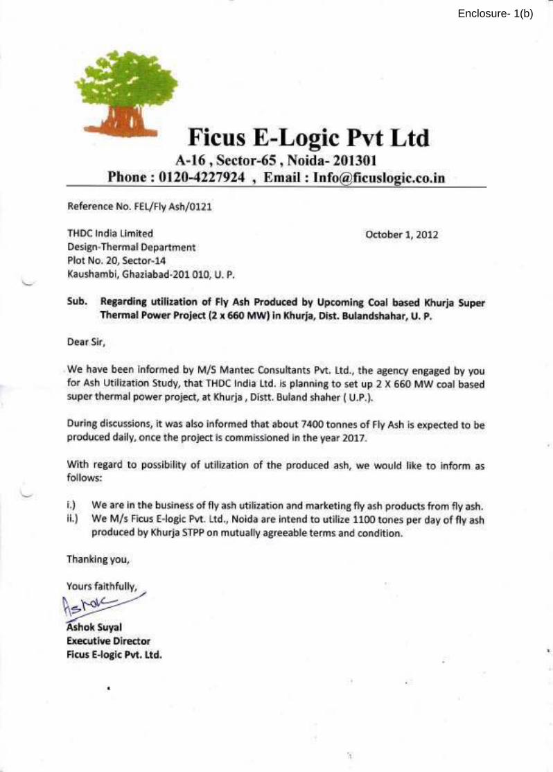
Ficus E-Logic Pvt LtdA-16 , Sector-65 , Noida- 201301
Phone z 0120-4227924 o Email : [email protected]
Reference No. FEL/Fly Ash/0L2L
THDC lndia LimitedDesign-Thermal DepartmentPlot No. 20, Sector-14Kaushambi, Ghaziabad-20L 010, U. P.
October L,2OL2
Sub. Regarding utilization of Fty Ash Produced by Upcoming Coal based Khurja SuperThermal Power Project (2 x 660 MW) in Khurja, Dist. Bulandshahar, U. p.
Dear Sir,
, We have been informed by M/S Mantec Consultants Pvt. Ltd., the agency engaged by youfor Ash Utilization Study, that THDC lndia Ltd. is planning to set up 2 X 660 MW coal basedsuperthermal power project, at Khurja, Distt. Buland shaher ( U.P.).
During discussions, it was also informed that about 7400 tonnes of Fly Ash is expected to beproduced daily, once the project is commissioned in the year 20L7.
With regard to possibility of utilization of the produced ash, we would like to inform asfollows:
We are in the business of fly ash utilization and marketing fly ash products from fly ash.We M/s Ficus E-logic Pvt. Ltd., Noida are intend to utilize 1L00 tones per day of fly ashproduced by Khurja STPP on mutually agreeable terms and condition.
Thanking you,
Yours faithfully,
\,"vg?/'ff,orsuyal
Executive DirectorFicus E-logic Pvt. Ltd.
i.)
ii. )
Enclosure- 1(b)
I,N AT E S I E N7 ERPR'SEf......CEMENTINC BONDS WITH COMMITMENT
THDC lndia LimitedDesign-Thermal DepartmentPlot No. zo, Sector-r4Kaushambi, Ghaziabad-zot oto, U. P.
oct. 5th, zo'i2
Sub. Regarding utilization of Fly Ash Produced by Upcoming Coal based Khuria Super
Thermal Power Proiect (z x 66o MW) in Khuria, Dist. Bulandshahar' U. P.
Dear Sir,
We have been informed by M/S Mantec Consultants Pvt. Ltd., the agency engaged by
you for Ash Utilization Study, that THDC lndia Ltd. is planning to set up z X 660 MW coal
based super thermal power proiect, at Khuria , Distt. Buland shaher ( U.P.).
During discussions, it was also informed that about 74oo tones of Fly Ash is expected tobe produced daily, once the proiect is commissioned in the year zot7.
With regard to possibility of utilization of the produced ash, we would like to inform as
follows:
i.) We are in the business of Ash utilization through RMC Plant, Bricks etc.
ii.) We M/s Mahesh Enterprises, Ghaziabad are intend to utilize zz5o tones per
day of fly ash produced by Khuria STPP on mutually agreeable terms and
condition.
With regards,
MCON ffi HEIDELBERCCEMENT
: 95-1 20-27 30042, 2834462: 95-1 20-4115562, 4115563
\
mycem
Fos- NIANES\'\ gfffStrs$ff f S#s
r 39, Naya Ganj, Ghaziabad - 201001 Ph.r lll-B-3, Nehru Nagar, Ghaziabad Telefax
Signatorr
Enclosure- 1 (c)

STAR CORPORAIIONtedts tr At( kind of Buitding Mate.iatoFflCE: 5/639, SECToR-5, VlSlAll, CHAZIABAD (U.P)
lILt! X | 0120-4136771GoDovlll r l$lDoLl $0c( t()NI 8AGHP T R0 D, ruxDou (U.P)
M tt". ....s+.l.;''t./..1 cM
We ore now lookng lotuordlo o$oc ole wilh THDC,
/"r)9VvftK a"p:r.
Desg. Thermo Deporlmenl
Kolshombi, Ghonobod 201 010. U P
Sob, Regqrdins ulilizqtion ol Fly ath Pbduced by Upcohins Cool bosedKhurjo super lhemql Power Project (2x 660Mw)ln Khurjd, DlslBulond3hdhor, U- P.
)
)
We ore in rhe b!si.e$ ol A5h ulillzolion ond lhe compony p.ofile s
enc osed os An.exurc Awe Adycon nlrostrucllres Pvi. Limiles,Ghozobocl ore nlend tout ize 20m toner per doy or lly osh prodlcecl by ftu4o STFP on1 Lo /oq-eobe -r'o_d o'dro
we hove been informecl lry M/5 Mo.iec cons!lonls Pvl. Lld., lhe ogencyengoged by yo! lor Ash tlt izoton Slucly, thol THDC ndio Lld. i5 plonfng 10
sel up 2 X 660 MW coo boseilsuper lhermolpower prcject, o1 Khu4q, Dn1.
Durng dscu$ions. il wos oso informed thqt qboll 7400 lonnes of Fy A5h is
erpected lo be prodlcecl do y. once the project is commnsioned in lhe
Wilh regord lo po$ b ly of ltlizollon ol the produced osh, we would ke to
Enclosure-1 (d)
Enclosure- 1 (e)
Enclosure- 1 (f)
Enclosure- 1(g)
Enclosure- 1(h)
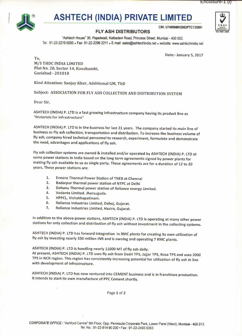
Enclosure-1 (i)
ENCLOSURE-2 (a) to 2 (i)
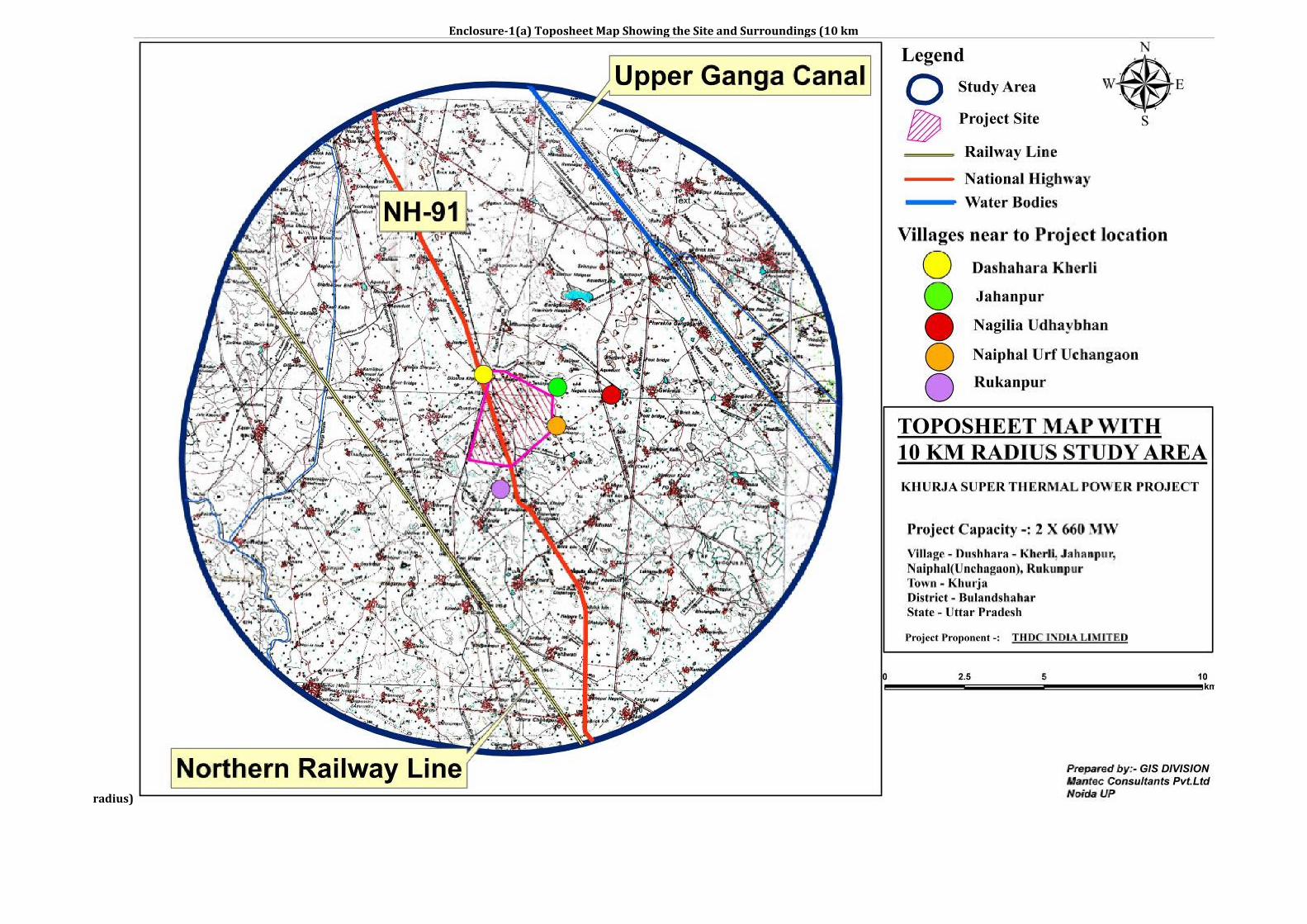
Enclosure-1(a) Toposheet Map Showing the Site and Surroundings (10 km
radius)
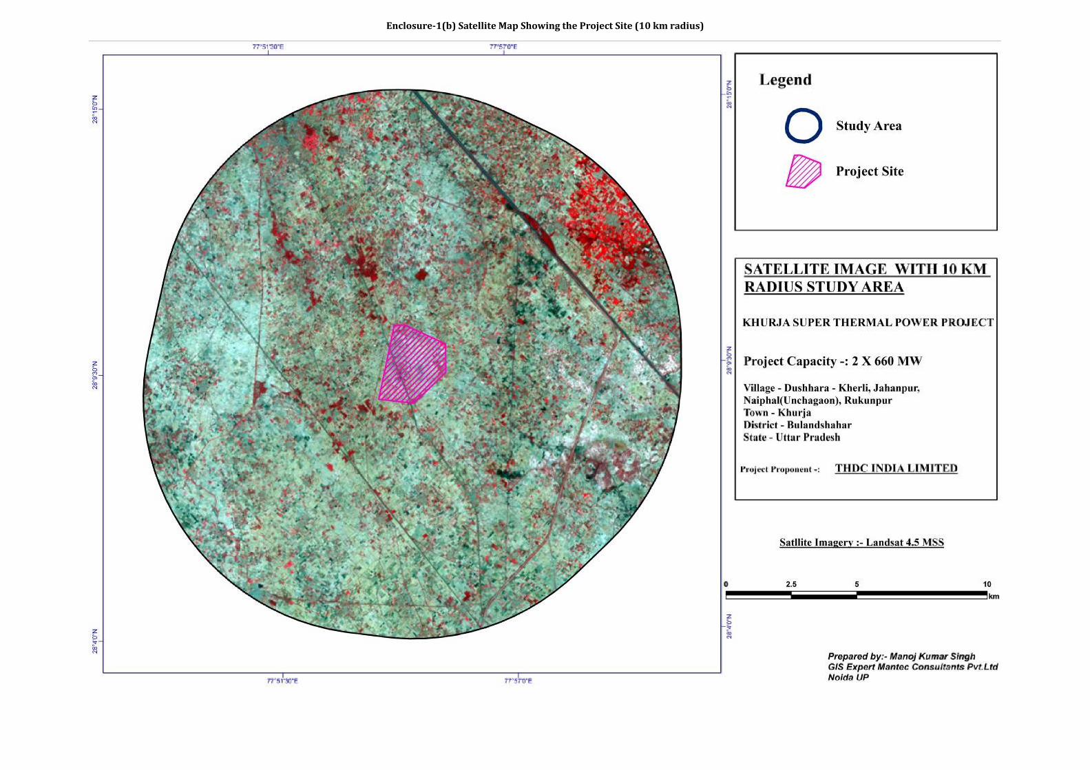
Enclosure-1(b) Satellite Map Showing the Project Site (10 km radius)
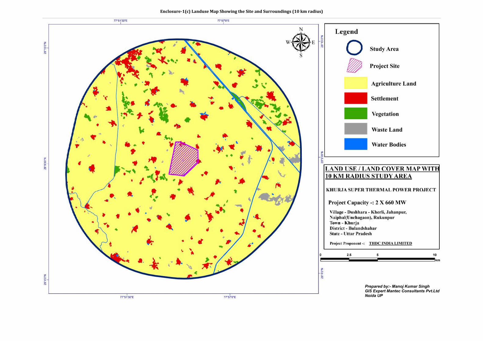
Enclosure-1(c) Landuse Map Showing the Site and Surroundings (10 km radius)
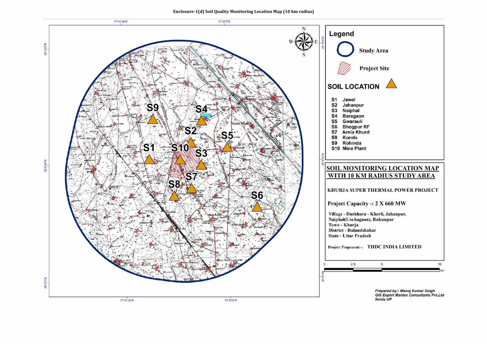
Enclosure-1(d) Soil Quality Monitoring Location Map (10 km radius)
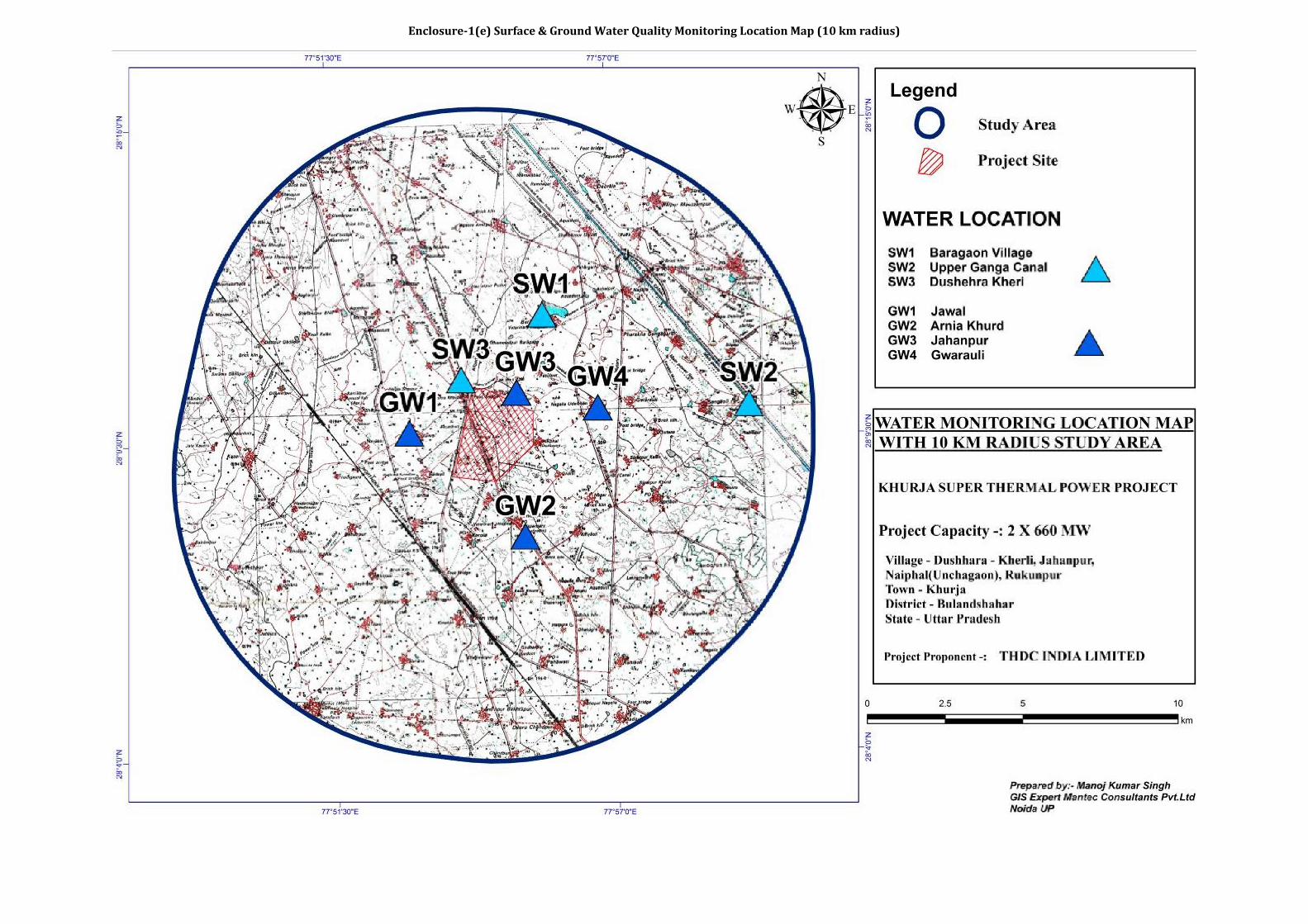
Enclosure-1(e) Surface & Ground Water Quality Monitoring Location Map (10 km radius)
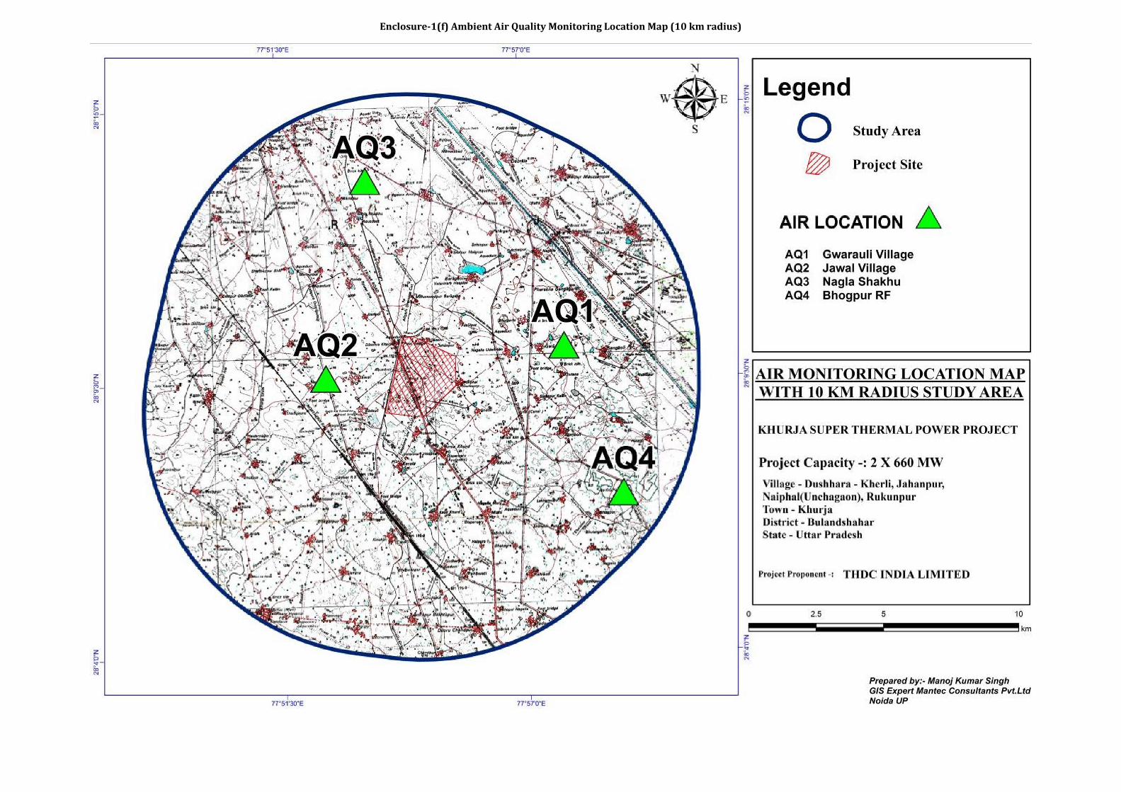
Enclosure-1(f) Ambient Air Quality Monitoring Location Map (10 km radius)
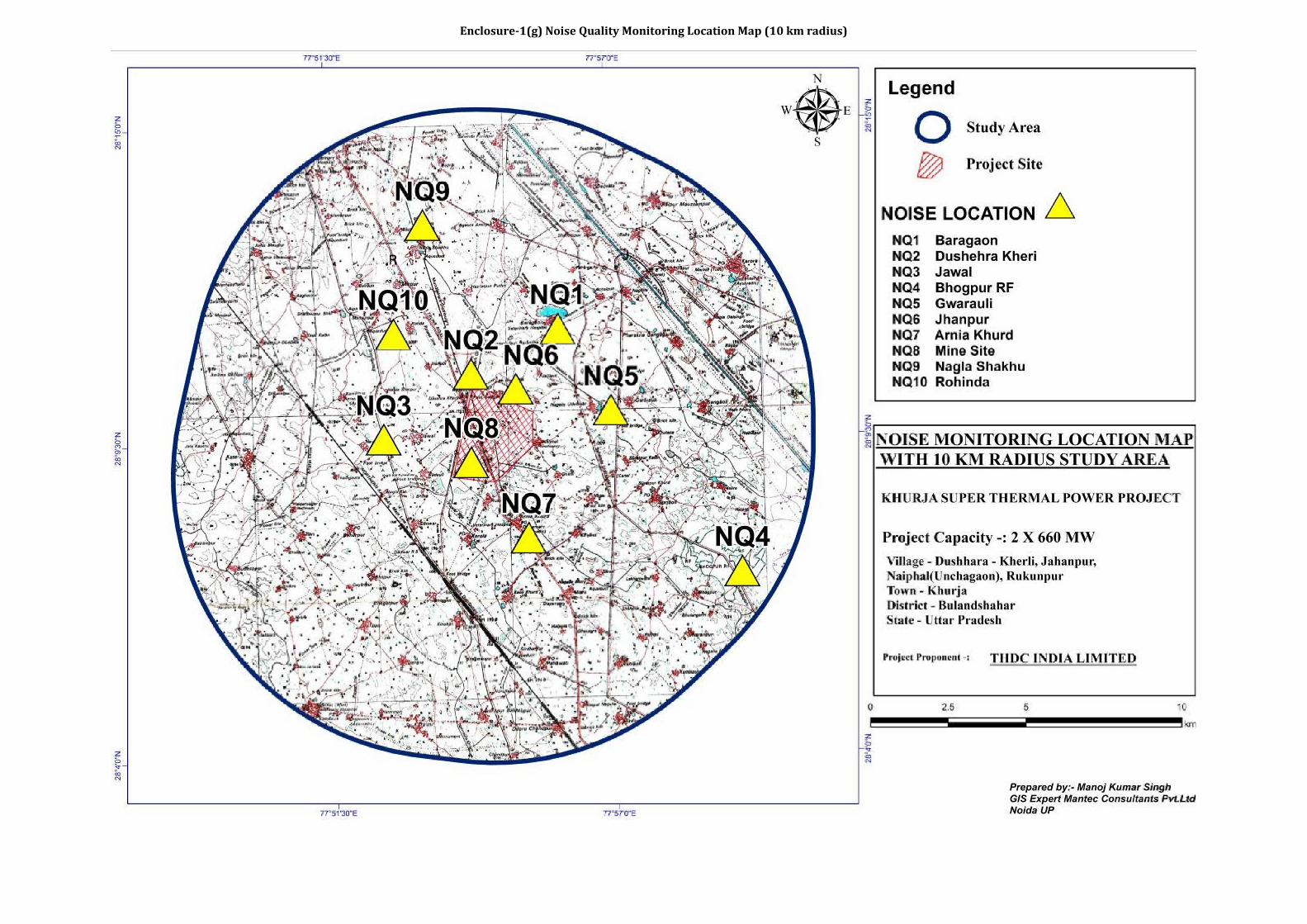
Enclosure-1(g) Noise Quality Monitoring Location Map (10 km radius)
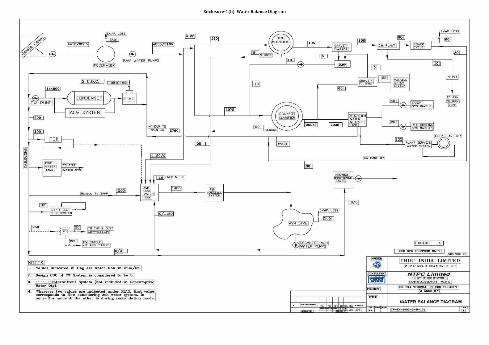
Enclosure-1(h) Water Balance Diagram
D
U
S
H
E
H
R
A
S
C
H
O
O
L
R
P
-
1
9
GENERAL LAYOUT PLAN
(2X660 MW PRESENT PROPOSAL + 1X660 MW FUTURE PROVISION )
THDC INDIA LIMITED
(A JV of GOVT. OF INDIA & GOVT. OF UP )
NOTES:
XX
X
X
X
X
X
X
X
X
X
X
X
X
X
X
X
X
X
X
X
X
X X
X
X
X
X
X
X
X
X
X
X
X
X
X
X
X
X
X
X
X
X
X
X
X
X
X
X
X
X
X
X
X
X
X
C O
F D
YK
E
CL
. O
F D
YK
E
TO KHURJA
11
D
I
V
E
R
T
E
D
A
L
I
G
A
R
H
D
R
A
I
N
NDCT-1
NDCT-2
NDCT-3
PROPOSED DIVERTED
ALIGNMENT OF NH-91
X X
EXISTING N
ATIONAL H
IGHWAY -9
1
ENCLOSURE-3
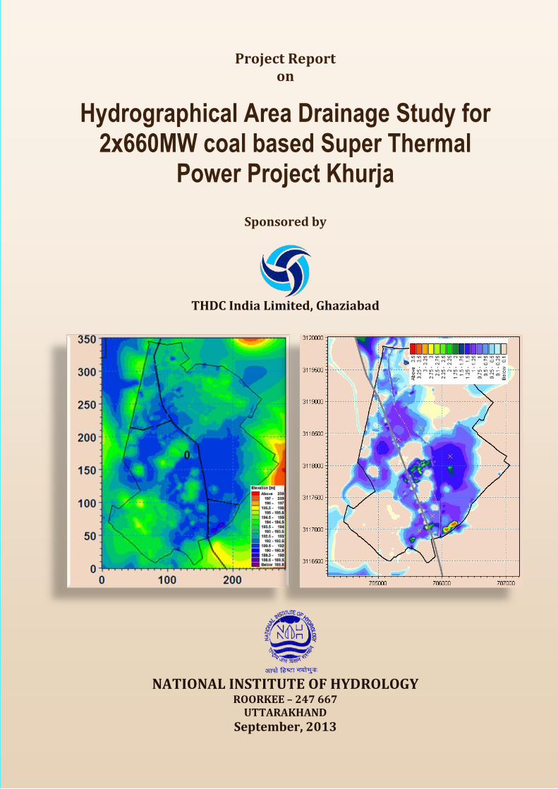
Project Report on
Hydrographical Area Drainage Study for 2x660MW coal based Super Thermal
Power Project Khurja
Sponsored by
THDC India Limited, Ghaziabad
NATIONAL INSTITUTE OF HYDROLOGY ROORKEE – 247 667
UTTARAKHAND September, 2013

Study Group
Director R. D. Singh
Study Group
Rakesh Kumar, Scientist F & Principal Investigator
Pankaj Mani, Scientist D J. P. Patra, Scientist B
R. D. Singh, Director
Technical Assistance T. R. Sapra, RA N.K. Bhatnagar, PRA
Contents
1 ABOUT THE PROJECT......................................................................................... 1
2 DESCRIPTION OF STUDY AREA ....................................................................... 2
2.1 General ................................................................................................................................. 2
2.2 Topography and Drainage ................................................................................................... 2
2.3 Climate ................................................................................................................................. 2
2.4 Rainfall ................................................................................................................................ 3
3 DATA AVAILABILITY ........................................................................................ 5
3.1 Data Availability for Unit Hydrograph Analysis ................................................................. 5
3.2 Data Availability for Rainfall frequency Analysis .............................................................. 6
3.3 Topographic and Drainage Network .................................................................................... 7
4 METHODOLOGY .................................................................................................. 8
4.1 Estimation of Rainfalls of Various Return Periods Using L-Moments Based Rainfall Frequency Analysis ............................................................................................................. 8
4.1.1 Probability weighted moments (PWMs) and L-moments ............................................ 8
4.1.2 Data screening and missing value correction ............................................................. 11
4.1.3 Test of regional homogeneity..................................................................................... 13
4.1.4 Frequency distributions used...................................................................................... 14
4.1.5 Goodness of fit measures ........................................................................................... 18
4.2 Preparation of Digital Elevation Model ............................................................................. 20
4.3 Catchment Delineation and Estimation of Catchment Characteristics .............................. 21
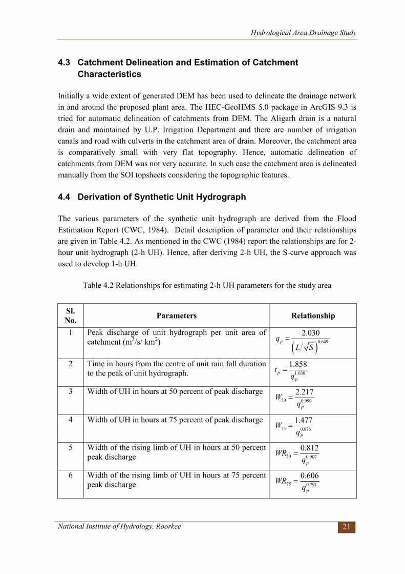
4.4 Derivation of Synthetic Unit Hydrograph.......................................................................... 21
4.5 Estimation of Flood Hydrographs ...................................................................................... 22
4.5.1 Design loss rate .......................................................................................................... 22
4.5.2 Base flow for design flood ......................................................................................... 22
4.5.3 Time adjustment of design rainfall ............................................................................ 22
4.5.4 Design storm duration ................................................................................................ 23
4.6 Estimation of Design Flood Hydrographs ......................................................................... 23
4.7 Flow Simulation and Flood Modelling .............................................................................. 23
4.7.1 Flow modelling by Mike 11 hydrodynamic model .................................................... 23
4.7.2 Two-Dimensional flow modelling by Mike 21 HD model ........................................ 27
4.7.3 Flood inundation modelling by MIKE FLOOD ......................................................... 28
4.8 Safe Grade Elevation ......................................................................................................... 29
4.9 Drainage Design ................................................................................................................ 29
5 ANALYSIS AND RESULTS ............................................................................... 31
5.1 Estimation of 1-day Annual Maximum Rainfall ............................................................... 31
5.2 Estimation of 1-Day Rainfall of Various Return Periods using L-Moments Based Rainfall Frequency Analysis ........................................................................................................... 32
5.2.1 Identification of robust distribution for 1-day maximum rainfall .............................. 32
5.3 Estimation of Synthetic Unit Hydrograph ......................................................................... 38
5.3.1 Base flow for design flood ......................................................................................... 42
5.3.2 Temporal Distribution ................................................................................................ 42
5.4 Estimation of Flood Hydrographs ...................................................................................... 42
5.4.1 Estimation of Flood hydrographs using 1-day annual maximum rainfall .................. 42
5.5 Flood simulation ................................................................................................................ 45
5.5.1 Flow through Aligarh drain ........................................................................................ 45
5.5.2 Modification of the Aligarh drain .............................................................................. 46
5.5.3 Combined flooding due to rainfall and flow through Aligarh drain .......................... 49
5.6 Safe Grade Elevation ......................................................................................................... 62
5.7 Proposed Drainage Network .............................................................................................. 63
5.7.1 Drainage layout .......................................................................................................... 63
5.7.2 Design of drain section .............................................................................................. 66
5.8 Limitation of the Study ...................................................................................................... 68
6 CONCLUSIONS ................................................................................................... 69
REFERENCES .................................................................................................................... 71 ANNEXURE ....................................................................................................................... 73
List of Figures
Figure 2.1: Index map of the study Area ............................................................................... 3
Figure 2.2: Drainage pattern around the Plant area ............................................................... 4
Figure 3.1: Layout of toposheets used in this study. ............................................................. 5
Figure 3.2: Rain-gauge stations with Thiessen Polygon ...................................................... 6
Figure 3.3 Topographical features of study area ................................................................... 7
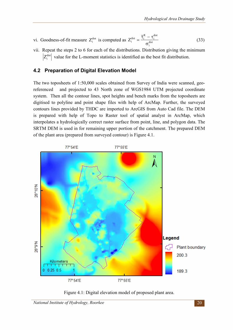
Figure 4.1: Digital elevation model of proposed plant area. ............................................... 20
Figure 4.2 : MIKE 11 computational grids ......................................................................... 24
Figure 4.3 : Drainage network in MIKE-11 ....................................................................... 25
Figure 4.4: Typical Cross-section of the drain. ................................................................... 30
Figure 5.1 : Annual 1-day maximum rainfall. ..................................................................... 31
Figure 5.2: L-moments ratio diagram for Aligarh for 1-day annual maximum rainfall ...... 34
Figure 5.3: L-moments ratio diagram for Bulandshar for 1-day annual maximum rainfall 35
Figure 5.4: L-moments ratio diagram for Khurja for 1-day annual maximum rainfall ....... 36
Figure 5.5: L-moments ratio diagram for Regional for 1-day annual maximum rainfall ... 37
Figure 5.6: Delineated Catchment area ............................................................................... 39
Figure 5.7: 1-h unit hydrograph. .......................................................................................... 41
Figure 5.8: Time duration curve for the 24-h rainfall.......................................................... 43
Figure 5.9: Rainfall hyetograph for 1-day maximum rainfall ............................................. 43
Figure 5.10: Design flood hydrographs for various return periods resulting from 1-day annual maximum rainfall. ............................................................................................ 44
Figure 5.11: Mike-11 setup of Aligarh drain. ...................................................................... 45
Figure 5.12: Existing and proposed re aligned Aligarh drain.............................................. 47
Figure 5.13: Existing cross-section of Aligarh drain at inlet and outlet .............................. 48
Figure 5.14: Proposed modified drain sections ................................................................... 48
Figure 5.15: Elevation profile along the realigned section of Aligarh drain ....................... 49
Figure 5.16 Bathymetry of the plant area ............................................................................ 50
Figure 5.17: Flood water depth due to 100 year return period rainfall. .............................. 51
Figure 5.18: Longitudinal profile of modified Aligarh drain .............................................. 52
Figure 5.19: Water depths at selected grids for 100 year return period flood ..................... 53
Figure 5.20: Water levels at selected grids for 100 year return period flood ...................... 54
Figure 5.21: Flood water depth due to 50 year return period rainfall ................................. 55
Figure 5.22: Flood water depth due to 25 year return period rainfall ................................. 56
Figure 5.23: Flood water depth due to 10 year return period rainfall ................................. 57
Figure 5.24 : Water levels for various return period flood. (a) to (g) for grid point 1 to 7 . 61
Figure 5.25: Percentage of area in existing levels. .............................................................. 63
Figure 5.26 : Proposed drainage layout ............................................................................... 64
Figure 5.27: Proposed drainage network with contributing runoff area.............................. 65
List of Tables
Table 3.1 Details of rainfall data availability ........................................................................ 6
Table 4.1 Critical values of discordancy statistic, Di .......................................................... 12
Table 4.2 Relationships for estimating 2-h UH parameters for the study area ................... 21
Table 5.1 Zi dist – Statistic of various distributions for 1-day annual maximum rainfall ..... 32
Table 5.2 Parameters of various distributions for 1-day annual maximum rainfall ............ 33
Table 5.3 Values of growth factors (RT/ R ) for 1-day annual maximum rainfall ............... 38
Table 5.4 1-day annual maximum rainfall (mm) for various return periods ....................... 38
Table 5.5 Catchment characteristics .................................................................................... 40
Table 5.6 Parameters of Synthetic Unit Hydrograph. ......................................................... 40
Table 5.7 Ordinates of 1-h unit hydrograph. ....................................................................... 41
Table 5.8: Details of selected grids ..................................................................................... 53
Table 5.9 : Maximum water level at selected grids for various return periods ................... 61
Table 5.10 Length, drainage area and peak flow of various sections. ................................. 66
Table 5.11 Design details of drain section for 50 year and 25 year return period .............. 67

List of Annexure
Annexure No Particulars Page No
I Scope of Work of the study as per THDCIL work order. 73 II Annual Maximum rainfall at various stations. 74 III Effective rainfall and Runoff for various sub basins. 75
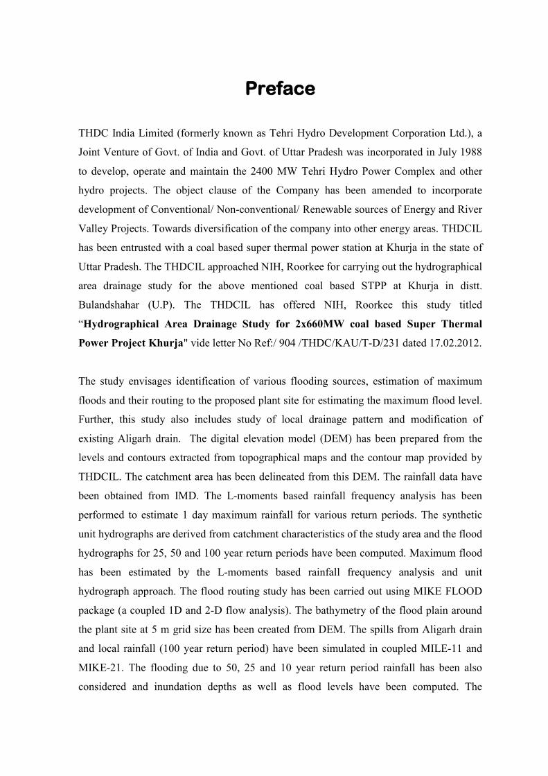
Preface THDC India Limited (formerly known as Tehri Hydro Development Corporation Ltd.), a
Joint Venture of Govt. of India and Govt. of Uttar Pradesh was incorporated in July 1988
to develop, operate and maintain the 2400 MW Tehri Hydro Power Complex and other
hydro projects. The object clause of the Company has been amended to incorporate
development of Conventional/ Non-conventional/ Renewable sources of Energy and River
Valley Projects. Towards diversification of the company into other energy areas. THDCIL
has been entrusted with a coal based super thermal power station at Khurja in the state of
Uttar Pradesh. The THDCIL approached NIH, Roorkee for carrying out the hydrographical
area drainage study for the above mentioned coal based STPP at Khurja in distt.
Bulandshahar (U.P). The THDCIL has offered NIH, Roorkee this study titled
“Hydrographical Area Drainage Study for 2x660MW coal based Super Thermal
Power Project Khurja" vide letter No Ref:/ 904 /THDC/KAU/T-D/231 dated 17.02.2012.
The study envisages identification of various flooding sources, estimation of maximum
floods and their routing to the proposed plant site for estimating the maximum flood level.
Further, this study also includes study of local drainage pattern and modification of
existing Aligarh drain. The digital elevation model (DEM) has been prepared from the
levels and contours extracted from topographical maps and the contour map provided by
THDCIL. The catchment area has been delineated from this DEM. The rainfall data have
been obtained from IMD. The L-moments based rainfall frequency analysis has been
performed to estimate 1 day maximum rainfall for various return periods. The synthetic
unit hydrographs are derived from catchment characteristics of the study area and the flood
hydrographs for 25, 50 and 100 year return periods have been computed. Maximum flood
has been estimated by the L-moments based rainfall frequency analysis and unit
hydrograph approach. The flood routing study has been carried out using MIKE FLOOD
package (a coupled 1D and 2-D flow analysis). The bathymetry of the flood plain around
the plant site at 5 m grid size has been created from DEM. The spills from Aligarh drain
and local rainfall (100 year return period) have been simulated in coupled MILE-11 and
MIKE-21. The flooding due to 50, 25 and 10 year return period rainfall has been also
considered and inundation depths as well as flood levels have been computed. The
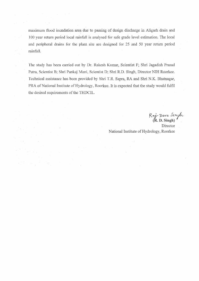
maximum flood inundation are~ due to passing of design discharge in Aligarh drain ~nd
100 year return period local rainfall is analysed for safe grade level estimation. The local
and peripheral drains for the plant site are designed for 25 and 50 year· return period
rainfall.
The study has been carried out by Dr. Rakesh Kumar, Scientist F; Shri Jagadish Prasad
Patra, Scientist B; Shri Pankaj Mani, Scientist D; Shri R.D. Singh, Director NIH Roorkee.
Technical assistance has been provided by Shri T.R. Sapra, RA and Shri N.K. Bhatnagar,
PRA ofNational Institute of Hydrology, Roorkee. It is expected that the study would fulfil
the desired requirements of the THDCIL.
R+1UN~J~~ (R. D. Singh)
Director National Institute ofHydrology, Roorkee
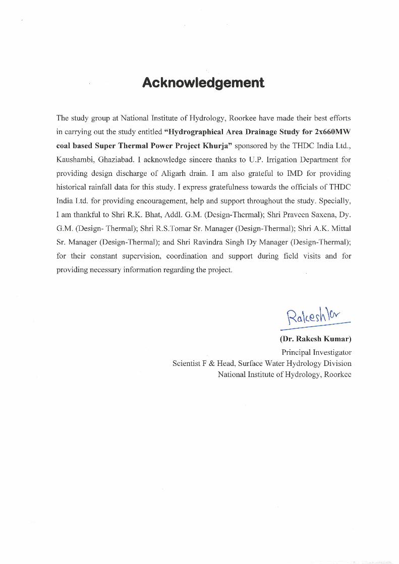
Acknowledgement
The study group at National Institute of Hydrology, Roorkee have made their best efforts
in carrying out the study entitled "Hydrographical Area Drainage Study for 2x660MW
coal based Super Thermal Power Project Khurja" sponsored by the THDC India Ltd.,
Kaushambi, Ghaziabad. I acknowledge sincere thanks to U .P. Irrigation Department for
providing design discharge of Aligarh drain. I am also grateful to IMD for providing
historical rainfall data for this study. I express gratefulness towards the officials of THDC
India Ltd. for providing encouragement, help and support throughout the study. Specially,
I am thankful to Shri R.K. Bhat, Addl. G.M. (Design-Thermal); Shri Praveen Saxena, Dy.
G.M. (Design- Thermal); Shri R.S.Tomar Sr. Manager (Design-Thermal); Shri A.K. Mittal
Sr. Manager (Design-Thermal); and Shri Ravindra Singh Dy Manager (Design-Thermal);
for their constant supervision, coordination and support during field visits and for
providing necessary information regarding the project.
(Dr. Rakesh Kumar)
Principal Investigator
Scientist F & Head, Surface Water Hydrology Division
National Institute of Hydrology, Roorkee
National Institute of Hydrology, Roorkee 1
1 ABOUT THE PROJECT
THDC India Limited, a Schedule ‘A’ Mini Ratna Company has signed a memorandum of understanding with Govt. of U.P to set up a 1320 MW super thermal power plant at Khurja, Distt. Bulandshahar (U.P). For the preparation of Detailed Feasibility Report, apart from various other studies a study on Hydrographical Area Drainage system of the proposed area is essential. THDC India Limited, Ghaziabad requested National Institute of Hydrology, Roorkee to undertake the study to access natural drainage pattern and to decide upon the drainage system in and around the plant area and to access the measures to be adopted to address modification of existing natural drainage pattern. The original scopes of work are:
1. Study of existing natural drainage pattern/system with available information in the form of reports, literature, satellite imageries, etc. for proposed project and its adjoining areas. The study shall include review of topographical features of the proposed site for the Power Project and its surrounding area.
2. Review and analysis of rainfall information to arrive at design storm scenarios. 3. Review and analysis of relevant Survey of India Topographical Sheets,
topographical survey and satellite imageries. 4. Estimation of flood hydrographs considering historical as well as design
rainfall to suggest complete scheme for storm water drainage of project and its adjoining areas including diversion of existing nalas/streams, if any. In case short interval observed rainfall runoff data would be not available then the standard regional approaches will be used for design flood estimation.
5. Estimation and routing of design flood hydrograph through the drainage system of concerned catchments considering appropriate boundary conditions including pre-project scenario as well as post-project scenario for suggesting Safe Grade Elevation for the plant.
6. Suggesting final disposal point for the storm water & plant drainage. 7. Site visit for acquaintance of prevailing conditions and collection of available
data at site. 8. Visit to THDC Office for discussions regarding the studies.
The scope of work as per the project proposal is given in Annexure-I.
National Institute of Hydrology, Roorkee 2
2 DESCRIPTION OF STUDY AREA
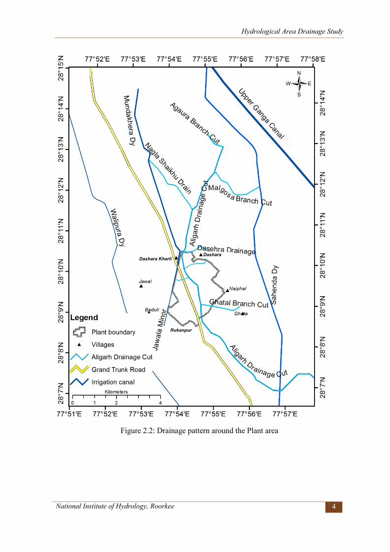
2.1 General The Plant site is located near village Dasehri, Dasehri Khrli, along NH 91 in Bulandshahr district of the state of Uttar Pradesh. The geographical extent of the proposed plant site is from 77°53.783'E to 77°55.373'E longitude and from 28°08.586'N to 28°10.417'N latitude approximately and covered in Survey of India toposheet no. 53H16 of 1:50000 scale. The project site is surrounded by villages namely: Dashara Khrli & Dashara in north; Rukanpur in south; Naiphal in east and Jawal in west. The majority area is uncultivated land and brick klin area. The geographical area of the plant site is about 5.3 km2. The location of the site is given in Figure 2.1. 2.2 Topography and Drainage The plant site is located in upper Indo- Ganga plains. The Aligarh drain and NH-91 passes through the proposed plant area. The general topography of the area is and elevation in the proposed plant area varies from 189.5 m to 196 m. The general land slope is towards South. The existing drainage in and around the site is given in Figure 2.2. The Aligarh drain is the main drain passing through the site. As per the information available the Aligarh drain starts from Agaura branch cut. Total length of the Aligarh drain is 121.204 km and the length of the drain up to entry to plant boundary is about 6.5 m. The Malgosa branch cut and Nagla shaikhu drain joins Aligarh drain in its upstream of plant boundary. The Ghatal branch cut joins to Aligarh drain inside plant boundary. Further one small drain after crossing the highway and another drain from other side of Aligarh drain joins to Aligarh drain inside plant boundary area. Apart from these there are two culverts in highway, to drain the runoff generated from the west side of highway area and join to Aligarh drain. 2.3 Climate Bulandhshahr is located in the Meerut division of Uttar Pradesh, between the Ganga and Yamuna rivers. The climate of Bulandshahr is extreme and tropical. The district average temperature in summer and winter season is 33.52°C and 14.33°C respectively. The summers are extremely hot and the maximum temperature goes as high as 45º C, while the winters remain cold, with temperature dipping to 2º C.
Hydrological Area Drainage Study
National Institute of Hydrology, Roorkee 3
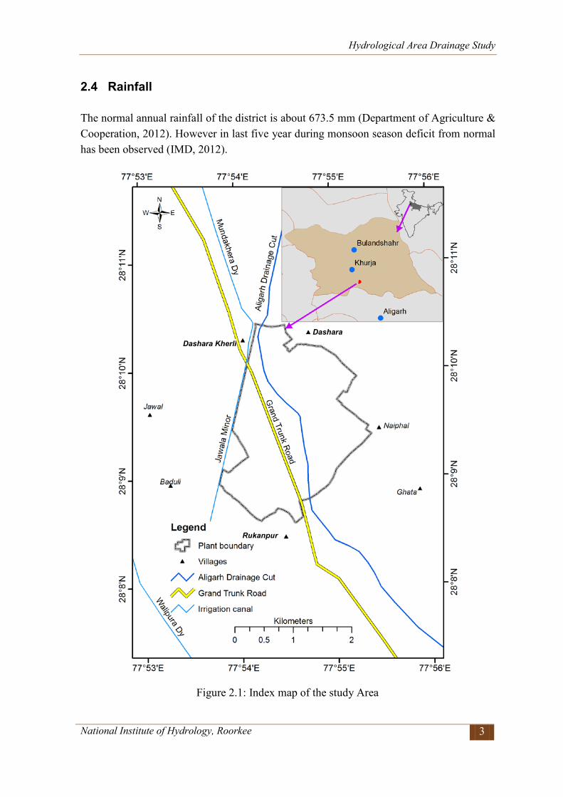
2.4 Rainfall The normal annual rainfall of the district is about 673.5 mm (Department of Agriculture & Cooperation, 2012). However in last five year during monsoon season deficit from normal has been observed (IMD, 2012).
Figure 2.1: Index map of the study Area
Dashara Dashara Kherli
Rukanpur
Hydrological Area Drainage Study
National Institute of Hydrology, Roorkee 4
Figure 2.2: Drainage pattern around the Plant area
Dashara Dashara Kherli
Rukanpur
National Institute of Hydrology, Roorkee 5
3 DATA AVAILABILITY
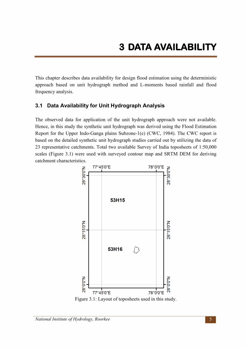
This chapter describes data availability for design flood estimation using the deterministic approach based on unit hydrograph method and L-moments based rainfall and flood frequency analysis. 3.1 Data Availability for Unit Hydrograph Analysis The observed data for application of the unit hydrograph approach were not available. Hence, in this study the synthetic unit hydrograph was derived using the Flood Estimation Report for the Upper Indo-Ganga plains Subzone-1(e) (CWC, 1984). The CWC report is based on the detailed synthetic unit hydrograph studies carried out by utilizing the data of 23 representative catchments. Total two available Survey of India toposheets of 1:50,000 scales (Figure 3.1) were used with surveyed contour map and SRTM DEM for deriving catchment characteristics.
Figure 3.1: Layout of toposheets used in this study.
Hydrological Area Drainage Study
National Institute of Hydrology, Roorkee 6
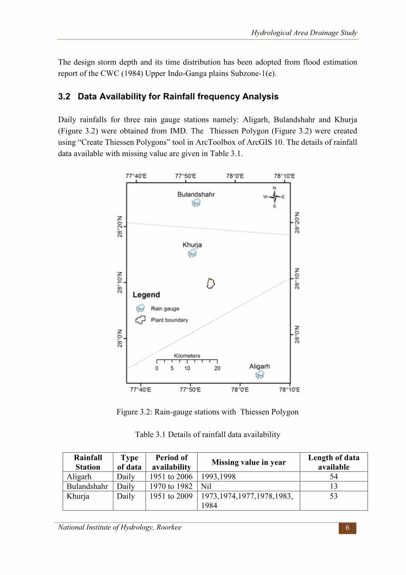
The design storm depth and its time distribution has been adopted from flood estimation report of the CWC (1984) Upper Indo-Ganga plains Subzone-1(e). 3.2 Data Availability for Rainfall frequency Analysis Daily rainfalls for three rain gauge stations namely: Aligarh, Bulandshahr and Khurja (Figure 3.2) were obtained from IMD. The Thiessen Polygon (Figure 3.2) were created using “Create Thiessen Polygons” tool in ArcToolbox of ArcGIS 10. The details of rainfall data available with missing value are given in Table 3.1.
Figure 3.2: Rain-gauge stations with Thiessen Polygon
Table 3.1 Details of rainfall data availability
Rainfall Station
Type of data
Period of availability Missing value in year Length of data
available Aligarh Daily 1951 to 2006 1993,1998 54 Bulandshahr Daily 1970 to 1982 Nil 13 Khurja Daily 1951 to 2009 1973,1974,1977,1978,1983,
1984 53
Hydrological Area Drainage Study
National Institute of Hydrology, Roorkee 7
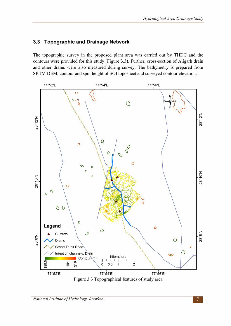
3.3 Topographic and Drainage Network The topographic survey in the proposed plant area was carried out by THDC and the contours were provided for this study (Figure 3.3). Further, cross-section of Aligarh drain and other drains were also measured during survey. The bathymetry is prepared from SRTM DEM, contour and spot height of SOI toposheet and surveyed contour elevation.
Figure 3.3 Topographical features of study area
National Institute of Hydrology, Roorkee 8
4 METHODOLOGY
The methodology used for estimation of design flood using the synthetic unit hydrograph approach and methodologies for analyzing flood inundation this flood described as follows. 4.1 Estimation of Rainfalls of Various Return Periods Using L-
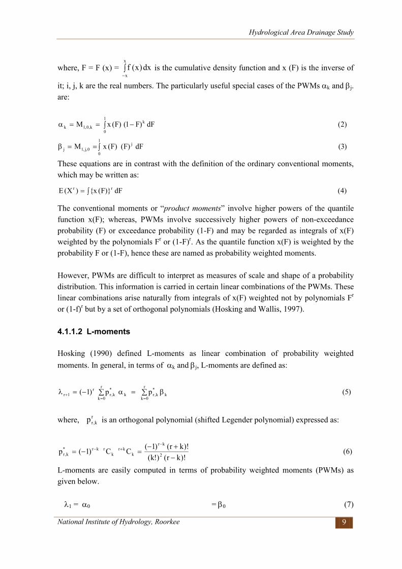
Moments Based Rainfall Frequency Analysis The following aspects of methodology of L-moments based regional frequency relationship for gauged catchments as well as ungauged catchments are discussed as follows. (i) Probability weighted moments (PWMs) and L-moments, (ii) Data screening and missing value correction, (iii) Test of regional homogeneity, (iv) Frequency distributions used, (v) Goodness of fit measures, and (vi) Development of relationship between mean annual peak flood and catchment area. In this study at-site rainfall frequency analysis and regional frequency analysis (Kumar and Chatterjee, 2005; Kumar et al., 2011) has been applied as discussed in Chapter 5.1. 4.1.1 Probability weighted moments (PWMs) and L-moments L-moments of a random variable were first introduced by Hosking (1990). Hosking and Wallis (1997) state that L-moments are an alternative system of describing the shapes of probability distributions. Historically they arose as modifications of the probability weighted moments’ (PWMs) of Greenwood et al. (1979). 4.1.1.1 Probability weighted moments (PWMs) Probability weighted moments are defined by Greenwood et al. (1979) as:
)1()1()()(1
0,, dFFFFxM kjikji −= ∫
Hydrological Area Drainage Study
National Institute of Hydrology, Roorkee 9
where, F = F (x) = ∫−
x
xdx)x(f is the cumulative density function and x (F) is the inverse of
it; i, j, k are the real numbers. The particularly useful special cases of the PWMs αk and βj. are:
)2(dF)F1()F(xM1
0
kk,0,1k ∫ −==α
)3(dF)F()F(xM j1
00,j,1j ∫==β
These equations are in contrast with the definition of the ordinary conventional moments, which may be written as:
)4(dF)F(x)X(E rr ∫=
The conventional moments or “product moments” involve higher powers of the quantile function x(F); whereas, PWMs involve successively higher powers of non-exceedance probability (F) or exceedance probability (1-F) and may be regarded as integrals of x(F) weighted by the polynomials Fr or (1-F)r. As the quantile function x(F) is weighted by the probability F or (1-F), hence these are named as probability weighted moments. However, PWMs are difficult to interpret as measures of scale and shape of a probability distribution. This information is carried in certain linear combinations of the PWMs. These linear combinations arise naturally from integrals of x(F) weighted not by polynomials Fr or (1-f)r but by a set of orthogonal polynomials (Hosking and Wallis, 1997). 4.1.1.2 L-moments Hosking (1990) defined L-moments as linear combination of probability weighted moments. In general, in terms of αk and βj, L-moments are defined as:
)5(pp)1( k
r
0k
*k,rk
r
0k
*k,r
r1r β∑=α∑−=λ
==+
where, r
k,rp is an orthogonal polynomial (shifted Legender polynomial) expressed as:
)6()!kr()!k()!kr()1(CC)1(p 2
kr
kkr
krkr*
k,r −+−
=−=−
+−
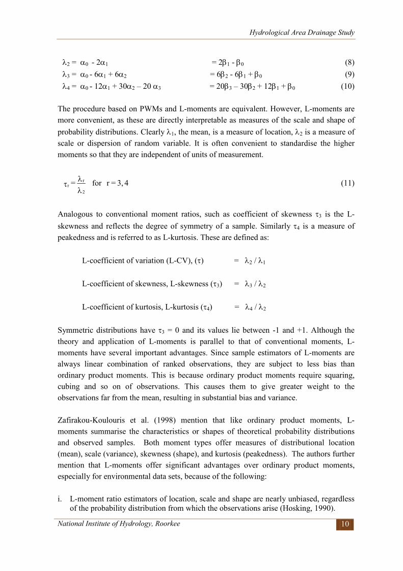
L-moments are easily computed in terms of probability weighted moments (PWMs) as given below. λ1 = α0 = β0 (7)
Hydrological Area Drainage Study
National Institute of Hydrology, Roorkee 10
λ2 = α0 - 2α1 = 2β1 - β0 (8) λ3 = α0 - 6α1 + 6α2 = 6β2 - 6β1 + β0 (9) λ4 = α0 - 12α1 + 30α2 – 20 α3 = 20β3 – 30β2 + 12β1 + β0 (10)
The procedure based on PWMs and L-moments are equivalent. However, L-moments are more convenient, as these are directly interpretable as measures of the scale and shape of probability distributions. Clearly λ1, the mean, is a measure of location, λ2 is a measure of scale or dispersion of random variable. It is often convenient to standardise the higher moments so that they are independent of units of measurement.
43, =r for = 2
rr
λλ
τ (11)
Analogous to conventional moment ratios, such as coefficient of skewness τ3 is the L-skewness and reflects the degree of symmetry of a sample. Similarly τ4 is a measure of peakedness and is referred to as L-kurtosis. These are defined as:
L-coefficient of variation (L-CV), (τ) = λ2 / λ1 L-coefficient of skewness, L-skewness (τ3) = λ3 / λ2 L-coefficient of kurtosis, L-kurtosis (τ4) = λ4 / λ2
Symmetric distributions have τ3 = 0 and its values lie between -1 and +1. Although the theory and application of L-moments is parallel to that of conventional moments, L-moments have several important advantages. Since sample estimators of L-moments are always linear combination of ranked observations, they are subject to less bias than ordinary product moments. This is because ordinary product moments require squaring, cubing and so on of observations. This causes them to give greater weight to the observations far from the mean, resulting in substantial bias and variance. Zafirakou-Koulouris et al. (1998) mention that like ordinary product moments, L- moments summarise the characteristics or shapes of theoretical probability distributions and observed samples. Both moment types offer measures of distributional location (mean), scale (variance), skewness (shape), and kurtosis (peakedness). The authors further mention that L-moments offer significant advantages over ordinary product moments, especially for environmental data sets, because of the following: i. L-moment ratio estimators of location, scale and shape are nearly unbiased, regardless
of the probability distribution from which the observations arise (Hosking, 1990).
Hydrological Area Drainage Study
National Institute of Hydrology, Roorkee 11
ii. L-moment ratio estimators such as L-Cv, L-skewness, and L-kurtosis can exhibit lower
bias than conventional product moment ratios, especially for highly skewed samples. iii. The L-moment ratio estimators of L-Cv and L-skewness do not have bounds which
depend on sample size as do the ordinary product moment ratio estimators of Cv and skewness.
iv. L-moment estimators are linear combinations of the observations and thus are less
sensitive to the largest observations in a sample than product moment estimators, which square or cube the observations.
v. L-moment ratio diagrams are particularly good at identifying the distributional
properties of highly skewed data, whereas ordinary product moment diagrams are almost useless for this task (Vogel and Fennessey, 1993).
4.1.2 Data screening and missing value correction In flood frequency analysis, the data collected at various sites should be true representative of the annual maximum peak flood measured and must be drawn from the same frequency distribution. The first step in flood frequency analysis is to verify that the data are appropriate for the analysis. The preliminary screening of the data must be carried out to ensure that the above requirements are satisfied. Errors in data may occur due to incorrect recording or transcription of the data values or due to shifting of the gauging site to a different location as well as due to changes in the measuring practices or as a result of water resources development activities. Tests for outliers and trends are well established in the statistical literature (e.g., Barnett and Lewis, 1994; W.R.C., 1981; Kendall, 1975). For comparison of data observed from different sites, some techniques such as double mass plots or quantile-quantile plots are commonly used. Hosking and Wallis (1997) mention that in the context of regional frequency analysis using L-moments, useful information can be obtained by comparing the sample L-moment ratios for different sites, incorrect data values, outliers, trends and shifts in the mean of a sample can all be related to L-moments of the sample. A convenient amalgamation of the L-moment ratios into a single statistic, a measure of discordancy between L-moment ratios of a site and the average L-moment ratios of a group of similar sites, has been termed as “discordancy measure”, Di. 4.1.2.1 Discordancy measure The aim of the discordancy measure is to identify those sites from a group of given sites that are grossly discordant with the group as a whole. Discordancy is measured in terms of
Hydrological Area Drainage Study
National Institute of Hydrology, Roorkee 12
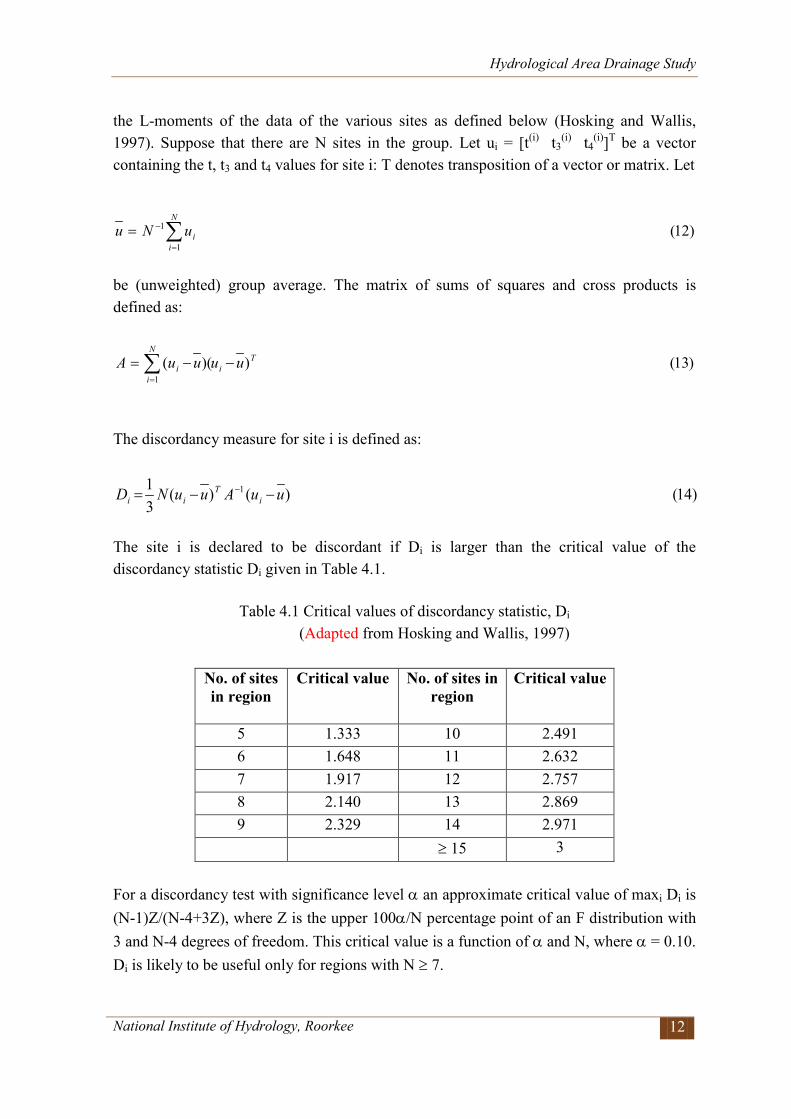
the L-moments of the data of the various sites as defined below (Hosking and Wallis, 1997). Suppose that there are N sites in the group. Let ui = [t(i) t3
(i) t4(i)]T be a vector containing the t, t3 and t4 values for site i: T denotes transposition of a vector or matrix. Let
be (unweighted) group average. The matrix of sums of squares and cross products is defined as:
The discordancy measure for site i is defined as:
)14()()(31 1 uuAuuND i
Tii −−= −
The site i is declared to be discordant if Di is larger than the critical value of the discordancy statistic Di given in Table 4.1.
Table 4.1 Critical values of discordancy statistic, Di
(Adapted from Hosking and Wallis, 1997)
No. of sites in region
Critical value No. of sites in region
Critical value
5 1.333 10 2.491 6 1.648 11 2.632 7 1.917 12 2.757 8 2.140 13 2.869 9 2.329 14 2.971 ≥ 15 3
For a discordancy test with significance level α an approximate critical value of maxi Di is (N-1)Z/(N-4+3Z), where Z is the upper 100α/N percentage point of an F distribution with 3 and N-4 degrees of freedom. This critical value is a function of α and N, where α = 0.10. Di is likely to be useful only for regions with N ≥ 7.
∑=
−=N
iiuNu
1
1 )12(
)13())((1
Ti
N
ii uuuuA −−= ∑
=
Hydrological Area Drainage Study
National Institute of Hydrology, Roorkee 13
4.1.3 Test of regional homogeneity A test statistic H, termed as heterogeneity measure has been proposed by Hosking and Wallis (1993). It compares the inter-site variations in sample L-moments for the group of sites with what would be expected of a homogeneous region. The inter-site variation of L-moment ratio is measured as the standard deviation (V) of the at-site LCV’s weighted proportionally to the record length at each site. To establish what would be expected of a homogeneous region, simulations are used. A number of, say 500 data regions are generated based on the regional weighted average statistics using a four parameter distribution e.g. Kappa or Wakeby distribution. The inter-site variation of each generated region is obtained and the mean (µv) and standard deviation (σv) of the computed inter-site variation is obtained. Let the proposed region has N sites with site i having record length ni and sample L-moment ratios t(i), t3
(i), and t4(i). The regional average L-CV, L-Skewness and L-Kurtosis
weighted proportionally to the sites’ record length for example, tR mentioned below. The various steps involved in computation of heterogeneity measure (H) are mentioned below.
(i) Compute the weighted regional average L moment ratios
i
N
1i
)i(i
N
1i
R ntntss
∑∑===
(15)
The value of R
4R3 tandt can also be computed similarly by replacing t(i) by t3
(i), and t4(i).
(ii) Compute the weighted standard deviation of at site LCV’s (t(i))
½
i
N
1i
2R)i(i
N
1in)tt(nV
∑−∑=
== (16)
(iii) Fit a general 4-parameter distribution (Kappa or 4 parameter Wakeby etc.) to the
regional average L-moment ratios, tR, R4
R3 tandt .
(iv) Simulate a large number of regions say 500 having same record lengths as the
observed data of the proposed region.
Hydrological Area Drainage Study
National Institute of Hydrology, Roorkee 14
(v) Repeat steps 1 and 2 for each of the 500 simulated regions and calculate the weighted standard deviations for each simulated region and take it as v1, v2, v3,…….v500.
(vi) Compute the mean (µv) and standard deviation (σv) of the values obtained in step
(v). (vii) Compute the Heterogeneity measure H as given below.
vVH v
σµ−
= (17)
The criteria established by Hosking and Wallis (1993) for assessing heterogeneity of a region is as follows. If H < 1 Region is acceptably homogeneous. If 1 ≤ H < 2 Region is possibly heterogeneous. If H ≥ 2 Region is definitely heterogeneous. 4.1.4 Frequency distributions used The following twelve frequency distributions have been used in this study.
i. Extreme value (EV1)/ Gumbel distribution ii. General extreme value (GEV)
iii. Logistic (LOS) iv. Generalized logistic (GLO) v. Normal (NOR)
vi. Generalized Pareto (GPA) vii. Generalized normal (GNO)
viii. Uniform (UNF) ix. Pearson Type-III (PT3) x. Kappa (KAP) and
xi. Wakeby (WAK) xii. Exponential (EXP)
The details about these distributions and relationships among parameters of these distributions and L-moments are available in literature (e.g. Hosking and Wallis, 1997) and the same are summarized below.
Hydrological Area Drainage Study
National Institute of Hydrology, Roorkee 15
4.1.4.1 Extreme value type-I distribution (EV1) Extreme Value Type-I distribution (EV1) is a two parameter distribution and it is popularly known as Gumbel distribution. The quantile function or the inverse form of the distribution is expressed as:
x (F) = u - α ln (- ln F) (18) Where, u and α are the location and scale parameters respectively, F is the non-exceedence probability viz. (1-1/T) and T is return period in years. 4.1.4.2 General extreme value distribution (GEV) General Extreme Value distribution (GEV) is a generalized three parameter extreme value distribution. Its theory and practical applications are reviewed in the Flood Studies Report (NERC,1975). The quantile function or the inverse form of the distribution is expressed as: x (F) = u + α 1- (-ln F) k/ k ; k ≠ 0 (19) x (F) = u - α ln (- ln F) k = 0 (20)
Where, u, α and k are location, scale and shape parameters of GEV distribution respectively. EV1 distribution is the special case of the GEV distribution, when k = 0. 4.1.4.3 Logistic distribution (LOS) Inverse form of the Logistic distribution (LOS) is expressed as: x (F) = u - α ln (1-F) / F (21) Where, u and α are location and scale parameters respectively. 4.1.4.4 Generalized logistic distribution (GLO) Inverse form of the Generalized Logistic distribution (GLO) is expressed as: x (F) = u + α [ 1 - (1-F) / Fk ] / k; k ≠ 0 (22)
Hydrological Area Drainage Study
National Institute of Hydrology, Roorkee 16
x (F) = u - α ln (1-F) / F; k = 0 (23) Where, u, α and k are location, scale and shape parameters respectively. Logistic distribution is the special case of the Generalized Logistic distribution, when k = 0. 4.1.4.5 Generalized Pareto distribution (GPA) Inverse form of the Generalized Pareto distribution (GPA) is expressed as: x (F) = u + α 1- (1-F)k / k; k ≠ 0 (24) x (F) = u - α ln (1-F) k = 0 (25) where, u, α and k are location, scale and shape parameters respectively. Exponential distribution is special case of Generalized Pareto distribution, when k = 0.
4.1.4.6 Generalized normal distribution (GNO) The cumulative density function of the three parameter Generalized normal distribution (GNO) is given below.
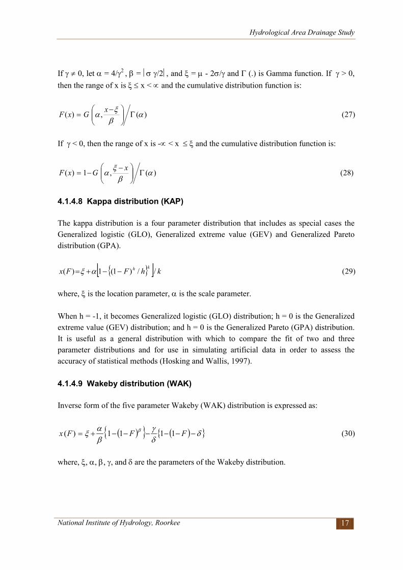
[ ] )26(/)(1log)( 1 αξφ −−−= − xkkxF where, ξ, α and k are its location, scale and shape parameters respectively. When k = 0, it becomes normal distribution with parameters ξ and α. This distribution has no explicit analytical inverse form. 4.1.4.7 Pearson Type-III distribution (PT-III) The inverse form of the Pearson type-III distribution is not explicitly defined. Hosking and Wallis (1997) mention that the Pearson type-III distribution combines Gamma distributions (which have positive skewness), reflected Gamma distributions (which have negative skewness) and the normal distribution (which has zero skewness). The authors parameterize the Pearson type-III distribution by its first three conventional moments viz. mean µ, the standard deviation σ, and the skewness γ. The relationship between these parameters and those of the Gamma distribution is as follows. Let X be a random variable with a Pearson type-III distribution with parameters µ , σ and γ. If γ > 0, then X - µ + 2 σ/γ has a Gamma distribution with parameters α = 4/γ2, β = σ γ/2. If γ = 0, then X has normal distribution with mean µ and standard deviation σ. If γ < 0, then -X + µ - 2 σ/γ has a Gamma distribution with parameters α = 4/γ2, β = σ γ/2.
Hydrological Area Drainage Study
National Institute of Hydrology, Roorkee 17
If γ ≠ 0, let α = 4/γ2 , β = σ γ/2, and ξ = µ - 2σ/γ and Γ (.) is Gamma function. If γ > 0, then the range of x is ξ ≤ x < ∝ and the cumulative distribution function is:
)27()(,)( αβξα Γ
−=
xGxF
If γ < 0, then the range of x is -∝ < x ≤ ξ and the cumulative distribution function is:
)28()(,1)( αβ
ξα Γ
−−=
xGxF
4.1.4.8 Kappa distribution (KAP) The kappa distribution is a four parameter distribution that includes as special cases the Generalized logistic (GLO), Generalized extreme value (GEV) and Generalized Pareto distribution (GPA).
[ ] )29(//)1(1)( khFFx kh−−+= αξ where, ξ is the location parameter, α is the scale parameter. When h = -1, it becomes Generalized logistic (GLO) distribution; h = 0 is the Generalized extreme value (GEV) distribution; and h = 0 is the Generalized Pareto (GPA) distribution. It is useful as a general distribution with which to compare the fit of two and three parameter distributions and for use in simulating artificial data in order to assess the accuracy of statistical methods (Hosking and Wallis, 1997).
4.1.4.9 Wakeby distribution (WAK) Inverse form of the five parameter Wakeby (WAK) distribution is expressed as:
( ) ( ) )30(1111)( δδγ
βαξ β −−−−−−+= FFFx
where, ξ, α, β, γ, and δ are the parameters of the Wakeby distribution.
Hydrological Area Drainage Study
National Institute of Hydrology, Roorkee 18
4.1.5 Goodness of fit measures In a realistically homogeneous region, all the sites follow the same frequency distribution. But as some heterogeneity is usually present in a region so no single distribution is expected to provide a true fit for all the sites of the region. In regional flood frequency analysis the aim is to identify a distribution which will yield reasonably accurate quantile estimates for each site of the homogeneous region. Assessment of validity of the candidate distribution may be made on the basis of how well the distribution fits the observed data. The goodness of fit measure assesses the relative performance of various fitted distributions and help in identifying the robust viz. most appropriate distribution for the region. A number of methods are available for testing goodness of fit of the proposed flood frequency analysis models. These include Chi-square test, Kolmogorov-Smirnov test, descriptive ability tests and the predictive ability tests. Cunnane (1989) has brought out a comprehensive description of the descriptive ability tests and the predictive ability tests. Apart from the aforementioned tests the recently introduced L-moment ratio diagram based on the approximations given by Hosking (1991) and the goodness of fit or behaviour analysis measure for a frequency distribution given by statistic dist
iZ described below, are also used to identify the suitable frequency distribution. 4.1.5.1 L-moment ratio diagram The L-moment statistics of a sample reflect every information about the data and provide a satisfactory approximation to the distribution of sample values. The L-moment ratio diagram can therefore be used to identify the underlying frequency distribution. The average L-moment statistics of the region is plotted on the L-moment ratio diagram and the distribution nearest to the plotted point is identified as the underlying frequency distribution. One big advantage of L-moment ratio diagram is that one can compare fit of several distributions using a single graphical instrument (Vogel and Fennessey, 1993). 4.1.5.2 dist
iZ Statistic as a goodness-of-fit measure
In this method also the objective is to identify a distribution which fits the observed data acceptably closely. The goodness of fit is judged by how well the L-Skewness and L-Kurtosis of the fitted distribution match the regional average L-Skewness and L-Kurtosis of the observed data. The goodness-of-fit measure for a distribution is given by statistic
distiZ .
Hydrological Area Drainage Study
National Institute of Hydrology, Roorkee 19
( )
disti
disti
Ridist
iZσ
τ−τ= (31)
where Riτ - weighted regional average of L-moment statistic i, dist
idisti and στ are the
simulated regional average and standard deviation of L-moment statistics i for a given distribution.
The distribution giving the minimum distZ value is considered as the best fit distribution.
When all the three L-moment ratios are considered in the goodness-of-fit test, the distribution that gives the best overall fit when all the three statistics are consider together is selected as the underlying regional frequency distribution. According to Hosking (1993),
distribution is considered to give good fit if distZ is sufficiently close to zero, a reasonable
criteria being ≤distZ 1.64.
Let the homogeneous region has Ns sites with site i having record length ni and sample L-moment ratios ti, t3i & t4i. Steps involved in computation of statistic dist
iZ are:
i. Compute the weighted regional average L-moment ratios.
i
SN
1i
ii
SN
1iR
n
tnt
∑
∑=
=
= (32)
The values of R
4R3 tandt are computed similarly by replacing ti by t3i and t4i
respectively.
ii. Fit the candidate distribution to the regional average L-moment ratios tR, R4
R3 tandt
and mean = 1. iii. Use the fitted distribution to simulate a number of regions, say 500, having same
record length as the observed data. iv. Repeat step 1 for each simulated region and the weighted regional average for the
simulations are taken as R
1t , R500
R2 t...t and similarly for R
4R3 t&t .
v. Compute the mean ( )dist
iτ and standard deviation ( )distiσ for the values computed in
step 4 above for each L-moment statistic i.
Hydrological Area Drainage Study
National Institute of Hydrology, Roorkee 20
vi. Goodness-of-fit measure distiZ is computed as dist
i
disti
Ridist
iZσ
τ−τ= (33)
vii. Repeat the steps 2 to 6 for each of the distributions. Distribution giving the minimum distiZ value for the L-moment statistics is identified as the best fit distribution.
4.2 Preparation of Digital Elevation Model The two toposheets of 1:50,000 scales obtained from Survey of India were scanned, geo-referenced and projected to 43 North zone of WGS1984 UTM projected coordinate system. Then all the contour lines, spot heights and bench marks from the toposheets are digitised to polyline and point shape files with help of ArcMap. Further, the surveyed contours lines provided by THDC are imported to ArcGIS from Auto Cad file. The DEM is prepared with help of Topo to Raster tool of spatial analyst in ArcMap, which interpolates a hydrologically correct raster surface from point, line, and polygon data. The SRTM DEM is used in for remaining upper portion of the catchment. The prepared DEM of the plant area (prepared from surveyed contour) is Figure 4.1.
Figure 4.1: Digital elevation model of proposed plant area.
Hydrological Area Drainage Study
National Institute of Hydrology, Roorkee 21
4.3 Catchment Delineation and Estimation of Catchment Characteristics
Initially a wide extent of generated DEM has been used to delineate the drainage network in and around the proposed plant area. The HEC-GeoHMS 5.0 package in ArcGIS 9.3 is tried for automatic delineation of catchments from DEM. The Aligarh drain is a natural drain and maintained by U.P. Irrigation Department and there are number of irrigation canals and road with culverts in the catchment area of drain. Moreover, the catchment area is comparatively small with very flat topography. Hence, automatic delineation of catchments from DEM was not very accurate. In such case the catchment area is delineated manually from the SOI topsheets considering the topographic features. 4.4 Derivation of Synthetic Unit Hydrograph The various parameters of the synthetic unit hydrograph are derived from the Flood Estimation Report (CWC, 1984). Detail description of parameter and their relationships are given in Table 4.2. As mentioned in the CWC (1984) report the relationships are for 2- hour unit hydrograph (2-h UH). Hence, after deriving 2-h UH, the S-curve approach was used to develop 1-h UH.
Table 4.2 Relationships for estimating 2-h UH parameters for the study area
Sl. No. Parameters Relationship
1 Peak discharge of unit hydrograph per unit area of catchment (m3/s/ km2)
2 Time in hours from the centre of unit rain fall duration
to the peak of unit hydrograph.
3 Width of UH in hours at 50 percent of peak discharge
4 Width of UH in hours at 75 percent of peak discharge
5 Width of the rising limb of UH in hours at 50 percent
peak discharge
6 Width of the rising limb of UH in hours at 75 percent peak discharge
( )0.6492.030
pqL S
=
1.038
1.858p
p
tq
=
50 0.990
2.217
p
Wq
=
75 0.876
1.477
p
Wq
=
50 0.907
0.812
p
WRq
=
75 0.791
0.606
p
WRq
=

Hydrological Area Drainage Study
National Institute of Hydrology, Roorkee 22
7 Base width of unit hydrograph in hours
8 Peak discharge of unit hydrograph in m3/s Where, L = Length of the main stream (km), S = Equivalent stream slope (m/km), A= Area of the catchment (km2). 4.5 Estimation of Flood Hydrographs Flood hydrographs for various return periods were estimated for 1-day maximum rainfall. The steps for estimating flood hydrographs are discussed in following sections. 4.5.1 Design loss rate Generally infiltration index and the initial losses values are derived from the available rainfall-runoff records for the severe storms in the basin. Assuming the basin would be saturated at the time of design storm the minimum infiltration rate and initial losses values would be considered. The minimum infiltration rate and minimum initial loss, thus obtained, are used to compute the effective rainfall of design storm. For this the initial losses must be subtracted first from the rainfall increments and thereafter a uniform loss rate equal to the minimum infiltration index is applied. Here, a loss rate of 0.3 cm/h is used as recommended in the CWC (1984) report. 4.5.2 Base flow for design flood Base flow is the portion of stream flow that comes from the sum of deep subsurface flow and delayed shallow subsurface flow. CWC (1984) has analyzed total 48 events for estimating base flow. The recommended value of base flow 0.05 m3/s/km2 for Subzone-1(a) is used in this study. 4.5.3 Time adjustment of design rainfall To determine the maximum depths for unrestricted periods and also to obtain short duration (less than 24-hours) increments of rainfall required for small and medium sized catchments, it is necessary to adjust the depth-duration curve of the design storm based on daily data. The Manual on estimation of design flood (CWC, 2001) analysed time distribution pattern of storms in the area for which adequate self recoding rain-gauge data are available. In the manual, depth duration analyses of maximum rainfall depths for standard duration of 6, 12, 18, 24, 36, 48 hours etc., were obtained for each of the storms and expressed as percentage of the total storm depth. Enveloping percentages are then obtained and applied to adjust the design rainfall based on observational day data. In
( )0.7797.744B pT t=
p pQ q A= ×

Hydrological Area Drainage Study
National Institute of Hydrology, Roorkee 23
absence of hourly rainfall data it is recommended to apply a factor of 1.15 to convert 1-day maximum rainfall to 24-h maximum rainfall. 4.5.4 Design storm duration The duration of storm rainfall which causes maximum discharge in a drainage basin is called design storm duration. The flood hydrographs due to 1-day maximum rainfall is correct for clock hour (24-h) and the hourly distribution was made according to recommended in the CWC (1984) report. 4.6 Estimation of Design Flood Hydrographs The flood hydrographs are estimated by first calculating annual maximum rainfall at each rain-gauge station for various return periods obtained from L-moments based rainfall frequency analysis. The regional rainfall is also estimated. The 24 hour rainfall is divided in to incremental hourly rainfall according to time distribution provided in the CWC (1984) report. To obtain the critical sequence of rainfall the largest of increments is placed against the peak of UH, then the next largest against the next UH ordinate and so on until all rainfall increments get arranged. Then the sequence is reversed to get the critical sequence for all spells. In case of 24-h duration rainfall the first and second 12 h blocks are interchanged to get critical situation. The design loss rate is subtracted from the hourly rainfall to obtain effective rainfall hyetograph and the direct runoff hydrograph is estimated by convoluting this effective rainfall with UH. Finally, the base flow is added to obtain design flood hydrograph. 4.7 Flow Simulation and Flood Modelling The flow in Aligarh drain and rainfall induced catchment flooding has been modelled MIKE 21 model. The MIKE 21 has been dynamically linked to the MIKE 11 model, into a single package called MIKE FLOOD developed at the Danish Hydraulic Institute (Rungo and Olesen, 2003) is widely used for flood inundation studies. (Sanders, 2007; Chatterjee et al., 2008; Patro et al., 2009 and Pramanik et al, 2010). The methodology and the working principal of MIKE FLOOD are being discussed in the following sections. 4.7.1 Flow modelling by Mike 11 hydrodynamic model MIKE 11 is a versatile and modular engineering tool for modelling hydrodynamic conditions in rivers, lakes/reservoirs, irrigation canals and other inland water systems. It is a fully dynamic modelling tool for the detailed analysis, design, management and operation of both simple and Complex River and channel systems (DHI, 2004). The hydrodynamic (HD) model is the nucleus of the MIKE 11 modelling system and forms the
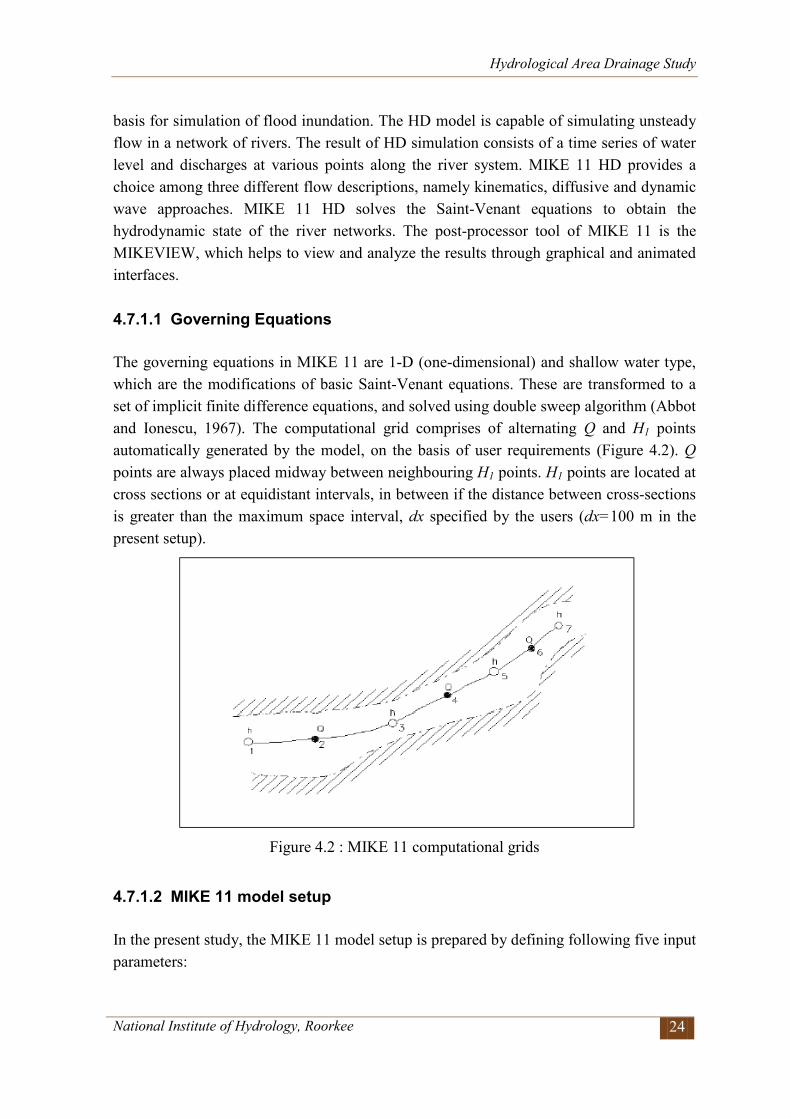
Hydrological Area Drainage Study
National Institute of Hydrology, Roorkee 24
basis for simulation of flood inundation. The HD model is capable of simulating unsteady flow in a network of rivers. The result of HD simulation consists of a time series of water level and discharges at various points along the river system. MIKE 11 HD provides a choice among three different flow descriptions, namely kinematics, diffusive and dynamic wave approaches. MIKE 11 HD solves the Saint-Venant equations to obtain the hydrodynamic state of the river networks. The post-processor tool of MIKE 11 is the MIKEVIEW, which helps to view and analyze the results through graphical and animated interfaces. 4.7.1.1 Governing Equations The governing equations in MIKE 11 are 1-D (one-dimensional) and shallow water type, which are the modifications of basic Saint-Venant equations. These are transformed to a set of implicit finite difference equations, and solved using double sweep algorithm (Abbot and Ionescu, 1967). The computational grid comprises of alternating Q and H1 points automatically generated by the model, on the basis of user requirements (Figure 4.2). Q points are always placed midway between neighbouring H1 points. H1 points are located at cross sections or at equidistant intervals, in between if the distance between cross-sections is greater than the maximum space interval, dx specified by the users (dx=100 m in the present setup).
Figure 4.2 : MIKE 11 computational grids
4.7.1.2 MIKE 11 model setup In the present study, the MIKE 11 model setup is prepared by defining following five input parameters:
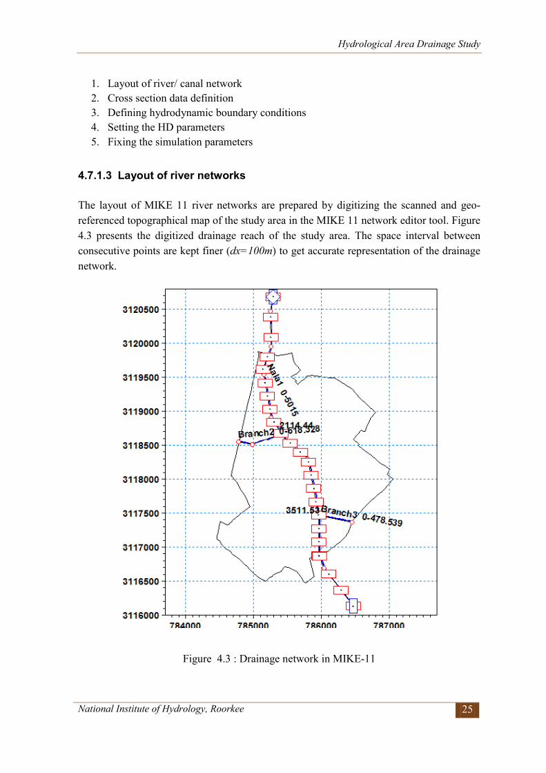
Hydrological Area Drainage Study
National Institute of Hydrology, Roorkee 25
1. Layout of river/ canal network 2. Cross section data definition 3. Defining hydrodynamic boundary conditions 4. Setting the HD parameters 5. Fixing the simulation parameters
4.7.1.3 Layout of river networks The layout of MIKE 11 river networks are prepared by digitizing the scanned and geo-referenced topographical map of the study area in the MIKE 11 network editor tool. Figure 4.3 presents the digitized drainage reach of the study area. The space interval between consecutive points are kept finer (dx=100m) to get accurate representation of the drainage network.
Figure 4.3 : Drainage network in MIKE-11
Hydrological Area Drainage Study
National Institute of Hydrology, Roorkee 26
4.7.1.4 Cross section data definition The topographical description of the area to be modelled is achieved through the specification of cross-sections of the drains, which lie approximately perpendicular to the direction of flow. Cross-sections are specified by a number of x-z co-ordinates where x is the transverse distance from a fixed point (often left bank top) and z is the corresponding bed elevation. Physically there should be a sufficient number of cross-sections to define adequately the variation in river shape. In the present study the actual measured cross-sections provided by THDC are used. The x-z co-ordinates are entered as raw data in the cross-section editor. The raw data are then automatically processed into a form used in the hydrodynamic calculations, i.e. the hydraulic parameters; cross-sectional area, hydraulic radius and width are calculated for a number of elevations between a minimum and a maximum which are either determined automatically or may be user specified. 4.7.1.5 Hydrodynamic boundary condition definition Boundary conditions are required at all model boundaries, i.e. upstream and downstream ends of model branch which are not connected at any junction. The boundary conditions may be internal or external. The internal boundary condition includes the specifications at nodal points and structures, whereas the external boundary condition includes the specification of constant values of H or Q or time varying values of Q or H at start and end points. In the present setup there are three branches, each having two open hydrodynamic boundaries. The upstream boundary condition for Aligarh drain is given as design discharge. The downstream boundary condition is given as constant water level.
4.7.1.6 Setting the HD parameters The HD parameters, in the present study, include the initial conditions of water level and discharge, friction coefficient (n) and output parameters options. Initial conditions are required to avoid the dry bed conditions. The n value is specified as 0.033. The global value for the initial condition for water level is kept at a low value of 0.01m to avoid dry bed conditions.
4.7.1.7 Fixing the simulation parameters Before running the model simulation, control parameters such as simulation period, simulation time step, data to be stored and storage time have to be specified. The simulation periods are specified by start and end dates specified by year, month, day and hour and minute. MIKE 11 checks the actual time and reads all the data given in the time series during the simulation. There exists a versatile relationship between the time step and
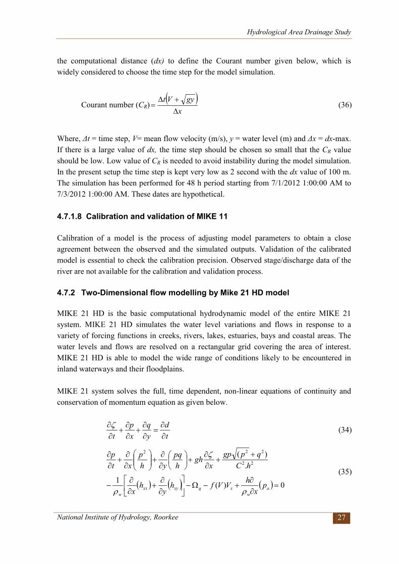
Hydrological Area Drainage Study
National Institute of Hydrology, Roorkee 27
the computational distance (dx) to define the Courant number given below, which is widely considered to choose the time step for the model simulation.
Courant number (CR)( )
xgyVt
∆+∆
= (36)
Where, Δt = time step, V= mean flow velocity (m/s), y = water level (m) and Δx = dx-max. If there is a large value of dx, the time step should be chosen so small that the CR value should be low. Low value of CR is needed to avoid instability during the model simulation. In the present setup the time step is kept very low as 2 second with the dx value of 100 m. The simulation has been performed for 48 h period starting from 7/1/2012 1:00:00 AM to 7/3/2012 1:00:00 AM. These dates are hypothetical. 4.7.1.8 Calibration and validation of MIKE 11 Calibration of a model is the process of adjusting model parameters to obtain a close agreement between the observed and the simulated outputs. Validation of the calibrated model is essential to check the calibration precision. Observed stage/discharge data of the river are not available for the calibration and validation process. 4.7.2 Two-Dimensional flow modelling by Mike 21 HD model MIKE 21 HD is the basic computational hydrodynamic model of the entire MIKE 21 system. MIKE 21 HD simulates the water level variations and flows in response to a variety of forcing functions in creeks, rivers, lakes, estuaries, bays and coastal areas. The water levels and flows are resolved on a rectangular grid covering the area of interest. MIKE 21 HD is able to model the wide range of conditions likely to be encountered in inland waterways and their floodplains. MIKE 21 system solves the full, time dependent, non-linear equations of continuity and conservation of momentum equation as given below.
td
yq
xp
t ∂∂
=∂∂
+∂∂
+∂∂ζ (34)
( ) ( ) ( ) 0)(1
.)(
22
222
=∂∂
+−Ω−
∂∂
+∂∂
−
++
∂∂
+
∂∂
+
∂∂
+∂∂
aw
xqxyxxw
px
hVVfhy
hx
hCqpgp
xgh
hpq
yhp
xtp
ρρ
ζ
(35)
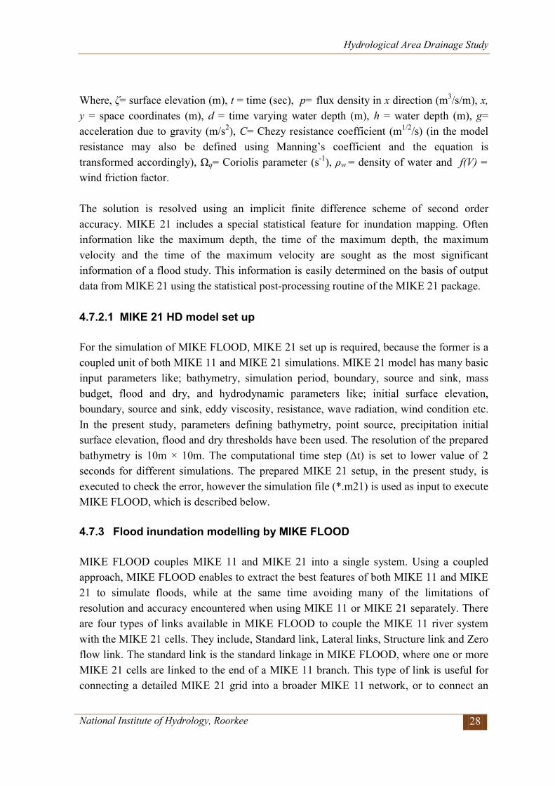
Hydrological Area Drainage Study
National Institute of Hydrology, Roorkee 28
Where, ζ= surface elevation (m), t = time (sec), p= flux density in x direction (m3/s/m), x, y = space coordinates (m), d = time varying water depth (m), h = water depth (m), g= acceleration due to gravity (m/s2), C= Chezy resistance coefficient (m1/2/s) (in the model resistance may also be defined using Manning’s coefficient and the equation is transformed accordingly), Ωq= Coriolis parameter (s-1), ρw = density of water and f(V) = wind friction factor. The solution is resolved using an implicit finite difference scheme of second order accuracy. MIKE 21 includes a special statistical feature for inundation mapping. Often information like the maximum depth, the time of the maximum depth, the maximum velocity and the time of the maximum velocity are sought as the most significant information of a flood study. This information is easily determined on the basis of output data from MIKE 21 using the statistical post-processing routine of the MIKE 21 package. 4.7.2.1 MIKE 21 HD model set up For the simulation of MIKE FLOOD, MIKE 21 set up is required, because the former is a coupled unit of both MIKE 11 and MIKE 21 simulations. MIKE 21 model has many basic input parameters like; bathymetry, simulation period, boundary, source and sink, mass budget, flood and dry, and hydrodynamic parameters like; initial surface elevation, boundary, source and sink, eddy viscosity, resistance, wave radiation, wind condition etc. In the present study, parameters defining bathymetry, point source, precipitation initial surface elevation, flood and dry thresholds have been used. The resolution of the prepared bathymetry is 10m × 10m. The computational time step (Δt) is set to lower value of 2 seconds for different simulations. The prepared MIKE 21 setup, in the present study, is executed to check the error, however the simulation file (*.m21) is used as input to execute MIKE FLOOD, which is described below. 4.7.3 Flood inundation modelling by MIKE FLOOD MIKE FLOOD couples MIKE 11 and MIKE 21 into a single system. Using a coupled approach, MIKE FLOOD enables to extract the best features of both MIKE 11 and MIKE 21 to simulate floods, while at the same time avoiding many of the limitations of resolution and accuracy encountered when using MIKE 11 or MIKE 21 separately. There are four types of links available in MIKE FLOOD to couple the MIKE 11 river system with the MIKE 21 cells. They include, Standard link, Lateral links, Structure link and Zero flow link. The standard link is the standard linkage in MIKE FLOOD, where one or more MIKE 21 cells are linked to the end of a MIKE 11 branch. This type of link is useful for connecting a detailed MIKE 21 grid into a broader MIKE 11 network, or to connect an
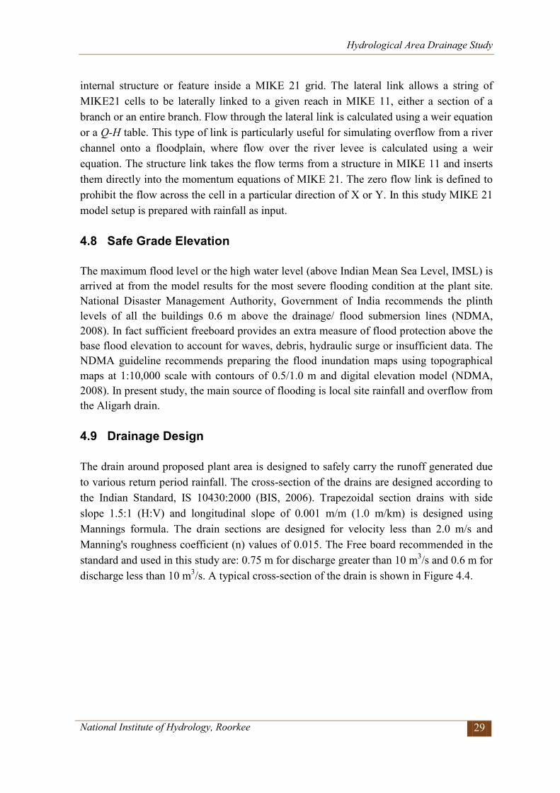
Hydrological Area Drainage Study
National Institute of Hydrology, Roorkee 29
internal structure or feature inside a MIKE 21 grid. The lateral link allows a string of MIKE21 cells to be laterally linked to a given reach in MIKE 11, either a section of a branch or an entire branch. Flow through the lateral link is calculated using a weir equation or a Q-H table. This type of link is particularly useful for simulating overflow from a river channel onto a floodplain, where flow over the river levee is calculated using a weir equation. The structure link takes the flow terms from a structure in MIKE 11 and inserts them directly into the momentum equations of MIKE 21. The zero flow link is defined to prohibit the flow across the cell in a particular direction of X or Y. In this study MIKE 21 model setup is prepared with rainfall as input. 4.8 Safe Grade Elevation The maximum flood level or the high water level (above Indian Mean Sea Level, IMSL) is arrived at from the model results for the most severe flooding condition at the plant site. National Disaster Management Authority, Government of India recommends the plinth levels of all the buildings 0.6 m above the drainage/ flood submersion lines (NDMA, 2008). In fact sufficient freeboard provides an extra measure of flood protection above the base flood elevation to account for waves, debris, hydraulic surge or insufficient data. The NDMA guideline recommends preparing the flood inundation maps using topographical maps at 1:10,000 scale with contours of 0.5/1.0 m and digital elevation model (NDMA, 2008). In present study, the main source of flooding is local site rainfall and overflow from the Aligarh drain. 4.9 Drainage Design The drain around proposed plant area is designed to safely carry the runoff generated due to various return period rainfall. The cross-section of the drains are designed according to the Indian Standard, IS 10430:2000 (BIS, 2006). Trapezoidal section drains with side slope 1.5:1 (H:V) and longitudinal slope of 0.001 m/m (1.0 m/km) is designed using Mannings formula. The drain sections are designed for velocity less than 2.0 m/s and Manning's roughness coefficient (n) values of 0.015. The Free board recommended in the standard and used in this study are: 0.75 m for discharge greater than 10 m3/s and 0.6 m for discharge less than 10 m3/s. A typical cross-section of the drain is shown in Figure 4.4.
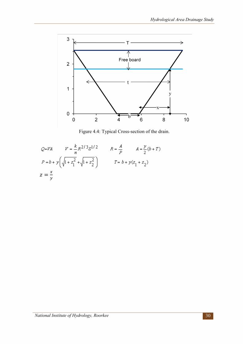
Hydrological Area Drainage Study
National Institute of Hydrology, Roorkee 30
Figure 4.4: Typical Cross-section of the drain.
𝑧 = 𝑥
𝑦
b
y
x
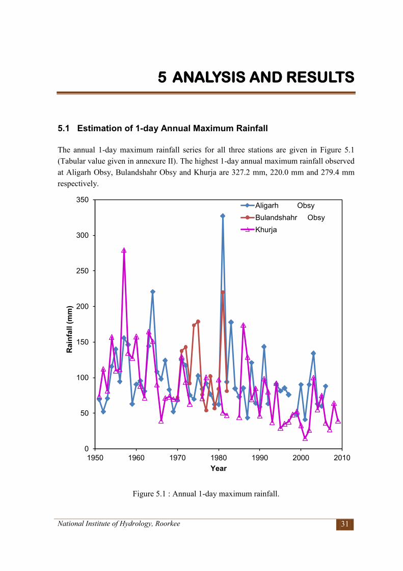
National Institute of Hydrology, Roorkee 31
5 ANALYSIS AND RESULTS
5.1 Estimation of 1-day Annual Maximum Rainfall The annual 1-day maximum rainfall series for all three stations are given in Figure 5.1 (Tabular value given in annexure II). The highest 1-day annual maximum rainfall observed at Aligarh Obsy, Bulandshahr Obsy and Khurja are 327.2 mm, 220.0 mm and 279.4 mm respectively.
Figure 5.1 : Annual 1-day maximum rainfall.
0
50
100
150
200
250
300
350
1950 1960 1970 1980 1990 2000 2010
Rai
nfal
l (m
m)
Year
Aligarh Obsy Bulandshahr Obsy Khurja
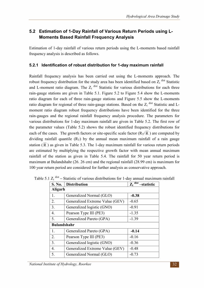
Hydrological Area Drainage Study
National Institute of Hydrology, Roorkee 32
5.2 Estimation of 1-Day Rainfall of Various Return Periods using L-Moments Based Rainfall Frequency Analysis
Estimation of 1-day rainfall of various return periods using the L-moments based rainfall frequency analysis is described as follows. 5.2.1 Identification of robust distribution for 1-day maximum rainfall Rainfall frequency analysis has been carried out using the L-moments approach. The robust frequency distribution for the study area has been identified based on Zi dist Statistic and L-moment ratio diagram. The Zi dist Statistic for various distributions for each three rain-gauge stations are given in Table 5.1. Figure 5.2 to Figure 5.4 show the L-moments ratio diagram for each of three rain-gauge stations and Figure 5.5 show the L-moments ratio diagram for regional of three rain-gauge stations. Based on the Zi dist Statistic and L-moment ratio diagram robust frequency distributions have been identified for the three rain-gauges and the regional rainfall frequency analysis procedure. The parameters for various distributions for 1-day maximum rainfall are given in Table 5.2. The first row of the parameter values (Table 5.2) shows the robust identified frequency distributions for each of the cases. The growth factors or site-specific scale factor (RT/ R ) are computed by dividing rainfall quantile (RT) by the annual mean maximum rainfall of a rain gauge station ( R ) as given in Table 5.3. The 1-day maximum rainfall for various return periods are estimated by multiplying the respective growth factor with mean annual maximum rainfall of the station as given in Table 5.4. The rainfall for 50 year return period is maximum at Bulandshahr (26. 26 cm) and the regional rainfall (28.99 cm) is maximum for 100 year return period are considered for further analysis as conservative approach.
Table 5.1 Zi dist – Statistic of various distributions for 1-day annual maximum rainfall S. No. Distribution Zi dist –statistic Aligarh 1. Generalized Normal (GLO) -0.38 2. Generalized Extreme Value (GEV) -0.65 3. Generalized logistic (GNO) -0.91 4. Pearson Type III (PE3) -1.35 5. Generalized Pareto (GPA) -1.39 Bulandshahr 1. Generalized Pareto (GPA) -0.14 2. Pearson Type III (PE3) -0.16 3. Generalized logistic (GNO) -0.36 4. Generalized Extreme Value (GEV) -0.48 5. Generalized Normal (GLO) -0.73
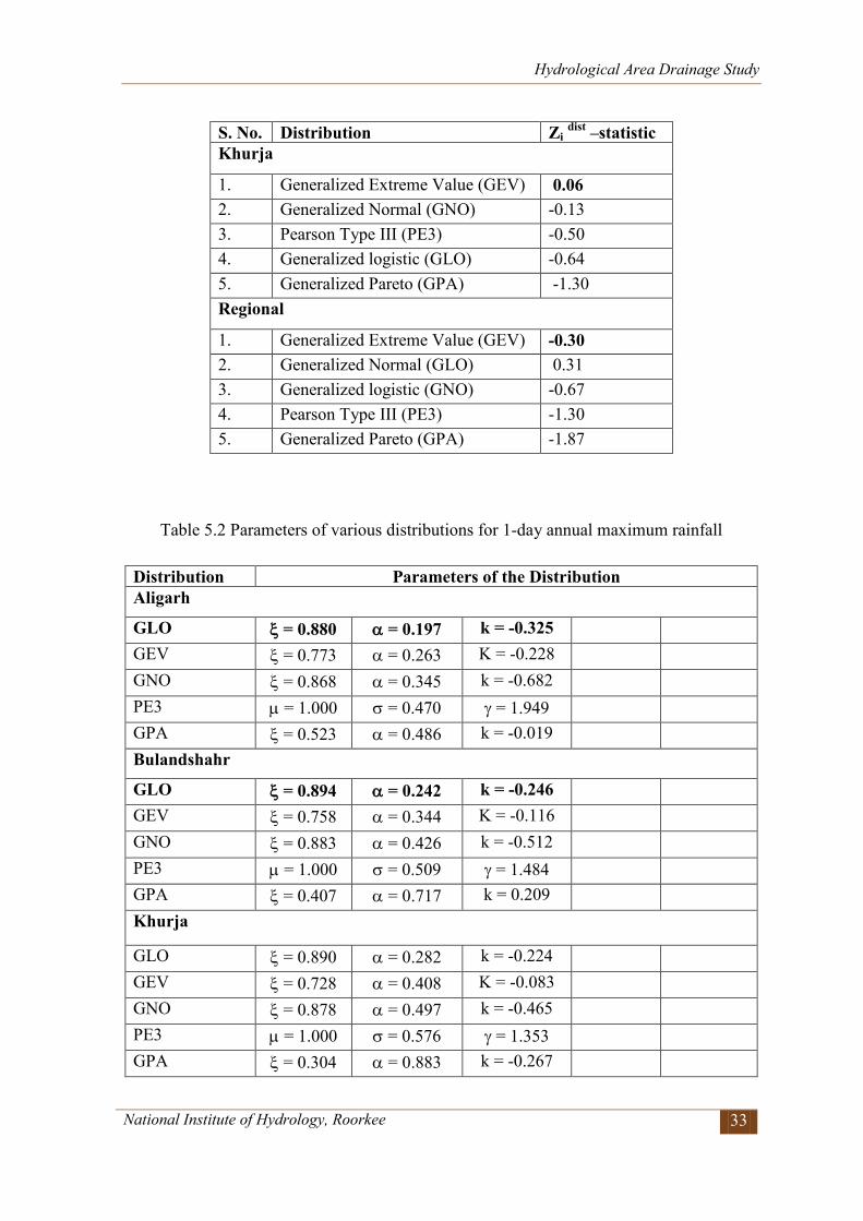
Hydrological Area Drainage Study
National Institute of Hydrology, Roorkee 33
S. No. Distribution Zi dist –statistic Khurja
1. Generalized Extreme Value (GEV) 0.06 2. Generalized Normal (GNO) -0.13 3. Pearson Type III (PE3) -0.50 4. Generalized logistic (GLO) -0.64 5. Generalized Pareto (GPA) -1.30 Regional
1. Generalized Extreme Value (GEV) -0.30 2. Generalized Normal (GLO) 0.31 3. Generalized logistic (GNO) -0.67 4. Pearson Type III (PE3) -1.30 5. Generalized Pareto (GPA) -1.87
Table 5.2 Parameters of various distributions for 1-day annual maximum rainfall
Distribution Parameters of the Distribution Aligarh
GLO ξ = 0.880 α = 0.197 k = -0.325 GEV ξ = 0.773 α = 0.263 K = -0.228 GNO ξ = 0.868 α = 0.345 k = -0.682 PE3 µ = 1.000 σ = 0.470 γ = 1.949 GPA ξ = 0.523 α = 0.486 k = -0.019 Bulandshahr
GLO ξ = 0.894 α = 0.242 k = -0.246 GEV ξ = 0.758 α = 0.344 K = -0.116 GNO ξ = 0.883 α = 0.426 k = -0.512 PE3 µ = 1.000 σ = 0.509 γ = 1.484 GPA ξ = 0.407 α = 0.717 k = 0.209 Khurja
GLO ξ = 0.890 α = 0.282 k = -0.224 GEV ξ = 0.728 α = 0.408 K = -0.083 GNO ξ = 0.878 α = 0.497 k = -0.465 PE3 µ = 1.000 σ = 0.576 γ = 1.353 GPA ξ = 0.304 α = 0.883 k = -0.267
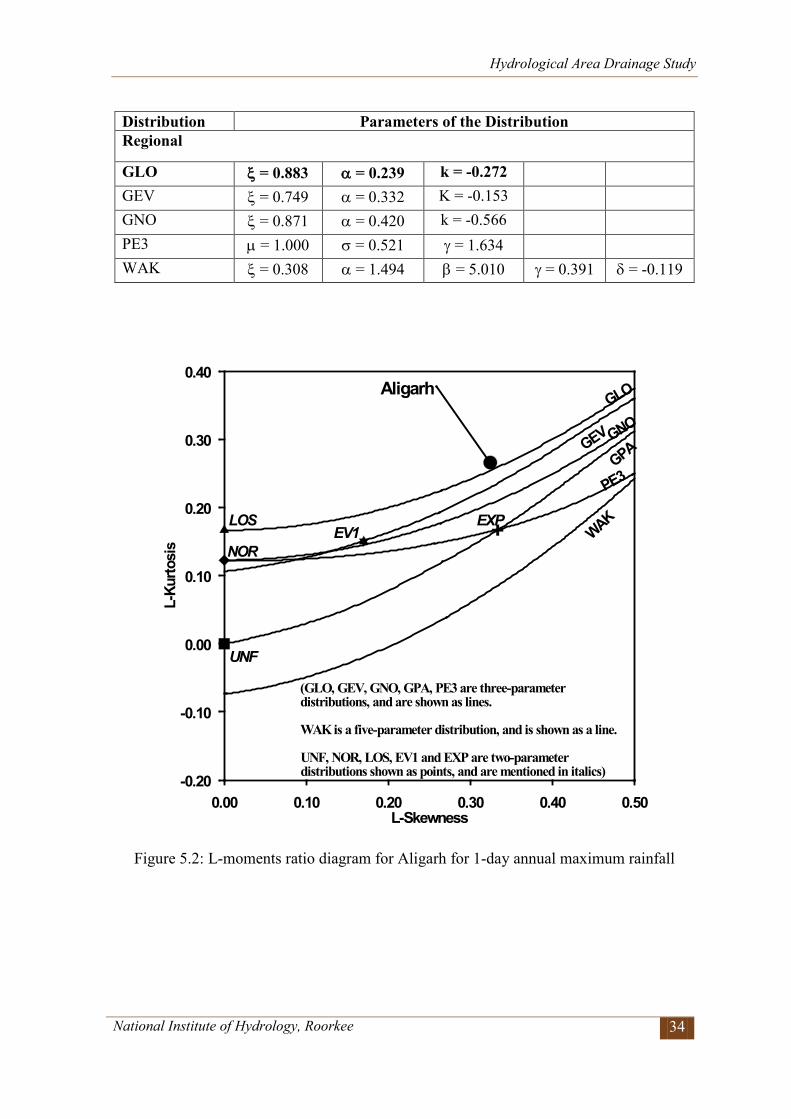
Hydrological Area Drainage Study
National Institute of Hydrology, Roorkee 34
Distribution Parameters of the Distribution Regional
GLO ξ = 0.883 α = 0.239 k = -0.272 GEV ξ = 0.749 α = 0.332 K = -0.153 GNO ξ = 0.871 α = 0.420 k = -0.566 PE3 µ = 1.000 σ = 0.521 γ = 1.634 WAK ξ = 0.308 α = 1.494 β = 5.010 γ = 0.391 δ = -0.119
Figure 5.2: L-moments ratio diagram for Aligarh for 1-day annual maximum rainfall
0.10 0.30 0.500.00 0.20 0.40L-Skewness
-0.10
0.10
0.30
-0.20
0.00
0.20
0.40
L-Ku
rtosi
s
GLO
GEV GNO
GPA
PE3
WAKEXPEV1
LOS
NOR
UNF
(GLO, GEV, GNO, GPA, PE3 are three-parameter distributions, and are shown as lines.
WAK is a five-parameter distribution, and is shown as a line.
UNF, NOR, LOS, EV1 and EXP are two-parameterdistributions shown as points, and are mentioned in italics)
Aligarh
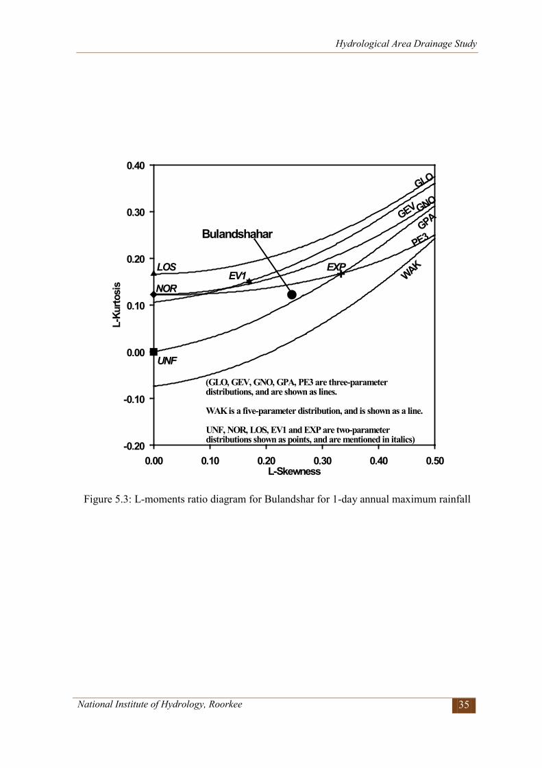
Hydrological Area Drainage Study
National Institute of Hydrology, Roorkee 35
Figure 5.3: L-moments ratio diagram for Bulandshar for 1-day annual maximum rainfall
0.10 0.30 0.500.00 0.20 0.40L-Skewness
-0.10
0.10
0.30
-0.20
0.00
0.20
0.40
L-Ku
rtosi
s
GLO
GEV GNO
GPA
PE3
WAKEXPEV1
LOS
NOR
UNF
(GLO, GEV, GNO, GPA, PE3 are three-parameter distributions, and are shown as lines.
WAK is a five-parameter distribution, and is shown as a line.
UNF, NOR, LOS, EV1 and EXP are two-parameterdistributions shown as points, and are mentioned in italics)
Bulandshahar
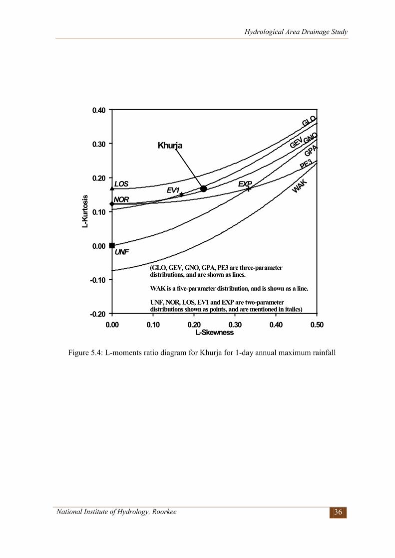
Hydrological Area Drainage Study
National Institute of Hydrology, Roorkee 36
Figure 5.4: L-moments ratio diagram for Khurja for 1-day annual maximum rainfall
0.10 0.30 0.500.00 0.20 0.40L-Skewness
-0.10
0.10
0.30
-0.20
0.00
0.20
0.40
L-Ku
rtosi
s
GLO
GEV GNO
GPA
PE3
WAKEXPEV1
LOS
NOR
UNF
(GLO, GEV, GNO, GPA, PE3 are three-parameter distributions, and are shown as lines.
WAK is a five-parameter distribution, and is shown as a line.
UNF, NOR, LOS, EV1 and EXP are two-parameterdistributions shown as points, and are mentioned in italics)
Khurja
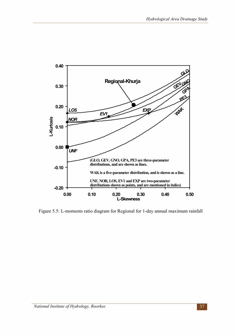
Hydrological Area Drainage Study
National Institute of Hydrology, Roorkee 37
Figure 5.5: L-moments ratio diagram for Regional for 1-day annual maximum rainfall
0.10 0.30 0.500.00 0.20 0.40L-Skewness
-0.10
0.10
0.30
-0.20
0.00
0.20
0.40
L-Ku
rtosi
s
GLO
GEV GNO
GPA
PE3
WAKEXPEV1
LOS
NOR
UNF
(GLO, GEV, GNO, GPA, PE3 are three-parameter distributions, and are shown as lines.
WAK is a five-parameter distribution, and is shown as a line.
UNF, NOR, LOS, EV1 and EXP are two-parameterdistributions shown as points, and are mentioned in italics)
Regional-Khurja
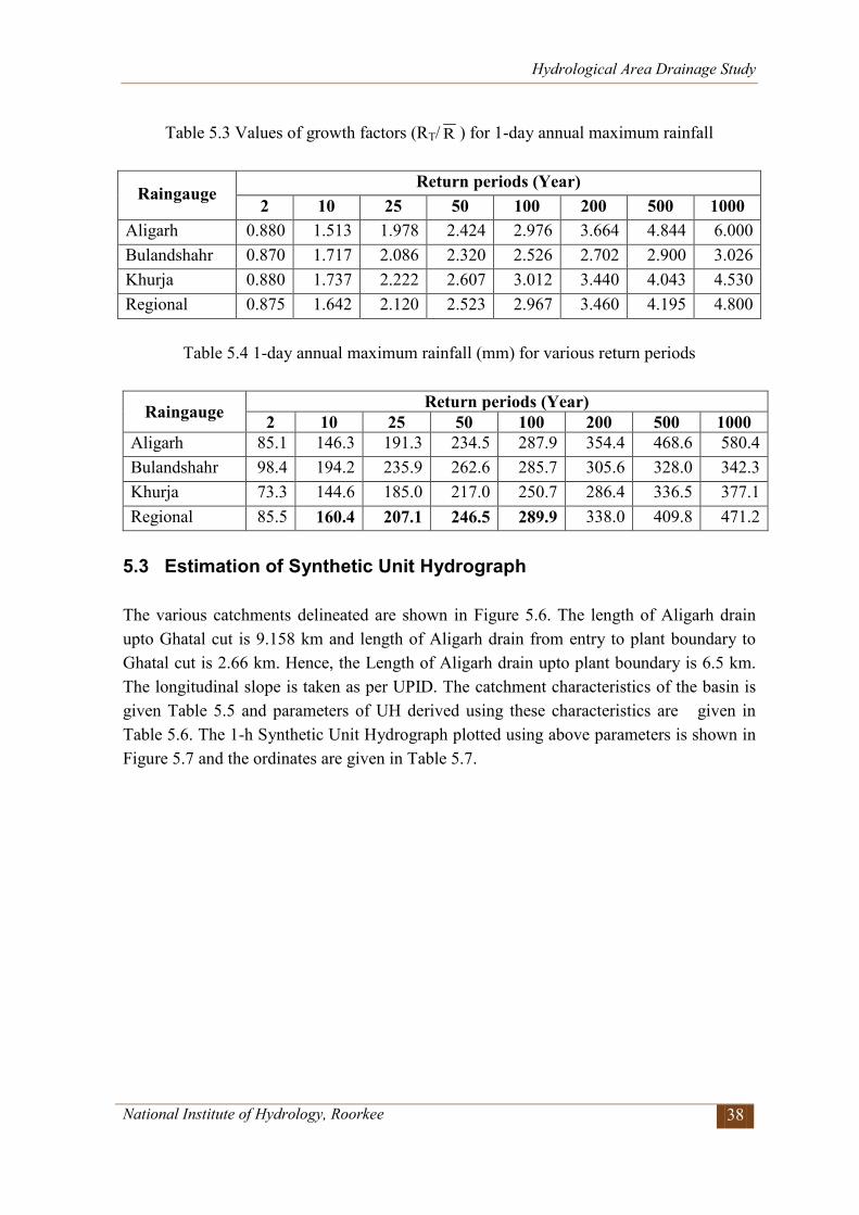
Hydrological Area Drainage Study
National Institute of Hydrology, Roorkee 38
Table 5.3 Values of growth factors (RT/ R ) for 1-day annual maximum rainfall
Raingauge Return periods (Year)
2 10 25 50 100 200 500 1000 Aligarh 0.880 1.513 1.978 2.424 2.976 3.664 4.844 6.000 Bulandshahr 0.870 1.717 2.086 2.320 2.526 2.702 2.900 3.026 Khurja 0.880 1.737 2.222 2.607 3.012 3.440 4.043 4.530 Regional 0.875 1.642 2.120 2.523 2.967 3.460 4.195 4.800
Table 5.4 1-day annual maximum rainfall (mm) for various return periods
Raingauge Return periods (Year) 2 10 25 50 100 200 500 1000
Aligarh 85.1 146.3 191.3 234.5 287.9 354.4 468.6 580.4 Bulandshahr 98.4 194.2 235.9 262.6 285.7 305.6 328.0 342.3 Khurja 73.3 144.6 185.0 217.0 250.7 286.4 336.5 377.1 Regional 85.5 160.4 207.1 246.5 289.9 338.0 409.8 471.2
5.3 Estimation of Synthetic Unit Hydrograph The various catchments delineated are shown in Figure 5.6. The length of Aligarh drain upto Ghatal cut is 9.158 km and length of Aligarh drain from entry to plant boundary to Ghatal cut is 2.66 km. Hence, the Length of Aligarh drain upto plant boundary is 6.5 km. The longitudinal slope is taken as per UPID. The catchment characteristics of the basin is given Table 5.5 and parameters of UH derived using these characteristics are given in Table 5.6. The 1-h Synthetic Unit Hydrograph plotted using above parameters is shown in Figure 5.7 and the ordinates are given in Table 5.7.
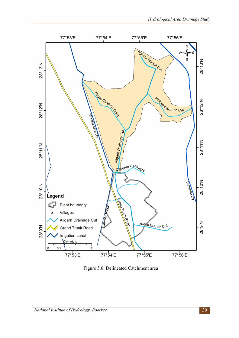
Hydrological Area Drainage Study
National Institute of Hydrology, Roorkee 39
Figure 5.6: Delineated Catchment area
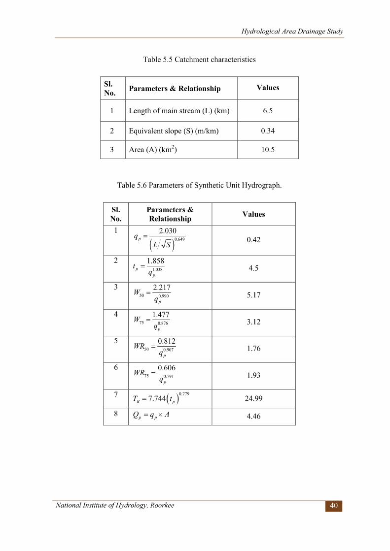
Hydrological Area Drainage Study
National Institute of Hydrology, Roorkee 40
Table 5.5 Catchment characteristics
Sl. No. Parameters & Relationship Values
1 Length of main stream (L) (km) 6.5
2 Equivalent slope (S) (m/km) 0.34
3 Area (A) (km2) 10.5
Table 5.6 Parameters of Synthetic Unit Hydrograph.
Sl. No.
Parameters & Relationship Values
1
0.42
2
4.5
3
5.17
4
3.12
5
1.76
6
1.93
7 24.99
8 4.46
( )0.6492.030
pqL S
=
1.038
1.858p
p
tq
=
50 0.990
2.217
p
Wq
=
75 0.876
1.477
p
Wq
=
50 0.907
0.812
p
WRq
=
75 0.791
0.606
p
WRq
=
( )0.7797.744B pT t=
p pQ q A= ×
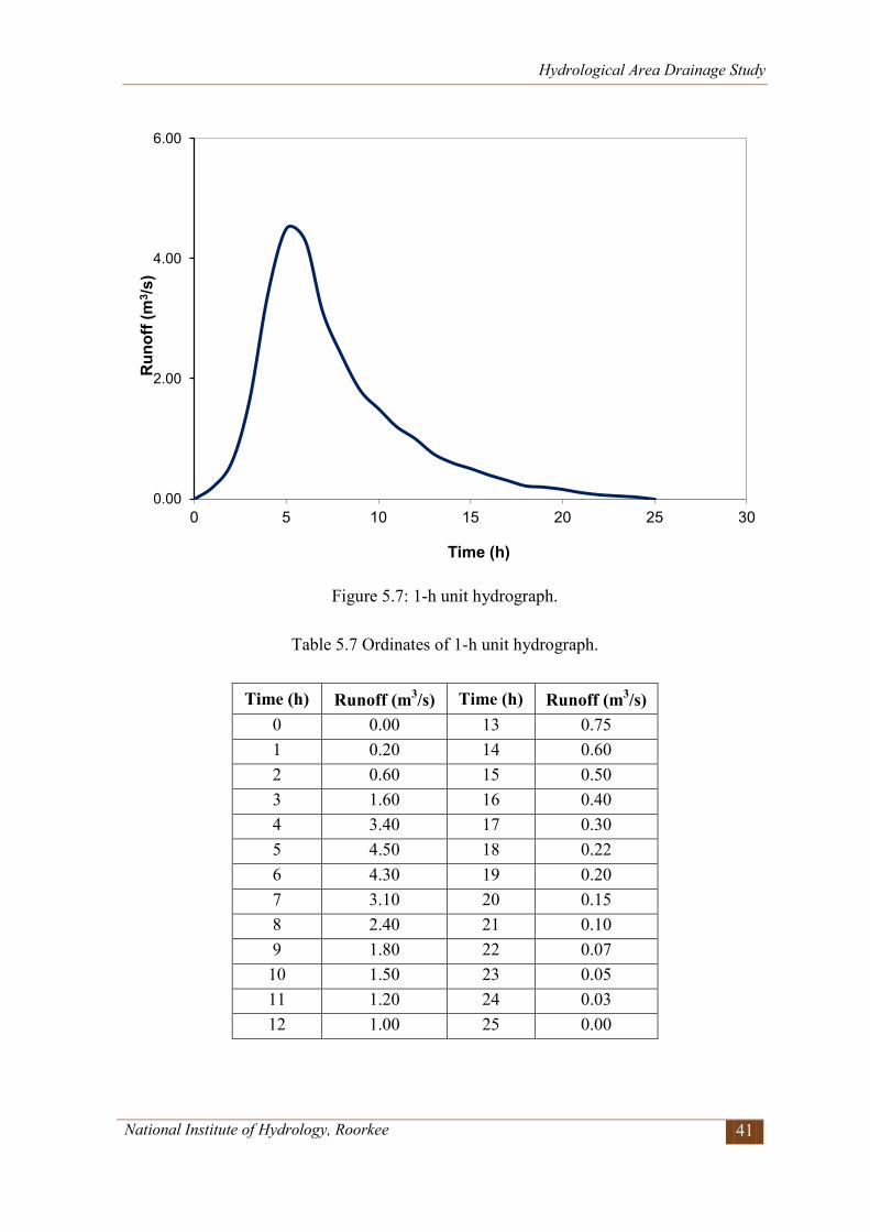
Hydrological Area Drainage Study
National Institute of Hydrology, Roorkee 41
Figure 5.7: 1-h unit hydrograph.
Table 5.7 Ordinates of 1-h unit hydrograph.
Time (h) Runoff (m3/s) Time (h) Runoff (m3/s) 0 0.00 13 0.75 1 0.20 14 0.60 2 0.60 15 0.50 3 1.60 16 0.40 4 3.40 17 0.30 5 4.50 18 0.22 6 4.30 19 0.20 7 3.10 20 0.15 8 2.40 21 0.10 9 1.80 22 0.07 10 1.50 23 0.05 11 1.20 24 0.03 12 1.00 25 0.00
0.00
2.00
4.00
6.00
0 5 10 15 20 25 30
Run
off (
m3 /s
)
Time (h)
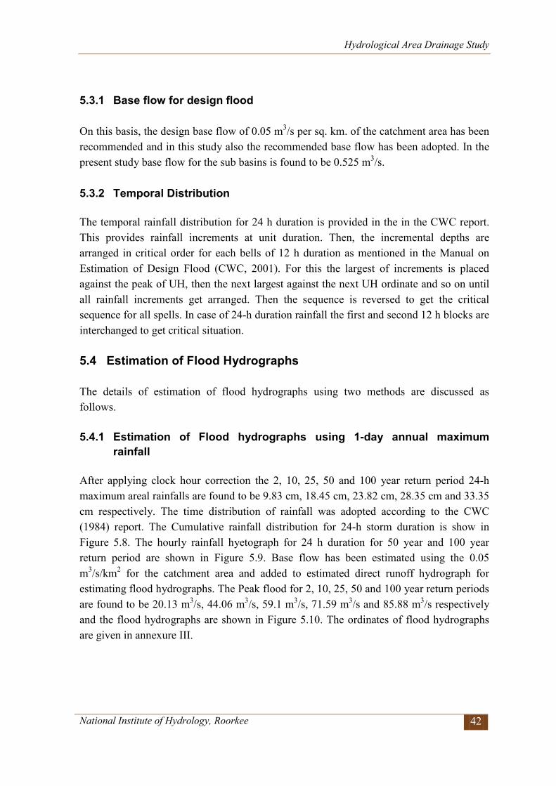
Hydrological Area Drainage Study
National Institute of Hydrology, Roorkee 42
5.3.1 Base flow for design flood On this basis, the design base flow of 0.05 m3/s per sq. km. of the catchment area has been recommended and in this study also the recommended base flow has been adopted. In the present study base flow for the sub basins is found to be 0.525 m3/s. 5.3.2 Temporal Distribution The temporal rainfall distribution for 24 h duration is provided in the in the CWC report. This provides rainfall increments at unit duration. Then, the incremental depths are arranged in critical order for each bells of 12 h duration as mentioned in the Manual on Estimation of Design Flood (CWC, 2001). For this the largest of increments is placed against the peak of UH, then the next largest against the next UH ordinate and so on until all rainfall increments get arranged. Then the sequence is reversed to get the critical sequence for all spells. In case of 24-h duration rainfall the first and second 12 h blocks are interchanged to get critical situation. 5.4 Estimation of Flood Hydrographs The details of estimation of flood hydrographs using two methods are discussed as follows. 5.4.1 Estimation of Flood hydrographs using 1-day annual maximum
rainfall After applying clock hour correction the 2, 10, 25, 50 and 100 year return period 24-h maximum areal rainfalls are found to be 9.83 cm, 18.45 cm, 23.82 cm, 28.35 cm and 33.35 cm respectively. The time distribution of rainfall was adopted according to the CWC (1984) report. The Cumulative rainfall distribution for 24-h storm duration is show in Figure 5.8. The hourly rainfall hyetograph for 24 h duration for 50 year and 100 year return period are shown in Figure 5.9. Base flow has been estimated using the 0.05 m3/s/km2 for the catchment area and added to estimated direct runoff hydrograph for estimating flood hydrographs. The Peak flood for 2, 10, 25, 50 and 100 year return periods are found to be 20.13 m3/s, 44.06 m3/s, 59.1 m3/s, 71.59 m3/s and 85.88 m3/s respectively and the flood hydrographs are shown in Figure 5.10. The ordinates of flood hydrographs are given in annexure III.
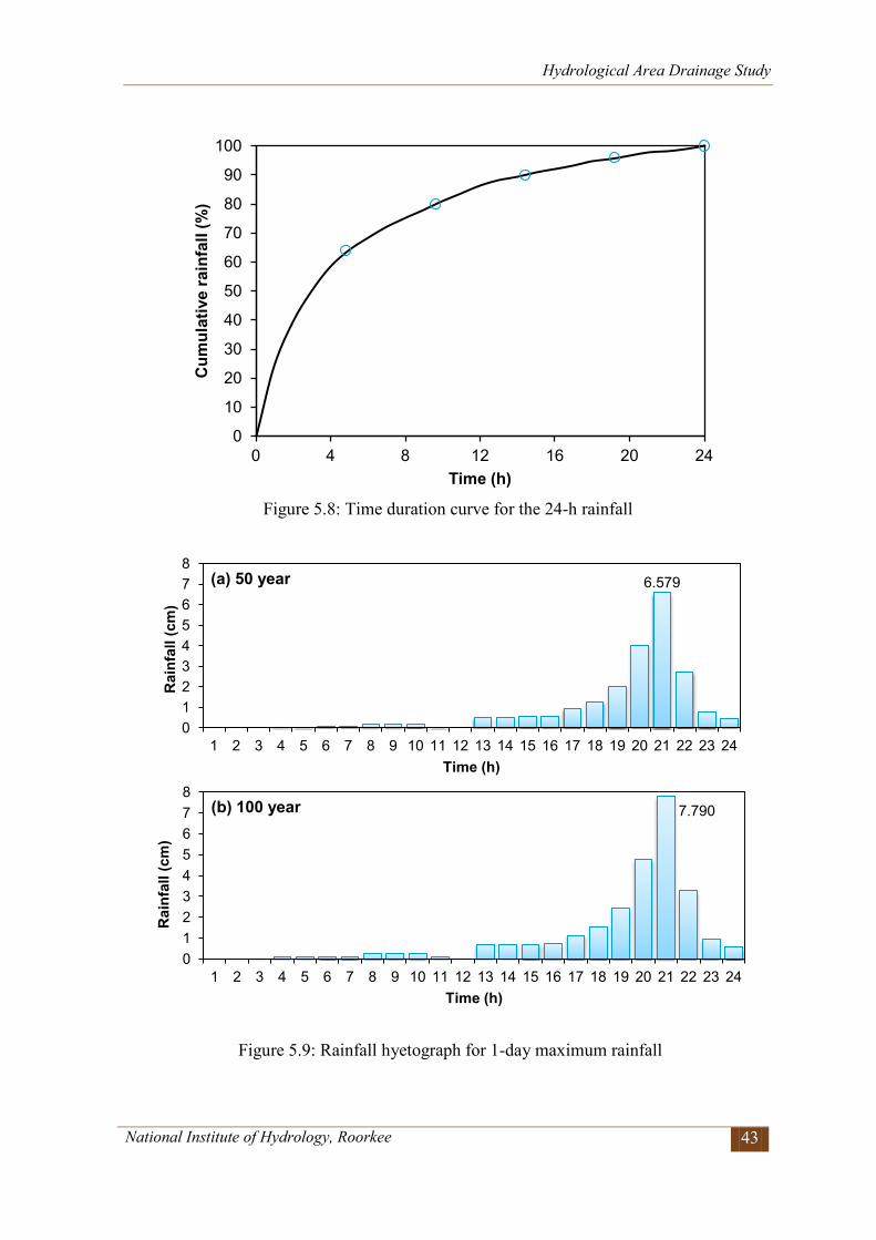
Hydrological Area Drainage Study
National Institute of Hydrology, Roorkee 43
Figure 5.8: Time duration curve for the 24-h rainfall
Figure 5.9: Rainfall hyetograph for 1-day maximum rainfall
0
10
20
30
40
50
60
70
80
90
100
0 4 8 12 16 20 24
Cum
ulat
ive
rain
fall
(%)
Time (h)
6.579
0 1 2 3 4 5 6 7 8
1 2 3 4 5 6 7 8 9 10 11 12 13 14 15 16 17 18 19 20 21 22 23 24
Rai
nfal
l (cm
)
Time (h)
(a) 50 year
7.790
0 1 2 3 4 5 6 7 8
1 2 3 4 5 6 7 8 9 10 11 12 13 14 15 16 17 18 19 20 21 22 23 24
Rai
nfal
l (cm
)
Time (h)
(b) 100 year
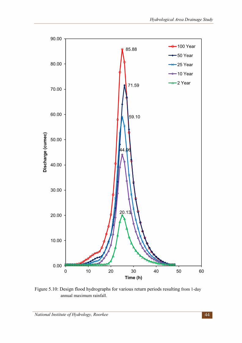
Hydrological Area Drainage Study
National Institute of Hydrology, Roorkee 44
Figure 5.10: Design flood hydrographs for various return periods resulting from 1-day
annual maximum rainfall.
85.88
71.59
59.10
44.06
20.13
0.00
10.00
20.00
30.00
40.00
50.00
60.00
70.00
80.00
90.00
0 10 20 30 40 50 60
Dis
char
ge (c
umec
)
Time (h)
100 Year
50 Year
25 Year
10 Year
2 Year
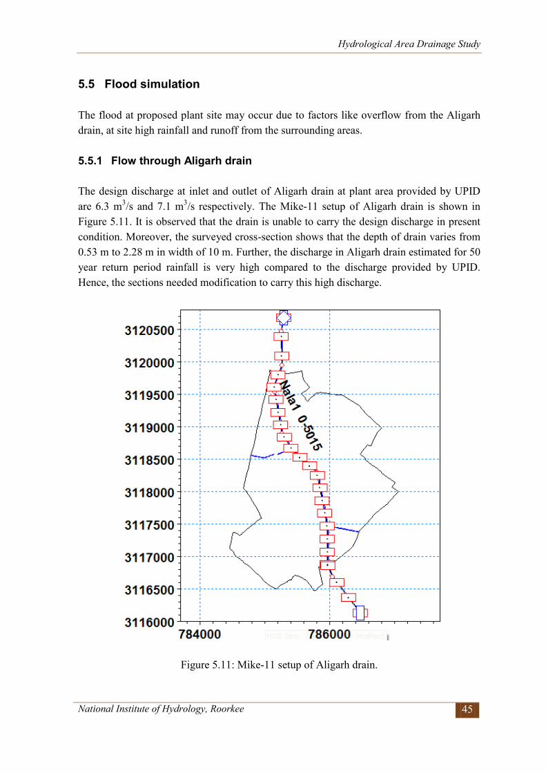
Hydrological Area Drainage Study
National Institute of Hydrology, Roorkee 45
5.5 Flood simulation The flood at proposed plant site may occur due to factors like overflow from the Aligarh drain, at site high rainfall and runoff from the surrounding areas. 5.5.1 Flow through Aligarh drain The design discharge at inlet and outlet of Aligarh drain at plant area provided by UPID are 6.3 m3/s and 7.1 m3/s respectively. The Mike-11 setup of Aligarh drain is shown in Figure 5.11. It is observed that the drain is unable to carry the design discharge in present condition. Moreover, the surveyed cross-section shows that the depth of drain varies from 0.53 m to 2.28 m in width of 10 m. Further, the discharge in Aligarh drain estimated for 50 year return period rainfall is very high compared to the discharge provided by UPID. Hence, the sections needed modification to carry this high discharge.
Figure 5.11: Mike-11 setup of Aligarh drain.

Hydrological Area Drainage Study
National Institute of Hydrology, Roorkee 46
5.5.2 Modification of the Aligarh drain The existing and proposed aligned Aligarh drain is shown in Figure 5.12. The existing ground surface elevation and proposed bead level profiles of the realigned section of Aligarh drain is shown in Figure 5.15. The existing cross-section of Aligarh drain at inlet and outlet is shown in the Figure 5.13. The drain sections are surveyed for 10m width. Here, the proposed modified drain section given in Figure 5.14 are designed for 10 m width due to the space constraints and the corresponding flooding due to 100, 50, 25 and 10 year return period rainfall are studied. The Aligarh drain is designed for lined trapezoidal section with Manning’s roughness of 0.015; 5 m base width and 1.5 m depth. The side slopes are 1.5:1 (H:V) and longitudinal slope is 0.35 m/km. Such section will be able to safely carry a discharge of 15.1 m3/s with a velocity of 1.3 m/s.
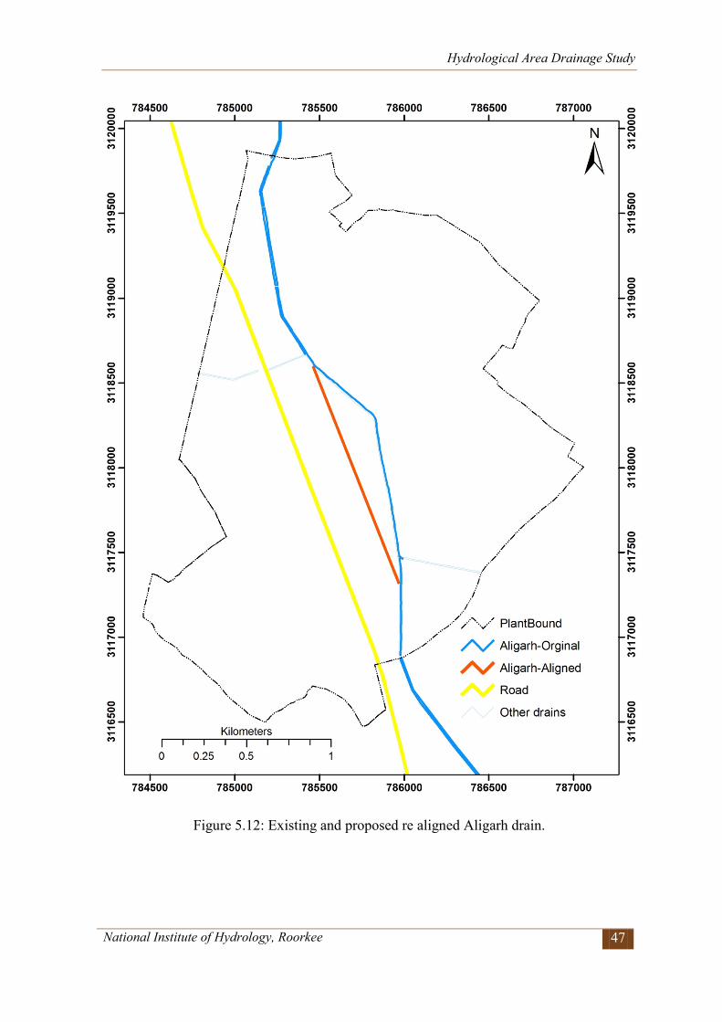
Hydrological Area Drainage Study
National Institute of Hydrology, Roorkee 47
Figure 5.12: Existing and proposed re aligned Aligarh drain.
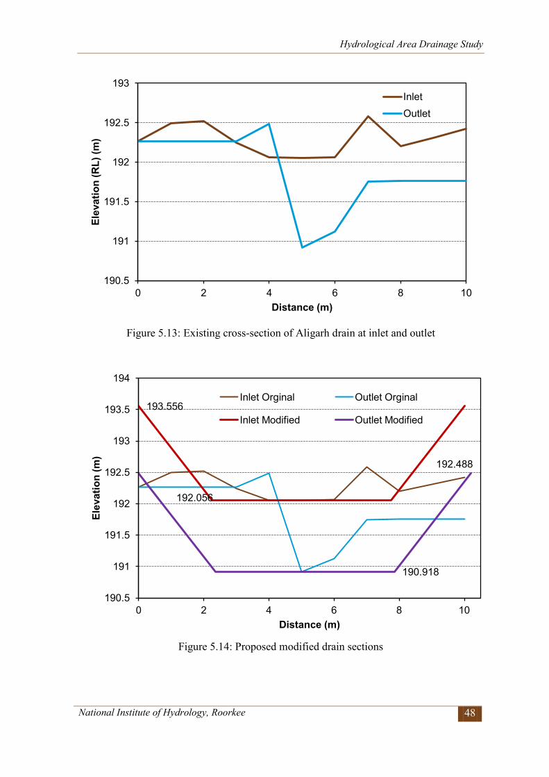
Hydrological Area Drainage Study
National Institute of Hydrology, Roorkee 48
Figure 5.13: Existing cross-section of Aligarh drain at inlet and outlet
Figure 5.14: Proposed modified drain sections
190.5
191
191.5
192
192.5
193
0 2 4 6 8 10
Elev
atio
n (R
L) (m
)
Distance (m)
Inlet Outlet
193.556
192.056
190.918
192.488
190.5
191
191.5
192
192.5
193
193.5
194
0 2 4 6 8 10
Elev
atio
n (m
)
Distance (m)
Inlet Orginal Outlet Orginal
Inlet Modified Outlet Modified
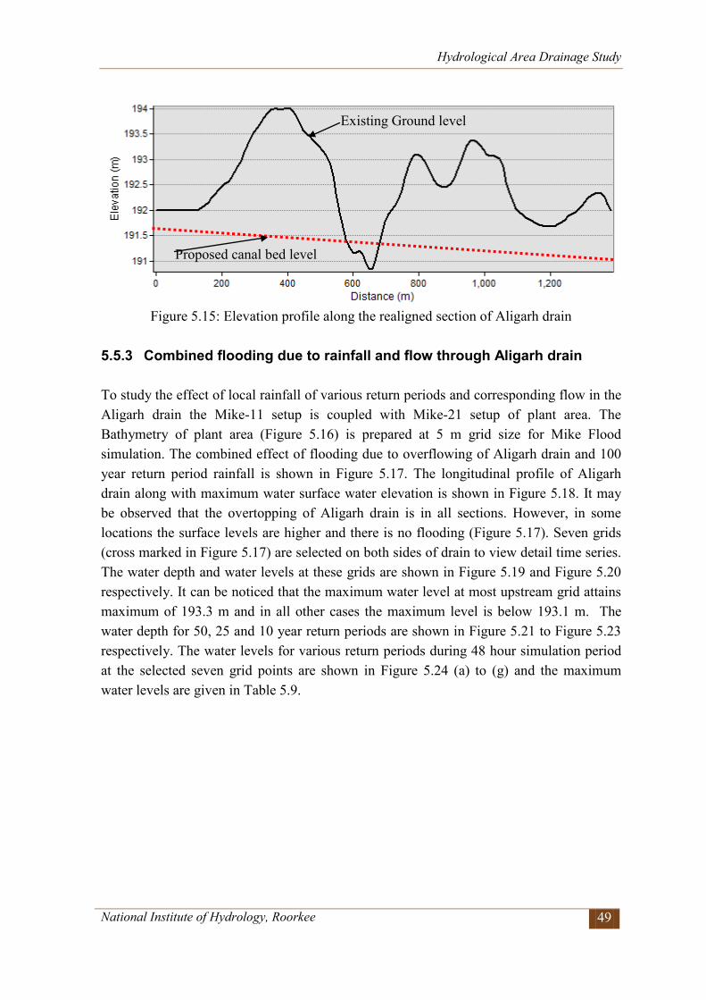
Hydrological Area Drainage Study
National Institute of Hydrology, Roorkee 49
Figure 5.15: Elevation profile along the realigned section of Aligarh drain
5.5.3 Combined flooding due to rainfall and flow through Aligarh drain To study the effect of local rainfall of various return periods and corresponding flow in the Aligarh drain the Mike-11 setup is coupled with Mike-21 setup of plant area. The Bathymetry of plant area (Figure 5.16) is prepared at 5 m grid size for Mike Flood simulation. The combined effect of flooding due to overflowing of Aligarh drain and 100 year return period rainfall is shown in Figure 5.17. The longitudinal profile of Aligarh drain along with maximum water surface water elevation is shown in Figure 5.18. It may be observed that the overtopping of Aligarh drain is in all sections. However, in some locations the surface levels are higher and there is no flooding (Figure 5.17). Seven grids (cross marked in Figure 5.17) are selected on both sides of drain to view detail time series. The water depth and water levels at these grids are shown in Figure 5.19 and Figure 5.20 respectively. It can be noticed that the maximum water level at most upstream grid attains maximum of 193.3 m and in all other cases the maximum level is below 193.1 m. The water depth for 50, 25 and 10 year return periods are shown in Figure 5.21 to Figure 5.23 respectively. The water levels for various return periods during 48 hour simulation period at the selected seven grid points are shown in Figure 5.24 (a) to (g) and the maximum water levels are given in Table 5.9.
Existing Ground level
Proposed canal bed level
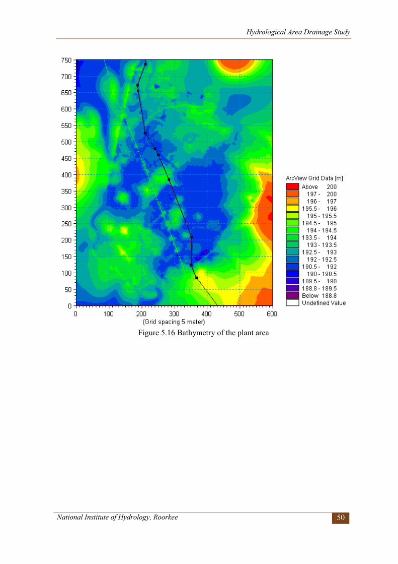
Hydrological Area Drainage Study
National Institute of Hydrology, Roorkee 50
Figure 5.16 Bathymetry of the plant area
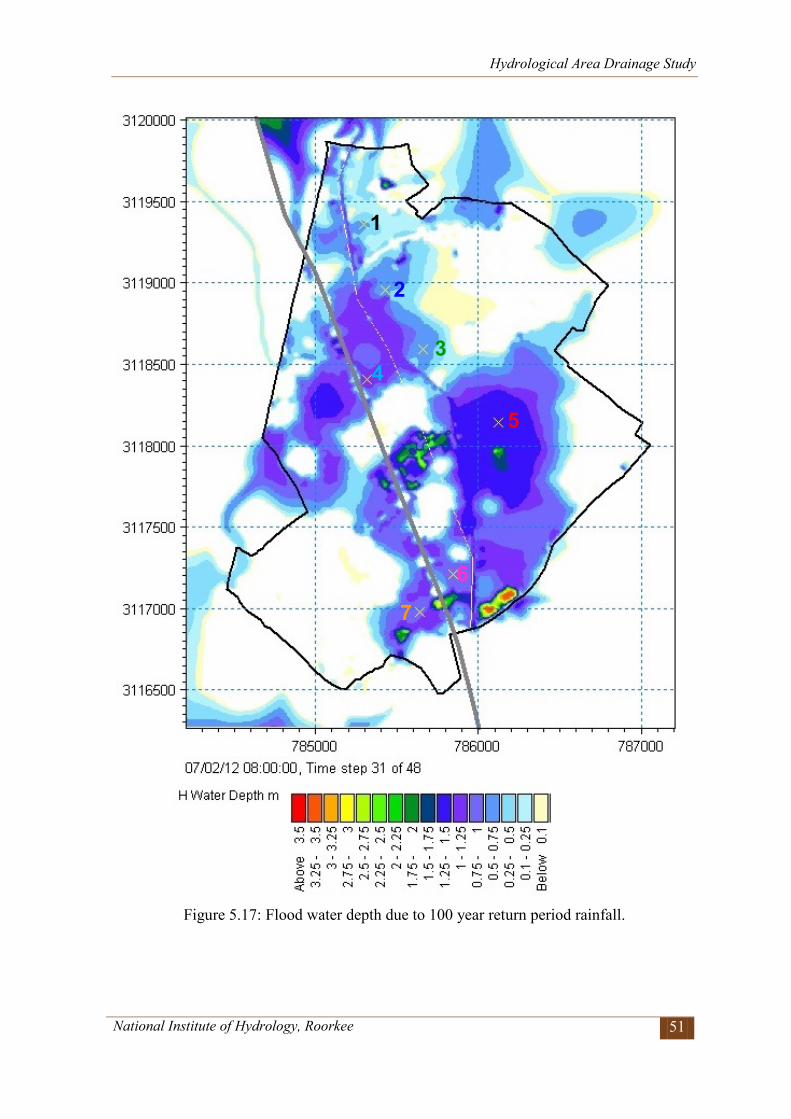
Hydrological Area Drainage Study
National Institute of Hydrology, Roorkee 51
Figure 5.17: Flood water depth due to 100 year return period rainfall.
1
2
3 4
5
6
7
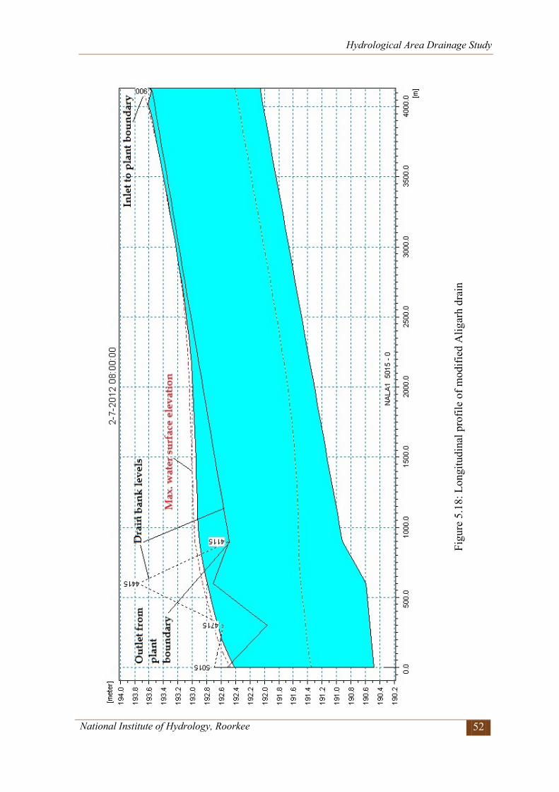
Hydrological Area Drainage Study
National Institute of Hydrology, Roorkee 52
Figu
re 5
.18:
Lon
gitu
dina
l pro
file
of m
odifi
ed A
ligar
h dr
ain
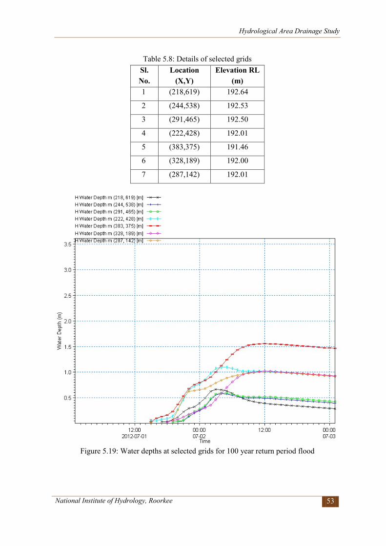
Hydrological Area Drainage Study
National Institute of Hydrology, Roorkee 53
Table 5.8: Details of selected grids Sl. No.
Location (X,Y)
Elevation RL (m)
1 (218,619) 192.64
2 (244,538) 192.53
3 (291,465) 192.50
4 (222,428) 192.01
5 (383,375) 191.46
6 (328,189) 192.00
7 (287,142) 192.01
Figure 5.19: Water depths at selected grids for 100 year return period flood
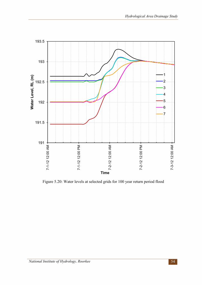
Hydrological Area Drainage Study
National Institute of Hydrology, Roorkee 54
Figure 5.20: Water levels at selected grids for 100 year return period flood
191
191.5
192
192.5
193
193.5 7-
1-12
12:
00 A
M
7-1-
12 1
2:00
PM
7-2-
12 1
2:00
AM
7-2-
12 1
2:00
PM
7-3-
12 1
2:00
AM
Wat
er L
evel
, RL
(m)
Time
1
2
3
4
5
6
7
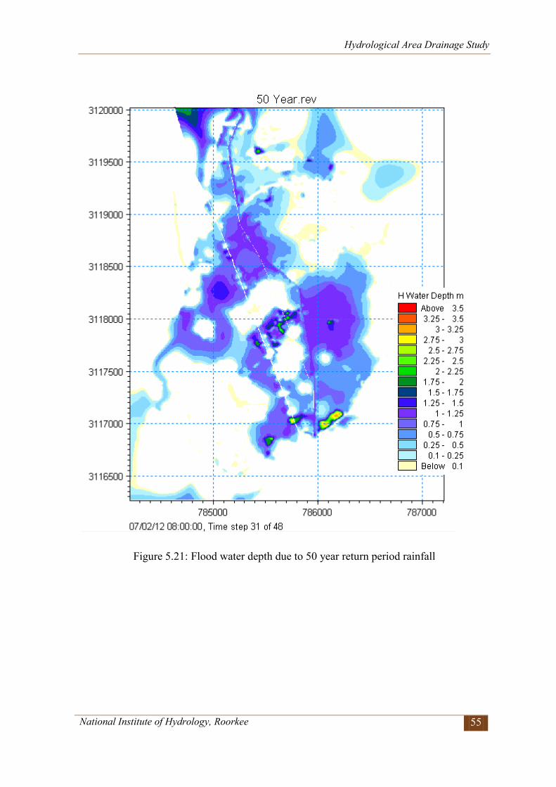
Hydrological Area Drainage Study
National Institute of Hydrology, Roorkee 55
Figure 5.21: Flood water depth due to 50 year return period rainfall
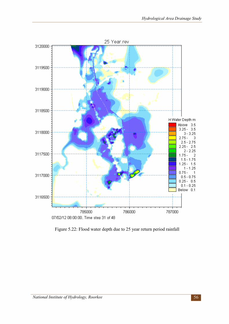
Hydrological Area Drainage Study
National Institute of Hydrology, Roorkee 56
Figure 5.22: Flood water depth due to 25 year return period rainfall
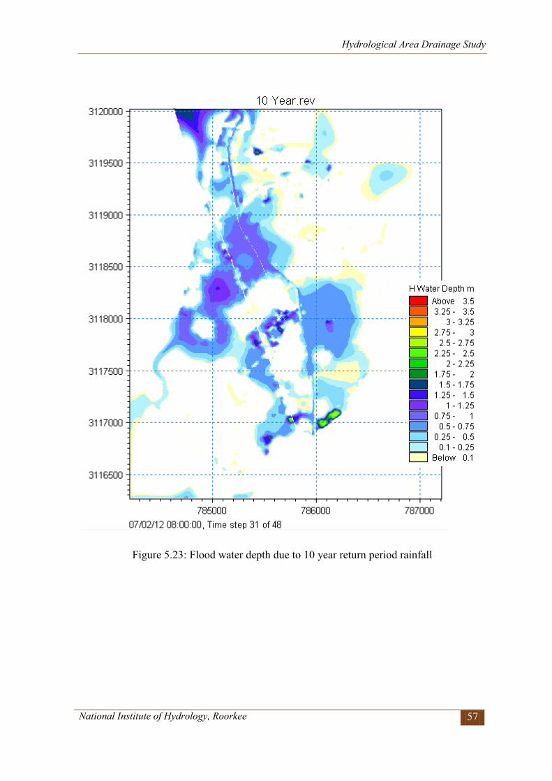
Hydrological Area Drainage Study
National Institute of Hydrology, Roorkee 57
Figure 5.23: Flood water depth due to 10 year return period rainfall
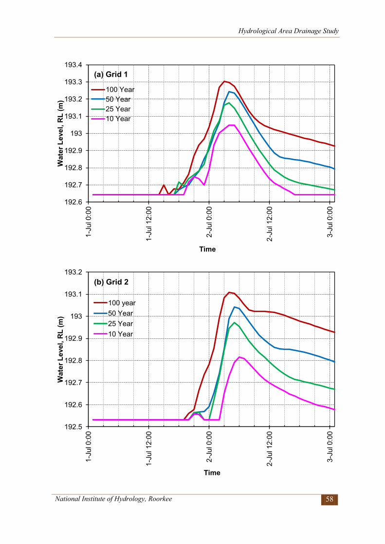
Hydrological Area Drainage Study
National Institute of Hydrology, Roorkee 58
192.6
192.7
192.8
192.9
193
193.1
193.2
193.3
193.4
1-Ju
l 0:0
0
1-Ju
l 12:
00
2-Ju
l 0:0
0
2-Ju
l 12:
00
3-Ju
l 0:0
0
Wat
er L
evel
, RL
(m)
Time
(a) Grid 1
100 Year 50 Year 25 Year 10 Year
192.5
192.6
192.7
192.8
192.9
193
193.1
193.2
1-Ju
l 0:0
0
1-Ju
l 12:
00
2-Ju
l 0:0
0
2-Ju
l 12:
00
3-Ju
l 0:0
0
Wat
er L
evel
, RL
(m)
Time
(b) Grid 2
100 year 50 Year 25 Year 10 Year
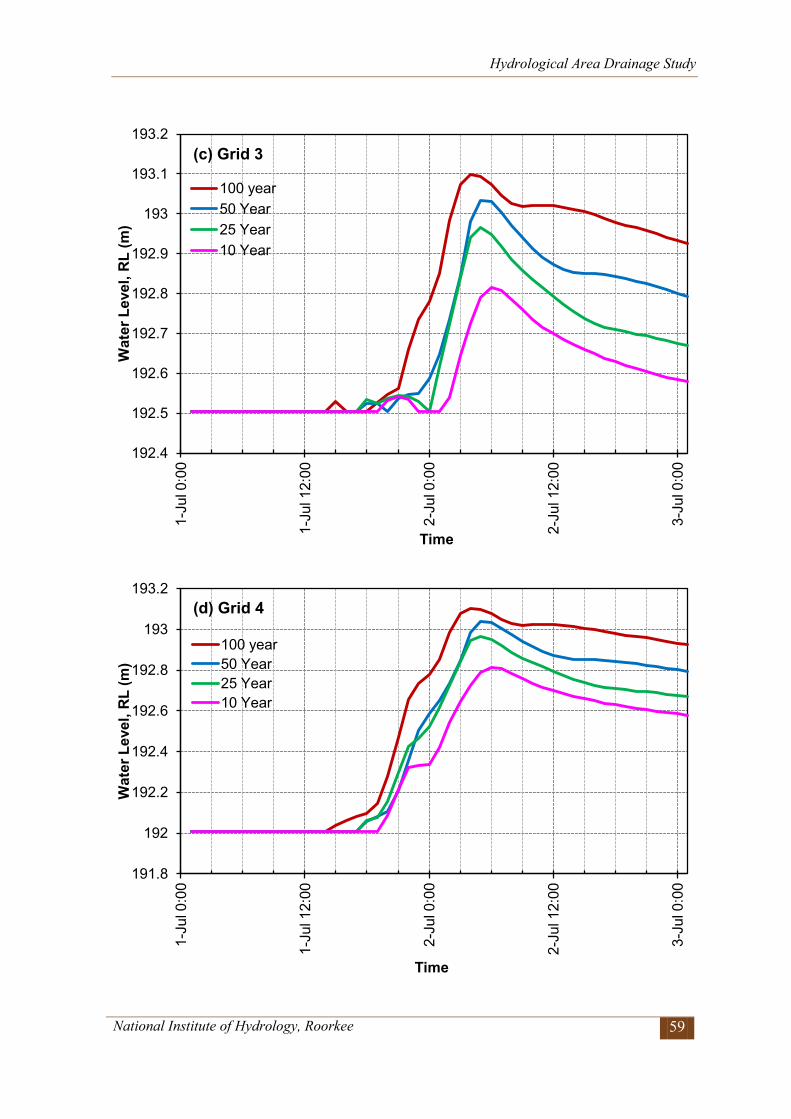
Hydrological Area Drainage Study
National Institute of Hydrology, Roorkee 59
192.4
192.5
192.6
192.7
192.8
192.9
193
193.1
193.2
1-Ju
l 0:0
0
1-Ju
l 12:
00
2-Ju
l 0:0
0
2-Ju
l 12:
00
3-Ju
l 0:0
0
Wat
er L
evel
, RL
(m)
Time
(c) Grid 3
100 year 50 Year 25 Year 10 Year
191.8
192
192.2
192.4
192.6
192.8
193
193.2
1-Ju
l 0:0
0
1-Ju
l 12:
00
2-Ju
l 0:0
0
2-Ju
l 12:
00
3-Ju
l 0:0
0
Wat
er L
evel
, RL
(m)
Time
(d) Grid 4
100 year 50 Year 25 Year 10 Year
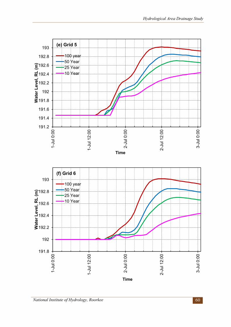
Hydrological Area Drainage Study
National Institute of Hydrology, Roorkee 60
191.2
191.4
191.6
191.8
192
192.2
192.4
192.6
192.8
193 1-
Jul 0
:00
1-Ju
l 12:
00
2-Ju
l 0:0
0
2-Ju
l 12:
00
3-Ju
l 0:0
0
Wat
er L
evel
, RL
(m)
Time
(e) Grid 5
100 year 50 Year 25 Year 10 Year
191.8
192
192.2
192.4
192.6
192.8
193
1-Ju
l 0:0
0
1-Ju
l 12:
00
2-Ju
l 0:0
0
2-Ju
l 12:
00
3-Ju
l 0:0
0
Wat
er L
evel
, RL
(m)
Time
(f) Grid 6
100 year 50 Year 25 Year 10 Year
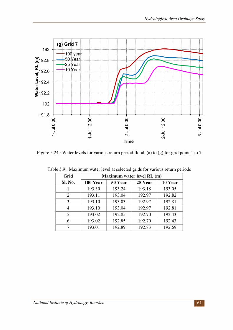
Hydrological Area Drainage Study
National Institute of Hydrology, Roorkee 61
Figure 5.24 : Water levels for various return period flood. (a) to (g) for grid point 1 to 7
Table 5.9 : Maximum water level at selected grids for various return periods Grid
Sl. No. Maximum water level RL (m)
100 Year 50 Year 25 Year 10 Year 1 193.30 193.24 193.18 193.05 2 193.11 193.04 192.97 192.82 3 193.10 193.03 192.97 192.81 4 193.10 193.04 192.97 192.81 5 193.02 192.85 192.70 192.43 6 193.02 192.85 192.70 192.43 7 193.01 192.89 192.83 192.69
191.8
192
192.2
192.4
192.6
192.8
193 1-
Jul 0
:00
1-Ju
l 12:
00
2-Ju
l 0:0
0
2-Ju
l 12:
00
3-Ju
l 0:0
0
Wat
er L
evel
, RL
(m)
Time
(g) Grid 7
100 year 50 Year 25 Year 10 Year
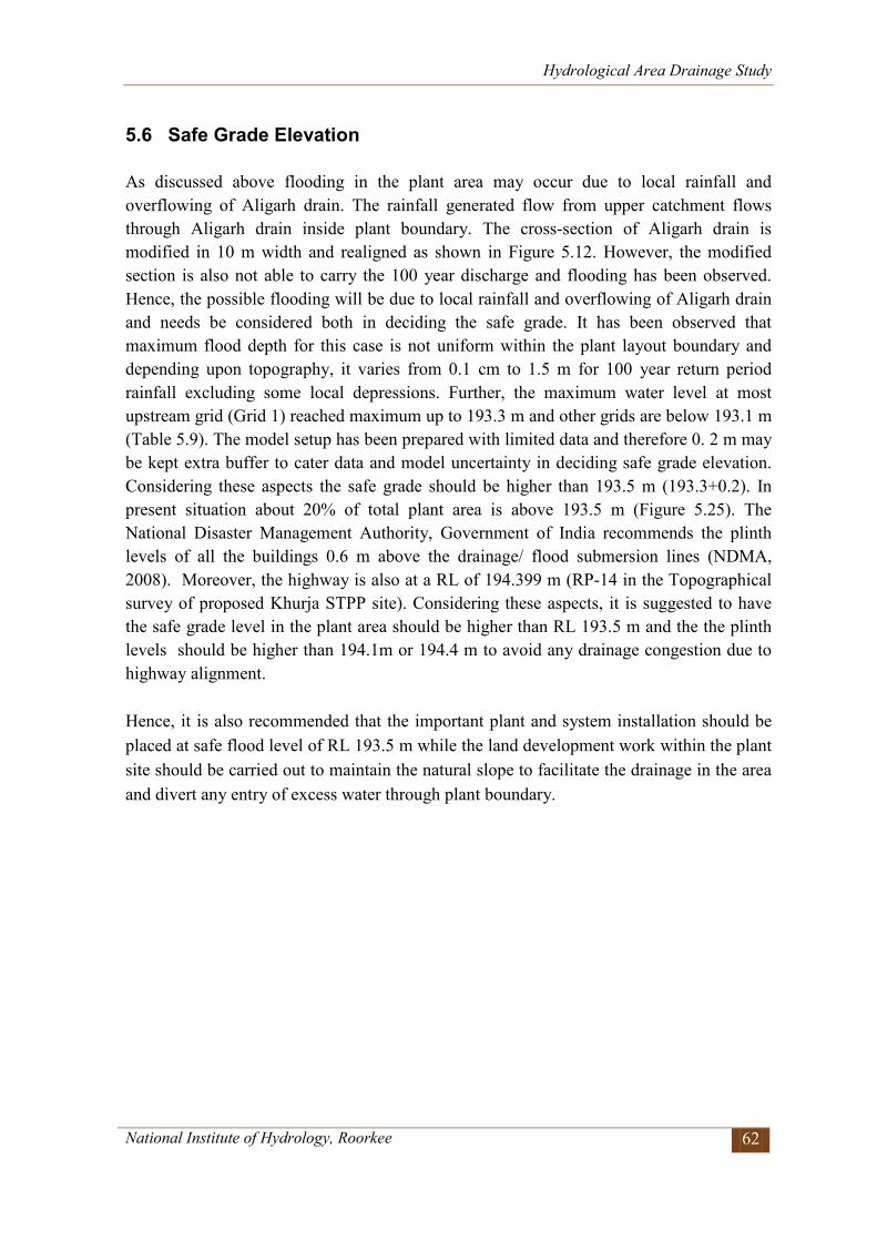
Hydrological Area Drainage Study
National Institute of Hydrology, Roorkee 62
5.6 Safe Grade Elevation As discussed above flooding in the plant area may occur due to local rainfall and overflowing of Aligarh drain. The rainfall generated flow from upper catchment flows through Aligarh drain inside plant boundary. The cross-section of Aligarh drain is modified in 10 m width and realigned as shown in Figure 5.12. However, the modified section is also not able to carry the 100 year discharge and flooding has been observed. Hence, the possible flooding will be due to local rainfall and overflowing of Aligarh drain and needs be considered both in deciding the safe grade. It has been observed that maximum flood depth for this case is not uniform within the plant layout boundary and depending upon topography, it varies from 0.1 cm to 1.5 m for 100 year return period rainfall excluding some local depressions. Further, the maximum water level at most upstream grid (Grid 1) reached maximum up to 193.3 m and other grids are below 193.1 m (Table 5.9). The model setup has been prepared with limited data and therefore 0. 2 m may be kept extra buffer to cater data and model uncertainty in deciding safe grade elevation. Considering these aspects the safe grade should be higher than 193.5 m (193.3+0.2). In present situation about 20% of total plant area is above 193.5 m (Figure 5.25). The National Disaster Management Authority, Government of India recommends the plinth levels of all the buildings 0.6 m above the drainage/ flood submersion lines (NDMA, 2008). Moreover, the highway is also at a RL of 194.399 m (RP-14 in the Topographical survey of proposed Khurja STPP site). Considering these aspects, it is suggested to have the safe grade level in the plant area should be higher than RL 193.5 m and the the plinth levels should be higher than 194.1m or 194.4 m to avoid any drainage congestion due to highway alignment. Hence, it is also recommended that the important plant and system installation should be placed at safe flood level of RL 193.5 m while the land development work within the plant site should be carried out to maintain the natural slope to facilitate the drainage in the area and divert any entry of excess water through plant boundary.
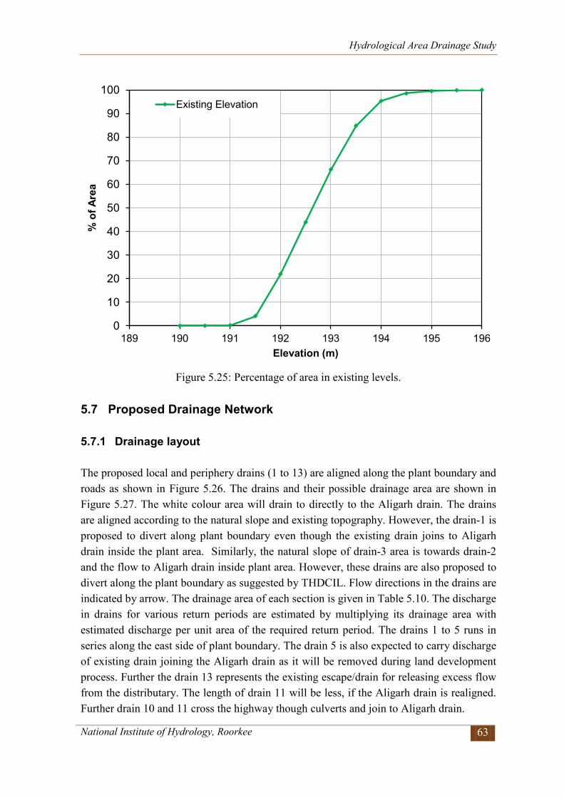
Hydrological Area Drainage Study
National Institute of Hydrology, Roorkee 63
Figure 5.25: Percentage of area in existing levels.
5.7 Proposed Drainage Network 5.7.1 Drainage layout The proposed local and periphery drains (1 to 13) are aligned along the plant boundary and roads as shown in Figure 5.26. The drains and their possible drainage area are shown in Figure 5.27. The white colour area will drain to directly to the Aligarh drain. The drains are aligned according to the natural slope and existing topography. However, the drain-1 is proposed to divert along plant boundary even though the existing drain joins to Aligarh drain inside the plant area. Similarly, the natural slope of drain-3 area is towards drain-2 and the flow to Aligarh drain inside plant area. However, these drains are also proposed to divert along the plant boundary as suggested by THDCIL. Flow directions in the drains are indicated by arrow. The drainage area of each section is given in Table 5.10. The discharge in drains for various return periods are estimated by multiplying its drainage area with estimated discharge per unit area of the required return period. The drains 1 to 5 runs in series along the east side of plant boundary. The drain 5 is also expected to carry discharge of existing drain joining the Aligarh drain as it will be removed during land development process. Further the drain 13 represents the existing escape/drain for releasing excess flow from the distributary. The length of drain 11 will be less, if the Aligarh drain is realigned. Further drain 10 and 11 cross the highway though culverts and join to Aligarh drain.
0
10
20
30
40
50
60
70
80
90
100
189 190 191 192 193 194 195 196
% o
f Are
a
Elevation (m)
Existing Elevation
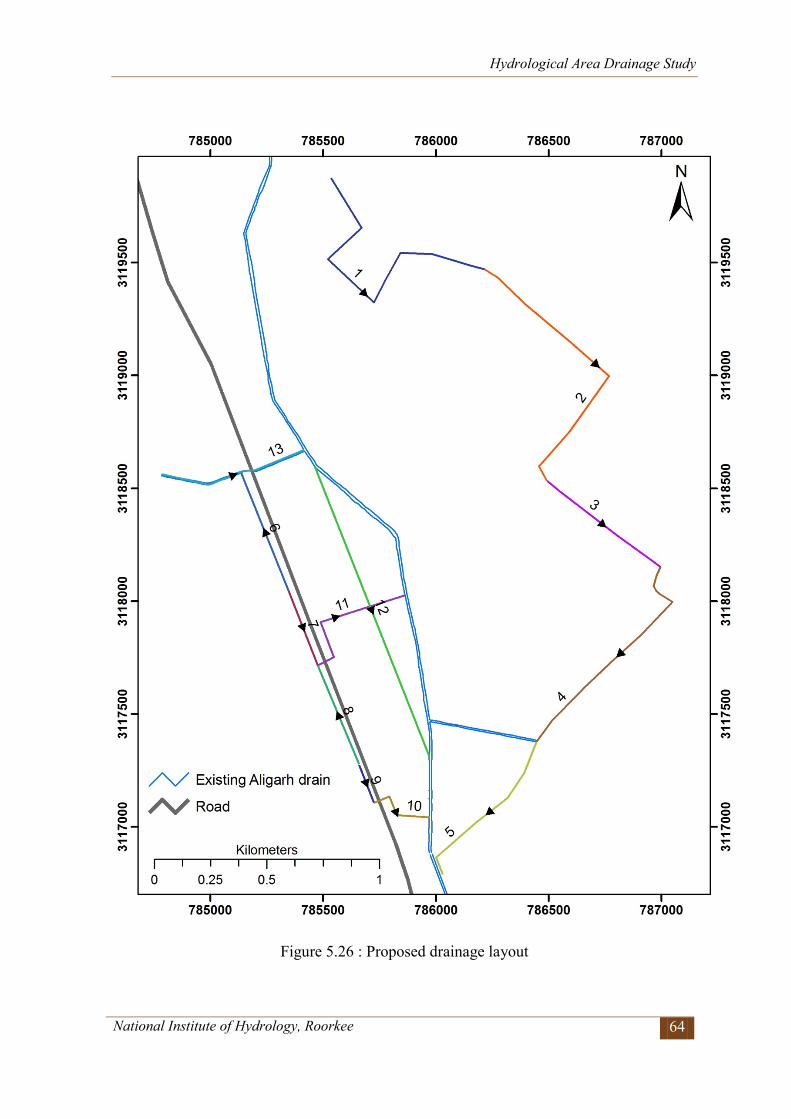
Hydrological Area Drainage Study
National Institute of Hydrology, Roorkee 64
Figure 5.26 : Proposed drainage layout
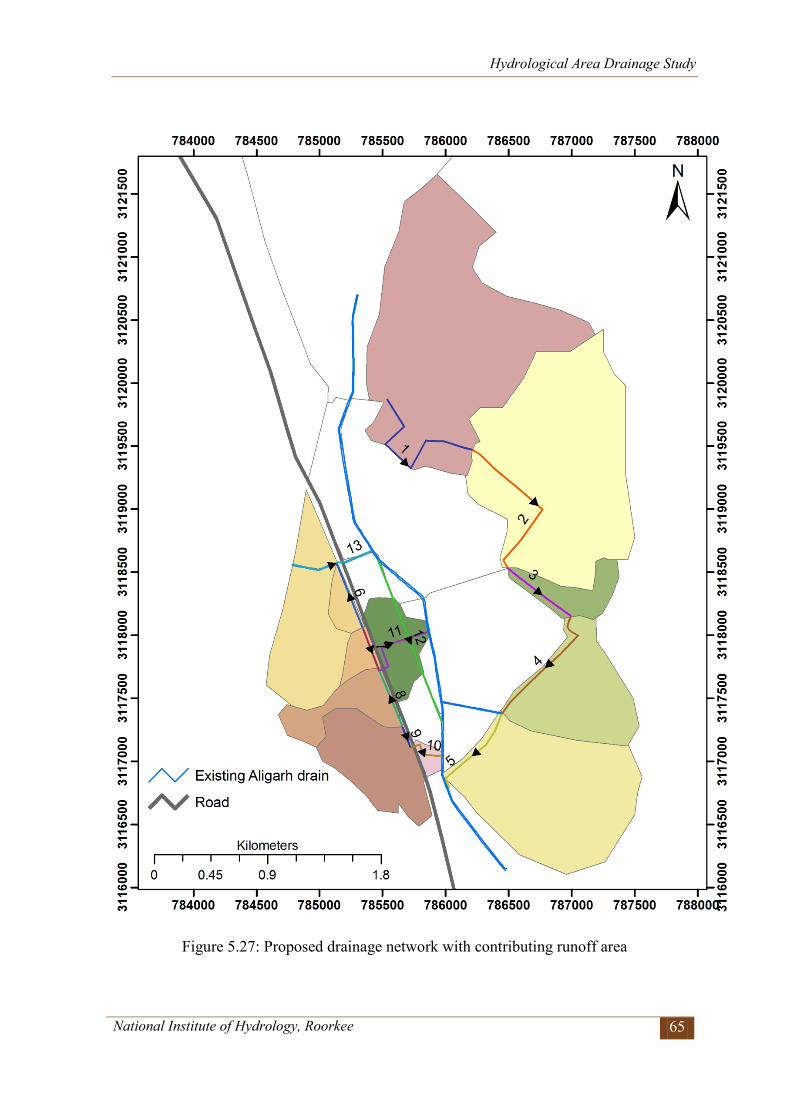
Hydrological Area Drainage Study
National Institute of Hydrology, Roorkee 65
Figure 5.27: Proposed drainage network with contributing runoff area
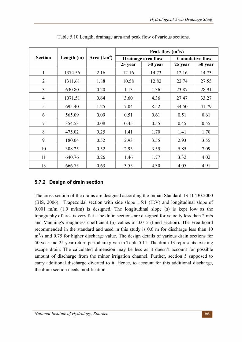
Hydrological Area Drainage Study
National Institute of Hydrology, Roorkee 66
Table 5.10 Length, drainage area and peak flow of various sections.
Section Length (m) Area (km2) Peak flow (m3/s)
Drainage area flow Cumulative flow 25 year 50 year 25 year 50 year
1 1374.56 2.16 12.16 14.73 12.16 14.73
2 1311.61 1.88 10.58 12.82 22.74 27.55
3 630.80 0.20 1.13 1.36 23.87 28.91
4 1071.51 0.64 3.60 4.36 27.47 33.27
5 695.40 1.25 7.04 8.52 34.50 41.79
6 565.09 0.09 0.51 0.61 0.51 0.61
7 354.53 0.08 0.45 0.55 0.45 0.55
8 475.02 0.25 1.41 1.70 1.41 1.70
9 180.04 0.52 2.93 3.55 2.93 3.55
10 308.25 0.52 2.93 3.55 5.85 7.09
11 640.76 0.26 1.46 1.77 3.32 4.02
13 666.75 0.63 3.55 4.30 4.05 4.91
5.7.2 Design of drain section The cross-section of the drains are designed according the Indian Standard, IS 10430:2000 (BIS, 2006). Trapezoidal section with side slope 1.5:1 (H:V) and longitudinal slope of 0.001 m/m (1.0 m/km) is designed. The longitudinal slope (s) is kept low as the topography of area is very flat. The drain sections are designed for velocity less than 2 m/s and Manning's roughness coefficient (n) values of 0.015 (lined section). The Free board recommended in the standard and used in this study is 0.6 m for discharge less than 10 m3/s and 0.75 for higher discharge value. The design details of various drain sections for 50 year and 25 year return period are given in Table 5.11. The drain 13 represents existing escape drain. The calculated dimension may be less as it doesn’t account for possible amount of discharge from the minor irrigation channel. Further, section 5 supposed to carry additional discharge diverted to it. Hence, to account for this additional discharge, the drain section needs modification..
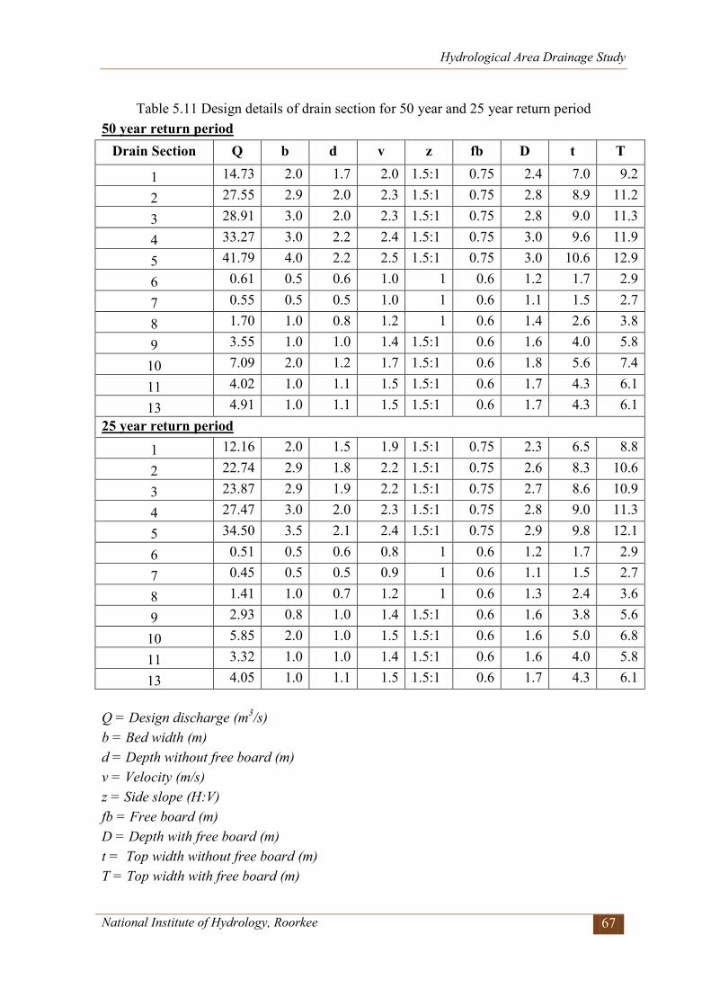
Hydrological Area Drainage Study
National Institute of Hydrology, Roorkee 67
Table 5.11 Design details of drain section for 50 year and 25 year return period 50 year return period
Drain Section Q b d v z fb D t T
1 14.73 2.0 1.7 2.0 1.5:1 0.75 2.4 7.0 9.2
2 27.55 2.9 2.0 2.3 1.5:1 0.75 2.8 8.9 11.2
3 28.91 3.0 2.0 2.3 1.5:1 0.75 2.8 9.0 11.3
4 33.27 3.0 2.2 2.4 1.5:1 0.75 3.0 9.6 11.9
5 41.79 4.0 2.2 2.5 1.5:1 0.75 3.0 10.6 12.9
6 0.61 0.5 0.6 1.0 1 0.6 1.2 1.7 2.9
7 0.55 0.5 0.5 1.0 1 0.6 1.1 1.5 2.7
8 1.70 1.0 0.8 1.2 1 0.6 1.4 2.6 3.8
9 3.55 1.0 1.0 1.4 1.5:1 0.6 1.6 4.0 5.8
10 7.09 2.0 1.2 1.7 1.5:1 0.6 1.8 5.6 7.4
11 4.02 1.0 1.1 1.5 1.5:1 0.6 1.7 4.3 6.1
13 4.91 1.0 1.1 1.5 1.5:1 0.6 1.7 4.3 6.1 25 year return period
1 12.16 2.0 1.5 1.9 1.5:1 0.75 2.3 6.5 8.8
2 22.74 2.9 1.8 2.2 1.5:1 0.75 2.6 8.3 10.6
3 23.87 2.9 1.9 2.2 1.5:1 0.75 2.7 8.6 10.9
4 27.47 3.0 2.0 2.3 1.5:1 0.75 2.8 9.0 11.3
5 34.50 3.5 2.1 2.4 1.5:1 0.75 2.9 9.8 12.1
6 0.51 0.5 0.6 0.8 1 0.6 1.2 1.7 2.9
7 0.45 0.5 0.5 0.9 1 0.6 1.1 1.5 2.7
8 1.41 1.0 0.7 1.2 1 0.6 1.3 2.4 3.6
9 2.93 0.8 1.0 1.4 1.5:1 0.6 1.6 3.8 5.6
10 5.85 2.0 1.0 1.5 1.5:1 0.6 1.6 5.0 6.8
11 3.32 1.0 1.0 1.4 1.5:1 0.6 1.6 4.0 5.8
13 4.05 1.0 1.1 1.5 1.5:1 0.6 1.7 4.3 6.1 Q = Design discharge (m3/s) b = Bed width (m) d = Depth without free board (m) v = Velocity (m/s) z = Side slope (H:V) fb = Free board (m) D = Depth with free board (m) t = Top width without free board (m) T = Top width with free board (m)
Hydrological Area Drainage Study
National Institute of Hydrology, Roorkee 68
5.8 Limitation of the Study The limitation of the study due to non availability of data and assumption in the model are as follows:
1. The contour of 0.5 m interval was only available for the proposed plant area. For the remaining area SOI contour and SRTM data is used.
2. The available observed hourly rainfall data was sufficient to generate hourly rainfall distribution curve, hence the time distribution of rainfall was done according to CWC (1984) report.
3. Drain alignments are made with exiting topography. This may be modified according to final level obtained after land levelling.
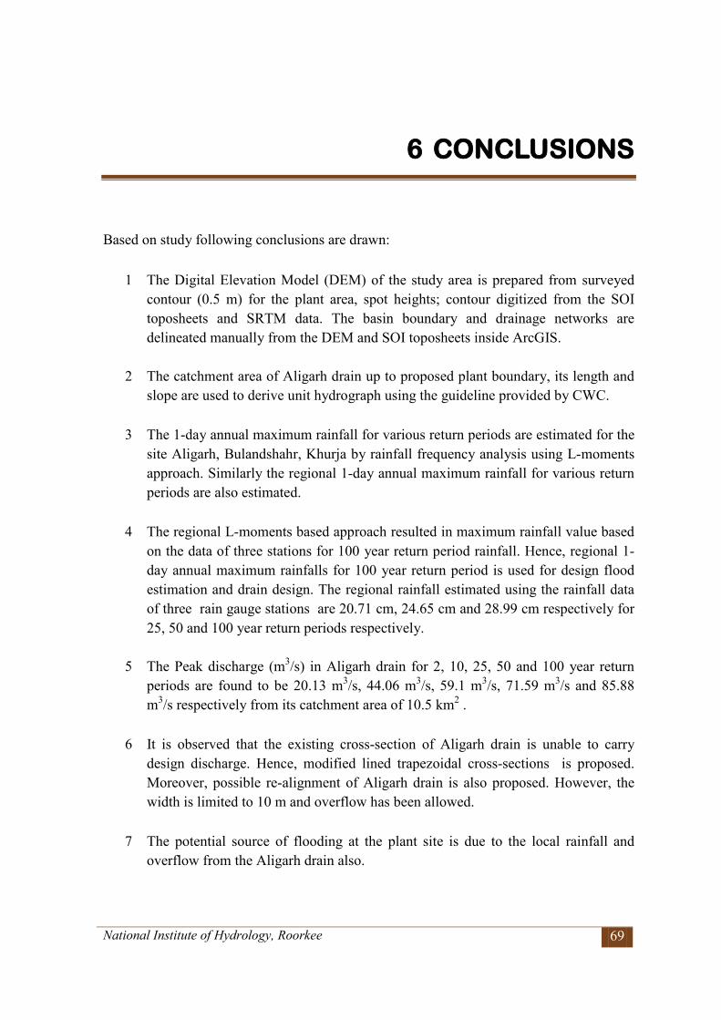
National Institute of Hydrology, Roorkee 69
6 CONCLUSIONS
Based on study following conclusions are drawn:
1 The Digital Elevation Model (DEM) of the study area is prepared from surveyed contour (0.5 m) for the plant area, spot heights; contour digitized from the SOI toposheets and SRTM data. The basin boundary and drainage networks are delineated manually from the DEM and SOI toposheets inside ArcGIS.
2 The catchment area of Aligarh drain up to proposed plant boundary, its length and slope are used to derive unit hydrograph using the guideline provided by CWC.
3 The 1-day annual maximum rainfall for various return periods are estimated for the site Aligarh, Bulandshahr, Khurja by rainfall frequency analysis using L-moments approach. Similarly the regional 1-day annual maximum rainfall for various return periods are also estimated.
4 The regional L-moments based approach resulted in maximum rainfall value based on the data of three stations for 100 year return period rainfall. Hence, regional 1-day annual maximum rainfalls for 100 year return period is used for design flood estimation and drain design. The regional rainfall estimated using the rainfall data of three rain gauge stations are 20.71 cm, 24.65 cm and 28.99 cm respectively for 25, 50 and 100 year return periods respectively.
5 The Peak discharge (m3/s) in Aligarh drain for 2, 10, 25, 50 and 100 year return periods are found to be 20.13 m3/s, 44.06 m3/s, 59.1 m3/s, 71.59 m3/s and 85.88 m3/s respectively from its catchment area of 10.5 km2 .
6 It is observed that the existing cross-section of Aligarh drain is unable to carry design discharge. Hence, modified lined trapezoidal cross-sections is proposed. Moreover, possible re-alignment of Aligarh drain is also proposed. However, the width is limited to 10 m and overflow has been allowed.
7 The potential source of flooding at the plant site is due to the local rainfall and overflow from the Aligarh drain also.

Hydrological Area Drainage Study
National Institute of Hydrology, Roorkee 70
8 The land formation level should be based on the computed maximum flood elevation for severe most flooding scenario (100 year return period), model uncertainty and limitation of data availability. Considering these aspects, it is suggested to have the safe grade level in the plant area higher than RL 193.5 m and the plinth levels should be higher than 194.1 m or 194.4 m to avoid any drainage congestion due to highway alignment. The land development work within the plant site should be carried out to maintain the natural slope to facilitate the drainage in the area and divert any entry of excess water through plant boundary.
9 The peak flow for 25 and 50 year return period rainfall is estimated for various local and periphery drain sections and the trapezoidal drains are designed using Mannings formula and free board is provided as per BIS standard IS 10430-2000.
10 The local and periphery drains are designed for trapezoidal section with a side slope of 1.5:1 (H:V) and longitudinal slope of 0.001 m/m (1.0 m/km) to carry the discharge generated locally. Moreover, the drain sections are designed for velocity less than 2 m/s and Manning's roughness coefficient (n) values of 0.015.
National Institute of Hydrology, Roorkee 71
References
Abbot, M. B. and Ionescu F. (1967) On the numerical computation of nearly horizontal flows. Journal of Hydraulic Research 5(2):97-117
BIS (2006). IS 10430-2000 Criteria for Design of Lined Canals and Guidance for Selection of Type of Lining. (Reaffirmed 2004).
Chatterjee C., Förster S. and Bronstert A. (2008) Comparison of hydrodynamic models of different complexities to model floods with emergency storage areas. Hydrological Processes 22 (24): 4695-4709
CWC (1984) Flood estimation report for upper Indo-Ganga plains (Subzone-1e). Central Water Commission. New Delhi, India
CWC (2001) Manual on estimation of design flood. Hydrology Studies Organization. Central Water Commission, New Delhi, India.
Department of Agriculture & Cooperation (2012). Agriculture Contingency Plan, Department of Agriculture & Cooperation, Ministry of Agriculture, Government of India. http://agricoop.nic.in/Agriculture%20Contingency%20Plan/UP/UP6-Bulandshahar-26.7.2012.pdf
DHI (2004) A modelling system for rivers and channels: Reference manual. DHI Water and Environment, Denmark.
Greenwood, J.A., Landwehr, J.M., Matalas, N.C., and Wallis, J.R. (1979) Probability weighted moments: Definition and relation to parameters of several distributions expressible in inverse form. Water Resources Research 15:1049-1054.
Hosking, J. R. M. (1990) L-moments: Analysis and estimation of distributions using linear combinations of order statistics. J. of the Royal Statistical Society, Series B, 52: 105-124.
Hosking, J. R. M., and Wallis, J. R. 1997. Regional Frequency Analysis-An Approach Based on L-moments. Cambridge University Press, New York.
IMD (2012) http://www.imd.gov.in/section/hydro/distrainfall/webrain/up/bulandshahr.txt
Kumar, R. and Chatterjee, C. (2005) Regional flood frequency analysis using L-moments for North Brahmaputra Region of India. J. Hydrologic Engineering, ASCE, 10(1), 1-7.
Hydrological Area Drainage Study
National Institute of Hydrology, Roorkee 72
NDMG (2008) National disaster management guidelines: Management of floods, National Disaster Management Authority, government of India, New Delhi, India.
Patro, S., Chatterjee, C., Mohanty, S., Singh, R. and Raghuwanshi, N.S. (2009) Flood Inundation modeling using MIKE FLOOD and remote sensing data. Journal of Indian Society of Remote Sensing 37:107-118.
Pramanik, N., Panda, R. K. and Sen, D. J. (2010) One dimensional hydrodynamic modeling of river flow using DEM extracted river cross-sections. Water Resources Management 24(5):835-852.
Rungo, M. and Olesen, K. W. (2003) Combined 1- and 2-dimensional flood modeling, 4th Iranian Hydraulic Conference, 21-23 October, Shiraz, Iran.
Sanders, B. F. (2007) Evaluation of on line DEM for flood inundation modeling. Advances in Water Resources 30: 1831-1843.
Vogel R.M., and Fennessey N.M. (1993) L-moments should replace product moments diagrams. Water Resources Research 29(6): 1745-1752.
Zafirakou-Koulouris, A., Vogel, R.M., Craig, S.M., and Habermeier, J. (1998) L moment diagrams for censored observations. Water Resources Research 34(5): 1241-1249.
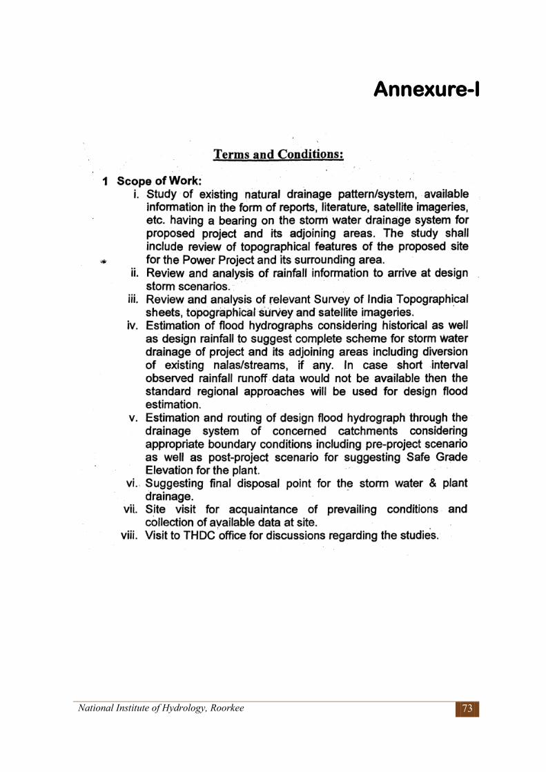
National Institute of Hydrology, Roorkee 73
Annexure-I
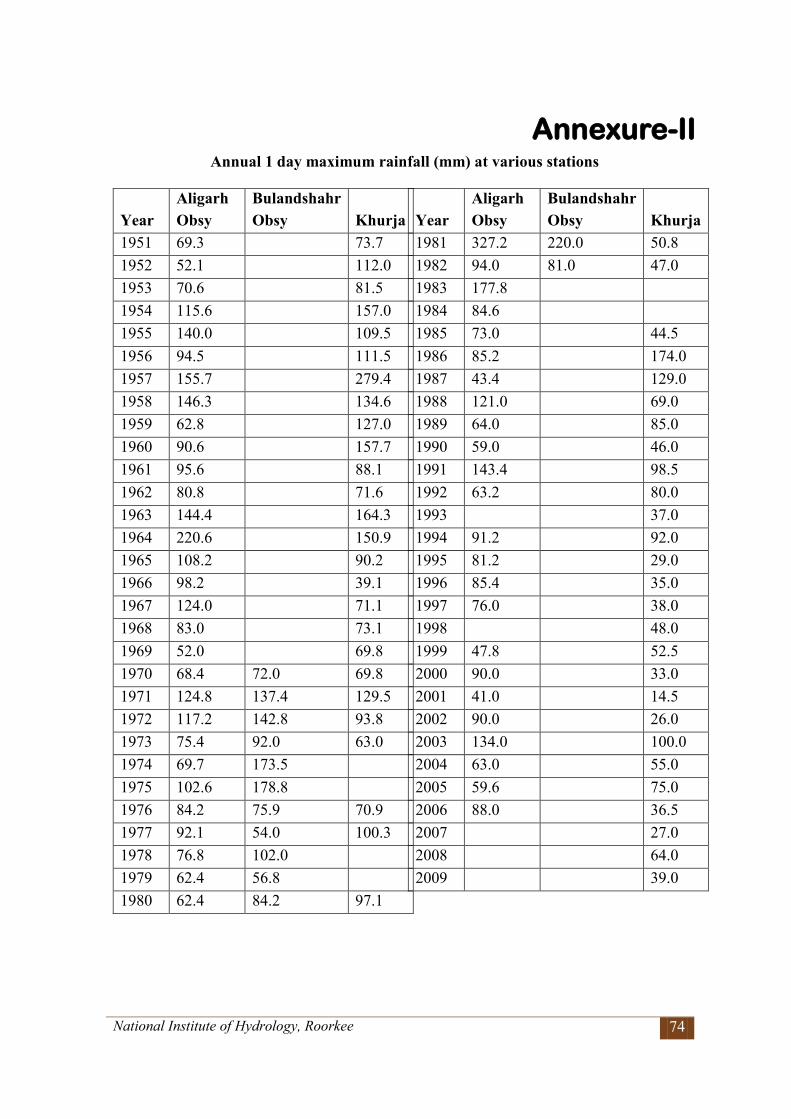
National Institute of Hydrology, Roorkee 74
Annexure-II Annual 1 day maximum rainfall (mm) at various stations
Year Aligarh Obsy
Bulandshahr Obsy Khurja
1951 69.3
73.7 1952 52.1
112.0
1953 70.6
81.5 1954 115.6
157.0
1955 140.0
109.5 1956 94.5
111.5
1957 155.7
279.4 1958 146.3
134.6
1959 62.8
127.0 1960 90.6
157.7
1961 95.6
88.1 1962 80.8
71.6
1963 144.4
164.3 1964 220.6
150.9
1965 108.2
90.2 1966 98.2
39.1
1967 124.0
71.1 1968 83.0
73.1
1969 52.0
69.8 1970 68.4 72.0 69.8 1971 124.8 137.4 129.5 1972 117.2 142.8 93.8 1973 75.4 92.0 63.0 1974 69.7 173.5
1975 102.6 178.8 1976 84.2 75.9 70.9
1977 92.1 54.0 100.3 1978 76.8 102.0
1979 62.4 56.8 1980 62.4 84.2 97.1
Year Aligarh Obsy
Bulandshahr Obsy Khurja
1981 327.2 220.0 50.8 1982 94.0 81.0 47.0 1983 177.8
1984 84.6 1985 73.0
44.5 1986 85.2
174.0
1987 43.4
129.0 1988 121.0
69.0
1989 64.0
85.0 1990 59.0
46.0
1991 143.4
98.5 1992 63.2
80.0
1993
37.0 1994 91.2
92.0
1995 81.2
29.0 1996 85.4
35.0
1997 76.0
38.0 1998
48.0
1999 47.8
52.5 2000 90.0
33.0
2001 41.0
14.5 2002 90.0
26.0
2003 134.0
100.0 2004 63.0
55.0
2005 59.6
75.0 2006 88.0
36.5
2007
27.0 2008
64.0
2009
39.0
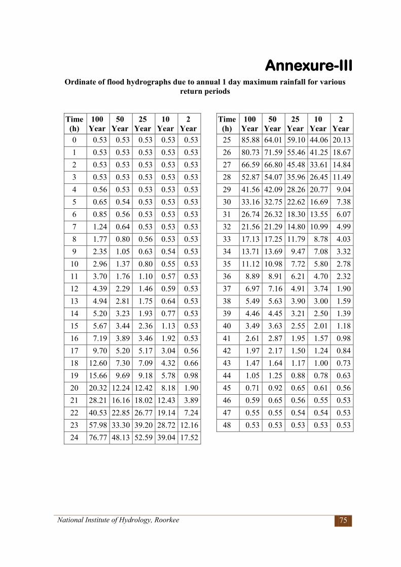
National Institute of Hydrology, Roorkee 75
Annexure-III Ordinate of flood hydrographs due to annual 1 day maximum rainfall for various
return periods
Time (h)
100 Year
50 Year
25 Year
10 Year
2 Year
0 0.53 0.53 0.53 0.53 0.53 1 0.53 0.53 0.53 0.53 0.53 2 0.53 0.53 0.53 0.53 0.53 3 0.53 0.53 0.53 0.53 0.53 4 0.56 0.53 0.53 0.53 0.53 5 0.65 0.54 0.53 0.53 0.53 6 0.85 0.56 0.53 0.53 0.53 7 1.24 0.64 0.53 0.53 0.53 8 1.77 0.80 0.56 0.53 0.53 9 2.35 1.05 0.63 0.54 0.53 10 2.96 1.37 0.80 0.55 0.53 11 3.70 1.76 1.10 0.57 0.53 12 4.39 2.29 1.46 0.59 0.53 13 4.94 2.81 1.75 0.64 0.53 14 5.20 3.23 1.93 0.77 0.53 15 5.67 3.44 2.36 1.13 0.53 16 7.19 3.89 3.46 1.92 0.53 17 9.70 5.20 5.17 3.04 0.56 18 12.60 7.30 7.09 4.32 0.66 19 15.66 9.69 9.18 5.78 0.98 20 20.32 12.24 12.42 8.18 1.90 21 28.21 16.16 18.02 12.43 3.89 22 40.53 22.85 26.77 19.14 7.24 23 57.98 33.30 39.20 28.72 12.16 24 76.77 48.13 52.59 39.04 17.52
Time (h)
100 Year
50 Year
25 Year
10 Year
2 Year
25 85.88 64.01 59.10 44.06 20.13 26 80.73 71.59 55.46 41.25 18.67 27 66.59 66.80 45.48 33.61 14.84 28 52.87 54.07 35.96 26.45 11.49 29 41.56 42.09 28.26 20.77 9.04 30 33.16 32.75 22.62 16.69 7.38 31 26.74 26.32 18.30 13.55 6.07 32 21.56 21.29 14.80 10.99 4.99 33 17.13 17.25 11.79 8.78 4.03 34 13.71 13.69 9.47 7.08 3.32 35 11.12 10.98 7.72 5.80 2.78 36 8.89 8.91 6.21 4.70 2.32 37 6.97 7.16 4.91 3.74 1.90 38 5.49 5.63 3.90 3.00 1.59 39 4.46 4.45 3.21 2.50 1.39 40 3.49 3.63 2.55 2.01 1.18 41 2.61 2.87 1.95 1.57 0.98 42 1.97 2.17 1.50 1.24 0.84 43 1.47 1.64 1.17 1.00 0.73 44 1.05 1.25 0.88 0.78 0.63 45 0.71 0.92 0.65 0.61 0.56 46 0.59 0.65 0.56 0.55 0.53 47 0.55 0.55 0.54 0.54 0.53 48 0.53 0.53 0.53 0.53 0.53

National Institute of Hydrology, Roorkee 76
NATIONAL INSTITUTE OF HYDROLOGY ROORKEE – 247 667, UTTARAKHAND
Website: www.nih.ernet.in
0.10 0.30 0.500.00 0.20 0.40L-Skewness
-0.10
0.10
0.30
-0.20
0.00
0.20
0.40
L-Ku
rtosi
s
GLO
GEV GNO
GPA
PE3
WAKEXPEV1
LOS
NOR
UNF
(GLO, GEV, GNO, GPA, PE3 are three-parameter distributions, and are shown as lines.
WAK is a five-parameter distribution, and is shown as a line.
UNF, NOR, LOS, EV1 and EXP are two-parameterdistributions shown as points, and are mentioned in italics)
Regional-Khurja

ENCLOSURE-4

Project- 2 x 660 MW Khurja STPP, UP Enclosure-4 Client- M/s THDC India Limited
QUANTITATIVE RISK ASSESSMENT
1.1 Introduction
Risk analysis follows an extensive hazard analysis. Identification of causes and types of hazards is the primary task for planning for risk assessment. Hazard can happen because of the nature of chemicals handled and the nature of process involved. So for risk analysis first step is to identify the hazardous chemicals which are to be studied for risk analysis.
It involves the identification and assessment of risks at the project site and in the neighboring population who could get exposed to, as a result of hazards present. This requires a thorough knowledge of failure probability, credible accident scenario, vulnerability of population etc.
In the sections below, the identification of various hazards, probable risks in the proposed power plant, maximum credible accident analysis, consequence analysis are addressed which gives a broad identification of risks involved in the plant.
Approach to the Study
Risk involves the occurrence or potential occurrence of some accidents consisting of an event or sequence of events. The risk assessment study covers the following:
Identification of potential hazard areas; Identification of representative failure cases; Visualization of the resulting scenarios in terms of fire (thermal radiation) and explosion; Assess the overall damage potential of the identified hazardous events and the impact zones
from the accidental scenarios; Assess the overall suitability of the site from hazard minimization and disaster mitigation
point of view Furnish specific recommendations on the minimization of the worst accident possibilities;
and Preparation of broad Disaster Management Plan (DMP), On-site and Off-site Emergency
Plan, which includes Occupational and Health Safety Plan.
1.2 Chemical Hazards
Identification of Hazardous Chemicals is done in accordance with The Manufacture, Storage and import of Hazardous Chemical Rules, 1989. Schedule-1, of the Rule provides a list of the Toxic and Hazardous chemicals and the flammable chemicals. It defines the flammable chemicals based on the flashpoint and boiling point.
"Major accident hazards (MAH) installations" is defined as the isolated storage and industrial activity at a site handling (including transport through carrier or pipeline) of hazardous chemicals equal to or, in excess of the threshold quantities specified in Column-3 of Schedule-2 and 3 respectively.
Schedule-3 has classified hazardous substances in an operating plant into 5 groups and has provided the threshold quantities for application of above rules.
Group1 & 2 – Toxic substances
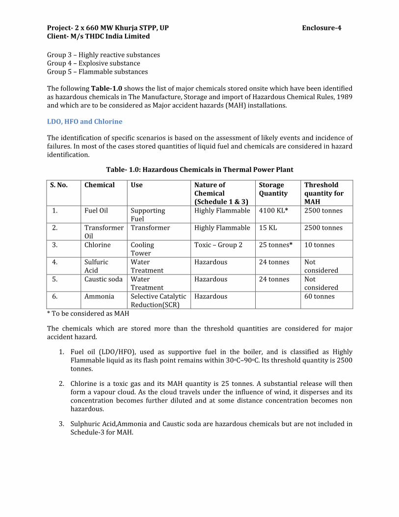
Project- 2 x 660 MW Khurja STPP, UP Enclosure-4 Client- M/s THDC India Limited
Group 3 – Highly reactive substances Group 4 – Explosive substance Group 5 – Flammable substances The following Table-1.0 shows the list of major chemicals stored onsite which have been identified as hazardous chemicals in The Manufacture, Storage and import of Hazardous Chemical Rules, 1989 and which are to be considered as Major accident hazards (MAH) installations.
LDO, HFO and Chlorine
The identification of specific scenarios is based on the assessment of likely events and incidence of failures. In most of the cases stored quantities of liquid fuel and chemicals are considered in hazard identification.
Table- 1.0: Hazardous Chemicals in Thermal Power Plant
S. No. Chemical Use Nature of Chemical (Schedule 1 & 3)
Storage Quantity
Threshold quantity for MAH
1. Fuel Oil Supporting Fuel
Highly Flammable 4100 KL* 2500 tonnes
2. Transformer Oil
Transformer Highly Flammable 15 KL 2500 tonnes
3. Chlorine Cooling Tower
Toxic – Group 2 25 tonnes* 10 tonnes
4. Sulfuric Acid
Water Treatment
Hazardous 24 tonnes Not considered
5. Caustic soda Water Treatment
Hazardous 24 tonnes Not considered
6. Ammonia Selective Catalytic Reduction(SCR)
Hazardous 60 tonnes
* To be considered as MAH
The chemicals which are stored more than the threshold quantities are considered for major accident hazard.
1. Fuel oil (LDO/HFO), used as supportive fuel in the boiler, and is classified as Highly Flammable liquid as its flash point remains within 30oC–90oC. Its threshold quantity is 2500 tonnes.
2. Chlorine is a toxic gas and its MAH quantity is 25 tonnes. A substantial release will then form a vapour cloud. As the cloud travels under the influence of wind, it disperses and its concentration becomes further diluted and at some distance concentration becomes non hazardous.
3. Sulphuric Acid,Ammonia and Caustic soda are hazardous chemicals but are not included in Schedule-3 for MAH.
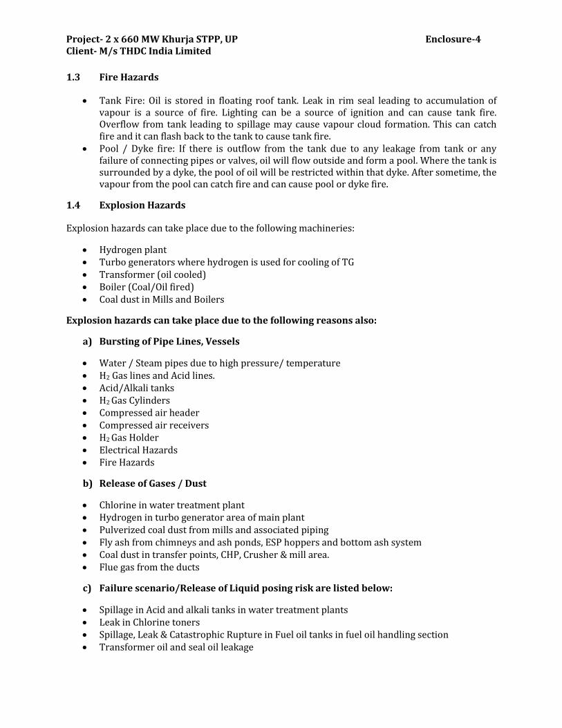
Project- 2 x 660 MW Khurja STPP, UP Enclosure-4 Client- M/s THDC India Limited
1.3 Fire Hazards
Tank Fire: Oil is stored in floating roof tank. Leak in rim seal leading to accumulation of vapour is a source of fire. Lighting can be a source of ignition and can cause tank fire. Overflow from tank leading to spillage may cause vapour cloud formation. This can catch fire and it can flash back to the tank to cause tank fire.
Pool / Dyke fire: If there is outflow from the tank due to any leakage from tank or any failure of connecting pipes or valves, oil will flow outside and form a pool. Where the tank is surrounded by a dyke, the pool of oil will be restricted within that dyke. After sometime, the vapour from the pool can catch fire and can cause pool or dyke fire.
1.4 Explosion Hazards
Explosion hazards can take place due to the following machineries:
Hydrogen plant Turbo generators where hydrogen is used for cooling of TG Transformer (oil cooled) Boiler (Coal/Oil fired) Coal dust in Mills and Boilers
Explosion hazards can take place due to the following reasons also:
a) Bursting of Pipe Lines, Vessels
Water / Steam pipes due to high pressure/ temperature H2 Gas lines and Acid lines. Acid/Alkali tanks H2 Gas Cylinders Compressed air header Compressed air receivers H2 Gas Holder Electrical Hazards Fire Hazards
b) Release of Gases / Dust
Chlorine in water treatment plant Hydrogen in turbo generator area of main plant Pulverized coal dust from mills and associated piping Fly ash from chimneys and ash ponds, ESP hoppers and bottom ash system Coal dust in transfer points, CHP, Crusher & mill area. Flue gas from the ducts
c) Failure scenario/Release of Liquid posing risk are listed below:
Spillage in Acid and alkali tanks in water treatment plants Leak in Chlorine toners Spillage, Leak & Catastrophic Rupture in Fuel oil tanks in fuel oil handling section Transformer oil and seal oil leakage
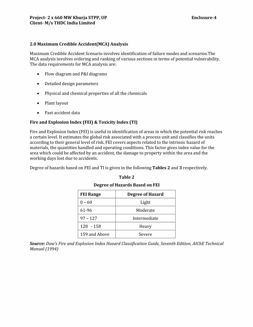
Project- 2 x 660 MW Khurja STPP, UP Enclosure-4 Client- M/s THDC India Limited
2.0 Maximum Credible Accident(MCA) Analysis
Maximum Credible Accident Scenario involves identification of failure modes and scenarios.The MCA analysis involves ordering and ranking of various sections in terms of potential vulnerability. The data requirements for MCA analysis are:
Flow diagram and P&I diagrams
Detailed design parameters
Physical and chemical properties of all the chemicals
Plant layout
Past accident data
Fire and Explosion Index (FEI) & Toxicity Index (TI)
Fire and Explosion Index (FEI) is useful in identification of areas in which the potential risk reaches a certain level. It estimates the global risk associated with a process unit and classifies the units according to their general level of risk. FEI covers aspects related to the intrinsic hazard of materials, the quantities handled and operating conditions. This factor gives index value for the area which could be affected by an accident, the damage to property within the area and the working days lost due to accidents.
Degree of hazards based on FEI and TI is given in the following Tables 2 and 3 respectively.
Table 2
Degree of Hazards Based on FEI
FEI Range Degree of Hazard
0 – 60 Light
61-96 Moderate
97 – 127 Intermediate
128 - 158 Heavy
159 and Above Severe
Source: Dow’s Fire and Explosion Index Hazard Classification Guide, Seventh Edition, AIChE Technical Manual (1994)
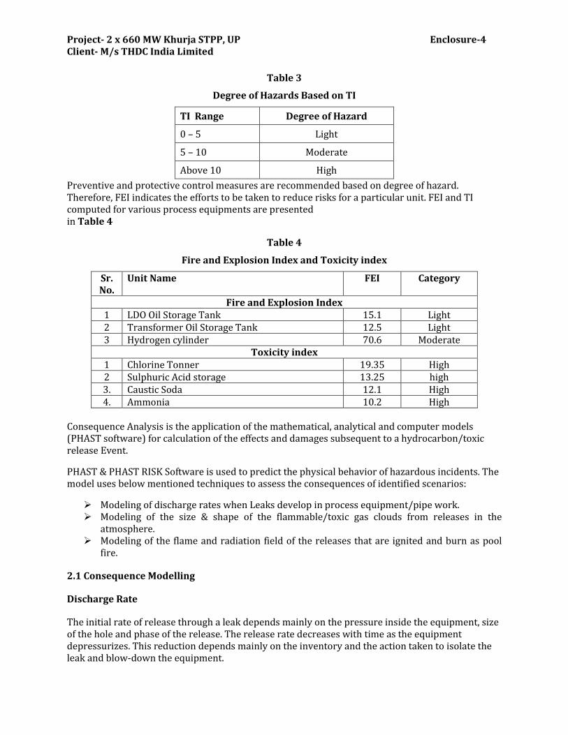
Project- 2 x 660 MW Khurja STPP, UP Enclosure-4 Client- M/s THDC India Limited
Table 3
Degree of Hazards Based on TI
TI Range Degree of Hazard
0 – 5 Light
5 – 10 Moderate
Above 10 High
Preventive and protective control measures are recommended based on degree of hazard. Therefore, FEI indicates the efforts to be taken to reduce risks for a particular unit. FEI and TI computed for various process equipments are presented in Table 4
Table 4
Fire and Explosion Index and Toxicity index
Sr. No.
Unit Name FEI Category
Fire and Explosion Index 1 LDO Oil Storage Tank 15.1 Light 2 Transformer Oil Storage Tank 12.5 Light 3 Hydrogen cylinder 70.6 Moderate
Toxicity index 1 Chlorine Tonner 19.35 High 2 Sulphuric Acid storage 13.25 high 3. Caustic Soda 12.1 High 4. Ammonia 10.2 High
Consequence Analysis is the application of the mathematical, analytical and computer models (PHAST software) for calculation of the effects and damages subsequent to a hydrocarbon/toxic release Event.
PHAST & PHAST RISK Software is used to predict the physical behavior of hazardous incidents. The model uses below mentioned techniques to assess the consequences of identified scenarios:
Modeling of discharge rates when Leaks develop in process equipment/pipe work. Modeling of the size & shape of the flammable/toxic gas clouds from releases in the
atmosphere. Modeling of the flame and radiation field of the releases that are ignited and burn as pool
fire.
2.1 Consequence Modelling
Discharge Rate
The initial rate of release through a leak depends mainly on the pressure inside the equipment, size of the hole and phase of the release. The release rate decreases with time as the equipment depressurizes. This reduction depends mainly on the inventory and the action taken to isolate the leak and blow-down the equipment.
Project- 2 x 660 MW Khurja STPP, UP Enclosure-4 Client- M/s THDC India Limited
Dispersion
Releases of gas into the open air form clouds whose dispersion is governed by the wind, by turbulence around the site, the density of the gas and initial momentum of the release. In case of flammable materials the sizes of these gas clouds above their Lower Flammable Limit (LFL) are important in determining whether the release will ignite. In this study, the results of dispersion modeling for flammable materials are presented LFL quantity.
Pool Fire
A cylindrical shape of the pool fire is presumed. Pool-fire calculations are then carried out as part of an accidental scenario, e.g. in case a hydrocarbon liquid leak from a vessel leads to the formation of an ignitable liquid pool. First no ignition is assumed, and pool evaporation and dispersion calculations are being carried out. Subsequently late pool fires (ignition following spreading of liquid pool) are considered. If the release is bounded, the diameter is given by the size of the bund. If there is no bund, then the diameter is that which corresponds with a minimum pool thickness, set by the type of surface on which the pool is spreading.
While modeling cases of lighter hydrocarbons in the range of ATF wherein the rainout fraction have been minimal (not leading to pool formation) due to the horizontal direction of release, downward impingement has been considered for studying the effects of pool fire for consequence analysis only.
Pool fires occur when spilled hydrocarbons burn in the form of large diffusion flames. Calculating the incident flux to an observer involves four steps, namely
Characterizing the flame geometry Estimation of the flame radiation properties Computation of the geometric view factors Estimation of flame attenuation coefficients and computation of geometric view factors
between observer and flame.
The size of the flame will depend upon the spill surface and the thermo chemical properties of the spilled liquid. In particular,the diameter of the fire, the visible height of the flame, the tilt and drag of the flame etc. The radioactive output of the flame will depend upon the fire size, the extent of mixing with air and the flame temperature. Some fraction of the thermal radiation is absorbed by the carbon dioxide and water vapor in the intervening atmosphere. In addition, large hydrocarbon fires produce thick smoke which significantly obscure flame radiation. The calculations for radiation damage distances start with estimation of the burning velocity: Y= 92.6 e – 0.0043TbMw10-7/(D X 6)
Where, y= burning velocity in m/s Mw= molecular weight in kg/kg mol Tb= normal boiling point The next step involves calculation of the equivalent diameter for the spreading pool- this depends upon the duration of the spill (continuous, instantaneous, finite duration etc.). This is calculated using expressions like:
Deq. =2(V/3.142y)1/2
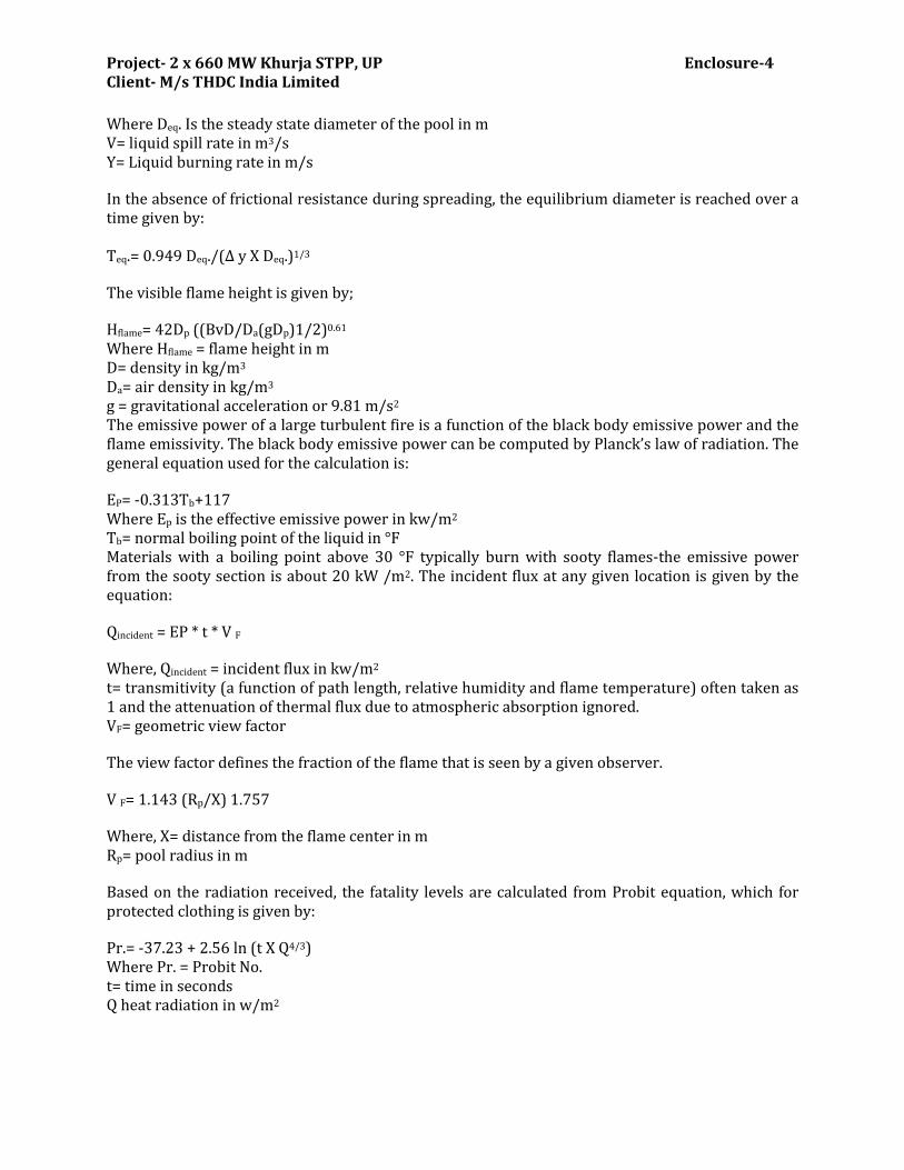
Project- 2 x 660 MW Khurja STPP, UP Enclosure-4 Client- M/s THDC India Limited
Where Deq. Is the steady state diameter of the pool in m V= liquid spill rate in m3/s Y= Liquid burning rate in m/s
In the absence of frictional resistance during spreading, the equilibrium diameter is reached over a time given by: Teq.= 0.949 Deq./(Δ y X Deq.)1/3
The visible flame height is given by;
Hflame= 42Dp ((BvD/Da(gDp)1/2)0.61 Where Hflame = flame height in m D= density in kg/m3
Da= air density in kg/m3
g = gravitational acceleration or 9.81 m/s2
The emissive power of a large turbulent fire is a function of the black body emissive power and the flame emissivity. The black body emissive power can be computed by Planck’s law of radiation. The general equation used for the calculation is:
EP= -0.313Tb+117 Where Ep is the effective emissive power in kw/m2
Tb= normal boiling point of the liquid in °F Materials with a boiling point above 30 °F typically burn with sooty flames-the emissive power from the sooty section is about 20 kW /m2. The incident flux at any given location is given by the equation:
Qincident = EP * t * V F
Where, Qincident = incident flux in kw/m2
t= transmitivity (a function of path length, relative humidity and flame temperature) often taken as 1 and the attenuation of thermal flux due to atmospheric absorption ignored. VF= geometric view factor
The view factor defines the fraction of the flame that is seen by a given observer.
V F= 1.143 (Rp/X) 1.757
Where, X= distance from the flame center in m Rp= pool radius in m
Based on the radiation received, the fatality levels are calculated from Probit equation, which for protected clothing is given by:
Pr.= -37.23 + 2.56 ln (t X Q4/3) Where Pr. = Probit No. t= time in seconds Q heat radiation in w/m2
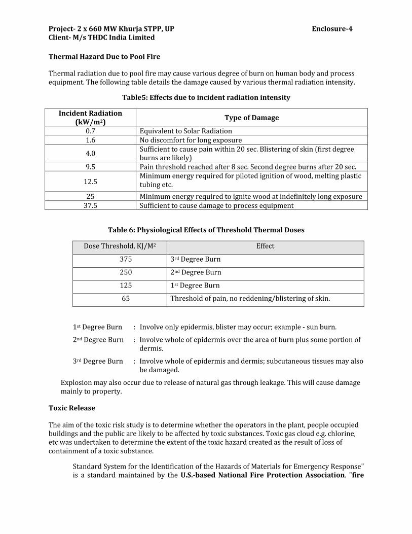
Project- 2 x 660 MW Khurja STPP, UP Enclosure-4 Client- M/s THDC India Limited
Thermal Hazard Due to Pool Fire
Thermal radiation due to pool fire may cause various degree of burn on human body and process equipment. The following table details the damage caused by various thermal radiation intensity.
Table5: Effects due to incident radiation intensity
Incident Radiation (kW/m2)
Type of Damage
0.7 Equivalent to Solar Radiation 1.6 No discomfort for long exposure
4.0 Sufficient to cause pain within 20 sec. Blistering of skin (first degree burns are likely)
9.5 Pain threshold reached after 8 sec. Second degree burns after 20 sec.
12.5 Minimum energy required for piloted ignition of wood, melting plastic tubing etc.
25 Minimum energy required to ignite wood at indefinitely long exposure 37.5 Sufficient to cause damage to process equipment
Table 6: Physiological Effects of Threshold Thermal Doses
Dose Threshold, KJ/M2 Effect
375 3rd Degree Burn
250 2nd Degree Burn
125 1st Degree Burn
65 Threshold of pain, no reddening/blistering of skin.
1st Degree Burn : Involve only epidermis, blister may occur; example - sun burn.
2nd Degree Burn : Involve whole of epidermis over the area of burn plus some portion of dermis.
3rd Degree Burn : Involve whole of epidermis and dermis; subcutaneous tissues may also be damaged.
Explosion may also occur due to release of natural gas through leakage. This will cause damage mainly to property.
Toxic Release
The aim of the toxic risk study is to determine whether the operators in the plant, people occupied buildings and the public are likely to be affected by toxic substances. Toxic gas cloud e.g. chlorine, etc was undertaken to determine the extent of the toxic hazard created as the result of loss of containment of a toxic substance.
Standard System for the Identification of the Hazards of Materials for Emergency Response" is a standard maintained by the U.S.-based National Fire Protection Association. "fire
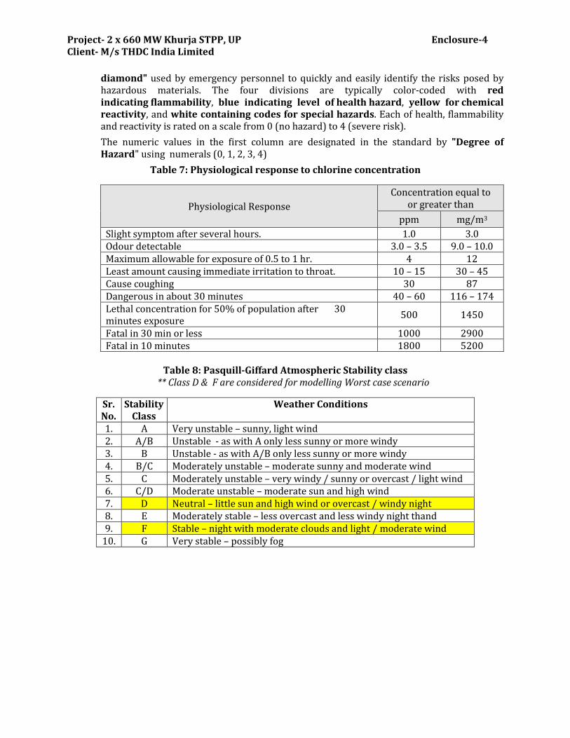
Project- 2 x 660 MW Khurja STPP, UP Enclosure-4 Client- M/s THDC India Limited
diamond" used by emergency personnel to quickly and easily identify the risks posed by hazardous materials. The four divisions are typically color-coded with red indicating flammability, blue indicating level of health hazard, yellow for chemical reactivity, and white containing codes for special hazards. Each of health, flammability and reactivity is rated on a scale from 0 (no hazard) to 4 (severe risk).
The numeric values in the first column are designated in the standard by "Degree of Hazard" using numerals (0, 1, 2, 3, 4)
Table 7: Physiological response to chlorine concentration
Physiological Response
Concentration equal to or greater than
ppm mg/m3
Slight symptom after several hours. 1.0 3.0 Odour detectable 3.0 – 3.5 9.0 – 10.0 Maximum allowable for exposure of 0.5 to 1 hr. 4 12 Least amount causing immediate irritation to throat. 10 – 15 30 – 45 Cause coughing 30 87 Dangerous in about 30 minutes 40 – 60 116 – 174 Lethal concentration for 50% of population after 30 minutes exposure
500 1450
Fatal in 30 min or less 1000 2900 Fatal in 10 minutes 1800 5200
Table 8: Pasquill-Giffard Atmospheric Stability class
** Class D & F are considered for modelling Worst case scenario
Sr. No.
Stability Class
Weather Conditions
1. A Very unstable – sunny, light wind 2. A/B Unstable - as with A only less sunny or more windy 3. B Unstable - as with A/B only less sunny or more windy 4. B/C Moderately unstable – moderate sunny and moderate wind 5. C Moderately unstable – very windy / sunny or overcast / light wind 6. C/D Moderate unstable – moderate sun and high wind 7. D Neutral – little sun and high wind or overcast / windy night 8. E Moderately stable – less overcast and less windy night thand 9. F Stable – night with moderate clouds and light / moderate wind
10. G Very stable – possibly fog
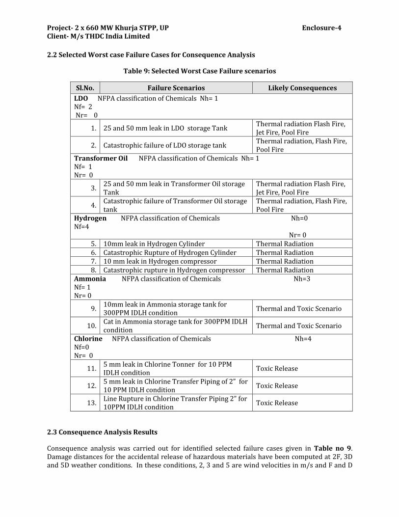
Project- 2 x 660 MW Khurja STPP, UP Enclosure-4 Client- M/s THDC India Limited
2.2 Selected Worst case Failure Cases for Consequence Analysis
Table 9: Selected Worst Case Failure scenarios
Sl.No. Failure Scenarios Likely Consequences
LDO NFPA classification of Chemicals Nh= 1 Nf= 2 Nr= 0
1. 25 and 50 mm leak in LDO storage Tank Thermal radiation Flash Fire, Jet Fire, Pool Fire
2. Catastrophic failure of LDO storage tank Thermal radiation, Flash Fire, Pool Fire
Transformer Oil NFPA classification of Chemicals Nh= 1 Nf= 1 Nr= 0
3. 25 and 50 mm leak in Transformer Oil storage Tank
Thermal radiation Flash Fire, Jet Fire, Pool Fire
4. Catastrophic failure of Transformer Oil storage tank
Thermal radiation, Flash Fire, Pool Fire
Hydrogen NFPA classification of Chemicals Nh=0 Nf=4 Nr= 0
5. 10mm leak in Hydrogen Cylinder Thermal Radiation 6. Catastrophic Rupture of Hydrogen Cylinder Thermal Radiation 7. 10 mm leak in Hydrogen compressor Thermal Radiation 8. Catastrophic rupture in Hydrogen compressor Thermal Radiation
Ammonia NFPA classification of Chemicals Nh=3 Nf= 1 Nr= 0
9. 10mm leak in Ammonia storage tank for 300PPM IDLH condition
Thermal and Toxic Scenario
10. Cat in Ammonia storage tank for 300PPM IDLH condition
Thermal and Toxic Scenario
Chlorine NFPA classification of Chemicals Nh=4 Nf=0 Nr= 0
11. 5 mm leak in Chlorine Tonner for 10 PPM IDLH condition
Toxic Release
12. 5 mm leak in Chlorine Transfer Piping of 2” for 10 PPM IDLH condition
Toxic Release
13. Line Rupture in Chlorine Transfer Piping 2” for 10PPM IDLH condition
Toxic Release
2.3 Consequence Analysis Results
Consequence analysis was carried out for identified selected failure cases given in Table no 9. Damage distances for the accidental release of hazardous materials have been computed at 2F, 3D and 5D weather conditions. In these conditions, 2, 3 and 5 are wind velocities in m/s and F and D
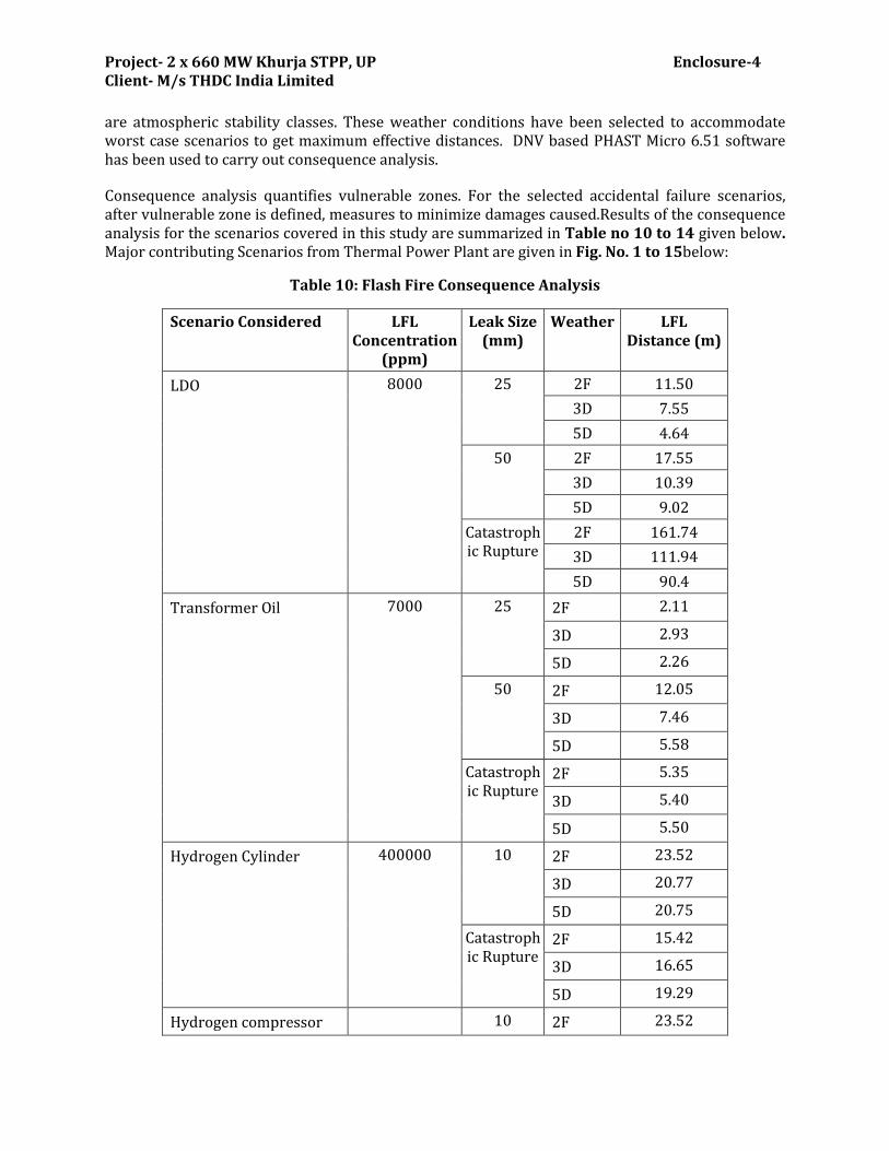
Project- 2 x 660 MW Khurja STPP, UP Enclosure-4 Client- M/s THDC India Limited
are atmospheric stability classes. These weather conditions have been selected to accommodate worst case scenarios to get maximum effective distances. DNV based PHAST Micro 6.51 software has been used to carry out consequence analysis.
Consequence analysis quantifies vulnerable zones. For the selected accidental failure scenarios, after vulnerable zone is defined, measures to minimize damages caused.Results of the consequence analysis for the scenarios covered in this study are summarized in Table no 10 to 14 given below. Major contributing Scenarios from Thermal Power Plant are given in Fig. No. 1 to 15below:
Table 10: Flash Fire Consequence Analysis
Scenario Considered LFL Concentration
(ppm)
Leak Size (mm)
Weather LFL Distance (m)
LDO 8000 25 2F 11.50
3D 7.55
5D 4.64
50 2F 17.55
3D 10.39
5D 9.02
Catastrophic Rupture
2F 161.74
3D 111.94
5D 90.4
Transformer Oil 7000 25 2F 2.11
3D 2.93
5D 2.26
50 2F 12.05
3D 7.46
5D 5.58
Catastrophic Rupture
2F 5.35
3D 5.40
5D 5.50
Hydrogen Cylinder 400000 10 2F 23.52
3D 20.77
5D 20.75
Catastrophic Rupture
2F 15.42
3D 16.65
5D 19.29
Hydrogen compressor 10 2F 23.52
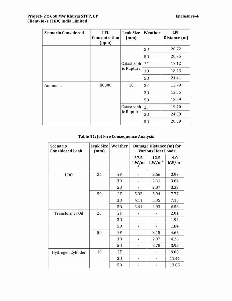
Project- 2 x 660 MW Khurja STPP, UP Enclosure-4 Client- M/s THDC India Limited
Scenario Considered LFL Concentration
(ppm)
Leak Size (mm)
Weather LFL Distance (m)
3D 20.72
5D 20.75
Catastrophic Rupture
2F 17.12
3D 18.43
5D 21.41
Ammonia 80000 10 2F 12.79
3D 13.05
5D 12.89
Catastrophic Rupture
2F 19.70
3D 24.08
5D 28.59
Table 11: Jet Fire Consequence Analysis
Scenario Considered Leak
Leak Size (mm)
Weather Damage Distance (m) for Various Heat Loads
37.5 kW/m
²
12.5 kW/m²
4.0 kW/m²
LDO 25 2F - 2.66 3.93
3D - 2.31 3.64
5D - 2.07 3.39
50 2F 5.92 5.94 7.77
3D 4.11 5.35 7.10
5D 3.61 4.93 6.58
Transformer Oil 25 2F - - 2.01
3D - - 1.94
5D - - 1.84
50 2F - 3.15 4.65
3D - 2.97 4.26
5D - 2.78 3.99
Hydrogen Cylinder 10 2F - 9.08
3D - - 11.41
5D - - 13.85
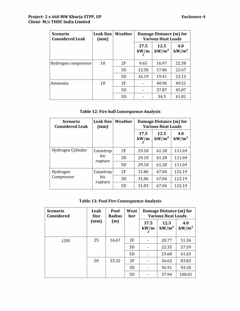
Project- 2 x 660 MW Khurja STPP, UP Enclosure-4 Client- M/s THDC India Limited
Scenario Considered Leak
Leak Size (mm)
Weather Damage Distance (m) for Various Heat Loads
37.5 kW/m
²
12.5 kW/m²
4.0 kW/m²
Hydrogen compressor 10 2F 9.65 16.97 22.38
3D 12.50 17.86 22.67
5D 16.19 19.41 23.13
Ammonia 10 2F - 40.96 49.51
3D - 37.87 45.87
5D - 34.3 41.81
Table 12: Fire ball Consequence Analysis
Scenario Considered Leak
Leak Size (mm)
Weather Damage Distance (m) for Various Heat Loads
37.5 kW/m
²
12.5 kW/m²
4.0 kW/m²
Hydrogen Cylinder Catastrophic
rupture
2F 29.18 61.28 111.69
3D 29.18 61.28 111.69
5D 29.18 61.28 111.69
Hydrogen Compressor
Catastrophic
rupture
2F 31.86 67.04 122.19
3D 31.86 67.04 122.19
5D 31.83 67.04 122.19
Table 13: Pool Fire Consequence Analysis
Scenario Considered
Leak Size
(mm)
Pool Radius
(m)
Weather
Damage Distance (m) for Various Heat Loads
37.5 kW/m
²
12.5 kW/m²
4.0 kW/m²
LDO 25 16.67 2F - 20.77 51.36
3D - 22.35 57.59
5D - 23.68 61.65
50 33.32 2F - 36.62 83.83
3D - 36.91 93.30
5D - 37.94 100.01
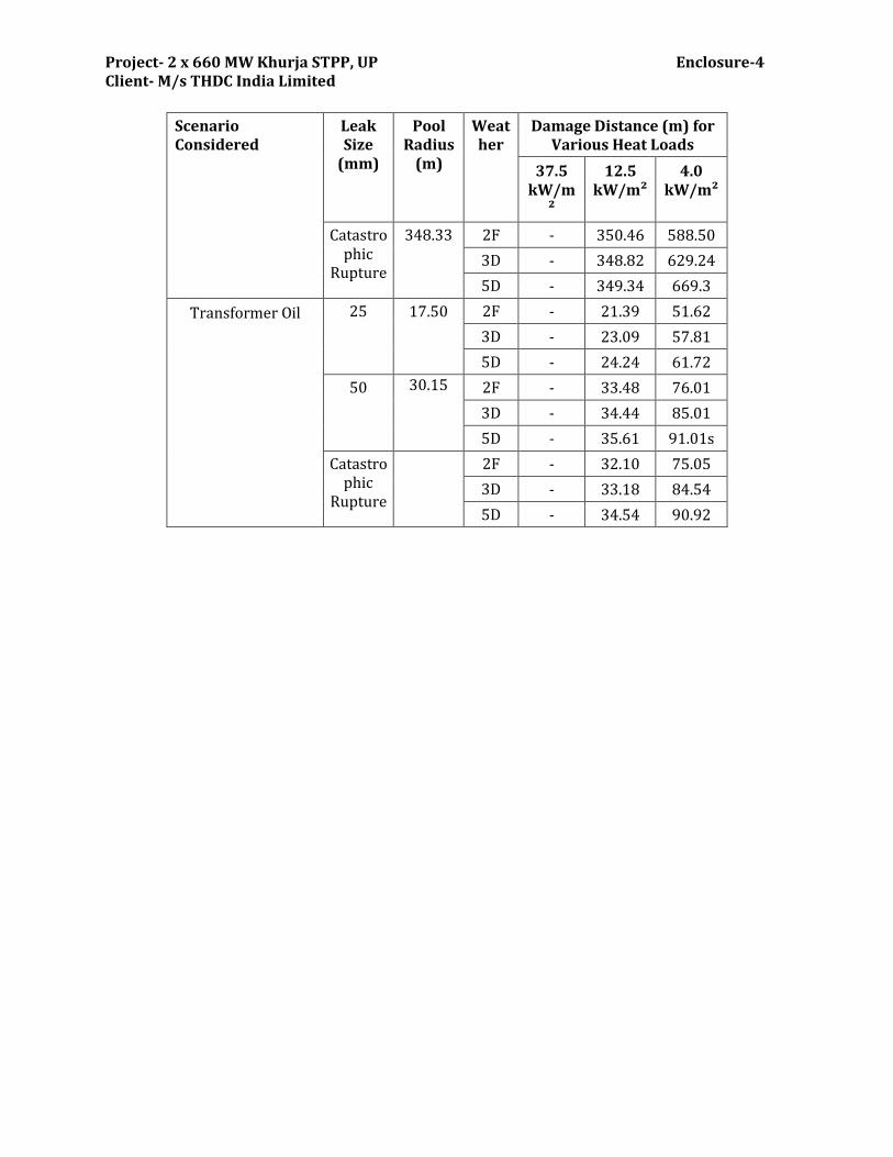
Project- 2 x 660 MW Khurja STPP, UP Enclosure-4 Client- M/s THDC India Limited
Scenario Considered
Leak Size
(mm)
Pool Radius
(m)
Weather
Damage Distance (m) for Various Heat Loads
37.5 kW/m
²
12.5 kW/m²
4.0 kW/m²
Catastrophic
Rupture
348.33 2F - 350.46 588.50
3D - 348.82 629.24
5D - 349.34 669.3
Transformer Oil 25 17.50 2F - 21.39 51.62
3D - 23.09 57.81
5D - 24.24 61.72
50 30.15 2F - 33.48 76.01
3D - 34.44 85.01
5D - 35.61 91.01s
Catastrophic
Rupture
2F - 32.10 75.05
3D - 33.18 84.54
5D - 34.54 90.92
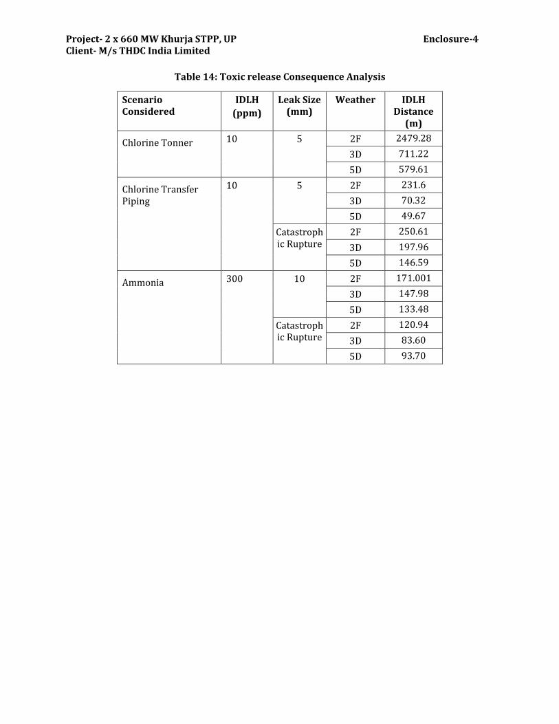
Project- 2 x 660 MW Khurja STPP, UP Enclosure-4 Client- M/s THDC India Limited
Table 14: Toxic release Consequence Analysis
Scenario Considered
IDLH
(ppm)
Leak Size (mm)
Weather IDLH Distance
(m)
Chlorine Tonner 10 5 2F 2479.28
3D 711.22
5D 579.61
Chlorine Transfer Piping
10 5 2F 231.6
3D 70.32
5D 49.67
Catastrophic Rupture
2F 250.61
3D 197.96
5D 146.59
Ammonia 300 10 2F 171.001
3D 147.98
5D 133.48
Catastrophic Rupture
2F 120.94
3D 83.60
5D 93.70
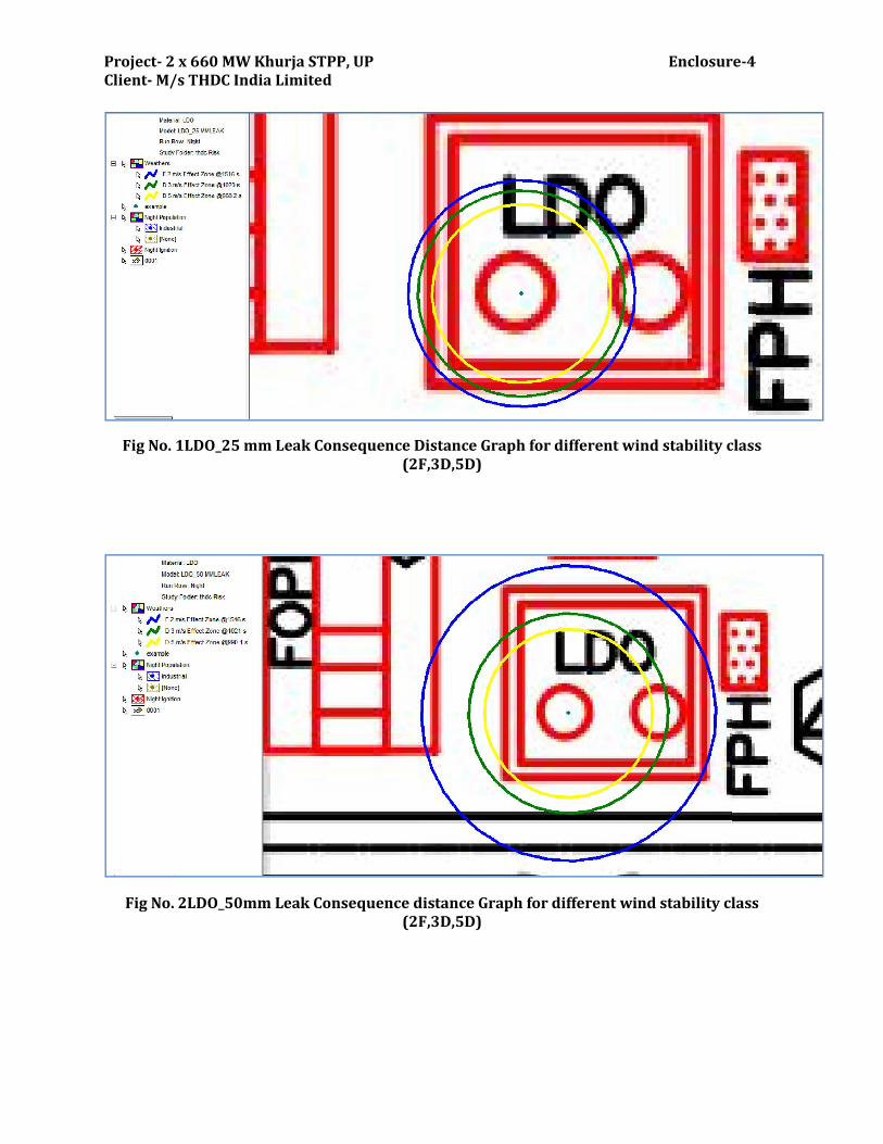
Project- 2 x 660 MW Khurja STPP, UP Enclosure-4 Client- M/s THDC India Limited
Fig No. 1LDO_25 mm Leak Consequence Distance Graph for different wind stability class (2F,3D,5D)
Fig No. 2LDO_50mm Leak Consequence distance Graph for different wind stability class (2F,3D,5D)
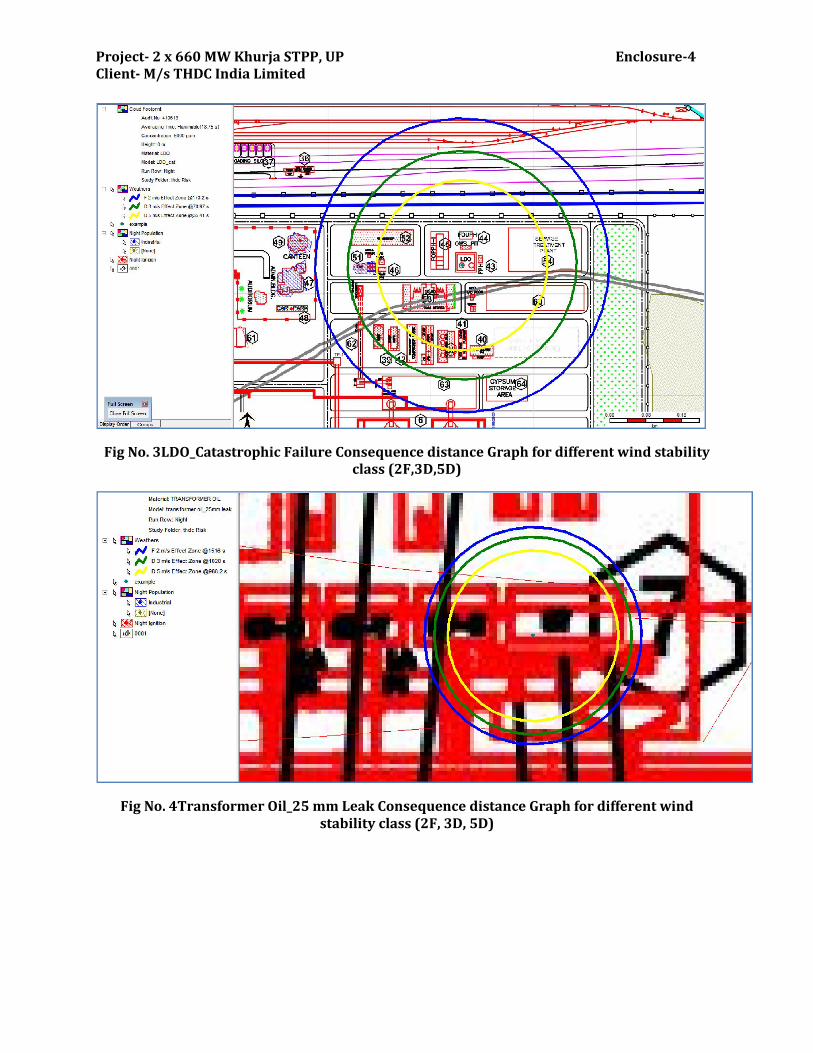
Project- 2 x 660 MW Khurja STPP, UP Enclosure-4 Client- M/s THDC India Limited
Fig No. 3LDO_Catastrophic Failure Consequence distance Graph for different wind stability class (2F,3D,5D)
Fig No. 4Transformer Oil_25 mm Leak Consequence distance Graph for different wind stability class (2F, 3D, 5D)
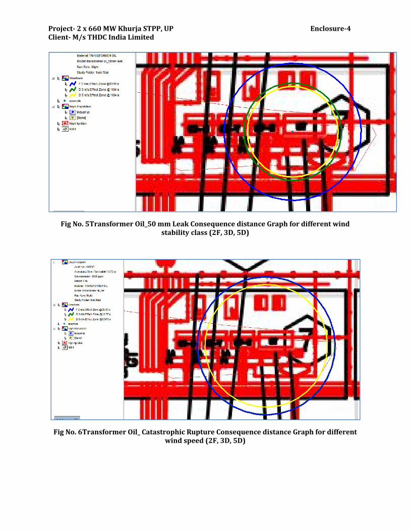
Project- 2 x 660 MW Khurja STPP, UP Enclosure-4 Client- M/s THDC India Limited
Fig No. 5Transformer Oil_50 mm Leak Consequence distance Graph for different wind stability class (2F, 3D, 5D)
Fig No. 6Transformer Oil_ Catastrophic Rupture Consequence distance Graph for different wind speed (2F, 3D, 5D)
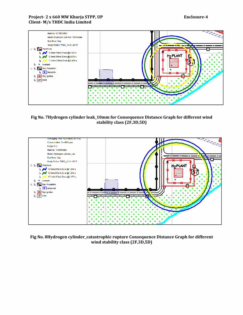
Project- 2 x 660 MW Khurja STPP, UP Enclosure-4 Client- M/s THDC India Limited
Fig No. 7Hydrogen cylinder leak_10mm for Consequence Distance Graph for different wind stability class (2F,3D,5D)
Fig No. 8Hydrogen cylinder_catastrophic rupture Consequence Distance Graph for different wind stability class (2F,3D,5D)
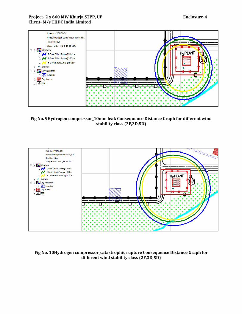
Project- 2 x 660 MW Khurja STPP, UP Enclosure-4 Client- M/s THDC India Limited
Fig No. 9Hydrogen compressor_10mm leak Consequence Distance Graph for different wind stability class (2F,3D,5D)
Fig No. 10Hydrogen compressor_catastrophic rupture Consequence Distance Graph for different wind stability class (2F,3D,5D)
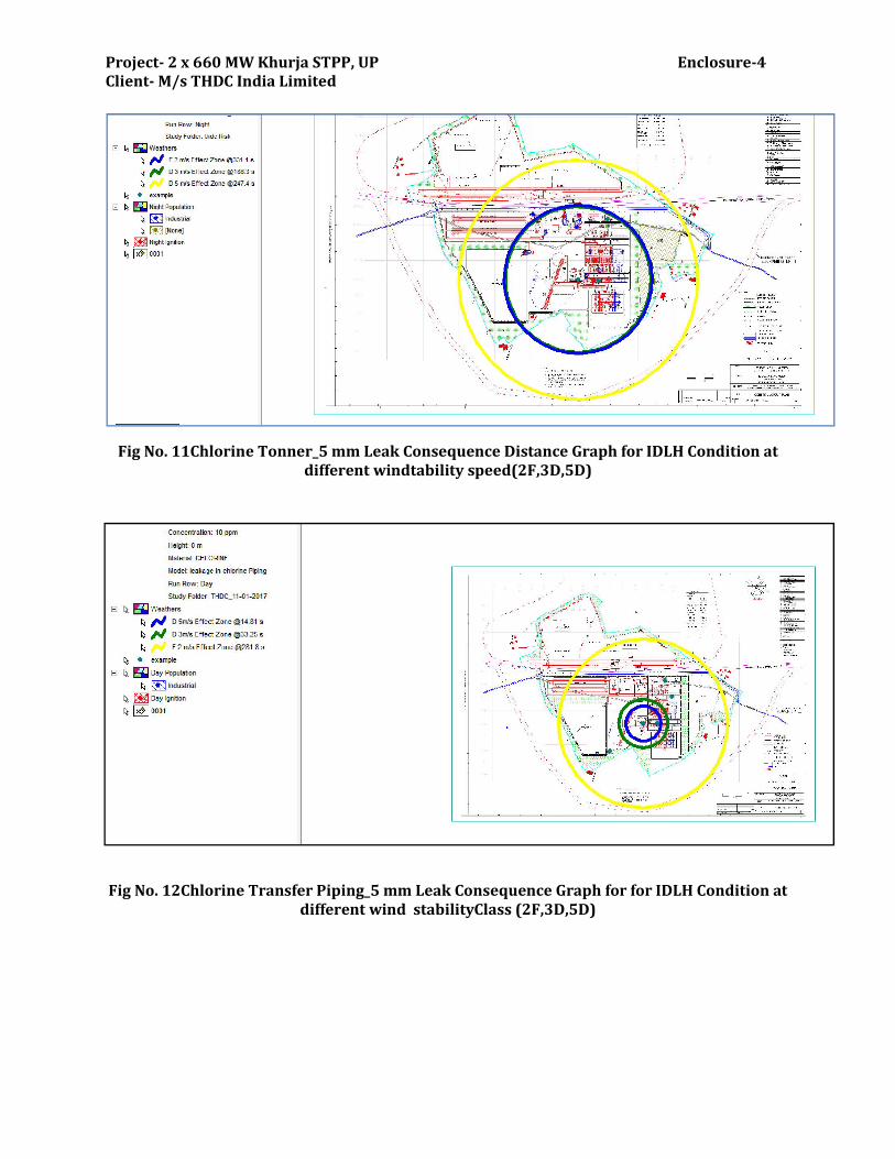
Project- 2 x 660 MW Khurja STPP, UP Enclosure-4 Client- M/s THDC India Limited
Fig No. 11Chlorine Tonner_5 mm Leak Consequence Distance Graph for IDLH Condition at different windtability speed(2F,3D,5D)
Fig No. 12Chlorine Transfer Piping_5 mm Leak Consequence Graph for for IDLH Condition at different wind stabilityClass (2F,3D,5D)
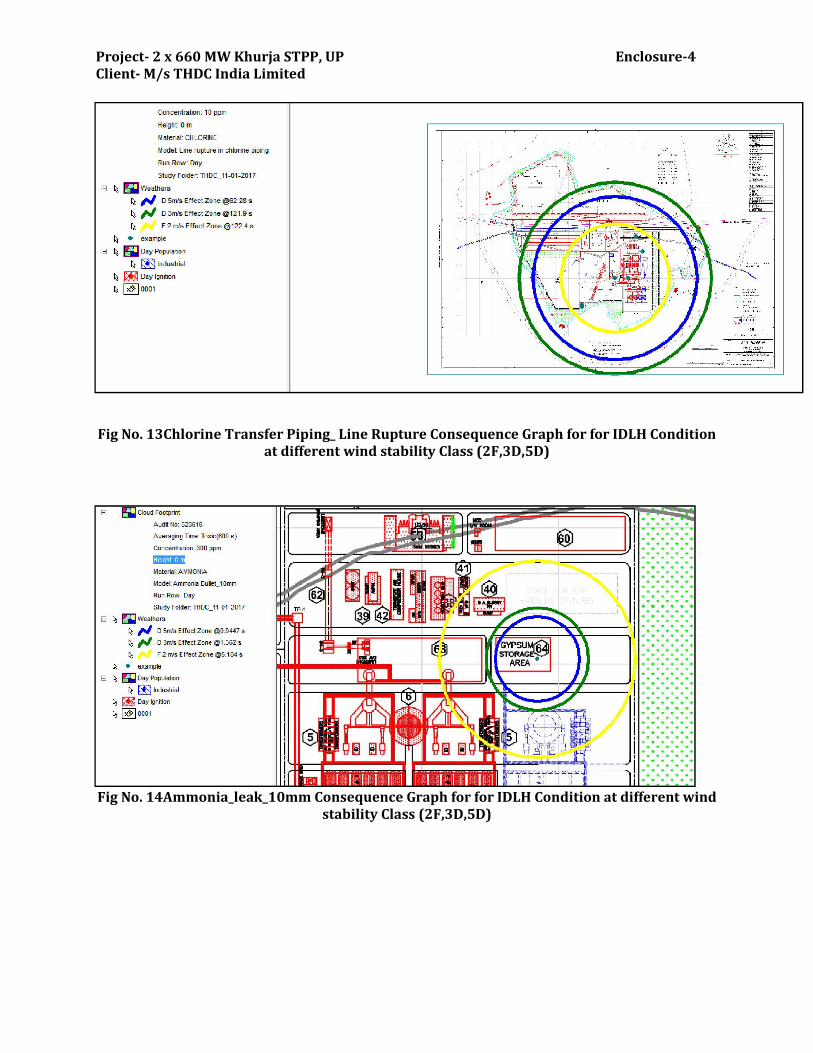
Project- 2 x 660 MW Khurja STPP, UP Enclosure-4 Client- M/s THDC India Limited
Fig No. 13Chlorine Transfer Piping_ Line Rupture Consequence Graph for for IDLH Condition at different wind stability Class (2F,3D,5D)
Fig No. 14Ammonia_leak_10mm Consequence Graph for for IDLH Condition at different wind stability Class (2F,3D,5D)
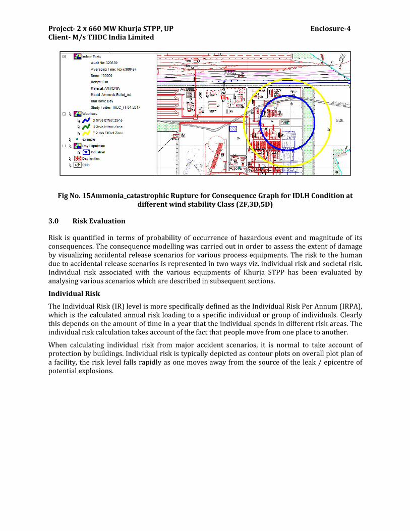
Project- 2 x 660 MW Khurja STPP, UP Enclosure-4 Client- M/s THDC India Limited
Fig No. 15Ammonia_catastrophic Rupture for Consequence Graph for IDLH Condition at different wind stability Class (2F,3D,5D)
3.0 Risk Evaluation
Risk is quantified in terms of probability of occurrence of hazardous event and magnitude of its consequences. The consequence modelling was carried out in order to assess the extent of damage by visualizing accidental release scenarios for various process equipments. The risk to the human due to accidental release scenarios is represented in two ways viz. individual risk and societal risk. Individual risk associated with the various equipments of Khurja STPP has been evaluated by analysing various scenarios which are described in subsequent sections.
Individual Risk
The Individual Risk (IR) level is more specifically defined as the Individual Risk Per Annum (IRPA), which is the calculated annual risk loading to a specific individual or group of individuals. Clearly this depends on the amount of time in a year that the individual spends in different risk areas. The individual risk calculation takes account of the fact that people move from one place to another.
When calculating individual risk from major accident scenarios, it is normal to take account of protection by buildings. Individual risk is typically depicted as contour plots on overall plot plan of a facility, the risk level falls rapidly as one moves away from the source of the leak / epicentre of potential explosions.
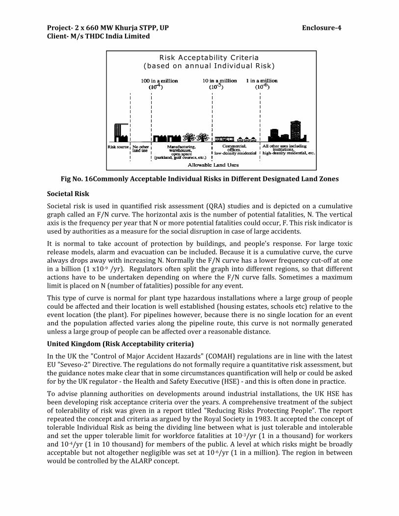
Project- 2 x 660 MW Khurja STPP, UP Enclosure-4 Client- M/s THDC India Limited
Fig No. 16Commonly Acceptable Individual Risks in Different Designated Land Zones
Societal Risk
Societal risk is used in quantified risk assessment (QRA) studies and is depicted on a cumulative graph called an F/N curve. The horizontal axis is the number of potential fatalities, N. The vertical axis is the frequency per year that N or more potential fatalities could occur, F. This risk indicator is used by authorities as a measure for the social disruption in case of large accidents.
It is normal to take account of protection by buildings, and people's response. For large toxic release models, alarm and evacuation can be included. Because it is a cumulative curve, the curve always drops away with increasing N. Normally the F/N curve has a lower frequency cut-off at one in a billion (1 x10⁻⁹ /yr). Regulators often split the graph into different regions, so that different actions have to be undertaken depending on where the F/N curve falls. Sometimes a maximum limit is placed on N (number of fatalities) possible for any event.
This type of curve is normal for plant type hazardous installations where a large group of people could be affected and their location is well established (housing estates, schools etc) relative to the event location (the plant). For pipelines however, because there is no single location for an event and the population affected varies along the pipeline route, this curve is not normally generated unless a large group of people can be affected over a reasonable distance.
United Kingdom (Risk Acceptability criteria)
In the UK the "Control of Major Accident Hazards" (COMAH) regulations are in line with the latest EU "Seveso-2" Directive. The regulations do not formally require a quantitative risk assessment, but the guidance notes make clear that in some circumstances quantification will help or could be asked for by the UK regulator - the Health and Safety Executive (HSE) - and this is often done in practice.
To advise planning authorities on developments around industrial installations, the UK HSE has been developing risk acceptance criteria over the years. A comprehensive treatment of the subject of tolerability of risk was given in a report titled "Reducing Risks Protecting People”. The report repeated the concept and criteria as argued by the Royal Society in 1983. It accepted the concept of tolerable Individual Risk as being the dividing line between what is just tolerable and intolerable and set the upper tolerable limit for workforce fatalities at 10-3/yr (1 in a thousand) for workers and 10-4/yr (1 in 10 thousand) for members of the public. A level at which risks might be broadly acceptable but not altogether negligible was set at 10-6/yr (1 in a million). The region in between would be controlled by the ALARP concept.
Risk Acceptability Criteria (based on annual Individual Risk)
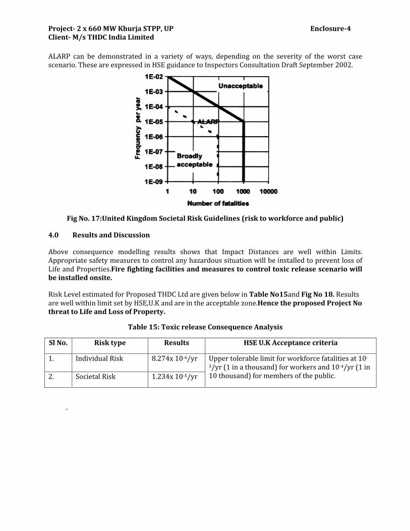
Project- 2 x 660 MW Khurja STPP, UP Enclosure-4 Client- M/s THDC India Limited
ALARP can be demonstrated in a variety of ways, depending on the severity of the worst case scenario. These are expressed in HSE guidance to Inspectors Consultation Draft September 2002.
Fig No. 17:United Kingdom Societal Risk Guidelines (risk to workforce and public)
4.0 Results and Discussion
Above consequence modelling results shows that Impact Distances are well within Limits. Appropriate safety measures to control any hazardous situation will be installed to prevent loss of Life and Properties.Fire fighting facilities and measures to control toxic release scenario will be installed onsite.
Risk Level estimated for Proposed THDC Ltd are given below in Table No15and Fig No 18. Results are well within limit set by HSE,U.K and are in the acceptable zone.Hence the proposed Project No threat to Life and Loss of Property.
Table 15: Toxic release Consequence Analysis
Sl No. Risk type Results HSE U.K Acceptance criteria
1. Individual Risk 8.274x 10⁻⁶/yr Upper tolerable limit for workforce fatalities at 10-
3/yr (1 in a thousand) for workers and 10-4/yr (1 in 10 thousand) for members of the public. 2. Societal Risk 1.234x 10⁻⁵/yr
.
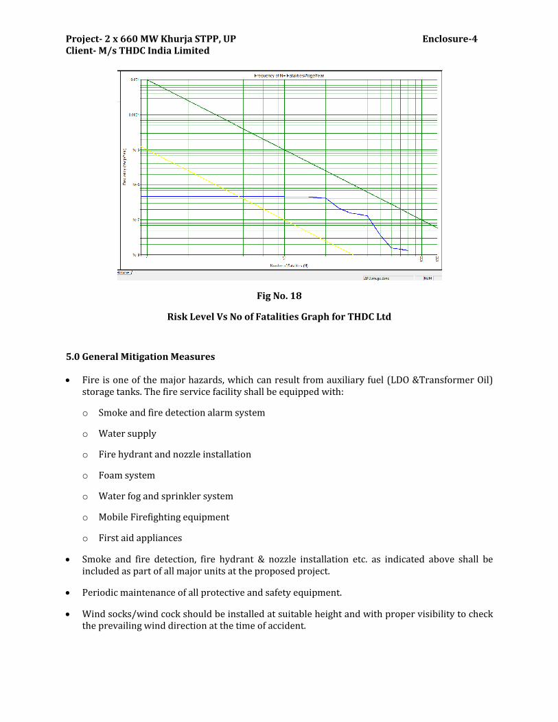
Project- 2 x 660 MW Khurja STPP, UP Enclosure-4 Client- M/s THDC India Limited
Fig No. 18
Risk Level Vs No of Fatalities Graph for THDC Ltd
5.0 General Mitigation Measures
Fire is one of the major hazards, which can result from auxiliary fuel (LDO &Transformer Oil) storage tanks. The fire service facility shall be equipped with:
o Smoke and fire detection alarm system
o Water supply
o Fire hydrant and nozzle installation
o Foam system
o Water fog and sprinkler system
o Mobile Firefighting equipment
o First aid appliances
Smoke and fire detection, fire hydrant & nozzle installation etc. as indicated above shall be included as part of all major units at the proposed project.
Periodic maintenance of all protective and safety equipment.
Wind socks/wind cock should be installed at suitable height and with proper visibility to check the prevailing wind direction at the time of accident.

Project- 2 x 660 MW Khurja STPP, UP Enclosure-4 Client- M/s THDC India Limited
Periodical training/awareness would be given to work force at the project as refresher courses to handle any emergency situation.
Periodic mock drills should be conducted so as to check the alertness and efficiency of the Disaster Management Plan (DMP) and corresponding records should be maintained.
Signboards including emergency phone numbers and no smoking signs should be installed at all appropriate locations.
Plant would have adequate communication system.
All major units/equipment shall be provided with smoke/fire detection and alarm system.
All electrical equipments shall be provided with proper earthing. Earthed electrode shall be periodically tested and maintained.
Emergency lighting shall be available at all critical locations including the operator’s room to carry out safe shut down of the plant, ready identification of fire fighting facilities such as fire water pumps, fire alarm stations, etc.
In addition to normal lighting each installation shall be equipped with emergency (AC) and critical (DC) lighting.
All electrical equipments shall be free from carbon dust, oil deposits, grease, etc.
Cable routing shall be planned away from heat sources, gas, water, oil, drain piping, air conditioning ducts, etc.
Cable route markers shall be provided in the permanent way at the location of changes in the direction of cables and at cable joint locations.
Chlorine detectors and Chlorine arresting kits would be provided at relevant locations.
There would be necessary provision for emergency stop of critical equipments from control room in the event of major leak/flash fire at Plant.
Clearly defined escape routes would be developed for the Station taking into account the impairment of escape by hazardous releases and sign boards be erected in places to guide personnel in case of an emergency.
Well defined assembly point in safe locations would be identified for personnel in case of an emergency.
Windsocks visible from all direction would be provided. This will assist people to escape in upwind or cross wind direction from flammable releases.
There should be an SOP established for clarity of actions to be taken in case of fire/leak emergency.
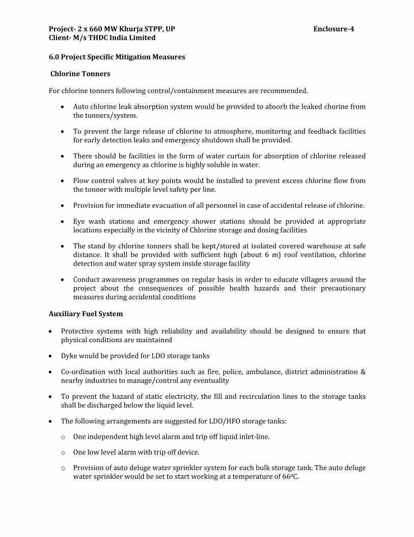
Project- 2 x 660 MW Khurja STPP, UP Enclosure-4 Client- M/s THDC India Limited
6.0 Project Specific Mitigation Measures
Chlorine Tonners
For chlorine tonners following control/containment measures are recommended.
Auto chlorine leak absorption system would be provided to absorb the leaked chorine from the tonners/system.
To prevent the large release of chlorine to atmosphere, monitoring and feedback facilities for early detection leaks and emergency shutdown shall be provided.
There should be facilities in the form of water curtain for absorption of chlorine released during an emergency as chlorine is highly soluble in water.
Flow control valves at key points would be installed to prevent excess chlorine flow from the tonner with multiple level safety per line.
Provision for immediate evacuation of all personnel in case of accidental release of chlorine.
Eye wash stations and emergency shower stations should be provided at appropriate locations especially in the vicinity of Chlorine storage and dosing facilities
The stand by chlorine tonners shall be kept/stored at isolated covered warehouse at safe distance. It shall be provided with sufficient high (about 6 m) roof ventilation, chlorine detection and water spray system inside storage facility
Conduct awareness programmes on regular basis in order to educate villagers around the project about the consequences of possible health hazards and their precautionary measures during accidental conditions
Auxiliary Fuel System
Protective systems with high reliability and availability should be designed to ensure that physical conditions are maintained
Dyke would be provided for LDO storage tanks
Co-ordination with local authorities such as fire, police, ambulance, district administration & nearby industries to manage/control any eventuality
To prevent the hazard of static electricity, the fill and recirculation lines to the storage tanks shall be discharged below the liquid level.
The following arrangements are suggested for LDO/HFO storage tanks:
o One independent high level alarm and trip off liquid inlet-line.
o One low level alarm with trip off device.
o Provision of auto deluge water sprinkler system for each bulk storage tank. The auto deluge water sprinkler would be set to start working at a temperature of 660C.

Project- 2 x 660 MW Khurja STPP, UP Enclosure-4 Client- M/s THDC India Limited
The ST turbine building, switchyard, transformer yard, administrative building canteen, first aid center, fire stations etc. shall be located safely, if viewed in the light of worst accident scenarios.
In case of any tank on fire or fire in the vicinity, the cooling of adjoining tank should be resorted promptly in addition to tank on fire so that neighboring tanks does not give away.
The night vision wind stocking be mounted on top of administrative building, main plant building and storage tanks so that people can move in upwind directions in the event of massive spillage or tank on fire.
No machinery of vital importance like fire fighting pump house, Hydrant and Fuel oil pump house shall be placed out of radiation contours of 37.5 kW/m2 heat intensity.
Maintenance plays a vital role in proper upkeep of plant. One important function is the monitoring of equipment health, pipelines and machines. Adoption of system like thickness
survey (including supports) maintenance practices will improve plant performance and safety.
**********

ENCLOSURE-5
Project- 2 x 660 MW Khurja STPP, UP Enclosure-5 Client- M/s THDC India Limited
Greenbelt Development Plan
1.1 Objectives
Objectives of the proposed green belt are as follows:
Mitigation of air pollution due to fugitive emissions;
Attenuation of noise generated from operation of different machines;
Improvement of bio-diversity of the area; and
Improvement of aesthetics of the site.
The main air pollutants likely to be generated from the proposed project are
Particulate matter,
Fugitive emission,
Sulphur dioxide, and
Nitrogen oxides.
1.2 Species for green belt
1.2.1 General Characteristics
The greenbelt would be designed in three tier system. The three tier system will be followed so
that it could provide complete canopy coverage from ground flora up to top canopy and could
provide considerable attenuation for noise and pollution impact. First inner rows will be facing
the plant, where flowering shrubs and herbs shall be planted in 5 m width.Small trees shall be
planted in the middle rows in 10m width, followed by taller trees in the last few rows. Adequate
space shall be kept between the trees, small trees. Since the project site falls under agro-climatic
zone namely Upper Gangetic Plains, the selection of plant species for greenbelt development was
based on “Guidelines for Developing Green Belts, PROBES/75/1999-2000”for differenent
purposes are as follows
For absorption of gases:
Tolerance towards pollutants in question,
Longer duration of foliage,
Freely exposed foliage, through
Adequate height of crown,
Openness of foliage in canopy
Big leaves with long and broad laminar surfaces,
Large number of stomatal apertures
Well exposed stomata

Project- 2 x 660 MW Khurja STPP, UP Enclosure-5 Client- M/s THDC India Limited
For removal of suspended particulate matter:
Height and spread of crown,
Leaves supported on firm petioles,
Abundance of surface on bark and foliage, through
Roughness of bark,
Epidermal outgrowth on petioles,
Abundance of axiliary hairs,
Hairs or scales on laminar surfaces, and
Protected stomata.
In view of the fact that atmosphere in industrial areas constitute more than one pollutant, the
guideline advices to choose plant species for green belt development, which are capable of
absorption of chemicals as well as particulate matter pollutants.
For plantation along road sides:
Vehicles are ground level mobile sources of gaseous and particulate matter pollutants. Species
selected for plantation along road sides shall therefore be capable of absorption of gaseous as well
as particulte matter pollutants. For green belt development along road sides, the CPCB Guideline
recommends plantation of shrubs of height 1 to 1.5 m and trees of 3 to 5 m height. The intermixing
of trees and shrubs should be such that the foliage area density in vertical is almost uniform.
1.2.2 Agro-climatic zone
The proposed site is located within Bulandshar District in Uttar Pradesh. As per agro-climatic zones
of India (CPCB Guidelines), the site falls within ‘Upper Gangetic Plains’, and sub-zone “North
Western Plains, with Dry Sub Humid to Semi Arid climate.
1.2.3 Selection of Species
The selection of species for the proposed green belt is based on the recommendations under the
CPCB guidelines for the applicable agro-climatic sub-zone. While selecting the species from the
recommended list, quick growing species with longer duration of foliage and tolerant to air
pollution have been preferred. With these considerations, the following species have been selected
for plantation within the green belt and along the roads.
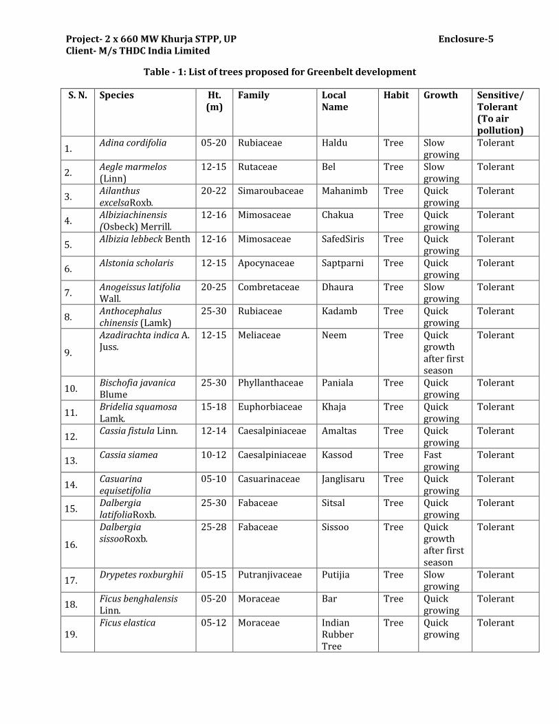
Project- 2 x 660 MW Khurja STPP, UP Enclosure-5 Client- M/s THDC India Limited
Table - 1: List of trees proposed for Greenbelt development
S. N. Species Ht. (m)
Family Local Name
Habit Growth Sensitive/ Tolerant (To air pollution)
1. Adina cordifolia 05-20 Rubiaceae Haldu Tree Slow
growing Tolerant
2. Aegle marmelos (Linn)
12-15 Rutaceae Bel Tree Slow growing
Tolerant
3. Ailanthus excelsaRoxb.
20-22 Simaroubaceae Mahanimb Tree Quick growing
Tolerant
4. Albiziachinensis (Osbeck) Merrill.
12-16 Mimosaceae Chakua Tree Quick growing
Tolerant
5. Albizia lebbeck Benth 12-16 Mimosaceae SafedSiris Tree Quick
growing Tolerant
6. Alstonia scholaris 12-15 Apocynaceae Saptparni Tree Quick
growing Tolerant
7. Anogeissus latifolia Wall.
20-25 Combretaceae Dhaura Tree Slow growing
Tolerant
8. Anthocephalus chinensis (Lamk)
25-30 Rubiaceae Kadamb Tree Quick growing
Tolerant
9.
Azadirachta indica A. Juss.
12-15 Meliaceae Neem Tree Quick growth after first season
Tolerant
10. Bischofia javanica Blume
25-30 Phyllanthaceae Paniala Tree Quick growing
Tolerant
11. Bridelia squamosa Lamk.
15-18 Euphorbiaceae Khaja Tree Quick growing
Tolerant
12. Cassia fistula Linn. 12-14 Caesalpiniaceae Amaltas Tree Quick
growing Tolerant
13. Cassia siamea 10-12 Caesalpiniaceae Kassod Tree Fast
growing Tolerant
14. Casuarina equisetifolia
05-10 Casuarinaceae Janglisaru Tree Quick growing
Tolerant
15. Dalbergia latifoliaRoxb.
25-30 Fabaceae Sitsal Tree Quick growing
Tolerant
16.
Dalbergia sissooRoxb.
25-28 Fabaceae Sissoo Tree Quick growth after first season
Tolerant
17. Drypetes roxburghii 05-15 Putranjivaceae Putijia Tree Slow
growing Tolerant
18. Ficus benghalensis Linn.
05-20 Moraceae Bar Tree Quick growing
Tolerant
19. Ficus elastica 05-12 Moraceae Indian
Rubber Tree
Tree Quick growing
Tolerant
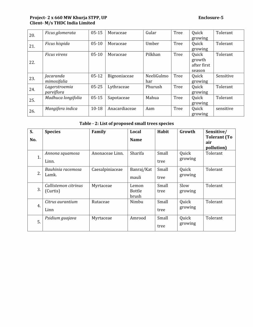
Project- 2 x 660 MW Khurja STPP, UP Enclosure-5 Client- M/s THDC India Limited
20. Ficus glomerata 05-15 Moraceae Gular Tree Quick
growing Tolerant
21. Ficus hispida 05-10 Moraceae Umber Tree Quick
growing Tolerant
22.
Ficus virens 05-10 Moraceae Pilkhan Tree Quick growth after first season
Tolerant
23. Jacaranda mimosifalia
05-12 Bignoniaceae NeeliGulmohar
Tree Quick growing
Sensitive
24. Lagerstroemia parviflora
05-25 Lythraceae Phurush Tree Quick growing
Tolerant
25. Madhuca longifolia 05-15 Sapotaceae Mahua Tree Quick
growing Tolerant
26. Mangifera indica 10-18 Anacardiaceae Aam Tree Quick
growing sensitive
Table - 2: List of proposed small trees species
S.
No.
Species Family Local
Name
Habit Growth Sensitive/ Tolerant (To air pollution)
1. Annona squamosa
Linn.
Anonaceae Linn. Sharifa Small
tree
Quick growing
Tolerant
2. Bauhinia racemosa Lamk.
Caesalpiniaceae Banraj/Kat
mauli
Small
tree
Quick growing
Tolerant
3. Callistemon citrinus (Curtis)
Myrtaceae Lemon Bottle brush
Small tree
Slow growing
Tolerant
4. Citrus aurantium
Linn
Rutaceae Nimbu Small
tree
Quick growing
Tolerant
5. Psidium guajava Myrtaceae Amrood Small
tree
Quick growing
Tolerant
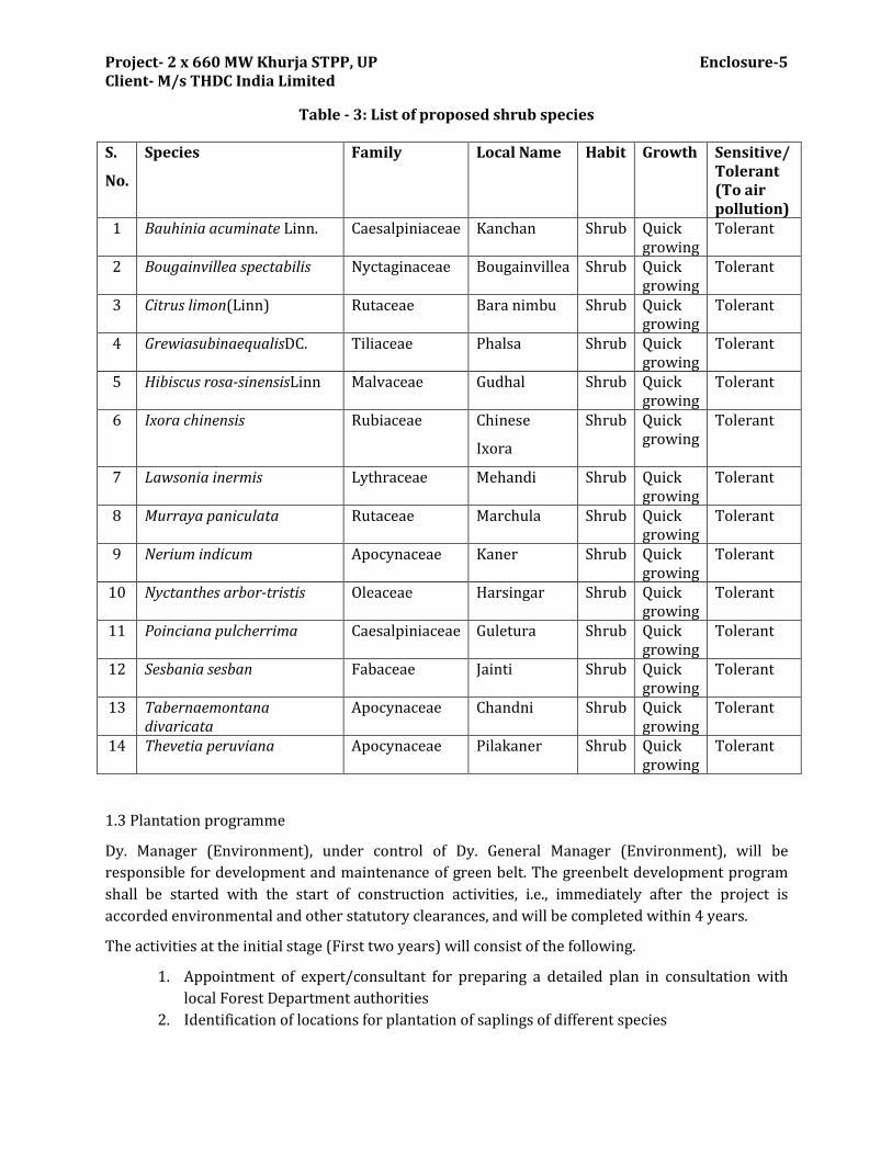
Project- 2 x 660 MW Khurja STPP, UP Enclosure-5 Client- M/s THDC India Limited
Table - 3: List of proposed shrub species
S.
No.
Species Family Local Name Habit Growth Sensitive/ Tolerant (To air pollution)
1 Bauhinia acuminate Linn. Caesalpiniaceae Kanchan Shrub Quick growing
Tolerant
2 Bougainvillea spectabilis Nyctaginaceae Bougainvillea Shrub Quick growing
Tolerant
3 Citrus limon(Linn) Rutaceae Bara nimbu Shrub Quick growing
Tolerant
4 GrewiasubinaequalisDC. Tiliaceae Phalsa Shrub Quick growing
Tolerant
5 Hibiscus rosa-sinensisLinn Malvaceae Gudhal Shrub Quick growing
Tolerant
6 Ixora chinensis Rubiaceae Chinese
Ixora
Shrub Quick growing
Tolerant
7 Lawsonia inermis Lythraceae Mehandi Shrub Quick growing
Tolerant
8 Murraya paniculata Rutaceae Marchula Shrub Quick growing
Tolerant
9 Nerium indicum Apocynaceae Kaner Shrub Quick growing
Tolerant
10 Nyctanthes arbor-tristis Oleaceae Harsingar Shrub Quick growing
Tolerant
11 Poinciana pulcherrima Caesalpiniaceae Guletura Shrub Quick growing
Tolerant
12 Sesbania sesban Fabaceae Jainti Shrub Quick growing
Tolerant
13 Tabernaemontana divaricata
Apocynaceae Chandni Shrub Quick growing
Tolerant
14 Thevetia peruviana Apocynaceae Pilakaner Shrub Quick growing
Tolerant
1.3 Plantation programme
Dy. Manager (Environment), under control of Dy. General Manager (Environment), will be
responsible for development and maintenance of green belt. The greenbelt development program
shall be started with the start of construction activities, i.e., immediately after the project is
accorded environmental and other statutory clearances, and will be completed within 4 years.
The activities at the initial stage (First two years) will consist of the following.
1. Appointment of expert/consultant for preparing a detailed plan in consultation with
local Forest Department authorities
2. Identification of locations for plantation of saplings of different species
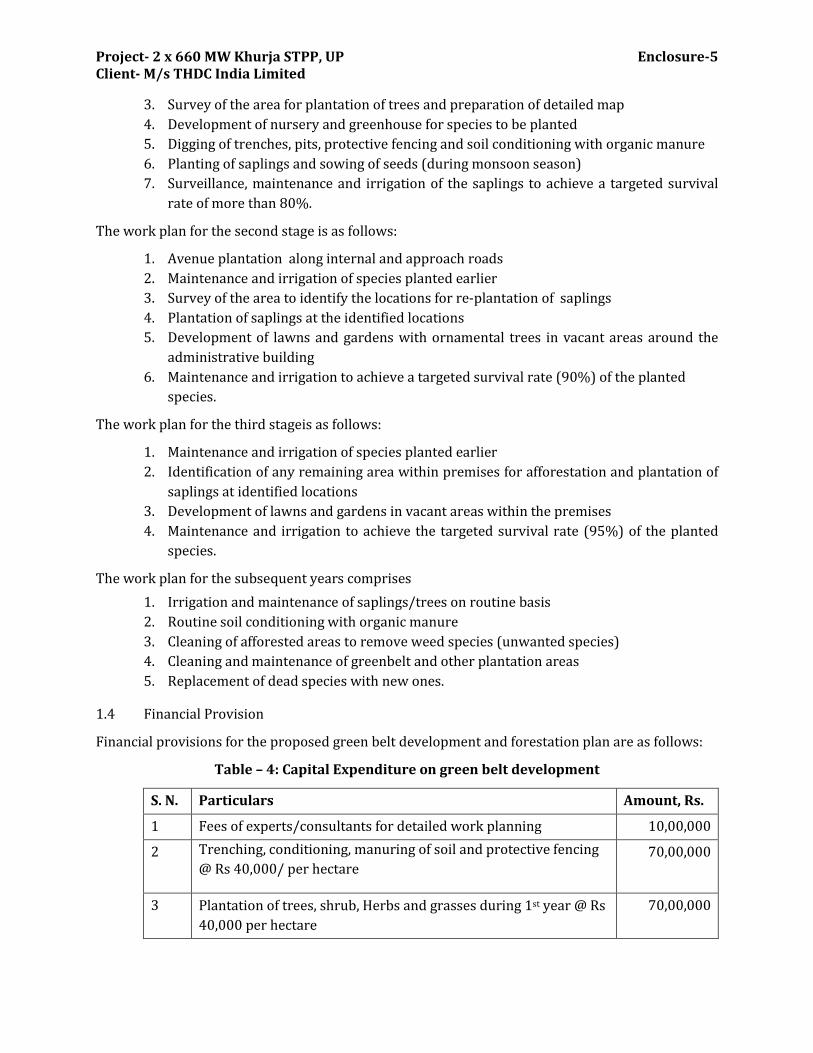
Project- 2 x 660 MW Khurja STPP, UP Enclosure-5 Client- M/s THDC India Limited
3. Survey of the area for plantation of trees and preparation of detailed map
4. Development of nursery and greenhouse for species to be planted
5. Digging of trenches, pits, protective fencing and soil conditioning with organic manure
6. Planting of saplings and sowing of seeds (during monsoon season)
7. Surveillance, maintenance and irrigation of the saplings to achieve a targeted survival
rate of more than 80%.
The work plan for the second stage is as follows:
1. Avenue plantation along internal and approach roads
2. Maintenance and irrigation of species planted earlier
3. Survey of the area to identify the locations for re-plantation of saplings
4. Plantation of saplings at the identified locations
5. Development of lawns and gardens with ornamental trees in vacant areas around the
administrative building
6. Maintenance and irrigation to achieve a targeted survival rate (90%) of the planted
species.
The work plan for the third stageis as follows:
1. Maintenance and irrigation of species planted earlier
2. Identification of any remaining area within premises for afforestation and plantation of
saplings at identified locations
3. Development of lawns and gardens in vacant areas within the premises
4. Maintenance and irrigation to achieve the targeted survival rate (95%) of the planted
species.
The work plan for the subsequent years comprises
1. Irrigation and maintenance of saplings/trees on routine basis
2. Routine soil conditioning with organic manure
3. Cleaning of afforested areas to remove weed species (unwanted species)
4. Cleaning and maintenance of greenbelt and other plantation areas
5. Replacement of dead species with new ones.
1.4 Financial Provision
Financial provisions for the proposed green belt development and forestation plan are as follows:
Table – 4: Capital Expenditure on green belt development
S. N. Particulars Amount, Rs.
1 Fees of experts/consultants for detailed work planning 10,00,000
2 Trenching, conditioning, manuring of soil and protective fencing
@ Rs 40,000/ per hectare 70,00,000
3 Plantation of trees, shrub, Herbs and grasses during 1st year @ Rs
40,000 per hectare
70,00,000

Project- 2 x 660 MW Khurja STPP, UP Enclosure-5 Client- M/s THDC India Limited
4 Plantation of trees, shrub, Herbs and grasses during 2nd year @ Rs
35,000 per hectare
61,25,000
5 Plantation of trees shrub, Herbs and grasses during 3rd year @
Rs25,000 per hectare
43,75,000
Total 2,55,00,000
Table – 5: Revenue Expenditure (Annual) on Green Belt Development
Sl. No. Particulars Amount, Rs.
1 Salaries of regular employees 80,00,000
2 Contract workers, 20 persons @ Rs300/- per day 21,90,000
3 Contingency and unforeseen expenses 1,43,10,000
Total 2,45,00,000
Table - 6: List of trees and their medicinal uses proposed for Greenbelt development
S. No. Species Local Name Medicinal Uses
Part of Plant Uses
1. Adina cordifolia Haldu Bark Dysentery, bacterial infections on the skin, cholera, cold and cough, fever and eczema
Leaf Infertility, headache, Scars and skin yellowish of body
Latex Toothache
2. Aegle marmelos Bel Ripe fruit Dyspepsia, bacillary dysentery
Roots and Bark
Fever
Leaf Inflammation, asthma, hypoglycemia, hepatitis etc.
3. Ailanthus excelsa Mahanimb Bark Fever, labor pain
Leaf Labor pain
4. Albizia chinensis Chakua Seeds Anti-inflammation
Bark Asthma, leucoderma, itching, skin disease, piles, excessive perspiration, inflammation, bronchitis, toothache, leprosy, deafness and strengthens the gums and teeth
5. Albizia lebbeck SafedSiris Leaf Bites and stings from venomous animals, ear pain and coughing
Bark Blood purification.
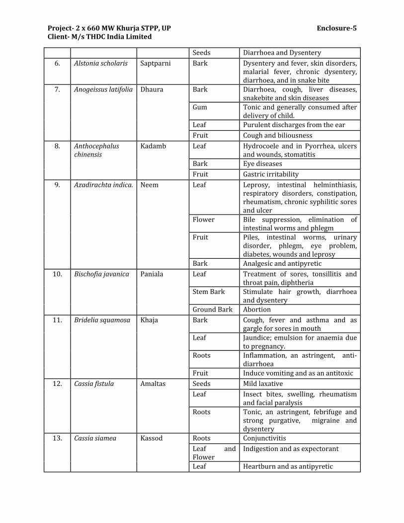
Project- 2 x 660 MW Khurja STPP, UP Enclosure-5 Client- M/s THDC India Limited
Seeds Diarrhoea and Dysentery
6. Alstonia scholaris Saptparni Bark Dysentery and fever, skin disorders, malarial fever, chronic dysentery, diarrhoea, and in snake bite
7. Anogeissus latifolia Dhaura Bark Diarrhoea, cough, liver diseases, snakebite and skin diseases
Gum Tonic and generally consumed after delivery of child.
Leaf Purulent discharges from the ear
Fruit Cough and biliousness
8. Anthocephalus chinensis
Kadamb Leaf Hydrocoele and in Pyorrhea, ulcers and wounds, stomatitis
Bark Eye diseases
Fruit Gastric irritability
9. Azadirachta indica. Neem Leaf Leprosy, intestinal helminthiasis, respiratory disorders, constipation, rheumatism, chronic syphilitic sores and ulcer
Flower Bile suppression, elimination of intestinal worms and phlegm
Fruit Piles, intestinal worms, urinary disorder, phlegm, eye problem, diabetes, wounds and leprosy
Bark Analgesic and antipyretic
10. Bischofia javanica Paniala Leaf Treatment of sores, tonsillitis and throat pain, diphtheria
Stem Bark Stimulate hair growth, diarrhoea and dysentery
Ground Bark Abortion
11. Bridelia squamosa Khaja Bark Cough, fever and asthma and as gargle for sores in mouth
Leaf Jaundice; emulsion for anaemia due to pregnancy.
Roots Inflammation, an astringent, anti-diarrhoea
Fruit Induce vomiting and as an antitoxic
12. Cassia fistula Amaltas Seeds Mild laxative
Leaf Insect bites, swelling, rheumatism and facial paralysis
Roots Tonic, an astringent, febrifuge and strong purgative, migraine and dysentery
13. Cassia siamea Kassod Roots Conjunctivitis
Leaf and Flower
Indigestion and as expectorant
Leaf Heartburn and as antipyretic
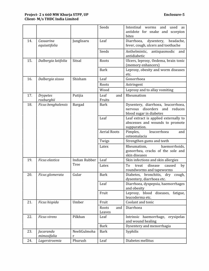
Project- 2 x 660 MW Khurja STPP, UP Enclosure-5 Client- M/s THDC India Limited
Seeds Intestinal worms and used as antidote for snake and scorpion bites
14. Casuarina equisetifolia
Junglisaru Leaf Diarrhoea, dysentery, headache, fever, cough, ulcers and toothache
Seeds Anthelmintic, antispasmodic and antidiabetic
15. Dalbergia latifolia Sitsal Roots Ulcers, leprosy, Oedema, brain tonic (memory enhancers)
Bark Leprosy, obesity and worm diseases etc.
16. Dalbergia sissoo Shisham Leaf Gonorrhoea
Roots Astringent
Wood Leprosy and to allay vomiting
17. Drypetes roxburghii
Putijia Leaf and Fruits
Rheumatism
18. Ficus benghalensis Bargad Bark Dysentery, diarrhoea, leucorrhoea, nervous disorders and reduces blood sugar in diabetes
Leaf Leaf extract is applied externally to abscesses and wounds to promote suppuration.
Aerial Roots Pimples, leucorrhoea and osteomalacia
Twigs Strengthen gums and teeth
Latex Rheumatism, haemorrhoids, gonorrhea, cracks of the sole and skin diseases
19. Ficus elastica Indian Rubber Tree
Leaf Skin infections and skin allergies
Latex To treat disease caused by roundworms and tapeworms
20. Ficus glomerata Gular Bark Diabetes, bronchitis, dry cough, dysentery, diarrhoea etc.
Leaf Diarrhoea, dyspepsia, haemorrhages and obesity
Fruit Leprosy, blood diseases, fatigue, leucoderma etc.
21. Ficus hispida Umber Fruit Coolant and tonic
Roots and Leaves
Diarrhoea
22. Ficus virens Pilkhan Leaf Intrinsic haemorrhage, erysipelas and wound healing
Bark Dysentery and menorrhagia
23. Jacaranda mimosifalia
NeeliGulmohar
Bark Syphilis
24. Lagerstroemia Phurush Leaf Diabetes mellitus
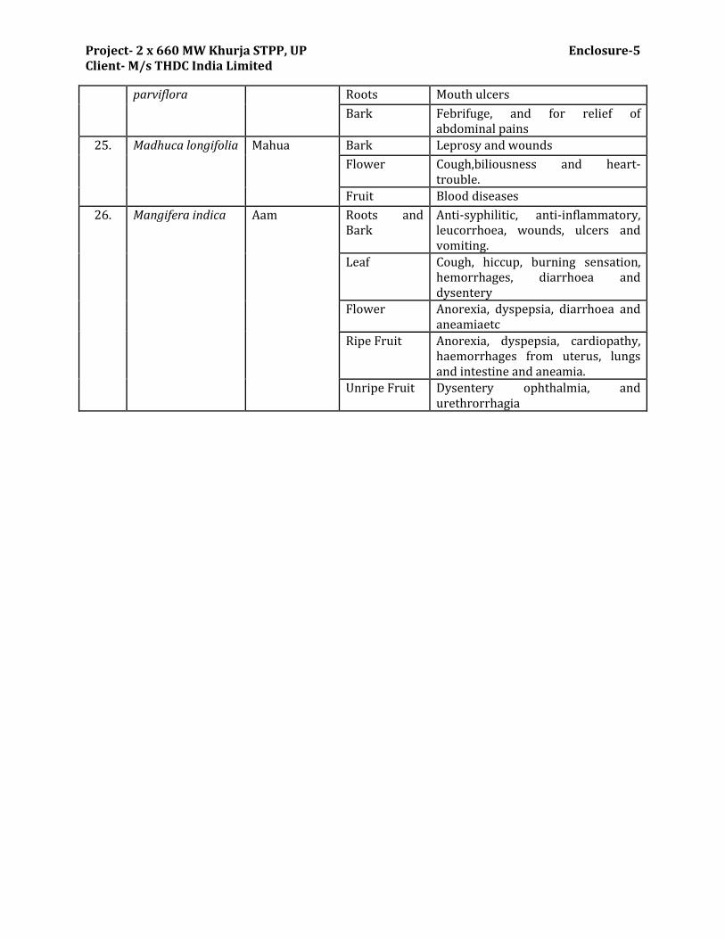
Project- 2 x 660 MW Khurja STPP, UP Enclosure-5 Client- M/s THDC India Limited
parviflora Roots Mouth ulcers
Bark Febrifuge, and for relief of abdominal pains
25. Madhuca longifolia Mahua Bark Leprosy and wounds
Flower Cough,biliousness and heart-trouble.
Fruit Blood diseases
26. Mangifera indica Aam Roots and Bark
Anti-syphilitic, anti-inflammatory, leucorrhoea, wounds, ulcers and vomiting.
Leaf Cough, hiccup, burning sensation, hemorrhages, diarrhoea and dysentery
Flower Anorexia, dyspepsia, diarrhoea and aneamiaetc
Ripe Fruit Anorexia, dyspepsia, cardiopathy, haemorrhages from uterus, lungs and intestine and aneamia.
Unripe Fruit Dysentery ophthalmia, and urethrorrhagia


