Embed Size (px)
Citation preview

e-ISBN 978-967-5770-48-7
Proceedings of the 2nd NatGrad Conference
Part 4: Civil Engineering
Paper ID
Author and Paper Title
1 13 Ali Sami Abdul Jabbar, Md. Ashraful Alam and Kamal Nasharuddin Mustapha. Critical investigations on using shear connectors to delay debonding of steel plate strips externally fixed for shear strengthening of RC beams
2 147 Nor Azlina Alias, Assoc. Prof. Dr. Ir. Lariyah Mohd Sidek, Development of an
Integrated 1D Shallow Water and Solute Transport Model
3 35 Masimawati Abdul Latif, Sivakumar Naganathan and Kamal Nasharuddin Mustapha. Industrial Waste Utilisation in Mortar and Concrete – A review
4 47 Harizah Haris and Mohd Aminur Rashid Mohd Amiruddin Arumugam. An Evaluation of Water Quality From Sungai Penchala Tributary
5 60 Ahmad Fauzan Mohd Sabri, Lariyah Mohd Sidek and Ahmad Sharmy Mohammed
Jaffar. Analysis of TMDL for River of Life Project (RoL) Gombak River
6 77 Md. Tanvir Ehsan Amin and Md. Ashraful Alam. Methods of anchoring to prevent end peeling of flexurally strengthened reinforced concrete beam
7 111 Nazirul Mubin Zahari, Chua Kok Hua and Lariyah Mohd Sidek. Influence of Contact Time on Effectiveness of Recycle Alum Sludge as Pollutant Removal
8 126
Faten Syaira Buslima, Dr. Rohayu Che Omar, Prof. Zainal Ariffin Ahmad, Intan
Nor Zuliana Baharuddin, Rasyikin Roslan, Mohamad Syazwan Shaharudin and Muhammad Izzat Mohd Hanafiah. Developing Technical Criteria for Substation Site Selection
9 134 Nur Hareza Redzuan. Hydrologycal Analysis For Bukit Merah Dam, Kerian, Perak Darul Ridzuan
10 125
Mohd Firdaus Md Alip, Rohayu Che Omar, Zainal Ariffin Ahmad, Intan Nor
Zuliana Baharuddin and Rasyikin Roslan. Development of Web Geospatial System : I-ESASIRF System
2nd
National Graduate Conference 2013,
18th
and 19th
February 2014,
UNITEN
1
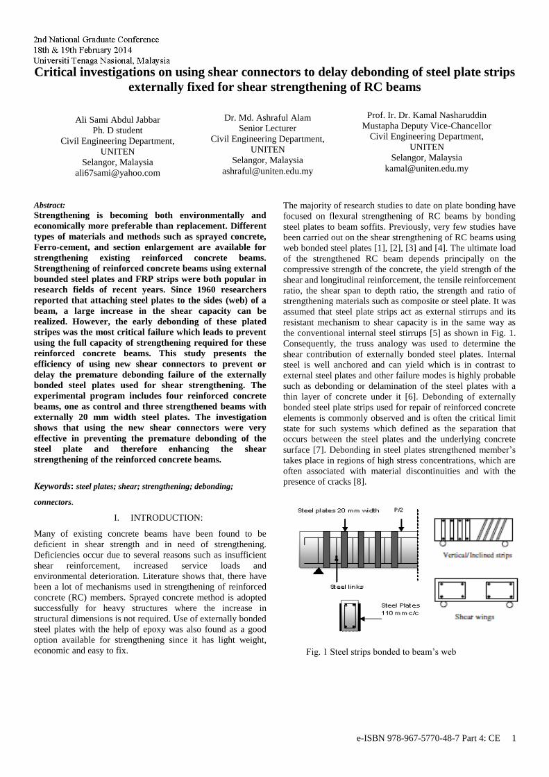
Fig. 1 Steel strips bonded to beam’s web
Critical investigations on using shear connectors to delay debonding of steel plate strips
externally fixed for shear strengthening of RC beams
Abstract:
Strengthening is becoming both environmentally and
economically more preferable than replacement. Different
types of materials and methods such as sprayed concrete,
Ferro-cement, and section enlargement are available for
strengthening existing reinforced concrete beams.
Strengthening of reinforced concrete beams using external
bounded steel plates and FRP strips were both popular in
research fields of recent years. Since 1960 researchers
reported that attaching steel plates to the sides (web) of a
beam, a large increase in the shear capacity can be
realized. However, the early debonding of these plated
stripes was the most critical failure which leads to prevent
using the full capacity of strengthening required for these
reinforced concrete beams. This study presents the
efficiency of using new shear connectors to prevent or
delay the premature debonding failure of the externally
bonded steel plates used for shear strengthening. The
experimental program includes four reinforced concrete
beams, one as control and three strengthened beams with
externally 20 mm width steel plates. The investigation
shows that using the new shear connectors were very
effective in preventing the premature debonding of the
steel plate and therefore enhancing the shear
strengthening of the reinforced concrete beams.
Keywords: steel plates; shear; strengthening; debonding;
connectors.
I. INTRODUCTION:
Many of existing concrete beams have been found to be
deficient in shear strength and in need of strengthening.
Deficiencies occur due to several reasons such as insufficient
shear reinforcement, increased service loads and
environmental deterioration. Literature shows that, there have
been a lot of mechanisms used in strengthening of reinforced
concrete (RC) members. Sprayed concrete method is adopted
successfully for heavy structures where the increase in
structural dimensions is not required. Use of externally bonded
steel plates with the help of epoxy was also found as a good
option available for strengthening since it has light weight,
economic and easy to fix.
The majority of research studies to date on plate bonding have
focused on flexural strengthening of RC beams by bonding
steel plates to beam soffits. Previously, very few studies have
been carried out on the shear strengthening of RC beams using
web bonded steel plates [1], [2], [3] and [4]. The ultimate load
of the strengthened RC beam depends principally on the
compressive strength of the concrete, the yield strength of the
shear and longitudinal reinforcement, the tensile reinforcement
ratio, the shear span to depth ratio, the strength and ratio of
strengthening materials such as composite or steel plate. It was
assumed that steel plate strips act as external stirrups and its
resistant mechanism to shear capacity is in the same way as
the conventional internal steel stirrups [5] as shown in Fig. 1.
Consequently, the truss analogy was used to determine the
shear contribution of externally bonded steel plates. Internal
steel is well anchored and can yield which is in contrast to
external steel plates and other failure modes is highly probable
such as debonding or delamination of the steel plates with a
thin layer of concrete under it [6]. Debonding of externally
bonded steel plate strips used for repair of reinforced concrete
elements is commonly observed and is often the critical limit
state for such systems which defined as the separation that
occurs between the steel plates and the underlying concrete
surface [7]. Debonding in steel plates strengthened member’s
takes place in regions of high stress concentrations, which are
often associated with material discontinuities and with the
presence of cracks [8].
Ali Sami Abdul Jabbar
Ph. D student
Civil Engineering Department,
UNITEN
Selangor, Malaysia
Dr. Md. Ashraful Alam
Senior Lecturer
Civil Engineering Department,
UNITEN
Selangor, Malaysia
Prof. Ir. Dr. Kamal Nasharuddin
Mustapha Deputy Vice-Chancellor
Civil Engineering Department,
UNITEN
Selangor, Malaysia
e-ISBN 978-967-5770-48-7 Part 4: CE 1
2nd
National Graduate Conference 2013,
18th
and 19th
February 2014,
UNITEN
2
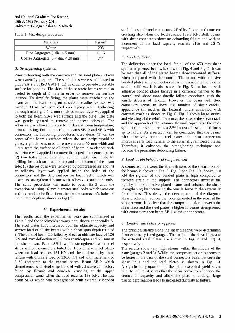
Fig. 3 Shear connector’s orientation and steel plates bonded
to the concrete surface of beams.
As most researchers reported that debonding of steel plates
was the most common type of failure which prevents the
strengthened member from reaching the full capacity of its
ultimate strengthening. This problem is very important in
strengthening the beams since there is no to date a dependable
design guidelines or standards to prevent debonding. In
general preventing debonding is a complicated phenomenon
since it is affected by various factors, such as concrete
cracking and stress concentrations at the concrete- steel plate’s
interface which makes it difficult to predict the ultimate
strength of steel plates retrofitted structures. Bolted steel plates
was one of the solutions to prevent the debonding failure [9],
Alternatively, some researchers stated that using bolt
anchorages may lead to initiate cracking in beams near the
bolts holes or lead to a brittle rapture failure of the bonded
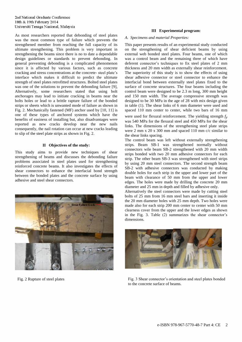
strips or sheets which is unwanted mode of failure as shown in
Fig. 2. Mechanically fastened (MF) anchor used by [10, 11] is
one of these types of anchored systems which have the
benefits of easiness of installing but, also disadvantages were
reported as new cracks develop near the new nails
consequently, the nail rotation can occur at new cracks leading
to slip of the steel plate strips as shown in Fig. 2.
II Objectives of the study:
This study aims to provide new techniques of shear
strengthening of beams and discusses the debonding failure
problems associated in steel plates used for strengthening
reinforced concrete beams. It also investigates the effects of
shear connectors to enhance the interfacial bond strength
between the bonded plates and the concrete surface by using
adhesive and steel shear connectors.
III Experimental program:
A. Specimens and material Properties:
This paper presents results of an experimental study conducted
on the strengthening of shear deficient beams by using
external web bonded steel plates. Four beams, one of which
was a control beam and the remaining three of which have
deferent connector’s techniques to fix steel plates of 2 mm
thickness and 20 mm width as externally shear reinforcement.
The superiority of this study is to show the effects of using
shear adhesive connector or steel connector to enhance the
interfacial bond between externally steel plates fixed to the
surface of concrete structures. The four beams including the
control beam were designed to be 2.3 m long, 300 mm height
and 150 mm width. The average compressive strength was
designed to be 30 MPa in the age of 28 with mix design given
in table (1). The shear links of 6 mm diameter were used and
spaced 110 mm center to center, while two bars of 16 mm
were used for flexural reinforcement. The yielding strength fy was 540 MPa for the flexural steel and 450 MPa for the shear
links. The dimensions of the strengthening steel plate strips
were 2 mm x 20 x 300 mm and spaced 110 mm c/c similar to
the shear links spacing.
The control beam was left without externally strengthening
strips. Beam SB-1 was strengthened normally without
connectors wile beam SB-2 strengthened with 20 mm width
strips bonded with two 20 mm adhesive connectors for each
strip. The other beam SB-3 was strengthened with steel strips
by using 20 mm steel connectors. The second strength beam
SB-2 with adhesive connectors was conducted by making
double holes for each strip in the upper and lower part of the
beam with clearance of 50 mm from the upper and lower
edges. The holes were made by drilling the concrete 20 mm
diameter and 25 mm in depth and filled by adhesive only.
Alternatively the steel connectors were made by cutting steel
bolts of 25 mm from 16 mm steel bars and inserting it inside
the 20 mm diameter holes with 25 mm depth. Two holes were
made also for each strip 200 mm center to center with 50 mm
clearness cover from the upper and the lower edges as shown
in the Fig. 3. Table (2) summarizes the shear connector’s
dimensions.
Fig. 2 Rupture of steel plates
e-ISBN 978-967-5770-48-7 Part 4: CE 2
2nd
National Graduate Conference 2013,
18th
and 19th
February 2014,
UNITEN
3
.
Table 1. Mix design properties
B. Strengthening systems:
Prior to bonding both the concrete and the steel plate surfaces
were carefully prepared. The steel plates were sand blasted to
grade SA 2.5 of ISO 8501-1 [12] in order to provide a suitable
surface for bonding. The sides of the concrete beams were also
peeled to depth of 5 mm in order to remove the surface
laitance. To simplify fixing, the plates were attached to the
beam with the beam lying on its side. The adhesive used was
Sikadur 30 as two part cold cure epoxy resin. Following
thorough mixing, a 1–2 mm thick adhesive layer was applied
to both the beam SB-1 web surface and the plate. The plate
was gently agitated to remove the excess adhesive. The
adhesive was allowed to cure for 7 days at room temperature,
prior to testing. For the other both beams SB- 2 and SB-3 with
connectors the following procedures were done: (1) on the
zones of the beam’s surfaces where the steel strips would be
glued, a grinder was used to remove around 50 mm width and
5 mm from the surface to all depth of beam, also cleaner such
as acetone was applied to remove the superficial cement paste;
(2) two holes of 20 mm and 25 mm depth was made by
drilling for each strip at the top and the bottom of the beam
side; (3) the residues were removed by compressed air and (4)
an adhesive layer was applied inside the holes of the
connectors and the strip surface for beam SB-2 which was
tested as strengthened beam with adhesive connectors only.
The same procedure was made to beam SB-3 with the
exception of using 16 mm diameter steel bolts which were cut
and prepared to be fit to insert inside the connector’s holes of
the 25 mm depth as shown in Fig (3).
V Experimental results
The results from the experimental work are summarized in
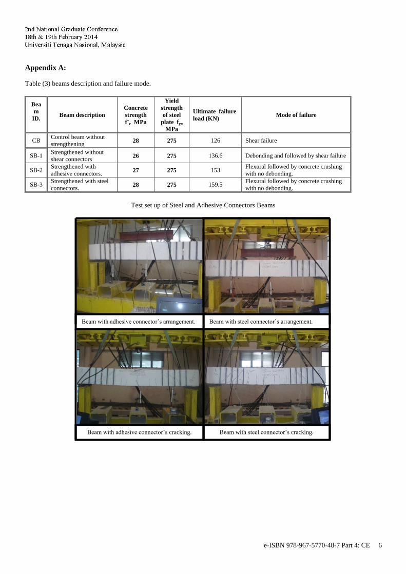
Table 3 and the specimen’s arrangement shown at appendix A.
The steel plates have increased both the ultimate capacity and
service load of all the beams with a shear span depth ratio of
2. The control beam CB failed by shear at ultimate load of 126
KN and max deflection of 9.6 mm at mid-span and 6.2 mm at
the shear span. Beam SB-1 which strengthened with steel
strips without connectors failed by debonding of steel plates
when the load reaches 131 KN and then followed by shear
failure with ultimate load of 136.6 KN and with increment of
8 % compared to the control beam. Beam SB-2 which
strengthened with steel strips bonded with adhesive connectors
failed by flexure and concrete crushing at the upper
compression zone when the load reaches 153 KN. The last
beam SB-3 which was strengthened with externally bonded
steel plates and steel connectors failed by flexure and concrete
crushing also when the load reaches 159.5 KN. Both beams
with shear connectors show no debonding failure and with an
increment of the load capacity reaches 21% and 26 %
respectively.
A. Load–deflection
The deflection under the load, for all of the 650 mm shear
span strengthened beams, is shown in Fig. 4 and Fig. 5. It can
be seen that all of the plated beams show increased stiffness
when compared with the control. The beams with adhesive
bonded plates with connectors show an immediate increase in
section stiffness. It is also shown in Fig. 5 that beams with
adhesive bonded plates behave in a different manner to the
control and show more ductile failure associated with the
tensile stresses of flexural. However, the beam with steel
connectors seems to show less number of shear cracks’
appearance till reaches the flexural failure combined with
concrete crash as shown in Fig. 6. Fig. 7 shows large strains
and yielding of the reinforcement at the base of the shear crack
and the approach of the ultimate flexural capacity at the mid-
span. It can be seen there is a 22% increase in section stiffness
up to failure. As a result it can be concluded that the beams
with adhesively bonded steel plates and shear connectors
improves early load transfer to the externally reinforced plates.
Therefore, it enhances the strengthening technique and
reduces the premature debonding failure.
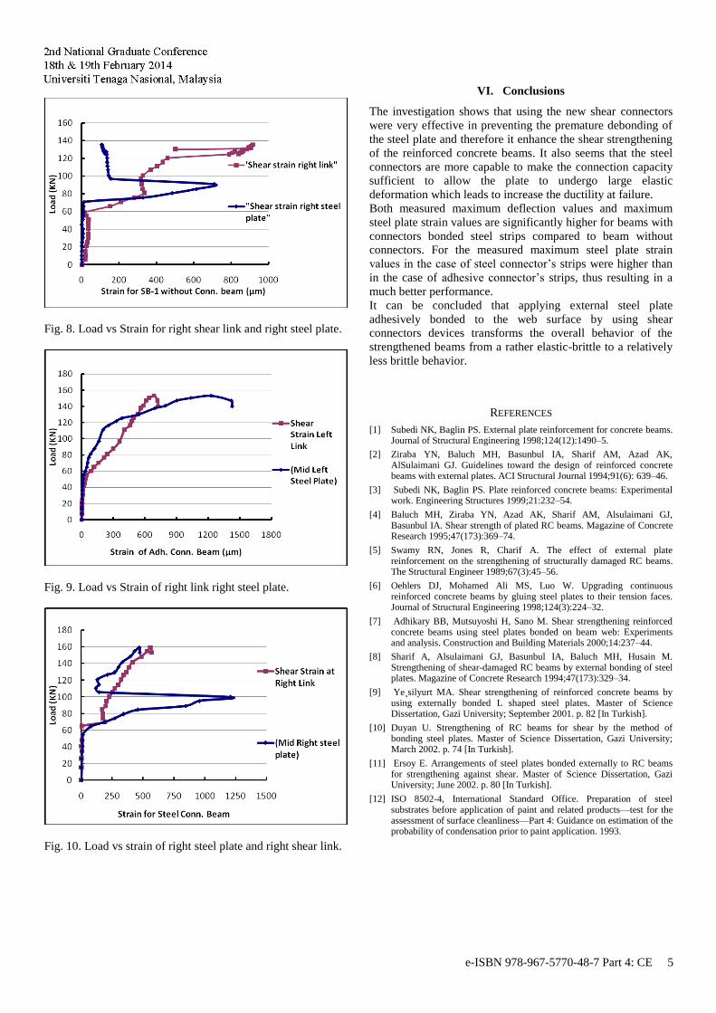
B. Load–strain behavior of reinforcement
A comparison between the strain stresses of the shear links for
the beams is shown in Fig. 8, Fig. 9 and Fig. 10. Above 110
KN the rigidity of the bonded plate is high compared to
reduced strain at the support. The connectors increase the
rigidity of the adhesive plated beams and enhance the shear
strengthening by increasing the tensile force in the externally
fixed plates. This delays the development of the diagonal
shear cracks and reduces the force generated in the rebar at the
support zone. It is clear that the composite action between the
shear links and the steel plates is higher in beams strengthened
with connectors than beam SB-1 without connectors.
C. Load–strain behavior of plates
The principal strains along the shear diagonal were determined
from externally fixed gauges. The strain of the shear links and
the external steel plates are shown in Fig. 8 and Fig. 9,
respectively.
The results show very high strains within the middle of the
plate (gauges 2 and 3). While, the composite action is seems to
be better in the case of the steel connectors beam between the
shear links and the steel plates as shown in Fig. 10.
A significant proportion of the plate exceeded yield strain
prior to failure; it seems that the shear connectors enhance the
connection capacity and allow the plate to undergo large
plastic deformation leads to increased ductility at failure.
Materials Kg /m3
Water 205
Fine Aggregate ( dia. < 5 mm) 1116
Coarse Aggregate (5 < dia. < 20 mm) 744
e-ISBN 978-967-5770-48-7 Part 4: CE 3
2nd
National Graduate Conference 2013,
18th
and 19th
February 2014,
UNITEN
4
Table 2. Dimensions of the shear connectors.
Fig. 4. Load vs deflection at shear span.
Fig. 5. Load vs deflection at mid span.
Fig. 6. Load vs concrete strain.
Fig.7. Load vs strain of flexural reinforcement.
Beam ID.
Steel Strip
dimensions
thickness x width
Shear Connectors
Type of
Connector.
Diameter of
Connector.
Depth of
Connector.
Number of Connectors
per each strip.
CB - - - - -
SB-1 2 X 20 - - - -
SB-2 2 X 20 Adhesive conn. 20 mm 25 mm 2
SB-3 2 X 20 16 mm Steel conn. 20 mm 25 mm 2
e-ISBN 978-967-5770-48-7 Part 4: CE 4
2nd
National Graduate Conference 2013,
18th
and 19th
February 2014,
UNITEN
5
Fig. 8. Load vs Strain for right shear link and right steel plate.
Fig. 9. Load vs Strain of right link right steel plate.
Fig. 10. Load vs strain of right steel plate and right shear link.
VI. Conclusions
The investigation shows that using the new shear connectors
were very effective in preventing the premature debonding of
the steel plate and therefore it enhance the shear strengthening
of the reinforced concrete beams. It also seems that the steel
connectors are more capable to make the connection capacity
sufficient to allow the plate to undergo large elastic
deformation which leads to increase the ductility at failure.
Both measured maximum deflection values and maximum
steel plate strain values are significantly higher for beams with
connectors bonded steel strips compared to beam without
connectors. For the measured maximum steel plate strain
values in the case of steel connector’s strips were higher than
in the case of adhesive connector’s strips, thus resulting in a
much better performance.
It can be concluded that applying external steel plate
adhesively bonded to the web surface by using shear
connectors devices transforms the overall behavior of the
strengthened beams from a rather elastic-brittle to a relatively
less brittle behavior.
REFERENCES
[1] Subedi NK, Baglin PS. External plate reinforcement for concrete beams. Journal of Structural Engineering 1998;124(12):1490–5.
[2] Ziraba YN, Baluch MH, Basunbul IA, Sharif AM, Azad AK, AlSulaimani GJ. Guidelines toward the design of reinforced concrete beams with external plates. ACI Structural Journal 1994;91(6): 639–46.
[3] Subedi NK, Baglin PS. Plate reinforced concrete beams: Experimental work. Engineering Structures 1999;21:232–54.
[4] Baluch MH, Ziraba YN, Azad AK, Sharif AM, Alsulaimani GJ, Basunbul IA. Shear strength of plated RC beams. Magazine of Concrete Research 1995;47(173):369–74.
[5] Swamy RN, Jones R, Charif A. The effect of external plate reinforcement on the strengthening of structurally damaged RC beams. The Structural Engineer 1989;67(3):45–56.
[6] Oehlers DJ, Mohamed Ali MS, Luo W. Upgrading continuous reinforced concrete beams by gluing steel plates to their tension faces. Journal of Structural Engineering 1998;124(3):224–32.
[7] Adhikary BB, Mutsuyoshi H, Sano M. Shear strengthening reinforced concrete beams using steel plates bonded on beam web: Experiments and analysis. Construction and Building Materials 2000;14:237–44.
[8] Sharif A, Alsulaimani GJ, Basunbul IA, Baluch MH, Husain M. Strengthening of shear-damaged RC beams by external bonding of steel plates. Magazine of Concrete Research 1994;47(173):329–34.
[9] Ye¸silyurt MA. Shear strengthening of reinforced concrete beams by using externally bonded L shaped steel plates. Master of Science Dissertation, Gazi University; September 2001. p. 82 [In Turkish].
[10] Duyan U. Strengthening of RC beams for shear by the method of bonding steel plates. Master of Science Dissertation, Gazi University; March 2002. p. 74 [In Turkish].
[11] Ersoy E. Arrangements of steel plates bonded externally to RC beams for strengthening against shear. Master of Science Dissertation, Gazi University; June 2002. p. 80 [In Turkish].
[12] ISO 8502-4, International Standard Office. Preparation of steel substrates before application of paint and related products—test for the assessment of surface cleanliness—Part 4: Guidance on estimation of the probability of condensation prior to paint application. 1993.
e-ISBN 978-967-5770-48-7 Part 4: CE 5
2nd
National Graduate Conference 2013,
18th
and 19th
February 2014,
UNITEN
6
Appendix A:
Table (3) beams description and failure mode.
Bea
m
ID.
Beam description
Concrete
strength
f’c MPa
Yield
strength
of steel
plate fyp
MPa
Ultimate failure
load (KN) Mode of failure
CB Control beam without
strengthening 28 275 126 Shear failure
SB-1 Strengthened without
shear connectors 26 275 136.6 Debonding and followed by shear failure
SB-2 Strengthened with
adhesive connectors. 27 275 153
Flexural followed by concrete crushing
with no debonding.
SB-3 Strengthened with steel
connectors. 28 275 159.5
Flexural followed by concrete crushing
with no debonding.
Test set up of Steel and Adhesive Connectors Beams
Beam with steel connector’s arrangement. Beam with adhesive connector’s arrangement.
Beam with steel connector’s cracking. Beam with adhesive connector’s cracking.
e-ISBN 978-967-5770-48-7 Part 4: CE 6
2nd National Graduate Conference
18th and 19th February 2014
Universiti Tenaga Nasional, Malaysia
Nor Azlina Alias
Department of Civil Engineering, College of Engineering
Universiti Tenaga Nasional
Kajang, Malaysia
Abstract—Nowadays, computer modelling has become the
primary tool in simulating flood flows. The one-dimensional
models have long been used in simulating hydrodynamics.
Engineers worldwide developed and simulated the flood flows
using computer model in planning, designing and operating flood
defences, flood risk management, etc. However, most of these
models are based on the solution to some approximate forms of
the fully 1D shallow water equations. The solute transport is a
common process that may take place in a flood event. Thus,
besides simulating only the flood flow, the solute transport is an
important aspects to be considered as pollutant could be spread
by flood flows which then worsened the affected areas. This
paper presents the development of an integrated one-dimensional
flow model to predict the flow hydrodynamics and
simultaneously simulate the pollutant transport under certain
flood conditions. In order to conserve the mass and momentum,
the fully dynamic St. Venant equation and the advection-
diffusion equation used to simulate the open channel flow and
contaminated flow simultaneously. At this stage, the model has
been validated against several benchmark tests and the results
are in well agreement. Ultimately, the integrated model will be
applied to simulate flooding and pollutant spreading at selected
sites. It is hoped that the proposed integrated model can be used
for flood risk management in the future.
Keywords— One Dimensional model; shallow water equations;
solute transport
I. INTRODUCTION
UE to drastically increase in populations, flood incidence
become more frequent especially in urban area. The
occurrence of flood inundation is due to breach of flood
defences or inadequate capability of the drainage systems after
heavy rainfall. Flood risk is expected to increase significantly
in and beyond the 21st century due to climate change and rapid
urbanisation.
Its been reported that flooding is one of the major natural
disasters to human life and assets. One-third of all losses due
to nature’s forces can be attributed to flooding [1] and
recently, losses generated by flood disaster have increased
drastically. As the computer modelling has now become the
primary tool in simulating flood flows, therefore it is essential
to develop or improve the flood modelling system in order to
cope with greater urbanisation and climate change.
In a flood event, the flood flows can be a major source of
Assoc. Prof. Dr. Ir. Lariyah Mohd Sidek
Department of Civil Engineering, College of Engineering
Universiti Tenaga Nasional
Kajang, Malaysia
pollution as well as it picks up potentially harmful substances
from surfaces such as oil, household chemicals and faecal
material. Those detrimental substances will then be transferred
to urban watercourses. This excess foul poses risks to human
health and impact to the environment. Due to this,
contaminated flow and solute transport are found as important
aspects to be considered in developing an intensive flow
model.
This work presents a development of a 1D hydraulic model
that will be extended to include the diffusion-advection
process. The integrated model will be used to simulate the
hydrodynamics flows in channels and rivers together with the
evolution of flood flows in the large-scale floodplain. It is
essential to have a reliable 1D fluvial flood model to simulate
and provide an accurate description of the flow
hydrodynamics in the river reach as in some cases it is
difficult to resolve the problematic river reach in a 2D manner.
As most of the 1D engines are based on the solution to an
approximated form of the fully 1D shallow water equations
[2], thus it is desirable to have a 1D component that can deal
with the highly dynamic and complex flow hydrodynamics
under flood conditions, with full consideration of the
convective and source terms.
II. AIM AND OBJECTIVES
This research aims to propose a 1D open channel flow
solver for hydrodynamic simulations. In order to develop an
integrated 1D model which can accurately simulate the
hydraulic process and the fate of pollutant simultaneously, the
detailed objectives are listed as follows:
1) To develop the 1D shallow flow model.
2) To integrate the 1D flow model together with the
contaminant model in order to simulate pollutant
transport during an urban flood event.
3) To validate the integrated model against benchmark tests,
laboratory measurements and field data.
4) To apply and implement the integrated proposed model
to selected sites.
III. METHODOLOGY
A. Development of 1D shallow flow model.
In this study, one of the main tasks is to develop the one-
Development of an Integrated 1D Shallow
Water and Solute Transport Model
D
e-ISBN 978-967-5770-48-7 Part 4: CE 7
2nd National Graduate Conference
18th and 19th February 2014
Universiti Tenaga Nasional, Malaysia
dimensional surface flow solved by the proposed numerical
scheme. The 1D open channel flow model will be integrated
with the pollutant transport that flows together during and
after the flood event. The dependent variables are the changes
in water level; h and the flow; q along the channel. Those
variables are predicted by numerically solving the St. Venant
or so called shallow water equations below; as they have been
experimentally confirmed [2] and are accepted for many
practical applications in modelling the unsteady flow in either
one or two dimensional approach [3]. The fundamental used in
the mathematical modelling of rivers are formalized in the
equation of unsteady one dimensional open channel flow and
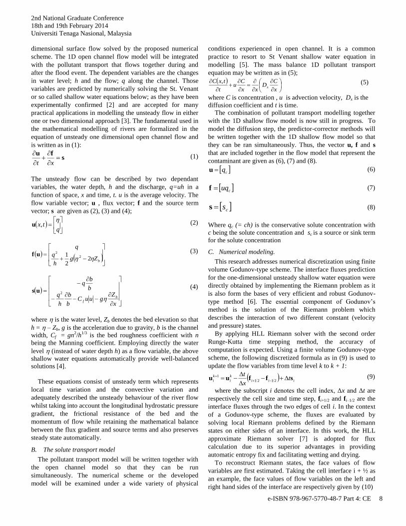
is written as in (1):
sfu
xt (1)
The unsteady flow can be described by two dependant
variables, the water depth, h and the discharge, q=uh in a
function of space, x and time, t. u is the average velocity. The
flow variable vector; u , flux vector; f and the source term
vector; s are given as (2), (3) and (4);
qtx
,u (2)
bZgh
q
q
22
1 22uf
(3)
x
ZguuC
b
b
h
qb
bq
b
f 2us
(4)
where is the water level, Zb denotes the bed elevation so that
h = – Zb, g is the acceleration due to gravity, b is the channel
width, Cf = gn2/h
1/3 is the bed roughness coefficient with n
being the Manning coefficient. Employing directly the water
level (instead of water depth h) as a flow variable, the above
shallow water equations automatically provide well-balanced
solutions [4].
These equations consist of unsteady term which represents
local time variation and the convective variation and
adequately described the unsteady behaviour of the river flow
whilst taking into account the longitudinal hydrostatic pressure
gradient, the frictional resistance of the bed and the
momentum of flow while retaining the mathematical balance
between the flux gradient and source terms and also preserves
steady state automatically.
B. The solute transport model
The pollutant transport model will be written together with
the open channel model so that they can be run
simultaneously. The numerical scheme or the developed
model will be examined under a wide variety of physical
conditions experienced in open channel. It is a common
practice to resort to St Venant shallow water equation in
modelling [5]. The mass balance 1D pollutant transport
equation may be written as in (5);
x
CD
xx
Cu
t
txCx
, (5)
where C is concentration , u is advection velocity, Dx is the
diffusion coefficient and t is time.
The combination of pollutant transport modelling together
with the 1D shallow flow model is now still in progress. To
model the diffusion step, the predictor-corrector methods will
be written together with the 1D shallow flow model so that
they can be ran simultaneously. Thus, the vector u, f and s
that are included together in the flow model that represent the
contaminant are given as (6), (7) and (8).
cqu (6)
cuqf (7)
css (8)
Where qc (= ch) is the conservative solute concentration with
c being the solute concentration and sc is a source or sink term
for the solute concentration
C. Numerical modeling.
This research addresses numerical discretization using finite
volume Godunov-type scheme. The interface fluxes prediction
for the one-dimensional unsteady shallow water equation were
directly obtained by implementing the Riemann problem as it
is also form the bases of very efficient and robust Godunov-
type method [6]. The essential component of Godunov’s
method is the solution of the Riemann problem which
describes the interaction of two different constant (velocity
and pressure) states.
By applying HLL Riemann solver with the second order
Runge-Kutta time stepping method, the accuracy of
computation is expected. Using a finite volume Godunov-type
scheme, the following discretized formula as in (9) is used to
update the flow variables from time level k to k + 1:
iii
k
i
k
i tx
tsffuu
2121
1 (9)
where the subscript i denotes the cell index, Δx and Δt are
respectively the cell size and time step, fi+1/2 and fi–1/2 are the
interface fluxes through the two edges of cell i. In the context
of a Godunov-type scheme, the fluxes are evaluated by
solving local Riemann problems defined by the Riemann
states on either sides of an interface. In this work, the HLL
approximate Riemann solver [7] is adopted for flux
calculation due to its superior advantages in providing
automatic entropy fix and facilitating wetting and drying.
To reconstruct Riemann states, the face values of flow
variables are first estimated. Taking the cell interface i + ½ as
an example, the face values of flow variables on the left and
right hand sides of the interface are respectively given by (10)
e-ISBN 978-967-5770-48-7 Part 4: CE 8

2nd National Graduate Conference
18th and 19th February 2014
Universiti Tenaga Nasional, Malaysia
1,21 5.0~ iiiiLi uuψuu and
iiiiRi uuψuu 111,21 5.0~
(10)
where ψ is the vector containing the minmod slope limiters [8]
calculated for the corresponding flow variables. The face
values of water depth, velocity and bed elevation on either
side of i+½ are given as (11), (12) and (13) where the
subscript L and R denotes the left and right faces respectively.
iiiiRiiiiiLi hhhhhhhh 111,211,21 5.0~
and 5.0~
(11)
(Liu ,21
~
and Riu ,21
~
) (12)
(LibZ ,21
~
and RibZ ,21
~
) (13)
Equation (14) facilitates the definition of the non-negative
Riemann states of water depth:
)~ ,0max( 212121 b i,Li,Li Zh and
)~0(max 212121 b i,Ri,Ri Zη, h
(14)
Equation (14) are then used to evaluate the Riemann states of
other flow variables as in (15)
212121 bi,Li,Li Zhη and ,Li,Li,Li huq 212121 (15)
The right Riemann states are obtained via a similar way.
To improve the temporal accuracy of the scheme and the
time marching, the second-order Runge-Kutta method is
applied and (9) now becomes (16):
)()(5.0 *1uKuKuu i
k
i
k
i
k
i t
(16)
The Runge-Kutta coefficients and the intermediate flow
variables are defined by (17) and (18) respectively.
iiii x sffK /)( 2121 (17)
)(* k
i
k
ii tK uuu (18)
At every time step, the Runge-Kutta coefficients are calculated
at two consecutive steps for updating the flow variables.
IV. FINDINGS TO DATE
The capability of the current model is demonstrated by
applying a number of experimental and analytical tests
involving changing in the channel width and bed profile. The
model successfully handles all of the tests and produces results
agreeing well with experimental measurements or analytical
solutions, which implies its potential in more practical
applications. For the time being, in order to check the
efficiency of the integrated model in dealing with the fate of
pollutant, the proposed integrated model has been tested on a
simple bench mark test and the results are compared with the
analytical solutions.
A. Tidal wave flow and flow over an irregular bed
Presented here is test on tidal flow proposed by Bermudes and
Vasquez [9]. The tidal flow over an irregular bed which is
defined by (19)
2
14sin10
405.50
L
x
L
xxH (19)
Where the channel length L is 14000 m. The initial condition
are xHxh 0, and 00, xu . The boundary conditions are
as (20)
2
1
86400
4sin440,0
tHth and 0, tLu (20)
Having simulated usng the proposed model, Figure 1 and 2
show the comparison of the numerical results with the
analytical solution at t =7552.13 s. These excellent agreements
suggest that the proposed scheme is accurate for tidal flow
problems.
Fig. 1 Tidal wave flow : Comparison of water surface
Fig. 2 Tidal wave flow : Comparison of velocity
In order to validate its performance on irregular bed, another
simulation was done by taking the tabulated data in Table 1 as
the bed profile of a channel. Replacing the 160 H , L=1500
m and xZHxH b 0 while maintaining the previous
initial and boundary conditions as (19) and (20), the tidal wave
over an irregular bed is validated.
TABLE I : BED ELEVATION, Zb AT POINT x
x 0 50 100 150 250 300 350 400
Zb 0 0 2.5 5 5 3 5 5
x 425 435 450 475 500 505 530 550
Zb 7.5 8 9 9 9.1 9 9 6
x 565 575 600 650 700 750 800 820
Zb 5.5 5.5 5 4 3 3 2.3 2
x 900 950 1000 1500
Zb 1.2 0.4 0 0
e-ISBN 978-967-5770-48-7 Part 4: CE 9
2nd National Graduate Conference
18th and 19th February 2014
Universiti Tenaga Nasional, Malaysia
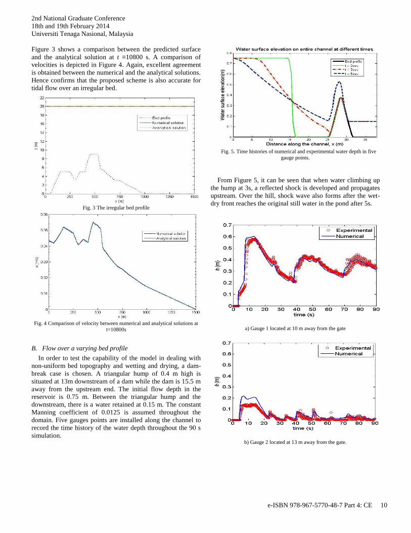
Figure 3 shows a comparison between the predicted surface
and the analytical solution at t =10800 s. A comparison of
velocities is depicted in Figure 4. Again, excellent agreement
is obtained between the numerical and the analytical solutions.
Hence confirms that the proposed scheme is also accurate for
tidal flow over an irregular bed.
Fig. 3 The irregular bed profile
Fig. 4 Comparison of velocity between numerical and analytical solutions at
t=10800s
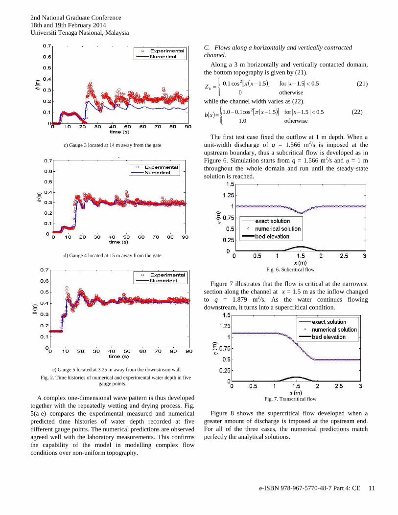
B. Flow over a varying bed profile
In order to test the capability of the model in dealing with
non-uniform bed topography and wetting and drying, a dam-
break case is chosen. A triangular hump of 0.4 m high is
situated at 13m downstream of a dam while the dam is 15.5 m
away from the upstream end. The initial flow depth in the
reservoir is 0.75 m. Between the triangular hump and the
downstream, there is a water retained at 0.15 m. The constant
Manning coefficient of 0.0125 is assumed throughout the
domain. Five gauges points are installed along the channel to
record the time history of the water depth throughout the 90 s
simulation.
Fig. 5. Time histories of numerical and experimental water depth in five
gauge points.
From Figure 5, it can be seen that when water climbing up
the hump at 3s, a reflected shock is developed and propagates
upstream. Over the hill, shock wave also forms after the wet-
dry front reaches the original still water in the pond after 5s.
a) Gauge 1 located at 10 m away from the gate
b) Gauge 2 located at 13 m away from the gate.
e-ISBN 978-967-5770-48-7 Part 4: CE 10
2nd National Graduate Conference
18th and 19th February 2014
Universiti Tenaga Nasional, Malaysia
c) Gauge 3 located at 14 m away from the gate
d) Gauge 4 located at 15 m away from the gate
e) Gauge 5 located at 3.25 m away from the downstream wall
Fig. 2. Time histories of numerical and experimental water depth in five
gauge points.
A complex one-dimensional wave pattern is thus developed
together with the repeatedly wetting and drying process. Fig.
5(a-e) compares the experimental measured and numerical
predicted time histories of water depth recorded at five
different gauge points. The numerical predictions are observed
agreed well with the laboratory measurements. This confirms
the capability of the model in modelling complex flow
conditions over non-uniform topography.
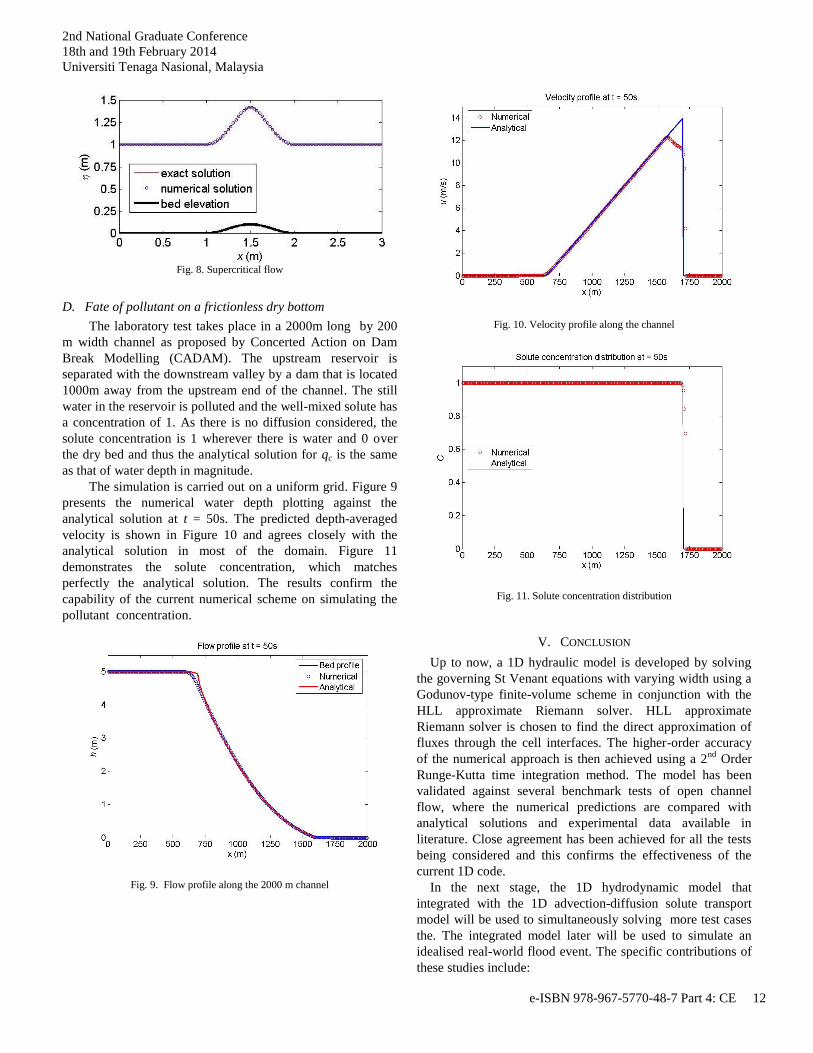
C. Flows along a horizontally and vertically contracted
channel.
Along a 3 m horizontally and vertically contacted domain,
the bottom topography is given by (21).
otherwise 0
5.05.1for 5.1cos1.0 2 xxZb
(21)
while the channel width varies as (22).
otherwise 0.1
5.05.1for 5.1cos1.00.1 2 xxxb
(22)
The first test case fixed the outflow at 1 m depth. When a
unit-width discharge of q = 1.566 m2/s is imposed at the
upstream boundary, thus a subcritical flow is developed as in
Figure 6. Simulation starts from q = 1.566 m2/s and η = 1 m
throughout the whole domain and run until the steady-state
solution is reached.
Fig. 6. Subcritical flow
Figure 7 illustrates that the flow is critical at the narrowest
section along the channel at x = 1.5 m as the inflow changed
to q = 1.879 m2/s. As the water continues flowing
downstream, it turns into a supercritical condition.
Fig. 7. Transcritical flow
Figure 8 shows the supercritical flow developed when a
greater amount of discharge is imposed at the upstream end.
For all of the three cases, the numerical predictions match
perfectly the analytical solutions.
e-ISBN 978-967-5770-48-7 Part 4: CE 11
2nd National Graduate Conference
18th and 19th February 2014
Universiti Tenaga Nasional, Malaysia
Fig. 8. Supercritical flow
D. Fate of pollutant on a frictionless dry bottom
The laboratory test takes place in a 2000m long by 200
m width channel as proposed by Concerted Action on Dam
Break Modelling (CADAM). The upstream reservoir is
separated with the downstream valley by a dam that is located
1000m away from the upstream end of the channel. The still
water in the reservoir is polluted and the well-mixed solute has
a concentration of 1. As there is no diffusion considered, the
solute concentration is 1 wherever there is water and 0 over
the dry bed and thus the analytical solution for qc is the same
as that of water depth in magnitude.
The simulation is carried out on a uniform grid. Figure 9
presents the numerical water depth plotting against the
analytical solution at t = 50s. The predicted depth-averaged
velocity is shown in Figure 10 and agrees closely with the
analytical solution in most of the domain. Figure 11
demonstrates the solute concentration, which matches
perfectly the analytical solution. The results confirm the
capability of the current numerical scheme on simulating the
pollutant concentration.
Fig. 9. Flow profile along the 2000 m channel
Fig. 10. Velocity profile along the channel
Fig. 11. Solute concentration distribution
V. CONCLUSION
Up to now, a 1D hydraulic model is developed by solving
the governing St Venant equations with varying width using a
Godunov-type finite-volume scheme in conjunction with the
HLL approximate Riemann solver. HLL approximate
Riemann solver is chosen to find the direct approximation of
fluxes through the cell interfaces. The higher-order accuracy
of the numerical approach is then achieved using a 2nd
Order
Runge-Kutta time integration method. The model has been
validated against several benchmark tests of open channel
flow, where the numerical predictions are compared with
analytical solutions and experimental data available in
literature. Close agreement has been achieved for all the tests
being considered and this confirms the effectiveness of the
current 1D code.
In the next stage, the 1D hydrodynamic model that
integrated with the 1D advection-diffusion solute transport
model will be used to simultaneously solving more test cases
the. The integrated model later will be used to simulate an
idealised real-world flood event. The specific contributions of
these studies include:
e-ISBN 978-967-5770-48-7 Part 4: CE 12

2nd National Graduate Conference
18th and 19th February 2014
Universiti Tenaga Nasional, Malaysia
1. A fully 1D hydrodynamic model that can deal with the
highly dynamic and complex flow hydrodynamics under
certain flood conditions.
2. An extended 1D model is expected to be capable to
simulate the fate of pollutant simultaneously for high flood
event in high dense areas.
3. The schemes used are able to deal with flow over irregular
topography and some other issues as discussed in literature.
Hence, a robust numerical tool that can predict the surface
flow as well as pollutant transport in an urban flood event will
be proposed to be used widely.
ACKNOWLEDGMENT
The first author thanks the Universiti Tenaga Nasional for
providing a conducive study environment. Not to forget she
also thanks her supervisor who support and continuously
guide towards her PhD.
REFERENCES
[1] P. D. Bates and A. P. J. Dee Roo. “A simple raster-based model
for flood inundation simulation”. Journal of Hydrology. vol 236, pp. 54–77, May. 2000.
[2] J. A. Cunge, F.M. Holly and A. Verwey. Practical Aspects of
Computational River Hydraullics. Pitman Advanced Publishing
Program. pp. 420, 1980. [3] P. Brufau, M.E. Vazquez-Cendon, and P. Garcia-Navarro. “A
numerical model for the flooding and drying of irregular domains”.
International Journal for Numerical Methods in Fluids, vol 39, pp. 247-275, 2002.
[4] J. Greenberg, and A. Y LeRoux. “A well-balanced scheme for the
numerical processing of source terms in hyperbolic equations”. SIAM Journal of Numerical Anaylsys.Vol 33, pp.1–16, 1996.
[5] A. Birman and J. Falcovitz. “Application of the GRP Scheme to Open
Channel Flow Equations”. Journal of Computational Physics, vol 222, pp. 131-154, Jul. 2006.
[6] E. F.Toro,“The HLL and HLLC Reiman solvers”, in Reimann Solvers
And Numerical Methods For Fluid Dynamis; A Practical Introduction, 2nd ed. Springer: Berlin.
[7] H. Amiram, D. L. Peter, V. L. Bram. “On upstream differencing and
Godunov-type schemes for hyperbolic conservation laws”. Society for Industrial and Applied Mathematics, vol 25, no.1, pp. 35–61, Jan.
1983.
[8] C. Hirsch. Numerical computation of internal and external flows. Vol. 2: Computational methods for inviscid and viscous flows. New York:
Wiley, 1990. [9] A. Bermudez and M. E. V´azquez, “Upwind methods for hyperbolic
conservation laws with source terms”, Journal of Computational Fluids.
vol. 23,1994
e-ISBN 978-967-5770-48-7 Part 4: CE 13
Industrial Waste Utilisation in Mortar and Concrete –
A review Masimawati Abdul Latif
#1, Sivakumar Naganathan, Dr
*2, Kamal Nasharuddin Mustapha
*3
#1 Student, Faculty of Civil Engineering, Universiti Tenaga Nasional Jalan UNITEN – IKRAM, 43000 Kajang, Selangor, Malaysia
*2 Dr, Senior Lecturer, Faculty of Civil Engineering, Universiti Tenaga Nasional Jalan UNITEN – IKRAM, 43000 Kajang, Selangor, Malaysia
*3 Professor, Faculty of Civil Engineering, Universiti Tenaga Nasional Jalan UNITEN – IKRAM, 43000 Kajang, Selangor, Malaysia
Abstract— Portland cement is one of the important
materials in the construction industry. The production of 1
tonne of Portland cement will contribute to the emission of 1
tonnes of carbon dioxides (CO2) in the atmosphere. Hence the
Portland cement usage should be reduced by introducing new
technologies and strategy in production process to reduce CO2
emissions and produce more energy efficient product to the
market. One of the strategy is the usage of supplementary
cementitous material. This review paper presents the literature
review on utilization of industrial waste focusing on fly ash
and calcium carbide residue in mortar and concrete.
Keywords— industrial waste, fly ash, calcium carbide residue
I. INTRODUCTION
Portland cement is one of the important materials in the
construction industry. The productions of 1 tonne of Portland
cement will contribute to the emission of 1 tonne of CO2 in
the atmosphere. In 1995, the world produces about 1.4 billion
tonnes and increase to 2 billion tonnes of cement in the year
2010. The increase in the cement production also generates
the increase of CO2 emissions, the major contributor to the
greenhouse effect and the global warming to approximately
about 2 billion tonnes [1]. The Portland cement production
dust emissions also pollutes the air [2].
Since the demand of cement keeps on increasing, in the
year 2012, the world produced about 3.7 billion tonnes of
cement [3] and the cement industry contributed to the world’s
5 percent of CO2 emission [4]. The cement production
consumes approximately 10-15% from the global total energy
use with 120kW h/t of cement [5, 6] as the Portland cement
raw materials required to be burn at 1500ºC temperatures [7].
Nevertheless, the cement production is predicted to increase
from 2,540 million tonnes (Mt) in 2006 to between 3,680 Mt
and 4,380 Mt in 2050 [4]. Hence the Portland cement usage
should be reduced [8] by introducing new technologies and
strategy in production process to reduce CO2 emissions and
produce more energy efficient product to the market [4]. One
of the strategy is the usage of supplementary cementitous
material [7].
The increasing cost of cement production contribute to the
rigorous research for supplementary material in cement with
waste materials [9]. The usage of supplementary cementing
materials from the industrial and biogenic wastes in concrete
production is reduction in CO2 emissions from cement
industry [10], the solution for environmental pollution and
depleting natural resources [11][12]. The energy use in
extracting, handling and reclaiming these materials can also
be saved [11].
There are varieties of wastes that can be used as
supplementary pozzolanic and cementing materials such as
Calcium Carbide Residue [7], [13]–[19], Fly Ash [1], [11],
[14], [20]–[24], Ground Granulated Blast Furnace Slag [25]–
[27], Municipal Solid Waste [15], [28], [29], Palm Oil Fuel
Ash [30]–[32], Rice Husk Ash [33]–[35] and many others
[36]–[38]. Most of these waste are waste from by-products,
industrial or even wastes from natural materials [12].
This review paper presents the research on utilization of
industrial waste focusing on Fly Ash and Calcium Carbide
Residue in mortar and concrete. The strength, advantages and
disadvantages of using these waste materials are described.
The concerns related to these waste incorporation in mortar
and concrete are also discussed.
II. INDUSTRIAL WASTE
Globally, there are many types of industrial waste produced.
The population rapid growth, current lifestyle and technology
development has increased the type and quantity of generated
waste [39]. Annually, billion tons of industrial waste are
produced[40]. Since most waste has no economically benefit
use, approximately 4.2 billion tons of non-hazardous by-
products produced from domestic, industrial, agricultural and
e-ISBN 978-967-5770-48-7 Part 4: CE 14
mineral sources has been used in land filling [41]. Landfills is
the common waste disposal method [17]–[19], [41].
These non-decaying landfilled wastes will cause waste
disposal crisis that contribute to severe global environmental
problems for example water, air and soil contamination [17],
[18], [41], [42]. The waste generated is increasing by years
and more land required just for waste disposal [43]. Lack of
space for land-filling and the increasing environmental
awareness drive the wastes utilization as an alternative to
dumping [42]. Extensive researched in enhancing concrete
durability and sustainability with waste incorporation as
supplementary cementitous were carried out over few decades
and currently it is widely used [44]. Some of these wastes
successfully utilized and improve properties of mortar and
concrete [16], [17], [19], [41], [42], [45]–[47] . A brief
explanation about the industrial waste under review are
summarized below.
A. Fly Ash (FA)
There are a few types of fly ash. Among the most common FA
is the coal burning power plant waste ash [14], [48]–[50] and
the incinerated municipal solid waste (MSWI) [16], [51]–[53].
Coal-fired power plant began in the 1920s [54]. Europe is the
leading in the utilization of coal burning power plants which
produce coal FA estimated around 47% while United States
(US) 39%. These plant generates million tons of by-products
inclusive of FA waste worldwide estimated around 750
million annually [55].
India generates over 112 million tons [56] while US
produced 120 million tons FA in 2007 and only 44% was
reused [57]. Meanwhile, China produce around 0.6 billion
tons of FA annually and until the year 2010, their utilization
ratio is still lower than 40% which contributed to 4 billion
tons has been landfilled [40].
The volume of municipal solid waste (MSW) is increasing
every year and for example, Bangkok already produced
approximately 8000 tons per day in the year 2002 [15]. The
disposal mechanism of MSW is also by landfill. The scarcity
of space for landfill and the increasing volume and operating
cost of MSW [16], [51], [55] has initiate the move to reduce
the volume of MSW thru incineration [58]. The incineration
process manages to reduce the waste volume but it creates
new waste which is the FA which still required to dispose by
landfill [8], [23], [50]. These by-products has been extensively
used in the concrete industry [23], [56].
Generally, FA is grey in colour [54]. The unburned carbon
quality in the ash will influence its colour from grey to black
[54] . FA is very fine and powdery particles, mostly either
solid or hollow spherical in shape, and typically glassy
(amorphous) [54][59]. FA is usually refractory, abrasive and
mostly alkaline [54]. FA specific gravity usually ranges from
1.81 to 2.7, while the specific surface area vary from 2390 to
6418 cm2/g [15], [23], [24], [45], [47], [57], [60]–[62].
The morphology for FA particles is agglomerated irregular
particles with lower <1 to 20µm [63]. FA cementitous nature
allow it to be used in concrete and it can also be characterized
as a pozzolanic properties and lime building capacity [54].
The property of FA has big variation, therefore it is
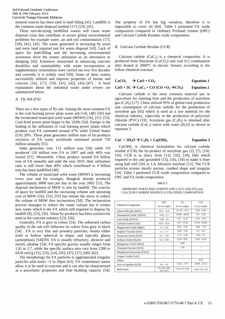
impossible to cover all [64]. Table I presented FA oxide
composition compared to Ordinary Portland cement (OPC)
and Calcium Carbide Residue oxide composition.
B. Calcium Carbide Residue (CCR)
Calcium carbide (CaC2) is a chemical composites. It is
produced from limestone (CaCO3) and coal (C) combination
after heated at 2000ºC in electric furnace according to the
follow chemical reaction:
CaCO3 CaO + CO2 Equation 1
CaO + 3C CaC2 + CO (CO +O2 CO2) Equation 2
Calcium carbide is the most common material use in
agriculture for ripening fruit and the production of acetylene
gas (C2H2) [17]. China utilized 95% of global total production
and consumption of calcium carbide for the production of
acetylene gas [65] which is used as a raw material for the
chemical industry, especially in the production of polyvinyl
chloride (PVC) [19]. Acetylene gas (C2H2) is obtained after
calcium carbide (CaC2) reacts with water (H2O) as shown in
equation 3.
CaC + 2H2O C2H2 + Ca(OH)2 Equation 3
Ca(OH)2 is chemical formulation for calcium carbide
residue (CCR) the by-product of acetylene gas [2], [7], [14],
[16]. CCR is in slurry form [13], [16], [18], [66] which
required to dry and grounded [13], [16], [18] to make it finer
using ball mill [16] or LA Abrasion machine [13]. The CCR
particles texture mostly porous, crushed shape and irregular
[16]. Table I presented CCR oxide composition compared to
OPC and FA oxide composition.
ABLE I:
ORDINARY PORTLAND CEMENT (OPC), FLY ASH (FA) and
CALCIUM CARBIDE RESIDUE (CCR) OXIDE COMPOSITION
Chemical Component OPC
(% by weight)
FA
(% by weight)
CCR
(% by weight)
Silicon Dioxide (SiO2) 20.9 – 21.8 41. 43 – 57.6 0.56 – 6.49
Aluminium Oxide (Al2O3) 4.59 – 5.7 18.49 – 26.05 0.4 – 2.56
Iron Oxide (Fe2O3) 2.99 – 3.6 5.57 – 12.57 0.22 – 1.87
Calcium Oxide (CaO) 62.9 – 65.4 1.67 – 13.65 51.94 – 83.90
Magnesium Oxide (MgO) 1.2– 2.26 0.97 – 3.79 0.46 – 1.70
Sulphur Trioxide (SO3) 1.3 – 2.7 0.05 – 1.62 0.1 – 0.6
Potassium Oxide (K2O) 0.3 – 1.39 2.17 – 2.59 0.03 – 0.1
Sodium Oxide (Na2O) 0.2 – 0.43 0.29 – 0.91 0.03 – 0.18
Manganese Oxide (MnO) - 0.04 -
Titanium Dioxide (TiO2) - 1.38 -
Phosphorus Pentoxide (P2O5) - - -
Copper Oxide (CuO) - - -
Others - - 0.04
Loss on ignition (LOI) 0.9 – 2.0 0.16 – 7.79 29.89 – 41.72
References [7], [20], [45],
[61], [67] [14], [22]–[24] [14], [15], [21]
e-ISBN 978-967-5770-48-7 Part 4: CE 15
CCR generated is projected to increase yearly as demand
for acetylene gas is high for welding and metal cutting [16].
Annually, Thailand generate over 21,500 tons of CCR [16]
while China discharged 1200 million tons of CCR [48]. Since
the residue amount is huge, CCR is disposed as landfills [7],
[13], [14], [16], [18]. CCR is not being classified as
dangerous/hazardous but CCR is high alkalinity with pH >12
and also contain metals such as Magnesium, Iron and others
[2]. This leads to environmental pollutions such as
contaminated the groundwater with the leaching of its harmful
compounds and high alkalinity [14][16]. Many attempts have
been made to use CCR and among it is in concrete
applications [7], [14], [16], [18].
III. RESULTS AND DISCUSSIONS
A brief review and discussion on the results for the utilization
of FA and CCR in concrete are summarized below.
A. Fly Ash (FA)
Concrete with fly ashe as cement replacement material or
as additive has many benefits. The most significant benefits of
incorporating FA in concrete and other composites are:
1. The engineering properties improved [62], [68].
2. Low permeability [1], [69]
3. Less sorption [23]
4. Reduction in water demand for fresh concrete due
to improves workability [62], [68], [70].
5. Heat of hydration is reduced [68], [71].
6. Drying shrinkage is control [1], [23], [70].
7. Expansion is reduced [1], [15], [69], [70], [72]
8. Resistance to chloride and sulphate attack is
increased [1], [23], [69], [70]
Concrete with FA has higher density [62],
reduced porosity [1], [71] and better resistance towards
deterioration [1], [23]. The summary of compressive
strength of control mix and FA blended mortars is
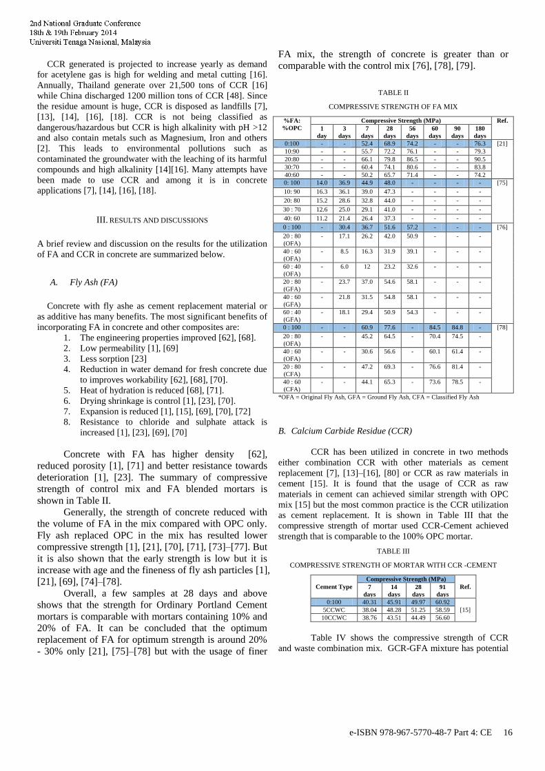
shown in Table II. Generally, the strength of concrete reduced with
the volume of FA in the mix compared with OPC only.
Fly ash replaced OPC in the mix has resulted lower
compressive strength [1], [21], [70], [71], [73]–[77]. But
it is also shown that the early strength is low but it is
increase with age and the fineness of fly ash particles [1],
[21], [69], [74]–[78].
Overall, a few samples at 28 days and above
shows that the strength for Ordinary Portland Cement
mortars is comparable with mortars containing 10% and
20% of FA. It can be concluded that the optimum
replacement of FA for optimum strength is around 20%
- 30% only [21], [75]–[78] but with the usage of finer
FA mix, the strength of concrete is greater than or
comparable with the control mix [76], [78], [79].
TABLE II
COMPRESSIVE STRENGTH OF FA MIX
%FA:
%OPC
Compressive Strength (MPa) Ref.
1
day
3
days
7
days
28
days
56
days
60
days
90
days
180
days
0:100 - - 52.4 68.9 74.2 - - 76.3 [21]
10:90 - - 55.7 72.2 76.1 - - 79.3
20:80 - - 66.1 79.8 86.5 - - 90.5
30:70 - - 60.4 74.1 80.6 - - 83.8
40:60 - - 50.2 65.7 71.4 - - 74.2
0: 100 14.0 36.9 44.9 48.0 - - - - [75]
10: 90 16.3 36.1 39.0 47.3 - - - -
20: 80 15.2 28.6 32.8 44.0 - - - -
30 : 70 12.6 25.0 29.1 41.0 - - - -
40: 60 11.2 21.4 26.4 37.3 - - - -
0 : 100 - 30.4 36.7 51.6 57.2 - - - [76]
20 : 80
(OFA)
- 17.1 26.2 42.0 50.9 - - -
40 : 60
(OFA)
- 8.5 16.3 31.9 39.1 - - -
60 : 40
(OFA)
- 6.0 12 23.2 32.6 - - -
20 : 80
(GFA)
- 23.7 37.0 54.6 58.1 - - -
40 : 60
(GFA)
- 21.8 31.5 54.8 58.1 - - -
60 : 40
(GFA)
- 18.1 29.4 50.9 54.3 - - -
0 : 100 - - 60.9 77.6 - 84.5 84.8 - [78]
20 : 80
(OFA)
- - 45.2 64.5 - 70.4 74.5 -
40 : 60
(OFA)
- - 30.6 56.6 - 60.1 61.4 -
20 : 80
(CFA)
- - 47.2 69.3 - 76.6 81.4 -
40 : 60
(CFA)
- - 44.1 65.3 - 73.6 78.5 -
*OFA = Original Fly Ash, GFA = Ground Fly Ash, CFA = Classified Fly Ash
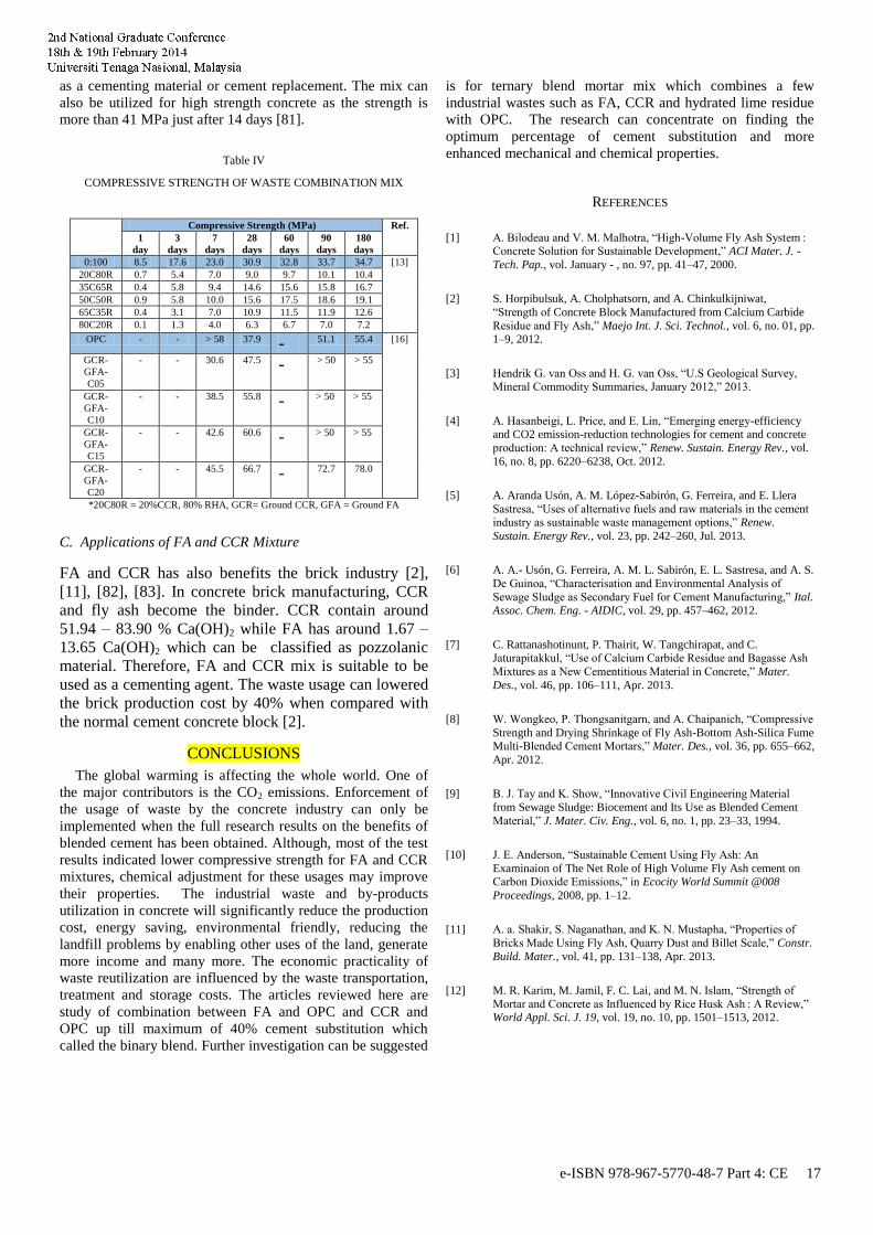
B. Calcium Carbide Residue (CCR)
CCR has been utilized in concrete in two methods
either combination CCR with other materials as cement
replacement [7], [13]–[16], [80] or CCR as raw materials in
cement [15]. It is found that the usage of CCR as raw
materials in cement can achieved similar strength with OPC
mix [15] but the most common practice is the CCR utilization
as cement replacement. It is shown in Table III that the
compressive strength of mortar used CCR-Cement achieved
strength that is comparable to the 100% OPC mortar.
TABLE III
COMPRESSIVE STRENGTH OF MORTAR WITH CCR -CEMENT
Cement Type
Compressive Strength (MPa)
Ref. 7
days
14
days
28
days
91
days
0:100 40.31 45.91 49.97 60.92
[15] 5CCWC 38.04 48.28 51.25 58.59
10CCWC 38.76 43.51 44.49 56.60
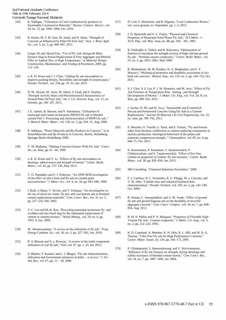
Table IV shows the compressive strength of CCR
and waste combination mix. GCR-GFA mixture has potential
e-ISBN 978-967-5770-48-7 Part 4: CE 16
as a cementing material or cement replacement. The mix can
also be utilized for high strength concrete as the strength is
more than 41 MPa just after 14 days [81].
Table IV
COMPRESSIVE STRENGTH OF WASTE COMBINATION MIX
Compressive Strength (MPa) Ref.
1
day
3
days
7
days
28
days
60
days
90
days
180
days
0:100 8.5 17.6 23.0 30.9 32.8 33.7 34.7 [13]
20C80R 0.7 5.4 7.0 9.0 9.7 10.1 10.4
35C65R 0.4 5.8 9.4 14.6 15.6 15.8 16.7
50C50R 0.9 5.8 10.0 15.6 17.5 18.6 19.1
65C35R 0.4 3.1 7.0 10.9 11.5 11.9 12.6
80C20R 0.1 1.3 4.0 6.3 6.7 7.0 7.2
OPC - - > 58 37.9 - 51.1 55.4 [16]
GCR-
GFA-
C05
- - 30.6 47.5 - > 50 > 55
GCR-
GFA-
C10
- - 38.5 55.8 - > 50 > 55
GCR-
GFA-
C15
- - 42.6 60.6 - > 50 > 55
GCR-
GFA-
C20
- - 45.5 66.7 - 72.7 78.0
*20C80R = 20%CCR, 80% RHA, GCR= Ground CCR, GFA = Ground FA
C. Applications of FA and CCR Mixture
FA and CCR has also benefits the brick industry [2],
[11], [82], [83]. In concrete brick manufacturing, CCR
and fly ash become the binder. CCR contain around
51.94 – 83.90 % Ca(OH)2 while FA has around 1.67 –
13.65 Ca(OH)2 which can be classified as pozzolanic
material. Therefore, FA and CCR mix is suitable to be
used as a cementing agent. The waste usage can lowered
the brick production cost by 40% when compared with
the normal cement concrete block [2].
CONCLUSIONS
The global warming is affecting the whole world. One of
the major contributors is the CO2 emissions. Enforcement of
the usage of waste by the concrete industry can only be
implemented when the full research results on the benefits of
blended cement has been obtained. Although, most of the test
results indicated lower compressive strength for FA and CCR
mixtures, chemical adjustment for these usages may improve
their properties. The industrial waste and by-products
utilization in concrete will significantly reduce the production
cost, energy saving, environmental friendly, reducing the
landfill problems by enabling other uses of the land, generate
more income and many more. The economic practicality of
waste reutilization are influenced by the waste transportation,
treatment and storage costs. The articles reviewed here are
study of combination between FA and OPC and CCR and
OPC up till maximum of 40% cement substitution which
called the binary blend. Further investigation can be suggested
is for ternary blend mortar mix which combines a few
industrial wastes such as FA, CCR and hydrated lime residue
with OPC. The research can concentrate on finding the
optimum percentage of cement substitution and more
enhanced mechanical and chemical properties.
REFERENCES
[1] A. Bilodeau and V. M. Malhotra, “High-Volume Fly Ash System : Concrete Solution for Sustainable Development,” ACI Mater. J. -
Tech. Pap., vol. January - , no. 97, pp. 41–47, 2000.
[2] S. Horpibulsuk, A. Cholphatsorn, and A. Chinkulkijniwat,
“Strength of Concrete Block Manufactured from Calcium Carbide
Residue and Fly Ash,” Maejo Int. J. Sci. Technol., vol. 6, no. 01, pp. 1–9, 2012.
[3] Hendrik G. van Oss and H. G. van Oss, “U.S Geological Survey,
Mineral Commodity Summaries, January 2012,” 2013.
[4] A. Hasanbeigi, L. Price, and E. Lin, “Emerging energy-efficiency and CO2 emission-reduction technologies for cement and concrete
production: A technical review,” Renew. Sustain. Energy Rev., vol.
16, no. 8, pp. 6220–6238, Oct. 2012.
[5] A. Aranda Usón, A. M. López-Sabirón, G. Ferreira, and E. Llera
Sastresa, “Uses of alternative fuels and raw materials in the cement industry as sustainable waste management options,” Renew.
Sustain. Energy Rev., vol. 23, pp. 242–260, Jul. 2013.
[6] A. A.- Usón, G. Ferreira, A. M. L. Sabirón, E. L. Sastresa, and A. S.
De Guinoa, “Characterisation and Environmental Analysis of
Sewage Sludge as Secondary Fuel for Cement Manufacturing,” Ital. Assoc. Chem. Eng. - AIDIC, vol. 29, pp. 457–462, 2012.
[7] C. Rattanashotinunt, P. Thairit, W. Tangchirapat, and C. Jaturapitakkul, “Use of Calcium Carbide Residue and Bagasse Ash
Mixtures as a New Cementitious Material in Concrete,” Mater.
Des., vol. 46, pp. 106–111, Apr. 2013.
[8] W. Wongkeo, P. Thongsanitgarn, and A. Chaipanich, “Compressive
Strength and Drying Shrinkage of Fly Ash-Bottom Ash-Silica Fume Multi-Blended Cement Mortars,” Mater. Des., vol. 36, pp. 655–662,
Apr. 2012.
[9] B. J. Tay and K. Show, “Innovative Civil Engineering Material
from Sewage Sludge: Biocement and Its Use as Blended Cement
Material,” J. Mater. Civ. Eng., vol. 6, no. 1, pp. 23–33, 1994.
[10] J. E. Anderson, “Sustainable Cement Using Fly Ash: An
Examinaion of The Net Role of High Volume Fly Ash cement on Carbon Dioxide Emissions,” in Ecocity World Summit @008
Proceedings, 2008, pp. 1–12.
[11] A. a. Shakir, S. Naganathan, and K. N. Mustapha, “Properties of
Bricks Made Using Fly Ash, Quarry Dust and Billet Scale,” Constr.
Build. Mater., vol. 41, pp. 131–138, Apr. 2013.
[12] M. R. Karim, M. Jamil, F. C. Lai, and M. N. Islam, “Strength of
Mortar and Concrete as Influenced by Rice Husk Ash : A Review,” World Appl. Sci. J. 19, vol. 19, no. 10, pp. 1501–1513, 2012.
e-ISBN 978-967-5770-48-7 Part 4: CE 17

[13] C. J. and B. Roongreung, “Cementing Material from Calcium Carbide Residue-Rice Husk Ash,” J. Mater. Civ. Eng., vol. 15, no.
October, pp. 470–475, 2003.
[14] N. Makaratat, C. Jaturapitakkul, and T. Laosamathikul, “Effects of
Calcium Carbide Residue – Fly Ash Binder on Mechanical
Properties of Concrete,” J. Mater. Civ. Eng., vol. 22, no. November, pp. 1164–1170, 2010.
[15] P. Krammart and S. Tangtermsirikul, “Properties of cement made by partially replacing cement raw materials with municipal solid
waste ashes and calcium carbide waste,” Constr. Build. Mater., vol.
18, no. 8, pp. 579–583, Oct. 2004.
[16] K. Amnadnua, W. Tangchirapat, and C. Jaturapitakkul, “Strength,
water permeability, and heat evolution of high strength concrete made from the mixture of calcium carbide residue and fly ash,”
Mater. Des., vol. 51, pp. 894–901, Oct. 2013.
[17] K. Somna, C. Jaturapitakkul, and P. Kajitvichyanukul,
“Microstructure of Calcium Carbide Residue – Ground Fly Ash
Paste,” J. Mater. Civ. Eng., vol. 23, no. March, pp. 298–304, 2011.
[18] N. Makaratat, C. Jaturapitakkul, C. Namarak, and V. Sata, “Effects
of Binder and CaCl2 Contents on The Strength of Calcium Carbide Residue-Fly Ash Concrete,” Cem. Concr. Compos., vol. 33, no. 3,
pp. 436–443, Mar. 2011.
[19] X. Liu, B. Zhu, W. Zhou, S. Hu, D. Chen, and C. Griffy-Brown,
“CO2 Emissions in Calcium Carbide Industry: An Analysis of
China’s Mitigation Potential,” Int. J. Greenh. Gas Control, vol. 5, no. 5, pp. 1240–1249, Sep. 2011.
[20] P. Chindaprasirt and S. Rukzon, “Pore Structure Changes of Blended Cement Pastes Containing Fly Ash , Rice Husk Ash , and
Palm Oil Fuel Ash,” J. Mater. Civ. Eng., vol. Vol. 21; N, no.
November, pp. 666–671, 2009.
[21] C. Sujivorakul, C. Jaturapitakkul, A. M. Asce, and A. Taotip,
“Utilization of Fly Ash , Rice Husk Ash , and Palm Oil Fuel Ash in Glass Fiber – Reinforced Concrete,” J. Mater. Civ. Eng., vol. 23,
no. SEPTEMBER, pp. 1281–1288, 2011.
[22] K. E. ˘du and P. T. ¨rker, “Effects of Fly Ash Particle Size on
Strength of Portland Cement Fly Ash Mortars,” Cem. Concr. Res.,
vol. 28, no. 9, pp. 1217–1222, 1998.
[23] P. Nath and P. Sarker, “Effect of Fly Ash on the Durability
Properties of High Strength Concrete,” in The Twelfth East Asia-Pacific Conference on Structural Engineering and Construction,
2011, vol. 14, no. Malhotra 2002, pp. 1149–1156.
[24] B. Kutchko and a Kim, “Fly ash characterization by SEM–EDS,”
Fuel, vol. 85, no. 17–18, pp. 2537–2544, Dec. 2006.
[25] A. C. I. R-, O. R. W. Ii, J. B. Ashby, L. W. Bell, B. W. Butler, J. T.
Deckman, E. J. Hyland, P. Klieger, J. H. Rose, J. V. I. Scanlon, and M. S. Williams, “Ground Granulated Blast-Furnace Slag as a
Cementitious Constituent in Concrete,” ACI Mater. J. - Comm.
Rep., vol. July - Aug, no. 84, pp. 327–342, 1987.
[26] S. Zhong, K. Ni, and J. Li, “Properties of mortars made by
uncalcined FGD gypsum-fly ash-ground granulated blast furnace slag composite binder.,” Waste Manag., vol. 32, no. 7, pp. 1468–72,
Jul. 2012.
[27] X. Guo and H. Shi, “Utilization of Steel Slag Powder as a Combined Admixture with Ground Granulated Blast Furnace Slag
(GGBFS) in Cement Based Materials,” J. Mater. Civ. Eng., no. 86,
p. 121212185944000, Dec. 2012.
[28] R. Siddique, “Use of municipal solid waste ash in concrete,”
Resour. Conserv. Recycl., vol. 55, no. 12, pp. 83–91, Dec. 2010.
[29] C.-G. Chen, C.-J. Sun, S.-H. Gau, C.-W. Wu, and Y.-L. Chen, “The
effects of the mechanical-chemical stabilization process for municipal solid waste incinerator fly ash on the chemical reactions
in cement paste.,” Waste Manag., vol. 33, no. 4, pp. 858–65, Apr.
2013.
[30] C. Chandara, K. A. Mohd Azizli, Z. A. Ahmad, S. F. Saiyid
Hashim, and E. Sakai, “Heat of Hydration of Blended Cement Containing Treated Ground Palm Oil Fuel Ash,” Constr. Build.
Mater., vol. 27, no. 1, pp. 78–81, Feb. 2012.
[31] W. Kroehong, T. Sinsiri, and C. Jaturapitakkul, “Effect of Palm Oil
Fuel Ash Fineness on Packing Effect and Pozzolanic Reaction of
Blended Cement Paste,” in The Twelfth East Asia-Pacific Conference on Structural Engineering and Construction, 2011, vol.
14, pp. 361–369.
[32] S. I. A. A.S.M. Abdul Awal, “Properties of Concrete Containing
High Volume Palm Oil Fuel ASh: A Short-Term Investigation,”
Malaysian J. Civ. Eng., vol. 23, no. 2, pp. 54–66, 2011.
[33] S. H. Sathawane, V. S. Vairagade, and K. S. Kene, “Combine Effect
of Rice Husk Ash and Fly Ash on Concrete by 30% Cement Replacement,” Procedia Eng., vol. 51, pp. 35–44, Jan. 2013.
[34] R. Khan, A. Jabbar, I. Ahmad, W. Khan, A. N. Khan, and J. Mirza, “Reduction in environmental problems using rice-husk ash in
concrete,” Constr. Build. Mater., vol. 30, pp. 360–365, May 2012.
[35] M. F. M. Zain, M. N. Islam, F. Mahmud, and M. Jamil, “Production
of rice husk ash for use in concrete as a supplementary cementitious
material,” Constr. Build. Mater., vol. 25, no. 2, pp. 798–805, Feb. 2011.
[36] S. A. K. and M. N. Abou-Zeid, “Characteristics of Silica-Fume Concrete,” J. Mater. Civ. Eng., vol. 6, no. 3, pp. 357–375, 1994.
[37] J. P. M. V. B. J. Monz&, “Use of Sewage Sludge Ash (SSA) - Cement Admixtures in Mortars,” Cem. Concr. Res., vol. 26, no. 9,
pp. 1389–1398, 1996.
[38] A. U. Elinwa and Y. A. Mahmood, “Ash from timber waste as
cement replacement material,” vol. 24, pp. 219–222, 2002.
[39] M. Batayneh, I. Marie, and I. Asi, “Use of selected waste materials
in concrete mixes.,” Waste Manag., vol. 27, no. 12, pp. 1870–6, Jan.
2007.
[40] T. Zhang, P. Gao, P. Gao, J. Wei, and Q. Yu, “Effectiveness of novel and traditional methods to incorporate industrial wastes in
cementitious materials—An overview,” Resour. Conserv. Recycl.,
vol. 74, pp. 134–143, May 2013.
[41] M. A. Issa, “Efficient and Beneficial Use of Industrial By-Products
In Concrete Technology,” Geo-Frontiers 2011, pp. 1182–1191, 2011.
e-ISBN 978-967-5770-48-7 Part 4: CE 18
[42] R. Siddique, “Utilization of Coal Combustion by-products in Sustainable Construction Materials,” Resour. Conserv. Recycl., vol.
54, no. 12, pp. 1060–1066, Oct. 2010.
[43] R. Karim, M. F. M. Zain, M. Jamil, and N. Islam, “Strength of
Concrete as Influenced by Palm Oil Fuel Ash,” Aust. J. Basic Appl.
Sci., vol. 5, no. 5, pp. 990–997, 2011.
[44] Liaqat Ali and Akmal Fiaz, “Use of Fly Ash Alongwith Blast
Furnace Slag as Partial Replacement of Fine Aggregate and Mineral Filler in Asphalt Mix, at High Temperature,” in Material Design,
Construction, Maintenance, and Testing of Pavements, 2009, pp.
112–118.
[45] a. K. H. Kwan and J. J. Chen, “Adding fly ash microsphere to
improve packing density, flowability and strength of cement paste,” Powder Technol., vol. 234, pp. 19–25, Jan. 2013.
[46] N. M. Altwair, M. Azmi, M. Johari, S. Fuad, and S. Hashim, “Strength Activity Index and Microstructural Characteristics of
Treated Palm Oil Fuel Ash,” Int. J. Civ. Environ. Eng., vol. 11, no.
October, pp. 100–107, 2011.
[47] J. E. Aubert, B. Husson, and N. Sarramone, “Utilization of
municipal solid waste incineration (MSWI) fly ash in blended cement Part 1: Processing and characterization of MSWI fly ash.,”
J. Hazard. Mater. Mater., vol. 136, no. 3, pp. 624–31, Aug. 2006.
[48] R. Siddique, “Waste Materials and By-Products in Concrete,” in in
WasteMaterials and By-Products in Concrete, Berlin, Heidelberg:
Springer Berlin Heidelberg, 2008.
[49] V. M. Malhotra, “Making Concrete Greener With Fly Ash,” Concr.
Int., no. May, pp. 61 –66, 1999.
[50] a. K. H. Kwan and Y. Li, “Effects of fly ash microsphere on
rheology, adhesiveness and strength of mortar,” Constr. Build. Mater., vol. 42, pp. 137–145, May 2013.
[51] V. G. Papadakis and E. J. Pedersen, “An AFM-SEM investigation of the effect of silica fume and fly ash on cement paste
microstructure,” J. Mater. Sci., vol. 4, no. 34, pp. 683–690, 1999.
[52] I. Kula, a Olgun, V. Sevinc, and Y. Erdogan, “An investigation on
the use of tincal ore waste, fly ash, and coal bottom ash as Portland
cement replacement materials,” Cem. Concr. Res., vol. 32, no. 2, pp. 227–232, Feb. 2002.
[53] T.-C. Lee and M.-K. Rao, “Recycling municipal incinerator fly- and scrubber-ash into fused slag for the substantial replacement of
cement in cement-mortars.,” Waste Manag., vol. 29, no. 6, pp. 1952–9, Jun. 2009.
[54] M. Ahmaruzzaman, “A review on the utilization of fly ash,” Prog.
Energy Combust. Sci., vol. 36, no. 3, pp. 327–363, Jun. 2010.
[55] R. S. Blissett and N. a. Rowson, “A review of the multi-component utilisation of coal fly ash,” Fuel, vol. 97, pp. 1–23, Jul. 2012.
[56] S. Dhadse, P. Kumari, and L. J. Bhagia, “Fly ash characterization , utilization and Government initiatives in India – A review,” J. Sci.
Ind. Res., vol. 67, pp. 11 – 18, 2008.
[57] D. Coil, E. Mckittrick, and B. Higman, “Coal Combustion Wastes,” vol. www.ground, no. September. pp. 1–3, 2012.
[58] J. D. Hamernik and G. C. Frantz, “Physical and Chemical Properties of Municipal Solid Waste Fly Ash,” ACI Mater. J. -
Tech. Pap., vol. May -June, no. 88, pp. 294 – 301, 1991.
[59] B. Felekoğlu, S. Türkel, and H. Kalyoncu, “Optimization of
fineness to maximize the strength activity of high-calcium ground
fly ash – Portland cement composites,” Constr. Build. Mater., vol. 23, no. 5, pp. 2053–2061, May 2009.
[60] R. Madandoust, M. M. Ranjbar, H. A. Moghadam, and S. Y. Mousavi, “Mechanical properties and durability assessment of rice
husk ash concrete,” Biosyst. Eng., vol. 110, no. 2, pp. 144–152, Oct.
2011.
[61] S. J. Choi, S. S. Lee, P. J. M. Monteiro, and M. Asce, “Effect of Fly
Ash Fineness on Temperature Rise , Setting , and Strength Development of Mortar,” J. Mater. Civ. Eng., vol. Vol. 24, N, no.
May, pp. 499–505, 2012.
[62] J. Zachar, D. Ph, and M. Asce, “Sustainable and Economical
Precast and Prestressed Concrete Using Fly Ash as a Cement
Replacement,” Journal Of Material s In Civil Engineering, vol. 23, no. June. pp. 789–792, 2011.
[63] S. Maschio, G. Tonello, L. Piani, and E. Furlani, “Fly and bottom ashes from biomass combustion as cement replacing components in
mortars production: rheological behaviour of the pastes and
materials compression strength.,” Chemosphere, vol. 85, no. 4, pp. 666–71, Oct. 2011.
[64] K. Kaewmanee, P. Krammart, T. Sumranwanich, P. Choktaweekarn, and S. Tangtermsirikul, “Effect of free lime
content on properties of cement–fly ash mixtures,” Constr. Build.
Mater., vol. 38, pp. 829–836, Jan. 2013.
[65] SRI Consulting, “Chemical Industries Newsletter,” 2008.
[66] F. a. Cardoso, H. C. Fernandes, R. G. Pileggi, M. a. Cincotto, and
V. M. John, “Carbide lime and industrial hydrated lime
characterization,” Powder Technol., vol. 195, no. 2, pp. 143–149, Oct. 2009.
[67] R. Somna, C. Jaturapitakkul, and A. M. Amde, “Effect of ground fly ash and ground bagasse ash on the durability of recycled
aggregate concrete,” Cem. Concr. Compos., vol. 34, no. 7, pp. 848–
854, Aug. 2012.
[68] B. M. H. Maher and P. N. Balaguru, “Properties of Flowable High-Volume Fly Ash - Cement composite,” J. Mater. Civ. Eng., vol. 5,
no. 2, pp. 212–225, 1993.
[69] K. D. Copeland, A. Member, K. H. Obla, R. L. Hill, and M. D. A.
Thomas, “Ultra Fine Fly ash for High Performance Concrete,”
Constr. Mater. Issues, no. 210, pp. 166–175, 2001.
[70] P. Chindaprasirt, S. Homwuttiwong, and V. Sirivivatnanon,
“Influence of fly ash fineness on strength, drying shrinkage and sulfate resistance of blended cement mortar,” Cem. Concr. Res.,
vol. 34, no. 7, pp. 1087–1092, Jul. 2004.
e-ISBN 978-967-5770-48-7 Part 4: CE 19

[71] Y. Z. Liguo Ma, “Study on the effect of fly ash to properties of cement admixtures,” in 2011 International Conference on Electric
Technology and Civil Engineering (ICETCE), 2011, pp. 787–789.
[72] B. Yılmaz and A. Olgun, “Studies on cement and mortar containing
low-calcium fly ash, limestone, and dolomitic limestone,” Cem.
Concr. Compos., vol. 30, no. 3, pp. 194–201, Mar. 2008.
[73] W. Changlong and F. Weihua, “Experimental Study and
Application of HPC by Mixing Fly Ash,” in 2009 Third International Symposium on Intelligent Information Technology
Application Workshops, 2009, pp. 444–447.
[74] A. G. Doven, M. Asce, A. Pekrioglu, and F. Ash, “Material
Properties of High Volume Fly Ash Cement Paste Structural Fill,”
J. Mater. s Civ. Eng., vol. 17, no. December, pp. 686–693, 2005.
[75] C. D. Atiş, A. Kiliç, and U. K. Sevim, “Strength and Shrinkage
Properties of Mortar Containing a Nonstandard High-Calcium Fly Ash,” Cem. Concr. Res., vol. 34, no. 1, pp. 99–102, Jan. 2004.
[76] S. Aydın, Ç. Karatay, and B. Baradan, “The effect of grinding process on mechanical properties and alkali–silica reaction
resistance of fly ash incorporated cement mortars,” Powder
Technol., vol. 197, no. 1–2, pp. 68–72, Jan. 2010.
[77] O. Kayali and M. Sharfuddin Ahmed, “Assessment of high volume
replacement fly ash concrete – Concept of performance index,” Constr. Build. Mater., vol. 39, pp. 71–76, Feb. 2013.
[78] P. Chindaprasirt, C. Jaturapitakkul, and T. Sinsiri, “Effect of fly ash fineness on compressive strength and pore size of blended cement
paste,” Cem. Concr. Compos., vol. 27, no. 4, pp. 425–428, Apr.
2005.
[79] P. Lawrence, M. Cyr, and E. Ringot, “Mineral admixtures in
mortars effect of type , amount and fineness of fine constituents on
compressive strength,” Cem. Concr. Res., vol. 35, pp. 1092–1105,
2005.
[80] L. Lu, P. Zhao, S. Wang, and Y. Chen, “Effects of Calcium Carbide
Residue and High-Silicon Limestone on Synthesis of Belite-Barium
Calcium Sulphoaluminate Cement,” J. Inorg. Organomet. Polym. Mater., vol. 21, no. 4, pp. 900–905, Aug. 2011.
[81] H. G. Russell, A. R. Anderson, J. O. Banning, J. E. Cook, G. C. Frantz, W. T. Hester, J. Moreno, B. R. Mastin, W. C. Moore, A. H.
Nilson, W. F. Perenchio, P. C. Aitcin, F. D. Anderson, R. W. Black,
I. G. Cantor, K. D. Drake, G. C. Frantz, T. G. Guennewig, M. D. Luther, W. C. Moore, A. H. Nilson, C. R. Ohwiler, and M. T.
Russell, “State-of-the-Art Report on High-Strength Concrete Reported by ACI Committee 363,” 1997.
[82] H. A. Razak, S. Naganathan, and S. N. A. Hamid, “Performance
appraisal of industrial waste incineration bottom ash as controlled
low-strength material.,” J. Hazard. Mater., vol. 172, no. 2–3, pp.
862–7, Dec. 2009.
[83] O. Kayali, “High Performance Bricks from Fly Ash,” in 2005
World of Coal Ash (WOCA), 2005, pp. 1–13.
[84] O. Peyronnard and M. Benzaazoua, “Estimation of the cementitious
properties of various industrial by-products for applications requiring low mechanical strength,” Resour. Conserv. Recycl., vol.
56, no. 1, pp. 22–33, Nov. 2011.
e-ISBN 978-967-5770-48-7 Part 4: CE 20
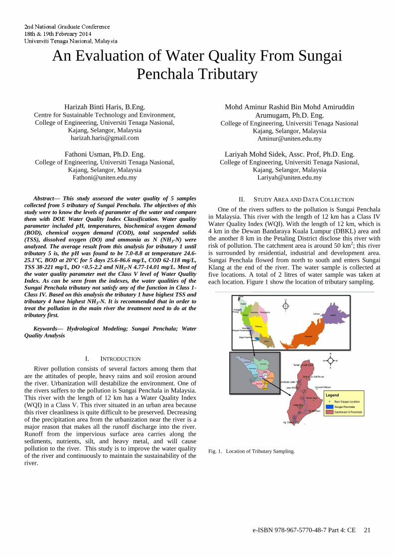
2nd
National Graduate Conference,
18th
and 19th
February 2014,
UNITEN
An Evaluation of Water Quality From Sungai
Penchala Tributary
Harizah Binti Haris, B.Eng. Centre for Sustainable Technology and Environment,
College of Engineering, Universiti Tenaga Nasional,
Kajang, Selangor, Malaysia
Mohd Aminur Rashid Bin Mohd Amiruddin
Arumugam, Ph.D. Eng. College of Engineering, Universiti Tenaga Nasional
Kajang, Selangor, Malaysia
Fathoni Usman, Ph.D. Eng. College of Engineering, Universiti Tenaga Nasional,
Kajang, Selangor, Malaysia
Lariyah Mohd Sidek, Assc. Prof, Ph.D. Eng. College of Engineering, Universiti Tenaga Nasional,
Kajang, Selangor, Malaysia
Abstract— This study assessed the water quality of 5 samples
collected from 5 tributary of Sungai Penchala. The objectives of this
study were to know the levels of parameter of the water and compare
them with DOE Water Quality Index Classification. Water quality
parameter included pH, temperatures, biochemical oxygen demand
(BOD), chemical oxygen demand (COD), total suspended solids
(TSS), dissolved oxygen (DO) and ammonia as N (NH3-N) were
analyzed. The average result from this analysis for tributary 1 until
tributary 5 is, the pH was found to be 7.0-8.8 at temperature 24.6-
25.1°C, BOD at 20°C for 5 days 25.6-86.6 mg/L, COD 62-118 mg/L,
TSS 38-221 mg/L, DO <0.5-2.2 and NH3-N 4.77-14.01 mg/L. Most of
the water quality parameter met the Class V level of Water Quality
Index. As can be seen from the indexes, the water qualities of the
Sungai Penchala tributary not satisfy any of the function in Class 1-
Class IV. Based on this analysis the tributary 1 have highest TSS and
tributary 4 have highest NH3-N. It is recommended that in order to
treat the pollution in the main river the treatment need to do at the
tributary first.
Keywords— Hydrological Modeling; Sungai Penchala; Water
Quality Analysis
I. INTRODUCTION
River pollution consists of several factors among them that are the attitudes of people, heavy rains and soil erosion around the river. Urbanization will destabilize the environment. One of the rivers suffers to the pollution is Sungai Penchala in Malaysia. This river with the length of 12 km has a Water Quality Index (WQI) in a Class V. This river situated in an urban area because this river cleanliness is quite difficult to be preserved. Decreasing of the precipitation area from the urbanization near the river is a major reason that makes all the runoff discharge into the river. Runoff from the impervious surface area carries along the sediments, nutrients, silt, and heavy metal, and will cause pollution to the river. This study is to improve the water quality of the river and continuously to maintain the sustainability of the river.
II. STUDY AREA AND DATA COLLECTION
One of the rivers suffers to the pollution is Sungai Penchala in Malaysia. This river with the length of 12 km has a Class IV Water Quality Index (WQI). With the length of 12 km, which is 4 km in the Dewan Bandaraya Kuala Lumpur (DBKL) area and the another 8 km in the Petaling District disclose this river with risk of pollution. The catchment area is around 50 km
2; this river
is surrounded by residential, industrial and development area. Sungai Penchala flowed from north to south and enters Sungai Klang at the end of the river. The water sample is collected at five locations. A total of 2 litres of water sample was taken at each location. Figure 1 show the location of tributary sampling.
Fig. 1. Location of Tributary Sampling.
e-ISBN 978-967-5770-48-7 Part 4: CE 21

2nd
National Graduate Conference,
18th
and 19th
February 2014,
UNITEN
In this study Sungai Penchala was chosen as the study area. Sungai Penchala also has been chosen in the One State One River programme. This program requires each state in Malaysia to choose one river to be rehabilitated. Main criteria that make Sungai Penchala have been chosen is because of this river is one of the polluted rivers in Selangor [2]. The water is polluted and only suitable for livestock drinking. At the middle of the river almost 70% of the original river course has been lined with concrete and not in the natural condition anymore. Figure 2 until Figure 6 are the location of the water sample taken and the picture of tributary involve in this study.
Tributary Number 1 Date: 6/6/2013 Time: 10.45 AM Weather: Normal Observed Land use: Residential & Commercial Coordinate: 3˚04’ 36.45” N 101˚37’ 17.03” E
Fig. 2. Tributary Number 1
Tributary Number 2 Date: 6/6/2013 Time: 11.45 AM Weather: Normal Observed land use: Industrial Coordinate: 3˚05’ 05.87” N 101˚37’ 55.28” E
Tributary Number 3 Date: 6/6/2013 Time: 12.30 PM Weather: Normal Observed land use: Industrial Coordinate: 3˚05’ 35.04” N 101˚37’ 51.79” E
Fig. 4. Tributary Number 3
Tributary Number 4 Date: 6/6/2013 Time: 12.50 PM Weather: Normal Observed land use: Industrial, Residential & Commercial Coordinate: 3˚06’ 13.75” N 101˚38’ 01.81” E
Fig. 5. Tributary Number 4
Fig.3. Tributary Number 1
e-ISBN 978-967-5770-48-7 Part 4: CE 22

2nd
National Graduate Conference,
18th
and 19th
February 2014,
UNITEN
Tributary Number 5 Date: 6/6/2013 Time: 1.30 PM Weather: Normal Observed land use: Industrial & Commercial Coordinate: 3˚06’ 45.27” N 101˚37’ 57.79” E
Fig. 6. Tributary Number 5
III. ASSESSMENT PARAMETERS AND METHODS
The water sample from this five tributary was tested by Taliworks Analytical Laboratory Sdn. Bhd. Several parameters were analysed include pH, Biochemical Oxygen Demand (BOD), Chemical Oxygen Demand (COD), Total Suspended Solid (TSS), Ammonia as N (NH
3N) and Dissolved Oxygen (DO). The
method are using is Standard Method for the Examination of Water and WasteWater (2005) 21st Edition, APHA, AWWA, WEF.
A. Water Quality Parameter
To classify the river water quality in Class I to IV, several parameters must be considered. In this study, the parameters are divided into physical and chemical groups.
1) Physical Parameter
There are several types of physical parameter but in this study only Total Suspended Solid taken into consideration. The particles in the water which is larger than 0.45 µm is refer as Total Suspended Solid (TSS). High suspended solid in the water can block the sunlight to penetrate into water and not good for the aquatic habitat and plants [3].
2) Chemical Parameter
In order to determine river water quality five parameters were used which is pH, Biochemical Oxygen Demand (BOD), Chemical Oxygen Demand (COD), Ammonia as N (NH3N) and Dissolved Oxygen (DO).
pH is used to measure the level of acid in the water. Concentration of hydrogen ions H+ contributes to the pH reading. When the pH reading is low and concentration of H+ are at the high levels means the river water is acidic [4]. Neutral pH is when the pH reading is 7.0.
Biochemical Oxygen Demand (BOD) is to determine the amount of oxygen required to stabilize domestic and industrial waste. Chemical Oxygen Demand (COD) test is used to measure the quantity of organic and inorganic oxidizable compound in water. The milligram per liter (mg/L) is use as a unit to show that the mass of oxygen consumed per liter of solution.
Nitrates can break into nitrites, and these nitrites are harmful to humans. Nitrites will affect the ability of red blood cells to carry oxygen. When the fish in the river affected by nitrites it can cause serious illnesses to the human that eat the fish [4].
DO is to measure the amount of available freely oxygen in water. The unit of DO is milligrams per liter or as a percent saturation. More cool the water, more oxygen it can hold [7].
IV. RESULTS AND DISCUSSIONS
A. Water Quality Parameter
1) pH - The pH of the water ranged 7.0 to 8.8. A pH range of 6.0 to 9.0 is the ph for clean river.
2) BOD - The BOD of the water ranged from 25.6-86.6 mg/L. The BOD value of not above 6.0 mg/L is suggested by the standard for Class III. The BOD for Sungai Penchala tributary is too high acceding the standard for Class III.
3) COD – The COD of the water ranged from 62-118 mg/L. A COD not above 50mg/L is generally suggested by the standards for Class III. All the COD value for Sungai Penchala tributary is not exceed the Class III DOE Water Quality Index Classification.
4) TSS - The TSS of the water ranged from 38-221 mg/L. A TSS not above 150 mg/L is generally suggested by the standards for Class III. The value of TSS at Tributary 1 is highest than other tributary because Tributary 1 is downstream of the river and the industrial land use.
e-ISBN 978-967-5770-48-7 Part 4: CE 23
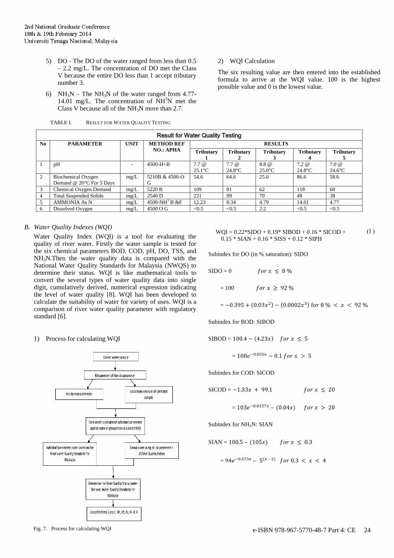
2nd
National Graduate Conference,
18th
and 19th
February 2014,
UNITEN
5) DO - The DO of the water ranged from less than 0.5 – 2.2 mg/L. The concentration of DO met the Class V because the entire DO less than 1 accept tributary number 3.
6) NH3N – The NH3N of the water ranged from 4.77-14.01 mg/L. The concentration of NH
3N met the
Class V because all of the NH3N more than 2.7.
TABLE I. RESULT FOR WATER QUALITY TESTING
B. Water Quality Indexes (WQI)
Water Quality Index (WQI) is a tool for evaluating the quality of river water. Firstly the water sample is tested for the six chemical parameters BOD, COD, pH, DO, TSS, and NH3N.Then the water quality data is compared with the National Water Quality Standards for Malaysia (NWQS) to determine their status. WQI is like mathematical tools to convert the several types of water quality data into single digit, cumulatively derived, numerical expression indicating the level of water quality [8]. WQI has been developed to calculate the suitability of water for variety of uses. WQI is a comparison of river water quality parameter with regulatory standard [6].
1) Process for calculating WQI
2) WQI Calculation
The six resulting value are then entered into the established formula to arrive at the WQI value. 100 is the highest possible value and 0 is the lowest value.
Subindex for DO (in % saturation): SIDO
SIDO = 0
= 100
= ( ) ( ) f
Subindex for BOD: SIBOD
SIBOD = ( )
=
Subindex for COD: SICOD
SICOD =
= – ( )
Subindex for NH3N: SIAN
SIAN = – ( )
= – ( – )
Result for Water Quality Testing
No PARAMETER UNIT METHOD REF
NO.: APHA
RESULTS
Tributary
1
Tributary
2
Tributary
3
Tributary
4
Tributary
5
1 pH - 4500-H+B 7.7 @
25.1°C
7.7 @
24.8°C
8.8 @
25.0°C
7.2 @
24.8°C
7.0 @
24.6°C
2 Biochemical Oxygen Demand @ 20°C For 5 Days
mg/L 5210B & 4500-O G
54.6 64.6 25.6 86.6 58.6
3 Chemical Oxygen Demand mg/L 5220 B 109 81 62 118 68
4 Total Suspended Solids mg/L 2540 D 221 99 70 48 38
5 AMMONIA As N mg/L 4500-NH3 B &F 12.23 8.34 4.79 14.01 4.77
6 Dissolved Oxygen mg/L 4500 O G <0.5 <0.5 2.2 <0.5 <0.5
WQI = 0.22*SIDO + 0.19* SIBOD + 0.16 * SICOD +
0.15 * SIAN + 0.16 * SISS + 0.12 * SIPH
Fig. 7. Process for Calculating WQI
Fig. 7. Process for calculating WQI
e-ISBN 978-967-5770-48-7 Part 4: CE 24
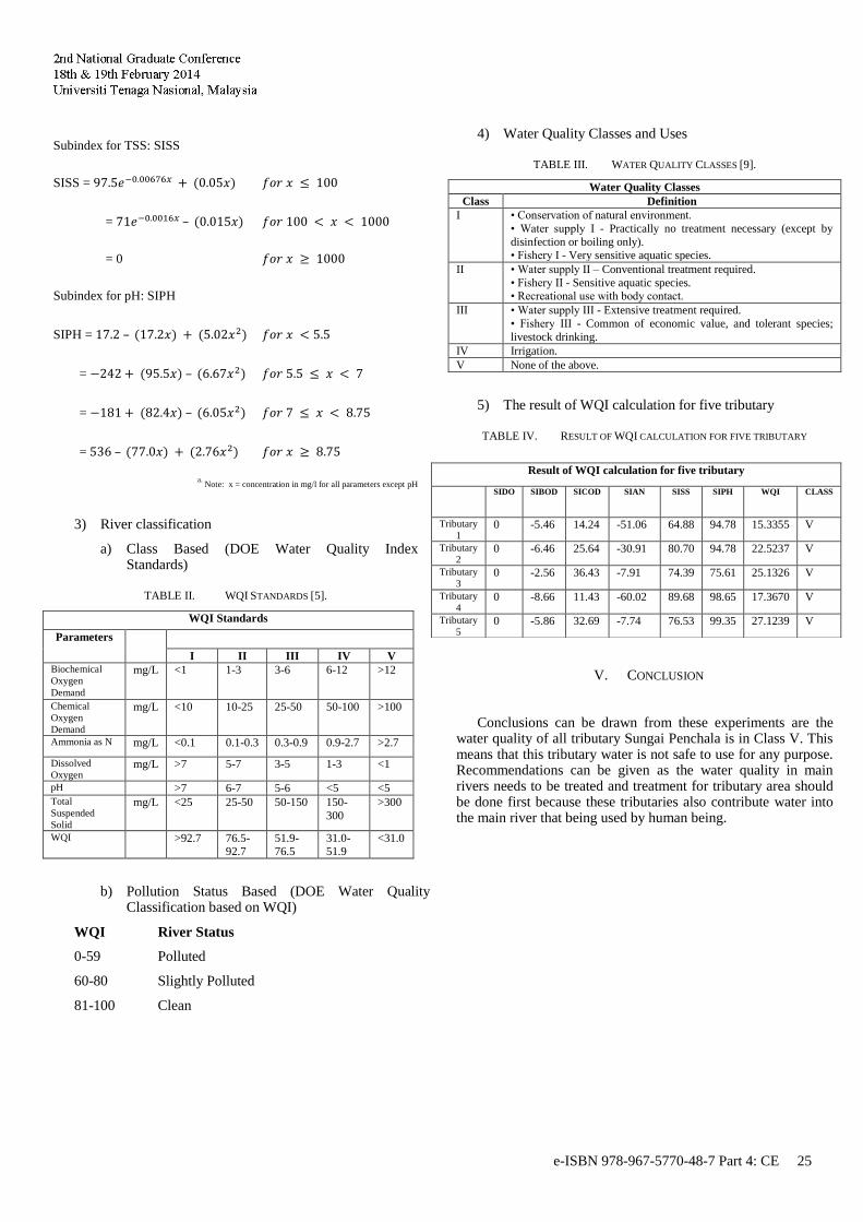
2nd
National Graduate Conference,
18th
and 19th
February 2014,
UNITEN
Subindex for TSS: SISS
SISS = ( )
= – ( )
= 0
Subindex for pH: SIPH
SIPH = – ( ) ( )
= ( ) – ( )
= ( ) – ( )
= – ( ) ( )
a. Note: x = concentration in mg/l for all parameters except pH
3) River classification
a) Class Based (DOE Water Quality Index Standards)
TABLE II. WQI STANDARDS [5].
WQI Standards
Parameters
I II III IV V Biochemical
Oxygen
Demand
mg/L <1 1-3 3-6 6-12 >12
Chemical
Oxygen
Demand
mg/L <10 10-25 25-50 50-100 >100
Ammonia as N mg/L <0.1 0.1-0.3 0.3-0.9 0.9-2.7 >2.7
Dissolved
Oxygen mg/L >7 5-7 3-5 1-3 <1
pH >7 6-7 5-6 <5 <5 Total
Suspended
Solid
mg/L <25 25-50 50-150 150-
300
>300
WQI >92.7 76.5-92.7
51.9-76.5
31.0-51.9
<31.0
b) Pollution Status Based (DOE Water Quality Classification based on WQI)
WQI River Status
0-59 Polluted
60-80 Slightly Polluted
81-100 Clean
4) Water Quality Classes and Uses
TABLE III. WATER QUALITY CLASSES [9].
Water Quality Classes
Class Definition
I • Conservation of natural environment.
• Water supply I - Practically no treatment necessary (except by
disinfection or boiling only). • Fishery I - Very sensitive aquatic species.
II • Water supply II – Conventional treatment required.
• Fishery II - Sensitive aquatic species. • Recreational use with body contact.
III • Water supply III - Extensive treatment required.
• Fishery III - Common of economic value, and tolerant species;
livestock drinking.
IV Irrigation.
V None of the above.
5) The result of WQI calculation for five tributary
TABLE IV. RESULT OF WQI CALCULATION FOR FIVE TRIBUTARY
V. CONCLUSION
Conclusions can be drawn from these experiments are the water quality of all tributary Sungai Penchala is in Class V. This means that this tributary water is not safe to use for any purpose. Recommendations can be given as the water quality in main rivers needs to be treated and treatment for tributary area should be done first because these tributaries also contribute water into the main river that being used by human being.
Result of WQI calculation for five tributary
SIDO SIBOD SICOD SIAN SISS SIPH WQI CLASS
Tributary
1 0 -5.46 14.24 -51.06 64.88 94.78 15.3355 V
Tributary
2 0 -6.46 25.64 -30.91 80.70 94.78 22.5237 V
Tributary
3 0 -2.56 36.43 -7.91 74.39 75.61 25.1326 V
Tributary
4 0 -8.66 11.43 -60.02 89.68 98.65 17.3670 V
Tributary
5 0 -5.86 32.69 -7.74 76.53 99.35 27.1239 V
e-ISBN 978-967-5770-48-7 Part 4: CE 25

2nd
National Graduate Conference,
18th
and 19th
February 2014,
UNITEN
ACKNOWLEDGMENT
This research paper is made possible through the help and
support from everyone, including: parents, teachers, family, friends, and in essence, all sentient beings. Please allow me to dedicate my acknowledgment of gratitude toward the following significant advisors and contributors:
First and foremost, I would like to thank to Dr. Mohd Aminur Rashid Bin Mohd Amiruddin Arumugam for his most support and encouragement. He kindly read my paper and offered invaluable detailed advices on grammar, organization, and the theme of the paper.
I would also like to thank the ministry of higher education which is the sponsor of the project Urban Ecohydrology for Resilient Environment (UCOREN) under the grant 012 001 101 LRGS.
Finally, I sincerely thank to my husband Muhammad Farezshafiq Bin Mohd Yeen, my parents, En. Haris Bin Mohd Sham and Puan Zainab Binti Ibrahim, family, and friends, who provide the advice and financial support. The product of this research paper would not be possible without all of them.
REFERENCES
[1] (n.d.). Retrieved July 2, 2012, from One State One River, Jabatan
Pengairan dan Saliran Negeri Selangor.
[2] Adli Shahar. Sukarelawan Bersih Sungai Penchala. Berita Harian, 2010.
[3] Avvannavar, S. M., and Shrihari, S. Evaluation of water quality index for drinking purposes for river Netravathi, Mangalore, South India. Environmental Monitoring and Assessment, 2007.
[4] Davis, A. P. & McCuen, R. H. Storm water management for smart growth. 1st edition. Springer Science and Business Media, 2005.
[5] Department of Environment Malaysia. (2005). Interim National Water Quality Standards for Malaysia. Retrieved on September 6, 2013 from http://www.doe.gov.my/index.php?option=comcontent&task=view&id=244&Itemid=615&lang=en.
[6] Khan, F., Husaini, T., and Lumb, A. Water quality evaluation and trend analysis in selected watersheds of the Atlantic region of Canada. Environmental Monitoring and Assessment. 2003, 88, Pg. 221–242.
[7] Said, A., Stevens, D. K., and Sehlke, G. An innovative index for evaluating water quality in streams. Environmental Management. 2004, 34(3), Pg. 406–414.
[8] Sarkar, C., and Abbasi, S. A. Qualidex – A new software for generating water quality indice. Environmental Monitoring and Assessment. 2006, 119, Pg. 201–231.
[9] Zaki Zainuddin. Benchmarking River Water Quality in Malaysia, JURUTERA. 2010, Pg. 13-15
e-ISBN 978-967-5770-48-7 Part 4: CE 26
2nd National Graduate Conference
18th & 19th February 2014
Universiti Tenaga Nasional, Malaysia
Analysis of TMDL for River of Life Project (RoL)
Gombak River Catchment Ahmad Fauzan Mohd Sabri
Centre for Sustainable Technology and Environment
Universiti Tenaga Nasional (UNITEN)
Putrajaya, Malaysia
Email: [email protected]
Lariyah Mohd Sidek
Centre for Sustainable Technology and Environment
Universiti Tenaga Nasional (UNITEN)
Putrajaya, Malaysia
Email: [email protected]
Ahmad Sharmy Mohamed Jaffar
RBM Sdn. Bhd.
Kuala Lumpur, Malaysia
Email: [email protected]
Abstract: Gombak River is one the main tributaries of Klang
River Basin under River of Life Project (RoL). The river water
quality was categorized within Class III to Class IV National Water
Quality Standards for Malaysia (NWQS) under Department of
Environmental Malaysia (DOE). Department of Irrigation and
Drainage Malaysia (DID) was given mandate of taking charge to
improve water quality to Class IIB. In this study three types of land
use 1.forested, 2.semi-urban and 3.urban will be used as boundary
criteria to analyze the Total Maximum Daily Load (TMDL).
InfoWorks RS as wide acceptable hydrodynamic model integrated
with Geographic Information System (GIS) application has been
used to simulate the flow data. The flow data then grouped into 5
zones, which are High Flows, Moist Conditions, Mid-range Flows,
Dry Conditions, and Low Flows to explain watershed
characteristics and flow patterns using Flow Duration Curve
(FDC). Based on analysis, the 90 percentile probability of the flow
adopted as flow for the TMDL calculation. Result showed great
effort required to reduce all point sources effluence to achieve
Class IIB for Gombak River.
Keywords – Gombak River; River of Life; InfoWorks RS; Total
Maximum Daily Load
I. INTRODUCTION
Gombak River is one the main tributaries of Klang River Basin under River of Life Project (RoL). Gombak River flows through two municipal areas which are Selayang Municipal Council (MPS) and Kuala Lumpur City Hall (DBKL). It covers 23 kilometer in stretch representing 119 square kilometer catchment areas (from Gunung Bunga Buah at Genting Highland area to confluence of Batu River). Fig. 1 depicts the Gombak River Basin in River of Life (RoL) Projects. The upper catchments of Gombak River are under virgin jungle area. The middle catchments are semi-urban and followed by densely populated residential and commercial at the lower catchment.
Wastewater or sullage from catchment area especially urban area discharged directly into Gombak River. The Biological Oxygen Demand (BOD), Chemical Oxygen Demand (COD) and Ammoniacal Nitrogen (AN) score were
very high and probably influenced by sewerage discharge and wastewater from these commercial and residential activities [1][2]. The pollutants of metal are essentially remain at same level [3].
Water quality of the river is the main factor to determine life of the river (DID, 2009). At present the water quality for River of Life Project are Class III to Class IV, i.e., not suitable for body contact and recreation used under National Water Quality Standards for Malaysia (NWQS) [2][5].
Fig.1 Depict of Gombak River in River of Life (RoL) Projects
e-ISBN 978-967-5770-48-7 Part 4: CE 27
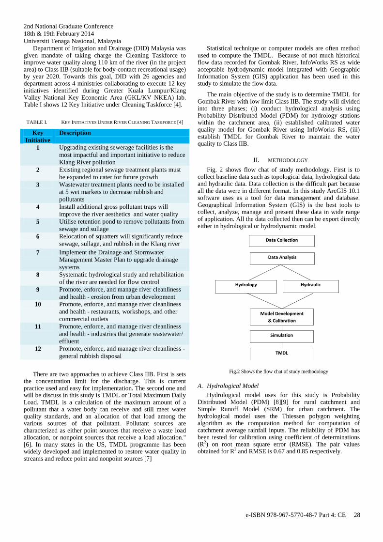
2nd National Graduate Conference
18th & 19th February 2014
Universiti Tenaga Nasional, Malaysia Department of Irrigation and Drainage (DID) Malaysia was
given mandate of taking charge the Cleaning Taskforce to improve water quality along 110 km of the river (in the project area) to Class IIB (suitable for body-contact recreational usage) by year 2020. Towards this goal, DID with 26 agencies and department across 4 ministries collaborating to execute 12 key initiatives identified during Greater Kuala Lumpur/Klang Valley National Key Economic Area (GKL/KV NKEA) lab. Table I shows 12 Key Initiative under Cleaning Taskforce [4].
TABLE I. KEY INITIATIVES UNDER RIVER CLEANING TASKFORCE [4]
Key
Initiative
Description
1 Upgrading existing sewerage facilities is the
most impactful and important initiative to reduce
Klang River pollution
2 Existing regional sewage treatment plants must
be expanded to cater for future growth
3 Wastewater treatment plants need to be installed
at 5 wet markets to decrease rubbish and
pollutants
4 Install additional gross pollutant traps will
improve the river aesthetics and water quality
5 Utilise retention pond to remove pollutants from
sewage and sullage
6 Relocation of squatters will significantly reduce
sewage, sullage, and rubbish in the Klang river
7 Implement the Drainage and Stormwater
Management Master Plan to upgrade drainage
systems
8 Systematic hydrological study and rehabilitation
of the river are needed for flow control
9 Promote, enforce, and manage river cleanliness
and health - erosion from urban development
10 Promote, enforce, and manage river cleanliness
and health - restaurants, workshops, and other
commercial outlets
11 Promote, enforce, and manage river cleanliness
and health - industries that generate wastewater/
effluent
12 Promote, enforce, and manage river cleanliness -
general rubbish disposal
There are two approaches to achieve Class IIB. First is sets the concentration limit for the discharge. This is current practice used and easy for implementation. The second one and will be discuss in this study is TMDL or Total Maximum Daily Load. TMDL is a calculation of the maximum amount of a pollutant that a water body can receive and still meet water quality standards, and an allocation of that load among the various sources of that pollutant. Pollutant sources are characterized as either point sources that receive a waste load allocation, or nonpoint sources that receive a load allocation." [6]. In many states in the US, TMDL programme has been widely developed and implemented to restore water quality in streams and reduce point and nonpoint sources [7]
Statistical technique or computer models are often method used to compute the TMDL. Because of not much historical flow data recorded for Gombak River, InfoWorks RS as wide acceptable hydrodynamic model integrated with Geographic Information System (GIS) application has been used in this study to simulate the flow data.
The main objective of the study is to determine TMDL for Gombak River with low limit Class IIB. The study will divided into three phases; (i) conduct hydrological analysis using Probability Distributed Model (PDM) for hydrology stations within the catchment area, (ii) established calibrated water quality model for Gombak River using InfoWorks RS, (iii) establish TMDL for Gombak River to maintain the water quality to Class IIB.
II. METHODOLOGY
Fig. 2 shows flow chat of study methodology. First is to collect baseline data such as topological data, hydrological data and hydraulic data. Data collection is the difficult part because all the data were in different format. In this study ArcGIS 10.1 software uses as a tool for data management and database. Geographical Information System (GIS) is the best tools to collect, analyze, manage and present these data in wide range of application. All the data collected then can be export directly either in hydrological or hydrodynamic model.
Fig.2 Shows the flow chat of study methodology
A. Hydrological Model
Hydrological model uses for this study is Probability Distributed Model (PDM) [8][9] for rural catchment and Simple Runoff Model (SRM) for urban catchment. The hydrological model uses the Thiessen polygon weighting algorithm as the computation method for computation of catchment average rainfall inputs. The reliability of PDM has been tested for calibration using coefficient of determinations (R
2) on root mean square error (RMSE). The pair values
obtained for R2 and RMSE is 0.67 and 0.85 respectively.
Data Collection
Data Analysis
Hydrology
Hydraulic
Model Development
& Calibration
Simulation
TMDL
e-ISBN 978-967-5770-48-7 Part 4: CE 28
2nd National Graduate Conference
18th & 19th February 2014
Universiti Tenaga Nasional, Malaysia
B. Hydrodynamic Model
InfoWorks River Simulation (RS) model uses for hydrodynamic model in this study. The model is mainly based on the full hydrodynamic model equations (Saint Venant) momentum and continuity equations The equations are solved based on finite differences (implicit computational scheme)[10]. Implementation of that model has been done by means of the InfoWorks RS river modeling software (Wallingford Software, UK). The model is based on river bed cross-sectional data approximately every 100 m along the modeled rivers, river bed roughness information and geometric data along the course of rivers.
Hydrodynamic model will generated flow from various catchments and cross-sections. The flow simulated then has been tested with calibration using coefficient of determinations (R
2) and Pearson Correlation Coefficient (PCC) at the cross-
section 088-BG1.010100.The pair values obtained for R2 and
PCC is 0.44 and 0.66 respectively.
The flow data simulated then used to develop Flow Duration Curve (FDC). The flow data grouped into 5 zones in FDC, which are High Flows, Moist Conditions, Mid-range Flows, Dry Conditions, and Low Flows, reflecting flow duration intervals of 0-10%, 10-40%, 40-60%, 60-90%, and 90-100%, respectively. These 5 zones can be used to explain watershed characteristics and flow patterns according to hydrologic conditions. The FDC can represent the relationship between magnitude and frequency of daily stream flow for a particular watershed. It provides a simple, comprehensive,
graphical view of the overall stream flow variability in a watershed [11].Fig. 4 shows the FDC observed (average2007-2012) and simulated (2011) for calibration. The flows after 20 percentile were well predicted while there were slight deviations between observed and simulated flows below 20 percentile. The performance tested using root mean square error (RMSE) with the value is 0.99.
C. Total Maximum Daily Load (TMDL)
TMDL is a term used to describe the maximum amount of a pollutant that a stream can assimilate without violating water quality standards. The TMDL process establishes the allowable loadings of pollutants or other quantifiable parameters for a water body based on the relationship between pollution sources and in-stream water quality conditions.
Generally, TMDL can be calculated by multiplying average annual or long-term stream-flow data by the water quality standard for specific pollutant. For the dynamic flow, the daily low flow data was used for the purpose of consideration pollutant discharge exceeded in critical cases.
In this study TMDL of three different land uses for Gombak River will be calculated based on low flow and dry condition data from FDC. The low flows and dry conditions data then will be multiplying by standard particular parameter Class IIB (DOE WQI) to get the TMDL for each location. 90 and 75 percentile probability of the flow will be adapted as low flow and dry conditions for the TMDL calculation based on DID recommendation. [1]
Fig.3 Shows the result for calibration at point 088-BG1.010100
e-ISBN 978-967-5770-48-7 Part 4: CE 29
2nd National Graduate Conference
18th & 19th February 2014
Universiti Tenaga Nasional, Malaysia
Fig.4 Shows FDC observed (2007-2012) vs simulated (2011) for calibration
III. RESULT AND DISCUSSION
Based on hydrodynamic simulation generated, three locations were selected represent three type of land use for flow analysis. The locations are 053-Bt. 12 Jln Gombak, 088-Tmn Greenwood and 169-Jln Tun Razak. From Fig. 5, it is noted that the lowest daily flow is 5m
3/s in three locations
while the 90 percentile low flows are 5.5m3/s for Bt.2 Jln
Gombak and Taman Greenwood and 7m3/s for Jln Tun Razak.
For average dry flow condition, 75 percentile value is 6m3/s for
Bt.2 Jln Gombak and Taman Greenwood and 10m3/s for Jln
Tun Razak.
With low limit Class IIB (DOE, WQI) BOD, COD, TSS and NH3N,the TMDL can be computed and the Table II to III gives the Class IIB TMDL for two flow conditions in Gombak River.
TABLE II. CLASS IIB TMDL FOR TWO FLOW CONDITIONS AT 053-BT.12
AND 088-TMN GREENWOOD
Parameter BOD COD TSS NH3N
(kg/d)
TMDL for 75 percentile 1555 12,960 25,920 156
TMDL for 90 percentile 1426 11,880 23,760 143
TABLE III. CLASS IIB TMDL FOR TWO FLOW CONDITIONS AT LOCATION
169-JLN TUN RAZAK
Parameter BOD COD TSS NH3N
(kg/d)
TMDL for 75 percentile 2592 21,600 43,200 259
TMDL for 90 percentile 1814 15,120 30,240 181
Fig.5 Shows FDC simulated for three locations in Gombak River
Result from Class IIB TMDL calculation, pollutant loading for forested and semi-urban land use for flow 75 and 90 percentile is not much difference while the loading for urban land use for flow 75 is 1.4 time higher than 90 percentile in average. This 90 percentile then compare with existing condition TMDL loading at 169-Jln Tun Razak.
TABLE IV. CLASS IIB TMDL AT LOCATION 169-JLN TUN RAZAK
COMPARE WITH EXISTING CONDITION.
Parameter BOD COD TSS NH3N
(kg/d)
Existing Loading [1] 1888 9603 7059 919
TMDL for 90 percentile 1814 15,120 30,240 181
Table IV shows Class IIB TMDL 90 percentile at location 169-Jln Tun Razak compare with existing condition. BOD is 74kg/d higher compare with maximum limit and NH3N is 5 times higher than maximum TMDL limit.
IV. CONCLUSION
Water Quality of the river is the main factor to determine life of the river. TMDL is one of the approaches to control water quality in the river. TMDL has been widely used all around the world especially for rising of discharge and rapid development in catchment area. The finding indicates that great effort required in improving water quality in Gombak River especially for BOD and NH3N.
V. ACKNOWLEDGMENT
The authors would like to acknowledge DID for provision of data sharing, HR Walingford Asia Sdn. Bhd.and Innovyze Sdn. Bhd. for software sponsored and technical assistance in this study.
e-ISBN 978-967-5770-48-7 Part 4: CE 30

2nd National Graduate Conference
18th & 19th February 2014
Universiti Tenaga Nasional, Malaysia
VI. REFERENCES
[1] DID, (2012). Study on Water Quality Improvement and Hydrological
Assessment for the Klang River. Report by Dr. Nik & Associates Sdn. Bhd.
[2] DOE, (2011). Malaysia Environmental Quality Report 2011. Percetakan Nasional Malaysia Berhad.
[3] Ismail Z., Primasari B., Shirazi S.M., (2011). Monitoring and management issues of heavy metal pollution of Gombak River, Kuala Lumpur. Int. J. Physical Sciences. 6(35), 7961-7968.
[4] PEMANDU, (2011). River of Life Progress Report 2011 through DID
[5] DID, (2009). Study on Water Quality Trends and Index in Peninsular Malaysia.
[6] US EPA, 2007, An Approach for Using Load Duration Curves in the Development of TMDLs
[7] Mostaghimi S., Benham B., Brannan K., Dillah T., Wynn J., Yagow G., Zeckoski R., (2003). Total maximum daily load development in Lincille Creek: Bacteria and general standard (Bentich) impairment, Biological Systems Engineering Department, Veginia Tech, Blackburg, Vergina.
[8] Moore. R.J., (2007). The PDM rainfall-runoff model. Hydrol. Earth Syst. Sci. 11(1), 483-499.
[9] Cabus P., (2008). River flow prediction through rainfall-runoff modelling with a probability
[10] Said S., Mah D.Y.S., Sumok P., Lai S.H., (2009) Proceding of Institusion of Civil Engineering, water management 162, water quality monitoring for Maun River, Malaysia
[11] Vogel, R.M., Neil, M.F.,(1994). Flow Duration Curve. I: new interpretation and confidence interval. Journal of Water Resources Planning and Management 120(4), 485-504M. Young, The Technical Writer’s Handbook. Mill Valley, CA: University Science, 1989.
e-ISBN 978-967-5770-48-7 Part 4: CE 31
Methods of anchoring to prevent end peeling of
flexurally strengthened reinforced concrete beam -A review
Md.Tanvir Ehsan Amin
Masters Student
Department of Civil Engineering
University Tenaga Nasional
Selangor, Malaysia
Dr. Md. Ashraful Alam
Senior Lecturer
Department of Civil Engineering
University Tenaga Nasional
Selangor, Malaysia
Abstract— Strengthening of reinforced concrete structure for
flexure using externally bonded plates is one of the most popular
choice to retrofit aged and deficient structures in the construction
industry. However, the premature failure at the end of the plate
is the weakest point of the system. It could be due to formation of
high interfacial shear and normal stresses at the end of the plate.
To overcome this problems anchors with a various type of
anchoring systems had been used. Although anchors had effects
to eliminate the premature failures proper method of anchoring
and to obtain the design guidelines of anchor plates are totally
absent. The main aim of this article is to review the existing
anchoring systems for elimination of premature end peeling.
Keywords— reinforced concrete beam, steel plate, CFRP
laminate, plate end debonding, end anchors, flexural
strengthening.
INTRODUCTION
Retrofitting of reinforced concrete structure is a significant task to maintain the existing structures now a days. Recently the demand of rehabilitation has been increased because of the damage of the structures, changes of uses of structures or because of flexural deficient structures due to under designed. The old structures are required to be strengthened since the complete replacement of the damaged or deficient structures is not cost effective practical choice. A significant number of research works have been conducted over last decades to strengthen reinforced concrete (RC) structures using various methods such as steel plate concrete composite method, mechanically fastened fiber reinforced polymer composite method, Sprayed fiber-reinforced polymer composites method, Near Surface Mounting method, externally bonded steel plate and CFRP laminate method. [1-15] However plate bonding method using steel plate and fiber reinforced polymer (FRP) laminates was found to be the most popular choice
Although plate bonding technique has been recognized worldwide, it is not free from its shortcomings. Concrete cannot resist higher tensile stress and that causes the debonding failure of the plate. Premature plate end debonding and intermediate crack induced (IC) debonding are the main disadvantages of this method which separate the plate from the surface and the concrete rip off along the tensile side of the
structure [1]. In general plate end debonding starts at the ends of the plate and propagates along the beam, whereas IC debonding occurs at flexural or shear cracks in the midspan of the beam and propagates towards the end of the plate [46]. The plate also could be debonded due to formation of high interfacial stresses at the end of the plate [6]. A significant number of researches carried out to investigate the mechanisms of debonding failures [2-5]. End debonding was found to be most common as compared to IC debonding. Thus elimination of this debonding failure is crucial to obtain the full strength and ductility of strengthened beam.
Plate end debonding failure could be prevented by end anchors. Researchers proposed various anchoring systems to mitigate end peeling such as Transverse anchor system, Ductile Anchor system, U-Jacket Anchorage system and L-shaped Anchorage system [15, 36, 37]. Mechanical anchorage system offers a real solution to prevent the problems. Different anchorage system has been developed including embedded metal threads, transverse anchors, ductile anchors, U-jackets anchors, near-surface mounted rods and anchors made with FRP (also known as spike anchors). Although various techniques has been introduced to reduce debonding failure, most of the tested specimens failed to prevent the end plate debonding failure [7, 8, 9, 10, 11]. This is due to the ineffectiveness of anchor bolts and FRP fibre
Normally, resisting normal stress rather than shear stress is very effective for strengthening plates. To overcome the shortcomings of anchor bolts, end anchors of U and L-shaped wrap and plates were used and experimentally investigated by a number of researchers [12, 13, 6, 14, 15]. It is reported that U and L-shaped end anchors significantly decrease the premature plate end debonding failure [14, 6].
Unfortunately, although many research works had been carried out on the effects of U and L-shaped end anchors to eliminate premature debonding failure, a systematic study to obtain the length of end anchors is lacking. In most cases, the lengths of end anchors were arbitrarily chosen. Since, the development of an excessive interfacial shear stress at the plate end is the main cause for premature failure, the length of end anchors could be obtained from the interfacial shear stress diagram of the strengthened beams.
e-ISBN 978-967-5770-48-7 Part 4: CE 32
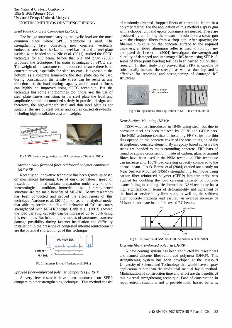
EXISTING METHODS OF STRENGTHENING
Steel Plate Concrete Composite (SPCC):
The bridge structures carrying the cyclic load are the most common place where SPCC technique is used. The strengthening layer consisting new concrete, vertically embedded steel bars, horizontal steel bar net and a steel plate welded with headed studs. Nie et al. (2011) studied the SPCC technique for RC beam, before that Nie and Zhao (2008) proposed the technique. The main advantages of SPCC are: The weight of the structure can be reduced because there is no concrete cover, especially for slab; no crack is exposed at the bottom; as a concrete framework the steel plate can be used during construction; the tensile stress can be resist at any direction and the load bearing capacity and flexural stiffness can highly be improved using SPCC technique. But the technique has some shortcomings too, those are: the use of steel plate causes corrosion; in the steel plate the level and amplitude should be controlled strictly in practical design, and therefore, the high-strength steel and thin steel plate is not suitable; the use of steel plates and cables caused drawbacks, including high installation cost and weight.
Fig 1: RC beam strengthening by SPCC technique (Nie et al. 2011)
Mechanically fastened fiber reinforced polymer composite
(MF-FRP):
Recently an innovative technique has been grown up based on mechanical fastening. Use of unskilled labors, speed of installation, minimal surface preparation under any kind of meteorological condition, immediate use of strengthened structure are the main benefits of MF-FRP. Many researches has been conducted and proved the effectiveness of this technique. Nardone et al. (2011) proposed an analytical model that able to predict the flexural behavior of RC structures strengthened with MF-FRP strips. Bank et al. (2003) showed the load carrying capacity can be increased up to 60% using this technique. But brittle failure modes of structures, concrete damage possibility during fastener installation and difficulty installation in the presence of congested internal reinforcement are the potential shortcomings of this technique.
Fig 2: fasteners layout (Nardone et al. 2011)
Sprayed fiber-reinforced polymer composites (SFRP):
A very few research have been conducted on SFRP compare to other strengthening technique. This method consist
of randomly oriented chopped fibers of controlled length in a polymer matrix. For the application of this method a spray gun with a chopper unit and epoxy containers are needed. These are produced by combining the stream of resin from a spray gun with the chopped fibers from a chop gun. After spraying the fiber/resin mixture on the concrete surface to the required thickness, a ribbed aluminum roller is used to roll out any entrapped air. Lee et al. (2004) investigated the strength and ductility of damaged and undamaged RC beam using SFRP. A series of three point bending test has been carried out on their research. In their study they proved that SFRP is capable of substantially increase the strength as well as ductility, and is effective for repairing and strengthening of damaged RC structures.
Fig 3: RC specimens after application of SFRP (Lee et al. 2004)
Near Surface Mounting (NSM):
NSM was first introduced in 1940s using steel, but due to
corrosion steel has been replaced by CFRP and GFRP bars.
The NSM technique consists of installing FRP strips into thin
slits opened on the concrete cover of the tension region of the
strengthened concrete element. By an epoxy based adhesive the
strips are bonded to the surrounding concrete. FRP bars of
round or square cross section, made of carbon, glass or aramid
fibres have been used in the NSM technique. This technique
can increase upto 150% load carrying capacity compared to the
normal beam. J.A.O. Barros et al (2004) carried out a study on
Near Surface Mounted (NSM) strengthening technique using
carbon fiber reinforced polymer (CFRP) laminate strips was
applied for doubling the load carrying capacity of concrete
beams failing in bending. He showed the NSM technique has a
high significance in terms of deformability and increment of
the load at serviceability limit state, as well as, the stiffness
after concrete cracking and assured an average increase of
91%on the ultimate load of the tested RC beams.
Fig 4: The position of NSM bar (T.H. Almusallam et al. 2012)
Discrete fiber-reinforced polyuria (DFRP):
A new coating system has been conducted by researchers
and named discrete fiber-reinforced polyurea (DFRP). This
strengthening system has been developed at the Missouri
University of Science and Technology that would have a spray
application rather than the traditional manual layup method.
Minimization of construction time and effort are the benefits of
this external strengthening technique. Ease of construction in
repair-retrofit situations and to provide multi hazard benefits,
Stirrup Main steel bars
Concrete Volume
NSM
bar(s)
e-ISBN 978-967-5770-48-7 Part 4: CE 33
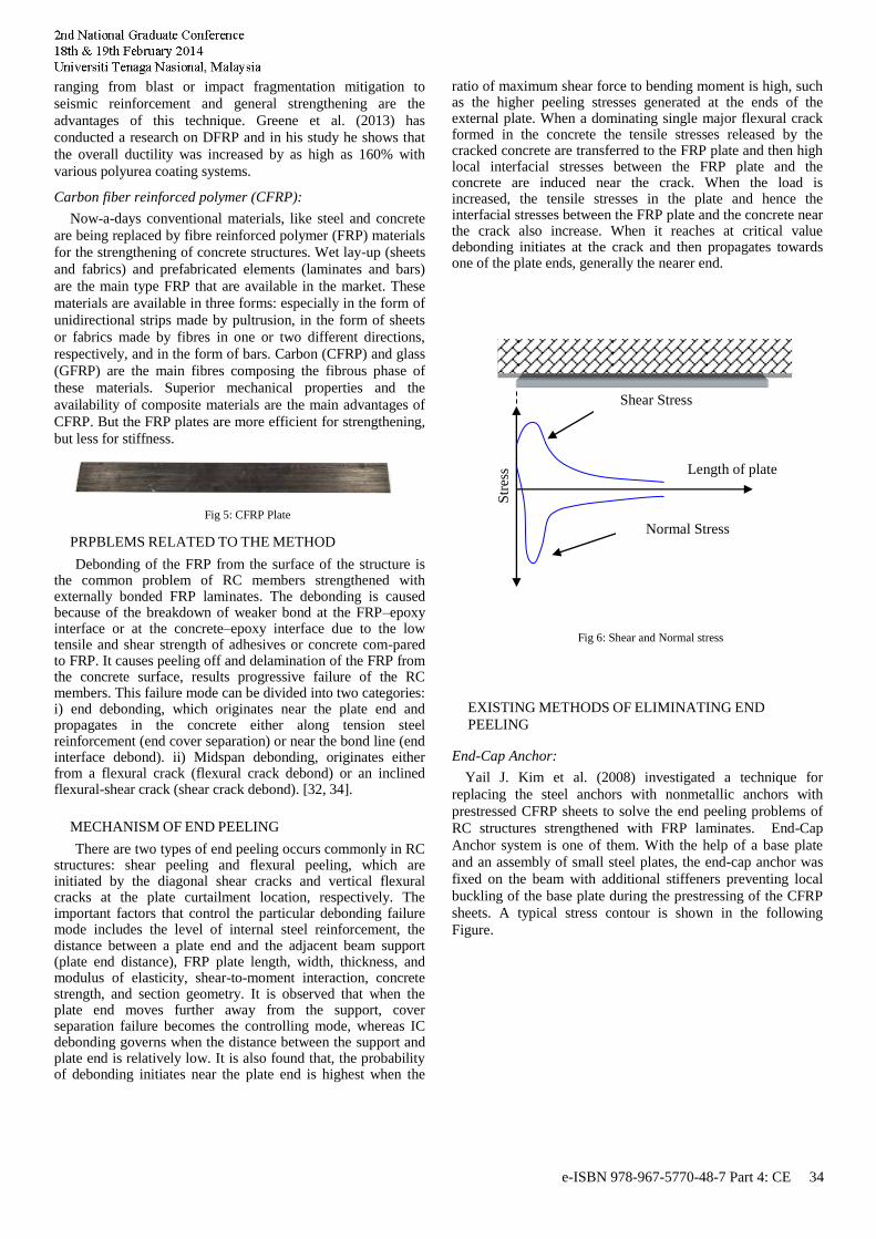
ranging from blast or impact fragmentation mitigation to
seismic reinforcement and general strengthening are the
advantages of this technique. Greene et al. (2013) has
conducted a research on DFRP and in his study he shows that
the overall ductility was increased by as high as 160% with
various polyurea coating systems.
Carbon fiber reinforced polymer (CFRP):
Now-a-days conventional materials, like steel and concrete
are being replaced by fibre reinforced polymer (FRP) materials
for the strengthening of concrete structures. Wet lay-up (sheets
and fabrics) and prefabricated elements (laminates and bars)
are the main type FRP that are available in the market. These
materials are available in three forms: especially in the form of
unidirectional strips made by pultrusion, in the form of sheets
or fabrics made by fibres in one or two different directions,
respectively, and in the form of bars. Carbon (CFRP) and glass
(GFRP) are the main fibres composing the fibrous phase of
these materials. Superior mechanical properties and the
availability of composite materials are the main advantages of
CFRP. But the FRP plates are more efficient for strengthening,
but less for stiffness.
Fig 5: CFRP Plate
PRPBLEMS RELATED TO THE METHOD
Debonding of the FRP from the surface of the structure is the common problem of RC members strengthened with externally bonded FRP laminates. The debonding is caused because of the breakdown of weaker bond at the FRP–epoxy interface or at the concrete–epoxy interface due to the low tensile and shear strength of adhesives or concrete com-pared to FRP. It causes peeling off and delamination of the FRP from the concrete surface, results progressive failure of the RC members. This failure mode can be divided into two categories: i) end debonding, which originates near the plate end and propagates in the concrete either along tension steel reinforcement (end cover separation) or near the bond line (end interface debond). ii) Midspan debonding, originates either from a flexural crack (flexural crack debond) or an inclined flexural-shear crack (shear crack debond). [32, 34].
MECHANISM OF END PEELING
There are two types of end peeling occurs commonly in RC structures: shear peeling and flexural peeling, which are initiated by the diagonal shear cracks and vertical flexural cracks at the plate curtailment location, respectively. The important factors that control the particular debonding failure mode includes the level of internal steel reinforcement, the distance between a plate end and the adjacent beam support (plate end distance), FRP plate length, width, thickness, and modulus of elasticity, shear-to-moment interaction, concrete strength, and section geometry. It is observed that when the plate end moves further away from the support, cover separation failure becomes the controlling mode, whereas IC debonding governs when the distance between the support and plate end is relatively low. It is also found that, the probability of debonding initiates near the plate end is highest when the
ratio of maximum shear force to bending moment is high, such as the higher peeling stresses generated at the ends of the external plate. When a dominating single major flexural crack formed in the concrete the tensile stresses released by the cracked concrete are transferred to the FRP plate and then high local interfacial stresses between the FRP plate and the concrete are induced near the crack. When the load is increased, the tensile stresses in the plate and hence the interfacial stresses between the FRP plate and the concrete near the crack also increase. When it reaches at critical value debonding initiates at the crack and then propagates towards one of the plate ends, generally the nearer end.
Fig 6: Shear and Normal stress
EXISTING METHODS OF ELIMINATING END
PEELING
End-Cap Anchor:
Yail J. Kim et al. (2008) investigated a technique for
replacing the steel anchors with nonmetallic anchors with
prestressed CFRP sheets to solve the end peeling problems of
RC structures strengthened with FRP laminates. End-Cap
Anchor system is one of them. With the help of a base plate
and an assembly of small steel plates, the end-cap anchor was
fixed on the beam with additional stiffeners preventing local
buckling of the base plate during the prestressing of the CFRP
sheets. A typical stress contour is shown in the following
Figure.
Shear Stress
Normal Stress
Str
ess Length of plate
e-ISBN 978-967-5770-48-7 Part 4: CE 34
Fig 7: End cap anchor system (Yail et. al 2008)
Transverse Anchors:
Another method proposed by Yail J. Kim et al. (2008) is
Transverse Anchor system. In this method mechanical anchors
set were installed to sustain the transversely applied forces in
U-wraps and one threaded rod was welded to a rectangular
steel plate and prepared the surface. A support plate made of
steel was prepared to mount the lateral anchor plates with nuts.
If U-wraps is a part of overall beam system, it can be anchored
through a slab. It may be possible to replace the lateral anchor
plate by other materials such as a GFRP plate. A typical set up
is shown by the following figure.
Fig 8: Transverse u-shaped anchor (Yail et. al 2008)
Ductile Anchor System:
K.Galal et al. (2009) proposed a new hybrid fiber-reinforced
polymer (FRP) sheet/ductile anchor system for rehabilitation
of reinforced concrete (RC) beams. The ductile anchor that
holds the CFRP sheet under the soffit of the specimen
consisted of one steel plate, having two threaded holes in its
thickness, one steel angle, having one hole in the middle and
two threaded holes in its thickness. Two steel tensile link
members, four high tensile threaded rods and one heavy duty
Hilti bolt at each end. The steel angle was fastened by the
heavy duty Hilti bolt with 45° inclination located in the
predrilled hole at the middle of the intersection point of the T-
beam’s soffit and the column stub. The two tensile steel link
members connected the angle to the steel plate via high tensile
rods, which were located in the holes in the thickness of both
the angle and the plate and it was fastened using nuts. In his
research he showed that the ultimate load of the T-beam
strengthened with externally bonded CFRP along with ductile
anchorage was about 27% higher and strength gain was 21%
higher than that of the control T-beam. But the midspan
deflection was 91 % higher than the control beam.
Fig 9: Hybrid FRP/ductile steel anchor system (K.Galal et al. 2009)
Surface-Bonded Flat Anchorage (SBFA) system:
SBFA anchorage system is a new technique and very few
research has been carried out. Mofidi et al (2012) applied the
SBFA end-anchorage system for beams strengthened using the
Externally Bonded (EB) method. The method has six steps:
(i) the area of the specimen where the continuous CFRP sheet
was to be glued was sandblasted to remove any surface
cement paste and to round off the beam edges; (ii) to achieve a
desirable smooth bond surface the bond area was grinded to
remove any possible irregularities; (iii) using compressed air
the residues were removed; (iv) a layer of U-shaped
continuous CFRP sheet was glued to the bottom and lateral
faces of the RC beam using a two-component epoxy resin; (v)
a thin layer of epoxy paste was applied continuously to the
two ends of the CFRP U-jacket; and (vi) a CFRP laminate
with a cross section of 20 × 2:5 mm was epoxy-bonded to the
two ends of the CFRP U-jacket along the shear span.
Fig 10: Elevation of specimen S3-EB-SBFA with surface-bonded CFRP
laminate end-anchorage system. (Mofidi et al. 2012)
Double-aluminum-plate mechanical end-anchorage
(DAMA) system:
To implement the DAMA end-anchorage system for beams
strengthened using the EB method, the following steps were
carried out: (i) 12-mm-diameter horizontal holes spaced at 175
mm were drilled perpendicular to the RC beam’s web surface.
The center line of the holes was 55 mm below the bottom of
the flange; (ii) a thin layer of epoxy paste was applied around
10-mm-diameter, 60-mm-long, threaded steel rods; (iii) the
10-mm-diameter stainless-steel threaded rods were installed
into the holes; (iv) a CFRP U-jacket was epoxy-bonded to the
RC beam’s shear span in the same way as previously
described for the specimen with no end anchorage; (v) a layer
of epoxy paste was applied continuously to the two ends of the
CFRP U- jacket; (vi) a 3∕8-in.-thick aluminum plate with
matching predrilled holes and embedded, threaded stainless-
steel rods was bonded onto the two ends of the CFRP U-jacket
along the shear span; (vii) the free ends of the CFRP sheet
were wrapped around the aluminum plate [Fig.(a)]; and (viii) a
similar aluminum plate was installed on top of the free ends of
the CFRP sheet, and the two aluminum plates were tightened
to each other using stainless-steel nuts on the embedded,
threaded steel mechanical anchor. [Fig. (b)].
e-ISBN 978-967-5770-48-7 Part 4: CE 35
Fig 11: Elevation of specimen S3-EB-DAMA: (a) first aluminum plate
installed; (b) second aluminum plate installed (Mofidi et al. 2012)
Embedded round CFRP bar end-anchorage system (ERBA):
To install the ERBA end-anchorage system for beams
strengthened using the EB method, the following procedures
were carried out: (i) grooves 15 mm in width and 15 mm in
depth were made along the shear span in the beam’s flange at
the flange-web intersection; (ii) the beam was then prepared in
the same way as previously described for the specimen with
no end anchorage; (iii) a thin layer of epoxy paste was applied
along the grooves; (iv) the free ends of the CFRP sheets
bonded to the beam’s web were bonded around the groove’s
surface; (v) the grooves were filled up to two-thirds of their
volume with the epoxy paste; (vi) 9.5-mm CFRP rods were
installed into the grooves in both sides of the beam’s flange;
and (vii) the excess epoxy paste was removed.
Fig 12: Specimen S3-EB-EERBA after installation of the embed round
FRP bar end-anchorage system (Mofidi et al. 2012))
Embedded flat CFRP laminate end-Anchorage system
(EFLA):
To implement the EFLA end-anchorage system for beams
strengthened using the EB method, the following steps were
carried out: (i) grooves 5 mm in width and 22 mm in depth
were made along the shear span in the beam’s flange at the
flange web junction; (ii) the beam was then prepared in the
same way as previously described for the specimen with no
end anchorage; (iii) a thin layer of epoxy paste was applied
along the grooves; (iv) the free ends of the CFRP sheets
bonded to the beam’s web were installed inside the grooves
using a 20 × 2:5 mm CFRP laminate (the CFRP sheet ends
were wrapped around the CFRP laminate); and (v) the grooves
were filled with epoxy paste.. For each of the end-anchorage
systems discussed previously, the CFRP sheet must be cut to
an exact length. Specimens strengthened using the EB method
with the DAMA, ERBA, and EFLA anchorage systems
achieved the highest efficiency among the end-anchorage
systems tested in this research study.
FRP Anchors:
The FRP anchorage system made from rolled fiber sheets or
bundled loose fibers are a promising form of anchorage
because they can be applied to wide FRP-strengthened
structural elements such as beams, slabs and walls. They are
discrete and do not suffer from the same constraints as U-
jackets. Such anchors are referred to as FRP spike anchors,
fiber anchors, fiber bolts, and FRP dowels, among other
names, but are herein collectively referred to as FRP anchors
(smith et al. 2010). The anchors can be hand made in
laboratory or in site, or manufactured from glass or carbon
fiber sheets or loose fibers that have been bundled or rolled
Fig a. One end of the anchor (herein referred to as an anchor
dowel) is inserted into a hole (filled by epoxy) in the concrete
substrate and the dowel length can be confined to the cover
region of the member. The other end of the anchor is epoxied
onto the surface of the FRP plate. The ends of the fibers which
are splayed and epoxied onto the surface of the plate in order
to disperse local stress concentrations are herein referred to as
the anchor fan.
Fig 13: FRP anchor (c) (smith et al. 2010)
Recently Koutas and Triantafillou (2013) has conducted their
study on the role of spike anchors in three-sided jacketing (U-
jackets) of reinforced concrete T-beams strengthened in shear
and to compare the effectiveness of different anchor system.
In FRP each anchor comprised a tow of fibers of the same
type used in the unidirectional sheets. The length of anchors
was 150 mm and their weight was 34g/m and 59g/m for
carbon and glass fiber anchors, respectively. Fiber anchor
spikes were formed by impregnating dry fibers [Fig. (a)] with
epoxy. The holes were filled with epoxy [Fig.(b)] to half of
their depths. This method of anchoring was selected on the
basis of transferring the tension forces from the FRP sheet
terminating below the concrete slab into the web or into the
slab for all other specimens with anchors.
Fig 14: The rolled sheet (smith et al. 2010))
Further research has been carried out and showed that for
improving the strength of RC members the use of FRP
anchors are very effective. Orton et al. (2008) determined that
two rows of three 10 mm diameter anchors were able to
develop the FRP tensile capacity and led to fracture of the
entire width of the FRP. They reported that FRP anchors
increased the efficiency of material usage of the FRP retrofit
to 57%, indicating that FRPs with anchors are able to achieve
a given strengthening capacity and require less material than
unanchored FRPs. In this case, the strength of the member
increased by 270%, with only a 175% increase in the FRP
material. In addition, it was found that a greater number of
e-ISBN 978-967-5770-48-7 Part 4: CE 36

smaller anchors and reduced spacings were more effective in
fully developing the capacity of the FRP fiber, as larger
spacings did not anchor the entire width of the FRPs, resulting
in partial debonding [38].
Table 1. Different strengthening systems
Author Anchoring system Strengthening Method Mode of
failure
Type of
anchor
Dimension
(mm)
Materi
al
Method
Nie et el. (2008)
Steel Plate Anchor
system
4700 X 230
Steel plate
Steel plate composite
method
Fatigue failure of the steel
plate and
flexural failure on the
concrete.
F. Nardone
et al. (2011)
Mechanica
lly fastened
FRP
650 X 50
X 3.2
FRP
strips
Mechanicall
y fastened fiber
reinforced
polymer composite
cleavage,
sustained bearing, shear-
out, net
tension, and pry-out failure.
T.H.
Almusallam et al.
(2012)
- Ø12, Ø14,
Ø16
GFRP near-surface
mounted GFRP bars
NSM rod
debonding and concrete cover
separation
Y.J.Kim et al. (2008)
U-wraps 750 X 150 X 0.33
Prestressed
CFRP
Nonmetallic Anchor
Systems
Premature debonding
failure
K. Ghalal
(2009)
Ductile
Anchor System
160X 40
X13
Hybri
d FRP
new hybrid
FRP sheet/ ductile
anchor
system for
flexural
strengthenin
g
Concrete
crushing, FRP rupture and
debonding
failure
A. Mofidi
et al. (2012)
U-jackets
end-
anchor
20 X 2.5 CFRP
lamin
ate
Surface-
Bonded Flat
Anchorage
Shear
A. Mofidi et al.
(2012)
U-jackets end-
anchor
CFRP lamin
ate
Double-aluminum-
plate
mechanical end-
anchorage
Flexure
A. Mofidi et al.
(2012)
U-jackets end-
anchor
9.5 CFRP lamin
ate
Embedded round CFRP
bar end-
anchorage system
Shear
A. Mofidi
et al. (2012)
U-jackets
end-anchor
20 X 2.5 CFRP
laminate
Embedded
flat CFRP laminate
end-
Anchorage system
Flexure
PROPOSED METHOD OF ANCHORING
From the review it is seen that the debonding or end peeling
occurs because of high interfacial shear and normal stresses.
The debonding failure could be prevented once normal stress
and shear stress could be minimized. U and L shaped anchor
plates found to be more effective in minimizing this stresses.
Alam and Jummat (2010) investigated the effects of those
anchor plates. However, the shear stress would significantly
reduced by the connector could apply at the end of the plate
and the normal stress could be reduced by anchor plates. This
hybrid system significantly reduces the dimension of the
anchor plates. This research is going to propose hybrid
anchoring system is in connectors and U-shaper anchor plates.
In this particular system shear connector would resist the
interfacial shear stress. Whether normal stress has been
resisted by anchor plates. Last the dimension of the plates
would be significantly optimized.
CONCLUSIONS
Using anchor to prevent the end peeling of FRP is the most
common process we have seen in this review. It is true that
these type of practices have gained popularity and reduced the
problem, but it cannot give a proper solution. However,
further research is necessary to prevent the end peeling. It is
recommended that future research should be focus on
examining various types of anchor in more details. Research
should carry on to make use of experimental and numerical
parametric studies to inform strength prediction models which
will develop the future FRP design guideline.
ACKNOWLEDGMENTS
The study was carried out at the Department of Civil
Engineering, University Tenaga Nasional. The authors would
like to thanks to MOHE for providing the grand under ERGS
012012 and the department for facilitating the study.
REFERENCES
[1] S.T. Smith and J.G. Teng, “FRP-strengthened RC beams. A review of
debonding strength models,” Engineering Structures, vol. 24, pp. 385–395, 2002.
[2] H. Saadatmanesh and A.M. Malek, “Design guidelines for flexural strengthening of RC beams with FRP plates,” J. Composites for Construction, ASCE, vol. 2(4), pp. 158-164, 1998.
[3] M.T. El-Mihilmy and J.W. Tedesco, “Prediction of anchorage failure for reinforced concrete beams strengthened with fiber-reinforced polymer plates,” ACI Structural Journal, vol. 98(3), pp. 301-314, 2001.
[4] J. Yao and J.G. Teng, “Plate end debonding in FRP-plated RC beams-II: Strength model,” Engineering Structures, vol. 29, pp. 2472-2486, 2007.
[5] J. Yang, J. Ye and Z. Niu, “Simplified solutions for the stress transfer in concrete beams bonded with FRP plates,” Engineering Structures, vol. 30, pp. 533-545, 2008.
[6] B.Y. Bahn and R.S. Harichandran, “Flexural behaviour of reinforced concrete beams strengthened with CFRP sheets and epoxy mortar,” J. Composites for Construction, vol. 12(4), pp. 387-395, 2008.
[7] M. Hussain, A. Sharif, A. Basunbul, M.H. Baluch and G.J. Al-Aulaimani, “Flexural behavior of precracked reinforced concrete beams strengthened externally by steel plates,” ACI Structural Journal, vol. 92(1), pp. 14-22, 1995.
e-ISBN 978-967-5770-48-7 Part 4: CE 37

[8] H.N. Garden and L.C. Hollaway, “An experimental study of the influence of plate end anchorage of carbon fibre composite plates used to strengthen reinforced concrete beams,” J. Composite Structures, vol. 42, pp. 175-188, 1998.
[9] R. Jones, R.N. Swamy and A. Charif, “Plate separation and anchorage of reinforced concrete beams strengthened by epoxy-bonded steel plates,” The Structural Engineering, vol. 66(5), pp. 85-94, 1998.
[10] S.T. Smith, S. Hu, S.J. Kim and R. Serancino, “FRP-strengthened RC slabs anchored with FRP anchors,” Engineering Structures, vol. 33(4), pp. 1075-1087, 2011.
[11] A. Chahrour and K. Soudki, “Flexural response of reinforced concrete beams strengthened with end-anchored partially bonded carbon fiber-reinforced polymer strips,” J. Composites for Construction, vol. 9(2), pp. 170-177, 2005.
[12] A. Hosny, A. lrahman and T. Elafandy, “Performance of reinforced concrete beams strengthened by hybrid FRP laminates,” J. Cement and Concrete Composites, vol. 28, pp. 906-913, 2006.
[13] F. Ceroni, M. Pecce, S. Matthys and L. Taerwe, "Debonding strength and anchorage devices for reinforced concrete elements strengthened with FRP sheets,” J. Composites, Part B, vol. 39, pp. 429-441, 2008.
[14] M.Z. Jumaat and M.A. Alam, “Behaviour of U and L shaped end anchored steel plate strengthened reinforced concrete beams.” European Journal of Scientific Research, vol. 22(2), pp. 184-196, 2008.
[15] Y. Kim, R.G. Wight and M.F. Green, “Flexural strengthening of RC beams with prestressed CFRP sheets: Using nonmetallic anchor system,” J. Composites for Construction, vol. 12(1), pp. 44-52, 2008.
[16] S.T. Smith and J.G Teng, “Interfacial stresses in plated beams.” Engineering Structures. vol. 23, pp. 857-871, 2001.
[17] Q.S. Yang, X.R. Peng and A.K.H. Kwan, “Finite element analysis of interfacial stresses in FRP-RC hybrid beams.” Mechanics Research Communications, vol. 31, pp. 331-340, 2004.
[18] A. Tounsi, T.H. Daouadji, S. Benyoucef and E.A.A. Bedia, “Interfacial stresses in FRP-plated RC beams: Effect of adherent shear deformation,” International Journal of Adhesion and Adhesives, vol. 29(4), pp. 343-351, 2009.
[19] A. Carpinteri, P. Cornetti and N. Pugno, “Edge debonding in FRP strengthened beams: Stress versus energy failure criteria,” Engineering Structures, vol. 31(10), pp. 2436-2447, 2009.
[20] L. Zhang and J.G Teng, “Finite element prediction of interfacial stresses in structural members bonded with a thin plate,” Engineering Structures, vol. 32(2), pp. 459-471, 2010.
[21] L.J. Li, Y.C. Guo, F. Liu and J.H. Bungey, “An experimental and numerical study of the effect of thickness and length of CFRP on performance of repaired reinforced concrete beams,” J. Construction and Building Materials, vol. 20, pp. 901-909, 2006.
[22] M.T. El-Mihilmy, “Design and behaviour of reinforced concrete beams strengthened with fiber reinforced plastics (FRP),” Ph.D thesis, Graduate faculty, Auburn University, 1998.
[23] J. Nie, Y. Wang, C.S. Cai, “Experimental Research on Fatigue Behavior of RC Beams Strengthened with Steel Plate-Concrete Composite Technique,” J. Structural Engineering, vol. 137, pp. 772-781, 2011.
[24] J.G. Nie and J. Zhao, “Experimental study on simply supported RC beams strengthened by steel plate-concrete composite technique,” J. Build. Struct., vol. 29(5), ppt. 50–56 (in Chinese), 2008.
[25] F. Nardone, G.P. Lignola, A. Prota, G. Manfredi, A. Nanni, “Modeling of flexural behavior of RC beams strengthened with mechanically fastened FRP strips,” J. Composite Structures, vol. 93, pp. 1973–1985, 2011.
[26] L.C. Bank, M.G. Oliva, D. Arora and D.T. Borowicz, “Rapid strengthening of reinforced concrete bridges,” Wisconsin highway research program, Report no. 03–06, Madison, WI: Wisconsin Department of Transportation, 2003.
[27] H.K. Lee, L.R. Hausmann, “Structural repair and strengthening of damaged RC beams with sprayed FRP,” J. Composite Structures, vol. 63, pp. 201–209, 2004.
[28] J.M. Sena-Cruz and J.A.O. Barros, “Bond between nearsurface mounted CFRP laminate strips and concrete,” J. Composite Structures, vol. 8(6), pp. 519–527, 2004a.
[29] J.M. Sena-Cruz and J.A.O. Barros, “Modeling of bond between near-surface mounted CFRP laminate strips and concrete,” J. Composite Structures, vol. 82(17–19), pp. 1513–1521, 2004b.
[30] T.H. Almusallam, H.M. Elsanadedy, “Experimental and numerical investigation for the flexural strengthening of RC beams using near-surface mounted steel or GFRP bars,” J. Construction and Building Materials, vol. 40, pp. 145–161, 2013.
[31] C.E. Greene, J.J. Myers, “Flexural and Shear Behavior of Reinforced Concrete Members Strengthened with a Discrete Fiber-Reinforced Polyurea System,” J. Compos. Constr., vol. 17, pp. 108-116, 2013.
[32] R. A-Amery, R. A-Mahaidi, “Coupled flexural–shear retrofitting of RC beams using CFRP straps,” J. Composite Structures, vol. 75, pp. 457–464, 2006.
[33] S. Ahmed, E.Y., “Numerical investigation into strengthening steel I-section beams using CFRP strips,” Proc., Structures Congress, Structural Engineering and Public Safety, ASCE, Reston, VA, 2006.
[34] Y.J. Kim, R.G. Wight and M.F. Green, “Flexural Strengthening of RC Beams with Prestressed CFRP Sheets: Development of Nonmetallic Anchor Systems,” J. Composites for Construction, vol. 12, pp. 35-43, 2008.
[35] Triantafillou, T. C. (1998). Strengthening of structures with advanced FRPs. Prog. J. Struct. Eng. Mater, 1(2), 126–134.
[36] K. Galal, A. Mofidi, “Strengthening RC Beams in Flexure Using New Hybrid FRP Sheet/Ductile Anchor System,” J. Composites for Construction, vol. 13(3), pp. 217-225, 2009.
[37] A. Mofidi, O. Chaallal, B. Benmokrane, K. Neale, “Performance of End-Anchorage Systems for RC Beams Strengthened in Shear with Epoxy-Bonded FRP,” Journal of Composites for Construction, vol. 16(3), pp. 22-331, 2012.
[38] S.L. Orton, J.O. Jirsa and O. Bayrak, “Design considerations of carbon fiber anchors,” J. Compos. Constr., vol. 12(6), pp. 608–616, 2008.
[39] P.J. Fanning and O. Kelly, “Ultimate Response of RC Beams Strengthened with CFRP Plates,” J. Compos. Constr., vol. 5, pp. 122-127, 2001.
e-ISBN 978-967-5770-48-7 Part 4: CE 38

[40] R.A. Hammoud and K. Soudki, T.H. Topper, “Fatigue Flexural Behavior of Corroded Reinforced Concrete Beams Repaired with CFRP Sheets,” J. Compos. Constr., vol. 15, pp. 42-51, 2011.
[41] J.A.O. Barros and A.S. Fortes, “Flexural strengthening of concrete beams with CFRP laminates bonded into slits,” J. Cement & Concrete Composites, vol. 27, pp. 471–480, 2005.
[42] I.G. Costa and J.A.O. Barros, “Flexural and shear strengthening of RC beams with composite materials – The influence of cutting steel stirrups to install CFRP strips,” J. Cement and Concrete Composites, vol. 32, pp. 544–553, 2010.
[43] S. Dritsos, K. Pilakoutast and E. Kotsira, “Effectiveness of flexural strengthening of RC members,” J. Construction and Building Materials, vol. 9(3), pp.165-171, 1995.
[44] L. Anania, A. Badala and G. Failla, “Increasing the flexural performance of RC beams strengthened with CFRP materials,” J. Construction and Building Materials, vol. 19, pp. 55–61, 2005
[45] M.R. Arama, C. Czaderski, M. Motavalli, “Debonding failure modes of flexural FRP-strengthened RC beams,” J. Composites, Part B, vol. 39, pp. 826–841, 2007.
e-ISBN 978-967-5770-48-7 Part 4: CE 39
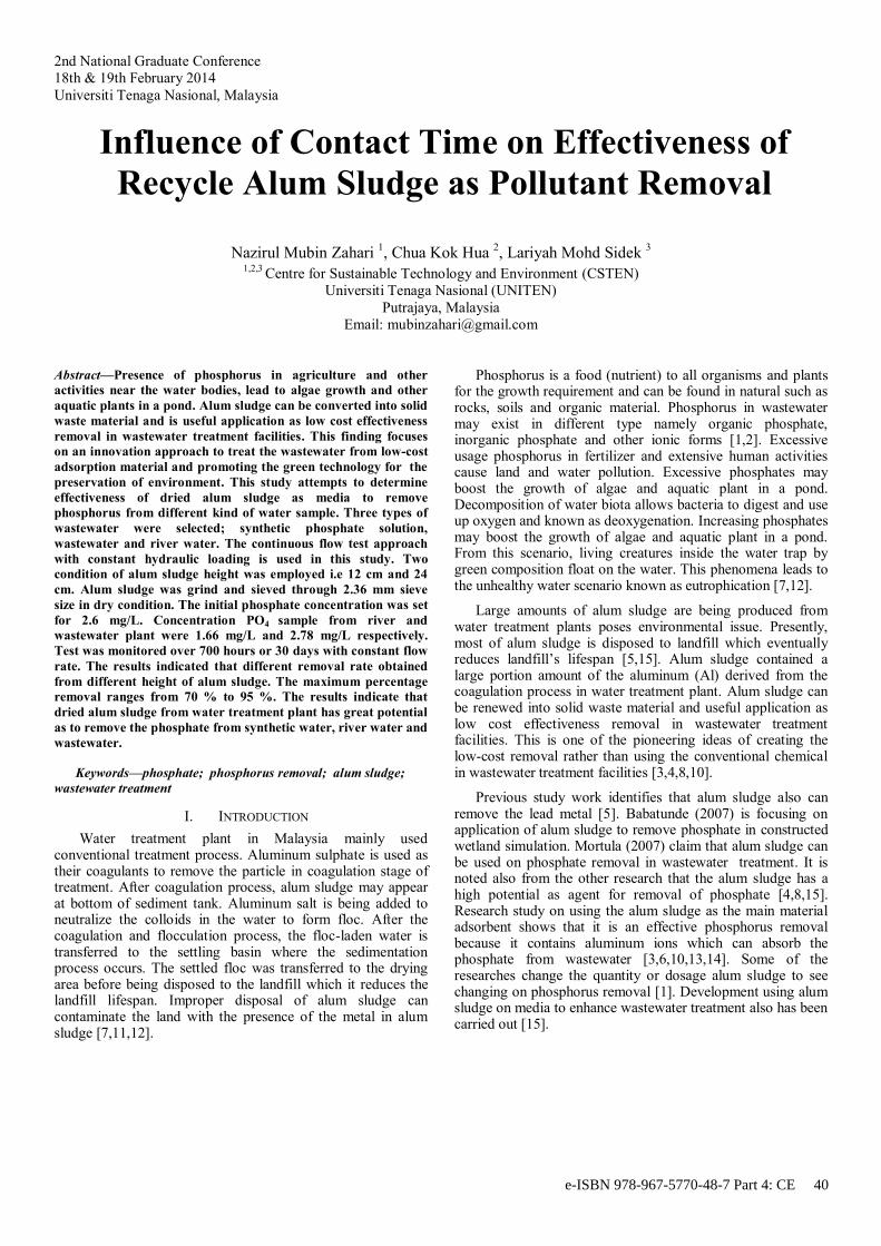
2nd National Graduate Conference
18th & 19th February 2014
Universiti Tenaga Nasional, Malaysia
Influence of Contact Time on Effectiveness of
Recycle Alum Sludge as Pollutant Removal
Nazirul Mubin Zahari 1, Chua Kok Hua
2, Lariyah Mohd Sidek
3
1,2,3 Centre for Sustainable Technology and Environment (CSTEN)
Universiti Tenaga Nasional (UNITEN)
Putrajaya, Malaysia
Email: [email protected]
Abstract—Presence of phosphorus in agriculture and other
activities near the water bodies, lead to algae growth and other
aquatic plants in a pond. Alum sludge can be converted into solid
waste material and is useful application as low cost effectiveness
removal in wastewater treatment facilities. This finding focuses
on an innovation approach to treat the wastewater from low-cost
adsorption material and promoting the green technology for the
preservation of environment. This study attempts to determine
effectiveness of dried alum sludge as media to remove
phosphorus from different kind of water sample. Three types of
wastewater were selected; synthetic phosphate solution,
wastewater and river water. The continuous flow test approach
with constant hydraulic loading is used in this study. Two
condition of alum sludge height was employed i.e 12 cm and 24
cm. Alum sludge was grind and sieved through 2.36 mm sieve
size in dry condition. The initial phosphate concentration was set
for 2.6 mg/L. Concentration PO4 sample from river and
wastewater plant were 1.66 mg/L and 2.78 mg/L respectively.
Test was monitored over 700 hours or 30 days with constant flow
rate. The results indicated that different removal rate obtained
from different height of alum sludge. The maximum percentage
removal ranges from 70 % to 95 %. The results indicate that
dried alum sludge from water treatment plant has great potential
as to remove the phosphate from synthetic water, river water and
wastewater.
Keywords—phosphate; phosphorus removal; alum sludge;
wastewater treatment
I. INTRODUCTION
Water treatment plant in Malaysia mainly used conventional treatment process. Aluminum sulphate is used as their coagulants to remove the particle in coagulation stage of treatment. After coagulation process, alum sludge may appear at bottom of sediment tank. Aluminum salt is being added to neutralize the colloids in the water to form floc. After the coagulation and flocculation process, the floc-laden water is transferred to the settling basin where the sedimentation process occurs. The settled floc was transferred to the drying area before being disposed to the landfill which it reduces the landfill lifespan. Improper disposal of alum sludge can contaminate the land with the presence of the metal in alum sludge [7,11,12].
Phosphorus is a food (nutrient) to all organisms and plants for the growth requirement and can be found in natural such as rocks, soils and organic material. Phosphorus in wastewater may exist in different type namely organic phosphate, inorganic phosphate and other ionic forms [1,2]. Excessive usage phosphorus in fertilizer and extensive human activities cause land and water pollution. Excessive phosphates may boost the growth of algae and aquatic plant in a pond. Decomposition of water biota allows bacteria to digest and use up oxygen and known as deoxygenation. Increasing phosphates may boost the growth of algae and aquatic plant in a pond. From this scenario, living creatures inside the water trap by green composition float on the water. This phenomena leads to the unhealthy water scenario known as eutrophication [7,12].
Large amounts of alum sludge are being produced from water treatment plants poses environmental issue. Presently, most of alum sludge is disposed to landfill which eventually reduces landfill’s lifespan [5,15]. Alum sludge contained a large portion amount of the aluminum (Al) derived from the coagulation process in water treatment plant. Alum sludge can be renewed into solid waste material and useful application as low cost effectiveness removal in wastewater treatment facilities. This is one of the pioneering ideas of creating the low-cost removal rather than using the conventional chemical in wastewater treatment facilities [3,4,8,10].
Previous study work identifies that alum sludge also can remove the lead metal [5]. Babatunde (2007) is focusing on application of alum sludge to remove phosphate in constructed wetland simulation. Mortula (2007) claim that alum sludge can be used on phosphate removal in wastewater treatment. It is noted also from the other research that the alum sludge has a high potential as agent for removal of phosphate [4,8,15]. Research study on using the alum sludge as the main material adsorbent shows that it is an effective phosphorus removal because it contains aluminum ions which can absorb the phosphate from wastewater [3,6,10,13,14]. Some of the researches change the quantity or dosage alum sludge to see changing on phosphorus removal [1]. Development using alum sludge on media to enhance wastewater treatment also has been carried out [15].
e-ISBN 978-967-5770-48-7 Part 4: CE 40
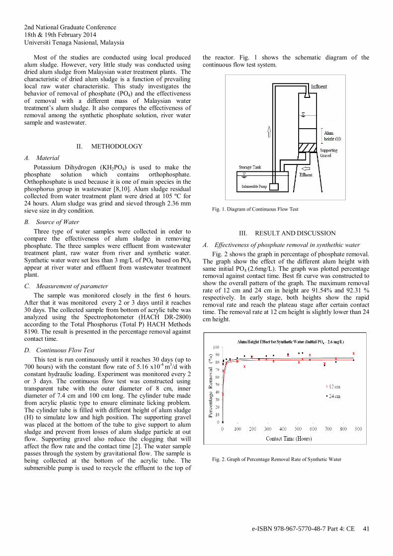
2nd National Graduate Conference
18th & 19th February 2014
Universiti Tenaga Nasional, Malaysia
Most of the studies are conducted using local produced
alum sludge. However, very little study was conducted using dried alum sludge from Malaysian water treatment plants. The characteristic of dried alum sludge is a function of prevailing local raw water characteristic. This study investigates the behavior of removal of phosphate (PO4) and the effectiveness of removal with a different mass of Malaysian water treatment’s alum sludge. It also compares the effectiveness of removal among the synthetic phosphate solution, river water sample and wastewater.
II. METHODOLOGY
A. Material
Potassium Dihydrogen (KH2PO4) is used to make the phosphate solution which contains orthophosphate. Orthophosphate is used because it is one of main species in the phosphorus group in wastewater [8,10]. Alum sludge residual collected from water treatment plant were dried at 105 ºC for 24 hours. Alum sludge was grind and sieved through 2.36 mm sieve size in dry condition.
B. Source of Water
Three type of water samples were collected in order to compare the effectiveness of alum sludge in removing phosphate. The three samples were effluent from wastewater treatment plant, raw water from river and synthetic water. Synthetic water were set less than 3 mg/L of PO4 based on PO4 appear at river water and effluent from wastewater treatment plant.
C. Measurement of parameter
The sample was monitored closely in the first 6 hours. After that it was monitored every 2 or 3 days until it reaches 30 days. The collected sample from bottom of acrylic tube was analyzed using the Spectrophotometer (HACH DR-2800) according to the Total Phosphorus (Total P) HACH Methods 8190. The result is presented in the percentage removal against contact time.
D. Continuous Flow Test
This test is run continuously until it reaches 30 days (up to 700 hours) with the constant flow rate of 5.16 x10
-4 m
3/d with
constant hydraulic loading. Experiment was monitored every 2 or 3 days. The continuous flow test was constructed using transparent tube with the outer diameter of 8 cm, inner diameter of 7.4 cm and 100 cm long. The cylinder tube made from acrylic plastic type to ensure eliminate licking problem. The cylinder tube is filled with different height of alum sludge (H) to simulate low and high position. The supporting gravel was placed at the bottom of the tube to give support to alum sludge and prevent from losses of alum sludge particle at out flow. Supporting gravel also reduce the clogging that will affect the flow rate and the contact time [2]. The water sample passes through the system by gravitational flow. The sample is being collected at the bottom of the acrylic tube. The submersible pump is used to recycle the effluent to the top of
the reactor. Fig. 1 shows the schematic diagram of the continuous flow test system.
Fig. 1. Diagram of Continuous Flow Test
III. RESULT AND DISCUSSION
A. Effectiveness of phosphate removal in synthethic water
Fig. 2 shows the graph in percentage of phosphate removal. The graph show the effect of the different alum height with same initial PO4 (2.6mg/L). The graph was plotted percentage removal against contact time. Best fit curve was constructed to show the overall pattern of the graph. The maximum removal rate of 12 cm and 24 cm in height are 91.54% and 92.31 % respectively. In early stage, both heights show the rapid removal rate and reach the plateau stage after certain contact time. The removal rate at 12 cm height is slightly lower than 24 cm height.
Fig. 2. Graph of Percentage Removal Rate of Synthetic Water
e-ISBN 978-967-5770-48-7 Part 4: CE 41
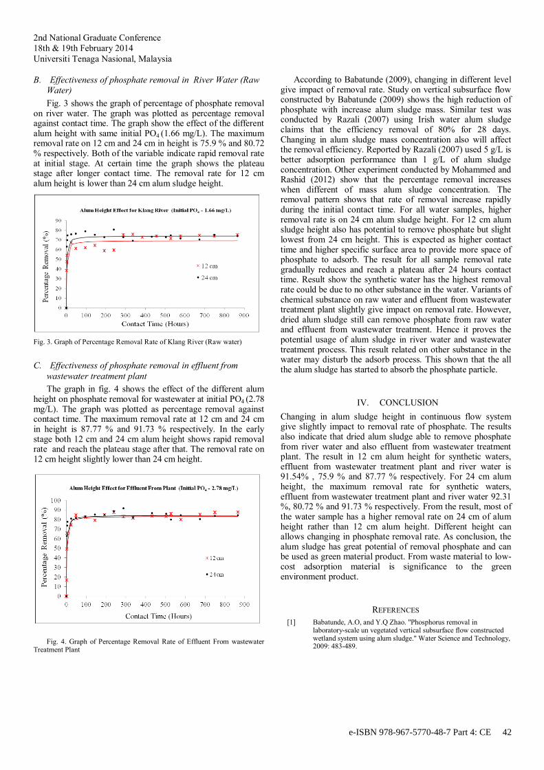
2nd National Graduate Conference
18th & 19th February 2014
Universiti Tenaga Nasional, Malaysia
B. Effectiveness of phosphate removal in River Water (Raw
Water)
Fig. 3 shows the graph of percentage of phosphate removal on river water. The graph was plotted as percentage removal against contact time. The graph show the effect of the different alum height with same initial PO4 (1.66 mg/L). The maximum removal rate on 12 cm and 24 cm in height is 75.9 % and 80.72 % respectively. Both of the variable indicate rapid removal rate at initial stage. At certain time the graph shows the plateau stage after longer contact time. The removal rate for 12 cm alum height is lower than 24 cm alum sludge height.
Fig. 3. Graph of Percentage Removal Rate of Klang River (Raw water)
C. Effectiveness of phosphate removal in effluent from
wastewater treatment plant
The graph in fig. 4 shows the effect of the different alum height on phosphate removal for wastewater at initial PO4 (2.78 mg/L). The graph was plotted as percentage removal against contact time. The maximum removal rate at 12 cm and 24 cm in height is 87.77 % and 91.73 % respectively. In the early stage both 12 cm and 24 cm alum height shows rapid removal rate and reach the plateau stage after that. The removal rate on 12 cm height slightly lower than 24 cm height.
Fig. 4. Graph of Percentage Removal Rate of Effluent From wastewater Treatment Plant
According to Babatunde (2009), changing in different level give impact of removal rate. Study on vertical subsurface flow constructed by Babatunde (2009) shows the high reduction of phosphate with increase alum sludge mass. Similar test was conducted by Razali (2007) using Irish water alum sludge claims that the efficiency removal of 80% for 28 days. Changing in alum sludge mass concentration also will affect the removal efficiency. Reported by Razali (2007) used 5 g/L is better adsorption performance than 1 g/L of alum sludge concentration. Other experiment conducted by Mohammed and Rashid (2012) show that the percentage removal increases when different of mass alum sludge concentration. The removal pattern shows that rate of removal increase rapidly during the initial contact time. For all water samples, higher removal rate is on 24 cm alum sludge height. For 12 cm alum sludge height also has potential to remove phosphate but slight lowest from 24 cm height. This is expected as higher contact time and higher specific surface area to provide more space of phosphate to adsorb. The result for all sample removal rate gradually reduces and reach a plateau after 24 hours contact time. Result show the synthetic water has the highest removal rate could be due to no other substance in the water. Variants of chemical substance on raw water and effluent from wastewater treatment plant slightly give impact on removal rate. However, dried alum sludge still can remove phosphate from raw water and effluent from wastewater treatment. Hence it proves the potential usage of alum sludge in river water and wastewater treatment process. This result related on other substance in the water may disturb the adsorb process. This shown that the all the alum sludge has started to absorb the phosphate particle.
IV. CONCLUSION
Changing in alum sludge height in continuous flow system give slightly impact to removal rate of phosphate. The results also indicate that dried alum sludge able to remove phosphate from river water and also effluent from wastewater treatment plant. The result in 12 cm alum height for synthetic waters, effluent from wastewater treatment plant and river water is 91.54% , 75.9 % and 87.77 % respectively. For 24 cm alum height, the maximum removal rate for synthetic waters, effluent from wastewater treatment plant and river water 92.31 %, 80.72 % and 91.73 % respectively. From the result, most of the water sample has a higher removal rate on 24 cm of alum height rather than 12 cm alum height. Different height can allows changing in phosphate removal rate. As conclusion, the alum sludge has great potential of removal phosphate and can be used as green material product. From waste material to low-cost adsorption material is significance to the green environment product.
REFERENCES
[1] Babatunde, A.O, and Y.Q Zhao. "Phosphorus removal in laboratory-scale un vegetated vertical subsurface flow constructed wetland system using alum sludge." Water Science and Technology, 2009: 483-489.
e-ISBN 978-967-5770-48-7 Part 4: CE 42

2nd National Graduate Conference
18th & 19th February 2014
Universiti Tenaga Nasional, Malaysia
[2] Babatunde, A.O, Y.Q Zhao, Y. Yang, and P. Kearney. "From "fills"
to filter: insight into the reuse of dewatered alum as a filter media in a constructed wetland." Journal of Residual Science & Technology, 2007: 147-152.
[3] Babatunde, A.O, Y.Q. Zhao, A.M. Burke, M.A Morris, and J.P. Hanrahan. "Characterization of aluminium-based water treatment residual for potential phosphorus removal in engineered wetlands." Envinronmental Pollution, 2009: 2830-2836.
[4] Babatunde, A.O., Y.Q. Zhao, Y. Yang, and P. Kearney. "Re-use of dewatered alumunium-coagulated water treatment residual to immobilize phosphorus : batch and column trials using a condensed phosphate." Chemical Engineering Journal, 2007: 108-115.
[5] Chu, Wei. "Lead Metal Removal By Recycle Alum Sludge." Wat. Res., 1999: 3019-3025.
[6] Jingxi, Tie, Zhao Lei, and Guo Hongcao. "Phosphorus Adsorption by Dewatered and Activated Alum Sludge." Fourth International Conference on Intelligent Computation Technology and Automation. 2011. 836-840.
[7] McGhee, Terence J. Water Supply And Sewerage International Edition 6th Edition. New York USA: McGraw Hill, Inc, 1991.
[8] Mohammed, W.T, and S.A Rashid. "Phosphorus removal from wastewater using oven-dried sludge." International Journal of Chemical, 2012: 1-11.
[9] Mortula, M.M., and G.A. Gagnon. "Alum residuals as a low technology for phosphorus removal from aquaculture processing water." Aquacultural Engineering, no. 36 (2007): 233-238.
[10] Razali, M., Y.Q. Zhao, and M. Bruen. "Effectiveness of a drinking-water treatment sludge in removing different phophorus species from aqueous solution." Separation and Purification Technology, 2007: 300-306.
[11] Rosenani, A.B., C.I Fauziah, and D.R. Kala. "Characterization of Malaysian sewage sludges and nitrogen mineralization in three soils treated with sewage sludge." Malaysia Society of Soil Science, 2008: 103-112.
[12] Water Environment Partnership in Asia (WEPA). TECHNOLOGIES : Technologies in operation : Type of wastewater. http://www.wepa-db.net/technologies/ (accessed 08 2, 2012).
[13] Yang, Y., D. Tomlinson, S. Kennedy, and Y.Q. Zhao. "Dewatered Alum Sludge: a potential adsorbent for phosphorus removal." Water Science & Technology, 2006: 207-213.
[14] Yang, Y., Y.Q Zhao, A.O. Babatunde, L. Wang, Y.X. Ren, and Y. Han. "Characteristic and mechanisms of phosphate adsorption on dewatered alum sludge." Separation and Purification Technology, 2006: 193-200.
[15] Zhao, Y.Q., A.O. Babatunde, Y.S.Hu, J.L.G Kumar, and X.H. Zhao. "Pilot field-scale demonstration of a novel alum sludge-based constructed wetland system for enhanced wastewater treatment." Process Biochemistry, 2011: 278-283.
e-ISBN 978-967-5770-48-7 Part 4: CE 43

2nd National Graduate Conference
18th & 19th February 2014
Universiti Tenaga Nasional, Malaysia
Developing Technical Criteria for
Substation Site Selection
Faten Syaira Buslima
Mohamad Syazwan Shaharudin
Muhammad Izzat Mohd Hanafiah
Rohayu Che Omar
Intan Nor Zuliana Baharuddin
Rasyikin Roslan
Center for Forensic Engineering College of Engineering, UNITEN
Kajang, Selangor, Malaysia
Zainal Ariffin Ahmad
Graduate Business School College of Graduate Studies, UNITEN
Kajang, Selangor, Malaysia
Abstract— This paper discusses the process of selecting and
measurement of technical criteria for site selection of new
substation. Documents from previous projects are reviewed using
comparative study analysis and hierarchy process based on
different group of expert suggestion. Based on the Technical
Criteria Selection Workshop, 12 technical criteria were used to
evaluate 66 proposed new substation sites around Peninsular
Malaysia. The findings suggest that the 12 technical criteria are
very relevant for assessing the proposed new substation.
Keywords— technical criteria; substation; site selection
I. INTRODUCTION
The purpose of this paper is to document the selection of criteria and measurement for selecting new substation site.
II. LITERATURE REVIEW
A. Substation and Switchyard
According to ASCE Manuals and Reports on Engineering Practice [1], substation and switchyard structures are used to support the above grade components and electrical equipment such as cable bus, rigid bus and strain bus conductors (switches, surge arresters, insulators and other equipment). A common definition for substation is an assemblage of equipment through which electrical energy in bulk passes for the purpose of switching or modifying its characteristics. Larger substations may contain control houses, transformers, interrupting and switching devices, and surge protection.
The term switchyard refers to the assemblage of the switches power circuit breakers, buses and auxiliary equipment that is used to collect power from the generators of a power plant and distribute it to the transmission line at a load point. The switchyard may include step-up or step-down power transformers.
III. METHODOLOGY
A. Technical Criteria for Substation Site Selection
During the Technical Criteria Selection Workshop on 11th
June 2012 [2], participants from different group of experts
discussed suitable criterion that can be to build a substation.
Each criterion has their features and different weighting. The
weightage for the features of each criterion according to the
range of 1 (suitable) to 5 (not suitable) and there are features
that are rejected. As shown in Table 1, 12 technical criteria
were identified to be used in substation site selection.
Table 1: Technical Criteria [2]
TC Technical Criteria
Description and Weightage
TC 1
Size of Substation Site & Buffer Zone
For site area of proposed substation, consideration must include the offset from building line, distance from lot’s boundary and voltage that will be generating. Avoid construction of substation in the middle of a lot (cadaster).
TC 2
Supply Zone Near to “supply zone” of existing substation.
TC 3
Transmission Line
Near to suggested transmission line or existing transmission line.
TC 4
Public Infrastructure
Near to public infrastructure: having access road, water supply, electric supply, sewage pipeline, tele-communication system, drainage system.
TC 5
Development Area
Avoid development area, e.g. cadaster lot, existing residential area, industrial area with pollution/ without pollution, water tank. Reject: field shooting, graveyard, school, university, college, polytechnic etc. (education), harbor/ jetty, railway station,
e-ISBN 978-967-5770-48-7 Part 4: CE 44
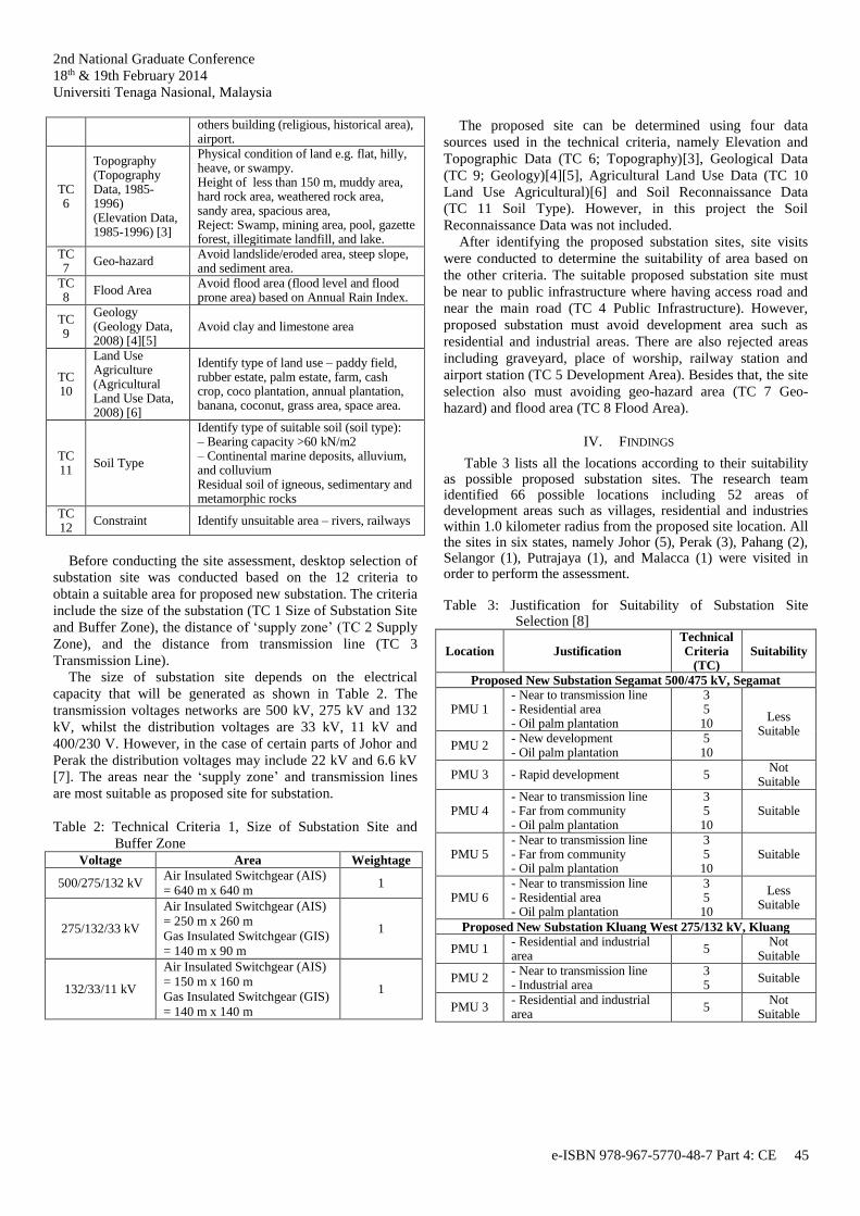
2nd National Graduate Conference
18th & 19th February 2014
Universiti Tenaga Nasional, Malaysia
others building (religious, historical area), airport.
TC 6
Topography (Topography Data, 1985-1996) (Elevation Data, 1985-1996) [3]
Physical condition of land e.g. flat, hilly, heave, or swampy. Height of less than 150 m, muddy area, hard rock area, weathered rock area, sandy area, spacious area, Reject: Swamp, mining area, pool, gazette forest, illegitimate landfill, and lake.
TC 7
Geo-hazard Avoid landslide/eroded area, steep slope, and sediment area.
TC 8
Flood Area Avoid flood area (flood level and flood prone area) based on Annual Rain Index.
TC 9
Geology (Geology Data, 2008) [4][5]
Avoid clay and limestone area
TC 10
Land Use Agriculture (Agricultural Land Use Data, 2008) [6]
Identify type of land use – paddy field, rubber estate, palm estate, farm, cash crop, coco plantation, annual plantation, banana, coconut, grass area, space area.
TC 11
Soil Type
Identify type of suitable soil (soil type): – Bearing capacity >60 kN/m2 – Continental marine deposits, alluvium, and colluvium Residual soil of igneous, sedimentary and metamorphic rocks
TC 12
Constraint Identify unsuitable area – rivers, railways
Before conducting the site assessment, desktop selection of
substation site was conducted based on the 12 criteria to
obtain a suitable area for proposed new substation. The criteria
include the size of the substation (TC 1 Size of Substation Site
and Buffer Zone), the distance of ‘supply zone’ (TC 2 Supply
Zone), and the distance from transmission line (TC 3
Transmission Line).
The size of substation site depends on the electrical
capacity that will be generated as shown in Table 2. The
transmission voltages networks are 500 kV, 275 kV and 132
kV, whilst the distribution voltages are 33 kV, 11 kV and
400/230 V. However, in the case of certain parts of Johor and
Perak the distribution voltages may include 22 kV and 6.6 kV
[7]. The areas near the ‘supply zone’ and transmission lines
are most suitable as proposed site for substation.
Table 2: Technical Criteria 1, Size of Substation Site and
Buffer Zone
Voltage Area Weightage
500/275/132 kV Air Insulated Switchgear (AIS)
= 640 m x 640 m 1
275/132/33 kV
Air Insulated Switchgear (AIS)
= 250 m x 260 m
Gas Insulated Switchgear (GIS)
= 140 m x 90 m
1
132/33/11 kV
Air Insulated Switchgear (AIS)
= 150 m x 160 m
Gas Insulated Switchgear (GIS)
= 140 m x 140 m
1
The proposed site can be determined using four data
sources used in the technical criteria, namely Elevation and
Topographic Data (TC 6; Topography)[3], Geological Data
(TC 9; Geology)[4][5], Agricultural Land Use Data (TC 10
Land Use Agricultural)[6] and Soil Reconnaissance Data
(TC 11 Soil Type). However, in this project the Soil
Reconnaissance Data was not included.
After identifying the proposed substation sites, site visits
were conducted to determine the suitability of area based on
the other criteria. The suitable proposed substation site must
be near to public infrastructure where having access road and
near the main road (TC 4 Public Infrastructure). However,
proposed substation must avoid development area such as
residential and industrial areas. There are also rejected areas
including graveyard, place of worship, railway station and
airport station (TC 5 Development Area). Besides that, the site
selection also must avoiding geo-hazard area (TC 7 Geo-
hazard) and flood area (TC 8 Flood Area).
IV. FINDINGS
Table 3 lists all the locations according to their suitability as possible proposed substation sites. The research team identified 66 possible locations including 52 areas of development areas such as villages, residential and industries within 1.0 kilometer radius from the proposed site location. All the sites in six states, namely Johor (5), Perak (3), Pahang (2), Selangor (1), Putrajaya (1), and Malacca (1) were visited in order to perform the assessment.
Table 3: Justification for Suitability of Substation Site
Selection [8]
Location Justification Technical Criteria
(TC) Suitability
Proposed New Substation Segamat 500/475 kV, Segamat
PMU 1 - Near to transmission line - Residential area - Oil palm plantation
3 5 10
Less Suitable
PMU 2 - New development - Oil palm plantation
5 10
PMU 3 - Rapid development 5 Not
Suitable
PMU 4 - Near to transmission line - Far from community - Oil palm plantation
3 5 10
Suitable
PMU 5 - Near to transmission line - Far from community - Oil palm plantation
3 5 10
Suitable
PMU 6 - Near to transmission line - Residential area - Oil palm plantation
3 5 10
Less Suitable
Proposed New Substation Kluang West 275/132 kV, Kluang
PMU 1 - Residential and industrial area
5 Not
Suitable
PMU 2 - Near to transmission line - Industrial area
3 5
Suitable
PMU 3 - Residential and industrial area
5 Not
Suitable
e-ISBN 978-967-5770-48-7 Part 4: CE 45
2nd National Graduate Conference
18th & 19th February 2014
Universiti Tenaga Nasional, Malaysia
PMU 4 - Near to transmission line - Far from community
3 5
Suitable
PMU 5 - Residential and industrial area
5 Not
Suitable
PMU 6 - Near to transmission line - Far from community
3 5
Suitable
Proposed New Substation Kulai East 275/132 kV, Kulai
PMU 1 - Near to transmission line - Far from community
3 5
Suitable
PMU 2 - Oil palm plantation - Near place of worship
10 5
Less Suitable
PMU 3 - Near to transmission line - Graveyard
3 5
Not Suitable
PMU 4 - Near to transmission line - Graveyard
3 5
Not Suitable
PMU 5 - Near to transmission line - Far from community
3 5
Suitable
PMU 6 - Residential area 5 Not
Suitable
Proposed Transition Yard Padang Mulud, Kota Tinggi
PMU 1 - Far from community - Oil palm plantation
5 10
Suitable
PMU 2 - Industrial area - Prawn farming
5 5
Not Suitable
PMU 3 - Industrial area 5 Less
Suitable
PMU 4 - Industrial area - Prawn farming
5 5
Not Suitable
PMU 5 - Far from community - Oil palm plantation
5 10
Suitable
PMU 6 - Industrial area 5 Less
Suitable
Proposed Transition Yard Tanjung Leman, Mersing
PMU 1 - Far from community - Oil palm plantation
5 10
Suitable
PMU 2 - Far from existing line - Oil palm plantation
3 10
Less Suitable
PMU 3 - Far from community - Oil palm plantation
5 10
Suitable
PMU 4 - Residential area 5 Not
Suitable
PMU 5 - Far from community - Oil palm plantation
5 10
Less Suitable
PMU 6 - Far from community - Oil palm plantation
5 10
Suitable
Proposed New Substation Terong 500 kV, Larut Matang
PMU 1 - Near to transmission line 3
Suitable PMU 2 - Near to transmission line 3
PMU 3 - Far from community - Oil palm plantation
5 10
Proposed New Substation New Seri Iskandar 275 kV, Perak Tengah
PMU 1 - Rapid development 5 Not
Suitable
PMU 2 - Existing substation 2 Not
Suitable
PMU 3 - Near to transmission line 3 Suitable
PMU 4 - New development 5 Not
Suitable
PMU 5 - Residential area 5 Less
Suitable
PMU 6 - Far from community 5 Suitable
Proposed New Substation Langkap 500 kV, Hilir Perak PMU 1 - Far from community 5
Suitable PMU 2 - Far from community 5
PMU 3 - Far from community 5
PMU 4 - Far from community 5
Proposed New Substation Merapuh 275/132 kV, Kuala Lipis
PMU 1 - No access road - Tourism area
4 5
Not Suitable
PMU 2 - Far from community 5
Suitable PMU 3 - Far from community 5
PMU 4 - Far from community 5
PMU 5 - Far from community 5
Proposed New Substation Sri Jaya 275/132 kV, Maran
PMU 1 - Far from community - Oil palm plantation
5 10
Suitable
PMU 2 - Far from community - Oil palm plantation
5 10
PMU 3 - Far from community - Oil palm plantation
5 10
PMU 4 - Far from community - Oil palm plantation
5 10
PMU 5 - Far from community - Oil palm plantation
5 10
PMU 6 - Far from community - Oil palm plantation
5 10
Proposed New Substation Hulu Langat 500 kV, Hulu Langat PMU 1 - Far from community 5 Suitable
PMU 2 - Industrial area 5 Not Suitable PMU 3 - Residential area 5
Proposed New Putrajaya South 275/132 kV, Sepang PMU 1 - Near to transmission line 3 Suitable
PMU 2 - Steep slope 7
Not Suitable
PMU 3 - Existing substation - Water treatment plant
2 4
PMU 4 - Valley 6
PMU 5 - Existing substation - Water treatment plant - Oil palm plantation
2 4 10
PMU 6 - Steep slope 7
Proposed New Chohong 275/132 kV, Jasin
PMU 1 - Near to transmission line - Far from community
3 5
Suitable PMU 2
- Near to transmission line - Far from community
3 5
PMU 3 - Far from existing line 3 Less
Suitable
Based on the site visits, majority of the 34 suitable locations satisfied two technical criteria, namely being located away from the community (TC 5 Development Area) and near the existing line (TC 3 Transmission Line Range). A few locations were located in the oil palm plantation (TC 10 Land Use Agricultural).
On the other hand, 32 locations were found to be less suitable for building proposed substation. As shown in Table 2, most did not satisfy technical criteria TC 3 and TC 5. For example, whereas the residents at PMU 2 and PMU 5 in Tanjung Leman, Mersing agreed with the proposed construction of the substation, the two locations were near
e-ISBN 978-967-5770-48-7 Part 4: CE 46

2nd National Graduate Conference
18th & 19th February 2014
Universiti Tenaga Nasional, Malaysia
FELDA community area (TC 5 Development Area) and far from existing transmission line (TC 3 Transmission Line). Also, some locations were unsuitable because near to ‘supply zone’ of existing substation (TC 2 Supply Zone), near to public infrastructure (TC 4 Public Infrastructure) such as water treatment plants and have steep slopes (TC 7 Geo-hazard).
V. CONCLUSION
Based on the survey results during the site visits, this paper
discussed the process of selecting and measurement of
technical criteria for site selection of new substation. The
findings suggest that the 12 technical criteria are very relevant
in evaluating proposed new substation sites.
ACKNOWLEDGMENT
The authors would like to thank all relevant personnel who
have contributed to the successful of this project, particularly
UNITEN R&D for U-SN-CR-13-22 consultancy research
funding, CeFE team members and TNBR for their support in
this consultancy research works.
REFERENCES
[1] ASCE Manuals and Reports on Engineering Practice No. 113. Substation Structure Design Guide, ASCE Publication, 2008.
[2] TNBR and UNITEN, Technical Criteria Selection Workshop, unpublished on 11th June 2013.
[3] Department of Survey and Mapping Malaysia, Topography and Elevation Map. 1996.
[4] Department of Mineral and Geoscience Malaysia, Geological Map. 2008.
[5] C.S. Hutchison and D.N.K. Tan. Geology of Peninsular Malaysia, University of Malaya and Geological Society of Malaysia, 2009.
[6] Department of Agricultural, Agricultural Land Use Map. 2008.
[7] TNB, Electricity Supply Application Handbook, TNB, 2007.
[8] Ahmad Z. A. (2014), Final Report for The Enhancement of Environment Sensitive Area, Safe and Intelligent Route Finder (ESASIRF) to Include Site Selection Process for the whole Peninsular Malaysia, Universiti Tenaga Nasional, Malaysia. Unpublished.
e-ISBN 978-967-5770-48-7 Part 4: CE 47
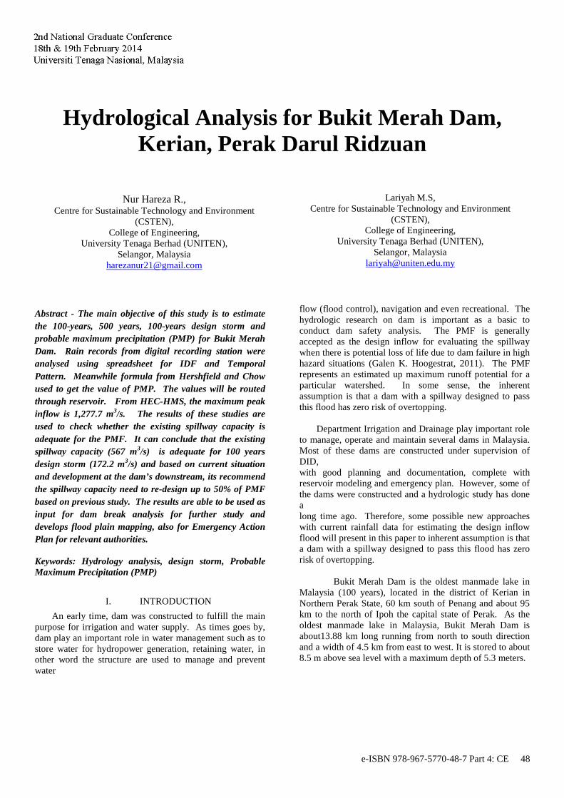
2nd National Graduate Conference, 18th and 19th February 2014, UNITEN
Hydrological Analysis for Bukit Merah Dam, Kerian, Perak Darul Ridzuan
Nur Hareza R.,
Centre for Sustainable Technology and Environment (CSTEN),
College of Engineering, University Tenaga Berhad (UNITEN),
Selangor, Malaysia [email protected]
Lariyah M.S,
Centre for Sustainable Technology and Environment (CSTEN),
College of Engineering, University Tenaga Berhad (UNITEN),
Selangor, Malaysia [email protected]
Abstract - The main objective of this study is to estimate the 100-years, 500 years, 100-years design storm and probable maximum precipitation (PMP) for Bukit Merah Dam. Rain records from digital recording station were analysed using spreadsheet for IDF and Temporal Pattern. Meanwhile formula from Hershfield and Chow used to get the value of PMP. The values will be routed through reservoir. From HEC-HMS, the maximum peak inflow is 1,277.7 m3/s. The results of these studies are used to check whether the existing spillway capacity is adequate for the PMF. It can conclude that the existing spillway capacity (567 m3/s) is adequate for 100 years design storm (172.2 m3/s) and based on current situation and development at the dam’s downstream, its recommend the spillway capacity need to re-design up to 50% of PMF based on previous study. The results are able to be used as input for dam break analysis for further study and develops flood plain mapping, also for Emergency Action Plan for relevant authorities.
Keywords: Hydrology analysis, design storm, Probable Maximum Precipitation (PMP)
I. INTRODUCTION
An early time, dam was constructed to fulfill the main purpose for irrigation and water supply. As times goes by, dam play an important role in water management such as to store water for hydropower generation, retaining water, in other word the structure are used to manage and prevent water
flow (flood control), navigation and even recreational. The hydrologic research on dam is important as a basic to conduct dam safety analysis. The PMF is generally accepted as the design inflow for evaluating the spillway when there is potential loss of life due to dam failure in high hazard situations (Galen K. Hoogestrat, 2011). The PMF represents an estimated up maximum runoff potential for a particular watershed. In some sense, the inherent assumption is that a dam with a spillway designed to pass this flood has zero risk of overtopping.
Department Irrigation and Drainage play important role
to manage, operate and maintain several dams in Malaysia. Most of these dams are constructed under supervision of DID, with good planning and documentation, complete with reservoir modeling and emergency plan. However, some of the dams were constructed and a hydrologic study has done a long time ago. Therefore, some possible new approaches with current rainfall data for estimating the design inflow flood will present in this paper to inherent assumption is that a dam with a spillway designed to pass this flood has zero risk of overtopping. Bukit Merah Dam is the oldest manmade lake in Malaysia (100 years), located in the district of Kerian in Northern Perak State, 60 km south of Penang and about 95 km to the north of Ipoh the capital state of Perak. As the oldest manmade lake in Malaysia, Bukit Merah Dam is about13.88 km long running from north to south direction and a width of 4.5 km from east to west. It is stored to about 8.5 m above sea level with a maximum depth of 5.3 meters.
e-ISBN 978-967-5770-48-7 Part 4: CE 48
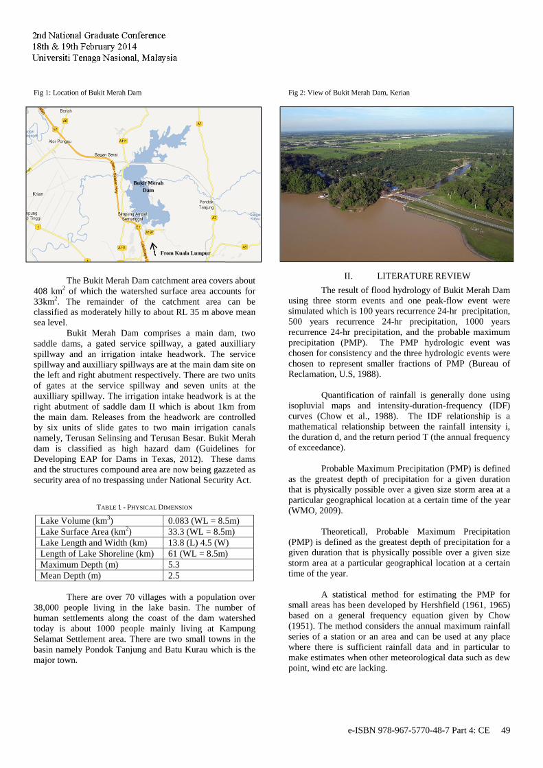
2nd National Graduate Conference, 18th and 19th February 2014, UNITEN
Fig 1: Location of Bukit Merah Dam
The Bukit Merah Dam catchment area covers about 408 km2 of which the watershed surface area accounts for 33km2. The remainder of the catchment area can be classified as moderately hilly to about RL 35 m above mean sea level. Bukit Merah Dam comprises a main dam, two saddle dams, a gated service spillway, a gated auxilliary spillway and an irrigation intake headwork. The service spillway and auxilliary spillways are at the main dam site on the left and right abutment respectively. There are two units of gates at the service spillway and seven units at the auxilliary spillway. The irrigation intake headwork is at the right abutment of saddle dam II which is about 1km from the main dam. Releases from the headwork are controlled by six units of slide gates to two main irrigation canals namely, Terusan Selinsing and Terusan Besar. Bukit Merah dam is classified as high hazard dam (Guidelines for Developing EAP for Dams in Texas, 2012). These dams and the structures compound area are now being gazzeted as security area of no trespassing under National Security Act.
TABLE 1 - PHYSICAL DIMENSION
Lake Volume (km3) 0.083 (WL = 8.5m) Lake Surface Area (km2) 33.3 (WL = 8.5m) Lake Length and Width (km) 13.8 (L) 4.5 (W) Length of Lake Shoreline (km) 61 (WL = 8.5m) Maximum Depth (m) 5.3 Mean Depth (m) 2.5
There are over 70 villages with a population over 38,000 people living in the lake basin. The number of human settlements along the coast of the dam watershed today is about 1000 people mainly living at Kampung Selamat Settlement area. There are two small towns in the basin namely Pondok Tanjung and Batu Kurau which is the major town.
Fig 2: View of Bukit Merah Dam, Kerian
II. LITERATURE REVIEW
The result of flood hydrology of Bukit Merah Dam using three storm events and one peak-flow event were simulated which is 100 years recurrence 24-hr precipitation, 500 years recurrence 24-hr precipitation, 1000 years recurrence 24-hr precipitation, and the probable maximum precipitation (PMP). The PMP hydrologic event was chosen for consistency and the three hydrologic events were chosen to represent smaller fractions of PMP (Bureau of Reclamation, U.S, 1988).
Quantification of rainfall is generally done using isopluvial maps and intensity-duration-frequency (IDF) curves (Chow et al., 1988). The IDF relationship is a mathematical relationship between the rainfall intensity i, the duration d, and the return period T (the annual frequency of exceedance).
Probable Maximum Precipitation (PMP) is defined
as the greatest depth of precipitation for a given duration that is physically possible over a given size storm area at a particular geographical location at a certain time of the year (WMO, 2009).
Theoreticall, Probable Maximum Precipitation (PMP) is defined as the greatest depth of precipitation for a given duration that is physically possible over a given size storm area at a particular geographical location at a certain time of the year.
A statistical method for estimating the PMP for small areas has been developed by Hershfield (1961, 1965) based on a general frequency equation given by Chow (1951). The method considers the annual maximum rainfall series of a station or an area and can be used at any place where there is sufficient rainfall data and in particular to make estimates when other meteorological data such as dew point, wind etc are lacking.
Bukit Merah Dam
From Kuala Lumpur
e-ISBN 978-967-5770-48-7 Part 4: CE 49

2nd National Graduate Conference, 18th and 19th February 2014, UNITEN
Chow (1951) proposed the following general equation for hydrologic frequency analysis:
Xt = Xn + K . σ n (1) Hershfield (1961, 1965) considered that for the
PMP estimation there is a value of K which will not be exceeded say Km and he used equation (1) in the form as:
Xpmp = Xn + Km . σ n (2)
Calculated the frequency factor Km for the station
by using the equation:
Km = (X1 – Xn-1) / σ n-1 (3) Where ; Xpmp is the PMP depth for a given station for a given duration. Xn and σn are respectively the mean, and standard deviation for the series of n annual maximum rainfall values of a given duration. Xn-1, σn-1 are respectively the mean and standard deviation for this series excluding the highest value X1 from the series.
Various types of computer software are available to simulate the runoff peak flow or hydrograph i.e. preadsheet, public domains software such as SWMM-5, HEC-RAS and HEC-HMS
III. METHODOLOGY
In this paper, the 100 years recurrence 24-hr precipitation, 500 years recurrence 24-hr precipitation and 1000 years recurrence 24-hr precipitation were obtained using data from digital recording station at Pusat Kesihatan Batu Kurau by using empirical equation and determining the equation parameters for the region. The available data recorded more than 30 years (1963-2012).
The objectives of the present hydrological studies are:-
i. estimation and determination 100 years recurrence 24-hr precipitation, 500 years recurrence 24-hr precipitation and 1000 years recurrence 24-hr precipitation
ii. estimation and determination the PMP iii. flow duration curve of 100 years recurrence 24-hr
precipitation, 500 years recurrence 24-hr precipitation and 1000 years recurrence 24-hr precipitation and PMF inflow
This hydrology analysis will be carried out using HEC-HMS by simulating the runoff hydrographs resulting from a design storm. It is designed to be applicable in a wide range of geographic areas for solving the widest possible range of problems. This includes large river basin water supply and flood hydrology, and small urban or natural watershed runoff. The obtained maximum values will be routed through the reservoir, and will be use to establish dam breech characteristics and routing of outflow hydrograph through the downstream valley.
IV. RESULTS AND DISCUSSION
Table 2 shows the values of 100 years recurrence 24-hr precipitation, 500 years recurrence 24-hr precipitation and 1000 years recurrence 24-hr precipitation and the PMP :-
TABLE 2: IDF’S STORM EVENT AND PMP FOR BUKIT MERAH DAM
IDF’s storm event and PMP for
Bukit Merah Dam 100-year 500-year 1000-year PMP
110 132 142 330
A hydrograph is the resulting from HEC-HMS, means a plot of discharge as a function of time, as shows in Figure 3 for 3 storm event and PMP. From the hydrograph, it shows that PMF inflow has the highest peak inflow compare to others three event which is 1,277.7 m3/s. All the spillways in the dam were design to maximum discharge 567 m3/s. The design requirement for reservoir volume at 100 acre-ft and 15.24 meter (50 ft.) high will using PMF value. Therefore, for Bukit Merah Dam with maximum depth 5.3 meter, the existing spillway capacity is adequate for 100 years design storm.
Fig 3: Inflow hydrograph for Bukit Merah Dam
0
200
400
600
800
1000
1200
1400
0 20 40 60 80 100 120Duration (hours)
Inflow Hydrograph for Bukit Merah Dam
100y Inflow
500y Inflow
1000y Inflow
PMF Inflow
Dis
cha
rge
(m
3/s
)
e-ISBN 978-967-5770-48-7 Part 4: CE 50

2nd National Graduate Conference, 18th and 19th February 2014, UNITEN
TABLE 3: ESTIMATED PEAK FLOW FOR INFLOW DESIGN FLOOD FOR
BUKIT MERAH DAM (M3/S)
Peak flow for inflow design flood for
Bukit Merah Dam (m3/s) 100-year 500-year 1000-year PMP
172.2 246.8 283.1 1,227.7
However, the PMF is required to perform risk analyses to determine the threshold flood event at downstream of Bukit Merah Dam. PMF events are recognized as practical upper limits to flood events at a given site assuming extreme precipitation conditions occur in conjunction with optimal runoff conditions. While development of the PMF does involve assumptions and uncertainties, the PMF is recognized as the industry-accepted standard used by most federal and state dam owners and regulating agencies to evaluate inflow design flood events for high and significant hazard dams.
Therefore, by defining dam-failure flood profiles downstream from the dam using the PMF, the inundation maps can be produces using dam break analysis. General international practices on dam safety would include procedures that suit practical management on the dam condition such as sending early warning and notification messages of emergency situation to the authorities, as well as information on inundation of critical areas for action case of emergency (M. Carmen Casas, 2010).
It also can be used as a reference to Department
Irrigation and Drainage that the dam should have adequate spillway capacity to pass the following floods without overtopping if the dam failure can cause loss of life, serious damage to homes, industrial or commercial buildings, important public utilities, main highways, and railroads from from dam break analysis (DEC, 1985).
V. CONCLUSION
The hydrological analyses for Bukit Merah Dam were successfully applied in this study to derive the 100 years recurrence 24-hr precipitation, 500 years recurrence 24-hr precipitation, 1000 years recurrence 24-hr precipitation and the probable maximum precipitation (PMP) to get inflow hydrographs of the events.
From the results and analysis carried out, the following
facts have been concluded:
• The existing spillway capacity (567 m3/s) is adequate for 100 years design storm as the design is back in 1906 which at that time, the dam is classified as Class "A"; dam failure will damage nothing more than isolated farm, buildings, undeveloped lands or township or country roads.
• From the hydrograph it was observed that the m a x i m u m i n f l o w i s P M P , reached its peak discharge of 1,227.7 m3/s.
• Based on current situation and development at the dam’s downstream, the dam now can be classified as Class C and its recommend the spillway capacity need to re-design up to 50% of PMF (DEC, 1985).
ACKNOWLEDGMENT The authors would like to take this opportunity to
recognize the efforts and assistance from DID Malaysia, CSTEN, UNITEN, and ZHL Engineer Sdn. Bhd. For their ideas, provision of relevant materials and data during the preparation and development, and providing valuable input to complete this research.
REFERENCES [1] Dam Safety Program, Critical Infrastructure Division, Texas
Commission on Environment Quality, “Guidelines for Developing Emergency Action Plans for Dams in Texas”, 2011.
[2] Division of Water (DEC), New York State Department of Environmental Conservation, “Guidelines for Design of Dams”, 1985.
[3] Chow, V. T., Maidment, D. R. & Mays, L. W., “Applied Hydrology”, McGraw-Hill, 1988.
[4] Galen K. Hoogestrat, “Flood Hydrology and Dam Breech Hydraulics Analyses of Four Reservoir in the Black Hills, South Dakota”, U.S Department of the Interior, U.S Geological Survey, 2011.
[5] Hershfield DM., “Estimating the probable maximum precipitation”, Proceedings American Society of Civil Engineers, Journal Hydraulics, 1961. Division 87(HY5): 99–106.
[6] M Carmen Casas, Raul Rodrıguez, Marc Prohom, Antonio Gazquez ´ and Angel Redano, “Estimation of the probable maximum precipitation in Barcelona (Spain)”, International Journal of Climatolgy, 2010.
[7] National Research Council, Safety of Dams, “Flood and Earthquake Criteria”, Committee of Safety Criteria for Dams, National Academy Press, Washington, D.C., 1985. 321p.
[8] U.S Bureau of Reclamation, “Downstream Hazard Classification Guidelines” , ACER Technical Memorandum No. 11, Engineering and Research, Denver, Colorado, 1988. 57 pp
[9] World Meteorological Organization, “Manual on Estimation of Probable Maximum Precipitation (PMP), 3rd Edition”, Geneva, 2009
e-ISBN 978-967-5770-48-7 Part 4: CE 51
2nd National Graduate Conference
18th & 19th February 2014
Universiti Tenaga Nasional, Malaysia
Development of Web Geospatial System : I-
ESASIRF System
Mohd Firdaus Bin Md Alip
Rohayu Binti Che Omar
Intan Nor Zuliana Binti Baharuddin
Rasyikin Binti Roslan
Center for Forensic Engineering
College of Engineering, UNITEN
Kajang, Selangor, Malaysia
Zainal Ariffin Ahmad
Graduate Business School
College of Graduate Studies, UNITEN
Kajang, Selangor, Malaysia
Abstract— This paper presented the system development process
for managing and visualization of the geospatial and non-
geospatial data for substation site selection name as I-ESASIRF
System. The geospatial data consist of the Geographical
Information system (GIS) data i.e. technical data for suitable site
substation development while the non-geospatial data consist
data based on social studies criteria from the Social Impact
Assessment studies. The goal of this system is to integrate the
non-restricted geospatial and non-geospatial data in one system
and can be used as a guideline for approval process from local
authority as part of development proposal report. Key features
such as viewing, querying, downloading and analysis, thematic
legend, control of transparency and others are available for the
user.
Keywords— System development, geospatial and non geospatial
data; I-ESASIRF System; GIS visualization.
I. Introduction
The recent advancement of information system with the integration of Geographical Information System (GIS) technology has given a new frontier for development of the system that can be used widely by organizations and users. It also enables organizations to manage their various geospatial and non-geospatial data within the organization and publish the non-restricted abovementioned data with their stakeholder and public. The aim of this paper is to document all the process in designing and develop the system that is user friendly and able to handle both geospatial and non-geospatial data at the client level and also at the user level. The development of I-ESASIRF System act as continuity to ensure that all the data gathered can be fully utilized by client and its stakeholder or public user. The system will fully utilized the ArcGIS Server software packages capabilities in developing this system. Various web geospatial system themes were developed such as for natural disaster, natural resources management, urban and regional planning, transportation and others. However it seems that there is no web geospatial
system currently available that used social impact assessment data and integrates it with the geospatial data to produce and execute analysis for the identification of safe and intelligent route finder for the purpose of substation site selection process. The whole process of developing this system involves the integration of multidisciplinary personnel such as geologist, civil engineers, GIS and Remote Sensing specialist, IT specialist and others.
II. Literature Review
A. System Development.
System development can be categorized into 6 main
activity which are needs assessment, design specification,
software design, develop and test, system implementation,
support operations, performance evaluation [1]. The
system development must take the consideration of its
lifecycle in order to ensure the system maintain is in good
condition because the expenses to kick start the system
development is very high [2].
B. Geospatial and non-geospatial data.
Geospatial data can be defined as geographically
referenced data where it described the locations and
characteristics of spatial features [3]. Non-geospatial data
refers to the data without inherently spatial qualities such
as attributes [4].
C. I-ESASIRF System.
As shown in figure 1, The basic idea of I-ESASIRF
System consist of several module where user can visualize
interacts with all the geospatial data that control by system
administrator using several key features such as
geovisualization, data query, reporting module and others.
e-ISBN 978-967-5770-48-7 Part 4: CE 52
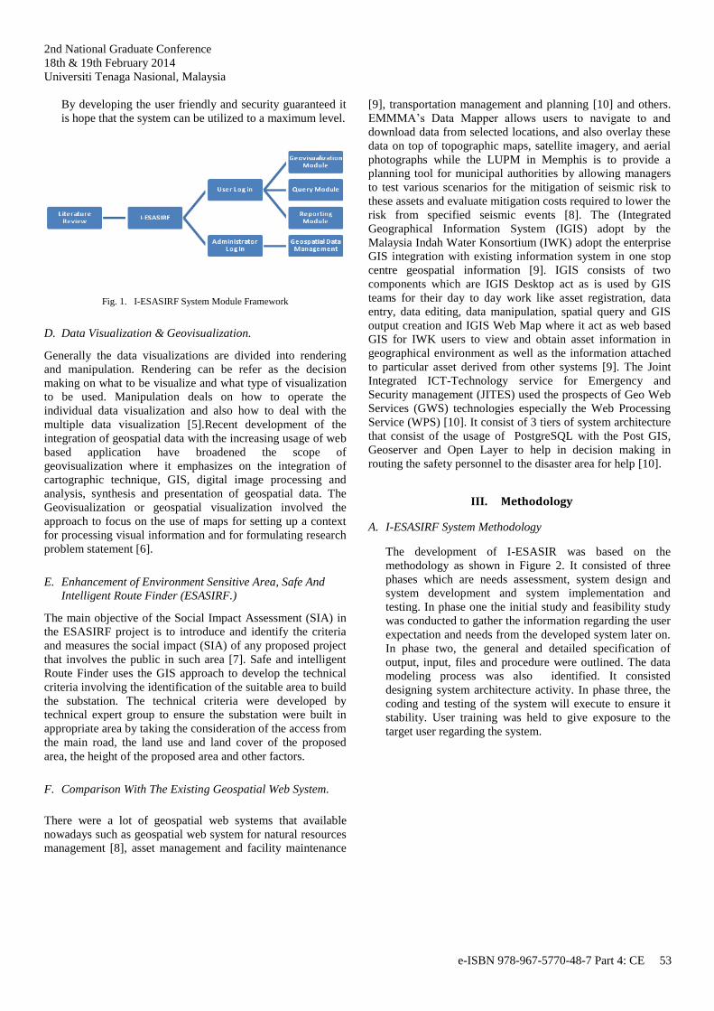
2nd National Graduate Conference
18th & 19th February 2014
Universiti Tenaga Nasional, Malaysia
By developing the user friendly and security guaranteed it
is hope that the system can be utilized to a maximum level.
Fig. 1. I-ESASIRF System Module Framework
D. Data Visualization & Geovisualization.
Generally the data visualizations are divided into rendering
and manipulation. Rendering can be refer as the decision
making on what to be visualize and what type of visualization
to be used. Manipulation deals on how to operate the
individual data visualization and also how to deal with the
multiple data visualization [5].Recent development of the
integration of geospatial data with the increasing usage of web
based application have broadened the scope of
geovisualization where it emphasizes on the integration of
cartographic technique, GIS, digital image processing and
analysis, synthesis and presentation of geospatial data. The
Geovisualization or geospatial visualization involved the
approach to focus on the use of maps for setting up a context
for processing visual information and for formulating research
problem statement [6].
E. Enhancement of Environment Sensitive Area, Safe And
Intelligent Route Finder (ESASIRF.)
The main objective of the Social Impact Assessment (SIA) in
the ESASIRF project is to introduce and identify the criteria
and measures the social impact (SIA) of any proposed project
that involves the public in such area [7]. Safe and intelligent
Route Finder uses the GIS approach to develop the technical
criteria involving the identification of the suitable area to build
the substation. The technical criteria were developed by
technical expert group to ensure the substation were built in
appropriate area by taking the consideration of the access from
the main road, the land use and land cover of the proposed
area, the height of the proposed area and other factors.
F. Comparison With The Existing Geospatial Web System.
There were a lot of geospatial web systems that available
nowadays such as geospatial web system for natural resources
management [8], asset management and facility maintenance
[9], transportation management and planning [10] and others.
EMMMA’s Data Mapper allows users to navigate to and
download data from selected locations, and also overlay these
data on top of topographic maps, satellite imagery, and aerial
photographs while the LUPM in Memphis is to provide a
planning tool for municipal authorities by allowing managers
to test various scenarios for the mitigation of seismic risk to
these assets and evaluate mitigation costs required to lower the
risk from specified seismic events [8]. The (Integrated
Geographical Information System (IGIS) adopt by the
Malaysia Indah Water Konsortium (IWK) adopt the enterprise
GIS integration with existing information system in one stop
centre geospatial information [9]. IGIS consists of two
components which are IGIS Desktop act as is used by GIS
teams for their day to day work like asset registration, data
entry, data editing, data manipulation, spatial query and GIS
output creation and IGIS Web Map where it act as web based
GIS for IWK users to view and obtain asset information in
geographical environment as well as the information attached
to particular asset derived from other systems [9]. The Joint
Integrated ICT-Technology service for Emergency and
Security management (JITES) used the prospects of Geo Web
Services (GWS) technologies especially the Web Processing
Service (WPS) [10]. It consist of 3 tiers of system architecture
that consist of the usage of PostgreSQL with the Post GIS,
Geoserver and Open Layer to help in decision making in
routing the safety personnel to the disaster area for help [10].
III. Methodology
A. I-ESASIRF System Methodology
The development of I-ESASIR was based on the
methodology as shown in Figure 2. It consisted of three
phases which are needs assessment, system design and
system development and system implementation and
testing. In phase one the initial study and feasibility study
was conducted to gather the information regarding the user
expectation and needs from the developed system later on.
In phase two, the general and detailed specification of
output, input, files and procedure were outlined. The data
modeling process was also identified. It consisted
designing system architecture activity. In phase three, the
coding and testing of the system will execute to ensure it
stability. User training was held to give exposure to the
target user regarding the system.
e-ISBN 978-967-5770-48-7 Part 4: CE 53

2nd National Graduate Conference
18th & 19th February 2014
Universiti Tenaga Nasional, Malaysia
Fig. 2. Methodology in Developing I-ESASIRF
B. I-ESASIRF System In Depth
The overall methodology of this paper consist of three
phase as outlined in Figure 2. Needs assessment consist of
initial study and feasibility study to reviewing the system
requirements in order to meets the client and user
requirement as well as performing comprehensive analysis
on the existing operational system. The system design and
system development consisted of detailed analysis on
features and operations of the proposed system in detail
including screen layouts, business rules, process diagram,
and other documentation. Besides, data modelling was also
conducted to create database using the several models
available such as hierarchical, network, relational or object
oriented data model. It also involved in producing the
overall system blueprint to enable user to decrease the
same coding to so that the efficient system can be
produced. I-ESASIRF System was developed with the
integration of GIS technology to enable the user to access
the database, perform necessary processing and generate
representative reports. System implementation and testing
act as the inspection of the overall system to ensure that all
system requirements will free from errors by executing
component and integration testing and also user acceptance
testing.
C. Format Convention
The data index table lists were developed where it act as
main framework of all the data included in the GIS
download library. Each entry in the table has the
characteristic of layer name link, layer snapshot link and
download link. The layer name link consists of the
metadata for each data layer. The snapshot link is the gif
symbol where a snapshot depicting the extent and the
complexity of the data layer. The download link describes
the path or location of the downloadable data
D. Map Projection
It is recommended that all the geospatial data, used the World Geodetic system (WGS 1984) projection as it is easy to be used and globally used.
E. Data Format
All the geospatial data must either in shapefile format (for
vector data) or images (for raster data) and the non-
geospatial data can be in pdf. The downloadable data are
provided as shapefiles or images (rasters). The shapefiles
are provided in .zip files, which can be unzipped using
the winzip utility. Image files are in jpeg, geotiff, mrsid, or
jpeg2000 format.
F. Platform
The GIS system development seems to be easy nowadays
where various geospatial consortiums such as ESRI offer
several ways for geovisualization. ESRI offers two
products which are ArcGIS Online and ArcGIS Server in
order to achieve this goal. ArcGIS Online specifically
develop for the user who have no prior experience with
web application development where it enables this type of
user to make and share the map on the web. Several
functions are available such as popup information, maps
sharing, cloud services, save, view and mark up map.
Another ESRI product is ArcGIS server where it offers
web mapping by employing API for Javascript, Flex and
Silverlight. It offers the functionality to build a web
application from scratch.
IV. FINDINGS
Based on the methodology as described in the literature
review the following findings were obtained.
A. I-ESASIRF System Proposed Design
As shown in Figure 3, the I-ESASIRF System proposed design consists of design environment and user and administrator environment. The design environment consists of software, programming language and technology used. I-ESASIRF System developed using ArcGIS Server and Adobe Flash Builder software. ActionScript and JavaScript were the programming language used in developing I-ESASIRF System. I-ESASIRF System will implement latest technology in web GIS such as ArcGIS for Flex and ArcGIS Viewer. User and administrator environment consist of map visualization, find and bookmark, analysis and query and also generating report. Administrator will focus to manage the overall system so that the user can access the web with no problem.
e-ISBN 978-967-5770-48-7 Part 4: CE 54
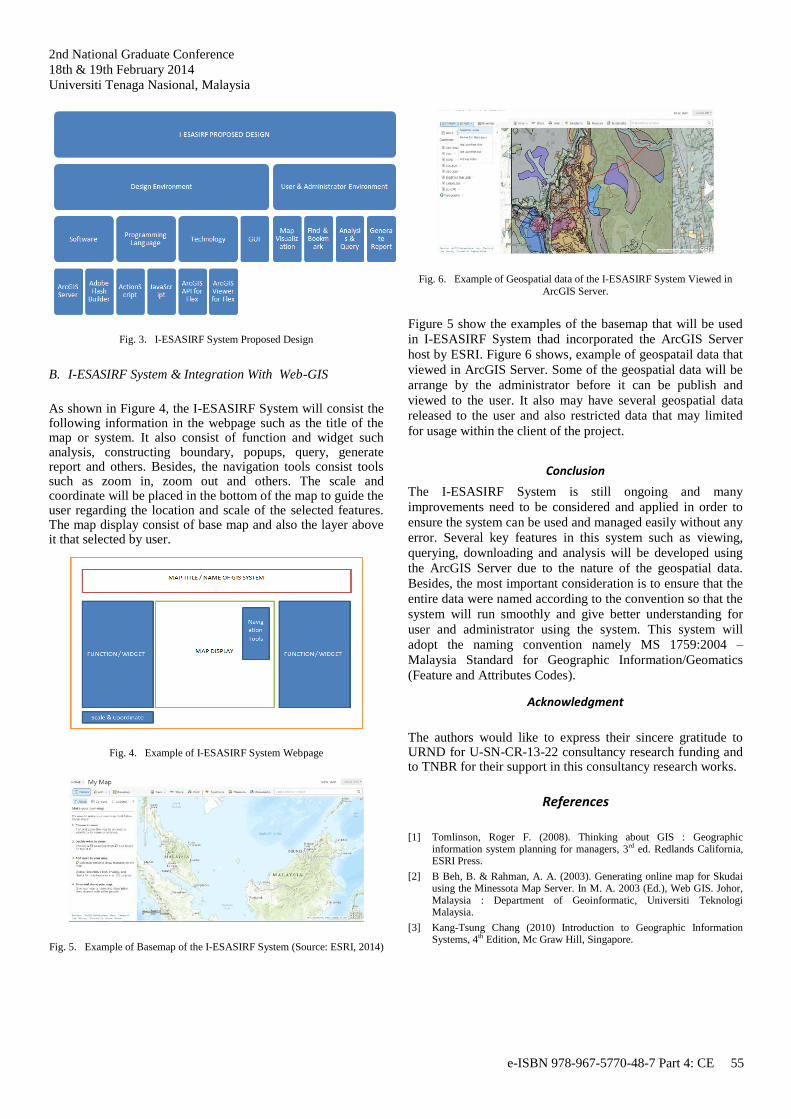
2nd National Graduate Conference
18th & 19th February 2014
Universiti Tenaga Nasional, Malaysia
Fig. 3. I-ESASIRF System Proposed Design
B. I-ESASIRF System & Integration With Web-GIS
As shown in Figure 4, the I-ESASIRF System will consist the following information in the webpage such as the title of the map or system. It also consist of function and widget such analysis, constructing boundary, popups, query, generate report and others. Besides, the navigation tools consist tools such as zoom in, zoom out and others. The scale and coordinate will be placed in the bottom of the map to guide the user regarding the location and scale of the selected features. The map display consist of base map and also the layer above it that selected by user.
Fig. 4. Example of I-ESASIRF System Webpage
Fig. 5. Example of Basemap of the I-ESASIRF System (Source: ESRI, 2014)
Fig. 6. Example of Geospatial data of the I-ESASIRF System Viewed in
ArcGIS Server.
Figure 5 show the examples of the basemap that will be used
in I-ESASIRF System thad incorporated the ArcGIS Server
host by ESRI. Figure 6 shows, example of geospatail data that
viewed in ArcGIS Server. Some of the geospatial data will be
arrange by the administrator before it can be publish and
viewed to the user. It also may have several geospatial data
released to the user and also restricted data that may limited
for usage within the client of the project.
Conclusion
The I-ESASIRF System is still ongoing and many
improvements need to be considered and applied in order to
ensure the system can be used and managed easily without any
error. Several key features in this system such as viewing,
querying, downloading and analysis will be developed using
the ArcGIS Server due to the nature of the geospatial data.
Besides, the most important consideration is to ensure that the
entire data were named according to the convention so that the
system will run smoothly and give better understanding for
user and administrator using the system. This system will
adopt the naming convention namely MS 1759:2004 –
Malaysia Standard for Geographic Information/Geomatics
(Feature and Attributes Codes).
Acknowledgment
The authors would like to express their sincere gratitude to URND for U-SN-CR-13-22 consultancy research funding and to TNBR for their support in this consultancy research works.
References
[1] Tomlinson, Roger F. (2008). Thinking about GIS : Geographic
information system planning for managers, 3rd ed. Redlands California, ESRI Press.
[2] B Beh, B. & Rahman, A. A. (2003). Generating online map for Skudai using the Minessota Map Server. In M. A. 2003 (Ed.), Web GIS. Johor, Malaysia : Department of Geoinformatic, Universiti Teknologi Malaysia.
[3] Kang-Tsung Chang (2010) Introduction to Geographic Information Systems, 4th Edition, Mc Graw Hill, Singapore.
e-ISBN 978-967-5770-48-7 Part 4: CE 55

2nd National Graduate Conference
18th & 19th February 2014
Universiti Tenaga Nasional, Malaysia
[4] Pinde F. & Jiulin S. (2011), Web GIS Principles and Applications, 1st
Edition, ESRI Press, California.
[5] Buja, A., Cook, D. & Swayne, D. F. (1996), `Interactive High Dimensional Data Visualization', Journal of Computational and Graphical Statistics.
[6] Crampton, J.: Authorization and antichains. Ph.D. thesis, Birkbeck, University of London, London, England (2002).
[7] Z. A. Ahmad , R. C. Omar, I. N. Z. Baharuddin,H. Othman, F. S. Buslima, J. Aminuddin and R. Roslan (2013). Social Impact Assessment:The Enhancement of Environment Sensitive Area (ESA) Safe and Intelligent Route Finder (ESASIRF) to Include Site Selection
Process for the Whole Peninsular Malaysia, Universiti Tenaga Nasional, Malaysia.Unpublished.
[8] Hearn, P.P., Wente, S.P., Donato, D.I., and Aguinaldo, J.J., 2006, EMMMA—A Web-based system for environmental mercury map-ping, modeling, and analysis: U.S. Geological Survey Open-File Report 2006–1086, 13 p.
[9] M. Z. Daud, Leveraging Geospatial Technology in Asset Management (2012), Malaysia Geospatial Forum, 6-7 March 2012, Malacca, Malaysia.
[10] Eszter Gálicz, Md. Imran Hossain, Wolfgang Reinhardt (2011), Geo Web Services for Transport Crisis Management in Alpine Region
e-ISBN 978-967-5770-48-7 Part 4: CE 56


