SWAT 2011 University of Castilla la ManCha toledo, spain

2011 International SWAT Conference Conference Proceedings

June 15-17, 2011

2011 International SWAT Conference - Conference Proceedings Dan Kiniry, Texas A&M University, USACourtney Smith, Texas AgriLife Research, USARaghavan Srinivasan, Texas AgriLife Research, USA

SWAT 2011

Jeff Arnold USDA-ARS, USA

Karim Abbaspour, EAWAG, SwitzerlandChehra Aboukinane, McGill University, Canada

José María Bodoque del Pozo University of Castilla La Mancha, Spain

Jeff Arnold, USDA-ARS, USA Jose Maria Bodoque Del Pozo, UCLM, Toledo, Spain

Javier de la Villa Albares University of Castilla La Mancha, Spain

Pierluigi Cau, CRS4, Italy Indrajeet Chaubey, Purdue University

Bouchra Haddad University of Castilla La Mancha, Spain

Debjani Deb, Texas A&M University, USANicola Fohrer, Christian-Albrechts-University, Germany

Francisco Olivera Texas A&M University, USA

Philip Gassman, Iowa State University, USA A.K. Gosain, Indian Institute of Technology, India

David Sanz Martínez University of Castilla La Mancha, Spain

Ann van Griensven, UNESCO-IHE, NL Fanghua HAO, Beijing Normal University, China

Raghavan Srinivasan Texas A&M University, USA

Jaehak Jeong, Texas AgriLife Research, USA Virginia Jin, USDA-ARS, USA

C. Allan Jones, Texas AgriLife Research, USA Valentina Krysanova, PIK, Germany

Taesoo Lee, Texas A&M University, USA Pedro Chambel Leitão, IST-MARETEC, Portugal Francisco Olivera, Texas A&M University, USA

Antonio Lo Porto, IRSA, IT Cole Rossi, USDA-ARS, USA

José M. Sánchez-Pérez, ECOLAB, France R. Srinivasan, Texas A&M University, USA

Pushpa Tuppad, Texas A&M University, USA Mike White, USDA-ARS, USA

Sue White, Cranfield University, UK Martin Volk, Helmholtz Centre for Env. Research, Germany

Organizing Committee Scientific Committee

SWAT 2011

Foreward

The organizers of the 2011 International SWAT Conference want to express their thanks to the organizations and individuals involved and their preparation and dedication to coordinate a successful conference. We would also like to thank the Scientific Committee for their support in preparing the conference agenda and allowing for scientists and researchers around the globe to participate and exchange their scientific knowledge at this conference. Organizations that have played a key role include:

- United States Department of Agriculture - Agricultural Research Service - Texas AgriLife Research - Texas A&M University - University of Castilla La Mancha. Campus of Fábrica de Armas

We would especially like to thank conference sponsors for making this conference possible:

- Jacobs Engineering Group Inc. - The Madrid Institute for Advanced Studies in Water Technologies IMDEA Water - The Ministry of Science and Innovation, Spain - ARNAIZ Consultores - United States Department of Agriculture - Agricultural Research Service - Texas AgriLife Research - Texas A&M University - University of Castilla La Mancha. Campus of Fábrica de Armas A special thank you to the University of Castilla La Mancha and Dr. José María Bodoque del Pozo and for his countless hours and efforts to host the SWAT Community. On behalf of the SWAT Community, we extend our sincere gratitude to you and your university for the kind invitation and welcoming hospitality.

The Conference Organizers hope you enjoy the conference and continue to view these SWAT gatherings as a positive opportunity for our international research community to share the latest innovations developed for the Soil and Water Assessment Tool.

Table of Contents 

Session A1 – Large Scale Applications SWAT Modelling at Pan European Scale: the Danube Basin Pilot Study         1‐14 Liliana Pagliero, Faycal Bouraoui, Patrick Willems, Jan Diels  Impact of the Ratio Between Subbasins and Climate Stations on the Performance of SWAT in the Rhine Basin                         15‐23 Christine Kuendig, Karim C. Abbaspour, R. Srinivasan 

  Session A3 – Best Management Practices (BMPs) Field Scale Modeling to Estimate Phosphorus and Sediment Load Reductions using a Simplified GUI for SWAT                        24‐34 A.R. Mittelstet, E.R. Daly, D.E. Storm, A.G. Tobergte, M.J. White, G.A. Kloxin  Application of BMP Design for an Inshore Alluvial Plain River System in North Jiangsu, China  35‐44 Zhou Tan, Cheng Hongguang, Zhang Xuan, Wang Bizhe   The Impact of Land Management on Drinking Water Quality: a Water Industry Application, East of England                       45‐56 Jenny Sandberg, Frances Elwell  

Session B1 – Model Development Soil Temperature Damping Depth in Boreal Plain Forest Stands and Clear Cuts: Comparison of Measured Depths versus Predicted based upon SWAT Algorithms            57‐69 G. Putz, B.M. Watson, J.A. Bélanger, E.E. Prepas  

Session B2 – Environmental Applications Challenges and Difficulties in Sediment Modeling Applied to Sedimentation Study of the Lobo Reservoir in Brazil                       70‐83 Julio Issao Kuwajima, Sílvio Crestana, Lázaro Valentin Zuquette, Frederico Fábio Mauad  Using Measurement Data on Water and Matter Fluxes in Small Homogeneous Mountainous Catchments for HRU‐Parameterization in SWAT                84‐94 Raphael Benning, Andreas Wahren, Filipa Isabel Lopez Tavares Wahren, Karl‐Heinz Feger  Cost‐Effectiveness Analysis for Controlling Water Pollution by Pesticides using SWAT and Bio‐Economical Modeling                      95‐112 J‐M Lescot, P. Bordenave, K. Petit, O. Leccia, J.M. Sanchez‐Perez, S. Sauvage, J.L. Probst  

Session B3 – Landscape Processes and Landscape/River Continuum SWAT LAI Calibration with Local LAI Measurements            113‐126 Carina Almeida, Pedro Chambel‐Leitão, Eduardo Jauch, Ramiro Neves    Session C1 – Pesticides, Bacteria, Metals & Pharmaceuticals Modeling Pesticide Fluxes during Highflow Events in an Intensive Agricultural Catchment: the Save River (Southwestern France) Case Study                127‐134 

Laurie Boithias, Sabine Sauvage, Séverine Jean, Francis Macary, Odile Leccia, Jean‐Luc Probst, Georges Merlina, Raghavan Srinivasan and José‐Miguel Sánchez‐Pérez    Session C2 – Hydrology Application of the SWAT Model to a Sprinkler‐Irrigated Watershed in the Middle Ebro River Basin of Spain Skhiri Ahmed, Dechmi Farida and Burguete Javier            135‐150                          Malfunctioning of Stream‐Gauge Stations in the Chanza and Arochete Rivers of Huelva, Spain Detected from Hydrological Modeling with SWAT                151‐161 L. Galván (1), M. Olías (1) and A. Van Griensven  Application and Validation of SWAT Model to an Alpine Catchment in the Central Spanish Pyrenees L. Palazón, A. Navas                    162‐172    Session C3 – Instream Sediment & Pollutant Transport Estimation of Transported Pollutant Load in Ardila Catchment Using the SWAT Model    173‐190 Anabela Durão, Pedro Chambel Leitão, David Brito, RM Fernandes, Ramiro Neves, Maria Manuela Morais  Soil Erosion Modelling in an Agro‐forested Catchment of NE Spain Affected by Gullying using SWAT Guevara‐Bonilla M., Martínez‐Casasnovas J.A., Ramos M.C.          191‐203    Session D1 – Biofuel & Plant Growth Mapping Sugarcane Yield for Ethanol Production in Veracruz, México        204‐215 Jesus Uresti Gil, Héctor Daniel Inurreta Aguirre, Elibeth Torres Benítez, Roberto de Jesús López Escudero  Mapping King‐Grass (Pennisetum purpureum) Biomass Yield for Cellulosic Ethanol Production in Veracruz, México                        216‐225 Jesús Uresti Gil, Roberto de Jesús López Escudero, Elibeth Torres Benítez, Héctor Daniel Inurreta Aguirre, Javier Francisco Enríquez Quiroz    Session D2 – Climate Change Applications Climate Change Impacts on Water Availability in Three Mediterranean Basins of Catalonia (NE Spain) Diana Pascual, Eduard Pla, Javier Retana, Jaume Terradas          226‐238    Session E1 – Climate Change Applications Quantifying SWAT Runoff Using Gridded Observations and Reanalysis Data for Dakbla River Basin, Vietnam Vu Minh Tue, Raghavan Srinivasan, Liong Shie‐Yui and Verwey Adri        239‐247    Session E3 – Hydrology Preliminary Results of the Hydrological Modeling of the Bouregreg Watershed of Morocco using SWAT Abdelhamid Fadil, Hassan Rhinane, Abdelhadi Kaoukaya, Youness Kharchaf      248‐256  Using MODIS Imagery to Validate the Spatial Representation of Snow Cover Extent Obtained from SWAT in a Data‐Scarce Chilean Andean Watershed              257‐268 Alejandra Stehr, Oscar Link, Mauricio Aguayo  Assessment of SWAT Potential Evapotranspiration Options and Data‐Dependence for Estimating Actual Evapotranspiration and Streamflow                269‐277 

Aouissi Jalel, Benabdallah Sihem, Lili Chabaâne Zohra, Cudennec Christophe    Session F1 – Model Development Evapotranspiration Forecast Using the SWAT Model and the Weather Forecast Model    278‐291 Pedro Chambel‐Leitão, Carina Almeida, Eduardo Jauch, Rosa Trancoso, Ramiro Neves, José Chambel Leitão    Session F2 – International SWAT Applications Review Application of the SWAT Model in Land Use Change in the Nile River Basin: A Review    292‐299 Marwa Ali, Okke Batelaan, Willy Bauwens    Session F3 – Urban Processes and Management Calibration of a Sub‐Daily SWAT Model and Validation using Different Land Use Data to Examine the Impacts of Land Use Changes                  300‐310 Roger H. Glick, P.E., Ph.D., Leila Gosselink, P.E.  Applying the Sub‐Daily SWAT Model to Assess Erosion Potential under Different Development Scenarios in the Austin, Texas Area                    311‐319 Roger H. Glick, P.E., Ph.D., Leila Gosselink, P.E.  Applying the Sub‐Daily SWAT Model to Assess Aquatic Life Potential under Different Development Scenarios in the Austin, Texas Area                320‐331 Ph.D., Leila Gosselink, P.E., Roger H. Glick, P.E.    Session G1 – Large Scale Applications Assessing Impacts of Rangeland Conservation Practices Prior to Implementation: A Simulation Case Study using APEX                      332‐352 Xiuying Wang, Carl Amonett, J. R. Williams, William E. Fox, Cheng Tu    Session G2 – Best Management Practices (BMPs) A Decision Support Tool for a Cost‐Effective Mitigation of Non‐Point Source Pollution    353‐367 Yiannis Panagopoulos, Christos Makropoulos and Maria Mimikou  SWAT‐APEX Modeling for SRI BMP Scenario Effect in an Agricultural Reservoir Watershed of South Korea C. G. Jung, H. J. Shin, J. Y. Park, H. K. Joe, J. W. Lee, S. J. Kim          368‐375    Session G3 – Sensitivity Calibration & Uncertainty Calibration and Sensitivity Analysis of SWAT for a Small Forested Catchment, North‐Central Portugal M. E. Rial‐Rivas, J. Santos, L. Bernard‐Jannin, A. K. Boulet, C. O. A. Coelho, A. J. D. Ferreira, J. P. Nunes, J. A. Rodríguez‐Suárez, M. L. Rodríguez‐Blanco, J. J. Keizer            376‐386    Poster Session Upgrading the Grid‐Based Discretization Scheme in SWAT          387‐397 Hendrik Rathjens, Natascha Oppelt  Reduction of Peak Streamflow as a Result of Vegetation Rehabilitation in the “Yesos of Barrachina” Protected Area                      398‐405 L. Jiménez, M. Morales, T. Sanz, M. T. Bellido  

  Session H1 – Sediment, Nutrients & Carbon Runoff and Soil Loss Prediction in a Vineyard Area at Very Detailed Scale using the SWAT Model: Comparison between Dry and Wet Years              406‐416 M. C. Ramos, J. A. Martínez‐Casasnovas, J. C. Balasch  Modelling Nitrogen in Streamflow from Boreal Forest Watersheds in Alberta, Canada, using SWAT Sanjeev Kumar, Brett M. Watson, Gordon Putz and Ellie E. Prepas        417‐429  Integration of a Landscape Sediment Deposition Routine into Soil and Water Assessment Tool Model N.B. Bonumá, J.G. Arnold, P.M. Allen, C.H. Green, M. Volk, J.M. Reichert        430‐437    Session H2 – Hydrology Selecting a Potential Evapotranspitration (PET) Method in the Absence of Essential Climatic Input Data  F. Kilonzo, A. Van Griensven, J. Obando, P. Lens and W. Bauwens         438‐446  Impacts of Precipitation Interpolation on Hydrologic Modeling in Data‐Scarce Regions    447‐457 Paul D. Wagner, Shamita Kumar, Florian Wilken, Peter Fiener and Karl Schneider    Session H3 – Large Scale Applications Studying the Viability of a Limno‐Reservoir Using SWAT: the Ompólveda River Basin (Guadalajara, Spain) as a Case Study                      458‐470 Eugenio Molina‐Navarro, Silvia Martínez‐Pérez, Antonio Sastre‐Merlín, Ramón Bienes‐Allas  Grid‐Based Hydrological Model Calibration and Execution by gSWAT Application      471‐482 Dorian Gorgan, Danut Mihon, Victor Bacu, Teodor Stefanut, Denisa Rodila, Lukasz Kokoszkiewicz, Elham Rouholahnejad, Karim Abbaspour, Ann van Griensven  Soil Erosion Hazard Prediction Using SWAT Model and Fuzzy Logic in a Large Highly Mountainous Watershed                      483‐491 A. Besalatpour, M. A. Hajabbasi, S. Ayoubi, M. Faramarzi, M. Amini    Session I1 – Database and GIS Application and Development Geospatial Infrastructure for Water Resources Planning and Assessment       492‐499 A. K. Gosain, Nagraj S. Patil, Chakresh Sahu, Raghavan Srinivasan, Sandya Rao, D. C. Thakur  SwatCube: An OLAP Approach for Managing Swat Model Results         500‐507 Chakresh Sahu, A.K. Gosian, S. Banerjee    Session I2 – Climate Change Applications Evaluation of Climate Change Impacts on Blue Nile Flow using SWAT        508‐525 Imtiaz Bashir, Jiri Nossent, Willy Bauwens, Okke Batelaan    Session I3 – Environmental Applications Economic Valuation and Hydrologic Analysis In View of Sustainable Watershed Management: The Case of Sigi Catchment in Tanzania                  526‐536 A.S. Hepelwa, W. Bauwens, and K. Kulindwa    Session I4 – Hydrology 

Runoff Simulation in a Glacier‐Dominated Watershed of the Rhone River Using a Semi‐Distributed Hydrological Model                    537‐545 Kazi Rahman, Emmanuel Castella, Pusterla Carol, and Anthony Lehmann 

SWAT Modelling at Pan European Scale: the Danube Basin Pilot Study

Liliana Pagliero Institute for Environment and Sustainability, Joint Research Centre, European Commission

Via E. Fermi 2749, I-21027 Ispra (VA), Italy liliana.pagliero@jrc.ec.europa.eu

Faycal Bouraoui

Institute for Environment and Sustainability, Joint Research Centre, European Commission Via E. Fermi 2749, I-21027 Ispra (VA), Italy

Patrick Willems

Dept. Civil Engineering, Hydraulics Section, Katholieke Universiteit Leuven Kasteelpark Arenberg 40, B-3001.Leuven, Belgium

Jan Diels

Dept. Earth and Environmental Sciences, Division of Soil and Water Management, Katholieke Universiteit Leuven

Celestijnenlaan 200E, B-3001 Leuven, Belgium

Abstract A harmonised pan European assessment of water resource availability and quality as affected by various management options is necessary for successful implementation of European environmental legislation. In this context we developed a methodology to predict surface water flow and nutrient loads at a pan European scale using readily available datasets. Among the hydrological models available, the Soil and Water Assessment Tool (SWAT) has been selected for its characteristics that make it suitable for large scale applications with limited data requirements. This paper presents the first hydrologic results for the Danube pilot basin. The Danube basin is one of the largest European watersheds covering 803,000 km2 and 14 countries. Modelling data used included pan European land use and management information, a detailed soil map and high resolution climate data. The Danube basin was divided into 4,663 subbasins of an average size of 179 km2. A protocol is proposed to overcome the problems of hydrological regionalization from gauged to ungauged catchments and the over-parameterization and identifiability problems present in calibration. The protocol involves cluster analysis for the determination of hydrological regions, sensitivity analysis at subbasin level and multi-objective calibration using SUFI-2 automated calibration of SWAT-CUP. The proposed protocol was successfully implemented and the modelled discharges captured well the overall hydrologic behaviour of the basin. Keywords: large-scale application, SWAT, hydrologic regionalization, sensitivity analysis

1

1. Introduction

A harmonised pan European assessment of water resource availability and quality as affected by various management options is necessary for a successful implementation of European environmental legislation. To date, the first step has been the implementation of a statistical approach referred to as the GREEN model (Geospatial Regression Equation for European Nutrient Losses) (Bouraoui et al., 2009a). GREEN computes total loads of nutrients into European seas at an annual basis. There is a need for refining these results both in time scale and in the processes involved.

Among the large collection of hydrological models available, the Soil and Water Assessment Tool (SWAT) (Arnold et al., 1998) has been selected. It has been used for assessing water quantity and quality for a wide range of spatial scales, climates and hydrological conditions worldwide. It has a modular structure where different processes (e.g. sediments, nutrients, pesticides) can be activated depending on the objectives and the availability of data. It is in the public domain, coded in Fortran, freely available on the web and allows further customization if needed. In addition, more recent versions of SWAT include a series of tools to facilitate calibration, uncertainty and sensitivity analysis which are key elements when assessing model performance. A comprehensive review of applications of SWAT with strengths and weaknesses can be found in Gassman et al. (2007). The SWAT/GIS interface (ArcSWAT) is also a key advantage, given the amount of data involved to perform the pan European scale modelling.

When implementing a model at large scale, problems inherent to hydrological modelling are exacerbated including regionalization, over-parameterization and parameter identifiability (Beven, 2006).

In this context, the aim of this research is to develop a physically-based methodology to predict surface water flow and nutrient loads at a pan European scale using readily available datasets. We chose the SWAT model to perform the hydrological and biochemical simulations. We also propose a methodology aiming at overcoming: • Regionalization of the calibrated parameter sets to ungauged areas of the model. • Over-parameterization and identifiability problems by improving calibration

transparency. For modelling purposes, Europe is divided into main regions. One of the largest and

the pilot basin for this study is the Danube river basin. Its large extension results in a variety of climates and hydrological responses that render it an interesting and challenging pilot basin. This paper presents the first results for the Danube river basin focussing the discussion on the proposed procedure to overcome the problems of large scale applications. 2. Materials and methods 2.1. Description of the study area

The Danube river basin is the second largest river basin in Europe, covering 803,000 km2 and fourteen countries (Figure 1). Due to its large extension and diverse topography (mean and maximum elevations of 463 and 3873 m.a.s.l, respectively), the Danube river basin shows an important climatic variability. The upper regions in the west show a strong influence from the Atlantic climate with high precipitation, whereas the eastern regions are affected by a continental climate with lower precipitation and typically cold winters (ICPDR, 2005). The mean annual precipitation and mean annual discharge for the period from 1980 to 2009 are 599 mm y-1 and 6387 m3 s-1, respectively.

2

Figure 1. Overview of the Danube river basin 2.2. SWAT model

SWAT is a basin scale, semi-distributed, physically based model that operates on a continuous time scale with a daily time step. Hydrology simulation in a watershed is based on the water balance equation and it is separated into two major components; the land phase, which simulates the amount of water, sediment, nutrient and pesticide loadings to the main channel in each subbasin, and the routing phase, which simulates the movement of water through the channel network of the watershed to the outlet. (Neitsch et al., 2005) 2.3. Model input

The model was set up using readily available datasets and others specifically adapted for this study. A Digital Elevation Map (DEM) at 100 × 100 m resolution was obtained from the Shuttle Radar Topography Mission (SRTM). A land use map at 1 × 1 km for the year 2000 was built from the combination of the CAPRI (Britz, 2004), SAGE (Monfreda et al., 2008), HYDE 3 (Klein and Van Drecht, 2006) and GLC2000 (Bartholome and Belward, 2005) databases. A soil map at 1 × 1 km was obtained from the Harmonized World Soil Database (HWSD) (FAO, 2008), using top soil layer data. The soil data required in this research were adapted directly from HWSD and calculated (when needed) using pedotransfer functions developed by Wösten et al. (1999) for saturated hydraulic conductivity and by Williams (1995) for the USLE equation soil erodibility factor. Watershed and stream delineation was based on the CCM2 database for continental Europe (Vogt et al., 2007). Reservoirs and lakes with an area larger than 20 km2 were included in the model using data from the Global Lakes and Wetland Database (GLWD) (Lehner and Döll, 2004) and the CCM2 database (Vogt et al., 2007).

Discharge data employed for parameter calibration were collected from different sources, including the Global Runoff Data Centre (GRDC) and the Danube River Protection Convention, resulting in 129 stations with daily data for the period 1980-2009 or subperiods. The period from 1995 to 2001 was chosen to be the calibration period, with about 100 stations with available data.

The climate data used in this study includes daily data for precipitation, temperature, solar radiation, wind speed and relative humidity from the MARS (Rijks et al., 1998) meteorological database, a gridded data set (25 × 25 km) interpolated on the basis of the European Meteorological monitoring infrastructure.

3

2.4. Modelling protocol

In this section we describe model setup and the development of the proposed procedure for addressing the problems of calibration transparency and hydrological regionalization for large scale hydrological modelling.

The model for the Danube river basin was built using the ArcSWAT interface. The setup of the model is presented in Figure 2. It corresponds to the Danube river basin as well as neighbouring small coastal basins that also drain into the Black Sea. The total area of the model is 833,908 km2 corresponding to 4,663 subbasins of an average size of 179 km2. It includes 29 lakes and reservoirs. Irrigated areas were defined by overlaying the land use map and the FAO global map of irrigated areas (Siebert et al., 2007). Elevation bands were implemented in steep subbasins. Figure 2 also presents the 129 points with discharge data available for this study.

Figure 2. SWAT model set-up of the Danube basin A problem for large scale applications of hydrological models is hydrological

regionalization from gauged to ungauged catchments. In our case (see Figure 2), there are only a limited number of gauging stations in the study area resulting in an important number of ungauged catchments.

As described in Abdulla and Lettenmaier (1997), most of the attempts at regionalization of parameters for rainfall-runoff models at ungauged catchments consist of developing regression relationships between the optimized parameters and catchment characteristics for a set of gauged catchments. Limitations of this approach, however, are that parameters may be poorly determined and strongly interrelated. Alternatives to this approach were investigated in Parajka et al. (2005), and the conclusion was reached that the similarity approach performed among the best methods of regionalization. An approach based on similarity finds a donor catchment for each unguaged catchment that is most similar in terms of its catchment attributes and transposes the complete parameter set to the ungauged catchment.

4

The similarity approach was applied in our study to define hydrological homogenous regions. These are regions with similar hydrological responses, and they are determined by catchment and flow characteristics using cluster analysis (Mazvimavi, 2003). The selection of catchment characteristics relevant for the clustering procedure was determined by employing Principal Components Analysis (PCA). PCA is a statistical tool used to reduce the dimensionality of a data set while retaining maximum information (Bouraoui et al., 2009b). PCA was performed considering catchment characteristics related to topography and soil, climate characteristics related to precipitation, temperature, flow characteristics, etc.

We employed hierarchical cluster analysis, as the number of clusters is not known a priori. Ward’s minimum variance linkage method together with Euclidean distance similarity was performed employing the “stats” package of R (R Development Core Team, 2010). To determine the number of clusters, the corrected Rand index, which measures the level of agreement in cluster membership between clusters, and the Meila’s variation information, which measures the distance between two partitions of the same dataset (Meila, 2007) were used as validity indices. They were calculated using the “fpc” package in R (Henning, 2010). The partition selected should be the one with the lowest corrected Rand index (maximizing the distance between clusters) and the highest Meila variation index (minimizing the distance within the cluster).

To overcome the problem of over-parameterization and parameter identifiability, sensitivity analysis and multi-objective calibration were used.

Sensitivity analysis was performed for each subbasin following the method developed by van Griensven et al. (2006). This method combines the Latin Hypercube Sampling (LHS) with one-factor-at-a-time (OAT) sampling making it very efficient and suitable for large scale applications. Fourteen parameters involved in the processes of baseflow, surface runoff and snow were selected for the analysis and are listed in Table 1. The assessment of the sensitive parameters is performed using water yield as model output. Table 1. Parameters for sensitivity analysis Parameter Description Process

ALPHA_BF Baseflow alpha factor [d] Baseflow CN2 SCS runoff curve number for moisture condition II Surface runoff GW_DELAY Groundwater delay [d] Baseflow GWQMN Threshold depth of water in the shallow aquifer required for return flow to

occur [mm] Baseflow

RCHRG_DP Groundwater recharge to deep aquifer [fr] Baseflow REVAPMN Threshold depth of water in the shallow aquifer for revap to occur [mm] Baseflow SFTMP Snowfall temperature [oC] Snow SMFMN Minimum melt rate for snow on Dec 21 [mm oC-1 d-1] Snow SMFMX Minimum melt rate for snow on Jun 21 [mm oC-1 d-1] Snow SMTMP Snow melt base temperature Snow SOL_AWC Available water capacity of the soil layer [fr] Surface runoff SOL_K Saturated hydraulic conductivity [mm h-1] Surface runoff SURLAG Surface runoff lag time [d] Surface runoff TIMP Snow pack temperature lag factor Snow

To improve the transparency in the calibration, a multi-objective calibration was

implemented by the separation of different catchment response outputs on three main subflows, namely, slow flow, interflow and quick flow. For this purpose the discharge data available for calibration were separated into these subflows following the filtering procedure described in Willems (2009).

Parameters were grouped into subgroups corresponding to the different processes underpinning each calibration objective. This classification was performed considering the

5

SWAT model structure (Nietsch et al., 2005). The calibration process was divided into three steps: a) calibrating the timing of the hydrographs by adjusting the snow parameters, b) calibrating of the surface runoff parameters to the quick runoff subflow, and c) calibrating the parameters that control the baseflow based on the slow runoff subflow. In this way the interflow was calibrated as well. Fourteen parameters were selected to perform the sensitivity analysis.

Because of the complexity and extent of the study area, we employed automated calibration. Sequential Uncertainty Fitting (SUFI-2) (Abbaspour, 2004) was selected. SUFI-2 combines parameter calibration and uncertainty prediction. It consists of a sequence of steps in which the initial range uncertainty in the model parameters is progressively reduced until certain criteria for prediction uncertainty are met. It uses LHS as implemented in the SWAT-CUP platform (Abbaspour, 2008).

Combining all the elements mentioned above, the proposed procedure for implementing and calibrating large scale hydrological applications can be summarized as follows: 1. Principal Component Analysis to derive the catchment characteristics most relevant for

cluster analysis of hydrological regions. 2. Defining cluster regions of the model domain using catchment, meteorological and flow

characteristics that are important in describing the variable under study, in this case river discharge.

3. Performing a sensitivity analysis at subbasin level to select significant parameters for calibration.

4. Selecting gauged catchments that are representative of every cluster and independent from the others, i.e., they can be calibrated simultaneously.

5. Performing simultaneous multi-objective calibration of the selected catchments to obtain a set of calibrated parameters representative for every cluster group.

6. Extrapolating a set of calibrated parameters to the corresponding cluster group. 3. Results and discussions 3.1. Principal components and clustering

Four principal components were extracted from the variables included in the analysis. The rotated matrix presented in Table 2 shows the relation between each variable and each component. Table 2. PCA results. Rotation method: Varimax with Kaiser Normalization

Variable Component 1 2 3 4

Average elevation 0.892 0.376 0.096 0.126 Median slope 0.826 0.408 -0.161 -0.036 Clay content -0.686 -0.393 -0.320 -0.170 Annual precipitation 0.113 0.875 0.319 0.030 Average temperature -0.926 -0.525 -0.262 -0.033 Annual potential evapotranspiration -0.574 -0.177 -0.654 0.021 Forest area -0.239 -0.119 -0.057 0.895

The Ward’s hierarchical cluster analysis with Euclidean distances was performed with the catchment descriptors listed in Table 1. Up to fifteen partitions were generated. To determine the best partition to fit the Danube data, the corrected Rand index and Maila’s variation of information are presented in Figure 3.

6

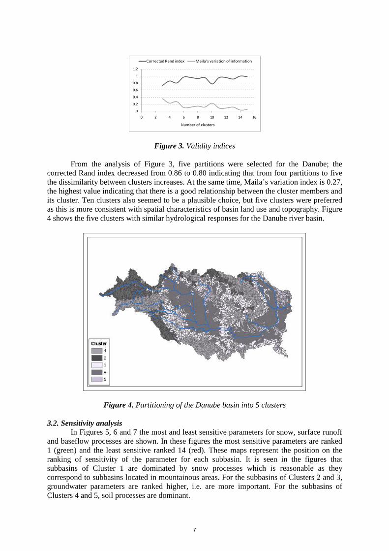
Figure 3. Validity indices

From the analysis of Figure 3, five partitions were selected for the Danube; the corrected Rand index decreased from 0.86 to 0.80 indicating that from four partitions to five the dissimilarity between clusters increases. At the same time, Maila’s variation index is 0.27, the highest value indicating that there is a good relationship between the cluster members and its cluster. Ten clusters also seemed to be a plausible choice, but five clusters were preferred as this is more consistent with spatial characteristics of basin land use and topography. Figure 4 shows the five clusters with similar hydrological responses for the Danube river basin.

Figure 4. Partitioning of the Danube basin into 5 clusters 3.2. Sensitivity analysis

In Figures 5, 6 and 7 the most and least sensitive parameters for snow, surface runoff and baseflow processes are shown. In these figures the most sensitive parameters are ranked 1 (green) and the least sensitive ranked 14 (red). These maps represent the position on the ranking of sensitivity of the parameter for each subbasin. It is seen in the figures that subbasins of Cluster 1 are dominated by snow processes which is reasonable as they correspond to subbasins located in mountainous areas. For the subbasins of Clusters 2 and 3, groundwater parameters are ranked higher, i.e. are more important. For the subbasins of Clusters 4 and 5, soil processes are dominant.

0

0.2

0.4

0.6

0.8

1

1.2

0 2 4 6 8 10 12 14 16

Number of clusters

Corrected Rand index Meila's variation of information

7

There is a clear correspondence between the sensitivity maps and the cluster results. This raises the question whether the sensitivity maps could be used instead of the PCA and clustering procedure to define the hydrological homogenous regions.

Figure 5. SFTMP (left) and TIMP (right) sensitivities for snow

Figure 6. SOL_AWC (left ) and SURLAG (right) sensitivities for surface runoff

Figure 7. GWQMN (left) and REVAPMN (right) sensitivities for baseflow 3.3. Calibration

Catchments selected for calibration fulfilled the following requirements: they have a long record of discharge data, they are head catchments thus allowing independent and

8

simultaneous calibration, and they are representative of a hydrological cluster. Following these requirements, nine gauged catchments were selected (Figure 8). There were no head catchments with available data located in Cluster 5. For this reason, and considering the limited extent of this cluster, we employed the same parameters as for Cluster 4. Altogether, the selected catchments correspond to near 20% of the basin area and cover different combinations of elevation, land use and soil type. To perform the calibration for the selected catchments, a new setup of the model including only these catchments was used (Figure 8), reducing considerably the time needed to perform automated calibration.

Figure 8. Overview of calibration catchments

Calibration was performed using a combination of SUFI-2 and a manual approach by maximising the Nash-Sutcliffe efficiency (NSE) criterion on the monthly river discharges. First the snow parameters were calibrated. As in SWAT, snow parameters are unique for the whole basin; they were calibrated for the catchment with the highest elevation. Subsequently, the subgroup of parameters corresponding to surface runoff were determined. Finally the subgroup of parameters corresponding to baseflow were determined. Results for the calibration of the selected catchments are shown in Figure 9 and Table 3. Next to the NSE, two other model performance statistics were considered: the coefficient of determination (R2) of model results versus observations of monthly river discharges, and the coefficient of regression R2 multiplied by the coefficient of the regression line (bR2).

0

100

200

300

400

500

600

Jun-94 Oct-95 Mar-97 Jul-98 Dec-99 Apr-01 Sep-02

Q [m

3/s]

Obs Sim

050

100150200250300350400

Jun-94 Oct-95 Mar-97 Jul-98 Dec-99 Apr-01 Sep-02

Q [m

3/s]

Obs Sim

9

(a) (b)

(c) (d) Figure 9. Calibration results for catchments representative of each cluster. (a) Cluster 1, (b) Cluster 2, (c) Cluster 3 and (d) Clusters 4 and 5 Table 3. Model performance evaluation for monthly flows in the catchments representative of each cluster Cluster 1 2 3 4 & 5 R2 0.77 0.73 0.64 0.23 bR2 0.75 0.72 0.51 0.17 NSE 0.70 0.70 0.61 0.14

As it is seen in Figure 9 and Table 3, results for Clusters 4 and 5 are poor. The

assessment of model performance was made using the R package hydroGOF (Zambrano, 2010).

Figure 10 shows the NSE for the Danube basin for selected calibrated and non-calibrated catchments with the original default parameters. Figure 11 shows the NSE after extrapolation of a calibrated set of parameters at each hydrological cluster. It can be seen that there is a clear improvement of NSE for ungauged catchments.

Figure 10. NSE for the gauged catchments, with no extrapolation of calibrated parameter sets within the clusters

01020304050607080

Jun-94 Oct-95 Mar-97 Jul-98 Dec-99 Apr-01 Sep-02

Q [m

3/s]

Obs Sim

050

100150200250300350400450500

Jun-94 Oct-95 Mar-97 Jul-98 Dec-99 Apr-01 Sep-02

Q [m

3/s]

Obs Sim

10

Figure 11. NSE for the gauged catchments, after extrapolation of calibrated parameter sets within the clusters

Figure 12 shows the gradual improvement of the simulated discharge at the outlet of

the Danube river basin. It started with an NSE of -0.03 for the simulation with the default parameters. After the catchments representative of the clusters were calibrated, the timing of the peaks in the simulated discharge showed a better agreement with the observed values and the NSE increased to 0.07. The runoff volume of the simulated discharge, however, became overestimated. The results of the final simulation with the calibrated parameters extrapolated to the whole basin show a better agreement both in time and in volume with respect to the observed discharge with an R2 value of 0.5 and NSE value of 0.4.

(a) (b)

(c) Figure 12. Simulation results at the outlet of the Danube river basin. (a) First run with default parameters, (b) After model calibration for the catchments representative of each cluster and (c) With calibrated parameters extrapolated

0

2000

4000

6000

8000

10000

12000

14000

Jun-94 Oct-95 Mar-97 Jul-98 Dec-99 Apr-01 Sep-02

Q [m

3/s]

Obs Sim

02000400060008000

1000012000140001600018000

Jun-94 Oct-95 Mar-97 Jul-98 Dec-99 Apr-01 Sep-02

Q [m

3/s]

Obs Sim

0

2000

4000

6000

8000

10000

12000

14000

Jun-94 Oct-95 Mar-97 Jul-98 Dec-99 Apr-01 Sep-02

Q [m

3/s]

Obs Sim

11

4. Conclusions

This paper illustrates the development of a protocol to simulate large scale hydrological systems using SWAT. The proposed protocol aims at addressing the problems of hydrological regionalization and calibration transparency and can be summarized as follows: 1. Derive catchment characteristics most relevant for cluster analysis of hydrological regions

using Principal Component Analysis. 2. Define cluster regions using catchment, meteorological and flow characteristics. 3. Perform a sensitivity analysis at subbasin level to select significant parameters for

calibration. 4. Select a number of catchments with available data representative of every cluster and

independent from each other. 5. Perform multi-objective calibration to obtain one set of calibrated parameters

representative of every cluster group. 6. Extrapolate the set of calibrated parameters in the corresponding cluster group to

ungauged subbasins. The proposed protocol was implemented and tested for the Danube river basin and

showed a promising performance. Sensitivity analysis at subbasin level was successfully implemented, as was the multi-objective calibration, which significantly improved the transparency of the calibration. The hydrological regionalization using PCA and cluster analysis and the posterior extrapolation of a calibrated set of parameters within each cluster resulted in a clear improvement in model performance at ungauged catchments.

The clear correspondence between sensitivity maps and cluster results raises the question of whether sensitivity maps could be used in combination with PCA and cluster analysis to refine the hydrological regionalization.

Finally, there are subsets of parameters, e.g. snow-related parameters, which are assumed to be uniform for the whole basin. We could therefore hypothesize that performance of the large-scale hydrological model could improve if these parameters were spatially refined at subbasin level. Acknowledgments We thank Alberto Aloe for pre-processing the GIS data needed for the SWAT implementation. References Abbaspour, K.C., Johnson, C.A. and M.Th. van Genuchten. 2004. Estimating Uncertainty and

Transport Parameters Using a Sequential Uncertainty Fitting Procedure. Vadose Zone Journal 3: 1340-1352.

Abbaspour, K.C. 2008. SWAT-CUP2: SWAT Calibration and Uncertainty Programs – A User

Manual. Department of Systems Analysis, Integrated Assessment and Modelling (SIAM), Eawag, Swiss Federal Institute of Aquatic Science and Technology, Duebendorf, Switzerland.

Abdulla, F. and D. Lettenmaier. 1997. Development of regional parameter estimation equations for a

macroscale hydrologic model. Journal of Hydrology 197: 230-257.

12

Arnold, J.G., Srinivasan, R., Muttiah, R.S. and J.R. Williams. 1998. Large area hydrologica modelling and assessment part I: model development. Journal of American Water Resources Association 34(1): 73-89.

Bartholome, E. and A.S. Belward. 2005. GLC2000: A new approach to global land cover mapping

from earth observation data. International Journal of remote Sensing. 26(9): 1959-1977.

Beven, K. 2006. A manifesto for the equifinality thesis. Journal of Hydrology 320: 1-18.

Bouraoui, F., Grizzetti, B. and A. Aloe. 2009a. Nutrient discharge from rivers to seas for year 2000. JRC Scientific and Technical Reports, EUR 24002 EN.

Bouraoui, F., Grizzetti, B., Adelskold, G., VanLiedekerke, M. and J. Zaloudik. 2009b. Basin

characteristics and nutrient losses: the EUROHARP catchment network perspective. Journal of Environmental Monitoring.11: 515-525.

Britz, W. 2004. CAPRI Modelling System Documentation. Final report of the FP5 shared cost project

CAP-STRAT “Common Agricultural Policy Strategy for Regions, Agriculture and Trade”. QLTR-2000-00394. Universitat Bonn.

FAO/IIASA/ISRIC/ISS-CAS/JRC. 2008. Harmonized World Soil Database (version 1.0). FAO,

Rome. Italy amd IIASA, Laxenburg, Austria. Gassman, P., Reyes, M.R., Green, C.H. and J.G. Arnold. 2007. The soil and water assessment tool:

Historical development, applications, and future research directions. Transactions of the ASABE 50(4): 1211-1250.

Henning, C. 2010. fpc: Flexible procedures for clustering. R package version 2.0-3. GRDC. The Global Runoff Data Centre, 56068 Koblenz, Germany. ICPDR. 2005. The Danube River Basin District. Part A – Basin-wide overview. ICPDR Document IC/084. International Commission for the Protection of the Danube River. Klein Goldewijk, K. and G. van Drecht. 2006. HYDE 3: Current and historical population and land

cover. In Integrated modelling of global environmental change. An overview of IMAGE 2.4, 93-111.

Netherlands Environmental Assessment Agency (MNP), Bilthoven, The Nederlands. Lehner, R. and P. Döll. 2004. Development and validation of a global database of lakes, reservoirs

and wetlands. Journal of Hydrology 296(1-4): 1-22. Mazvimavi, D. 2003. Estimation of flow characteristics of ungauged catchments. Case study in

Zimbabwe. Ph.D. Thesis. Wageningen University. Meila, M. 2007. Comparing clusterings - an information based distance. Journal of Multivariate

Analysis 98: 873-895. Monfreda, C., Ramankutty, N. and J. Foley. 2008. Farming the planet: 2. Geographic distribution of

crop areas, yields, physiological types, and net primary production in the year 2000. Global Biochem. Cycles, 22, GB1022.

13

Neitsch, S.L., Arnold, J.G., Kiniry, J.R. and J.R. Williams. 2005. Soil and water assessment tool. Theoretical documentation. Version 2005. Grassland, Soil and Water Research Laboratory. Agricultural Research Service – Blackland Reseacrh Center. Texas Agricultural Experiment Station.Texas.

Parajka, J., Merz, R. and G. Bloschl. 2005. A comparison of regionalisation methods for catchment

model parameters. Hydrology and Earth System Sciences 9: 157-171. R Development Core Team. 2010. R: A language and environment for statistical computing. R

Foundation for Statistical Computing, Vienna, Austria, URL http://www.R-project.org/. Rijks, D., Terres, J. and P. Vossen. 1998. Agrometeorological applications for regional crop

monitoring and production assessment. JRC Scientific and Technical Reports, EUR 17735. Siebert S., Doll, P., Feick, S., Hoogeveen, J. and K. Frenken. 2007. Global Map of Irrigated Areas

version 4.0.1. Johann Wolfgang Goethe University, Frankfurt am Main, Germany / Food and Agriculture Organization of the United Nations, Rome, Italy.

van Griensven, A., Meixner, T., Grunwald, S., Bishop, T., Diluzio, M. and R. Srinivasan. 2006. A

global sensitivity analysis tool for the parameters of multi-variable catchment models. Journal of Hydrology 324: 10-23.

Vogt, J. et al., 2007. A pan-European River and catchment Database. JRC Reference Reports, EUR

229220 EN. Willems, P. 2009. A time series tool to support the multi-criteria performance evaluation of rainfall-

runoff models. Environmental Modelling & Software 24:311-321. Wösten, J.H.M., Lilly, A., Nemes, A. and C. Le Bas. 1998. Using existing soil data to derive

hydraulic parameters for simulation models in environmental studies and in land use planning. Final Report on the European Union Funded project 1998. Report 156. DLO Winand Staring Centre, Wageningen, The Netherlands.

Zambrano, M. 2010. HydroGOF: Goodness-of-fit functions for comparison of simulated and observed

hydrological time series. R package version 0.2-1.

14

Impact of the Ratio between Subbasins and Climate Stations on the Performance of SWAT in the Rhine Basin

Christine Kuendig

Eawag, Swiss Federal Institute of Aquatic Science and Technology, 8600 Duebendorf, Switzerland, christine.kuendig@eawag.ch

Karim C. Abbaspour

Eawag, Swiss Federal Institute of Aquatic Science and Technology, 8600 Duebendorf, Switzerland, abbaspour@eawag.ch

R. Srinivasan

Spatial Sciences Laboratory, Texas A&M University, Texas Agricultural Experimental Station, College Station, Texas, USA, r-srinivasan@tamu.edu

Abstract

Climate data is perhaps the most important driving input data in watershed models. As there are often a limited number of observation stations, watershed models suffer from a chronically large uncertainty with respect to climate data. This uncertainty has profound impact on model calibration of parameters, leading to wrong parameters which cause erroneous process identification. In this paper, we used the Climate Research Unit’s (CRU’s) 0.5-degree gridded climate data to test the ratio of the number of climate stations to the number of subbasins. As SWAT only uses one climate station per subbasin, the spatial extent of subbasins may have a significant impact on model performance. The results of this study show that on the local scale, heterogeneity in precipitation may lead to a substantial difference in runoff. Further downstream this influence becomes less pronounced. We conclude that the ratio of the number of climate stations to subbasins should ideally be close to one, implying that subbasin area should be of the same magnitude as the climate station grid size. Keywords: SWAT, large scale application, Europe, hydrological modeling, climate dataset, delineation threshold

15

1. Introduction

Climate data observations are the key ingredient to successful application of a

hydrological model. The spatial and temporal resolution of precipitation data has a significant impact on simulated discharge. As the SWAT model assigns one climate station to each subbasin, not only the primary climate station distribution but also the spatial overlap of subbasins and the climate grid defines model performance.

On small-scale simulations, the number of climate stations is usually lower than the number of subbasins. However, if we increase the study scale, the area of the watersheds will increase simultaneously and at some point more than one climate station will be located in a single subbasin. As the SWAT model only makes use of one climate station inside each subbasin, this situation leads to a loss of information.

In large-scale modeling, the required time for a model run is important as calibration requires a high number of simulations. If the number of subbasins can be kept low without a loss in model performance, the calibration process will speed up.

The river basin used for this study is part of the European Continental SWAT model. To gain information about the convenient subbasin size for the Continental setup, the Rhine basin was chosen as a test case. To assess model performance regarding observed discharge values, this study uses two simulations with different mean subbasin areas. The first simulation is built using a delineation threshold of 50,000 ha, and the second simulation was assigned a threshold of 150,000 ha. The climate dataset which serves as forcing data is the CRU TS3.0 dataset of the University of East Anglia and is evenly distributed on a regular 0.5° grid.

2. Methods and Data

Data sources used in this project are free of charge and mostly available on the internet. The following datasets have been used: • A Digital Elevation Model (DEM) was constructed from the US Geological Survey's

(USGS) public domain geographic database HYDRO1k (http://edc.usgs.gov/ products/elevation/gtopo30/hydro/index.html), which is derived from their 3,000 digital elevation model of the world GTOPO30. HYDRO1k has a consistent coverage of topography at a resolution of 1 km.

• The land use map is a product of the European Environmental Agency. The CORINE Land Cover project (http://www.eea.europa.eu/data-and-maps/data/corine-land-cover-2000-raster) provides land use information for all EU countries on a resolution of 100 m. To cover the non-EU countries, the CORINE map was combined with the U.S. Geological Survey's public domain land use map with an original resolution of 1 km (http://edcsns17.cr.usgs.go/glcc/glc.html).

• The soil map was published by the Food and Agriculture Organization of the United Nations (FAO, 1995). It holds around 5,000 soil types at a spatial resolution of 10 km.

• The stream network from the Digital Chart of the World (DCW, http:// www.maproom.psu.edu/dcw) homepage was used for the project.

16

Discharge observations on a mean monthly resolution for the Rhine River and 4 tributary rivers were obtained from the Global Runoff Data Centre (GRDC).

2.1. Climate data

The climate dataset consists of daily precipitation and maximum and minimum temperature obtained from the Climate Research Unit (CRU) dataset which is available on http://badc.nerc.ac.uk. The CRU dataset has a 0.5° spatial and monthly time resolution. To acquire the daily SWAT input data, a statistical weather generator (dGEN, Schuol and Abbaspour, 2007) was applied. 2.2. Model setup

The model setup on the Rhine River catchment was carried out using the ArcSwat interface on ArcGIS (Winchell et al., 2007). To obtain two different model setups with the intended mean subbasin areas, delineation thresholds of 50,000 ha and 150,000 ha were chosen during the watershed delineation. The Rhine watershed has a total area of 163,737 km2, and the Rhine River originates in the Swiss Alps at an elevation of around 3000 m. 8.63% of the total watershed area is located at an elevation higher than 1000 m. The distribution of climate and discharge stations over the catchment can be seen in Figure 1. The six discharge stations used for this study are located on four tributary rivers, the Aare at Untersiggenthal, the Neckar at Rockenau, the Main at Kleinhuebach, the Moselle at Cochem and at two locations on the Rhine River: a very upstream station located at Diepoldsau and a very downstream station at Lobith.

Figure 1. The Rhine basin and the five sub-watersheds. Left to right: model setup with 50,000 ha watershed delineation, model setup using 150,000 ha watershed delineation, and location of discharge stations.

The coarse delineation threshold creates 73 subbasins with a mean subbasin size of 2,243 km2. With 53 stations representing precipitation and discharge, a ratio between subbasin number and climate stations of 1.38 is reached. Using the high subbasin resolution, 77 climate stations are used with a total of 170 subbasins which results in a ratio of 2.2. Ideally, the ratio between the number of subbasins and climate stations should be 1 and subbasin area should not outsize the grid size of the climate station dataset. In Table 1, the ratios between numbers of subbasins and climate stations are

17

shown. As subbasin shapes are irregular, there will always be a loss of information when transforming climate data from station information to the subbasin level. Using the high resolution, we are able to use more climate stations in total for the whole Rhine basin, but the ratio between number of subbasins and climate stations is rather high. This indicates that a high number of climate stations have been assigned to the same subbasin and a high number of subbasins are represented by a climate station considerably far away from the subbasin centroid. The ratio between number of subbasins and climate stations is between 2 and 2.3 for the high resolution model setup. For the low resolution setup, the ratio is lower, between 1 and 1.5. But there are situations where a ratio of one is reached because the subbasin area exceeds the grid size of the climate grid as in the upper Rhine watershed (see Figure 1). Table 1. Subbasin and climate stations for each basin for the high and low model setup Basin Subbasins / climate stations Ratio High Low High Low

Rhine upstream 7 / 3

1 / 1 2.33 1 Aare 18 / 9 7 / 7 2 1 Neckar 12 / 6 6 / 4 2 1.5 Main 23 / 10 10 / 7 2.3 1.4 Moselle 32 / 14 15 / 10 2.3 1.5 Rhine 173 / 77 73 / 53 2.2 1.38

For the definition of the Hydrological Response Units (HRUs), a threshold of

10% for soil, land-use and slope was chosen. In Table 2 the main land-use types inside each watershed are listed. Discharges at

the outlets of the Aare and the upstream Rhine catchment are dominated by mountainous areas; more than 40% and 80% of the catchment areas, respectively, are located higher than 1000 m. The upstream Rhine catchment is dominated by forested areas (59.53%) while the main land-use inside the Aare catchment is agriculture (57.11%). The Main, Neckar and Moselle rivers are lowland rivers with maximum elevations around 1000 m. The major land-use is agriculture (around 50% each) followed by forested areas (around 35%). The entire Rhine catchment has is dominated by land-uses of agriculture (45%) and forest (37%), and 8.6% is located at an elevation of 1000 m or higher.

Table 3 shows the initial parameter changes applied to run the two model setups. A preliminary analysis of the 6 discharge stations led to the changes from the initial parameters which are shown below. Only values that differ from the default parameters are listed. Changes were applied to the groundwater, management, soil and basin parameters. Additionally, elevation bands starting at 1000 m with a 500-m bandwidth were added with a temperature lapse rate of -6.5. Potential evapotranspiration is modeled using the empirical Hargreaves equation (Hargreaves and Samani, 1985). Table 2. Characteristics of Rhine watershed: Percentage of watershed area Land-use Rhine upstream Aare Neckar Main Moselle Rhine Agriculture 11.33 57.11 48.31 57.37 38.75 45.78 Forest 59.53 32.3 35.51 38.93 38.09 37.07 Pasture 10.07 0.2 10.77 3.68 21.33 10.69

18

Residential 5.41 1.83 4.32 Tundra / bare ground 19.08 7.78 1.24 Waterbodies / wetlands 2.81 0.78 Urban / industrial 0.12

Topography Below 1000m 17 59.33 99.63 100.00 99.74 91.37 Above 1000m 83 40.66 0.37 0 0.26 8.63 Above 1500m 65.11 21.02 0 0 0 4.98 Above 2000m 39.57 10.16 0 0 0 2.65

Table 2. Parameters changes applied to the two model setups. The identifier r__<parameter>.<extension> indicates a relative change of the initial parameter of a given value Groundwater parameters (.mgt) SHALLST : Initial depth of water in the shallow aquifer [mm] 750 DEEPST : Initial depth of water in the deep aquifer [mm] 1000 GW_DELAY : Groundwater delay [days] 5 ALPHA_BF : Baseflow alpha factor [days] 0.003 GWQMN : Threshold depth of water in the shallow aquifer required before [mm] 650 Watershed parameters (.bsn) SFTMP : Snowfall temperature [ºC] 1 SMTMP : Snow melt base temperature [ºC] 1.5 SMFMX : Melt factor for snow on June 21 [mm H2O/ºC-day] 4.5 SMFMN : Melt factor for snow on December 21 [mm H2O/ºC-day] 3 TIMP : Snow pack temperature lag factor 0.2 FFCB : Initial soil water storage expressed as a fraction of field capacity water content 0.8 ICN : Daily curve number calculation method 1 CNCOEF : Plant ET curve number coefficient 0.5 IPET: PET method 2 Soil parameters (.sol) r__SOL_K().sol : Soil hydraulic conductivity [] 0.05 r__SOL_AWC().sol : Soil available water holding capacity [mm] 0.05 Management parameters (.mgt) r__CN2.mgt -0.05 Subbasin parameters (.sub) Elevation bands with a 500m bandwidth: TLAPS starting from 1000m [C°] -6.5

19

3. Results In this section the results are discussed based on the two SWAT simulations using

different delineation thresholds. In Figure 2, mean monthly values for the six discharge locations are displayed for both simulations as well as for the observed time series.

There is no obvious pattern to detect over all six discharge locations. At the upper Rhine catchment the timing of the discharge peak is delayed by two for the coarse simulation. As the upstream Rhine catchment is a mountainous catchment, the temperature data is the determining factor for the occurrence of snowmelt. Obviously, the temperature data vary between the two simulations with a lower spring temperature using the coarse resolution. This results in a postponed runoff peak due to snowmelt in the month of July compared to the peak timing in May for the high resolution simulation. At the Neckar catchment, the overall amount of discharge is substantially larger using the high resolution. At the Main and the Moselle rivers, the differences are rather small. These features results in a small difference at the Rhine outlet in Lobith. The different subbasin resolutions may influence the discharge regime locally; in this study, however, the differences diminish more downstream.

Figure 2. Observed and simulated mean monthly discharge values for the 1973 - 1992 time period at six discharge gauges using both subbasin resolutions. From the top left corner clockwise: Rhine River at Diepoldsau, Aare River at Untersiggenthal, Neckar River at Rockenau, Main River at Kleinhuebach, Moselle River at Cochem and Rhine River at Lobith.

Table 4 shows the statistics of the six catchments, the Nash-Sutcliffe Efficiency (NS), the R2 value, the mean and standard deviation of simulated and observed discharge. Both model simulations greatly overestimate mean discharge at the upper Rhine catchment which leads to a low NS value for both simulations. The only catchment where a large change in the NS value can be observed is the Neckar catchment. The high-resolution simulation leads to an NS value of 0.40 which is about 0.6 higher than the low-resolution.

20

R2 values improve from low- to high-resolution at the upper Rhine catchment (0.14) and the Rhine basin (0.03) and decrease slightly at the other four catchments. Table 3. Model performance statistics for both simulations. Nash-Sutcliffe Efficiency [-], R2 [-], mean[m3/s] and standard deviation [m3/s] for high and low resolution runs for the six catchments. NS R2 Mean Standard dev.

Catchment high Low high Low high low obs. high low obs.

Upper Rhine

-0.62 -0.56

0.57 0.71 313.84 310.13 236.75 237.70 258.43 140.23

Aare -

0.13 -0.37 0.35 0.28 513.53 504.83 566.50 269.54 278.31 217.00

Neckar 0.40 -0.27 0.62 0.52 106.83 61.30 138.76 94.02 61.18 87.45

Main -

0.05 0.05 0.47 0.50 99.20 109.63 156.00 105.41 111.22 95.63

Moselle 0.66 0.65 0.72 0.71 313.05 294.28 343.39 283.20 273.78 266.98

Rhine 0.21 0.29 0.53 0.56

2079.41

1942.70

2285.33

1159.85

1035.24 934.19

Figure 3. Long term annual mean values at the subbasin scale: Difference between low- and high-resolution relative to the high resolution values [(low - high) / high].

21

Figure 3 shows the mean annual values of some water balance components on the

subbasin scale. The highest percentage of difference in precipitation occurs in the Neckar and upstream Rhine basins with a decrease in precipitation between 30 and 45% using the low resolution. This change in precipitation leads to a decreased amount of snowfall and snowmelt of up to 50%. A change in snowfall/snowmelt may not only be triggered by a change in precipitation amount, but also may be caused by a change in temperature and elevation of the climate station which explains why the spatial pattern of relative changes are not consistent between precipitation and snowfall/-melt. The same applies to ET: a higher amount of precipitation is expected to lead to a higher latent heat flux. However, as the model uses the empirical Hargreaves method to calculate ET, the temperature values also affect ET. Relative changes in ET are highest for alpine subbasins. Runoff at the subbasin scale is affected by up to 37% in the upstream Rhine basin and up to -70% in the Neckar basin while on the outlet of the Rhine basin in Lobith, only a difference of -0.07% can be detected.

4. Conclusions

With the variation of the delineation threshold, precipitation values are affected substantially at the local level which has implications on snow accumulation, snow melt, evapotranspiration, water yield and runoff. Model performance regarding runoff at the tributary rivers was increased to a certain degree at the Neckar river, while other tributaries neither showed a considerable increase nor decrease in Nash-Sutcliffe or R2 value. The largest differences in the mean monthly time series of the two simulations can be observed at the smallest catchments: the upper Rhine River and the Neckar River. The upper Rhine River, as the most mountainous catchment, shows a high sensitivity to temperature data which results in a shift of the snowmelt season. While the impact of the spatial extent of the subbasins is mostly visible at the local scale on the upstream basins, on the downstream outlet at the Rhine River the impacts of the various changes in climate at the local scale overlap and no significant signal can be detected.

To choose an appropriate spatial extent of subbasins for a specific study area, the following points should be considered: the grid size of the climate station grid should be in the same range as that of the mean area of the subbasins, and the number of subbasins should be low enough to keep model calibration time within a reasonable magnitude. References FAO (Food and Agricultural Organization), 1995. The digital soil map of the world and derived

soil properties. CD-ROM, Version 3.5, Rome. Hargreaves, G., Samani, Z.A., 1985. Reference crop evapotranspiration from temperature. Appl. Eng. Agric. 1, 96–99. Schuol, J., Abbaspour K.C., 2007. Using monthly weather statistics to generate daily datain a

SWAT model application to West Africa. Ecological Modelling. 201:301-311

22

Mitchell, T.D., Jones, P.D., 2005. An improved method of constructing a database of monthly climate observations and associated high-resolution grids. Int. J. Climatol. 25 (6), 693-712.

Winchell, M., Srinivasan, R., Di Luzio, M., Arnold, J.G., 2007. ArcSWAT interface for

SWAT2005 - User’s Guide. Blackland Research Center, Texas Agricultural Experiment Station and Grassland, Soil and Water Research Laboratory, USDA Agricultural Research Service, Temple, Texas.

23

Field Scale Modeling to Estimate Phosphorus and Sediment Load Reductions using a Simplified GUI for SWAT

A.R. Mittelstet1, Research Engineer and Ph.D. Student E.R. Daly2, M.S. Student

D.E. Storm3, Ph.D., Professor A.G. Tobergte4, M.S. Student M.J. White5, Ph.D., Scientist

G.A. Kloxin6, Assistant Director

Abstract Streams throughout the North Canadian River watershed in northwest Oklahoma, USA have elevated levels of nutrients and sediment. SWAT (Soil and Water Assessment Tool) was used to identify areas that likely contributed disproportionate amounts of phosphorus (P) and sediment to Lake Overholser, the receiving reservoir at the watershed outlet of the project area. These sites were then targeted by the Oklahoma Conservation Commission (OCC) to implement conservation practices such as conservation tillage, pasture planting, and riparian exclusion and buffers as part of a US Environmental Protection Agency Section 319(h) project. Practices were implemented on 238 fields. The objective of this project was to evaluate conservation practice effectiveness on these fields using TBET, a simplified user interface for SWAT developed for field-scale application. TBET was applied on each field to predict the effects of conservation practice implementation on P and sediment loads. These data were used to evaluate the cost (per kg of pollutant) associated with these reductions. Overall the implemented practices were predicted to reduce P loads to Lake Overholser by nine percent. The ‘riparian exclusion’ and ‘riparian exclusion with buffer’ practices provided the greatest reduction in P load while ‘conservation tillage’ and ‘converting wheat to Bermuda’ produced the largest reduction in sediment load. The most cost efficient practices were ‘converting wheat to Bermuda or native range’ and ‘riparian exclusion’. This project illustrates the importance of conservation practice selection and evaluation prior to implementation. This information may lead to the implementation of more cost effective practices and an improvement in the overall effectiveness of water quality programs. Keywords: SWAT, phosphorus management, hydrologic modeling, conservation practices 1 Department of Biosystems and Agricultural Engineering, Oklahoma State University, 114 Agricultural Hall, Stillwater, OK 74078-6016, aaron.mittelstet10@okstate.edu 2 Department of Biosystems and Agricultural Engineering, Oklahoma State University, 209 Agricultural Hall, Stillwater, OK 74078-6016, erin.daly@okstate.edu 3 Department of Biosystems and Agricultural Engineering, Oklahoma State University, 121Agricultural Hall, Stillwater, OK 74078-6016, dan.storm@okstate.edu 4 Department of Biosystems and Agricultural Engineering, Oklahoma State University, 209 Agricultural Hall, Stillwater, OK 74078-6016, alex.tobergte@okstate.edu 5 Grassland Soil and Water Research Laboratory, USDA-ARS, 808 East Blackland Rd. Temple, TX 76502, mike.white@ars.usda.gov 6 Oklahoma Conservation Commission, Water Quality Division, 4545 N Lincoln Blvd, Lincoln Plaza Office, Suite 11A, Oklahoma City, OK 73105, greg.kloxin@conservation.ok.gov

24

1. Introduction In agricultural watersheds, non-point sources are often the dominate contributor to water

quality impairment. Phosphorus (P) and sediment are two of the most common contributors to aquatic impairment with agricultural sources responsible for 46% of the sediment and 47% of the P released into U.S. waters (Allan, 1995; Rao et al., 2009). P is a necessary nutrient for agricultural crops, yet over application of fertilizer may lead to elevated P levels in streams, reservoirs and lakes. Several conservation practices are effective in reducing sediment and P loss from agricultural fields, including riparian buffers, conservation tillage, crop rotation, and filter strips. Knowing the efficiency of these conservation practices (i.e. Best Management Practices) in a particular setting is critical to providing policy makers the knowledge they need for future resource allocations (Tuppad et al., 2010). Published data on P and sediment reduction for various conservation practices are available, yet these data provide only a general estimate of practice efficiency as site characteristics always vary. A watershed or field scale model provides an alternative to these generalized efficiencies and may produce more accurate site-specific P and sediment reductions from conservation practice implementation.

SWAT (Soil and Water Assessment Tool) (Arnold et al., 1995) is a watershed scale model widely used to evaluate conservation programs. It was utilized by Tuppad et al. (2010) and Vache et al. (2002) to model the reduction of sediment and nutrients due to conservation practice implementation. Simulated scenarios by Tuppad et al. (2010) showed decreases from 3% to 37% for sediment load and up to a 30% decrease in P load for individual conservation practices for the Bosque River watershed in northern Texas, USA. Overall the most effective conservation practices for the Bosque River watershed in Texas were recharge structures, terraced fields and filter strips. Vache et al. (2002) examined three future land use scenarios in central Iowa, USA where two of the scenarios showed significant reductions in sediment and nutrient loads. By using a combination of conservation practices (conservation tillage, strip intercropping, rotational grazing, etc), predicted sediment loads were reduced by 37% to 67% and nutrients by 54% to 75%. Another example is the field scale water table management model ADAPT (Agricultural Drainage and Pesticide Transport) (Chung et al., 1992). Coupled with a dynamic watershed scale modeling approach (Gowda et al., 1999), ADAPT was used to simulate the reduction of sediment and P loads in the Sand Creek watershed in south-central Minnesota (Dalzell et al., 2004). By simulating the implementation of various conservation practices (conservation tillage, reduced application rates of P fertilizer, and conversion of crop land to pasture), they predicted that sediment loads could decrease by up to 24% and P loads by up to 23%.

Though several studies have evaluated the effect of conservation practice implementation on P and sediment losses from agricultural fields, few have considered the cost per unit load reduction. It is important to make this information available to policy makers to aid them in determining the largest P and sediment reduction for the least cost. Secchi et al. (2007) found that by implementing conservation practices in 13 Iowa watersheds, SWAT predicted sediment loads could be reduced from 6% to 65% and the P loads from 28% to 59% at a cost of $2.4-4.3 billion over ten years. Chang et al. (2009) evaluated the number and location of conservation practices vs. pollutant reduction. They showed that although there continued to be a reduction in pollutant load per added conservation practice, there was an optimal quantity of conservation practices where the largest pollutant reduction per cost was achieved. Gitau et al. (2004) utilized

25

SWAT to determine the optimal selection and placement of conservation practices to identify cost-effective solutions for nonpoint source reduction.

The objective of this project was to estimate the reduction in P and sediment loads from 238 fields in the North Canadian Watershed in northwestern Oklahoma resulting from the implementation of conservation practices using TBET, a simplified GUI for SWAT. Costs for conservation practice implementation for both the federal government and the rancher and farmer per ton of sediment and kg of P reduction were also calculated and their efficiency evaluated. 2. Materials and Methods 2.1. North Canadian watershed

The Canton-Overholser corridor of the North Canadian watershed (Figure 1), which includes parts of Blaine, Canadian, and Dewey Counties, located in northwest Oklahoma, USA, occupies a drainage area of approximately 1,970 km2. Streams throughout this wheat and cattle producing area are impaired due to excess nutrients, suspended solids, and siltation. Storm et al.

(2007) used SWAT to identify the non-urban areas that contributed disproportionate nutrient loads (Figure 1). Cropland (small grain and row crops), bare soil, and urban development were the primary sources of nutrient and sediment loads, with 60% of the total nutrient load contributed from only 20% of the total watershed area. They simulated several conservation practice implementation scenarios to determine potential P load reductions at the watershed outlet. If all fields with small grains and row crops implemented conservation tillage and farming on the contour, P loads were predicted to be reduced by 22%. By converting all small grains and row crops to pasture or all grazing pastures to hay, P loads were predicted to be reduced by 15% and 12%, respectively. The greatest single P load reduction (22%) resulted from adding a 10 m buffer strip to all agricultural lands bordering the Northern Canadian River. 2.2. Conservation practices

The Oklahoma Conservation Commission (OCC) applied finite funding

from the US Environmental Protection Agency 319(h) Program to cost share the implementation of conservation practices at 238 field sites within the watershed project area to reduce P and sediment loads (Figure 2). Although OCC prioritized implementation target areas of elevated P (per Storm et al., 2007), implementation efforts were ultimately constrained by landowner participation. The targeted area made up a total of 54 km2 and the 238 field sites occupied a total

Figure 1. The North Canadian River Watershed Project area in northwest Oklahoma, USA with Canton Lake in the north draining to Lake Overholser in the south connected by the North Canadian River. Areas in red indicate identified areas of elevated sources of total phosphorus load to the river.

26

of 65 km2, with field sizes ranging from 0.01 to 1.2 km2 (1.2-120 ha). The targeted areas and field sites with conservation practices mutually occurred on 44 of the 238 field sites with an area of 14 km2. Six types of conservation practices were implemented within the watershed with annual costs provided in Table 1. The fraction of the total cost subsidized by the cost share

program differed by practice. For some practices, such as conservation tillage, 100% of the cost was paid by the federal government. For other costs, such as the installation of fence and the establishment of Bermuda grass, the cost was shared between the government (80%) and the farmer or rancher (20%). Some practices required single implementation (conservation tillage), while others required multiple installations such as animal exclusion (fence, watering facility, pipeline, and pump). The practical life of the conservation practices

were also taken into account. For example, based on the US Department of Agriculture Natural Resources Conservation Service (NRCS) Field Office Technical Guide (FOTG), native rangeland implementation had a practical life of 10 years compared to 20 years for a watering facility (USDA-NRCS, 2011). 2.3. Phosphorus and sediment load modeling

Due to its ease of use and applicability at the field scale, TBET (Dr. M.J. White, personal communication, 2010) was selected to estimate the average annual P and sediment loss from the 238 field sites. TBET is a software tool which predicts P and sediment in runoff from agricultural fields in Oklahoma, Texas, and surrounding states. It is an updated and expanded form of PPM Plus (White, 2007; White et al., 2009, 2010). Using a region-specific 15-yr weather period, TBET predicts the average annual P and sediment transport rates delivered to the nearest stream from a single agricultural field. TBET was extensively validated using 283 field years of field scale data from several sites across the southern United States (White, 2007; White et al., 2010). The sites varied based on cropping system, location, nutrient application, size, soil type, and Soil Test Phosphorus (STP) levels.

TBET is based on the Soil and Water Assessment Tool (SWAT) (Arnold et al., 1998), a product of more than 30 years of model development by the U.S. Department of Agriculture, Agricultural Research Service. While models like SWAT are a valuable tool for highly trained specialists, their complexity becomes prohibitive for use by most conservation and nutrient management planners. TBET was designed to simplify the operation of SWAT in order to put the predictive power of a proven water quality model into the hands of people who make daily decisions that affect water quality. Required data for TBET simulations include crop system and management practices, soil type, field area, distance to stream, and STP. A myriad of

Figure 2. The North Canadian River Watershed Project area in northwest Oklahoma, USA showing the 238 field sites where the conservation practices were implemented based on distance to a waterbody and slope

27

management options can be simulated by accounting for detailed field characteristics and land management. Table 1. Conservation practices implemented in the North Canadian River Watershed Project, their costs to the federal government and the ranchers and farmers, their practical life expectancy, and total cost per year in 2011 USA Dollars Conservation practice

Number of fields

Total area (ha)

Cost to federal government

Cost to farmer or rancher

Practical life (yrs)

Total cost per year

Conservation tillage 205 6040 $48.70/ha $0.00 1 $48.70/ha Wheat to Bermuda 23 305 $190.69/ha $47.67/ha 10 $23.84/ha

Wheat to native range

2 37 $55.62/ha $13.91/ha 10 $6.95/ha

Riparian exclusion 2

13

$3.99/ linear m fence $3.99/linear m pipe

Watering facility-$139.10 Solar water pump-$3.93

$1.00 /linear m fence $1.00/linear m pipe

Watering facility-$34.77 Solar water pump-$0.98

20 20 10 15

$0.25/m $0.25/m $17.38 $0.33

Riparian exclusion with conservation

tillage

2

45

$3.99/ linear m fence $3.99/linear m pipe

Watering facility-$139.10 Solar water pump-$3.93

$48.70 ha-1

$1.00/linear m fence

$1.00/linear m pipe Watering facility-$34.77 Solar water pump-$0.98

$0.00

20 20 10 15 1

$0.25/m $0.25/m $17.38 $0.33

$48.70/ha Riparian exclusion

with buffer

4 33 $3.99 linear m fence $3.99/linear m pipe

Watering facility-$139.10 Solar water pump-$3.93

$223.20 ha-1

$1.00/linear m fence

$1.00/linear m pipe Watering facility-$34.77 Solar water pump-$0.98

$0.00

20 20 10 15 15

$0.25/m $0.25/m $17.38 $0.33

$14.88/ha

Each field site was modeled pre and post conservation practice implementation. For wheat fields with conservation tillage, pre conservation practice conditions were simulated with conventional tillage and post conservation practice with conservation tillage with 70% crop residue. Other wheat fields were converted to Bermuda or native grasses as a conservation practice. Due to cattle prices, precipitation, and other factors, anywhere from 30-70% of the fields may be grazed in any one year; therefore all fields were simulated as both grazed and ungrazed and the average used for all statistics. Grazing was assumed to be continuous for a 90 day period at various densities (Table 2). The sites which bordered streams had fences installed to prevent animal entry and establish/reestablish riparian vegetation for filtering and stabilizing benefits. This conservation practice was implemented individually or coupled with conservation tillage or a buffer. These field sites were only modeled as grazed. Table 2. Crop management data for TBET simulations with crop system, fertilization and grazing management data, and field Mehlich III Soil Test Phosphorus levels

Crop system Fertilizer rates and time of application

Grazing management

(animal unit/ha)

Soil test phosphorus

(ppm) Winter Wheat

Bermuda Grass Native range

34 kg N, 2.7 kg P (Pre-plant) 136 kg N, 34 kg P (Spring)

None

0.82 1.85 0.62

39-41 40

26-30 2.4. Data acquisition

The OCC provided the locations and areas of the field sites. In TBET up to three soil types and their percentages can be selected for each field site. SSURGO data (USDA-NRCS, 2007) were chosen due to its high resolution. Slopes from 0.01-12.7% with an average of 2.2%

28

were calculated in ArcGIS using 10-m National Elevation Dataset (NED) (USGS, 1999). National Agricultural Statistics Service (30-m resolution) (USDA-NASS, 2009) was used to obtain the current crop system for each field site of which the majority was wheat fields, but also included pasture and rangeland. Crop management data were obtained from the OCC, Oklahoma State Cooperative Extension papers (PSS-2263 and NREM-2869), and from Hossain et al. (2004) (Table 2). STP levels were based on a previous survey from Storm et al. (2007).

3. Results and Discussion

The average annual reduction from the 238 field sites due to the implementation of the conservation practices was 4,200 kg of P per year (0.65 kg ha-1yr-1) and 3,000 t of sediment per year (0.47 tons ha-1yr-1). This corresponded to a nine percent average annual reduction in P load to Lake Overholser based on loads estimated by Storm et al. (2007). The vast majority of these reductions were from the ‘conservation tillage’ and ‘wheat to Bermuda’ practices due to the large number of fields where these practices were implemented; however the largest reductions in P and sediment per unit area were achieved with the ‘riparian exclusion with buffer’ (i.e. cattle exclusion) practice and the ‘wheat to Bermuda’ practices, respectively (Figure 3). Although

‘riparian exclusion’ greatly reduced P loads to the stream, it did little for the sediment load reductions (neglecting streambank erosion). On the other hand, ‘conservation tillage’ and ‘converting wheat to Bermuda’ significantly reduced both P and sediment loads. Based on a Mann-Whitney ranked sum test, the median P reduction for the conservation practice ‘converting wheat to Bermuda’ was not significantly greater than the median P reduction due to ‘conservation tillage’ at a p-value of 0.05 (0.62 and 0.47 kg ha-1); however it had a significantly greater reduction (p-value of 0.044) in sediment (0.41 and 0.29 t ha-1). Statistical analysis was not performed on the other conservation practices due to their small sampling size.

The Mann-Whitney rank sum test was also utilized to analyze the effect of field slope and distance to a waterbody on P and sediment loads. Fields with a slope greater than 2% (112 fields) had a median P load

reduction of 0.95 kg ha-1 and the load reductions were significantly greater than fields with a slope less than 2% (126 fields) with a reduction of 0.29 kg ha-1. The results were similar for

Figure 2. Unit area Phosphorus and sediment load reduction per year summary for each conservation practice for the 238 fields sites based on TBET simulations (Rip = Riparian; Exe = Exclusion; Cons = Conservation; w = with; Exclusion = cattle exclusion)

29

sediment loads with a reduction of 0.76 t ha-1 for the fields with a greater than a 2% slope and 0.19 t ha-1 for the fields with less than a 2% slope. There were 99 fields within a distance of 200 m of a waterbody (based on 1:24,000 USGS blue line streams) that contributed median P and sediment load reductions of 0.76 kg ha-1 and 0.41 t ha-1, respectively. These were significantly greater than the fields with distances greater than 200 m from a waterbody where the median P and sediment loads were reduced by 0.41 kg ha-1 and 0.25 t ha-1, respectfully. Each had a p-value less than 0.005.

Forty of the field sites where conservation practices were implemented were identified as targeted areas by Storm et al. (2007). The median P reduction from these 44 field sites was 1.13 kg ha-1 compared to 0.41 kg ha-1 for the non-targeted field sites. The median sediment loads were also significantly greater with a 0.88 t ha-1 reduction for the targeted areas and 0.24 t ha -1 for the remaining sites. Fifty field sites had both a slope greater than 2% and were within 200 m of a waterbody. Of the 50 sites, 42% were also targeted areas. These sites had median P and sediment reductions of 1.38 kg ha-1 and 1.08 t ha-1, respectfully (Figure 4).

Figure 4. Average annual unit area total phosphorus and sediment load reductions from targeted areas, field sites with slopes greater than 2%, and fields within 200 m of a waterbody. When selecting which conservation practice(s) to implement, the total cost of P and sediment load reduction per kg or t and the practical life of the practice must be taken into account (Figures 5 and 6). For example, the cost per ha for ‘conservation tillage’ was $48.70 with a life expectancy of one year whereas the cost of ‘converting wheat to Bermuda’ costs $238.36 over ten years or only $23.84 per year. ‘Converting wheat to Bermuda’ cost $52.21 per ton of sediment reduction and $38.72 per kg of P. These were both significantly less than the load

0

0.5

1

1.5

Targeted Areas Slope >2% Within 200 m of Waterbody

Slope >2% and within 200 m of Waterbody

Phos

phor

us (k

g) a

nd S

edim

ent (

t) Re

duct

ion

per H

a pe

r Ye

ar

Method of Selecting Fields with ElevatedPhosphorus and Sediment Levels

Phosphorus Sediment

30

reductions for ‘conservation tillage’ with a P reduction of $103.28 per kg and $166.60 per t of sediment. Statistics were not utilized with the remaining practices due to their small sample sizes. The most cost efficient practice for P reduction was ‘converting wheat to native range’ and ‘riparian exclusion’. For sediment reduction, ‘converting wheat to either Bermuda or to native range’ were the most efficient. Although buffers were predicted to be effective at reducing P and sediment, the small field sites and total pollutant reductions were small compared to the large size and cost of the buffers.

Finally, when deciding which conservation practice(s) to promote to the farmers and ranchers, it is important to consider the costs to both the landowner and the federal government. Typically farmers and ranchers are more willing to implement conservation practices that pay for themselves with increased crop yields or decreased inputs, are easy to install and maintain, and do not alter their management requirements. However, each conservation practice considered in this project requires some change in management. Thus, the cost share rate must provide the incentive to implement the practice, or the practice must provide a reasonable cost savings or increased revenue. For example, to convert from conventional to conservation tillage, the additional capital investment requirement to purchase additional equipment and the added pesticide costs may be offset by reduced fertilizer and fuel costs, and improved soil quality resulting in increased crop yields. Based on the results from this project, the most efficient

Figure 5. Conservation practice implementation cost for both the federal government and the farmer or rancher for total phosphorus load reduction in 2011 USA dollars reduction of P to both the farmer and the federal government was ‘converting wheat to native range’ and ‘riparian exclusion’, and for sediment reduction the most cost effective conservation

$148.67

$40.96$21.88 $22.17

$135.62

$218.17

$0.00

$10.24$5.47 $5.55

$6.21

$39.46

$0

$100

$200

$300

Conservation Tillage

Wheat to Bermuda Wheat to Native Range

Riparian Exclusion Riparian Exclusion with Conservation

Tillage

Riparian Exclusion with Conservation

Buffer

Cos

t per

kg

of P

hosp

horu

s R

educ

tion

per y

r

Conservation Practice

Federal Farmer or Rancher

31

practices was ‘converting wheat to either Bermuda or native range’. However, the potential reduction in economic returns from native range or Bermuda compared to wheat production should also be considered. In addition, the increased management requirements for riparian exclusion may also be a factor for some farmers and ranchers.

Figure 6. Conservation practice implementation cost for both the federal government and the farmer or rancher for sediment load reduction in 2011 USA dollars 4. Conclusions

Agricultural fields contribute a large percentage of P and sediment to our nation’s waterways each year. Implementing conservation practices can aid in reducing these pollutant loads and thereby have the potential to increase the water quality in the receiving streams, rivers, reservoirs and lakes. This study modeled P and sediment loads from 238 field sites before and after the implementation of conservation practices. The total load reduction, load reduction per ha, and the efficiency of each conservation practice were analyzed using TBET. The average annual reduction from the 238 field sites due to the implementation of the conservation practices was 4,200 kg of P per year (0.65 kg ha-1yr-1) and 3,000 t of sediment per year (0.47 tons ha-1yr-

1). This corresponded to a nine percent annual reduction in P load to Lake Overholser based on loads estimated by Storm et al. (2007). Results from these model simulations demonstrated that the conservation practice ‘riparian exclusion’ had the largest P reduction and was the most cost efficient; however this practice was only implemented on two of the 238 field sites. One of the most implemented practices, ‘converting wheat to bermuda’, was not only efficient at reducing P loads, but also sediment loads. Though there was a large reduction in P load for the conservation practices ‘riparian exclusion’ coupled with a buffer or conservation tillage, the combined costs were expensive compared to other practices. Eighty-six percent of the field sites implemented ‘conservation tillage’, which resulted in predicted average P and sediment load reductions of 89% and 92%, respectively.

$266.53

$62.10$37.09

$0.00

$15.52

$9.28

$0

$100

$200

$300

Conservation Tillage Wheat to Bermuda Wheat to Native Range

Cos

t per

t of

Sed

imen

t Red

uctio

n pe

r yr

Conservation Practice

Federal Farmer or Rancher

32

Typically farmers and ranchers are more willing to implement conservation practices that pay for themselves with increased crop or forage yields and/or decreased inputs, are easy to install and maintain, and do not alter their management requirements. Therefore, the out of pocket cost and the impact on the management of their operation to implement a conservation practice must be considered when selecting conservation practices to recommend for cost share programs. However, at the same time the cost per mass of pollutant reduction must be a primary consideration to determine the cost share rates. TBET provided an easy to use and cost effective and efficient tool to provide information to help determine cost share rates for new water quality programs as well as providing the potential load reductions for actual conservation practices implemented.

References Allan, J.D., 1995. Stream Ecology: Structure and Function of Running Waters. Chapman and Hall,

London, United Kingdom. Arnold, J.G., R. Srinivasan, R.S. Muttiah, and J.R. Williams. 1998. Large area hydrologic model

development and assessment part 1: model development. J. Am. Water Resourc. As. 34(1): 73-89. Bidwell, T.J. and B. Woods, 2002. Management strategies for rangeland and introduced pastures.

Oklahoma Cooperative Extension Service NREM-2869, Oklahoma State University. http://pods.dasnr.okstate.edu/docushare/dsweb/Get/Document-2564/NREM-2869web.pdf.

Chang, C.L., S.L. Lo, and S.M. Huang. 2009. Optimal strategies for best management practice placement

in a synthetic watershed. Environ Monit Assess 153:359-364. Chung, S.O., A.D. Ward, and C.W. Schalk, 1992. Evaluation of the hydrologic component of the ADAPT

water table management model. Trans ASAE 35(2): 571-579. Dalzell, B.J., P.H. Gowda, and D.J. Mulla. 2004. Modeling sediment and phosphorus losses in an

agricultural watershed to meet TMDLs. J. Am Water Resourc Assoc 40(2):533-543. Gitau, M.W., T.L. Veith, and W.J. Gburek. 2004. Farm-level optimization of CONSERVATION

PRACTICE placement for cost-effective pollution reduction. Trans ASAE 47(6): 1923-1931. Gowda, P.H., A.D. Ward, D.A. White, D.B. Baker, and J.G. Lyon. 1999. An approach for using field

scale models to predict daily peak flows on agricultural watersheds. J. Am Water Resourc Assoc 35(5):1223-1232.

Hossain, I., F.M. Epplin, G.W. Horn, and E.G. Krenzer, 2004. Wheat production and management

practices used by Oklahoma grain and livestock producers. Agricultural Economics Department, Oklahoma State University, Stillwater, Okla.

Rao, N.S., Z.M. Easton, E.M. Schneiderman, M.S. Zion, D.R. Lee, and T.S. Steenhuis. 2009. Modeling

watershed-scale effectiveness of agricultural best management practices to reduce phosphorus loading. J Environ. Manag. 90(3): 1385-1395.

Redferan, D., B. Arnall, H. Zhang, and C. Rice, 2010. Fertilizing bermudagrass hay and pasture.

Oklahoma Cooperative Extension Service PSS-2263, Oklahoma State University. http://pods.dasnr.okstate.edu/docushare/dsweb/Get/Document-7126/PSS-2263web.pdf.

33

Secchi, S., P.W. Gassman, M. Jha, L. Kurkalova, H.H. Feng, T. Campbell, and C.L. Kling. 2007. The

cost of cleaner water: Assessing agricultural pollution reduction at the watershed scale. J. Soil Water Cons. 62(1):10-21.

Storm, D.E., P.R. Busteed, M.J. White, S. Stoodly, B.J. Berasi, and B. Haggard 2007. Middle North

Canadian Basin-targeting critical source areas and modeling Lake Overholser : Final report submitted to the Oklahoma Conservation Commission. Biosystems and Agricultural Engineering Department, Division of Agricultural Sciences and Natural Resources, Oklahoma State University, November 30, 2007.

Storm, D.E., White, M.J., Smolen, M.D., Zhang H., and Gibson, T., 2007. Monitoring Edge of Field P

Loss to Validate P Loss Index for the Spavinaw Creek Watershed: Final report submitted to the Oklahoma Conservation Commission. November 29, 2007. Biosystems and Agricultural Engineering Department, Oklahoma State University, Stillwater, Okla.

Tuppad, P., N. Kannan, R. Srinivasan, C.G. Rossi, and J.G. Arnold. 2010. Simulation of agricultural

management alternatives for watershed protection. Water Resour Manag. 24:3115-3144. USDA-NASS. 2009. National agricultural statistics service database. Washington D.C.: USDA-NASS.

Available at: http://usda.mannlib.cornell.edu/reports/nassr/field/planting/uph97.html. Accessed November, 2010.

USDA-NRCS. 2011. Field Office Technical Guide (FOTG). Washington D.C.: USDA-NRCS. Available at: http://efotg.sc.egov.usda.gov/treemenuFS.aspx. Accessed March, 2011.

USDA-NRCS. 2007. Soil survey geographic (SSURGO) database. Washington D.C.: USDA-NRCS.

Available at: http://soildatamart.nrcs.usda.gov. Accessed October, 2010. USGS. 1999. National Elevation Dataset (NED). Reston, VA: USGS. Available at: http://ned.usgs.gov/.

Accessed October, 2010. Vache, K.B., J.M. Eilers, and M.V. Santelmann. 2002. Water quality modeling of alternative agricultural

scenarios in the U.S. corn belt. J. Am Water Resourc Assoc 38(3):773-787. White, M.J., 2007. Development and Validation of a Quantitative Phosphorus Loss Assessment Tool.

Oklahoma State University, Stillwater. PhD Dissertation Available at: <http://storm.okstate.edu/PPM./Mike%20White%20Dissertation%20Complete.pdf> (accessed 2.22.10).

White, M.J., Storm, D.E., Smolen, M.D., Zhang, H., 2009. Development of a quantitative pasture

phosphorus management tool using the SWAT model. J. Am. Water Resourc. As. 45, 397-406. White, M.J., Storm, D.E., Busteed, P.R., Smolen, M.D., Zhang, H., Fox, G.A., 2010. A quantitative

phosphorus loss assessment tool for agricultural fields. Environ. Model. Softw. 25, 1121-1129.

34

Application of BMP Design for an Inshore Alluvial Plain

River System in North Jiangsu, China

ZHOU Tan

Beijing Normal University, Beijing, China, 100875

CHENG Hongguang* Beijing Normal University, Beijing, China, 100875, chg@bnu.edu.cn

ZHANG Xuan

Beijing Normal University, Beijing, China, 100875

WANG Bizhe Beijing Normal University, Beijing, China, 100875

Abstract

Best management practices (BMPs) are routinely used to reduce nonpoint-source pollution resulting from agricultural activities and to improve water quality. Models are useful tools to investigate effects of such management practice alternatives on the watershed level. The river system of the northern Jiangsu Plain was manually divided into three sub-systems for modeling purposes. This area consists of an inshore alluvial plain (2,374km2) with an extremely dense river system (1.56km/km2) with less than 8 meters’ difference in elevation as well as overloaded fertilizer application (1,062.91kg/ha). Based on the generalized river systems, stream flow and phosphorus transportation processes were constructed and calibrated using the Soil and Water Assessment Tool (SWAT 2005) from 2003 to 2008. Spatial distribution of water flow and TP were calculated. The BMP simulation was designed in order to reveal the relationship between different fertilizer rates and P nutrient yields in three land use types. Calibration results presented acceptable precision (0.62<R2<0.99, 0.34<NS<0.96). This means the manually design watersheds and generalized river systems were capable of representing local hydrological features. The spatial distribution showed a higher water and TP yield in the east and lower yield in the west. The scenarios’ results indicated that phosphorus load is positively correlated to the fertilizer rates in three different land use types. Soluble P is the most sensitive nutrient in the three forms of P nutrients. In three land usages, paddy field had a great P reduction response, while arid land and orchard had a moderate response. Keywords: SWAT, manually designed watersheds, spatial distribution, BMPs

35

1. Introduction The Soil and Water Assessment Tool (SWAT) predicts the impact of land

management practices on water, sediment and agricultural chemical yields in watersheds with varying soils, land use and management conditions over time (Arnold et al., 1998). The continuous-time, process-based model requires specific information about weather, soil properties, topography, vegetation, presence of ponds or reservoirs, groundwater, the main channel and land management practices.

In recent years, BMPs research with the SWAT model mainly concentrated on TMDL (Benham et al., 2006), tillage practices (Kirsch et al., 2002), harvest routine (Stewart et al., 2006) and manure and nutrient (Santhi et al., 2006). Based on the current situation of extreme fertilizer over use, fertilizer application research in this area is the most urgent topic.

Several scientists of China have investigated into hydrological features or non-point source (NPS) pollution in plain river systems, but their research was based on analysis of monitor data. HU Xiao-wen (2008) constructed a water flow model for a river system in the plains. TANG Ying-zhou (2006) simulated water quality with WASP5 in this area.

With the development of society and economy, citizens and the local government of the north Jiangsu province city of Dafeng have become more and more concerned about agricultural pollution in recent years. Part of the reason for their concern is that the drainage of this area flows directly into the Yellow Sea. Therefore, water quality of the water flow in this area contributes greatly to the sea water quality. Moreover, Dafeng Milu National Nature Reserve (DMNNR) lies on the alluvial plain – downstream of the river system. Water quality that cannot meet the safety standard will undoubtedly do harm to DMNNR.

Industrial environmental pollution in this area was well controlled. The local population has not exceeded 750,237 since 2000, but agricultural activity in this area is extremely high. The fertilizer rates of China and Dafeng city are 36.65 kg/ha and 1,062.91 kg/ha respectively (China Agriculture Yearbook, 2006; Environmental quality report of Yancheng, 2005). The great deal of over use of fertilizer undoubtedly does harm to the environmental quality. Therefore, the research concentrating on fertilizer application activity is greatly important. What’s more, the local natural system is very sensitive. There are two state-level nature reserves, and water discharge of this area goes into Yellow Sea directly. Mechanical models are rarely used in this region because of the complexity of the hydrological process. Thus, NPS research in this region has concentrated on statistical analysis of monitoring data or fertilizer usage. The Soil and Water Assessment Tool (SWAT) was used in this area founded on the manual designed subbasin system.

The objective of this study is to reveal the spatial distribution of water and TP yield for the inshore alluvial plain river system in northern Jiangsu, China. This research presented land use-based nutrient yield strength and the relationship between phosphorous contamination yield and the amount of fertilizer used in order to analyze the response disciplines of three phosphorous nutrient forms in three land use types.

36

2. Materials and methods 2.1. Study area description

The research area focuses on Dafeng city which extends between latitudes 32°56’ N and 33°36’ N and longitudes 120°13’ E and 120°56’ E (Figure 1). Dafeng city lies on the Jiangsu shore alluvial plain, whose elevation ranges from 0 to 8 within 2,367 km2 area. Dafeng city belongs to the North Subtropical Monsoon Climate Zone. Mean temperature of the research area is 14.7ºC while the maximum 36.6ºC minimum -8.6ºC. Dafeng is an agriculturally dominant city, where agriculture contributed 22.2% of the GDP in 2007.

Figure 1. Research area: Dafeng City, Jiangsu Province, China 2.2. Data source

Daily temperature and precipitation data of this area from 2003 to 2008 were drawn from the adjacent Dongtai weather station, which were available from the China Meteorological Data Sharing System. The digital elevation model (DEM) was developed in the ARC/INFO platform based on the 87 m resolution data provided by the Data Center for Resources and Environmental Sciences of the Chinese Academy of Sciences. A Land-sat image of the research area in 2005 with 30 m resolution was used to map the land use. A soil database was established by reclassifying the soil type data provided by the Institute of Soil Sciences of the Chinese Academy of Sciences. Monthly stream flow from 2003 to 2008 as well as organic phosphorus and mineral phosphorus in three hydrometric stations were used in the model calibration. Hydrology stations upstream provided the inlet data. Crop management information such as fertilizer rate was drawn from the yearbook and environmental quality report of Dafeng city in 2005, while the fertilization schedule was obtained by field investigation. The research area was identified as a plain with a slow water flow rate, where sediment in the runoff was not taken into consideration for the rare concentration and absence of sediment monitoring. 2.3. Manually designed watersheds and streams

37

The classical subbasin delineation cannot be used for this extremely intensive river network with less than 8 meters’ difference in elevation and complicated hydrologic connections among the rivers. The pre-defined watersheds and rivers module was executed in the ArcSWAT interface.

First of all, the banded spatial features that cut off hydrologic connections should be identified for the subbasin delineation (Figure 2). In the research area, the artificial road network and railroad can be considered as the divide because the subgrade of road or rail road would be sufficiently substantial to keep them adequately firm. Similar to the natural divide, when precipitation occurs around the road or railway runoff flows to each side, so that the hydrologic connection is cut off by the divide. When rivers intersect with roads, bridges will help to keep the hydrologic connection. In this research, subbasin is delineated on the basis of the road and rail networks.

Natural DivideRoad & Railway

Precipitation

Precipitation

Water Flow Water Flow Water Flow Water Flow

Figure 2. Analogy map of natural divide and the road & railway system in water diversion

Although the difference in elevation of this area cannot be the determinant attribute of subbasin delineation, the water diversion due to elevation change cannot be ignored. Elevation difference was also taken into consideration to modify the primary subbasin delineation on the basis of the road and rail networks.

There are three main estuaries in the research area, Doulonggang, Simaoyou and Wanggang. This situation cannot be simulated by the SWAT model if the watershed contains a single upstream and multiple outlets. Thus, the watershed delineation was carried out according to the location of three estuaries and the availability of water flow. The hydrological connection was designed by adding point source.

Finally, the subbasin delineation was complemented according to the database provided by the National Basic Geographic Data Sharing System (NBGDSS) with the scale of 1:1,000,000. 2.4. BMPs design

Fertilizer rate in the research area is extremely high. Fertilizer reduction in this area will be a reasonable and useful practice in order to control the degraded water environment. Founded on this train of thought, a series of fertilizer rates were designed and simulated for investigating the relationship between fertilizer application amount and phosphorous yield.

38

The scenarios were designed based on the actual fertilizer rate of 2005. A serial variation represented the scenario fertilizer rates. A 3% step was chosen because it is short enough to reveal the possible details of response and long enough to represent the potential downward capability of total fertilizer rate. The range was limited to between 85% and 100% of the fertilizer rate in 2005. The fertilizer database consists of phosphate fertilizer and compound fertilizer.

3. Results and discussion 3.1. Watershed and stream delineation

Figure 3. Flowchart of watershed delineation and the final result of the manually designed watersheds

The initial result was obtained by the overlay of the road layer and railway layer (Figure 3). Result 1 presented relative rough sub-basin delineation. But this sketch provided a foundation for the next step. Result 2 contained two aspects of spatial feature: Result 1 and a DEM. Based on Result 2, river network features were next considered in order to cut a whole basin into three independent basins. Finally, NBGDSS was taken into account in order to generate more precise subbasin systems. The river system of Dafeng city was cut into three watersheds: Doulonggang, Simaoyou and Wanggang. In these three watersheds, 40 subbasins were generated based on multiple aspects. The final step was to add a river system founded on the manually designed subbasins. The SWAT model could then be used utilizing the classic procedure since the watershed delineation was finished. 3.2. Calibration results

SWAT-CUP software was used to calibrate the model. Hydrology, organic phosphorus and mineral phosphorus monitored data from 2003 to 2008 is the base of the calibration. Four groups of 700 times SWAT simulation could lead to a reasonable result (Table 1). Table 1. Pearson Correlation Coefficient and Nash-Sutcliffe Coefficient in three watersheds

Watershed Items Pearson Correlation (R2) Nash-Sutcliffe Doulonggang Water Flow 0.96 0.80 Organic Phosphorus 0.77 0.56 Mineral Phosphorus 0.93 0.43

Simaoyou Water Flow 0.99 0.96

39

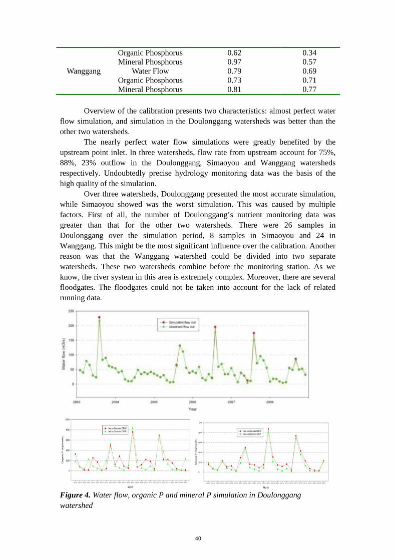
Organic Phosphorus 0.62 0.34 Mineral Phosphorus 0.97 0.57

Wanggang Water Flow 0.79 0.69 Organic Phosphorus 0.73 0.71 Mineral Phosphorus 0.81 0.77

Overview of the calibration presents two characteristics: almost perfect water

flow simulation, and simulation in the Doulonggang watersheds was better than the other two watersheds.

The nearly perfect water flow simulations were greatly benefited by the upstream point inlet. In three watersheds, flow rate from upstream account for 75%, 88%, 23% outflow in the Doulonggang, Simaoyou and Wanggang watersheds respectively. Undoubtedly precise hydrology monitoring data was the basis of the high quality of the simulation.

Over three watersheds, Doulonggang presented the most accurate simulation, while Simaoyou showed was the worst simulation. This was caused by multiple factors. First of all, the number of Doulonggang’s nutrient monitoring data was greater than that for the other two watersheds. There were 26 samples in Doulonggang over the simulation period, 8 samples in Simaoyou and 24 in Wanggang. This might be the most significant influence over the calibration. Another reason was that the Wanggang watershed could be divided into two separate watersheds. These two watersheds combine before the monitoring station. As we know, the river system in this area is extremely complex. Moreover, there are several floodgates. The floodgates could not be taken into account for the lack of related running data.

Figure 4. Water flow, organic P and mineral P simulation in Doulonggang watershed

40

In detail (Figure 4), among the three factors that we were concerned with,

water flow displayed the best simulation. The simulation of organic P and mineral P were not as good as water flow, but the results were acceptable. In water flow simulation, the most significant feature was the flood peaks of simulation obviously higher than those of the monitor data. This phenomenon was caused by the flood storage of the dense river system. In the Dafeng city area, the river system is extended to every single field; even peasant households are surrounded by streams. As rain falls on the streams, overflow will not occur until the entire river way is filled. 3.3. Simulation results

Figure 5. Spatial distribution of average water yield and TP in Dafeng from 2003 to 2008

Spatial distribution of average water yield and TP (Figure 5) showed a relatively coinciding result. Water flow in the east is higher than that in the west. There was no obvious difference between the north and the south. Downstream of Simaoyou and Wanggang watersheds has the highest water yield (59.0 mm/month). The lowest yield occurred in the middle of the research area (45.73 mm/month). TP spatial distribution presented similar characteristics to water yield. 3.4. Scenario results

41

Figure 6. Scenario results of different land use types’ response to the different fertilizer rates

Arid land contributed the most organic P, soluble P and sediment P of the three land use types. Orchard’s yield of phosphorus pollutants was significantly less than the other two yields. Of three types of phosphorus pollutants, organic P contributed the most P load, while soluble P had the least output. All kinds of land use presented positive correlation with fertilizer reduction.

The reduction of fertilizer application leads to little reduction of organic P yield. For orchard and paddy field, zero reduction of organic P was found. Soluble P’s response was significant, as can be seen in Figure 6. But the 94% fertilizer reduction differs little from the 97% reduction output. The same characteristics of soluble P can be seen in sediment P.

42

Over all three P pollutants, soluble P showed the most obvious sensitivity to fertilizer application reduction (Table 2). Organic P has very little response to fertilizer reduction. For the three land usages, paddy field had the greatest P reduction response, while arid land and orchard exhibited moderate responses. Table 2. Various P Pollutants’ Reduction with 15% Fertilizer Application Reduction

Nutrient Arid Land Orchard Paddy field Organic P 0.53% - - Soluble P 11.33% 12.71% 14.93%

Sediment P 6.89% 5.56% 7.61%

4. Conclusions Calibration results showed that the SWAT 2005 model carried out a precise

water flow simulation of the research area, the precision of which was mostly benefited by the upstream point inlet setting. The organic and mineral phosphorus simulation results were acceptable for the BMP design as well. Consequently, the method of manual subbasin delineation based on using the road and rail networks as artificial divisions was proved to be reasonable enough for presenting the hydrological connections of the shore alluvial plain.

The spatial distribution of average water and TP yield showed a relatively coinciding result, where the water flow and TP yield in the east were both higher than that in the west.

The scenarios concluded that phosphorus load had a linear correlation to the fertilizer rates in three different land use types. Soluble P showed the most obvious sensitivity to fertilizer application reduction, while organic P had very little response to the fertilizer reduction. In the three land usages, paddy field presented great P reduction response. Arid land and orchard had more moderate responses.

References

Arnold, J. G., R. Srinivisan, R. S. Muttiah, and P. M. Allen. 1998. Large-area hydrologic modeling and assessment: Part I. Model development. J. American Water Resources Assoc. 34(1):73-89.

Benham, B. L., C. Baffaut, R. W. Zeckoski, K. R. Mankin, Y. A. Pachepsky, A. M. Sadeghi,

K. M. Brannan, M. L. Soupir, and M. J. Habersack. 2006. Modeling bacteria fate and transport in watershed models to support TMDLs. Trans. ASABE 49(4): 987-1002.

Department of Yancheng Environment Protection. 2005. Environmental quality report of

Yancheng. HU Yao-wen，GUO Lei，TANG Ju-shan ，MA Jiong，ZHOU Fen. 2008. Research on the

Runoff M odel for River Networks in Plains (in Chinese). China Rural Water and Hydropower. 8 :22-28

43

Kirsch, K., A. Kirsch, and J. G. Arnold. 2002. Predicting sediment and phosphorus loads in the Rock River basin using SWAT. Trans. ASAE 45(6): 1757-1769.

Ministry of Agriculture of P.R.China. 2006. China Agriculture Yearbook. Santhi, C., R. Srinivasan, J. G. Arnold, and J. R. Williams. 2006. A modeling approach to

evaluate the impacts of water quality management plans implemented in a watershed in Texas. Environ. Model. Soft. 21(8): 1141-1157.

Stewart, G. R., C. L. Munster, D. M. Vietor, J. G. Arnold, A. M. S. McFarland, R. White, and

T. Provin. 2006. Simulating water quality improvements in the upper North Bosque River watershed due to phosphorus export through turf grass sod. Trans. ASABE 49(2): 357-366.

TANG Ying-zhou, RUAN Xiao-hong, WANG Wen-yuan. 2006. Application of water quality

model W ASP5 in water environment simulation of plain river network areas. Water Resources Protection. 22 (6): 43-50.

44

The Impact of Land Management on Drinking Water Quality: a Water Industry Application, East of England

Jenny Sandberg1*

, Frances Elwell2

1 Catchment Modeller, Water Resources Management Team, Anglian Water Services, Cambridge, UK 2 Water Quality Scientist, Integrated Water Resources Management, Mott MacDonald, Cambridge,

UK

* jsandberg@anglianwater.co.uk

Abstract In 2007, following the development of improved techniques for detecting low levels of trace substances in water, the concern for pesticides in drinking water across England increased. Metaldehyde and clopyralid are currently of highest concern, as they have been detected in drinking water across the region at levels exceeding the European drinking water standard of 0.1 µg/L. As these are difficult and costly to treat, Anglian Water Services is assessing the effectiveness of using catchment management measures as an alternative to treatment options. Such measures could bring significant long-term benefits in the form of improved raw water quality and corresponding reduction in capital and operational expenditure, carbon emissions and improved biodiversity. The Soil and Water Assessment Tool (SWAT) is being applied to surface water catchments to assess changes in water quality in a raw water storage reservoir under various land use scenarios. The chosen study area is located in the East of England, in an area dominated by agricultural activities. Approximately half of the reservoir water derives from natural streams, while the remaining half is pumped from an adjacent catchment. Both catchments are dominated by clay soils with a high shrink-swell potential. Thus, bypass flow to the underlying tile drainage system is likely to be an important pathway for pesticides found in the reservoir. The models were successfully calibrated for hydrology and pesticide concentrations in the river and streams feeding into the reservoir. For the reservoir itself, however, the model slightly underestimated metaldehyde concentrations and was not able to replicate the peaks. This is a result of the way reservoirs and streams are modelled in the SWAT model, where a single well-mixed water body is assumed. Keywords: SWAT, catchment management, river basin management, pesticide, diffuse pollution, drinking water quality, land use

45

1. Introduction

Changes in land use and land management practices can have significant impacts on water quality in surface water systems. With an increasing trend in the cost of drinking water treatment, the UK water industry is currently looking at the effectiveness of using catchment management as an alternative to traditional treatment solutions. This is a response to findings in 2007, where improved techniques for detecting low levels of trace substances in water resulted in detection of pesticides in drinking water across England and Wales at levels exceeding the drinking water standard of 0.1 µg/L. Metaldehyde (a molluscicide often used on oilseed rape, wheat and potatoes) and clopyralid (a herbicide often used on wheat and sugar beet) are currently of highest concern as there is no effective treatment solution in place for these substances.

Anglian Water Services (AWS) is a water and wastewater company supplying water and wastewater services to more than six million domestic and business customers in the East of England and Hartlepool. The geographical area is shown in Figure 1. This area is dominated by arable activities, predominantly cereal production. Given this, clopyralid and metaldehyde are commonly used across the region, and high concentrations of these pesticides are seasonally found in raw waters such as rivers, streams and raw water storage reservoirs.

Using the Soil and Water Assessment Tool (SWAT), AWS is currently assessing the feasibility of using catchment management options to improve raw water quality and subsequently reducing the need for raw water treatment. The modelling allows an assessment of the cause of the problem, what land use management practices to promote and where, what impact on raw water quality the different measures would have, and how soon any impacts would be seen. The output will be compared to more traditional treatment solutions through cost benefit analysis, where all costs are weighed against benefits.

The work is divided into two phases; the pilot phase and the roll-out phase. In the pilot phase (presented in this paper) a modelling approach was developed and tested on two selected pilot catchments. In the roll-out phase, the chosen modelling approach will be applied to the remaining catchments.

This paper presents the chosen modelling approach and the results from some of the initial scenario runs on metaldehyde concentrations. Additionally, a discussion regarding future data acquisition to improve the accuracy of the model result, and advantages and limitation of the modelling approach are presented.

Figure 1. The geographical area of AWS water and wastewater supply: East of England and Hartlepool

46

2. Materials and Methods

2.1. Study area The study area, located in the East of England, consists of two catchments which feed

a raw water storage reservoir, used for water supply (Figure 2). Approximately half of the water entering the reservoir is from the larger catchment (approximately 320 km2), from which water is pumped from the River Nene to the reservoir. The direct catchment to the reservoir is significantly smaller (approximately 50 km2). Water enters the reservoir from this catchment via natural feeder streams and local runoff.

With an annual average rainfall of approximately 600 mm and an average annual effective rainfall of 150 mm, the East of England is one of the driest parts of the country. The annual effective rainfall across England and Wales is on average 460 mm. The study area is dominated by arable cultivation, where winter wheat and winter oilseed rape are the most common crops. Some pasture also exists within the catchments. The altitude varies between 60 and 200 m above sea level with a slope between 0% and 20%, and the average being 5%. The area is characterised by relatively heavy clay soils and some loamy soils. Some of the soils also have a high shrink-swell potential (Figure 3).

Since 2008, raw water quality samples to detect metaldehyde and clopyralid concentrations have been taken on a weekly basis in surface water intakes across the Anglian Water region. Additionally, for the purpose of this study, the sampling frequency was increased to daily samples during weekdays between October and December 2010. A summary of metaldehyde concentrations found in the three feeder streams, the River Nene and the reservoir is provided in Figure 4.

A SWAT (Soil and Water Assessment Tool) model was developed for each of the two catchments contributing to the reservoir. The model output from the pumped catchment was used to create one of the model inputs for the direct catchment to the reservoir. The models were run from 2007 to 2010 using a daily time-step. In the hydrological model, a warm-up period of approximately 10 months was applied, followed by a

calibration and verification period. At the time of model configuration, pesticide application data was only available for 2008 and 2009. The water quality model was consequently calibrated from June 2008 to June 2009, followed by a verification period from August 2009 to July 2010.

Figure 2. Location of the study area

Figure 3. Shrink-swell potential of the soils (NSRI, 2010)

47

2.2. Model description The SWAT model is a physically based, continuous time model allowing long-term

predictions of the impact of land management practices in water environments (Neitsch et al., 2005). The catchment (or watershed) is partitioned into sub-catchments based on their characteristics such as soil type or land use. Each sub-catchment is further divided into Hydrological Response Units (HRUs), which are defined by a unique combination of land cover, soil type, and land management.

Input data is required for each sub-catchment and includes climatic data, spatial data, hydrological data, chemical data and information on land management practices. The driving force behind the catchment processes is the water balance (Neitsch et al., 2005). The model simulates water and solute transport into the stream network via surface runoff and lateral sub-surface flow. Drain flow can also be simulated, although pesticide loadings in the drains are not included. The model also allows for simulation of bypass flow as a result of soil cracking. This can be an important transport pathway in heavy clay soils, leading to rapid transport of water and solutes down to deeper soil layers and tile drains, where degradation potential often is poor.

Pesticides can be transported in solution or sorbed to sediments and can be lost from the soil profile, foliage, and ground surface, by volatilisation, degradation, leaching and runoff (Neitsch et al., 2005). In water, the amount of pesticides is reduced through removal in outflow, degradation, volatilisation, and settling and diffusion into the underlying sediment. The model assumes a well-mixed layer of water overlying a sediment layer; no spatial variation within the reservoir is modelled.

2.3. Data collection All data used in this study were derived from AWS or publicly available sources. A

summary is provided in Table 1.

Figure 4. Metaldehyde concentrations in raw water feeding into the reservoir

48

Table 1. Description of input data Data Type Description Data Source Topography Topographic map. Topographical data from UK Ordnance Survey. Land use Land use information was obtained from a number

of sources of various spatial resolutions and level of details on land use categories.

The European Environment Agency (EEA, 2004), Edina Agcensus data set (The University of Edinburgh, 2004), land use mapping from UK Ordnance Survey (OS, 2011).

Soil An ArcGIS map layer (1:250 000) outlining the dominant soil types (soil series) in the region, and a number of non-spatial datasets which describe the characteristics of the soil types.

National Soil Resources Institute (NSRI), 2010.

Weather Precipitation, wind speed, solar radiation, relative humidity, temperature.

A local weather station, the UK Met Office and the European Commission Joint Research Centre.

Reservoir Historical water level data, abstraction and operational details.

AWS.

River/stream hydrology

Gauging Stations and spot measurements. The UK Environment Agency, AWS

Pesticide Management

Monthly pesticide application by region. The UK Food and Environment Research Agency (FERA).

Water Quality Pesticide concentrations in raw water (streams, river and reservoir).

AWS, the UK Environment Agency.

2.4. Data processing 2.4.1. Soil data

A user defined soil database was created using national soil maps (NSRI, 2010) and associated datasets describing physical and hydrological properties of the dominant soil types (soil series). For a small number of soil properties required to run the model no data was available, hence, this needed to be estimated. This included the hydrologic soil group (A-D) and the crack volume. These parameters were estimated based on information on shrink-swell potential of the different soil types (Table 2). The maximum cracking volume (0.25), applied to soils classified as having very high shrink-swell potential, was estimated based on literature values (Novák, 1999; Olsen & Haugen, 1998).

Table 2. Estimated values for Hydrologic Soil Group and crack volume based on the shrink-swell potential of the soils Shrink Swell Potential* Hydrologic Soil Group Crack volume Very Low A 0 Low B 0 Moderate C 0.1 High D 0.2 Very high D 0.25 *Source: NSRI, 2010

2.4.2. Land use A land use map was created using data from three sources. The Corine Land Cover

Map (EEA, 2010) and the UK Ordnance Survey VectorMap District (OS, 2011) were used to identify arable land, pasture, woodland, water bodies and urban areas (Figure 5). Details of different crop types were added to the land classified as arable using Edina Agcensus data (University of Edinburgh, 2004).

49

2.4.3. Soil drainage No information on drainage design and

location of drains was available for this study. Given this, a methodology was developed in which the catchments were partitioned into drained and undrained areas based on land use and soil type (Figure 6). Only slowly permeable soils were assumed to have drainage systems installed. These were identified using the Hydrology of Soil Types (Boorman et al., 1995), which is a categorisation of the British soils based on their soil hydrology. Furthermore, drainage systems were assumed to only be installed on land under arable cultivation or pasture. Two types of drainage design were considered; mole channels at a depth of 500 mm or standard pipe drains at a depth of 1000 mm. The allocation of drainage design was based on the clay content and land use. Mole drains were

assumed on soils used for arable cultivation and with a clay content ≥ 30%.

2.5. Model calibration and validation This section describes the methodology applied for calibration of the models. Details

regarding the parameters adjusted during the calibration, and results are given in section 3.1.

2.5.1. Hydrological model The calibration of the hydrological

models was carried out using gauged flows from the pumped catchment and reservoir volumes from the direct catchment. The two models were calibrated in parallel and the same parameter adjustments were made to both models.

2.5.2. Water quality model The calibration of the water quality

models was undertaken based on measured pesticide concentrations in the three main streams directly feeding the reservoir, in the river from which water is pumped to the reservoir, and at the reservoir abstraction point. The two models were calibrated in parallel and the same parameter adjustments were made to both models.

Figure 5. Land use map showing urban

area, pasture, woodland, arable land and water (EEA, 2011)

Figure 6. Map showing drained and undrained

land

50

3. Results and Discussion 3.1. Model calibration and validation 3.1.1. The hydrological model

The primary parameters adjusted during the hydrological calibration are shown in Table 3. To reduce the amount of surface runoff, the curve number (CN) had to be significantly reduced from the initial values. Table 3. Primary SWAT model hydrological parameters adjusted during calibration Parameter Description Unit Calibration CH_N Manning’s “n” (roughness coefficient) in channel - Set to 0.08 OV_N Manning’s “n” for overland flow - Set to 0.5 CN Curve number – controls the amount of rainfall

runoff - Initial values were selected based on the

SWAT user guide. These were reduced to 70% of initial estimates.

CH_L Channel length – estimated by SWAT based on topography but details of meandering can be lost due to resolution

km Increase by 20% to account for meandering.

GWLAG Groundwater lag – controls response time of baseflow to rainfall

days Set to 150 days

CNCOEFF Plant ET curve number coefficient – allows the model to adjust the curve number based on the plant evapotranspiration

- Set to 2

ESCO Soil evaporation compensation factor - Default value reduced to 0.7 to account for some cracking.

FFCB Initial soil water storage fraction Set to 0.8 for the pumped catchment and 1.0 for the direct reservoir catchment.

The model calibration for the pumped catchment is illustrated in Figure 7. It shows a

model warm-up period of about 10 months, followed by a calibration period and a validation period.

The calibration period shows good agreement with baseflows and the timing of flow peaks, though with a tendency to slightly over-estimate the magnitude of flow peaks. The fit remains good through the verification period, with a generally similar pattern of good fit to baseflow and an overestimation of some peaks. The most dramatic over-estimation is at the beginning of the verification period (late July/early August 2009) when the model simulates two flood peaks of about 13 and 22 m3/s, while the recorded flow did not exceed 4 m3/s. The discrepancy is so great that there is a suspicion that the high rainfalls on 29th July and 6th August come from particular rain gauge records that do not fairly represent conditions of the catchment as a whole on those days. Given that the recorded flows over the remainder of the calibration and verification period are reasonably well simulated, it is considered that the July/August period should be treated as an outlier. Adjusting the model to match the recorded flows at that time would require major changes to parameters that would almost certainly destroy the good fit over the remaining period.

The model calibration of the direct reservoir catchment is illustrated in Figure 8. Once the model warm-up was completed, the fit between modelled and recorded reservoir storage was found to be good both for the calibration and verification periods. On three occasions the modelled storage started to drop slightly before the recorded storage, but the difference in storage remains small. In view of the number of potential inaccuracies or uncertainties in the various components of the water balance calculations (inflows, abstractions, evaporation, rainfall, bathymetry), the close match for most of the period is an excellent result.

51

Figure 7. Hydrological calibration and verification for gauged river flow

Figure 8. Hydrological calibration and validation for reservoir volumes

3.1.2. The water quality model The primary parameters adjusted during the water quality calibration are shown in

Table 4.

52

Table 4. Primary SWAT model pesticide parameters adjusted during calibration Parameter Description Unit Calibration AP_EF Application efficiency, i.e. fraction of pesticide applied that is deposited on

soil or foliage. Fraction 0.5

FILTERW Width of filter strips at edge of fields m 3 CHPST_REA Reaction rate of pesticides in stream, calculated from information on half-

life in water. day-1 0.07

HLIFE_S Half-life in soil days 10 HLIFE_F Half-life on foliage days 5 SKOC Soil adsorption coefficient mg/kg or

mg/l 120

The model calibration of metaldehyde concentrations at the river intake from the

pumped catchment to measured data is illustrated in Figure 9. Flow data at the gauging station is also shown to illustrate the timing of metaldehyde peaks in relation to flows. The model produces a good match both to the low levels through the bulk of the year and the higher values during the critical autumn period.

Figure 9. Metaldehyde calibration for river abstraction

Calibration results for metaldehyde concentrations in the feeder streams to the

reservoir are shown in Figure 10. The metaldehyde results for the reservoir itself are shown in Figure 11, with the

reservoir inflow and storage shown as background information. The inflow hydrograph exhibits a slightly unusual shape because of the combination of runoff from a natural catchment and pumped inflow from the river Nene. The model results show a reasonable match to the recorded concentrations towards the end of the period but do not simulate the variation in the earlier period.

53

Figure 10. Metaldehyde calibration for reservoir feeder streams

Figure 11. Metaldehyde concentrations for reservoir

Analysis of the metaldehyde data available from water quality measurements in the

reservoir, the river and the three feeder streams showed that the concentrations of metaldehyde in the reservoir are generally higher than those measured in any of the feeder streams or in the water pumped from the river (Figure 4). These observations suggest that either the pesticide accumulates in the reservoir or that there is a local source in the catchment close to the reservoir draw-off location, at which the sampling point also is located. The model is unable to accurately reproduce the localised effect of a local source because the reservoir is modelled as a single, well-mixed water body. In reality there will be spatial variation within the reservoir.

3.2. Land use scenarios At this stage of the study only initial scenario runs have been made, of which two are

presented in this paper:

54

Table 5. Description of land use scenarios Scenario Description Filter strips In the baseline model it was assumed that all arable land had filter strips of 3 m width; this was based

on observations made on site. Two scenarios related to filter strips were trialled using the SWAT model; No filter strips and filter strips with 6 m width.

Proportional land use change

Metaldehyde applications were stopped in over half of the wheat areas of the pumped catchment (Figure 12). This represents a scenario where an alternative molluscicide is being used on over half of the catchment.

By doubling the width of the

filter strips from 3 m to 6 m, a reduction of approximately one-third of the peak in-stream concentrations of metaldehyde was achieved. If removed completely, the peak concentration of metaldehyde approximately doubled.

The result from the proportional land use scenario showed a 40% reduction in peak metaldehyde levels at the river abstraction point.

4. Conclusions

As part of a pilot study, two

SWAT models were developed for two catchments in East of England to predict pesticide concentrations in a raw water storage reservoir under varying land use scenarios. They were successfully calibrated for hydrology and pesticide concentrations in the feeding river and streams based on the available data for the period from 2008 to 2010. In the reservoir, however, the model slightly underestimates metaldehyde concentrations and was not able to replicate the peaks. Analysis of monitored metaldehyde data shows that the concentrations of metaldehyde in the reservoir, measured at the draw-off for raw water supply, are generally higher than those measured in any of the feeder streams or in the pumped water from the river Nene. These observations suggest that either the pesticide accumulates in the reservoir or that there is a local source in the catchments close to the draw-off location.

In SWAT, reservoirs and streams are modelled as a single well-mixed water body and spatial variation is not taken into account. To assess the impact this simplification has on water quality simulations at the reservoir abstraction point, it would be necessary to run the scenarios using a 2D reservoir model. There is also some degree of uncertainty associated with some of the pesticide input variables, particularly the degradation half-life in water. To be able to assess the potential for pesticide degradation in water, the pesticide half-life needs to be further assessed. This is important as it likely to impact travel time and degree of pesticide accumulation, hence, the relative contribution of the different sub-catchments on the water quality measured at the reservoir abstraction point.

A large part of the study area is characterised by heavy clay soil with a high shrink-swell potential. Given this, the features of bypass flow and drain flow were enabled in this study. Due to the importance of accurate prediction of surface runoff and infiltration when assessing the impacts of land management measures (particularly filter strips) on water quality, it is recommended that, in the future, detailed sensitivity runs of parameters controlling bypass flow and drain flow are carried out. Drainage systems are also likely to be an important transport pathway of metaldehyde in the study area. However, the model cannot simulate pesticide transport via drainage systems. This is important to take into consideration

Figure 12. Illustration of the proportion of land in

which metaldehyde application was stopped

55

when assessing the impact of various land management measures such as buffer strips. Under the current specification of the model, the effectiveness of buffer strips will probably be overestimated.

One of the limitations of this study is the lack of available data, including frequent water quality data and flow data for feeder streams. In the near future, SWAT models will also be applied to catchments feeding water to a number of water treatment works in the AWS region using the approach developed in the pilot study. Drawn from the experience of this study, the need to increase sampling frequency of metaldehyde and clopyralid should be assessed. Additionally, it may be necessary to revisit the models when more knowledge and experience are gained.

Overall, the SWAT model has proved to perform well in the two catchments and will be a useful tool in the future, when the impact of water quality will be assessed using more targeted land use scenarios.

Acknowledgements The authors would like to thank the following people who have contributed to the work of this project at various stages: Anna Chivers, Mike Cook, Jane Dottridge, Peter Ede, Simon Eyre, Louisa Peaver, and Gerry Spraggs. The views expressed in this paper are those of the authors only. References Boorman, D.B., Hollis, J.M and Lilly, A. 1995. Hydrology of soil types: a hydrologically-based

classification of the soils of the United Kingdom. Institute of Hydrology Report No.126. Institute of Hydrology, Wallingford.

European Environment Agency (EEA). 2010. Corine Land Cover 2000 (CLC 2000) Map. Available at: http://www.eea.europa.eu/data-and-maps/data/corine-land-cover-2000-raster. Accessed 15.05.2011.

National Soil Resources Institute (NSRI). 2010. Land Information System (LandIS) Digital soil dataset.

Neitsch, S.L., Arnold, J.G., Kiniry, J.R., and Williams, J.R. 2005. Soil and Water Assessment Tool. Theoretical Documentation. Grassland, Soil and Water Research Laboratory, Agricultural Research Service, Temple, Texas.

Novák, V. 1999. Soil-Crack Characteristics—Estimation Methods Applied to Heavy Soils in the NOPEX Area. Agricultural and Forest Meteorology. 98: 501-507.

Olsen, P.A., and Haugen, L.E. 1998. A new model to of the shrinkage characteristics applied to some Norwegian soils. Geoderma. 83(1-2):67-81.

The UK Ordnance Survey (OS). 2011. UK Ordnance Survey VectorMap District. Available at: http://www.ordnancesurvey.co.uk/oswebsite/products/os-vectormap-district/index.html. Accessed 16.05.2011.

The University of Edinburgh. 2004. Edina Agcensus for 2004. Available at: http://edina.ac.uk/agcensus/. Accessed on 16.05.11.

56

Soil Temperature Damping Depth in Boreal Plain Forest Stands and Clear Cuts: Comparison of Measured Depths versus Predicted

based upon SWAT Algorithms

G. Putz and B.M. Watson Department of Civil and Geological Engineering, University of Saskatchewan, Saskatoon, Saskatchewan,

Canada, S7N 5A9

J.A. Bélanger Faculty of Engineering, Lakehead University, Thunder Bay, Ontario, Canada, P7B 5E1

E.E. Prepas Faculty of Forestry and the Forest Environment, Lakehead University, Thunder Bay, Ontario, Canada, P7B 5E1 and Department of Biological Sciences, University of Alberta, Edmonton, Alberta, Canada, T6G 2E9

Abstract The Forest Watershed and Riparian Disturbance (FORWARD) Project operates within the Boreal Plain ecozone in Western Canada. One focus of the study has been to adapt the SWAT model for stream-flow prediction in forested watersheds of the Boreal Plain and to use the model to assist forestry companies with landscape management decisions. FORWARD has collected data on soil temperature and water content since 2005. Continuous measurements have been conducted at multiple sites representing five different characteristic soil and vegetation cover types within the ecozone and at sites harvested via clear cut operations. Each site was automated to record daily air temperature at 0 and 2 m and soil temperature and water content at depths ranging from 0.1 to 3 m. Soil temperature predictions within SWAT play an important role in the redistribution of water since no flow of water can occur to or from a given soil layer if the temperature of that layer is 0C or below. Hence soil temperature has a strong influence upon streamflow simulation. A key factor for the prediction of daily soil temperature within SWAT is the estimation of the damping depth of the soil profile. The damping depth is estimated as a function of soil bulk density, moisture content and maximum damping depth. The results of the soil temperature and soil moisture measurements at sites representing deciduous forest, conifer forest and clear cuts are presented in this paper and analyzed to determine a range of typical damping depths. The analysis results are compared to estimates using the SWAT model predictor equations. The results indicate that damping depth is significantly underestimated for conditions on the Canadian Boreal Plain. A simple modification to the maximum damping depth equation is proposed to improve the soil temperature simulation for boreal forest sites. Keywords: soil temperature, damping depth, SWAT model, boreal forest

57

1. Introduction Soil temperature is an important parameter in hydrological and nutrient transformation

processes. Within the Soil and Water Assessment Tool (SWAT), water flow to or from a soil layer can only occur if the temperature of that layer is 0ºC or above (Neitsch et al. 2005). Soil temperature therefore has a strong influence upon streamflow simulation in cold regions that experience frozen soils. Soil temperature also influences the simulation of nutrient transport in SWAT because it controls the rate of decomposition and mineralization of organic nitrogen and phosphorus and the nitrification and volatilization of ammonia within the soil profile (Neitsch et al., 2005).

Soil temperature is calculated in SWAT based upon a series of empirical equations derived for unspecified locations and environmental conditions. The main objective of the work presented in this paper was to determine if the damping depth, a key parameter used in SWAT soil temperature calculations, is well predicted by SWAT for sites within the boreal forest in Western Canada. The consequential effect of poor representation of the damping depth upon soil temperature simulations is also investigated. SWAT damping depth predictions are assessed by comparison to soil temperature and moisture content data collected by the Forest Watershed and Riparian Disturbance (FORWARD) project.

The FORWARD project operates within the Boreal Plain ecozone in Western Canada. The project conducts streamflow, water quality and ecosystem studies in small to medium scale forested watersheds for pre and post tree harvest conditions. One focus of the study has been to adapt the SWAT model for streamflow prediction in forested watersheds of the Boreal Plain and to use the model simulations to assist forestry companies with landscape management decisions.

2. Background 2.1. SWAT soil temperature algorithm

SWAT utilizes an index model to predict daily soil temperature for each soil layer based upon environmental conditions and the soil layer temperature of the previous day. A more comprehensive heat flow and energy balance approach to the soil temperature calculations would require definition of the thermal properties of the soil. Thermal properties of soil are seldom measured or available in conventional soil databases hence the need for a simplified modelling approach. A complete description of the soil temperature equations and parameters can be found in Sections 1:1.3.3 and 1:1.2.5.1 of Neitsch et al. (2005). A brief overview of the equations and parameters that are most relevant to the work described in this paper is presented below.

The soil temperature Tsoil(z, dn) at a specific depth (z) in mm on the current day is given by Equation 1:

Equation 1 where Tsoil(z, dn-1) is the previous day’s temperature, λ is a lag coefficient, df is a depth factor, TAAir is the average annual air temperature based on long-term data, and Tssurf is the soil surface temperature on the current day. All temperatures are expressed in ºC. The lag coefficient λ controls the influence of the previous day’s temperature on the current day (set at 0.8 as default in SWAT), and df accounts for the insulating influence of the overlying soil (Neitsch et al., 2005).

The depth factor df for a soil layer is calculated based upon a unitless depth ratio zd and the following empirical relationship:

58

Equation 2 where zd is calculated by dividing the depth at the center of the soil layer (z) in mm by the damping depth (dd) in mm. Neitsch et al. (2005) define dd as the depth in the soil profile at which the soil temperature is within 5% of TAAir.

The damping depth is determined based upon soil bulk density, soil moisture content and maximum damping depth using the following empirical equations:

Equation 3

where ϕ is a scaling factor that modifies the damping depth based upon the water content of the soil and ddmax is the maximum damping depth. The scaling factor ϕ is given by:

Equation 4 where SW/ztot is the water content in the soil profile in mm/mm and ρb is the bulk density of the soil in Mg/m3. SW is the amount of water in the soil profile expressed as depth in mm and ztot is the depth of the soil profile in mm. The maximum damping depth (ddmax) is calculated using the following empirical equation:

Equation 5

The soil surface temperature (Tssurf) in Equation 1 is a function of a soil cover weighting factor (bcv) and the temperature of the bare soil (Tbare). The temperature of bare soil is calculated using the average, maximum and minimum air temperatures and a radiation term that is calculated empirically from the daily incoming solar radiation and surface albedo on the current day. SWAT varies the albedo depending on the surface cover. Albedo for a snow-covered surface is set as 0.8. In the absence of snow, the albedo depends on the amount of vegetation biomass covering the soil surface, the plant albedo and the soil albedo. A complete description of the parameters and empirical expressions used in SWAT to calculate Tssurf is presented by Neitsch et al. (2005). 3. Temperature and Soil Moisture Monitoring 3.1. Monitoring sites

The FORWARD project study area is located approximately 225 km northwest of Edmonton, Alberta, Canada (Figure 1). Soil temperature monitoring sites are located across six watersheds. The climate of the Boreal Plain is sub-humid (Zoltai et al., 1998) and is characterised by long, cold winters and short, hot summers. Long-term climate normals (1971 to

59

2000) for precipitation and mean annual air temperature are 578 mm and 2.6oC, respectively, with 24% of total annual precipitation falling as snow (Environment Canada, 2009). Generally, snowfall begins in October or November and the area remains snow-covered for six to seven months of the year (Environment Canada, 2009).

Figure 1. Location of study area and monitoring sites

The monitoring sites can be characterized by five different land classifications: upland

burned, upland harvested, upland coniferous, upland deciduous and peat lands. Only the harvested, coniferous and deciduous sites (Table 1) are considered in this paper. There are minor differences in elevation (Table 1) and slope (range 0.01 to 0.04%) among sites. Upland soils across the study area are mostly fine-grained Orthic Gray Luvisols overlaying deep glacial tills (Whitson et al., 2003). Coniferous and deciduous stands across the study area are dominated by lodgepole pine (Pinus cortorta Dougl. ex Loud.var. latifolia Engelm) and trembling aspen (Populus tremuloides Michx.), respectively (Ecological Stratification Working Group, 1996) (Table 1). The harvested sites are the result of logging activity that occurred in January 2004. Regrowth since harvesting is sparse and consists of lodgepole pine and white spruce (Picea glauca (Moench) Voss).

Table 1. Monitoring sites description

3.2. Monitoring instrumentation

Soil temperature was measured hourly and recorded either by water/soil temperature sensors and HOBO® dataloggers (Onset Computer Corporation, Bourne, MA, USA) for coniferous and

60

deciduous sites or YSI thermistors (YSI Incorporated, Yellow Springs, OH, USA) and Data Dolphin loggers (Optimum Instruments Inc., Edmonton, AB, Canada) for harvested sites.

Measurements were taken at 100, 300, 500, 1000, 2000 and 3000 mm depths for soil temperature and at the ground surface and 2000 mm above ground level for air temperature. Soil moisture content was measured hourly with theta probes (Delta-T Devices Ltd., Burwell, Cambridge, UK) at 100, 500 and 1000 mm depths and recorded by either a DL6 soil moisture datalogger (Delta-T Devices Ltd.) or a Data Dolphin datalogger. 4. Measurement Results 4.1. Soil temperature

Soil temperature data has been collected at all monitoring sites since 2006. Many sites were subject to intermittent operation due to equipment failures resulting from the harsh climate conditions and damage caused by wildlife. In total, one conifer site (C2), two deciduous sites (D1 and D3) and two harvest sites (H1 and H3) provided a period of three to four years of data suitable for analysis. An example of one year of record at harvested site H1 is shown in Figure 2. The effect of depth upon temperature lag during warming of the soil profile can be seen in Figure 2. The maximum temperature in the upper soil layers (≤ 300 mm) occurs in August corresponding to the occurrence of maximum air temperature, whereas the maximum soil temperature at 3000 mm does not occur until late October. In contrast, the minimum soil temperatures in the soil profile are more closely grouped in time and occur in late April to May.

Figure 2. Soil temperature versus depth at a harvested boreal forest site

4.2. Soil water content Soil water content was measured at each of the temperature monitoring sites. An example of

one year of record at harvested site H1 is shown in Figure 3. The influence of precipitation

61

and drying upon the soil water content of the upper soil layer is very evident in Figure 3. At greater depths in the soil profile, the effects of wetting and drying cycles are attenuated. At the 1000 mm depth the soil water content is relatively consistent throughout the year.

Figure 3. Soil water content versus depth at a harvested boreal forest site 5. Analysis of Monitoring Results 5.1. Estimated damping depth from soil temperature measurements

The active temperature zone within the soil profile must be delineated in order to determine the largest annual damping depth from the soil temperature monitoring data. The active temperature zone is the portion of the soil profile in which the temperature fluctuates between a yearly maximum and minimum. An example plot for harvested site H3 is shown in Figure 4. The plot shows the range in air temperature and range is soil temperature with depth in the active zone. Note the range in soil temperature attenuates with depth which is consistent with the trend in soil temperature time series shown in Figure 2.

Figure 5 shows the variation in the active zone (at a conifer site) over a four-year period. The yearly maximum temperature at a selected depth in the soil profile is relatively consistent and primarily influenced by variation in annual maximum air temperature. In contrast the yearly minimum temperature at a selected depth in the soil profile is more variable as a result of varying minimum temperature and accumulated snow depth from one winter to the next.

Two difficulties were encountered in determining the largest annual damping depth at a site based upon the soil temperature measurements. The first difficulty is related to the definition of damping depth presented by Neitsch et al. (2005), i.e. the depth at which the soil temperature is within 5% of TAAir. Unfortunately, a definition relative to TAAir causes the actual range in temperature at the damping depth to vary depending upon geographic location and the

62

corresponding TAAir. At the monitored sites in this study TAAir is only a few degrees. Under these conditions the range in temperature defining the damping depth would be much smaller than for warmer locations. A damping depth definition based upon a specified temperature range would be more preferable for consistency. Assuming the relative definition for damping depth was derived for Temple, Texas or nearby where the average annual air temperature is approximately 20oC, the actual range in temperature at the damping depth would be approximately 2oC or ±1oC. Therefore, a temperature range of 2oC in the active zone was adopted in order to define the damping depth.

Figure 4. Air and soil temperature range at site H3, 2009

Figure 5. Air and soil temperature range at site C2, 2006 to 2009

The second difficulty encountered was the largest annual damping depth at all the boreal forest monitored sites extended beyond the deepest monitoring depth, i.e. beyond 3 m. Therefore

63

an extrapolation procedure was required to estimate the largest annual damping depth based upon the 2oC temperature range discussed above. The procedure utilized was to plot the active zone temperature range versus depth, fit an exponential curve to the data points for 1, 2 and 3 m, and then apply the best fit curve to predict the depth at which the temperature range was 2oC. An example of the procedure is shown in Figure 6.

The largest annual damping depth was determined for each site and year using the extrapolation procedure outlined above. A compilation of the results is presented in Table 2. The largest annual damping depth determination could only be performed for those years when sufficient data was available to define the entire active zone. A comparison of the results indicates the largest annual damping depth is relatively consistent at each site from year to year. Further, there does not appear to be any obvious difference in largest annual damping depth between coniferous, deciduous and harvested sites.

64

Figure 6. Example of curve-fitting procedure to determine largest annual damping depth

Table 2. Calculated largest annual damping depths and average water content

Table 2 – Cont. Calculated largest annual damping depths and average water content

5.2. Comparison of predicted and estimated largest annual damping depths

Calculations conducted using Equations 3, 4 and 5 were used to predict a feasible range in largest annual damping depth for the monitoring sites based upon typical bulk density of the soil (1.45 Mg/m3) and a typical range in water content. The range in average annual water content measured at 1 m depth for all sites (see Table 2) was used in the calculations. The range in damping depths predicted by the SWAT equations is indicated in Figure 7 (1.85 to 2.35 m) and

65

shown in Figure 8 superimposed upon the largest annual damping depths determined based upon the monitoring data. It is clear from the comparison shown in Figure 8 that the largest annual damping depths for the boreal forest sites are significantly underestimated by the SWAT equations.

Figure 7. Damping depth versus soil moisture content for original and modified Equation 5

Figure 8. Largest annual damping depth compared to calculated range in damping depth

66

6. Application of Results 6.1. Modified maximum damping depth equation

Comparison of the predicted range in damping depths and the largest annual damping depths determined based upon field measurements indicates that Equation 5 significantly underestimates ddmax. An adjustment can be made to the leading numerical constant (i.e. 1000) in Equation 5 to increase the magnitude of ddmax. For this preliminary investigation, the leading constant was simply increased by trial and error to obtain a good visual fit to the measured largest annual damping depths (see Figure 8). A leading constant of 7000 produced a range in calculated damping depths (3.87 to 5.67 m) with an improved fit to the observed largest annual damping depths. A more rigorous statistical fit to the data to determine the leading constant is warranted and will be conducted when additional field data have been collected and compiled for use in the analysis.

6.2. Effect upon soil temperature predictions Bélanger et al. (2009) previously presented suggested modifications to parameters in the

SWAT soil temperature equations. These suggested modifications were based upon a comparison of measured and predicted soil temperatures over a two year period at several FORWARD boreal forest monitoring sites. The suggested modifications dealt with refinements to the magnitude of albedo for snow, vegetation and soil for boreal forest conditions and adjusting the magnitude of the lag coefficient λ in Equation 1 to optimize the goodness of fit with observed data. Bélanger et al. (2009) concluded that further modifications were required to improve soil temperature simulations during winter conditions with snow cover. These additional modifications were needed to represent the insulating effect of the snow cover and could be implemented by either increasing bcv or dd.

As additional years of field data from multiple FORWARD project sites became available, it seemed prudent to evaluate the SWAT capabilities to predict dd. The purpose of the evaluation was to ensure that the dd calculations for warm weather conditions were representative before tackling the more complicated issue of representation of snow cover effects upon soil temperature. Hence the current study.

For convenience, the input conditions and observed data used by Bélanger et al. (2009) were applied in this study to assess the effect of an improved estimate of maximum damping depth upon SWAT soil temperature simulations for boreal forest conditions. Plots of observed and predicted temperatures are show in Figures 9 and 10. The soil temperature predictions using the original version of Equation 5 are shown in comparison to the modified version using a leading constant of 7000. All other parameters were set to the defaults suggested in the SWAT documentation.

The simulation results show the modified maximum damping depth equation has little effect upon predicted temperature close to the soil surface. However, the predicted soil temperatures much deeper in the soil profile are significantly affected. The improved estimate of maximum damping depth provides improved simulation of maximum soil temperature during spring, summer and early fall. Unfortunately, little improvement in the prediction of soil temperature during winter and snow cover conditions is evident.

67

Figure 9. Predicted and observed soil temperature at 0.1 m, Site H3

Figure 10. Predicted and observed soil temperature at 1.0 m, Site H3 7. Discussion and Conclusions

The comparison of measured and predicted damping depths at boreal forest sites presented

in this paper suggests that modifications to the calculation of maximum damping depth are required within SWAT. An improvement in maximum damping depth representation is easily implemented by adjusting the leading constant in Equation 5. Ideally, a function should be incorporated into Equation 5 that would adjust the leading constant as a function of environmental conditions. A compilation of measured damping depths and soil characteristics at several geographically

68

dispersed sites would be required to derive the function. A soil temperature model based upon energy balance considerations could also be used as a guide to derive the function.

The determination of damping depth from measured temperatures in the soil profile requires a definition based upon a specified range in temperature rather than a percent variability. A definition based upon a specified temperature rate will allow a more consistent comparison of damping depths determined at locations with widely varying annual average air temperatures.

Improvements in the calculation of maximum damping depth in SWAT have an increasingly significant effect upon soil temperature simulation as depth in the soil profile increases. Problems in representation of the damping depth during periods with no snow cover should be resolved before improvements in soil temperature prediction under snow cover and freezing conditions are attempted. Acknowledgements FORWARD research on the Boreal Plain of Western Canada was funded by an NSERC Collaborative Research and Development Grant and Millar Western Forest Products Ltd., as well as Alberta Newsprint Company (ANC Timber) Ltd., Blue Ridge Lumber Inc. (a Division of West Fraser Timber Company Ltd.), Buchanan Lumber (a division of Gordon Buchanan Enterprises Ltd.), Vanderwell Contractors (1971) Ltd., EDFOR Co-operative Ltd., PetroBakken Energy Ltd., Talisman Energy Inc., Vanderwell Contractors (1971) Ltd., Alberta Innovates BioSolutions, the Forest Resource Improvement Association of Alberta and the Canada Foundation for Innovation. References Bélanger, J.A., Putz, G., Watson, B.M. and Prepas, E.E. 2009. Annual freeze/thaw temperature cycles in

soils on the Canadian Boreal Plain : Comparison of SWAT predictions to measured data. Proceedings, 2009 International SWAT Conference. August 5 – 7, 2009. University of Colorado at Boulder, Boulder, Colorado.

Ecological Stratification Working Group. 1996. A national ecological framework for Canada. Centre for

Land and Biological Resources Research, Research Branch, Agriculture and Agri-Food Canada, Ottawa, Ont.

Environment Canada, 2009. Digital archive of the Canadian climatological data (surface) [online].

Atmospheric Environment Service. Canadian Climate Centre, Data Management Division, Downsview, Ont. Available from: http://www.climate.weatheroffice.ec.gc.ca/ climateData/canada_e.html [accessed 25 Mar 2010].

Neitsch, S. L., J. G. Arnold, J. R. Kiniry, and J. R. Williams. 2005. Soil and Water Assessment Tool

Theoretical Documentation, Version 2005. Temple, TX: Agricultural Research Service and Texas Agricultural Experiment Station.

Whitson, I.R., Chanasyk, D.S., and Prepas, E.E. 2003. Hydraulic properties of Orthic Gray Luvisolic

soils and impact of winter logging. J. Environ. Eng. Sci. 2 (Suppl. 1): 41-49. Zoltai, S.C., Morrissey, L.A., Livingston, G.P., de Groot, W.J., 1998. Effects of fires on carbon cycling in

North American boreal peatlands. Environ. Rev. 6(1), 13-24. doi:10.1139/er-6-1-13.

69

Challenges and Difficulties in Sediment Modeling Applied to Sedimentation Study of the Lobo Reservoir in Brazil

Julio Issao Kuwajima

M.S. Student – CNPq scholarship, Department of Hydraulics and Sanitation, São Carlos School of Engineering, University of São Paulo, Brazil, julio.kuwajima@usp.br.

Sílvio Crestana

Senior Research Scientist, Agriculture Instrumentation, Embrapa, Brazil.

Lázaro Valentin Zuquette Professor, Department of Geotechnical Engineering, São Carlos School of Engineering,

University of São Paulo, Brazil.

Frederico Fábio Mauad Assistant Professor, Department of Hydraulics and Sanitation, São Carlos School of

Engineering, University of São Paulo, Brazil.

Abstract

The Lobo reservoir is located at the Alto Jacaré-Guaçu, a 2,277 km² watershed in the state of São Paulo. The main tributaries that feed the 221 MW hydropower dam constructed in 1936 are Itaqueri River, Lobo stream and Feijão stream. A new legislation enacted by both the Brazilian Water Agency (ANA) and the Brazilian Electric Energy Agency (ANEEL) in 2010 obliges the monitoring of sedimentation inside this reservoir. Although São Paulo is the richest state in Brazil and much research has been performed in this region of the state, there is a lack of sedimentary data and all data available are seasonal so no continuous data series can be found. Moreover, some parameters used by SWAT simulations are not suitable for Brazilian soil conditions e.g. SCS soil classifications and runoff factors for the SCS-CN function. The model database which contains default information for crop types and land use cover are equally unsuitable for the region because agricultural management practices adopted in the region are different from those observed in temperate countries. There is a general lack of studies in these fields. The present study seeks to highlight and suggest further studies to advance the development of the SWAT model in Brazil.

Keywords: tropical agriculture, runoff, sediment modeling, reservoir sedimentation.

70

1. Introduction SWAT (Soil and Water Assessment Tool) is a physically-based, continuous-

time watershed-scale model; a distributed-parameter hydrologic model that uses spatially distributed data on topography, land use, soil and weather for hydrologic modeling (Arnold et al., 1998; Arnold and Fohrer, 2005). According to the same authors, SWAT was developed by the USDA to predict hydrologic impacts of land management practices including such factors as sediment, pesticides, nutrients and other agricultural chemicals in watersheds.

Gassman et al. (2007) have made an extensive list of more than 250 published SWAT-related articles and classified them into the categories of hydrologic assessments, climate and land use change studies, pollutant load assessments, model comparisons, model interfaces, sensitivity analyses and calibration techniques. The SWAT model has been broadly used in different parts of the world for studies regarding hydrological and sediment processes and/or climate and land use change.

Hiepe (2008) stated that the number of applications has increased worldwide very quickly over the last few years due to the numerous advantages of the model. However, applications in the tropics are rare, and most applications are limited to hydrological studies of catchments in temperate climate regions of the United States and Europe. Although many tropical applications have been presented in conference proceedings, many of those studies must be considered as preliminary and often show severe limitations or unsatisfying simulation results due to limited data availability.

In Brazil a few SWAT applications can be found, namely Oliveira (1999), Machado (2002), Barasnti et al. (2003), Moro (2005), Prado (2005), Neves (2005), Balsissera (2005), Minoti (2006), Adriolo et al. (2008), Blanski et al. (2008), Baltokoski (2008), Lopes (2008), Lino (2009), Lelis, T.A. & Calijuri, M.L. (2010) and Baltokoski et al. (2010). Most of these studies took place in the southeastern and southern regions of Brazil. Still there is a noted lack of continuity to the SWAT applications due to the absence of a specific SWAT research group and a relative lack of experience and information exchange between the research groups that have used the model.

1.1. The Lobo-Broa reservoir

The Lobo-Broa reservoir is located between the municipal districts of Itirapina and Brotas in São Paulo, a state located in southeastern Brazil (Figure 1 – 22° 15' S and 47° 49' W). It was built in 1936 for hydroelectric energy generation (Tundisi, 1986). The main tributaries of the 221 MW hydropower dam are Itaqueri River, Geraldo River, Lobo stream, Feijão stream.

71

Figure 1. The Lobo-Broa reservoir location (Tundisi et al. 2004)

The watershed is affected by the unavoidable impacts of antropic activity and

water demand such as the discharge of untreated residential sewage, deforestation, sand mining, tourism and intense sport fishing (Tundisi et al., 2003).

The climate of the area is of the type Cwa, according to Köppen. This means it is subtropical mesothermic with a wet summer and dry winter under the influence of cold fronts arriving from the south mainly in the winter and autumn. The average annual pluviosity is of 1,300 mm, and the dry season extends from April to September (Tundisi, 1986). Table 1 shows the main characteristics of the reservoir.

Table 1. Lobo-Broa reservoir characteristics (Tundisi, 1986)

Length 8 km Maximum width 2 km Average width 0.9 km Maximum depth 12 m Average depth 3 m Superficial area 6.8 km² Perimeter 21.0 km

Volume 22.0 x 106

m³ The lake is 7.5 km long and has a very flat basin with a mean water depth of 3

m. A maximum depth of 12 m is observed near the dam site. The water level fluctuates within a range of 1.5 m, being high in April at the end of the rainy season and low in September at the end of the dry season. Figure 2 shows the SHP Lobo´s dam.

72

Figure 2. SHP Lobo’s dam (International Lake Environment Committee, 2010) The watershed of the Lobo-Broa reservoir has been studied thoroughly over

almost 30 years; the limnology of this reservoir was opened by Brazilian scientists in 1971. Several other areas of study such as climatological, hydrological, biological and water chemistry aspects were researched. The number of scientific papers so far published regarding this lake now amounts to approximately 200, including several masters and doctoral theses prepared at the University of S. Paulo and the Federal University of S. Carlos. The Centre for Hydrological Research and Applied Ecology, University of S. Paulo, is currently engaged in scientific projects including the modeling of the Broa reservoir system. Educational programs using the lake area as a natural laboratory have been in place since 1985.

Throughout nearly 30 years of research, very few studies focused on estimating or measuring the siltation and sedimentation processes inside the dam. One reason for the lack of research in this field is that before the 1990s the computational technologies where not available, and the other reason is that bathymetric surveys are very expensive, requiring costly gear and software. Figure 3 shows an example of a bathymetric survey result that was performed on the Lobo-Broa reservoir.

Figure 3. Sample spots and raster image presenting 2007 EMT, “zigzag method”

(Estigoni et al.2010)

73

The SWAT model emerged as a reasonable tool capable of performing sediment

process evaluation without the need of cutting-edge equipment or the long, expensive campaign that a bathymetric survey requires.

A new piece of legislation enacted by both the Brazilian Water Agency (ANA) and the Brazilian Electric Energy Agency (ANEEL) in 2010 requires sedimentation monitoring inside these reservoirs. Some studies have arisen driven by this new regulation: Estigoni et al. (2010) attempted to estimate sediment accumulation comparing two bathymetric surveys and two master’s theses are in progress, one of which could shed some light on the sediment accumulation processes.

2. Challenges and Difficulties

Brazilian watersheds generally have poor or no monitoring; the monitored

watersheds are limited to southern and southeastern regions. Even with many research projects and studies taking place in the Lobo-Broa Dam Watershed, there is still a scarcity of data. There is only a fluviometric station downstream of the reservoir, and none of the tributaries are monitored. The weather data is monitored by a meteorological station that belongs to Universidade de São Paulo. Only scarce and fragmented sediment and water quality data are available.

But the new legislation, RESOLUÇÃO CONJUNTA Nº3 de 10/08/2010 ANA/ANEEL, establishes conditions and procedures regarding installation, operation and maintenance of hydrometric stations in order to monitor rainfall, limnimetric, fluviometric, sedimentometric and water quality associated with hydropower projects. However, the agencies do not have a deadline established by which they must install and operate these stations.

2.1. Tropical agriculture in Brazil

The agricultural techniques used in Brazil are temperate and cold weather techniques roughly adapted for tropical conditions. One example is tillage; the soil is intensively worked as in European countries with plowing and disking. After using these tillage techniques the soil is superficially irrigated and left exposed uncovered to the sun and to the strong tropical precipitation. The result of the use of these techniques is accelerated degradation and erosion of the fertile superficial layer of the soil.

The substrate exposure to tropical sun heat can cause opposite effects to those intended. The high temperature dries the soil and extinguishes the microbiological fauna which normally would enhance decomposition and nutrient utilization. Tillage also facilitates erosion, which could become a major problem in regions with heavy and intense rainfalls.

As a result of these wrongly-applied tillage techniques, modernization of Brazilian tropical agriculture practices strives to minimize soil disturbance by using no-till farming or strip-till techniques with garrison crops residues as ground cover, helping to maintain the moisture and protecting the soil from sun and rainfall.

2.2. Traditional practices

Another difference that can be observed in Brazilian conditions is the presence of subsistence farming; this kind of agriculture is characterized by use of traditional techniques by families. These techniques typically demand more water and inputs and exhibit lower productivity and efficiency.

In general, less higher technology is used in Brazil, and there is a lack of

74

efficient use of fertilizers, irrigation, agrochemicals and tillage techniques compared to farms in Europe and North America.

Preparing the soil with traditional agricultural practices such as slash and burn causes great loss of soil nutrients through atmospheric scattering, leaching, percolation and entrainment (Kato; Lato; Denich e Vvlek, 1999). These traditional techniques often leave the soil exposed, disturbed and vulnerable to erosion.

Slash and burn is a common practice for cultivating sugarcane in Brazil, including in the vicinity of the Lobo-Broa reservoir watershed. Primavesi (1979) stated that the soil and nutrient losses due to such practices are not noticed in the first years after the vegetation is removed because the ashes of the previous cover fertilizes the soil. Some elements are mineralizated, making them available to plants in early plantings but then they are unavailable to future crops. In soils with clay hydrophobic particles may be formed; these are aliphatic carbon atoms which hinder water infiltration into the soil.

A state law of São Paulo (Lei 11.241, de 19 de Setembro de 2002), however, imposes restrictions on burn activities associated with sugarcane harvesting. An enforced gradual reduction of slash and burn practices for sugarcane is predicted to culminate in the prohibition of such methods in 2031. This regulation encourages mechanization and modernization in the harvesting processes.

2.3. Tropical crop behavior

Species from temperate countries exhibit a distinct behavior in the tropics. This can be attributed to the change in photoperiod between tropical and temperate zones. The temperate summer day is usually long, about 15 to 16 hours, while in the tropics a summer day only lasts about 13 hours (Paterniani, 2001)

Because of this difference, more photosynthesis activity and higher CO2 fixation is expected to occur in temperate zones than tropical zones. In addition, colder and shorter nights mean a shorter period of breathing and CO2 emission. Paterniani (1990) studied differences in maize behavior between these regions, summarized in Table 2.

75

Table 2. Comparison of tropical and temperate Maize crops (Paterniani, 1990) - Modified.

Characteristics Temperate Tropical Growth Conditions

Annual weather variation Relatively stable Variable, not predictable Annual rainfall variation Relatively uniform Variable, not predictable Photoperiod Long days Short days Night temperature Fresh Warm Soil conditions Usually favorable Frequently adverse Seeding period Restricted (few days) Broad (several months) Seeding season Restricted (few days) Broad (several months) Growing season Well-defined Variable, broad Difficulties for germination

Cold soil and fungus Soil insects

Maize types Vegetative cycle Uniform, adapted to the

growing season. Variable, to adapt to weather conditions.

Plant size Low to medium Usually tall

Some differentiations in performance can be related to genetic improvement; some species are mutated in order to be successfully introduced into a different climatic zone. Some species that with a variety developed for Brazilian conditions are listed below:

• Coffee: The variety developed for Brazilian conditions produces 2340 kg/ha, 314% more than the Arabica variety (745 kg/ha) (Carvalho & Fazuoli, 1993 apud Paternani, 2001). • Maize: New varieties are more productive and can be grown outside of the regular summer planting season. • Soya: Until 1970, Brazil accounted for only 2% of world production; today 20% of the soya of the world comes from Brazilian farms. From 1961 to 1999 there was an annual productivity increase of 31.6 kg/ha/year, amounting a total of 1200 kg/ha in 38 years of research (Vencovsky & Ramalho, 2000 apud Paterniani, 2001).

2.4. Runoff

Runoff can be estimated in SWAT using two methods: the SCS curve number procedure and the Green & Ampt infiltration method. A major limitation of the curve number method is that rainfall intensity and duration are not considered and only total rainfall volume is used. The Green-Ampt method is a time-based model and can simulate impacts of rainfall intensity and duration on infiltration processes.

In the state of the São Paulo and in most parts of Brazil there is a large occurrence of thick, multi-layered soils. Brazilian soils are rich in iron and aluminum; usually the predominant colors are red and yellow

Rainfall is much more severe and plentiful in the tropics than it is in the temperate zone. Intense rainfall events are of great importance because of their impact on erosion processes. Intense rainfall is a common event during the summer season in the state of São Paulo. Table 3 compares the rainfall in these regions.

76

Table 3. Comparison between weather in Ames, Iowa, USA and Piracicaba, SP, Brazil. Paterniani, 1990 – Modified.

Ames, Iowa, USA Piracicaba, SP, Brazil Period Average

(mm) Standard

Derivation (mm)

Period Average (mm)

Standard Derivation

(mm) July 92.6 35.51 December 218.9 75.88

August 97.6 40.74 January 216.1 94.10 Ames, Iowa, US, 42° N, 93° W Piracicaba, SP, Brazil, 22° S, 47° W

2.5. SCS curve number

Curve Number is a model for estimation of runoff that was developed by the USDA in the 1950s; the model has gone through more than 20 years of studies and research. The use of SCS-CN is very simple; it is a function of precipitation, soil permeability, land use and antecedent water content of the soil.

The original SCS hydrologic soil group classification focuses mainly on the soil texture, and the depth and deeper layer characteristics are briefly and subjectively described. Some of these characteristics not included in the SCS classification are important for assessing the formation of runoff. In practice, for tropical Brazilian soils it is difficult to frame a soil unit into these classes of hydrologic soils. This fact leads most users of the curve number method in Brazil to consider only the uppermost soil layers in order to fit into the original classification system.

Three classification systems for the hydrologic soil groups of the state of São Paulo have been proposed (Setzer & Porto, 1979; Lombardi Neto et al., 1989; Kutner et al., 2001). According to Sartori (2004), the Lombardi Neto et al. (1989) proposal for classification is the most convenient and similar to the original classification and therefore more easily applied. The other methodologies have complications and limitations for application.

The Lombardi Neto et al. (1989) classification is more thorough than the original classification because it takes into account depth, texture, texture gradient within the soil superficial and subsuperfical horizons, porosity of the soil and expansive clay activity. Nevertheless the Lombardi Neto et al. (1989) proposal is controversial because some clay soils where put in the groups A and B (low runoff) while some sandy soils where classified in the groups C and D (high runoff). Table 4 presents the Lombardi Neto et al. (1989) hydrologic soil classification.

77

Table 4. Groups of soils according to their qualities, characteristics and resistance and erosion. Lombardi Neto et al. (1989)

Group Erosion

resistance group

Main Characteristics

Depth Permeability Texture Texture gradient

(1)

Great grouping of soils (4)

A High Very deep (>2

m) or deep( 1 to 2 m)

Fast/Fast Moderated/Fast

Loamy/Loamy Clay/Clay

Clay loam/Clay Loam

< 1.2

LR,LE, LV, LVr, LVt, LH LEa and

LVa

B Moderated Deep (1 to 2 m) Fast/Fast

Moderated/Fast Moderated/Moderated

Sandy/Sandy Sandy/Loamy Sandy/Clay

Loam Loamy/Clay

Loam Clay Loam/Clay

1.2 – 1.5

LJ, LVP, PV, PVL, Pln, TE, PVls, R,

RPV, RLV, LEa(3) and

LVa(3)

C Low

Deep (1 to 2 m) or moderately

deep (0.5 to 0.1 m)

Slow/Fast Slow/Moderated Fast/Moderated

Sandy/Loamy(2) Loamy/Clay

Loam(2) Sandy/Clay

Loam Sandy/Clay

>1.5

Pml, PVp,

PVIs, Pc and M

D Very Low

Moderately deep (0.5 to

0.1m) or shallow (0.25 to

0.50m)

Fast, moderated or slow over slow Highly variable Highly

variable

Li-b, Li-ag, gr, Li-fi, Li-ac and PVp (shallow)

(1): Average of the clay content in horizon B (excluding B3) divided by the average all clay content in horizon A. (2): Only with an abrupt shift between the texture in horizons A to the B. (3): Only with a sandy horizon A. (4): Brazilian nomenclature.

Sartori (2004) compared the runoff hydrographs obtained by the SCS classification and the Lombardi Neto et al. (1989) classification for watersheds in the São Paulo state and observed a general trend of the SCS classification to underestimate values. The Brazilian adapted classification was found to be more consistent, but not optimal and in need of improvement.

A study using the SWAT model in Benin (a tropical country) reported overestimation of the total discharge using the SCS curve number approach (Hiepe, 2008). This was attributed to two discharge peaks (150 and 200 mm per week), for which the model overreacted. This study discovered from a sensitivity analysis that for mean daily discharge and sediment yield measurements the SCS curve number was by far the most sensitive parameter, confirming the high sensitivity of the SWAT model to changes in the curve number.

2.6. Green & Ampt infiltration method

This equation assumes that the soil profile is homogenous and antecedent moisture is uniformly distributed in the profile. As water infiltrates the soil, the model assumes that the soil above the wetting front is completely saturated and that there is a sharp break in the moisture content at the wetting front.

78

This model can simulate rainfall intensity and rainfall events that tend to be more severe in the tropics, but there is a loss of data due to regression equations that are needed to parameterize the model (Wilcox et al., 1990 apud King et al. 1999). But the application of the Green Ampt approach requires hourly rainfall data. However, using the Green Ampt approach instead of the SCS curve number approach does not necessarily improve modeling results (King et al. 1999). When modeling hydrologic systems of large areas, one must consider the overall goal in selecting an excess rainfall procedure. As drainage area increases, stream flow peaks tend to smooth out and the use of Green Ampt becomes ineffective.

3. Discussion

The SWAT model was developed for weather and soil conditions in the USA, a

temperate weather country. The application of SWAT in tropical countries requires modifications of equations, databases and parameters. The greatest limitation is the difficulty in finding regional parameters that can be inputted into the SWAT database.

For example the till.dat that addresses tillage techniques does not have an option for the slash and burn method, which obviously causes great disturbance to the soil characteristics affecting the moisture, temperature, nutrient (phosphorus and nitrogen mainly) and physical properties (permeability). The model does not include an alteration of inherent soil properties due to soil erosion or agricultural management, which leads in the long term to an underestimation of sediment loss.

In the region of the Lobo-Broa reservoir the main agriculture is sugarcane and cattle breeding. In order to reconstruct pastures for cattle and to prepare the soil with fertilizers before planting the saplings of sugarcane, the soil is disturbed and the superficial layers are homogenized which alters their original behavior.

The crop database which contains SWAT plant growth parameters must be modified; the existing land cover/plant parameters are not suitable for tropical conditions. But there is little or no experimental data or literature available for Brazilian crops and weather that would be necessary to enable any changes.

Another challenge is how to assess the contribution of the unpaved roads that are used to transport agricultural production. There is a suggestion that these roads contribute more to the sedimentation and siltation processes than the sugarcane crops.

Unlike sugarcane crops, they usually tread a path against the relief contour, creating straight lines. The soil is very compacted by the weight of the trucks, making it almost impermeable. The rainfall easily washes off the top layer. There are unpublished studies as well as some studies that are in progress whose topic is an estimation of their contribution to the Lobo-Broa reservoir sedimentation processes. Figure 4 shows the erosion processes on roads near the sugarcane crops.

79

Figure 4. Erosion on unpaved roads in the sugarcane crops King et al. (1999) indicated a high sensitivity of model performance to the

applied surface runoff estimation technique. Sartori (2004) studied a watershed with similar weather and soil properties to the Lobo-Broa Reservoir and stated that the current Brazilian adaptation is more suitable than the original proposition but still needs to be improved.

4. Conclusion

The wide range of SWAT applications that have been reported underscore that

the model is a very flexible and robust tool that can be used to simulate a variety of watershed problems. The ability of SWAT in temperate conditions has been confirmed in numerous studies. However, the model performance in tropical conditions is not completely satisfactory, the main weaknesses being the lack of component modifications, which support more accurate simulation of specific processes or regions.

SWAT has potential to be applied as a powerful tool for evaluation and monitoring of reservoir and dam sedimentation. SWAT could also help water resource management in watersheds with reservoirs since it is possible to use it to do simulations and scenarios evaluating effects of changes in the landscape regarding the siltation and sedimentation processes.

More studies must be done to discover the full application of the SWAT. Research must yield experimental data for tropical conditions in order to build a database of land use and crop behavior, the effect of different agricultural practices and different soil properties. In addition, more comparisons between the runoff methods for tropical conditions must be studied.

These findings will help reveal the capabilities of the SWAT model in regions with scarce and low-quality data and will extend the SWAT user databases for tropical soils and land use types.

Acknowledgements The present work was accomplished with the support of the CNPq, Conselho Nacional de Desenvolvimento Científico e Tecnológico – Brazil. This work is dedicated to my parents, who have given me all the support that I need to do my research, and I´d like to thank all my colleagues in the Hydrometric Centre EESC/USP, my advisor Prof. Frederico Fábio Mauad, Sílvio Crestana from EMBRAPA and Prof. Lázaro Valentin Zuquette for all advice and support for my research.

80

References Journal articles Arnold, J. G., R. Srinivasan, R. S. Muttiah, AND J. R. Williams. 1998. Large Area Hydrologic

Modeling and Assessment Part I: Model Development. Journal of the American Water Resources Association 34: 73-89.

Arnold, J.G. & Fohrer, N.2005. SWAT 2000: Current capabilities and research opportunities in

applied watershed modeling. Hydrol. Process, 9(1):563-572. Baltokoski, V.; T., Ferreira, M. H.; Machado, Ronalton, E. and De Oliveira, M. P.. 2010.

Calibração de modelo para a simulação de vazão e de fósforo total nas sub-bacias dos Rios Conrado e Pinheiro - Pato Branco (PR). Rev. Bras. Ciênc. Solo.34, (1): 253-262.

Gassman, P.W., M. Reyes, C.H. Green, and J.G. Arnold. 2007. The Soil and Water Assessment

Tool: Historical development, applications, and future directions. Transactions of the American Society of Agricultural and Biological Engineers (Invited Paper Series) 50(4): 1211-1250.

Kato, M. S. A; Lato, O. R.; Denich, M. e Vvlek, P. L. G. 1999, Fire-free alternatives to slash-

and-burn for shifting cultivation in the eastern Amazon Region: the role of fertilizers. Field Crops Research, (62); 225-237. Amsterdan, EIsevier Science.

King, K. W., J. G. Arnold & R. L. Binger (1999). "Comparison of Green-Ampt and curve

number methods on Goodwin Creek Watershed using SWAT." Transactions of the American Society of Agricultural Engineers (ASAE) 42(4): 919-925.

Lelis, T.A.; Calijuri, M.L., 2010. Modelagem hidrossedimentológica de bacia hidrográfica na

região sudeste doBrasil, utilizando SWAT. Ambi-água, 5 (2): 158-174. Paterniani, E. 2001. Agricultura sustentável nos trópicos. Estud. Av., 15 (43), pp. 303-326. Paterniani, E.1990. Maize breeding in the tropics. Critical Reviews in Plant Sciences. 9: 125-

154. Tundisi, J. G. et al.2004. The response of Carlos Botelho (Lobo, Broa) reservoir to the passage

of cold fronts as reflected by physical, chemical, and biological variables. Braz. J. Biol.64(1) 177-186.

Tundisi, J.G. et al. 1986. The Lobo (Broa) ecosystem. Ciência Interamericana.25(114):.18-31. Books NEITSCH, S.L., ARNOLD, J.G., KINIRY, J.R., WILLIAMS, J.R., 2005. Soil and Water

Assessment Tool Theoretical Documentation Version 2005. Grassland, Soil and Water Research Laboratory; Agricultural Research Service; USA.

Primavesi, A. 1979. Manejo ecológico do solo: a agricultura em regiões tropicais – São Paulo:

Ed. Nobel. Vögtle, T.; Bähr H.P. 1999. Gis for Environmental Monitoring. Stuttgart: Scheizerbart. Bulletins and Reports ICOLD, International Commission on Large Dams. 1989. Sedimentation control of

reservoirs/Maîtrise de l'alluvionnement des retenues. Committee on Sedimentation of Reservoirs. Paris.

81

Setzer, J; Porto, R.L.L. 1979. Tentativa de avaliação do escoamento superficail de acordo com o solo e sue recebimento vegetal nas condições do Estado de São Paulo. Boletim Técnico DAEE. 2(2):.81-104. São Paulo.

Tundisi, J.G.; Matsumura-Tundisi, T.; Rodríguez, S.L. 2003 . Gerenciamento e recuperação das

bacias hidrográficas dos rios Itaqueri e do Lobo e da Represa Carlos Botelho (Lobo-Broa). IIE, IIEGA, PROAQUA, ELEKTRO.

Published Papers Adriolo,M.V.;Santos,I.;Gilbertoni,R.C.;Camargo,A.S.G. 2008. Calibração do modelo SWAT

para a produção e transporte de sedimentos In: Simpósio Brasileiro sobre pequenas e médias centrais hidrelétricas, 6.,2008, Belo Horizonte.Anais...Rio de Janiero;CBDB, 2008.

Barsanti,P.; Disperati,L.; Marri,P.; Mione,A., 2003. A soil erosion and multi-temporal analysis

in two Brrazilian basins. In: International SWAT Conference, 2., 2003. Bari. Reports…College Station:TWRI

Blainski,E.; Silveira,F.A.;Conceição,G. 2008. Utilização do modelo hidrológico SWAT para

estudos na microbacia hidorgráfica do rio Araranguá/SC. In: Taller International Red Riegos Cyted, 2008, Florianópolis. Anais... Florianópolis:CEER, 2008.

Estigoni, M. V. ; Matos, A. J. S. ; Mauad, F. F. 2010. Comparison between two bathymetric

survey methods to estimate sediment accumulation in the lobo SHP reservoir. In: Australia's National Water Conference and Exhibition - Ozwater'10, 2010, Brisbane.

Kutner, A.S.; Conte, A.E.; Nitta, T. 2001. Análise geológica e caracterização dos solos para

avaliação do coeficiente de escoamento superficial na bacia do Alto Tietê. In: XIV Simpósio Brasileiro de Recursos Hídricos, Aracajú-SE.

Lombardi Neto,F.; Bellinazzi Júnior, R.; Galeti, P. A.; Bertolini,D.; Lepsch, I.F.; Oliveira, J.B.

1989.Nova abordagem para cálculo de espaçamento entre terraços. In Simpósio sobre terraceamento agrícola. Campinas. Fundação Cargill. P.99-124

Dissertations and Thesese Baldissera, G.C., 2005. Aplicabilidade do modelo de simulação hidrológica SWAT (Soil and

Water Assessment Tool) para a bacia hidrográfica do Rio Cuiabá, MT. MS thesis. Cuiabá: Universidade Federal dos Mato Grosso.

Baltokoski, V., 2008. Modelo SWAT2005 aplicado às sub-bacias dos rios Conrado e Pinheiro –

Pato Branco/PR. MS thesis. Cascavel: Universidade Estadual do Oeste do Paraná. Hiepe,C., 2008. Soil degradation by water erosion in a sub-humid West-African catchment: a

modeling approach considering land use and climate change in Benin. PhD diss. Bonn, Germany.: Universität Bonn, Mathematisch-Naturwissenschaftliche Fakultät.

Lino,J.F.L., 2009. Análise da dinâmica hidrossediemntológica da bacia hidorgráfica do Rio

Preto (SC) com o modelo SWAT. MS thesis. Florianópolis: Universidade Federal de Santa Catarina.

Lopes, N.H.Y., 2008. Análise da produção de água e sedimentos em microbacias experimentais

com o modelo SWAT. MS thesis. Florianópolis: Universidade Federal de Santa Catarina – Departamento de Engenharia Sanitária e Ambiental.

82

Machado, R.E., 2002. Simulação de escoamento e de produção de sedimentos em uma microbacia hidrográfica utilizando técnicas de modelagem e geoprocessamento. PhD diss – Piracicaba:.Univerisdade de São Paulo - Escola Superior de Agricultura Luiz de Queiroz.

Moro, M., 2005. A utilização da interface SWAT-GIS no estudo da produção de sedimentos e

do volume de escoamento superficial com simulação de cenáriso alternativos. MS thesis. Piracicaba: Universidade de São Paulo - Escola Superior de Agricultura Luiz de Queiroz.

Neves,F.F., 2005. Análise prospectiva das áreas de risco à erosão na microbacia hidrográfica do

Rio Bonito (Descalvado-SP), potencialmente poluidoras por dejetos de granjas. MS thesis. São Carlos: Universidade de São Paulo- Escola de Engenharia de São Paulo.

Oliveira, M.Q.C.,1999. Impacto de mudanças no uso do solo nas características

hidrossedimentológicas da bacia hidrográfica do rio Joanes e sua repercussão na zona costeira. MS thesis- Salvador: Universidade Federal da Bahia.

Prado, T.B.G.; 2005. Evolução do uso das terras e produção de sedimentos na bacia hidrográfica

do rio Jundiaí-Mirim, MS theis. Campinas: Instituto Agronômico de Campinas. Sartori, A. 2004. Avaliação da classificação hidrológica do solo para determinação do excesso

de chuva do método do serviçp de conservação dos solo dos Estados Unidos. MS thesis. Campinas: Universidade Estadual de Campinas – Faculdade de Engenharia Civil, Arquitetura e Urbanismo.

Online Source International Lake Environment Committee. 2010. Photos of the Lobo/Broa reservoir. World

Lakes Database. Shiga, Japan.: available at: www.illec.or.jp. Accessed 10/05/2010

83

Using Measurement Data on Water and Matter Fluxes in Small Homogeneous Mountainous Catchments for HRU-

Parameterization in SWAT

Raphael Benning, Dipl.-Forstwirt (Forestry) Technische Universität Dresden, Institute of Soil Science and Site Ecology, Pienner Str. 19, 01737

Tharandt, Germany, raphael.benning@tu-dresden.de

Andreas Wahren, Dipl.-Hydrologist Technische Universität Dresden, Institute of Soil Science and Site Ecology

Filipa Isabel Lopez Tavares Wahren, Msc. Environmental Sciences Technische Universität Dresden, Institute of Soil Science and Site Ecology

Karl-Heinz Feger, Prof. Dr. Technische Universität Dresden, Institute of Soil Science and Site Ecology

Abstract Securing water resources has become increasingly important as changing climatic conditions are anticipated to affect both water quality and quantity. This is particularly important in regions where the supply of drinking water is allocated by large reservoirs. Modeling of discharge and stream flow nutrient concentration on the catchment scale is an important tool to predict changes in water quality and quantity. However, these modeling efforts are often hindered by a lack of knowledge about the parameterization of different land-use types. Within the catchment of the drinking water reservoir Lehnmühle (Ore Mountains/Germany), a discharge-dependent monitoring program has been established. This monitoring program gathers information regarding the contribution of diffuse nutrient and pollutant sources for the catchment’s three main land-use types (cropland, forest and grassland) and for the catchment as a whole. The monitoring program includes continuous discharge measurements in three small subbasins with homogenous land-use as well as weekly water samplings which are analyzed for four main quality parameters: nitrate-nitrogen (NO3-N), ortho-phosphate-phosphorus (PO4-P), total phosphorus (TP), and dissolved organic carbon (DOC). The measured data show clear differences in NO3-N, PO4-P and DOC exports with stream flow between the land-use types. Highest NO3-N and PO4-P inputs occur at agricultural sites while high DOC concentrations seem to originate from organic-rich wet forest sites, moors, and unidentified point sources. A biogeochemical measurement program was set up to gather important data which is needed for process-based parameterization of the SWAT model. Hence, the model is used to analyze the input of diffuse sources into streams under current climatic conditions and to predict the impact of future climate, land-use and management changes on stream matter input. Keywords: water quality, forest simulation, climate change, biogeochemical measurements, different land-use types, nutrient pollution, reservoirs

84

1. Introduction

Model-based simulations of future climate, land-use and management changes are important tools for helping to develop adaptive land management strategies for securing water resources under these changing conditions. For this reason, the German REGKLAM-Project established an Integrated Regional Climate Change Adaption Program for to model the region of Dresden. A primary focal point of this program is water quantity and quality. Most of the drinking water supply for the model region is provided by a network of reservoirs located south of Dresden in the Eastern Ore Mountains. Therefore, it is important to analyze the water quality and quantity of that network, especially focusing on the diffuse pollution sources.

Spatially distributed modeling of water quantity and quality requires a detailed knowledge of the underlying chemical and physical processes at the plot scale as well as at the catchment scale. This is needed especially for the site-specific and process-based parameterization of the SWAT-model. The main land-use types within the catchment of the Lehnmühle reservoir are cropland, grassland and forest, for which there is a lack of knowledge of the nutrient effluxes from these land-use types. To help improve our knowledge of the nutrient fluxes in these land cover types, a monitoring program was established in three small subbasins with homogenous land-use. This program monitors discharge with bio-geochemical measurements at the outlets of the subbasins and the whole catchment. It includes continuous discharge measurements and weekly water samplings which are analyzed for four main quality parameters: nitrate-nitrogen (NO3-N), ortho-phosphate (PO4-P), total phosphorus (TP) and dissolved organic carbon (DOC). The collected data is used to set up the parameterization of the water and matter fluxes in the SWAT model both on the plot scale (which corresponds to the subbasin scale) and the catchment scale.

Current climate change predictions (IPCC, 2007) anticipate changes in water and matter fluxes at both the plot and catchment scale. Understanding the affect of these changes, particularly at the catchment scale, is critical for the protection of drinking water supplies. In our study, the SWAT model is used to investigate climate change effects on the water quality of streams at the catchment scale.

2. Materials and Methods

2.1. Site description The Ammelsdorf gauge, which measures the inflow to the Lehnmühle reservoir, is

located in the Eastern Ore Mountains (Saxony, NE Germany, 50°48’18.06” North, 13°36’24.54” East). In this mountainous region, the population density is low, and the land-use structure is dominated by forests (≈ 52 % of the area), followed by grassland (≈ 34 % of the area) and cropland (≈ 9 % of the area). The elevation in the whole catchment ranges from 520 m a.s.l. to 800 m a.s.l.

To investigate the influence of the three main land-use types (forest, grassland, and cropland), three small subbasins were identified which represent a single land-use type each. The size of the subbasins varies between 2 ha (cropland) and 21 ha (forest). In the outlet of each subbasin, a gauging weir with continuous discharge measurement (with high-resolution) was installed. In addition to the measurements in the subbasins, high-resolution discharge measurements are recorded at the Ammelsdorf gauge, which provides measurements at the entire catchment scale. 2.2. Sampling of streamflow

The weekly stream flow sampling campaign started on July 21, 2009 and is still in progress to date. In addition to continuous weekly sampling, event-based samples were

85

collected. For this purpose, automatic water samplers (ISCO Company, 3700 Portable Samplers) in each subbasin and at the Ammelsdorf gauge were installed. The automatic collection of samples works depending on water level and discharge. During a flood, samples can be collected at different points in time. The samples were stored in a cooler box during transportation. 2.3. Analytical methods

The samples were stored in a refrigerator and kept at 4°C until analysis. The unfiltered samples were analyzed for TP following the methodology established by DIN-EN-ISO-6878 (2004). Immediately after receiving the samples in the laboratory, sulfuric acid was added to the unfiltered samples to prevent changes in TP concentrations. The sample was then digested with persulfate. Dissolved phosphate was then measured photometrically as molybdenum blue complex (wavelength of 880 nm).

About half of the volume of each sample (about 400 - 500 ml) was filtered through a 45 µm-membrane filter. The filtered samples were analyzed for nitrate-nitrogen (NO3

--N), ammonium-nitrogen (NH4

+-N), chloride (Cl-) and dissolved phosphate-P (PO4--P) using the

Segment Flow Analyzer SANplus (Skalar Analytics). Dissolved organic carbon (DOC) was analyzed using the infrared absorber heraeus liquid TOC (FOSS). In addition to this, the concentrations of the cations Na2+, K+, Ca2+, Mg2+, Al3+, Fe2+, Mn2+, Zn2+ and the anions SO4

2- and SiO44- in the water sample were analyzed using the ICP (Inductively Coupled

Plasma) Spektroscop Spectro (Ciros). 2.4. Modeling with Soil and Water Assessment Tool (SWAT)

The established monitoring program captures the nutrient fluxes under current climatic conditions. However, for the model region of Dresden, Bernhofer et al. (2009) detected changes in climatic conditions when comparing the period 1991 – 2005 with a climatic baseline period of 1961 – 1990. The annual mean temperature of the period 1991 – 2005 increased about 0.6 ºC compared to the climatic baseline period, showing increasing mean temperatures in spring, summer and winter and a low decrease in the mean temperature in autumn. They also observed changes in the mean annual amount of precipitation. The mean annual precipitation increased during the period from 1991 – 2005 compared with the climatic baseline period. The interannual variability reveals a decrease in precipitation in spring and an increase in winter. These observed climatic shifts at the regional scale agree with the predicted IPCC scenarios (IPCC, 2007). Future changes in climatic conditions will have an impact on the turnover of nutrients in soils and the export of nutrients to streams. For instance, Borken and Matzner (2008) reported decreasing cumulative soil N mineralization due to extended summer droughts which could result in lower NO3

- inputs into stream water. To predict diffuse depositions of N and P into the inflow of the Lehnmühle reservoir under future climate change scenarios, the Soil and Water Assessment Tool (Arnold and Fohrer, 2005; Arnold et al., 1998) will be utilized in this study. The first step will be to simulate the whole catchment of the Ammelsdorf gauge in the model for the present land-use distribution. The data collected from the monitoring program is used for the process-based parameterization of the model. This data contains both discharge and nutrient concentrations in stream water and data about the chemistry and physics of the main soil types in the three subbasins. After model validation, the climatic conditions will be changed to represent the future climate change scenarios based on the IPCC scenarios (IPCC, 2007). This approach gives an estimation of the impact of climate change on the efflux of nutrients into stream water.

86

3. Results

3.1. Stream discharge Figure 1 shows that there is no seasonal variability in the discharge from the sub-

catchments or from the whole catchment (Ammelsdorf gauge). The hydrograph for the cropland shows only marginal variability which may be caused by the structure of the gauging weir rather than the actual discharge rates. The geological bedrock underlying the gauging weir consists of unconsolidated rock which may be permeable to water flowing around the gauging weir. This may result in a portion of discharge which may flow beneath and/or around the gauging weir and therefore may not provide an accurate representation of the

discharge rates of this subbasin. Comparison of the hydrographs from grassland, forest and the total catchment reveals an initial rise at the end of March and the beginning of April 2010 which is caused by snowmelt. Another rise is shown at the beginning of June which is caused by a high amount of precipitation after a longer dry period. In autumn 2010 there was another high precipitation event at the end of September. During this event, a maximum discharge rate of 320 l s-1 km-2 appeared in the grassland catchment. By contrast, the maximum discharge rate at the forested catchment was only ≈ 170 l s-1 km-2. The maximum discharge rate at the Ammelsdorf gauge was ≈ 240 l s-1 km-2. After this event, the discharge decreased to its normal level. The highest discharge rate occurred in mid-January 2011 in the grassland catchments with a discharge rate of nearly 700 l s-1 km-2 which was the largest flood event in the measuring period. During the same event, the discharge from the forested catchment increased to nearly 190 l s-1 km-2 and at the Ammelsdorf gauge to nearly 370 l s-1 km-2. The mean values for the daily discharge rates of the catchments are shown in Table 1.

Figure 1. Hydrographs of the discharge rates in the three sub-catchments (cropland, grassland, forest) and the total catchment of the Ammelsdorf gauge

87

Table 1. Basic statistics of the analyzed parameters during the period 21.07.2009 - 01.11.2010

3.2. Nitrate-N concentrations

As shown in Figure 2 and Table 1, the concentration of nitrate-N varies among the three land-use types. The highest concentrations of nitrate can be measured in the cropland catchment. The mean N concentration on this site is ≈ 8.5 mg l-1. In the grassland sub-catchment, the mean N concentration is ≈ 5.2 mg l-1. The N concentration in the stream in the forested catchment is much lower, with a value of ≈ 0.8 mg l-1. At Ammelsdorf gauge, a mean concentration of ≈ 1.8 mg l-1 was measured. A seasonal trend or seasonal variability in N concentration can be detected only in the cropland and grassland sites. In the grassland site, the nitrogen concentration started at a low level in July 2009 and rose first at the end of the vegetation period in October. Until April 2010 it remained more or less at a constant level and decreased during a drier period in June and July 2010. In September 2010 the concentration increased and remained at a higher level until February 2011. This higher level was only interrupted three times by lower concentrations when higher discharge was measured. There is no significant seasonal variability for the cropland site. Very high concentrations were measured twice, which can be attributed to fertilizer application on the field. Both the forested catchment and the total catchment (at Ammelsdorf gauge) do not show any seasonality in NO3-N concentration.

Minimum Average Median Maximum

Cro

p la

nd Daily discharge (l s-1 km-2) 0.2 4.9 3.1 37.9

NO3-N (mg/l) 5.6 8.5 8.3 16.7 NH4-N (mg/l) 0.001 0.100 0.012 2.200 TP-P (µg/l) 11.5 37.3 29.0 107.0 PO4-P (µg/l) 4.5 14.5 15.0 22.7 DOC (mg/l) 0.03 0.50 0.40 4.40

Gra

ssla

nd Daily discharge (l s-1 km-2) 0.06 26.80 10.67 683.30

NO3-N (mg/l) 2.5 5.2 5.4 10.4 NH4-N (mg/l) 0.002 0.067 0.016 0.765 TP-P (µg/l) 17.2 31.5 26.3 80.0 PO4-P (µg/l) 1.0 17.2 17.1 28.5 DOC (mg/l) 1.01 1.97 1.66 7.47

Fore

st la

nd Daily discharge (l s-1 km-2) 0.1 19.9 12.5 188.3

NO3-N (mg/l) 0.5 0.8 0.8 1.1 NH4-N (mg/l) 0.001 0.024 0.008 0.286 TP-P (µg/l) 1.0 9.0 4.8 44.9 PO4-P (µg/l) 0.5 1.8 1.5 10.0 DOC (mg/l) 0.43 1.11 0.88 4.70

Am

mel

sdor

f ga

uge

Daily discharge (l s-1 km-2) 0.5 26.7 16.9 369.0 NO3-N (mg/l) 1.0 1.8 1.8 2.9 NH4-N (mg/l) 0.001 0.022 0.009 0.412 TP-P (µg/l) 0.9 12.4 9.3 82.9 PO4-P (µg/l) 0.6 3.0 3.0 9.8 DOC (mg/l) 1.11 2.62 2.05 7.89

88

Figure 2. Time series of discharge and nitrate-N concentrations for the different land-use types and the total catchment

3.3. Phosphorus concentrations In Figure 3, the PO4-P concentration in the (sub) catchments are shown. A high

variability in concentrations between the different land-use types becomes obvious. The mean PO4-P concentrations (shown in Table 1) vary between 17.2 µg l-1 in the grassland site, 14.5 µg l-1 in the cropland site, 3.0 µg l-1 at the Ammelsdorf gauge and the lowest value at the forested site of 1.8 µg l-1.

As shown in Figure 3, the four (sub) catchments can be divided into two groups: a group with seasonal variability in PO4-P concentration (cropland and grassland) and another group without seasonal variability (the forested site and the total catchment at Ammelsdorf gauge). During the March 2010 to September 2010 period, the PO4-P concentration in the cropland stream and most notably in the grassland stream is lower than before and after this period. There is a remarkable increase in the PO4-P concentration in the grassland in the periods from January 2010 to March 2010 and January 2011 to March 2011. In both periods the concentration rises about 10 µg l-1. It is also noticeable that, especially in the grassland stream with increasing discharge, the PO4-P concentration decreases (March 1st, 2010; March 22nd, 2010; October 4th, 2010; January 10th, 2011; January 17th, 2011). In contrast, an increasing discharge results in higher PO4-P concentrations at the Ammelsdorf gauge (March 22nd, 2010; September 27th, 2010; January 10th, 2011).

89

Figure 3. Time series of discharge and ortho-phosphate concentrations for the different land-use types and the total catchment

3.4. Dissolved Organic Carbon (DOC)

As presented in Figure 4, there is no explicit seasonal variation in the DOC concentration. However, there is a variation in the concentration levels between the four (sub) catchments. The lowest DOC concentrations are measured in the cropland stream with a mean concentration of 0.5 mg l-1 followed by the forest stream with 1.1 mg l-1 and the grassland stream with 2.0 mg l-1. The highest DOC concentrations are measured at the Ammelsdorf gauge with a mean concentration of 2.6 mg l-1 (see Table 1).

90

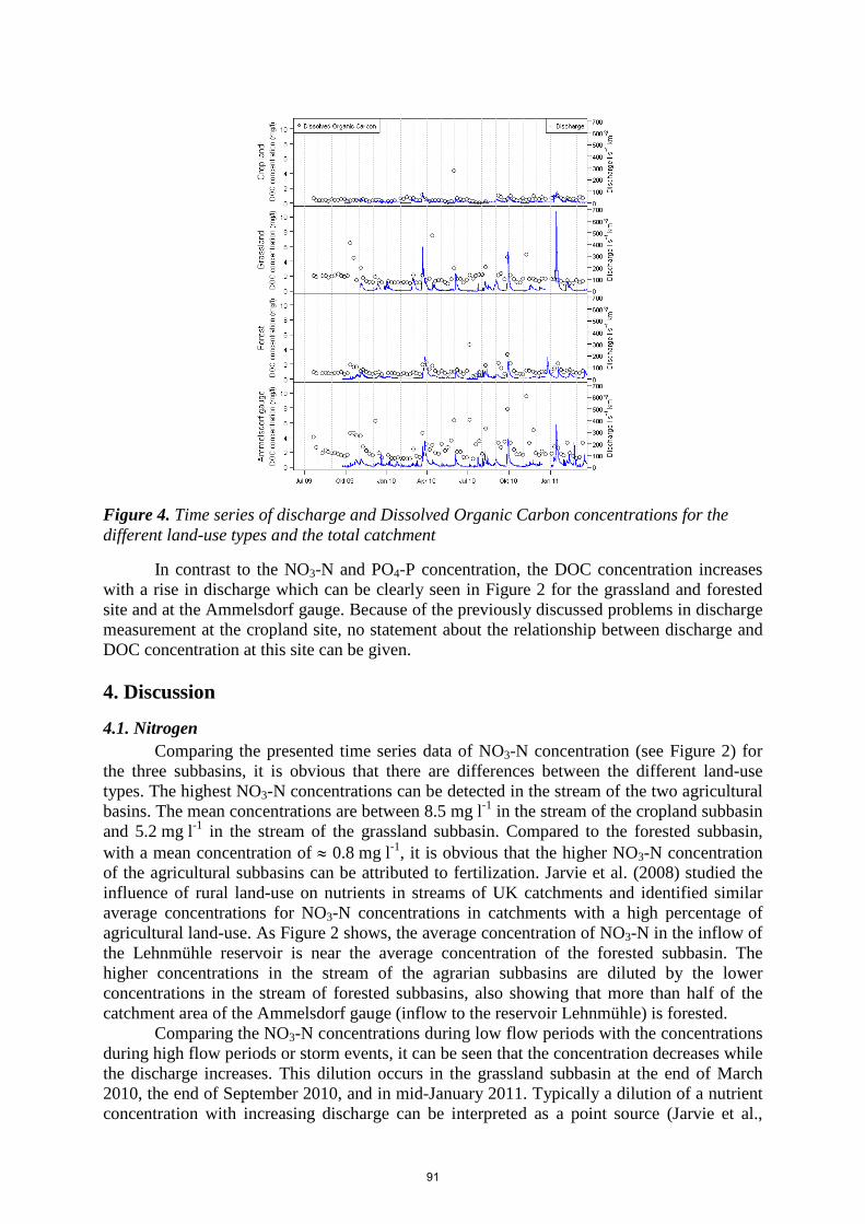
Figure 4. Time series of discharge and Dissolved Organic Carbon concentrations for the different land-use types and the total catchment

In contrast to the NO3-N and PO4-P concentration, the DOC concentration increases with a rise in discharge which can be clearly seen in Figure 2 for the grassland and forested site and at the Ammelsdorf gauge. Because of the previously discussed problems in discharge measurement at the cropland site, no statement about the relationship between discharge and DOC concentration at this site can be given.

4. Discussion

4.1. Nitrogen Comparing the presented time series data of NO3-N concentration (see Figure 2) for

the three subbasins, it is obvious that there are differences between the different land-use types. The highest NO3-N concentrations can be detected in the stream of the two agricultural basins. The mean concentrations are between 8.5 mg l-1 in the stream of the cropland subbasin and 5.2 mg l-1 in the stream of the grassland subbasin. Compared to the forested subbasin, with a mean concentration of ≈ 0.8 mg l-1, it is obvious that the higher NO3-N concentration of the agricultural subbasins can be attributed to fertilization. Jarvie et al. (2008) studied the influence of rural land-use on nutrients in streams of UK catchments and identified similar average concentrations for NO3-N concentrations in catchments with a high percentage of agricultural land-use. As Figure 2 shows, the average concentration of NO3-N in the inflow of the Lehnmühle reservoir is near the average concentration of the forested subbasin. The higher concentrations in the stream of the agrarian subbasins are diluted by the lower concentrations in the stream of forested subbasins, also showing that more than half of the catchment area of the Ammelsdorf gauge (inflow to the reservoir Lehnmühle) is forested.

Comparing the NO3-N concentrations during low flow periods with the concentrations during high flow periods or storm events, it can be seen that the concentration decreases while the discharge increases. This dilution occurs in the grassland subbasin at the end of March 2010, the end of September 2010, and in mid-January 2011. Typically a dilution of a nutrient concentration with increasing discharge can be interpreted as a point source (Jarvie et al.,

91

2008). In this case it is not possible to identify a point source as the source for the NO3-N effluxes. 4.2. Phosphorus

The measured values of PO4-P in the streams of the subbasins and the Ammelsdorf gauge indicate that the concentration of PO4-P in streams is higher when fertilizers are applied to the soils in the catchment area. In Figure 3, the time series of discharge and PO4-P concentration in the streams are presented. When one compares the cropland or grassland subbasins to the forested subbasin there are obvious concentration differences. While the average concentration for the subbasins under agricultural land-use is ≈ 15.8 µg l-1 the average concentration for the forested subbasin is ≈ 1.8 µg l-1, much lower. These results are in agreement with results of Jarvie et al. (2008) and Sharpley & Syers (1979). They observed that the P loads in fertilized watersheds compared to non-fertilized watersheds are higher and diffuse sources from agricultural sites are the main contributors of long-term P loads in basins. For the cropland and grassland subbasins, the concentration of stream PO4-P decreases with increasing discharge. This behavior is typical for diffuse sources while increasing concentrations in streams during increasing discharge is typical for point sources (Jarvie et al., 2008; Edwards & Withers, 2008). The stream PO4-P concentration increases with increasing discharge at the Ammelsdorf gauge. This indicates that there are point sources in the catchment area. 4.3. Dissolved Organic Carbon

While the highest NO3-N and PO4-P concentrations can be identified in the subbasins with agricultural land-use, the highest DOC concentrations can be detected in the stream draining the total catchment (Ammelsdorf gauge). This is due to the fact that part of the stream originates from wetland and peatland areas on the upland plateau of the Eastern Ore Mountains both on the German and the Czech sides. The low DOC concentrations of the forest subbasin can be explained by the fact that this subbasin has well-drained (terrestrial) soils without the influence of wetland or peatland areas.

The graphs in Figure 4 show that there is a relationship between DOC concentration in the stream and discharge. High discharge correlates with higher DOC concentration as can be seen in April 2010, October 2010 and January 2011. Thus, the DOC concentration is positively correlated with the discharge. Also Raymond and Saiers (2010) and Ågren et al. (2010) reported higher DOC concentrations during storm events causing higher discharge. They identified that the bigger portion of DOC is transported to the stream when discharge rises. A positive correlation between DOC concentration and discharge is evidence for diffuse sources as DOC sources.

5. Conclusions

The results presented indicate that the export behavior of the nutrients NO3-N, PO4-P

and DOC is different for each of the three land-use types of cropland, grassland and forests. The highest exports of NO3-N and PO4-P occur under agricultural land-use. While the NO3-N exports can be characterized as diffuse sources, the characterization of the PO4-P exports varies depending on the scale considered. On the plot scale (cropland and grassland subbasins) the export is qualified as diffuse source while on the scale of the total catchment (at the Ammelsdorf gauge) point sources appear to control the PO4-P export. DOC contributions to streams clearly originate from point sources. The tributary to the Lehnmühle drinking water reservoir can be certified as rather good quality because no substance concentration achieved critical values.

92

The previously mentioned results will be used to parameterize the SWAT model to assess the water quality and quantity under current climate conditions and under future climate change scenarios. At present, the experimental results reveal a clear land-use-specific behaviour in the effluxes to streams. This has to be reproduced in the model. For example, when considering water quantity, forests have a higher infiltration capacity than cropland or grassland which leads to lower discharge throughout flood events and consequently higher storage of water in the forest soils. With respect to water quality, the use of fertilizer for increasing crop yield tends to result in higher nutrient concentrations in the draining stream water. Therefore, changing management practices in the agricultural companies as well as changes in land-use distribution will clearly affect water quality. Hence, the underlying chemical and physical processes have to be parameterized quite well in the SWAT model at the scale of Hydrologic Response Units (HRUs) or subbasins. For this purpose, the collected experimental data will be highly useful. Acknowledgements This study is part of the REGKLAM project “Development and Testing of an Integrated Regional Climate Change Adaptation Programme for the Model Region of Dresden” financed by the German Federal Ministry for Education and Research (01LR0802B). References Agren, A., M. Haei, S. J. Köhler, K. Bishop, and H. Laudon. 2010. Regulation of stream water

dissolved organic carbon (DOC) concentrations during snowmelt; the role of discharge, winter climate and memory effects. Biogeosciences. 7(9). 2901-2913.

Arnold, J. G. and N. Fohrer. 2005. SWAT2000: current capabilities and research opportunities in

applied watershed modelling. Hydrological Processes. 19(3). 563-572. Arnold, J. G., R. Srinivasan, R. S. Muttiah, and J. R. Williams. 1998. Large Area Hydrologic

Modelling And Assessment Part I: Model Development. Journal Of The American Water Resources Association. 34(1). 73-89.

Borken, W. and E. Matzner. (2008). Reappraisal of drying and wetting effects on C and N

mineralization and fluxes in soils. Global Change Biology. 15(4). 808-824. DIN-EN-ISO-6878. 2004. Wasserbeschaffenheit – Bestimmung von Phosphor – Photometrisches

Verfahren mittels Ammoniummolybdat. Edwards, A. C. and P. J. A. Withers. 2008. Transport and delivery of suspended solids, nitrogen and

phosphorus from various sources to freshwaters in the UK. Journal of Hydrology. 350(3-4). 144-153.

IPCC. 2007. Climate Change 2007 : Synthesis Report. Contribution of Working Groups I, II and III to

the Fourth Assessment Report of the Intergovernmental Panel on Climate Change. (p. 104). Geneva. Switzerland.

Jarvie, H. P., P. J. A. Withers, R. Hodgkinson, A. Bates, M. Neal, and H. D. Wickham. 2008.

Influence of rural land use on streamwater nutrients and their ecological significance. Journal of Hydrology. 350(3-4). 166-186.

Raymond, P. A. and J. E. Saiers. 2010. Event controlled DOC export from forested watersheds.

Biogeochemistry. 100(1-3). 197-209. Sharpley, A. N. and J. K. Syers. 1979. Phosphorus inputs into a stream draining an agricultural

watershed. Water Air and Soil Pollution. 11(4). 417-428.

93

Bernhofer, C., J. Matschullat and A. Bobeth. 2009. Das Klima in der REGKLAM-Modellregion

Dresden. 1st ed. Berlin. Rhombos-Verlag.

94

Cost-Effectiveness Analysis for Controlling Water Pollution by

Pesticides using SWAT and Bio-Economical Modeling

J-M Lescot(1)*, P. Bordenave(1), K. Petit(1), O. Leccia(1), J.M. Sanchez-Perez(2,3), S. Sauvage(2,3), J.L. Probst(2,3)

(1) Cemagref, Agriculture and Rural Areas Dynamics Research Unit; 50, avenue de Verdun, Gazinet, 33612 Cestas cedex, France. E-mail: jean-marie.lescot@cemagref.fr

(2) University of Toulouse; INPT; UPS; Laboratoire Ecologie Fonctionnelle et Environnement

(EcoLab); avenue de l'Agrobiopole BP 32607 Auzeville Tolosane 31326 Castanet Tolosan cedex, France

(3) CNRS; EcoLab; 31326 Castanet-Tolosan cedex, France.

Abstract The EU Water Framework Directive requires policy to address non-point source pollution as part of an overall integrated strategy to improve the ecological and chemical status of water bodies. Farmers and taxpayers would benefit from more cost-effective control measures adequately implemented within watersheds. With this objective, we propose a framework for a spatially-distributed cost-effectiveness analysis of some mitigation measures (buffer strips, longer rotations, mechanical weeding and catch crops) included in agri-environmental programs of rural development plans. We used the SWAT model to assess the effectiveness of the applied measures, and we developed an aggregated bio-economic model using GAMS to evaluate the costs of implementation, identifying synergies and trade-offs. Finally, we proposed a ranking of these measures based on their cost-effectiveness ratios and, for each measure, a map of cost-effectiveness ratios by subbasin within the watershed. This approach is applied to the upper stream region of the Gers river basin in southwestern France. Findings clearly demonstrate that some measures, like grass strips and mechanical weeding, could be considered as the most cost-effective measures allowing reduction in pesticide concentration up to 65%. Other measures, such as longer rotation sequences and catch crops, although they appeared less costly to implement, fall short in reducing pollution by pesticides with much higher cost-effective ratios. Possibilities and problems for integrating the SWAT model and bio-economic modeling with spatial and temporal scale issues are discussed along with the use of this integrated framework as communication tools in participatory river basin management. Keywords: cost-effectiveness analysis, SWAT, bio-economic modeling, pesticides, mitigation measures

95

1. Introduction Over the last few decades, intensification of agricultural practices has led to a

widespread use of pesticides in parallel with the growing use of fertilizers. This use has resulted in pollution of soil and water via spray drift, dispersal of pesticides into the soil, and runoff during or after cleaning of equipment or via uncontrolled disposal. Protection of surface water quality in respect to pollutants requires measures be taken to reduce if not eliminate emissions, discharges and losses of pesticides. To combat problem of waters pollution, the European Union (EU) has launched several regulations and directives such as the Nitrate Directive (91/676/EEC), the Water Framework Directive (2000/60/EC) and recently the Pesticide Directive (2009/128/EC). Compliance with the Water Framework Directive (WFD) implies a reduction in the impact of agricultural pressures. Furthermore, public participation in water management required by international conventions (United Nations, 2000; Aarhus Convention, 1998; World Water Commission, 2000; WFD, 2000) should be meaningful when issues are complex and uncertainties high.

Moreover, characteristics of agricultural production such as soils, slopes, farming systems and proximity of streams may differ across a catchment from one place to another within river subbasins. Agri-environmental measures defined at national or more recently at regional levels can lead to extremely different results in terms of implementation costs and environmental effectiveness. In addition to these uncertainties, government and water agencies have to manage limited budgets allocated to the implementation of measures. Questions arise about how to use available funds in an effective and relevant way. Cost-effectiveness (CE) analysis could then help to choose between measures considered as effective for the reduction of water pollution or erosion. Although literature demonstrates that targeting has been shown to improve the effectiveness of non-point source (NPS) pollution control by focusing on critical areas (Dickinson et al., 1990), implementation costs for these areas need nevertheless to be considered and a CE analysis of implementing measures only on most sensitive or vulnerable areas should first be carried out. We illustrate in this paper how the use of modeling tools for analyzing the different impacts and costs of environmental policy measures could help evaluate their relative interests as a function of the characteristics and opportunities of the territories of a catchment.

2. Methodology - Simulation and Assessment of the Scenarios

CE analysis is a decision-support tool that could help identify economically efficient

ways to fulfill the objective of reducing water pollution (Pearce et al., 2007) and could be a suitable approach for evaluating mitigation measures for NPS pollution where measurement of intangible benefits is difficult and uncertain. Finally, CE analysis is particularly useful for comparing two or more measures and has been used in watershed management for the selection and placement of BMPs for nutrient management (Bonham et al., 2006) and pesticide control (Maringanti et al., 2008). Most studies (Gitau et al., 2004; Maringanti et al., 2008) that are developed for determining cost-effective farm or watershed-level scenarios through optimization techniques incorporate a genetic algorithm, the SWAT model and a BMP tool. Combination of initial pollutant loadings from SWAT with literature-based pollution reduction efficiencies and costs are used to determine cost-effective watershed scenarios.

96

The framework proposed (Figure 1) is a bottom-up approach focusing on the cost of implementing measures at the field, subbasin and watershed level while assessing environmental effectiveness at the subbasin and watershed level. Bottom-up approaches, which consider proximate decisions taking place at the local or regional level, are important to adequately reflect the relevant actors and factors of agricultural land use (Busch, 2006). Feedback on the use of models as policy support tools for stakeholders, particularly decision-makers, is another important issue in land cover change modeling (Verburg et al., 2001) and participatory river basin management (Welp, 2001).

Figure 1. Cost-Effectiveness Analysis framework

If the subbasin and/or watershed level are suitable scales for an effectiveness

assessment, calculation of costs is carried out first on the commune level (the lowest French administrative level) because of data availability. Costs are then assessed on the watershed level by allocating the costs proportionally to the acreage of the commune within each subbasin. The different steps of the integrated approach are further described in Figure 2. 2.1. Appropriate time horizon for integration

The effectiveness of remediation measures can be assessed with regard to intermediate goals by the use of pressure indicators (pressure reduction) or final goals with assessment of impacts on water pollution using hydrological models. As results rather than mitigation measures are now set (WFD, 2000), the impacts of mitigation measures need to be evaluated. Hydrological modeling offers the possibility of assessing impacts over a long period of time covering several years of measure implementation. Another point to be stressed is the cause and effect delay between catchment response and sub-river response to measure implementation. The effectiveness of measures should then be assessed over a long period with measures being applied each year (Roa-García and Weiler, 2010; Gascuel-Odoux et al., 2010). The costs of measure implementation are assessed on a yearly basis with reference to the implementation year prices for inputs and outputs and are then aggregated over 25 SWAT-simulated using the discounted sum of yearly costs. 2.2. Agri-environmental measures

Within the framework of rural development policy, agri-environmental schemes were introduced into EU agricultural policy as an instrument for supporting specific farming practices that help to protect the environment and maintain the countryside. The main promoted measures are crop rotation, soil winter cover and catch crops (which limit leaching, runoff and erosion during the wet seasons), the "buffer" effect of non-fertilized grass strips along watercourses and ditches, good management and restriction of cultivation on steeply sloping soils. Such measures initially considered for limiting soil erosion and nitrate pollution may also reduce pesticide pollution. Measures presented here address mainly the switch to good agricultural practices and have been chosen according to the following criteria: (a) effectiveness on water quality issues related to pesticides, and (b) most widely implemented within the upstream area so far. However, other issues like erosion or Nitrogen leaching, as gathered from meetings with stakeholders, are most likely to be accepted and implemented by farmers (Table 1).

Scenarios Measure or combination of measures

Economic component Mixed Integer Linear Programming model

(Commune level)

Targeting action programmes

Cost assessment of implementing measures

(Commune then sub river basin level)

Spatially distributed Cost Effectiveness Analysis of scenarios at the sub basin level

Stakeholders Acceptability

Up scaling at common geographical scale

Environmental component SWAT Model (Soil and Water Assessment Tool model) (Management practices defined at the commune level)

Effectiveness of mitigation measures on reduction of pesticides concentration in the outlets

(Hydrologic Response Unit then sub river basin level)

97

2.3. Monetary compensation for implementation of measures

Farmers who commit themselves to adopting environmentally-friendly farming techniques for a five-year minimum period receive payments in return that compensate for the additional costs and loss of income arising as a result of modified farming practices. Administrative monetary compensation calculations are mainly based on budgeting considerations with a constant compensation rate per hectare. Therefore a whole-farm analysis is used for cost assessment because many practices and consequently measures that appear profitable in a single analysis may prove less attractive when analyzed as part of the whole-farm system (Feuz and Skold, 1991). Furthermore, consideration of only a limited number of budgets may unrealistically restrict substitution possibilities. The economic optimization methodology is thus expected to reveal more favorable trade-offs between farm incomes and water quality in comparison with budgeting techniques. 3. Case Study Catchment

The Gers river basin is a subbasin of the Garonne River basin situated in the South-western part of France (Figure 2). The Gers catchment drains an area of 1,230 km2 and is 176 km long. The region stretching from South to North has a hilly landscape and is interspersed with a total of 17 small rivers and streams (Côteaux de Gascogne zone of 9,000 km²) which, because of morphological structure, have only extremely small water catchment areas. Hydrological processes are characterized by superficial water transfers fed by shallow water tables with limited capacity. Water flow would not be possible all year round under normal conditions, and to improve the availability of water, a link canal (the Neste canal) has been created both for agricultural purposes and for drinking water supplies.

Dem

Land use

Soils

Practices Definition of typical crop rotations for communes of the watershed Principal Components Analysis (PCA) and Cluster Analysis (CA) to identify communes with homogeneous characteristics with respect to the production activities in terms of land use (crops) and practices (management sequences). Analyses are performed for all the 1,385 communes of the Midi-Pyrenees region.

PCA is used to simplify land use in order to reduce the number of variables (crops) and detect structure in relationships between variables. Cluster analysis then is performed for the first three factor axes of the PCA, explaining 59% of the variance. From the tree clustering analysis we obtained 11 classes of crops rotation.

Application of the GenLU model for SWAT modeling The GenLU model creates tables with practices (SWAT tables mgt1 and mgt2) for each HRU from average practices by crops constituting the crop sequence.

98

Defining scenarios Measure or combination of

measures defined by stakeholders and

water agency

SWAT modeling Effectiveness assessment at the sub-watershed level Average concentration over the ten last years of hydrological simulation Baseline concentration

Bio-economic modeling Calculation of direct cost of implementing measures Max Z= f(x)

2, , , , ,( ) ( * * )c i p k c ipk i i p k ki p k

f X X y p cv inc= − + +∑∑∑

, , , ,* *l p c l p l l pl p

X y p cv−∑∑

For all c

with c: commune (commune with at least 10% of its area within the watershed) i: crop activity l: livestock activity p: level of practice intensiveness (intensive, average, extensive) k: standard practices k1 or with agro environmental measure k2 Xipkc: acreage of the activity for crop i, intensiveness p and practice k (ha)within the commune c yipk: yield of the activity [ton grains or dry Matter ha-1] by crop, level intensiveness and type of practice pi: price for crop I (€ ha-1), pl: price for meat or milk (€ kg-1) cvi,p,k: variable costs of production by crop, level intensiveness and type of practice (€ ha-1) inck: incentive needed to have the activity with agro environmental measure k adopted (€ ha-1)

Mapping subbasin CE ratios dispersion

Comparing agri-environmental measures according to their costs and effectiveness

0

500

1000

1500

2000

2500

3000

0 0,2 0,4 0,6 0,8 1 1,2 1,4

Total concentration mgl-1(outlet)

Tota

l Cos

ts (K

€)

BS10_ZP_ext (2) BS20_ZP(2) BS20_ZP_ext (3) MW_ZP (61) LR_ZP(1537)CC_ZP(474) BS20_GA (7) MW_GA (37) LR_GA (1435) CC_GA (538)

Figure 2. Main steps of the methodology applied for the CE analysis of mitigation measures

This canal, fed by storage dams in the Pyrenees mountains, carries water both to the river Neste and to the head of the other small rivers, amongst which is the Gers river. It thus provides minimum flows of water even during the time of the year when these rivers would normally run dry. In addition to an absolute minimum flow of 4 m3s-1, the cumulative total of a further 5 m3s-1 (6.5 m3s-1 in autumn and winter) has to be maintained in the re-supplied streams and rivers at the point of entry into the Garonne in order to sufficiently dilute the sewage waste released from cities.

The area of the catchment considered here is restricted to the upstream part of the Gers river basin (UGRB) which stretches from the springs of the Gers river on the Lannemezan plateau down to the Roquelaure drinking water intake point which constitutes the outlet of the watershed studied. The UGRB covers 470 km² mainly dedicated to agriculture (72% of the area) with maize for grains or silage, spring and winter wheat, durum wheat, sunflower, permanent and temporary grassland as main crops. Soils types are of different characteristics such as alluvium, colluviums, loamy clayey soils and clayey soils. Pollution by pesticides is a matter of great concern as 65% of water quality controls show at least one pesticide molecule with concentrations higher than the EU drinking water standards1 for individual pesticides (0.1 µgl-1).

1 We can notice that the value of 0.1 µgl-1 is a substitute for zero, not present in water or below the detection limit and that the parametric values for individual pesticides (0.1 µg.l-1) and for total pesticides (0.5 µg.l-1) are not based on any scientific findings, the WHO using a different approach with set guideline values for a large number of individual pesticides. All pesticides that are officially registered for use and are likely to be used in the watershed area should then be monitored and the total sum calculated by adding all concentrations that exceed the parametric value/detection limit of 0.1 µg.l-1. It is

[ ][ ]

-1

-1

s μgl(%)

0 μgl

CEffectiveness = 1 - × 100

C

[ ] -10 μglC

[ ] -1s μglC

99

4. Effectiveness Assessment using the SWAT Model It is expected that the use of model results would be an objective source of information on the short and long-term impacts of agro environment measures that can be used to support decisions. The effectiveness of mitigation strategies is assessed using the semi-distributed river basin Soil and Water Assessment Tool (SWAT) model (SWAT 2005). This model is considered as one of the most suitable models for predicting long-term impacts of land management measures on water sediment and agricultural chemical yield in large complex watersheds with varying soils, land use and management conditions (Arnold and Fohrer 2005; Neitsch et al., 2005). SWAT model was chosen for its ability to simulate stream pesticide concentration at the watershed scale, its worldwide use and its potential to simulate agricultural management practices. The comparison of effectiveness is considered in terms of the relative reduction in a particular pollutant (main herbicides and fungicides used for cereals, maize and sunflower within the basin) following measure implementation. Concentrations reduction are calculated from the SWAT main channel output file (.rch)

Average concentration over the ten last years of hydrological simulation Baseline concentration

Effectiveness of the measures is assessed first when the measures are applied to the whole UGRB and second, for some measures, only in priority zones (defined for their vulnerability2). The effectiveness of measures is assessed over a period of 25 years with measures being applied each year and we retained the average values of pesticide concentrations calculated on the ten last years basis for the modeling period. 5. Model Setup The current situation (Scenario 0) considered as the baseline scenario is first defined assuming that the compulsory measure of 10 meters width buffers strips is set within the watershed. Scenarios are then assessed by difference with this baseline scenario. From tables relating to Scenario 0 implemented in Access model databases (SWAT2005.mdb) and Access base dedicated to the project, scenarios for simulations are built with a software developed by Cemagref-Adbx research unit. 5.1. Management practices SWAT models physical processes only once for each unique portion of the watershed determined by the hydrologic response units (HRU) which are defined by coincidence of soil type and land use. Each subbasin of the watershed is divided into HRUs. In addition to physical processes are modeled crops rotations, irrigation, fertilizers application, pesticides spraying, tillage, harvesting. Only one management inputs file is defined by HRU which is the smallest unit used to simulate at a daily time step, all the processes of the simulation. In parallel, we identified and characterized homogeneous cropping and management inputs through standard management sequences. When shifting from crops to rotation, timing of management sequences are adapted with respect to the preceding and following crops. Sources of input data used to develop the SWAT input files are diverse. A Digital Elevation Model (DEM) from IGN (National Geographic Institute) with a 25 meter (82 feet) grid cell

therefore not possible to answer the question of how many pesticides should be considered in total as this will vary between watershed areas and could add up to hundreds of pesticides. 2 Critical area is usually defined as the most sensitive or vulnerable area within the watershed that gives the largest contribution to water pollution. Soil types identified as presenting high risks of leaching and/or runoff of selected pesticides will be classified as critical areas. Vulnerability is then crossed with pressure indicators (number of pesticides applications) to define priority zones where actions are carried out for remediation. Have been used the priority zones defined initially by the Adour-Garonne Water Agency.

[ ] -10 μglC

[ ][ ]

-1

-1

s μgl(%)

0 μgl

CEffectiveness = 1 - × 100

C

[ ] -1s μglC

100

size is used with the European Corine Landcover 2000 Database for land use/cover of the area. Further more detailed information on land cover is obtained from the 2000 General Agriculture Census for communes and from classified Landsat satellite pictures. The initial hydrographic network from the Carthage National database is recorded into ArcView to create a more accurate network (extended network with streams and ditches) which has been used for scenarios assessments. Soils from digitalized soil maps (at 1/250000 scale) associated with a physical and chemical database of soil properties is provided by the IGCS (Inventaire, Gestion et Conservation des Sols) from INRA (French National Institute for Agricultural Research). Daily weather values come from the nearby Auch weather station managed by Meteo France. Information on practices comes from regional references provided by the Regional Agricultural Council (Chambre d’Agriculture de Midi-Pyrénées) and Farm Management Centre (Centre de Gestion Conseil Gascogne Adour). Before its use in input data files, information on practices is first compared for validation with local farmers’ practices (quantities and timing of cultivation and spraying practices) either through surveys carried out within the area either by expertise. Because of the lack of exhaustive data within zones of the catchment, we first used a combination of Principal Components Analysis (PCA) and Cluster Analysis (CA) to identify areas with homogeneous characteristics of identified crop rotations. For SWAT modeling, these crops rotations were further improved using a model developed by Cemagref in Visual basic named hereafter GenLU. This model defines typical crop rotations from land cover data by applying agronomical decision rules. Crops sequences are defined by sorting possible rotation crops as rotation head such as dominant cereals, secondary cereals with a probability that a crop follow to itself. A second decision rule tables gives the expected number of years a crop could succeed to itself e.g. 4 for rape, 1 for maize, 1 for wheat and barley etc. By applying a random spatial function, GenLU produces as many HRUs as there are different types of crop rotations. For costs calculation, we took into account only the principal rotation identified for each commune and considered that it was applied on the whole cultivable area of the commune.

The GenLU model creates tables with practices (SWAT tables mgt1 and mgt2) for each HRU from average practices by crops constituting the crop sequence (consecutive series of crops over two or more years on the same field). Furthermore, spreading applications over many different days within the growing period as opposed to lumping them into a single application within each subbasin, results in significantly better simulations (Winchell et al., 2005). Dates of management practices are then generated randomly from identified average values. Practically, if it is difficult to have detailed information on practices such as e.g. dates of fertilizer applications or pesticides spaying, it is easier to get information about the average periods of these operations on a given zone. File created by GenLU is a raster file type (.asc) that is used further in the SWAT model as a Landuse file to define the HRU by crossing layers. The table created (table mgt1) is afterward used by the GenLU model to produce the cultivation practices tables (tables mgt2) with the dates of sowing, of fertilizers and applications, of tillage, of grazing) for each crop of the crops sequence. Tables mgt1, mgt2 and HRU are then used for deducting simulations either by using either the GenLU model either the SWAT functions, either by changing properties of crops, fertilizers, pesticides in the main input database of SWAT. GenLU is applied on every zone defined as agricultural zone. As far as no specific problems on point source (PS) pollution are reported on the watershed, only agricultural NPS pollution was taken into consideration. In addition, we can consider that application of the new Pesticides Framework Directive will considerably limit PS pollution and allow extensive responsible uses. With regard to the pesticides, we identified the chemicals used by farmers within the watershed and the timing of their application. We retained the most frequently used active substances with their average application rate for defining standard management sequences.

101

Besides, we need to mention that average practices do not take account of excessive use of pesticides which is any case difficult to assess. Calibration and verification were carried out with data from the current measurement points network managed by the Water agency, from potable water supply intakes when available and from measurement points on experimental watersheds managed by Cemagref (Rebx and Adbx research Units). Verification was carried out on the other following parameters: yield and Nitrogen uptake of catch crops, Nitrogen cycle and balance, pesticides balance, specific flow of suspended solids. Model calibration has been performed on average crops yield from agricultural surveys. The scenarios (Table 1) assessed are the following: Grass buffer strips with different variants depending of the strip width (10 m and 20 m), the area where measures are applied - the whole upstream area or only on targeted zones (ZwP) and based either on the IGN hydrographical network either on the extended hydrographical network (Scenario 1); switching from chemical weeding to mechanical weeding with no herbicides application and three tillages during the growing period (Scenario 2); modification of crop rotation schemes with longer rotation and a succession of four crops minimum (Scenario 3); catch crop during the inter-crop period with sowing of rye-grass (Scenario 4); switching from arable land to temporary grassland (Scenario 5). Table 1. Scenarios with measures and implementation with the SWAT and bio economic models

applied only on zones with

priority

applied on the whole upstream

area

1 Riparian buffer strips:Grass strip with rye-grass.

1.1 Buffer strips width 10m: 5meters on either side of the watercourse. Basis line scenario.

1.2* BS10_ZP_ext* BS 10_GA_ext Buffer strips width 10meters extended

hydrographical network.

1.3 BS20_ZP* BS20_GA* Buffer strips 2x10meters (BS 2x10m).

1.4* BS20_ZP_ext* BS20_GA_ext Buffer strips 2x10meters extended (BS

2x10m_ext).

2 MW_ZP MW_GASwitching from chemical weeding to mechanical weeding. No herbicides application and tillage.

Modification of management parameters.

Modification of parameters: inputs + technical practices

Y LR_ZP LR_GAModification of crop rotation schemes (longer rotation with succession of 4 crops minimum).

Modification of management parameters.

Possibility for introducing news crops in rotation sequence and new constraints

4 CC_ZP CC_GACatch crop during the inter-crop period (sowing of ryegrass between winter crops and spring crops).

Modification of management parameters.

Modification of parameters: inputs + technical practices to sequence with bare soils

5 SGL_ZP* SGL_GAIncrease of grassland/ decrease of arable land. Switching from arable land (maize, wheat…) to temporary grassland (rye grass).

Modification of the land use files (shape-files). Changes of crop activities

Implementation in the bio economic model

New activity limited to the area concerned

Modification of the land use files (shape-files): Design of new polygons alongside the hydrographical network (Arc-GIS Buffer command) and accordingly modification of the parameter FILTERW .

Scenario

Measures applied

Description Implementation in the SWAT model

* Variants of the measure which have not been assessed; ext: Extended Hydrographical Network

Before calibration and validation of the SWAT model, manual sensitivity analysis is carried out using a method similar to the one proposed by Ulrich and Volk (2009). The most sensitive parameters are CN2, USLE-P and FILTERW. These parameters are calibrated by comparison with measurement data on the watershed (water flows, sediment loading, pesticide flows) at four points of measurement. In urban zones, we took weeding practices into account with information from surveys and local maintenance department and made changes on the impermeability of the soil surface layer relating to these zones.

102

5.2. Modeling water flow

0

20

40

60

80

100

120

1995-10-0

1

1996-09-3

0

1997-09-3

0

1998-09-3

0

1999-09-3

0

2000-09-2

9

2001-09-2

9

2002-09-2

9

2003-09-2

9

2004-09-2

8

2005-09-2

8

Date

Spec

ific d

ischa

rge Q

s (l/s/

km²)

SWAT Measured Data

Figure 3. Simulated and observed specific discharge on a daily time step

0

200000

400000

600000

800000

1000000

1200000

1400000

1600000

1800000

2000000

10/1/19

95

9/30/19

96

9/30/19

97

9/30/19

98

9/30/19

99

9/29/20

00

9/29/20

01

9/29/20

02

9/29/20

03

9/28/20

04

9/28/20

05

Date

Disc

harg

e Q

(m3 )

SWAT Measured Data

Figure 4. Simulated and observed cumulative flows (calibration: 1985-1995, validation: 1995-2005)

The SWAT model was calibrated and validated using observed discharge data. Simulated and observed discharge are reported in Figure 3 and evaluation of the model performance by the coefficient of determination (R²) and the Nash-Sutcliffe Index (NSI) in Table 2.

Irrigation water needs calculated with SWAT are considered and quantities of water withdrawal validated in comparison with data surveys on irrigation water applied (doses and frequencies).

Nevertheless, uncertainties in the actual irrigation doses and in low water management by water supplies from the Neste canal remain. Only the yearly amount of water supply available from CACG reports has been considered. These uncertainties could explain discrepancies in daily simulated and observed values (Figures 3 and 4).

Table 2. Simulated versus observed statistics for the Gers river validation and calibration Calibration period

(1985 to 1995) Validation period

(1995 to 2005) R² 0.80 0.72 NSI 0.65 0.63 Specific discharge Qs (liter per second per square km)

Measured Qsobs 5.44 l/s/km² Simulated (Swat) Qscal 5.40 l/s/km²

5.3. Modeling pesticides runoffs

From a survey carried out on 50 farms within the UGRB area, we drew up for each crop (soft wheat, durum wheat, sunflower, rape and soya) the set of active substances applied as well as the frequency of their use. In order to reduce time calculation for assessing the effectiveness, we first reduced the number of active substances to the most widely used molecules, keeping the average dose (arithmetic mean) applied by farmers.

103

Pesticides concentration measured in 2006 - Roquelaure measurement point

0,00

0,50

1,00

1,50

6 April 26 April 2 May 17 May 30 May 13 June 28 June 12 July

Pes

tici

de

con

cen

trat

ion

(mg

/l)

Bentazone Triclopyr total subsitued urea (4)total aryloxy acid (3) total amides/chloroacetamides (4) total sulfonylurea (1)total triketone(2) total triazines (2) totalglyphosate + derivatestotal carbamates (2)

Figure 5. Pesticides concentrations at the outlet of the UGRB (2006)

Pesticides concentration measured in 2007 - Roquelaure measurement point

0,0

0,5

1,0

1,5

2,0

2,5

12 Febr. 5 April 18 April 2 May 15 May 30 May 12 June 27June 9July

Pes

tici

de

con

cen

trat

ion

(mg

/l)

total triazoles (5) total subsitued urea (4) total aryloxy acid (3)total amides/chloroacetamides (4) total sulfonylurea (1) total triazines (2)totalglyphosate + derivates total carbamates (2) TriclopyrMetalaxyl Bentazone Aclonifen

Figure 6. Pesticides concentrations at the outlet of the UGRB (2007)

When a chemical class is widely applied (fungicides of the sulfonylurea, triazole and strobilurin groups or herbicides with a mix of three or four active substances), we defined a new “average active ingredient” (AAI) for its physical and chemical properties (Koc3, DT504 and solubility) weighted for a mix of active substances by their relative concentration in the pesticide used. Similarly, we defined an average application rate, calculated as the average application rate weighted by its frequency of use. The number of molecules applied to consider drops then from 60 to 15. Moreover, water analysis show that four molecules represent 80% of the total pesticide concentration (Figures 5 and 6). These are herbicides (Glyphosate, S-Metolachlor), insecticides (Carbofuran) and fungicides from the triazole group (Tebuconazole). Simulations are carried out for each of these four AAIs and the sum of their daily SWAT-simulated concentrations used as results. Spraying practices within the watershed are compared to the average practices set at the regional scale from a much wider sample of farms.

5.4. Verification/calibration of pesticides

Concentrations of pesticides have been analyzed at four measurement points alongside the river Gers within the program “Action test Gers-Amont”. Within the framework of

3 Sorption coefficient normalized to organic carbon content. 4 Time for 50% decline of the initial pesticide concentration.

104

another study, water analysis for 15 measurement points have been carried out on the main rivers of the Gascogne Côteaux zone from 2005 to 2008 (Morin et al., 2009). The frequency of sampling (4 to 5 measurements per year) is nevertheless too low for precise daily or monthly calibration and/or validation in contrary to information related to inflows. Nevertheless, values have been used for verification of SWAT model calculations on the same points of the streams by comparing the ranking of the yearly in situ measured concentrations (sum of molecules) to the ranking of simulated concentrations. For this purpose, the SWAT model has been implemented on the whole Côteaux de Gascogne zone and calibrated in order to reproduce total yearly pesticide concentration (1.2 µgl-1) at the UGRB outlet (Roquelaure measurement point). We compared the relative ranking of these points in regards to their average yearly concentration alongside each stream of the area. If average simulated concentrations and measures differ sometimes heavily, the ranking of the simulated measurement points match exactly the ranking of actual measurement points for all points.

Differences between simulated and measured concentrations do not however imply that model calibration is wrong because of the uncertainty on the measurements themselves (related to their frequency and the number of values within a month and year). 6. Results for Effectiveness

SWAT simulation results show that, for the conditions prevailing in the upper stream of the Gers river, pesticide loss may be effectively decreased by implementing measures. For a given measure, effectiveness nevertheless varies widely between subbasins within the watershed (Figure 4). The best results (highest reduction) could be achieved by restoration measures, such as the creation of riparian grass buffer strips (Scenario 1). These measures do indeed have a significant effect on pesticide reduction in water streams, varying however when applied in priority zones or in the entire GA area (Table 3).

Model results are in accordance with results from previous studies by Smitt et al. (1999), Lacas et al. (2005), Popov et al. (2006) and Borin et al. (2010). A switch from chemical weeding to mechanical weeding (Scenario 2) could have an immediate effect on pesticide loads. The effect would be enhanced if the measure were applied to the whole upstream area (MW_GA). These results could be explained by the type of chemicals detected at high concentrations which are mainly herbicides (particularly Metolachlor and Glyphosate) or their metabolites. On the other hand, we can note the relative inefficiency of other changes in management practices, like the use of catch crops on bare soils (Scenario 3) or changes in crop rotation schemes (Scenario 4). These measures implemented on the upper stream area fall short in reducing pesticide concentrations in watercourses. The results are consistent with what is actually observed in areas of the watershed where these measures have been applied for a few years on already diversified farming systems without any changes observed in levels of pesticide concentrations in water analyses. Finally we can notice that the concentration objective of 0.5 µgl-1 is only reached for one scenario. Reaching the objective would require an effective combination of agri-environmental measures that need first to be assessed.

105

Table 3. Effectiveness analysis (SWAT Model simulation results), total costs and CE ratios Implementation Scenario Measures Total concentration

mgl-1(outlet)Effectiveness (% reduction)

Total costs (€) C(k€)/E ratios

1.21.2 BS10_ZP_ext 0.85 29 1021979 351.3 BS20_ZP 0.78 35 1002726 291.4 BS20_ZP_ext 0.72 40 1795194 452 MW_ZP 0.96 20 18136446 9073 LR_ZP 1.19 0.5 11372194 227444 CC_ZP 1.18 1 7012277 7012

1.21.3 BS20_GA 0.66 45 4601327 1022 MW_GA 0.38 68 37536281 5523 LR_GA 1.18 1 21238345 212384 CC_GA 1.17 2 15929465 79655 SGL_GA 0.66 45 125629621 2792

Measure applied on the zones with

priority

Basis line scenario

Measure applied on the whole area of the upstream part

Basis line scenario

*Relatively to baseline scenario (i.e. before implementing measures). Implementation of the measure BS10 (buffer strips of 5 meters on either side of the watercourses) is compulsory and therefore considered to be already implemented. **Sum of molecules (yearly average calculated from daily concentrations at the Roquelaure watershed outlet measurement point). Concentration for the baseline scenario: 1.2 µgl-1. 7. Cost Assessment Using Bio-Economic Modeling

The economic analysis aims at addressing the question of whether the program objective can be achieved in the most cost-effective way i.e. at the least cost. Because the marginal costs of mitigation measures are not equal, it is theoretically possible to obtain the same level of water pollution reduction at lower cost by shifting from expensive to inexpensive measures (Brouwer and De Blois, 2008). To resort to representative (in an average concept) or typical farms (in a modal concept) is usually the most satisfactory way of modeling farms5. However, this practice involves potential bias from aggregating farm-level data or using average or aggregate data at the farm level. This approach with a farm-scale economic simulation model (FEM model) is used in the economic component of the CEEOT_LP integrated modeling system (Osei, 2003), the environmental component consisting of the field-level agricultural policy/environmental extender (APEX) model (Gassman et al., 2010) and the SWAT model. FEM simulates annual costs and returns of proposed policy scenarios.

The economic budgeting approach may reflect real-word behavior, playing an important part for the farmer in the decision-making. Nevertheless, the major disadvantage is that budgets may not reflect efficient decisions from an economic perspective.

To derive a meaningful trade-off curve, all economic methodologies need to allow farmers the ability to interchange a variety of optional strategies into the decision-making framework (Lee, 1998). Failure to do so will may exacerbate the nature of trade-offs between water quality improvement and farm income. The methodology of economic optimization is more relevant for cost analysis of mitigation measures because of the possibility it offers decision-makers of substituting alternative strategies.

Moreover, using representative or typical farms leaves out the spatial distribution of holdings. The alternative form of aggregation we use that overcomes these problems involves modeling farms together as if they were a single mega-farm. Doing so may overstate the flexibility and co-ordination of agricultural production, but it is a widely-accepted means of modeling large areas (O'Callaghan, 1996) and may also be appropriate for small areas like communes. The model is developed in mixed integer linear programming using GAMS software (Brooke et al., 1988; MacCarl, 2009).

Because of data availability, assessment of costs was carried out on the commune level frequently representing a small number of farms, but further research should focus on 5 The types of data required and the analysis performed, as well as the interpretation of the results, are considerably different for a typical farm (in a modal concept) compared to a representative farm (in an average concept).

106

methods allowing calculation of costs at the HRU level. The objective is to maximize the Total Gross Margin on the commune level for crops and livestock activities (Figure 2). Ratios between outputs and inputs are assumed to be constant (deterministic model) as are their prices, using their mean value for the current year. Agri-environmental measures are introduced into the bio-economic farm model either as new activities (riparian buffer strips, grassland) or by modifying the parameters for practices.

For cost calculation of measures we assume that the levels of incentive linked with a measure and required to make it appear in optimal modeled solutions could be considered to give the direct costs of its implementation as the shadow cost is regarded to represent the direct cost of the non-optimal activity (with measure).

When the decision variable (activity with measure) appears in optimum solution, incentive and marginal costs cancel each other out. Besides, if marginal values (shadow costs) indicate how far each activity is from entering the optimal solution, giving a reliable indication of how large the improvement (incentive) is for the non-optimal activity to enter the optimal solution, it does not indicate what would be the optimal level of the activity if it did enter the solution, nor does it indicate how the optimal level of other activities currently in the solution would be affected. To determine exactly what changes would occur, it is necessary to alter the model and resolve it as incentive levels increase. Optimization runs on the watershed level show the trade-offs and abatement cost curves illustrating the relationship between costs and implementation of each measure for the different communes. Moreover, model outcomes reveal the changes in land use when the measures are implemented, and simulations could be used to assess the tradeoffs between implemented measures and land use changes on the commune and the catchment level for increasing levels of incentive. The total cost of implementing measures over the simulation period (CT) is calculated by aggregation of yearly total costs for commune (Cyt) and defined as:

( )=∑

n -1

tt 1

CT= 1+i .Cy with

i= discount rate (5%) n = years of the simulation period

8. Results for Costs

For a given measure, calculated marginal costs and total costs vary widely between

communes as changes are applied to different crops, rotation sequences and farming systems (Figure 7). Generally, average costs are slightly higher when measures are implemented only in priority zones than if they were implemented in the whole upstream area. Total costs for communes are calculated by integrating marginal costs for increasing implementation areas until the measure is applied to the whole acreage throughout the UGR territory where it could be implemented. Total costs, however, could be calculated for different levels of implementation and similarly could assess the effectiveness of the measure applied on a given area. When we compare total costs of the different measures, we note that some measures are relatively inexpensive to implement on the watershed level depending on their average cost per hectare (catch crops) or the area implemented (buffer strips). Questions then arise as to where to apply a measure for minimal cost and maximum effectiveness and what minimum acreage is needed to reach pesticide reduction objectives. Different studies have been carried out on the first issue using optimization models for finding the most effective location of mitigation measures or land use changes to reduce pollution (Braden et al., 1989; Bonham et al., 2006). Recent developments on finding the best placement of mitigation measures use optimization heuristics for cost-effective pollution control on the watershed level (Veith et al., 2003). The second issue on the minimum acreage needed to reach the objectives can be addressed by carrying out simulation runs for different levels of surface area implemented with measures.

107

0

5000

10000

15000

20000

25000

30000

BS20_GA

MW_GA

LR_GA

CC_GA

SGL_GA

BS10_ZP_ext

BS20_ZP

BS20_ZP_ext

MW_ZP

LR_ZPCC_ZP

Area

impl

emen

ted (h

a)

0

100

200

300

400

500

600

700

800

900

Comp

lianc

e cos

ts (€

/ha)

- ra

nge o

f mar

gina

l cos

ts

Area (ha) Average costs(€/ha)

Figure 7. Implementation costs of mitigation measures (average costs, range of marginal costs and area dedicated to the measure) 9. Cost-Effectiveness Analysis For a given measure, implementation costs and effectiveness spatially vary significantly. As a result, Cost-Effectiveness ratios (CE ratios) depend on the location where the measure is implemented. By adding up subbasin total costs and effectiveness, CE ratios for a whole catchment could be calculated, highlighting measures that would lead to the best results at the lowest costs. Mapping costs and effectiveness on the sub-river level reveals the locations where implementing measures (within confidence intervals) will be the most cost-effective (Figure 8). The buffer strip measure is the most cost-effective. Moreover, a better effectiveness is gained by enlarging the width of the buffer strip either with larger grass strips or by applying this measure to a longer hydrographical network. Buffer strips have been widely reported to reduce pesticide transfer by surface runoff from fields to streams (Lacas et al., 2005), and although this measure turns out to be more costly than others per hectare implemented, its low CE ratio puts it ahead of the other cost-effective measures. Introducing mechanical weeding instead of chemical weeding could also be considered as a cost effective measure (MW_ZP, MW_GA) for pesticide reduction. It should be stressed that “effectiveness” refers only to pesticide reduction and that some scenarios, although with a much higher CE ratio e.g. Scenario 4 and Scenario 2, could also favorably impact other NPS pollution (Nitrogen, Phosphorus, etc.) or have adverse effects on erosion which needs anyhow to be assessed more accurately. Longer rotation measures are definitely less cost-effective for reducing pollution by pesticides. However, this measure is the most widely contracted within the UGRB area probably because of an endowment effect. Questions then arise on the efficiency of environmental public policies of the water agencies that define measures that could receive financial support within large territories of river basins and priority zones where actions should focus. We have to notice that ten-meter-wide buffer strips (2 x 5 m), although mandatory and used for the baseline, have not always been carried out. A better application of regulations, and consequently a larger implementation of these buffer strips, should reduce pesticide concentrations in surface waters.

108

Figure 8. Spatial distribution of costs, effectiveness and CE ratios for a given mitigation measure (here switching from chemical to mechanical weeding) 10. Discussion - Advantages and Limitations of the Tool

The objectives of the this study were to highlight how field characteristics, types of farming (implying different cropping practices and application methods) and their spatial location within a watershed affect the cost-effectiveness of mitigation measures. Locations for implementing these measures are actually commonly identified by defining and targeting zones based on criteria uniformly applied across river basins. By aggregating the resources of the commune and modeling the aggregated variables as a single large farm, we attempted to overcome the problem of data availability while neglecting the individual farm constraints. Evaluation of the effects of alternative spatial representation of farms on estimated implementation costs need then to be further assessed. New information data like the Land Use/Cover Area frame statistical Survey (LUCAS) (Eurostat, 2008), integrating agricultural an environmental data, could help overcome some of the issues of more accurate land use and holding locations and help favorably model environmental and agricultural policies.

In addition, we have to stress that only direct implementation costs have been considered, leaving out all other costs such as indirect and transaction costs. If assessment of indirect costs turns out to be difficult, we can reasonably assume similar transaction costs for all the measures. CE analysis is then a simple and effective evaluation tool for comparing measures with the same objective of reduction of pesticide concentrations in water streams. Furthermore, CE analysis could be an educational communication tool that summarizes the outcomes in a single quantifiable indicator. Data and results presented graphically are moreover useful in participatory integrated assessment (Dahinden et al., 2000), indicating the variability of CE ratios across the area contributing this way to participatory approaches with stakeholders who often need integrated information. This approach has limitations, however, because CE analysis focuses on the main direct outcome of the mitigation measures, such as pesticide reduction simplification hence the assessment of the effectiveness of the expected results. If we consider, for example, pesticide pollution reduction and nitrogen load reduction simultaneously, measuring effectiveness and CE analysis ratios may not be relevant. The use of CE analysis could therefore be irrelevant when intervention measures generate secondary and/or indirect results. Furthermore, if the method proposed can help assess the costs and effectiveness of measures and help rank them, it will never assess their relevance. Choice of best measures to apply on a given watershed should thus be first wisely decided between scientists and stakeholders with CE analysis based on the impact of measures rather than on pressure reduction.

109

11. Conclusion

The framework presented here could be useful for policy analysis to shed light on resource allocation problems for river basin management by selecting control measures within a watershed. The policies are presented here in terms of alternative allocation of resources, the objective being to find the changes in crops and practices that will contribute most to achieving goals at minimum cost.

By integrating environmental and economic issues at a diverse scale, such an approach could help water districts better target implementation of measures and financial incentives to farmers where appropriate. By choosing between measures, CE analysis could help decision-makers fully appreciate the tradeoffs between costs and environmental effectiveness, as the achievement of highest environmental improvements may not always entail increased cost.

The uncertainty of model outcomes is a continuing source of difficulty. Although this issue can be addressed, explicit assessments of this uncertainty in environmental data and models are needed. Giving ranges of costs and effectiveness could help classify and identify measures to be implemented in order to better manage pesticide pollution. For ranking conservation measures based on their diverse environmental effects on NPS pollution and costs, multi-criteria analysis may be a supplementary and useful selection tool. Moreover, results can be discussed and analyzed collectively by stakeholders for better targeting application of selected mitigation measures and allocating available funds. Early involvement of stakeholders in the process of selecting measures is an important element for promoting efficiently the acceptability and participation in pollution mitigation programs, in the opinion of the authors.

From the results obtained, we can stress that the measures proposed by stakeholders and the water agency are not the most effective. In fact, impact of these measures on water pollution has been very limited to date, with high levels of pesticide concentration still regularly measured by water analysis until now. Acknowledgments Part of the material of this paper was developed during the European-funded Life Concert’Eau Program. The objectives of the European Life Environment Concert'Eau Program and the Adour-Garonne Water Agency were to demonstrate a Collaborative Technological Platform (CTP) as a decision-making assistance tool for stakeholders in water and agriculture in the choice of scenarios for changing agricultural practices. References Journal articles Arnold J. G., Fohrer N., 2005. SWAT2000: current capabilities and research opportunities in applied

watershed modelling, Hydrol. Process. 19 (2005), pp. 563–572. Bonham, J. G., Bosch D. J. and Pease J.W., 2006. Cost-Effectiveness of Nutrient and Buffers:

Comparisons of Two Spatial Scenarios. Journal of Agricultural and Applied Economics, 38,1 (April 2006):17-32

Borin, M., Passoni M., Thiene M., Tempesta T., 2010. "Multiple functions of buffer strips in farming

areas." European Journal of Agronomy 32(1): 103-111. Braden J. B., Johnson G. V., Bouzaher A., Miltz D., 1989. Optimal spatial management of agricultural

pollution. American Journal of Agricultural Economics 71(2): 404-413. Brouwer, R. and De Blois C., 2008. "Integrated modelling of risk and uncertainty underlying the cost

and effectiveness of water quality measures. Environmental Modelling & Software 23(7): 922-937.

110

Busch, G., 2006. "Future European agricultural landscapes-What can we learn from existing quantitative land use scenario studies?" Agriculture, Ecosystems & Environment 114(1): 121-140.

Dahinden U., Querol C., Jäger J., Nilsson M., 2000. Exploring the use of computer models in

participatory integrated assessment; experiences and recommendations for further steps. Integrated Assessment 1:253–266

Day, R.H., 1963. On aggregating linear programming models of production. Journal of Farm

Economics 45: 797-813. Dorioz J.M., Wang D., Poulenard J., Trévisan D., 2006. The effect of grass buffer strips on

phosphorus dynamics - A critical review and synthesis as a basis for application in agricultural landscapes in France; Agriculture, Ecosystems & Environment, Volume 117, Issue 1, October 2006, Pages 4-21.

Feuz D.M., Skold M.D., 1991. Typical farm Theory in Agricultural Research. Journal of Sustainable

Agriculture 2:43-58. Gascuel-Odoux C., Aurousseau P., Durand P, Ruiz L., and Molenat J., 2010. The role of climate on

inter-annual variation in stream nitrate fluxes and concentrations. Science of the Total Environment, 408 (23), 5657-5666.

Lacas J.G., Voltz M., Gouy V., Carluer N. and Gril J.J., 2005. Using grassed strips to limit pesticide

transfer to surface water: a review, Agron. Sustain. Dev. 25 (2005), pp. 253–266. Lee L.K., 1998. Groundwater Quality and farm Income: What Have we learned? Review of

Agricultural Economics, Volume 20, Number 1:168-185. Morin, S., M. Bottin, et al. (2009). "Linking diatom community structure to pesticide input as

evaluated through a spatial contamination potential (Phytopixal): A case study in the Neste river system (South-West France)." Aquatic Toxicology 94(1): 28-39.

Müller, K., Bach, M. , Hartmann, H. , Spiteller, M. , Frede, G., 2002. Point- and nonpoint- source

pesticide contamination in the Zwester Ohm catchment, Germany. J. Environ. Qual., 31, 309-318.

Osei, E., P. W. Gassman, et al. (2003). Environmental benefits and economic costs of manure

incorporation on dairy waste application fields. Journal of Environmental Management 68(1): 1-11.

Popov, V.H, Cornish P.S., Sun H., 2006. Vegetated biofilters: The relative importance of infiltration

and adsorption in reducing loads of water-soluble herbicides in agricultural runoff; Agriculture, Ecosystems & Environment, Volume 114, Issues 2-4, June 2006, pages 351-359

Roa-García, M. C. and M. Weiler (2010). "Integrated response and transit time distributions of

watersheds by combining hydrograph separation and long-term transit time modeling." Hydrol. Earth Syst. Sci. Discuss. 7(1): 1-32.

Schmitt T.J., Dosskey M.G. and Hoagland K.D., 1999. Filter strip performance and processes for

different vegetation, widths, and contaminants, J. Environ. Qual. 28 (1999), pp. 1479–1489 Ullrich, A., Volk M., 2009. "Application of the Soil and Water Assessment Tool (SWAT) to predict

the impact of alternative management practices on water quality and quantity". Agricultural Water Management 96(8): 1207-1217.

Veith. T. L., Wolfe M. L., Heatwole C. D., 2003. Optimization procedure for Cost Effective BMP

placement at a watershed scale. Journal of the American Water Resources Association 39(6):1331-1343.

111

Verburg, P.H., Veldkamp A., 2001."The role of spatially explicit models in land-use change research: a case study for cropping patterns in China. Agriculture, Ecosystems & Environment 85 (1-3):177-190.

Welp M., 2001. The use of decision support tools in participatory river basin management; Physics

and Chemistry of the Earth, Part B: Hydrology, Oceans and Atmosphere, Volume 26, (7-8), 2001: 535-539.

Book O’Callaghan, J.R., 1996. Land Use, the interaction of economics, ecology and hydrology, Chapman

and Hall, London. Bulletin or Report Pearce D. W.; Atkinson G.; Mourato S., 2007. Analyse coûts-bénéfices et environnement:

Développements récents. OECD Publishing, Paris. Published Papers Gassman, P. W. J. R. Williams, X. Wang, A. Saleh, E. Osei, L. M. Hauck, R. C. Izaurralde, J. D.

Flowers. The Agricultural Policy/Environmental eXtender (APEX) model: An emerging tool for landscape and watershed environmental analyses; Transactions of the ASABE, Vol. 53(3): 711-740 2010 American Society of Agricultural and Biological Engineers ISSN 2151-0032.

Gitau, M. W., Veith, T. L., and Gburek, W. J., 2004. Farm-level optimization of BMP placement for

cost-effective pollution reduction, Transactions of the ASAE, 47(6), 1923–1931, 2004. Maringanti, C., Chaubey I., Arabi M.. 2008. Development of a multi-objective optimization tool for

the selection and placement of BMPs for pesticide control. Paper No. 083536, Annual International Conference of the ASABE, Providence, RI. June 29-July 2

Winchell, M.F, Srinivasan, R., Estes, T.L., Alexander, S.S., 2005. Development of complex

hydrologic response unit (HRU) schemes and management. 3rd International SWAT conference, Zurich, Switzerland, 11-15 July.

Software Brooke, A., Kendrick D., Meeraus A., 1988. GAMS: A User's Guide. The Scientific Press, South. San

Francisco, CA, 1988. McCarl GAMS User Guide; 2009.Version 23.3.; Bruce A. McCarl,. Alex Meeraus, Paul van der Eijk,

Michael Bussieck, Steven Dirkse, Pete Steacy; GAMS Development Corporation Neitsch, S.L., Arnold J.G., Kiniry J.R., Srinivasan R., Williams J.R., 2005. Soil and Water Assessment

Tool Theoretical Documentation, version 2005. Temple, TX: Grassland, Soil and Water Research Laboratory, Agricultural Research Service.

Online Sources Directive 91/676/EEC concerning the protection of waters against pollution caused by nitrates from

agricultural sources. Official Journal of the European Communities L 375, 31/12/1991 pp. 1-8. Directive 2000/60/EC establishing a framework for the Community action in the field of water policy.

Official Journal of the European Communities L327, pp. 1–72. Directive 2009/128/EC establishing a framework for Community action to achieve the sustainable use

of pesticides. Official Journal of the European Communities L 309 , pp. 71 –86. Eurostat, New insight into land cover and land use in Europe; Statistics in focus, 33 2008.

112

SWAT LAI Calibration with Local LAI Measurements

Carina Almeida

Instituto Superior Técnico, Technical University of Lisbon Av. Rovisco Pais

1049-001 Lisbon, Portugal.

Pedro Chambel-Leitão Instituto Superior Técnico, Technical University of Lisbon

Av. Rovisco Pais 1049-001 Lisbon, Portugal.

Eduardo Jauch

Instituto Superior Técnico, Technical University of Lisbon Av. Rovisco Pais

1049-001 Lisbon, Portugal.

Ramiro Neves Instituto Superior Técnico, Technical University of Lisbon

Av. Rovisco Pais 1049-001 Lisbon, Portugal.

Abstract The leaf area index (LAI) is defined as the area of green leafs per area of land. LAI can be used as an indicator of crops conditions, but it can also be used for estimating other parameters like evapotranspiration or biomass. In fact, leaf area determines the partition between transpiration and evaporation and at the same time determines the amount of intercepted photosynthetically active radiation (which in turn determines biomass). The SWAT model simulates the LAI values, assuming a potential LAI growth that is corrected with stress factors (water, nutrients and temperature). At the beginning stages of plant growth, potential LAI depends on temperature and empirical factors of each crop. SWAT has a database with empirical factors for many crops. LAI estimated with SWAT might not be accurate because of stress factor uncertainty and empirical factors in some cases (when one considers different cultivars of a crop). To evaluate the accuracy of SWAT LAI estimations for corn, local measurements were obtained using hemispherical photographs (pictures with 180 degrees of amplitude) from a camera with a fish-eye lens. 260 photographs were taken in three different corn fields in Sorraia Valley throughout the crop campaign from May to October, 2010. Hemisphere software was used to estimate the LAI in each picture. When calibrated using field measurements, SWAT LAI values are found to be sufficiently accurate. The impact on evapotranspiration and biomass production is positive, making them more realistic and close to real values in the study area. Keywords: SWAT model, leaf area index, calibration, evapotranspiration, biomass

113

1. Introduction

Leaf area index (LAI) monitoring in vegetation areas is extremely important as an indicator of crop conditions and changes in canopy structures throughout time, but it can also be used for estimating other parameters like evapotranspiration or biomass. At the same time, leaf area determines the amount of intercepted photosynthetically active radiation. Monteith (1977b) established the empirical relationship between the accumulation of dry matter and the amount of solar radiation intercepted by a crop, and that radiation use efficiency for biomass production is influenced mainly by the photosynthetic capacity of leaves.

SWAT model estimates LAI values assuming a potential growth that is corrected with stress factors (temperature, water and nutrients). These stress factors can vary greatly and the calibration of the model with real measurements is crucial. In this work the SWAT model was calibrated with local LAI measurements obtained with hemispherical photographs.

The study area is the Sorraia Valley, a large irrigated area in Portugal where corn is a representative crop and crop monitoring is very important for biomass production control. LAI measurements were taken from five visits to three farm fields growing corn.

The hemispherical photographs are a non-destructive method that consists of taking pictures with 180 degrees of amplitude with a fish-eye lens camera. Hemisfer Software was used to estimate the LAI from each picture. In all, 260 photographs were taken between May and October 2010, obtaining a representative behavior of what was observed in the study area.

This study was focused on LAI SWAT model calibration with LAI local measurements. The first section introduces the materials and methods used in this study: a short description of the study area, a brief description of the SWAT model (and the modules considered relevant), field measurement procedure and how estimations were made with the Hemisfer software. Next, the results obtained from the study are presented with a focus on the LAI results with and without calibration and the impact that this calibration has on the biomass and evapotranspiration. Finally, the conclusions of this study are given.

2. Materials and Methods

2.1. Study area description

The study area is the Sorraia Valley in Portugal which was chosen because of the amount of irrigated farmland (Figure 1). Mean annual temperature and precipitation for 2010 at Sorraia were 16.2°C and 953 mm, respectively. Sorraia Valley, with about 15,500 ha, is the largest area of irrigated agriculture in Portugal. Its main crops are corn, tomatoes and rice. The growing season runs approximately from May 23 to October 15. The mean temperature of the period from May and October was 19.9ºC.

114

Figure 1. Study area location with farmers’ fields selected

2.2. SWAT (Soil and Water Assessment Tool) 2.2.1. SWAT description

The Soil and Water Assessment Tool (SWAT) was developed by the USDA Agricultural Research Service (USDA-ARS). SWAT is a physically based simulation model operating on a daily time step. It was developed to simulate land management processes and rainfall-runoff processes with a high level of spatial detail by allowing the watershed to be divided into subbasins. Each subbasin is divided into several land use, slope and soil type combinations, called hydrologic response units (HRUs). The subbasin simulation processes of SWAT include major components such as hydrology, climate, erosion, soil temperature, crop growth and agricultural management.

2.2.2. Plant growth

In SWAT the potential evapotranspiration can be calculated with the methods of Hargreaves (Hargreaves et al., 1985), Priestley-Taylor (Priestley and Taylor, 1972) or Penman-Monteith (Monteith, 1965). The latter method is perceived as an international standard method and is widely used.

The actual evapotranspiration is calculated as the sum of three components: evaporation from plant canopy, plant transpiration and soil evaporation. For the calculation of transpiration, the leaf area index is necessary. This parameter is estimated for each HRU using a standard plant growth.

SWAT calculates the potential growth of the plant for each day of simulation as a function of the energy the plant intercepts and the efficiency of its conversion into biomass. Energy is estimated as a function of solar radiation and leaf area index.

Maximum biomass growth is dependent on the quantity of photosynthetically active radiation intercepted by leaves and the efficiency of radiation use. Actual growth and actual leaf area index are dependent on stress factors like water, temperature and nutrients.

Whenever the base temperature is higher than the base temperature of the plant, growth is accumulated. The difference between daily temperature and the base temperature of the plant accumulated daily basis is called the "heat unit". Optimal leaf area index is related with crop stage which in turn depends on the crop heat units. These heat units are defined in the SWAT database for each crop.

In SWAT the leaf area index is simulated as a function of heat units:

𝑓𝑟𝑃𝐻𝑈 =∑ 𝐻𝑈𝑖𝑑𝑖=1

𝑃𝐻𝑈

115

Where frPHU is the fraction of potential heat units accumulated for the plant on day d in the growing season, HU is the heat units accumulated on day i (heat units), and PHU is the total potential heat units for the plant (heat units). (Neitsch S.L. et al., 2005)

Total leaf area index for a given day is calculated with the next equation:

𝐿𝐴𝐼𝑖 = 𝐿𝐴𝐼𝑖−1 − ∆𝐿𝐴𝐼𝑖 Where ΔLAIi is the leaf area added on day i, and LAIi and LAIi-1 are the leaf area

indices for day i and i-1, respectively. Leaf area index is defined as the area of green leaf per unit area of land (Watson, 1947). Once the maximum leaf area index is reached, LAI will remain constant until leaf senescence begins to exceed leaf growth. Once leaf senescence becomes the dominant growth process, the leaf area index is calculated:

𝐿𝐴𝐼 = 16. 𝐿𝐴𝐼𝑚𝑥 . (1 − 𝑓𝑟𝑃𝐻𝑈)2

Where LAI is the leaf area index for a given day, LAImx is the maximum leaf

area index and frPHU is the fraction of potential heat units accumulated for the plant on a given day in the growing season (Neitsch S.L. et al., 2005).

2.2.3. Input data

The SWAT model was applied to the Sorraia Valley using the ArcSWAT interface which is an ArcGIS extension from ESRI. The whole project was developed in Portugal ETRS coordinates, and the data input project was stored in a georeferenced database. The input data described below are all in raster and ESRI shapefile format.

The Corine Land Cover 2006 map with a 1:1,000,000 scale for mainland Portugal was used to obtain the land use that is typical for the Sorraia Valley (Table 1). The topography is based on Shuttle Radar Topography Mission (SRTM) 90 m Digital Elevation Data. The soil type were used in digital format, scale 1:25,000 from Service Recognition and Agrarian Planning (SROA) based on "soils classification in Portugal." Specialist literature was also consulted, most notably the work of J.C. Cardoso (Cardoso, J.V.J.C., 1965) that focuses on the classification, characterization and genesis of soils in the south of the Tagus river (Table 2).

Table 1. Land use SWAT correspondence and area distribution in Sorraia Valley

LAND USE SWAT code

Area [ha]

Area [%]

Forest-deciduous FRSD 98953 40.77 Range-grasses RNGE 66182 27.27 Agricultural land-close-grown AGRC 27049.2 11.14 Pine PINE 21145.1 8.71 Agricultural land-row crops AGRR 8901.8 3.67 Rice RICE 5248.7 2.16 Orchard ORCD 4374.9 1.8 Corn CORN 3995.5 1.65 Industrial UIDU 1907.3 0.79 Tomato TOMA 1315.2 0.54 Pasture PAST 1202.3 0.5 Residential-low density URLD 962.3 0.4 Residential-high density URHD 913.5 0.38

116

Range-brush RNGB 258.7 0.11 Residential-medium density URMD 198.4 0.08 Residential-med/low density URML 104.9 0.04

Table 2. Soil type name and area distribution in Sorraia Valley Soil Type (Portugal

classification) Soil correspondece with FAO 98 Area

[ha] Area [%]

Vt Eutric Cambisol 105383.7 43.42 Px Haplic Cambisol 37335.9 15.38 Pz Haplic Podzol 30963.6 12.76 A Eutric Fluvisol 18892.9 7.78 Ca Gleyc Fluvisol 17431.7 7.18 Rg Haplic Arenosol 16566.2 6.83 Vx Cromic Luvisol 5328.7 2.2 Ex Eutric / Distric Leptosol 4078.5 1.68 Pc Calcic Cambisol 2697.5 1.11 Sb Eutric Fluvisol 1063.6 0.44 Vc Cromic Calcic Cambisol 1002.5 0.41 Bvc Cromic Calcic Vertisol 881.8 0.36 Ps Eutric Planosol 580.2 0.24

Bpc Pelic Calcic Vertisol 311.7 0.13 Pzh Gleyc Podzol 188.9 0.08 Sp Gleyc Podzol 5.3 0

The meteorological data were from eight stations run by the ARBVS

(Associação de Regantes e Beneficiários do Vale do Sorraia), an irrigation association of the Sorraia Valley (Figure 2), and this data consisted of temperature, precipitation, wind speed and relative humidity. The solar radiation data were obtained from the MM5 model (Mesoscale Meteorological Model, Version 5), a well known numerical weather model currently operational at IST1.

Figure 2. ARBVS meteorological stations localization in the Sorraia watershed All agricultural practices used as input in the model were derived from

information provided by local farmers (Table 3). The management schedule was used in subbasins with CORN and AGRR land use, representing all irrigated crops in the

117

Sorraia Valley. For this schedule, 16 irrigation events with a total of 560 mm of water were considered.

Table 3. Management schedule input model

Year Month Day Operation Crop 1 5 23 11 Auto fertilization initialization 1 5 23 1 Plant/begin. growing season CORN/AGRR 1 5 24 2 Irrigation operation 1 5 31 2 Irrigation operation 1 6 12 11 Auto fertilization initialization 1 6 14 2 Irrigation operation 1 6 21 11 Auto fertilization initialization 1 6 28 11 Auto fertilization initialization 1 6 28 2 Irrigation operation 1 7 5 11 Auto fertilization initialization 1 7 5 2 Irrigation operation 1 7 12 11 Auto fertilization initialization 1 7 12 2 Irrigation operation 1 7 19 2 Irrigation operation 1 7 19 11 Auto fertilization initialization 1 7 26 2 Irrigation operation 1 7 26 11 Auto fertilization initialization 1 8 2 11 Auto fertilization initialization 1 8 2 2 Irrigation operation 1 8 9 2 Irrigation operation 1 8 12 11 Auto fertilization initialization 1 8 16 2 Irrigation operation 1 8 23 2 Irrigation operation 1 8 30 2 Irrigation operation 1 8 31 11 Auto fertilization initialization 1 9 6 2 Irrigation operation 1 9 13 2 Irrigation operation 1 9 20 2 Irrigation operation 1 10 15 5 Harvest and kill operation

1 http://meteo.ist.utl.pt

2.2.4. Model calibration LAI calibration focused on heat unit values and on BLAI (maximum leaf area

index), parameters used to quantify leaf area index development of a plant species during the growing season. BLAI maximum was modified to 3 instead of 6. The fields from which data was collected contained different corn species, so they naturally have differing growth behaviour. Because of this, heat unit values in question were changed after the field measurements for the three fields (Table 4).

118

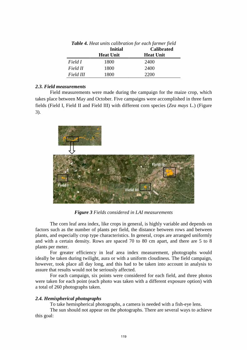
Table 4. Heat units calibration for each farmer field

Initial Heat Unit

Calibrated Heat Unit

Field I 1800 2400 Field II 1800 2400 Field III 1800 2200

2.3. Field measurements

Field measurements were made during the campaign for the maize crop, which takes place between May and October. Five campaigns were accomplished in three farm fields (Field I, Field II and Field III) with different corn species (Zea mays L.) (Figure 3).

Figure 3 Fields considered in LAI measurements The corn leaf area index, like crops in general, is highly variable and depends on

factors such as the number of plants per field, the distance between rows and between plants, and especially crop type characteristics. In general, crops are arranged uniformly and with a certain density. Rows are spaced 70 to 80 cm apart, and there are 5 to 8 plants per meter.

For greater efficiency in leaf area index measurement, photographs would ideally be taken during twilight, aura or with a uniform cloudiness. The field campaign, however, took place all day long, and this had to be taken into account in analysis to assure that results would not be seriously affected.

For each campaign, six points were considered for each field, and three photos were taken for each point (each photo was taken with a different exposure option) with a total of 260 photographs taken.

2.4. Hemispherical photographs

To take hemispherical photographs, a camera is needed with a fish-eye lens. The sun should not appear on the photographs. There are several ways to achieve

this goal:

119

• Take the photographs before sunrise or after sunset which limits the time available;

• Take the photographs when the sky is overcast. The more homogenous, the better.

At LAI values of 2 or less, it is safe to rely on the aperture and/or speed automatically chosen by the camera. Under denser canopies (and especially for digital cameras), it becomes necessary to underexpose the pictures. Otherwise, the camera tries to compensate for the dark canopy by letting too much light come through the gaps. This results in a saturation of these gaps which tends to overflow or bloom over the dark parts of the picture, “eating” the edges of the foliage.

The hemispherical photographs were taken throughout the corn crop campaign, allowing LAI estimation during crop development (Figure 4).

Figure 4. Hemispherical photographs evolution for each campaign in one of the farmers field

The exposure level of the camera was considered and labeled using three values:

minimum, average or maximum exposure bias (-2, 0 or +2 respectively). This option has the advantage of minimizing the negative effects of luminosity excess around noon. With three different photographs using three different exposures for each point, it was possible to select the most representative photograph of reality (Figure 5). Hemisfer software was used to estimate LAI from the hemispherical photographs.

Figure 5. Hemispherical photographs with different exposure

2.5. Hemisfer software Hemisfer software was developed by the Swiss Federal Institute for Forest,

Snow and Landscape Research (WSL). It was designed to estimate the leaf area index (LAI) from hemispherical photographs (Schleppi et al., 2006).

All methods used in Hemisfer are based on the classification of pixels to either white (=sky) or black (=canopy) by applying a brightness threshold to the analyzed

Exposure

Exposure bias Exposure bias

120

picture. The light transmission is then calculated as the proportion of white pixels within analysis rings, i.e. as a discrete function of the zenith angle Θ (theta). The next step is to calculate the average number of times that a light ray would touch the canopy when travelling a distance equal to the thickness of the canopy. This number is called the contact number, or K (Thimonier A. et al., 2010).

𝐾 = −𝑐𝑜𝑠 𝜃 𝑙𝑛 𝑇

The K values are finally integrated over the rings to give the LAI, but this step

differs among methods. Hemisfer writes its results into plain-text files. It shows results of different

methods that have been published to estimate the leaf area index from the transmission of light measured either directly under a canopy or on hemispherical photographs. Some of these methods also estimate an average leaf angle in the canopy. Flat leaves obscure the sky when one looks up towards the zenith, but towards the horizon they let light come through. The contrary applies to erect leaves. The inclination angle of the leaves therefore affects the appearance of the canopy on the hemispherical photograph. Because not all leaves have the same angle, their statistical distribution has to be taken into account when estimating LAI.

2.6. Hemisfer software calibration

Hemisfer software calibration depends on size and characteristics of photographs that will be used (Figure 6). Parameters in software that were adjusted are as follows: radius (1295.5 reduced to 920), center (1295.5 to the value 1325) and north (0 to 180).

Figure 6. Hemisfer software layout

3. Results To analyze leaf area index (LAI), biomass and evapotranspiration results were

considered only for subbasins corresponding to the vicinity of fields that were visited during the campaign (Figure 7).

121

Figure 7. Subbasins corresponding to farm fields

3.1. LAI calibration results Simulated results with and without calibration were compared to LAI field

measurement values. The maximum LAI values for curves that were not calibrated are dissimilar to

what was observed in the field (Figures 8, 9 and 10). Reduction of the maximum LAI setting for the model is necessary in order to achieve LAI results similar to the maximum values observed in the field. These changes, however, were not enough because crop growth behaviour is different.

Because the crop cycle and different growth phases depend on temperature and base temperature which are characteristics of each species, the amount of heat units varies for each species. Each corn field exhibited a different behaviour during its development cycle. In Field III it was observed that initial growth began earlier than the others, which influenced the calibration. Hemisfer-estimated LAI values are consistent with the observed values from field campaigns, making them consistent. However, it was observed that for the second campaign the LAI values for Fields I and III decreased. This was probably due to the fact that Field I had a great amount of pollen and Field III experienced an insect plague, resulting in poor quality photographs. In spite of this, the field LAI measurements were generally taken with success.

Figure 8. Leaf area index model results and field measurements for Field I

122

Figure 9. Leaf area index model results and field measurements for Field II

Figure 10. Leaf area index model results and field measurements for Field III 3.2. Impact on biomass and evapotranspiration results with LAI calibration

As explained previously, LAI, biomass and evapotranspiration depend on each other. So with LAI calibration it is expected that the amount of biomass produced and actual crop evapotranspiration results change.

The results show a decrease in LAI (halved), and with growth curve modification in respect to heat units, the amount of biomass decreased as expected (Figures 11, 12 and 13). For all three fields there was a maximum value decrease of about 14% (33,062 kg/ha to 28,462 kg/ha). In general, biomass values decreased about 32% for Fields I and II and 17% for Field III. These results are satisfactory based on the Cameira (1999) study that shows approximate maximum values of 25,000 kg/ha of biomass for the corn crop in the Sorraia Valley.

Figure 11. Biomass SWAT results with and without LAI calibration for Field I

123

Figure 12. Biomass SWAT results with and without LAI calibration for Field II

Figure 13. Biomass SWAT results with and without LAI calibration for Field III

Impact on actual evapotranspiration (Figures 14, 15 and 16) was lower, with a decrease of only 9%. This reduction is due to fact that leaf area was reduced which decreases the cultural transpiration component of evapotranspiration (Figures 14, 15 and 16).

Figure 14. Actual evapotranspiration and cultural transpiration results with and without LAI calibration for Field I

124

Figure 15. Actual evapotranspiration and cultural transpiration results with and without LAI calibration for Field II

Figure 16. Actual evapotranspiration and cultural transpiration results with and without LAI calibration for Field III

4. Conclusions

In this study the SWAT model was applied to simulate leaf area index values for

corn in the Sorraia Valley of Portugal. The most important input data include meteorology, topography, local soil data (spatial distribution and characteristics), land use and agricultural practices. SWAT outputs were calibrated by comparing simulated LAI to local LAI measurements.

The results of this study show that estimates of LAI values can be successfully determined using hemispherical photographs and Hemisfer software.

The model calibration process, with two parameters changes, resulted in highly realistic results which influence many others important crop results. LAI calibration in SWAT had a positive impact on LAI results and biomass production (with a maximum value decrease of 14%), resulting in a close match to observed values for the study area. Evapotranspiration results in general had an insignificant impact with an average decrease of 9%.

These results can be significant for the farmers of the Sorraia Valley by showing them the development of their fields throughout the campaigns. The calibration used in this study is extremely important because it will be applied for farms of the Enxoé basin, an area that has similar crop characteristics. References Cameira M.R., 1999, Balanço de água e azoto em milho regado no Vale do Sorraia: discussão

dos processos de transferência e aplicação do modelo, PhD Tesis, Lisbon: Agronomy Institute, Department of Rural Engineer

125

Cardoso, J.V.J.C., 1965 - "Os Solos de Portugal - sua classificação, caracterização e génese. 1. A Sul do Rio Tejo" Ministry of Agriculture, DGSA, Lisbon.

Hargreaves, G.L., G.H. Hargreaves, and J.P. Riley. 1985. Agricultural benefits for Senegal

River Basin. J. Irrig. and Drain. Engr. 111(2):113-124. Monteith, J.L. 1965. Evaporation and the environment. p. 205-234. In The state and movement

of water in living organisms. In 19th Symposia of the Society for Experimental Biology. Cambridge Univ. Press, London, U.K.

Monteith J.L., 1977b. Climate and the efficiency of crop production in Britain. Philosophical

Transaction Royal society of London, Ser. B, 281, 277-294. Neitsch, S.L., Arnold, J.G., Kiniry, J.R., Williams, J.R., 2005. Soil and Water Assessment Tool,

Theoretical Documentation, Version 2005. Blackland Research Center/Soil and Water Research Laboratory, Agricultural Research Service, Grassland/Temple, TX.

Priestley, C.H.B. and R.J. Taylor. 1972. On the assessment of surface heat flux and evaporation

using large-scale parameters. Mon. Weather Rev. 100:81- 92. Schleppi P., Conedera M., Sedivy I., Thimonier A., 2007. Correcting non-linearity and slope

effects in the estimation of the leaf area index of forests from hemispherical photographs. Agric. Forest Meteorol. 144: 236–242.

Thimonier A., Sedivy I., Schleppi P., 2010. Estimating leaf area index in different types of

mature forest stands in Switzerland: a comparison of methods. Eur. J. For. Res. 129: 543-562

Watson, D.J. 1947. Comparative physiological studies on the growth of field crops. 1. Variation

in net assimilation rate and leaf area index between species and varieties and within and between years. Ann. Bot. N.S. 11:41- 76.

126

Modeling Pesticide Fluxes during Highflow Events in an Intensive

Agricultural Catchment: the Save River (Southwestern France) Case Study

Laurie Boithias1,2,*, Sabine Sauvage1,2, Séverine Jean1,2, Francis Macary3, Odile Leccia3, Jean-Luc Probst1,2, Georges Merlina1,2, Raghavan Srinivasan4 and José-Miguel Sánchez-Pérez1,2

1 University of Toulouse; INPT; UPS; Laboratoire Ecologie Fonctionnelle et Environnement

(EcoLab), ENSAT, Avenue de l’Agrobiopole, 31326 Castanet Tolosan Cedex, France. 2 CNRS; EcoLab, 31326 Castanet Tolosan Cedex, France.

3 Cemagref, Adbx Research Unit, 50 avenue de Verdun 33612 Gazinet-Cestas Cedex, France 4 Spatial Sciences Laboratory, Texas A&M University, College Station, Texas, USA.

*laurie.boithias@ensat.fr

Abstract The SWAT model was tested at a daily time step to assess the fate of pesticides of a wide range of solubility. SWAT was applied on an 1100 km² intensive agricultural catchment (Save river, southwestern France). Simulated pesticide concentrations were compared to data collected at the catchment outlet from July 2009 to June 2010, with weekly measurements during low flow and daily or sub-daily measurements during flood events. SWAT was able to accurately reproduce measured pesticide concentrations during base flow and flood events, especially concentrations of pesticides in the soluble phase. During the simulation period, the simulated preferred pathway for pesticide transport from land area to stream network was surface runoff. Flood events were responsible for most pesticide transfer. The SWAT model hindcasted daily pesticide concentrations back to 1998 and possible pesticide concentrations exceeding water quality policy thresholds depending on climate.

Keywords: discharge, pesticides, flood, SWAT, modelling, Save river, agricultural catchment, AguaFlash

127

1. Introduction Rising pesticide levels in streams draining from intensively managed agricultural land

has become a widespread problem throughout Europe in recent decades because of the detrimental effect on terrestrial and aquatic ecosystems. Excessive loading of pesticides, transferred in the environment through various pathways (e.g. runoff) either in solution or sorbed to sediment particles, may rend stream water and groundwater unfit for human consumption.

In Europe, pesticides are considered hazardous substances in accordance with current legislation regarding water (EC, 2006). European directives state a drinking water quality standard that may not exceed 0.1 µg.L-1 for a single pesticide concentration and 0.5 µg.L-1 for total pesticides concentration (EC, 1998). Directives adopted river basins as the territorial management unit. Therefore, the combination of watershed models and river water quality models is needed to calculate pesticide fluxes to the river and transformation processes in the river.

Few works have been published yet on pesticide fate modeling with the Soil and Water Assessment Tool (SWAT). The fate of various molecules of a wide range of solubility was simulated (e.g. Atrazine, Metolachlor, Trifluralin, Diazinon and Chlorpyrifos). Time-steps were either daily or monthly. Modeled catchments ranged from 30 to 15000 km² (Boithias et al., in revision(a); Neitsch et al., 2002; Holvoet et al., 2005; Larose et al., 2007; Luo et al., 2008).

The objective of this preliminary work was to test the ability of SWAT to simulate at daily time-step the fate of metolachlor and aclonifen applied on an 1100 km² intensive agricultural catchment (Save river, southwestern France) at both the long-term and flood-event scales.

2. Material and Methods 2.1. Study area

The Save catchment is a 1110 km² agricultural intensive catchment located in the Coteaux de Gascogne area (southwest France) (Figure 1). The Save river has its source at an altitude of 663 m in the Pyrenees piedmont and joins the Garonne river after a 140 km course at an altitude of 92 m. The Larra gauging station elevation is 114 m (Figure 1).

Figure 1. Location of Save catchment, Larra gauging station and meteorological stations

The climate is oceanic. Save river hydrology is regulated by rainfall with a maximum

discharge in May and low flows during summer (July to September). Annual average rainfall

128

is 721 mm with a 99 mm standard deviation. Annual evaporation is about 500-600 mm. Calcic soils represent 61% in the whole catchment with a clay content ranging from 35% to 50%. Non-calcic silty soils represent 30% of the soil in this area (40-60% silt). Alluviums represent 9%. Because of its high clay content, catchment substratum is relatively impermeable. River discharge is consequently mainly supplied by surface and subsurface runoffs. Save river mean annual discharge (1965-2006) is 6.1 m3.s-1. During low flows, river flow is sustained upstream by the Neste canal (about 1 m3.s-1).

90% of catchment area is used for agriculture. The upstream part of the catchment is a hilly agricultural area mainly covered with pasture and forest with cereals and corn on small plateaus. The lower flat part is devoted to intensive agriculture with mainly a 4-year crop rotation alternating winter wheat with sunflower and corn. Fertilizers are applied from late winter to spring. Yearly nitrate-equivalent supply among the catchment is about 590 kg.ha-1. Various pesticides are applied in the catchment all year long depending on the crops. Our study focuses on two of them: each year, 30 tons of metolachlor, a highly soluble chemical, and 58 tons of aclonifen, a poorly soluble chemical, are applied on the catchment. Both pesticides are herbicides applied on sunflower, corn and sorghum in April (Table 1). These three crops are grown on 23% of the catchment (25700ha).

Table 1. Average management practices for sunflower, corn and sorghum grown on the Save catchment including metolachlor and aclonifen spreading Type of operation Date of operation Quantity (kg.ha-1) SUNFLOWER Sowing 15 April - Pesticides spreading: aclonifen 20 April 2.7 Harvest 25 August - CORN and SORGHUM Sowing 1 April - Pesticides spreading: metolachlor 7 April 1.5 Pesticides spreading: aclonifen 7 April 0.25 Harvest 15 ctober - 2.2. Observed data

The Save river has been monitored since 1965 for discharge. Nitrate, suspended sediment and pesticides have been monitored since 2007 at Larra gauging station both manually and automatically.

Automatic sampling was performed by a Sonde YSI 6920 (YSI Incorporated, Ohio, USA) measuring probe and an Automatic Water Sampler (ecoTech Umwelt-Meßsysteme GmbH. Bonn, Germany). They were installed at the Save catchment outlet (Larra bridge) to continuously monitor water quality. The water sampler connecting with the probe was programmed to activate pumping water on the basis of water level variations of 30 cm. Manual sampling was also undertaken near the probe position at weekly intervals during low flow. Laboratory analysis and daily load calculation for nitrate and suspended sediments were performed as described in Oeurng et al. (2010a; 2010b) and Oeurng et al. (2011a). Laboratory analysis and daily load calculation for pesticides were performed as reported by Taghavi et al. (2010) and Boithias et al. (in revision(a)). Additional data from Agence de l’Eau Adour-Garonne (AEAG) were used for long term total pesticide concentration comparison (Source: Système d’Information sur l’Eau du Bassin Adour-Garonne, data exported in 2009). 2.3. Pesticide modeling approach with SWAT

Pesticide processes in SWAT are divided into three components: (1) pesticide processes in land areas, (2) transport of pesticide from land areas to the stream network, and (3) instream pesticide processes. The partitioning of a pesticide between the dissolved and the

129

sorbed phases in each modeled compartment is defined by a partition coefficient depending on the compartment. 2.4. SWAT data inputs

SWAT inputs were: - the digital elevation model with a 25m×25m resolution from BD TOPO R IGN France - the soil map digitized and aggregated by Cemagref-ADBX, from paper maps prepared by

soil scientists of the CACG (Companie d’Aménagement des Coteaux de Gascogne) in the 1960s, and layer properties

- land use data from Landsat 2009 with associated management practices provided by Cemagref-ADBX

- climate data from 1994 to 2010 of 5 stations (Figure 1) provided by Météo-France - daily discharge of Neste canal, supplying water as a upstream point source to Save river

network given by CACG Version 2009.93.3 of ArcSWAT with AcrGIS 9.2.1 was used. The catchment was

discretized into 73 subbasins which minimal area was 500 ha. 2985 HRUs were generated integrating 23 land uses classes, 6 soil classes and 5 slope classes (%: 0-2, 2-5, 5-10, 10-15 and 15-over).

2.5. Model calibration and validation

Whole simulation was carried out daily from January 1998 to June 2010 (excluding four years warm up from 1994 to 1997). Parameter sensitivity analysis was performed with the ArcSWAT2009 sensitivity analysis tool (Van Griensven et al., 2006). Discharge, nitrate load, suspended sediment and pesticide concentrations were manually calibrated at daily time step, based on catchment understanding and previous modeling work on the Save catchment (Boithias et al., in revision(a); Boithias et al., in revision(b); Oeurng et al., 2011b). 2.6. Model evaluation

The daily performance of the model for simulating discharge, nitrate load, suspended sediment and pesticide concentrations was evaluated graphically by Nash-Sutcliffe efficiency (ENS) and by coefficient of determination (R²). 2.7. Water quality simulation

Loads of pesticides at the catchment outlet were calculated summing up daily loads for April to June flood (04/23/2010 to 06/06/2010) and low flow and high flow (using the 6.1m3.s-1 threshold). Total pesticide concentration was the concentration of pesticides as measured in unfiltered water. Simulated total concentration was calculated as the total of dissolved and sorbed pesticide concentration. Fraction of pesticides in a sorbed phase was calculated as the sorbed pesticide load divided by the total pesticide load. Exportation rate was calculated as the ratio from pesticide load exported annually at outlet and the amount of pesticide annually applied among the catchment. The percentages of pesticide exported during flood at outlet and percentage of annual flood duration were calculated according to the 6.1 m3.s-1 threshold. As pesticide toxicity is more relevant as concentration than as load, long term simulation concentrations (2001-2010) were compared to European drinking water quality standards of 0.1 µg.L-1 for a single pesticide and of 0.5 µg.L-1 for both pesticides.

130

3. Results and Discussion 3.1. Discharge, dissolved and sorbed phases simulation

Whole simulation of discharge (Figure 2), nitrate and suspended sediment was carried out daily from January 1998 to June 2010. Prediction errors can be explained by various approximations in both observed and simulated data and simplified processes in the model. Discharge, nitrate load and suspended sediment concentration prediction and observation fitting have been made only on one location (Larra outlet). No suspended sediment or nitrate measurements were performed in Neste water and their input loads were set in the model as a constant concentration of 20 mg.L-1 and 2 mg.L-1 respectively.

Goodness-of-fit indices were satisfactory (Table 2) although quality of suspended sediments simulation is weak. Simulation results relevant with previous work on the Save river (Boithias et al., in revision(a); Boithias et al., in revision(b); Oeurng et al., 2011b). The model was then able to model pesticide fluxes for both the dissolved and the sorbed phases and considered to hindcast with little error past daily and annual loads down to 1998. Nitrate and suspended sediment annual loads were well correlated to water yield at the catchment outlet (R² = 0.89 and 0.53 respectively). 2005 was the year of lowest water yield (73mm) whereas 2000 was the year of highest water yield (202mm).

Figure 2. Observed and simulated daily discharge (m3.s-1) at Larra outlet (July 2009 to June 2010)

Table 2. Goodness-of-fit indices for daily discharge, nitrate load and suspended sediment concentration simulation at Larra outlet Periods R2 p-value ENS Discharge – calibration 1998-2006 0.40 << 0.05 0.28 Discharge – validation 2009-2010 0.55 << 0.05 0.56 Nitrate load 2009-2010 0.48 << 0.05 0.45 Suspended sediments concentration

2009-2010 0.21 << 0.05 0.18

3.2. Pesticide simulation

The range of daily simulated concentrations (Figure 3) of pesticides in the dissolved and sorbed phase and concentration (Figure 4) of total pesticide fitted the range of respective measurements. Concentration peaks were mostly simulated.

In terms of loads, simulation fitted the measured range of value but both metolachlor and aclonifen loads were overestimated during the April-June flood (Table 3). Errors in predictions may be related to an inadequate calibration of parameters governing pesticide dynamics, including parameters governing suspended sediments for sorbed phase calibration. The dates of pesticide spreading operations may also not be precise enough in spring 2010.

131

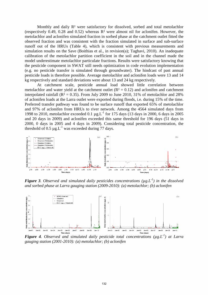
Monthly and daily R² were satisfactory for dissolved, sorbed and total metolachlor (respectively 0.49, 0.28 and 0.52) whereas R² were almost nil for aclonifen. However, the metolachlor and aclonifen simulated fraction in sorbed phase at the catchment outlet fitted the observed fraction and was consistent with the fraction simulated in surface and sub-surface runoff out of the HRUs (Table 4), which is consistent with previous measurements and simulation results on the Save (Boithias et al., in revision(a); Taghavi, 2010). An inadequate calibration of the metolachlor partition coefficient in the soil and in the channel made the model underestimate metolachlor particulate fractions. Results were satisfactory knowing that the pesticide component in SWAT still needs optimization in code evolution implementation (e.g. no pesticide transfer is simulated through groundwater). The hindcast of past annual pesticide loads is therefore possible. Average metolachlor and aclonifen loads were 13 and 14 kg respectively and standard deviations were about 13 and 24 kg respectively.

At catchment scale, pesticide annual load showed little correlation between metolachlor and water yield at the catchment outlet (R² = 0.12) and aclonifen and catchment interpolated rainfall (R² = 0.35). From July 2009 to June 2010, 31% of metolachlor and 28% of aclonifen loads at the Larra outlet were exported during floods, i.e. during 15% of the time. Preferred transfer pathway was found to be surface runoff that exported 65% of metolachlor and 97% of aclonifen from HRUs to river network. Among the 4564 simulated days from 1998 to 2010, metolachlor exceeded 0.1 µg.L-1 for 175 days (13 days in 2000, 6 days in 2005 and 20 days in 2009) and aclonifen exceeded this same threshold for 196 days (51 days in 2000, 0 days in 2005 and 4 days in 2009). Considering total pesticide concentration, the threshold of 0.5 µg.L-1 was exceeded during 77 days.

Figure 3. Observed and simulated daily pesticides concentrations (µg.L-1) in the dissolved and sorbed phase at Larra gauging station (2009-2010): (a) metolachlor; (b) aclonifen

Figure 4. Observed and simulated daily pesticide total concentrations (µg.L-1) at Larra gauging station (2001-2010): (a) metolachlor; (b) aclonifen

132

Table 3. Unfiltered and filtered metolachlor and aclonifen loads (kg) during a flood event at Larra outlet (April, 23rd to June, 6th 2010). Metolachlor Aclonifen Measured unfiltered load 28.5 0.8 Simulated total load 81.5 3.8 Measured filtered load 22.4 0.2 Simulated dissolved load 74.1 1.1 Table 4. Observed and simulated fraction in the sorbed phase of metolachlor and aclonifen out of HRUs and at catchment outlet (2009-2010). Metolachlor Aclonifen Observed Simulated Observed Simulated HRUs 0.02 0.74 Catchment outlet

0.16 0.09 0.72 0.72

4. Conclusion

The SWAT model reliably simulated metolachlor and aclonifen fate at the outlet of the

1110 km² agricultural intensive Save catchment, as well as the partition between dissolved and sorbed phases, although modelled transfer processes were simplified. The preferred pathway of pesticide exportation is surface runoff. Most of the pesticide loads are exported during flood events. Hindcast of pesticide concentrations exceeding European drinking water standards is made possible. SWAT is a promising tool for assessing river network pesticide contamination in case of flooding and will help indentify factors that control pesticide exportation for both insoluble and highly soluble molecules.

Acknowledgements This work was performed as part of the EU Interreg SUDOE IVB program (SOE1/P2/F146 AguaFlash project, http://www.aguaflash-sudoe.eu) and funded by ERDF and the Midi-Pyrénées Region. References Boithias, L., S. Sauvage, L. Taghavi, G. Merlina, J.L. Probst and J.M. Sánchez-Pérez. In revision(a).

Occurrence of metolachlor and trifluralin losses in the Save River agricultural catchment during floods. Journal of Hazardous Materials.

Boithias, L., S. Sauvage, R. Srinivasan and J.M. Sánchez-Pérez. In revision(b). Assessment of

hydrology and nitrate load transport in a large intensive agricultural catchment using the SWAT model. Science of the Total Environment.

EC. 1998. Directive 98/83/EC of 3 November 1998 on the quality of water intended for human

consumption, Off. J. Eur. Communities L330. EC. 2006. Directive 2006/11/EC of the European Parliament and of the Council of 15 February 2006

on pollution caused by certain dangerous substances discharged into the aquatic environment of the Community, Off. J. Eur. Communities L64.

Holvoet, K., A. van Griensven, P. Seuntjens and P.A. Vanrolleghem. 2005. Sensitivity analysis for

hydrology and pesticide supply towards the river in SWAT. Physics and Chemistry of the Earth. Parts A/B/C 30:518–526.

133

Larose, M., G.C. Heathman, L.D. Norton and B. Engel. 2007. Hydrologic and atrazine simulation of the Cedar Creek watershed using the SWAT model. Journal of environmental quality. 36(2):521-531.

Luo, Y., X. Zhang, X. Liu, D. Ficklin and M. Zhang. 2008. Dynamic modeling of organophosphate pesticide load in surface water in the northern San Joaquin Valley watershed of California. Environmental Pollution. 156:1171–1181.

Neitsch, S.L., J.G. Arnold and R. Srinivasan. 2002. Pesticides Fate and Transport Predicted by the Soil and Water Assessment Tool (SWAT) - Atrazine, Metolachlor and Trifluralin in the Sugar Creek Watershed. 96p.

Oeurng, C., S. Sauvage and J.M. Sánchez-Pérez. 2010a. Dynamics of suspended sediment transport and yield in a large agricultural catchment, southwest France. Earth Surface Processes and Landforms. 35:1289-1301.

Oeurng, C., S. Sauvage and J.M. Sánchez-Pérez. 2010b. Temporal variability of nitrate transport through hydrological response during flood events within a large agricultural catchment in south-west France. Science of the Total Environment. 409:140-149.

Oeurng, C., S. Sauvage, A. Coynel, E. Maneux, H. Etcheber and J.M. Sánchez-Pérez. 2011a. Fluvial transport of suspended sediment and organic carbon during flood events in a large agricultural catchment in southwest France. Hydrological Processes. DOI: 10.1002/hyp.7999

Oeurng, C., S. Sauvage and J.M. Sanchez-Perez. 2011b. Assessment of hydrology, sediment and particulate organic carbon yield in a large agricultural catchment using the SWAT model. Journal of Hydrology. 401:145-153.

Taghavi, L. 2010. Dynamique de transfert des pesticides en périodes de crue sur les bassins versants agricoles gascons. Université de Toulouse. (PhD thesis).

Taghavi, L., J.L. Probst, G. Merlina, A.L. Marchand, G. Durbe and A. Probst. 2010. Flood event impact on pesticide transfer in a small agricultural catchment (Montousse at Aurade, south west France). International Journal of Environmental Analytical Chemistry. 90:390-405.

Van Griensven, A., T. Meixner, S. Grunwald, T. Bishop, M. Diluzio and R. Srinivasan. 2006. A global sensitivity analysis tool for the parameters of multi-variable catchment models. Journal of Hydrology. 324:10–23

134

Application of the SWAT Model to a Sprinkler-Irrigated Watershed in the Middle Ebro River Basin of Spain

Skhiri Ahmed1, Dechmi Farida2* and Burguete Javier3

1 PhD student, Agrifood Research and Technology Centre of Aragon. Soils and Irrigation Department (CITA-DGA). Avda. Montañana 930, 50059 Zaragoza, Spain (askhiri@aragon.es)

2 Researcher, Agrifood Research and Technology Centre of Aragon. Soils and Irrigation Department (CITA-DGA). Avda. Montañana 930, 50059 Zaragoza, Spain (fdechmi@aragon.es)

3 Researcher, Aula Dei Experimental Station, CSIC. Soil and Water Department (EEAD-CSIC) Avda. Montañana 1005, 50059 Zaragoza, Spain (jburguete@eead.csic.es)

Abstract The Soil and Water Assessment Tool (SWAT) is a well-established and well-distributed hydrologic model. However, in the case of Del Reguero watershed (DRW) it has been shown that the SWAT2005 version doesn’t correctly reproduce the irrigation return flow generated under sprinkler irrigation systems. The objective of this study was to adapt and assess the SWAT2005 model for correctly simulating the main hydrological processes in the study area. The main model source code modification was focused on the maximum amount of water to be applied as an irrigation event. The adjusted version of the model was named SWAT-IRRIG and was calibrated and validated for streamflow, sediment and phosphorus loads. SWAT-IRRIG was calibrated using data from January to December 2009, and an independent 12-month period was used for the validation process (January to December 2009). A sensitivity analysis was conducted to aid in model calibration. Model source code modification increased the Nash-Suttcliffe coefficient of efficiency (ENS) for monthly flows from -0.50 to 0.90. The monthly ENS value was 0.80 for the validation process. Average monthly sediment losses were underestimated with 15% of the measured data and the corresponding monthly ENS was 0.72 for calibration and 0.52 for validation processes. SWAT-IRRIG also adequately predicted monthly trends in average total phosphorus loading during the calibration and validation periods with NSE values of 0.66 and 0.63, respectively. The results of this study indicate that SWAT-IRRIG is an efficient tool for the evaluation of best management practices’ effects on water quality in terms of water yield, sediments loss and total phosphorus load. Keywords: hydrological and water quality modeling, sediments, phosphorus, SWAT model, model modification

135

1. Introduction Application of watershed simulation models is indispensable when pollution is

generated by nonpoint sources such as agricultural practices. A wide range of watershed models are offered to predict the impact of land management practices on water, sediment and agricultural chemical yields. Examples of those models are the physically based event model ANSWERS (Beasley, 1991), the empirically based SWATCATCH model (Holman et al., 2001), the physically based DWSM model (Borah and Bera, 2003) and the semi-empirically based SWAT model (Gassman et al., 2007).

The Soil and Water Assessment Tool (SWAT) is the most capable model for long-term simulation in watersheds dominated by agricultural land uses. The model has proven to be an effective tool for assessing nonpoint source pollution problems for a wide range of scales and environmental conditions (Gassman et al., 2007). The SWAT model has been widely applied across the United States (FitzHugh and Mackay, 2000; Arabi et al., 2006); Europe (Nasr et al., 2007; Galván et al., 2009) and other parts of the world (Bouraoui et al., 2005; Watson et al., 2005).

The SWAT model has been modified and adapted to provide improved simulations of specific processes for specific watersheds (Gassman et al., 2007). Lenhart et al. (2005) modified SWAT99.2 for percolation, hydraulic conductivity and interflow functions to provide improved flow predictions for typical conditions in low mountain ranges in Germany. Extended SWAT (ESWAT) incorporated several modifications onto the original SWAT model in order to simulate runoff at an hourly time step (van Griensven and Bauwens, 2005). The Soil and Water Integrated Model (SWIM), based on hydrological components of SWAT, was designed to simulate “mesoscale” watersheds (Krysanova et al., 2005). Lenhart et al. (2003) used the modified version SWAT-G to simulate sediment and phosphorus in the Dill catchment of Hessen, Germany. Van Liew (2009) modified SWAT2005 to consider losses of organic phosphorus from bank erosion of the top soil layer in three drainage areas located in the Bitterroot watershed.

In this study, a modified version of the SWAT2005 model was used which was dubbed SWAT-IRRIG. The objective was to assess and improve SWAT2005 performance in the sprinkler-irrigated middle Ebro River Basin systems of Spain for predicting water yield, sediment and phosphorus transfer at the system outlet. The hydrological process modification as well as calibration and validation of the model are presented in this study. 2. Material and Methods 2.1. Study area

The Del Reguero watershed (DRW) has a total drainage area of 18.6 km2 with elevation ranging from 208 to 502 m and average land surface slope of 4.4%. The watershed belongs to the Alto Aragon Irrigation Scheme area located on the right bank of the middle Ebro River Basin in Spain (Figure 1). The main cultivated crops are corn (41%), barley (19%), alfalfa (15%), and sunflower (9%) and represent about 84% and 83% of the watershed’s irrigated area during 2008 and 2009, respectively.

136

Figure 1. Del Reguero watershed localization

The climate is semiarid with an average annual precipitation and reference evapotranspiration of 391 mm and 1,294 mm, respectively. The mean annual temperature is 13.1ºC with a large temperature difference between winter and summer. Irrigation practices began in 1982 using sprinkler irrigation systems (mainly solid-set sprinkler irrigation). Two geomorphologic soil units can be distinguished in the study zone. The first unit (38% of the DRW area) corresponds to platform soils, and the second unit (62% of the DRW area) corresponds to alluvial soils.

2.2. Model modification

The application of the SWAT2005 original version in a semiarid irrigated area such as the DRW using actual irrigation practices of farmers was not possible because of its limitation on the maximum value of irrigation dose that could be applied as an irrigation event. Indeed, the model’s original version uses the irrigation doses specified in the irrigation operation as inputs to fill the soil layers up to field capacity. If the amount of water specified in an irrigation operation exceeds the amount needed to fill the soil layers up to field capacity, the excess water is returned to the source (Neitsch et al., 2005) and therefore not considered in the daily soil water balance calculation. In practice this is not true because when water applied exceeds the amount of water needed to fill the soil layers up to field capacity the excess water is lost from the soil profile by the deep percolation process as irrigation return flow. Therefore, the following modification in the source code was performed to include the eventual mentioned excess water in the soil water balance calculation:

1- The maximum amount of water to be applied corresponds to the depth of irrigation water applied to an HRU specified by the user instead of the amount of water held in the soil profile at field capacity. 2- As the model percolation calculation subroutine includes only precipitation excess, a new variable that corresponds to water excess generated from irrigation practices when the amount of irrigation water applied exceed the soil layers field capacity was added in the soil percolation depth calculation.

137

3- In the SWAT2005 source code, for the subroutine “subbasin” that controls the simulation of the land phase of the hydrologic cycle the soil water routing is performed before performing the irrigation operations from sources outside the watershed. After making the previous changes, the simulation order of the land phase of the hydrological cycle was changed. The SWAT model was modified to perform the irrigation operations before performing the soil water routing.

2.3. Model calibration and validation

Simulations were carried out from January 1st, 2007 to December 31st, 2009 using the standard split sample calibration-validation procedure (Klemeš, 1986). The period from January 1st, 2007 to January 14th, 2008 served as a warm up period for the model in order to take for granted realistic initial values for the calibration period. Data from January 15th, 2008 to December 31st, 2008 were used for the calibration and the remaining data for validation. The simulated streamflows (FLOW_OUT) were compared with daily measured flows at DRW outlet. For the case of sediments, the simulated sediment yield (SYLD) was compared to total suspended sediments measured at DRW outlet. On the other hand, the simulated soluble phosphorus (SOL_P) was compared to measured total dissolved phosphorus (TDP), while the simulated organic phosphorus (ORG_P) was compared to the measured particulate phosphorus (PP). The summation of SOL_P and ORG_P fractions was compared to total phosphorus (TP) loading, which is the result of summation of TDP and PP. 2.4. SWAT-IRRIG performance

Graphical method (time series plot) and statistical indices were used to evaluate the SWAT-IRRIG performance based on the measured data. Five statistical criteria were used to evaluate calibration and validation results: (i) the coefficient of determination (R2), (ii) the Nash-Sutcliffe efficiency (NSE) (Nash and Sutcliffe, 1970), (iii) the root mean square error (RMSE), (iv) the percent bias (PBIAS) (Gupta et al., 1999), and (v) the RMSE-observation standard deviation ratio (RSR) (Moriasi et al., 2007). The R2 represents the percentage of variance in the measured data that is explained by the simulated data. The NSE indicates how well the plots of observed versus simulated data fit to the 1:1 line. The RMSE is equal to the square of the variance. A smaller RMSE indicates a better performance of the model. The PBIAS measures the average tendency of the simulated data to be larger or smaller than their observed counterparts. The RSR is defined as the ratio of the RMSE to the standard deviation of measured data (Moriasi et al., 2007). The optimal value of RSR is 0.0, which indicates zero RMSE or residual variation and therefore perfect model simulation. Based on the guideline proposed by Moriasi et al. (2007), model performance can be evaluated as satisfactory if NSE > 0.5, RSR ≤ 0.70, PBIBAS < ± 25% for streamflow, PBIAS < ± 55% for sediments and PBIAS < ± 70% for phosphorus at a monthly time step.

3. Results and Discussion 3.1. SWAT crop model calibration and validation

Crop yields were calibrated and validated using observed data gathered from field surveys performed in 2008 (calibration) and 2009 (validation). Overall, the SWAT-IRRIG model adequately estimated the observed mean yields of alfalfa, corn, sunflower and barley in the DRW. Results indicate a good correlation between simulated and observed mean crop yields in the DRW obtained during the calibration and validation periods

138

(Figure 2). On average, the mean simulated production for alfalfa is about 15.1 Mg ha-1 instead of 14.0 Mg ha-1 as mean observed production, indicating that SWAT-IRRIG over-estimated alfalfa yield by almost 7.5%. The variability of the observed alfalfa yield (CV = 13%) was higher than that of simulated yield (CV = 5%). SWAT-IRRIG also over-estimated mean barley yield by 9.6% (5.8 Mg ha-1 vs. 6.3 Mg ha-1). Barley simulated yield presented less variability (3%) than observed yield (15%).

0

6

12

18

Alfalfa Corn Barley Sunflower

Yie

ld (M

g ha

-1)

0200400600800

1000

Alfalfa Corn Barley Sunflower

ET

a (m

m)

0

6

12

18

Alfalfa Corn Barley Sunflower

Yie

ld (M

g ha

-1)

0200400600800

1000

Alfalfa Corn Barley Sunflower

ET

a (m

m)

S

Simulated SWAT-IRRIG Observed Calculated SWB

Figure 2. Average calibration (left) and validation (right) results of crop yield (top) and actual evapotranspiration (ETa) (bottom) for alfalfa, corn, barley and sunflower in the study area

On the other hand, mean simulated yields of corn and sunflower were less than mean observed yields. On average, the SWAT-IRRIG model underestimated mean corn yield by 4.5%, whereas mean sunflower yield was underestimated by 6.7%. On average the variability of the observed corn yield was quite similar to that of the simulated yield (10% vs. 9%, respectively). Concerning crop actual evapotranspiration (Figure 2), results indicate that on average the mean annual ETa values simulated by SWAT-IRRIG (736, 730, 515 and 696 mm, for alfalfa, corn, barley and sunflower, respectively) were quite similar to those calculated with another soil water balance computer-based program (Causapé, 2009) . The error value between simulated and calculated ETa for corn, barley and sunflower ranged from 3.7 to 7.0%. In the case of alfalfa, the soil water balance over-estimated the value of ETa by almost 17.4%.

3.2. SWAT2005 vs. SWAT-IRRIG

The comparison between streamflows measured and estimated by SWAT2005 default and SWAT-IRRIG is presented in Table 1 and Figure 3. Results showed a very large difference between monthly observed and SWAT2005-simulated stream discharge. This difference was due to the fact that the excess of applied irrigation water was not considered in the calculation of the lateral flow (LATQ), baseflow (GW_Q) and transmission losses (TLOSS).

Using the default SWAT2005 simulation approach, the model predictions for LATQ, GWQ and TLOSS were underestimated by 74.0, 341.1 and 6.7%, respectively (Table 1). This was because the irrigation dose applied was more than enough to fill up the soil field capacity, so the remaining amount of water applied was lost and not used in the soil daily water balance calculation. As a result, the total water yield (WYLD) in the study

139

area outlet is underestimated by 117.6%, which creates a very large difference between simulated and observed stream discharge (Table 1). The Nash and Sutcliffe (NSE) SWAT2005 model efficiency is about -0.50 enhanced to 0.90 when the modified version was used. Also the percentage error (PBIAS) between monthly simulated and observed discharge of SWAT2005 (51.8%) was reduced to 1.1% when SWAT-IRRIG was considered. This result is “very good” according to Moriasi et al. (2007).

Other modified versions of SWAT have demonstrated a capacity for improving calibration results for watersheds with specific characteristics. Eckhardt et al. (2002) found that the modifications adopted in SWAT-G resulted in greatly improved simulation of subsurface interflow in German low mountain conditions. They have succeeded in increasing the model NSE from -0.17 to 0.76 using SWAT-G instead of SWAT99.2 (Eckhardt et al., 2002). A modified version of SWAT2000 was used to simulate the rapid subsurface water movement in the karst terrain of the Guadalupe River watershed (Afinowicz et al., 2005). These authors reported that simulated baseflows matched well-measured streamflows after modifications introduced to SWAT2000.

Table 1. Comparison between SWAT2005 default and SWAT-IRRIG modified versions. Difference between the two versions is calculated. Parameter SWAT2005

version SWAT-IRRIG

version Underestimation

(%) Lateral flow (LATQ, mm) 4.6 8.0 74.0 Groundwater flow (GW_Q, mm) 14.4 63.5 341.1 Transmission losses (TLOSS, mm) 0.2 0.2 6.7 Total water yield (WYLD, mm) 44.7 97.1 117.6 NSE -0.5 0.9 - PBIAS (%) 51.8 1.1 -

0

50

100

150

200

250

300

350

J-08 F-08 M-08 A-08 M-08 J-08 J-08 A-08 S-08 O-08 N-08 D-08Date (Month-Year)

Dis

char

ge (1

03 m3 )

Observed data

SWAT-IRRIG

SWAT2005

Figure 3. Comparison of monthly water discharge between observed data simulated with SWAT2005 and with SWAT-IRRIG 3.3. Streamflow calibration and validation

For the model calibration, monthly flow predictions were compared with monthly observed data of Del Reguero stream discharge for the period of January 15th, 2008 to December 31st, 2008. The results of the calibration statistical indices are shown in Table 2. Baseflow calibration results at the study area outlet showed agreement with baseflow

140

values separated from total measured streamflow using the approach of the different electrical conductivity. The calculated baseflow fraction was about 0.80 of the total streamflow simulated by SWAT-IRRIG, and about 0.77 using the approach of different electrical conductivity.

For the calibration process, a good agreement between monthly observed and simulated stream discharge was observed (Figure 4B). However, on a daily basis a slight discrepancy between observed and simulated stream discharge can be observed (Figure 4A). The R2 value considering daily data was about 0.55, which can be considered as acceptable. However the NSE value was very low (NSE = -0.23). This low value of NSE is mainly driven by the two very high stream discharge values recorded on the dates of 10/28/08 and 11/02/08. It seems that SWAT-IRRIG overestimated streamflow during periods of high discharge. If these high stream discharge values are not considered, the NSE value increases to 0.47.

Table 2. Values of coefficient of determination (R2), Nash-Sutcliffe efficiency (NSE), percent bias (PBIAS), root mean square error (RMSE), and the RMSE-observation standard deviation ratio (RSR) for the calibration (Jan 15th – Dec 31st, 2008) and validation (Jan 1st – Dec 31st, 2009) processes

0

100

200

300

400

500

- 100 200 300 400 500

Observed (103 m3)

Sim

ulat

ed (1

03 m3 ) B

0

550

1100

1650

2200

0 550 1100 1650 2200

Observed (L s-1)

Sim

ulat

ed (L

s-1) A

11/02/08

10/28/08

0

100

200

300

400

500

0 100 200 300 400 500Observed (103 m3)

Sim

ulat

ed (1

03 m3 ) D

0

550

1100

1650

2200

0 550 1100 1650 2200Observed (L s-1)

Sim

ulat

ed (L

s-1) C 11/04

08/09

Figure 4. Comparison of daily (A and C) and monthly (B and D) stream discharge observed and simulated with SWAT-IRRIG at the Del Reguero watershed outlet for the calibration (A and B) and validation (C and D) periods. The diagonal line represents the 1:1 relationship.

During the calibration period, the calculated value of R2 on a monthly basis was 0.90, indicating a very good agreement between simulated and observed monthly stream discharge. Also, the NSE value for the monthly stream calibration was 0.90. According to the model evaluation guidelines proposed by Moriasi et al. (2007), SWAT-IRRIG simulated “very good” the Del Reguero stream discharge. For calibration 26.4 RMSE (103

Statistic parameter Calibration Validation R2 0.90 0.82 NSE 0.90 0.80 PBIAS (%) 1.10 3.20 RMSE (103 m3) 26.4 46.3 RSR 0.33 0.45

141

m3) was obtained. To better judge this value, RMSE should be standardized by the use of observed data. Calculated as the ratio of the RMSE and standard deviation of observed data, the RSR shows a value of 0.33. This value indicates that SWAT-IRRIG performance for stream discharge is “very good” according to Moriasi et al. (2007). Absolute value of the PBIAS for the 2008 calibration year is 1.1%, overestimating the Del Reguero stream discharge. This value indicates that the average magnitude of simulated streamflow values was within the range of “very good” (PBIAS < ± 10%). Overall, monthly calibration statistics indicated a “very good” SWAT-IRRIG performance in describing monthly streamflow in the DRW.

Values of R2 and NSE greater than 0.8 were also found in several SWAT hydrological calibration studies (Kalin and Hantush, 2006; Wang and Melesse, 2006). Kalin and Hantush (2006) reported accurate surface runoff and streamflow results for the Pocono Creek watershed in eastern Pennsylvania. They achieved values of R2 and NSE of 0.87 for both. Accurate streamflow predictions were achieved by Wang and Melesse (2006) for the Elm River North Dakota watershed. The validation process results are presented in Figure 4C and D. A good adjustment between measured and simulated monthly stream discharge can be observed (Figure 4D), whereas discrepancy between the measured and simulated daily stream discharge can be noted (Figure 4C). The R2 value on a daily basis is 0.74, indicating a good agreement between observed and simulated daily streamflows. The difference between observed and simulated data is for the most part driven by the values of streamflow obtained during the dates 11/04/09 and 08/09/09. The value of NSE obtained using all daily data is -0.64, enhanced to 0.22 when the two high values are eliminated. Monthly validation statistics generally indicated a “very good” SWAT-IRRIG performance for Del Reguero stream discharge (Table 2). Good correlation between simulated and observed stream discharge was found with a R2 value of 0.82. The NSE value for the monthly stream discharge validation is 0.80, considered as “very good.” 46.3 RMSE (103 m3) was obtained, which has been standardized using the observed data. The RSR, obtained by dividing the RMSE value by the observed data standard deviation, shows a value of 0.45, which is also considered as “very good.” The value of PBIAS is 3.2%, overestimating the monthly Del Reguero stream discharge but considered as “very good” (PBIAS < ±10%). Similar monthly SWAT performance results were also found in various SWAT hydrologic modeling studies (Wu and Xu, 2006; Zhang et al., 2007). 3.4. Water quality calibration and validation 3.4.1. Sediments

Figure 5 shows the relationship between observed and simulated total suspended sediment (TSS) loads at the study area outlet during the calibration and validation period considering daily and monthly data. On a daily basis, large discrepancies between observed and simulated TSS loads can be observed (R2 = 0.12). This could be attributed to underestimation of the streamflow. On a monthly basis, the trend of simulated TSS basically follows the measured data except during June, July and August 2008 (Figure 5B). However the coefficient of determination (R2 = 0.87) showed a very good correlation between simulated and observed TSS loads (Table 3). In addition, values of NSE and PBIAS (0.72 and 15.9%, respectively) are considered as “good” and the RMSE-observation standard deviation ratio (RSR) value (0.38) is considered as “very good.”

On a monthly basis, similar sediment predictions were reported by Hao et al., (2004), and Santhi et al., (2001). Hao et al. (2004) successfully tested SWAT using sediment data collected from the Lushi watershed in China. They concluded that agreement between observed and SWAT-predicted sediment loads was good with values of R2 and

142

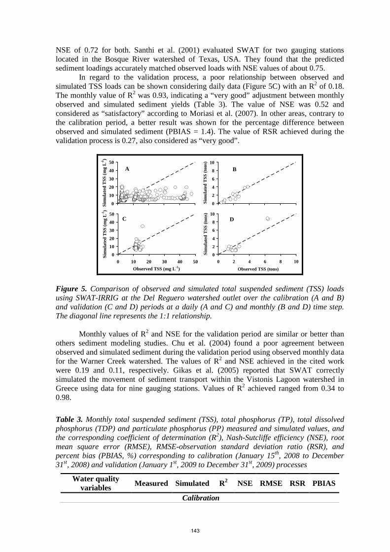
NSE of 0.72 for both. Santhi et al. (2001) evaluated SWAT for two gauging stations located in the Bosque River watershed of Texas, USA. They found that the predicted sediment loadings accurately matched observed loads with NSE values of about 0.75.

In regard to the validation process, a poor relationship between observed and simulated TSS loads can be shown considering daily data (Figure 5C) with an R2 of 0.18. The monthly value of R2 was 0.93, indicating a “very good” adjustment between monthly observed and simulated sediment yields (Table 3). The value of NSE was 0.52 and considered as “satisfactory” according to Moriasi et al. (2007). In other areas, contrary to the calibration period, a better result was shown for the percentage difference between observed and simulated sediment (PBIAS = 1.4). The value of RSR achieved during the validation process is 0.27, also considered as “very good”.

0

2

4

6

8

10

0 2 4 6 8 10Observed (tons)

Sim

ulat

ed T

SS (t

ons)

B

0

2

4

6

8

10

0 2 4 6 8 10Observed TSS (tons)

Sim

ulat

ed T

SS (t

ons)

D

0

10

20

30

40

50

0 10 20 30 40 50Observed (mg L-1)

Sim

ulat

ed T

SS (m

g L-1

)

A

0

10

20

30

40

50

0 10 20 30 40 50Observed TSS (mg L-1)

Sim

ulat

ed T

SS (m

g L-1

)

C

Figure 5. Comparison of observed and simulated total suspended sediment (TSS) loads using SWAT-IRRIG at the Del Reguero watershed outlet over the calibration (A and B) and validation (C and D) periods at a daily (A and C) and monthly (B and D) time step. The diagonal line represents the 1:1 relationship.

Monthly values of R2 and NSE for the validation period are similar or better than others sediment modeling studies. Chu et al. (2004) found a poor agreement between observed and simulated sediment during the validation period using observed monthly data for the Warner Creek watershed. The values of R2 and NSE achieved in the cited work were 0.19 and 0.11, respectively. Gikas et al. (2005) reported that SWAT correctly simulated the movement of sediment transport within the Vistonis Lagoon watershed in Greece using data for nine gauging stations. Values of R2 achieved ranged from 0.34 to 0.98.

Table 3. Monthly total suspended sediment (TSS), total phosphorus (TP), total dissolved phosphorus (TDP) and particulate phosphorus (PP) measured and simulated values, and the corresponding coefficient of determination (R2), Nash-Sutcliffe efficiency (NSE), root mean square error (RMSE), RMSE-observation standard deviation ratio (RSR), and percent bias (PBIAS, %) corresponding to calibration (January 15th, 2008 to December 31st, 2008) and validation (January 1st, 2009 to December 31st, 2009) processes

Water quality variables Measured Simulated R2 NSE RMSE RSR PBIAS

Calibration

143

TSS (tons) 23.3 19.6 0.87 0.72 0.41 0.38 -15.9 TP (kg) 272.4 245.8 0.70 0.66 7.05 0.57 -9.8 TDP (kg) 233.6 206.0 0.50 0.38 6.82 0.74 -11.8 PP (kg) 38.8 39.9 0.66 0.66 2.84 0.61 2.7

Validation TSS (tons) 31.6 31.2 0.93 0.52 0.49 0.27 -1.4 TP (kg) 173.2 209.3 0.71 0.63 7.32 0.56 20.9 TDP (kg) 156.7 188.0 0.67 0.56 6.84 0.60 20.0 PP (kg) 16.5 21.3 0.60 0.52 1.34 0.66 29.2

3.4.2. Total phosphorus (TP)

Figure 6 shows the comparison of observed and simulated TP loads at the DRW outlet during the calibration period considering daily (Figure 6A) and monthly data (Figure 6B). The daily observed and simulated TP load values showed a relatively good agreement (R2 = 0.34), and the simulated data match well with the measured data when monthly TP load values were considered (Figure 6B). The NSE, RSR, and PBIAS values (0.66, 0.57, and 9.8%, respectively) indicate a “good” simulation of monthly TP loadings during the calibration period (Table 3). The R2 value of 0.70 shows a strong linear relationship between observed and simulated TP loadings. These results are considerably better than the monthly TP calibration reported by Grunwald and Qi (2006). They obtained lower NSE values ranging from -0.89 to 0.07. Hanratty and Stefan (1998) calibrated SWAT phosphorus predictions using measured data collected for the Cottonwood watershed in Minnesota, and they reported satisfactory SWAT TP predictions with an NSE value of 0.54. Using nine gauging stations within the Vistonis Lagoon watershed of Greece, Gikas et al. (2005) found a good model performance for TP monthly loads with R2 values ranging from 0.50 to 0.82.

The comparison between observed and simulated TP loads at the DRW outlet during the validation period (2009) is shown in Figures 6C and 6D. For the daily time step, a good relationship between observed and simulated TP loads can be shown in Figure 6C with an R2 value of about 0.70. When monthly data is used, a very good correspondence between simulated and observed TP loads is obtained (Figure 6D). Statistical results indicate a “satisfactory” SWAT-IRRIG performance for predicting monthly TP yield at the DRW outlet for the validation process. The R2 value obtained of 0.71 indicates a very good agreement between simulated and observed TP loadings for a monthly time step (Table 3). The value of NSE was 0.763, also considered as “satisfactory.” The percent bias (PBIAS) between simulated and observed TP loads shows that simulated TP loads are relatively over-predicted (PBIAS of 20.85%), but they are considered as “very good” according to the values of NSE proposed by Moriasi et al. (2007). A monthly RSR of 0.56 was obtained, which is considered to be “good.”

Monthly values of R2 and NSE achieved during the validation period are similar to or better than those reported in other SWAT modeling studies. Saleh and Du (2004) achieved a monthly NSE value of 0.71 for the Upper North Bosque River watershed in Texas. In a study performed by Tolson and Shoemaker (2007) in the Cannonsville watershed of Texas, the reported values of R2 (from 0.72 to 0.83) and NSE (from 0.52 to 0.76) were more or less similar to those found for the Del Reguero watershed. In another case of study performed by White and Chaubey (2005), the values of R2 and NSE ranged between 0.58 to 0.76 and -0.29 to 0.67, respectively, for three gauges located in the Beaver Reservoir watershed of Arkansas, USA.

144

0102030405060

0 10 20 30 40 50 60Observed (kg)

Sim

ulat

ed (k

g) B

0102030405060

0 10 20 30 40 50 60Observed TP (kg)

Sim

ulat

ed (k

g) D

05

1015202530

0 5 10 15 20 25 30Observed (kg)

Sim

ulat

ed T

P (k

g) A

05

1015202530

0 5 10 15 20 25 30Observed TP (kg)

Sim

ulat

ed T

P (k

g) C

Figure 6. Comparison of observed and simulated total phosphorus (TP) loads using SWAT-IRRIG at the Del Reguero watershed outlet for calibration (A and B) and validation (C and D) considering daily (A and C) and monthly (B and D) data. The diagonal line represents the 1:1 relationship. 3.4.3. Total dissolved phosphorus (TDP)

The relationship between observed and simulated TDP loads at the DRW outlet for the calibration process is presented in Figure 7A and 7B for daily and monthly data, respectively. A relatively good relationship between daily observed and simulated TPD loads can be shown (R2 = 0.35). This relationship was improved when monthly observed and simulated TDP loads were considered (R2 = 0.50). However, an underestimation of TDP loads during the period from February to May was shown. This explains the relatively low NSE (NSE = 0.38) obtained (Table 3). Low values of NSE on a monthly basis were also reported in other SWAT modeling studies. Bouraoui et al. (2002) performed a study of climate change impacts on nutrient loads in the Yorkshire Ouse watershed of the UK. The monthly value of NSE for TDP calibration was 0.02, which was judged as very low. Also Chu et al. (2004) achieved a negative value for monthly time step NSE of -0.08 for TDP prediction in the Warner Creek watershed.

For the 2009 validation period considering daily data (Figure 7C), a good relationship between observed and simulated TP loads can be shown (R2 = 0.72). Validation Results were better than calibration ones. Also, good adjustment between monthly observed and simulated TDP loads was found (Figure 7D), and the statistical results indicate a “satisfactory” SWAT-IRRIG performance in describing monthly TDP yields at the Del Reguero watershed outlet (Table 3). The validation monthly values of R2 and NSE achieved in this study are within the range of variation of those achieved in the study performed by Bracmort et al. (2006) in the Dreisbach and Smith Fry watersheds of Indiana, USA. Performance values presented by the cited authors were 0.63 and 0.86 for R2, whereas values of NSE ranged from 0.51 to 0.74. Values of R2 (0.65) and NSE (0.55) found by Chu et al. (2004) for a monthly time step are similar to those found in this study. In the Upper North Bosque River watershed of Texas, Saleh and Du (2004) reported TDP validation NSE of 0.40 for monthly values.

145

0102030405060

0 10 20 30 40 50 60Observed (kg)

Sim

ulat

ed (k

g) B

0102030405060

0 10 20 30 40 50 60Observed TDP (kg)

Sim

ulat

ed (k

g) D

05

1015202530

0 5 10 15 20 25 30Observed (kg)

Sim

ulat

ed T

DP

(kg)

A

05

1015202530

0 5 10 15 20 25 30Observed TDP (kg)

Sim

ulat

ed T

DP

(kg)

C

Figure 7. Comparison total observed and simulated dissolved phosphorus (TDP) loads using SWAT-IRRIG at the Del Reguero watershed outlet over the calibration (A and B) and validation (C and D) periods and considering daily (A and C) and monthly (B and D) data. The diagonal line represents the 1:1 relationship. 3.4.4. Particulate phosphorus (PP)

For the PP calibration process, results indicate a very poor agreement between daily observed and simulated yield data (Figure 8A) with an R2 value about 0.04. For monthly data an R2 value of 0.66 was obtained, suggesting that simulations matched measured PP loadings reasonably well. The NSE value found on a monthly basis was better than those obtained from other SWAT modeling studies. Saleh et al. (2000) evaluated SWAT using data measured at the Upper Bosque River watershed outlet. They found that the parameters of the monthly calibration statistics generally indicated good model performance for PP loads (NSE = 0.54). In Texas, Saleh and Du (2004) tested SWAT predictions of PP using measured data within the Upper Bosque River watershed. They concluded that SWAT satisfactorily simulated PP losses with a monthly calibration NSE value of 0.59. The percent difference between simulated and observed PP loads shows that simulated PP loads are moderately over-predicted (PBIAS of 2.68%) but still considered to be “very good.” The RMSE-observation standard deviation ratio (RSR) showed a monthly value of 0.61 and is also considered in the satisfactory category (Moriasi et al., 2007).

With an R2 of 0.36, validation results showed stronger agreement than calibration results for daily data (Figure 8C). The agreement between observed and simulated PP loads was even greater for monthly data (Fig 8D and Table 3). An NSE value of about 0.52 was obtained, indicating a “satisfactory” prediction of monthly PP loadings during the validation period. The NSE value obtained during the validation period was within the range of variation found by Santhi et al. (2001) for the Bosque River watershed in Texas. Considering the PBIAS value of 29.2%, results indicated that simulated PP loads are over-predicted but still considered in the “good” category according to Moriasi et al. (2007). In addition, the RSR value of 0.66 was considered to be “satisfactory”.

146

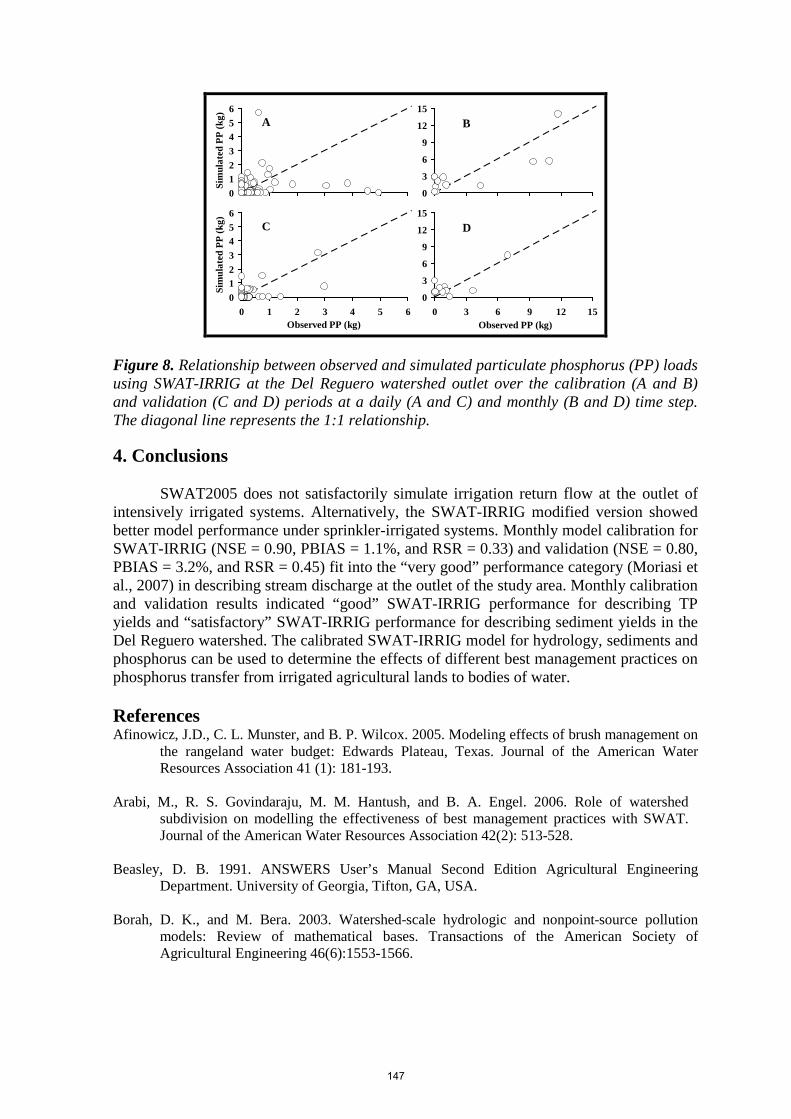
0

3

6

9

12

15

0 3 6 9 12 15Observed (kg)

Sim

ulat

ed (k

g) B

0

3

6

9

12

15

0 3 6 9 12 15Observed PP (kg)

Sim

ulat

ed (k

g) D

0123456

0 1 2 3 4 5 6Observed (kg)

Sim

ulat

ed P

P (k

g) A

0123456

0 1 2 3 4 5 6Observed PP (kg)

Sim

ulat

ed P

P (k

g) C

Figure 8. Relationship between observed and simulated particulate phosphorus (PP) loads using SWAT-IRRIG at the Del Reguero watershed outlet over the calibration (A and B) and validation (C and D) periods at a daily (A and C) and monthly (B and D) time step. The diagonal line represents the 1:1 relationship. 4. Conclusions SWAT2005 does not satisfactorily simulate irrigation return flow at the outlet of intensively irrigated systems. Alternatively, the SWAT-IRRIG modified version showed better model performance under sprinkler-irrigated systems. Monthly model calibration for SWAT-IRRIG (NSE = 0.90, PBIAS = 1.1%, and RSR = 0.33) and validation (NSE = 0.80, PBIAS = 3.2%, and RSR = 0.45) fit into the “very good” performance category (Moriasi et al., 2007) in describing stream discharge at the outlet of the study area. Monthly calibration and validation results indicated “good” SWAT-IRRIG performance for describing TP yields and “satisfactory” SWAT-IRRIG performance for describing sediment yields in the Del Reguero watershed. The calibrated SWAT-IRRIG model for hydrology, sediments and phosphorus can be used to determine the effects of different best management practices on phosphorus transfer from irrigated agricultural lands to bodies of water. References Afinowicz, J.D., C. L. Munster, and B. P. Wilcox. 2005. Modeling effects of brush management on

the rangeland water budget: Edwards Plateau, Texas. Journal of the American Water Resources Association 41 (1): 181-193.

Arabi, M., R. S. Govindaraju, M. M. Hantush, and B. A. Engel. 2006. Role of watershed

subdivision on modelling the effectiveness of best management practices with SWAT. Journal of the American Water Resources Association 42(2): 513-528.

Beasley, D. B. 1991. ANSWERS User’s Manual Second Edition Agricultural Engineering

Department. University of Georgia, Tifton, GA, USA. Borah, D. K., and M. Bera. 2003. Watershed-scale hydrologic and nonpoint-source pollution

models: Review of mathematical bases. Transactions of the American Society of Agricultural Engineering 46(6):1553-1566.

147

Bouraoui, F., L. Galbiati, and G. Bidoglio. 2002. Climate change impacts on nutrient loads in the Yorkshire Ouse catchment (UK). Journal of Hydrology and Earth System Sciences 6 (2): 197-209.

Bouraoui, F., S. Benabdallah, A. Jrad, and G. Bidoglio. 2005. Application of the SWAT model on

the Medjerda River basin (Tunisia). Journal of Physics and Chemistry of the Earth 30(8-10):497-507.

Bracmort, K.S., M. Arabi, J. R. Frankenberger, B. A. Engel, and J. G. Arnold. 2006. Modeling

long-term water quality impact of structural BMPs. Transactions of the American Society of Agriculture and Biological Engineering 49 (2), 367-374.

Causapé J. 2009. A computer-based program for the assessment of water-induced contamination in

irrigated lands. Environmental Monitoring and Assessment 158(1-4): 307-314. Chu, T.W., A. Shirmohammadi, H. Montas, and A. Sadeghi. 2004. Evaluation of the SWAT

model’s and nutrient components in the piedmont physiographic region of Maryland. Transactions of the American Society of Agricultural Engineering 47(5): 1523-1538.

Eckhardt, K., S. Haverkamp, N. Fohrer, and H. G. Frede. 2002. SWATG, a version of SWAT99.2

modified for application to low mountain range catchments. Journal of Physics and Chemistry of the Earth 27 (9-10): 641-644.

FitzHugh, T.W., and D.S. Mackay. 2000. Impacts of input parameter spatial aggregation on an

agricultural nonpoint source pollution model. Journal of Hydrology 236:35-53. Galván, L., M. Olías, R. Fernández de Villarán, J. M. Domingo Santos, J. M. Nieto, A. M.

Sarmiento, and C. R. Cánovas. 2009. Application of the SWAT model to an AMD-affected river (Meca River, SW Spain). Estimation of transported pollutant load. Journal of Hydrology 377:445-454.

Gassman, P. W., M. R. Reyes, C. H. Green, and J. G. Arnold. 2007. The Soil and Water

Assessment Tool: historical development, applications and future research directions. American Society of Agricultural and Biological Engineers 50(4): 1211-1250.

Gikas, G.D., T. Yiannakopoulou, and V. A. Tsihrintzis. 2005. Modeling of nonpoint-source

pollution in a Mediterranean drainage basin. Journal of Environmental Modeling and Assessment 11 (3): 219-233.

Grunwald, S., and C. Qi. 2006. GIS-based water quality modeling in the Sandusky watershed,

Ohio, USA. Journal of the American Water Resources Association 42(4): 957-973. Gupta, H. V., S. Sorooshian, and P. O. Yapo. 1999. Status of automatic calibration for hydrologic

models: Comparison with multilevel expert calibration. Journal of Hydrologic Engineering 4(2): 135-143.

Hanratty, M.P., and H. G. Stefan. 1998. Simulating climate change effects in a Minnesota

agricultural watershed. Journal of Environmental Quality 27 (6): 1524-1532. Hao, F.H., X. S. Zhang, and Z. F. Yang. 2004. A distributed nonpoint source pollution model:

Calibration and validation in the Yellow River basin. Journal of Environmental Science. 16 (4): 646-650.

Holman, I. P., J. M. Hollis, G. Alavi, P. H. Bellamy, N. Jarvis, G. Vachaud, P. J. Loveland, A.

Gardenas, C. J. Tao C Bo, and J. Kreuger. 2001. CAMSCALE-Upscaling Predictive

148

Models and Catchment Water Quality. Draft Final Report to DGXII, Commission of the European Communities under Contract ENV4-CT97-0439.

Kalin, L., and M. Hantush. 2006. Hydrologic modeling of an eastern Pennsylvania watershed with

NEXRAD and rain gauge data. Journal of Hydrologic Engineering 11(6): 555-569. Klemeš, V. 1986. Operational testing of hydrological simulation models. Journal of Hydrological

Sciences 31:13-24. Krysanova, V., F. Hatterman, and F. Wechsung. 2005. Development of the ecohydrological model

SWIM for regional impact studies and vulnerability assessment. Journal of Hydrology Processes 19(3): 763-783.

Lenhart, T., A. Van Rompaey, A. Steegen, N. Fohrer, H.G. Frede, and G. Govers. 2005.

Considering spatial distribution and deposition of sediment in lumped and semi-distributed models. Journal of Hydrological Processes 19(3):785-794.

Lenhart, T., N. Fohrer, and H. G. Frede. 2003. Effects of land use changes on the nutrient balance

in mesoscale catchments Journal of Physics and Chemistry of the Earth 28:1301-1309. Moriasi, D. N., J. G. Arnold, M. W. Van Liew, R. L. Bingner, R. D. Harmel, and T. L. Veith. 2007.

Model evaluation guidelines for systematic quantification of accuaracy in watershed simulations. Transactions of the American Society of Agricultural and Biological Engineers 50(3):885-900.

Nash, J. E., and J. E. Sutcliffe. 1970. River flow forecasting through conceptual models: Part1. A

discussion of principles. Journal of Hydrology 10(3):282-290. Nasr, A., M. Bruen, P. Jordan, R. Moles, G. Kiely, and P. Byrne. 2007. A comparison of SWAT,

HSPF, and SHETRAN/GOPC for modeling phosphorus export from three catchments in Ireland. Journal of Water Resources 41(5):1065-1073.

Neitsch, S.L., J.G. Arnold, J.R. Kiniry, and J.R. Williams. 2005. Soil and Water Assessment Tool

theoretical documentation version 2005: Draft-January 2005, US Department of Agriculture-Agricultural Research Service, Temple, Texas.

Saleh, A., J. G. Arnold, P. W. Gassman, L. W. Hauck, W. D. Rosenthal, J. R. Williams, and A. M.

S. McFarland. 2000. Application of SWAT for the upper North Bosque River watershed. Transactions of the American Society of Agricultural Engineering 43 (5): 1077-1087.

Saleh, A., and B. Du. 2004. Evaluation of SWAT and HSPF within BASINS program for the upper

North Bosque River watershed in central Texas. Transactions of the American Society of Agricultural Engineering 47 (4): 1039-1049.

Santhi, C., J. G. Arnold, J. R. Williams, W. A. Dugas, R. Srinivasan, and L. M. Hauck. 2001.

Validation of the SWAT model on a large river basin with point and nonpoint sources. Journal of the American Water Resources Association 37 (5): 1169-1188.

Tolson, B. A., and C. A. Shoemaker. 2007. Cannonsville reservoir watershed SWAT2000 model

development, calibration, and validation. Journal of Hydrology 337(1-2): 68-86. van Griensven, A., and W. Bauwens. 2005. Application and evaluation of ESWAT on the Dender

basin and Wister Lake basin. Journal of Hydrologic Processes 19(3):827-838.

149

Van Liew, M. W., 2009. Streamflow, sediments and nutrient simulation of the Bitterroot watershed using SWAT. Proceedings of the 2009 International SWAT conference, August 5-7, 2009, Boulder, Colorado.

Wang, X., and A. M. Melesse. 2006. Effects of STATSGO and SSURGO as inputs on SWAT

model's snowmelt simulation. Journal of the American Water Resources Association 42(5): 1217-1236.

Watson, B. M., R. Srikanthan, S. Selvalingam, and M. Ghafouri. 2005. Evaluation of three daily

rainfall generation models for SWAT. Transactions of the American Society of Agricultural and Biological Engineers 48(5):1697-1711.

White, K. L., and I. Chaubey. 2005. Sensitivity analysis, calibration, and validations for a multisite

and multivariable SWAT model. Journal of the American Water Resources Association 41(5): 1077-1089.

Wu, K., and Y. I. Xu. 2006. Evaluation of the applicability of the SWAT model for coastal

watersheds in southeastern Louisiana. Journal of the American Water Resources Association 42(5): 1247-1260.

Zhang, X., R. Srinivasan, and F. Hao. 2007. Predicting hydrologic response to climate change in

the Luohe River basin using the SWAT model. Transactions of the American Society of Agricultural and Biological Engineers 50(3): 901-910.

150

Malfunctioning of Stream-Gauge Stations in the Chanza and Arochete Rivers of Huelva, Spain Detected from Hydrological

Modeling with SWAT

L. Galván (1), M. Olías (1) and A. Van Griensven (2)

(1) University of Huelva, Department of Geodynamics and Palaeontology, Avda. Fuerzas Armadas, s/n 21071, Huelva, Spain. E-mail: laura.galvan@dgyp.uhu.es (2) UNESCO-IHE Water Education Institute, Deparment of Hydroinformatics and Knowledge Management, PO Box 3015, 2601 DA Delft, The Netherlands.

Abstract To carry out the hydrological modeling of the Odiel river of southwest Spain using the SWAT program, stream gauge stations to the north of the basin are necessary because, due to the outcrop of carbonate materials, this zone has a hydrological behaviour that is different from the rest of the catchment. In neighboring catchements to the north of the Odiel basin there are two stream gauge stations located on the Chanza and Arochete rivers. The aim of this study is to develop a hydrological model of these rivers using SWAT in order to transfer the parameters of these basins to the northern subcatchments inside the Odiel basin. The models are calibrated and validated using SWAT-CUP. The statistical indexes obtained are acceptable: the Chanza river in the calibration period (1980-1993) obtained a value for the NSE (Nash and Sutcliffe Efficiency) of 0.54 for daily flow and a diversion of the volume of runoff (DV) of 0.95. For the Arochete river, which was calibrated for the period 1980-1990, the value of NSE is 0.52 for daily flow and the DV is 1.13. The main problems are the obtained mass balance results. In the Chanza river, the value for the deep aquifer recharge variable (RCHRG_DP) is too high to be supported by any hydrogeological reason. For the Arochete river, the value for this variable is also too high. In addition, an excessive decrease in the curve number (CN2) and an increase for soil available water capacity (sol_awc) was obtained. This can be explained by the bad quality of the observed stream data for these rivers that seem to underestimate the flow values. Due to these errors, SWAT_CUP has to increase the recharge to a deep aquifer and soil available water capacity and decrease the curve number. This indicates that these stream-gauge stations are not suitable for calibrating the model. Keywords: hydrological modeling, SWAT, SWAT-CUP, Chanza river, quality of stream-gauge data

151

1. Introduction

The Odiel river drainage network, located in the Huelva province southwest of the Iberian Peninsula, is highly contaminated by acid mine drainage coming from numerous mines scattered across the Iberian Pyrite Belt. To assess the contaminant load carried by the Odiel river, water quality analysis and spatial and temporal continuous discharge data must be available. Galván et al. (2008) point out the lack of streamflow gauges in the Odiel basin and the need to generate discharge data for this basin. To accomplish this, the hydrological model Soil and Water Assesment Tool (SWAT) is used. To calibrate this model, only two points with streamflow data were used, both located at the south zone of the basin. Even though good results were obtained (NSE > 0.75 at the monthly level), some points to calibrate the model in the northern area are necessary, as the carbonate materials outcropping presents a different hydrogeological behavior from the rest of the basin. Two streamflow gauges are found just to the north of the Odiel basin with similar characteristics on the Chanza and Arochete rivers (Figure 1)

The aim of this study is to model the hydrological behaviour of the Chanza and Arochete river basins in order to obtain the representative parameter values of the northern area of the Odiel basin and to assess the quality of the available streamflow data. 2. Study Area

Until the points considered, the Chanza river basin has a surface area of 87 km2, whereas the Arochete subbasin is 46 km2 (Figure 1). The maximum elevation of the Chanza basin is 762 m, and its mean height is 548 m. Arochete subbasin presents a similar maximum altitude of 794 m, whereas its mean height is slightly minor, 475 m. The mean annual rainfall of the area is 841 mm even though it presents a high interannual and intraannual variability. The mean annual temperature is 16ºC.

The mains soil uses are pasture (28%), forest (27%), brush (20%) and agricultural (18%). The predominant soil (30% of the surface) according to the FAO classification is Alisol and Lithic Haploxeralf according to Soil Taxonomy. The lithologic map represented in Figure 1 shows that the materials drained by these rivers are mainly gneisses, diorites and quartz diorites and phyllites. In the southern area of the basin there are some sands, gravels and conglomerates outcrops. The carbonate materials (marbles with calcoschists) are more abundant in the Chanza subbasin (Figure 1).

152

Figure 1. Location of the study area, lithology, location of streamflow gauge and weather stations

3. Methodology

The software SWAT 2005 (Neitsch et al., 2005a y 2005b) and the extension of ArcGIS 9.2 called ArcSWAT 2.1.6 (Winchell et al., 2008) have been used. The modeling starts with the Digital Elevation Model (DEM) of the Andalusia Regional Government (2005), with a spatial resolution of 10 m/pixel. The high elevations are located in the eastern area of the basin (Figure 2).

153

Figure 2. Elevation map

Delineation of the subbasins has been established with a threshold area value of 800

ha, which creates five subbasins (Figure 1). 60% of the basin is included in the range of slope of 6%-30%, and almost 20% is higher than 36% (Table 1).

Table 1. Slope ranges and surface percent of the basin Slope range Surface (%)

0 – 6 9.49 6 – 18 28.47 18 – 30 30.68 30 – 36 12.05

> 36 19.31

The land use map used in the model has been provided by the Environmental Council of the Andalusia Regional Government using photointerpretation of a flight from 1999. Soil information was obtained from an edaphic study of the zone (Fernández de Villarán, personal communication), and 12 edaphic units have been differentiated (Table 2). Available water capacity has been calculated from the texture data by the Saxton et al. (1986) equation.

HRUs were obtained with a threshold of 2% for land use, soil type and slope; percents smaller than the threshold are not taken into account by the program. The total number of HRUs generated is 157.

154

Table 2. Main characteristics of considered soil types (AWC: available water capacity, SHC: saturated hydraulic conductivity)

Soil code 1 2 3 4 5 6 7 8 9 10 11 12 Basin surface (%) 15 2.6 3.2 2.2 0.2 30 12 7.4 17 4.4 1.4 4 Depth (cm) 103 85 75 105 82 68 50 96 123 101 161 108 AWC (% vol.) 0.11 0.14 0.13 0.14 0.14 0.15 0.16 0.15 0.12 0.12 0.08 0.14 Rock fragment (%) 8 4 42 57 41 44 37 27 16 19 2 22 Clay (%) 19 17 24 15 22 23 21 23 20 15 6.7 14 Silt (%) 24 44 31 45 41 44 49 47 28 32 11 44 Sand (%) 57 39 45 40 38 33 30 30 52 53 83 42 Organic matter (%) 2.7 2.3 2.2 4.7 1.7 5.1 1.8 2.9 2.7 1.6 1.2 2.2 SCH at 10 cm (cm/h) 8.6 1.6 2.6 5.7 2.9 2.3 1.8 1.4 2.6 1.7 24 1.6 SCH at 50 cm (cm/h) 3.4 0.2 0.8 0.9 0.8 0.8 0.9 0.4 0.6 1.3 17 0.8 Bulk density (g/cm3) 1.4 1.3 1.4 1.3 1.3 1.2 1.1 1.3 1.4 1.4 1.5 1.3 Soil hydrologic group C C C C C C C D C C B C

Three meteorological stations exist with rainfall and minimum and maximum

temperature daily data (Figure 1). These data from 1980 to 2006 have been checked and completed by statistical methods. Potential evapotranspiration (PET) is calculated using the Hargreaves method (Hargreaves, 1985; Neitsch et al., 2005a). To account for orographic effects on precipitation in mountainous areas, SWAT allows up to 10 elevation bands in each subbasin. Considering the regional distribution of rainfall, elevation bands have been used. This establishes an orographic rainfall gradient of 0.79 mm/m.

First, a manual calibration to adjust the parameters was performed, and then the application of SWAT-CUP software and SUFI-2 (Abbaspour, 2009) as uncertainty analysis routines optimized the calibration. SUFI-2 performs a combined optimization and uncertainty analysis using a global search procedure and can deal with a large number of parameters (Abbaspour et al., 2004; Abbaspour et al., 2007). Daily flow data from available streamflow gauges were used to calibrate the model. For the Chanza river the calibration period was from 1980 to 1993, and for the Arochete river it was from 1980 to 1990. For model validation, the period from 1994 to 2006 was used for the Chanza river and 1991 to 2000 was used for Arochete were reserved (this station only has data up to 2000).

To assess the fit quality between measured and simulated values, the following statistical index has been calculated: Pearson correlation coefficient (r), efficient coefficient of Nash and Sutcliffe (NSE, Nash and Sutcliffe, 1970), mean square error (RMS, Hogue et al., 2006) and runoff volume deviation (DV, Boyle et al., 2000). 4. Results and Discussion

To perform the manual calibration of the model, the following variables were modified: GW_DELAY, ALPHA_BF, GWQMN, GW_REVAP, REVAPMN, RCHRG_DP, SURLAG, ESCO, CN2 and SOL_AWC. Modified values are given in Table 3. With these values the NSEs for both the Chanza and Arochete rivers are considered to be unsatisfactory according to Moriasi et al., (2007). Furthermore, in the Arochete river a 31% overestimation of measured flow has been produced whereas in the Chanza river there is a slight overestimation (Tables 3 and 4).

155

Table 3. Object parameter calibration and obtained values for manually calibration Parameter Descripiton Chanza Arochete GW_DELAY Groundwater delay time (days) 70 70 ALPHA_BF Baseflow alpha factor (days) 0.024 0.048

GWQMN Threshold depth of shallow aquifer water required for return flow (mm H2O) 1500 1500

GW_REVAP Groundwater “revap” coefficient 0.02 0.02 REVAPMN Threshold depth of water in the shallow aquifer for “revap" (mm H2O) 1 1 RCHRG_DP Deep aquifer percolation fraction 0.05 0.05 SURLAG Surface runoff lag coefficient 0.15 0.15 ESCO Soil evaporation compensation factor 0.01 0.01 CN2 SCS runoff number -30% -30% SOL_AWC Available water capacity of the soil layer (mm H2O/ mm soil) 25% 25% Table 4. Statistics index values (daily) to calibration period for manually calibration and SWAT-CUP

Manual calibration SWAT CUP

Index Chanza Arochete Chanza Arochete

r 0.69 0.63 0.76 0.74 NSE 0.46 0 0.54 0.52

RMS (m3/s) 0.92 0.37 0.85 0.25

DV 1.02 1.31 0.95 1.13

A second automatic model calibration and uncertainty analysis was performed with

SWAT-CUP and SUFI-2 (Sequential Uncertainty Fitting Ver. 2). These methods consist of a sequence of steps in which the initial uncertainty in the model parameters is progressively reduced until certain calibration criteria for prediction uncertainty fit. The software uses an efficient sampling procedure (Latin hypercurbe) along with a global search algorithm that examines the behaviour of an objective function (Abbaspour et al., 2004). The key output of SUFI-2 is a “best range” for each parameter. Parameter combinations within the parameter ranges are ensured to produce high quality simulations. Starting with some initial parameter value ranges, SUFI-2 is iterated until the 95% prediction uncertainty (95PPU) between the 2.5th and 97.5th percentiles brackets is more than 90% of the measured data and the average distance between the 2.5th and 97.5th percentiles is smaller than the standard deviation of the measured data.

For this calibration, we first establish absolute minimum and maximum ranges for the optimized parameters (Table 5). These parameter ranges and the starting initial ranges were selected based on minimums and maximums established by SWAT (Neitsch et al., 2005b) and our experience in the area. After 1,000 simulations with the initial range, the optimized range was obtained. Finally, after sampling for a total of 10 simulations we obtained the optimized value (Table 5). The daily statistical indices are satisfactory according to Moriasi et al. (2007). In Arochete, the overestimation decreased from 31% to 13%, and in Chanza, the final results show a slight underestimation (Table 4). These differences are due to the decrease in the manual calibration of CN2 to 30% and in the SWAT-CUP calibration an additional 43% for the Arochete river and 6.5% for the Chanza river. Simultaneously, SWAT-CUP increases RCHRG_DP in both cases without apparent reason, because in the area there is a small aquifer in the carbonate materials outcrop to the south of the Chanza subbasin (Figure 1), but in the rest of the basin there is no outcropping of aquifer materials. Therefore, there is no possibility of a significant amount of water flowing from the studied basins to others through deep flow.

156

The presence of the carbonate materials in the Chanza subbasin is reflected on the calibration results for SWAT-CUP, in which the low ALPHA_BF indicates the presence of materials with a slow response to recharge. This fact also has been reflected in the parameter GW_DELAY with a much higher value in Chanza than in Arochete (Table 5).

Table 5. Initial range, optimized range and optimized value of SWAT-CUP and SUFI-2. The letter at the beginning of the parameter name means: v - the existing parameter value is to be replaced by a given value; a - a given quantity should be added to the existing parameter value; and r - the existing parameter value should be multiplied by a given value. Chanza Arochete

Parameter Initial Range Optimized Range Optimized value Optimized Range Optimized value

v_GW_DELAY 0 – 80 66.78 - 80.32 75.58 7.37 - 17.14 12.41 v_ALPHA_BF 0 – 1 0.13 - 0.71 0.28 0.38 - 1 0.51 a_GWQMN 0 – 1500 400 - 1202 2261 383 - 1016 2666 v_GW_REVAP 0.02 - 0.2 0.02 - 0.02 0.02 0.02 - 0.02 0.02 v_REVAPMN 1 – 500 159 - 481 305 339 - 569 391 v_RCHRG_DP 0 – 1 0.063 - 0.65 0.33 0.44 - 0.79 0.612 v_SURLAG 0.15 – 4 1 - 5 1.18 0.79 - 2.93 4.34 v_ESCO 0.01 – 1 0.070 - 0.64 0.035 0.02 - 0.48 0.015 r_CN2 -25 % - 25% - 4.8% - 0.5% -2% - 95% - 36% -43% r_SOL_AWC -25 % - 25% -4% - 38% 6.50% 6.5% - 50% 28%

Figures 3 and 4 show the daily flow evolution for the calibration period with SWAT-

CUP for the Chanza and Arochete rivers. Even though acceptable fits have been obtained between measured and simulated flows, the specific flows obtained are low considering that this zone has a slightly mountainous relief: 3.07 L⋅s-1⋅km-2 for Chanza and 3.11 L⋅s-1⋅km-2 for Arochete. Compare these values to other basins with similar characteristics such as those for the Múrtigas and Caliente rivers. Located close to the E zone, they show a specific flow of 12.8 and 10.6 L⋅s-1⋅km-2 (Galván et al., 2010) even though this area is slightly more humid, with a mean annual rainfall of 922 mm. Compare it to a less mountainous basin, such as that for the Meca river to the south with a mean altitude of 152 m and a mean annual rainfall of 632 mm; the Meca basin also shows a higher specific flow of 5.4 L⋅s-1⋅km-2 (Galván et al., 2009). Furthermore, the entire Odiel river watershed shows a higher specific flow (8.4 L⋅s-

1⋅km-2) than those obtained for the Chanza and Arochete rivers, although its mean altitude is just 270 m.

157

0.001

0.01

0.1

1

10

100

Jan-80 Jan-81 Jan-82 Jan-83 Jan-84 Jan-85 Jan-86

Flow

(m3 /s

)MeasuredSimulated

0.001

0.01

0.1

1

10

100

Jan-87 Jan-88 Jan-89 Jan-90 Jan-91 Jan-92 Jan-93

Flow

(m3 /s

)

MeasuredSimulated

Figure 3. Daily evolution of measured and simulated flows from 1980 to 1993 for the Chanza

river calibrated with SWAT-CUP

0.001

0.01

0.1

1

10

Jan-80 Jan-81 Jan-82 Jan-83 Jan-84

Flow

(m3 /s

)

MeasuredSimulated

0.001

0.01

0.1

1

10

Jan-85 Jan-86 Jan-87 Jan-88 Jan-89 Jan-90

Flow

(m3 /s

)

MeasuredSimulated

Figure 4. Daily evolution of measured and simulated flows from 1980 to 1990 for the Arochete river calibrated with SWAT-CUP

158

In Table 6 we see that the deep aquifer recharge is high in both basins but especially in the Arochete river, in which the value of the variable RCHRG_DP is higher than in the Chanza river.

Table 6. Average annual basin values for Chanza and Arochete river (in mm) Chanza Arochete PRECIP 726.3 775.5 SURFACE RUNOFF Q 23.07 1.16 LATERAL SOIL Q 74.92 103.69 GROUNDWATER Q 8.14 0 REVAP 17.99 8.57 DEEP AQ RECHARGE 52.98 108.26 TOTAL AQ RECHARGE 162.04 177.01 ET 462.1 488.7 TRANSMISSION LOSSES 0.73 0.05

These results show that the existing streamflow data for both basins are of poor quality

and are highly underestimated. These data are not reliable for calibrating the model, so the validation was not carried out. This problem seems to be widespread in the area; the calibration of two nearby basins with similar characteristics was carried out and poor quality streamflow data was similarly detected (Galván et al., 2010). Therefore, it is necessary to improve stream gauge data to reliably quantify water resources in this region. 5. Summary and Conclusions

A hydrological modelling of the Chanza and Arochete rivers has been developed and calibrated with streamflow data from two gauges. In the manual calibration, unsatisfactory values of NSE (Moriasi et al., 2007) were obtained for both the Chanza and Arochete rivers. To optimize the manual calibration, the autocalibration program SWAT-CUP (SUFI-2) was applied in order to obtain satisfactory daily values (Moriasi et al., 2007). Parameter ALPHA_BF reached a value of 0.28 in the Chanza subbasin. This indicates the presence of aquifer materials that have a slow response to recharge; this is also indicated by the GW_DELAY values.

Nevertheless, the definition of a good simulation can be very subjective because visually different parameter combinations may yield identical values for the objective functions (Boyle et al., 2000; Abbaspour et al., 2004). Despite the results achieved by SWAT-CUP, it is important to point out the need for the software to reduce flow. This can be done by reducing the CN2 and SOL_AWC variables while increasing SOL_AWC. In addition, an unreasonably high value for RCHRG_DP was found for the Chanza river. The specific flow in both subbasins is unusually low when compared to other watersheds with similar characteristics, and this indicates the bad quality of stream flow data used for the calibration.

The results obtained in this work show the need for streamflow gauges in the area with good quality spatial and temporal continuous recorded flows which would allow for accurate simulations of the hydrological behaviour of the basins. Acknowledgements This work has been financed by the Environmental Council of the Andalusia Regional Government through the project ‘‘Mining contamination evaluation, acid mine drainage treatment, hydrologic modelling of the Odiel River basin and study of the contaminant load to the Huelva estuary” and a FPU fellowship of the Education and Science Ministry of the

159

Spanish Government. The authors are also grateful to Dr. Fernández de Villarán for soil information for the area. The authors also thank the FP7 AQUAREHAB project for their support. References Abbaspour, K. 2009. SWAT-CUP2. SWAT Calibration and Uncertainty Programs. Version 2. Eawag. Abbaspour, K.C., Jonson, A., van Genuchten, M.Th. 2004. Estimating uncertain flow and tranport

parameters using a sequential uncertainty fitting procedure. Vadose Zone Journal 3, 1340-1352.

Abbaspour, K.C., Yang, J., Maximov, I., Siber, R., Bogner, K., Mieleitner, J., Zobrist, J., Srinivasan,

R. 2007. Modelling hydrology and water quality in the pre-alpine/alpine Thur watershed using SWAT. Journal of Hydrology 333, 413-430.

Boyle, D.P., Gupta, H.V., Sorooshian, S. 2000. Towards improved calibration of hydrologic models:

Combining the strengths of manual and automatic methods. Water Resour. 36, 3663-3674 Galván, L., Olías, M. Fernández de Villarán, R. and Domingo, J.M. 2008. Aplicación del modelo

hidrológico SWAT (Soil and Water Assessment Tools) a la cuenca del río Odiel (SO, España). Geo-Temas 10.

Galván, L., Olías, M., Fernández de Villarán, R., Domingo Santos, J.M., Nieto, J.M., Sarmiento,

A.M., Cánovas, C.R. 2009. Application of the SWAT model to an AMD-affected river (Meca River, SW Spain). Estimation of transported pollutant load. Journal of Hydrology 377, 445-454.

Galván, L., Olías, M. 2010. Modelización hidrológica de las cuencas de los ríos Múrtigas y Caliente

(Huelva, España). Calidad de los datos de aforos. Geogaceta 48, 123-126. Hargreaves, G.L., Hargreaves, G.H., Riley, J.P. 1985. Agricultural benefits for Senegal River Basinn.

J. Irrig and Drain. Engr. 111(2), 113-124. Hogue, T.S., Gupta, H.V., Sorooshial, S. 2006. A ‘User-Friendly’ approach to parameter estimation in

hydrologic models. Journal of hydrology 320, 202-217. Junta de Andalucía 2005. Modelo digital del terreno de Andalucía. Relieve y Orografía. Consejería de

Obras Públicas y Transportes, Consejería de Agricultura y Pesca y Consejería de Medio Ambiente, Sevilla. DVD.

Moriasi, D.N., Arnold, J.G., Van Liew, M.W., Bingner, R.I., Harnel, R.D., Veith, T.L. 2007. Model

evaluation guidelines for systematic quatification of accuracy in watershed simulations. American Society of Agricultural and Bilogical Engineers 50, 885-900

Nash, J.E., Sutcliffer, J.V. 1970. River flow forecasting through conceptual models 1. A discussion of

principles. Journal of Hydrology 10, 282-290 Neitsch, S.I., Arnold, J.G., Kiniry, J.R., Willliams, J.R. 2005. Soil and Water Assessment Tool

Theoretical Documentation: Version 2005. Texas Water Resources Institute Report TR-191. Neitsch, S.I., Arnold, J.G., Kiniry, J.R., Srinivasan, R., Willliams, J.R. 2005. Soil and Water

Assessment Tool Input/Output File Documentation: Version 2005. Texas Water Resources Institute Report TR-191.

160

Winchell, M., Srinivasan, R., Di Luzio, M. Arnold, J. 2008. ArcSWAT 2.1 Interface for SWAT 2005: User’s Guide. Texas Water Resources Institute Report TR-191.

161

Application and Validation of SWAT Model to an Alpine Catchment in the Central Spanish Pyrenees

L. Palazón1*, A. Navas1

1Department of Soil and Water. Estación Experimental de Aula Dei (EEAD)-CSIC, Campus de

Aula Dei, Avda. Montañana 1005, Zaragoza, 50059, Spain *Email: lpalazon@eead.csic.es

Abstract Modeling runoff and sediment transport at catchment scale are key tools for predicting water and sediment yields with the purpose of preserving soil and water resources. This study aims to validate the SWAT model for its use in an alpine catchment as a simulator of processes related to water quantity and soil erosion in order to minimize indirect impacts such as reservoir siltation and loss of water quality. The newest version of Soil and Water Assessment Tool (SWAT2009), coupled with a GIS interface (ArcSWAT), was applied to the Barasona Reservoir catchment located in the central Spanish Pyrenees. The 1,509 km2 catchment presents an altitudinal range close to 3000 meters and a precipitation variation of 1000 mm/km. The high mountainous characteristics of the catchment required specific definitions for some parameters. The snowmelt is a significant process in the hydrologic regime of the drainage area of the reservoir. The snowmelt was defined with the temperature-index plus elevation bands algorithm. The model was calibrated and validated using continuous streamflow data from gauge stations. Calibration and validation results showed good agreement between simulated and measured data. Model performance was evaluated using several statistical parameters, such as the Nash–Sutcliffe coefficient. The information gained with this research will be of interest to identify sediment sources and areas of high sediment yield risk, and to identify erosion and sediment transport patterns in the catchment. Keywords: SWAT, mountainous catchment, snowmelt, streamflow, alpine catchment

162

1. Introduction In the last century, topographical and hydrological characteristics of the Spanish

Pyrenees were considered to be appropriate for constructing reservoirs. Many Pyrenean rivers have been dammed to provide electricity and irrigation water to the lowland areas. The rugged topography, the regime of the rivers with frequent floods, and the changes in land use which have occurred during the past few decades have triggered soil erosion and consequently siltation and reservoir management problems (Valero-Garcés et al., 1999; Navas et al., 2009). In this paper we investigate the drainage area of the Barasona Reservoir which is located in the Central Spanish Pyrenees.

Since it is difficult to obtain continuous direct measurements with sufficient spatial coverage in mountain ecosystems, a robust computational hydrologic model that simulates fluxes of energy and water between the atmosphere and the land surface can be an effective means of studying land-surface dynamics (Stratton et al., 2009). The need to better understand the hydrologic characteristics of a snow-dominated catchment at the regional scale of a reservoir basin is highlighted by problems related to preserving soil and water resources.

Snow-dominated mountain catchments present considerable challenges for spatially distributed modeling due to highly heterogeneous climate drivers, complex topography, and environmental gradients (Stratton et al., 2009). Because of the limited climatic data in these areas, extrapolation of temperature and precipitation is required with the difficulty that this implies through mountainous terrain. Therefore, both precipitation and temperature lapse rates computed for this data-limited region can only be an approximation and they can restrict the ability of the model to capture the catchment processes. Complex topography introduces diverse snowmelt patterns, and large elevation gradients can produce complicated precipitation distributions. A review of the historical development and applications of SWAT was conducted by Gassman et al. (2007). SWAT has been implemented to adequately estimate streamflow volumes and timing from mountainous catchments. Fontaine et al. (2002) first applied SWAT to the Upper Wind River basin of Wyoming by adding elevation bands, an areal depletion curve, and snowpack temperature and meltwater production routines, which significantly improved SWAT´s runoff simulation capability. Lemmonds and McCray (2007), Ahl et al. (2008) and Stratton et al. (2009) have since applied these hydrologic changes within SWAT to experimental watersheds in Montana and Idaho with reasonable success. Eckhardt et al. (2002) and Govender and Everson (2005) all describe additional hydrologic applications worldwide (Germany and Africa). Zang et al. (2008) compared snowmelt algorithms incorporated into SWAT in the headwaters of the Yellow River and concluded that utilization of temperature index plus elevation bands gave satisfactory results. However, fewer studies have been conducted to evaluate sediment production with SWAT in mountainous topography. For example, Gikas et al. (2005) found acceptable agreement of predicted sediment yields for the Vistonis Lagoon watershed, a low-gradient, mountainous agricultural catchment in northern Greece. Abbaspour et al. (2007) report very good agreement between simulated and observed sediment on the Thur River, a predominantly agricultural, 1,700 km2 pre-alpine watershed in northern Switzerland. Finally, Rostamian et al. (2008) and Van Liew et al. (2007) describe work in western Iran and Northern Montana, respectively, in which limited availability of suspended sediment data precluded making any robust conclusions about the predictive ability of the model.

163

The work of this study aims at the calibration and validation of a mountainous catchment with limited climatic data, important snowmelt-induced streamflow and a main dammed river.

2. Materials and Methods 2.1. Study area

The catchment studied corresponds to the drainage basin of the Barasona Reservoir in the Central Spanish Pyrenees (Figure 1). The Barasona Reservoir was built in 1932 for irrigation purposes and power generation. The initial water capacity was 71 hm3 and was increased in 1972 to a maximum water storage capacity of 92 hm3. Today, the surface of the reservoir is 692 ha. The Aragón and Cataluña canals that originate in the reservoir provide irrigation water to 104,850 ha. The irrigation season extends from March to October, with a maximum demand in May, July and August. The Barasona Reservoir supplies an agroforestry catchment of about 1,509 km2.

Figure 1. Location of the Barasona Catchment

The study area is characterized by a heterogeneous topography and lithology composed of four principal Pyrenees Structural Units (WNW–ESE trending geologic units) disposed from north to south as follows: the Axial Pyrenees composed of Paleozoic rocks (quartzites, limestone, shales) and granodiorites with peaks above 3000 m.a.s.l.; the Internal Ranges composed of Cretaceous and Paleogene sediments with several Internal Depressions formed upon more erodible materials (Eocene marls); The Intermediate Depression, a relatively lowland area composed of Miocene continental sediment; and the External Ranges that bound the basin to the south and are composed mainly of Tertiary materials

164

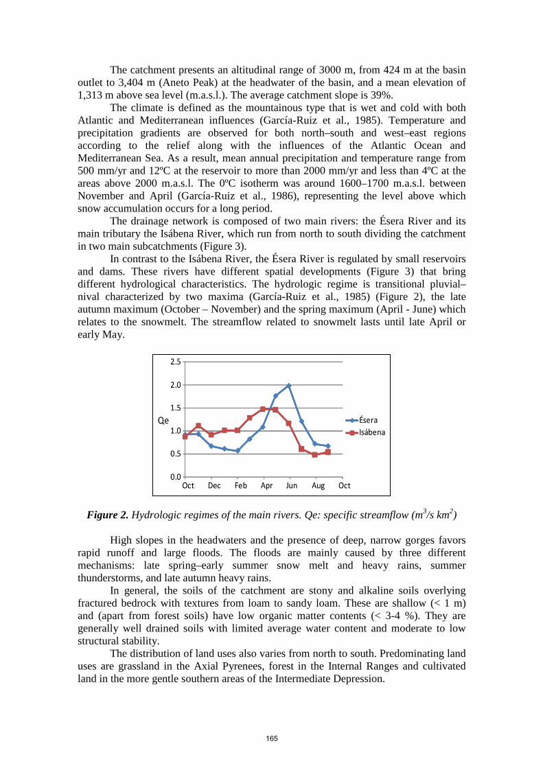
The catchment presents an altitudinal range of 3000 m, from 424 m at the basin outlet to 3,404 m (Aneto Peak) at the headwater of the basin, and a mean elevation of 1,313 m above sea level (m.a.s.l.). The average catchment slope is 39%.

The climate is defined as the mountainous type that is wet and cold with both Atlantic and Mediterranean influences (García-Ruiz et al., 1985). Temperature and precipitation gradients are observed for both north–south and west–east regions according to the relief along with the influences of the Atlantic Ocean and Mediterranean Sea. As a result, mean annual precipitation and temperature range from 500 mm/yr and 12ºC at the reservoir to more than 2000 mm/yr and less than 4ºC at the areas above 2000 m.a.s.l. The 0ºC isotherm was around 1600–1700 m.a.s.l. between November and April (García-Ruiz et al., 1986), representing the level above which snow accumulation occurs for a long period.

The drainage network is composed of two main rivers: the Ésera River and its main tributary the Isábena River, which run from north to south dividing the catchment in two main subcatchments (Figure 3).

In contrast to the Isábena River, the Ésera River is regulated by small reservoirs and dams. These rivers have different spatial developments (Figure 3) that bring different hydrological characteristics. The hydrologic regime is transitional pluvial–nival characterized by two maxima (García-Ruiz et al., 1985) (Figure 2), the late autumn maximum (October – November) and the spring maximum (April - June) which relates to the snowmelt. The streamflow related to snowmelt lasts until late April or early May.

Figure 2. Hydrologic regimes of the main rivers. Qe: specific streamflow (m3/s km2)

High slopes in the headwaters and the presence of deep, narrow gorges favors rapid runoff and large floods. The floods are mainly caused by three different mechanisms: late spring–early summer snow melt and heavy rains, summer thunderstorms, and late autumn heavy rains.

In general, the soils of the catchment are stony and alkaline soils overlying fractured bedrock with textures from loam to sandy loam. These are shallow (< 1 m) and (apart from forest soils) have low organic matter contents (< 3-4 %). They are generally well drained soils with limited average water content and moderate to low structural stability.

The distribution of land uses also varies from north to south. Predominating land uses are grassland in the Axial Pyrenees, forest in the Internal Ranges and cultivated land in the more gentle southern areas of the Intermediate Depression.

165

2.2. SWAT model

The Soil and Water Assessment Tool (SWAT) is a physical based and continuous, long-term, distributed-parameter model designed to predict the effects of land management practices on the hydrology, sediment and contaminant transport in agricultural watersheds with varying soils, land use, and management conditions (Arnold et al., 1998). SWAT is based on the concept of hydrologic response units (HRUs) which are portions of a subcatchment that possess unique land use/management/soil attributes. The runoff, sediment, and nutrient loadings from each HRU are calculated separately using input data about weather, soil properties, topography, vegetation, and land management practices. This data is ultimately used to determine the total loadings from the subcatchment.

The most current version of the model, SWAT2009, was used in this work as an extension within the Environmental Systems Research Institute (ESRI) GIS software package ArcMAP (9.3). Fundamental spatially distributed input data required for ArcSWAT include topography, land use, soils and climate.

Estimation of key parameters pertaining to soil (e.g., available water content and saturated hydraulic conductivity), snow (e.g., lapse rates, melting) and vegetation (e.g., leaf area index and maximum canopy index) by using additional field observations in the catchment is critical for better prediction. These characteristics make it a good tool for studying the hydrologic cycle at basin scale. 2.3. Catchment configuration

A digital elevation model (DEM) obtained from the Aragón Territorial Information System (SITAR, 2010) with a spatial resolution of 20 m was used to delineate the catchment. Different subdivisions of the catchment were assessed to improve the results of the simulation. The limited daily climatic data for high altitudes caused problems which restricted the subdivision of the basin in the first simulations. The highest one is at Serraduy (1402 m.a.s.l.). Finally, the catchment was subdivided into four subbasins and 290 HRUs. The gauge stations of the catchment were used to define the subbasins in the final best project. 2.4. Soil property inputs

The soil map and parameterization was derived from the digital Soil Map of Aragón and the Harmonized World Soil Database (HWSD, 2008). The soil map includes 19 types of soil at a scale of 1:500,000 (Soil Map of Aragón, Machín J, awaiting publication). A user soil database was developed with the information of the HWSD and input into the SWAT2009 database to supplement the information of the soils. Soil parameters were defined based on FAO (2007) soil type map and field observations. 2.5. Land use

The land use map was obtained from the European Project Corine Land Cover (1990) with a resolution of 100 m and 44 classifications of land use. The land cover of the catchment is mostly classified as forest (> 50 %, table 1). Each Corine Land Cover Classification has been given an equivalent in the SWAT2009 database.

166

Table 1. Simplified land cover in the 1508 km2 Barasona Catchment (a) Land cover Type Area (%) Urban 0.1 Water 0.5 Range, grass 7.9 Bare rock, perennial ice and snow 8.5 Range, brush 11.2 Forest, deciduous 13.3 Forest, transitional and mixed 13.3 Agricultural land 16.5 Forest, evergreen 28.6

(a) Source Corine Land Cover (CLC1990) (European Environment Agency) 2.6. Climate data

Climate inputs available and utilized in this SWAT application were daily minimum and maximum temperature and rainfall. All of these inputs were based on measured data within or close to the region for the period 1987-1996. Data sources were obtained from the Governmental Meteorological Agency (AEMET Agencia Estatal de Meteorología). The increase in precipitation and decrease in temperature have been well documented. There are no climatic continuous data in the upper part of the catchment (above 1,402 m.a.s.l.) to feed into the model, so results of the model are not as satisfactory as would have been expected. Table 2. Meteorological stations Rainfall stations Elevation (m) Temperature station Elevation (m)

(9829) Mediano 483 (9756) Benabarre 734

(9840) Eriste 1078 (9828) Tierrantona 635

(9841) Sesue 943 (9829D) Trillo 597

(9853) Serraduy 905 (9851) Las Paules 1402

2.7. Hydrological data

Three gauge stations were used in the model. Two gauge stations are situated in the main rivers near the end of the Barasona Reservoir (Graus and Capella) and the other one is situated at the headwater of the Ésera River (Eriste) (Figure 2). Linsoles Reservoir, situated in the Ésera River, was configured in the model in the gauge station named Eriste. The streamflow data information was provided by the Ebro River Hydrographic Administration (CHE: Confederación Hidrográfica del Ebro).

167

Figure 2. Distributions of the subcatchments and locations of the gauge stations 2.8. Model parameterization

Before applying auto-calibration, a rigorous manual parameterization exercise was performed for a better characterization of the catchment. To alleviate the problems associated with the nonexistence of climatic data in high altitude elevations bands, temperature lapse rates and precipitation lapse rates were defined. The elevation bands were 300 m in width. A total of ten elevation bands were established for each subcatchment. The calculated precipitation lapse rate (PLAPS) was 1000 mm/km and temperature lapse rate (TLAPS) was -5 ºC/km. These values were used for the whole catchment.

As a result of the nonexistence of data corresponding to the snow routine in SWAT, a process of trial and error was used to increase the quality of the snowmelt parameterization. The initial values of the parameters of the snow routine were defined in a way to obtain resultant snowfall and snowmelt values in good agreement with those expected in the region (Table 3). Table 3. Defined parameters relating to the snow routine: Parameter Value Snow fall temperature, SFTMP (ºC) 2 Snowmelt temperature, SMTMP (ºC) 1.5 Maximum melt rate of snow during a year, SMFMX (mm⁄ ºC⁄ day)

3.5

Minimum melt rate of snow during a year, SMFMN (mm⁄ ºC⁄ day)

0.1

Snow pack temperature lag factor (TIMP) 0.1 Minimum snow water content at 100% snow cover, SNOCOVMX (mm) 200 Snow water equivalent at 50% snow cover, SNO50COV 0.1

168

3. Model Calibration and Validation

Calibration efforts focused on improving model streamflow predictions at the two gauge stations (Graus and Capella) which are close to the reservoir. Prior to the auto-calibration of the parameters, the Nash–Suttcliffe coefficient (NSE, Nash and Suttcliffe, 1970) and the deviation in total volume (Dv, ASCE, 1993) were used to quantitatively assess the ability of the model to replicate monthly temporal trends in measured data.

Because of the dammed characteristics of the Ésera River, only the data of the gauge station of the Isábena River (Capella gauge station) were used like observed data in the auto-calibration process. For this purpose, the SUFI-2 (Abbaspour et al., 2007) algorithm of SWAT-CUP (Abbaspour et al., 2010) was used, choosing the Nash-Sutcliffe efficiency (NSE) as the objective function. Among parameters, thirteen parameters were used in the calibration. The first six parameters were ranked high in the sensitivity analysis and others were related to the snow routine (Table 4). The model was calibrated only for flow. The calibration period corresponded to 1987-1991 and the validation period to 1992-1996.

4. Results and Discussion

NSE values for calibration of the model varied. Initial NSE values of 0.64 and 0.51 were found for the Capella and Graus gauge stations, respectively, while NSE values obtained after calibration were 0.65 and 0.40 for the Capella and Graus gauge stations, respectively. The Dv achieved values from -3.91% and -0.68% to 0.41% and 0.11% calibrated values, respectively to Capella and Graus gauge stations.

Calibration slightly improved the NSE of the Capella gauge station but did not improve the NSE of the Graus gauge station. This produced an increment of the available water in the catchment. Table 4. Calibrated parameters results Parameter Fitted Value r__CN2.mgt 0.08075 v__ALPHA_BF.gw 0.0215 v__GW_DELAY.gw 25.32625 v__CH_N2.rte 0.00885 v__CH_K2.rte 2.61225 v__ALPHA_BNK.rte 0.60485 v__SFTMP.bsn 1.33603 v__SMTMP.bsn 4.3 v__SMFMX.bsn 1.375 V__SMFMN.bsn 0.375 V__TIMP.bsn 0.09775 V__SNOCOVMX.bsn 462.5 v__SNO50COV.bsn 0.25475 r: multiply by (1+x) value; v:replace by value

Simulation improvement after calibration was less than expected but within the range of acceptable error (Figure 3). The error of streamflow in the high flows occurred in the summer (Figure 3); this might be caused by uncertainties in observed

169

precipitation data related to local thunderstorm events. This, coupled with limited climatic data in altitude and the inferred snow routine, may explain the rest of the error.

Figure 3. Observed and calibrated streamflow at Capella gauge station

Model validation for the period 1992-1996 produced an acceptable simulation for the Capella gauge station with an NSE of 0.46 and a Dv of 0.30%. For the Graus gauge station, the simulation had an insufficient NSE of -0.12 and a Dv of 0.08 %.

5. Conclusions

Rugged topography and lack of meteorological data at headwaters are limitations to SWAT simulation in this alpine catchment. As a consequence, simulation of snow, snowmelt and streamflow presents some inconsistencies. Therefore, an improved definition of the climatic data for the catchment is necessary in order to produce more adjusted simulations. The dammed characteristics of the Ésera River may also affect the simulation results of the Esera subcatchment and a more detailed adjustment of inflow-outflow data for the Linsoles reservoir might also contribute to an improved calibration for the Esera subcatchment.

Acknowledgments This research was supported by the MEDEROCAR project (CGL2008-00831/BTE). References Abbaspour K.C., J. Yang, I. Maximov, R. Siber, K. Bogner, J. Mieleitner, J. Zobrist, R.

Srinivasan. 2007. Modelling hydrology and water quality in the pre-Alpine/Alpine Thur watershed using SWAT. Journal of Hydrology 333: 413-430.

Abbaspour, K.C., Vejdani M., Srinivasan R. 2010. SWAT-CUP: A Calibration and Uncertainty

Analysis Program for SWAT. Proceedings of the SWAT Conference, Seoul, Korea. Ahl, R.S., Woods S.W., and Zuuring H.R., 2008. Hydrologic Calibration and Validation of

SWAT in a Snow-Dominated Rocky Mountain Watershed, Montana. Journal of the American Water Resource Association 44(4):1-21.

Arnold, J.G., Srinivasan R., Muttiah R.S., and Williams J.R., 1998. Large Area Hydrologic

Modelling and Assessment Part I: Model Development. Journal of the American Water Resources Association 34(1):73-89.

170

ASCE (American Society of Civil Engineers Task Committee on Definition of Criteria for Evaluation of Watershed Models of the Watershed Management Committee, Irrigation, and Drainage Division), 1993. Criteria for Evaluation of Watershed Models. Journal of Irrigation and Drainage Engineering 119(3) 429-442.

Corine Land Cover 1990 http://www.eea.europa.eu/data-and-maps/data/corine-land-cover-

clc1990-100-m-version-12-2009 Eckhardt, K., Haverkamp S., Fohrer N., and Frede H.-G., 2002. SWAT-G, a Version of

SWAT99.2 Modified for Application to Low Mountain Range Catchments. Physics and Chemistry of the Earth 27(9-10):641-644.

FAO/IIASA/ISRIC/ISS-CAS/JRC, 2008. Harmonized World Soil Database (version 1.0). FAO,

Rome, Italy and IIASA, Laxenburg, Austria. Fontaine, T.A., Cruickshank T.S., Arnold J.G., and Hotchkiss R.H., 2002. Development

of a Snowfall-Snowmelt Routine for Mountainous Terrain for the Soil Water Assessment Tool (SWAT). Journal of Hydrology 262:209-223.

García-Ruiz. J. M., Puigdefábregas, J. & Creus, J. 1985. Los recursos hídricos superficiales del

Alto Aragón (Surface water resources of the High Aragón). Instituto de Estudios Altoaragoneses. Huesca, Spain.

García-Ruiz, J. M., Puigdefábregas, J. & Creus, J. 1986. La acumulación de la nieve en el

Pirineo Central y su influencia Hidrológica (Snow accumulation and its hydrological influence in the Central Spanish Pyrenees) Pirineos 127, 27–72.

Gassman, P.W., Reyes M.R., Green C.H., and Arnold J.G., 2007. The Soil and Water

Assessment Tool: Historical Development and Future Research Directions. Transactions of the American Society of Agricultural and Biological Engineers 50(4):1211-1250.

Gikas, G. D., Yiannakopoulou, T., and Tsihrintzis, V. A. 2005. Modeling of nonpoint-source

pollution in a Mediterranean drainage basin. Environ. Model. Assess. 11 (3): 219-233 Govender M.,and Everson C. S.2005 Modelling streamflow from two small South African

experimental catchments using the SWAT model. Hydrol. Process. 19, 683–692 IUSS Grupo de Trabajo WRB. 2007. Base Referencial Mundial del Recurso Suelo. Primera

actualización 2007. Informes sobre Recursos Mundiales de Suelos No. 103. FAO, Roma.

Lemonds, P.J. and McCray J.E., 2007. Modeling Hydrology in a Small Rocky Mountain

Watershed Serving Large Urban Populations. Journal of Water Resources 43(4):1-13. Nash, J.E. and Sutcliffe J.V., 1970. River Flow Forecasting Through Conceptual Models: I. A

Discussion of Principles. Journal of Hydrology 10:282-290. Navas, A., Valero-Garcés, B.L, Gaspar, L., Machín, J. 2009. Reconstructing the history of

sediment accumulation in the Yesa reservoir: an approach for management of mountain reservoirs. Lake and Reservoir Management, 25 (1) 15-27.

Rostamian et al. (2008) Rostamian, R., Jaleh A., Afyuni M., Mousavi S. F., Heidarpour M.,

Jalalian A., and Abbaspour K. C. 2008. Application of a SWAT model for estimating

171

runoff and sediment in two mountainous basin in central Iran. Hydrolog. Sci. J. 53(5): 977-988

Stratton, B.T., Sridhar, V., Gribb, M.M., McNamara, J.P., Narasimhan, B., 2009. Modeling the

spatially varying water balance processes in a semi-arid mountainous watershed of Idaho. Journal of the American Water Resources Association 45 (6), 1390–1408.

Valero-Garcés B. L., Navas A., Machín J., Walling D., 1999. Sediment sources and siltation in

mountain reservoirs: a case study from the Central Spanish Pyrenees. Geomorphology 28 : 23–41

Van Liew, M. W., Flynn K. F., and Marshall D. T. 2007. Simulation of streamflow, sediment,

and nutrients on the Blackfoot watershed in western Montana using SWAT. In Proc. 4th Annual Conf. on Watershed Mgmt. to Meet Water Quality Standars and TMDLS. St. Joseph, Mich.: ASABE

Zhang, X., Srinivasan R., Debele B., and Hao F., 2008. Runoff Simulation of the Headwaters of

the Yellow River Using the SWAT Model With Three Snowmelt Algorithms. Journal of the American Water Resources Association 44(1):48-61

172

Estimation of Transported Pollutant Load in Ardila Catchment Using the SWAT Model

Anabela Durão1,3*, Pedro Chambel Leitão2, David Brito2, RM Fernandes1, Ramiro Neves2, Maria Manuela Morais3

1 Departamento de Engenharia - Instituto Politécnico de Beja, Rua Pedro Soares Campus do IPB 7800-295 Beja - Portugal, e-mail: adurao@ipbeja.pt

* PhD student of ICAAM - Universidade de Évora

2 Secção de Ambiente e Energia - Instituto Superior Técnico - MARETEC Av. Rovisco Pais 1049-001 Lisboa - Portugal

3Laboratório de Água/ICAAM - Universidade de Évora Rua Barba Ralanº1 Parque Industrial e Tecnológico 7005-345 Évora - Portugal

Abstract

Excess of organic matter and nutrients in bodies of water promotes algae blooms, which can accelerate the eutrophication process, a situation often observed in the Ardila river. This river was identified as very polluted and classified as critical for the Alqueva-Pedrogão System. The aim of this study was to estimate the transported nutrients load in a trans-boundary catchment using the SWAT (Soil and Water Assessment Tool) model and to determine the contribution of nutrients load in the entire catchment. Ardila catchment is about 3711 Km2 and is located in eastern Portugal (22%) and the Badajoz province on Spanish soil (78%). It was discretized into 32 sub-basins using the automated delineation routine, and 174 hydrologic response units. Monthly average meteorological data (time period from 1947 to 1998) were used to generate daily values through the Weather Generator Model incorporated in SWAT. Real daily precipitation series data (1931 to 2003) were introduced. The model was calibrated and verified using: flow data (1950 to 2000) and nutrients (1981 to 1999). Model performance was evaluated using statistical parameters, such as Nash-Sutcliffe efficiency (NSE) and root mean square error (R2). Calibration and verification flow results showed a satisfactory agreement between simulated and measured monthly data from 1962 to 1972 (NSE=0.8; R2 = 0.9). The results showed that the most important diffuse pollution comes from the two main tributaries of Spain. The estimated nitrogen and phosphorous load contribution per year was about 72%, 59% respectively (Spain) and 28%, 41% (Portugal). The SWAT model application reveals a useful tool for integrated water management. Keywords: diffuse pollution, SWAT model, nutrients, integrated water management

173

1. Introduction The major cause of water quality deterioration of the water bodies is mostly

associated today with diffuse source pollution, due to the intensification of agricultural activities and the development of large urban centers. Nutrient inputs can enhance crop growth, but excessive nutrient input can result in the impairment of water quality. Eutrophication and ecological damage to rivers or lakes can be accelerated by an excess of organic matter and nutrients in bodies of water.

Since continuous water quality monitoring is very expensive, time consuming and spatially impractical at the watershed level, mathematical modeling has become a primary technology for analyzing diffuse pollution and its spatial distribution. When the measured data are insufficient to depict pollution levels within a watershed, models can be used to assess the pollutant load discharged into the receiving body of water (Chu et al., 2004).

The evaluation of body of water degradation caused by point and diffuse source pollution requires modeling studies in order to assess the pollutant loading and water pollution in the surrounding environment (Lam et al., 2010). Modeling is also a necessary step in the implementation of the Water Framework Directive (WFD) (Pisinaras et al., 2010). The WFD establishes an integrated approach to management and protection of Europe’s aquatic environment. The main aim of the WFD is to achieve good chemical and ecological status for receiving waters by 2015.

The SWAT model is a mathematical model, originated in 1996 and continuously developed since then by the Agricultural Research Service and Texas A&M University, whose main function is to analyze the impacts of land management practices as well as different soil and land use patterns on the surface water and groundwater flow, sediment yield and water quality (Neitsch et al., 2005). The SWAT model has been widely used all around the world to predict stream discharge and nutrient load from watersheds of various sizes (Gassman et al., 2006 in Lam et al., 2010), for developing total maximum daily load by simulating the hydrology, sediment, nutrient and pollutant loading of large basins (Narasimhan et al, 2010) and for watershed scale studies dealing with water quantity and quality. Model scenarios can be helpful in finding reasonable measures for assessing environmental ecological status while taking into account relevant factors such as climate, land, and water use (Krysanova et al., 2005; Højberg et al., 2007 in Lam et al., 2010). As reported by Chu et al. (2004), in general, application of SWAT for assessing diffuse pollution has shown reasonable results.

In this study the SWAT model was used to simulate the hydrology and quantify the nutrients load in the Ardila catchment.

The Ardila river is an international river which rises in Spain and flows into Portugal on the left bank of the Guadiana river, south of the Alqueva dam of the largest reservoir in Europe. This river was classified as a very polluted river and as a critical for the Alqueva-Pedrogão System. It often experiences algae blooms due to excessive presence of organic matter and nutrients (Durão et al., unpublished). It is important to quantify the nutrient load as well as its provenance. Therefore, the aim of this study was (1) to estimate the streamflow; (2) to estimate the transported nutrients load in a trans-boundary catchment using the SWAT model; (3) to determine the contribution of nutrient load in the entire catchment in order to understand what happens and recommend what should be done by the management to minimize the influent load.

174

2. Methodology 2.1. Study area descriptions

Portugal is located between latitudes 37ºN and 42ºN and longitudes of 9.5ºW and 6.5ºW. The country lies in the transition zone stretching from the subtropical anticyclones (the Azor anticyclone) to the area of sub poles depressions. The factors that most affect the climatic conditions in the region are the latitude, the orography and the influence of the Atlantic Ocean (Venâncio et al., 2006).

The Ardila river, located at 7.467º W and 38.2º N, is an international river which arises in Spain at Tentudia at 1100 m altitude and flows into Portugal on the left bank of the Guadiana river at elevation 95 m, near the Moura city, south of the Alqueva dam, the largest reservoir in Europe. The total length is about 160 km. This river crosses the southern part of Jerez de los Caballeros and Oliva de la Frontera cities (Badajoz province). Among its tributaries, the most relevant are Benferre stream, which only runs on Spanish soil, and Murtega stream already in Portugal (CHGuadiana, 2008).

The location of the basin, discharge, water quality and meteorology gauges are shown in Figure 1.

Figure 1. Location of the Ardila catchment and the gauges

The study area, Ardila catchment, is about 3711 Km2 and is located in the lower

Alentejo Region of eastern of Portugal and the Badajoz province on Spanish soil. About 78% of the basin is located in Badajoz province and 22% in Moura council.

The climate of the Alentejo Region is Mediterranean in general, characterized by a temperate climate that features warm, dry summers and winters with precipitation. According to the Thornthwaite classification, the climate type is defined by water index, which combines the indices of aridity and humidity. These factors influence precipitation, temperature and evapotranspiration. The Portuguese part of Ardila catchment (Moura) is Mesothermal semiarid (D) with a water index between -20 and -40 (PBH, 1999).

The mean precipitation is 533.6 mm/year, maximum is 816.9 mm/year and the minimum is 242.9 mm/year (Amareleja gauge, 1931-1999). The mean air maximum

175

temperature is 32.6ºC in August and the mean air minimum is 5.3 ºC in January (Beja, 1971-2000 in IMP, 2000) 2.2. SWAT model input data

The SWAT hydrological model has been chosen to calibrate and validate the Ardila Foz data flow. The SWAT model calibration and validation for streamflow was carried out using data recorded at two flow gauges of the watershed located at Ardila Fronteira, located at 7.127ºW and 38.178ºN and Ardila Foz, located at 7.129º W and 38.172º N (Figure 1). The available daily flow data is for the period from 1950 to 2000 (SNIRH, 2008).

To determine the load transported by the Ardila river, time-continuous data on flow and water quality at some points of the basin are needed. The water quality data available is for the hydrologic years from 1981 to 1999 (SNIRH, 2008a), concerning the Ardila Capt gauge, located at 7.237ºW and 38.152ºN and Ardila Fronteira gauge, located at 7.127ºW and 38.178ºN. These gauges are situated in Portugal (Figure 1).

The ArcSWAT interface for SWAT version 2005 was used to compile the SWAT input files. The basic data sets required to set up the model inputs are: Digital Elevation Model (DEM), soil, land use and climatic data.

The DEM information was used for automatic delineation of the watershed. The DEM determines the direction of flow as well as the physical characteristics of the basin. In this study the DEM (raster format with a grid resolution of 70 m) has been clipped from the Shuttle Radar Topography Mission (SRTM) DEM data (Hounam and Werner, 1999).

The hydrographic network can be determined automatically from the DEM or can be provided via a map. In this study the hydrographic network was determined automatically.

The daily values of precipitation, radiation, relative humidity, wind speed and maximum and minimum temperatures data that SWAT requires can be entered directly through a file or can be simulated by the model. In this study the Weather Generator Model (WXGEN) incorporated into SWAT was used. WXGEN generates daily values based on monthly averages data from meteorological Beja gauge, localized at 7,868ºW and 38,018º N (Figure 1), corresponding to 41 years of data (1947 to 1998). The weather variable that has a significant influence on the flow is precipitation. The real daily precipitation series data were obtained from Amareleja’s meteorological station (SNIRH, 2003), located on the Portuguese side, at 7,229º W and 138,210º N (Figure 1). Daily precipitation data were obtained from the Amareleja gauge because it was the only one that has a long, complete time series corresponding to 72 years of data (1931- 2003) and the gauge is located inside of the Ardila catchment (Figure 1). This option is selected because the inter-annual variations in rainfall affect the estimated loads.

The land use and soil types associated with meteorological data are important data, which will significantly influence the water balance. The land use map has been clipped from the CORINE (released in 2000 obtained in http://dataservice.eea.europa.eu/dataservice/) whose legend is based on the CORINE level 3 legends. The original legend entries were reclassified and, in some cases, aggregated to conform to the land use database present in the SWAT model (the watershed results included 11 land use classes).The soil map 1:1,000,000 was gathered from the European Environmental Agency (EEA) data center in vector form covering the entire Ardila watershed. This data set was first digitalized by Platou, et al. (1989) and further improved by Vossen and Meyer-Roux (1995).

176

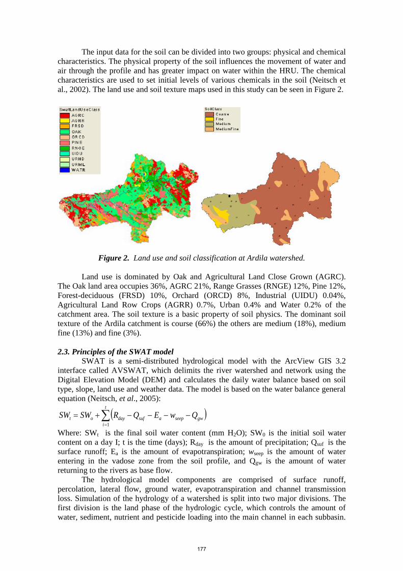
The input data for the soil can be divided into two groups: physical and chemical characteristics. The physical property of the soil influences the movement of water and air through the profile and has greater impact on water within the HRU. The chemical characteristics are used to set initial levels of various chemicals in the soil (Neitsch et al., 2002). The land use and soil texture maps used in this study can be seen in Figure 2.

Figure 2. Land use and soil classification at Ardila watershed.

Land use is dominated by Oak and Agricultural Land Close Grown (AGRC). The Oak land area occupies 36%, AGRC 21%, Range Grasses (RNGE) 12%, Pine 12%, Forest-deciduous (FRSD) 10%, Orchard (ORCD) 8%, Industrial (UIDU) 0.04%, Agricultural Land Row Crops (AGRR) 0.7%, Urban 0.4% and Water 0.2% of the catchment area. The soil texture is a basic property of soil physics. The dominant soil texture of the Ardila catchment is course (66%) the others are medium (18%), medium fine (13%) and fine (3%). 2.3. Principles of the SWAT model

SWAT is a semi-distributed hydrological model with the ArcView GIS 3.2 interface called AVSWAT, which delimits the river watershed and network using the Digital Elevation Model (DEM) and calculates the daily water balance based on soil type, slope, land use and weather data. The model is based on the water balance general equation (Neitsch, et al., 2005):

( )∑=

−−−−+=t

igwseepasufdayot QwEQRSWSW

1

Where: SWt is the final soil water content (mm H2O); SW0 is the initial soil water content on a day I; t is the time (days); Rday is the amount of precipitation; Qsuf is the surface runoff; Ea is the amount of evapotranspiration; wseep is the amount of water entering in the vadose zone from the soil profile, and Qgw is the amount of water returning to the rivers as base flow.

The hydrological model components are comprised of surface runoff, percolation, lateral flow, ground water, evapotranspiration and channel transmission loss. Simulation of the hydrology of a watershed is split into two major divisions. The first division is the land phase of the hydrologic cycle, which controls the amount of water, sediment, nutrient and pesticide loading into the main channel in each subbasin.

177

The second division is the water phase or routing phase that can be defined as the movement of water, sediment, nutrients, etc. through the channel network of the watershed to the outlet (Neitsch et al., 2005).

The SWAT model represents the large-scale spatial heterogeneity of the study area by dividing the watershed into multiple subwatersheds. Each subwatershed is subdivided into several hydrologic response units (HRU) with homogeneous characteristics of land use, soil type and management. The HRU represent percentages of the subwatershed area and are not identified spatially in the simulation (Gassman et al., 2007). The climatic variables required by SWAT include daily precipitation, maximum/minimum air temperature, solar radiation, wind speed and relative humidity. Major components of the model include hydrology, weather, and agricultural management. The details of all components can be found in Neitsch et al. (2005).

The hydrologic balance is simulated for each HRU, including canopy interception of precipitation, portioning of precipitation and irrigation water between surface runoff and infiltration, redistribution of water within the soil profile, evapotranspiration lateral subsurface flow from the soil profile, and return flow from shallow aquifers. To estimate surface runoff from HRUs the combination of daily rainfall and the Soil Conservation Service curve number (CN) procedure was used, which is a function of the soil type, slope, initial soil moisture state, land use and management practices (Gassmen et al., 2007). The CN scale corresponds non-linearly with the moisture content of the soil; it ranges from 0 to 100. These extreme values correspond to permeable and impermeable (waterproof) cover, respectively.

SWAT offers various methods to estimate the potential evapotranspiration (PET) such as Hargreaves, Penman-Monteith and Priestlley. To calculate PET, the Penman-Monteith method was used. This method needs relative humidity, wind speed, solar radiation and temperature. The maximum and minimum temperature inputs are used to estimate daily soil and water temperature. Recharge below the soil is portioned between shallow and deep aquifers. The return flow to the stream system and PET from the deep-rooted plants (revap) can occur from shallow aquifers. The movement and the transformation of nitrogen (N) and phosphorus (P) within an HRU are simulated as a function of nutrient cycles consisting of several inorganic and organic pools. Simulated losses of N and P from the soil can occur by crop uptake and in surface runoff in both the solution phase and on eroded sediment. Losses of N can also occur in percolation below the root zone, in lateral subsurface flow including tile drains, and volatilization to the atmosphere (Gassmen et al., 2007).

SWAT models the movement of water into adjacent unsaturated areas as a function of water demand for evapotranspiration. This process has been termed revap. The revap is significant in watersheds where the saturated zone is not very far below the surface or where deep-rooted plants are growing. SWAT simulates the nitrogen cycles in the soil profile and in the shallow aquifer. In soil and water, nitrogen is extremely reactive and exists in a number of dynamic forms. It may be added to the soil in the form of fertilizer, manure or residue application, as well as bacteriological fixation and rain. It can be removed from the soil through plant uptake, soil erosion, leaching, volatilization and denitrification. In the SWAT model there are five different pools of nitrogen in the soil. Two of the pools are inorganic forms of nitrogen (NH4

+ and NO3-),

while the other three pools are organic forms of nitrogen (active, stable and fresh). Nitrate may be transported with surface runoff, lateral flow or percolation. Nitrate entering a shallow aquifer in recharge from the soil profile through percolation may remain in the aquifer, move with groundwater flow into the main channel, or be transported into a deep aquifer with water moving into the soil zone in response to water

178

deficiencies. For a lowland catchment, the groundwater component is a dominant pathway and plays an important role in transporting nitrate from the shallow aquifer to the main channel or to the soil zone through the upwelling of groundwater processes. The amount of nitrate moved with the water is calculated by multiplying the nitrate concentration in the mobile water by the volume of water moving in each pathway. The concentration of nitrate in the mobile water fraction is calculated as (Neitsch et al., 2005):

𝑁𝑂3,𝑚𝑜𝑏𝑖𝑙𝑒 =𝑁𝑂3𝑙𝑦 �1 − 𝑒𝑥𝑝 � −𝑊𝑚𝑜𝑏𝑖𝑙𝑒

(1 − θ𝑒)𝑆𝐴𝑇𝑙𝑦)��

𝑊𝑚𝑜𝑏𝑖𝑙𝑒

Where: NO3,mobile is the concentration of nitrate in the mobile water for a given layer (KgN/mmH2O), NO3ly is the amount of nitrate in the layer (kg N/ha), Wmobile is the amount of mobile water lost by surface runoff (Qsurf,, only for top 10mm of soil), lateral flow (Qlat,ly) or percolation (Qperc,ly) in the layer (mm H2O), θe is the fraction of porosity from which anions are excluded, and SATly is the saturated water content of the soil layer (mm H2O).

𝑊𝑚𝑜𝑏𝑖𝑙𝑒 = 𝑄𝑠𝑢𝑟𝑓 + 𝑄𝑙𝑎𝑡,𝑙𝑦 + 𝑊𝑝𝑒𝑟𝑐,𝑙𝑦

Surface runoff is allowed to interact with and transport nutrients from the top 10mm of soil. The nitrate removed on the surface (NO3surf) is calculated:

𝑁𝑂3𝑠𝑢𝑟𝑓 = 𝛽𝑁𝑂3.𝑁𝑂3,𝑚𝑜𝑏𝑖𝑙𝑒.𝑄𝑆𝑢𝑟𝑓 Where: βNO3 is the nitrate percolation coefficient that allows the user to set the concentration of nitrate in surface runoff to a fraction of the concentration in percolate.

Organic N transport with sediment is calculated with a loading function developed by McElroy et al. (1976) and modified by William and Hann (1978) for application to separate runoff events. Estimation of the daily organic N runoff loss is based on the concentration of organic N in the topsoil layer, the sediment yield and the enrichment ratio. The enrichment ratio is the ratio of the mass of organic N in sediment to organic N in the soil. The plant uptake nitrogen is estimated using a supply and demand approach (Neitsch et al., 2005).

SWAT monitors six different pools of phosphorus in the soil, three of which are inorganic forms of phosphorus and three of which are organic forms. The soluble P and organic P concentrations should be specified by the user otherwise SWAT will initialize levels of phosphorus in the different pools. While SWAT allows nutrient levels to be input as concentrations, it performs all calculations on a mass basis. Phosphorous is not soluble, so SWAT allows soluble P to leach only from the top 10 mm of soil. 2.4. Nutrients

Nutrients of interest in the SWAT model prediction are nitrate nitrogen (NO3-N), ammonia nitrogen (NH4-N), total Kjeldahl nitrogen (TKN), soluble phosphorus (PO4-P) and total phosphorus (TP). The PO4-P and NO3-N are important water quality parameters used to indicate water pollution. PO4-P is the main form of phosphorus assimilated by aquatic plants. The amount of (NO3-N) in runoff is only considered in the top soil layer (10mm thickness). NO3-N loading is estimated as the product of the volume of runoff and nitrate concentration in the first layer. Amounts of NO3-N contained in lateral subsurface flow and percolation are estimated as products of the volume and the average concentration of NO3-N in each layer (Chu, et al 2004). The

179

total nutrient loading is the summation of loading from both surface runoff and base flow.

Daily quality simulations were performed from 1981 to 1999. This simulation period was chosen according to the availability of water quality information at the Ardila Capt gauge. The measured nitrate concentration series available is reported from 1981 to 1999.

As SWAT provides the record of daily flow (m3/s), the monthly flow is the sum of the daily multiplying the 86400 (s). The simulated load was calculated multiplying the concentration by the SWAT flow. The product of measured daily nitrate concentration and simulated flow were used to estimate the daily observed nitrate load. The simulated results of nutrient concentration were compared with the corresponding measured data at Ardila Capt gauge.

The simulated dissolved P was compared to observed phosphate. The summation of phosphorus runoff and phosphorus groundwater loading of each subbasin was assumed as Total Phosphorus loading. 2.5. Watershed delineation

The watershed discretization in the SWAT model is approached through subwatersheds defined by the watershed DEM and HRU, which comprise similar land use and soil type combinations within the subwatershed. The Watershed Delineation module of AVSWATX is based on some elementary raster functions provided by ArcView and the Spatial Analyst extension. In this study the SWAT model was conducted by dividing the Ardila watershed into 32 subbasins and 174 HRU (Figure 3).

Figure 3. Ardila watershed delineation (32 subbasin and 174 HRU).

3. Results and Discussion 3.1. Simulation of flow

The simulated results of flow were compared with the corresponding measured data at Ardila Foz gauge. For the model calibration, the flow series was compared with daily data for the hydrologic years 1949-2000. The application of the model in the first simulation showed differences between simulated and observed flows, mainly because the groundwater default values established by the model do not reflect the watershed reality. The variables of groundwater with more influence in the calibration process, which need to be adjusted, are: baseflow recession coefficient (ALFA_BF), groundwater Revap (GW_REVAP) and groundwater delay time (GW_DELAY) (Table 1).

180

Table 1. Initial and final values for the calibrated variables

Variable name Allowable range Initial value Simulation 1

Final value Simulation 2

ALFA_BF 0.1 - 1.0 0.048 1.0 GW_REVAP 0.02 – 0.20 0.02 0.02 GW_DELAY 0 - 500 200 3 USLE_K 0.01 - 0.65 0.1 0.3

The ALPHA_BF is a direct index of groundwater flow response to changes in recharge. For a land with slow response to recharge, the values vary from 0.1 to 0.3 and for a land with rapid response the values vary from 0.9 to 1.0 (Jeong, 2008). The value adopted, in this study, was 1.0 due to the rapid response of the basin.

The Groundwater Revap coefficient (GW_REVAP) regulates the movement of water from the shallow aquifer to an overlying unsaturated zone. The value was set at a default value (0.02), because the saturated zone is very far below the surface in this watershed.

The groundwater delay time (GW_DELAY), is the time that the water released by the soil bottom layer travels until reaching the shallow aquifer. It will depend on the depth to the water table and the hydraulic properties of the geologic formations in the vadose and groundwater zones (Galván et al., 2009). The values vary from 0 to 500 day. For this study, in the second simulation the GW_DELAY was set at 3 days. According with Vazquez-Amábile & Enguel (2005) when the GW_DELAY is set at zero days it is assuming that there was no vadose zone between the lower limit of the soil bottom layer and the shallow aquifer, which fluctuated from the surface to 2.5 m during the year.

The term soil erodibility reflects that some soils erode more easily than others even when all factors are the same. It is caused by the properties of the soil itself. Wischmeier and Smith (1978) define the soil erodibility (K) factor as the soil loss rate per erosion index unit for a specified soil as measured on a unit plot. A unit plot is 22.1 m long, with a uniform length-wise slope of 9%, in continuous fallow, tilled up and down the slope (Neistch et al., 2005). The soil erodibility (K) factor is reflected by the conditions of soil reaction to the erosion process of hydrological nature. The values of USLE_K vary from 0.01 to 0.65 (Mukundan et al., 2010). In this study the USLE_K adopted for calibration was 0.3, because it is a common value in Alentejo (Pimenta, 1998).

Figure 4 shows the results of streamflow after calibration.

181

Figure 4. Comparison of the observed and the simulated flow at the Ardila Foz gauge.

The model considers a decline in 1960, coinciding with the observed value, given the absence of observed data in 1959 and 1961, and from 1973 to 1976. From 1981, the simulated flow is greater than the observed flow, although the progress of the curve is similar. This situation suggests that the decrease in flow observed from 1981 is probably due to (1) the change in flow curves of the hydrometric Ardila Foz gauge; (2) the flow retention on the Spanish side.

Hydrologic calibration and validation use the regression correlation coefficient (R2) and the Nash‐Sutcliffe model efficiency (NSE) coefficient. The R2 value measures how well the simulated versus observed regression line approaches an ideal match and ranges from 0 to 1. A value of 0 indicates no correlation and a value of 1 representing that the predicted dispersion equals the measured dispersion (Krause et al., 2005). The NSE ranges from −∞ to 1 and measures how well the simulated versus observed data match the 1:1 line. An NSE value of 1 again reflects a perfect fit between the simulated and measured data.

Observed and simulated results were compared using R2 and the NSE for daily, monthly and all data for different period (Table 2, 3, 4, 5). There is no observed flow during the period from 1961 to 1962 and from 1973 to 1976. As a result, the model efficiency for the antecedent period (1958-1959) and after period (1977-1988) is negative (Table 2 and 3). A value of 0 or less than 0 indicates that the mean of the observed data is a better predictor than the model output.

According to Gassman et al. (2007) no absolute criteria for judging model performance have been firmly established in the literature to date. However, Moriasi et al. (2007) proposed that NSE values should exceed 0.5 in order for model results to be judged as satisfactory for hydrologic and pollutant loss evaluations performed on a monthly time step and that appropriate relaxing and tightening of the standard be performed for daily and annual time step evaluations, respectively. The results show a satisfactory agreement between simulated and observed monthly time step for the period from 1949 to 1958 (0.594), 1962 to 1972 (0.840) and from 1988 to 1994 (0.739).

182

Table 2. Correlation coefficient (R2) and Nash‐Sutcliffe model efficiency (NSE) coefficient for 1949-1958 and 1958-1959.

1949-1958 1958-1959 All monthly daily All monthly daily Qmobserved (mm) 94 95 94 181 181 182 Qmsimulated (mm) 113 114 113 316 314 317 R2 0.595 0.745 0.596 0.869 0.972 0.869 NSE 0.443 0.594 0.445 0.119 -0.514 0.119

Table 3. Correlation coefficient (R2) and Nash‐Sutcliffe model efficiency (NSE) coefficient for 1959-1960 and 1962-1972.

1959-1960 1962-1972 All monthly daily All monthly daily Qmobserved (mm/year) 151 141 151 168 170 168 Qmsimulated (mm/year) 242 231 242 192 197 192 R2 0.708 0.848 0.708 0.706 0.892 0.706 NSE -0.631 -0.129 -0.630 0.644 0.840 0.644

Table 4. Correlation coefficient (R2) and Nash‐Sutcliffe model efficiency (NSE) coefficient for 1977-1988 and 1988-1993.

1977-1988 1988-1993 All monthly daily All monthly daily Qmobserved (mm/year) 79 84 79 58 58 58 Qmsimulated (mm/year) 133 139 133 89 90 89 R2 0.546 0.770 0.546 0.687 0.906 0.677 NSE -0.185 0.065 -0.185 0.463 0.739 0.434

Table 5. Correlation coefficient (R2) and Nash‐Sutcliffe model efficiency (NSE) coefficient for 1994-2000.

1994-2000 All monthly Daily

Qmobserved (mm) 52 62 52 Qmsimulated (mm) 105 160 N R2 0.522 0.707 N NSE -0.251 -4.943 N

The weaker results (1994-2000) can be attributed to inadequate representation of

rainfall inputs due to either a lack of adequate rain gauges in the simulated watershed, the inaccuracies in measured streamflow data or the retention water in the Spanish soil. 3.2. Contribution of nutrients

After calibration and validation, to have the same basis of comparison, flow data obtained from the SWAT hydrologic model was used to estimate the nitrate loading for both simulated and observed due to the 1991-1999 period of water quality measured data in which the measured flow was under the SWAT predict flow, as seen in Figure 4. It was noted that the frequency of sampling for observed data was twice or only once per month, so for the bi-monthly frequency a mean value was chosen and considered to be the monthly value. The product of the average monthly concentration and the simulated flow was performed to estimate the monthly observed loading. It also was

183

noted failure on the monthly observed data. Therefore those years without sufficient data were eliminated to analyze the annual observed loading. The simulated or observed annual loading was estimated as a summation of the monthly average loadings for the corresponding year. 3.2.1. Nitrate

Annual nitrate loading was calibrated/validated for the hydrologic years from 1991 to 1999. The comparison between simulated and observed results of the annual nitrate load at the Ardila Capt gauge is shown in Figure 5. The annual nitrate loading simulated is higher than the observed, except in the wet years 1995/1996 and 1997/1998, where the observed flow was higher (Figure 6). In those years SWAT shows high concentrations at the beginning of winter (Figure 7), but after that it reduces with the dilution effect, whereas in the observed values it was assumed that the concentration stays the same throughout each month. In those wet years the measured concentration values were high (Figure 7), producing a nitrate load based on higher values.

Figure 5. Simulated and observe annual nitrate loading (ton N/year) for hydrologic year (1991-1999)

Figure 6. Monthly evolution of simulated streamflow during the period (1991-1999).

0500

100015002000250030003500

1990 1992 1994 1996 1998 2000

tonN

/yea

r

Hydrologic year

NO3-N loading SWAT SWATFlow+ArdilaCapt

0200400600800

100012001400160018002000

Nov

/199

0

Jun/

1991

Dec

/199

1

Jul/1

992

Jan/

1993

Aug

/199

3

Mar

/199

4

Sep

/199

4

Apr

/199

5

Oct

/199

5

May

/199

6

Dec

/199

6

Jun/

1997

Jan/

1998

Jul/1

998

Feb/

1999

Aug

/199

9

Mar

/200

0

m3/

s

Date

184

Figure 7. Simulated and observed nitrate concentration (mg N/L) during the period (1991-1999)

For validation and calibration of the 1991-1999 period, simulated and observed results for monthly nitrate loading were compared using R2 and the NSE. The R2 value measures how well the simulated versus observed regression lines approach an ideal match and ranges from 0 to 1, a value of 0 indicating no correlation and 1 indicating a perfect fit. The average monthly nitrate load obtained by the model was 25.4 ton N/month and for observed values was 65,9 ton N/month . The model underestimated the average monthly nitrate load, so the R2 and NSE obtained was 0.42 and 0.25 respectively. These poor results may be due to (1) the fact that field data concentrations on a monthly basis may have occurred in extreme events (e.g. higher flow) not representing an average value occurring during the month or (2) the lack of data that underestimates nitrogen sources in the watershed. Similar findings were reported by Chu et al. (2004), who obtained R2= 0.27 and NSE=0.16 for calibration period and R2= 0.38 and NSE=0.36 for validation period.

In accordance with river classification for multiple uses (DSRH, 1998) the results for nitrate concentration (Figure 7) show that the Ardila river can be classified as a polluted river (5.67<NO3-N <11.30 mg N/L) tending to be very polluted (11.32<NO3-N <18.07 mg N/L) in wet years. Nitrogen is commonly used as an indicator of pollution from human activities. The results suggested that the contamination may be caused by human activities such as fertilizer. 3.2.2. Dissolved phosphorus

The comparison between simulate and observed results of annual dissolved phosphorus loading at the Ardila Capt gauge is shown in Figure 8.

During the dry years 1992, 1995, 1997 and 1999 (Figure 6) the observed annual dissolved P loadings were above the simulated results (Figure 8), contrary to the wet years in which the observed dissolved P concentrations were higher than dry years but not as high as the SWAT dissolved P predictions of the wet years (Figure 9). This can be attributed to the fact that we have assumed that the dissolved P concentration stays the same all month although collection of field data may coincide with peak dissolved P concentration.

0.002.004.006.008.00

10.0012.0014.0016.0018.00

Nov

/199

0

Jun/

1991

Dec

/199

1

Jul/1

992

Jan/

1993

Aug

/199

3

Mar

/199

4

Sep

/199

4

Apr

/199

5

Oct

/199

5

May

/199

6

Dec

/199

6

Jun/

1997

Jan/

1998

Jul/1

998

Feb/

1999

Aug

/199

9

Mar

/200

0

Oct

/200

0

Apr

/200

1

mgN

/L

Date

NO3-N SWAT ArdilaCapt

185

Figure 8. Simulated and observed annual phosphate loading (ton P/year) during the hydrologic year (1991-1999)

Figure 9. Observed and simulated dissolved phosphorous concentration (mg P/L) during the period (1991-1999).

The SWAT model over-predicted dissolved P monthly concentrations (Figure 9), and as a consequence the simulated annual dissolved P loads for the dry hydrologic years (1991/1992 and 1998/1999) were higher than the observed loads. It can be concluded that the model overestimated the dissolved P concentration in the dry period.

The average monthly dissolved P load obtained by the model was 2.8 ton P/month and for observed values was 4.9 ton P/month. R2 and NSE obtained were 0.47 and 0.45, respectively. The model underestimated the average monthly dissolved P load, although the results can be considered reasonable for dissolved P, because the NSE (0.45) is within the range (0.39 to 0.93) found in the literature for monthly validation (Gassman et al., 2007).

During the summer periods of 1996, 1997 and 1998, the model simulated well for both dissolved P and nitrate concentration. In contrast, during the autumn and winter

0

50

100

150

200

1990 1992 1994 1996 1998 2000

TonP

/yea

r

Hydrologic year

dissolved_P load SWAT SWATFlow+ArdilaCapt

0.000.200.400.600.801.001.201.401.601.802.00

Nov

/199

0

Jun/

1991

Dec

/199

1

Jul/1

992

Jan/

1993

Aug

/199

3

Mar

/199

4

Sep

/199

4

Apr

/199

5

Oct

/199

5

May

/199

6

Dec

/199

6

Jun/

1997

Jan/

1998

Jul/1

998

Feb/

1999

Aug

/199

9

Mar

/200

0

Oct

/200

0

Apr

/200

1

mgP

/L

Date

Dissolved-P concentration SWAT ArdilaCapt

186

periods the model underestimated for both dissolved P and nitrate concentration. The hydrologic years 1993, 1994 and 1995 lack data.

In accordance with river classification for multiple uses (DSRH, 1998), the phosphate concentration results (Figure 9) show that the Ardila river can be classified as a polluted river (phosphate<0.41 mg P/L) and a very polluted river in the summer (phosphate>0.41 mg P/L). Phosphorus is the key nutrient responsible for over-fertilizing streams, freshwater lakes and ponds. Although it is essential for algal and aquatic plant productivity, increases in the amount of phosphorus can trigger tremendous increases. These results can be associated with the use of phosphate-based detergents, lawn and garden fertilizers, improperly sited and maintained wastewater systems, leaking sewers, agricultural drainage, pet waste and urban storm water runoff. 3.2.3. Nutrient load

Nutrient concentrations in streams are influenced by diffuse sources within the watershed. To evaluate the incoming pollution and to quantify the nutrients load entering the entire watershed, nutrient load in stream water was simulated at different subbasin outlets (SB) along the longitudinal Ardila river, including: SB1, SB2, SB3, SB4 and SB5. Daily simulations were performed from 1981 to 1999. This simulation period was chosen according to the availability of water quality information (Ardila Capt gauge).

The contribution of the nutrient load at the outlet of subbasins was examined. The nutrient load results at the different subbasin outlets were drawn from upstream to downstream (Figure 10).

Figure 10. Average annual loads of nutrients at subbasin outlets along the longitudinal Ardila river.

The watershed in its present state has a diffuse average total nitrogen load of 612 ton N/year and total phosphorus load of 86 ton P/year.

The main nutrient load contribution comes from Spanish stream tributaries. The estimated average nutrient load contribution per year that comes from Spain is about 72% of the total nitrogen load and 50% of the total phosphorus load; from Portugal they are about 28% and 41%, respectively.

187

4. Conclusions

In this study the SWAT model was applied to simulate the flow and to estimate the transported nutrient load in the Ardila catchment, a trans-boundary catchment in eastern Portugal and the Badajoz province of Spain. The basis input data included climate, topography, soil, land use and water quality data.

The calibration and validation of the SWAT output were implemented by comparing simulated flow, nitrate load and phosphorus load with corresponding in-stream measurements at the Ardila watershed. Simulations of flow, nitrate and dissolved phosphorus load were performed in a daily time step. The results were organized per month and per hydrological years. The results of this study showed a good agreement between simulated and observed monthly flow with an NSE and R2 of 0.59 and 0.75 for the period from 1949 to 1958; 0.84 and 0.89 for 1962 to 1972; 0.74 and 0.91 for 1988 to 1994.

The statistical coefficients of the average nitrate load model performance were poor (NSE and R2 of 0.25 and 0.42). However, characteristic nitrate behavior with high concentrations and load in winter months and low nitrate loads in drier summer months were observed.

The statistical coefficients of the average dissolved P load model performance were relatively reasonable (NSE and R2 of 0.45 and 0.47).

The results indicated that the contributions of nitrogen and phosphorus load from Spain to the Ardila catchment are about 72% and 59% respectively, and that Portugal contributes 28% to the nitrogen load and 41% to the phosphorus load.

The SWAT model is a useful tool to reproduce flow historical records and simulate results whenever gauging data are unavailable. The main disadvantages are the numerous input parameters. Real data at some points of the watershed are absolutely necessary to achieve reliable results. To calibrate and validate the simulated results, daily inputs obtained at Ardila watershed locations within Portugal, were used. However, further studies using additional data (precipitation, water quality, etc.) from Spain are recommended. An evaluative analysis of the influence of point sources and different land use cover types should be made. Acknowledgements This study has been supported by PROTEC – Support program for advanced training of the Polytechnic teachers in the reducing the hours of teaching (2010/2011) of Anabela Durão. References CHGuadiana.2008. Confederactión Hidrográfica del Guadiana. Mapa de la Cuenca. Ministerio

de Medio Ambiente y Medio Rural y Marino. Avaiable at: www.chguadiana.es. Accessed 16 June 2010.

Chu, T. W., A. Shirmohammadi, H. Montas, A. Sadeghi. 2004. Evaluation of the SWAT

model´s sediment and nutrient components in the piedmont physiographic region of Maryland. Trans. ASAE. 47(5): 1523-1538.

Corine. 2000. Land Use Map and Land Cover. Available at: www.dataservice.eea.europa.eu.

Accessed 19 October 2009.

188

DSRH. 1998. M5. Metodologia de avaliação da qualidade das águas superficiais. Direcção de Serviços de Recursos Hídricos. Lisboa. Available at: http://gdeh.fct.unl.pt/eai_prat/Amostragem/dsrh_m5.pdf. Accessed 30 April 2011

Durão, A., A. Serrano, R. M. Fernandes, M. M. Morais. (unpubliched). Contribuição para

minimização de impactes negativos no rio Ardila - Estudo de caso. Galván, L., M. Olías, R. Fernandez de Villarán, J.M. Domingo Santos, J.M. Nieto, A.M.

Sarmiento, C.R. Cánovas. 2009. Application of the SWAT model to an AMD-affected river (Meca River, SW Spain): Estimation of transported pollutant load. Journal of Hydrology. 377, 445–454. (Galván et al., 2009).

Gassman, P. W., M. R. Reyes, C. H. Green, J. G. Arnold. 2007. The soil and water assessment

tool: historical development, applications, and future research directions. Trans. ASABE. 50(4): 1211– 1250.

Hounam D., M. Werner. 1999. The Shuttle Radar Topography Mission (SRTM) In: Proceedings

of ISPRS-Workshop "Sensors and Mapping from Space 1999“, Hannover, Germany, CD-ROM. Available at: www.ipi.uni-hannover.de.

IMP. 2000. Normais Climatológica Beja: 1971-2000. Instituto de Meteorologia do Portugal.

Lisboa. Avaiable at: http://meteo.pt. Accessed 11 February 2011. Jeong, Jaehak. 2008. Sensitivity analysis on selected SWAT parameters. Postdoctoral Research

Associate. Blackland Research Center. Temple. Available at: www.jaehak.info. Acessed: 08 September 2010.

Lam, Q. D., B. Schmalz, N. Fohrer. 2010. Modelling point and diffuse source pollution of

nitrate in a rural lowland catchment using the SWAT model. Agricultural Water Management. 97: 317-325.

Moriasi, D. N., J. G. Arnold, M. W. Van Liew, R. L. Bingner, R. D. Harmel and T. L.

Veith.2007. Model evaluation guidelines for systematic quantification of accuracy in watershed simulations. Trans. ASABE. 50(3):885-900.

Mukundan, R., D. E. Radcliffe, and L. M. Risse. 2010. Spatial resolution of soil data and

channel erosion effects on SWAT model predictions of flow and sediment. Soil and Water Conservation. 65(2)92-104.

Narasimhan, B., R. Srinivasan, S. T. Bednarz, M. R. Ernst, P. M. Allen. 2010. A

Comprehensive modeling approach for reservoir water quality assessment and management due to point and nonpoint source pollution. Trans. ASABE. 53(5): 1605-1617.

Neitsch, S. L., J. G. Arnold, J.R. Kiniry, J. R. Williams. 2005. Soil and Water Assessment Tool.

Theoretical documentation, version 2005. Grassland, Soil and Water Research Laboratory. Agricultural Research Service. Texas. Available at: http://swatmodel.tamu.edu/documentation. Accessed 13 December 2009.

Neitsch, S. L., J. G. Arnold, J.R. Kiniry, R., Srinivasan, J.R. Williams. 2004 Soil and Water

Assessment Tool – Input/output file documentation. Version 2005. Blackland Research Center. Agricultural Experiment Station. Texas. Available at: http://swatmodel.tamu.edu/documentation. Accessed 13 December 2009.

189

Neitsch, S.L., J.G. Arnold, J.R. Kiniry, R. Srinivasan, J.R. Williams. 2002. Soil and Water Assessment Tool User´s Manual. Version 2002

PBH. 1999. Plano de Bacia Hidrográfica do Rio Guadiana. Volume IV. Diagnóstico Parte 3.

Situações Extremas. Available at: www.inag.pt/inag2004. Accessed 14 August 2006. Pimenta, M. T. 1998. Caracterização da erodibilidade dos solos a sul do rio Tejo.

INAG/Direcção de Serviços de Recursos Hidricos. Pisinaras, V., C. Petalas, G. D. Gikas, A. Gemitzi, V. A. Tsihrintzis. 2010. Hydrological and

water quality modeling in a medium-sized basin using the Soil and Water Assessment Tool (SWAT). Desalination. 250: 274–286.

SNIRH. 2003. Amareleja meteorological station data: 1931-2003. Sistema Nacional de

Informação de Recursos Hídricos Database. Lisboa, Instituto da Água I.P. Available at: http://snirh.pt. Accessed 19 October 2009.

SNIRH. 2008. Ardila Flow data: 1950-2000. Sistema Nacional de Informação de Recursos

Hídricos Database. Lisboa, Instituto da Água I.P. Available at: http://snirh.pt. Accessed 19 October 2009.

SNIRH. 2008a. Water quality data: 1982-2008. Sistema Nacional de Informação de Recursos

Hídricos Database. Lisboa, Instituto da Água I.P. Available at: http://snirh.pt. Accessed 19 October 2009.

Vazquez-Amábile, G. G. and B. A. Engel. 2005. Use of SWAT to compute groundwater table

depthand streamflow in the Muscatatuck river watershed. Trans. ASAE. 48(3): 991−1003.

Venâncio A., F. Martins, P. Chambel, R. Neves. 2006. Modelacão hidrológica da bacia drenante

da Albufeira de Pracana Faro. Available at: www.sapientia.ualg.pt. Accessed 29 January 2010.

Vossen and Meyer-Roux. 1995. Soil Map 1:1000000. Physical proprieties. Available at:

www.eusoils.jrc.it/ESDB_Archive/ESDBv2/index.htm. Accessed 19 October 2009.

190

Soil Erosion Modelling in an Agro-forested Catchment of NE Spain Affected by Gullying using SWAT

Guevara-Bonilla M.

Department of Environment and Soil Science. University of Lleida, Alcalde Rovira Roure 191, 25198 Lleida, magbo10@gmail.com

Martínez-Casasnovas J.A. (*)

Department of Environment and Soil Science. University of Lleida Alcalde Rovira Roure 191, 25198 Lleida, j.martinez@macs.udl.es

Ramos M.C.

Department of Environment and Soil Science. University of Lleida Alcalde Rovira Roure 191, 25198 Lleida, cramos@macs.udl.es

Abstract Soil erosion is recognized as the major cause of land degradation in Mediterranean and semiarid environments. The present work shows the first results of the application of SWAT (ArcSWAT 2009.93.5) to model soil erosion in an agro-forested catchment (2049 ha) located in the Anoia-Penedés region (NE Spain). This area belongs to the Penedés Tertiary Depression, where unconsolidated materials (marls) outcrop. The area is severely affected by gully erosion processes. The main agricultural uses are vineyards, rain fed herbaceous crops (winter barley) and olive trees. An important part of the area is covered by natural vegetation (Pinus halepensis, Quercus ilex, Quercus faginea) that mainly occupies the steepest slopes affected by gullying. The main data sources with which to run SWAT were the detailed Soil Map of Catalonia, a 5 m resolution DEM and land use/vegetation maps of 2005 and 2010. The first was adapted from the Land Cover Map of Catalonia (3rd edition) and a supervised classification of a WorldView-2 multispectral image (2 m resolution) from July 6, 2010. Soil losses for periods with different climatic characteristics were analysed (2005, with low precipitation, 365 mm, and 2010, above the average, 729 mm). Average annual soil losses ranged between 2.9 and 40.7 t/ha, with clear differences between HRUs depending on land use and soil characteristics. The highest values correspond to vineyard lands. Forest plays a very important role as protective cover on gully walls, helping to avoid major sediment production rates. Nevertheless, the increase in runoff by almost 350% in the wet year with respect to the dry year favours the actuation of processes other than sheet and rill erosion on gully walls (e.g. bank erosion, mass movements) which are not estimated by MUSLE integrated into SWAT. Keywords: soil loss, agro-forestry catchment, detailed scale, wet and dry years

191

1. Introduction

Soil erosion is a widespread problem throughout Europe. In Mediterranean areas, factors such as climate, topography, soil characteristics, land use change and intensive agricultural practices have turned soil erosion into the major cause of land degradation (Cerdà, 2008).

The region of Anoia-Penedès located in Catalonia (NE Spain) is a particular example of these land characteristics and changes that result in intensive erosion processes. In this region, the coincidence of extensive vineyard cropping, frequent high intensity rainfall, highly erodible soil parent materials (marls and unconsolidated sandstones) together with land use changes, the abandonment of traditional soil conservation measures and an increase in extreme rainfall events have accelerated the erosion processes and led to the development of a dense and deep gully network (Ramos and Martínez-Casasnovas 2006). This type of erosion process (gullying) should not be ignored because, although less studied than other processes (e.g. sheet and rill erosion), it has been recognized as the main source of sediments in developed catchments, contributing an average of 50-80% to sediment production by water erosion (Martínez-Casasnovas et al., 2004).

In a region of high agricultural interest where forests seem to play an important role in soil protection, soil erosion evaluation is very important in order to asses sediment yield, determine the relative contributions of potential sediment sources and identify areas susceptible to erosion. The identification of these areas is helpful to identifying sources of potential erosion, improving the knowledge of the affected areas and for developing control measure programs for diminishing soil erosion (Valentin et al., 2005).

A large number of studies have been done to quantify runoff, sediment yield and the relationship between land cover and erosion in semi arid environments. For example, some studies focused on direct field measurements (Bochet et al., 1998; Dunjó et al., 2004), and some more recently focused on the use of physical simulation models (e.g. Bathurst et al., 2006; Martínez-Carreras et al., 2007; Mueller et al., 2009). The use of models running at watershed scale has become an important tool for estimating runoff and sediment yield and for quantifying the impacts of conservation practices at various spatial and temporal scales (Chiang et al., 2010).

In this respect, the Soil and Water Assessment Tool (SWAT) arises as a well-known and very useful model for quantify soil erosion and sediment yield (Arnold et al., 2008). SWAT can, in a fast and accurate manner, assess the effect of individual storms, as well as different topographic, soil and land cover scenarios on runoff and sediment yield (Gassman et al., 2007).

Even though there are several examples of studies that utilize SWAT to simulate soil erosion and sediment yield, there are few examples of applications in forested areas and none specifically addressed to study sediment yield in areas covered by gullies. As Arnold and Fohrer (2005) stated, the plant growth component of SWAT was originally developed for agricultural crops, although in recent years the model has been adapted for forest covers. Nevertheless, it still needs some improvements. Therefore, the present work is a contribution to the application of SWAT in agro-forested areas at detailed scale in a region where the development of gullies (mainly covered by forest) is an important erosion process. Here we present the first results of the study.

192

2. Materials and Methods 2.1. Study area

The study area is located in the Catalonia region of northeastern Spain (1º 47' 45" E, 41º 31' 00" N), about 30 km southwest of Barcelona (Figure 1). The total area of the catchment is 2049 hectares. It is part of the Penedès Tertiary Depression, where calcilutites (marls) and occasionally sandstones and conglomerates crop out. The climate is Mediterranean, with a mean annual temperature of 15°C and a mean annual rainfall of 550 mm (Ramos and Martínez-Casasnovas, 2010). The rainfall mainly occurs in two periods: September to November and April to June. High intensity rainstorms are frequent during the latter period (e.g.>100 mm h-1 in 5-min periods). The rainfall erosivity factor (R = kinetic energy x maximum intensity in 30-min period) ranges between 1049 and 1200 MJ mm ha-1 h-1 y-1 (Ramos, 2002). Two different landscape units were identified according to the methodology proposed by Zinck (1988): (i) piedmont areas and (ii) slope and gully areas. The dominant soil subgroups in the first unit are Calcixerollic Xerochrepts and Typic Xerorthents, while in the latter the most frequent soil is Typic Xerorthents (Martínez-Casasnovas and Ramos, 2009).

The main agricultural land use of the region is vineyards for the production of high quality vines. The steepest slopes affected by gullying are covered by natural vegetation of Pinus halepensis, Quercus ilex, Quercus faginea and herbaceous species such as Rosmarinus officinalis and Thymus vulgaris, among others.

Figure 1. Location of the study area

193

2.2. Soil and Water Assessment Tool The Soil and Water Assessment Tool (SWAT) is a physical process-based model

developed by the United States Department of Agriculture (USDA) and the Agricultural Research Service (ARS) which is addressed to simulate and predict impacts of landscape processes and/or management practices on water, sediment and agricultural chemical yields on a catchment scale (Arnold et al., 1998). The model uses climate, soil and land use and land management (e.g. crop growth, agricultural management) data to predict surface runoff, infiltration, sediment yields and nutrient yields among other things. For modelling purposes, SWAT divides a catchment into different watersheds and splits them into smaller units called Hydrological Response Units (HRU) according to land uses, soil types and slope data (Gassman et al., 2007). The division into HRUs is useful when the watershed has several land uses and soil types. 2.3. Sediment yield prediction using SWAT

Generally erosion processes caused by rainfall and runoff are calculated using the Universal Soil Loss Equation (USLE). However, SWAT utilizes the Modified Universal Soil Loss Equation (MUSLE) to estimate soil losses. This equation developed by Williams (1975) uses the amount of runoff generated in each HRU to simulate sediment yield for each HRU in each watershed, which are added to compute the contribution of sediment yield for the whole catchment. As a result, sediment yield predictions are improved, the accuracy of the prediction is increased and sediment yields on individual climatic events (e.g. storms) can be estimated (Neitsch et al., 2002). 2.4. Data input

SWAT was applied for simulating runoff and sediment yield for the years 2005 and 2010. These years were selected because they represent the actual trend in the region, with more extreme situations including dry and wet years and intensive rainfall events. For this study we used the ArcSWAT 2009.93.5 version compatible with ArGIS 9.3. The GIS input files to SWAT included a detailed soil map of the study area (1:25000) (Ascaso et al., 2008), a 5 m resolution Digital Elevation Model (DEM) and two land use/ cover maps (2005 and 2010). The land use/cover map of 2005 was adapted from the Land Cover Map of Catalonia (3rd edition) (Ibàñez and Burriel, 2008), while the 2010 map was derived from a hybrid process of visual interpretation and supervised classification of a WorldView-2 2 m resolution multispectral image from July 2010. As a first step, the non-forested areas in the 2004 land use/cover map were updated by means of the visual interpretation process. Forest areas were then classified through a supervised classification. After the classification, an accuracy assessment to determine the global accuracy as well as omission and commission errors was carried out. For the land use/cover maps we used the legend that is shown in Table 1.

194

Table 1. Land use classes in the study area Land use Description

Pine forest Land covered by pine forest (Pinus halepensis) Mixed forest

Land covered by Pinus halepensis, Quercus ilex and Quercus faginea.

Pine Regeneration

Land covered mostly by Pinus halepensis saplings

Scrubland

Perennial bush vegetation with a height less than 7 m. The main species are: Arundo donax, Rubus ulmifolius, Rosmarinus officinalis, Thymus vulgaris Cistus albidus, Crateagus monogyna, Daphne gnidium, Genista sp.

Riparian vegetation

It is similar to the scrubland unit but with the presence of deciduous species like Populus and Platanus

Vineyard

Land used for grape production

Olives

Land dominated by olive plantations

Fruit trees

Land covered by almond, apple or pear orchards

Cereals

Crop lands mostly of winter barley

Grasslands Land covered by naturally occurring grass or former crop lands now cover by grasses and herbaceous vegetation

Residential areas

Composed of high and low density urban areas

Industrial areas

Composed of industrial polygon areas

Bare soil Areas with no vegetation cover. Can be by anthropogenic factors or can be bare gully sidewalls.

Water

Area covered by small water bodies

The DEM was used to delineate the catchment and the watersheds and to

provide information about slope degree. Soil units were extracted from the Detailed Soil Map of Catalonia (DO Penedès region, Ascaso et al., 2008). Additional information about soil properties was obtained from the description of soil cartographic and taxonomic units (soil series) included in the memory of the soil survey (Ascaso et al., 2008). The following soil families dominate the study area (according to Soil Taxonomy and World Reference Base of FAO): Typic Xerorthents, fine-loamy, carbonatic, thermic (SSS, 1999), Haplic Regosols (calcaric) (WRB, 1998), present in 37.4% of the study area (mainly in the gully areas), with a K-factor of 0.53; Typic Calcixerepts, loamy-skeletal, mixed, thermic (SSS, 1999), Haplic Calcisols (skeletic) (WRB, 1998), present in 11.7% (gentle slope areas), with a K-factor of 0.45; Typic

195

Xerorthents, fine-loamy, mixed, thermic (SSS, 1999), Haplic Regosols (WRB, 1998), covering 10.4% of the study area (moderate slopes), with K-factor value of 0.49; Fluventic Haploxerepts, loamy-skeletal, mixed, thermic (SSS, 1999), Fluvic Cambisols (skeletic) (WRB, 1998), covering 6.1% of the study area and located in gentle to moderate slopes, with a k-factor of 0.49; and Typic Xerorthents, fine-loamy, carbonatic, thermic (SSS, 1999), Haplic Regosols (calcaric) (WRB, 1998), covering 3.4% of the area in moderate slopes, with a k-factor of 0.46.

For both years, weather inputs included daily data of precipitation, minimum and maximum temperature, solar radiation, wind speed and relative air humidity. These data were collected from a meteorological station located in Hostalets de Pierola (1º 48' 30.50" E, 41º 31' 51.71" E), which belongs to the network of the Meteorological Service of Catalonia. 3. Results 3.1. Land use changes

Some land use changes in the catchment occurred between the two study years (Table 2). In general, most of the land classes covered by arboreal vegetation increased. Pine forest, pine regeneration and riparian vegetation increased respectively by 5%, 0.40% and 1.8%. The only forest class that decreased was the mixed forest that changes from 0.84% in 2005 to 0.32% in 2010.

Agricultural areas remained relatively constant with a small reduction on all crops (vineyards, olives and fruit trees). On the other hand, grasslands and bare soil due to anthropogenic factors increased. The land uses that did not change were the urban, industrial, transportation areas and bare soil in gully sidewalls, which remained the same during the five-year period. Table 2. Land use changes in the basin

Land use 2005 2010 Area (ha) % Area (ha) %

Pine forest 490.79 23.95 593.21 28.95 Mixed forest 17.21 0.84 6.65 0.32 Pine regeneration 41.10 2.01 49.28 2.41 Scrubland 187.77 9.16 88.77 4.33 Riparian vegetation 53.75 2.62 90.48 4.42 Vineyard 536.35 26.17 494.66 24.14 Olives 29.59 1.44 26.87 1.31 Fruit trees 53.75 2.62 43.95 2.14 Cereals 235.06 11.47 224.24 10.94 Grasslands 59.54 2.91 78.85 3.85 Residential areas 167.30 8.16 167.54 8.18 Low density residential areas 7.32 0.36 7.32 0.36 Industrial areas 113.94 5.56 113.94 5.56 Transportation areas 18.58 0.91 18.58 0.91 Bare soil 7.08 0.35 14.72 0.72 Bare soil in gullies 22.59 1.10 22.59 1.10 Water bodies 7.63 0.37 7.33 0.36 TOTAL 2049 100 2049 100

196

3.2. Surface runoff and sediment yield

With the SWAT model, the annual average surface runoff and sediment yield for the years 2005 and 2010 were simulated (Table 2). Table 2. Summary of surface runoff and sediment yield for the study years

Variable Year 2005 2010 2000-2010

Precipitation (mm) 365.00 729.40 534.00 Surface runoff (mm) 32.15 112.04 62.65 Sediment yield (t/ha) 2.92 40.65 15.51

Precipitation values show that the two considered years have very different

climatic characteristics. The year 2005 recorded a precipitation of 365 mm, which is lower than the average for the period 2000-2010 (534 mm), while the year 2010 had a total annual rainfall of 729.4 mm. For both years, despite the total annual rainfall, a reduced number of high intensity, greater than 20 mm rainfall events (4 in 2005 and 5 in 2010) are responsible for most of the annual sediment production.

The average annual surface runoff for the 2000-2010 period was 62.65 mm producing a sediment yield of 15.51 t/ha. Runoff values for the analyzed years varied from 32.15 mm in 2005 to 112.04 mm in 2010. This created sediment yields that ranged from 2.92 and 40.65 t/ha. Furthermore, there were clear differences in surface runoff and sediment yield between HRUs depending on land use (Table 3). Table 3. Average annual surface runoff and sediment yield according land use

Land use 2005 2010

Surface runoff (mm)

Sediment yield (t/ha)

Surface runoff (mm)

Sediment yield (t/ha)

Pine forest 18.44 < 0.01 88.65 1.98 Mixed forest 17.47 < 0.01 57.51 0.99 Pine regeneration 20.78 < 0.01 77.10 10.02 Scrubland 35.40 0.12 116.30 29.07 Riparian vegetation 30.15 0.01 116.23 15.60 Vineyard 30.46 0.70 114.25 43.66 Olive trees 35.72 < 0.01 147.95 3.55 Fruit trees 35.80 < 0.01 135.79 12.10 Cereals 44.24 2.25 164.50 24.55 Grasslands 42.77 8.73 160.44 172.47 Bare soil 100.13 17.44 290.37 221.97 Bare soil in gullies 109.31 38.00 307.76 315.19

The total average annual surface runoff and sediment yield by land use type is

shown in Table 4. During the wet year, agricultural lands had a greater contribution than forests and gully walls. Average runoff generation was 56.19% vs. 43.81% and sediment yield was 56.19% vs. 43.81% respectively for agricultural and forest areas. However, in the dry year sediment yields were greater in forest areas and unprotected gully walls than in agricultural lands. This fact may be mainly explained by the high

197

rates of soil loss in the bare gully sidewalls that represented almost the total soil loss in gully areas (99.58% of total sediment yield in 2005).

In 2010 other vegetated gully areas also contributed to sediment production, representing 15.46% of the total soil loss, while nonvegetated walls were responsible for the remaining 84.54% of total soil erosion in forest and gully cover zones. Table 4. Total average annual surface runoff and sediment yield by land use type: agricultural land versus forest and gully walls

Land use type 2005 2010

Surface runoff (mm)

Sediment yield (t/ha)

Surface runoff (mm)

Sediment yield (t/ha)

Agricultural land 289.12 29.14 1013.3 478.30 Forest and gully walls 231.55 38.16 763.55 372.85

Differences in total rainfall affected runoff values substantially. The difference

between 2005 (dry year) and 2010 (wet year) was close to 350%. Furthermore, for the two analysed years average annual runoff rates differed between all land use types including land classes with similar coverage (e.g. forest land uses). Classes with dense aboveground vegetation had smaller values than agricultural crops.

For both years, bare soil in gully sidewalls presented the highest runoff and sediment production values (Figure 2). Among the agricultural uses, cereals had the higher sediment values, while in 2010 the greatest sediment yield was in vineyards. Generally, forests played a very important role as protection cover on gully eroded areas, avoiding major sediment production rates.

Figure 2. Example of bare soil in gully sidewalls of the study area. This is the land use/cover class with the highest values of runoff and sediment production due to the

lack of soil protection by vegetation cover, high slope degree and high erodibility of the lithological materials.

Although there are big differences in soil losses between the two years, the

sediment yield showed similar spatial distributions (Figure 3). The most intensively eroded watersheds were located in the central and northern part of the study area.

198

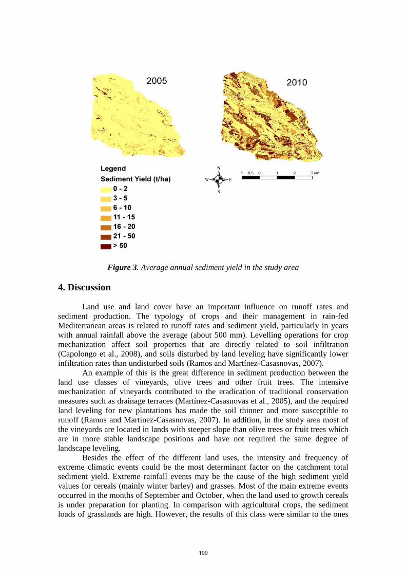
Figure 3. Average annual sediment yield in the study area 4. Discussion

Land use and land cover have an important influence on runoff rates and sediment production. The typology of crops and their management in rain-fed Mediterranean areas is related to runoff rates and sediment yield, particularly in years with annual rainfall above the average (about 500 mm). Levelling operations for crop mechanization affect soil properties that are directly related to soil infiltration (Capolongo et al., 2008), and soils disturbed by land leveling have significantly lower infiltration rates than undisturbed soils (Ramos and Martínez-Casasnovas, 2007).

An example of this is the great difference in sediment production between the land use classes of vineyards, olive trees and other fruit trees. The intensive mechanization of vineyards contributed to the eradication of traditional conservation measures such as drainage terraces (Martínez-Casasnovas et al., 2005), and the required land leveling for new plantations has made the soil thinner and more susceptible to runoff (Ramos and Martínez-Casasnovas, 2007). In addition, in the study area most of the vineyards are located in lands with steeper slope than olive trees or fruit trees which are in more stable landscape positions and have not required the same degree of landscape leveling.

Besides the effect of the different land uses, the intensity and frequency of extreme climatic events could be the most determinant factor on the catchment total sediment yield. Extreme rainfall events may be the cause of the high sediment yield values for cereals (mainly winter barley) and grasses. Most of the main extreme events occurred in the months of September and October, when the land used to growth cereals is under preparation for planting. In comparison with agricultural crops, the sediment loads of grasslands are high. However, the results of this class were similar to the ones

199

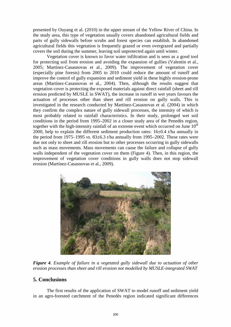
presented by Ouyang et al. (2010) in the upper stream of the Yellow River of China. In the study area, this type of vegetation usually covers abandoned agricultural fields and parts of gully sidewalls before scrubs and forest species can establish. In abandoned agricultural fields this vegetation is frequently grazed or even overgrazed and partially covers the soil during the summer, leaving soil unprotected again until winter.

Vegetation cover is known to favor water infiltration and is seen as a good tool for protecting soil from erosion and avoiding the expansion of gullies (Valentin et al., 2005; Martínez-Casasnovas et al., 2009). The improvement of vegetation cover (especially pine forests) from 2005 to 2010 could reduce the amount of runoff and improve the control of gully expansion and sediment yield in these highly erosion-prone areas (Martínez-Casasnovas et al., 2004). Then, although the results suggest that vegetation cover is protecting the exposed materials against direct rainfall (sheet and rill erosion predicted by MUSLE in SWAT), the increase in runoff in wet years favours the actuation of processes other than sheet and rill erosion on gully walls. This is investigated in the research conducted by Martínez-Casasnovas et al. (2004) in which they confirm the complex nature of gully sidewall processes, the intensity of which is most probably related to rainfall characteristics. In their study, prolonged wet soil conditions in the period from 1995–2002 in a closer study area of the Penedès region, together with the high-intensity rainfall of an extreme event which occurred on June 10th 2000, help to explain the different sediment production rates: 16±0.4 t/ha annually in the period from 1975–1995 vs. 83±6.3 t/ha annually from 1995–2002. These rates were due not only to sheet and rill erosion but to other processes occurring in gully sidewalls such as mass movements. Mass movements can cause the failure and collapse of gully walls independent of the vegetation cover on them (Figure 4). Then, in this region, the improvement of vegetation cover conditions in gully walls does not stop sidewall erosion (Martínez-Casasnovas et al., 2009).

Figure 4. Example of failure in a vegetated gully sidewall due to actuation of other erosion processes than sheet and rill erosion not modelled by MUSLE-integrated SWAT 5. Conclusions

The first results of the application of SWAT to model runoff and sediment yield in an agro-forested catchment of the Penedès region indicated significant differences

200

between dry and wet years, with important soil losses in forested gully sidewalls which represent the highest values in the study area of 38.0 and 315.19 t/ha in 2005 and 2010 respectively. Therefore, vegetation on gully walls plays a very important role in erosion control.

Regardless of the fact that MUSLE-integrated SWAT does not model erosion processes other than sheet and rill erosion, the results obtained in the gully areas are consistent with previous research carried out to determine the contribution of sediment yield in gullies to total sediment yield generated in a catchment. This is because bare gully sidewalls have a very high degree of slope and have very highly erodible soils (or unconsolidated marls outcrops) which make them very prone to sheet and rill erosion. Other processes, such as the ones that produce gully wall failure, suppose the displacement and preparation of materials, but these are washed out of the wall and/or gully by surface runoff processes.

2010, the wet selected year, represents an example of the situations that more and more frequently could occur in the area under a climate change scenario with extreme high intensity rainfall events happening more often. It may have multiple effects on those areas where soil is bare during most parts of the year. Wet years with extreme rainfall events are likely to do particular damage to areas with higher slope, areas where infiltration had been reduced due to land use changes and areas with unsuitable management practices. Acknowledgements This work is part of the research project AGL2009-08353 funded by the Spanish Ministry of Science and Innovation. The authors also want to thank the consortium of universities that provide the Master of Science in European Forestry Erasmus Mundus (http://www.europeanforestry.net/) for the financial support given to the first author. References Arnold, J. G., Fohrer, N. 2005. SWAT2000: Current capabilities and research opportunities in

applied watershed modelling. Hydrological Processes 19(3): 563-572.

Arnold, J. G., R. Srinivasan, R. S. Muttiah and J. R. Williams. 1998. Large area hydrologic modeling and assessment part I: Model development. Journal of the American Water Resources Association 34(1): 73-89.

Bathurst, J. C., A. Burton, B. G. Clarke and F. Gallart. 2006. Application of the SHETRAN basin-scale, landslide sediment yield model to the Llobregat basin, Spanish Pyrenees. Hydrological Processes 20(14): 3119-3138.

Bochet, E., J. L. Rubio and J. Poesen. 1998. Relative efficiency of three representative matorral species in reducing water erosion at the microscale in a semi-arid climate (Valencia, Spain). Geomorphology 23(2-4): 139-150.

Capolongo, D., L. Pennetta, M. Piccarreta, G. Fallacara and F. Boenzi. 2008. Spatial and temporal variations in soil erosion and deposition due to land-levelling in a semi-arid area of Basilicata (Southern Italy). Earth Surface Processes and Landforms 33(3): 364-379.

Cerdà, A. and Universitat de València. 2008. Erosión y degradación del suelo agrícola en España. València: Universitat de València, Càtedra Divulgació de la Ciència.

201

Chiang, L., I. Chaubey, M. W. Gitau and J. G. Arnold. 2010. Differentiating impacts of land use changes from pasture management in a CEAP watershed using the SWAT model. Transactions of the ASABE 53(5): 1569-1584.

Dunjó, G., G. Pardini and M. Gispert. 2004. The role of land use-land cover on runoff generation and sediment yield at a microplot scale, in a small Mediterranean catchment. Journal of Arid Environments 57(2): 239-256.

FAO. 1998. World Reference Base for Soil Resources. Roma: FAO.

Gassman, P. W., M. R. Reyes, C. H. Green and J. G. Arnold. 2007. The soil and water assessment tool: Historical development, applications, and future research directions. Transactions of the ASABE 50(4): 1211-1250.

Martínez-Carreras, N., M. Soler, E. Hernández and F. Gallart. 2007. Simulating badland erosion with KINEROS2 in a small Mediterranean mountain basin (Vallcebre, Eastern Pyrenees). Catena 71(1): 145-154.

Martínez-Casasnovas J.A., Ramos M.C., Ribes-Dasi M. 2005. On-site effects of concentrated flow erosion in vineyard fields: some economic implications. Catena 60: 129–146.

Martínez-Casasnovas, J. A., M. C. Ramos and D. García-Hernández. 2009. Effects of land-use changes in vegetation cover and sidewall erosion in a gully head of the Penedès region (northeast Spain). Earth Surface Processes and Landforms 34(14): 1927-1937.

Martínez-Casasnovas, J. A., M. C. Ramos and J. Poesen. 2004. Assessment of sidewall erosion in large gullies using multi-temporal DEMs and logistic regression analysis. Geomorphology 58(1-4): 305-321.

Mueller, E. N., T. Francke, R. J. Batalla and A. Bronstert. 2009. Modelling the effects of land-use change on runoff and sediment yield for a meso-scale catchment in the Southern Pyrenees. Catena 79(1): 103-111.

Nietsch, S.L.; Arnold, J.G.; Kinirv, J.R.; William, J.R; King, K.W. 2002. Soil and Water Assessment Tool theoretical information. Temple, Texas: Texas Water Resources Institute

Ouyang, W., F. Hao, A. K. Skidmore and A. G. Toxopeus. 2010. Soil erosion and sediment yield and their relationships with vegetation cover in upper stream of the Yellow River. Science of the Total Environment 409(2): 396-403.

Ramos, M. C. and J. A. Martínez-Casasnovas. 2010. Effects of field reorganisation on the spatial variability of runoff and erosion rates in vineyards of northeastern Spain. Land Degradation and Development 21(1): 1-12.

Ramos, M. C. and J. A. Martínez-Casasnovas. 2007. Soil loss and soil water content affected by land levelling in Penedès vineyards, NE Spain. Catena 71(2): 210-217.

Ramos, M. C. and J. A. Martínez-Casasnovas. 2006. Trends in precipitation concentration and extremes in the Mediterranean Penedès-Anoia region, NE Spain. Climatic Change 74(4): 457-474.

202

Soil Survey Staff. 1999. Soil taxonomy: a basic system of soil classification for making and interpreting soil surveys (2ª ed.). Washington, DC: US Department of Agriculture Soil Conservation Service.

Valentin, C., J. Poesen and Y. Li. 2005. Gully erosion: Impacts, factors and control. Catena 63(2-3): 132-153.

Williams, J.R. 1975b. Sediment-yield prediction with universal equation using runoff energy factor. p. 244-252. In Present and prospective technology for predicting sediment yield and sources: Proceedings of the sediment yield workshop, USDA Sedimentation Lab., Oxford, MS, November 28-30, 1972. ARS-S-40.

Zink, J.A. 1988. Physiography and Soils. Soil survey courses. Subject matter K6. ITC lecture

notes SOL-41.

203

Mapping Sugarcane Yield for Ethanol Production in Veracruz, México

Jesus Uresti Gil1

Héctor Daniel Inurreta Aguirre2 Elibeth Torres Benítez2

Roberto de Jesús López Escudero2

1Instituto Nacional de Investigaciones Forestales, Agrícolas y Pecuarias (INIFAP) e-mail: uresti.jesus@inifap.gob.mx

2Colegio de Postgraduados

e-mail: inurreta.hector@colpos.mx

Abstract Ethanol from sugarcane is accepted as the most cost, energy and greenhouse gas mitigation efficient biofuel to substitute for fossil gasoline. Ethanol yield may be increased if residues (tops, leaves and bagasse) are used for cellulosic bioethanol production. However, to efficiently achieve maximum biomass yield and avoid competition with food production, highly and marginally productive areas must be identified. The objective of this study was to map sugarcane yield in Veracruz, Mexico to assist decision-makers in planning rural development and establishment of ethanol refineries. The SWAT (Soil and Water Assessment Tool) model was used to simulate total sugarcane biomass yield throughout the 7.18 million hectares of Veracruz. To define the Hydrological Response Units, a base digital elevation model as well as soil and land use maps scale 1:250,000 and 90x90 m pixel size acquired from INEGI were used. Weather data was taken from 95 uniformly distributed weather stations with at least 20 years of records between 1960 and 2000. The sugarcane management was designed for highest yield attainment. Most sensitive crop parameters such as LAI, RUE, Tb, HU, biomass partition and rooting depth were taken from previous local research and peer review literature. Total theoretical ethanol (sugar ethanol + cellulose + hemicellulose ethanol) was calculated and mapped. Results are presented and discussed in terms of productivity class maps of sugarcane biomass and total (sugar + cellulose + hemicellulose) theoretical ethanol yield and amount as well as spatial distribution of highly and marginally productive areas. Keywords: biofuel, Geographical Information Systems, ArcSwat, simulation models, rural development

204

1. Introduction

Ethanol from sugarcane sugars is accepted worldwide as the most cost-efficient, energy-efficient and greenhouse gas-mitigating biofuel to substitute for fossil gasoline. At a global scale, since the early 70’s Brazil has produced the largest amount of sugarcane ethanol and is planning to increase production (IICA, 2007, Carvalho-Junior et al., 2008). In Mexico ethanol production from sugarcane is incipient, but many public and private institutions are strongly promoting its production and use (SAGARPA, 2007; SENER, 2007; DOF-SENER, 2009).

Three reasons that sugarcane is strongly promoted worldwide as a bioenergy crop are the large capacity to produce biomass and sugars at an acceptable cost-effective ratio, the Net Energy Ratio (NER) for sugarcane biofuel production and the high reduction of greenhouse gas emissions for sugar crop bioenergy. Fresh cane yields under rain-fed conditions are around 73, 84, 93 and 110 t ha-1 in México (SIAP, 2011), India, South Africa and Colombia, respectively (Goldenberg and Guardabassi, 2010) with ethanol yields ranging from 6,000 to 8,500 L ha-1. Menichetti and Otto (2009), FAO (2008), Liska and Cassman (2008) and Goldemberg and Guardabassi (2010) reported NER values of 8, 2 and 1.5 for bioethanol from sugarcane, sugar beet and corn, respectively. The reported figures for ethanol greenhouse reduction emissions are between 70 and 90% for sugarcane, between 40 and 60% for sugar beet and between 10 and 30% for corn. Ethanol yield per unit area, NER and reduction of greenhouse gas emission may be increased if cane residues (tops, leaves and bagasse) are used for cellulose + hemicellulose ethanol production.

However, for the implementation of projects to efficiently achieve maximum total sugar and biomass yield and avoid competition with food production, highly and marginally productive areas most be identified. Simulation models that work under the environment of geographical information systems are useful tools for planning such sustainable projects. The objective of this work was to use SWAT to simulate and map sugarcane and its theoretical ethanol yield in the state of Veracruz, México in order to identify both highly and marginally productive areas to assist decision-makers in planning rural development and establishing ethanol refineries. 2. Materials and Methods

In order to achieve the stated objective, the Soil and Water Assessment Tool (SWAT) model (Neitsch et al., 2005) was used to simulate and map sugarcane biomass yield throughout the 7.18 million hectares of the state of Veracruz, México. 2.1. Study area and crop settings

The following data describing the state of Veracruz was taken from the digital thematic maps published by the Instituto Nacional de Estadistica, Geografía e Informática (INEGI). Veracruz is located between the 17º 00’ and 22º 20’ north latitudes and between the -93º 35’ and -98 º 34’ west longitudes along the gulf in the tropical southeastern part of México (Figure 1). Table 1 shows topography and land use while Table 2 shows types of soils and climate in Veracruz. Most of the land is flat with land slope less than 8%. The climate is mainly tropical warm, humid and sub-humid. Most soils (67% of total area) are fertile, ranging from heavy clays to deep loamy, while 27% of the total area is covered with

205

sandy and acidic soils. Mountainous land makes up about 14% of the total area; the shallow soils are found here. 53% of the total area is grassland, 24.6% is crops and 18% is still forest.

Table 1. Land slope and land use in Veracruz, México; Total area: 7.18 million hectares Land slope (%) % of area Land use category % of area

0 - 3 63 Forest 18.0 3 – 8 15 Grassland 53.0 8 -15 8 Agricultural 24.6

15-30 8 Water bodies and urban 3.6 >30 6 Total 100

Total 100 Table 2. Climate (Köppen classification) and soil types (FAO soil classification) in Veracruz, México. Total area: 7.18 million hectares Type of Climate % of

area Type of soil % of

area Warm, humid: Am1 38 Heavy Clayey

(VR, GL)2 34

Warm, sub-humid: Aw 48 Medium Loamy (PH, FL, KS, CM, LV, O)

33

Semi-warm, humid and sub-humid: (A)C(m) and (A)C(w)

7 Light Sandy (RG, AR, CL, SC)

12

Temperate, humid and sub-humid: C(m) and C(w)

6 Acid (AC, AN, NT, PL)

15

Temperate, semi-arid: Bs 1 Shallow (LP)

6

Total 100 Total 100

206

1Köppen climate classification keys. 2 FAO soil classification Keys.

In México, sugarcane is grown mainly for the sugar market; production of ethanol from sugarcane is incipient. Table 3 shows the general statistics of the sugarcane crop in México overall as well as Veracruz in particular. Table 3. Average (1997-2007) planted and harvested area (X1000 has) and yield (t ha-1) of sugarcane (fresh stem) in México and Veracruz (SIAP, 2011) Sugarcane item In México In Veracruz Planted area (has) 689 253 Harvested area (has) 645 248 Cane (fresh stem) yield (t ha-1) 73.4 72.2 Sugar yield (kg t-1 of fresh stem) 112 112

2.2. SWAT modeling procedure

Simulation and mapping of sugarcane biomass yield was carried out step by step as recommended in the various SWAT manuals and software. The entire area of the state of Veracruz was considered as the basin. 2.2.1. Watershed delineation

Watershed delineation was done from a Digital Elevation Model (DEM) with pixel size of 90x90 meters acquired from INEGI from a mask larger than the state of Veracruz to assure proper shape clip. To increase the flow accuracy in the basin, a river mask was added to the process. The flow direction and accumulation was carried out based on the DEM. The stream network was created using the minimum mapping area. The watershed was delineated by selecting all the outlets available, and the subbasin parameters were calculated with the skip longest flow path calculation on. For the entire area of Veracruz, 224 subbasins were created. 2.2.2. Hydrological Response Units Analysis

The Hydrological Response Units (HRUs) were defined from a slope map with five slope categories (0-3, 3-8, 8-15, 15-30 and >30%), 46 soil sub-units (FAO soil classification) and one land use map. It was assumed that the entire state of Veracruz was growing sugarcane. The slope categories were worked out from the DEM, while the soil and land use maps (scale 1:250,000) were obtained from INEGI. The above process resulted in 4,053 HRUs. 2.2.3. Database Inputs

2.2.3.1. Soils The typical soil profile for each of the 46 soils was characterized from 829 soil

description data sets presented by INEGI along with the digital soil maps. Soil data not given by INEGI was obtained and/or estimated from various sources. The soil profile of an Acrisol humico (ACh) is presented as an example in Table 4.

207

Table 4. Characteristics of a typical Acrisol humico soil profile Horizon Depth

(mm) Clay (%)

Silt (%)

Sand (%)

pH O.C. (%)

Albedo K (mmhr-1)

AWC

BD (g cm-3)

A 157 28 27 45 4.80 3.55 0.05 3.7 0.12 1.37 B1 202 39 24 37 4.75 1.58 0.11 2.0 0.12 1.30 B2t 856 44 22 34 4.79 0.66 0.18 1.7 0.12 1.28

O.C.: Organic carbon, K: Saturated hydraulic conductivity, AWC: Available Water Capacity, BD: Bulk density.

2.2.3.2. Land cover/plant growth The sugarcane physiological parameters fed into the model are presented in Table 5

and were derived from Inman-Bamber (2004) and local expert opinion. Other parameters were left to be assigned by SWAT. Table 5. Sugarcane physiological parameters fed into SWAT

Species RUE (Kgha-1/Mjm-2)

2nd point RUE

LAI HI Canopy Height

(m)

Root depth (m)

Optimum temp. ⁰C

Base temp ⁰C

Sugarcane 35 42 8 0.7 3.0 2.0 25 11

2.2.3.3. Weather stations Weather data was taken from 95 uniformly distributed weather stations

automatically pulled up by the model processes with at least 20 years of records from the period 1960-2000 (taken from a loaded 136 weather stations network). Weather statistics were worked out using the EPIC weather generator (Sharpley and Williams, 1990). Daily maximum and minimum temperature and rainfall data from 1990 to 2000 were fed into the model, while solar radiation was left to be estimated by SWAT.

2.2.3.4. Crop management Sugarcane management was designed for high biomass yield attainment under rain-

fed conditions, according to García-Espinoza (1984) and local expert opinion of field technicians of the sugar mills “La Gloria” located in the municipality of La Antigua and “San José de Arriba” located in the municipality of Omealca, Veracruz. Table 6 shows the general management practices for the sugarcane crop. Table 6. General crop management operation of sugarcane Activity Operation Input rate (kg ha-1) Date Land preparation

Slash-blading 2nd May Sub-soiling 12th May Plowing 20th May Harrowing 29th May Cross harrowing 30th May Furrowing 31st May

Cane establishment

Planting

12,000 (0.60m cane stems)

1st June

Fertilization

1st fertilization 130-65-90 NPK 30th June 2nd fertilization 130-00-90 NPK 31st August

1st chemical control 1.528+1.528 (Ametrine+Atrazine) 5th June

208

Weed control

1st cultivation 1st July 2nd chemical control 1.815+1.020 (Ametrine+2-4-D) 31st July 2nd cultivation 1st Sept. 3rd chemical control 1.815+1.020 (Ametrine+2-4-D) 30th October

Pest control

1st control 1.75 (Carbofuran) 1st June 2nd control 1.2 (Monocrotophos) 18th Sept. 3rd control 1.05 (Carbofuran) 27th Nov. 4th control 1.2 (Monocrotophos) 27th January

Harvest 1st harvest 31st May 2.3. Theoretical ethanol calculation procedure

The theoretical ethanol yield was calculated for every HRU as the sum of ethanol from sucrose, which made up approximately 40% of the total ethanol yield, plus the ethanol from the sugars contained in the cellulose and hemicellulose of tops (crop residue) and bagasse, which made up the other 60% of the total.

Theoretical ethanol from sucrose was calculated as the product of fresh stem yield times the rate of theoretical ethanol production per unit of fresh cane which was assumed to be 73 L t-1 (Martínez-Jiménez, 2005). The dry biomass yield reported by SWAT was expressed as fresh cane yield, assuming 65% moisture content (Goldemberg and Guardabassi, 2010).

The theoretical ethanol from tops and bagasse was calculated by multiplying their simulated amount of dry biomass times the rate of theoretical ethanol production per unit of biomass. The dry biomass of tops (crop residues) was estimated as recommended by Johnson et al. (2006) from the dry biomass weight reported by SWAT and a harvest index of 0.7. The dry biomass of bagasse was estimated by assuming that 30% of the fresh cane yield was bagasse with a moisture content of 50% after milling (Reyes-Montiel et al., 2005).

The rate of ethanol production from tops and bagasse was calculated with the Theoretical Ethanol Yield Calculator of the Biomass Program of the Department of Energy of the United States of America (http://www1.eere.energy.gov/biomass/ethanol_yield_calculator.html). Table 7 shows the average (six samples) chemical composition of cane bagasse taken from the above electronic page. The fraction of sugars from six and five carbon forms were input into the model to calculate both top and bagasse theoretical ethanol yield. Results show volumes of theoretical ethanol of 269 and 158 L t-1 from sugars of five and six carbons, respectively, giving a total volume of 427 L t-1 of dry tops and bagasse biomass. Table 7. Average chemical composition of sugarcane dry bagasse biomass

Item

Cellular components (%) of dry matter

Dry matter sugars (%) 6-carbons 5-carbons

Cellulose Hemicellulose Lignin Gluc Gal Man Xyl Arab Chemical

composition

40.23

24.38

23.56

40.23

0.50

0.33

21.87

1.68 Gluc: Glucan, Gal: Galactan, Man: Mannan, Xyl: Xylan, Arab: Arabinan 2.4. Biomass and theoretical bioethanol yield mapping

Fresh cane yield was mapped, and the obtained map was overlaid by a land use map showing cropland, grassland, forest, water body and urban land usages. This operation was

209

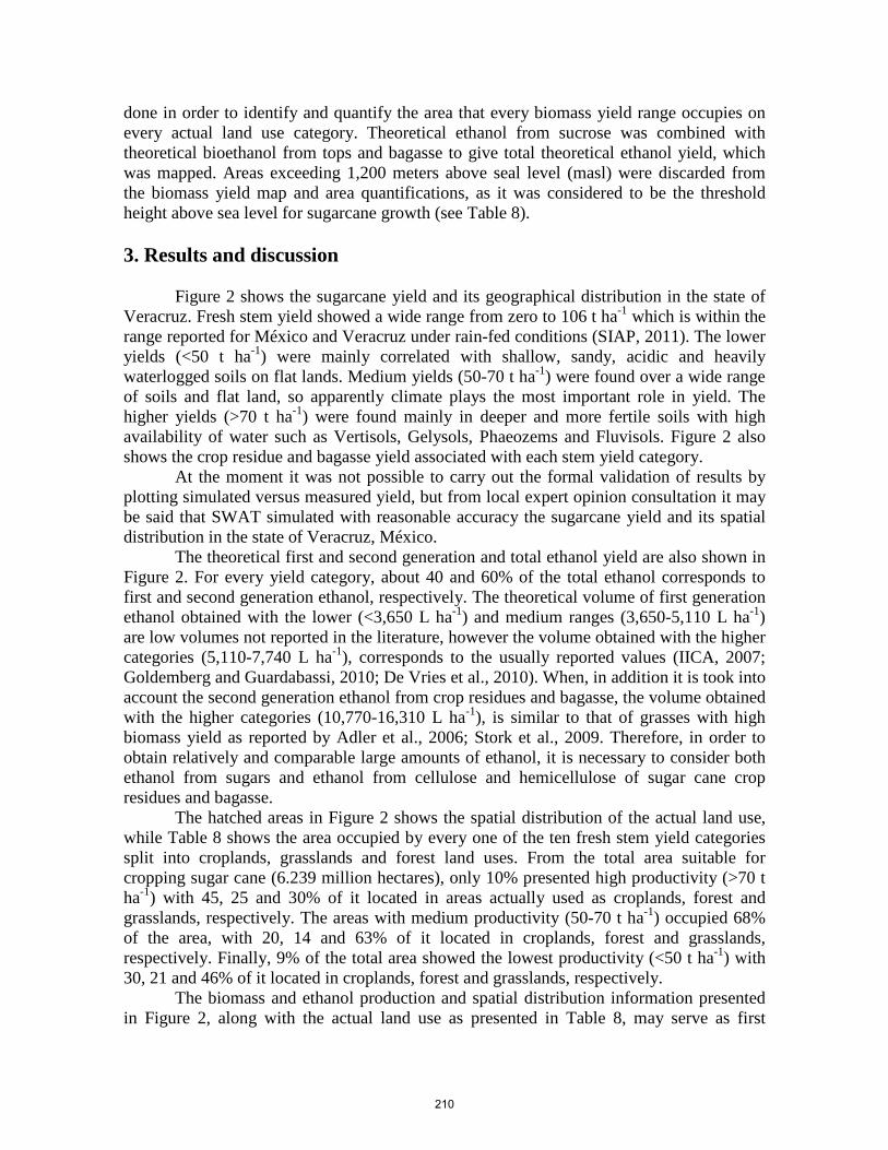
done in order to identify and quantify the area that every biomass yield range occupies on every actual land use category. Theoretical ethanol from sucrose was combined with theoretical bioethanol from tops and bagasse to give total theoretical ethanol yield, which was mapped. Areas exceeding 1,200 meters above seal level (masl) were discarded from the biomass yield map and area quantifications, as it was considered to be the threshold height above sea level for sugarcane growth (see Table 8).

3. Results and discussion

Figure 2 shows the sugarcane yield and its geographical distribution in the state of Veracruz. Fresh stem yield showed a wide range from zero to 106 t ha-1 which is within the range reported for México and Veracruz under rain-fed conditions (SIAP, 2011). The lower yields (<50 t ha-1) were mainly correlated with shallow, sandy, acidic and heavily waterlogged soils on flat lands. Medium yields (50-70 t ha-1) were found over a wide range of soils and flat land, so apparently climate plays the most important role in yield. The higher yields (>70 t ha-1) were found mainly in deeper and more fertile soils with high availability of water such as Vertisols, Gelysols, Phaeozems and Fluvisols. Figure 2 also shows the crop residue and bagasse yield associated with each stem yield category.

At the moment it was not possible to carry out the formal validation of results by plotting simulated versus measured yield, but from local expert opinion consultation it may be said that SWAT simulated with reasonable accuracy the sugarcane yield and its spatial distribution in the state of Veracruz, México.

The theoretical first and second generation and total ethanol yield are also shown in Figure 2. For every yield category, about 40 and 60% of the total ethanol corresponds to first and second generation ethanol, respectively. The theoretical volume of first generation ethanol obtained with the lower (<3,650 L ha-1) and medium ranges (3,650-5,110 L ha-1) are low volumes not reported in the literature, however the volume obtained with the higher categories (5,110-7,740 L ha-1), corresponds to the usually reported values (IICA, 2007; Goldemberg and Guardabassi, 2010; De Vries et al., 2010). When, in addition it is took into account the second generation ethanol from crop residues and bagasse, the volume obtained with the higher categories (10,770-16,310 L ha-1), is similar to that of grasses with high biomass yield as reported by Adler et al., 2006; Stork et al., 2009. Therefore, in order to obtain relatively and comparable large amounts of ethanol, it is necessary to consider both ethanol from sugars and ethanol from cellulose and hemicellulose of sugar cane crop residues and bagasse.

The hatched areas in Figure 2 shows the spatial distribution of the actual land use, while Table 8 shows the area occupied by every one of the ten fresh stem yield categories split into croplands, grasslands and forest land uses. From the total area suitable for cropping sugar cane (6.239 million hectares), only 10% presented high productivity (>70 t ha-1) with 45, 25 and 30% of it located in areas actually used as croplands, forest and grasslands, respectively. The areas with medium productivity (50-70 t ha-1) occupied 68% of the area, with 20, 14 and 63% of it located in croplands, forest and grasslands, respectively. Finally, 9% of the total area showed the lowest productivity (<50 t ha-1) with 30, 21 and 46% of it located in croplands, forest and grasslands, respectively.

The biomass and ethanol production and spatial distribution information presented in Figure 2, along with the actual land use as presented in Table 8, may serve as first

210

instance to decision makers to select, from a wide range of options, the most suitable areas for maximum ethanol production, while conserving natural resources and avoiding or minimizing competition with food production. In addition, the capacity of the bio-refinery may be also outlined form these data. Table 8. Occupied area (X1000 has) by every biomass yield category of sugar cane, split into cropland, forest and grassland actual use categories

Fresh stem Yield

Categories (t ha-1)

Total area

(x1000 has) (%) Cropland Forest Grasslands

Water Bodies and

Urban Discarded*

0-10 52 0.7 14 32 5 0 0 10-20 24 0.3 11 1 11 0 0 20-30 69 1.0 19 34 14 1 0 30-40 150 2.1 74 20 53 4 0 40-50 328 4.6 70 40 204 14 0 50-60 2901 40.4 489 457 1854 101 0 60-70 2005 27.9 511 225 1209 60 0 70-80 314 4.4 131 100 82 1 0 80-90 128 1.8 58 29 39 1 0

90-106 268 3.7 121 49 94 5 0 Discarded* - - - - - - 948

Total

6239

86.8

1,500

(20.9%) 989

(13.8%) 3,565

(49.6%) 186

(2.6%) 948

(13.2%) *Discarded area because of exceeding the sugar cane threshold value of 1,200 meters above sea level.

211

Figure 2. Biomass and Theoretical Ethanol Yield of Sugar Cane as Simulated by SWAT in Veracruz, México

212

4. Conclusions

The biomass and theoretical bioethanol yield of sugarcane from sugars and biomass was simulated and mapped with reasonable accuracy by the SWAT model in the entire state of Veracruz, México. This and related data may assist decision-makers in planning bioenergy projects. The SWAT model is a useful tool for planning bioenergy projects and sustainable rural development in tropical watersheds. In addition, it is strongly recommended to validate these results using measured yield data from sugar mills located within the state of Veracruz. Acknowledgements This research was founded by the Mexican Consejo Nacional de Ciencia y Tecnología (CONACYT) and the Consejo Veracruzano de Investigación Científica y Desarrollo Tecnológico (COVEICYDET) through the project VER-2009-C03-128049. References Adler, P.R., M.A. Sanderson, A.A. Boateng, P.J. Weimer, A.J.G. Jung. 2006. Biomass yield and

biofuel quality of switchgrass harvested in fall or spring. Agronomy Journal 98: 1518-1525. Carvalho-Junior, A.M., J. C. Maciel-Ramundo, C. E. de Siqueira-Cavalcanti, P. de S. Faveret-

Filho, N.I. Pfefer, S. E. Silveira-da Rosa, A.Y. Milane. 2008. Bioetanol de cana-de-açúcar : Energia para o desenvolvimento sustentável. Organização BNDES e CGEE. – Rio de Janeiro: BNDES. Rio de Janeiro, Brasil. 316p.

De Vries, S.C., G.W.J. Van de Ven, M.K. Van Iterrsum, K.E. Giller. 2010. Resource use efficiency

and environmental performance of nine major biofuel crops, processed by first generation conversion techniques. Biomass and Bioenergy 34:588-601.

Diario Oficial de la Federación (DOF) Secretaría de Energía (SENER). 2009. Reglamento de la Ley

de Promoción y Desarrollo de los Bioenergéticos. 19p. Available at: www.diputados.gob.mx/LeyesBiblio/regley/Reg_LPDB.pdf. Accessed on 23th March 2010.

FAO 2008. The Sate of Food and Agriculture: Biofuels: prospects, risks and opportunities. 129p. García-Espinoza, A. 1984. Manual de campo en caña de azúcar. Instituto para el Mejoramiento de

la Producción de Azúcar en México. Serie Divulgación Técnica IMPA. 224p. Goldemberg, J., P. Guardabassi, 2010. The potential for first-generation ethanol production from

sugarcane. Biofuels, Bioprod. Bioref. 4: 17-24. Inman-Bamber, N. G., 2004. Review of knowledge of sugarcane physiology and climate-crop-soil

interaction. Sugar Research and Development Corporation. Australian Government. Final Report No. CSE-006. 77p.

Instituto Interamericano de Cooperación para la Agricultura (IICA) 2007. Atlas de la Bioenergía y

los Biocombustibles en las Américas. I. Etanol. IICA, San José, Costa Rica. 181p.

213

Johnson, J.M.F., R.R. Allmaras, D.C. Reicosky. 2006. Estimating Source Carbon from Crop Residues, Roots and Rhizodeposits Using the National Grain-Yield Database. Agron. J. 98:622-636.

Liska, A. J., K. G. Cassman. 2008. Towards standardization of Life-Cycle metrics for biofuels:

Greenhouse emissions mitigation and net energy yield. Journal of Biobased Materials and Bioenergy. Vol 2. 187-203

Martínez-Jiménez, A. 2005. Uso y beneficio de los biocombustibles. En: Foro: Calidad del aire en

el Distrito Federal y Cambio Climático. Secretaría del Medio Ambiente, México. Mayo del 2005. 23p.

Menichetti, E., M. Otto. 2009. Energy balance & greenhouse gas emissions of biofuels from a life

cycle perspective. In: R. W. Howarth and S. Bringezu (eds) Biofuels: Environmental consequences and interactions with changing land use. Proceedings of the scientific committee on problems of the environment (SCOPE) international biofuels project rapid assessment. 22-25 september 2008, Gummerbach, Germany. Cornell University, Ithaca, NY, USA. p81-109.

Neitsch, S.L., J.G. Arnold, J.R. Kiniry, J.R. Williams. 2005. Soil and Water Assessment Tool.

Theoretical Documentation, Version 2005. Grassland, Soil and Water Research Laboratory-Agricultural Research Service. Blackland Research Center-Texas Agricultural Experiment Station. Temple, Texas, USA. 476p.

Reyes-Montiel, J.R., R.P. Bermúdez, J. B. Mena. 2005. Uso de la biomasa cañera como alternativa

para el incremento de la eficiencia energética y la reducción de la contaminación ambiental. Documento interno de trabajo. Centro de Estudios de Termoenergética Azucarera, Universidad Central de las Villas, Santa Clara, Cuba. 9p.

Secretaría de Agricultura, Ganadería, Desarrollo Rural, Pesca y Alimentación (SAGARPA). 2007.

Programa de producción sustentable de insumos para bioenergéticos y de desarrollo científico y tecnológico. Gobierno Federal, México. 42p. Available at: www.sagarpa.gob.mx/agricultura/.../PROINBIOS_20091013.pdf. Accessed on 9th March 2010.

Secretaría de Energía (SENER). 2007. Programa de introducción de bioenergéticos. Gobierno

Federal, México. 32p. Available at: www.energia.gob.mx/res/0/Prog%20Introd%20Bioen.pdf accessed on16th March 2010.

Stork, J., M. Montross, R. Smith, L. Schwer, W. Chen, M. Reynolds, T. Phillips, T. Coolong, S.

Debolt. 2009. Regional examination show potential for native feedstock options for cellulosic biofuel production. GCB Bioenergy 1: 230.239.

United States of America. Department of Energy. Biomass Program. Theoretical Ethanol Yield

Calculator. Available at: http://www1.eere.energy.gov/biomass/ethanol_yield_calculator.html Accessed on 8th April 2011.

214

Servicio de Información Agroalimentaria y Pesquera (SIAP) 2011. Available at: http://w4.siap.gob.mx/sispro/portales/agricolas/cania/descripcion.pdf Accessed on 27th January 2011.

Sharpley, A.N., J.R. Williams. 1990. EPIC-Erosion/Productivity Impact Calculator: 1. Model

documentation. U. S. Department of Agriculture. Technical bulletin No. 1768. 235p.

215

Mapping King-Grass (Pennisetum purpureum) Biomass Yield for Cellulosic Ethanol Production in Veracruz, México

Jesús Uresti Gil1

Roberto de Jesús López Escudero2

Elibeth Torres Benítez2

Héctor Daniel Inurreta Aguirre2

Javier Francisco Enríquez Quiroz1

1Instituto Nacional de Investigaciones Forestales, Agrícolas y Pecuarias (INIFAP)

e-mail: uresti.jesus@inifap.gob.mx

2Colegio de Postgraduados E-mail: lopez.roberto@colpos.mx

Abstract Cellulosic ethanol from grass biomass is considered to be the most promising alternative to fossil fuel, in part due to higher biomass production, net energy ratio and greenhouse mitigation potential, as compared to other plant species. To efficiently achieve maximum biomass yield and avoid competition with food production, highly and marginally grass-producing areas must be identified. The objective of this work was to simulate and map the biomass yield of king-grass in Veracruz, in order to assist decision-makers in planning rural development and ethanol bio-refinery establishment. The SWAT model was used to simulate total biomass yield throughout the 7.18 million hectares of Veracruz. To define the Hydrological Response Units, a base digital elevation model as well as soil and land use maps were used. Weather data was taken from 95 uniformly distributed weather stations with at least twenty years of records between 1960 and 2000. King-grass management was designed for high yield attainment. Most sensitive crop parameters such as LAI, RUE, Tb, HU, biomass partition and rooting depth were taken from previous local research and peer review literature. Total theoretical cellulosic ethanol was calculated and mapped. Results are presented and discussed in terms of productivity class maps of king-grass dry biomass and total theoretical cellulosic ethanol yield, identification of compact areas for bio-industrial development (development poles) and projected cellulosic ethanol refinery capacity for each of the development poles identified. Keywords: biofuel, Geographical Information Systems, ArcSwat, simulation models, rural development

216

1. Introduction

At a global scale, since the early 70’s the driving forces behind the unprecedented massive promotion and use of biofuels are the fossil energy crisis, the ever-increasing need for energy supply and security, the effort to reduce greenhouse gas emissions to mitigate climate change and the need for sustainable rural development to provide a new income stream for farmers (FAO, 2008a; IICA, 2007; SAGARPA, 2008). The main biofuels are ethanol and biodiesel. Ethanol is mainly produced in the United States of America (USA) from corn starch and in Brazil from sugar cane (First generation ethanol). Biodiesel is mainly produced in Europe from vegetable oils. However, these types of biofuels are being severely criticized by the scientific community (Crutzen et al., 2008; Doornbosch and Steenblik, 2007; Santa Barbara, 2007; Giampietro and Mayumi, 2009) and international institutions (FAO, 2008a; OECD, 2008), by arguing that liquid first generation biofuels will actually present a limited contribution to energy security and a negative impact in greenhouse gas emissions and food security (FAO 2008b; Von Braun, 2007).

Second generation ethanol from sugars contained in the cellulose and hemicellulose of plant biomass seems to be the most promising, as their net energy ratios and reduction of greenhouse gas emissions are scored better than first generation ethanol (Schmer et al., 2008; FAO, 2008a; Menichetti and Otto, 2009). However, production of second generation biofuel is much more complicated than fermentation of C6 sugar and is still far from being cost-effective as compared to the production of ethanol from starch or sugar crops (Kumar et al., 2008). In the USA there are 1,865 biofuel companies out there, and sometimes it seems that there are at least 1,865 different ways of turning every manner of biological material into biofuel for cars, trucks, trains or planes (Fahey, 2009). Cellulosic ethanol from grass biomass is considered to be the most promising source of second generation biofuel and an alternative to liquid fossil biofuels in part due to the higher biomass production, net energy ratio and greenhouse mitigation potential compared to other plant species (FAO, 2008a; Schmer, 2008). To efficiently achieve maximum biomass yield and avoid competition with food production, high and marginal grass-producing areas must be identified. The objective of this work was to simulate and map the biomass and ethanol yield from king-grass in Veracruz, México in order to assist decision-makers in planning rural development and ethanol refinery establishment. 2. Materials and Methods

In order to achieve the stated objective, the Soil and Water Assessment Tool (SWAT) model (Neitsch et al., 2005) was used to simulate and map the king-grass biomass yield throughout the 7.18 million hectares of the state of Veracruz, México. 2.1. Study area and crop settings

The following data, describing the state of Veracruz, was taken from the digital thematic maps published by the Instituto Nacional de Estadistica, Geografía e Informática (INEGI). Veracruz is located between the 17º 00’ and 22º 20’ north latitudes and between the -93º 35’ and -98 º 34’ west longitudes along the gulf in the tropical southeast part of México (Figure 1). Table 1 show the topography and land use while Table 2 shows the types of soils and climate in Veracruz. Most of the land is flat with land slopes of less than

217

8%. The climate is mainly tropical warm, humid and sub-humid. Most soils (67% of total area) are fertile, ranging from heavy clays to deep loamy, while 27% of the total area is covered with sandy and acid soils. Mountainous land has an extension of about 14% of the total area; the shallow soils are found here.

Table 1 shows that 53% of the land in Veracruz is actually occupied by grasses.

Most of these are native and introduced. King-grass, as a non-native grass, is cropped in an insignificant area, but it is currently being strongly promoted by government agencies (SAGARPA, 2011) as feedstock for the paper industry and for future cellulosic ethanol production. Table 1. Land slope, and land use in Veracruz, México; total area: 7.18 million hectares Land slope (%) % of area Land use category % of area

0 – 3 63 Forest 18.0 3 – 8 15 Grassland 53.0 8 -15 8 Agricultural 24.6

15-30 8 Water bodies and urban 3.6 >30 6 Total 100

Total 100 Table 2. Climate (Köppen classification) and soil types (FAO soil classification) in Veracruz, México; total area: 7.18 million hectares Type of Climate % of

area Type of soil % of

area Warm, humid: Am1 38 Heavy Clayey

(VR, GL)2 34

Warm, sub-humid: Aw 48 Medium Loamy (PH, FL, KS, CM, LV, O)

33

Semi-warm, humid and sub-humid: (A)C(m) and (A)C(w)

7 Light Sandy (RG, AR, CL, SC)

12

Temperate, humid and sub-humid: C(m) 6 Acid 15

218

and C(w) (AC, AN, NT, PL) Temperate, semi-arid: Bs 1 Shallow

(LP) 6

Total 100 Total 100 1Köppen climate classification keys. 2 FAO soil classification Keys. 2.2. SWAT modeling procedure

Simulation and mapping of king-grass biomass yield was carried out step by step as recommended in the various SWAT manuals and software. The entire area of the state of Veracruz was considered as the basin. 2.2.1. Watershed delineation

Watershed delineation was done from a Digital Elevation Model (DEM) with a pixel size of 90x90 meters, acquired from INEGI from a mask larger than the state of Veracruz to assure proper shape clip. To increase the flow accuracy in the basin, a river mask was added to the process. The flow direction and accumulation was carried out based on the DEM. The stream network was created using the minimum mapping area. Watersheds were delineated by selecting all outlets available, and subbasin parameters were calculated with the skip longest flow path calculation on. For the entire area of Veracruz, 224 subbasins were created. 2.2.2. Hydrological Response Units analysis

The Hydrological Response Units (HRUs) were defined from a five slope category map (0-3, 3-8, 8-15, 15-30 and >30%), a 46 soil sub-units (FAO soil classification) map and a land use map assuming the entire state of Veracruz was cropped to king-grass. The slope categories were worked out from the DEM, while the soil and land use maps (Scale 1:250,000) were obtained from INEGI. The above process resulted in 4,053 HRUs. 2.2.3. Database inputs

2.2.3.1. Soils A typical soil profile for each of the 46 soils was characterized, forming 829 soil

description datasets presented by INEGI along with the digital soil maps. Soil data not given by INEGI was obtained and/or estimated from various sources. The soil profile of a Cambisol eutrico (CMe) is presented as an example in Table 3. Table 3. Characteristics of a typical Cambisol eutrico soil profile Horizon Depth

(mm) Clay (%)

Silt (%)

Sand (%)

pH O.C. (%)

albedo K (mmhr-1)

AWC

BD (g cm-3)

A 152 15 37 48 6.1 2.35 0.08 14.3 0.13 1.47 B1 190 17 37 46 6.8 0.9 0.16 12.2 0.13 1.45 B2 732 19 30 51 6.7 0.37 0.20 11.5 0.12 1.45

O.C.: Organic carbon, K: Saturated hydraulic conductivity, AWC: Available Water Capacity, BD: Bulk density.

2.2.3.2. Land cover/plant growth The king-grass physiological parameters fed into the model are presented in Table 4

and were derived from Whiteman (1980) and local expert opinion. Other parameters were left to be assigned by SWAT.

219

Table 4. King-grass physiological parameters fed into SWAT Species RUE

(Kgha-1/Mjm-2) 2nd

point RUE

LAI

HI Canopy Height

(m)

Root depth (m)

Optimum temp. ⁰C

Base temp ⁰C

King-grass

45 53 8 0.95 3.0 2.5 37 15

2.2.3.3. Weather stations Weather data was taken from 95 uniformly distributed weather stations with at least

twenty years of records from the period 1960-2000. Weather statistics were worked out using the EPIC weather generator (Sharpley and Williams, 1990). Daily maximum and minimum temperature and rainfall data from 1990 to 2000 were fed into the model, while solar radiation was left to be estimated by SWAT.

2.2.3.4. Crop management King-grass management was designed for high biomass yield attainment under rain-

fed conditions according to Enriquez et al. (1999). Table 5 shows the general management of the king-grass. King-grass was harvested twice: at 122 and 214 days after planting. 2.3. Theoretical ethanol calculation procedure

Theoretical ethanol yield was calculated for every HRU by multiplying the simulated amount of biomass times the rate of theoretical ethanol production per unit of biomass. The rate of ethanol production was calculated with the Theoretical Ethanol Yield Calculator of the Biomass Program of the Department of Energy of the United States of America (http://www1.eere.energy.gov/biomass/ethanol_yield_calculator.html), which uses as input data the fraction of sugars of six and five carbons as shown in Table 6. The chemical composition assumed for king-grass biomass is shown in Table 6 and was taken from Uresti et al. (2010). Results show volumes of theoretical ethanol of 260 and 163 L t-1 from sugars of five and six carbons, respectively, giving a total volume of 423 L t-1 of king-grass dry biomass. Table 5. General management operation of king-grass Activity Operation Input rate (kg ha-1) Date of application Land preparation

Slash-blading 2nd may Sub-soiling 12th may Plowing 20th may Harrowing 29th may Cross harrowing 30th may Furrowing 31st may

Grass establishment Planting 1st June Fertilization

1st fertilization 75-33-10 NPK 30th June 2nd fertilization 150-66-20 NPK 30th July 3rd fertilization 75-33-10 NPK 31st October

Harvest 1st harvest 30th September 2nd harvest 31st December

220

Table 6. Average chemical composition of King-grass (Pennisetum purpureum)

Item Cellular components

(%) of dry matter Dry matter Sugars (%)

6-carbons 5-carbons Cellulose Hemicellulose Lignin Gluc Gal Man Xyl Arab

Chemical composition

38

26

13

38.21

1.17

0.39

21.34

2.91

Gluc: Glucan, Gal: Galactan, Man: Mannan, Xyl: Xylan, Arab: Arabinan 2.4. Biomass and theoretical ethanol yield mapping

Total dry biomass yield from first and second harvests was mapped and overlaid by a four-category (agricultural, grassland, forest and water bodies and urban) land use map. This operation was done in order to identify and quantify the area that every biomass yield category occupies on every actual land use category. With a biomass-ethanol conversion rate of 423 L t-1 of dry biomass, the total theoretical ethanol yield was calculated. From the above map, compacted areas with high biomass production potential were pin-pointed and bio-refinery capacity was estimated. Areas exceeding 2,000 meters above sea level (masl) were discarded from the biomass yield map and area quantifications; that elevation was considered to be the threshold height above sea level for king-grass growth (see Table 7). 3. Results and discussion

Figure 2 shows king-grass biomass yield and its geographical distribution in the state of Veracruz. Biomass yield showed a wide range, from near zero to 45 t ha-1, which is within the range reported by various authors for tropical conditions similar to those found in Veracruz (López, 1988; Roman, et al., 2009). Lower yields (<15 t ha-1) were mainly correlated with shallow and sandy soils on steep lands and waterlogged soils on flat lands, and medium yields (20-35 t ha-1) were found for the whole range of soils. Therefore, climate is apparently playing the most important role in yield. Higher yields (>35 t ha-1) were found mainly in deeper, flatter and more fertile soils with high water availability. For the moment it was not possible to carry out the formal validation of results by plotting simulated versus measured yield, but from expert opinion consultation it may be said that SWAT simulated with reasonable accuracy the king-grass biomass yield and its spatial distribution in the state of Veracruz, México.

The hatched areas in Figure 2 show the spatial distribution of the actual land use while Table 7 shows the area occupied by every one of the nine dry biomass yield categories split into croplands, grasslands and forest land uses. From the total area suitable for cropping king-grass (6.549 million hectares), only 15% presented high productivity (>35 t ha-1) with 28, 21 and 50% of it located in areas actually used as croplands, forest and grasslands, respectively. The areas with medium productivity (15-35 t ha-1) occupied 80% of the area, with 23, 16 and 58% of it located in croplands, forest and grasslands, respectively. Finally, 5% of the total area showed the lowest productivity (<15 t ha-1) with 34, 38 and 28% of it located in croplands, forest and grasslands, respectively. Since most of the areas with medium and highest biomass yield are already used as grasslands for raising cattle, two scenarios may be expected when promoting king-grass as ethanol feedstock: either the promotion and adoption of king-grass may be facilitated as farmers have knowledge, skills and infrastructure to crop the grass or else farmers may choose to keep

221

Figure 2. Biomass and Theoretical Ethanol Yield of King-Grass (Pennisetum purpureum) as Simulated by SWAT in Veracruz, México

cropping their normal grass for raising cattle and contributing to food security. However, the cost and benefit of each enterprise will probably be the most important parameter farmers will take into account to support their decision. The above is a rough statement of how the SWAT plant grow model may assist in planning bioenergy projects.

222

Table 7. Occupied area (X1000 has) by every biomass yield category of king-grass split into cropland, forest and grassland actual use categories

Dry biomass yield

categories t ha-1

Total area

(x1000has)

(%) Cropland Forest Grasslands Water

bodies and urban

Discarded*

0-5 18 0.3 5 9 4 0 0 5-10 144 2.2 40 80 24 0 0

10-15 166 2.5 68 35 63 1 0 15-20 126 1.9 14 59 50 3 0 20-25 207 3.2 47 113 43 3 0 25-30 1903 29.1 373 339 1,114 78 0 30-35 2993 45.7 779 298 1,826 90 0 35-40 940 14.4 253 207 469 12 0 40-45 51 0.8 20 0 26 5 0

Discarded* - - - - - - 638

Total

6,549

91.1

1,600

(22.3%) 1,140

(15.9%) 3,618

(50.3%) 191

(2.7%) 638

(8.9%) *Discarded area because of exceeding the king-grass threshold value of 2,000 meters above sea level.

The theoretical volume of ethanol obtained with every dry biomass category is shown in the legend of Figure 2. The lower volume (<6,000 L ha-1), associated with the areas with the lowest productivity corresponds to that reported for other grass species (Adler et al., 2006; Stork et al., 2009; Yan et al., 2010) while for the medium and high range (8,000 - 19,000 L ha-1) references were not found in the literature. This larger volume is mainly due to the effect of the higher biomass yield rather than the effect of the sugar content in the king-grass biomass since it is similar to other grasses as reported by Adler et al. (2006), Mandebvu et al. (1999) and Yan et al. (2010). 4. Conclusions

The biomass and theoretical ethanol yield of king-grass was simulated and mapped with reasonable accuracy by the SWAT model in the entire state of Veracruz, México; this and related data may assist decision-makers in planning bioenergy projects. The SWAT model is a useful tool for planning bioenergy projects and sustainable rural development in tropical watersheds. It is recommended to validate these results against measured data. Acknowledgements This research was founded by the Mexican Consejo Nacional de Ciencia y Tecnología (CONACYT) and the Consejo Veracruzano de Investigación Científica y Desarrollo Tecnológico (COVEICYDET) through the project VER-2009-C03-128049. References Adler, P.R., M.A. Sanderson, A.A. Boateng, P.J. Weimer, A.J.G. Jung. 2006. Biomass yield and

biofuel quality of switchgrass harvested in fall or spring. Agronomy Journal 98: 1518-1525.

223

Crusten, P. J., A. R. Moiser, K. A. Smith, W. Winiwarter. 2008. N2O release from agro-biofuel production negates global warming reduction by replacing fossil fuels. Atmos. Chem. Phys., Vol. 8, 389-395.

Doornbosch, R., R. Steenblik 2007. Biofuels: is the cure worse than the disease?. Round Table on

Sustainable Development. OECD paper SG/SD/RT(2007)3. 11-12 September 2007, Paris, France. 57p.

Enriquez, Q.F.J., F. Melendez-Nava, E.D. Bolaños-Aguilar. 1999. Tecnología para la producción y

manejo de forrajes tropicales en México. INIFAP.CIRGOC. Campo Experimental Papaloapan. Libro Técnico Número 7. Veracruz, México. 262p.

FAO 2008a. The Sate of Food and Agriculture: Biofuels: prospects, risks and opportunities. 129p. FAO 2008b. Assessment of the world food security and nutrition situation. Committee on world

food security. Thirty-fourth session. October 14-17, 2008. Rome, Italy. 18p. Fahey, J. 2009. Biofuels Battle: Chemistry versus Biology. What is the best way to turn plants into

biofuels?. Available at: http://www.forbes.com/2009/04/28/biofuels-ethanol-virent-technology-breakthroughs-biofuels.html. Accessed on 21st July 2009.

Giamprieto, M., K. Mayumi. 2009. The biofuel delusión. The Fallacy of large scale agro-biofuel

production. ISBN 9781844076819. 320p. Instituto Interamericano de Cooperación para la Agricultura (IICA) 2007a. Atlas de la Bioenergía y

los Biocombustibles en las Américas. I. Etanol. IICA, San José, Costa Rica. 181p. Kumar, R., S. Singh, O.V. Singh. 2008. Bioconversion of lignocellulose biomass: Biochemical and

molecular perspectives. J. Ind. Microbiol Biotechnol. 35: 377-391. López, G.I. 1988. Rendimiento de material seca y proteína cruda de siete garmíneas cosechadas a

cuatro frecuencias de corte en clima cálido sub-húmedo. Tesis de licenciatura, Universidad Autónoma Agraria Antonio Narro. Saltillo, Coahuila, México. 67p.

Mandebvu, P., J.W. West, G.M. Hill, R.N. Gates, R.D. Hatfield, B.G. Mullinix, A.H. Parks, A.B.

Caudle. 1999. Comparison of Tifton 85 and coastal Bermuda grasses for yield, nutrients, traits, intake and digestion by growing beef steers. J. Anim. Sci. 77: 1572-1586.

Menichetti, E., M. Otto. 2009. Energy balance & greenhouse gas emissions of biofuels from a life

cycle perspective. In: R. W. Howarth and S. Bringezu (eds) Biofuels: Environmental consequences and interactions with changing land use. Proceedings of the scientific committee on problems of the environment (SCOPE) international biofuels project rapid assessment. 22-25 september 2008, Gummerbach, Germany. Cornell University, Ithaca, NY, USA. p81-109.

Neitsch, S.L., J.G. Arnold, J.R. Kiniry, J.R. Williams. 2005. Soil and Water Assessment Tool.

Theoretical Documentation, Version 2005. Grassland, Soil and Water Research Laboratory-Agricultural Research Service. Blackland Research Center-Texas Agricultural Experiment Station. Temple, Texas, USA. 476p.

224

Organisation for Economic Co-Operation and Development (OECD). 2008. Economic assessment of biofuels support policies. Directorate for trade and agriculture, OECD. 119p.

Román, P.H., L.Ortega R., L. Hernández, A., E. Díaz, A., J.A. Espinosa, G., G. Núñez H., H.R.

Vera A., M. Medina, C., F.J. Ruiz L. 2009. Producción de leche de bovino en el sistema de doble propósito. Libro Técnico Número 22. INIFAP.CIRGOC. Veracruz, México. 355p.

Santa Barbara, J. 2007. The false promise of biofuels. A special report from the international forum

on globalization and the institute for policy studies. USA. 31p. Schmer, M. R., K. P. Vogel, R. B. Mitchell, R. K. Perrin. 2008. Net energy of cellulosic ethanol

from switchgrass. PNAS. Vol. 105 (2) 464-469. Secretaría de Agricultura, Ganadería, Desarrollo Rural, Pesca y Alimentación (SAGARPA) 2008.

Estrategia Intersecretarial y Programas de Producción Sustentable de Insumos e introducción de Bioenergéticos en México. Resumen Ejecutivo. Gobierno Federal, México. 9p.

Secretaría de Agricultura, Ganadería, Desarrollo Rural Pesca y Alimentación (SAGARPA). 2011. TRÓPICO HÚMEDO. Proyecto estratégico para el Desarrollo Rural Sustentable de la Region Sur-Sureste de México. 32p.

Sharpley, A.N., J.R. Williams. 1990. EPIC-Erosion/Productivity Impact Calculator: 1. Model

documentation. U. S. Department of Agriculture. Technical bulletin No. 1768. 235-p. Stork, J., M. Montross, R. Smith, L. Schwer, W. Chen, M. Reynolds, T. Phillips, T. Coolong, S.

Debolt. 2009. Regional examination show potential for native feedstock options for cellulosic biofuel production. GCB Bioenergy 1: 230.239.

United States of America. Department of Energy. Biomass Program. Theoretical Ethanol Yield

Calculator. Available at: http://www1.eere.energy.gov/biomass/ethanol_yield_calculator.html Accessed on 8th April 2011.

Uresti, G.J., F.J. Enríquez-Quiroz, I. López-Guerrero, V.D. Hernández-Hernández. Pastos

Tropicales, mina renovable de biocombustibles: Estimación preliminar del rendimiento teórico de etanol. En: J.A. Cueto-Wong, L.A. Macías-García, O.E. Ortiz-Rivas (Eds.) Memoria de la V Reunión de Innovación Agrícola. 22-27 de Noviembre del 2011, San Francisco de Campeche, Campeche, México. p-117.

Von Braun, J. 2007. The world food situation. New driving forces and required actions. Food

Policy Report. International Food Policy Research Institute (IFPRI). Washington, D. C. USA. 18p

Whiteman, P.C. 1980. Tropical Pasture Science. New York, Oxford University Press. 392p. Yuan, J., Z. Hu, Y. Pu, E. C. Brummer, A.J. Ragauskas. 2010. Chemical compositions of four

switchgrass populations. Biomass and Bioenergy 34: 48-53.

225

Climate Change Impacts on Water Availability in Three Mediterranean Basins of Catalonia (NE Spain)

Diana Pascual, Eduard Pla, Javier Retana, Jaume Terradas

CREAF (Centre for Ecological Research and Forestry Applications) – Autonomous University of Barcelona – 08193 Bellaterra, Spain

accua@creaf.uab.cat

Abstract The Mediterranean region might become one of the most vulnerable areas in Europe in regards to climate change. There is a social concern related to climate change impacts on water resources. In this context, the IPCC Fourth Assessment Report (2007) points out a significant decrease in runoff in Mediterranean regions at the end of the century. This work assesses the main climate change impacts in three medium-sized catchments in Catalonia (NE Spain): Fluvià, Tordera and Siurana. Each of the three catchments has distinct environmental conditions. The main aim of the study is to develop adaptive measures to cope with the expected climatic and social changes. The Soil and Water Assessment Tool (SWAT) was used to simulate the hydrologic response to climate changes. Downscaled projections of ECHAM5 GCM under two IPCC emission scenarios (A2, B1) were used. In comparison with baseline conditions (1984-2008), climate projections predicted a 12% (B1) to 28% (A2) reduction in precipitation and a 2.2ºC (B1) to 3.6ºC (A2) rise in mean annual temperature at the end of the 21st century (2076-2100). SWAT simulations predicted a 22% and 48% reduction in streamflow and a 14% and 25% reduction in real evapotranspiration for 2076-2100 under B1 and A2, respectively. Autumn and summer were the most affected seasons. These results highlight the strong impact of climate change in regional water resources and reflect the importance of incorporating this analysis into adaptive management in the Mediterranean region. This work is part of the ACCUA project (www.creaf.uab.cat/accua), which aims to evaluate the territorial vulnerability of the Mediterranean coast for the main effects of global change in relation to water availability. Keywords: climate change, water availability, SWAT, Mediterranean

226

1. Introduction The latest climatic models predict that during this century the climate of the

Mediterranean region will become warmer and drier (Christensen et al., 2007). As a biogeographical transition zone, the Mediterranean area is one of the most sensitive biomes to present and future climatological changes (Lavorel et al., 1998).

Observational studies revealed a global trend toward warmer conditions during recent decades (Solomon et al., 2007). Regional studies based on recorded meteorological data in Catalonia (NE Spain) have already confirmed an upward mean temperature trend over recent decades (1950-2008) even though annual precipitation did not vary significantly in this region (Llebot, 2010).

Besides temperature increases, global circulation models predict an annual precipitation decrease in the Mediterranean basin as well as changes in its seasonal distribution at the end of the 21st century (Christensen et al., 2007). As a consequence, lower water availability is also expected for local watershed systems of this region. The combination of these trends of decreasing precipitation coupled with increasing temperature and thus increasing evapotranspiration results in even stronger decreases in water availability than would be expected from considering precipitation changes only.

The hydrologic response of Mediterranean catchments to global change is currently the subject of much scientific concern. An example of this concern is the ACCUA project (www.creaf.uab.cat/accua) which assesses territorial vulnerability of three medium-sized catchments in Catalonia (NE Spain) with regard to the effects of global change on water availability.

The Soil and Water Assessment Tool (SWAT, Neitsch et al., 2002) was used to simulate hydrologic responses to climate change. This is a physically based, semi-distributed hydrological model that operates on a daily time step. SWAT has been widely used throughout the world for many water resource applications but scarcely in studies focused on climate change impacts in Mediterranean watersheds of the Iberian Peninsula (Nunes et al., 2008).

The results obtained will provide an assessment of water availability vulnerability to climate change with the aim of projecting trends that will aid in the design of adaptation strategies.

2. Study Area The study area was chosen to represent Mediterranean heterogeneity at a local

level. Three pilot catchments representative of littoral conditions were selected: Fluvià, Tordera and Siurana (Figure1). These three catchments represent a climatic gradient across the Catalonian coast as well as diversity in land use, pressures and environmental conditions. All three are unregulated watersheds except for three small reservoirs on Siurana. Fluvià is a forested basin of agricultural importance with a strong touristic pressure in its lowest part. Tordera is closer to Barcelona and has strong urban development and industrial pressure. Siurana is the drier area where agriculture and natural systems are in a very fragile situation. All three catchments have presented similar trends in land use changes during recent decades. Where the forest area has slightly increased, agricultural land has dropped and urban space has grown (Figure 2).

227

Figure 1. Watershed locations across the Catalan coast (NE Spain)

Figure 2. Main land uses in each watershed in 1993, 2000 and 2005 (Data source: Land Cover Map of Catalonia 1993, 2000 and 2005) The analysis of the historic climate has shown a temperature increase during recent decades which is consistent with global registered trends along the Mediterranean area (1.25ºC throughout the period 1951-2000). The main rise was observed for maximum temperature. An insignificant decrease in annual precipitation was observed,

ForestAgriculture

Urban

ForestAgriculture

Urban

19931.9

4.6

0.9

23.6

15.4

30.4

74.2

80

68.5

20002.8

6.1

0.9

20.8

11.4

25.2

76.2

82.5

73.7

20002.8

6.1

0.9

20.8

11.4

25.2

76.2

82.5

73.7

20053.1

9.2

1.5

19

10

21.8

77.3

80.6

76.1

20053.1

9.2

1.5

19

10

21.8

77.3

80.6

76.1

Fluvià

Tordera

Siurana

97.320 ha

86.469 ha

61.444 ha

228

but reductions were significant on some specific months (July and March) while there was a significant increase in January.

Figure 3. Mean temperature trends from 1914 to present based on measured data from AEMET climatic stations. The Fabra station is not within the study areas but it is frequently used as a reference series. The other climatic stations are located within the studied catchments.

3. Data and Methods 3.1. SWAT calibration and validation

The Soil and Water Assessment Tool (SWAT) was used to simulate the hydrologic response to climate change. In the first phase, the model was calibrated and validated with measured climatic and flow discharge data. In the second phase, the calibrated model was used to evaluate climate change impacts on water resources. In this phase, the climatic projections from SMC (a regional climate centre called the Meteorological Service of Catalonia) were used for the period from 2000 to 2100.

SWAT input data used on the calibration includes the digital elevation model from Catalonia (30 m spatial resolution) developed by the Catalonian Cartographic Institute (ICC), a soil map created from geological maps and adapted to research aims, land use data from the Land Cover Map of Catalunya (2000 version, at 2 m spatial resolution) developed by the Centre for Ecological Research and Forestry Applications (CREAF), and climatic series from metereological stations located on the watersheds (AEMET, Spanish Meteorological Agency, and SMC). Climatic series included precipitation, temperature, radiation, relative humidity and wind speed in seven/eight points per study area. These series were filled and corrected by the effects of orography on precipitation and temperature with SWAT equations.

Model calibration was based on measured streamflow values along the watersheds. In these specific watersheds, flow series were often scarce, incomplete and of bad quality. Initially, a 25-year period (1984-2008) was chosen to calibrate and

13

14

15

16

17

18

1914 1924 1934 1944 1954 1964 1974 1984 1994 2004

Mea

n te

mpe

ratu

re (º

C)

Fabra

TorderaVilobí d'Onyar

SiuranaTivissa

FluviàL'Estartit

229

validate the model, the longest time slice in which both climatic and flow data were available. Within this time slice, calibration was made with shorter periods, usually two or three years, depending on the quality of data from the gauging station. Calibration was carried out at a daily time step to target three main objectives: (1) similarity of simulated curves to measured ones, (2) mean flow values and total contributions similarity between simulated and measured data, and (3) good statistics for Nash and Sutcliffe efficiency coefficient (NSE) and RMSE-observations standard deviation ratio (RSR). Moriasi et al. (2007) proposed threshold values for these statistics to evaluate the goodness of fit of the model at a monthly time step (Table 1). Table 1. General performance ratings of statistics for a monthly time step (from Moriasi et al. 2007)

Performance rating RSR NSE Very good 0.00 ≤ RSR ≤ 0.50 1.00 ≤ NSE < 0.75

Good 0.50 < RSR ≤ 0.60 0.75 ≤ NSE < 0.65 Satisfactory 0.60 < RSR ≤ 0.70 0.65 ≤ NSE < 0.5

Unsatisfactory RSR > 0.70 NSE ≤ 0.5

Sensitivity analysis and preliminary model trials were developed to identify the most influential parameters, which were adjusted during the calibration. Parameters related to base flow generation (ALPHA_BF, GWQMN, GW_REVAP, REVAPMN, RCHRG_DP), surface runoff (CN2, SOL_K, SOL_AWC, ESCO, CH_N) and basin response (SURLAG, CH_K) were changed until project goals were reached.

Calibration was performed both manually and through SWAT-CUP (SWAT Calibration Uncertainty Procedures, Abbaspour et al., 2008). Model parameters were adjusted independently among sub-watersheds, depending on available streamflow data. Within calibration, water extraction for urban, industrial and agricultural uses were introduced as consumptive water and removed from the basin. In the Fluvià basin, the subterranean water transfer from the High Garrotxa headwater to different points within the basin (Serinyà river) and outside the basin (Banyoles lake on Ter basin) was considered. Previous studies have quantified in 12 hm3 per year water transfer to the outside of the Fluvià basin (EPTISA, 1988). In the Siurana basin, simulations included three small reservoirs situated in the headwater area. Two of them, the Siurana and Guiamets reservoirs, had registered daily outflow from 1984 to 2008. The other one, the Margalef reservoir, is managed for agricultural purposes and no registered data were available. This reservoir was simulated as an uncontrolled one.

Figure 4 and Table 2 show calibration outputs in one gauging station per basin, usually the closest to the river mouth (Garrigàs station in Fluvià, Can Serra station in Tordera and Cornudella de Montsant station in Siurana; this last gauging station is situated on the headwater and under the Siurana reservoir influence). The graphical comparison between simulated and measured data shows a good fit, although simulations overestimate maximum flood peaks in all three basins. In Fluvià and Tordera, simulations overestimate mean and total streamflow values (27 and 19%, respectively). NSE and RSR statistics are satisfactory, although analysis was carried out at a daily time step.

230

Figure 4. Calibration results: measured and simulated daily discharge in three points, one per basin: Garrigàs at Fluvià basin, Can Serra at Tordera and Cornudella de Montsant at Siurana Table 2. Calibration results: mean daily discharge values from both simulated and measured data and adjust statistics in each basin Statistics

Simulated mean daily discharge (m3/s)

Observed mean daily discharge (m3/s) NSE RSR

Fluvià (Garrigàs) 9.1 7.1 0.5 0.7 Tordera (Can Serra) 4.3 3.6 0.5 0.7 Siurana (Cornudella) 0.2 0.2 0.6 0.7

The validation measures model prediction capacity through the comparison of simulated results to measured data in a different time period. Validation was also made with short time slices depending on observed data quality. Table 3 shows the validation results per basin. As in calibration results, simulations overestimated mean discharge values, although in a lower percentage (20% in Fluvià and 8% in Tordera). Statistics were found to be satisfactory except in the Tordera basin. Table 3. Validation results: mean daily discharge values from both simulated and measured data and adjust statistics in each basin Statistics

Simulated mean daily discharge (m3/s)

Observed mean daily discharge (m3/s) NSE RSR

Fluvià (Garrigàs) 8.5 7.1 0.5 0.7 Tordera (Can Serra) 5.1 4.8 0.4 0.7 Siurana (Cornudella) 0.4 0.3 0.7 0.6

0

100

200

300

1987 1988 1989Year

Dai

ly s

trea

m fl

ow

(m3/

s)Fluvià

0

50

100

150

200

1996 1997 1998 1999Year

Dai

ly s

trea

m fl

ow

(m3/

s)0

1

2

3

1991 1992 1993Year

Dai

ly s

trea

m fl

ow

(m3/

s)Tordera

Siurana Measured data

SWAT simulated data

231

Figure 5 and Table 4 show calibration results for the whole period (1984-2008) at a monthly time step. Graphics, mean values and statistics showed a good performance ratio and a general overestimation between 10 and 15%. Figure 5. Measured and simulated monthly discharge in Garrigàs, at the Fluvià basin Table 4. Mean monthly discharge values from both simulated and measured data and statistics Statistics

Simulated mean daily discharge (m3/s)

Observed mean daily discharge (m3/s) NSE RSR

Fluvià (Garrigàs) 8.5 7.3 0.7 0.5 Tordera (Can Serra) 3.9 3.5 0.8 0.4 Siurana (Cornudella) 0.3 0.2 0.7 0.6 3.2. Climate projections

Future climate data were provided by the SMC (Catalan Meteorological Service), which has generated downscaled projections of ECHAM5 GCM under two IPCC emission scenarios (A2, B1). Future projections have a high temporal and spatial resolution (6 h and 15 km) for the period 2001-2100 and for the reference period 1971-2000 (Calbó et al., 2010).

Climate projections estimate a precipitation reduction between 12% (scenario B1) and 28.3% (A2) and a mean annual temperature increment between 2.2ºC (B1) to 3.6ºC (A2) by the end of the 21st century (2076-2100). Figure 6 shows annual precipitation and mean annual temperature trends across the century for the Fluvià basin.

0

20

40

60

1986 1989 1992 1995 1998 2001 2004 2007Year

Mon

thly

str

eam

flow

(m

3/s)

Measured dataSWAT simulated dataFluvià

232

Figure 6. Annual precipitation and mean annual temperature five-year running mean variations from 1984 to 2100 for the Fluvià basin Table 5. Mean precipitation and temperature values per time slices per scenario; precipitation reduction percentage and temperature degrees incremented are also shown. Mean annual precipitation

Reference period (1984-2008)

Short term (2006-2030) % reduction

Long term (2076-2100) % reduction

B1 Fluvià 1013.3 983.1 -3.0% 863 -14.8% Tordera 778.1 759.7 -2.4% 683 -12.2% Siurana 532.9 517.9 -2.8% 451.2 -15.3% A2 Fluvià 1076.3 972.8 -9.6% 771.3 -28.3% Tordera 828.1 750.9 -9.3% 626.4 -24.4% Siurana 553.5 511.2 -7.6% 420.7 -24.0%

Mean annual temperature

Reference period (1984-2008)

Short term (2006-2030) ºC increment

Long term (2006-2030) ºC increment

B1 Fluvià 13.1 13.7 0.6 15.3 2.3 Tordera 14.2 14.7 0.5 16.4 2.2 Siurana 14.8 15.4 0.6 17.0 2.2 A2 Fluvià 13.0 13.4 0.5 16.5 3.5

0

500

1000

1500

1984 1999 2014 2029 2044 2059 2074 2089

Ann

ual p

reci

pita

cion

(mm

)

10

12

14

16

18

20

1984

1994

2004

2014

2024

2034

2044

2054

2064

2074

2084

2094M

ean

annu

al te

mpe

ratu

re (º

C)

Five-years running mean reference period

Five-years running mean scenario B1

Five-years running mean scenario A2

233

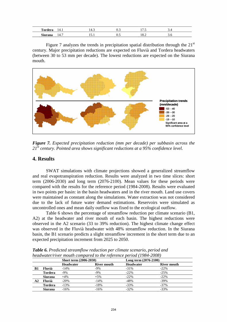
Tordera 14.1 14.3 0.3 17.5 3.4 Siurana 14.7 15.1 0.5 18.2 3.6

Figure 7 analyzes the trends in precipitation spatial distribution through the 21st

century. Major precipitation reductions are expected on Fluvià and Tordera headwaters (between 30 to 53 mm per decade). The lowest reductions are expected on the Siurana mouth. Figure 7. Expected precipitation reduction (mm per decade) per subbasin across the 21st century. Pointed area shows significant reductions at a 95% confidence level.

4. Results SWAT simulations with climate projections showed a generalized streamflow

and real evapotranspiration reduction. Results were analyzed in two time slices: short term (2006-2030) and long term (2076-2100). Mean values for these periods were compared with the results for the reference period (1984-2008). Results were evaluated in two points per basin: in the basin headwaters and in the river mouth. Land use covers were maintained as constant along the simulations. Water extraction was not considered due to the lack of future water demand estimations. Reservoirs were simulated as uncontrolled ones and mean daily outflow was fixed to the ecological outflow.

Table 6 shows the percentage of streamflow reduction per climate scenario (B1, A2) at the headwater and river mouth of each basin. The highest reductions were observed in the A2 scenario (33 to 39% reduction). The highest climate change effect was observed in the Fluvià headwater with 48% streamflow reduction. In the Siurana basin, the B1 scenario predicts a slight streamflow increment in the short term due to an expected precipitation increment from 2025 to 2050. Table 6. Predicted streamflow reduction per climate scenario, period and headwater/river mouth compared to the reference period (1984-2008)

Short term (2006-2030) Long term (2076-2100) Headwater River mouth Headwater River mouth B1 Fluvià -14% -9% -31% -22% Tordera -9% -9% -22% -25% Siurana +4% +5% -22% -22% A2 Fluvià -20% -14% -48% -39% Tordera -13% -18% -33% -37% Siurana -16% -16% -32% -33%

Precipitation trends (mm/decade)

-53 - -40-39 - -30-29 - -20-19 - -10Significant area at a 95% confidence level

Precipitation trends (mm/decade)

-53 - -40-39 - -30-29 - -20-19 - -10Significant area at a 95% confidence level

234

Figure 8 shows the distribution of streamflow reduction among seasons for the short term for the Fluvià river mouth, and results for the other basins are similar. Large reductions were predicted in spring and summer for the B1 scenario, where the most affected seasons were winter and spring for the A2 scenario. Figure 8. Expected runoff variation (%) per scenario. Results from the Fluvià river mouth estimated as change percentage from short term mean runoff (2006-2030) to the reference period mean runoff (1984-2008).

In the long term, autumn and summer will be the most affected seasons concerning runoff reduction in the two scenarios (Figure 9) while slight increments will be expected in winter. Figure 9. Expected runoff variation (%) per scenario. Results from the Fluvià river mouth estimated as change percentatge from long term mean runoff (2076-2100) to the reference period mean runoff (1984-2008).

Potential and real evapotranspiration (PET and ETr) were estimated by the Penman-Monteith equation incorporated in SWAT. Results showed a PET-increment by the end of the XXI Century due to the expected temperature increment. A 14% to 25% real evapotranspiration reduction was predicted because of the expected precipitation reduction (Table 7).

Scenario A2

-4.1%

-10.0%

-18.4%-21.2%

-30

-20

-10

0Winter Spring Summer Autumn

Stre

am fl

ow v

aria

tion

perc

enta

ge /

seas

on

Scenario B1

-1.1% -4.6%

-10.1%-11.8%

-30

-20

-10

0Winter Spring Summer Autumn

Stre

am fl

ow v

aria

tion

perc

enta

ge /

seas

on

Scenario A2

-44.7%-40.2%-40.7%

-34.3%

-50

-40

-30

-20

-10

0

10

Winter Spring Summer Autumn

Stre

am fl

ow v

aria

tion

perc

enta

ge /

seas

on

Scenario B1

-36.1%

-25.5%-22.0%

2.5%

-50

-40

-30

-20

-10

0

10

Winter Spring Summer Autumn

Stre

am fl

ow v

aria

tion

perc

enta

ge /

seas

on

235

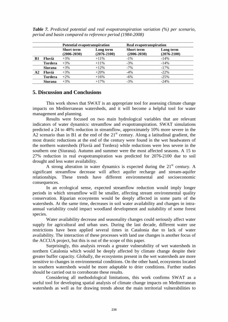
Table 7. Predicted potential and real evapotranspiration variation (%) per scenario, period and basin compared to reference period (1984-2008)

Potential evapotranspiration Real evapotranspiration Short term

(2006-2030) Long term (2076-2100)

Short term (2006-2030)

Long term (2076-2100)

B1 Fluvià +3% +11% -1% -14% Tordera +3% +11% -3% -14% Siurana +3% +12% -7% -17% A2 Fluvià +3% +20% -4% -22% Tordera +2% +16% -6% -25% Siurana +3% +17% -3% -24%

5. Discussion and Conclusions

This work shows that SWAT is an appropriate tool for assessing climate change

impacts on Mediterranean watersheds, and it will become a helpful tool for water management and planning.

Results were focused on two main hydrological variables that are relevant indicators of water dynamics: streamflow and evapotranspiration. SWAT simulations predicted a 24 to 48% reduction in streamflow, approximately 10% more severe in the A2 scenario than in B1 at the end of the 21st century. Along a latitudinal gradient, the most drastic reductions at the end of the century were found in the wet headwaters of the northern watersheds (Fluvià and Tordera) while reductions were less severe in the southern one (Siurana). Autumn and summer were the most affected seasons. A 15 to 27% reduction in real evapotranspiration was predicted for 2076-2100 due to soil drought and less water availability.

A strong alteration in water dynamics is expected during the 21st century. A significant streamflow decrease will affect aquifer recharge and stream-aquifer relationships. These trends have different environmental and socioeconomic consequences.

In an ecological sense, expected streamflow reduction would imply longer periods in which streamflow will be smaller, affecting stream environmental quality conservation. Riparian ecosystems would be deeply affected in some parts of the watersheds. At the same time, decreases in soil water availability and changes in intra-annual variability could impact woodland development and suitability of some forest species.

Water availability decrease and seasonality changes could seriously affect water supply for agricultural and urban uses. During the last decade, different water use restrictions have been applied several times in Catalonia due to lack of water availability. The interaction of these processes with land use changes is another focus of the ACCUA project, but this is out of the scope of this paper.

Surprisingly, this analysis reveals a greater vulnerability of wet watersheds in northern Catalonia which would be deeply affected by climate change despite their greater buffer capacity. Globally, the ecosystems present in the wet watersheds are more sensitive to changes in environmental conditions. On the other hand, ecosystems located in southern watersheds would be more adaptable to drier conditions. Further studies should be carried out to corroborate these results.

Considering all methodological limitations, this work confirms SWAT as a useful tool for developing spatial analysis of climate change impacts on Mediterranean watersheds as well as for drawing trends about the main territorial vulnerabilities to

236

changes in water availability. Results highlight the strong impact of climate change on regional water resources and reflect the importance of incorporating these analyses into adaptive management in the Mediterranean region.

Acknowledgments This work is part of the ACCUA project (www.creaf.uab.cat/accua) coordinated by CREAF with different research partners (UPC, IRTA, ETC-SIA and UB). Valuable contributions were made by the Catalan Water Agency (ACA). Regional climatic projections were provided by the Catalan Meteorological Service (SMC). ACCUA was founded by CatalunyaCaixa.

References Abbaspour, K. C., J. Yang, M. Vejdani, and S. Haghighat (2008), SWATCUP: Calibration and

uncertainty programs for SWAT, 4th Int. SWAT Conf. Proc., in press. Calbó, J.; Sanchez-Lorenzo, A.; Cunillera, J. and Barreda-Escoda, A. (2010): Projeccions i

escenaris de futur. A: Llebot, J.E. (Ed.): Segon informe sobre el canvi climatic a Catalunya. Institut d’Estudis Catalans and Generalitat de Catalunya. Consell Assessor per al Desenvolupament Sostenible de Catalunya, 183-239. Barcelona. ISBN 978-84-9965-027-2

Christensen, J.H., B. Hewitson, A. Busuioc, A. Chen, X. Gao, I. Held, R. Jones, R.K. Kolli, W.-

T. Kwon, R. Laprise, V. Magaña Rueda, L. Mearns, C.G. Menéndez, J. Räisänen, A. Rinke, A. Sarr, P. Whetton (2007) A: Climate Change 2007: The Physical Science Basis. Contribution of Working Group I to the Fourth Assessment Report of the Intergovernmental Panel on Climate Change. Cambridge University Press, Cambridge, United Kingdom and New York, NY, USA.

EPTISA, 1988. Estudio hidrogeológico del lago de Bañolas. Estudios hidrogeológicos en la cuenca hidrográfica del Pirineo Oriental.

Lavorel, S.; Canadell, J.; Rambal, S.; Terradas, J. (1998) Mediterranean terrestrial ecosystems: research priorities on global change effects. Global Ecology and Biogeography 7: 157-166.

Llebot, J.E. (Ed) (2010) Segon informe sobre el canvi climatic a Catalunya. Institut d’Estudis

Catalans and Generalitat de Catalunya. Consell Assessor per al Desenvolupament Sostenible de Catalunya. Barcelona. ISBN 978-84-9965-027-2

Moriasi, D.N., Arnold, J.G., Van Liew, M.W., Bingner, R.L., Harmel, R.D., Veith, T.L. (2007). Model evaluation guidelines for systematic quantification of accuracy in watershed simulations. Transactions of the ASABE. 50(3):885-900

Neitsch, S.L., Arnold, J.G., Kiniry, J.R., Williams, J.R., King, K.W. (2002). Soil and water assessment tool. Theoretical documentation. Version 2000. Texas Water Resources Institute Report TR-191, Texas, USA, 458p.

Nunes J.P., Seixas J., Pacheco N.R. (2008) Vulnerability of water resources, vegetation productivity and soil erosion to climate change in Mediterranean watersheds. Hydrological Processes. 22, 16, 3115-3134.

Solomon, S., D. Qin, M. Manning, Z. Chen, M. Marquis, K.B. Averyt, M. Tignor and H.L. Miller (eds.). (2007) Climate Change 2007: The Physical Science Basis. Contribution of

237

Working Group I to the Fourth Assessment Report of the Intergovernmental Panel on Climate Change. Cambridge University Press, Cambridge, United Kingdom and New York, NY, USA, 996 pp.

238

Quantifying SWAT Runoff Using Gridded Observations and Reanalysis Data for Dakbla River Basin, Vietnam

Vu Minh Tue1,2, Raghavan Srinivasan1,2, Liong Shie-Yui1 and Verwey Adri2

1Tropical Marine Science Institute (TMSI), National University of Singapore 2Singapore-Delft Water Alliance (SDWA), National University of Singapore

Abstract Many research studies that focus on basin hydrology have used the SWAT model to simulate runoff. One common practice in calibrating the SWAT model is the application of station data rainfall to simulate runoff. But in regions lacking robust station data, there is a problem of applying the model to study the hydrological responses. To overcome this limitation, this research study uses available gridded high resolution precipitation datasets to simulate runoff. Four popular gridded observation precipitation datasets- APHRODITE, TRMM, PERSIANN and GPCP and one reanalysis dataset (NCEP/NCAR) are used to simulate runoff over the Dakbla river (a small tributary of the Mekong River) of the Sesan river basin in Vietnam. Wherever possible, available station data are also used for comparison. Bilinear interpolation of these gridded datasets is used to input the precipitation data at the closest grid points to the station locations. Sensitivity analysis and auto-calibration are performed for the SWAT model. The Nash-Sutcliffe Efficiency (NSE) and coefficient of determination (R2) indices are used to benchmark the model performance. This entails a good understanding of the response of the hydrological model to different datasets, and the uncertainties in these datasets are quantified. Such a methodology is also useful for planning rainfall runoff and even reservoir/river management both at rural and urban scales. Keywords: SWAT, gridded observations, rainfall runoff, uncertainties

239

1. Introduction The rainfall runoff model is a typical hydrological modeling tool that determines the

runoff signal which leaves the watershed basin from the rainfall signal received by the basin. Therefore, precipitation is the most important parameter in hydrological modeling. The Soil and Water Assessment Tool (SWAT) (Arnold et al., 1998) was developed in order to quantify runoff and concentration load due to distributed precipitation and other meteorological data based on watershed topography, soil and land use condition. For some countries and remote areas, the rainfall data collection task might be omitted due to many different reasons such as lack of technology, war and financial limitations that lead to difficulty in constructing runoff data. Many research institutes around the world have developed gridded observation precipitation data for global and local domain under different temporal and spatial resolutions. The most popular gridded datasets that have been used in many research studies are the CRU (Climatic Research Unit, from University of East Anglia, UK) and UDEL (University of Delaware precipitation dataset). Both datasets are constructed based on the ground truth data for the world domain with grid size of 0.5o (~50 km) and in monthly intervals. Besides, some other datasets, mostly satellite based, also have temporal resolutions of about three hours and spatial resolutions of about 0.250 which are ideal for rainfall runoff modeling in daily and sub-daily scales. The other datasets that have been used in this study are: APHRODITE (Asian Precipitation Highly Resolved Observational Data Integration Towards the Evaluation of Water Resources) developed in Japan, TRMM (Tropical Rainfall Measuring Mission) from the USA, PERSIANN (Precipitation Estimation from Remote Sensing Information using Artificial Neural Network) from the USA, GPCP (Global Precipitation Climatology Project) from the USA, and the popular NCEP/NCAR (National Centers for Environment Prediction/National Center for Atmospheric Research).

An eleven-year daily precipitation dataset from 1995 to 2005 for three different rainfall stations is used for Dakbla river basin in Vietnam (a small tributary of the Mekong river) in which calibration will use the later period 2000-2005 with 2000 as the warm-up year and validation uses 1995-2000 with 1995 as the warm-up time. SWAT’s built-in sensitivity analysis and auto-calibration using the PARASOL method (PARAmeter SOLution) (Griensven and Meixner, 2006) are applied. The Nash-Sutcliffe Efficiency (NSE) (Nash and Sutcliffe, 1970) and the Coefficient of Determination (R2) are used as the benchmarking indices for runoff. After calibration, the gridded data are interpolated to the three rainfall stations considered in this study and are applied to the model using calibrated parameters to generate runoff.

The aim of this paper is to test the usefulness and suitability of the application of gridded observation precipitation and reanalysis datasets to runoff over the study region. The effects of different spatial resolutions of these gridded products are also analysed. Application of gridded precipitation data will later be used in climate change studies where regional climate modeling is applied in order to quantify the change in future runoff under different climate change scenarios.

2. Methodology 2.1. Study catchment

The Dakbla catchment lies in the central highland of Vietnam and is one tributary of the Mekong river. Its total area is 2,560 km2 and the river length is about 80 km. Three rainfall stations are used inside and outside of the catchment: Konplong, Kontum, Dakdoa (Figure 1).

240

There is a discharge station at Kontum that measures downstream runoff. This runoff station data will later be used in the calibration part.

The watershed is covered mostly by tropical forests which are classified as: tropical evergreen forest, young forest, mixed forest, planned forest and shrub. The local economy is based heavily on rubber and coffee plantations on typical red basalt soil. Besides, agricultural production also acts as an important contributor to the local economy. Therefore, predicting rainfall runoff becomes extremely important.

The climate of this region follows the pattern of central highlands in Asia with an annual average temperature of about 20-25o and total annual average rainfall of about 1,500-3,000 mm with a high evapotranspiration rate of about 1,000-1,500 mm per annum. The southwest monsoon season (May to September) brings more rain to this region.

Figure 1. The study region and its spatial data; from left to right: DEM (Digital Elevation Model), land use and soil 2.2. Model and data

SWAT is a river basin scale model developed by the United States Department of Agriculture (USDA) - Agriculture Research Service (ARS) in the early 1990s. SWAT is a physical based model which is designated to work for a large river basin in a long period of time. Its purpose is to quantify the impact of land management practices on water, sediment and agriculture chemical yields with varying soil, land use and management conditions.

In this study, SWAT version 2005, coupled with an ArcGIS interface, is applied. SWAT input requires spatial data like a DEM (Digital Elevation Model), land use map and soil map. The DEM with a resolution of 250 m was obtained from the Department of Survey and Mapping (DSM), Vietnam. A land use map was taken from the Forest Investigation and Planning Institute (FIPI) of Vietnam. Soil map was implemented by the Ministry of Agriculture and Rural

241

Development (MARD) based on the FAO (Food and Agriculture Organization) category. Daily precipitation data was used from 1995 to 2005 from three stations for the catchment for both calibration and validation processes (Figure 1).

3. Calibration and Validation

The SWAT model was run on a daily scale. The calibration period was done between the years 2000 and 2005 with 2000 as the warm-up year and the validation period was between the years 1995 and 2000 with the first year taken as the warm-up period. Model sensitivity analysis is applied for runoff parameters, and auto-calibration was done using the PARASOL method for eleven parameters that have the highest ranking in the sensitivity analysis (Table 1).

Table 1. Sensitivity analysis and calibrated parameters

Sensitivity analysis order Parameter Description Parameter

range Optimal

value 1 Alpha_Bf Baseflow recession constant 0 ~ 1 0.02 2 Cn2 Moisture condition II curve no 35 ~ 98 40.33 3 Ch_N2 Manning n value for the main channel -0.01 ~ 0.3 0.04 4 Ch_K2 Effective hydraulic conductivity in main

channel -0.01 ~ 500 129 5 Sol_K Saturated hydraulic conductivity 0 ~ 2000 150.7 6 Sol_Awc Available water capacity 0 ~ 1 0.32 7 Surlag Surface runoff lag coefficient 1 ~ 24 1.58 8 Esco Soil evaporation compensation factor 0 ~ 1 1 9 Gwqmn Threshold water level in shallow aquifer

for base flow 0 ~ 5000 0.36 10 Gw_Revap Revap coefficient 0.02 ~ 0.2 0.09 11 Gw_Delay Delay time for aquifer recharge 0 ~ 500 466.2

The NSE and R2 for calibration and validation are shown in Figure 2.

242

Figure 2. Calibration and validation for Dakbla river basin at the Kontum runoff station

The indices, NSE and R2 for the calibration phase were 0.68 and 0.71, respectively, showing that the SWAT model was able to generate a reasonably good rainfall runoff process. The validation phase has lower comparing values of indices. This could be attributed to errors in the precipitation data recorded at these rainfall stations. The next section will introduce the application of gridded precipitation data to SWAT runoff for the 2000 to 2005 calibration period only.

4. Application of Gridded Observation and Reanalysis Data 4.1. Gridded observations and reanalysis data

As mentioned earlier, this section describes the results of using gridded observation and reanalysis data for precipitation. The interpolation method that was used to ascertain rainfall values closer to the chosen stations is also described. APHRODITE A daily gridded precipitation dataset for 1951-2007 was created by collecting rain gauge observation data across Asia through the activities of the Asian Precipitation Highly Resolved Observational Data Integration Towards the Evaluation of Water Resources (APHRODITE)

243

project. The basic algorithm that has been adopted is presented in Xie et al. (2007) with further details on all methodology used. However, it is important to notice that the gridded precipitation values from the APHRODITE project are available only for all land area covering Asia and not available for oceanic areas. More information can be found in Yatagai et al. (2009). TRMM The Tropical Rainfall Measuring Mission (TRMM) is a joint satellite mission between NASA and JAXA (the Japanese Space Agency) to monitor tropical and subtropical precipitation and to estimate its associated latent heating (NASA 2007). The daily product TRMM 3B42 is used in this study. The purpose of the 3B42 algorithm is to produce TRMM-adjusted merged-infrared (IR) precipitation and root-mean-square (RMS) precipitation-error estimates. The version 3B42 has a 3-hourly temporal resolution and a 0.25-degree by 0.25-degree spatial resolution. The spatial coverage extends from 50 degrees south to 50 degrees north by latitude. The daily accumulated rainfall product is derived from this 3-hourly product. PERSIANN The PERSIANN algorithm provides global precipitation estimation using combined geostationary and low orbital satellite imagery. Although other sources of precipitation observation, such as ground-based radar and gauge observations, are potential sources for the adjustment of model parameters, they are not included in the current PERSIANN product generation. Evaluation of PERSIANN product using gauge and radar measurements is ongoing to ensure the quality of generated rainfall data. PERSIANN generates near-global (50°S- 50°N) product at 0.25° spatial resolution and hour to 3-hourly temporal resolutions. Additional information can be obtained from Wheater (2007). GPCP The GPCP (Global Precipitation Climatology Project) was established by the World Climate Research Programme to quantify the distribution of precipitation around the globe over many years. Data from over 6,000 rain gauge stations, satellite geostationary, low-orbit infrared, passive microwave and sounding observations have been merged to estimate monthly rainfall on a 2.5-degree global grid from 1979 to the present. The careful combination of satellite-based rainfall estimates provides the most complete analysis of rainfall available to date over the global oceans and adds necessary spatial detail to the rainfall analyses over land. The GPCP data have already been found capable of revealing changes in observed precipitation on seasonal to inter-annual time scales. The GPCP 1-Degree Daily Combination (1DD) dataset is used in this study. More information about this dataset can be found in Huffman (2001). NCEP Reanalysis: The National Centers for Environmental Prediction (NCEP) and National Center for Atmospheric Research (NCAR) have cooperated in a project (denoted "Reanalysis") to produce a 40-year record of global analyses (Kalnay et al., 1996) of atmospheric fields in support of the needs of the research and climate monitoring communities. The NCEP/NCAR re-analyses provide information of a horizontal resolution of T62 (~209 km) and 28 vertical levels. This dataset has now been extended from 1948 onwards and is available until date. Most of the variables are available at a resolution of 2.5º x 2.5º on a regular latitude and longitude grid. Table 2 shows the different datasets used in this study.

244

Table 2. Gridded observations and reanalysis datasets DATASET Period Resolution (0) Temporal Region

APHRODITE 1951-2007 0.25 daily Monsoon Asia TRMM 1998-present 0.25 3 hourly Global

PERSIANN 2000-present 0.25 3 hourly Near Global GPCP 1997-present 1 daily Global NCEP 1957-2003 2.5 daily Global

4.2. Application to runoff over Dakbla river basin

The above five different datasets were bilinear interpolated to the three rainfall stations for the study period of 2000-2005. Hence the calibrated parameters were applied on a daily scale over the study region. The following results are shown in daily and monthly scales from these daily simulations for five years (Figure 3).

Figure 3. Application of gridded observations and reanalysis data to runoff over Dakbla river. The NSE and R2 indices for each dataset are displayed in Table 3.

245

Table 3. NSE and R2 indices for gridded observation and reanalysis data applied to runoff over Dakbla river

Data Daily Monthly NSE R2 NSE R2

Station 0.68 0.71 0.86 0.88 APHRODITE 0.54 0.55 0.70 0.72

TRMM 0.28 0.32 0.27 0.36 PERSIANN 0.30 0.34 0.50 0.54

GPCP 0.46 0.51 0.80 0.88 NCEP -0.78 0.01 -1.13 0.01

The results show that the APHRODITE dataset performs very well on the daily

simulation when it has the closest NSE (0.54) and R2 (0.55) indices when compared to the station data (0.68 and 0.71). The GPCP is the next best dataset that was applied to runoff modeling with a lower NSE and R2 of 0.46 and 0.51, respectively. The PERSIANN and TRMM data-driven runoff do not show good agreement compared to the station data as the NSE and R2 indices show a low value of 0.3.

On a monthly scale, the GPCP shows a very good match against the station data. Its NSE and R2 value are about 0.8. The APHRODITE dataset shows good results with NSE and R2 above 0.70. The PERSIANN dataset also shows reasonable agreement while the TRMM data, despite high temporal and spatial resolution, does not show a good match. The errors in satellite measurements could be one factor but more work is needed to determine why the TRMM dataset fares less well than the others.

The NCEP/NCAR reanalysis does not show a good agreement, probably due its coarse resolution. 5. Conclusion

The SWAT model was applied for a catchment in the central highland of Vietnam. The

first part of the paper focused on the sensitivity analysis and auto-calibration, which was conducted for five years from 2001-2005. The comparing indices prove that SWAT is a good and reliable hydrological model to simulate the rainfall runoff process for this catchment.

Later, a quantification of the application of different gridded observations and reanalysis datasets was done. Among all five datasets used in this study, the rain-gauge based APHRODITE data shows its best match to station data in daily scale and the satellite based GPCP data, despite its relatively coarser resolution proves that it is a very good precipitation dataset under a monthly scale. The uncertainties that exist in the different observational datasets are being highlighted from this study. Although the temporal and spatial resolution may be higher, the different sources of errors in these datasets need further investigation and much more work is needed to that end. Nevertheless, the usefulness and suitability of applying these gridded products has been highlighted and it is promising that in areas where there is a paucity of station observations, these gridded products can be used well for applications for rainfall runoff modeling. It also highlights the suitability of the SWAT model in the rainfall runoff study. Further work is likely to use regional climate model outputs under a changing climate to study

246

rainfall runoff with these gridded observations serving as the benchmark to quantify climate model simulated rainfall.

Acknowledgements This research study is part of the research collaboration between the Tropical Marine Science Institute and the Singapore-Delft Water Alliance (SDWA) under the Multi-Objective Multiple Reservoir Management research programme (R-264-001-005-272). References Arnold, J.G., Srinivasan, R., Muttiah, R.S. and Williams, J.R. 1998. Large area hydrologic modeling and

assessment, part I: Model development. Journal of American Water Resources Association, 34(11): 73-89.

Griensven V. and Meixner T. 2006. Methods to quantify and identify the sources of uncertainty for river basin water quality models. Water Science and Technology. 53(1): 51-59.

Huffman, G.J., R.F. Adler, M. Morrissey, D.T. Bolvin, S. Curtis, R. Joyce, B McGavock and J. Susskind. 2001. Global Precipitation at One-Degree Daily Resolution from Multi-Satellite Observations. Journal of Hydrometeor. 2: 36-50.

Kalnay E., Kanamitsu M., Kistler R., Collins W., Deaven D., Gandin L., M. Iredell, Saha S., White G., Woollen J., Zhu Y., Leetmaa A. and Reynolds R. 1996. The NCEP/NCAR 40-Year Reanalysis Project. Bulletin of the American Meteorological Society.

NASA. 2007. Tropical Rainfall Measuring Mission TRMM: Senior Review Proposal.

Nash, J.E. and Sutcliffe, J.V. 1970. River flow forecasting through conceptual models, Part 1 – A discussion of principles. Journal of Hydrology. 10(3): 282-290.

Wheater H., Sorooshian S. and Sharma, K. D. Hydrological Modelling in Arid and Semi-Arid Areas. Cambridge University Press, 2007. Cambridge Books Online. Cambridge University Press. 10 May 2011, http://dx.doi.org/10.1017/CBO9780511535734.003.

Xie P.P., Yatagai A., Chen M.Y., Hayasaka T., Fukushima Y., Liu C.M. and Yang S. 2007. A Gauge-based analysis of daily precipitation over East Asia. Journal of Hydrometeorology. 8: 607-626. DOI: 10.1175/jhm583.1.

Yatagai A., O. Arakawa, K. Kamiguchi, H. Kawamoto, Nodzu M.I. and Hamada A. 2009. A 44-year daily gridded precipitation dataset for Asia based on a dense network of rain gauges. SOLA, 137-140.

247

Preliminary Results of the Hydrological Modeling of the Bouregreg Watershed of Morocco using SWAT

Abdelhamid FADIL

Hassan RHINANE

Abdelhadi KAOUKAYA

Youness KHARCHAF

Geosciences Laboratory, Faculty of Sciences Ain Chock, Hassan II Univertsity

Km 8, Route d'El Jadida, B.P 5366, Casablanca, Morocco E-mail: a_fadil@yahoo.com

Abstract The SWAT model has been tested and calibrated in different worldwide sites but has never been applied to large-scale basins of Morocco. Thus, the aim of this study is to test the application of the SWAT model in the Bouregreg watershed located in north-central Morocco. The big problem for implementation of such a model in this area is the unavailability or scarcity of data, especially for the daily step time. Therefore, it was a challenge to prepare and gather all of the data necessary to run the model, taking into account the very large size of the study area (9600 km²) and the combination of data coming from various sources and scales (data collected from local organizations, data delivered by international agencies and data generated from satellite images or by using GIS). The parameters of the model were calibrated from 1996 to 2000 and validated from 2001 to 2005 using the ArcSWAT tool and the autocalibration method. The preliminary results obtained for both calibration and validation showed a good correlation for the monthly average discharge (R² > 0.8 and NSE > 0.8) and low concordance for the daily discharge (R² < 0.4 and NSE < 0.3). These first results prove that this model can represent the hydrological functioning of semi-arid areas such the Bouregreg watershed especially if we take into account the different approximations made in the context of this work due to the unavailability of more accurate and more spatial data. Keywords: hydrological modeling, large-scale basin, Bouregreg watershed, Morocco, SWAT

248

1. Introduction

During the last decade, Morocco has launched multiple structured projects targeting the development of its different economic sectors such as agriculture (Morocco Green Plan), tourism (Blue Plan), industry, energy, etc. In addition to the success of this strategy, the challenge is to ensure the achievement of these projects in full compliance with the environmental system and respect for sustainable development rules.

Water resources are the basic component of any strategy or human activity. The availability and the rational use of these resources are the core of national and regional politics, particularly in arid or semi-arid regions that are characterized by high population growth, scarcity of freshwater and high vulnerability of water resources.

Hydrological modeling is generally the tool used worldwide to manage and assess water resources at different spatial and temporal scales.

The goals of modeling Bouregreg watershed, located in north-central Morocco, are to determine if the model can depict the functioning of the entire basin and to model and predict its response to phenomena and risks it encounters such as erosion, inundations, drought, pollution, etc. Specifically, the main aim is to model the loads to the dam of Sidi Mohamed Ben Abdellah (SMBA), located at the outlet of the Bouregreg basin. Indeed, this dam has an important role because it is the source of freshwater for about 6 million people living in the area between the administrative capital of Rabat and the economic capital of Casablanca. In summary, the objective is to study the hydrological system of the Bouregreg basin, to estimate and model the factors influencing the water quality of the SMBA dam and to develop an efficient decision framework to manage, assess and plan the basin’s natural resources.

In Morocco, many models and techniques have been used and tested for water management resources in different basins but the SWAT model had never been tested on large scale basins. The only referenced study using the SWAT model is the one done by Chaponnière (2008) to understand and evaluate the hydrological processes in a mountainous environment by application of SWAT to the small basin of Rheraya (225 km²) located in south-central Morocco.

In Africa, the SWAT model was tested in many regions and particularly in West Africa (Schuol, 2007, Shimelis, 2008 and Ashagre, 2009), but few studies were conducted in North Africa.

Therefore, the objective of this study is to test the capability of the SWAT model to represent the functioning of large scale Moroccan basins through the application of this model to the Bouregreg watershed.

This paper focuses on the hydrological modeling of the Bouregreg basin by presenting the results obtained for both daily and monthly time-steps.

2. Materials and Methods

2.1. Description of the study area The Bouregreg watershed is located in north-central Morocco near Rabat (Figure 1).

The outlet considered in this study is the SMBA dam situated 15 km from the Atlantic Ocean. It covers an area of 9570 km² with an elevation that varies between 46 m (SMBA outlet) and 1630 m at the southeast mountains. The main rivers are Bouregreg River (125 km) and Grou River (260 km). The climate of the region is semiarid with a yearly average precipitation of 400 mm and annual air temperature varying between a minimum of 11°C and a maximum of 22°C. The amount of runoff entering the dam is about 600 Mm³/year.

249

The dominant land uses in the basin are pasture-bare land (46%), forest (28%) and agriculture (24%).

Figure 1. Map of Bouregreg basin

2.2. Model inputs The SWAT model is a physically-based continuous model that operates on a daily

time step (Neitsch et al., 2005). It requires many sets of data such as meteorological (precipitation, temperature, etc.) and spatial data (topography, land use, soil, etc.). The big problem of applying this model to developing countries is the scarcity or unavailability of required data.

The aim of this study is to set up and calibrate the SWAT model with the existing data in order to illustrate the possibility of adapting this model to depict the functioning of large-scale semi-arid watersheds. Therefore, for the first run of SWAT on the Bouregreg basin we used the data obtained from the following sources:

• A Digital Elevation Model (DEM) extracted from the ASTER Global Digital Elevation Model (ASTER GDEM) with a spatial resolution of 30 m.

• A land use map obtained from Landsat images (TM) with a spatial resolution of 30 m. Classification and photo-interpretation techniques were used to derive and distinguish between the most present land use classes in the Bouregreg basin. The six classes were forest, agriculture, pasture, grassland, water and urban areas.

• A soil map obtained from the Harmonised World Soil Database of the Food and Agriculture Organization of the United Nations (Nachtergaele et al., 2009), which provides data for 16,000 different soil mapping units containing two layers (0–30 cm and 30–100 cm depth) at a scale of 1:5,000,000. Seven soil units are then extracted and completed by additional information from literature and national soil documents.

250

• Daily precipitation and daily discharge data gathered from eight hydrometric stations existing in the Bouregreg basin were obtained from the General Hydraulic Direction (DGH). These gauges are shown in Figure 2.

• Given that we didn’t have access to data for the closest weather stations to the Bouregreg basin, we acquired the monthly maximum and minimum temperatures for eight points (Figure 2) from the UK Climate Research Unit (CRU) for the period from 1980 to 2009 (http://badc.nerc.ac.uk/browse/badc/cru/data/cru_ts_3.10). Thereafter we used the WXGEN weather generator model (Sharpley and Williams, 1990) to generate the daily maximum and minimum temperatures.

Figure 2. Location of stream and weather gauges

2.3. Model Calibration and Validation Hydrological modeling of the Bouregreg basin was carried out using the ArcSWAT

interface for the SWAT2005 (Winchell et al., 2009) extension implemented in the ArcGIS software.

The model was set up using the threshold of 300 km² drainage area for delineating the watershed. This resulted in 488 subbasins which were then characterized by dominant soil, land use and slope using 20%, 10% and 20%, respectively, as thresholds. This led to the creation of 164 HRUs that were used as the basic hydrological units for this study.

A run of sensitivity analysis was done to highlight the most sensitive parameters to be used in the calibration phase.

The auto-calibration method (Parasol) was therefore used to adjust the model using observed river discharge.

251

The calibration of the model was done using a daily and a monthly step time for the period from 1996 to 2000. The validation period was conducted over five years from 2001 to 2005.

The evaluation of performance of the model was based on the coefficient of determination (R²) and the Nash-Sutcliffe efficiency coefficient (Nash & Sutcliffe, 1970).

3. Results

The sensitivity analysis of the river discharge showed that the most sensitive parameters for hydrological modeling of the Bouregreg basin are CN2, ALPHA_BF, SOL_AWC and ESCO. This coincided with the results of many studies which confirm that three parameters (CN2, SOL_AWC, and ESCO) are more sensitive than others (White et al., 2005). The ranking of the twelve parameters chosen and used in the calibration phase is given in Table 1.

Table 1. Ranking of parameters used in calibration of flow 1 Cn2 Moisture condition II curve number 2 Alpha_Bf Baseflow alpha factor 3 Esco Soil evaporation compensation factor 4 Sol_Awc Available water capacity of the soil layer 5 Sol_Z Depth from soil surface to bottom of layer 6 Sol_K Saturated hydraulic conductivity of first layer 7 Gwqmn Threshold water level in shallow aquifer for base flow 8 Revapmn Threshold water level in shallow aquifer for revap 9 Slope Slope 10 Ch_K2 Effective hydraulic conductivity of main channel 11 Ch_N2 Manning’s “n” value for the main channel 12 Surlag Surface runoff lag coefficient

The calibration was carried out based on the two main rivers of the Bouregreg basin:

Grou River at the hydrometric station Ras El Fathia (RF) and the Bouregreg River at the station Aguibat Ezziar (AZ).

After calibration, the comparison between observed flow and SWAT-simulated flow showed good results not just for the monthly average discharge at both flow gauges but also for the monthly amount of water entering the SMBA dam (Figure 3 and Figure 4) with a coefficient of determination (R²) and a Nash-Sutcliffe efficiency coefficient (NSE) greater than 0.8. The daily discharge, however, showed less accurate simulation (Figure 4) with an R² of only 0.4 and an NSE of only 0.3 (Figure 5).

The same observation can be made for the validation period where the observed flow and simulated flow are closely similar with R² > 0.9 and NSE > 0.85 for the monthly average discharge and low concordance for the daily discharge with both R² and NSE less than 0.2. The peaks are well represented for the monthly discharge except for the years 2004 and 2005, where the model overestimated the discharge at a time when the flow rate was very low globally, but the peak position was generally well respected.

For the daily discharge, the global trend of the model is to underestimate the flow rate. It gives poor correlation for the peaks although it does capture the peak position.

252

Calibration Period (1996-2000)

0

10

20

30

40

50

60

70

80

Aug-9

6

Nov-9

6

Feb-97

May-97

Aug-9

7

Nov-9

7

Feb-98

May-98

Aug-9

8

Nov-9

8

Feb-99

May-99

Aug-9

9

Nov-9

9

Feb-00

May-00

Aug-0

0

Nov-0

0

Flow

(m³/s

)

Qobs (m³/s) Qsim (m³/s)

Validation Period (2001-2005)

0

10

20

30

40

50

60

70

80

janv

-01

avr-

01

juil-

01

oct-0

1

janv

-02

avr-

02

juil-

02

oct-0

2

janv

-03

avr-

03

juil-

03

oct-0

3

janv

-04

avr-

04

juil-

04

oct-0

4

janv

-05

avr-

05

juil-

05

oct-0

5

Flow

(m³/s

)

Qobs (m³/s) Qsim (m³/s)

Figure 3. Comparison between monthly measured and simulated discharge for the RF gauge

R² 0.91

NSE 0.87

R² 0.84

NSE 0.84

253

Calibration Period (1996-2000)

0

100

200

300

400

500

600

700

août-

96

nov-9

6

févr-9

7

mai-97

août-

97

nov-9

7

févr-9

8

mai-98

août-

98

nov-9

8

févr-9

9

mai-99

août-

99

nov-9

9

févr-0

0

mai-00

août-

00

nov-0

0

Volu

me

(m³)

VOLmes (m³) VOLsim (m³)

Validation Period (2001-2005)

050

100150200250300350400450500

janv

-01

avr-0

1ju

il-01

oct-0

1ja

nv-0

2av

r-02

juil-

02oc

t-02

janv

-03

avr-0

3ju

il-03

oct-0

3ja

nv-0

4av

r-04

juil-

04oc

t-04

janv

-05

avr-0

5ju

il-05

oct-0

5

Vol

ume

(m³)

VOLmes (m³) VOLsim (m³)

Figure 4. Comparison between monthly measured volume of water entering SMBA dam (VOLmes) and simulated volume using SWAT model (VOLSim)

R² 0.82 NSE 0.81

R² 0.92 NSE 0.87

254

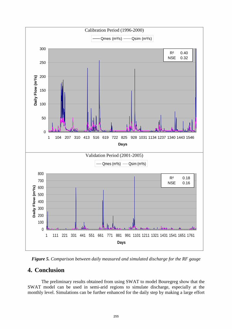
Calibration Period (1996-2000)

0

50

100

150

200

250

300

1 104 207 310 413 516 619 722 825 928 1031 1134 1237 1340 1443 1546

Days

Daily

Flo

w (m

³/s)

Qmes (m³/s) Qsim (m³/s)

Validation Period (2001-2005)

0

100200

300400

500

600700

800

1 111 221 331 441 551 661 771 881 991 1101 1211 1321 1431 1541 1651 1761

Days

Dai

ly F

low

(m³/s

)

Qmes (m³/s) Qsim (m³/s)

Figure 5. Comparison between daily measured and simulated discharge for the RF gauge

4. Conclusion

The preliminary results obtained from using SWAT to model Bouregreg show that the SWAT model can be used in semi-arid regions to simulate discharge, especially at the monthly level. Simulations can be further enhanced for the daily step by making a large effort

R² 0.40 NSE 0.32

R² 0.18 NSE 0.16

255

to improve the quality of data especially for soil layer and climate data that are generated from monthly data.

The enhancement of data quality and the expansion of the calibration period to more years can lead to more accurate parameter values able to depict the real functioning of the watershed. This will be the aim of the second round of SWAT application to the Bouregreg basin in order to model nutrient transfer to the SMBA dam in the future.

References Ashagre, B. B. 2009. SWAT to identify watershed management options: Anjeni watershed, Blue Nile

Basin, Ethiopia. MS thesis. N.Y., Cornell University, Department of Biological and Environmental Engineering

Chaponnière, A., G. Boulet, A. Chehbouni, and M. Aresmouk. 2008. Understanding hydrological

processes with scarce data in a mountain environment. Hydrological Processes. 22(12): 1908-1921

Schuol, J., K.C. Abbaspour. 2007. Using monthly weather statistics to generate daily data in a SWAT

model application to West Africa. Ecological modelling. 201: 301–311 Neitsch, S.L., J.G. Arnold, J.R. Kiniry, and J.R. Williams. 2005. Soil and Water Assessment Tool.

Theoretical documentation. Version 2005. USDA Agricultural Research Service, USA Nash, J., and J. Sutcliffe. 1970. River flow forecasting through conceptual models, Discussion of

principles. J. of Hydrology. 10: 282–290 Sharpley, A.N., and J.R. Williams. 1990. EPIC-Erosion Productivity Impact Calculator, Model

documentation. U.S. Department of Agriculture, Agricultural Research Service, Tech. Bull., 1768

Winchell, M., R. Srinivasan, M. Di Luzio, and J. Arnold. 2009. ArcSWAT 2.3.4 Interface for

SWAT2005: User's Guide, September 2009, Texas Agricultural Experiment Station, Texas, and USDA Agricultural Research Service, Temple, Texas.

Nachtergaele, F., H.van Velthuizen, and L.Verelst. 2009. Harmonized World Soil Database (HWSD),

FAO. White, K. L., and I. Chaubey (2005), Sensitivity analysis, calibration, and validations for a multisite

and multivariable swat model, Journal of the American Water Resources Association, 41(5):1077-1089.

Shimelis, G. S., R. Srinivasan, and B. Dargahi. 2008. Hydrological Modelling in the Lake Tana Basin,

Ethiopia Using SWAT Model. The Open Hydrology Journal. 2008(2): 49-62

256

Using MODIS Imagery to Validate the Spatial Representation of Snow Cover Extent Obtained from SWAT in a Data-Scarce

Chilean Andean Watershed

Alejandra Stehr Centro EULA, Universidad de Concepción, Barrio Universitario s/n, Concepción, Chile.

astehr@udec.cl

Oscar Link Facultad de Ingeniería, Departamento de Ingeniería Civil, Universidad de Concepción,

Barrio Universitario s/n, Concepción, Chile. olink@udec.cl

Mauricio Aguayo Centro EULA, Universidad de Concepción, Barrio Universitario s/n, Concepción,

Chile. maaguayo@udec.cl

Abstract Andean watersheds experience important snow coverage during the winter season depending on relative altitude and ambient temperature. Snowpack stores significant amounts of precipitation which is released to surface runoff and groundwater when solar radiation increases mainly during the spring and summer seasons, controlling the shape of the annual hydrograph and affecting the water balance at monthly and shorter scales. Thus, the effect of snowmelt on water balance is critical for agriculture, hydropower generation and wildlife habitat quality. However, in the case of the Chilean Andes (as in many places around the world), there is a lack of both meteorological input and hydrological validation data which complicates the analysis of those hydrological processes that take place in this important part of many of the country’s river basins. The objective of this study is to use remotely-sensed snow cover information obtained from MODIS imagery in order to validate the spatial snow cover extent and thus the representation of stream hydrology calculated with SWAT. Obtained results showed satisfactory to good general model performance for representation of long-term and annual mean discharge at the basin outlet as well as a reasonably good description of snow cover extent under a number of circumstances.

Keywords: snow hydrology, MODIS, SWAT

257

1. Introduction

Depending on the relative altitude and ambient temperature, Andean watersheds experience important snow coverage during the winter season. Snowpack stores significant amounts of precipitation water which is released to surface runoff and groundwater when solar radiation increases mainly during the spring and summer season, controlling the shape of the annual hydrograph and affecting the water balance at monthly and shorter scales. Thus, the effect of snowmelt on the water balance is critical for agriculture, hydropower generation and wildlife habitat quality. In particular, 25% of the south central Chilean surface (8th and 9th Region) is contained in areas where snow precipitation takes place during a normal winter (DGA 1995). However, in the case of the Chilean Andes (as in many places around the world), there is a lack of both meteorological input and hydrological validation data which complicates the analysis of those hydrological processes that take place in this important part of many of the country’s river basins.

Remote sensing provide a promising opportunity to enhance the assessment and monitoring of spatial and temporal variability of the different variables involved in the precipitation runoff process in areas where data availability for hydrological modelling is scarce (Simic et al., 2004; Boegh et al., 2004; Melesse et al., 2007; Montzka et al., 2008; Milzowa et al., 2009; Er-Raki et al., 2010; Stehr et al., 2009). The use of satellite data has improved during recent years due to the launch of several new satellite observing systems with advanced capabilities such as the Moderate Resolution Imaging Spectroradiometer (MODIS) onboard the Terra and Aqua satellites and the Advanced Microwave Sounding Radiometer for Earth Observing System (EOS, AMSR-E) onboard Aqua (König et al., 2001; Hall et al., 2002). Kuchment et al. (2010) used satellite information from AEDySno, MOD10 L2, MOD11 L2, MOD43C1 and NOAA-AVHRR to determine the equivalent snow water, snow cover maps, daily land surface temperature, land surface albedo and land cover.

Particularly in Chile, distributed hydrological modelling offers an immense opportunity to close gaps of knowledge and extend existent hydrologic records of snowmelt contribution to surface runoff and groundwater because the costs of measuring techniques and remote sensing for quantification of snow coverage and snow melt are not feasible in the country. The objective of this study is to use remotely-sensed snow cover information obtained from MODIS imagery in order to validate the spatial snow cover extent and thus the representation of stream hydrology calculated with SWAT. 2. Materials and Methods 2.1. Remote sensing techniques

Complementary information on snow cover can be derived from satellite imagery, combined with information collected in the field. Specific spectral reflectance of snow (higher reflectance in the visible compared to the mid infrared electromagnetic spectrum) allows snow-covered areas (SCA) to be accurately distinguished from snow-free areas in the absence of clouds or vegetation canopies using optical remote sensing methods. Compared with other remote sensing techniques such as microwave remote sensing which can be used to map snow water equivalent (SWE), optical remote sensing which is used to map snow area extent (SAE) has a much higher spatial resolution (Zhou et al., 2005; Zeinivand and De Smedt, 2009b). As SAE is not a quantity that directly characterizes the water storage within a snow pack, a variety of approaches for

258

determining SWE based on SAE have been developed (Zhou et al., 2005; Schaper et al., 1999). Especially in data-sparse regions such as the Himalayan or Andean mountains, satellite-derived (NOAA-AVHRR, MODIS, etc.) SCA information provides a promising opportunity to enhance the assessment and monitoring of the spatial and temporal variability of snow characteristics (Lee et al., 2006; Kuchment et al., 2010; Li and Wang, 2010). The spatial distribution and temporal variability characterization of snow distribution can be improved by combining satellite snow cover products with field data and snowpack models (Kuchment et al., 2010). Specifically in MODIS, classification of SCA is done based on the Normalized Difference Snow Index (NDSI) of a visible (MODIS Band 4 at 0.545–0.565 µm) and a shortwave infrared (MODIS Band 6 at 1.628–1.652 µm) band (Hall et al., 1995):

6) 4 6)/( 4 ( BandBandBandBandNDSI +−= (1)

MODIS pixels in a non-densely forested region are mapped as snow if 1) NDSI ≥ 0.40, 2) the reflectance in MODIS Band 2 (0.841–0.8765 µm) > 11% and 3) the reflectance in MODIS Band 4 ≥ 10% (Hall et al., 2002). In the case of snow-covered and forested MODIS pixels that have NDSI values considerably lower than 0.40 and to correctly classify these MODIS pixels as snow-covered, the NDSI is combined with the NDVI to aid in distinguishing between snow-covered and snow-free forests (Klein et al., 1998). The NDVI is calculated using Band 1 (0.620–0.670 µm) and Band 2 (0.841–0.8765 µm) as:

1) 2 1)/( 2 ( BandBandBandBandNDVI +−=

(2)

As snow has a much higher visible reflectance than soil or leaves, the primary

change in reflectance occurs in the visible wavelengths. The reflectance in the visible spectra will often increase with respect to the near infrared reflectance; snow will tend to lower the NDVI. If the NDVI ∼ 0.1, the pixel is mapped as snow even if NDSI < 0.4 (Klein et al., 1998).

For a first approximation, MODIS MOD10A1 and MOD10A2 product were validated for 2010 at one observation point in a Chilean Andean watershed using measured snow depth data obtained from a Sonic Ranging Sensor (SR50A/AT). 2.2. Hydrological modelling with snowmelt

In order to take the effect of spatial heterogeneity on the surface runoff and groundwater flow into account, the hydrological behavior of a watershed can be modelled in a physically-based distributed or semi-distributed manner (Kouwen, 1993; Schumann, 1993; Singh and Woolhiser, 2002; Reed et al., 2004; Tomassetti et al., 2005; Doten et al., 2006; Stehr et al., 2008; Zeinivand and De Smedt, 2009a; Vélez et al., 2009). Semi-distributed hydrological models divide the watershed into subbasins and each subbasin is again divided into hydrological response units (HRUs) that are homogeneous in their hydrological characteristics (soil type, land use and slope). In the following, the semi-distributed approach of surface runoff, which is included in the SWAT model (Neitsch et al., 2005), with emphasis on snowmelt contribution is discussed.

SWAT uses the Soil Conservation Service Curve Number (SCS, 1972) procedure, where the Curve Number value depends on land cover, soil type, slope and

259

antecedent soil moisture conditions. Snow accumulation and snowmelt are modelled using a temperature-index snowmelt relationship:

[ ]TMLT2)T(Tsno*bSM mxsnowpackcovmlt −+= (3)

( )

−

−+

+= 81d

3652πsin

2SMFMXSMFMN

2SMFMXSMFMNb nmlt (4)

where SM is snowmelt (mm H2O day-1), bmlt is the melt factor for that day (mm H2O day-1- °C), Tsnowpack is the snow pack temperature (ºC), Tmx is the maximum air temperature on a given day (ºC), TMLT is the threshold temperature for snowmelt to occur (ºC), snocov is the fraction of area covered by snow, SMFMN is the melt factor for June 21, SMFMX is the melt factor for December 21 and dn represents the day of the year. Snowfall (SF) occurs if the mean daily temperature is below the critical temperature SFTMP (ºC). The snowpack water equivalent (SWE; mm H2O day-1) increases with snowfall and decreases with snowmelt (SM; mm H2O day-1) or sublimation (ES; mm H2O day-1).

S1)(dayday ESMSFSWESWE −−+= − (5) 2.3. Study Area

The following rainfall-runoff modelling application focuses on the Lonquimay watershed. This watershed is located in the Andes Mountain Range (38°20’ – 38°41’ S and 71°13’ - 71°35’ W; Figure 1) and has an area of 455 km2. Elevation ranges from 880 to 2,533 m a.s.l. Flow regime is pluvio-nival, with maximum and minimum mean monthly discharges occurring during the months of June (45.75 m3/s) and March (8.96 m3/s), respectively. A secondary snowmelt peak occurs during October. 2.4. Model setup

For SWAT modelling (Neitsch et al., 2005a; Neitsch et al., 2005b) of the Lonquimay watershed, a 90 m x 90 m Digital Elevation Model (DEM) based on the final SRTM data sets was used as a basis for the delineation of the river basin. Meteorological and fluviometric input data were obtained from the National Water Data Bank of the Chilean General Water Directorate DGA (Figure 1). The land use description for the basin is based on the interpretation of aerial photographs (scale 1:70,000 and 1:115,000) from 1996-1998 which were combined with information from the “National Inventory of Vegetational Resouces of Chile" (CONAF - CONAMA – BIRF, 1995). The model was run for the period from 2001 to 2003 for calibration and 2004-2007 for validation.

260

Figure 1. Study area

To validate the area of the snow cover as estimated by the model, the MOD10A2 snow product (Hall et al., 2006) was used. The MOD10A2 pixels were classified as missing data, no decision, night, no snow, lake, ocean, cloud, lake ice, detector saturated, fill or snow. As the only pixels needed are the snow pixels, basin images were reclassified as snow (1) were MODIS indicated the presence of snow and no snow (0) in other cases. 3. Results and Discussion 3.1. MODIS validation

At this time, the MOD10A2 product was validated for April to September of 2010 at one observation point (1,190 m a.s.l.) in the Malleco watershed (Figure 1). MOD10A2 gives a daily snow area extent for each day and eight-day maximum extent, respectively, which are represented by a value of 200 on the imagines. The comparison with observed data was done with snow accumulation over an eight-day period. Figure 2 illustrates an example of a MOD10A2 product in an area where ground observations of snow depth are available.

261

Figure 2. Example of MOD10A2 (07/13 -07/20 2010) images at the study area

Table 1. Results obtained comparing observed snow depths with MOD10A21 snow cover data for April to September 2010 Date “1” if snow depth > 0 “1” if Modis pixel value = snow Match up 4/07/2010 0 0 Match 4/15/2010 0 0 Match 4/23/2010 0 0 Match 5/01/2010 0 0 Match 5/09/2010 1 0 No match 5/17/2010 1 1 Match 5/25/2010 1 1 Match 6/02/2010 1 1 Match 6/10/2010 1 1 Match 6/18/2010 1 1 Match 6/26/2010 1 1 Match 7/04/2010 1 1 Match 7/12/2010 1 1 Match 7/20/2010 1 1 Match 7/28/2010 1 1 Match 8/05/2010 1 1 Match 8/13/2010 1 1 Match 8/21/2010 1 0 No match 8/29/2010 1 1 Match 9/06/2010 1 1 Match 9/14/2010 1 1 Match 9/22/2010 1 1 Match 9/30/2010 1 0 No match

262

It is observed that there are 23 MOD10A2 images available for April to September 2010. For this period, snow depth data from the station located at the Malleco watershed are available. The snow depth sensor indicated presence of snow during 83% of the time, while MODIS10A2 indicated 87% of the time. In the specific case of the day 8/21/2010 the area of the image at the observation point is classified as cloud, but the surrounding area is classified as snow. Thus it is assumed that the presence of snow at the observation point matches up to 91%.

Previous studies have compared MODIS snow maps with ground observations and snow maps produced by The National Operational Hydrologic Remote Sensing Center, USA (NOHRSC) (Hall et al., 2002; Klein and Barnett, 2003; Tekeli et al., 2005; Aulta et al., 2006). A validation done by Klein and Barnett (2003) in a study on the Upper Rio Grande River Basin, USA, showed an 86% agreement between the MODIS and NOHRSC snow maps. When comparing MODIS and NOHRSC products with ground observations (SNOTEL measurements), Klein and Barnett (2003) obtained an overall accuracy of 94% and 76% for MODIS and NOHRSC, respectively. These results are in agreement with those obtained in this study. 3.2. Modelling results

MOD10A2 is an eight-day composite image, and SWAT calculates daily snow water equivalent (SWE). Therefore, for calibration and validation two temporal scales will be used, namely eight days and one month. In both cases, SWAT results will be aggregated for the considered time scale.

For each day or month, cells indicating presence of snow within each subbasin were counted and the corresponding area covered by snow was calculated. Subsequently, subbasins were classified as 0 (snow cover area less than or equal to 5% of total subbasin area) or 1 (snow cover area greater than 5% of total subbasin area). Snowpack was calculated using the values obtained for snowfall, snowmelt and sublimation by means of Equation 5. In a similar way as was done in the case of the MODIS images, modelled snowpack values were reclassified for each subbasin using a value of 0 for representing no snow and a value of 1 to represent snow presence. A value of 0 was assigned only if snowfall, snowmelt, sublimation and snowpack were all zero. After reclassification, values obtained from the modeling process were subtracted from the MODIS results. A value of zero indicates agreement between the imagery and model results, a value of -1 indicates that model results reveal presence of snow where the MODIS imagery does not and a value of 1 indicates that the model does not represent the presence of snow in areas where the MODIS imagery does. 4. Calibration and Validation 4.1. Calibration

Calibration was done using measured flows and MOD10A2 data. First, a sensitivity analysis including snowfall temperature, maximum melt factor for snow, minimum melt factor for snow, snowmelt base temperature, snow pack temperature lag factor, temperature lapse rate and precipitation lapse rate was conducted. Results obtained from the sensitivity analysis for both time scales (eight days and one month) indicate that the four most sensitive parameters are snowfall temperature, snowmelt base temperature and maximum melt factor for snow. Following the sensitivity analysis, the most sensitive parameters were calibrated in order to decrease the total error obtained between simulated snow cover area (SCA) and MOD10A2 data. Table 2 shows the sub-estimation, over-estimation and total percentages of error obtained when

263

comparing differences between simulated and MOD10A2 for the watershed over the entire calibration period (2001-2004) for both time scales. Table 2. Snow cover area calibration results, 2001-2004 Time scale Sub-estimation (%) Over-estimation (%) Total error (%) Eight-day 15.5 5.7 21.2 Monthly 8.0 5.7 13.7

The agreement between simulated and MOD10A2 SCA is greater when a monthly scale is considered. In this case, sub-estimation was lower. With the aim of distinguishing if errors are bigger during accumulation or melt season, obtained results on the monthly time scale were disaggregated for every month. Table 3 shows the sub-estimation, over-estimation and total percentages of error obtained for the watershed for each month over the entire calibration period (2001-2004) considering monthly outputs. Table 3. Monthly snow cover area results for calibration period 2001-2004 Sub-estimation (%) Over-estimation (%) Total error (%) April 17.2 4.4 21.7 May 17.8 0.6 18.3 June 12.2 0.6 12.8 July 6.7 0.0 6.7 August 6.1 0.0 6.1 September 3.9 2.8 6.7 October 6.1 12.2 18.3 November 12.2 11.1 23.3 December 8.3 10.6 18.9 January 0.6 9.4 10.0 February 5.0 4.4 9.4 March 0.6 12.2 12.8

During calibration, SWAT better represented the processes related to snow

accumulation (July-September) than those related to the melt process (October-December). 4.2. Validation

Validation was done using MOD10A2 imagines and simulated data for 2005-2007. As in the calibration process, simulated SCA data were compared with MOD10A2 data. Table 4 shows the sub-estimation, over-estimation and total percentages of error obtained for the watershed over the entire validation period for the eight-day and monthly time scales. Table 4. Snow cover area validation results 2005-2007 Time scale Sub-estimation (%) Over-estimation (%) Total error (%) Eight-day 12.6 8.4 21.0 Monthly 7.5 9.8 17.2

The agreement between simulated and MOD10A2 SCA is greater when a monthly scale is considered, being that sub-estimation is lower. The total percentage of error is smaller during validation than during calibration. When results are

264

disaggregated for every month (Table 5), the same tendency as during calibration is observed i.e. smaller errors during accumulation season than during melt season. Table 5. Monthly snow cover area results for validation period 2005-2007 Sub-estimation (%) Over-estimation (%) Total error (%) April 28.1 4.4 32.6 May 19.3 0.0 19.3 June 15.6 1.5 17.0 July 0.0 2.2 2.2 August 0.0 5.2 5.2 September 2.2 5.9 8.1 October 3.7 6.7 10.4 November 13.3 13.3 26.7 December 1.5 16.3 17.8 January 0.0 20.7 20.7 February 3.7 15.6 19.3 March 2.2 25.2 27.4

Comparing simulated with observed discharge data after calibration and

validation (Table 6), it can be concluded that for the calibration period the model satisfactorily reproduced the order of magnitude of the observed discharges. During validation, however, results were not good enough. It is important to remember that only parameters regarding snow accumulation and melt were calibrated. As a next step, it would be interesting to include other parameters in the calibration process. Table 6. Efficiency and determination coefficients calculated for calibration (2001–2004) and validation (2005 -2007) periods Calibration Validation RRMSE 0.64 0.64 ABSERR 12.59 12.64 EF 0.61 0.35 R2 0.68 0.80 5. Conclusion

When comparing MOD10A2 data with ground snow observations at one location, good results are obtained. This indicates that this product is suitable for calibration and validation of snow cover area.

Results obtained from the presented SWAT model application for the Lonquimay subbasin, located in the Central Chilean Andes, show a good performance when comparing snow cover area obtained from MOD10A2 with snow cover area obtained from simulations done with SWAT.

The model shows a satisfactory general performance in terms of representation of monthly mean discharge at the basin outlet. Improvements that can be done in the future include more parameters in the calibration process.

Although a reasonably good description of snow cover extent could be obtained under most circumstances, the present case study shows the limitations inherent in the low density of stations providing meteorological input data for basins featuring high altitudinal gradients.

265

Acknowledgments This investigation has been partially financed by the following projects: FONDECYT Nº 1090428 and FONDECYT 11100119. References Aulta, T. W., K. P. Czajkowskia, T.Benkoa, J. Cossa, J. Strublec, A. Spongbergb, M. Templinc,

and C. Grossd. 2006. Validation of the MODIS snow product and cloud mask using student and NWS cooperative station observations in the Lower Great Lakes Region. Remote Sens. Environ. 105(4): 341-353.

Boegh, E., M. Thorsen, M. B. Butts, S. Hansen, J. S. Christiansen, P. Abrahamsen, C. B.

Hasager, N. O. Jensen, P.van der Keur, J. C. Refsgaard, K. Schelde, H. Soegaard, and A. Thomsen. 2004. Incorporating remote sensing data in physically based distributed agro-hydrological modeling. J Hydrol. 287: 279–299.

DGA. 1995. Manual de Cálculo de Crecidas y Caudales Mínimos en Cuencas Sin Información Fluviométrica.

Doten, C. O., L. C. Bowling, E. P. Maurer, J. S. Lanini, and D. P. Lettenmaier. 2006. A spatially distributed model for the dynamic prediction of sediment erosion and transport in mountainous forested watersheds. Water Resour. Res. 42 (4): W04417, doi:10.1029/2004WR003829.

Er-Raki, S., A. Chehboun, and B. Duchemin. 2010. Combining Satellite Remote Sensing Data with the FAO-56 Dual Approach for Water Use Mapping In Irrigated Wheat Fields of a Semi-Arid Region. Remote Sens. 2: 375-387.

Hall, D.K., G.A. Riggs, and V.V. Salomonson. 1995. Development of methods for mapping global snow cover using Moderate Resolution Imaging Spectroradiometer (MODIS) data. Remote Sens. Environ. 54:127-140.

Hall, D. K., G. A Riggs, V. V. Salomonson, N. E. DiGirolamo, and K. J. Bayr. 2002 MODIS snow-cover products. Remote Sens. Environ. 83: 181–194.

Klein, A.G., D.K. Hall, and G. Riggs. 1998 Improving snow-cover mapping in forests through the use of a canopy reflectance model. Hydrol. Process. 12:1723-1744.

Klein, A. G. and A. C. Barnett. 2003. Validation of daily MODIS snow cover maps of the Upper Rio Grande River Basin for the 2000 - 2001 snow year. Remote Sens. Environ. 86: 162 - 176.

König, M., J. G. Winther, and E. Isacsson. 2001. Measuring snow and glacier ice properties from satellite. Rev. Geophys. 39: 1–27.

Kouwen, N., E. D. Soulis, A. Pietroniro, J. Donald, and R. A. Harrington. 1993. Grouped response units for distributed hydrologic modeling. J Water Res Pl-ASCE. 119 (3): 289–305.

Kuchment, L. S., P. Romanov, A. N. Gelfan, and V. N. Demidov. 2010. Use of satellite-derived data for characterization of snow cover and simulation of snowmelt runoff through a distributed physically based model of runoff generation. Hydrol Earth Syst Sc. 14: 339–350.

266

Lee, S. Klein, A. G. and Over, T. M (2006) A Comparison of MODIS and NOHRSC Snow-Cover Products for Simulating Streamflow using the Snowmelt Runoff Model. Hydrol. Process. 19(15): 2951-2972.

Li, H.Y. and J. Wang. 2010. Simulation of snow distribution and melt under cloudy conditions in an Alpine watershed. Hydrol Earth Syst Sc. Disc. 7: 3189–3211.

Melesse A. M., Q. H. Weng, P. S. Thenkabail, and G. B. Senay. 2007. Remote sensing sensors and applications in environmental resources mapping and modeling. Sensors. 7 (12): 3209-3241.

Milzowa, C., L. Kgotlhan, W. Kinzelbach, P. Meier, and P. Bauer-Gottwein. 2009. The role of remote sensing in hydrological modelling of the Okavango Delta, Botswana. J Environ Manage. 90 (7): 2252-2260.

Montzka C., M. Canty, R. Kunkel, G. Menz, H. Vereecken, and F. Wendland. 2008. Modelling the water balance of a mesoscale catchment basin using remotely sensed land cover data. J Hydrol. 353: 322-334.

Neitsch, S. L., J. C. Arnold, J. R. Kiniry, and J. R. Williams. 2005. Soil and Water Assessment Tool Theoretical Documentation. Version 2005. Texas, Texas Water Resources Institute, College Station.

Reed, S., V. Koren, M. Smith, Z. Zhang, F. Moreda, and D. J. Seo. 2004. Overall distributed model intercomparison project results. J Hydrol. 298(1–4): 27–60.

Schaper, J., J. Martinec, and K. Seidel., 1999. Distributed mapping of snow and glaciers for improved runoff modeling. Hydrol. Process. 13: 2023-2031.

Schumann, A. H. 1993. Development of conceptual semi-distributed hydrological models and estimation of their parameters with the aid of GIS. Hydrolog Sci J. 38 (6): 519-528.

SCS. 1972. SCS National Engineering Handbook, Section 4, Hydrology. Washington D.C.

Simic, A., R. Fernandes, R. Brown, P. Romanov, and W. Park. 2004. Validation of Vegetation, MODIS, and GOES Plus SSM/I Snow-Cover Products Over Canada Based on Surface Snow Depth Observations. Hydrol. Process. 18(6):1089-1104.

Singh, V. P., and D. A. Woolhiser. 2002. Mathematical Modeling of Watershed Hydrology. J Hydrol Eng. 7 (4): 270-292.

Stehr, A., P. Debels, F. Romero, and H. Alcayaga. 2008. Hydrological modelling with SWAT under limited conditions of data availability: evaluation of results from a Chilean case study. Hydrolog Sci J. 53 (3): 588-601.

Stehr, A. P. Debels, J. L. Arumi, F. Romero. and H. Alcayaga. 2009. Combining the Soil and Water Assessment Tool (SWAT) and MODIS imagery to estimate monthly flows in a data-scarce Chilean Andean basin. Hydrolog Sci J. 54: 1053-1067.

Tekeli, A. E., Z. Akyürek, A. A. Sorman, A. Sensoy, and A. Ü. Sorman. 2005. Using MODIS snow cover maps in modeling snowmelt runoff process in the eastern part of Turkey. Remote Sens. Environ. 97, 216-230.

Tomassetti, B., E. Coppola, M. Verdecchia, and G. Visconti. 2005. Coupling a distributed grid based hydrological model and MM5 meteorological model for flooding alert mapping. ADGEO. 2: 59–63.

267

Vélez, J. J., M. Puricelli, F. López Unzuand, and F. Francés. 2009. Parameter extrapolation to ungauged basins with a hydrological distributed model in a regional framework. Hydrol Earth Syst Sc. 13: 229-246.

Zeinivand, H., and F. De Smedt. 2009a. Hydrological Modeling of Snow Accumulation and Melting on River Basin Scale. Water Resour Manag. 23:2271–2287.

Zeinivand, H., and F. De Smedt. 2009b. Simulation of Snow Covers Area by a Physical based Model. WASET. 55: 469-474.

Zhou X., H. Xie, and J. M. H. Hendrickx. 2005. Statistical evaluation of remotely sensed snow-cover products with constraints from streamflow and SNOTEL measurements. Remote Sens. Environ. 94: 214-231.

268

Assessment of SWAT Potential Evapotranspiration Options and Data-Dependence for Estimating Actual Evapotranspiration and Streamflow

Aouissi Jalel

INAT, Lab. STE, 1082 Tunis, Tunisia Agrocampus-INRA Ouest, UMR1069, Soil Agro and hydroSystem, F-35000 Rennes, France

Benabdallah Sihem

Center for Water Research and Technologies,. BP 273. Soliman 8020. Tunisia

Lili Chabaâne Zohra

INAT, Lab. STE, 1082 Tunis, Tunisia

Cudennec Christophe Agrocampus Ouest-INRA, UMR1069, Soil Agro and hydroSystem, F-35000 Rennes, France

Abstract

Evapotranspiration is a major component of the water balance at the watershed scale. However, its measurement has always been difficult, especially at the watershed spatial scale. The SWAT model offers the possibility of using several methods for computing the potential evapotranspiration including: (i) Penman-Montheith (PM), (ii) Hargreaves (H) and (iii) Priestly-Taylor (PT). The main objective of this study is to compare the subset of potential evapotranspiration (PET) models provided by SWAT and to assess their impact on actual evapotranspiration and on streamflow for a 418 km² watershed located in a sub humid context. In the first part, we focus on the PM model that requires five climatic parameters: temperature, solar radiation, wind speed and vapour pressure. The SWAT weather generator was used to estimate different climatic parameters for computing PET and the results are compared with the complete data from the Beja meteorological weather station. For each run the results are compared based on two statistical parameters: the Nash-Sutcliffe efficiency and correlation coefficient. Our results show that the SWAT weather generator was relevant for predicting data missing from a nearby meteorological station. A good performance of PM method was observed with generated data. In the second part, the model was executed using the different PET models. The results showed that the different PET computation methods did not considerably affect streamflow but did affect the predicted actual evapotranspiration AET. The Priestly-Taylor method underestimated predicted AET; the Penman-Monteith method overestimated it compared to the Hargreaves method. Keywords: potential evapotranspiration, weather generator, Penman-Monteith, Hargreaves, Priestly Taylor, SWAT model, subhumid Tunisia

269

1. Introduction

Evapotranspiration (ET) is an important variable for climatological and hydrological studies, as well as for irrigation planning and management. Evapotranspiration (ET) is the simultaneous process of transfer of water to the atmosphere by transpiration and evaporation in a soil-plant system (Allen et al., 1998; Verstraeten et al., 2005). In dry periods, the ET has been a negative impact. Lake levels used for freshwater supply and groundwater will likely be increased due to increasing demand (Harmsen et al., 2009). It is difficult to measure ET directly at the watershed scale. Generally, measurement of ET for water budget is complex and cost prohibitive. When taking into consideration the cost of measuring true ET, most researchers come to the conclusion that calculating or estimating potential evapotranspiration (PET) is acceptable for use in water budgets and models (Earls and Dixon, 2008).

Further, PET is a key process for predicting climatologic demand in hydrological models. It has a critical role in hydrologic budgets, rainfall-runoff models, infiltration calculations and drought prediction models (Earls and Dixon, 2008).

The concept of the ET in hydrologic models has been presented by different methods used for estimating potential evapotranspiration. The Penman-Monteith method needs five kinds of daily climatic data in order to calculate potential evapotranspiration. In some parts of the word daily meteorological data are not always available. For such cases the SWAT model uses a weather generator to estimate missing data.

The aim of our study was to evaluate the capacity of the weather generator to predict missing data that are required by the Penman-Monteith method for estimating potential evapo-transpiration and to determine sensitivity analysis of the SWAT model to PET calculation methods for predicting actual evapotranspiration (ET) and streamflow (Q).

The SWAT model presents two options related to meteorological variables. It can either simulate weather information using its weather generator capability to compute the needed information or it can assign measured values introduced by the user.

The weather generator uses long-term climate statistics to generate climatic time series (Menking et al., 2003).

SWAT requires daily weather data. These are not always available or or of good quality, and there are often large amounts of missing data. The purpose of integrating a weather generator into the SWAT model was to generate daily solar radiation (R), wind speed (U), temperature (T) and relative humidity (ea) when daily parameters are missing based on monthly statistical data (Schuol and Abbaspour, 2007, Neitch et al., 2010).

Three methods were incorporated into the SWAT model to estimate potential evapotranspiration (Penman-Monteith (PM), Hargreaves (H) and Priestly Taylor (PT)). The Penman-Monteith method has been considered a universal standard for estimating PET (Paulo et al., 2009; Immerzeel et al., 2008; Jabloun and Sahli, 2008; Allen et al., 2000). However, this method requires many parameters related to the evaporation process: solar radiation (R), air temperature (T), relative humidity (ea) and wind speed (U). Daily data for: R, U, ea and T were collected from the Beja meteorological station.

In the first part of this study, the PM method was used for estimating PET with measured daily data from the Beja weather station. Several simulations were then run by omitting one of the key model parameters and using the weather generator. The impact on PET, ET and stream flow was then assessed. The second part of the paper compares the use of the different ET models on monthly runoff production.

2. Methodology

2.1. Study area The Joumine watershed is located in northern Tunisia. It is a rural catchment draining an area of

418 km2. The main river (Joumine) has a total length of 46 km with two major tributaries: El Hlallif and El Bagratt rivers. The elevation ranges from 35 m at the outlet of the watershed to 716 m on Bondrar Mountain.

The site is characterized by a Mediterranean climate with an annual precipitation ranging from 430-1,113 mm (1991-2003), the majority of which falls between September and May with no rain in the summer. The greatest rainfall of the year (103-165 mm) occurs during December. In this area the main

270

crops are wheat, sunflowers and oats. This watershed contains an important part of the country’s freshwater. The water stored in the dam of Joumine, the outlet of this study area, is used for drinking and irrigation (Figure 1).

Figure 1. Study area location and rain gauges distribution in and around the catchment

The catchment is located at a diverse climate interaction between the Atlantic and Mediterranean regimes (Slimani et al., 2007). Near the reservoir, monthly measured evaporation exceeds monthly precipitation with the exception of the period from November to February (Figure 2). The annual precipitation ranges from less than 500 mm in the downstream part (rain gauge S4) to over 800 mm in the mountains (rain gauge S1) with an average of 750 mm for the whole basin. Figure 2 shows the monthly precipitation (P), evaporation (EVAP) and average temperature measured at the Arima station located near the dam. EVAP is measured by pan evaporation. High annual evaporation is over 2000 mm ranging from 280 mm/month in July to less than 50 mm/month in December. Temperature ranges from 23°C in August to 8°C in January. Evaporation is one of the fundamental elements in the hydrological cycle which affects the yield of river basins, the capacity of reservoirs, the consumption of water by crops and the yield of underground supplies (Keskin et al., 2004).

Figure 2. Monthly precipitation (P), evaporation and average temperature from 1990 to 2003

Tunis

Djerba Tunisia

271

The required basic SWAT model input consists of a digital elevation model, a land use map, a soil map and soil profile data, weather data and land cover characteristics. These spatial data were obtained from the Tunisian Ministry of Agriculture.

The daily rainfall data, recorded and published by the hydrological service of the Water Resources Directorate in the Ministry of Agriculture (DGRE, 1991-2006), were collected from the seven stations (Bazina (S1), Joumine Delegation (S2), Antra (S3), Beja climat (S6), Smadah (S5), Joumine barrage (S4), Ghezala Barrage (S7)) in and around the watershed (Figure 1). S6 also has a meteorological station.

2.2. Adopted approach Daily climatic data are not always available in all parts of the country. Few weather stations

provide complete measured parameters required for the model. In this watershed, there is a nearby weather station maintained by the Tunisian National Meteorological Institute which is not the case for most Tunisian watersheds. The SWAT model developed an optional weather generator that uses monthly statistics to fill in the missing data (Arnold et al., 1998; Schuol and Abbaspour, 2007). In this study, the weather generator is used to compare SWAT runs using complete climatic data to runs using the weather generator to complete information based on monthly values of the same weather stations. Thus, for each run one or more measured climatic parameter are omitted from the PM model and estimated by the weather generator. The generated climatic parameters are wind speed (U), actual vapor pressure (ea), temperature (T) and solar radiation (R). The results are compared using the Nash-Sutcliffe coefficient (EFF) and the coefficient of determination (R²) given below.

∑

∑

−

−−= N

imyi

N

iii

obsobs

simobsEFF

2

2

)(

)(1

(1). where EFF is the Nash-Sutcliffe Efficiency (Nash and Sutcliffe, 1970), the optimal statistical value occurs when the value reaches 1.

∑

∑

−

−= N

imyi

N

iii

obsobs

simobsR

2

2

2

)(

)( (2).

where R² is the coefficient of determination. The optimal statistical value is close to 1, with Obs: observed value, sim: simulated value, obsmy: average observed values and N: number of observations.

The results of PET estimated by the PM method with R, ea, U and T obtained with the weather generator were compared with PET results computed with a full measured dataset.

In the second part, the SWAT model was run using different ET models (Priestly Taylor, Hargreaves along with Penman-Monteith). The results of PET were also compared and their impact on the observed stream is then discussed.

3. Results and Discussion

3.1. Evapotranspiration The study was performed in two parts. First, we focused on the Penman-Monteith

evapotranspiration model with the measured climatic parameter values. The results were compared to those obtained using the weather generator to estimate the following combinations:

1. Only wind speed U 2. Wind speed U and temperature T 3. Wind speed U, temperature T, and solar radiation R 4. Wind speed and solar radiation 5. Temperature and solar radiation 6. Only temperature 7. Only solar radiation

The results of the different simulations are shown in Table 1. Analysis of the results indicate that there is a high correlation between PET estimated with measured data and those with generated data (R² exceeds

272

0.78 for all model runs). The values of Nash indices (EFF) ranged from 0.78 to 0.93 for PET (-U, -R, -T) and PET (-T) respectively. The climatic parameter that has the least impact on PET is the wind speed, while the combination number 3 (-U, -R, -T) gave the lowest correlation. As we introduce more unknowns into the weather generator, the results worsened for the PM model (Figure 3). The impact on actual evapotranspiration is more distinct as R² falls to 0.65 for combination number 3. In fact, the soil moisture function plays its role in deriving actual evapotranspiration from potential evapotranspiration as the soil water availability and conditions are different at the spatial scale. In fact, the impact on runoff production is felt only for dry years or for low flow seasons (Figure 4). Results in Table 1 show good agreement between daily streamflow simulated using measured data and those simulated with generated data. The Nash coefficient and the correlation is around 98%.

Table 1. Results comparison for daily model runs Nash (EFF), coefficient of determination (R²), for relationship between daily SWAT Predicted potential evpotraspiration (PET), actual evapotranspiration (ET)

and stream flow (Q) using Penman-Monteith method for estimating potential evapotranspiration considering all weather data and missing data: -U=without wind speed, -R=without solar radiation, -T= without temperature.

Used PET (measured climatic data) reference PET PET (P, R, T, U) (-U) (-U,-T) (-U,-R,-T) (-R,-U) (-T,-R) (-T) (-R) Nash 0.91 0.86 0.78 0.8 0.89 0.93 0.92 R² 0.91 0.86 0.84 0.86 0.9 0.94 0.95 Used ET (measured climatic data) reference

ET ET (P,R,T, U) (-U) (-U,-T) (-U,-R,-T) (-R,-U) (-T,-R) (-T) (-R) Nash 0.92 0.78 0.65 0.99 0.73 0.85 0.84 R² 0.92 0.8 0.7 0.57 0.77 0.87 0.86 Used Q(measured climatic data) reference Q Q (P, R, T, U) (-U) (-U,-T) (-U,-R,-T) (-R,-U) (-T,-R) (-T) (-R) Nash 0.99 0.99 0.98 0.97 0.99 0.99 0.99 R² 0.99 0.99 0.99 0.99 0.99 0.99 0.99

Figure 3 shows the regression results between PET values when R, U, T and ea values generated

by the weather generator were compared with those calculated with the full data sets (measured data). The figure shows more scattered points when wind speed, temperature and solar radiation were generated. The results for the monthly model runs using the conditions listed above are given in Table 2. The Nash-Sutcliffe coefficient is closed to 0.99 and R² is closed to 0.99 even when most ET parameters are generated.

Table 2. Results comparison for monthly model runs

Used PET (measured climatic data) reference PET PET (P, R, T, U) (-U) (-U,-T) (-U,-R,-T) (-R,-U) (-T,-R) (-T) (-R) Nash 0.98 0.97 0.9 0.88 0.96 0.98 0.94 R² 0.99 0.99 0.99 0.99 0.99 0.99 0.99 Used AET (measured climatic data) reference

ET ET (P,R,T, U) (-U) (-U,-T) (-U,-R,-T) (-R,-U) (-T,-R) (-T) (-R) Nash 0.99 0.93 0.93 0.97 0.94 0.94 0.98 R2 0.99 0.94 0.94 0.97 0.94 0.94 0.98 Used Q(measured climatic data) reference Q Q (P, R, T, U) (-U) (-U,-T) (-U,-R,-T) (-R,-U) (-T,-R) (-T) (-R) Nash 0.99 0.99 0.99 0.99 0.99 0.99 0.99 R² 0.99 0.99 0.99 0.99 0.99 0.99 0.99 Used observed streamflow reference Q Q (P, R, T, U) (-U) (-U,-T) (-U,-R,-T) (-R,-U) (-T,-R) (-T) (-R) Nash 0.76** 0.757 0.77 0.74 0.72 0.74 0.77 0.73 R² 0.88** 0.88 0.88 0.88 0.87 0.88 0.88 0.88

** indicated the comparison of simulated streamflow with measured data and those with generated data with observed streamflow.

273

Figure 3. Comparison between SWAT model-predicted PET estimates by PM method using measured weather and those with generated weather

y = 0.9353xR2 = 0.9136

0

2

4

6

8

10

12

14

0 2 4 6 8 10 12 14

PET(P,R,T,U)

PET(

-U)

y = 0.96xR2 = 0.8621

0

2

4

6

8

10

12

14

0 2 4 6 8 10 12 14

PET(P,R,T,U)

PET(

-U,-T

)

y = 0.8427xR2 = 0.8133

0

2

4

6

8

10

12

0 2 4 6 8 10 12 14

PET(P,R,T,U)

PET(

-U,-T

,-R)

y = 0.8201xR2 = 0.862

0

2

4

6

8

10

12

0 2 4 6 8 10 12 14

PET(P,R,T,U)

PE

T(-R

,-U)

y = 0.9167xR2 = 0.9048

0

2

4

6

8

10

12

14

16

0 2 4 6 8 10 12 14

PET(P,R,T,U)

PET(

-T.-R

)

y = 1.029xR2 = 0.9438

0

2

4

6

8

10

12

14

16

18

0 2 4 6 8 10 12 14

PET(P,R,T,U)

PET(

-T)

y = 0.8905xR2 = 0.9578

0

2

4

6

8

10

12

14

0 2 4 6 8 10 12 14

PET(P,R,T,U)

PET(

-R)

274

Figure 4. Comparison of the monthly observed streamflow with the simulated values based on measured as well as on generated weather data

3.2 Runoff modeling The SWAT model was applied to determine monthly runoff based on the three ET models, that is, the Penman-Monteith, Hargreaves and Priestly Taylor methods, for the period 1990-2003. Figure 5 illustrates the obtained results without calibration. It is shown that the magnitude and temporal variation of simulated monthly flow matched closely with the observed runoff values. Timings of occurrence of the peaks for observed and simulated runoff matched as well. However, the model over-predicted runoff values during dry and average years (1992-1995; 2000-2002) and it also over-predicted some peak values. These results could be enhanced after calibration. On the other hand, all ET models gave almost the same results. Table 3 demonstrated the respective correlations between the different model runs. For PET and ET, the results of Penman and Hargreaves correlates very well with 95 and 97% respectively, and slightly less with Priestly-Taylor ET model (94 and 93% respectively).

0

5

10

15

20

25

30

35

40

Jan-9

0Ju

l-90

Jan-9

1Ju

l-91

Jan-9

2Ju

l-92

Jan-9

3Ju

l-93

Jan-9

4Ju

l-94

Jan-9

5Ju

l-95

Jan-9

6Ju

l-96

Jan-9

7Ju

l-97

Jan-9

8Ju

l-98

Jan-9

9Ju

l-99

Jan-0

0Ju

l-00

Jan-0

1Ju

l-01

Jan-0

2Ju

l-02

Jan-0

3Ju

l-03

month

Stre

amflo

w (m

3 s-1)

Qobs Q(P,R,T,U) Q(-U) Q(-U,-T) Q(-U,-R,-T) Q(-R,-U) Q(-T,-R) Q(-T) Q(-R)

275

Figure 5. Comparison of the monthly observed streamflow with values simulated using PM, H and PT methods for estimating potential evapotranspiration

Table 3. Correlation between models runs using different ET models

4. Conclusion The generated daily weather data were tested to evaluate the Penman-Monteith method for

estimating potential evapotranspiration (PET) based on the application of the SWAT model to simulate daily and monthly river streamflow and actual evapotranspiration in a subhumid Tunisian watershed.

The results show that the generated data did reproduce acceptably well the computations of ET passed into the Penman-Monteith method. However, using generation procedures to replace missing climatic data had an impact on daily actual evapotranspiration simulations. Daily and monthly streamflow modeling results showed a good similarity between those computed based on generated data and those with measured data from a local climatic station. The advantage of generating climatic data-based PET methods is that it provides an option for estimating these variables when weather stations do not have a full dataset.

The alternative ET methods (PM, H, PT) integrated into the SWAT model for estimating PET showed a low influence on monthly streamflow and actual evapotranspiration simulations.

Acknowledgement This work was financed under the project "Integrated management of the Ichkeul river basin water resources by taking into account the preservation of the Ichkeul ecosystem" funded by CIDA and managed by Wetlands International. The authors thank them.

0

5

10

15

20

25

30

35

40

Jan-9

0

Jan-9

1

Jan-9

2

Jan-9

3

Jan-9

4

Jan-9

5

Jan-9

6

Jan-9

7

Jan-9

8

Jan-9

9

Jan-0

0

Jan-0

1

Jan-0

2

Jan-0

3

month

Stre

amflo

w (m

3 s-1)

Qobs Q(PM) Q(H) Q(PT)

(PM) (H) (PT)

R² Simulated PET (PM) 0.95 0.94

R² Simulated ET (PM) 0.97 0.93

R² Simulated Streamflow (PM) 0.99 0.99

R²Observed Streamflow reference 0.88 0.88 0.88

276

References Allen, R. G., L. S. Pereira., R. Dirk., S. Martin. 2000. FAO Irrigation and Drainage Paper No. 56 Crop

Evapotranspiration (guidelines for computing crop water requirements). Arnold, J.G., R. Srinivasan, R. S. Muttiah, and J.R. Williams. 1998. Large area hydrologic modeling and

assessment part I: model development. J. Am. Water Resour. As. 34 (1): 73–89. Earls, J., and B. Dixon. 2008. A Comparison of SWAT Model-Predicted Potential Evapotranspiration Using Real

and Modeled Meteorological Data. Vadose Zone J (7): 570-580. Jabloun, M., and A. Sahli. 2008. Evaluation of FAO-56 methodology for estimating reference evapotranspiration

using limited climatic data: applications to Tunisia. Agriculture Water Management. (27): 365-371. Harmsen, E.W., L. M. Norman, N. J. Schlegel, and J.E. Gonzalez. 2009. Seasonal climate change impacts on

evapotranspiration, precipitation deficit and crop yield in Puerto Rico. Agriculture water Management (96): 1085-1095.

Immerzeel, W.W., and P. Droogers. 2008. Calibration of a distributed hydrological model based on satellite

evapotranspiration. Journal of Hydrology. (349) : 411– 424. Keskin, E. M., O. Terzi, and D. Taylan. 2004. Fuzzy logic model approaches to daily pan evaporation estimation in

western Turkey. Hydrological Sciences–Journal, 49(6): 1001-1010. Menking, K.M., K.H. Syed, R.Y. Anderson., N.G. Shafike and J.G. Arnold. 2003. Model estimates of runoff in the

closed, semiarid Estancia basin, central New Mexico, USA. Hydrological Sciences Journal. (6): 953 — 970.

Nash, J.E., and J.V. Sutcliffe. 1970. River flow forecasting through conceptual models Part 1- A Discussion of

Principles. Journal of Hydrology 10 (3): 282-292. Neitch, S.L., J.G. Arnold, J.R. Kiniry., R. Srinivasan, J.R. Williams. 2010. Soil and Water Assessment Tool

Input/Output File Documentation Version 2009. Schuol, J., and K.C. Abbaspour. 2007. Using monthly weather statistics to generate daily data in a SWAT model

application to West Africa. Ecological Modelling. (201): 301-311. Sentelhas, P.C., T. J. Gillespie, A. S. Eduardo. 2010. Evaluation of FAO Penman-Monteith and alternative methods

for estimating reference evapotranspiration with missing data in southern Onatario, Canada. Agriculture water management. (97): 635–644.

Slimani, M., C. Cudennec, and H. Feki. 2007. Structure du gradient pluviométrique de la transition Méditerranée-

Sahara en Tunisie: déterminants géographiques et saisonnalité. Hydrological Sciences Journal, 52 (6): 1088 - 1102.

Verstraeten, W. V., F. Veroustraeten, and J. Feyen. 2005. Estimating evapotranspiration of European forests from

NOAA-imagery at satellite overpass time: Towards an operational processing chain for integrated optical and thermal sensor data products. Remote Sensing of Environment. (96): 256–276.

277

Evapotranspiration Forecast Using the SWAT Model and the Weather Forecast Model

Pedro Chambel-Leitão (1), Carina Almeida (1), Eduardo Jauch (1), Rosa Trancoso (1), Ramiro Neves (1), José Chambel Leitão (2)

(1) Technical Superior Institute, Technical University of Lisbon, Portugal. (2) Hidromod, Portugal.

Abstract SWAT calculates reference evapotranspiration (ETo) using three different methods: i) Priestley-Taylor ii) Hargreaves and iii) Penman-Monteith (P-M). All the methods use meteorological measurements for this calculation. The P-M method is the most intensive in terms of meteorological measurements but is also considered the most accurate one. SWAT uses ETo to estimate actual evapotranspiration (AET). For this it takes into consideration water availability in the soil as well as the developmental stage of the plant. Water availability depends on soil properties and irrigation practices while plant development depends on agricultural practices and meteorology. The accuracy of these variables is very much dependent on input. Traditionally farmers estimate a crop evapotranspiration (ETc) which is calculated by multiplying the ETo by a crop coefficient (Kc). The calculation of these variables has been standardized by FAO using a set of tables with successive corrections to Kc to obtain AET. These corrections have a correspondence to SWAT plant stresses and Kc has correspondence to the SWAT plant module. An accurate estimation of AET is very important for farmers because it allows them to better estimate the amount of water that is being removed from the soil. With this they can better estimate how much water they must use in irrigation. Using this perspective, SWAT model can run in forecast mode using meteorological data from the previous week and forecasts for the next week. The weather data, including precipitation, temperature, relative humidity, wind speed and solar radiation, is from the closest station to each field. The weather forecasts come from a weather forecast model that is utilized for Portugal. This service runs for Portugal’s Sorraia Valley, which is a typical irrigated agricultural area mainly growing corn. The SWAT model results were sent by mobile phone messages to the corn producers in the Sorraia Valley every week during the irrigation season of 2010 (May-September). Farmers received the temperature, precipitation and actual evapotranspiration data measured for the previous week as well as the forecast for the next week. This presentation will show the implemented service but will also show the accuracy of AET estimations using meteorology from weather forecast model. Keywords: SWAT model, evapotranspiration, Penman-Monteith, irrigation

278

1. Introduction

SWAT is a watershed model that can calculate reference evapotranspiration (ETo) with three different methods: i) Priestley-Taylor ii) Hargreaves and iii) Penman-Monteith (P-M). All methods use meteorological measurements for this calculation with P-M being the most intensive one. P-M is considered to be the most accurate (Monteith, 1965; Allen, 1986; Allen et al., 1989). SWAT uses ETo to estimate actual evapotranspiration (AET), taking into consideration water availability in the soil as well as the developmental stage of the plant. Water availability depends on soil properties and irrigation practices while plant development depends on agricultural practices and meteorology. The accuracy of these variables is very much dependent on input data. Traditionally, farmers estimate crop evapotranspiration (ETc) by multiplying ETo by the crop coefficient (Kc). These variables are standardized by FAO using a set of tables with successive corrections to Kc to obtain AET. These corrections have a correspondence to the SWAT plant stresses and Kc has correspondence to the SWAT plant module.

An accurate estimation of AET is very important for farmers because it allows for better estimation of the amount of water that is being removed from the soil which dictates the amount of water needed in irrigation.. The study area is located in the Sorraia Valley of Portugal and was chosen because of the large area of irrigated agriculture (Figure 1). Sorraia Valley has about 15500 ha and is the largest area of irrigated agriculture in Portugal. It’s main crops are corn, tomatoes and rice. The growing season starts at about May 23rd and ends at about October 15th. In 2010, mean annual temperature and mean annual precipitation at Sorraia were 16.2 °C and 953 mm, respectively. The mean temperature in the period between May and October was 19.9 ºC.

Figure 1. Study area location with farmer’s fields selected

This paper shows the implemented service but will also show the accuracy of

AET estimations using meteorology from the weather forecast model.

2. Operational Forecast Service

The SWAT model was set up for forecast mode using meteorological data from the previous week and forecasts for the next week (Figure 2). Weather data including precipitation, temperature, relative humidity, wind speed and solar radiation from the previous week was taken from the closest station. Weather forecasts were produced by the numerical model MM5 running at IST for Portugal in a 9 km2 grid (Sousa, 2002) and converted to a format that can be read by the MOHID and SWAT models.

279

Figure 2. Flow chart and hardware setup for operational model

SWAT model results were sent every week during the irrigation season of 2010 (May-September) to the corn producers in the Sorraia Valley by mobile phone messages containing temperature, precipitation and actual evapotranspiration data measured the previous week as well as those forecasted for the next week. Figure 3 shows the work flow and hardware setup of the complete service. Daily forecasts for the next six days were also shown on the internet (Figure 4) according to the AquaPath-Soil project guidelines.

280

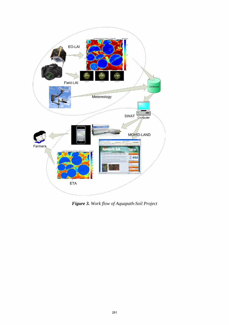
Figure 3. Work flow of Aquapath-Soil Project

281

Figure 4. SWAT forecast mode available in the internet (www.agro-evapo.eu) 2.1. SWAT forecast modeling

The system is contained in one main working folder. This folder then contains 7 folders: MEASUREMENTS, MM5, METEO, SMS, SWAT, BACKUP, LOGS. The MEASUREMENTS folder contains the GetMeteoFromNet executable that downloads via HTTP the data from the ARBVS (Famers Irrigation association: www.arbvs.pt) or INAG-SNIRH (national water information system: snirh.pt) online meteorological data databases.

The MM5 folder contains 2 folders: GetMM5TimeSeries and UploadToDatabase. The GetMM5TimeSeries folder contains the program (GetMM5TimeSeries) that directly extracts time series from the Mesoscale Meteorological Model, Version 5 (MM5) results (day before and next six days) for the designated meteorological stations. The UploadToDatabase folder contains the program (TimeSeriesManager) that uploads the meteo extracted time series to the database.

The METEO folder contains the files responsible for generating digested meteo time series for each local station, using a combination of at least 2 different data sources already in the database: forecast data from MM5 forecasts (added to database in the previous step with UploadToDatabase folder) and measured data (added to database in the MEASUREMENTS folder) for each station.

The SWAT folder contains three standard folders: txtinout, res and database. Txtinout and res folders are the two standard folders for running the SWAT model and have the standard SWAT-Mohid versions of the SWAT model as described in Chambel-Leitão et al (2007) and the Mohid wiki available on the internet. In txtinout one can find all the input data files that are daily updated by the operating system,

282

namely the file.cio (containing the initial and final dates for the simulation) and the meteorological forcing files (pcp1.pcp, tmp1.tmp, slr.slr, wnd.wnd and hmd.hmd). In the database folder the SWAT results are uploaded to a database.

The upload is made to two different database tables: one that has only the best available forecast and another that has the best available simulation (including hindcast–using measured data).

The SMS folder contains the SMSGenerator executable, which is responsible for generating the sms text that will be sent to the users of the service. The SMSGenerator.exe runs once a day after all the simulations and needed database operations are done.

The BACKUP folder is the folder where all the results and input files of each daily simulation are stored. Each day a new folder is created inside BACKUP labeled with the initial and final date of that simulation. This folder is subdivided into 2 folders:

− Meteo (contains the best time series used for the day’s simulation, both hourly and daily)

− Swat (contains the SWAT input files in the input folder and the SWAT results in the Results folder)

The LOGS folder contains daily generated log files with details of the running evolution of the operational tool tasks. 2.2. SWAT forecast database

All the data involved in the SWAT-Operational is stored in a single database in MS ACCESS 2007. Data is stored in different tables, each one corresponding to a different data source and a specific local point (time series). The database is composed of different tables:

- The “TimeSeries” table with metadata and details of each time series found in the database (name, geographical coordinates, etc)

- The “TimeSeriesTypes” table with descriptions of the different types of time series that can be found in the database

- Many timeseriestables (data sources for each local point): o Meteorological measured data from SNIRH-INAG or ARBVS o Meteorological predictions (from MM5); o SWAT best available simulations (hindcast + forecast); o SWAT best available forecasts (only forecasts)

To add new local stations to the system, database tables must be created and new rows must be added to the Metadata table describing new table names, geographical locations, etc.

To the SMS service, another set of tables exists in the database.

3. System Validation 3.1. Reference evapotranspiration

The first step in model validation was focused on potential evapotranspiration. For this, SWAT results were compared to the Penman-Monteith formulas in FAO56 (Allen et al., 1998). These equations were used with data from the ARBVS meteorological station for the year 2009. Figure 5 compares both time series, and it can be seen that results are very consistent. This was expected because SWAT and FAO56 use the same formula for evapotranspiration. Differences occurred mainly for April and June and will be further explained.

283

Figure 5. SWAT evapotranspiration results compared with standard FAO56 paper calculation

Secondly, the impact that using different meteorological stations has on

evapotranspiration calculation was studied. Temperature (maximum and minimum), wind speed and relative humidity data from Barragem de Magos of SNIRH and Paul de Magos of ARBVS stations (Figure 6) were used. These two stations are close in proximity but run by different institutions.

Figure 6. Potential evapotranspiration results using different meteorological stations

Figure 6 shows that different meteorological stations can find different results for potential evapotranspiration values. The reason for this difference is wind and relative humidity. In fact, when we use the same wind and relative humidity, both meteorological stations return similar potential evapotranspiration (Figure 7).

284

Figure 7. Comparison of evapotranspiration values for both stations with equal wind and humidity values

The effect of using different reference crops for the values of reference

evapotranspiration was also investigated Figure 8 shows the comparison of potential evapotranspirations for grass and alfalfa in Barragem de Magos, where differences can be seen between crops mainly in the irrigation season. Alfalfa always has higher evapotranspiration values because the canopy resistance of this crop is higher than that for grass. Also, alfalfa crop height can reach 40 cm while grass only reaches 12 cm.

Figure 8. Evapotranspiration calculated for grass and alfalfa crops 3.2. Evapotranspiration

Figure 9 shows the evapotranspiration components that are leaf area index curve, crop transpiration and soil evaporation. In the initial period only soil evaporation is represented because crops have not yet started their growth. When crops begin to grow,

285

transpiration and LAI increase. With this increase soil evaporation decreases because a portion of the water initially in the soil is consumed by crops and transpired. Therefore, it can be concluded that is possible to obtain evapotranspiration from LAI values.

Figure 9. LAI, evaporation and transpiration in the SWAT model Model outputs for cultural and reference evapotranspiration were compared to

observed data (Figure 10 and Figure 11). The ARBVS (Associação de Regantes e Beneficiários do Vale do Sorraia) meteorological station was used to validate SWAT and MOHID models.

First, observed data for reference evapotranspiration were compared to MOHID model-predicted data (Figure 10), and similar, matching line behavior for most of the time period can be observed (the period whose values are zero at the meteorological station is due to a lack of data). Thus it was observed that the MOHID model can simulate reference evapotranspiration.

For cultural evapotranspiration, results from both models were compared to the observed data from the ARBVS meteorological station (Figure 11). It was concluded that the simulations of both models were consistent with the observed data.

286

Figure 10. Reference evapotranspiration comparison: meteorological station data (ARBVS) and Mohid model results

Figure 11. Cultural evapotranspiration comparison: meteorological station data (ARBVS), SWAT and Mohid model results

3.3. Weather forecast validation

SWAT forecasts use both measured and forecasted meteorological data, and the consistency between these is important for proper ETA forecasts. This is investigated by comparing the numerical forecasts with measured values of the APBVS station. Figure 12 (a) through (c) show that temperature, relative humidity and precipitation forecasts of SWAT are similar to those measured at the APBVS station, with slight overestimation of daily maximum temperature. Figure 12 (d) shows that wind speed forecasts are not very consistent with observations in the small fluctuations. However, the daily behavior is quite similar.

287

(a)

(b)

288

(c)

(d)

Figure 12. Comparison of observed and SWAT-predicted temperature, relative

humidity, precipitation and wind speed 3.4. AET forecast validation

AET forecasts and measured values of the previous week are sent by SMS to farmers. Table 1 shows an example of the information sent each week with forecasts in the second column, correspondent measured AET (previous week in the message of next week) in the third column, the difference between these two in the third column and the error in the last column. It can be seen that only week 2 and 4 have high discrepancies between forecasts and observations.

289

Table 1. Comparison example of previous week and next week ETA estimation for one of the users

Week Initial Date

Next Week (model forecasts)

Previous Week (user estimations)

Error % of Error

1 19-07-2010 30 38 -3 -8% 2 26-07-2010 41 60 13 22% 3 02-08-2010 47 50 -2 -4% 4 09-08-2010 52 51 8 16% 5 16-08-2010 43 32 -1 -3% 6 23-08-2010 33 31 1 3% 7 30-08-2010 30 36 -2 -6% 8 06-09-2010 38 24 -5 -21% 9 13-09-2010 29 25 -1 -4% 10 20-09-2010 26 15 -6 -40% 11 27-09-2010 21 14 -4 -29% 12 04-10-2010 18 8 3 38% 13 11-10-2010 5 6 - -

4. Conclusions

Mesoscale Meteorological Model, Version 5 (MM5) predictions of temperature, precipitation and relative humidity are found to be consistent with local meteorology. ETo values estimated with data from meteorological stations close by were compared. Observed wind and humidity values from two close stations were different enough to change the result of ETo significantly.

SWAT, MOHID and FAO56 gave similar evapotranspiration values for the present study site.

The SWAT model was set up successfully to run in forecast mode using meteorological data from the previous week and forecasts for the next week. Acknowledgements This study was developed by the AquaPath-Soil project and supported by the European Space Agency (ESA). References Allen, R.G., L.S. Pereira, D. Raes, and M. Smith. 1998. Crop evapotranspiration: Guidelines for

computing crop water requirements. Irr.& Drain. Paper 56.UN-FAO, Rome, Italy. Allen, R.G. 1986. A Penman for all seasons. J. Irrig. and Drain Engng., ASCE, 112(4): 348-368. Allen, R.G., M.E. Jensen, J.L. Wright, and R.D. Burman. 1989. Operational estimates of

evapotranspiration. Agron.J. 81:650-662. Reisner, J. Rasmussen R. M., Bruintjes R. T. (1988) Explicit forecasting of supercooled liquid

water in winter storms using the MM5 mesoscale model. Quarterly Journal of the Royal Meteorological Society.Volume 124, Issue 548, pages 1071–1107, April 1998 Part B

290

Sousa, T. (2002) Previsão Meteorológica em Portugal Continental utilizando o modelo operacional e de investigação MM5. Dissertação para obtenção do Grau de Mestre em Ecologia, Gestão e Modelação dos Recursos Marinhos no Instituto Superior Técnico .

291

Application of the SWAT Model in Land Use Change in the Nile River Basin: A Review

Marwa Ali1 Okke Batelaan1 Willy Bauwens1

1 Vrije Universiteit Brussel, Dept. of Hydrology and Hydraulic Engineering, Pleinlaan 2, 1050 Brussels, Belgium. Correspondence to: ali.marwa19@gmail.com

Abstract

Land use change has become a worldwide concern, and it is one of the major topics in current global change studies. It is caused by a number of natural and human driving forces. Whereas natural effects such as climate change are felt only over a long period of time, the effects of human activities are immediate and often radical (Woldeamlak, 2002). In any watershed, land use change has an impact on hydrological processes, such as infiltration, base flow, runoff and groundwater recharge. The Nile River is the longest river in the world with a length of 6,650 km with a total catchment area of nearly 3 million km2, which covers about 10% of the area of Africa, spread over ten countries. During the last decades strong changes in land use occurred causing a significant effect on river streamflow and erosion. The Soil and Water Assessment Tool (SWAT) is one of the tools that has been most intensively used to investigate the hydrologic cycle of the Nile. This paper provides a review of studies performed with SWAT on the impact of land use changes on the hydrology and erosion in Nile River Basin. In general, SWAT model adequately simulates river flows in the study catchments with proper global spatial data or accessible limited data in catchments within the Nile countries. Keywords: SWAT, Nile Basin, land use change

292

1. Introduction

The Nile River is the longest river in the world. It is 6,825 km in length and has a drainage area of about 3,254,555 km² (about 10% of the area of Africa), and ten countries share it. The Nile Basin has two different hydraulic regimes; the Blue Nile, which has large flow variability between summer and winter, and the White Nile, which has constant flow over the year (Fig.1). The Nile is historically important to livelihood, and supports presently (2005) about 200 million people. It is estimated that in 2030 about 300 million people will depend on its water (FAO Nile, 2005), which will inevitably mean increased water demand and pressure on natural resources.

Figure 1. Nile River Basin (Source: Nile Basin Initiative)

The population pressure along the Blue Nile has led to serious land degradation and conversion to agricultural land which results in increased soil erosion (Assefa, 2011); hence the land use changes have an impact on the hydrological processes such as infiltration, baseflow,

293

runoff and groundwater recharge. The Soil and Water Assessment Tool (SWAT) has been used in many countries to quantify the impact of land management practices in large and complex watersheds. SWAT is a river basin scale, physically based, and continues time model which uses readily available inputs and enables modellers to study long-term impacts (Neitsch et al., 2005). For modeling purpose, the watershed is partitioned into a number of subwatersheds and subbasins, which are georeferenced and which are sub-divided into hydrologic response units (HRUs). Each HRU corresponds to a particular combination of soil and land use within the subbasin. The process of merging the landscape into separate HRUs is a common method; once HRUs are defined, the rainfall-runoff processes within each unit must be identified and parameterized.

2. SWAT Model Application to Land Use Assessment

SWAT has been applied in various studies to assess watershed response to land use change. A summary of SWAT model applications in selected catchments in Nile Basin countries is presented in the next section with information over the case studies, catchment hydrological characteristics, and purpose of model applications. The locations of the study cases are classified to the main two tributaries of the Nile. 2.1. White Nile

• Nyando Basin, Kenya The Nyando River Basin is located in western Kenya where it drains into Lake Victoria.

While it is small compared to some other basins that drain into Lake Victoria, it has a heavy influence on the ecology of the lake (Johnson, 2009). Sang (2005) describes a study of the Nyando Basin, which aimed to evaluate the impact of changes in land use, climate and reservoir storage on flooding. Two land use maps for 1980 and 2003 were obtained to be used in the model and describe the changes in land use over the years. The study showed that there has been a considerable increase in the conversion of forest and swamps to agricultural land, especially sugarcane plantations which increased by 157% due to population pressure. Four scenarios for land use have been used to study the change on streamflow; they revealed that 100% of forest cover is related to less frequent high flows and more frequent low flows. On the other hand, 0% forest cover is associated with more frequent high streamflow and lower dry season streamflow.

Another study (Opere et al., 2011) came up with a similar result using four scenarios for land use, which were developed from the same land use maps as in the previous study. The result showed that for decreased forest cover up to 0%, the mean and peak of the streamflow increased, while for increased forest cover i.e. up to 100%, the mean and peak streamflow decreased.

• Sondu River Basin, Kenya

The Sondu River drains a land area of 3050 km2 into Lake Victoria and is located in the mountainous regions of western Kenya near the equator. Jayakrishnan et al. (2005) assessed the environmental impacts of changes in land use. Three scenarios were studied using a combination of population data and demographic survey data from 1960–90. Due to the fact that the basin is located in an area with intensive dairy farming, it was assumed that the increase in Napier grass area from the traditional dairy technology scenario to the future adoption scenario would be at the expense of the native grass area, and that the Napier grass coverage in the traditional scenario

294

was zero. Both the traditional and the future adoption scenarios resulted in reduced streamflow compared to the current adoption scenario.

• Mara River Basin, Kenya-Tanzania

Mara River is a transboundary river shared between Kenya and Tanzania that drains into Lake Victoria with a basin area of 13,750 km². Land use and land cover vary within the basin because of the different activities of the stakeholders. The changes originate from the damage to the Mau Forest in the upper Mara and the conversion of natural land to agriculture. These human activities have been perceived to have a profound effect on the flow of the Mara River, causing increased peak flows during the rainy season and reduced low flows during the dry season (Mati et al., 2005). In a study intended to investigate the effect of land use and climate change scenarios on the water flux of the upper Mara river flow, three land use scenarios were considered based on the 2008 land use data which was obtained from a Landsat (TM) image (Mango, 2010). The three land use change scenarios are partial deforestation, complete deforestation, and complete conversion of the forest to agriculture in the Amala watershed. These scenarios showed considerable impact on the discharge and water balance components of the upper Mara River. The replacement of forest by agriculture scenario proved to have the most profound effect of extreme high and low river flows, increased sediment load in the Nyangores and Amala Rivers and the highest reduction in groundwater recharge. The sediment yield was threefold more than for the other two scenarios. From the monthly simulations it was noticeable that all three scenarios would result in reduced monthly discharge.

• Nzoia River Basin, Kenya

Nzoia River Basin is one of the main tributaries of the White Nile; it drains into Lake Victoria. Its flow regime varies and is occasionally as low as 20 m3/s, but its extreme floods may exceed 1100 m3/s. In a study meant to assess the past and potential future environmental changes and their impact on the hydrology of the Nzoia catchment (Githui, 2008), the land cover changes within the watershed were examined through classification of satellite images in combination with a land cover change model, which generated land cover change scenarios for the year 2020. The study analyzed land cover changes for the period 1973-2001 and their effect on the hydrology of the catchment. The analysis showed that the agricultural area has increased from about 39.6 to 64.3% between 1973 and 2001, while forest area has decreased from 12.3 to 7.0%. Results from the calibrated model showed that runoff was highest from agricultural lands, followed by shrubland, grasslands and forest.

Odira et al. (2010) studied also the Nzoia catchment with the objective of simulating the streamflow changes as a result of the land use/cover status in 1973, 1986 and 2000. Land cover maps were based on Landsat images and showed a considerable change in land use: between 1973 and 1986 a decrease of 48.3% occurred in forest cover. However, there was an increase of forest cover of 41.3% between 1986 and 2000. The agricultural area decreased between 1973-1986 and 1986-2000 with 22.4% and 4.6% respectively. To study the effect of land use change, four different land use change scenarios were applied. The first scenario, which is called the baseline scenario, was selected on the basis of the results obtained from an analysis using 1986 Landsat images. The other scenarios are based on hypothetical land use/cover situations. The second scenario was based on expansion of agricultural land up to 75% with 0% for forest. In the third scenario, the entire Nzoia Basin was assumed to be 100% covered by forest. For the forth scenario, the area under urbanization was expanded to up to 35% of the total basin. The

295

simulated discharges were compared to the baseline scenario. All four scenarios gave an increase in discharge during wet months and a decrease during dry periods. 2.2. Blue Nile The Blue Nile is one of the main tributaries of the Nile. It provides about 60% of the annual flow of the main Nile measured at High Aswan Dam (Sutcliffe, 2009). Sead (2009) evaluated the impacts of land use and climate change on the hydrology of the catchment. Two hypothetical land use and cover change scenarios were developed based on the estimation by IPCC 2007 that arid and semi-arid land cover will increase by 5-8% by 2080. The annual water yield decreased when the percentage of savanna increased by 10%, while it increased when the savanna percentage decreased by 8%, which can be explained by the fact that as more and more land is suffering from deforestation, natural (e.g. fire…) and anthropogenic (e.g. fuel, industry, cropland…), the more it will be prone to erosion and thus increased runoff.

Daily sediment yield simulations in the upper Blue Nile under different Best Management Practice (BMP) scenarios was presented by Betrie et al. (2011). Four scenarios were tested: maintaining existing conditions, introducing filter strips, applying stone bunds (parallel terraces), and reforestation. The land use map of the Global Land Cover Characterization (GLCC) was used to estimate vegetation and their parameters for input into the SWAT model. In the first scenario, filter strips were placed on all agricultural HRUs that combined dryland cropland, all soil types and slope classes. In the second scenario, stone bunds were placed on agricultural HRUs that combined dryland cropland, all soil types and slope classes. In the third scenario, the impact of reforestation was simulated on sheet erosion. 8% of the area occupied by cropland, shrubland, barren, mixed forest and deciduous forest were replaced by evergreen forest. The impact of BMPs at the subbasin level showed a wider spatial variability on sediment reduction from current conditions. The sediment reductions ranged from 29% to 68% under the filter strips scenario, 9% to 69% under the stone bunds scenario and 46% to 77% under reforestation scenario.

• Beles Basin, Ethiopia

Beles is located in the northeastern part of Ethiopia. The Beles River is one of the outstanding streams of the area. It is the major tributary of the upper Blue Nile. The topographic height and the high surface runoff of the area are favorable conditions and provide a high potential resource for hydropower development and irrigation. Surur (2010) used land use maps derived from Landsat imagery from 1986, 1999 and 2004 to evaluate the land use/cover change and its impacts on the streamflow of the Beles Basin. The forest coverage was 19.3% of the basin in 1986, was reduced to 4.2% in 1999, but in 2004 it had increased again to 10% of the basin area. Throughout the whole period an increase is noticed in the amount of cultivated land. Overall, during the eighteen-year period forestland decreased 13% whereas cultivated land increased 21.4 %. The model result revealed that the decrease in forest cover caused an increase in streamflow, which was due to the decrease in evapotranspiration and soil retention of the area.

• Hare River Basin, Ethiopia

Hare River, which is located in the Southern Rift Valley Lakes Basin in Ethiopia, was studied using SWAT. Tadele et al. (2007) investigated the changing dynamics of land use and the consequent changes in streamflow. A black and white aerial photograph from 1975 and satellite images from 2004 were used to detect land use change and were used as input in the

296

SWAT model. The measured and predicted streamflow was calibrated and validated on monthly and annual time steps with the Nash-Sutcliffe coefficient varying from 0.41-0.92 for annual and 0.43-0.82 for monthly calibrations and validations. The model provides an acceptable hydrological performance, notwithstanding the limitation in readily available data.

• Awassa Lake, Ethiopia

The Lake Awassa (also known as Hawassa) catchment is located in the central part of the higher Ethiopian Rift region. It is part of the main Rift Valley Lakes Basin. Shewangizaw et al. (2010) investigated the hydrological response of the catchment in relation to the land cover data of 1965 and 1998. The result of the remote sensing assessment on the land cover of the catchment indicated that natural vegetation decreased by 9.06% between 1995-1998 due to expansion of agricultural and urban areas. A scenario for land cover change in 2017 was adapted based on a master plan study for the Rift Valley Lakes Basin, and it was used to compare to a scenario from 1998. The future scenario was marked by both increasing cultivated land and urban area versus a decrease in natural vegetation. The result showed that the average inflow to the lake will increase from 3.15 m³/s in 1998 to 3.5 m³/s in 2017. In consequence, there is an expectation of a rising lake level.

• Awash River Basin, Ethiopia

The Awash Basin is bordered by the catchment of the Wabi Shebelle River to the south and the catchment of the Blue Nile to the west. Chekol et al. (2007) studied the upper part of the Awash River in regards to the spatial distribution of water resources and evaluated the impacts of different land management practices on hydrology and soil erosion. Farming activities in this catchment are changing very rapidly due to population pressure. Therefore, nine scenarios for different land management practices have been built to understand the effects of these changes on water quantity and sedimentation. The study showed that the model produces reliable estimates of daily, weekly and monthly discharge with quite high Nash-Sutcliffe model efficiencies for calibration and validation. Results demonstrate that land management/conservation measures within the watershed can result in reduction of sediment yield by about 10-72%. A simulation using parallel terraces with a reduction of slope length by 75% gave the highest reduction in sediment yield, and it showed a capability of conserving water resources with the highest increment in water yield being 11%. Comparison of these scenarios showed that implementation of these soil conservation measures would significantly reduce sediment yields at the outlets of the watershed.

3. Conclusion and Recommendation

The semi-distributed hydrological SWAT model has been applied in various catchments of the Nile River Basin under different topographic, hydrologic, and climatic conditions. The application covered small to large watersheds. The performance of the model can be inferred from the fact that the setup and calibration of SWAT in a catchment with variable land cover, soils and topography is a feasible task and gives acceptable results if reliable data is available and proper attention is given to manual or automatic calibration. The simulations by SWAT to evaluate land use changes during a specified period and their impact on streamflow were done by changing the land use scenarios and keeping all other datasets and parameters unchanged. Overall, the model gave high streamflow estimates when scenarios of decreasing forest cover

297

were applied for all the studied watersheds. This would increase the risk of frequent flooding and raise sediment loads in the streams due to soil erosion.

The studied basins are characterized by scarce data, and most of the studies used coarse spatial and temporal data with missing values. Hence, an effort is required to gather required representative data, particularly precipitation, by exchanging information without restriction and increasing research collaboration between Nile Basin countries. This will lead to a better understanding of the needs of the different Nile countries and will help develop scenarios with mutual benefits for them all.

Based on the review, Nile Basin catchments are facing serious land use degradation. The driving forces of this degradation are growing population and increasing human intervention in land use. Therefore, understanding how land use changes and how it influences basin hydrology will allow planners to formulate policies to minimize the undesirable effects of future land use changes.

The land use change scenarios explored were those predicted to have a negative effect on water, so further work should be done to identify land use changes with positive effects on the hydrology of the Nile River Basin. This could help resource managers and policy makers implement effective and appropriate changes that would be helpful for natural resource management and stakeholders. Finally, two important questions are raised by this study: To what extent can these change scenarios be enacted, and how would these changes affect the hydrologic regime and socio-economic situation on the river basin scale? Further research is needed and will be valuable to the people of the Nile River Basin.

References Assefa, M. M. 2011. Nile River Basin Hydrology, Climate and Water use. Springer Science+Business

Media. Betrie, G. D., Y. A. Mohamed, A. Van Griensven, and R. Srinivasan. 2011. Sediment management

modelling in the Blue Nile Basin using SWAT model. Hydrol. Earth Syst. Sci. 15(3): 807-818 Chekol, D. A., B. Tischbein, H. Eggers, and P. Vlek. 2007. Application of SWAT for assessment of

spatial distribution of water resources and analyzing impact of different land management practices on soil erosion in Upper Awash River basin watershed. FWU Water Resources Publication 06: 110-117.

FAONile. 2005. Population pressure and agricultural production in the Nile basin (2005-2030). Available

at: http://www.ehproject.org/PDF/phe/fao-nile.pdf. Githui, F. W. 2008. Assessing the impacts of environmental change on the hydrology of the Nzoia

catchment, in the Lake Victoria Basin. PhD diss. Vrije Universiteit Brussel, Department of Hydrology and Hydraulic Engineering.

Jayakrishnan, R., R. Srinivasan, C. Santhi, and J. G. Arnold. 2005. Advances in the application of the

SWAT model for water resources management. Hydrol. Process. 19(3): 749-762. Johnson, N. 2009. Sustaining inclusive collective action that links across economic and ecological scales

in upper watersheds (Scales). CPWF Project Number 20: CGIAR Challenge Program on Water and Food Project Report series.

298

Mango, L. M. 2010. Modeling the effect of land use and climate change scenarios on the water flux of the upper Mara river flow, Kenya. MS thesis. FIU Electronic Theses and Dissertations. Available at: http://digitalcommons.fiu.edu/etd/159.

Mati, B. M., S. Mutie, P. Home, F. Mtalo, and H. Gadain. 2005. Land use changes in the transboundary

Mara Basin: A threat to pristine wildlife sanctuaries in East Africa. 8th International River Symposium. Brisbane, Australia.

Ndomba, P. M., and B. Z. Birhanu. 2008. Problem and prospects of SWAT model applications in

NILOTIC catchment: A review. Nile Water Science & Eng. 1(1): 41-51. Neitsch, S. L., J. G. Arnold, J. R. Kiniry, and JR. Williams. 2005. Soil and water assessment tool

theoretical documentation. Temple TX, USA: Soil and Water Research Laboratory, Agricultural Research Service and Texas Agricultural Experiment Station.

Odira, P. M. A., M. O. Nyadawa, B. O. Ndwallah, N. A. Juma, and J. P. Obiero. 2010. Land use /cover

dynamics on streamflow: A case of Nzoia river catchment, Kenya. Nile Water Science & Eng. 3(2): 64-78.

Opera, A. O., and B. N. Okello. 2011. Hydrologic analysis for river Nyando using SWAT. Hydrol. Earth

Syst. Sci. Discuss. 8: 1765–1797. Sang, J. K. 2005. Modeling the impact of changes in land use, climate and reservoir storage on flooding

in the Nyando basin. MS thesis. Jomo Kenyatta University of Agriculture and Technology, Department of Biomechanical and Environmental Engineering.

Sead, A. 2009. Analysis of the impact of land use change and climate change on the flows in the Blue

Nile River using SWAT. MS thesis. Vrije Universiteit Brussel, Department of Hydrology and Hydraulic Engineering.

Shewangizaw, D., and Y. Michael. 2010. Assessing the effect of land use change on the hydraulic

regime of Lake Awassa. Nile Water Science & Eng. 3(2): 110-118. Surur, A. 2010. Simulated impact of land use dynamics on hydrology during a 20-year-period of Beles

basin in Ethiopia. MS thesis. Royal Institute of Technology, Department of Land and Water Resources Engineering.

Sutcliffe, J. V., and Y. P. Parks. 1999. The hydrology of the Nile. Wallingford, Oxfordshire, United

Kingdom: The International Association of Hydrological Sciences (IAHS) Special Publication no. 5.

Tadele, K., and F. Gerd. 2007. Impact of land use / cover change on streamflow: The case of Hare River

watershed, Ethiopia. FWU Water Resources Publication (06): 80-84. Woldeamlak, B. 2002. Land cover dynamics since the 1950s in Chemoga watershed, Blue Nile Basin,

Ethiopia. Mountain Research and Development. 22(3): 263-269.

299

Calibration of a Sub-Daily SWAT Model and Validation using Different Land Use Data to Examine the Impacts of Land Use

Changes

Roger H. Glick, P.E., Ph.D. Watershed Protection Department

City of Austin, Texas PO Box 1088

Austin, TX 78767 Roger.glick@ci.austin.tx.us

Leila Gosselink, P.E.

Watershed Protection Department City of Austin, Texas

PO Box 1088 Austin, TX 78767

Leila.gosselink@ci.austin.tx.us

Abstract The City of Austin Watershed Protection Department examined the validity of developing and calibrating a sub-daily SWAT model based on one land-use dataset and then applied different land-use datasets to examine the impacts of different development scenarios. A sub-daily SWAT model was developed for the 145.8 km2 Walnut Creek watershed, which encompasses portions of northern and eastern Austin, Texas, based on an existing daily SWAT model. The sub-daily model used fifteen-minute precipitation data and land use patterns based on 2003 data. Most calibration parameters were left at their default values, but the routing method was changed to Muskingum and the gamma function unit hydrograph method was used. Alpha baseflow was also changed substantially for the sub-daily model. The model was calibrated at a fifteen-minute time-step resulting in an NSE = 0.74 for fifteen-minute data and NSE = 0.86 for aggregated daily results. The model was then run using land-use estimates from 1964 based on aerial photography and rainfall from that time period, but since only hourly rainfall data was available for this period the hourly totals were divided into four in order to approximate fifteen-minute rainfall. The resulting NSE was 0.572, which was considered acceptable given the data limitations. Other measures of the hydrologic regime were also considered during calibration and validation. The third model was created using a land-use dataset approximating full build-out of the watershed. All three models were run using weather inputs from 1990-2007 to produce fifteen-minute flows at various locations in the watershed under different scenarios. Keywords: SWAT, sub-daily, modeling, urban, land use

300

1. Introduction

Urban planners consider the impacts of various factors such as transportation, schools and economic development when evaluating different future growth scenarios, but the hydrologic impacts are rarely considered. The City of Austin (COA) Watershed Protection Department (WPD) is responsible for protecting lives, property and the environment of the community by reducing the impacts of flooding, erosion and water pollution. This is accomplished by a two-pronged approach: by implementing various rules and regulations affecting any new development and by constructing or modifying structural controls in areas that do not conform to current regulations. While these activities are informed by the best available science and data, it is often difficult to evaluate different options with respect to all three missions of WPD: flooding, erosion and water quality.

WPD envisioned a paradigm for evaluating the impacts of different future scenarios on flooding, erosion and water quality. This paradigm would consist of modeling existing conditions in the watershed and then changing the land-use portion of the model to reflect a future scenario. Running the model with the same climatic inputs will allow for a comparison of the impacts of change in land use only. Due to the rapid changes in urbanized streams, this modeling effort will require a model with a sub-daily time-step.

This paper outlines the efforts of WPD staff to calibrate a sub-daily time step SWAT model for an urban watershed in Austin, validates the model using different land use data and creates modeled flows for future conditions that can be compared to current conditions.

2. Study Area

The Walnut Creek watershed, which includes the tributaries Little Walnut and Buttermilk, was selected to test this project because it has a substantial record of measured flow and the land uses in the watershed have changed substantially during that period of record. The watershed is 145.8 km2 stretching from northwest Austin through the central part of the city and emptying into the Colorado River to the east (see Figure 1). US Geological Survey (USGS) and COA have operated a flow-gauging station in the lower portion of this watershed at Webberville Road (08158600) since 1966 resulting in a continuous daily flow record to present and a sub-hourly flow record since 1986. In 1964, the watershed was approximately 21% developed. By 2003 it was 71% developed and expected to be fully developed (10% open space) by 2040 (see Figure 2). In addition, the watershed is also included in the COA Flood Early Warning System area which has been collecting 1 mm event-based rainfall data through a network of more that 75 rain gauges since 1987, eighteen of which are in the Walnut Creek area.

An initial SWAT model for a daily time step (Glick and Gosselink, 2009) was developed using ArcSWAT and SWAT2005 (Neitsch, et al., 2005). This model was based on a 3.048 m (10 ft) digital elevation map (DEM) generated from LIDAR data collected by COA in 2003, SURRGO soils data, land use maps developed by WPD based on zoning and 2003 aerial photography, FEWS rainfall data, and temperature data from the National Weather Service (NWS) station at Austin (Camp Mabry). Automatic watershed delineation was used with a 25 ha threshold resulting in 298 subbasins. The automatic delineation did not follow known watershed boundaries in all cases, primarily due to underground storm sewers changing flow direction, but this was negligible. Three slope categories were used: 0-1, 1-5 and >5%. Minimum HRU

301

thresholds were set at 5% for all soils, slopes and land uses except residential areas, which were exempted from the threshold limits, resulting in approximately 4500 HRUs. The channel dimensions were adjusted using DEM data to reflect the wider and deeper channels found in urban areas. Management options included grazing on agricultural land, lawn maintenance (irrigation, fertilization and frequent mowing) in residential and commercial areas and biannual mowing on other urban land uses. Daily rainfall was used with the curve number method for runoff.

Figure 1. Walnut Creek watershed study location in Austin, Texas

302

Figure 2. Land use assumptions for Walnut Creek watershed. Land use for 1964 is on the left, 2003 in the center and 2040 (full build-out) is on the right.

This model was run for seventeen years, 1990-2007, with the first two years as a warm up period omitted from further analyses. The model was calibrated for the period based on the land use inputs of 2002-2004. The model reasonably simulated daily flows as shown by an NSE of 0.87, but total flow was under-predicted by 12%.

3. Sub-Daily Calibration

This daily model was used as the starting point for development of a sub-daily SWAT model utilizing a modified version of SWAT2005 developed at Blackland Research Center (Jeong et al., 2010) that can run at any time step based on the periodicity of the rainfall input, which was fifteen minutes for this project. The initial run of the sub-daily model had an acceptable NSE (0.81) for the aggregated daily data but poorly predicted sub-daily flows (NSE=-1.78). Manual calibration was conducted focusing on factors most likely to impact the sub-daily results while limiting impacts on the daily results. The largest improvement in the model was caused by changing the routing method to Muskingum. Utilizing a gamma function rather than the triangular form for the unit hydrograph created more realistic hydrograph shapes. Very large changes were also made to GW_delay and alpha_bf; these parameters were modified for use in the sub-daily model so changes were not unexpected (Jeong, et al., 2010). Selected calibration parameters for the daily and sub-daily model are in Table 1.

Table 1. Calibration parameters for daily and sub-daily models for Walnut Creek Daily Sub-daily Iuh Triangular Gamma Ualpha n/a 3

303

IRTE Variable Storage Muskingum Alpha_bf 0.03 0.75 GW_Delay 60 10 ch_n 0.014 0.01 ch_k2 0 10 AWC +3% 0 CN -3 0

The resulting model reasonably predicted flows on an aggregated daily basis (NSE =

0.86, R2 = 0.87) and on a sub-daily basis (NSE = 0.74, R2 = 0.78). Figures 3 and 4 are the scatter plots of the daily and sub-daily model results, respectively. There is, as expected, more scatter in the sub-daily model and there appears to be some hysteresis which may indicate timing of the model may be off to some extent. This can be seen more clearly in Figure 5 which shows the month of November, 2004.

The ratio of storm flow to base flow is reasonably predicted, but total flow is under-predicted. Comparing the flow duration curves (Figure 6) indicates that the model generally predicts lower flow rates. Several factors may be affecting model performance. First, additional calibration may be needed; the authors calibration efforts were limited because there are existing water quality control structures in the watershed, and these could not be simulated with this sub-daily version of SWAT. Second, research in the Austin area has indicated that a significant portion of flow in some creeks is from non-natural sources, such as leaking water and wastewater lines, which were not simulated in this model.

Figure 3. Aggregated daily SWAT results for Walnut Creek, 2003-4. NSE = 0.86, R2 = 0.87

304

Figure 4. Sub-daily SWAT results for Walnut Creek, 2003-4. NSE = 0.74, R2 = 0.78

0

50

100

150

200

250

01-N

ov-2

004

04-N

ov-2

004

07-N

ov-2

004

10-N

ov-2

004

13-N

ov-2

004

16-N

ov-2

004

19-N

ov-2

004

22-N

ov-2

004

25-N

ov-2

004

28-N

ov-2

004

01-D

ec-2

004

Flow

(cm

s)

0

5

10

15

20

25

30

35

40

45

50

Rai

nfal

l (m

m)

RainfallMeasuredModeled

Figure 5. Measured and predicted hydrographs in Walnut Creek, November 2004

305

0.001

0.01

0.1

1

10

100

1000

0 10 20 30 40 50 60 70 80 90 100

Percent Exceedance

Flow

Rat

e (c

ms)

MeasureModeled

Figure 6. Measured and predicted flow duration curves for Walnut Creek 2002-2004.

Based on known intended uses of this model, WPD staff considered other factors during model calibration that may not otherwise be considered. These include the fraction of flow exceeding the mean flow rate, the fraction of time the creek is dry, the number and duration of dry and high flow periods, the average rate of flow increase and decrease and the baseflow ratio. These factors may be used to evaluate changes in flooding, erosion and aquatic life in the creek.

Aggregating the sub-daily model results into daily values predicted these parameters (and others) with a general error range between +/- 25%. These predictions were better than those produced by the original daily model. While the predictions for these parameters from the sub-daily model were generally in the same range, the average rates of flow increase and decrease were over-predicted by ~200%. This could indicate that additional calibration may be needed or the model needs to simulate various flow controls (BMPs) that are common in developed watersheds. Knowing the shortcomings of the model, WPD staff believes it is sufficient to evaluate current conditions when compared to modeled results of different development scenarios.

4. Model Validation and Land Use Changes

4.1. Historic land use Validating the sub-daily model and comparison of model results using different land

usages were accomplished in the same step. However, data limitations affected the robustness of the exercise. WPD staff created a land use map for the Walnut Creek watershed based on aerial photographs taken in 1964. This period was selected because it would give the largest change in land use but still be close to the time where calibration data existed. Current planimetric maps were compared to the 1964 aerial photographs; roads and building that did not appear on the aerial photographs were removed. Buildings and roads absent from the planimetric maps were

306

added. The resulting planimetric map based on 1964 data was compared to the current land use maps. Parcels with a developed current land use and impervious cover in 1964 were assumed to have the same land use; parcels without impervious cover in 1964 were assumed to be pasture. This estimated land use map was used to create a new sub-daily SWAT model. Since distributed FEWS rainfall data were not available for this time period, hourly rainfall data from the National Weather Service were used with the assumption that rainfall was evenly distributed during the hour to create fifteen-minute rainfall data.

The model was run for thirteen years, 1960-1972, with the first two being skipped as a warm-up period. 1967-1970 was used as a four-year validation period. Since sub-daily flow data were not available at the USGS gauge during this time, the validation was only performed on the daily data, NSE = 0.57, R2 = 0.56. Contrary to expectations due to the use of hourly rainfall data, it appears that the model does not predict peak runoff rates well. This also results in higher than expected baseflow following several events. The model also over-predicted total flow by 10%, which lends some credence to the assumption that non-natural flow was the cause of the under-prediction for the original model. Even though NSE and R2 for the validation model were lower, the predictions of other metrics were in the same range as those seen with the calibration model.

Table 2. Future land use assignment weighting ratios Land Use Within Buffer Outside Buffer Residential 0.36 0.47 Commercial 0.30 0.07 Industrial 0.19 0.18 Civic 0.06 0.05 Open Space 0.09 0.23

Figure 7. Aggregated daily SWAT results for Walnut Creek, 1967-70 NSE = 0.57, R2 =0.56

307

4.2. Future land use After validating the theory that a sub-daily SWAT model could be developed and

calibrated using one land use dataset and that a second model, created using a different land use dataset but the same calibration parameters, would produce reasonable estimates of flow, WPD started developing a SWAT model to estimate future flow conditions in Walnut Creek. The future land use dataset was developed based on 2003 land uses and regulations with several assumptions. The first assumption was that current zoning would remain in effect within the existing city limits, and that parcels would be developed to the maximum for their zoning; e.g. if a parcel was currently developed as low-density single-family but was zoned for high density, high-density was assumed for the future. In areas where existing neighborhood plans had been approved, the most intense use allowed by zoning, the plan or current use was assumed. In areas where there was no zoning nor neighborhood plan in place, undeveloped parcels were gridded into 2 ha (5 acre) cells and a future land use was assigned based on the proportion of what was then existing in the area with non-residential land uses being more heavily weighted in areas within a 150 or 300 m (500 or 1000 ft) buffer of existing or planned minor and major roadways respectively (See Table 2).

0

50

100

150

200

250

300

350

29-J

un-0

2

1-Ju

l-02

3-Ju

l-02

5-Ju

l-02

7-Ju

l-02

Flow

(cm

s)

CurrentFuture1964

Figure 8. Flows predicted with SWAT for Walnut Creek under different development conditions June 29, 2002 – July 2, 2002

This land use dataset was applied and the model was run using the same 1992-2007

weather data that were used for the original model. This produced comparable flows based on the existing land use and an assumed future land use that could be evaluated with respect to the impacts on flooding, erosion and aquatic life. The model based on 1964 land use was also run for this time period as a reference for the watershed representing a less developed condition.

308

5. Results and Discussion

The three SWAT models for Walnut Creek demonstrate that the hydrologic regime of a creek can change substantially as the land use changes from predominantly rural to suburban to fully urbanized. The ability to recognize, anticipate, quantify and address these changes before they occur will be critical to preserving the natural stream processes.

Figures 8 and 9 show two short periods of flow in Walnut Creek based on weather data from 2002 under different development conditions. Figure 8 reflects a 2-week period in July 2002 which includes one of the larger runoff events during this modeling period. The peak flow rate for the event on July 2nd is considerably higher when compared to the 1964 land use. While this increase would be expected, the percentage increases for events on June 30th and July 1st are greater.

Figure 9 reflects a period on October and November of the same year with a series of smaller rainfall events after a dry period. The first event on October 19th indicates much higher runoff for the developed conditions, primarily due to direct runoff from impervious areas. The low runoff from the undeveloped scenario is due to lower soil moisture and a lower water table in the shallow aquifer. As the series of rainfall events progress and water in the soil and shallow aquifer increases, the runoff from the undeveloped scenario increases to the point it exceeds the runoff from the developed scenarios.

0

10

20

30

40

50

60

17-O

ct-0

2

19-O

ct-0

2

21-O

ct-0

2

23-O

ct-0

2

25-O

ct-0

2

27-O

ct-0

2

29-O

ct-0

2

31-O

ct-0

2

2-N

ov-0

2

4-N

ov-0

2

6-N

ov-0

2

Flow

(cm

s)

CurrentFuture1964

Figure 9. Flows predicted with SWAT for Walnut Creek under different development conditions, October 17, 2002 through November 6, 2002

309

6. Conclusions

Converting an existing daily SWAT model to the sub-daily version SWAT may be done with minimal additional calibration but this may not always be the case. The results of the sub-daily model aggregated to daily values produce better predictions of flow and other measures of the hydrologic regime than the daily version. Accurate calibration of a sub-daily model may be tedious if comparing it to sub-daily data because the rising and receding limbs of the hydrograph must be matched. In urban areas this may require the inclusion of various BMPs that impact flow.

The impact of changing land use on stream hydrology can be modeled accurately using the sub-daily version of SWAT. Understanding these changes in the hydrologic regime on a continuous basis rather than based on design storms will allow urban planners and engineers to evaluate the impacts of different development scenarios on area water bodies. It will also allow them to develop strategies for the implementation of best management practices to mitigate those impacts on flooding, erosion and aquatic life and to alleviate the impacts caused by prior development.

References Glick, R.H. and Gosselink, L. 2009. Predicting Aquatic Life Potential under Various Development

Scenarios in Urban Streams using SWAT. Proceedings of the 2009 International SWAT Conference. Boulder CO, USA.

Jeong, J., Kannan, N., Arnold, J.G., Glick, R., Gosselink, L., Srinivasan, R. 2010. Development and

integration of sub-hourly rainfall-runoff capabilities within a watershed model. Water Resource Management. 24:4505-4527.

Neitsch, S.L., Arnold, J.G., Kiniry, J.R., and Williams, J.R. 2005. Soil and Water Assessment Tool

Theoretical Documentation Version 2005. Blackland Research Center, Temple, TX 76502.

310

Applying the Sub-Daily SWAT Model to Assess Erosion Potential under Different Development Scenarios in the Austin, Texas Area

Roger H. Glick, P.E., Ph.D. Watershed Protection Department

City of Austin, Texas PO Box 1088

Austin, TX 78767 Roger.glick@ci.austin.tx.us

Leila Gosselink, P.E.

Watershed Protection Department City of Austin, Texas

PO Box 1088 Austin, TX 78767

Leila.gosselink@ci.austin.tx.us

Abstract The sub-daily version of SWAT was applied to the 145.8 km2 Walnut Creek watershed encompassing portions of northern and eastern Austin, Texas using land use patterns from 2003. The model was calibrated at a fifteen-minute time-step with an NSE = 0.74 for fifteen-minute data and an NSE = 0.86 for aggregated daily results. The model was then run using land use from 1964 and estimated build-out land use using the same calibration parameters and weather inputs. Changes in flooding and erosion potential due to increased urbanization were evaluated at four locations on Walnut Creek. Flooding was evaluated based on the changes in the frequency and duration of bank-full flow rates. Erosion was evaluated based on the changes in annual average cumulative excess shear. The frequency of bank-full flows increased with increasing urbanization while the average duration for these flows decreased, indicating flashier storm flows. Erosion potential increased with increasing development. The City of Austin Watershed Protection Department plans to use these data along with further enhancements in SWAT for urban applications to create plans and locate hydrologic and water quality controls to help mitigate the impacts of urbanization. Keywords: SWAT, modeling, urban, land use, erosion, flooding

311

1. Introduction

Changes in hydrology due to changes in land use can have a wide range of impacts on waterways, especially on flooding and erosion potential. In most cases, flooding impacts are quantified by evaluating the impact on the stage height of a design storm such as the 100-year storm. While this method does evaluate changes in existing floodplains for large events and may be used to protect buildings, it does not take into account the possible increased frequency of the events or the change in the duration of those events. It also does not allow for an evaluation of increased erosion potential, because many smaller events contribute to erosion without resulting in flooding. The Watershed Protection Department (WPD) of the City of Austin (COA) has developed a set of tools to allow planners to evaluate the impacts on flooding and erosion of different development scenarios and also test different combinations of best management practices (BMPs) to mitigate those impacts.

2. Study Area

Figure 1. Walnut Creek watershed study location in Austin, Texas

WPD staff has calibrated and validated sub-hourly SWAT models for the Walnut Creek

watershed in Austin, TX based on three different land use scenarios (Glick and Gosselink, 2011). The Walnut Creek watershed is 145.8 km2 in area. It stretches from northwest Austin through the central part of the city and emptyies into the Colorado River to the east of Austin (see Figure 1). US Geological Survey (USGS) and COA have operated a flow-gauging station in the lower portion of this watershed at Webberville Road (08158600) since 1966, resulting in a continuous

312

daily flow record to present and a sub-hourly flow record since 1986. Sub-daily models were used rather than daily in order to better reflect the rapid changes in flow common in urban hydrology.

The three models for the watershed were developed based on land use patterns for 1964, 2003 and a future build-out condition (see Figure 2). In 1964 the watershed was approximately 21% developed. By 2003 it was 71% developed and expected to be fully developed (10% open space) by 2040. Potential flooding and erosion impacts were evaluated at four locations along the main stem of Walnut Creek: at Metric Blvd., at Interstate 35, at Old Manor Road and at the Southern-Pacific railroad bridge (Figure 3). These locations were selected because they are part of the COA Environmental Integrity Index (EII) monitoring program and were part of a more intensive study that included an evaluation of particle sizes in the stream. Flooding concerns may be evaluated at any sub-watershed outlet and erosion at any outlet with particle size information.

The evaluation locations differed greatly in slope, cross-section and particle size distribution, reflecting the different geological regions that the creek crosses (see Figure 4 and Table 1). The most upstream location at Metric Blvd. is on the edge of the Balcones Escarpment and is characterized by limestone banks. The channel has the highest slope but is not highly incised and has a broad floodplain on the right bank. The second station is at the Interstate 35 crossing. At this location the channel is still fairly rocky with a moderate slope, and it is more incised compared to the channel at Metric Blvd. and has a small floodplain on the left bank. As Walnut Creek crosses Old Manor Road, the creek flows over the Blackland Prairie region, characterized by deep clay soils. The channel had a broad floodplain on both sides of the main channel and the lowest slope of the four sites. The Southern Pacific Railroad crossing is highly incised and has a broad, flat bottom. Here the banks are primarily of deep clay soils, and there is a minimal floodplain. The four stations are generally representative of the different portions of the Walnut Creek channel. The bank-full flow rates at each location were estimated based on historical flooding information and existing flood models based on design storms. Channel cross-sections and slope were determined using 3.048-m (10ft) digital elevation maps.

Figure 2. Land use assumptions for Walnut Creek watershed; 1964 is on the left, 2003 in the center and 2040 (full build-out) is on the right

313

Figure 3. Flood and erosion potential evaluation locations

0

2

4

6

8

10

12

-100 -75 -50 -25 0 25 50 75 100

Width (m)

Dept

h (m

)

MetricI-35Old ManorRR Bridge

Figure 4. Channel cross-section at the four study locations on Walnut Creek.

314

Table 1. Study location cross-section dimensions, slope and bank-full flow rate

Site Name Slope (m/m)

Depth (m)

Width (m)

Q bank-full (m3/s)

Metric Blvd 0.0059 2.44 19.81 62.0 I-35 0.0045 3.05 25.60 119.0 Old Manor Road 0.0012 3.35 21.18 110.0 SP Railroad Bridge 0.0042 5.18 32.00 225.0

3. Methodology and Results

3.1. Flood analyses Flooding impacts were evaluated based on the frequency of the flow rates greater than

bank-full flow and the duration of the event of such high flows. The fifteen year modeled hydrograph for each land use was analyzed and the number of contiguous flooding events and the total duration of the events were determined. These are presented in Figures 5 and 6, respectively.

As expected, the number of high flow events per year increased with increased development. The frequency increases 33-50% from 1964 to 2003 and an additional 25-30% from 2003 to the full build-out predicted condition of the watershed. The duration of these high flow events does decrease with increased development, reflecting the increased variability or flashiness of the creek. Even though the duration of the high flow events decreases, the increased number of high flow events per year results in an increase in the total time of inundation on an average year. These analyses were conducted assuming a constant channel shape. If channel enlargement does occur, the flow rate associated with bank-full flows may increase, thus reducing the frequency of bank-full-excess events. However, relying on erosion to address flooding potential is not a sustainable practice.

315

0

0.5

1

1.5

2

2.5

3

Metric I-35 Old Manor RR Bridge

High

Flo

w E

vent

s (p

er y

ear)

19642003Future

Figure 5. Average number of high flow events on Walnut Creek under development scenarios

0

0.5

1

1.5

2

2.5

3

3.5

4

Metric I-35 Old Manor RR Bridge

Ave

rage

Hig

h Fl

ow D

urat

ion

(hr)

1964

2003

Future

Figure 6. Average high flow duration on Walnut Creek under different development scenarios

316

3.2. Erosion potential analyses The changes in erosion potential were assessed using average annual cumulative excess

shear over the fifteen year evaluation period. Excess shear is a function of the channel shape, geomorphology and flow. As previously noted, particle size data for these sites were collected as part of another study, not specifically for erosion assessment, and the methodology differs from what would be used in a typical erosion assessment. The minimum and maximum median particle sizes (d50) from these studies are presented in Table 2.

Table 2. Median particle size and critical shear stress at Walnut Creek study locations

Site Name d50 min (mm)

d50 max (mm)

τc min (Pa)

τc max (Pa)

τc avg (Pa)

Metric Blvd 30 43 22.80 32.69 27.75 I-35 54 75 41.05 57.01 49.03 Old Manor Road 19 27 14.44 20.52 17.48 SP Railroad Bridge 14 21 10.64 15.96 13.30

Hydraulic properties of the cross-section were estimated using WinXSPRO 3.0 (Hardy et

al., 2005). This program uses the channel cross-section and slope to develop a stage-discharge relationship based on Manning’s equation. Manning’s n for each cross-section was estimated at different flow rates using a relationship developed by Jarrett (1984):

16.038.039.0 −= RSn where, S = slope of the channel R = hydraulic radius

Shear and critical shear were computed using the following equations:

wHw SD ••= γτ and

( ) 501 dS Wgcc ••−= γθτ where, γw = density of water DH = depth of water Sw = channel slope Sg = specific gravity of soil, 2.65 d50 = median particle diameter, mm θc = critical Shield’s parameter, 0.047 See Table 2 for critical shear at each study location.

Cumulative excess shear was defined as: ( )∑ − cττ for all τ>τc

A table relating excess shear (τ-τc) to discharge was developed for each evaluation point and loaded into Hydstra version 9.6.4 (Kisters, 2008). The HYCSV routine in Hydstra was then used to compute cumulative excess shear for every year during the fifteen year study period

317

based on flow generated by the sub-daily SWAT model. This was repeated for each evaluation location and for the different development scenarios. The average annual excess shear results are presented in Figure 6. Excess shear increases with increased development intensity, as expected, but the level of increase is not uniform.

Excess shear at Old Manor Road and I-35 has the largest percentage increases from 2003 to full build-out, 47.3 and 40.0%, respectively, but the total increase in excess shear is fairly small, 68.6 and 321.2 Pa, respectively. The reasons for the smaller increases in excess shear at these two sites are very different and need to be considered when evaluating options. The average d50 particle size at I-35 is larger than the maximum estimation of d50 at all of the other sites, thus increasing the critical shear. On the other hand, the channel slope at the Old Manor Road site is very low (0.0012) which reduces the overall shear in the channel even though the d50 is similar to that near the railroad bridge. This would indicate that solutions for excess shear in one part of the watershed may be ineffective or possibly detrimental to other parts of the watershed, even those with similar d50 values.

0.0

5000.0

10000.0

15000.0

20000.0

25000.0

30000.0

Metric I-35 Old Manor Rd RR Bridge

Aver

age

Annu

al E

xces

s Sh

ear (

Pa)

1964 Land use2003 Land useFuture Land use

Figure 7. Annual average cumulative excess shear under different development scenarios

By comparing Figures 5 and 6 with Figure 7 it becomes clear that the changes in land use will have different impacts on different parts of the creek. The change in the number and duration of bank-full flooding events at Metric Blvd. and at Old Manor Road is similar but the change in excess shear at Old Manor Road is minimal compared to the other evaluation sites. The number of bank-full events at Interstate 35 increases substantially but there is a minimal

318

change in erosion. Conversely, the changes in flooding at the railroad bridge are insignificant, but there is a substantial increase in cumulative excess shear.

4. Conclusions

The ability to evaluate the impacts of different land use scenarios with respect to flooding and erosion will assist urban planners and engineers in creating more sustainable developments for the future and addressing specific concerns in a watershed without adversely impacting other concerns. The sub-daily SWAT model can be used to evaluate changes in hydrology relating to flooding and excess shear. These may be used to prevent future problems through better planning and to design solutions for existing problems in one area while still evaluating changes in other areas.

References Glick, R.H. and Gosselink, L. 2011. Calibration of a sub-daily SWAT model and validation using

different land use data to examine the impacts of land use changes. Proceedings of the 2011 International SWAT Conference. Toledo, Spain.

Hardy, T., Panja, P and Mathias, D. 2005. WinXSPRO, a channel cross section analyzer, user’s manual,

version 3.0. United States Department of Agriculture, Forest Service. General Technical Report RMRS-GRT-147.

Jarrett, Robert D. 1984. Hydraulics of high-gradient streams. Journal of Hydraulic Engineering.

American Society of Civil Engineers, 110(11):1519-1539. Kisters, Pty, Ltd. 2008. Hydstra, V.9.6.4 [software]. Weston Creek, Canberra, Australia.

319

Applying the Sub-Daily SWAT Model to Assess Aquatic Life Potential under Different Development Scenarios in the Austin,

Texas Area

Leila Gosselink, P.E. Watershed Protection Department

City of Austin, Texas PO Box 1088

Austin, TX 78767 Leila.gosselink@ci.austin.tx.us

Roger H. Glick, P.E., Ph.D.

Watershed Protection Department City of Austin, Texas

PO Box 1088 Austin, TX 78767

Roger.glick@ci.austin.tx.us

Abstract The use of SWAT-modeled flow for an Austin, Texas watershed in conjunction with a statistical model of aquatic health based on hydrologic metrics is demonstrated as a tool for allowing evaluation of impacts to biological community structure under different development scenarios and in response to watershed management measures. One measure of the effect of urbanization on streams in the City of Austin is the health of its biological communities. The difficulty in identifying direct relationships between aquatic biology and measurable stream data limits planning and design efforts for improving the aquatic environment. In Austin, Texas, hydrologic alteration due to development is an important stressor in biological community degradation (Scoggins, 2000). A statistical analysis of the correlation of individual measures and composited indices of biological communities with daily and sub-daily hydraulic metrics was conducted, expanding the work of Glick et al. (2009). Critical hydrologic metrics are identified and compared with those from a calibrated sub-daily version of SWAT applied to the 145.8 km2 Walnut Creek watershed encompassing portions of northern and eastern Austin, Texas with land use patterns from 2003. In addition, flow outputs from a historic model using land use from 1964 as well as a future scenario model using estimated build-out conditions were used to compute the critical hydrologic parameters for subbasins with benthic monitoring sites. These metrics were used to estimate impacts on aquatic communities under the three different development scenarios. The identification of critical flow characteristics coupled with the ability to use SWAT models to predict relative improvements to the hydrologic regime and water biological communities may lead the City to make changes in management strategies. Keywords: SWAT, modeling, urban, land use, aquatic life, benthic community

320

1. Introduction

A major role of the City of Austin’s Watershed Protection Department is to evaluate the relative condition of its waterways and to set goals for their protection. While the hydrologic changes associated with the changes in impervious cover and urbanization may be modeled (and often are), the impacts of flow alterations on stream biology are often not considered when new developments are proposed. One of the tools being used by the City to evaluate the effectiveness of Best Management Practices (BMPs) and future land use changes are a set of Soil and Water Assessment Tool (SWAT) models in development for each watershed in the Austin area. Incorporation of the ability to model a sub-hourly time-step as well as incorporating new BMP routines will allow evaluation of flow alterations that adequately represent changes in storm characteristics. This study begins the effort to use SWAT as a tool to include watershed hydrologic responses and their impact on the aquatic communities in the City’s assessment and planning efforts. One important implication of conducting these analysis is the identification of the limitation or highest “aquatic life potential” possible under a given hydrologic response.

Biological assessment has long been used to measure the health of impaired lakes, rivers and streams. In order to set goals and measure the effectiveness of solutions, expectations of achievable biological life need to be considered. Several authors have suggested that hydrologic alteration is the primary cause of declining biological richness as basins become urbanized (DeGasperi, 2009). Scoggins (2000) conducted an initial investigation into how biological assessments in the Austin area may be influenced by hydrological conditions and concluded that the physical variability may be far more important than chemical inputs.

Defined relationships between hydrology and aquatic life would be highly useful in watershed planning and restoration. The Water Environment Research Foundation (WERF, 2001) is continuing work on linking BMP performance to receiving water impacts and recommends including the urban “biological potential” in assessing stream ecosystems by identifying the environmental factors that have the greatest influence on water (WERF, 2008). Glick et al. (2009) developed a regression model relating daily flow statistics to the City’s Aquatic Life Score (ALS, COA 2008), a combination of benthic macroinvertebrate and diatom metrics.

This study will use further analysis of relationships between aquatic life and hydrologic metrics with output from a SWAT model of the Walnut Creek watershed to demonstrate the use of SWAT to evaluate how development may affect the future AQuatic life Potential (AQP). Hydrology is both well modeled with SWAT and a significant driver for aquatic life conditions. Urban planners have suggested methods to control runoff from post-development conditions that may mimic pre-development conditions in such a way as to minimize the impacts on biological communities (Roesner and Rohrer, 2006). Use of SWAT flow output with a statistical model of aquatic life will provide a tool which can also estimate the effectiveness of BMPs to offset aquatic life degradation caused by hydrologic permutations.

321

2. Study Area The Walnut Creek watershed is 145.8

km2 in area and stretches from northwest Austin through the central part of the city and empties into the Colorado River to the east of Austin (see Figure 1). US Geological Survey (USGS) and COA have operated a flow-gauging station in the lower portion of this watershed at Webberville Road (08158600) since 1966 resulting in a continuous daily flow record to present and a sub-hourly flow record since 1986. Sub-daily models were used rather than daily to better reflect the rapid changes in flow common in urban hydrology. The WPD staff has calibrated and validated sub-hourly SWAT models for the Walnut Creek watershed in Austin, TX based on three different land use scenarios (Glick and Gosselink, 2011).

The three models for the watershed were developed based on land use patterns for 1964, 2003 and a future build-out condition (see Figure 2). In 1964 the watershed was approximately 21% developed. By 2003 it was 71% developed and expected to be fully developed (10% open space) by 2040.

Figure 2. Land use assumptions for Walnut Creek watershed. Land use for 1964 is on the left, 2003 in the center and 2040 (full build-out) is on the right.

Figure 1. Walnut Creek watershed study location in Austin, Texas

322

Hydrologic metrics were evaluated along the main stem of Walnut Creek (WLN) and at three stations along each of the tributaries, Little Walnut and Buttermilk Creeks (Figure 3). These locations were selected because they are part of the COA Environmental Integrity Index (EII) monitoring program, which includes assessment of biological communities through an Aquatic Life index (COA, 2002). Evaluation locations differed greatly in development conditions (see Figure 4). Of particular interest in the development patterns are the tributaries, Little Walnut Creek (LWA) and Buttermilk Creek (BMK), where the majority of development had occurred by 2003, while the watershed along the mainstem was still approximately 50% open space.

Figure 3. Walnut and tributaries and Aquatic Life Sampling Sites

[¡

[¡

[¡

[¡

[¡

[¡

[¡

[¡

[¡

[¡

[¡

[¡

WLN4

WLN2

WLN1

WLN3

LWA3

WLN5

LWA2

LWA1

LWA4

BMK1

BMK3

BMK2

323

0%10%20%30%40%50%60%70%80%90%

100%Pe

rcen

t of W

ater

shed

Are

a

Buttermilk Subbasin Land Use (sq km)

Commercial/Industrial 0.61 1.40 2.02

ROW (roads & utils.) 0.69 0.99 0.97

Residential 0.54 1.25 1.23

Undeveloped 2.46 0.48 0.07

1964 2003 Future

0%

10%

20%

30%

40%

50%

60%

70%

80%

90%

100%

Perc

ent o

f Wat

ersh

ed A

rea

Walnut Mainstem Land Use (sq km)

Com 7.14 21.27 36.59

ROW 6.89 16.90 17.16

Res 2.81 23.10 36.31

Undev 95.50 49.97 20.39

1964 2003 Future

Figure 4. Land use changes in Walnut Creek mainstem vs. tributary Buttermilk Creek demonstrating full development in tributaries preceding development in Walnut

324

3. Statistical Model

Hydrologic metrics were developed for all USGS and City of Austin continuous flow monitoring sites where biological data were available. As described in Glick et al. (2009), metrics were calculated at each site for both water year and multi-year periods where land use and impervious cover estimates were available, or impervious cover periods (ICP). Analyses were conducted by City staff using both unit-value data (15-min increments) and daily values aggregated from sub-daily flow (Richter, 2011). These data were paired with available aquatic life data and WPD staff-performed regression analyses, evaluating relationships with individual biological metrics as well as the aquatic life composite score. This initial data analysis included only data collected for the Environmental Integrity Index for any samples taken. The analysis determined that ICPs provided better relationships overall than when calculated by water year. Aquatic life assessments are integrators of cumulative effects of stressors, so the community health metrics may be expected to correlate better with flow data representing the aggregate impact of fluctuations for a longer period. Water year data for both aquatic life and hydrology may be unduly biased by a single wet or dry period, or in the case of the aquatic population sampled, by the immediately preceding period. Another initial finding was that the aggregate Aquatic Life Score was as well or better predicted by statistical models compared to regression models found for individual aquatic life metrics. This validates the need for the multiple metrics to quantify different aspects of a healthy aquatic community. Further work is being done by the City of Austin to extricate the relationships between various biological measures and hydrologic metrics; the aquatic life predicted using a statistical model based on flow might be considered the AQP for that site, assuming water chemistry impacts would be similar to those found at the sites sampled.

For use with the SWAT model, some additional considerations need taken into account when selecting a regression model to use for predicted flow. Sites used for the statistical analyses were primarily at USGS sites with large drainage areas and continuous flow metrics which caused some bias in the data. Testing the best regressions from Richter (2011) for use with SWAT flows, some anomalous predictive values were found. Area-adjusted metrics, when implemented in small subbasins, caused unrealistically high EII scores. In addition, some parameters are not modeled well, and some relationships included terms which over development or time were related in an inverse manner than causality suggests. An example would be a positive relationship of AQP with increasing steepness of the falling limb of storm events. Additional statistical analyses were performed for this study to find regressions for the AQP using a dataset incorporating biological data from additional studies to the EII as well as including a “best set” analysis. Analyses were conducted using STATISTICA (StatSoft Inc., 2011) hydrologic metrics from the ICPs as well as daily and unit-value data (UV). A multiple linear regression was run using the Statistica General Regression (GRM) Model which provides a best subset analysis based on the best adjusted r2. Raw aquatic life scores, which were not normalized to a reference condition, were also included as an alternate dependent variable to include temporal effects since hydrologic metrics are not normalized in that manner. Resulting statistical models were evaluated for the specific purposes of 1) using the statistical model to predict AQP or a change from current conditions based on future land use for all Austin watersheds, 2) using modeled hydrologic metrics, thus requiring that the metrics be modeled well, and 3) to consider multiple scales so that flows below BMPs in small watersheds be consistently modeled. The model selected, with r2 = 0.8216 and adjusted r2 = 0.6493, for

325

applying sub-daily SWAT model output to assess the AQP for Walnut Creek watershed is shown below. The aquatic life predicted is not normalized to a reference area. AQP = 87.7539 – 1.5961 * (Qpeak/Area) + 4.3842 * ln(Q90) - 21.2655 * (Avg_Rise) Where:

Qpeak/Area = peak flow rate in cms/sq km Q90 = 90th percentile flow rate in cms, 90% of flow is below this value Avg_Rise = mean of positive differences between consecutive rising values (rise rate, cms/sec)

The natural climate and hydrology can play an important role in which metrics are important in any area. For example, the lack of baseflow in some areas of Austin is a limiting factor for aquatic life. Baseflow may also be lacking because of development and increased impervious cover; baseflow may also be limited in small watersheds particularly during summer months. These types of inferences may lead to relationships that reflect the variation between large and small watersheds rather than with the development condition, perhaps showing that an increased Q90 will improve aquatic life (and thus showing improved aquatic life with development). If a watershed-specific relationship were desired, data would be limited to similar sized watersheds; however, the tool desired for Austin would allow consideration in all watersheds, in particular to be able to evaluate what difference a BMP would make in both a large and a small watershed. Therefore, only models with relationships consistent across both watershed size and development condition were considered. The statistical model used in this paper represents the current state of the science at the City of Austin for our particular climate and for use as a tool as described. 4. Methods and Results

Fifteen minute flow output from the calibrated sub-daily Walnut Creek SWAT model for land use scenarios 1964, 2003 and future was used to calculate the flow metrics needed to estimate the Aquatic Life Potential with the regression model. The flow was extracted at subbasins corresponding to Environmental Integrity stream reaches (EII) shown in Figure 3 and an AQP calculated for each reach for each model period (1964, 2003, and future).

The metrics used in the Aquatic Life Potential equation for the subbasins are shown in Figure 5 as simulated by the Walnut SWAT model over time. Results are shown by subbasin, moving upstream to downstream from left to right. Although generally in order by watershed size, the headwater of Little Walnut, LWA4, is smaller than BMK3, likewise WLN5 is smaller than LWA3. Some of the metrics appear to be influenced by the basin size, increasing or decreasing downstream, but differences at the headwaters of Walnut and Little Walnut may indicate that the time of concentration or stream order may also have some effect. For example, the peak flows normalized to area at the headwater sites WLN5 and LWA4 are lower than subbasin sites with similar drainage areas. The development patterns, with more impervious cover in the smaller subbasins, may also cause effects that seem related to size. The changes over time, between simulations, are driven solely by land use changes.

As expected, peak flow (Figure 5) increased with development. The biggest changes when normalized to area were seen in the smaller subbasins of Buttermilk and Little Walnut

326

Creeks. The 90th percentile flow rate demonstrates an increasing pattern downstream within each subbasin and a decrease (shift down) with development; change over time in the smaller tributaries is proportionally larger than in the mainstem.

EII Reach - Drainage Area

1

10

100

1,000

BMK3BMK2

BMK1LWA4

LWA3LWA2

LWA1WLN5

WLN4WLN3

WLN2

8158

600

WLN1

Are

a (s

q km

)

Qpeak/area

0

5

10

15

20

25

Flow

cm

s/sq

km

Average Rise

0.0

0.5

1.0

1.5

Ris

e, c

ms

90th Percentile Flow Rate

0.001

0.01

0.1

1

10

BMK3BMK2

BMK1LWA4

LWA3LW

A2LWA1

WLN5WLN4

WLN3

WLN2

8158

600

WLN1

Flow

, cm

s

19642003Future

Figure 5. SWAT model hydrologic metrics for Walnut Creek under three development scenarios

327

The peak flow and ln(Qpeak) also showed a relationship with watershed size. It decreases with development, which in our semi-arid climate characterizes a move towards a flashier flow regime with higher peaks but reduced flow and duration between peaks, reducing the already scarce flow in Austin creeks. The average rise showed the most variable pattern. Glick and Gosselink (2011) report that rises and falls are over-predicted by the Walnut SWAT model. However, the relative change with development is still represented for evaluating changes in aquatic life. Both the highest values and the highest differences were seen in the three downstream sites of Little Walnut: LWA1, LWA2 and LWA3. The biggest changes occurred primarily between 1964 and 2003 as these watersheds were developed early and are not expected to have much further growth.

Using these metrics, the changes in aquatic life potential were assessed for each EII reach in the Walnut watershed. Figure 6 shows the AQP for each period, again by watershed size. The changes in modeled aquatic life scores between 1964 and 2003 on Buttermilk and Little Walnut creeks showed a marked drop while Walnut Creek showed less precipitous changes. This is consistent with land use changes (Figures 2 and 4); the majority of development in the tributaries was complete by 2003 while the mainstem was still less than 50% developed. The response seen in the AQP would be consistent with expected consequences to community health from developmental impacts. Decreased impacts might occur as requirements to abate flood and water quality impacts are put in place; in fact they may even be part of the response within the regression equation over time.

Aquatic Life Potential (AQP) Walnut Creek Austin, TX

0

10

20

30

40

50

60

70

80

90

BMK3BMK2

BMK1LWA4

LWA3LWA2

LWA1WLN5

WLN4WLN3

WLN2

8158

600

WLN1

AQ

P

1964

2003

Future

Figure 6. AQP using SWAT 15-min modeled flow for three developmental conditions

The modeled AQP for Walnut Creek represents what has indeed happened: degradation from 1964 to present. AQP values estimated for the future predict a continued decline as

328

expected with continued development. Figure 7 shows a decrease in the AQP along the scale used in the City’s Environmental Integrity Index (not adjusted for reference conditions). EII levels are represented by 12.5 point ranges with a descriptor such as good or poor. Accordingly, a change of 12 points would be expected to cause a notable decline in aquatic health as seen in the tributaries Buttermilk and Little Walnut under development with fewer regulatory controls (1964-2003). Geographic changes in AQP are represented in Figure 7. Smaller changes, between 3 and 12 points, could move a creek from an anticipated AQP of fair to poor, depending on future development. The future land use for the SWAT model assumes that current regulations were in place which would provide more protection than those in place during the development in Little Walnut and Buttermilk creeks. The relatively smaller decline in aquatic life for the future in the mainstem of Walnut, compared to the larger changes since 1964 in the smaller tributaries on the west, may be due in part to regulations which affect future land use possibilities. As BMP routines are incorporated into SWAT, calibrated models will be better able to represent the actual watershed conditions in place and to gauge the effects of required BMPs. The future AQP will then, more appropriately, become a function of land use changes and management methods that are assumed to be part of future development processes. Many retrofit projects and management practices put into place in an effort to restore currently impaired urban creeks will also be incorporated.

AQP Decrease1964 - 2003

>18

15 - 18

12 - 15

9 - 12

6 - 9

3 - 6

.5 - 3

insignificant + or -

[¡

[¡

[¡

[¡

[¡

[¡

[¡

[¡

[¡

[¡

[¡

[¡

WLN4

WLN2

WLN1

WLN3

LWA3

WLN5

LWA2

LWA1

LWA4

BMK3

BMK2 BMK1

AQP Decrease 2003 - Future

>18

15 - 18

12 - 15

9 - 12

6 - 9

3 - 6

.5 - 3

insignificant + or -

[¡

[¡

[¡

[¡

[¡

[¡

[¡

[¡

[¡

[¡

[¡

[¡

WLN4

WLN2

WLN1

WLN3

LWA3

WLN5

LWA2

LWA1

LWA4

BMK3

BMK2 BMK1

Figure 7. Estimated changes in aquatic life over time for Walnut Creek

329

5. Conclusions

A statistical model for Aquatic Life Potential was derived based on flow metrics and applied to the Walnut Creek watershed, both historically and for a future land use scenario, with reasonable results. Models such as these, utilizing the ability to evaluate the response of aquatic life to hydrologic changes, will give scientists, engineers and planners an additional tool in not only evaluating management scenarios, but in setting goals as well. Limiting future degradation may depend on designing regulations and control structures that will restore hydrologic patterns to less developed conditions; determining which flow characteristics are most important is still an ongoing work and may be specific to locales and climates.

Although many studies have shown that hydrology can be the factor driving aquatic community changes, confounding factors such as climatic influences, geography, and watershed size can make the development of a predictive relationship difficult to apply over a large area and highly variable watershed sizes and types. Data used for development of the relationship can also obscure some responses. The metrics in this study sometimes varied more by the watershed size than by the development condition; and this observation was further confounded by the geographic layout of Austin, Texas. Each major watershed flows towards the Colorado River (Ladybird Lake) in the downtown area. As development has grown, the central area has been filled in where smaller urban watersheds are found. The larger watersheds extend far outside of the City’s jurisdiction, and development does not begin to approach the same levels of impervious cover on a percentage land cover basis as the urban areas. Even within these watersheds there is a geographic pattern, with more development occurring downstream near the receiving water body, the Colorado River. Walnut Creek data exhibits this to a degree; the subbasins fall generally into two categories: (i) small and more developed or (ii) large and less developed. More overlapping classifications and a bigger spread of biological characterizations may be seen as the City collects more biological data with increasing development pressure in larger watersheds.

Further analyses are being carried out to refine a statistical model linking hydrology and biology. Additional evaluation will address issues including the correlation of hydrology parameters with watershed size, co-variance between parameters, the sampling season (benthic sampling has been conducted under multiple programs), the possible use of a reference site condition, and the time-step which best represents each hydrologic descriptor. The AQP, as predicted from a regression model of hydrologic descriptors, provided insight into which metrics may best describe the alterations in the flow regime that will have the greatest impact on aquatic life.

The evaluation of the potential to obtain a desired aquatic life community based on hydrology is important in evaluating both the “goals” for specific watersheds, which may be limited based on lack of flow even in an undeveloped condition, and the possible success of regulations or Best Management Practices (BMPs). Identifying flow-limiting regimes may prevent unnecessary expenditures on traditional water quality solutions through capture and treatment of stormwater; water quality treatment may not provide much improvement where flashy creeks cannot maintain aquatic life. Moreover, the hydrologic implications of implementing few large or multiple small controls may provide the key to addressing aquatic life impairments where toxicity or oxygen stressors are not dominant. The City of Austin is currently anticipating incorporation of Austin area-specific BMPs into the SWAT 15-minute model and will continue to work to link the SWAT output to indices of aquatic life.

330

Acknowledgements Many thanks to City staff Aaron Richter and Chris Herrington for the primary work on aquatic life data, explaining and interpreting biological data calculations and conducting statistical analyses with many permutations of real and SWAT-modeled flow metrics. References City of Austin (COA). 2002. Environmental Integrity Index Methodology. City of Austin, Watershed

Protection Department. COA-ERM 1999-01. DeGasperi, C.L., H.B. Berge, K.R. Whiting, J.J. Burkey, J.L. Cassin and R.R. Fuerstenberg. 2009.

Linking hydrologic alteration to biological impairment in urbanizing streams of the Puget lowlands, Washington, USA. Journal of the American Water Resources Association 45(2):512-533.

Edgerly, J.P. 2006. Quantifying Urban-Induced Flow Regime Alteration Using Mathematical Models

and Hydrologic Metrics. Thesis. Colorado State University, Fort Collins, CO Glick, R.H. and L. Gosselink. 2011. Calibration of a sub-daily SWAT model and validation using

different land use data to examine the impacts of land use changes. Proceedings of the 2011 International SWAT Conference. Toledo, Spain.

Richter, A. 2011 (DRAFT). SR-11-13. Linking Biologic Metrics to Hydrologic Characteristics in Austin

Streams.” Scientific Report. City of Austin, Watershed Protection Department. Scoggins, M. 2000. Effects of hydrology on bioassessment in Austin, Texas. City of Austin technical

report number SR-00-02. Accessed 02 MAY 08. http://www.ci.austin.tx.us/watershed/publications/files/SR-00-02%20BioHydrology%20in%20Austin%20Creeks.pdf

StatSoft, Inc. (2011) STATISTICA (data analysis software system), version 10. www.statsoft.com. Water Environment Research Foundation (WERF). 2007. Bioassessment A Tool for Managing Urban

Aquatic Life Uses for Urban Streams. 01-WSM-3. http://www.werf.org//AM/Template.cfm?Section=Home

331

Assessing Impacts of Rangeland Conservation Practices Prior to Implementation: A Simulation Case Study using APEX

Xiuying Wang, Blackland Research & Extension Center, 720 E. Blackland Rd., Temple, TX 76502 USA.

Carl Amonett,

Posthumously, USDA-NRCS, 808 E. Blackland Rd., Temple, TX 76502 USA.

J. R. Williams, Blackland Research & Extension Center, Temple, TX 76502 USA.

William E. Fox,

Blackland Research & Extension Center, 720 E. Blackland Rd., Temple, TX 76502 USA.

Cheng Tu, Texas A&M University, College Station, TX 77843 USA.

Abstract Information on grazing land conservation practices and their effectiveness in controlling nonpoint source pollution and watershed health at the watershed/landscape scale is necessary for future planning and resource allocation. Utilizing computer simulation allows land managers the ability to leverage empirically derived data at smaller scales to evaluate potential impacts of conservation measures at larger scales. The objectives of the current study were to test the Agricultural Policy/Environmental eXtender (APEX) model and utilize it to test possible conservation practices within a rangeland watershed. The model was calibrated and validated for flow and sediment yield for the Cowhouse Creek watershed (1178 km2) in north central Texas. The Nash–Sutcliffe efficiencies (NSE) ranged from 0.67 to 0.81 for monthly streamflow. Monthly sediment yields were compared for both the calibration and validation periods. Scenario analyses identified substantial reductions in overland sediment losses for conversion of range brush to range grass on Evant soil areas, with an average reduction of 58.8% from treated areas, followed by brush conversion on Eckrant soil areas (an average reduction of 53.8% for converting to brush on both soils). Combining conversion on these soils to brush grass and reducing stocking rate from 10 ha/herd to 15 ha/herd on all grazing lands would result in an average overland sediment loss reduction of 30% from treated areas and a watershed sediment yield reduction of 18%. The study shows that the APEX model is a useful tool for simulating rangeland managements. Keywords. APEX, conservation practices, sediment, watershed modeling

332

1. Introduction

Rangelands across the globe have changed and continue to change at an accelerated pace (Wilcox, 2007) due to overgrazing, desertification, woody plant encroachment or invasion by nonnative species, etc. Depleted and/or degraded rangelands produce vegetation cover far below their potential and result in accelerated soil erosion processes. These systems often require restoration to recover ecosystem functions and processes desired by society. These actions are often associated with conservation practices such as brush control, reduced stocking rates or re-vegetation to improve or maintain watershed health. The hydrologic effects of common range improvement practices have been the topic of study by many researchers (e.g., Rosa and Tigerman 1951, Rich 1961, Rowe and Reimann 1961, Dragoun 1969, Blackburn and Skau 1974; Brock et al., 1982; Dugas and Mayeux, 1991; Wang et al., 2010). Dortignac and Hickey (1963) reported that ripping and seeding in New Mexico reduced runoff and soil loss was decreased by 86% and 30% for the first and third years, respectively. Contour ripping reduced runoff by 40-46% and sediment yield by 54-62% for subbasins in the Shoal Creek watershed in north central Texas (Wang et al., 2009). However, inconsistent results have been reported with respect to the impacts of brush control on runoff and soil erosion due to different conditions, uncertainties and complexities involved. However, it is technically difficult and financially infeasible to conduct paired/replicated watershed studies to test the multitude of practices that could be employed. To better understand the implications of rangeland degradation and the mitigation potential of watershed conservation strategies, scientists can comprehensively assess actions through simulation modeling, but to be successful, the modeling exercises must be combined with appropriate levels of field information and monitoring. The models must not only be able to simulate processes at the appropriate scale, but must also be rigorously calibrated and field-tested to ensure realistic output. This effort reports on initial studies using the APEX model for rangeland systems. Efforts have been undertaken to illustrate the utility of the simulation platform and its application on rangeland landscapes. Further development of management scenarios is ongoing and results will be presented in subsequent literature.

The “Agricultural Policy/Environmental eXtender” (APEX) model was developed for use in whole farm/watershed management (Williams and Izaurralde, 2006). The model simulates the hydrological, biological, chemical and meteorological processes of farming systems involving multiple crops, soil types, field delineations and structural and agronomic conservation practices across the landscape (Williams and Izaurralde, 2006). The APEX model and its predecessor, the Environmental Policy Integrated Climate (EPIC) model (Williams, 1995), have had a long history of use in simulation of agricultural and environmental processes, as well as in agricultural technology and government policy (Gassman et al., 2005; Gassman et al., 2010). The model was chosen for the National Cropland Assessment component of the Conservation Effects Assessment Project (CEAP) (Duriancik et al., 2008; USDA�NRCS, 2009); and is now being used for one of the initial studies for the National Integrated Water Quality

333

Program – CEAP grazing land watershed study. The objectives of this study were 1) to calibrate and validate the APEX model for simulating hydrology and sediment yield for a rangeland-dominated watershed and 2) to use the calibrated model to explore the impact of potential conservation practices on sediment yield. 2. Materials and Methods 2.1. APEX model

The APEX model is an outcome of extensive biophysical/environmental/hydrologic model development conducted over the past four decades by the United States Department of Agriculture-Agriculture Research Service (USDA-ARS) and the Texas A&M System’s Texas AgriLife Research (formerly, Texas Agricultural Experiment Station) located in Temple, Texas. The farm or watershed may be subdivided into subareas based on fields, soil types, landscape positions and land use/land cover, therefore users can incorporate spatial detail. Each subarea is assumed to be homogeneous in soil, slope, land use, management and weather. It operates on a continuous basis using daily time step. The major components simulated on an individual subarea include weather, hydrology, soil erosion, manure erosion, nutrients (nitrogen, phosphorus, carbon), pesticide fate, crop growth, soil temperature, tillage, plant environment control (drainage, irrigation, fertilization, liming, furrow diking) and economics. The model enables simulation of mixed stands with plant competition for light, water and nutrients. The routing mechanisms in APEX can route water, sediment, nutrients and pesticides across landscapes and channel systems to the watershed outlet. Reservoir and groundwater components have been incorporated into the APEX model in addition to these routing components. APEX has a grazing component which provides flexibility to simulate confined or partially confined area feeding, intensive rotational grazing, cropland grazing after harvest, etc. The general model input, major model components and their functions/simulated processes are given in Figure 1. For a complete description of the APEX model see Williams and Izaurralde (2006).

334

Figure 1. Major processes simulated in the APEX model 2.2. Watershed description and input data

The Cowhouse Creek is located in north central Texas. It is a tributary of the Brazos River, most of which is rangeland within the Lampasas Cut Plain. From the headwaters in northeast Mills County, the creek flows southeast for approximately 90 miles through Hamilton, Coryell and Bell counties and drains into Belton Lake (Figure 2). The study area is the watershed area upstream of the USGS gauge site 08101000 (Figure 2) which has a drainage area of 1178 km2. Watershed elevation ranges from 228 to 541 m (Figure 3). Long-term annual precipitation averages at 775 mm. The major soil series include Nuff (silty-clayey), Doss (silty-clayey), Topsey (clayey-loamy) and Brackett (clayey-loamy), followed by Evant (silty-clayey) and Eckrant (Clayey-skeletal, smectitic, thermic Lithic Haplustolls).

335

Figure 2. Location of the Cowhouse Creek in north central Texas

Figure 3. Digital Elevation Model (10 m x 10 m) used to delineate the Cowhouse watershed upstream of the USGS station 08101000

336

A Digital Elevation Model (DEM) of 10 m by 10 m resolution was used to establish the topographic characteristics of the watershed using the ArcAPEX interface (Tuppad et al., 2009). The watershed was divided into 445 subareas (Figure 4). The USDA-Natural Resources Conservation Service (NRCS) land use/land cover data (Figure 5) and SSURGO soils data (Figure 6) were used to define the subarea land use and soil characteristics.

Figure 4. Subarea delineation of the Cowhouse watershed upstream of the USGS station 08101000

The watershed is predominantly brush range (62%) and range (34%) (Figure 5).

Cropping systems were chosen that represented vegetation community and management practices in the area. The brush range was assigned grass and mesquite trees. The grasses on the brush range and rangeland were grazed at a stocking rate of 10 ha/herd. Heavy woodlands (4%) were simulated by a cover of deciduous trees with no harvesting of biomass and agricultural land is less than 0.1% with continuous corn seeded with a planter in April and harvested in September. The tillage system consisted of one field cultivation operation and disk tillage before planting for seedbed preparation. Fertilizers were broadcast at the rates of 65 kg N ha-1 before planting corn.

337

Figure 5. Land use/land cover of the Cowhouse watershed as defined by 2001 National Land Cover Data

Figure 6. Soil SUrvey GeOgraphic (SSURGO) data used to define soil attributes in the APEX model of the Cowhouse watershed

338

Measured daily precipitation and maximum and minimum air temperature data were available from the weather stations in Figure 3 and were used for the simulation period (1950-2008). The missing daily precipitation and air temperature data from these weather stations as well as daily solar radiation, relative humidity and wind speed were generated in APEX using long-term monthly weather statistics developed for Goldthwaite (in Mills County), TX (31°27′N, 98°34′W) (available in the APEX weather database). 2.3. APEX calibration and validation

The APEX model was set up to run from 1950 to 2008. The monthly record of streamflow at the USGS gauge station 08101000 (Figure 2) was used to calibrate (1/1951 – 12/1978) and validate (1/1979 – 12/2008) the hydrology component of the APEX model. The Blackland Research and Extension Center (BREC) began collecting water quality and quantity data for this watershed in 1998. From 1998 to 2008 the bigger events took place toward the later years; therefore, in order to include some large events in the calibration period, the monthly sediment yields from 4/1998 to 12/2004 were used for calibration and remaining data from 1/2005 to 12/2008 were used for validation of the erosion/sedimentation component of the APEX model. The model options chosen for this study were the NRCS curve number (CN) method for runoff estimation, the variable daily CN soil moisture index method to estimate daily CN, the modified rational equation to calculate peak flow, the Hargreaves method to calculate potential evapotranspiration, and a variation of the modified Universal Soil Loss Equation - the MUSLE equation (Williams, 1995) to calculate erosion/sedimentation.

Runoff simulation in APEX is strongly influenced by the curve number index coefficient (CNIC) (Wang et al., 2006). The erosion/sedimentation component is sensitive to the crop management C factor because plant cover varies during the plant growth cycle. APEX calculates the C factor for all days when runoff occurs as a function of the above ground crop-residue, crop height, standing live crop biomass and soil surface random roughness. The C factor value is sensitive to the coefficients, parm(46) and parm(47). The parm(46) regulates the crop-residue effect on the C factor. The effect of crop height on the C factor is governed by the exponential coefficient parm(47). Sediment is routed through the channel and floodplain. The sediment routing is a variation of Bagnold's sediment transport equation (Bagnold, 1977) which estimates the transport concentration capacity as a function of velocity. The sediment routing exponent, parm(18), is the exponent of water velocity function for estimating potential sediment concentration. The parm(19) is the sediment concentration at a flow velocity of 1.0 m/s. High values of parm(19) cause overestimation of sediment transport. These parameters were adjusted within suggested ranges (Williams et al., 2006) during model calibration (Table 1).

339

Table 1. Calibration parameters, their range, and the actual calibrated/used values Parameter Description Range

(Williams et al., 2006) Used value

LUN Land use number from NRCS Land use-Hydrologic Soil Group Table (for looking up Curve Number values)

- 3 for cropland 21 for range 29 for forest

CNIC SCS curve number index coefficient that regulates the effect of potential evapotranspiration in driving the SCS curve number retention parameter.

0.5-1.5 1.5

RFPO Return flow ratio: (Return flow)/(Return flow + Deep percolation)

0.05 - 0.95 0.5

Parm(46) RUSLE c factor coefficient in exponential residue function in residue factor.

0.5-1.5 1.0

Parm(47) RUSLE c factor coefficient in exponential crop height function in biomass factor.

0.01-3.0 0.015

Parm(18) Sediment routing exponent of water velocity function for estimating potential sediment concentration

1-1.5 1.5

Parm(19) Potential sediment concentration when flow velocity is 1.0 m/s

0.005-0.05 0.005

Statistical measures including mean, standard deviation, R2, Nash–Sutcliffe

efficiency (NSE) (Nash and Sutcliffe, 1970), percent bias (PBIAS), and ratio of the root mean square error to the standard deviation of observed data (RSR) were used to evaluate the model performance. The NSE, PBIAS, and RSR are calculated as:

(1)

(2)

1

)()(1

2

1

2

n

OO

n

OPRSR

n

ii

n

iii

(3)

where Pi and Oi are predicted and observed values at each comparison point i, respectively; and are the arithmetic means of predicted and observed values, respectively; and n is the number of observations during the simulated period. Possible NSE values range from -∞ to 1.0 (1 inclusive). A value of 1 means that modeled results match perfectly with recorded data. There is no official performance rating for common watershed modeling statistics. The statistics recommended by Moriasi et al. (2007) were used because they provide standardized model evaluation guidelines that support watershed modeling in Conservation Effects Assessment Project Watershed Assessment Study (CEAP-WAS). In general, model simulation can be judged as satisfactory if NSE > 0.50 and RSR < 0.70, and if PBIAS is within ±25% for streamflow and ±55% for sediment (Moriasi et al., 2007).

n

i

n

iiii OOOPNSE

1 1

22 )(/)(1

%100

O

OPPBIAS

P O

340

2.4. Scenario analysis Rangeland management scenarios of brush control and reduced grazing were

analyzed using the calibrated APEX model. Long-term scenario simulation results of sediment yields (1951-2008) were compared with that from the baseline condition. Three brush control scenarios with the removal of mesquites: from all range brush areas, from areas with Evant soil, and from areas with Evant or Eckrant soils; two reduced grazing scenarios: stocking rate reduced from 10 ha/herd to 15 or 20 ha/herd; and four combined treatment scenarios: reducing stocking rate to 15 or 20 ha/herd and removal of range brush from areas with Evant and/or Eckrant soils, were considered in this study. These practices were simulated with all inputs held consistent with the baseline, except the removal of mesquite and stocking rates used to represent a practice. The benefits of conservation practices on sediment yield were reported both at the subarea level (overland processes) and at the watershed outlet (which includes overland contribution and routing of the constituent through the stream network within the watershed). 3. Results and Discussion 3.1. Streamflow and sediment yield

The simulated annual and monthly streamflow compared well with observed values for both calibration and validation periods, as evidenced by the values of NSE (0.67-0.81), R2 (0.74-0.83), PBIAS (-9% - 13%), and RSR (0.43-0.58) in Table 2. Based on the statistical criteria proposed by Moriasi et al. (2007), the model performance is good for streamflow for the entire simulation period (1951 – 2008). Simulated annual and monthly flow for both calibration and validation periods showed trends similar to the corresponding observed data (Figure 7 and Figure 8). Observed flow as a percentage of precipitation for both the calibration period (1951-1978) and the validation period (1979-2008) averaged about 9.7%, as compared with the corresponding percentages of simulated flow vs. precipitation of about 9.0% for the calibration period and 10.7% for the validation period.

Table 2. Annual and monthly streamflow (m3/s) calibration and validation results at USGS gauging station (08101000)

Observed (m3/sec) Simulated (m3/sec)

NSE R2 PBIAS

(%) RSR‡

Mean Std Mean Std

Calibration 1/1951 – 12/1978

Annual 2.59 2.28 2.39 2.45 0.71 0.76 -7.4 0.53

Monthly 2.58 5.86 2.34 6.94 0.67 0.76 -9.3 0.58

Validation 1/1979 – 12/2008

Annual 3.00 3.18 3.38 2.74 0.81 0.83 12.7 0.43

Monthly 3.03 7.20 3.35 7.56 0.71 0.74 10.8 0.54 ‡RSR: Ratio of the root mean square error to the standard deviation of observed data.

341

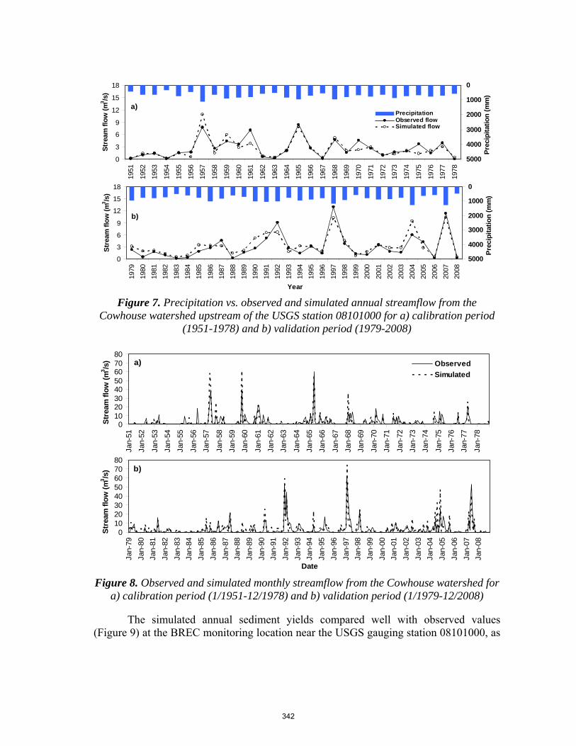
Figure 7. Precipitation vs. observed and simulated annual streamflow from the

Cowhouse watershed upstream of the USGS station 08101000 for a) calibration period (1951-1978) and b) validation period (1979-2008)

Figure 8. Observed and simulated monthly streamflow from the Cowhouse watershed for

a) calibration period (1/1951-12/1978) and b) validation period (1/1979-12/2008)

The simulated annual sediment yields compared well with observed values (Figure 9) at the BREC monitoring location near the USGS gauging station 08101000, as

0

3

6

9

12

15

18

1951

1952

1953

1954

1955

1956

1957

1958

1959

1960

1961

1962

1963

1964

1965

1966

1967

1968

1969

1970

1971

1972

1973

1974

1975

1976

1977

1978

Stre

am fl

ow (m

3 /s)

0

1000

2000

3000

4000

5000

Prec

ipita

tion

(mm

)

PrecipitationObserved flowSimulated flow

a)

0

3

6

9

12

15

18

1979

1980

1981

1982

1983

1984

1985

1986

1987

1988

1989

1990

1991

1992

1993

1994

1995

1996

1997

1998

1999

2000

2001

2002

2003

2004

2005

2006

2007

2008

Year

Stre

am fl

ow (m

3 /s)

0

1000

2000

3000

4000

5000

Prec

ipita

tion

(mm

)

b)

01020304050607080

Jan-

51

Jan-

52

Jan-

53

Jan-

54

Jan-

55

Jan-

56

Jan-

57

Jan-

58

Jan-

59

Jan-

60

Jan-

61

Jan-

62

Jan-

63

Jan-

64

Jan-

65

Jan-

66

Jan-

67

Jan-

68

Jan-

69

Jan-

70

Jan-

71

Jan-

72

Jan-

73

Jan-

74

Jan-

75

Jan-

76

Jan-

77

Jan-

78

Stre

am fl

ow (m

3 /s) Observed

Simulateda)

01020304050607080

Jan-

79Ja

n-80

Jan-

81Ja

n-82

Jan-

83Ja

n-84

Jan-

85Ja

n-86

Jan-

87Ja

n-88

Jan-

89Ja

n-90

Jan-

91Ja

n-92

Jan-

93Ja

n-94

Jan-

95Ja

n-96

Jan-

97Ja

n-98

Jan-

99Ja

n-00

Jan-

01Ja

n-02

Jan-

03Ja

n-04

Jan-

05Ja

n-06

Jan-

07Ja

n-08

Date

Stre

am fl

ow (m

3 /s) b)

342

evidenced by a R2 value of 0.9 and a NSE value of 0.84. Simulated mean and standard deviation of the monthly sediment yields compared closely to the observed values for both the calibration and validation periods (Table 3). Based on the statistical criteria for establishing satisfactory water quality model performance proposed by Moriasi et al. (2007), the model performance is satisfactory for monthly sediment yields for both the calibration and validation periods, as evidenced by the values of NSE (0.58 and 0.84), RSR (0.70 and 0.85), and PBIAS (-2% and -23%). Simulated monthly sediment yield followed the pattern of observed values during both the calibration and the validation periods (Figure 10).

Figure 9. Observed and simulated annual sediment yield from the Cowhouse watershed

upstream of the USGS station 08101000 Table 3. Monthly sediment yield calibration and validation at the monitoring location near the USGS gauging station (08101000)

Observed (t/ha/mon) Simulated (t/ha/mon)

NSE R2 PBIAS

(%) RSR‡

Mean Std Mean Std

Calibration (4/1998 – 12/2004) 0.02 0.04 0.02 0.05 0.58 0.70 -2.1 0.65

Validation (1/2005-12/2008) 0.05 0.12 0.04 0.11 0.84 0.85 -22.6 0.40 ‡RSR: Ratio of the root mean square error to the standard deviation of observed data.

0

0.5

1

1.5

2

2.5

1998 1999 2000 2001 2002 2003 2004 2005 2006 2007 2008

Year

Sedi

men

t yie

ld (t

/ha) Observed (mean=0.37)

Simulated (mean=0.32)R2 = 0.90NSE = 0.84PBIAS = -15.5%

343

Figure 10. Observed and simulated monthly sediment yield at outlet of the Cowhouse watershed for a) calibration period (4/1998-12/2004) and b) validation period (1/2005-12/2008) 3.2. Analysis of conservation practice effectiveness

The long-term simulation was used to target critical areas. Although the predicted average annual sediment yield at the watershed outlet is 0.23 t/ha from 1958 to 2008 (0.32 t/ha from 1998 to 2008, Figure 9), the predicted overland sediment losses ranged from 0.0 to 6.7 t/ha. The high sediment losses were from the agriculture lands and some range brush lands (Figure 11). Because agricultural land makes up less than 0.1%, the critical areas are range brush lands. There are 249 out of 445 subareas simulated as range brush. The overland sediment losses averaged 0.86 t/ha with the maximum loss of 3.0 t/ha and a standard deviation of 0.83 t/ha.

0

0.1

0.2

0.3

0.4

0.5

0.6

Apr-9

8

Aug-

98

Dec-

98

Apr-9

9

Aug-

99

Dec-

99

Apr-0

0

Aug-

00

Dec-

00

Apr-0

1

Aug-

01

Dec-

01

Apr-0

2

Aug-

02

Dec-

02

Apr-0

3

Aug-

03

Dec-

03

Apr-0

4

Aug-

04

Dec-

04

Apr-0

5

Aug-

05

Dec-

05

Apr-0

6

Aug-

06

Dec-

06

Apr-0

7

Aug-

07

Dec-

07

Date

Mon

th s

edim

ent y

ield

(t/h

a)

ObservedSimulated

Calibration Validation

344

Figure 11. Average annual sediment losses (1958 – 2008) from each subarea in the Cowhouse watershed

Figure 12 plots the overland sediment losses for each range brush subarea

grouped by soils. On average, the subareas with Evant soil have relatively higher sediment losses, followed by areas with Eckrant soil, among the range brush lands. These two soils are classified as hydrologic soil group D. Therefore, they have high runoff potential. In addition to those two soils, Pidcoke, Tarpley and Real soils of the study area also belong to hydrologic soil group D. A mapping of the surface runoff overlay with soils confirms that these soils have higher surface runoff. However, Evant and Eckrant have relatively higher soil erodibility factors. Since the subareas with Evant and Eckrant soils have relatively higher sediment losses among the range brush lands, the scenario analysis was conducted for the conversion of range brush on Evant and Eckrant soils (18% of the range brush area) to range grasses. This was compared to the scenario for removal of all the range brush (Table 4).

345

Figure 12. Average annual sediment losses (1958 – 2008) from each range brush

subarea in the Cowhouse watershed

The conversion of all the range brush to range grass (63% of the total watershed area) resulted in a 27% reduction in sediment loading to the watershed outlet. However, sediment load reductions of 7% and 12% were predicted for the removal of range brush on Evant soil areas (6.2% of the total watershed area) and on areas with Evant or Eckrant soils (11% of the total watershed area), respectively, based on long-term model predictions (Table 4). The results indicate that it is more effective to control soil erosion by treating critical areas. The removal of mesquite competition increases the grass stand and cover to protect the soil surface, control erosion, and reduce sediment (Bedunah and Sosebee, 1986). The conversions of range brush to range grass were predicted to slightly decease water yield (under 2% reduction). Converting mesquite to range grass or to pasture (for hay) along with nutrient management resulted in decreases in surface runoff, averaging 13% and 22%, respectively, in Tuppad et al. (2010). Conservation Practice Physical Effects (CPPE) by NRCS (USDA�NRCS 2007) also reported a moderate decrease in runoff due to brush management.

Researchers have reported different findings in water yield and sediment production while converting range brush to range grasses. In general, brush control practices have apparently increased infiltration rates and reduced erosion (Rosa and Tigerman 1951, Rich 1961, Rowe and Reimann 1961, Dragoun 1969, Blackburn and Skau 1974). However, these practices in some cases have failed to improve watershed conditions (Rowe and Reimann 1961, Blackburn and Skau 1974, Gifford and Busby 1974). It is interesting to compare this current study with another modeling study conducted by Wang et al. (2010). They simulated the same watershed using SWAT. Their results indicated that the conversion of all the range brush to range grasses would result in water yield and sediment yield increases, although the conversion on some soils was predicted to have no detectable effects on water yield.

0

0.5

1

1.5

2

2.5

3

3.5

Bol

ar

Nuf

fTa

rrant

Rea

lS

lidel

l

Bra

cke

Tops

ey

Dos

s

Tarp

ley

Pid

cok

Eck

ran

Eva

ntV

enus

Car

ada

Cho

Cis

coH

ext

Kru

mLa

mpa

Leer

ayO

gles

b

Soils

Ove

rland

sed

imen

t los

s (t/

ha)

0

2

4

6

8

10

12

Slop

e (%

)

Sediment lossAvg sediment lossSlope

346

Model inputs, calibration and how scenarios are represented in a model have an impact on simulation-based scenario analyses. Between the present study and the Wang et al. (2010) study, different DEMs and different soil maps were used. Wang et al. (2010) used a 30 m by 30 m resolution DEM and the STATSGO soil map, while the present study used a 10 m by 10 m resolution DEM and the SSURGO soil map. Different watershed delineations and HRU/subarea analyses also result in different land use distributions represented in the two models (130 subbasins with 546 HRUs for SWAT vs. 445 subareas for APEX), for example, range brush of 55% in Wang et al. (2010) vs. 63% in this study. However, the major differences between the two modeling studies are the sediment yield data used for calibration and the representations of the brush removal scenario. The amount of quality data available for model calibration/validation greatly impacts modeling results from which natural resource managers make decisions (Green and van Griensven, 2008).

Although in both studies the streamflows were calibrated and validated using the same USGS gauging station data (with a longer time series in this present study), the sediment-related parameters were adjusted in Wang et al. (2010) based on the annual average sediment yield of 1.72 t/ha from the Cedar Creek watershed study by Narasimhan et al. (2007). However, the measured annual average sediment yield from the BREC monitoring site (location close by the USGS streamflow station in Figure 2) is only about 0.37 t/ha (1998-2008).

The Cedar Creek watershed in the Trinity River basin is about 150 km north of the Cowhouse Creek watershed with about 3.2% agriculture land. The annual average precipitation is about 1000 mm and streamflow from USGS gauging stations within the watershed is about 18.9 m3/s. Yet a nearby monitoring station at Hico for the rangeland-dominated drainage area (4.3% cropland) in the North Bosque River watershed has a long-term annual average precipitation of 842 mm with measured annual average streamflow of 4.4 m3/s and annual average sediment yield of 0.57 t/ha (1993-1998). The current study of the Cowhouse Creek watershed has a long-term annual average precipitation of 775 mm.

Its land is only 0.1% agricultural and has an annual average streamflow of about 3.5 m3/s. With lower precipitation, one would expect a lower sediment yield from the Cowhouse watershed than from the Cedar Creek watershed. However, by referring to the reported annual average sediment yield of 1.72 t/ha in Narasimhan et al. (2007) for the Cedar Creek watershed, Wang et al. (2010) adjusted the SWAT model to predict an annual average sediment yield of 1.76 t/ha for the study Cowhouse watershed (1984-2006). From 1984 to 2006, APEX predicted an annual average sediment yield of 0.30 t/ha. Wang et al. (2010) predicted much greater sediment production for the same time period.

In the present study, the removal of range brush was simulated by including no mesquite trees in the management file without changing other model parameters/inputs. Without the mesquite competing for water, nutrients and light, the grass grew better. As plant cover and mulch increase, there is a reduction in raindrop impact. Because plant cover varies during growth, the crop management C-factor is evaluated using the

347

modified RUSLE equation (Williams and Izaurralde, 2006) for all days when runoff occurs using the above ground crop-residue, crop height, standing live crop biomass and soil surface random roughness without the requirement of a minimum C-factor input value. This contrasts with the method used in SWAT, in which a unique minimum C-factor value is required to be input. Wang et al. (2010) indicated that a smaller C-factor was used for range brush than for range grasses, and therefore it is not surprising to see greater sediment production potential from range grasses than from range brush in their study.

Table 4. APEX-predicted effects of rangeland management practices (1951-2008)

Scenarios (% of treated area)

Sediment loading to watershed outlet

Average overland sediment loss reduction for

treated areas (%) t/year reduction

(%)

Baseline 34060 - -

Conversion of range brush to

range grass

Range brush on Evant soil to range grass 6% 31719 -6.9 -58.8

Range brush on Evant and Eckrant soils to range grass 11% 29840 -12.4 -53.8

All range brush to range grass 63% 24769 -27.3 -48.5

Reduction of stocking

rate

Stocking rate on range brush & range grass from 10 to 15 ha/herd 96% 32541 -4.5 -6.3

Stocking rate on range brush & range grass from 10 to 20 ha/herd 96% 31949 -6.2 -7.9

Combined

Stocking rate from 10 to 15 ha/herd and range brush on Evant soil to range grass

96% 29942 -12.1 -21.5

Stocking rate from 10 to 20 ha/herd and range brush on Evant soil to range grass

96% 29486 -13.4 -22.7

Stocking rate from 10 to 15 ha/herd and range brush on Evant and Eckrant soils to range grass

96% 28021 -17.7 -29.5

Stocking rate from 10 to 20 ha/herd and range brush on Evant and Eckrant soils to range grass

96% 27569 -19.1 -30.4

The options of reducing the stocking rate from the baseline 10 ha/herd to 15 or 20

ha/herd were examined, with the predicted sediment loadings reduced by 4.6% and 6.2% (Table 4), respectively. The reduced stocking rates were less effective compared to the brush removal scenarios since the baseline 10 ha/herd stocking rate is not a heavy stocking rate to begin with. The scenarios of combined practices reduced sediment loading to the watershed outlet by 12.1% to 19.1% (Table 4). The reductions at the watershed outlet were less compared to the reductions predicted at the subarea level (see overland sediment loss reduction for treated areas in Table 4). The most effective treatment to reduce overland sediment loss is the conversion of range brush to range grass on Evant soil areas, which reduced sediment by 58.8% on average at the subarea level. 4. Conclusions

Scenario analyses (1951-2008) indicated substantial reductions in overland sediment losses for areas converted from range brush to range grass on Evant soil, with an average reduction of 58.8% from treated areas. These reductions are based upon 100%

348

removal of shrub species and replacement with herbaceous species within the treated subareas. It is understood that this is not necessarily the case for many rangeland restoration programs and the authors recognize this fact. However, for the purposes of the current effort, demonstrating the applicability of APEX as a decision support tool, we chose to apply the 100% removal scenario within the treated subareas. Further case studies are being developed to test outcomes based upon results of other rangeland research programs. Comparisons for stocking rate reductions on range brush and range grass lands from a baseline of 10 ha/herd to 15 or 20 ha/herd, the APEX model indicates reduced overland sediment losses from treated areas by 6.3% and 7.9%, respectively. The overall sediment loading to the watershed outlet was reduced by 27.3% if all range brush land (63% of total watershed area) would be converted to range grass. However, converting only the range brush on areas with Evant and Eckrant soils (11% of total watershed area) would result in a 12.4% sediment loading reduction to the watershed outlet. Therefore, it is more effective to treat those critical areas. Sediment loadings to the watershed outlet were reduced by 4.5% and 6.2% for the two reduced grazing scenarios, which both have 96% of the area treated. Therefore, reducing grazing alone is not an effective management practice in this watershed. By combining brush conversion on Evant and Eckrant soils to brush grass and reducing stocking rate on all grazing lands, the watershed sediment yield could be reduced by 17.7% to 19.1%. The study shows that the APEX model is a useful tool for simulating rangeland management practices.

Understanding how specific grazing land conservation practices and suites of those practices affect watershed processes at the watershed/landscape scale is necessary for future planning and resource allocation. The use of simulation models as a decision support system for management of conservation practices and assessment of their quantitative benefits at the watershed level prior to implementation is beginning to gain acceptance. The results indicate that the model performance is satisfactory for monthly flow and sediment yield based on accepted statistical criteria. Utilizing the above approach provides land managers with the ability to test land management considerations prior to allocation of resources, thus reducing some of the uncertainty and risk associated with best management practices. In doing so, land managers have a valuable tool at their disposal that will provide guidance as to what practices are feasible for specific locations within the landscape and some predictive capacity for evaluating the cost/benefit of application. This process also provides land managers with the ability to test practices at specific locations within a watershed as a means for effectively selecting and implementing practices on specific landscapes where the highest reduction of erosion is predicted. We propose that these capabilities will be of great value in aiding natural resource management agencies, whether local, state or federal, in optimizing the use of limited conservation resources to provide the highest impact within communities where land management practices are being proposed. Development of further best management practices can be carried out to expand the capabilities of the simulation process and to incorporate further scenarios of probable land management programs.

349

References Bagnold, R.A. 1977. Bed-load transport by natural rivers. Water Resources Research 13(2):303-

312. Blackburn, W.H., and C.M. Skau. 1974. Infiltration rates and sediment production of selected

plant communities in Nevada. J. Range Manage. 27:476-480. Brock, J. H., W.H. Blackburn and R.H. Haas. 1982. Infiltration and sediment production on a

deep hardland range site in North Central Texas. Journal of Range Management 35(2):195-198.

Dortignac, E. J., and W. C. Hickey, Jr. 1963. Surface runoff and erosion as affected by soil

ripping. Proceedings of the Federal Inter-Agency Sedimen tation Conference, 1963. Miscellaneous Publication Number 970, pp 156-165.

Dragoun, F.J. 1969. Effect of cultivation and grass on surface runoff. Water Resourc. Res.

5:1078-1083. Dugas,W.A., Mayeux, H.S., 1991. Evaporation from rangeland with and without honey mesquite.

J. Range Manage. 44:161–170. Duriancik, L.F., D. Bucks, J.P. Dobrowski, T. Drewes, S.D. Eckles, L. Jolley, R.L. Kellogg, D.

Lund, J. R. Makuch, M. P. O'Neill, C. A. Rewa, M. R. Walbridge, R. Parry, and M. A. Weltz. 2008. The first five years of the Conservation Effects Assessment Project. J. Soil Water Conserv. 63(6): 185A�197A.

Gassman, P.W., Williams, J.R., Benson, V.W., Izaurralde, R.C., Hauck, L., Jones, C.A., Atwood,

J.D., Kiniry, J. and Flowers, J.D. 2005. Historical development and applications of the EPIC and APEX models. Working Paper 05 WP�397. Ames, Iowa: Iowa State University, Center for Agricultural and Rural Development. Available at: www.card.iastate.edu/publications/synopsis.aspx?id=763. Accessed 28 September 2007.

Gassman, P.W., Williams, J.R., Wang, X., Saleh, A., Osei, E., Hauck, L., Izaurralde, R.C. and

Flowers, J.D. (2010) The Agricultural Policy Environmental Extender (APEX) model: An emerging tool for landscape and watershed environmental analyses. Trans. ASABE 53(3):711-740.

Green, C.H. and van Griensven, A. 2008. Autocalibration in hydrologic modeling: Using

SWAT2005 in small-scale watersheds. Environmental Modelling & Software 23:422-434. Moriasi, D.N., Arnold, J.G., Van Liew, M.W., Bingner, R.L., Harmel, R.D., Veith, T.L., 2007.

Model evaluation guidelines for systematic quantification of accuracy in watershed simulations. Trans. ASABE 50(3): 885–900.

Nash, J.E. and J.V. Sutcliffe. 1970. River flow forecasting through conceptual models. Part 1: A

discussion of principles. Journal of Hydrology 10(3):282–290.

350

Rich, L.R. 1961. Surface runoff and erosion in the Lower Chaparral zone, Arizona. U.S. Dep. Agr. Forest Serv., Rocky Mountain Forest Range Exp. Sta., Res. Pap. No. 66.

Rosa, J.M., and M.H. Tigerman. 1951. Some methods for relating sediment production to

watershed condition. U.S. Dep.. Agr. Forest Serv., Intermountain Forest Range Exp. Sta., Res. Pap. No. 26.

Rowe, P.B., and L.F. Reimann. 1961. Water use by brush, grass and grassforb vegetation. J.

Forest. 59:175-181. Tuppad, P., C. Santhi, X. Wang, J.R. Williams, R. Srinivasan, P.H. Gowda. 2010. Simulation of

conservation practices using the APEX model. Applied Engineering in Agriculture 26(5):779-794.

Tuppad, P., Winchell, M., Srinivasan, R., Williams, J.R. 2009. ArcAPEX: ArcGIS interface for

Agricultural Policy Environmental eXtender (APEX) hydrology/water quality model. International Agricultural Engineering Journal 18(1-2):59-71.

USDA�NRCS (USDA Natural Resources Conservation Service). 2007. National Handbook of

conservation Practices. USDA�NRCS, Washington, DC. Available at: www.nrcs.usda.gov/technical/standards/nhcp.html.

USDA�NRCS. 2009. Conservation Effects Assessment Project (CEAP). Washington, D.C.:

USDA National Resources Conservation Service. Available at: www.nrcs.usda.gov/technical/NRI/ceap/.

Wang, X., D. W. Hoffman, J. E. Wolfe, J. R. Williams, and W. E. Fox. 2009. Modeling the

effectiveness of conservation practices at Shoal Creek watershed, Texas, using APEX. Trans. ASABE 52(4): 1181�1192.

Wang, X. (Xiuying), S.R. Potter, J.R. Williams, J.D. Atwood, and T. Pitts. 2006. Sensitivity

analysis of APEX for national assessment. Transactions of the American Society of Agricultural and Biological Engineers 49(3): 679–688.

Wang, X. (Xixi), Shiyou Shang, Wanhong Yang, Calvin R. Clary, Dawen Yang. 2010.

Simulation of land use–soil interactive effects on water and sediment yields at watershed scale. Ecological Engineering 36:328-344.

Wilcox, B. P. 2007. Does rangeland degradation have implications for global streamflow?

Hydrological Processes 21:2961-2964. Williams, J.R. 1995. The EPIC Model. pp 909-1000 In V.P. Singh, Computer Models of

Watershed Hydrology. Highlands Ranch, CO: Water Resources Publications. Williams, J. R. and R. C. Izaurralde. 2006. The APEX model. In Watershed Models, 437-482.

Singh, V.P. and D.K. Frevert, eds. Boca Raton, FL: CRC Press, Taylor & Francis.

351

Williams, J.R., E. Wang, A. Meinardus, W.L. Harman, M. Siemers, J.D. Atwood. 2006. APEX users guide. V.2110. Temple, TX: Texas A&M University, Texas Agricultural Extension Service, Texas Agricultural Experiment Station, Blackland Research Center.

Wood, M.K. and W.H. Blackburn. 1981. Sediment Production as Influenced by Livestock

Grazing in the Texas Rolling Plains. J. Range Management. 34(3): 228-231.

352

SWAT-APEX Modeling for SRI BMP Scenario Effect in an Agricultural Reservoir Watershed of South Korea

C. G. Jung, Graduate student

Konkuk University, Dept. of Civil and Environmental System Eng., 1 Hwayang dong, Gwangjin-gu, Seoul 143-701, South Korea

H. J. Shin, Post-doctoral researcher

Konkuk University, Dept. of Civil and Environmental System Eng., 1 Hwayang dong, Gwangjin-gu, Seoul 143-701, South Korea

J. Y. Park, Ph.D. Candidate

Konkuk University, Dept. of Civil and Environmental System Eng., 1 Hwayang dong, Gwangjin-gu, Seoul 143-701, South Korea

H. K. Joe, Graduate student

Konkuk University, Dept. of Civil and Environmental System Eng., 1 Hwayang dong, Gwangjin-gu, Seoul 143-701, South Korea

J. W. Lee, Graduate student

Konkuk University, Dept. of Civil and Environmental System Eng., 1 Hwayang dong, Gwangjin-gu, Seoul 143-701, South Korea

S. J. Kim*, Professor

Konkuk University, Dept. of Civil and Environmental System Eng., 1 Hwayang dong, Gwangjin-gu, Seoul 143-701, South Korea

Abstract

Environmental models are used to evaluate various best management practices (BMPs) at watershed level or field level with a limited number of BMP scenarios individually. The SWAPP (SWAT-APEX Program), the coupling of SWAT (Soil and Water Assessment Tool) watershed model and APEX (Agricultural Policy/Environmental eXtender) field model, is capable of evaluating the BMP scenarios from the watershed to the field application successively. This study tries to evaluate the SRI (System of Rice Intensification) BMP scenario for a typical agricultural watershed (465.1 km2) of South Korea using SWAPP. The watershed includes a reservoir, Yedang, which irrigates rice paddies downstream. As a feasible SRI BMP scenario, the control of irrigation amount, that is, the reduction of ponding depth was applied. The SWAPP was calibrated with 2 years (2000-2001) of daily streamflow and monthly water quality (T-N and T-P) data, and validated for another 4 years (2002-2005) data. The average Nash–Sutcliffe model efficiency of streamflow during validation was 0.65, and the coefficient of determination (R2) of T-N and T-P were 0.74, 0.76 respectively. The application of SRI scenario by control of ponding depth from present to 25%, 50% and 75% reduction in the paddy showed that the T-N and T-P (25% scenario) decreased 26.6% and 28.2% by saving the total irrigation water of 26.98 ton/ha/day during 25% scenario.

Keywords: SWAPP (SWAT-APEX Program), nonpoint source pollution, SRI scenario

368

1. Introduction

Agriculture is the main cause of non-point source (NPS) pollution that affects streams and aquifers throughout the country (Yu et al., 2004). The driving force of NPS pollution is the rainfall-runoff process, which tends to be a complex non-linear, time-varying, and spatially distributed process in agricultural watersheds. A wide range of structural and management based practices, collectively known as best management practices (BMPs), are used to control pollutant losses (Dillaha, 1990; NRCS, 2004).

This study, in regards to NPS pollution, has to simulate water quality to estimate NPS pollution and analyze effects by applying BMP. Environmental hydrologic models such as SWAT and APEX are very useful for effective evaluation of the impact of BMP. Water quality simulation models can assist with total maximum daily loads (TMDL) development by simulating loads into receiving water bodies under various BMPs. Models, in combination with observational data from historical and current monitoring programs, will provide the information for waste/load allocations and implementation strategies (Santhi, 2001).

Recently, several BMP studies have been carried out by using a watershed model. Lee et al. (2006) evaluated the NPS pollution reduction by applying BMP using the SWAT model. Wang et al. (2009) evaluated effectiveness of conservation practices by applying gully plugs and contour soil ripping using the APEX model. Saleh et al. (2007) simulated the SWAT and APEX models in the SWAPP and compared streamflow with water quality. Also, Saleh et al. (2010) carried out SWAT-APEX modeling by using SWAPP and evaluated environmental pollutants for cost-effective targeting.

As interest in stream and reservoir water quality problems in rural areas has increased, research for quantification of NPS pollution from livestock and crop cultivation areas is necessary. In this study, the combined SWAT and APEX models in the SWAPP (SWAT-APEX Program) were calibrated and verified by using the historical measured data collected in the Yedang agricultural dam watershed. Also, the aim of this study was to assess the reduction effect of NPS pollution loads from rice paddies by applying the SRI scenario.

2. Materials and Methods 2.1. Study watershed and data

Figure 1 shows the Yedang reservoir of the study watershed. It has a total area of 462.1 km2 and is located in Chungcheongnam province, South Korea.

The elevation ranges from 10 to 560 m with average hillslope of 25.9% and average elevation of 315 m. The annual average precipitation was 1,226.6 mm and mean temperature was 13.4°C over the last 10 years. Yedang reservoir dam has 47.1 million tons in volume. Also, total area of rice paddy fields is 117.9 km2 and the irrigation area is 78.9 km2. Generally, the irrigation period of the watershed is from April to September. The Yedang reservoir irrigates rice paddies downstream.

This study used SWAPP to evaluate NPS loads from the study watershed at both the watershed and field levels, in before and after applying the SRI scenario. Simulated results for both periods were compared to consider hydrologic effects and reduction of NPS loads.

The watershed spatial data of elevation, land use, and soil were prepared for SWAT and APEX model setup. Elevation data was rasterized from a 1:5,000 vector

369

map supplied by the Korea National Geography Institute (KNGI). Soil data of texture, depth and drainage attributes were rasterized from a 1:25,000 vector map supplied by the Korea Rural Development Administration.

For the model setup, ten years (2000-2009) of daily weather data from three weather stations (Cheonan, Boryung and Buyeo) and precipitation data from 3 AWS (automatic weather precipitation) were used. The daily streamflow was obtained from the Ministry of Land, Transport and Maritime Affairs at the Wonpyong water level gauging station (WP). Monthly water quality (T-N and T-P) data was obtained from the Ministry of Environment at Muhanchun2 water quality gauging station (MH2). Additionally, the study required the use of reservoir dam data (irrigation, spillover water) for applying the SRI scenario.

Figure 1. Locations of the Yedang dam watershed and the weather stations, streamflow and stream water quality stations

2.2. SWAT-APEX model description

Gassman et al. (2002) reported on studies that have taken advantage of the capabilities of the combined SWAT and APEX models by simulating an environmental baseline and BMPs at the field level with APEX and then routing the results from APEX and the remaining land uses within a watershed using SWAT. SWAPP (SWAT/APEX Program) provides opportunities for more efficient and reliable simulation of the water quality impacts of many scenarios, particularly those related to agriculture. The SWAT-APEX (SWAPP) model process starts with data files created by the AVSWAT program. The SWAPP process occurs in four major phases.

Phase I. By using the “SWAT-APEX” subprogram of SWAPP, all the required APEX data files for selected land use(s) from SWAT format are transferred to APEX format. These files include management operation, soil data, field geometry, weather data, and all general databases, such as crop.dat, fert.dat, parm.dat, and till.dat, which are commonly used by SWAT and APEX. The land use areas simulated by APEX are also subtracted from the original sub-basin areas simulated by SWAT to avoid

370

duplicate simulation of APEX land areas by SWAT. During this phase SWAT data files such as soil and management, which are related to selected land use for the APEX simulation, are converted to APEX format.

Phase II. During this phase, the specified land uses are simulated in APEX, and the results, including the daily flow and loading of sediment and nutrients, are stored in .SWT files. For example, in case .SWT files obtained from each individual field within a subarea are merged together into one, .SWT is obtained from the last routed field within a subarea.

Phase III. In this phase the “SWAT_ADD” subprogram of the SWAPP is used to add daily inputs from any possible point sources to the APEX input files (.SWT) within a specific sub-basin. The results obtained from this process are input into SWAT at the sub-basin level. The “recday” command within SWAT program reads in the daily flow, sediment, and nutrient loading stored in the “.SWT” files as point source input at the outlet of each appropriate sub-basin.

Phase IV. The SWAT program, which includes the .SWT files, is executed in the last phase (Saleh et al., 2007).

2.3. SRI scenario

Stoop et al. (2002) stated the major principles of SRI to be the following. (1) Rice is not an aquatic plant; it survives under flooded conditions but does not thrive. (2) Rice seedlings lose much of their growth potential if they are transplanted more than 15 days after emergence. (3) During transplanting, trauma to seedlings, especially roots, should be minimized. (4) Wide spacing of plants leads to more root growth and tillering.

In South Korea, paddy farming has to maintain ponding depth during irrigation periods. Ponding depth ranges from 10 mm to 80 mm for the duration of growth. Because rainfall is heavy during summer periods, it is important that the agricultural dam secures the supply of irrigation water. The SRI for saving water volume is necessary in Korea, and SRI modeling has to simulate the water quality before applying SRI in the field. In this study, we simulate the SRI scenario by applying water and nutrient management (Table 1). Actually, Chung et al. (1986) studied rice production at different ponding depths (2, 4, 6 and 8 cm). The results showed that rice production didn’t decreased by reducing ponding depth. For applying the SWAT-APEX model, the SRI scenario in this study was applied by reducing irrigation quantity in the SWAT model. The SRI scenario was simulated by reducing ponding depth in the rice field to 75%, 50% and 25% of conventional practices in the SWAT-APEX model.

Table 1. Application of SRI scenario

Management SRI Conventional management

transplanting plant spacing and density

At least 25 cm by 25 cm, up to 50 cm by 50 cm apart on good soils Typically about 20 cm by 20 cm

Weed control Hand-weed regularly starting 10 days after planting and continuing every 10 days until the canopy closes

Pre-emergence herbicides and h and-weeding to control early weeds up to 21 days

Water management

The fields are kept flooded with a thin layer of water (1–2 cm)

The field are maintained at approximately a thin layer of water (5-10 cm)

Nutrient management

apply no nutrients or some mineral fertilizers

Provide nutrients to the crop in the amount and mineral fertilizers at the time required

371

3. Results and Discussions 3.1. Model calibration and validation

The SWAT model was calibrated by using 2 years (2000-2001) of daily streamflow data from the Wonpyong station and water quality (T-N and T-P) data from the Muhanchun2 station, and validated with another 4 years (2002-2005) of data.

The average Nash and Sutcliffe (1970) model efficiency (NSE) of streamflow during validation and the coefficient of determination (R2) were 0.65 and 0.70. Table 2 shows the statistical summary T-N and T-P of model calibration and validation respectively.

The peak runoff errors may be caused by the difference between real and simulated runoff mechanisms in paddy fields. Unlike the unsaturated flow mechanism in a natural environment, a paddy has artificial factors such as irrigation scheduling and levee height management that increase the uncertainty of the water budget. During the paddy cultivation periods, farmers control levee heights artificially for their own water management. Irrigating water before rainfall and draining water after rainfall affect the streamflow with significant quantity. In the study, we considered the spillover water at reservoir dam by using observed (irrigation, spillover water) data.

Table 2. Statistical summary of water quality for the calibration and validation periods at Muhanchun2

Parameter SWAT modeling SWAT-APEX modeling

T-N R2 0.72 0.74

NSE 0.67 0.72

T-P R2 0.72 0.76

NSE 0.70 0.73 No. of Obs. Data 72 R2 : Coefficient of Determination, NSE : Nash-Sutcliffe Model Efficiency

3.2. Hydrologic effects of SRI scenario Water requirements with SRI are usually reduced by about half since paddies

are not kept flooded during the entire crop cycle. Water is much reduced during the vegetative growth phase, and only a minimum of water is kept on the field during the reproductive phase. This will become increasingly important in the agricultural sector.

In short, the application of SRI scenarios has the effect on securing the water volume of 6.75 ton/ha/day (75% scenario), 13.49 ton/ha/day (50% scenario) and 26.98 ton/ha/day (25% scenario) respectively.

3.3. NPS reduction effects of the SRI scenario

As a practical and easy approach in our country, the effect of SRI was evaluated by ponding depth of paddy in the watershed. Table 5 shows the SRI scenarios including the ponding depth of 100%, 75%, 50% and 25%. The ponding depth of 100% means conventional management while ponding depths of 75%, 50% and 25% mean SRI management scenarios simulating a reduction in irrigation.

The 25%, 50% and 75% reductions of ponding depth were evaluated and the results are shown in Table 5. The removal efficiency of T-P was higher than that of T-N because of the reduction in ponding depth. The results of T-N (75%, 50% and 25%)

372

scenarios average removal efficiency -11.0 %, -19.3 % and -26.6% respectively. Also, T-P (75%, 50% and 25%) scenarios result in average removal efficiencies of -11.4%, -20.2% and -28.2% respectively (Fig. 2).

Figure 2. Comparison of T-N and T-P loads reduction effects

4. Summary and Conclusions

The SRI was evaluated by using SWAT-APEX model data for a Yedang

reservoir study watershed in South Korea. The SRI of BMP scenario classified the water management and nutrient management in the rice paddy field. Using SWAT-APEX model, Nonpoint sources pollutant at the field level simulated intensive. The average Nash–Sutcliffe model efficiency of streamflow during validation was 0.65, and the coefficient of determination (R2) was 0.70. Also, the average Nash–Sutcliffe model efficiency of T-N and T-P during validation was 0.72 and 0.73 respectively. By applying the Ponding depth control for rice paddy field in the watershed, the reduction of NPS loads was evaluated. For the 25% and 50 % reduction of Ponding depth, the reduction ratio of T-P load was higher than that of T-N load.

The results of this study provided a new BMP scenario for rice paddy fields and to use the combined SWAT and APEX model. This study indicates that SRI scenario has effects on saving water volume and removal NPS loads.

Finally, the SRI scenario for reducing NPS loads applies to the rice paddy field when the rain has dropped during rain storm events. Future research for the SRI monitoring prove rice production to be made no difference and evaluate effects on hydrologic and reduction of NPS. Then, SRI is expected to be applied as non structured BMP in rice paddy fields. Acknowledgments This work was supported by Han River Environmental Research Center, National Institute of Environmental Research, Kyungki-Do, 476-823, South Korea.

373

References Dillaha, T. A. 1990. Role of BMPs in restoring the health of Chesapeake Bay: Assessments of

effectiveness. In Perspectives on Chesapeake Bay, 1990: Advances in Estuarine Sciences, 57−81. Chesapeake Bay Program, CPB/TR541/90. Washington, D.C.: U.S. EPA

Gassman, P. W., E. Osei, A. Saleh, and L.M. Hauck. 2002. Application of an environmental and

economic modeling system for watershed assessments. Journal of the American Water Resources Association 38(2):423-438.

Chung, H., W. 1986. Establishment of computation method for crop consumptive use of water,

Ministry of Agriculture and Fishery. Lee, M., S. 2010. Evaluation of non-point sources pollution reduction by appling Best

Management Practices using a SWAT model and QuickBird high resolution satellite imagery. Journal of Environmental Sciences 22(6): 826-833.

Yu, C., W. J. Northcott, and G. F. McIsaac. 2004. Development of an artificial neural network

for hydrologic and water quality modeling of agricultural watersheds. Trans. ASAE 47(1): 285-290.

Osei, E., P.W. Gassman, R.D. Jones, S.J. Pratt, L.M. Hauck, L.J. Beran, W.D. Rosenthal, and

J.R. Williams. 2000. Economic and environmental impacts of alternative practices on dairy farms in an agricultural watershed. Journal of Soil and Water Conservation 55(4):466-472.

Park, J., Y. 2009. Assessment of future climate change impact on hydrological behavior and

stream water quality using SWAT model. MS thesis. Kwangjin-gu, Seoul, Konkuk University, Department of Civil and Environmental System Engineering.

Saleh, A. and O. Gallego. 2007. Evaluation of SWAT and APEX Linkage Program (SWAPP)

for Upper North Bosque River Watershed in Texas. Submitted for review in May 2006 as manuscript number SW 6460; approved for publication by the Soil & Water Division of ASABE in April 2007.

Saleh, Ali, Edward Osei, and Oscar Gallego. 2007. Application of SWAT, APEX and FEM

Models Using CEEOT-SWAPP for the Upper North Bosque River Watershed in Texas. Santhi, C., Arnold, J. G., Williams, J. R., Hauck, L. M. and Dugas, W. A. 2001. Application of a

watershed model to evaluated management effects on point and nonpoint source pollution. Transactions of the American Society of Agricultural Engineers. 44. 1559-1570.

Sheehy, J.E., Peng, S., Dobermann, A., Mitchell, P.L., Ferrer, A., Yang, J.C., Zou, Y.b., Zhong,

X.H., Huang, J.L. 2004. Fantastic yields in the system of rice intensification: fact or fallacy?. Field Crops Research 88: 1-8.

374

Wang, X., Hoffman, D. W., Wolfe, J. E., Williams, J. R., Fox, W. E. 2009. Modeling the Effectiveness of Conservation Practices at Shoal Creek Watershed, Texas, using APEX. American Society of Agricultural and Biological Engineers. ISSN 0001-2351

375

Calibration and Sensitivity Analysis of SWAT for a Small Forested Catchment, North-Central Portugal

Rial-Rivas, M.E.1; Santos, J. 1;Bernard-Jannin L. 1 ; Boulet, A.K. 1 ; Coelho, C.O.A. 1; Ferreira, A.J.D.4; Nunes, J.P. 1 ; Rodríguez-Suárez J.A. 1, 2; Rodríguez-Blanco M.L. 1,3; Keizer, J.J. 1

1CESAM and Dept. Environment & Planning. University of Aveiro. 3810-193 Portugal. E-mail: m.rial@ua.pt

2Vegetal Biology and Soil Science Department. University of Vigo. Spain. 3 Faculty of Sciences, University of A Coruña, A Zapateira, 15008 A Coruña, Spain.

4CERNAS, Coimbra Agrarian Technical School. Portugal.

Abstract The Soil and Water Assessment Tool (SWAT) was applied to a small forested watershed covered predominantly by commercial eucalyptus plantations (Eucalyptus globulus Ait.) in North-Central Portugal. The initial model parameterization was carried out using a data set composed of widely available information. A sensitivity analysis was conducted using 26 SWAT parameters. The most sensitive parameters were, in order of decreasing importance, the following: Esco (soil evaporation compensation factor), Gwqmn (threshold depth of water in the shallow aquifer required for return flow to occur), Sol_Awc (available water capacity of the soil layer), Canmx (canopy interception), Cn2 (SCS curve number), Sol_Z (depth from soil surface to bottom of layer), Gw_Revap (revap coefficient), Blai (maximum potential leaf area index), Alpha_Bf (baseflow alpha factor), Ch_K2 (effective hydraulic conductivity in tributary channel alluvium), Sol_K (saturated hydraulic conductivity), Biomix (biological mixing efficiency) and Slope (average slope steepness). Three different auto-calibrations using flow related parameters were performed, resulting in a Nash-Sutcliffe model efficiency (NSE) > 0.58 for the calibration period and also for the validation period. Keywords: forest catchment, sensitivity analysis, auto-calibration.

376

1. Introduction During the last two decades, hydrological modelling has seen major advances with the

appearance of increasingly process-based and spatially-distributed models as well as sophisticated model-assessment methods involving uncertainty and sensitivity analysis. Process-based models are now widely accepted, especially due to their elevated potential for testing the current understanding of hydrological processes as well as for their ability to project hydrological impacts of possible climate and land-use change scenarios (Beven, 2000). A major drawback of process-based models, however, is their elevated data input requirements. Exploratory modelling work using LISEM in forested catchments of north-central Portugal revealed that little to no information was available for almost half of the selected model input variables (Tuinenberg et al., 2006). For example, there was a lack of detailed information on soil properties for the entire study area, and a basic soil characteristic like saturated hydraulic conductivity was measured at no more than a handful of imprecisely recorded locations. Therefore a stepwise procedure is now being implemented in which model results are used to guide the collection of additional field and laboratory data for: (i) improved model parameterizations; (ii) assessment of model predictions from multiple, likely model parameterizations. In this framework, the present work concerns the initial modelling using SWAT and widely available data of the hydrological behaviour of one of a series of small, experimental catchments in north-central Portugal. 2. Study Area

The so-called “Serra de Cima” experimental catchment belongs to a set of four

experimental catchments located in the foothills of the Caramulo mountain range, north-central Portugal (Figure 1). The Serra de Cima catchment has an area of 0.53 km2 and consists predominantly of commercial eucalyptus plantations (Eucalyptus globulus Ait.). The catchment’s elevation varies from 405 to 487 m with a mean catchment slope of 30% and a mean river slope of 15%. In September 2009, the existing hydrometric station that has been at the outlet of the Serra de Cima catchment since the 90’s was complemented with a new station comprising a cut-throat flume equipped with an ultra-sound level recorder, especially to improve stage-discharge and stream-flow information gathering. Data from the two stations were combined to assess SWAT performance over the measurement period.

Figure 1. Location of the experimental catchment

377

3. Materials and Methods The Soil and Water Assessment Tool (SWAT) model, developed by the USDA

Agricultural Research Service (Arnold et al., 1998), was selected for the present study. SWAT was developed to predict the impact of land management practices on water, sediment and agricultural chemical yields, especially also for large complex watersheds with varying soils, land-use and management conditions and for long periods of time. SWAT is a physically based model, uses readily-available input data, is computationally efficient and enables users to study long-term impacts. The input data for SWAT is grouped into five categories: climate, terrain, land cover and use, and soil. Hydrologic Response Units (HRU) are defined and consist of unique combinations of terrain slope, land use and soil type. Runoff is predicted separately for each HRU and then routed to obtain total runoff for the entire watershed. SWAT allows detailed insight into the water balance of the distinct HRUs and into the underlying hydrological processes (evaporation, infiltration, overland flow, interflow, baseflow and deep aquifer recharge).

The SWAT model was set up using the ArcGIS interface ArcSWAT 2009. ArcSWAT includes procedures for sensitivity analysis, auto-calibration and uncertainty analysis. The method for sensitivity analysis in the ArcSWAT 2009 interface combines Latin Hypercube (LH) and One-factor-At-a-Time (OAT) sampling. The auto-calibration procedure is based on a multi-objective calibration and involves a single, global optimization criterion that evaluates multiple output parameters and employs the Nash-Sutcliffe model efficiency (NSE; Nash and Sutcliffe, 1970). Amongst the different auto-calibration methodologies available in ArcSWAT 2009, the Parameter Solution (ParaSol) with an uncertainty analysis method was applied here. ParaSol aggregates objective functions (OF) into a global optimization criterion (GOC) and then minimizes these OF’s or a GOC using the Shuffled Complex Evolution algorithm (SCE-UA) (van Griensven and Meixner, 2006). All auto-calibration procedures were made using “ParaSol with uncertainty analysis,” fixing the number of simulation runs at 20,000 and the optimization settings as the default.

SWAT was applied using a so-called regional input data set that concerns readily-available information from European and national sources. Climate information was obtained from the water resources information system in Portugal (SNIRH) using the nearest meteorological stations: Bouça (09G/03UG) 10 km north of the study area and located at an altitude of 152 m and Barragem Castelo Burgaes (08G/01C) located 30 km north of the study area at an altitude of 306 m. Input data on land cover was obtained from the CORINE Land Cover project (CLC2006; 1:100,000) of the European Environment Agency. Topography information was obtained from the DTMs (25 m x 25 m) of the Geographical Institute of the Portuguese Army, and soil type data was obtained from the Portuguese Atlas of the Environment (1:1,000,000).

To assess the influence of the number of parameters included in the auto-calibration and their ranges of variation, the following three auto-calibrations were carried out: Auto-calibration A: 26 flow-related parameters and full default ranges of variation. Auto-calibration B: 13 flow-related parameters and full default ranges of variation. Auto-calibration C: 13 flow-related parameters and narrow ranges of variation. The model was evaluated using three quantitative statistics:

378

A) Nash-Sutcliffe efficiency (NSE): NSE indicates how well the plot of observed versus simulated

data fits the 1:1 line. NSE ranges between -∞ and 1, NSE = 1 being the optimal value. Values between 0.0 and 1.0 are generally viewed as acceptable levels of performance whereas values lower than 0.0 indicate that the mean observed value is a better predictor than the simulated value which indicates unacceptable performance (Moriasi et al., 2007).

B) Percent bias (PBIAS): PBIAS measures the average tendency of the simulated data to be larger or smaller than their observed values (Moriasi et al., 2007). Positive values indicate model underestimation bias, and negative values indicate model overestimation bias (Gupta et al., 1999), the optimal value of PBIAS being zero. PBIAS values lower than 25% using SWAT are considered satisfactory, less than 10% are very good and between 10-15% are good.

C) Root Mean Square Error (RMSE): RMSE is a commonly used error statistic with model performance decreasing with increasing RMSE values. According to Singh et al. (2004), RMSE values can be considered low when they are less than half the standard deviation of the observed data.

4. Results and Discussion

Based on the CORINE land-cover map, two land cover types were identified inside the

watershed: broad-leaved forest and transitional woodland-shrub. Previous work in Portugal (Nunes et al., 2008) made a regional parameterization of the vegetation characteristics for these land-uses which was used in the present work as initial parameters. The single soil type in the watershed is Humic Cambisols, also parameterized by Nunes et al. (2008) using global soil texture data and pedo-transfer functions. The terrain was divided in three slope classes, i.e. smaller than 3%, from 3 to 6% and greater than 6%. The resulting HRU map of the catchment comprised six elements.

A warm-up period from 27/11/2001 to 31/12/2008 was defined to allow the model to “stabilize” and to obtain adequate model results for the period under study (01/01/2009 – 31/12/2010). The data used to calibrate models have a direct effect on the results obtained. Ideally, model calibration should be based on three to five years of data that include dry, average, and wet years so that it encompasses a sufficient range of hydrologic events to activate all model constituent processes during calibration (Gan et al., 1997). However, since the data that are currently available for the Serra de Cima catchment are limited to two years, they were separated into a calibration period (01/01/2009-31/12/2009) and a validation period (01/01/2010-31/12/2010). 2009 and 2010 present a similar distribution of rainfall over the four seasons, and their total rainfall amounts were 1,585 and 1,367 mm, respectively (Figure 2).

379

0

10

20

30

40

50

60

WINTER SPRING SUMMER AUTUMN

%An

nual

Rai

nfal

l

Calibration period Validation period

Figure 2. Seasonal distribution of rainfall during the periods used for SWAT calibration (01/01/2009 – 31/12/2009) and validation ((01/01/2010 – 31/12/2010) 4.1. Sensitivity analysis

To decide what parameters to remove from the auto-calibration procedure, a sensitivity analysis was done using the two methods available in the ArcSWAT interface: (i) using only simulated data to identify the impact of adjusting a parameter value on average stream-flow and (ii) using observed data to provide an estimation of “goodness of fit” of the simulated and observed data. Table 1 gives the 26 flow-related parameters, their upper and lower variation bounds (SWAT default bounds in this case) as well as the changing methodology used (iMet) by the sensitivity analysis procedure.

Table 1. Flow related parameters and initial ranges used in the sensitivity analysis Alpha_Bf Biomix Blai Canmx Ch_K2 Ch_N2 Cn2 Epco Esco

LB 0 0 0 0 0 0 -25 0 0 UB 1 1 1 10 150 1 25 1 1 iMet 1 1 1 1 1 1 3 1 1

Gw_Delay Gw_Revap Gwqmn Revapmn Sftmp Slope Slsubbsn Smfmn Smfmx LB 0.001 0.001 0.001 0.001 0 -25 -25 0 0 UB 10 0.036 1000 100 5 25 25 10 10 iMet 2 2 2 2 1 3 3 1 1

Smtmp Sol_Alb Sol_Awc Sol_K Sol_Z Surlag Timp Tlaps LB -25 -25 -25 -25 -25 0 0 0 UB 25 25 25 25 25 10 1 50 iMet 3 3 3 3 3 1 1 1 LB: Lower bound;UB: Upper bound; iMet 1: Change value; iMet 2: Add to initial value; iMet 3: Add % to initial value

The analysis using observed data is the one that could give us more useful information within the objectives of the present work. The most sensitive parameters using observed data were, in order of decreasing importance, the following: Esco (Soil evaporation compensation factor), Gwqmn (Threshold depth of water in the shallow aquifer required for return flow to occur), Sol_Awc (Available water capacity of the soil layer), Canmx (Canopy interception), Cn2 (SCS Curve number), Sol_Z (Depth from soil surface to bottom of layer), Gw_Revap (Revap coefficient), Blai (Maximum potential leaf area index), Alpha_Bf (Baseflow alpha factor), Ch_K2 (Effective hydraulic conductivity in tributary channel alluvium), Sol_K (Saturated hydraulic conductivity), Biomix (Biological mixing efficiency) and Slope (Average slope

380

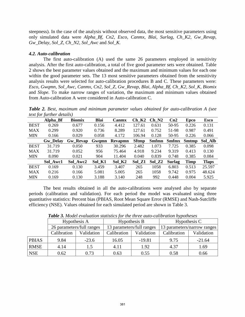
steepness). In the case of the analysis without observed data, the most sensitive parameters using only simulated data were Alpha_Bf, Cn2, Esco, Canmx, Blai, Surlag, Ch_K2, Gw_Revap, Gw_Delay, Sol_Z, Ch_N2, Sol_Awc and Sol_K. 4.2. Auto-calibration

The first auto-calibration (A) used the same 26 parameters employed in sensitivity analysis. After the first auto-calibration, a total of five good parameter sets were obtained. Table 2 shows the best parameter values obtained and the maximum and minimum values for each one within the good parameter sets. The 13 most sensitive parameters obtained from the sensitivity analysis results were selected for auto-calibration procedures B and C. These parameters were: Esco, Gwqmn, Sol_Awc, Canmx, Cn2, Sol_Z, Gw_Revap, Blai, Alpha_Bf, Ch_K2, Sol_K, Biomix and Slope. To make narrow ranges of variation, the maximum and minimum values obtained from Auto-calibration A were considered in Auto-calibration C. Table 2. Best, maximum and minimum parameter values obtained for auto-calibration A (see text for further details) Alpha_Bf Biomix Blai Canmx Ch_K2 Ch_N2 Cn2 Epco Esco BEST 0.269 0.677 0.156 4.412 127.61 0.631 50-95 0.226 0.131 MAX 0.299 0.920 0.736 8.289 127.61 0.752 51-98 0.987 0.491 MIN 0.166 0.029 0.058 4.172 106.94 0.128 50-95 0.226 0.066 Gw_Delay Gw_Revap Gwqmn Revapmn Sftmp Smfmn Smfmx Smtmp Sol_Alb BEST 31.719 0.050 933 30.296 2.482 1.073 7.725 0.385 0.098 MAX 31.719 0.052 956 75.464 4.918 9.234 9.319 0.413 0.130 MIN 8.090 0.021 904 11.404 0.040 0.839 0.748 0.385 0.084 Sol_Awc1 Sol_Awc2 Sol_K1 Sol_K2 Sol_Z1 Sol_Z2 Surlag Timp Tlaps BEST 0.169 0.130 3.459 3.407 265 1058 6.803 0.513 25.597 MAX 0.216 0.166 5.081 5.005 265 1058 9.742 0.975 48.624 MIN 0.169 0.130 3.188 3.140 248 992 0.448 0.004 5.925

The best results obtained in all the auto-calibrations were analysed also by separate periods (calibration and validation). For each period the model was evaluated using three quantitative statistics: Percent bias (PBIAS, Root Mean Square Error (RMSE) and Nash-Sutcliffe efficiency (NSE). Values obtained for each simulated period are shown in Table 3.

Table 3. Model evaluation statistics for the three auto-calibration hypotheses Hypothesis A Hypothesis B Hypothesis C 26 parameters/full ranges 13 parameters/full ranges 13 parameters/narrow ranges

Calibration Validation Calibration Validation Calibration Validation PBIAS 9.84 -23.6 16.05 -19.81 9.75 -21.64 RMSE 4.14 1.5 4.11 1.92 4.37 1.69 NSE 0.62 0.73 0.63 0.55 0.58 0.66

381

0

30

60

90

120

1/1/2009 1/31/2009 3/2/2009 4/1/2009 5/1/2009 5/31/2009 6/30/2009 7/30/2009 8/29/2009 9/28/2009 10/28/2009 11/27/2009 12/27/2009

Dai

ly S

tream

flow

, mm

0

30

60

90

120

Dai

ly R

ainf

all,

mm

Daily Rainfall, mm

Daily Observed Flows, mm (Calibration period)

Auto-calibration A: Daily Simulated Flows, mm (Calibration period)

0

30

60

90

120

1/1/2009 1/31/2009 3/2/2009 4/1/2009 5/1/2009 5/31/2009 6/30/2009 7/30/2009 8/29/2009 9/28/2009 10/28/2009 11/27/2009 12/27/2009

Dai

ly S

tream

flow

, mm

0

30

60

90

120

Dai

ly R

ainf

all,

mm

Daily Rainfall, mmDaily Observed Flows, mm (Calibration period)Auto-calibration B: Daily Simulated Flows, mm (Calibration peri

0

30

60

90

120

1/1/2009 1/31/2009 3/2/2009 4/1/2009 5/1/2009 5/31/2009 6/30/2009 7/30/2009 8/29/2009 9/28/2009 10/28/2009 11/27/2009 12/27/2009

Dai

ly S

tream

flow

, mm

0

30

60

90

120

Dai

ly R

ainf

all,

mm

Daily Rainfall, mmDaily Observed Flows, mm (Calibration period)Auto-calibration C: Daily Simulated Flows, mm (Calibration period)

Figure 3. Observed and simulated flows during calibration period (01/01/2009 - 31/12/2009) for each auto-calibration

The best PBIAS results from the calibration period in Serra de Cima were obtained for Auto-calibrations C and A which reached the range of very good values and indicated an underestimation bias. Auto-calibration B also shows underestimation bias but in this case with satisfactory values. During the validation period, the PBIAS values were negative for all the data sets and lowest in Auto-calibration B. In general, all results indicate satisfactory or better model performance. Bias towards underestimation of the observed values for the calibration period and bias towards overestimation for the validation period could be justified by the facts that: (i) a split-sample evaluation is used and (ii) the PBIAS values for stream-flow tend to vary more during dry years than during wet years (Gupta et al., 1999).

The NSE values for all six sets were above 0.5 both for the calibration and validation periods. However, the values for Auto-calibration A were slightly better. NSE within Auto-

382

calibrations A and C were higher for the validation period than for the calibration period, which was not expected. Compared to previous studies with SWAT (Santhi et al., 2001; Saleh et al., 2000), the NSE values obtained here indicate adequate model performance in most instances (NSE = 0.54 - 0.65) and very good performance (NSE > 0.65) for the validation periods of Auto-calibrations A and C.

In the present case, the best RMSE values for the calibration period were for auto-calibrations B and A with RMSE values slightly above the satisfactory threshold (SD = 6.72) which however can also be considered a low RMSE. For the validation period, RMSE was better in Auto-calibrations A and C with low values indicating good model performance.

During the year 2009, the observed runoff in the catchment was 838 mm including a total of 98 days without data due to technical problems, 61 during the dry season corresponding to low or no flows in the catchment. Missing data were reconstructed using the best model results, and the annual runoff in the catchment resulted in 1,004 mm (annual runoff coefficient = 63%). The best simulation results from the same year were 921 mm of annual runoff (annual runoff coefficient = 58%). As can be observed in Figure 3, important differences between the observed and simulated data occur. There were some rainfall events between March and October 2009 with poor or no hydrologic response from the catchment. The rainfall between March and October 2009 was 329 mm and the observed runoff 15 mm, while the simulated runoff was 122 mm. In this year, from March to October the rainfall events within the study area could be insufficient to generate runoff due to the dry conditions in the catchment.

There is also a lack of data in 2010 for observed runoff (in this case 12 days at the beginning of the year). These data were also reconstructed using simulated flows in the same way as those in the previous year. After that, the annual runoff observed was 671 mm (annual runoff coefficient of 49%). Best model results for this year were 813 mm (annual runoff coefficient of 59%). During the dry season, the same behaviour as the previous year was observed with poor or no hydrologic response from the catchment (Figure 4).

383

0

20

40

60

01/01/10 01/31/10 03/02/10 04/01/10 05/01/10 05/31/10 06/30/10 07/30/10 08/29/10 09/28/10 10/28/10 11/27/10 12/27/10

Dai

ly S

tream

flow

, mm

0

20

40

60

80

100

120

140

160

180

200

Dai

ly R

ainf

all,

mm

Daily Rainfall, mmDaily Observed Flows, mm (Validation period)Auto-calibration A: Daily Simulated Flows, mm (Validation period

0

20

40

60

01/01/10 01/31/10 03/02/10 04/01/10 05/01/10 05/31/10 06/30/10 07/30/10 08/29/10 09/28/10 10/28/10 11/27/10 12/27/10

Dai

ly S

tream

flow

, mm

0

20

40

60

80

100

120

140

160

180

200

Dai

ly R

ainf

all,

mm

Daily Rainfall, mmDaily Observed Flows, mm (Validation period)Auto-calibration B: Daily Simulated Flows, mm (Validation period

0

20

40

60

01/01/10 01/31/10 03/02/10 04/01/10 05/01/10 05/31/10 06/30/10 07/30/10 08/29/10 09/28/10 10/28/10 11/27/10 12/27/10

Dai

ly S

tream

flow

, mm

0

20

40

60

80

100

120

140

160

180

200

Dai

ly R

ainf

all,

mm

Daily Rainfall, mmDaily Observed Flows, mm (Validation period)Auto-calibration C: Daily Simulated Flows, mm (Validation period

Figure 4. Observed and simulated flows during validation period (01/01/2010 - 31/12/2010) for each auto-calibration

Analysing these results, important differences can be observed between simulated and observed data that can be attributed to differences in patterns and amounts of rainfall recorded between the selected climate station and the study catchment. This could highlight the importance of local input data, mainly rainfall, to obtaining good modelling results at this scale.

5. Conclusions

Auto-calibrations using different numbers of parameters and different ranges of variation

for these parameters produced the best results for the set with the largest number of parameters and the widest ranges of variation. Nonetheless, sensitivity analysis was helpful in reducing the

384

number of parameters included in the auto-calibration and, thereby, auto-calibration time without seriously affecting model results. The use of narrow ranges of variation for the parameters also reduced the time needed for auto-calibration while still producing results that can be regarded as adequate, especially for general-purpose studies.

In this study, only the quantitative statistics from total stream flow were analysed, without taking into account the fact that several parameter sets have given good results indicating a possible problem with equifinality of model parameterization. Future work will address this issue and will take into account other water balance components than total stream-flow.

Ongoing work is focused on testing SWAT with data obtained from a meteorological station in the study area as well as from fieldwork in the Serra de Cima catchment; this work is aimed at improving model results and decreasing problems related to equifinality. References Arnold J.G., Srinivasan, R., Muttiah R.S. and Williams J.R. 1998. Large area hydrologic modeling and

assessment, Part I: model development. Journal of the American Water Resources Association 34, pp. 73-89

Beven K. 2000. Rainfall-Runoff Modelling – The Primer. John Wiley & Sons, Chichester. Gan, T. Y., Dlamini, E. M. and Biftu, G. F. 1997. Effects of model complexity and structure, data quality,

and objective functions on hydrologic modeling. Journal of Hydrology 192(1): 81-103. Gupta, H. V., Sorooshian, S. and Yapo, P. O. 1999. Status of automatic calibration for hydrologic models:

Comparison with multilevel expert calibration. J. Hydrologic Eng. 4(2): 135-143. Moriasi, D.N., Arnold, J. G., Van Liew, M. W., Bingner, R. L., Harmel, R. D. and Veith, T. L. 2007.

Model evaluation guidelintes for systematic quantification of accuracy in watershed simulations. Transactions of the ASABE. Vol. 50(3): 885−900.

Nash, J.E. and Sutcliffe J.V. 1970. River Flow Forecasting Through Conceptual Models – Part I: A

Discussion of Principles. Journal of Hydrology 10(3):282-290 Nunes J.P., Seixas J., Pacheco N.R. 2008. Vulnerability of water resources, vegetation productivity and

soil erosion to climate change in Mediterranean watersheds. Hydrological Processes. 22, 16, 3115-3134

Saleh, A., Arnold, J. G., Gassman, P. W., Hauk, L. M., Rosenthal, W. D., Williams, J. R. and

MacFarland, A. M. S. 2000. Application of SWAT for the upper North Bosque River watershed. Trans. ASAE 43(5): 1077-1087.

Santhi, C., Arnold, J. G., Williams, J. R., Dugas, W. A., Srinivasan, R. and Hauck, L. M. 2001.

Validation of the SWAT model on a large river basin with point and nonpoint sources. J. American Water Resources Assoc. 37(5): 1169-1188.

Singh, J., Knapp, H. V. and Demissie, M. 2004. Hydrologic modeling of the Iroquois River watershed

using HSPF and SWAT. ISWS CR 2004-08. Champaign, Ill.: Illinois State Water Survey. Tuinenburg, O.A., Keizer J.J., Verzandvoort S.J.E., Stolte, J., Coelho, C.A. and Ferreira, A.D. 2006.

Rainfall-runoff modeLling using lisem in small forested catchments in north-central Portugal: a

385

stepwise monte-carlo approach for coping with uncertanties in model input maps. ERB2006 Conference “Uncertainties in the ‘monitoring-conceptualisation-modelling’ sequence of catchment research” (Luxembourg; 20-22/09/2006).

van Griensven, A. and Meixner, T. 2006. Methods to quantify and identify the sources of uncertainty for

river basin water quality models. Water Science and Technology, 53(1):51-59 van Griensven, A. and Meixner, T. 2007. A global and efficient multi-objective auto-calibration and

uncertainty estimation method for water quality catchment models. Journal of Hydroinformatics 9:4 277-291.

386

Upgrading the Grid-Based Discretization Scheme in SWAT

Hendrik Rathjens, Natascha Oppelt

Kiel University, Department of Geography, Ludewig-Meyn-Str. 14, 24098 Kiel, Germany

Abstract

For modeling purposes a watershed has to be spatially discretized. Because of the routing command language implemented in SWAT, it is theoretically possible to model a watershed based on either grid cells or representative hill slopes or by partition into sub-watersheds. All current interfaces use sub-watershed discretization which divides a watershed into subbasins based on topographic features and management practices. The sub-watershed discretization scheme is unable to account for spatial variability within a watershed, and for large watersheds currently there is no interface available generating the SWAT input files based on grid cells. A grid-based model approach has been developed. “SWATgrid” has successfully accomplished the first model runs using SWAT test data sets. First, a watershed configuration file is generated by processing a digital elevation model using TOPAZ (TOpograpic PArametriZation, version 3.1). Then the remaining SWAT input files are created using grid-based data. Thus, SWATgrid enables a conservation of detailed spatial information such as remote sensing data. In this paper, the functioning of SWATgrid will be demonstrated by comparing results of SWATgrid with conventional SWAT model results and the development of the grid-based discretization scheme will be presented. The paper focuses on the performance, problems and advantages of grid-based discretization within SWAT. Keywords: grid cell, grid-based, discretization scheme, SWATgrid, model interface

387

1. Introduction

Simulation of hydrological balance is essential for watershed applications, and SWAT has proved to be very useful under many simulation conditions (Gassman et al., 2007). Nevertheless, accurate input data often are neither available nor accessible, thus model interfaces were developed to prepare the input data. The first step in setting up a watershed simulation is to discretize the watershed spatially, i.e. define the spatial arrangement of the watershed elements such as subbasins, reach segments and point sources (Neitsch et al., 2010). Due to its computational efficiency and the possibility of implementing it in Geographic Information Systems (GIS) software (ArcGIS; Winchell et al., 2010) and MapWindow (George and Leon, 2008), the sub-watershed configuration turned out to be the most common technique. However, during this process spatial information given by grid files, such as land use or soil maps, is lost.

Remote sensing and GIS provide an increasing amount of spatial detail, which partly is lost when this data is generalized by using the sub-watershed configuration. Nevertheless, the need to derive spatially detailed model input is high (Arnold et al., 2010). Currently, remote sensing data is used to obtain land use maps (Pandey et al., 2005; Ouyang et al., 2010; Xue et al., 2008), management practices (Quansah et al., 2008; White et al., 2010) and climate data (Yan et al., 2010; Immerzeel and Droogers, 2008; Xie and Zhang, 2010).

Arnold et al. (2010) suggest that simple routing methods as well as complex landscape representations can be calibrated with a minimum of spatial discretization. They also mention a need for a more adequate spatial mapping of watersheds during simulation, because generalizing discretization schemes often are less reliable to changes in land use, soil or weather conditions and therefore need to be re-calibrated for every scenario. SWATgrid is a model interface that sets up SWAT based on grid cells, and it was developed to overcome the difficulty of spatial generalization. The current version of SWATgrid has accomplished first runs successfully. The functionality is demonstrated by comparing conventional SWAT (ArcSWAT 2009.93.5 for SWAT 2009) model results and the results of the grid-based approach (SWATgrid, see Rathjens and Oppelt, 2011).

This paper deals with the advantages, difficulties and challenges of the grid-based SWAT approach which are figured out by interpretation of results of both SWAT architecture and model set-ups. The functioning of SWATgrid is explained as well as SWAT’s handling of spatial discretization. Major results and suggestions for further research are presented. 2. Discretization Schemes

Some facts have to be mentioned to demonstrate the loss of spatial information when using the Sub-Watershed Discretization (SWD) scheme. Neitsch et al. (2010) list three techniques to discretize a watershed: the grid cell, the representative hillslope and the sub-watershed configuration. All schemes have specific strengths and weaknesses, but the grid cell scheme is most appropriate for implementing spatial detail into a simulation (Arnold et al., 1994). The SWAT routing command language enables the use of each scheme, but due to the limited availability of proper interfaces most SWAT users choose the sub-watershed configuration.

SWAT divides the hydrological cycle of a watershed into two major phases: the land phase quantifies the flow of water, sediments, nutrients and pesticides of the subbasins entering

388

the reach, and the routing phase determines the movement of the loadings through the channel network of the watershed to the outlet (Neitsch et al., 2005).

SWD divides the watershed into a number of sub-watersheds or subbasins based on topographic features. A subbasin contains at least one Hydrologic Response Unit (HRU) and a main channel or reach. The subbasins represent the first level of spatial discretization. They have a defined position in the watershed, and they are spatially related to one another. They are the smallest unit within a watershed having spatial information and topographic attributes like slope, slope length or channel width. These parameters are calculated or averaged at subbasin level (Neitsch et al., 2010). A subbasin has usually a size greater than that of a grid cell; thus, during processing each subbasin partly loses spatial information given by those grid cells. Figure 1 shows a typical SWD of the SWAT example data set (Winchell et al., 2010). The subbasins have an averaged area of 2.705 ha while the grid cells have a size of 1 ha each.

The land area of a subbasin may be divided into HRUs which represent a part of a subbasin with similar land use, management and soil attributes. Although areas with specific attributes may be scattered throughout a subbasin, they might be combined to form one HRU. Thus, this concept may well describe the heterogeneity of a subbasin, but the knowledge about the spatial distribution is lost. Loadings of each HRU are calculated separately and summed up to determine the total loading of the subbasin. SWAT passes these loadings to the associated reach segment of the channel network (Neitsch et al., 2010). Consequently, spatial model output is only available at the outlet of each subbasin.

The Grid Cell Discretization (GCD) enables consideration of spatial heterogeneity during simulation. The size of the grid cells should be sufficient to map spatial details important for the study. The subbasin is the smallest unit that includes information about its location. Increasing the number of subbasins is the only way to increase spatial variability during a SWAT simulation. Therefore, each grid cell is treated as a subbasin. Regarding Figure 1, there are 55,560 GCD subbasins in comparison to 18 SWD subbasins.

Figure 1. ArcSWAT sub-watershed discretization (Lake Fork)

389

3. Methods

The ArcSWAT interface was used to prepare the conventional input data and SWATgrid for the grid-based approach. The ArcSWAT model set-up is explained by Winchell et al. (2010); Rathjens and Oppelt (2011) describe SWATgrid in detail. For both model runs, all parameters are set as described by Winchell et al. (2010). Some parameters such as trapezoidal channel dimension are not available in a spatially distributed form. Therefore, the SWD values have to be averaged and set as constants in the GCD model run. Thus, the model set-ups are equal except for the discretization scheme.

Since the SWAT test data set was used for this study, the study area is located at Lake Fork (Texas, US; Winchell et al., 2010; http://swatmodel.tamu.edu/software/arcswat). The data set includes raster data in the Albers Equal Area projection with a grid cell size of 100 m ×100 m such as a digital elevation model (DEM), a land use and a soil type map. Auxiliary data files include characteristic soil type parameters, management practices and vegetation parameters. Temperature and precipitation data is provided in a two-year series (01/01/1977 to 12/31/1978). Remaining weather parameters such as solar radiation, wind speed or relative humidity are computed using the SWAT weather generator (Neitsch et al., 2005). 3.1. SWATgrid

SWATgrid is a command line-based interface preparing SWAT data to set up the grid-based discretization scheme. The program is written in Fortran 90. In the current version (1.0), many parameters are set as constant values in the program code. Up to now SWATgrid contains three tools: “SWATgrid_fig” generates the watershed configuration file using the digital landscape analysis tool TOPAZ (TOPographic PArametriZation, version 3.1, see Garbrecht and Martz [2000]) which provides drainage characteristics; “SWATgrid_inp” prepares the remaining input files (.hru, .mgt, .pnd, .rte, .sub, .swq, .wus) using raster data. Program functionality and performance as well as required input data are explained in detail by Rathjens and Oppelt (2011). Due to the large number of subbasins being defined, the SWAT 2009 code had to be slightly modified, e.g. in modparm.f, the dimensions of hydgrp, kirr and snam have to be set to the number of subbasins used for a simulation.

The third tool, “SWATgrid_out,” generates maps of SWAT spatial output parameters which are stored in the output files output.hru, output.sup and output.rch. The tool uses the watershed boundary generated by TOPAZ and the algorithms of SWATgrid_fig. The generated maps can directly be visualized and post-processed in ArcGIS. 4. Results and Discussion

In this section, grid-based model results of the test data set are summarized and compared to conventional model results. Differences between the model runs and output parameters are discussed. 4.1. Model set-ups

The SWD scheme divided the watershed into 18 subbasins (see Figure 1) and 128 HRUs. When using the SWATgrid input data, the basin is discretized into 55,560 subbasins (100 m × 100 m) containing one HRU each. This demonstrates an enhanced representation of existing heterogeneities and their spatial relationships using SWATgrid. Regarding the ArcSWAT basin

390

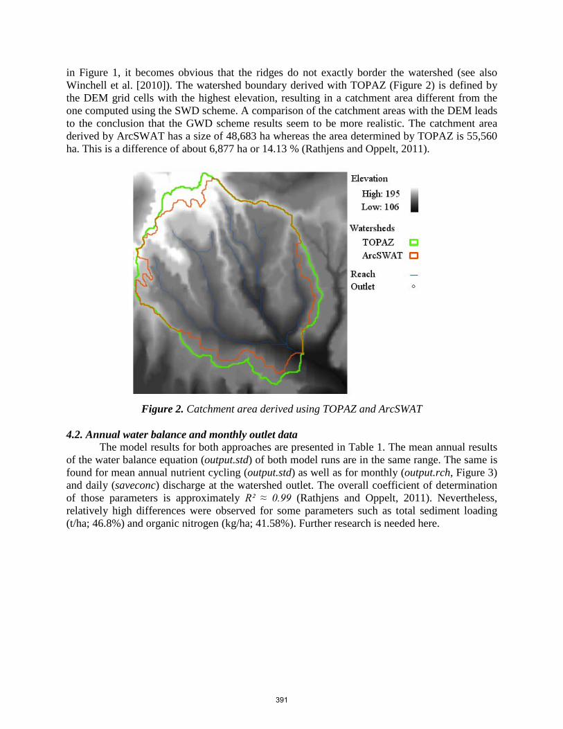
in Figure 1, it becomes obvious that the ridges do not exactly border the watershed (see also Winchell et al. [2010]). The watershed boundary derived with TOPAZ (Figure 2) is defined by the DEM grid cells with the highest elevation, resulting in a catchment area different from the one computed using the SWD scheme. A comparison of the catchment areas with the DEM leads to the conclusion that the GWD scheme results seem to be more realistic. The catchment area derived by ArcSWAT has a size of 48,683 ha whereas the area determined by TOPAZ is 55,560 ha. This is a difference of about 6,877 ha or 14.13 % (Rathjens and Oppelt, 2011).

Figure 2. Catchment area derived using TOPAZ and ArcSWAT

4.2. Annual water balance and monthly outlet data

The model results for both approaches are presented in Table 1. The mean annual results of the water balance equation (output.std) of both model runs are in the same range. The same is found for mean annual nutrient cycling (output.std) as well as for monthly (output.rch, Figure 3) and daily (saveconc) discharge at the watershed outlet. The overall coefficient of determination of those parameters is approximately R² ≈ 0.99 (Rathjens and Oppelt, 2011). Nevertheless, relatively high differences were observed for some parameters such as total sediment loading (t/ha; 46.8%) and organic nitrogen (kg/ha; 41.58%). Further research is needed here.

391

Table 1. SWD and GCD model results of the Lake Fork watershed SWD GCD Area 48683 ha 55560 ha Number of subbasins 18 55560 Average subbasin area size 2705 ha 1 ha Number of HRUs 128 55560 Length of reach network 195.32 km 6350.58 km Trapezoidal channel dimensions Variable Constant Mean annual total aquifer recharge 144.60 mm 168.56 mm Mean annual transmission losses 2.06 mm 29.29 mm Mean two-year runoff 8.89 m³/s 9.03 m³/s

Figure 3. Modelled mean monthly discharge for SWD- and GCD-based model runs (Rathjens and Oppelt, 2011)

Figure 3 indicates that, although monthly results fit quite well, the GCD computes larger runoff values than the conventional approach. The GCD watershed is 14% larger than the ArcSWAT basin, but the mean two-year runoff differs only by about 0.78% or 0.14 m³/s. The larger GCD basin area seems to be compensated by the transmission losses and the aquifer recharge parameters (see Table 1). Figure 3 supports this assumption: at peak runoff, the GCD discharge is significantly larger than the SWD discharge while being even lower at some of the low water events.

Each GCD subbasin contains at least one reach segment where the loadings are passed through. Fluxes between the subbasins are computed in the routing phase. Therefore, interaction between subbasins only occurs at the reach. However, if the edge length of a grid cell is shorter than the distance to the nearest watercourse, this method will probably provide inaccurate results, especially for sediment or nutrient transport. This problem might be solved by modifying the

392

SWAT code to enable substance transport between the subbasins at the land phase. Besides the lack of subbasin interaction, allocation of at least one reach to each subbasin results in an overestimation of the total length of the reach network. In this study the ArcSWAT reach network has an overall length of 195.32 km versus 6350.58 km for the grid-based approach.

In this context, the derivation of a spatially variable trapezoidal reach dimension is another challenge. This task could be solved by setting the dimension in functional dependencies to the number of upstream cells draining into each grid cell. These parameters are not available spatially for the test data, so they have been set as average values of the conventional model run. The facts mentioned above result in an overestimation of transmission losses which implies an overestimation of the aquifer recharge. The total GCD-based aquifer recharge is 23.96 mm larger than the SWD-based aquifer recharge. This difference is similar to that for the transmission losses, i.e. 27.23 mm (see Table 1).

4.3. Spatial output

Besides considering spatially variable input data during simulation, obtaining spatial model output with the same spatial resolution as the grid input data is a great advantage of GCD. SWATgrid_out maps any SWAT output parameter which is spatially available. Figure 4 shows the spatially distributed output of four parameters, i.e. evapotranspiration, discharge and number of nitrogen stress days. The model is not calibrated at this stage, so the maps could not be evaluated quantitatively. The spatial distribution of the output values displays the impact of land use classes, soil types, and the digital elevation model. Comparing Figure 4 and the SWD shown in Figure 1, it becomes obvious that the output parameters are not distributed homogeneously within the subbasins.

The actual evapotranspiration during December 1977 and July 1978 is mapped in Figure 4c and 4d. Its spatial distribution demonstrates the influences of land cover (transpiration, Figure 4a) and soil types (evaporation, Figure 4b) on this parameter. While land cover dominates actual evapotranspiration during the period of plant growth (Figure 4d), features of soil types determine actual evapotranspiration during the winter. The maps seem to provide a realistic distribution because type and condition of vegetation as well as soil water content and temperature strongly affect evapotranspiration.

Figure 4e shows the dependency of land use (Figure 4a) on the number of nitrogen stress days. There is certainly no nitrogen stress at water surfaces (land use class WATR). A similar behavior is found for corn-growing acreage (AGRL) which is most probably due to fertilizer applications as the arithmetic mean of stress days in this area is 5.0 days. The number of days rises in forested areas (FRSD, mean: 45.7, minimum: 1, maximum: 100) while the maximum values (mean: 116, minimum: 112, maximum: 119) are located at pastures (PAST).

The modeled discharge for June 1978 (Figure 4f) indicates a stream network. Obviously, the digital elevation model determines the spatial distribution of discharge. The SWD reach network (Figure 1) and the GCD discharge results show a concordant behaviour.

393

Figure 4. Subset of spatially distributed SWATgrid output parameters

394

5. Conclusion

The command line-based model interface SWATgrid enables the user to set up SWAT based on grid cells. It is a semi-automatic tool for creating the input files required to run SWAT 2009. The general performance of SWATgrid has been proven by comparing conventional model results with the grid-based approach which fit together well. The overall coefficient of determination of mean daily and monthly parameters of the water equation, as well as values describing the nutrient cycling, are about 0.99 (Rathjens and Oppelt, 2011).

Due to the rapid development of GIS and remote sensing, an increasing amount of spatially and temporally detailed data becomes available. The integration of these data into well-established eco-hydrological models seems to be very promising for enhanced spatial analysis of environmental issues within a watershed. Therefore, the challenges and problems inherent to the grid-based approach seem to be justified.

SWAT was primarily designed for the SWD approach, so some of the problems described are caused by the model architecture. Besides the improvement of SWATgrid into a user-friendly tool, some aspects should be considered. The next steps and further developments necessary are mentioned in the following. 5.1. Memory requirements and computation time

Obviously the grid based approach results in a massive increase of computation time. This is caused by the multiplicative number of calculations that have to be done at subbasin and HRU level (see Table 1). While the SWD model run takes less than four seconds per year on a 2.67 GHz processor, the GCD scheme lasts about five hours per year. Arnold et al. (2010) state that a simulation of the Upper Mississippi River basin using a one-hectare grid (nearly 50,000,000 grid cells) would require about 13 days per year of simulation. In this context, parallel processing would be an option to significantly decrease processing time.

The memory requirement is another great challenge which has to be dealt with. SWAT input parameters are transferred by various input files. For some parameters such as subbasin elevation (m) (.sub) or channel width-depth ratio (.rte) it is necessary that each subbasin, HRU or reach obtains data from a specific input file. Thus, SWATgrid computes a large number of input files, which makes a model set-up complicated. This problem could be faced by the development of an alternative data transfer method.

5.2. Interactions between subbasins

Every SWAT subbasin contains at least one main reach or channel (Neitsch et al., 2005). As mentioned before, the edge length of a grid cell is often shorter than the distance to the nearest watercourse. The current version of SWAT does not allow sediment, runoff and other loadings to interact between cells by using the land-phase. Therefore, interaction between the grid cells is part of the routing phase. Thus, the GCD model setup may provide inaccurate results of sediment transport and nutrient cycling parameters.

However, to enable interaction between the subbasins by using the land-phase, modifications of the SWAT code and the routing command language are necessary. Arnold et al. (2010) developed a command routing structure similar to the sub-watershed routing (Neitsch et al., 2010) which enables an overland routing fraction. Currently, the new developed routing method is used in a modified version of SWAT but might be implemented in one of the next

395

SWAT versions. This would simplify the solution of flux interaction concerning transmission losses, sediment transport and nutrient cycling. 5.3. Channel dimensions and reach network

As mentioned above, each subbasin contains at least one main channel or reach. This results in an overestimation of the reach network length and causes transmission losses (Rathjens and Oppelt, 2011). The trapezoidal channel dimensions are currently not available spatially but could be calculated in functional dependencies of the number of upstream cells draining into the current cell. However, errors due to the overestimation of the reach network length, and thus the overestimation of transmission losses and aquifer recharge terms might only be avoided or minimized when interaction between subbasins at the land phase becomes possible. References Arnold, J.G., R. Srinivasan, B.A. Engel. 1994. Flexible watershed configurations for simulation models.

Hydrolog. Sci. Tech. 10(1-4): 1-9 Arnold, J.G., P.M. Allen, M. Volk, J.R. Williams and D.D. Bosch. 2010. Assessment of different

representations of spatial variability on SWAT model performance. T. ASABE 53(5): 1433-1443. Garbrecht, J. and L. Martz. 2000. TOPAZ - Version 3.1 User Manual. National Agricultural Water

Quality Laboratory, USDA, Agricultural Research Service, El Reno, Oklahoma. Gassman, P.W., M.R. Reyes, C.H. Green and J.G. Arnold. 2007. The Soil and Water Assessment Tool:

Historical Development, Applications and Future Research Directions. T. ASABE 50(4): 1211–1250.

George, C. and L.F. Leon. 2008. WaterBase: SWAT in an open source GIS. The Open Hydrology Journal

1: 19 – 24. Immerzeel, W.W. and P. Droogers. 2008. Calibration of a distributed hydrological model based on

satellite evapotranspiration. J. Hydrol. 349(3-4): 411–424. Neitsch, S.L., J.G. Arnold, J.R. Kiniry, R. Srinivasan and J.R. Williams. 2010. Soil and Water Assessment

Tool Input/Output File Documentation. Texas Water Resources Institute, College Station, Texas. Neitsch, S.L., J.G. Arnold, J.R. Kiniry and J.R. Williams. 2005. Soil and Water Assessment Tool

Theoretical Documentation. Texas Water Resources Institute, College Station, Texas. Ouyang, W., A.K. Skidmore, A.G. Toxopeus and F. Hao. 2010. Long-term vegetation landscape pattern

with non-point source nutrient pollution in upper stream of Yellow River basin. J. Hydrol. 389(3-4): 373–380.

Pandey, V.K., S.N. Panda and S. Sudhakar. 2005. Modelling of an agricultural watershed using remote

sensing and a geographic information system. Biosyst. Eng. 90(3): 331–347. Quansah, J.E., B.A. Engel and I. Chaubey. 2008. Tillage practices usage in early warning prediction of

atrazine pollution. T. ASABE 51(4): 1311–1321.

396

Rathjens, H. and N. Oppelt. 2011. SWATgrid: An interface for setting up SWAT in a grid-based discrezitation scheme. Comput. Geosci., submitted

White, M., D. Storm, P. Busteed, S. Stoodley and S. Phillips. 2010. Evaluating Conservation Program

Success with Landsat and SWAT. Environ. Manage. 45(5): 1164-1174. Winchell, M., R. Srinivasan, M. Di Luzio and J.G. Arnold. 2010. ArcSWAT Interface for SWAT 2009:

User’s Guide. Texas Agricultural Experiment Station, Texas, and USDA Agricultureal Research Service, Temple, Texas

Xie, X. and D. Zhang. 2010. Data assimilation for distributed hydrological catchment modeling via

ensenble Kalman filter. Adv. Water Resour. 33(6): 678–690. Xue, B., K. Ma, L. Yang, Z. Jieyu and Z. Xiaolei. 2008. Differences of ecological functions inside and

outside the wetland nature reserves in Sanjiang Plain, China. Acta Ecologica Sinica 28(2):620 – 626.

Yan, E., A. Milewski, M. Sultan, A. Abdeldayerm, F. Soliman and K.A. Gelil. 2010. Remote-Sensing

Based Approach to Improve Regional Estimation of Renewable Water Resources for Sustainable Development. In US–Egypt Work-shop on Space Technology and Geo–information for Sustainable Development, Cairo, Egypt.

397

Reduction of Peak Streamflow as a Result of Vegetation Rehabilitation in the “Yesos of Barrachina” Protected Area

Jiménez, L. Asociación de Ciencias Ambientales (ACA), Ctra Madrid-Barcelona K.33 (Facultad) 28805,

Alcalá de Henares (Madrid), ljm310879@hotmail.com

Morales, M. Centro de Estudios del Jiloca (CEJ), C/. Castellana, 39. 44200 Calamocha (Teruel).

Sanz, T.

Centro de Estudios del Jiloca (CEJ), C/. Castellana, 39. 44200 Calamocha (Teruel).

Bellido, M.T. Centro de Estudios del Jiloca (CEJ), C/. Castellana, 39. 44200 Calamocha (Teruel).

Abstract The objective of this study was to evaluate the impact of vegetation rehabilitation in the “Yesos of Barrachina” protected area of Spain using a modelling approach. The SWAT model was applied in the Jiloca watershed. We present the Pancrudo subbasin results where the protected area is located. The model was calibrated for monthly streamflow using a ten-year data record obtained in three monitoring stations (NSE between 0.52 and 0.63; RSR between 0.60 and 0.69 and PBIAS between 5.27 and 22.67). The model simulated streamflow successfully in the Pancrudo River when the rainfall events were generated by active Atlantic fronts. However, high intensity convective thunderstorms were not captured by the model. The calibration scenario represents conditions of the subbasin prior to the implementation of rehabilitation treatments, while the “Vegetation” scenario represents the conditions of the watershed after a simulated rehabilitation process. Mean streamflow in the “Vegetation” scenario was 26% lower (0.022 m3 s-1) than in pre-treatment conditions. For the events generated by active Atlantics fronts, the daily streamflow was 83% lower (5.194 m3 s-1). For the estimated high intensity convective events, daily streamflow was 37% lower (1.433 m3 s-1). Overall, our results reflected a reduction of the peak streamflow as a result of vegetation rehabilitation. Keywords: peak streamflow, rehabilitation, storm, SWAT model.

398

1. Introduction

The use of watershed computer models lets us know the functionality of complex hydrologic systems. In a catchment, it is difficult to predict the effect generated by a specific management practice in the whole system. If we previously asses specific effects, we can save money and time. Hydrological models such as SWAT enable the assessment process. Model calibration is difficult due to the high quantity of parameters used and the interactions between them. However, if the model is satisfactorily calibrated, assessment of management scenarios can be made easily. In this paper, we present the SWAT calibration results in the Jiloca watershed and the vegetation rehabilitation results in the Pancrudo subbasin.

Therefore, the main objective of this paper is to evaluate the impact of a simulated vegetation rehabilitation process in the “Yesos of Barrachina” protected area on its catchment streamflow using a modelling approach. 2. Material and Methods 2.1. Study area description

The Jiloca watershed is located in Zaragoza and Teruel provinces, Spain (Figure 1). The Jiloca River has its source in the Ojos de Monreal site (Monreal del Campo village) and flows into the Jalon River (Caltayud village), a tributary of Ebro River. The Pancrudo River is the only tributary of the Jiloca River.

Figure 1. Jiloca watershed location

The Jiloca River flows through a 126-km waterway and its catchment has a surface of 1,957 km2. The mean flow, near Calatayud, is 293 m3 year-1. The flow is

399

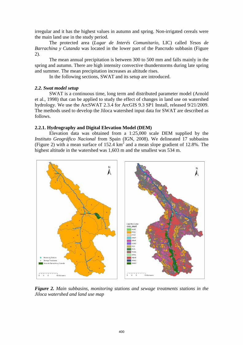
irregular and it has the highest values in autumn and spring. Non-irrigated cereals were the main land use in the study period.

The protected area (Lugar de Interés Comunitario, LIC) called Yesos de Barrachina y Cutanda was located in the lower part of the Pancrudo subbasin (Figure 2).

The mean annual precipitation is between 300 to 500 mm and falls mainly in the spring and autumn. There are high intensity convective thunderstorms during late spring and summer. The mean precipitation increases as altitude rises.

In the following sections, SWAT and its setup are introduced. 2.2. Swat model setup

SWAT is a continuous time, long term and distributed parameter model (Arnold et al., 1998) that can be applied to study the effect of changes in land use on watershed hydrology. We use the ArcSWAT 2.3.4 for ArcGIS 9.3 SP1 Install, released 9/21/2009. The methods used to develop the Jiloca watershed input data for SWAT are described as follows. 2.2.1. Hydrography and Digital Elevation Model (DEM)

Elevation data was obtained from a 1:25,000 scale DEM supplied by the Instituto Geográfico Nacional from Spain (IGN, 2008). We delineated 17 subbasins (Figure 2) with a mean surface of 152.4 km2 and a mean slope gradient of 12.8%. The highest altitude in the watershed was 1,603 m and the smallest was 534 m.

Figure 2. Main subbasins, monitoring stations and sewage treatments stations in the Jiloca watershed and land use map

400

2.2.2. Land Use/Land Cover We generated a land use map using the Mapa de Cultivos y Aprovechamientos

(MCA), scale 1:50,000 (MARM, 2008). We reclassified the categories from the MCA, assigning the SWAT land use classification (Table 1 and Figure 2). Table 1. Land use codes used for SWAT, MCA, land use types and percentage of area in the Jiloca watershed Code land use SWAT Land use type Percentage (%) Code land use MCA.

OCRD Orchard 0.63 ME, CE, CI, MA, PE ALMD Almonds 1.93 AL, NO, AL+V WWHT Winter wheat 5.41 CH TOMA Tomato 0.08 H, H+CH GRAP Vineyard 1.83 V WBAR Winter barley 40.77 L OLIV Olives 0 OL WPAS Winter pasture 0.33 P GRAR Grarigue 28.06 M, P/M FRSE Forest evergreen 3.45 PH POPL Poplar 0.57 PO FRSD Forest deciduous 15.38 QI

URML Residential-med/low density 1.55 I

2.2.3. Soils

We generated a soil map using the Soil European Map (scale 1:1,000,000) that is distributed by the Joint Research Centre (JRC) of the European Commission (2006a). We added the soil parameters in the tables of the ArcSWAT software. The physical and chemical properties of each soil type were obtained from the JRC European soil profiles database (JRC, 2006a and b).

2.2.4. Hydrologic Response Units (HRUs)

The slope classes used for this process were 0% to 5%, 5% to 15%, and 15% and above, resulting in 1438 HRUs. However, using a threshold operation of 15% for land use, soil, and slope reduced the number of HRUs to 197.

2.2.5. Weather

We used the daily precipitation and mean air temperature recorded in six gauges distributed at different heights in the watershed. In addition, we used the daily wind speed and relative humidity of an additional gauge. No solar radiation gauge was available in the watershed, so we used the weather generation algorithms included in the ArcSWAT. It is very important to use complete precipitation series in all rain gauges. Therefore, we introduced weather data records between 1993 and 2002 into the model since almost all gauges had lots of data gaps in other time series. 2.2.6. Streamflow

We obtained all daily streamflow observation data from the Confederación Hidrográfica del Ebro (CHE, 2009) website. 2.2.7. Other input data

We did not include the Cañizar lake as a reservoir because it was drained during the study period.

We only included the Fuente de Cella spring as a point source because the water infiltrated into another watershed. The spring flow data were obtained from the Instituto

401

Geológico y Minero de España (IGME) (1995a and 1995b) and from SIAS (IGME, 2005).

We included the sewage treatment stations located in the Jiloca watershed. The mean streamflow measurements were obtained from the Instituto Aragonés del Agua (2010). 2.3. Model calibration and evaluation

This paper focuses on hydrologic simulation. We used three streamflow stations (Figure 2) to calibrate and validate the model in the Jiloca watershed. The first is located on the Jiloca River (Calamocha Station), the second on the Pancrudo River (Pancrudo Station) and the third is further downstream on the Jiloca River (Morata Station) (Figure 2). The model was calibrated and validated, taking into account the evaluation guidelines described by Moriasi et al. (2007).

We made a sensitivity analysis in each monitoring station to obtain the most sensitivity parameters for the model. These parameters were frequently modified during manual calibration using the tool present in ArcSWAT.

We modified the model parameters until the simulated streamflow was similar to the real measurements (CHE, 2009). The model was calibrated for monthly and yearly streamflow at the three monitoring stations using an eight-year data record (1993-2000). The model was validated for monthly and yearly streamflow in the three monitoring stations using a two-year data record (2001-2002). 2.4. Rehabilitation process.

The calibration scenario represents conditions of the Pancrudo subbasin, where the protected area is located, prior to the implementation of rehabilitation treatments while the “Vegetation scenario” represents the conditions of the watershed after a simulated rehabilitation process.

In order to simulate the rehabilitation process, the HRUs located in Subbasin 9 were reassigned as follows: (i) winter barley (WBAR) to grarigue (GRAR) and (ii) grarigue (GRAR) to forest deciduous (FRSD). The SWAT associated parameters (CN2, CAN_MAX, OV_N) were changed in Subbasin 9. The new values were obtained in the calibration process. 3. Results and Discusión

The objective of this paper was to evaluate the impact of a simulated vegetation

rehabilitation process in the Yesos of Barrachina y Cutanda protected area on its catchment streamflow using a modelling approach. 3.1. Sensitivity analysis

Table 2 shows most of the model sensitivity parameters obtained for the Jiloca watershed. Table 2. Sensitivity parameters obtained in ArcSWAT Monitoring station Pancrudo Calamocha Morata

Subbasin 9 8 2 Order 1 Cn2 Cn2 Cn2 Order 2 Gwqmn Gwqmn Gwqmn Order 3 Esco Esco Esco Order 4 Sol_AWC Sol_AWC Sol_AWC Order 5 Sol_z Sol_z Can_max

402

3.2. Model calibration Taking into account the evaluation guidelines described by Moriasi et al. (2007),

the model simulation for the Jiloca watershed can be judged as satisfactory (Table 3). Table 3. Annual and monthly data obtained in the evaluation of the Jiloca watershed Annual Monthly Monitoring stations (calibration scenarios) NSE RSR PBIAS

(%) NSE RSR PBIAS (%)

Acceptable limits (Moriasi et al. (2007) >0.5 <0.7 ± 25 >0.5 <0.7 ± 25

Pancrudo (no Storm) 0.67 0.57 19.3 0.52 0.69 18.83 Calamocha (no Storm) 0.54 0.68 5.27 0.63 0.60 5.27 Morata (no Storm) 0.45 0.74 21.9 0.58 0.64 22.67

In the province of Teruel, Moreno-de las Heras et al. (2010) differentiated four

categories of rainfall events: (i) Non-erosive rains, the most frequent events, that do not produce runoff, (ii) low intensity rains generated by non-active Atlantic fronts, which are the most frequent events that generate runoff, (iii) active Atlantic events that generate an important amount of runoff, and (iv) high intensity convective thunderstorms during late spring and summer that generate more runoff and are less frequent.

The Jiloca watershed model simulated streamflow adequately in the Pancrudo River when the rainfall events were generated by active or non-active Atlantics fronts. However, the events occasioned by high intensity convective thunderstorms were not detected by the model. In fact, although the flow gauge registered two peaks in the Pancrudo River (Figure 3), the rain gauges used in the area did not register the high intensity precipitation, and the model could not simulate correctly the runoff response. In general, the convective thunderstorms were generated in small areas and it is possible that the rain was not registered accurately.

0

0.5

1

1.5

2

19/08

/97

20/08

/97

21/08

/97

22/08

/97

23/08

/97

24/08

/97

25/08

/97

26/08

/97

27/08

/97

28/08

/97

29/08

/97

30/08

/97

Real Data (CHE) Calibration (Simulated Storm)

Calibration (No Storm) Vegetation Scenario Figure 3. Flow in the Pancrudo Station (m3 s-1) at 08/22/1997 and 06/06/1998

In order to evaluate the simulated process of vegetation rehabilitation and test its effect during convective thunderstorms, we added two precipitation storms (60 mm depth in 24 hours at 08/22/1997 and 06/06/1998) in a new calibration scenario: “simulated storm.” Near the study area, Moreno-de las Heras et al. (2010) registered storms with a mean I30 of about 30.2 mm h-1, and Peña et al. (2002) recorded summer storms that reached up to 100 mm in 24 hours. The measurements made by the

0

2

4

6

8

03/06/98

04/06/98

05/06/98

06/06/98

07/06/98

08/06/98

09/06/98

10/06/98

11/06/98

12/06/98

13/06/98

14/06/98

15/06/98

16/06/98

17/06/98

Real Data (CHE) Calibration (Simulated Storm)Calibration (No Storm) Vegetation Scenario

403

Confederación Hidrográfica del Ebro (CHE) were similar to the simulated streamflow obtained in the modelled storm scenario (Figure 3). The parameters calculated to evaluate the new calibration scenario were better. Table 4. Annual and monthly data obtained in the evaluation of the Pancrudo subbasin after adding the two convective thunderstorms Annual Monthly Monitoring stations (calibration scenarios) NSE RSR PBIAS

(%) NSE RSR PBIAS (%)

Acceptable limits (Moriasi et al. (2007) >0.5 <0.7 ± 25 >0.5 <0.7 ± 25

Pancrudo (simulated storm) 0.76 0.49 13.2 0.59 0.64 12.8 3.3. Rehabilitation process.

The calibration scenario (simulated storm) represents conditions of the subbasin prior to the implementation of rehabilitation treatments, while the “vegetation scenario” represents the conditions of the watershed after a simulated rehabilitation process. The flow data of the Pancrudo station are presented in Table 5. Table 5. Daily flow in the Pancrudo station and mean flow in the total period

Calibration

scenario (m3 s-1)

Vegetation scenario (m3 s-1)

Flow difference

(m3 s-1)

Percentage (%)

Active Atlantic fronts

01/08/1997 5.504 0.753 4.751 86.3 01/09/1997 7.090 1.453 5.637 79.5 Mean value 6.297 1.103 5.194 82.9

Convective thunderstorm

08/22/1997 1.844 1.167 0.677 36.7 06/06/1998 5.776 3.588 2.188 37.9 Mean value 3.810 2.378 1.433 37.3

Mean total period (1993-2002) 0.086 0.063 0.022 26.2

Mean streamflow in the “vegetation scenario” was 26% lower (0.022 m3 s-1) than in pre-treatment conditions. For the events generated by active Atlantic fronts, the daily streamflow was 83% lower (5.194 m3 s-1). For the estimated high-intensity convective events, daily streamflow was 37% lower (1.433 m3 s-1).

Vegetation rehabilitation reduced flow in the peaks generated by active Atlantic fronts and high intensity convective events, while the flows generated by weekly rains or non-rainy days were not modified substantially (Figure 3: see diagrams after peak). 4. Conclusion

Our results reflect a reduction in peak streamflow as a result of vegetation

rehabilitation. Acknowledgements This research was supported by Obra Social Caja Madrid, ADRI Jiloca-Gallocanta and INAEM Calamocha. The authors would like to thank the Centro de Estudios del Jiloca for logistical cooperation.

404

References Arnold, J.G., Srinivasan, R., Muttiah, R.S., Williams, J.R., 1998. Large area hydrologic

modeling and assessment Part I: model development. Journal of the American Water Resources Associatio. 34 (1): 73-89.

Confederación Hidrográfica del Ebro (CHE) (2009). Datos diarios de caudal en la cuenca del

Ebro. Available at: www.chebro.es/. Accessed 13 November 2009. Instituto Geológico y Minero de España (IGME). (1995a). Mapa Hidrogeológico de España y

memoria. Escala 1:200.000. Teruel (47:7-6). Ministerio de Industria y Energía. Instituto Geológico y Minero de España (IGME). (1995b). Mapa Hidrogeológico de España y

memoria. Escala 1:200.000. Daroca (40:7-5). Ministerio de Industria y Energía. Instituto Geológico y Minero de España (IGME). (2005). SIAS. Sistema de Información del

Agua Subterránea. Versión 1.0. Ministerio de Ciencia e Innovación. Instituto Aragonés del Agua (2010). Estaciones depuradoras en la Comunidad Autónoma de

Aragón. Available at: http://www.aragon.es/DepartamentosOrganismosPublicos/Organismos/Instituto- Aragonés-del-

Agua). Accessed 20 January 2010. IGN (2008). MDT25. Escala 1:25000. (MDT25©INSTITUTO GEOGRÁFICO NACIONAL

DE ESPAÑA.2008). JRC (Joint Research Centre). (2006a). The European Soil Database v2.0: Soil Geographical

Database of Eurasia at scale 1:1,000,000; SGDBE, v4 beta. European Commission. JRC (Joint Research Centre). (2006b). The European Soil Database v2.0: Soil Profile Analytical

Database of Europa (SPADBE), version 2.1.0.0. European Commission. MARM. (2008). Mapa de cultivos y aprovechamientos de España (MCA), escala 1:50.000.

Hojas: 540 Y 541. Moreno-de las Heras, M, Nicolau, J.M., Merino-Martín, L., Wilcox, B.P. (2010). Plot-scale

effects on runoff and erosion along a slope degradation gradient. Water Resources Research, 46: 1-12.

Peña, J. L., J. M. Cuadrat, and M. Sánchez (2002), El Clima de la Provincia de Teruel. Instituto

de Estudios Turolenses, Diputación Prov. de Teruel, Teruel, Spain.

405

Runoff and Soil Loss Prediction in a Vineyard Area at Very Detailed Scale using the SWAT Model: Comparison between

Dry and Wet Years

Ramos M.C.

Department of Environment and Soil Science. University of Lleida, Alcalde Rovira Roure 191, 25198 Lleida, cramos@macs.udl.es

Martínez-Casasnovas, J.A.

Department of Environment and Soil Science. University of Lleida Alcalde Rovira Roure 191, 25198 Lleida, j.martinez@macs.udl.es

Balasch J.C.

Department of Environment and Soil Science. University of Lleida Alcalde Rovira Roure 191, 25198 Lleida, cbalasch@macs.udl.cat

Abstract The present work shows an application of SWAT (ArcSWAT 2009.93.5) to map soil erosion at the watershed scale in the Penedés (NE Spain) in which important erosion problems are recorded. The main crop is vineyards, followed by cereals and olive trees. The main data sources were the detailed Soil Map of Catalonia, a 5 m resolution DEM and a crop/land use map derived from 2010 orthophotos. In addition, a 0.5 m multispectral image of a reference vineyard was acquired at the end of July 2010 by means of a multispectral camera (SpecTerra Services, Au) to compute the Normalised Difference Vegetation Index (NDVI). Runoff and soil losses for years with different climatic characteristics were analysed (two dry years with 447.8 mm and 365 mm and two wet years with 75.5 mm and 729.4 mm with different distributions throughout the year). For the analysed basin (46 ha), differences in annual runoff rates ranged between 10% and 23% of annual rainfall for dry and wet years, respectively. Soil losses ranged between 1.5 and 25.5 Mg/ha with clear differences between watersheds depending on soil characteristics and slope degree. This means N losses ranging between 4.4 and 48 kg N-Org/ha and P losses between 1.3 and 7.4 kg P-Org/ha, mainly associated with sediment losses. The results also highlight a relationship between soil losses and crop development measured by the NDVI at grape veraison, which is particularly significant in the Hydrological Response Units (HRUs) in which gullies are developed within the vineyard field. Keywords: runoff and soil loss, NDVI, nutrient losses, vineyards, wet and dry years

406

1. Introduction Climate change and its potential impacts on viticulture and viniculture have

become increasingly important as a consequence of changes in global temperature, radiation budget and hydrological cycles. Most works referring to climate change impacts on agriculture have focused on changes of temperature due to increases in greenhouse gases and their effects on annual crops. However, particularly for rain-fed agriculture, the main problem may be associated with water budgets. This is particularly important in the Mediterranean area where higher irregularities in rainfall distribution may be produced with an increase of rainfall concentration in a small number of events (Ramos and Martínez-Casasnovas, 2006a; Goubanova, 2007; de Luis et al., 2009).

The higher irregular rainfall distribution may cause water deficits not only because water is not available at the right time but because higher runoff may occur if intensity is higher than steady-state infiltration rates. In addition, soil erosion rates and nutrient losses may considerably increase due to changes in rainfall erosivity (Favis-Mortlock and Boardman, 1995; Nearing et al., 2004; Ramos and Martínez-Casasnovas, 2009).

At present, the Soil and Water Assessment Tool (SWAT) constitutes a powerful platform to analyse in a spatially distributed manner the effects of topography, soils, land cover, land management and weather to predict runoff, sediment and nutrient losses among other things (Arnold et al., 1998; Douglas-Manking et al., 2010). SWAT is increasingly being used to assist in watershed planning with increased sophistication for targeting critical pollutant source areas and practices (Douglas-Manking et al., 2010). However, few studies have been focused on applications at very detailed scales in basins with land characteristics prone to erosion such as the conditions that are given in some Mediterranean regions or others with similar climatic characteristics (Potter and Hiatt, 2009).

The aim of this research was to analyse the impacts of rainfall amount and their distribution throughout the year at watershed scale, in an area where vineyard is the main land use. For that purpose SWAT was used to estimate runoff and soil and nutrient losses. The study was carried out in the Penedès area (NE Spain) where a comparison between the effects of dry and wet years was done.

2. Material and Methods 2.1. Study area

The study area is located in the municipality of Piera about 40 km northwest of Barcelona (1.769722 E, 41.53111 N). This area has a long tradition of vineyard cultivation under the Penedès Designation of Origin (DO). A small basin of 0.46 km2 was selected for this study (Figure 1).

The soils are on alluvial deposits from the Pleistocene where gravels, sands and lutites are the main lithological material, with a subtratum of Miocen sandstones and conglomerates. A high percentage of coarse elements of metamorphic origin are present. According to the soil map (1:25,000) from the Instituto Geológico de Cataluña, soils in the basin are classified as Typic Xerorthent and Fluventic Haploxerept. 2.2. SWAT input data

A detailed scale soil map (1:25,000) from the Instituto Geológico de Cataluña (Ascaso et al., 2008) was used as input data for the model. Additional soil characteristics were obtained from a soil survey carried out in 2010 with the objective of condensing

407

soil observations. That survey consisted of the sampling of 23 points distributed throughout the basin. The soil samples collected were analysed for texture, bulk density, organic matter content, steady infiltration rate and available water capacity. In addition, K-erodibility factor was estimated for each point.

Figure 1. Location of the study basin in the municipality of Piera (Barcelona province, NE Spain)

A 1-m resolution digital elevation model of the study area was also used. This model was generated from a low-altitude photogrammetric aerial survey carried out in 2010. This survey allowed the restitution of elevation data (spot heights and contours) and break lines from stereoscopic pairs to generate the digital elevation model. It allowed slope degree determination at each grid cell (1-m resolution) of the study area. Using the color image derived from the ortho-rectification of the 2010 aerial photos, a land use map was created by means of on-screen digitizing using ArcGIS and field checking. These data was incorporated into the SWAT land use database. The main land use in the area is vineyard, although other crops like olive trees, alfalfa, winter barley, winter pasture and ranges are found in the basin. The rest of the land is occupied by urban areas and transportation routes (paved and un-paved roads).

Climatic information was taken from the Els Hostalest de Pierola observatory, which belongs to the Instituto Meteorológico de Cataluña (1.809 E; 41.5328 N, 316 m.a.s.l.). The average values from a 15-year series (1996-2010) of daily temperatures (maximum and minimum), precipitation, solar radiation, relative humidity and wind velocity were considered to run the model. In this analysis, we compared the results observed in dry and wet years of the 15-year series available under different rainfall distributions: two dry years (2001 and 2005) with total precipitation below the average (447.8 and 365 mm, respectively) and two wet years (2008 and 2010) with total precipitation above the average (751.5 and 729.4 mm, respectively). In both scenarios (dry and wet) we compared the effects of an irregular rainfall distribution with a significant rainfall amount concentrated in a short time period. Daily rainfall with P > 9 mm, considered by some authors as erosive rainfall (Mannaerts and Gabriels, 2000),

408

were considered in a detailed rainfall analysis. ArcSWAT 2009.93.5 was run at daily time scale for the selected years. The

information for soil water content was tested with data obtained in the field during 2010 using soil moisture TFR probes (Decagon). The probes were installed at different depths (10-30, 30-50, 50-70 and 70-90 cm) in three Hydrological Response Units (HRUs) located within the study basin. 3. Results and Discussion 3.1. Soil properties

Table 1 shows the summary statistics of soil properties in the study basin. Most soils are loamy or loamy-sandy soils with a mean percentage of coarse elements ranging between 9.8 and 28.4% in the top horizon. The organic matter content was relatively low, ranging between 0.9 and 2.34%, the available water capacity ranged between 7.7 and 12.2 mm and the steady infiltration rate ranged between 8 and 29.5 mm/h. Table 1. Summary statistics of soil properties in the study basin: organic matter (O.M.), texture fractions, coarse elements, bulk density (BD), available water capacity (AWC), electrical conductivity (CE); steady infiltration rate (StIR); K- erodibility USLE factor. Some soils in the basin are very erodible with a K-factor up to 0.65 (ranging between 0.25 and 0.65). Soil depth ranged between 80 and 110 cm, and all the soils sampled had good drainage.

O.M. (%)

Clay (%)

Silt (%)

Sand (%)

Coarse elem. (%)

BD (kg/m3)

AWC (mm)

CE (dS/m)

StIR (mm/h)

K (Mg.h/ MJmm)

Mean 1.48 19.23 32.34 48.14 20.35 1534 9.78 0.15 20.4 0.45 Std 0.38 4.11 6.49 5.01 8.88 248 1.51 0.02 8.3 0.15 Max 2.34 27.40 45.00 65.40 28.43 1879 12.22 0.19 29.5 0.65 Min 0.92 13.40 19.60 34.40 9.83 1258 7.68 0.13 8.0 0.25

3.2. Climate characteristics

Figure 2 shows the rainfall characteristics of the selected years: 2001 and 2005 were selected as dry years and 2008 and 2010 as wet years but with different rainfall distribution.

In 2001, 447.8 mm were recorded throughout the year. Daily rainfall ranged between < 1 and 51 mm with 16 erosive events (P > 9mm). Those events accounted for 58% of annual rainfall. In 2005, the driest analysed year, 365 mm were recorded and daily precipitation ranged between 1 and 34 mm. Only 11 events recorded more than 9 mm, which represented 58% of t h e annual rainfall. The years 2008 and 2010 were very wet with annual rainfall values of 751.5 and 729.4 mm, respectively. The year 2008 was wet and had uniformly distributed precipitation throughout the year. In that year, 28 events recorded more than 9 mm which accounted for more than 80% of annual rainfall. In 2010, however, the distribution was more irregular, and three extreme events recorded 34.7% of total annual rainfall. Daily rainfall ranged between < 1 and 97.7 mm.

409

Figure 2. Rainfall distribution of selected years

3.3. Runoff and erosion modelling

Thirty-four watersheds were defined in the study basin. Soil type, slope and land use allowed the definition of 1,180 HRUs whose extension varied between 0.001 and 1.386 ha. Vineyard was the main land use in the area occupying 62.81% of the surface. Other crops in the basin were olive trees (4.7%), alfalfa (8.47%), winter barley (9.45%), winter pasture (1.49%) and ranges (3.5%). Urban areas and roads (paved and un-paved) represented about 9.33% of the area (Figure 3).

The hydrological characteristics of the analysed years a s we l l as sediment and nutrient losses are presented in Table 2. In 2001, 16 erosive events produced about 60 mm of runoff which included 13% of the annual rainfall. Among those rainfall events, three of them were responsible for more than 68% of annual runoff and four additional events originated an additional 19.8% of annual runoff. Those seven events gave rise to 3.91 Mg/ha of soil loss (92% of average annual soil loss). Six of the seven events were recorded in autumn and produced significant nutrient losses. Nitrogen was lost by percolation as nitrate (N-Nitrate) and as organic nitrogen (N-Org); 12.71 kg/ha of N-Nitrate and 12.43 kg/ha of N-org were lost. P losses were 2.46 kg/ha (2.3 kg/ha as organic phosphorous, P-Org, and 0.16 kg/ha as dissolved phosphorous, P-Dis) for the same events. The proportion between dissolved and organic P associated with particles in runoff was lower than 10%, similar to data observed in other soils in the same region (Ramos and Martinez-Casasnovas, 2006b). The result is also in agreement with that observed by Daverede et al. (2003) in ploughed plots, which indicated that 93% of P losses were phosphorus associated with particles. The results were also consistent with the texture characteristics of the soil in the basin (silt content greater than 30% and fine sand content greater than 20%). In this respect, Andraski et al. (2003) and Sharpley and Kleiman (2003), indicated that the dominant fraction is dissolved P for soils with fine texture, while in soil with medium texture the predominant fraction is the phosphorus associated with particles.

410

Figure 3. Land uses in the study basin

In 2005, the driest analysed year, total runoff was about 38 mm which represented

about 10% of annual rainfall. As in the previous case, autumn rainfall was responsible for most of runoff; only four events recorded in autumn generated 81.7% of total runoff. Soil losses were much lower than in the previous case with a total annual soil loss of 1.54 Mg/ha and also very low nutrient-loss runoff (5.8 kg/ha of N-Org and 1.32 kg/ha of P-Org). However, similar N losses by percolation (17.6 kg/ha) and similar P-Dis losses (0.15 kg/ha) were recorded in both years.

In 2008, the year in which rainfall was more uniformly distributed, estimated runoff was 173 mm which represented about 23% of total rainfall. Runoff rates of individual events ranged between 2 and 48% of rainfall. Runoff was produced in all seasons, and rainfall from spring and autumn produced similar runoff amounts (74.2 and 72.4 mm, respectively). Soil losses of about 17.7 Mg/ha were produced in that year. The main soil losses were recorded in spring which was opposite to that observed in previous years. Nutrient losses associated with runoff were very high (44.94 kg/ha of N-Org and 7.39 kg/ha of P). A higher percentage of P-Dis was observed (near 24%), and also high N-Nitrate losses were recorded under such wet conditions (58.79 kg/ha). This was probably due to higher percolation processes produced by soil saturation after the main rainfall events.

In 2010, the other wet year, the three main events which recorded 34.7% of annual rainfall produced 114 mm of runoff (79% of annual runoff). These events were recorded in May, September and October. Additionally, 20 other events with P > 9 mm were recorded and generated about 20 mm of runoff. Nutrient losses associated with the organic fraction were higher than in the above analysed wet year although the dissolved fraction was smaller. The main nutrient losses were due to only three events which caused N-org losses of about 48 kg/h and P-Org losses of about 6.3 kg/ha. N-Nitrate losses of 23.8 kg/ha were smaller than those in 2008 (43.17 kg/ha) in the 20 erosive events which were mainly registered in spring (16.4 kg/ha) and winter (6.2 kg/ha).

411

Table 2. Hydrological responses of the selected years: Precipitation (P); surface runoff (R), percolation (Per), number of rainfall events with P > 9 mm (NeP>9); soil loss; nitrogen losses by percolation N-Nitrate; N-Org. losses; dissolved phosphorus losses (P-Dis); organic phosphorus losses (P-Org)

Year P R Per NeP>9 Soil loss N-Nitrate Loss

N-Org loss

P-Dis loss

P-Org loss

(mm) (mm) (mm) (Mg/ha) k g/ha 2001 447.8 59.9 68.8 16 4.25 17.58 13.65 0.19 2.5 2005 365.0 37.9 44.2 11 1.54 17.58 5.91 0.18 1.32 2008 751.1 173.0 271.0 28 17.66 58.79 44.94 0.49 7.39 2010 729.4 143.8 139.7 23 25.53 43.17 54.19 0.10 7.13

The comparison of the results of similar rainfall amounts allows the

determination of the influence of rainfall amount and distribution on runoff and on soil and nutrient losses. In the driest year, runoff rates were less than o t h e r analysed years, and soil losses were a l s o very low. In addition, N-Org and P-Org losses were lower. However, no differences were observed in dissolved N in relation with the year 2001 in which percolation was greater than in the driest year (68.8 mm vs. 44.2 mm). Dissolved P was also very low in the wettest analysed year.

When dry and wet years were compared, soil losses were observed to be up to 16 times higher in the wet than in the driest year. We can also highlight the influence of the extreme events recorded in 2010 which produced much higher soil losses than those produced in the other wet year as well as a more homogeneous rainfall distribution. The result also indicated greater nitrogen soil losses by runoff, up to about 54 kg/ha which is a very high value. No differences in P-org losses between both wet years were found, but they were near three times higher than in 2001 and up to six times the estimated losses in 2005, the driest year.

No significant differences were found between land uses, although vineyard is the dominant crop in the study area, and it is the land use for which higher erosion rates may be expected since vines are cultivated with bare soil. However, within the basin we observed a great influence of soil properties and slope of each watershed in water runoff and sediment yield prediction. Figure 4 shows the spatially distributed sediment yield generated in the basin for two of the analysed years (dry-2005 and wet-2008). We could observe the greater contribution to the sediment yield of the steep slope areas near the catchment outlet. They were particularly high during the wet years reaching sediment yields in some watersheds ranging between 25 and 41 Mg/ha with values up to 100 Mg/ha in some areas. Those values were even higher in 2010 which was the wettest year and the one in which the most extreme and erosive events happened. In 2010, sediment yields in the same watersheds ranged between 40.5 and 54.72 Mg/ha with values greater than 100 Mg/ha in the areas close to the basin outlet.

412

Figure 4. Sediment yield in the study basin for 2005 (dry year) and 2008 (wet year)

Other dominant factors on soil and nutrient losses resulted from micro-

topographic features such as ephemeral gullies generated within the basin. In this respect, we could observe the influence of concentrated flow erosion on the development of ephemeral gullies and its impact on crop development throughout NDVI analysis (Normalised Difference Vegetation Index; Rouse et al., 1973). Figure 5 shows the NDVI for one vineyard plot located within the basin for the year 2010. The NDVI was derived from a multispectral aerial image 0.5-m resolution acquired at the beginning of August. The areas in which the ephemeral gullies were formed were the ones were the lowest NDVI values were observed (near 0.15). Although the sediment yields for those areas were not the highest recorded in that analysed year, the successive soil loss in those areas contributed to the progressive loss of soil fertility, negatively affecting crop development. In fact, in some of these areas vine roots outcrop due to soil erosion.

413

Figure 5. Comparison of NDVI (left) and sediment yield (right) maps for a vineyard plot within the study basin. The effect of ephemeral gully formation and sediment yield contribution from those areas can be observed. 5. Conclusions

The present work is a contribution to the application of SWAT in agricultural areas of Western Mediterranean Europe at a very detailed scale with land and climate conditions prone to soil erosion. The results of the runoff and soil loss simulation using the SWAT model for years with different rainfall characteristics indicate the influence of rainfall distribution and intensity on soil and nutrient losses. This may be particularly high in some areas of the basin, particularly near the outlet. The simulation for one of the wettest years of the last decade, in which high erosive rainfall events were recorded, is an example of the potential risk that this type of event, associated with a scenario of climate change, can cause in the case study region. Runoff rates (between 10 and 23% of rainfall in the analysed years) should be also considered due to the fact that rainfall is the only water resource in the area for agriculture. Further research focused on the incidence of temperature on evaporative demand should be done to complete the analysis of water availability for typical crops in the region.

The research has also highlighted the relation between soil losses and crop development measured by the NDVI at grape veraison. This is particularly relevant in the hydrological response units (HRUs) in which gullies develope within the vineyard fields. Acknowledgement This work is part of the research project AGL2009-08353 funded by the Ministerio de Ciencia e Innovación. Gobierno de España.

414

References Andraski, T. W., Bundy, L. G. and Kilian, K. C. 2003. Manure history and long- term tillage

effects on soil properties and phosphorus losses in runoff. J. Environ. Qual. 32:1782–1789.

Arnold, J.G., Srinivasan, R., Muttiah, R.S., and Williams, J.R. 1998. Large area hydrologic

modeling and assessment part I: Model development. Journal of the American Water Resources Association 34: 73-89.

Ascaso, E., Baldrich, J., Bustos, O., Carrillo, G., Julian, M., Raluy, X., and Vicens, M., 2008.

Mapa de sòls (1:25.000) de l'àmbit geogràfic de la Denominació d'Origen Penedès. Departament d'Agricultura, Alimentació i Acció Rural (Generalitat de Catalunya), Consell Comarcal de l'Alt Penedès, DO Penedès, DO Cava. Grid 70-30 and 71-31.

Daverede, I. C., Kravchenko, A. N., Hoeft, R. G., Nafziger, E. D., Bullock, D. G., Warren, J. J. and

Gonzini, L. C. 2003 Jul-Aug. Phosphorus runoff: effect of tillage and soil phosphorus levels. J Environ Qual.; 32(4):1436-44.

de Luis M., González-Hidalgo, J.C., Longares, L.A. and Štepánek, P. 2009. Seasonal

precipitation trends in the Mediterranean Iberian Peninsula in second half of 20th century. International Journal of Climatology 29 (9): 1312-1323

Douglas-Mankin, K.R., Srinivasan, R., and Arnold, J.G. 2010. Soil and water assessment tool

(SWAT) model: Current developments and applications. Transactions of the ASABE 53: 1423-1431.

Favis-Mortlock, D.T. and Boardman, J. 1995. Nonlinear responses of soil erosion to climate

change: a modelling study on the UK South Downs. Catena 25: 365-387. Goubanova, K. 2007. Extremes in temperature and precipitation around the Mediterranean basin

in an ensemble of future climate scenario simulations. Global and Planetary Change 57: 27-42.

Mannaerts, C.M., and Gabriels, D. 2000. Rainfall erosivity in Cape Verde. Soil and Tillage

Research 55: 207-212. Nearing, M.A., Pruski, F.F. and O'Neal, M.R. 2004. Expected climate change impacts on soil

erosion rates: a review. Journal of Soil and Water Conservation 59 (1): 43-50 Potter, C., and Hiatt, S. 2009. Modeling river flows and sediment dynamics for the Laguna de

Santa Rosa watershed in Northern California. Journal of Soil and Water Conservation 64: 383-393.

Ramos, M.C. and Martínez-Casasnovas, J.A. 2006a. Trends in precipitation concentration in the

Penedès-Anoia region, NE Spain. Climatic Change 74: 457-474. Ramos, M.C. and Martínez-Casasnovas, J.A. 2006b. Nutrient losses by runoff in vineyards of

the Mediterranean. Alt Penedès region (NE Spain). Agriculture, Ecosystems and Environment 113: 356–363.

Ramos, M.C. and Martínez-Casasnovas J.A. 2009. Impacts of annual precipitation extremes on

soil and nutrient losses in vineyards of NE Spain. Hydrol. Process. 23, 224–235 (2009) Rouse, J. W., Haas, R.H., Schell, J.A., and Deering, D.W. 1973. Monitoring vegetation systems

415

in the Great Plains with ERTS, Third ERTS Symposium, NASA SP-351 I, 309-317. Sharpley, A. N. and Kleinman, P. J. A., 2003. Effect of rain simulator and plot scale on

overland flow and phosphorus transport. J. Environ. Qual. 32: 2172-2179.

416

Modelling Nitrogen in Streamflow from Boreal Forest Watersheds in Alberta, Canada, using SWAT

Sanjeev Kumar* 1, 2, Brett M. Watson2, Gordon Putz2 and Ellie E. Prepas1

1 Faculty of Natural Resources Management, Lakehead University, Thunder Bay, ON P7A 5E1, Canada 2 Department of Civil and Geological Engineering, University of Saskatchewan, Saskatoon, SK S7N 5A9, Canada *Corresponding author: sanjeev_research@yahoo.com

Abstract

The present study, which is part of a long-term project (FORWARD: Forest Watershed and Riparian Disturbance) intended to integrate data from watershed ecosystem studies to landscape management, explores the feasibility of using the Soil and Water Assessment Tool (SWAT) as a nitrogen export modelling tool in a forest dominated watershed on the Canadian Boreal Plain. SWAT (in its distributed form as well as a version to better represent nitrogen cycling in forested ecosystems) was used to model nitrate (NO3

-) and ammonium (NH4+) concentrations in the Willow Creek watershed (~ 15.1 km2) in the

Swan Hills region of Alberta, Canada. Water quality and streamflow data collected during 2002- 2004 were used to calibrate the model. Preliminary results for NO3

- and NH4+ concentrations and monthly

loads suggest that the model can predict reasonably well only for some periods while showing substantial deviations from the observed values for the rest. Both original and modified nitrogen conversion and pathway routines did not yield satisfactory results, probably indicating the limitations of the algorithms used in SWAT to represent the biogeochemical processes in forested ecosystems. Moreover, the distinct characteristics of the study area such as cold climate, relatively low precipitation (average annual ~ 480 mm) and episodic events (snow melt etc.) along with growth season and evapotranspiration may also have an effect on the temporal variation in NO3

- and NH4+ export from the watershed.

417

1. Introduction Natural (e.g., wildfire and weather) and anthropogenic (e.g., thinning, harvesting and

controlled fire) disturbances of forested watersheds have the potential to alter the hydrologic budget of watersheds and surface water quality. Understanding how watershed disturbances, particularly harvesting, alter nutrient cycling in soils is important if we are to assess the short and long-term implications of such practices upon forest productivity, surface water quality and biogeochemical cycling. Studies conducted to decipher the role of forest harvesting on nutrient cycling have shown an increase in nitrogen (N) availability, net N mineralization, and nitrification after harvest (e.g., Frazer et al., 1990; Knoepp and Swank, 1997; Holmes and Zak, 1999). Forest disturbances also often expose soils to potential leaching and exposure resulting in excess nutrient transport via streams to downstream lakes. This could be detrimental for these lakes (Smith et al., 1999). Therefore, it is important to assess the potential changes in nutrient transport from watershed to streams due to changes in nutrient cycling. It is extremely important for countries like Canada with a vast expanse of Boreal forest (~ 77 % of the forested land), which is regularly harvested (Smith et al., 2003), to have an effective management tool in place to link forest disturbance with its effect on surface water quality. Despite well-established knowledge about the linkage between harvesting activities, vegetation and soil characteristics in the watershed, and aquatic biodiversity, the Canadian forestry sector had not begun the development of such an integrated tool until recent times (Ayenshu et al., 1999; Smith et al., 2003). To address such needs, a long term project named FORWARD (Forest Watershed and Riparian Disturbance) was initiated with the broad objective of integrating data from forested watershed ecosystem studies for application to landscape management of the Canadian Boreal Plain (Smith et al., 2003). Development of a range of hydrological and ecological models for predicting the impacts of natural and anthropogenic disturbances on streamflow quantity and quality is an important component of the FORWARD project (Prepas et al., 2006). The present study is a preliminary step in that direction and aims to explore the effectiveness of the Soil and Water Assessment Tool (SWAT) (Arnold et al., 1998) for modelling N in streamflow from forested watersheds on the Canadian Boreal Plain. Based on a range of criteria, Putz et al. (2003) found SWAT to be the model of choice for the FORWARD project. However, SWAT is a model developed for watersheds dominated by agricultural practices. Its application in forested watersheds is not common, due to its inability to accurately simulate forest growth (Watson et al., 2005). Several studies have attempted to modify SWAT for watersheds dominated by forests (e.g., Watson et al., 2005; Wattenbach et al., 2005; Kirby and Durrans, 2007), showing its potential for adaptation to forested watersheds. For the FORWARD project, SWAT has been modified to incorporate important hydrological and ecological processes occurring in forested watersheds on the Boreal Plain (McKeown et al. 2005; Watson et al., 2008). Similar to constraints regarding hydrology in forested ecosystems, SWAT also has some significant limitations for water quality modelling, particularly for N. These limitations are mainly due to intrinsic differences in N cycling within agricultural (NO3

- dominated) and forested ecosystems (both NH4

+ and NO3- dominated). The N cycle representation in SWAT is

based on the EPIC model (Williams et al., 1984) which distinguishes one passive and one active organic N pool. SWAT utilizes a net-mineralisation model where organic N is directly converted to NO3

- and N losses that occur during the stepwise oxidation of organic N into NH4+, NO2 and

418

NO3- are ignored (Pohlert et al., 2007). Also, NH4

+ can only be found in a given soil layer when NH4

+ fertilizer is applied and plants can only take up N in the form of NO3- (Figure 1).

Figure 1. Schematic diagram representing major aspects of N cycling in SWAT (SWATBF) adapted from Neitsch et al. (2002) and Pohlert et al. (2007) Therefore, a basic issue which needs to be addressed in SWAT before it can be fully utilized in forested ecosystems is the importance of NH4

+ in relation to N biogeochemistry. It is well known that in forested ecosystems both NH4

+ and NO3- are taken up by the plants (Schimel

and Bennet, 2004). Another important aspect which must be tackled is the inclusion of NH4+ in

the mineralization process. According to the current conceptual representation in SWAT, organic N is converted directly to NO3

-, which is contrary to the present understanding of the mineralization process in forested ecosystems (Schimel and Bennett 2004). Organic N is not converted directly to NO3

- but is mineralized to a reduced N form (usually NH4+) before being

taken up by plants and/or subsequently being converted to NO3-. Atmospheric deposition of

NH4+ is also an issue, and needs to be incorporated as an input in SWAT.

Overall, the present study focuses on exploring the usefulness of SWAT as a tool to predict N loads from watersheds on the Canadian Boreal Plain. It also examines the potential for improvement by incorporating necessary N cycling modifications relevant to forested ecosystems. 2. Materials and Methods 2.1. Study site

The present study focuses on a small watershed, Willow Creek (hereafter Willow), in the Swan Hills region of Alberta, Canada (Figure 2). This watershed, which is approximately 230 km northwest of the City of Edmonton, is one of twenty watersheds currently being monitored within FORWARD for streamflow and water chemistry, including weekly and event-based measurements of NO3

- and NH4+ along with several other parameters from April to October each

year (Prepas et al., 2008; Pelster et al., 2008). The area of Willow Creek is 15.1 km2. The elevation of the watershed ranges from 870 m at the gauging station to 1061 m at the highest point. The terrain is gently sloping with hillslopes ranging from 0 to 13% (Watson et al., 2008).

419

Figure 2. Location of Willow Creek watershed in the Swan Hills, Alberta, Canada (adapted from Li et al., 2008)

The watershed is heavily forested with 44% predominant deciduous and 24% predominant coniferous forest cover. An additional 25% of the area is covered with mixed deciduous and coniferous forest. The remaining land uses within the watershed include forested and non-forested wetlands, cut lines for gas exploration, and gravel roads used by logging trucks (Watson et al., 2008). Dominant soil types in the area are Luvisols, Organics and Brunisols with small patches of Gleysols and Regosols also being present (Ecological Stratification Working Group, 1996). The climate of the study area is sub-humid (Zoltai et al., 1998) with variable annual precipitation. The mean annual precipitation measured at a meteorological station located in the center of the watershed is 480 mm (2001-2006). The variability in annual precipitation across the region is also reflected in the runoff pattern of its major streams. For example, the total annual runoff from the Sakwatamau River, located near Willow, varied by a factor of more than 6 from 1980 to 2004 (Environment Canada, 2005). The mean annual runoff from Willow watershed is 57 mm (2001-2006). The mean daily temperature in January is –12 ºC whereas it is 12 ºC in July (Watson et al. 2008). No major disturbances have taken place within the watershed since the initiation of FORWARD. Detailed descriptions of the FORWARD watersheds can be found elsewhere (Burke et al., 2005; Prepas et al., 2003, 2006). 2.2. Model

To explore the utility of SWAT in the study region and keep the model as simple as possible, we planned a three step approach. In the first step, we ran SWAT in its original form with some changes related only to the hydrological components of the model (SWATBF; Watson

420

et al., 2008). This exercise was performed to provide a comparison base with the modelling results to be obtained during the next two steps. In the second step we introduced changes in the N compartments and transformation pathways while retaining the changes introduced for hydrological purposes. The changes were: (a) introduction of NH4

+ as an input via precipitation, (b) a change in mineralization pathway from organic N to NH4

+ as compared to NO3- in

SWATBF, (c) uptake of NH4+ along with NO3

- by plants, and (d) transport of NH4+ from the

watershed to streams. The fundamentals of algorithms representing N transformations were not changed for this step (Figure 3). In the third step, which is not addressed in this paper, we intend to revise the N transformation algorithms to improve their representation of N conversions in Boreal Forest Ecosystems.

Figure 3. Schematic diagram representing N cycling in Step 2. Thicker lines represent major changes in N cycling pathways introduced during Step 2 3. Results and Discussion

For the Willow watershed, the model was initially calibrated for streamflow and then run for three years (2002- 2004) for both Step 1 and Step 2. These three years were chosen to investigate N modelling due to the high level of confidence in the streamflow results for Willow with a Nash-Suttcliffe Efficiency value (ENS) of 0.75 (Watson et al., 2008). Inaccuracies or lower confidence in streamflow results would lead to confounding errors in modelled N within the streamflow. Five water quality parameters (CMN, N_UPDIS, NPERCO, RSDCO and BIOMIX) were used to calibrate the model (Table 1) for N concentrations in the streamflow. These parameters were selected based on a literature survey (e.g., Santhi et al., 1999; Saleh and Du, 2004; Ouyange et al., 2008; Scilling and Wolter, 2009; Pisinaras et al., 2010) and an independent sensitivity analysis. The sensitivity analysis was performed for a larger set of parameters (soil NO3

-, soil organic N and groundwater NO3

- along with the ones mentioned above) by varying their values

421

and observing model response for the average annual basin-wide NO3- yield. NPERCO, CMN,

N_UPDIS and BIOMIX were found to have higher change in NO3- yield than others (results not

shown here). Table 1. List of adjusted parameters for nutrient calibration in Step 1 and 2. The parameters with asterisk marks were introduced during Step 2 of the simulation

Best fit values

Variable Description Range Nitrate Ammonium

Step 1 Step 2 Step 2

CMN Rate factor for humus mineralization of active organic N 0.0003-0.03 0.0003 0.0003 0.02

N_UPDIS Nitrogen uptake distribution parameter 1.00-20.00 13.58 20.00 12.38

NPERCO Nitrate percolation coefficient 0.01-1.00 0.01 0.01 0.47

RSDCO Residue decomposition coefficient 0.01-0.05 0.02 0.03 0.03

BIOMIX Biological mixing efficiency 0-1.00 1.00 0.71 1.00

NH4PERCO* Ammonium percolation coefficient 0.01-1.00 0.01

NH4ADS* Ammonium adsorption factor 0.01-1.00 0.20 In the second step, modifications were introduced to include the transport of NH4

+ from the watershed to the stream. SWAT in its original form does not have provision for modelling NH4

+ transport to the stream as it assumes that NH4+ is easily adsorbed by soil particles. The

only pathway for NH4+ input to the stream is from point sources and as a result of in-stream N

conversion processes (Hoang et al., 2010). However, the 2002-2004 data from the Willow watershed suggest a significant amount of NH4

+ stream input with an average concentration almost twice that of NO3

- (0.021 vs. 0.013 mg N/L; Figure 4). Therefore, it was logical to introduce a transport mechanism for NH4

+. For simplicity, in Step 2, we used the same transport algorithm for NH4

+

from the watershed as for NO3-. However,

keeping in mind the potential for adsorption of NH4

+ on soil particles, an adsorption coefficient was introduced, which allowed different percentages of the total potential transportable NH4

+ to be adsorbed (NH3ADS; Table 1). The allowable range and the final values for the calibration parameters are listed in Table 1.

Figure 4. Observed NO3- and NH4

+ concentrations in Willow Creek

The observed and predicted NO3- concentrations obtained in Step 1 (SWATBF) for the

Willow watershed are shown in Figure 5. Daily concentration values predicted by the model are shown only for days with an observed value. Observed data were available from April to October each year. The observed concentrations were higher in April each year and had a tendency to

422

decrease afterwards, except during the mid-sampling season of 2004. These higher observed concentrations during April coincide with early spring melt. The predicted NO3

- concentrations did not follow the pattern of the observed concentrations. In general, the predicted NO3

- concentrations are higher than the observed during the middle and end of a sampling season. This difference in the observed and predicted NO3

- concentrations led to a poor ENS value of −1.20. Very similar NO3

- concentrations were predicted during Step 2. The modifications introduced did not lead to a significant improvement, with the overall pattern remaining similar to that in Step 1 (Figure 6).

Figure 5. The observed and predicted daily NO3

- concentrations using Step 1

Figure 6. The observed and predicted daily NO3

- concentrations using Step 2

423

Figure 7. Daily observed and predicted NH4

+ concentrations with ammonium adsorption coefficient of (a) 0.20 and (b) 0.70

Ammonium concentrations modelled during the second step, however, appear to provide a better result compared to NO3

- . Predicted daily NH4+ concentrations follow the general pattern

of the observed concentrations much better when the adsorption coefficient was relatively low (< 0. 20). In other words, the predicted daily NH4

+ concentrations match the observed concentrations better when less than 20% of the total potential transportable NH4

+ is adsorbed on the soil particles (Figure 7). When the NH4

+ adsorption coefficient is set higher than 0.20, the daily predicted NH4

+ concentrations are underestimated. For the study region, the NH4+

424

predictions are relatively better for 2003 and 2004 than for 2002, when the majority of observed values are higher than the predicted ones at the start of the sampling season. In general, the ENS value for NH4

+, although poor, is much better (− 0.31) than that observed for NO3-.

The monthly predicted loads for NO3- were calculated for the study period using results

obtained during Step 1 as results using both steps were similar. This calculation was performed to evaluate if monthly load predictions are in better agreement with observations than daily concentration predictions. However, the calculation of monthly loads for comparison purposes is somewhat intricate because of the lower frequency of the observed data in most cases. In the absence of a significant rainfall event, observed data is available only once a week, which means that typically only four data points are available for many months in a given year. Considering the remoteness of the study site and the associated logistical and analytical challenges, weekly sampling for nutrients is the best frequency that can be achieved. Weekly frequency of sampling is typical of most other similar studies (Glavan et al., 2010).

Formulation of a method to compare monthly nutrient loads obtained using data with different sampling/prediction frequencies is a challenge. For this purpose, we used two methods based upon the days when observations were made. This approach was taken to maintain consistency for the comparison. In the first method, we used the observed and predicted flows as they were; however, a ‘weighted’ scheme was adopted for the concentrations. Concentrations for days between two observation dates were assumed to be the same as the concentration on the nearest observation day. Subsequently, flows and corresponding concentrations were multiplied to obtain daily loads, which were summed on a monthly basis to estimate monthly loads. In the second method, both observed and predicted flows and concentrations were averaged for only those days in a month when an observed value was available. Subsequently, the product of the average flows and corresponding average concentrations were multiplied by the number of days in a month to obtain the monthly loads. Table 2. Observed and predicted monthly loads for year 2003 based on two different averaging methods

Monthly load (kg NO3-N) Method 1 Method 2

Observed Predicted Observed Predicted Apr 35.40 2.15 38.42 3.24 May 12.44 1.19 11.15 1.87 June 0.33 1.63 0.33 1.85 July 0.14 1.61 0.21 1.68 Aug 0.01 0.52 0.02 0.81 Sep 0.03 2.50 0.02 1.61 Oct 0.18 0.15 0.03 0.30

As previously seen for daily concentrations, the observed monthly loads during the initial portion of the sampling season were large compared to the remaining months. This trend was more obvious during 2002 and 2003 than 2004, when loads were significantly lower throughout the sampling period (Table 2 and Figure 8 show monthly loads for the year 2003). No such prominent trend was observed in the predicted monthly loads which were always less than 9 kg NO3

--N, regardless of the method used. Observed loads were large compared to the predicted loads in first two months of sampling during 2002 and 2003 whereas predicted loads were relatively higher in the later part of the sampling season (Table 2). Overall, it appears that the

425

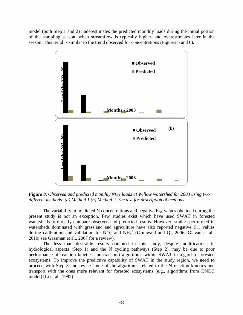
model (both Step 1 and 2) underestimates the predicted monthly loads during the initial portion of the sampling season, when streamflow is typically higher, and overestimates later in the season. This trend is similar to the trend observed for concentrations (Figures 5 and 6).

Figure 8. Observed and predicted monthly NO3

- loads at Willow watershed for 2003 using two different methods: (a) Method 1 (b) Method 2. See text for description of methods The variability in predicted N concentrations and negative ENS values obtained during the present study is not an exception. Few studies exist which have used SWAT in forested watersheds to directly compare observed and predicted results. However, studies performed in watersheds dominated with grassland and agriculture have also reported negative ENS values during calibration and validation for NO3

- and NH4+ (Grunwald and Qi, 2006; Glavan et al.,

2010; see Gassman et al., 2007 for a review). The less than desirable results obtained in this study, despite modifications in hydrological aspects (Step 1) and the N cycling pathways (Step 2), may be due to poor performance of reaction kinetics and transport algorithms within SWAT in regard to forested ecosystems. To improve the predictive capability of SWAT in the study region, we need to proceed with Step 3 and revise some of the algorithms related to the N reaction kinetics and transport with the ones more relevant for forested ecosystems (e.g., algorithms from DNDC model) (Li et al., 1992).

Loa

d (k

g-N

O3-

N)

Months - 2003

Observed

Predicted

Loa

d (k

g-N

O3-

N)

Months - 2003

Observed

Predicted

(b)

426

4. Conclusions

In general, it appears that in a forest-dominated watershed on the Canadian Boreal Plain it is not feasible to obtain satisfactory results for NO3

- and NH4+ in streams by using SWAT in its

original form. Although predictions can be slightly improved by incorporating some crucial aspects of N cycling observed in forested ecosystems, it seems a replacement of some of the algorithms pertinent to a forested environment is needed in order to obtain satisfactory N loading results using SWAT. Acknowledgement FORWARD research on the Boreal Plain was funded by an NSERC Collaborative Research and Development Grant and Millar Western Forest Products Ltd., as well as Alberta Newsprint Company (ANC Timber) Ltd., Blue Ridge Lumber Inc. (a Division of West Fraser Timber Company Ltd.), Buchanan Lumber (a division of Gordon Buchanan Enterprises Ltd.), Vanderwell Contractors (1971) Ltd., EDFOR Co-operative Ltd., PetroBakken Energy Ltd., Talisman Energy Inc., Vanderwell Contractors (1971) Ltd., Alberta Innovates BioSolutions, the Forest Resource Improvement Association of Alberta and the Canada Foundation for Innovation. References Arnold, J.G., R. Srinivasan, R.S. Muttiah, and J.R. Williams. 1998. Large area hydrologic modeling and

assessment. Part I. Model development. J. Am. Water Resour. Assoc. 34: 73–89. Ayensu, E., D.R. van Claasen, and M. Collins. 1999. International ecosystem assessment. Science

(Washington, D.C.). 286: 685–686. Burke, J.M., E.E. Prepas, and S. Pinder. 2005. Runoff and phosphorus export patterns in large forested

watersheds on the western Canadian Boreal Plain before and for 4 years after wildfire. J. Environ. Eng. Sci. 4:319–325.

Ecological Stratification Working Group.1996. A National ecological framework for Canada. Centre for

Land and Biological Resources Research, Research Branch, Agriculture and Agri-food Canada, Ottawa, Ont.

Environment Canada. 2005. National water data archive. Water Survey of Canada. National Water

Quantity Survey Program. Frazer, D.W., J.G. McColl, and R.F. Powers. 1990. Soil nitrogen mineralization in a clearcutting

chronosequence in a northern California conifer forest. Soil Sci. Soc. Am. J. 54: 1145-1152. Gassman, P. W., M.R. Reyes, C.H. Green, J.G. Arnold. 2007. The Soil and Water Assessment Tool:

Historical development, applications, and future research directions. Trans. ASABE, 50(4): 1211-1250.

Glavan, M., S. White, I. Holman. 2010. Evaluation of river water quality simulations at a daily time step

– experience with SWAT in the Axe Catchment, UK. Clean – Soil, Air, Water. 1–12 Grunwald, S., and C. Qi. 2006. GIS-based water quality modelling in the Sandusky watershed, Ohio,

USA. J. American Water Resources Assoc. 957-973.

427

Hoang, L., A.V. Griensven, P.V.D. Keur, L. Troldborg, B. Nilsson, and A. Mynett. 2010. Comparison of

the SWAT Model versus the DAISY-MIKE-SHE Model for simulating the flow and nitrogen processes. In Intern. SWAT conf. Proc. 306-319.

Holmes, W.E., and D.R. Zak. 1999. Soil microbial control of nitrogen loss following clear-cut harvest in

northern hardwood ecosystems. Ecol. Appl. 9: 202-215. Kirby, J.T., and S.R. Durrans. 2007. PnET-II3SL/SWAT: Modelling the combined effects of forests and

agriculture on water availability. J. Hydrol. Eng. 12(3): 319–326. Knoepp, J.D., and W.T. Swank. 1997. Forest management effects on surface soil carbon and nitrogen.

Soil Sci. Soc. Am. J. 61: 928-935. Li, C., S. Frolking, T. Frolking. 1992. A model of nitrous oxide evolution from soil driven by rainfall

events: model structure and sensitivity. J.Geophys. Res. 97: 9759-9776. McKeown, R.A., G. Putz, J. Arnold, and M. Di Luzio. 2005. Modifications of the Soil and Water

Assessment Tool (SWATC) for streamflow modeling in a small, forested watershed on the Canadian Boreal Plain. In Proc. 3rd Intern. SWAT Conf., 189–199. R. Srinivasan, J. Jacobs, D. Day, and K. Abbaspour, eds.

Neitsch, S.L., J.G. Arnold, J.R. Kinry, J.R.Williams. 2002. Soil and Water Assessment Tool. Version

2000. Theoretical Documentation. USDA-ARS, Temple, TX. Ouyang W., F. Hao, X.Wang, H. Cheng. 2008. Nonpoint source pollution responses simulation for

conversion cropland to forest in mountains by SWAT in China, Environ. Manag. 41: 79-89. Pelster, D.E., J.M. Burke, and E.E. Prepas. 2008. Runoff and inorganic nitrogen export from Boreal

Plain watersheds six years after wildfire and one year after harvest. J. Environ. Eng. Sci. 7: S51–S61.

Pisinaras, V., C. Petalas, G.D. Gikas, A. Gemitzi, V.A. Tsihrintzis. 2010. Hydrological and water quality

modeling in a medium-sized basin using the Soil and Water Assessment Tool (SWAT), Desalination. 250: 274–286.

Pohlert, T., J.A. Huisman, L. Breuer, and H.G.Freude. 2007. Integration of a detailed biogeochemical

model into SWAT for improved nitrogen predictions: Model development, sensitivity, and GLUE analysis. Ecol. Model. 203:215-228.

Prepas, E.E., J.M. Burke, D.S. Chanasyk, D.W. Smith, G. Putz, S. Gabos, W. Chen, D. Millions, and M.

Serediak. 2003. Impact of wildfire on discharge and phosphorus export from the Sakwatamau watershed in the Swan Hills, Alberta, during the first two years. J. Environ. Eng. Sci., 2(Suppl. 1): S63–S72.

Prepas, E.E., J.M. Burke, I.R. Whitson, G. Putz, and D.W. Smith. 2006. Associations between watershed

characteristics, runoff, and stream water quality: Hypothesis development for watershed disturbance experiments and modelling in the Forest Watershed and Riparian Disturbance (FORWARD) project. J. Environ. Eng. Sci. 5(Suppl. 1): S27–S37.

428

Prepas, E.E., J.M. Burke, G. Putz, D.W.Smith. 2008. Dissolved and particulate phosphorus concentration and export patterns in headwater streams draining Boreal Plain watersheds one year after experimental forest harvest and post-harvest silvicultural activities. J. Environ. Eng. Sci. 2: S63–S77.

Putz, G., J.M.Burke, D.W.Smith, D.S. Chanasyk, E.E. Prepas, and E. Mapfumo. 2003. Modelling the

effects of boreal forest landscape management upon streamflow and water quality: Basic concepts and considerations. J. Environ. Eng. Sci. 2: S87–S101.

Saleh, A., and B. Du. 2004. Evaluation of SWAT and HSPF within BASINS program for the upper North

Bosque River watershed in central Texas. Trans. ASAE. 47(4): 1039 – 1049. Santhi, C., J.G. Arnold, J.R. Williams, W.A. Dugas, R. Srinivasan, and L.M. Hauck. 1999. Validation of

the SWAT model on a larger river basin with point and non point sources. JAWRA. 37 (5): 1169-1188.

Schimel, J.P., and J. Bennett. 2004. Nitrogen mineralization: Challenges of a changing paradigm.

Ecology. 85(3): 591-602. Schilling, K. E., and C.F.Wolter. 2009. Modeling nitrate-nitrogen load reduction strategies for the Des

Moines river, Iowa using SWAT. Environ. Manag. 44:671–682. Smith, V.H., G.D. Tilman, J.C. Nekola. 1999. Eutrophication: impacts of excess nutrient inputs on

freshwater, marine, and terrestrial ecosystems. Environ. Poll. 100:179-196. Smith, D.W., E.E. Prepas, G. Putz, J.M. Burke, W.L. Meyer, and I. Whitson (2003) The Forest Watershed

and Riparian Disturbance study: a multi-discipline initiative to evaluate and manage watershed disturbance on the Boreal Plain of Canada. J. Environ. Eng. Sci., 2(Suppl. 1): 1–13.

Wattenbach, M., F. Hattermann, R. Weng, F. Wechsung, V. Krysanova, and F. Badeck. 2005. A

simplified approach to implement forest eco-hydrological properties in regional hydrological modeling. Ecol. Model. 187: 40–59.

Watson, B.M., N. Coops, S. Selvalingam, and M. Ghafouri. 2005. Improved simulation of forest growth

for the Soil and Water Assessment Tool (SWAT). 142–152. In Proc. 3rd Intern. SWAT Conf. R. Srinivasan, J. Jacobs, D. Day, and K. Abbaspour, eds.

Watson, B.M., R.A. McKeown, G. Putz, and J.D. MacDonald .2008. Modification of SWAT for

modelling streamflow from forested watersheds on the Canadian Boreal Plain. J. Environ. Eng. Sci. 7: S145–S159.

Williams, J.R., C.A. Jones, P.T. Dyke. 1984. A modeling approach to determining the relationship

between erosion and soil productivity. Trans. ASAE. 27: 129–144. Zoltai, S.C., L.A. Morrissey, G.P. Livingston, and W.J. de Groot. 1998. Effects of fires on carbon cycling

in North American boreal peatlands. Environ. Rev. 6: 13–24.

429

Integration of a Landscape Sediment Deposition Routine into Soil and Water Assessment Tool Model

N.B. Bonumá Department of Soils, Federal University of Santa Maria, Brazil, nadiabonuma@yahoo.com.br

J.G. Arnold

USDA-ARS, Grassland, Soil and Water Research Laboratory, Temple, Texas, USA

P.M. Allen Department of Geology, Baylor University, Waco, Texas, USA

C.H. Green

USDA-ARS, Grassland, Soil and Water Research Laboratory, Temple, Texas, USA

M. Volk Department of Computational Landscape Ecology, UFZ Helmholtz Centre for Environmental

Research, Leipzig, Germany

J.M. Reichert Department of Soils, Federal University of Santa Maria, Brazil

Abstract Sediment delivery from hillslopes to rivers is spatially variable; this may cause long-term delays between initial erosion and the related sediment yield at the watershed outlet. The concept of sediment transport capacity of overland flow is often applied to the modeling of watershed erosion. The Soil and Water Assessment Tool (SWAT) model already models landscape processes using slope classes while dividing the HRUs, however, it does not account for the deposition process across the landscape. In an attempt to simulate a landscape unit routing of sediment, SWAT model version 2009 was modified. A sediment transport capacity of overland flow was calculated using a landscape delineation routine. The new routine was tested on the Arroio Lino watershed of Brazil. Simulation results indicated that approximately 60% of the mobilized soil is being deposited before it reaches river channels. Hence, sediment delivery from hillslopes to river channels is rather limited with an average value of 19.70 t ha-1 year-1. The modified model provided reasonable simulations of sediment transport across the landscape positions. Despite the promising results of the new SWAT sediment routine simulation, calibration of the transport capacity parameters (ktc) in the new sediment routine has yet to be adequately solved, so further research is needed to address the uncertainties involved. This new sediment routine needs to be applied and evaluated using other input datasets, especially in areas where reliable spatial sediment transport patterns and spatially distributed depositional data is available. Keywords: landscape positions, soil erosion, sediment delivery modeling

430

1. Introduction It is well known that only a fraction of the eroded sediment within a drainage basin will

find its way to the basin outlet and be represented in the sediment yield of the basin (Walling, 1983). Sediment particles are detached within the watershed if the sediment load carried by the flow is smaller than the sediment transport capacity of flow and the shear stress exerted by flow is greater than the critical shear stress that is required for sediment particles to be entrained. Conversely, if the flow has a sediment load exceeding its transport capacity, the particles will be deposited (Aksoy and Kavvas, 2005). This concept of sediment transport capacity is commonly used in modeling sediment movement via overland flow and in channel transport models (Merritt et al., 2003).

The Soil and Water Assessment Tool (SWAT; Arnold et al., 1998) is a watershed scale model that has been applied to watersheds throughout the world (Arnold and Fohrer, 2005; Gassman et al., 2007) to determining the impact of land management practices on water, sediment and agricultural chemical yields (Neitsch et al., 2005). It uses the Modified Universal Soil Loss Equation (MUSLE; Williams, 1975) for calculating soil erosion and sediment yield in each Hydrologic Response Unit (HRU). The original SWAT model already models landscape processes using slope classes while dividing the HRUs, but it does not account for the deposition process across the landscape.

In order to account for sediment movement across the watershed’s slopes, the SWAT routines were carefully examined and some improvements in the sediment routines were proposed.

2. Sediment Transport Capacity of Overland Flow

Using dimensional analysis, Julien and Simons (1985) demonstrated that when rainfall

intensity is spatially uniform, sediment transport capacity per unit width of slope, denoted qs, can be represented by the following relationship:

γβSqkq 1s = (1)

where q is the discharge per unit width; S is the local energy gradient; and k1, β and γ are derived either empirically or theoretically.

The discharge is most practically estimated using some relationship between upslope contributing area and discharge. Rustomji and Prosser (2001) used a modified form of the relationship proposed by Kirkby (1988):

λakq 2= (2)

where a is hillslope area per unit width of contour (m2/m) and λ and k2 are empirically derived constants.

Rustomji and Prosser (2001) incorporated Equation 2 into Equation 1 to produce a purely topographic rule for predicting the sediment transport capacity of overland flow across a landscape (assuming parameters k1 and k2 are held spatially constant):

431

γβλ Sakkq 21s )(= (3) The value of λ can be varied to represent several modes of hillslope hydrology behaviour.

For steady-state flow condition, λ = 1. Prosser and Rustomji (2000) found that selecting a median value of 1.4 for the constants

β and γ is appropriate for use in sediment transport modeling. Therefore, Equation 3 can be rewritten as:

4141

21s Sakkq ..= (4) On the other hand, Desmet and Govers (1995) calculated sediment transport as a

proportion of the local erosion potential (Ep):

nm1p SAkE = and p2Ek t cT C= (5)

where TC equals the transport capacity of overland flow and Ktc2 is a proportionality factor.

This concept was used by Van Rompaey et al. (2001) to calculate the transport capacity in the SEdiment DElivery Model (SEDEM):

)... (.. .80s14L SKRk t cT C −= (6) where TC is transport capacity (kg m-2 year-1), ktc is the transport capacity coefficient, R is the rainfall erosivity factor (MJ mm m-2 h-1 year-1), K is the soil erodibility factor (kg h MJ-1 mm-1), LS is the slope and slope length factor, and s the slope gradient (m m-1).

The product of the constants k1 and k2 in Equation 4 reflects landscape characteristics that influence sediment transport, such as rainfall intensity, soil erodibility and vegetation, and landscape characteristics that influence runoff generation. Verstraeten et al. (2007) replace these constants with the R and K factors as these equations represent rainfall and soil characteristics.

3. Materials and Methods 3.1. SWAT sediment routine

The SWAT model uses the Modified Universal Soil Loss Equation (MUSLE) (Williams, 1975) for calculating soil erosion and sediment yield in each hydrological response unit (HRU):

CL SPCKa r e aqQ81 1s e d 5 60

h r up ....)... (, ,s u p= (7)

where sed is the sediment yield in tons on a given day, Qsup is the surface runoff volume (mm/ha), qp is the peak runoff rate (m3/s), areahru is the area of the HRU (ha), K is the USLE soil erodibility factor, C is the USLE cover and management factor, P is the USLE support practice factor, LS is the USLE topographic factor and CFRG is the coarse fragment factor.

SWAT models sediment yield for each unique HRU in the watershed, independent of position within each subbasin. There is currently no way to include upslope contributing area while defining HRUs (White, 2009).

432

In an attempt to simulate a landscape unit routing of sediment, SWAT model version 2009 was modified. A sediment transport capacity of overland flow (Rustomji and Prosser, 2001; Verstraeten et al., 2007) was calculated using a landscape delineation routine (Volk et al., 2007). The landscape sediment transport capacity was included in the SWAT code to limit the sediment delivery from the HRUs to the reaches.

Landscape delineation routine: According to Volk et al., (2007) the slope position of a cell is its relative position between the valley floor and the ridge top. Filling sinks and leveling peaks is the first step of the method, and this is important for making the valleys and ridges fairly continuous. Downhill and “uphill” flow accumulation values greater than user specified limits are used to identify valleys and ridges, respectively. When large limits are used, only large valleys and ridges will be identified as such, and small valleys and ridges will be considered somewhere mid-slope. Slope position is calculated for the cells in the output grid as the elevation of each cell relative to the elevation of the valley which the cell flows down to and the ridge it flows up to. This is presented as a ratio, ranging from 0 (valley floor) to 100 (ridge top). Hillslope areas are represented by the values between these two ranges.

The landscape transport capacity (TC) was calculated using the following equation (Verstraeten et al., 2007):

4141 SaKRk t cT C ..***= (8)

whereby ktc reflects the vegetation component within the transport capacity. The transport capacity parameter (ktc) represents the slope length needed to produce an amount of sediment equal to a bare surface with an identical slope gradient (Verstraeten, 2006).

The hillslope area per unit width of contour (a) is referred to as unit hillslope area and is a measure of mean hillslope length (Rustomji and Prosser, 2001):

)( _

__

l e nx v a l l e2a rh i l l s lt o t a la = (9)

For each hillslope-valley floor element, the hillslope area (m2) and the length of valley

floor (m) were calculated. Slope (S) is calculated as the mean gradient of the valley side cells in the DEM:

n

s l o p8dS

n

1ii∑

== (10)

If the sum of the sediment input and the local sediment production is lower than the

transport capacity, then all the sediment is routed further downslope. If this sum exceeds the transport capacity then sediment output is limited to the transport capacity. In the latter case, limited erosion will occur if the transport capacity exceeds the sediment input. If the transport capacity is lower than the sediment input, there will be sediment deposition (Van Rompaey el al., 2001).

433

3.2. Case study: the Arroio Lino watershed The new SWAT sediment routines were tested on the Arroio Lino watershed (4.8 km2),

located in Southern Brazil. The landscape of the small watershed is very hilly to steep (Kaiser et al., 2010).

The landscape transport capacity parameters for the Arroio Lino watershed were derived from the same input data for SWAT model, such as topography, soil properties, land use and climate data.

Land use was determined by field surveys, assisted by a GPS with GIS software (Pellegrini et al., 2009). The land use map provides a spatial coverage of the transport capacity parameter (ktc). Land use categories were grouped into five major categories: water, urban land use, crops, forest and pasture. Initial ktc values were applied to every land use category (based on the values adopted by Verstraeten et al., 2007): 0 for waters and urban land use, 0.04 for forest, 0.6 for pasture and 4 for crops.

The mean annual rain erositivity (R) was assumed to be constant throughout the watershed at 6400 MJ mm ha-1 h-1 year-1 based on rainfall data for the meteorological station.

Soil erodibility (K) was estimated from the soil map and soil physical and chemical properties. The K values range from 0.12 to 0.15 t h MJ-1mm-1; with a mean value of 0.14 t h MJ-

1 mm-1. The watershed was divided into 21 subbasins using the automated delineation tool of the

GIS interface based on the Digital Elevation Model (DEM) for the watershed. The slope map was divided in five slope classes: 0-5%, 5-15%, 15-30% and 30-45%. The combination of land use, soil type and slope classes resulted in 344 HRUs. The landscape delineation routine based on the DEM (Volk et al., 2007) resulted in a landscape units map (Figure 1) with three main landscape units: divide, hillslope and floodplain. 4. Results and Discussion

Table 1 gives the predicted sediment yield from hillslopes to river channels in the Arroio Lino watershed.

Table 1. Prediction of hillslope sediment delivery for the Arroio Lino watershed

Subbasin TC SY_MUSLE SY DEP

(t ha-1) (t) (t ha-1) (t) (t ha-1) (t) (t ha-1) (t) 1 2.45 44.51 37.02 673.21 2.45 44.51 34.57 628.69 2 23.87 585.65 53.34 1308.56 23.87 585.65 29.47 722.89 3 0.58 1.98 13.28 45.35 0.58 1.98 12.71 43.37 4 40.00 1670.80 70.57 2947.75 40.00 1670.80 30.57 1276.95 5 0.00 0.00 1.08 0.14 0.00 0.00 1.08 0.14 6 60.32 1561.36 46.43 1201.89 46.43 1201.88 0.00 0.00 7 18.81 620.48 43.31 1428.52 18.81 620.48 24.50 808.02 8 91.08 642.39 49.00 345.60 49.00 345.60 0.00 0.00 9 3.97 82.76 36.18 753.32 3.97 82.76 32.21 670.58 10 11.53 138.70 50.14 603.33 11.53 138.70 38.61 464.63 11 3.17 33.14 56.90 593.98 3.17 33.14 53.73 560.84 12 32.59 293.73 59.96 540.50 32.59 293.73 27.38 246.77 13 - - 1.01 0.04 1.01 0.04 0.00 0.00 14 1.44 17.30 43.72 524.89 1.44 17.30 42.28 507.59

434

15 0.95 2.08 29.81 65.61 0.95 2.08 28.87 63.53 16 1.10 9.30 30.27 257.04 1.10 9.30 29.17 247.74 17 1.97 16.87 76.47 654.81 1.97 16.87 74.50 637.94 18 2.38 14.92 45.19 283.03 2.38 14.92 42.81 268.11 19 3.07 55.85 54.69 993.64 3.07 55.85 51.62 937.82 20 31.05 490.21 45.17 712.95 31.05 490.21 14.11 222.75 21 14.52 428.36 43.49 1282.82 14.52 428.36 28.97 854.47

Total 21.84 6710.40 49.52 15217.00 19.70 6054.17 28.33 9162.83

The sediment supply (contribution) from the HRUs (SY_MUSLE) is calculated with the MUSLE equation (Equation 7). The landscape transport capacity (TC) is calculated with Equation 8. The predicted sediment yield from hillslopes to river channels (SY) is limited by the TC value (Figure 2). Approximately 60% of mobilized soil is being deposited (DEP) before it reaches river channels. Hence, sediment delivery from hillslopes to river channels is rather limited with an average value of 19.70 t ha-1 year-1. The predicted total soil loss equals 15,217 t, but only 6,054 t of sediment are being delivered from hillslopes to the channel network in the Arroio Lino watershed.

Figure 1. Landscape units map of Arroio Lino watershed

Figure 2. Spatial distribution of sediment

delivery modeled by SWAT deposition routine

5. Conclusions

In this study, an attempt was made to include the sediment transport capacity description in the source code of the SWAT model version 2009. The modified model provided reasonable simulations of sediment transport across the landscape positions. The application demonstrates the applicability of the model to simulate sediment yield in watersheds with steep slopes. Despite the promising results of the new SWAT sediment routine simulation, the calibration of the transport capacity parameters (ktc), a very important issue of SWAT sediment routine, has yet to be adequately solved, so further research is needed to address the uncertainties involved. Further

435

work is still needed to more broadly test the model in areas with other topography configurations and land uses. Acknowledgements The authors would like to thank Ms. Nancy Sammons and Ms. Georgie Mitchell for their help with the SWAT model routines. References Aksoy, H., M. L. Kavvas, 2005. A review of hillslope and watershed scale erosion and sediment transport

models. Catena 64: 247–271. Arnold, J.G., R. Srinivasan, R. S. Muttiah, J. R. Williams. 1998. Large area hydrologic modeling and

assessment – Part 1: Model development. Journal of the American Water Resources Association 34(1): 73–89.

Arnold, J. G., N. Fohrer. 2005. SWAT2000: Current capabilities and research opportunities in applied

watershed modeling. Hydrological Processes 19: 563–572. Desmet, P. J. J., G. Govers. 1995. GIS-based simulation of erosion and deposition patterns in an

agricultural landscape: a comparison of model results with soil map information. Catena 25: 389–401.

Gassman, P. W., M. R. Reyes, C. H. Green, J. G. Arnold. 2007. The Soil and Water Assessment Tool:

Historical development, applications, and future research directions. Transactions of the American Society of Agricultural and Biological Engineers 50(4):1211-1250.

Julien, P. Y., D. B. Simons. 1985. Sediment transport capacity of overland flow. Transactions of the

American Society of Agricultural Engineers 28: 755–762. Kirkby, M. J. 1988. Hillslope runoff processes and models. Journal of Hydrology 100: 315–339. Merritt, W. S., R. A. Latcher, A. J. Jakeman. 2003. A review of erosion and sediment transport models.

Environmental Modelling & Software 18: 761– 799. Neitsch, S. L., J. G. Arnold, J. R. Kiniry, J. R. Williams. 2005. Soil and Water Assessment Tool -

Theoretical Documentation: Version 2005. Temple, Blackland Research Center, Texas Agricultural Experiment Station.

Pellegrini, J. B. R., D. R. Rheinheimer, C. S. Gonçalves, A. C. C. Copetti, E. C. Bortoluzzi, D. Tessier.

2009. Impacts of anthropic pressures on soil phosphorus availability, concentration, and phosphorus forms in sediments in a Southern Brazilian watershed. Journal of Soils and Sediments 10(3): 451-460.

Prosser, I. P., P. Rustomji. 2000. Sediment transport capacity relations for overland flow. Progress in

Physical Geography 24: 179–193. Rustomji, P., I. P. Prosser. 2001. Spatial patterns of sediment delivery to valley floors: sensitivity to

sediment transport capacity and hillslope hydrology relations. Hydrological Processes 15: 1003–1018.

436

Van Rompaey, A. J. J., G. Verstraeten, K. Van Oost , G. Govers, J. Poesen. 2001. Modelling mean annual sediment yield using a distributed approach. Earth Surface Processes and Landforms 26: 1221– 1236.

Verstraeten, G. 2006. Regional scale modelling of hillslope sediment delivery with SRTM elevation data.

Geomorphology 81: 128–140. Verstraeten, G., I. P. Prosser, P. Fogarty. 2007. Predicting the spatial patterns of hillslope sediment

delivery to river channels in the Murrumbidgee catchment, Australia. Journal of Hydrology 334(3/4): 440–454.

Volk, M., J. G. Arnold, D. D. Bosch, P. M. Allen, C. H. Green. 2007. Watershed Configuration and

Simulation of Landscape Processes with the SWAT Model. In Oxley, L. and Kulasiri, D. (eds) MODSIM 2007 International Congress on Modelling and Simulation. Modelling and Simulation Society of Australia and New Zealand, 74-80.

Walling, D. E. 1983. The sediment delivery problem. Journal of Hydrology 65: 209-237. White, E. D. 2009. Development and application of a physically based landscape water balance in the

SWAT model. Thesis (Master of Science) - Cornell University. Williams, J.R. 1975. Sediment routing for agricultural watersheds. Water Resources Bulletin 11(5): 965-

974.

437

Impacts of Precipitation Interpolation on Hydrologic Modeling in Data-Scarce Regions

Paul D. Wagner1*, Shamita Kumar2, Florian Wilken1, Peter Fiener1 and Karl

Schneider1

1Hydrogeography and Climatology Research Group, Institute of Geography, University of Cologne, D-50923 Köln, Germany

2Institute of Environment Education & Research, Bharati Vidyapeeth University, Pune 411043, India

*E-mail: paul.wagner@uni-koeln.de

Abstract Accurate precipitation data are of prime importance as hydrologic model input. Monsoon regions often exhibit large spatial and temporal variability in precipitation. Available measurements are scarce in these regions, often show data gaps and require careful analysis of data quality. Our study aims at analyzing different precipitation interpolation methods and their effect upon runoff model results calculated with the Soil and Water Assessment Tool (SWAT). The study was carried out in the meso-scale catchment of the Mula and Mutha Rivers (2,036 km²) upstream of the city of Pune, India. Measured precipitation data were tested for homogeneity and consistency using double mass curves and were corrected for wind effects. Data gaps were filled. Corrected precipitation was spatially interpolated using three different methods: (i) Thiessen polygons, (ii) a geostatistical pooled kriging approach and (iii) a combined regression - inverse distance weighting method. Quality of the different interpolation methods was analyzed a) with respect to their capability to reproduce measured data and b) with regards to their effects upon SWAT model results, particularly runoff. We found that the more complex methods (ii and iii) better reproduce the measured precipitation data. Differences in the catchment’s modeled water balance are small. However, runoff at the sub-catchment level shows more pronounced differences for the different interpolation schemes. Hence, addressing spatial heterogeneities, the chosen interpolation method is very important particularly in data-scarce regions to accurately reproduce runoff. Keywords: SWAT, precipitation interpolation, pooled kriging, data-scarce environment, India

447

1. Introduction

Accurate precipitation data are of prime importance as input into hydrologic models. However, in many regions of the world, precipitation measurements are scarce and of poor quality. Measurements are affected by systematic as well as non-systematic errors. Thus, a thorough analysis of the available precipitation measurements is a prerequisite for model application and subsequent validation with runoff gauge measurements as well as for calibration of model parameters. Moreover, analyzing and understanding results of spatially-distributed hydrological modeling requires special attention to be drawn to the representation of the spatial precipitation patterns which are usually interpolated from point measurements (Tabios and Salas, 1985; Zhang and Srinivasan, 2009). Direct measurements of precipitation patterns e.g. using radar systems are typically not available. Therefore, the effects arising from the spatial interpolation scheme for precipitation require careful analysis (Goovaerts, 2000). Particularly in mountainous areas, spatial patterns are consistently affected by topography and wind direction (Barros and Lettenmaier, 1993; Barry, 1992). In the Western Ghats, with its steep topography, precipitation patterns are highly spatially and temporally variable. In a previous study performed in the meso-scale catchment of the Mula and Mutha Rivers (2,036 km²) upstream of the city of Pune, India, precipitation input was identified as a major source of error for runoff modeling (Wagner et al., 2011). Notably, the western summit regions of the mountainous catchment, with high amounts of precipitation and high temporal variability, were not sufficiently represented by applied interpolation techniques. Hence, this study focuses on the correction of precipitation data and the analysis of interpolation techniques. The main objective of this paper is to analyze different precipitation interpolation methods in regards to their suitability for hydrological modeling in a monsoon-dominated region with scarce precipitation measurements. 2. Materials and Methods 2.1. Study area

The meso-scale catchment of the Mula and the Mutha Rivers (2,036 km²) is located in the Western Ghats upstream of the city of Pune (18.533°N, 73.85°E; Figure 1). It is a subbasin and source area of the Krishna River, which drains eastward into the Bay of Bengal. The catchment has a tropical wet and dry climate that is characterized by seasonal rainfall from June to October and low annual temperature variation with an annual mean of 25°C at the catchment outlet in Pune. There is a pronounced west (approximately 3,500 mm) to east (750 mm) decline of annual precipitation in the catchment (Gadgil, 2002; Gunnell, 1997). Equally, the relief decreases from 1,300 m on the top ridges in the Western Ghats to 550 m in Pune. Land use is dominated by semi-natural vegetation with forests (20.6%) mainly on the higher elevations in the west, whereas shrubland (26.6%) and grassland (22.8%) occupy lower elevations. Agriculture comprises only 10.6% of the catchment and is mainly located in proximity to rivers and to six large dams (5.8% of the catchment is covered by water). Agriculture is dominated by small fields (< 1 ha) with rain-fed agriculture during monsoon season and irrigation during the dry season. Typically, two crops per year are harvested. The eastern part of the catchment is dominated by the city of Pune and its surrounding settlements (1.9% high density and 11.1% medium density urban area). 2.2. SWAT model

The study was carried out with the help of the Soil and Water Assessment Tool (SWAT; Arnold et al., 1998). The SWAT model has proven its capability to model water

448

fluxes in regions with limited data availability (Ndomba et al., 2008; Stehr et al., 2008). It was utilized in the Mula-Mutha catchment in a preceding study (Wagner et al., 2011). Although model performance was satisfying for three of four gauges, water yield was underestimated by the model, especially in headwater catchments. This shortcoming was attributed to insufficient representation of precipitation patterns. Hence, this study is based on the same, mainly freely available input data, but uses different precipitation inputs.

A Digital Elevation Model (DEM) with a spatial resolution of 30 m was derived from ASTER satellite data. Spatial soil distribution was taken from the Digital Soil Map of the World (FAO, 2003). This database shows two soil types in the study region: a sandy clay loam (Hh11-2bc, Haplic Phaeozem) covering 92.5% and a clay (Vc43-3ab, Chromic Vertisol) which covers 7.5% of the catchment. Soil parameterization was partly adapted from a modeling study of the region by Immerzeel et al. (2008). The land use map was derived from a satellite image taken by LISS-III on the Indian satellite IRS-P6 (Wagner et al., 2011). Crop rotations as well as irrigation schemes were set up for the agricultural land (rice 4.7%, sugarcane 0.7% and mixed cropland 5.3% of the catchment area) to account for the two main cropping seasons in the region. Additionally, the forest growth module was modified to represent local conditions. For the six major dams in the catchment, a management scheme was developed which is based on general management rules allowing for water storage in the rainy season and water release in the dry season (Wagner et al., 2011).

Daily temperature, humidity, solar radiation and wind speed data were only available at the weather station in Pune (ID 430630, 18.533°N, 73.85°E, 559 m) that is maintained by the Indian Meteorological Department (IMD). To account for temperature differences within the catchment, temperature values were adjusted for every subbasin using the adiabatic temperature gradient (0.98°C/100 m on a dry day, 0.44°C/100 m on a wet day; Weischet, 1995). With the help of these subbasin-specific temperature values and the specific humidity values measured in Pune, relative humidity was calculated for every subbasin. Solar radiation and wind speed from Pune are used for the whole catchment. This setup resulted in 25 subbasins which are subdivided into 975 Hydrological Response Units (HRUs). The model was run for eight years from 2000 to 2007, but only seven years were used for analysis, allowing for a one-year model spin-up phase. 2.3. Precipitation input

Daily measurements of precipitation at sixteen gauges within or close to the catchment were provided by the Nashik Water Resources Department and the Pune IMD. Five of them only record data during the monsoon season and a few gauges had a small amount of missing values. To provide suitable precipitation inputs for the SWAT model, the following measures were applied: (i) filling of data gaps, (ii) test for homogeneity and consistency, (iii) correction of systematic measurement errors and (iv) analysis of three different interpolation schemes. 2.3.1. Gap filling, quality control and correction

Daily precipitation measurements were available for this study. Missing values were filled using a regression-based gap filling approach. The available data at the gauge with data gaps was summed up, and corresponding precipitation sums were calculated for every gauge using the same dates. Using these data, a linear regression was carried out to establish a relationship between the incomplete and each of the other stations. The slope of the regression was used as a factor to estimate missing data at the incomplete station from each of the other gauges. To identify the gauge most suitable for filling the incomplete station, 120 randomly chosen precipitation days (four months) were estimated from each of the other rain gauges. Subsequently, the Root Mean Square Error (RMSE) was calculated to evaluate the

449

performance of each station. This procedure was repeated ten times, providing a mean RMSE for identifying the most suitable station. Filling was not applied if measurements for a whole year were missing.

Furthermore, a test for homogeneity and consistency of the precipitation measurements was performed using double mass curves (Searcy et al., 1960). Inconsistencies and heterogeneities were corrected accordingly. Due to the higher amounts of rainfall and larger number of rain days in the upper catchment, stations within the western part and stations within the eastern part were tested separately. Questionable data were marked as missing values (in some cases missing values were not marked properly but instead were given a 0 mm rainfall value). These values were corrected using the described regression-based gap filling approach.

The derived precipitation data set consists of ten gauges with complete daily records from 1988 to 2008 and six gauges with gaps that comprised one or more years. Finally, to account for systematic precipitation measurement errors due to wind loss, wetting loss and evaporation, a correction method developed by Richter (1995) was applied. This method is based on Hellmann gauges of the German measurement network and applies different coefficients based on precipitation type and wind exposition (shielding). To account for the precipitation character given in India, we chose the coefficients for summer rain (ε = 0.38) and light shielding (b = 0.31). Precipitation (P) was corrected by using the following equation:

εbPPPcor += , which provides corrected precipitation data (Pcor) for every station. 2.3.2. Interpolation schemes

Spatial representation of precipitation is very important for providing suitable model input. This is particularly true in a mountainous catchment where precipitation amounts vary significantly (Barry 1992). The SWAT standard method of using the nearest weather station for each subbasin does not provide an accurate representation of precipitation patterns, as the measurement network within the catchment is rather coarse (Figure 1). Therefore, three different interpolation schemes were utilized and compared which also use data from neighboring catchments. The interpolation schemes were carried out on a 1 km² grid. Model input was derived from this grid by calculating an average of the grid values for each subbasin.

As a reference, Thiessen polygons (Thiessen, 1911) were used. Each grid point was assigned the value of the nearest rain gauge. This simple approach balances the contributions of the nearest stations and is therefore superior to the SWAT standard method that only uses the nearest station. Furthermore, two methods that are more complex, a geostatistical and a knowledge-based regression approach, were utilized.

450

Geostatistical methods are commonly used for spatial interpolation of rainfall (Goovaerts, 2000; Zhang and Srinivasan, 2009). However, a large number of measurement locations are needed to supply an accurate empirical semivariogram and to detect spatial autocorrelation. Furthermore, variogram analysis and fitting of variogram models are very important and have to be carried out carefully. To meet these requirements, pooled semivariograms (Fiener and Auerswald, 2009; Schuurmans et al., 2007) for each month were used. Mean daily precipitation values were calculated for every month in every year. These monthly values were pooled and used as input data for the empirical semivariogram, resulting in 312 data sets (21 years x 16 stations - 24 years missing from different stations) that give 1,938 point pairs for every semivariogram which were grouped into 14 lag classes. A Gaussian semivariogram model was fitted to these empiric semivariograms (Figure 2) using the gstat package (Pebesma, 2004) of the statistical software GNU R version 2.13.0 (R Development Core Team, 2011). Due to the small amounts of precipitation in the dry season, no spatial autocorrelation was found during that time. Therefore, ordinary kriging was only applied from June to September whereas inverse distance weighting (IDW) was used in the remaining months. A local kriging approach was utilized, where only stations within a 30-km distance were used for interpolation.

The knowledge-based approach combines a regression technique with an inverse distance interpolation scheme. Mauser and Bach (2009) used this method, calculating a linear regression of elevation and mean daily measured rainfall amount. However, in our study area, it was found that the x-coordinate is more suitable as an explanatory variable than is elevation (R²=0.92, p<0.001). Due to the general north-south direction of the Western Ghats, the x-coordinate represents the distance in wind direction from the Ghat (Figure 3). ‘Ghat’ means ‘step’ and refers to the step-like decline from the Western Ghats mountain range to the coastal plain that marks the western boundary of the catchment. Thus, the x-coordinate expresses the downwind fetch and consequently the west to east decline of precipitation starting from the Ghat. Regression of precipitation and the x-coordinate was calculated for every wet day (at least one station recorded precipitation on this day) using a mean precipitation value comprising a period from three days before to three days after the interpolation day. It was tested for every day if the derived regression was significant (p<0.1) and if the correlation was negative (expressing a west to east decline of precipitation amounts). If these criteria are met, the regression is used to estimate mean precipitation for every grid point and to calculate residuals for every measurement station (daily rainfall - regression rainfall). These residuals were interpolated to every grid point

Figure 2. Semivariogram and Gaussian model fit for July (nugget 10, sill 900, range 60 km)

Figure 3. X-coordinate represents distance in wind direction from the Ghat

451

using an IDW scheme. Finally, by adding the interpolated residuals to the mean daily rainfall values calculated from the regression equation, a rainfall estimate was derived for every grid point. Otherwise, if the criteria are not met, IDW is used to interpolate rainfall to the grid. Figure 4 shows that requirements for a valid regression were mostly given in the rainy season, whereas in dry seasons the local convective rainfall events do not meet the regression requirements and are therefore interpolated using IDW. 2.4. Validation

The interpolation schemes were validated in two steps. Firstly, a cross-validation was carried out by estimating the whole time series at one station using all other stations. With the help of the root mean square error (RMSE) and the Nash-Sutcliffe efficiency (NSE, Nash and Sutcliffe 1970) the different interpolation schemes were tested for their capability to reproduce measured values. Secondly, the different interpolation inputs were used as model input for SWAT. Model outputs were compared in regards to water balance and runoff dynamics. The SWAT model was not calibrated with ground based measurements since the focus of this study is set on relative differences between the different model inputs. The model itself showed satisfactory to good performance at the river gauges G1 and G4 (Figure 5) for all inputs (NSE: 0.47-0.70) based on daily discharge during rainy seasons. In the highly managed catchments, model performance was poor (NSE at G2: 0.38-0.40) and unsatisfactory (NSE at G3: 0). Runoff dynamics will therefore be compared using the two gauges with satisfactory performances. 3. Results and Discussion 3.1. Cross-validation

Performance of the

Figure 4. Validity of the regression approach (p < 0.1 and correlation coefficient < 0) for every day from 1988 to 2008

Figure 5. Location of river gauges and reservoirs in the Mula-Mutha catchment

452

interpolation schemes to reproduce measured values was evaluated using a cross-validation method. The mean RMSE indicated that Thiessen polygons performed poorly (12.3 mm), while ordinary kriging performed better (10.5 mm) and the regression method showed the best performance (10.0 mm). This ranking is generally reflected by the performance at the gauges, indicated by the NSE in Figure 6. The regression method was the only method that had positive NSE at every gauge, whereas the NSE was negative at one station applying ordinary kriging and at three stations using Thiessen polygons. However, the performance varies from one gauge to another. The worst interpolation performance was found at the most eastern gauge, Wagholi. As Thiessen and kriging show negative NSE here, it can be concluded that the nearest gauges are not representative of this gauge. The regression approach performs better at this site as it does not rely as much on neighboring stations but uses large scale conditions. Thiessen polygons typically show reasonable performance for gauges where the nearby gauge is representative of the estimated gauge (e.g. Kumbheri and Mulshi). If this is not the case, Thiessen polygons do not perform as well as the two other methods (e.g. Paud). In summary, the more complex methods performed generally better than the simple Thiessen polygon approach. Moreover, the regression method shows a better performance than the pooled ordinary kriging approach. Therefore, in the analysis of model reaction to the different inputs, regression interpolation is used as the reference model run.

3.2. Impact on water balance and runoff dynamics

On the catchment scale, differences in the water balance of the different interpolation methods are small (Table 1). Thiessen polygon interpolation produced 53 mm (-2.3%) and pooled ordinary kriging produced 17 mm (-0.7%) less mean annual precipitation compared to the regression method. Primarily, the lower amounts of precipitation resulted in lower water yields and slightly lower evapotranspiration. Although the differences in the water balance at the

Figure 6. Interpolation performance at the rain gauges indicated by the Nash-Sutcliffe efficiency (NSE)

Table 1. Water balance for different interpolation schemes

Interpolation scheme Precipitation Water yield Evapotranspiration

Thiessen polygons 2285 mm 1523 mm 691 mm

Ordinary kriging 2321 mm 1545 mm 706 mm

Regression-IDW 2338 mm 1560 mm 705 mm

453

catchment scale are small, this is not necessarily the case for runoff dynamics. To measure differences in runoff dynamics, the model run based on interpolated

rainfall of the best interpolation method (regression method) was used as a reference. The deviations from this run were evaluated using the NSE and the percentage of deviation in total runoff (summation of runoff values for the whole seven years). Table 2 shows that runoff dynamics of the model run based on kriging are very similar to the run based on the regression method (NSE of 0.98 and 0.99). The more simple Thiessen polygon approach results in runoff dynamics that deviate much more from the reference run (NSE of 0.92 and 0.96). A closer look at the differences between the sub-catchments gauged by G1 and G4 (Figure 5) indicates that the deviations in total rainfall and total runoff are smaller for the larger sub-catchment G1 and larger for the smaller headwater catchment G4. This suggests that effects depend upon scale. In large sub-catchments, over- and underestimations might cancel out while this is less likely in small catchments. Obviously, the deviation in runoff is larger than the deviation in rainfall (Table 2). This may partly result from differences in the subbasin weather inputs of the sub-catchments G1 and G4, but also indicates a non-linear system response.

There are two reasons for the deviation of Thiessen polygon interpolation from the

regression approach. These can be derived from Figure 7 which shows runoff at G1 and the storage volume of the upstream Pawana dam (Figure 5) for Thiessen polygon and regression interpolation during the rainy seasons of 2004. Firstly, rainfall differences lead directly to differences in runoff which is most clearly observable for runoff peaks (e.g. June 14, June 26 and September 30). Secondly, these primarily small differences add up so that full storage capacity of the dam is reached at different dates. Hence, once full storage capacity is reached in one model run there is no longer any dampening effect of the dam on runoff. If this point is reached at different dates in the models, pronounced differences in runoff follow (e.g. peak on August 8 and August 14). With these kinds of processes in a model, different interpolation schemes can make an important difference for runoff dynamics. However, it should be noted that deviations in total rainfall and total runoff are comparatively small considering the simplicity of the Thiessen polygon approach. This can be attributed to the rather coarse input into the model on the subbasin level. As all interpolation methods were performed on a 1-km² grid and then averaged for each subbasin, most pronounced local differences are smoothed out. Nevertheless, the more complex methods provide more accurate results in terms of their performance to reproduce measured precipitation data.

Table 2. Differences in runoff dynamics given by the Nash-Sutcliffe efficiency (NSE), in total rainfall, and in total runoff at the river gauges G1 and G4 compared to the regression interpolation model run

Interpolation scheme

G1 G4

NSE Deviation in rainfall

Deviation in runoff NSE Deviation

in rainfall Deviation in runoff

Thiessen polygons 0.96 + 0.6 % + 3.2 % 0.92 - 10.2 % - 12.9 %

Ordinary kriging 0.99 - 2.8 % - 3.7 % 0.98 + 5.3 % + 7.3 %

454

4. Summary and Conclusion

In this study, precipitation data for the catchment of the Mula and the Mutha Rivers

was analyzed, corrected and interpolated using three different interpolation methods. A simple approach (Thiessen polygons) and two more complex methods (combined regression with the IDW approach and ordinary kriging based on pooled semivariograms) were evaluated in regards to their ability to reproduce measured rainfall data. Furthermore, a SWAT model was set up and three model runs were performed using the differently interpolated precipitation inputs. Differences in model outputs were analyzed with respect to the model run for the most accurate method (regression approach), which was used as a reference run. It was found that differences in the catchment’s modeled water balances are small. However, deviations in total runoff for two analyzed sub-catchments were higher (up to 12.9%). The model run based on the Thiessen polygon precipitation input showed the largest differences from the reference run, whereas the kriging approach performed similar to the reference. For runoff dynamics it was found that small differences can lead to larger deviations in runoff if reservoirs reach full storage capacity at different times. From our findings, we conclude that the more complex methods are more suitable for reproducing measured precipitation data. However, the shortcomings of the simple Thiessen polygon method are not that obvious as the input data was averaged on the subbasin level. Therefore, deviations in the modeled water balances are small and this method may be sufficient for water balance studies. Runoff dynamics are more affected by the different interpolation inputs and therefore one of the more sophisticated methods should be used to account for an accurate model quality. Ordinary kriging based on pooled variograms performed almost as good as the knowledge-based regression approach. Unlike the regression method, the kriging

Figure 7. Runoff at gauge G1 and the storage volume of the upstream Pawana dam for Thiessen polygon and regression interpolation during the rainy season of 2004

455

approach is directly transferable to other regions. As a consequence, it can be recommended for applications in data-scarce regions. Acknowledgements We gratefully acknowledge support by a grant from the German National Academic Foundation. We would like to thank Pune IMD, the Nashik Water Resources Department, Khadakwasla Irrigation Division Pune, the Pune Groundwater Department, the Pune Department of Agriculture and Hyderabad NRSC for supplying environmental data, good cooperation and discussions. Moreover, we acknowledge the supply of ASTER data by the USGS Land Processes Distributed Active Archive Center. Special thanks go to the students from the Institute of Environment Education & Research at Bharati Vidyapeeth University Pune for assistance with the field measurements. References Arnold, J.G., R. Srinivasan, R.S. Muttiah, and J.R. Williams. 1998. Large area hydrologic modeling

and assessment - Part 1: Model development. Journal of the American Water Resources Association 34: 73-89.

Barros, A.P., and D.P. Lettenmaier. 1993. Dynamic modeling of the spatial distribution of

precipitation in remote mountainous areas. Monthly Weather Review 121: 1195–1214. Barry, R.G. 1992. Mountain climatology and past and potential future climatic changes in mountain

regions. Mountain Research and Development 12(1): 71-86. Food and Agriculture Organization of the United Nations (FAO). 2003. Digital Soil Map of the World

and Derived Soil Properties. Rom. Fiener, P., and K. Auerswald. 2009. Spatial variability of rainfall on a sub-kilometre scale. Earth

Surface Processes and Landforms 34: 848-859. Gadgil, A. 2002. Rainfall characteristics of Maharashtra. In Geography of Maharashtra, 89-102. J.

Diddee, S. R. Jog, V. S. Kale, and V. S. Datye, eds. Jaipur, India: Rawat Publications. Goovaerts, P., 2000. Geostatistical approaches for incorporating elevation into the spatial

interpolation of rainfall. Journal of Hydrology 228:113-129. Gunnell, Y. 1997. Relief and climate in South Asia: The influence of the Western Ghats on the

current climate pattern of peninsular India. International Journal of Climatology 17: 1169-1182.

Immerzeel, W.W., A. Gaur, and S.J. Zwart. 2008. Integrating remote sensing and a process-based

hydrological model to evaluate water use and productivity in a south Indian catchment. Agricultural Water Management 95: 11-24.

Mauser, W., and H. Bach. 2009. PROMET – Large scale distributed hydrological modelling to study

the impact of climate change on the water flows of mountain watersheds. Journal of Hydrology 376 (3-4): 362-377.

Nash, J. E., and J. V. Sutcliffe. 1970. River flow forecasting through conceptual models part I - A

discussion of principles. Journal of Hydrology 10 (3): 282-290. Ndomba, P., F. Mtalo, and A. Killingtveit. 2008. SWAT model application in a data scarce tropical

complex catchment in Tanzania. Physics and Chemistry of the Earth 33: 626-632.

456

Pebesma E.J. 2004. Multivariable geostatistics in S: the gstat package. Computers & Geosciences 30:

683-691. R Development Core Team. 2011. R: A language and environment for statistical computing. Ver.

2.13.0. Vienna, Austria: R Foundation for Statistical Computing. Richter, D. 1995. Ergebnisse methodischer Untersuchungen zur Korrektur des systematischen

Meßfehlers des Hellmann-Niederschlagmessers. Berichte des Deutschen Wetterdienstes 194. Offenbach, Germany.

Schuurmans J.M., M.F.P. Bierkens, E.J. Pebesma, and R. Uijlenhoet. 2007. Automatic prediction of

high-resolution daily rainfall fields for multiple extents: the potential of operational radar. Journal of Hydrometeorology 8: 1204-1224.

Searcy, J.K., C.H. Hardison, and W.B. Langbein. 1960. Double mass curves. Geological Survey

Water Supply Paper 1541-B. Washington, DC: US Geological Survey. Stehr, A., P. Debels, F. Romero, and H. Alcayaga. 2008. Hydrological modelling with SWAT under

conditions of limited data availability: evaluation of results from a Chilean case study. Hydrological Sciences Journal 53: 588-601.

Tabios, G.Q. and J.D. Salas. 1985. A comparative analysis of techniques for spatial interpolation of

precipitation. Journal of the American Water Resources Association 21: 365–380. Thiessen, A.H., 1911. Precipitation averages for large areas. Monthly Weather Review 39(7):1082-

1084. Wagner, P.D., S. Kumar, P. Fiener, and K. Schneider. 2011. Hydrological modeling with SWAT in a

monsoon-driven environment – experience from the Western Ghats, India. Transactions of the ASABE, accepted.

Weischet, W. 1995. Einführung in die Allgemeine Klimatologie. 6th ed. Stuttgart, Germany: Teubner. Zhang, X. and R. Srinivasan, 2009. GIS-based spatial precipitation estimation: A comparison of

geostatistical approaches. Journal of the American Water Resources Association 45(4):894-906.

457

Studying the Viability of a Limno-Reservoir Using SWAT: the Ompólveda River Basin (Guadalajara, Spain) as a Case Study

Eugenio Molina-Navarro Department of Geology, School of Sciences, University of Alcalá. Ctra. Madrid-Barcelona Km.

33,6. C.P. 28871. Alcalá de Henares. Madrid. Spain. eugenio.molina@uah.es

Silvia Martínez-Pérez Department of Geology, University of Alcalá.

Antonio Sastre-Merlín

Department of Geology, University of Alcalá.

Ramón Bienes-Allas Department of Geology, University of Alcalá.

Instituto Madrileño de Investigación y Desarrollo Rural, Agrario y Alimentario (IMIDRA). Apdo. de Correos 127, 28800, Alcalá de Henares, Madrid. Spain.

Abstract The construction of small dams on the edge of large reservoirs, creating a body of water with a constant level which we have termed limno-reservoirs, is an innovative idea designed to counteract some of the negative impacts caused by the construction and use of reservoirs. Pareja Limno-reservoir, located in the left margin of Entrepeñas Reservoir (Guadalajara province) is among the first limno-reservoirs in Spain. Earlier reservoirs were constructed to create a habitat for birds, but the Pareja Limno-reservoir is the first to promote socio-economic development. However, its construction raises some questions about hydrologic viability, siltation risk and possible eutrophication problems. Pareja Limno-reservoir is just placed at the outlet of the Ompólveda River Basin, where a stream-flow gauging station was installed and operative until 2004. This fact makes it an extraordinary place to apply most of the possibilities that the SWAT model offers. The SWAT model has been calibrated and validated in order to analyse the hydrologic response of the basin and, overall, the model had a good performance reproducing the observed stream-flows. It will allow prediction of river discharges into the reservoir after 2004 and will dispel some doubts about Limno-reservoir viability. SWAT also can predict sediment yield at the basin outlet and, consequently, the sediment load into the Pareja Limno-reservoir. Although this component could not be calibrated and validated, results suggest that most sediment produced in the basin would not reach the Pareja Limno-reservoir. Further results will be compared with studies that are ongoing in the Ompólveda River Basin. Keywords: Ompólveda River Basin, runoff, sediment, SWAT

458

1. Introduction

The term “limno-reservoir,” which we have proposed, refers to a small reservoir created by the building of a small dam on the edge of a big reservoir. These dams are known as “edge dams” or “flood dams” and have the goal of maintaining a body of water with a constant level which is independent of the management of the main reservoir. Therefore, limno-reservoirs are a corrective and/or compensatory action to remediate the negative environmental impacts caused by construction of large reservoirs in areas under Mediterranean climate. These include environmental, socio-economic and landscape impacts due to the “arid band” phenomenon generated in the drawdown zone of a reservoir (Molina Navarro et al., 2010a).

The first initiatives of this kind in Spain were proposed in the late 80s and the early 90s with the primary aim being the creation of a suitable habitat for birds (Rodríguez Cabellos, 1995; Ministerio de Medio Ambiente y Comité Nacional Español de Grandes Presas, 1996). Pareja Limno-reservoir is located on the edge of the Entrepeñas reservoir of Guadalajara, central Spain which has a capacity of 835 hm3 and 3,213 ha of potential inundation and consequently has suffered the environmental problems mentioned above. Thus, the limno-reservoir attempts to provide the surroundings with an infrastructure that favours hydrologic-environmental recovery as well as economic promotion of the area. The construction of Pareja Limno-reservoir finished in 2006 and became the first limno-reservoir to have a dual function: environmental and recreational. It is open for bathing or for taking a walk; it has a jetty for motorless craft, two artificial islands that act as bird refuges, and a fish ladder (Molina Navarro et al., 2010a, 2011).

Due to the innovative nature of this water management initiative and coinciding with the end of the reservoir-filling process, we set up an environmental observatory at the Pareja Limno-reservoir with the main aim of studying its viability through a multidisciplinary perspective. This project started in 2008 and is still ongoing. Among other studies, it is very important to gain knowledge about the hydrologic response of the Ompólveda River Basin, which feeds the limno-reservoir, as it is supposed to maintain a constant level of water. A stream-flow gauging station was located just where the Ompólveda River flows into the Pareja Limno-reservoir but became inoperative with its creation. Nevertheless, the existence of water yield data at the outlet of the basin makes it possible to create a hydrologic model to estimate the water yield of the basin in the following years. In particular, the program SWAT (Soil and Water Assessment Tool) has been used.

Another concern is the siltation risk of the limno-reservoir. Its study becomes very important in order to evaluate the environmental viability of the infrastructure. Some work has been done to analyse soil loss in the basin. Arévalo (2008), in her Environmental Sciences Final Degree Project, performed a study of the soil loss in the Ompólveda River Basin, obtaining average soil loss rates from 9 to 11 t·year-1· ha-1. We have also installed a network of erosion and sedimentation plots and profiles throughout the whole basin in order to study the soil loss in-situ (Molina Navarro et al., 2010a, 2010b). However, to study the siltation risk, the sediment load into the Pareja Limno-reservoir is needed and can be estimated by SWAT.

Thus, the main objectives of this study are to analyse the hydrologic response of the Ompólveda River Basin and its sediment yield. The SWAT hydrologic model is applied for this purpose. First, the study area and the data inputs are presented. Then, the model setup and performance are presented, followed by an analysis of simulation results.

459

2. Material and Methods 2.1. The study area

The Ompólveda River Basin has an area of 85.5 km2. It is located in the south of the Guadalajara Province, at the head of the Tajo River Basin. The Ompólveda River is a tributary of the Tajo River and flows into it with NE-SW direction. Its main tributary is the Valdetrigo stream, merging from the NE. Figure 1 shows the location of the basin within the drainage network and the Digital Elevation Model (DEM) which shows the present location of the Pareja Limno-reservoir, finished in 2006.

The climate has Mediterranean characteristics. The annual average daily temperature in the nearby Entrepeñas Reservoir ranged from -9ºC in January to 40ºC in August, with an annual mean temperature of 12.5ºC. Average annual precipitation at the Escamilla station (at the border of the basin) is 600 mm, although it shows high intra- and inter-annual variability (Molina Navarro et al., 2010a). Recorded minimum and maximum mean daily stream-flow of the Ompólveda River at the E-3270-Pareja gauging station, located in the basin outlet (and operative until the creation of the limno-reservoir), were 0.004 m3 s-1 from July 29 to August 24, 2002 and 3.197 m3 s-1 on January 21, 1997. Discharges were generally low from June to November, while peaks of highest discharges did not show a specific pattern, rising either in winter or spring, or even in both seasons during the same year. About 300 inhabitants live in the basin area, most of them in the village of Pareja whose population quadruples in summer.

En cuanto al aprovechamiento del suelo, predominan las extensiones de matorral y

pinar, muchas veces de repoblación. La superficie cultivada es escasa, destacando el olivar en secano en algunas laderas suaves y el cereal en la superficie del páramo.

Figure 1. Location of the Ompólveda River Basin, current location of the Pareja Limno-reservoir and digital elevation model 2.2. Principles of the SWAT model

SWAT is a physically based, watershed-scale, continuous-time and semi distributed hydrologic model that uses spatial data on topography, land use, soil and weather for hydrologic modeling and operates on a daily time step. It has an ArcGIS interface called ArcSWAT, which delineates the river watershed and network using the DEM. SWAT subdivides watersheds into a number of subbasins for modeling purposes.

TAJO BASIN 

OMPÓLVEDA RIVER BASIN

460

Each subbasin delineated within the model is simulated as a homogeneous area in terms of climatic conditions, but additional subdivisions are used within each subbasin to represent different soils and land use types. Each of these individual areas is referred to as a Hydrologic Response Unit (HRU) and is assumed to be spatially uniform in terms of soil, land use, and topography (Arnold et al., 1998; Arnold and Fohrer, 2005; Wang et al., 2010).

SWAT calculates the daily water balance based on soil type, slope, land use and weather data. To calculate the surface runoff, the U.S. Soil Conservation Service (SCS) curve number procedure was used. This method calculates surface runoff based on soil type, slope, initial soil moisture state, land use and management practices (Arnold et al., 1995). The Hargreaves method (Hargreaves and Samani, 1985), which only needs daily values for minimum and maximum temperatures and geographical location, was used to estimate potential evapotranspiration (PET). The portion of rainfall that does not turn into surface runoff is divided into percolation and evaporation. Water that percolates into the ground can return to surface streams either by lateral flow through the soil profile or as base flow coming from the aquifer. SWAT divides the groundwater system into two aquifers: one unconfined, which contributes to surface water flow, and one deep, confined aquifer where infiltrated water does not return to the system (Galván et al., 2009).

SWAT simulates sediment yield using the Modified Universal Soil Loss Equation (MUSLE; Williams, 1995). MUSLE predicts the amount of eroded soils in an HRU that would be delivered into the channel of the inclusive subbasin. In the channel network, sediment transport is modeled as a function of deposition and degradation, two processes that operate simultaneously in the reach. The maximum amount of sediment that can be transported from a reach segment is a function of peak channel velocity (Wang et al., 2010). A more detailed description of SWAT procedures can be found in Arnold et al. (1998), Srinivasan et al. (1998), Winchell et al. (2009) and Stehr et al. (2010).

2.3. Data inputs and model set up

Topographical data was obtained from the Digital Elevation Model (DEM) of the Castilla-La Mancha Regional Government (Instituto de Desarrollo Regional, 2008) with a resolution of 5 x 5 m (Figure 1). The program draws the slope map using the DEM, defines the drainage network and delineates the basin and subbasins. Outlets generated were edited in order to obtain nine subbasins (Figure 2).

Land use data were obtained from the updated version (1999-2008) of the Spanish Ministry of the Environment Land Uses Map. Land uses in the map were related to those included in the SWAT database. Ten different land uses were found in the Ompólveda River Basin. Scrubland is the main land use, covering 36% of the basin area, while 27% is covered by a combination of pine (50%) and oak (50%) forest. 17% is covered by non-irrigated cereal crops. Basin area percentage of other land uses is lower than 10% (Figure 3).

461

Figure 2. Ompólveda River Basin, subbasin division and location of the precipitation and gauging stations

Figure 3. Land uses in the study area from the Spanish Ministry of the Environment map

Prior to the start of this research, the only soil information available for the study

area was that found in the Guadalajara Province Soils Maps (Guerra Delgado et al., 1970). This map has a 1:250,000 scale, so the resolution is not very high. Then, in 2008, Arévalo started to study the soil of the Ompólveda River Basin, looking for different combinations of lithology, geomorphology, land cover and orientation which could originate different soil types and selecting 22 sampling points for studying the soil

462

characteristics. With Arévalo’s soil results and following the United States Department of Agriculture Soil Taxonomy (USDA, 1999), 17 different soils were identified and mapped in the Ompólveda River Basin. The main characteristics of the basin soils are shown in Table 1. 61.5% of the basin surface was covered by entisols (subgroups Typic Xerorthent, 36%, Lithic Xerorthent, 15.5% and Typic Xerofluvent, 10%); while 38.5% was covered by alfisols (subgroups Typic Haploxeralf, 29% and Lithic Haploxeralf, 9.5%) (Figure 4). The SWAT Users Soils database was modified to include the soils found. The required parameters were filled thanks to soil sample analysis or were inferred following USDA (1993), Schoeneberger et al. (2002), Fuentes Yagüe (2003) and Porta Casanellas and López-Acevedo Reguerín (2005). Table 1. Main characteristics of the soils in the Ompólveda River Basin (AWC: available water capacity, SHC: saturated hydraulic conductivity, OC: organic carbon)

Typic Xerorthent Lithic Xerorthent 1 2 3 4 5 6 1 2 3 4

Basin surf. (%) 0.84 5.55 2.93 6.89 9.10 10.63 5.09 2.22 5.26 3.07

Depth (cm) 60 70 70 55 65 70 40 40 40 40 Hydrologic group C C B B C C C C C C

Texture SCL L L L SCL CL CL L L SIL Bulk dens. (g cm-3)

1.53-1.63

1.54-1.74

1.34-1.50

1.05-1.15

1.01-1.11

1.18-1.45

1.16-1.36

1.28-1.43

1.00-1.15

1.19-1.30

AWC (mm mm-1) 0.09 0.07 0.09 0.09 0.09 0.12 0.11 0.09 0.10 0.10

OC content (% wt.)

0.09-0.45

0.09-1.99

0.06-0.94

0.05-1.66

0.05-1.15

0.03-1.22

0.03-0.96

0.03-1.78

0.03-2.55

0.06-1.12

SHC (mm h-1) 8.0 7.5 7.5 7.5 8.0 5.0 5.0 7.5 7.5 10.0

USLE K factor

0.196-0.205

0.519-0.650

0.417-0.478

0.328-0.438

0.290-0.332

0.265-0.311

0.301-0.311

0.366-0.464

0.265-0.449

0.510-0.573

Typic Xerofluvent

Typic Haploxeralf Lithic Haploxeralf 1 2 3 4 5

Basin surf. (%) 9.76 3.60 1.98 3.62 18.63 1.17 9.52

Depth (cm) 125 60 60 60 60 90 49 Hydrologic group B C C C B C B

Texture SL L-CL SICL-C L-CL L-CL CL-C L Bulk dens. (g cm-3) 1.28-1.50 0.97-1.15 1.22-1.52 1.35-1.65 1.03-1.33 1.05-1.35 0.98-1.45

AWC (mm mm-1) 0.07-0.11 0.09-0.10 0.12-0.14 0.09-0.11 0.09-0.10 0.11-0.12 0.08-0.10

OC content (% wt.) 0.06-1.69 0.05-4.03 0.05-0.58 0.05-3.90 0.05-1.80 0.05-3.97 0.05-2.72

SHC (mm h-1) 12.0 5.0-7.5 2.5-7.5 5.0-7.5 5.0-7.5 2.5-5.0 7.5

USLE K factor 0.356-0.470

0.248-0.521

0.262-0.366

0.335-0.607

0.350-0.480

0.130-0.270

0.271-0.382

463

Figure 4. Soil types of the Ompólveda River Basin

The slope was divided into three classes following the FAO criteria for preparation of soil degradation maps. These classes are 0-8%, 8-30% and >30%. Slopes lower than 8% lead to rill and interrill erosion. Between 8% and 30%, gully erosion takes place, and when slopes are higher than 30%, process of stream and channel erosion start (FAO, 1980).

Once land uses, soils and slope information were entered, subdivision into HRUs was carried out. Threshold levels of 15% for land use and 10% for soils and slope were selected and the ArcSWAT interface defined 252 HRUs for the model (from 22 to 36 HRUs per subbasin). These threshold values are used by the interface to eliminate minor land uses, soils or slopes in each subbasin.

Weather data was obtained from the National Weather Agency (AEMET). Among the available precipitation stations, the Escamilla station (located in the SE border of the basin, Figure 2) is the closest to the center of all subbasins. Closer daily maximum and minimum temperatures were found in the Guadalajara station. This station is around 45 km away from the basin, but temperatures in both locations are nearly the same. Data were preprocessed into database files with the SWAT required format.

SWAT inputs (watershed, water use, routing, subbasin, ground water) were edited in order to run the model, working as described in Section 2.2. Simulation was performed from January 1, 1986 to December 31, 2003. The period from January 1, 1986 to December 31, 1990 was used to allow the initial values of the model parameters to reach equilibrium. The remaining period was used for model evaluation (calibration and validation). Building of the Pareja Limno-reservoir had not yet started by this period, so the E-3270-Pareja gauging station was still active, and model performance could be compared with river discharge data obtained there.

After a first SWAT run, a sensitivity analysis was performed to identify parameters that are most influential in governing stream-flow. The method in the ArcSWAT interface combines the Latin Hypercube (LH) and One-factor-At-a-Time (OAT) sampling (Van Griensven, 2006). Then, the automatic calibration procedure Parameter Solution Method (PARASOL, Van Griensven et al., 2003) was used to determine the optimal parameter values based upon observed data at Pareja gauging station. Calibration was performed from January 1, 1991 to December 31, 1996.

464

Automatic calibration results were improved with manual calibration. Finally, validation of the model was carried out from January 1, 1997 to December 31, 2003.

Model performance was judged by visualization plots showing modeled versus observed stream-flows at the basin outlet, as well as using Pearson’s correlation coefficient (r) and the Nash-Sutcliffe coefficient (E2). r describes the degree of collinearity between simulated and measured data. It ranges from 0 to 1, values close to 0 implying that there is no linear relationship between observed and simulated data and values over 0.75 considered as “very good” (Moriasi et al., 2007). The value of E2 can range from -∞ to 1, with higher values indicating a better overall fit. A positive E2 indicates that the simulated stream-flows are more reliable than using the average of observed stream-flows (Wang et al., 2010). Based on Motovilov et al. (1999), simulated stream-flows are considered “good” for values of E2>0.75 and “satisfactory” for values between 0.75 and 0.36. However, other authors have suggested that the E2 value depends on a number of factors and its application is somewhat subjective (Gassman et al., 2007). 3. Results and Discussion 3.1. Sensitivity analysis and auto-calibration.

The application of the model in the first simulation showed that the model over-predicted greatly the flow, although the modeled flow was sometimes lower than observed flow during moments of lowest flow. It seemed that the model was generating high surface flow, little evaporation and maybe little base flow too. The groundwater values established surely did not reflect watershed reality.

Sensitivity analysis showed that the most influential parameters were the threshold depth of water in the shallow aquifer required for return flow to occur (GWQMN), the soil evaporation compensation factor (ESCO), the SCS curve number (CN2), the groundwater ‘revap’ coefficient (GW_REVAP) and the available water capacity of the soils (SOL_AWC). These results are in agreement with the observations made by other authors in similar areas (Galván et al., 2009; Pisinaras et al., 2010; Oeurng et al., 2011).

These most sensitive parameters, along with others which may improve model results, were calibrated for 1991-2006 in order to reproduce discharges at the Pareja gauging station. The automatic calibration process PARASOL was used, but the model output after auto-calibration was improved by manually modifying the baseflow recession coefficient (ALPHA_BF). The list of SWAT parameters adjusted after the whole calibration process is shown in Table 2.

Figures 5 and 6 show the observed and simulated discharges after calibration for 1991-1996, on a monthly and annual basis. Visually, a good adjustment is observed. The model satisfactorily reproduced the order of magnitude of the observed discharges and their tendencies to change in time. However, the model overestimated peak discharges during some months while for other months discharge was unpredicted. The values of r were 0.68 on a monthly basis and 0.91 on an annual basis, showing a moderate and high correlation, respectively. E2 values were 0.36 (monthly) and 0.72 (annual), showing a satisfactory performance in simulating the monthly and annual mean discharges.

465

Table 2. Initial and final values for the adjusted parameters

Parameter Description Initial value

Final value

ALPHA_BF Baseflow recession coefficient 1.00 0.01 CANMX (mm) Maximum canopy storage 0 10

CH_K2 (mm h-1) Effective hydraulic conductivity in the main channel alluvium

0.1 29.6

CH_N2 Manning’s n value for the main channel 0.04 0.60 CN2 SCS curve number for soil moisture condition II 35.0-63.0 38.8-70.0 EPCO Plant uptake compensation factor 1.00 0.53 ESCO Soil evaporation compensation factor 0.01 1.00 GW_DELAY (days) Delay time for aquifer recharge 5.0-15.0 4.4-14.4 GW_REVAP Groundwater “revap” coefficient 0.10 0.11

GWQMN (mm) Threshold water depth in the shallow aquifer for base flow

200 1055

RCHRG_DP Deep aquifer percolation fraction 0.05 0.36

REVAPMN (mm) Threshold water depth in the shallow aquifer for “revap”

1 58

SOL_AWC (mm mm-1)

Soil available water capacity 0.07-0.12 0.07-0.12

SOL_K (mm h-1) Soil saturated hydraulic conductivity 2.5-12.0 2.6-12.6 SURLAG (days) Surface runoff lag coefficient 3.0 4.3

Figure 5. Observed and simulated mean monthly discharges during the calibration period (1991-1996) 3.2. Validation and limno-reservoir viability assessment.

Once the model was calibrated, the next step was its validation with observed data from the Pareja gauging station for 1997-2003. Figures 7 and 8 show observed and computed discharges for the validation period. The visual adjustment observed is good in the last four years (2000-2003), but the model did not precisely reproduce

Figure 6. Observed and simulated mean annual discharges during the calibration period (1991-1996)466

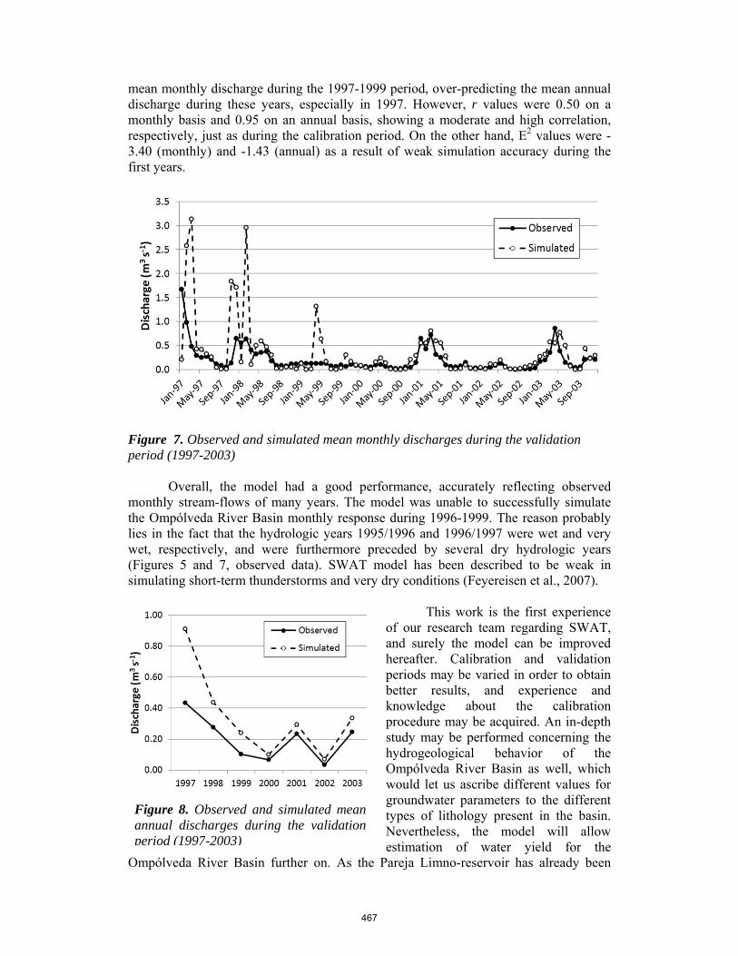
mean monthly discharge during the 1997-1999 period, over-predicting the mean annual discharge during these years, especially in 1997. However, r values were 0.50 on a monthly basis and 0.95 on an annual basis, showing a moderate and high correlation, respectively, just as during the calibration period. On the other hand, E2 values were -3.40 (monthly) and -1.43 (annual) as a result of weak simulation accuracy during the first years.

Figure 7. Observed and simulated mean monthly discharges during the validation period (1997-2003)

Overall, the model had a good performance, accurately reflecting observed monthly stream-flows of many years. The model was unable to successfully simulate the Ompólveda River Basin monthly response during 1996-1999. The reason probably lies in the fact that the hydrologic years 1995/1996 and 1996/1997 were wet and very wet, respectively, and were furthermore preceded by several dry hydrologic years (Figures 5 and 7, observed data). SWAT model has been described to be weak in simulating short-term thunderstorms and very dry conditions (Feyereisen et al., 2007).

This work is the first experience

of our research team regarding SWAT, and surely the model can be improved hereafter. Calibration and validation periods may be varied in order to obtain better results, and experience and knowledge about the calibration procedure may be acquired. An in-depth study may be performed concerning the hydrogeological behavior of the Ompólveda River Basin as well, which would let us ascribe different values for groundwater parameters to the different types of lithology present in the basin. Nevertheless, the model will allow estimation of water yield for the

Ompólveda River Basin further on. As the Pareja Limno-reservoir has already been

Figure 8. Observed and simulated mean annual discharges during the validation period (1997-2003)

467

built and the gauging station is inoperative, these estimations will be useful for performing a water balance of the limno-reservoir and to discover if the Ompólveda River Basin water availability is high enough to maintain the limno-reservoir at its maximum capacity throughout the whole year, even during the driest years, as it is supposed.

The siltation risk has great importance concerning limno-reservoir environmental viability. Because observed data on sediment concentration and loading were unavailable for the study area, the sediment component of the model could not be calibrated and validated. However, average annual sediment yield predicted by the model was 0.79 t ha-1, with a minimum value of 0.02 t ha-1 during 1993 and 1994, and a maximum value of 6.59 t ha-1 during 1997, the wettest year of the series. Looking at soil loss rates obtained by Arévalo (2008) ranging from 9 to 11 t h-1 year-1, average annual sediment yield predicted by the model would suggest that most of the sediment loss produced in the basin would not reach its outlet and, consequently, would not enter into the Pareja Limno-reservoir. Further on, sediment yield data obtained by improved SWAT simulations will be compared with the results obtained by our research team in the in-situ soil loss studies (Molina Navarro et al. 2010a, 2010b) and with information that we are obtaining directly from limno-reservoir sediments. 4. Conclusions

The hydrologic response of the Ompólveda River Basin was analyzed using the

semi-distributed model, SWAT. Calibration of the SWAT model was performed for 1991-1996, obtaining a satisfactory performance of the model. The adjustment decreased during the validation period (1997-2003). During these years, better adjustment was achieved during dry and normal years, whereas the differences between simulated and observed flows in wet years, especially during 1997, were higher. The statistics used to judge the model performance (r and E2) showed better simulation accuracy during the calibration period, and they showed better values on an annual basis than on a monthly basis both in calibration and the validation procedures.

Nevertheless, the application of the SWAT model to the Ompólveda River Basin may be improved. An improvement of the calibration process and a better knowledge of the hydrogeological behavior of the basin will lead to a more accurate model which will enable study of the hydrologic viability of the Ompólveda Limno-reservoir.

Finally, despite the impossibility of calibrating and validating the sediment component of the model, the sediment yield obtained suggests that most of the sediments produced in the basin would not reach its outlet and, consequently, the Pareja Limno-reservoir. Further results with improved versions of the model will be compared to in-situ studies that are ongoing in the basin.

Acknowledgements

Funding for this research came from the Social Acting of Ibercaja and the Government of Castilla-La Mancha (Science and Education Department, research project PAI08-0226-1758). Eugenio Molina-Navarro received additional support from a predoctoral grant from the University of Alcalá. We want to thank the Pareja City Hall and the Confederación Hidrográfica del Tajo for their support. Thanks also to Diana Arévalo for kindly offering her soil data and to Prof. Dr. R. Srinivasan for his assistance in the set-up of the model.

468

References Arévalo, D. 2008. Estimación de da Erosión del Suelo en la Cuenca del Ompólveda (unedited).

Environmental Sciences Final Degree Project, University of Alcalá. Arnold, J.G., J.R. Williams and D.R. Maidment. 1995. Continuous-time water and sediment-

routing model for large basins. Journal of Hydrology 121: 171-183. Arnold, J.G., R. Srinivasan, R.S. Muttiah and J.R. Williams. 1998. Large-area hydrologic

modeling and assessment: Part I. Model development. J. Am. Water. Res. Assoc. 34(1): 73-89.

Arnold, J.G. and N. Fohrer. 2005. SWAT2000: current capabilities and research opportunities

in applied watershed modeling. Hydrol. Procesess 19: 563.572. FAO, PNUMA, UNESCO. 1980. Metodología provisional para la evaluación de la degradación

de los suelos. FAO, Roma, Italy. Feyereisen, G.W., T.C. Strickland, D.D. Bosch and D.G. Sullivan. 2007. Evaluation of SWAT

manual calibration and input parameter sensitivity in the Little River watershed. Trans. ASAE 50(3): 843–855.

Fuentes Yagüe, J.L. 2003. Técnicas de riego. 4th Ed. Ministerio de Agricultura, Pesca y

Alimentación. Madrid, Spain. Galván, L., M. Olías, R. Fernández de Villarán, J.M. Domingo Santos, J.M. Nieto, A.M.

Sarmiento and C.R. Cánovas. 2009. Application of the SWAT model to an AMD-affected river (Meca River, SW Spain). Estimation of transported pollutant load. Journal of Hydrology 377: 445-454.

Gassman, P.W., M.R. Reyes, C.H. Green and J.G. Arnold. 2007. The soil and water assessment

tool: historical development, applications, and future research directions. Trans. ASAE 50(4): 1211–1250.

Guerra Delgado, A., F. Monturiol Rodríguez, T. Bodorrey Penacho, J.L. de la Horra Ruiz, J.L.

Labrandero Sanz, J.J. Carlevaris Muñiz and J. García-Vaquero Piqueras. 1970. Memoria explicativa del mapa de suelos de Guadalajara escala 1:250.000. Consejo Superior de Investigaciones Científicas. Madrid. Spain.

Hargreaves, G.H. and Z.A. Samani. 1985. Reference crop evapotranspiration from temperature.

Appl. Eng. Agric. 1: 96-99. Instituto de Desarrollo Regional, Junta de Comunidades de Castilla-La Mancha. 2008.

Infraestructura de datos espaciales de Castilla-La Mancha - Zona de Descarga. Available at: http://ide.jccm.es/descargapnoa/. Accessed 25 January 2011.

Molina Navarro, E.; S. Martínez Pérez and A. Sastre Merlín. 2010a. El Limnoembalse de Cola

de Pareja (Guadalajara): aspectos medioambientales e hidrológicos. Boletín Geológico y Minero 121(1): 69-80.

Molina Navarro, E., R. Bienes Allas, S. Martínez Pérez and A. Sastre Merlín. 2010b. Los

limnoembalses de cola y su riesgo de aterramiento: el caso del Limnoembalse de Pareja (Guadalajara). In IX Jornadas Españolas de Presas. Comunicaciones. Comité Nacional Español de Grandes Presas, T&B Editores.

469

Molina-Navarro, E., S. Martínez-Pérez, A. Sastre-Merlín, J. Soliveri, I. Fernández-Monistrol and J.L. Copa-Patiño. 2011. Microbiological water quality and its relation to nitrogen and phosphorus at the Pareja Limno-reservoir (Guadalajara, Spain). Journal of Environmental Management 92 (3): 773-779.

Moriasi, D.N., J.G. Arnold, M.W. Van Liew, R.L. Bingner, R.D Harmel and T.L. Veith. 2007.

Model evaluation guidelines for systematic quantification of accuracy in watershed simulations. Trans. ASAE 50(3): 885–900.

Motovilov, Y.G., L. Gottschalk, K. England and A. Rodhe, A. 1999. Validation of a distributed

hydrological model against spatial observations. Agric. For. Meteorol. 98–99: 257–277. Oeurng, C., S. Sauvage and J.M. Sánchez-Pérez. 2011. Assessment of hydrology, sediment and

particulate organic carbon yield in a large agricultural catchment using the SWAT model. Journal of Hydrology 401: 145-153.

Pisinaras, V., C. Petalas, G.D. Gikas, A. Gemitzi and V.A. Tsihrintzis. 2010. Hydrological and

water quality modeling in a medium-sized basin using the Soil and Water Assessment Tool (SWAT). Desalination 250: 274-286.

Porta Casanellas, J. and M. López-Acevedo Reguerín. 2005. Agenda de campo de suelos.

Información de suelos para la agricultura y el medio ambiente. Mundi-Prensa, Madrid, Spain.

Schoeneberger, P.J., D.A. Wysocki, E.C. Benham and W.D. Broderson (editors). 2002. Field

book for describing and sampling soils, Version 2.0. Natural Resources Conservation Service, National Soil Survey Center, Lincoln, NE, USA.

Srinivasan, R., T.S. Ramanarayanan, J.G. Arnold and S.T. Bednarz. 1998. Large-area

hydrologic modelling and assessment: Part II. Model application. J. Am. Water Res. Assoc. 34(1): 91-101.

Stehr, A., M. Aguayo, O. Link, O. Parra, F. Romero and H. Alcayaga. 2010. Modelling the

hydrologic response of a mesoscale Andean watershed to changes in land use patterns for environmental planning. Hydrology and Earth System Sciences 14: 1963-1977.

USDA Soil Survey Division Staff. 1993. Soil survey manual. Soil Conservation Service. U.S.

Department of Agriculture Handbook 18. Van Griensven, A. and W. Bauwens. 2003. Multiobjective autocalibration for semidistributed

water quality models, Water Resources Research 39(12): 1348-1357. Van Griensven, A., T. Meixner, S. Grunwald, T. Bishop and R. Sirinivasan. 2006. A global

sensitivity analysis tool for the parameters of multi-variable catchment models. Journal of Hydrology 324: 10–23.

Wang, X., S. Shang, W. Yang, C.R. Clary and D. Yang. 2010. Simulation of land use-soil

interactive effects on water and sediment yields at watershed scale. Ecological engineering 36: 328-344.

Winchell, M., R. Srinivasan, M. Di Luzio, J. G. Arnold. 2009. ArcSWAT 2.3.4 Interface for

SWAT2005. User’s Guide. Grassland, Soil and Water Research Laboratory, Agricultural Research Service; Blackland Research Center, Texas Agricultural Experiment Station, Temple, Texas.

470

Grid-Based Hydrological Model Calibration and Execution by gSWAT Application

Dorian Gorgan 1, Danut Mihon 1, Victor Bacu 1, Teodor Stefanut 1, Denisa Rodila 1, Lukasz Kokoszkiewicz 2, Elham Rouholahnejad 3, Karim Abbaspour 3,

Ann van Griensven 4

1 UTCN, Technical University Cluj-Napoca, Romania {dorian.gorgan, victor.bacu, vasile.mihon, teodor.stefanut, denisa.rodila}@cs.utcluj.ro

2 CERN, European Organization for Nuclear Research, Geneva, Switzerland

lukasz.kokoszkiewicz@cern.ch

3 EAWAG, Swiss Federal Institute for Aquatic Science and Technology, Switzerland elham.rouholahnejad@eawag.ch, karim.abbaspour@eawag.ch

4 UNESCO-IHE, Institute for Water Education, Department of Hydroinformatics and Knowledge

Management, Delft, The Netherlands a.vangriensven@unesco-ihe.org

Abstract This paper is concerned with key concepts and architectures supporting calibration and execution of the SWAT hydrological model over Grid infrastructures. The Grid capabilities are required due to the large number of runs required in both calibration and execution processes. The assessment of sustainability and vulnerability in the Black Sea catchment is one of the goals of the FP7 enviroGRIDS project. By developing a spatial data infrastructure for this catchment region, different scenarios based on environmental changes and water quality models could be simulated. The gSWAT application is integrated as a module in the enviroGRIDS portal in order to support the hydrologic experts on the development and the execution of an already calibrated model. The user may monitor the Grid-based execution and visualize the results in different outputs and formats. To optimize the SWAT calibration over the Grid, a parallel approach at the data level is used. The Grid-based approach speeds up the entire calibration flow of the model and significantly reduces the total execution time compared to the same process that runs on a single machine that in some cases could take hours or even days. The large user community of SWAT may greatly benefit from a Grid version of the software. Keywords: SWAT model, hydrological model calibration, hydrological scenario, parallel and distributed processing, Grid infrastructure.

471

1. Introduction

The gSWAT platform was developed in the framework of the enviroGRIDS FP7 project, funded by the European Commission. The main goal of this platform is the assessment of the sustainability and vulnerability of the Black Sea catchment using the SWAT (Soil and Water Assessment Tool) hydrological model. This paper describes the SWAT calibration and execution phases by pointing out the main features integrated within the gSWAT platform.

When applying the SWAT hydrological model to large watersheds (e.g. the Black Sea catchment), the calibration and execution processes became difficult to control and implement. In such cases, large volumes of data needed to be processed. Standalone machines (even multi-core ones) became inefficient when dealing with such amounts of information. Based on the previously-mentioned remarks, this paper proposes the Grid as a development infrastructure for the gSWAT platform due to its storage and parallel computation capabilities.

The main goal of the SWAT hydrological model is to simulate and predict the effects of land management practices on water quantity and quality within small, medium or large watersheds. It is based on daily information collected from the ground stations distributed across the watershed region. This information is collected in the form of soil and water properties but also as the vegetation and topography characteristics of the watershed stored in a TxtInOut file (Pohlert et al., 2006, Jacobs et al., 2005).

Generally speaking, the calibration process represents the act of adjusting the accuracy of the measured parameters through different measurement techniques (Liu et al., 2005). The manual parameter adjustment is a subjective process of comparing the observed values with those obtained during a simulation of the calibration process. This scenario is time-consuming because of the large number of hydrological parameters that need to be adjusted. Because of this, the development of a semi-automated process is taken into account as one of the gSWAT features.

SWAT model execution is useful in building user scenarios based on an already calibrated model. Different scenarios could be implemented for simulating or predicting hydrological phenomena (e.g. water-use sustainability, floods, irrigation system improvement, etc) (Zhang et al., 2008). Gassman et al. (2007) describe the applicability of the SWAT model for the Mississippi River Basin in order to perform macro-scale assessments in this watershed.

The gSWAT platform integrates the SWAT calibration and execution processes. Based on the process complexity, a different number of Grid workers are used in the execution process. The main advantage of the Grid infrastructure is that it offers support for running multiple jobs in parallel mode, improving the overall execution time. The final result is then generated based on all of the intermediate results collected from all of the Grid workers.

The following sections of this paper will detail the SWAT model calibration process from the Grid execution point of view. The calibration output validity is proved by the experiments and presented in the “Experimental Results” section. Also, some of the most important features of the gSWAT platform will be described along with their utility for the end user. 2. Related Works

The main goal of the gSWAT platform is related to the assessment of the sustainability and vulnerability of the Black Sea catchment. Performing the SWAT calibration process for the Black Sea watershed on a standalone machine is inefficient because of the large volume of data that need

472

to be processed. The Grid and Cloud infrastructure and also some high performance multi-core machines could be used as alternative solutions.

SWAT-CUP (SWAT Calibration and Uncertainty Procedures) is a software tool that provides complex capabilities related to the SWAT model calibration process (Abbaspour, 2008). It offers different calibration algorithms such as: GLUE, ParaSol, SUFI2 and MCMC. Through the graphical interface, the user is able to calibrate and validate the SWAT model and to analyze its output in a friendly manner. Initially it was implemented to work only on single-core machines, but the newer versions of these tools allow its use on multi-core computers. The SWAT-CUP application is efficient on small and medium SWAT models, but when dealing with large watersheds its overall execution time increases to tens of hours.

The Grid and Cloud infrastructures represent efficient solutions for simulating the SWAT model for large watersheds. This is possible due to the storage and parallel computing capabilities offered by these two distributed infrastructures. In other words, the entire calibration process is divided into multiple groups that can be executed in parallel over the Grid and Cloud infrastructures. This way the overall execution time is significantly reduced. The main difference between these two platforms is that Grid offers its services free of charge to any kind of user that has valid Grid certificates bestowed by a competent CA (Certificate Authority). The Cloud infrastructure demands a fee for each provided service (Mihon et al., 2011). Therefore, the Grid application was chosen to be used for gSWAT.

Because of the dynamic nature of Grid, the calibration and execution of the SWAT model are processes that are difficult to implement. Due to the GANGA (Moscicki et al., 2009) and Diane (DIstributed ANalysis Environment) (Moscicki, 2004) tools, Grid resource management is easier to accomplish. The GANGA application allows the user the possibility to configure, monitor and manage all the jobs of the Grid processes. Another important feature integrated into this application offers support for dividing complex jobs into sub-jobs and executes them independently. The sub-job merge module generates the final output based on the intermediate sub-jobs results. The Diane tool provides efficient usage of Grid resources through the failure management system and error recovery policies. It allocates the Grid workers for each execution process based on an internal scheduler. The integration with the GANGA tool is also possible due to different communication modules integrated within the Diane application.

BASINS (Better Assessment Science Integrating point & Non-point Sources) is an environmental application used for analyzing water quality in different geographical watersheds (Bicknell et al., 1997). It allows users to perform watershed delineation, and to analyze and visualize the output in an animated manner. Its newer versions include the HSPF (Hydrological Simulation Program - FORTRAN) (Bicknell et al., 2001) and WASP7 (Golden et al., 2011) hydrological models.

3. System-Related Architecture

Figure 1 presents the gSWAT system-related client-server architecture built upon the Grid infrastructure. The graphical user interface links with the data processing layer through the GANAGA and Diane tools that act like a middleware communication module in sending and receiving information to and from the Grid workers. The top architectural layer is represented by the gSWAT graphical interface that exposes to the user all the services needed for the calibration and execution of the SWAT hydrological model. In other words, the users have direct access only to this module of the application, thereby hiding the complex data processing that takes place on

473

the Grid infrastructure. The client side, or graphical interface, is built as a Web application using the latest Adobe Flex technology. The analysis and visualization of the SWAT model-based scenarios are possible through the Bashyt platform (Cau and Manca, 2007). This platform allows the user to visualize the SWAT model execution output scenario as an animated 2D map that displays the stations in the watersheds along with some essential characteristics. Scaling and translating the map using mouse events is also possible in the framework of this platform.

All user requests are performed at this architectural level. The input data, the external dependencies and the execution workflow structure are also defined in this stage based on user requests and sent to the Grid infrastructure through the GANGA and Diane tools. The Diane application analyzes the calibration process complexity and decides the number of Grid workers necessary for the execution phase. After that, all data are sent to these nodes and executed in a parallel manner.

Figure 1. Architecture of the gSWAT system: graphical user interface of the gSWAT application, Web services, SWAT process resources and Grid infrastructure

The monitoring component implemented within the GANGA tool offers important feedback

about the calibration processes running on the Grid infrastructure. This feedback could then be displayed to the user in the gSWAT graphical interface in terms of: total execution time depicted as an animated progress bar, Grid process status (Schedule, Submitted, Waiting, Running, Completed), execution details in the form of a system log (contains all internal processing messages and error), etc.

The Grid infrastructure offers high storage and parallel computation capabilities in order to successfully calibrate and execute the SWAT hydrological model for different geographical

474

watersheds. Because the output of these processes could reach a few Gb in size, a standalone machine becomes inefficient. The SE (Storage Element) nodes inside the Grid offer storage support for large volumes of data. Accessing these recourses requires valid Grid certificates, emitted by a competent CA (Certificate Authority). The data transfer between SE nodes and Grid applications is based on the GSIFTP (Grid Security FTP) protocol. The SRM (Storage Resource Manager) (Brzezniak et al., 2008) manages all SE nodes inside the Grid infrastructure and offers support for error and trial recovery mechanisms, minimizes data replication, allocates a specific SE that has enough memory space to support the entire Grid process output, etc.

It is worth saying that all the gSWAT and Bashyt functionalities will be integrated into a Web portal and could be accessible for all kinds of users, as long as they have valid Web and Grid credentials. A SSO (Single Sign On) mechanism should be integrated into this portal, allowing the users to access these features with a single authentication process. In other words, any time one of the gSWAT or Bashyt functionalities requires a user authentication, the SSO mechanism automatically provides the right user credentials. This is useful when calibrating the SWAT model using the gSWAT platform and visualizing scenario results using the Bashyt platform.

After all the Grid workers finish their execution, a collection mechanism is applied in order to generate the final output based on all the intermediate results obtained during the workers’ executions. When the final output is available, the user can analyze it based on the gSWAT and Bashyt platforms.

4. SWAT Model Calibration Workflow

There are multiple algorithms that could be used to calibrate the SWAT hydrological model: GLUE, ParaSol, SUFI2 and MCMC. At this stage of development, the gSWAT platform allows only the usage of the SUFI2 (Sequential Uncertainty Fitting) calibration algorithm (Abbaspour et al., 2007). One of the future work objectives is to offer the user the possibility to choose its own calibration method from a predefined set of algorithms. The SUFI2 is useful because it can perform uncertainty analysis of the SWAT hydrological model. Another important aspect of this method consists in its ability to decrease the total execution time for the calibration process compared with the other three algorithms.

A common feature related to any calibration process is that this whole process is repeated until an objective function is satisfied. In the case of performing SUFI2 calibration, these objective functions could be determined based on root means square error, Chi square, Nash-Sutcliffe, R2 and bR2.

Another important aspect related to the SUFI2 calibration algorithm is that it supports a specific folder structure and no deviations are allowed. This structure basically contains the calibration inputs folder (files that store the parameter intervals and the observed values for these parameter lists), calibration outputs folder (statistical files organized as tables, best simulation values for all the input parameters), backup folder (useful when building multiple scenarios) and executable files (for pre-processing, processing and post-processing phases of the SWAT model calibration process). This folder structure (known as TxtInOut folder), along with other metadata information, represents a project within the gSWAT platform. In other words, when the user creates a new project, one of the steps involved in this process is to upload the TxtInOut folder. Because of the large number of contained files, this structure is uploaded only as an archive. An animated upload progress bar gives users feedback about the state of this process.

475

It is worth mentioning that initially all the files are copied to the application server. At this level the project structure is generated: naming the project, creating a new input in the application database, checking if all the files were successfully copied, and transferring the project dependencies onto an SE node for faster data access when executing the calibration process.

The Grid infrastructure is very complex and hard to understand even for the most experienced specialists. The error logs provided by the services of this infrastructure represent a starting point in the problem fixing and debugging process. In order to reduce as much as possible the end user interaction with the Grid infrastructure, a new set of statuses and error messages were defined within the gSWAT platform. The most important ones are: Running iteration (displayed when the calibration process takes place), Finished iteration (the entire iteration process finished successfully and the results are available for download) and Incomplete iteration (this status is displayed when the calibration failed due to some technical problems). These are the only messages displayed to the user in case of execution errors. For experienced users, a system log is also available where all errors are registered, and each error contains the full description of the problem that caused it.

Each calibration process consists of multiple iterations, executed until a calibration criterion is satisfied. Within each iteration there are variable numbers of simulations. At the iteration level there are three main phases of execution: pre-processing, actual execution of data and the post-processing phase (Figure 2). The following paragraphs shortly describe all internal processes. 4.1. Pre-processing phase

It is worth mentioning that a values interval is attached to each SWAT input parameter. Taking this into account, one iteration takes a discrete random value for each parameter from the corresponding interval and executes the calibration algorithm. For a better output accuracy, the iteration process should consist of a high number of simulations in order to cover all values inside these intervals. In general this number is limited to 500 simulations per calibration process.

At the gSWAT level, this phase allows the user to edit the SWAT input parameters list based on the text editor module integrated within this platform. Only the calibration input files are allowed to be edited. This module is built in such a manner that it could display large data files (even with tens of thousands of lines). An input data validation mechanism will be considered for future work. This means that a set of rules should be deducted from the calibration input file structures and applied on the modifications made by the user.

This mechanism identifies and highlights the possible errors made by the users when editing the input files. Each error will be marked with a red dot and contains a suggestive error message, understandable to any kind of user. Although this is useful for non-specialist users, in some situations it could save a lot of time for even hydrology domain field specialists. At this stage the project should contain the TxtInOut folder, uploaded by the user. 4.2. Execution phase

This represents the most time-consuming part of the entire SWAT model calibration process. It requires parallel execution support of the Grid architecture. In other words, based on the process complexity, a differing numbers of Grid workers can be allocated for this job.

After all project dependencies are successfully generated on the client side, they are transferred to the Grid workers in order to be processed. Depending on the number of simulations chosen by the user, a different number of worker nodes will be involved in this execution process. Generally speaking, if the iteration contains 500 simulations, 50 smaller groups will be created.

476

Figure 2. SWAT model calibration workflow: sequence of iterations consisting of pre-processing, set of simulations, and post-processing

Each group will have 10 simulations and run on a different Grid node. Even though there is

a parallel execution at the group level, inside each group the 10 simulations will be executed sequentially. Increasing or decreasing the number of Grid workers in order to increase the performance gain represents a statistical function that depends on the complexity of the calibration process and the distributed nature of the Grid infrastructure. In other words, a large number of workers will not always give better execution time. Instead, a statistical formula has to be implemented that could allocate a specific number of workers based on the SWAT model calibration process complexity.

All the data are initially transferred from the application server to the Grid nodes using the GANGA and Diane scripts. Execution and monitoring of the SWAT calibration processes are also allowed with these tools.

The user should be aware of the calibration process that runs over the Grid infrastructure. The gSWAT platform offers the user some feedback about the status of this process through an animated progress bar that represents the percentage of simulations executed. Another important feature integrated within the gSWAT platform is the capability to manage multiple projects simultaneously. This is possible through the usage of the projects list. Each input from this list gives some minimal details about the project execution: total execution time, project status and calibration progress.

The gSWAT platform offers the user the possibility to perform other actions in parallel with the SWAT model calibration process. In other words, the user could create new projects, upload different SWAT models as TxtInOut folders, analyze results, create scenarios, etc. The execution progress displayed at the graphical interface level is periodically updated by interrogating the application database that stores all Grid process information.

477

4.3. Post-processing phase Just like the pre-processing phase, it takes place on the gSWAT application server after all

the Grid workers finish their execution. A collection mechanism generates the final calibration output based on all intermediate results given by Grid workers. An interesting aspect is that initially all these results are stored inside SE nodes. When the user makes a request for this result it is archived and sent to the application server and from there to the graphical user interface.

The gSWAT platform offers a significant speedup for the total SWAT model calibration time by using the Grid infrastructure. Another important aspect of this platform is represented by the analysis and visualization features of the output calibration process. As shown in Figure 2, the calibration process continues until a goodness function is satisfied. This is a subjective process that depends on the hydrologic field specialist that performs the SWAT model calibration.

All these results are placed inside the calibration output folder within the SWAT specific structure. The majority of the files contain the ASCII data format that can be analyzed based on the text editor module implemented within gSWAT platform. The content of the 95ppu.sf2 file could take the chart form representation and offers high resolution visualization details about the values computed for the SWAT input parameters list during the calibration process (Figure 3).

The GorganFig3.tif chart defines the best estimated parameter values (obtained during the SWAT calibration process) and the observed ones (measured from stations spread across the entire watershed) in order for the specialist to make a statistical approximation of the calibration accuracy. Also, an uncertainty analysis could be performed based on this kind of data representation.

The input data chart is sent from the application server using the JSON format. This represents an elegant data transfer method because of its simplicity of usage (the client side application has good knowledge in encoding and decoding this kind of data format). Each chart inflexion point allows the user the possibility of visualizing the best estimated and ground measured values of the SWAT parameters. The user could also increase or decrease the temporal interval by using an animated slider with two thumbs. Each thumb represents one extremity of the time interval.

5. Experimental Results

Two kinds of experiments were conducted in order to prove the superior efficiency of the

Grid infrastructure over standalone machines (single or multi-core). It is worth mentioning that the second experiment highlights the Grid distributed nature meaning that it is hard to keep the same contextual execution background when new tests are performed. The vo.gear.cern.ch VO (Virtual Organization) site was used for both experiments.

The first experiment was performed based on a small-scale SWAT hydrological model (around 20,000 input files) that represents the Danube watersheds. A single SWAT iteration was performed on a standalone machine (2xQuad core processor at 2.13 GHz, 48 GB of RAM) and on the Grid infrastructure. The number of simulations for the current iteration was set to 100. It is worth saying that each calibration process is executed on multiple Grid workers. Each of them represents a computing machine with one or multiple processors. The Grid process submission using the GANGA and Diane tools does not allow the possibility of specifying what kind of hardware resources to use for the execution phase. This way a random group of Grid workers are selected with different hardware capabilities.

478

In the case of Grid execution, the 100 simulations were divided into ten groups of ten simulations. The Grid execution was performed in parallel at group level and sequentially for all the iterations inside each group. The three calibration phases described in the previous section were also applied in this experiment by using the GANGA and Diane tools for data transfer and execution.

Figure 3. Interactive visualization of the results throughout the calibration process

After all the inputs were specified, the experiment began. A seven minute total execution time per simulation was obtained on the standalone machine. The same simulation took only four minutes to complete in the case of the Grid calibration process due to its parallel execution support. This experiment shows an improvement of almost 50% for executing the SWAT calibration process with 100 simulations per iteration.

It is well known that the Grid becomes efficient for large volumes of data processing. Taking this into account, the execution gain between Grid nodes and standalone machines is enhanced for larger numbers of simulations. This aspect represents the basis of the second experiment. It is worthwhile to mention that the total Grid execution time depends on:

. The time required to allocate a Grid worker node for each group of simulations; . The time required to send all the inputs and the external dependencies to that worker.

Because the SWAT hydrological model is already stored inside Grid on the SE nodes, this time is less relevant that in the case of transferring data from the application server;

. The actual execution process, as described in the previous sections;

. The time to generate the final calibration result based on all intermediate outputs generated by the Grid parallel executions;

. The total Grid execution time also depends on the Grid usage degree at that moment and on the network traffic.

The second experiment (Figure 4) represented in this section highlights how the total execution time fluctuates when varying the Grid worker nodes for the same number of SWAT

479

model simulations. Based on this remark, this experiment takes into account a variable number of simulations for a single calibration process. The SWAT model used in this case was a large one (e.g. 70,000 input files) that represented the same Danube watershed distribution.

Figure 4. Execution time per simulation by varying the number of simulations and the number of Grid workers involved in the parallel and distributed processing

By keeping the same number of simulations (i.e. 100, 150, 200 or 250), the second variable

of this experiment was represented by the number of Grid workers allocated to execute these simulations (i.e. 30, 40 and 50 worker nodes). The nodes allocation and processes schedule were possible through the GANGA and Diane tools.

The idea of creating smaller simulation groups is also maintained within this second experiment. In other words, if 50 Grid workers were allocated for a total number of 200 simulations, then each group contains 40 such simulations that will be executed sequentially on the same Grid node. The general tendency of the results, presented in Figure 4, suggests a slight improvement of the overall simulation execution time for larger numbers of Grid worker nodes.

The interpretation of the results obtained within this second experiment is the following: when increasing the number of simulations, a larger number of Grid workers should be allocated for this calibration process in order to obtain better execution times. This remark is not valid all the time. For example, allocating a Grid node for each simulation will generate a visible performance loss because the time required to copy all the inputs to that Grid node is higher than the actual execution time. This experiment is also used as a statistical study of generating a method that automatically allocates a specific number of Grid workers depending on the calibration process complexity.

6. Conclusions

This paper fully describes the calibration and execution processes of the SWAT

hydrological model through the gSWAT platform. The Grid infrastructure is one of the distributed

480

platforms that provide a significant performance gain when calibrating the SWAT model. The communication mechanisms between the architectural modules of the gSWAT platform were also highlighted throughout this paper.

The section of Experimental Results attempted to validate the proposed architectural design of the gSWAT platform based on two straightforward experiments. The first one points out Grid efficiency superiority over standalone machines, while the second one analyzes SWAT calibration behavior on different Grid execution backgrounds. Acknowledgments This research is supported by the FP7 enviroGRIDS Project funded by the European Commission through the Contract 226740. References Abbaspour, K.C. 2008. SWAT-CUP2: SWAT Calibration and Uncertainty Programs – A User Manual.

Department of Systems Analysis, Integrated Assessment and Modeling. Eawag, Swiss Federal Institute of Aquatic Science and Technology. Duebendorf, p.11. Available at: http://www.eawag.ch/forschung/siam/software/swat/man3.1.5.pdf. Accessed 30 July 2011.

Abbaspour, K.C., J. Yang, I. Maximov, R. Siber, K. Bogner, J. Mieleitner, J. Zobrist, and R. Srinivasan.

2007. Modelling hydrology and water quality in the pre-alpine/alpine Thur watershed using SWAT. Journal of Hydrology, 333: 413-430.

Bicknell, B. R., J. C. Imhoff, J. L. Kittle Jr, A. S. Donigian, and R. Johanson. 2001. Hydrologic Simulation

Program- Fortran User’s Manual for Release 12. Exposure Research Laboratory, Office of Research and Development, US Environmental Protection Agency, Athens, Georgia.

Bicknell, B.R., J. C. Imhoff, J. L. Kittle Jr, A. S. Donigian, and R. C. Johanson. 1997. Hydrological

Simulation Program - FORTRAN, User's manual for version 11. US Environmental Protection Agency, National Exposure Research Laboratory, Athens, Georgia.

Brzezniak, M., N. Meyer, M.D.Flouris, R. Lachaiz, and A. Bilas. 2008. An Analysis of Grid Storage

Element Architectures: High-end Fiber-Chanel vs. Emerging Cluster-based Networked Storage, Book Chapter. In Book on Grid Middelware and Services: 187-201.

Cau, P., and S. Manca. 2007. The Bashyt DSS: a Web Based Decision Support System for Water Recourses

Management. 4th International SWAT Conference, Sardinia. Available at: http://www.brc.tamus.edu/swat/4thswatconf/docs/rooma/session5/Cau-Bashyt.pdf

Gassman, P.W., M.R. Reyes, C.H. Green and J.G. Arnold. 2007. The Soil and Water Assessment Tool:

Historical Development, Applications, and Future Research Directions, Transactions of the American Society of Agricultural and Biological Engineers, Vol.50: 1211-1240.

Golden , H. E., and C. D. Knightes. 2011. Simulated Watershed Mercury and Nitrate Flux Responses to

Multiple Land Cover Conversion Scenarios. Environmental Toxicology and Chemistry, 30(4): 773-786.

Jacobs, J.H. and R. Srinivasan. 2005. Application of SWAT in developing countries using readily available

data. In Proc. 3rd International SWAT Conference, Zurich, Switzerland. July 13-15, EAWAG, Switzerland.

481

Liu, Y. B., O. Batelaan, F. De Smedt, J. Poorova, and L. Velcicka. 2005. Automated calibration applied to a

GIS-based flood simulation model using PEST, in: Floods, from Defence to Management, 317–326. Edited by: Van Alphen, J., van Beek, E., and Taal, M.,Taylor & Francis Group, London.

Mihon, D., T. Stefanut, V. Bacu, D. Rodila, K. Abbaspour, L. Kokoszkiewicz, E. Rouholahnejad, A. Van

Griensven, and D. Gorgan. 2011. Grid Based Hydrologic Model Calibration and Execution. In Proc. CSCS-18, 18th International Conference on Control Systems and Computer Science, 833-840.

Moscicki, J.T. 2004. DIANE – Distributed Analysis Environment for GRID-enabled Simulation and

Analysis of Physics Data. In IEEE Nuclear Science Symposium Record, Vol.3: 1617-1620. Moscicki, J.T. , F. Brochu, J. Ebke, U. Egede, J. Elmsheuser, K. Harrison, R.W.L. Jones, H.C. Lee, D. Liko,

A. Maier, A. Muraru, G.N. Patrick, K. Pajchel, W. Reece, B.H. Samset, M.W. Slater, A. Soroko, C.L. Tan, D.C. van der Ster and M. Williams. 2009. GANGA: A tool for computational-task management and easy access to Grid resources. Computer Physics Communications, 180(11): 2303-2316.

Obtaining and using Grid certificates, Available at: http://gridcanada.ext.nrc.ca/?q=node/7 Pohlert, T., L. Breuer, J. A. Huisman, and H.-G. Frede. 2006. Assessing the model performance of an

integrated hydrological and biogeochemical model for discharge and nitrate load predictions, Hydrologic Earth System Science, 3(5): 2813-2851.

Zhang, X., R. Srinivasan, and M. Van Liew. 2008. Multi-Site Calibration of the SWAT Model for

Hydrological Modeling, Transactions of the American Society of Agricultural and Biological Engineers, Vol.51: 2039-2049.

482

Soil Erosion Hazard Prediction Using SWAT Model and Fuzzy Logic in a Large Highly Mountainous Watershed

A. Besalatpour

Department of Soil Sciences, College of Agriculture, Isfahan University of Technology, Isfahan, Iran, 84156-83111, a_besalatpour@ag.iut.ac.ir

M.A. Hajabbasi

Department of Soil Sciences, College of Agriculture, Isfahan University of Technology, Isfahan, Iran, 84156-83111, hajabbas@cc.iut.ac.ir

S. Ayoubi

Department of Soil Sciences, College of Agriculture, Isfahan University of Technology, Isfahan, Iran, 84156-83111, ayoubi@cc.iut.ac.ir

M. Faramarzi

Department of Natural Resources, Isfahan University of Technology, Isfahan, Iran, 84156-83111, monireh.faramarzi@cc.iut.ac.ir

M. Amini

Eawag, Swiss Federal Institute for Aquatic Science and Technology, Ueberlandstrasse 133, PO Box 611, CH-8600 Dübendorf, Switzerland, manouchehr.amini@eawag.ch

Abstract

Soil erosion is a major environmental threat to sustainability and agricultural productivity. It can adversely affect the quality of surface and groundwater by adding transported sediments, nutrients and pesticides, as well as by increasing turbidity. The purpose of this study is to identify and prioritize the critical subbasins in the highly mountainous Bazoft watershed of southwestern Iran using imprecise and uncertain available data. The Soil and Water Assessment Tool (SWAT) was used to develop a hydrologic model for the study area. In combination with SWAT, a Sequential Uncertainty Fitting Program (SUFI-2) was used to calibrate and validate the model using the daily river discharge and daily sediment load. Uncertainty analysis was also performed for model reliability. A fuzzy logic approach was also developed to assess the soil erosion hazard in the area and further compared with the SWAT model predictions. For this, three important landscape features related to soil erosion hazard including vegetation cover, slope and soil erodibility factor were used. The calibration and validation results of the SWAT model showed that most of the predicted discharge and sediment yields agreed well with the observed data. However, the predicted discharge values were more satisfactory than the sediment values. The subbasins S5, S6, S4 and S31 accounted for about 76% of the total soil loss from the watershed, while they only covered about 11% of total area of the watershed. Furthermore, a large part of the watershed (24 subbasins) was predicted to be in danger of high or very high erosion using the fuzzy logic model and only 4 subbasins fell under the very low erosion hazard class. Keywords: soil erosion hazard, SWAT, fuzzy logic, watershed management.

483

1. Introduction

Soil erosion constitutes a global economic, social and environmental problem (Lal, 2001). It causes loss of fertile topsoil and reduces the productive capacity of the land and thereby creates risk to global food security. It also negatively affects the natural water storage capacity of catchments, design-life of man-made reservoirs and dams, quality of surface water resources, aesthetic landscape beauty, and ecological balance in general (Bewket and Teferi, 2009). Nevertheless, in most cases only a few areas of a large watershed might be critical and more responsible for high amounts of soil and nutrient losses. Implementation of best management practices is required in those critical erosion-prone areas of the watershed for controlling the loss of soil and nutrient. Identification of these critical areas is also essential for the effective and efficient implementation of watershed management programs (Tripathi et al., 2003).

Soil erosion by water is the most pressing environmental problem in Iran, particularly in highlands where the topography is highly rugged, population pressure is high, steep-lands are cultivated and rainfall is erosive. Therefore, identification of the critical sub-watersheds in these areas for implementation of the best management practices for soil conservation is an urgent need. The use of physically-based distributed parameter models, remote sensing techniques and geographic information systems may assist management agencies in both identifying the most vulnerable erosion-prone areas of watersheds and selecting appropriate management practices. The main objective of this study was to assess soil erosion hazard in a highly mountainous watershed (Bazoft watershed, southwestern Iran) using a physical model created by the Soil and Water Assessment Tool (SWAT). The potential use of a simple erosion hazard assessment approach, fuzzy logic, integrated with satellite remote sensing and geographical information systems for identification and prioritization of the critical subbasins was also evaluated.

2. Materials and Methods The study area was the Bazoft watershed (31°37′ to 32°39′ N and 49°34′ to 50°32′ E) located in

the northern part of the Karun river basin in southwestern Iran (Figure 1). The elevation ranges from 880 m at the southern end of the watershed to 4,300 m on Zardkuh mountain. The long-term average rainfall and temperature ranges in the region are 500-1,400 mm and 8-20°C, respectively. The slope class of 40-70% is the major class of slope in the watershed, which covers about 46% of the study area. The dominant slope shape in the watershed is convex. Approximately 56% of the watershed area is covered by pastures and the rest is covered by forest and bare lands. The watershed was subdivided into 41 subbasins. The SWAT (2005) program was used to simulate runoff and sediment in the study area. The simulation time period was from 1989 to 2008. The model was then calibrated with uncertainty analysis using the sequential uncertainty fitting (SUFI-2) program (Abbaspour, 2007). The calibrated and validated SWAT model was used to identify the critical subbasins on the basis of average annual sediment yield. The erosion rates and their classes used for identifying the critical subbasins are presented in Table 1.

Three important landscape features related to soil erosion hazard in the watershed including vegetation cover, slope and soil erodibility factor (K factor) were used for developing the soil erosion hazard prediction map using the fuzzy logic approach (Figure 2). The landscape variables were fuzzified by applying triangular fuzzy membership functions represented by fuzzy linguistic (including low, moderate, high, and very high) and fuzzy sets. Steps followed for modeling soil erosion hazard using the fuzzy logic algorithm within a GIS environment are summarized in Figure 3. The critical subbasins were identified on the basis of the average annual sediment yield for each subbasin according to the mentioned erosion rates and their classes in Table 1.

484

Figure 1. Location and the subbasins of Bazoft watershed in southwestern Iran

Table 1. Annual soil erosion ranges and severity classes

Figure 2. Landscape features used in developing the soil erosion hazard prediction map using the fuzzy logic approach

Soil erosion class Soil erosion range (t ha-1 yr-1) Very low <5

Low 5-12 Moderate 12-25

High 25-50 Very high >50

Slope Vegetation Cover Soil Erodibility

485

Figure 3. Steps followed in modeling of soil erosion hazard using fuzzy logic algorithm within a GIS environment

Landscape variables Fuzzy sets

Medium High Low

Fuzzy membership function (Fuzzification)

Variable sub layers

Slope % Low

Slope (%) Medium

Slope (%) High

K factor Low K factor

Medium K factor High

Vegetation cover (%) Low

Vegetation cover (%) High

Fuzzy overly between linguistic terms (low, medium, high) Fuzzy maximum operator (Or)

Low erosion hazard

0.8 Medium erosion hazard

0.6

High erosion hazard 0.6

Soil erosion hazard: Low With possibility of 0.8 validation

486

3. Results and Discussion 3.1. Soil erosion hazard prediction using SWAT

An initial sensitivity analysis resulted in the choice of parameters that were calibrated as listed in Table 2. The results of daily discharge and sediment calibrations at the watershed are also presented in Figure 4. The model simulated the runoff and sediment yields satisfactorily, however, the predicted runoff values were much more in agreement with the measured data than those for the sediment values (Figure 4). Based on the spatial distribution of the erosion hazard in the watershed, 19 out of 41 subbasins fell under high and very high soil erosion categories, of which 2 and 17 subbasins were in the high and very high categories, respectively (Figure 5). The subbasins S5, S6, S4, and S31 were accounted for about 76% of the total soil loss from the watershed, while they only covered about 11% of the total area of the watershed. The high erosion rate predicted in these subbasins may be attributed to insufficient use of the land, scanty vegetative cover, steep sloping areas, high population pressure, cultivating of the steep-lands and other environmental problems. These four critical subbasins were assigned as top priorities and recommended to be considered for future conservation plans.

Table 2. Description of SWAT (2005) input parameters selected for calibration

Parameter Description Initial range Final range Min Max Min Max

*r_CN2.mgt Curve number for moisture condition II -0.4 0.4 0.01 0.19 r_SOL_BD.sol Soil bulk density -0.3 0.3 0.20 0.30 r_SOL_AWC.sol Soil available water storage capacity -0.3 0.3 0.29 0.51 r_SOL_K.sol Soil hydraulic conductivity -0.8 0.8 -0.62 -0.15 r_SOL_ALB.sol Moist soil albedo -0.5 0.5 -0.38 -0.16 v_ALPHA_BF.gw Baseflow alpha factor 0 1 0.08 0.24 v_GW_DELAY.gw Groundwater delay time 0 400 122 256 v_REVAPMN.gw Threshold water in shallow aquifer 0 100 28 50 v_GW_REVAP.gw Revap coefficient 0.02 0.2 0.12 0.16 v_SHALLST.gw Initial depth of water in the shallow aquifer 0 1000 470 700 v_RCHRG_DP.gw Deep aquifer percolation fraction 0 1 0.30 0.56 v_GWQMN.gw Threshold depth of water in the shallow aquifer required

for return flow to occur. 0 500 208 342

v_EPCO.hru Plant uptake compensation factor 0.01 0.2 0.25 0.42 v_ESCO.hru Soil evaporation compensation factor 0.01 0.3 0.53 0.74 v_SLSUBBSN.hru Average slope length 10 150 49 72 v_OV_N.hru Manning’s n value for overland flow 0 0.8 0.25 0.37 v_CH_N2.rte Manning’s n value for the main channel 0 0.3 0.10 0.15 v_CH_K2.rte Main channel conductivity 0 150 92 107 v_SFTMP.bsn Snowmelt temperature -5 5 0.34 2.10 v_SMTMP.bsn Snowmelt base temperature -5 5 3.03 4.70 v_SMFMX.bsn Melt factor for snow on 21 June 0 10 3.75 6.95 v_SMFMN.bsn Melt factor for snow on 21 December 0 10 4.82 7.25 v_TIMP.bsn Snow pack temperature lag factor 0.01 1 0.69 0.99 v_MSK_CO1.bsn Muskingum coefficient 0 10 8.53 9.51 v_MSK_CO2.bsn Muskingum coefficient 0 10 3.18 5.87 v_SURLAG.bsn Surface runoff lag coefficient 1 24 13 17 v_PRF.bsn Peak factor for sediment routing channel 0 1 0.11 0.25 r_ROCK.sol Rock fragment counter -0.3 0.3 -0.2 0 v_ADJ_PKR.bsn Peak factor for sediment routing subbasin 0.2 2 1.2 1.8 r_USLE_K.sol USLE soil erodibility factor -0.4 0.4 0.15 0.3

487

* r__ means the existing parameter value is multiplied by (1 plus a given value) and v__ means the default parameter is replaced by a given value

Figure 4. Daily runoff and sediment calibration results.

v_SPCON.bsn Channel sediment routing parameter 0.001 0.01 0.002 0.006 v_SPEXP.bsn Exponent parameter for calculating sediment re-

entrained in channel 1 1.5 1.1 1.3

v_CH_EROD.rte Channel erodibility factor 0 0.3 0.16 0.28 v_CH_COV.rte Channel cover factor 0.04 0.6 0.15 0.25 v_USLE_P.mgt USLE equation support practice factor 0.1 0.9 0.55 0.85 v_LAT_SED.hru Sediment concentration in lateral and groundwater flow 0 200 90 160 v_HRU_SLP.hru Average slope steepness 0 0.6 0.38 0.55 v_FILTERW.mgt Wide of edge-of-field filter strip 0 100 40 80

p-Factor = 0.64 r-Factor = 1.10

p-Factor = 0.71 r-Factor = 1.03

488

Figure 5. Prioritization of the subbasins of Bazoft watershed according to the SWAT model results 3.2. Soil Erosion hazard prediction using the fuzzy logic model

Figure 6 shows the spatial distribution of soil erosion hazard in the Bazoft watershed predicted by the fuzzy logic model. A large part of the watershed was predicted to suffer from a high or very high erosion risk. This might be due to the high average surface slope with the critical undulating topography of the study area. By determining the mean erosion rate for each subbasin of the watershed, only 4 subbasins fell under very low erosion hazard class (Figure 7). The 27 sub-watersheds in the two erosion severity classes, high and very high, accounted for about 74% of the total soil loss from the watershed. After arranging the subbasins in ascending order, subbasins S30, S28, S33, and S6 were found to be more critical and were assigned as the top priorities for developing appropriate management practices.

Comparing the obtained results in determining the top critical priorities using investigated models revealed that the SWAT model may be more reliable in identifying and prioritizing the critical subbasins for management purposes in the study area. The SWAT-determined top critical subbasins were much more in agreement with the results of studies on soil erosion hazard assessment in these top critical priorities using satellite images and field surveys. In other words, the field surveys confirmed that the top four critical subbasins determined by the SWAT model in fact have a higher erosion risk than the top four critical subbasins determined by the fuzzy logic model.

489

Figure 6. Erosion hazard prediction using the fuzzy logic model in the Bazoft watershed Figure 7. Prioritization of the subbasins of Bazoft watershed according to the fuzzy logic model results

490

4. Conclusion

The results of the current study revealed that a large part of the watershed is predicted to be in a

state of high or very high erosion risk. Despite the fact that the performance of the proposed fuzzy logic model was not satisfying, studies on this approach should continue in an effort to relate more easily available data to the soil erosion hazard, and its advantages should motivate soil scientists to work further on it in the future. Furthermore, the methods used here are quite useful, particularly in the case of many developing countries in which measured data are unavailable in each subbasin of a watershed. The method can be applied in other watersheds for erosion risk assessment and delineation of erosion-prone areas for prioritization of sub-watersheds for conservation intervention and enabling efficient use of limited resources.

References Abbaspour, K.C. 2007. User Manual for SWAT-CUP, SWAT Calibration and Uncertainty Analysis Programs.

Swiss Federal Institute of Aquatic Science and Technology, Eawag, Dübendorf, Switzerland. Bewket, W. and E. Teferi. 2009. Assessment of soil erosion hazard and prioritization for treatment at the

watershed level: case study in the Chemoga watershed, Blue Nile Basin, Ethiopia. Land Degrad. Develop. 20: 609-622.

Lal, R. 2001. Soil degradation by erosion. Land Degrad. Develop. 12: 519–539. Tripathi, M.P., R.K. Panda, and N.S. Raghuwanshi. 2003. Identification and prioritization of critical sub-

watersheds for soil conservation management using the SWAT model. Biosyst. Engin. 85: 365–379.

491

Geospatial Infrastructure for Water Resources Planning and Assessment

A. K. Gosain1, Nagraj S. Patil2, Chakresh Sahu3, Raghavan Srinivasan4, Sandya Rao5, D. C. Thakur6

1 Professor, Department of Civil Engineering, Indian Institute of Technology –Delhi, New Delhi 110016, India. 2 Research Scholar, Department of Civil Engineering, Indian Institute of Technology, Delhi, New Delhi 110016, India 3Student, School of Information Technology, Indian Institute of Technology Delhi, New Delhi 110016, India 4 Professor, Spatial Sciences Laboratory, TexasA&M University, College Station, TX 77843, USA 5Exec. Director, INRM Consultants Pvt Ltd, New Delhi 110 016, India 6 Project Associate, Department of Civil Engineering, Indian Institute of Technology, Delhi, New Delhi 110016, India

Abstract Water resources projects are inherited with overlapping and at times conflicting objectives. These projects are often varied in size, ranging from major projects with command areas of millions of hectares to very small projects implemented at the local level. Thus there is seldom the proper coordination which is essential for ensuring collective sustainability. Integrated water resources development and management is the accepted answer but in practice this requires a comprehensive framework that can enable planning processes which involve all stakeholders at different levels and scales. Such a unified hydrological framework is essential for evaluating the causes and effects of all the proposed actions within drainage basins. The present paper describes a hydrological framework developed in the form of a Hydrologic Information System (HIS) which is intended to meet the specific informational needs of the various line departments of a typical state connected with water related aspects. The HIS consists of a hydrologic information database coupled with tools for collating primary and secondary data and tools for analyzing and visualizing the data and information. The HIS also incorporates a hydrological model base (SWAT model output) for indirect assessment of various entities of water balance in space and time. The framework showcases the mechanism for maintaining and updating the most accurate data and information required for planning and management. This framework provides a common information base to all line departments and can serve as the first step towards a truly integrated approach to water resources management. The paper presents the implementation of Web-based GIS (ArcGIS Server) that is available at http://gisserver.civil.iitd.ac.in. The aggregation of information is done by placing a database server and by formulating the Hydro data model. Implementation has been designed to ensure that internal GIS capabilities are shared with users in the line departments, while a Web-based platform is maintained for dissemination to external users. Keywords: hydro data model, hydrological information system, water resource management, SWAT model

492

1. Introduction

Integrated water resource management planning is a comprehensive planning process involving all stakeholders within the drainage system, who cooperatively work towards identifying the water resource issues and concerns as well as developing and implementing plans with solutions that are environmentally, socially and economically sustainable at various levels of connectivity to the drainage system.

It is important to understand that integrated water resource management should not merely imply the maintenance of an inventory of different activities to be undertaken within a hydrological unit. It also requires the collation of relevant information needed to evaluate the causes and effects of all the proposed actions within the drainage basin. The watershed is the smallest unit where the evaluation of man-induced impacts upon natural resources becomes possible. Therefore, although the Panchayat (cluster of villages) remains the preferred implementation unit, the watershed should be the evaluation unit used in assessing impacts.

Since a watershed is considered the smallest unit of a drainage basin, a hydrological framework that can keep track of the interconnections of these units is essential. The impact resulting from actions taken at the watershed level will be experienced at a higher level within the drainage basin, and the assessment of these impacts will require the availability of the framework. Such a framework will require regular maintenance and updating to reflect fully the most accurate ground-truth data and the infrastructure requirements for planning and management of the relevant planning departments. Such a framework, once available, could be used by all the line departments and updated by the relevant departments which have designated jurisdiction over the data entry.

Development of a Hydrologic Information System (HIS) is a logical response in order to meet the specific information technology needs of the various line departments. An HIS consists of a hydrologic information database coupled with tools for acquiring data to fill the database and tools for analyzing, visualizing and modeling.

This GIS portal (http://gisserver.civil.iitd.ac.in) exposes the general users to a Web Mapping Application for accessing hydrological information based on observations and SWAT model outputs. 2. Methodology

The objective of this research is to design a geospatial framework for water resource information. The steps taken in the development of this framework for water resource information include: need assessment, geodatabase design and implementation, generation of indirect information through simulation, and dissemination of information through the GIS server. 2.1. Need assessment

A need assessment was conducted in order to take a systematic look at how departments function and what their spatial data needs are in order to do their work as part of the work conducted for formulating an action plan for water resource management for the Himachal Pradesh state (WRMHP, 2006). The present study considers the state of Himachal Pradesh as a case where the framework has been implemented. The principal departments that are responsible for water resources development and utilization in the state for various purposes are the

493

Irrigation and Public Health Department (IPH), the Agriculture Department, the Rural Development Department (RDD) and the Forest Department (FD). 2.2. Geodatabase design and implementation

Large amounts of data related to water resources are being currently maintained in hard copy format by most of the line departments. Many of these elements are common to many departments and thus result in duplication of effort and resources. The availability of a common database helps to achieve all the benefits of a database such as integrity, security, efficiency of retrieval, etc., and can also facilitate the use of various models for planning and decision making for water resources at the state level. The usability of water resources data will be greatly enhanced if spatial attributes are captured. The main objective of the geodatabase design is to compile all water-related data that is required for basic water balance analysis at various drainage system levels. The database should also cater to the requirements of modeling that may be used for generation of indirect information on water resources that is required for analysis and management of water resources. 2.3. Hydro geodatabase

The geodatabase is designed by considering the four datasets of administrative area, hydrography, drainage area and land-use/soil as well as non-spatial data consisting of socio-economic aspects, demography, etc.

The administrative dataset consists of feature classes like state, district, tehsil and village. The hydrography dataset consists of feature classes like dam, water body, borewell, hydrologic projects, irrigation scheme, water supply scheme, sewage treatment plant, industry, rain gauge and monitoring point.

The dam feature class is related with non-spatial data like area capacity, water utilization, reservoir (static data), reservoir water levels, etc. The borewell feature class is related with non-spatial data such as discharge, groundwater table and water quality parameter. The sewage treatment plant feature class is related with non-spatial data such as its capacity and effluent discharge. The water treatment plant feature class is related with water quality parameters and characteristics of the pump station.

The drainage area and drainage line dataset consists of basin, catchment, sub-catchment, watershed and the drainage line feature class. The land-use and soil dataset contains the land-use and soil feature class.

Other non-spatial data (object class) include demography, livestock data, irrigated area, agriculture area, crop, fertilizer and pesticide data. 2.4. Model base and hydro geodatabase

The HIS contains a central geodatabase and a model base which is a collection of the range of simulation models used for generating indirect information required for the analysis. The outputs of simulation models are imported into the central geodatabase in order to be used as inputs for another simulation model or for further geospatial analysis and interpretation of results.

Two additional object classes, namely subbasin and reach, were created in the hydro geodatabase to support the output from the SWAT model. In the present study, SWAT model version 2.1.3 was run on the desktop system using the ArcGIS interface and the model results of

494

subbasin and reach with monthly and daily time steps were uploaded to the hydro geodatabase (central geodatabase). 2.5. Data migration

Once the physical database design was completed, the data pertaining to respective departments was collected and processed into suitable formats. Some of these data are available in various formats. Therefore, facilitation for migration of these data has been provided. Under this facility, attribute fields from existing data are matched with their respective counterparts in a feature class in the physical database. Only fields of similar data type can be migrated. Once data layers are in a state conducive for migration, ArcCatalog is used to physically migrate the data from its existing format to the hydro geodatabase. 2.6. Dissemination of information through GIS server

All of the integrated information can be of tremendous use if disseminated effectively to all the end-users. A server-based GIS is a centrally-hosted GIS computing system. Internal GIS capabilities are shared with users in the department network while a Web-based platform is maintained for the external users. The aggregation of information is done at the center by a GIS server and database server. The users are connected to the central GIS servers using desktop GIS software, web browsers and custom applications as depicted in Figure 1. This system shall aid the state in creating a common geo-spatial data infrastructure to be used by all the line departments for various activities. This will aid in data collection, processing and dissemination between the line departments and at all levels.

Figure 1. State-wide application configuration 2.7. Use of the SWAT hydrological model for generating indirect information

The SWAT hydrological model was set up for the Indus river system which covers a major portion of the Himachal Pradesh state. Figure 2 shows the complete Indus basin with the generated drainage network. The model runs were performed using regional scale datasets of land-use from global land cover, soil from the FAO and SRTM terrain models. A huge amount of output has been generated on various components of water balance. Some of the important water balance components such as water yield, ground water recharge and evapotranspiration

495

have been selected for mapping in the framework for each of the sub-catchments. The modeled flow at the sub-catchment outlets were also evaluated for the various scenarios. To start with, the basin was modeled using the Indian Meteorological Department (IMD) gridded precipitation and temperature datasets. A limited validation was done due the scarcity of available observed flow data. A good comparison was found between the observed and simulated flow at one of the locations on the Beas river. In the present study, outputs for climate change scenarios have also been created. These include scenarios A2 and B2, as well as the baseline (BL) scenario pertaining to HadRM3 and A1B and BL scenario for PRECIS. These results would provide a good basis for selecting appropriate adaptation strategies for responding to climate change impacts.

Figure 2. Extent of Indus basin 2.8. Web interface for water resources applications

A wide range of applications relevant for the planning and management of water resources at the macro and micro level are demonstrated using this framework. This web portal can be accessed by the request of the URL http://gisserver.civil.iitd.ac.in. As part of the demonstration, part of the information from the IPH and other departments pertaining to their activities has been incorporated into the Web-based GIS portal. Figure 3 shows the appearance of the main page of the portal. Users can query all this information using the interface which in itself can be very useful for various purposes.

496

Figure 3. A sample depiction of the HIS framework 2.9. Connecting SWAT model output to the framework

The framework further incorporates an interface for connecting SWAT model outputs. Water balance components generated from river basin to the watershed levels have been made available through the selection by the user. Presently, monthly water balance components are available. This has made it possible for general users to get connected to water resources issues at the local level and understand hydrologic conditions. On the other extreme, the framework shall help water managers to address the issue of externalities and make it possible to apply the much-desired integrated water resources management approach in a true sense.

Water balance components from the modeling outputs provide information about water availability and changes in water availability under anthropogenic and climate change conditions. Sufficient information on hydrologic and environmental sustainability of the drainage system can be derived using the framework and can in turn be used for planning, management and evaluation processes. These water balance components are usually required in various feasibility studies of water projects as well as their design and operation.

Figure 4 shows a template from the web interface depicting the water balance components that are obtained for the selected sub-system and length of simulation using the SWAT model. The user is given an option to select the catchment, sub-catchment and watershed level outputs as per their requirement.

497

Figure 4. Template showing the water balance components for a selected drainage system. The interface provides many other options for viewing the model outputs in many different forms

and details such as water quality aspects, flow as equivalent depth etc.

3. Conclusions

The proposed framework is a unique attempt at creating tools to help implement a truly integrated water resources management strategy. Information pertaining to different departments of a typical state has been collated and shared through networked databases. A valuable addition to the framework is the provision of outputs of the SWAT hydrological model in space and time. Model-generated information helps to evaluate hydrological characteristics of the drainage area and to decide upon possible interventions while evaluating their environmental sustainability.

Acknowledgements The authors are thankful to the Department of Science and Technology of the Government of India for sponsoring the project titled “Development and Implementation of Hydro Data Model for Building of State Wide Hydrological Infrastructure.” References Abbott, M.B., and Minns, A.W., 1998. “Computational hydraulics” (2nd Ed.), Ashgate Press, Aldershot,

557p. Arnold, J.G., Srinivasan, R., Muttiah, R.S., Williams, J.R., 1998. Large area hydrologic modeling and

assessment- Part 1: Model development. Journal of the American Water Resources Association 34(1),73-89.

Chow, V.T., Maidment, D.R., Mays, L.W., 1988. Applied Hydrology. McGraw-Hill, New York. Cunge, J.A., 1969. On the subject of a flood propagation method (Muskingum Method). Journal of

498

Hydraulics Research 7(2), 205-230. Gray, W.G., Leijnse, A., Kollar, R.L., Blain, C.A., 1993. “Mathematical tools for changing spatial scales

in the analysis of physical system.” CRC Press, Boca Raton, FL,232p. Naiman, R.J. and Bilby, R.E., 1998. (ed.) “River Ecology and Ma nagement” , Springer, New York,

705p. Pinder, G.F., 2002. “Groundwater Modeling using geographical information systems”, Wiley, New York,

231p. Spotsylvania County Government, 2008. “Spotsylvania County Enterprise-Wide Applications”

<https://www.spotsylvania.va.us/emplibrary/Enterprise-ide_Solutions.pdf> (accessed May 22, 2008)

Quattrochi, D.A., and Goodchild, M.F., 1997. “Scale and remote sensing in GIS”, Lewis Publishers,

Boca Raton, Florida. WRMHP, 2006. “Water resources management of Himachal Pradesh” Report, INRM Consultants &

Technology House Consortium, New Delhi. Wilson, J.P., and Gallant, J.C., 2000. “Terrain analysis, principles and applications” Wiley, New York,

479p. Williams, J.R., 1995. The EPIC model. In: Singh, V.P.(Ed.), Computer Models of watershed

Hydrology. Water Resources Publication, Colorado, USA, pp.909-1000.

499

SwatCube: An OLAP Approach for Managing Swat Model Results

Sahu Chakresh1, Gosian A.K.2, Banerjee S.3 1Student, School of Information Technology, Indian Institute of Technology Delhi, New Delhi, India. Email: chakresh_sahu@yahoo.com 2Professor, Department of Civil Engineering, Indian Institute of Technology Delhi, New Delhi, India. Email: gosain@civil.iitd.ac.in 3Professor, Department Computer Science & Engineering, Indian Institute of Technology Delhi, New Delhi, India. Email: suban@cse.iitd.ernet.in

Abstract Currently, Data Warehouse and OnLine Analytical Processing (OLAP) is a well-known technology in financial services, retail and other market-oriented applications. But its application to water resources management is comparatively new. In the present study, an OLAP cube has been used for analysis and visualization of large data sets of SWAT model-generated results to support high performance querying. Analyzing SWAT model-simulated output presents a special challenge because large data volumes are generated much faster than is supported by the available data analysis and summarization technologies. An OLAP server facilitates rapid and flexible exploration and complex analysis of SWAT model results stored in the data warehouse which is typically modelled multidimensionally. OLAP provides functionalities such as summarization, consolidation and aggregation as well as the ability to view SWAT model results from different aspects. This system shall provide the ability to discern new or unanticipated relationships between variables, the ability to identify the parameters necessary to handle large amounts of data to create an unlimited number of dimensions, and to specify cross-dimensional conditions and expressions. OLAP has been implemented on the output of a case study area, and usefulness of OLAP strategy has been demonstrated to process and manage SWAT output efficiently. An ASP.NET application accessing the SQL Server Analysis Services (SSAS) using the ADOMD.NET Client dynamic-link library has been used in the implementation. Keywords: data warehouse, Online Analytical Processing (OLAP), SWAT hydrological model

500

1. Introduction

Progressive steps have been made since the Rio and Dublin (1992) conferences in catchment and watershed management in the endeavour to apply integrated water resource management. The United Nations Millennium Declaration in 2000 followed by the Rio+10 Johannesburg Summit in 2002 and the 3rd World Water Forum in 2003, which led to the World Water Development Report by the UN have further laid out fresh initiatives for implementing integrated water resource management.

To this end, it is emphasized that advanced and information-based approaches should replace classical methods and that powerful methodologies, like Decision Support Systems and Multi Criteria Analysis, should be developed and used in water resources management. Complex integrated modelling can meet those objectives when based on comprehensive information systems and when incorporated into a Decision Support System (DSS) comprised of databases, GIS and expert systems as well. Multidisciplinary information is needed for analysis of strategies and evaluation of their effects, taking into account economic, hydrologic and environmental interrelationships (McKinney et al., 1999; Bouwer, 2000; Albert et al., 2001).

There has been a rise in multitier, multi-stakeholder communities of geospatial data producers and consumers over the past decade. Spatial Database Infrastructures (SDIs) provide platforms for collaborative initiatives between national, provincial/state, regional and local organizations to develop technical, institutional and management frameworks that seeks to promote open access and exchange of spatial datasets (Ashoo et al., 2009).

At present, the national hydrological infrastructure of national water resources has been built, which includes the construction of a series of comprehensive databases. Multiple services have been carried out progressively. In order to serve as a comprehensive decision support, a system needs to be established which could provide fast data analysis oriented towards the theme of hydrology, and flexible statistical reporting oriented towards macroscopic decision goals must also be in place. The system has been designed and realized by means of advances in data warehousing, data mining and powerful display software for front-end data.

The first step in formulating the SWATCube was to design the data warehouse. 2. Data Warehouse

Data warehousing is a “subject-oriented, integrated, time-varying, non-volatile collection of data” (Inmon, 1992). It enables better decision-making and analytical analysis. Apparently a data warehouse contains huge amounts of data which are collected from heterogeneous sources and are maintained separately from the organization’s operational databases. Operational databases are optimized for on-line transaction processing (OLTP), where consistency and recoverability are critical. Transactions are typically small and access a small number of individual records based on the primary key. Operational databases maintain current state information (Chaudhuri et al., 1997) and use a normalization approach.

In contrast, data warehouses use a dimensional approach. They maintain historical, summarized and consolidated information and are designed for on-line analytical processing (OLAP) (Cod, 1995), that is, analysis techniques with functionalities such as summarization, consolidation and aggregation as well as the ability to view information from different angles. To facilitate complex analyses and visualization, the data in a warehouse is typically modelled multidimensionally.

Remember Inmon’s definition: “In data warehouse only analytic data are stored and they are subject-oriented.” The meaning of other terms used in Inmon’s definition include:

501

“integrated” means data warehouse should extract data from all data sources which contains useful data to the DSS mission; “time-variant” means data warehouse should contain many historical data that enable analysis of weather evolution and rules over time; “non-volatile”, means the data in data warehouses are only for analysis and no more low level process (insert, modify, delete, etc.)(X. Tan, 2006).

In the recent years, data warehouses have been used in many scientific studies, but their use in water resources management is apparently new. 2.1. Online Analytical Processing (OLAP)

OnLine Analytical Processing (OLAP) Analysis Technique has been defined as "the name given to the dynamic enterprise analysis required to create, manipulate, animate and synthesize information from exegetical, contemplative and formulaic data analysis models. This includes the ability to discern new or unanticipated relationships between variables, the ability to identify the parameters necessary to handle large amounts of data in order to create an unlimited number of dimensions, and to specify cross-dimensional conditions and expressions" (Codd et al., 1993).

OLAP technology is based on the multidimensional database approach which introduces concepts that differ from the concepts found in the transactional database approach. Key multidimensional concepts include: dimensions, members, measures, facts and data cubes (Berson et al., 1997).

The concept of multidimensionality refers to neither the x, y, z or t dimensions typically addressed by the GIS community nor the multiple formats (such as vector, raster or DTM) considered by some GIS specialists. The dimensions represent the themes of interest for a user, or the analysis axes of an N-dimensional thematic space are organized hierarchically according to levels of granularity. For example, “hydrologic unit” would be a dimension with a hierarchy starting with “hydrologic region” (Watershed Atlas of India) at the top of the hierarchy and with “watershed” at the lowest level.

Dimensions contain members that are organized hierarchically into levels, each level having a different granularity going from coarse at the most aggregated level to fine at the most detailed level. Taking the example of the Ganga River system, “Ganga Region” would be a member of “hydrologic region” dimension while “Betwa Watershed” would be a member of “Watershed.” The members of one level can be aggregated (regrouped) to form the members of the next higher level. Time can also be a dimension, in which case hierarchies would include items such as “day,” “month” and “year.”

The measures are the numerical attributes analyzed against the different dimensions which are built-in functions such as sum, count and average as well as complex, user-defined formulas. Dimensions provide the context for the measure and together they constitute facts. For example, the statement "Total Amount of dissolved oxygen measurements in SWAT simulation output in Betwa watershed is 200" is a fact where "Total Amount" is the measure while "dissolved oxygen" and "Betwa watershed" are members of different dimensions.

The measures at the finest level of granularity can be aggregated or summarized following this hierarchy and provide information at the higher levels according to the aggregation rules or algorithms. A set of measures aggregated according to a set of dimensions forms what is often called a data cube of hypercube (Thomsen et al., 1999).

Several data cubes can be built from the same database for different analysis needs. Aggregations can be pre-computed to a certain level to increase query performance.

502

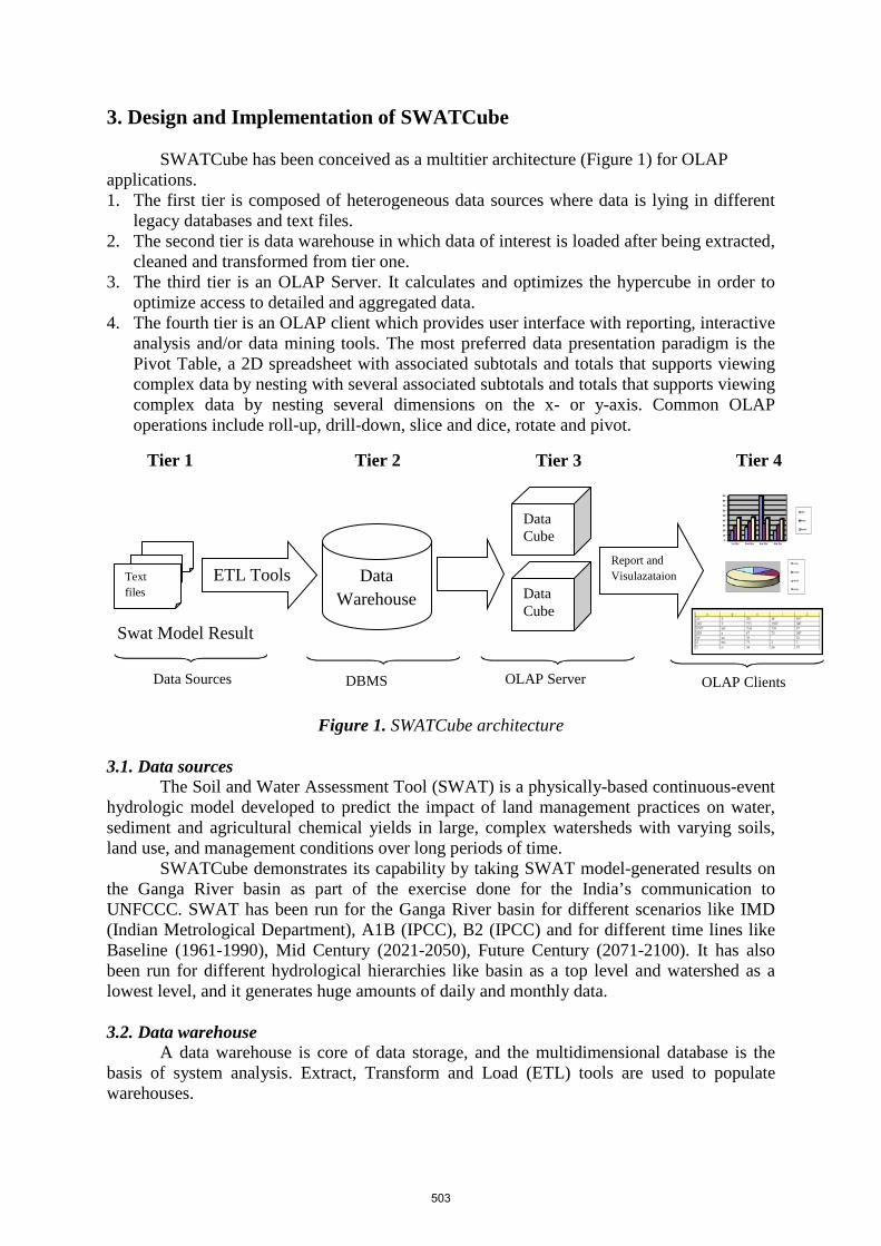
3. Design and Implementation of SWATCube

SWATCube has been conceived as a multitier architecture (Figure 1) for OLAP applications. 1. The first tier is composed of heterogeneous data sources where data is lying in different

legacy databases and text files. 2. The second tier is data warehouse in which data of interest is loaded after being extracted,

cleaned and transformed from tier one. 3. The third tier is an OLAP Server. It calculates and optimizes the hypercube in order to

optimize access to detailed and aggregated data. 4. The fourth tier is an OLAP client which provides user interface with reporting, interactive

analysis and/or data mining tools. The most preferred data presentation paradigm is the Pivot Table, a 2D spreadsheet with associated subtotals and totals that supports viewing complex data by nesting with several associated subtotals and totals that supports viewing complex data by nesting several dimensions on the x- or y-axis. Common OLAP operations include roll-up, drill-down, slice and dice, rotate and pivot.

Figure 1. SWATCube architecture 3.1. Data sources

The Soil and Water Assessment Tool (SWAT) is a physically-based continuous-event hydrologic model developed to predict the impact of land management practices on water, sediment and agricultural chemical yields in large, complex watersheds with varying soils, land use, and management conditions over long periods of time.

SWATCube demonstrates its capability by taking SWAT model-generated results on the Ganga River basin as part of the exercise done for the India’s communication to UNFCCC. SWAT has been run for the Ganga River basin for different scenarios like IMD (Indian Metrological Department), A1B (IPCC), B2 (IPCC) and for different time lines like Baseline (1961-1990), Mid Century (2021-2050), Future Century (2071-2100). It has also been run for different hydrological hierarchies like basin as a top level and watershed as a lowest level, and it generates huge amounts of daily and monthly data. 3.2. Data warehouse

A data warehouse is core of data storage, and the multidimensional database is the basis of system analysis. Extract, Transform and Load (ETL) tools are used to populate warehouses.

ETL Tools Data Warehouse Data

Cube

Report and Visulazataion Text

files

0

10

20

30

40

50

60

70

80

90

1st Qtr 2nd Qtr 3rd Qtr 4th Qtr

East

West

North

1st Qtr

2nd Qtr

3rd Qtr

4th Qtr

Swat Model Result

OLAP Server DBMS Data Sources OLAP Clients

Tier 1 Tier 2 Tier 3 Tier 4

Data Cube

503

An ETL tool allows one to Extract data from different heterogeneous sources (transactional databases, web resources, XML or flat files, Excel spreadsheets, LDAP, sensors, etc.), Transform (perform integration, data cleansing, data structure, “updating”, etc function) these data according to a target schema/data structure and Load the data in a data warehouse (Badard et al., 2009).

The ETL tool has been used to convert SWAT model-generated reach and subbasin monthly and daily results from text files into CSV format. CSV data is uploaded in data warehouses by using SQL Server Integration Services (SSIS).

According to data warehouse flexibility, only daily data for watershed hydrological units of SWAT model result has been uploaded in warehouse. Time is by day and space is by watershed. Furthermore, time is summarized by week, month and year. Space is summarized by watershed, subcatchment, catchment, subbasin or basin. 3.3. OLAP Server

The OLAP data cube is generated according to the data warehouse logical model. OLAP data cube data is organized by analysis themes. An SQL Server Analysis service provides full-fledged OLAP functionalities based on a multidimensional data model. Data cube enables rapid and flexible exploration and analysis of large amounts of data stored in a data warehouse. 3.4. OLAP Client

The OLAP client allows the end-user to visualize the data using different types of diagrams (e.g. bar charts and pie charts) and tables. It also allows the user to explore and analyze data using different operators such as drill-down (shows a more detailed level inside a dimension), roll-up (shows a more general level inside a dimension), drill-across (shows another theme at the same level of detail) and swap (interchanges visible dimensions in the chart or table). The system is built especially to navigate within the data cube i.e. to go from one fact to another in a simple manner and to obtain fast responses (Y. Bedard et al., 2003).

In the present implementation, ASP.NET technology has been applied to create a user interface which accesses SQL Server Analysis Services (SSAS) using the ADOMD.NET client dynamic link library and to read cube metadata like dimensions, hierarchies and levels. 4. Database Design Methodology

Entity relationship diagrams and normalization techniques are popularly used for

database design in OLTP environments. However, the database designs recommended by ER diagrams are inappropriate for decision support systems where efficiency in querying and in loading data (including incremental loads) is important (Chaudhuri et al., 1997).

SWATCube uses a star schema to represent the multidimensional data model. The database consists of a single fact table and a single table for each dimension. Each tuple in the fact table consists of a pointer (foreign key – often uses a generated key for efficiency) to each of the dimensions that provides its multidimensional coordinates and stores the numeric measures for those coordinates. Each dimension table consists of columns that correspond to attributes of the dimension.

Taking SWAT model result data as an example, star schema organization of the multi-dimensional data is shown in Figure 2.

504

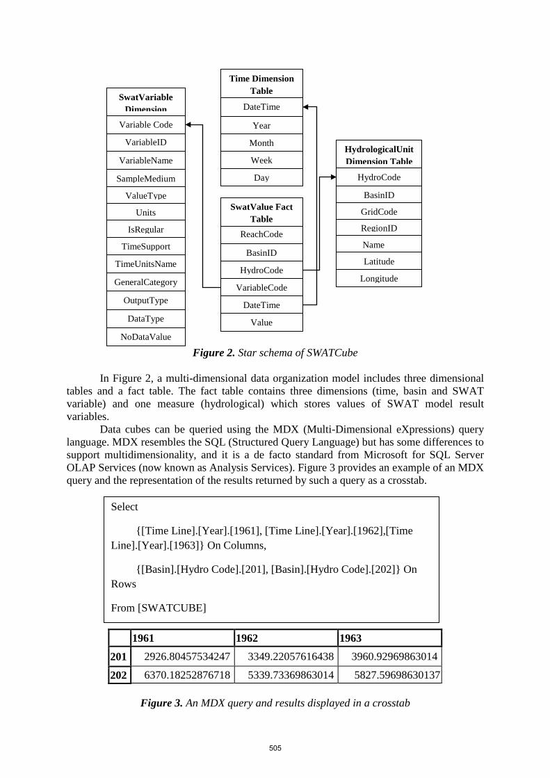
Figure 2. Star schema of SWATCube

In Figure 2, a multi-dimensional data organization model includes three dimensional

tables and a fact table. The fact table contains three dimensions (time, basin and SWAT variable) and one measure (hydrological) which stores values of SWAT model result variables.

Data cubes can be queried using the MDX (Multi-Dimensional eXpressions) query language. MDX resembles the SQL (Structured Query Language) but has some differences to support multidimensionality, and it is a de facto standard from Microsoft for SQL Server OLAP Services (now known as Analysis Services). Figure 3 provides an example of an MDX query and the representation of the results returned by such a query as a crosstab.

1961 1962 1963

201 2926.80457534247 3349.22057616438 3960.92969863014

202 6370.18252876718 5339.73369863014 5827.59698630137

Figure 3. An MDX query and results displayed in a crosstab

ReachCode

BasinID

HydroCode

VariableCode

DateTime

Value

SwatValue Fact Table

VariableName

SampleMedium

ValueType

Units

IsRegular

TimeSupport

VariableID

Variable Code

TimeUnitsName

GeneralCategory

OutputType

DataType

NoDataValue

SwatVariable Dimension DateTime

Year

Month

Week

Day

Time Dimension Table

HydroCode

BasinID

GridCode

RegionID

Name

Latitude

Longitude

HydrologicalUnit Dimension Table

Select

{[Time Line].[Year].[1961], [Time Line].[Year].[1962],[Time Line].[Year].[1963]} On Columns,

{[Basin].[Hydro Code].[201], [Basin].[Hydro Code].[202]} On Rows

From [SWATCUBE]

505

5. Conclusions and Future Work

This work uses OLAP to analyse SWAT model result output in order to allow rapid analysis and easy navigation of different levels of information. OLAP can be useful for finding out interesting patterns from large amounts of data where traditional database technology lags behind. Data warehouse and OLAP can be ground-breaking technologies in water resources management.

Future work includes Spatial Online Analytical Processing (SOLAP), currently in prototype, which will provide huge advantages in complex analysis. SOLAP will be a coupling of GIS, Data Warehouse (DW) and OLAP technology. GIS, DW and OLAP are used to create a Spatial Data Warehouse (SDW) which allows spatial analysis to be carried out with great ease.

References McKinney, D.C, Cai, X, Rosegrant, M.W., Ringler, C. and Scott C.A. (1999), Modeling Water

Resources Management at the Basin Level: Review and Future Directions, International Water Management Institute, SWIM Paper 6.

Bouwer, H. (2000), Integrated Water Management: Emerging Issues and Challenges, Agricultural Water Management, 45, 217-228.

Albert, X., Mark, O., Babel, M.S., Gupta, A.D. and Fugl, J. (2001), Integrating Resource Management in South East Asia, Water21 October 2001, 25-30

Ashoo Anand, Robert Feick , Spatial Database Infrastructure (SDIs) and Emergency Planning and Management: Challenges and Motivations for Local Government Organizations (LGOs), GSDI 11 Spatial Data Infrastructure Convergence : Building SDI Bridges to address Global Challenges, 2009

Natcom India, http://gisserver.civil.iitd.ac.in/natcom/

Inmon, W.H., Building the Data Warehouse. John Wiley, 1992.

Surajit Chaudhuri,Umeshwar Dayal, An Overview of Data Warehousing and OLAP Technology,SIGMOD Record,26(1): 65-74 , 1997.

E. F. Codd. Twelve rules for on-line analytical processing. In Computerworld, April 1995, 1995.

X. Tan. Data Warehousing and Its Potential Using in Weather Forecast. Proc. 22nd Int. Conf. on Interactive Information Processing Systems for Meteorology, Oceanography, and Hydrology. Atlanta, GA. 2006.

Ozer, S., Szalay, A., Szlavecz, K., Terzis, A., Musaloiu-E., R., Cogan, J., Using Data-Cubes in Science: an Example from Environmental Monitoring of the Soil Ecosystem, MSR-TR-2006-134, 2006.

Codd, E. F., and Salley, C. T., 1993. Providing OLAP (On-Line Analytical Processing) to User-Analysts: An IT Mandate. Hyperion white paper, 20 p., 1993.

Berson, A., Smith, S.J., 1997. Data Warehousing, Data Mining and OLAP. McGraw-Hill.

WaterShed Atlas of India, http://www.cgwb.gov.in/watershed/about-ws.html

506

Thomsen, E., Spofford, G., Chase, D., 1999. Microsoft OLAP Solutions. John Wiley and Sons.

Thierry Badard, Etienne Dube, Open Source Business Resource, September 2009: Business Intelligence

SQL Server Integration Services, http://msdn.microsoft.com/en-us/library/ms141026.aspx

Yvan Bedard, Pierre Gosselinb, Sonia Rivesta, Marie-Jose´e Proulxa, Martin Nadeaua, Germain Lebelc, Marie-France Gagnonc, Integrating GIS components with knowledge discovery technology for environmental health decision support, International Journal of Medical Informatics (2003) 70, 79-94

ASP.NET, a web application framework developed and marketed by Microsoft to allow programmers to build dynamic web sites, web applications and web services. http://www.asp.net/ .

SQL Server Analysis Server, An integrated view of business data for reporting, OLAP analysis, Key Performance Indicator (KPI) scorecards, and data mining, http://www.microsoft.com/sqlserver/en/us/solutions-technologies/business-intelligence/analysis-services.aspx

ADOMD.NET Client Concepts and Object Model, http://msdn.microsoft.com/en-us/library/bb522641.aspx

507

Evaluation of Climate Change Impacts on Blue Nile Flow using SWAT

Imtiaz Bashir1, Jiri Nossent1, Willy Bauwens1, Okke Batelaan1,2

[1] {Dept. of Hydrology and Hydraulic Engineering, Vrije Universiteit Brussel, 1050 Brussels, Belgium} [2] {Dept. of Earth and Environmental Sciences, Katholieke Universiteit Leuven, Celestijnenlaan

200E, 3001 Heverlee, Belgium} Correspondence to: Imtiaz Bashir (imtiaz.bashir@vub.ac.be)

Abstract

This contribution aims at the quantitative assessment of the impacts of climate change on the water resources and hydrological flow pattern of the Blue Nile River basin using hydrological modeling technique. The Blue Nile River contributes around 60% of the total mean annual flow of the Nile, and most of this flow is generated during the flooding season (July – October) by high precipitation received in the Upper Blue Nile catchment. Large irrigation schemes in Sudan and Egypt are mainly dependent on the flooding in the Blue Nile, which get water from several reservoirs built along the system. However, recent observations show that the climate has changed at an unprecedented rate during the last decade, with an evident increase in extreme precipitation events and temperature in eastern parts of Africa. This increases the vulnerability of downstream located countries for probable effects on their widespread agricultural based economic activities. This research analyzed the climate change impacts on the Blue Nile River basin by the year 2025, through use of the hydrological model SWAT, with spatial maps and synthetic weather data input. The model was calibrated at a monthly time scale against observed discharge series of four gauging stations of the Blue Nile. The climate change scenarios were constructed using outcomes of two General Circulation Models (MIROC and INMCM) for emission scenarios A2 and A1B, by adjusting the baseline climatic variables that represents the current precipitation and temperature patterns. The constructed climate scenarios were applied to the calibrated and validated hydrological model, to generate runoff and investigate climate change impacts on water yield and hydrological flow patterns. The results show that the climate is likely to become wetter and warmer in 2025 (2010-2039) in most of the Blue Nile basin; annual water yield is expected to increase at basin scale and low flows become higher, while, the outflows from the Rosieres reservoir show substantial increase in magnitude under combined pressure of climate change and loss of the reservoir storage due to sedimentation. However, uncertainties on the results are high on account of the quality of the baseline climate data, the discharge series and the accuracy of climate models. Overall, the study suggests that the water resources of the Blue Nile River basin will not be adversely affected by climate change depending on future actions. The increase in precipitation and resulting water resources may help to meet future water needs in the region.

Keywords: SWAT, climate change, hydrological model, the Blue Nile, water yield

508

1. Introduction A greater tendency for maximizing the utilization of transboundary freshwater resources

within territorial limits resulted in instigating and/or escalating conflicts among communities in almost every region of the world. Climate change, population growth, demographic changes and economic development are leading factors producing pronounced quantitative and qualitative impacts on transboundary water resources (Brekke et al., 2009). Scientists are on high alerts, particularly, to anticipate natural variability and uncertainty in weather patterns, and to human induced climate changes (IPCC, 2007). The Fourth Assessment Report by the Intergovernmental Panel on Climate Change, previous assessment reports and related documents (IPCC, 2001 and 2007) present evidence of global climate change, with particular focus on issues likely to be faced by the water resources managers.

It is argued that the future changes in overall magnitude and variability of the river flows, and the timing of the peak flow events are amongst the frequently debated hydrologic issues (Frederick 2002; Wurbs et al., 2005). Observed records of climatic and hydrological variables during the twentieth century, show that many natural systems are being greatly affected by the regional climate changes, particularly, by the increase in temperature (Hansen et al., 2006) and the variation of precipitation events (Houghton et al., 2001). Such changes in precipitation events and flow patterns may lead to enhanced chances of droughts and floods occurrences, either more frequently and/or be more severe under future climatic conditions (IPCC, 2007). Similar trends can be followed in the African continent reporting increase in the frequency of heavy precipitation events over most of the land areas and widespread changes in extreme temperatures over the past 50 years. Recent trends show a tendency towards greater extremes: arid or semi-arid areas in northern, western, eastern and parts of southern Africa are becoming steadily drier, and increased variability of precipitation and storms is observed.

A typical example of a transboundary river basin in Africa is the Nile River basin, which is the longest river in the world, draining almost 10% of the whole continent. It comprises of two major tributaries: the White Nile and the Blue Nile. The latter is the source of most of the water and fertile soil in the Nile basin area. Historical footprints along the river banks in Egypt, Ethiopia and Sudan show established water uses of the Nile River since ancient times and indicate its importance for agricultural, economic, social and cultural aspects of human life (Whittington, 2005). Most a re a s of the Nile River basin have been found to be sensitive to climatic variation (Conway and Hulme 1996; Conway 2005; Kim et al 2008). Changes in runoff and their consequences on the economies of riparian countries were studied by Gleick (1991); Conway and Hulme (1996); Strzepek and Yates (1996); Yates and Strzepek (1996, 1998a, b); Sene et al. (2001); Conway (2005). Rising conflicts on account of increasing water demands by the riparian countries have asserted great realization upon water resources managers to investigate further likely climate impacts for sustainable river basin management to assure peace and tranquility in the region.

The Blue Nile, major tributary of the Nile River, drains around 10% of the entire Nile basin area in Ethiopia and Sudan, but its flow is of vital importance for downstream usage in Sudan and Egypt. The river flows contribute around 60% of total mean annual flow measured at High Aswan Dam (Waterbury, 1979; Sutcliffe and Parks, 1999; Conway, 2005). The long-term variability of the Blue Nile flows become of particular interest for the riparian countries. Especially to Ethiopia, wherein most of the Blue Nile flow is generated, but it does not have any established rights on the use of river water. People have small scale irrigated and/or rain-fed agriculture based livelihood in this area. On the other hand, the agricultural based economies of Sudan and Egypt is greatly dependent on the flow generation in Ethiopia. Therefore, efforts for understanding changes in temporal and spatial patterns of streamflow on account of future climate changes are crucial for food security in the region (NMSA, 2001;

509

MOWR, 2002; UNESCO, 2004; Conway, 2005). Elshamy et al. (2009) assessed the water balance of Blue Nile for future climate using outputs of 17 General Circulation Models (GCMs) and reported less water in the Blue Nile River by 2100. Similarly, Kim et al. (2008) used outputs of six GCMs to assess climate impacts on hydrology and water resources of the Upper Blue Nile river basin and reported an increase of low flows.

The Soil and Water Assessment Tool (SWAT) has been widely used for evaluating the influence of climate variability on watersheds (Neitsch et al., 2005). This is done in the form of sensitivity analysis where baseline climatic conditions are used to simulate streamflow and then compared with simulation for the future changes in precipitation, temperature and other climate variables. This analysis provides information on the direction and the change of magnitude of streamflow and gives insight into which variables are most significant in predicting these changes. Stonefelt et al. (2000) and Fontaine et al. (2001) applied SWAT to assess climate change impacts on annual water yield and streamflow predictions of some river basins in North America, and used arbitrary changes in weather inputs based on GCM/RCM projections. The study concluded that coupled variable analyses represent a more realistic climate change regime and reflect the combined response of the basin. Githui et al. (2009) used SWAT to assess future climate impacts on the Nzoia River in Kenya and reported higher expected streamflows in the coming decade. On the other hand, Van Liew and Garbrecht (2001) and Varanou et al. (2002) used SWAT to investigate the impacts of climate change on the water yield.

Although, the wide applicability of SWAT for investigating climate change impact assessment on hydrology for different parts of the world has been demonstrated, few applications of SWAT have been published on the Blue Nile River basin. Most studies used deterministic and stochastic modeling techniques to smaller river catchments of the Blue Nile River basin (Elshamy et al., 2009; Kim et al., 2008). Betri et al. (2011) and Easton et al. (2010) used the SWAT hydrological model to analyze runoff and sediment management in the Upper Blue Nile River basin. In this study, we developed a SWAT hydrological model for the entire Blue Nile River basin to assess climate change impacts on the Blue Nile flows by the year 2025. 2. Study Area

This study covers the entire Blue Nile River basin including Lake Tana and its drainage area. The Blue Nile River basin has a drainage area of about 310,000 km2 just upstream of Khartoum (Sudan), where it eventually joins the White Nile. This area covers most of Ethiopia and part of Sudan between longitude 32ºE and 40ºE and latitude 9ºN and 16ºN (Figure 1).

510

Figure 1. The Blue Nile River in Africa and representation of topography in the basin

2.1. Topography, land use and soil

The Blue Nile and all of its tributaries originate in Ethiopian Plateau at an elevation of 2000 m to 3000 m a.s.l. About 35 km downstream of Lake Tana exit, the river drops approximately 50 m into Tis Issat Falls and starts flowing in a deep gorge about 1200 m below the ground level of the plateau. The Blue Nile emerges from the plateau close to the western border of Ethiopia, where it turns in north-west direction and enters Sudan at an altitude of 490 m a.s.l. Just before crossing the border of Sudan, the river enters a clay plain where it flows to Khartoum to eventually merge into the White Nile to form the Nile River. Downstream of Rosieres, the Blue Nile is a mild stream with a slope of about 0.12x10-3, 1/10th of the slope of the torrential stream which prevails from the Lake Tanexit to Rosieres (Figure 2).

Most of the Ethiopian Plateau is hilly with grassy downs, swamp valleys, and scattered trees (Shahin, 1985). Figure 3 shows the dominant land use/land cover type in the basin. Savanna covers around 71% of the basin area with concentrated growth in central part, and diminishing trends of this can be noticed towards the basin outlet at Khartoum. Other main land cover types are dryland cropland and pasture; grassland; and cropland/woodland mosaic covering 18%, 4% and 3% respectively of the basin area. The basin area is generally characterized by clayey soils, which covers about 52% of the basin area. Table 1 tabulates top seven dominant soil classes according to FAO-UNESCO soils classification along with respective soil composition in 1st and 2nd layers of 300 mm and 1000 mm thickness, respectively.

Figure 2. Longitudinal profile of Blue Nile River

511

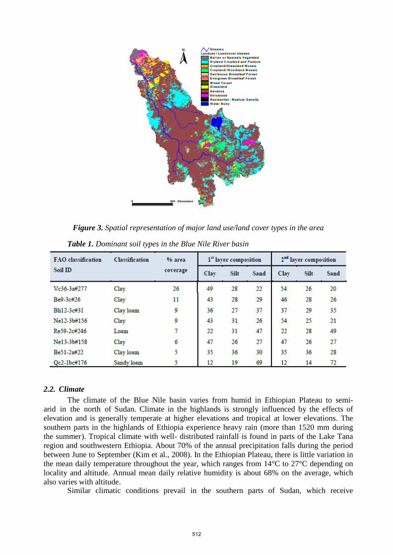
Figure 3. Spatial representation of major land use/land cover types in the area Table 1. Dominant soil types in the Blue Nile River basin

2.2. Climate

The climate of the Blue Nile basin varies from humid in Ethiopian Plateau to semi-arid in the north of Sudan. Climate in the highlands is strongly influenced by the effects of elevation and is generally temperate at higher elevations and tropical at lower elevations. The southern parts in the highlands of Ethiopia experience heavy rain (more than 1520 mm during the summer). Tropical climate with well- distributed rainfall is found in parts of the Lake Tana region and southwestern Ethiopia. About 70% of the annual precipitation falls during the period between June to September (Kim et al., 2008). In the Ethiopian Plateau, there is little variation in the mean daily temperature throughout the year, which ranges from 14°C to 27°C depending on locality and altitude. Annual mean daily relative humidity is about 68% on the average, which also varies with altitude.

Similar climatic conditions prevail in the southern parts of Sudan, which receive

512

around 1270 mm rain over nine-month period between March and November, with the maximum occurring in August (Shahin, 1985). Maximum and minimum temperatures are recorded between March and June, and December or January respectively, while the annual average relative humidity remains around 55%. The rainy season, which occurs in the South from March to November, gets shortened and confined to July and August in the Northern part of central Sudan with around 250 mm rainfall annually and average annual relative humidity of 31%. The minimum temperature occurs in January and the maximum in May or June, when it rises to a daily average of 37°C in Khartoum. The annual free surface water evaporation varies from 3.0 mm/day for Lake Tana to 6.5 mm/day in Sennar and eventually to 7.8 mm/day around Khartoum. The potential evapotranspiration, based on Penman’s method, varies from 1150 mm around Lake Tana to 2000-2100 mm around Rosieres and 2300-2400 mm around Khartoum (Shahin, 1985). 2.3. Hydrology

The catchment area of Lake Tana is around 14,500 km2, while the lake surface area ranges from 3,000 to 3,500 km² depending on the season and rainfall. Because of the large storage capacity and the regulation at its outlet, the peak outflows occur in September, two months after the maximum rainfall in July (USBR, 1964). Hurst et al. (1950) estimated the flow at station Kilo330 downstream of lake exit, at about 2.2 x 106 m3/day during the low stage period and about 220 x 106 m3/day in the flood season, which is about 10 times as much as its initial value at lake exit. About 935 km below Lake Tana exit, the river discharge at Rosieres is about 7 x 106 m3/day in the low stage period, which indicates reach contribution between Kilo330 and Rosieres. The average flow volume at Rosieres for the period 1912-1973 is 49.2 x 109 m3/year with a peak flow in August, and that at Sennar is 47.2x109 m3/year. Total transmission losses in the reach are around 2 109 m3/year mainly accounted for evaporation in the reach and from the reservoir (Shahin, 1985).

Usually little additional runoff is generated North of Rosieres except for the two tributaries, the Dinder and the Rahad. Both the tributaries join the Blue Nile downstream of Sennar close to Wad Medani and also have their headwaters in the Ethiopian Highlands. Peak discharges of around 480 m3/sec and 160 m3/sec respectively recorded in these rivers in triangular shaped hydrographs with a base width of about 200 days. The annual flow volume in the Blue Nile River at Khartoum is nearly 50.4 109 m3/year, which is around 8% higher than at Sennar with estimated transmission losses of 0.85 109 m3/year mainly due to evaporation and seepage (Shahin, 1985). However, Hurst et al. (1950), estimated that the average flow volume at Sennar remain equal or larger to that of Khartoum. 2.4. Lakes, reservoirs and irrigation schemes

Lake Tana, a natural lake, and two manmade reservoirs are situated in the Blue Nile River basin. The manmade reservoirs, located at Rosieres and Sennar, were completed in 1966 and 1925 respectively, for irrigation and power generation purposes. The Gezira Scheme, Sudan’s oldest and largest gravity irrigation scheme, was progressively expanded since its inception in 1925. It receives water from Sennar reservoir with present coverage of about 880,000 hectares divided into 114,000 tenancies (Coutsoukis, 2004). The increase of Sudan’s share from the Nile water, under the 1959 Nile Waters Agreement with Egypt, led to the construction of the Managil extension of the Gezira Scheme, situated between the White and the Blue Nile Rivers upstream of Khartoum. Major existing irrigation schemes, largely dependent on the Blue Nile River flows, have been listed in Table 2.

513

Table 2. List of Irrigation Schemes in the Blue Nile River basin (FAO Aquastat Programme, 2007)

Irrigation Scheme

Year of

Water with-drawal

Area (hec.)

Main Crops *

Gezira and Managil

1931 and 1963

Sennar

874,300

C,G,W,S

Rahad 1977 (1st supply)

1981 (80% area)

1983 (entire area)

Rosieres

126,000

C,G,S

Blue Nile Agri. Pro.

1970s

Sennar

122,640

C

El Suki

Early 1970s

Sennar

36,500

C,G,S

Guneid Sugar Co.

1955

Sennar

16,250

Sr.C

Guneid Extension

Mid 1970s

Sennar

19,070

C,G * C: Cotton; G: Groundnut; S: Sorghum; W:Wheat; Sr.C: Sugarcane

Sudan was expected to become the bread basket of the Arab World in the 1970s, and irrigation schemes such as the Rahad Scheme were established with large investments from oil-rich Gulf nations (Coutsoukis, 2004). Large-scale irrigated agriculture expanded in Sudan from 1.17 million hectares in 1956 to more than1.73 million hectares by 1977. 3. Methodology 3.1. Input data

SWAT is a physically based semi-distributed hydrological model, and it needs spatial topographical and meteorological data as main input. This input data, which is used to develop the hydrological model of the Blue Nile River basin, can be grouped into four major categories:

I. Spatial topographical information at 1 Km spatial resolution comprising of a Digital Elevation Model (DEM), a Digital Stream Network (DSN) and land use/land cover maps were obtained from the Earth Resources Observation Systems Data Center (EROSDC) of USGS, South Dakota - USA. The soil map was obtained from FAO-UNESCO and provides soil characteristics of about 5000 soil types at a spatial resolution of 10 km. Other soil properties concerning particle size distribution, bulk density, organic carbon content, available water capacity and saturated hydraulic conductivity, were obtained from Reynolds et al. (1999). II. Hydro-meteorological information comprised of monthly discharge data series at four measurement stations shown in Figure 1 and daily time series of rainfall, temperature, wind speed, solar radiation and relative humidity. The monthly river discharge data was obtained from the Global Runoff Data Centre, Koblenz - Germany. Daily time series of rainfall (mm); and maximum and minimum temperature (ºC) for the period 1971-1995, were obtained from the Swiss Federal Institute of Aquatic Science and Technology – EAWAG (Schuol and Abbaspour, 2007). The data set contains generated information for 200 synthetic stations distributed over the entire Nile basin, out of which 20 stations are located in the drainage area of the Blue Nile River basin. Monthly statistics of wind speed, relative humidity and solar radiation were derived using CropWat 8.0 freely available from Food and Agriculture Organization (FAO), Rome, Italy. III. Annual irrigated area and water withdrawals were taken from FAO Aquastat Programme (2007), while lake/reservoirs characteristics and monthly irrigated areas were taken from LNFDC/ICC project van der Krogt (2005) undertaken at The Delft. IV. Crop and soil characteristics in SWAT database files were updated for local conditions in

514

the study area. Concerned parameterization of the land use classes e.g. leaf area index, maximum stomata conductance, maximum root depth, optimal and minimum temperature for plant growth were based on literature and the available SWAT land use classes. While, the characteristics/conditions of the urban areas and fertilizers assumed to have been similar to those in United States given in SWAT database files. 3.2. Quality control

A quality control was performed for checking the homogeneity of the available hydro-meteorological data at 95% significance level using the tool RAINBOW. This tool performs frequency analysis and test the homogeneity of datasets (Raes et al., 2006). Average annual and monthly values of precipitation, maximum and minimum temperature, and discharge series were tested at four locations: Kessie, Rosieres, Sennar and Khartoum. Generally, the hydrological data and precipitation records meet the data homogeneity criteria, however, a number of temperature stations failed the homogeneity test for average annual values. 3.3. Future climate scenarios

General Circulation Models (GCMs) are reliable scientific platforms to simulate the impacts of increased greenhouse gases on climatic variables (Conway and Hulme, 1996; IPCC, 1999; Dibike and Coulibaly, 2005; Wilby and Harris, 2006). Outcomes of these GCMs are commonly forced as input to the hydrologic models to project changes in water resources (Nash and Gleick, 1993; Arnell and Reynard, 1996; Conway and Hulme, 1996; Yates and Strzepek, 1998; Kim et al., 2004; Wilby and Harris, 2006). Adopting this methodology, the hydrological models are initially calibrated for the current climatic data, followed by defining future climatic data either by generating future climatic variables or perturbing the current climatic data and finally simulating the scenarios to compare the simulated results with those under present climate. A similar methodology has been used to investigate the impacts of climate change on the Nile River basin (Conway and Hulme, 1996; Yates and Strzepek, 1998; NMSA, 2001). However, coarse gridded outcomes of these GCMs remain a major limitation in applying them to small study areas. IPCC proposed several methods to apply the GCM outcomes to regional level studies (IPCC, 1999). The simplest application is the direct use of the original grid information nearest to the considered measurement station, which has been adopted in this study.

According to IPCC (2007), no driver other than Green House Gasses (GHGs) provides a scientifically sound explanation for most of the warming and changes in precipitation patterns observed both globally and regionally over the past few decades. IPCC has identified five major story lines of GHGs emission scenarios, out of which A2 and A1B were selected for this study. Main reasons for selecting A2 scenario are prevailing and expected high population growth rates and fight for survival of regional identities in the study area, which fit perfectly in the framework of this emission scenario. A1B scenario was selected to pose an optimistic approach for a prospering and conflict free region, aiming at low population growth rate. GCMs outcomes can be obtained either as the estimates of average annual and monthly precipitation and temperature for the future climate, or as change in climate variables relative to baseline period 1961-1990. Change in precipitation and temperature fields imposed on the baseline time series is one of the approaches to study climate change impact assessment on the water resources (IPCC, 2001). Based on selected emission scenarios and spatial resolution of GCMs, outputs of two models MIROC3.2 and INMCM3.0 were selected. These models have been developed by the research centers CCSR/NIES/FRCGC (Japan) and Institute of Numerical Mathematics (Russian Academy of Science, Russia) respectively.

The GCMs outcomes of monthly relative change in the baseline precipitation and temperature fields predicted for the period 2010-2039 were obtained from IPCC Data Distribution Centre. These mean monthly relative changes were applied to baseline climatic

515

records on pro-rata basis for generating averaged future climate by the year 2025. It helped to preserve temporal and spatial correlation of climatic events in the baseline period for the future climate. The impacts of these outputs on annual precipitation, and maximum and minimum temperature were averaged over various reaches of the study area (Figure 4). Generally, both GCMs show a considerable increase in precipitation by the year 2025 in the basin except MIROC-A2 for Sennar and Khartoum reaches, where a decrease in average annual precipitation is projected. Maximum and minimum daily temperature predictions by both GCMs are consistent, and an increasing trend can be observed. However, model INMCM predicts a remarkable increase in minimum temperature for both the emission scenarios.

Figure 4. GCMs predictions for average annual change in precipitation and maximum and minimum temperature by the year 2025 in the Blue Nile River Basin

Average monthly relative changes in climatic variables are presented for both Rosieres

and Khartoum in Figure 5.

(a) Average monthly precipitation change in Rosieres reach (b) Average monthly precipitation change in Khartoum reach

516

Figure 5. GCMs prediction for relative monthly changes in average precipitation, minimum and maximum temperature averaged over Rosieres and Khartoum reaches

The precipitation Ethiopian highlands falling from July to October is higher in magnitude and causes about 80% of the annual flows of the Blue Nile, hence, a small change shown during this period means larger change in rainfall amount. An increasing trend in precipitation during the wet season in the drainage area of Rosieres is predicted, except for MIROC-A2, which shows a decrease in precipitation in the later months of the wet season. However, relatively consistent outputs are predicted for the wet season in the drainage area of Khartoum by both models. During the dry period, INMCM gives relatively higher precipitation increases for Rosieres and Khartoum areas than MIROC. Maximum and minimum temperature in Rosieres and Khartoum drainage areas are generally expected to increase in both models, however, a relatively smaller increase is predicted than INMCM. 3.4. Model development 3.4.1. Model build-up

SWAT model for the Blue Nile River basin was developed using AVSWATX -

517

SWAT2005. The model build-up primarily consists of necessary steps of automatic watershed delineation, implementation of reservoirs, irrigation water withdrawals and weather data input. Considering the data availability and application of the model for climate change impact assessment, the existing reservoirs were implemented using specified water release rates, while, the irrigation water withdrawals from Rosieres and Sennar were implemented as consumptive water uses. SWAT calculates evaporation separately from upland and reservoir processes. Therefore, it is accounted twice in case of reservoir implementation and needs to be ignored in either of the two. Amongst three existing reservoirs implemented in the model, Rosieres and Sennar being smaller in the surface area, were ignored during the HRUs definition process by setting threshold values of 4% and 7% for land use and soil classes respectively. Lake Tana has a large surface area and needed special pre-processing of topographical data to enclose the entire lake in a subbasin for ignoring evaporation losses from the upland processes. For this purpose, a threshold area of 303,947 hectares was chosen to form an isolated subbasin preserving the original inlet and outlets of the lake.

Stream outlets were selected based on three factors: i) Inlets and outlet of Lake Tana were retained; ii) Delineation of subbasins to contain at least one precipitation and temperature gauge in each subbasin; iii) Saving simulation results at discharge measurement stations of Kessie, Rosieres, Sennar and Khartoum. The model was run for the period 1971 to 1982, with the first two years used as a warm-up period. The calibration and validation periods were respectively 1973 to 1978 and 1979 to 1982. Muskingum method, Penmen Monteith equation and CN method were used to simulate channel routing, evapotranspiration and surface runoff, respectively. 3.4.2. Parameter sensitivity, calibration and validation

The climate and hydrological regime is highly variable along the Blue Nile River from its origin in the Ethiopian plateau to its outlet in the Sudanese plains. Therefore, it was important to perform a sensitivity analysis and an optimization process at four locations namely, Kessie, Rosieres, Sennar and Khartoum (Figure 1). Monthly observed discharge series at respective locations were used to perform a Latin Hypercube – One At Time (LH-OAT) sensitivity analysis (Van Griensven, 2002), using the sum of the squared errors (SSQ) between the observed and simulated values as an objective function. Optimization of the 10 most sensitive parameters was performed using the Shuffled Complex Evolution algorithm (SCE- UA), included in SWAT as the Parameter Solution (ParaSol) tool (Van Griensven et al., 2002; Vandenberghe et al., 2001).

Multi-site calibration (1972-1978) process was started from the most upstream measurement station of Kessie, followed by subsequent downstream stations and finalizing the optimization of the entire drainage area at Khartoum, outlet of the Blue Nile River basin. During the optimization process, the parameters were changed in a distributed way for 91 HRUs, which were selected for being dominant in area coverage in a subbasin. The calibrated model was validated for the independent period of 1979-1982 and evaluated by comparing annual water yield, graphical comparison and goodness of fit statistics. 4. Results 4.1. Model performance evaluation

The quality of the model was evaluated by comparing the values of simulated and actual values for the annual water yield and graphical evaluation of discharge series, which was further complemented with statistical indicators of coefficient of determination (R2), the Nash-Sutcliffe Efficiency (NSE) and uncertainty quantification for the calibration and validation

518

periods. The goodness of fit statistics for the streamflow during calibration and validation periods are presented in Table 3. A maximum of 27% difference is observed in the mean annual streamflow at Kessie during the validation period for which only one year data was available for comparison. Standard deviation of simulated annual streamflow during the calibration period is lower than observed, which is a result of lower simulated peak flows due to combined effect of synthetic weather data input and assumptions made for implementing the reservoirs. High NSE and coefficient of determination (R2) values illustrate the model performance to simulate reality in close approximation. The values of NSE and the coefficient of determination remain higher than 0.62 and 0.71 in all the cases. Graphical comparison results are not shown here, but, it is important to mention that generally the simulated peaks were underestimated at all the stations, which is explained by the assumptions made for low outflow release rates from the reservoirs. However, fair simulation of low flows were observed at all the stations except Sennar, where some pronounced differences are visible. Table 3. Goodness of fit statistics of the model results

Station Name

Annual mean flow (m3/sec) Standard deviation (m3/sec)

NSE R2

Actual SWAT Actual SWAT Kessie Calibration 498 452 61 59 0.91 0.92 Validation 350 255 46 32 0.62 0.83 Rosieres Calibration 1434 1510 270 236 0.82 0.83 Validation 1196 1082 133 142 0.83 0.86 Sennar Calibration 1188 1275 300 232 0.79 0.79 Validation 891 836 144 160 0.83 0.85 Khartou

Calibration 1329 1595 177 219 0.80 0.83

Validation 1000 1134 185 234 0.70 0.71

The predictive non-uniqueness of the model from inherent uncertainties (Beven et al., 2001) in synthetic weather data, measurement errors and optimization method was quantified for annual water yield (depth of water generated over the entire catchment area annually) and monthly flows at basin scale. Uncertainty quantification at 95% significance level after applying Box-Cox transformation is presented in Table 4. Though wide predictive ranges of simulated flows were observed, the overall assessment of the model results supported its application for climate change scenario. Overall, the goodness of fit statistics and graphical comparison demonstrate model‘s ability to predict the realistic approximation of river flows. Table 4. Predictive range of annual water yield at 95% confidence interval of the Blue Nile River basin

Station

Observed

(mm)

Calibrated

(mm) Minimum

prediction (mm) Maximum

prediction (mm)

% range

Kessie

678

615

418

916

-32

t

49 Rosieres 244 257 154 355 -40 t

38

Sennar 186 199 113 281 -43 t

41 Khartoum 136 165 73 238 -56 t

44

4.2. Model Application for climate change

Output of GCMs MIROC and INMCM for both the emission scenarios A2 and A1B were applied to the calibrated and validated model to predict the future climate change impacts by the year 2025. The impacts on the variation in water yield and flows at outlet of the basin were

519

studied at annual and seasonal scale. The impact assessment assumes no substantial change in water withdrawals and man-made infrastructure in the Blue Nile river basin by the year 2025. 4.2.1 Annual water yield

Amongst the major concerns coupled with climate changes in shared river basins, the annual water yield is of vital importance. Table 5 presents comparative insight into expected changes in annual water yield and potential evapotranspiration in the Blue Nile River basin for future climate changes by the year 2025. Table 5. Average annual changes in climate variables and water yield by 2025

Emission

Scenario

GCM

ΔP (%)

ΔTmax (oC)

ΔTmin (oC) ΔPET (%)

ΔWYLD (%)

A2

MIROC

0

0.7

1.0

2

-11 INMCM 5 0.8 2.2 1 2 A1B MIROC 9 0.4 0.8 3 18 INMCM 4 0.9 2.3 2 25

MIROC presents relatively cooler climate for both the emission scenarios than that of

INMCM, which shows higher increase in temperature in both cases. Generally, the results show increase in annual water yield at basin scale up to +25% except for MIROC-A2, which predicts water deficit in the Blue Nile River basin. The A1B scenario representing a future world of very rapid economic growth, low population growth, and rapid introduction of new and more efficient technologies, shows 18% to 25% increase of the Blue Nile water yield. However, contrasting results are seen for A2 emission scenario, which represents prevailing population growth rates and fight for sustaining cultural and regional identities. For A2, MIROC predicts 11% decrease of the water yield, while INMCM shows an increase of only 2%. The tabulated changes in climate variables present the averaged impact over the entire study area, and therefore, these values do not demonstrate correlation of climate variables in individual sub-catchments with similar changes in the water yield. Furthermore, any change in precipitation does not result in immediate conversion to water yield, and correlated analysis of the hydrological cycle may yield better insight. Except MIRCO-12, results show improved water prospects for the riparian countries. 4.2.2 Low and high flow periods

The Blue Nile River is a flooding river, with 80% of the total yearly flow appearing in a period of only four months. These flows are important for managing the reservoirs and droughts in the region. For this purpose, predicted water yields during low flow periods (January to June) and high flow periods (July to December) have been presented in Table 6. Results show a consistent increase in the water yield at basin scale during the low flow periods, with a maximum of around 80% predicted by the INMCM-A1B scenario. A1B also predicted a maximum of 20% increase in water yield during high flow periods. However, the prevailing situation in the region closely approximated by A2, shows a considerable decrease in expected water yield during high flow period for both the models, with a maximum decrease of 15% predicted for MIROC. This situation can seriously hamper the filling of the reservoirs during the high flow periods, resulting in moisture deficits for agricultural crops in later months and enhanced drought threats.

520

Table 6. Average water yield during low and high flow period at basin scale by 2025

Description Baseline

MIROC

INMCM

A2 A1B

A2 A1B

Water yield during low flow period (mm) Water yield during high flow period (mm)

9

112

11 12 96 131

13 16 110 135

4.2.3 Seasonal hydrological response

In addition to the availability of the flow in the river, its timing is of great concern to regulate and manage the reservoir operations and the cropping pattern in Sudan and Egypt. Figure 6 presents the model predictions of average monthly flows at Rosieres (left) and Khartoum (right) by the year 2025.

Figure 6. Comparison of average monthly flows at (left) Rosieres (right) Khartoum by 2025

Currently, the wet seasons spans from July to October with maximum flows occurring in August at both stations. Generally, increased outflows from Rosieres reservoir are observed throughout the year, except in April. This increase in reservoir outflows is understood to be a combined effect of climate change and the loss of reservoir storage due to the sedimentation. The impact of increased outflow at Rosieres, start appearing at downstream located Khartoum from September and continues until April with consistent prediction of flow increase during low flow periods. However, the increase in magnitude at Khartoum does not correspond with that of Rosieres, which is explained by evapotranspiration losses due to high temperature in the 700 km long reach from Rosieres to Khartoum.

The simulated shift of the maximum river flow from August to September at Rosieres and subsequently at Khartoum in case of MIROC-A1B is pronounced, it is caused by the precipitation increase in respective months predicted in Rosieres reach (Figure 5). Similarly, A2 predicts a decrease in river flows at Khartoumduring July to September and an increase during October to December. On the other hand, A1B shows a decrease in river flows at Khartoum for July and August only. This is indeed a great concern for filling reservoirs in Egypt, which may enforce late filling of reservoirs in Egypt but at the same time, low evaporation losses from the reservoirs in cooler months may be expected. However, this late increase in river flows during low flow period at Khartoum, needs to be checked by incorporating ongoing heightening of Rosieres dam with likely completion by the year 2015.

521

5. Conclusions

This study is an effort to assess climate change impacts on the water resources of the Blue Nile River basin by the year 2025. The hydrological modeling tool Soil and Water Assessment Tool (SWAT) was employed to set up the model, using spatial maps with reasonably fine resolution, synthetic weather data and limited information on the spatial distribution of irrigation schemes and reservoir management. This study has contributed greatly for acquiring comprehensive information about operation and management of reservoirs and irrigation water withdrawals with special emphasis on checking the data quality and identifying the problematic data sets. Considering the topographical, climatic and hydrological regime variability in the basin, the model was optimized at multiple sites along the river route from the Ethiopian highlands to Sudanese plains, namely Kessie, Rosieres, Sennar and Khartoum. The model performance was judged by comparing the simulated and observed annual water yield, using graphical plots and statistical indices for calibration and validation periods. Both NSE and coefficient of determination remain higher than 0.62 in all the cases, which correspond to values of a good hydrological model in the cited literature.

Uncertainty in the outputs of GCMs is generally high, because of lack of scientific understanding of various processes and monitoring facilities, therefore, climate change impacts were assessed by using outputs from two GCMs. The scenarios application was implemented using the outputs of the GCMs MIROC and INMCM for the emission scenarios A2 and A1B, to the calibrated and validated SWAT model of the study area. The GCMs output, given as a relative change of the baseline records of the climatic variables, were implemented on the daily time series of precipitation and maximum and minimum temperature. The study suggests the following major findings: i) Increase in annual water yield at the basin scale is predicted by both models for emission scenario A1B, while contrasting results in the water yield is observed in case of emission scenario A2. ii) Generally, an increase in precipitation magnitude during low flow months over the entire basin is predicted by both the models. iii) Consistent increase in low flows and decrease in high flows during July and August at outlet of the basin is predicted for both the GCMs. iv) A substantial increase in reservoir outflows at Rosieres during high flow period is observed, which is seen as a combined result of increase in precipitation in the reach and loss of reservoir storage due to the sedimentation.

Overall, the results suggest that the water resources of the Blue Nile River basin may not be adversely affected by climate change, but it is dependent on future actions taken. Expected increase in water resources may help to meet future water needs in the region. Continuation of the study to investigate the effects on environmental and ecological processes may be of great interest towards an integrated basin solution. References Arnell, N. W., and N. S. Reynard. 1996. The effects of climate change due to global warming on

river flows in Great Britain. Journal Hydrology 183:397–424. Betrie, G. D., Y. A. Mohamed, A. Van Griensven and R. Srinivasan. 2011. Sediment management

modeling in the Blue Nile Basin using SWAT model. Hydrol. Earth Syst. Sci. 15: 807-818.

522

Beven, K., and J. Freer. 2001. Equifinality, data assimilation and uncertainty in the mechanistic

modeling of complex environmental systems using the GLUE methodology. Journal Hydrology 249:11-29.

Brekke, L. D., J. E. Kiang, J. R. Olsen, R. S. Pulwarty, D. A. Raff, D. P. Turnipseed, R. S. Webb and K.

D. White. 2009. Climate change and water resources management - A federal perspective: U.S. Geological Survey Circular 1331, 65 p. USGS.

Conway, D., and M. Hulme. 1996. The impacts of climate variability and future climate change in the

Nile basin on water resources in Egypt. Water Resources Development 12 (3): 277-296. Conway, D. 2005. From headwater tributaries to international river: Observing and adapting to climate

variability and change in the Nile Basin. Global Environmental Change 15: 99-114. Coutsoukis, P. 2004. Sudan Irrigated Agriculture [Online]. The Library of Congress Country Studies;

CIA World Fact book. Available at http://www Dibike, Y. B., and P. Coulibaly. 2005. Hydrologic impact of climate change in the saguenay

watershed: comparison of downscaling methods and hydrologic models. Journal of Hydrology 307(1-4):145-163.

Easton, Z. M., D. R. Fuka, E. D. White, A. S. Collick, B. Biruk Ashagre, M. McCartney, S. B.

Awulachew, A. A. Ahmed, and T. S. Steenhuis. 2010. A multi basin SWAT model analysis of runoff and sedimentation in the Blue Nile, Ethiopi. Hydrol. Earth Syst. Sci. 14: 1827-1841.

Elshamy, M. E., I. A. Seierstad and A. Sorteberg. 2009. Impacts of climate change on Blue Nile

flows using bias-corrected GCM scenarios. Hydrol. Earth Syst. Sci., 13:551-565. FAO Aquastat Progamme. 2007. Dams and Agriculture in Africa: Water Development and

Management Unit (NRLW). Food and Agriculture Organization of the United Nations (FAO), Rome, Italy.

Fontaine, T. A., J. F. Klassen, T. S. Cruickö and R. H. Hotchkiss. 2001. Hydrological response to climate

change in the Black Hills of South Dakota - USA. Hydrologic Sciences Journal 46:27–40. Frederick, K. D. 2002. Introduction: Water Resources and Climate Change - Frederick, K. D. (ed.)

514pp. Northampton MA: Edward Elgar Publishing. Githui, F., W. Gita, F. Mutua and W. Bauwens. 2009. Climate change impact on SWAT simulated

streamflow in western Kenya. International Journal of Climatology 29:1823-1834. Gleick, P. H. 1991. The vulnerability of runoff in the Nile basin to climatic changes.

Environmental Professional 13:66-73. Hansen, J., Mki. Sato, R. Ruedy, K. Lo, D. W. Lea and M. Medina-Elizade. 2006. Global

temperature change. Proc. Natl. Acad. Sci.,103:14288-14293, doi:10.1073/pnas.0606291103. Houghton, J. T., Y. Ding, D. J. Griggs, M. Noguer, P. J. van der Linden, X. Dai, K. Maskell and C. A.

Eds. Johnson. 2001. Climate Change 2001: The Scientific Basis. 881 pp. Cambridge University Press.

Hurst, H.E., R. P. Black and Y. M. Simaika. 1959. The Nile Basin: Volume-IX. The hydrology of Sobat

and White Nile and the topography of the Blue Nile and Atbara. Ministry of Public Works,

523

Physical Department, Cairo, Egypt. IPCC (Intergovernmental Panel on Climate Change). 1999. Guidelines on the use of scenario data for

climate impact and adaptation assessment: Version 1, prepared by Carter, T. R., M. Hulme and M. Lal. Task Group on scenarios for climate impact assessment. Geneva, Switzerland: IPCC. 69 pp.

Intergovernmental Panel on Climate Change (IPCC). 2001. Climate Change 2001: The Scientific

Basis. Contribution of Working Group I to the Third Assessment Report of the Intergovernmental Panel on Climate Change [Houghton, J.T., et al. (eds.)]. Cambridge University Press, Cambridge, United Kingdom and New York, NY, USA.

IPCC (Intergovernmental Panel on Climate Change). 2007. Climate change 2007: Impacts, adaptation and

vulnerability. Contribution of Working Group II to the Fourth Assessment Report of the Intergovernmental Panel on Climate Change. Cambridge, UK. 976 pp. Cambridge University Press.

Kim, U., D. Lee, and C. Yoo. 2004. Effects of climate change on the streamflow for the Daechung dam

watershed. Journal of Korea Water Resources Association 37(4): 305-314. Kim, U., J. J. Kaluarachchi, and V. U. Smakhtin. 2008. Climate change impacts on hydrology and water

resources of the Upper Blue Nile River Basin, Ethiopia. International Water Management Institute, Colombo, Sri Lanka. 27p (IWMI Research Report 126).

MOWR (Ministry of Water Resources). 1998. Abbay River Basin Integrated Development Master

Plan Project: Phase 2, Vol. VI, Water Resources Development, Part 2, Large Irrigation and Hydropower Dams. Report, Addis Ababa, Ethiopia. pp. 22-24.

Neitsch, S. L., J. G. Arnold, J. R. Kiniry, and J. R. Williams. 2005. Soil and Water Assessment Tool

Theoretical Documentation: Version 2005. Grassland, Soil and Water Research Laboratory, Agricultural Research Service, Texas, USA.

NMSA (National Meteorological Service Agency). 2001. Initial national communication of Ethiopia to

the United Nations Framework Convention on Climate Change (UNFCCC) - Addis Ababa, Ethiopia. pp 113.

Raes, D., P. Willems, and F. GBaguidi. 2006. RAINBOW – a software package for analyzing data

and testing the homogeneity of historical data sets. Proceedings of the 4th International Workshop on ‘Sustainable management of marginal drylands’, 27-31. Islamabad, Pakistan.

Reynolds, C. A., T . J. Jackson, and W. J. Rawls. 1999. Estimated available water content from the FAO

soil map of the world, Global soil profile databases, and pedo-transfer functions. Proceedings of the AGU 1999 Spring Conference, Boston, MA. May 31-June 4. 1999.

Schuol, J. and K. C. Abbaspour. 2007. A daily weather generator for predicting rainfall and

maximum- minimum temperature using monthly statistics based on a half-degree climate grid. Ecol. Model. 201: 301–311. 2007.

Sene, K. J., E. L. Tate, and F. A. K. Farquharson. 2001. Sensitivity studies of the impacts of

climate change on White Nile flows. Climatic Change 50:177-208. Shahin, M. Hydrology of the Nile Basin. 1985. Elsevier Science Publishers, Amsterdam. pp575. Stonefelt, M. D., T. A. Fontaine, and R. H. Hotchkiss. 2000. Impacts of climate change on water yield

524

in the upper Wind River basin. Journal of the American Water Resources Association 36(2):321-336.

Strzepek, K. M. and D. N. Yates. 1996. Economic and social adaptation to climate change impacts

on water resources: a case study of Egypt. Water Resources Development 12:229-244. Sutcliffe, J. V. and Y. P. Parks. 1999. The Hydrology of the Nile. International Association of

Hydrological Sciences. IAHS Special Publication No. 5: 179 pp. UNESCO (United Nations Educational, Scientific and Cultural Organization). 2004. National Water

Development Report for Ethiopia. Reference No. UN-WATER/WWAP/2006/7, World Water Assessment Program, Report, MOWR, Addis Ababa, Ethiopia. 273 pp.

USBR. 1964. Land and Water Resource of the Blue Nile Basin, Ethiopia. Appendix IV Land

classification. United States Department of Interior Bureau of Reclamation, Washington, DC, USA.

Van der Krogt, W.N.M. 2005. Annex C: Simulation of Lake Nasser inflow (RIBASIM). Prepared

for LNFDC/ICC Report Q3181.00, WL/ Delft Hydraulics, The Netherlands. Van Griensven, A., A. Francos and W. Bauwens. 2002. Sensitivity analysis and auto-calibration of an

integral dynamic model for river water quality. Water Science and Technology, 45(5): 321-328. 2002.

Van Liew, M. W., and J. Garbrecht. 2001. Sensitivity of hydrologic response of an experimental

watershed to changes in annual precipitation amounts. American Society of Agriculture and Biological Engineers, Paper 012001.

Varanou, E., E. Gkouvatsou, E. Baltas, and M. Mimikou. 2002. Quantity and quality integrated

catchment modeling under climatic change with use of Soil and Water Assessment Tool model. J. Hydrol. Engr. 7(3): 228-244.

Waterbury, J. 1979. Hydropolitics of the Nile Valley. 301 pp. Syracuse University Press, New York.

Whittington, D., X. Wu and C. Sadoff. 2005. Water resources management in the Nile basin: The economic value of cooperation. Water Policy 7:227-252.

Wilby, R. L., and I. Harris. 2006. A framework for assessing uncertainties in climate change

impacts: Low-flow scenarios for the River Thames, UK. Water Resources Research 42: W02419. Wurbs, R. A., R. S. Muttiah and F. Felden. 2005. Incorporation of climate change in water

availability modeling. Journal of Hydrologic Engineering, 10(5): 375-385. Yates, D. N., and K. M. Strzepek. 1998a. An assessment of integrated climate change impacts on

the agricultural economy of Egypt. Climatic Change 38:261–287. Yates, D. N. and K. M. Strzepek. 1998b. Modeling the Nile Basin under climatic change. Journal

of Hydrologic Engineering 3(2):98-108.

525

Economic Valuation and Hydrologic Analysis In View of Sustainable Watershed Management: The Case of Sigi Catchment

in Tanzania

Authors: A.S. Hepelwa a,b , W. Bauwens,a and K. Kulindwa b

Affiliations:

a Vrije Universiteit Brussel, Belgium, b University of Dar es Salaam, Tanzania

Abstract Watershed management options are increasingly faced with conflicting goals between development and conservation. In Tanzania, forest and water resources management authorities and the local communities have not joined in one platform to lay down joint strategies to address conservation and development matters. As a result, the increased use of resources for production and consumption of goods to improve household welfare is the priority under the developmental goal. However, continued use of these resources in production and consumption increases pressure and results in watershed degradation. On the other hand, the conservation goal centers on restricting the direct use of the watershed resources as a means of ensuring watershed sustainability. This situation has put watershed conservation and human development policy options in great conflicts, thus jeopardizing the sustainability of many watersheds in the country. This paper presents the methodology and results from a developed model to bridge this policy gap. The study used an integrated economic valuation and hydrologic analysis to identify the hotspot areas for conservation and crop production in the Sigi catchment in Tanzania. Through the Soil and Water Assessment Tool (SWAT), a hydrologic analysis established homogeneous zones or Hydrologic Response Units (HRUs) and the crop yield in the study area. An economic analysis established the crop revenue of the HRUs. The study found average maize yield to be 1.72 ton/ha. HRUs in the “forest” land use category were found to have higher crop yield and revenue than HRUs in the land use category “intensive cultivation,” “shrub land” and “scattered cropland.” The implication is that high yield differentials would cause households currently cultivating in low yield areas to encroach upon forested areas for crop cultivation. Investments in awareness creation of improved farming methods necessary to boost crop productivity are needed in the study area. The novelty of this paper is that crop yield estimation by the SWAT model fits well as a link variable between the biophysical and the socioeconomic attributes of the sections of the watershed. As such, the methodology allows for cost-effective identification of areas suited for both the conservation goals and for the economic development at a catchment scale. Keywords: SWAT, economic valuation, hydrologic valuation, integrated valuation, watershed conservation, household welfare

526

1. Introduction

In developing countries, watersheds are the main source of livelihood for the majority of households for goods and services, including non-timber forests (NTFPs) and freshwater supply services. These resources offer an avenue mostly to poor people for undertaking economic activities for poverty reduction and suitability of livelihoods (Chambers, 1992; Rennie and Singh, 1996; Carney, 1998). Consequently, many watersheds are under increasing pressure and suffer degradation due to overuse. This condition jeopardizes livelihood sustainability and welfare of poor people who make the most use of these watersheds.

In rural Tanzania, most people harvest NTFPs (charcoal, firewood, poles, grasses, medicines, wild meat and fruits) in order to make their living. Harvest of forest products has increased thus causing forest degradation and deforestation. Most NTFPs are harvested from watershed areas and therefore cause degradation of these watersheds. Efforts towards development and conservation of watersheds are made in isolation. Forest and water resources management authorities and local communities have not joined in one platform to lay down joint strategies for addressing the problem of conservation and development. Therefore, watershed management options have come to face conflicting goals between development and conservation forces. With this policy gap, the sustainability of water resources and the welfare of the people are jeopardized in many watershed areas. Thus, efforts for a remedial solution to sustain the household welfare and the health of watersheds are indispensable in Tanzania. In this thesis, a methodology for bridging the policy gap between development and conservation goals is developed, and it quantifies the sustainability indicators of watershed environmental resources. The methodology is tested at the Sigi catchment where both water conservation and livelihood options are taking place but with no integrated management in place. Linking economic development with environmental conservation would create harmony between growth of human welfare and good health of the watershed environment.

2. Materials and Methods 2.1. Study site

Sigi watershed is located between latitude 40 48’ and 50 06’ south and longitude 380 35’ and 380 35’ east in northeastern Tanzania (Figure 1). It is found on the eastern slopes of the of the east Usambara mountain block of the eastern arc mountain forests http://www.easternarc.org/html/map.html. The catchment has a total area of about 1,100 km2 and has elevation between 2 and 1,265 meters above sea level and the mean elevation of about 355.44 meters above sea level.

The area has a bi – modal rainfall pattern, which receives rainfall in two rainy seasons. The long rain period is March – May and the short rain period is October – January. The major land use type in the area is agriculture and the dominant economic activities by households in the catchment are crop cultivation, harvest of NTFPs and grazing.

527

Figure 1. Map of catchment and location of some surveyed village

2.2. Hydrologic analysis using the SWAT model

SWAT is a river basin or watershed scale model developed to evaluate and quantify the impact of land management practices on runoff, subsurface flow, ground water, erosion and sediments, nutrients and pesticides in large watersheds (Arnold et al., 1996). Various components of the SWAT model include hydrology, weather, sedimentation, soil temperature, crop growth, nutrients, pesticides and agricultural management associated with a given watershed (Srinivasan et al., 1998). It is a physical process-based model that simulates continuous-time landscape processes at a catchment scale (Arnold et al., 1998; Neitsch et al., 2005). It uses input data such as Digital Elevation Model (DEM), climate, soil and land use data through the Geographic Information Systems (GIS) interface. The climatic inputs in SWAT drive the hydrological processes and these are precipitation, maximum and minimum air temperature, solar radiation, wind speed and relative humidity. The hydrological processes simulated include surface runoff calculated from daily simulated or measured rainfall values, percolation modeled by a layered storage technique where water fills layers sequentially, lateral subsurface flow, groundwater flow to streams and shallow aquifers, evapotranspiration, snowmelt, transmission losses from streams, and water storage and losses from ponds. The model predicts the hydrology at each hydrological response unit (HRU) using the water balance equation (Equation 1) which includes daily precipitation, runoff, evapotranspiration, percolation and return flow components.

528

(1) 𝑆𝑊𝑡 = 𝑆𝑊0 + ∑ �𝑅𝑑𝑎𝑦 − 𝑄𝑠𝑢𝑟𝑓 − 𝐸𝑎 −𝑊𝑑𝑒𝑒𝑝 − 𝑄𝑔𝑤�𝑡𝑖=1

where 𝑆𝑊𝑡 is the final soil water content (mmH2O), 𝑆𝑊0is the initial soil water content on day i (mmH2O), 𝑡 is the time (days), 𝑅𝑑𝑎𝑦 is the amount of precipitation on day 𝑖 (mmH2O), 𝑄𝑠𝑢𝑟𝑓 is the amount of surface runoff on day i (mmH2O), 𝐸𝑎 is the amount of evapotranspiration on day 𝑖 (mmH2O), 𝑊𝑑𝑒𝑒𝑝 is the amount of water going into the deep aquifer on day i (mmH2O), and 𝑄𝑔𝑤 is the amount of return flow on day 𝑖 (mmH2O).

Surface runoff is estimated using two options: the natural resources conservation curve number (CN) method (USDA SCS, 1972) and the Green and Ampt method (Green and Ampt, 1911). In this study, the natural resources conservation curve number (CN) method was used. SWAT uses three methods to estimate evapotranspiration, namely Penman–Montieth (Monteith, 1965), Hargreave (Hargreave and Riley, 1985) and Priestley–Taylor (Priestley and Taylor, 1972). These methods differ in input data requirements. Penman–Montieth requires solar radiation, air temperature, relative humidity and wind speed. The Priestley–Taylor method requires solar radiation, temperature and relative humidity. The Hargreave method requires only air temperature. In setting up the SWAT model for this study, the Penman-Montieth method was selected for predicting evapotranspiration. Percolation through each soil layer is predicted using storage routing techniques combined with a crack-flow model (Arnold et al., 1996). 2.3. Sigi SWAT model setup

To set up the SWAT model for the Sigi watershed, the initial step in development of input files was the delineation of the watershed into discrete adjoining subbasins that comprise the overall area of interest. The watershed delineation process subdivided the area into smaller hydrological units using the DEM. The second step in setting up the Sigi model was performing map projection. Delineation and subdivision of the watershed requires that relevant GIS data to be imported into the arc view project have the same projection so that they overlay each other. Projection also defines the spatial coordinates and orientation of the image. Here GIS data were projected using Lambart azimuthal equal area projection. After importing the DEM and projecting it, the step that followed is threshold area definition. Threshold area value is an indication of the resolution of the stream network. It defines the drainage area used to determine the distribution of sub-watersheds within the area of interest. The DEM was constructed from the CGIAR-CSI GeoPortal and has a spatial resolution of 90 m. http://srtm.csi.cgiar.org

Loading the land use and soil data is the next step. In this step, soil and land use data are imported and overlay each other. This was done using the land use and soil classification tool. The tool enables soil and land use GIS data to be loaded and processed by SWAT to determine the area and hydrological parameters of each land use – soil category simulated within each sub-watershed. Land use data used was constructed from the USGS global land cover facility. This provided a 1 km spatial resolution map representing 24 classes. Plant parameters such as leaf index, maximum stomatal conductance, maximum root depth and optimal and minimum temperatures for plant growth were determined based on the available SWAT land use classes. In addition, a soil map was contracted from the global soil map of the Food and Agriculture Organization of the United Nations. For SWAT to process and calculate necessary parameters, it requires both input data (soil and land use) and databases with all required physical and chemical values associated with each land use and soil type. The link is done through the use of a look up table. The look up table links the land use and soil descriptions included in the attributes table of the land use and soil GIS files. In setting up the SWAT model, it is necessary to define the

529

location and coverage of the HRUs, and this is done after determination of land use and soil classes. There are two options available for HRU distribution. The first is assigning a single HRU to each subbasin defined by the dominant land use – soil combination. Second is assigning multiple HRUs to each subbasin with the possibility of eliminating land use and soil classes that only comprise a relatively small or insignificant portion of the total sub-watershed. To set up the Sigi model, assigning multiple HRUs for each subbasin was adopted in order to maintain relatively high resolution detail so as to increase the efficiency of SWAT calculation as the simulation covers a large area.

Thereafter, weather data were incorporated to run the simulation. SWAT allows the user to select weather data either using the U.S. weather database or to supply a custom user weather station database for a specific site of interest. In this study, the custom user weather station database was used. Daily precipitation, maximum and minimum temperature, relative humidity and wind speed were obtained from the Tanzania Meteorological Agency (TMA). The solar radiation data were estimated from the HelioClim solar radiation database – European Joint Research Centre. http://re.jrc.ec.europa.eu/pvgis 2.4. Model sensitivity analysis, calibration and validation

A sensitivity analysis on the model parameters was performed, and the model was calibrated and validated. The sensitivity analysis was carried out using the Latin Hypercube and ‘One-factor-At-a Time’ (LH-OAT) method while the Parameter estimation (PEST) tool was used to calibrate the model. 2.5. SWAT model calibration and validation

The model was calibrated and validated at Lanconi using observed river discharge time series data obtained from the Ministry of Water – Pangani Basin Water Office, Tanga sub-office in Tanzania. Simulation was done for an eleven-year period extending from January 1995 to December 2005. Data for the first two years (1995-1996) were used as a warm-up period for the model setup and were not considered in the calibration analysis. Calibration was done for five years (1997-2001). The rest of the period (2002-2005) was used for validation of the model. The sensitivity results guided the selection of parameters that required calibration.

2.6. Evaluation of model efficiency

To evaluate model performance, simulated stream flows were related to observed flows. Three evaluation criteria were used in assessing model performance. First is the use of Nash Sutcliffe efficiency (NSE); this is computed as the ratio of residual variance to the measured data variances (Nash and Sutcliffe, 1970). Nash Sutcliffe is given by the following equation:

(2) 𝑁𝑆𝐸 = 1 − ∑ (𝑋𝑖−𝑌𝑖)2𝑛

𝑖=1∑ (𝑋𝑖−𝑋�)2𝑛𝑖=1

where 𝑋𝑖 is observed flow, 𝑌𝑖 is simulated flow, 𝑋� is the mean of the observed flows and 𝑛is the number of observations. According to this equation, a value closer to unity means the model explains the variance better. The second method for model performance evaluation was the percent bias (PBIAS). This measures the average tendency of the simulated data to be larger or smaller than their observed counterpart (Gupta et al., 1999). This measure is estimated as

530

(3) 𝑃𝐵𝐼𝐴𝑆 = ∑ [𝑋𝑖−𝑌𝑖]𝑛𝑖=1∑ 𝑋𝑖𝑛𝑖=1

∗ 100

The third method used is the ratio of the root mean square error to the standard deviation

of the measured data (RSR). It is calculated as

(4) 𝑅𝑆𝑅 = �∑(𝑋𝑖−𝑌𝑖)2

�∑(𝑋𝑖−𝑋�)2

2.7. Economic analysis 2.7.1. Theoretical and empirical model

The theoretical thinking in this paper is based on the land use in the study area. The spatial land allocation literature indicates that land could be divided between different uses in view of the maximum land rent obtainable subject to the characteristics, physical conditions and location of the land in question. The profitability of land use depends on the output and relative prices of products in different land use categories. The user of land would be seeking to maximize the total land rent from different land uses by allocating the total land area optimally between different uses. Therefore, land users’ problem is to maximize the profit, constrained by the total land area available for use:

(5) 𝑀𝑎𝑥 𝑁𝑒𝑡 𝑅𝑒𝑣𝑒𝑛𝑢𝑒(𝑃𝑖𝐴𝑖) = ∑ {𝑃𝑖𝑄(𝐴𝑖𝐼𝑖) − (𝐶𝑖𝐼𝑖𝑘

𝑖=1 )} Subject to ∑ 𝐴𝑖𝑘

𝑖=1 ≤ 𝐴; 𝐴𝑖, 𝐼𝑖 ≥ 0 where 𝑃𝑖s are scalar for the price of products produced from the land; 𝐴𝑖s are sizes of land areas allocated to produce the respective products; 𝐼𝑖s are the quantities of inputs used; 𝑄𝑖s are output produced1; and 𝐶𝑖s are the unit cost of input used. The production functions are such that the marginal products of land and inputs are positive but decreasing in each land used category2.

To obtain the maximum profit relevant to the farmer who is producing in the land in question, we follow the optimization procedures. First we set up the Lagrange Equation below:

(6) 𝐿 = ∑ [𝑃𝑖𝑄𝑖(𝐴𝑖, 𝐼𝑖) − (𝐶𝑖𝐼𝑖 + 𝜆(𝐴 − ∑ 𝐴𝑖𝑘

𝑖=1𝑘𝑖=1 )

This leads us to establish the Kuhn–Tucker conditions which are necessary (but not

sufficient) for a point to be a maximum as shown below:

(7) 𝜕𝐿𝜕𝐴𝑖

= 𝑃𝑖𝜕𝑄𝑖𝜕𝐴𝑖

− 𝜆 ≤ 0, 𝐴𝑖 ≥ 0 𝐴𝑖 �𝑃𝑖𝜕𝑄𝑖𝜕𝐴𝑖

− 𝜆� = 0

(8) 𝜕𝐿

𝜕𝐼𝑖= 𝑃𝑖

𝜕𝑄𝑖𝜕𝐼𝑖

− 𝜆 ≤ 0, 𝐼𝑖 ≥ 0 𝐼𝑖 �𝑃𝑖𝜕𝑄𝑖𝜕𝐴𝑖

− (𝐶𝑖� = 0

1 This also dependents on number of factors such as physical and chemical characteristics of the land (topography, soil type, water amount and quality, optimal and minimum temperature for plant growth), socioeconomic and demographic characteristics of the producer important to influence technical efficiency (financial capital, human capital, social capital etc) and input used. 2 𝜕𝑄𝜕𝐴

> 0, and 𝜕2𝑄𝜕𝐴2

< 0 ; and 𝜕𝑞𝜕𝐼

> 0, and 𝜕2𝑌𝜕𝐼2

< 0

531

(9) 𝜕𝐿

𝜕𝜆= 𝐴 − ∑𝐴𝑖 ≥ 0, 𝜆 ≥ 0 𝜆 (𝐴 − ∑𝐴𝑖) = 0

From Equations 7, 8 and 9, we obtain the equilibrium condition (Equation 10). According

to this, the ratio of the marginal products of land under production 𝑗 and 𝑖 is equal the ratio of net prices of the products 𝑖 and 𝑗.

(10) 𝜕𝑄𝑗𝜕𝐴𝑗

𝜕𝑄𝑖𝜕𝐴𝑖� = 𝑃𝑖

𝑃𝑗� , 𝑖 ≠ 𝑗

From the first order conditions, the optimal revenue (𝑅∗) for different product productions is a function of the product prices, the input price total area, yield potential and socioeconomic attributes. The associated empirical model for crop revenue maximization within a catchment is

(11) 𝑅∗ = 𝑓(𝑃,𝐶,𝐴,𝑄,𝑌, 𝑆𝐸) where 𝑃 is the vector of output prices, 𝐶is cost of inputs, 𝐴is total land area in the catchment, 𝑄is quantity of output, 𝑌is potential yield and 𝑆𝐸is the socioeconomic attributes. The expected relationship between land areas to maximize revenue is that output prices, input costs and potential yield are non-negative. 2.7.2. Empirical estimation of economic value

Economic valuation technique is used to quantity the crop revenue of the watershed at HRU level for identification of areas that need conservation and development. Economic value is based on the fact that the watershed environment provides both use-related benefits and environmental benefits. Use-related benefits are benefit values that accrue to households as a result of direct production in the catchment. These include crop production, livestock and harvesting of wood and non-wood products for sale and home consumption. From the cost–benefit approach, we quantify total net benefit accruing to household (𝑇𝐵ℎ) from the activity output (𝑄𝑖) practiced in the catchment using Equation 12 below.

(12) 𝑇𝐵ℎ = ∑ ∑ [𝑄𝑖𝑙 − 𝐶𝑖𝑙]𝑣𝑙=1

𝑘𝑖=1

where 𝑄represents output value for an activity, 𝐶stands for costs incurred in the production process, 𝑖 = 1, 𝑖 = 2, … . . 𝑖 = 𝑘 represent activities undertaken by households and 𝑙 = 1, 𝑙 =2, … . . 𝑙 = 𝑣 represent villages from which households were sampled.

Note that Equation 12 estimates total net benefit value of activities by one household. For sample households in the catchment, the value of benefits is obtained by adding value of benefits in Equation 13 for all households from a sampled village, that is

(13) 𝑇𝐵𝑐 = ∑ 𝑇𝐵ℎ𝑝ℎ=1

where 𝑇𝐵𝑐 is the total benefit accruing to households in the catchment and ℎ = 1,ℎ = 2, … . .ℎ =𝑝 represents sampled households.

532

2.8. Integrating biophysical and socioeconomic attributes

To associate economic value with each watershed section, or HRU, the crop yield variable is used as a link between economic and hydrologic analysis. In order to estimate crop yield, the SWAT model uses plant biomass values, harvest index, water stress factors and evapotranspiration. These are related to plant radiation–use efficiency and intercepted photosynthetically active radiation. Within the watershed area, households are involved in economic activities (land use). These activities influence the evapotranspiration process (potential and actual evapotranspiration). The effect of economic activities is first gauged by the water stress factor (𝑊𝑠) obtained from the relationship between potential and actual evapotranspiration (Equation 14).

(14) 𝑊𝑠 = (1 − 𝐸𝑇𝑎

𝐸𝑇𝑝)

where 𝐸𝑇𝑎 and 𝐸𝑇𝑝 are actual evapotranspiration and potential evapotranspiration, respectively. Actual water uptake by plants and potential evapotranspiration influence plant biomass. Actual biomass is estimated from potential biomass and the water stress factor as shown in Equation 14.

(15) 𝐵𝑖𝑜𝑎 = 𝐵𝑖𝑜𝑝 ∗ (1 −𝑊𝑠) where 𝐵𝑖𝑜𝑎 is actual biomass, 𝐵𝑖𝑜𝑝 is potential biomass and 𝑊𝑠 is water stress.

Yield is related to biomass through use of potential harvest index. SWAT calculates the harvest index for each day in the plant growing season and uses this value to determine crop yield. The SWAT model estimates crop yield of each HRU by relating biomass and harvest index (Equation 16)3.

(16) 𝑌𝐻𝑅𝑈 = 𝑏𝑖𝑜𝑎𝑔 ∗ 𝐻𝐼

where 𝑌𝐻𝑅𝑈 is the HRU crop yield, 𝑏𝑖𝑜𝑎𝑔 is the biomass above the ground and 𝐻𝐼 is potential harvest index.

In order to estimate actual crop production by households at HRU level, we use the yield index constructed below. Since SWAT is not designed as a farm scale bio-physical model, its simulation of crop yield may not always be entirely reliable. Therefore, simulated yields are normalized (Equation 17) to obtain standard values 𝑜𝑟 𝑐𝑟𝑜𝑝 𝑖𝑛𝑑𝑒𝑥 (𝐶𝑌𝐼) by dividing the yield value (𝑌𝐻𝑅𝑈𝑖) of each HRU by the minimum crop yield value (𝑀𝑖𝑛(𝑌𝐻𝑅𝑈))of the watershed (Tihomir Ancev, 2004).

(17) 𝐶𝑌𝐼𝑖 = 𝑌𝐻𝑅𝑈𝑖

𝑚𝑖𝑛(𝑌𝐻𝑅𝑈)

Estimation of revenue at HRU level We estimate crop production per HRU by using crop index (Equation 17) and average

crop production (Equation 13). The index is multiplied by the average net crop value to obtain the HRU crop net value (𝑅𝐻𝑅𝑈𝑖) (Equation 18). 3 Note that, Harvest index is estimated from the relationship between potential harvest and the fraction of potential heat and the

533

(18) 𝑅𝐻𝑅𝑈𝑛 = 𝐶𝑌𝐼𝑖 ∗ 𝑇𝐵𝑐

3. Data 3.1. Weather data

Weather data are required for the hydrologic model (SWAT) build up and simulation of water flows. The weather data which include daily precipitation, maximum and minimum temperature, relative humidity, solar radiation and wind speed were collected from secondary sources and used in this study. Two sources of weather data were used to extract needed data for this study. Daily precipitation, temperature, relative humidity and wind speed were obtained from the Tanzania Meteorological Agency (TMA). The solar radiation data were estimated from the HelioClim solar radiation database – European Joint Research Centre. http://re.jrc.ec.europa.eu/pvgis. 3.2. Land use, soil and Digital Elevation Model

To set up the SWAT model, the study used land use data for 2000 obtained from the USGS global land cover facility. In addition, the study used land use data for 1975 and 1986 for the analysis of the evolution of land use and land cover in the study area. The soil map was contracted from the global soil map of the Food and Agriculture Organization of the United Nations. A DEM was constructed from the CGIAR-CSI GeoPortal and has a spatial resolution of 90 m. http://srtm.csi.cgiar.org. 3.3. Socioeconomic data

Both secondary and primary data sources were used to collect the economic and demographic data used in this study. The secondary sources were the National Bureau of Statistics (NBS) which provided population data for the 1957, 1967, 1978, 1988 and 2002 censuses. The primary source data are those obtained through household surveys of 764 households selected randomly in 27 villages.

4. Results and Discussion 4.1. SWAT model calibration

Running the SWAT model resulted in the formation of eighteen HRUs. During model calibration, simulated results were compared with observed flow. The model was found to predict water yield well. The statistical efficiency measures of 0.67, 3.36% and 0.63 for the NSE, PBIAS and RSR, respectively, were obtained for daily level data. These efficiency measures were improved further for the monthly step data with an NSE of 0.77, a PBIAS of 1.5% and an RSR 0.47.

4.2. Estimated crop yield and revenue potentials in the study area

The average maize yield in Sigi catchment was 1.72 ton/ha. These results are consistent with the maize yield for the Muheza district of 1.7 ton/ha estimated by EARSE (2008). However, significant differences of yield between land uses were found. The estimated crop yield for the forest land use was found to be between 3 and 5.3 ton/ha. For the agriculture land use category, potential yields of were found to be between 0.30 and 0.83 ton/ha. Other land use categories were found to have a yield potential below 0.3 ton/ha. In terms of revenue, the study found the

534

average maize net value of HRUs in the forest land use category to be Tsh 2.9 million while the net value for the agriculture land use was only Tsh 0.3 million. HRUs in other land uses such as scattered cropland and shrub land were found to have a crop revenue of about Tsh 0.19 million and Tsh 0.15 million, respectively. Crop revenue was found to correspond with the crop yield potential of the HRU. This implies that farm households are likely to be attracted to produce in forested land because of the high crop yield potential, and this would cause more forest clearing and deterioration of the watershed condition.

5. Conclusion and Policy Implication

Economic valuation and hydrologic analysis methods were successfully integrated at Sigi

catchment. The findings on the higher crop yield potential in the forest land use category would cause households to increasingly encroach upon forested areas to search for improved crop productivity. This would continue to have a negative effect on the sustainability of the catchment. A deliberate effort to improve crop productivity in the agricultural land use areas is needed to ensure watershed sustainability and community welfare in the surrounding area. The methodology developed in this paper allows for demarcation of areas (HRUs) that have potential to offer a win–win situation to the conservation and development twin policy objective for the watershed. This methodology can also be adapted to other watersheds within Tanzania and elsewhere. Acknowledgement This work is part of the PhD research funded by the Belgian Technical Cooperation (BTC). References Arnold, J., J. Williams, et al. 1996. "Soil and Water Assessment Tool, User s Manual. USDA, Agriculture

Research Service, Grassland." Soil and Water Research Laboratory 808. Carney, D. 1998. "Sustainable rural livlihoods What contribution can we make?". Chambers, R. a. C., G.R. 1992. Sustainable rural livelihoods: practical concepts for the 21st century:

University of Sussex. Institute of Development Studies, Institute of development studies Brighton, UK.

DFID 1999. Sustainable livelihoods guidance sheets 1–4. Department for International Development:.

London. Doorenbos, J., Kassam, A. H. 1986, Yield response to water. FAO irrigation and

drainage paper 33. Food and Agricultural Organization of the United Nations, Rome.

Lambin, E., H. Geist, et al. 2003. "D YNAMICS OF L AND-U SE AND L AND-C OVER C HANGE IN

T ROPICAL R EGIONS." Annual review of environment and resources 28(1): 205-241. Liu, X., L. Ren, et al. 2009. "Quantifying the effect of land use and land cover changes on green water

and blue water in northern part of China." Hydrology and Earth System Sciences 13(6): 735-747.

535

Rennie, J. and N. C. Singh 1996. Participatory research for sustainable livelihoods: a guidebook for field projects, Iisd.

Srinivasan,R., X. Zhang, J. Arnold 2010, SWAT Ungauged: Hydrological Budget and yield predictions in

the Upper Mississippi river basin. Tihomir Ancev, W. V., and Inakwu O.A. Odeh 2004. Economic Evaluation of Watershed Management

Options in the Irrigated Cotton Areas of the Upper Murray-Darling Basin in New South Wales, Australia

536

Runoff Simulation in a Glacier-Dominated Watershed of the Rhone River Using a Semi-Distributed Hydrological Model

Kazi Rahman, Emmanuel Castella, Pusterla Carol, and Anthony Lehmann

Institute for Environmental Sciences, University of Geneva, Switzerland (kazi.rahman@unige.ch)

Abstract The semi-distributed hydrological model Soil Water Assessment Tool (SWAT) has been applied successfully in agricultural watersheds all over the world but very little in mountainous glacier-dominated catchments. To address this application gap, a pilot study was undertaken to apply SWAT to a glacier-dominated watershed located in the Rhone River catchment in Switzerland. This work is part of the 7th Framework European project entitled ACQWA (Assessing climate change impact on quantity and quality of water). The catchment has an area of 40 km2, where most of the land cover is dominated by glacier that covers 48 percent of the watershed. Stream flow calibration was done both monthly and daily for the 2001-2006 period and validated for 2006-2009. The ice thickness of the glacier was converted to equivalent water using an empirical equation and substituted to four elevation bands. Model performance was evaluated both visually and statistically, and a good relation between observed and simulated discharge was found. NSE for monthly and daily calibration was 88 and 80 percent and between 70 and 80 percent for the validation period. Information gained from this study can be applicable for the high elevation snow and glacier-dominated catchments with similar hydro-physiographic constraints. Keywords: temperature index model, snow melt, snow fall, elevation band

537

1. Introduction

Snow and glacier melt runoff from mountains is the main source of many regional water supplies, with downstream processes, such as hydropower-based energy production (Viviroli and Weingartner, 2004), biodiversity and ecological balance (Brown et al., 2006), controlled by processes at higher elevations. Many models have long been introduced to enable the simulation of snowmelt processes in the watershed ranging from simple temperature-based equations to complex and sophisticated process-based equations (Debele et al., 2010). A lack of process understanding and a reliance on sparsely distributed observation networks together limit our ability to simulate and predict hydrologic processes in mountainous regions, especially in a changing climate. Such change is likely to perturb the partitioning of energy and mass balances in ways that cannot be resolved by empirical approaches such as temperature index models. Temperature index models have been the most common approach (Hock, 2003) for melt modeling due to various reasons such as wide availability of air temperature data, relatively easy interpolation and forecasting possibilities of air temperature, and generally good model performance despite their simplicity. Applications cover a wide range including prediction of melt for operational flood forecasting and hydrological modeling. However, two shortcomings are evident: (1) although working well over long time periods, their accuracy decreases with increasing temporal resolution, and (2) spatial variability cannot be modeled accurately as melt rates may vary substantially due to topographic effects such as shading, slope and aspect angles. These effects are particularly crucial in mountainous areas (Hock, 2003). Therefore, the specific objective of this research is to assess the capabilities of the SWAT model for runoff simulation in a glacier-dominated watershed based on two different snow melt modules: temperature index and temperature index with elevation approach.

1.1. Study area

The Rhone basin above the village Gletsch is located in central Switzerland (46°62'N, 8°41'E) and contains both glaciated and unglaciated areas (Klok et al., 2001). Its altitude ranges from 1,757 m a.s.l. (gauging station Gletsch) to 3,630 m a.s.l. (Damma Stock) and has a mean value of 2,720 m a.s.l. The basin covers an area of 39.6 km2 of which 48% is glaciated. The River Rhone originates in this basin. The Rhone Glacier (17.4 km2) is the dominant source of runoff during the melt season. The Mutt Glacier, located in the southeast of the basin, is much smaller (0.57 km2). During the 1850-1970 period, the Rhone Glacier retreated 2.2 km (Klok et al., 2001). The vegetation of the basin is highly differentiated due to the fact that the altitude of the area ranges from higher sub-alpine regions to the main alpine regions. 1.2. Data used and sources

In this study, the Gletsch watershed was subdivided into three subbasins and ten HRUs. Figure 1. Study area

538

Watershed parameterization and model input were derived using the ArcSWAT (Neitsch, 2005) interface, which provides a graphical support to the disaggregation scheme and allows construction of the model input from digital maps. The basic data sets required to develop the model input are: topography, soil, land use and climatic data. The data used in modeling are listed in the table below. Table 1. Type of data and the sources used for model development

Data type Data source Digital Elevation Model (DEM)

Swiss-topo (grid cell: 25 m · 25 m) www.swisstopo.ch

Land use Swiss Federal Statistical Office (grid cell: 100 m · 100 m) http://www.bfs.admin.ch

Soil type Swiss Federal Statistical Office (grid cell: 100 m · 100 m) http://www.bfs.admin.ch

River & channel network

Swiss Federal Statistical Office (grid cell: 100 m · 100 m) http://www.bfs.admin.ch

Hydrometeorlogic data MeteoSwiss (weather station data) http://www.meteosuisse.admin.ch

River flows Swiss Federal Office for the Environment (FOEN) http://www.hydrodaten.admin.ch/e/index.htm?lang=en

2. Methodology

Melt models generally fall into two categories: energy balance models which attempt

to quantify melt as residual in the heat balance and melt rates equation, and temperature-index models which assume an empirical relationship between air temperatures. In this study, a temperature index model is used with the enhanced temperature with elevation band approach. 2.1. Snow pack accumulation

Mean daily air temperature is the indicator for precipitation in SWAT, and the boundary temperature (Ts−r) is used by the user to categorized precipitation as rain or snow. It is defined in such a way that if the mean daily air temperature is below the boundary temperature, the precipitation will be modeled as snow. Similarly, if the temperature is above the boundary temperature, precipitation will be considered as liquid rain. Snow fall is stored on the ground surface in the form of snow pack, and the amount of water stored in snow pack is reported as a snow water equivalent. The snow pack will increase with additional snow fall or decrease with snow melt or sublimation. The mass balance for snow pack is

SNO = SNO + Rday − Esub − SNOmlt

where SNO is the water content of pack on a given day (mm H2O), Rday is the amount of precipitation on a given day (added only if Tav���� ≤ Ts−r) (mm of H2O). Esub is the amount of sublimation on a given day (mm H2O) and SNOmlt is the amount of snow melt on a given day (mm of H2O). Snow pack distribution is not uniform for the entire watershed due to a large number of variable influences such as irregular topography, drifting and shading. This results in a fraction of the subbasin area that is bare of snow. This fraction must be computed for quantification of the snowmelt in the subbasin. Factors that contribute to variable snow coverage usually have similar values from year to year, making it possible to correlate the

539

areal coverage of snow with the amount of snow present in the subbasin at the given time. For this study, an aerial depletion curve was used to express the seasonal growth and decay of the snow pack as a function of the amount of snow present in the basin. This curve is based on a natural logarithm and is calculated as

SNOcov =SNO

SNO100× �

SNOSNO100

+ exp (cov1 − cov2 ×SNO

SNO100)�−1

where SNOcov is the fraction of HRU area covered by snow, SNO is the water content of the snow pack on a given day (mm of H2O), SNO100 is the threshold depth of snow at 100% coverage (mm of H2O), and cov1 and cov2 are coefficients that define the shape of the curve. The values used for cov1 and cov2 are determined by solving two known points; these are at 95% coverage at 95% SNO100 and 50% coverage at a user-specific fraction of SNO100. 2.2. Snow pack temperature

The snow pack temperature of the current day is calculated using the equation

Tsnow(dn) = Tsnow(dn−1).(1−lsno) + Tav����. lsno where Tsnow(dn) is the snow pack temperature on a given day (oC), Tsnow(dn−1) is the snow pack temperature on the previous day (oC), lsno is the snow temperature lag factor and Tav���� is the mean air temperature on the current day (oC). As lsno approaches 1.0, the mean air temperature on the current day exerts an increasingly great influence on the snow pack temperature where the snow pack temperature from the previous day exerts less and less influence. 2.3. Snowmelt process

The temperature index approach and the temperature index with elevation band approach are used for this case study (Hock, 2003). Snow melt is controlled by the air and snow pack temperatures, the melting rate and the areal coverage of snow. The SWAT model considers melted snow as rainfall in computing runoff and percolation. Rainfall energy from the fraction of snow melt is set to zero while computing snowmelt and is estimated assuming uniformly melted snow for 24 hours of the day. 2.4. Temperature-index approach

Temperature is considered as a major controlling factor for snow melt in the temperature index method (Hock, 2003). Snow melt in SWAT is calculated as a linear function of the difference between the average snow pack-maximum air temperature and the base or threshold temperature for snow melt:

SNOmlt = bmlt . snocov . �Tsnow + Tmx

2− Tmlt�

SNOmlt is the amount of snow melt on a given day (mm H2O), bmlt is the melt factor for the day (mm H2O/day-oC), snocov is the fraction of HRU area covered by snow, Tsnow is the snow pack temperature on a given day (oC), Tmx is maximum air temperature on a given day (oC) and Tmlt is the base temperature above which snow melt is allowed (oC).The melt factor allows seasonal variation with maximum and minimum values occurring on summer and winter solstices:

540

bmlt = �bmlt6 + bmlt12

2�+ �

bmlt6 − bmlt122

� × sin�2π

365(dn − 81)�

where bmlt is the melt factor for the day (mm H2O/day-oC), bmlt6 is the melt factor for June 21 (mm H2O/day-oC), bmlt12 is the melt factor for December 21 (mm H2O/day-oC) and dn is the day number of the year. 2.5. Temperature index with elevation band approach

Elevation is considered to be one of the very important variables linked with meteorological parameters (Zhang et al., 2008). SWAT allows subbasins to be split into a maximum of ten elevation bands, and snow cover and snowmelt are simulated separately for each elevation band (Fontaine et al., 2002). By subdividing the subbasin into elevation bands, the model is able to assess the differences in snow cover and snowmelt caused by orographic variation in precipitation and temperature. In this study, four elevation band used for the sub basin based on the snow cover. The temperature and precipitation for each band was adjusted using

TB = T + (ZB − Z). dT/dZ

PB = P + (ZB − Z). dP/dZ

where TB is the elevation band mean temperature (oC). T is the temperature measured at the weather station (oC), ZB is the midpoint elevation of the band (m), Z is the weather station`s elevation (m), PBis the mean precipitation of the band (mm), P is the precipitation measured at the weather station (mm), dT/dZ is the precipitation lapse rate (mm/km) and dP/dZ is the temperature lapse rate (oC/km). Four elevation bands were set up at 2,247 m, 2,704 m, 3,161 m and 3,617 m keeping equal vertical distance from the mean elevation of the study area. Snow water equivalents were calculated from the ice thickness map of Huss et al. (2008) based on a contour map of the study area and plugged into each elevation band. Precipitation lapse rate (dP/dZ) and temperature lapse rate (dT/dZ) were set to 0.5 mm/km and -0.5 (oC/km) following local lapse rate calculation (Klok et al., 2001). 2.6. Model performance statistics

Model evaluation is essential for verifying the robustness of the model. In this study, three model evaluation methods were used following the model evaluation guidelines of Moriasi et al. (2007). These methods are (i) Nash-Sutcliffe efficiency (NSE), (ii) percent bias (PBIAS), and (iii) ratio of the root mean square error to the standard deviation of measured data (RSR). The Nash-Sutcliffe efficiency (NSE) is computed as the ratio of residual variance to measured data variances (Nash and Sutcliffe, 1970). Nash-Sutcliffe is calculated with the equation

NSE = 1 − �∑ �Xiobs − Xisim�

2ni=1

∑ �Xiobs − Ximean�2n

i=1

�

where Xiobs is the observed variable (flow in m3s−1), Xisim is the simulated variable (flow in m3s−1), Ximean is the mean of n values and n is the number of observations. Percent bias (PBIAS) measures the average tendency of the simulated data to be larger or smaller than their observed counterparts. PBIAS is calculated with the equation

541

PBIAS = �∑ �Xiobs − Xisim�× 100ni=1

∑ �Xiobs�ni=0

�

The ratio of root mean square error to the standard deviation of measured data (RSR)

is calculated as the ratio of the Root Mean Square Error (RMSE) and standard deviation of the observed data, RSR is calculated as

RSR =RMSE

STDEVobs=

⎣⎢⎢⎡ �∑ �Xiobs − Xisim�

2ni=1

�∑ �Xiobs − Ximean�2n

i=1 ⎦⎥⎥⎤

According to Moriasi et al. (2007), model simulation is considered to be satisfactory if

NSE > 0.5, RSR ≤ 0.70, PBIAS = ± 25% 3. Result and Discussion

In all, thirteen years of daily and monthly discharge data were evaluated from 1997 to 2009. The first four years (1997-2000) were used as a warm-up period, 2001-2006 were considered for calibration and 2007-2009 were considered as a validation period. 3.1. Calibration

The major problems identified before implementing elevation bands and parameter optimization were that the simulated hydrograph started earlier then the measured hydrograph and that there was systematic underestimation both in low and high flow of the entire calibration period. Moreover, the simulated hydrograph produced secondary peaks which are not found in the observed hydrograph. Eventually the correlation statistics were also poor (R2=0.00042).

Figure 2. Daily (top) and monthly (bottom) observed and simulated relationships before calibration

Parameter optimization was done using LHOAT technique and most sensitive parameters were related to the snow melt process. Most sensitive parameters include snowfall temperature (SFTMP), initial snow water content (SNOEB), snowmelt base temperature (SMTMP), snowpack temperature lag factor (TIMP), melt factor for snow on December (SMFMN), melt factor for snow on June (SMFMX) and minimum snow water content that corresponds to 100% snow cover (SNOCOVMX). The snow-related parameter “surface water

R² = 0.0042

0

5

10

15

20

25

0 5 10 15 20 25

R² = 0.01

0

2

4

6

8

10

12

0 2 4 6 8 10 12

542

lag coefficient (SURLAG)” is also modified from the default value of four days to one day. Beside considering the parameterization in the glacier melt computation, a point source for each subbasin was included and the percent contribution of the melt runoff was estimated using the end member mixing technique (Christophersen et al., 1990). End member mixing was basically done to separate the hydrograph based on chemical tracers. In this research, silica, sulfate, water temperature and electric conductivity were used as tracers. NSE obtained for the calibration period was 88 together with a PBIAS of 5% and an RSR of 0.4.

Figure 3. Daily (top) and monthly (bottom) observed and simulated relationships after calibration Table 2. Selected parameters and their optimized values

3.2. Validation

Model validation basically is extended calibration; the objective of validating the results is to assess how well the model produces output within an independent period which is different from the calibration period. Validation was done both visually and statistically to find a satisfactory result. NSE for the validation period was 82, PBIAS was 7% and RSR was 0.45.

R² = 0.80

0

5

10

15

20

0 5 10 15 20

R² = 0.89

0

2

4

6

8

10

12

0 2 4 6 8 10 12

543

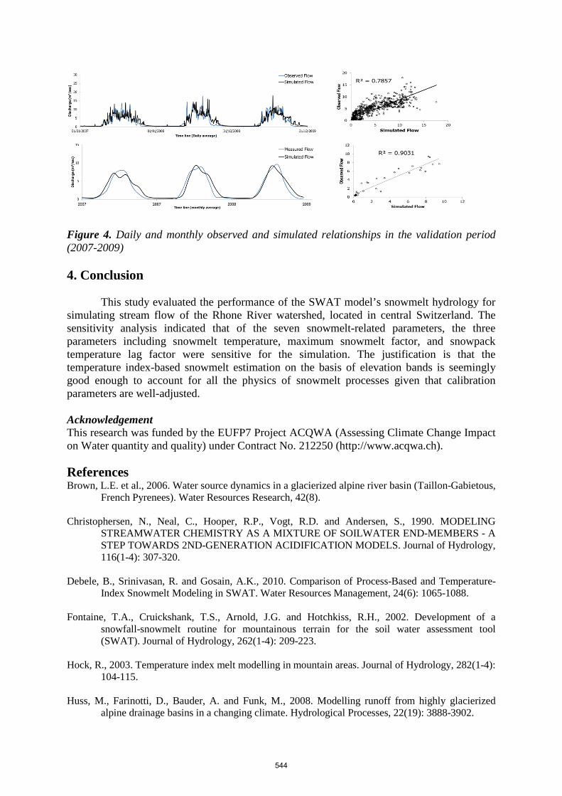
Figure 4. Daily and monthly observed and simulated relationships in the validation period (2007-2009) 4. Conclusion

This study evaluated the performance of the SWAT model’s snowmelt hydrology for simulating stream flow of the Rhone River watershed, located in central Switzerland. The sensitivity analysis indicated that of the seven snowmelt-related parameters, the three parameters including snowmelt temperature, maximum snowmelt factor, and snowpack temperature lag factor were sensitive for the simulation. The justification is that the temperature index-based snowmelt estimation on the basis of elevation bands is seemingly good enough to account for all the physics of snowmelt processes given that calibration parameters are well-adjusted. Acknowledgement This research was funded by the EUFP7 Project ACQWA (Assessing Climate Change Impact on Water quantity and quality) under Contract No. 212250 (http://www.acqwa.ch). References Brown, L.E. et al., 2006. Water source dynamics in a glacierized alpine river basin (Taillon-Gabietous,

French Pyrenees). Water Resources Research, 42(8). Christophersen, N., Neal, C., Hooper, R.P., Vogt, R.D. and Andersen, S., 1990. MODELING

STREAMWATER CHEMISTRY AS A MIXTURE OF SOILWATER END-MEMBERS - A STEP TOWARDS 2ND-GENERATION ACIDIFICATION MODELS. Journal of Hydrology, 116(1-4): 307-320.

Debele, B., Srinivasan, R. and Gosain, A.K., 2010. Comparison of Process-Based and Temperature-

Index Snowmelt Modeling in SWAT. Water Resources Management, 24(6): 1065-1088. Fontaine, T.A., Cruickshank, T.S., Arnold, J.G. and Hotchkiss, R.H., 2002. Development of a

snowfall-snowmelt routine for mountainous terrain for the soil water assessment tool (SWAT). Journal of Hydrology, 262(1-4): 209-223.

Hock, R., 2003. Temperature index melt modelling in mountain areas. Journal of Hydrology, 282(1-4):

104-115. Huss, M., Farinotti, D., Bauder, A. and Funk, M., 2008. Modelling runoff from highly glacierized

alpine drainage basins in a changing climate. Hydrological Processes, 22(19): 3888-3902.

544

Klok, E.J., Jasper, K., Roelofsma, K.P., Gurtz, J. and Badoux, A., 2001. Distributed hydrological

modelling of a heavily glaciated Alpine river basin. Hydrological Sciences Journal-Journal Des Sciences Hydrologiques, 46(4): 553-570.

Moriasi, D.N. et al., 2007. Model evaluation guidelines for systematic quantification of accuracy in

watershed simulations. Transactions of the Asabe, 50(3): 885-900. Neitsch, S.L., Arnold, J. G., Kiniry, J., andWilliams, J. R., 2005. Soil and water assessment tool

theoretical documentation , USDA Agricultural Research Service and TexasA&MBlackland Research Center, Temple, Texas.

Viviroli, D. and Weingartner, R., 2004. The hydrological significance of mountains: from regional to

global scale. Hydrology and Earth System Sciences, 8(6): 1016-1029. Zhang, X.S., Srinivasan, R., Debele, B. and Hao, F.H., 2008. Runoff simulation of the headwaters of

the Yellow River using the SWAT model with three snowmelt algorithms. Journal of the American Water Resources Association, 44(1): 48-61.

545

SWAT 2011

We would like to THANK our Conference Sponsors