Embed Size (px)
Citation preview
VOLUME LXXVI
PROCEEDINGS
OF THE
NUMBER 145
Casualty Actuarial Society ORGANIZED 1914
1989 VOLUME LXXVI
Number I45-November I989
COPYRIGH’I IYYO
CASUALTY ACTIIARIAI. SOCItT~
ALL RIGHTS RkStRVb.Il
Library of Congress Catalog No. HGYYSh.C3
ISSN 0x93.19x0
This publication is available in microform
Univcrslty Mi~rofilrm Intcmational
300 North Zreh Road 30-32 Mort~mcr Street Dept. P.R. kpt P.R Ann Arbor. Mi. 4X 10⁶ London WIN 7RA U.S.A. England
FOREWORD
The Casualty Actuarial Society was organized in 1914 as the Casualty Actuarial and Statistical
Society of America, with 97 charter members of the grade of Fellow; the Society adopted its present name on May 14. 1921.
Actuarial science originated in England in 1792, m the early days of life insurance. Due to the technical nature of the business, the first actuaries were mathematicians; eventually their
numerical growth resulted in the formation of the Institute of Actuaries in England in 184X. The Faculty of Actuaries was founded in Scotland in 1856, followed in the United States by the
Actuarial Society of America in 1889 and the American Institute of Actuaries in 1909. In 1949 the two American organizations were merged into the Society of Actuaries.
In the heginning of the twentieth century in the United States. problems requiring actuarial
treatment were emerging in sicknes, disability. and casualty insurance-particularly in workers’ compensation-which was introduced in I91 I The differences between the new problems and
those of traditional life insurance led to the organization of the Society. Dr. 1. M. Ruhinow, who was responsible for the Society’\ formation, became its first president. The object of the Society was. and is, the promotion of actuarial and statistical science as applied to insurance other than
lift inxurance. Such promotion is accomplished by communication with those affected by insur- ance, presentation and discussion of papers, attendance at seminars and workshops. collection of
a library, research. and other means.
Since the problems of workers’ compensation were the most urgent, many of the Society’s original members played a leading part in developing the scientific basis for that line of insurance. From the beginning, however, the Society has grown constantly, not only in membership, but
also in range of interest and in scientific and related contributions IO all lines of insurance other than life, including automobile, liability other than automobile, fire, homeowners and commercial multiple peril. and others. These contributions are found principally in original papers prepared
by members of the Society and published in the annual Proc~~~dings. The presidential addresses. also published in the Proceeding.s, have called attention lo the most pressing actuarial problems, some of them still unsolved, that have faced the insurance industry over the years.
The membership of the Society includes actuaries employed by insurance companies, rate- making organizations, national brokers, accounting firms, educational institutions, state insurance
departments. and the federal government; it also includes independent consultants. The Society has two &sea of members, Fellows and Associates. Both classes are achieved by successful completion of examinations, which are held in May and November in various cities of the United States and Canada.
The publications of the Society and their respective prices are listed in the Yeurhook which is
published annually. The S~llubus of E.rcrmincrrions outlines the course of study recommended for the examinations. Both the Yeurhook, at a $20 charge, and the SyNabus o/Ercrminarions, without charge. may he obtained upon request to the Casualty Actuarial Society. One Penn Plaza, 250 West 34th Street, New York. New York IO1 19.
III
JANUARY I, 1990
*EXECUTIVE COUNCIL
MICHAEL Fusco ..................................... President
CHARLES A. BRYAN ............................. Presidenr-Elect
ROBERT F. CONGER .................. Vice President-Admirlistrarior?
MICHAEI. L. TOOTHMAN ................. Vice Prrsitlrttt-Admissiorls
IRENE K. BASS Vkc Prcsitlent-ContitluinR Education
RICHARD I. FEIN Viw PrPsiclclttt-Pt-ogrcrms wd Commutzicnrions
ALBER I‘ J. BEER ........... Vice Prc,.sid~~tt1-R~,.srtrrch trnd Deveiotpmen~
THE BOARD OF DIRECTORS
*OjiWS: MICHAEL Fusco ...................................... President
CHARLES A. BRYAN .............................. Pwsidrnl-Elect
tlmneditrte Pmr I’re-riikrlt. KEVIN M. RYAN.. ........................................ 1990
:E/rcwc/ Direc~ror..s. ALAN C. CURRY .......................................... 1990 CHARLES L. MCCLENAHAN .............................. 1990 RICHARD J. ROTH, JR. (a) ................................ 1990
JEROME A. SCHEIBL ...................................... 1990 WALTER J. FITZGIBB~N, JR. ............................. 1991 CHARLES A. HACHEMENXR ................................ 1991 STEVEN G. LEHMANN
LEE R. STEENECK
RONAL.D L. BORNHUETIXR
JANET L. FACAN WAYNE H. FISHER
STEPHEN W. PHIL.BRICK
I 991 991 992 992 992 992
* Term expires at 1990 Annual Meeting. All mcmher\ ot the Executlw Council are Ol‘ficers The Vice Presidrnt-Administration also sewe\ ;i\ Secretary and Treawrer
i Term cxpircs at Annual Meeting oF gcx given (a) Elected tq Board of Director\ to till the uncxptrcd term 01’ Alhcrt .I Beer
1V
1989 PROCEEDINGS CONTENTS OF VOLUME LXXVI
Page
PAPERS PRESENTED AT THE NOVEMBER 1989 MEETING
Exposure Bases Revisited Amy S. Bouska . . . 1
The Aging Phenomenon and Insurance Prices Stephen P. D’Arcy and Neil A. Doherty.. . . 24
On Becoming An Actuary of the Third Kind Stephen P. D’Arcy . . . 45
Application of Collective Risk Theory to Estimate Variability in Loss Reserves
Roger M. Hayne . .._._............_......................._.......... 77
Determination of Outstanding Liabilities for Unallocated Loss Adjustment Expenses
Wendy Johnson . . . . . . . . . . . . . . . . . . . . . . . . . . . . . . . . . . . . . . . . . . Ill
The Effect of Trend on Excess of Loss Coverages Clive L. Keatinge . . . . . . . . . . . . . . . . . . . . . . . . . . . . . . . . . . . . . . . . . . . 126
An Analysis of the Capital Structure of an Insurance Company Glenn Meyers......................................................... 147
Risk Theoretic Issues in Loss Reserving: The Case of Workers Compensation Pension Reserves
Glenn Meyers......................................................... I71
DISCUSSION OF PAPER PUBLISHED IN VOLUME LXXV
Recent Developments in Reserving for Losses in the London Reinsurance Market
Harold E. Clarke (May, 1988) Discussion by John C. Narvell.. . . . . 193
REPRINT OF PAPER PUBLISHED IN VOLUME XXVI
The First Twenty-Five Years Francis S. Perryman . 215
REPRINT OF PAPER PUBLISHED IN VOLUME LI
The First Fifty Years Dudley M. Pruitt......................................................225
DIAMOND JUBILEE ADDRESS
The First Seventy-Five Years M. Stanley Hughey....................................................264
1989 PROCEEDINGS CONTENTS OF VOLUME LXXVI-CONTINUED
ADDRESS TO NEW MEMBERS-NOVEMBER 1989
Page
P. Adger Williams.......................................................29 7
PRESIDENTIAL ADDRESS-NOVEMBER 1989
Kevin M. Ryan .......................................................... 302
MINUTES OF THE NOVEMBER 1989 MEETING ............................... 309
REKIRT OF THE VICE PRESIDENT-ADMINISTRATION ....................... 326
FINANCIAL REPORT. ........................................................ 331
1989 EXAMINATION~~SUCCESSFUL CANDIDA’TES ........................... 332
OBITUARIES
William P. Amlie ...................................................... 349
Margaret A. Burt ...................................................... 350
Edwin A. Cook ....................................................... 351
Laurence H. Longley-Cook.............................................35 2
John H. Miller ........................................................ 353
Kent T. Penniman ..................................................... 354
John Phillips .......................................................... 354
Morris Pike ........................................................... 355
INDEX TO VOLUME LXXVI ................................................. 356
NOTICE
Papers submitted to the Proceedings of the Casualty Acruarial Society are subject to review by the members of the Committee on Review of Papers and, where appropriate, additional individuals with expertise in the relevant topics. In order to qualify for publication, a paper must be relevant to casualty actuarial science, include original research ideas and/or techniques or have special educational value, and must not have been previously published or be concurrently considered for publication elsewhere. Specific instructions for preparation and submission of papers are included in the Yearbook of the Casualty Actuarial Society.
The Society is not responsible for statements of opinions expressed in the articles, criticisms, and discussions published in these Proceedings.
VI
EDITOR’S COMMENT
The Casualty Actuarial Society participated with the American Acad- emy of Actuaries, the Canadian Institute of Actuaries, the Conference of Actuaries in Public Practice and the Society of Actuaries in the Centennial Celebration of the Actuarial Profession in North America which was held in Washington, D.C. on June 12, 13 and 14 of 1989. Hence, this volume of the PROCEEDINGS does not include the custom- ary report of activities usually held at our Spring Meeting.
VII
No. 145 Volume LXXVI, Part 1
PROCEEDINGS
November 12, 13, 14, 15, 1989
EXPOSURE BASES REVISITED
AMY S. BOUSKA
Abstract
The paper has muny purposes. They are: (I) to review the definition and selection of an exposure base and to clarifji the distinction between the exposure base and variables which are used in classijcation; (2) to review the exposure bases currently in use for manually rated risks, and to note how the manual exposure base becomes less important as the risk size increases; (3) to highlight problems in the determination of an exposure base (including temporal mismatch, interpretive mismatch, und complexity of hazurd); and (4) to discuss both the current controversy regurding the use of payroll as the esposure buse for workers compensation and the recent change in the exposure bases for general liability.
The author w*ould like to thank Marshall Auck, Scott Bradley. Lisa Chanzit. Jenni Ermisch. Mike Levin. Jim Morrow, Debbie Moyer, Deborah Rennie. Bill Safreed. and Susan Woerner. all of whom read drafts of the paper. Special thanks to
Rich Hofmann. who shredded the second draft and greatly improved the final product.
EXPOSURE BASES
1. INTRODUCTION
The business of insurance presumes an exposure to loss: if there is no possibility of a loss, there is no need for insurance. However, if an entity does have an exposure to loss, it is desirable that the cost of transferring that loss to another party be proportional to the expected loss, which is assumed to vary with the size of the exposure base. Thus, the selection of an exposure base, which quantifies and proxies for the exposure, is a fundamental step in the insurance process.
The following discussion is limited to the property and casualty lines of insurance in the United States and is not intended to address the life, pension, or accident and health lines or foreign business; nor is it intended to be an exhaustive survey of all exposure bases or rating plans used by individual companies.
2. DEFINITION
The classic definitions of exposure and premium bases were supplied by Paul Dorweiler in his 1929 paper “Notes on Exposure and Premium Bases” [ 11. In that paper, he wrote that “when critical conditions and injurable objects exist in such relationship that accidents may result there is said to be exposure” and “. . . premium funds are accumulated from charges called the rate collected per unit exposure. The exposure medium selected as the basis for the charge of the premium is known as the premium basis.”
He notes that the premium basis cannot be selected arbitrarily: “Ob- viously, the premiums collected are to be proportional to the hazard which is measured by the losses. . The medium most desirable as a premium basis is the one possessing a combination of these two quali- fications in the largest degree: 1. Magnitude of the Medium should vary with hazard. . . . 2. The Medium should be practical and preferably already in use.”
Although the premium basis is somewhat less accurately referred to as the exposure base today, the defnition and requirements are as correct and pertinent now as they were sixty years ago.
In their text Insurance Company Operations [2], Webb et al. ex- panded on Dorweiler’s requirement of “practicality” by stating that “A
EXPOSURE BASES 3
good exposure base should have three characteristics. First and foremost, of course, it should be an accurate measure of the exposure to loss. Second, it should be easy for the insurer to determine. Finally, it should be difficult for the insured to manipulate.” Adding one more level of cynicism (or realism, as the case may be), we should also require that the exposure base be immune to manipulation by underwriters.
Underlying all of these definitions are two themes: the relatively simple and reliable development of correct premiums for the insurers (i.e., the exposure base should accurately reflect the overall exposure to loss, be simple to compile, and not be subject to manipulation) and equitable distribution of those premiums among the insureds (i.e., the exposure base should accurately reflect differences in exposure to loss). It is not surprising that some historically appropriate exposure bases are showing signs of failing to satisfy these two conditions. The bases may have functioned well-or at least without controversy-in a world where the risks were relatively well understood, the insured commercial pop- ulation was regulated, the economic and social structures were stable, and the insurers used bureau rates. Changes in these external conditions and internal weaknesses in the underlying insurance structure are causing exposure base problems.
3. SELECTION OF AN EXPOSURE BASE
Before considering the impact of the changing environment, however, it is important to pause and consider the process involved in selecting an exposure base for a line of insurance.
The first step is to analyze the coverage offered and the coverage trigger to determine what factors influence the expected losses. Some of these factors will not be usable in the determination of premiums (see the Comments later in this section). Those which are usable will be divided into two groups: the first group, consisting of one factor, will be the exposure base, and the second group will be the rating variables, which influence the projected expected losses indirectly by affecting the rate.
This division is based on the simple theoretical equation:
(number of exposure units) X (loss cost per exposure unit) = expected losses. (1)
This is derived from the equation we detine to be true:
f(exposure) = expected losses. (2)
As will be discussed later, the true exposure is complex and changing, so we must simplify by selecting a proxy for the true exposure. This is the exposure base. The theoretical model is then quantified to become:
(number of exposure base units) X (loss cost per exposure base unit) = expected losses. (3)
Once the exposure base has been selected, projection of the loss cost per exposure base unit (usually by projection of frequency and severity) is the core of the ratemaking process. The loss cost generally varies with different combinations of the other factors. These combinations are known as the rating variables or class plan, and they may affect the loss cost through either the frequency or the severity or both. Equation (3) can also be written as:
(number of exposure base units) X (expected number of losses per exposure base unit) X (expected dollars per loss) = expected
IOSSCS. (4)
or
(number of exposure base units) X (frequency) X (severity) = expected losses. (5)
The final step in the manual ratemaking process is the inclusion of expenses, which leads to the equation:
(number of premium base units) X (rate per premium base unit) = manual premium. (6)
In practice, the exposure base unit in equation (3) and the premium base unit in equation (6) are always the same and the terms are used interchangeably.
Thus, expected losses (and premium) do not vary only with the exposure base, but also with many other factors which are built into the rating variables. Any factor that affects the losses but has not been quantified in either the exposure base or the class plan will allow the company that recognizes it in underwriting to “skim the cream” of the business. In this way, simple classification plans provide the opportunity
EXPOSURE BASES 5
for sophisticated companies to make profits by accepting only the better risks within a class.
In general, the factor selected as the exposure base should have a uniform multiplicative relationship with all of the expected loss costs and rates; i.e., within any rating class, the same rate will be used for one unit or fifty units (as opposed to requiring a higher or lower rate with increasing volume). Thus, a policy covering two physicians prac- ticing the same specialty in the same territory will use the same rate but multiply it by two, producing twice the premium.’
It is also desirable that the factor selected as the exposure base be simple and have an obvious relationship to losses. In addition to making the plan easier to use, simplicity is likely to enhance its perceived equity, even if the technical accuracy is not improved.
It is important to make note of two things that exposure bases are nor. First, the exposure base is not the true exposure. The exposure base is a proxy for the true exposure, which we are unable to know, both because it is constantly changing and because it is generally a function of a large number of variables. For example, the collision exposure of a private passenger auto is effectively zero when it is parked in a secure garage, somewhat higher when it is being driven on an isolated highway by an alert and competent driver, and substantially higher on a crowded street with a drunk driver. The exposure base (car-month) recognizes the average situation rather than these fluctuations in the true exposure to loss. As is noted later, there are even situations where the exposure base is zero, but a significant exposure still exists. The best way to keep this distinction clearly in mind is to think of the exposure base as the “units” designator (square footage, payroll, etc.) of a blank to be filled in on the premium calculation worksheet.
1 This simple multiplicative relationship is occasionally modified later in the calculation of the premium, either to reflect some exposure effect or to recognize the decrease in unit expenses associated with larger policies. Examples include (I) the multi-car discount in private passenger auto. which retlects the reduced usage and improved loss experience on policies covering multiple
cars, and (2) premium discount plans in worker\ compensation and other commercial lines. which reflect the decreased percentage of the premium required IO cover fixed expenses for large premium policies.
6 EXPOSURE BASES
Second, the exposure base is not a rating variable, although the dividing line between the two is somewhat arbitrary at times. In order to determine the correct manual premium for a risk, it is first necessary to classify the risk, based on whatever the rating variables are for the risk under consideration. Once the risk’s classification is known, the rate for that classification is multiplied by the number of exposure units to produce the premium. As is noted above, the use of a variable in the exposure base implies a uniform and continuous multiplicative relation- ship between the variable and the expected losses; use as a rating element implies a discrete, nonlinear relationship. For example, physician-month is an exposure base; and coverage for two physician-months costs twice as much as the coverage for one physician-month. On the other hand, age is a rating variable; and coverage for Driver A, who is twice as old as Driver B, does not (usually) cost twice as much.
Comments
It is important to remember that, for most lines of business, the exposure to loss varies with a substantial number of factors. Some of these cannot be used in determining the premium because they are either indeterminate, too subjective, or fluctuate too rapidly. An example of such a factor would be the mood of an automobile driver-while it could be argued that a person who is angry (either momentarily or on average) is more likely to have an accident, this is not used in any rating scheme.
Some factors may have a demonstrable or assumed correlation with losses but may be socially unacceptable as a rating variable or exposure base. Foremost among these are race and religion; age and gender are still used in many private passenger automobile rating plans but are being attacked (and defended) on social equity grounds.
Other factors that are observable but not quantifiable are allowed to influence commercial lines rates through the individual risk rating plans. Schedule rating plans for commercial general liability, for example, allow modification of the rate based on upkeep of the premises and management attitude.
The variables that are left-those which are socially acceptable, quantifiable, and demonstrably related to the level of losses-may be used directly in determining the premium. The one with the most uniform relationship to the losses will be the exposure base. The others can be used in the classification plan.
EXPOSURE BASES 7
A nonexhaustive list of the factors affecting the final premium for some of the major lines of business includes:
Property: construction, occupancy, location (territory), external hazards (technically called “exposure” but not in the same sense as the topic of this paper), internal protection (sprinklers, smoke alarms), external protection (local fire department and police), amount of insurance.
Automobile liability: driver’s age, gender, marital status, driving record, and school record; business or pleasure use; mileage or distance to work; radius of operation; location (territory of principal garaging); truck weight; insurance limit; number of vehicles; claims experience (safe driving credit (personal) or experience modification (commer- cial)).
Automobile physical damage: car make, model and year for private passenger auto, or vehicle age and original cost new for commercial autos; number of vehicles; territory; deductible; claims experience.
Workers compensation: location (territory), occupation, claims experi- ence (experience modification), payroll.
General liability: classification; territory; insurance limit; type of cover- age (claims-made or occurrence); claims experience; square footage or acreage, payroll or receipts; new/discontinued businesses.
Some of these factors-notably territory-are proxies for more basic influences on the level of losses, such as cost of medical care, traffic density and tendency to litigate.
As these lists make clear, many factors affect the expected losses (and, therefore, the premium) in any given line or subline of insurance, but only one becomes the exposure base.
4. A SUMMARY OF THE MAJOR LINES OF INSURANCE AND THEIR
EXPOSURE BASES
Property Coverages (Annual Statement Lines I, 2, 12 & 25) Glass coverage is rated on the square footage; all other coverages
are based on the limit of insurance in hundreds of dollars, which is assumed to be related to the value of the property insured.
8 EXPOSCIRF BASES
Homeowners and Furmowners Multiperil (Annual Stutement Lines 3 & 4) The property and crime sections of these policies generally use the
insured value (in hundreds or thousands of dollars) as an exposure base. The liability section has an implicit exposure base of one household.
Oceun und Inlund Marine (Annum/ Stutement Lines H & 9) These lines are essentially property coverages and are generally based
on the insured value in whole dollars. However, there are numerous exceptions, since “inland marine” covers a multitude of sins.
Aircraft-Ail Perils (Annuul Stutement Line 22) Aircraft hull coverage is rated on the insured value (in thousands of
dollars); liability is based on revenue-passenger miles (or kilometers).
Burglury and Theft (Crime) (Annuul Statement Line 26) The crime coverages are rated on the insured value in thousands of
dollars.
Boiler and Muchinerv (Annuul Stutement Line 27) Boiler and machinery coverage uses the number of objects as its
exposure base.
Credit (Ann& Statement Line 28) Credit coverage is based on the dollars of indebtedness.
Fidelity und Surety (Annual Stutement Lines 23 & 24) Fidelity coverages are rated on the number of persons; surety, on the
amount of coverage (contract cost) in thousands of dollars.
Automobile (Annuul Stutement Lines 19 & 21) All private passenger and commercial liability, no-fault, and physical
damage coverage is based on the number of car-months.
Workers Compensation (Annuul Stutement Line 16) There has been a great deal of discussion about the exposure base
for workers compensation, but it remains payroll (limited payroll for officers and sole proprietors and partners) in every state except Wash- ington.
Medical Mulpructice (Annual Stutement Line I I) Hospitals and other health care facilities are rated on occupied beds
and outpatient visits; premiums for health care providers (physicians & surgeons, dentists, optometrists, etc.) are based on provider-months.
EXPOSURE BASES 9
General Liability (Annuul Statement Line 17) The exposures bases for the various general liability sublines and
classes used to range from mundane (square footage) to mercenary (payroll) to morbid (number of bodies). Since the introduction of the Insurance Services Office (HO) Simplification Program in 1986, most classes are now rated on either gross sales or payroll, although apartment exposures use the number of units, and rates for offices and lessors are based on area. There are numerous other exceptions, such as the use of number of tanks for underground tank pollution liability rating.
Reinsurunce (Annual Statement Line 30) Facultative reinsurance has as many different exposure bases as does
primary insurance; treaty reinsurance is generally rated as a percentage of the underlying premium.
5. LARGE RISKS
Large risks are an exception to almost all of the above because they are frequently subject to either composite or loss rating plans that modify the usual exposure bases.
Under a composite rating plan, the risk’s premium is calculated normally and then divided by a proxy exposure base, such as mileage or receipts for long-haul trucking firms. This gives a rate per proxy unit. When the policy expires, the firm’s records are audited in order to determine the actual receipts (or mileage), and this is used to calculate the final premium.
The intention is to simplify the rating for insureds with hundreds of vehicles in their auto fleets or many insured locations. The proxy base should have at least some reasonable relationship to the expected losses, but it does not usually reflect the detail of the underlying exposure bases and classification systems.
If a large risk is loss-rated, the premium is calculated directly from its historical losses without any reference to the standard rating plans. In this case, it is correct to say that the exposure base is the risk itself and the rate is its expected losses. If, in addition, a composite rating procedure is used in order to reflect changes during the year, then a proxy base is introduced.
10 EXPOSURE BASES
Recall equation (6):
(number of premium base units) X (rate per premium base unit) = manual premium (6)
In this equation, the rate is a classification or manual rate (the subject of Part 6). Such a manual premium is used directly only for small risks. The premium for a medium-sized risk is frequently modified by schedule rating and expense modifiers, which reflect characteristics of the indi- vidual risk, and experience modifications and dividends, both of which give some recognition to the risk’s own experience. This changes equa- tion (6) to give:
(number of premium base units) X (rate per premium base unit) X (schedule modifiers) X (experience
modifiers) = manual premium X modifiers = charged premium. (7)
If the risk is composite-rated, this equation is continued to:
“charged” premium = (number of expected proxy units) X (rate per proxy unit.) (8)
At the fmal audit, the actual number of proxy units is determined and multiplied by the rate derived above to give the final premium.
As the size of the risk increases, more and more weight is put on the individual risk, diminishing the importance of the manual rate. In the case of a very large, loss-rated risk. the normal underlying exposure base and class plan disappear, leaving:
expected losses + expense load = charged premium. (9)
6. THE CHANGlNG ENVIRONMENT
There is a pervasive feeling that accurately forecasting losses in some lines of insurance has become impossible. The problem is frequently attributed to the degradation of the tort system, an increase in litigious- ness, and the search for “deep pockets.” These have clearly made it very difficult to accurately estimate the future frequency and severity of losses. However, in some cases, it may be more correct to say that we have not been able to identify an exposure base which successfully reflects these and other changes.
EXPOSURE BASES 11
As we will see, many of the problems of mismatch between exposure bases and the underlying exposures for which they are proxies arise from the exchange of a steady-state universe for one subject to abrupt changes. Determining the expected losses is easy when all factors are constant; the demands become somewhat greater but are still generally manageable if constant change, such as a constant rate of growth, is introduced into the system (see, for example, S. Philbrick’s paper “Implications of Sales as an Exposure Base for Products Liability” [3]). In recent years, these changes include emerging theories of liability, economic inflation, social inflation, changing insurance requirements and preferences, new products and services, increased tendencies towards acquisitions and divestitures, deregulation of industries such as trucking, technological advances, and the emergence of long-tail exposures. When severe discontinuities ap- pear, the underlying correspondence between the expected losses and the exposure base can be disrupted beyond correction. The following is a discussion of three types of problems in the selection of the exposure base: temporal mismatch, interpretive mismatch, and complexity of hazard.
These problems should not be confused with the ever-present rate- making problem of future shock. A failure to accurately predict the frequency and/or severity of future losses is usually a problem with our crystal balls (or other ratemaking tools), not the sign of a failing exposure base. For example, medical malpractice occurrence rates were histori- cally inadequate in spite of having a coverage trigger which is rarely a matter of dispute.
Problems: Temporal Mismatch
As the tail of liability losses lengthens and coverage triggers are changed in order to ease pricing and reserving problems, the possibility of a temporal mismatch between expected losses and an otherwise ac- ceptable exposure base arises. The two outstanding examples of this are claims-made policies and products liability.
Claims-made policies are triggered by the notice of a claim but rated on the normal occurrence exposure base, a physician-month in medical malpractice, for example. If the practice of medicine for a year causes a number of claims, some of them will generally be filed after the policy expires, giving rise to a loss under an occurrence policy but not under a
claims-made policy. No other candidate for the exposure base of a claims- made policy has been identified and the problem has been solved by the incorporation of a rating step to recognize the number of years since the retroactive date (i.e., the year in claims-made). The calculation of this modification is thoroughly discussed in “Rating Claims-Made Insurance Policies” by J.O. Marker and F.J. Mohl [4].
Careful evaluation of the trigger is necessary when making the ad- justment, since, for example, the new CGL claims-made form is trig- gered when notification has been received and recorded by any insured or by the insurer. This may be a relatively long time before a formal claim is filed with the insurance company.
Products liability coverage is triggered by the injury, but the exposure base is sales (with the exception of the few classes where products coverage is included with the premises and operations coverage). If the trigger were based on the date of manufacture or if the product were to have a short lifespan, it appears that sales would be a reasonable exposure base (ignoring for a moment ratemaking problems arising from the long tail, social inflation, etc.). However. triggering coverage on the date of injury gives rise to a mismatch. The problem is most easily illustrated by the case of a manufacturer who has gone out of business and therefore has no sales but whose products are still being used and producing injuries. The situation is frequently encountered in the case of the ac- quisition of a company with a discontinued product line that is still in use or the evaluation of a conglomerate that has actively acquired and disposed of subsidiaries over the years.
One possible solution to this mismatch would be to change the exposure base to “products in use during the year.” Unfortunately, while more precise in its reflection of the exposure, this is not an easily available figure; and it therefore fails the second test of a potential exposure base, namely that it be easily available and not subject to manipulation.
A more acceptable answer has been proposed by S. Philbrick in his paper “Implications of Sales as an Exposure Base for Products Liability” [3]. In this article, he also develops the adjustment methodology that could be used as an input to schedule rating to correct for the mismatch.
In general, the temporal mismatch problem can be solved, although the solution is likely to be inexact.
EXPOSURE BASES 13
Problems: Interpretive Mismutch
The exposure base selected must be compatible with policy language that is sufficiently precise so that mismatch does not arise through delib- erate or accidental misinterpretation of the coverage trigger. For example, a pollution policy meant to cover losses arising out of disposal activities starting after policy inception could be rated on tons of waste produced (or disposed of, if there is a lag between production and disposal). This is a reasonable prospective exposure base; but the policy language must be precise and enforceable or there is a possibility that courts will find coverage for losses from past disposal activities, for which a different exposure base would be necessary.
Without commenting on the appropriateness of the asbestos coverage theories used to date and ignoring the fact that products liability is already subject to temporal mismatch, the fact that it is possible for injury to one person to trigger many policies indicates that interpretive mismatch is also a problem for the affected products policies. Even if these policies had been rated on “products in use during the year,” coverage would not have been expected from the policies triggered after the asbestos work stopped (the “injury in residence” and “manifestation” triggers).
Problems: Complexity of Huzard
In some cases, the problems are much more basic than those men- tioned previously. The difficulty frequently lies in the first step of deter- mining the exposure base; i.e., making a complete list of all factors affecting the level of losses. What, for instance, would be contained in such a list for directors and officers (D&O) insurance? Obvious candi- dates include:
- the number of directors and officers - business activities - (change in) revenues - (change in) profits - (change in) assets - number of stockholders - number of employees - hiring/firing policies - (change in) overall financial condition as rated by S&P - (change in) stock price
14 EXPOSURE BASES
- attractiveness as an acquisition - responses to past acquisition offers (e.g., “poison pills”) - state of domicile - response to any recent emergencies (accidents, etc.) - recent changes in management - ‘77 . . . . .
All of these are believed to have some bearing on the likelihood or size of D&O claims, which have been known to arise from abrupt changes in a company’s stock price, resistance on the part of the directors to being acquired, and wrongful termination of employees. But is the list complete? Probably not. Even if it is, the numerical relationship of the factors to the loss level is unclear even for the most obvious candidate for the exposure base: does a company with twice as many directors have twice the exposure to loss’? Probably not.
It could be argued that the general reluctance of the industry to offer this coverage is an outgrowth of our inability to determine a meaningful exposure base for it. [5] It is to be hoped that when (if ?) we are able to correlate the losses with some other measurable factor, the “D&O crisis” will abate.
7. THE INTERNAL ENVIRONMENT
In fairness to the world at large, it must be admitted that not all problems with exposure bases arise outside of the insurance industry. Two serious problems are based on insurance company practices them- selves: (1) exposure estimates can be (and are) manipulated in response to the competitive situation; and (2) even when the policy premium is based on the correct exposures, the coding of the exposure information into the computer records is often poor, with whole dollars frequently switched with “per hundreds” or “per thousands.”
Mechanical rating and direct production of the statistical records from the policy rating files will solve the second problem, but control of the first is likely to be more elusive. Most companies track their average premium per policy rather than the average premium per exposure unit so that good exposure data is not considered necessary. In addition, competitive pressures tend to degrade the exposure data. In a very competitive (soft) insurance market, a low price can be produced in a variety of ways. a number of which are legitimate but frequently require
EXPOSURE BASES 15
documentation, such as the aggressive use of schedule rating. In some instances, it is easier for the underwriter to “low-ball” the exposure estimate. In theory, such “errors” will be corrected when the policy is audited, but that is usually eighteen months in the future (and after the renewal). Under the calendar/accident year ratemaking used for many lines, audit premiums are reported and fully earned in the calendar year of the audit, not the calendar year(s) when the policy premium was earned. Thus, even in the case of perfectly correct audits, a severe mismatch between the premiums and losses can be introduced by low exposure estimates. In a steady state, the rates eventually respond to a systematic underestimation of the exposures; but when the insurance cycle changes quickly and the “low-balling” stops abruptly, the problem of excessive rates appears.
Thus, some of the practical mismatch between exposures and expo- sure bases can be attributed to the pricing practices of the industry as a whole, rather than a more esoteric theoretical failure.
8. CHANGING EXPOSURE BASES: CAUSES AND CONTROVERSY
Once established, the exposure base for a line of insurance tends to acquire an aura of sanctity. It is very difficult and very expensive to change the exposure base for a widely written line: difficult, because the historical data uses the old base, but the new rates must refer to the new base; and expensive, because data on both bases must be collected for at least one year prior to the change or all insureds must be contacted to determine their new exposure and then all policies must be rerated and reissued.
So why change ? In theory, change could be caused by a better understanding of the nature of the exposure. In practice, this does not seem to be the case, either because a line does not become widely written until the exposure is reasonably well understood, or because the marginal gain is less than the cost, or because inertia is stronger than the profit motive. Thus, the two recent exposure base controversies have been forced on the industry by changes in the world that is being insured. One of these-in workers compensation-was caused by increasing dis- content among insureds over inequities in the rating mechanism; the other-in general liability-was the result of both the industry’s difficulty in keeping rates current and the increasing automation of commercial lines.
16 EXIWSL’RF. H.\Sl:S
It should be noted that the frequent discussions regarding the use of driving record in place of age, gender and/or marital status in determining private passenger auto premiums concern only the rating plan, not the exposure base. To date, there has been very little discussion of the use of car-months, although Andrew Tobias in his book The Invisible Bank- ers [6] suggested a plan based on fuel consumption, and the National Organization for Women has proposed an odometer mileage exposure base.[7] However, as the workers compensation changes illustrate, the line between the exposure base and the rating plan is very fine, and a discussion which begins on one side of that line may well finish on the other.
The problem is simple: consider two construction tirms, one of which is unionized and one of which is not. Assume they have the same number of employees. do the same type of work. and have the same expected number and type of losses. If the unionized company pays more per hour, it will have a higher payroll and, therefore. pay more for its workers compensation coverage. To the extent that its indemnity losses (based on lost wages) are higher, this premium difference is correct; however, to the extent that the losses arise from medical payments or are capped by the maximum benefits payable under state law, the difference is not justified in terms of expected losses. Obviously. there is no problem if the work is sufficiently different that separate classilications are used.
For many years, limited payroll-reflecting the limited benelits- was the exposure base for workers compensation (WC) in all states other than Washington, which used and still uses work-hours. In the early 1980s. the payroll limitation was removed. This change obviously made the problem worse.
In 1984-85, the perceived inequity became a matter of national debate between the National Council on Compensation Insurance (NCCI) on the one hand and insureds (both labor and management) on the other. It was caused not only by union/nonunion differentials, but also by the varying wage scales that appeared as a result of deregulation in many industries. Based on these differences. the insureds proposed both hours- worked and mixed hours-worked/payroll as exposure bases, while the NCCI preferred to retain unlimited payroll. because it is easy to verify
EXPOSURE BASES 17
and it reduces the size of the annual rate revisions needed. Regulators were concerned that, whatever program resulted, it should be fair and encourage workplace safety.
Because wage level and unionization status are not recorded in the standard WC data, insurance records at NCCI and insurance companies could not resolve the question. Therefore, the state of Oregon did a special “Study of Premium Equity by Employer Groups.” Obviously, the issue was not important to very large employers whose experience is fully credible, so the study addressed primarily the small (nonexperi- ence-rated) and medium (experience-rated but not fully credible) em- ployers.
NCCI’s analysis of the Oregon data found no bias against either union or high wage paying employers among the small employers, but it did show that high wage paying and union employers in the medium- sized group developed lower loss costs per premium dollar (11% and 12% less, respectively). This result appears somewhat counter-intuitive, since one would expect, N priori, that the availability of experience rating would reduce the bias.
Among others, the Florida Labor/Management Council proposed a mixed rating base, using both payroll (for wage-related benefits) and worker-hours (for medical-related benefits).
Payroll won out in the exposure base arena, but concessions were made on the classification side. In California, each of six construction classes were split into two new classifications (high and low wage rates); in Florida, a table of credits based on wage rates was implemented for all contracting classes; in Oregon, the legislature authorized the collection of worker-hour data by the NCCI and the Oregon workers compensation division; and the NCCI-proposed Loss Ratio Adjustment Program (LRAP) was put into place in Oregon, Illinois, Maryland and Nebraska, although the approved version differed by state.
LRAP is a modification to the WC experience rating plan for the specific construction classifications shown to have problems. Its effect is to make the experience rating plan more responsive to the individual employer’s three-year loss ratio. NCCI favored this response because it was problem-specific (i.e., did not affect other classifications), did not require an overall rate change, and encouraged workplace safety.
18 EXPOSURE BASES
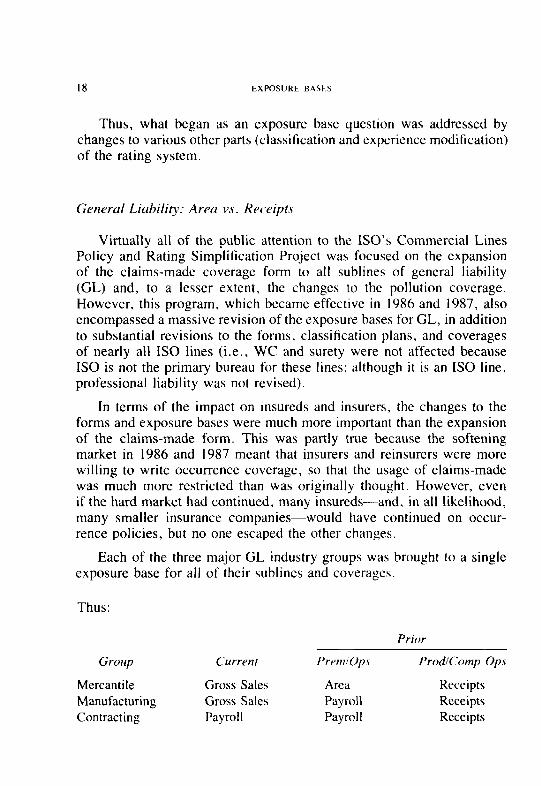
Thus, what began as an exposure base question was addressed by changes to various other parts (classification and experience modification) of the rating system.
General Liability: Area vs. Receipts
Virtually all of the public attention to the ISO’s Commercial Lines Policy and Rating Simplification Project was focused on the expansion of the claims-made coverage form to all sublines of general liability (GL) and, to a lesser extent, the changes to the pollution coverage. However, this program, which became effective in 1986 and 1987, also encompassed a massive revision of the exposure bases for GL, in addition to substantial revisions to the forms, classification plans, and coverages of nearly all IS0 lines (i.e., WC and surety were not affected because IS0 is not the primary bureau for these lines; although it is an IS0 line, professional liability was not revised).
In terms of the impact on insureds and insurers, the changes to the forms and exposure bases were much more important than the expansion of the claims-made form. This was partly true because the softening market in 1986 and 1987 meant that insurers and reinsurers were more willing to write occurrence coverage, so that the usage of claims-made was much more restricted than was originally thought. However, even if the hard market had continued, many insureds-and, in all likelihood, many smaller insurance companies-would have continued on occur- rence policies, but no one escaped the other changes.
Each of the three major GL industry groups was brought to a single exposure base for all of their sublines and coverages.
Thus:
Prior
Group
Mercantile Manufacturing Contracting
Current
Gross Sales Gross Sales Payroll
PretttlOps
Area Payroll Payroll
ProdlComp Ops
Receipts Receipts Receipts
EXPOSURE BASES 19
Some exceptions to the above remain. The most major of these are apartments, which were rated on area but changed to units, and office buildings, which were and are based on area.
The short diagram above conceals the true extent of the simplifica- tion. In order to calculate the premium for a small contractor before simplification, for example, the underwriter needed to know (I) the payroll . . . for the M&C coverage; (2) receipts _ . . for the products/ completed ops coverage; (3) total contract cost . . . for the contractual liability; (4) the building’s fire rate . . . for fire damage legal liability; (5) the M&C property damage rate . . . for broad form property damage coverage; and the M&C bodily injury rate . . . for persona1 and adver- tising injury. Under the new structure, all of these coverages are based on payroll.
These changes were implemented for a variety of reasons, including (I) simplification of rating, both manual and mechanized, (2) sensitivity to inflation, and (3) sensitivity to economic cycles. It is, of course, very desirable to have an exposure base that incorporates inflation, fully or partially, since this reduces the need for frequent and relatively large rate filings.
The changeover was not easy for many reasons. Among the most important of the difficulties were the premium swings caused by the change of exposure bases.
IS0 realized that the change from area to receipts (gross sales) would cause large premium swings for some insureds and filed a transition program along with the new policies. The transition program was meant to cap the premium effect of only the exposure base change. Using Dun & Bradstreet data, IS0 calculated the average ratio of receipts to area for each class, territory and state and used this to convert the current area-based rates to the new receipts base. If an insured had a higher- than-average ratio of receipts to area, this would cause its premium to increase substantially. The increase (and decrease) was capped by the establishment of maximum and minimum ratios for each class, territory and state. The caps increased over five years to bring the insureds to their new premium gradually.
ISO’s preliminary investigations indicated that the manufacturing and contracting classes did not have as much variability in their exposure
base ratios, so no transition program was developed for these classes. However, as companies began to implement the simplified policies, it quickly became apparent that there was a problem. This was exacerbated by the effects of the change to a combined single limit and the inclusion of other coverages in the base rate. IS0 responded by tiling a transition program for other than mercantile risks, but it used countrywide caps rather than varying them by state and territory.
On the whole, the expanded transition program was successful, but it was given very little credit. In many cases, the first renewal on the simplified forms followed the hardening of the market. This meant that premium increases due to changes in companies’ rates and deviations were frequently blamed on the exposure base change. Premium increases from changes in the increased limits tables (also part of the simplification program) made this problem worse.
From the companies’ viewpoint, the transition program was a mixed blessing. On the negative side, it represented another training and pro- gramming hurdle; it introduced another step in the rating process which will persist for five years for many risks: and it was difficult to explain to insureds. On the positive side, once it was expanded, it did what it was designed to do, and it provided a convenient scapegoat for rate increases.
One long-term result of the exposure base change which has been given relatively little consideration is the effect of using an audited exposure base for many risks that were previously rated on area. This increases expenses somewhat for the insurer (many of these risks have products coverage, for which an audit was already required) and increases uncertainty for the insured, since the final premium is not known until after the policy expires. Of course, many smaller risks will be audited by mail or by telephone; but this increases the opportunity for manipu- lation of the premium while decreasing the audit cost.
In light of the expense and confusion surrounding the change of exposure bases, it is reasonable to ask whether the insurance commu- nity-both insureds and insurers-is in a better long-term position than it was before the change. It is clear that the simplification program as a whole eliminated many inconsistencies in the rating process and vastly simplified policy rating. This could not have been accomplished without changing the exposure bases. To the extent that the automation of the
EXPOSURE BASES 21
commercial lines has been accelerated, the program also decreased ex- penses. The price of these improvements was short-term upheaval and a possible long-term increase in audit costs.
The above points may well have been sufficient cause for the change, but it is also reasonable to ask whether receipts are a better exposure base than area for most mercantile risks. Recall that this should be judged on the basis of (I) ease of collectibility, (2) difficulty of manip- ulation, and (3) correct reflection of the underlying losses. To the extent, that the fringe coverages, such as contractual liability and fire legal liability, are rated more fairly (i.e., with greater precision) on other exposure bases, the simplification may have reduced the correct reflection of these underlying losses.
Since receipts are used for other purposes, most notably tax calcu- lations, it is easy to collect the data. However, the use of receipts requires a post-expiration audit unless the insurer decides to forego the possible change in premium. While the risk may well have already required an audit for its products coverage, the change does mean that the premium for two coverages must now be checked. On the whole, it is difficult to say that there has been a net improvement on this point over area, which is relatively easily available (although requiring a detailed definition) and does not require an audit.
It has been amply demonstrated over the course of the last insurance cycle that both area and receipts can be manipulated by both the insured and the underwriter. It has been argued that the introduction of the audit step, especially if it is done by telephone and relies on the insured’s reporting, increases the number of opportunities for manipulation.
With no clear advantage to either exposure base on the first two criteria, the question becomes one of correlation with losses. If the traffic of customers and suppliers through a mercantile establishment can be assumed to be correlated with the loss exposure, then receipts may be more closely correlated with losses. Thus, an establishment with a thriv- ing business has more customers, more loss exposure, higher receipts and a higher premium. On the other hand, one must consider the effect of price on receipts: a store selling expensive imported shoes may have the same total receipts as a mass-market store but far fewer clients and a lower exposure to loss (unless “upscale” clients are more prone to sue).
22 EXPOSIJRI: HASES
Time will judge the appropriateness of the exposure bases. Any inequities between classes of business will be erased as the rates adjust to the information passed into the ratemaking process. The real long- term test will be within classes: whether a stronger correlation between a risk’s exposure and its expected losses exists for receipts or area. Of course, even if receipts should fail this test, it may be easier to adjust the class plan in some way than to change the exposure base again.
The exposure base is a fundamental part of the distribution of loss costs among insureds, i.e., of the premium calculation. The tests that it must meet are relatively simple and clear, but changes in external envi- ronment and problems in the internal environment have made it more difficult to satisfy those tests. In addition, insurance coverages for which the exposure base is not immediately obvious have been developed or are more in demand. The insurance industry has reacted differently in the two cases where change was forced by outside conditions: adapting the classification and individual risk modification system in one case, and completely revising the exposure base and rating system in the other. The IS0 Simplification was an example of some of the problems and responses to be expected in the course of a changeover, which can be studied as a prototype of the changes which are undoubtedly to come.
EXPOSURE BASES 23
REFERENCES
[I] Paul Dorweiler, “Notes on Exposure and Premium Bases,” PCAS XVI, 1929, p. 319; reprinted PCAS LVIII, 1972, p. 59.
[2] B. L. Webb, J. J. Launie, W. P. Rokes, N. A. Baglini, Insurance Company Operations, Volume II, American Institute for Property and Liability Underwriters, 1978.
[3] Stephen W. Philbrick, “Implications of Sales as an Exposure Base for Product Liability,” PCAS LXVII, 1980, p. 181.
[4] J. 0. Marker and F. J. Mohl, “Rating Claims-Made Insurance Pol- icies,” Pricing Property and Casunlt~~ Insurance Products, CAS Discussion Paper Program, 1980, p. 265.
[5] Thomas S. Bloom, “Liability Rating Scheme Faulted for ’80s Crunch,” National Underwriter, September 5, 1986, p. 8.
[6] Andrew Tobias, “Pay-As-You-Drive: How God Would Restructure Automobile Insurance,” The Invisible Bankers, Washington Square Press, 1982, p. 230.
[7] Patrick utler, Twiss Butler and Laurie L. Williams, “Sex-Divided I3 Mileage, Accident, and Insurance Cost Data Show that Auto Insurers Overcharge Most Women,” Journal of Insurance Regulation, Vol. 6, Nos. 3 & 4, March & June 1988, p. 243.
24
THE AGING PHENOMENON AND INSURANCE PRICES
STtI’HEN P I)‘,\RC‘\r
Abstrwt
Abstrwt
A well known but little documented tendency of property-liability insurance contracts is for the 10~5 ratio on mature business, the book of policies that has been with the insurer for a number of renewal cycles, to exhibit constant improvement. The cause of this tcndcncy, termed the aging phenomenon or seasoning of business. has been addressed by Kunreuther and Pauly [S] and D’Arcy and Doherty 141 and theorized to be the result of the accumulation ot’ private information by the contracting insurer. This information allows the insurer to classify the policyholders properly as valid information about the risk is collected, as opposed to
I'Ht AGING PHENOMENON 2s
the initial information included in the application and obtained in the initial underwriting screening. Such information could include a verified loss history, as the insurer knows about claims that occur during the coverage period, the condition of the insured property and the degree of cooperation demonstrated by the insured in settling any claims. This insurer also is able to renew policies selectively to weed out the least desirable risks. The remaining policyholders represent a continually im- proving book of business as more high-risk insureds are properly clas- sified and appropriately charged and the culling process continues to cancel policyholders whose risk profile is higher than the indicated rate level would reflect. For example, a private passenger automobile insured with one at-fault accident may have proven to be such an uncooperative defense witness that the insurer is unwilling to renew the policy even at the classification rate for one accident. As the contracting insurer has an advantage in access to this information, competition does not work to reduce the premium level on this desirable business in proportion to the improvement in loss experience.
The aging phenomenon is believed to occur for all lines of property- liability insurance, although little published information confirms this belief. Eight insurers have provided the authors with confidential infor- mation demonstrating this effect, subject to the condition that they not be identified, and many other insurers have confirmed that the trend also occurs on their business as well. The disparity of record keeping tech- niques and internal procedures among insurers makes exact measurement of the extent of aging impossible at this point. However, the widespread confirmation of this trend and its importance in pricing and marketing strategy calls for an analysis of the effect of aging on insurance pricing.
The purpose of this paper is to incorporate the aging phenomenon into a pricing model. The initial model is based on fairly simple as- sumptions in order to clearly demonstrate the effect of aging on prices and to derive numerical results. The assumptions are later altered to reflect more realistic conditions in additional models. Hopefully, indi- viduals with access to their company’s databases will be encouraged to generate additional tests of these models.
2. NOTATION
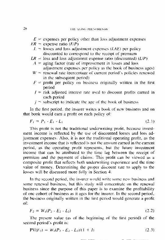
The following notation will be used in the initial model: P = premium level per policy
26 I111; 4(.IN(; I’lit.NOhlt.NON
E = expenses per policy other than loss adjustment expenses ER = expense ratio (E/P)
L = losses and loss adjustment expenses (LAE) per policy discounted to correspond to the receipt of premium
LR = loss and loss adjustment expense ratio (discounted) (L/P) A = aging factor (rate of improvement in losses and loss
adjustment expenses per policy as the book of business ages) W = renewal rate (percentage of current period’s policies renewed
in the subsequent period) F = profit per policy on business originally written in the tirst
period I = risk adjusted interest rate used to discount profits earned in
each period j = subscript to indicate the age of the book of business
In the first period, the insurer writes a book of new business and on that book would earn a profit on each policy of:
F, = P, - E, - L, (2.1)
This profit is not the traditional underwriting profit. because invest- ment income is reflected by the use of discounted losses and loss ad- justment expenses. Also, it is not the traditional operating profit, as the investment income that is reflected is not the amount earned in the current period, as the operating profit represents, but the future investment income that can be attributed to the time lag between the receipt of premium and the payment of claims. This profit can be viewed as a composite profit that reflects both underwriting experience and the time value of money. Determining the proper discount rate to apply to the losses will be discussed more fully in Section 4.
In the second period, the insurer would write some new business and some renewal business, but this study will concentrate on the renewal business since the purpose of this paper is to examine the profitability of one cohort of business as it ages for the insurer. In the second period, the business originally written in the tirst period would generate a profit of:
Fz = W,(Pz - Er - Lz) (2.2)
The present value (as of the beginning of the first period) of the second period’s profit is:
PV(F?) = W,(Pz - EJ - Lz)l(l + I) (2.3)
THE AGING PHENOMENON 21
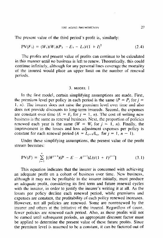
The present value of the third period’s profit is, similarly:
PV(Fd = (W,)(W,)(P, - Ej - L3)/(1 + I)* (2.4)
The profits and present value of profits can continue to be calculated in this manner until no business is left to renew. Theoretically, this could continue infinitely, although for any personal lines coverage the mortality of the insured would place an upper limit on the number of renewal periods.
3. MODEL I
In the first model, certain simplifying assumptions are made. First, the premium level per policy in each period is the same (P = P, forj = 1, n). The insurer does not raise the premium level over time and also does not provide discounts to long-term insureds. Second, the expenses are constant over time (E = E, for j = 1, n). The cost of writing new business is the same as renewal business. Next, the proportion of policies renewed each year is the same (W = Wj for j = 1, n). Finally, the improvement in the losses and loss adjustment expenses per policy is constant for each renewal period (A = fij+ r/Lj, forj = 1, n - I).
Under these simplifying assumptions, the present value of the profit stream becomes:
PV(F) = 2 [(W’-‘)(P - E - A-‘-‘(L))l(l + I)‘-‘] jz 1 (3.1)
This equation indicates that the insurer is concerned with achieving an adequate profit on a cohort of business over time. New business, although it may not be profitable to the insurer initially, must produce an adequate profit, considering its first term and future renewal cycles with the insurer, in order to justify the insurer’s writing it at all. As the losses per policy decline each renewal period, while premiums and expenses are constant, the profitability of each policy renewed increases. However, not all policies are renewed. Some are nonrenewed by the insurer and others at the initiative of the insured. Regardless of cause, fewer policies are renewed each period. Also, as these profits will not be earned until subsequent periods, an appropriate discount factor must be applied to determine the present value of these future profits. Since the premium level is assumed to be a constant, it can be factored out of
28 I HE ,AtiING I’tiI~YOMI,NON
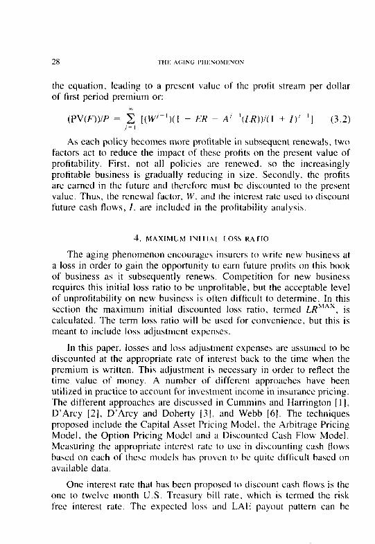
the equation, leading to a present value of the profit stream per dollar of first period premium or:
(PV(F))IP = 2 [(W’-‘)(l - ER - A’ ‘(LR))I(l + I)-’ ‘1 (3.2) j= I
As each policy becomes more profitable in subsequent renewals, two factors act to reduce the impact of these profits on the present value of profitability. First, not all policies arc renewed. so the increasingly profitable business is gradually reducing in size. Secondly, the profits are earned in the future and therefore must be discounted to the present value. Thus, the renewal factor, W, and the interest rate used to discount future cash flows, I, are included in the profitability analysis.
4. MAXIMUM INITIAI. LOSS RATIO
The aging phenomenon encourages insurers to write new business at a loss in order to gain the opportunity to earn future profits on this book of business as it subsequently renews. Competition for new business requires this initial loss ratio to be unprofitable, but the acceptable level of unprofitability on new business is often difficult to determine. In this section the maximum initial discounted loss ratio, termed LRMAX, is calculated. The term loss ratio will be used for convenience, but this is meant to include loss adjustment expenses.
In this paper, losses and loss adjustment expenses are assumed to be discounted at the appropriate rate of interest back to the time when the premium is written. This adjustment is necessary in order to reflect the time value of money. A number of different approaches have been utilized in practice to account for investment income in insurance pricing. The different approaches are discussed in Cummins and Harrington [ I], D’Arcy [2], D’Arcy and Doherty [3 1. and Webb [6]. The techniques proposed include the Capital Asset Pricin g Model, the Arbitrage Pricing Model, the Option Pricing Model and a Discounted Cash Flow Model. Measuring the appropriate interest rate to USC in discounting cash flows based on each of these models has proven to bc quite difficult based on available data.
One interest rate that has been proposed to discount cash flows is the one to twelve month U.S. Treasury bill rate, which is termed the risk free interest rate. The expected loss and LAE payout pattern can be
THE AGING PHENOMENON 29
discounted based on this rate to determine the actual initial loss ratio in comparison with the maximum loss ratios determined in this paper. One other advantage of using discounted loss ratios is the comparability across coverages and lines. The same discounted loss ratio will apply to fast settling lines such as collision and comprehensive as well as long-tailed lines such as liability, as the investment income component is directly reflected in the discounted loss ratio.
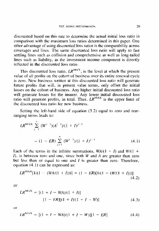
This discounted loss ratio, LRMAX, is the level at which the present value of all profits on the cohort of business over its entire renewal cycle is zero. New business written at this discounted loss ratio will generate future profits that will, in present value terms, only offset the initial losses on the cohort of business. Any higher initial discounted loss ratio will generate losses for the insurer. Any lower initial discounted loss ratio will generate profits, in total. Thus, LRMAX is the upper limit of the discounted loss ratio for new business.
Setting the left-hand side of equation (3.2) equal to zero and rear- ranging terms leads to:
r
LR MAX ,F, (W’-‘)(A’+)/( 1 + I)‘-’
= (1 - ER) 5 (W/+)/(1 + I)‘-’ (4.1) ./= 1
Each of the terms in the infinite summations, WA/( 1 + I) and W/( 1 + I), is between zero and one, since both W and A are greater than zero but less than or equal to one and I is greater than zero. Therefore, equation (4.1) can be expressed as:
LR M”x]l/(l - (WA/(1 + Z)))] = (I - ER)[II(l - (W/(1 + ()))I (4.2)
or
LR M~‘X = [( 1 + I - WA)/( 1 + 1)]
[l - ER][(I + Ml + / - W)]
or
LR MAX = [(I + I - WA)/( 1 + I - W)][l - ER]
(4.3)
(4.4)
30 THE AGING; i’HI~,NOMFNON
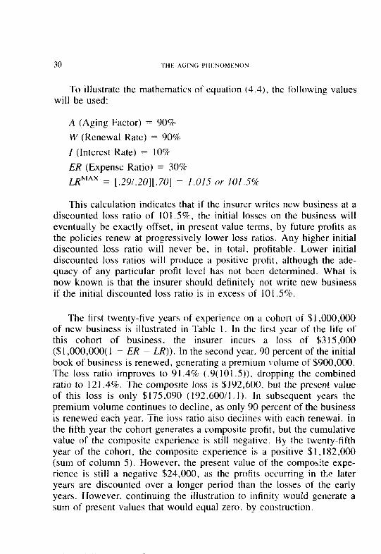
To illustrate the mathematics of equation (4.4). the following values will be used:
A (Aging Factor) = 90% W (Renewal Rate) = 90%
I (Interest Rate) = 10%
ER (Expense Ratio) = 30%
LR MAX = [.29/.20][.70] = 1.015 or lO/.S7c
This calculation indicates that if the insurer writes new business at a discounted loss ratio of 101.50/c, the initial losses on the business will eventually be exactly offset, in present value terms, by future profits as the policies renew at progressively lower loss ratios. Any higher initial discounted loss ratio will never be, in total, profitable. Lower initial discounted loss ratios will produce a positive profit, although the ade- quacy of any particular profit level has not been determined. What is now known is that the insurer should definitely not write new business if the initial discounted loss ratio is in excess of 101.5%.
The first twenty-five years of experience on a cohort of $1 ,OOO,OOO of new business is illustrated in Table 1. In the first year of the life of this cohort of business, the insurer incurs a loss of $3 15,000 ($1 ,OOO,OOO( 1 - ER - LR)). In the second year. 90 percent of the initial book of business is renewed, generating a premium volume of $900,000. The loss ratio improves to 9 I .4% ( .9( 101.5)), dropping the combined ratio to 121.4%. The composite loss is $192,600, but the present value of this loss is only $175,090 ( 192.600/1.1). In subsequent years the premium volume continues to decline, as only 90 percent of the business is renewed each year. The loss ratio also declines with each renewal. In the fifth year the cohort generates a composite prom, but the cumulative value of the composite experience is still negative. By the twenty-fifth year of the cohort, the composite experience is a positive $1,182,000 (sum of column 5). However, the present value of the composite expe- rience is still a negative $24,000, as the profits occurring in the later years are discounted over a longer period than the losses of the early years. However, continuing the illustration to infinity would generate a sum of present values that would equal zero, by construction.
THE AGING PHENOMENON 31
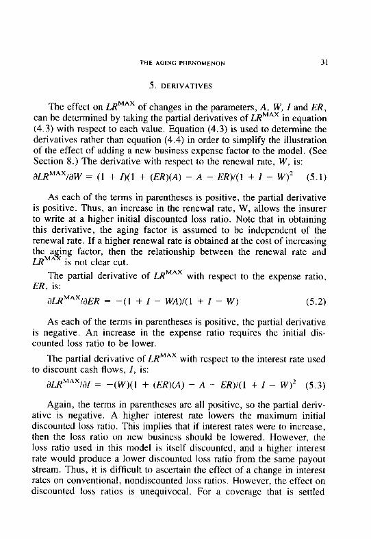
5. DERIVATIVES
The effect on LRMAX of changes in the parameters, A, W, I and ER, can be determined by taking the partial derivatives of LRMAX in equation (4.3) with respect to each value. Equation (4.3) is used to determine the derivatives rather than equation (4.4) in order to simplify the illustration of the effect of adding a new business expense factor to the model. (See Section 8.) The derivative with respect to the renewal rate, W, is:
dLR MAXIdW = (1 + I)( 1 + @R)(A) - A - ER)I(l + I - W)* (5.1)
As each of the terms in parentheses is positive, the partial derivative is positive. Thus, an increase in the renewal rate, W, allows the insurer to write at a higher initial discounted loss ratio. Note that in obtaining this derivative, the aging factor is assumed to be independent of the renewal rate. If a higher renewal rate is obtained at the cost of increasing the a ing factor, then the relationship between the renewal rate and
5 LRMA is not clear cut. The partial derivative of LRMAX with respect to the expense ratio,
ER, is:
dLR MAXIdER = -( 1 + I - WA)I( 1 + I - W) (5.2)
As each of the terms in parentheses is positive, the partial derivative is negative. An increase in the expense ratio requires the initial dis- counted loss ratio to be lower.
The partial derivative of LRMAX with respect to the interest rate used to discount cash flows, I, is:
dLR MAX/az = -(W)(l + (El?)(A) - A - ER)I(~ + I - w)* (5.3)
Again, the terms in parentheses are all positive, so the partial deriv- ative is negative. A higher interest rate lowers the maximum initial discounted loss ratio. This implies that if interest rates were to increase, then the loss ratio on new business should be lowered. However, the loss ratio used in this model is itself discounted, and a higher interest rate would produce a lower discounted loss ratio from the same payout stream. Thus, it is difficult to ascertain the effect of a change in interest rates on conventional, nondiscounted loss ratios. However, the effect on discounted loss ratios is unequivocal. For a coverage that is settled
32 I llt 4(ilN(; PHI-NOMI-NON
quickly, such as comprehensive or collision, a change in the interest rate used to discount the loss payout pattern would have little effect. In contrast, changing the interest rate for determining present values of composite profits would be significantly affected. For such coverages, the initial loss ratios should decline with increases in interest rates, as future profits will have a smaller impact in offsetting initial losses. This finding contradicts most other studies on the effect of investment income on loss ratios and is based on viewing profitability on a cohort basis instead of in aggregate.
For example, consider the situation in which there is no lag between the receipt of premium and the payment of claims so the discounted loss ratio is equal to the actual loss ratio and, thus. unaffected by interest rates. Short term policies with a lag in collecting premiums (perhaps from an agent or broker) and in which insurers can pay losses as soon a they occur (such as automobile collision or comprchcnsivc) may ap- proach such a situation. Paid loss retrospective coverage would also have this behavior. As illustrated in Section 4. for the selected values of the variables, the maximum loss ratio at which the insurer should write new business is 101.5 percent. If interest rates were to increase from 10 percent to 12 percent. then the maximum loss ratio would drop to 98.6 percent [( 1 + .I2 + (.9)(.9))/( 1 + .I 2 ~- .9)][ 1 - .3]. Since the actual and discounted loss ratios are the same, the insurer has to raise premiums when interest rates rise. This occurs because the future profits on this cohort are discounted at a higher intcrcst rate and, thus, have a reduced impact in offsetting the initial losses incurred on the cohort.
The partial derivative of LKh”” with respect to the aging factor, A, is:
dLR ““‘/dA = -(W)( 1 - ER)/( I + I - N’) (5.4)
This value is also negative as the terms in parenthcscs are each positive. An increase in the aging factor. that is, as it moves closer toward enc. reduces the maximum initial discounted loss ratio.
Once LR ‘IAS is determined, the insurer sets a premium level that maximizes the profitabilit of the cohort of business over its lifetime with the insurer. Since LR”“” lndlcates the highest initial loss ratio that can be obtained for an insurer to achieve the minimum acceptable rate of return over the life of the cohort, then the initial premium level must
THE AGING PHENOMENON 33
be set so the initial loss ratio is less than or equal to LRMAX. The premium level that optimizes this long run profitability depends on the elasticity of demand in this region of premium levels.
Elasticity of demand is the relationship between the price level and the quantity of policies sold. Unitary elasticity is defined as the point at which a marginal price increase is exactly offset by an equal decrease in the quantity sold, so that the total revenue remains constant. For example, at an elasticity of one, a 10 percent premium level increase reduces the quantity of policies sold by 9. I percent, so that the total premiums written do not increase. The insurer collects the same premium income, but with fewer policies, each paying a higher premium per policy. The elasticity of demand of greater than one is when an increase in the premium level per policy reduces the quantity of policies sold to a greater extent than the premium increase, so that total revenue declines. Conversely, inelastic demand is the range where the elasticity of demand is less than one, so a premium level increase reduces the quantity of policies sold by a lesser amount, and therefore the total revenue rises.
If the elasticity of demand is greater than one at LRMAX, then the insurer will maximize profits by charging a premium level that is equal to l/LRMAx. This premium level produces a zero profit (based on the definition of profit explained in Section 2), but the insurer does achieve a risk adjusted rate of return on the business written. This return results from the use of the risk adjusted interest rate to discount the cash flows from the cohort of business. Any higher premium level decreases total revenue by more than the reduction in losses that occurs from writing a smaller book of business.
If the elasticity of demand is less than one at the premium level that produces an initial loss ratio of LRMAX, then the insurer maximizes proms by raising the price level until unitary elasticity is reached. Un- fortunately, this is difficult to determine in practice, because the elasticity of demand function is not known, but must be estimated. This elasticity is likely to vary by insurer and over time. In fact, the existence of positive profits, those in excess of the minimum risk adjusted required rate of return, would most likely encourage other insurers to compete for this business. New entry would continue to be encouraged until these profits are eliminated. The fear of competition for profitable business is one reason that insurers keep data of the aging phenomenon confidential. Thus, the optimal premium level, the one that maximizes long run profits,
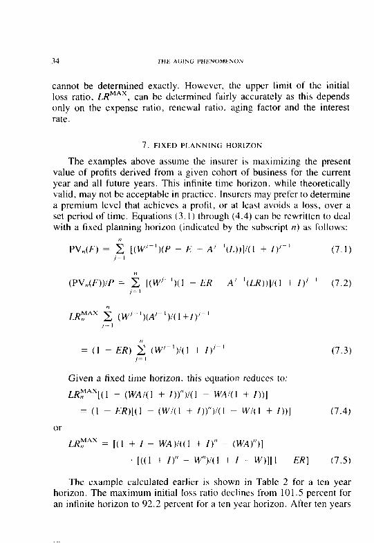
34 THt AGING PHENOMENON
cannot be determined exactly. However, the upper limit of the initial loss ratio, LRMAX, can be determined fairly accurately as this depends only on the expense ratio, renewal ratio, aging factor and the interest rate.
7. FIXED PI.ANNING HORIZON
The examples above assume the insurer is maximizing the present value of profits derived from a given cohort of business for the current year and all future years. This infinite time horizon, while theoretically valid, may not be acceptable in practice. Insurers may prefer to determine a premium level that achieves a profit, or at least avoids a loss, over a set period of time. Equations (3.1) through (4.4) can be rewritten to deal with a fixed planning horizon (indicated by the subscript tz) as follows:
PV,,(F) = i [(W’+)(P - E - A’ ‘(L))]/(I + I)‘-’ (7.1) j-i
(PV,,(F))IP = i [(W’- ‘)(I - ER ~ A’ ‘(LR))]/(l + I)’ ’ (7.2) j- I
LA,, MAX ,gl (W’ +)(A’-‘)/( 1 +f)‘-’
= (1 - ER) i (W’-I)/( 1 + I)‘+ j= I
(7.3)
Given a fixed time horizon, this equation reduces to:
LR,, MAX[(l - (WA/(1 + /))‘I)/(1 - WA/(1 + I))]
= (1 - ER)[( 1 - (W/( 1 + /))‘I)/( 1 - W/( I + f))] (7.4)
or LR;lAX zz [(I + f - WA)/((l + I)” - (WA)“)]
. [(( 1 + f)” - W’Y(l + f - W,][ 1 - RR] (7.5)
The example calculated earlier is shown in Table 2 for a ten year horizon. The maximum initial loss ratio declines from 101 .S percent for an infinite horizon to 92.2 percent for a ten year horizon. After ten years
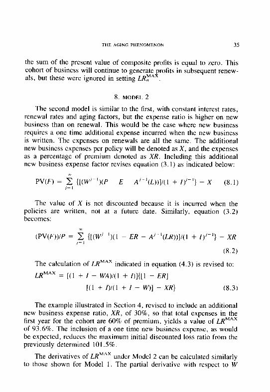
THE AGING PHENOMENON 35
the sum of the present value of composite profits is equal to zero. This cohort of business will continue to generate als, but these were ignored in setting LR?* f
refits in subsequent renew- .
8. MODEL 2
The second model is similar to the first, with constant interest rates, renewal rates and aging factors, but the expense ratio is higher on new business than on renewal. This would be the case where new business requires a one time additional expense incurred when the new business is written. The expenses on renewals are all the same. The additional new business expenses per policy will be denoted as X, and the expenses as a percentage of premium denoted as XR. Including this additional new business expense factor revises equation (3.1) as indicated below:
PV(F) = 5 {[(W’-‘)(P - E - A”-‘(L))]/(l + f)‘-‘} - X 03.1) ,= I
The value of X is not discounted because it is incurred when the policies are written, not at a future date. Similarly, equation (3.2) becomes:
(PV(F))IP = 5 {[(W’+)( 1 - ER - A,‘-‘(LR))]I( 1 + f)j-‘} - XR .,= I
(8.2)
The calculation of LRMAX Indicated in equation (4.3) is revised to:
LR MAX = [( 1 + f - WA)/(l + I)]{[ 1 - ER]
[( 1 + L)/( 1 + f - W)] - XR} (8.3)
The example illustrated in Section 4, revised to include an additional new business expense ratio, XR, of 30%, so that total expenses in the first year for the cohort are 60% of premium, yields a value of LRMAX of 93.6%. The inclusion of a one time new business expense, as would be expected, reduces the maximum initial discounted loss ratio from the previously determined 101.5%.
The derivatives of LRMAX under Model 2 can be calculated similarly to those shown for Model 1. The partial derivative with respect to W
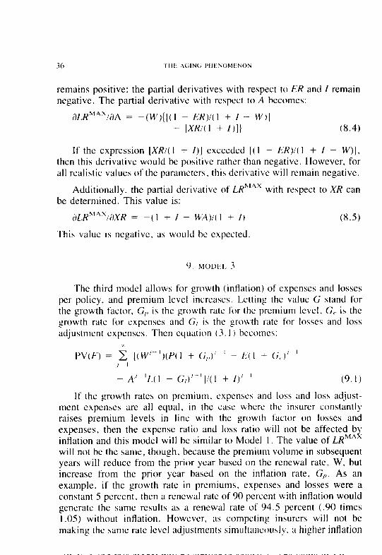
remains positive; the partial derivatives with respect to ER and f remain negative. The partial derivative with respect to A becomes:
dLR n”4Xli)A = -(W){[( 1 ~ ER)/( 1 + f - W,J - [XRI( 1 + f )I} (8.4)
If the expression [XR/( I + f)] exccedcd [( I - ER)/( 1 + f - W)], then this derivative would be positive rather than negative. However, for all realistic values of the parameters. this derivative will remain negative.
Additionally, the partial derivative of LRkiAx with respect to XR can be determined. This value is:
dLR”‘.“‘IdXR = -( 1 + f - WA)/( I + f)
This value is negative, as would be expected.
(8.5)
The third model allows for growth (inflation) of expenses and losses per policy. and premium level increases. Letting the value G stand for the growth factor. G,, is the growth rate for the premium level. G,. is the growth rate for expenses and ~3, is the growth rate for losses and loss adjustment expenses. Then equation (3.1) becorncs:
PV(F) = 2 [(w’-- ’ )(P( I + G,,)’ ’ - E( I -t G,.)’ ’ / ’ - A-’ ‘L( I + G,)’ ‘I/( I + I)’ ’ (9.1)
If the growth rates on premium. expenses and loss and loss adjust- ment expenses are all equal, in the case where the insurer constantly raises premium levels in line with the growth factor on losses and expenses, then the expense ratio and loss ratio will not be affected b 1 inflation and this model will be similar to Model 1. The value of LR”* x
will not be the same, though, because the premium volume in subsequent years will reduce from the prior year based on the renewal rate, W, but increase from the prior year based on the inflation rate, G,,. As an example. if the growth rate in premiums, expenses and losses were a constant 5 percent, then a renewal rate of 90 pcrccnt with inflation would generate the same results as a renewal rate of 94.5 percent (.90 times I .OS) without inflation. However, as competing insurers will not be making the same rate level adjustments simultaneously. a higher inflation
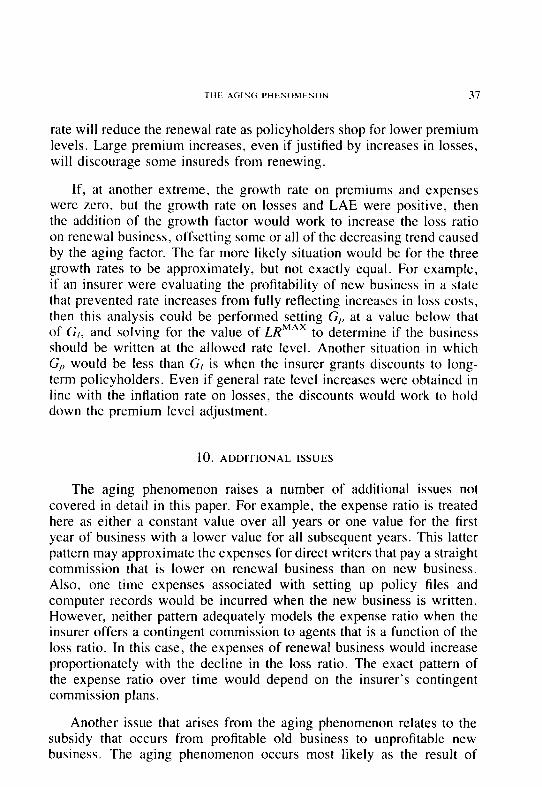
I-HE AGIN<; I’HI,NOMI~,NON 37
rate will reduce the renewal rate as policyholders shop for lower premium levels. Large premium increases, even if justified by increases in losses, will discourage some insureds from renewing.
If, at another extreme, the growth rate on premiums and expenses were zero, but the growth rate on losses and LAE were positive, then the addition of the growth factor would work to increase the loss ratio on renewal business, offsetting some or all of the decreasing trend caused by the aging factor. The far more likely situation would be for the three growth rates to be approximately, but not exactly equal. For example, if an insurer were evaluating the profitability of new business in a state that prevented rate increases from fully reflecting increases in loss costs, then this analysis could be performed setting G,, at a value below that of G,, and solving for the value of LRMAX to determine if the business should be written at the allowed rate level. Another situation in which G,, would be less than G, is when the insurer grants discounts to long- term policyholders. Even if general rate level increases were obtained in line with the inflation rate on losses, the discounts would work to hold down the premium level adjustment.
10. ADDITIONAL ISSUES
The aging phenomenon raises a number of additional issues not covered in detail in this paper. For example, the expense ratio is treated here as either a constant value over all years or one value for the first year of business with a lower value for all subsequent years. This latter pattern may approximate the expenses for direct writers that pay a straight commission that is lower on renewal business than on new business. Also, one time expenses associated with setting up policy files and computer records would be incurred when the new business is written. However, neither pattern adequately models the expense ratio when the insurer offers a contingent commission to agents that is a function of the loss ratio. In this case, the expenses of renewal business would increase proportionately with the decline in the loss ratio. The exact pattern of the expense ratio over time would depend on the insurer’s contingent commission plans.
Another issue that arises from the aging phenomenon relates to the subsidy that occurs from profitable old business to unprofitable new business. The aging phenomenon occurs most likely as the result of
38 THE AGIN<; Plii:NOM~,NON
relevant information that is not known to the insurer when the policy is first written, but develops over the time while the insurer covers the risk. Thus, poor risks are given a rate that is actually too low to reflect their loss likelihood. However, due to the inability to differentiate accurately the level of risk when the new business is written, the insurer incurs a loss. However, this loss is later recouped by overcharging the business that has been with the insurer for a long period. Many insurers offer some form of discount for long-term policyholders, either to all or to those with no claims, in recognition of this improvement in experience. However, the discounts are not as large as the improvement in loss experience would warrant. Thus, long-term policyholders are subsidizing new business. particularly the poor risks that move from insurer to insurer as their true risk exposure is discovered.
The aging phenomenon also affects the behavior of insurers when the regulatory regime in a state begins to refuse adequate rate increases. Typically, insurers put up with this environment for a considerable period of time before withdrawing from the market. This apparent patience in the face of inadequate rates is actually reflective of the profit potential in the existing book of business. If the insurer withdraws from the market, future renewals on the existing book of business, which are likely to be quite profitable, are no longer possible. If the rate levels are not adequate to justify writing new business, they still may be acceptable for renewal business. Thus, typical reactions involve reducing or elimi- nating new business, but continuing to service the existing book of business. Only when the losses on existing business are such that they are unlikely to be offset by future profitability on the book of business does it become economically justifiable to withdraw from the market.
In the models presented in this paper. the renewal rate and the aging factor were assumed to be constant over the life of the cohort. These values likely vary in practice, and this variation can easily be included in the models. The renewal rate is probably lowest on the first few renewals as those insureds least likely to renew, or be renewed, lapse. After a few renewal cycles a constant value, somewhat higher than the early renewal rates, may be achieved. However, for personal lines es- pecially, the renewal rate is likely to decrease substantially after a point as the insured faces mortality risk. In personal lines insurance, the assumption that the insurer can potentially renew policies to infinity is violated.
THE AGING PHENOMENON 39
The constant aging factor used in the current model results in a loss ratio that tends to zero as a book of business ages. Although this con- vergence would require more renewal cycles than actual policies would experience, this situation represents a potential problem with this model. One way around this continual decline in loss ratios is for the aging factor to increase to one after a certain number of renewals. In this case, no further improvement in the loss ratio would be expected. Little is known about the true behavior of the aging factor over time, as insurers justifiably treat this information as confidential. However, five of the eight insurers providing information on aging maintain data in a form that allows an analysis of this factor over a short period of time. For each insurer the loss ratios (in some cases including loss adjustment expenses) were provided for a given period broken down by the age of the book of business. The aging factors were calculated from this infor- mation by dividing the loss ratio for each renewal cycle by the corre- sponding ratio for business one period younger. These values are shown in Table 3. For three of these insurers, Firms A, B and E, the aging factor is lower initially and then increases. One insurer, Firm D, has a fairly constant aging factor. The other insurer, Firm C, has an aging factor that gradually decreases. Thus, no consistent pattern emerges from this limited analysis. Hopefully, future research can address this issue. In the meantime, the models can easily be revised to reflect any pattern of aging factors.
Current insurance accounting conventions ignore the cohort concept of profitability and aggregate all business together. Thus, premiums, expenses and losses and LAE do not reflect the experience of an indi- vidual cohort of business, but the total company operations. If an insurer has written a constant premium volume for as long a period as policies could conceivably renew, then the total profitability would equal the present value of the profitability of any new business written. However, no such ideal insurer exists. For a typical insurer growing in exposure count, the aggregate profitability will be less than the present value of profitability of a cohort approach. The losses experienced on new busi- ness exceed the profitability on renewal business, as the current new business cohort is larger than the previously written cohorts. Future profitability on current policies is not adequately reflected in aggregate profit statements.
Conversely, for an insurer that is reducing exposure counts, either in total or for a particular state, the aggregate method of accounting over-
10 IHt: ,A(iIS(; Pti~,NOMt?NON
states the profitability of an individual cohort. The losses on a smaller volume of new business are overweighted by the profits on long-term business. Thus, an insurer could be misled to write additional new business that would actually be unprotitable in the long run due to the apparent profitability of the total book of business. Accounting for in- dividual cohorts could avoid the distortions generated by aggregate ac- counting.
1 i. SUMMARY
The aging phenomenon represents an additional dimension of the insurance equation that is often overlooked in pricing. Insurers should maintain records by policy cohort in order to determine optimal pricing levels. The use of aggregate statistics can mislead an insurer about the true profitability of a book of business. The effect of higher interest rates on acceptable loss ratios for new business is complex, since a higher rate lowers the discounted loss ratio while reducing the impact of future profitability. However, for short tailed lines, a higher interest rate clearly lowers the acceptable new business loss ratio if aging is considered. This result contrasts with the effect assumed if aging is ignored.
Much additional work remains to be done on aging and many issues must be solved before accurate dctcrminations of acceptable new business loss ratios can be made. The models developed in this paper represent simplifications of the actual aging phenomenon in order to perform initial tests of the effect of aging on insurance pricing. More information must be collected to determine if renewal and aging rates are constant, as assumed in these models, or change over time. Another key issue is the appropriate risk adjusted interest rate, both for the loss payout patterns of each year as well as for future years’ profitability. Accurate statistics on aging must be compiled in order to facilitate more in depth research. Hopefully, this paper will inspire more insurers to collect this information and apply these techniques.
THE AGING PHENOMENON 41
REFERENCES
[ l] J. David Cummins and Scott A. Harrington, Fair Rate of Return in Property-Liability Insurutzce, Kluwer-Nijhoff Publishing, Boston, 1987.
[2] Stephen P. D’Arcy, “Use of the CAPM to Discount Property-Lia- bility Loss Reserves,” Journnl cf Risk and /nsurance, 55, p. 48 I, September, 1988.
(31 Stephen P. D’Arcy and Neil A. Doherty, The Financial Theory of Pricing Property-Liuhilig Insurance Contructs, Richard D. Irwin, Inc., Homewood. IL, 1988.
[4] Stephen P. D’Arcy and Neil A. Doherty, “Adverse Selection, Private Information and Lowballing in Insurance Markets,” Journal qf Busi- ness, 63, p. 145, April, 1990.
[5] Howard Kunreuther and Mark Pauly, “Market Equilibrium with Pri- vate Knowledge: An Insurance Example,” Journal of Public Eco- notnics, 26, p. 269, 1985.
[6j Bernard L. Webb, “Investment income in Insurance Ratemaking,” Journul of Insurance Regul&)n, 1, p. 46, 1982.
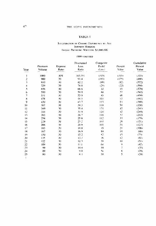
TABLE t
8
9
IO
II
I?
13
I4
IS
16
I7
IX
IY
20
21
22
23
24
25
low
900
XI0
72’)
656
590
531
47x
430
3x7
349
314
2x2
254
229
206
18.5
I67
I SO
I35
I22
IO9
99
89
x0
30%
30
30
30
30
30
30
30
30
30
30
30
30
30
30
30
30
30
30
30
30
30
30
30
30
IO1 .S%
YI.4
82.2
74.0
66.6
5Y.Y
53 Y
4x 5
43 7
3Y 3
35.4
71 Y
2x 7
25.8
23 2
20.9
IX x
16.‘)
IS.?
13.7
12.3
II I
IO 0
Y.0
x I
(3151
(193)
(9’11
(2Yl
22
60
x5
10.3
II3
II’)
121
I20
I I6
I I?
I07
IO1
YS
KY
x2
76
71)
64
59
SJ
SO
(319)
(175)
IX?)
1221
IS
37
4X
53
53
50
47
42
37
33
2X
24
71
IX
IS
I2
III
Cumulative
Present
VdltK
(315)
(490) C.572)
(SY4)
(S7Y)
(542)
(494)
I‘MI) (388)
(3381
(2911 (2491
(212)
1179) 1151)
1127)
(106)
(XX)
(73)
(61)
(51)
(42) (35)
(29)
(24)
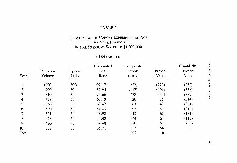
TABLE 2
Year Premium Expense Volume Ratio
1 2 3 4 5 6 7 8 9
10 Total
1000 30% 92.17% 900 30 82.95 810 30 74.66 729 30 67.19 656 30 60.47 590 30 54.43 531 30 48.98 478 30 44.08 430 30 39.68 387 30 35.71
ILLUSTRATION OF COHORT EXPERIENCE BY AGE TEN YEARHORIZON
INITIAL PREMIUMS WRITTEN: $1,000,000
(000) OMITTED
Discounted Loss Ratio
Composite Profit/ (Loss)
(222) (222) (117) (106)
(38) (31) 20 15 63 43 92 57
112 63 124 64 130 61 133 56 297 0
Present Value
2 Cumulative m
Present $ Value z
I (222) Fs (328) : (359) (344)
P
(301) (244) (181) (117) (56)
0
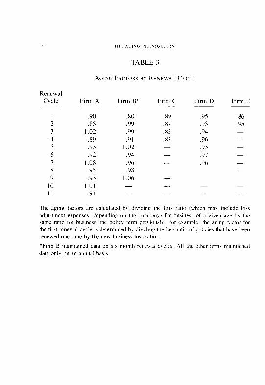
IHk A(;INCi PHFNOLlk,NON
TABLE 3
AGING FACTORS BY RENEWAL Cvcr.t:
Renewal Cycle Firm A Firm B* Firm C Firm D Firm E
1 .90 2 .x5 3 1.02 4 .XY 5 .Y3 6 .92 7 I .0x x .Y5 9 .93
10 1.01 11 .94
.XY .YS .86
.x7 .YS .95
.x5 .94
.x3 .96 - .95 .Y7 .96 -
The aging kturs ;IK calculated by dividin g the loss ratio (which may include loss adjustment expenses. depending on the company) for business of ;I given age by the same ratio for business one policy term previously. For example. the aging factor for the first renewal cycle is determined by dividin g the loss ratio of policies that have been renewed one time by the new business loss ratio.
*Firm B maintained data on six month rencual cycle\. All the other firms maintained data only on an annual basis.
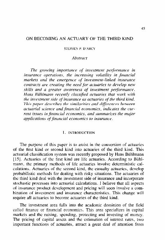
45
ON BECOMING AN ACTUARY OF THE THIRD KIND
STEPHEN P. D'ARCY
Abstract
The growing importance of investment performance in insurance operutions, the increusing volutility in finnnciul markets und the emergence of investment-linked insurance contructs are creating the need for actuaries to develop new skills and a greater awareness of investment performance. Huns Biihlmann recently classified actuaries that work with the investment side of insurunce as actuaries of the third kind. This paper describes the similarities and differences between actuarial science and financial economics, indicates the cur- rent issues in financial economics, and summarizes the mujor applications of fmuncial economics to insurance.
1. INTRODUCTION
The purpose of this paper is to assist in the conversion of actuaries of the first kind or second kind into actuaries of the third kind. This actuarial classification system was recently proposed by Hans Biihlmann [ 151. Actuaries of the first kind are life actuaries. According to Btihl- mann, the primary methods of life actuaries involve deterministic cal- culations. Actuaries of the second kind, the casualty actuaries, develop probabilistic methods for dealing with risky situations. The actuaries of the third kind deal with the investment side of insurance and incorporate stochastic processes into actuarial calculations. I believe that all aspects of insurance product development and pricing will soon involve a com- bination of investment and insurance characteristics. This change will require all actuaries to become actuaries of the third kind.
The investment area falls into the academic dominion of the field called finance or financial economics. This area specializes in capital markets and the raising, spending, protecting and investing of money. The pricing of capital assets and the estimation of interest rates, two important functions of actuaries, attract a great deal of attention from
46 ACTUARY 01: .rtit IHIRII KINI)
financial economists. However, the basic concepts and perspectives of financial economists are, in some regards, alien to actuaries. Thus, the second section of this paper discusses how actuaries and financial econ- omists each view some very basic common issues. The third section provides a synopsis of the leading issues in financial economics. The fourth section describes applications of financial economics to insurance. The final section draws some conclusions concerning the converging paths of actuarial science and financial economics and discusses likely future developments.
2. FINANCIAL ECONOMICS AND [‘HI: ACTUARY
Development
Actuaries and financial economists could be compared to distant cousins that would be surprised at discovering their degree of consan- guinity. Both are mathematically inclined, address monetary issues and incorporate risk into their calculations. Both insurance and finance have ancient roots, and both have undergone dramatic transformations several times. The most notable transformations relevant for life actuarial science were the development of mortality tables, institution of nonforfeiture provisions and the recent connection of benefit levels to investment performance. For property-liability insurance the significant develop- ments include the entrenchment of regulatory power. the elimination of traditional distinctions, initially leading to multiple line policies and eventually to full financial service firms, and the expansion of legal liability. Similar epochal developments for finance would be the devel- opment of central banks, organized stock exchanges. security regulation, modern portfolio theory and the development of markets for derivative securities such as options and futures.
Actuarial science and financial economics have developed tools to address the relevant issues for their disciplines independently. As in any profession, each has developed a specialized language to describe terms and techniques in the field. This specialized language, in some aspects similar to a secret code, serves as much to exclude outsiders as to facilitate communication within the field. However, now that insurance is moving into the investment domain, both in offering products tied to investment performance and in developing corporate investment strate-
ACTUARY OF THE THIRD KIND 47
gies, the specialized languages are becoming a handicap, especially where similar terms have different meanings in the different disciplines. Financial economists are hindered in their analysis of insurance problems by the difficulty in understanding insurance terminology and practices. Actuaries are at a similar disadvantage in addressing issues in finance. This introduction will serve as a bridge between the areas of actuarial science and financial economics by discussing some very basic issues in these fields and illustrating the different approaches taken by the two specialties.
Risk
Risk is a central, if not the central, element in both insurance and finance. Individuals are assumed to be risk averse and thus would be willing to pay a premium over expected losses to reduce risk; initially, a similar assumption was often made about corporations, but more recent work has treated corporations as a web of contractual relationships (em- ployer-employee, stockholder-bondholder-manager, supplier-consumer) that is itself risk neutral. Individuals purchase insurance because risk exists and they seek to minimize or avoid the financial consequences inherent in risk. In the area of finance, risk is involved in explaining the price level and required rate of return on different investments as well as the optimal investment strategies. However, how risk is considered in the two areas differs significantly.
In insurance, risk is generally defined as uncertainty concerning loss. A measure of risk is the expected deviation between actual and expected losses, generally scaled to the expected loss value. For an individual insured, the expected losses would commonly be a small value, repre- senting the product of the loss frequency and the loss severity. Actual losses will generally be zero, but the possibility of a large value, rep- resenting some point on the loss distribution, must also be considered. For most lines of business, individual risks are assumed to be indepen- dent, so for an insurer the risk of a collection of policies will be less than the sum of the risk of the policies, or even the average risk level on the policies. Notable exceptions include financial guarantee, flood and earthquake coverages. In actuarial science, the law of large numbers dictates that the riskiness of a portfolio of independent risks will reduce as the size of the portfolio increases. In general, actuaries assume that the risk is eliminated from the point of view of the insurer as a result of
48 AC‘IUARS 01, [III: TIIIRII KINI)
writing a large number of policies. Thus. the riskiness of an individual insured is not relevant to the price of the policy. In most cases, only the expected value of the loss is used to establish the price level for an insured.
In investments, the potential wealth changes are not restricted to be zero or negative, as is the case for insurance policies, but can also be positive. Thus, the definition of risk is expanded to be the uncertainty concerning outcome. In general, the standard deviation of the return distribution is used as the measure of risk. although higher moments have also been used.
The key difference between actuarial scicncc and finance in regard to risk is the effect of combining separate risks into a portfolio. The standard deviation is commonly used as a measure of risk. If R,, is used to denote the return on a portfolio in which the variance of each of II elements in the portfolio is denoted by CT’ and the covariance between any two elements within the portfolio is yo’, then the risk of a portfolio can be calcualted as follows:
Var(R,,) = (o’in)[l + ()?P l)ql, (2.1)
where R,, = expected outcome (expected loss for an insurance policy or expected return for an asset) for the portfolio of elements;
u = standard deviation of outcomes for the individual ele- ments;
II = number of individual clcments combined in the portfo- lio;
q = correlation coefticicnt between any two elements.
If the elements are not correlated (y = 01, then the portfolio risk converges to zero as II approaches infinity. This is, for insurers, the law of large numbers. However, if the elements are correlated, then the portfolio risk does not converge to zero, but to some value dependent on the degree of correlation. This relationship is the key aspect of portfolio theory in investment analysis. Individual investments are not independent of each other. Thus, the risk of a portfolio will not reduce to zero by combining a large number of different investments. This residual risk is a central concern to financial economists. Financial econ- omists classify investment risk on an individual security into two com-
A(“I’UARY OF THt ‘I HIRD KIND 49
ponents, diversihable and systematic risk. Diversifiable risk is the degree of fluctuation that is uncorrelated with other securities. This risk does cancel out in a portfolio, similar to the effect of the law of large numbers on insurance policies. Also similar to insurance, this form of risk is ignored in most asset pricing models. As an investor can eliminate this type of risk from his or her portfolio by diversifying, diversifiable risk is assumed to be irrelevant in pricing capital assets.
The remaining risk inherent in individual investments is termed sys- tematic risk. This risk does not cancel out in a portfolio, because it is common to all risky investments. As the investor cannot eliminate this form of risk, it becomes important in pricing the capital asset. A high level of systematic risk requires a greater rate of return.
Thus, an actuary views risk as a component of an individual insured that cancels out at the level of the insurer due to the law of large numbers. The financial economist views risk as a combination of two factors, diversifiable risk that is irrelevant for pricing assets and systematic risk that enters into the asset pricing determination.
interest Rutes
Although casualty actuaries have ignored interest rates in pricing insurance until recently, life actuaries have traditionally included an interest rate factor in the determination of rates. The interest rate used to price policies has generally been a conservative level that the actuary feels certain can be achieved by the company under almost any economic conditions. Through the early 1970s in the United States, rates of three or four percent were used in setting rate levels. The interest rate levels chosen to price guaranteed rate life insurance policies were not current market rates and were not historic levels earned by the insurer, but instead, worst case scenario types of values. Actuaries tended to view interest rates as a one dimensional value and inherently assumed that they would be constant over the policy period. This attitude is changing only gradually.
For financial economists, interest rates have multiple dimensions. Initially, all rates of return, including interest rates, are classified as ex ante, those expected to occur in a future period, or ex post, actual realized returns. Ex post results can be viewed as a sample drawn from the ex ante distribution and, thus, provide only limited information about
the true return distribution. Interest rates are then categorized as “real” or “nominal.” Nominal interest rates are the full rates earned on invest- ments. These rates vary over time and have been extremely volatile in recent years. Real interest rates have inflation (or inflationary expecta- tions) factored out so that they represent the purchasing power effect of interest. This relationship between interest rates and inflation is known as the Fisher Effect based on work by Irving Fisher [35]. As interest rates tend to move in line with inflation, the real interest rate is much less volatile than nominal interest rates (Ibbotson and Sinquefeld [40]). If a life insurance policy were providing a benetit that were indexed to inflation, then the real interest rate would be relevant for pricing the policy. For traditional fixed benefit policies, the nominal interest rate is the proper one to use. Similarly, if loss reserves are to be discounted, the real interest rate should be used if unpaid losses will be affected by future inflation. If the values are unaffected by inflation, then the nominal interest rate is appropriate.
Another dimension to interest rates recognized by financial econo- mists is termed the yield curve and represents the different interest rates available on similar bonds of different maturities. Often short term bonds have the lowest interest rate, with the interest rate increasing as the time to maturity increases. This occurs because the prices of longer term bonds are more volatile, creating greater risk for the long term bond holder. An alternative explanation for the normal slope of the yield curve is termed a liquidity premium, as money is tied up longer in long term bonds. For whatever reason, the normal yield curve is continually upward sloping. Occasionally an inverted yield curve occurs in which short term interest rates are higher than longer term rates. This tends to occur when inflation increases, but the general expectation is that it will reduce in the future. Other expectations about future economic conditions can lead to mountain shaped yield curves or even flat yield curves.
A third dimension of interest rates reflects differences between similar maturity bonds that are issued by different guarantors. This difference, termed a risk premium, reflects the different levels of risk inherent in different debtors. Frequently bonds issued by major industrial nations are considered risk free in their own currency, although this is an overly optimistic view under any long term historical perspective. Bonds issued by corporations would pay an interest rate that exceeds the national debt rate by varying amounts depending on the perceived riskiness of the issuer.
ACTUARY OF THE THIRD KIND 51
Another interest rate distinction considered important by financial economists is whether the interest rate is a market rate or a historical rate. Market rates are those interest rates available in the financial markets when the analysis is being performed, basically the current interest rates. Historical rates can be mean values for interest rates of a given risk classification and maturity over a known period of time, or achieved interest rates on a portfolio over a recent time period. Any measure of past performance, though, is a historical rate that does not necessarily reflect current market conditions. A standard consideration in applica- tions of financial economics to pricing is that the market rate be used rather than historical rates. The current market conditions, not prior, perhaps unavailable rates, influence prices of financial instruments.
Related to the distinction between market and historical interest rates is another major difference between how actuaries and financial econo- mists view interest rates. Most actuaries consider interest rates to be deterministic, or unchanging. An interest rate used as an actuarial as- sumption is considered to be at that level over the duration of the contract. Financial economists now are tending to view interest rates as stochastic, or essentially a random variable. Interest rates are expected to fluctuate over any future period. A number of different models have been devel- oped to forecast interest rate movements, with differing degrees of suc- cess. No universally accepted stochastic interest rate model has yet been developed. However, these models tend to explain actual interest rate levels much more effectively than the deterministic models.
Actuaries, especially casualty actuaries, tend to use a profit margin as the measure of profitability. The difference between premiums (plus investment income in some cases) and losses plus expenses is divided by the premiums to determine the profit as a percent of premium income. Target profit margins are established and actual performance is compared with these goals.
Financial economists tend to ignore profit margins, on the assumption that excess profits would be competed away, and concentrate on rates of return and, where appropriate, risk adjustments. The rate of return is determined by dividing the profit achieved by the investment made in order to earn the profit. For insurance the profit remaining after deducting losses and expenses from premiums and investment income is calculated,
52 AC’fL’AK\ Of. 1111 IfIfHI) KINI)
but this profit is divided by the investment necessary to initiate the insurance contract. generally the surplus of the insurer, rather than the premium income. Rates of return can be calculated for an insurance firm in aggregate, but adjustments must be made to statutory values in order to get a reasonable estimate of the true economic value of the initial investment. Allocating the investment amount, as well as many of the expense components, on a more specific level is increasingly difficult. Thus, at the current time, rates of return for insurance are generally determined only for the insurer in aggregate. and not by line or policy type.
When providing a valuation of the assets and liabilities of an insurer, actuaries need to be aware that adjustments to the statutory (also known as “book”) values are necessary. Statutory values are the ones recognized by insurance regulatory authorities and are considered to be conservative values. These values do not represent the market value of various assets or liabilities. For example. bond investments are valued at the amortized value, which is determined by gradually adjusting any difference between the purchase price and the maturity value of a bond over the remaining life of the bond. As the market value of a bond fluctuates inversely with interest rate changes, the amortized value of a bond can deviate signifi- cantly from the market value. In times of rising interest rates, amortized values of bonds exceed market values, which is not a conservative valuation. In times of falling interest rates. the market values exceed amortized values, which would impart a degree of conservatism depend- ing on the speed and amount of the interest rate reduction.
Statutory values for liabilities arc also generally set at conservative values, although the degree of conservatism is not constant. For casualty insurance the largest liability i\ the loss reserve. In the United States the loss reserves are not discounted to reflect the time value of money, except for fixed periodic payments or specific regulatory exceptions. For life insurance the statutory value of rcservcs for future benefit payments are established based on conservative mortality and interest rate values. However, some future liabilities are not recognized. For example, in the United States no reserve for future taxes on unrealized capital gains is established, despite the inclusion of equity investments at their market value which could exceed the purchase price.
A(‘1 UARY OF THf: THIRD KIND 53
Financial economists place great faith in the ability of competitive markets to price assets accurately. Therefore, the market value of specific assets and liabilities would be used in any valuation determination. For insurer assets this would be relatively easy, as most assets are in types of investments for which market prices could be readily determined. Real estate investments could present one problem in determining market value, but appraisals of the property value could provide usable values. Similar problems exist in evaluating private placement bonds and mort- gages. In general, though, the liabilities of insurers are more difficult to calculate a market value for, as these liabilities are rarely traded, and when they are, through a reinsurance contract, the price is not publicly available.
Empirical studies of the insurance industry performed by financial economists are generally restricted to the few pure insurers, not part of a conglomerate, for which equity is publicly traded. As these studies are forced to exclude mutual insurers, a major force in both life and property- liability insurance markets, as well as financial service firms that own insurance companies, the conclusions from such data are limited. Finan- cial economists are hampered in attempting to estimate market values of assets and liabilities not publicly traded by a lack of understanding of the composition of these components. Actuaries, who understand what the figures consist of, are also hampered in this regard, but for actuaries the handicap is derived from a professional tendency towards conserva- tism and statutory valuation. Hopefully, the third kind of actuary will be able to overcome such prejudices and arrive at a more market-oriented valuation of assets and liabilities.
Surnmcq
Actuaries and financial economists are kindred spirits with a wide divergence in terminology and techniques separating their respective specialties. Volatile financial markets, higher nominal interest rates and the connection of benefit levels with investment performance will require a closer working relationship between the two groups. Such basic con- cepts as risk, interest rates, profitability and valuation are viewed diffcr- ently by the two areas. Actuaries must recognize the viewpoint of finan- cial economists in order to cope with the expanding actuarial horizons.
54 ACTUARY 01; I’H[: ‘THIRD KIND
3. CURRENT STATE OF FINANCIAL ECONOMICS
Valuution
Before beginning to present what tinancial economists do know, or at least claim to know, about tinancial markets, a brief discussion of what is not known is in order. Financial economists do not know what the price of a stock will be at any future date. In the early years of this specialty, much attention was given to determining the value of an individual stock (Reilly [58]). Valuation models were developed that purported to indicate the intrinsic value of a stock. Investments made in stocks that were underpriced were expected to yield abnormally high profits. Numerous valuation models have been proposed and some claim to have worked over numerous investment cycles. Unfortunately, val- uation models do not explain why prices diverge from the intrinsic value, thus producing opportunities for excessive profits, or how long it will take for prices to return to this benchmark level. More recently, most research in finance has adopted the efficient market hypothesis that states that the current price of a stock accurately reflects all publicly available information. Based on this hypothesis, the market price cannot diverge from the intrinsic value, negating much of the valuation theory research. It should be easy to understand that, when frustrated by not being able to explain what a stock price should be, claiming that whatever price exists is, by definition, the proper price, is an understandable approach.
Asset Pricing Models
After shifting away from attempting to explain price levels for stocks, attention moved to explaining the rate of return on different investments. The Capital Asset Pricing Model (CAPM) was developed to explain the rate of return on specific investments (Lintner [45], Mossin [51] and Sharpe [63]). The CAPM is explained and analyzed in such texts as Brealey and Myers [8], Ross and Westerfield 1611 and Haugen [38]. The formulation of the CAPM is:
E(R) = Rf + fME&) - Rv), (3.1)
where Ri = return on a specific security; Rf = risk free rate of return;
ACTUARY OF THE THIRD KIND 55
R,,, = return on the market portfolio; E = expected value operator; p, = Cov(R;, R,,,)la~ = systematic risk.
The term systematic risk, the p in equation (3. l), was introduced to describe the covariability of a specific investment’s return with the market return. This single relationship replaced all the covariances between individual securities in the portfolio and greatly simplified the determi- nation of portfolio risk. Unsystematic risk, the variation of returns on an investment that is independent of the market fluctuations, was assumed to cancel out in a diversified portfolio and therefore was considered irrelevant in pricing a given investment. The systematic risk level of an investment indicated the required rate of return on an investment and therefore determined the current price. The expected return on any in- dividual asset was determined by multiplying the p times a value rep- resenting the market return in excess of the risk free rate and adding the product to the risk free rate. The value for the excess market return is generally assumed to be a constant and has been estimated in the range of 7 to 8.5 percent. If the (nominal) risk free rate were 6 percent and the excess market return were 8 percent, then a security with a p of 1.5 would have an expected return of 18 percent (6 + 1.5(8)).
Thus, based on the CAPM, the total variability of a stock price was not important for determining the rate of return on an investment. Only the systematic risk was important in determining the expected rate of return for an individual security.
Empirical tests of the CAPM tended to support the theory, but notable exceptions surfaced. Seasonal factors, size factors and some economic factors appeared to influence the achieved rates of return in addition to the systematic risk level. Additionally, the systematic risk factors were found to vary over time, in many cases tending to revert to the mean value, or one. Eventually, researchers recognized that tests of the CAPM were essentially joint tests of the CAPM and the proxy used for the market (Roll [59]). A more general asset pricing model, termed the Arbitrage Pricing Model (APM), of which the CAPM is simply a spe- cialized application, has been introduced and is being widely tested (Ross [60]). The APM is explained and evaluated in such texts as Ross and Westerfield [61] and Haugen [38]. The formulation of the APM is:
E(R,) = R,’ + i h,,h,, (3.2) j=/
where R; = expected return on the zero systematic risk portfolio: ho = sensitivity of asset’s return to a specific index; A, = excess return in a portfolio with only one unit of systematic
risk of that factor and no other systematic risk.
One major limitation of the APM is its failure to specify the number of factors that are expected to impact on security prices or what those factors should be. The CAPM is a special case of the APM under which one factor. the market performance in excess of the risk free rate. is assumed to be the only relevant factor. In this case. R,’ would bc equal to R,, h would equal p, and h would be the excess market return.
The reliance of APM tests on the data used for the test, and the constantly changing investment environment, make tests of this model difficult to judge. In general, financial economists cannot say what the price of a stock should be, or exactly what rate of return should be expected on an investment. However, another. possibly more fruitful, area of pricing has developed.
Optim Pricillg Models
Although failing. to date, to explain security prices or rates of return, financial theory has moved in the direction of trying to explain the prices of derivative securities, those dependent on the price of another security. Many types of options, where an option is defined as a security that derives its value based on an underlying stock’s price, are now traded on different exchanges. Perhaps coincidentally, the Option Pricing Model was developed only slightly prior to the explosive growth of the options market. An option gives the owner the right, but not the obligation, to trade a given security at a predetermined price either at a specitic future date (European options) or any time up to a specific date (American options). A call option confers the right to buy a security, and a put option gives the owner the right to sell a security. The purchaser of the option has control over whether or not the future transaction is under- taken. The seller of the option commits to enter into the future transaction at the choice of the purchaser.
Options on major common stocks and stock indices are now widely traded. An option is described by its striking. or exercise, price, which
ACTUARY OF THF. THIRD KIND 57
is the price per share of stock at which the potential future transaction will be made, and the expiration date, which is the date at which, or by which, the transaction must be effected. The price of the option (which is often termed the premium) is the cost of buying the option, which does not include the price of the underlying security on which the option is written. Options and option pricing models are presented in detail in such books as Cox and Rubinstein [ 181, Jarrow and Rudd [42], Haugen [38], Brealey and Myers [8] and Ross and Westerfield [6 I], and in a paper by Wilkie [74].
The Black&holes [7] Option Pricing Model determines a value for the option based on the total variability, not just the systematic risk, of the underlying asset. This model takes the form:
PC. = P., N(d,) - XC” N(d& (3.3)
where P,. = price of a call option of the European type when no dividend
is paid; P, = current asset price; X = exercise price; d, = (ln(P.,/X) + (r+o”/2)t)/at”‘; dz = d, - UP; r = continuously compounded risk-free interest rate; t = time to expiration of the option; u = annualized standard deviation of the returns of the underlying
asset; N = normal distribution function.
For example, the value of a one year call option with an exercise price of $100 for a stock with a current price is $90 and a standard deviation of 30 percent per year if the risk free interest rate is IO percent is:
dl = (ln(901100) + .l + .3’/2)/.3 = ,132; d? = .132 - .3 = -.l68; N(.132) = .5525; N(-.168) = .4333; P,. = 90(.5525) - 90.48(.4333) = 10.52.
58 ACI UARY OF IHE I’HIRD KIND
The assumption that security returns are lognormally distributed is essential to this model. As option markets developed, historical returns on the options themselves were not available to help participants establish price levels. The Black-Scholes model, despite its initial apparent com- plexity, was actually quite easy to use once the practitioner became familiar with it. The required inputs for the model were readily available, except for the measure of the underlying security’s variability. This value could be estimated from historical data or backed out of the market price for other derivative securities. The popularity of the Black-Scholes model was such that some dealers circulated the price level determined by the model to traders as a recommended value for an option. Thus, the model was being used to influence price levels almost from the start of stock option trading.
Despite the bias introduced by the model’s being used to set prices of options, subsequent empirical tests of the Black-Scholes OPM found that it worked only fairly well. The model tended not to explain the prices of options that had striking prices far from the current market price of the underlying security, that were on securities with volatility measures that were considerably above or below standard volatility mea- sures, or that had a very long time to expiration (Black and Scholes [6], Chiras and Manaster [ 161, Galai 1361, Rubinstein [62] and Whaley [70]). Despite these limitations, the option pricing approach became very pop- ular for addressing other issues in finance, including capital structure, valuation, capital budgeting and insurance pricing (Firth and Keane [34], Smith [67] and Smith 1651).
Diffusion processes are the more general type of models from which option pricing models are derived. Diffusion processes are stochastic processes with continuous paths. The first noted application of a diffusion process was documented by Robert Brown in 1827 in describing the path of minute particles suspended in liquid, and the term Brownian motion recognizes his contribution to this area. The mathematics of Brownian motion were presented by Albert Einstein 13 I ] and enhanced by Norbert Wiener (1923). The term Wiener process is often used to mean diffusion models, but technically this term is restricted to a specific diffusion model with an initial value of zero. a mean of zero and a variance of 1.
The attraction of Brownian motion for mathematicians is that the probability distribution for the path of particles after a period of time is
ACTUARY OF THE THIRD KIND 59
normally distributed, or, if the particles are subject to an absorbing barrier that affects the amount of movement as the particle approaches the barrier, then lognormally distributed. The models can be extended by including a drift factor, allowing the variance to change over time and even including a jump factor, usually a Poisson process, that introduces a discontinuity in the process. Financial economics focused on these processes for describing security prices (Ingersoll [4l] and Malliaris and Brock [47]). Individual security prices were assumed to be subject to random movements over time, generally with an upward drift. The attraction of a lognormal distribution was the fact that a security cannot have a negative price and, once attaining a level of zero, cannot be allowed to have a positive price in any future period or else an individual could buy a security for nothing and have the possibility of a positive price at some future time, violating the no arbitrage condition required for efficient prices. The jump processes accounted for exogenous changes in the market.
Diffusion models have been widely, and very successfully, applied in such divergent fields as physics, biology, engineering and risk theory in insurance. An early application of diffusion processes to investments was presented by Bachelier [l] which attempted to explain movements in the French stock market by use of a Markov process. In the insurance area, Lundberg [46] applied a diffusion model in developing collective risk theory. Both of these researchers were working independently of Einstein but arrived at very similar conclusions.
A Markov process is defined as a stochastic process in which only the current value of the random variable is relevant in forecasting future values. Past values, other than the latest one, do not affect future values. The Black-Scholes Option Pricing Model and all other option pricing models are also based on the assumption that security prices follow Markov processes.
The assumption that a random variable has no “memory” of prior values seems a reasonable one when describing particle movements, transmission of genetic characteristics, production line defects and in- surance claim activity. However, when this lack of memory is applied to prices of financial assets, which are set by individuals who do have a memory of past prices, this assumption may introduce an unacceptable amount of error. Individuals do relate current price levels to past levels, base decisions on whether a stock price is increasing or decreasing, and on how rapidly a price is changing. Assuming that these individual
tendencies cancel out in aggregate may be inaccurate. Empirical studies indicate that over short trading periods, stock prices do approximate diffusion processes. However, over longer periods (for example, several years or longer), autoregressive tendencies become apparent. An exten- sive study of the characteristics of investment performance is included in Wilkie ([7 I], [72], [73]). The issue of whether the diffusion models can be used to explain security returns is not yet settled.
Hedging
Arranging one’s financial affairs such that one cannot suffer adverse consequences from future developments is termed hedging. In many regards hedging in finance is similar to hedging bets by taking offsetting positions so, regardless of the outcome of the contingent event, the economic effect is assured. Insureds typically hedge when they purchase insurance, thus offsetting the financial risk of loss. Financial institutions can also hedge by allocating their assets in such a way that any event affecting their liabilities has a similar but offsetting effect on their assets. Numerous hedging strategies for lirms have been developed, varying in degrees of complexity, practicality and expense. A recent hedging strat- egy involving a combination of equity investments and derivative secu- rities, termed portfolio insurance, has been proposed that adjusts the distribution of investments depending on equity price movements (Leland [44]). This strategy has received extensive publicity, mostly unfavorable, as a consequence of the October, 1987 market decline (Sloan and Stem 1@1).
The simplest way, in principle, for a hnancial institution to hedge its known future obligations perfectly is to invest in instruments that pay off exactly when the obligation matures. For banks that typically offer certificates of deposit (CD) for periods of no more than ten years, this strategy is at least possible. To match a CD maturing in seven years, a zero coupon bond with the same maturity can be purchased. The insti- tution has assured itself, subject only to risk of default, that the funds needed to satisfy the liability will be available. Interim interest rate fluctuations will not affect the availability of funds to discharge the liability. However, for life insurers that accept obligations to make pay- ments as far as a lifetime in advance, or even longer for annuitized benefits, the financial instruments that could match these payout patterns exactly simply do not exist. Alternative approaches to hedge a set of
ACTUARY OF THE .fHIRD KIND 61
liabilities without exact asset-liability matching are based on a concept known as duration.
The concept of duration was developed by Macaulay [48], and more recently discussed by Ferguson [33] and Tilley [69], to combine the size and timing of coupon payments with the time to maturity. Duration is the weighted average length of time prior to full recovery of principal and periodic payments. Each payment is weighted by its present value. Equivalently, the duration is the negative of the derivative of the present value of a stream of cash flows with respect to the interest rate divided by the present value of the stream of cash flows. The formulae for calculating duration are:
D = z= I C,(tM 1 + r,)’ x:’ , C,/( 1 +r,y ’
where D = duration C, = interest or principal payment at time f; (r) = length of time to payment; I1 = length of time to maturity; rr = yield per period for an asset maturing at time t;
or
D = -(dpV(C)/dr)/PV(C),
(3.4)
(3.5)
where d = partial derivative operator; PV(C) = present value of a stream of cash flows; r = current interest rate.
The denominator of equation (3.4) is the present value of the fixed income investment. The numerator is the present value of the payments weighted by the length of time until they are received. The higher the duration, the longer into the future the payments will, on average, be received. In many cases, the r,‘s are assumed to be equal, implying a flat yield curve. As this is rarely the case in practice, equation (3.4) allows for interest rates to vary by the length of time to maturity. In equation (3.5) the duration is shown to be the negative of the effect of
62 ACTUARY OF 1'Hk IHIKI) KIN,)
change in interest rates on the present value of the cash flows in relation to the present value of the cash flows. This equation will hold for any shape yield curve.
The effect of interest rate changes on bond prices is proportional to the duration of the bond. This suggests a strategy of hedging, or im- munizing, a portfolio by matching the duration of the assets and liabil- ities, without the necessity of exactly matching the terms of each. Thus, by applying the concept of duration, an alternative hedging strategy can be developed.
A complication that arises in measuring the duration of a bond is that the duration value depends on the structure of interest rates. Under deterministic interest rates, which are assumed not to change over the life of the bond, one measure of duration is determined. If interest rates are allowed to be stochastic, or random variables, then different duration values result. Several researchers have compared the duration measures based on different interest rate structures (Bierwag ([5] and [4]) and Boyle ([ 121 and [ 131)). In general, the duration measure is lower under stochastic interest rates than under deterministic interest rates. Thus, to immunize a given set of liabilities a financial institution would have to invest in more long term bonds under fluctuating interest rates.
4. APPLICATIONS OF FINANCIAL ECONOMICS TO INSURANCE
Introduction
The increasing interrelationship between insurance and financial eco- nomics has been recognized by both financial economists and insurance specialists. Smith [66] analyzes the convergence of the fields of insurance and finance, but indicates that few researchers combine an understanding of the mechanics of insurance with a knowledge of the analytical tools of finance. Thus, sophisticated financial research tends to apply insurance inappropriately whereas more accurate models of the insurance industry tend to lack the rigorous technical approach. Garven [37] also describes applications of finance to insurance issues. Borch (1 l] explains the reluctance of actuaries to adopt financial models and proposes a solution to some of the drawbacks of financial models.
Initial applications of financial economics to insurance issues covered pensions and life insurance. More recently, extensive applications of
ACTUARY OF THE THIRD KIND 63
financial economics to property-liability issues have been developed. While this paper will concentrate on property-liability applications, a review of the major directions of research in the other insurance areas will serve as an introduction.
Pensions
As a result of the Employee Retirement Income Security Act of 1974 (ERISA), pension plan assets became a major aspect of corporate finance. Finance academics began to look into how pension fund management affected firm value. Such issues were addressed as whether firm value is affected by the pension plan investment strategy, how pension assets should be invested optimally, and whether under or over funding of pension plans is reflected in the market value of the firm. Actuarial science and financial economics converged on the valuation issue, as financial economists examined the effect of funding on firm value but relied on actuarial science to produce estimates of future liabilities. In many cases, the dichotomy described by Smith [66] led to inaccurate assumptions by financial economists. The results of these efforts are described by D’Arcy and Chen [22]. In general, the findings support the effectiveness of the market to evaluate liabilities correctly.
Life Insurunce
New forms of life insurance policies, introduced in the last decade under the names of maturity guarantee contracts or variable life or universal life, provide a benefit level that fluctuates with the performance of some investment index. Additionally, many of these policies include guarantees that assure the policyholder of some minimum benefit level. Thus, the benefit provided under those contracts with a guarantee is equal to:
B = Max[M, S(r,Jl, (4.1)
where B = benefit level; M = guaranteed minimum amount; s(t) = investment index value at time t; t m = time of maturity of the contract.
The similarity of the payment formulation of this policy and that of an option was quickly noted and addressed. Various models were de- veloped to determine the optimal investment strategy for the insurer offering this type of contract. The conventional strategy expounded by Benjamin [3] suggested investing an amount sufficient to provide the variable investment in the variable asset, with any residual assets invested in fixed interest investments. With this strategy the insurer is at risk in case the terminal value of the variable investment is less than the guar- antee by more than the terminal value of the fixed interest investment.
An alternative approach to investing assets for a maturity guarantee contract, developed by Brennan and Schwartz (191. [ lo]), is to vary the allocation of the investment portfolio between the variable assets under- lying the guarantee and cash depending on the likelihood of the final value of the variable investment being less than or greater than the guarantee. The likelihood of the variable investment exceeding the guar- antee is determined based on the Black-Scholes OPM, with the current value of the variable asset, the guarantee. the time to expiration and the volatility all affecting this likelihood. Collins [ 171 tested the two strate- gies on the period 1930 through 1978 and found that the conventional strategy worked better. The primary reason for this performance related to the sharp increase in prices following the 1974 market decline. A similar effect occurred more recently. The dramatic market decline on October 19, 1987, followed tive years of unusually high rates of return. The diffusion process upon which the option pricing model rests does not anticipate such a reaction. The autoregressive tendency documented by Wilkie ([72], [73]) explains this behavior. The option pricing meth- odology greatly reduced the holding of variable investments in 1974 as the value of the market declined. Thus, this strategy was underinvested when the sharp price increase occurred. Conversely. this strategy gen- erated a greatly increased holding of variable investments as the market increased up through 1987.
One problem faced by life insurers in applying option pricing models to maturity guarantee contracts is that the contracts arc usually multiple payment contracts; so, at any given point in time. future income will be received by the insurer. The Black-Scholes model is essentially a single payment contract. However, an extension of the OPM by Merton ([49]), which was derived to allow for dividend payments on the underlying security, can be utilized to apply to multiple payment life insurance
ACTUARY OF THE THIRD KIND 65
contracts. The future payments on the contract are considered negative dividends, thus payments in rather than payouts.
Another area of application of financial economics to life insurance addressed the issue of asset-liability matching. This area is also appli- cable to property-liability insurance, but the initial insurance applications focussed on life insurance for several reasons. Life insurers were more adversely affected by the interest rate volatility of the late 1970s and early 198Os, have longer term contracts and have fixed dollar contracts.
Life insurers contract to make future payments to policyholders or beneficiaries. Although the timing of these payments on an individual contract is a random variable, the independence of most risks tends to generate a fairly predictable payment schedule. Thus, mortality risk is ignored in most liability determinations. The payment schedule on lia- bilities runs for the maximum lifespan of existing insureds, plus addi- tional maximum potential lifespans of any beneficiaries who elect to receive the policy proceeds in the form of a life annuity. As a result, the liability composition of life insurers can stretch for over a century.
If a life insurer invested the assets intended to cover these liabilities for a shorter term than that of the liabilities, then the proceeds from these investments would have to be reinvested at an uncertain interest rate level at the maturity of the investment. The insurer could not be sure of the interest rate to be earned on the assets intended to cover the liabilities. In this case, the insurer faces interest rate risk.
Even if the insurer invested the assets in a fixed interest rate invest- ment that matures when the liability is to be paid, the insurer still faces interest rate risk on the coupon payments that will be received on the investment prior to the need for funds. These interim receipts will be received periodically and reinvested until the liability is to be paid. The only way to avoid this interest rate risk is to invest in zero coupon bonds that mature at the time needed to satisfy the liability. If this strategy of exactly matching assets and liabilities were adopted, the insurer would not be exposed to any interest rate risk. However, the risk of the liability payout pattern differing from the projected rate, which has been assumed away, does still exist. Unfortunately for life insurers, zero coupon bonds, or even any coupon bonds, with maturities running for as long as a century do not exist. This situation has led researchers to recommend that life insurers use duration as a means of avoiding interest rate risk.
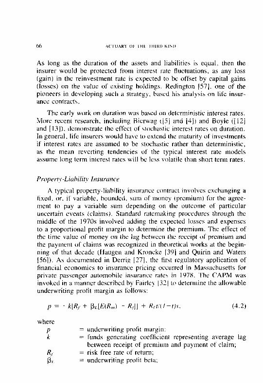
66 ACIWARY 01, I HP I IIIRI) kINI)
As long as the duration of the assets and liabilities is equal, then the insurer would be protected from interest rate fluctuations, as any loss (gain) in the reinvestment rate is expected to be offset by capital gains (losses) on the value of existing holdings. Redington [S7], one of the pioneers in developing such a strategy, based his analysis on life insur- ance contracts.
The early work on duration was based on deterministic interest rates. More recent research, including Bierwag (151 and [4]) and Boyle ([ 121 and [ 131). demonstrate the effect of stochastic interest rates on duration. In general, life insurers would have to extend the maturity of investments if interest rates are assumed to be stochastic rather than deterministic, as the mean reverting tendencies of the typical interest rate models assume long term interest rates will be less volatile than short term rates.
Proprrry-Litrhility Insurance
A typical property-liability insurance contract involves exchanging a fixed. or, if variable, bounded, sum of money (premium) for the agree- ment to pay a variable sum depending on the outcome of particular uncertain events (claims). Standard ratemaking procedures through the middle of the 1970s involved adding the expected losses and expenses to a proportional profit margin to determine the premium. The effect of the time value of money on the lag between the receipt of premium and the payment of claims was recognized in theoretical works at the begin- ning of that decade (Haugen and Kronckc [39] and Quirin and Waters 1561). As documented in Derrig 1271, the first regulatory application of financial economics to insurance pricing occurred in Massachusetts for private passenger automobile insurance rates in 197X. The CAPM was invoked in a manner described by Fairlcy [ 32 ] to determine the allowable underwriting profit margin as follows:
I’ = -UR, + ~f.MR,n) - R,]] + R, r/(/ -1)s, (4.2)
where P k
RI PL-
= underwriting profit margin: = funds generating coefficient representing average lag
between receipt of premium and payment of claim; = risk free rate of return; = underwriting profit beta;
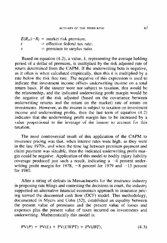
ACTUARY OF THE THIRD KIND 67
E(R,,)-R, = market risk premium; t = effective federal tax rate; s = premium to surplus ratio.
Based on equation (4.2), a value, k, representing the average holding period of a dollar of premium, is multiplied by the risk adjusted rate of return determined from the CAPM. If the underwriting beta is negative, as it often is when calculated empirically, then this k is multiplied by a rate below the risk free rate. The negative of this expression is used to indicate that investment income offsets underwriting income on a total return basis. If the insurer were not subject to taxation, this would be the relationship, and the indicated underwriting profit margin would be the negative of the risk adjusted (based on the covariance between underwriting returns and the return on the market) rate of return on investments. However, as the insurer is subject to taxation on investment income and underwriting profits, then the last term of equation (4.2) indicates that the underwriting profit margin has to be increased by a value proportional to the leverage of the insurer to account for this taxation.
The most controversial result of this application of the CAPM to insurance pricing was that, when interest rates were high, as they were in the late 197Os, and when the time lag between premium payment and claim payment was sizeable, then the indicated underwriting profit mar- gin could be negative. Application of this model to bodily injury liability coverage produced just such a result, indicating a -4 percent under- writing profit margin for 1978, -8 percent for 1979 and - 13 percent for 1980.
After a string of defeats in Massachusetts for the insurance industry in proposing rate filings and contesting the decisions in court, the industry supported an alternative financial economics approach to insurance pric- ing termed the discounted cash flow (DCF) model. This methodology, documented in Myers and Cohn [52], established an equality between the present value of premiums and the present value of losses and expenses plus the present value of taxes incurred on investments and underwriting. Mathematically this model is:
PV(P) = PV(L) + PV(UWP7’) + PV(IBT), (4.3)
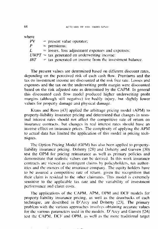
68 ACTUARY OF tttt: ItitRt~ KtF-.t)
where PV = present value operator; P = premiums; L = losses, loss adjustment expenses and expenses; UWPT = tax generated on underwriting income; IBT = tax generated on income from the investment balance.
The present values are determined based on different discount rates, depending on the perceived risk of each cash flow. Premiums and the tax on investment income are discounted at the risk free rate. Losses and expenses and the tax on the underwriting profit margin were discounted based on the risk adjusted rate as determined by the CAPM. In general this discounted cash flow model produced higher underwriting profit margins (although still negative) for bodily in.jury, but slightly lower values for property damage and physical damage.
Kraus and Ross [43] applied the arbitrage pricing model (APM) to property-liability insurance pricing and determined that changes in nom- inal interest rates should not affect the competitive rate of return on insurance contracts, but changes in real interest rates should have an inverse effect on insurance prices. The complexity of applying the APM to actual data has limited the application of this model in pricing tech- niques.
The Option Pricing Model (OPM) has also been applied to property- liability insurance pricing. Doherty 128) and Doherty and Garven 130) test the OPM for pricing reinsurancc as well as primary policies and demonstrate that realistic values can be derived. In this work insurance contracts arc viewed as contingent claims by policyholders, tax author- ities and the owners of the insurance company. The equity holders have to be assured a competitive rate of return, given the recognition that their claim is residual to the other claimants. This model is extremely sensitive to the applicable tax rate and the variability of investment performance and claim costs.
The applications of the CAPM, APM, OPM and DCF models for property-liability insurance pricing. as well as the drawbacks of each technique, are described in D’Arcy and Doherty [23]. The primary problem with the various approaches involves obtaining accurate values for the various parameters used in the models. D’Arcy and Garven 1241 test the CAPM. DCF and OPM. as well as the more traditional target
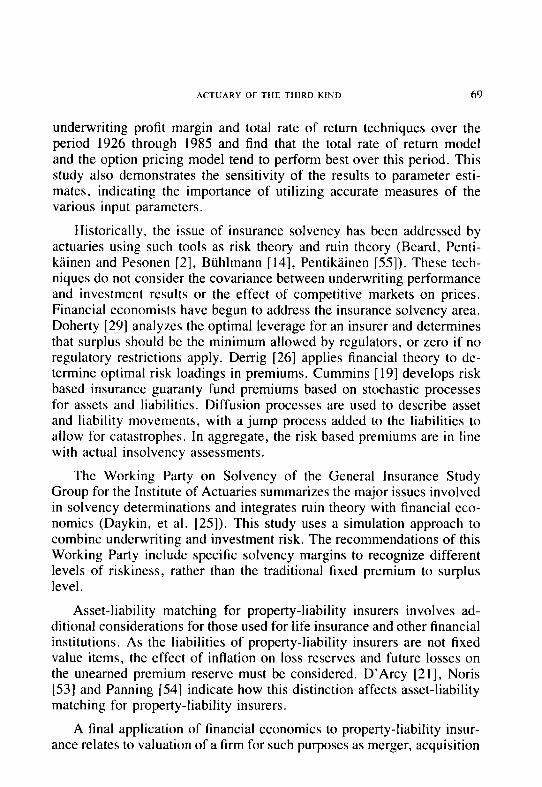
ACTUARY OF THE THIRD KIND 69
underwriting profit margin and total rate of return techniques over the period 1926 through 1985 and find that the total rate of return model and the option pricing model tend to perform best over this period. This study also demonstrates the sensitivity of the results to parameter esti- mates, indicating the importance of utilizing accurate measures of the various input parameters.
Historically, the issue of insurance solvency has been addressed by actuaries using such tools as risk theory and ruin theory (Beard, Penti- kainen and Pesonen [2], Biihlmann [14], Pentikainen [55]). These tech- niques do not consider the covariance between underwriting performance and investment results or the effect of competitive markets on prices. Financial economists have begun to address the insurance solvency area. Doherty [29] analyzes the optimal leverage for an insurer and determines that surplus should be the minimum allowed by regulators, or zero if no regulatory restrictions apply. Derrig [26] applies financial theory to de- termine optimal risk loadings in premiums. Cummins [19] develops risk based insurance guaranty fund premiums based on stochastic processes for assets and liabilities. Diffusion processes are used to describe asset and liability movements, with a jump process added to the liabilities to allow for catastrophes. In aggregate, the risk based premiums are in line with actual insolvency assessments.
The Working Party on Solvency of the General Insurance Study Group for the Institute of Actuaries summarizes the major issues involved in solvency determinations and integrates ruin theory with financial eco- nomics (Daykin, et al. [25]). This study uses a simulation approach to combine underwriting and investment risk. The recommendations of this Working Party include specific solvency margins to recognize different levels of riskiness, rather than the traditional fixed premium to surplus level.
Asset-liability matching for property-liability insurers involves ad- ditional considerations for those used for life insurance and other financial institutions. As the liabilities of property-liability insurers are not fixed value items, the effect of inflation on loss reserves and future losses on the unearned premium reserve must be considered. D’Arcy [2 I], Noris [53] and Panning [54] indicate how this distinction affects asset-liability matching for property-liability insurers.
A final application of financial economics to property-liability insur- ance relates to valuation of a firm for such purposes as merger, acquisition
70 ACTUARY OF THE IHIRD KIN!)
or conversion from a mutual to a stock ownership form. Sturgis 1681 and Miccolis [50] address this issue. Such considerations as valuing future renewals and reputation enter into this determination. In these situations, statutory valuation is inappropriate. Statutory valuation centers on an insurer going out of business, whereas valuation for merger purposes considers an insurer an on-going concern.
5. CONCLUSION
Financial economists have developed a number of tools to aid in understanding financial markets. A number of pricing models have been proposed and, although none is accepted as being a perfect explanation of prices or rates of return, the CAPM, APM and OPM provide useful insights into the workings of financial markets. As life insurers offer products tied to investment performance, as property-liability insurers guarantee financial instruments, and as both life and property-liability insurers seek to manage their own investment portfolios more effectively, knowledge of the tools and models of tinancial economics is becoming more important for actuaries. Thus, all actuaries may need to become, in the not-too-distant future, actuaries of the third kind.
Future insurance related research by financial economists and actu- aries of the third kind is likely to be directed at developing improved estimates of the input parameters for the various pricing, hedging and solvency models. All models are sensitive to parameter estimation, and many prior estimated values have been derived from the limited publicly available data. More extensive testing will require the cooperation of insurers in providing data. Greater actuarial involvement in the direction and application of future studies may encourage increased cooperation. Additionally, the long term nature of insurance contracts, as opposed to the fairly short expiration periods of most traded options, may require the development of security price models that are not Markov processes but include some autoregressive tendencies.
The convergence of financial economics and insurance suggests that future insurance based research will focus on financial economic issues. When this research is conducted by actuaries, or other insurance expe- rienced individuals, it should have the joint advantages of being aimed at the key insurance issues, be documented in terminology familiar to insurance practitioners and incorporate previously unavailable empirical data.
AC’I‘UARY OF THE THIRD KIND 71
REFERENCES
[I] L. Bachelier, (1900) Theory o?f’ Speculation, translated in P. H. Cootner, ed. The Random Chnracter of Stock Market Prices, M. I.T. Press, Cambridge, 1964.
[2] R. E. Beard, T. Pentiktiinen, and E. Pesonen, Risk Theory: The Stochastic Basis of Insurunce, Third Edition, Chapman and Hall, London. 1984.
[3] S. Benjamin, “Maturity Guarantees for Equity-Linked Policies,” Trunsactions of rhe 20th lnterrzational Congress of Acluaries, 1, p. 17, 1976.
[4] G. 0. Bierwag, Duration Analysis: Munaging interest Rate Risk, Ballinger, 1987.
[5] G. 0. Bierwag, “Immunization, Duration, and the Term Structure of Interest Rates,” Journal of Financial and Quantitative Analysis, 12, p. 725, 1977.
[6] Fischer Black and Myron Scholes, “The Valuation of Option Con- tracts and a Test of Market Efficiency,” Journal of Finance, 27, p. 399. 1972.
[7] Fischer Black and Myron Scholes, “The Pricing of Options and Corporate Liabilities,” Journal of Political Economy, 8 1, p. 637, 1973.
[8] Richard A. Brealey, and Stewart C. Myers, Principles of Corporare Finance, Third Edition, McGraw-Hill Book Company, New York, 1988.
[9] Michael J. Brennan, and Eduardo S. Schwartz, “The Pricing of Equity-Linked Life Insurance Policies with an Asset Value Guar- antee,” Journal of Financial Economics, 3, p. 195, 1976.
[lo] Michael J. Brennan and Eduardo S. Schwartz, “Alternative Invest- ment Strategies for the Issuers of Equity-Linked Life Insurance Policies with an Asset Value Guarantee,” Journal of Business, 52, p. 63, 1979.
[ 1 I] Karl H. Borch, “A Theory of Insurance Premiums,” The Geneva Papers on Risk and Insurance, 10, p. 192, 1985.
72 ACTUARY OF I tll,. I HIRI) KItiD
[ 121 Phelim P. Boyle, “Immunization Under Stochastic Models of the Term Structure,” Journcrl qf’thr Institute ofActuaries, 105, p. 177, 1978.
[ 131 Phelim P. Boyle, “Recent Models of the Term Structure of Interest Rates with Actuarial Assumptions.” Trunsnctions of the 2 1st Inter- rwtioncll Congress of Actuaries. p. 95, 1980.
[ 141 Hans Biihlmann, Muthenwticul Methnds in Risk Theory, Springer- Verlag, New York, 1970.
[ 151 Hans Biihlmann, “Actuaries of the Third Kind’?” ASTIN Bl4lletjn.
17, p. 137, 1987.
[ 161 D. P. Chiras and S. Manaster, “The Information Content of Option Prices and a Test of Market Efficiency.” Jorrrrurl of Fincmcicd Economics, 6, p. 2 13, 1978.
[ 17J T. P. Collins, “An Exploration of the Immunization Approach to Provision for Unit-Linked Politics with Guarantees.” Jourrurl of the Institute of Actutrries. 109, p. 24 1 . 1982.
I181 J. C. Cox and M. Rubinstcin, Options Mcrrkets, Prentice-Hall, Englewood Cliffs. NJ, 1985.
1191 J. D. Cummins, “Risk-Based Premiums for Insurance Guaranty Funds,” Journtrl oj’ Fintrnce. 43. p. 823. 1988.
1201 J. D. Cummins and S. A. Harrington editors, Fair Rate of‘Return ill Pn,l’ert~-Liahilit~ /n.surcrncr, Kluwer-Nijhoff, Boston. 1987.
(21 ] S. P. D’Arcy, Discussion of Ferguson. “Duration,” PCAS, LXXI, p. 8, 1984.
122) S. P. D’Arcy and K. C. Chen, “The Effect of Changes in Pension Plan Interest Rate Assumptions on Security Prices,” Journal of Economic.s md Bu.siness. 40, p. 243, 1988.
[23] S. P. D’Arcy and N. A. Doherty. The Finmcial Theory of Pricing PI-o)pert?~-Liclhiiit~~ Imur~~m~e Cotrtrwts, Hucbner Foundation Mon- ograph, 15, Richard D. Irwin, Homewood. IL. 1988.
(241 S. P. D’Arcy, and J. R. Garven, “Property-Liability Insurance Pricing Models: An Empirical Evaluation,” Cmrrrrlt~ Actuariul So- ciep Discussion Paper Pro,qmn. 1 , p. 1 13. I 990.
ACTUARY OF THE THIRD KIND 73
[25] C. D. Daykin, G. D. Bernstein, S. M. Coutts, E. R. F. Devitt, G. B. Hey, D. I. W. Reynolds and P. D. Smith, “Assessing the Solvency and Financial Strength of a General Insurance Company,” Journal of the Institute of Actuaries, 114, p. 227, 1987.
[26] R. A. Derrig, “Solvency Levels and Risk Loadings Appropriate for Fully Guaranteed Property-Liability Insurance Contracts: A Finan- cial View,” International Conference of Insurance Solvency, 1986.
[27] R. A. Derrig, “The Use of Investment Income in Massachusetts Private Passenger Automobile and Workers’ Compensation Rate- making,” Chapter 6 in Cummins and Harrington, 1987.
[28] N. A. Doherty, “The Pricing of Reinsurance Contracts,” presented to the National Council of Compensation Insurers, New York, 1985.
[29] N. A. Doherty, “On the Capital Structure of Insurance Firms,” international Conference on Insurance Solvency, 1986.
[30] N. A. Doherty and J. R. Garven, “Price Regulation in Property Liability Insurance: A Contingent Claims Approach,” Journal of Finance, 41, p. 1031, 1986.
[3 l] A. Einstein, Investigations of the Theory of Brownian Movement, edited with notes by R. Furth, translated by A. D. Cowper, Dover, New York, 1905, 1956.
[32] W. B. Fairley, “Investment Income and Profit Margins in Property Liability Insurance: Theory and Empirical Results,” Bell Journal of Economics, IO, p. 192, 1979. Reprinted as Chapter 1 in Cum- mins and Harrington, 1987.
[33] R. E. Ferguson, “Duration,” PCAS, LXX, 1983, p. 265.
[34] Michael Firth and Simon N. Keane, editors, tssues in Finance, Philip Allan Publishers, Ltd., p. 158, 1986.
[35] I. Fisher, The Theory of interest, Macmillan, New York, 1930.
[36] D. Galai, “Tests of Market Efficiency of the Chicago Board of Options Exchange,” Journal of Business, 50, p. 167, 1977.
[37] James R. Garven, “On the Application of Finance Theory to the Insurance Firm,” Journal of Financial Services Research, 1, p. 57, 1987.
74 ACTUARY 01: I’HI, IHIRD KIND
[38] Robert A. Haugen, Modern tnl~estment Theory, Prentice-Hall, En- glewood Cliffs, N.J., 1986.
[39] R. A. Haugen and C. 0. Kroncke, “Rate Regulation and the Cost of Capital in the Insurance Industry,” Journal of Financial and Quantitative Analysis, 6, p. 1283, 197 I
[40] R. G. Ibbotson and R. A. Sinquefeld, Stocks, Bonds, Bills and Injlation: The Past and The Future, Financial Analysts Research Foundation, Charlottesville, Virginia, 1982.
[41] J. E. Ingersoll, Theory of Financial Decision Making, Rowan and Littlefield, Totowa, N.J., 1987.
[42] R. A. Jarrow and A. Rudd, Option Pricing, Richard D. Irwin, Homewood, IL, 1983.
[43] A. Kraus and S. A. Ross, “The Determination of Fair Profits for the Property-Liability Insurance Firm,” Journal cjf Finance, 37, p. 1015, reprinted as Chapter 5 in Cummins and Harrington, 1987.
[44] H. Leland, “Who Should Buy Portfolio Insurance?” Journal oj Finance, 35, p. 581, 1980.
[45] J. Lintner. “Security Prices, Risk and Maximal Gains from Di- versification,” Journal of Finance, 20, p. 587, 1965.
[46] F. Lundberg, “On the Theory of Risk,” Transactions of the Sixth International Congress of Actuaries, 1, p. 877, 1909.
[47] A. G. Malliaris and A. W. Brock, Stochastic Methods in Economics and Finance, North Holland, Amsterdam, 1982.
[48] F. R. Macaulay, Some Theoretical Problems Suggested b? the Movement of interest Rates, Bond Yields und Stock Prices m the United States Since 18.56, National Bureau of Economic Research.
[49] R. C. Met-ton, “Theory of Rational Option Pricing,” Bell Journal of Economics and Management Science. 4, p. 141, 1973.
[50] R. S. Miccolis, “An Investigation of Methods, Assumptions and Risk Modeling for the Valuation of Property-Casualty Insurance Companies,” Casual8 Actuarial Society, Discussion Puper Pro- gram, p. 281, 1987.
[5 I ] J. Mossin, “Equilibrium in a Capital Asset Market,” Econometrica, 34, p. 768, 1966.
ACTUARY OF THE THIRD KIND 75
[52] S. C. Myers and R. A. Cohn, “A Discounted Cash Flow Approach to Property-Liability Insurance Rate Regulation,” Chapter 3 in Cummins and Harrington, 1987.
[53] P. D. Noris, “Asset/Liability Management Strategies for Property & Casualty Companies,” Morgan Stanley, 1987.
[54] W. H. Panning, “Asset/Liability Matching: Beyond Interest Rate Risk,” Casualty Actuarial Society Discussion Paper Program, p. 322, 1987.
[55] T. Pentikainen, “On the Solvency of Insurers: A Survey on the Aspects Involved,” International Conference on Insurance Sol- vency, 1986.
[56] D. G. Quirin and W. R. Waters, “Market Efficiency and the Cost of Capital: The Strange Case of Fire and Casualty Insurance Com- panies,” Journal of Finance, 30, p. 427, 1975.
[57] F. M. Redington, “Review of the Principles of Life-Office Valua- tions,” Journal of the Institute of Actuaries, 78, p. 286, 1952.
[58] F. K. Reilly, Investment Analysis & Portfolio Management, Dryden Press, Hinsdale, IL, p. 223, 1979.
[59] R. Roll, “A Critique of the Asset Pricing Theory’s Tests, Part 1: On Past and Potential Testability of the Theory,” Journal of Finan- cial Economics, 4, p. 129, 1977.
[60] S. A. Ross, “The Arbitrage Theory of Capital Asset Pricing,” Journal of Economic Theory, 13, p. 341, 1976.
[61] Stephen A. Ross and Randolph W. Westerfield, Corporate Finance, Times Mirror/Moseby College Publishing, St. Louis, 1988.
[62] M. Rubinstein, “Nonparametric Tests of Alternative Option Pricing Models Using All Reported Trades and Quotes on the 30 Most Active CBOE Option Classes from August 23, 1976, through Au- gust 31, 1978,” Journal of Finance, 40, p. 455, 1985.
[63] W. F. Sharpe, “Capital Asset Prices: A Theory of Market Equilib- rium under Conditions of Risk,” Journal of Finance, 19, p. 425, 1964.
[64] A. Sloan and R. L. Stem, “How V, = V,N(dt)-(Ele”)N(dz) Led to Black Monday,” Forbes, p. 55, January 25, 1988.
1651 Clifford W. Smith, “Applications of Option Pricing Analysis,” Handbook r~FiFluFlc~iu~ Economics, edited by J. L. Bicksler, p. 79, 1979. Amsterdam, North-Holland.
[66] Clifford W. Smith. “On the Convergence of Insurance and Finance Research,” Journal of Risk uncl Insurance, 5.3, p. 693, 1986.
[67] Clifford W. Smith, “Option Pricing-A Review,” Journal of Fi- nancial Economics, 3. p. 3, 1976.
[68] R. W. Sturgis, “Actuarial Valuation of Property/Casualty Insurance Companies,” PCAS, LXVIII, p. 146, 198 I.
[69] J. A. Tilley, “The Application of Modern Techniques to the In- vestment of Insurance and Pension Funds,” Trun.suc1ioFz.s of the 23rd Internutionul Congress of Actrrurie.s.
[70] R. Whaley, “Valuation of American Call Options on Dividend- Paying Stocks: Empirical Tests,” Jmurnul of Finunciul Economics, IO. p. 29, 1982.
[71] A. D. Wilkie, “On the Calculation of Real Investment Returns,” Joiirnul oj’ the Institute of Actuaries, I I I . p. 149, 1984.
[72] A. D. Wilkie, “Steps Towards a Stochastic Investment Model Comprehensive,” O.A.R.D., 36, Institute of Actuaries. 1984.
[73] A. D. Wilkie, “A Stochastic Investment Model for Actuarial Use,” Trunsuctions oj’ the Fucul~ of Actrruries. 79. p. 34 I . 1986.
[74] A. D. Wilkie, “An Option Pricing Approach to Bonus Policy,” Journul of the Institute of Actuuries, I 14, p. 2 1 . 1987.
77
APPLICATION OF COLLECTIVE RISK THEORY TO ESTIMATE VARIABILITY IN LOSS RESERVES
ROGER M. HAYNE
Abstract
The intent of this paper is to present un introduction to Collective Risk Theory for the first time reader and consid- erations in applying that theory to estimate variability in loss reserves. It begins with u brief introduction to the basic con- cepts of Collective Risk Theory along with a survey of some of the techniques developed to date to estimate the aggregate distribution of losses. With this framework, descriptions of some applications to loss reserves are discussed, with atten- tion paid to the assumptions inherent in those methods and some problems that arise in applying this theory to reserves. Of note are questions that are not directly addressed b>l this model; in purticular, parumeter uncertainty. Included are ref- erences which, it is hoped, will lead the interested reader .further into the applications to date.
1. INTRODUCTION
The question of the amount of variability inherent in loss reserve estimates has gained more notice in recent years. In fact, Principles 3 and 4 of the Statement of Principles Regarding Property and Casualty Loss and Loss Adjustment Expense Reserves [I] state,
“3. The uncertainty inherent in the estimation of required provisions for unpaid losses or loss adjustment expenses implies that a range of reserves can be actuarially sound. The true value of the liability for losses or loss adjustment expenses at any accounting date can be known only when all attendant claims have been settled.
4. The most appropriate reserve within a range of actuarially sound estimates depends on both the relative likelihood of estimates within the range and the financial reporting context in which the reserve will be presented.”
Quantification of the variability in reserve estimates will thus be useful in the determination mentioned in Principle 4. In addition, knowl-
78 VARlABlLITY IN 1,OSS RESERVES
edge of the statistical distribution of reserves is also useful in discussing the impact of reserve discounting on insurer capacity and solidity. One author has already cited this as a favorable result of discounting in that discounting of reserves would “increase the statutory capacity of the insurance industry. Statutory surplus would increase as loss reserve lia- bilities were reduced [2].” However, simply discounting reserves will not necessarily increase financial strength or capacity. Rather, a better measure of that capacity is probably the ability of surplus to protect solvency. Without knowledge of the variability of the reserve estimates, the assessment of the strength of a company at a given level of surplus, and hence capacity, probably cannot be made accurately.
There are several techniques which are available to assess the finan- cial solidity of a given amount of surplus. Methods that have been advanced for this purpose include “confidence limit” approaches, Ruin Theory, and Utility Theory, along with a rather comprehensive model of the operations of an insurer (see [3] and [4] for this latter application). In each case, however, their application requires an estimate of the statistical distribution of the reserves.
The intent of this paper is to discuss the framework of Collective Risk Theory as one approach that can be used to estimate the statistical distribution of reserves. No prior exposure to Collective Risk Theory is assumed; however, it is hoped that the references will provide a good starting place for the reader who wants to pursue this subject further.
2. THE COLLECTIVE RISK MODEL
The basic collective risk model approaches the question of the dis- tribution of total reserves by modeling the claim process faced by an insurer. It considers the interaction between the distribution of the number of claims and the distribution(s) of the individual claims by calculating loss (or reserve) T as the sum
T = X, + Xz + . . . + X,v, (2.1)
where the number of claims N is randomly selected. and each of the claims XI, XZ, . . , X,%, is randomly selected from claim size distribu- tion(s).
There is a significant amount of literature which addresses this model and its applications to casualty insurance. The primary source is probably the text by Beard, Pentikainen and Pesonen 151. Other complete texts
VARIABILITY IN LOSS RESERVES 79
dealing with Collective Risk Theory and its applications are those by Borch [6], Biihlmann [7] and Seal [8]. The papers by Borch [9] and Pentikainen [lo] also consider this model from a fairly broad point of view.
There are some useful properties of the distribution T under rather broad assumptions. In particular, if
1. The number of claims N has moments
v =E(N)
vi = E[(N - v)‘] for i = 2, 3, and 4;
2. All claims are drawn from the same population with moments
x = E(X)
xi = E[(X - x)~] for i = 2, 3, and 4; and
3. All claims X and the number of claims N are all independent, then the first four moments of the random variable T exist and are given by
E(T) = vx (2.2)
E({T - E(r)}*] = x2v + x*v2 (2.3)
E[{T - J3T)131 = x3v + 3X2XV2 + x3v,3 (2.4)
E[{T - E(~3)41 = X4V + 3X2*(V2 - V + V*) + ‘tXX3vz +
~X*XZ(V~ + VV~) + x4v4. (2.5)
Comparable formulae for higher moments can also be derived if the corresponding moments of the claim count and size distributions exist. The paper by Mayerson, Jones and Bowers [ 1 l] gives a derivation of these formulae.
These facts can and should be used to test the reasonableness of any approximation to the distribution of T. In fact, one of the methods used to approximate that distribution relies on these relationships.
3. APPROXIMATIONS OF THE DISTRIBUTION OF T
There have been many approaches used in estimating the distribution of T, given distributions for the number of claims N and the size of those claims. These methods can be broadly grouped into 3 classes:
80 VARIABILITY IN LOSS KbS1-RVkS
1. Monte Carlo Simulation. 2. Approximate Distributions, and 3. Analytic Approximation.
Monte Curio Simulation
Probably the most flexible of these approaches is that of Monte Carlo Simulation. The idea is simple and directly follows the basic Collective Risk Model above. Simply stated. the Monte Carlo Simulation algorithm is composed of five steps:
1. Randomly select the number of claims N from the claim count distribution.
2. Randomly select N claims, XI, X2. . X,V, from the claim size distribution.
3. Calculate one observation from the distribution of T by the sum x, + x* + ... + Xh..
4. Repeat steps 1 through 3 “several” times. 5. Estimate the distribution of T using the points generated in this
manner.
Conceptually, there is no limit on the form of the claim count or size distributions used in Monte Carlo Simulation. They can both be discrete or the claim size distribution can be continuous. Simulation with de- ductibles and/or per claim loss limitations can also be easily handled in this framework. In addition, the combination of several lines of insurance or accident years can also be accommodated without much difficulty.
There are, however, prices to pay. First, the answer to how many is “several” in step 4 is not clear. Often a signifcant number of simulations must be run to obtain a clear enough picture of the distribution of T to be useful in applications. One technique. though admittedly “brute force ,” is to compare the results of two sets of simulations, say each of 1,000 trials. If the resulting distributions are “close enough” for the task at hand, the combined distribution could be used as an approximation. If, however, they differ significantly, more trials may be indicated. The moments of the simulated distributions should bc compared to the the- oretically expected moments in (2.2) through (2.5) to see if the simulation is sufficiently close.
Another practical consideration is how to simulate the random selec- tions from the claim count and claim size distributions. Care should be
VARIABILITY IN LOSS RESERVES 81
taken as to the representations of the distributions. Finite distributions, such as those based solely on empirical data, implicitly have upper bounds. Thus, unless those upper bounds are to be explicitly considered in the model, some of the variability inherent in the underlying distri- bution may be lost.
One solution to this difficulty could be to use analytic distributions, such as the lognormal or Pareto, to estimate the distributions in the “tail.” In this way the empirical data could be used, and yet some of the potentially unlimited nature of some risks can be captured.
The process used to make the random selections from the claim size and count distributions may not be obvious. Most computer software packages do provide “random” number generators which correspond to a uniform distribution. In addition, there are algorithms which allow for selections from other distributions, either directly or from selections from the uniform distribution. The very useful text A Guide fo Simulation by Bratley, Fox and Schrage [ 121 includes some of these algorithms for a number of statistical distributions. That text also includes listings of computer programs to perform those calculations.
One final consideration regarding Monte Carlo Simulation is the cost in computer time. Factors influencing this time include the complexity of the model used, the expected number of claims E(N), the degree of accuracy required, and the amount of dispersion in the claim size distri- bution. Simulations involving a great number of expected claims will of course take longer to run. Not immediately obvious, though, is the fact that if the claim size distribution is dispersed (a large standard deviation as compared to the mean), there will generally be a greater number of simulations necessary to achieve a desired level of accuracy than if the claim size distribution is less dispersed.
Appro,uimate Distributions
Another method used to estimate the distribution of T involves as- suming a statistical distribution and then using the “known” moments of T to select the parameters of that distribution. Probably falling into this category is the Normal-Power, or NP Approximation. This approach is described in Beard, Pentikainen and Pesonen [5] and used by Mayerson, Jones and Bowers [ 1 I] and by Patrik and John [ 131. Although relatively easy to apply, it does not seem to be sufficiently skewed for many casualty applications. However, caution should be taken in applying this
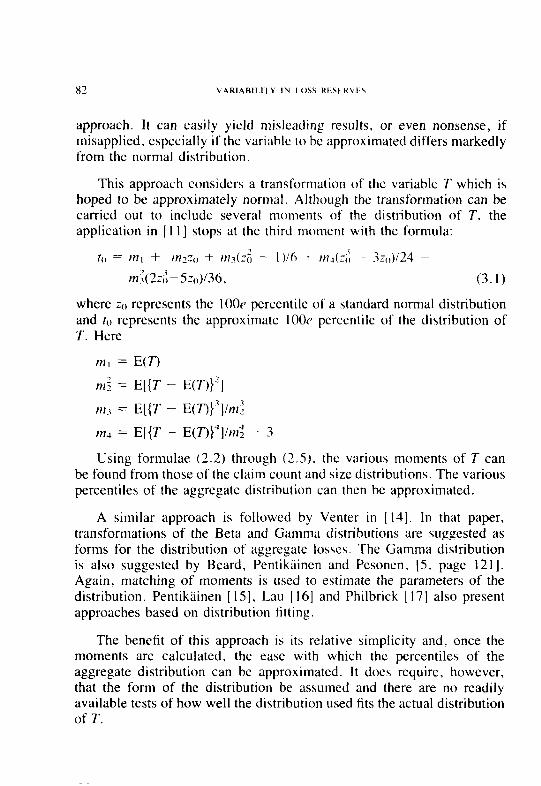
82 VARIABILI I Y IN LOSS HtSf.KVI,S
approach. It can easily yield misleading results, or even nonsense, if misapplied, especially if the variable to be approximated differs markedly from the normal distribution,
This approach considers a transformation of the variable T which is hoped to be approximately normal. Although the transformation can be carried out to include several moments of the distribution of T, the application in [ I l] stops at the third moment with the formula:
ro = ml + PI-:() + n& - I )ih + nrj(z;: - 3=,,)/‘24 - m:(2+5zo)/36, (3.1)
where z() represents the 1OOe percentile of a standard normal distribution and f. represents the approximate 100~ percentile of the distribution of T. Here
111 , = W-I
m; = E[{T - E(7-)}‘]
n.3 = E[{T - E(7-)}3]/m;
UL, = E[{T - E(7-)}4]/rn: - 3
Using formulae (2.2) through (2.5). the various moments of T can be found from those of the claim count and size distributions. The various percentiles of the aggregate distribution can then be approximated.
A similar approach is followed by Venter in [ 141. In that paper, transformations of the Beta and Gamma distributions are suggested as forms for the distribution of aggregate losses. The Gamma distribution is also suggested by Beard, Pentikainen and Pesonen, [ 5, page 1211. Again, matching of moments is used to estimate the parameters of the distribution. Pentikainen [ 151, Lau [ 161 and Philbrick [ 171 also present approaches based on distribution fitting.
The be&it of this approach is its relative simplicity and, once the moments are calculated, the ease with which the percentiles of the aggregate distribution can be approximated. It does require, however, that the form of the distribution be assumed and there are no readily available tests of how well the distribution used fits the actual distribution of T.
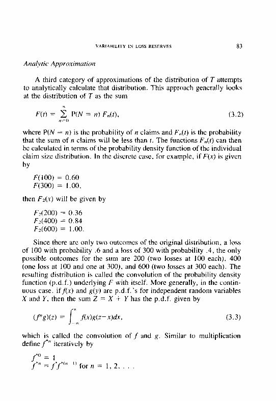
VARIABILITY IN LOSS RESERVES 83
Analytic Appro.uimation
A third category of approximations of the distribution of T attempts to analytically calculate that distribution. This approach generally looks at the distribution of T as the sum
F(t) = 2 P(N = n) F,,(t), n=o
(3.2)
where P(N = n) is the probability of n claims and F,,(r) is the probability that the sum of n claims will be less than t. The functions F,,(r) can then be calculated in terms of the probability density function of the individual claim size distribution. In the discrete case, for example, if F(K) is given by
F(100) = 0.60 F(300) = 1.00,
then F?(x) will be given by
F2(200) = 0.36 F2(400) = 0.84 F2(6OO) = 1.00.
Since there are only two outcomes of the original distribution, a loss of 100 with probability .6 and a loss of 300 with probability .4, the only possible outcomes for the sum are 200 (two losses at 100 each), 400 (one loss at 100 and one at 300), and 600 (two losses at 300 each). The resulting distribution is called the convolution of the probability density function (p.d.f.) underlying F with itself. More generally, in the contin- uous case, if&) and R(J)) are p.d.f.‘s for independent random variables X and Y, then the sum Z = X + Y has the p.d.f. given by
(f*g)(z) = lx f(x)&-ax, -r
(3.3)
which is called the convolution off and g. Similar to multiplication define f*” iteratively by
f*n =f*f*(“-‘) for n = 1, 2, . .
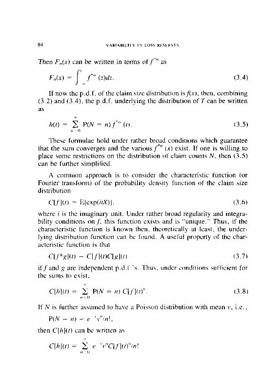
84 VARIAB1I.I I’Y IN LOSS RF.SEKVES
Then F,,(s) can be written in terms off*‘* as
I
I F,,(x) = ox f‘*” (z)dz. (3.4)
If now the p.d.f. of the claim size distribution isf(x), then, combining (3.2) and (3.4), the p.d.f. underlying the distribution of T can be written as
h(r) = c P(N = n)f*” (1). (3.5) ,I =o
These formulae hold under rather broad conditions which guarantee that the sum converges and the various f*” (.w) exist. If one is willing to place some restrictions on the distribution of claim counts N, then (3.5) can be further simplified.
A common approach is to considcr the characteristic function (or Fourier transform) of the probability density function of the claim size distribution
C[.f‘](r) = E[exp(irX)j. (3.6)
where i is the imaginary unit. Under rather broad regularity and integra- bility conditions onJ: this function exists and is “unique.” Thus, if the characteristic function is known then, theoretically at least, the under- lying distribution function can hc found. A useful property of the char- acteristic function is that
clJ‘*glcf, = Cl,mKIgl(t) (3.7)
iff‘and s arc independent p.d.f.‘s. Thus, under conditions sufficient for the sums to exist.
Clhl(t) = c P(N = 11) C’[,f‘]($. (3.8) ,1--o
If N is further assumed to have a Poisson distribution with mean \‘, i.e.,
P(N = II) = e “r-“/n! ,
then C(h](r) can be written as
C[h](r) = c TV “v”C[.f’](t)“/r~! ,, -0
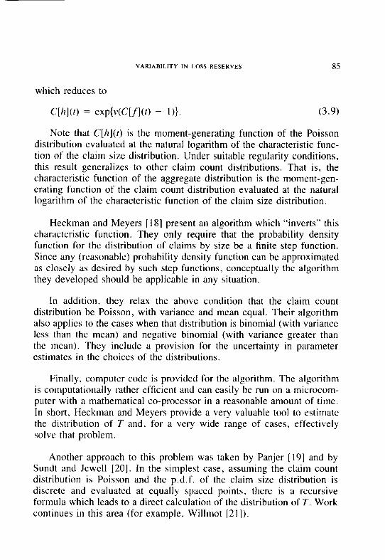
VARIABILITY IN LOSS RESERVES 85
which reduces to
C[hl(Q = exp~~~(WlO) - 1)). (3.9)
Note that C[h](r) is the moment-generating function of the Poisson distribution evaluated at the natural logarithm of the characteristic func- tion of the claim size distribution. Under suitable regularity conditions, this result generalizes to other claim count distributions. That is, the characteristic function of the aggregate distribution is the moment-gen- erating function of the claim count distribution evaluated at the natural logarithm of the characteristic function of the claim size distribution.
Heckman and Meyers [ 181 present an algorithm which “inverts” this characteristic function. They only require that the probability density function for the distribution of claims by size be a finite step function. Since any (reasonable) probability density function can be approximated as closely as desired by such step functions, conceptually the algorithm they developed should be applicable in any situation.
In addition, they relax the above condition that the claim count distribution be Poisson, with variance and mean equal. Their algorithm also applies to the cases when that distribution is binomial (with variance less than the mean) and negative binomial (with variance greater than the mean). They include a provision for the uncertainty in parameter estimates in the choices of the distributions.
Finally, computer code is provided for the algorithm. The algorithm is computationally rather efficient and can easily be run on a microcom- puter with a mathematical co-processor in a reasonable amount of time. In short, Heckman and Meyers provide a very valuable tool to estimate the distribution of T and, for a very wide range of cases, effectively solve that problem.
Another approach to this problem was taken by Panjer [ 191 and by Sundt and Jewel1 [20]. In the simplest case, assuming the claim count distribution is Poisson and the p.d.f. of the claim size distribution is discrete and evaluated at equally spaced points, there is a recursive formula which leads to a direct calculation of the distribution of T. Work continues in this area (for example, Willmot [21]).
86 VARIAHII.If’Y IN I OSS RtStRVtS
4. APPLICATIONS IN LOSS RESERVES
It is interesting to note that the majority of the references listed so far either deal with Risk Theory on its own or in relationship to various aspects of ratemaking. There have been some recent papers dealing with risks and uncertainty in loss reserve estimates (see [3], 141, [22], [23], and [24]), but we have been unable to find any which deal directly with considerations which enter with the application of this model to the estimation of variability in loss reserves.
The model of the insurance process provided by Collective Risk Theory seems a natural tool to apply in evaluating the degree of uncer- tainty in loss reserve estimates. If, for example, under the independence hypotheses listed in Section 2, the distribution of open and IBNR claims (N) is known and the distribution of the size of those claims (X) is also known, the methods outlined in Section 3 all provide ways to estimate the distribution of total reserves (T).
One approach used at this point takes the actuary’s best estimate of ultimate claim counts and losses as an estimate of the expected number of claims E(N) and average claim size E(X). Statistical distributions are then selected for each of these quantities.
If the Poisson is chosen as a model of the claim count distribution, then the only parameter to estimate is its mean. Other distributions, such as the binomial and negative binomial, allow for the variance of N to differ from its mean. These are “well behaved” and can be easily accom- modated in the algorithm described in [ 181.
The claim size distribution is usually assumed to be more complex. Common choices include the lognormal, Pareto, and a transformed Gamma, among others. An ad iwc approach is to select the distribution to be used, assume that its mean corresponds with the average claim size derived by the actuary’s best estimate, and then select the other parameter(s) either judgmentally or based on characteristics of the line under evaluation. This may be all that can be done in situations where data for further analysis is lacking. If sufficient data is available, how- ever, the techniques described by Hogg and Klugman [25] provide pow- erful tools to select the “proper” distributions.
To better model the distribution of reserves for an insurer or self- insured, accident (report, or policy) years are often considered separately,
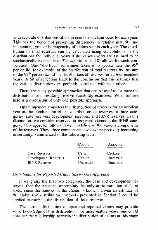
VARIABILITY IN LOSS RESERVES 87
with separate distributions of claim counts and claim sizes for each year. This has the benefit of preserving differences in relative maturity and maintaining greater homogeneity of claims within each year. The distri- bution of total reserves can be calculated using convolutions of the distributions for individual years if the various years are assumed to be stochastically independent. The algorithm in [ 181 allows for such con- volution. One “short-cut” sometimes taken is to approximate the 9.51h percentile, for example, of the distribution of total reserves by the sum of the 95’h percentiles of the distributions of reserves for various accident years. A bit of reflection leads to the conclusion that this assumes that the various distributions are perfectly correlated with each other.
There are many possible approaches that can be used to estimate the distributions and resulting reserve variability estimates. What follows here is a discussion of only one possible approach.
This refinement considers the distribution of reserves for an accident year as the combination of the distributions of reserves in three cate- gories: case reserves, development reserves, and IBNR reserves. In this discussion, we consider reserves for reopened claims in the IBNR cate- gory. This approach allows closer modeling of the various components of the reserves. These three components also have respectively increasing uncertainty, summarized in the following table:
Case Reserves Development Reserves IBNR Reserves
Counts Amounts
Certain Certain Certain Uncertain Uncertain Uncertain
Distributions for Reported Claim Sizes-One Approach
If we group the first two categories, the case and development re- serves, then the statistical uncertainty lies only in the variation of claim sizes, since the number of the claims is known. Given an estimate of the claim size distribution, methods presented in Section 2 could be applied to estimate the distribution of these reserves.
The current distribution of open and reported claims may provide some knowledge of this distribution. For more mature years, one could consider the relationship between the distribution of claims at this stage
88 VARIAHII IIY IN LOSS KI:SI:R\ lb5
of development with the “ultimate” distribution of those same claims and incorporate it. with the current distribution. to estimate the ultimate distribution of claims.
As an example of one possible approach, Ict us assume that the lognormal is an appropriate model for the distribution of X, the claim size random variable. Then Z = In(X) has a normal distribution, and the lognormal can be completely parameterized by the mean m and variance .Y’ of Z. We select this parameterization for the distribution of X.
It then follows (see, for example, p. 38 of [26J) that maximum likelihood estimators for m and ,s2 arc obtained from the sample mean and variance of the values ln(X,) where X, arc observed claims. As in the normal case, the sample variance. using the number of sample points as the denominator, is a biased estimate for .v2: therefore, a denominator of jr - I is used to estimate s’.
Suppose, for example. that we arc trying to estimate the claim size distribution for open and reported claims for accident year 1981 as of December 3 1, 1988. That accident year is currently 84 months from the beginning of I98 I.
We can calculate the estimators /?rxJ and sft of the VI and s2 parameters for reported claims for “mature” accident years at 84 months of devel- opment. We can also calculate the estimators I?~,,I, and s:l, for the distri- bution of ultimate values of those same claims. Using regression we can find constants which best fit
muI1 = (I + fWFlxj NIld (4.1) 7 .Suh = (’ + d&j (4.2)
for the “mature” years. These parameters, along with the estimators ,niJ and SE: for the current distribution of claims for accident year 1981 as of December 31, 1988, yield the following estimates of the parameters for the ultimate distribution of currently reported and open claims for accident year I98 I :
rnzl, = (1 + I%& and (4.3)
s:; = (’ + ‘1s~:. (4.4)
Exhibits 1 and 2 provide a numerical example of this approach using purely hypothetical data. In these exhibits. we assume losses for the first
VARIABILITY IN LOSS RESERVES 89
seven accident years are sufficiently developed so that we “know” their ultimate distributions and wish to estimate the distribution for accident year 1981.
The distributions of claims reported at 84 months are shown in Exhibit 1. Also shown in Exhibit I are the ultimate distributions for the claims reported at 84 months for the first seven accident years, as well as the corresponding parameters from the fitted lognormal distributions.
Exhibit 2 shows the results of the regression and corresponding constants (u and c above) and coefficients (b and d above). Given the lack of significance of the coefficient in the fit for s2, we assume no relationship between s;: and s::. We thus use the sample mean and variance for the ultimate distributions for the first seven years as our parameter estimates. The bottom portion of Exhibit 2 then shows the resulting estimates for the parameters of the ultimate distribution for accident year 198 1.
At this point, other analyses (e.g., usual reserve estimation tech- niques) could be used to modify these parameters to reflect the results of those projections. It is a property of the lognormal distribution that the coefficient of variation (ratio of the standard deviation to the mean) can be expressed only in terms of the parameter s2:
c.v.z = exp(.?)- 1 . (4.5)
Thus, adjustments made to the rn:rt parameter will affect the mean of the final distribution but not its relative variation, as measured by the coefficient of variation. This technique does, however, have the benefit of incorporating information regarding the current distribution of open and reported claims in deriving the estimate for the ultimate distribution of those claims.
We note that there is no chance of zero claims in the lognormal distribution. If we were to use only that distribution as a model for reported claims, then, strictly speaking, the number of claims is not certain, for there may be open claims that will close without payment. This can also be overcome by estimating the portion of those claims which will close with payment separately, possibly also with the use of regression.
90 VARIABII.ITY IN I OSS RESERVFS
Distributions for IBNR Reserves-One Approuch
For estimating the distribution of IBNR reserves, both the claim counts and severity are uncertain. The parameters for the claim size distribution could be considered in light of the ultimate value of claims for more “mature” years which were reported after 84 months. The trend in those costs could also be considered in selecting the distribution of claim sizes.
One approach to estimating the distribution of claim counts would be to assume it is Poisson and estimate the expected number of IBNR claims using usual actuarial projection methods. Another approach, sim- ilar to that used by Weissner [27], considers the reporting emergence as a statistical distribution with known data truncated from above. Maxi- mum likelihood estimators are then used to estimate the parameters of that distribution. A beneft of this approach is that it can result in estimates of both the mean and variance of the claim count distribution.
This approach begins by postulating a development curve in the form of a probability distribution and then uses maximum likelihood estimators along with known reported claims to estimate the ultimate number of reported claims as well as an approximate distribution of that ultimate. Though the application is in terms of reported claims, there is no inherent reason that the same approach cannot be used to estimate the distribution of ultimate losses directly.
We first assume that the number of claims reported through time t can be expressed as
iJF(t;@. (4.6)
Here U is the (unknown) ultimate number of claims, and F(t$) is a cumulative distribution function with parameter(s) 0 representing the percent of ultimate claims reported through time t.
In this application, we think of the number of claims reported in time period i as a grouped sample containing ,f; points in the interval (c. ,, c,) from the distribution. We can use methods described in [25] to iteratively approximate the maximum likelihood estimator of the pa- rameter(s) 8 given these k observations. To this end, detine
P,.(6) = [F(cI-:&F(c.,-- ,;@]lF(cx;@. (4.7)
VARlABlLlTY IN LOSS RESERVES 91
Here cr- I and c,. are the endpoints of the interval containing the fr observations. Let f* denote the total number of claims reported through k time periods, that is,
Define A(6) to be the matrix composed of the elements
and let the vector S(6) have the elements
(4.9)
With these functions, which involve only first derivatives of the cumulative probability function with respect to its parameters, iteratively calculate
6, = iin-, + [A(e,,-,)]-‘s(e,,-,). (4.11)
Now let h = F(ck;&) be the estimated percentage of claims reported by time ck. The actual number of claims reported by time ck can then be thought of as having a binomial distribution with (unknown) mean Uh and variance Uh( 1 - h). Assume at this point that the binomial can be approximated by a normal distribution. Thus, approximately,
T - N(Uh, Uh(1 - h)). (4.12)
Hence U = T/h is approximately normal:
U - N(f*lh, f(l - h)lh*). (4.13)
This results in an approximate distribution of IBNR claims I, where +u-f- N(f*lh -f*, f*(l - h)lh*). (4.14)
Given these distribution estimates, an estimate of the distribution of IBNR reserves for accident year 198 1 as of December 3 1, 1988 can then be obtained. If it is assumed that this distribution and the distribution of reserves for reported claims are stochastically independent, then an es- timate of the distribution of total reserves can be made by convoluting these two distributions.
92 VARIABILI rY IN I OSS RESERVkS
The assumption of independence may not be too restrictive in this case. As of December 31, 1988. reported and IBNR claims form two distinct populations. It is unlikely that fluctuations in the loss amounts for a fixed number of known claims will lead to fluctuations in the amounts, or counts, of claims yet to be reported. This does not, however, address the question of parameter estimation for these populations and the potential interrelationships there.
As an example of this approach, Exhibit 3 shows a hypothetical claim emergence pattern for the first 84 months of development. We selected a Weibull distribution to model this claims emergence. That distribution’s cumulative density function can be written as
F(~;0~,8~) = 1 - exp{-exp[81 In(x/Oz)]}. (4.15)
The methods from [25] were then used to derive the parameter estimates shown in Exhibit 3. These parameters result in an h-value of 0.930, with the resulting estimate of the expected number of IBNR claims of 137 with a variance of 147.46.
Cornbinution of Years
The above calculations lead to an estimate of the distribution of total reserves for a single accident year, in this case 1981. Though not ex- plicitly stated, in practice they would probably be calculated for a single coverage or line of insurance. For a multiple line company, however, the distribution of total reserves, for all lines and for all years, is of concern.
If one assumes that the distributions for the various lines of business and accident years are all stochastically independent, the distribution of total reserves could be estimated by convoluting the distributions for individual lines and accident years. In some situations, the assumption of independence may not be too restrictive.
In other situations, however, the reserve distributions for various lines may not be independent; for example, in the bodily injury and property damage portions of automobile liability coverage, some corre- lations may sometimes be expected, especially in the distributions of the number of claims.
There has been some activity in extending the Collective Risk Model to include such interrelated events. Cummins and Wiltbank in [28] and
VARIABILITY IN LOSS RESERVES 93
[29] consider multivariate models for claim count and size distributions. These models can be thought of as considering the distribution of claims arising from potentially different, but not independent perils. The paper in [28] specifically addresses the automobile liability situation noted above.
5. OTHER AREAS OF UNCERTAINTY
The applications discussed thus far have only addressed one area of uncertainty, the statistical “noise” inherent in the insurance process, assuming that ull distributions are correct. Not yet addressed are other areas of uncertainty regarding the loss reserve estimates, such as:
1. How close are the selected parameters to the “real” parameters? 2. Are the distributions used in the model correct? 3. Is the Collective Risk Model the right one to use?
None of these questions has been answered yet, nor has the uncer- tainty they imply been incorporated in the estimated distribution of reserves. The first question, that regarding parameter uncertainty, is sufficiently significant as to be the topic of a paper by Meyers and Schenker [30]. In some situations, the variation due to parameter uncer- tainty can outweigh the variation from the pure Collective Risk Model itself. Needless to say, this should be recognized in any application of the Collective Risk Model.
Also recognizing the importance of parameter uncertainty, Patrik and John in [ 131 reserve the term “Collective Risk Model” to a generalization of what we present here. That generalization recognizes parameter un- certainty by considering the parameters themselves as randomly drawn from some probability space.
Often, parameter uncertainty is recognized by “expanding” the var- iability of the component claim count or size distributions. If data is lacking, such judgmental approaches may be all that is possible.
The possible approaches included above ( “Distributions for Reported Claim Sizes,” . . . , “Distributions for IBNR Reserves”} lend themselves for inclusion of parameter uncertainty. In the claim size distribution estimates for reported claims, the parameter m:l, is estimated using linear
94 VARIABILI’I’Y IN L.OSS RESERVES
regression. Usual regression theory leads to the conclusion that the variance of rniII can be expressed as
$ = (n - 2)Sf+(n - 41, (5.1)
where n is the number of points used in estimating the tit. and SE, is the standard error of the forecast given the observed value for mk (“Distri- butions for Reported Cluim Sixs” ).
We now assume that the claim size distribution is lognormal with parameters m* and s:t, where m* is now unknown, but having a normal distribution with mean rn:,, and variance SF. In this case, the final claim size distribution will again be lognormal with parameters m:l, and s:?~ + sf. Thus, the uncertainty regarding the scale parameter rnk is translated to a widening of the coefficient of variation of the original distribution. Other such “mixings” of distributions can be found in [31].
The bottom portion of Exhibit 2 continues with the example presented above ( “Distributions fiw Reportcdd Cluim Sizes” ). For example, for accident year 198 1, the standard deviation of the forecast of mk is 0.136 while the fitted SEE is 1.921. This results in an adjusted parameter of 1.939 for use with the lognormal distribution.
The maximum likelihood estimator methods presented in [25], as outlined above (“Distributions,fcw lBNR Reserves” ), also provide means to estimate the distribution of those estimators. What follows uses the notation of Section 4 (“Distributions for IBNR Reseri,es”) and is an application of those methods based on an unpublished presentation made by Gary Venter.
Under suitable restrictions on the cumulative distribution function F, the values of Cl,,, given in (4.J 1) converge-to the maximum likelihood estimators of the parameters 8, call them t&. Also under suitable con- ditions, the resulting parameters have a joint_ly normal distribution with mean &I and variance-covariancc matrix [A(&)] ‘.
Now, h = F(cx;&) is a function of the maximum likelihood estimators 6,) and, following [25, pages 117-l 181 has an approximate normal dis- tribution with mean 11,) = F(c~;$‘,). where 6,: denotes the estimate of the maximum likelihood estimator IL. Apprcximately, then.
Tjh - N(Uho, c/Ml - ht,)). (5.2)
VARIABILITY IN LOSS RESERVES 95
The variance of h can be approximated as
Var(h) = ,Jg, a,(%) $ (6;) g (6;). I J
(5.3)
Her: U;j denotes the i, j element of the approximate covariance matrix [A(W)]- I. Thus, approximately,
T - N(Uho, Uho( 1 - ho) + u’Var(h)). (5.4)
Taking now
Uo = f*/ho (5.5)
as an estimate of the expected value of ultimate claims U, then, approx- imately,
U = T/ho - N(Clo, [Uohdl - ho) + iJ: Var(h)llhz). (5.6)
There are admittedly many approximations in this estimation process. It does, however, attempt to directly recognize the variability inherent in the estimate of ultimate claims.
Using these approximations, the distribution of IBNR claims is then approximately
I=U-f- N(fL - f*, [Cloho(l - ho) + Ug Var(h)llh$). (5.7)
When compared with formula (4.14), this indicates that parameter un- certainty adds a factor of
iJi Var( h)lhi (5.8)
to the variance of the original unadjusted distribution. In the example in Exhibit 3, Var(h) = 0.000135 for the fitted values of 0, and OZ. Also shown in Exhibit 3 are the approximate parameter covariance matrix and the partial derivatives used in calculating Var(h). In this case, the addi- tional variance from (5.8) is 599.01, resulting in an indicated variance in the projection of IBNR claims of 746.47.
In the examples presented here, we have used a single specific method to estimate the parameters of the claim size distribution and distribution of IBNR claims. Both of these methods are stochastic in nature and thus supply information, under certain assumptions, regarding the uncertainty inherent in their particular projections.
96 VARIABILI I’Y IN I OSS RESERVES
Usual actuarial projection methodology as described, for example, by Skurnick [32] or Berquist and Sherman ]33] does not begin with an underlying statistical model. Thus. the distribution of the projections does not have a readily apparent statistical form. This problem is com- pounded in practice where the actuary considers the results of several different projection methods, often yielding different results. and selects a best estimate of what the ultimate losses for a given coverage in a given accident year will be.
As mentioned above, an approach used in these situations is to use the best estimates of ultimate claim counts and severities as estimates of E(N) and E(X) and then to select the claim count and size distributions to have these expected values. Other parameter(s) are then selected to represent the estimated variance in these two distributions and are derived either by considering appropriate distributions of claims or judgmentally. Paramctcr uncertainty may then be addressed by widening the resulting distributions.
Thcsc methodologies do have the strength of addressing different influences which may be apparent in the data. They also allow for the introduction of seasoned judgment in interpreting the results of the pro- jections or influences in the underlying data.
There arc also a variety of models which are statistically based. Taylor’s work 1.341 summarizes many different reserve estimation meth- ods, and Ashc [22] provides a discussion of some of the work which has been done to estimate variance in reserve projections using these methods. Of particular note are regression-based methods of Taylor [ 35) and Kalman Filter-based methods of DeJong and Zehnwirth 1361. Both techniques look only to the historical development of losses for their projections. It could be argued with this data that, put simply, “not all that can happen has happened.” If that is true. thcsc methods may end up understating the amount of variation in reserve projections. However, they could be useful to quantify parameter uncertainty in the estimates for the Collective Risk Model as presented here.
The answer to the question of how much uncertainty is added because of the other two questions cited above is not nearly as clear as that for parameter uncertainty. Estimates of parameter variability may address some of the uncertainty inherent in the choice of a particular distribution for the model. This may be further mitigated by reviewing the hts of
VARIABILITY IN LOSS RESERVES 97
various distributions to the data available to minimize the chance of picking the “wrong” one from a particular collection. However, it is unlikely that, in actual applications, the second or third questions posed above can be completely answered.
6. CONCLUSION
As can be seen from some of the questions raised, there appears to be more work necessary to completely answer the question “How good are our reserve estimates?” It has been the intent of this paper to present an introduction to Collective Risk Theory for the first time reader, along with a survey of some of the work that has been done which can be used to attempt an answer to this question.
Without proper understanding, many tools can be misused. This is true with Collective Risk Theory. The basic framework only addresses certain portions of the potential variability in reserve estimates. Parameter uncertainty is one significant area not specifically addressed by the basic model; thus, it should be considered in any serious application to quan- tifying reserve variability. Though some of the techniques outlined here to address parameter uncertainty are necessarily complex and somewhat abbreviated due to the intended scope of this paper, it is hoped that the reader will appreciate the importance of this aspect of the Collective Risk Model.
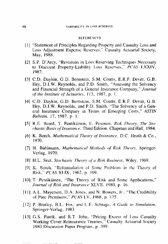
98 VARtABlLlTY IN LOSS RESERVES
REFERENCES
[l] “Statement of Principles Regarding Property and Casualty Loss and Loss Adjustment Expense Reserves,” Casualty Actuarial Society, May, 1988.
[2] S.P. D’Arcy, “Revisions in Loss Reserving Techniques Necessary to Discount Property-Liability Loss Reserves,” PCAS LXXIV, 1987.
[3] C.D. Daykin, G.D. Bernstein, S.M. Coutts, E.R.F. Devitt, G.B. Hey, D.I.W. Reynolds, and P.D. Smith, “Assessing the Solvency and Financial Strength of a General Insurance Company,” Journal of the Institute of Actuaries, I 13, 1987. p. 1.
[4] C.D. Daykin, G.D. Bernstein, S.M. Coutts, E.R.F. Devitt, G.B. Hey, D.I.W. Reynolds, and P.D. Smith, “The Solvency of a Gen- eral Insurance Company in Terms of Emerging Costs.” ASTZN Bulletin, 17, 1987, p. I.
[5] R.E. Beard, T. Pentiktiinen, E. Pesonen, Risk Theory, The Sto- chastic Basis uflnsurance, Third Edition. Chapman and Hall, 1984.
[6] K. Borch, Mathematical Theor?, @‘Insurance, D.C. Heath & Co., 1970.
[7] H. Biihlmann, Mathematicd Methods of Risk Theory, Springer- Verlag, 1970.
[8] H.L. Seal, Stochastic Theory of’ (1 Risk Bl4siness, Wiley, 1969.
[9] K. Borch, “Reformulation of Some Problems in the Theory of Risk,” PCAS XLIX, 1962. p. 109.
[ lo] T. Pentiktiinen, “The Theory of Risk and Some Applications,” Journal @‘Risk und /nsurtmce XLVII. 1980, p. 16.
[l l] A.L. Mayerson, D.A. Jones, and N. Bowers, Jr.. “The Credibility of Pure Premiums,” PCAS LV, 1968, p. 175.
[ 121 P. Bratley, B.L. Fox, and L. E. Schrage, ,4 Cr4ide to Simulation, Springer-Verlag , 1983.
[13] G.S. Patrik, and R.T. John, “Pricing Excess of Loss Casualty Working Cover Reinsurance Treaties,” Casualty Actuarial Society 1980 Discussion Paper Program, p. 399.
VARIABILITY IN LOSS RESERVES 99
[14] G.G. Venter, “Transformed Beta and Gamma Distributions and Aggregate Losses,” PCAS LXX, 1983, p. 156.
[ 151 T. Pentikainen, “Approximative Evaluation of the Distribution Function of Aggregate Claims,” ASTIN Bulletin 17, 1987, p. 15.
[ 161 Hon-Shiang Lau, “An Approach for Estimating the Aggregate Loss of an Insurance Portfolio,” Journal of Risk and Insurance LI, 1984, p. 20.
[ 171 S. Philbrick, “An Alternative Approach to Estimating Aggregate Loss Distributions,” The Actuarial Review, v. 14, 1987, no. 3, p. 8.
[18] P.E. Heckman and G.G. Meyers, “The Calculation of Aggregate Loss Distributions from Claim Severity and Claim Count Distri- butions,” PCAS LXX, 1983, p. 22.
[ 191 H. Panjer, “Recursive Evaluation of a Family of Compound Dis- tributions,” ASTIN Bulletin, 12, 1981, p. 22.
[20] B. Sundt, and W. Jewel], “Further Results on Recursive Evaluation of Compound Distributions,” ASTIN Bulletin, 12, 1981, p. 27.
[21] G. Willmot, “Mixed Compound Poisson Distributions,” ASTIN Bulletin, 16, 1986, p. S59.
[22] F. Ashe, “An Essay at Measuring the Variance of Estimates of Outstanding Claim Payments,” ASTIN Bulletin, 16, 1986, p. S99.
[23] T. Pentikainen and J. Rantala, “Runoff Risk as a Part of Claims Fluctuation,” ASTIN Bulletin, 16, 1986, p. 113.
[24] J.N. Stanard, “A Simulation Test of Prediction Errors of Loss Reserve Estimation Techniques,” PCAS LXXII, 1985, p. 124.
[25] R.V. Hogg and S.A. Klugman, Loss Distributions, Wiley, 1984.
[26] J. Aitchison and J.A.C. Brown, The Lognormal Distribution With Special Reference to its Uses in Economics, Cambridge University Press, 1969.
[27] E.W. Weissner, “Estimation of the Distribution of Report Lags by the Method of Maximum Likelihood,” PCAS LXV, 1978, p. 1.
100 VARIABILITY IN I.OSS RESERVES
[28] J.D. Cummins and L.J. Wiltbank, “Estimating the Total Claims Distribution Using Multivariate Frequency and Severity Distribu- tions,” JourrwI oj’Risk and Insurance L, 1983, p. 377.
1291 J.D. Cummins and L.J. Wiltbank. “A Multivariate Model of the Total Claims Process,” ASTIN Bulletin 14, 1984, p. 45.
[30] G.G. Meyers and N. Schenker, “Parameter Uncertainty in the Col- lective Risk Model,” PCAS LXX, 1983, p. Il.
[31] G.G. Venter, “Scale Parameter Mixing with Heavy Tailed Loss Distributions,” Unpublished. 1985.
1321 D. Skumick, “A Survey of Loss Reserving Methods.” PCAS LX, 1973, p. 16.
[33] J.R. Berquist and R.E. Sherman, “Loss Reserve Adequacy Testing: A Comprehensive, Systematic Approach.” PCAS LXIV, 1977, p. 123.
[ 34) G .C. Taylor, Claim Reserving in Non-l$) Irzsldr(lrzce, North-Hol- land. 1986.
[35] G.C. Taylor, “Regression Models in Claims Analysis I: Theory,” PCAS LXXIV, 1987, p. 354.
[36] P. DeJong and B. Zehnwirth, “Claims Reserving. State-space Mod- els and the Kalman Filter,” Journul of the Institute qf Actuaries, 110, 1982, p. 157.
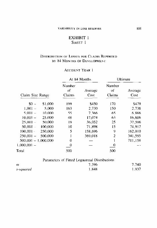
VARIABILITY IN LOSS RESERVES 101
EXHIBIT 1 SHEET 1
DISTRIBUTION OF LOSSES FOR CLAIMS REPORTED BY 84 MONTHS OF DEVELOPMENT
Claim Size Range
$0 - $1,000 1,001 - 5,000 5,001 - 10,000
10.001 - 25,000 25,001 - 50,000 50,001 - 100,000
100.001 - 250.000 250,001 - 500,000 500,001 - 1.000.000
I ,000,001 -
Total
ACCIDENT YEAR I
At 84 Months
Number of Average
Claims CO9
199 $450 163 2,730 55 7,366 48 17,074 19 36,052 IO 71,898 5 158.696 1 369,0 I 8 0 - 0 -
500
Ultimate
Number of
Claims Average
cost
170 $479 150 2,738 65 6,866 63 16,606 25 37,506 I5 74,917 9 162,010 2 341,595 I 71 1,158 0 -
500
m s-syuur-ed
Parameters of Fitted Lognormal Distributions 7.396 I .848
7.740 1.937
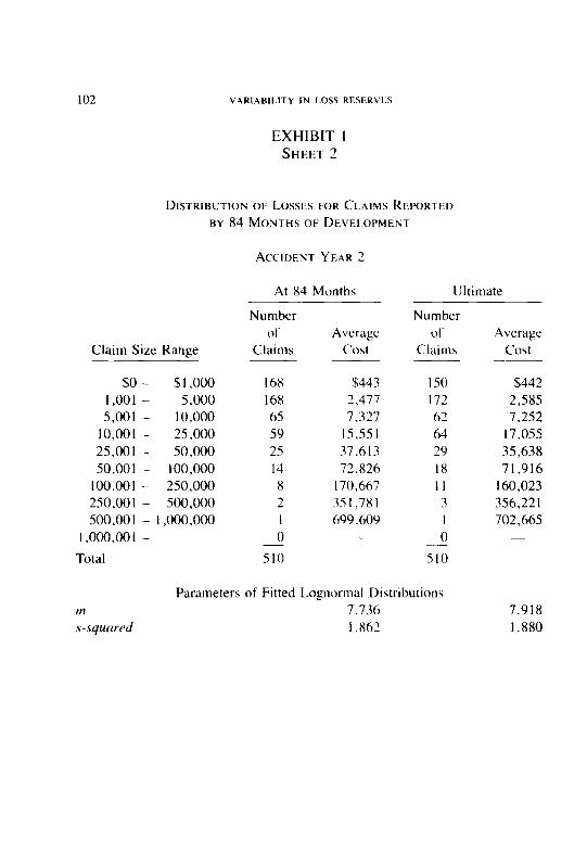
102 VARIABILITY IN LOSS RESERVES
EXHIBIT I SHEET 2
DK~RIBIJTION OF LOSSES FOR CLAIMS RWQRTED BY 84 MONTHS OF DEVELOPMENT
Claim Size Range
$0 - $1,000 1,001 - 5,000 5,001 - 10,000
10,001 - 25 .OOO 25,001 - 50,000 50,001 - 100,000
100.001 - 250,000 250,001 - 500,000 500,001 - 1,000,000
1,000,001 -
Total
ACCIDENT YEAR 2
At 84 Months
Number 01
Claims Average
cost
16X $443 168 2,477 65 7,327 59 15,55 I 25 37,613 14 72,826 8 170,667 2 351.781 I 699,609 0 -
510
Ultimate
Number ol
Claims Average
cost
150 $442 172 2,585 62 7,252 64 17,055 29 35,638 I8 71,916 II 160,023 3 356,221 I 702,665 0
5 I 0
m s-squared
Parameters of Fitted Lognormal Distributions 7.736 I.862
7.918 1.880
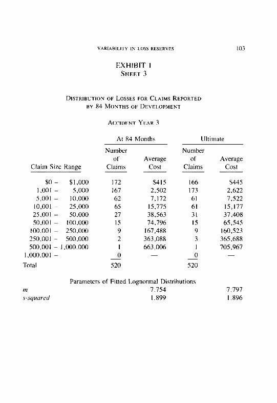
VARIABILITY IN LOSS RESERVES 103
EXHIBIT 1 SHEET 3
DISTRIBUTION OF LOSSES FOR CLAIMS REPORTED BY 84 MONTHS OF DEVELOPMENT
Claim Size Range
$0 - $1,000 1,001 - 5,000 5,001 - 10,000
10,001 - 25,000 25,001 - 50,000 50,001 - 100,000
100,001 - 250,000 250,001 - 500,000 500,001 - I ,ooo,oOO
I ,ooo,oo I -
Total
ACCIDENT YEAR 3
At 84 Months
Number of
Claims Average
cost
172 $415 167 2,502 62 7, I72 65 15,775 27 38,563 I5 74,796 9 167,488 2 363,088 I 663,006 0
520
Ultimate
Number of
Claims Average
cost
166 $445 173 2.622 61 7,522 61 15,177 31 37,408 I5 65,545 9 160,523 3 365,688 1 705,967 0
520
Parameters of Fitted Lognormal Distributions 7.754 1.899
7.797 I .896
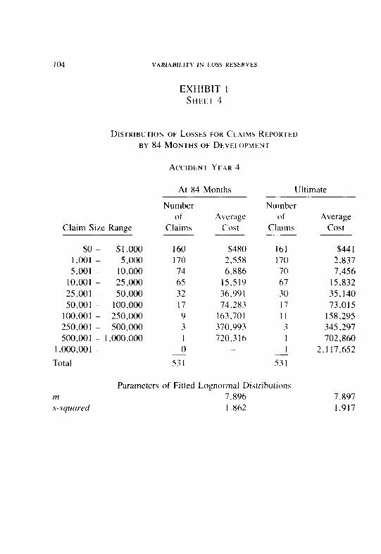
104 VARIABILITY IN I.OS.5 RISERVtS
EXHIBIT 1 SHt:kI 4
DISTRIBUTION OF LWSES FOR CLAIMS REPORTED BY 84 MON.I-HS OF DEL’EI OPM~;N'T
Claim Size Range
$0 - $1,000 I.001 - 5,000 5,001 - 10,000
10,001 - 25,000 25,001 - 50,000 50,001 - 100,000
100.001 - 250,000 250,001 - 500,000 500,001 - 1,000.000
1,000,001 -
Total
ACCIDEN r Y~.AR 4
At X4 Months
Number of
Claims Average
cost
160 $480 170 2,558 74 6.886 65 15,519 32 36,991 17 74.283 Y 163.701 3 370.993 I 720.3 I6 0
531
Ultimate
Number of
Claims Average
cost
I61 $44 I 170 2,837 70 7,456 67 15,832 30 35,140 17 73,015 II 158,295 3 345,297 I 702,860 I 2, I 17,652
531
Parameters of Fitted Lognormal Distributions 7.X96 I .X62
7.897 I.917
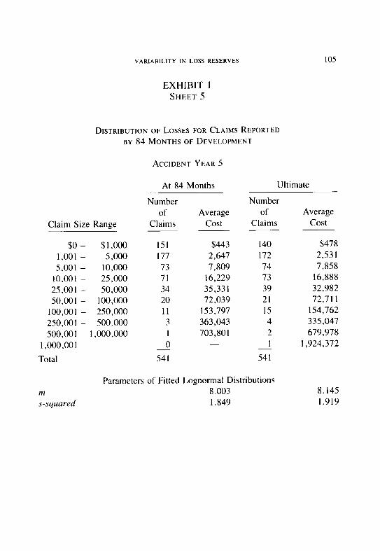
VARIABILITY IN LOSS RESERVES
EXHIBIT 1 SHEET 5
DISTRIBUTION OF LOSSES FOR CLAIMS REPORTED BY 84 MONTHS OF DEVELOPMENT
105
Claim Size Range
$0 - $ I ,000 1,001 - 5,000 5,001 - 10,000
10,001 - 25,000 25,001 - 50,000 50,001 - 100,000
100,001 - 250,000 250,001 - 500,000 500,001 - I ,ooo,ooo
1,000,001 -
Total
ACCIDENT YEAR 5
At 84 Months Ultimate
Number of
Claims Average
cost
Number of
Claims Average
cost
I51 $443 I77 2,647 73 7,809 71 16,229 34 35,331 20 72,039 II 153,797 3 363,043 I 703,801 0
541
140 $478 172 2,531 74 7,858 73 16,888 39 32,982 21 72,711 I5 154,762 4 335,047 2 679,978 I I ,924,372
541
m
s-squared
Parameters of Fitted Lognormal Distributions 8.003 1.849
8.145 I .919
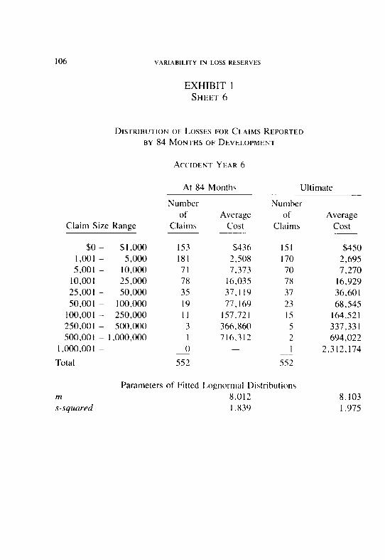
106 VARIABILITY IN LOSS RESERVES
EXHIBIT 1 SHEET 6
DISTRIBUTION OF LOSSES FOR CLAIMS REPORTED BY 84 MONI‘HS OF DEVELOP~IENT
Claim Size Range
$0 - $ I ,000 I.001 - 5,000 5,001 - 10,000
10,001 - 25,000 25,001 - 50,000 50,001 - 100,000
100,001 - 250,000 250,001 - 500,000 500,001 - 1,000,000
I ,ooo.oo I -
Total
AKIDENI YEAR 6
At 84 Months
Number of
Claims Average
cost
I53 $436 181 3.50x 71 7,373 78 16,035 35 37,119 19 77.169 II 157,721 3 366,860 I 716.312 0
552
Ultimate
Number Of
Claims Average
cost
I51 $450 I70 2,695 70 7,270 7x 16,929 37 36,601 23 68,545 15 164,521 5 337,331 2 694,022 I 2,312,174
552
m
s-squared
Parameters of Fitted Lognormal Distributions 8.012 I .x39
8.103 1.975

VARIABILITY IN LOSS RESERVES
EXHIBIT 1 SHEET 7
DISTRIBUTION OF LOSSES FOR CLAIMS REPORTED BY 84 MONTHS OF DEVELOPMENT
107
Claim Size Range
Number of
Claims Average
cost
$0 - $1,000 140 $466 1,001 - 5,000 187 2,697 5,001 - 10,000 72 7,144
10,001 - 25,000 74 15,859 25,001 - 50,000 42 38,555 50,001 - 100,000 26 73,586
100,001 - 250,000 I4 158,619 250,001 - 500,000 5 364,353 500,001 - I ,ooo,ooo 2 721,218
1,000,001 - I 2,128,700
Total 563
ACCIDENT YEAR 7
At 84 Months Ultimate
Number of
Claims Average
cost
149 $468 I83 2,587 72 8,010 77 16,430 37 34,613 23 72,933 I5 156,530 4 343,411 2 736,468 1 2,045,068 -
563
m
s-squared
Parameters of Fitted Lognormal Distributions 8.180 I .909
8.105 1.923
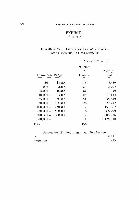
10X VARIARII.ITY IN I OSS RESkRVI5
EXHIBIT I SHEl:I’ 8
DISTKIBUTION OF LOSSES FOR CI AIMS REPORI’EI> BY 84 MON OHS 01: DEVF.I OPMI:W
Accident Year I Y8 I
Claim Size Range
Number of
Claims
$0 - $ I,000 1,001 - 5 ,ooo 5,001 - 10,000
10,001 - 25.000 2S,ool - 50.000 50,001 - 100,000
100,001 - 250.000 250,001 - 500.000 500,001 - I .ooo.ooo
1,000,001 -
Total
IIX IX3 x4 86 51 26 I7 6 2 1
456
Average Cost
$45’) 2,707 7,Y4Y
17.1 I4 3.5.679 72,272
151.062 366.2YY 685,736
2.126.918
Parameters of Fitted Lognormal Dictributions 111 8.41 I s-srpured I.835
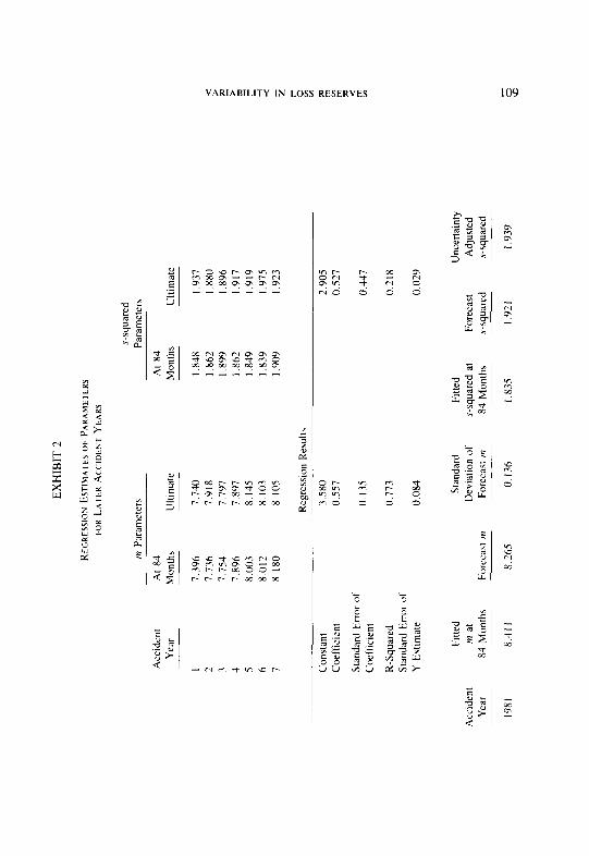
VARIABILITY IN LOSS RESERVES 109
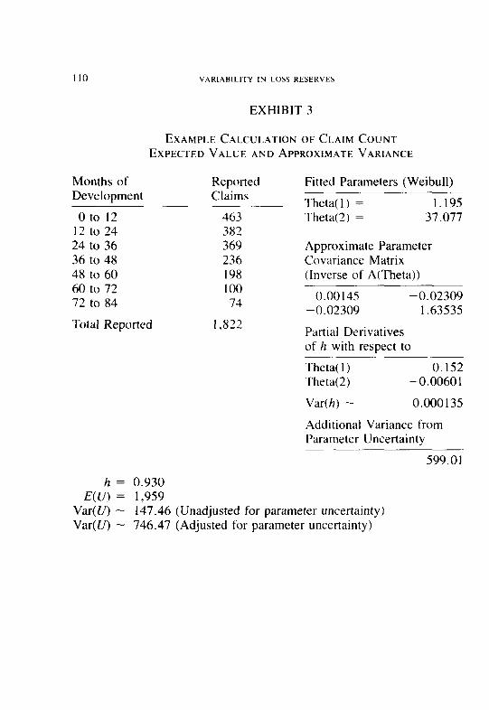
110 VARIABILITY IN LOSS KESERVES
EXHIBIT 3
Months of Reported Development Claims
EXAMPLE CALCULATION OF CI.AIM COUNT EXPECTED VALUE AND APPROXIMATE VARIANCE
Oto 12 463 12 to 24 382 24 to 36 369 36 to 48 236 48 to 60 198 60 to 72 100 72 to 84 74
Total Reported 1,822
Fitted Parameters (Weibull)
Theta( 1) = 1.195 Theta(2) = 37.077
Approximate Parameter Covariance Matrix (Inverse of A(Theta))
0.00145 -0.02309 -0.02309 1.63535
Partial Derivatives of h with respect to
Theta( 1) 0.152 Theta(2) -0.00601
Var(h) - 0.000135
Additional Variance from Parameter Uncertainty
599.01
h = 0.930 E(U) = 1,959
Var(U) - 147.46 (Unadjusted for parameter uncertainty) Var(U) - 746.47 (Adjusted for parameter uncertainty)
111
DETERMINATION OF OUTSTANDING LIABILITIES FOR UNALLOCATED LOSS ADJUSTMENT EXPENSES
WENDY JOHNSON
Abstract
Little has been published to date on the determination of outstanding liabilities for unallocated loss adjustment expen- ses (ULAE). The only method mentioned in the literature is the calendar year paid-paid method, and upon reJection it is apparent that this method will only give good results for vet-q short-tailed, stable lines of business. This paper presents a conceptual approach to estimating MAE liabilities which is significantly more flexible, based directIF on claim reporting and closure patterns, and which allo,ls one to take into direct consideration changes in claim department operating cost levels. The paper describes the approach using an example from medical malpractice insurance, and discusses and eval- uates the sensitiviq of the results to specific factors in the claim settlement environment.
Little has been published to date on the determination of outstanding liabilities for unallocated loss adjustment expenses. To a large extent, this may be because the attentions of insurance company management and the actuary are usually directed to the much larger and therefore more important outstanding liabilities for losses and allocated loss ad- justment expenses. For example, typical ratios of paid ULAE to paid loss and allocated loss adjustment expenses (ALAE) range from four to twenty percent. However, when the subject does become the focus of attention for any reason, the actuary has few sources for ideas on how to estimate the liability.
The classical method, according to such recognized experts as Strain and Salzmann [I], has been to base the ULAE reserve on the ratio of calendar year ULAE payments to calendar year loss payments. Using the assumption that 50% of the ULAE is paid when the claim is opened and the other 50% when it is closed, the ULAE reserve is set by applying 50% of the historical ratio of paid ULAE to paid loss to the full out- standing loss reserve, and 50% of the same ratio to the IBNR reserve.
112 UNALLOCATED LOSS ADJUSTMENT EXPENSES
This method came into use at a time when most lines developed in well under five years, cost inflation was low and level if it existed at all, most calculations were made using only pencil and paper, and claim reporting and payment patterns were stable. We no longer live in this kind of environment. Our estimation methods should be adapted to fit the current environment and grounded firmly in our understanding of the claims process, even for estimation of peripheral liabilities like ULAE.
The conceptual approach to be presented in this paper relies on a claim reporting pattern and a claim closure pattern. It allows the actuary to recognize directly the sixteen considerations in setting loss reserves enumerated in the Casualty Actuarial Society ‘Statement of Principles Regarding Property and Casualty Loss and Loss Adjustment Expense Liabilities.” The actuary must have available historical calendar year ULAE payments, historical numbers of open claims at year end, and historical numbers of claims opened during the year. This data is some- what more extensive than that required for the Annual Statement, which does not require numbers of claims opened during a year or historical calendar year ULAE payments. However, it is data that is also highly useful for evaluating loss reserves, and the historical calendar year ULAE payments can usually be obtained from successive Schedules 0 and P.
To see how the approach can be applied, consider an example from some medical malpractice data from a state with a relatively low level of litigation activity. Like many medical malpractice carriers, the com- pany from which this data was derived was formed in the late 1970’s, so the lirst several years of data presented arose while the company was just getting started.
Exhibit 1 shows the first scvcral steps in the application of the approach. The underlying assumption is that ULAE will be incurred throughout the life of the claim, from the time that it is reported until it is closed, but that the effort associated with maintaining the claim tile will be twice as great in the tirst year as in subsequent years. Thus, it there were no inflation in claim department expense levels. ULAE in the year in which the claim tile is opened would bc twice as great as in any subsequent year. This assumption seems to have some factual basis for this particular body of data, based on conversations with company claims personnel.
The example in the exhibit does not, of course, precisely reflect this assumption because it makes no allowance for the claims closed within
UNALLOCATED LOSS ADJUSTMENT EXPENSES 113
the year. This could be of greater significance for lines with shorter tails than medical malpractice. One simple modification would be to use the average of the numbers of claims open at year end and the number of claims open at the previous year end. Another might be to assume that all claims open at the end of one year continue to be open throughout the subsequent year. More sophisticated modifications could also be developed. One might assume, for example, that the effort associated with maintaining the claim file will be twice as great in both the year in which the claim is opened and the year it is closed. Other modifications may be necessary in situations where the line of business is growing rapidly or the claim disposal rate is changing.
The calculations are based on the assumption that unallocated loss adjustment expenses have little or nothing to do with the nature of particular claims; ULAE are effectively file maintenance costs. For some companies that make use of internal counsel and do not allocate claim defense expenses according to New York Rule 42 this assumption will not be appropriate. In these cases, either the approach must be modified or an allocation procedure for defense expenses must be devised. For example, the internal counsel staff could charge their time to the various files on which they work, at a rate commensurate with their salary and benefits costs.
The exhibit shows that historical calendar year ULAE payments from the Annual Statement are divided by the historical numbers of weighted open claims to determine the historical expense per weighted open claim. The historical numbers of weighted open claims are the sums of the historical numbers of open claims at year end, and the historical numbers of claims opened during the year, in keeping with the underlying as- sumption stated above. They are called “weighted” because there is essentially twice as much weight assigned to the newly opened claims as to the already open claims.
It should be emphasized that other assumptions about the relative ULAE payment levels throughout the life of the claim could very well be appropriate. The important point is that the approach can easily be tailored to a variety of assumptions. The assumption used here seems to be appropriate for this body of data and the exposure from which it arose. One of the problems with unallocated loss adjustment expenses is that it is difficult to test one’s assumptions about them because the expenses by definition are generally hard to allocate and therefore hard
114 UNALLOCATED LOSS ADJUSTMENT EXPENSES
to track. The only real way that comes to mind to test assumptions would be to conduct a claim expense study, such as a time and motion study, which establishes artificial expense allocation procedures for a temporary time period.
Exhibit 1 shows that the historical expenses per open claim for this company show a rather dramatic upward trend of 17.4% per year. While a trend of this magnitude is not surprising for medical malpractice losses, it is surprising for ULAE. It is possible that other choices of cost weightings for newly opened, closing, and ongoing claims would have yielded slightly different expense trends, and thus different estimates of outstanding ULAE liabilities. However, it is rather apparent in this particular example that the company has a high claim expense cost trend, and different weightings in applying the approach will not change that conclusion. One of the first benefits of the method is that it highlights claim department cost levels from a possibly different viewpoint, and may help management to identify areas where costs are out of control.
Exhibit 2 shows the way the claims arising from accident years prior to December 31, 1986 (the date at which the outstanding liability is being estimated) can be expected to be reported and settled, based on the claim reporting and closure patterns developed for the data. Again, the weighted totals are the sums of the numbers of open claims at each year end and the numbers of claims opened during the year. The numbers of claims for each year have been rounded to the nearest whole number. After 1991, the assumption is that no new claims will be reported, so the numbers of open claims at each year end are not adjusted.
It should be clear, from the year by year unfolding of the numbers of open claims at year end and numbers of claims opened during the year, that it is possible to assume more complicated claim reporting and payment patterns which allow for varying proportions of claims to be reported, reopened, and closed from year to year. For example, if tort reform legislation could be expected to reduce the numbers of claims reported after a certain date, then the effects of that legislation could be taken into consideration directly when using this approach.
The estimated outstanding liability is calculated in Exhibit 3, based on the observed expense cost trend of 17.4% per year. The weighted numbers of open claims for each future year are multiplied by the estimated cost per claim for that year, and the total outstanding liability is the sum of the products for each year.
UNALLOCATED LOSS ADJUSTMENT EXPENSES 115
If it can be assumed that the company can control its expense cost levels more carefully in the future, the approach can easily be modified to allow for a lower expense cost trend. Exhibit 4 shows the outstanding liability that results if the assumed expense cost trend is 5%.
An example of the results of the approach if the numbers of late- reported claims are drastically reduced is given in Exhibit 5. The weighted numbers of open claims for each of the future years have been calculated assuming that only half as many claims will be reported after l2/3 1186 for each accident year and reporting period.
Exhibit 6 shows the results of the application of the classical calendar year paid-paid method to the same body of data. Note that the observed historical ratio of ULAE payments to loss payments is very high, on the order of 20%. The ratio is so high because the ultimate loss dollars for each accident year are being paid out much more slowly than the unal- located expense dollars. This would tend typically to be true for very long-tailed lines like medical malpractice, but it would also be true for newly established or rapidly growing lines of business in highly infla- tionary loss cost environments.
The exhibit shows that the outstanding liability estimate resulting from the classical ULAE method is significantly greater than that from the approach presented here. This is the result of the very high observed ratio of ULAE to loss payments, which in turn is a result of the fact that the larger claims typically take longer to settle. Even though the alternate approach presented here relies on the assumption that less than 50% of the ULAE are paid in the year in which the claim is opened in a long- tail line, it provides a lower estimated outstanding liability than the classical method because the ULAE are not assumed to be proportional to the loss payments. The difference is that the classical method relies on the assumption that much of the ULAE are paid when the claim is paid, while the approach presented here relies on the assumption that there are ongoing expenses associated with maintaining a claim file.
What is really at issue in reviewing the different results provided by the two methods is the allocation of calendar year ULAE payments between claims outstanding at any given point in time and newly arising claims. When thought of in this way another variation in the approach immediately comes to mind. For many smaller companies, the claims department staff, and therefore the unallocated expenses, are relatively fixed. Unless the company changes significantly in size, no new person-
116 UNALLOCATED LOSS ADJUSTMEN I’ tXPtNSES
nel will be hired or office space acquired. Thus it may be reasonable to think in terms of a fixed rate of ULAE payments over the next several years, perhaps increasing at a moderate rate commensurate with increases in the cost of living. Then estimating the outstanding liability becomes a matter of estimating the proportion of the total numbers of open claims on the books in future years that will be attributable to past years. This is shown in Exhibit 7.
The approach presented here leads naturally to a method of allocating the outstanding liability to accident year. The calculation is shown in Exhibit 8. Currently the NAIC requires its own specific allocation pro- cedure, a variation of the classical 50-50 rule. ULAE reserves determined using the approach presented in this paper but booked into the Annual Statement according to its rules will show adverse runoff according to that procedure, both in total and by accident year and sometimes signif- icantly so. This may require explanation to the regulators.
In conclusion, this paper has presented an approach to the calculation of the outstanding liability for unallocated loss adjustment expenses. The approach is straightforward, flexible. and makes use of relevant, readily available data. It also gives results significantly different in many cases from those of the classical method generally in use.
Of course, medical malpractice data typically has many extreme characteristics, but actuarial methods should be flexible enough to handle the extreme cases. In many respects, the extreme cases are the best tests of whether a method or approach has been developed to a sufficient level of detail.
REFERENCES
[I] Robert W. Strain, Propru~-Liclhiliry /ns~-unce Accounting, New York: The College of Insurance, 1984, p. 82 and p. 189.
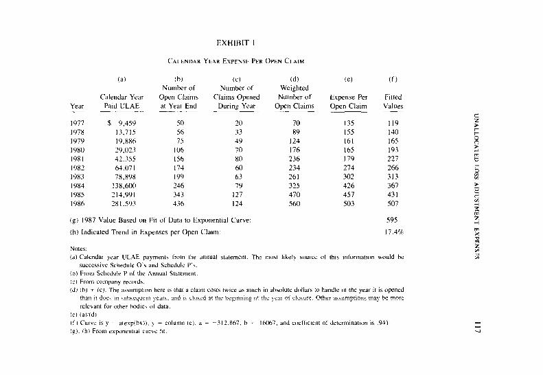
(a)
Calendar Year Year Paid ULAE -
(b) Number of
Open Claims at Year End
(c-1 Number of
Claims Opened During Year
Cd) Weighted
Number of
Open Claims
(e) (f)
Expense Per Open Claim
Fitted Values
I977 % 9,459 50 20 70 135 119 1978 13,715 56 33 89 IS.5 140 1979 19.886 7s 49 124 161 165 1980 29,023 106 70 176 165 193
1981 42.355 IS6 80 236 179 227
19x2 64.071 174 60 234 214 266
1983 78,898 199 63 261 302 313
1984 138.600 246 79 325 426 367
I985 214.991 343 127 470 451 431
1986 28 I.593 436 124 560 503 507
EXHIBIT I
CALENDAR YEAR EXPENSE PER OPEN CLAIM
(g) 1987 Value Based on Fit of’ Data to Exponential Curve:
(h) Indicated Trend in Expenses per Open Claim:
Notes:
595
17.4%
(a) Calendar year ULAE payments from the annual statement. The most likely source of rhls mtormation would be
successive Schedule O’s and Schedule P‘r
(b) From Schedule P of the Annual Statement. Cc) From company records.
Cd) tb) + tel. The assumption here IS that a clann costs twice a> much in absolute dollars to handle in the year it IS opened
than it does in subsequent years. and is closed at the begmnmg of the year of closure. Other assumptmns may be more
relevant for other bodic\ of data
lr) (a)/(d)
ti) Curve IS y = atexpcbx)). 4 = column tel. a = -3 12.867. h = .16067. and coefticlent of determmatmn is ,941.
lg). th) From exponential curve fit.
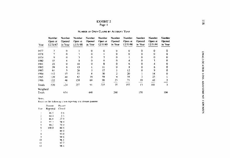
EXHIBIT 2
Page I
Number
Open ar YeaI 12/31/X7
I977 3 1978 7 I WY 9 1980 IS l9Ri 23
I982 39 1983 61
1984 112
19x.5 139 I986 I22
T01al5 530
Weighted
‘roral\
Number Number
Opened open at
1” Year 12131188
Opened
in Year
Number Number Number Open at Opened Open at
I2/3 I189 in Year 12/31/90
0 0 0 4 0 x 5
IS 44
4x
I24
653
3 3
8
IO
IS 26
51
x2
IS8
3 8
I9
60
0
3 6
8
II I7
30
s9
9R
2 9
23
3S7 233 35
268
0 0 I
4
6 8
I2
20 35
71
IS7
Number Number
Opened Open at
in Year 12/31/91 - -
0 0
0 0 0 0
0 3
0 4
0 6
0 9
I I4 2 23
IO 42
I3 Gl
170
2
3
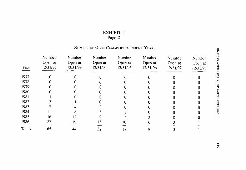
EXHIBIT 2 Page 2
Year
1977 1978 1979 1980 1981 1982 1983 1984 198.5 1986
Totals
Number Number Number Number Number Number Open at Open at Open at Open at Open at Open at 1213 1 I92 1213 l/93 I 213 l/94 1213 1195 1213 1 I96 1213 1197
0 0 0 0 0 0 0 0 0 0 0 0 0 0 0 0 0 0 0 0 0 0 0 0 1 0 0 0 0 0 3 1 0 0 0 0 7 4 3 0 0 0
11 8 5 3 0 0 16 12 9 5 3 0 27 19 15 IO 6 3
65 44 2 18 9 3
NUMBER OF OPEN CLAIMS BY ACCIDENT YEAR 2 F
Number E Open at ; 12131198 fi
w
0 1 - 1
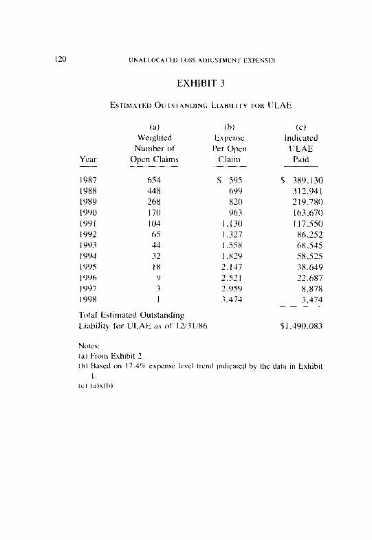
120 UNALLOCATED LOSS ADJUSTMENT tiX1’ENSF.S
1987 IO88 19x9 1990 1Y91 19Y2 I YY3 1994
654 $ 595 $ 38Y,l30 448 699 312,941 268 820 219,780 170 93 163,670 104 I. I30 117.550 65 1,327 X6.252 44 I.558 68,545 32 I ,x2’) 58,525
I YYS 18 2.147 38,649 1996 9 2.521 22,687 1Y97 3 2.YSV 8,878 1998 1 3.474 3,474
Total Estimated Outstanding Liability for ULAE as of 12/31/X6 $1.4YO,OX3
EXHIBIT 3
ESTIMATKD OUTSTANDING LIAHIL.ITY FOR ULAE
Year
(a) Weighted
Number of Open Claims
(b) Expense
Per Open Claim
(cl Indicated
ULAE Paid
Notch: (a) From Exhibit 2. (b) Bawd on 17.3% expense Icvel trend indicated bq’ the data in Exhibit
I. (CJ lLiJX(hJ
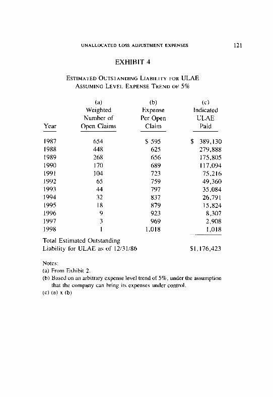
1987 654 $ 595 $ 389,130 1988 448 625 279,888 1989 268 656 175,805 1990 170 689 I 17,094 991 104 723 75,216 992 65 759 49,360 993 44 797 35,084 994 32 837 26,791 995 18 879 15,824 996 9 923 8,307
3 969 2,908 I 1,018 1,018
Total Estimated Outstanding Liability for ULAE as of 12/31/86 $1,176,423
1997 1998
UNALLOCATED LOSS ADJUSTMENT EXPENSES 121
EXHIBIT 4
ESTIMATED OUTSTANDING LIABILITY FOR ULAE ASSUMING LEVEL EXPENSETRENDOF~YC
Year
(4 Weighted
Number of Open Claims
(b) Expense Per Open
Claim
(cl Indicated ULAE Paid
Notes: (a) From Exhibit 2. (b) Based on an arbitrary expense level trend of 5%, under the assumption
that the company can bring its expenses under control. (cl (a) x (b)
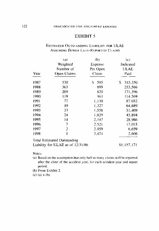
122 UNALLOCATED LOSS ADJUSTMENT EXPENSES
Year
1987 1988 1989 1990 1991 1992 1993 1994 I995 1996 1997 1998
EXHIBIT 5
ESTIMATED OUTSTANDING; LIABILITY FOR ULAE ASSUMING FEWER LA ISREPORTED CI.AIMS
(a) (b) CC) Weighted Expense Indicated
Number of Per Open ULAE ODen Claims Claim Paid
530 363 209 119 77 49 33 24 I4
2
$ 595 $ 315,350 699 253,566 820 171,396 963 114.569
1,130 87,032 I .327 64,689 1,558 5 I ,409 1,829 43,894 2.147 28,986 2.521 17,015 2.959 6,659 3,474 2,606
Total Estimated Outstanding Liability for ULAE as of l2/3 l/86 $l.l57,171
Notes: (a) Based on the assumption that only half as many claima will be reported
after the close of the accident year. for each accident year and report period.
(b) From Exhibit 2. Cc) (a) x (b)
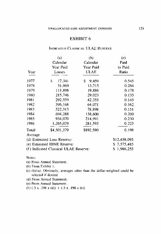
Year
I977 1978 1979 1980 1981 I982 1983 I984 1985 1986
(a) (b) (c) Calendar Calendar Paid Year Paid Year Paid to Paid
Losses ULAE Ratio
$ 17,341 $ 9,459 0.545 5 1,969 13,715 0.264
1 I 1,898 19,886 0.178 215,746 29,023 0.135 292,559 42,355 0. I45 396, I68 64,071 0.162 522,3 I3 78,898 0.151 694,288 138,600 0.200 934,070 214,991 0.230
I ,265,029 28 1,593 0.223
$4,501,379 $892,590 0.198 Total/ Average (d) Estimated Loss Reserve: $12,458,095 (e) Estimated IBNR Reserve: $ 7,575,485 (f) Indicated Classical ULAE Reserve: $ 1,986,255
UNALLOCATED LOSS ADJUSTMENT EXPENSES 123
EXHIBIT 6
INDICATED CLASSICAL ULAE RESERVE
Notes: (a) From Annual Statement. (b) From Exhibit I. (c) (b)/(a). Obviously, averages other than the dollar-weighted could be
selected if desired. (d) From Annual Statement. (e) From Annual Statement. (f) (..5 x .I98 x (d)) + (.5 x ,198 x(e))
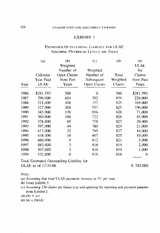
124 UNALLOCATED LOSS ADJUSI~MEN’~ EXPENSF3
Year
Calendar Year Paid
ULAE
1986 $28 1,593 1987 296.000 1988 3 I I ,000 1989 327.000 1990 343,000 1991 360,000 1992 378,000 1993 397,000 1994 417.000 I995 438.000 1996 460,000 1997 483,000 1998 507,000 1999 532,000
EXHIBIT 7
ESTIMATED OUTSTANDING LIAHIIJTY FOK ULAE ASSUMING OVERHEAD LEL’EIS ARK FIXED
(a) lb) Weighted
Number of Open Claims
from Past Years
560 654 448 268 170 104 65 44 32 18 9 3
0
(c)
Weighted Number of Subsequent
Open Claims
Total Weighted
Claims
(e) ULAE
for Claims
from Past Years
0 560 $28 1,593 202 856 226,000 377 825 169,000 557 825 106,000 656 826 71,000 722 826 45,000 758 823 30,000 780 824 21,000 795 827 16,000 807 825 10,000 812 821 5,000 816 819 2,000 818 819 I ,000 818 818 0
(d)
Total Estimated Outstanding Liability for ULAE as of 1213 1186 $ 702,000
Notes: (a) Assuming that total ULAE payments increase at 5% per year (b) From Exhibit 3. (c) Assuming 220 claims per future year and applying the reporting and payment patterns
from Exhibit 2. (4 (b) + (cl (e) (a) x (b)/(d)
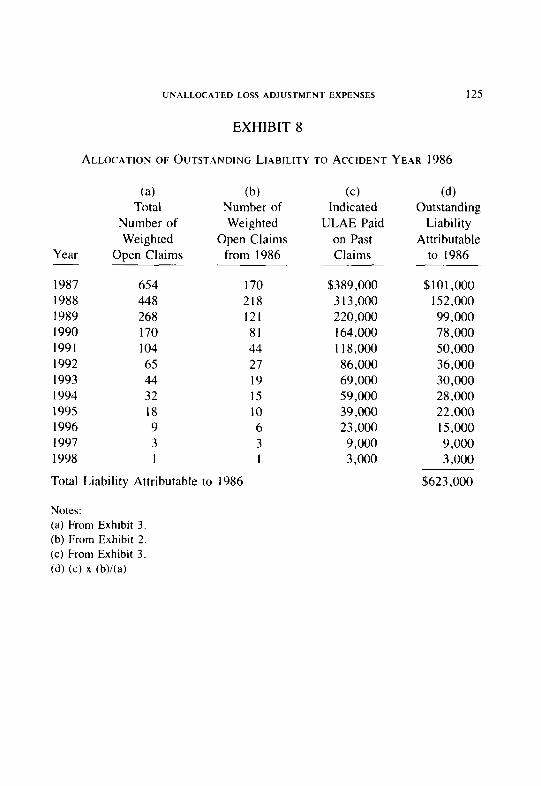
Year
(4 (b) (cl (4 Total Number of Indicated Outstanding
Number of Weighted ULAE Paid Liability Weighted Open Claims on Past Attributable
Open Claims from 1986 Claims to 1986
1987 654 170 $389,000 $101,000 1988 448 218 313,000 152,000 1989 268 121 220,000 99,000 1990 170 81 164,000 78,000 1991 104 44 I 18,000 50,000 1992 65 27 86,000 36,000 1993 44 19 69,000 30,000 1994 32 15 59,000 28,000 1995 18 10 39,000 22,000 1996 9 6 23,000 15,000 1997 3 3 9,000 9,000 1998 1 1 3,000 3,000
UNALLOCATED LOSS ADJUSTMENT EXPENSES 125
EXHIBIT 8
ALLOCATION OF OUTSTANDING LIABILITY TO ACCIDENT YEAR 1986
Total Liability Attributable to 1986 $623,000
Notes: (a) From Exhibit 3. (b) From Exhibit 2. (c) From Exhibit 3. (4 (cl x (b)/(a)
126
THE EFFECT OF TREND ON EXCESS OF LOSS COVERAGES
CLIVE L. KEATINGE
Ahstruct
The subject (fl the eflect qf trcrd or1 EXC’~SS of‘ loss cover- ages has been &dressed quite -frequently in the Proceedings ol’er the years. Set,erul uuthors have made the point that Mdth u jixed retention und un@m trend by size oj’ loss, expected exces.s losses increase proportionally much more thun indi- cated by the general rute of injation. This is certainly true ,chen considering uncapped excess losws. but it may not he true brvhen considering a specijic Iuyer of e.vcess losses. This is because just us the eflect oj’ inflation is leivraged ut the retention, it is dampened ut the upper limit of the luger.
This paper uses gruphs to e.raminr horr) the le\leraging eflect und dumpening e$tect c.ombine to a&ct lugers of’ excess losses. This particular issue bus hi,storically received very little attention in the Proceedings. The puper begins by e.r- umining the e.we.s.s luger trenci.fact0r.s of u typiiul loss distri- bution, und then proceeds to demon.strute howl chunging each qf’ the titv parameters qf’ this distribution aflect.s the trend ,filc.tor.s. The puper then looks ut the eff2c.t of changing the t!pe of distriblrtion. Finully, the puper erumines the t@ct oj introduc,ing the concept of \wrying trend 1~~ size of loss.
The subject of the effect of trend on excess of loss coverages has been addressed quite frequently in the Proceedings over the years. Sev- eral authors have made the point that with a fixed retention and uniform trend by size of loss. expected excess losses increase proportionally much more than indicated by the general rate of inflation ([31. (41, (71, and [8]). This is certainly true when we consider uncapped excess losses, but it may not be true when we consider a specific layer of excess losses. This is because just as the effect of inflation is leveraged at the retention, it is dampened at the upper limit of the layer. The dampening effect on
TREND ON EXCESS COVERAGES 127
layer losses at the upper limit is equivalent to the dampening effect on basic limit losses at the retention.
This paper will examine how the leveraging effect and dampening effect combine to affect layers of excess losses. From a reinsurer’s point of view, it is much more meaningful to look at a layer of excess losses rather than at uncapped excess losses, since a reinsurer virtually never provides unlimited coverage excess of a retention. We will begin by examining the excess layer trend factors of a typical loss distribution, and we will proceed to observe how changing each of the two parameters of this distribution affects the trend factors. We will then look at the effect of changing the type of distribution. Finally, we will see what happens when we introduce the concept of varying trend by size of loss. Graphs will be used to illustrate the results. The formulas used in generating the graphs are shown in the Appendix. Also, it should be noted that this paper presupposes some familiarity with common loss distributions.
2. A TYPICAL DISTRIBUTION
We will first look at what might be considered a typical general liability loss distribution, a Pareto with parameters B = 10,000 and Q = I .I We will assume a general rate of inflation of 10%. The trended distribution becomes a Pareto with B = 11,000 and Q = 1 .Z Exhibit 1 shows the effect of this inflation rate on excess layers. Note that the graph uses a double logarithmic scale with retention along the x-axis and layer width along the y-axis. Each contour line represents various reten- tion-layer width combinations with equivalent multiplicative trend fac- tors.’ As expected, the trend factors increase as the retention and/or layer width increase. However, contrary to what one might expect, the trend
I The Pareto has been chosen because it is the distribution currently used by IS0 to generate increased limits factors.
2 With uniform trend, the Pareto may be trended by simply trending the R parameter and leaving the Q parameter unchanged. For more information on trending loss distributions under the assump- tion of uniform trend, see Hogg and Klugman[Sj.
i The term “layer width” is used in place of the term “limit” so as to avoid confusion with the
“limits” shown along the top and right side of the graph. Also, the contour lines on the graph are approximate. Although they do not appear completely smooth on the graph, in reality they are completely smooth.
128 TREND ON EXCESS COVERAGES
factors never increase beyond 1.10, which represents the general rate of inflation. This can be seen by examining the limits shown at the top and right side of the graph. The limits along the top are the limits for various retentions as the layer width approaches infinity. The limits along the right side are the limits for various layer widths as the retention ap- proaches infinity. The limit at the upper right corner is the limit as both retention and layer width approach infinity.J
3. CHANGING THE SCALF. PARAMETER
Exhibits 2 and 3 show what happens when we change the scale parameter B. Exhibit 2 shows how the trend factors behave when B = 1,000 and Q = 1; Exhibit 3 shows trend factor behavior when B = 100,000 and Q = 1. Note that the only significant difference between these graphs and Exhibit 1 is that the graphs are displaced slightly. Decreasing the scale parameter B moves the contour lines closer to the origin; increasing the scale parameter B moves the contour lines further away from the origin. This type of behavior can also be observed with other distributions where one parameter can be used to change the scale.5
4. CHANGING THE SHAPE PARAMETER
Exhibits 4 and 5 show what happens when we change the shape parameter Q. Exhibit 4 shows how the trend factors behave when B = 10,000 and Q = 0.5; Exhibit 5 shows trend factor behavior when B = 10,000 and Q = 1.5. Note that the trend factors are smaller with the thicker-tailed distribution of Exhibit 4 and larger with the thinner- tailed distribution of Exhibit 5. Similarly, the limits on the graphs exhibit the same pattern.6
4 11 is important to note that although for a lixed retention, the limit a\ the layer width approaches
intinity exists, the multiplicative trend factor which would apply to uncapped lose\ excess of a fixed retention doe\ not exist. This is because the mean doe\ not exl\t for this distribution (and
does not exist for any Pareto distribution with Q 5 I )
’ For example. p IS the scale parameter of the lognormal and A I\ the \cuI~’ parameter of the
Weibull.
(’ For the Pareto in general. we can say that if (I i\ the trend lactor repre\entmg the general rate of Inflation. the limits on the top will all be (1” if Q -= I and wdl progress from (I to # if Q > I.
The limit5 on the right side u’ill always be (I “, as will the limit at the upper right corner. As noted
by Philbrick[ I I], for the Single Parameter Pareto. the trend factor i\ # regardless of layer. Thus.
for this distribution, the trend fxtors over the entire graph would be (1
TREND ON EXCESS COVERAGES 129
The fact that the trend factors are smaller with a thicker-tailed dis- tribution and larger with a thinner-tailed distribution is intuitively rea- sonable. Since a thicker-tailed distribution falls off more slowly, there are more dollars which are subject to the dampening effect at the upper limit of the layer relative to the dollars which are subject to the leveraging effect at the retention than is the case with a thinner-tailed distribution. This type of behavior can also be observed with other distributions where one parameter can be used to change the shape.’
5. CHANGING THE TYPE OF DISTRIBUTION
Exhibit 6 shows the trend factors for a lognormal distribution such that E[X; $1 ,OOO,OOO] and E[X2; $1 ,OOO,OOO] are the same as those for the Pareto distribution in Exhibit 1 .8 $1 ,OOO,OOO was chosen as the censorship point since this might very well be the point beyond which actual loss data is very sparse. Thus, it is conceivable that distributions similar to those in Exhibit 1 and Exhibit 6 could be fitted from the same set of data. The graph shows that the trend factors in lower layers are not too different from the corresponding trend factors in Exhibit 1. However, in higher layers, the trend factors of the lognormal are sub- stantially greater than the trend factors of the Pareto. Note that the top limits of the lognormal progress from 1.10 to infinity, and the right side limits as well as the upper right comer limit are infinity. This is in stark contrast to the limits of the Pareto. This pattern occurs because the lognormal inherently has a thinner tail than the Pareto. Just as the shape parameter affects the thickness of the tail (and thus the magnitude of the trend factors) for any given type of distribution, the type of distribution itself also affects the thickness of the tail.
This example also provides an illustration of the hazards of extrap- olating distributions. Although the behaviors of two different types of distributions may look rather similar over the portion of the distributions which contains the data used for fitting them, their behaviors in the tail beyond this area may be very different.
’ For example, cr is the shape parameter of the lognormal and T is the shape parameter of the
Weibull.
8 Moments cannot be matched over the complete uncensored distributions since for a Pareto with
Q 5 I, moments for the complete uncensored distribution do not exist.
130 TREND ON EXCESS COVERAGES
Exhibit 7 shows the trend factors for a Weibull distribution such that E[X; $1 ,OOO,OOO] and E[X’; $ I ,OOO.OOO] are the same as those for the Pareto distribution in Exhibit 1. The comments regarding the lognormal also apply here, though with the Weibull. the increase in trend factors at higher layers is much greater. This is because the Weibull inherently has an even thinner tail than the lognormal.“
6. VARYING TREND
Back in 198 I, Rosenberg and Halpert presented the hypothesis that loss trend varies by claim size [ 121. They asserted that trend is greater at larger claim sizes. I0 Rosenberg and Halpert concluded that the formula U.Y” can be used to model trend, where .II- is the claim size, h is a constant which indicates the magnitude of the varying trend and (1 is a constant which can be adjusted to yield a desired overall trend for the entire distribution. A positive b indicates increasing trend by claim size, a negative b indicates decreasing trend by claim size, and a h of zero indicates uniform trend by claim size.
To examine the effect of varying trend on excess layer trend factors, we will trend the distribution in Exhibit I using a 6 of .02 and a b of -.02. We will choose u such that the overall trend of the distribution from $0 to $1 ,OOO,OOO is lO%.” A Pareto which has varying trend applied to it becomes a Burr (or Transformed Pareto) distribution. For this example, the trended distributions were calculated and then Pareto
’ For more information on the relattve thtchnesses of the tail\ of yartou~ loss dtstributiom. see
Beard. Pcntikhmen and Pesonenl I) and Hogg and Klugman(S].
‘(’ Recently, this issue has been the subject of \ome debate. For example. \ee Feldblum(Z]. I’ With h = .O2, trend ranges from -13.X% at $1 IO -5.5% at Slot) to 3.6% at SlO.OOfl to 13.6%
at S1.000,000 to 24.6% at S100.000.000. Wtth h = ~ 02. trend range, from 40.2% at 51 to 27.0% at $100 to 16.6’L at SlO.000 to 6.4% at $ I .OOO.OtH) to X0’% at S100.000.000. Since very small or negative trend is probably unrealistic in most cases. Rosenberg and Halpertl 121 presented an enhancement to the varying trend model which assumes that trend is subject to some minimum value. This enhanced model is essentially a hybrid between the uniform trend model and the pure varying trend model. Thus. the graphs of trend factors which would be generated hy this hybrid
model would have characteristics of both the graphs generated by the uniform trend model and the graphs generated by the pure varying trend model. The IS0 varying trend procedure makes use of
this hybrid model. For a description of the IS0 varymg trend procedure. see Insurance Services
Office[6].
TREND ON EXCESS COVERAGES 131
distributions with E[X; trended value of $1 ,OOO,OOO] and E[X*; trended value of $1 ,OOO,OOO] matching the trended distributions were derived. I2 With increasing varying trend, the Q parameter becomes smaller (and thus the tail thicker), while with decreasing varying trend, the Q param- eter becomes larger (and thus the tail thinner).
Exhibit 8 shows the resulting trend factors with increasing varying trend. Instead of approaching a limit, the trend factors continue to increase. In fact, all the limits at the edge of the graph are now infinity. Exhibit 9 shows the resulting trend factors with decreasing varying trend. The trend factors increase for awhile, but eventually begin to decrease. All the limits at the edge of the graph are now zero. Somewhat similar effects can be expected when varying trend is applied to other types of distributions.
Exhibit 10 provides a concise summary of the results which have been presented in the first nine exhibits.
7. CAVEATS
At this point, a few words of caution are in order. The conclusions that can be drawn from the graphs are only as valid as the size of loss distributions and trend assumptions that underlie them. In addition, pol- icy limits can exert a significant effect on observed loss data by censoring losses below their true values. Also, changing policy limit distributions can significantly affect the change in expected losses in excess layers from year to year. Furthermore, given any general rate of inflation, the impact of trend on any specific excess layer will change from year to year as the distribution changes. These are just a few of the many complicating factors which must be considered when analyzing the effect of trend on excess of loss coverages.
8. CONCLUSION
In this paper, we have examined the effect of trend on layers of excess losses, as opposed to uncapped excess losses. We have observed that expected losses in excess layers do not necessarily trend at a rate greater than that indicated by the general rate of inflation. We have seen
‘I The IS0 varying trend procedure uses a similar idea. See Insurance Services Office[6].
132 TREND ON EXCESS COVERAGES
that trend in excess layers is signihcantly affected by the values of the parameters of the loss distribution under consideration, the type of loss distribution employed, and the assumption that is made regarding the relationship of trend to claim size. Of particular note is that we have seen that excess layers of thinner-tailed distributions are more greatly affected by trend than excess layers of thicker-tailed distributions. Fi- nally, we have taken heed of a few caveats which must be considered before drawing any conclusions from the results presented here. While this paper certainly leaves many questions unanswered and thus open for further investigation, hopefully it has given the reader a better under- standing of the effect of trend on excess of loss coverages.
TREND ON EXCESS COVERAGES 133
REFERENCES
[l] R. E. Beard, T. Pentikainen and E. Pesonen, Risk Theory: The Stochastic Basis ofInsurance, Third Edition, New York, Chapman and Hall, 1984.
[2] Sholom Feldblum, “Varying Trend Factors by Size of Loss,” Cas- ualty Actuarial Society Forum, Fall 1988, p. I 1.
[3] Ronald E. Ferguson, “Nonproportional Reinsurance and the Index Clause,” PCAS LXI, 1974, p. 141.
[4] Robert J. Finger, “A Note on Basic Limits Trend Factors,” PCAS LXIII, 1976, p. 106.
[5] Robert V. Hogg and Stuart A. Klugman, Loss Distributions, New York, John Wiley & Sons, 1984.
[6] Insurance Services Office, “Report of the Increased Limits Subcom- mittee: Varying Trend by Claim Size,” 1982.
[7] Jeffrey T. Lange, “The Interpretation of Liability Increased Limits Statistics,” PCAS LVI, 1969, p. 163.
[8] Yoong-Sin Lee, “The Mathematics of Excess of Loss Coverages and Retrospective Rating-A Graphical Approach,” PCAS LXXV, 1988, p. 49.
[9] Robert S. Miccolis, “On The Theory of Increased Limits and Excess of Loss Pricing,” PCAS LXIV, 1977, p. 27.
[lo] Gary Patrik, “Estimating Casualty Insurance Loss Amount Distri- butions,” PCAS LXVII, 1980, p. 57.
[ 1 l] Stephen W. Philbrick, “A Practical Guide to the Single Parameter Pareto Distribution,” PCAS LXXII, 1985, p. 44.
[12] Sheldon Rosenberg and Aaron Halpert, “Adjusting Size of Loss Distributions for Trend,” InJation implications for Property-Cas- ualty Insurance Products, 198 1 Casualty Actuarial Society Discus- sion Paper Program, p. 458.
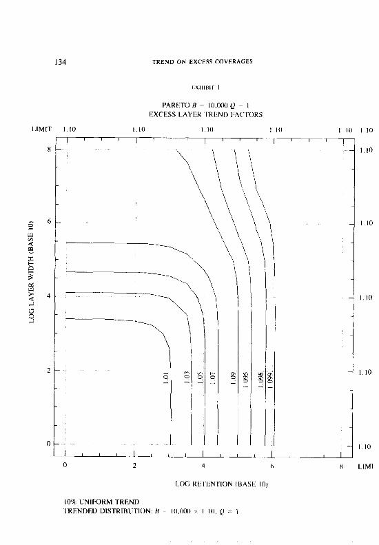
LIMIT
134 TREND ON EXCESS COVERAGES
PARETOB = lO.OOOQ = I
EXCESS LAYER TREND FACTORS
1.10 1.10 1.10 I IO I IO I IO
10
I.10
1.10
.I0
I .I0
, 1
0 2 4 6 x LIMI
LOG RETENTION (BASE 10)
10% UNIFORM TREND
TRENDED DISTRIBUTION: tl = IO.OOO x I IO, Q = I
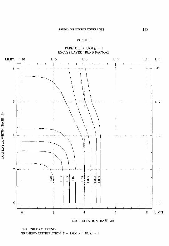
TREND ON EXCESS COVERAGES 135
EXHIBIT 2
PARETOE = 1,OOOQ = I
EXCESS LAYER TREND FACTORS
LIMIT
L
I. 10 1.10 1.10 1.10 1.10 I.10
I ’ ’ ’ I ’ ’ ’ I I I I 1 I I I I
\ I\
- I.10
- I.10
- I.10
I I.10
I I I I I I I
0 2 4 6 x LlMIT
LOG RETENTION (BASE IO)
IO% UNIFORM TREND TRENDED DISTRIBUTION: 5 = I.000 X 1.10. Q = I
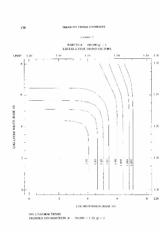
136
LIMIT
TREND ON EXCESS COVERAGES
/I
0 1
---. -‘\
.\ ‘\
=
I. I(
I I(
l.lC
I.IC
I.I(
l.l(
LIiV
10% UNIFORM TREND
TRENDED DISTRIBUTION. H = 100.000 . I IO. Q I
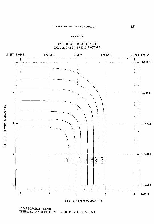
TREND ON EXCESS COVERAGE.5 137
EXHIBIT 4
PARETO E = 10.000 Q = 0.5 EXCESS LAYER TREND FACTORS
LOG RETENTION (BASE IO)
10% UNIFORM TREND TRENDED DISTRIBUTION: B = 10,000 x 1.10, Q = 0.5
I .04881
I .0488 1
1.04881
1.04881
I .W88 I
LIMIT
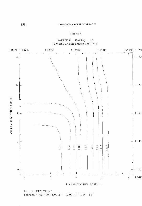
138 TREND ON EXCESS COVERAGES
~YH11111 5
PARE7‘0 H = IO.(H)0 Q = I.5
EXCESS LAYER TREND FACTORS
LIMIT I I OWO I I0050 I. 13K’J I ISi1
t
1 i
\\\,,
\ \
I.()(; Kt~.TI~N~l‘ION / I%ASI: IO,
1.1.5368 1.1.53
--‘i
I.153
: - I.153
i ~1
x LIMS
IO’i I’I\;tbOKM TRENt)
TKtiNDt:l~ l>ISTKIRIITION: N = 10.000 fl I IO. CJ I 5
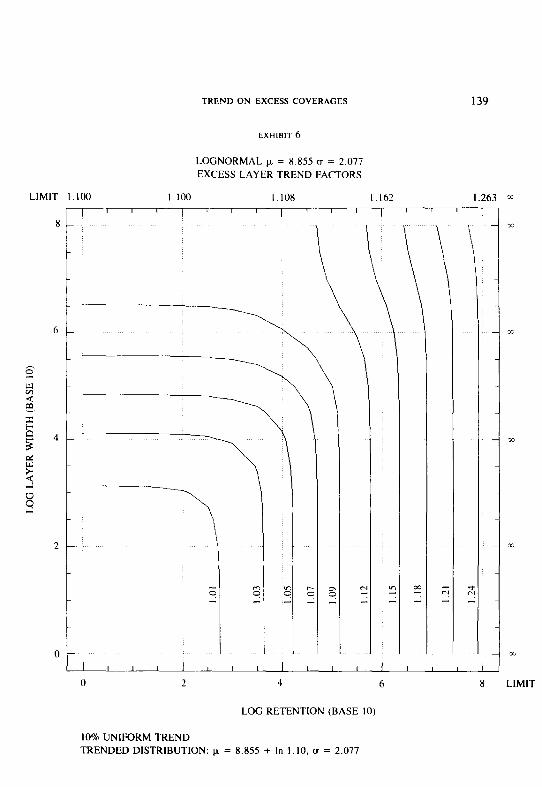
TREND ON EXCESS COVERAGES 139
EXHIBIT 6
LOGNORMAL p. = 8.855 cr = 2.077 EXCESS LAYER TREND FACTORS
LIMIT I. 100 I.100 I.108 1.162 1.263 =
0 2 4 6 8
LOG RETENTION (BASE IO)
10% UNIFORM TREND TRENDED DISTRIBUTION: & = 8.855 + In 1.10, D = 2.077
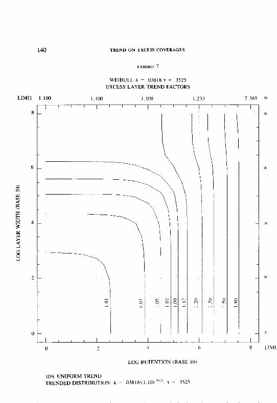
140 TREND ON EXCESS COVERAGES
EXHIBIT 7
WEIBULL A = .03818 7 = .3525 EXCESS LAYER TREND FACTORS
LIMI? I.100 1.100 1.108 1.233
4
i
h
LOG RETENTION (BASE 10)
IO% UNIFORM TREND TRENDED DISTRIBUTION: A = ,038 IX/( 1. IO) ““, 7 = .3525
2.385 x
LIMI’
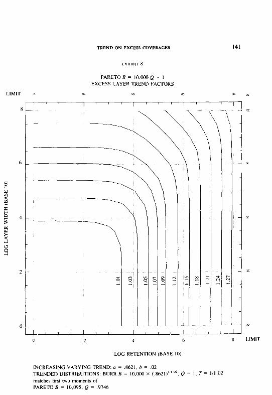
LIMIT
141 TREND ON EXCESS COVERAGES
EXHIBIT 8
PARETO B = 10,000 Q = I
EXCESS LAYER TREND FACTORS
-< ‘\’ \
\
LOG RETENTION (BASE 10)
INCREASING VARYING TREND: (I = .8621, b = .02 TRENDED DISTRIBUTIONS: BURR B = lO,CKMJ X (.8621)“’ “*, Q = I, T = I/I.02
matches first two moments of PARETO 13 = 10,095, Q = .9746
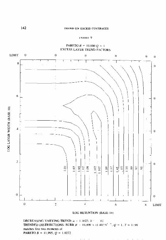
142 TREND ON EXCESS COVERAGES
PARETO B = 10,000 0 = 1 EXCESS LAYER TREND FACTORS
0 0 0 0 0
I I I I I ’ ’ ’ I / / I I I I ,
1 0
i .
, / I I I I I I -L--L--L IL 1 I / 2 4 6 X
LOG RETENTION (BASE ItI)
DECREASING VARYING TREND: o = I 4023. b = -.O? TRENDED DISTRIBUTIONS: BURR B = lO.ooO x (I 4023)’ ‘)*. Q = I. I’ = 1,.9X
matches first two moments of
PARETO B = I 1,995. Q = I .0272
I
0
0
0
0
0
JMIT
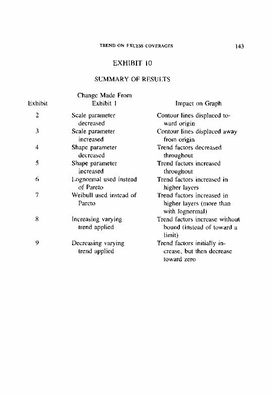
TREND ON EXCESS COVERAGES 143
EXHIBIT 10
SUMMARY OF RESULTS
Change Made From Exhibit Exhibit 1
2 Scale parameter decreased
3 Scale parameter increased
4 Shape parameter decreased
5 Shape parameter increased
6 Lognormal used instead of Pareto
7 Weibull used instead of Pareto
8 Increasing varying trend applied
9 Decreasing varying trend applied
Impact on Graph
Contour lines displaced to- ward origin
Contour lines displaced away from origin
Trend factors decreased throughout
Trend factors increased throughout
Trend factors increased in higher layers
Trend factors increased in higher layers (more than with lognormal)
Trend factors increase without bound (instead of toward a limit)
Trend factors initially in- crease, but then decrease toward zero
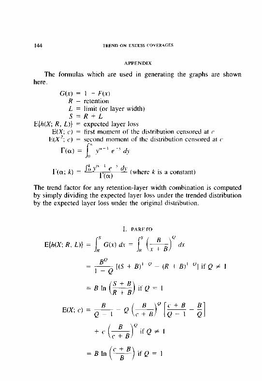
144 TREND ON EXCESS COVERAGES
APPENDIX
The formulas which are used in generating the graphs are shown here.
G(x) = 1 - F(x) R = retention L = limit (or layer width) S=R+L
E{h(X; R, L)} = expected layer loss E(X; c) = first moment of the distribution censored at c
E(X’; C) = second moment of the distribution censored at c
r(o; k) = ” Yai;i)’ ” (where k is a constant)
The trend factor for any retention-layer width combination is computed by simply dividing the expected layer loss under the trended distribution by the expected layer loss under the original distribution.
I. PARETO
E{h(X; R, L)} = [ G(x) du = 1 [-$) dx
= & [(S + B)‘-” - (R + B)‘-‘J if Q # 1
= B In S+B
i ! R+B IfQ==I
B - - E(X; c) = Q _ 1
ifQ# I
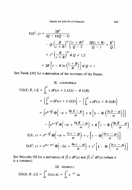
TREND ON EXCESS COVERAGES 145
E(X*; c) = 2B2 K! - l>(Q - 2)
- Q (A)" [ ",'":* _ =;-'1"' + $1
if Q # 1,2
=~B[c-BIn(F)]ifQ= 1
See Patrik [lo] for a derivation of the moments of the Pareto.
11. LOGNORMAL
I
s E{A(X; R, L)} = x dF(x) + S G(S) - R G(R)
R
R = x dF(x) + S G(S) -
1 if x dF(x) + R G(R)
0
IJ- ) .,[l -@(y- “)I]
- {e’i&+u + lnRu- “) + R [I - <o (lnR,- “)I
E(X; c) = e @+$a -a+lnc-P ( u
) +c[l -@(y- “)]
E(X’; c) = e2F+2u2 @ y- “) + c* [I - Q, (y- “)]
See Miccolis [9] for a derivation of j$ n dF(x) and Ji x2 C@(X) (where k is a constant).
111. WEtBULL
E{h(X; R, L)} = 1’ G(x) dx = j-’ e-hrT & R R

146 TREND ON EXCESS COVERAGES
= r 1 + 1 [r(l/T; h&s’) - r(l/T; AR’)] ( 1 7 A I 17
r( 1 + l/7; AC’) + ‘- r XC.’ A I/s
See the appendix of Hogg and Klugman [S] for an illustration of the techniques used in these derivations.
Iv. BURR Q
E(X; c) = Q B “’ Q
E(X2; c) = Q B2’T (1 - V)*‘3,Q-2’7‘-’ dv + c2
See the appendix of Hogg and Klugman I.51 for an illustration of the techniques used in these derivations.
147
AN ANALYSIS OF THE CAPITAL STRUCTURE OF AN INSURANCE COMPANY
GLENN MEYERS
Abstract
This paper attempts to analyze the capital structure of an insurance company in a way that (I) views the insurance company as an ongoing enterprise and (2) allows for the stochastic nature of insurance business. A model is developed. This model is used to analyze the effect of uncertainty in the loss reserves, the underwriting cycle and the cost of insurance regulation to the consumer. The paper considers both the investor’s and the regulator’s points of view.
The research for this paper was supported by a grant from the Actuarial Education and Research Fund.
1. INTRODUCTION
An insurance company is in the business of transferring risk. It does this by accepting premium from policyholders and paying claims. It can happen that the premium collected is less than the total amount paid for claims. If this is the case, the insurer is expected to pay for the claims from the capital’ of the insurance company.
This paper addresses the following question.
How much capital will be invested in a given insurance company?
The owners of (or investors in) the insurance company are concerned with the return and the safety of their investment. The money they invest in the insurance company must be competitive with respect to the return and safety of alternative investments. The insurance regulator has a vital interest in this question. The concern is that the insurance company have enough money to fulfill its obligations to the policyholders.
’ We shall use the terms “capital” and “surplus” interchangeably to represent the owner’s equity in the insurance company. In addition, for simplicity’s sake, we shall ignore expenses, loss adjustment
expenses, and investment income from the delayed payment of losses.
148 ANALYSIS OF CAPITAL STRUCTURE
A deterministic analysis of the capital structure of an insurance company might proceed as follows.
Let
P = risk premium (or expected loss), L = security (or profit) loading (we assume L > 0). U = initial surplus, and I,, = interest rate earned on the surplus.
The expected rate of return on the owner’s equity, i, satisfies the following equation:
iJXi=PXL+UXi,,. (1.1)
If P, L and i,, are fixed, it is easily seen that lowering U will increase the rate of return, i. There are two forces that limit how low U will go. First, the rate of return may get sufficiently high to attract more capital. For example, let
P = $20,000,000, L = .025, and 1,‘ = .06.
Suppose the competitive rate of return is found to be i = 12%. We can solve equation 1.1 for U = $8,333,333. If the surplus were to fall below $8,333,333, then we assume that investors would supply new capital to this insurance company. Conversely, if the surplus were to go above $8,333,333, the owners could invest the excess surplus elsewhere and obtain a greater return on their investment.
A second limiting force is that of regulation. Regulators are interested in assuring that the insurance company can fulfill its obligation to the policyholders. Putting a lower bound on U will help accomplish this purpose. However, it should be pointed out that this action is not without cost to the policyholders. Suppose, in the above example, the regulator decides to require a surplus of $9,333,333. If the competitive rate of return remains at 12%, the insurance company will be forced to raise its profit loading, L. Solving equation 1.1 gives L = ,028. Raising U by $l,OOO,OOO will cost the policyholders $60,000 annually.
ANALYSIS OF CAPITAL STRUCTURE 149
While this analysis captures some essential points of insurance com- pany operations, there are many other factors that should be considered. These factors include the following.
1. An insurance company is an ongoing operation. 2. The amount paid for claims varies from year to year. 3. The insurance industry is very competitive. The profit loading
varies from year to year in a fashion described as the “underwriting cycle.”
4. The ultimate claim cost is not determined at the end of the policy year. The result is uncertainty in the liabilities, and hence in the surplus of the insurance company.
This paper analyzes the effect these factors will have on the capital structure of an insurance company. The analysis will consider the same questions as the deterministic analysis given above; namely, (1) what surplus will give a competitive rate of return to the insurance company owners, and (2) what is the cost to policyholders of minimum surplus regulation? We begin with a model that describes how claim amounts vary.
2. THE COLLECTIVE RISK MODEL
We shall use the collective risk model to describe the incurred losses, X,, in year f. This model assumes separate claim severity distributions and claim count distributions for each line of insurance written by the insurer. We shall use the version of the model described by Heckman and Meyers [ lo] and Meyers and Schenker [ 121.
This version of the model can be described by the following algo- rithm.
I. Select p at random from an inverse gamma distribution with E[ l/ p] = 1 and Var[l/P] = b.
2. For each line of insurance, k, do the following. 2.1 Select X at random from a gamma distribution with E[X] =
I and Var[X] = ck. 2.2 Select a random number of claims, N, from a Poisson distri-
bution with mean x X xk. 2.3 Select N claims at random from the claim severity distribution
for line of insurance k.
150 ANALYSIS OF CAPITAL STRUCTURE
3. Set X, equal to the sum of all claims selected in step 2, multiplied by P.
The parameter c~, called the contagion parameter, is a measure of uncertainty in our estimate of the expected claim count, hr, for line k. The parameter 6, called the mixing parameter, is a measure of uncertainty of the scale of the claim severity distributions. Note that the random scaling factor, B. acts on all claim severity distributions simultaneously.
For demonstration purposes, we have selected a comparatively small insurance company writing a single line of insurance. The claim severity distribution is a Pareto distribution with cumulative distribution function (CW
S(z) = 1 - (ul(u+z))” (2.1)
where (I = 10,000 and cx = 2. Each claim is subject to a $500,000 limit.
The expected number of claims, A, is set equal to 2039.544. The parameters b and c are set equal to 0 and .04 respectively. The resulting risk premium for this insurer is $20,000,000.
Exhibit 1 shows the resulting aggregate loss distribution as calculated by the Heckman/Meycrs algorithm [ IO]. We will refer to this example as the ABC Insurance Company in what follows.
3. THE DISTRIBUTION OF SURPLUS
We will view the insurance company as an ongoing operation. It collects premiums, pays claims, and pays dividends to the owners (or stockholders). Occasionally, the owners will be required to contribute additional capital in order to maintain the surplus at a level specified by the regulator.
The financial status of an insurance company is usually measured at year end. Accordingly, a discrete treatment of financial results is as- sumed; i.e., the state of a company’s finances will be calculated at time t = 0, I, 2, where f is in years.
Let P = risk premium (assumed constant for all years), L, = security loading for year t.
ANALYSIS OF CAPITAL STRUCTURE 151
X, = incurred loss during year t, D, = stockholder dividends paid at the end of year t, R, = additional capital contributed at the end of year t, U, = surplus at the end of year t, and Ju = rate of return (assumed constant) earned on surplus.
Our model of insurance company operations can be described as follows. Given the surplus U,- !, define the random variable V, by
v, = u,-, x (l+iJ + P x (l+L) - x. (3.1)
Let Urn,, be the maximum surplus and Umin be the minimum surplus determined by the insurance company management and/or regulators. Then we define
D, = MAX(V,-U,,,,O), (3.2)
R, = MAX(U,i”-Vt,O), and (3.3)
iJ, = V, - D, + R,. (3.4)
While the dividend and minimum surplus decisions are usually more complex, they should be reasonable for modeling purposes. This model is similar to that described by Beard, Pentikiinen and Pesonen [l, p. 2151.
Let F,(v) be the CDF for V,. Let M = U,,,,, x (1 +iJ + P x (1 +L,) * M represents the maximum value of V,. F,(v) = 1 for v I M.
Let &, d,, and rt represent the expected values of the surplus, U,, the dividend, D,, and the additional contributed capital, RI, at time f respec- tively. We have
I
“l!W u, = v x dF,(v) + U,,, X ( 1 -F,(U,,,,))
“Ill,” + Urnin X Ft(Umin); (3.5)
d, = I i” (v-Umax) x dFt(v); (3.6) mar

152 ANALYSIS OF CAPI. AL STRUCT URt
I lJ,,,l,
r, = (Um - \r) x dF,( 1‘). (3.7) -x
Note that U, + d, - r, = E[V,].
Also of interest are the probability of paying a dividend at time ?, P,(D), and the probability of having to contribute additional capital at time t, P,(R).
The requirement that additional capital be contributed applies even when the surplus is negative. It is possible for reinsurance companies or guaranty funds to contribute money to raise the surplus to 0. Cummins [6] discusses a way to price this reinsurance.
Some notes on the history of this operating strategy are in order. This dividend-paying strategy originated in the risk theory literature in a paper by de Finetti [9]. It has been discussed by Biihlmann [4, p. 1641 and Borch [3, p. 2251. A more general version of this strategy has been discussed by Tapiero, Zuckerman and Kahane [ 131. They insert an additional level, Ul,,,e, between U ,,,,,, and Cl,,,,,. When V, goes above Uh”g, the amount, V, - Ulong, is put into long-term investments. Meyers [ 1 I] addresses the same questions addressed by this paper with an op- erating strategy that does not require the contribution of additional cap- ital.
4. YIELD RATES
The yield rate of an investment is detined to be the interest rate at which the present value of the investments is equal to the present value of the returns.
Let T be the investor’s time horizon. The investments consist of the initial surplus at time zero and the additional contributions to surplus at each time f. The returns consist of dividends payable at each time t, and the average surplus at time T. Of course, any yield rate calculation must reflect the probability that the payments are actually made.
Let i be the yield rate. The yield rate must satisfy the following equation.
T
u. + x r, X (l+i)-’ = 5 d, x (l+i) ’ + 117‘ x (l+i)-7‘. (4.1) ,= I r= I
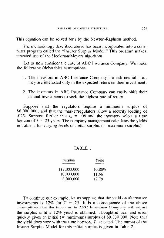
ANALYSIS OF CAPITAL STRUCTURE 1.53
This equation can be solved for i by the Newton-Raphson method.
The methodology described above has been incorporated into a com- puter program called the “Insurer Surplus Model.” This program makes repeated use of the HeckmaniMeyers algorithm.
Let us now consider the case of ABC Insurance Company. We make the following (debatable) assumptions.
1. The investors in ABC Insurance Company are risk neutral; i.e., they are interested only in the expected return on their investment.
2. The investors in ABC Insurance Company can easily shift their capital investments to seek the highest rate of return.
Suppose that the regulators require a minimum surplus of $6,000,000, and that the market/regulators allow a security loading of .025. Suppose further that i, = .06 and the investors select a time horizon of T = 25 years. The company management calculates the yields in Table 1 for varying levels of initial surplus (= maximum surplus).
TABLE 1
Surplus Yield
$12,000,000 10.80% 10,000,000 11.66 8,000,OOO 12.79
To continue our example, let us suppose that the yield on alternative investments is 12% for T = 25. It is a consequence of the above assumptions that the investors in ABC Insurance Company will adjust the surplus until a 12% yield is obtained. Thoughtful trial and error quickly gives an initial (= maximum) surplus of $9,330,000. Note that the yield does vary with the time horizon, T, selected. The output of the Insurer Surplus Model for this initial surplus is given in Table 2.
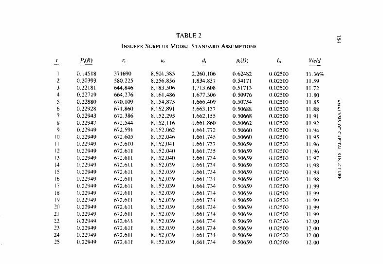
t - P,(R) r, -
U, -
1 0.14518 371690 8,501,385 2 0.20393 580,225 8,256,856 3 0.22181 644,846 8,183,506 4 0.22719 664,276 8.161.486 5 0.22880 670,109 8,154,875 6 0.22928 67 1,860 8,152,891 7 0.22943 672,386 8.152.295 8 0.22947 672.544 8,152,116 Y 0.22949 672,591 X.1.52.062
10 0.22949 672.605 X,152,046 11 0.22949 672.610 8.152.041 12 0.22949 672.611 8.152.040 13 0.22949 672.61 1 8,152,040 14 0.22949 672.61 I 8,152,039 I5 0.22949 672.611 X.152.039 16 0.22949 672.611 8.152.039 17 0.22949 672.611 8.152.039 18 0.22949 672,6 11 8.152,039 19 0.22949 672.611 8.152,039 20 0.22949 672,61 I x,152.039 21 0.22949 612.611 X, 152.039 22 0.22949 672.61 I X.152,039 23 0.22949 672.611 X. 152,039 24 0.22949 672,61 I 8,152,039 25 0.22949 672,611 8.1.52.039
TABLE 2
INSURER SURPLUS MODEL STANDARD ASSUMPTIONS
d - P,(D) L, - Yield
2,260,106 0.62482 0.02500 11.36% 1,834,837 0.54171 0.02500 11.59 I ,713,608 0.51713 0.02500 11.72 1,677,306 0.50976 0.02500 11.80 1,666,409 0.50754 0.02500 11.85 1,663,137 0.50688 0.02500 11.88 1,662,155 0.50668 0.02500 11.91 1,661,860 0.50662 0.02500 11.92 1.661.772 0.50660 0.02500 11.94 I,661,745 0.50660 0.02500 11.95 I .661.737 0.50659 0.02500 II.96 1,661,735 0.50659 0.02500 11.96 1,661,734 0.50659 0.02500 11.97 I-661.734 0.50659 0.02500 I I .98 I .661,734 0.50659 0.02500 11.98 1,661.734 0.50659 0.02500 11.98 1.661.734 0.50659 0.02500 II.99 I,661.734 0.50659 0.02500 11.99 1.661.734 0.50659 0.02500 II.99 I .66 1.734 0.50659 0.03500 II.99 I .661,734 0.50659 0.02500 11.99 1.661,734 0.50659 0.02500 12.M) I .661,734 0.50659 0.02500 12.00 1,661,734 0.50659 0.02500 12.00 1,661,734 0.50659 0.02500 12.00
ANALYSIS OF CAPITAL STRUCTURE 155
One does not need the Insurer Surplus Model to find the yield for T= I.
U() + r,l(l+i) = (U,+d,)l(l+i) (4.1)
(l+i) X ug = u~+d,-r, = E[V,] (4.2)
i = E[V,]luo - 1. (4.3)
Now:
E[V,] = uo(l+L) + P X L,. (4.4)
Thus:
i = i, + P X Lllu0. (4.5)
Note that equation 4.5 can also be derived from equation 1.1.
5. UNCERTAINTY IN LOSS RESERVES
The time t=O does not have to be the date the insurance company begins operation. The old advertising jingle “Today is the first day of the rest of your life” applies also to insurance companies. Applying the above approach to an ongoing insurance company presents a special problem which is discussed here.
Probably the largest and most uncertain liability for a property and casualty insurance firm is the loss reserve. This creates uncertainty in the initial surplus, UO. We attempt to model this by making the additional assumption:
U. has a normal distribution with known mean and variance
The debate concerning the variability of loss reserves has taken on new life within the last few years. Publications by the Casualty Actuarial Society Committee on the Theory of Risk [5], De Jong and Zehnwirth [7] and Taylor [14] deal with this problem extensively. Even so, the author considers the problem far from solved.
156 ANALYSIS OF (‘APII~AI. SI’RLKI L’Rt-
In our example, the ABC Insurance Company, we will use $1,790,035 as the standard deviation of the loss reserve, i.e., the initial surplus. This figure was derived from the following assumptions.
1. The claim severity distribution is known. 2. Claims are paid out over a period of eight years. The paid to
ultimate ratios are .05, .20. .40, .60, .75. .90, .96 and 1.00, respectively.
3. The smallest claims are settled tirst.
The details of this derivation are in the Appendix.
Using the Insurer Surplus Model we calculate that a value of $9,340,000 for uo and U,,,,, will result in a yield of 12% if all other inputs remain the same. Table 3 contains the output.
This example suggests that the uncertainty in loss reserves has little effect on surplus levels from the investor’s point of view. More will be said about this later.
6. THE UNDERWRITIN’S <‘YC‘l.lt
We now consider the case when the security loading varies from year to year in a cyclic manner. This is a well established phenomenon in casualty insurance which is felt. at least by the author, to be caused by intense competition from within the insurance industry. Berger ]2] pro- poses a model whereby the underwriting cycle results from (I) the desire to maximize profits and (2) aversion to bankruptcy.
To model the underwriting cycle we assume that
L, = Lo + A X sin (o X (f-1)+$). (6.1)
This is a special case of the AR(Z) model considered by Beard, Pentikainen and Pesonen [ 1, p. 202 and p. 3881 for cyclic variation.
To demonstrate the effects of the underwriting cycle on the ABC Insurance Company we set L cl = ,025, A = .02394 and o = n/4. These parameters will produce an eight year cycle with a reasonable amount of variation.
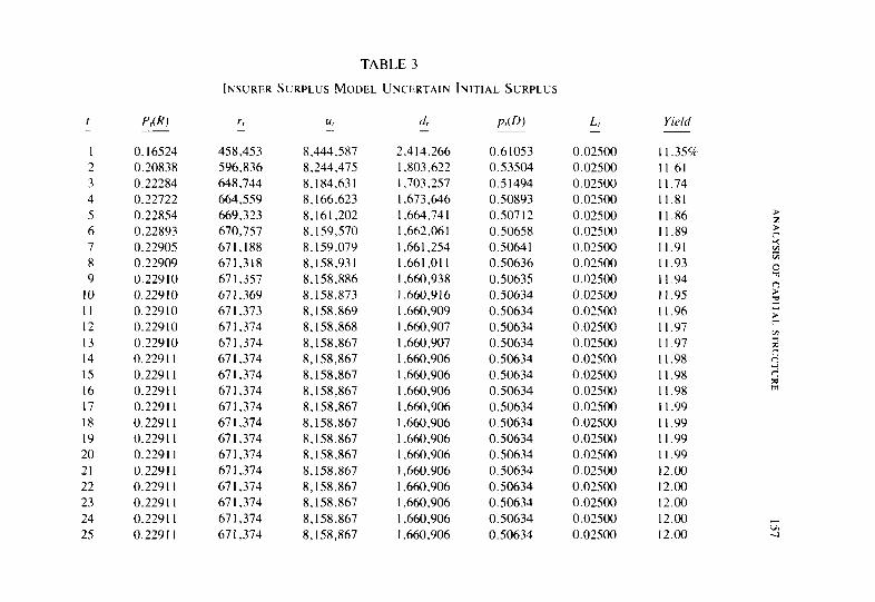
t - f,(R)
I 0.16524 2 0.20838 3 0.22284 4 0.22722 5 0.22854 6 0.22893 7 0.22905 8 0.22909 9 0.22910
IO 0.22910 II 0.22910 12 0.22910 13 0.22910 14 0.2291 I 15 0.2291 I I6 0.2291 I I7 0.2291 I 18 0.2291 I 19 0.2291 I 20 0.2291 I 21 0.22911 22 0.2291 I 23 0.2291 I 24 0.2291 I 2.5 0.2291 I
TABLE 3
INSURER SURPLUS MODEL UNCERTAIN INITIAL SURPLUS
rr - u, -
458,453 8.444.587 596,836 X.244.475 648,744 8.184.631 664,559 8,166.623 669,323 8.161.202 670.757 8,159.570 671,188 8.159.079 671,318 8.158.931 67 1,357 8,158.886 671,369 8.158.873 671,373 8.158,869 67 1,374 8.158,868 67 I ,374 8.158.867 671,374 8.158.867 67 I ,374 8.158.867 671,374 8.158.867 67 1,374 8.158.867 67 I ,374 8,158.867 671,314 8.158.867 671,374 8.158.867 671,374 8.158.867 67 I ,374 8.158.867 671,374 8.158.867 67 I ,374 8,158,867 671,374 8,158,867
d - PO) L
2.414.266 0.61053 0.02500 I .803.622 0.53504 0.02500 I .703.257 0.51494 0.02500 I .673.646 0.50893 0.02500 I ,664,741 0.50712 0.02500 I ,662.061 0.50658 0.02500 1,661,254 0.50641 0.02500 1,661,Ol I 0.50636 0.02500 1,660,938 0.50635 0.02500 I ,660,916 0.50634 0.02500 I ,660,909 0.50634 0.02500 I ,660,907 0.50634 0.02500 I ,660,907 0.50634 0.02500 I ,660,906 0.50634 0.02500 I ,660,906 0.50634 0.02500 I ,660,906 0.50634 0.02500 I ,660,906 0.50634 0.02500 I .660,906 0.50634 0.02500 I .660,906 0.50634 0.02500 I ,660,906 0.50634 0.02500 I ,660,906 0.50634 0.02sOO I ,660,906 0.50634 0.02500 I ,660,906 0.50634 0.02500 I ,660,906 0.50634 0.02500 I .660,906 0.50634 0.02500
Yield
I I.354 I I .6l II.74 II.81 II.86 s II.89 F I I.91 2 II.93
E
II.94 ,o II.95 2
” Il.96 2 II.97 7
II.97 i;
I I .98 c 3
II.98 C
II.98 6
II.99 Il.99 II.99 II.99 12.00 12.00 12.00 12.00 12.00 s
158 ANALYSIS OF CAPITAI. S.FRUCTlJRE
We first consider what happens when we catch the cycle on the way up. If we set 4 = 0 along with the assumptions stated immediately above and in Section 4, we calculate that a value of $10,600,000 for ug and I/,,, will result in a yield of 12%. The results of the Insurer Surplus Model for this case are in Table 4.
Let us next consider what happens when we catch the cycle on the way down. If we set 4 = IT along with the assumptions stated imme- diately above and in Section 4, we calculate that a value of $7,975,000 for ~4~ and U,,,,, will result in a yield of 12%. The results of the Insurer Surplus Model for this case are in Table 5.
7. RUIN THEORY
Thus far, our assumption has been that the investors in an insurance company will adjust the surplus so that the expected yield will be constant. An alternative to this assumption is provided by ruin theory. Ruin theory’ makes the assumption that the investors in an insurance company will adjust the surplus so that the probability of insolvency (i.e., the probability of ruin) will remain constant. In this section, we shall demonstrate that these two assumptions imply quite different results.
It is sufficient to consider the probability of ruin for a one-year time span. Let E be the selected probability of ruin. We have:
Pr{U, < 0} = E if and only if LI(,( 1 +i,,) + P( 1 +Lr) = -T~-~.
where xl pc is the 1 -eth percentile of the random loss X. If E is fixed, it can be seen that a reduction in L, should be accompanied by a corre- sponding increase in uo, and conversely an increase in L, should be accompanied by a corresponding decrease in uo.
Equation 4.5 indicates the opposite behavior. If i is fixed, it can be seen that L, and U. move in the same direction. This behavior also holds in the multiyear analysis of the underwriting cycle. If the cycle is on the way down, iJIII~lx also goes down and the insurance company’s surplus is reduced. The opposite happens when the cycle is on the way up.
L See. for example. Beard. Pentiklinen and Pesonen Il. ch. 31.
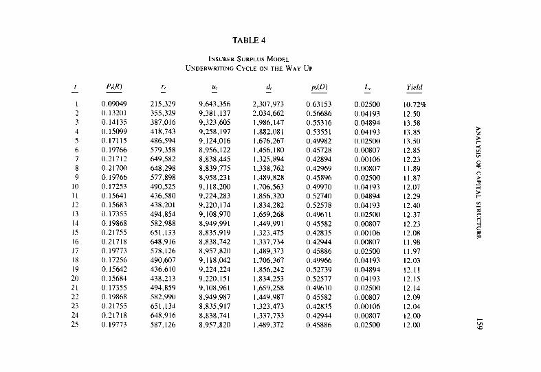
t - PO0
1 0.09049 2 0.13201 3 0.14135 4 0.15099 5 0.171 I5 6 0.19766 1 0.21712 8 0.21700 9 0.19766
IO 0.17253 II 0.15641 I2 0.15683 13 0.17355 14 0.19868 I5 0.21755 I6 0.21718 I7 0.19773 18 0. I7256 I9 0.15642 20 0.15684 21 0. I7355 22 0.19868 23 0.21755 24 0.21718 25 0.19713
rr -
ur - d, - Pm L, - Yield
215,329 9,643,356 2,307,973 0.63153 0.02500 10.72% 355,329 9,381,137 2,034,662 0.56686 0.04193 12.50 387,016 9.323.605 I ,986, I47 0.55316 0.04894 13.58 418,743 9,258,197 I ,882,08 I 0.53551 0.04193 13.85 486,594 9,124,016 I ,676,267 0.49982 0.02500 13.50 579,358 8,956,122 I ,456, I80 0.45728 0.00807 12.85 649,582 8,838,445 1,325,894 0.42894 0.00106 12.23 648,298 8.839.775 I ,338,762 0.42969 0.00807 11.89 577,898 8.958.231 I ,489,828 0.45896 0.02500 II.87 490,525 9,118,200 I ,706,563 0.49970 0.04193 12.07 436,580 9.224.283 I ,856,320 0.52740 0.04894 12.29 438,201 9.220.174 I ,834,282 0.52578 0.04193 12.40 494,854 9.108.970 I ,659,268 0.4961 I 0.02500 12.37 582,988 8.949.991 I ,449,99 I 0.45582 0.00807 12.23 651,133 8,835,919 I ,323,475 0.42835 0.00106 12.08 648,916 8.83X.742 I ,337,734 0.42944 0.00807 II.98 578,126 8,957,820 1,489,373 0.45886 0.02500 II.97 490,607 9,118,042 I ,706,367 0.49966 0.04193 12.03 436.610 9,224,224 I ,856,242 0.52739 0.04894 12.11 438,213 9,220,151 I ,834,253 0.52577 0.04193 12.15 494,859 9.108.961 I ,659,258 0.49610 0.02500 12.14 582,990 8.949.987 I ,449,987 0.45582 0.00807 12.09 651,134 8,835,917 I ,323,473 0.42835 0.00106 12.04 648,916 8,838,741 I ,337.733 0.42944 0.00807 12.00 587,126 8,957,820 I ,489,372 0.45886 0.02500 12.00
TABLE 4
INSURER SURPLUS MODEL
UNDERWRITING CYCLE ON THE WAY UP
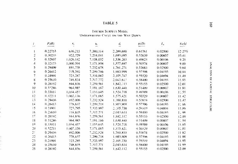
I -
I 2 3 3 5 6 7 x Y
IO II I’
Ii IJ
I5
I6
17
IX
I9
‘0 71
27
23
23
15
PAR 1
0.72753 (I.30233
0.32807
0.32173
0.2940’)
0.26412
0.2490 I
0.25610
0.2XlY1
0 312Xh
0.3301 I
0.3121 I
0.794lh
O.ZhJI3
0 24001 0.2ShlO
0 7XlY7 O.il?Xh
0 3301 I
0.322 I I
0.294 I6
0.16413
0.24901
0.75610
0.18191
TABLE 5
INSI!R~K SI:RPLLIS MODEL
UND~KMRITING CVCI E ON THE WAY DOWN
636.2 I5
Y72.72’)
1.076. I42
I .000.5Y4 x9 I ,73x
77X.592
7732x7
748.X3-1
844.X36
Y64.YXS
I .034.457 I .002.136
xY~,ooh
77X.637
723.295
74x,x35
X44.X36
Y63.YXS
I .0?4,4S7
I.OC)1.136 X97.006
77X.637
773.295
738.835
844.836
7.3x0. I I4 7.213.031
7.15X.032
7.171.89X
7.732.67X
7299,746
7.334.002
7.311.772
7.259.Shl
7.191.167
7.153.64.S
7. I7 I .OhS 7.32 574 , - 7.799.71x
l.W,YY7
7.117.711 7.759.561
7.191.166
7.153.645
7.171.065 731.524
7299.718
7.333.997
7.317.771
7.259.561
(1,
2.2UY.600 I .693.095
I ,536.263
1277.697
1.761.271 I .9X3,999
2.105.747
1.043.617
1.X42.113
I .h30,440
1.574.71x
I .575.421 I .760.X10
I .Y83.90’)
2.105.730
2.043.614
1.x47.112
I ,630,440
1.5Z4.7IX
I ,575,42l
I .760.810
I .9X3.90’)
2.105.730
2.043.613 1.X42.1 I2
P,(l))
0.61761 0.02500
0.52639 0.00807
0.49623 0.00106
0. so374 u.OOxo7
0.53683 0.02500
0.57398 0.04193
0.59310 0.04894
0.5x400 0.04193
0.55 IS3 0.02500
0.5 I 4OY o.ouxo7
0.493X0 0.00106
0.50319 0.00807
0.53673 0.02500
0.57396 0.04193
0.503 I9 0.04x94
0.5x400 0.04193
O.SSlS3 0.11’500
0.514OY 0.00807
0.19389 O.WlO6
0.50329 0.00807
0.53673 o.o2s(xl
0.57396 0.04193
0.59319 0.04894
0.5x400 0.04193
0 55153 0.02500
Yield
12.27%
IO.41 Y.20
Y.00
9.64
IO.64
I I.40
Il.95
12.01
I LX1
I I .SS
I I.42
Il.47
I I.66
I LX6
I I.% I ‘.oU
I I.91
II x.5
II.81 II x7
11.8X I I.95
I I.99
12.00
ANALYSIS OF CAPITAL STRUCTURE 161
The two assumptions have different implications when we consider uncertainty in loss reserves. It was demonstrated in the example above that uncertainty in the loss reserves has little effect on the surplus. The surplus increases from $9,330,000 to $9,340,000. Suppose we are sat- isfied with the probability of ruin for the standard assumptions (Table 2). Using the Insurer Surplus Model with I/,,,i” = 0, we calculate that the probability of ruin after one year is .0152. If the standard deviation of the loss reserve is $1,790,035, as in Table 3, it requires a surplus of $10,045,000 to maintain the probability of ruin of .0152 for the first year.
8. THE COST OF REGULATION
It is the regulator’s job to impose standards that promote the solvency of insurance companies. One way of doing this is to impose a minimum surplus so that the probability of ruin is acceptably low. It was demon- strated in the last section that such a regulatory strategy may not be in accordance with the wishes of insurance company owners.
The owners don’t have any choice in the matter. The regulators set the standards and the insurance companies comply with them. A higher minimum standard will result in a higher level of surplus in the industry as a whole, and a higher profit loading will be demanded. The purpose of this section is to find this additional cost of solvency regulation to insurance consumers.
Let us consider the example in Table 2. We will vary the minimum surplus and calculate the security loading that will result in a yield rate of 12% after 25 years. The results are in Table 6.
Note that if the minimum surplus goes above $9,330,000 the mini- mum surplus becomes the maximum surplus, and the security loading can be obtained by solving equation I. I.
The changes in the market conditions brought on by increasing the minimum surplus are clearly more complex than is assumed by the above example. However, this may be an indication that the cost of regulation is small if the minimum surplus is not too high.
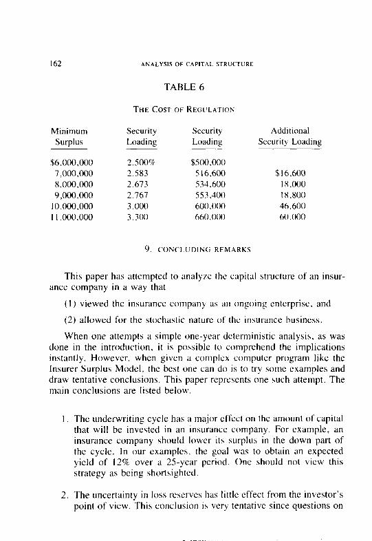
162 ANALYSIS OF CAPITAL STRUCTURE
TABLE 6
THE Cosr OF REGUI.AIION
Minimum Security Surplus Loading
$6.000,000 2.500%’ 7 .ooo,OOO 2.583 8,000,000 2.673 9,000,000 2.767
10.000,000 3.000 I I .ooo.ooo 3.300
Security Loading
$500,000 5 16,600 534.600 5 5 3,400 600.000 660,000
Additional Security Loading
$16,600 IX,000 IX.800 46,600 60 ~ 000
9. CONCI.CJDING REMARKS
This paper has attempted to analyze the capital structure of an insur- ance company in a way that
(I) viewed the insurance company as an ongoing enterprise. and
(2) allowed for the stochastic nature of the insurance business
When one attempts a simple one-year deterministic analysis, as was done in the introduction, it is possible to comprehend the implications instantly. However, when given a complex computer program like the Insurer Surplus Model, the best one can do is to try some examples and draw tentative conclusions. This paper represents one such attempt. The main conclusions are listed below.
1, The underwriting cycle has a major effect on the amount of capital that will be invested in an insurance company. For example, an insurance company should lower its surplus in the down part of the cycle. In our examples. the goal was to obtain an expected yield of 12% over a 25-year period. One should not view this strategy as being shortsighted.
2. The uncertainty in loss reserves has littlc effect from the investor’s point of view. This conclusion is very tentative since questions on
ANALYSIS OF CAPITAL STRUCTURE 163
the variability of loss reserves still remain. However, uncertainty in loss reserves can have a substantial effect from the regulator’s point of view.
3. Whether the investors like it or not, the regulators may require a minimum surplus. If this minimum is below what the investors would voluntarily allow, the cost to the policyholders is relatively small. As this regulatory minimum increases, the cost to the policyholders becomes substantial.
There are several items that should enter this analysis, but did not. A discussion of some of these items follows.
We assumed that the investor would seek the same expected yield in all circumstances. One could reasonably argue that the investor should seek a higher yield when the surplus is low because of the increased variability of the return. This is debatable. It is unlikely that the investor would invest all of his/her assets in a single enterprise, and so the investor’s risk aversion should not be much of a factor. However, the author would like to keep the debate open.
The issue of asset risk has been omitted from this entire discussion. It could very well be as important as any of the items mentioned above. Any analysis of asset risk must include strategies for asset/liability match- ing. A good place for casualty actuaries to start would be the paper “Duration” by Ronald E. Ferguson [8]. Further research needs to be done in order to integrate asset risk into the above approach for analyzing the capital structure of an insurance company.
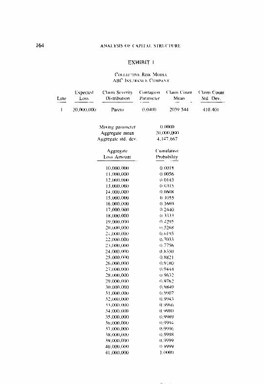
164 ANAi.YSIS OF (‘API I ,A[. STKII(“VIIRE
EXHIBIT I
Claim Se\ent> Contagion Claim Count Claim Count
Dktrihution Paramctcr Mean Std. Dev. ~-.____
I 20.ooo.000 Pareto
Mixmp parameter
Aggregate mean
Aggrcpate std. dev
Aggregate
Loss Amount
10.000.ooo
I I .ooa.ooa
12 ,ooo.ooo
13 .ooo.ooo
14.ooo.000
IS ,ooo,ooo
l6.(K)O.WU
17.ooo.cKlo
18.ooo.000
I’),000,000
20,(K)0,ooo
7 I .ooo.ooo
‘2 ,ooo .ooo
13.ooo.000
~4.040.000
25.000,ooo
x.ooo.o~X)
27 .ow.ooo
2x.090.000
29,000,oi)0
30.ooo.000
3 I .00+1.000
3Z.000.009
33.000.000
34.000.000
35.ooo.000
3b.000.000
37 .om.ooo
3x.000.000
39.000.000
40,ooo.000
41.000,0(x1
0 0.400 203Y. SW 410.401
o.owo
‘0.000.ooo
4.147.667
Cumulative
Probability
0.0018
0 0056
0.0143
0 0315
0.060x
0.105s
0. 166’)
(I 2440
0 3333
0 4ZY5
0 S?hX
0 6145
0.7033
0 77%
0.x350
0 XX? I
0.9 IX0
0 9444
0 Y632
0.Y762
O.YX4Y
O.YYO7
0 YYJi
0 YYbh
0 YYXO
0 YWY
O.YYY4
0 WYh
I).YYYX
O.YYYY
O.YYYY
I OOIH)
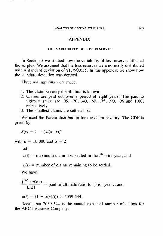
ANALYSIS OF CAPITAL STRUCTURE 165
APPENDIX
THE VARIABILITY OF LOSS RESERVES
In Section 5 we studied how the variability of loss reserves affected the surplus. We assumed that the loss reserves were normally distributed with a standard deviation of $1,790,035. In this appendix we show how the standard deviation was derived.
Three assumptions were made.
1. The claim severity distribution is known. 2. Claims are paid out over a period of eight years. The paid to
ultimate ratios are .05, .20, .40, .60, .75, .90, .96 and 1 .OO, respectively.
3. The smallest claims are settled first.
We used the Pareto distribution for the claim severity. The CDF is given by:
S(z) = 1 - (al(a+z))”
with a = 10,000 and (x = 2.
Let:
c(i) = maximum claim size settled in the ith prior year; and
n(i) = number of claims remaining to be settled.
We have
J;?’ zds(z)
WI = paid to ultimate ratio for prior year i; and
n(i) = (1 - S(c(i))) X 2039.544.
Recall that 2039.544 is the annual expected number of claims for the ABC Insurance Company.
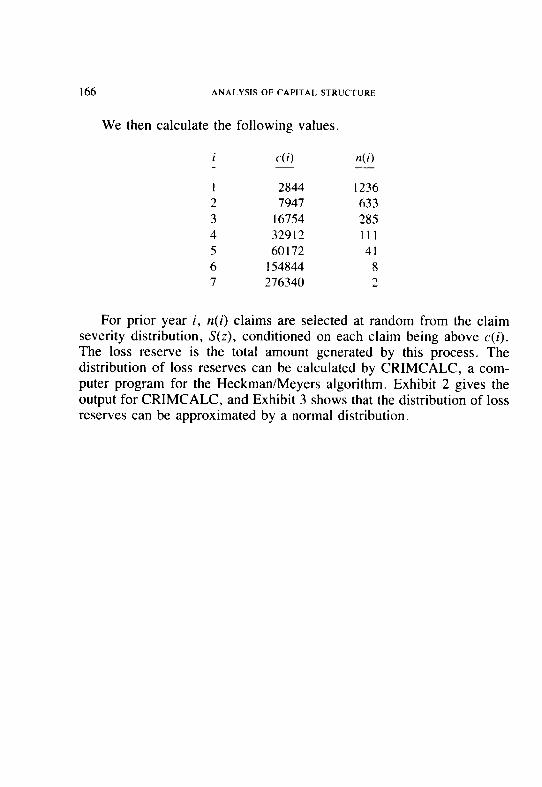
166 ANALYSIS OF CAPITAL STRUCTURE
We then calculate the following values
i c(i) n(i)
1 2844 I236 2 7947 633 3 16754 285 4 32912 111 5 60172 41 6 154844 8 7 276340 2
For prior year i, n(i) claims are selected at random from the claim severity distribution, S(z), conditioned on each claim being above c(i). The loss reserve is the total amount generated by this process. The distribution of loss reserves can be calculated by CRIMCALC, a com- puter program for the Heckman/Meyers algorithm. Exhibit 2 gives the output for CRIMCALC, and Exhibit 3 shows that the distribution of loss reserves can be approximated by a normal distribution.
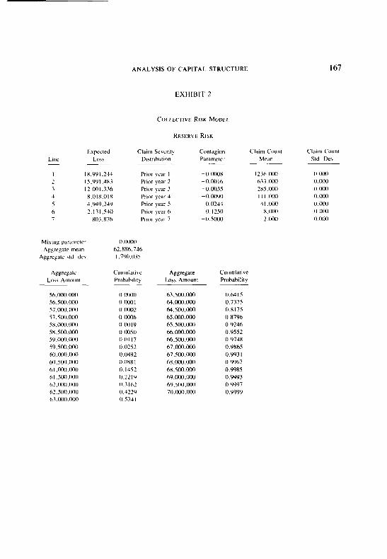
ANALYSIS OF CAPITAL STRUCTURE 167
EXHIBIT 2
EKpKlCd LlW LO\\
I IX.99 I.244 2 IS.YY I .4X3 3 12.Wl.336 4 x.OIx.OIx 5 J,YJY.?JY 6 2.13l.s40 7 X03.X76
o.otMM~ 62.XXh.7Jh I .7YO.O3S
Pnor pear I Prw year 2 Prior )car 3 Pnor year 4 Prior )rar S Prior year 6 Prior wdr 7
Sh .txltl .lWXl 56.500.wu 57.Cw.000 57..50(l.000 SX.tWWl.ow sx.sno.tKKl s9.wo.wo 5Y.500.ow Ml.txx).ow K~.400.wtl 61 .OOO.~MHl 61 .stxl.00~1 62.OKK1.000 62..50(l.000 63.tMlO.otM)
0 owe 0 ow I (I IX)02 0 wo6 0 WIY 0 lwlso 00117 0 t1252
0.0492 o.onx I 0 I452 II ??.I’) 0 3162 0 422’) 0 5341
- 0 ntHlX -0.wl6 -0 003s -0 WY0 -0 0244 -0 I250 -0 5oLw
63,SOO.IKKI 64.tm.rKKl 64.soo.wo 65.ooO.ooO 6s.sOO.~Mx1 M.WWXXl 66.500.wt1 67.ooO.tXIo 67.SOO.Wtl 6X.000.000 6X.5M.wl1 6Y,ox).NM hY.S(MI.IMH) 7U.tMlO.t~OO
Cumulall\e Prohahilit\ 1
0641s 0.7375 0 8175 0 8796 0.9246 0 9552 0 974x 0 YXhS 0 9931 (1 9967 0 99x5 0 9993 0 9997 O.YWY
Claim Count Mean
Clam1 Count Std De\
1276,tHM) 633.OtM) 285.lHX) I I I .tMMl 4 I .(XH)
X.tMMl 2 ow
0 wil 0 tMX1 0 tMX) tl (MM1 0 CiKl 0 ow 0 IWKI
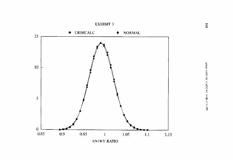
15
10
5
0
n CRIMCALC + NORMAL
0.85 0.9 0.95 1 1.05 1.1 1.15
ENTRY RATIO
EXHIBIT 3
ANALYSIS OF CAPITAL STRUCTURE 169
REFERENCES
[l] R.E. Beard, T. Pentikainen, and G. Pesonen, Risk Theory, Chap- man and Hall, 1984.
[2] Lawrence Berger, “A Model of the Underwriting Cycle in the Property and Casualty Insurance Industry,” Journal of Risk and Insurance, 1988.
[3] Karl Borch, The Marhemarical Theory of Insurance, D.C. Heath and Company, 1974.
(41 Hans Btihlmann, Marhematical Methods of Risk Theory, Springer- Verlag, 1970.
[5] Casualty Actuarial Society Committee on the Theory of Risk, “Risk Theoretic Issue in Loss Reserving,” Casualty Actuarial Society, 1986.
161 J. David Cummins, “Risk Based Premiums for Guaranty Funds,” Proceedings of the International Conference on Insurer Solvency, June, 1986.
[7] Piet De Jong and B. Zehnwirth, “Claims Reserving, State-Space Models and the Kalman Filter,” Journal qf the Institute of Actuaries, V. 110, 1983.
(81 Ronald E. Ferguson, “Duration,” PCAS LXX, 1983.
(91 B. de Finetti, “Su un’ impostazione alternativa delta teoria collec- tiva del rischio,” Transactions of the International Congress of Actuaries, 2, 1957, p. 433.
[ lo] Philip E. Heckman and Glenn G. Meyers, “The Calculation of Aggregate Loss Distributions from Claim Severity and Claim Count Distributions,” PCAS LXX, 1983.
[ 1 I ] Glenn Meyers, “Equilibrium in the Capital Structure of an Insurance Company,” Proceedings of the Inrernational Conference on insurer Solvency, June, 1986.
[ 121 Glenn Meyers and Nathaniel Schenker, “Parameter Uncertainty and the Collective Risk Model,” PCAS LXX, 1983.
[ 131 Charles S. Tapiero, Dror Zuckerman, and Yehuda Kahane, “Opti-

170 ANALYSIS OF CAPITAL STRUCIURE
mal Investment-Dividend Policy of an Insurance Firm under Reg- ulation,” Scandinavian Actuarial Journal, 1983. p. 65.
[ 141 G.C. Taylor, Claims Re.wr\ping irr Non-I,(fe /nsutwzw, North Hol- land. 1986.
171
RISK THEORETIC ISSUES IN LOSS RESERVING: THE CASE OF WORKERS COMPENSATION PENSION RESERVES
GLENN MEYERS
Abstract
Opposition to the discounting of loss reserves is based on the premise that loss reserves are uncertain and insurance com- panies must retain additional funds in order to reduce the chance of insolvency. This paper explores the explicit calcu- lation of a risk load for discounted loss reserves. Underlying considerations include: (I) the random nature of the claim settlements; (2) our ability to describe the distribution of actual results; and (3) how the risk load we use for loss reserves compares to the profit load we use for pricing insur- ance. These ideas are expressed in terms of an example: workers compensation pension reserves.
The research for this paper was supported by a grant from the Society of Actuaries upon recommendation of the Actuarial Education and Research Fund.
1. INTRODUCTION
Should loss reserves be determined with an explicit recognition of risk? This question was posed by the Casualty Actuarial Society’s Com- mittee on the Theory of Risk at the November, 1984 CAS annual meet- ing.’ For the sake of discussion, the committee assumed that the answer was yes, and then proceeded to outline several points that should be considered in setting a risk load for loss reserves.
The issue of discounting reserves is linked to the issue of risk loading. It could be argued that carrying reserves at the nominal value rather than
1 The Committee on the Theory of Risk made similar presentations in 1985 at meetings of the Midwest Actuarial Forum and the Casualty Actuaries of Greater New York. Copies of the presen-
tation, titled “Risk Theoretic Issues in Loss Reserving,” are available from the Casualty Actuarial
Society.
172 LOSS RESERVING
the present (or discounted) value represents an implicit risk load. The long tailed lines have the most uncertain reserves and the largest differ- ence between the nominal and present values.
The discounting of loss reserves has received a lot of recent attention. The federal Tax Reform Act of 1986 requires that property and casualty insurers calculate their taxes using discounted reserves. However, the Loss Reserve Discounting Study Group of the National Association of Insurance Commissioners declared that “. . discounting of loss reserves is not a generally accepted statutory accounting practice, except in re- gards to fixed and determinable payments, such as those emanating from workers compensation and long-term disability claims.” [I] Very re- cently, a prominent actuary declared himself to be “solidly in favor of reserve discounting, unless the change would take place without con- comitant recognition of the need for contingency reserves.” (2)
While the Committee on the Theory of Risk discussed several im- portant principles on risk loading in their presentation, they did not provide a unified example applying these principles. This paper will give such an example.
Our goal is to calculate risk loads for workers compensation pension reserves. The author considers this to be a good place to start for two reasons: (1) it is a line with perhaps the longest tail of reserves; and (2) much of the necessary mathematical work has already been done. The new textbook Actuarid Mathematics [3] views the future lifetime of an individual as a random variable. Formulas are provided which enable one to quantify uncertainty in the loss reserves.
While we are focusing on workers compensation pension reserves, it is hoped that this example will be rich enough to highlight issues that are relevant to other lines of insurance.
This paper is being written in the spirit of the Committee on the Theory of Risk’s presentation, that is, to provoke discussion. The reader is warned in advance that a number of debatable assumptions will be made. It is hoped that the state of the art of loss reserving will be advanced by this debate.
LOSS RESERVING 173
2. UNDERLYING CONSIDERATIONS
It should be clear that the risk load becomes more important when reserves are discounted. Thus we assume that reserves are discounted. We shall also assume that the interest rate is known and fixed. While this is clearly not the case, there are a number of strategies available to the insurer which minimize the effect of varying interest rates. In addi- tion, Woll [4] argues that the insurance operation of an insurance com- pany should get “credited for funds it provides to the investment de- partment at risk-free rates” and that the “difference between the amount of investment income and its cost of funds” is the profit earned by the investment department.
We define the expected reserve as an estimate of the expectation of the present value of future payments to be made.
Let n be the total number of claims which are open. Let Pi, be a random variable denoting the payment made for the ifh claim at the t’* time period. Let Fir be an estimate of the expected value of Pir and let 6 be the force of interest. In this case the expected reserve, R, is:
(2.1)
Since Pi, is a random variable, the expected reserve may be different from the amount, R, necessary to pay the claims. If the distribution of each P,, is known, it is possible to calculate the distribution of the amount necessary to pay the claims. We shall refer to the risk created by the randomness of Pit as the process risk. Bowers, et al. [3, Chapter 51, describe the distribution of R for the case of life annuities (i.e. workers compensation pension reserves).
In practice, the distribution of Pi, is not known. It must be estimated. The uncertainty in the distribution of Pi, creates an additional risk which we refer to as parameter risk. There may be a number of ways to estimate the distribution of Pi,. The amount of parameter risk will depend on how this distribution is estimated.
The risk load in the loss reserve should reflect both process risk and parameter risk.
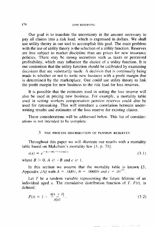
174 LOSS RESERVING
Our goal is to translate the uncertainty in the amount necessary to pay all claims into a risk load, which is expressed in dollars. We shall use utility theory as our tool to accomplish this goal. The main problem with the use of utility theory is the selection of a utility function. Reserves are less subject to market discipline than are prices for new insurance policies. There may be strong incentives such as taxes or perceived profitability, which may influence the choice of a utility function. It is our contention that the utility function should be calibrated by examining decisions that are voluntarily made. A decision that is continually being made is whether or not to write new business with a profit margin that is determined by the marketplace. One could use utility theory to link the profit margin for new business to the risk load for loss reserves.
It is possible that the estimates used in setting the loss reserve will also be used in pricing new business. For example, a mortality table used in setting workers compensation pension reserves could also be used for ratemaking. This will introduce a correlation between under- writing results and estimates of the loss reserve for existing claims.
These considerations will be addressed below. This list of consider- ations is not intended to be complete.
3. THE PROCESS DISTRIBUTION OF PENSION RESERVES
Throughout this paper we will illustrate our results with a mortality table based on Makeham’s mortality law 13, p. 71):
s(x) = e --A\ -MC.‘- I l!ln(~-I
(3.1)
where B > 0, A 2 -B and c 2 1.
In this section we assume that the mortality table is known (3, Appendix 2AJ with A = .0007, B = .OOOOS and c = IO “‘.
Let T be a random variable representing the future lifetime of an individual aged x. The cumulative distribution function of T, F(t), is defined:
F(f) = I - s(x + t)
s(x) . (3.2)
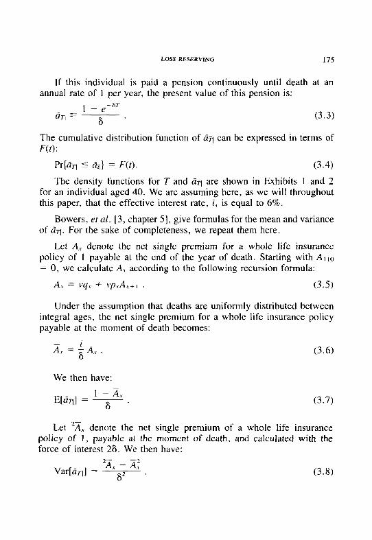
LOSS RESERVING 17.5
If this individual is paid a pension continuously until death at an annual rate of I per year, the present value of this pension is:
The cumulative distribution function of Lfrl can be expressed in terms of F(r):
Pr{& I &I} = F(r). (3.4)
The density functions for T and &I are shown in Exhibits I and 2 for an individual aged 40. We are assuming here, as we will throughout this paper, that the effective interest rate, i, is equal to 6%.
Bowers, er al. [3, chapter 51, give formulas for the mean and variance of +I. For the sake of completeness, we repeat them here.
Let A., denote the net single premium for a whole life insurance policy of I payable at the end of the year of death. Starting with Al 1o = 0, we calculate A., according to the following recursion formula:
A., = vy, + cprAx+, . (3.5)
Under the assumption that deaths are uniformly distributed between integral ages, the net single premium for a whole life insurance policy payable at the moment of death becomes:
We then have:
I - A, E[crrl] = 6 .
(3.6)
(3.7)
Let 2A., denote the net single premium of a whole life insurance policy of I, payable at the moment of death, and calculated with the force of interest 26. We then have:
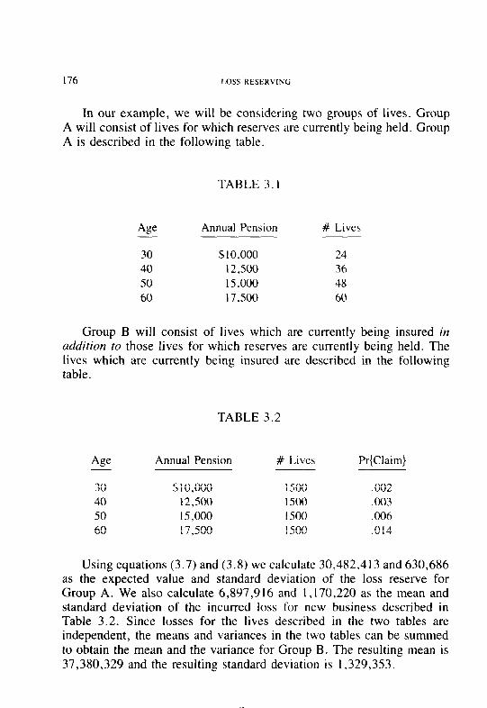
176 LOSS RESERVING
In our example, we will be considering two groups of lives. Group A will consist of lives for which reserves are currently being held. Group A is described in the following table.
TABLE 3.1
As Annual Pension
30 $10,000 40 12,500 50 15,000 60 17,500
# Lives
24 36 48 60
Group B will consist of lives which are currently being insured in addition to those lives for which reserves are currently being held. The lives which are currently being insured are described in the following table.
TABLE 3.2
Age Annual Pension
30 $10,000 40 12,500 50 15,000 60 17,500
# Lives Pr{Claim}
1500 .002 1500 ,003 1500 ,006 1500 ,014
Using equations (3.7) and (3.8) we calculate 30,482,413 and 630,686 as the expected value and standard deviation of the loss reserve for Group A. We also calculate 6,897,916 and I, 170,220 as the mean and standard deviation of the incurred loss for new business described in Table 3.2. Since losses for the lives described in the two tables are independent, the means and variances in the two tables can be summed to obtain the mean and the variance for Group B. The resulting mean is 37,380,329 and the resulting standard deviation is 1,329,353.
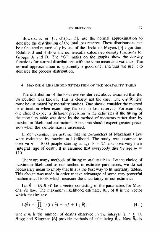
LOSS RESERVING 177
Bowers, et al. [3, chapter 51, use the normal approximation to describe the distribution of the total loss reserve. These distributions can be calculated numerically by use of the Heckman-Meyers [5] algorithm. Exhibits 3 and 4 show the numerically calculated density functions for Groups A and B. The “0” marks on the graphs show the density functions for normal distributions with the same mean and variance. The normal approximation is apparently a good one, and thus we use it to describe the process distribution.
4. MAXIMUM LIKELIHOOD ESTIMATION OF THE MORTALITY TABLE
The distribution of the loss reserves derived above assumed that the distribution was known. This is clearly not the case. The distribution must be estimated by mortality studies. One should consider the method of estimation when examining the risk in loss reserves. For example, one should expect a different precision in the estimates if the fitting of the mortality table was done by the method of moments rather than by maximum likelihood estimation. Also, one should expect greater preci- sion when the sample size is increased.
In our example, we assume that the parameters of Makeham’s law were estimated by maximum likelihood. The study was assumed to observe n = 1000 people starting at age to = 25 and observing their (integral) age of death. It is assumed that everybody dies by age o = 110.
There are many methods of fitting mortality tables. By the choice of maximum likelihood as our method to estimate parameters, we do not necessarily mean to imply that this is the best way to fit mortality tables. This choice was made in order to take advantage of some very powerful mathematical tools which measure the uncertainty of our estimates.
Let 6 = (A&J) be a vector consisting of the parameters for Mak- eham’s law. The maximum likelihood estimate, GM, of 6 is the vector which maximizes:
w-1
L(8) = n [S(f ; 6) - s(f + 1 ; 6)]“’ t=t, (4.1)
where n, is the number of deaths observed in the inteval [t, t t 11. Hogg and Klugman [6_] provide methods of calculating 0~. Now tl,,., is
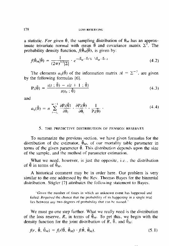
178 LOSS RESERVING
a statistic. For given 0, the sampling distribution of 6.~ has an approx- imate trivariate normal with mean 6 and covariance matrix E-. The probability density function, fc&#), is given by:
The elements a,(e) of the information matrix .cQ = C-‘, are given by the following formulas [6].
and
lo-’ aP,(e) JP,(G) I a,j(ij) = n 2 - * __ . - . ,=I<> de, de, P,(0)
(4.3)
(4.4)
5. THE PREDICTIVE DISTRIBUTION 01; PENSlON RESERVES
To summarize the previous+section, we have given formulas for the distribution of the estimator, 0,~~ of our mortality table parameter in terms of the given parameter 6. This distribution depends upon the size of the sample, and the method of parameter estimation.
What we nee_d, however, is just the opposite, i.c., the distribution - of 0 in terms of 8,,,.
A historical comment may be in order here. Our problem is very similar to the one addressed by the Rev. Thomas Bayes for the binomial distribution. Stigler [7] attributes the following statement to Bayes.
“G&W the number of times in which an unknown event has happened and
failed: Reqrcirecl the chance that the probability of its happening in a single trial
lies between any two degrees of probability that can he named.”
We must go one step further. W@at we really need is the distribution of the loss reserve, R, in terms of 0,,.,. To get _this. w,e begin with the density function for the joint distribution of R. 8, and 8,~:
(5.1)
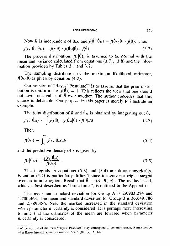
LOSS RESERVING 179
Now R is independent of GM, andf(8, GM> = f($#) * f(e). Thus
f(r, 6, hf> = fir@) * fl6~@) * f(6). (5.2)
The process distribution, f(rl&, is assumed to be normal with the mean and variance calculated from equations (3.7), (3.8) and the infor- mation provided by Tables 3. I and 3.2.
T_he sampling distribution of the maximum likelihood estimator, fl&#) is given by equation (4.2).
Our version of “Baye_s’ Postulate”* is to assume that the prior distri- bution is uniform, i.e. f(e)) = I. This reflects the view that one should not favor one value of 6 over another. The author concedes that this choice is debatable. Our purpose in this paper is merely to illustrate an example.
The joint distribution of R and 6, is obtained by integrating out 6.
fir, &I) = /fir@) *f(Gk#) *f(G>d6 (5.3)
Then
fl6~4) = ,P fcr. 6bfM)dr I (5.4)
and the predictive density of r is given by
(5.5)
The integrals in equations (5.3) and (5.4) are done numerically. Equation (5.4) is particularly difficuit since it involves a triple integral over an infinite region. Recall that 0 = (A, B, c)‘. The method used, which is best described as “brute force”, is outlined in the Appendix.
The mean and standard deviation for Group A is 29,903,274 and 1,700,463. The mean and standard deviation for Group B is 36,649,786 and 2,389,486. Note the marked increased in the standard deviation when parameter uncertainty is considered. It is perhaps more interesting to note that the estimates of the mean are lowered when parameter uncertainty is considered.
2 While our use of the term “Bayes’ Postulate” may correspond to common usage, it may not be
what Bayes himself actually assumed. See Stigler 171. p. 127.
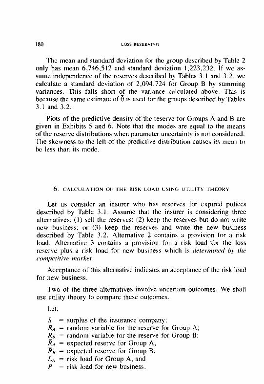
180 LOSS RESERVING
The mean and standard deviation for the group described by Table 2 only has mean 6,746,5 I2 and standard deviation I ,223,232. If we as- sume independence of the reserves described by Tables 3. I and 3.2, we calculate a standard deviation of 2,094,724 for Group B by summing variances. This falls short of the variance calculated above. This is because the same estimate of 6 is used for the groups described by Tables 3. I and 3.2.
Plots of the predictive density of the reserve for Groups A and B are given in Exhibits 5 and 6. Note that the modes are equal to the means of the reserve distributions when parameter uncertainty is not considered. The skewness to the left of the predictive distribution causes its mean to be less than its mode.
6. CALCULATION OF THE RISK LOAD USING UTILITY THEORY
Let us consider an insurer who has reserves for expired polices described by Table 3. I. Assume that the insurer is considering three alternatives: (I) sell the reserves; (2) keep the reserves but do not write new business; or (3) keep the reserves and write the new business described by Table 3.2. Alternative 2 contains a provision for a risk load. Alternative 3 contains a provision for a risk load for the loss reserve plus a risk load for new business which is determined hq’ the competitivr murket.
Acceptance of this alternative indicates an acceptance of the risk load for new business.
Two of the three alternatives involve uncertain outcomes. We shall use utility theory to compare these outcomes.
Let:
S = surplus of the insurance company; RA = random variable for the reserve for Group A: Re = random variable for the reserve for Group B; i& = expected reserve for Group A; i& = expected reserve for Group B; LA = risk load for Group A; and P = risk load for new business.
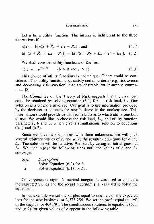
LOSS RESERVING 181
Let u be a utility function. The insurer is indifferent to the three alternatives if:
u(S) = E[u(S + RA + LA - RA)]; and (6.1)
E[u(S + ji, + ,!,A - RA)] = E[u(S + Re + LA + p - &)I. (6.2)
We shall consider utility functions of the form !&) = -e-‘.“b” (b > 0 and c I 1). (6.3
This choice of utility functions is not unique. Others could be con- sidered. This utility function does satisfy certain criteria (e.g. risk averse and decreasing risk aversion) that are desirable for insurance compa- nies. [S]
The Committee on the Theory of Risk suggests that the risk load could be obtained by solving equation (6.1) for the risk load, LA. Our solution is a bit more involved. Our goal is to use information provided by the decision to compete for new business in the marketplace. This information should provide us with some hints as to which utility function to use. We would like to choose the risk load, LA, and utility function parameters, b and c, which give a simultaneous solution to equations (6.1) and (6.2).
Since we have two equations with three unknowns, we will pick several arbitrary values of c, and solve the resulting equations for b and LA. The solution will be iterative. We start by taking an initial guess at LA. We then repeat the following steps until the values of b and LA converge.
Step Description 1. Solve Equation (6.2) for b. 2. Solve Equation (6.1) for LA.
Convergence is rapid. Numerical integration was used to calculate the expected values and the secant algorithm [9] was used to solve the equations.
In our example we set the surplus equal to one half of the expected loss for the new business, or 3,373,256. We set the profit equal to 12% of the surplus, or 404,791. The simultaneous solutions to equations (6.1) and (6.2) for given values of c appear in the following table.
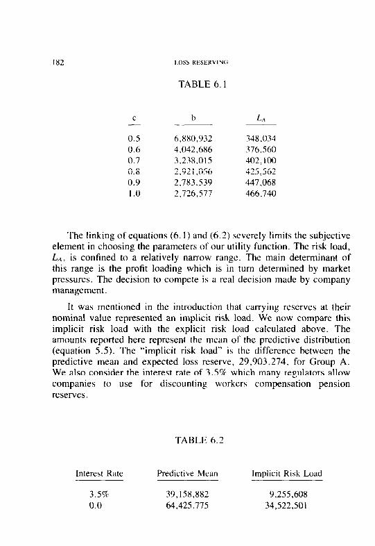
182 LOSS RESERVING
TABLE 6.1
C -
0.5 0.6 0.7 0.8 0.9 I .o
b LA
6,880,932 348,034 4,042,686 376,560 3.238.015 402,100 2.92 I ,056 425,562 2,783,539 447,068 2,726,577 466,740
The linking of equations (6.1) and (6.2) severely limits the subjective element in choosing the parameters of our utility function. The risk load, LA, is confined to a relatively narrow range. The main determinant of this range is the profit loading which is in turn determined by market pressures. The decision to compete is a real decision made by company management.
It was mentioned in the introduction that carrying reserves at their nominal value represented an implicit risk load. We now compare this implicit risk load with the explicit risk load calculated above. The amounts reported here represent the mean of the predictive distribution (equation 5.5). The “implicit risk load” is the difference between the predictive mean and expected loss reserve, 29,903,274, for Group A. We also consider the interest rate of 3.5% which many regulators allow companies to use for discounting workers compensation pension reserves.
TABLE 6.2
Interest Rate Predictive Mean
3.5% 39,158,882 0.0 64,425,775
Implicit Risk Load
9,255,608 34,522,501
LOSS RESERVING 183
7. DISCUSSION
This paper has presented an example of how one might approach the problem of calculating risk loads for loss reserves. This being an ex- ample, we took great latitude in our assumptions and methods. We believe that this example is illustrative of a general approach that can be taken. However there are a number of conceptual and technical problems that must be addressed.
Central to this approach is that a probabilistic model for loss reserves must be specified. In our case we assumed that the future lifetime for an individual is a random variable whose distribution is given by Make- ham’s mortality law.’ It will be difficult to come up with such a model which is appropriate for other lines of insurance.
The reason for selecting a model is that the parameters of the model must be estimated from data. The design of the study and the method of estimation will determine the predictive distribution of the loss re- serves. Jewel1 [lo] demonstrates the effect of study design for predicting claims which have been incurred but not yet reported. His methods are similar to those described above.
This approach is Bayesian. Great care must be exercised in selecting the prior distribution. While our assumption that the 8’s are uniformly distributed may seem innocent enough, consider a reparameterization of Makeham’s law. For example, could then estimate 6
we could have 6’ = (0:, 02, 0:)‘. One M, and assume that the 4’s are uniformly distrib-
uted. Question: would this make a noticeable difference in our estimation of the expected loss reserve, or the risk load? [ 1 l]
There are computational problems with this approach. The dimension of the integral is equal to the number of parameters estimated. Actuarial models tend to have many parameters. Also, the integrand can be time consuming to evaluate. This is not an overwhelming problem. With the powerful computers that are available today, the problem can be solved. It would be nice to find a better solution.
These are only a few of the problems that must be solved.
1 It is not even agreed that Makeham’s law is appropriate for future lifetime. See Dick London, Gradunrion, ACTEX Publications, 1985, and Sunivu/ Models, ACTEX Publications, 1987, for a description of other approaches to fitting mortality tables.
184 IOSS RESERVING
The purpose of this paper is to continue the debate on risk loading and discounting of loss reserves. It is hoped that it provides a clearer view of the issues involved and an indication of what might be possible.
APPENDIX
Most of the calculations in this paper can be done with elementary numerical analysis. This subject is well within the grasp of most actu- aries. However, evaluating the integral in equation (5.3) requires con- siderable effort. This appendix outlines the method of evaluating this integral.
The probability distributions involve several numerical constants which cancel when we form the quotient in equation (5.5). In what follows we will indicate the omission of the numerical constants in the probability distributions by replacing the symbol ‘I=” with “x”.
Our goal is to evaluate:
Jr, e, = fcrp, *f&f(e) +Mx I (5.2)
We have:
f(rlh x e -(r-)&l+2cr~ %ij)
with ~(6) and a-‘(6) determined from equations (3.7). (3.8) and the information in Tables 3.1 and 3.2.
We have: fcj&)) cx p-1 . ,-lA,-7i,,X ‘Iii,--?irJ
with C-’ = ~4 = (a,j(G)). The formula for the LI,,‘s is given by Equation (4.4).
The general form of the partial derivative dP,(G)/iN, is given by Hogg and Klugman [5).
:i’s method 1X(-’ was calculated by factoring ,X = LL’ by Cholesk [9] and multiplying the diagonal elements of I!..
We chose f(6) = 1 when the restrictions of equation satisfied andf(8) = 0 otherwise.
(3.1) were
LOSS RESERVING 185
Equation (5.2) can now be integrated numerically over a large three dimensional rectangle. The integral could be more easily evaluated if we had some idea how large this rectangle should be. We tried the following linear transformation:
where CL is the covariance matrix for 6 = 6,. The motivation for this transformation was that if C was approximately constant, than the rec- tangle could be contained in a region corresponding to the high density region of a normal distribution, say - 3 5 Z; I 3 for i = 1, 2 and 3.
It didn’t work. The region looked like a tadpole with the body in the high density region of a normal distribution, but the tail extended out quite far. After considerable trial and error, we settled on the following rectangular region.
-6 I Z, 5 3, -12 5 Z2 5 6 and -40 I Z3 5 6.
The numerical integration was done by the trapezoidal rule with 9 intervals along the Z,-axis, 19 intervals along the Zz-axis and 45 intervals along the Zj-axis. The author feels comfortable with the numerical results obtained in the final answers, but there ought to be a better way to do this.
186 LOSS RESERVING
REFERENCES
[1] Gary D. Simms, “NAIC Report,” The Actuarial Update, August, 1987.
[2] Frederick W. Kilboume, The Actuarial Review, November, 1987, p. 11.
[3] N. L. Bowers, H. U. Gerber, J. C. Hickman, D. L. Jones, and C. J. Nesbitt, Actuarial Mathematics, Society of Actuaries, 1986.
[4] Richard G. Wall, “Insurance Underwriting Profits: Keeping Score,“Financial Analysis of Insurance Companies, Casualty Ac- tuarial Society, 1987.
[5] Philip E. Heckman and Glenn G. Meyers, “The Calculation of Aggregate Loss Distributions from Claim Count and Claim Severity Distributions,” PCAS LXX. The companion program, CRIM- CALC, written by Glenn Meyers, was used to perform the calcu- lations.
[6] Robert V. Hogg and Stuart A. Klugman, Loss Di.stribution.s, John Wiley & Sons, 1984, Chapter 4.3.
[ 71 Stephen M. Stigler, The History of’ Statistics-The Measurement of Uncertainty before I900, The Belknap Press of Harvard University Press, 1987, p. 123.
18) Gary Venter, “Utility Theory with Decreasing Risk Aversion,” PCAS LXX.
[9] Richard L. Burden and J. Douglas Faires, Numerical Anafysis, 3rd Edition, Prindle, Weber & Schmidt, 1985, p. 47.
[ lo] William S. Jewell, Predicting IBNYR E\jerrr,s trrrci Delays, (In prep- aration).
[I I] George E. P. Box and George C. Tiao, Bayesian Inzference in Statistical Analysis, Addison-Wesley, 1973, Ch. I, for a discussion of the use of noninformative prior distributions.
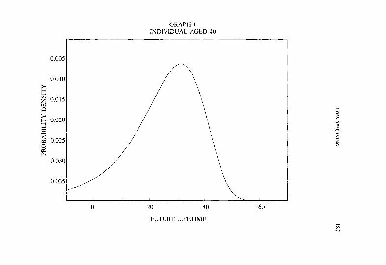
GRAPH 1 INDIVIDUAL AGED 40
0 20 40 60
FUTURE LIFETIME
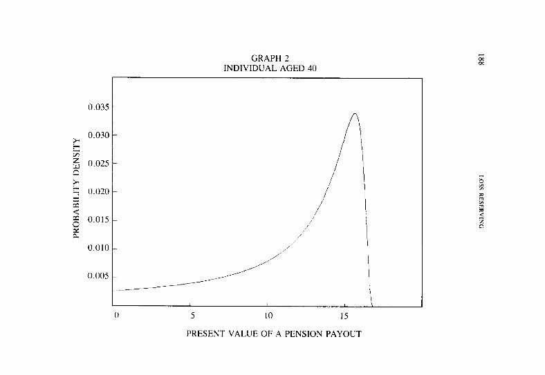
0.035
~ 0.030 k 5; z 0.025
GRAPH 2 INDIVIDUAL AGED 40
0 5 10 15
PRESENT VALUE OF A PENSION PAYOUT
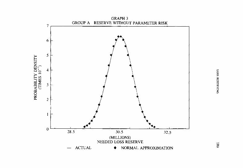
GRAPH 3 GROUP A RESERVE WITHOUT PARAMETER RISK
I I y+ I 28.5 30.5 32.5
(MILLIONS) NEEDED LOSS RESERVE
- ACTUAL 4 NORMAL APPROXIMATION
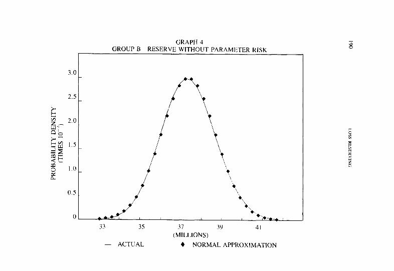
2.5
m 2
1 .o
0.5
0
GRAPH 4 GRAPH 4 GROUP B RESERVE WITHOUT PARAMETER RISK - GROUP B RESERVE WITHOUT PARAMETER RISK
-/
33 35 37 39 41 (MILLIONS)
- ACTUAL + NORMAL APPROXIMATION
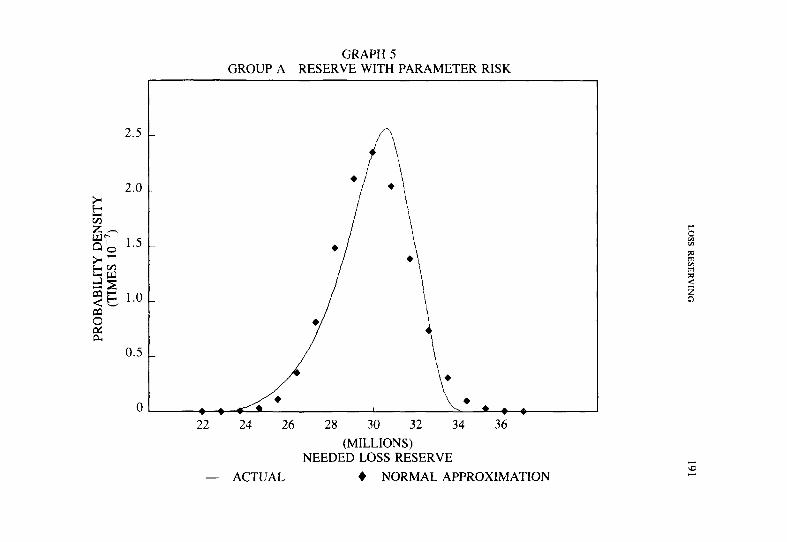
GRAPH 5 GROUP A RESERVE WITH PARAMETER RISK
0 4 4
4 I
22 24 26 28 30 32 34 36 (MILLIONS)
NEEDED LOSS RESERVE
- ACTUAL + NORMAL APPROXIMATION
J
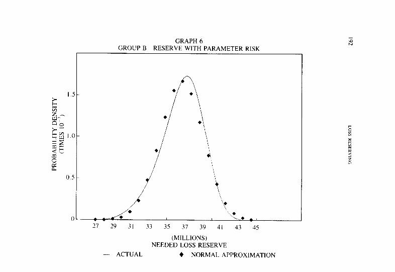
GRAPH 6 GROUP B RESERVE WITH PARAMETER RISK
I
27 29 31 33 35 37 39 41 43 45
(MILLIONS) NEEDED LOSS RESERVE
- ACTUAL + NORMAL APPROXIMATION
193
DISCUSSION OF PAPER PUBLISHED IN VOLUME LXXV
RECENT DEVELOPMENTS IN RESERVING FOR LOSSES IN THE LONDON REINSURANCE MARKET
HAROLD E. CLARKE
DISCUSSION BY JOHN C. NARVELL
1. INTRODUCTION
Mr. Clarke has written a fine paper [ 1] which should be read by all actuaries who practice loss reserving. He has introduced two concepts that will broaden the horizons of actuaries in the U.S. and should provoke them to sharpen their skills.
The first concept is the introduction of a new curve for the fitting of loss development data. This “negative exponential” curve has the for- mula:
L(t) = A X [ 1 - exp( -[t/B]‘)].
The second concept is the use of regression techniques to provide a weighting scheme between Bornhuetter-Ferguson (B-F) and loss devel- opment factor (LDF) projections. Although it is not emphasized in the paper, these two concepts may be used separately or with other more traditional loss development techniques. In the course of the paper the two concepts are commingled, but the astute reader should be able to separate the two.
The first observation that the reader should make is that there are actuaries outside of North America who are developing skills in the property and casualty area. In many instances these actuaries are taking a fresh perspective to old problems and are producing novel solutions. This paper is an example of such innovation. The other item to note is that there are significant variations in terminology in the insurance in- dustry, especially outside of North America. For example, in this paper the author uses data that is categorized by “account year.” An account year is analogous to an underwriting year in reinsurance or a policy year for direct insurance. As stated in the paper, the techniques would be equally applicable to data categorized by underwriting year, policy year, accident year or even report year.
194 REINSURANC’F RESERVING
2. NEGATIVE EXPONENTIAL CURVE
The negative exponential curve is different from curves that many American actuaries use in that it fits loss development data instead of loss development factors. This curve models the upward growth of the losses as they asymptotically approach the ultimate losses (A) from below. Most development curves in the North American literature (e.g., Sherman’s inverse power curve [2]) model loss development factors (LDFs) instead of losses.
By using the negative exponential curve, an entire step in the analysis process is bypassed; i.e., LDFs do not have to be calculated. There are numerous other advantages to the use of loss data instead of age-to-age LDFs.
The negative exponential curve ostensibly has three parameters, A, B and C. The A parameter of the curve is defined in the paper as the ultimate loss ratio. This could just as easily have been defined as the ultimate losses, since the ultimate loss ratio is a simple transform of the ultimate losses. The reason for the use of loss ratios is apparent in the latter part of the paper where loss ratios are used in the regression model.
Another alternative would be to set A = I. This could be accom- plished by dividing the historical losses by year by the estimated ultimate losses for each year. This alternative perspective shows the true nature of this loss development model. By defining each historical observation as a percentage of ultimate losses, the model may be thought of as a variation of a multiplicative LDF projection. If one takes the reciprocal of the percent of ultimate, then cumulative LDFs are easily produced.
In the original implementation of this curve, as introduced by David Craighead, a simple LDF implementation was advocated. On page 66 of his paper [ 31, he says:
“In practice. all that is necessary, gven values of fl and I. i\ to obtain values of
exp -(/if3)‘] (I ~ exp[ -r/B)‘]) and then apply them IO ligures of claim\ paid plus claims outstanding in order to obtain figures of IBNR for each cell of busmess.”
This is clearly a multiplicative LDF method. It is notable in the above equation that Craighead assumed a value of 2.0 for the C parameter. In fact Craighead’s research “resulted in a conclusion to fix the value of C at 2.0” (page 54). He continues:
REINSURANCE RESERVING 195
“The value of C is, in fact, too sensitive and has little effect on the overall results. It can
be influenced easily by the random positioning of a few points at an early stage, where they are least reliable. It also appears to have a counteracting effect on the value of
B. Fixing C at 2.ooO shows that, in most cases, the lit is almost as good as when C is allowed to float and, indeed, in several cases is actually better.”
Mr. Clarke implicitly admits this aspect of the negative exponential curve in his paper (page 9) where “in this particular example C was set equal to 1.5 and only A and B were fitted.” Thus it appears that some variation in the C parameter is allowed in practice but that C is usually fixed before the other parameters are fitted.
The reason for the counteracting effect on the B parameter is easily understood if one reexamines the form of the negative exponential curve. The equation may be rewritten as:
L(r) = A x [1 - Bfrc] where B’ = exp[- l/(Bc)].
As C gets bigger, B’ has to get smaller. This alternative formula is easier to understand; the C parameter is unchanged and the B’ parameter simplifies the form of the equation. B’ is allowed to vary in the range from 0 to 1.
The difference between a simple LDF and the more sophisticated approach in this present paper is that the most current observation is not simply multiplied by the appropriate LDF to ultimate. Rather there is some consideration for a random error contained in the endpoint. This error is measured as the deviation of the endpoint away from a curve which is fit through the entire loss history for that year.
The best way to understand this is to consider an extreme example. Consider losses that exhibit sawtooth variations about a generally rising curve. The true underlying loss development pattern is in the middle with random variations about it. The negative exponential curve can extract the shape of the development curve and project it to ultimate. Effectively each historical data point is given equal credibility in the estimation of ultimate losses.
This is in contrast to traditional LDF projections where only the most recent observation is used; i.e., the endpoint is multiplied by a cumulative factor to ultimate to estimate the ultimate losses. Data observations prior to the endpoint do not affect the estimate. Further, as soon as a new endpoint is known, the previous end points are almost completely ig-
196 REINSURANCF RESERVING
nored. In the sawtooth example, the ultimate projections would fluctuate up and down from period to period in LDF projections but would be more stable in the smoothed negative exponential implementation.
This points out a major difference between the author’s approach and the traditional LDF or B-F methods. When projecting a year from age t to ultimate, the negative exponential considers only the develop- ment patterns for the particular year before age t. In contrast, for most traditional LDF or B-F methods. only development data after age t (for other years) is considered.
Some LDF curve fitting techniques, such as the inverse power curve, can also look at all LDF data simultaneously to extract the true LDF patterns excluding randomness. In fact, the inverse power curve can be used in an analogous fashion to the negative exponential curve if suffi- cient credible data exists. LDFs for a single (accident) year can be used to estimate the remaining loss development tail for that year. However, one major limitation of the inverse power curve in its simplest imple- mentation is that it cannot handle downward LDFs without performing some data smoothing which would destroy the true patterns. Also the data for a single year may produce unstable results similar to the fluc- tuating parameters for the negative exponential curves in the paper.
The theoretical advantages of the negative exponential curve form are numerous. First, the curve can handle many different data anomalies including downward development which, for example, the inverse power curve cannot. Also it is decomposable into as many time intervals as are available from the data. These time intervals do not need to be regularly spaced although the implementation in the paper imposes this limitation. Another major advantage is that the curve form naturally leads to graph- ical display and interpretation. Some of these advantages are not limited to the negative exponential curve but are true for curve fitting methods in general.
There is one potential disadvantage of the negative exponential method. For the curve fitting to be effective, many data points are required. Craighead states (page 65), “This will require the use of . . . loss ratios at least at quarterly intervals, preferably even monthly, and for at least two years, to give any meaningful result.”
On the other hand, an advantage of the proposed methodology is that it is less subject to distortion arising from unintentional bias in the
REINSURANCE RESERVING 197
selection of loss development factors. This is especially true in those cases where a mixture of upward and downward development is evident. Frequently, loss reserve analysts will exclude downward (and very small upward) development factors from consideration in the selection of loss development factors. In the curve fitting algorithm, there is less subjec- tivity in the selection of loss development factors both for the stages where there is historical data and for the “tail” development beyond the range of historical data. While interpretation and curve parameter selec- tion will still be required of the loss reserve analyst, the use of such curve fitting techniques will introduce more science into the art of loss development projections.
3. PROJECTIONS BY INDIVIDUAL YEAR
An innovation in the model is the analysis of each year separately. The model does not require a large history of average loss development factors either for data within the range of the available loss development or for the calculation of a “tail” factor for development beyond the range of the available data. This is a very powerful advantage. However, as noted above, the method does require frequent observations (quarterly or monthly) for the curve to be well defined.
4. REGRESSION MODEL
In the worked example in the paper, the negative exponential curve was used for the older account years to project the loss development of the years individually. In contrast, the regression model (“line of best fit”) was used for the three most recent account years. As noted in the last paragraph of Section 5, the regression model does not require the use of the negative exponential projections for the older years. The only data required for the line of best fit are: a) the historical loss ratios by year of account, and b) the estimated ultimate loss ratios for those years. It is immaterial how those ultimate loss ratios are calculated.
Regression analysis is not new to the members of the CAS. It has been used in many different contexts and is now on the Syllabus of Examinations (Part 3). Its use in this present paper should not be triv- ialized, however. The assumptions and procedures in this particular context merit review and consideration.
198 REINSURANCE RESERVING
The regression model projects losses (loss ratios) from their current status to ultimate in one step. The incremental steps of individual loss development factors are bypassed. This is accomplished by comparing the historical loss ratios at each age with the ultimate loss ratios for the previous account years.
For example, in order to project the 1982 year from 14 quarters to ultimate, a least squares regression of the 1971-81 years’ loss ratios at 14 quarters with their corresponding estimated ultimate ratios is calcu- lated. The resulting formula is used to project the loss ratio from 14 quarters to ultimate for the 1982 year. The 197 l-81 years’ loss ratios at 10 quarters are then regressed with their corresponding ultimate ratios to project the 1983 year from 10 quarters to ultimate. The 1984 year at 6 quarters is projected to ultimate in a similar fashion. In the worked example in the paper, some years are judgmentally excluded from the regression analysis.
In theory the number of years in the regression could have been increased. This is because the earlier years of account were regressed first; e.g., the 1982 year of account could have been included in the regression for the projection of the 1983 year. This would have permitted the inclusion of more observations including the most recent data.
A review of the regression formula shows that the ultimate loss ratio is equal to the immature loss ratio times some factor plus a constant. This may be contrasted with multiplicative loss development wherein the ultimate losses are simply a cumulative loss development factor (F) times the losses to date (L) with no additive constant.
Alternatively, a B-F model may be considered as an additive model; i.e., ultimate losses equal losses to date (L) plus some estimate of the remaining loss development. In the traditional B-F model, the estimate of the remaining future loss development (Fur) is equal to the percent unreported (or unpaid) times an initial loss estimate (E). The future percent is equal to the complement of the reciprocal of the LDF to ultimate ( I- l/F).
The possibility of lack of fit exists with every regression model. This lack of fit may be thought of as lack of correlation or predictive ability of the independent versus the dependent variables. This element of variation necessitates the inclusion of an additional component in the process. This component is the naive estimate; i.e., a flat loss ratio. In
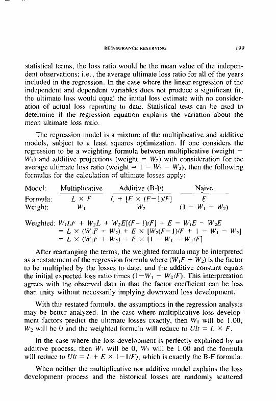
REINSURANCE RESERVING 199
statistical terms, the loss ratio would be the mean value of the indepen- dent observations; i.e., the average ultimate loss ratio for all of the years included in the regression. In the case where the linear regression of the independent and dependent variables does not produce a significant fit, the ultimate loss would equal the initial loss estimate with no consider- ation of actual loss reporting to date. Statistical tests can be used to determine if the regression equation explains the variation about the mean ultimate loss ratio.
The regression model is a mixture of the multiplicative and additive models, subject to a least squares optimization. If one considers the regression to be a weighting formula between multiplicative (weight = Wi) and additive projections (weight = WZ) with consideration for the average ultimate loss ratio (weight = 1 - WI - W*), then the following formulas for the calculation of ultimate losses apply:
Model: Multiplicative Additive (B-F) Naive
Formula: LxF L + [E x (F-1)/F] Weight: WI w2 (I-w:-W2)
Weighted: W,LF + W2L + W2E[(F-1)/F] + E - W,E - WPE = L x (W,F + W,) + E x [Wz(F-1)/F + I - W, - W,] = L x (W,F + W,) + E x [ 1 - W, - WdF]
After rearranging the terms, the weighted formula may be interpreted as a restatement of the regression formula where (WIF + WZ) is the factor to be multiplied by the losses to date, and the additive constant equals the initial expected loss ratio times (1 -WI - W2lF). This interpretation agrees with the observed data in that the factor coefficient can be less than unity without necessarily implying downward loss development.
With this restated formula, the assumptions in the regression analysis may be better analyzed. In the case where multiplicative loss develop- ment factors predict the ultimate losses exactly, then WI will be 1 .OO, Wr will be 0 and the weighted formula will reduce to Ult = L X F.
In the case where the loss development is perfectly explained by an additive process, then WI will be 0, WZ will be 1.00 and the formula will reduce to U/f = L + E X I- l/F), which is exactly the B-F formula.
When neither the multiplicative nor additive model explains the loss development process and the historical losses are randomly scattered
200 REINSURANCE RESERVING
about the expected losses (E), then both WI and WZ will be 0 and the weighted formula will reduce to CJfr = E.
In the regression equation, the initial expected losses (E) will be the average ultimate loss ratio of the historical data included in the regres- sion. The R’ of the regression model measures the proportion of the variation about this mean that is explained by the independent variables (the immature loss ratios). In the case where the historical data is ran- domly scattered about the average ultimate (E), the R’ is 0.
Although this reviewer has not derived a method for determining the respective weights, they, nonetheless, provide an attractive intuitive in- terpretation of the regression model. While the derivation of such weights is not required for the proper working of the regression model, further research into their calculation might produce interesting results.
For the regression the author proposes the inclusion of calculated observations from the fitted curves by year when the actual observations are either missing or are “very variable.” This appears to violate the assumptions of the regression whereby a least squares weighting of the LDF, B-F and naive projections is desired.
The negative exponential curve tit produces an LDF projection with an additive offset for the random variance of the endpoint from the smooth curve. By removing the random variances of the endpoints of the historical data, more weight will be given in the regression to the LDF projections. The substitution of a smoothed negative exponential observation for an actual (or missing) observation will bias the regres- sion and produce a weight (W,) for the LDF that is artificially high. If the data are missing or “very variable,” then exclusion of that year from the regression would be preferable to the LDF bias that would be introduced.
The only possible argument for the inclusion of such a smoothed observation is to try to include consideration of the curve parameters for that particular year. Since the negative exponential curve is fit for each year individually, the only time that all of the years are examined simultaneously is in the regression model.
Benjamin and Eagles suggest another variation of this application. In paragraph 22.3.7 of their paper [4], they advocate the use of projected loss ratios from the curves for more recent years to facilitate regression
REINSURANCE RESERVING 201
equations for the earlier years. For example if there are nine years of data in the triangle (e.g., 197 l-79), the curves for years 1974-77 would be projected to produce loss ratios at age 7. These values would be combined with the actual observations at age 7 for 1971 and 1972 to produce a regression equation to be used to project the 1973 year from age 7 to ultimate. The reason given for this sleight of hand is to enable the production of confidence intervals for the earlier years. One should question the meaning of confidence intervals calculated in such fashion.
5. ALL YEARS AT ONCE
Our British associates seem to prefer the examination of data one year at a time before subsequently looking at all years at once. This is in great contrast to the North American tradition of examining many years simultaneously. If one thinks of data in triangular form, this paper advocates a horizontal perspective instead of a vertical perspective. The growth patterns within a year are examined instead of average growth factors for previous years at the same age.
One troubling item in the paper is the instability of the B parameter in the negative exponential curve fits. For a single line of business, one would expect greater consistency from year to year. Perhaps the modeling of each year individually cuts the data too finely. In contrast, the grouping of all of the years for the regression model assumes the comparability of the various years. Similar grouping of the data in the negative expo- nential model would give greater stability to the B parameters.
The use of many years simultaneously in the regression appears to be in contradiction to the individual analysis of the account years for curve fitting; i.e., the combination of years assumes a degree of homo- geneity and comparability among the years.
The question then naturally arises: Why are the curves not also determined on a multi-year basis ? In fact one might argue that this procedure should be reversed; i.e., that the curves should be determined on a combined basis. The curve fitting of the B and C parameters would be more stable if more years were included. In fact, for any particular line of business, the loss development characteristics should remain relatively consistent over time.
202 REINSURANC’E RESERVING
In contrast, rate levels (and loss ratios) are subject to cyclical market pressures. Therefore loss development patterns, which are relatively immune to distortion resulting from rate movements, should be deter- mined on a multi-year basis. In contrast, premium based loss ratio statistics may not be reliable over varying ups and downs of the market. One possible way to correct for this would be to introduce a rate adequacy adjustment vector to the premiums by year. While such an adjustment is open to arguments of subjectivity, it would nonetheless be more theoretically attractive.
The author discusses this latter option in the context of a case wherein the slope of the regression equation is not significantly different from zero. In this circumstance the average ultimate loss ratio (ULR) from the data is the best estimate for the ULR of the year to be projected. He states that “it would obviously be desirable to adjust the ULR’s to allow for changes in premium rates that may have taken place.” Such modifi- cation should be considered in all cases in order to extract the maximum amount of unbiased information from the data.
6. GRAPHS
In order to expand upon the graphical foundations of this paper, the historical loss ratios for the individual account years have been repro- duced on a multi-year basis for this discussion. Years of account 1973- 78 are shown together on Graph IA, and years 1979-84 are shown on Graph IB. When viewed simultaneously, the years 1973 through 1979 appear to exhibit a variety of differing paths in contrast to the five most recent years (80-84), which are closely packed on top of one another.
A better way to isolate the loss development patterns is to translate each curve onto a common vertical scale. It is recommended that the historical losses (loss ratios) be divided by the ultimates by year to produce curves that show percentages of ultimate losses. The various curves all approach a common horizontal asymptote of 100% of ultimate losses. Such calculations produced Graphs 2A, 2B and 2C. When viewed this way, there appears to be much greater stability and consistency in the loss development patterns.
However, two years, 1978 and 1979, still distinguish themselves as unusual. This is evidence that these two years ought to be examined in
REINSURANCE RESERVING 203
further detail for possible exclusion from the development projections for the other years. The author was able to identify 1978 but was not able to differentiate 1979. The graphical examination of all years simul- raneously allows for easier identification of data problems.
The graphs of the percentages of ultimate losses provide a quick and valuable test of reasonableness of the ultimate projections. By examining the endpoints of curves by year, one can visually compare current indi- cated reserves with hindsight indicated reserves. For example, for the 1978 year the endpoint is at 86.4%, indicating that 13.6% (100-86.4) of the ultimate losses need to be reserved. This percentage of ultimate is far outside the range of any historical observation for the preceding 7 years. Similar observations are applicable for other years, most notably 1977 and 1980. This indicates possible overreserving for these years.
Graphs 1C and 2C are the same as Graphs 1B and 2B but with expanded scale to show detail. This maximizes the advantages of graph- ical analysis and interpretation. In a similar way the graph of the regres- sion from 7 to ultimate has been reproduced at larger scale and with the data points by year labelled (similar to the Benjamin and Eagles presentation).
From this alternative graph one can gain further insight. For example, it appears that the 1973, 1974 and 1979 years fall into a different cluster than the other years. This clustering might indicate that different consid- eration should be given to high loss ratio years versus low loss ratio years. The clustering was not as apparent when the data points were displayed in a small cramped section of an overscaled graph.
Another observation from the graph is that the range of validity of the line of best fit might be limited to the range of the minimum and maximum values used in the fit. Otherwise unexpected results may occur. For example in the line of best fit from 6 (22 quarters in the paper) to ultimate, for loss ratios above 84.1% the indicated reserve requirement is negative. While the prediction of downward development was appro- priate for the one extreme case in the data history where the loss ratio was above lOO%, the downward movement for that year appears more likely to have been caused by a calendar year miscoding of a reinsurance recovery to the 1978 year that was subsequently corrected into the 1979 year. Indeed, the general pattern of development after this age to ultimate is upward, indicating the impropriety of a negative reserve.
204 REINSURANCE RESERVING
Theoretically, a negative reserve can result if the factor coefficient is less than unity or if the additive constant is negative.
7. COMPARISON WITH THE INVERSE POWER CURVE
A comparison of the negative exponential curve with the inverse power curve for LDFs reveals numerous differences. As mentioned previously, the negative exponential curve is an upward rising curve which is fit to the cumulative loss amounts that approaches a horizontal asymptote which is defined as the ultimate losses. In contrast, the inverse power curve fits incremental growth factors and is a downward sloping curve that approaches the horizontal asymptote of I .OO as time goes to infinity. This aspect of the inverse power curve agrees with the empirical observation that loss development factors converge to unity as the losses eventually stop increasing.
On the other hand, one of the similarities of the two curves is their inability to fit loss data at early development stages. Clarke handles this problem by ignoring the early loss development; Craighead advocates a weighting of the errors using a time vector in addition to ignoring the first data observation.
A comparison of the curves produced by these two equations indicates that the inverse power curve is longer tailed than the negative exponen- tial. When an inverse power curve is fit to a perfect negative exponential curve, the inverse power curve will project a longer tail than that which is contained in the negative exponential.
Attempts by this reviewer to fit the negative exponential curve to long-tailed casualty data from the United States have produced estimated ultimate losses that were unrealistically low. This indicates that the negative exponential curve may be too short tailed to fit truly long-tailed data. This may be due to differing underlying characteristics of the loss development data. In discussing the B curve parameter, Craighead notes (page 63):
“R is a mezure of all the delay factor\ thal ;Iffect prem!um or clam rrportmg. whether
those delay factors arise from the facl that it 1s reinsurance huwwss that is involved. or from the method of accounting. or from the length of the claims tail. Some of the values
of R. for example. \tem more from the method of accounting than from the length of the
tail :’
REINSLJRANCE RESERVING 205
Considering the reporting delays in the fragmented London reinsur- ante market, the loss development tail for those losses may well be better explained by the negative exponential curve. There are initial delays in reporting, followed by a steady stream of losses that then trail off relatively rapidly. The negative exponential starts slower but finishes faster. The general nature of the loss development delays for London market reinsurance are different than those of casualty exposures in North America, which, in contrast, are largely driven by social inflation forces such as increased claims consciousness and litigiousness.
8. REGULATORY OPTIONS FOR MINIMUM RESERVES
The current Schedule P formula for the “Excess of statutory reserves over statement reserves” is a crude means of mandating minimum re- serves. These minimum loss ratios are even simpler than the current Lloyd’s audit reserve calculations. For example, minimum loss ratios do not consider the actual reported loss experience to date. At least the current Lloyd’s audit percentages produce varying minimum loss ratios for varying levels of reported paid losses.
The proposed mixed (multiplicative and additive) formula in the paper is a much more responsive means of establishing formula reserves. However, there are many issues that need to be addressed in the area of statutory minimum reserves. For example, should industry average fac- tors be applicable to all companies? Or should it be the average minus one standard deviation in order to achieve the goal of merely producing a lower bound that will prevent ridiculously low reserves?
One option would be to use loss ratios for each individual company from Schedule P data. With the availability of ten years of data on Schedule P, it would be possible to include seven (or more) years of company data in a regression to produce minimum reserves for the three most recent accident years for the company. Actual investigation into this possibility should be easily performed by those who have computer access to a large volume of companies’ Schedule P data.
9. RESERVE SETTING
One option not proposed in the paper is in the area of prospective reserve setting as opposed to retrospective reserve testing. With the
206 REINSURANCE RESERVING
availability of historical losses by quarter (or month), it would be possible to perform regressions with quarterly (or monthly) data to produce re- sponsive formulas that could then be applied to the actual paid and/or incurred losses at the end of each period to produce periodic IBNR reserves. In fact, in the paper the reserves are calculated at midyear, although the regressions are ambiguously labelled as being at the end of the year.
10. SUMMARY
This paper has presented a fresh perspective to the challenge of loss reserving whereby loss development is not measured in stages but rather is projected in one jump from the current status to ultimate. This process has advantages in those cases where erratic up and down movements disguise the underlying development. The introduction of the negative exponential curve facilitates the author’s approach.
However, this new alternative is not without problems. First of all, frequent data observations are required for the method to produce stable results. Even with frequent data points, the data may not produce stable curve parameters. In particular it may be necessary to fix the C parameter, thereby losing some of the predictive shape of the curve. And finally the shape of the negative exponential curve may be too short-tailed. Caution should be exercised by all actuaries who attempt to use this curve for casualty data from the United States.
REINSURANCE RESERVING 207
REFERENCES
[I] Harold E. Clarke, “Recent Developments in Reserving for Losses in the London Reinsurance Market,” PCAS LXXV, 1988, p. 1.
[2] Richard E. Sherman, “Extrapolating, Smoothing, and Interpolating Development Factors,” PCAS LXXI, 1984, p. 122.
[3] David Craighead, “The Financial Analysis of a Reinsurance Office,” Risk Research Group Ltd., London, England, 1982.
[4] S. Benjamin and L. M. Eagles, “Reserves in Lloyd’s and the London Market,” J.Z.A. Vol. 113, Part II, 1986.
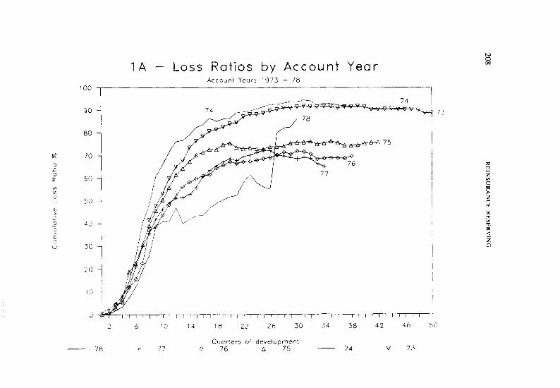
100
1A - Loss Ratios by Account Year Account Years 1973 - 70
7
90 -
0
2 6 10 14 18 22 26 30 34 30 42 46 Si!
Ouorters of development - 78 + 77 0 76 A 75 - 74 V 73
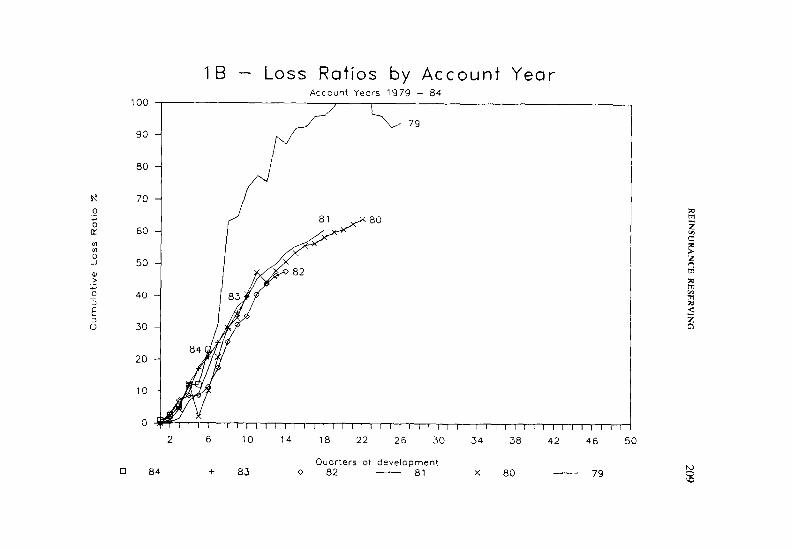
1B - Loss Ratios by Account Year Account Years 1979 - 84
2 6 10 14 18 22 26 30 34 38 42 46 50
Ouorters of development Cl 84 + 83 0 82 - 81 X 80 - 79
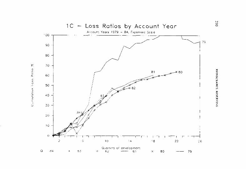
a0
5 5
40
E i: 30
1c - Loss Ratios by Account Year Account Years 1979 - 84; Expanded Scale
2 6 IO 14 18 22 26
Ouarters of development 0 d4 l 83 0 a2 - 81 X 80 - 79
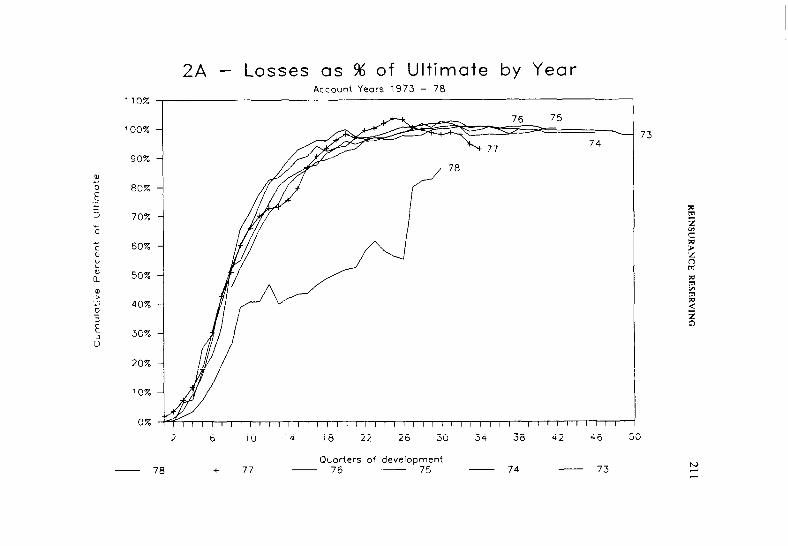
2A - Losses as % of Ultimate by Year Account Years 1973 - 78
110%
100% -
90% -
80% -
70% -
60% -
50% -
40% -
30% -
20% -
10% -
0%
2 6 10 14 18 22 26 30 34 38 42 46 50
Ouorters of development - 7R r 77 - 76 - 75 - 74 - 73
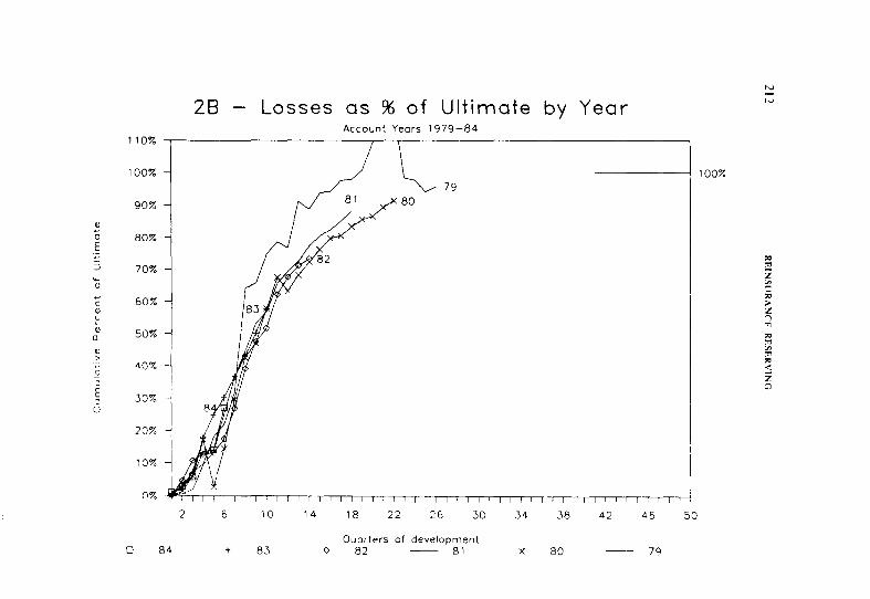
110%
100%
90%
80%
70%
60%
50%
40%
30%
20%
10%
0%
2B - Losses as % of Ultimate by Year Account Years 1979-84
2 6 10 14 18 22 26 30 34 38 42 46 50
Ouorters of development 0 84 + 83 0 82 - 81 X 80 - 79
100%
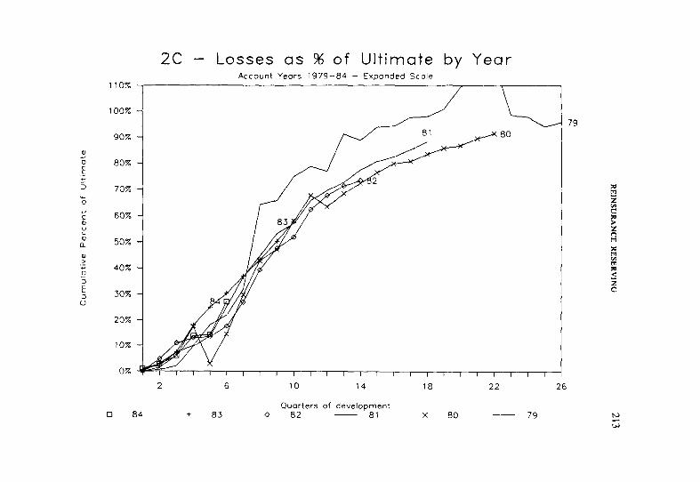
110%
100%
Account Years 1979-84 - Expanded Stole
79
90%
80%
70%
60%
50%
40%
30%
20%
10%
0%
2 6 10 14 18 22 26
Ouorters of development 0 a4 + 83 0 82 __ 81 X 80 - 79
2c - Losses as % of Ultimate by Year
N
w
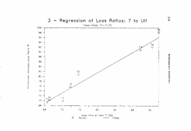
100
90
96
94
92
90
88
86
84
82
00
78
76
74
72
70
68
3- Regression of Loss Ratios: 7 to Ult Years Fitted: 71-77.79
I , I I / I I / 1 I
68 72 76 80 a4 08 92
Loss ratio at Yeor 7 (26) 0 Actual - Fitted
215
REPRINTED FROM VOLUME XXVI
PRESIDENTIAL ADDRESS-NOVEMBER 16. 1939
THE FIRST TWENTY-FIVE YEARS
FRANCIS S. PERRYMAN
This is the occasion of the celebration of the Twenty-Fifth Anniver- sary of the Society, and consequently this address rather inevitably will fall into the category of a review of the quarter of a century that has elapsed since that memorable day in November, 1914, when forty of our founder members met together at the first meeting of this Society. How- ever, the historical part of the review will be brief. I am not attempting to give a history of the period or of the Society, for in any case I am not the one to write such a chronicle; there are many here who have played a more active part over the whole period and who are much more competent to undertake the role of historian. I will, nevertheless, ask you to bear with me while I rapidly scan the twenty-five years.
First it is worthy of more than passing notice that the quarter century in question extends from the outbreak of the first World War to what may well prove to be the outbreak of the second. It is, of course, a coincidence of a purely accidental kind that the first war should have been broken out just when our founders had decided the time was ripe to launch our Society and that the second war should come almost exactly twenty-five years later and that we consider twenty-five a nice round number of years and worth celebrating. What needs serious concern, however, is that while the lapse of twenty-five years is, for a Society such as ours, a good time at which to take stock and while twenty-five years is a good slice out of the active business life of most of us as individuals, yet it is an impossibly short time to elapse between world wars. By impossibly short time I mean a time so short that it is impossible for our civilization to stand the strain of having these upheavals at the rate of four a century, with the intervening periods of turmoil and uncertainty. If civilized man does not find a way to avoid having a world war every twenty-five years, he will soon cease to be civilized man. This is not an actuarial conclusion but a statement of common sense.
The twenty-five years of our Society’s life can be divided mathe- matically into five periods of five years each and, as it happens, these
216 THE FIRST rWENTY-FIVE YEARS
five-year periods form a rather suitable division of the period from the historical point of view. The first five years were from I9 14 to 1919, marking the duration of the World War and the making of the peace. As respects our Society it marked the beginning of modern casualty insur- ance and casualty actuarial science. During this period there was a great, almost unbelievable, increase in the volume of casualty insurance. Com- pensation insurance was introduced quite widely in this country during the period, and the automobile business started on its phenomenal growth.
The second five years, from 1919 to 1924. covers the period of post- war depression and recovery and the beginning of the “New Era” that was hailed as the inauguration of a new and better world for us to live in. The period, as far as casualty insurance is concerned, was marked by continued growth, with only a temporary set-back on account of the 192 1 depression. During this time casualty insurance settled down some- what, and the five years saw the setting up of many of our major rating organizatons in the form that they still have today.
The third five-year period, 1924 to 1929, covers the “New Era” in full flower. Despite the gloomy and scarcely heeded mutterings of a few critics, American business continued to go ahead and go ahead, and casualty insurance followed in its wake. The volume of casualty insur- ance reached at the end of the period was a peak that was not going to be surpassed for many years thereafter. Of course, looking back upon this time from the vantage point of 10 or 15 years it is easy to see the folly of much that was then done and to realize that during this “New Era” were sown the seeds of much future trouble; but at the time everything looked quite rosy. From the particular viewpoint of casualty insurance the period included the inauguration of the “permanent rate- making program” for compensation insurance and the introduction of further refinements in casualty underwriting and rate making.
The fourth five-year period, 1929 to 1934, covers the great depres- sion. Casualty insurance was not of course immune to the effects of the storm and many of its worst crises arose during the period. Compensation insurance, with its intimate connections with general business, became one of the most serious of problems, and the “permanent” rate-making program of the previous period had to be hastily amended. The spectre of occupational diseases arose to add one more to the list of threatening disasters. Other aspects of casualty business that caused the gravest
THE FIRST TWENTY-FIVE YEARS 217
concern to the stronger companies and pushed some of the weak ones over the brink arose out of the terrific drop in investment values, a direct threat to all companies, a collateral threat also to those which had undertaken great commitments on guarantee bonds, such as those cov- ering mortgages and note issues. The history of the period, of course, is solely one of depression, of disaster and of the measures taken to stem the tide.
The fifth period, 1934-1939, is characterized by the recovery from the sorry state in which the country found itself at the end of the previous period. As to the extent and efficacy of this recovery opinions may differ, but certainly the casualty business is in a much more healthy state than it was five years ago. From our point of view the period is marked by the effects of the recovery and by the renewal and intensification of competition between the different parties in our held.
No account of the quarter century would be complete without some more specific reference to the almost unbelievable growth of casualty insurance during this time. It is not easy nor is it necessary to find comprehensive figures dealing with all the classes of insurance coming within the purview of our Society. Most of these are written by private insurance carriers of several varieties, usually either so called life or casualty or surety companies, but in addition a certain portion is handled by public or semi-public carriers and some kinds are considered to be more or less direct governmental functions. For my purpose, a sufficient index is the total writings of all casualty and surety companies doing business in New York State-the figures while not covering the whole field comprise enough of it to illustrate the gigantic growth. In 1914 the total countrywide writings of all casualty and surety carriers entered in New York totaled $139,000,000. By 1919 this had jumped up nearly 150% to $329,000,000; by 1924 the writings had reached $541 ,OOO,OOO; and by 1929 the total attained the colossal figure of $811 ,OOO,OOO. From this there was a considerable recession-in 1933 the writings were only $581 ,OOO,OOO but thereafter the volume of business increased again to $856,000,000 in 1937. In 1938 the volume was approximately the same, $849,000,000. It would appear that allowing for the writings not included in these figures that we service a billion-dollar-a-year business. Contrast this with the 1914 figures.
In my brief outline of the background of the last few years I have deliberately, so far, omitted any reference to general world conditions,
218 THE FIRST TWENTY-Fl\‘t YtAKS
to the world-wide unrest and discontent, to the growth of new and subversive ideas of human conduct particularly in certain countries, accompanied by the sporadic outbreak of open hostilities in different parts of the world. All this, viewed from our domestic scene, has furnished an ominous and sinister background to this nation’s efforts to achieve “recovery” and has finally culminated in a major war the eventual outcome and consequences of which we cannot forecast.
This brief survey of the history of the twenty-five years being now finished, I want to discuss for a few minutes what the Society has done and how it has done it. I do not intend to give a critical account of our technical achievements-these can speak for themselves. Rather, I want to evaluate the efficiency in our accomplishments, as such and in relation to our Society’s expressed aims, and to do this along the lines of attempting to estimate the worth of the Society to its members, to the business of casualty and social insurance, and to the nation at large.
How far have we succeeded in fulfilling our avowed purposes as a Society? How have we done what we have done? And can we fairly say that the Society, in doing what it has done and in the methods employed, has been and is as useful a unit of our civilization as it could and should be’?
First then we will look to see what success the Society has had in the way of fulfilling its aims. These aims are, and have been from the beginning: “the promotion of actuarial and statistical science as applied to casualty and social insurance by means of personal intercourse, the presentation and discussion of appropriate papers, the collection of a library and such other means as may be found desirable.” The second Article of the Constitution, entitled “Object,” has never been amended.
Dr. Rubinow, in his letter to the Society on the occasion of its twentieth anniversary five years ago, said: “I have no doubt in my own mind that it was because of the Casualty Actuarial Society that casualty insurance has become so very much more scientific in this country than it had been, for instance, in England, and the value of the work of these twenty years, the value of the twenty volumes of publications accrued not only to the insurance carriers, but what is very much more important to the American people, for scientific insurance means insurance on a basis equitable to the insured as well as to the insurer and useful to the people at large.” These words are as true now as then. There is a good deal more work being done abroad in respect to casualty actuarial subjects
THE FIRST TWENTY-FIVE YEARS 219
than most of us realize. A perusal of the actuarial literature of countries like Italy, France and Germany will show this. However, most of this work abroad is along the lines of theoretical studies by persons not always actively engaged in the business of insurance, and the practical side of casualty insurance and casualty actuarial work in those and other foreign countries is still very primitive as compared with the work done in this country. I am in the service of an organization with interests in many parts of the world, and so I have more opportunities than many of you to realize this; it happens that several times recently I have been impressed by the statements of persons connected with our interests abroad as to the comparatively advanced stage of casualty practices in this country as contrasted with the rough-and-ready methods used abroad. These statements particularly apply to what we know as the actuarial aspects of our business-that is, those phases of our business where the influence of the members of this society has been most felt. One of the outstanding characteristics of this young and vigorous country has always been its willingness to experiment with new methods and ideas. Perhaps sometimes it has rushed too quickly and none too wisely into some new development, but corrections and improvements have followed. This is the way to make progress-it cannot be made by standing still. The casualty insurance business has exemplihed this urge for rapid progress, and to say that the Casualty Actuarial Society has reflected this is an understatement. I would rather put it that the Society has fostered and promoted a lot of this forward-looking activity. This does not mean to say that the Society has done as much towards the aims of promoting casualty and social insurance as may have been wished by the founders. The truth is that our efforts have been spotty in the sense that some branches of insurance have received far more attention than others; certainly compensation insurance has received from us much more at- tention than any other kind of insurance and other forms of social insurance have in many ways been sadly neglected. No doubt this will ultimately be corrected, particularly as the nation’s views on social insurance are considerably different from what they were twenty-five years ago, have changed radically in the last few years and have not yet finished changing. In my address to the Society last May I expressed my views as to the function of the Society and its members in respect of these social insurance problems, and so I will not repeat them now.
Next let us consider how the Society has functioned. The quotation from the Constitutioin given above mentions some methods to be fol-
220 THE FIRST TWENTY-FIVI, YI:ARS
lowed-personal intercourse, the presentation and discussion of appro- priate papers, the collection of a library and such other means as may be found desirable. Taking first the more formal aspects, “the presenta- tion and discussion of appropriate papers.” During the twenty-five years we have had papers of varying kinds and varying merits and on many different subjects. We have had forma1 discussion of these and we have added many informal discussions of these and other subjects. These articles have received publicity by publication in our Proceedings and in the insurance press. All this has been very valuable to the insurance business and therefore to the whole community. What is contained in the pages of the twenty-five volumes of the Pro~~erdin~~s r,J’rhr Casualr~ Acruurid Sociefy reflects these formal contributions to (as Rubinow puts it in the sentence just quoted) “not only the insurance carriers but what is much more important the American people.” As to the library, we certainly have a library, but whether what w’c have is in an adequate fulfillment of the conception the founders of our Society had is a question that I rather think the founders would answer in the negative. Our library should be much more than a place where our students can get access to certain prescribed textbooks; I believe a larger scope is both desirable and possible.
The more formal contributions of the Society to the building up and improvement of casualty and social insurance. that I have just been talking about, form the background or framework of our Casualty Ac- tuarial Society. However, despite the extreme importance of such formal material-important as it is and difficult as it is to get sometimes (as can be readily testified by those whose lot it has been to secure such material for inclusion in our written records)-it is not everything, as our Con- stitution definitely recognizes by calling for personal intercourse, that intangible thing which, after all, makes the wheels of the world go round. Those whose gifts do not run to the ready production of formal papers can take some comfort from this other method of achieving our aims as a body of casualty actuaries. Many of our members, past and present, whose more formal contributions have not been large, have nevertheless conferred and are conferring benefits to our casualty actu- arial science that are actually just as valuable. and in many cases more valuable than the writing of formal papers, and this they have done and are doing by the means of personal intercourse. What I have personally valued and cherished, and still do, has been above all the opportunity of meeting the other actuaries in my own chosen field. When fifteen
THE FIRST TWENTY-FIVE YEARS 221
years ago I came into casualty insurance (from life insurance in another land) I was very fortunate to find our Society flourishing in its tenth year. Although my duties brought me in contact with many other casualty actuaries, I found that the Society gave me a much wider opportunity to get to know you all. This personal intercourse is the flesh and blood of our Casualty Actuarial Society, just as the more formal part of our proceedings is the framework, and by means of it our Society has accomplished great things.
This analogy of our formal work as the framework, and our personal intercourse as the flesh and blood, like all analogies cannot be pushed too far; but we can safely say that a structure merely of framework and of flesh and blood could not be a living organization; something else is needed, the spark of life. If our Society is to be a living organization it must live and survive. This means, it must undertake the training and educating of new and younger members to take over from the present membership as time inexorably marches on. This question of education, while not specihcally mentioned in the objects of the Society as quoted above, is to be implicitly understood. Our Society is a scientific one; it was formed to act as an agency for the dissemination of knowledge pertinent to our held and this surely includes the function of promoting the education of casualty actuaries-or in other words, the training of successors to carry on our scientific work. How have we made out in this matter of education? Here, of course, I am not trying to evaluate the tangible, but rather the intangible. I am not looking to see how many students have sat for our examinations and how many have passed, but I am seeking to find if we have trained casualty actuaries and built up a society that is a living and continuing organism. Yes, we hold exami- nations and we have a syllabus and we have a course of reading and we have a library. We have examined a large number of candidates and have passed many of them. Our formal arrangements for education are not so elaborate as those of some of the other actuarial societies, but we have had a steady stream of new members coming in, and, I believe, properly trained new members. Whether we have had as many such new members as we should is a different question. Believing as I do that the scope of actuarial work should be enlarged, and that our Society has not completely covered every corner of its field, I suppose my conclusion must be that we should, and doubtless would have obtained more such trained new members if our Society’s activities had extended more completely over the whole field of casualty and social insurance. Never-
222 THE FIRST TWENTY-FIVE YtARS
theless, within our held as we have developed it (or should I say culti- vated it) we have reaped a good crop, and with some notable exceptions we have in our membership very nearly all those who should be with us. And what have we to report concerning the quality of our crop? Are we training the successors of men like Rubinow, J. D. Craig, Woodward, Flynn, Mowbray, Ryan, Leslie, Michelbacher. Perkins, Moore, Tarbell, Dorweiler, Green and Senior? (Here let me say I did not select the men to appear on this list-you did. for it is a list of the past presidents of our Society). Are we training men who like these and many others can face whatever they may be called upon to tackle and who can achieve the same measure of success that they have? I believe that the answer is “yes.” for as I take stock of the younger members of our Society I am quite encouraged. Our Society is showing no sign of inability to develop suitable manpower. I ascribe this, not solely to our formal program of education, but in a large measure to that more intangible personal inter- course to which once again I attribute a large portion of the credit for the success of our Society.
Does this all mean that the objects of the Society have been suc- cessfully achieved in the twenty-five years? It does in the sense that the Society has made great progress and has been of great help to those phases of our social structure that it was formed to aid. But of course we have not been 100% successful: nothing human ever is. There are, as I have indicated, many directions in which our Casualty Actuarial Society has not progressed as much as it might, and there are some directions in which seemingly no progress has been made. The larger part of our efforts, at any rate our “formal” efforts, seem to have been directed towards compensation insurance and not so much attention has been given to many of the other kinds of insurance usually considered as belonging to the held of Casualty and Social Insurance.
In the less formal parts of the work of our Society. as typified by the “personal intercourse” I have spoken of, the Society’s success has, I consider, been rather greater, although this is not uniformly true as regards our entire membership. many of whom are not particularly active in our corporate work. The reasons for this arc not at all obscure: the membership of our Society is not as homogeneous as that of the other actuarial societies. Many of our members are life actuaries whose present interests in our casualty aims is not very great. Again, another large section of our mcmbcrship consists of undcrwritcrs or executives of casualty companies whose direct interest in the purely actuarial aspects
THE FIRST TWENTY-FIVE YEARS 223
of the business is not as great as it may have been at one time. That leaves a somewhat reduced proportion of our membership with a con- tinuing active interest in casualty actuarial work. For reasons such as these, it is not possible to get all of our members to share equally in our endeavors to carry out the objects of our Society, and it may therefore have seemed to some that the actual work of running our Society has been not so widely spread as it might have been. This does not mean that those who do the work object to doing it, but it does help to explain why the actual running of the Society has apparently been confined to what, while it is a large majority, is still a somewhat restricted proportion of our membership.
Now the danger of this state of affairs is that, if most of the work of the Society falls on those whose chief immediate interest is, say, compensation insurance, then inevitably the Society tends to interest itself predominantly in compensation insurance and in refining this to the rzth degree, so that other kinds of social insurance, that possibly should be studied and developed, remained unduly neglected. No doubt ultimately this will be corrected, if public interest calls for the neglected to be developed. The Society should try to avoid the over-emphasis of some parts of its field and the neglect of others, and the way to do this is to bring within its membership all of the workers in the various parts of its field, and to place the running of the Society on the broadest possible cross-section of its membership. Your past and present officers and your Council continually have these considerations in mind and have, I know, been ever on the alert to place the running of the Society on as broad a base as possible. There has been no inclination or endeavor to keep the control in any one particular group. An instance of the steps taken to keep this control as broad as possible is the recent appointment of a Nominating Committee-the objective of which is, of course, not to restrict the field for candidates for office but to extend it.
I think that we can say, then, that we have made a good start during the first quarter of a century towards attaining the objects of the Society. On the formal side we have done a lot but a great deal remains to be done, and probably always will so remain. On the more informal side, meaning by this the building up of a capable group of Casualty Actuaries, we have done, I should judge, even more-and perhaps this is actually the most important thing we have done or could have done. For there is no assurance of the perpetuation in its present form of our system of casualty and social insurance or indeed of our whole insurance system.
223 I-HE FIRS’1 IWENTY-FIVE YCARS
For insurance, as we know it, is bound up with our economic system of capitalism. This capitalism, like any other living organism, cannot and does not stand still, and we seem to be in an era of great changes. Therefore, what is important is that we have a systematized actuarial science and a body of actuaries capable of ready adaptation so as to be able to take care of any changes that may come in our social organization. Let me repeat-what is important is that the principles of the actuarial science that we have set out to establish should bc built on a sound basis, and, above all, that we should have developed and trained a body of actuaries capable of applying these scientific principles to whatever changes this country finds is desirable to make. What these changes may be is not for me to discuss hem, although it does seem that they must tend towards the simplification and extension of insurance. I cannot believe that social insurance will not bc considerably extended in scope with the passing of the years, and further I cannot avoid the belief that some of the forms of insurance will be considerably simplified. Those kinds of insurances with which we have had most particularly to deal have been growing in complexity during the life of our Society, and the time is not far distant when some broader generalizations and simplifi- cations will have to be made. However, what the changes may be is not the point I am considering at the moment; the point is, whether our Society, that is to say our members, are capable of dealing with whatever changes are coming. I think the answer is undoubtedly “yes.” and that implies that our Society’s work has not been unsuccessful.
225
REPRINTED FROM VOLUME LI
THE FIRST FIFTY YEARS
DUDLEY M. PRUlTT
I. HOW WE BEGAN
UPON curried motion, the president was uuthorixd to uppoitlt a committee.
-Minutes of First Meeting, C.A.S.11 1
Let me say at the beginning that this is not a history of the Casualty Actuarial Society. I have neither the time nor the talent to do the research and analysis necessary for such an undertaking, and more importantly, there are others eminently more qualified if a definitive history is to be written. I hope such a history will be written some day. This is but a footnote to that undertaking and if, in this presentation, you find that I have given a certain skewness to the story, an offbalance of the facts, if the wrong things are emphasized and the right ones omitted, please forgive my wayward pen. There is such a vast amount of material, important and trivial, serious and silly, dull and lively, that I have had to be selective to stay within considered and considerate limitation, and I have selected, quite frankly, what interested or amused me, thinking, I hope rightly, that it would interest or amuse you.
In the span of history fifty years is brief indeed, but in the span of the life of a man or of an actuarial society fifty years encompasses tremendous change, so that the earlier is hardly recognizable in the later. It is fashionable to point out that the past fifty years have witnessed greater changes in the pattern of our lives than had perhaps the preceding fifty decades. Our infant Society was born into an ancient world where horses and beards were still seen on the streets, where the Atlantic Ocean was still a very wide body of water, and where no casualty actuary, to my knowledge, had ever heard of the negative binomial. But the forces of change were on the move and we may well consider the year 1914 as the birth date for a new world, as well as for our new Society.
226 THE FIRSI FIFTY Y-EARS
On May 28, 1914, a group of men, meeting as the Statistical Com- mittee of the Workmen’s Compensation Service Bureau, decided that what they needed, in view of the problems presented by the new work- men’s compensation laws, was a professional society. One month later the Archduke Francis Ferdinand of Austria was assassinated. On July 27 our organizing committee addressed a call to such persons as might be interested in joining a casualty actuarial and statistical organization, and the next day Austria declared war on Serbia. The organization meeting of the Society was held at the City Club of New York on November 7, the day after Japan took Tsingtao from the Germans. That day our charter members not only founded the Casualty Actuarial and Statistical Society of America*, adopted a constitution and by-laws and elected officers and a council, but also listened to the presentation of three papers (one of which was by our still active member, Win Greene), ate their first Society dinner at 7:Oo P.M., and digested it with ten after-dinner speeches. Times have changed!
The First World War, of course, was destined to influence profoundly the course of history for both the world and our Society, but nothing in the record of that first organization meeting indicated even an awareness of its progress. At that time Europe seemed far away indeed.
What was of much more pressing interest, perhaps, to our group of pioneers, was the new spirit of adventure that seemed to be taking hold of American industry. It had been on January 5 of this same year that Henry Ford announced his five dollar minimum wage and his eight hour day, and on July 1, 1914 the broad new New York Workmen’s Com- pensation Law became effective. Mark Sullivan called it a period of “dynamic energy accompanied by a dynamic humanitarianism.“[4] A new day was dawning!
Here were the required elements for the founding of a successful actuarial and statistical society: dynamic energy. dynamic humanitari- anism, an eight-hour five dollar day, a whole wave of new workmen’s compensation laws taking over one state after another. a body of men inspired by and somewhat overwhelmed by the new problems these laws presented, and a few men who were prepared to act boldly.
* This was the original t’omm of our name. The words “and Stati\tlcal of Anxrica” were
amputated in IWI [2] supposedly without pre.judice to the \tatisti<;tl elemant in our mcrnbershap, though with considerable unhappiness to our founder.\31
THE FIRST FIFTY YEARS 227
II. THE PIONEERS
There wtere giants in the earth in those days.
-Genesis 64
You shall sir at the feet of Winfield Greene. that slughorn tooter tough. Or become u second Michelbucher-though one is quite enough.
--Clarence W. Hobbs[ I]
One of the benevolent dispositions of Providence seems to be that when, in the course of human events, it becomes necessary to have giants, giants are provided. So it was in the founding of our country, and so it was also in the founding of our Society. Isaac M. Rubinow, James D. Craig, Joseph H. Woodward, Benedict D. Flynn, Albert H. Mowbray, Harwood E. Ryan, William Leslie, Gustav F. Michelbacher, George D. Moore, Winfield W. Greene, Leon S. Senior-these charter members were also elected presidents of the Society and each gave his own unique contribution to its achievements. There were in all ninety- seven charter members, though only forty attended the organization meeting. Many of them were outstanding men and made outstanding contributions, but any selection by me of some would undoubtedly run the risk of omitting others of equal importance. The charter member presidents were giants enough and to spare for the birth of one actuarial and statistical society.
Dr. Isaac M. Rubinow is the acknowledged founder of our Society and the first president. He was what one might call a fortuitous circum- stance, a chance occurrence, that had no good excuse for being in the business when our time had come. He belonged in the social sciences, not in business, and he was in business really just long enough to found our Society. Dr. Rubinow was born in Russia and brought up in Man- hattan. He took a medical degree, but practiced only a short time, went to Washington in government service for a few years, and in 1911 came to the Ocean Accident and Guarantee Corporation as Chief Statistician. This job lasted less than five years. He then joined the staff of the American Medical Association and after that the Federal Trade Com- mission, leaving this to become the director of the American Zionist Medical Unit in Palestine, next the director of the Jewish Welfare Society in Philadelphia, and, for the last seven years of his life, the secretary of B’nai B’rith.
228 ‘THE FIRST I-IFIY YEARS
One thing that seems clear about Dr. Rubinow was his deep dedi- cation to the cause of social insurance. In 1913, before the organization of our Society, he had already published a book entitled Sock1 Insurance with Special Reference to American Conditions, which ran to 525 pages. Win Greene relates that he found the book most useful in the work he did in early 1914 for the purpose of establishing a basis for workmen’s compensation rates under the New York law effective July 1, 1914. Dr. Rubinow, from all accounts, was a man of strong opinions and of liberal social convictions. Emma Maycrink, who took a course under him at the New York School of Philanthropy, says that, although she has “always opposed socialist tendencies,” she found him quiet and one who spoke with authority. Others have called him “opinionated” and “out- spoken,” but all agree that he was a man of very real ability, an expert in social statistics when experts were really needed and when our business was first called upon to establish rates and procedures for workmen’s compensation insurance. He was chairman of the first statistical com- mittee that laid the foundations for the compensation rate structure. He prepared the “Standard Accident Table” which was the guide for rate- making until useable experience became available.
He was not, of course, universally admired-what pioneer ever is? And it is told that at least one company threatened to prohibit membership in the Society on the part of its employees if he was to continue as president. This seems to have been because of his “socialist tendencies,” and apparently it was no more than a threat. Nevertheless, twenty years later Dr. Rubinow, himself, writes, “I have not altogether forgotten the sharp conflicts and sometimes bitter feelings centering around the term ‘social insurance’ and its proponents in this country in years gone by. Perhaps if it had not been for that unhappy antagonism I might still be actively in the field, yet happily those days are gone.“[2] Or are they?
Of the other ten charter presidents only seven were college graduates and seven were members of the life actuarial societies, but the correlation between these two was not perfect. Two of those who did not graduate from college, Craig and Flynn, were Fellows by examination of the Actuarial Society of America, Craig serving once as president of that society and Flynn as a member of the Council.
Michelbacher was the youngest, being only twenty-three at the time the Society was organized and thirty-three when he became president.
THE FIRST FIFTY YEARS 229
Michelbacher has been the most financially rewarding member of the Society, having allowed us the royalties from his book, Casualry fnsur- ance Principles, for many years. He is the only one of the ten to have become a company president.
Senior, like Rubinow, was born in Russia. He came to this country at the age of fifteen, graduated from New York University at the age of twenty and then had to wait a year till he was old enough to be allowed to take the Bar examinations. He was the master of five languages.
Greene wrote poetry (and perhaps still does) and introduced his papers with literary allusions, whereas Leslie had an engaging way when it came to beguiling insurance commissioners. Woodward had an ex- tremely warm and friendly personality; Ryan had a keen analytical turn of mind. Moore was a practical statistician.
Of the fifteen papers published in Volume I of the Proceedings, ten were written by these charter member presidents. All of them have contributed to the Proceedings, some very frequently, and many did tremendous service in the early development of the science of workmen’s compensation ratemaking.
One man must be mentioned here among the pioneers who was neither a charter member nor a president. Richard Fondiller was admitted to membership as a Fellow on February 19, 1915 at the second meeting of the Society and was thereafter the most useful member the Society has ever had. For thirty-five years, from 1918 to 1953, he served as Secretary-Treasurer handling the vast amount of detail of that office with considerable satisfaction to most people, though there was an occasional grumble that the thick lenses of Richard’s glasses kept him from seeing what he did not want to see. He also was a member of the New York Bar and a Fellow of the Society of Actuaries. To a young Associate attending his first Society meeting, and to some of us for years after that, his reports on the meetings of the Council made us imagine that the Council had met on Mount Olympus with all the power and prestige of Zeus and the pantheon.
230 THE FIRST FIFTY YEARS
III. SOCIAL. INSURANCE
It is a little difficult for us in this disillusioned and unsettled day to recapture the enthusiasm for progress and social reform that went along with the Ford five dollar day and the bright new workmen’s compensation acts. The people and their government were on the move and industry was acting, at least at times, as a cooperative handmaiden. Our Society was born out of the needs of the first great wave of social insurance legislation and many of our charter members had the commitment of their profession to seeing that the new ideas were successful. Emma Maycrink remembers that at that time Joseph Woodward suggested that she sign up for a course in social insurance because it “was the next big move in the insurance world.” Dr. Rubinow had great hopes for the Society as an instrument for the advancement of the social welfare, and believed it to be “quite obvious that the United States, having made the first step, is bound to proceed with its ever broadening policy of social provision against the social ills. Throughout the country a powerful propaganda for sickness insurance, maternity insurance, old age pen- sions, unemployment insurance, and mothers’ pensions is rising.“[2] This was on February 19, 1915.
Shortly thereafter Dr. Rubinow. by then the secretary of the Social Insurance Committee of the American Medical Association, saw evi- dence of a growing and friendly interest in social insurance on the part of the medical profession in the publication of a comprehensive AMA committee report on the subject.[3] The AMA’s attitude seems to have changed materially in subsequent years.
The propaganda which the doctor saw rising, though it may have been of influence in the medical profession and quite possibly elsewhere in the country, actually had little effect on the production of social insurance papers by the members of our Society. if workmen’s compen-
THE FIRST FIFTY YEARS 231
sation is excepted. Our Fellowship examinations, however, carried ques- tions such as the one in 1919 on the “Principles and History of Social Insurance”: “(a) What is social insurance?” and “(b) What effect will the unsettled conditions and industrial unrest throughout the world be likely to have in connection with social insurance?”
Perhaps the scarcity of papers on the subject was due partly to the fact that our members were too busy with the problems facing them day by day in the fields of insurance currently being written and partly to the very real lack of enthusiasm for social insurance among some of our outstanding insurance executives of the time. In 1922 Mowbray gave a presidential address on “The Value of the Social Point of View in the Conduct of the Casualty Business,” but he was the actuary for the National Council on Compensation Insurance and, therefore, somewhat above the disciplines of the free enterprise system. Under Mowbray’s presidency Professor Leo Wolman of the New School for Social Research addressed the Society by invitation on “Unemployment Insurance.“[4] The record does not give the reaction to this of the various insurance executives.
Very little more was said in our Proceedings about Social Insurance until 1928 when Dr. Rubinow, writing from the professional detachment of his position as Executive Director of the Jewish Welfare Society in Philadelphia, contributed a paper asking the question, “Can Insurance Help the Unemployment Situation?” in which he seemed to be sounding a note of disappointment: “It was always my ambition,” he said, “to see this organization of highly trained experts become not only the center of technical information on insurance matters, but also a force for extension of the insurance principle into greater social usefulness.“[5]
The great depression came shortly thereafter and presented us with many acute social problems which could not be ignored, but the pre- vailing point of view among insurance men was, I imagine, fairly ex- pressed in Tom Tarbell’s presidential address of May 15, 1931. “Society , . . in the United States,” he said, “still places the responsibility of providing food, clothing and shelter upon the individual, provided he is physically and mentally fit to assume that responsibility.“[6] Many of us, perhaps, who hold Tom Tarbell in our hearts with great respect and affection, though we may have accepted that point of view at the time, have been forced to move away from it today, however reluctantly.
232 THt FIRS.1 FIFTY YI:,ZRS
There were two good papers on Social Insurance in the next decade inspired by the introduction of our national Social Security program. The first, a most learned treatise on “Social Insurance and the Constitution”[7] was by Clarence W. Hobbs, who, of all our members, might properly be allowed to speak from Mount Olympus, since he was what one might call an official’s official, being the special representative of the National Association of Insurance Commmissioners to the National Council on Compensation Insurance. This paper was presented on November 15, 1935, just three months after the United States Social Security Act had been passed by Congress and signed into law. It was a very thorough discussion of the subject, as anything Clarence Hobbs did was thorough. He expressed basic opposition to the national program because to him it seemed “too one-sided,” “not conciliatory, ” and he was convinced it was completely unconstitutional. He was expressing what seemed at the time the prevailing viewpoint of insurance men, or at least of conservative insurance men, and one wondered at that time what other kind there were.
But two years later at the November 1937 meeting we were presented with a refreshingly freewheeling paper, entitled “Social Budgeting,” by that most independent of all actuaries, W. R. Williamson, then actuarial consultant to the Social Security Board.181 It is hard to characterize Bill Williamson either as a liberal or as a conservative. The news magazine Time once asserted that he was “too conservative even for the Travelers,” from which company he had graduated into the New Deal atmosphere of Washington. This was said of him during one of his many running battles with our National Social Security approach. But a review of his utterances in our Society would hardly indicate conservatism. Most of us, in fact. thought him a bit on the radical side even if he did not agree exactly with the way the New Deal was handling Social Security. We also felt that the subject was too political for actuaries and continued in general to ignore it. The 1939 examinations. for instance, had not a single question on social insurance.
Eleven years passed from the time of Tom Tarbell’s statement of rugged individualism at the depression’s depth, through the New Deal, to the entry of the United States in the Second World War, and not a single company actuary showed concern through our Proceedings for what was happening in the social insurance field until Jarvis Farley stole the show at the November 1942 meeting with his paper, “An Approach to a Philosophy of Social Insurance.” It was a considered paper, well
THE FIRST FIFTY YEARS 233
planned and well expressed, and most of us in the mood of the time nodded approval as he unfolded his theme. Two brief excerpts will suffice to show how time and technology can play havoc with philosophy.
“When the war is over the country will have a national debt many times greater than ever before. The interest burden alone will require, in effect, that everyone of us work
several hours more each week.“[9] “The American people must decide in effect how many hours a day they are willing to work. and must buy only those things which that amount of time can pay for. We as a
people must recognize that we can have social insurance if we want it, and as much social insurance as we want, but we must first ask ourselves how many of all the valuable choices
offered to us we can afford to have, and how much of each.“191
Comment on Farley’s paper did not come from company actuaries, but from two Social Security actuaries, Robert J. Myers, who had just become an Associate of the Society at the time, and our “radical” member Williamson, and also from Professor C. A. Kulp of the University of Pennsylvania, a Fellow of the Society. They all disagree strongly but gently. A quotation from Williamson makes one wonder how the Trav- elers could have found him too conservative. “I do not recommend protecting the citizens from securing a fair knowledge of what they may be in for when social budgeting gets under way, nor do I see why they should wait till ‘they know all.’ Under such caution marriage would be impossible, new enterprises would not arise, the spirit of adventure would die. The times are auspicious for more pioneering, not less, more enter- prise, more effective American ingenuity.“[ IO]
At the same meeting that Farley presented his paper, Professor Ralph Blanchard told us:
“If it is proposed that the government furnish an insurance service which is generally
needed, there are four tenable answers: that the service is entirely impracticable, that the government cannot properly furnish the service, that private initiative can furnish it to better general advantage, or that it should be furnished by the government. either direct or through the agency of private carriers. In any event the actuary should lend his special
competence to the solution of whatever problems may arise.“1 I I]
This was the sort of thing one could say from the ivy-covered towers of Columbia University.
The next year, 1943, Williamson wrote once more on Social Secu- rity,[ 121 and then for the next twenty-one years there have been just two papers, an invitational address, the report of one seminar, and a few book reviews dealing with the subject. No president has found it of
234 THE FIRST FIFTY YEARS
sufficient moment to make it the subject of his address. An invitational address on medical care insurance was given by Gilbert W. Fitzhugh, President of the Metropolitan Life Insurance Company. at the May 1963 meeting. It expresses the position held by many insurance companies, which is rather parallel with the current position of the American Medical Association and rather far removed from the position that seemed implicit in Dr. Rubinow’s hopes and in the employment of Dr. Rubinow by the American Medical Association in 19 15. [ 131 The doctor would, I suspect, have been rather disappointed.
On the other hand our examinations for some years have been doing fair justice to the subject. Dr. Rubinow would be happy at that.
IV. EXAMINATIONS, ADMISSIONS AND MEMBERSHIP
The First Syllabus: One of the first tasks to which the Society addressed itself was the establishment of a system of examinations for membership. Joseph H. Woodward, Actuary of the New York State Industrial Com- mission, was the first chairman of the Committee on Examinations, and the first syllabus and rules regarding examinations were adopted by the Council on March 29, 1915.
This first syllabus was ambitious, that for Associateship being in four parts, each part having four sections. or sixteen sections in all. Part I covered elementary algebra, plane trigonometry, analytical geometry and, of all things, double entry bookkeeping. Part II covered advanced algebra. differential and integral calculus, finite differences, and proba- bilities. Part III included compound interest and annuities certain, statis- tics, life annuities and assurances, and again, of all things, the elements of economics. Lastly Part IV included the practical side of the business: practical problems in statistics, policy forms and underwriting practice
THE FIRST FIFTY YEARS 235
in casualty insurance, practical problems in insurance accounting and statistics, and insurance law.
The syllabus for the Fellowship examinations was much simpler, consisting of only two parts, each containing four sections. Part I covered calculation of premiums and reserves, inspection of risks, and the ad- justment and settlement of claims, investments of insurance companies, and an all-encompassing section called “current problems.” It is a clear indication of the bent of mind of our founders that the whole of Part II, one half of the entire Fellowship examination, was devoted to Social Insurance or its relatives, covering the principles and history of Social Insurance, compilation and use of census or other government statistics, systems of invalidity, old age and unemployment insurance, and the calculation of premiums for and valuation of pension funds.
Although the syllabus was most ambitious in its requirements for Associateship, it was immediately evident that the practical situation at the time made the syllabus unworkable. Announcement was, therefore, made that only Part IV, that part covering the practical side of the business, would be required and given for enrollment as Associate in 1915 and that only Parts III and IV would be required and given in 1916 and 19 17. Parts I and II would not be required until 19 18. This waiving of Parts I and II was later extended to 19 19 and again to 1920.
The first examinations, then, of the Casualty Actuarial Society were held October 6, 1915, and consisted of Part IV of the Associateship only. Since there were no Associates presently enrolled there was no one eligible for the Fellowship examinations and none were given. The first question given carried a table of sickness experience of a European Local Sick Benefit Society by principal age periods 1909 and 1912, and asked the candidate, given this table, to discuss the differences in the sickness rate of the two sexes by age. A later question in the same examination is of interest because it gives the first indication anywhere that I can find that the Society knew there was a war on; this question read: “Discuss the probable effect on workmen’s compensation experience of the great increase in the manufacture of war materials in the United States. What points should be considered in estimating the catastrophe hazard in the war munitions industries?”
Thirteen candidates passed these examinations and were enrolled as Associates as of October 22, 1915, just sixteen days after they had taken them. This constitutes a record in speed our current examination com-
236 THE FIRST FIFTY YEARS
mittee would do well to emulate. Of the thirteen successful enrollees one is still active in our affairs, our “radical conservative,” W. Rulon Williamson, then known as William R. Williamson and on the staff of the Travelers Insurance Company.
The next year, 1916, the examinations were shifted to May and have remained there ever since. Parts III and IV of the Associateship only were required and given and Part I only of the Fellowship was given, though Part II was not waived for admission as a Fellow. There is no reason given for this omission and one is led to the conjecture that no one was ready and registered to take it.
One of the questions on the Fellowship examination is of particular interest to us today because, among other implications, it rears the ugly head of Schedule P. It is in three parts:
“a. Explain the uniform rule prescribed by law m xvcral \tateb for computing liability
loss reserves.
b. Is this rule properly applicable to workmen‘s compensation insurance?
c. Formulate a rule for computing loss reserves under workmen’s compensation insurance policies which would apply with equal justtce IO a stock company charging low non-
participating rates and a mutual company charging high participating rates.”
Eight more passed these Associateship examinations and were en- rolled as Associates October 27, I9 16, and two Associates passed Part I of the Fellowship examinations.
On May 2 and 3, 1917, again the abridged Associateship examina- tions were given and for the first time a full set of Fellowship exami- nations. Six more passed the Associateship and two were transferred from Associate to Fellow by examination. The honor of being the first Fellows of the Society to achieve that status by examination went to A. H. Brockway and Robert J. McManus. both characteristically from the Travelers.
The 1921 Revision: But there was developing within the Society a certain uneasiness. To some it seemed a bit anomalous to set up a syllabus for enrollment as Associate, only half of which was actually required year after year. The whole question of examinations was reviewed and a comprehensive report made by the Educational Committee.[2] Appar- ently some statisticians had been a bit restive and were asking for more than equal treatment. The committee determined. however, that the
THE FlRST FIFTY YEARS 231
difference between the actuary and the statistician “was mainly a slight difference in point of view” and that there should be no distinction in examination requirements between the two groups. The committee felt that there was some virtue in pursuing an easier examination policy in the earlier years of the Society with the conscious expectation of tight- ening up as we grew stronger, citing the example of the Actuarial Society of America as a worthy precedent. Then the committee discussed the distinction between Fellow and Associate, expressing the opinion that the Associateship should be more than merely a step toward the Fellow- ship, and should “be an evidence of certain qualifications which might justify an executive of a casualty company entrusting certain work def- initely to those who had so passed Associate examinations.”
The committee then proposed a radical change in the syllabus which abridged the Associateship portion materially, retaining generally the elementary mathematics and the practical insurance problems of the old Part IV though adding the word “simple” in front of “practical problems.” The more advanced mathematics, statistics, and life contingencies were transferred to the Fellowship portion and Social Insurance which had been the main thrust of a full half of the old Fellowship examination was reduced to two words in one section which read: “advanced practical problems in compilation and use of statistics relating to casualty (includ- ing social) insurance problems.” This report was adopted May 28, 1920 to be effective in 1921. Our syllabus had finally become practical indeed.
The I925 Revision: But this did not last for long. On November 17, 1925, the Council adopted a second complete revision of the syllabus, which concentrated all the mathematics sections into the Associateship and all the “practical problems” of the insurance business into the Fel- lowship. Gone was the concept that a casualty company executive might entrust certain work to Associates. Henceforth Associates might gain all the needed know-how from college textbooks.
The 1941 Revision: And here it rested for sixteen years while many of us present-day old-timers sneaked into the Society. In 1941 the Society decided that an Associate should be qualified for an element of trust from the company executive after all and reintroduced insurance practice to the Associateship by adding two non-mathematical sections: Policy Forms and Underwriting Practice, and Casualty Ratemaking Procedures. Social Insurance was most honorably restored to a full section of the Fellowship, but it was no longer considered “practical” enough to share
238 THE FIRST FIFTY YEARS
with casualty insurance the “practical problems” questions by the par- enthetical “(including social).”
The I948 and 1955 Revisions: Effective with 1948 Algebra was dropped, and, although Harmon T. Barber(31 in his 1951 presidential address rather warmly lauded the value of mathematical disciplines, mentioning geometry with especial affection, the most radical “de-mathing” of our examinations in our history then followed with the elimination of all mathematical sections except Statistics, Probability, and Elementary Life Insurance Mathematics in the 1955 Syllabus. Still more of the “practical” insurance sections, including the one on Social Insurance, were trans- ferred from the Fellowship to the Associateship, and “Machine Methods” was now introduced as a field of questioning for would-be Fellows. This was the high-water mark in “practicality” reached in our fifty year history.
The expressed theory behind this shift in emphasis was that exam- ining a candidate in basic mathematics was unnecessary, since a good working knowledge was implicit in the sections devoted to applied mathematics. Although this theory was probably sound enough, the candidates did not understand it that way, and proceeded to demonstrate, by their wretched showing in the remaining sections, that they, along with some vocal elements in our membership, thought we were letting down the bars.
The I960 Revision: Then the pendulum swung back. The nature of our mathematical requirements was the subject of an open meeting of the Educational Committee in May, 1956, and also received thorough dis- cussion at several Council meetings. Finally effective with 1960 “General Mathematics” as the first examination was introduced with considerably stiffer mathematical requirements than ever before, and in 1963 we finally achieved mathematical status, or sold out to the competition, depending on your point of view, when this section of the Associateship examination was sponsored jointly with the Society of Actuaries.
The history of our examination syllabus has been a long and confus- ing story of high theory and practical compromise and the last chapter is not written. There will be many more changes. It can be said honestly, however, that the examination process has done a good job of selection. We who are already in are appalled at the level of learning currently required of candidates, feeling full sure that we could never get in again were we thrown out, but the approach is constantly changing. What was difficult for our parents was easy for us, and our high hurdles will be
THE FIRST FIFTY YEARS 239
low hurdles to our children. Each generation solves its own problems and wonders why the folks who came before had so much trouble with the problems so conveniently solved today.
The difficulty has not always been in mathematics. Our old friend Charlie Crouse had no trouble with Laplace and Poisson-we called him “Duck Soup” Crouse because of the time he was presenting a summary of a paper before the Society and was progressively covering blackboard after blackboard with the most involved mathematical development when suddenly, apparently sensing the rather dazed and submerged condition of his audience, he turned from the blackboard and said, “Now the rest is duck soup.” Duck or chicken, most of us had been in the soup all along. The moment gave comic relief and a battery of august actuaries split their sides. At any rate, Charlie Crouse was denied membership year after year because his very real mathematical aptitude did not help him pass the accounting examination, which he attempted regularly every year. Finally the gods, or the examination committee, took pity on him and he passed.
The generally unsung heroes of the examination system have been the members of the Examination Committee who have put in much time and energy with no reward. It used to be that we had a fairly regular seven year progression. Each new member of the committee started as third man in the Associate section, advancing to become chairman of that section in his third year, then graduated to the Fellowship section for three years, the last as chairman, and in his seventh and last year, if spirit and health held out, he had the ineffable honor of being the general chairman. This practice was highly desirable as providing continuity of content of examinations and also was easy on the President since he had to persuade only one new man to accept service on the committee each year. The system nearly collapsed in 1930 and we almost had a mass resignation when the candidates presenting themselves for the Associ- ateship jumped to sixty-three, more than there had been for the preceding three years combined. Upon investigation it developed that a Professor Warren of the University of Manitoba had given his class in actuarial mathematics the choice of either taking his final examination or one of the examinations of our Society covering the same field. Naturally the students flocked to our examinations as a way both to acquire professional standing and to pass the course for a fee of only five dollars. Norton E. Masterson was chairman of the Associateship section at the time and
240 THE FIRST FIF1.Y YEARS
deserved what came to him, since the young man who suggested the idea to the professor was working for Masterson at the time.
Other Routes to Membership: As an alternative to passing all the ex- aminations set forth in the syllabus the rules have until recently permitted Associates who have passed certain portions of the Fellowship exami- nations to submit a thesis on an approved subject in lieu of the remaining examinations. In more recent years. Associates of twenty years standing have been permitted to waive all the Fellowship examinations by the presentation of an approved thesis. For many years also candidates for Associate membership who have reached a certain level of age and experience in the business were permitted the substitution of a thesis for all the Associateship examinations. Although the so-called “paper route” to membership has not been heavily traveled, it has produced some, though not many, useful papers and valued members. It has also been a source of confusion and embarrassment. There was the question of jurisdiction as between the Examination Committee and the Committee on Review of Papers, since the assumption has usually been made that a paper so submitted should be a useful addition to the Proceedings. This was finally resolved in favor of the Committee on Review of Papers. There was also the question as to whether or not the criteria for the acceptance of papers from members for publication in the Proceedings should also apply to “paper route” papers. The rule was finally amended to require that a thesis submitted in lieu of Fellowship examinations “shall be of a character which would qualify it for printing in the Proceedings.”
The Society was also embarrassed from time to time with the as- sumption by basically unqualified candidates that the “paper route” was a road of admission especially designed for them. The greatest embar- rassment of all occurred occasionally when a candidate, usually of some moment in the business, after obtaining approval of the subject, produced with evidence of hard labor, an unacceptable paper. For many years the Society needed both members and papers rather urgently, or so we felt, and the “paper route” served its day. That route was closed in 1962 and no longer may the submission of papers be substituted for the taking of examinations.
The original constitution permitted the Society, upon the recommen- dation to Council, to admit persons as Fellows without examination by ballot with not more than four negative votes and not less than twenty affirmative votes. This was later changed to three fourths of the Fellows
THE FlRST FIFTY YEARS 241
present and voting, and is still in effect. At an early date Council was granted the privilege of waiving the Associateship examinations for candidates who had certain minimum experience qualifications. This privilege was withdrawn in 1962.
The “invitation route” has been at times extensively used by the Society, though now seldom taken. In the early years, however, when we were striving for recognition and the candidates presenting themselves for examination were few, it was a most useful practice to invite into membership prominent insurance executives, many of whom, as Ham Barber expresses it, “had never turned the crank of a Monroe.” Most of these gentlemen accepted graciously; in fact some leaders were not averse to letting it be known that they were receptive. They paid their dues, whjch was important in view of the thin condition of the Society’s treasury. Although it is not in the written record, it is had on good authority that the secretary-treasurer in those days would send each of the elected nonactuarial Fellows a full set of the Proceedings together with a bill. Apparently the accounts were collected in full. Not only were these members of value financially and in the matter of prestige, but many of them contributed usefully to the Proceedings and more particularly to the discussions.
In 195 1, when the Society extended its interest to property insurance we added several members from that industry through the “invitation route .” The Secretary-Treasurer did not, however, send them the nearly forty volumes of Proceedings by then published together with a bill. By then the tables were turned: instead of being a publisher’s overstock, early Proceedings had become collectors’ items.
V. MEETINGS AND PROCEEDINGS
A feast is made .fi)r iuughter, and wine maketh merry.
--Ecclesiastes IO: 19
242 THE FlRS.1. FIFTY YtARS
The Pattern: For the first two years of our history we held three meetings a year, settling down thereafter to the basic pattern we have today of a spring and a fall meeting. The only break in this pattern came with the Second World War when the May meetings were dropped from 1943 to 1946, and no meetings were held whatever during 1944. That year, in view of the emergency situation, we suspended the by-laws quite arbi- trarily and continued the officers of the Society for a second year without benefit of election.
The war had a most dramatic and rather permanent effect on our Proceedings. For some years the size, if not the quality, of the volumes had been growing to the point that Volume XXVIII, covering the No- vember 1941 and the May 1942 meetings, contained an amazing 65 I pages and was three inches thick. The wartime shrinkage was dramatic. Volumes XXIX, XXX, and XXX1 contained respectively 208, 127, and 88 pages; the last, being for the year in which we held no meetings, included a presidential address and one paper only. With the resumption of two meetings a year in 1947, the decision was made to have each volume cover both meetings of the same year, so that Volume XXXIV includes the May and November meetings, both of 1947. Since the war the volumes have seldom been more than an inch thick. The question of why our members were more prolific before the war than after has been a matter of considerable concern and in 19.54 a Committee on Devel- opment of Papers was appointed. In spite of their efforts the quantity of papers seems not to have increased, though quite possibly the quality may be better.
One thing that has remained unchanged for fifty years-the volumes have always been blue.
Business Meetings: Our business meetings, prescribed by the Constitu- tion, have been uniformly dull. Only twice, so far as I have been able to discover, has the breath of life momentarily sparked the sessions. The minutes of the annual meeting of November 15. I91 8, show that we elected three vice presidents, with the single word “resigned” following one of them.[2] The record gives no more. Yet the circumstance is charged with potential drama and questions keep pressing-why should a candidate resign after he had been nominated and elected. and so soon that his successor could be elected at the same meeting‘? One can picture the turmoil, the running about, the whispered consultation between the chairman of the nominating committee and the presiding officer. I have
THE FIRST FIFTY YEARS 243
queried several members who were listed as present at that meeting, but they just can’t seem to remember anything except that there was an unusual hullabaloo. After forty-six years the picture has faded.
The second incident I have not found in the records. It is remembered by Charlie Haugh, though the exact date has faded from memory. I tell it as he told it to me. It has always been the custom for the Society to accept without question the slate of candidates presented by the Nomi- nating Committee. At times only one candidate for an office has been named and then that candidate is elected. If the Committee decrees that there shall be a contest, it nominates two contenders and the membership duly choose between the two. Only once and it must have been in the Thirties, some Philistine rose and nominated a candidate for president in addition to the single candidate named by the Committee. Conster- nation reigned this time also: ballots were now needed; tellers had to be appointed; paper had to be tom into little squares; the Nominating Com- mittee’s confidence was shattered. The vote was taken and the count was a tie vote. Again more paper was tom up and passed out. In the run-off the candidate of the Nominating Committee won and orthodoxy has prevailed ever since.
Sociability: Much of the lasting achievement of our Society has not been in the formal meetings nor yet in the printed Proceedings, but has developed through the fellowship of the off-hours spent at our semi- annual meetings. Matt Rodermund at the piano; Ham Barber telling a story; Charlie Crouse arguing in a loud voice all night long outside my bedroom door, with whom, I never knew; Arthur Bailey at the hotel bar, late at night, with a soft drink and an attitude toward life that warmed our hearts. We could and did say all manner of nasty things about Arthur Bailey during those years when he was the keeper of our consciences as the actuary of the New York Insurance Department Rating Bureau. But we learned to respect his integrity and stature from knowing him in the after-hours. It is these times we remember best and conjure up when reliving the past fifty years. I regret that time and space restrain me from indulging in a host of reminiscences.
The events of one meeting, however, were so unique that it is still most happily remembered, and was called to my attention by two past presidents. I shall give it here in the words of Charlie Haugh, the central figure in the drama.
244 THE FIRS1 FIkIY YtARS
“The first meeting of the Society l’ollowing my electron as president was held at the
Biltmore, where I had reserved a room for the night before the meeting. The importance of the office in the eyea of the staff of the hotel wab evidenced by my waitmg until midnight to be assigned my accommodation>. which turned out to be a cot in the Turkish bath located m the sub-basement!
On the day of the meeting, about noon. Rxhard Fond&r was ualled nut and returned
quite disturbed. He whispered to me that a bartender with a portable bar w’as outside and asked what we should do. I immediately ad,journed the mectinp with the announcement that drinks were available in the reception room, and it proved to be B very popular
innovation. Later we learned that some organization of women (not the WCTU) had ordered the bar for noon that day, and the Society WBX billed for a few gallons of martinis
and manhattan\. Richard seemed to believe that neither the indignity with which the
president had been treated the previous mght, nor the fact that we had nut ordered the bar and therefore might well believe it to have been a friendly gesture on the part of the
management warranted our refusal to pay the bill.”
Harmon T. Barber says that this event “came near to establishing a precedent which was found very difficult to upset at the next few meet- ings. It seemed to be much more sociable to imbibe publicly under the lights, than to slink off with a few cronies to a darkened corner of a subterranean lounge.” On one thing Ham Barber is misinformed: Actu- aries never “slink off.”
Our Lirerury Tradition: Erudite quotation starts with Rubinow, who in his second presidential address broke into Latin with “Feci quod potui, faciant meliorcr potentes,” which he then translated as, “I have done what I could. Let those who can do better.“[3] It has been with us most fashionable to open our papers, or even each chapter, with a quotation from classical or other literature. Today I am following a worthy prec- edent in the pattern of my chapter headings. Two who have been most adept at this sort of thing have been Tom Carlson and Laurie Longley- Cook, who have seldom let an opportunity slip for the apt quotation. Arthur Bailey occasionally quoted from the Bible and Gus Michelbacher had his favorite source, the old mandarin of Christopher Morley.
The most extensive use of quotations will be found in Volume XXXVIII. Tom Carlson in his monumental work, “Rate Regulation and the Casualty Actuary,” opened each section with a useful quotation. The paper was a masterpiece for the insurance learning it encompassed, and the quotations added considerable brilliance to the whole. Since Tom was representing the Bureau point of view I felt it encumbent on me in my discussion of his paper to state the case for the Independents, with all the quotations I could muster, aided by Bartlett and any other source
THE FIRS-~ FIFTY YEARS 245
I could find. We had fun that day, and I still chuckle a bit at the quotation from Kon Tiki, a best seller of the time, which, as used in the discussion, represented the National Bureau as a half-blind shark which had to have the independent pilot fish show him the way to get about.[4]
Some members have excelled in literary parody, the two masters being Win Greene and Clarence Hobbs. These same two gentlemen were equally adept at producing topical skits, bringing us much enjoyment in an evening’s light entertainment. Matt Rodermund seems currently to have inherited this mantle. Clarence Hobbs was also our most noted versifier, being given to rhyming at the slightest provocation. A couple of quotations have already been given in this paper, and space does not permit much more. One quatrain from “The Lady Casualty and Her Servitors” presented at the Society’s twenty-fifth anniversary should by its content be repeated here:
“So now our goodly Society we hail with three times three, As it rounds the happy milestone of its quarter century; And while our Lady’s service does not favor longevity. When the fiftieth anniversary comes, may we all be there to see!“[Sj
Many others, besides Clarence Hobbs, are back with us in spirit enjoying our fiftieth anniversary celebrations.
VI. THE SOCIETY’S PROFESSIONAL CONTRIBUTIONS
And .‘e shall know the truth. and rhe truth shall make you free
-John 832
In spilr of the confident words urtered by Dr. Rubinow in 1914. scienfifc rate makitq is .rrill n pool rcrrher rhan cm crccomplishment.
-W. W. Greene[l]
Our Society was founded for the purpose, fundamentally, of applying scientific principles to the insurance business. The founders were con- vinced that Casualty Ratemaking could be made scientific, a conviction shared probably by no one else in the business at the time, and then proceeded upon a very small foundation to build a science. It was an act of considerable faith and courage, and a measure of the men who did it.
246 THE FIRST FIFTY YtARS
The first paper in Volume 1 of the Proceedings was a brave beginning: “Scientific Methods of Computing Compensation Rates” by Dr. Rubi- now, our founder. The second paper, “How Extensive a Payroll Exposure is Necessary to Give a Dependable Pure Premium?” by Albert H. Mow- bray, has become a classic, the foundation on which much of the sub- sequent work done on Credibility Theory has been built.
Credihilify: In my research for this historical excursion I asked various members what they felt were the more significant contributions made by our Society. There was a considerable consensus that perhaps the most distinctive contribution made has been the development of statistical procedures for recognizing experience too limited to receive full credi- bility, “the Theory of Non-Credibility” as Russ Goddard put it. Although the work has generally been done by individuals, the Society has pro- vided the incentive and the forum, and the running record in the Pro- ceedings has made a steady evolution possible.
From that first work by Mowbray there has been a continuous stream of papers adding new insights, and making it impossible for a reviewer to do justice to them all. I must make a selection and shall unfortunately have to omit mention of many important contributions.
Perhaps one of the most significant meetings of the Society was held the afternoon of May 20, 1918. This was a “credibility” afternoon. First Albert M. Mowbray added further to his earlier work with “A New Criterion by Adequacy of Exposure,” followed by “The Theory of Ex- perience Rating” by Albert W. Whitney and “The Practice of Experience Rating” by G. F. Michelbacher. Reading the Whitney paper today one feels the inherent drama in it, though perhaps at the time his audience, like a CAS audience today, was polite and a bit sleepy and uncomfortable in those small hotel chairs. (Actually the meeting was being held at the Yale Club in New York City.1
The first sentence explained, “This paper traces in an informal way the general line of reasoning that was pursued in an investigation into the theory of experience rating which was made recently by the Actuarial Section of the National Reference Committee on Workmen’s Compen- sation Insurance.“[2] He did not mention the names of the actuaries, but we find they were Greene, Flynn, Moore, Mowbray and Woodward, every one a charter member of, and destined to be in time, a president of the Casualty Actuarial Society.[3]
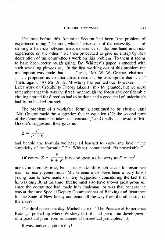
THE FIRST FIFTY YEARS 247
The task before this Actuarial Section had been “the problem of experience rating,” he said, which “arises out of the necessity . . . of striking a balance between class-experience on the one hand and risk- experience on the other.” He then proceeded to give us a step by step description of the committee’s work on this problem. To them it seems to have been pretty rough going. Dr. Whitney’s paper is studded with such revealing phrases as, “In the first working out of this problem the assumption was made that . . . ,” and, “Mr. W. W. Greene, chairman . . . ) proposed as an alternative treatment the assumption that. . . .” Then, again: “As Mr. A. H. Mowbray has pointed out, however. . . .” Later work on Credibility Theory takes all this for granted, but we must remember that this was the first time through the forest and considerable circling around for direction had to be done and a good deal of underbrush had to be hacked through.
The problem of a workable formula continued to be elusive until “Mr. Greene made the suggestion that in equation (22) the second term of the denominator be taken as a constant,” and finally as a result of Mr. Greene’s suggestion they gave us
P z=P+K
and behold the formula we have all learned to know and love! “The simplicity of the formula,” Dr. Whitney commented, “is remarkable.”
Of course Z = & is not so great a discovery as E = mc2
nor as unalterably true, but it has made life much easier for insurance men for many generations. Mr. Greene must have been a very brash young man to have made so many suggestions considering the fact that he was only 30 at the time, but he must also have shown great promise, since the committee had made him chairman, or was that because he was at the time Special Deputy Commissioner of Banking and Insurance for the State of New Jersey and came all the way from the other side of the river?
The third paper that day, Michelbacher’s “The Practice of Experience Rating,” picked up where Whitney left off and gave “the development of a practical plan from fundamental theoretical principles.“[3]
It was, indeed, quite a day!

248 THE FIRST FIFIY YEARS
And there it rested for over ten years. There were good papers on ratemaking but not much new and original work until Francis Perryman started writing papers in 1932. Ten years after that Arthur L. Bailey appeared on the scene, and from then on there has been a continuing submission of notable papers on Credibility Theory. Tom Carlson has said that Arthur Bailey was “probably the most profound contributor to casualty actuarial theory the United States has produced.“[4] It is rather fashionable for the author of a good mathematical paper even today to start with a quotation from the works of Arthur Bailey. Not only were his mathematical developments outstanding but his English text was lucid. His language broke through the fog even for lay actuaries. An example is the following cogent statement of our basic actuarial problem:
“Thus the losses paid by an insurer newr actually reflect the hazard covered. but are always an isolated sample of all of the powible amounts of losses whvzh might have been
incurred. It is this condition. of never bemg able to determine, even from hindsiphr. what the exact value of the inherenl coverage was. that ha> brought the casualty actuary into
being.“lb]
Arthur Bailey often expressed amazement at the statistically unortho- dox development of credibility theory. He can be quoted to this effect in a dozen different places. Writing of the need for different schedules of credibility for the three compensation loss components, serious, non- serious, and medical, he says, “It is at this point in the discussion that the ordinary individual has to admit that, while there seems to be some hazy logic behind the actuaries’ contentions, it is too obscure for him to understand. The trained statistician cries ‘Absurd! Directly contrary to any of the accepted theories of statistical estimation.’ The actuaries themselves have to admit that they have gone beyond anything that has been proven mathematically, that all of the values involved are still selected on the basis of judgment, and that the only demonstration they can make is that, in actual practice, it works. Let us not forget, however, that they have made this demonstration many times. It does work!“[7]
It has not always been easy to persuade state officials and underwri- ters that credibility factors are valid. I can recall the occasion when one of the more thorny insurance commissioners remarked rather testily, “You have supported everything else in the filing with actual experience, where is the experience supporting your credibility factor‘?” Whereupon we hastily changed the subject. Gus Michelbacher tells of Albert Whitney “presenting a mathematical demonstration of the fundamental principles
THE FIRST FIFTY YEARS 249
underlying experience rating. One underwriter asked, ‘Where did you get that Z factor?’ and braced himself expecting a formidable explanation. Mr. Whitney thought for a moment, adding to the suspense of the occasion, and then replied, “In Michelbacher’s dining room!‘“[8]
The history of the CAS would be most incomplete without reference to the negative binomial. If the negative binomial had not existed already, I am sure Lester Dropkin or those twins, LeRoy Simon and Bob Bailey, would have invented it. Tom Carlson has called attention to the fact that actually it first appeared in the CAS Proceedings in 1942 and that Arthur Bailey derived it again in 1950.[5] But that was all until 1959. Now, for the past five years it has become a basic doctrine in the actuarial neo-orthodoxy of the 1960’s and a big help in making automobile merit rating scientific. It was only a few years ago that the experience of a single car was considered by most of us, even some of our more respected members, as being of so little credibility that to allow it to affect the rate was out of the question. Yes, the negative binomial was a great discovery.
The Society is in debt to L. H. Longley-Cook for preparing “An Introduction to Credibility Theory.“[9] In this treatise he has brought together in concise and readably simple form the essential elements of credibility theory as they have developed over the past fifty years. This has great value, not only for students for whom it was prepared, but also for fellow actuaries who have neither the facility nor the time to wade through all the papers written on the subject. This is normally the second step in the conquest of the unknown. The pioneers come first hacking their way through the forests, trekking up blind valleys, and doubling back to try a new approach. It is a painful and prolonged process. But after this has been done the cartographer comes along and with a high skill at illumination makes the going clear, or at least clearer, for the rest of us.
Restrospective Rating: Although retrospective rating did not come into use until 1936, it is interesting to note that one of the early professional controversies in the Society was between the advocates of prospective and retrospective rating, with those who did not believe in either taking potshots at both. This was in 1916. Clairvoyance won, and retrospective rating had to wait twenty years. Space prohibits a discussion of the arguments, pro and con, put forth at that time; one gets the impression
250 THI- FIRS1 FII~IY I.1 ARS
in reading them now, particularly between the lines, that the chief ar- gument for retrospective rating was that it provided some opportunity for the stock companies to compete with the mutuals on large risks, and the chief argument against it was that the agents would never be able to manage it. The best potshot taken against experience rating in general was provided by Win Greene in 1916.
“It has been the intention of the writer to indicate in the foregoing pages that in all probability any system of compensation rate\ dependent upon the experience of the indi- vidual risk will be if universally applied so unpopular as IU be viriually unworkable: that
the chief grrwi!, of the demand for conaideratwn of mdlbidual experience in rating compensation risks lies in the hope for competitive advantage on the part of the carrier;
and finally that although experience rating plans have sincere advocates among those who
feel that such plans may constitute powerful inlluenccs toward accident prevention. there i> reason to fear that experience rating m any form may harm rather than help the employer through givmg the employer a financial interest in mmimvme hl\ workmen’\ claim\.“1 IO]
“The employer should not be encouraged m the faire Idea that his own experience is a proper critermn for an equitable rate.“1 IO]
Just two years later Win Greene was made chairman of the actuarial committee that developed the experience rating credibility formula. He was a good soldier.
At this early time Dr. Whitney had shown interest in retrospective rating, and it may be that this interest was transferred to his admiring young understudy at the National Workmen’s Compensation Service Bureau, Paul Dorweiler. During this twenty year gap. between 1916 and 1936, Paul Dorweiler did considerable work on excess insurance costs, which laid the foundation for the later work underlying the first retro- spective plans. In 1927 he presented a paper in which he gave the first treatment in our Proceedings of insurance that takes effect in excess of given loss ratios.[ 1 l] This paper won the Society’s Woodward Prize. His presidential address in November 1933112) was credited with pro- viding the method used in compiling the experience underlying the insurance charges in the 1936 plan.] 131 His 1936 paper, “On the use of Synthetic Risks in Determining Pure Premium Excess Ratios for Large Compensation and Liability Risks,” is still read and its techniques ad- mired by students of retrospective theory.]141 And finally in 1941 he presented a paper in which he explained the graduation work that had been done in the name of the Actuarial Committee of the New York Compensation Rating Board.[ 151 Dorweiler’s methods and results were used for the insurance charges of the revised New York retrospective
THE FIRST FIFTY YEARS 251
plan and also became the basis of the 1943 National Council retrospective program under which retrospective rating really attained the considerable importance it now holds.
It should be acknowledged that Paul Dorweiler has earned the right to be called the actuarial father of retrospective rating, one of the im- portant achievements of our profession.
The American Remarriage Table: Most of the professional work recorded in the Proceedings was done by individual members or industry com- mittees; very little has been done in the name of the Society. One significant contribution made by the Society itself was the development of an American Remarriage Table. This was the work of a committee appointed in 1929 and was completed for presenting to the Society at its May 1933 meeting.[ 161 Of the seven man committee that did the work Paul is the only one left with us.
Table of Mortality fur Disabled Lives: For this work the Society ap- pointed a committee of three in 1937, which was expanded to seven in 1938. Paul Dorweiler was chairman of this committee. The completed work was presented to the Society at the November 1946 meeting. [ 171
Schedule P: An area where the Society has very definitely been unsuc- cessful in making a contribution, in spite of repeated efforts, has been in the improvement of, or hopefully the elimination of, the Schedule P reserve formula for compensation and liability loss reserves. Schedule P is an ancient monstrosity; its basic pattern was with us when the Society was founded, though originally it was designed to apply to liability insurance only. In Volume II of our Proceedings we find Robert K. Orr presenting the same basic criticisms of the formula approach to loss reserving as have been given ever since.[l8] In 1924 the Society ap- pointed a committee to see what could be done about Schedule P. After six years of hard labor this committee presented its report. [ 191 This did not go so far as perhaps most members of the Society would have liked, but it did make some valid recommendations, which were ignored com- pletely by supervisory authority.
In 1947 another committee was appointed with Joseph Linder as chairman. This committee’s report, released in 1949, was much more sweeping in its recommendations than the former one.[20] To actuaries, in general, it made sense, and it received about as much attention from supervisory authority as the former report had. The problem, of course,
252 THt FIRS1 FIFTY YEARS
is that the Schedule P formula is written into the laws of many states and into the hearts of many state supervisory officials.
VII. OUR LIFE 1NSURANCE BRETHREN
In spite of the fact that many of our charter members were also active in the life societies, we as an actuarial body were for years held in rather low esteem by those, our professional brothers. We were a bit upstart at the beginning and our scientific stature had yet to be proven. Then, too, an actuary has been generally considered to be “one who makes those calculations as to the possibilities of human life upon which the issuance of life insurance and annuity contracts depends,“[2] and was not thought to include non-life hazards in this tield. But we were keen for recognition and a bit of fraternization, and item 2 of the minutes of the Council meeting held September 17, 19 19, begins a story: “The Board of Gov- ernors of the American Institute of Actuaries was requested to consider the subject of a joint meeting in May 1920. No response having been received, the matter was laid on the table to be taken up at the next Council meeting.” Item 1 of the minutes of the next Council meeting ends the story: “The plan to hold the May 20 meeting in Chicago in conjunction with the American Institute of Actuaries was laid indefinitely on the table.”
Actually there has always been considerable cordiality shown us by our life friends. At our twenty-live year celebrations both Mr. Ray D. Murphy, President of the Actuarial Society of America, and Mr. R. A. Hohaus, President of the American Institute of Actuaries, were present as official guests. Mr. Murphy being also a Fellow of our Society. At other times, too, a life society president has attended our annual banquet at our official invitation, and we have been proud to have him. But 1 think it fair to say that the life Societies have in the past made it clear that. much as they liked us, they could not consider us professional equals.
THE FIRST FIFTY YEARS 253
Most of us were not inclined to blame them. We recognized that our general mathematical stature was somewhat lower than theirs, though catching up rapidly. Nevertheless, we held our heads up with the con- viction that a Casualty Fellow had to know more about “other things” than a Life Fellow did.
And then, as so often happens, a threatened danger from without has helped to bring about unity within this, our actuarial family. Because so many charlatans were calling themselves “actuaries” without having achieved membership in any society and were performing legally re- quired functions as though they were really actuaries, the Society of Actuaries and the Conference of Actuaries in Public Practice took the initiative to approach us as well as the Fraternal Actuarial Association with the thought that something might be done to set up standards of accreditation and that government might then cooperate.[3] (Here we suppressed a bit of snobbishness, for these other two organizations did not require any examinations for membership.) A CAS committee was appointed in 1958 to meet with representatives from the other organi- zations. Their work has proceeded with a remarkable degree of harmony. Finally a Joint Committee on Organization of the Actuarial Profession was set up with one member from each of the four societies, L. H. Longley-Cook being our official representative, though the practical work of this committee has required the participation of many members of all four societies, and very considerable work has been done by William Leslie, Jr., Daniel McNamara, and Frank Harwayne. This committee has prepared a charter, by-laws, election procedure, and committee struc- ture for the organization of a new actuarial body, the American Academy of Actuaries, with the expectation that membership in the Academy may be recognized as a satisfactory accreditation for an actuary. To start with, the Academy would take in the entire membership of the four parent bodies, except that Associates would require several years of experience in responsible actuarial work.
At our May 1964 meeting the CAS approved this project, and, the other three bodies having also given their approval, the joint committee is in the process of seeking federal incorporation. To date our bill has passed the Senate, but not the House.
But this is not all. We have, in fact, grown more respectable. We no longer invite into membership dues paying executives who have never “turned the crank of a Monroe” and by far the greater part of our membership has had to pass examinations. We now require a general
254 THE FIRSI f;ltll’ YEARS
mathematics examination identical with that of the Society of Actuaries, and we have had as our president from 1961 to 1963 a former life actuary who is an unusually able ambassador of good will, and an able actuary to boot. We have had others like him, of course, before Laurie Longley- Cook took up our cause, and they have all helped, but Laurie has really done the job. The relationship we had sought in 1919 when we were young and gauche has now developed in the fullness of time. The 1963 fall meetings of both the Society of Actuaries and the Casualty Actuarial Society were scheduled for consecutive days in the same city with each body inviting the members of the other to its meeting and with a part of both programs on subjects of common interest. This recognition of joint interest and the joint work, mentioned above, which has been done by the four actuarial bodies looking to the formation of the American Academy of Actuaries speaks well for the future of our profession.
VIII. WHAT IS A CASUALTY ACTUARY’?
One of the more challenging questions the members of our Society have had to grapple with, and one which has generated considerable disputation, has been, in its general form, “What is an Actuary?” and in its more specific form, “What is a Casualty Actuary?” Like Narcissus we have indulged to a greater extent than we sometimes like to admit in gazing at our reflection, and sometimes it has pleased us and sometimes not. More often than not we find that the image has been distorted because the reflecting pool has been roughly agitated by such rude fellows as underwriters. They have not always understood and respected us, and we do like to be understood and respected.
Those Underwriters: Benedict D. Glynn. our fourth president, once wrote:
“When the Society was organized. the Caualt) actuary wa\ generalI} looked upon wth
suspicion by underwriters and others connected with the general management of the
THE FIRST FIFTY YEARS 255
business. This was due to the fact that the actuaries had very little knowledge of under- writing principles and the underwriters had not been educated to the value of the statistical methods used by the actuary.“[2]
It was perhaps out of delicacy that Mr. Flynn spoke of this incom- patibility between actuaries and underwriters as in the past. Actually, like Punch and Judy, these two important members of the insurance household have been taking swipes at each other off and on, mostly on, throughout the history of the Society. This has been both bad and good for the business. It has been bad when it has been accompanied by ill will and obstructive behavior; it has been good when it has operated as a natural system of checks and balances between two properly imperfect approaches to truth. An insurance business completely devoid of under- writers or of actuaries and completely dominated by the other, in this complicated world of today, would be carrying within it the seeds of its own destruction. It is interesting to speculate what problems we would have been faced with at the time of the Supreme Court’s Southeastern Underwriters Association decision if the casualty business had not had the thirty year benefit of the Casualty Actuarial Society.
Actually there exists a great deal of mutual respect between actuaries and underwriters, and there have been many able insurance executives who have combined the best characteristics of both. William Leslie, Sr., in a presidential address put it well when he said, “The practical actuary and the logically minded underwriter should have no trouble getting along together but the theoretical actuary and the illogically minded underwriter had better keep away from each other.“[3]
There have been several historic verbal battles between the two groups in the past, but space permits me to mention only one. One has the feeling in reviewing this particular fracas that both parties had their tongues in their cheeks, for they were both practical and logical men, both Fellows of this Society, the one a chief executive of his company, the other destined to be in a few years.
In his November 1925 presidential address G. F. Michelbacher had told the Society that he did not think much of the use of judgment in ratemaking.[4] He contrasted it with the scientific, or, as he called it, the statistical method and said, “It must be obvious that the writer’s preference is for the statistical method.” Nevertheless he did allow a minor place for judgment, though hardly the kind of judgment exercised
by underwriters, rather a refined sort of intellectual process one might call actuarial judgment that interprets facts “as to their adequacy and reliability” and chooses “that particular formula which best meets the requirements.”
Frederick Richardson, U. S. Manager of the General Accident, was undoubtedly the most literate and articulate gift Great Britain has ever contributed to American insurance. Hc presented a written discussion of the Michelbacher paper at the next meeting, in which he gave what has been perhaps the most lavish description of the underwriter’s picture of an actuary yet written. Here it is in part:
“lt might not be out of place at thlh time to exprcs\ tour \t‘nsr of hatisfaction and our feilowhhip pride in (Michelbacher’s) recent appom~mcnt to a 411 more eminent position
in the world of insurance. His entry into th< arena 01 practical and competuivc husinehs
has some significance for us. and will. moreover. have an influence upon hi\ own YEWS concerning the aims, and amhltlons of In~runcc Companies. Doubtless he wrill continue to xek the lofty and hyperborean atmorpherc of thcsc ts\emblir\. here to renew and refresh his spirit in studying and admiring the lambent tire> and coruscatmm that play
about the aurora borealis of abstract mathematics. Here we can gather together with our O’S and our h’s and our .r. y, :‘s and our graphic outlines to postulate the cost of this and the incidence of that. and if our calculation\ happen to go awr?, we. individually, arc not a penny the worse. The burden of the experiment fall5 upon other\. “IS]
It took Gus Michelbacher six years to make his reply. I have no explanation of the long delay, save that Frederick Richardson was always a formidable opponent worth training for. At the May 1932 meeting Gus made his reply in a paper he called “Criticisms and Answers.“[6] He did not mention Richardson but he made his purpose clear by quoting that stuff about “lambent fires and coruscations.” In this good, well- reasoned, document his point was that “the criticisms of the actuary himself might have been in order at one stage of the game, but they are no longer tenable,” and that “criticisms of the results produced by ac- tuaries fail to take into consideration the nature of the problem. . . ”
And then Frederick Richardson landed on him with a whole avalanche of quotations, from, among others, a seventh century Chinese poet, Voltaire, and the Brooklyn Cirizen. It was a sharp and delightful piece presented to the November 1932 meeting as a discussion.[7]
Michelbacher, as the original author, replied, in part, “Ouch,” and, “We are not so far apart after all. This may be because I have modified my ideas with the passage of time.“(8] An actuary is always a gentleman.
THE FIRST FIFTY YEARS 251
The Fire Actuaries, if any: Early in our Society’s career we cast sidelong glances at the tire insurance business. In 1923 Harwood Ryan wrote, “Finally we should begin to look forward to the time when the rates for fire insurance will be statistically determined,“[9] and Edward R. Hardy expressed the hope that fire insurance ratemaking might become some day semi-scientific, though he found considerable resistance within the industry. [ IO] After that, for more than twenty years, we stopped looking over the fire fence. With the SEUA decision and Public Law 15 it seemed reasonable to expect that fire insurance ratemaking might see the need for at least a veneer of science, if nothing more, to make it acceptable to state regulatory authorities in view of the danger of Federal take-over. The CAS began to hope we might be called in as firemen for a burning house. Though the call was amazingly slow in coming we started our preparations for it. In 1950 we amended our constitution to state that our field of endeavor was “insurance, other than life insurance,” instead of the former words “casualty and social insurance,” and we tried very hard to find a name for ourselves that would be more inclusive. At one informal discussion session we experimented with such names as, “Property and Casualty Actuarial Society,” “The Actuarial Society for Insurance other than Life,” and similar monstrosities, with no success whatever. Finally we concluded that our old name was the best name, that, after all, fires were really casualties in the broad sense, and our fire friends would have to take our name if they wanted to take us. In 195 1 several fire insurance ratemaking papers were presented to the Society, and we took in, by the invitation route, six prominent men in the fire insurance ratemaking field. What is a casualty actuary? He may be a fireman.
While it is true that, compared to casualty underwriters, old time fire underwriters are even more intransigent about actuaries, the fire insurance business is gradually getting used to the actuarial invasion it has suffered, and science is creeping into their processes. Mirabiie dictu!
As We See Ourselves: Casualty actuaries have always fancied themselves as normal people, in spite of popular expressions to the contrary, which we view with a modicum of tolerant amusement. Here we have Syd Pinney’s delightful dissertation, given at the celebration of Richard Fon- diller’s twenty-five years as Secretary-Treasurer, when he asked us in succession:
258 'THE FIRST FtFry YEARS
“Whor is SO peculiar about an actuary’!” .‘What is SO peculiar about an actuary?”
“what is so peculiar about an actuary?”
“What is SO prc~licv about an actuary’!” and “What is SO peculiar about an ccctuary’T’( 1 I ]
This last, he maintained, gave the question the proper perspective. He presented, we felt, a superb performance, delivering a measured speech of well over a half hour completely from memory and in the most delightful spirit. When he was finished we were all convinced that there could be nothing possibly peculiar about an actuary, particularly if his name was Syd Pinney.
We are quite proud of our profession, though we have suffered somewhat from the sense of inferiority imposed on us by our older brothers. the life actuaries. But we have insisted that qualities are de- manded of us not required of life actuaries. In comparing the two, Francis Perry man said, “Casualty business involves less technical and mathe- matical work and essentially deals more with what I term ‘humanities’ and quicker results are looked for. “[12]
Francis Perryman was perhaps one of our very finest casualty actu- aries and certainly our most respected actuarial philosopher. He had a high regard for the profession and saw for it a proud future, which he expressed in those words-no one has said it better:
“Hi5 (the actuaq‘s) will be the privilege of wing hi, knouledge and experience. his actuarial tools and methudb. so as tu solve our modem wc~al problems. uur problem\ of
living together in harmon) and cwperatircnes\: l’or thih i\ wrc. that wch problems will be solved and they can be dealt with only b) wicntitic method\ that we In essence those we use and knou a:, our actuarral ones.“[ I.?/
This is the casualty actuary at full stature and we arc indebted to Francis Perryman for giving us the dream-a dream not unlike the one Rubinow had when we were founded.
In gathering dutcl for this puper I have hud help from N greut many people. I fear I cannot acknowledge them 011, but I UF?? purticularly indebted to HARMON T. BARBER, RAL.PH BI.ANC.HARD. PAUL DOR- WEILER, RUSSELL P. GODDARD, WINFIELD W. GREENE, CHARLES J. HAUGH, JOSEPH LINDER, NORTON E. MASTERSON, EMMA C. MAYCRINK, GUSTAV F. MICHELBACHER, MATTHEW RODERMUND, LEROY J. SIMON,
trrld NELS M. VAIARIUS. But ubove ~11 1 trm irdrhted to LAURENCE H.

THE FIRST FIFTY YEARS 259
LONGLEY-COOK, not only for his good counsel, but also for the use of his library, a desk in his of/ice, and the services of his most gracious and ef&cient secretary, MISS LUCY ALTRICHTER.
260 THE FIRS7 f;fFf’Y YFARF
REFERENCES
Roman numerals, followed by the page number. refer to the Proceedings of the Casualt? Actuarial Society.
SECTION I
[I] Minutes of the First Meeting, I, 5.
[2] Minutes of the Meeting, May 24, 1921, VII, 460.
[3] I. M. Rubinow, “Origin of the Casualty Actuarial Society,” XI, 17.
[4] Mark Sullivan, Our Times-The War Begins, .17
SECTION II
[I] C. W. Hobbs, “The Lady Casualty and Her Servitors,” XXVI, 169.
[2] I. M. Rubinow, “A Letter,” The Cusualt~ Actuarial Society, 1914- 34, Addresses and Sketches, 2.
SECTION III
[I] I. M. Rubinow, Address of the President. II. 8.
[2] I. M. Rubinow, “Our Problems,” I. 87.
[3] I. M. Rubinow, Address of the President, II, 7.
14) Leo Wolman, “Unemployment Insurance,” IX, 86.
[S] I. M. Rubinow, “Can Insurance Help the Unemployment Situa- tion?” XIV, 373.
[6] T. F. Tarbell, “Unemployment and Insurance,” XVII, 161.
[7] C. W. Hobbs, “Social Insurance and the Constitution,” XXII, 32.
[S] W. R. Williamson, “Social Budgeting,” XXIV, 17.
THE FIRST FIFTY YEARS 261
[9] Jarvis Farley and Roger Billings, “An Approach to a Philosophy of Social Insurance,” XXIX, 29.
[lo] W. R. Williamson, Discussion, XXX, 70.
[ 1 l] R. H. Blanchard, “The Casualty Actuary and Social Insurance,” XXIX, 4.
[12] W. R. Williamson, “Some Background to American Social Secu- rity,” XXX, 5.
[ 131 G. W. Fitzhugh, “Medical Care Insurance-Compulsory or Free- dom of Choice?” L, 50.
SECTION IV
[l] I. M. Rubinow, Address of the President, II, 8.
[2] Report of the Educational Committee, VI, 420.
[3] H. T. Barber, “The Gateway to Membership,” XXXVIII, 88.
SECTION V
[1] I. M. Rubinow, “Our Problems,” I, 79.
[2] Minutes of the Fifth Annual Meeting, November 15, 1918, V, 189.
[3] I. M. Rubinow, “Schedule Rating in Compensation Insurance,” I, 211.
[4] D. M. Pruitt, Discussion, XXXVIII, 227.
[5] C. W. Hobbs, “The Lady Casualty and Her Servitors,” XXVI, 170.
SECTION VI
[l] W. W. Greene, Reviews of Publications, IX, 135.
[2] A. W. Whitney, “The Theory of Experience Rating,” IV, 274.
262 THE FIRS‘1 FIFTY YEARS
[3] G. F. Michelbacher, “The Practice of Experience Rating,” IV, 293.
141 T. 0. Carlson, “Observations on Casualty Insurance Rate Making Theory in the United States,” Transactions of the 17th international Congress of Acruuries, 54 1
[5] Ibid., 554.
[6] Arthur Bailey, “Sampling Theory in Casualty Insurance,” XXIX, 50.
[7] Arthur Bailey, “Credibilility Procedures.” XXXVII. 8.
[8] G. F. Michelbacher, “Reminiscences of an Ex-Actuary,” The Cas- ualty Actuarial Socie?, /Y/4--34. Addresses und Sketches, 23.
[9] L. H. Longley-Cook, “An Introduction to Credibility Theory,” XLIX, 194.
[lo] W. W. Greene, “Should the Compensation Premium Reflect the Experience of the Individual Risk?” II, 354.
[ II] Paul Dorweiler, “Observations on Making Rates for Excess Com- pensation Insurance,” XIII, 154.
[12] Paul Dorweiler, “Policy Limits in Casualty Insurance,” XX, 1
[13] S. D. Pinney, “The Retrospective Rating Plan,” XXIV, 341.
[ 141 Paul Dorweiler, “On the Use of Synthetic Risks,” XXIII, 77.
[15] Paul Dorweiler, “On Graduating Excess Pure Premium Ratios,” XXVIII, 132.
[ 161 W. F. Roeber and R. M. Marshall, “An American Remarriage Table,” XIX, 279.
[ 171 Report of Committee on Mortality for Disabled Lives, XxX11, 123.
[ 181 R. K. Orr, “Liability and Workmen’s Compensation Loss Re- serves,” II, 136.
[ 191 Report of Committee on Compensation and Liability Loss Reserves, XVII, 137, 333.
[20] Report of Committee on Compensation and Liability Loss and Loss Expense Reserves, XXXV, 56.
THE FIRST FIFTY YEARS 263
SECTION VII
[I] Quoted in I. M. Rubinow, “Our Problems,” I, 77.
[2] Encyclopedia Britannica, Article on “Actuary.”
[3] D. M. Pruitt, “The Seat of Wisdom,” XLV, 11.
SECTION VIII
[I] S. B. Perkins, “A Message to and Concerning the Casualty Actu- arial Society,” XIII, 149.
[2] B. D. Flynn, “Review of the Society’s First Ten Years and a Glance into the Future,” XI, 29.
[3] William Leslie, “The Present Outlook for Casualty Actuarial Sci- ence,” X, 105.
[4] G. F. Michelbacher, “On the Use of Judgment in Rate Making,” XII, I.
[5] Frederick Richardson, Discussion, XII, 320.
[6] G. F. Michelbacher, “Criticisms and Answers,” XVIII, 260.
[7] Frederick Richardson, Discussion, XIX, 127.
[8] G. F. Michelbacher, Discussion, XIX, 144.
[9] H. E. Ryan, “The Society and Its Relation to Ratemaking Associ- ations,” X, 8.
[lo] E. R. Hardy, “Some Random Thoughts Concerning Fire Insur- ance,” X, 119.
[I I] S. D. Pinney, “What is So Peculiar About an Actuary?” XXX, 9 1.
[12] F. S. Perryman, “The Casualty Actuary,” XXV, 294.
[ 131 Ibid., 296.
164
THE FIRST SEVENTY-FIVE YEARS
hf. STAKl,t:Y HI’(;titI
This update of the chronicle of the Casualty Actuarial Society through 1989 presumes a thorough remembrance of Dudlcy Pruitt’s “The First Fifty Years.” As the attitudes and actions of the grown man are influenced by the days of his childhood, so the maturing casualty actuarial profession has its deep roots in the attitudes and actions of the Casualty Actuarial Society (CAS) from 1914 to 1964, and these were well recorded in Dudley’s paper. New circumstances and new challenges in the last 25 years‘? Of course. And it is the evolutionary and revolutionary changes during this more rcccnt period that we will try to highlight, tying to the past where pertinent, but recognizing the true revolutionary winds of change where they have prevailed.
II. I,EAIXRSHIP, h(‘l’lVl’l IES, AND DlRECI‘ION
A BRIEF CHRONOI.OGIC‘AI. Rt:\‘Il;W
Other segments of this history build on the themes established in Dudley Pruitt’s recital. but it stems appropriate to include. at least as background, a chronological rcvicw of some of our activities during the last quarter century. Some of the subjects and activities noted in this chronological development arc also included in other sections, as they become part of a particular thcmc.
The Golden Anniversary Banquet in New York City celebrated the tirst SO years of the CAS. The American Academy of Actuaries (AAA) was formed, with Henry Rood. president (ACAS but more closely as- sociated with the Society of Actuaries (SOA)): Thomas Murrin, presi- dent-elect (also president of the CAS 1963- 1964); and Laurence Long- Icy-Cook, vice president (and immediate past-president of the CAS).
THE FIRST SEVENTY-FIVE YEARS 265
LeRoy Simon presented a paper on the 1965 Table M, and Charlie Hewitt discussed credibility (with many more discussions to come). There were also discussions of loss reserves, annual statements, rate regulation, ratemaking, education of actuaries, and accident and health. All of these were subjects that were to be revisited frequently over the years ahead.
Package policy ratemaking was considered, and the new statistical plan for homeowners and comprehensive dwelling policies was dis- cussed.
The November 1965 meeting in Boston was attended by 98 Fellows, 58 Associates, and 46 Guests, a very good representation of the total membership of 408.
1966-1967
The 1966 examinations for admission introduced joint administration with the Society of Actuaries for Parts 1 and 2. A major panel tackled automobile compensation plans as a forerunner to the no-fault auto development, and Frank Harwayne presented a paper on the costs of a basic protection plan.
Bob Foster helped us understand budgeting, George Morison reported on “The 1965 Study of Expenses by Size of Risk,” and Jeff Lange expounded on “General Liability Insurance Ratemaking,” a paper that is still required reading in the Syllabus.
I968-I969
Norton E. (Dot) Masterson tied our liability and property claim costs to economic factors, which he has kept up to date with several subsequent releases. Allen Mayerson, Donald Jones and Newton Bowers presented a paper on credibility and Robert Ferrari had a paper on total return on owners’ equity. A panel reviewed investment income in insurance rates, a subject to be hotly debated in the years to come. The participants included Allen Mayerson, John Carleton, John McGuinness, Jack Mose- ley and Irving Plotkin (economist with Arthur D. Little, Inc.)
Other topics covered in panels and papers included riot insurance problems, education of future actuaries, and flood insurance plans. One of the delightfully entertaining skits authored by Matt Rodermund was greeted with great enthusiasm.
266 .THF. FIRST SEVENTY-FIVt YEARS
The Arthur D. Little, Inc. studies of the insurance industry’s profit- ability and rates of return, commissioned by the American Insurance Association and the National Association of Independent Insurers, cre- ated a lot of interest and discussion. Dr. Irving Plotkin. principal author, found many not agreeing with some of his material, with Bob Bailey taking a leadership role in responding. Well attended by actuaries, the PlotkiniBailey debates were highlights of several subsequent meetings.
Effective with the 1969 examinations, the Associateship section was expanded to five parts. adding material on insurance statistics and data processing.
Al Skelding retired as secretary-treasurer of the CAS after 15 years of dedicated service in that office.
1970-1971
Discussions concentrated on profitability and pricing, annual state- ments, open competition, automobile insurance systems. and regulation for solvency. Charlie Hewitt presented his paper, “Credibility for Sever- ity,” and Dan McNamara in his Presidential Address made a strong case for ecumenicism, envisioning one professional actuarial society with a number of specialties. Both papers opened up avenues for much discus- sion.
The U.S. Department of Transportation published a series of studies dealing with automobile insurance and compensation for injuries. Many actuaries were involved in gathering the mountain of statistics, from insurance company claims and from a wide variety of direct solicitation sources where insurance claims were not involved. These studies pro- vided a great deal of information, never before available, on the eco- nomic impact of automobile accidents and injuries, and represented a valuable reference work for those actuaries working on automobile in- surance reparations systems.
“Federal Income Taxes” for property-liability insurance companies came under examination by Woody Beckman. Auto no-fault insurance, investment income in ratemaking, national health insurance, medical malpractice, and the future course of the Society were the subjects of discussion panels. A major revision of the “Guides to Professional Con- duct” was developed and adopted.
THE FIRST SEVENTY-FIVE YEARS 267
1972-1973
Reflecting a growing concern about the adequacy of loss reserves and the adverse developments that were showing up, several papers considered various aspects of this important subject. Authors included Ruth Salzmann, Rafal Balcarek, Ron Ferguson and David Skumick. Ron Bornhuetter and Ron Ferguson also contributed their paper on IBNR which fathered the “Bornhuetter/Ferguson method’ for testing loss re- serves.
Dave Bickerstaff’s paper on automobile collision rating, plus work done by the Insurance Institute for Highway Safety, sparked a growing recognition of the place of damageability and repairability in setting collision insurance rates. Panel discussions covered no-fault auto, cor- porate modeling, computerization, catastrophe insurance, and group mar- keting.
1974-197s
A new Syllabus became effective in 1975, requiring new Associates to successfully complete the first 7 of 10 parts. The Board of the CAS felt that this requirement would assure adequate experience for those qualifying to certify loss reserves and for Associateship in the CAS.
The Actuarial Review was started under the guidance of Matt Rod- ermund, and has proved to be an eloquent mouthpiece for the casualty actuarial profession.
Key papers presented included Mike Walters’ on homeowners, Dave Skurnick’s on Table L, Ron Ferguson’s on indexing, and Stan Khury’s on personal lines pricing.
Panel discussions covered a wide range of topics, including inflation, corporate planning, malpractice, residual markets, the energy crisis, captive insurance companies, trend factors, state regulation, and profit- ability.
Evaluation or certification of casualty loss reserves was raised as an issue. The need was increasingly in evidence, but how it should be done, the standards required, and the availability of casualty actuaries were sticky problems to be resolved.
The Actuarial Education and Research Fund was established to en- courage actuarial research. While the program has developed more slowly than originally anticipated, it has served to bring together a) needed research projects, b) researchers to do the work, and c) money to fund the research efforts.
While they are not all noted individually in this chronology, a number of special interest seminars were held during the late 1960s and 197Os, and these have continued. Frequently these seminars were co-sponsored with other actuarial organizations.
1976-/977
Loss reserves continued to receive a lot of attention. Bob Finger and Chuck McClenahan authored papers suggesting the USC of mathematical modeling in analyzing reserves. Jim Berquist and Rich Sherman pre- sented a paper on loss reserve adequacy testing. Dave Flynn moderated a panel consisting of Ruth Salzmann and Messrs. Balcarek, Otteson, and Snader; this panel tackled the lively question of discounting loss reserves. A special interest seminar on loss reserves was held in Scptem- ber 1976, and the first call paper program in November 1977 was on loss reserves.
An ASTIN meeting (Actuarial Studies in Non-Life Insurance, the non-life section of the International Actuarial Association) was tied into a CAS meeting and featured a panel discussion of actuarial work around the world.
Workers compensation also continued to receive attention with two papers of Frank Harwayne’s, one on using national experience and the second on accident limitations for retrospective rating. Panel discussions dealt with government regulation, model building, trends in expense elements. and econometrics.
I97#-1979
Evaluating loss and loss expense reserves reached a milestone. A “Statement of Principles Regarding Property and Casualty Loss and Loss Adjustment Expense Liabilities ” was published, becoming a base for this
THE FIRST SEVENTY-FIVE YEARS 269
major activity of casualty actuaries. The issue of certification of loss reserves was resolved, after much discussion, leaving room for both actuaries and qualified reserve specialists, who were not actuaries, to sign the required “Statement of Opinion.” The American Academy of Actuaries (AAA) played a key role in achieving nearly automatic rec- ognition of CAS members as qualified, with Ron Bornhuetter leading the effort.
Another milestone was the election of our very capable Ruth Salz- mann as president in 1978, the first woman to become president of a North American actuarial society.
Major papers included a discussion of automobile insurance rate- making by Mike Miller, a discussion of fitting curves by size of loss by Charlie Hewitt and Benjamin Lefkowitz, and a number of call papers on total return. Panel discussion subjects included professional conduct, financial reporting, insolvencies, inflation and risk classification.
In his annual report, Dave Flynn, secretary, noted that it took 40 years for the CAS to reach 300 members, 21 years to add another 300, and 6 years to add the third 300 members. (As a matter of interest, the CAS is currently adding about 80 members per year.)
1980-1981
An article in the Actuarial Review in May 1980 called attention to the growing number of women in the CAS. Through the 1950s and 1960s about 3 percent of our members were women, but starting in the 1970s the percentage definitely turned upward, reaching 6.5 percent in 1979.
Papers presented highlighted standards for loss reserves (Stan Khury), credibility concepts (Steve Philbrick), risk classification (Mike Walters), and valuation of property/casualty insurance companies (Bob Sturgis). Panels and call papers covered pricing, the actuary as an expert witness, risk theory, and investments. The first Casualty Loss Reserve Seminar was sponsored jointly by the CAS and AAA in September 198 1.
The CAS changed to a mail balloting procedure for its election in 1981, reflecting its increased size. A Statement of Education Policy was published.
270 ‘I’HE FIRSI SFVENTY-FIVI: YEARS
1982-I 9#3
The CAS reorganized its structure in 198.3 to better manage the day- to-day affairs of its continuing operations. This change established four vice presidents-for membership, development. programs, and admin- istration. The thrust of the change was to have the vice presidents responsible for specified areas of CAS operations, with the Board of Directors concentrating on policy matters. With six years of experience, the wisdom of this change has been clearly demonstrated, and a consti- tutional amendment to authorize five vice presidents was adopted effec- tive July 1, 1989 (with some realignment of responsibilities).
Special Interest Sections were authorized, with Actuaries in Regu- lation becoming the first such section and Casualty Actuaries in Rein- surance the second ( 1989).
Topics touched on in papers and panel discussions included loss reserving, investment procedures, a remarriage table, workers compen- sation competitive rating, classification issues, structured settlements, and data base availability.
1984-1985
The Continuing Education Committee reported on an actuarial inter- est survey. The topics of most interest were loss reserves, investment income in rates, corporate planning, reinsurance, competition, solvency, and economic indications.
The long awaited book on loss distributions was published under the joint sponsorship of the Actuarial Education and Research Fund and the CAS. It filled a real need and represented an authoritative work on this subject.
Panels and papers emphasized financial solvency, loss portfolio rein- surance, residual auto markets, environmental issues, standards of prac- tice, and actuarial malpractice.
In February 1985, the CAS Board adopted a strengthened policy on Loss Reserve Opinion Statements. recommending that the person signing such an opinion be a) a member of the American Academy of Actuaries,
THE FIRST SEVENTY-FIVE YEARS 271
or b) a person deemed qualified by the Commissioner. The previous policy had, in effect, permitted self-qualification for those who were not members of the Academy.
A major revision of tax regulation for property/casualty companies was proposed. As a new and complex tax system involving loss reserve discounting, it precipitated a great deal of study and discussion. (Reserve discounting, of course, was not a new subject, having sparked a lot of back and forth consideration for at least ten years.)
1986-l 987
CAS membership reached I ,36 1 as of November 16, 1987, and continued to climb rapidly. Activities have broadened, and the demand has expanded for the services casualty actuaries can provide.
Actuarial principles were adopted for ratemaking and loss reserving, and a similar set of principles was undertaken for valuation. These form the basis for Actuarial Standards of Practice. The Interim Actuarial Standards Board demonstrated its effectiveness in developing standards of practice and was transformed into the “Actuarial Standards Board” as of July I, 1988.
The passage of the Federal Income Tax Reform Act in 1986 had the effect of resolving some of the issues surrounding discounting loss re- serves, but many of the long recognized practical problems will be solved only from actually working with the new requirements over a period of years.
At long last, a textbook on casualty actuarial science was nearing completion under the leadership of Irene Bass. Topics touched on in panels, papers, and call papers covered a wide range, including credi- bility, reinsurance, loss reserves, insurance company ratings, mergers and acquisitions, and educational policy.
/9&v/989
As the time line we are reviewing approaches today and tomorrow, it is more difficult and less important to try to record what is happening.
272 THE FIRS1 ShVFls’TY-FIVE YEARS
All of it, we hope, is fresh in our minds, and it will be the assignment of later historians to sort out key current steps in the progress of the CAS.
Dave Hartman has called my attention to the changes that have taken place in the committee structure over the years. For one thing, the total number of committees has increased sharply (from 16 in 1966 to 27 in 1989, with the numbers depending a bit on how you count task forces and liaison representatives).
Even more interesting, however, is the change in the nature of many of the committee charges. A comparison of 1966 committees with 1989 committees indicates that in both years committees were working on education, examinations, papers, program and public relations. Beyond that, however, 1966 committees dealing with subjects such as social insurance, annual statements and research have been dropped. New committees added by 1989 include those addressing current problem areas such as ratemaking, reserves, risk classification and valuation principles, and several charged directly with developing programs for special interest seminars. The change in emphasis is quite evident toward direct research into the development and dissemination of currently use- able actuarial knowledge.
A study of ways to strengthen the actuarial profession emphasized the importance of interfacing with other actuaries, with other professions, with regulators, and with all of our various publics. To assist in this program the study group has recommended that all or nearly all CAS members also be members of the AAA or the Canadian Institute of Actuaries (CIA). This whole report, including some revisions, is still under discussion. In any case, it does not achieve the unification of the actuarial profession that has been visualized by some. but it does reflect a new high in cooperation among the various actuarial organizations.
California’s Proposition 103 calls for a flat 20 percent reduction in many rates, including auto, and attempts to ban “territorial pricing.” In recent developments, Proposition 103 was largely upheld by the Cali- fornia Supreme Court, but with a “reasonable return” clause. Applicable regulations are still evolving, but California quickly has become a lab- oratory for new automobile classification systems and complex rate fil- ings. Proposition 103 also adds a strong push toward a social dimension in auto rates.
THE FIRST SEVENTY-FIVE YEARS 273
As a personnel note, Edee Morabito retired from her position as executive secretary and manager of the CAS office, after 33 years of conscientious, efficient and pleasantly helpful service.
Finally, and quite unexpectedly, the actuarial profession has received a lot of recent good publicity. The Jobs Rated Almanac has concluded that an “actuary” is the highest rated job in the country. It is great to receive this kind of recognition.
III. SOCIAL INSURANCE AND THE
SOCIAL EXTENSION OF PRIVATE INSURANCE
In 19 14, our founding fathers were inspired to form a new profes- sional society to deal with the rating problems of a wave of new workers’ compensation laws. At the time, the new laws were seen by many as the leading edge of a massive movement toward social insurance. Dr. Isaac M. Rubinow, our acknowledged founder and first president, be- lieved it to be “quite obvious that the United States, having made the first step, is bound to proceed with its ever broadening policy of social provision against the social ills. Throughout the country a powerful propaganda for sickness insurance, maternity insurance, old age pen- sions, unemployment insurance, and mothers’ pensions is rising.”
‘The vision thus expressed was clearly looking forward to the classic dictionary definition of social insurance-“protection of the individual against economic hazards (as unemployment, old age, or disability) in which the government participates or enforces the participation of em- ployers and affected individuals.”
274 THE FIRST SEVEN I \ -I;lb I, k’I.ARS
Except for workers compensation insurance and Social Security, the first 50 years of our history did not follow the direction visualized and even predicted by our founders.
Workers compensation rating dominated early CAS discussions, and efforts to devise a plan of experience rating for these risks led to the credibility formula (2 = P/(P + K)) that underlies most of the credibility studies undertaken since then. Retrospective rating, excess of loss rating, the notorious Table M, and even the more recent works in developing loss projections were rooted in workers compensation, a keystone of social insurance.
The Social Security Act, with its subsequent amendments, was also social insurance in its classic form. providing a universal pension pro- gram. medical care for the elderly, and disability coverage under certain circumstances.
Dealing with the ramitications of Social Security, the demographics involved, and the impact of inflation, certainly requires actuarial exper- tise. However, in recent years this subject has increasingly been the focus of actuaries trained in the life disciplines, while casualty actuaries have directed their interest and activities in other directions.
Another social insurance program. unemployment insurance, has been universally adopted, but here again the actuarial thrust for these programs has not attracted the attention of casualty actuaries, as our founders visualized. There appear to be relatively few casualty or life actuaries working on unemployment insurance, and for the most part those thus employed have not yualitied for or have elected not to join one of the North American actuarial organizations.
The interests, activities, and attention of casualty actuaries in the last 25 years have been largely controlled by their employers, and increas- ingly these employers have been property/casualty companies and the consultants who serve that industry. In 1965, 60 percent of CAS Fellows and Associates worked for non-life insurance companies and the bureaus and consulting firms who served them. In I988 this percentage had grown to 82 percent of more than three times as many CAS members. This change is a reflection of the demand for people trained to help solve casualty insurance company problems. but it also explains why the Society’s attention was focused on building insurance mechanisms de-
THE FIRST SEVENTY-FIVE YEARS 275
signed to expand private enterprise rather than building up schemes that would qualify as social insurance.
Auto insurance was insignificant 75 years ago, but today it dominates the volume of most property/casualty insurance companies. In large part it has escaped the usual social insurance parameters, and individual companies defend very vigorously their right to refuse to sell voluntary coverage to a potential policyholder that they believe does not meet their qualifications.
Further, there are only a very few cases where a government unit is writing auto insurance. Thus, it might be concluded that auto insurance has avoided becoming social insurance, at least in the form contemplated. However, any knowledgeable casualty actuary will quickly point out the growing body of governmental restrictions that bring auto insurance much closer to social insurance than defenders of free enterprise care to see.
Compulsory auto has had a long run in Massachusetts and is being legislated in other areas. For those risks not accepted voluntarily, the mechanisms for allocation to company, and for setting the price, place a social insurance stamp on the whole procedure. Where auto insurance is not compulsory, various systems have evolved-sometimes voluntary, sometimes under regulation-where everyone who wants to buy coverage has the opportunity to do so.
Unfair discrimination has been held to be illegal in most jurisdictions. Over the years, ratemaking has been based on identifying homogeneous groups, determining probable future experience for the group, and pro- jecting rates on that basis. On a cost basis, this practice has been felt to be “fair” discrimination. More recently, pressure has been building to exclude certain widely accepted risk classifications (sex of driver, loca- tion of risk, etc.). Such a restriction adds a social dimension to the procedure, because rates are no longer based purely on cost, but must be “fair” in the minds of the sponsors of social equality. Thus, the concepts of “actuarial equity” and “social equity” emerge as distinct entities and are not always synonymous.
California Proposition 103 is, of course, the latest and one of the more dramatic illustrations of this pressure to tailor auto insurance cov- erages to fit social insurance characteristics. Just how the insurance
276 THE FIRST SEVENTY-FIVE YEARS
industry will deal with the many different provisions of the proposition remains uncertain, but there is nothing uncertain about the need for actuaries to devise a new risk classification system and determine how effective it is in marketing and pricing risks.
Health insurance has progressed through a different but somewhat comparable social insurance sequence. Insurance companies operating as private enterprises have offered policies with prices established to lit particular sets of characteristics, as cost-based as practical. Because of the different loss patterns, such factors as age, sex, and health record at policy inception have been recognized in establishing the rates used. In recent years, sponsors of social equality have pushed for eliminating these differences in rates based on risk classification, clearly adding a social insurance dimension. The current bitter battle over the ability of insurance companies to test for the AIDS virus among prospective in- sureds promises a major outbreak of this inherent conflict.
Cutting through the mountains of discussion, presentations, petitions, regulations, and legal battles, the real issue is whether the insurance mechanisms that have been designed as private enterprises should be transformed by the will of society into instruments of social policy.
Individual actuaries, depending on their attitudes and values, may incline to one side or the other. Recognizing the preponderance of actuaries working for insurance companies. we should probably expect that most actuaries would support the thesis that the greatest good for the most people would ultimately be achieved by working out these problems under a free enterprise concept. However, it needs to be em- phasized that individual actuaries may have strong social concerns, and that an actuary’s training and skills lean to neither the right nor the left.
Our job as actuaries, in this kind of issue. is to identify the actuarial concepts, encourage and promote public understanding. and assure full communication-all with the aim of having society as a whole make the best decision possible withg a full understanding of the ramitications and economic and societal costs of the decision reached.
As we look to the next 75 years, the complexities of our society are such that the training and skills of the casualty actuary will be in demand, however this particular issue develops.
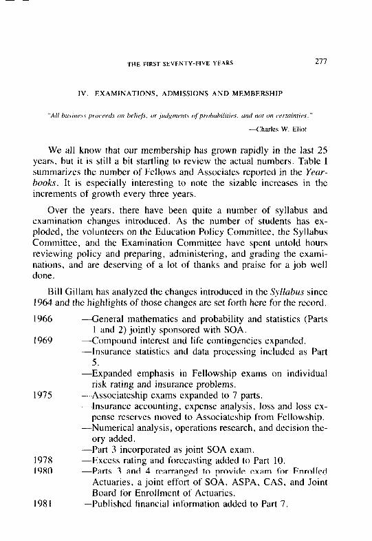
THE FIRST SEVENTY-FIVE YEARS 271
IV. EXAMINATIONS, ADMISSIONS AND MEMBERSHIP
We all know that our membership has grown rapidly in the last 25 years, but it is still a bit startling to review the actual numbers. Table I summarizes the number of Fellows and Associates reported jn the Year- books. It is especially interesting to note the sizable increases in the increments of growth every three years.
Over the years, there have been quite a number of syllabus and examination changes introduced. As the number of students has ex- ploded, the volunteers on the Education Policy Committee, the Syllabus Committee, and the Examination Committee have spent untold hours reviewing policy and preparing, administering, and grading the exami- nations, and are deserving of a lot of thanks and praise for a job well done.
Bill Gillam has analyzed the changes introduced in the Syllabus since 1964 and the highlights of those changes are set forth here for the record.
1966
1969
-General mathematics and probability and statistics (Parts I and 2) jointly sponsored with SOA.
-Compound interest and life contingencies expanded. -Insurance statistics and data processing included as Part
5.
1975
-Expanded emphasis in Fellowship exams on individual risk rating and insurance problems.
-Associateship exams expanded to 7 parts. -Insurance accounting, expense analysis, loss and loss ex-
pense reserves moved to Associateship from Fellowship. -Numerical analysis, operations research, and decision the-
ory added.
1978 1980
1981
-Part 3 incorporated as joint SOA exam. -Excess rating and forecasting added to Part 10. -Parts 3 and 4 rearranged to provide exam for Enrolled
Actuaries, a joint effort of SOA, ASPA, CAS, and Joint Board for Enrollment of Actuaries.
-Published financial information added to Part 7.
278 THE FIRS1 SEVtNIY-FlVt YtAKS
1983
1985 1987
-Part 3 expanded to include statistical analysis (in 1987 this exam was split into three parts).
-Part 4 expanded to include both life and casualty contin- gencies and credibility theory.
-Part 4 expanded to include loss distributions. -Part 8 revised to differentiate U.S. and Canadian special-
ties. -Introduction of flexible education effort.
The popularity and success of loss reserve and other special interest seminars is commented on elsewhere, but their contribution to the overall educational effort needs to be noted in this section as well. Also con- tributing are the nine Regional Affiliates and two Special Interest Sec- tions.
The Harold W. Schloss Memorial Scholarship Fund provides funds for deserving students of actuarial science and represents a noteworthy addition to our educational program.
Since its early years, the CAS has made a special effort to encourage women and minorities to enter the actuarial ranks. The response of the women has been especially gratifying. At the end of 1985, a total of 139 out of 1,182 members were women ( 11.8 percent compared with 3 percent in 1960). As noted in an editorial in the Actuarin1 Reviews in February 1987, women made up 20 percent of the new members during the years 1976 through 1985.
In the last few years, the number of actuaries joining the consulting ranks has grown rapidly. This development is a reflection of the need for actuarial services among client-based companies and non-insurance risk financing entities, as well as traditional insurance and reinsurance companies. Overall, it is healthy for the profession.
V. MEETING AND PROCEEDINGS-IMPRINTS I.EFT BEHIND
The 1964 annual meeting--The Golden Anniversary meeting held in New York City-was a notable affair. In honor of the occasion, many turned out in formal attire, and it was by far the largest gathering of casualty actuaries ever recorded up to that time. A total of 218 attendees (128 Fellows, 49 Associates and 41 Guests) saluted the completion of 50 years, and toasted what all hoped would be a solid and distinguished growth in the next 50 years.
THE FIRST SEVENTY-FIVE YEARS 279
Dudley Pruitt’s paper “The First Fifty Years” was a big hit, and was widely acclaimed. Matt Rodermund, in his own inimitable fashion, rolled out a thoughtful commentary on “How to Tell a Pure Actuary From a Lay Actuary.” Intended or not, this has become a classic, and is probably quoted and misquoted more than any other single paper, during the unrecorded rump sessions that tend to erupt, usually near liquid refresh- ments, at all casualty actuarial meetings.
Adger Williams recalls that an aggregation from Travelers (Paul Liscord, Bob Foster, Lu Tarbell and Adger Williams, known as “the Bumbershoots”) did some rather informal singing at CAS meetings in the late ’50s and early ’60s. Their efforts inspired Matt Rodermund’s tremendous musical talent to create actuarial words to go with otherwise familiar songs. (One of them, “Underwriters in the Morning,” was sung by the Bumbershoots at a CAS meeting in 1962.)
As the years progressed, these songs developed into skits, all to the great delight of the audience. For the 1968 Fall meeting in Washington, D.C., Matt Rodermund wrote, organized, produced, and starred in what was to become a sequence of full blown musical comedies. The titles don’t do them justice, but give some idea of the seriousness of the subject matter that was bandied around in the most irreverent way.
1968
1969 1970
1973
-“Son of Of All Sad Words, a Property/Liability Play with Decreasing Credibility.” (Actually, a follow up of Matt’s 1959 skit entitled “Of All Sad Words.“)
-“An Assumed Risk Anthology,” Matt Rodermund, author. -“Naked Comes the Actuary,” John Muetterties, author. A
take-off on Shakespeare with most of Shakespeare taken off.
--“How to Succeed as an Actuary,” Matt Rodermund, au- thor. Built on the familiar musical “How to Succeed in Business Without Really Trying.”
This production was the most elaborate and most success- ful of these entertainment efforts. With a view to the future, it was recorded, and is still pulled up and listened to with lots of nostalgia. Perhaps its greatest compliment was a revival at the 1977 joint meeting of the CAS and ASTIN, where it again “brought down the house.”
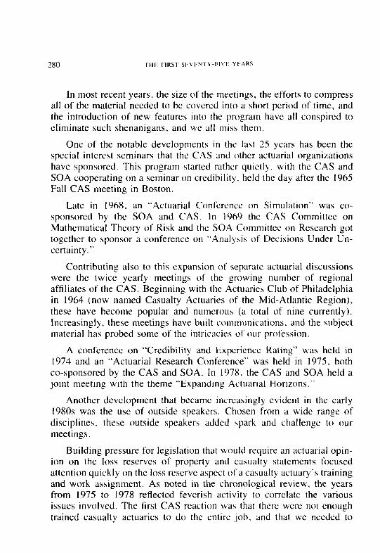
280 I‘HE FIRS1 WVFN’I’Y-f’lV1, YIARS
In most recent years, the size of the meetings, the efforts to compress all of the material needed to be covered into a short period of time, and the introduction of new features into the program have all conspired to eliminate such shenanigans, and WC: all miss them.
One of the notable developments in the last 25 years has been the special interest seminars that the CAS and other actuarial organizations have sponsored. This program started rather quietly, with the CAS and SOA cooperating on a seminar on credibility, held the day after the 1965 Fall CAS meeting in Boston.
Late in 1968, an “Actuarial Conference on Simulation” was co- sponsored by the SOA and CAS. In 1969 the CAS Committee on Mathematical Theory of Risk and the SOA Committee on Research got together to sponsor a conference on “Analysis of Decisions Under Un- certainty.”
Contributing also to this expansion of separate actuarial discussions were the twice yearly meetings of the growing number of regional affiliates of the CAS. Beginning with the Actuaries Club of Philadelphia in 1964 (now named Casualty Actuaries of the Mid-Atlantic Region), these have become popular and numerous (a total of nine currently). Increasingly, these meetings have built communications, and the subject material has probed some of the intricacies of our profession.
A conference on “Credibility and Experience Rating” was held in 1974 and an “Actuarial Research Conference” was held in 1975, both co-sponsored by the CAS and SOA. In 1978, the CAS and SOA held a joint meeting with the theme “Expanding Actuarial Horizons.”
Another development that became increasingly evident in the early 1980s was the use of outside speakers. Chosen from a wide range of disciplines, these outside speakers added spark and challenge to our meetings.
Building pressure for legislation that would require an actuarial opin- ion on the loss reserves of property and casualty statements focused attention quickly on the loss reserve aspect of a casualty actuary’s training and work assignment. As noted in the chronological review, the years from 1975 to 1978 reflected feverish activity to correlate the various issues involved. The first CAS reaction was that there were not enough trained casualty actuaries to do the cntirc job. and that we needed to
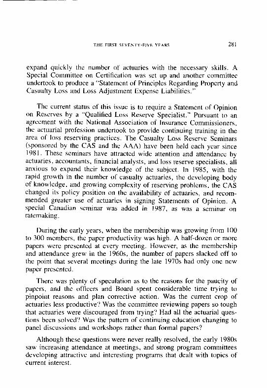
THE FIRST SEVENTY-FIVE YEARS 281
expand quickly the number of actuaries with the necessary skills. A Special Committee on Certification was set up and another committee undertook to produce a “Statement of Principles Regarding Property and Casualty Loss and Loss Adjustment Expense Liabilities.”
The current status of this issue is to require a Statement of Opinion on Reserves by a “Qualified Loss Reserve Specialist.” Pursuant to an agreement with the National Association of Insurance Commissioners, the actuarial profession undertook to provide continuing training in the area of loss reserving practices. The Casualty Loss Reserve Seminars (sponsored by the CAS and the AAA) have been held each year since 1981. These seminars have attracted wide attention and attendance by actuaries, accountants, financial analysts, and loss reserve specialists, all anxious to expand their knowledge of the subject. In 1985, with the rapid growth in the number of casualty actuaries, the developing body of knowledge, and growing complexity of reserving problems, the CAS changed its policy position on the availability of actuaries, and recom- mended greater use of actuaries in signing Statements of Opinion. A special Canadian seminar was added in 1987, as was a seminar on ratemaking.
During the early years, when the membership was growing from 100 to 300 members, the paper productivity was high. A half-dozen or more papers were presented at every meeting. However, as the membership and attendance grew in the 1960s the number of papers slacked off to the point that several meetings during the late 1970s had only one new paper presented.
There was plenty of speculation as to the reasons for the paucity of papers, and the officers and Board spent considerable time trying to pinpoint reasons and plan corrective action. Was the current crop of actuaries less productive? Was the committee reviewing papers so tough that actuaries were discouraged from trying? Had all the actuarial ques- tions been solved‘? Was the pattern of continuing education changing to panel discussions and workshops rather than formal papers?
Although these questions were never really resolved, the early 1980s saw increasing attendance at meetings, and strong program committees developing attractive and interesting programs that dealt with topics of current interest.
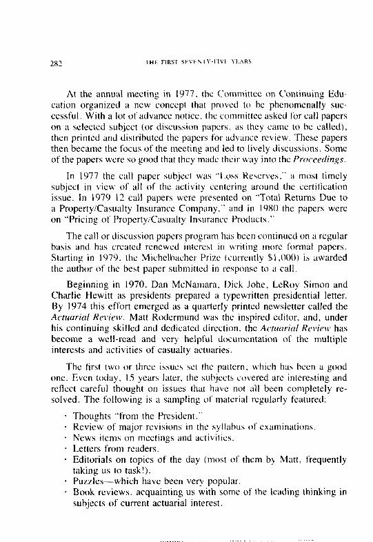
282 THE FIRS1 Sb.Vt.N I Y-t,IVb Yf AK\
At the annual meeting in 1977. the Committee on Continuing Edu- cation organized a new concept that proved to be phenomenally suc- cessful. With a lot of advance notice, the committee asked for call papers on a selected subject (or discussion papers. as they came to be called), then printed and distributed the papers for advance review. These papers then became the focus of the meeting and led to lively discussions. Some of the papers were so good that they made their way into the Proceedings.
In 1977 the call paper subject was “Loss Reserves,” a most timely subject in view of all of the activity centering around the certification issue. In 1979 12 call papers were presented on “Total Returns Due to a Property/Casualty Insurance Company.” and in 1980 the papers were on “Pricing of Property/Casualty Insurance Products.”
The call or discussion papers program has been continued on a regular basis and has created renewed interest in writing more formal papers. Starting in 1979, the Michelbacher Prize (currently $1,000) is awarded the author of the best paper submitted in response to a call.
Beginning in 1970, Dan McNamara, Dick Johe, LeRoy Simon and Charlie Hewitt as presidents prepared a typewritten presidential letter. By 1974 this effort emerged as a quarterly printed newsletter called the Acruarial Reivierc. Matt Rodermund was the inspired editor, and, under his continuing skilled and dedicated direction, the Actuarial Rc~~v’rw has become a well-read and very helpful documentation of the multiple interests and activities of casualty actuaries.
The first two or three issues set the pattern, which has been a good one. Even today, 15 years later, the subjects covered arc interesting and reflect careful thought on issues that have not all been completely re- solved. The following is a sampling of material regularly featured:
. Thoughts “from the President.” * Review of major revisions in the syllabus of examinations. . News items on meetings and activities. * Letters from readers. * Editorials on topics of the day (most of them by Matt, frequently
taking us to task!). * Puzzles-which have been very popular. * Book reviews, acquainting us with some of the leading thinking in
subjects of current actuarial interest.
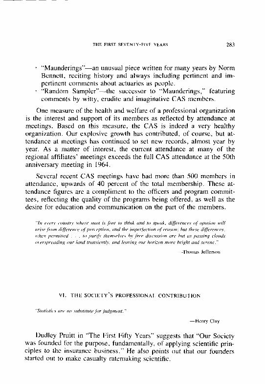
THE FIRST SEVENTY-FIVE YEARS 283
* “Maunderings-an unusual piece written for many years by Norm Bennett, reciting history and always including pertinent and im- pertinent comments about actuaries as people.
* “Random Sampler”-the successor to “Maunderings,” featuring comments by witty, erudite and imaginative CAS members.
One measure of the health and welfare of a professional organization is the interest and support of its members as reflected by attendance at meetings. Based on this measure, the CAS is indeed a very healthy organization. Our explosive growth has contributed, of course, but at- tendance at meetings has continued to set new records, almost year by year. As a matter of interest, the current attendance at many of the regional affiliates’ meetings exceeds the full CAS attendance at the 50th anniversary meeting in 1964.
Several recent CAS meetings have had more than 500 members in attendance, upwards of 40 percent of the total membership. These at- tendance figures are a compliment to the officers and program commit- tees, reflecting the quality of the programs being offered, as well as the desire for education and communication on the part of the members.
VI. THE SOCIETY’S PROFESSIONAL CONTRIBUTION
Dudley Pruitt in “The First Fifty Years” suggests that “Our Society was founded for the purpose, fundamentally, of applying scientific prin- ciples to the insurance business.” He also points out that our founders started out to make casualty ratemaking scientific.
284 I-HE FIRS1 SEVliNTY-FIVE YEARS
Article II of our 1962 Constitution had evolved to the point of stating that the object of our Society “shall be the promotion of actuar- ial and statistical science as applied to insurance, other than life insurance. ”
This article was amended in 1968 to provide that the objects of the Society “shall be to advance the knowledge of actuarial science as applied to the problems of insurance, other than life insurance, and to promote and maintain high standards of conduct and competence within the actuarial profession. .”
Article II remained unchanged through several subsequent amend- ments, but in the 1988 amendment it was adjusted to provide that the Society’s “Statement of Purpose” is to “advance the body of knowledge of actuarial science in applications other than life insurance. to establish and maintain standards of qualitication for membership. to promote and maintain high standards of conduct and competence for the members, and to increase the awareness of actuarial science.”
The increased emphasis on standards of qualification and conduct in the current “Statement of Purpose” stands out. but the concept of apply- ing scientific principles to insurance ratemaking remains unchanged.
It would be a boost to the profession if we could report that, after many years of trying, at least workers compensation ratemaking is now a neatly packaged scientific procedure, producing expected results year after year in state after state. Unfortunately, such factors as inflation, competition, rate regulation, varying patterns of loss distribution, the redefinition of coverage by court interpretation, and late recognition of the hazards created by carcinogens and toxic substances. have added immensely to the rating problems, year after year. Improved scientific methods have been developed to deal with many of these factors, but it is evident that one or more of them seems to keep popping up to extend the horizon of the problem. Perhaps WC should be pleased to have dealt with the problems as well as we have, but very few of today’s casualty actuaries seem to be satisfied that rating procedures, and even our work- ers compensation ratemaking procedures, are meeting all the needs of our very complex and troubling non-life insurance climate.
THE FIRST SEVENTY-FIVE YEARS 285
Credibility Theor)
Matt Rodermund, the long-time editor of the Actuarial Review and a keen observer of casualty actuarial trends, has termed the concept of credibility the casualty actuary’s most important contribution to actuarial science. Dudley Pruitt’s history recounts the early developments, and calls particular attention to the work of Arthur Bailey and Laurie Long- ley-Cook. Among his other accomplishments, Arthur explored the Baye- sian roots of credibility theory, and Laurie’s 1962 monograph on the subject went a long way toward making the intricacies more understand- able for those of us who tend to get lost when the formulas get a bit complicated.
In 1959, Bob Bailey (Arthur Bailey’s son) and LeRoy Simon au- thored a paper entitled “An Actuarial Note on the Credibility of Expe- rience of a Single Private Passenger Car.” Largely as a result of that effort, the concept of experience rating was introduced into private passenger auto rates. Also having a major impact on auto rating was the introduction of the negative binomial distribution of the probability of the number of auto accidents for a single risk.
Allen Mayerson summarized the Bayesian relevance to credibility theory in his 1964 paper “A Bayesian View of Credibility,” and followed this in 1968 with a paper “On the Credibility of the Pure Premium” (written with the collaboration of his University of Michigan colleagues Donald Jones and Newton Bowers, Jr.).
In 1970, Charlie Hewitt added a paper on “Credibility for Severity” to his very substantial work on the concept of credibility. Both the second Mayerson paper and the Hewitt paper represented major advances in the concept of credibility theory by demonstrating the effect that combining the average size of loss with the claim frequency (the components of the pure premium) has on credibility factors; previously, claim frequency alone had been the basis of credibility.
Table M
One major element in workers compensation retrospective rating was the long-in-gestation Table M, the table of insurance charges. Scratching his memory, LeRoy Simon recalled that the 1965 effort to update this table began with 1960 data, and was not completed until 1965. While

286 THE FlRST SEVEN I Y-FIVE YEARS
memories are a bit vague as to whether the calculation involved a 6’h or 7’h degree polynominal, LeRoy and Adger Williams solved one of the mysteries of actuarial literature-the letter M came from Harry Williams’ secretary’s name, Mabel, who did the typing for the original working group.
In 1974, a new table of insurance charges, which included the cost of the required per accident limit in the charge, was constructed for California. This table was named “Table L.” Dave Skurnick reported that Table L was so named because 1) L was adjacent to M, 2) it was tied to limited losses, 3) Les Dropkin fathered it. or 4) all of the above.
More Recent Activities and Contributions
Beginning with its inception in 1974, the Actuarial Review has pro- vided an easy-to-follow record of some of the more important casualty actuarial professional developments.
Inflation: Casualty actuaries didn’t invent inflation, but inflation has certainly created a great many problems to work on. Loss trend lines, expense graduation, controlled rates. ballooning loss reserves, inflated settlements, major shifts in reinsurance methods and arrangements, cap- tive insurance companies, self-insurance plans, off-shore insurance com- panies, and a host of other developments can be traced at least indirectly to the impact of inflation on the casualty insurance business.
Loss Reserve Evaluation: The last 15 years have seen an enormous growth in the time casualty actuaries have devoted to valuing and pro- jecting ultimate values of loss reserves. As workers compensation laws have extended the benefit periods, as settlement and payout periods of auto liability claims have been extended, and as product liability and malpractice claims have experienced very, very long payout periods, the reserves that need to be carried have become much larger, much more difficult to determine accurately, and much more important in determin- ing the financial well-being of casualty insurance companies.
In September 1976, Ron Bornhuetter as CAS president and Martin Bondy as chairman of the CAS Committee on Loss Reserves organized the first loss reserve special interest session. Thib symposium attracted the attendance not only of actuaries. but also of investment analysts, accountants. and others, all very concerned about this growing problem.
THE FIRST SEVENTY-FIVE YEARS 287
As noted under Section V, Casualty Loss Reserve Seminars have been held annually since 1981 by the CAS and AAA, and have had an ever-expanding attendance. Most important, these annual seminars have clearly served to place casualty actuaries at the forefront of the continuing effort to establish scientific approaches to setting adequate and accurate loss reserves.
Financial Developments: Beginning approximately in the early 197Os, many casualty actuaries were drawn into various aspects of cas- ualty companies’ financial operations. Several states introduced profit- ability regulation in one form or another, and investment income, mea- sured as a percent of premium, increased sharply. The interrelated concepts of incorporating investment return in ratemaking, measuring pro&ability by line by state, recognizing total return, and determining and defining a fair return for casualty insurance companies, became topics of many hot discussions. Tangential issues included methods for allocating investment income (including the very troublesome handling of realized and unrealized capital gains), allocating expenses, and the assignment of surplus to support the different lines of business.
With loss reserves playing such a major role in determining the financial health of casualty companies, it is not surprising that actuaries have established a substantial role in financial reporting. Establishing measures of capitalization requirements, valuing insurance companies, and developing financial reporting principles-both for statutory and Generally Accepted Accounting Principles (GAAP) reports-have served to expand the scope of actuarial activities in recent years.
When a major federal tax revision was mounted in the mid-1980s, it was natural for casualty actuaries to be in the thick of the discussions. Interestingly, the revised tax law did define some new parameters in the long simmering debate on the use of discount factors in calculating loss reserves.
New Ratemaking Challenges: Efforts to make casualty ratemaking more scientific were sharpened by developments in the 1970s and 1980s that posed .a host of new challenges. The introduction of no-fault auto in most major states called for rates on which there was almost no accumulation of past statistics, and a great many adaptations of related facts and new assumptions were used in getting this new coverage under way. Variations in state laws and very high losses from insured car
drivers and passengers created some unexpected problems that involved several years’ experience before proper rating procedures could be de- veloped.
Growing claim consciousness, high medical costs, and aggressive plaintiff lawyers pushed medical malpractice insurance into the crisis stage in the late 1970s. The long tail on occurrence policies. the almost universal seriously adverse development pattern on loss reserves, and very high settlements, caused insurers large losses, and projected big jumps in needed rates. Concerned about the total uncertainty of future experience, many companies pulled back on the coverage, and doctors, hospitals, regulators, and the public generally were caught in the resulting eruption. One solution was the organization of a great many new mon- oline medical liability companies. which concentrated but didn’t ease the ratemaking problems. A second solution was the development of the claims-made policy coverage, which changed the pattern of the mammoth IBNR problem, but in turn called for new’ ratcmaking procedures.
Self-insurance, captive insurance companies, and off-short place- ment of coverage have become increasingly popular in the last decade or so. Since these usually involve layers of coverage, some form of rcinsurance is usually involved, and the rating of each layer of retained coverage and reinsured covcragc crcatcs rating challenges. At the same time, servicing this business as well as dealing with inflation on more normal coverages have posed ratin, tr challcngcs of the most intricate kind c to reinsurance companics. Under these circumstances. we should not be surprised that dozens of CAS membcra have been hired by reinsurance cornpanics during the last 10 to 15 years.
Insurance companies have long voluntcercd or been forced into pro- viding coverage for essentially all risks, using pools or residual market mechanisms for those risks that do not meet normal underwriting re- quirements. On some of these the loss cxpcricnce has been extremely high, and the current and projected assessments are troubiesomc, to put it mildly. Rating solutions acceptable to the parties involved are still being sought.
As noted in the section on Social Insurance. “fair” discrimination among various classifications of insureds has always been an accepted goal of actuaries in their rating procedures. From time to time. certain groups have attempted to add a social dimension to “fair” which involves
THE FIRST SEVENTY-FIVE YEARS 289
changes from traditional rating procedures. Classifications based on lo- cation, size of risks, and type of risk have been questioned, sometimes successfully. One new challenge is to sex discrimination in auto rates (similar to the ongoing challenge in life, pension, and health insurance rating) and the resulting back-and-forth argument is heating up. Another is the territorial challenge in California Proposition 103.
VII. ACTUARIAL STRUCTURE
--Chinese proverb
The first 50 years of our history were marked by a separateness from our life insurance brethren. Nevertheless, some of our members have also been members of the life societies, thus emphasizing both some commonality of training and separation of interest. Also, in other coun- tries a distinction among actuarial disciplines never was created. Spec- ulation on the reasons for a separation in the United States has been the subject of many a pre-nightcap round of relaxing discussion. While never fully resolved, there are several suggested elements. Perhaps most im- portant, the almost explosive growth of workers compensation rating in this country needed immediate attention, but the then leaders of the Actuarial Society of America were not interested. As a result, our found- ers started off on their own.
This major development was followed in rapid fire order, (speaking, of course, from historical perspective) by mushrooming automobile in- surance, and various tort liability coverages in their famous and infamous forms. The rating and loss reserving for these coverages fell naturally to the CAS. Later, when a new class of rating problems developed, it was understandable that they too were added to the CAS area of responsibil- ity. These new rating problems included reinsurance, self-insurance, and inflation in their interrelated intertwinings, and, later, the problem of dealing with the multiple demons of claim consciousness, unanticipated no-fault entitlement, various forms of malpractice, liabilities for toxic substances, and the uncertainties of occurrence versus claims made ex- posures.
290 .THE FIRST SEVENTY-FIVt YEARS
Originally, our mathematical requirements were somewhat less rig- orous than those of our professional comrades in the life field, but as requirements have stiffened and our assignments have grown more com- plex, most of us now feel that the relationship is best characterized as one of similarly trained professionals going in different directions, with no consideration of the scale of difficulty of entrance requirements. As a matter of fact, Laurie Longley-Cook (a life actuary before he came to the CAS) wrote a paper for the SOA in 1961 indicating that the areas of credibility theory required a standard of mathematics higher than is required in any life actuarial work.
The combination of a separate organization to start with, a separate set of problems to deal with, and a sharply increased need to deal with those different problems, has resulted in the CAS achieving very rapid growth, as a separately functioning unit. in both numbers and overall strength. (Membership in November 1964 was 397; in November 1988, 1,437.)
At the same time there has been a persistent effort to coordinate if not unify the profession. In 1963 Laurie Longley-Cook. Bill Leslie, Jr., Dan McNamara and Frank Harwayne were working on a Joint Committee of the Profession “to explore means of obtaining legal accreditation of actuaries in the United States, including plans for creating a national association of actuaries .”
In 1965, this effort culminated in the formation of the American Academy of Actuaries. CAS members were prominent in the organiza- tion of the Academy, including Tom Murrin as the original president- elect with Dot Masterson and several Joint Committee members serving as officers and directors. The original hope for a federal charter had to be abandoned. but the need for the actuarial profession to present a united front on at least some issues served as a cohesive force as the Academy and the profession struggled to define the Academy’s role.
The year 1972 saw the organization of what came to be called the Council of Presidents, made up of the presidents and presidents-elect of all of the North American actuarial bodies. Operating on a strictly informal basis, it has served as a strong unifying force. exchanging information and coordinating activities.
THE FIRST SEVENTY-FIVE YEARS 291
Beginning in 1975, a substantial effort was mounted to reorganize and perhaps combine some of the different actuarial organizations. Long discussions struggled with the dual problems of presenting a unified front to our publics and improving efficiency by eliminating duplicate func- tions. The merger part foundered on the unwillingness of each of the organizations to give up its separateness. However, the effort did serve to significantly raise the level of overall professional awareness, to elevate the understanding and respect for the different specialties, and to develop a willingness to work together on projects of joint interest. Further, it led to the consolidation of a number of functions. Perhaps most important, it also clarified the different roles each organization could and should play in helping actuaries achieve a more publicly acceptable image, if not as a single entity, at least as a carefully coor- dinated profession.
Reflecting slow but steady progress under the coordinating efforts of the Council of Presidents, a joint research and education mechanism, the Actuarial Education and Research Fund, was organized in 1975.
Another joint effort has been the Guides and Opinions to Professional Conduct, as developed over several years and several revisions. The American Institute of Certified Public Accountants’ efforts to put values on life insurance companies sparked the first actuarial standards of prac- tice. The discussions also raised the all-pervasive issue of the indepen- dence of the actuary with respect to the accountant and with respect to the insurance company whose financial condition was at issue.
An important outgrowth of this near confrontation between accoun- tants and actuaries on life problems was the appointment of respective accounting and actuarial relations committees to provide a regularly available facility for communication between the two professions (AICPA for accountants, AAA for actuaries).
With casualty loss reserves evidencing increasing volatility and grow- ing rapidly as a proportion of property/casualty liabilities, the National Association of Insurance Commissioners in 1978 recommended that loss reserve opinions should be rendered each year by a qualified actuary. (A similar requirement had been adopted for life reserves in 1975.)
292 THE l;IRSI SI.VI.NI-Y-FIVE YEARS
The ensuing discussions were lengthy and at times bitter and con- fused. Casualty actuaries argued that the reserve opinion assignment should be unique to someone fully trained in loss reserve techniques; CPAs felt that it should be viewed as part of the auditing function in which they had the primary role; and several companies using experts in loss reserves, but not actuaries, to dcvclop loss reserves, did not want to change their ways.
The end result was that beginning in 1980 about one-third of the states adopted a requirement that the property/casualty annual statement blank should include a statement of opinion on loss and loss expense reserves by a member of the AAA, or by a “qualilicd loss reserve specialist.” (An important element in arriving at this compromise was the background of experience and communication built up with the accounting profession over the years.) Several years of experience have demonstrated shortcomings in the present arrangement from the view- point of the Insurance Commissioners, and it is reasonable to expect a further evaluation and probable tightening of the requirement.
The first actuarial Standards of Practice for Financial Reporting of Stock Life Companies had been developed in the early 1970s. The NAIC requirement for a statement of opinion on casualty loss and loss expense reserves led to a practice standard for the Statement of Actuarial Opinion for Fire and Casualty Insurance Company Statutory Annual Statements. adopted in 1978 by the Academy. As with most of the earlier standards, it was designed to meet an immediate need. and for many years it was the only standard of practice applicable to casualty actuaries.
The need for explicit actuarial standards of practice has evolved as actuarial practitioners have struggled to establish themselves as a true profession. By 1979 a basic framework was established for converting the somewhat haphazard development of standards of practice to meet immediate needs into a concept of a permanent Actuarial Standards Board that would oversee the development and administration of a more com- prehensive set of standards which could be used as guides by the entire profession.
From 1979 to 1988, a series of task forces and committees developed a step-by-step program for developing such standards. An Interim Ac- tuarial Standards Board was established in 1985 and, as of July I, 1988, the Actuarial Standards Board took over this responsibility for the profes- sion.
THE FIRST SEVENTY-FIVE YEARS 293
Throughout this massive effort, the Casualty Actuarial Society, the Society of Actuaries, the Conference of Actuaries in Public Practice, and the American Academy of Actuaries worked side by side. The fact that a common purpose could be achieved by separate organizations is a reflection of the increasing respect shared by the organizations for each other, and the increasing awareness on the part of the individual actuaries of all disciplines of the need for coordinated effort.
In 1988, a Task Force on Strengthening the Actuarial Profession was formed to again consider whether some form of unification of the profes- sion would be helpful. The Task Force report is currently being studied, but, significantly, does not recommend unitication. Instead, it urges all or nearly all of the members of the specialized organizations to join the American Academy of Actuaries or Canadian Institute of Actuaries, so that these organizations can become the true representatives of the ac- tuarial profession, and its spokesmen.
VIII. WHAT IS A CASUALTY ACTUARY?
In preparing his summary of “The First Fifty Years” of the CAS, Dudley Pruitt wrestled diligently with the challenging question, “What is a casualty actuary. 3” In the original insurance concept, an actuary is one who sets premium rates, according to probabilities based on statis- tical records.
Dudley carefully recounts the efforts of the actuaries to build scien- tific or statistical bases for rates, substituting where practical for the skilled but sometimes uncertain judgment of the underwriters. Workers compensation started it all, of course, but the actuaries’ efforts were expanded rather quickly to other casualty coverages, and the ratemaking field keeps widening.
Fire insurance ratemaking added new challenges, but the structure of schedule rating established long ago by tire underwriters has been im- possible for actuaries to systematize.
294 THE F1KS.I SE\‘f.NTS-FIVE YbAK.5
Homeowners and commercial package policies have introduced a whole set of new problems in establishing combined rates for previously monoline coverages.
Auto ratemaking is adjusting to developments such as no-fault and increased emphasis on individual cxpericnce, but new challenges keep coming.
Medical malpractice and various other liability coverages continue to pose new problems for the actuaries who arc trying to establish and maintain scientific ratemaking procedures.
In other areas, too, the field of casualty actuaries is expanding. Loss reserve work clearly is a major current activity of actuaries, and this activity almost automatically brings in valuation assignments. Investment analysis, modeling, related research work, corporate planning, tax plan- ning, expense analysis and control, risk management, reinsurance prob- lems, profitability measurement. and mergers and acquisitions are all types of projects where actuarial training can be useful, and where casualty actuaries are now involved.
From our review of the activities of casualty actuaries during the last 25 years, perhaps the most important impression is that their field of endeavor is widening. Actuaries arc employing their professional skills in any way that is useful to the various publics they serve, and that is all to the good. Further, they welcome the continuing expansion of actuarial functions.
As our activities have expanded, many of us have tried to come up with a definition that recognizes the much broader scope of our activities. Some of these have been humorous. and my favorite in that category is the following:
Actuary---one who bits in the back xut of the car. telling the Jriyer where to go by looking out the rear window.
Of the more serious efforts, the definition with the greatest acceptance is Fred Kilbourne’s as set forth in the Actuuricrl Rc+ertv of November 1983.
Actuary-+mc whose work is to evaluate and control the tinancial consequences of uncertainty about the future.
THE FIRST SEVENTY-FIVE YEARS 295
(In his November 1983 presidential address, Fred recites a variation of this definition, that actuaries “evaluate the current financial implications of’ future contingent events.” Both dcfinitiona have been widely quoted.)
Starting with a small, limited purpose group in 1914 (but one with broad vision), the Casualty Actuarial Society, over 7.5 years, has achieved a growth and expansion of purpose and professionalism that has been both exciting and challenging.
Acknowledgments
A great many people have contributed their time and efforts to pulling together the material for this paper, and my thanks and appreciation go out to all of them. There are too many to include a complete list, but special acknowledgments are due Bob Bailey, Bill Gillam, Dave Hart- man, Charlie Hewitt, Stan Khury, George Morison, Matt Rodermund, LeRoy Simon, Dave Skurnick, and Adger Williams. Also, Alexandra Hordynskyj and Ylonda Spears, who stretched their assignments as for- mer associates to handle the transcribing and organization of this histor- ical record. However, as author, I take full responsibility for all the statements and opinions included.
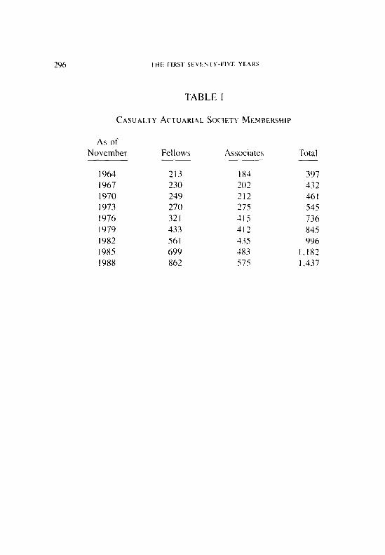
2% I’HE FIKSI SEVENTY-FIVE YI.AKS
TABLE I
CASUALTY ACTUAKIAI. SOCIETY MEMBERSHIP
As of’ November Fellows Associates Total
1964 213 1967 230 1970 249 1973 270 1976 321 1979 433 1982 561 I985 69’) 198X 862
IX4 397 202 432 212 461 275 545 115 736 412 845 435 996 483 I, 182 57s I .437
297
ADDRESS TO NEW MEMBERS-NOVEMBER 13, 1989
P. ADGER WILLIAMS
Good morning and congratulations to all of you. Thanks, Kevin for that kind introduction, even though it did sound a little like I’d been exhumed just for this occasion. I’d also like to thank Kevin for inviting me to speak to this, the largest group of Fellows and Associates ever to be welcomed into the Casualty Actuarial Society at one meeting. I think it’s appropriate that this is occurring on the 75th birthday of our Society.
When we look at how many are in this group, I can’t help but do some comparing. There were 97 charter members of the CAS who met right here in this hotel in 1914. Today we are honoring more than 170, over 100 of them new Associates. It’s as if we’re starting all over again. If this group spawns the same kinds of accomplishments as our founders, we have a bright future indeed.
As is the case with most speakers on occasions such as this, I’m going to say a lot of things you already know. But isn’t that what actuaries usually deal with, things we already know? What we hope to do is organize things in a way that they give us some vision of the future.
One of the things we already knew that took the rest of the world just a little longer to find out is that we’re number one, not just among the professions but of all jobs. We’re number one! Quite an honor! And well deserved, I might add.
But just saying we’re number one isn’t very definitive. When I talk to actuarial candidates or students, and try to describe the value of the actuarial profession, I think back to what appealed to me when I first entertained the idea of becoming an actuary and those things that have been the sustaining attraction of the profession since.
First of all, you could make a living while studying to become a professional. That was quite an incentive for me. And long before there was a civil rights movement, the CAS made it clear what you had to do to become an actuary. It didn’t make any difference what race you were, what color you were, or what religion you were. You didn’t have to be male or female. Well, I guess you did need to be one or the other. And you didn’t have to go to the “right” school or know somebody to get
298 ADDRESS I’0 NEW MEMBERS
ahead. All you had to do was pass the exams and you have shown you can do that.
At the 50th anniversary celebration, Matt Rodermund presented a paper which pointed out the differences between a pure actuary and a lay actuary. This distinction said more than even he realized; it pointed out the wide range of opportunity to someone with actuarial training. This training is still the most versatile that can be found in insurance.
We can point with pride to CAS members who have become insur- ance commissioners, bureau heads, presidents, CEO’s, and managers in a wide range of disciplines: data processing, finance, underwriting, audit, marketing and many others. All of these are examples of lay actuaries whose training was a stepping stone into management. But most actuaries don’t want to be managers. That’s where the pure actuary comes in. You can have a fulfilling, and I might add, lucrative career as an actuarial professional doing actuarial work.
Before going any farther, I’d like to say a few words just to the new Associates. Get your Fellowship! Become an F.C.A.S.
At this point in your career, it’s very easy to look around and say to yourself “Why do I need to pass more exams?”
You can recite the reasons why you shouldn’t:
* your work doesn’t require more knowlcdgc; * you’re really too busy to study: * besides. your job is interesting (mom intcrcsting than studying); * you have a great boss who would just as soon see you work more
and study less; . you’ve been getting regular promotions in a great organization, and
you’re well paid; * you work with a really great bunch of people;
Those are petty good reasons to stop studying. aren’t they‘? But let me tell you, times change. Companies change, bosses change, friends change, or more likely, leave. And, sometimes, worst of all, your job doesn’t change. You wake up some morning and realize you’re at a dead end, and you want a ticket out. That ticket is the professionalism which comes with Fellowship I see some of my friends smiling who have been in that situation. Having their Fellowship allowed them career choices that would have been unavailable otherwise.
ADDRESS TO NEW MEMBERS 299
Jim Valvano, the much publicized N.C. State coach gives a very good talk on motivation, getting ahead, and succeeding. At the end of one of his lectures, someone asked him how he went about making sure his team was going to win. His reply was that nobody can do that, but what you can do is go through all the necessary training and preparation so that you put your team in a position to win. Then fate can decide the outcome.
So put yourself in a position to win. Get your Fellowship. You’ll never forgive yourself if you don’t.
So where are you at this point? You are now a member of the CAS which makes you an actuary, a professional. This gives you the oppor- tunity to choose any kind of career you wish. As I said before, you can become an executive, a manager, a managing actuary, a consultant, or a pure research actuary. Your professionalism gives you countless op- portunities.
But professionalism also brings with it responsibility. Now I’m not talking about what you often hear some long-time actuaries saying, “The profession has been good to me so I want to give something back to the profession.” That is a worthwhile sentiment, and I think it would be wonderful if some or all of you would put in some time working for the CAS or elsewhere in the profession. But that’s not what I mean.
I’m talking about the responsibility that comes with the mantle of professionalism that has now been draped over your shoulders. You studied actuarial science to pass the exams. Much of that science is contained in the CAS Proceedings and other actuarial literature. It would seem that all you have to do is apply what you’ve learned. After all, this is the 75th anniversary of the CAS, and how much could be left to discover or develop?
Early in my career, back in 1960, I got sidetracked into a data processing project to develop the first computer-communications system in the insurance business. As we approached the time to go on the air in 1964 with our gigantic computers (“gigantic” in those days meant a 64K memory), a young man who had just joined the project said to me, “gee, I wish I could have gotten into data processing early while there was still something new to be contributed.”
300 ADDRESS TO NEW MEMBERS
Don’t make the same mistake that young man made. We owe much of the work that has been done during our first 75 years, but we have just scratched the surface of actuarial science+specially casualty ac- tuarial science. You should view yourselves as pioneers, entering the profession, not at the end or the middle but, at the beginning.
So the work that has gone before, the body of actuarial knowledge that has been developed is both a gift and (I fegucy. Now it becomes your responsibility. If that body of knowledge is deserving of your support, then apply it and defend it. Where it is lacking, it’s up to you to improve or replace it. But it should never be taken for granted.
Somehow it just doesn’t seem fair, does it‘? You’ve had your new actuarial designation for only 12 minutes, 42 seconds, and you’ve already been given the responsibility for 75 years worth of activity in the CAS.
That’s not all! There are several other responsibilities that come with the actuarial mantle-the responsibility for the advancement of actuarial science. It’s up to you to see to it that our science has substance. There are those who contend that what we do is an art, not a science. And we do have to be careful not to tie ourselves in knots with rigid rules which stifle actuarial innovation. At the same time, we can’t let the desire for actuarial art lead us to actuarial anarchy.
Next, there’s the responsibility for actuarial standards which must march hand-in-hand with the advancement of the science. Here we have no choice. If we don’t see our own standards, someone will set them for us. But we must set them in a way that gives us actuarial freedom within a framework of sensible boundaries.
We also have the responsibility for communicating our knowledge in a way that it can be understood. Some of you may have read Stephen Hawking’s book, A Brief History r,$ Time, in which he tackles and attempts to explain, in simple terms, some of the most complex theories relating to the universe and the quest for a unified theory. But he concludes that even if the theory is discovered, it will do no good if it is only understood by a few scientists; it must be communicated so that it is “understandable in broad principle by everyone.” That is our task and our responsibility, to communicate in such a way that the least knowledgeable of our audience understands what WC mean.
ADDRESS TO NEW MEMBERS 301
Finally, there is the responsibility for actuarial integrity, which to me is the heart of professionalism. There are many directions your careers will take, positions in regulation, industry, consumerism, risk manage- ment, and many others. As you advance, you must remain keenly aware of when you’re speaking as an actuary and when you’re not. And you can never completely shed the responsibilities of professionalism when you’re speaking in those areas where your training gives you that unique capability that designates you as an actuary.
With all of these responsibilities, you’re probably beginning to won- der what you get out of being an actuary. To answer that, let’s reminisce forward about your actuarial career. As you look back on these years that are ahead of you, you’ll find that being an actuary really did put you in a position to win . . . A position to influence the outcome of your employment, a position to influence your industry, a position to influence your profession, and if you were willing to participate, a chance to be part of the rule setting process rather than the rule following process.
Look around you at those who are in this historic group of new Fellows and Associates. As the years go by they will form what I like to call an accumulation of actuarial acquaintances which will become the continuity in your life. Ultimately I think you will find, as I did, that being an actuary is not only a profession, it is a process of life enrich- ment .
302
PRESIDENTIAL ADDRESS - NOVEMBER 14. 1989
KEVIN M RYAN
I direct your attention to the following quote from the Prc~vedin~.s of the Casualty Actuarial Society:
Mr. Rjan was modest. kindly. cheerful; hi5 human sympathy wah immediatelq apparent IO all who met him. In conqucnce hc gained without conscious effort the loyalty and love of all with whom he came in contact--associates and subordinates alike. Few men have won the affcctlonatr regard in which Mr. Ryan ~‘35 universally held.
So reads the obituary of a former president of the CAS and a former head of the National Council on Workmen’s Compensation, Mr. Har- wood Eldridge Ryan, the sixth CAS president and first president of the National Council.
In his CAS Presidential address hc said, “I suppose everybody who holds this office, in casting about for a suitable subject for the yearly address, is constrained to impress upon the membership the importance of the organization’s mission.” Despite an absence of Harwood’s kinship and conspicuous esteem, we share much in common, not the least of which is that sentiment for organizational introspection.
It is my intent to continue the customary presidential practice of reflecting on some basic questions, as we mark the seventy-fifth year of the existence of this Society. It is not unduly introspective to question whether we are successfully fulfilling those challenges laid down for us by our founding fathers. Have we done and are we now doing what those who went before us trusted us to do‘? Can we point with pride that our stewardship of this important professional society is without blemish? Have we preserved our heritage? Or is it that we have done less than we are capable of? Less than we ought to have done? Far less than what was expected‘?
For fear that we rush to false evaluation. it is incumbent that we focus on the mission or objective of the CAS as it was originally framed and as it is now stated. This should not prove difficult. As actuaries we are both skeptical and focused.
PRESIDENTIAL ADDRESS 303
Our skepticism is best shown by the story of the journalist and the actuary who were riding together and passed a flock of sheep. “Look,” said the journalist, “the sheep have all been shorn.” The actuary replied, “At least, on this side.”
Our focus is exemplified by our continuing struggle to define the basic purpose of the organization and by a recognition of the role that we play. Initially, it was a narrow focus. As Isaac Rubinow enunciated in the concluding lines of the very first presidential address “What is really needed is a constructive plan . . for rating statistically, . . . so that . . rating should be definitely established, not only as a measure of justice between one individual and another, but also as a potent factor for the furthering of the safety movement, without however bringing about a situation under which insurance is being sold below cost. “Today I imagine that he would admonish us to be just, promote safety, but- remarkably from one who was a reputed socialist-make an underwriting profit. We have been cursed from the start with the dichotomous role of scientist and businessman.
Little changed in the stated aims of our Society throughout our early history. At the twenty-fifth celebration the then president Francis Per- ryman proudly noted that the second Article of the Constitution had never changed. The article proclaimed the aim of the Society to be “the promotion of actuarial and statistical science as applied to casualty and social insurance by means of personal intercourse, the presentation and discussion of appropriate papers, the collection of a library and such other means as may be found desirable.” Scant attention was paid to either Rubinow’s underwriting profit, or what have become today’s important facets-qualification and conduct. These aspects were only recently focused on.
Just last year, the statement of purpose was changed to “advance the body of knowledge of actuarial science in applications other than life insurance, to establish and maintain standards of qualification for mem- bership, to promote and maintain high standards of conduct and com- petence for the members, and to increase the awareness of actuarial science .”
To facilitate our review today I will restate that same purpose in different words:
304 PRESIDENTIAL. ADDRESS
To further the non-life actuarial profession by
1. Developing knowledge 2. Qualifying members 3. Maintaining standards of conduct, and 4. Increasing awareness of the actuarial profession
It will be against these four aims that our efforts must be judged.
As to the first purpose, have we advanced the body of knowledge of actuarial science‘? The results are uneven in that regard and we can have honest disagreement on the results. Such possible disagreement reminds me of Lady Nancy Astor, who, listening to Winston Churchill and growing more and more angry over the views he was expressing, said to him, “If you were my husband I’d put poison in your coffee.” Churchill replied, “If I were your husband, I’d drink it.”
We certainly have made considerable contributions to actuarial knowledge through the publication of papers in the Prowdings. In 1914 there were fourteen papers published in the Prowedin,q.s, almost all of them dealing with workers compensation. In I939 we published six papers. In that twenty-fifth anniversary year, there was still a prepon- derance of workers compensation papers. Only one of them dealt with a subject other than workers compensation. That particular paper should interest us as an example of the potential value of expanded actuarial insight. It is titled “The Effect of Daylight Saving Time on the Number of Motor Vehicle Fatalities.”
At the tifty year mark we had eight papers and went from a prepon- derance on workers compensation to only one paper on that subject. We were also blessed in that volume with the magnificent treatise “How to Tell a Pure Actuary from a Lay Actuary.” In most recent years we have shown a clear break from our early years by publishing usually seven or eight papers with very few dealing with workers compensation.
Is this a sufficient record’? Have WC accomplished what we have stated is our objective? I believe the answer is inconclusive. The quality is outstanding, and the quantity is impressive. The subject matter is not. As a profession we offer to society the service of analytical minds and an understanding of the basic mathematical principles underlying risks that daily impede fertile commercial transactions. However, we have
PRESIDENTIAL ADDRESS 305
allowed the use of our talents to be bounded by the insurance industry. It need not be. Is not the world of investment management, financial services, and econometrics in need of the basic talents possessed by casualty actuaries? Why are we reluctant to pursue a broader agenda, a more influential role in a society that could benefit from our talents? If our goal is to expand the body of actuarial knowledge, we must expand beyond the self imposed limit of casualty insurance.
If we do not accept the challenges presented by a growing awareness of risk in finance, then we are sure to leave the work to those who are both less qualified and less equipped. Accountants and finance practi- tioners have their role; it is not that of quantitative analysis of financial and insurance risk. Our response should be as clear as the challenge.
To quote once again the Ryan of 65 years ago: “It should logically fall to the casualty actuary to prepare the business in which he is engaged for larger opportunities. In recent years our national government has devoted considerable study to questions relating to the possible appli- cation of insurance principles to the solution of important economic problems . . . [We] should be even more alert and more ready to recognize such possibilities and be prepared with foreknowledge to ac- cept the responsibilities which the discovery of new needs may create.”
Our second objective is to qualify members. The accurate assessment, although self aggrandizing, is that we have been very successful in developing talented, productive, and successful actuaries. Many point to the examination process itself rather than the content of the exams that has produced this result; the size of the exams and their length have contributed to developing a group of successful students who have been able to balance work related duties and considerable study. This process has produced individuals marked by their ability to balance enormous demands, gifted in assigning priorities and juggling duties. As a result we need to exercise a great deal of caution as we approach the question of splitting our exams into smaller pieces.
Currently the CAS leadership is reviewing the question of whether we would be aiding the educational process by dividing the examinations into more but smaller parts. Both for the reasons mentioned earlier, and for fear that such a step would increase the average time it takes to pass all the exams, the Board will only proceed to implement the “partitioning of the exams” if it is convinced partition results in a better system that
306 PRESIDENTIAL ADDRESS
on average requires no extension of the time taken to complete the examinations.
In this preparation and examination cycle, the process itself can have as much value as the achievement to which the process is dedicated. It is much like the story of Tommy Brown. No matter what happened to Tommy Brown, he always described it as pure luck. He decided to prospect for gold and went into the mountains through a bitter winter, nearly freezing to death as he kept looking for a golden vein in the rugged ground, not unlike the perils of an actuarial student seeking a passing grade. Finally, as the ground thawed in the spring and he was down to his last meager ration of food and his mule was gasping its last, he broke into the earth in a likely looking spot and dug and dug until at last he hit a box. With no food left and his strength fast ebbing, a million miles from nowhere, he managed to lift the box out and open it. Inside was a carton of Army C rations. “Boy am I lucky,” he said, “it could have been gold.”
Have we been successful in this objective to qualify members‘? 1 believe the answer is yes. We have developed a strong carp of qualified, proficient actuaries. Not only do they possess the appropriate quality that will always be our first concern, but the quantity is also beginning to match our needs. We currently have a membership of 1447, comprised of 862 Fellows and 575 Associates. But more important, we now have more students than members and are well on our way to meeting some of today’s critical demands.
Our third objective is the enforcement of proper conduct and the requirement for competence. In no other area are we so obviously defi- cient. The noteworthy steps in publishing Principles and the development of Standards of Practice have been singularly successful. But does not the absence of meaningful disciplinary actions strike the membership as unusual? There is no resolve to question, no pressure to guide, no desire to admonish, or in those rare cases, no heart to punish. Why? Are we so unsure of ourselves that when our professional opinions lead to failure, when our advice leads to inadequate pricing. when our proposals are followed by financial ruin, we cannot question those involved.
We must not hestitate to question those involved in such activities. I am not suggesting we initiate harsher strictures or do anything to curtail actuarial creativity. We must be accountable, if we are to imbue our profession with competence and high standards of conduct.
PRESIDENTIAL ADDRESS 307
A severe limitation on our ability to institute strictures on unprofes- sional performance is our status as practitioners without license. Consider the American Medical Association, which has had meaningless, if not non-existent, discipline procedures in place. Because the AMA is a membership organization, it does not have the self-discipline procedure necessary to regulate its members’ performance. There is no licensing requirement that says a doctor must be an AMA member. The role of disciplinarian falls to the licensing body and that is a major difference for us. We know how difficult the discipline process is for doctors, yet they have the distinct advantage of being licensed. Without a licensing procedure the problem takes on a more difficult facet and requires sig- nificantly more self-regulation.
Accordingly the actuarial profession should devote a great deal more effort to discipline and guidance for professional conduct. The Council of President’s Task Force on Strengthening the Profession proposes extensive revisions to our discipline procedures. For us, more awareness of the need, and more appreciation of the role and use of the discipline process that enforces regulation of professionalism, must come from within. It is another price to be paid for not having a license.
Even if our first step is only to question those involved in assignments that had questionable outcomes, insolvency, or rate inadequacy, then it should be done and done quickly.
We know enough of the particulars of medical malpractice to be aware that some of the medical professions’ difficulties stem from its inability to discipline itself effectively. Not all doctors practice properly, as the following story dramatizes.
A man telephoned his doctor and said, “I have this shooting pain in my throat when I swallow and I’m very hoarse. What should I do?” The doctor replied, “Until you can see me at the office tomorrow, just keep your neck swathed in hot compresses.” “My maid told me to use cold compresses,” protested the man. “Nonsense,” said the doctor, “my maid says hot compresses .”
Our fourth and final objective is that of increasing the public aware- ness of the actuarial profession. Again, this area has been one of some success and some failure. Much ignorance shrouds the attempts to in- crease the public exposure of actuaries. We have delegated the role of public spokesman to the American Academy of Actuaries. As a result it
308 PRFSIDLN 1141 ,ZDDRl~.SS
speaks on our behalf in advocacy roles and in its role as disciplinarian. But we must maintain a public image for the CAS’s own role as a learned society. We must be clearly identified with the casualty actuarial edu- cational process. We are separate and distinct from the Society of Ac- tuaries and the American Academy of Actuaries. As such we should have our own identity and our own public relations posture. We must encourage potential students and potential employers to help develop a public awareness of what the CAS education means and the abilities it develops. We have not been successful in obtaining such public aware- ness. We arc now experimenting with new approaches to becoming more visible, yet we meet resistance to change. If we are to be effective we must be visible.
Public relations is like the problem of the farmer with his stubborn old mule. The farmer hit the mule over the head with a bat. Why? For the same reason that so many causes need public relations. The first thing you have to do is to make sure you have the target’s attention.
In summary, we are casualty actuaries and we hold claim to an honored profession, a profession in which we take justifiable pride, a profession of intelligent men and women who through the exercise of our profession add value to the society in which we live.
In keeping with the aims of that profession we must strive to expand our influence, ensure our integrity, educate our successors and do it all visibly and proudly.
I am proud to be one of you; I am grateful to have been allowed to serve you; I am thankful for your fellowship.
MINUTES OF THE 1989 ANNUAL MEETING
November 12-l 4, 1989
WALDORF-ASTORIA. NEW YORK
Sunday, Notpernber /2, 1989
The Board of Directors held their regular quarterly meeting from I:00 P.M. to 4:00 P.M.
Registration was held from 4:00 P.M. to 6:30 P.M.
From 5:30 P.M. to 6:30 P.M. there was a special presentation to new Associates and their guests. This session included an introduction to standards of professional conduct and the CAS committee structure.
A general reception for all members and guests was held from 6:30 P.M. to 8:30 P.M. There was a reception for 25-year members from 6 P.M. t0 7 P.M.
Mondaql, November 13, 1989
Registration continued from 7:00 A.M. to 8:00 A.M.
President Kevin M. Ryan opened the meeting at 8:00 A.M. The first order of business was to introduce Stan Hughey to provide an overview of his paper.
Kevin Ryan then introduced Robert Conger to give the secretary’s and treasurer’s report. Robert Conger also announced the results of elections of officers and directors.
The members of the Executive Council will be Vice President-Ad- ministration, Robert F. Conger; Vice President-Development, Charles A. Bryan; Vice President-Membership, Michael L. Toothman; and Vice President-Programs, Richard I. Fein.
Mike Toothman introduced 76 new Associates for 1988 and 34 new Associates for 1989. Mike Fusco introduced 14 new Fellows for 1988 and 52 new Fellows for 1989. The names of these individuals follow:
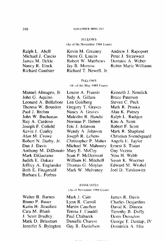
310 NOVEMBER MINUTES
FELLOWS
(As of the November 19XX Exam)
Ralph L. Abel1 Kevin M. Greaney Michael J. Cascio Pierre G. Laurin James M. Dekle Robert W. Matthews Nancy R. Einck Jay B. Morrow Richard Gauthier Richard T. Newell. Jr.
FELLOWS
(As of the May lY89 Examt
Manuel Almagro, Jr. Louise A. Fransis John G. Aquino Judy A. Gillam Leonard A. Bellafiore Len Goldberg Theresa W. Bourdon Gregory T. Graves Paul J. Brehm Nancy A. Graves John W. Buchanan Malcolm R. Handte Ruy A. Cardoso Norman P. Hebert Joseph F. Cofield Eric J. Johnson Kevin J. Conley Wendy A. Johnson Alan M. Crowe Joseph R. Lebens Robert N. Darby. Jr. Christopher P. Maher Dan J. Davis Michael W. Mahoney Anthony M. DiDonato Mary E. McCoy Mark DiGaetano Judith E. Dukatz Jeffrey A. Englander Beth E. Fitzgerald Barbara L. Forbus
Walter B. Barnes Bruno P. Bauer Karin H. Beaulieu Cara M. Blank J. Scott Bradley Mark D. Brissman Jennifer S. Byington
Sean P. McDermott William H. Mitchell Thomas G. Moylan Mark W. Mulvaney
ASSOCIATES
Andrew J. Rapoport Peter J. Siczewicz Dominic A. Weber Robin Marie Williams
Kenneth J. Nemlick Bruce Paterson Steven C. Peck Mark R. Proska Alan K. Putney Ralph L. Rathjen Kim A. Scott Robert F. Scott Mark R. Shapland Christian Svendsgaard Angela E. Taylor Ernest S. Tistan Guy Vezina Nina H. Webb Susan K. Woemer Edward M. Wrobel Joel D. Yatskowitz
Mark J. Cain Lynn R. Carroll Martin Cauchon Teresa J. Caudill Paul Chabarek Danielle Charest Guy R. Danielson
James R. Davis Charles Desjardins David K. Dineen Timothy B. Duffy Denis Dumulon George T. Dunlap, IV Dominick A. Elia
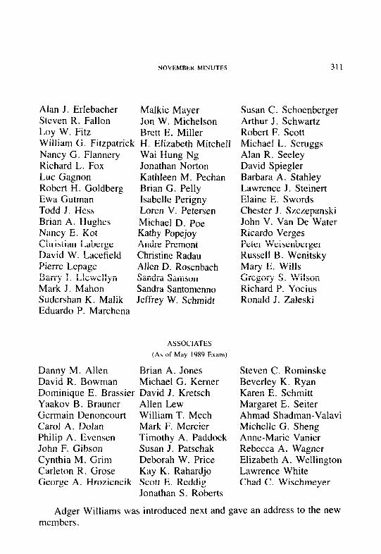
NOVEMBER MINUTES 311
Alan J. Erlebacher Malkie Mayer Steven R. Fallon Jon W. Michelson Loy W. Fitz Brett E. Miller William G. Fitzpatrick H. Elizabeth Mitchell Nancy G. Flannery Richard L. Fox Luc Gagnon Robert H. Goldberg Ewa Gutman Todd J. Hess Brian A. Hughes Nancy E. Kot Christian Laberge David W. Lacefield Pierre Lepage Barry I. Llewellyn Mark J. Mahon Sudershan K. Malik Eduardo P. Marchena
Danny M. Allen David R. Bowman
Wai Hung Ng Jonathan Norton Kathleen M. Pechan Brian G. Pelly Isabelle Perigny Loren V. Petersen Michael D. Poe Kathy Popejoy Andre Premont Christine Radau Allen D. Rosenbach Sandra Samson Sandra Santomenno Jeffrey W. Schmidt
ASSOCIATES
(As of May 1989 Exam)
Brian A. Jones Michael G. Kerner
Dominique E. Brassier David J. Kretsch Yaakov B. Brauner Allen Lew Germain Denoncourt William T. Mech Carol A. Dolan Mark F. Mercier Philip A. Evensen Timothy A. Paddock John F. Gibson Susan J. Patschak Cynthia M. Grim Deborah W. Price Carleton R. Grose Kay K. Rahardjo George A. Hroziencik Scott E. Reddig
Jonathan S. Roberts
Susan C. Schoenberger Arthur J. Schwartz Robert F. Scott Michael L. Scruggs Alan R. Seeley David Spiegler Barbara A. Stahley Lawrence J. Steiner-t Elaine E. Swords Chester J. Szczepanski John V. Van De Water Ricardo Verges Peter Weisenberger Russell B. Wenitsky Mary E. Wills Gregory S. Wilson Richard P. Yocius Ronald J. Zaleski
Steven C. Rominske Beverley K. Ryan Karen E. Schmitt Margaret E. Seiter Ahmad Shadman-Valavi Michelle G. Sheng Anne-Marie Vanier Rebecca A. Wagner Elizabeth A. Wellington Lawrence White Chad C. Wischmeyer
Adger Williams was introduced next and gave an address to the new members.
312 NOVtMBER MlNlllIIS
Rich Fein gave a summary of the program and Chuck Bryan sum- marized the Proceeding Papers being presented. He called for reviews of previous papers from the floor. There were none. The following awards were presented:
Woodward-Fondiller Prize:
Dorweiler Prize:
Michelbacher Prize:
Schloss Memorial Fund:
Emanuel Pinto and Daniel F. Gogol ( 1988)
Manuel Almagro and Thomas L. Ghezzi ( 1989)
Stephen J. Ludwig and Robert McAuley
Louise A. Francis
Jcna Ann Losey
Also presented was the AERF Award as well as a “Life-Time Achievement” Award to Matthew Rodermund.
The first panel to be presented was the panel of past presidents.
Moderam-: Mike Fusco (C. A. S. President-Elect) Executive Vice President Insurance Services Office
Ptrnelisrs: Norton E. Masterson (C. A. S. President I 955- 1956) Retired
Thomas E. Murrin (C.A.S. President 1963-1964) Executive Consultant Coopers & Lybrand
Ronald L. Bornhuetter (C.A.S. President 1975) President & Chief Executive Officer NAC Re Corp.
C. K. Khury (C.A.S. President 1984) Managing Director Mercer Meidinger Hansen
This was followed by a luncheon with a Presidential Address by Kevin Ryan. Lunch was from l2:oO P.M. to 1:4S P.M.
The afternoon was devoted to concurrent sessions which consisted of various panels and papers.
NOVEMBER MINUTES 313
The panel presentations covered the following topics:
I. Insurance Pricing: Return on Equity vs. Return on Sales
Moderator: David G. Hartman (C.A.S. President, 1987) Senior Vice President & Actuary Chubb Group of Insurance Companies
PaflPlisrs: Richard G. Woll Actuary Allstate Research and Planning Center
Yehuda Kahane, Prof. Dr., Director The Erhard Center for Higher Studies and Research in Insurance, Tel-Aviv University, Israel
Bernard A. Pelletier Associate Actuary Aetna Life & Casualty
2. Pricing Tort Reform
Moderator: Paul S. Liscord (C.A.S. President, 1973) Consulting Actuary Liscord, Ward & Roy, Inc.
Punelists: Philip D. Miller Vice President & Actuary Insurance Services Office
Robert A. Buchanan Robert Buchanan Consulting Australia
Claus S. Metzner Associate Actuary Aetna Life & Casualty
3. Partitioned Examinations
Moderator: Jerome A. Degemess (Chairman, Partitioned Examination Task Force) Actuarial Officer St. Paul Fire & Marine Insurance Company
314 NOVEMRER MINUTES
Gustave A. Krause (Chairman, Educational Policy Committee) Consulting Actuary Tillinghast, A Towers Perrin Company
4. Questions & Answers with the CAS Board of Directors
Moderator. Richard I. Fein (Vice President-Programs) Executive Vice President National Council on Compensation Insurance
Current Board Members: Michael Fusco (President-Elect)
Executive Vice President Insurance Services Office, Inc.
Irene K. Bass (Elected 1986) Principal Mercer Meidinger Hansen
Alan C. Curry (Elected 1987) Vice President & Actuary State Farm Mutual Automobile Insurance Co.
Charles A. Hachemeister (Elected 1988) Vice President F&G Re. Inc.
5. Insurance Accounting Issues of the 1990s
Modercrtor: Jerome A. Scheibl (C.A.S. President 1980) Vice President-Industry Affairs Wausau Insurance Companies
Ptmelists: John T. Bailey Coopers & Lybrand International Insurance Industry Practice
Bruce A. Bunner Partner Peat Marwick Main & Company
NOVEMBER MINUTES 31.5
Patrick W. Kenney Senior Vice President Aetna Life & Casualty Company
6. Practical Applications of Determining Loss Development Factors for Casualty Excess-of-Loss Business
Moderator: W. James MacGinnitie (C.A.S. President 1979) Consulting Actuary
Panelists: Daniel K. Lyons Second Vice President General Reinsurance Corporation
Harold Clarke Bacon & Woodrow, U.K.
Benjamin Zehnwirth Professor School of Economics and Finance Macquarie University Australia
The new Proceedings papers were:
I. “Application of Collective Risk theory to Estimate Variability in Loss Reserves”
Author: Roger M. Hayne Milliman & Robertson
2. “Determination of Outstanding Liabilities for Unallocated Loss Adjustment Expenses”
Author: Wendy Johnson Coopers & Lybrand
3. “The Aging Phenomenon and Insurance Prices”
Author: Stephen P. D’Arcy University of Illinois
Neil A. Doherty University of Pennsylvania
316 NOVEMBER MINLi I ES
4. “The Effect of Trend on Excess of Loss Coverages”
Author: Clive Keatinge Prudential Reinsurance Company
5. “An Analysis of the Capital Structure of an Insurance Company”
Author: Glenn Meyers Insurance Services Office
The officers held a reception for new Fellows and their guests from 5 P.M. to 6 P.M.
There was an off-site reception at the Metropolitan Museum of Art from 7 P.M. to 9 P.M.
Tuesduy, November I4
Kevin Ryan described the format for the session which started at 8:30 A.M. The featured speaker was Walter Wriston, retired Chairman and CEO of Citicorp. Mr. Wriston spoke from 8:30 to 9: 15 A.M. This was followed by a panel of CEOs.
Moderator: Kevin M. Ryan (C.A.S. President 1988) President National Council on Compensation
Panelists: Edward H. Budd Chairman & Chief Executive Officer The Travelers Corporation
Jack Moseley Chairman United States Fidelity & Guaranty Company
Walter B. Wriston Retired Chairman & Chief Executive Ofticer of Citicorp.
Following a break, there were concurrent sessions.
The panel presentations covered the following topics:
I. Taxation of P/C Insurance Companies
NOVEMBER MINUTES 317
Moderator: Steven H. Newman (C.A.S. President, 1981) Chairman & Chief Executive Officer Underwriters Reinsurance Company
Panelists. Steven Eldridge Partner, National Insurance Tax Ernst & Whinney
Herbert E. Goodfriend First Vice President Prudential-Bathe
2. Regulation of P/C Insurance Companies
Moderator: Michael A. Walters (C.A.S. President 1986) Consulting Actuary Tillinghast, A Towers Pen-in Company
Panelists: Earl Pomeroy Commissioner of Insurance North Dakota
Linda Golodner Executive Director National Consumers League
Peter Lardner Chairman, President & Chief Executive Officer Bituminous Casualty Corporation
The new Proceedings Papers were:
1. “On Becoming an Actuary of the Third Kind”
Author: Stephen P. D’Arcy University of Illinois
2. “Exposure Bases Revisited”
Author: Amy S. Bouska Tillinghast, A Towers Perrin Company
318 NOVEMBER MINUTES
3. A Review of Harold Clarke’s Paper, “Recent Developments in Reserving for Losses in the London Reinsurance Market”
Author: John C. Narvell Coopers & Lybrand
The afternoon was free.
There was a reception from 6 P.M. to 7 P.M., followed by a dinner/ dance from 7 P.M. to 11 P.M.
Wednesduy, November I5
Once again, Kevin Ryan outlined the program for the day and wel- comed ASTIN. Kevin Ryan introduced Jean Lemaire and asked Jean to tell the audience about ASTIN.
This was followed by a joint panel with ASTIN:
Moderator: LeRoy J. Simon (C.A.S. President, 1971) Executive Consultant Coopers & Lybrand
Panelists: Sidney Benjamin Bacon & Woodrow, U.K.
Hans Btihlmann ETH-Zentrum, Switzerland
Charles C. Hewitt (C.A.S. President, 19721 Retired
Jean Lemaire Wharton School
After the transfer of the presidency, Mike FUSCO gave the closing remarks.
This was followed by three concurrent sessions which were: Loss Development-Practical Applications, Return on Sales vs. Return on Equity, and Pricing Tort Reform. All three of these sessions were pre- sented earlier in the meeting.
November, I989 Attendees
In attendance, as indicated by the registration records, were 379 fellows, 193 associates and 143 guests, subscribers and students. The list of their names follows.

NOVEMBER MINUTES 319
Abell, R. L. Addie, B. J. Alff, G. N. Alfuth, T. J. Almagro, Jr., M. Aquino, J. G. Asch, N. E. Atkinson, R. A. Atkinson, R. V. Bailey, R. A. Bailey, V. M. Barrette, R. Bartlett, W. N. Bass, I. K. Bassman, B. C. Baum, E. J. Beer, A. J. Bellafiore, L. A. Ben-Zvi, P. N. Bennett, R. S. Berquist, J. R. Bertles, G. G. Bertrand, F. Bevan, J. R. Bickerstaff, D. R. Bill, R. A. Biondi, R. S. Blakinger, J. M. Blanchard, R. S. Blivess, M. P. Boccitto, B. L. Boison, L. A. Bornhuetter, R. L. Bourdon, T. W. Bouska, A. S. Bradley, J. S. Braithwaite, M. E. Braithwaite, P. Brannigan, J. F.
FELLOWS
Brehm, P. J. Brian, R. A. Bryan, C. A. Buchanan, J. W. Burger, G. Cardoso, R. A. Carter, E. J. Cascio, M. J. Cathcart, S. B. Caudill, T. J. Chernick, D. R. Childs, D. M. Chuck, A. Clinton, R. K. Cofield, J. F. Cohen, H. L. Cohen, H. S. Conger, R. F. Connell, E. C. Cross, S. L. Crowe, A. M. Curran, K. F. Currie, R. A. Curry, A. C. D’Arcy, S. P. Daino, R. A. Darby, R. N. Davis, D. J. Dawson, J. Deede, M. W. Defalco, T. J. Degerness, J. A. Dekle, J. M. Demelio, J. J. Deutsch, R. V. Diamantoukos, C. DiDonato, A. M. DiGaetano, M. Dodd, G. T.
Dolan, M. C. Downer, R. B. Drummond-Hay, E. T. Duda, D. S. Dukatz, J. E. Dyck, P. N. Dye, M. L. Easlon, K. Easton, R. D. Eddy, J. H. Ehrlich, W. S. Einck, N. R. Ellefson, T. J. Englander, J. A. Engles, D. Evans, G. A. Faber, J. A. Fagan, J. L. Fallquist, R. J. Farnam, W. E. Fein, R. I. Fiebrink, M. E. Finger, R. J. Fisher, R. S. Fitzgerald, B. E. Fitzgibbon, W. J. Forbus, B. L. Ford, E. W. Fowler, T. W. Francis, L. A. Fresch, G. W. Friedberg, B. F. Furst, P. A. Fusco, M. Gannon, A. H. Gapp, S. Gardner, R. W. Gauthier, R. Giambo, R. A.

320 NOVEMBER MINUTES
Gillam, J. A. Jean, R. W. Gillam, W. R. Jerabek, G. J. Gillam, W. S. Johe. R. L. Gillespie, J. E. John, R. T. Gluck, S. M. Johnson, E. J. Goldberg, L. R. Johnson, M. A. Goldberg, S. F. Johnson, W. A. Goldfarb, I. H. Josephson, G. R. Golz, J. F. Judd, S. W. Gottlieb, L. R. Kallop, R. H. Grannan, P. J. Kane, A. B. Grant, G. Karlinski, III, F. J. Graves, G. T. Kaufman, A. M. Graves, N. A. Keatingc, C. L. Groh, L. M. Keen, E. R. Gruber, C. Kelly, A. E. Hachemeister, C. A. Khury, C. K. Haefner, L. A. Kist, F. 0. Hall, A. A. Kleinman, J. M. Hall, J. A. Klinker, F. L. Hallstrom, R. C. Kneuer, P. J. Handte, M. R. Kollar, J. J. Hartman. D. G. Krause, G. A. Harwayne, F. Kreuzer, J. H. Haskell, G. E. Lamb, D. K. Hayne, R. M. Lange, D. L. Hazam, W. J. Larose, G. J. Hebert, B. J. Lattanzio, F. J. Hebert. N. P. Laurin, P. G. Hewitt, C. C. Lebens, J. R. Higgins, B. J. Ledbetter. A. R. Honebein, C. W. Lee, R. H. Hoppe, K. J. Lehman, M. R. Horowitz, B. A. Lehmann, S. G. Hughey, M. S. Leimkuhler, U. E. Hutter, H. E. Leonard, G. E. lnkrott, J. G. Leong, W. Jaeger, R. M. Lerwick, S. N.
Levin, J. W. Linden, 0. M. Lino, R. Lino, R. A. Lipton, B. C. Liscord, P. S. Livingston, R. P. Lommele, J. A. Lotkowski, E. P. Lowe. s. P. Ludwig, S. J. Lyle. A. C. MacGinnitie, J. W. Mahcr, C. P. Mahler. H. C. Mahoney, M. W. Makgill, S. S. Mashitz, I. Masterson, N. E. Mathewson, S. B. Mayer, J. H. McClenahan, C. L. McConnell, C. W. McCoy. M. E. McDermott, S. P. McGuinness, J. S. McMurray, M. A. McNamara, D. J. Meyers, G. G. Miccolis, J. A. Miccolis. R. S. Miller. M. J. Miller, N. F. Miller, P. D. Miller, R. R. Miller, S. M. Mohl, F. J. Morrow, J. B.

NOVEMBER MINUTES 321
Moylan, T. G. Mucci, R. V. Mueller, N. D. Muetterties, J. H. Mulder, E. T. Muller, R. G. Mulvaney, M. W. Munt, D. S. Murad, J. A. Murphy, W. F. Murrin, T. E. Narvell, J. C. Nemlick, K. J. Nester, K. L. Newell, R. T. Newman, S. H. Newville, B. S. Nichols, R. W. Nickerson, G. V. Niswander, R. E. O’Connell, P. G. Onufer, L. M. Otteson, P. M. Paterson, B . Patrik, G. S. Pearl, M. B. Peck, S. C. Pelletier, B. A. Peraine, A. Perreault, S. L. Petlick, S. Pflum, R. J. Philbrick, S. W. Phillips, G. N. Phillips, H. J. Pinto, E. Placek, A. C. Plunkett, R. C.
Port Walker, R. Potts, C. M. Prevosto, V. R. Proska, M. R. Purple, J. M. Putney, A. K. Quintano, R. A. Racine, A. Radau, C. E. Raman, R. K. Ransom, G. K. Rapoport, A. J. Rathjen, R. L. Richardson, J. F. Roberts, L. H. Robertson, J. P. Rodermund, M. Rosenberg, D. M. Rosenberg, S. Ross, G. M. Roth, Jr., R. J. Rowland, W. J. Ryan, K. M. Scheibl, J. A. Scheid, J. E. Schmidt, N. J. Schwab, D. Schwartzman, J. A. Scott, K. A. Scott, R. F. Shapland, M. R. Sherman, H. A. Sherman, 0. L. Shoop, E. C. Siczewicz, P. J. Simon, L. J. Skumick, D. Smith, F. A.
Smith, L. M. Snader, R. H. Sobel, M. J. Soul, H. W. Spitzer, R. C. Splitt, D. L. Stanard, J. N. Steeneck, L. R. Steer, G. D. Stephenson, E. A. Stergiou, E. J. Stewart, C. W. Strug. E. J. Suchoff, S. B. Surrago, J. Svendsgaard, C. Switzer, V. J. Taylor, A. E. Taylor, F. C. Teufel, P. A. Tiller, M. W. Tistan, E. S. Tom, D. P. Toothman, M. L. Townsend, C. J. Treitel, N. R. Tuttle, J. E. Van Ark, W. R. Van Slyke, 0. E. Vaughan, R. L. Veilleux, A. Venter, G. G. Vezina, G. Visner, S. M. Vitale, L. A. Volponi, J. L. Votta, J. C. Wdcker, G. M.

322 NOVEMBER MINUltS
Walker, G. M. Walker, R. D. Walters, M. A. Walters, M. A. Wargo, K. A. Webb, N. H. Weber, D. A. Webster, P. J. Weissner, E. W. Westerholm, D. C. White, J. White. W. D.
Allard, J. E. Allen, D. M. Anderson, R. C. Artes, L. J. Bauer, B. P. Beldon, S. C. Blank, C. M. Book, S. W. Boucek, C. H. Bowman, D. R. Brassier, D. E. Brauner, Y. B. Brutto. R. S. Byington, J. S. Cain, M. J. Caron, L. Carroll, L. R. Caulfield, M. J. Cellars, R. M. Chabarek, P. Charest, D.
Whitehead, G. H. Whiting, D. R. Whitman, M. Wickwire, J. D. Williams, P. A. Williams, R. M. Willsey, L. W. Wilson, R. L. Wisecarver, T. L. Wiser, R. F. Woerner, S. K.
ASSOC’IATES
Chen, C. Cherlin, G. Y. Chou, P. S. Cieslak, W. P. Conner. J. B. Connor. V. P. Cooper, W. P. Crofts, G. Curry, M. K. Dahlquist, R. A. Danielson, G. R. Davis, B. W. Davis, J. R. Denoncourt , G. Desjardins, C. Dineen, D. K. Diss, G. F. Duffy, T. B. Dumulon, D. Elia, D. A. Eramo, R. P.
Wall, R. G. Woodruff, P. B. Woods, P. B. Wrobel, E. M. Yatskowitz, J. D. Yonkunas. J. P. Young, R. J. Zatorski, R. T. Zelenko, D. A. Zicarelli, J. D. Zubulake, T. J.
Erlebacher, A. J. Evensen, P. A. Fallon. S. R. Fiebrink, D. C. Fitz, L. W. Fox, R. L. Friedman. H. H. Galiley, B. J. Gebhard, J. J. Gergasko, R. J. Gibson, J. F. Gidos. P. M. Godbold, N. ‘1’. Gogol. D. F. Goldberg, R. H. Goldberg. S. B. Goldberg. T. L. Gould. D. E. Green. B. H. Grcenwalt. A. G. Grim. C. M.

NOVEMBER MINUTES 323
Grose. C. R. Grossack, M. J. Gutman, E. Halpert, A. Hammer, S. M. Harbage, R. A. Harrison, D. C. Head, T. F. Henry, T. A. Hess, T. J. Hroziencik, G. A. Hughes, B. A. Hurley, J. M. Jensen, J. P. Johnston, D. J. Jones, B. A. Kadison, J. P. Kemer, M. G. Kido, C. T. Koegel, D. Kolk, S. L. Kollmar, R. Kolojay, T. M. Koufacos, C. G. Kretsch, D. J. Kryczka, J. R. Kufera, K. E. Kulik, J. M. Lacefield, D. W. Lepere, C. M. Lew, A. Licitra, S. F. Liebers, E. C. Lis, Jr., R. S. Llewellyn, B. I. Maguire, B. P. Mahon, M. J. Mair, S. A.
Malik, S. Marles, B. C. Mayer, M. McDaniel, G. P. McGovern, E. Mech, W. T. Mercier, M. F. Meyer, R. J. Michelson, J. W. Miller, B. E. Mitchell, H. E. Moody, A. W. Morgan, S. T. Nelson, C. E. Neuhauser, F. Ng, K. C. Ng, W. H. Norton, J. Nyce, G. C. Ogden, D. F. Ottone, J. M. Paddock, T. A. Pagliaccio, J. A. Patschak, S. J. Pechan, K. M. Pelly, B. G. Perigny, I. Plano, R. A. Poe, M. D. Popejoy, K. Poutanen, R. Y. Price, D. W. Radin, K. D. Rahardjo, K. K. Reddig, S. E. Reed, D. J. Roberts, J. S. Robinson, R. D.
Rominske, S. C. Rosenbach, A. D. Rowland, V. T. Ryan, J. F. Salton, J. C. Samson, S. Sandler, R. M. Sansevero, M. Santomenno, S. C. Sarosi, J. F. Schmidt, J. W. Schmitt, K. E. Schoenberger, S. C. Scruggs, M. L. Seiter, M. E. Shadman-Valavi, A. Sheng, M. G. Silbertstein, B. Silverman, J. K. Skolnik, R. S. Skrodenis, D. P. Smith, B. W. Snook, L. D. Snow, D. C. Somers, E. C. Spiegler, D. Stadler, E. Stahley, B . A. Stein, D. R. Steiner-t, L. J. Stenmark, J. A. Stone, E. C. Suchar, C. M. Swanstrom, R. J. Swords, E. E. Szczepanski, C. J. Theisen, J. P. Thompson, R. W.

Aam, H. Afffeck, A AltschuJer, ‘M. Arvidsson, M, b-es, K. L Ayres, W. p’ Bailey, J. T Banfield, c.’ Barnes, B. Beck, J. Benjamin, s. Bennett, M Bhnme, A’ Bonsdorff. k Boysen, K. k Brickman, s ’ Brubaker, R.‘E. Buchanan, B BuMmann, ~1 Bunner, B. Butler, P. Cart wright, D, Cassut0, I. A. Cerulli, T. Clarke, L. Cocoa, M. Cohen, S. Colafrancesco, L. Conti, B.
barzan, F, Federman, A Golodner, L Goodfriend, ‘H. Goovaerts, M. Gray. M. o Guaschi. F. Guldberg, A. Gundberg, C. Harbitz, G Harbitz, Ml Heilmann, W. h-rig, J. Hesselager, 0. Hewitt, D Hoyland, i. Huang, M 1Yengar. S.’ s Jackson, V. G,
Van de water, J. w, vanier, A, Verges, R.
Wellington, E. A.
Wagner. R. A white, L. wildman, P. w.
Wilson. G. s,
walker, D. G.’ Williams, L. B, wischmeyer, C. c.
weisenbergcr, p. A. yak M. w
Wills, M. E. yocius, R. b Zaleski, R. J.’
Eldridpe, s, Eska, C. E.
Jean-Pierre, D, Jensen, P. Johnson. K. Johnson, P Johnston, i, Kahanc, Y. Kenney. P. Keusch, K. Knox, F.
Kopel. N. A. Kroon. J. Km. S. Lardner, P. Lelllairc. J.
Lenaens. w.
LWy, E. J. Levine, A, Lisi, L. Mahon. J. R/lair, S. Manchandra, s Mango, D . Mango Id, &. Metzner. C. Min, D. Murphy, J. Nayska, P Nichols, s: Mcholson, J.

NOVEMBER MINUTES 325
Nielsen, C, Novik, J. Odomirok, K. Olivieri, G. Olsen, R. A. Page, F. Pentikainen, T. Picard, P. Pomeroy , E. Poyhonen, J Press, E. Quigley, M. Quintilian, K. Rabenold, E. Radhakrishnan, R. Ramos, S. Reich, A. Reid, H. Reimer, P.
Revilla, V. U. Roche, B. Ruggieri, G. A. Salton, M. A. Sande, T. Sanders, D. Schwartz, A. Sealand Reale, P. Seeley, A. Senia, V. M. Share, R. D. Signore, R. Sogn, E. T. Spangler, J. Stanford, A. Steinberg, K. F. Stenson, T. stoop, c. Struzzieri, P. J.
Sullivan, B. Sundrom, A. Sunot, B. Svendsen, 0. D. Taylor, G. Tote, T. Tray lot-, J. Traynor, T. Treen, R. Umansky, S. D. Van Leer, P. Ware, B. Winn, J. Winnan, N. Noosley, J. Wootton, G. Zea, R. Zehnwirth, B.
326
REPORT OF THE VICE PRESIDENT-ADMINISTRATION
The purpose of this report is to provide the membership with a brief summary of CAS activities since the last annual meeting.
For the CAS, 1989 was a year marked by growth and celebration. First, the actuarial profession in North America celebrated its Centennial in June with a joint meeting of the various actuarial organizations in Washington, D.C. The CAS was well-represented at that meeting; in fact, our percentage attendance was the highest of any of the organiza- tions. Then in November, the CAS celebrated its Diamond Jubilee with a gala Annual Meeting at the Waldorf Astoria in New York City. Nearly one thousand members and guests attended, far exceeding the attendance at any previous CAS meeting. Also in November, the CAS hosted the 2lst ASTIN Colloquium (in New York), welcoming actuaries from around the world. This international gathering convened during the Ju- bilec and continued after the gala ended.
With the addition of I IO new members in 1989, the CAS raised its total membership to 1,541 as of November 1, 1989. Seventy-six new Associates were admitted in the spring; thirty-four were admitted this autumn. And, the number of members who became Fellows during 1989 totaled sixty-six. In accordance with recent amendments to the CAS Constitution, Associateship status is granted upon approval by the CAS Board, and Fellowship status upon completion of the examinations, rather than at the next CAS meeting. However, since the CAS did not hold a spring meeting this year, all of these new Fellows and Associates were recognized during the Diamond Jubilee.
The prospects for future growth appear strong, as well. The number of candidates for CAS exams (Parts 4-10) approached 2,900 during 1989, a 24%’ increase over the prior year. Interest in the profession is on the rise; clearly, the CAS has benefited from some planned and unplanned publicity. The Jobs Ruted Alumunc I988 pronouncement that actuaries have the best jobs in the United States continues to generate numerous inquiries from potential actuaries, and a new recruiting book prepared jointly by the CAS and the Society of Actuaries during 1989 is playing an important role in disseminating information about the profession. During 1989, the CAS has enlisted help from the Insurance Information Institute (on a trial basis) in producing publicity about CAS meetings, and a more general “audit” of the public relations needs of
REPORT OF THE VICE PRESIDENT-ADMINISTRATION 327
the CAS is being conducted for the CAS by the staff of the American Academy of Actuaries.
This growth has presented a number of challenges to our paid staff and to our volunteer committee members and chairpersons. The CAS continues to rely heavily on committees to perform a wide array of critical functions, ranging from examination design, preparation and grading, to research and development of new concepts and new literature. These committees also prepare CAS publications, and plan and run our meetings and seminars. Our members owe a debt of gratitude to these volunteers; without them we could not perform many of the tasks that are central to the CAS. One such volunteer who deserves special mention is Matt Rodermund, who is retiring after sixteen years as Editor of the Actuurial Reviebv. Many of us remember that the ActuaricrI Ret+e,tl provided our first window through which to view the CAS during our days as actuarial students. Our best wishes go to Matt, as well as to Stan Khury and Ted Zubulake, who will assume the positions of Editor-in- Chief and Managing Editor, respectively, of the AR.
Decisions to change the organizational structure were considered in 1989. As background, the organizational structure of the CAS commit- tees was changed significantly in 1984; and in 1988, the Organizational Review Task Force concluded that the new structure was working well, but that some fine-tuning was needed. One of the recommendations called for the addition of a fifth vice president, which would allow for more effective interaction with the committee structure. The constitutional amendment to effect this change was approved by the membership during 1989, and the change is now being implemented. The alignment of committees reporting to each of the vice presidents also is being modi- fied, and the titles of the vice presidents revised. The details of these structural changes will be reflected in the 1990 Yearbook.
One of the challenges faced by each committee chairperson is re- cruiting adequate volunteer committee members. Following the recom- mendations of a Task Force on Committee Staffing, a new Participation Survey has been designed and mailed to all CAS members. This survey provides an opportunity for members to indicate their willingness to serve on specific committees, and we urge all members to return the form to the CAS Office. To date, over 400 members have responded. The Task Force also recommended that Associates be invited but not be expected to participate on Committees. The Board approved this change, and Associates also have received the participation survey.
328 REPORT OF THE VICt PRESIDEN I-ADMINIS IRA I ION
With the growth of our organization. it has also become clear that certain traditional volunteer functions place unrealistic demands on vol- unteer committee members. Accordingly. we have started a process of examining whether certain functions could and should be performed by paid staff, or by outside contractors, rather than by volunteers. Some functions already have been moved to the CAS Office. Realistically, however, we do not expect this to be a rapid process, as the CAS continues to operate with a small administrative office-Iive staff mem- bers-already burdened by the effects of growth on existing duties.
In addition, several changes were implemented in the CAS Office during 1989. Following Edee Morabito’s retirement in November 1988, Theresa Cullinan was named Office Administrator. While the transition from Edee to Terry was completed during 1989, Edee’s long years of dedicated service to the CAS left a legacy in the Office that will be long- remembered. Linda Burnett joined the CAS as Financial Administrator, succeeding Terry in that position; and Stacy Lawlor was hired as Ex- amination Administrator. Her position was created to allow the Office to process the increasing volume of examination candidates as well as take on some additional duties. Kathy Spicer continues to serve the CAS as Meeting Planner, and Gloria Sessa as Administrator. Additional com- puter hardware and software was acquired during 1989 as well, to assist the Office staff in performing their duties.
The role of the CAS as a learned society has been highlighted this year by the publication of the “Statement of Principles Regarding Prop- erty and Casualty Valuations,” which joins the statements on ratemaking and reserving principles published last year. And, after years in the planning, the CAS will publish the textbook, entitled Foundutions of Cusuulry Acruarial Science, at the end of 1989. This book will be a valuable addition to every actuarial library and will be used extensively in the education and examination process.
Several important changes in the examination process were addressed during 1989. Following a landmark White Paper on the educational content of the Syllabus, a new examination part entitled “Introduction to Property/Casualty Insurance” was formulated; Finance topics are being added to Part Five, and the CAS is removing Operations Research from the S~lfuhus. The CAS is also reviewing whether to divide the exami- nations into smaller segments. Input from members and students has been solicited during presentations at regional affiliate meetings and through mailings.
REPORT OF THE VICE PRESIDENT-ADMINISTRATION 329
With the ASTIN Colloquium being held in the United States this year, it is appropriate that a new committee, the Committee on Intema- tional Relations, was formed and activated during 1989. The continuing diversification of CAS members’ interests and involvements also mani- fested itself in the formation of a new Special Interest Section, Casualty Actuaries in Reinsurance. The nine Regional Affiliates and the one other Special Interest Section continue to thrive.
The CAS continued its co-sponsorship (with the American Academy of Actuaries) of the Casualty Loss Reserve Seminar. In addition, the CAS sponsored two other seminars during 1989, one focusing on Rate- making and one on Valuation issues.
The Board of Directors, with prime responsibility for setting policy, met four times in 1989. New members elected to the Board for next year include Ronald Bomhuetter, Janet Fagan, Wayne Fisher, and Ste- phen Philbrick. The membership elected Charles Bryan to the position of President-Elect, and Michael Fusco will be President for the 1989- 1990 year.
The Executive Council, with primary responsibility for day-to-day activities, met several times during the year. Continuing a precedent, the Committee Chairpersons meeting was held in conjunction with the April meeting of the Executive Council. The Board of Directors elected the following Vice Presidents for the coming year:
Vice President - Administration Robert Conger Vice President - Admissions Michael Toothman Vice President - Continuing Education Irene Bass Vice President - Programs and Communications Richard Fein Vice President - Research and Development Albert Beer
The CAS remains financially healthy. A budget of approximately $800,000 was approved by the Board of Directors. Dues for next year will be $175, an increase of $15; and the Invitational Program fee also was raised $15, to $2 15. Examination fees for Parts Four through Ten will remain unchanged at $1 IO.
Finally, the Audit Committee examined the CAS books for fiscal year 1989 and found the accounts to be properly stated. The year ended with an increase in surplus of $48,758.60. Members’ equity now stands at $465,3 16.7 I, subdivided as follows:
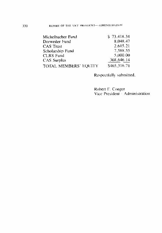
330 REPORT OF TtlI‘: \‘ICh 1’RESIDF.N I---ADII1INlSTRATION
Michelbacher Fund $ 73,418.34 Dorweiler Fund 8,048.47 CAS Trust 2.615.21 Scholarship Fund 7.588.55 CLRS Fund 5.000.00 CAS Surplus 368.646. I4 TOTAL MEMBERS’ EQUITY $465.316.71
Respectfully submitted,
Robert F. Conger Vice President - Administration
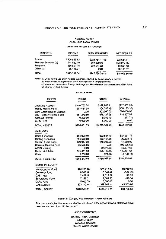
REPORT OF THE VICE PRESIDENT-ADMINISTRATION
FINANCI*L REPORT FSCAL YEAR ENDED 900189
FUNCTION INCOME DISBURSEMENTS NET RESULTS
Exams s3ow65 a2 $228.164.11 (a) 576.681.71 Member Services (b) 244,632 10 364.60395 (139.977 65) Programs 385.597 75 334,944 32 50.653 43 Other (c) 56146.37 0.00 56.146 37
TOTAL $993.242.04 5947.738.38 (a) t45.503 66 (d)
Naes la) Does not include Exam R&led Expenses wuned by me develcqmenl fw~lan (b) Areas under Ihe s~pwvwon of VP-Admnwaf~n 6 VP--pment (C) lW.Sl”W”t l”cw”e l&e. Farelgn Exchange and Mlscell~r~~~ bank debIts, and ASTIN Fund Id) Change I” CAS Surplus
ASSETS
Checking Account Money Market Fund Bank Cenlflcales Of Deposit U.S. Treasq Notes 8 8111s Accrued Interest CLRS Fund
TOTAL ASSETS
LIABILITIES
Office Expenses Printing Expenses PrepaId Exam Fees Montreal Meeting Fees ASTIN Meeting Diamond Jubilee Other
TOTAL LIABILITIES
MEMBERS EOUITY
Michelbacher Fund Dome~ler Fund CAS Trust Scholarship Fund CLAS Fund CAS Surplus
TOTAL E0Ull-Y
9/30/86 93w89 CHANGE
5146.753.74 $126.887 11 262,467.55 104.267.45
003 3w.m.w 561.270.60 676,127 65
9,30990 9.06219 5.wo 00 5.ooo.M)
($17.86663) (158,160.lO) 3oo.m.00 116,657 05
(227 71) 0.00
$984.801 79 $1.225364 40 $240.582 61
s65.ooo.w S92.591 79 162.568.06 163.407 66 106.017.00 148.w5.00
95.59566 0.W 0.00 59.377.63
135.311 94 275.71355 3.750.00 971 66
$27.591 79 20.838.76 41.96600
(95.595 66) 59,377 63
140.40161 (2.776.14)
S.566.243.68 S760.067 69 $191.624 01
$70,205 96 $73 41 a.34 $3.212.36 6.563.46 6.048.47 (534 99) 2,467 16 2.61521 146.03 7.15901 7.566.55 429.54 5.ooo.00 5.wo.w 000
323.142.46 366646.14 45.503.66
$416.556.11 $465.316 71 548,758 60
Roben F. Conger, Vtce President . Adinwwstratkm
This 1s to certify.that the assets and accounts shown I” the above finatwal statement have been audlled and found lo be correct.
AUDIT COMMITTEE Dawd M Klem. Chalm
Albeit J. Qulrln Willnm J. Rowland
Charles Walter Stewart
331
332
1989 EXAMINATIONS-SUCCESSFUL CANDIDATES
Examinations for Parts 4, 6, 8 and 10 of the Casualty Actuarial Society were held on May 2, 3, 4 and 5. Examinations for Parts 5, 7 and 9 wee held on November 6, 8, and 9.
Examinations for Parts 1, 2 and 3 (SOA courses 100, 110, 120, 130 and 135) are jointly sponsored by the Casualty Actuarial Society and the Society of Actuaries. Parts 1 and 2 were given in February, May and November of 1989 and Part 3 was given in May and November of 1989. Candidates who were successful on these examinations were listed in the joint releases of the two societies.
The Casualty Actuarial Society and the Society of Actuaries jointly awarded prizes to the undergraduates ranking the highest on the Part 1 examination.
For the February, 1989 examination the $200 first prize was awarded to Marshall A. Whittlesey. The $100 prize winners were Joseph D. Hoffman, Timothy L. Swenson, Hok S. Wong and Gerald J. Wuchter.
For the May, 1989 examination the $200 first prize was awarded to Andrew Harold Kresch. The $100 prize winners were Mitra Amin- Asgari, Mark E. Hamwee, Weeliang Heng and Mei-Chi Tung.
For the November, 1989 examination the $200 first prize was awarded to Pierre-Paul Renaud. The $100 prize winners were William Clifford Black, Meng-Chu Hsieh, Joseph Lee and Andrew Przeworski.
The following candidates were admitted as Fellows and Associates at the November, 1989 meeting as a result of their successful completion of the Society requirements in the May, 1989 examinations.
Almagro, Manuel Co&y, Kevin Aquino, John G. Crowe, Alan M. Bellafiore, Leonard A. Darby. Robert N. Bourdon, Theresa A. Davis, Dan J. Brehm, Paul J. DiDonato, Anthony M Buchanan, John W. DiGaetano, Mark Cardoso, Ruy A. Dukatz. Judith E. Cofield, Joseph F. Englander, Jeffrey A.
Fitzgerald, Beth E. Forbus, Barbara L. Francis, Louise A. Gillam. Judith A. Goldberg, Leonard R. Graves. Gregory T. Graves. Nancy A. Handte. Malcolm R.
1989 EXAMINATIONS-SUCCESSFUL CANDIDATES 333
Hebert, Norman P. Johnson, Eric J. Johnson, Wendy A. Lebens, Joseph R. Maher, Christopher P. Mahoney, Michael W. McCoy, Mary E. McDermott, Sean P. Mitchell, William H.
Allen, Danny M. Bowman, David R. Brassier, Dominique E Brauner, Jack B. Denoncourt, Germain Dolan, Carol A. Evensen, Phillip A. Gibson, John F. Grim, Cynthia M. Grose, Carleton R. Hroziencik, George A.
Moylan, Thomas G. Mulvaney, Mark W. Nemlick, Kenneth J. Paterson, Bruce Peck, Steven C. Proska, Mark R. Putney, Alan K. Rathjen, Ralph L. Scott, Kim A.
ASSOCIATES
Jones, Brian A. Kerner, Michael G. Kretsch, David J. Lew, Allen Mech, William T. Mercier, Mark F. Paddock, Timothy A Patschak, Susan J. Price, Debbie W. Rahardjo, Kay K. Reddig, Scott E. Roberts, Jonathan S.
Scott, Robert F. Shapland, Mark R. Svendsgaard, Christian Taylor, Angela E. Tistan, Ernest S. Vezina, Guy Webb, Nina H. Woerner, Susan K. Wrobel, Edward M. Yatskowitz, Joel D.
Rominske, Steven C. Ryan, Beverley K. Schmitt, Karen E. Seiter, Margaret E. Shadman-Valavi, Ahamad Sheng, Michelle G. Vanier, Anne-Marie Wagner, Rebecca A. Wellington, Elizabeth A. White, Lawrence Wischmeyer, Chad C.
The following is the list of successful candidates in examinations held in May, 1989.
Part 4
Addiego, Mark A. Bault, Todd R. Adee, Marc J. Bazin, Dominic Ahn, Chul H. Beaulieu, Andre Allen, Danny M. Benarosch, Xavier Arnold, Richard T. Bensics, Frank G. Auger, Nathalie J. Besman, Eric D. Ayres, William P. Bibbero, Herbert S.
Blais, Annie Blau, Daniel D. Bouvin, Erik R. Bowen, Alicia E. Bowman, David R. Broda, Sam S. Broffitt, James D.
334 ,989 t;XAMINATIONS-SUTCtSSFLil (‘ANIIIDATFS
Brueckman, Laura D. Brunetti, Christopher G Burke, Anthony J. Cavaliere, Carol A. Chadowski, Julie S. Chang, Hsiu-Mei Chittenden, John S. Chu, Kuei-Hsia R. Chuang. Wei Ciardiello, Gary T. Collins, Peter J. Conway, Thomas P. Cote, Clement Couture, Martin L. Cox Jr., Samuel H. Dagher, Sami M. Dagneau, Francois Daigneault, Wayde A. Daly, Michael K. Debigare, Manon Demers, Marie-Julie Desson, Herb Devlin, Patrick K. Dickson, Kevin G. Dionne, Pierre Dionne, Michel Doherty, Shawn F. Dolan, Carol A. Donaldson, Jeffrey D. Dossett, A. Mark Doyle, Leonard G. Dubin, Michael C. Dussault. Patrick Emmons, Karen W. Ericson, S. Anders Farzan, Farzad Feder. Denise A. Federspiel, Karen A. Felisky, Kendra M.
Fescos, George Foley, David A. Garland, Kim B. Gastineau, Michael K Gervais. Simon Gibson, John F. Gifford, Bruce R. Ginnelly, Michael A. Glemza. Linas Goldie, Charles T. Gordon, Cynthia L. Grandisson, Marc C. Graver. Jeffrey W. Gray, Margaret 0. Grubbs, Dawson T. Hadaway. Kristy A. Halliwell, Leigh J. Han, Li-Ming Hancock, Paul J. Hanlon, Gerald D. Hansen, Timothy J. Harbus, Jonathan M. Hartzen, Gayle L. Hinds. Thomas E. Homer, David L. Horovitz, Bernard R. Hroziencik, George A Huang, Cheng-Chi Huddleston. John Hussian. Paul R. Ireland, Kathleen M. Iuliano. Anthony James, Peter H. Job, Arlene J. Kenyon, Deborah E. Kiehm, Jean-Luc E. Kilroy, Joseph P. Kim, Ho K. Kim. Changseob
Kirschner, Gerald S. Kirste, Richard 0. Kroggel. Mary C. Labelle, Mylene J. Lafond, Andre Lajeunesse. Elaine Lamb, Donald S. LaPalme, Marc Lee, Thomas Lefebvre. Marc-Andre Lemieux-Roy, Julie LePera. Giuseppe F. Levine. Kenneth A. Lin. Hsin-Hui G. Liu. Ling-Ling Livingstone, Paul R. Lusk, Vicki S. Manktelow, Blair E. Mann, Katherine A. Maravankin, Gabriel 0. Marcinko, Carole F. Margulis, Galina Marlo. Leslie R. Martin, Suzanne Mathre. Keith A. McCutcheon, John W. McGee, Stephen J. McNeal. Van A. McNecse, Dennis T. Mentz. John P. Merlino, Paul M. Miller. Linda K. Miller, Robert L. Min. Douglas H. Morissette, Nicolas Morrow. Michelle M. Munson, Todd B. Neghaiwi, Antoine A. Nellis. Sarah L.
IYXY EXAMINATIONS-SUCCESSFUL CANDIDATES 335
Nguyen, Hiep T. Nissenbaum, John Olsen, Richard A. Olszewski, Laura A. Ondrich, Naomi S. Ouellet, Jean-Francois Ouellet, Nathalie O’Brien, Daniel E. Paddock, Timothy A. Paffenback, Teresa K. Partosoedarso, Erica Patel, Chandrakant C. Perrine, Julia L. Perry, Daniel B. Philippeaux, Hughes Poole, Brian D. Porcelli, Christine A. Powell, Daniel A. Price, Debbie W. Provencher, Yves Quintilian, Kenneth P. Rabenold, Eric K. Rainey, Donald K. Raymond, Yves Reynolds, Margaret M.
Purr 6
Baker, Mark S. Barton, Frances H. Beaulieu, Gregory S. Bechtel, David P. Beck, Douglas L. Belleau, Richard Blair, Gavin C. Blais, Jean-Francois Blanco, Roberto G. Boardman, Thomas S. Booher, John P.
Rhodes, Al J. Riczko, Elizabeth M. Rivard, Michel Roche, William E. Rowe, Bradley H. Roy, Clement Rozema, Michael R. Ruane, John M. Rupp, Douglas A. Ruth, Maureen S. Ryan, Beverley K. Saint-Loup, Yves Sandilya, Manalur S. Schepak, Michael K. Schuette, Donald R. Shannon, Derrick D. Shepherd, David M. Smaga, James J. Smolen, Tom A. Steenken, Lisa N. Suljak, Katie Sullivan, Francis P. Tang, Yuan-Yuan Tardif, Francois
Bourassa, Pierre Brassier, Dominique E. Brauner, Jack B. Carrier, Benoit Chan, Dennis K. Charbonneau, Scott K. Cloutier, Jean Colton, Gary S. Cox, Brian K. Curry, Robert J. Darby, David J.
Tedeschi, John L. Toledano, Mike Traynor, Theresa A. Treskolasky, Susan M. Tzeng, Ching-Horn Valentine, Peter S. Vigliaturo, Phillip C. Vincent, Dale G. Visintainer, Michael A. Vu, Hao-Nhien Q. Vu, Sebastian Wagner, Jennifer M. Wang, Alice M. Weinstein, Marjorie C. White, Lawrence Wick, Kevin Wignarajah, Gnana K. Wilson, Elizabeth J. Wolter, Kathy A. Woosley, John M. Yesker, Charles J. Yezzi Jr., Vincent F. Yost, Nancy E. Yu, Sheng Hau
Denoncourt, Germain Doyon, Yves Eastwood, Brad C. Ebert, Maribeth Effinger, Robert D. Evensen, Philip A. Fenrich, Karen M. Finnerty, Deborah C. Fischer, Brian C. Fisher, Michele P. Fortin, France
336 IYXY I:xAMINA’~IoNs-su(‘~‘~SSF~I ~‘ANDID4 I1.S
Fung, Kai Y. Galiardo, Scott F. Gariepy, Louis Goss, Linda M. Grim, Cynthia M. Grose, Carleton R. Gross, Marian R. Gusler, Terry D. Haidu, Deborah D. Halpin, Sandra K. Hardy, Ellen M. Hausserman, Diane K. Hayes, Thomas L. Hwang, Li Hwan Ill, Jeffrey R. Jones, Brian A. Jones, Terre11 A. Kelso, Kevin E. Kemer, Michael G. Kozlowski, Ronald T. Kretsch, David J. Kunze, David R. Kwon, Frank 0. Lannutti, Nicholas J. Laurin, Michel Lehecka, Stephen E. Ling, Frank K. Loisel, Andre
McFarlane, Liam M. McKay, Donald R. Mech, William T. Mercier, Mark F. Moncher, Richard B. Moore, Kelly L. Moynihan, Kevin J. Ncrone, Anthony J. Niemczyk, William A Nystrom, Keith R. Palmer, Joseph M. Pasley, Jacqueline E. Patschak, Susan J. Perez, Andre Perrine, Julia L. Petker, Jill Petrocik, Michael J. Poison, Jennifer A. Pouliot, Lisa M. Quinn, Timothy P. Raguse, Jeffrey C. Rahardjo, Kay K. Rathgeber, John F. Reddig, Scott E. Reinhardt, Karin L. Rhoads, Karin M. Roberts, Jonathan S. Rominske. Steven C.
Mackenzie, Kathleen A. Roth, Scott J. MacMahon, Brian E. Russell, Stephen P. Mango, Donald F. Sadwin, Stuart G. Marlowe, Burton F. Schmitt, Karen E.
Part 8
Beaulieu, Karin H. Boisvert Jr., Paul Becker, Allan R. Book, Steven W. Bender, Robert K. Boucek, Charles H. Blank, Cara M. Buchanan. John W.
Schutte, Robert J. Scott. Gordon L. Seiter, Margaret E. Shadman-Valavi, Ahamad Shalack, Theodore R. Share, Robert D. Sheng, Michelle G. Smcrald, Christopher M. Smolen, Patricia E. Spore. Louis B. Stayton, Stephen D. Taylor. Rae M. Teng. Ting-Shih Thomas, Richard D. Tote, Thomas C. Trafecanty, Janet A, Tremblay. Martin-Eric Turner, Mary L. Turvill, Melanie A. Van Laar, Kenneth R. Vanier, Anne-Marie Wagner, Rebecca A. Walder, Lawrence M. Walker, Christopher P. Walton, Patrick M. Weinstein. Scott P. Wellington, Elizabeth A. Weltmann, Nicholas Wickenden, Leigh F. Wischmeyer, Chad C. Yenke, Robert S.
Burns, Patrick J. Cardoso, Ruy A. Casale, Kathleen N. Caulfield, Michael J.
1989 EXAMINATIONS-SUCCESSFUL CANDIDATES 337
Charest, Danielle Clark, David R. Cloutier, Denis Conley, Kevin Czabaj, Daniel J. Davis, Dan J. Desjardins, Charles Duffy, Timothy B. Dumulon, Denis Edlefson, Dale R. Ely, James Englander, Jeffrey A. Evans, Karen F. Forbus, Barbara L. Fox, Richard L. Gagnon, Luc Gebhard, James J. Gill, Bonnie S. Gillam. Judith A.
Part 10
Almagro, Manuel Francis, Louise A. Aquino, John G. Frank, Jacque B. Bellafiore, Leonard A. Goldberg, Leonard R. Bourdon, Theresa A. Graves, Gregory T. Bradley, J. Scott Graves, Nancy A. Brathwaite, Malcolm E Hebert, Norman P. Brehm, Paul J. Hill, Anthony D. Carroll, Lynn R. Jasper, Jane E. Caudill, Teresa J. Johnson, Eric J. Cofield, Joseph F. Johnson, Wendy A. Crowe, Alan M. Klawitter, Warren A. Darby, Robert N. Lebens, Joseph R. DiDonato, Anthony M. Maher, Christopher P. DiGaetano, Mark Mahoney, Michael W. Dodge, Scott H. Math, Steven E. Dukatz, Judith E. McDermott, Sean P. Fitzgerald, Beth E. Mitchell, William H.
Grossack, Marshall J. Handte, Malcolm R. Heyman, David R. Higgins, James S. Hurley, John M. Ikeda, Joanne K. Jovinelly, Edward M. Kerin, Allan A. Klenow, Jerome F. Kryczka, John R. Lepage, Pierre Lew, Allen McCoy, Mary E. Michelson, Jon W. Mitchell, H. Elizabeth Ottone, Joanne M. Palmer, Donald D. Paterson, Bruce Pridgeon, Ronald D.
Ramanujam, Srinivasa Schlenker, Sara E. Schmid, Valerie L. Schmidt, Jeffrey W. Schulz, Richard T. Schwandt , Jeffory C. Sclafane, Susanne Scott, Robert F. Seeley, Alan R. Steinberg, Karen F. Steiner-t, Lawrence J. Stone, Edward C. Suchar, Christopher M. Swanstrom, Ronald J. Tistan, Ernest S. Urschel, Frederick A. Wills, Mary E. Winslow, Martha Wrobel. Edward M.
Moylan, Thomas G. Mulvaney, Mark W. Nemlick, Kenneth J. Norton, Jonathan Peck, Steven C. Petersen, Loren V. Proska, Mark R. Putney, Alan K. Radau, Christine E. Rathjen, Ralph L. Schwab, Debbie Scott, Kim A. Scott, Robert F. Shapland, Mark R. Spiegler, David Stadler, Elisabeth Svendsgaard, Christian
338 1989 EXAMINATIONS-SUCCESSFUL CANDIDATES
Taylor, Angela E. Watkins, Nancy P. Wildman, Peter W. Tucker, Warren B. Webb, Nina H. Woerner, Susan K. Vasek, William Wick, Peter G. Yatskowitz, Joel D. Vezina, Guy
The following candidates were admitted as Fellows and Associates as a result of their successful completion of the Society requirements in the November, 1989 examinations.
FELLOWS
Bradley, J. Scott Fanning, William G. Brathwaite, Malcolm E. Fleming, Kirk G. Caudill, Teresa J. Dodge, Scott H. Donnelly, Vincent T. Ellefson. Thomas J.
Beaulieu, Gregory S. Eska, Catherine E. Bechtel, David P. Finnerty, Deborah C. Beck, Douglas L. Fitzpatrick, Kerry L. Becker, Allan R. Fonticella, Ross C. Blair, Gavin C. Fortin, France Blais, Jean-Francois Galiardo, Scott F. Blanco, Roberto G. Gevlin, James M. Charbonneau, Scott K. Goss, Linda M. Closter, Donald L. Grab, Edward M. Cloutier, Jean Gross, Marian R. Coca, Michael A. Gust, Michcle P. Cossette. Charles Hayes, Thomas L. Cote, Jean Hinds, Kathleen A. Curry, Robert J. Ikeda, Joanne K. Czabaj, Daniel J. Jones, Terre11 A. Deigl, Jeffrey F. Jonske, James W. Dew, Edward D. Jovinelly, Edward M. Doe, David A. Kelley, Kevin J. Effinger Jr., Bob D. Kerin, Allan A.
Hertling, Richard J Jasper, Jane E. Joyce, John J.
ASSOCIATES
Ellingrod, John W. Kligman, Daniel F.
Radau, Christine E. Scholl, David C. Schwab, Debbie Somberger, George C. Stadler, Elisabeth
Kozlowski, Ronald T. Leveille, Jean-Marc Li, Siu Kuen Loisel. Andre MacMahon, Brian E. Manley, Laura Marlowe, Burton F. McFarlane, Liam M. Moncher, Richard B. Moore, Kelly L. Moynihan, Kevin J. Murphy, Daniel M. Nerone. Anthony J. Niemczyk, William A. Nystrom, Keith R. Pasley, Jacqueline E. Perez, Andre Pestcoe, Marvin Petker, Jill Petrocik, Michael J.

1989 EXAMINATIONS-SUCCESSFUL CANDIDATES 339
Polson, Jennifer A. Samson, Pierre A. Turvill, Melanie A. Pouliot, Lisa M. Scanlon, Edmund S. Quinn, Timothy P.
Walker, Christopher P. Shalack, Theodore R. Walton, Patrick M.
Raguse, Jeffrey C. Simons, Rial R. Rhoads, Karin M.
Washburn, Monty J.
Romito, A. Scott Smerald, Christopher M. Weinstein, Scott P. Steinberg, Karen F. Weltmann, Jr., L.
Rosenstein, Kevin D. Teng, Ting-Shih Nicholas Roth, Scott J. Thomas, Richard D. Sadwin, Stuart G.
Wickenden, Leigh F. Turner, Mary L.
Salton, Melissa A. Wilk, Roger A.
The following is the list of successful candidates in examinations held in November, 1989.
Part 5 Adee, Marc J. Albright, Kristen M. Alnes, Ann L. Aman, Timothy P. Anderson, Mary Beth Arico, Nancy L. Avagliano, Guy A. Bablin, Barry L. Bamett, Jack Bault, Todd R. Begin, Nathalie Benarosch, Xavier Benedict, Douglas S. Bensics, Frank G. Bibbero, Herbert S. Black, Suzanne E. Blackbum, Wayne E. Blakeney, Gina L. Blau, Daniel D. Bok, Ann M. Borden, Paul A. Bowens, Alicia E. Bowls, David B. Bradley, George P.
Brancel, Robert E. Brannon, Mark L. Broda, Sam S. Brooks, Ward M. Brown, Louis M. Brubaker, Lisa J. Bruns, Scott T. Bull, Michelle M. Bum, Elliot R. Carey, Jeanne L. Cavaliere, Carol A. Chang, Hsui-Mei Chen, Daoguang E. Chuang, Wei Chung, Kasing L. Ciardiello, Gary T. Clark, Alan R. Cochran, James P. Cockley, Jo E. Coe, Carolyn J. Collins, Peter J. Coiton, Gary S. Connors, Pamela A. Conway, Thomas P.
Corbett, Mary L. Cote, Clement Cote, Gregory L. Couture, Martin L. Cremin, Timothy J. Cullather, David A. Currie, Richard J. Cuzzi, Gregory A. Daly, Michael K. Davis, Robin M. Debigare, Manon DeMattei, Michael L. Derstine, Karen D. Devlin, Patrick K. DiCenso, Stephen R. Dickson, Kevin G. Dionne, Michel Dionne, Pierre Dorman, Dean P. dos Santos, Victor G. Dove, William F. Draznin, Paul D. Dubin, Michael C. Dugan, Stephen C.
340 IYXY EXAMINATIONS-SUCTtSSFUI (‘ANDIDA7ES
Dumas, Francois Dussault, Patrick Elzayn, Haytham H. Emmons, Karen W. Emmons, William E. Ericson, Anders Fagelbaum, Darlene Fandrey, Sheila M. Farris, W. Scott Fay, Matthew C. Feder, Denise A. Fenrich, Karen M. Finan, Janine A. Finch, Stephen A. Fish, Joyce L. Folkesson, John B. Fullmer, Richard K. Galiardo, Scott F. Gant, James E. Garcia, Perriann R. Garland, Andrew E. Garland, Kim B. Gamier, Susan T. Gervais, Simon Gise, Mary K. Goldfarb, Richard S. Goldie, Charles T. Granger, Bradley A. Grillo, Monica A. Groeschen, Steven J. Grossack, Victoria A, Gusler, Terry D. Hakala, Todd R. Halliwell, Leigh J. Hancock, Paul J. Hansen, Timothy J. Hanson, Bradley A. Hardy, Ellen M. Hehr, Noel M.
Heirich, Fritz J. Helmeci, Ronald L. Henning, Paul D. Hill, Michael R. Holler, Keith D. Homer, David L. Homyak, Chet B. Howard, Terrie L. Huang, Ming-I Huddleston. John Hughes, Jeffrey R. Johnson, Anita J. Johnson, Kurt Johnson, Mark R. Jordan, Edwin G. Kimble, Regina M. Kirschner, Gerald S. Klanderman, Jeffrey A Klauke, Paul H. Kliethermes, Craig W. Kolber, Elizabeth Korthals, Gilbert M. Kreuser, Adam J. Kroggel, Mary C. Kunze, David R. Kwon, Sun J. Laganiere, Benoit Lajeunesse, Elaine Lamb, Donald S. Larson, Michael D. Lecky, Steven L. Lefkowitz, Scott J. Litwack, Kim D. Livingstone, Paul R. Lord, Jennifer S. Lothschultz, Laura J. Lowery, Robert G. Maguire, Richard Mahanna, Cathy A.
Manis, Donald E. Manktelow, Blair E. Maratea, Stephen N. Maravankin, Gabriel 0. Margulis, Galina Markowski, Sharon L. Martin, Leslie A. Martin, Suzanne Mathre, Keith A. McCorkle, Teresa J. McCutcheon, John W. McDonald, Richard T. Melas, Brian Mentz, John P. Merkey. Stephen V. Messier, Timothy Miller, Todd M. Min, Douglas H. Monaghan, James E. Moore, Russell E. Morrow, Michelle M. Muller. Raymond D. Mullins, Kimberly J. Na, David Y. Neghaiwi, Antoine A. Nellis. Sarah L. Nelson, Lowell D. Nguyen, Quang C. Niemczyk, William A. Njakou, Victor Nonken, Peter M. O’Brien, Daniel E. Olsen, Richard A. Ouellet. Nathalie Palisi, Gerard J. Pannell, John E. Patel, Chandrakant C. Perrine, Julia L. Picardo, Paul E.
19x9 EXAMINATIONS-SUCCESSFUL CANDIDATES 341
Pipia, Anthony J. Polofsky, Janice Pontbriand, Lise A. Poole, Brian D. Poon, On Cheong Powell, Daniel A. Price, Michael D. Quintilian, Kenneth P. Ram, Karen L. Raszka, Rosemary A. Regnier, Steven J. Reinhardt, Karin L. Robinson, Sallie S. Roche, William E. Romine, Laura A. Roth, Daniel G. Roy, Jean Russell, Kevin L. Saint-Loup, Yves Santoro, Lawrence Saunders, Melodee J. Sauthoff, Stephen P. Schafer, Marilyn E.
Part 7
Anderson, Richard R. Ashman, Martha E. Beaulieu, Gregory S. Bechtel, David P. Beck, Douglas L. Becker, Allan R. Biskner, Laverne J. Blair, Gavin C. Blais, Jean-Francois Blanco, Roberto G. Blue, Betsy L. Brasley, Donna D. Bukowski, Paul A. Burrill, Linda J.
Schlenke, David 0. Senak, Peter Shalack, Theodore R. Shampo, Jonathan N. Shamula, Marc Shannon, Derrick D. Share, Robert D. Shepherd, David M. Shubat, Kerry S. Small, Deborah J. Smith, Katherine R. S. Smith, David A. Spindel, Alan H. Staley, Ruth E. Stonehill, John W.
Tote, Thomas C. Toney, Charles F. Toth, Michael J. Tremblay, Paul Tu, Son Trong Tures, Patrick N. Valentine, Peter S. VanKampen, Charles E. VanKoevering, David B. Vaughan, Therese M. Veres, Charles J. Vigorita, Charles A. Visintainer, Michael A. Ward, Kimberley A. Weisbecker, Joyce
Stringfellow, William M. Welch, John P. SulliGan, Brian K. Suttie, Collin J. Swanay, Scott J. Tedeschi, John L. Thomas, Edward E. Tinter, Daniel J. Tio, Tony
Charbonneau, Scott K Closter, Donald L. Cloutier, Jean Coca, Michael A. Cole, Jeffrey R. Cossette, Charles Cote, Jean Curry, Robert J. Czabaj, Daniel J. Dagneau, Francois Deigl, Jeffrey F. Dew, Edward D. Doe, David A. Effinger Jr., Bob D.
Wick, Kevin Wilson, Elizabeth J. Wolfe, Terry C. Woody, Lynne M. Wu, Chien-Chien L. Zirin, Joshua A.
Ellingrod, John W. Eska, Catherine E. Faggella, Madelyn C. Feldmeier, Judith Felisky-Watson, Kendra Fields, David N. Finnerty, Deborah C. Fitzpatrick, Kerry L. Foley, David A. Fonticella, Ross C. Fortin, France Galiardo, Scott F. Gardner, Andrea Gevlin, James M.
342 IYXY EXAMINATIONS-SUCCESSFUI. CANDIDATES
Godt, Beth M. McGee, Stephen J. Goss, Linda M. McNeese, Dennis T. Grab, Edward M. McPadden, Matthew S Gross, Marian R. Merlino. Paul M. Grubbs, Dawson T. Milford, Alison M. Gust, Michele P. Miller, Linda K. Hansen, George M. Miller, Robert L. Harbus, Jonathan M. Mills, Paul W. Hausserman, Diane K. Mitzel, Charles B . Hayes, Thomas L. Moncher, Richard B. Hess, Thomas G. Moore, Kelly L. Hinds, Kathleen A. Munson, Todd B . Hostager, Beth M. Murphy, Daniel M. Hostetter, David B. Nerone, Anthony J. Ikeda, Joanne K. Nissenbaum, John Jones, Terre11 A. Nordquist, Randall S. Jonske, James W. Nystrom. Keith R. Jovinelly, Edward M. Olszewski, Laura A. Kantor, Stephen H. Ondrich, Naomi S. Kelley, Kevin J. Paffenback, Teresa K. Kellner, Tony J. Palmer, Joseph M. Kerin, Allan A. Pasley, Jacqueline E. Kincaid, Bryan J. Perez, Andre Kligman, Daniel F. Pestcoe, Marvin Kozlowski, Ronald T. Petker, Jill Lamy, Mathieu Petrocik, Michael J. LeBlanc, France Polson, Jennifer A. Lemieux, Eric F. Pouliot, Lisa M. Leveille, Jean-Marc Quinn, Timothy P. Li, Siu Kuen Raguse, Jeffrey C. Ling, Frank K. Rathgeber, John F. Loisel, Andre Raws III, Alfred MacMahon, Brian E. Reynard, Alan T. Main, William G. Rhoads, Karin M. Mango, Donald F. Riemer, Gregory L. Manley, Laura Rohn, Diane R. Mann, Katherine A. Romito ‘A. Scott Marlowe, Burton F. Rosenstein, Kevin D. McBride, Heidi J. Roth, Scott J. McFarlane, Liam M. Ruane Jr.. John M.
Rundle, Timothy J. Sadwin, Stuart G. Salton, Melissa A. Samson, Pierre A. Scanlon, Edmund S. Scott. Gordon L. Shalack, Theodore R. Simon, Christy L. Simons, Rial R. Smerald. Christopher M. Smolen, Tom A. Sogge, Elizabeth L. Stanford, Thomas N. Steenken. Lisa N. Stefanek, John P. Steinberg, Karen F. Sturm, Elissa M. Subeck, Jeffrey L. Tasker III, Joseph W. Teetsel, Marianne Teng, Ting-Shih Theocharides, Georgia A. Thomas, Richard D. Treskolasky, Susan M. Turner, Mary L. Turvill, Melanie A. Vandermyde, Scott D. Vincent Jr., Dale G. Walder, Lawrence M. Walker, Christopher P. Walton, Patrick M. Ware, Bryan C. Washburn, Monty J. Weinstein, Marjorie C. Weinstein, Scott P. Weltmann Jr., L. Nicholas Wickenden, Leigh F. Wilk, Roger A. Yenke, Robert S. Yost, Nancy E.
343 1989 EXAMINATIONS-SUCCESSFUL CANDIDATES
Part 9
Adams, Jeffrey Greenhill, Eric L. Barnes, W. Brian Grim, Cynthia M. Bradley, J. Scott Hertling, Richard J. Brathwaite. Malcolm E. Hess, Todd J. Cain, Mark J. Carroll, Lynn R. Cauchon, Martin Caudill, Teresa J. Caulfield, Michael J. Cellars, Ralph M. Charest, Danielle Cloutier, Denis Denoncourt, Germain Dodge, Scott H. Donnelly, Vincent T. Duffy, Timothy B. Dumulon, Denis Ellefson, Thomas J. Ely, James Ewert, John S. Fallon, Steven R. Fanning, William G. Fleming, Kirk G. Fox, Richard L. Franklin, Barry A. Gibson, Richard N. Gray, Margaret 0.
Higgins, James S. Hines, Alan M. Hurley, John M. Jasper, Jane E. Johnston, Steven J. Joyce, John J. Kretsch, David J. Krissinger, Kenneth R. Kufera, Kay E. Kulik, John M. Kuo, Chung-Kuo Lacko, Paul E. Lalonde, David A. Lamb, John A. Lepage , Pierre Lew, Allen Liebers, Elise C. Mahon, Mark J. McGovern, Eugene McShea, Christopher J. Mech, William T. Michelson, Jon W. Mitchell, H. Elizabeth Norton, Jonathan
Ottone, Joanne M. Perigny, Isabelle Petersen, Loren V. Poe, Michael D. Prescott, Richard W. Price, Deborah W. Radau, Christine E. Ramanujam, Srinivasa Reddig, Scott E. Robinson, Richard D. Rominske, Steven C. Scholl, David C. Schug, Richard D. Schwab, Debbie Seiter, Margaret E. Somberger, George C. Spiegler, David Stadler, Elisabeth Steinert, Lawrence J. Suchar, Christopher M. Tingley, Nanette Trafecanty, Janet A. Vanier, Anne-Marie Verges, Ricardo Werland, Debra L. Wischmeyer, Chad C. Yocius, Richard P.
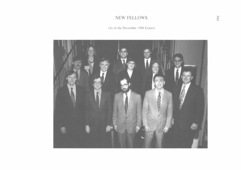
NEW FELLOWS
:/ \ f ‘\
I
NEW ASSOCIATES w %
(As of the November 198X Exams)
*I I 1
NEW FELLOWS
(As of the May 1989 Exam)
NEW ASSOCIATES % cc
(As of the May 1989 Exams)
349
OBITUARIES
William P. Amlie Margaret A. Burt
Edwin A. Cook Laurence H. Longley-Cook
John H. Miller Kent T. Penniman John H. Phillips
Morris Pike
WILLIAM PAUL AMLIE 1929-1989
William P. Amlie, a Fellow of the Casualty Actuarial Society since 1972 and a Member of the American Academy of Actuaries since 1966, died on August 20, 1989 in Piedmont, California at the age of 60.
Bill was born in Elkhorn, Wisconsin and attended Wisconsin High School in Madison. Graduating with honors in 1946, he was accepted into the National Honor Society. Bill graduated from the University of Wisconsin with honors in 1952.
Although Bill started his insurance career with the Kemper Group, he spent most of his career in Boston, with the Commercial Union Insurance Companies. Prior to his death, Bill was the actuary for the Department of Labor & Industry in Olympia, Washington.
Bill’s specialty was workers compensation insurance and he served on many industry committees in this area. In addition, Bill served on the CAS Education and Examination Committee and contributed to the review and discussions of CAS papers.
Bill was an amateur genealogist and would devote hours to research in the Boston Library. He was an accomplished cellist and had a great love for music. He was also a student of the French language. His father, Thomas Amlie, served in the US House of Representatives in the late thirties. As the son of a progressive congressman from Wisconsin, Bill shared a deep concern for the quality of life of his fellow man.
350 OBI’I‘UAKIES
Bill is survived by his sister, Marian Nelson who resides in Piedmont, California and three brothers, Robert in Los Angeles, California, Thomas in Bethesda, Maryland and Frederick in Madison, Wisconsin.
To his family, friends, and colleagues, he will be deeply missed.
MARGARET A. BURT 1891-1989
Margaret Allen Burt, an Associate of the Casualty Actuarial Society since 1920, died at her home in Brooklyn, New York on June 21, 1989. She was 98 years old.
Ms. Burt was born in Easthampton, Massachusetts. She graduated from Smith College in Northampton, Massachusetts in 1912 and became the first employee of Buck Consultants on August I, 1916.
Working closely with George B. Buck, Sr.. the firm’s founder, Ms. Burt was instrumental in developing the young company into a successful actuarial and benefit consulting firm. Her management capabilities, knowledge of the pension field, and steadfast maintenance of high stan- dards of practice were greatly admired by the actuaries and consultants she worked with during her 44 years at Buck.
Ms. Burt retired on August I, 1960 and resided in Brooklyn, New York throughout her retirement. At the time of her death, she was the oldest living CAS member. She is survived by a sister, Katherine B. Cracker of Hinsdale, Massachusetts.
OBITUARIES 351
EDWIN A. COOK 1903-1989
Edwin A. Cook, a Fellow of the Casualty Actuarial Society since 1934, died on January 8, 1989 in Mineola, New York. He was born on December 6, 1903 in New York City.
Mr. Cook started his career with Interboro Mutual in 1921. He remained with the same company for his entire career and retired as the President and Chairman of the Board in 1983. He also was retained as a consultant by Interboro Mutual for the next six years.
Mr. Cook is survived by his wife, Anne, and by two daughters, Marie Ingram and Theresa Stephens, and one son, Edwin, Jr.
352 OH17 L:ARltS
LAURENCE HERBERT LONGLEY-COOK 1909-1989
Laurence H. Longley-Cook, a Fellow of the Casualty Actuarial So- ciety since 195 I and a pre-eminent member of the actuarial profession, died on July 16, 1989 in Coronado, California. Mr. Longley-Cook was also a Fellow of the Institute of Actuaries and Royal Statistical Society in the United Kingdom, an Associate of the Society of Actuaries and one of the founders of the American Academy of Actuaries.
Born in Tunbridge Wells, Kent, England on July 1, 1909, Mr. Longley-Cook graduated from Cambridge University in 193 I and began his employment with the Prudential Assurance Company in London. He qualified as a Fellow of the Institute of Actuaries in 1937.
He was on active service in the Royal Navy in World War II, being Radar Officer on the H.M.S. Norfolk. In 1949 hc decided to emigrate to the United States and unexpectedly found his opportunity in the casualty rather than the life field with the Insurance Company of North America in Philadelphia. This made it necessary for him to tackle our examinations - twelve years after hc had finished those of the Institute. He was admitted as an Associate in 1950 and ~1s a Fellow in 19.5 I - completing the exams in two years.
He became the Chief Actuary of the Insurance Company of North America. In 1967 Mr. Langley-Cook moved to Bermuda to work as a consultant to the American International Reinsurance Company. When his health began to fail he moved to Coronado, California in 1979.
Laurie’s contributions to the CAS were numerous and notable. He was a prolific writer with papers frequently appearing in the Procndings. He was also on numerous committees and served as the president of the CAS in I96 I- 1962. He also served as one of the charter vice-presidents of the American Academy of Actuaries in 1965-1967.
Laurie’s exceptional grasp of actuarial fundamentals, his facility of expression, his helpfulness and his sense of humor will be long remem- bered.
He authored the well-known actuarial text Au Introc~uc~~ior~ to Crcd- i&/it! T/war-v which continues to be required reading in our examination process.
He is survived by his wife Billie and two sons. Mark and Alastair, the latter being a Fellow of the Society of Actuaries.
OBITUARIES 353
JOHN H. MILLER 1906-1988
John H. Miller, a Fellow of the Casualty Actuarial Society since 1938, died on Christmas Day 1988. Mr. Miller was also a Fellow of the Society of Actuaries.
Born in Washington, Pennsylvania on May 29, 1906, Mr. Miller graduated in 1927 from Washington & Jefferson College of that city. After brief experience in a Pittsburgh contracting firm he joined the actuarial staff of Metropolitan Life Insurance Company. In June 1929 he entered consulting work in the Woodward, Fondiller and Ryan firm in New York City. In 193 1, while at this firm, he was admitted as a Fellow of the Society of Actuaries.
In 1934 Mr. Miller entered the service of Monarch Life Insurance Company in Springfield, Massachusetts and became Vice President and Actuary in 1939. He retired from Monarch in 1966 with the rank of Executive Vice President.
Mr. Miller had a major role in organizing the American Academy of Actuaries. He was the one who suggested the concept of a body that would be neither subordinate to, nor would have authority over, any of the existing actuarial bodies. He served as a charter Vice President of the Academy in 1965 and President in 1967-1968.
John was energetic, progressive, cordial, unselfish and a powerful influence on the actuarial profession. He is survived by four children and six grandchildren.
354 OHITUARIES
KENT. T. PENNIMAN 1945-1988
Kent T. Penniman, an Associate of the Casualty Actuarial Society since 1972, died on September 2 I, 1988 at the age of 43.
Kent started his actuarial career in 1968 when he joined Aetna Life and Casualty in Hartford. While he was writing exams, Kent was an integral member of the student fraternity at Aetna. playing on the softball team and eagerly participating in other activities with his colleagues. He enjoyed working hard and playing hard.
Kent’s early career was interrupted by a tour of duty in Vietnam. He returned to Aetna to continue his career and attained his Associateship in 1972. Later Kent also worked for Agway Insurance in East Syracuse and Merchants Insurance in Buffalo.
JOHN H. PHILLIPS 1892-1989
John H. (Jack) Phillips, an Associate of the Casualty Actuarial Society since 1929, died December 3 1, 1989 in Wausau, Wisconsin. He was born July 20, 1892, in St. Paul, Minnesota.
Mr. Phillips was a veteran of World War I, serving in the fledgling aviation area. His actuarial career began at the Minnesota Insurance Department. He spent seven years as Secretary-Actuary of the Minnesota Compensation Insurance Board. In 1935, he joined what were then called the Employers Mutuals Companies in Wausau. becoming the first CAS member employed there. He retired in 1957 as Vice President and Actuary.
Mr. Phillips had wide-ranging interests, including wood carving, photography, aviation, golf, and outdoor activities. He was a member of the American Legion, active in the Boy Scouts of America, and a member of St. John the Baptist Episcopal Church. Wausau.
OBITUARIES 355
Mr. Phillips was preceded in death in 1986 by Dorothy (Kueffner), his wife of 65 years. He is survived by a son, Dr. John F. Phillips, a daughter, Patricia P. Bauder, six grandchildren, and seven great grand- children.
MORRIS PIKE 1896-l 989
Morris Pike, an Associate of the Casualty Actuarial Society since 1920, died in White Plains, New York on January 27, 1989. He was 92 years old. Mr. Pike was also an Associate of the Society of Actuaries and a member of the New York State Bar.
Mr. Pike was born in Lomza, Russia on July 3, 1896. He graduated from the City College of New York in 1915 and in November 1917, after about a year as a mathematics teacher, he joined the actuarial staff of Home Life Insurance Company.
From 19 19 to 1927 Mr. Pike was an examiner for the New York State Insurance Department, and from 1927 to 1929 he was the actuary of Judea Life Insurance Company. During this time he earned his As- sociateship in the Casualty Actuarial Society (1920) and his Associate- ship in the Society of Actuaries (1923) and also enrolled in the law school of St. John’s College in Brooklyn. He earned his law degree in 1928 and admission to the New York State Bar the following year.
Mr. Pike retired as Vice President of John Hancock Mutual in 1962. After retirement he served as a consulting actuary for the New York Insurance Department for five years. He is survived by a son, Bertram, of Weston, Massachusetts, who is a Fellow of the Society of Actuaries and a daughter, Norma Taft, in White Plains, and four grandchildren and four great-grandchildren.
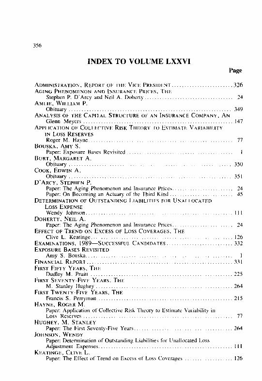
356
INDEX TO VOLUME LXXVI Page
ADMINISTRATION, REPORT OF THE VICE PRESIDENT.. _. ,326 AGING PHENOMENON AND INSURANCE PRICES. THE
Stephen P. D’Arcy and Neil A. Doherty _. 24 AMLIE, WILLIAM P.
Obituary . . ..__...._._........._..._._...................._..........._. 349 ANALYSIS OF THE CAPITAL STRUCTURF. OF AN INSURANCE COMPANY, AN
Glenn Meyers . . . . . . . . . . . . . . . . 147 APPLICATION OF COLLECTIVE RISK THEORY TO Es MMA-T~ VARIABILL~Y
IN Loss RESERVES Roger M. Hayne................ .._..................___....._. 77
BOUSKA, AMY S. Paper: Exposure Bases Revisited 1
BURT, MARGARET A. Obituary 350
COOK, EDWIN A. Obituary 35 I
D’ARcY, STEPHEN P. Paper: The Aging Phenomenon and Insurance Price>. 24 Paper: On Becoming an Actuary of the Third Kind 45
DETERMINATION OF OUTSTANDING LIAHILITIES FOR UNALI.OCATED Loss EXPENSE Wendy Johnson............................ __.... .._.........._. III
DOHERTY, NEIL A. Paper: The Aging Phenomenon and Insurance Prices.. 24
EFFECT OF TREND ON EXCESS OF Loss COVERAGES. THE Clive L. Keatinge........................................................ 126
EXAMINATIONS, 1989-Successful. CANDIDATES.. _. _. _. _. 332 EXPOSURE BASES REVISITED
Amy S. Bouska................................ .._......_...._ 1 FINANCIAL REPORT.. . 33 I FIRST FIFTY YEARS, THE
Dudley M. Pruitt 225 FIRST SEVENTY-FIVE YEARS, THE
M. Stanley Hughey.............................. . . . . . . . . . . . . . . ...264 FIRST TWENTY-FIVE YEARS, THE
Francis S. Perryman 215 HAYNE, ROGER M.
Paper: Application of Collective Risk Theory to Estimate Variability in Loss Reserves ..,,....,.,.._._.,......,.............,....,,......,. ..,.. 77
HUGHEY, M. STANLEY Paper: The First Seventy-Five Years.. 264
JOHNSON, WENDY Paper: Determination of Outstanding Liabilities for Unallocated Loss Adjustment Expenses.. 1 I I
KEATINGE, CLIVE L. Paper: The Effect of Trend on Excess of Loss Coverages 126
INDEX-CONTINUED
351
Page
LONGLEY-COOK, LAURENCE H. Obituary.. .............................................................. 352
MEYERS, GLENN Paper: An Analysis of the Capital Structure of an Insurance Company ........ 147 Paper: Risk Theoretic Issues in Loss Reserving: The Case of Workers Compensation Pension Reserves. .......................................... 17 1
MILLER, JOHN H. Obituary.. .............................................................. 353
MINUTES November 1989 Meeting.. ............................................. ..30 9
NARVELL, JOHN C. Discussion: Recent Developments in Reserving Losses in the London Reinsurance Market ...................................................... 193
OBITUARIES William P. Amlie ........................................................ 349 Margaret A. Burt ........................................................ 350 Edwin A. Cook..........................................................35 1 Laurence H. Longley-Cook ............................................... 352 John H. Miller ........................................................... 353 Kent T. Penniman ....................................................... 354 John Phillips ............................................................ 354 Morris Pike ............................................................. 355
ON BECOMING AN ACTUARY OF THE THIRD KIND Stephen P. D’Arcy ....................................................... 45
PENNIMAN, KENT T. Obituary ................................................................ 354
PERRYMAN, FRANCIS S. Paper: The First Twenty-Five Years ....................................... 215
PHILLIPS, JOHN Obituary ................................................................ 354
PIKE, MORRIS Obituary.. .............................................................. 355
PRESIDENTIAL ADDRESS-NOVEMBER I989 Kevin M. Ryan .......................................................... 302
PRUITT, DUDLEY M. Paper: The First Fifty Years .............................................. 225
RECENT DEVELOPMENTS IN RESERVING FOR LOSSES IN THE LONDON REINSURANCE MARKET Harold E. Clarke (May, 1988) Discussion by John C. Narvell............................................ 193
RISK THEORETIC ISSUES IN Loss RESERVING: THE CASE FOR WORKERS COMPENSATION PENSION RESERVES Glenn Meyers.. ......................................................... 171
RYAN, KEVIN M. Presidential Address-November 1989. .................................... 302
WILLIAMS, P. ADCER Address to New Members-November 1989 ............................... 297
358
EDITORIAL COMMITTEE. PROCEEL)INGS Editors
RON,N.I) E. GKIX‘O, EDITOK


