L12. Evaluating Machine Learning Algorithms II

Evaluating Machine Learning Models 2

José Hernández-Orallo

Universitat Politècnica de València

2

Evaluation I (recap): overfitting, split, bootstrap

Cross validation

Cost-sensitive evaluation

ROC analysis: scoring classifiers, rankers and AUC

Beyond binary classification

Lessons learned

Outline

3

Classification, regression, association rules,

clustering, etc., use different metrics.

In predictive tasks, metrics are derived from the

errors between predictions and actual values.

o In classification they can also be derived from (and

summarised in) the confusion matrix.

We also saw that imbalanced datasets may require

specific techniques.

Recap: Evaluation I

4

What dataset do we use to estimate all previous metrics?

o If we use all data to train the models and evaluate them, we get overoptimistic models:

Over-fitting:

o If we try to compensate by generalising the model (e.g., pruning a tree), we may get:

Under-fitting:

o How can we find a trade-off?

Recap: Overfitting?

5

Common solution:

o Split between training and test data

Recap: Split the data

training

test

Models

Evaluation

Best model

Sx

S xhxfn

herror 2))()((1

)(

data

Algorithms

What if there is not much data available?

GOLDEN RULE: Never use the same example

for training the model and evaluating it!!

6

Too much training data: poor evaluation

Too much test data: poor training

Can we have more training data and more test data

without breaking the golden rule?

o Repeat the experiment!

Bootstrap: we perform n samples (with repetition) and test

with the rest.

Cross validation: Data is split in n folds of equal size.

Recap: the most from the data

7

We can train and test with all the data!

Cross validation

o We take all possible

combinations with n‒1

for training and the

remaining fold for test.

o The error (or any other

metric) is calculated n

times and then

averaged.

o A final model is trained

with all the data.

8

In classification, the model with highest accuracy is not necessarily the best model.

o Some errors (e.g., false negatives) may be much more expensive than others.

This is usually (but not always) associated to imbalanced datasets.

A cost matrix is a simple way to account for this.

In regression, the model with lowest error is not necessarily the best model.

o Some errors (e.g., overpredictions) may be much more expensive than others (e.g., underpredictions).

A cost function is a simple way to account for this.

Cost-sensitive Evaluation

9

Classification. Example: 100,000 instances (only 500 pos)

o High imbalance (π0=Pos/(Pos+Neg)=0.005).


9

c1 open close

OPEN 300 500

CLOSE 200 99000

Actual

Pred.

c3 open close

OPEN 400 5400

CLOSE 100 94100

Actual

c2 open close

OPEN 0 0

CLOSE 500 99500

Actual

ERROR: 0,7%

TPR= 300 / 500 = 60%

FNR= 200 / 500 = 40%

TNR= 99000 / 99500 = 99,5%

FPR= 500 / 99500 = 0.5%

PPV= 300 / 800 = 37.5%

NPV= 99000 / 99200 = 99.8%

Macroavg= (60 + 99.5 ) / 2 =

79.75%

ERROR: 0,5%

TPR= 0 / 500 = 0%

FNR= 500 / 500 = 100%

TNR= 99500 / 99500 = 100%

FPR= 0 / 99500 = 0%

PPV= 0 / 0 = UNDEFINED

NPV= 99500 / 10000 = 99.5%

Macroavg= (0 + 100 ) / 2 =

50%

ERROR: 5,5%

TPR= 400 / 500 = 80%

FNR= 100 / 500 = 20%

TNR= 94100 / 99500 = 94.6%

FPR= 5400 / 99500 = 5.4%

PPV= 400 / 5800 = 6.9%

NPV= 94100 / 94200 = 99.9%

Macroavg= (80 + 94.6 ) / 2 =

87.3%

Which classifier is best?

Sp

ecif

icit

y S

ensi

tivi

ty

Recall

Precision

10

Not all errors are equal.

o Example: keeping a valve closed in a nuclear plant when it

should be open can provoke an explosion, while opening a

valve when it should be closed can provoke a stop.

o Cost matrix:

o The best classifier is the one with lowest cost


open close

OPEN 0 100€

CLOSE 2000€ 0

Actual

Predicted

11


open close

OPEN 0 100€

CLOSE 2000€ 0

Actual

Predicted

c1 open close

OPEN 300 500

CLOSE 200 99000

Actual

Pred

c3 open close

OPEN 400 5400

CLOSE 100 94100

Actual

c2 open close

OPEN 0 0

CLOSE 500 99500

Actual

c1 open close

OPEN 0€ 50,000€

CLOSE 400,000€ 0€

c3 open close

OPEN 0€ 540,000€

CLOSE 200,000€ 0€

c2 open close

OPEN 0€ 0€

CLOSE 1,000,000€ 0€

TOTAL COST: 450,000€ TOTAL COST: 1,000,000€ TOTAL COST: 740,000€

Confusion Matrices

Cost

Matrix

Resulting Matrices

Easy to calculate (Hadamard product):

12


20

1

2000

100

FNcost

FPcost199

500

99500

Pos

Neg 1199 9.95

20slope

Classif. 1: FNR= 40%, FPR= 0.5%

M1= 1 x 0.40 + 9.95 x 0.005 = 0.45

Cost per unit = M1*(FNCost*π0)=4.5

Classif. 2: FNR= 100%, FPR= 0%

M2= 1 x 1 + 9.95 x 0 = 1

Cost per unit = M2*(FNCost*π0)=10

Classif. 3: FNR= 20%, FPR= 5.4%

M3= 1 x 0.20 + 9.95 x 0.054 = 0.74

Cost per unit = M3*(FNCost*π0)=7.4

What affects the final cost?

o Cost per unit = FNcost*π0*FNR + FPcost*(1-π0)*FPR

If we divide by FNcost*π0 we get M:

M = 1*FNR + FPcost*(1-π0)/(FNcost*π0)*FPR = 1*FNR + slope*FPR

For two classes, the value “slope” (with FNR and FPR)

is sufficient to tell which classifier is best.

This is the operating condition, context or skew.

13

The context or skew (the class distribution and the

costs of each error) determines the goodness of a

set of classifiers.

o PROBLEM:

In many circumstances, until the application time, we do not

know the class distribution and/or it is difficult to estimate the

cost matrix. E.g. a spam filter.

But models are usually learned before.

o SOLUTION:

ROC (Receiver Operating Characteristic) Analysis.

“ROC Analysis” (crisp)

14

The ROC Space

o Using the normalised terms of the confusion matrix:

TPR, FNR, TNR, FPR:


14

ROC Space

0,000

0,200

0,400

0,600

0,800

1,000

0,000 0,200 0,400 0,600 0,800 1,000

False Positives

Tru

e P

os

itiv

es

open close

OPEN 400 12000

CLOSE 100 87500

Actual

Pred

open close

OPEN 0.8 0.121

CLOSE 0.2 0.879

Actual

Pred

TPR= 400 / 500 = 80%

FNR= 100 / 500 = 20%

TNR= 87500 / 99500 = 87.9%

FPR= 12000 / 99500 = 12.1%

15

ROC space: good and bad classifiers.


0 1

1

0 FPR

TPR

• Good classifier.

– High TPR.

– Low FPR.

0 1

1

0 FPR

TPR

0 1

1

0 FPR

TPR

• Bad classifier.

– Low TPR.

– High FPR.

• Bad classifier (more realistic).

16

The ROC “Curve”: “Continuity”.


ROC diagram

0 1

1

0

FPR

TPR

o Given two classifiers:

We can construct any

“intermediate” classifier just

randomly weighting both

classifiers (giving more or less

weight to one or the other).

This creates a “continuum” of

classifiers between any two

classifiers.

17

ROC Curve. Construction.


ROC diagram

0 1

1

0

FPR

TPR The diagonal

shows the worst

situation

possible.

o Given several classifiers:

We construct the convex hull of their

points (FPR,TPR) as well as the two

trivial classifiers (0,0) and (1,1).

The classifiers below the ROC curve

are discarded.

The best classifier (from those

remaining) will be selected in

application time…

We can discard those which are below because

there is no combination of class distribution / cost

matrix for which they could be optimal.

18

In the context of application, we choose the optimal

classifier from those kept. Example 1:


21

FNcost

FPcost

Neg

Pos 4

224 slope

Context (skew):

0%

20%

40%

60%

80%

100%

0% 20% 40% 60% 80% 100%

false positive rate

tru

e p

osit

ive

ra

te

19

In the context of application, we choose the optimal

classifier from those kept. Example 2:


FPcost

FNcost 18

Neg

Pos 4

slope 48 .5

Context (skew):

0%

20%

40%

60%

80%

100%

0% 20% 40% 60% 80% 100%

false positive rate

tru

e p

osit

ive

ra

te

What have we learned from this?

o The optimality of a classifier depends on the class

distribution and the error costs.

o From this context / skew we can obtain the “slope”, which

characterises this context.

If we know this context, we can select the best classifier,

multiplying the confusion matrix and the cost matrix.

If we don’t know this context in the learning stage, by using ROC

analysis we can choose a subset of classifiers, from which the

optimal classifier will be selected when the context is known.


Can we go further than this?

20

Crisp and Soft Classifiers:

o A “hard” or “crisp” classifier predicts a class between a

set of possible classes.

o A “soft” or “scoring” classifier (probabilistically) predicts a

class, but accompanies each prediction with an

estimation of the reliability (confidence or class

probability) of each prediction.

Most learning methods can be adapted to generate this

confidence value.

True ROC Analysis (soft)

21

ROC Curve of a Soft Classifier:

o A soft classifier can be converted into a crisp classifier

using a threshold.

Example: “if score > 0.7 then class A, otherwise class B”.

With different thresholds, we have different classifiers, giving

more or less relevance to each of the classes

o We can consider each threshold as a different classifier

and draw them in the ROC space. This generates a

curve…


We have a “curve” for just one soft classifier

22

ROC Curve of a soft classifier.


23

Actual Class

n n n n n n n n n n n n n n n n n n n n

Predicted Class

p p p p p p p p p p p p p p p p p p p p

p n n n n n n n n n n n n n n n n n n n

p p n n n n n n n n n n n n n n n n n n

...

© Tom Fawcett

23



24



In this zone the best classifier is “insts”

In this zone the best classifier is“insts2”

© Robert Holte

We must preserve the classifiers that have at least

one “best zone” (dominance) and then behave in

the same way as we did for crisp classifiers. 25

What if we want to select just one crisp classifier?

o The classifier with greatest Area Under the ROC Curve

(AUC) is chosen.

The AUC metric

For crisp classifiers AUC is equivalent

to the macroaveraged accuracy.

ROC curve

0,000

0,200

0,400

0,600

0,800

1,000

0,000 0,200 0,400 0,600 0,800 1,000

False Positives

Tru

e P

osit

ives

AUC

26

What if we want to select just one soft classifier?

o The classifier with greatest Area Under the ROC Curve

(AUC) is chosen.

The AUC metric

In this case

we select B.

Wilcoxon-Mann-Whitney statistic: The AUC really estimates the probability

that, if we choose an example of class 1 and an example of class 0, the

classifier will give a higher score to the first one than to the second one.

27

AUC is for classifiers and rankers:

o A classifier with high AUC is a good ranker.

o It is also good for a (uniform) range of operating

conditions.

A model with very good AUC will have good accuracy for all

operating conditions.

A model with very good accuracy for one operating condition

can have very bad accuracy for another operating condition.

o A classifier with high AUC can have poor calibration

(probability estimation).

The AUC metric

28

AUC is useful but it is always better to draw the curves and choose depending on the operating condition.

Curves can be estimated with a validation dataset or using cross-validation.

AUC is not ROC

29

Cost-sensitive evaluation is perfectly extensible for

classification with more than two classes.

For regression, we only need a cost function

o For instance, asymmetric absolute error:


ERROR actual

low medium high

low 20 0 13

medium 5 15 4

predicted

high 4 7 60

COST actual

low medium high

low 0€ 5€ 2€

medium 200€ -2000€ 10€

predicted

high 10€ 1€ -15€

Total cost:

-29787€

30

ROC analysis for multiclass problems is troublesome.

o Given n classes, there is a n (n‒1) dimensional space.

o Calculating the convex hull impractical.

The AUC measure has been extended:

o All-pair extension (Hand & Till 2001).

o There are other extensions.


c

i

c

ijj

HT jiAUCcc

AUC1 ,1

),()1(

1

31

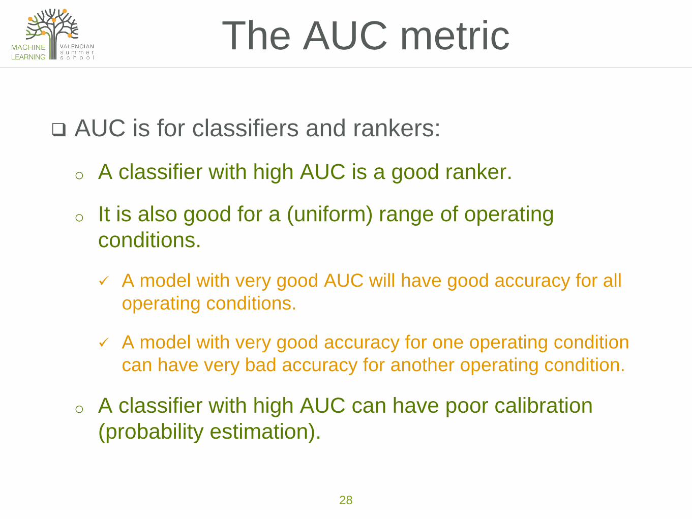
ROC analysis for regression (using shifts).

o The operating condition is the asymmetry factor α. For instance if α=2/3 means that underpredictions are twice as expensive than overpredictions.

o The area over the curve (AOC) is ½ the error variance. If the model is unbiased, then it is ½ MSE.


32

Model evaluation goes much beyond accuracy or MSE.

Models can be generated once but then applied to

different operating conditions.

Drawing models for different operating conditions allow

us to determine dominance regions and the optimal

threshold to make optimal decisions.

Soft models are much more powerful than crisp models.

ROC analysis really makes sense for soft models.

Areas under/over the curves are an aggregate of the

performance on a range of operating conditions, but

should not replace ROC analysis.

Lessons learned

33

Hand, D.J. (1997) “Construction and Assessment of Classification Rules”, Wiley.

Fawcett, Tom (2004); ROC Graphs: Notes and Practical Considerations for Researchers, Pattern Recognition Letters, 27(8):882–891.

Flach, P.A.; Hernandez-Orallo, J.; Ferri, C. (2011). "A coherent interpretation of AUC as a measure of aggregated classification performance." (PDF). Proceedings of the 28th International Conference on Machine Learning (ICML-11). pp. 657–664.

Wojtek J. Krzanowski, David J. Hand (2009) “ROC Curves for Continuous Data”, Chapman and Hall.

Nathalie Japkowicz, Mohak Shah (2011) “Evaluating Learning Algorithms: A Classification Perspective”, Cambridge University Press 2011.

Hernandez-Orallo, J.; Flach, P.A.; Ferri, C. (2012). "A unified view of performance metrics: translating threshold choice into expected classification loss" (PDF). Journal of Machine Learning Research 13: 2813–2869.

Flach, P.A. (2012)“Machine Learning: The Art and Science of Algorithms that Make Sense of Cambridge University Press.

Hernandez-Orallo, J. (2013). "ROC curves for regression". Pattern Recognition 46 (12): 3395–3411.

Peter Flach’s tutorial on ROC analysis: http://www.rduin.nl/presentations/ROC%20Tutorial%20Peter%20Flach/ROCtutorialPartI.pdf

To know more

34

http://www.rduin.nl/presentations/ROC Tutorial Peter Flach/ROCtutorialPartI.pdf

http://www.rduin.nl/presentations/ROC Tutorial Peter Flach/ROCtutorialPartI.pdf

Data & Analytics

L12. Evaluating Machine Learning Algorithms II