Кластеризация графов и поиск сообществ

Кирилл Рыбачук, DCA

Что такое сообщество?• Сообщество — интуитивное понятие, нет единого определения

• Глобальный взгляд: «такое скопление не может быть случайно»

• Модулярность: сравнение со случайным графом (почти Эрдёша-Ренью)

• Локальный взгляд: «внутри больше связей, чем снаружи рядом»

• В слабом смысле: internal degree > external degree

• В сильном смысле: internal degree > external degree для каждой вершины

• Совсем локальный взгляд: скопление «похожих» вершин

• Мера Жаккарда:

j belong to the same cluster. Another way of looking at it is that an edge that is a

part of many triangles is probably in a dense region i.e. a cluster. We use the Jaccard

measure to quantify the overlap between adjacency lists. Let Adj(i) be the adjacency

list of i, and Adj(j) be the adjacency list of j. For simplicity, we will refer to the

similarity between Adj(i) and Adj(j) as the similarity between i and j itself.

Sim(i, j) =|Adj(i) ∩Adj(j)|

|Adj(i) ∪Adj(j)|(5.1)

Global Sparsification

Based on the above heuristic, a simple recipe for sparsifying a graph is given in

Algorithm 8. For each edge in the input graph, we calculate the similarity of its end

points. We then sort all the edges by their similarities, and return the graph with

the top s% of all the edges in the graph (s is the sparsification parameter that can

be specified by the user). Note that selecting the top s% of all edges is the same as

setting a similarity threshold (that applies to all edges) for inclusion in the sparsified

graph.

Algorithm 8 Global Sparsification AlgorithmInput: Graph G = (V,E), Sparsification ratio s

Gsparse ← ∅for each edge e=(i,j) in E do

e.sim = Sim(i, j) according to Eqn 5.1end for

Sort all edges in E by e.simAdd the top s% edges to Gsparse

return Gsparse

However, the approach given in Algorithm 8 has a critical flaw. It treats all edges

in the graph equally, i.e. it uses a global threshold (since it sorts all the edges in the

graph), which is not appropriate when different clusters have different densities. For

example, consider the graph in Figure 5.2(a). Here, the vertices {1, 2, 3, 4, 5, 6} form

a dense cluster, while the vertices {7, 8, 9, 10} form a less dense cluster. The sparsified

graph using Algorithm 8 and selecting the top 15 (out of 22) edges in the graph is

shown in Figure 5.2(b). As can be seen, all the edges of the first cluster have been

79

Почему это важно?1. Сегменты DMP

2. Товарные рекомендации

3. Центральность внутри сообществ: реальные потоки информации

4. Сравнение с номинальными сообществами (общежития, группы vk)

5. Компрессия и визуализация

Как искать сообщества?• Graph partitioning: оптимальное разбиение на заранее заданное количество подграфов k.

как хорошо выбрать это k?

• Community finding: нахождение отдельных скоплений

k не контролируется напрямую

не обязательно полное покрытие сообществами

сообщества могут перекрываться

Как оценить успех?• Целевые функции

• Оптимизация на графе целиком — только приближенные эвристики

• Сравнение результатов разных алгоритмов

• Выбор наилучшего k для graph partitioning’a

• Если есть ground truth — использовать стандартные метрики для задач классификации

• часто WTF — самая лучшая метрика — смотреть глазами

Клики

Клики• Просто клика: полный подграф

• Все знают всех

• Иногда требуют еще максимальность: нельзя никого добавить

• Алгоритм Брона-Кербоша (1973): n — число вершин, d_max — максимальная степень

O(n · 3dmax/3)

Недостатки клик• Слишком строгая предпосылка:

• Большие клики почти не встречаются

• Маленькие клики часто встречаются даже в графе Эрдёша-Ренью

• Исчезновение одного ребра уничтожает клику

• Нет центра и окраины сообщества

• Симметрия: нет смысла в центральности

Обобщения• n-clique: максимальный подграф, где путь между любыми вершинами не длиннее n.

• При n =1 вырождается в просто клику

• Внутри n-clique может быть даже несвязна!

• n-club: n-clique с диаметром n. Всегда связна.

• k-core: максимальный подграф, где у каждой вершины не менее k внутренних соседей.

• p-clique: у каждой вершины доля внутренних соседей не меньше p (от 0 до 1)

Алгоритм нахождения k-cores

• Алгоритм Batagelj and Zaversnik (2003): O(m) m — число ребер

• Вход: граф G(V,E)

• Выход: значение k для каждой вершины

Метрики и целевые функции

Модулярность• Пусть — степень вершины i,

• m — число ребер, A — матрица смежности

• Перемешаем все ребра, сохраняя распределение степеней

• Вероятность того, что i и j будут соединены (грубая оценка!):

• Модулярность: мера «неслучайности» сообщества:

ki

kikj

2m

Q =1

2m

!

i,j

"

Aij −kikj

2m

#

I$

ci = cj%

Свойства модулярности

• m_s — число ребер в сообществе s, d_s — суммарная степень вершин в s

• Максимальное значение: при S разъединенных кликах Q = 1-1/S

• Максимум для связного графа: при S равных подграфах, соединенных одним ребром

• В этом случае Q = 1 - 1/S - S/m

Q ≡

!

s

"

ms

m−

#

ds

2m

$2%

Недостатки модулярности• Предел разрешения (resolution

limit)!

• Сообщества c сливаются в одно

• Если на рисунке клики имеют размер n_s, то они сливаются при

• Смещение размера кластера в сторону выравнивания

ms <

√

2m

ns(ns − 1) + 1 < S

WCC• Пусть S — сообщество (его вершины)

• V — все вершины

• — число треугольников внутри S, в которых участвует вершина x

• — число вершин из S, образующих хотя бы один треугольник с вершиной x

• Weighted Community Clustering для одной вершины:

• Для всего сообщества просто усредняем: WCC(S) =

1

|S|

!

x∈S

WCC(x, S)

WCC

• Произведение двух компонент

• Треугольник = «компашка»

• Слева: какая доля компашек с участием x находится внутри его «домашнего» сообщества?

• Справа в числителе: сколько всего людей участвует в компашках вместе с x?

• Справа в знаменателе: сколько людей участвовало бы в компашках с x, если бы S был кликой?

WCC

Алгоритмы

Newman-Girvan• Иерархический divisive алгоритм

• По очереди удаляем ребро с самым большим betweenness

• Останавливаемся при выполнении критерия (например, получили k связных компонент)

• O(n*m) на вычисление кратчайших путей

• O(n+m) на пересчет связных компонент

• Весь алгоритм — не меньше O(n^3)

• Не используется на графах крупнее нескольких сотен узлов

k-medoids• k-means: требуется нормированное пространство

• В графе расстояние определено только между вершинами (например, 1 - Jaccard) => k-means не годится

• k-medoids: в качестве центроидов выступают только имеющиеся точки

• Нужно задавать k заранее (graph partitioning)

• Самый известный вариант называется PAM

k-medoids: PAM1.Явным образом задаем k — количество кластеров.

2.Инициализируем: выбираем k случайных узлов в качестве медоидов.

3.Для каждой точки находим ближайший медоид, формируя исходное разбиение на кластеры.

4.minCost = функция потерь от исходной конфигурации

5.Для каждого медоида m:

5.1. Для каждой вершины v != m внутри кластера с центром в m:

5.1.1. Перемещаем медоид в v

5.1.2. Перераспределяем все вершины между новыми медоидами

5.1.3. cost = функция потерь по всему графу

5.1.4. Если cost < minCost:

5.1.4.1. Запоминаем медоиды

5.1.4.2. minCost = cost

5.1.5. Кладем медоид на место (в m)

6.Делаем наилучшую замену из всех найденных (то есть внутри одного кластера меняем один

медоид)

7.Повторяем пп. (4)-(5) до тех пор, пока медоиды не стабилизируются

k-medoids: новая эвристика1.While True:

1.1.Для каждого медоида m:

1.1.1. Случайно выбираем s точек внутри кластера с центром в m

1.1.2. Для каждой вершины v из s:

1.1.2.1. Перемещаем медоид в v

1.1.2.2. Перераспределяем все вершины между новыми медоидами

1.1.2.3. cost = функция потерь по всему графу

1.1.2.4. Если cost < minCost:

1.1.2.4.1. Запоминаем медоиды

1.1.2.4.2. minCost = cost

1.1.2.5. Кладем медоид на место (в m)

1.1.3. Если наилучшая замена из s улучшает функцию потерь:

1.1.3.1. Производим эту замену

1.1.3.2. StableSequence = 0

1.1.4. Иначе:

1.1.4.1. StableSequence += 1

1.1.4.2. Если StableSequence > порога:

1.1.4.2.1. Возвращаем текущую конфигурацию

k-medoids: clara• «Bagging» для кластеризации графов

• Выбирается случайная подвыборка и кластеризуется

• Оставшиеся узлы просто присоединяются в самом конце к ближайшим медоидам

• Прогоняется несколько раз, и выбирается лучший вариант

• Ускорение только при сложности выше O(n)

• У PAM сложность O(k * n^2 * число_итераций)

• У новой эвристики сложность O(k * n * s * число итераций)

k-medoids для сегментов DMP

• Строим граф доменов

• Данные: выборка пользователей, для каждого — set посещенных доменов

• Пусть U_x — юзеры, посетившие домен x

• Вес ребра между доменами x и y:

• Отсечение шумов:

1. Порог для вершин (доменов) — хотя бы 15 посещений

2. Порог для ребер — аффинити хотя бы 20

affinity(x, y) =|Ux ∩ Uy||U |

|Ux||Uy|=

p̂(x, y)

p̂(x)p̂(y)

Сколько данных? Сколько кластеров?

• 30000 юзеров дают около 1200 доменов и около 12 интерпретируемых сообществ

• 500000 юзеров: 10000 доменов, около 30 сообществ

Интерпретация картинки• Размер узла — число посещений

• Цвет узла — сообщество

• Цвет ребра = цвету сообщества, если оно внутреннее, иначе серый

• Толщина ребра — аффинити

• Для networkx слишком сложно!

• Недостатки визуализации в networkx:

1. Негибкая

2. Неинтерактивная

3. Неустойчивая

4. Медленная

• По возможности пользуйтесь graph-tool!

Новостные сайты

Фильмы и сериалы

Рефераты, мультики, автомобили

Кулинария

Казахстан

Книги; Законы

Предобработка: Local Sparsification

• Прореживаем граф, сохраняя структуру сообществ

• Алгоритмы быстрее, картинки красивее

• Вариант 1: Сортируем всех соседей по мере Жаккарда по убыванию и удаляем хвост

• Плохо: плотные сообщества останутся нетронутыми, а разреженные уничтожатся совсем

• Вариант 2: Для каждой вершины сортируем соседей и оставляем ребер

• d_i — степень i, e от 0 до 1. При e=0,5 прорежение в 10 раз

• Сохраняется power law, почти сохраняется связность!

min{1,dei}

Local sparsification: иллюстрация

Стабильные ядра• Рандомизированные алгоритмы нестабильны

• Разные прогоны — разные результаты

• Добавление / удаление 2% узлов может полностью поменять кластеризацию

• Стабильные ядра: запускаем алгоритм 100 раз и считаем долю, сколько раз каждая пара вершин попала в один и тот же кластер

• Иерархическая кластеризация на результате

Louvain• Blondel et al, 2008

• Самый яркий представитель modularity-based алгоритмов

• Многоуровневые сообщества

• Очень быстрый

1. Инициализация: все вершины отдельно (n сообществ по 1 вершине)

2. Итеративно объединяем пары сообществ, дающих наибольший прирост модулярности

3. Когда прирост закончится, представляем каждое сообщество как 1 узел в новом графе

4. Повторяем пп. 2-3, пока не останется 2 сообщества

Louvain: иллюстрация• Бельгийский мобильный оператор

• 2,6 млн клиентов

• 260 сообществ больше 100 клиентов, 36 — больше 10000

• 6 уровней сообществ

• Французский и голландский сегменты почти не соприкасаются

MCL• Markov Cluster Algorithm (van Dongen, 1997-2000)

• Нормируем столбцы матрицы смежности:

• «Доля денег для каждого друга» или «Вероятность перехода случайного блуждания»

• Итеративно повторяем 3 шага:

• Expand:

• Inflate: (больше r — больше кластеров)

• Prune: Обнулять самые маленькие элементы в каждом столбце

• Повторять пока M не сойдется

• Сложность ~ n * d^2 на первую итерацию (следующие — быстрее)

3.1 Preliminaries

Let G = (V, E) be our input graph with V and E denoting the node set and edge

set respectively. Let A be the |V|× |V| adjacency matrix corresponding to the graph,

with A(i, j) denoting the weight of the edge between the vertex vi and the vertex vj .

This weight can represent the strength of the interaction in the original network - e.g.

in an author collaboration network, the edge weight between two authors could be the

frequency of their collaboration. If the graph is unweighted, then the weight on each

edge is fixed to 1. As many interaction networks are undirected, we also assume that

G is undirected, although our method is easy to extend to directed graphs. Therefore

A will be a symmetric matrix.

3.1.1 Stochastic matrices and flows

A column-stochastic matrix is simply a matrix where each column sums to 1. A

column stochastic (square) matrix M with as many columns as vertices in a graph G

can be interpreted as the matrix of the transition probabilities of a random walk (or

a Markov chain) defined on the graph. The ith column of M represents the transition

probabilities out of the vi; therefore M(j, i) represents the probability of a transition

from vertex vi to vj. We use the terms stochastic matrix and column-stochastic matrix

interchangeably.

We also refer to the transition probability from vi to vj as the stochastic flow or

simply the flow from vi to vj. Correspondingly, a column-stochastic transition matrix

of the graph G is also refered to as a flow matrix of G or simply a flow of G. Given

a flow matrix M , the ith column contains the flows out of node vi, or its out-flows ;

correspondingly the ith row contains the in-flows. Note that while all the columns (or

out-flows) sum to 1, the rows (or in-flows) are not required to do so.

The most common way of deriving a column-stochastic transition matrix M for a

graph is to simply normalize the columns of the adjacency matrix to sum to 1

M(i, j) =A(i, j)

!nk=1 A(k, j)

In matrix notation, M := AD−1, where D is the diagonal degree matrix of G with

D(i, i) =!n

j=1 A(j, i). We will refer to this particular transition matrix for the graph

29

as the canonical transition matrix MG. However, it is worth keeping in mind that

one can associate other stochastic matrices with the graph G.

Both MCL and our methods introduced in Section 3.2 can be thought of as sim-

ulating stochastic flows (or simulating random walks) on graphs according to certain

rules. For this reason, we refer to these processes as flow simulations.

3.1.2 Markov Clustering (MCL) Algorithm

We next describe the Markov Clustering (MCL) algorithm for clustering graphs,

proposed by Stijn van Dongen [41], in some detail as it is relevant to understanding

our own method.

The MCL algorithm is an iterative process of applying two operators - expansion

and inflation - on an initial stochastic matrix M , in alternation, until convergence.

Both expansion and inflation are operators that map the space of column-stochastic

matrices onto itself. Additionally, a prune step is performed at the end of each

inflation step in order to save memory. Each of these steps is defined below:

Expand: Input M , output Mexp.

Mexp = Expand(M)def= M ∗M

The ith column of Mexp can be interpreted as the final distribution of a random walk of

length 2 starting from vertex vi, with the transition probabilities of the random walk

given by M . One can take higher powers of M instead of a square (corresponding to

longer random walks), but this gets computationally prohibitive very quickly.

Inflate: Input M and inflation parameter r, output Minf .

Minf (i, j)def=

M(i, j)r

!nk=1 M(k, j)r

Minf corresponds to raising each entry in the matrix M to the power r and then

normalizing the columns to sum to 1. By default r = 2. Because the entries in the

matrix are all guaranteed to be less than or equal to 1, this operator has the effect of

exaggerating the inhomogeneity in each column (as long as r > 1). In other words,

flow is strengthened where it is already strong and weakened where it is weak.

Prune: In each column, we remove those entries which have very small values (where

“small” is defined in relation to the rest of the entries in the column), and the retained

30

as the canonical transition matrix MG. However, it is worth keeping in mind that

one can associate other stochastic matrices with the graph G.

Both MCL and our methods introduced in Section 3.2 can be thought of as sim-

ulating stochastic flows (or simulating random walks) on graphs according to certain

rules. For this reason, we refer to these processes as flow simulations.

3.1.2 Markov Clustering (MCL) Algorithm

We next describe the Markov Clustering (MCL) algorithm for clustering graphs,

proposed by Stijn van Dongen [41], in some detail as it is relevant to understanding

our own method.

The MCL algorithm is an iterative process of applying two operators - expansion

and inflation - on an initial stochastic matrix M , in alternation, until convergence.

Both expansion and inflation are operators that map the space of column-stochastic

matrices onto itself. Additionally, a prune step is performed at the end of each

inflation step in order to save memory. Each of these steps is defined below:

Expand: Input M , output Mexp.

Mexp = Expand(M)def= M ∗M

The ith column of Mexp can be interpreted as the final distribution of a random walk of

length 2 starting from vertex vi, with the transition probabilities of the random walk

given by M . One can take higher powers of M instead of a square (corresponding to

longer random walks), but this gets computationally prohibitive very quickly.

Inflate: Input M and inflation parameter r, output Minf .

Minf (i, j)def=

M(i, j)r

!nk=1 M(k, j)r

Minf corresponds to raising each entry in the matrix M to the power r and then

normalizing the columns to sum to 1. By default r = 2. Because the entries in the

matrix are all guaranteed to be less than or equal to 1, this operator has the effect of

exaggerating the inhomogeneity in each column (as long as r > 1). In other words,

flow is strengthened where it is already strong and weakened where it is weak.

Prune: In each column, we remove those entries which have very small values (where

“small” is defined in relation to the rest of the entries in the column), and the retained

30

MCL: пример

Figure 3.1: Toy example graph for illustrating MCL.

Interpretation of M as a clustering: As just mentioned, after some number of

iterations, most of the nodes will find one “attractor” node to which all of their flow

is directed i.e. there will be only one non-zero entry per column in the flow matrix

M. We declare convergence at this stage, and assign nodes which flow into the same

node as belonging to one cluster.

3.1.3 Toy example

We give a simple example of the MCL process in action for the graph in Fig-

ure 3.1.3. The initial stochastic matrix M0 obtained by adding self-loops to the graph

and normalizing each column is given below

M0 =

⎛

⎜

⎜

⎜

⎜

⎜

⎜

⎜

⎜

⎜

⎝

0.33 0.33 0.25 0 0 0

0.33 0.33 0.25 0 0 0

0.33 0.33 0.25 0.25 0 0

0 0 0.25 0.25 0.33 0.33

0 0 0 0.25 0.33 0.33

0 0 0 0.25 0.33 0.33

⎞

⎟

⎟

⎟

⎟

⎟

⎟

⎟

⎟

⎟

⎠

32

The result of applying one iteration of Expansion, Inflation and the Prune steps

is given below:

M1 =

⎛

⎜

⎜

⎜

⎜

⎜

⎜

⎜

⎜

⎜

⎝

0.33 0.33 0.2763 0 0 0

0.33 0.33 0.2763 0 0 0

0.33 0.33 0.4475 0 0 0

0 0 0 0.4475 0.33 0.33

0 0 0 0.2763 0.33 0.33

0 0 0 0.2763 0.33 0.33

⎞

⎟

⎟

⎟

⎟

⎟

⎟

⎟

⎟

⎟

⎠

Note that the flow along the lone inter-cluster edge (M0(4, 3)) has evaporated to 0.

Applying one more iteration results in convergence.

M2 =

⎛

⎜

⎜

⎜

⎜

⎜

⎜

⎜

⎜

⎜

⎝

0 0 0 0 0 0

0 0 0 0 0 0

1 1 1 0 0 0

0 0 0 1 1 1

0 0 0 0 0 0

0 0 0 0 0 0

⎞

⎟

⎟

⎟

⎟

⎟

⎟

⎟

⎟

⎟

⎠

Hence, vertices 1, 2 and 3 flow completely to vertex 3, where as the vertices 4, 5 and

6 flow completely to vertex 4. Hence, we group 1, 2 and 3 together with 3 being the

“attractor” of the cluster, and similarly for 4, 5 and 6.

3.1.4 Limitations of MCL

The MCL algorithm is a simple and intuitive algorithm for clustering graphs that

takes an approach that is different from that of the majority of other approaches to

graph clustering such as spectral clustering [104, 36], divisive/agglomerative clustering

[89], heuristic methods [64] and so on. Further more, it does not require a specification

of the number of clusters to be returned; the coarseness of the clustering can instead

be indirectly affected by varying the inflation parameter r, with lower values of r (upto

1) leading to coarser clusterings of the graph. MCL has received a lot of attention

in the bioinformatics field, with multiple researchers finding it to be very effective at

clustering biological interaction networks ([22, 77]).

However, there are two major limitations to MCL:

33

The result of applying one iteration of Expansion, Inflation and the Prune steps

is given below:

M1 =

⎛

⎜

⎜

⎜

⎜

⎜

⎜

⎜

⎜

⎜

⎝

0.33 0.33 0.2763 0 0 0

0.33 0.33 0.2763 0 0 0

0.33 0.33 0.4475 0 0 0

0 0 0 0.4475 0.33 0.33

0 0 0 0.2763 0.33 0.33

0 0 0 0.2763 0.33 0.33

⎞

⎟

⎟

⎟

⎟

⎟

⎟

⎟

⎟

⎟

⎠

Note that the flow along the lone inter-cluster edge (M0(4, 3)) has evaporated to 0.

Applying one more iteration results in convergence.

M2 =

⎛

⎜

⎜

⎜

⎜

⎜

⎜

⎜

⎜

⎜

⎝

0 0 0 0 0 0

0 0 0 0 0 0

1 1 1 0 0 0

0 0 0 1 1 1

0 0 0 0 0 0

0 0 0 0 0 0

⎞

⎟

⎟

⎟

⎟

⎟

⎟

⎟

⎟

⎟

⎠

Hence, vertices 1, 2 and 3 flow completely to vertex 3, where as the vertices 4, 5 and

6 flow completely to vertex 4. Hence, we group 1, 2 and 3 together with 3 being the

“attractor” of the cluster, and similarly for 4, 5 and 6.

3.1.4 Limitations of MCL

The MCL algorithm is a simple and intuitive algorithm for clustering graphs that

takes an approach that is different from that of the majority of other approaches to

graph clustering such as spectral clustering [104, 36], divisive/agglomerative clustering

[89], heuristic methods [64] and so on. Further more, it does not require a specification

of the number of clusters to be returned; the coarseness of the clustering can instead

be indirectly affected by varying the inflation parameter r, with lower values of r (upto

1) leading to coarser clusterings of the graph. MCL has received a lot of attention

in the bioinformatics field, with multiple researchers finding it to be very effective at

clustering biological interaction networks ([22, 77]).

However, there are two major limitations to MCL:

33

MCL: иллюстрация

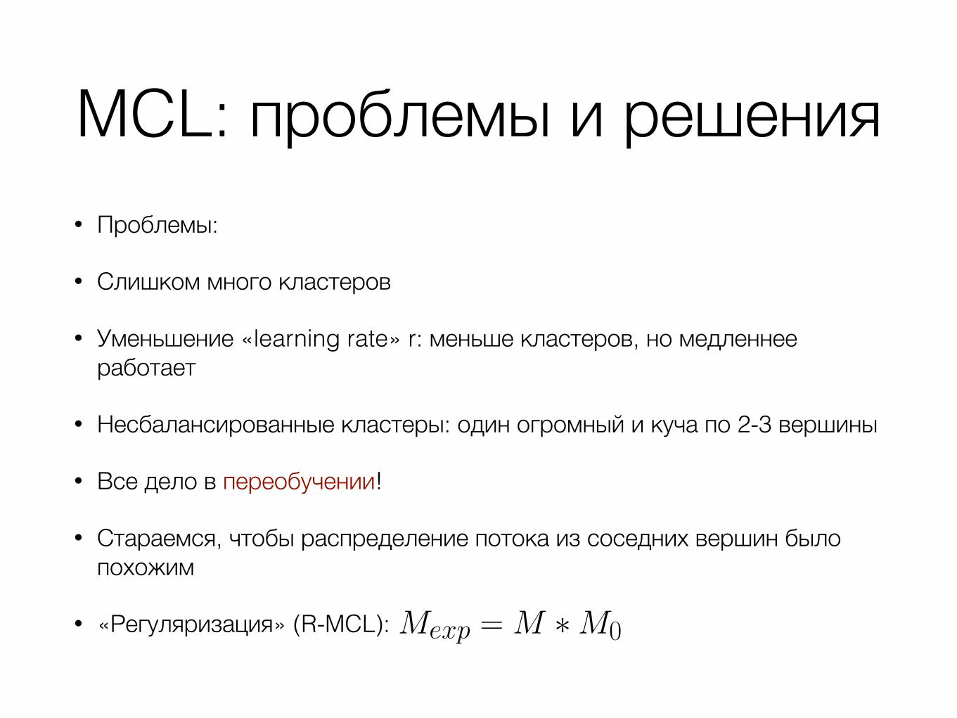
MCL: проблемы и решения• Проблемы:

• Слишком много кластеров

• Уменьшение «learning rate» r: меньше кластеров, но медленнее работает

• Несбалансированные кластеры: один огромный и куча по 2-3 вершины

• Все дело в переобучении!

• Стараемся, чтобы распределение потока из соседних вершин было похожим

• «Регуляризация» (R-MCL): Mexp = M ∗M0

SCD: шаг 1• Приближенная максимизация WCC

• Сначала считаем треугольники

• Удаляем все ребра, не формирующие треугольников

• Грубое разбиение (algorithm 1):

1. Сортируем вершины по локальному кластерному коэффициенту

2. Первое сообщество: Первая вершина + все ее соседи

3. Второе сообщество: Первая вершина из оставшихся (еще не посещенных) + все ее соседи

4. …

• Сложность: O(n*d^2 + n*log(n))

SCD: шаг 2• Итеративно улучшаем результат

algorithm 1, пока WCC не перестанет улучшаться (algorithm 2)

• Для каждой вершины ищем bestMovement (MapReduce)

• bestMovement: добавить / удалить / переместить

• Выполняем bestMovement одновременно для всех вершин

• Сложность: О(1) на один bestMovement, O(d+1) для одной вершины, O(m) — для всего графа

• Весь алгоритм: O(m*log(n))

SCD: эксперимент

Spinner• На основе label propagation

• Реализовано в Okapi (Mahout) компанией Telefonica

• Симметризуем исходный граф D: вес w(u,v) = 1, если ребро было в одну сторону, и 2, если в обе.

• Регулируем баланс: задаем максимальное число ребер, возможное в сообществе (с можно менять от 1 до 10-15):

• Загруженность сообщества l — текущее количество ребер в сообществе l:

• Относительная загруженность:

• Заранее задаем число кластеров k, как в k-medoids; c = 1, …, k.

• Какой лейбл присвоить вершине v? Тот, который чаще встречается среди соседей v:

• Поправка на сбалансированность:

V is the set of vertices in the graph and E is the set of edges suchthat an edge e 2 E is a pair (u,v) with u,v 2 V . We denote byN(v) = {u : u 2 V,(u,v) 2 E} the neighborhood of a vertex v, andby deg(v) = |N(v)| the degree of v. In a k-way partitioning, wedefine L as a set of labels L= {l1, . . . , lk} that essentially correspondto the k partitions. a is the labeling function a : V ! L such thata(v) = l j if label l j is assigned to vertex v.

The end goal of Spinner is to assign partitions, or labels, to eachvertex such that it maximizes edge locality and partitions are bal-anced.

3.1 K-way Label PropagationWe first describe how to use basic LPA to maximize edge locality

and then extend the algorithm to achieve balanced partitions. Ini-tially, each vertex in the graph is assigned a label li at random, with0 < i k. Subsequently, every vertex iteratively propagates its la-bel to its neighbors. During this iterative process, a vertex acquiresthe label that is more frequent among its neighbors. Every vertex vassigns a different score for a particular label l which is equal to thenumber of neighbors assigned to label l. A vertex shows preferenceto labels with high score. More formally:

score(v, l) = Âu2N(v)

d (a(u), l) (1)

where d is the Kronecker delta. The vertex updates its label to thelabel lv that maximizes its score according to the update function:

lv = argmaxl

score(v, l) (2)

We call such an update a migration as it represents a logical vertexmigration between two partitions.

When multiple labels satisfy the update function, we break tiesrandomly, but prefer to keep the current label if it is among them.This break-tie rule improves convergence speed [6], and in our dis-tributed implementation reduces unnecessary network communica-tion (see Section 4). The algorithm halts when no vertex updatesits label.

Note that the original formulation of LPA assumes undirectedgraphs. However, very often graphs are directed (e.g. the Web).Even the data models of systems like Pregel allow directed graphs,to support algorithms that are aware of graph directness, like PageR-ank. To use LPA as is, we would need to convert a graph to undi-rected. The naive approach would be to create an undirected edgebetween vertices u and v whenever at least one directed edge existsbetween vertex u and v in the directed graph.

This approach, though, is agnostic to the communication patternsof the applications running on top. Consider the example graph inFigure 1 that we want to partition to 3 parts. In the undirected graph(right), there are initially 3 cut edges. At this point, according to theLPA formulation, which is agnostic of the directness of the originalgraph, any migration of a vertex to another partition is as likely, andit would produce one cut edge less.

However, if we consider the directness of the edges in the orig-inal graph, not all migrations are equally beneficial. In fact, eithermoving vertex 2 to partition 1 or vertex 1 to partition 3 would inpractice produce less cut edges in the directed graph. Once thegraph is loaded into the system and messages are sent across thedirected edges, this latter decision results in less communicationover the network.

Figure 1: Conversion of a directed graph (left) to an undirectedgraph (right).

Spinner considers the number of directed edges connecting u,vin the original directed graph D, by introducing a weighting func-tion w(u,v) such that:

w(u,w) =

(1, if (u,v) 2 D� (v,u) 2 D2, if (u,v) 2 D^ (v,u) 2 D

(3)

where � is the logical XOR. We extend now the formulation in (1)to include the weighting function:

score0(v, l) = Âu2N(v)

w(u,v)d (a(u), l) (4)

In practice, the new update function effectively counts the num-ber of messages exchanged locally in the system.

3.2 Balanced Label PropagationUntil now we have not considered partition balance. In Spin-

ner, we take a different path from previous work [24, 25], wherea centralized component is added to LPA to satisfy global balanceconstraints, possibly limiting scalability. Instead, as our aim is toprovide a practical and scalable solution, Spinner relaxes this con-straint, only encouraging a similar number of edges across the dif-ferent partitions. As we will show, this decision allows a fully de-centralized algorithm. While in this work we focus on the presenta-tion and evaluation of the more system-related aspects of Spinner,we plan to investigate theoretical justifications and guarantees be-hind our approach in future work.

Here, we consider the case of a homogeneous system, whereeach machine has equal resources. This setup is often preferredin synchronous graph processing systems like Pregel, to minimizethe time spent by faster machines waiting at the synchronizationbarrier for stragglers.

We define the capacity C of a partition as the maximum numberof edges it can have so that partitions are balanced:

C = c · |E|k

(5)

Parameter c > 1 ensures additional capacity to each partition isavailable for migrations. We define the load of a partition as theactual number of edges in that partition:

B(l) = Âv2G

deg(v)d (a(v), l) (6)

A larger value of c increases the number of migrations to eachpartition allowed at each iteration, possibly speeding up conver-gence, but it may increase unbalance, as more edges are allowed tobe assigned to each partition over the ideal value |E|

k .

3

V is the set of vertices in the graph and E is the set of edges suchthat an edge e 2 E is a pair (u,v) with u,v 2 V . We denote byN(v) = {u : u 2 V,(u,v) 2 E} the neighborhood of a vertex v, andby deg(v) = |N(v)| the degree of v. In a k-way partitioning, wedefine L as a set of labels L= {l1, . . . , lk} that essentially correspondto the k partitions. a is the labeling function a : V ! L such thata(v) = l j if label l j is assigned to vertex v.

The end goal of Spinner is to assign partitions, or labels, to eachvertex such that it maximizes edge locality and partitions are bal-anced.

3.1 K-way Label PropagationWe first describe how to use basic LPA to maximize edge locality

and then extend the algorithm to achieve balanced partitions. Ini-tially, each vertex in the graph is assigned a label li at random, with0 < i k. Subsequently, every vertex iteratively propagates its la-bel to its neighbors. During this iterative process, a vertex acquiresthe label that is more frequent among its neighbors. Every vertex vassigns a different score for a particular label l which is equal to thenumber of neighbors assigned to label l. A vertex shows preferenceto labels with high score. More formally:

score(v, l) = Âu2N(v)

d (a(u), l) (1)

where d is the Kronecker delta. The vertex updates its label to thelabel lv that maximizes its score according to the update function:

lv = argmaxl

score(v, l) (2)

We call such an update a migration as it represents a logical vertexmigration between two partitions.

When multiple labels satisfy the update function, we break tiesrandomly, but prefer to keep the current label if it is among them.This break-tie rule improves convergence speed [6], and in our dis-tributed implementation reduces unnecessary network communica-tion (see Section 4). The algorithm halts when no vertex updatesits label.

Note that the original formulation of LPA assumes undirectedgraphs. However, very often graphs are directed (e.g. the Web).Even the data models of systems like Pregel allow directed graphs,to support algorithms that are aware of graph directness, like PageR-ank. To use LPA as is, we would need to convert a graph to undi-rected. The naive approach would be to create an undirected edgebetween vertices u and v whenever at least one directed edge existsbetween vertex u and v in the directed graph.

This approach, though, is agnostic to the communication patternsof the applications running on top. Consider the example graph inFigure 1 that we want to partition to 3 parts. In the undirected graph(right), there are initially 3 cut edges. At this point, according to theLPA formulation, which is agnostic of the directness of the originalgraph, any migration of a vertex to another partition is as likely, andit would produce one cut edge less.

However, if we consider the directness of the edges in the orig-inal graph, not all migrations are equally beneficial. In fact, eithermoving vertex 2 to partition 1 or vertex 1 to partition 3 would inpractice produce less cut edges in the directed graph. Once thegraph is loaded into the system and messages are sent across thedirected edges, this latter decision results in less communicationover the network.

Figure 1: Conversion of a directed graph (left) to an undirectedgraph (right).

Spinner considers the number of directed edges connecting u,vin the original directed graph D, by introducing a weighting func-tion w(u,v) such that:

w(u,w) =

(1, if (u,v) 2 D� (v,u) 2 D2, if (u,v) 2 D^ (v,u) 2 D

(3)

where � is the logical XOR. We extend now the formulation in (1)to include the weighting function:

score0(v, l) = Âu2N(v)

w(u,v)d (a(u), l) (4)

In practice, the new update function effectively counts the num-ber of messages exchanged locally in the system.

3.2 Balanced Label PropagationUntil now we have not considered partition balance. In Spin-

ner, we take a different path from previous work [24, 25], wherea centralized component is added to LPA to satisfy global balanceconstraints, possibly limiting scalability. Instead, as our aim is toprovide a practical and scalable solution, Spinner relaxes this con-straint, only encouraging a similar number of edges across the dif-ferent partitions. As we will show, this decision allows a fully de-centralized algorithm. While in this work we focus on the presenta-tion and evaluation of the more system-related aspects of Spinner,we plan to investigate theoretical justifications and guarantees be-hind our approach in future work.

Here, we consider the case of a homogeneous system, whereeach machine has equal resources. This setup is often preferredin synchronous graph processing systems like Pregel, to minimizethe time spent by faster machines waiting at the synchronizationbarrier for stragglers.

We define the capacity C of a partition as the maximum numberof edges it can have so that partitions are balanced:

C = c · |E|k

(5)

Parameter c > 1 ensures additional capacity to each partition isavailable for migrations. We define the load of a partition as theactual number of edges in that partition:

B(l) = Âv2G

deg(v)d (a(v), l) (6)

A larger value of c increases the number of migrations to eachpartition allowed at each iteration, possibly speeding up conver-gence, but it may increase unbalance, as more edges are allowed tobe assigned to each partition over the ideal value |E|

k .

3

We introduce a penalty function to discourage assigning verticesto nearly full partitions. Given a partition indicated by label l, thepenalty function p(l) is defined as follows:

p(l) = B(l)C

(7)

To integrate the penalty function we normalize (4) first, and re-formulate the score function as follows:

score00(v, l) = Âu2N(v)

w(u,v)d (a(u), l)Âu2N(v) w(u,v)

�p(l) (8)

3.3 Convergence and HaltingConvergence and halting of LPA are not well understood. LPA is

formally equivalent to minimizing the Hamiltonian for a ferromag-netic Potts model [6]. The global optimum solution for any graphwould assign the same label to each vertex. However, as verticesmake decisions based on local information, LPA converges to localoptima. This characteristic is at the basis of the ability of LPA todetect communities [6]. Unfortunately, even in asynchronous sys-tems, LPA does not prevent cycles where the partitioning fluctuatesbetween the same states, preventing the algorithm to converge. Insuch cases, the halting condition described in Section 3.1 will notwork. A number of strategies have been proposed to guarantee thehalting of LPA in synchronous systems. These strategies are eitherbased on different heuristics applied to tie breaking and halting cri-teria, or on the order with which vertices are evaluated [27]. How-ever, due to the contribution of the penalty function introduced inSection 3.2, these cannot be applied to to our approach.

We use a different strategy instead. At a given iteration, we de-fine the score of the partitioning for graph G as the sum of thecurrent scores of each vertex:

score(G) = Âv2G

score00(v,a(lv)) (9)

In practice, this is the aggregate score that the vertices try to op-timize by making local decisions. We consider a partitioning tobe in a stable state, when the score of the graph is not improvedmore than a given e for more than w consecutive iterations. Thealgorithm halts when a stable state is reached. While through ewe can control the trade-off between the cost of executing the al-gorithm for more iterations and the improvement obtained by thescore function, with w it is possible to require a more strict defini-tion of stability, as absence of improvement is accepted for a largernumber of iterations.

Note that this condition, commonly used by iterative hill-climbingoptimization algorithms, does not guarantee halting at the optimalsolution. However, as we present in Section 3.4, according to ourapproach the partitioning algorithm is expected to be restarted pe-riodically to adapt to changes to the graph or the compute environ-ment. Within this continuous perspective, the impact of occasion-ally halting in a suboptimal state is minimal.

3.4 Incremental Label PropagationGraphs are dynamic. Edges and vertices are added and removed

over time. As the graph changes, the computed partitioning be-comes outdated, possibly degrading the global score. We want toupdate the partitioning to the new topology without repartitioningfrom scratch. As the graph changes affect local areas of the graph,we want to update the latest stable partitioning only in the portionsthat are affected by the graph changes.

Due to its local and iterative nature, LPA lends itself to incre-mental computation. Intuitively, the effect of the graph changes

is to “push” the current stable state away from the local optimumit converged to, towards a state with lower global score. As a re-sult, we restart the algorithm with the effect of letting the algorithmlook for a new local optimum. The vertices evaluate their new localscore, possibly deciding to migrate to another partition. The algo-rithm continues as described previously. As far as new vertices isconcerned, we assign them to the least loaded partition.

The number of iterations required to converge to a new stablestate depends on the number of graph changes and the last state.Clearly, not every graph change will have the same effect. Some-times, no iteration may be necessary at all. In fact, certain changesmay not affect any vertex to the point that the score of a differentlabel is higher than the current one. As no migration is caused, thestate remains stable. On the other hand, other changes may causemore migrations due to the disruption of certain weak local equilib-riums. In this sense, the algorithm behaves as a gradient descendingoptimization algorithm.

3.5 Elastic Label PropagationBecause the partitions are tied to machines, capacity C should be

bound to a maximum capacity Cmax that depends on the resourcesavailable to the machines. As the graph grows, the capacity C ofthe partitions will eventually reach the maximum capacity Cmax.In this case, a number of machines can be added, and the graphcan be spread across these new machines as well. Moreover, thenumber of machines can be increased to increase parallelization.On the other hand, as the graph shrinks or the number of availablemachines decreases, a number of partitions can be removed. In thiscase, a number of vertices should migrate from these partitions tothe remaining ones.

In both cases, we want the algorithm to adapt to the new numberof partitions without repartitioning the graph from scratch. More-over, we want the algorithm to make decisions based on a decentral-ized and lightweight heuristics. We let each vertex decide indepen-dently whether it should migrate. To do so, we use a probabilisticapproach. When n new partitions are added to the system, eachvertex will migrate with a probability p such that:

p =n

k+n(10)

In the trivial case where n partitions are removed, all the verticesassigned to those partitions migrate. In both cases, the verticeschoose uniformly at random the partition to migrate to. After thevertices have migrated, we restart the algorithm to adapt the parti-tioning to the new assignments. As in the case of incremental LPA,the number of iterations required to converge to a new stable statedepends on a number of factors, such as the graph size, the numberof partitions added or removed, etc.

This simple strategy clearly disrupts the current partitioning de-grading the global score. However, it has a number of interestingcharacteristics. First, it matches our requirements of a decentral-ized and lightweight heuristic. The heuristic does not need a globalview of the partitioning or a complex computation to decide whichvertices to migrate. Second, by choosing randomly, the partitionsremain fairly balanced. Third, it injects a factor of randomizationinto the optimization problem that may allow the solution to jumpout of a local optimum.

Given a large n, the cost of adapting the partitioning to the newnumber of partitions may be quite large, due to the random migra-tions. However, in a real system, the frequency with which par-titions are added or removed is low, compared for example to thenumber of times a partitioning is updated due to graph changes.Although vertices are shuffled around, the locality of the vertices

4

We introduce a penalty function to discourage assigning verticesto nearly full partitions. Given a partition indicated by label l, thepenalty function p(l) is defined as follows:

p(l) = B(l)C

(7)

To integrate the penalty function we normalize (4) first, and re-formulate the score function as follows:

score00(v, l) = Âu2N(v)

w(u,v)d (a(u), l)Âu2N(v) w(u,v)

�p(l) (8)

3.3 Convergence and HaltingConvergence and halting of LPA are not well understood. LPA is

formally equivalent to minimizing the Hamiltonian for a ferromag-netic Potts model [6]. The global optimum solution for any graphwould assign the same label to each vertex. However, as verticesmake decisions based on local information, LPA converges to localoptima. This characteristic is at the basis of the ability of LPA todetect communities [6]. Unfortunately, even in asynchronous sys-tems, LPA does not prevent cycles where the partitioning fluctuatesbetween the same states, preventing the algorithm to converge. Insuch cases, the halting condition described in Section 3.1 will notwork. A number of strategies have been proposed to guarantee thehalting of LPA in synchronous systems. These strategies are eitherbased on different heuristics applied to tie breaking and halting cri-teria, or on the order with which vertices are evaluated [27]. How-ever, due to the contribution of the penalty function introduced inSection 3.2, these cannot be applied to to our approach.

We use a different strategy instead. At a given iteration, we de-fine the score of the partitioning for graph G as the sum of thecurrent scores of each vertex:

score(G) = Âv2G

score00(v,a(lv)) (9)

In practice, this is the aggregate score that the vertices try to op-timize by making local decisions. We consider a partitioning tobe in a stable state, when the score of the graph is not improvedmore than a given e for more than w consecutive iterations. Thealgorithm halts when a stable state is reached. While through ewe can control the trade-off between the cost of executing the al-gorithm for more iterations and the improvement obtained by thescore function, with w it is possible to require a more strict defini-tion of stability, as absence of improvement is accepted for a largernumber of iterations.

Note that this condition, commonly used by iterative hill-climbingoptimization algorithms, does not guarantee halting at the optimalsolution. However, as we present in Section 3.4, according to ourapproach the partitioning algorithm is expected to be restarted pe-riodically to adapt to changes to the graph or the compute environ-ment. Within this continuous perspective, the impact of occasion-ally halting in a suboptimal state is minimal.

3.4 Incremental Label PropagationGraphs are dynamic. Edges and vertices are added and removed

over time. As the graph changes, the computed partitioning be-comes outdated, possibly degrading the global score. We want toupdate the partitioning to the new topology without repartitioningfrom scratch. As the graph changes affect local areas of the graph,we want to update the latest stable partitioning only in the portionsthat are affected by the graph changes.

Due to its local and iterative nature, LPA lends itself to incre-mental computation. Intuitively, the effect of the graph changes

is to “push” the current stable state away from the local optimumit converged to, towards a state with lower global score. As a re-sult, we restart the algorithm with the effect of letting the algorithmlook for a new local optimum. The vertices evaluate their new localscore, possibly deciding to migrate to another partition. The algo-rithm continues as described previously. As far as new vertices isconcerned, we assign them to the least loaded partition.

The number of iterations required to converge to a new stablestate depends on the number of graph changes and the last state.Clearly, not every graph change will have the same effect. Some-times, no iteration may be necessary at all. In fact, certain changesmay not affect any vertex to the point that the score of a differentlabel is higher than the current one. As no migration is caused, thestate remains stable. On the other hand, other changes may causemore migrations due to the disruption of certain weak local equilib-riums. In this sense, the algorithm behaves as a gradient descendingoptimization algorithm.

3.5 Elastic Label PropagationBecause the partitions are tied to machines, capacity C should be

bound to a maximum capacity Cmax that depends on the resourcesavailable to the machines. As the graph grows, the capacity C ofthe partitions will eventually reach the maximum capacity Cmax.In this case, a number of machines can be added, and the graphcan be spread across these new machines as well. Moreover, thenumber of machines can be increased to increase parallelization.On the other hand, as the graph shrinks or the number of availablemachines decreases, a number of partitions can be removed. In thiscase, a number of vertices should migrate from these partitions tothe remaining ones.

In both cases, we want the algorithm to adapt to the new numberof partitions without repartitioning the graph from scratch. More-over, we want the algorithm to make decisions based on a decentral-ized and lightweight heuristics. We let each vertex decide indepen-dently whether it should migrate. To do so, we use a probabilisticapproach. When n new partitions are added to the system, eachvertex will migrate with a probability p such that:

p =n

k+n(10)

In the trivial case where n partitions are removed, all the verticesassigned to those partitions migrate. In both cases, the verticeschoose uniformly at random the partition to migrate to. After thevertices have migrated, we restart the algorithm to adapt the parti-tioning to the new assignments. As in the case of incremental LPA,the number of iterations required to converge to a new stable statedepends on a number of factors, such as the graph size, the numberof partitions added or removed, etc.

This simple strategy clearly disrupts the current partitioning de-grading the global score. However, it has a number of interestingcharacteristics. First, it matches our requirements of a decentral-ized and lightweight heuristic. The heuristic does not need a globalview of the partitioning or a complex computation to decide whichvertices to migrate. Second, by choosing randomly, the partitionsremain fairly balanced. Third, it injects a factor of randomizationinto the optimization problem that may allow the solution to jumpout of a local optimum.

Given a large n, the cost of adapting the partitioning to the newnumber of partitions may be quite large, due to the random migra-tions. However, in a real system, the frequency with which par-titions are added or removed is low, compared for example to thenumber of times a partitioning is updated due to graph changes.Although vertices are shuffled around, the locality of the vertices

4

V is the set of vertices in the graph and E is the set of edges suchthat an edge e 2 E is a pair (u,v) with u,v 2 V . We denote byN(v) = {u : u 2 V,(u,v) 2 E} the neighborhood of a vertex v, andby deg(v) = |N(v)| the degree of v. In a k-way partitioning, wedefine L as a set of labels L= {l1, . . . , lk} that essentially correspondto the k partitions. a is the labeling function a : V ! L such thata(v) = l j if label l j is assigned to vertex v.

The end goal of Spinner is to assign partitions, or labels, to eachvertex such that it maximizes edge locality and partitions are bal-anced.

3.1 K-way Label PropagationWe first describe how to use basic LPA to maximize edge locality

and then extend the algorithm to achieve balanced partitions. Ini-tially, each vertex in the graph is assigned a label li at random, with0 < i k. Subsequently, every vertex iteratively propagates its la-bel to its neighbors. During this iterative process, a vertex acquiresthe label that is more frequent among its neighbors. Every vertex vassigns a different score for a particular label l which is equal to thenumber of neighbors assigned to label l. A vertex shows preferenceto labels with high score. More formally:

score(v, l) = Âu2N(v)

d (a(u), l) (1)

where d is the Kronecker delta. The vertex updates its label to thelabel lv that maximizes its score according to the update function:

lv = argmaxl

score(v, l) (2)

We call such an update a migration as it represents a logical vertexmigration between two partitions.

When multiple labels satisfy the update function, we break tiesrandomly, but prefer to keep the current label if it is among them.This break-tie rule improves convergence speed [6], and in our dis-tributed implementation reduces unnecessary network communica-tion (see Section 4). The algorithm halts when no vertex updatesits label.

Note that the original formulation of LPA assumes undirectedgraphs. However, very often graphs are directed (e.g. the Web).Even the data models of systems like Pregel allow directed graphs,to support algorithms that are aware of graph directness, like PageR-ank. To use LPA as is, we would need to convert a graph to undi-rected. The naive approach would be to create an undirected edgebetween vertices u and v whenever at least one directed edge existsbetween vertex u and v in the directed graph.

This approach, though, is agnostic to the communication patternsof the applications running on top. Consider the example graph inFigure 1 that we want to partition to 3 parts. In the undirected graph(right), there are initially 3 cut edges. At this point, according to theLPA formulation, which is agnostic of the directness of the originalgraph, any migration of a vertex to another partition is as likely, andit would produce one cut edge less.

However, if we consider the directness of the edges in the orig-inal graph, not all migrations are equally beneficial. In fact, eithermoving vertex 2 to partition 1 or vertex 1 to partition 3 would inpractice produce less cut edges in the directed graph. Once thegraph is loaded into the system and messages are sent across thedirected edges, this latter decision results in less communicationover the network.

Figure 1: Conversion of a directed graph (left) to an undirectedgraph (right).

Spinner considers the number of directed edges connecting u,vin the original directed graph D, by introducing a weighting func-tion w(u,v) such that:

w(u,w) =

(1, if (u,v) 2 D� (v,u) 2 D2, if (u,v) 2 D^ (v,u) 2 D

(3)

where � is the logical XOR. We extend now the formulation in (1)to include the weighting function:

score0(v, l) = Âu2N(v)

w(u,v)d (a(u), l) (4)

In practice, the new update function effectively counts the num-ber of messages exchanged locally in the system.

3.2 Balanced Label PropagationUntil now we have not considered partition balance. In Spin-

ner, we take a different path from previous work [24, 25], wherea centralized component is added to LPA to satisfy global balanceconstraints, possibly limiting scalability. Instead, as our aim is toprovide a practical and scalable solution, Spinner relaxes this con-straint, only encouraging a similar number of edges across the dif-ferent partitions. As we will show, this decision allows a fully de-centralized algorithm. While in this work we focus on the presenta-tion and evaluation of the more system-related aspects of Spinner,we plan to investigate theoretical justifications and guarantees be-hind our approach in future work.

Here, we consider the case of a homogeneous system, whereeach machine has equal resources. This setup is often preferredin synchronous graph processing systems like Pregel, to minimizethe time spent by faster machines waiting at the synchronizationbarrier for stragglers.

We define the capacity C of a partition as the maximum numberof edges it can have so that partitions are balanced:

C = c · |E|k

(5)

Parameter c > 1 ensures additional capacity to each partition isavailable for migrations. We define the load of a partition as theactual number of edges in that partition:

B(l) = Âv2G

deg(v)d (a(v), l) (6)

A larger value of c increases the number of migrations to eachpartition allowed at each iteration, possibly speeding up conver-gence, but it may increase unbalance, as more edges are allowed tobe assigned to each partition over the ideal value |E|

k .

3

Spinner: Масштабируемость• Вычисление в парадигме Pregel — идеально для label propagation

• Легко добавлять / убирать кластеры (1 кластер — один воркер)

• Легко пересчитывать при добавлении / удалении узлов

• Масштабируемость Spinner при кластеризации случайного графа (Watts-Strogatz):

• Экономия ресурсов при добавлении новых ребер или новых ссобществ (воркеров):

(a) Partitioning of the Twitter graph. (b) Partitioning of the Yahoo! graph.Figure 4: Partitioning of (a) the Twitter graph across 256 partitions and (b) the Yahoo! web graph across 115 partitions. The figureshows the evolution of metrics f , r , and score(G) across iterations.

(a) Runtime vs. graph size (b) Runtime vs. cluster size (c) Runtime vs. k

Figure 5: Scalability of Spinner. (a) Runtime as a function of the number of vertices, (b) runtime as a function of the number ofworkers, (c) runtime as a function of the number of partitions.

supersteps. This approach allows us to factor out the runtime of al-gorithm as a function the number of vertices and edges.

Figure 5.2 presents the results of the experiments, executed ona AWS Hadoop cluster consisting of 116 m2.4xlarge machines. Inthe first experiment, presented in Figure 5(a), we focus on the scal-ability of the algorithm as a function of the number of vertices andedges in the graph. For this, we fix the number of outgoing edgesper vertex to 40. We connect the vertices following a ring latticetopology, and re-wire 30% of the edges randomly as by the func-tion of the beta (0.3) parameter of the Watts-Strogatz model. Weexecute each experiment with 115 workers, for an exponentiallyincreasing number of vertices, precisely from 2 to 1024 millionvertices (or one billion vertices) and we divide each graph in 64partitions. The results, presented in a loglog plot, show a lineartrend with respect to the size of the graph. Note that for the firstdata points the size of the graph is too small for such a large clus-ter, and we are actually measuring the overhead of Giraph.

In the second experiment, presented in Figure 5(b), we focuson the scalability of the algorithm as a function of the number ofworkers. Here, we fix the number of vertices to 1 billion, still con-structed as described above, but we vary the number of workerslinearly from 15 to 115 with steps of 15 workers (except for the laststep where we add 10 workers). The drop from 111 to 15 secondswith 7.6 times more workers represents a speedup of 7.6.

In the third experiment, presented in Figure 5(b), we focus onthe scalability of the algorithm as a function of the number of parti-tions. Again, we use 115 workers and we fix the number of verticesto 1 billion and construct the graph as described above. This time,we increase the number of partitions exponentially from 2 to 512.Also here, the loglog plot shows a near-linear trend, as the com-plexity of the heuristic executed by each vertex is proportional tothe number of partitions k, and so is cost of maintaining partition

(a) Cost savings (b) Partitioning stabilityFigure 6: Adapting to dynamic graph changes. We vary thepercentage of new edges in the graph and compare our adap-tive re-partitioning approach and re-partitioning from scratchwith respect to (a) the savings in processing time and messagesexchanged, and (b) the fraction of vertices that have to moveupon re-partitioning.

loads and counters through the sharded aggregators provided byGiraph.

5.3 Partitioning dynamic graphsDue to the dynamic nature of graphs, the quality of an initial

partitioning degrades over time. Re-partitioning from scratch canbe an expensive task if performed frequently and with potentiallylimited resources. In this section, we show that our algorithm min-imizes the cost of adapting the partitioning to the changes, makingthe maintenance of a well-partitioned graph an affordable task interms of time and compute resources required.

Specifically, we measure the savings in processing time and num-ber of messages exchanged (i.e. load imposed on the network) rel-ative to the approach of re-partitioning the graph from scratch. Wetrack how these metrics vary as a function of the degree of change

8

(a) Partitioning of the Twitter graph. (b) Partitioning of the Yahoo! graph.Figure 4: Partitioning of (a) the Twitter graph across 256 partitions and (b) the Yahoo! web graph across 115 partitions. The figureshows the evolution of metrics f , r , and score(G) across iterations.

(a) Runtime vs. graph size (b) Runtime vs. cluster size (c) Runtime vs. k

Figure 5: Scalability of Spinner. (a) Runtime as a function of the number of vertices, (b) runtime as a function of the number ofworkers, (c) runtime as a function of the number of partitions.

supersteps. This approach allows us to factor out the runtime of al-gorithm as a function the number of vertices and edges.

Figure 5.2 presents the results of the experiments, executed ona AWS Hadoop cluster consisting of 116 m2.4xlarge machines. Inthe first experiment, presented in Figure 5(a), we focus on the scal-ability of the algorithm as a function of the number of vertices andedges in the graph. For this, we fix the number of outgoing edgesper vertex to 40. We connect the vertices following a ring latticetopology, and re-wire 30% of the edges randomly as by the func-tion of the beta (0.3) parameter of the Watts-Strogatz model. Weexecute each experiment with 115 workers, for an exponentiallyincreasing number of vertices, precisely from 2 to 1024 millionvertices (or one billion vertices) and we divide each graph in 64partitions. The results, presented in a loglog plot, show a lineartrend with respect to the size of the graph. Note that for the firstdata points the size of the graph is too small for such a large clus-ter, and we are actually measuring the overhead of Giraph.

In the second experiment, presented in Figure 5(b), we focuson the scalability of the algorithm as a function of the number ofworkers. Here, we fix the number of vertices to 1 billion, still con-structed as described above, but we vary the number of workerslinearly from 15 to 115 with steps of 15 workers (except for the laststep where we add 10 workers). The drop from 111 to 15 secondswith 7.6 times more workers represents a speedup of 7.6.

In the third experiment, presented in Figure 5(b), we focus onthe scalability of the algorithm as a function of the number of parti-tions. Again, we use 115 workers and we fix the number of verticesto 1 billion and construct the graph as described above. This time,we increase the number of partitions exponentially from 2 to 512.Also here, the loglog plot shows a near-linear trend, as the com-plexity of the heuristic executed by each vertex is proportional tothe number of partitions k, and so is cost of maintaining partition

(a) Cost savings (b) Partitioning stabilityFigure 6: Adapting to dynamic graph changes. We vary thepercentage of new edges in the graph and compare our adap-tive re-partitioning approach and re-partitioning from scratchwith respect to (a) the savings in processing time and messagesexchanged, and (b) the fraction of vertices that have to moveupon re-partitioning.

loads and counters through the sharded aggregators provided byGiraph.

5.3 Partitioning dynamic graphsDue to the dynamic nature of graphs, the quality of an initial

partitioning degrades over time. Re-partitioning from scratch canbe an expensive task if performed frequently and with potentiallylimited resources. In this section, we show that our algorithm min-imizes the cost of adapting the partitioning to the changes, makingthe maintenance of a well-partitioned graph an affordable task interms of time and compute resources required.

Specifically, we measure the savings in processing time and num-ber of messages exchanged (i.e. load imposed on the network) rel-ative to the approach of re-partitioning the graph from scratch. Wetrack how these metrics vary as a function of the degree of change

8

(a) Cost savings (b) Partitioning stabilityFigure 7: Adapting to resource changes. We vary the num-ber of new partitions and compare our adaptive approach andre-partitioning from scratch with respect to (a) the savings inprocessing time and messages exchanged, and (b) the fractionof vertices that have to move upon re-partitioning.

in the graph. Intuitively, larger graph changes require more time toadapt to an optimal partitioning.

For this experiment, we take a snapshot of the Tuenti [3] socialgraph that consists of approximately 10 million vertices and 530million edges, and perform an initial partitioning. Subsequently,we add a varying number of edges that correspond to actual newfriendships and measure the above metrics. We perform this ex-periment on an AWS Hadoop cluster consisting of 10 m2.2xlargeinstances.

Figure 6(a) shows that for changes up to 0.5%, our approachsaves up to 86% of the processing time and, by reducing vertex mi-grations, up to 92% of the network traffic. Even for large graphchanges, the algorithm still saves up to 80% of the processing time.Note that in every case our approach converges to a balanced parti-tioning, with a maximum normalized load of approximately 1.047,with 67%-69% local edges, similar to a re-partitioning from scratch.

5.4 Partitioning stabilityAdapting the partitioning helps maintain good locality as the

graph changes, but may also require the graph management sys-tem (e.g. a graph DB) to move vertices and their associated state(e.g. user profiles in a social network) across partitions, poten-tially impacting performance. Aside from efficiency, the value ofan adaptive algorithm lies also in maintaining stable partitions, thatis, requiring only few vertices to move to new partitions upon graphchanges. Here, we show that our approach achieves this goal.

We quantify the stability of the algorithm with a metric we callpartitioning difference. The partitioning difference between twopartitions is the percentage of vertices that belong to different par-titions across two partitionings. This number represents the frac-tion of vertices that have to move to new partitions. Note that thismetric is not the same as the total number of migrations that occurduring the execution of the algorithm which only regards cost ofthe execution of the algorithm per se.

In Figure 6(b), we measure the resulting partitioning differencewhen adapting and when re-partitioning from scratch as a functionof the percentage of new edges. As expected, the percentage of ver-tices that have to move increases as we make more changes to thegraph. However, our adaptive approach requires only 8%-11% ofthe vertices to move compared to a 95%-98% when re-partitioning,minimizing the impact.

5.5 Adapting to resource changesHere, we show that Spinner can efficiently adapt the partitioning

when resource changes force a change in the number of partitions.Initially, we partition the Tuenti graph snapshot described in Sec-tion 5.3 into 32 partitions. Subsequently we add a varying number

of partitions and either re-partition the graph from scratch or adaptthe partitioning with Spinner.

Figure 7(a) shows the savings in processing time and number ofmessages exchanged as a function of the number of new partitions.As expected, a larger number of new partitions requires more workto converge to a good partitioning. When increasing the capacityof the system by only 1 partition, Spinner adapts the partitions 74%faster relative to a re-partitioning.

Similarly to graph changes, a change in the capacity of the com-pute system may result in shuffling the graph. In Figure 7(b), wesee that a change in the number of partitions can impact partitioningstability more than a large change in the input graph (Figure 6(b)).Still, when adding only 1 partition Spinner forces less than 17% ofthe vertices to shuffle compared to a 96% when re-partitioning fromscratch. The high percentage when re-partitioning from scratch isexpected due to the randomized nature of our algorithm. Note,though, that even a deterministic algorithm, like modulo hash par-titioning, may suffer from the same problem when the number ofpartitions changes.

5.6 Impact on application performanceIn this section, we focus on the impact on runtime performance

of using the partitioning computed by Spinner in Giraph, while run-ning real analytical applications. First, we focus on assessing theimpact of partitioning balance on worker load balance. To this end,we evaluate the impact of the unbalanced obtained by a randompartitioning of the Twitter graph across 256 partitions, as describedin Sec. 5.1, and presented in Figure 4.

We use our computed partitioning in Giraph as follows. Theoutput of the partitioning algorithm is a list of pairs (vi, l j) thatassigns each vertex to a partition. We make use of this output toload vertices assigned to the same partition in the same worker. Bydefault, when a graph is loaded for a computation, Giraph assignsvertices to workers according to hash partitioning, e.g. vertex vi isassigned to one of the k workers according to h(vi) mod k. To usethe results of our partitioning in Giraph, and make sure that verticeswith the same label are assigned to the same worker, we plugged thefollowing partitioning strategy into Giraph. Given that each vertexhas an id vi assigned, which uniquely identifies it, and that the idis used to assign the vertex to a worker through hash partitioning,we define a new vertex id type. This new vertex id type is definedas the computed pair (vi, l j), where l j is the partition the vertexwas partitioned to. When Giraph computes the hash partitioningfunction for a vertex vi (for example when the vertex is initiallyloaded into memory, or when a message is sent to that vertex andthe destination worker needs to be identified), the function utilizesthe l j field of the pair, ensuring that vertices labelled with the samelabel are partitioned consistently. For conditions where the actual idof the vertex is required, such as in the getId() call of the API, vi isreturned instead. This way, our partitioning strategy is transparentto the user and no change in user code is required. It also does notrequire an external directory table where the mapping is stored.

Intuitively, an unbalanced partitioning would generate unevenload across the workers. In a synchronous engine like Giraph, theresult would be that the most loaded worker would force the otherworkers idling at the synchronization barrier. To validate this hy-pothesis, we run 20 iterations of PageRank on the Twitter graphacross 256 workers by using (i) standard hash partitioning (ran-dom), and (ii) the partitioning computed by Spinner. For each run,we measure the time to compute a superstep by all the workers(Mean), the fastest (Min) and the slowest (Max) (standard devia-tion is computed across the 20 iterations). Table 4 shows the resultsof this experiment. The results show that with hash partitioning the

9

Инструменты• NetworkX: клики, k-cores, blockmodels

• graph-tool: очень быстрый blockmodels, визуализация

• okapi (mahout): k-cores, Spinner

• GraphX (spark): пока ничего

• Gephi: MCL, Girvan-Newman, Chinese Whispers

• micans.org : MCL от создателя

• mapequation.org : Infomap

• sites.google.com/site/findcommunities/ : Louvain от создателей (C++)

• pycluster (coming soon): k-medoids

Литература• Mining of Massive Datasets (ch.10 «Mining social

networks graphs», pp 343-402)

• Data Clustering Algorithms and Applications (ch 17 «Network clustering», pp 415-443)

• Курс на Coursera по SNA: www.coursera.org/course/sna

• Отличный обзор по нахождению сообществ: snap.stanford.edu/class/cs224w-readings/fortunato10community.pdf

• Статьи с разобранными методами и кейсами с ними (пришлю)

Спасибо