Credit risk (Swed regulator)

STAFF MEMO

A model of credit risk in the corporate sector based on bankruptcy prediction

NO. 20 | 2016

IDA NERVIK HJELSETH

AND ARVID RAKNERUD

Staff Memos present reports and documentation written by staff members and

affiliates of Norges Bank, the central bank of Norway. Views and conclusions

expressed in Staff Memos should not be taken to represent the views of Norges Bank.

© 2016 Norges Bank

The text may be quoted or referred to, provided that due acknowledgement is given to

source.

Staff Memo inneholder utredninger og dokumentasjon skrevet av Norges Banks

ansatte og andre forfattere tilknyttet Norges Bank. Synspunkter og konklusjoner i

arbeidene er ikke nødvendigvis representative for Norges Bank.

© 2016 Norges Bank

Det kan siteres fra eller henvises til dette arbeid, gitt at forfatter og Norges Bank

oppgis som kilde.

ISSN 1504-2596 (online)

ISBN 978-82-7553-942-5 (online)

A model of credit risk in the corporate sector based onbankruptcy prediction∗

Ida Nervik Hjelseth† and Arvid Raknerud‡

November 2, 2016

Abstract: We propose a method for assessing the risk of losses on bank lending tothe non-financial corporate sector based on bankruptcy probability modelling. We esti-mate bankruptcy models for different industries and attach a risk weight to each firm’sdebt in a given year. The risk weight is equal to the probability of bankruptcy. By sum-ming all risk-weighted debt in an industry, we obtain an estimate of the share of debtin bankruptcy accounts in a given year. A key feature of our model is the inclusion ofeconomic indicators at the industry level, observed in real time, as explanatory variablestogether with standard financial accounting variables and real-time credit rating informa-tion. We find that historically, during 2000–2014, there is good correspondence betweenour estimated measure of risk-weighted debt and actual debt in bankruptcy accounts.Moreover, bank losses according to bank statistics and debt in bankruptcy accounts dis-play a similar pattern over time in most industries.

∗We would like to thank Kristine Høegh-Omdal, Haakon Solheim, Torbjørn Hægeland, Bjørn HelgeVatne and Veronica Harrington for valuable comments and suggestions. Earlier versions of this paper havebeen presented in December 2015 at the 9th International Conference on Computational and FinancialEconometrics (CFE) in London and in February 2016 at the Department of Economics, University ofNottingham. We appreciate useful comments from many seminar participants.†Financial Stability department, Norges Bank.‡Financial Stability department, Norges Bank and Research department, Statistics Norway.

1

1 Introduction

A large proportion of banks’ lending is to the corporate sector. Losses on corporate

loans have historically exceeded losses on household loans by a wide margin both during

banking crises and in periods without major solvency crises. This applies both to Norway

during the banking crisis of 1988-1993 and internationally, e.g. during the 2008 financial

crisis (see Kragh-Sørensen and Solheim, 2014). The purpose of this paper is to describe a

framework for assessing the risk of losses on bank lending to the non-financial corporate

sector. Banks’ losses on loans to corporations are strongly related to bankruptcy. This

link has been demonstrated both empirically, e.g. in Norges Bank’s SEBRA model (see

Bernhardsen, 2001 Bernhardsen and Larsen, 2007), and in numerous theoretical papers,

such as the seminal contribution by Merton (1974).

In this paper, we use a reduced-form framework to i) assess the degree of banks’ credit

risk by estimating bankruptcy models for different industries and ii) attach a risk weight

to each firm’s debt – the risk weight being equal to the probability of bankruptcy during a

given year conditional on the information at the time of prediction. By summing all risk-

weighted debt in an industry, we obtain an estimate of the share of debt in bankruptcy

accounts in a given year.

Our data set covers the whole population of Norwegian limited liability enterprises

during the period 1999–2016Q3. The basis for the bankruptcy probability prediction (the

information set) consists of key financial variables from companies’ financial accounts

and real-time information about credit rating from a credit rating agency. In addition,

we use economic indicators relevant for the industry under study as proxies for business

conditions. The typical prediction problem during a given year will be to predict the

probability of bankruptcy either during the same year (nowcasting) or in a later year

(forecasting) given real-time information about key financial indicators, credit ratings and

economic indicators. The novelty of our approach compared to the previous literature is

2

that we combine real-time economic indicators, real-time rating information and accounts

data to produce nowcasting and forecasting predictions.

The rest of this paper is organised as follows. In Section 2, we discuss bankruptcy

modelling in the existing literature and present definitions and operationalizations of main

concepts, including the key concept of risk-weighted debt. In Section 3, we present the

data and our sample. In Section 4, we introduce our econometric model of bankruptcy

prediction and present estimates of parameters, marginal effects and risk-weighted debt.

We also consider the out-of-sample performance of our preferred model and compare

it to several alternative specifications. Further specification issues are discussed in an

Appendix. Finally, Section 5 concludes.

2 Bankruptcy models

Before the pioneering work of Beaver (1966) and Altman (1968), financial institutions’

analyses of credit risk on corporate loans were largely subjective judgments (“expert”

opinions) based on a few key variables such as leverage, collateral and earnings. Modern

credit score systems combine information on several accounting variables to obtain a

credit risk score, or default probability. Such credit score systems are typically based on

either probability models (linear, probit or logit) or discriminant analysis. An example

of the former is Norges Bank’s SEBRA model (see Bernhardsen, 2001) and of the latter

the influential ZETA discriminant model (Altman et al., 1977). Discriminant models are

generally criticised for not adapting to fast-moving changes in borrowers’ conditions and

for being linear, so that a given increment in an explanatory variable will have the same

effect regardless of the level of the variable. Moreover, they do not have any theoretical

foundation, merely lumping together a large number of financial indicators into a “black

box” statistical model.

A class of bankruptcy models with a theoretical foundation is the risk-of-ruin model

(Wilcox, 1973 Scott, 1981) and the option pricing model of Merton (1974). In the risk-

of-ruin model, a firm will go bankrupt if the value of its assets falls below that of its debt

3

obligations, whereas in the Merton model a firm’s probability of bankruptcy depends

on asset value relative to outside debt, and the asset value volatility. Golombek and

Raknerud (2015) estimate a continuous–discrete choice model derived from stochastic

dynamic programming that determines both exit and investment simultaneously. In their

model, the exit decision is a trade-off between the value of installed capital if production

is continued and the value of installed capital if the firm exits. A critical discussion of the

merits of structural versus reduced-form bankruptcy models is found in Wu et al. (2010).

Their main conclusion is that there is little to gain in terms of improved predictive ability

by invoking option-theory models of bankruptcy compared to reduced-form models (e.g.

logit or probit). The latter typically include accounting information, market data and

comprehensive firm characteristics as explanatory variables.

2.1 Operationalizations

Banks’ loan losses There are no precise measures of a bank’s actual loan losses

in any given period. Before realising a loss, a default on the loan must occur, i.e., the

debtor has failed to make interest or principal payments for 30 or 90 days (i.e., the loan

is non-performing) or the bank must expect to realise a loss based on the information

concerning the loan. The bank must then write the debt down and finally net the write-

downs against any reversals. The write-downs also include collective impairment losses

on loans to problem sectors where banks expect losses to occur without knowing which

customers will generate the losses. In this paper, we use banks’ annual net write-downs

as a proxy for loan losses.

Bankruptcy There is obviously a strong relationship between debt in bankruptcy

accounts and loan losses in the corporate sector. A firm’s failure to serve loan obligations

is perhaps the most common cause of bankruptcy (according to bankruptcy legislation, an

insolvent debtor must begin bankruptcy proceedings). However, only a subset of banks’

loan losses is due to bankrupt firms. Banks recognise substantial impairment losses also

4

on loans to firms that have not gone bankrupt, e.g. related to debt restructuring. Debt

restructuring may occur if the debtor believes that the firm will become profitable in

the future conditional on debt reduction, payment deference, etc. On the other hand,

when collateral is pledged for a loan, the bank will not normally lose the entire sum of

the loan when the enterprise goes bankrupt. Despite discrepancies, the debt of bankrupt

enterprises has historically shown a strong correlation with banks’ loan losses, as shown in

Figure 1. Debt in bankruptcy accounts behaves much more smoothly, but has the same

cyclical pattern as loan losses. There are visible timeliness problems related to using

write-downs as a measure of losses: the negative “losses” in 2005–2006 reflect reversals of

the relatively high write-downs in 2002–2003.

Figure 1: Banks’ loan losses as a share of total loans to the corporate sector and bankdebt in bankruptcy accounts as a share of total bank debt. Percent. 2000–2015

-0.2

0.2

0.6

1

1.4

1.8

-0.2

0.2

0.6

1

1.4

1.8

2000 2002 2004 2006 2008 2010 2012 2014

Loan losses

Bank debt in bankruptcy accounts¹

1) Projections for 2015 (shaded)

Our data show that orderly liquidations (liquidations without bankruptcy, excluding

mergers and demergers, i.e., when the activity continues under a new firm identifier) are

typically associated with very little debt. Thus little is gained by including debt in or-

derly liquidation accounts in a measure of potential loan losses. Figure 2 shows debt

in both bankruptcy accounts and orderly liquidation accounts (mergers and demergers

excluded). First, debt in bankruptcy accounts is about three times larger than debt in

5

orderly liquidation accounts during 2000–2015. Second, the latter shows very little varia-

tion over the business cycle, indicating that the orderly liquidations are not responding to

economic conditions but are motivated by other factors. It is reasonable to assume that

only a limited number of orderly liquidations lead to losses on bank loans and, hence, that

bankruptcy is a much stronger signal of loan losses than liquidations. This is our reason

for only focusing on bankruptcies in this paper.

Figure 2: Bank debt in bankruptcy accounts and orderly liquidation accounts as a shareof total bank debt. Percent. 2000–20151)

0

0.5

1

1.5

0

0.5

1

1.5

2000 2002 2004 2006 2008 2010 2012 2014

Orderly liquidation accounts

Bankruptcy accounts


One problem with bankruptcy is that its actual timing is somewhat arbitrary, both

because bankruptcy proceedings take time and because of a delay in the registration of

bankruptcies in the statistics. There is typically a lag of one or two years, or sometimes

even longer, between the date of the last approved financial accounts and the official date

of bankruptcy. To address this issue, we define our bankruptcy indicator variable, Bit, as

follows: Bit = 1 if t− 1 is the last year the firm is registered as being active at the end of

the year and the firm is declared bankrupt within year t+1 (i.e., in t or t+1).1 Otherwise,

Bit = 0. The year of bankruptcy is thus assumed to be the year when the firm’s activity

comes to a stop. Registered activity either means that the firm filed (approved) financial

1The firm is also defined as bankrupt if the liquidation of the firm was registered as compulsory. Thesefirms are shown to have some of the same properties as bankrupt firms.

6

Table 1: Timing of bankruptcy registration

Year of last No. of Share ofregistered bankruptcies bankruptciesfinancial registered within registered within

accounts (t) t+2 years t+2 years

1999 1118 84.42000 1431 86.32001 1650 89.82002 1526 91.22003 1177 86.22004 959 86.72005 733 79.72006 931 79.62007 1714 88.02008 1391 85.42009 1296 87.12010 1086 84.12011 1039 86.22012 1158 87.42013 1016 86.7

accounts for the year t − 1 or that there was a new credit rating of the firm at the end

of year t− 1. In the case of missing financial accounts for a firm that was deemed active,

these were imputed using the financial accounts from the previous year. Figure 1 indicates

that our timing of the bankruptcy, as defined by Bit, coincides well with the timing of

banks’ write-downs on loans to bankrupt firms (see also Figure 6).

Table 1 shows that our definition picks up about 85 percent of the bankruptcies in

our sample (about 30 percent of bankruptcies are registered in the first year after the

last approved accounts). The requirement could be relaxed to maximum three years’

lag instead of two. However, this comes at a cost. First, the estimation sample would

be reduced by one year. Second, and more importantly, a three-year lag is a long time

between the last available information and the registered bankruptcy, which could weaken

the predictive ability of our model.

Risk-weighted debt The share of bank debt in bankruptcy accounts for industry

S in year t is:

LSt =

∑i∈S Bit Di,t−1∑

i∈S Di,t−1

7

where Di,t−1 is the amount of bank debt at the end of year t−1 of firm i (this information

is available from the financial accounts of year t − 1) and S is the set of firms in the

industry. Clearly, given our definition of Bit, LSt cannot be completely determined until

the end of year t+ 1. Hence it must be assessed based on predictions from observed data.

Our estimate of the share of debt in bankruptcy accounts in t for a given industry S

is assumed to have the following mathematical form:

RWSt (θS) =

∑i∈S pit(θ

S)Di,t−1∑i∈S Di,t−1

where pit(θS) is the probability of bankruptcy during t given explanatory variables Xi,t−1

with unknown parameter vector θS (the dependence of pit on Xi,t−1 is suppressed in the

notation for simplicity). The probability pit(θS) is obtained from an econometric model

(see below), with the parameter vector θS being estimated using data for Xi,t−1 and Bit.

We will henceforth denote RWSt (θS) as the risk-weighted debt.2 To assess the fit of our

model to actual bank losses, we compare the estimated risk-weighted debt to both the

share of bank debt in bankruptcy accounts, LSt , and reported losses in bank statistics.

3 Data and sample

Data on non-financial firms Norges Bank uses a database with balance sheets,

income statements and firm-specific information for all Norwegian-registered firms that

submit their financial accounts to the Brønnøysund Register Centre. The data is delivered

by Bisnode, which also delivers its own credit rating and information on bankruptcies

and liquidation dates. At present, the data covers the financial accounts for the fiscal

years 1999–2015, and bankruptcy registration and rating data for 1999–2016Q3. Our

dataset covers a period without any major solvency crises in Norway, hence the average

bankruptcy frequency is relatively low in most industries. However, the period covers two

downturns where loan losses and bankruptcies increased.

2Note that RWSt (θS) is the debt-weighted average bankruptcy probability in year t among firms that

are active at the end of t− 1 (with weights equal to Di,t−1/∑

i∈S Di,t−1)

8

We only include non-consolidated financial accounts in our analyses and exclude all

financial firms. Moreover, our sample includes only limited liability enterprises, covering

about 90 percent of the total bank debt of all non-financial firms. Observations of firms for

which no industry code has been registered are excluded from the dataset. The accounts

data include information about debt to credit institutions (here referred to as “bank

debt”) at the end of the accounting year for each firm. Since we are interested in banks’

credit risk associated with loans to the corporate sector, we exclude observations of firms

without bank debt.

Table 2 shows the number of firms in our sample for the fiscal year 2014, together with

the share of bank debt in each industry and each industry’s average annual bankruptcy

frequency for the period 2000–2014. 35 percent of bank debt is held by firms in Commer-

cial real estate and the industry has a very low bankruptcy frequency during the period.

This does not mean that lending to commercial real estate is always less risky than lending

to other industries. During the banking crisis of 1988–1993, a large share of Norwegian

banks’ loan losses came from commercial real estate. Property-related corporate lend-

ing also appear to have been the main cause of bank losses in several other crises (see

Kragh-Sørensen and Solheim, 2014).

The group Other industries is a heterogeneous residual group, including firms in ship-

ping, oil and gas exploration, support activities for oil and gas exploration and electricity

and water supply. While Norwegian banks experienced significant losses to the shipping

industry after the financial crisis, this was not accompanied by a comparable increase

in bankruptcies or bankruptcy debt in our firm sample. There are also some very large

publicly owned companies in this group, especially in electricity and water supply (e.g.,

Statkraft) and in oil exploration (e.g., Statoil). These companies have a very low risk of

bankruptcy and they tend to dominate risk-weighted debt in the industry. Because of

these idiosyncrasies, we exclude Other industries from our analyses below.

The Bisnode credit rating system consists of five categories: AAA, AA, A, B and

9

Table 2: Descriptive statistics

AnnualNo. of Share of bankruptcy

Industry firms bank debt frequency(2014) (2014) (2000-2014)

Fishing and fish farming 993 2.9 1.8Manufacturing, mining and quarrying 4,747 6.9 2.3Retail trade, hotels and restaurants 15,026 5.6 3.2Construction 12,202 8.2 2.1Commercial real estate 23,678 35.3 0.4Services1) 14,735 14.7 1.8Other industries2) 1,844 26.5 1.4

1) Includes all service activities, information and communication and transportation and storageexcluding international shipping.2) Oil and gas exploration, support activities for oil and gas exploration, international shipping,electricity and water supply and renovation activities, agriculture and forestry.

C.3 Each firm’s rating is determined based on assessments from four areas: basic facts,

ownership information, financial figures and payment history. Figure 3 shows the share of

firms in each rating category per year: about 85–90 percent of the firms have one of the

mid ratings (AA, A or B), 5–10 percent have the highest rating (AAA) and 3–5 percent

the lowest rating (C). There are visible, albeit modest, changes in the share of firms in

each rating category along the business cycle – most visible for the rating categories B and

C during the financial crisis. Regarding mobility between the rating categories, we find

that the share of firms whose rating is the same in two consecutive years (conditional on

survival) lies roughly between 55 and 70 percent for the four lowest categories, but is only

just above 40 percent for AAA. The probability that an AAA-ranked firm is downgraded

to AA at the end of the next year is 45 percent.

Data on banks’ loans and loan losses Banks report their loans and loan losses

by industry directly to Finanstilsynet (Financial Supervisory Authority of Norway) once

a year. Due to data availability, only Norwegian banks’ reported loans and loan losses

are used in our analyses. Loans and loan losses of branches of foreign banks operating

in Norway are thus excluded. We use annual data for loans and loan losses per industry

3Non-rated firms are in a separate category. Firms rated AN (”new firm”) are lumped together withfirms in category A because they perform similarly with regard to bankruptcy risk.

10

Figure 3: Share of firms in each credit rating category. 1999–2015

0

20

40

60

80

100

0

20

40

60

80

100

1999 2001 2003 2005 2007 2009 2011 2013 2015

C B A (and AN) AA AAA No rating

covering the period 2000–2015.

Norwegian banks’ share of loans to each industry in our sample (Other industries

excluded) is very similar to the share of bank debt in each industry in the financial

accounts, see Figure 4. If we included Other industries, the discrepancies between the

two data sources would be higher with regard to the share of loans to each industry.

Figure 4: Bank debt according to the financial accounts of the sample industries andbanks’ lending to the sample industries (Other industries excluded). Percent. As of2014Q4

5%

9%

8%

12%

47%

19%

Fishing and fishfarming

Manufacutring, miningand quarrying

Retail trade, hotelsand restaurants

Construction

Commercial realestate

Services

4%

9%

8%

11%

48%

20%

Share of bank debt of the sample industries Banks’ lending to the sample industries

Source: the financial accounts Source: banks’ reported loans and loan losses

11

4 An econometric model of bankruptcy prediction

The probability of bankruptcy during the calendar year t + 1 for firm i in industry S,

given that the firm is active at the end of year t, is assumed to be given by a logit model:

ln(pSi,t+1

1− pSi,t+1

) = βSxit + πSrit + µS + λSt+1 (1)

where xit is a vector of firm-specific time-varying variables obtained from the financial

accounts, rit is a vector of dummy variables indicating rating category, µS is the intercept

and λSt+1 is a common year effect for all firms in the industry. Both xit and rit are dated

end of year t. The corresponding coefficient vectors are βS and πS. We use the notation

θS to denote the coefficient vector pertaining to industry S (for specifications of θS, see

below).

The following variables are included in xit:

1. Return on total assets (RoA) = Results before extraordinary items and taxes + Interest expensesTotal assets

2. Equity ratio (ER) = EquityTotal assets

(opening balance)

3. Real total assets4 (RA) on logarithmic and squared logarithmic form

The financial accounting variables RoA and ER are subject to truncation: The lowest

and highest 2 percent of the observations are replaced by the value of the 2nd and 98th

percentile.

Our specification above includes just a small set of variables. Other potential measures

are e.g. debt-servicing capacity, degree of interest burden and measures of liquidity.

However, none of these measures adds much extra value in terms of increased goodness-

of-fit and some of the variables were not robustly significant or did not have the expected

sign across all industries. We have also tested other functional form assumptions, such

as including interactions between xit and rit (allowing the impact of financial variables to

4Nominal prices are converted into fixed prices using the consumer price index.

12

differ across rating categories). Our maintained specification is driven by considerations

of parsimony and robustness.

The rating, rit, is published in real time and is based on financial indicators as well

as information about overdue payments, audit remarks, etc. Because of the publication

lag of about three quarters with regard to the financial accounts data, only lagged values

of xit are generally known to the rating agency when rit is determined. Thus xit contains

new information relative to rit.

We estimate two versions of the model: a benchmark model and a predictive model. In

the benchmark model, λSt+1 is treated as a fixed parameter to be estimated for each t (with

one zero-restriction for the reference year). In that case, the unknown coefficient vector is

θS = (βS, πS, µS, λS2 , ..., λST ), where T is the last year with observations on the dependent

variable, Bit, in the estimation sample. The coefficient λSt+1 captures all industry-wide

effects in year t that are not captured by other variables in the model. The inclusion of

time dummies implies that the model will perfectly fit annual bankruptcy rates in-sample

at the aggregate (industry) level:

∑i∈S

Bi,t+1 =∑i∈S

pSi,t+1(θST )

where θST is the logit estimate based on data on bankruptcies until year T (T ≥ t+ 1).

On the other hand, in the predictive model λSt+1 is assumed to be a function of (a

vector of) economic indicators, zSt+1, measured at the industry level as follows:

λSt+1 = ρSzSt+1 (2)

where ρS is an unknown parameter or parameter vector to be estimated and zSt is a

scalar or vector of economic indicators relevant to the industry. In this case, the unknown

coefficient vector consists of far fewer parameters: θS = (βS, πS, µS, ρS). Unlike the

benchmark model, the specification (2) will not give perfect in-sample fit to aggregate

bankruptcy rates at the industry level. To make real-time predictions, zSt+1 must be

predicted based on data available at the time of prediction.

13

4.1 Risk-weighted debt in the benchmark model

In Figure 5 we compare the estimated aggregate risk-weighted debt across all industries

with the share of debt in bankruptcy accounts (see Table A.1 in Appendix A for the

parameter estimates). The aggregate risk-weighted debt has been made by adding all

risk-weighted debt per industry together.

Figure 5: Aggregated risk-weighted debt and bank debt in bankruptcy accounts as ashare of total bank debt. Benchmark model. Percent. 2000–2014

0

0.5

1

1.5

2

0

0.5

1

1.5

2

2000 2002 2004 2006 2008 2010 2012 2014

Risk-weighted debt

Bank debt in bankruptcy accounts

Figure 6, charts (a)–(f) shows the same data together with loan losses at the industry

level. Estimated risk-weighted debt and the share of debt in bankruptcy accounts are

fairly equal. One exception is Manufacturing, which has a big spike in bankruptcy debt

in 2012 due to a single firm. Another exception is in 2003, related to the slump in

the fish farming industry. In that case, a few firms with very high bank debt went

bankrupt and caused large write-downs in the banking sector. In 2003 both bank losses

and debt in bankruptcy accounts were fairly equal, whereas risk-weighted debt is much

lower. However, we see that some of the original write-downs were reversed in 2003–2005

(when “losses” were negative). We observe a somewhat similar pattern for all of the other

industries in 2001–2005.

14

Figure 6: Risk-weighted debt (benchmark model), bank debt in bankruptcy accountsand banks’ loan losses. Percent. 2000–2014

(a) Fishing and fish farming (b) Manufacturing, min. and quar.

(c) Retail, hotels and restaurants (d) Construction

(e) Commercial real estate (f) Services

Risk-weighted debt


Banks’ loan losses

15

4.2 Predictive model

We will now discuss the implementation of the prediction version of the bankruptcy model

where i) we take into account when information is published in real time and ii) the

common year effect λSt+1 is a function of real-time economic indicators as specified in

Equation (2).

First, let us now assume that information is published quarterly for the highest-

frequency variables. To capture this, the time variable – year – is allowed to take non-

integer values, such that t+ q/4 (q = 1, ..., 4) denotes the q′th quarter of year t+ 1 (that

is, years passed since the base year, t = 0). For example, t + 1/4 is at the end of (“just

after”) the first quarter of the calendar year t + 1, and t + 1 is at the end of this year

(“last day” of year t+ 1).

For any variable Xt, let Xt|t′ denote the predicted value of Xt given the information set

at time t′. For example, xi,t+s|t+q/4 and zSt+s|t+q/4 (for s = 0, 1, 2, ...) denote the predicted

value of xi,t+s and zSt+s given the information available just after t+q/4. In our predictive

model, the probability of bankruptcy in year t + s + 1 given the information just after

t+ q/4 (for q = 1, ..., 4) is assumed to be given by the logit model:

ln(pi,t+s+1|t+q/4(θ

S)

1− pi,t+s+1|t+q/4(θS)) = βSxi,t+s|t+q/4 + πS ri,t+s|t+q/4 + µS + ρS zSt+s+1|t+q/4 (3)

where θS = (βS, πS, µS, ρS). In practice, θS must be estimated. We discuss the importance

of the estimation sample and return to a comparison of the in-sample and out-of-sample

properties of the (predictive) model in Section 4.4. Until then, we will assume that θS is

estimated as in the benchmark model, with the modification that the dummy coefficient

λSt+1 is replaced with ρSzSt+1.

In this paper, we will only discuss two values of s: s = 0 (nowcast) and s = 1 (one

year ahead forecast). Furthermore, we will present predictions given information dated

either t+ 3/4 (“just after” third quarter of year t+ 1) or t+ 1 (“last day” of year t+ 1).

The real-time updating of the information about the explanatory variables can be

16

described as follows:

RoAi,t|t+3/4 = RoAit, RAi,t|t+3/4 = RAit, Di,t|t+3/4 = Dit,

ERi,t|t−1+3/4 = ERit, ri,t|t = rit, zSt|t = zSt and Bi,t|t+1 = Bit

That is: the accounting data (xit, Dit) are published with a three-quarter lag, except the

equity ratio (ERit) which is obtainable from the outgoing balance of the accounts of year

t − 1 (published “just after” t − 1 + 3/4). The rating rit and the economic indicator

zSt are observed quarterly.5 Finally, Bit is published at the end of t + 1 (recall that

Bit = 1 if t− 1 is the last year the firm filed approved financial accounts and the firm is

registered as bankrupt by the end of year t+ 1). Hence, for the calculation of pi,t+1|t+3/4

(nowcast) all relevant firm-specific explanatory variables are observed (xi,t|t+3/4 = xit

and ri,t|t+3/4 = rit) whereas for a one year ahead forecast made at the same time, i.e.,

the calculation of pi,t+2|t+3/4, we use the predictors xi,t+1|t+3/4 = xit (with the exception

that ERi,t+1|t+3/4 =ERi,t+1) and ri,t+1|t+3/4 = ri,t+3/4. For the economic indicators, both

zSt+1|t+3/4 and zSt+2|t+3/4 are forecasts as of Q3 of year t+ 1.

We define predicted risk-weighted (RW) debt as:

RW St+1+s|t+q/4(θ

S) =

∑i∈S pi,t+s+1|t+q/4(θ

S)Di,t+s|t+q/4∑i∈S Di,t+s|t+q/4

(4)

When nowcasting is done at the end of t + 1 – after xit is published – both the nowcast

for t+ 1 (s=0) and the forecast for t+ 2 (s=1) is of interest (recall that it is not until the

end of t+ 2 that we actually observe the realised bankruptcies of year t+ 1).

4.3 Parameter estimates and risk-weighted debt in the predic-tive model

Tables 3–4 depict estimation results and average estimated marginal effects for the pre-

dictive model. The marginal effect of an explanatory variable is the estimated average

percentage point change in bankruptcy probability when the variable changes by one unit

5We ignore publication lags with respect to zSt . The importance of such lags in our context (e.g. withregard to quarterly GDP) is small compared to the timeliness problems of accounts data.

17

(see the notes to Table 4 for the unit of measurement for each variable).6

We first observe that the rating variables are highly significant across the industries.

The reference category is firms with an AAA-rating, hence all parameter estimates re-

garding rating must be interpreted as the effect of changing the rating category from

AAA to the rating category under consideration. We see that a lower rating comes with a

significantly higher bankruptcy probability. The estimates are significant at the 1 percent

level in all industries with regard to the two lowest rating categories. In three of the in-

dustries all rating categories are significant at the 1 percent level. The marginal effects in

Table 4 show that, cet. par., going from rating category AAA to C increases bankruptcy

probability by 4–13 percentage points on average. The corresponding effects for category

B are more modest: an increase of about 2–3 percentage points, except for Commercial

real estate, where the estimated marginal effect is less than 1 percentage point.

In all industries return on assets (RoA) is significant at the 1 percent level. The effect

of RoA is very similar across industries. From Table 4, we see that a one percentage

point increase in returns on assets (RoA) decreases bankruptcy probability by 0.01–0.07

percentage points on average. The strongest effect is found in Retail trade, hotels and

restaurants. The equity ratio (ER) is also a significant variable in all the industries, albeit

the effect of this variable is smaller than for RoA: a one percentage point increase in the

share of equity decreases bankruptcy probability by 0.01–0.02 percentage points, except in

Commercial real estate, where the estimated marginal effect is less than 0.01 percentage

point.

Table 3 shows that the impact of total real assets (RA) is statistically significant,

except in Commercial real estate, but the size effect is non-monotone: the typical pattern

is that moderately large firms have a higher probability of bankruptcy than very small

ones, but when the firms’ assets cross a certain threshold (extremal point), bankruptcy

6The estimates in Tables 3–4 can be compared to the corresponding estimates for the benchmarkmodel reported in Tables A.1–A.2. The difference is that in the predictive model, economic indicatorsare included as explanatory variables instead of time dummies.

18

probability starts to decrease.7 The first (positive) relation could reflect that a creditor

has more to gain from bankruptcy proceeding in the case of an asset-rich firm compared

to a firm with little assets. The second effect is the dominant one according to numerous

empirical studies about bankruptcy and firm liquidation; some examples are Mata et al.

(1995), Olley and Pakes (1996) and Foster et al. (2008). A negative relation could reflect

that larger firms have more financial muscle to withstand temporary economic setbacks,

or to re-negotiate debt conditions in times of crisis.8

Annual mainland GDP growth is the sole economic indicator used in most industries.

The exceptions are: Commercial real estate, where we used annual growth in real rental

prices for office premises and an interest rate swap, and Fishing and fish farming, where

the economic indicator is a price index for salmon. The economic indicators are highly sig-

nificant in all industries, with a p-value of less than 1 percent everywhere. The estimated

marginal effects in Table 4 reveal that a one percentage point increase in GDP growth

reduces the average estimated bankruptcy probability by 0.14–0.27 percentage points in

Manufacturing, Retail trade, hotels and restaurants, Construction and Services, with the

largest impact in Manufacturing.

We now discuss how well our predictive model predicts bankruptcies in-sample. To do

this we construct ROC curves for each industry as follows (see Figure A.1, charts (a)–(f)

in Appendix A).9 First, we use the estimated model to calculate the probability that

a firm will go bankrupt during the next year. Next, we choose a threshold probability

p. Among firms that went bankrupt, the share with probability above p (classified as:

7The estimated extremal point (in 1000 NOK) can be derived from the estimates in Table 3:exp(−1/2×RA(log)/RA(logsq)), where the variable names refer to the corresponding coefficient esti-mate in Table 3. The estimates of the extremal point vary a lot: from below NOK 2 million to aboveNOK 35 million in total assets.

8Golombek and Raknerud (2015) show that in a theory model with adjustment costs of capital ahigher stock of capital has two opposite effects: More capital will increase production, and thereforeraise the value of the firm if it continues to operate – this tends to lower the liquidation probability. Onthe other hand, more capital increases the amount of money obtained if the firm sells its entire stock ofcapital – this tends to increase the liquidation probability. They show that with costly reversibility ofinvestment, the first effect always dominates.

9ROC (Receiver Operating Characteristic) curves are common in medicine to assess how well a decisionrule, using clinical results, predicts a disease (see, for example, van Erkel and Pattynama, 1998). Tomeasure the degree of predictability of the test, the area below the ROC curve is calculated: it is 1 if thetest is perfect and 0.5 if the test is worthless.

19

positive) is termed the true positive rate. Among firms that did not go bankrupt, the

share with probability above the threshold p is termed the false positive rate. For each

p the observed true and false positive rate represent one point on the ROC curve. By

increasing p from 0 to 1 we construct the entire curve. The straight lines in Figure A.1

correspond to the case where the false positive rate always equals the true positive rate.

The success of the model in predicting bankruptcy is measured by the area below the ROC

curve (AUC). As a rule of thumb, if the area exceeds 0.9 the test is typically regarded

as excellent. The results in Table 3 shows that the area below the ROC curve is slightly

lower than 0.9 in all industries, indicating at least a very good in-sample fit.

20

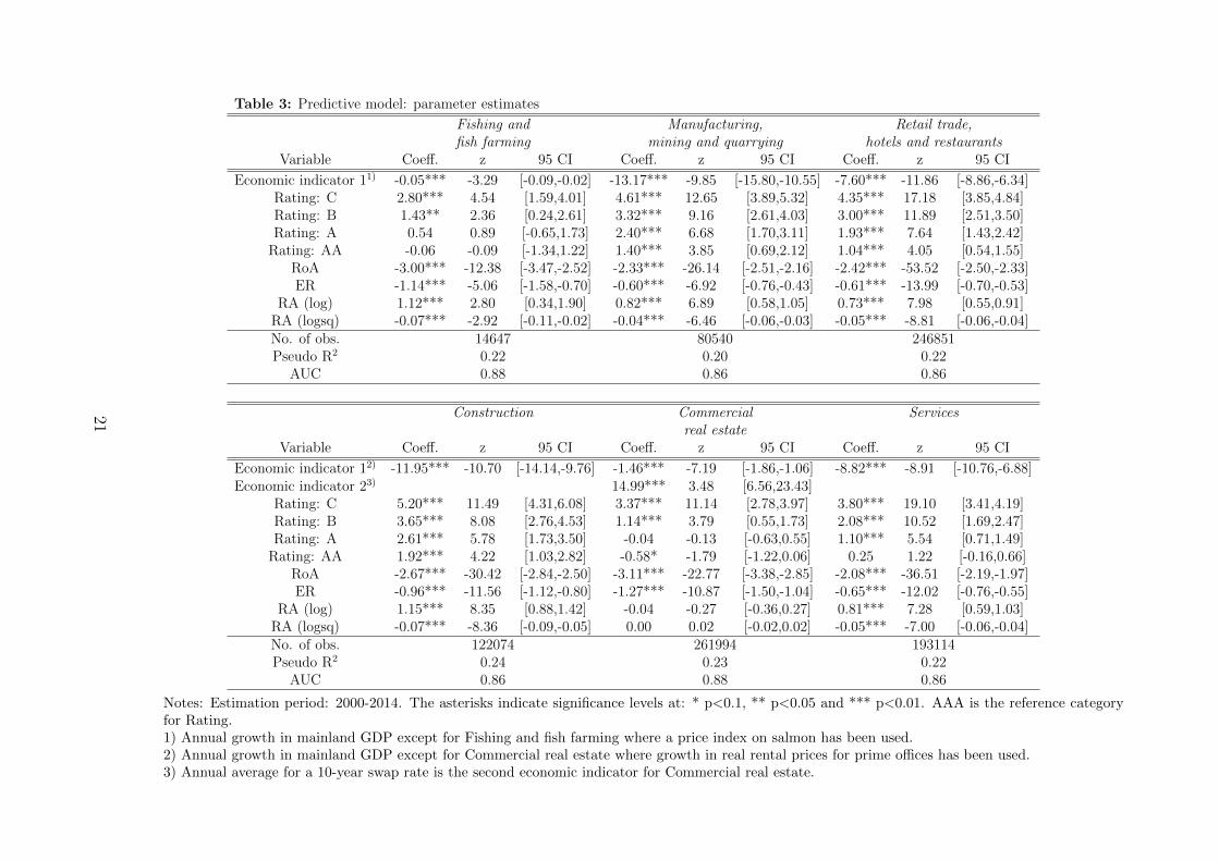
Table 3: Predictive model: parameter estimates

Fishing and Manufacturing, Retail trade,fish farming mining and quarrying hotels and restaurants

Variable Coeff. z 95 CI Coeff. z 95 CI Coeff. z 95 CI

Economic indicator 11) -0.05*** -3.29 [-0.09,-0.02] -13.17*** -9.85 [-15.80,-10.55] -7.60*** -11.86 [-8.86,-6.34]Rating: C 2.80*** 4.54 [1.59,4.01] 4.61*** 12.65 [3.89,5.32] 4.35*** 17.18 [3.85,4.84]Rating: B 1.43** 2.36 [0.24,2.61] 3.32*** 9.16 [2.61,4.03] 3.00*** 11.89 [2.51,3.50]Rating: A 0.54 0.89 [-0.65,1.73] 2.40*** 6.68 [1.70,3.11] 1.93*** 7.64 [1.43,2.42]

Rating: AA -0.06 -0.09 [-1.34,1.22] 1.40*** 3.85 [0.69,2.12] 1.04*** 4.05 [0.54,1.55]RoA -3.00*** -12.38 [-3.47,-2.52] -2.33*** -26.14 [-2.51,-2.16] -2.42*** -53.52 [-2.50,-2.33]ER -1.14*** -5.06 [-1.58,-0.70] -0.60*** -6.92 [-0.76,-0.43] -0.61*** -13.99 [-0.70,-0.53]

RA (log) 1.12*** 2.80 [0.34,1.90] 0.82*** 6.89 [0.58,1.05] 0.73*** 7.98 [0.55,0.91]RA (logsq) -0.07*** -2.92 [-0.11,-0.02] -0.04*** -6.46 [-0.06,-0.03] -0.05*** -8.81 [-0.06,-0.04]No. of obs. 14647 80540 246851Pseudo R2 0.22 0.20 0.22

AUC 0.88 0.86 0.86

Construction Commercial Servicesreal estate


Economic indicator 12) -11.95*** -10.70 [-14.14,-9.76] -1.46*** -7.19 [-1.86,-1.06] -8.82*** -8.91 [-10.76,-6.88]Economic indicator 23) 14.99*** 3.48 [6.56,23.43]

Rating: C 5.20*** 11.49 [4.31,6.08] 3.37*** 11.14 [2.78,3.97] 3.80*** 19.10 [3.41,4.19]Rating: B 3.65*** 8.08 [2.76,4.53] 1.14*** 3.79 [0.55,1.73] 2.08*** 10.52 [1.69,2.47]Rating: A 2.61*** 5.78 [1.73,3.50] -0.04 -0.13 [-0.63,0.55] 1.10*** 5.54 [0.71,1.49]

Rating: AA 1.92*** 4.22 [1.03,2.82] -0.58* -1.79 [-1.22,0.06] 0.25 1.22 [-0.16,0.66]RoA -2.67*** -30.42 [-2.84,-2.50] -3.11*** -22.77 [-3.38,-2.85] -2.08*** -36.51 [-2.19,-1.97]ER -0.96*** -11.56 [-1.12,-0.80] -1.27*** -10.87 [-1.50,-1.04] -0.65*** -12.02 [-0.76,-0.55]

RA (log) 1.15*** 8.35 [0.88,1.42] -0.04 -0.27 [-0.36,0.27] 0.81*** 7.28 [0.59,1.03]RA (logsq) -0.07*** -8.36 [-0.09,-0.05] 0.00 0.02 [-0.02,0.02] -0.05*** -7.00 [-0.06,-0.04]No. of obs. 122074 261994 193114Pseudo R2 0.24 0.23 0.22

AUC 0.86 0.88 0.86

Notes: Estimation period: 2000-2014. The asterisks indicate significance levels at: * p<0.1, ** p<0.05 and *** p<0.01. AAA is the reference categoryfor Rating.1) Annual growth in mainland GDP except for Fishing and fish farming where a price index on salmon has been used.2) Annual growth in mainland GDP except for Commercial real estate where growth in real rental prices for prime offices has been used.3) Annual average for a 10-year swap rate is the second economic indicator for Commercial real estate.

21

Table 4: Predictive model: average estimated marginal effects1)


Variable ME z 95 CI ME z 95 CI ME z 95 CI

Economic indicator 12) -0.00*** -3.23 [-0.00,-0.00] -0.27*** -9.65 [-0.33,-0.22] -0.21*** -11.83 [-0.25,-0.18]Rating: C 6.74*** 6.82 [4.81,8.68] 11.45*** 20.42 [10.35,12.55] 13.10*** 44.98 12.53,13.67]Rating: B 1.58*** 4.02 [0.81,2.35] 3.51*** 20.47 [3.17,3.84] 3.87*** 40.89 [3.69,4.06]Rating: A 0.37 1.10 [-0.29,1.03] 1.38*** 14.63 [1.19,1.56] 1.25*** 18.06 [1.12,1.39]

Rating: AA -0.03 -0.09 [-0.70,0.64] 0.43*** 6.13 [0.29,0.56] 0.40*** 6.01 [0.27,0.53]RoA -0.05*** -10.73 [-0.06,-0.04] -0.05*** -23.42 [-0.05,-0.04] -0.07*** -49.32 [-0.07,-0.06]ER -0.02*** -5.05 [-0.03,-0.01] -0.01*** -6.87 [-0.02,-0.01] -0.02*** -13.95 [-0.02,-0.01]



Economic indicator 13) -0.21*** -10.58 [-0.26,-0.18] -0.01*** -7.06 [-0.01,-0.00] -0.14*** -8.86 [-0.17,-0.11]Economic indicator 24) 0.01*** 3.46 [0.02,0.09]


Rating: AA 0.43*** 8.03 [0.33,0.54] -0.07 -1.46 [-0.17,0.02] 0.08 1.32 [-0.04,0.20]RoA -0.05*** -28.57 [-0.05,-0.04] -0.01*** -19.71 [-0.01,-0.01] -0.03*** -33.31 [-0.04,-0.03]ER -0.02*** -11.46 [-0.02,-0.01] -0.00*** -10.44 [-0.01,-0.00] -0.01*** -11.91 [-0.01,-0.01]

Notes: Estimation period: 2000-2014. The asterisks indicate significance levels at: * p<0.1, ** p<0.05 and *** p<0.01. AAA is the reference categoryfor Rating.1) Average of estimated marginal effects for each observation in percentage points of a unit change in the explanatory variables. A unit change is from0 to 1 for the rating variables and 1 percentage point for RoA and ER. For the economic indicators a unit change is 1 NOK for the salmon price indexand 1 percentage point for GDP growth, rental price growth and the swap rate, see 2), 3) and 4).2) Annual growth in mainland GDP except for Fishing and fish farming where a price index for salmon has been used.3) Annual growth in mainland GDP except for Commercial real estate where growth in rental prices for prime offices has been used.4) Annual average for a 10-year swap rate is the second economic indicator for Commercial real estate.

22

Figure 7 compares aggregate in-sample risk-weighted debt in the benchmark model

and the predictive model for 2000–2014, along with debt in bankruptcy accounts. Figure

7 also depicts – using the predictive model – the following: i) real-time nowcasts for 2015

based on information dated end of 2015, ii) nowcasts for 2016 based on information dated

2016Q3 and iii) forecast for 2017 based on information also dated 2016Q3. Figure 8,

charts (a)–(f) displays the same information as Figure 7, but separately for each of the

six industries. From these figures, we conclude that the benchmark and predictive model

yield remarkably similar in-sample aggregate predictions.10

Figure 7: Aggregated risk-weighted debt (benchmark model and predictive model) andbank debt in bankruptcy accounts. Percent. 2000–20171)

0

0.5

1

1.5

2

0

0.5

1

1.5

2

2000 2002 2004 2006 2008 2010 2012 2014 2016


Benchmark model

Predictive model

1) Projections (dotted lines)

Figure 9 depicts a decomposition of aggregate risk-weighted debt – calculated using

the predictive model – into contributions from the six industries. Although Commercial

real estate has very low risk-weighted debt, the industry’s contribution to the aggregate is

significant because of its high share of total bank debt. Note that the actual contribution

to debt in bankruptcy accounts and risk-weighted debt differ substantially for some years

and industries, e.g. Fishing and fish farming in 2003.

10Also, with regard to both the parameter estimates and the goodness-of-fit measures (Pseudo R2 andAUC), there are no substantial differences between the benchmark model reported in Table A.1 and thepredictive model reported in Table 3.

23

Figure 8: Risk-weighted debt (benchmark model and predictive model) and bank debtin bankruptcy accounts. Percent. 2000–2017. Dotted lines are projections





Benchmark model

Predictive model

24

Figure 9: Contribution from each industry to aggregated risk-weighted debt. Predictivemodel. Percent. 2000–20171)

0

0.5

1

1.5

0

0.5

1

1.5

2000 2002 2004 2006 2008 2010 2012 2014 2016

ServicesCommercial real estateConstructionRetail trade, hotels and restaurantsManufacturing, mining and quarryingFishing and fish farming


4.4 Out-of-sample performance and alternative specifications

Out-of-sample prediction of risk-weighted debt We have demonstrated above that

the in-sample performance of the predictive model with economic indicators is good com-

pared to a benchmark model where year-dummies were used to fit annual aggregate

bankruptcy rates (perfectly) at the industry level. However, good in-sample performance

is no guarantee against poor real-time nowcasting or forecasting properties. If, for exam-

ple, the estimated relations between the economic indicators at the industry level and the

dependent variable are unstable, the model may quickly break down when used to make

predictions out-of-sample.

In order to evaluate out-of-sample properties, let θSt denote the estimate of θS (see

(3)) based on firm-level bankruptcy data until year t, i.e., using Bi1, ..., Bit, with t ≤ T .

Given θSt , it is possible to use the estimated model to make out-of-sample predictions.

Estimated risk-weighted debt, RW St+1+s|t+1(θ

St ), is a nowcast when s = 0 and a one-year

ahead forecast when s = 1.

We now compare two measures of risk-weighted debt for a given year t+1: i) in-sample

25

risk-weighted debt, RW St+1|t+1(θ

ST ), where data for 2000–2014 were used to estimate θS,

and ii) real time-nowcasts, RW St+1|t+1(θ

St ), where data up until year t is used to estimate

θS. In both cases, explanatory variables included in the information set at the end of year

t+ 1 were used to calculate risk-weighted debt.

We illustrate the results in Figures 10–11. Starting with t = T = 2014, which is

currently (2016Q3) our last available year, the two curves corresponding to the predictive

model are identical, as RW St+1|t+1(θ

ST ) by definition is a real-time nowcast in this case.

Then we repeat the calculations for t = T − 1, T − 2, ... . The smallest t for which

RW St+1|t+1(θ

St ) is displayed is t = 2007. Then, to calculate the corresponding real-time

nowcast of risk-weighted debt, only data for 2000–2006 were used in the estimation. If

we use an even shorter estimation period, the estimated coefficients of the economic

indicators become erratic and unstable. The main impression is that during the period

2007–2015, the agreement between in-sample and out-of-sample risk-weighted debt is

good. The largest discrepancies are found during the financial crisis in the industries

Construction and Services. The out-of-sample nowcasts of bankruptcy probabilities were

in these instances somewhat higher than the actual bankruptcy outcome during the crisis.

Figure 10: Aggregated risk-weighted debt. In-sample benchmark model, in-samplepredictive model and out-of-sample nowcasts. Percent. 2000–2015

0

0.5

1

1.5

0

0.5

1

1.5

2000 2002 2004 2006 2008 2010 2012 2014

In-sample benchmark model

In-sample predictive model

Out-of-sample nowcasts

26

Figure 11: Risk-weighted debt. In-sample benchmark model, in-sample predictive modeland out-of-sample nowcasts. Percent. 2000–2015




In-sample benchmark model

In-sample predictive model

Out-of-sample nowcasts

27

Alternative specifications To make further comparisons, we show in Figure 12

aggregated risk-weighted debt from our preferred (predictive) model together with risk-

weighted debt from two alternative specifications where we i) only include economic indi-

cators, or ii) include economic indicators together with rating variables. Thus, both alter-

native specifications exclude the financial accounting variables. We see that specification

i) substantially overstates bankruptcy debt. Also ii) overstates bankruptcy debt, but less

so than i). The predictive model gives the best results compared to realised bankruptcy

debt. To interpret these results, it is important to recognise that a model with only

industry-wide variables accommodates no firm heterogeneity with respect to bankruptcy

probability. That is, in a given year risk-weighted debt equals average bankruptcy prob-

ability. Including firm-specific information in the form of rating, as in specification ii),

gives lower risk-weighted debt, reflecting a negative correlation between (firm-specific)

probabilities and shares of debt (recall that risk-weighted debt is the debt-weighted aver-

age bankruptcy probability; cf. Footnote 2). Our preferred predictive model discriminates

even more between firms than do ii), leading to further lowered risk-weighted debt. The

main reason is the impact of total assets: very large firms have lower bankruptcy proba-

bilities and more debt than small firms and this relationship is not fully picked up by the

rating categories.

Figure 12 reveals that both groups of firm-specific variables contribute substantially to

predicted risk-weighted debt at the industry level and that excluding financial accounting

variables and/or the rating variables from our model leads to serious omitted variable

bias.

Further specifications issues are addressed in Appendix B.

28

Figure 12: Aggregated risk-weighted debt. Predictive model with different model spec-ifications. Percent. 2000–20171)

0

1

2

3

0

1

2

3

2000 2002 2004 2006 2008 2010 2012 2014 2016


Predictive model

Model with economic indicator

Model with rating variables and economic indicator

1) Projections (dotted lines)

5 Conclusions

In this paper we have proposed a method for assessing the risk of losses on bank lend-

ing to the non-financial corporate sector based on bankruptcy probability modelling. A

strong link between bankruptcies and bank losses has been demonstrated in the previous

literature, e.g. in Norges Bank’s SEBRA model and in numerous theoretical papers based

on option pricing theory. Moreover, bank losses according to bank statistics and debt in

bankruptcy accounts display a similar pattern over time in most industries.

We have estimated bankruptcy models for different industries and attached a risk

weight to each firm’s debt in a given year. The risk weight is equal to the estimated

probability of bankruptcy during the year given the information at the time of prediction.

By summing all risk-weighted debt in an industry, we obtained a prediction of the share

of debt in bankruptcy accounts in a given year.

We have discussed and proposed solutions to timeliness problems due to a considerable

lag in the publication of bankruptcy and accounts data. A key feature of our approach

is the inclusion of economic indicators at the industry level, observed in real time, as

explanatory variables alongside standard financial accounting and real-time credit rating

information in a predictive model which is useful for nowcasting and forecasting. We found

29

that historically, during 2000–2014, there is good correspondence between our estimated

measure of risk-weighted debt and actual debt in bankruptcy accounts.

To evaluate the out-of-sample properties of our approach, we have compared two

measures of risk-weighted debt for any given year (t+1): i) in-sample risk-weighted debt,

where the whole data period (2000–2014) was used to estimate the model, and ii) real-

time nowcasts, where only data up until year t were used. In both cases, risk-weighted

debt was calculated using explanatory variables included in the information set at the end

of year t + 1. The out-of-sample nowcasts of the model are generally close to in-sample

risk-weighted debt after 2006 (using at least seven years of data). The most notable

discrepancies are found in some industries during the financial crisis, where out-of-sample

nowcasts are higher than in-sample risk-weighted debt.

We have also compared risk-weighted debt from our preferred (predictive) model to

risk-weighted debt from two alternative specifications were we i) included only industry-

wide economic indicators, or ii) included these indicators together with rating variables

(excluding financial accounting variables). Our analyses show that excluding financial

accounting and/or rating variables from our model lead to a severely misspecified model

due to omitted variable bias. The main source of the bias seems to be the negative

correlation between firm-specific shares of debt and bankruptcy probabilities. Hence it

is important to have a model that is able to predict bankruptcy probabilities at the firm

level even if the main focus is on aggregate measures of risk-weighted debt.

There are issues that are either not discussed or not fully resolved in this paper that

might be addressed in future work. One is the application of our framework for stress

testing purposes. This would require projecting rating categories and other firm specific

variables as functions of macroeconomic scenarios, which is challenging. Another issue

is the utilization of real-time bankruptcy registrations (i.e., during the same year) to

improve nowcasts, i.e. by combining preliminary data on bankruptcies with our (ex ante)

statistical model. We envisage that this can be done in a way that is similar to Bayesian

information updating.

30

References

[1] Altman, E.I. (1968): Financial ratios, discriminant analysis and the prediction of

corporate bankruptcy. Journal of Finance, 23, 589–609.

[2] Altman, E.I., Haldeman, R. and P. Narayanan (1977): ZETA analysis: A new model

to identify bankruptcy risk of corporations: Journal of Banking and Finance, 10,

29–54.

[3] Beaver, W.H. (1966): Financial ratios as predictors of failure. Journal of Accounting

Research, 71–111.

[4] Bernhardsen, E. (2001): A model of bankruptcy prediction. Working Paper 2001/10,

Norges Bank.

[5] Bernhardsen, E. and K. Larsen (2007): Modelling credit risk in the enterprise sector -

further development of the SEBRA model. Economic Bulletin 2007/3, Norges Bank,

78, 102–108.

[6] Foster, L., J. Haltiwanger and C. Syverson (2008): Reallocation, Firm Turnover, and

Efficiency: Selection on Productivity or Profitability? American Economic Review,

98(1), 394–425.

[7] Golombek, R. and A. Raknerud (2015): Exit dynamics of start-up firms. Does profit

matter? CESifo Working Paper Series 5172.

[8] Mata, J., P. Portugal and P. Guimaraes (1995): The survival of new plants: Start-up

conditions and post-entry evolution. International Journal of Industrial Organization,

13 (4), 459–481.

[9] Merton, R.C. (1974): On the pricing of corporate debt: risk structure of interest

rates. Journal of Finance, 29, 449–470.

31

[10] Olley, G. S. and A. Pakes (1996): The dynamics of productivity in the telecommu-

nications equipment industry. Econometrica, 64, 1263–1297.

[11] Scott, K. (1981): The probability of bankruptcy: A comparison of empirical predic-

tions and theoretical models. Journal of Banking and Finance, 317–344.

[12] Kragh-Sørensen,K and H. Solheim (2014): What do banks lose money on during

crises? Staff Memo 3/2014, Norges Bank.

[13] van Erkel, A. R. and P. M. T. Pattynama (1998): Receiver operating characteristic

(ROC) analysis: Basic principles and applications in radiology. European Journal of

Radiology, 27, 88.

[14] Wilcox, J.W.: A prediction of business failure using accounting data: Journal of

Accounting Literature, 2, 163–179.

[15] Wu, Y., Gaunt, C. and S. Gray (2010): A comparison of alternative bankruptcy

prediction models. Journal of Contemporary Accounting & Economics, 6, 34–45.

32

Appendix A: Supplementary tables and figures

Figure A.1: ROC curves - Predictive model




33

Table A.1: Benchmark model: parameter estimates



Rating: C 2.79*** 4.53 [1.58,4.00] 4.59*** 12.59 [3.87,5.30] 4.34*** 17.14 [3.84,4.83]Rating: B 1.40** 2.32 [0.22,2.58] 3.31*** 9.12 [2.60,4.02] 3.00*** 11.88 [2.50,3.49]Rating: A 0.46 0.77 [-0.72,1.65] 2.39*** 6.62 [1.68,3.09] 1.93*** 7.63 [1.43,2.42]

Rating: AA -0.11 -0.17 [-1.39,1.17] 1.39*** 3.82 [0.68,2.11] 1.04*** 4.04 [0.54,1.55]RoA -2.97*** -11.92 [-3.46,-2.48] -2.33*** -26.14 [-2.51,-2.16] -2.42*** -53.55 [-2.51,-2.33]ER -1.18*** -5.06 [-1.63,-0.72] -0.61*** -7.09 [-0.78,-0.44] -0.62*** -14.16 [-0.70,-0.53]

RA (log) 0.96** 2.54 [0.22,1.70] 0.76*** 6.37 [0.53,0.99] 0.78*** 7.64 [0.58,0.98]RA (logsq) -0.06*** -2.65 [-0.10,-0.01] -0.04*** -5.91 [-0.05,-0.03] -0.06*** -8.32 [-0.07,-0.04]No. of obs. 14647 80540 246851Pseudo R2 0.24 0.21 0.22

AUC 0.88 0.86 0.86




Rating: AA 1.92*** 4.22 [1.03,2.81] -0.59* -1.82 [-1.22,0.05] 0.22 1.07 [-0.19,0.63]RoA -2.67*** -30.29 [-2.84,-2.49] -3.13*** -22.68 [-3.40,-2.86] -2.06*** -36.01 [-2.17,-1.95]ER -0.96*** -11.60 [-1.13,-0.80] -1.26*** -10.84 [-1.49,-1.04] -0.65*** -11.92 [-0.76,-0.54]

RA (log) 1.09*** 7.58 [0.81,1.37] -0.06 -0.35 [-0.37,0.26] 0.62*** 6.04 [0.42,0.83]RA (logsq) -0.07*** -7.54 [-0.08,-0.05] 0.00 0.10 [-0.02,0.02] -0.04*** -5.74 [-0.05,-0.02]No. of obs. 122074 261994 193114Pseudo R2 0.24 0.23 0.23

AUC 0.86 0.87 0.86

Notes: Estimation period: 2000-2014. The asterisks indicate significance levels at: * p<0.1, ** p<0.05 and *** p<0.01. AAA is the reference categoryfor Rating.

34

Table A.2: Benchmark model: average estimated marginal effects1)



Rating: C 6.83*** 6.76 [4.85,8.81] 11.37*** 20.44 [10.28,12.46] 12.99*** 44.76 [12.42,13.56]Rating: B 1.58*** 3.91 [0.79,2.37] 3.50*** 20.44 [3.17,3.84] 3.87*** 40.73 [3.68,4.05]Rating: A 0.32 0.92 [-0.36,1.00] 1.37*** 14.52 [1.18,1.55] 1.26*** 18.03 [1.12,1.39]

Rating: AA -0.06 -0.16 [-0.75,0.63] 0.43*** 6.07 [0.29,0.56] 0.40*** 6.00 [0.27,0.53]RoA -0.05*** -10.5 [-0.06,-0.04] -0.05*** -23.41 [-0.05,-0.04] -0.07*** -49.36 [-0.07,-0.06]ER -0.02*** -5.02 [-0.03,-0.01] -0.01*** -7.04 [-0.02,-0.01] -0.02*** -14.12 [-0.02,-0.01]




Rating: AA 0.043*** 8.02 [0.33,0.54] -0.07 -1.48 [-0.17,0.02] 0.07 1.15 [-0.05,0.20]RoA -0.05*** -28.47 [-0.05,-0.04] -0.01*** -19.65 [-0.01,-0.01] -0.03*** -32.94 [-0.04,-0.03]ER -0.02*** -11.5 [-0.02,-0.01] -0.00*** -10.42 [-0.01,-0.00] -0.01*** -11.82 [-0.01,-0.01]

Notes: Estimation period: 2000-2014. The asterisks indicate significance levels at: * p<0.1, ** p<0.05 and *** p<0.01. AAA is the reference categoryfor Rating.1) Average of estimated marginal effects for each observation in percentage points of a unit change in the explanatory variables. A unit change is from 0to 1 for the rating variables and 1 percentage point for RoA and ER.

35

Appendix B: Further specification issues

The timing of the explanatory variables The latest available information at

the end (“last day”) of year t for predicting pi,t+1 (forecasting) is (xi,t−1, rit, zSt+1|t) (for

simplicity of notation we ignore now that we actually observe the ER from the outgoing

balance of the previous year). Then, pi,t+1|t in (3) simplifies to:

ln(pi,t+1|t(θ

S)

1− pi,t+1|t(θS)) = βSxi,t−1 + πSrit + µS + ρS zSt+1|t (A.1)

To obtain Equation (A.1) from (3): first set q = 4, then replace t + 1 with t and finally

set xi,t|t = xi,t−1. An alternative model would be to estimate Equation (A.1) directly

instead of first estimating (1)–(2) and then replace xit with the trivial prediction xi,t|t =

xi,t−1. Furthermore, to use all available information for nowcasting suggests the regression

equation:

ln(pi,t|t(θ

S)

1− pi,t|t(θS)) = β

∗Sxi,t−1 + π∗Srit + µ

∗S + ρ∗SzSt (A.2)

Arguably, Equation (A.1) is more intuitive than (3) for forecasting purposes and we

will discuss its properties below.11 On the other hand, Equation (A.2) is not a valid

regression equation because of reverse causality: the rating of a firm dated the same year

as the dependent variable could be a direct consequence of the latter. The reason is that

a rating from the same year tells us that the firm is probably still active. Conversely, a

firm on the verge of collapse may be downgraded if this is known to the rating agency.

A bankruptcy could also be registered in the same year as it occurs. Recall that in our

preferred model, bankruptcy probability is the conditional probability of bankruptcy in

the future year for an active firm given firm-specific variables dated at the end of the

current year.

To evaluate the properties of our original model against the alternative (A.1), we

11As discussed in Section 4, information about xi,t−1 is already incorporated into the rating, rit,whereas xit includes new information. Thus our preferred specification accommodates more informationand allows any information updating about xit during year t+1, for example utilizing quarterly accountsfrom public limited companies. It is outside the scope of this paper to explore this possibility, but thepoint is that no new estimation is needed to accommodate an arbitrary information updating scheme.

36

estimate (A.1) directly and compare its in-sample implied forecasts of risk-weighted debt

with RW St+1|t(θ

ST ) from our predictive model. To eliminate the uncertainty stemming from

zSt+1|t, we assume for simplicity that zSt+1|t = zSt+1 (“perfect foresight”). To summarise the

estimation results (not displayed): both Pseudo R2 and AUC are decreased by 0.02–0.04

points in the alternative model compared to the original model. The impacts of the

economic indicators and the rating variables (especially the dummy for rating category

C), measured either by the magnitude of the average marginal effects or the z values, have

increased moderately. On the other hand, the impact of the financial variables is reduced,

with lower z values than in the original model, although they are still significant. Figure

B.1 reveals that predicted risk-weighted debt from the alternative model is very similar

to our preferred (predictive) model.

Figure B.1: Aggregated risk-weighted debt. Predictive model (forecasts), alternativeforecast model and bank debt in bankruptcy accounts. Percent. 2000–2015

0

0.5

1

1.5

2

0

0.5

1

1.5

2

2001 2003 2005 2007 2009 2011 2013 2015

Alternative forecast model

Predictive model (forecasts)

Bank debt in bankruptcy accounts¹

1) Projection for 2015 (dotted line)

Utilizing early bankruptcy registration Overall, typically about 15–20 percent

of the bankruptcies that we date t+ 1 is registered by t+ 3/4, i.e., Q3 of year t+ 1 (only

by t+2 is the registration complete). This means that there is a share of the bankruptcies

of year t + 1 that are “revealed early”. To see how this information can be utilised, it

37

is convenient to frame our model using Bayesian terminology. First, the probability of

bankruptcy from our predictive model, Pr(Bi,t+1 = 1) (Bi,t+1 is the bankruptcy indicator

as defined before), can be termed the prior probability. The information updating problem

is then to calculate the posterior probability that Bi,t+1 = 1 given the early bankruptcy

registrations. Obviously, the posterior bankruptcy probability among the bankrupt firms

is 1. Second, the posterior bankruptcy probability of the remaining firms must be altered

relative to their prior probability to reflect that they were not (yet) registered as bankrupt.

To study this information-updating problem formally, assume that

χi,t+1 = Bi,t+1Ui,t+1

where Ui,t+1 is an indicator which is 1 if the value of Bi,t+1 is revealed by t+ 3/4. Then,

χi,t+1 is a binary variable which is 1 if and only if Bi,t+1 = 1 and Ui,t+1 = 1 (indicating

an early bankruptcy registration). Assuming that αi,t+1 ≡ Pr(Ui,t+1 = 1|Bi,t+1 = 1) is a

known probability, it is straightforward to show, using Bayes’ formula, that

Pr(Bi,t+1 = 1|χi,t+1 = 0) =αi,t+1 Pr(Bi,t+1 = 1)

αi,t+1 Pr(Bi,t+1 = 1) + Pr(Bi,t+1 = 0)

To apply this formula in practice, αi,t+1 could be estimated. However, using the his-

toric average as a common estimator over all firms and years, our attempts to calculate

Pr(Bi,t+1 = 1|χi,t+1 = 0) led to erratic and unreliable results. One could imagine a

Bayesian version of this method, assuming a prior distribution on αi,t+1. Although inter-

esting, it is outside the scope of this paper to pursue this approach further.

38

Business

Credit risk (Swed regulator)