Embed Size (px)
DESCRIPTION
Citation preview


Special Relativity


Michael Tsamparlis
Special Relativity
An Introduction with 200 Problemsand Solutions
123
Dr. Michael TsamparlisDepartment of Astrophysics, Astronomy and MechanicsUniversity of AthensPanepistimiopolisGR 157 84 [email protected]
Additional material to this book can be downloaded from http://extra.springer.com.Password: 978-3-642-03836-5
ISBN 978-3-642-03836-5 e-ISBN 978-3-642-03837-2DOI 10.1007/978-3-642-03837-2Springer Heidelberg Dordrecht London New York
Library of Congress Control Number: 2009940408
c© Springer-Verlag Berlin Heidelberg 2010This work is subject to copyright. All rights are reserved, whether the whole or part of the material isconcerned, specifically the rights of translation, reprinting, reuse of illustrations, recitation, broadcasting,reproduction on microfilm or in any other way, and storage in data banks. Duplication of this publicationor parts thereof is permitted only under the provisions of the German Copyright Law of September 9,1965, in its current version, and permission for use must always be obtained from Springer. Violationsare liable to prosecution under the German Copyright Law.The use of general descriptive names, registered names, trademarks, etc. in this publication does notimply, even in the absence of a specific statement, that such names are exempt from the relevant protectivelaws and regulations and therefore free for general use.
Cover design: eStudio Calamar S.L.
Printed on acid-free paper
Springer is part of Springer Science+Business Media (www.springer.com)

Omnia mea mecum feroWhatever I possess I bear with me


Preface
Writing a new book on the classic subject of Special Relativity, on which numerousimportant physicists have contributed and many books have already been written,can be like adding another epicycle to the Ptolemaic cosmology. Furthermore, it isour belief that if a book has no new elements, but simply repeats what is writtenin the existing literature, perhaps with a different style, then this is not enoughto justify its publication. However, after having spent a number of years, both inclass and research with relativity, I have come to the conclusion that there exists aplace for a new book. Since it appears that somewhere along the way, mathemat-ics may have obscured and prevailed to the degree that we tend to teach relativity(and I believe, theoretical physics) simply using “heavier” mathematics without theinspiration and the mastery of the classic physicists of the last century. Moreovercurrent trends encourage the application of techniques in producing quick resultsand not tedious conceptual approaches resulting in long-lasting reasoning. On theother hand, physics cannot be done a la carte stripped from philosophy, or, to put itin a simple but dramatic context
A building is not an accumulation of stones!
As a result of the above, a major aim in the writing of this book has been thedistinction between the mathematics of Minkowski space and the physics of rel-ativity. This is necessary for one to understand the physics of the theory and notstay with the geometry, which by itself is a very elegant and attractive tool. There-fore in the first chapter we develop the mathematics needed for the statement anddevelopment of the theory. The approach is limited and concise but sufficient for thepurposes it is supposed to serve. Having finished with the mathematical concepts wecontinue with the foundation of the physical theory. Chapter 2 sets the frameworkon the scope and the structure of a theory of physics. We introduce the principleof relativity and the covariance principle, both principles being keystones in everytheory of physics. Subsequently we apply the scenario first to formulate NewtonianPhysics (Chap. 3) and then Special Relativity (Chap. 4). The formulation of Newto-nian Physics is done in a relativistic way, in order to prepare the ground for a properunderstanding of the parallel formulation of Special Relativity.
Having founded the theory we continue with its application. The approach is sys-tematic in the sense that we develop the theory by means of a stepwise introduction
vii

viii Preface
of new physical quantities. Special Relativity being a kinematic theory forces usto consider as the fundamental quantity the position four-vector. This is done inChap. 5 where we define the relativistic measurement of the position four-vector bymeans of the process of chronometry. To relate the theory with Newtonian reality,we introduce rules, which identify Newtonian space and Newtonian time in SpecialRelativity.
In Chaps. 6 and 7 we introduce the remaining elements of kinematics, that is,the four-velocity and the four-acceleration. We discuss the well-known relativisticcomposition law for the three-velocities and show that it is equivalent to the Ein-stein relativity principle, that is, the Lorentz transformation. In the chapter of four-acceleration we introduce the concept of synchronization which is a key concept inthe relativistic description of motion. Finally, we discuss the phenomenon of accel-eration redshift which together with some other applications of four-accelerationshows that here the limits of Special Relativity are reached and one must go over toGeneral Relativity.
After the presentation of kinematics, in Chap. 8 we discuss various paradoxes,which play an important role in the physical understanding of the theory. We chooseto present paradoxes which are not well known, as for example, it is the twin para-dox.
In Chap. 9 we introduce the (relativistic) mass and the four-momentum by meansof which we distinguish the particles in massive particles and luxons (photons).
Chapter 10 is the most useful chapter of this book, because it concerns relativisticreactions, where the use of Special Relativity is indispensible. This chapter containsmany examples in order to familiarize the student with a tool, that will be necessaryto other major courses such as particle physics and high energy physics.
In Chap. 11 we commence the dynamics of Special Relativity by the introductionof the four-force. We discuss many practical problems and use the tetrahedron ofFrenet–Serret to compute the generic form of the four-force. We show how the well-known four-forces comply with the generic form.
In Chap. 12 we introduce the concept of covariant decomposition of a tensoralong a vector and give the basic results concerning the 1 + 3 decomposition inMinkowski space. The mathematics of this chapter is necessary in order to under-stand properly the relativistic physics. It is used extensively in General Relativitybut up to now we have not seen its explicit appearance in Special Relativity, eventhough it is a powerful and natural tool both for the theory and the applications.
Chapter 13 is the next pillar of Special Relativity, that is, electromagnetism. Wepresent in a concise way the standard vector form of electromagnetism and subse-quently we are led to the four formalism formulation as a natural consequence. Afterdiscussing the standard material on the subject (four-potential, electromagnetic fieldtensor, etc.) we continue with lesser known material, such as the tensor formulationof Ohm’s law and the 1+3 decomposition of Maxwell’s equations. The reason whywe introduce these more advanced topics is that we wish to prepare the student forcourses on important subjects such as relativistic magnetohydrodynamics (RMHD).
The rest of the book concerns topics which, to our knowledge, cannot be foundin the existing books on Special Relativity yet. In Chap. 14 we discuss the concept

Preface ix
of spin as a natural result of the generalization of the angular momentum tensorin Special Relativity. We follow a formal mathematical procedure, which revealswhat “the spin is” without the use of the quantum field theory. As an application, wediscuss the motion of a charged particle with spin in a homogeneous electromagneticfield and recover the well-known results in the literature.
Chapter 15 deals with the covariant Lorentz transformation, a form which is notwidely known. All four types of Lorentz transformations are produced in covariantform and the results are applied to applications involving the geometry of three-velocity space, the composition of Lorentz transformations, etc.
Finally, in Chap. 16 we study the reaction A+ B −→ C + D in a fully covariantform. The results are generic and can be used to develop software which will solvesuch reactions directly, provided one introduces the right data.
The book includes numerous exercises and solved problems, plenty of whichsupplement the theory and can be useful to the reader on many occasions. In addi-tion, a large number of problems, carefully classified in all topics accompany thebook.
The above does not cover all topics we would like to consider. One such topicis relativistic waves, which leads to the introduction of De Broglie waves and sub-sequently to the foundation of quantum mechanics. A second topic is relativistichydrodynamics and its extension to RMHD. However, one has to draw a line some-where and leave the future to take care of things to be done.
Looking back at the long hours over the many years which were necessary forthe preparation of this book, I cannot help feeling that, perhaps, I should not haveundertaken the project. However, I feel that it would be unfair to all the students andcolleagues, who for more that 30 years have helped me to understand and developthe relativistic ideas, to find and solve problems, and in general to keep my interestalive. Therefore the present book is a collective work and my role has been simplyto compile these experiences. I do not mention specific names – the list would betoo long, and I will certainly forget quite a few – but they know and I know, and thatis enough.
I close this preface, with an apology to my family for the long working hours;that I was kept away from them for writing this book and I would like to thank themfor their continuous support and understanding.
Athens, Greece Michael TsamparlisOctober 2009


Contents
1 Mathematical Part . . . . . . . . . . . . . . . . . . . . . . . . . . . . . . . . . . . . . . . . . . . . . 11.1 Introduction . . . . . . . . . . . . . . . . . . . . . . . . . . . . . . . . . . . . . . . . . . . . . 11.2 Elements From the Theory of Linear Spaces . . . . . . . . . . . . . . . . . . 2
1.2.1 Coordinate Transformations . . . . . . . . . . . . . . . . . . . . . . . 21.3 Inner Product – Metric . . . . . . . . . . . . . . . . . . . . . . . . . . . . . . . . . . . . 61.4 Tensors . . . . . . . . . . . . . . . . . . . . . . . . . . . . . . . . . . . . . . . . . . . . . . . . . 10
1.4.1 Operations of Tensors . . . . . . . . . . . . . . . . . . . . . . . . . . . . 131.5 The Case of Euclidean Geometry . . . . . . . . . . . . . . . . . . . . . . . . . . . 141.6 The Lorentz Geometry . . . . . . . . . . . . . . . . . . . . . . . . . . . . . . . . . . . . 17
1.6.1 Lorentz Transformations . . . . . . . . . . . . . . . . . . . . . . . . . . 181.7 Algebraic Determination of the General Vector Lorentz
Transformation . . . . . . . . . . . . . . . . . . . . . . . . . . . . . . . . . . . . . . . . . . 261.8 The Kinematic Interpretation of the General Lorentz
Transformation . . . . . . . . . . . . . . . . . . . . . . . . . . . . . . . . . . . . . . . . . . 401.8.1 Relativistic Parallelism of Space Axes . . . . . . . . . . . . . . . 401.8.2 The Kinematic Interpretation of Lorentz Transformation 42
1.9 The Geometry of the Boost . . . . . . . . . . . . . . . . . . . . . . . . . . . . . . . . 431.10 Characteristic Frames of Four-Vectors . . . . . . . . . . . . . . . . . . . . . . . 48
1.10.1 Proper Frame of a Timelike Four-Vector . . . . . . . . . . . . . 481.10.2 Characteristic Frame of a Spacelike Four-Vector . . . . . . 49
1.11 Particle Four-Vectors . . . . . . . . . . . . . . . . . . . . . . . . . . . . . . . . . . . . . . 501.12 The Center System (CS) of a System of Particle Four-Vectors . . . . 52
2 The Structure of the Theories of Physics . . . . . . . . . . . . . . . . . . . . . . . . . . 552.1 Introduction . . . . . . . . . . . . . . . . . . . . . . . . . . . . . . . . . . . . . . . . . . . . . 552.2 The Role of Physics . . . . . . . . . . . . . . . . . . . . . . . . . . . . . . . . . . . . . . 562.3 The Structure of a Theory of Physics . . . . . . . . . . . . . . . . . . . . . . . . 592.4 Physical Quantities and Reality of a Theory of Physics . . . . . . . . . 602.5 Inertial Observers . . . . . . . . . . . . . . . . . . . . . . . . . . . . . . . . . . . . . . . . 622.6 Geometrization of the Principle of Relativity . . . . . . . . . . . . . . . . . . 63
2.6.1 Principle of Inertia . . . . . . . . . . . . . . . . . . . . . . . . . . . . . . . 632.6.2 The Covariance Principle . . . . . . . . . . . . . . . . . . . . . . . . . 64
2.7 Relativity and the Predictions of a Theory . . . . . . . . . . . . . . . . . . . . 66
xi

xii Contents
3 Newtonian Physics . . . . . . . . . . . . . . . . . . . . . . . . . . . . . . . . . . . . . . . . . . . . . 673.1 Introduction . . . . . . . . . . . . . . . . . . . . . . . . . . . . . . . . . . . . . . . . . . . . . 673.2 Newtonian Kinematics . . . . . . . . . . . . . . . . . . . . . . . . . . . . . . . . . . . . 68
3.2.1 Mass Point . . . . . . . . . . . . . . . . . . . . . . . . . . . . . . . . . . . . . 683.2.2 Space . . . . . . . . . . . . . . . . . . . . . . . . . . . . . . . . . . . . . . . . . . 693.2.3 Time . . . . . . . . . . . . . . . . . . . . . . . . . . . . . . . . . . . . . . . . . . . 71
3.3 Newtonian Inertial Observers . . . . . . . . . . . . . . . . . . . . . . . . . . . . . . . 743.3.1 Determination of Newtonian Inertial Observers . . . . . . . 753.3.2 Measurement of the Position Vector . . . . . . . . . . . . . . . . 77
3.4 Galileo Principle of Relativity . . . . . . . . . . . . . . . . . . . . . . . . . . . . . . 783.5 Galileo Transformations for Space and Time – Newtonian
Physical Quantities . . . . . . . . . . . . . . . . . . . . . . . . . . . . . . . . . . . . . . . 793.5.1 Galileo Covariant Principle: Part I . . . . . . . . . . . . . . . . . . 793.5.2 Galileo Principle of Communication . . . . . . . . . . . . . . . . 80
3.6 Newtonian Physical Quantities. The Covariance Principle . . . . . . . 813.6.1 Galileo Covariance Principle: Part II . . . . . . . . . . . . . . . . 81
3.7 Newtonian Composition Law of Vectors . . . . . . . . . . . . . . . . . . . . . 823.8 Newtonian Dynamics . . . . . . . . . . . . . . . . . . . . . . . . . . . . . . . . . . . . . 83
3.8.1 Law of Conservation of Linear Momentum . . . . . . . . . . 84
4 The Foundation of Special Relativity . . . . . . . . . . . . . . . . . . . . . . . . . . . . . 874.1 Introduction . . . . . . . . . . . . . . . . . . . . . . . . . . . . . . . . . . . . . . . . . . . . . 874.2 Light and the Galileo Principle of Relativity . . . . . . . . . . . . . . . . . . 88
4.2.1 The Existence of Non-Newtonian Physical Quantities . . 884.2.2 The Limit of Special Relativity to Newtonian Physics . . 89
4.3 The Physical Role of the Speed of Light . . . . . . . . . . . . . . . . . . . . . . 924.4 The Physical Definition of Spacetime . . . . . . . . . . . . . . . . . . . . . . . . 93
4.4.1 The Events . . . . . . . . . . . . . . . . . . . . . . . . . . . . . . . . . . . . . 944.4.2 The Geometry of Spacetime . . . . . . . . . . . . . . . . . . . . . . . 94
4.5 Structures in Minkowski Space . . . . . . . . . . . . . . . . . . . . . . . . . . . . . 964.5.1 The Light Cone . . . . . . . . . . . . . . . . . . . . . . . . . . . . . . . . . . 964.5.2 World Lines . . . . . . . . . . . . . . . . . . . . . . . . . . . . . . . . . . . . 974.5.3 Curves in Minkowski Space . . . . . . . . . . . . . . . . . . . . . . . 984.5.4 Geometric Definition of Relativistic Inertial
Observers (RIO) . . . . . . . . . . . . . . . . . . . . . . . . . . . . . . . . 994.5.5 Proper Time . . . . . . . . . . . . . . . . . . . . . . . . . . . . . . . . . . . . 994.5.6 The Proper Frame of a RIO . . . . . . . . . . . . . . . . . . . . . . . . 1004.5.7 Proper or Rest Space . . . . . . . . . . . . . . . . . . . . . . . . . . . . . 101
4.6 Spacetime Description of Motion . . . . . . . . . . . . . . . . . . . . . . . . . . . 1024.6.1 The Physical Definition of a RIO . . . . . . . . . . . . . . . . . . . 1034.6.2 Relativistic Measurement of the Position Vector . . . . . . 1044.6.3 The Physical Definition of an LRIO. . . . . . . . . . . . . . . . . 105
4.7 The Einstein Principle of Relativity . . . . . . . . . . . . . . . . . . . . . . . . . . 1054.7.1 The Equation of Lorentz Isometry . . . . . . . . . . . . . . . . . . 106
Contents xiii
4.8 The Lorentz Covariance Principle . . . . . . . . . . . . . . . . . . . . . . . . . . . 1084.8.1 Rules for Constructing Lorentz Tensors . . . . . . . . . . . . . 1094.8.2 Potential Relativistic Physical Quantities . . . . . . . . . . . . 110
4.9 Universal Speeds and the Lorentz Transformation . . . . . . . . . . . . . 110
5 The Physics of the Position Four-Vector . . . . . . . . . . . . . . . . . . . . . . . . . . 1175.1 Introduction . . . . . . . . . . . . . . . . . . . . . . . . . . . . . . . . . . . . . . . . . . . . . 1175.2 The Concepts of Space and Time in Special Relativity . . . . . . . . . . 1175.3 Measurement of Spatial and Temporal Distance
in Special Relativity . . . . . . . . . . . . . . . . . . . . . . . . . . . . . . . . . . . . . . 1185.4 Relativistic Definition of Spatial and Temporal Distances . . . . . . . 1205.5 Timelike Position Four-Vector – Measurement
of Temporal Distance . . . . . . . . . . . . . . . . . . . . . . . . . . . . . . . . . . . . . 1215.6 Spacelike Position Four-Vector – Measurement
of Spatial Distance . . . . . . . . . . . . . . . . . . . . . . . . . . . . . . . . . . . . . . . 1265.7 The General Case . . . . . . . . . . . . . . . . . . . . . . . . . . . . . . . . . . . . . . . . 1295.8 The Reality of Length Contraction and Time Dilation . . . . . . . . . . 1305.9 The Rigid Rod . . . . . . . . . . . . . . . . . . . . . . . . . . . . . . . . . . . . . . . . . . . 1325.10 Optical Images in Special Relativity . . . . . . . . . . . . . . . . . . . . . . . . . 1345.11 How to Solve Problems Involving Spatial and Temporal Distance 141
5.11.1 A Brief Summary of the Lorentz Transformation . . . . . . 1415.11.2 Parallel and Normal Decomposition of Lorentz
Transformation . . . . . . . . . . . . . . . . . . . . . . . . . . . . . . . . . 1425.11.3 Methodologies of Solving Problems Involving Boosts . 1435.11.4 The Algebraic Method . . . . . . . . . . . . . . . . . . . . . . . . . . . . 1465.11.5 The Geometric Method . . . . . . . . . . . . . . . . . . . . . . . . . . . 150
6 Relativistic Kinematics . . . . . . . . . . . . . . . . . . . . . . . . . . . . . . . . . . . . . . . . . 1556.1 Introduction . . . . . . . . . . . . . . . . . . . . . . . . . . . . . . . . . . . . . . . . . . . . . 1556.2 Relativistic Mass Point . . . . . . . . . . . . . . . . . . . . . . . . . . . . . . . . . . . . 1556.3 Relativistic Composition of Three-Vectors . . . . . . . . . . . . . . . . . . . . 1596.4 Relative Four-Vectors . . . . . . . . . . . . . . . . . . . . . . . . . . . . . . . . . . . . . 1666.5 The three-Velocity Space . . . . . . . . . . . . . . . . . . . . . . . . . . . . . . . . . . 1746.6 Thomas Precession . . . . . . . . . . . . . . . . . . . . . . . . . . . . . . . . . . . . . . . 177
7 Four-Acceleration . . . . . . . . . . . . . . . . . . . . . . . . . . . . . . . . . . . . . . . . . . . . . 1857.1 Introduction . . . . . . . . . . . . . . . . . . . . . . . . . . . . . . . . . . . . . . . . . . . . . 1857.2 The Four-Acceleration . . . . . . . . . . . . . . . . . . . . . . . . . . . . . . . . . . . . 1867.3 Calculating Accelerated Motions . . . . . . . . . . . . . . . . . . . . . . . . . . . . 1937.4 Hyperbolic Motion of a Relativistic Mass Particle . . . . . . . . . . . . . 197
7.4.1 Geometric Representation of Hyperbolic Motion . . . . . . 2007.5 Synchronization . . . . . . . . . . . . . . . . . . . . . . . . . . . . . . . . . . . . . . . . . . 204
7.5.1 Einstein Synchronization . . . . . . . . . . . . . . . . . . . . . . . . . . 2047.6 Rigid Motion of Many Relativistic Mass Points . . . . . . . . . . . . . . . 205

xiv Contents
7.7 Rigid Motion and Hyperbolic Motion . . . . . . . . . . . . . . . . . . . . . . . . 2067.7.1 The Synchronization of LRIO . . . . . . . . . . . . . . . . . . . . . 2087.7.2 Synchronization of Chronometry . . . . . . . . . . . . . . . . . . . 2097.7.3 The Kinematics in the LCF Σ . . . . . . . . . . . . . . . . . . . . . . 2117.7.4 The Case of the Gravitational Field . . . . . . . . . . . . . . . . . 214
7.8 General One-Dimensional Rigid Motion . . . . . . . . . . . . . . . . . . . . . 2167.8.1 The Case of Hyperbolic Motion . . . . . . . . . . . . . . . . . . . . 217
7.9 Rotational Rigid Motion . . . . . . . . . . . . . . . . . . . . . . . . . . . . . . . . . . . 2197.9.1 The Transitive Property of the Rigid Rotational Motion 222
7.10 The Rotating Disk . . . . . . . . . . . . . . . . . . . . . . . . . . . . . . . . . . . . . . . . 2247.10.1 The Kinematics of Relativistic Observers . . . . . . . . . . . . 2247.10.2 Chronometry and the Spatial Line Element . . . . . . . . . . . 2257.10.3 The Rotating Disk . . . . . . . . . . . . . . . . . . . . . . . . . . . . . . . 2287.10.4 Definition of the Rotating Disk for a RIO . . . . . . . . . . . . 2297.10.5 The Locally Relativistic Inertial Observer (LRIO) . . . . . 2307.10.6 The Accelerated Observer . . . . . . . . . . . . . . . . . . . . . . . . . 235
7.11 The Generalization of Lorentz Transformationand the Accelerated Observers . . . . . . . . . . . . . . . . . . . . . . . . . . . . . 2397.11.1 The Generalized Lorentz Transformation . . . . . . . . . . . . 2407.11.2 The Special Case u0(l ′, x ′) = u1(l ′, x ′) = u(x ′) . . . . . . . 2427.11.3 Equation of Motion in a Gravitational Field . . . . . . . . . . 247
7.12 The Limits of Special Relativity . . . . . . . . . . . . . . . . . . . . . . . . . . . . 2487.12.1 Experiment 1: The Gravitational Redshift . . . . . . . . . . . . 2497.12.2 Experiment 2: The Gravitational Time Dilation . . . . . . . 2517.12.3 Experiment 3: The Curvature of Spacetime . . . . . . . . . . 252
8 Paradoxes . . . . . . . . . . . . . . . . . . . . . . . . . . . . . . . . . . . . . . . . . . . . . . . . . . . . 2538.1 Introduction . . . . . . . . . . . . . . . . . . . . . . . . . . . . . . . . . . . . . . . . . . . . . 2538.2 Various Paradoxes . . . . . . . . . . . . . . . . . . . . . . . . . . . . . . . . . . . . . . . . 254
9 Mass – Four-Momentum . . . . . . . . . . . . . . . . . . . . . . . . . . . . . . . . . . . . . . . 2659.1 Introduction . . . . . . . . . . . . . . . . . . . . . . . . . . . . . . . . . . . . . . . . . . . . . 2659.2 The (Relativistic) Mass . . . . . . . . . . . . . . . . . . . . . . . . . . . . . . . . . . . . 2669.3 The Four-Momentum of a ReMaP . . . . . . . . . . . . . . . . . . . . . . . . . . . 2679.4 The Four-Momentum of Photons (Luxons) . . . . . . . . . . . . . . . . . . . 2759.5 The Four-Momentum of Particles . . . . . . . . . . . . . . . . . . . . . . . . . . . 2789.6 The System of Natural Units . . . . . . . . . . . . . . . . . . . . . . . . . . . . . . . 278
10 Relativistic Reactions . . . . . . . . . . . . . . . . . . . . . . . . . . . . . . . . . . . . . . . . . . 28310.1 Introduction . . . . . . . . . . . . . . . . . . . . . . . . . . . . . . . . . . . . . . . . . . . . . 28310.2 Representation of Particle Reactions . . . . . . . . . . . . . . . . . . . . . . . . . 28410.3 Relativistic Reactions . . . . . . . . . . . . . . . . . . . . . . . . . . . . . . . . . . . . . 285
10.3.1 The Sum of Particle Four-Vectors . . . . . . . . . . . . . . . . . . 28610.3.2 The Relativistic Triangle Inequality . . . . . . . . . . . . . . . . . 288

Contents xv
10.4 Working with Four-Momenta . . . . . . . . . . . . . . . . . . . . . . . . . . . . . . . 28910.5 Special Coordinate Frames in the Study of Relativistic Collisions 29110.6 The Generic Reaction A + B → C . . . . . . . . . . . . . . . . . . . . . . . . . . 292
10.6.1 The Physics of the Generic Reaction . . . . . . . . . . . . . . . . 29310.6.2 Threshold of a Reaction . . . . . . . . . . . . . . . . . . . . . . . . . . . 297
10.7 Transformation of Angles . . . . . . . . . . . . . . . . . . . . . . . . . . . . . . . . . . 30410.7.1 Radiative Transitions . . . . . . . . . . . . . . . . . . . . . . . . . . . . . 30810.7.2 Reactions With Two-Photon Final State . . . . . . . . . . . . . 31210.7.3 Elastic Collisions – Scattering . . . . . . . . . . . . . . . . . . . . . 317
11 Four-Force . . . . . . . . . . . . . . . . . . . . . . . . . . . . . . . . . . . . . . . . . . . . . . . . . . . . 32511.1 Introduction . . . . . . . . . . . . . . . . . . . . . . . . . . . . . . . . . . . . . . . . . . . . . 32511.2 The Four-Force . . . . . . . . . . . . . . . . . . . . . . . . . . . . . . . . . . . . . . . . . . 32511.3 Inertial Four-Force and Four-Potential . . . . . . . . . . . . . . . . . . . . . . . 340
11.3.1 The Vector Four-Potential . . . . . . . . . . . . . . . . . . . . . . . . . 34211.4 The Lagrangian Formalism for Inertial Four-Forces . . . . . . . . . . . . 34311.5 Motion in a Central Potential . . . . . . . . . . . . . . . . . . . . . . . . . . . . . . . 35011.6 Motion of a Rocket . . . . . . . . . . . . . . . . . . . . . . . . . . . . . . . . . . . . . . . 35511.7 The Frenet–Serret Frame in Minkowski Space . . . . . . . . . . . . . . . . 363
11.7.1 The Physical Basis . . . . . . . . . . . . . . . . . . . . . . . . . . . . . . . 36811.7.2 The Generic Inertial Four-Force . . . . . . . . . . . . . . . . . . . . 372
12 Irreducible Decompositions . . . . . . . . . . . . . . . . . . . . . . . . . . . . . . . . . . . . . 37712.1 Decompositions . . . . . . . . . . . . . . . . . . . . . . . . . . . . . . . . . . . . . . . . . . 377
12.1.1 Writing a Tensor of Valence (0,2) as a Matrix . . . . . . . . 37812.2 The Irreducible Decomposition wrt a Non-null Vector . . . . . . . . . . 379
12.2.1 Decomposition in a Euclidean Space En . . . . . . . . . . . . . 37912.2.2 1+ 3 Decomposition in Minkowski Space . . . . . . . . . . . 383
12.3 1+1+2 Decomposition wrt a Pair of Timelike Vectors . . . . . . . . . . 389
13 The Electromagnetic Field . . . . . . . . . . . . . . . . . . . . . . . . . . . . . . . . . . . . . . 39513.1 Introduction . . . . . . . . . . . . . . . . . . . . . . . . . . . . . . . . . . . . . . . . . . . . . 39513.2 Maxwell Equations in Newtonian Physics . . . . . . . . . . . . . . . . . . . . 39613.3 The Electromagnetic Potential . . . . . . . . . . . . . . . . . . . . . . . . . . . . . . 39913.4 The Equation of Continuity . . . . . . . . . . . . . . . . . . . . . . . . . . . . . . . . 40513.5 The Electromagnetic Four-Potential . . . . . . . . . . . . . . . . . . . . . . . . . 41213.6 The Electromagnetic Field Tensor Fi j . . . . . . . . . . . . . . . . . . . . . . . . 415
13.6.1 The Transformation of the Fields . . . . . . . . . . . . . . . . . . . 41513.6.2 Maxwell Equations in Terms of Fi j . . . . . . . . . . . . . . . . . 41713.6.3 The Invariants of the Electromagnetic Field . . . . . . . . . . 418
13.7 The Physical Significance of the Electromagnetic Invariants . . . . . 42113.7.1 The Case Y = 0 . . . . . . . . . . . . . . . . . . . . . . . . . . . . . . . . . 42213.7.2 The Case Y �= 0 . . . . . . . . . . . . . . . . . . . . . . . . . . . . . . . . . 423

xvi Contents
13.8 Motion of a Charge in an Electromagnetic Field – The LorentzForce . . . . . . . . . . . . . . . . . . . . . . . . . . . . . . . . . . . . . . . . . . . . . . . . . . . 426
13.9 Motion of a Charge in a Homogeneous Electromagnetic Field . . . 42913.9.1 The Case of a Homogeneous Electric Field . . . . . . . . . . 43013.9.2 The Case of a Homogeneous Magnetic Field . . . . . . . . . 43413.9.3 The Case of Two Homogeneous Fields of Equal
Strength and Perpendicular Directions . . . . . . . . . . . . . . 43613.9.4 The Case of Homogeneous and Parallel Fields E ‖ B . . 438
13.10 The Relativistic Electric and Magnetic Fields . . . . . . . . . . . . . . . . . 44013.10.1 The Levi-Civita Tensor Density . . . . . . . . . . . . . . . . . . . . 44013.10.2 The Case of Vacuum . . . . . . . . . . . . . . . . . . . . . . . . . . . . . 44213.10.3 The Electromagnetic Theory for a General Medium . . . 44513.10.4 The Electric and Magnetic Moments . . . . . . . . . . . . . . . . 44813.10.5 Maxwell Equations for a General Medium . . . . . . . . . . . 44813.10.6 The 1+ 3 Decomposition of Maxwell Equations . . . . . . 449
13.11 The Four-Current of Conductivity and Ohm’s Law . . . . . . . . . . . . . 45413.11.1 The Continuity Equation J a
;a = 0for an Isotropic Material . . . . . . . . . . . . . . . . . . . . . . . . . . 458
13.12 The Electromagnetic Field in a Homogeneousand Isotropic Medium . . . . . . . . . . . . . . . . . . . . . . . . . . . . . . . . . . . . . 459
13.13 Electric Conductivity and the Propagation Equation for Ea . . . . . . 46313.14 The Generalized Ohm’s Law . . . . . . . . . . . . . . . . . . . . . . . . . . . . . . . 46513.15 The Energy Momentum Tensor of the Electromagnetic Field . . . . 46713.16 The Electromagnetic Field of a Moving Charge . . . . . . . . . . . . . . . 475
13.16.1 The Invariants . . . . . . . . . . . . . . . . . . . . . . . . . . . . . . . . . . . 47713.16.2 The Fields Ei , Bi . . . . . . . . . . . . . . . . . . . . . . . . . . . . . . . 47813.16.3 The Lienard–Wiechert Potentials and the Fields E, B . . 478
13.17 Special Relativity and Practical Applications . . . . . . . . . . . . . . . . . . 48913.18 The Systems of Units SI and Gauss in Electromagnetism . . . . . . . 492
14 Relativistic Angular Momentum . . . . . . . . . . . . . . . . . . . . . . . . . . . . . . . . . 49514.1 Introduction . . . . . . . . . . . . . . . . . . . . . . . . . . . . . . . . . . . . . . . . . . . . . 49514.2 Mathematical Preliminaries . . . . . . . . . . . . . . . . . . . . . . . . . . . . . . . . 495
14.2.1 1+ 3 Decomposition of a Bivector Xab . . . . . . . . . . . . . 49514.3 The Derivative of Xab Along the Vector pa . . . . . . . . . . . . . . . . . . . 49814.4 The Angular Momentum in Special Relativity . . . . . . . . . . . . . . . . . 500
14.4.1 The Angular Momentum in Newtonian Theory . . . . . . . 50014.4.2 The Angular Momentum of a Particle in Special
Relativity . . . . . . . . . . . . . . . . . . . . . . . . . . . . . . . . . . . . . . 50214.5 The Intrinsic Angular Momentum – The Spin Vector . . . . . . . . . . . 506
14.5.1 The Magnetic Dipole . . . . . . . . . . . . . . . . . . . . . . . . . . . . . 50614.5.2 The Relativistic Spin . . . . . . . . . . . . . . . . . . . . . . . . . . . . . 51014.5.3 Motion of a Particle with Spin in a Homogeneous
Electromagnetic Field . . . . . . . . . . . . . . . . . . . . . . . . . . . . 51514.5.4 Transformation of Motion in Σ . . . . . . . . . . . . . . . . . . . . 517

Contents xvii
15 The Covariant Lorentz Transformation . . . . . . . . . . . . . . . . . . . . . . . . . . 52115.1 Introduction . . . . . . . . . . . . . . . . . . . . . . . . . . . . . . . . . . . . . . . . . . . . . 52115.2 The Covariant Lorentz Transformation . . . . . . . . . . . . . . . . . . . . . . . 523
15.2.1 Definition of the Lorentz Transformation . . . . . . . . . . . . 52315.2.2 Computation of the Covariant Lorentz Transformation . 52415.2.3 The Action of the Covariant Lorentz Transformation
on the Coordinates . . . . . . . . . . . . . . . . . . . . . . . . . . . . . . 52915.2.4 The Invariant Length of a Four-Vector . . . . . . . . . . . . . . . 534
15.3 The Four Types of the Lorentz Transformation Viewedas Spacetime Reflections . . . . . . . . . . . . . . . . . . . . . . . . . . . . . . . . . . 534
15.4 Relativistic Composition Rule of Four-Vectors . . . . . . . . . . . . . . . . 53715.4.1 Computation of the Composite Four-Vector . . . . . . . . . . 54015.4.2 The Relativistic Composition Rule for Three-Velocities 54215.4.3 Riemannian Geometry and Special Relativity . . . . . . . . 54415.4.4 The Relativistic Rule for the Composition
of Three-Accelerations . . . . . . . . . . . . . . . . . . . . . . . . . . . 54815.5 The Composition of Lorentz Transformations . . . . . . . . . . . . . . . . . 550
16 Geometric Description of Relativistic Interactions . . . . . . . . . . . . . . . . . 55516.1 Collisions and Geometry . . . . . . . . . . . . . . . . . . . . . . . . . . . . . . . . . . 55516.2 Geometric Description of Collisions in Newtonian Physics . . . . . . 55616.3 Geometric Description of Relativistic Reactions . . . . . . . . . . . . . . . 55816.4 The General Geometric Results . . . . . . . . . . . . . . . . . . . . . . . . . . . . . 559
16.4.1 The 1+3 Decomposition of a Particle Four-Vectorwrt a Timelike Four-Vector . . . . . . . . . . . . . . . . . . . . . . . 561
16.5 The System of Two to One Particle Four-Vectors . . . . . . . . . . . . . . 56316.5.1 The Triangle Function of a System of Two Particle
Four-Vectors . . . . . . . . . . . . . . . . . . . . . . . . . . . . . . . . . . . 56516.5.2 Extreme Values of the Four-Vectors (A ± B)2 . . . . . . . . 56716.5.3 The System Aa, Ba, (A + B)a of Particle
Four-Vectors in CS . . . . . . . . . . . . . . . . . . . . . . . . . . . . . . 56816.5.4 The System Aa, Ba, (A + B)a in the Lab . . . . . . . . . . . . 570
16.6 The Relativistic System Aa + Ba → Ca + Da . . . . . . . . . . . . . . . . 57416.6.1 The Reaction B −→ C + D . . . . . . . . . . . . . . . . . . . . . . . 587
Bibliography . . . . . . . . . . . . . . . . . . . . . . . . . . . . . . . . . . . . . . . . . . . . . . . . . . . . . . . 589
Index . . . . . . . . . . . . . . . . . . . . . . . . . . . . . . . . . . . . . . . . . . . . . . . . . . . . . . . . . . . . . 591
Chapter 1Mathematical Part
1.1 Introduction
As will become clear from the first chapters of the book, the theories of physicswhich study motion have a common base and structure and they are not indepen-dent and unrelated considerations, which at some limit simply produce the samenumerical results. The differentiation between the theories of motion is either dueto the mathematical quantities they use or in the way they describe motion or both.
The Theory of Special Relativity was the first theory of physics which introduceddifferent mathematics from those of Newtonian Physics and a new way of describ-ing motion. A result of this double differentiation was the creation of an obscurityconcerning the “new”mathematics and the “strange”physical considerations, whichoften led to mistaken understandings of both.
For this reason the approach in this book is somewhat different from the oneusually followed in the literature. That is, we present first the necessary mathematicsper se without any reference to the physical ideas. Then the physical principles ofthe physical theory of Special Relativity are stated and the theory is developed con-ceptually. Finally the interrelation of the two parts is done via the position vector andthe description of motion in spacetime. In this manner the reader avoids the “para-doxes”and other misunderstandings resulting partially from the “new” mathematicsand partially from remnants of Newtonian ideas in the new theory.
Following the above approach, in the first chapter we present, in a concise man-ner, the main elements of the mathematical formalism required for the developmentand the discussion of the basic concepts of Special Relativity. The discussion givesemphasis to the geometric role of the new geometric objects and their relation tothe mathematical consistency of the theory rather than to the formalism. Needlessto say that for a deeper understanding of the Theory of Special Relativity and thesubsequent transition to the Theory of General Relativity, or even to other morespecialized areas of relativistic physics, it is necessary that the ideas discussed inthis chapter be enriched and studied in greater depth.
The discussion in this chapter is as follows. At first we recall certain elementsfrom the theory of linear spaces and coordinate transformations. We define the con-cepts of dual space and dual basis. We consider the linear coordinate transformations
M. Tsamparlis, Special Relativity, DOI 10.1007/978-3-642-03837-2 1,C© Springer-Verlag Berlin Heidelberg 2010
1

2 1 Mathematical Part
and the group GL(n, R), whose action preserves the linear structure of the space.Subsequently we define the inner product and produce the general isometry equa-tion (orthogonal transformations) in a real linear metric space. Up to this point thediscussion is common for both Euclidean geometry and Lorentzian geometry (i.e.,Special Relativity). The differentiation starts with the specification of the inner prod-uct. The Euclidean inner product defines the Euclidean metric, the Euclidean space,and introduces the Euclidean Cartesian coordinate systems, the Euclidean orthogo-nal transformations, and finally the Euclidean tensors. Similarly the Lorentz innerproduct defines the Lorentz metric, the Minkowski space or spacetime (of SpecialRelativity), the Lorentz Cartesian coordinate systems, the Lorentz transformations,and finally the Lorentz tensors. The parallel development of Newtonian Physics andthe Theory of Special Relativity in their mathematical and physical structure is atthe root of our approach and will be followed throughout the book.
1.2 Elements From the Theory of Linear Spaces
Although the basic notions of linear spaces are well known it would be useful torefer to some basic elements from an angle suitable to the physicist. In the followingwe consider a linear (real) space of dimension three, but the results apply to any(real) linear space of finite dimension. The elements of a linear space V 3 can bedescribed in terms of the elements of the linear space R3 if we define in V 3 a basis.Indeed if {eμ} (μ = 1, 2, 3) is a basis in V 3 then the vector v ∈ V 3 can be written as
v =3∑
μ=1
vμeμ, (1.1)
where vμ ∈ R (μ = 1, 2, 3) are the components of v in the basis {eμ}. If in the spaceV 3 there are functions {xμ} (μ = 1, 2, 3) such that ∂
∂xμ = eμ (μ = 1, 2, 3) then thefunctions {xμ} are called coordinate functions in V 3 and the basis {eμ} is calleda holonomic basis. In V n there are holonomic and non-holonomic bases. In thefollowing by the term basis we shall always mean a holonomic basis. Furthermorethe Greek indices μ, ν, . . . take the values 1, 2, 3 except if specified differently.
1.2.1 Coordinate Transformations
In a linear space there are infinitely many coordinate systems or, equivalently, bases.If {eμ},{eμ′ } are two bases, a vector v ∈ V 3 is decomposed as follows:
v =3∑
μ=1
vμeμ =3∑
μ′=1
vμ′eμ′ , (1.2)

1.2 Elements From the Theory of Linear Spaces 3
where vμ, vμ′ are the components of v in the bases {eμ}, {eμ′ }, respectively. Thebases {eμ}, {eμ′ } are related by a coordinate transformation or change of basisdefined by the expression
eμ′ =3∑
μ=1
aμ
μ′eμ μ′ = 1, 2, 3. (1.3)
The nine numbers aμ
μ′ define a 3× 3 matrix A = (aμ
μ′) whose determinant doesnot vanish. The non-singular matrix A is called the transformation matrix from thebasis {eμ} to the basis {eμ′ }. The matrix A is not in general symmetric and we mustconsider a convention as to which index of aμ
μ′ counts rows and which columns. Inthis book we make the following convention concerning the indices of matrices:
Notation 1.21 (Convention of matrix indices) (1) We shall write the basis vec-tors as the 1 × 3 matrix (e1, e2, e3) ≡ [eμ]. In general the lower indices willcount columns.
(2) We shall write the components v1, v2, v3 of a vector v in the basis [eμ] as the3× 1 matrix:
⎛
⎝v1
v2
v3
⎞
⎠ = [vμ]{eμ} = [vμ].
In general the upper indices will count rows.
According to the above convention we write the 3 × 3 matrix A = [aμ
μ′] asfollows:
A =
⎛
⎜⎝a1
1′ a12′ a1
3′
a21′ a2
2′ a23′
a31′ a3
2′ a33′
⎞
⎟⎠ . (1.4)
In this notation the vector v is written as a product of matrices as follows:
v = [eμ][vμ].
We note that this form is simpler than the previous v =3∑
μ=1vμeμ because it does
not have the∑
symbol. However, it is still elaborate because of the brackets of thematrices. In order to save writing space and time and make the expressions simplerand more functional, we make the following further convention:
Notation 1.22 (Einstein’s summation convention) When in a mononym (i.e., asimple term) an index is repeated as upper index and lower index, then it will be

4 1 Mathematical Part
understood that the index is summed over all its values and will be called a dummyindex. If we do not want summation over a particular repeated index, then we mustspecify this explicitly.
Therefore instead of3∑
μ=1aμbμ we shall simply write aμbμ. According to the con-
vention of Einstein relation (1.3) is written as
eμ′ = aμ
μ′eμ. (1.5)
Similarly for the vector v we have v = vμeμ = vμ′eμ′ = vμ′a μ
μ′ eμ which gives
vμ = aμ
μ′vμ′ .
We note that the matrices of the coordinates transform differently from the matri-ces of the bases (in the left-hand side we have vμ and not vμ′). This leads us to con-sider two types of vector quantities: the covariant with low indices (which transformas the matrices of bases) and the contravariant with upper indices (which transformas the matrices of the coordinates). Furthermore we name the upper indices con-travariant indices and the lower indices covariant indices.
The sole difference between covariant and contravariant indices is their behaviorunder successive coordinate transformations. Indeed let (aμ
μ′), (aμ′μ′′) be two succes-
sive changes of basis. The composite transformation (aμ
μ′′) is defined by the productof matrices:
[aμ
μ′′] = [aμ
μ′][aμ′μ′′]
or simply
aμ
μ′′ = aμ
μ′aμ′μ′′ . (1.6)
Concerning the bases we have, in a profound notation,
[e′] = [e]A , [e′′] = [e′]A′ ⇒[e′′] = [e]AA′ (1.7)
whereas for the coordinates,
[v] = A[v′], [v′] = A′[v′′]⇒[v′′] = A′−1 A−1[v] = (AA′)−1[v]. (1.8)
Relations (1.7) and (1.8) show the difference in the behavior of the two types ofindices under composition of coordinate transformations.

1.2 Elements From the Theory of Linear Spaces 5
Let V 3 be a linear space and V 3∗ the set of all linear maps U of V 3 into R:
U (au+ bv) = aU (u)+ bU (v) ∀a, b ∈ R, u, v ∈ V 3.
The set V 3∗ becomes a linear space if we define the R-linear operation as
(aU + bV )(u) = aU (u)+ bV (u) ∀a, b ∈ R, u ∈ V 3,U, V ∈ V 3∗.
This new linear space V 3∗ will be called the dual space of V 3. The dimensionof V 3∗ equals the dimension of V 3. In every basis [eμ] of V 3 there corresponds aunique basis of V 3∗, which we call the dual basis of [eμ], write1 as [eμ], and defineas follows:
eμ(eν) = δμν ,
where δμν is the delta of Kronecker. It is easy to show that to every coordinate trans-formation A = [αν
μ′] of V 3 there corresponds a unique coordinate transformation of
V 3∗, which is represented by the inverse matrix A−1 = [Bμ′ν ]. We agree to write this
matrix as αμ′ν . Then the corresponding transformation of the dual basis is written as
eμ′ = αμ′
νeν .
As a result of this last convention we have the following “orthogonality relation”for the matrix of a coordinate transformation A:
αμ
μ′αμ′μ′′ = δ
μ
μ′′ .
As we remarked above in a linear space there are linear and non-linear coordinatetransformations. The linear transformations f : V 3 → V 3 are defined as follows:
f (au+ bv) = a f (u)+ b f (v) a, b ∈ R, u, v ∈ V 3.
They preserve the linear structure of V 3 and they are described by matrices withconstant coefficients (i.e., real numbers). Geometrically they preserve the straightlines and the planes of V 3. The matrices defining the non-linear transformations arenot constant and do not preserve (in general) the straight lines and the planes.
As a rule in the following we shall consider the linear transformations only.2 Weshall write the set of all linear transformations of V 3 as L(V 3).
1 The notation of the dual basis with the same symbol as the corresponding basis of V 3 but withupper index is justified by the fact that the dual space of the dual space is the initial space, that is,(V 3∗)∗ = V 3. Therefore we need only two positions in order to differentiate the bases and this isachieved with the change of the position of the corresponding indices.2 However, we shall consider non-linear transformations when we study the four-acceleration (seeSect. 7.11).
6 1 Mathematical Part
In a basis [eμ] of V 3 a linear map f ∈ L(V 3) is represented by a 3 × 3 matrix( f μ′
ν ), which we call the representation of f in the basis [eμ]. There are two waysto relate the matrix ( f μ′
ν ) with a transformation: either to consider that ( f μ′ν ) defines
a transformation of coordinates [vμ′] → [vμ] or to assume that it defines a trans-formation of bases [eμ] → [eμ′]. In the first case we say that we have an activeinterpretation of the transformation and in the second case a passive interpreta-tion of the transformation. For finite-dimensional spaces the two interpretations areequivalent. In the following we shall follow the trend in the literature and select theactive interpretation.
The set L(V 3) of all linear maps of a linear space V 3 into itself becomes a linearspace of dimension 32 = 9, if we define the operation
(λ f + μg)(v) = λ f (v)+ μg(v) ∀ f, g ∈ L(V 3), λ, μ ∈ R, v ∈ V 3.
Furthermore the set L(V 3) has the structure of a group with operation the com-position of transformations (defined by the multiplication of the representativematrices).3 We denote this group by GL(3, R) and call the general linear groupin three-dimensions.
1.3 Inner Product – Metric
The general linear transformations are not useful in the study of linear spaces inpractice, because they describe nothing more but the space itself. For this reasonwe use the space as the substratum onto which we define various geometric (andnon-geometric) mathematical structures, which can be used in various applications.These new structures inherit the linear structure of the background space in thesense (to be clarified further down) that they transform in a definite manner under theaction of certain subgroups of transformations of the general linear group GL(3, R).
The most fundamental new structure on a linear space is the inner product and isdefined as follows:
Definition 1 A map ρ : V 3 × V 3 → R is an inner product on the linear space V 3 ifit satisfies the following properties:
α. ρ(u, v) = ρ(v,u).β. ρ(μu+ νv,w) = μρ(u,w)+ νρ(v,w), ∀u, v,w ∈ V 3, μ, ν ∈ R.
3 A group G is a set of elements (a, b, . . .), in which we have defined a binary operation “◦” whichsatisfies the following relations:a) ∀b, c ∈ G the element b ◦ c ∈ G.b) There exists a unique unit element e ∈ G such that ∀a ∈ G : e ◦ a = a ◦ e = a.c) ∀b ∈ G there exists a unique element c ∈ G such that b ◦ c = c ◦ b = e. We call the elementc the inverse of b and write it as b−1.

1.3 Inner Product – Metric 7
Obviously ρ( , ) is symmetric4 and R-linear. A linear space endowed with aninner product will be called a metric space or a space with a metric. We shall indicatethe inner product in general with a dot ρ(u, v) = u · v. The length of the vector uwith reference to the inner product “·” is defined by the relation u2 ≡ u·u = ρ(u,u).
In a linear space it is possible to define many inner products. The inner productfor which u2 > 0 ∀u ∈ V 3 and u2 = 0 ⇒ u = 0 we call the Euclidean innerproduct and denote by ·E or by a simple dot if it is explicitly understood. TheEuclidean inner product is unique in the property u2 > 0 ∀u ∈ V 3−{0}. In all otherinner products the length of a vector can be positive, negative, or zero.
To every inner product in V 3 we can associate in each basis [eμ] of V 3 the 3× 3symmetric matrix:
gμν ≡ eμ · eν . (1.9)
We call the matrix gμν the representation of the inner product in the basis [eμ].The inner product will be called non-degenerate if det [gμν] �= 0. We assume allinner products in this book to be non-degenerate.
A basis [eμ] of V 3 will be called g-Cartesian or g-orthonormal if the represen-tation of the inner product in this basis is gμν = ±1. Obviously there are infiniteg-orthonormal bases for every inner product. We have the following result.
Proposition 1 For every (non-degenerate) inner product there exist g-orthonormalbases (Gram – Schmidt Theorem) and furthermore the number of +1 and −1 isthe same for every g-orthonormal basis and it is characteristic of the inner product(Theorem of Sylvester). If r is the number of −1 and s the number of +1. We callthe number r − s the character of the inner product.
As is well known from algebra a non-degenerate symmetric matrix with distinctreal eigenvalues can always be brought to diagonal form with elements±1 by meansof a similarity transformation.5 This form of the matrix is called the canonical form.The similarity transformation which brings a non-degenerate symmetric matrix to itscanonical form is not unique. In fact for each non-degenerate symmetric matrix thereis a group of similarity transformations which brings the matrix into its canonicalform. Under the action of this group the reduced form of the matrix remains thesame.
4 The inner product is not necessarily symmetric. In this book all inner products are symmetric.5 Two n × n matrices A and B over the same field K are called similar if there exists an invertiblen × n matrix P over K such that P−1 AP = B. A similarity transformation is a mapping whosetransformation matrix is P . Similar matrices share many properties: they have the same rank, thesame determinant, the same trace, the same eigenvalues (but not necessarily the same eigenvectors),the same characteristic polynomial, and the same minimal polynomial. Similar matrices can bethought of as describing the same linear map in different bases. Because of this, for a given matrixA, one is interested in finding a simple “normal form” B which is similar to A and reduce thestudy of the matrix A. This form depends on the type of eigenvalues (real or complex) and thedimension of the corresponding invariant subspaces. In case all eigenvalues are real and distinctthen the canonical form is of the diagonal form with entries ±1.

8 1 Mathematical Part
Let gμν be the representation of the inner product in a general basis and Gρσ therepresentation in a g-orthonormal basis. If f μ
ρ is the transformation which relates thetwo bases then it is easy to show the relation gμν = ( f −1) ρ
μ Gρσ f σν . This relation
implies that the transformation f μρ is a similarity transformation, therefore it always
exists and can be found with well-known methods.We conclude that in a four-dimensional space we can have at most three inner
products:
• The Euclidean inner product with character −4 and canonical form gi j =diag(1, 1, 1, 1)
• The Lorentz inner product with character −2 and canonical form gi j =diag(−1, 1, 1, 1)
• The inner product (without a specific name) with character 0 and canonical formgi j = diag(−1,−1, 1, 1)
A linear space (of any finite dimension n) endowed with the Euclidean innerproduct is called Euclidean space and is denoted by En . A linear space of dimensionfour endowed with the Lorentz inner product is called spacetime or Minkowski spaceand written as M4. Newtonian Physics uses the Euclidean space E3 and the Theoryof Special Relativity the Minkowski space M4.
Every inner product in the space V 3 induces a unique inner product in the dualspace V 3∗ as follows. Because the inner product is a linear function it is enoughto define its action on the basis vectors. Let [eμ] be a basis of V 3 and [eμ] itsdual in V 3∗. We define the matrix gμν of the induced inner product in V 3∗ by therequirement
gμν ≡ eμ · eν := [gμν]−1
or equivalently
gμνgνρ = δρμ. (1.10)
For the definition to be acceptable it must be independent of the particular basis[eμ]. To achieve that we demand that in any other coordinate system [eμ
′] holds:
gμ′ν ′gν ′ρ ′ = δ
ρ ′μ′ . (1.11)
In order to find the transformation of the matrices gμν, gμν under coordinatetransformations we consider two bases [eμ] and [eμ′], which are related with thetransformation f μ
μ′ :
eμ′ = f μ
μ′ eμ.
Using relation (1.9) and the linearity of the inner product we have

1.3 Inner Product – Metric 9
gμ′ν ′ = eμ′ · eν ′ = f μ
μ′ f νν ′eμ · eν ⇒
gμ′ν ′ = f μ
μ′ f νν ′gμν. (1.12)
We conclude that under coordinate transformations the matrix gμν is transformedhomogeneously (there is no constant term) and linearly (there is only one gμν in therhs). We call this type of transformation tensorial and this shall be used extensivelyin the following.
Exercise 1 Show that the induced matrix gμν in the dual space transforms tensori-ally under coordinate transformations in that space.
Because the transformation matrices f ρ ′μ , f μ
μ′ are inverse to one another they sat-isfy the relation
δρ ′μ′ = f ρ ′
μ f μ
μ′ , (1.13)
which can be written as
δρ ′μ′ = f ρ ′
σ δστ f τ
μ′ . (1.14)
The last equation indicates that the 3× 3 matrices δστ under coordinate transfor-mations transform tensorially. The representation of the inner product in the dualspaces V 3 and V 3∗ with the inverse matrices gμν, gμν , respectively, the relation of
the dual bases with the matrix δμν , and the fact that the matrices gμ′ρ ′ , gμ′ρ ′ , and δρ ′μ′
transform tensorially under coordinate transformations lead us to the conclusion thatthe three matrices gμν, gμν, δμν are the representations of one and the same geomet-ric object. We call this new geometric object the metric of the inner product. Thusthe Euclidean inner product corresponds/leads to the Euclidean metric gE , and theLorentz inner product to the Lorentz metric gL .
The main role of the metric in a linear space is the selection of the g-Cartesian org-orthonormal bases and coordinate systems, in which the metric has its canonicalform gμν = diag(±1,±1, . . .). For the Euclidean metric gE we have the EuclideanCartesian frames and for the Lorentz metric gL we have the Lorentz Cartesianframes. In the following in order to save writing we shall refer to the first as ECFand the second as LCF.
As we shall see later the ECF correspond to the Newtonian inertial frames andthe LCF to the relativistic inertial frames of Special Relativity.
Let K (g, e) be the set of all g-Cartesian bases of a metric g. This set can be gen-erated from any of its elements by the action of a proper coordinate transformation.These coordinate transformations are called g-isometries or g-orthogonal transfor-mations. The g-isometries are all linear6 transformations of the linear space whichleave the canonical form of the metric the same. If [ f ] = ( f μ′
μ) is a g-isometrybetween the bases eμ, eμ′ ∈ K (g, e) and [g] is the canonical form of g, we have therelation (similarity transformation)
6 Not necessarily linear but we shall restrict our considerations to linear transformations only.

10 1 Mathematical Part
[ f −1]t [g][ f −1] = [g′]. (1.15)
Equation (1.15) is important because it is a matrix equation whose solution givesthe totality (of the group) of isometries of the metric g. For this reason we call(1.15) the fundamental equation of isometry.7 The set of all (linear) isometries of ametric of a linear metric space V 3 is a closed subgroup of the general linear groupGL(3, R). From (1.15) it follows that the determinant of a g-orthogonal transfor-mation equals ±1. Due to that we distinguish the g-orthogonal transformationsin two large subsets: The proper g-orthogonal transformations with determinant+1 and the improper g-orthogonal transformations with determinant −1. Theproper g-orthogonal transformations form a group whereas the improper do not(why?). Every metric has its own group of proper orthogonal transformations. Forthe Euclidean metric this group is the Galileo group and for the Lorentz metric thePoincare group.
The group of g-orthogonal transformations in a linear space of dimension n hasdimension n(n + 1)/2. This means that any element of the group can be describedin terms of n(n+1)
2 parameters, called group parameters.8 From these n(= dim V )refer to “translations”along the coordinate lines and the rest n(n+1)
2 − n = n(n−1)2 to
“rotations” in the corresponding planes of the coordinates. How these parametersare used to describe motion in a given theory is postulated by the kinematics of thetheory. The Galileo group has dimension 6 (3 translations and 3 rotations) and thePoincare group dimension 10 (4 translations and 6 rotations). The rotations of thePoincare group form a closed subgroup called the Lorentz group.
We conclude that the role of a metric is manifold. From the set of all bases of thespace selects the g-Cartesian bases and from the set of all linear (non-degenerate)automorphisms of the space the g-orthogonal transformations. Furthermore the met-ric specifies the g-tensorial behavior which will be used in the next section to definegeometric objects more general than the metric and compatible with the linear andthe metric structure of the space.
1.4 Tensors
The vectors and the metric of a linear space are geometric objects, with one and twoindices, respectively, which transform tensorially.9 The question arises if we need toconsider geometric objects with more indices, which under the action of GL(n, R)
7 This is essentially Killing’s equation in a linear space.8 We recall that translation is a transformation of the form u → u′ = u + a ∀u, u′ ∈ V 3 androtation is a transformation of the form u→ u′ = Au where the matrix A satisfies the fundamentalequation of isometry (1.15) and u, u′ ∈ V 3. The translations follow in an obvious way and we needonly to compute the rotations.9 A geometric object is any quantity whose components have a specific transformation law (notnecessarily linear and homogeneous, i.e., tensorial) under coordinate transformations.

1.4 Tensors 11
or of a given subgroup G of GL(n, R) transform tensorially. The study of geome-try and physics showed that this is imperative. For example the curvature tensor isa geometric object with four indices. We call these new geometric objects with acollective name tensors and they are the basic tools of both geometry and physics.Of course in mathematical physics one needs to use geometric objects which are nottensors, but this will not concern us in this book.
We start our discussion of tensors without specifying either the dimension of thespace or the subgroup G of GL(n, R), therefore the results apply to both Euclideantensors and Lorentz tensors. Let G be a group of linear transformations of a linearspace V n and let F(V n) be the set of all bases of V n . We consider an arbitrary basisin F(V n) and construct all the bases which are obtained from that basis under theaction of the group G. This action selects in general a subset of bases in the setF(V n). We say that the bases in this set are G-related and we call them G-bases.From the subset of remaining bases we select a new basis and repeat the procedureand so on. Eventually we end up with a set of sets of bases so that the bases ineach set are G-related and bases in different sets are not related with an elementof G.10 We conclude that the existence of a group G of coordinate transformationsin V n makes possible the division of the bases and the coordinate systems V n inclasses of G-equivalent elements. The choice of G-bases in a linear space makespossible the definition of G-equivalent geometric objects in that space, by means ofthe following definition.
Definition 2 Let G be a group of linear coordinate transformations of a linear spaceVn and suppose that the element of G which relates the G-bases [e] → [e′] is rep-resented by the n × n matrix Am ′
n . We define a G-tensor of order (r, s) and write asT i1...ir
j1... jsa geometric object which
1. Has nr+s components of which nr are G-contravariant (upper indices i1 . . . ir )and ns are G-covariant (lower indices j1 . . . js).
2. The nr+s components under the action of the element Am ′n of the group G trans-
form tensorially, that is:
Ti ′1...i
′r
j ′1... j ′s= A
i ′1i1. . . A
i ′rir
A j1j ′1. . . A js
j ′sT i1...ir
j1... js, (1.16)
where T i1...irj1... js
are the components of the tensor in the basis [e] and Ti ′1...i
′r
j ′1... j ′sthe
components in the G-related basis [e′].
From the definition it follows that if we know a tensor in one G-basis then wecan compute it in any other G-basis using (1.16) and the matrix Am ′
n representingthe element of G relating the two bases. Therefore we can divide the set of alltensors, T (V n) say, on the linear space V n , in sets of G-tensors in the same manner
10 To be precise using G we define an equivalence relation in F(V n) whose classes are the subsetsmentioned above.

12 1 Mathematical Part
we divided the set of bases and the set of coordinate systems in G-bases and G-coordinate systems, respectively. In conclusion,
For every subgroup G of GL(n, R) we have G-bases, G-coordinate systems, and G-tensors.
The discussion so far has not specified either the group G or the dimension of thespace n. In order to define a specific group G of transformations in a linear spacewe must introduce a geometric structure in the space whose symmetry group willbe the group G. Without getting into details, we consider in the linear space V n thestructure inner product. As we have shown, the inner product defines the group ofisometries in V n , which can be used as the group G. In that spirit the Euclidean innerproduct defines the Euclidean tensors and the Lorentz inner product the Lorentztensors.
The selection of the dimension of the linear space and the group of coordinatetransformations G by a theory of physics is made by means of principles whichsatisfy certain physical criteria:a. The group of transformations G attains physical meaning only after a correspon-dence has been defined between the G-coordinate systems and the characteristicframes of reference of the theory.b. The physical quantities of the theory are described in terms of G-tensors.
As a result of the tensorial character it is enough to give a physical quantity inone characteristic frame of the theory11 and compute it in any other frame (with-out any further experimentation of measurements!) using the appropriate elementof G relating the two frames. This procedure achieves the “de-personalization” ofphysics, that is, all frames (observers) are “equal,” and defines the “objectivity”of the theories of physics. More on that topic is in Chap. 2, when we discuss thecovariance principle.
An important class of G-tensors which deserves special reference is the G-invariants. These are tensors of class (0, 0), so that they have no indices and underG-transformations retain their value, that is, their transformation is
a′ = a. (1.17)
It is important to note that a scalar is not necessarily invariant under a groupG whereas an invariant is always a scalar. Scalar means one component whereasG-invariant means one component and in addition this component must transformtensorially under the action of G. Furthermore a G-invariant is not necessarily aG ′-invariant for G �= G ′. For example the Newtonian time is invariant under theGalileo group (i.e., t = t ′) but not invariant under the Lorentz group (as we shallsee t ′ = γ (t − βx/c)).
A question we have to answer at this point is
Given a G-tensor how we can construct/define new G-tensors?
11 In the Newtonian theory and the Theory of Special Relativity these frames/observers are theinertial frames/observers.

1.4 Tensors 13
The answer to this question is the following simple rule.
Proposition 2 (Construction of G-tensors) There are two methods to constructG-tensors from given G-tensors:
(1) Differentiation of a G-tensor with a G-invariant(2) Multiplication of a G-tensor with a G-invariant
1.4.1 Operations of Tensors
The G-tensors in V n are linear geometric objects which can be combined with alge-braic operations.
Let T = T i1i2...irj1 j2... js
and S = Sk1k2...krl1l2...ls
be two G-tensors of order (r, s) and let R =Rt1t2...tm
s1s2...snbe a G-tensor of order (m, n). (All components refer to the same G-basis!)
We define
(1) Addition (subtraction) of tensorsThe sum (difference) T ± S of the G-tensors T, S is defined to be the G-tensorof type (r, s) whose components are the sum (difference) of the components ofthe tensors T = T i1i2...ir
j1 j2... jsand S = Sk1k2...kr
l1l2...ls.
(2) Multiplication of tensors (tensor product)The tensor product T ⊗ S is defined to be the G-tensor of type (r + m, s + n)whose components are the product of the components of the tensors T, R.
(3) Contraction of indicesWhen in a G-tensor of order (r, s) we sum over a contravariant and a covariantindex then we obtain a G-tensor of type (r − 1, s − 1).
In this book we shall use the tensor operations mainly for vectors and tensors ofsecond order, therefore we shall not pursue the study of these operations further.
There is a final important point concerning tensors in a metric space. Indeed insuch a space the metric tensor can be used to raise and lower an index as follows:
ga0i1 T i1i2...irj1 j2... js
= T i2...ira0 j1 j2... js
,
ga0 j1 T i1i2...irj1 j2... js
= T a0i1i2...irj2... js
.
This implies that in a metric space the contravariant and the covariant indices losetheir character and become equivalent. Caution must be paid when we change therelative position of the indices in a tensor, because that may effect the symmetriesof the tensor. However, let us not worry about that for the moment.
In Fig. 1.1 we show the role of the Euclidean and the Lorentz inner product on
(1) The definition of the subgroups E(n) and L(4) of GL (n, R)(2) The definition of the ECF and the LCF in the set F(V n)(3) The definition of the T E(n)-tensors and the T L(4)-tensors in T GL(n, R)-
tensors on V n

14 1 Mathematical Part
GL(n,R)
L(4)
TL (4)
E(n)
TE (n)
LCF
ECF
Lorentz inner product
Euclidean inner product
Tensors in V n
set of cartesian frames in V n
Fig. 1.1 The role of the Euclidean and the Lorentz inner products
1.5 The Case of Euclidean Geometry
We consider the Euclidean space12 E3 and the group gE of all coordinate transfor-mations, which leave the canonical form of the Euclidean metric, the same, that is,gEμ′ν ′ = gEμν = diag(1, 1, 1) = I . These coordinate transformations are the gE -canonical transformations, which in Sect. 1.4 we called Euclidean orthogonal trans-formations (EOT) and the group they form is the Galileo group. The gE -coordinatesystems are the Euclidean coordinate systems (ECF) mentioned in Sect. 1.3. In anECF, and only in these coordinate systems, the expression of the Euclidean innerproduct and the Euclidean length are written as follows:
u · v = uμvμ = u1v1 + u2v2 + u3v3, (1.18)
u · u = uμuμ = (u1)2 + (u2)2 + (u3)2, (1.19)
where (u1, u2, u3)t and (v1, v2, v3)t are the components of the vectors u, v in thesame ECF and t indicates the transpose of a matrix.
In order to compute the explicit form of the elements of the Galileo group weconsider the fundamental equation of isometry (1.15) and make use of the definitiongEμ′ν ′ = gEμν = diag(1, 1, 1) = I of ECF. We find immediately that the transfor-mation matrix A satisfies the relation
At A = I. (1.20)
Relation (1.20) means that the inverse of a matrix representing an EOT equalsits transpose. In order to compute all EOT it is enough to solve the matrix equation
12 The following holds for a Euclidean space of any finite dimension.

1.5 The Case of Euclidean Geometry 15
(1.20). This equation is solved as follows. We consider first the simple case of atwo-dimensional (n = 2) Euclidean space in which the dimension of the group of
Galileo is three(
2(2+1)2
), therefore we need three parameters to describe the general
element of the isometry group. Two of them (n = 2) are used to describe translationsand the rest 2(2+1)
2 − 2 = 2(2−1)2 = 1 is used for the description of rotations.
In order to compute the rotations we write
A =(
a1 a2
a3 a4
), (1.21)
where a1, a2, a3, a4 are functions of the (group) parameter φ (say). Replacing in(1.20) we find that the functions a1, a2, a3, a4 must satisfy the following relations:
a21 + a2
2 = 1, (1.22)
a1a3 + a2a4 = 0, (1.23)
a23 + a2
4 = 1. (1.24)
This is a system of four simultaneous equations in three unknowns, therefore thesolution is expressed in terms of a parameter, as expected. It is easy to show that thesolution of the system is
a1 = a4 = ± cosφ, a2 = −a3 = ± sinφ, (1.25)
where φ is the group parameter.The determinant of the transformation a1a4 − a2a3 = ±1. This means that the
Euclidean isometry group has two subsets. The first defined by the value det A = +1is called the proper Euclidean group of rotations and it is a subgroup of E(3). Theother set defined by the value det A = −1 is not a group (because it does not containthe identity element). We conclude that the elements of the proper two-dimensionalrotational Euclidean group have the general form
A =(
cosφ − sinφ
sinφ cosφ
). (1.26)
In order to give the parameter φ a geometric meaning we consider the space E2
to be the plane x–y of the ECF Σ(xyz ). Then the parameter φ is the (left-hand)rotation of the plane x–y around the z-axis.
From the general expression of an EOT in two dimensions we can produce thecorresponding expression in three dimensions as follows. First we note that thenumber of required parameters is 3(3+1)
2 = 6, three for translations along the coor-dinate axes and three for rotations. There are many sets of three parameters for the

16 1 Mathematical Part
rotations, the commonest being the Euler angles. The steps for the computation ofthe general EOT in terms of these angles are the following (see also Fig. 1.2)13:
(i) Rotation of the x–y plane about the z-axis with angle φ:
⎛
⎝cosφ − sinφ 0sinφ cosφ 0
0 0 1
⎞
⎠ . (1.27)
Let X, Y, z be the new coordinate axes.(ii) Rotation of the Y –z plane about the X -axis with angle θ :
⎛
⎝1 0 00 cos θ − sin θ
0 sin θ cos θ
⎞
⎠ . (1.28)
Let X, Y ′, z′ be the new axes.(iii) Rotation of the X–Y ′ plane about the z′-axis with angle ψ :
⎛
⎝cosψ − sinψ 0sinψ cosψ 0
0 0 1
⎞
⎠ . (1.29)
Let x ′, y′, z′ be the new axes.
Y
y
X
x
φ
φ
z ′, z
z
X
θ
z
X
ψ
θY ′Y ′
x′
y ′
z ′z
′
ψ
Fig. 1.2 Euler angles
13 For more details see H. Goldstein, C. Poole, J. Safko Classical Mechanics Third Edition. Addi-son Wesley (2002).

1.6 The Lorentz Geometry 17
Multiplication of the three matrices gives the total EOT {x, y, z} → {x ′, y′, z′}:⎛
⎝cosψ cosφ − sinφ cos θ sinφ cosψ sinφ + sinψ cos θ cosφ sinψ sin θ
− sinψ cosφ − cosψ cos θ sinφ − sinψ sinφ + cosψ cos θ cosφ cosψ sin θ
sin θ sinφ − sin θ cosφ cos θ
⎞
⎠ .
(1.30)
The three angles θ , φ, ψ (Euler angles) are the three group parameters whichdescribe the general rotation of a Euclidean isometry. We recall at this point thatthe full Euclidean isometry is given by the product of a general translation and ageneral rotation in any order, because the two actions commute. This result is thegeometric explanation of the statement of Newtonian mechanics that any motion ofa rigid body can be described in terms of one rotation and one translation in anyorder.
1.6 The Lorentz Geometry
The Theory of Special Relativity is developed on Minkowski space M4. TheMinkowski space is a flat linear space of dimension n = 4 endowed with theLorentz inner product or metric. The term flat14 means that we can employ a uniquecoordinate system to cover all M4 and map all M4 in R4. We call the vectors of thespace M4 four-vectors and denote as ui , vi , . . . where the index i = 0, 1, 2, 3. Thecomponent which corresponds to the value i = 0 shall be called temporal or zerothcomponent and the rest three spatial components. The spacetime indices shall bedenoted with small Latin letters i , j , k, a, b, c . . . and will be assumed to take thevalues 0, 1, 2, 3. The Greek indices will be used to indicate the spatial componentsand take the values 1, 2, 3.
The group of gL -isometries of spacetime is the Poincare group. The elementsof this group are linear transformations of M4 which preserve the Lorentz innerproduct and consequently the lengths of the four-vectors. The Lorentz metric isnot positive definite and the Lorentz length u2 = gLi j ui u j of a four-vector can bepositive, negative, or zero. Because the length of a four-vector is invariant undera Lorentz isometry we can divide the four-vectors in M4 in three large and non-intersecting sets:
Null four-vectors: u2 = 0Timelike four-vectors: u2 < 0Spacelike four-vectors: u2 > 0
Considering an arbitrary point O of spacetime as the origin we can describe anyother point by its position vector wrt this origin. Applying the above classificationof four-vectors we can divide M4 in three large and non-intersecting parts. The firstpart consists of the points whose position vector wrt O is null. This is a three-dimensional subspace (a hypersurface) in M4, which we call the null cone at O .
14 The spacetime used in General Relativity has curvature and in general there does not exist aunique chart to cover all spacetime.

18 1 Mathematical Part
The second (resp. third) part consists of the points inside (resp. outside) the nullcone and consists of all points with a timelike (resp. spacelike) position vector wrtthe selected origin O of M4. We note that the null cone is characteristic of the pointO , which has been selected as the origin of M4. That is, at every point there existsa unique null cone associated with that point and different points have different nullcones. From the three parts in spacetime we shall use mostly the timelike and thenull. The reason is that the null cone concerns events associated with light raysand the timelike part events which describe the motion of massive particles andobservers.
Concerning the geometry of M4 we have the following simple but importantresult.15
Proposition 3 The sum of timelike or timelike and null four-vectors is a timelikefour-vector except if, and only if, all four-vectors are null and parallel in which casethe sum is a null four-vector parallel to the null four-vectors.
This result is important because it allows us to study reactions of elementaryparticles including photons. Indeed as we shall see the elementary particles are char-acterized with their four-momenta, which is null for photons and timelike for the restof the particles. Then Proposition 3 means that the interaction of particles and pho-tons results again in particles and photons, and in the case of a light beam consistingonly of parallel photons, this stays a light beam as it propagates. As we shall see, theexistence of light beams in Minkowski space is vital to Special Relativity becausethey are used for the measurement of the position vector (= coordinatization)inspacetime.
1.6.1 Lorentz Transformations
The Poincare group consists of all linear transformations of M4, which satisfy thematrix equation [ f −1]t [η][ f −1] = [η] where [η] = diag(−1, 1, 1, 1) is the canoni-cal form of the Lorentz metric. The dimension of the Poincare group is 4(4+1)
2 = 10,therefore an arbitrary element of the group is described in terms of 10 parame-ters. Four of these parameters (n = 4) concern the closed (Abelian) subgroup oftranslations and the rest six the subgroup of rotations. This later subgroup is calledthe Lorentz group and the resulting coordinate transformations the Lorentz trans-formations. As was the case with the Galileo group every element of the Poincaregroup is decomposed as the product of a translation and a Lorentz transformation(rotation) about a characteristic direction. Therefore in order to compute the gen-eral Poincare transformation it is enough to compute the Lorentz transformations(rotations) defined by the matrix equation
[L]t [η][L] = [η]. (1.31)
15 For a proof see Theorem 1, Sect. 16.4.

1.6 The Lorentz Geometry 19
In Sect. 1.7 we solve this equation directly using formal algebra and computeall Lorentz transformations. However, this solution lacks the geometric insight anddoes not make clear their relation with the Euclidean transformations. Therefore atthis point we work differently and compute the Lorentz transformations in the sameway we did for the Euclidean rotations. For that reason we shall use the Euler angles(see Sect. 1.5) and in addition three more spacetime rotations, that is, rotations oftwo-dimensional planes (l, x), (l, y), (l, z) (to be defined below) about the spatialaxes. These planes have a Lorentz metric and we call them hyperbolic planes. Letus see how the method works.
We consider first a 3 × 3 EOT, E say, in three-dimensional Euclidean spatialspace and the 4× 4 block matrix16:
R =(
1 00 E
). (1.32)
The matrix E satisfies Et E = I3 and it is described in terms of three parameters(e.g., the Euler angles), therefore the same holds for the matrix R. It is easy to showthat the matrix R satisfies the equation
RtηR = η,
therefore it is a Lorentz transformation. Furthermore one can show that the set of allmatrices R of the form (1.32) is a closed subgroup of the group of Lorentz transfor-mations. This means that the general Lorentz transformation can be written as theproduct of two matrices as follows:
L(β,Φ) = L(β)R(Φ), (1.33)
where L(β) is a transformation we must find and R(Φ) is a Lorentz transformationof the form (1.32). The vector β(= βμ) involves three independent parameters andthe symbol Φ refers to the three parameters of the Euclidean rotations (e.g., theEuler angles). We demand that the general Lorentz transformation L(β,Φ) satisfiesthe defining equation (1.31) and get
Rt LtηL R = η⇒ LtηL = η, (1.34)
which implies that L(β) is also a Lorentz transformation.The Lorentz transformation L(β) contains the non-Euclidean part of the general
Lorentz transformation, therefore it contains all spacetime rotations, that is, rota-tions which involve in some way the zeroth component l. There can be two types ofsuch transformations: Euclidean rotations about the l-axis and rotation of one of the
16 A block matrix is a matrix whose elements are matrices. With block matrices we can performall matrix operations provided the element matrices are of a suitable dimension. Here the element(1, 2) is a 1× 3 matrix and the element (2, 1) a 3× 1 matrix.

20 1 Mathematical Part
planes (l, x), (l, y), (l, z) about the corresponding normal spatial axes x , y, z. Thislatter type of Lorentz transformations is called boosts. We have already computedthe Euclidean rotation in Sect. 1.5. Therefore the rotation of the hyperbolic planesremains to be computed.
We consider the linear transformation (boost)
l ′ = al + bx,x ′ = cl + dx,
which defines the transformation matrix
L(ψ) =(
a bc d
).
The parameter ψ is a real parameter whose geometric significance has to bedetermined. We demand the matrix L(ψ) to satisfy the equation of isometry (1.34)and find the following conditions on the coefficients a, b, c, d:
a2 − c2 = 1,
d2 − b2 = 1,
ab = cd.
This system of simultaneous equations has two solutions:
a = d = coshψ, (1.35)
c = b = sinhψ
and
a = −d = coshψ, (1.36)
c = −b = sinhψ.
It follows that geometrically ψ is the hyperbolic angle of rotation in the plane(l, x). We call ψ the rapidity of the boost. The solution (1.35) has det L(ψ) = +1and leads to the subgroup of proper Lorentz transformations. The solution (1.36)has det L(ψ) = −1 and leads to the improper Lorentz transformations which donot form a group. Because we have also two types of Euclidean transformationseventually we have four classes of general Lorentz transformations. We choose thesolution (1.35) and write
L(ψ) =(
coshψ sinhψ
sinhψ coshψ
). (1.37)

1.6 The Lorentz Geometry 21
It is easy to prove the relation
L(ψ)L(−ψ) = 1,
that is the inverse of L(ψ) is found if we replace ψ with −ψ . We introduce the newparameter β (|β| ≤ 1) with the relation
coshψ = γ = 1√1− β2
β ∈ (−1, 1). (1.38)
We compute sinhψ = ±βγ and finally we have for a boost in the (l, x) plane
L(β) =(
γ −βγ−βγ γ
). (1.39)
We have the obvious relation L−1(β) = L(−β).We continue with the computation of the general Lorentz transformation. We
assume that the three parameters (β1, β2, β3) (|βμ| ≤ 1) which concern the generalLorentz transformation L(β) define in the three-dimensional spatial space the direc-tion cosines of a characteristic direction specified uniquely by the LCFs (l, x, y, z),(l ′, x ′, y′, z′). The rotations involved in L(β) must be rotations of hyperbolic planesabout a spatial axis, therefore there is no room for Euclidean rotations. This impliesthat we must consider the axes (xyz), (x ′y′z′) of the two LCFs as being “parallel.”This parallelism is of a Euclidean nature, therefore it is not Lorentz invariant andmust be defined. We do this below.
Without restricting the generality of our considerations, and in order to have thepossibility of visual representation, we suppress one dimension and consider theLCFs (l, x, y), (l ′, x ′, y′). In order to calculate L(β) we shall use the anglesof rotation of the Euclidean case with the difference that they will be treated ashyperbolic instead of Euclidean. Following the discussion of Sect. 1.5 we have thethree rotations (see Fig. 1.3):
(A1) Rotation of the Euclidean plane (x, y) about the l-axis with Euclidean angleφ so that the new coordinate Y will be parallel to the characteristic spatialdirection defined by the direction cosines βx , βy . The transformation is
(l, x, y)→ (l, X, Y )
and has matrix
A1 =⎛
⎝1 0 00 cosφ sinφ
0 − sinφ cosφ
⎞
⎠ . (1.40)

22 1 Mathematical Part
Y
y
X
x
φ
φ
l
X
Y ′
l′l
ψ
X
Y ′
x′
y ′
l′l
–φ
–φ
Fig. 1.3 The Lorentz transformation
(L1) Rotation of the hyperbolic plane (l, y) about the X -axis with hyperbolic angle
ψ , which is fixed by the parameter β =√β2
x + β2y via the relations coshψ =
γ, sinhψ = βγ . The transformation is
(l, X, Y )→ (l ′, X, Y ′)
and has matrix
L1(β) =⎛
⎝γ βγ 0βγ γ 00 0 1
⎞
⎠ . (1.41)
(A2) Rotation of the Euclidean plane (X, Y ′) about the l ′-axis with Euclidean angle−φ in order to reverse the initial rotation of the spatial axes and make them(by definition!) “parallel.” The transformation is
(l ′, X, Y ′)→ (l ′, x ′, y′)
and has matrix
A2 =⎛
⎝1 0 00 cosφ − sinφ
0 sinφ cosφ
⎞
⎠ . (1.42)

1.6 The Lorentz Geometry 23
We note that A1 A2 = I . This relation defines the parallelism of the spatial axes(“Euclidean parallelism”) in the geometry of the Minkowski space M4. We notethat in M4 the initial and the final axes do not coincide and are not parallel in theEuclidean sense, as someone might have expected. Indeed the rotation −φ takesplace in the plane (X ′, Y ), which is normal to l ′ whereas the rotation φ in the plane(x, y), which is normal to the l-axis. Therefore the axes (x ′, y′) (in the space M4)are on a different plane from the initial axes (x, y).
Obviously we must expect a different and “strange” behavior of the Euclidean“parallelism” in the geometry of M4. For example if the spatial axes of the LCFs(l, x, y) and (l ′, x ′, y′) are parallel and the same holds for the LCFs (l ′, x ′, y′)and (l ′′, x ′′, y′′) then the spatial axes of the LCFs (l, x, y) and (l ′′, x ′′, y′′) arenot in general parallel in the Euclidean sense. We shall discuss the consequencesof the Euclidean parallelism in Minkowski space when we consider the Thomasprecession.
The general Lorentz transformation L(β) is the combination of these three rota-tions in the same way the general Euclidean transformation is derived from thecomposition of the three Euler rotations. That is we have
L(β) = A2(−φ)L1(β)A1(φ). (1.43)
Replacing the matrices from relations (1.40), (1.41), and (1.42) and writingβx = β cosφ, βy = β sinφ we compute easily the following result:
L(βμ) =
⎛
⎜⎜⎜⎜⎝
γ −γβx −γβy
−γβx 1+ (γ−1)β2 β2
x(γ−1)β2 βxβy
−γβyγ−1β2 βxβy 1+ (γ−1)
β2 β2y
⎞
⎟⎟⎟⎟⎠. (1.44)
This matrix can be written in a more compact form which holds generally, that isincluding the ignored coordinate z, as follows:
L(βμ) =⎛
⎝γ −γβμ
−γβμ δμν + (γ−1)β2 βμβν
⎞
⎠ . (1.45)
The transformation (1.45) holds only when the axes of the initial and the finalLCF are parallel and have the same orientation (that is both left-handed or bothright-handed). According to (1.43) the most general Lorentz transformation is givenby the product of this transformation and a transformation of the form (1.32) definedby a Euclidean rotation.
Exercise 2 Multiply the matrices in (1.43) and show that the matrix (1.44) andthe matrix (1.45) satisfy the isometry equation L(β)tηL(β) = η. Compute the

24 1 Mathematical Part
determinant of this transformation and show that equals +1. Conclude that thetransformation (1.45) describes indeed the general proper Lorentz transformation.
It can be shown17 that the general Lorentz transformation (not only the proper)has the form
L(β) =⎛
⎝±γ ∓γβ t
∓γβ ±[I + detL(γ−1)β2 ββ t ]
⎞
⎠ . (1.46)
The transformation (1.46) has four families depending on the sign of the (00)element and the detL = ±1. In order to distinguish the four cases we use for thesign of the term 00 the arrows ↑ / ↓ as follows:
L↑(β) : A0 A0′ > 0,
L↓(β) : A0 A0′ < 0.
Concerning the sign of the determinant we use one further index ±. As a resultof these conventions we have the following four families of Lorentz transforma-tions18:
(1) Proper Lorentz transformations (det L = 1):
L+↑(β) =⎛
⎝γ −γβ t
−γβ I + γ−1β2 ββ t
⎞
⎠ . (1.47)
(2) Space inversion Lorentz transformations (det L = 1):
L−↑(β) =⎛
⎝γ −γβ t
−γβ −I − γ−1β2 ββ t
⎞
⎠ . (1.48)
(3) Time-inversion Lorentz transformations (det L = −1):
L+↓(β) =⎛
⎝−γ γβ t
γβ I − γ+1β2 ββ t
⎞
⎠ . (1.49)
(4) Spacetime-inversion Lorentz transformations (det L = −1):
17 See Sect. 15.2 for the derivation of the general forms of Lorentz transformation.18 Note that
γ − 1
β2= γ 2 γ − 1
γ 2β2= γ 2 γ − 1
γ 2 − 1= γ 2
γ + 1.
Therefore it is possible to write the Lorentz transformation in terms of the parameter γ only.

1.6 The Lorentz Geometry 25
L−↓(β) =⎛
⎝−γ γβ t
γβ −I + γ+1β2 ββ t
⎞
⎠ . (1.50)
Only the proper Lorentz transformations form a group (a closed subgroup of theLorentz group). All four types of Lorentz transformations are important in physics,but in the present book (and in most applications) we use only the proper Lorentztransformations.
In order to express the Lorentz transformations in terms of components we
consider a four-vector Ai which in the LCFs Σ and Σ′ has components
(A0
A
)
Σ
,(
A0′
A′
)
Σ′which are related by the proper Lorentz transformation L+↑(β) relating
Σ,Σ′ :
(A0′
A′
)
Σ′= L+↑(βμ)
(A0
A
)
Σ
.
Replacing L+↑(β) from (1.47) we find
A0′ = γ (A0 − β · A), (1.51)
A′ = A+ γ − 1
β2 (β · A)β − γ A0β. (1.52)
A special type of proper Lorentz transformations are the boosts, defined by therequirement that two of the three direction cosines vanish. In this case we say thatthe LCFs Σ and Σ′ are moving in the standard configuration along the axis specifiedby the remaining direction cosine. For example if βy = βz = 0 we have the boostalong the x-axis with factor β and the boost is
A0′ = γ(
A0 − βAx),
Ax ′ = γ(
Ax − βA0), (1.53)
Ay′ = Ay,
Az′ = Az .
Exercise 3 Show that the proper Lorentz transformation for the position four-vector(lr
)is
l ′ = γ (l − β · r), (1.54)
r′ = r+ γ − 1
β2 (β · r)β − γ lβ. (1.55)

26 1 Mathematical Part
In the special case of the boost along the x-axis show that the transformation ofthe position four-vector is
l ′ = γ (l − βx),
x ′ = γ (x − βl), (1.56)
y′ = y,
z′ = z.
Example 1 Prove that the proper Lorentz transformation does not change the sign ofthe zero component of a timelike four-vector.Solution
Let Ai be a timelike four-vector which in the LCF Σ has components Ai = (l, r)t ,and let that in its proper frame Σ+ has components Ai = (l+, 0)t . From the properLorentz transformation we have for the zeroth coordinate l = γ l+, which provesthat l, l+ have the same sign.
The result of Example 1 allows us to consider in a covariant manner the timelikevectors in future directed which have l > 0 and are directed in the “upper part” ofthe null cone and the past directed which have l < 0 and are directed in the “lowerpart” of the null cone.
1.7 Algebraic Determination of the General Vector LorentzTransformation
It is generally believed that the determination of the analytical form of the Lorentztransformation in an LCF requires the use of Special Relativity. This is wrong.Lorentz transformations are the solutions of the mathematical equation η = LtηLwhere η is the 4× 4 matrix diag(−1, 1, 1, 1) and L is a matrix to be determined.For that reason in this section we solve this equation using pure algebra and producethe so-called vector Lorentz transformation. In a subsequent chapter (see Chap. 15),when the reader will be more experienced, we shall derive the covariant form of theLorentz transformation.
In order to solve (1.34) we consider an arbitrary LCF and write L as the blockmatrix:
L =[
D CB A
], (1.57)
where the submatrices A, B,C, D are as follows:D : 1× 1 (a function but not necessarily an invariant!)B : 3× 1C : 1× 3A : 3× 3

1.7 Algebraic Determination of the General Vector Lorentz Transformation 27
Equation (1.34) is written as the following matrix equation:
[D Bt
Ct At
] [−1 00 I3
] [D CB A
]=
[−1 00 I3
].
Multiplying the block matrices we find the matrix equations
At A − Ct C = I3, (1.58)
Bt A − DC = 0, (1.59)
Bt B − D2 = −1, (1.60)
whose solution determines the explicit form of Lorentz transformation. Before weattempt the general solution we look at two special solutions of physical importance.
Case 1. C = 0, A �= 0
In this case (1.58) implies At A = I3, therefore A is a Euclidean matrix. Then(1.59) implies B = 0 and (1.60) D = ±1. Therefore we have the two specialLorentz transformations:
R+(E) =[
1 00 E
], R−(E) =
[−1 00 E
]. (1.61)
It follows that the EOTs are impeded in a natural manner in the Lorentz transfor-mations. We note the relations
det R+(E) = +1, det R−(E) = −1 (1.62)
and
Rt+(E)R+(E) = I4, Rt
−(E)R−(E) = I4, Rt+(E)R−(E) = η. (1.63)
Case 2. A = diag(K , 1, 1) (K ∈ (−1, 1)− {0}).Let Bt = (B1, B2, B3) , C = (C1, C2, C3). Then (1.58) gives
diag(K 2, 1, 1
)− diag(C2
1 , C22 , C2
3
) = diag(1, 1, 1)
from which follows
C1 = ±√
K 2 − 1, C2 = C3 = 0.
Equation (1.59) gives
(K B1, B2, B3) = (±D√
K 2 − 1, 0, 0)

28 1 Mathematical Part
from which follows
B1 = ±D
K
√K 2 − 1, B2 = B3 = 0.
Finally relation (1.60) implies
D = ±K .
We conclude that in Case 2 we have the solution (K ∈ (−1, 1)− {0})
A = diag(K , 1, 1), C =(±√
K 2 − 1, 0, 0),
B =(±√
K 2 − 1, 0, 0)t
, D = ±K , (1.64)
which defines the following sixteen Lorentz transformations (C1 = ±√
K 2 − 1):
L+ =
⎡
⎢⎢⎣
K C1 0 0C1 K 0 00 0 1 00 0 0 1
⎤
⎥⎥⎦ , L2 =
⎡
⎢⎢⎣
−K −C1 0 0C1 K 0 00 0 1 00 0 0 1
⎤
⎥⎥⎦ ,
L3 =
⎡
⎢⎢⎣
K C1 0 0−C1 K 0 0
0 0 1 00 0 0 1
⎤
⎥⎥⎦ , L4 =
⎡
⎢⎢⎣
−K C1 0 0−C1 K 0 0
0 0 1 00 0 0 1
⎤
⎥⎥⎦ .
The special solutions L+ are called boosts.
General solutionWe define the 3× 1 matrix β with the relation
B = −Dβ.
Replacing in (1.60) we find
D−1 = ±√
1− β2,
where β2 = β tβ is a scalar and we assume 0 < β2 < 1 in order D ∈ R. Equation(1.59) implies
−Dβ t A − DC = 0⇒ C = −β t A.

1.7 Algebraic Determination of the General Vector Lorentz Transformation 29
Replacing in (1.58) we find19
At A − Atββ t A = I3 ⇒ At (I3 − ββ t )A = I3,
At (I3 − ββ t ) = A−1 ⇒ AAt (I3 − ββ t ) = I3.
To continue we need the inverse of the matrix (I − ββ t ). We claim that (I −ββ t )−1 = I + D2ββ t . Indeed
(I − ββ t )(I + D2ββ t ) = I − ββ t + D2ββ t − D2ββ tββ t
= I + (−1+ D2 − D2β2)ββ t
= I + [−1+ D2(1− β2)]ββ t = I.
Therefore AAt = I + D2ββ t . In order to compute the matrix A we note that
(I + D − 1
β2ββ t
)2
= I + 2D − 1
β2ββ t +
(D − 1
β2
)2 (ββ t
)2
= I + D − 1
β2(2+ D − 1)ββ t = I + (D − 1)(D + 1)
β2ββ t
= I + D2 − 1
β2ββ t = I + D2ββ t .
Using the fact that ββ t is a symmetric matrix one can easily show that
I3 + D2 − 1
β2ββ t =
(I3 + D2 − 1
β2ββ t
)t
.
This implies
AAt = I3 + D2ββ t =(
I + D − 1
β2ββ t
)(I + D − 1
β2ββ t
)
=(
I + D − 1
β2ββ t
)(I + D − 1
β2ββ t
)t
⇒
A = ±(
I + D − 1
β2ββ t
)E,
19 Note that ββ t is a symmetric 3× 3 matrix.

30 1 Mathematical Part
where the 3 × 3 matrix E is an EOT, that is, satisfies the property Et E = I3.Replacing in C = −β t A we find for the matrix C ,
C = ∓β t
(I + D − 1
β2ββ t
)E = ∓ (
β t + (D − 1)β t)
E = ∓Dβ t E .
We conclude that the general Lorentz transformation is
L(β, E) = L(β)R(E), (1.65)
where the matrix R(E) is one of the solutions of Case 1 (Euclidean solution) andthe matrix L(β) (relativistic solution) is defined by the block matrix
L(β) =⎡
⎣D ∓Dβ t
−Dβ ±(
I + D−1β2 ββ t
)
⎤
⎦ , (1.66)
where D = ±γ, γ =√
1− β2.There result 16 different Lorentz transformations which are defined by the signs
of the terms with D, the sign of the term I + D−1β2 ββ t . If we take into consideration
the rotation matrices R±(E) we have in total 32 cases. In the following with the termLorentz transformation we shall mean the matrix L(β), which is the relativistic partof the transformation. The role of the Euclidean part R(E) will be discussed inSect. 1.8.1. From (1.66) we find four disjoint subsets of Lorentz transformationsclassified by the sign of the determinant of the transformation and the sign of thecomponents20 with D.
Based on the above results we have the following four classes of Lorentz trans-formations:
(a) Proper Lorentz transformation (D = γ ):
L+↑(β) =[
γ −γβ t
−γβ I + γ−1β2 ββ t
]. (1.67)
(b) Lorentz transformation with space inversion (D = γ ):
L+↓(β) =[
γ γβ t
−γβ −I − γ−1β2 ββ t
]. (1.68)
(c) Lorentz transformation with time inversion (D = −γ ):
20 The first parameter has to do with the orientability of M4 and the second with the preservationof the sense of direction of the timelike curves.

1.7 Algebraic Determination of the General Vector Lorentz Transformation 31
L−↑(β) =[−γ γβ t
γβ I − γ+1β2 ββ t
]. (1.69)
(d) Lorentz transformation with spacetime inversion (D = −γ ):
L−↓(β) =[−γ −γβ t
γβ −I + γ+1β2 ββ t
]. (1.70)
All four forms of the Lorentz transformation are useful in the study of phys-ical problems. But as a rule we use the proper Lorentz transformations becausethey form a (continuous) group of transformations. A closed subgroup in thisgroup is the boosts which are the proper Lorentz transformations defined by βx =(1, 0, 0),β y = (0, 1, 0),β z = (0, 0, 1). For example the boost along the x-axis andalong the y-axis, respectively, is
L+↑, x (β) =
⎡
⎢⎢⎢⎢⎢⎣
γ −γβ 0 0
−γβ γ 0 0
0 0 1 0
0 0 0 1
⎤
⎥⎥⎥⎥⎥⎦, L+↑, y(β) =
⎡
⎢⎢⎢⎢⎢⎣
γ 0 −γβ 0
0 1 0 0
−γβ 0 γ 0
0 0 0 1
⎤
⎥⎥⎥⎥⎥⎦.
(1.71)
Example 2 Compute det L(β) and comment on the result.Solution
We set ε = ±1, k = D−1β2 and have
L(β) =
⎡
⎢⎢⎢⎢⎢⎣
D −εDβ1 −εDβ2 −εDβ3
−Dβ1 ε + εkβ21 εkβ1β2 εkβ1β3
−Dβ2 εkβ1β2 ε + εkβ22 εkβ2β3
−Dβ3 εkβ1β3 εkβ2β3 ε + εkβ23
⎤
⎥⎥⎥⎥⎥⎦. (1.72)
A standard computation gives
det L(β) = −ε2 D[(D − kε)β2
1 + (D − kε)β22 + (D − kε)β2
1 − ε]
= −D[(D − kε)β2 − ε
] = 1+ D(ε − 1). (1.73)
We consider the following cases:
(1) If ε = +1 ⇒ det L(β) = +1 and the resulting matrices L(β) form a groupwith group operation the matrix multiplication. This class contains 16 cases.

32 1 Mathematical Part
(2) If ε = −1 ⇒ det L(β) = 1 − 2D �= +1 and the resulting transformations donot form a group. This class contains the remaining 16 cases.
In order to write the proper Lorentz transformation as a coordinate transformationin M4 we consider an arbitrary four-vector and write21
(l′
r′
)= L(β)
(lr
). (1.74)
Then we find the following “vector expressions” of the Lorentz transformation:
(a) Proper Lorentz transformation:
r′ = r+ γ − 1
β2(β · r)β − γ lβ, l ′ = γ (1− β · r). (1.75)
(b) Lorentz transformation with space inversion:
r′ = −r− γ − 1
β2(β · r)β − γ lβ, l ′ = γ (1+ β · r). (1.76)
(c) Lorentz transformation with time inversion:
r′ = r−γ + 1
β2(β · r)β + γ lβ, l ′ = −γ (1− β · r). (1.77)
(d) Lorentz transformation with spacetime inversion:
r′ = −r+ γ + 1
β2(β · r)β + γ lβ, l ′ = −γ (1+ β · r). (1.78)
In the following example we give a simpler version of the derivation of Lorentztransformations using simple algebra.
Example 3 Consider in space R4 the linear transformations
R4 → R4,
(l, x, y, z)→ (l ′, x ′, y′, z′),
which
21 The Euclidean part of the transformation E is ignored because we assume that it defines therelative orientation of the axes of the two coordinate frames related by the Lorentz transformationand does not effect the transformation of the four-vectors (and more generally tensors) in M4.Moreover in Sect. 1.8.1 we shall define that the space axes of two LCFs are parallel if E = I3. Inother words the Lorentz transformation L(β) relates the coordinates of two LCFs whose spatialaxes are parallel. This has always to be kept in mind.
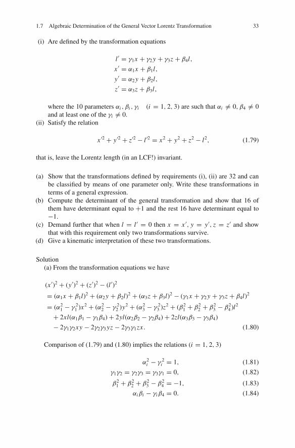
1.7 Algebraic Determination of the General Vector Lorentz Transformation 33
(i) Are defined by the transformation equations
l ′ = γ1x + γ2 y + γ3z + β4l,
x ′ = α1x + β1l,
y′ = α2 y + β2l,
z′ = α3z + β3l,
where the 10 parameters αi , βi , γi (i = 1, 2, 3) are such that αi �= 0, β4 �= 0and at least one of the γi �= 0.
(ii) Satisfy the relation
x ′2 + y′2 + z′2 − l ′2 = x2 + y2 + z2 − l2, (1.79)
that is, leave the Lorentz length (in an LCF!) invariant.
(a) Show that the transformations defined by requirements (i), (ii) are 32 and canbe classified by means of one parameter only. Write these transformations interms of a general expression.
(b) Compute the determinant of the general transformation and show that 16 ofthem have determinant equal to +1 and the rest 16 have determinant equal to−1.
(c) Demand further that when l = l ′ = 0 then x = x ′, y = y′, z = z′ and showthat with this requirement only two transformations survive.
(d) Give a kinematic interpretation of these two transformations.
Solution(a) From the transformation equations we have
(x ′)2 + (y′)2 + (z′)2 − (l ′)2
= (α1x + β1l)2 + (α2 y + β2l)2 + (α3z + β3l)2 − (γ1x + γ2 y + γ3z + β4l)2
= (α21 − γ 2
1 )x2 + (α22 − γ 2
2 )y2 + (α23 − γ 2
3 )z2 + (β21 + β2
2 + β23 − β2
4 )l2
+ 2xl(α1β1 − γ1β4)+ 2yl(α2β2 − γ2β4)+ 2zl(α3β3 − γ3β4)
− 2γ1γ2xy − 2γ2γ3 yz − 2γ3γ1zx . (1.80)
Comparison of (1.79) and (1.80) implies the relations (i = 1, 2, 3)
α2i − γ 2
i = 1, (1.81)
γ1γ2 = γ2γ3 = γ3γ1 = 0, (1.82)
β21 + β2
2 + β23 − β2
4 = −1, (1.83)
αiβi − γiβ4 = 0. (1.84)

34 1 Mathematical Part
Relations (1.81), (1.82), (1.83) and (1.84) constitute a system of nine simultane-ous equations which can be used to express nine parameters in terms of one. Indeed(1.82) implies that two of the γi are equal to zero. Without restricting the generalitywe assume γ1 �= 0⇒ γ2 = γ3 = 0. Then (1.81) gives
α1 = ±√
1+ γ 21 , (1.85)
α2 = ±1, α3 = ±1. (1.86)
Then from (1.83) and (1.84) it follows that
β1 = γ1
α1β4, (1.87)
β2 = β3 = 0, (1.88)
β4 = ±√
1+ γ 21 . (1.89)
We note that all coefficients of the transformation (1.79) have been expressed interms of the parameter γ1. The general form of the transformation is
⎛
⎜⎜⎝
l ′
x ′
y′
z′
⎞
⎟⎟⎠ =
⎡
⎢⎢⎣
β4 γ1 0 0γ1β4
α1α1 0 0
0 0 α2 00 0 0 α3
⎤
⎥⎥⎦
⎛
⎜⎜⎝
lxyz
⎞
⎟⎟⎠ = L(γ1)
⎛
⎜⎜⎝
lxyz
⎞
⎟⎟⎠ ,
where the quantities α1, β4 are defined in terms of the parameter γ1 via relations(1.85) and (1.89), respectively. It follows that we have in total 25 = 32 possibleone-parameter transformations, L(γ1) say, which are specified by the different com-binations of signs of the components of the transformation. Because the parameterγ1 appears as 1+ γ 2
1 we introduce a new parameter γ with the relation
1+ γ 21 =
1
1− β2= γ 2 (−1 < β < 1, γ > 0) (1.90)
and have
γ1 = ±γβ. (1.91)
Then the expression of the various parameters in terms of the new parameter γ is
α1 = ±γ, α2 = ±1, α3 = ±1, β4 = ±γ.
The 32 transformations are written in terms of the parameter β (or γ ):

1.7 Algebraic Determination of the General Vector Lorentz Transformation 35
l ′ = ε1γβx + ε2γ l,
x ′ = ε3γ x + ε1ε2ε3βγ l, (1.92)
y′ = ε4 y,
z′ = ε5z,
where the quantities εi = ±1 (i = 1, 2, 3, 4, 5) are defined by the relations
α1 = ε3γ, α2 = ε4, α3 = ε5, β4 = ε2γ, γ1 = ε1γβ. (1.93)
(b) The determinant of the matrix L(β) equals
det L(β) =
∣∣∣∣∣∣∣∣
ε2γ ε1γβ 0 0ε1ε2ε3βγ ε3γ 0 0
0 0 ε4 00 0 0 ε5
∣∣∣∣∣∣∣∣= ε2ε3ε4ε5. (1.94)
The possible values of the determinant are ±1. The requirement det L(β) = +1is equivalent to the condition
ε2ε3ε4ε5 = 1, (1.95)
which gives 24 = 16 cases. Therefore, the condition that the determinant equals +1or −1 selects 16 cases, respectively. We select the first set because it contains theidentity transformation (whose determinant equals +1). The transformations in thisset form a group and their general form is given by the transformation equations(1.92).(c) We consider next the transformations which in addition to the condition det L =+1 satisfy the condition that when l ′ = l = 0 then x = x ′, y = y′, z = z′. The newcondition implies the equations
βγ x = 0, x = ε3γ x, y = ε4 y, z = ε5z, (1.96)
which are satisfied by the following values of the parameters:
β = 0 (or γ = 1), ε3ε4ε5 = 1.
The last equation and (1.95) imply
ε2 = 1. (1.97)
There remains only one parameter free, the ε1, therefore there are two familiesof single-parametric Lorentz transformations with det L(β) = +1. The transforma-tions in these families constitute a group and they are called boosts with parameter

36 1 Mathematical Part
β (ε1 = −1) and −β (ε1 = 1), respectively. The transformation equations foreach case are as follows:ε1 = 1
l ′ = γ (l + βx),
x ′ = γ (x + βl), (1.98)
y′ = y, z′ = z.
ε1 = −1
l ′ = γ (l − βx),
x ′ = γ (x − βl), (1.99)
y′ = y, z′ = z.
In the following table we summarize the results concerning the number offree parameters and the number of the corresponding transformations for eachrequirement.22
Requirements Free parameter Possible transformations
Conditions (1.79,1.80) 1 32det L(β) = +1 or −1 1 16l = l ′ = 0⇒ r′ = r 1 2
(d) We shall give the geometric interpretation of the transformation in Sect. 1.8.1.Concerning the kinematic interpretation (that is interpretation involving the timeand the space) of the transformation we note the following:
• The transformation is single-parametric, therefore it must be related with onescalar kinematic quantity only.
• The transformation is symmetric in the sense that if the coordinates (l ′, x ′, y′, z′)are expressed in terms of (l, x, y, z) with β then the (l, x, y, z) are expressed interms of (l ′, x ′, y′, z′) with −β (prove this).
• The transformation must satisfy the initial condition l = l ′ = 0, then x = x ′, y =y′, z = z′ (or r = r′).
The above results lead to the following kinematic interpretation of the transfor-mation. The coordinates l, l ′ concern the time and the coordinates x, x ′, y, y′, z, z′
the orthonormal (in the Euclidean sense!) spatial axes of two Relativistic inertialobservers. At the time moment l = l ′ = 0 the spatial axes of the observers coincideand subsequently they are moving so that the plane y− z is parallel transported with
22 We note that a pure Lorentz transformation (i.e., Euclidean rotations and translations excluded)depends on six parameters. Here we are left with one parameter due to the simplified form of thetransformation.

1.7 Algebraic Determination of the General Vector Lorentz Transformation 37
y
z z ′
y ′
OO′ x,x′
β < 0
z ′
y ′
x,x′
z
y
OO′
β > 0
Fig. 1.4 Kinematic interpretation of Lorentz transformation
respect to the plane x ′ − z′ (because during the motion y = y′) and similarly theplane x − y is parallel transported with respect to the plane x ′ − y′ (because duringthe motion z = z′).
We conclude that there are only two motions possible:
• One motion in which the x ′-axis slides along the x-axis in the direction x > 0• One motion in which the x ′-axis slides along the x-axis in the direction x < 0
We consider that the first type of motion corresponds to the values 1 > β > 0while the second to the values 0 > β > −1. We identify the parameter β with thequotient v/c where |v| < c (because β < 1) is the speed of the relative velocity ofthe parallel axes x, y, z and x ′, y′, z′ and c is a universal constant, which we identifywith the speed of light in vacuum (see Fig. 1.4).
Exercise 4 Prove the identities23
γ 2 = γ 2β2 + 1, (1.100)
γ
(β1 ± β2
1± β1β2
)= γ (β1)γ (β2) (1± β1β2) , (1.101)
dγ = γ 3βdβ, d(γβ) = γ 3dβ, (1.102)
γ = 1+ 1
2β2 + 3
8β4 + . . . . (1.103)
Exercise 5 Consider the matrix
Li ′j (β) =
⎡
⎢⎢⎣
γ −γβ 0 0−γβ γ 0 0
0 0 1 00 0 0 1
⎤
⎥⎥⎦ ,
where γ = 1/√
1− β2, β ∈ [0, 1).
(a) Compute the inverse Lij ′(β).
(b) Prove that Li ′j (β) is a Lorentz transformation.
23 Identity (1.100) is used extensively in the calculations. Identity (1.101) expresses the relativisticcomposition of three-velocities under successive boosts.

38 1 Mathematical Part
(c) Define the hyperbolic angle φ with the relation coshφ = γ and prove that theboost along the x-axis is written as
Lij (β) =
⎡
⎢⎢⎣
coshφ − sinhφ 0 0− sinhφ coshφ 0 0
0 0 1 00 0 0 1
⎤
⎥⎥⎦ ,
where sinhφ = βγ . Also show that tanhφ = β and eφ =√
1+β1−β . The parameter
φ is called the rapidity of the transformation.
[Hint: (a) The inverse is
Lij (β) =
⎡
⎢⎢⎣
γ γβ 0 0γβ γ 0 00 0 1 00 0 0 1
⎤
⎥⎥⎦ .
(b) It is enough to show that ηi j = ηrs Lri Ls
j or in the form of matrices η = LtηLwhere η = diag(−1, 1, 1, 1).]
Example 4 Consider the LCFs {K ′, xi ′ ,Ei ′ }, {K , xi ,Ei } which are related by thetransformation
x1′ = − sinhφx0 + coshφx1,
x2′ = x2, x3′ = x3,
x0′ = − sinhφx1 + coshφx0,
where φ is a real parameter.
(a) Prove that the transformation K → K ′ is a Lorentz transformation.(b) A four-vector V i in K has components (0, 1, 0, 1)t . Compute the components
of V i in K ′. A Lorentz tensor Ti j of type (0, 2) in K ′ has all its componentsequal to zero except the T1′1′ = T3′3′ = 1. Compute the components of Ti j inK . Compute in K the covariant vector Ti j V i and the invariant Ti j V i V j .
Solution
(a) The matrix transformation between K , K ′ is
Lij (β) =
⎡
⎢⎢⎣
coshφ − sinhφ 0 0− sinhφ coshφ 0 0
0 0 1 00 0 0 1
⎤
⎥⎥⎦ .

1.7 Algebraic Determination of the General Vector Lorentz Transformation 39
It is easy to show that this is a Lorentz transformation (see Exercise 5).(b) For the four-vector V i we have
V i′ = ∂xi
′
∂xiV i = Li
′
i V i .
Hence
V 0′ = L0
′
i V i = L0′
0 V 0 + L0′
1 V 1 + L0′
2 V 2 + L0′
3 V 3 = − sinhφ,
V 1′ = L1
′
i V i = L1′
0 V 0 + L1′
1 V 1 + L1′
2 V 2 + L1′
3 V 3 = coshφ,
V 2′ = L2
′
i V i = L2′
0 V 0 + L2′
1 V 1 + L2′
2 V 2 + L2′
3 V 3 = 0,
V 3′ = L3
′
i V i = L3′
0 V 0 + L3′
1 V 1 + L3′
2 V 2 + L3′
3 V 3 = 1.
Therefore [V i ] = (− sinhφ, coshφ, 0, 1)t .Similarly for the tensor Ti j we have
Ti j = ∂xi′
∂xi
∂x j′
∂x jTi ′ j ′ = Li
′
i L j′
j Ti ′ j ′ = L1′
i L1′
j T1′1′ + L3′
i L3′
j T3′3′
= L1′
i L1′
j + L3′
i L3′
j ,
where we have used the fact that in K ′ only the components T1′1′ , T3′3′ do not vanishand are equal to 1. From this relation we compute the components of Ti j in K usingthe standard method. For example for the T00 component we have
T00 = L1′0 L1′
0 + L3′0 L3′
0 = sinh2 φ.
In the form of a matrix the components of Ti j in K are
[Ti j ] =
⎡
⎢⎢⎣
sinh2 φ − sinhφ coshφ 0 0− sinhφ coshφ cosh2 φ 0 0
0 0 0 00 0 0 1
⎤
⎥⎥⎦
K
.
In K we have for the vector ai = Ti j V j :
a0 = T00V 0 + T01V 1 + T02V 2 + T03V 3 = − coshφ sinhφ,
a1 = T10V 0 + T11V 1 + T12V 2 + T13V 3 = cosh2 φ,
a2 = T20V 0 + T21V 1 + T22V 2 + T23V 3 = 0,
a3 = T30V 0 + T31V 1 + T32V 2 + T33V 3 = 1.

40 1 Mathematical Part
1.0
0.8
0.6
0.4
0.2
0 0.25 0.50 0.75 1.0
1/γ
β 0 0.2 0.4 0.6 0.8 1.0
5.0
4.0
3.0
2.0
1.0
γ
β
Fig. 1.5 The factors γ and 1γ
Finally for the invariant ai V i = Ti j V i V j we have (in all LCFs!)
ai Vi = a0V 0 + a1V 1 + a2V 2 + a3V 3 = cosh2 φ + 1.
Exercise 6 Derive the results of Example 4 using matrix multiplication as follows:
[ V ]K ′ = [L][V ]K , [T ]K ′ = [L−1]t [T ]K [L−1], [a]K = ([T ]t [V ]K )t ,
ai Vi = [a]K [V ]K .
Example 5 Compute the values of the functions γ = (1− β2
)− 12 and γ−1 for the
values β = 0.100, 0.300, 0.600, 0.800, 0.900, 0.950, 0.990. Plot the results.Solution
β 0.100 0.300 0.600 0.800 0.900 0.950 0.990
1/γ 0.995 0.954 0.800 0.600 0.436 0.312 0.141γ 1.005 1.048 1.250 1.667 2.294 3.203 7.089
Using the figures of the table we draw the curves of Fig. 1.5 from which we notethat the relativistic effects become significant for values β > 0.8. This is the reasonwhy we expect the relativistic effects to appear at high relative velocities.
1.8 The Kinematic Interpretation of the General LorentzTransformation
1.8.1 Relativistic Parallelism of Space Axes
In Sect. 1.7 we have shown that the general Lorentz transformation L(β, E) can bewritten as the product of two transformations:
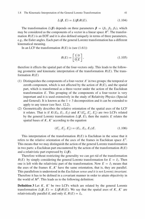
1.8 The Kinematic Interpretation of the General Lorentz Transformation 41
L(β, E) = L(β)R(E). (1.104)
The transformation L(β) depends on three parameters β = (β1, β2, β3), whichmay be considered as the components of a vector in a linear space R3. The transfor-mation R(E) is an EOT and it is also defined uniquely in terms of three parameters,e.g., the Euler angles. Each part of the general Lorentz transformation has a differentkinematical meaning.
In an LCF the transformation R(E) is (see (1.61))
R(E) =[
1 00 E
], (1.105)
therefore it effects the spatial part of the four-vectors only. This leads to the follow-ing geometric and kinematic interpretation of the transformation R(E). The trans-formation R(E)
(1) Distinguishes the components of a four-vector Ai in two groups: the temporal orzeroth component, which is not affected by the action of R(E), and the spatialpart, which is transformed as a three-vector under the action of the Euclideantransformation E . This grouping of the components of a four-vector is veryimportant and it is used extensively in the study of Relativity Physics (Specialand General). It is known as the 1+ 3 decomposition and it can be extended toapply to any tensor (see Sect. 12.2).
(2) Geometrically describes the relative orientation of the spatial axes of the LCFit relates. That is if K (E0, E1, E2) and K ′(E ′0, E ′1, E ′2) are two LCFs relatedby the general Lorentz transformation L(β, E), then the matrix E relates thespatial bases of K , K ′ according to the equation
(E ′1, E ′2, E ′3) = (E1, E2, E3)E . (1.106)
This interpretation of the transformation R(E) is Euclidean in the sense that itrefers to the relative orientation of the axes of the frames in Euclidean space E3.This means that we may distinguish the action of the general Lorentz transformationin two parts: a Euclidean part encountered by the action of the transformation R(E)and a relativistic part expressed by L(β).
Therefore without restricting the generality we can get rid of the transformationR(E) by simply considering the general Lorentz transformation for E = I3. Thenone is left with the relativistic part of the transformation. Now E = I3 means thatthe axes of the frames K , K ′ have the same orientation, that is, they are parallel.This parallelism is understood in the Euclidean sense and it is not Lorentz invariant.Therefore it has to be defined in a covariant manner in order to attain objectivity inthe world of M4. This leads us to the following definition:
Definition 3 Let K , K ′ be two LCFs which are related by the general Lorentztransformation L(β, E) = L(β)R(E). We say that the spatial axes of K , K ′ arerelativistically parallel if, and only if, R(E) = I4.

42 1 Mathematical Part
This concept of parallelism is directly comparable to the Euclidean concept ofparallelism in E3 because the latter can be defined as follows:
Definition 4 Let Σ,Σ′ be two ECF which are related with the EOT E . We say thatthe axes of Σ,Σ′ are parallel if, and only if, E = I3 where I3 = diag(1, 1, 1) is theidentity matrix.
The fact that the Euclidean and the relativistic parallelism of space axes areclosely related is frequently misunderstood and has led to erroneous conclusions. Onthe other hand it has important applications as, for example, the Thomas rotation.The difference between the two types of parallelism is that they coincide for twoLCFs K , K ′ but not necessarily for more. That is, if K , K ′, K ′′ are three LCFs suchthat the axes of the pairs K , K ′ and K ′, K ′′ are relativistically parallel then it doesnot follow (in general) that the space axes of the LCFs K , K ′′ are relativisticallyparallel. Of course this is not the case for the Euclidean parallelism.
The “broken parallelism” is due to the fact that the action of the second gen-eral Lorentz transformation L(βK ′′ ) acts on the Euclidean part R(EK ′′ ) of the firstLorentz transformation so that the latter becomes �= I4, which “brakes” the relativis-tic parallelism of the space axes of K , K ′′.
The interpretation of the transformation R(E) in terms of the relative directionof the space axes is possible because we assume isotropy of three-space, thereforeall directions in space are equivalent. From the point of view of physics this meansthat the orientation of space axes in the geometric space does not affect the physicalproperties of physical systems. Such conditions are known as gauge conditions andplay an important role in theoretical physics.
1.8.2 The Kinematic Interpretation of Lorentz Transformation
In order to give a kinematic interpretation of the (pure) Lorentz transformation L(β)we use the fact that this transformation depends on the vector β only and not on thematrix E . Therefore we identify
L(β) = L(β, I3),
that is, we consider that the Lorentz transformation is the general Lorentz transfor-mation when the axes of Σ and Σ′ are relativistically parallel. We identify the vectorβ with the relative velocity of Σ and Σ′. This kinematic interpretation is shown inFig. 1.6.
With the above interpretation, the general Lorentz transformation in M4 isdecomposed into two general Lorentz transformations: one transformation L(β, I3)in which the space axes of the related LCF are parallel and their relative velocity β
and a second transformation L(0, E) which rotates the axes in the Euclidean spaceE3 about the (fixed) origin in order to make them parallel. The relativistic part of thetransformation is what we call the (pure) Lorentz transformation. This interpretationimplies that the relativistic effects show up only when we have relative motion!

1.9 The Geometry of the Boost 43
x
z
y
z′
y′
x′
β
Fig. 1.6 The kinematic interpretation of Lorentz transformation
Geometrically it is possible to view the Lorentz transformation as a “hyperbolicrotation” around the space direction β with a hyperbolic angle ψ , defined by therelation
coshψ = |γ |. (1.107)
We call the hyperbolic angle ψ rapidity.
1.9 The Geometry of the Boost
As we have shown in Sect. 1.7 the Lorentz transformation L(β)24 can be expressedas the product of a boost and two Euclidean rotations. These rotations concern thedirection of the relative velocity in the (parallel) axes of the two LCFs related by theLorentz transformation. This decomposition is helpful in practice because we solvea specific problem for a boost and then we use the Euclidean rotations to get the(usually more complicated) answer. Therefore it is important to study the geometricstructure of the boost.
We recall that if (l, x, y, z) and (l ′, x ′, y′, z′) are the coordinates of a point P inM4 in the LCF Σ and Σ′, respectively, then the boost L(β) (to be precise we shouldwrite L(β)x ) along the direction of the x-axis is the transformation
x ′ = γ (x − βl), y′ = y, z′ = z, l ′ = γ (l − βx). (1.108)
Let us represent this transformation on the Euclidean plane25 (l, x) – the y, zcoordinates are not affected by the transformation and we ignore them. The boost
24 Not the general Lorentz transformation L(β, E)!25 It is generally believed that this plane is a two-dimensional Minkowski space, that is, a two-dimensional linear space endowed with the Lorentz metric. This is wrong and leads to many

44 1 Mathematical Part
L(β) and its inverse L−1(β) are represented with the following matrices:
L(β) =[
γ −βγ−βγ γ
], L−1(β) =
[γ βγ
βγ γ
]. (1.109)
Because L(β) is a linear transformation it is enough to study its action on thebasis vectors e0,Σ = (1, 0)Σ, e1,Σ = (0, 1)Σ of the LCF Σ. We have
(e0, Σ′ , e1, Σ′) = (e0, Σ, e1, Σ)L−1 = (e0, Σ, e1, Σ)
[γ βγ
βγ γ
]⇒
e0, Σ′ = γ e0, Σ + βγ e1, Σ, e1, Σ′ = βγ e0, Σ + γ e1, Σ. (1.110)
Concerning the Euclidean length and the Euclidean angles of the basis vectorswe have
|e0, Σ| = |e1, Σ| = 1,
|e0, Σ′ | = |e1, Σ′ | = γ√
1+ β2 =√
1+ β2
1− β2> 1, (1.111)
e0, Σ · e1, Σ = 0, e0, Σ′ · e1, Σ′ = 2βγ 2,
e0, Σ · e0, Σ′ = e1, Σ · e1, Σ′ = γ.
These results lead to the representation of the basis vectors in the Euclidean plane(l, x) as shown in Fig. 1.7.
l
l′l′′
x′
x
x′′
x = −l′
e0,Σ′′ e0,Σ′
e1,Σ′
e1,Σ′′
x = l
Fig. 1.7 The action of boost on the basis vectors
misunderstandings in Special Relativity. It should always be borne in mind that the blackboardis and stays a two-dimensional Euclidean space no matter what we draw on it!

1.9 The Geometry of the Boost 45
In Fig. 1.7 the Euclidean angle φ is defined by the relation
tanφ = β. (1.112)
We note that the vectors e0,Σ′ = (1, 0)Σ′ , e1,Σ′ = (0, 1)Σ′ make equal angleswith the basis vectors e0,Σ = (1, 0)Σ, e1,Σ = (0, 1)Σ and furthermore they aresymmetric about the internal bisector. When β = 1 then tanφ = 1 hence φ = 45o
and the vectors e0,Σ′ = (1, 0)Σ′ , e1,Σ′ = (0, 1)Σ′ coincide with the internal bisectorl = x of the axes (l, x).
If the LCFs Σ and Σ′ are moving with factor −β then the vectors e0,Σ′ =(1, 0)Σ′ , e1,Σ′ = (0, 1)Σ′ make a common external angle φ with the vectorse0,Σ′ = (1, 0)Σ′ , e1,Σ′ = (0, 1)Σ′ (see Fig. 1.7 ).
Exercise 7 Prove that the Lorentz length of the basis vectors e0,Σ, e1,Σ, e0,Σ′ , e1,Σ′
equals ±1. Also show that the vectors of each basis are Lorentz orthogonal and thatthe Lorentz angle between, e.g., the vectors e1,Σ, e1,Σ′ is given by the relation
coshφL = e1,Σ ◦ e1,Σ′
|e1,Σ|L |e1,Σ′ |L = γ, (1.113)
where ◦ indicates Lorentz product in the plane (l, x).
Note that in (1.113) we are using cosh and not cos because γ > 1.
Exercise 8 Show that the Euclidean lengths satisfy the relation
|ei,Σ′ | = 1√cosh 2φ
|ei,Σ| i = 0, 1 (1.114)
and conclude that
|ei,Σ′ | > |ei,Σ|. (1.115)
The geometric meaning of the inequality (1.115) is that the Euclidean length ofthe unit rod along the x ′-axis is larger than the Euclidean length of the unit rodalong the x-axis. Therefore an object lying along the x-axis (e.g., a rod) when it ismeasured with the unit of Σ gives the number d(Σ) and when it is measured withthe unit of Σ′ gives another number d ′(Σ′) smaller than d(Σ) because
d(Σ)|ei,Σ| = d ′(Σ′)|ei,Σ′ |. (1.116)
The physical meaning of the inequality d ′(Σ′) < d(Σ) is that the (Euclidean!)length of the rod as measured in Σ (that is the number d(Σ)) is smaller than the(Euclidean!) length d ′(Σ′) as measured in Σ′. This inequality of (Euclidean!) lengthmeasurements has been called length contraction. Concerning the unit along thetimelike vector e0,Σ we identify d(Σ) with the negative of time duration. Then the

46 1 Mathematical Part
inequality d ′(Σ′) < d(Σ) means that the (Newtonian!) time duration of a phe-nomenon in Σ is smaller than the (Newtonian!) duration of the same phenomenonin Σ′. This result has been called time dilation effect. Both length contraction andtime dilation will be discussed in Chap. 5.
A simple way to draw the vectors e0,L and e1,L on the Euclidean plane E2 is the
following. We consider a Lorentz unit vector (in E2!) with components
(xy
)and
demand
(x y
) (−1 00 1
)(xy
)= ±1
from which follows
−x2 + y2 = ±1.
We infer that the tip of the Lorentz unit vectors moves on hyperbolae with asymp-totes x = ±y (see Fig. 1.8).
If we consider orthonormal coordinates (l, x) in the Euclidean plane then thesehyperbolae are symmetric about the bisectors at the origin. For each value of theparameter β they make an angle φ with the l, x-axes. In order to compute this anglein terms of the parameter β we consider the Euclidean inner product of the vectorse0, L , e1, L with the basis vectors i, j. For the vector e1, L we have
e1,L · i = cosφ|e1,L |E
from which follows
cosφ = γ√2γ 2 − 1
. (1.117)
x
yy
′
x ′
Fig. 1.8 The Lorentz transformation in the Euclidean plane

1.9 The Geometry of the Boost 47
l′′
x′′x′x
l′l
xx′K
l′′ l′ l
x = lx = l
x′′
φ1
φ2
φ3
1φφ
2φ
3
Fig. 1.9 Combination of β-factors under successive boosts
With this result we can draw in the Euclidean plane (l, x), the vectors e0,L ande1,L for every value of the parameter β.
Example 6 Consider three LCFs Σ,Σ′,Σ′′, which are moving in the standard con-figuration with factors β1, β2, respectively, along the common axes x, x ′, x ′′. Usethe geometric representation of the boost to compute the factor β between the LCFsΣ,Σ′′ (see also (1.101)).
ProofFrom Fig. 1.9 we have tanφ3 = tan(φ1 + φ2). Hence
β3 = β1 + β2
1+ β1β2. (1.118)
Another simple method to represent the boost in the Euclidean plane (l, x) is thefollowing. We consider two orthogonal axes l, x and consider the boost (1.108),which defines the new axes l ′, x ′ on the same plane. The l ′-axis is defined by therequirement
x ′ = 0⇒ x = βl,
therefore it is a straight line with an inclination β wrt the axis l. Similarly the x ′-axisis defined by the requirement l ′ = 0, therefore it is the set of points
l = βx,
which is a straight line with inclination β wrt the axis x .
In Fig. 1.7 we have taken the axes l, x to be orthogonal but this is not necessaryand what we say holds for non-orthogonal axes. We have also drawn the axes x ′′, l ′′
with inclination −β.

48 1 Mathematical Part
1.10 Characteristic Frames of Four-Vectors
We have divided the four-vectors in M4 in timelike, spacelike, and null according toif their length is < 0,> 0, or = 0, respectively. In this section we show that the firsttwo types of four-vectors admit characteristic LCF in which they retain their reducedform, that is the timelike vectors have zero spatial components and the spacelikevectors have zero time component. As we shall see in the subsequent chapters thereduced form of the timelike and the spacelike vectors is used extensively in thestudy of Lorentz geometry and in the Theory of Special Relativity.
1.10.1 Proper Frame of a Timelike Four-Vector
Consider the timelike four-vector Ai which in the LCF Σ has decomposition(A0
A
)
Σ
. When the zeroth component A0 > 0 (respectively, A0 < 0) we say that the
four-vector Ai is directed along the future (respectively, past) light cone. Becausethe proper Lorentz transformation preserves the sign of the zeroth component it ispossible to divide the timelike four-vectors in future directed and past directed.For every timelike four-vector Ai we have A2 − (A0)2 < 0, therefore there existsalways a unique LCF, Σ+ say, in which the spatial components of Ai vanish and the
four-vector takes its reduced or canonical form
(A0+
0
)
Σ+. We name the frame Σ+
the proper frame of the four-vector Ai .In order to determine Σ+ when Ai is given in an arbitrary LCF Σ, we must
find the β-factor β of Σ+ with respect to Σ. This is done from the proper Lorentztransformation (1.51), (1.52) using the reduced form of Ai . We find
A0 = γ (A0)+, (1.119)
A = γβ(A0)+. (1.120)
From these relations,
γ = A0
A0+ , (1.121)
β = AA0
. (1.122)
Equations (1.121) and (1.122) fix the proper frame Σ+ of the four-vector Ai
by giving the three parameters βμ wrt an arbitrary LCF Σ in which we know thecomponents of the four-vector Ai .
In the proper frame Σ+ of Ai the length Ai Ai = −(A0+)2, therefore the com-ponent A0+ is not simply a component but an invariant (tensor), so that it has thesame value in all LCFs. We use this fact extensively in relativistic physics in order

1.10 Characteristic Frames of Four-Vectors 49
to define timelike four-vectors which have a definite physical meaning. Indeed wedefine the timelike four-vector in its proper frame and then we compute it in anyother LCF using the appropriate Lorentz transformation. One such example is thefour-velocity of a relativistic particle which, as we shall see, is a four-vector withconstant length c, where c is the speed of light in empty space. Because in SpecialRelativity we consider c to be an invariant (in fact a universal constant) we define
the four-velocity of the relativistic particle in its proper frame to be ui =(
c0
)
Σ+.
In any other frame with axes parallel to those of Σ+ and with β-factor β relations
(1.51), (1.52) give that the four-velocity is ui =(
γ cγ cβ
)
Σ
.
1.10.2 Characteristic Frame of a Spacelike Four-Vector
Let Ai be a spacelike four-vector which in an LCF Σ has decomposition
(A0
A
)
Σ
.
We are looking for another LCF Σ− in which Ai has the reduced form
(0
A−
)
Σ−.
The two decompositions of the four-vector are related with a proper Lorentz trans-formation, therefore the transformation equations (1.51), (1.52) give
B0 = γβ · B−, (1.123)
B = B− + γ − 1
β2(β · B−)β. (1.124)
We consider the Euclidean inner product of the second equation with β and get
β = B0
B||,
where B|| = β·Bβ
. It follows that it is not possible to define β completely (we can fixonly the length of β) as in the case of the timelike four-vectors. Therefore there areinfinitely many LCFs in which a spacelike four-vector has its reduced form.
However, in the set of all these frames there is a unique LCF defined as follows.We consider the position four-vectors of the end points A, B of the spacelike four-vector ABi and assume that in a characteristic frame Σ− they are decomposed as(
A0
A−eA
)
Σ−,
(A0
B−eB
)
Σ−. Then we specify a unique characteristic frame by the
condition eA = −eB . This particular characteristic frame of the spacelike four-vector ABi is called the rest frame of ABi . The rest frame is used to describe themotion of rigid rods in Special Relativity.

50 1 Mathematical Part
1.11 Particle Four-Vectors
The timelike and the null four-vectors play an important role in Special (and Gen-eral) Relativity, because they are associated with physical quantities of particles andphotons, respectively. Since in many problems the study of particles and photonsis identical it is useful to introduce a new class of four-vectors, the particle four-vectors.
Definition 5 A four-vector is a particle four-vector if and only if
• It is a timelike or a null four-vector.• The zeroth component in an LCF is positive (i.e., it is future directed).
For particle four-vectors we have the following result which is a consequence ofProposition 3.
Proposition 4 The sum of particle four-vectors is a particle four-vector.
This result indicates that geometry allows us to describe systems of particleswith corresponding systems of particle four-vectors and, furthermore, to study thereaction of these particles by studying the sum of the corresponding particle four-vectors. We consider two cases: the case of parallel propagation of a beam of parti-cles and the triangle inequality in M4.
Proposition 5 If two future-directed null vectors are parallel (antiparallel), thentheir spatial directions are parallel (antiparallel) for all observers. Equivalently theproperty of three-parallelism (three-antiparallelism) of null vectors is a covariantproperty.
ProofConsider two future-directed null vectors which in the LCF Σ have components
Aa(I ) = E(I )
(1
e(I )
)E(I ) > 0, I = 1, 2.
Then by Theorem 1 we have[∑n
I=1
(Aa
(I )
)]2=0, hence
(E1 + E2, e1 E1 + e2 E2)2 = 0⇒−(E1 + E2)2 + (e1 E1 + e2 E2)2 = 0⇒
e1 · e2 = 1⇒ e1//e2 ⇒ e1 E1//e2 E2.
Second ProofWe have
Aa(I )//Aa
(J ) ⇒ Aa(I ) = λAa
(J )(λ ∈ R).
Considering the components of the four-vectors in Σ we have

1.11 Particle Four-Vectors 51
E(I ) = λE(J ), e(I ) = λe(J ) I, J = 1, 2. �
Proposition 6 Let O, A, B be three points in M4 such that the four-vectors O Aa
and O Ba are future-directed timelike four-vectors. Then the four-vector ABa is afuture-directed four-vector and the absolute value of the Lorentz lengths (positivenumbers) of the three four-vectors satisfy the relation
(O B) ≥ (O A)+ (AB), (1.125)
where the equality holds if, and only if, the three points O, A, B are on a straightline.
ProofThe linearity of M4 implies
ABa = −O Aa + O Ba .
From Proposition 4 we conclude that ABa is a timelike four-vector. The length
− (AB)2 = −(O A)2 − (O B)2 − 2O Aa O Ba . (1.126)
In the proper frame of O Aa we have
O Aa =(
(O A)0
)
Σ(O A)
((O A) > 0) and suppose that O Ba =(
(O B)0
(OB)
)
Σ(O A)
where (O B)0 > 0 because
O Ba is future directed. The invariant
O Aa O Ba = −(O A)(O B)0.
But−(O B)2 = −(O B)02+(OB)2 < 0 because O Ba is timelike, hence (O B)0 >
(O B) > 0 =⇒ (O A)(O B)0 ≥ (O A)(O B). Finally
O Aa O Ba ≥ (O A)(O B),
where the equality holds only if (OB) = 0, that is the four-vectors O Aa and O Ba
are parallel, hence the three points O, A, B lie on the same straight line (in M4).Replacing in (1.126) we find
(AB)2 = (O A)2 + (O B)2 + 2O Aa O Ba ≤ ((O A)− (O B))2 =⇒(AB) ≤ (O A)− (O B) =⇒ (O B) ≥ (O A)+ (AB),
which completes the proof. �
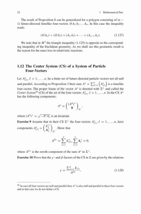
52 1 Mathematical Part
The result of Proposition 6 can be generalized for a polygon consisting of (n −1) future-directed timelike four-vectors O A1 A2 . . . An . In this case the inequalityreads:
(O An) > (O A1)+ (A1 A2)+ · · · + (An−1 An). (1.127)
We note that in M4 the triangle inequality (1.125) is opposite to the correspond-ing inequality of the Euclidean geometry. As we shall see this geometric result isthe reason for the mass loss in relativistic reactions.
1.12 The Center System (CS) of a System of ParticleFour-Vectors
Let Aa(I ), I = 1, . . . , n, be a finite set of future-directed particle vectors not all null
and parallel. According to Proposition 3 their sum Aa =∑nI=1
(Aa
(I )
)is a timelike
four-vector. The proper frame of the vector Aa is denoted with Σ+ and called theCenter System26 (CS) of the set of the four-vectors Aa
(I ), I = 1, . . . , n. In the CS Aa
has the following components:
Aa =(
(A0)+
0
)
Σ+,
where (A0)+ = √−Aa Aa is an invariant.
Exercise 9 Assume that in their CS Σ+ the four-vectors Aa(I ), I = 1, . . . , n, have
components Aa(I ) =
(E+IA+I
)
Σ+. Show that
A0+ =n∑
I=1
E+(I ),
n∑
I=1
A+I = 0,
where A0+ is the zeroth component of the sum Aa in Σ+.
Exercise 10 Prove that the γ - and β-factors of the CS in Σ are given by the relations
γ =∑n
I=1 E(I )
A0+ , (1.128)
26 In case all four-vectors are null and parallel then Aa is also null and parallel to these four-vectorsand in that case we do not define a CS.

1.12 The Center System (CS) of a System of Particle Four-Vectors 53
β =∑n
I=1 AI∑nI=1 E(I )
. (1.129)
Verify that the above quantities satisfy the relation γ 2 = 11−β2 .
[Hint: Recall that if a timelike four-vector in an LCF Σ has components Aa =(A0
A
)
Σ
then the γ - and β-factors of the proper frame of Aa in Σ are given by the
relations
γ = A0
√−Aa Aa, β = A
A0.
](1.130)
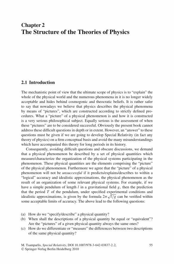
Chapter 2The Structure of the Theories of Physics
2.1 Introduction
The mechanistic point of view that the ultimate scope of physics is to “explain” thewhole of the physical world and the numerous phenomena in it is no longer widelyacceptable and hides behind cosmogonic and theocratic beliefs. It is rather saferto say that nowadays we believe that physics describes the physical phenomenaby means of “pictures”, which are constructed according to strictly defined pro-cedures. What a “picture” of a physical phenomenon is and how it is constructedis a very serious philosophical subject. Equally serious is the assessment of whenthese “pictures” are to be considered successful. Obviously the present book cannotaddress these difficult questions in depth or in extent. However, an “answer” to thesequestions must be given if we are going to develop Special Relativity (in fact anytheory of physics) on a firm conceptual basis and avoid the many misunderstandingswhich have accompanied this theory for long periods in its history.
Consequently, avoiding difficult questions and obscure discussions, we demandthat a physical phenomenon be described by a set of physical quantities whichmeasure/characterize the organization of the physical systems participating in thephenomenon. These physical quantities are the elements comprising the “picture”of the physical phenomenon. Furthermore we agree that the “picture” of a physicalphenomenon will not be unsuccessful if it predicts/explains/describes to within a“logical” accuracy and idealistic approximations, the physical phenomenon as theresult of an organization of some relevant physical systems. For example, if wehave a simple pendulum of length l in a gravitational field g, then the predictionthat the period T of the pendulum, under specified experimental conditions andidealistic approximations, is given by the formula 2π
√l/g can be verified within
some acceptable limits of accuracy. The above lead to the following questions:
(a) How do we “specify/describe” a physical quantity?(b) When shall the descriptions of a physical quantity be equal or “equivalent”?
Are the “pictures” of a given physical quantity always the same ones?(c) How do we differentiate or “measure” the differences between two descriptions
of the same physical quantity?
M. Tsamparlis, Special Relativity, DOI 10.1007/978-3-642-03837-2 2,C© Springer-Verlag Berlin Heidelberg 2010
55
56 2 The Structure of the Theories of Physics
All these questions and many more of the same kind have been and will be posedthroughout the course of human history. To these questions there are not definiteand unique answers and this is the reason we have made extensive use of quota-tion marks. The answers given to such questions can only be beliefs and “logical”explanations which, in turn, are based on other more fundamental beliefs and expla-nations and so on. This infinite sequence of reasoning is the realm of philosophy.However, in science, and more specifically in physics, we cannot afford the luxuryof an endless series of questions, beliefs, and explanations. This is because physicsis an applied science, which acquires meaning and substance in the laboratory andin everyday practice. For example there is no room for beliefs and explanations con-cerning the take-off of an airplane, or the safety of a nuclear reactor. In conclusion,the practicalities of life itself impose upon us a definite “real” world of objectivephysical phenomena to which science is called upon to consider and offer systemat-ically formed views and propositions corresponding to its purposes. This “imposed”reality is the realm of science and this is the “world” we want to “explain” in termsof the human concept of reality, created by our senses and perception.
In the following sections we develop one approach/explanation as to how themethodology of physics as a science is systematically formed. Obviously otherwriters have a different approach and the reader may have his/her own. However,no matter which approach one takes the common agreement is that
(a) There is not “the correct” approach but some of them are more “successful”than others in certain subsets of phenomena.
(b) Whichever approach is adopted, the final numeric answer to a given physicalphenomenon or set of phenomena must be within the accuracy of the experi-mental measurements or observations, otherwise the approach is not acceptable.
2.2 The Role of Physics
Our interaction with the environment is always by means of some kind of sensors.These sensors can be either the sensors of the human body (direct action) or man-made sensors such as lenses, clocks, meters, etc. (indirect action). The first type ofsensors shall be called basic sensors and the second type measuring sensors. Physicsis the unique science which is concerned with the development, use, and study of themeasuring sensors. This gives physics a distinct position against all other sciencesin the study for an “objective” reality.
The basic function of the measuring sensors is the observation of a physical phe-nomenon or of a characteristic quantity(ies) of a physical phenomenon. The result ofan observation is (as a rule) a set of numbers. Therefore observation is the procedurewith which a physical quantity is described in the mathematical world of geometry.Because
• The result of an observation depends on the specific observer performing theobservation.
• The nature of the physical quantity is independent of the observer observing it.

2.2 The Role of Physics 57
We are led to demand that the sets of numbers associated by the various observers toa given physical quantity shall be related by means of some transformations. Mathe-matically this means that the sets of numbers of each observer are the components ofa geometric object for that observer. Equivalently we can say that the mathematicaldescription of the physical quantities will be done in terms of geometric objects ina proper geometric space. We emphasize that the result of an observation is not anelement of the objective world (reality), but an element of the world of geometry.The description of a phenomenon by means of a set of geometric objects is calledthe image of the observed physical phenomenon.
According to this view the sensors we use for the observation of the real worldcreate another world of images. Science studies this world of images and tries todiscover its internal structure, if any, or the internal structure of a subset of imagesof a given class. The mechanistic point of view, which prevailed at the end of the19th century, can be understood as the belief that there exists one and only oneinternal structure of the world of images and the scope of science is to discover thisstructure. Today, as we remarked at the beginning of this section, this position isconsidered as being too strong. It is our belief that there exist internal structures insubsets of certain types of images that do not appear in the set of all images of theobjective world, i.e., different structures for different subsets.1
In the game of science, physics enters with a special role. The fundamentalrequirement of physics is that whichever internal structure relates a subset of images,it must be “objective,” or to put it in another way, non-personalized. Due to thisrequirement, in physics one uses (in general) images which are created by measuringsensors only.
Furthermore, it is required that physics be concerned only with images whichhave a definite qualitative and quantitative character. This means that the imagesstudied in physics will be “geometric,” that is they will be described by means ofconcrete mathematical quantities defined on mathematical sets with definite math-ematical structure (linear spaces, manifolds, etc.). These spaces are the space ofphysics. The type and the quantity of the geometric objects which describe theimages of a theory geometrize these images and define the “reality” of that the-ory of physics. For example, in Newtonian Physics the physical quantity “position”is associated with the geometric element position vector in the Euclidean three-dimensional space.
Physics has shown that indeed the set of images created by the measuring sen-sors is divided into more than one subset, with each subset having its own internalstructure. This has resulted in many theories of physics, each theory having a dif-ferent “reality.” For example Newtonian Physics has one reality (that of the Newto-nian Physical phenomena geometrized by Euclidean tensors in three-dimensionalEuclidean space), Special Relativity another (the special relativistic phenomenageometrized by Lorentz tensors defined on a four-dimensional flat metric spaceendowed with a Lorentzian metric). The unification of these different realities as
1 In our opinion the question of the existence of a universal internal structure involving all imagesof the objective world is equivalent to the question if there is an omnipresent super power or not!

58 2 The Structure of the Theories of Physics
parts of a super or universal reality has raised the problem of the unification ofthe theories of physics in a Unified Theory, a problem which has occupied manydistinguished physicists over the years and which remains open.
Each theory of physics is equally strong to any other within the subset of imagesto which it applies. Therefore the statement “this theory of physics is not valid”makes no sense. For example Newtonian Physics holds in the subset of Newtonianphenomena only and does not hold in the subset of relativistic phenomena. SimilarlySpecial Relativity holds in the subset of special relativistic phenomena only.
The above analysis makes clear that every theory of physics is intimately anduniquely related to the geometrization of the subset of images of the world it studies.This geometrization has two branches:
(a) The correspondence of every image in the subset with a geometric object ofspecific type
(b) The description of the internal structure of the subset of images by means ofgeometric relations among the geometric objects of the theory (these include –among others – the laws of that theory of physics)
Fig. 2.1 The structure of a theory of physics

2.3 The Structure of a Theory of Physics 59
Figure 2.1 describes the above by means of a diagram. We note that in Fig. 2.1every subset of images is defined by a different window of measuring sensors. Inthe following sections we discuss the general structure of a theory of physics inpractical terms.
2.3 The Structure of a Theory of Physics
As we mentioned in the last section the images studied in physics are created bymeans of the measuring sensors and are described mathematically by geometricobjects. The images of physical phenomena are generated by the observers by obser-vation.
The observer in a theory of physics is the “window” of Fig. 2.1. Its sole role is togenerate geometric images of the various physical phenomena, which are observed.In practical terms we may think the observer as a machine – robot (EGO does notexist in physics!) – which is equipped with the following:
• A set of specific measuring sensors, which we call observation means or obser-vation instruments
• A definite set of instructions concerning the use of these sensors
Depending on the type of the observation instruments and the directions of usethe observers create geometrized images of the physical phenomena. Every the-ory of physics has its own observers or, equivalently, there are as many types ofobservers as viable theories of physics. For each class of observers there correspondsa “reality”, which is the world made up by the subset of images involved in thetheory.
In a sense the observers operate as “generalized functions”2 from the set of allphysical phenomena to the space of images Rn (for a properly defined n). The valueof n is fixed by the characteristic quantity of the theory. For the theories of physicsstudying motion the space of images is called spacetime and the characteristic quan-tity is the position vector.
For example in Newtonian Physics the characteristic quantity of the theory ismotion and it is described with the image orbit in a linear space. Practical experiencehas shown that the orbit is fully described with three numbers at each time moment,therefore the spacetime is a four (n = 4) dimensional linear space (endowed withan extra structure, which we shall consider in the following). There is no point toconsider a spacetime of higher dimension in Newtonian Physics, because the extracoordinates will always be zero, and therefore redundant. In general the dimensionof the space of a theory of physics equals the minimum number of componentsrequired to describe completely the characteristic quantity of the theory. We callthis number the dimension of the space of the theory.
2 This type of functions are called functors in Category Theory, but this is something outside thescope of this book.

60 2 The Structure of the Theories of Physics
We summarize the above discussion as follows:
• The observer of a theory of physics is a machine (robot) which is equipped withspecific instrumentation and directions of use, so that it can produce componentsfor the characteristic quantities of the physical phenomena.
• Observation or measurement is the operation of the observer which has as a resultthe production of components for the characteristic quantities of a specific phys-ical phenomenon or physical system.
• There exists neither a unique type of observers nor a unique type of observation.Every class of observers produces a set of images of the outside world, which isspecific to that class of observers and type of observation. For example, we havethe sequences: Newtonian observers – Newtonian Physics – Newtonian world,Relativistic observers – Relativistic physics – Relativistic world.
2.4 Physical Quantities and Reality of a Theory of Physics
From the previous considerations it becomes clear that the image of a physicalphenomenon depends on the observer (i.e., the theory) describing it. However, thefundamental principle of physics is that the image of a single observer for a physicalphenomenon has no objective value. The “reality” of one has no place in today’sscience and specifically in physics, where all observers are considered to be (withineach theory!) equivalent and similar in all respects. The objectivity of the descriptionof physical phenomena within a given theory of physics is achieved by means of thefollowing methodology:
(1) We consider the infinity of the specific type of observers (i.e., identical robotsequipped with the same instrumentation and the same programming) used bythe theory.
(2) We define a specific and unique code of communication amongst these observers,so that each observer is able to communicate the image of any physical quantityto any other observer in that same class of observers.
(3) We define a procedure which we agree will “prove” that a given physical phe-nomenon is described successfully by a specific theory of physics.
Following the above approach, we define the “successfulness” of the image of aphenomenon within a (any) theory of physics by means of the procedure describedin the general scheme of Fig. 2.2.
In Fig. 2.2 there are two major actions:
(1) The observation of the physical phenomenon by an observer with the measuringmeans and the procedures, defined by the specific theory of physics. The resultof each observation is the creation of geometric objects (in general elements ofRn) for the characteristic quantity(ies) of the observed physical phenomenon.
(2) The verification of the “objectivity” of the concerned physical phenomenon bythe comparison of the geometric images created by procedure 1. This second

2.4 Physical Quantities and Reality of a Theory of Physics 61
Characteristic quantity
of physical phenomenon
Observation of observer 1
Geometric picture
of observer 1
Geometric picture
of observer 2
Observation of observer 2
Procedure of existence
of physical quantity
Fig. 2.2 Generating diagram of principles of relativity
activity involves the transfer of the image of a phenomenon observed by theobserver 1 to observer 2 and vice versa, according to the esoteric code of com-munication of the observers specified by the specific theory of physics. Morespecifically, observer 2 compares the image of the phenomenon created bydirect observation (direct image) with the communicated image of observer 1(communicated image). If these two images do not coincide (within the spec-ified limits of observation and possible idealizations) then the physical phe-nomenon is not a physical quantity for that specific theory of physics. If they do,then observer 2 communicates his direct image to observer 1, who accordinglyrepeats the same procedure. If the two images of observer 1 coincide then theconcerned physical phenomenon is potentially a physical quantity for that the-ory of physics. If the coincidence of the images holds for any pair of observersof the specific theory then this physical phenomenon is a physical quantity forthat theory of physics.
The set of all physical quantities of a theory comprises the reality of this theory ofphysics. We note that the reality for physics is relative to the theory used to “explain”the physical phenomena. That is, the reality of Newtonian Physics is different fromthe reality of the Theory of Special Relativity, in the sense that the physical quanti-ties of Newtonian Physics are not physical quantities for Special Relativity and viceversa. For example the physical quantities time and mass of Newtonian Physics donot exist in the Theory of Special Relativity and, for the same reason, the speed oflight and the four-momentum of Special Relativity do not exist (i.e., are not physicalquantities) in Newtonian Physics.
It must be understood that the reality of the physical world we live in is beyondand outside the geometric reality of the theories of physics. On the other handthe reality of the world of images of a theory of physics is a property which canbe established with concrete and well-defined procedures. This makes the theoriesof physics the most faithful creations of human intelligence for the understandingand the manipulation of the physical environment. The fact that these creationsindeed work is an amazing fact which indicates that the basic human sensors andthe human “operational system” (that is the brain) function in agreement with the

62 2 The Structure of the Theories of Physics
laws of nature. This is the prime reason which led to the initial identification of theobserver – robot with the actual human observer.
The procedure with which one assesses the existence of a physical quantity inthe realm of the world of a theory of physics is called the Principle of Relativityof that theory. The Principle of Relativity involves transmission (i.e., communica-tion) of geometric images among two observers of a theory of physics, therefore itis of a pure geometric nature and can be described mathematically in appropriateways. It must be clear that it is not possible to have a theory of physics without aPrinciple of Relativity, because that will be a theory without any possibility of beingtested against the real phenomena. In the sections to follow we shall show how thesegeneral considerations apply in the cases of Newtonian Physics and the Theory ofSpecial Relativity.
From the above considerations it is wrong to conclude that the identification ofa physical quantity is simply a comparison of images (direct and communicatedimage) based on the Principle of Relativity. Indeed, the identification of a physicalquantity is a twofold activity:
(a) A measuring procedure (the observation, direct image) with which the geomet-ric image of the quantity is created and involves one observer and one physicalphenomenon
(b) A communication and comparison of images which involves two observers anda specified physical phenomenon
2.5 Inertial Observers
The Principle of Relativity of a theory of physics concerns the communication(exchange of information – images) between the observers of the theory. Geometri-cally this is expressed by groups of transformations in the geometric space of imagesof the theory. But how does one define a Principle of Relativity in practice?
In the present book we shall deal only with the cases of Newtonian theory and theTheory of Special Relativity. Therefore in the following when we refer to a theoryof physics we shall mean one of these two theories only.
As we have said in the previous sections, the observers of a theory of physics aremachines equipped with specific instrumentation and directions of use and producefor each physical quantity a set of numbers, which we consider to be the componentsof a geometric object. Two questions arise:
• In which coordinate system are these components measured?• What kind of geometric objects will be associated with this set of components or,
equivalently, which is the group of transformations associated with that theory?
Both these questions must be answered before the theory is ready to be used inpractice.

2.6 Geometrization of the Principle of Relativity 63
The first question involves essentially the geometrization of the observers, thatis, their correspondence with geometric objects in Rn. These objects we consider tobe the coordinate systems. In a linear space there are infinitely many coordinate sys-tems. One special class of coordinate systems is the Cartesian coordinate systems,which are defined by the requirement that their coordinate lines are straight lines,that is, they are described by equations of the form
r = at + b,
where a,b are constant vectors in Rn and t ∈ R.If the Cartesian coordinate systems are going to have a physical meaning in a
theory of physics (this is not necessary, but it is the case in Newtonian Physics andin the Theory of Special Relativity) the observers who are associated with these sys-tems must have the ability to define straight lines3 and in the real world by means ofa physical process. The observers who have this ability are called inertial observers.
In a theory of physics the existence of these observers is guaranteed with anaxiom. In Newtonian Physics this axiom is Newton’s First Law and in the Theoryof Special Relativity there exists a similar axiom (to be referred to later on). At thispoint it becomes clear that the inertial observers of Newtonian Physics are differentfrom those of Special Relativity. For this reason we shall name the first Newtonianinertial observers (NIO) and the latter Relativistic inertial observers (RIO).
2.6 Geometrization of the Principle of Relativity
The Principle of Relativity is formulated geometrically by means of two new prin-ciples: the Principle of Inertia and the Principle of Covariance.
The first defines the inertial observers of the theory and the second the geometricnature (that is the type of the mathematical objects or the transformation group) ofthe theory. Let us examine these two principles in some detail.
2.6.1 Principle of Inertia
From the point of view of physics the concept “inertial observer” concerns theobserver – robot as a physical system and not as a Cartesian coordinate system.There are not inertial coordinate systems, but only inertial observers who are related
3 A straight line in a linear metric space can be defined in two different ways: either as the curve towhich the tangent at every point lies on the curve (this type of lines is called autoparallels) or as thecurve with extreme length between any of its points (these curves are called geodesics). These twotypes of curves need not coincide; however, they do so in Newtonian Physics, Special Relativity,and General Relativity.

64 2 The Structure of the Theories of Physics
to the Cartesian systems by means of a specified procedure. An inertial observer canuse any coordinate system to refer his/her measurements (observations). For exam-ple, an inertial observer in R2 can change from the Cartesian coordinates (x, y) tonew coordinates u, v defined by the transformation u = xy, v = x − y and sub-sequently express all his measurements in the new coordinate system (u, v). Obvi-ously the coordinate system (u, v) is not Cartesian. However, this is not a problembecause it is possible for the observer to transfer his data to a Cartesian coordinatesystem by means of the inverse transformation. (Think of a similar situation wherea novel written in one language is translated either to other dialects of the samelanguage or to other languages altogether. The novel in all these changes of languageis the same.) The inertiality of an observer is a property which can be verified andtested experimentally. The Principle of Inertia specifies the experimental conditions,which decide on the inertiality or not of an observer. The Principle of Inertia isdifferent in each theory of physics.
According to the above the question that a given observer – robot – is inertialmakes sense only within a specified theory of physics. For example in NewtonianPhysics it has been found that the coordinate system of the distant stars is inertial(because Newton’s First Law is satisfied). Similarly it has been verified that (withinspecified experimental limits) the coordinate system based on the solar system is aNewtonian inertial observer, for restricted motions and small speeds (compared tothe speed of light) within the solar system.
In order to prevent questions and misunderstandings which arise (as a rule) withthe concept of the inertial observer in dynamics, we consider the Second Law ofNewton. This law does not define the Newtonian inertial observers but concerns thestudy of the motion (all motions) in space by Newtonian inertial observers. Thatis, this law does not make sense for non-inertial Newtonian observers, for exam-ple for Relativistic inertial observers (to be considered below). The mathematicalexpression of this law is the same for all Newtonian inertial observers and definesthe Newtonian physical quantity force. For non-Newtonian inertial observers thislaw makes no sense and the physical quantity Newtonian force is not defined as, forexample, is the case with Special Relativity.
2.6.2 The Covariance Principle
After establishing the relation between the inertial observers of a theory with theCartesian coordinate systems in Rn, it is possible to quantify geometrically the Rel-ativity Principle of that theory. This is achieved with a new principle, which we callthe Covariance Principle and is as follows.
Let K be the set of all Cartesian coordinate systems in Rn (for proper n), whichcorrespond to the inertial observers of the theory. Let G K be the group of all (lin-ear!) transformations between the Cartesian systems in K . We demand the geomet-ric objects which describe the physical quantities of the theory to be invariant underthe action of G K . This means that if Σ, Σ′ are two elements of K with Σ′ = B Σ
where B is an element (n × n matrix with coefficients parameterized only by the

2.6 Geometrization of the Principle of Relativity 65
parameters which relate Σ, Σ′ in K ) of G K and T the geometric object correspond-ing to a physical quantity of the theory with components T i ′... j ′
r ′...s ′ in Σ′ and T i ... jr ...s in Σ,
then the two sets of components are related by the following relation/transformation:
T i ′... j ′r ′...s ′ = Bi ′
i . . . B j ′j Br
r ′ . . . Bss ′ T
i ... jr ...s .
In Newtonian Physics the Cartesian coordinate systems (that is, the set K ) arethe Newtonian Cartesian systems and the transformations (that is the group G K ) isthe group of Euclidean orthogonal transformations or the group of transformationsof Galileo. In the Theory of Special Relativity the Cartesian systems (set K ) are theLorentz Cartesian coordinate systems and the corresponding set of transformations(i.e., the G K ) is the group of Lorentz (or to be more precise the Poincare) trans-formations. In both cases the transformation groups are subgroups of the group oflinear transformations GL(n, R) for n = 3, 4, respectively. In Newtonian Physicsthe geometric objects corresponding to physical quantities are the Newtonian (orEuclidean) tensors and in the Theory of Special Relativity the Lorentz tensors.
The Principle of Covariance in contrast to the Principle of Inertia does notinvolve experimental procedures and concerns only exchange of information (i.e.,images) by means of transformations in the geometric space of a theory. We give theschematic diagram of Fig. 2.3 (compare with the corresponding diagram of Fig. 2.2).Note that the arrow which corresponds to the Principle of Covariance is bidirectional(refers to bidirectional communication and not one directional observation) and it isdifferent from the single arrow of observation (the observer observes the observantbut not vice versa!).
We also note that the physical quantities of a theory of physics are those forwhich the diagram of Fig. 2.3 commutes. This means that the image of a physicalquantity for observer 1 (direct image) must coincide with the image received fromobserver 2 (communicated image) and vice versa. This “locking” of the diagram isthe criterion that decides, in a unique way, the “reality” or “existence” of a physicalquantity in a theory of physics.
Characteristic quantity
of physical phenomenon
Observation of observer 1
Geometric picture
of observer 1
Geometric picture
of observer 2
Observation of observer 2
Covariance Principle
of theory
Fig. 2.3 Diagram of Principles of Covariance

66 2 The Structure of the Theories of Physics
2.7 Relativity and the Predictions of a Theory
The geometrization of the Principle of Relativity of a theory of physics allows themathematical manipulation of the geometric objects, which describe the images ofthe physical quantities created by the theory. Therefore working in the geometricspace of the images of the theory, it is possible to construct mathematically newimages which satisfy the Principle of Covariance of the theory. The below questionarises:
Do the new mathematically constructed images correspond to images of existing physicalquantities/phenomena or are they simply consistent mathematical constructions?
The assessment that they do correspond is a prediction of the theory, which canbe true or false. Therefore the verification of a prediction of a theory consists in theverification of a proposed experimental/measuring procedure (creation of a directimage) of a physical quantity by an inertial observer of the theory. In conclusion,the verification of a prediction of a theory of physics is an iterative process whichfollows the following algorithm:
(a) We choose a physical phenomenon.(b) We propose an experimental procedure for its measurement by an inertial
observer of the theory.(c) We compare the image obtained through an inertial observer with the one con-
structed mathematically by the theory (for an arbitrary inertial observer of thetheory).
(d) If the two images coincide the prediction is verified. If not, then we may proposea different method of measurement or discard the prediction as false.
The prediction and the verification of a prediction by experimental/measuringprocedures is a powerful tool of physics and gives it a unique position against allother sciences. Essentially the verification of a prediction increases our belief that agiven theory of physics is “correct,” in the sense that it describes well the “outsideworld.” At the same time predictions set the limits of the theories of physics, becauseas we have already remarked, no theory of physics appears to be THE ULTIMATETHEORY, which can explain and predict everything. However, this is a difficult andopen issue, which need not, and should not, concern us further in this book.
Chapter 3Newtonian Physics
3.1 Introduction
Newtonian Physics is the first theory of physics which was formulated scientificallyand became the milestone for the Theory of Special (and General) Relativity. Allrelativistic ideas are hidden into the Newtonian structure, therefore it is imperativethat before we proceed with the development of the Theory of Special Relativity,we examine Newtonian Physics from the relativistic point of view. In the standardtreatment, the concepts and the structure of Newtonian Physics are distinguished in afundamental (and not formal as it is often stated) way, in two parts: kinematics anddynamics. Kinematics considers (a) the various structures (e.g., mass point, rigidbodies) which experience motion and (b) the substratum (space and time) in whichmotion occurs. Dynamics involves the study of motion by means of equations ofmotion, which relate the causes (forces) with the development of motion (trajectory)in space and time.
The same kinematics supports many types of forces. For example Newtoniankinematics applies equally well to the motion of a mass point in the gravitationalfield and the motion of a charge in the electromagnetic field. In general kinematicslies in the foundations of a theory of motion and it is not possible to be changedunless the theory itself is changed. On the other hand dynamics is possible to bechanged within a given theory of physics, in the sense that one can consider differentequations for the laws of motion in a given scenario. One such example is the forcelaw on an accelerating charge moving in an electromagnetic field, where variousforce equations have been suggested.
In what follows we present and discuss briefly the concepts which comprise thekinematics and the dynamics of Newtonian Physics. The presentation is neitherdetailed nor complete because its purpose is to prepare the ground for the intro-duction of the Theory of Special Relativity through the known “relativistic” envi-ronment of Newtonian Physics, and not the Newtonian Physics per se. Of coursethe presentation which follows is based on the general discussion concerning thetheories of physics presented in Chap. 2.
M. Tsamparlis, Special Relativity, DOI 10.1007/978-3-642-03837-2 3,C© Springer-Verlag Berlin Heidelberg 2010
67

68 3 Newtonian Physics
3.2 Newtonian Kinematics
The fundamental objects of Newtonian kinematics are
– Mass point– Space– Time
In the following we deal with each of these concepts separately starting with themass point, which is common in Newtonian and relativistic kinematics.
3.2.1 Mass Point
The mass point in Newtonian kinematics is identified with a geometric point inspace and its motion is characterized completely by the position vector r at everytime moment t in some coordinate system. The change of position of a mass point inspace is described with a curve r(t), which we call the trajectory of the mass point.The purpose and the role of kinematics is the geometric study of this curve. Thisstudy is achieved by the study of the first dr/dt and the second d2r/dt2 derivative1
along the trajectory. At each point, P say, of the trajectory we call these quantitiesthe velocity and the acceleration of the mass point at P .
In dynamics the mass point attains internal characteristics, which correspond toPhysical quantities, e.g., mass, charge. These new Physical quantities are used todefine new mixed Physical quantities (e.g., linear momentum), which are used inthe statement of the laws of dynamics. The laws of dynamics are mathematicalexpressions which relate the generators of motion (referred with the generic nameforces or dynamical fields) with the form of the trajectory r(t) in space. Newton’sSecond Law
F = md2rdt2
relates the quantities
F = Cause of motion,d2rdt2= Form (curvature) of the trajectory r(t) in space,
m = Coupling coefficient between F andd2rdt2
.
1 It is a standard result that given the first and the second derivative of a (smooth) curve in aEuclidean (finite-dimensional) space at all the points of the curve, it is possible to construct thecurve through any of its points. This is the reason we do not need to consider higher derivativesalong the trajectory.

3.2 Newtonian Kinematics 69
In this law the force F is not specified and depends on the type of the dynamicalfield which causes the motion and the type of matter of the mass point. For exampleif the mass point has charge q and inertial mass m and moves in an electromagneticfield (E,B) then the force F has the form (Lorentz force)
F = kq(E+ v× B),
where k is a coefficient, which depends on the system of units, and v is the velocityof the mass point.
3.2.2 Space
In Newtonian Physics space is defined as follows2:
Absolute space, in its own nature, without regard to anything external, remains always sim-ilar and immovable.
This definition was satisfactory at the time it was given, because it had the neces-sary philosophical support allowing a theoretical perception of the world. However,it is not satisfactory today, when science has made so many and important steps intothe knowledge of the structure of matter and the processing of information. This factwas recognized by Einstein (and others), who emphasized that the concept of spacemust be brought “down to earth” and become a fundamental tool in the theory andthe laboratory.3 Therefore we have to give a “practical” answer to the question:
What properties does the physical system space have?
The answer we shall give will not conflict the previous “classical” definition,but will make it clear and place it in the chessboard of today’s knowledge andexperience.
2 This definition was given by Newton in his celebrated book “Principia.” For a more recentreference see A. Sommerfeld, Lectures in theoretical physics. Vol. I, Mechanics, Academic Press,p. 9 (1964).3 In Einstein’s own words “. . .The only justification for our concepts and system of con-
cepts is that they serve to represent the complex of our experiences; beyond this they haveno legitimacy. I am convinced that the philosophers have had a harmful effect upon theprogress of scientific thinking in removing certain fundamental concepts from the domainof empiricism, where they are under our control, to the intangible heights of a priori. Foreven if it should appear that the universe of ideas cannot be deduced from experience bylogical means, but is, in a sense, a creation of the human mind, without which no science ispossible, nevertheless the universe of ideas is just as little independent of the nature of ourexperiences as clothes are of the form of the human body. This is particularly true of ourconcepts of time and space, which physicists have been obliged by the facts to bring themdown from the Olympus of the a priori in order to adjust them and put them in a serviceablecondition. . . .” Extract from the book The meaning of Relativity by Albert Einstein Mathuen,Sixth Edition London (1967).

70 3 Newtonian Physics
A Physical system can have two types of properties:
• Properties which refer to the character of the various fundamental units of thesystem
• Properties which concern the interaction among the fundamental units of the sys-tem and comprise what we call the structure of the system
For example according to this point of view, the simple pendulum of Fig. 3.1(a)is the following system:
Fundamental parts: (a) Mass point of mass m and (b) Supporting string of lengthl = l1 + l2.Structure: The mass m is fixed at one end of the supporting string, whose other endis fixed.
The structure can be different although the fundamental parts remain the same.For example with the same parts we can construct the oscillator of Fig. 3.1(b), whosephysical properties (that is, motion – e.g., period of oscillation – in the gravitationalfield) are different from those of the simple pendulum.
Let us consider now the system space, which is our concern.We define the fundamental units of the system space to be the points. The points
are not defined in terms of simpler entities and in this respect are self-sufficientwith respect to their existence. According to Newtonian Physics the points have noquantity and quality and they do not interact in any of the known ways with the restof the Physical systems. Due to this latter property, we say that the points of spaceare “absolute.”
The structure of space is expressed with mathematical relations among its points.These relations constitute a complete and logically consistent structure, in which wegive the generic name geometry. The set of points of a given space admits infinitelymany geometries, in exactly the same way that the fundamental parts of the simplependulum can create infinitely many systems by different combination of the lengthsl1, l2.
Newtonian Physics demands that whichever geometry is selected for the structureof the space, this is also “absolute,” in the sense that the relations which describe itdo not change (are not affected) by the physical phenomena (not only the motion!)occurring in space. In conclusion,
Space is comprised of absolute fundamental parts (the points) and has an absolute structure(geometry).
Fig. 3.1 Fundamental partsand structure
m
l ll1 2g
O O O
(a) (b)
m

3.2 Newtonian Kinematics 71
This is what we understand from the phrase of the classical definition “space isabsolute.”
Newtonian Physics makes fundamental assumptions, which concern the generalcharacteristics of Newtonian observation. According to our discussion in Chap. 2,these assumptions are necessary for observation to be a well-defined procedure. InNewtonian Physics these assumptions are as follows:
(1) The position of a mass point in space is described by the position vector, whichis a vector in the linear space R3. Consequently the space of Newtonian Physicsis a real three-dimensional space and the coordinate systems of NewtonianPhysics involve three (real) coordinate functions.
(2) The position of the origin of a Newtonian coordinate system in space is imma-terial or, equivalently, all points of space can serve as origin of a Newtoniancoordinate system. In practice this means that the point of space where anexperiment or observation is made does not affect the quality or the quantity ofthe physical phenomenon under consideration. This property of space is calledhomogeneity of space and it is fundamental in the development of NewtonianPhysics.
(3) In space there exist motions whose trajectories are straight lines (in the sense ofgeometry) described by equations of the form4
r = at + b,
where t ∈ R and a,b ∈ R3. This type of motions is called inertial.(4) In Newtonian Physics inertial motions can occur in all directions. In practice
this implies that the basis vectors of a Newtonian frame can have any directionin space. We call this property of space isotropy.
(5) An inertial motion is preserved in time if no external causes (i.e., forces) areexerted on the moving mass point. Therefore the straight lines extend endlesslyand continuously in space. This property means that the space is flat or, equiva-lently, its curvature is constant and equals zero.
The above assumptions specify the environment where the Newtonian measure-ments and observations will take place. They do not define the geometry of thespace, which will be defined by the Principle of Relativity of the theory.
We continue with the other fundamental concept of Newtonian Physics, the time.
3.2.3 Time
In Newtonian Physics time is understood as follows5:
Absolute time, and mathematical time, by itself, and from its own nature, flows equallywithout regard to anything external and by another name it is called duration.
4 In geometry the linear spaces which admit straight lines are called affine spaces.5 See Footnote 2.

72 3 Newtonian Physics
As was the case with the definition of space, the above definition of time is alsonot usable in practice. In order to arrive at a concrete and useful definition we followthe same path we took with the concept of space. That is, we are approaching timeas a Physical system which has fundamental parts and a structure defined by rela-tions among these parts. Such elements must exist because according to NewtonianPhysics, time exists.
We consider the fundamental parts of time to be points, which we call “timemoments” or simply “moments.” They have no quantity or quality (as the points ofspace). Concerning the structure (that is, the geometry) of time, we demand thatthe set of moments has the structure of a one-dimensional real Euclidean space.Mathematically this assumption means that
(1) The time moments are described by one real number only.(2) All real numbers, which correspond to the time moments, cover completely the
real line with its standard Euclidean structure. We call this line “straight line oftime” or “cosmic straight line of time.”
In practice the above imply that in order to define a system for the measurementof time (that is, a coordinate system in the “space” of time) it is enough to consideran arbitrary Physical system which has the ability to produce numbers. We shall callthese Physical systems with the generic name clock. There are numerous clocks innature. Let us mention some of them:
(1) The sun, whose mass is continuously reduced. The value of the mass of thesun provides numbers in a natural manner and therefore can be considered as aclock.
(2) The position of the Earth on its orbit. Every point of the trajectory of the Earthalong the ecliptic is specified by a single number (the arc length from a referencepoint). These numbers can be used to define the coordinate of time. This is donein practice and the resulting time is known as the calendar time. We definesimilar measurements of time with other elements of the motion of the Earth.For example, the daily rotation of the Earth defines the astronomical time andthe average value of the calendar time of two successive passages of the sunover the same point of the Earth during a calendar year gives the average solartime.
(3) The mass of a radioactive material, e.g., the content in C14 is used in radiometryto measure the age of archaeological findings. Similarly, we have the atomicclocks which measure time with great accuracy.
(4) We can also define a time coordinate by mechanical systems. Such systems areall types of mechanical clocks used for many years in everyday life.
(5) Finally, we mention the quartz crystals which produce numbers by their oscil-lations under certain conditions.
From the above examples we see that clocks exist in all areas of physics, from themotion of the planets to the radioactivity of the nucleus or the solid state physics.This is a noticeable fact which emphasizes the universality of time in the cosmos ofNewtonian Physics.

3.2 Newtonian Kinematics 73
It is important that we differentiate between the concepts of clock and time.Indeed,
• A clock is any Physical (material) system, which produces single numbers. Timeis not a Physical system.
• Clocks do not have an absolute character and they react with their environment.Time is absolute.
• Clocks are considered as good, bad, etc., whereas time has no quality. A “good”clock is one which produces numbers which flow equally and furthermore it is noteffected substantially during its operation by the external environment. Accord-ing to this view, an atomic clock is considered to be better than a mechanicalclock. Obviously the better a clock is, the closer the concept of absolute time isrepresented.
We return to the definition of time and specifically to the part flows which wehave not considered yet. The concept of flow is related to the concept of direction.This defines the so-called arrow of time and has the following meaning:
– Geometrically means that the cosmic line of time is oriented. Therefore the cos-mic straight line of time is the real axis and not simply the real line.
– Physically means that in Newtonian Physics the Physical systems age with thesame rate, irreversibly, irrevocably, and independently of their choice. This is so,because time being absolute and universal affects everything and it is affected bynothing. Therefore there exist the past and the future, and they are independent ofeach other, however common to all Physical systems in the cosmos. The demandof the direction in the “flow” of time restricts the Physical systems, which can beused as clocks, because the numbers they produce must appear continuously andin ascending order.
We examine now the concept equally in the definition of time.Geometrically it means that the direction of the arrow of time is constant, that is,
independent of the point of time. With this new assumption the cosmic straight lineof time is identified naturally6 with the line of real numbers as we use it, with originat the number zero (which corresponds to the present). Then the positive numberscorrespond to the “future” and the negative numbers to the “past.” We note that theconcepts future and past are relative to the present, which is specified arbitrarily.
Physically it means that the clocks we are using for the measurement of theNewtonian time must be unaffected by the environment and, furthermore, shouldwork in a way so that they produce numbers continuously, in ascending order andwith constant rate. The rate has to do with the structure of the clock and not with theactual value of the “time rate,” which is the result of the operation of the clock. Forexample, for a mass clock the rate dm
dtmust be constant between two numbers, but
the value of this constant is not prefixed.
6 That is without reference to coordinates, but directly point by point.

74 3 Newtonian Physics
Obviously such clocks do not exist in nature, because no Physical system is ener-getically closed. Therefore the requirement for the measurement of Newtonian timetakes us to the limit of the “ideal clock,” which is independent of everything, effectedby nothing, absolutely isochronous, and above all hypothetical. This ideal clock isthe universal and absolute governor and in other words, it is the transfer of the divineconcept in Newtonian Physics. It is important to note that the ideal clock does nothave a universal beginning7 but only a universal rate (rhythm). Furthermore, it isthe same for all physical phenomena and for every point of the space (“everywherepresent”). This clock is absolute and it is the clock of Newtonian Physics.
As we shall see presently, the Theory of Special Relativity abandoned the conceptof Newtonian time – and accordingly the absolute universal clock – and replacedit with the concept of synchronization, which involves two clocks. In that the-ory, there is neither (universal) beginning nor (universal) rate (rhythm) commonto all observers, but these concepts are absolute only for every and each relativisticobserver. Naturally the Theory of Special Relativity introduced universal quantitieswith absolute character, but at another level. For the human intelligence, the absoluteis always imperative for the definition of the relative, which is at the root of ourperception and understanding of the world.
3.3 Newtonian Inertial Observers
As we remarked in Chap. 2 every theory of physics has its own “means” of obser-vation and “directions” of use. It is due to these characteristics that the study ofmotion is differentiated from theory to theory. Furthermore, the “reality” of a theoryof physics is determined by two fundamental principles:
(1) The prescription of the procedure(s) for the observation of the fundamentalPhysical quantities by the observers robots of the theory
(2) The “Physical interpretation” of the results of the measurements, expressed bythe Principle of Relativity of the theory
In Newtonian Physics both these principles are self-evident, because NewtonianPhysics has a direct relation with our sensory perception of the world (primarysensors), especially so for the space, the time, and the motion. In the Theory ofSpecial Relativity we do not have this direct sensory feeling of the “reality” (sec-ondary sensors), therefore we have to work with strictly prescribed procedures and
7 The clock and the Newtonian concept of time had been used by ancient Greeks. However, theclock of Aristotle had a fixed origin (beginning). Due to this, the Greeks were making Cosmogonyand not Cosmology. Today we arrived again at the concept of the “beginning” of the Universe withthe Big Bang theory. However, we do Cosmology because the cosmos of Aristotle was constructedonce and for all, whereas in our approach the Universe is constantly changing as a dynamicalsystem. The interested reader should look for these fascinating topics in special books on thesubject. However, he/she should be cautious to distinguish between the “myth” and the “truth.”

3.3 Newtonian Inertial Observers 75
practices, which will define the relativistic Physical quantities. Let us discuss thesetwo principles in the case of Newtonian Physics.
In Newtonian Physics it is assumed/postulated that the Newtonian observer isequipped with the following three measuring systems:
(1) An ideal unit rod, that is, a one-dimensional rigid body whose Euclidean lengthis considered to equal unity, which is unaffected in all its aspects (i.e., rigidityand length) by its motion during the measurement procedure.8
(2) A Newtonian gun for the determination of directions. This is a machine whichfires rigid point mass bullets and it is fixed on a structure which returns the valueof the direction (e.g., two angles on the unit sphere) of the gun at each instance.
(3) An ideal replica of the absolute clock, which has been set to zero at somemoment during its existence.
In Newtonian Physics it is assumed that there is no interaction between the mea-surement of the length and the measurement of time, because the ideal unit rod,the Newtonian gun, and the ideal clock are considered to be absolute and closed tointeractions with anything external.
The Newtonian observer uses this equipment in order to perform two operations:
• To testify that it is a Newtonian inertial observer• If it is a Newtonian inertial observer, to measure the position vector of a mass
point in the Physical space and associate with it a time moment
3.3.1 Determination of Newtonian Inertial Observers
In the last section we have seen that Newtonian Physics introduces a special classof observers (the Newtonian inertial observers) and the reality it creates (that is theset of all Newtonian Physical quantities) refers only to these observers. However,how does one Newtonian observer find out/determine that it is9 a Newtonian inertialobserver?
In order for a Newtonian observer to determine if it (no he/she!) is a Newtonianinertial observer the following procedure is applied:
At some nearby point in space a smooth rigid metallic plane is placed and anelastic mass bullet is shut toward the plane. Let us assume that the bullet hits theplane and it is reflected elastically. There are two options:
8 A prototype ideal unit rod was kept in Paris at the Institute of Standards. Today the standard unitof length and time are defined with atomic rather than with mechanical Physical systems. Morespecifically, the standard unit of 1 m is defined as the length of 1650763.73 wavelengths of thered line in the spectrum of 86Kr and the standard unit of time interval (1 s) as the time requiredfor 9192631770 periods of the microwave transfer between the two superfine levels of the groundstate of the isotope of Cesium 133Cs.9 We use “it” and not “he/she” because observers in physics are machines (robots), not humans.The identification of the observers with humans is a remnant of Newtonian Physics and the earlyanthropomorphic approach to science is due mainly to the close relation of Newtonian Physics andearly science with the sensory perception of physical phenomena.

76 3 Newtonian Physics
Either the direction of incidence coincides with the direction of reflection, inwhich case the mass bullet returns to the Newtonian gun or not. In case of the firstoption, we say that the direction of firing is an instantaneous inertial direction. Incase the second option occurs, we say the Newtonian observer is not a Newtonianinertial observer.
Assume that the Newtonian observer finds an inertial direction. Then it registersthis direction by the direction pointer of its Newtonian gun and repeats the sameprocedure with the purpose to find two more independent instantaneous inertialdirections. If this turns out to be impossible then the Newtonian observer is notan inertial Newtonian observer. If such directions are found and they last for aperiod of time then the Newtonian observer is an inertial Newtonian observer forthat period of time. Motions which define Newtonian inertial directions are calledinertial motions.
The following questions emerge:
• Do Newtonian inertial directions exist and consequently Newtonian inertialobservers?
• If they do, why are there at most three independent inertial directions, which aNewtonian observer can find experimentally?
The answer to both questions is given by the following axioms.
3.3.1.1 Newton’s First Law
There do exist Newtonian inertial observers or, equivalently, there exist Newtonian inertialdirections in space
3.3.1.2 Axiom on the Dimension of Space
Space has three dimensions
The above axioms assess the inertial Newtonian observers from the point of viewof physics, that is, in terms of Physical measurements. However, in order for theNewtonian inertial observers to be used for the study of motion it is necessary thatthey be identified in geometry. Obviously the geometric determination of an inertialNewtonian observer cannot be done by means of unit rods, clocks, and guns butin terms of “geometric” objects. We define geometrically the Newtonian inertialobservers by means of the following requirements/characteristics:
(1) The trajectory of a Newtonian inertial observer in the three-dimensionalEuclidean space of Newtonian Physics is a straight line and its velocity is con-stant.
(2) The coordinate systems of Newtonian inertial observers are the Euclidean coor-dinate frames (ECF). Therefore the numbers which are derived by the obser-vation/measurement of a Newtonian Physical quantity by a Newtonian inertial

3.3 Newtonian Inertial Observers 77
observer are the components of the corresponding geometric object describingthe quantity (i.e., the Newtonian tensor) in the ECF of the Newtonian inertialobserver.
The existence of Newtonian inertial observers is of rather theoretical value.Indeed in practice most observers move non-inertially or, equivalently, most motionsin practice are accelerated. Then how do we make physics for accelerated observers?To answer this question we generalize the concept of the Newtonian inertial observeras follows.
At a point P (say) along the trajectory of an accelerated Newtonian observer (thistrajectory cannot be a straight line, except in the trivial case of one-dimensionalaccelerated motion) we consider the tangent line, which we identify with the tra-jectory of an inertial Newtonian observer. We call this Newtonian inertial observerthe instantaneous Newtonian inertial observer at the point P. With this procedure aNewtonian accelerated observer is equivalent to (or defines) a continuous sequenceof inertial Newtonian observers, each observer with a different velocity. Then theobservations at each point along the trajectory of an accelerated observer are madeby the corresponding Newtonian inertial observer at that point.
3.3.2 Measurement of the Position Vector
The primary element which is measured by all theories of physics studying motionis the position of the moving mass point at every instant in physical space. Thisposition is specified by the position vector in the geometric space where the theorystudies motion. In Newtonian Physics motion is studied in the three-dimensionalEuclidean space, therefore the position vector is a vector r(t) in that space. The pro-cedures of the observation/measurement of the instantaneous position in NewtonianPhysics is defined only for the Newtonian inertial observers and it is the following.
Consider a Newtonian inertial observer who wishes to determine the positionvector of a point mass moving in space. The observer points his Newtonian gunat the point P and fires an elastic bullet. The bullet moves inertially, because theobserver is a Newtonian observer and it is assumed that it has infinite speed (actionat a distance). Assume that the bullet hits the point P where it is reflected by meansof some mechanism and returns to the gun of the observer along the direction offiring. The observer marks this direction and identifies it as the direction of theposition vector of the point P. In order to determine the length of the position vectorthe observer draws the straight line connecting the origin of his coordinate system,O say, with the point P. Then the observer translates the ideal unit rod along thisstraight line O P (this procedure is called superposition) and measures (as it isdone in good old Euclidean geometry) its length. The observer identifies the numberresulting from this measurement with the length of the position vector of the point P .
There still remains the measurement of the time coordinate. Newtonian Physicsassesses that the measurement of time is done simply by reading the ideal clock indi-cation at the moment of completing the measurement of the position vector. Because

78 3 Newtonian Physics
in Newtonian theory time and space are assumed to be absolute, the independentmeasurement of the space coordinates and the time coordinate of the position vec-tor is compatible and therefore acceptable. This completes the measurement of theposition vector by the Newtonian inertial observer. In the following we shall writeNIO for Newtonian inertial observer.
3.4 Galileo Principle of Relativity
With the measuring procedure discussed in the last section every NIO describes theposition vector of any mass point with four coordinates in the coordinate frame it(not he/she) uses. However, as we have remarked in Chap. 2 the measurements ofone NIO have no Physical significance if they are not verified with the correspond-ing measurements of another NIO. This verification is necessary in order for themeasured Physical quantity to be “objective,” that is, independent of the observerobserving it. According to what has been said in Chap. 2, the procedure of verifica-tion is established by a Relativity Principle, which specifies
• An internal code of communication (= transformation of measurements/images)between NIO, which establishes the existence of Newtonian Physical quantities
• The type of geometric objects which will be used for the mathematical descrip-tion of the images of the Newtonian Physical quantities
The Principle of Relativity in Newtonian Physics is the Galileo Principle of Rel-ativity and it is described by the diagram of Fig. 3.2, which is a special case of thegeneral diagram of Fig. 2.2.
The Galileo Principle of Relativity is of a different nature than the direct New-tonian observation, because it relates the images of one NIO with those of anotherNIO and not an observer with an observed Physical quantity. For this reason thearrow which represents the Galileo Principle is bidirectional (mutual exchange ofinformation).
Physical Quantity
Motion of Mass Point
Newtonian Observation
Measurement of Newtonian
Inertial Observer 1
Measurement of Newtonian
Inertial Observer 2
Newtonian observation
GalileoPrinciple of Relativity
Fig. 3.2 The Galileo Relativity Principle

3.5 Galileo Transformations for Space and Time – Newtonian Physical Quantities 79
More specifically, let us consider the NIO O and let K be its Euclidean Carte-sian coordinates in space. Consider a second NIO O ′ with the Euclidean Cartesiancoordinate system K ′. Then the Galileo Relativity Principle says that there existsa transformation which relates the coordinates of all points in space in the systemsK , K ′. We demand that this coordinate transformation be linear and depend only onthe relative velocity of the coordinate frames K , K ′.
We note that the triangle formed by the various arrows is closed, which meansthat if a Newtonian Physical quantity is observed by one NIO, then the Physicalquantity can be observed by all NIOs. Finally, the triangle commutes, which meansthat in order to describe the motion of a mass particle, it is enough to use one NIOto perform the measurement of the position vector and then communicate the resultto any other NIO by means of the proper Galileo coordinate transformation.
3.5 Galileo Transformations for Space and Time – NewtonianPhysical Quantities
The transformation of coordinates specified by the Principle of Relativity of a theoryof physics is a well-defined mathematical procedure if it leads to a set of transfor-mations which follow the below rules:
• They form a group under the operation of composition of maps.• Each transformation is specified uniquely in terms of the relative velocity of the
observers it relates.
In Newtonian Physics the Galileo Principle of Relativity leads to the Galileotransformations. These transformations relate the coordinate systems of NIO andthey define the Galileo group10 under the composition of transformations.
In order to compute the Galileo transformations, one needs a minimum number offundamental Newtonian Physical quantities, which will be the basis on which moreNewtonian Physical quantities will be defined. The space and the time must be thefirst fundamental Newtonian Physical quantities, because they are the substratum onwhich motion is described and studied. Therefore the first demand/requirement ofthe Galileo Principle of Relativity is as follows:
3.5.1 Galileo Covariant Principle: Part I
For NIO the position vector and the time coordinate are Newtonian Physical quantities.
In order to compute the analytic expression of the Galileo transformations, weconsider the ideal unit rod and let A, B be its end points whose position vectors
10 This is the isometry group of the three-dimensional Euclidean space.

80 3 Newtonian Physics
in K , K ′ are, respectively, rA, rB and r′A, r′B . Then the Galileo Relativity Principlespecifies the exchange of information between the NIOs K , K ′ by the requirements:
3.5.2 Galileo Principle of Communication
(a) The Euclidean distance of the points A and B is an invariant.(b) The time moment of the points A, B is the same and it is also an invariant.
These two requirements when expressed mathematically lead to the followingequations:
(AB) = (AB)′, t = t ′
or
(rA − rB)2 = (r′A − r′B)2, (3.1)
t = t ′. (3.2)
Equation (3.1) is the equation of Euclidean isometry, which we studied inSect. 1.5. Therefore Galileo transformations are the group SO(3) of Euclideanorthogonal transformations (EOT), which in two general, not necessarily orthog-onal, frames K1, K2 are given by the equation
At [g]K1 A = [g]K2 . (3.3)
Especially for a Euclidean Cartesian coordinate system (and only there!) [g]K1 =[g]K2 = I3, where I3, is the unit 3× 3 matrix δμν , and the transformation matrix Asatisfies the orthogonality relation
At A = I3. (3.4)
Under the action of the Galileo transformations the position vector transforms asfollows:
r′ = Ar+O′O. (3.5)
In this relation r is the position vector as measured by the NIO O , r′ is theposition vector (of the same mass point!) as measured by the NIO O ′, and A is theGalileo transformation relating the observers O , O ′.
It remains the time transformation equation (3.2). However, this simply saysthat time is an invariant of the group of Galileo transformations. In conclusion, theGalileo Principle of Relativity provides us with one Newtonian vector quantity (the

3.6 Newtonian Physical Quantities. The Covariance Principle 81
position vector) and one Newtonian scalar quantity (the time). In the next section weshow how these two fundamental Newtonian Physical quantities are used to definenew ones.
3.6 Newtonian Physical Quantities. The Covariance Principle
The Galileo Principle of Relativity introduced the Newtonian Physical quantities,position vector and time. However, in order to develop Newtonian Physics oneneeds many more Physical quantities. Therefore we have to have a procedure, whichwill allow us to define additional Newtonian Physical quantities. This procedure isestablished by a new principle, called the Principle of Covariance, whose generalform has been given in Sect. 2.6.2 of Chap. 2.
3.6.1 Galileo Covariance Principle: Part II
The Newtonian Physical quantities are described with Newtonian tensors.
More specifically the Newtonian Physical quantities have 3n, n = 0, 1, 2, . . .,components, which under the Galileo transformations transform as follows:
T μ1′μ2′μ3′ ··· = Aμ1′μ1
Aμ2′μ2
Aμ3′μ3· · · T μ1μ2μ3···, (3.6)
where T μ1′μ2′μ3′ ···, T μ1μ2μ3··· are the components of the Newtonian Physical quantityT as measured by the NIOs O ′ and O , respectively, and Aμi ′
μi (i, i ′ = 1, 2, 3) is theEuclidean orthogonal transformation relating O ′, O and defined by the transforma-tion of the connecting vector(!).
Obviously for n = 0 one gets the Newtonian invariants, for n = 1 the Newto-nian vectors, etc. The Galileo Covariance Principle does not say that all Newtoniantensors are Newtonian Physical quantities. It says only that a Newtonian tensor isa potential Newtonian Physical quantity and it is physics which will decide if thisquantity is indeed a Physical quantity or not! More on that delicate subject shall bedealt with when we discuss the Theory of Special Relativity.
From given Newtonian tensors we define new ones by the general rules stated inSect. 2:
Rule I:If we differentiate a Newtonian tensor of order (r, s) wrt a Newtonian invariant
then the new geometric object we find is a Newtonian tensor of order (r, s).
82 3 Newtonian Physics
Rule II:If we multiply a Newtonian tensor of order (r, s) with a Newtonian invariant
then the new geometric object we find is a Newtonian tensor of order (r, s).
3.7 Newtonian Composition Law of Vectors
The composition of Newtonian vectors is vital in the study of Newtonian Physics;however, many times it is approached as a case by case matter, thus losing its deepergeometric significance. The commonest rule of composing vectors in NewtonianPhysics is the composition of velocities. Indeed the composition of velocities isa simple yet important issue of Newtonian kinematics and constitutes one of thereasons for the introduction of the Theory of Special Relativity.
We consider a point P with position vector r and r′ wrt to the Cartesian coordi-nate systems K and K ′ of the NIOs O, O ′, respectively. The linearity of the spaceimplies the relation
r−OO′ = r′. (3.7)
The left-hand side of relation (3.7) contains the vectors r, OO′, which are mea-sured by the observer O and in the right-hand side the vector r′ which is measuredby observer O ′. The linearity of space implies that these two “different” conceptionsof the point P are the same. We differentiate (3.7) wrt the time t of observer O andfind
drdt− dOO′
dt= dr′
dt(3.8)
or, in terms of the velocities,
VP − VO O ′ = dr′
dt. (3.9)
In (3.9) VP ,VO O ′ are the velocities of P and O ′ as measured by the observer O .The quantity dr′
dt in the right-hand side is not a velocity, because the time t is not thetime of the observer O ′.
Let t ′ be the time of observer O ′. Then (3.9) is written as
VP − VO O ′ = dt ′
dtV′P , (3.10)
where V′P is the velocity of P as measured by observer O ′. However, in NewtonianPhysics t ′ = t (because time is an invariant!), therefore dt ′
dt = 1, and relation (3.10)gives the following law of composition of velocities in Newtonian Physics:
VP − VO O ′ = V′P . (3.11)

3.8 Newtonian Dynamics 83
Now relation (3.11) is the Galileo transformation of the vector VP from the coor-dinate system K of O to the coordinate system K ′ of O ′, that is,
K → K ′,VP → V′P = VP − VO O ′ , (3.12)
where VO O ′ is the velocity of O ′ as measured by O .Having the above as a guide we define the composition law of a Newtonian vector
quantity AP , say, observed by the NIOs O and O ′ with the relation
AP → A′P = AP − AO O ′ , (3.13)
where AO O ′ is the corresponding vector A of O ′ as it is measured by O . Equiva-lently, if Γ(O, O ′) is the Galileo transformation relating O, O ′ we may define thecomposition law of the Newtonian vector AT with the relation
A′T = Γ(O, O ′)AT . (3.14)
For example if aT (respectively, a′T ) is the acceleration of the point P as measuredby the observer O (respectively, O ′) and AO O ′ is the acceleration of observer O ′ asmeasured by observer O then
a′P = Γ(O, O ′)aT = aT − aO O ′ . (3.15)
We conclude that the law of composition of the Newtonian vector Physical quan-tities is equivalent to the Galileo transformation. This is the reason why the dis-covery that the velocity of light did not obey this composition law resulted in thenecessity of the introduction of a new theory of motion, which was the Theory ofSpecial Relativity.
3.8 Newtonian Dynamics
Newtonian kinematics is concerned with the geometric study of the trajectory ofa mass point in space, without involving the mass point itself. For this reason theNewtonian Physical quantities which characterize the trajectory of a mass point arelimited to the position vector, the velocity, and the acceleration. Newtonian dynam-ics is the part of Newtonian Physics which studies motion including the mass point.In order to make this possible, one has to introduce new Physical quantities, whichcharacterize the mass point itself.
The simplest new Newtonian Physical quantities to be considered are the invari-ants, the most basic being the inertial mass m of the mass point. The mass (inertial)m is the first invariant Newtonian Physical quantity after the time and connects thekinematics with the dynamics of the theory.

84 3 Newtonian Physics
We recall that a Newtonian invariant is a potentially Newtonian Physical quantityand becomes a Physical quantity only after a definite measuring or observationalprocedure has been given. Therefore if we wish to have a mass m associated witheach mass point, we must specify an experimental procedure for its measurement.This is achieved by the introduction of a new Physical quantity, the linear momen-tum.
For a mass point of mass m we define the vector p = mv, which we namethe linear momentum of the mass point. Because v is a Euclidean vector and m aEuclidean invariant the quantity p is a Euclidean vector, therefore a potential New-tonian Physical quantity. For this new vector we define a conservation law whichdistinguishes it from other Newtonian vectors (otherwise p would be an arbitraryvector without any Physical significance).
3.8.1 Law of Conservation of Linear Momentum
A Physical system consisting of Newtonian mass points will be called closed if the trajecto-ries of all mass points comprising the system move inertially.11 If pi is the linear momentumof the i th particle of a closed system of mass points then we demand that the followingequation holds:
∑pi = constant . (3.16)
Relation (3.16) is the mathematical expression of the law of conservation of lin-ear momentum. The word “law” means that (3.16) has been proved true in everycase we have applied so far; however, we cannot prove it in general. We remark thatthis law holds for each and all NIO and, furthermore, that it is compatible with theGalileo Principle of Relativity.
The deeper significance of the law of conservation of linear momentum is thatit makes the linear momentum from a potentially Newtonian Physical quantity to aNewtonian Physical quantity. This is done as follows: We consider two solid bodies(properly chosen, e.g., spheres) which rest on a smooth frictionless surface con-nected with a spring under compression and a string which keeps them in place. Atone moment we cut the string and the bodies are moving apart in opposite directions(we assume one-dimensional motion). We calculate the velocities of the bodies justafter the string is cut.
We number the bodies by 1 and 2 and consider two NIOs O, O ′ with relativevelocity u. Let m1,m2 be the masses of the bodies wrt the observer O and m ′1,m ′2wrt observer O ′. We assume that the bodies 1,2 initially rest wrt observer O andthat after the cutting of the string they have velocities V1,V2 wrt the observer O andV′1,V′2 wrt the observer O ′. Conservation of the linear momentum for observers Oand O ′ gives
11 In which case every mass point can be associated with an NIO.

3.8 Newtonian Dynamics 85
m1V1 + m2V2 = 0, (3.17)
−(m ′1 + m ′2)u = m ′1V′1 + m ′2V′2. (3.18)
From the Newtonian composition law for velocities we have
V′1 = V1 − u, V′2 = V2 − u.
Replacing in (3.18) we find
m ′1V1 + m ′2V2 = 0. (3.19)
From (3.17) and (3.19) it follows that:
m ′1m ′2= m1
m2, (3.20)
which implies that the quotient of the inertial masses of the bodies m1m2
is a Euclideaninvariant. This invariant is a Euclidean Physical quantity because it can be measuredexperimentally. Therefore if the mass of body 1 (say) is k times the mass of body 2for one NIO then this is true for all NIOs. By choosing one body to have unit massfor one NIO (therefore for all NIOs because we assume mass to be an invariant)we have an experimental measurement for mass. Therefore mass is a NewtonianPhysical quantity.
Using the mass of a mass point and the acceleration we define the new potentiallyNewtonian Physical quantity:
ma.
The Second Law of Newton says that this new quantity is a Newtonian Physicalquantity, which we call force:
F = ma. (3.21)
A subtle point which was pointed out for the first time by Special Relativity isthe covariant character of (3.21). That is if O ′ is another NIO then we demand that
F′ = dp′
dt, (3.22)
where F′,p′ (of course t ′ = t ) are the Physical quantities F,p as measured by O ′.This requirement says that in addition to the demand that the Newtonian Physicalquantities must be expressed in terms of Newtonian tensors, the dynamical equa-tions must also be tensor equations, that is covariant under the action of the Galileotransformations. This requirement, which has been (unfortunately) called againCovariance Principle, has been considered at times as trivial, since the right-hand

86 3 Newtonian Physics
side of (3.22) defines a Newtonian Physical quantity. However, this point of viewis not correct because at this elementary level everything is profound. However,in more general cases (field theory) the Principle of Covariance attains a practicalsignificance in the formulation of the dynamical equations. Closing, we emphasizethat what has been said for (3.22) applies to all dynamical equations of NewtonianPhysics, whatever dynamical Newtonian Physical quantities they involve.

Chapter 4The Foundation of Special Relativity
4.1 Introduction
In Chap. 3 we developed Newtonian Physics from the relativistic point of view. Wehave discussed the deeper role of the Galileo Principle of Relativity and the con-cept of Newtonian physical quantity. In this chapter we shall use these Newtonianrelativistic concepts to formulate the Theory of Special Relativity. We emphasizethat concerning their structure both Newtonian Physics and Special Relativity aresimilar, the difference between the two theories being in the method of positionmeasurement.
Why had the Theory of Special Relativity to be introduced? How long did it takefor the theory to be developed and when did these take place? For a detailed answerto these and similar questions the interested reader should consult the relevant lit-erature. In the following we shall refer briefly some historic elements mainly forthe conceptual understanding and the historic connection. Newtonian Physics wasin its colophon by the end of the 19th century when the mechanistic (deterministic)conception of the world was the prevailing trend in science. Indeed it was believedthat one could provide the future and the past of a system (not necessarily a systemof physics) if one was given the present state of the system and its “equation of evo-lution.” Consequently everything was predetermined concerning the development inspace and time, a point of view which was in agreement with the view of absolutetime and absolute space. More specifically it was believed that all physical phenom-ena were described by Newtonian physical quantities and interactions among thesequantities.
During the second part of the 19th century a number of experiments, carriedout mainly by Michelson and Morley, were indicating that there was a fundamentalphysical system which could not be described by a Newtonian physical quantity.That was the light whose kinematics was appearing to be at odds with Newtoniankinematics. Specifically the speed of light was appearing to be independent of thevelocity of the emitter and the receiver.
As was expected this radical result could not be accepted by the establishedscientific community and physicists tried to manipulate the Newtonian theory withthe view to explain the “disturbing” non-Newtonian behavior of the speed oflight. However, the changes were not considered at the level of the foundations of
M. Tsamparlis, Special Relativity, DOI 10.1007/978-3-642-03837-2 4,C© Springer-Verlag Berlin Heidelberg 2010
87

88 4 The Foundation of Special Relativity
Newtonian Physics (i.e., Galileo Principle of Relativity, Newtonian physical quanti-ties, etc.) but instead they focussed on the modification of the properties of physicalspace. A new cosmic fluid was introduced, which was named ether to which wereattributed as many properties as were required in order to explain the newly dis-covered non-Newtonian phenomena, with prevailing the constancy of the speed oflight. Soon the ether attained too many and sometimes conflicting properties and itwas becoming clear that simply the “new” phenomena were just not Newtonian.
Poincare understood that and began to consider the existence of non-Newtonianphysical quantities, a revolutionary point of view at that time. He reached very closeto formulate the Theory of Special Relativity. However, the clear formulation of thetheory was made by A. Einstein with his seminal work1 (‘On the electrodynamicsof moving bodies’ Annalen der Physik, 17 (1905) ).
In the following we present the foundation of Special Relativity starting fromthe non-Newtonian character of the light and subsequently stating the Einstein’sPrinciple of Relativity and the definition of the relativistic physical quantities.
4.2 Light and the Galileo Principle of Relativity
4.2.1 The Existence of Non-Newtonian Physical Quantities
In Newtonian Physics the Galileo Principle of Relativity is a consequence of thedirect sensory experience we have for motion. Due to this, the principle is “obvious”and need not be considered at the foundations of Newtonian Theory but only afterthe theory has been developed and one wishes to differentiate it from another theoryof physics.
A direct result of the assumptions of Newtonian Physics concerning the spaceand the time is the Newtonian law of composition of velocities. The special atten-tion which has been paid to that law is due to historic reasons. Because due to thislaw it was shown for the first time that there are physical quantities which can-not be described with Newtonian physical quantities or, equivalently, which werenot compatible with the Galileo Principle of Relativity. In practice this means thatone cannot employ inertial Newtonian observers to measure the kinematics of lightphenomena with ideal rods and ideal clocks and then compare the measurementsof different observers using the Galileo transformation. One could argue that wealready have a sound theory of optics which is widely applied in Newtonian Physics.This is true. However, one must not forget that the theory of Newtonian optics con-cerns observers and optical instruments which have very small relative velocities
1 An English translation of this paper can be found in the book Principle of relativity by H. Lorentz,A. Einstein, H. Minkowski, H. Weyl, Dover (1952). In this volume one can find more papers whichlead to the development of the Theory of Special Relativity including the work of Einstein wherethe famous relation E = mc2 appeared for the first time as well as the introduction of the termspacetime by H. Minkowski.

4.2 Light and the Galileo Principle of Relativity 89
compared to the speed of light, therefore the divergency of the measurements aremuch smaller than the systematic errors of the instruments. For observers with rela-tive speed comparable to the speed of light (e.g., greater than 0.8c) the experimentalresults differentiate significantly and are not compatible with the Galileo Principleof Relativity. Due to the small speeds we are moving, these results do not trigger thedirect sensory experience and one needs special devices to do that, which in Chap. 2we called secondary sensors.
Finally, today we know that at high relative speeds it is not only the light phe-nomena which diverge from the Newtonian reality but all physical phenomena (e.g.,the energy of elementary particles). It is this global change of physics at high speedswhich is the great contribution of Einstein and not the Lorentz transformation, whichwas known (with a different context) to Lorentz and Poincare. Normally only atomicand nuclear phenomena are studied at these speeds, therefore these are the phenom-ena which comprise the domain of Special Relativity.
4.2.2 The Limit of Special Relativity to Newtonian Physics
Our senses (primary sensors) work in the Newtonian world, therefore every theoryof physics eventually must give answers in that world, otherwise it is of no use.For this reason we demand that the new theory we shall develop below, in the limitof small relative velocities, will give numerical results which coincide (within theexperimental accuracy) with the corresponding Newtonian ones, provided that theyexist. Indeed it is possible that some relativistic phenomena do not have Newtonianlimit, as for example the radioactivity where the radioactive source can be at rest inthe lab.
The coincidence of the results of Special Relativity with the correspondingresults of Newtonian Physics in the limit of small relative velocities must not beunderstood in the context that at that limit the two theories coincide. Each theoryhas its own distinct principles and assumptions which are different from those ofthe other theory. The limit concerns only the numerical values of the components ofcommon physical quantities.
The requirement of the limit justifies the point of view that there is a continu-ation in nature and the phenomena occurring in it and, in addition, enables one toidentify the physical role (in our Newtonian environment) of the physical quantitiesof Special Relativity. Schematically these ideas are presented as follows:
⎡
⎣Physicsof highspeeds
⎤
⎦ u�c−→[
NewtonianPhysics
].
Exercise 11 Define the variable l = ct and consider the D’Alembert operator
�2 = ∇2 − ∂2
∂l2. (4.1)

90 4 The Foundation of Special Relativity
Let V 4 be a four-dimensional linear space and let (l, x, y, z), (l ′, x ′, y′, z′) be twocoordinate systems in V 4, which are related by the linear transformation
x = ax ′ + bl ′ , y = y′ , z = z′ , l = bx ′ + al ′. (4.2)
(1) Show that under this coordinate transformation the D’Alembert operator trans-forms as follows :
�′2 = (a2 − b2)�2.
(2) Consider two Newtonian inertial observers O and O ′ whose coordinate axesx, y, z and x ′, y′, z′ are parallel and the x ′-axis moves parallel to the x-axiswith velocity u = ui. Show that the Galileo transformation defined by the twoobservers is obtained from the general transformation (4.2) if one takes a = 1,b = β = u
c . Infer that under Galileo transformation the D’Alembert operatortransforms as follows:
�′2 = (1− β2)�2 = 1
γ 2�2,
where γ = (1 − β2)−1/2. (What is the meaning of the case β = 0?) Concludethat the D’Alembert operator is not covariant (that is, its form changes) under aGalileo transformation.
(3) Show that the D’Alembert operator transforms covariantly (that is �′2 = �2)if the coefficients a, b satisfy the relation/constraint a2 − b2 = 1. One solutionof this equation is a = γ , b = βγ , γ = (
1− β2)−1/2
, β ∈ (0, 1). Writethe resulting coordinate transformation in the space V 4 using these values ofthe coefficients and the general form (4.2). As will be shown below this trans-formation is the boost along the x-axis and is a particular case of the Lorentztransformation.
(4) The wave equation for the electromagnetic field φ is �2φ = 0. Show that thewave equation is not covariant under a Galileo transformation and that it iscovariant under a Lorentz transformation. This result shows that light waves arenot Newtonian physical quantities.
[Hint: ∂∂x ′ = ∂x
∂x ′∂∂x + ∂l
∂x ′∂∂l = a ∂
∂x + b ∂∂l , etc.]
When Einstein presented Special Relativity people could not understand the newrelativistic physical quantities, because they appeared to behave in a “crazy,” i.e.,non-Newtonian way. For that reason he devised simple but didactic argumentswhose main characteristic is the simple mathematics and the essential physics.These arguments have been called thought experiments (or Gedanken experimentein German) and have contributed essentially to the comprehension of the theory. Wepresent one such experiment in the following example.

4.2 Light and the Galileo Principle of Relativity 91
Example 7 Consider a box of mass M which is resting on a smooth horizontal planeof a Newtonian inertial observer. Suddenly and without any external cause twosmall equal masses m (< M/2) are emitted from the box in opposite directionswith equal speeds (see Fig. 4.1). Prove that this phenomenon cannot be explainedif one assumes the conservation of mass, conservation of linear momentum, andconservation of energy. Furthermore show that the phenomenon can be explainedprovided one assumes
(a) The relation E = Δmc2 where Δm is the reduction in mass, E is the kineticenergy of the fragments, and c is a universal constant (the speed of light) and
(b) The mass is not preserved
Assuming conservation of linear momentum we infer that the remaining partof the box will continue to be at rest after the emission of the masses m. Assumingconservation of mass we have that the mass of the box after emission equals M−2m.
Concerning the conservation of energy we have that before the emission the(kinetic) energy of the system equals zero whereas after the emission it equals2p2
2m = p2
m , where p is the measure of the linear momentum of each mass m.Therefore we have a violation of the law of conservation of energy. This violationwould not bother us if no such phenomena exist in nature. However, observation hasshown that this is not so and one such example is the spontaneous disintegration ofa radioactive nucleus. Therefore we must be able to “explain” such phenomena withtheory.
In order to give an “explanation” of the phenomenon we have to abandon oneof the three conservation laws and, at the same time, abandon Newtonian Physics.Conservation of linear momentum is out of question, because we know that it worksvery well. Between the conservation of mass and the conservation of energy weprefer to abandon the first. Therefore we assume that after the emission the (rel-ativistic, not the Newtonian!) mass of the remaining box equals M − 2m − Δmwhere Δm is a correcting factor necessary to keep the energy balance. Still weneed a relation which will relate the (relativistic, not Newtonian!) energy with the(relativistic) mass. Of all possible relations we select the simplest, that is E = λΔmwhere λ is a universal constant. A dimensional analysis shows that λ has dimen-sions [L]2[T ]−2, that is, speed2. But experiment has shown that a universal speeddoes exist and it is the speed c of light in vacuum. We identify λ with c andwrite
E = mc2.
Fig. 4.1 Spontaneousemission
v v
92 4 The Foundation of Special Relativity
Using this relation the conservation of energy gives
Δmc2 = p2
m= 2EK ,
where EK is the (relativistic) kinetic energy of each fragment in the coordinate sys-tem we are working. This equation shows that part of the mass of the box has beenchanged to kinetic energy of the masses m. This effect allows us to say that matter inrelativity exists in two equivalent forms: (relativistic) mass and (relativistic) energy.
We emphasize that in the above example both mass and energy must be under-stood relativistically and not in the Newtonian context, otherwise one is possible tobe led to erroneous conclusions.
4.3 The Physical Role of the Speed of Light
The speed of light has two characteristics which make it important in the study ofphysical phenomena. As we have already remarked the speed of light is not com-patible with the velocity composition rule of Newtonian Physics, hence light is nota Newtonian physical quantity. This means that we must develop a new theory ofphysics in which the Newtonian method of measuring space and time intervals, thatis absolute meter sticks and absolute clocks, does not exist.
The second property is that the speed of light in vacuum is constant and indepen-dent of the velocity of the emitter and the receiver. This is not a truly establishedexperimental fact because all experiments measure the speed of light in two ways(“go” and “return”), therefore they measure the average speed. However, we acceptthis result as a law of physics and wait for the appropriate experiment which willvalidate this law.
The second property of light is equally important as the first because while thefirst prohibits the rigid rods and the absolute clocks, the second allows us to definenew ways to measure space distances and consequently to propose procedures whichwill define Relativistic inertial observers and Relativistic physical quantities. Theseprocedures are known with the collective name chronometry.
Chronometry defines a new arrow, in analogy with the Newtonian arrow of pre-relativistic physics:
⎡
⎣Physical Quantity
orphenomenon
⎤
⎦ Chronometry−→ [Observer
].
We call the new type of observation defined by chronometry relativistic obser-vation and the new class of observers relativistic observers. The theory of theseobservers is the Theory of Special Relativity. The new theory needs a RelativityPrinciple to define its objectivity. We call the new principle the Einstein Principle

4.4 The Physical Definition of Spacetime 93
Physical Quantity
Motion of Relativistic Mass Point
Relativistic Observation
Measurement of Relativistic
Observer 1
Measurement of Relativistic
Observer 2
Relativistic Observation
Einstein Principle
of Relativity
Fig. 4.2 The Einstein principle of relativity
of Relativity and it is shown schematically in Fig. 4.2 with a diagram similar to theone of the Galilean Principle of Relativity (see Fig. 3.2).
Concerning this diagram we make the following observations:
(a) The arrow between the two observers (although it has been drawn the same) isdifferent from the corresponding arrow of Fig. 3.2. This is due to the fact thatin Special Relativity there are events which are observable from the relativisticobserver 1 but they are not so from the relativistic observer 2 and vice versa,contrary to what is the case with the Newtonian Physics.
(b) For the relativistic observation the sharp distinction between the observed andthe observer still holds. This means that Special Relativity is a classical theoryof physics. In the non-classical theories of physics this distinction does not holdand one speaks for quantum theories of physics, relativistic or not.
Finally in Special Relativity the Einstein Principle of Relativity concerns theexchange of information between the relativistic observers and it is foreign to therelativistic observation. This principle is quantified by a transformation group whichdefines the covariance group of the theory and subsequently (a) the mathematicalnature of the relativistic physical quantities and (b) the mathematical form of thelaws of Special Relativity.
4.4 The Physical Definition of Spacetime
Every theory of physics creates via its observers “images” of the physical phenom-ena in a geometric space, the “space” of the theory. In Newtonian Physics this spaceis the Euclidean space E3. In Special Relativity this space is called spacetime and isfundamentally different from the space E3 of Newtonian Physics.
For the first time the concept of spacetime was introduced by H. Minkowski inhis seminal talk at the 80th Congress of the German Scientists of Physical Sciences,which took place in Cologne on 21 September 1908, three years after the celebrated

94 4 The Foundation of Special Relativity
work of Einstein on the Theory of Special Relativity. The words of H. Minkowskiin that congress are considered to be classical and are as follows:
The views of space and time which I wish to lay before you have sprung from the soil ofexperimental Physics, and therein lies their strength. They are radical. Henceforth space byitself, and time by itself, are doomed to fade away into mere shadows, and only a kind ofunion of the two will preserve an independent reality.
In order to define the concept of spacetime (which apparently is a bad wordbecause it has nothing to do with either space or time!) we use the same methodol-ogy we followed with the concepts of space and time in Newtonian Physics, that is,we develop the concept of spacetime by defining its parts (points) and its structure(geometry).
4.4.1 The Events
We call the points of spacetime events. In contrast to the points of Newtonian spacethe events have identity. Indeed we consider that each event refers to somethingthat happened to a physical system or systems (the event does not characterize thephysical system per se). For example consider the disintegration of a nucleus. Thepoint of spacetime is the fact that the nucleus disintegrated not where and when thishappened. The latter are the coordinates of the point of spacetime (the event) in somecoordinate system. The coordinates can change depending on the coordinate systemused; however, the event remains the same! In a sense spacetime is the aggregate ofall facts which happened to all physical systems.
We infer immediately that Newtonian space and Newtonian time are not rela-tivistic physical quantities, that is, they have no objectivity in Special Relativity asindividual entities. Because no event is possible either for the (Newtonian) space orfor the (Newtonian) time, because they are absolute!
4.4.2 The Geometry of Spacetime
In addition to its points, spacetime is characterized by its geometry. In Special Rel-ativity it is assumed that the geometry of spacetime is absolute, in the sense thatthe relations which describe it remain the same – are independent of the variousphysical phenomena, which occur in physical systems. The geometry of spacetimeis determined in terms of a number of assumptions which are summarized below:
(1) Spacetime is a four-dimensional real linear space.(2) Spacetime is homogeneous. From the geometric point of view this means that
every point in spacetime can be used equivalently as the origin of coordinates.Concerning physics, this means that where and when an experiment (i.e., event)takes place has no effect on the quality and the values of the dynamical variablesdescribing the event.

4.4 The Physical Definition of Spacetime 95
(3) In spacetime there are straight lines, that is unbounded curves which aredescribed geometrically with equations of the form
r = at + b,
where t ∈ R, a,b ∈ R4. From the physics point of view these curves are thetrajectories of special motions of physical systems in R4 which we call rela-tivistic inertial motions. All motions which are not relativistic inertial motionsare called accelerating motions. With each accelerated motion we associate afour-force in a manner to be defined later on.
(4) Spacetime is isotropic, that is all directions at any point are equivalent. Theassumptions of homogeneity and isotropy imply that the spacetime of SpecialRelativity is a flat space or, equivalently, has zero curvature. In practice thismeans that one is possible to define a coordinate system that covers all space-time or, equivalently, spacetime is diffeomorphic (i.e., looks like) to the linearspace R4.
(5) Spacetime is an affine space, that is, if one is given a straight line or a hyper-plane (=three-dimensional linear subspace with zero curvature) in spacetimethen (axiom!) there exists at least one hyperplane which is parallel to them, inthe sense that it meets the straight line or the other hyperplane at infinity.
(6) If we consider a straight line in spacetime then there is a continuous sequenceof parallel hyperplanes which cut the straight line once and fill up all spacetime.We say that these hyperplanes foliate spacetime. Due to the fact that there arenot absolute straight lines in spacetime there are infinitely many foliations. InNewtonian space there is the absolute straight line of time. Therefore there is apreferred foliation (that of cosmic time; see Fig. 4.3).
(7) Spacetime is a metric vector space. The necessity of the introduction of themetric is twofold: (a) Selects a special type of coordinate systems (the Carte-sian systems of the metric) which are defined by the requirement that in thesecoordinate systems the metric has its canonical form (i.e., diagonal with compo-nents ±1). We associate these coordinate systems with the Relativistic inertialsystems. (b) Each timelike straight line defines the foliation in which the parallelplanes are normal to that line.
(8) The metric of spacetime is the Lorentz metric, that is, the metric of the four-dimensional real space whose canonical form is (−1, 1, 1, 1). The selection of
Newtonian Foliation Relativistic Foliation( )b(a)
Fig. 4.3 Newtonian and (Special) relativistic foliations of spacetime

96 4 The Foundation of Special Relativity
the Lorentz metric is a consequence of the Einstein Relativity Principle as willbe shown in Sect. 4.7. The spacetime endowed with the Lorentz metric is calledMinkowski space (see also Sect. 1.6). In the following we prefer to refer toMinkowski space rather than to spacetime, because Special Relativity is not atheory of space and time but a theory of many more physical quantities, whichare described with tensors defined over Minkowski space. In addition it is bestto reserve the word spacetime for General Relativity.
4.5 Structures in Minkowski Space
The Lorentz metric is very different from the Euclidean metric. The most character-istic difference is that the Lorentz distance of two different spacetime points can be> 0,< 0, or even = 0 whereas the Euclidean distance is always positive. Using thisproperty we divide at any point spacetime into three regions.
4.5.1 The Light Cone
We consider all points Q of Minkowski space whose Lorentz distance from a fixedpoint P equals zero, that is,
(PQ)2 = 0.
If the coordinates of the points P, Q in some coordinate system are (ct(Q), r(Q))and (ct(P), r(P)), respectively, we have
(r(Q)− r(P))2 − c2(t(Q)− t(P))2 = 0.
This equation defines a three-dimensional conic surface in Minkowski space whosetop is at the point P . This surface is called the light cone at P and the vectors P Qnull vectors. At each point in Minkowski space there exists only one null cone withvertex at that point.
The light cone divides the Minkowski space into three parts (A), (B), (C) asshown in Fig. 4.4. Region (A) contains all points Q whose Lorentz distance from Pis negative and the zeroth component is positive. This region is called the future lightcone at P and the four-vectors P Qi future-directed timelike four-vectors. Region(B) contains all points Q whose Lorentz distance from the reference point P isnegative and their zeroth component is negative. This region is called the past lightcone at P and the four-vectors P Qi past-directed timelike four-vectors. Finallyregion (C) consists of all points whose Lorentz distance from the reference pointP is positive.
In Special Relativity we consider that region (A) (respectively, (B)) contains allevents from which one can receive (respectively, emit) information from

4.5 Structures in Minkowski Space 97
Fig. 4.4 The light cone
( )
( )
( )
(respectively, to) the point P . We say that regions (A), (B) are in causal relationwith the reference point P .
The light cone at P concerns all the light signals which arrive or are emitted fromP . These signals are used to transfer information from and to P .
The events in the region (C) are not connected causally with the reference pointP , in the sense that no light signals can reach P from these points. The event horizonat the point P is the null cone at P .
The fact that some events of Minkowski space do not exist (in the context thatit is not possible to get information about these events via light signals) for a givenpoint in Minkowski space sometimes is difficult to understand due to the absoluteand instantaneous possibility of global knowledge of Newtonian Physics. However,because light transfers information with a finite speed it is possible that no informa-tion or interaction can reach points in Minkowski space beyond a distance.
4.5.2 World Lines
In Newtonian Physics the motion of a Newtonian mass point is represented by itstrajectory in E3. In Special Relativity the “motion” of a “relativistic mass point” isrepresented by a curve in Minkowski space. We call this curve the world line of therelativistic mass point.2 The world line represents the history of the mass point, inthe sense that each point of the curve contains information about the motion of themass point collected by the proper observer of the mass point. The photons are notconsidered to be mass points in that approach. The events in spacetime are absolutein the sense that the information they contain is independent of who is observing theevents. Because the description of the information depends on the observer describ-ing the event we consider that the “absolute” (or reference) information is the oneprovided by the proper observer of the physical system (photons excluded).
2 A relativistic mass point should be understood as a particle with non-zero proper mass and speed< c. In Sect. 6.2 we shall give a geometric and precise definition of the relativistic mass point.

98 4 The Foundation of Special Relativity
4.5.3 Curves in Minkowski Space
Let x(τ ) be a curve in Minkowski space parameterized by the real parameter τ . Thetangent vector to the curve at each point is the four-vector
ui = dxi/dτ.
From the totality of curves in spacetime there are three types of curves which areused in Special Relativity.
(a) Timelike curvesThese are the curves in Minkowski space whose tangent vector at all theirpoints is timelike, that is,
ηi j ui u j < 0.
The geometric characteristic of these curves is that their tangent four-vector atevery point lies in the timelike region of the null cone at that point. Concerningtheir physical significance we assume that the timelike curves are world lines ofrelativistic mass points, that is, particles with non-zero mass. Because the speedof particles with non-zero mass is less than c we call them bradyons (from theGreek word βραδυs). All known elementary particles with non-zero rest massare bradyons, e.g., electron, proton, pion, lepton.
(b) Null curvesThese are the curves in Minkowski space whose tangent vector pi at all pointsis null:
ηi j pi p j = 0.
The null curves lie entirely on the light cone and we assume that they representthe world lines of relativistic systems of zero proper mass and speed c. Onesuch system is the photon (and perhaps the neutrino). These particles are calledluxons.
(c) Spacelike curvesThese are the curves whose tangent vector ni at all their points is spacelike,that is,
ηi j ni n j > 0.
The tangent vector of these curves at all their points lies outside the light cone.We assume that these curves represent the field lines of various dynamical vectorfields, e.g., the magnetic field. The study of the geometry of these curves can beused to rewrite the dynamic equations of these fields in terms of geometry and thenuse geometrical methods to deal with physical problems. We shall not do this inthe present book but the interested reader can look up information in the web onthe term spacelike congruences. At some stage people attempted to associate withthese curves particles with imaginary mass and speed greater than c. These “parti-cles” have been named tachyons (from the Greek work ταχυs which means fast).

4.5 Structures in Minkowski Space 99
Although the theory does not exclude the existence of such particles, it is safer thatwe restrict the role of the spacelike curves to field lines of dynamic fields.
We emphasize that the three types of curves we considered do not exhaust thepossible curves in Minkowski space. For example we do not consider curves whichare in part spacelike and in part timelike. These curves do not interest us. Finallywe note that each particular set of curves we considered is closed in the sense thata given curve is not possible to belong to two different sets. This corresponds to thefact that a bradyon can never be a luxon or a tachyon and vice versa.
4.5.4 Geometric Definition of Relativistic Inertial Observers (RIO)
In Newtonian Physics we divide the curves in E3 into two classes: the straightlines and the rest. The straight lines are identified with the trajectories of theNewtonian inertial observers and the rest with the trajectories of the acceleratedobservers. Furthermore all linear coordinate transformations in E3 which preservethe Euclidean distance define the Galileo transformations we considered in Sect. 3.5.The Galileo transformations relate the measurements of two Newtonian inertialobservers.
In analogy with the above we define in Special Relativity the Relativistic inertialobservers (RIO) as the observers whose world lines are straight lines in Minkowskispace. The world lines which are not straight lines is assumed to correspond toaccelerated relativistic mass points. Furthermore the group of linear transforma-tions of Minkowski space which preserves the Lorentz metric is called the Poincaretransformations and a closed subgroup of them (to be defined properly later) is theLorentz transformations. The Poincare transformations relate the measurements oftwo RIOs.
The identification of the world lines of RIO with the timelike straight lines inMinkowski space is compatible with the concept of foliation of Minkowski space,which has been mentioned in Sect. 4.4.
Special Relativity and Lorentz transformations involve straight lines only. Howcan one study accelerated motions which are described by non-straight lines? Thisis done as in Newtonian Physics (see Sect. 3.3.1) by means of the instantaneousRelativistic inertial observers (IRIO) defined as follows. Each world line of anaccelerated motion can be approximated by a great number of straight line segmentsas shown in Fig. 4.5. Each of these straight line segments defines the world line of aRIO, a different RIO at each point of the world line. The RIO at a point of the worldline is called the IRIO at that point and it is assumed that an accelerated relativisticmotion is equivalent to a continuous sequence of inertial motions. This is a point onwhich we shall return when we study four-acceleration.
4.5.5 Proper Time
The world lines are parameterized by a real parameter. Out of all possible parame-terizations there is one class of parameters, called affine parameters, defined by the

100 4 The Foundation of Special Relativity
Fig. 4.5 World lineaccelerated observer
RIO 1
RIO 2
RIO 3
requirement that the tangent vector ui = dxi
dτ has fixed Lorentz length at all points ofthe world line . It is easy to show that if τ is an affine parameter, then τ ′ = ατ + β
where α, β ∈ R are also affine parameters. Out of all possible affine parameters, weselect the ones for which the constant length of the tangent vector is c2, that is wedemand
ηi jdxi
dτ
dx j
dτ= −c2. (4.3)
We identify this affine parameter with the time measured by the proper observerof the world line and call proper time. The demand that the length of the tangentvector equal a universal constant makes all proper clocks to have the same rate forall RIOs. Therefore, the only freedom left for the proper time is to set the “timezero” along the world line.
4.5.6 The Proper Frame of a RIO
Let xi (τ ) be the world line of a relativistic (not necessarily inertial) observer where τis an affine parameter. At each point P along the world line there exists a comovingobserver, that is an observer with respect to whom the three-velocity of the relativis-tic observer equals zero. From all LCF3 systems in Minkowski space we select theone which satisfies the following conditions:
(a) Its origin is at P , that is rP = 0.(b) The tangent vector of the world line at P has components ui = (c, 0).
We call this LCF instantaneous proper frame and denote by Σ+P . If the properobserver is accelerating – equivalently the world line is not a straight line in
3 Recall that an LCF is a coordinate system in which the Lorentz metric has its canonical formdiag(−1, 1, 1, 1).

4.5 Structures in Minkowski Space 101
Minkowski space – then the instantaneous proper frame is different from pointto point along the world line. Every instantaneous proper frame corresponds to aninstantaneous proper observer we described in Sect. 4.5.4. The aggregate of all theseframes comprises the proper frame of the accelerated observer.
If the relativistic observer is a RIO then the instantaneous proper frame is thesame all along the world line; we call it the proper frame of the RIO and denotewith Σ+.
4.5.7 Proper or Rest Space
At every point P along the world line of a relativistic observer, affinely parameter-ized with proper time τ , we consider the hyperplane (Lorentz) normal to the worldline at the point P . This hyperplane is called the proper space of the observer at thepoint P. For the case of a RIO the proper space at every point along its world lineis the space E3. The proper spaces of a RIO are parallel and create a foliation ofMinkowski space as shown in Fig. 4.3.
The proper spaces of an accelerated observer are not parallel (see Fig. 4.6).If the proper spaces and the proper times of two RIOs Σ1, Σ2 coincide then we
consider them to be the same observer. If two RIOs Σ1, Σ2 move with constantrelative velocity then their world lines (which are straight lines) make an angle inMinkowski space and their proper spaces intersect as shown in Fig. 4.3. The properspaces of each RIO give a different foliation of Minkowski space.4
The angle φ between the world lines is called rapidity and is given by the relation
1
2
1
2
Cosmic Line of anAccelerated Observer
Proper Space
Proper Space
Fig. 4.6 Proper spaces of an accelerated observer
4 It is instructive to mention at this point that Newtonian Physics can be formulated in a four-dimensional Euclidean space, where one dimension is for the time and three dimensions are for theEuclidean space E3 in the same way it is done in Minkowski space. This four-dimensional spaceis foliated by the hyperplanes E3; however, due to the absolute nature of time, this foliation is thesame for all Newtonian inertial observers. The fundamental difference (apart from the character ofthe metric) between the two theories is the different foliations of Special Relativity and the uniquefoliation of Newtonian Physics.

102 4 The Foundation of Special Relativity
tanhφ = β, coshφ = γ, sinhφ = βγ, (4.4)
where β = uc and u is the relative speed of Σ1, Σ2. We note that tanhφ takes its
maximum value when β = 1, i.e., u = c, that is when the relative speed of the twoRIOs equals the speed of light in vacuum. This emphasizes the limiting character ofc in Special Relativity.
4.6 Spacetime Description of Motion
The Theory of Special Relativity is a theory of motion, therefore the concept of posi-tion vector is fundamental. That is one has to specify the means and the procedures(= directions of use) which must be given to a RIO in order to determine thecomponents of the position vector of an event in spacetime. The use of rigid rodsis out of question because they take one back to Newtonian Physics. Instead theproperties of light signals must be used because they are universal in Special Rela-tivity and, furthermore, light is the fundamental relativistic physical system of thattheory.
Following the above, we equip the relativistic observers with two measuringdevices:
(a) A photongunThis is a device which emits beams of photons (e.g., a torch) and has a con-struction which makes possible the specification of the direction of the emittedbeam. For example the photongun can be a monochromatic small laser emitterplaced at the center of a transparent sphere on the surface of which there aremarked equatorial coordinates which make possible the reading of the sphericalcoordinates of the emitted beam.
(b) A personal clock (proper clock)This is every physical system which produces numbers in a specified way (seebelow) and it is used by the observer to associate a number with each distancemeasurement. This number is the time or zeroth component of the position four-vector. We demand that
(1) The proper clock will be the same for all RIOs.(2) The rate of production of numbers by the proper clock will be constant and
independent of the way a RIO moves.(3) It will operate continuously.
We identify the numbers produced by the proper clock with the proper time ofthe RIO. Each RIO has its own proper clock and the clocks of two RIOs in relativemotion cannot coincide except at one point, which is the event that both RIOs setthe indication of their clocks to zero. This activity is called synchronization of theclocks. We see that in Special Relativity there is no meaning of speaking about

4.6 Spacetime Description of Motion 103
“time” because there is no unique, universal clock which will measure it and thecorresponding Newtonian inertial observers who will use it as a common reference.
From the definition of the proper clock it is seen that the proper time of a rela-tivistic observer increases continuously. This means that the world line is oriented,that is one can have a sense of direction along this line. We say that this directiondefines the arrow of time for each observer. It is accustomed to say that at each pointof a world line there exists past and future. This terminology is not quite successfuland can cause confusion because these terms refer to the Newtonian conceptionof the world, where time is absolute and universal for all Newtonian observers. InSpecial Relativity each RIO has its own past and its own future.
The photongun and the proper clock can be used by a relativistic observer inorder to perform two fundamental operations:
(1) To determine if it (not he/she!) is a RIO.(2) In case it is a RIO, and only then, to determine the coordinates of the posi-
tion four-vector of events in spacetime following a measuring procedure to bespecified below.
The two operations are different, independent, and equally important. We discusseach of them below.
4.6.1 The Physical Definition of a RIO
In order for a relativistic observer to testify that it is a RIO it must follow a pro-cedure which is identical to the corresponding procedure of a Newtonian observerwith the sole difference that the Newtonian gun is replaced with the photongun.There is no point repeating this procedure here and we refer the reader to Sect. 3.3.1where the procedure is described in detail and ask him/her to simply change theword gun with photongun. The three relativistic inertial directions which specify aRIO, Σ say, are called relativistic inertial directions of Σ. If a relativistic observercannot determine three independent inertial directions the observer is an acceleratedrelativistic observer.
The question which arises is: Do RIOs exist? The answer is given by the follow-ing axiom.
Axiom of Relativistic Inertia
There exist relativistic observers, whose world lines in Minkowski space are timelikestraight lines. These lines are called lines of time. For these observers there are at mostthree independent relativistic inertial directions in physical space, which is equivalent tothe fact that physical space is three dimensional.
This axiom has physical and geometric consequences.Concerning the physical consequences the axiom declares that the RIOs perceive
the physical space as continuous, isotropic, homogeneous, and three dimensional,that is, exactly as the Newtonian observers do. Furthermore their proper time is

104 4 The Foundation of Special Relativity
independent of their perception of space and it is described by a one-dimensionalEuclidean space. In conclusion a RIO is identical with the typical Newtonian inertialobserver, as far as the perception of space and time is concerned. However, differentRIOs have different perceptions of space and time.
The three independent inertial directions determined by a RIO define in physicalspace a frame which we call a Relativistic light frame. A RIO can always find inertialdirections which are mutually perpendicular (in the Euclidean sense). The framedefined by such directions is called a Lorentz Cartesian frame (LCF).
Concerning the geometric implications of the axiom they are the following:
(a) The axiom associates each RIO with one timelike straight line in Minkowskispace, therefore with a definite foliation of Minkowski space. The three-dimen-sional hyperplanes of this foliation (i.e., the proper spaces of the RIO) corre-spond to the perception of the physical space by that RIO.
(b) The LCFs correspond to the LCFs of Minkowski space, that is, the coordinateframes in which the Lorentz metric attains its canonical form diag(−1, 1, 1, 1).
We note that the action of the axiom of relativistic inertia is similar to the New-ton’s First Law, that is, geometrizes the concept of RIO as well as the concept ofLCF.
4.6.2 Relativistic Measurement of the Position Vector
Having established the concept of a RIO and that of an LCF we continue with theprocedure of measurement of the coordinates of the position vector in spacetime bya RIO. This procedure is called chronometry.
Consider the RIO Σ and a point P in spacetime whose position vector is to bedetermined. We postulate the following operational procedure.
The RIO Σ places at the point P a small plane mirror and sends to P a lightbeam at the indication τ of the proper clock. There are two possibilities: eitherthe light beam is reflected on the mirror and returns to the RIO along the samedirection of emission or not. If the second case occurs Σ changes the direction ofthe photongun until the first case results. This is bound to happen because there areinertial directions for a RIO. Then the RIO fixes that direction of the photongun andreads
(1) The time interval 2Δτ (P) between the emission and the reception of the lightbeam
(2) The direction er of emission of the light beam using the scale of measurementof directions of the photongun
Subsequently Σ defines the position vector r(P) of P in three-space as follows:
r(P) = cΔτ (P)er ,

4.7 The Einstein Principle of Relativity 105
where c is the speed of light in vacuum. Concerning the time coordinate of the pointP , Σ sets the number τ + Δτ (P) where τ is the indication (proper time) of theproper clock at the event of emission of the beam. Eventually the coordinates of theposition four-vector of the event P are5 (cτ + cΔτ (P), cΔτ (P)er ). We see that themeasurement of the components of the position vector requires the measurement oftwo readings of the proper clock and one reading of the scale of directions of thephotongun.
4.6.3 The Physical Definition of an LRIO
Since chronometry has been defined only for RIO, many times the erroneous pointof view is created that Special Relativity cannot study accelerated motions. If thatwas true, then that theory would be of pure theoretical interest, because inertialmotions are the exception rather than the rule.
The extension of chronometry to non-relativistic inertial observers is done via theconcept of locally Relativistic inertial observer (LRIO) we defined geometrically inSect. 4.5.4. In the present section we define the LRIO from the physics point ofview.
Consider a relativistic mass which is accelerating wrt the RIO Σ. Let P be apoint along the trajectory of the mass point where r(t), v(t), a(t) are the position,the velocity, and the acceleration vector at time t in Σ, respectively.
We consider another RIO Σ′ which wrt Σ has velocity u = v(t). This observer isthe LRIO of the mass point at the event P . Due to the acceleration at time t +dt theposition of the moving mass will be r(t + dt) and its velocity v(t + dt), thereforeat the point r(t + dt) there is a different LRIO. Because the orbit of the movingmass is independent of observation, the continuous sequence of LRIO is inherentto the motion of the mass. This sequence of LRIOs is called the proper observerof the accelerating mass point. With this mechanism we extend chronometry to theaccelerated observers.
There is another way to understand accelerated relativistic observers by relaxingthe condition that the Lorentz transformation is linear and that preserves the canon-ical form of the Lorentz metric. This approach takes us very close to the theory ofGeneral Relativity. More on this topic shall be said in Chap. 7.
4.7 The Einstein Principle of Relativity
The “world” of a theory of physics consists of all physical quantities of the theorywhich are determined by the Principle of Relativity of the theory as explained inChap. 2. For example the Galileo Principle of Relativity determines the physical
5 We write cτ instead of τ for the time component, because the components of a vector must havethe same dimensions, that is space length [L]1[T ]0[M]0.

106 4 The Foundation of Special Relativity
quantities of Newtonian Physics. In the same spirit the Einstein Principle of Rela-tivity determines the physical quantities of Special Relativity. More specifically theEinstein Principle of Relativity acts at three levels:
(a) Defines a code of exchange of information (transformation of “pictures”)between RIOs and determines the group of transformations of the theory(Poincare group)
(b) Defines a Covariance Principle which determines the kind of geometric objectswhich will be used by the RIOs for the mathematical description of the rela-tivistic physical quantities (Lorentz tensors)
(c) Defines the mathematical nature of the equations of the theory(Covariance Prin-ciple)
4.7.1 The Equation of Lorentz Isometry
Consider a RIO Σ who observes a light beam passing through the points A, B ofreal space. Let Δr be the relative position vector of the points as measured by Σ
and Δt the time required according to the proper clock of Σ in order for the light tocover the distance AB. From the principle of the constancy of the speed of light wehave
Δr2 − c2Δt2 = 0,
where c is the speed of light in vacuum.6 For another RIO Σ′ who is observing thesame light beam (events) let the corresponding quantities be Δr′ and Δt ′. For Σ′ wehave again the relation
Δr′2 − c2Δt ′2 = 0.
The last two equations imply
Δr′2 − c2Δt ′2 = Δr2 − c2Δt2.
This equation relates the measurements of the components of events referringto light beam and it is a direct consequence of the principle of the constancy ofc. The question which arises is: What will be the relation for events concerningmass points, e.g., an electron? The answer has been given – and perhaps this is hisgreatest contribution – by Einstein who stated the following principle and foundedthe Theory of Special Relativity:
6 Note that the four-vector ABi is defined by the events: A: The light beam passes the point A andB: The light beam passes the point B. The four-vector ABi is a null vector.

4.7 The Einstein Principle of Relativity 107
Definition 6 (Principle of Communication of Einstein) Let (cΔt,Δr), (cΔt ′,Δr′)be the components of the position four-vector ABi (not necessarily null!) as mea-sured by the RIOs Σ,Σ′, respectively. Then the following equation holds:
Δr′2 − c2Δt ′2 = Δr2 − c2Δt2, (4.5)
which determines the communication of measurements for one RIO to the other.
The physical significance of (4.5) is that it determines the code of communication(i.e., the code for transferring information) between RIOs. We find the geometricsignificance of (4.5) if we write it in the LCF of the Σ,Σ′, respectively. In thesesystems (and only there!) (4.5) takes the form
(cΔt,Δx,Δy,Δz)diag(−1, 1, 1, 1)(cΔt,Δx,Δy,Δz)t
= (cΔt ′,Δx ′,Δy′,Δz′)diag(−1, 1, 1, 1)(cΔt ′,Δx ′,Δy′,Δz′)t . (4.6)
The lhs of (4.6) (see also Sects. 1.3 and 3.5) consists of two parts:
• A. The 1× 4 matrix (cΔt,Δx,Δy,Δz).• B. The 4× 4 matrix diag(−1, 1, 1, 1).
The first matrix concerns the chronometric measurements of the RIO and quanti-fies the first relativistic physical quantity, the position four-vector xi = (ct, r) whosecomponents depend on the RIO. The second matrix is independent of the RIO.7 Thematrix diag(−1, 1, 1, 1) can be considered as the canonical form of a metric in afour-dimensional real vector space. If this is done, then this metric is the Lorentzmetric. If we set η = diag(−1, 1, 1, 1) relation (4.6) is written as
(ct, r)t (η − LtηL)(ct, r) = 0,
where L is the transformation matrix relating Σ,Σ′ and defined by the requirement(ct ′, r′)t = (ct, r)t Lt (t = transpose matrix). This relation must be satisfied for allposition four-vectors, therefore we infer that the matrix L is defined by the relation
η = LtηL . (4.7)
Relation (4.7) is the isometry equation for the Lorentz metric in two LCFs. Weinfer that the coordinate transformations between RIOs using LCF are the Lorentztransformations we introduced in (1.31) of Sect. 1.3. Therefore, as is the case inNewtonian Physics where the Galileo Relativity Principle introduces the Galileotransformations, in Special Relativity the Einstein Relativity Principle introducesthe Lorentz transformation as the transformations relating the components of four-vectors (and tensors in general) of two RIOs. These ideas are described pictoriallyin Fig. 4.7.
7 However, the form diag(−1, 1, 1, 1) changes if frames different than LCF are used.

108 4 The Foundation of Special Relativity
Position four vector
Chronometry 1
( t, r ) t ( t , r ) t
Chronometry 2
L
(L t )− 1
Fig. 4.7 Principle of Communication of Einstein
The general solution of (4.7) has been given in Sect. 1.6 and it is a matrix of theform L(β, E) = L(β)R(E). In this solution the matrix L(β) is the pure relativisticpart of the Lorentz transformation and it is given by (1.44) and (1.45). It is param-eterized by the relative velocity β of the LCF whose space axes are parallel. Thematrix R(E) is a generalized Euclidean orthogonal transformation which dependson three parameters (e.g., Euler angles) and brings the axes of the LCF to be parallel.
4.8 The Lorentz Covariance Principle
In order to define the mathematical description of the relativistic physical quantitieswe must define the mathematical nature of the fundamental physical quantities ofthe theory. These quantities are – as in Newtonian theory – two: one four-vector andone invariant. In Special Relativity we also have two such quantities: the positionfour-vector and the invariant speed of light in vacuum. Based on this observation wedefine the first part of the Lorentz Covariance Principle as follows:
Lorentz Covariance Principle: Part I
The position four-vector and the Lorentz distance (equivalently the Lorentz metric) arerelativistic physical quantities.
The position four-vector and the Lorentz distance are not sufficient for the devel-opment of Special Relativity in the same manner that the position vector and thetime are not enough for the development of Newtonian Physics. Therefore we haveto introduce more relativistic physical quantities and this is done by means of theCovariance Principle. In Newtonian Physics the position vector and the time definedthe mathematical character of the Newtonian Physical quantities via the GalileoPrinciple of Relativity and the second part of the Principle of Covariance. Similarlyin Special Relativity the position four-vector and the spacetime distance define thenature of the relativistic physical quantities via the Lorentz Covariance PrinciplePart II:

4.8 The Lorentz Covariance Principle 109
Lorentz Covariance Principle: Part II
The relativistic physical quantities are described with Lorentz tensors.
This means that the relativistic physical quantities are described with geometricobjects which
(a) Are tensors of type (m, n) in Minkowski space, that is they have 4n × 4m com-ponents (m, n = 0, 1, 2, 3, . . .), where m is the number of contravariant indicesand n the number of covariant indices.
(b) If T i ′ j ′...a′b′... and T i j ...
ab... are the components of a Lorentz tensor T wrt the RIOs Σ′
and Σ, respectively, then
T i ′ j ′ ···a′b′... = Li ′
i L j ′j . . . La
a′Lbb′ . . . T i j ...
ab..., (4.8)
where Li ′i is the Lorentz transformation which relates Σ and Σ′ and Li
i ′ is itsinverse.
4.8.1 Rules for Constructing Lorentz Tensors
The rules of Proportion 2 which were applied in order to define new Newtoniantensors from other Newtonian tensors also apply to Lorentz tensors. That is we havethe following rules:
Rule 1:
d
⎡
⎣LorentzTensor
type (r, s)
⎤
⎦ /d
⎡
⎣Lorentz
Invariant
⎤
⎦ =⎡
⎣LorentzTensor
type (r, s)
⎤
⎦ . (4.9)
Rule 2:
⎡
⎣Lorentz
Invariant
⎤
⎦
⎡
⎣LorentzTensor
type (r, s)
⎤
⎦ =⎡
⎣LorentzTensor
type (r, s)
⎤
⎦ . (4.10)
In Newtonian Physics Rule 1 is used to define the kinematic quantities of thetheory (velocity, acceleration, etc.) and Rule 2 is used for the definition of thedynamical quantities (momentum, force, etc.). In a similar manner in Special Rel-ativity Rule 1 defines the four-velocity, the four-acceleration, and Rule 2 the four-momentum, the four-force, etc. These four-vectors are studied in the chapters tofollow.

110 4 The Foundation of Special Relativity
4.8.2 Potential Relativistic Physical Quantities
We come now to the following point: Does every Lorentz tensor represent a rel-ativistic physical quantity? The answer to this question is the same with the onewe gave in Newtonian Physics where we introduced the potential Newtonian phys-ical quantities. These quantities were Euclidean tensors which possibly describe aNewtonian physical quantity. Based on that we consider that each Lorentz tensoris a potential relativistic physical quantity and in order to be a relativistic physicalquantity it must satisfy the following criteria:
• In case it has a Newtonian limit for a characteristic observer (e.g., the properobserver) then that limit must correspond to a Newtonian physical quantity.
• In case it does not have a Newtonian limit (e.g., the speed of light) then it willobtain physical status only by means of a principle (e.g., as is done with the speedof light in vacuum).
In the chapters to follow we shall have the chance to see how these criteria areapplied in practice.
4.9 Universal Speeds and the Lorentz Transformation
The purpose of the determination of the (proper) Lorentz transformation in Sect. 1.6.1as the solution of the isometry equation LtηL = η was to show that the Lorentztransformation as such is of a pure mathematical nature. The physics of the Lorentztransformation comes from its kinematic interpretation.
In this section we shall derive the proper Lorentz transformation using the phys-ical hypothesis that there exist in nature universal speeds, not necessarily one only.This approach is closer to the standard approach of the literature; however, it hasa value because it produces at the same time the Galileo transformation and incor-porates the kinematic interpretation of the transformation. Furthermore this deriva-tion of the Lorentz transformation, although simple, is useful because it follows anaxiomatic approach which familiarizes the reader with this important methodologyof theoretical physics.8
8 In the literature one can find many derivations of the proper Lorentz transformation – mainly ofthe boosts – using a more or less axiomatic approach. Some of them are
1. D. Sardelis “Unified Derivation of the Galileo and the Lorentz transformation” Eur. J. Phys.3, 96–99, (1982).
2. A.R. Lee and T.Malotas “Lorentz Transformations from first Principles” Am. J. Phys. 43,434–437, (1975) and Am. J. Phys. 44, 1000–1002, (1976).
3. V.Berzi and V. Gorini “Reciprocity Principle and the Lorentz Transformation” J. Math. Phys.10, 1518–1524, (1968).
4. C. Fahnline “A covariant four-dimensional expression for Lorentz transformations” Am. J.Phys. 50, 818–821, (1982)

4.9 Universal Speeds and the Lorentz Transformation 111
Consider two observers (not NIO or RIO but just observers who in some wayproduce coordinates for the physical phenomena in some four-dimensional space)Σ, Σ′ with coordinate systems (ct, x, y, z) and (ct ′, x ′, y′, z′). We relate these coor-dinates with a number of mathematical assumptions which must satisfy the follow-ing criteria:
(a) Have a physical meaning or significance(b) Are the least possible(c) Lead to a unique result
Assumption I
There are linear transformations among the coordinates (ct, x) and (ct ′, x ′)which are parameterized by a real parameter V (whose physical significance willbe given below).
This assumption implies that we can write
[ct
x
]=
[α1 α2
β1 β2
] [ct ′
x ′
]+
[γ
δ
], (4.11)
where α1, α2, β1, β2, γ, δ are well-defined (i.e., continuous and infinite differen-tiable) real functions of the real parameter V . We assume that the parameter V issuch that the following assumption is satisfied:
Assumption II
(a) If t = t ′ = 0, then x = x ′ = 0. (4.12)
(b) If x ′ = 0 for all t, then x = V t. (4.13)
(c) If x = 0 for all t ′, then x ′ = −V t ′. (4.14)
(d) If V = 0, then x = x and t = t ′. (4.15)
Let us examine the implications of Assumption II to geometry and kinematics.Condition (a) means that the transformation (4.11) is synchronous, that is, when theorigins of Σ and Σ′ coincide then the times t and t ′ are made to coincide. Condition(b) means that the plane (y′, z′) which is defined with the equation x ′ = 0 is alwaysparallel to the plane (y, z) which is defined at each time coordinate t with the relationx = V t . Similar remarks hold for condition (c) with the difference that now theplane (y, z) is kept parallel to the plane (y′, z′). Finally, condition (d) implies thatfor the value V = 0 the two coordinate systems coincide and Σ is not differentiatedfrom Σ′.
From (b) and (c) it follows that the parameter V has dimensions [LT−1], there-fore its physical meaning is speed. We continue with the consequences of Assump-tion II on the coefficients α1, α2, β1, β2. Equation (4.12) implies γ = δ = 0 hencethe transformation is homogeneous. Equation (4.13) implies

112 4 The Foundation of Special Relativity
β1 = Vα1
c.
Similarly (4.14) gives
β1 = Vβ2
c.
From these it follows thatα1 = β2.
Therefore, the transformation equation (4.11) becomes
[ct
x
]=
[β2 α2Vβ2
c β2
] [ct ′
x ′
]. (4.16)
In this expression we have two unknowns – the functions α2, β2 – thus we needtwo more assumptions before we determine the transformation.
We introduce the quantities U = xt and U ′ = x ′
t ′ where (ct, x) and (ct ′, x ′) are thecoordinates of a moving particle in the frames Σ and Σ′, respectively. The quantitiesU,U ′ represent the x- and x ′-components of the velocity of the particle wrt Σ andΣ′, respectively. From the transformation equation (4.16) it follows easily (β2 �= 0)that
U = x
t= U ′ + V
1+ ( α2β2c )U ′
. (4.17)
Equation (4.17) is a general relation which relates the velocities U , U ′ with theparameter V . In order to determine the ratio α2
β2we consider one more assumption:
Assumption IIIThere are at least two universal speeds, one with value infinity and the other with
finite value c which are defined by the following requirements:If U −→ +∞ then U ′ −→ +∞ (V finite).If U −→ c then U ′ −→ c.
The first speed gives (β2 �= 0)
α2 = 0 (4.18)
and the second
α2 = V
cβ2. (4.19)
Assumption III is not an assumption without content (that is, there do exist innature such speeds) and this is what the experiments of Michelson–Morley haveshown. Furthermore in Newtonian Physics we accept that the interactions are prop-agating with infinite speed (action at a distance). The value of the constant c is

4.9 Universal Speeds and the Lorentz Transformation 113
the speed of light in vacuum. The above do not exclude further universal speeds;however, since they have not been found yet we shall ignore them.
There is still one parameter to determine, therefore we need one more assump-tion. This assumption has to do with the isometry property of the transformation andhas as follows:
Assumption IVThe determinant of the transformation (4.16) equals +1.In order to quantify this assumption we compute the determinant D of the trans-
formation. We find
D = β22 −
(V
c
)α2β2 = β2
(β2 − Vα2
c
). (4.20)
In the first case of infinite speed α2 = 0 and Assumption IV gives β2 = ±1. Thevalue β2 = −1 is rejected because it leads to t = −t ′ for all values of V and thiscontradicts (4.15). Hence β2 = 1 and the transformation becomes
t = t ′ x = x ′ +Ut ′. (4.21)
These equations are the Galileo transformation of time and space coordinates ofNewtonian Physics. We note that in this case (4.17) gives
U = U ′ + V, (4.22)
which is the formula of composition of velocities of Newtonian Physics.We come now to the case of finite speed in which α2 �= 0. The assumption
D = 1 and (4.20) in combination with (4.19) imply
β2 = ±(
1− V
c2
)−1/2
= ±γ. (4.23)
From (4.16) we find for V = 0, β2(0) = +1, therefore we take the positive sign.In this case the transformation is
x ′ = γ (x − V t),
t ′ = γ
(t − xV
c2
). (4.24)
This is the boost along the common x, x ′-axes with relative velocity V . Trans-formation (4.24) is symmetric. This can be seen if it is written as follows:
x ′ = γ (x − βct),
ct ′ = γ (ct − βx). (4.25)

114 4 The Foundation of Special Relativity
y y
z z
x, x
βc
Fig. 4.8 Standard configuration of relative motion of two LCFs
We infer that the physical interpretation of the parameter V is that it correspondsto the relative speed of Σ, Σ′ in the case the x, x ′-axes are common and they moveas in Fig. 4.8. This arrangement of motion shall be called standard configuration inorder to economize space.
We examine condition (4.17) in order to determine the rule of composition ofvelocities for the case of the finite speed. Replacing in (4.24) (or otherwise) wecompute
U = U ′ + V
1+ U ′Vc2
. (4.26)
This relation is the transformation of the three-velocities under the boost (4.25).It is easy to show that if U = c then U ′ = c, as required by the universality ofthe speed c.9 Also we note that the inverse transformation which expresses (ct, x)in terms of (ct ′, x ′) is the same as (4.24) with the difference that V is replaced with−V .
All the above assume a common spatial direction in the two LCFs Σ,Σ′. Alongthis direction the transformation of coordinates between Σ and Σ′ has the charac-teristic that it is reversed if we take V in place of −V , that is, instead of consideringΣ to move wrt Σ′ we consider Σ′ to move wrt Σ. This symmetry of relative motionbetween Σ,Σ′ has been called reciprocity of motion. This direction is obviouslyrelated to the relative velocity of Σ and Σ′, that is the VΣΣ′ and VΣ′Σ. This leads usto the next assumption:
Assumption V
VΣ′Σ = −VΣΣ′ . (4.27)
This assumption defines the common direction between the Σ and Σ′. Its geomet-ric role is to “cut” the three-dimensional space into two-dimensional slices (y, z),
9 Universal is a scalar physical quantity which has the same value in all (and the accelerated!)coordinate systems of the theory, whose is a physical quantity.

4.9 Universal Speeds and the Lorentz Transformation 115
(y′, z′) (a foliation of the three-dimensional space!). Assumption V gives V the gen-eral physical significance as the relative velocity of Σ and Σ′.
With Assumption V we have assumed that the planes (y, z) and (y′, z′) remainparallel; however, we have not excluded that the axes y, z do not rotate as the plane(y, z) moves along the common axis x, x ′. This requires one more assumption:
Assumption VIDirections perpendicular to the characteristic common direction of Σ and Σ′ do
not rotate.This implies that for the special type of motion we have considered
y = y′,z = z′. (4.28)
With (4.28) we have completed the derivation of the boost (and the Galileo trans-formation!) along the common direction x, x ′.
Using Assumptions V and VI one is possible to produce the general Lorentztransformation for which no axis is coinciding with the characteristic common direc-tion, the relative velocity is arbitrary, and the axes of the coordinate frames parallel.However, this has already been done in Chap. 1.

Chapter 5The Physics of the Position Four-Vector
5.1 Introduction
The fundamental vector to all theories of motion is the position vector. In each suchtheory this vector is defined by means of a definite procedure, which reflects theway the theory incorporates the concepts of space and time. The position vectoris a profound concept in Newtonian Physics due to the sensory relation of thistheory with the concepts of space and time. However, the case is different withSpecial Relativity. The measurement of the position four-vector with light signals(chronometry) leads to a relation between the two concepts and necessitates theirreconsideration. In the present chapter we consider the “relativistic” view of spaceand time and their relation (via a definition!) with the corresponding concepts ofNewtonian Physics. This correspondence is necessary because we conceive theworld via our Newtonian sensors. The results we find comprise the physics of theposition four-vector and specify the relativistic kinematics at the level of everydayexperience in the laboratory.
5.2 The Concepts of Space and Time in Special Relativity
In Newtonian Physics the measurement of the position vector is achieved by meansof two procedures (=reading of scales) and three different and absolute (that is, thesame for all Newtonian observers) physical systems: the mass gun, the (absolute)unit rigid rod, and the (absolute) cosmic clock. In Special Relativity the measure-ment of the position four-vector is done with one procedure, the chronometry asdeveloped in Sect. 4.6.2, and two physical systems, the photongun and the properclock, none of which is absolute (that is, common for all relativistic observers).
Unfortunately chronometry does not suffice for the study of physical problemsin practice for the following reasons:
a. In the laboratory we still use the “absolute” rigid rod of Newtonian Physics tomeasure space distances. Furthermore our clocks are based (as a rule) on Newtonianphysical systems, which we understand and use as being absolute.
M. Tsamparlis, Special Relativity, DOI 10.1007/978-3-642-03837-2 5,C© Springer-Verlag Berlin Heidelberg 2010
117

118 5 The Physics of the Position Four-Vector
The measurement of spatial and temporal differences involves the coordinates oftwo events whereas chronometry is concerned with the position vector of a singleevent.
Therefore standard practice imposes the question/demand:
How will one measure Newtonian spatial and Newtonian temporal differences in SpecialRelativity?
The answer to this question/demand will be given in the pages to follow. Morespecifically we shall define a new procedure, which we call the chronometry of twoevents which will associate the relative spacetime distance of two events, with aNewtonian spatial and temporal distance. The misunderstanding of this procedurehas led to a type of problems in Special Relativity known as paradoxes. The “para-doxicalness” of these problems is always due to the mistaken interpretation of therelativistic measurement of either the spatial distance or the temporal difference.
5.3 Measurement of Spatial and Temporal Distancein Special Relativity
Consider two events P, Q in spacetime with position four-vector1 xiP = (l, r)t
Σ =(l ′, r′)t
Σ′ and xiQ = (l + dl, r + dr)t
Σ = (l ′ + dl ′, r′ + dr′)tΣ′ in the RIOs Σ and Σ′,
respectively. The four-vector P Qi has components
(P Q)i = (dl, dr)tΣ = (dl ′, dr′)t
Σ′ . (5.1)
We collect this information in Table 5.1.In order to find all allowable possibilities we consider the relations which connect
the quantities dl, dr and dl ′, dr′. These relations are the following two:
a. The invariance of the Lorentz length of the four-vector (P Q)i :
Table 5.1 Table of coordinates of two eventsΣ Σ′
P : (l, r)tΣ (l ′, r′)t
Σ′
Q : (l + dl, r+ dr)tΣ (l ′ + dl ′, r′ + dr′)t
Σ′
P Q : (dl, dr)tΣ (dl ′, dr′)t
Σ′
1 With xiP = (l, r)t
Σ we mean xiP =
(lr
)
Σ
. The sole reason for this writing is to economize space.
Recall that according to our convention a contravariant vector has upper index and is representedby a column matrix and a covariant vector has lower index and it is represented by a row matrix.
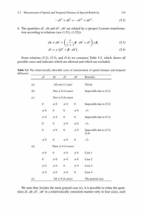
5.3 Measurement of Spatial and Temporal Distance in Special Relativity 119
− dl2 + dr2 = −dl ′2 + dr′2. (5.2)
b. The quantities dl, dr and dl ′, dr′ are related by a (proper) Lorentz transforma-tion according to relations (see (1.51), (1.52)):
dr = dr′ +(
γ
γ + 1β · dr′ + dl ′
)γβ, (5.3)
dl = γ(dl ′ + β · dr′
). (5.4)
From relations (5.2), (5.3), and (5.4) we construct Table 5.2, which shows allpossible cases and indicates which are allowed and which are excluded.
Table 5.2 The relativistically allowable cases of measurement of spatial distance and temporaldifference
dl dr dl ′ dr′ Remarks
(a) All zero (1 case) Trivial
(b) One �= 0 (4 cases) Impossible due to (5.2)
(c) Two �= 0 (6 cases)
0 �= 0 �= 0 0 Impossible due to (5.2)
�= 0 0 0 �= 0 –//–
�= 0 �= 0 0 0 Impossible due to (5.3)
0 0 �= 0 �= 0 –//–
0 �= 0 0 �= 0 Impossible due to (5.3),(5.4)
�= 0 0 �= 0 0 –//–
(d) Three �= 0 (4 cases)
�= 0 0 �= 0 �= 0 Case 1
0 �= 0 �= 0 �= 0 Case 2
�= 0 �= 0 0 �= 0 Case 3
�= 0 �= 0 �= 0 0 Case 4
(e) All �= 0 (4 cases) The general case
We note that, besides the most general case (e), it is possible to relate the quan-tities dl, dr, dl ′, dr′ in a relativistically consistent manner only in four cases, each

120 5 The Physics of the Position Four-Vector
case being characterized by the vanishing of one of the quantities dl, dr, dl ′, dr′.This result demands that we consider each of these cases as defining the relativisticmeasurement of the spatial and the temporal distance in the RIOs Σ and Σ′. Inorder to find the exact role for each case we consider the Newtonian measurementof spatial and temporal distance and note the following:
• The Newtonian measurement of spatial distance involves two points in space (i.e.,dr �= 0 or dr′ �= 0) and takes place at one time moment (i.e., dl = 0 or dl ′ = 0).
• The Newtonian measurement of temporal difference involves one point in space(i.e., dr =0 or dr′ = 0) and two time moments (i.e., dl = 0 or dl ′ = 0).
Having as a guide the Newtonian method of measuring spatial distance and tem-poral difference we give the following definition for the measurement of the rela-tivistic spatial distance and the measurement of the relativistic temporal difference.
Definition 7 Condition dr = 0 (respectively, dr′ = 0) defines the relativistic mea-surement of temporal difference at one spatial point by the RIO Σ (respectively, Σ′).Condition dl = 0 (respectively, dl ′ = 0) defines the relativistic measurement ofspatial distance at one time moment by the RIO Σ (respectively, Σ′).
Definition 7 suffices in order
• To define a unique and consistent procedure for the measurement of the relativis-tic spatial distance and the relativistic temporal difference in Special Relativityand
• To define a well-defined correspondence between the relativistic measurement ofthe spatial distance and temporal difference with the corresponding Newtonianquantities.
We shall need the following result.
Example 8 Show that if two events coincide in a RIO Σ then they coincide inall RIOs.Solution
Consider two events A, B say, which coincide in the RIO Σ. Then in Σ the four-vector (ABi )Σ = 0. Any other RIO is related to Σ via a Lorentz transformation. TheLorentz transformation is homogenous and therefore preserves the zero four-vector.This means that in all RIO ABi = 0, that is, the events A, B coincide.
5.4 Relativistic Definition of Spatial and Temporal Distances
Consider the events P, Q in spacetime and the four-vector P Qi they define. Thereare three possibilities: P Qi timelike, spacelike, or null. In each case the measure-ment of the vector P Qi has a different meaning. In accordance with what has beensaid in Sect. 5.3 we give the following definition:

5.5 Timelike Position Four-Vector – Measurement of Temporal Distance 121
Definition 8 If the four-vector P Qi is timelike then the measurement of the distanceof the events P, Q concerns temporal difference. If the four-vector P Qi is space-like the measurement of the distance of the events P, Q concerns spatial distance.Finally if P Qi is null then the measurement of the distance of the events P, Q isnot defined.
Definition 8 is compatible with Definition 7 because the vanishing of either dl ordl ′ implies that the position four-vector is spacelike whereas the vanishing of eitherdr or dr′ means that the position four-vector is timelike. We conclude that in orderto study the four allowable cases of Table 5.2 it is enough to study the cases that theposition four-vector is timelike and spacelike.
5.5 Timelike Position Four-Vector – Measurementof Temporal Distance
Consider two events P, Q which define a timelike position four-vector P Qi . LetΣ+P Q be the proper observer of the timelike four-vector P Qi . The events P, Q definetwo hyperplanes in spacetime, which we call Σ+P and Σ+Q , respectively (see Fig. 5.1).Let Σ be the world line of another RIO whose world line makes (in spacetime) anangle φ with the world line of Σ+P Q . We are looking for a definition/procedurewhich will determine the time difference of the events P, Q for Σ.
In order to do that we recall that the measurement of time difference by a New-tonian observer requires that the events occur at the same spatial point. At this pointone places a clock and reads the indications of the clock when the events occur, thedifference of these indications being the required temporal difference of the eventsfor the observer (and all other Newtonian observers!). We transfer these ideas inSpecial Relativity as follows.
We consider the two spatial hyperplanes Σ+P and Σ+Q of Σ+P Q at the points P, Q.These planes contain all spatial events of spacetime which are simultaneous for Σ+P Qwith the events P, Q, respectively. The world line of Σ intersects the hyperplanesat the points P1, Q1, respectively. We define the temporal difference of the eventsP, Q for the RIO Σ to be the (Lorentz) distance of the events P1, Q1 (see Fig. 5.1).
Fig. 5.1 Relativisticmeasurement of timedifference of two events
+
+
+
1
1
∑
∑
∑∑P Q

122 5 The Physics of the Position Four-Vector
Fig. 5.2 Hyperbolic trianglefor the measurement of timedifference
0
+
∑
∑
C
Let (P Q)Σ+P Q= cτ0 be the distance (temporal difference) of the events P, Q as
measured by the proper observer Σ+P Q with two readings of his clock (=Newtonianway of measuring time difference) and let (P1 Q1)Σ = cτ be the correspondingdistance (temporal difference) measured relativistically by the procedure we definedabove by Σ. The two quantities τ0 and τ are related by the Lorentz transformationwhich connects the observers Σ+P Q and Σ. The components of the four-vector P Qi
in the LCFs Σ+P Q and Σ are P Qi = (cτ0, 0)Σ+P Qand P Qi = (cτ,PQ)Σ, respectively.
The Lorentz transformation for the zeroth component gives
τ = γ τ0, (5.5)
where γ = (1− β2
)−1/2and for the space component gives the trivial relation
v = PQτ
. We remark that these relations can be obtained from the hyperbolic geom-etry of an orthogonal triangle if we make the following conventions (see Fig. 5.2):
(1) The side AB=time difference of the events P, Q as measured by Σ+P Q .(2) The side BC = space distance of the events P, Q as measured byΣ.(3) The angle φ is related to the rapidity (i.e., relative speed) of Σ+P Q, Σ by the
relation
coshφ = γ.
It is easy to see that with these conventions relation (5.5) is found from the(hyperbolic) orthogonal triangle ABC in the form τ = τ0 coshφ = γ τ0.
Because γ > 1, τ > τ0. Therefore the result of the measurement of the temporaldifference of the events P, Q for two RIOs is different and the minimum valueoccurs for the proper observer Σ+P Q . In words (5.5) can be stated as follows2:
⎡
⎢⎢⎢⎢⎣
Relativisticallymeasured
temporal differenceof the events P, Q
in the LCF of the RIO Σ
⎤
⎥⎥⎥⎥⎦= γ
⎡
⎢⎢⎢⎢⎣
Newtonianmeasured
temporal differenceof the events P, Q
in the proper frame Σ+P Q
⎤
⎥⎥⎥⎥⎦. (5.6)
2 Spacetime measurement means: with the use of light signals (radar method). Newtonian mea-surement means: with direct reading of the observer’s (not the absolute!) clock.

5.5 Timelike Position Four-Vector – Measurement of Temporal Distance 123
We note that the quantity cτ0 = −(P Q)2 has the following properties:
(1) It is invariant, therefore the value τ0 is the same for all RIOs.(2) The value τ0 is determined experimentally with a procedure similar to the New-
tonian one (i.e., reading the clock indication) only by the proper observer Σ+P Q .
The inequality τ > τ0 has been called time dilation. The name is not the mostappropriate (and has created a lot of confusion) because the quantities τ and τ0 referto different measurements of different observers with different methods and concerntemporal (i.e., coordinate) distance and not time difference.
We arrive now at the following question:
Is it possible for a Newtonian observer (as we are!) to measure relativistic temporaldifference of two events in spacetime?
The answer is “yes” and it is given in the following example.
Example 9 A clock moves along the x-axis of a RIO Σ with constant velocityu = u i. In order for the observer in Σ to measure the time difference of the “mov-ing” clock the observer decides to apply the following procedure:
The observer considers two positions P, Q along the x-axis which are at a dis-tance d(P Q) apart and with its clock measures the time interval Δt required for themoving clock to pass through the point P (event A) and through the point Q (eventB). Then the observer defines the time interval Δt+ measured by the moving clockof the two events P, Q to be Δt+ = Δt/γ . Is this method of measuring relativis-tic time difference with Newtonian observations compatible with the chronometricmethod proposed above?
Answer3 using (a) the algebraic method and (b) the geometric method.
SolutionLet Σ+(AB) be the proper frame of the moving clock, which has (unknown) speed
u along the x-axis of the LCF Σ.
(a) Algebraic solution
We consider the events:
A: The moving clock passes through point P .B: The moving clock passes through point Q.
Because the events A, B are points of the world line of a clock they define a timelikefour-vector ABi . We write the coordinates of the events A, B in the frames of Σ
and Σ+AB in the following table:The boost relating Σ+AB, Σ gives
d(AB) = γ uΔt+,Δt = γΔt+.
3 The algebraic and the geometric method of solving problems in Special Relativity involvingspatial and temporal differences is explained below in Sect. 5.11.3.

124 5 The Physics of the Position Four-Vector
Σ Σ+AB
A : (ctA, xA) (ct+A , 0)
B : (c(tA +Δt), xA + dAB ) (c(t+A +Δt+), 0)
AB : (cΔt, dAB )Σ (cΔt+, 0)Σ+AB
Eliminating Δt+ we find
u = d(AB)
Δt, (5.7)
which is compatible with the Newtonian measurement of the speed of the movingclock in Σ. The second relation gives
Δt+ = Δt
γ,
where γ is computed from the speed u which is measured with Newtonian meth-ods (5.7). This relation is similar to (5.5) and leads us to the conclusion that withthe proposed method observer Σ is able, with Newtonian means and methods, todetermine relativistic temporal differences of a moving clock.
(b) Geometric solution
We consider Fig. 5.3:Explanation of the figureEventsA, B : Events of “moving” clock.Σ: World line of observer Σ.Σ+: World line of the “moving” clock.φ: Rapidity of the “moving” clock wrt observer Σ.
Fig. 5.3 Newtonian methodof measurement of timedifferences

5.5 Timelike Position Four-Vector – Measurement of Temporal Distance 125
Data(AB1): Time interval of the events A, B measured relativistically by observer
Σ, (AB1) = c Δt .(AB): Time interval of the events A, B measured by Newtonian methods by the
proper observer of the moving clock, (AB1) = c Δt+.(B1 B): Space distance of the events A, B as measured with Newtonian methods
by Σ.RequestedRelation between (AB), (AB1).From the triangle AB1 B we have
(AB1) = (AB) coshφ = γ (AB)
from which follows
Δt = γ Δt+,
the same as before.Again we note that
dAB = (B B1) = (AB) sinhφ = (AB)βγ = u Δt
as expected from the Newtonian measurement.
In Fig. 5.4 the measurement of the temporal difference AB of a clock from twoRIOs Σ1 and Σ2 with speeds v1 < v2, respectively, wrt the clock (i.e., Σ+) isshown. We note that t1 < t2, that is, the faster observer measures a larger timedifference and as v2 → c the t2 → ∞. It is important to note that the normals areon the world line of the observer Σ1, Σ2 and not on the world line of the “moving”clock.
Fig. 5.4 Change of value ofmeasured time difference fordifferent speeds

126 5 The Physics of the Position Four-Vector
5.6 Spacelike Position Four-Vector – Measurementof Spatial Distance
Consider two events P, Q which define a spacelike four-vector P Qi and let Σ− bea characteristic frame of P Qi . In Σ− the events P, Q occur at the same time and thefour-vector P Qi has components (0, PQ−) where PQ− is the vector giving the rel-ative spatial position of the events P, Q in Σ−. We consider a RIO Σ, which moveswrt Σ− with parallel axes and relative speed βc. In order to “measure” the relativespatial position of the events P, Q in Σ we must associate two corresponding eventswhich are simultaneous in Σ. To achieve that we consider the hyperplane which isnormal to the world line of the observer Σ at the point Q. This plane contains allevents which are simultaneous with Q. The world line of Σ−, which passes throughthe point P , intersects the hyperplane at a point P1, hence this is the simultaneousevent of Q for Σ. We define the spatial distance P QΣ of the events P, Q forobserver Σ to be the spacetime distance of the events Q, P1 (see Fig. 5.5).
To quantify the above we consider the (hyperbolic) orthogonal triangle Q P1 Pand take
P1 QΣ = P QΣ−
coshφ= P Q−
γ. (5.8)
In order to understand the physical meaning of (5.8) we note that P QΣ− is thespatial distance of the events P, Q measured in the Newtonian way in Σ− and P QΣ
is (by definition!) the relativistic measurement of the same quantity in Σ. Then (5.8)can be understood as follows:
⎡
⎢⎢⎢⎢⎣
RelativisticMeasurement of the
Spatial Distanceof the events P, Q
by the RIO Σ
⎤
⎥⎥⎥⎥⎦= 1
γ
⎡
⎢⎢⎢⎢⎣
NewtonianMeasurement of the
Spatial Distanceof the events P, Q
by the RIO Σ−
⎤
⎥⎥⎥⎥⎦. (5.9)
Fig. 5.5 Relativisticmeasurement of spacedistance

5.6 Spacelike Position Four-Vector – Measurement of Spatial Distance 127
Because γ > 1 the P QΣ− > P1 QΣ, therefore P QΣ− is the minimal value of thespatial distance of the events P, Q among all RIOs. This relation has been namedlength contraction where length means Euclidean length. The term “length” cre-ates confusion because the concept “length” is absolute in Newtonian Physics andEuclidean geometry, therefore it appears to be absurd that the spatial distance of twoevents is different for relatively moving observers. However, this is not so, because(5.8) involves different quantities. In the rhs P QΣ− is Newtonian length measuredby the Newtonian method (of superposition) and by observer Σ− whereas in the lhsthe quantity P1 QΣ is the spatial (Euclidean) distance measured chronometricallyby the observer Σ. The difference between these two lengths is due to the differentmethod of measurement.
We arrive again at the question:
Is it possible for a Newtonian observer (as we are!) to measure the relativistic spatial differ-ence of two events in spacetime?
The answer is affirmative and it is given in the following example.
Example 10 Consider a rod which slides along the x-axis of the LCF Σ with(known) constant velocity u = ui. In order for the observer Σ to measure exper-imentally the length of the rod it applies the following procedure: at first it measuresthe time period Δt required for the two ends of the rod to pass through a fixedpoint along the x-axis. Subsequently it multiplies with the speed of the rod in Σ andcalculates the length L of the rod in Σ. Then Σ defines the “length” L− of the rodin a characteristic RIO Σ− to equal γ L . Is the above procedure of measurement ofspatial distance of events compatible (as far as the numeric results are concerned)with the relativistic? Answer using (a) the algebraic method and (b) the geometricmethod.
(a) Algebraic Solution
Let P, Q be the end points of the rod and x the coordinate of the observationpoint along the x-axis of the LCF of Σ. We consider the events P, Q to be thepassage of the respective ends of the rod from the observation point. The coordinatesof the events P, Q in the LCFs Σ and Σ− are shown in the following table:
Σ Σ−
P : (ctA, x) (ct−A , 0)Q : (c(tA +Δt), x) (c(t−A +Δt−), L−)P Qi : (cΔt, 0)Σ (cΔt−, L−)Σ−
where L− is the length of the rod in Σ−. From the boost relating Σ and Σ− weobtain
L− = γ u Δt. (5.10)
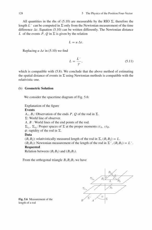
128 5 The Physics of the Position Four-Vector
All quantities in the rhs of (5.10) are measurable by the RIO Σ, therefore thelength L− can be computed in Σ only from the Newtonian measurement of the timedifference Δt . Equation (5.10) can be written differently. The Newtonian distanceL of the events P, Q in Σ is given by the relation
L = u Δt.
Replacing u Δt in (5.10) we find
L = L−
γ, (5.11)
which is compatible with (5.8). We conclude that the above method of estimatingthe spatial distance of events in Σ using Newtonian methods is compatible with therelativistic one.
(b) Geometric Solution
We consider the spacetime diagram of Fig. 5.6:
Explanation of the figureEventsA1, B1: Observation of the ends P, Q of the rod in Σ.Σ: World line of observer.A, B : World lines of the end points of the rod.ΣtA , ΣtB : Proper spaces of Σ at the proper moments ctA, ctB .φ: rapidity of the rod in Σ.Data(B1 B2): relativistically measured length of the rod in Σ, (B1 B2) = L .(B2 B3): Newtonian measurement of the length of the rod in Σ−, (B2 B3) = L−.RequestedRelation between (B1 B2) and (B2 B3).
From the orthogonal triangle B1 B2 B3 we have
Fig. 5.6 Measurement of thelength of a rod
ΣtA
ΣtB
B A
A1
B3
B1 B2L
L−
Σ−Σ
φ
φ φ
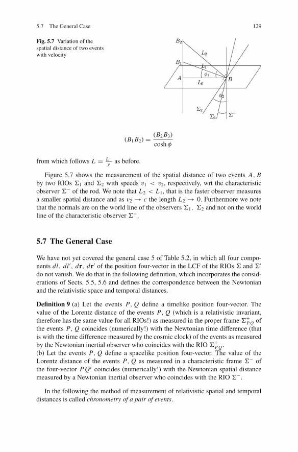
5.7 The General Case 129
Fig. 5.7 Variation of thespatial distance of two eventswith velocity
(B1 B2) = (B2 B3)
coshφ
from which follows L = L−γ
as before.
Figure 5.7 shows the measurement of the spatial distance of two events A, Bby two RIOs Σ1 and Σ2 with speeds v1 < v2, respectively, wrt the characteristicobserver Σ− of the rod. We note that L2 < L1, that is the faster observer measuresa smaller spatial distance and as v2 → c the length L2 → 0. Furthermore we notethat the normals are on the world line of the observers Σ1, Σ2 and not on the worldline of the characteristic observer Σ−.
5.7 The General Case
We have not yet covered the general case 5 of Table 5.2, in which all four compo-nents dl, dl ′, dr, dr′ of the position four-vector in the LCF of the RIOs Σ and Σ′
do not vanish. We do that in the following definition, which incorporates the consid-erations of Sects. 5.5, 5.6 and defines the correspondence between the Newtonianand the relativistic space and temporal distances.
Definition 9 (a) Let the events P, Q define a timelike position four-vector. Thevalue of the Lorentz distance of the events P, Q (which is a relativistic invariant,therefore has the same value for all RIOs!) as measured in the proper frame Σ+P Q ofthe events P, Q coincides (numerically!) with the Newtonian time difference (thatis with the time difference measured by the cosmic clock) of the events as measuredby the Newtonian inertial observer who coincides with the RIO Σ+P Q .(b) Let the events P, Q define a spacelike position four-vector. The value of theLorentz distance of the events P, Q as measured in a characteristic frame Σ− ofthe four-vector P Qi coincides (numerically!) with the Newtonian spatial distancemeasured by a Newtonian inertial observer who coincides with the RIO Σ−.
In the following the method of measurement of relativistic spatial and temporaldistances is called chronometry of a pair of events.

130 5 The Physics of the Position Four-Vector
Example 11 Two rods 1, 2 of length l1 and l2 = nl1, respectively, move with con-stant speed along parallel directions and in the opposite sense. An observer Σ1 atone end of the rod 1 measures that a time interval τ1 = l1/k (k > 1) is required forthe rod 2 to pass in front of him. Calculate
(a) The relative speed of the rods(b) The time interval measured by the observer Σ2 at one end of the rod 2, required
for the rod 1 to pass in front of him
SolutionLet A, B be the events of observation of the ends of the rod l2 as it passes in front
of the observer Σ1 positioned at one end of the rod l1. We have the following tablefor the coordinates of these events in the LCF of the RIOs Σ1, Σ2:
Σ1 Σ2
A : (0, 0) (0, 0)B : (cτ1, 0) (cτ2, l2)AB : (cτ1, 0)Σ1 (cτ2, l2)Σ2
where τ2 is the time interval required for the rod l1 to pass from one end of the rodl2. We have τ2 = l2
cβ where cβ is the relative speed of the rods. The boost relatingΣ1, Σ2 gives τ2 = γ τ1, hence
l2 = cγβτ1 ⇒ βγ = l2
cτ1= nl1
cl1/k= nk
c.
Using the identity γ 2 − 1 = γ 2β2 we find eventually
γ =√
1+ n2k2
c2, β = nk√
c2 + n2k2.
(b) The result does not change if we interchange the names of the rods 1 → 2.Therefore without any further calculations we write
τ2 = l1
cβγ= l1
nk.
5.8 The Reality of Length Contraction and Time Dilation
It is natural to state the question: Does the phenomenon of length contraction andtime dilation exist? The answer to that question is crucial in order to avoid confusionespecially with the various paradoxes which, as a rule, are concerned with these twophenomena.

5.8 The Reality of Length Contraction and Time Dilation 131
Definition 9 relates the measurement of the relativistic spatial and temporal dis-tance of two events, with the corresponding Newtonian measurement of these quan-tities. Verbally it can be stated as follows:
⎡
⎢⎢⎣
Time difference dl+
of events P, Q measuredrelativistically in the
proper frame Σ+P Q
⎤
⎥⎥⎦ ≡
⎡
⎢⎢⎣
Newtonian measurement of thetime difference of the events P, Q taken
by the Newtonian inertial observerwho coincides with Σ+P Q
⎤
⎥⎥⎦ ,
⎡
⎢⎢⎢⎢⎣
Spatial distance dr−‖of events P, Q measured
relativistically in thecharacteristic frame
Σ−P Q
⎤
⎥⎥⎥⎥⎦≡
⎡
⎢⎢⎢⎢⎣
Newtonian measurementof the spatial distanceof events P, Q taken
by the Newtonian inertial observerwho coincides with Σ−P Q
⎤
⎥⎥⎥⎥⎦.
With this definition the relativistic measurements/observations of the spatial andtemporal distance from the characteristic observer and the proper observer, respec-tively, attain a Newtonian “reality.” However, this is true only for these observers!For the rest RIO there is no “Newtonian reality” – that is, comparison with a corre-sponding Newtonian physical quantity – and one must use the appropriate Lorentztransformation to estimate the value of spatial distance and time difference. There-fore relations (5.5) and (5.8) must be understood as follows:
⎡
⎢⎢⎣
Chronometric measurementof time difference
of the events P, Qby the RIO Σ
⎤
⎥⎥⎦ = γ
⎡
⎢⎢⎣
Newtonian measurementof time differenceof the events P, Q
in the proper frame Σ+P Q
⎤
⎥⎥⎦
and⎡
⎢⎢⎣
Chronometric measurementof spatial distanceof the events P, Q
by the RIO Σ
⎤
⎥⎥⎦ = γ−1
⎡
⎢⎢⎣
Newtonian measurementof spatial distanceof the events P, Q
in the proper frame Σ−P Q
⎤
⎥⎥⎦ .
Therefore the validation or not of the phenomena of length contraction and timedilation in nature does not concern the validity of Special Relativity as a theory(=logical structure) but the chronometry, that is, the proposed method of measur-ing/estimating Newtonian spatial distances and Newtonian time differences. Obser-vation has confirmed that the above relations are true, and therefore validates thechronometry of the two events. In practice this means that if we produce in the labo-ratory a beam of particles at the point A and wish to focus them at the point B, thenthe Euclidean distance (AB) must be determined relativistically. That is the position

132 5 The Physics of the Position Four-Vector
of the point B depends on the energy (speed) of the particles of the beam, which isnot the case with Newtonian Physics. In a similar manner we determine the lifetimeof a given unstable particle. In the laboratory the experimentally measured lifetimeof an unstable particle depends on the speed of the particle contrary to the Newto-nian view that the lifetime of a particle is unique. According to our assumption theunique value of the Newtonian approach coincides with the relativistic measurementof the lifetime of the particle in its proper frame (photons excluded, they are stableanyway).
From the above we conclude that the phenomena of length contraction and timedilation are real and must be taken into consideration in our (obligatory!) Newtonianmeasurements in the laboratory and/or in space.
The dependence of the spatial distance and the time difference of two events fromthe velocity of the particles must not worry us in our everyday activities. Indeed,as we have already seen, the effects of relativistic kinematics are appreciable andshow up at high (relative) speeds, far beyond the speeds of our sensory capabilities.Problems which refer to cars entering a garage while traveling with speeds, e.g.,0.9c concern “realities” limited at the level of student exercises and not furtherthan that.
5.9 The Rigid Rod
The rigid rod is a purely Newtonian system which lies in the roots of Newtonian the-ory and expresses the absoluteness of three-dimensional space. The rigid rod doesnot exist in Special Relativity, in the sense that spatial distance is not a relativisticphysical quantity. However, in practice and in the laboratory we do use rigid rods(e.g., the standard meters) to measure distances, therefore it is important and usefulthat we shall define the concept of rigid rod in Special Relativity. This “relativistic”rigid rod shall be associated via a correspondence principle with the Newtonianrigid rod, in the same way we did in Sect. 5.7 for the spatial distance and thetime interval.
Definition 10 The (one-dimensional relativistic) rigid rod in Special Relativity isdefined to be a (relativistic) physical system which in spacetime is represented by abundle of timelike straight lines such that
(a) All lines are parallel (in the spacetime sense).(b) All lie in the same timelike plane.
The system (relativistic) rigid rod is characterized by a single number (Lorentzinvariant!), which we call rest length or proper length of the rigid rod. This numberis specified by the following procedure.

5.9 The Rigid Rod 133
Fig. 5.8 Relativisticmeasurement of the length ofa rigid rod
Each line in the bundle of the timelike straight lines defining the rigid rod canbe associated with the world line of a RIO. If this is done then one can consider the(relativistic) rigid rod as a set of RIOs which have zero relative velocity.4
Let A, B be the limiting outmost world lines of the bundle of the timelike linesdefining the rigid rod (see Fig. 5.8). Consider a RIO Σ and let Στ be the properspace of Σ at proper time τ . This plane intersects the bundle of the lines definingthe rigid rod at line P Q say. The points P, Q are the intersection of the outmostRIOs A, B of the rod with Στ . The four-vector P Qi is spacelike because it lies onthe spacelike hyperplane Στ . The length of the four-vector P Qi is called the lengthof the (relativistic) rigid rod as measured by the observer Σ.
The length (P Q) is uniquely defined for each RIO Σ because of the following:
(1) It is defined geometrically by the intersection of two planes, each one uniquelydefined by the rigid rod and the observer.
(2) The length of the rod is independent of the proper moment τ of Σ because Σ isa RIO and all proper spaces are parallel, therefore the length of the intersectionwith the two-dimensional plane defining the rigid rod is independent of the pointat which we consider the proper plane.
From Fig. 5.8 we note two important properties concerning the length of a (rela-tivistic) rigid rod:
• The length is not absolute, that is the same for all RIOs, and varies with the speedof the rod .
• The events P, Q are not simultaneous for the outmost observers A, B of the rod(τA,P �= τA,Q and similarly for B) while they are so for the observer Σ.
The RIOs for which the value of the distance (P Q) takes its maximum valueare called characteristic observers of the rigid rod. Obviously the world lines ofthese observers are parallel to the world lines A, B which means that they have zerovelocity relative to the rod. The characteristic observer whose world line has the
4 These observers are called comoving observers of the rigid rod. With a similar token one studiesthe motion of a relativistic fluid.

134 5 The Physics of the Position Four-Vector
Fig. 5.9 Length of a(relativistic) rigid rod andLorentz transformation
same spatial distance from the world lines A, B is called rest observer5 of the rigidrod and denoted by Σ0.
If the length of the rigid rod measured by a characteristic observer is L0 and asmeasured by a RIO Σ, with rapidity φ wrt the characteristic observer, is L , then thefollowing relation holds between the two lengths (see Fig. 5.9):
L = L0
coshφ= L0
γ.
Because γ > 1⇒ L < L0 from which it follows that the characteristic observermeasures larger length for the rigid rod and in fact the maximal length (lengthcontraction).
5.10 Optical Images in Special Relativity
The considerations of the previous sections were concerned with the temporal andthe spatial components of the position four-vector and their relation with the corre-sponding concepts of time interval and space distance of Newtonian Physics. Thereis one more Newtonian physical quantity, the creation of optical images, which isrelated to the position vector but not to the measurement of the time difference andspace distance because it does not involve the Lorentz transformation. The trans-fer of this quantity to Special Relativity is important although it applies only toextended luminous bodies, which as a rule do not have practical applications inSpecial Relativity.
In order to define the concept “appear” (= create optical image) in Special Rela-tivity we generalize the corresponding concept of Newtonian Physics. In NewtonianPhysics when we “see” a luminous object we receive at the eye (or the lens ofa camera) simultaneously photons from the various parts of the body. Due to thefinite speed of light and the different distances of the various points of the body
5 The rest observer is the unique characteristic observer with the property that if it (recall that wedo not use he/she) emits simultaneously two light signals toward the end points of the rod and thesesignals are reflected at these points, then it will receive back the two signals simultaneously andalong antiparallel directions.

5.10 Optical Images in Special Relativity 135
from the eye the photons which arrive simultaneously at the eye must be emittedat different times. If the luminous body moves slowly wrt the eye then we mayassume that the photons are emitted simultaneously from all points of the body(Newtonian approximation). In this case we have a “faithful” depiction of the body.But for relativistic speeds this approximation does not hold and one should expectdistortion of the optical image. Due to the above we define the creation of opticalimages in Special Relativity as follows.
Definition 11 The optical image of a set of luminous points at one space point andat one time moment of a RIO Σ is created from the points of emission, which aresimultaneous in Σ.
Before we continue we need the following simple result.
Exercise 12 Let Σ and Σ′ be two LCFs with parallel axes and relative speed β. Con-
sider a four-vector Ai which in the LCFs Σ and Σ′ has components Ai =(
A0
A
)
Σ
and Ai =(
A0′
A′
)
Σ′. Show that
A0 = 1
β
(A‖ − 1
γA′‖
), (5.12)
where A‖ = 1β
(A · β), A′‖ = 1β
(A′ · β) .[Hint: Consider the Lorentz transformation which connects Σ, Σ′:
A0′ = γ (A0 − β · A),
A = A′ + γ − 1
β2(β · A)β + γ A0′β
and in the second equation (a) substitute A0′ and (b) project parallel to β.]
Suppose a photon is emitted from a point in space (event A) and the same photonis received at another point in space (event B). Let Σ be a RIO for which the events
A, B have components
(ctA
rA
)
Σ
,
(ctB
rB
)
Σ
. The four-vector ABi is a null vector
(because it concerns the propagation of a photon), therefore
−c2(tB − tA)2 + (rB − rA)2 = 0.
We write RAB =| rB − rA | and assuming that tB > tA (both time momentsin Σ!) we have
tB = tA + RAB
c. (5.13)

136 5 The Physics of the Position Four-Vector
This relation connects in Σ (!) the distance covered by the photon after its emis-sion in terms of the time interval after its emission. Let another RIO Σ′ move wrt Σ
with parallel axes and arbitrary constant velocity. Let
(ct ′Ar′A
)
Σ′be the components
of the event A in Σ′. According to Exercise 12 for the zeroth component of thefour-vector Ai we have
ctA = 1
β
(rA‖ − 1
γr ′A‖
), (5.14)
where rA‖ = 1β
(r · β), r ′A‖ = 1β
(r ′ · β) . From (5.13), (5.14) we have the relationwhich connects the spatial position of the event A of emission in Σ′ with the timeand the spatial distance covered by the photon in Σ:
ctB = 1
β
(rA‖ − 1
γr ′A‖
)+ RAB ⇒
r ′A‖ = γ(rA‖ − βctB + βRAB
). (5.15)
This relation gives the distance of the image r ′A‖ in Σ′ as a function of the distancerA‖ in Σ.
Normal to the direction of the velocity β the Lorentz transformation has noeffect, hence
rA⊥ = r′A⊥. (5.16)
Using relations (5.15) and (5.16) it is possible to compute the image in Σ if weknow a luminous object in Σ′. Indeed let A,Γ be two points of a luminous bodywhich are observed at the point B of Σ, the time moment t0 (of Σ). Then for eachpoint (5.15), (5.16) hold separately and the condition of the creation of the imagesof the points A,Γ in Σ is that the time in the rhs of the equations is common andequal to t0. Subtracting (5.15) for the points A,Γ and eliminating the time t0 we findthe equation
r ′A‖ − r ′Γ‖ = γ (rA‖ − rΓ‖ + β(RAB − RΓB)), (5.17)
which expresses the “parallel” spatial distance of the points A,Γ as it is seen bythe observer Σ at the point B of Σ. We note that this expression is independentof the time of observation in Σ, hence the image parallel to the relative velocityremains the same; it is “frozen” as we say. In addition we note that for c→∞ ther ′A‖ − r ′Γ‖ = rA‖ − rΓ‖, that is we have the absolute depiction of Newtonian Physics.
Without restricting generality one may consider the point B to be the origin ofthe LCF Σ in which case R2
A = r2A = x2
A + y2A + z2
A and R2Γ = r2
Γ = x2Γ + y2
Γ + z2Γ.
If in addition we restrict our considerations to boosts, then r‖A = xA, r ′‖A = x ′A and(5.15), (5.17) read

5.10 Optical Images in Special Relativity 137
x ′A = γ (xA − βctB + βRA), (5.18)
x ′Γ = γ (xΓ − βctB + βRΓ)⇒ (5.19)
x ′A − x ′Γ = γ [xA − xΓ + β(RA − RΓ)]. (5.20)
This relation holds if Σ′ moves wrt Σ with speed β. If the velocity of Σ′ is −βthe relation remains the same with the change that the dashed quantities have to beinterchanged with the unprimed, that is
xA − xΓ = γ[x ′A − x ′Γ + β(R′A − R′Γ)
]. (5.21)
Example 12 A rod AC of length l ′ is resting parallel to the x ′-axis and in the planey′x ′ of the RIO Σ′ while Σ′ is moving in the standard configuration along the x-axisof the RIO Σ with velocity β. Calculate the length l of the image of the rod on afilm which is placed at the origin O of Σ.
SolutionLet
| x ′A − x ′C |= l ′, | xA − xC |= l.
From (5.20) we have
| x ′A − x ′C |= γ [| xA − xC | +β(RA − RC )]. (5.22)
We consider two cases depending on whether the rod is resting along the x ′- axisor not.
(A) The rod is resting along the x ′-axis, hence y′ = y = 0.
We consider two cases depending on whether the rod is approaching or movingaway from the origin O of Σ. In the first case we have x ′A− x ′C = −l ′ = −l−, xA−xC = −l, RA − RC = −l and replacing in (5.20) we find
l− =√
1+ β
1− βl ′ > l ′. (5.23)
Fig. 5.10 Relativisticobservation of an opticalimage
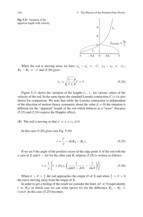
138 5 The Physics of the Position Four-Vector
Fig. 5.11 Variation of theapparent length with velocity
When the rod is moving away we have x ′A − x ′C = −l ′, xA − xC = −l+,RA − RC = −l ′ and (5.20) gives
l+ =√
1− β
1+ βl ′ < l ′. (5.24)
Figure 5.11 shows the variation of the lengths l+, l− for various values of thevelocity of the rod. In the same figure the standard Lorentz contraction (l ′/γ ) is alsoshown for comparison. We note that while the Lorentz contraction is independentof the direction of motion (hence symmetric about the value β = 0) the situation isdifferent for the “apparent” length of the rod which behaves as a “wave” (because(5.23) and (5.24) express the Doppler effect).
(B) The rod is moving so that y′ = y = c1 �= 0.
In this case (5.20) gives (see Fig. 5.10)
l = l ′
γ− β(RA − RC ). (5.25)
If we set θ the angle of the position vector of the edge point A of the rod with thex-axis in Σ and θ −Δθ for the other end B, relation (5.25) is written as follows:
l = 1
γ
[l ′ + βγ y1
(1
sin(θ −Δθ )− 1
sin θ
)]. (5.26)
When π > θ > π2 the rod approaches the origin O of Σ and when π
2 > θ > 0the rod is moving away from the origin of Σ.
In order to get a feeling of the result we consider the limit Δθ � 0 (equivalentlyl � RA) in which case we can write (prove it!) for the difference RA − RC =l cos θ . In this case (5.25) becomes

5.10 Optical Images in Special Relativity 139
l = l ′
γ (1+ β cos θ ). (5.27)
We infer that in this case the observer sees the standard Lorentz contraction onlyif the observer looks along the direction of the y-axis (that is θ = π
2 ).
Example 13 A right circular cylinder6 of radius R and length L0 is rotating withconstant angular speed ω about its axis, which coincides with the x-axis of the LCFΣ. Let Σ′ be another RIO which moves in the standard configuration along thecommon x, x ′-axes with speed β.
(a) Prove that in Σ′ the cylinder appears to be a right circular cylinder of radiusR and length L0
γ.
(b) Assume that along the surface of the cylinder have been marked some points(for example with the fixing of small flags whose height is negligible comparedto the radius of the cylinder) which in the RIO Σ appear to be along a directrixof the cylinder. Prove that in Σ′ these points do not appear to be along a directrixof the cylinder, but along a spiral which appears from one end of the cylinderand disappears at the other end of the cylinder.
Solution
(a) The equation of the surface of the (right circular) cylinder in Σ is y2+ z2 = R2.The boost relating Σ, Σ′ gives y′ = y, z′ = z. Therefore in Σ′ the equation ofthe surface is y′2 + z′2 = R2, which is the surface of a right circular cylinder ofradius R. For the remaining two coordinates (ct, x) and (ct ′, x ′) the boost gives
x ′ = γ (x − ut),
ct = γ (ct ′ + βx ′)
from which follows x ′ = 1γ
x − ut ′. Let A, B be the points of intersection ofthe base planes of the cylinder with the x-axis. The coordinates of these pointsin Σ are 0, L0. At the moment t ′ of Σ′ these points have coordinates whosedifference is x ′B − x ′A = 1
γL0 which is the expected Lorentz contraction and at
the same time the height of the cylinder in Σ′.(b) The points of a directrix of the cylinder in Σ have coordinates
x, y = R cosωt, z = R sinωt
and velocity
v = (0,−Rω sinωt, Rω cosωt).
6 This problem has been proposed by the German physicist von Laue at the early steps of SpecialRelativity.

140 5 The Physics of the Position Four-Vector
We compute the corresponding quantities in Σ′. The coordinates are
x ′ = 1
γx − ut ′,
y′ = y = R cosωt = R cosωγ/c(ct ′ + βx ′) = R cos
(ω
γt ′ + βω
cx
),
z′ = z = R sinωt = R sinωγ/c(ct ′ + βx ′) = R sin
(ω
γt ′ + βω
cx
).
In order to define how Σ′ “sees” the marked points we consider t ′ =constant.From the equation of the transformation it follows that the marked points liealong a (right circular) helix of radius R and pace 2πc
βω. The helix develops all
along the length of the cylinder and it is “frozen” during the motion becauseboth its radius and its pace are independent of t ′. The effect of the rotation isthat the helix appears in Σ′ to emerge from the nearest end of the cylinder anddisappear at the other end (see Fig. 5.12).
In order to calculate the velocity of the marked points of the cylinder in Σ′
we take the derivative7 of the coordinates of the points in the LCF Σ′ withrespect to t ′. The answer (assuming x =constant) is
v′ =(−u,− Rω
γsin
(ω
γt ′ + βω
cx
),
Rω
γcos
(ω
γt ′ + βω
cx
)).
This motion can be considered as a combination of two motions. A trans-lational motion along the common x, x ′- axes with speed −β and a rotationalmotion about the same axis with angular speed ω′ = ω
γ. (Question: What hap-
pens when the speed u of Σ′ is such that ω = γ ?)
Fig. 5.12 The image ofmarked points in Σ′
Σ Σ′
7 One can also use the relativistic rule of composition of velocities.

5.11 How to Solve Problems Involving Spatial and Temporal Distance 141
5.11 How to Solve Problems Involving Spatialand Temporal Distance
In this section we present a number of methods for the solution of problems involv-ing the application of Lorentz transformation – mainly the boosts in problemsinvolving spatial and temporal distance. These methods can be used for calculationsin the laboratory and especially in the discussion of the paradoxes which are basedin the misunderstanding of the relativistic spatial and temporal distance and theirrelation to the corresponding Euclidean quantities. In any case we strongly suggestthat the material of this chapter should be studied thoroughly by those who are notexperienced with Special Relativity.
5.11.1 A Brief Summary of the Lorentz Transformation
Before we proceed we collect the results we have found so far for the Lorentz trans-formation.
Consider two LCFs Σ and Σ′ with parallel axes and relative velocity u. The(proper) Lorentz transformation L+↑ which relates the physical quantities of Σ andΣ′ is (see (1.47))
L+↑ =⎡
⎣γ −γβ t
−γβ I + (γ−1)β2 ββ t
⎤
⎦ . (5.28)
For example for the position four-vector (l, r) the transformation (5.28) gives
⎧⎪⎨
⎪⎩
r′ = r+[γ−1β2 (β · r)− γ l
]β,
l ′ = γ (l − β · r).
(5.29)
The vector form of the Lorentz transformations (5.28) and (5.29) holds only ifthe axes of Σ and Σ′ are parallel (in the Euclidean sense) in the same Euclideanspace. Relations (5.28) and (5.29) are not quantitative and, in general, can be usedin qualitative analysis only. In case we want to make explicit calculations we haveto employ a coordinate system and write these equations in coordinate form.
A special and important subclass of Lorentz transformations is the boosts. Thisis due to the fact (see (1.43)) that a general Lorentz transformation can be writtenas a product of two Euclidean rotations and one boost. Two LCFs are related with aboost of velocity β if and only if they move in the standard configuration, that is
(1) The axes x, x ′ are common and the axes y, y′, z, z′ are parallel.(2) The speed u of Σ′ relative to Σ is parallel to the common axis x .

142 5 The Physics of the Position Four-Vector
(3) The clocks of Σ and Σ′ have been synchronized so that when the origins coin-cide (that is x = y = z = x ′ = y′ = z′ = 0) the clocks are reset to zero (that ist = t ′ = 0).
The boost relating the coordinates (l, x, y, z) and (l ′, x ′, y′, z′) of an event P , say,in Σ and Σ′ reads
x ′ = γ (x − βl),
y′ = y,
z′ = z, (5.30)
l ′ = γ (l − βx).
The inverse Lorentz transformation from Σ′ to Σ is
x = γ (x ′ + βl ′),y = y′,z = z′, (5.31)
l = γ (l ′ + βx ′),
that is, the sign of β in (5.30) changes. The matrix form of the transformation is
L+(β) =
⎡
⎢⎢⎣
γ −γβ 0 0−γβ γ 0 0
0 0 1 00 0 0 1
⎤
⎥⎥⎦ . (5.32)
This matrix is symmetric. This is not the case for the matrix representing thegeneral Lorentz transformation (i.e., parallel axes and arbitrary relative velocity).
5.11.2 Parallel and Normal Decomposition of LorentzTransformation
As we have seen the Lorentz transformation has no effect normal to the direc-tion of the relative velocity u while parallel to the direction of u the action of theLorentz transformation is a boost. This observation leads us to consider the follow-ing methodology of solving problems in Special Relativity. Consider a four-vectorAi = (A0,A) (not necessarily the position vector) and let u be the relative velocityof two LCFs Σ and Σ′. We decompose in Σ the vector A along and normal to u:
A = A‖ + A⊥ , A‖ = A · ββ2
β , A⊥ = A− A‖

5.11 How to Solve Problems Involving Spatial and Temporal Distance 143
and write in a profound notation: Ai = (A0, A‖, A⊥)Σ. Suppose that in Σ′ thefour-vector Ai has components Ai = (A′0, A′‖, A′⊥)Σ′ . Then the (proper) Lorentztransformation gives the relations
A′0 = γ (A0 − β · A‖),A′‖ = γ (A‖ − β A0),
A′⊥ = A⊥. (5.33)
For the Euclidean length A′2 we have
A′2 = A′2‖ + A′2⊥ = A2⊥ + γ (A‖ − β A0)2. (5.34)
The angle θ between the directions of A and u is given by
tan θ = |A⊥||A‖| . (5.35)
The corresponding angle θ ′ of A′ with the velocity u in Σ′ is computed asfollows:
tan θ ′ = |A′⊥||A′‖|= |A⊥|
γ (|A0β − A‖|) =|A| sin θ
γ (A0β − |A| cos θ ). (5.36)
We note that θ �= θ ′ for every three-vector A. This result has many applicationsunder the generic name aberration.
5.11.3 Methodologies of Solving Problems Involving Boosts
The difficult part in the solution of a problem in Special Relativity is the recognitionof the events and their coordinate description in the appropriate LCF of the problem.As a rule in a relativistic problem there are involved
(a) Two events (or relativistic physical quantities) A, B (say),(b) Two LCFs Σ and Σ′ (say), and(c) Data concerning some of the components of the events in one LCF and some
data in the other. With the aid of the Lorentz transformation relating Σ and Σ′
one is able to compute all the components of the involved quantities (usuallyfour-vectors) A, B.
For the solution of problems in Special Relativity involving space distances andtime distances one has to assign correctly who is the observer measuring the relevantquantity directly and who is the observer computing it via the appropriate Lorentz
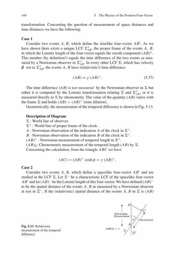
144 5 The Physics of the Position Four-Vector
transformation. Concerning the question of measurement of space distances andtime distances we have the following:
Case 1Consider two events A, B, which define the timelike four-vector ABi . As we
have shown there exists a unique LCF Σ+AB , the proper frame of the events A, B,in which the Lorentz length of the four-vector equals the zeroth component (AB)+.This number (by definition!) equals the time difference of the two events as mea-sured by a Newtonian observer in Σ+AB . In every other LCF Σ, which has velocityβ wrt to Σ+AB , the events A, B have (relativistic!) time difference
(AB) = γ (AB)+. (5.37)
The time difference (AB) is not measured by the Newtonian observer in Σ buteither it is computed by the Lorentz transformation relating Σ and Σ+AB , or it ismeasured directly in Σ by chronometry. The value of the quantity (AB) varies withthe frame Σ and holds (AB) > (AB)+ (time dilation).
Geometrically, the measurement of the temporal difference is shown in Fig. 5.13.
Description of DiagramΣ : World line of observer.Σ+ : World line of proper frame of the clock.A : Newtonian observation of the indication A of the clock in Σ+.B : Newtonian observation of the indication B of the clock in Σ+.(AB)+ : Newtonian measurement of temporal length in Σ+.(AB)Σ: Chronometric measurement of the temporal length (AB) by Σ.Concerning the calculation, from the triangle ABC we have
(AC) = (AB)+ coshφ = γ (AB)+.
Case 2Consider two events A, B, which define a spacelike four-vector ABi and are
studied in the LCF Σ. Let Σ− be a characteristic LCF of the spacelike four-vectorABi and let (AB)− be the Lorentz length of this four-vector. We have defined (AB)−
to be the spatial distance of the events A, B as measured by a Newtonian observerat rest in Σ−. If the (relativistic) spatial distance of the events A, B in Σ is (AB)
Fig. 5.13 Relativisticmeasurement of the temporaldifference

5.11 How to Solve Problems Involving Spatial and Temporal Distance 145
Fig. 5.14 Chronometricmeasurement of spatialdistance
(measured chronometrically) and the relative speed of Σ,Σ− is β, Lorentz transfor-mation gives the relation
(AB) = (AB)−
γ. (5.38)
The length (AB)− is an invariant whereas the length (AB) is not and dependson the observer Σ (the factor β). We have the obvious inequality (AB) < (AB)−
(spatial distance contraction or, as it has been inappropriately established, lengthcontraction).
The measurement of spatial distance is described geometrically in Fig. 5.14.
Description of DiagramΣ :World line of observer.Σ1 : World line of end A of spatial distance.Σ2 : World line of end B of spatial distance.ΣA : Proper space of Σ at the point A.C : Intersection of proper space ΣA with world line Σ2.AB− : Common (Lorentz) normal of Σ1, Σ2 at the event A.(AB)− : Newtonian distance (proper distance) L0 of world lines in the character-
istic LCF Σ−AB .(AC): Spatial distance of world lines Σ1 and Σ2 as measured chronometrically
by Σ.Concerning the calculations, from the triangle ABC of Fig. 5.14 we find
(AB)− = (AC) coshφ = γ (AC).
Case 3Consider two events A, B which define a null vector. A null four-vector does
not have a characteristic LCF, therefore it makes no sense to measure (relativistic)spatial or temporal distance.

146 5 The Physics of the Position Four-Vector
5.11.4 The Algebraic Method
This method involves the construction of a table containing the coordinates of thefour-vectors in the LCFs Σ, Σ′ and subsequently the application of the Lorentztransformation relating the data of the table. More precisely, for every pair of eventsA, B one constructs the following table of coordinates:
Σ Σ′
A : (lA, xA, yA, z A) (l ′A, x ′A, y′A, z′A)
B : (lB , xB , yB , zB ) (l ′B , x ′B , y′B , z′B )
ABi : (lB − lA, xB − xA, . . .)Σ (l ′B − l ′A, x ′B − x ′A, . . .)Σ′
The two events define the four-vector ABi whose components in Σ and Σ′ equalthe difference of the components of the events A, B in Σ and Σ′, respectively, andare related by the Lorentz transformation. In case Σ, Σ′ move in the standard con-figuration with velocity β we have the following equations:
l ′B − l ′A = γ [(lB − lA)− β(xB − xA)] ,
x ′B − x ′A = γ [(xB − xA)− β (lB − lA)] ,
y′B − y′A = yB − yA,
z′B − z′A = zB − z A.
Usually these equations suffice for the solution of the problem. It is important thatbefore inserting the data in the table one clarifies which observer does the Newtonianand which the chronometric measurement of space and time distances. This methodof solving relativistic problems is called the algebraic method.
Example 14 A rod AB moves in the plane xy of the LCF Σ in such a way that theend A slides along the x-axis with constant speed u whereas the rod makes at alltimes (in Σ!) with the x-axis a constant angle φ. Consider another LCF Σ′ whichmoves relative to Σ in the standard configuration along the x-axis with speed v. Letm = tanφ be the inclination of the rod in Σ. Calculate the corresponding quantitym ′ in Σ′.
First SolutionWe consider the end points A, B of the rod and assume that the measurement of
the length of the rod is done in Σ′. Furthermore we assume that at time t = 0 of Σ
the point A is at the origin of Σ. These assumptions lead to the following table ofcoordinates of the events A, B:
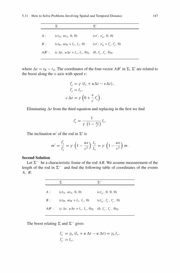
5.11 How to Solve Problems Involving Spatial and Temporal Distance 147
Σ Σ′
A : (ctA, utA, 0, 0) (ct ′, x ′A, 0, 0)
B : (ctB , utB + lx , ly, 0) (ct ′, x ′A + l ′x , l ′y, 0)
ABi : (c Δt, uΔt + lx , ly, 0)Σ (0, l ′x , l ′y, 0)Σ′
where Δt = tB − tA. The coordinates of the four-vector ABi in Σ, Σ′ are related tothe boost along the x-axis with speed v:
l ′x = γ (lx + uΔt − vΔt) ,
l ′y = ly,
c Δt = γ(
0+ v
cl ′x).
Eliminating Δt from the third equation and replacing in the first we find
l ′x =1
γ(1− uv
c2
) lx .
The inclination m ′ of the rod in Σ′ is
m ′ = l ′yl ′x= γ
(1− uv
c2
) ly
lx= γ
(1− uv
c2
)m.
Second SolutionLet Σ− be a characteristic frame of the rod AB. We assume measurement of the
length of the rod in Σ− and find the following table of coordinates of the eventsA, B:
Σ Σ−
A : (ctA, utA, 0, 0) (ct−A , 0, 0, 0)
B : (ctB , utB + lx , ly, 0) (ct−A , l−x , l−y , 0)
ABi : (c Δt, uΔt + lx , ly, 0)Σ (0, l−x , l−y , 0)Σ−
The boost relating Σ and Σ− gives
l−x = γu (lx + u Δt − u Δt) = γu lx ,
l−y = ly,

148 5 The Physics of the Position Four-Vector
hence
m− = l−yl−x= ly
γu lx= m
γu.
Because Σ is arbitrary we write without any further calculations for Σ′:
m− = m ′
γu′.
It follows:
m ′
γu′= m
γu.
But we know that the γ -factors are related as follows8
γu′ = γu γv
(1− uv
c2
). (5.39)
Replacing γu′ we find
m ′ = γv
(1− uv
c2
)m.
Third Solution (With Relative Velocities)We assume (chronometric) measurement of the length of the rod in Σ and have
the following table of coordinates of the events A, B:
Σ Σ−
A : (ctA, utA, 0, 0) (ct ′A, x ′A, 0, 0)
B : (ctA, utA + lx , ly, 0) (ct ′B , x ′B , l ′y, 0)
ABi : (0, lx , ly, 0) (c Δt ′, x ′B − x ′A, l ′y, 0)
8 Proof of (5.39).One method to prove (5.39) is to replace each γ in terms of the velocity and make direct calcu-lations. This is awkward. The simple and recommended proof is to use the four-velocity vector,whose zeroth component is γ c, and apply the Lorentz transformation for the four-velocity. Let ussee this proof. The four-velocity of the event A in the LCFs Σ and Σ′ has components
(γuc, γuu, 0, 0)Σ, (γu′c, γu′u′, 0, 0)Σ′ .
These two expressions are related with a boost as above. For the zeroth component we have
γu′c = γv
(γuc − v
cγu u
)= γv γu c
(1− uv
c2
).
Check the boost for the space components. The result will be used in the next solution.

5.11 How to Solve Problems Involving Spatial and Temporal Distance 149
The boost relating Σ, Σ′ gives
x ′B − x ′A = γ lx ,
Δt ′ = −γ v
c2lx .
But in Σ′
x ′B − x ′A = u′Δt ′ + l ′x
because the events A, B are not simultaneous in Σ′. From the relativistic rule ofcomposing three-velocities (see end of Footnote 8) we have
u′ = u − v
1− uvc2
.
On replacing,
x ′B − x ′A = l ′x −u − v
1− uvc2
γ v
c2lx = γ lx .
It follows:
l ′x =lx(
1− uvc2
)γ.
Replacing in the relation m ′ = l ′y/ l ′x one obtains the previous result.
Example 15 Two events A, B are simultaneous in the LCF Σ and have a spacedistance (in Σ!) c km along the x-axis. Compute the β-factor of another LCF Σ′
moving in the standard way along the x-axis so that the event A has a time distance(i) 1/10 s, (ii) 1 s, (iii) 10 s from event B.
Algebraic SolutionThe two events are simultaneous in Σ. Hence we have the following table of
coordinates:
Σ Σ′
A : (ct, xA) (ct ′A, x ′A)
B : (ct, xA + d) (ct ′B , x ′B )
ABi : (0, d)Σ (−cΔt ′, x ′B − x ′A)Σ′
where d is the distance of the events in Σ. The boost relating Σ,Σ′ gives
150 5 The Physics of the Position Four-Vector
−cΔt ′ = γ (0− β d) = −γβd ⇒ βγ = cΔt ′
d.
Squaring and making use of the (useful!) identity γ 2 β2 = γ 2 − 1 we find
γ 2 = 1+ c2 Δt ′2
d2.
Replacing γ in terms of β and setting d = c we get eventually
β = c Δt ′(c2 Δt ′2 + d2
)1/2 =Δt ′√
1+Δt ′2.
For the given values of Δt ′ we find the following:
(i) For Δt ′ = 1/10 s, β = 0.0995 or v = 0.0995c (≈ 10% c).(ii) For Δt ′ = 1 s, β = 0.707 or v = 0.707c (≈ 71% c).
(iii) For Δt ′ = 10 s, β = 0.995 or v = 0.995c (≈ 99.5% c).
We observe that the more the speed of Σ′ increases the more the event A delays(in Σ′!) wrt the event B. Indeed, solving the last expression for Δt ′, we find Δt ′ =βγ =
√γ 2 − 1.
5.11.5 The Geometric Method
For the solution of problems involving relativistic spatial and temporal distances wecan use spacetime diagrams. This methodology, which is suitable mainly for simpleproblems, is called the geometric method and it is realized in the following steps:
(1) Events:Draw the world lines of the observers involved and identify the events whichconcern the problem.
(2) Quantities:Construct in the spacetime diagram the given space and time distances.
(3) Requested:Construct in the spacetime diagram the requested space and/or time distances.
(4) Solution:Use relations (5.30) and (5.31), which give (as a rule) direct solution to theproblem.
As is the case with the algebraic method, when one draws the various quantities inthe spacetime diagram, he/she must be aware of who measures with the Newtonianmethod and who with the chronometric.

5.11 How to Solve Problems Involving Spatial and Temporal Distance 151
Example 16 Two spaceships 1, 2, each of length l, pass each other moving paralleland in opposite directions. If an observer at one end of spaceship 1 measures thattime T is required for the spaceship 2 to pass in front of him, find the relative speedu of the spaceships.
Algebraic SolutionWe consider the events:
Event A: The “nose” of spaceship 2 passes in front of the observer.Event A: The “tail” of spaceship 2 passes in front of the observer.
The table of coordinates of the events A, B in the LCF of the two spaceships is
Spaceship 1 Spaceship 2
A : (ctA, x) (ct ′A, x ′A)
B : (ctB , x) (ct ′A + clu , x ′A + l)
ABi : (cT, 0)1 ( lβ, l)2
l/u is the time required for spaceship 2 to pass in front of the nose of spaceship 1.The boost relating the components of the position four-vector ABi gives (β = u/c)
βγ = l
cT⇒ β = l√
c2T 2 + l2.
Geometric SolutionWe consider the spacetime diagram of Fig. 5.15:
12 12
Fig. 5.15 Geometric measurement of the length of the spaceship

152 5 The Physics of the Position Four-Vector
Description of DiagramEvents:A1, B1: World lines of observers at the end points of spaceship 1.A2, B2: World lines of observers at the end points of spaceship 2.C : The nose of spaceship 2 passes in front of the nose A1 of the spaceship 1.D: The tail of spaceship 2 passes in front of the nose A1 of the spaceship 1.DZ : Proper space of observer B2 at the event D.Data:C D: Time distance required for spaceship 2 to pass in front of the tip A1 of
spaceship 1, (C D) = T c.DE : Proper length of spaceship 1, (DE) = l.DZ : Proper length of spaceship 2, (DZ ) = l.Requested:Angle φ.From the triangle C Z D we have
(DC) = (DZ )/ sinhφ = l/βγ ⇒ βγ = l
cT⇒ β = l√
c2T 2 + l2.
Example 17 An astronaut on a cosmic platform sees a spaceship moving towardhim with constant speed 0.6 c. Checking in the database of the known spaceships hefinds that the spaceship could be the Enterprize. According to the file in the databasethe length of the Enterprize is 120 m and emits recognition signals every 80 s. Theastronaut measures the length of the spaceship and finds 96 m. He measures theperiod of the emitted light signals and finds 100 s. Is it possible to conclude fromthese measurements that the approaching spaceship is the Enterprize?
Algebraic SolutionWe consider the events:
A: Observation of one end of the unknown spaceshipB: Observation of other end of the unknown spaceship
Consider Σ to be the platform and let Σ′ be the proper frame of the spaceship. Forthe (chronometric) measurement of the length of the approaching spaceship at thetime t of Σ we have the following table of coordinates of the events A, B: The boostrelating the components of the four-vector ABi in Σ and Σ′ gives
Σ Σ′
A : (ct, xA, 0, 0) (ct ′A, x ′A, 0, 0)
B : (ct, xA +Δx, 0, 0) (ct ′A + cΔt ′, x ′A, 0, 0)
ABi : (0, Δx, 0, 0)Σ (c Δt ′, Δx ′, 0)Σ′

5.11 How to Solve Problems Involving Spatial and Temporal Distance 153
Δx ′ = γ (Δx − β · 0) = γ Δx,
where γ = (1− 0.6)−1/2 = 1.25. Replacing we find Δx ′ = 1.25× 96 m = 120 m,which coincides with the length of Enterprize given in the database.
We continue with the identification of the emission signal. Now the events A, Bare the emission of successive light signals (from the same position of the space-ship). Let Δt ′ be the time distance of the light signals in Σ′ and Δt the correspondingdifference in Σ. We have the following table of coordinates for the events A, B :
Σ Σ′
A : (ctA, x, 0, 0) (ct ′A, x ′A, 0, 0)
B : (ctA+c Δt, x+Δx, 0, 0) (ct ′A + cΔt ′, x ′A, 0, 0)
ABi : (cΔt, Δx, 0, 0)Σ (c Δt ′, 0, 0, 0)Σ′
The boost relating the components of ABi in Σ,Σ′ gives
c Δt = γ (c Δt ′ + β 0) = γ cΔt ′ = 1.25× 80 s = 100 s
and coincides with the period of signals given in the database. The astronaut con-cludes that as far as he can say the approaching spaceship is the Enterprize.
Geometric SolutionConsider the spacetime diagram of Fig. 5.16:
Description of Diagram(a) Length measurement:Events:Σ: World line of cosmic platform.A1, B1 : World lines of the end points of the unknown spaceship.A, B: Events of measurement of the space length of the unknown spaceship at
the moment tB of the platform.ΣA: Proper space of the platform at the event A.Data:(B E) : (Proper) length of Enterprize, (B E) = 120 m.
Fig. 5.16 Geometricmeasurement of spatial andtemporal distance
154 5 The Physics of the Position Four-Vector
(B A): Measured length of unknown spaceship, (B A) = 96 m.φ : tanhφ = β = 0.6, coshφ = γ = 1.25.Requested:Compatibility of the data.
From triangle B E A we have
(B E) = (B A) coshφ = (B A) γ = 96× 1.25 m = 120 m,
therefore the space lengths are compatible.
(b) Measurement of the time distance (period) of the recognition signal.We consider again the spacetime diagram of Fig. 5.16:Description of DiagramEvents:Σ: World line of cosmic platform.C, D: Events of emission of successive light signals.C, D1: Events of observation of successive light signals from the platform.ΣD: Proper space of the space platform Σ at the event D.Data:(C D) = 80 s (proper) time distance of successive light signals emitted from
Enterprize.(C D1) = 100 s, measured time distance of successive light signals in the space
platform Σ.φ : tanhφ = β = 0.6, coshφ = γ = 1.25.Requested:Compatibility of the data.
From triangle C DD1 we have
(C D1) = (C D) coshφ = γ (C D) = 1.25× 80 s = 100 s,
which is compatible with the data of the database.

Chapter 6Relativistic Kinematics
6.1 Introduction
In the previous chapters we developed the basic concepts of relativistic motion, thatis, the time and spatial distance. The methodology we followed was the definition ofthese concepts, in agreement with the corresponding concepts of Newtonian theory,which is already a “relativistic” theory of motion.
In the present chapter we continue with the development of the kinematics ofSpecial Relativity. We introduce the basic four-vectors of four-velocity and four-acceleration. We define the concept of relative four-vector and finally show howthe Lorentz transformation defines the law of composition of three-velocities. Thefour-acceleration is discussed in a separate chapter, due to the “peculiarities” and itscrucial role in both kinematics and dynamics of Special Relativity.
6.2 Relativistic Mass Point
Special Relativity is a geometric theory of physics. Therefore all its concepts mustbe defined geometrically before they are studied. The basic Physical object of kine-matics is the “moving point,” which in Special Relativity is described by a worldline, that is, a spacetime curve whose position four-vector and the tangent four-vector at all its points is timelike or null. The reason we consider two types ofcurves is because in Special Relativity there are two types of particles with differentkinematic (and dynamic) properties: the particles with mass and the photons. Theparticles with mass are called Relativistic mass points (ReMaP) and geometrizewith a timelike world line, whereas the photons we correspond to null world lines.In this section we develop the kinematics of ReMaPs. The kinematics of photonsare studied in another place.
A timelike world line can be affinely parameterized.1 The affine parameter iscalled the proper time τ of the ReMaP.
1 Affine parameterization means that the length of the tangent vector dxi
dτ has constant length alongthe world line. Proper time is the affine parameter (modulo a linear transformation) for which thisconstant equals −c2.
M. Tsamparlis, Special Relativity, DOI 10.1007/978-3-642-03837-2 6,C© Springer-Verlag Berlin Heidelberg 2010
155

156 6 Relativistic Kinematics
In order to do physics we must associate with ReMaP relativistic Physical quanti-ties. We assume that with each ReMaP there are associated two relativistic Physicalquantities: the position four-vector xi and the proper time τ . These quantities aresufficient to the kinematics of the ReMaP. Concerning the dynamics, one has toassociate additional Physical quantities to a ReMaP.
Using the Physical quantities xi , τ we define new ones along the world line, usingthe two basic rules of constructing new tensors from given ones (see Proposition2): multiplication with an invariant and differentiation wrt an invariant. These newtensors are potential relativistic Physical quantities and become relativistic Physicalquantities, either by means of a principle or by identifying with a Newtonian Physi-cal quantity in a specific frame. From xi , τ we define five new Lorentz tensors (twofour-vectors and three invariants):
ui = dxi
dτ, (6.1)
ai = d2xi
dτ 2, (6.2)
ui ui , ai ui , ai ai . (6.3)
In order to study the new four-vectors we use special coordinate systems in whichthese vectors attain their reduced form. Because xi (τ ) is a timelike curve it admitsa proper frame Σ+ in which xi = (cτ
0
)Σ+ . In this frame we compute
ui = dxi
dτ=
(c0
)
Σ+
as well as
ui ui = −c2.
From these two relations we infer the following:
(1) The timelike vectors xi , ui have common proper frame.(2) The length of the four-vector ui is the universal constant c.(3) The four-vector ui is determined in its proper frame by c only, hence it is com-
mon for all particles with mass.
Because ui is determined only in terms of c, which (in Special Relativity) isa Physical quantity, we infer that ui is a relativistic Physical quantity. This newrelativistic quantity is called the four-velocity of the ReMaP at the point xi (τ ).
We continue with the rest of the quantities defined by (6.2) and (6.3). Relationui ui = −c2 =⇒ ui ai = 0, which implies the following:
(1) The four-vector ai is normal to ui , therefore it is a spacelike four-vector.(2) The invariant ui ai is trivial.(3) In the proper frame Σ+ of the four-vectors xi , ui the four-vector ai has components
(why?)

6.2 Relativistic Mass Point 157
ai =(
0a+
)
Σ+. (6.4)
We note that Σ+ is the characteristic frame of the spacelike four-vector ai . If weidentify in Σ+ the three-vector a+ with the Newtonian acceleration of the mass pointin Σ+, then the four-vector ai becomes a relativistic Physical quantity. We call thisnew quantity four-acceleration of the world line at the point xi (τ ). Geometricallythe four-acceleration accounts for the curvature of the world line at each of its points,therefore the vanishing of the four-acceleration (equivalently of the three-vector a+)means that the world line is a straight line in spacetime. This result is consistentwith the requirement that the world line of a Relativistic inertial observer (RIO) is astraight line. Furthermore we see that with this correspondence the Newtonian iner-tial observers correspond to Relativistic inertial observers (RIO) which is important,because all observations are made by Newtonian observers (i.e., us).
Based on the above analysis, we give the following important definition.
Definition 12 Relativistic mass point (ReMaP) with timelike world line A(τ ) is theset of all relativistic Physical quantities, which are defined at every point of A(τ ) andhave common proper frame or characteristic frame, depending on whether they aretimelike or spacelike four-vectors.
According to this definition, xi is the position four-vector, ui is the four-velocity,and ai is the four-acceleration of the ReMaP, whose world line is the curve xi (τ ).
It is to be noted that the above apply to particles with mass, not to photons (orparticles with speed c), which are described by null position four-vectors. The posi-tion vectors of photons do not have a special type of frame in which they obtain areduced form. The kinematics of photons is studied by means of other four-vectors.
Example 18 Calculate the components of the four-velocity ui in the LCF, in whichthe particle has three-velocity v.Solution
Consider a ReMaP P with world line xi (τ ) and let Σ be an LCF, in which
the position four-vector xi =(
ctr
)
Σ
. In the proper frame Σ+ of P we have
xi =(
cτ0
)
Σ+. The two expressions are related with a Lorentz transformation (not
necessarily a boost), hence
ct = γ cτ ⇒ t = γ τ. (6.5)
The components of the four-velocity ui of P in Σ are
ui = dxi
dτ= dt
dτ
dxi
dt= γ
(cu
)
Σ
, (6.6)
where u is the three-velocity of the ReMaP in Σ. We find the same result if we apply
the general Lorentz transformation (1.51), (1.52) to the four-vector ui =(
c0
)
Σ+.

158 6 Relativistic Kinematics
Exercise 13 Using the above expression for the coordinates of ui in Σ, show that inΣ ui ui = −c2, which reaffirms that the quantity ui ui is an invariant.
In the following example we show how the four-velocity is computed for certainmotions.
Example 19 The LCF Σ′ is moving in the standard configuration with speed u wrtthe LCF Σ. A particle moves in the x, y plane of Σ with constant speed v arounda circular orbit of radius r centered at the origin of Σ. Calculate the four-velocityof the particle in Σ′. Calculate the γ ′-factor of the particle in Σ′. Find the relationbetween the time t in Σ with the proper time τ of the particle. Write the equation ofthe trajectory of the particle in Σ in terms of the proper time τ .First solution
The equation of the orbit of the particle in Σ is
x = r cosωt = r cos
(vt
r
), y = r sinωt = r sin
(vt
r
).
Therefore the three-velocity of the particle in Σ is
vx = −v sin
(vt
r
), vy = v cos
(vt
r
)
and the four-velocity
vi = (γ c, γ vx , γ vy, 0)Σ =(γ c,−γ v sin
(vt
r
), γ v cos
(vt
r
), 0
)
Σ
,
where γ = 1/√
1− v2
c2 .
In order to compute the four-velocity of the particle in Σ′, we consider the boostrelating Σ, Σ′. For the zeroth component we have
γ ′c = γu
(γ c − u
cγ vx
)= γuγ c
(1− uvx
c2
)⇒ γ ′ = γuγ Q, (6.7)
where Q ≡ (1− u·vc2 ) and γu = 1/
√1− u2
c2 . For the spatial components we compute
vx ′ = vx − u
Q, (6.8)
vy′ = vy
γu Q. (6.9)

6.3 Relativistic Composition of Three-Vectors 159
Hence the four-velocity of the particle in Σ′ is
viΣ′ =
⎛
⎜⎜⎝
γ ′cγ ′vx ′
γ ′vy′
0
⎞
⎟⎟⎠
Σ′
=
⎛
⎜⎜⎝
γuγ Qcγuγ (vx − u)
γ vy
0
⎞
⎟⎟⎠
Σ′
=
⎛
⎜⎜⎜⎜⎝
γuγ Qc
−γuγ (v sin vtr + u)
γ v cos vtr
0
⎞
⎟⎟⎟⎟⎠
Σ′
.
The proper time of the particle in Σ is τ = tγ
, where t is the time in Σ. Thereforethe orbit of the particle in Σ in terms of the proper time is
x = r cos(vγ τ
r
), y = r sin
(vγ τr
).
[What do you have to say for the four-vector ( dtdτ ,
dxdτ ,
dydτ , 0)Σ?]
Second solutionFirst we transform the orbit of the particle in Σ′ and then we compute the four-
velocity using derivation wrt time. The boost relating Σ,Σ′ gives
ct ′ = γu
(ct − u
cx), x ′ = γu(x − ut), y′ = y.
From the first equation it follows that
dt ′ = γu
(dt − u
c2vx dt
)= γu Qdt ⇒ dt
dt ′= 1
γu Q,
hence
v′x =dx ′
dt ′= dx ′
dt
dt
dt ′= vx − u
1− uvx
c2
= −1
Q
[v cos
(vt
r
)+ u
],
v′y =dy′
dt ′= dy′
dt
dt
dt ′= vy
γu(1− uvx
c2
) = 1
γu Q
[v sin
(vt
r
)].
The rest of the solution is the same.
6.3 Relativistic Composition of Three-Vectors
A basic result of Newtonian Physics, with numerous applications, is the compo-sition rule for Newtonian three-vectors. This rule relates the observations of twoNewtonian inertial observers (NIO) and concerns one Newtonian Physical quantity.Let us recall how this rule is defined.

160 6 Relativistic Kinematics
Consider two NIOs N1 and N2 and the Newtonian mass point P , which wrt toN1, N2 has, respectively,
• Position vector : rP1 , rP2
• Velocity : uP1 ,uP2
• Acceleration : aP1 , aP2
Then, if the NIO N2 wrt the NIO N1 has
• Position vector : rN21
• Velocity : uN21
• Acceleration: aN21
Newtonian kinematics postulates the relations
rP2 = rP1 + rN21 ,
uP2 = uP1 + uN21 , (6.10)
aP2 = aP1 + aN21 ,
which are called the Newtonian composition rule for the Newtonian position vector,velocity, and acceleration, respectively. This rule applies to any other Newtonianthree-vector associated with the Newtonian point mass.
We note that relations (6.10) express the Galileo transformation for the position,velocity, and acceleration three-vectors, respectively. This observation is important,because it shows that the Newtonian composition rule for three-vectors is fun-damental to geometry (it expresses the linearity of the Newtonian space) and tophysics, because it expresses the Galileo Principle of Relativity. This explains whythe breaking of this rule by the velocity of light necessitated the introduction ofSpecial Relativity.
Using the above observation, we extend the three-vector (not anymore Newtonianthree-vector!) composition rule in Special Relativity by a direct application of theLorentz transformation. Working in a similar manner we consider two LCFs Σ1 andΣ2 and one ReMaP P , which relatively to Σ1, Σ2 has, respectively,
(1) Position four-vector : xiP1, xi
P2
(2) Four-velocity : uiP1, ui
P2
(3) Four-acceleration: aiP1, ai
P2
If L(1, 2) is the Lorentz transformation relating Σ1, Σ2 then the following rela-tions apply:
xiP2= L(1, 2)xi
P1,
uiP2= L(1, 2)ui
P1, (6.11)
aiP2= L(1, 2)ai
P1.

6.3 Relativistic Composition of Three-Vectors 161
These equations induce a relation among the three-vectors of the spatial parts ofthe respective four-vectors. We call this relation the relativistic composition rule forthree-vectors. This rule is different from the Newtonian composition rule, becausethe first expresses the linearity of space and the Galileo Principle of Relativity,whereas the latter the linearity of Minkowski space and the Einstein Principle ofRelativity.
Obviously, the detailed expression of the relativistic composition rule will dependon the four-vector concerned. Most useful (and important) is the relativistic compo-sition rule for three-velocities, which we derive in the next example.
Example 20 a. Consider two LCFs Σ, Σ′ with parallel axes and relative velocity u.Let a ReMaP be P which in Σ, Σ′ has velocities v and v′, respectively. Provethat
v′ = 1
γu Q
{v+
[u · vu2
(γu − 1)− γu
]u}, (6.12)
where γv′ = γuγv Q and Q = 1− u·vc2 .
Replace 1u2 = 1
c21
1− 1γ 2
u
to find the equivalent form:
v′ = 1
γu Q
{v+
[γu
1+ γu
u · vc2− 1
]γuu
}. (6.13)
In the special case that the velocity u is parallel to the x-axis so that Σ, Σ′ arerelated with a boost, show that (6.12) reduces to (Q = 1− uvx
c2 )
vx ′ = vx − u
Q,
vy′ = vy
γu Q, (6.14)
vz′ = vz
γu Q.
b. Using the results of (a) prove that if the velocity of Σ′ wrt Σ is v, then the velocityof Σ wrt Σ′ is −v.
c. Consider three LCFs Σ1, Σ2, and Σ3 such that Σ2 is moving in the standardconfiguration wrt the LCF Σ1 with speed u along the common axis x1, x2 and Σ3
moves wrt Σ2 in the standard configuration with speed v along the common axisy2, y3. Let v31 be the three-velocity of Σ3 wrt Σ1 and v13 the three-velocity of Σ1
wrt Σ3. Show that the angle θ31 of v31 with the x1-axis is given by tan(θ31) = vuγ (u)
and the angle θ13 of v13 with the axis x3 is given by tan(θ13) = vγ (v)u . Compute
the difference Δθ = θ13 − θ31 in terms of the speeds u, v and discuss the result.
SolutionThe four-velocity vi of P in Σ,Σ′, respectively, is
162 6 Relativistic Kinematics
vi = (γvc, γvv)tΣ = (γv′c, γv′v′)t
Σ′ .
These coordinates are related by the Lorentz transformations (1.51) and (1.52)relating Σ,Σ′. For the zeroth component we find (Q = 1− u·v
c2 )
γv′c = γu
(γvc − u · γvv
c
)=⇒ γv
γv′= 1
γu(1− u·v
c2
) = 1
γu Q. (6.15)
For the spatial components we have
γv′v′ = γvv+[(γu − 1)
u · γvvu2− γu
cγvc
]u
= γv
{v+
[(γu − 1)
u · vu2− γu
]u}.
It follows:
v′ = γv
γv′
{v+
[(γu − 1)
u · vu2− γu
]u}. (6.16)
Replacing γvγv′
from (6.15) we find the required result.If in (6.16) we consider u = ui we obtain (6.14).
Second solutionWe consider first the boost for the position vector between Σ and Σ′:
t ′ = γu
(t − ux
c2
),
x ′ = γu(x − ut),
y′ = y,
z′ = z.
It follows:
v′x =dx ′
dt ′= dx ′
dt
dt
dt ′= γu(vx − u)
dt
dt ′.
From the transformation of the zeroth component we have
cdt ′ = γu
(cdt − u · vdt
c2
)⇒ dt
dt ′= 1
γu(1− u·v
c2
) = 1
γu Q. (6.17)
Replacing we find
v′x =vx − u
Q.
6.3 Relativistic Composition of Three-Vectors 163
Similarly, we calculate
v′y =dy′
dt ′= dy′
dt
dt
dt ′= vy
γu Q,
v′z =vz
γu Q.
In the general case we have
v′ = dr′
dt ′= dr′
dt
dt
dt ′= dt
dt ′d
dt
{r+
[(γu − 1)
u · ru2− γut
]u}
= dt
dt ′{
v+[(γu − 1)
u · vu2− γu
]u}.
Replacing dtdt ′ from (6.17) (which holds for general motion with parallel axes),
we obtain (6.12).b. The velocity v of Σ wrt itself equals 0. Replacing in (6.16) v = 0 we find
v′ = −u.c. We consider Σ3 to be the proper frame of P and apply (6.12). Let v31 be the
relative velocity of Σ3 wrt Σ1 and v32 = (0, v, 0) wrt Σ2. The velocity of Σ1 wrt Σ2
is v12 = (−u, 0, 0). Relation (6.12) gives
v31 = dt2dt1
{v32 +
[(γ12 − 1)
v12 · v32
v212
− γ12
]v12
}⇒ v31 =
(u,
v
γu, 0
),
where we have used that
dt2dt1= 1
γ21(1− v32·v12
c2
) = 1
γu.
Similarly, for v13 we have
v13 = dt2dt3
{v12 +
[(γ32 − 1)
v12 · v32
v232
− γ32
]v32
}⇒ v13 =
(− u
γv,−v, 0
).
We note that the two three-velocities lie in the planes x1 y1 and x3 y3. Therefore,in order to give their direction, it is enough to give the angle they make with the axesx1 and x3, respectively. The angle of v31 with the x1-axis is
tan θ31 = v
uγu
and similarly that of v13 with the x3-axis is
tan θ13 = vγv
u.

164 6 Relativistic Kinematics
In Newtonian Physics the following holds (because γu = γv = 1):
θ31 = θ13.
In relativistic kinematics this does not hold and the two relative velocities are notcollinear. They have a deviation Δθ = θ31 − θ13 as follows:
tan Δθ = tan(θ31 − θ13) = tan θ31 − tan θ13
1+ tan θ13 tan θ31= 1− γuγv
u2γu + v2γvuv.
Replacing the lengths u2, v2 in terms of the corresponding γ, we find the result
tan Δθ = − γuγv
γu + γv
uv
c2.
We note that in general Δθ �= 0. Kinematically this means that the Lorentz trans-formation does not preserve the three-directions. This does not bother us becausethree-directions are not covariant (as in the case of Newtonian Physics). Assumingspeeds vi � c, the γi = 1+ O(β2
u , β2v ) (i = u, v) and Δθ = − tan−1(βuβv/2) =
−βuβv/2 + O(β2u , β
2v ). This result is related to the Thomas precession, which will
be considered in Sect. 6.6.In Sect. 4.5.2 we classified the relativistic particles in terms of the type of their
world lines and their speed. More specifically, the particles with timelike world lineand speed u < c are named bradyons, the particles with null world line and speedu = c luxons, and the (hypothetical) “particles” with spacelike world line and speedu > c tachyons. Because the speed is not a relativistic quantity, we have to provethat this classification is covariant. That is, if a photon is a photon for one LCF thenit must be a photon for all LCFs and not change to a mass particle for some LCFs.However, the frequency of the photon can change.
Example 21 A ReMaP P has three-velocity u and u′ in the LCFs Σ and Σ′, respec-tively. Assuming that Σ′ is related to Σ with a boost along the common x, x ′-axeswith speed v, show that
(a) If v < c then u′ < c⇒ u < c and u′ > c⇒ u > c.(b) Prove that γ (u′)
γ (u) = γ (v)(1− u·v
c2
).
Solution
(a) From the invariance of the length of the position vector we have
−c2dt2 + dx2 + dy2 + dz2 = −c2(dt ′)2 + (dx ′)2 + (dy′)2 + (dz′)2 ⇒dt2(c2 − u2) = dt ′2(c2 − u′2). (6.18)
The boost relating Σ and Σ′ gives
dt ′ = γ (v)
(dt − β
cdx
)⇒ dt ′ = γ (v)dt
(1− u · v
c2
). (6.19)
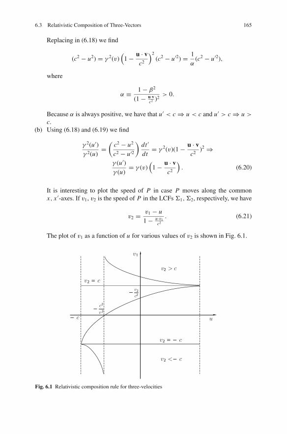
6.3 Relativistic Composition of Three-Vectors 165
Replacing in (6.18) we find
(c2 − u2) = γ 2(v)(
1− u · vc2
)2(c2 − u′2) = 1
α(c2 − u′2),
where
α ≡ 1− β2
(1− u·vc2 )2
> 0.
Because α is always positive, we have that u′ < c⇒ u < c and u′ > c⇒ u >
c.(b) Using (6.18) and (6.19) we find
γ 2(u′)γ 2(u)
=(
c2 − u2
c2 − u′2
)dt ′
dt= γ 2(v)(1− u · v
c2)2 ⇒
γ (u′)γ (u)
= γ (v)(
1− u · vc2
). (6.20)
It is interesting to plot the speed of P in case P moves along the commonx, x ′-axes. If v1, v2 is the speed of P in the LCFs Σ1,Σ2, respectively, we have
v2 = v1 − u
1− u·v1c2
. (6.21)
The plot of v1 as a function of u for various values of v2 is shown in Fig. 6.1.
2 =
–2
2
– 22
2
2 =
2
–
1
–
–
Fig. 6.1 Relativistic composition rule for three-velocities
166 6 Relativistic Kinematics
We note that the plane (v1, u) is divided into five distinct regions as follows:
v1 < −c, v1 = −c, −c < v1 < c, v1 = c, v1 > c.
In each part we have values for the parameter v2 so that v1 and v2 are alwaysin the same region. For example, if the value of v1 is in the region −c < v1 < c,then in the same region is the value of v2. This result shows that the classification ofthe particles according to their speed is covariant. More specifically, bradyons arealways in the region (−c, c), photons in the region v1 = v2 = ±c, and “tachyons”in the region (c,+∞) ∪ (−∞,−c).
6.4 Relative Four-Vectors
Another important relation among velocity, acceleration, and Newtonian vectors ingeneral is the relative velocity, acceleration, and vector, respectively. The conceptof relative vector involves one observer and two mass points, contrary to the ideaof the composition of vectors, which involves two observers and one mass point.Consequently, the concept of relative vector cannot involve the Galileo transforma-tion, which also concerns two Newtonian observers. Let us recall the definition ofrelative vectors in Newtonian Physics.
Consider an NIO N wrt which two Newtonian mass points P, Q have, respec-tively,
• Position vectors: rP , rQ
• Velocities: vP , vQ
• Accelerations: aP , aQ
Then the relative position vector PQ of the Newtonian mass point Q wrt theNewtonian mass point P with reference to the observer N is defined to be the vector
PQ = rPQ = rQ − rP .
For the velocity we have, respectively,
vPQ = vQ − vP (6.22)
and for the acceleration
aPQ = aQ − aP .
This definition expresses the linearity of the space of Newtonian Physics and it isforeign to the rule of composition of Newtonian vectors, which is a consequence ofthe Galileo transformation (and involves two observers). The fact that the two defi-nitions seem to “coincide” is due to the simplicity of the geometric structure of the

6.4 Relative Four-Vectors 167
linear space R3 (something similar occurs with the real numbers, which practicallyshare all properties).
The concept of relative vector is taken directly over to Special Relativity asfollows. Consider an LCF Σ wrt which two relativistic mass points P, Q have,respectively,
(1) Position four-vector: xiP , xi
Q
(2) Four-velocity : viP , v
iQ
(3) Four-acceleration : aiP , ai
Q
Then the relative position four-vector of Q wrt P with reference to the observerΣ is defined to be the four-vector
xiP Q = xi
Q − xiP .
In a similar manner, the relative four-velocity viP Q and the relative four-acceleration
aiP Q of Q wrt P with reference to the observer Σ are defined to be the four-vectors
viP Q = vi
Q − viP , (6.23)
aiP Q = ai
Q − aiP . (6.24)
The definition of the relative four-vector in Special Relativity expresses the lin-earity of the Minkowski space and, as is the case with Newtonian Physics, it isdifferent from the composition rule of four-vectors.2
The most important of the relative vectors is the relative velocity, which is usedin the study of colliding beams, in order to determine the maximum interactionenergy. For photons, the concept of relative velocity and acceleration makes no sensebecause these four-vectors are not defined for photons.
Consider the LCF Σ with four-velocity ui and a ReMaP P with four-velocity vi .The inner product uivi is an invariant, therefore its value is the same in all LCFs. Inthe proper frame Σ+ of Σ one has
ui =(
c0
)
Σ+, vi =
(γ (v)cγ (v)v
)
Σ+
from which it follows that
uivi = −γ (v)c2 ⇒ γ (v) = − 1
c2uivi . (6.25)
2 The concept of relative four-vector cannot be extended to theories of physics formulated overa non-linear space, i.e., curved spaces (e.g., General Relativity). The reason is that the relativevector involves the difference of vectors defined at different points in space, therefore one has to“transport” one of the vectors at the point of application of the other, an operation which involvesnecessarily the curvature of the space.
168 6 Relativistic Kinematics
Relation (6.25) expresses the γ -factor of a ReMaP wrt an observer in terms ofthe inner product of their four-velocities. Consider now two ReMaPs, the 1, 2 say,with four-velocities vi
1, vi2 and relative four-velocity vi
21 = vi1 − vi
2.Then
vi21(v21)i = (vi
1 − vi2) [(v1)i − (v2)i ] = −2c2 − 2vi
1(v2)i .
Let v21 be the three-velocity of ReMaP 2 as measured in the proper frame of 1.Then according to (6.25)
γ (v21) = − 1
c2vi
1(v2)i , (6.26)
hence
vi21(v21)i = −2c2 + 2c2γ (v21) = 2c2[γ (v21)− 1]. (6.27)
Relation (6.27) leads to two conclusions:
(1) γ (v21) > 1 ⇒ vi21(v21)i > 0, which means that the relative four-velocity is a
spacelike vector, hence not a four-velocity.(2) The speed of v12 is determined uniquely from the speeds of the two ReMaPs in
Σ.
The second result is not obvious and it will be useful to prove it. Suppose that inΣ the four-velocities of 1, 2 are
vi1 =
(γ (v1)cγ (v1)v1
)
Σ
, vi2 =
(γ (v2)cγ (v2)v2
)
Σ
.
Then in Σ we have
vi1v2i = −γ (v1)γ (v2)c2 + γ (v1)γ (v2)(v1 · v2) = − γ (v1)γ (v2)c2
(1− v1 · v2
c2
).
From (6.27) we conclude
γ (v12) = γ (v21) = 1− 1
2γ (v1)γ (v2)Q, (6.28)
where Q = 1 − v1·v2c2 . Replacing the γ -factors in terms of β = v/c we find the
symmetric relation
β212 = 1− (1− β2
1)(1− β22)
(1− β1 · β2)2. (6.29)
We note that the right parts of (6.28) and (6.29) are symmetric wrt the speedsv1, v2. This implies that if v12 is the relative velocity of 1 wrt 2 and v21 is the relative

6.4 Relative Four-Vectors 169
velocity of 2 wrt 1 then
|v12| = |v21| , (6.30)
that is, the relative speeds are equal (but as will be shown below, their velocities aredifferent!). Furthermore, we note that the relative speed obtains its maximum valuewhen the denominator in (6.29) takes its maximum value, that is, when β1·β2 = −1.This happens when 1, 2 move antiparallel in Σ.
Relation (6.29) can be written in a different form, useful in the solution of prob-lems.
Exercise 14 Making use of the three-vector identity a×b = |a|2|b|2− (a ·b)2 showthat (6.29) can be written as
β212 =
(β1 − β2)2 − (β1 × β2)2
(1− β1 · β2)2. (6.31)
Up to this point we have determined only the speeds, which are measured inthe proper frames of the particles in terms of their velocities in Σ. The followingquestion arises: Is it possible to determine completely the velocities v12, v21, whichare measured in the proper frames of the particles 1 and 2 in terms of the veloci-ties v1, v2 which are measured in Σ? The answer is “yes,” provided that we workas we did for the composition of four-vectors. That is, we consider in Σ,Σ2 thecomponents of the four-velocity of particle 1:
vi1 =
(γ (v1)cγ (v1)v1
)
Σ
, vi1 =
(γ (v12)cγ (v12)v12
)
Σ2
and demand the two expressions of vi1 to be related with a Lorentz transformation
with velocity v2. The three-velocities v21, v12 defined in this way are called relativethree-velocity of particle 2 wrt particle 1 and relative velocity of the particle 1 wrtparticle 2, respectively. In Newtonian Physics we have
v21 = −v12 = v2 − v1.
However, in Special Relativity nothing is obvious and everything has to be cal-culated explicitly. Let us compute v12. Using the general result of (6.13) of Exam-ple 20, we write
v12 = 1
γ (v2)Q
{v1 +
[γ (v2)
γ (v2)+ 1
v1 · v2
c2− 1
]γ (v2)v2
}. (6.32)

170 6 Relativistic Kinematics
The term in the brackets is written as
v1 − v2 +{
1+[
γ 2(v2)
γ (v2)+ 1
v1 · v2
c2− γ (v2)
]}v2
= v1 − v2 + 1
γ (v2)+ 1
[1− γ 2(v2)+ γ 2(v2)
v1 · v2
c2
]v2
= v1 − v2 + 1
γ (v2)+ 1
[−γ 2(v2)
v22
c2+ γ 2(v2)
v1 · v2
c2
]v2
= v1 − v2 −γ 2(v2) v
22
c2
γ (v2)+ 1
[1− v1 · v2
v22
]v2
= v1 − v2 − [γ (v2)− 1]
[1− v1 · v2
v22
]v2,
where in the last two steps we have used the identity γ 2 − 1 = γ 2β2. Finally
v12 = 1
γ (v2)(1− v1·v2
c2
){
v1 − v2 − [γ (v2)− 1]
[1− v1 · v2
v22
]v2
}. (6.33)
We note that (6.33) is not symmetric in v1, v2. Indeed, we calculate
v21 = 1
γ (v1)(1− v1·v2
c2
){
v2 − v1 − [γ (v1)− 1]
[1− v1 · v2
v21
]v1
}�= −v12.
(6.34)This result is different from the expected Newtonian result v12 = −v21. This must
not bother us, because the vectors v12, v21 are three-vectors of different relativisticobservers (the proper observers Σ1 and Σ2 of the particles 1, 2, respectively) and thekinematics of relativistic observers is different from that of Newtonian observers.3
The three-velocities v12, v21 differ only by a Euclidean rotation, therefore thereexists an angle ψ and a direction e normal to the plane defined by the velocitiesv12, v21 such that the rotation of v12 about the direction e for an angle ψ takes itover to v21. The angle ψ is known as Wigner angle and has wide use in the study
3 There is a significant difference, which must be pointed out. The relative (relativistic) velocity v21
refers to the velocity of the particle 2 in the proper frame Σ1 of particle 1 and therefore involvesthe relativistic measurement of velocity (not photon!) and the inequality |v12| < c is expected tohold. Indeed, if we consider two particles, one moving along the positive x-axis with speed c/2and the other moving along the negative x-axis with speed c/2, then using (6.31) we compute thatthe (relativistic) relative speed of the particles equals 4c/5 < c, whereas the Newtonian relativespeed is c.

6.4 Relative Four-Vectors 171
of elementary particles.4 In order to compute the Wigner angle we set A ≡ v212 =
γ 212−1γ 2
12= 1− 1
γ 21 γ
22 Q2 where γi = γ (vi ) (i = 1, 2) and get
cosψ = v12 · v21
v12v21
= − 1
A
[(v1 − v2)2 − (γ2 − 1)
(v1 · v2 − v22)
v22
− (γ1 − 1)(v1 · v2 − v2
1)
v21
+ (γ1 − 1)(γ2 − 1)(v1 · v2)(v1 · v2 − v2
2)(v1 · v2 − v22)
v21v
22
]. (6.35)
We write v1 · v2 = v1v2 cosφ and after a standard calculation we find
cosψ = 1− 2 sin2 φ
1+ 2ρ cosφ + ρ2, (6.36)
where ρ =[
(γ1+1)(γ2+1)(γ1−1)(γ2−1)
] 12
(1 ≤ ρ ≤ ∞). Other equivalent forms of (6.36) are
tanψ
2= sinφ
ρ + cosφ, (6.37)
sinψ = 2 sinφ(ρ + cosφ)
1+ 2ρ cosφ + ρ2. (6.38)
We note that the angle ψ
- Is in the region [π2 , π ]- Depends symmetrically on v1, v2
Exercise 15 Prove that for φ = π2 the angle ψ is given by the relation
ψ = tan−1
[v1v2(γ1γ2 − 1)
γ1v21 + γ2v
22
]= 2 cot−1 ρ.
Assume v1 = v2 and show that in the Newtonian limit the angle ψ → 0 (is oforder O (ε2)), while in the relativistic limit ψ → π
2 . Finally, show that for photonsψ = π
2 .
Exercise 16 Working with the relative position, derive relation (6.33). Moreover,assume that the position four-vector of a particle 1 in the LCFs Σ and Σ2 is, respec-tively,
4 The interested reader can find more on the Wigner angle in, e.g., A. Ben-Menahem “Wigner’srotation revisited” Am. J. Phys. 53, pp. 62–66, (1983).

172 6 Relativistic Kinematics
xi1 =
(l1
r1
)
Σ
,
(l12
r12
)
Σ2
.
Then consider the Lorentz transformation, which relates r12 with r1, and calcu-late the relative velocity from the relation v12 = dr12
dτ2, where τ2 is the proper time of
Σ2.
In the following example, we demonstrate the use of relative velocity in a “prac-tical” problem.
Example 22 A mobile is sliding freely along the positive x-axis with constant speedac (0 < a < 1). A smaller mobile is moving freely on the first along the samedirection with relative speed ac. A third even smaller mobile moves freely on thesecond in the same direction with relative speed ac and so on.
(1) Assuming that Newtonian kinematics applies, prove that the speed cvr+1 of ther + 1 mobile wrt the x-axis is
vr+1 = vr + a, (6.39)
where r = 1, 2, . . .. Also prove that in Newtonian kinematics the speed of thenth mobile is given by the relation
vn+1 = (n + 1)a. (6.40)
Conclude that the speeds vn are members of an arithmetic series with step a.Finally, show that lim
n→∞ vn →+∞.
(2) Repeat the same questions for relativistic kinematics and show that
vr+1 = vr + a
1+ avr,
vn = (1+ a)n − (1− a)n
(1+ a)n + (1− a)n,
limn→∞ vn = 1.
(6.41)
Discuss the result.
SolutionThe Newtonian part is obvious. Concerning the relativistic part, let cvr be the
speed of the r th mobile wrt the x-axis and ac the relative speed of the r + 1 mobilewrt the mobile r . From the relativistic composition rule for three-velocities we have
cvr+1 = cvr + ac
1+ cvr acc2
= cvr + a
1+ vr a⇒ vr+1 = vr + a
1+ vr a. (6.42)

6.4 Relative Four-Vectors 173
Consider the sequence ζr = 1−vr1+vr
, r = 1, 2, . . .. We find
ζr+1 = 1− vr+1
1+ vr+1= 1− vr+a
1+vr a
1+ vr+a1+vr a
= 1+ avr − vr − a
1+ avr + vr + a
= (1− a)(1− vr )
(1+ a)(1+ vr )= 1− a
1+ aζr .
This reduction formula gives
ζr =(
1− a
1+ a
)r−1
ζ1,
which implies that the terms ζr of the sequence are members of a geometric serieswith step 1−a
1+a ∈ (0, 1). Obviously, this sequence converges to limr→∞ ζr = 0, hence
the velocity limr→∞ cvr = c as expected. The first term of the series is5
ζ1 = 1− v1
1+ v1= 1− a
1+ a,
thus ζr =(
1−a1+a
)r. From the relation defining ζr we have
1− vr
1+ vr=
(1− a
1+ a
)r
from which follows:
vr = (1+ a)r − (1− a)r
(1+ a)r + (1− a)r.
The rest are left as an exercise for the reader.
5 The solution of the problem is a particular case of the sequence an = κan+λμan+ρ , whose terms an
converge to a common value x . In this case, we set x = κx+λμx+ρ and compute the roots ρ1, ρ2 of the
quadratic equation. Then the following recursion formula holds:
an+1 − ρ1
an+1 − ρ2= A
an − ρ1
an − ρ2,
where A is a constant. [Study the case ρ1 = ρ2.] In our example an = vr and κ = 1, λ = a, μ = 1,ρ = a. The equation x = x+a
ax+1 ⇒ ax2 + x = x + a ⇒ x = ±1, hence the reduction relation is
vr+1 − 1
vr+1 + 1= A
vr−1
vr+1or ζr+1 = Aζr .
In order to calculate A, we consider the terms ζ2 = Aζ1 and replacing we find A = 1−a1+a , etc.

174 6 Relativistic Kinematics
6.5 The three-Velocity Space
In Special Relativity we introduce various spaces besides the standard spacetime.Such a space is the three-velocity space, which is used to study geometrically rel-ative motion. The three-velocity of a particle is described in terms of three com-ponents, therefore in a three-dimensional space the three-velocity of a particle cor-responds to a point. Following this observation, we consider a RIO Σ0 and twoparticles, which in Σ0 have velocities6 vI 0 I = 1, 2. Then the velocity of Σ0 isthe origin, O say, of the coordinates of the velocity space (the zero velocity 0) andthe velocities vI 0 I = 1, 2 are two other points, the 1, 2 say, of that space. Joiningthe points O, 1, 2 with a “straight line” (note the quotation marks!) we obtain thetriangle O12 (Fig. 6.2).
Fig. 6.2 The hyperbolictriangle
1 2
12
0102
12
00
0
12
In order to give a kinematic interpretation of this triangle we relate the sides ofthe triangle with the speeds of the corresponding velocities. Thus we relate the side01 to the length of the velocity v10 and the length of the side 12 to the length ofthe relative velocity v12 (in Σ0!). Because the vI J = −vJ I the side I J is of thesame length as the side J I with I, J = 0, 1, 2. In Newtonian kinematics due tothe Newtonian composition rule of three-velocities (6.22) the velocity triangle is atypical triangle of Euclidean geometry, hence the velocity space is also a Euclideanspace. In Special Relativity, due to the relativistic composition formula (6.23), thistriangle is not Euclidean and the three-velocity space is not a linear space, neither isthe Minkowski space.7
6 In this section we follow the notation that two indices in a velocity indicate the first quantity withreference to the second. For example the velocity of Σ1 wrt Σ2 will be denoted as v12. Concerningthe angles we follow the notation that the angle between the velocities v10, v20 of Σ1 and Σ2 in Σ0
will be denoted by A12.7 As we shall show in Sect. 15.4.3, when we study the covariant form of the Lorentz transformation,the three-velocity space is a three-dimensional Riemannian manifold of constant negative curvaturewhose metric is Lorentz covariant. Such spaces are known as Lobachevsky spaces.

6.5 The three-Velocity Space 175
In order to find more information about the three-velocity space, we study thevelocity triangle. We consider a RIO Σ0 and let the RIOs be Σ1,Σ2 with veloc-ities v10, v20, respectively, wrt Σ0. Then the relative velocity v21 of Σ2 wrt Σ1
(as measured by Σ0!) is given by (6.34) and its γ -factor γ21 = γ (v21) is given by(6.26) or equivalently by (6.28). Furthermore, according to the composition formula(6.33) the three three-velocities v10, v20, v21 are coplanar (in Σ0). Let γI 0 be theγ -factor of vI 0 and αI 0 I = 1, 2 the corresponding rapidity. Then γI 0 = coshαI 0 ,vI 0 = 1
c tanhαI 0eI 0, where eI 0 is the unit along the direction of the three-velocityvI 0 I = 1, 2. Let γ21 = coshα12 be the corresponding quantities for the relativevelocity. Then (6.28) gives for γ21
coshα21 = coshα10 coshα20 (1− tanhα10 tanhα20e10 · e20)
= coshα10 coshα20 − sinhα10 sinhα20 cos A12, (6.43)
where A12 is the angle between the unit vectors e01, e02 along the three-velocitiesv10, v20 in Σ0. Equation (6.43) is the cosine law of hyperbolic Euclidean geometryfor a hyperbolic triangle of sides α10, α20, α21 and angles A12, A01, A02. This geom-etry is identical to the Euclidean spherical trigonometry of a triangle with sidesiα10, iα20, iα21 and angles A12, A01, A02 and we have considered the correspon-dence
cos(iα) = coshα. (6.44)
In order to make sure that we have a triangle in hyperbolic Euclidean geometrywe must prove that the above result holds for all three vertices of the triangle. To dothat we go to the definition of relative velocity and write
vi21 = vi
20 − vi10 ⇒ vi
20 = vi21 + vi
10 = vi10 − vi
12.
But γ21 = γ12, i.e., coshα12 = coshα21. It is an easy exercise to show that
coshα20 = coshα12 coshα10 coshα12 − sinhα10 sinhα12 cos A02, (6.45)
where A02 is the angle between the velocities v12 and v02 in Σ2. Similarly, we provethe corresponding relation for the quantity coshα10. These three relations establishthat the three-velocity triangle is a hyperbolic triangle with sides α10, α20, α21 andcorresponding angles A12, A01, A02 in a three-dimensional hyperbolic Euclideanspace. Note that the sides of this triangle are the rapidity and not the speed of thethree-velocities.
A crucial question is if the relative velocity is compatible with the Lorentz trans-formation. This is not obvious, although it is suggested by the result we have justderived. To prove that this is the case, we note that the three-velocity of Σ0 in Σ1 is−v10 and in Σ2 is −v20 whereas the three-velocity of Σ2 wrt Σ1 is v21. Thereforethe definition of the relative velocity we gave will be compatible with the Lorentz

176 6 Relativistic Kinematics
transformation if the components of the four-velocity of Σ0 in Σ1 and Σ2 are relatedby a proper Lorentz transformation with velocity v21.
We choose the coordinate frame in Σ0 so that the x-axis is along the direc-tion of v21. According to the composition formula (6.33) the three three-velocitiesv10, v20, v21 are coplanar (in Σ0). We choose the y-axis to be normal to the x-axis inthe plane of the three-velocities. We recall that the angle between v21 and v01 is A01,hence between v21 and−v10 (the three-velocity of Σ0 in Σ) is π− A10 and similarlythe angle between v21 and −v20 is π − A02. We write for the four-velocities of Σ0
in Σ1 and Σ2 :
vi01 =
⎛
⎜⎜⎝
c coshα10
−c sinhα10 cos A01
c sinhα10 sin A01
0
⎞
⎟⎟⎠
Σ1
, vi02 =
⎛
⎜⎜⎝
c coshα20
−c sinhα20 cos A02
c sinhα20 sin A02
0
⎞
⎟⎟⎠
Σ2
.
The matrix representing the Lorentz transformation in the coordinate system wehave chosen is
L(v21) =
⎛
⎜⎜⎝
coshα21 sinhα21 0 0sinhα21 coshα21 0 0
0 0 1 00 0 0 1
⎞
⎟⎟⎠ ,
therefore we must have
[vi20]Σ2 = [L(v21)] [vi
10]Σ1
or
coshα20 = coshα10 coshα21 − sinhα10 sinhα21 cos A02,
sinhα20 cos A02 = sinhα21 coshα10 − coshα21 sinhα10 cos A01,
sinhα20 sin A02 = sinhα10 sin A01. (6.46)
The first equation is identical with (6.45) while the rest two are identities ofEuclidean spherical trigonometry if we use imaginary sides iα1, iα2, iα21. Forexample, the last relation is the “sine law.” Equivalently, they are the relations ofhyperbolic trigonometry, that is the trigonometry of the hyperbolic sphere. We con-clude that the definition of relative motion is compatible with the Lorentz transfor-mation.
In plane Euclidean trigonometry the angles of a triangle add to π . In spherical andhyperbolic trigonometry this does not hold and one defines the spherical/hyperbolicdefect ε by the formula
ε = π − (A01 + A02 + A12). (6.47)

6.6 Thomas Precession 177
In spherical trigonometry ε is negative and its absolute value equals the areaof the triangle (on the unit sphere). In hyperbolic trigonometry ε is positive. Anexpression of ε in terms of the three sides and an angle is the following8:
sinε
2=
[(coshα2 − 1) (coshα12 − 1)
2(coshα1 + 1)
]1/2
sin A01 (6.48)
and cyclically for each vertex. It is important to see that the velocity triangle containsall the information concerning the relativistic relative three-velocity, that is, givesboth the speeds and the relative directions of the velocities.
6.6 Thomas Precession
The Thomas precession is a purely relativistic kinematic phenomenon, which is dueto the properties of the Lorentz transformation, and more specifically, to the non-covariant character of Euclidean parallelism. The first to note this property of theLorentz transformation was L. Thomas9 who applied it in the study of the emissionspectra of certain atoms. According to the simple model of the atom at that time,the electrons were considered as negatively charged spheres, which were rotatingaround the axis of their spin like gyroscopes and also around the positive-chargednucleus. According to the Newtonian theory, the two rotations do not interact andafter a complete rotation about the nucleus the axis of spin returns to its originalposition. However, the non-covariant character of Newtonian parallelism under theaction of Lorentz transformation leads to an interaction of these two rotations withthe effect that after a complete revolution around the nucleus the axis of spin makesan angle with its initial direction. This type of rotational motion is called precession.The special case we consider here has been called Thomas precession.
In order to study the Thomas precession we consider three LCFs Σ1,Σ2,Σ3
such that Σ1,Σ2 and Σ2,Σ3 have parallel axes and non-collinear relative veloci-ties. Let the Lorentz transformations, which relate the pairs Σ1,Σ2 and Σ2,Σ3, beL12 and L23, respectively. The composite Lorentz transformation L23L12 relatingΣ1,Σ3 is also a Lorentz transformation, because Lorentz transformations form agroup. However, as we shall show, this transformation is of a different type thanthe L12, L23 and corresponds to a Lorentz transformation in which the space axesof the transformed Σ1 are not parallel (in the Euclidean sense) with the space axesof the original Σ1. This rotation of the space axes is a purely kinematic relativisticphenomenon, without a Newtonian analogue, which we call Thomas phenomenon.
8 See for example B.P. (1929) Peirce A short table of integrals ginn, Boston formulae 631 and 632pp. and for a theoretical treatment A. Ungar Foundations of Physics 28, 1283–1321, (1998).9 L.H. Thomas The kinematics of an electron with an axis, Philosophical Magazine 3, 1–22 (1927).

178 6 Relativistic Kinematics
We have seen a first approach to Thomas phenomenon in Example 20, where westudied the composition of boosts along different directions. However, as we shallsee below, the real power of the Thomas phenomenon is in accelerated motions.
Consider two LCFs Σ1,Σ2 with parallel space axes and let u be the velocity ofΣ2 wrt Σ1. The Lorentz transformation L12(u) which relates Σ1,Σ2 is given by thegeneral relations (1.51), (1.52), or, equivalently in the form of a matrix, from (1.47):
Li(12) j (u) =
(γ −γβμ
−γβμ δμν + γ 2
1+γ βμβν
), (6.49)
where cβμ = u =⎛
⎝u1
u2
u3
⎞
⎠
Σ1
and cβμ = (u1, u2, u3)Σ1 . The inverse Lorentz trans-
formation is Li(21) j (−u) =
[Li
(12) j
]−1.
We consider a third LCF Σ3, which has space axes parallel to those of Σ2 andvelocity v. The Lorentz transformation Li
(23) j (v) relating Σ2 and Σ3 is again of thegeneral form (1.51) and (1.52). Because the Lorentz transformations form a group,there must exist a third Lorentz transformation Li
(13) j (w) relating Σ1, Σ3 with veloc-ity w, say, defined by the relation
Li(13) j (w) = Li
(12)k(u)Lk(23) j (v). (6.50)
In order to compute the velocity w, we note that Σ2 has velocity −u wrt Σ1 andΣ3 has velocity v wrt Σ2. Therefore w, which is the velocity of Σ3 wrt Σ1, is givenfrom relation (6.12) of Example 20, which is
w = 1
γu Q
{v+ u
[u · vu2
(γu − 1)+ γu
]}. (6.51)
Now we examine if the composite Lorentz transformation Li(13) j (w) is of the
general form (1.51) and (1.52) as it is the case with the transformations Li(12) j (u),
Li(23) j (v). For that, we examine if the space axes of Σ3 are parallel (in the Euclidean
sense!) to those of Σ1.We consider an arbitrary spacetime point, whose position four-vector in the LCFs
Σ1,Σ2,Σ3 has components
(l1
r1
)
Σ1
u=⇒(
l2
r2
)
Σ2
v=⇒(
l3
r3
)
Σ3
. (6.52)

6.6 Thomas Precession 179
Then relations (1.51) and (1.52) giveL12(u):
l2 = γu
(l1 − u · r1
c
), (6.53)
r2 = r1 − γuul1
c+ (γu − 1)
u · r1
u2u. (6.54)
L23(v):
l3 = γv
(l2 − v · r2
c
), (6.55)
r3 = r2 − γvvc
l2 + (γv − 1)v · r2
v2v. (6.56)
From (6.53), (6.54), and (6.55) we have
l3 = γv
[γu
(l1 − u · r1
c
)− v
c·(
r1 − γuuc
l1 + (γu − 1)u · r1
u2u)]
= γuγv
(1+ u · v
c2
)[l1 − B
cγu(1+ u·v
c2
)], (6.57)
where
B = v · r1 + (γu − 1)1
u2(u · r1)(u · v)+ γuu · r1
= r1 ·[v+ γuu+ (γu − 1)
u · vu2
u]
= γu
(1+ u · v
c2
)(r1 · w).
Replacing B in (6.57) we find
l3 = γuγv
(1+ u · v
c2
) [l1 − w · r1
c
]. (6.58)
But we know that (see (6.7))
γw = γuγv
(1+ u · v
c2
),
therefore
l3 = γw
(l1 − w · r1
c
). (6.59)

180 6 Relativistic Kinematics
We conclude that, as far as the zeroth component of the position four-vector isconcerned, the composite Lorentz transformation L13(w) behaves as a Lorentz trans-formation with parallel axes and velocity w. This means that whatever differencesof L13(w) concern the spatial part r of position four-vector and more specificallyeither the length or the direction of r, or both. We treat each case separately.
Let r3(w) be the spatial part of the position four-vector after the action of Li13 j (w)
(on the
(l1
r1
)
Σ1
) and let l3(w) be the temporal component. The invariance of the
Lorentz length of the four-vector implies
l23(w)− r2
3(w) = l23 − r2
3.
From (6.59) we have l3(w) = l3, hence
r23(w) = r2
3. (6.60)
We conclude that the two three-vectors r3(w), r3 of Σ3 differ only in theirdirection (a Euclidean rotation), therefore they must be related with an orthogonalEuclidean transformation A, say
r3(w) = Ar3, (6.61)
where At A = I3. This Euclidean transformation is the essence of the Thomas phe-nomenon. In order to compute the matrix A, we consider the infinitesimal form ofthe Euclidean transformation. We write v = δu and have in second-order approxi-mation O(δu2)
r3(w) = r3 + dΩ× r3(w)+ O(δu2)
or
r3(w)− dΩ× r3(w) = r3 + O(δu2). (6.62)
The three-vector dΩ of Σ3 represents the rotation angle dφ(u), which corre-sponds to the Euclidean matrix A. Because the matrix A is the same for all four-vectors in Minkowski space, we take the four-vector xi to be timelike and further-more we take Σ1 to be its proper frame. Then r1 = 0 and l2
1 = −xi xi . From (6.53)and (6.54) we find in Σ2 for this four-vector
l2 = γul1,
r2 = −γuuc
l1. (6.63)

6.6 Thomas Precession 181
The three-vector dΩ is an axial three-vector,10 which depends on the three-vectors u, δu and vanishes when u, δu are parallel. Indeed, we observe that in caseu//v the composite velocity w//u and the spatial axes of Σ1,Σ2,Σ3 are parallel.This means that dΩ has the general form
dΩ =αu× δu, (6.64)
where α is a function, which has to be determined. In this general form, (6.56)combined with (6.63) and (6.53) gives
r3 = r2 − γδuδuc
l2 + O(δu2)
= −γu
c(u+ δu)l1 + O(δu2), (6.65)
where in our approximation γδu = 1.Concerning r3(w), we have from (1.52) for velocity w and r1 = 0 (Q = 1+ u·δu
c2 ),
r3(w) = −γw wc
l1.
Equation (6.51) gives for w if we set v = δu and apply the composition of theγ s, i.e., γw = γuγδu Q:
r3(w) = −γuγδu Q1
γu Qc
[δu+ γuu+ (γu − 1)
u · δuu2
u]
l1
= −1
c
[δu+ γuu+ (γu − 1)
u · δuu2
u]
l1. (6.66)
The term11
dΩ× r3(w) = α(u× δu)×(−1
c
){δu+
[γu + (γu − 1)
u·δuu2
]u}
l1
= −α
c
[γuu2δu+ γu(u·δu)u+O(δu2)
]l1.
Replacing in (6.62) we find
(−1+ αγuu2 + γu)δu+[−γu + (γu − 1)
u·δuu2+ αγu(u·δu)+γu
]u=0⇒
(−1+ αγuu2 + γu)
(δu+u·δu
u2u)= 0.
10 These vectors are one-forms but this is not crucial for our considerations here.11 Apply the identity A× (B× C) = (A · C) B− (B · A)C.

182 6 Relativistic Kinematics
This relation holds for all u, δu, therefore
α = 1− γu
γuu2. (6.67)
Replacing α in (6.64) we find
dΩ = −γu − 1
γu
u× δuu2
. (6.68)
This formula gives dΩ in terms of δu, which is velocity relative to Σ2. As it turnsout, in applications we need the velocity δv1 relative to Σ1. In order to calculate δv1,we apply the general relation (6.12) for the following velocities:
u→−u (Σ2 → Σ1),
v→ δu (Σ2 → Σ3),
v′ → δv1 (Σ1 → Σ3)
and have
δv1 = 1
γu Q
[δu+γuu+ (γu − 1)
u · δuu2
u]⇒
u× δv1 = 1
γu Qu× δu.
Then (6.68) becomes
dΩ = −γu − 1
u2Qu× δv1. (6.69)
In case the velocities u, δu� c the Q � 1+ O(δu2) and dΩ reduces to
dΩ = −γu − 1
u2(u× δv1). (6.70)
The rotation dΩ in Σ1 takes place with angular velocity ωT , which is defined bythe relation
ωT = dΩ
dt1= −γu − 1
u2u× a, (6.71)
where a = dv1dt1
is the three-acceleration of the origin of Σ3 the moment the velocityof Σ3 wrt Σ2 is δu.
Although the Thomas precession has a direct geometric explanation, in generalit is considered as abstruse. This is due to the fact that it is a purely relativistic

6.6 Thomas Precession 183
phenomenon incompatible with the Euclidean concept of parallelism, which is astrongly empirical concept.
In order to give a Physical meaning to the Thomas precession, we consider thesimple atom model (by now obsolete!), which is a nucleus with electrons rotatingaround it with constant angular velocity. We assume that the LCF Σ1 is the properframe of the nucleus and let τ be the proper time of a rotating electron. Then, ateach point along the trajectory of the electron, the position three-vector r1(τ ) andthe three-velocity are determined by the proper time τ . The relation between theproper time τ and the time t1 in Σ (the nucleus) is
t1 = γ (u)τ.
Consider the neighboring points along the trajectory of the electron with positionvectors r1(τ ) and r3(τ +φτ ). At the point r1(τ ) we consider the LCF Σ2 with spaceaxes parallel to the axes of Σ1 and at the point r3(τ + φτ ) we consider the LCFΣ3 with space axes parallel to the axes of Σ2. Due to the Thomas phenomenon, thespace axes of Σ3 will appear to rotate in Σ1 with angular velocity ωT . The angle ofrotation in time dt1 is ωT dt1. Because the velocity is normal to the acceleration a,a = u2
ρ, where ρ is the radius of the atom in Σ1 (proper frame of the nucleus), we
have
ωT = −γu − 1
u2u
u2
ρn = −(γu − 1)
u
ρn, (6.72)
where n is the unit normal to the plane u×a (in which lies the orbit of the electron).Obviously, due to the small value of the quantity γu−1 for usual speeds, the angularvelocity ωT of precession is very small. If we set ω = u
ρ, where ω is the angular
speed of the electron around the nucleus, we find that in Σ1
ωT = −(γu − 1)ωn. (6.73)
Taking the coordinates so that the z-axis is along the direction of n, we have thatthe x−y plane is rotating counter-clockwise with angular velocity ωT = (γu−1)ωz.For every complete rotation of the electron, the precession angle is 2π (γu − 1) rad.
Corollary 1 Assuming that the period or rotation of the electron (in Σ1) is T , provethat the period of the Thomas precession is TT = T
γu−1 , where u is the (constant)speed of rotation of the electron. Show that for usual speeds TT � T .

Chapter 7Four-Acceleration
7.1 Introduction
Although the study of accelerated motion is necessary in Special Relativity, as arule, in standard textbooks little attention is payed to this subject. Perhaps this isdue to the difficulty of the comprehension of “acceleration” in spacetime and itsinvolved “behavior” under the Lorentz transformation. Indeed, with the exemptionof the proper frame, the zeroth component of the acceleration four-vector entersin the spatial part creating confusion. Furthermore the Lorentz transformation ofthe acceleration four-vector does not reveal a clear kinematic role for the temporaland the spatial parts. However, the extensive study of four-acceleration is necessary,because it completes our understanding of relativistic kinematics, relates kinematicswith the dynamics and finally it takes Special Relativity over to General Relativityin a natural way. In addition the four-acceleration finds application in many physicalphenomena, such as, the radiation of an accelerated charge, the annihilation of anti-proton, the resonances of strange particles.
The structure of this chapter is as follows. In the first sections we study thegeneral properties of four-acceleration and its behavior under the Lorentz trans-formation, especially under boosts. We prove a number of general results whichare applied to one-dimensional accelerated motion and in particular to hyperbolicmotion, which is a covariant relativistic motion. We consider two types of hyperbolicmotion: the case of a rigid rod and the case of a “fluid,” the later being characterizedby the fact that the relative velocity between its parts (particles) does not vanish.
The most important concept in the study of accelerated motion is the syn-chronization of the clocks of the inertial and the accelerated observer. As wehave seen the clocks of two inertial observers are synchronized with chronometry(Einstein synchronization), whereas we have not defined a synchronization proce-dure between an inertial and an accelerated observer. The definition of a synchro-nization for accelerated observers is necessary if we want to compare the kinematicsof such observers. We emphasize that there is not a global synchronization for allaccelerated observes and one defines a synchronization per case.
We shall also discuss the extension of the Lorentz transformation betweenan inertial and an accelerated observer and shall introduce the concept of the
M. Tsamparlis, Special Relativity, DOI 10.1007/978-3-642-03837-2 7,C© Springer-Verlag Berlin Heidelberg 2010
185

186 7 Four-Acceleration
“generalized” Lorentz transformation. The generalized Lorentz transformation willlead us to examine the incorporation of gravity within Special Relativity. The resultwill be negative as it will be shown by means of three thought experiments, thegravitational redshift, the gravitational time dilatation, and finally the curvature ofspacetime, which leads directly to General Relativity.
7.2 The Four-Acceleration
Consider a relativistic mass particle (ReMaP) P (not a photon!) with position four-vector xi and four-velocity ui = dxi
dτ . The four-acceleration ai of P is defined asfollows [see (6.2)]:
ai = dui
dτ, (7.1)
and it is a spacelike vector normal to the four-velocity vector (because ui ai = 0).Consider an arbitrary RIO Σ, say, in which the four-vectors xi and ui have compo-
nents xi =(
lr
)
Σ
and ui =(
cγγ v
)
Σ
, respectively, where γ = (1 − β2)−1/2 and
l = ct . Then in Σ the components of the four-acceleration are
ai = dt
dτ
dui
dt= γ
(cγ
vγ + γ v
)
Σ
, (7.2)
where a dot over a symbol indicates derivative wrt t , e.g., γ = dγdt . We set v = a,
the three-acceleration of P in Σ and (7.2) is written as follows:
ai = γ
(cγ
vγ + γ a
)
Σ
. (7.3)
One computes the quantity γ most conveniently by means of the orthogonalitycondition ui ai = 0. Indeed we have
(vγ + γ a) · v− c2γ = 0⇒ γ = 1
c2γ 3(v · a). (7.4)
Replacing in (7.3) we obtain the final expression
ai =(
ca0
a0v+ γ 2a
)
Σ
, (7.5)

7.2 The Four-Acceleration 187
where
a0 = γ γ = 1
c2γ 4(v · a) = v · a
(c2 − v2)2c2. (7.6)
We note that both the temporal part and the spatial part of the four-vector ai
depend on both v and a. Therefore it is not obvious why we should consider the four-vector ai as the “generalization” of acceleration of Newtonian Physics in SpecialRelativity. In addition we note that the temporal part a0 enters the spatial part. Theseobservations indicate that we should be careful and search for proper answers.
We recall (see Sect. 6.2) that the proper frame Σ+ (say) of P is also a character-istic frame of the four-vector ai and that in Σ+ ai has the form
ai =(
0a+
)
Σ+, (7.7)
where a+ is the three-acceleration of P in its proper frame. But how can the state-ment “I am accelerating in my own proper frame” be conceived kinematically? Theanswer is as follows.
We consider two relativistic mass particles, the P, Q say, which at some momentt in the frame of a RIO Σ have relative velocity vP Q(t) = 0 and relative positionvector rP Q(t). Furthermore we consider that P has constant velocity in Σ whereasQ is accelerating in Σ. Then the proper frame Σ+P of P is a RIO (related to Σ
with a Lorentz transformation) whereas the proper frame Σ+Q of Q is not a RIO andit is not related with a Lorentz transformation either with Σ or with Σ+P . This isexpected because the Lorentz transformation relates two RIO and not a RIO with anaccelerated observer. There are two options to continue
• Either find a way to interpret the accelerated motion in terms of inertialmotions or
• Extend by means of some new definitions and principles the Lorentz transforma-tion to relate a RIO with an accelerated observer. In this generalization one mustdemand that in the limit of vanishing acceleration the transformation will reduceto the standard Lorentz transformation.
In this section we consider the first option and leave the second for subsequentsections.
The moment t+dt of Σ the relative position of P, Q in Σ is rP Q(t+dt) differentfrom rP Q(t) and to be specific
rP Q(t + dt) = rP Q(t)+ vP Q(t + dt)dt,
where the relative velocity vP Q(t + dt) of P, Q the moment t + dt of Σ is
vP Q(t + dt) = aP Q(t)dt,

188 7 Four-Acceleration
where aP Q(t) is the relative acceleration of Q in Σ+P . Because Σ+P is a RIO aP Q(t)equals the acceleration of Q in Σ, therefore it is different from zero. From thisanalysis we infer the following:
(1) At the moment t of Σ the proper frames Σ+P and Σ+Q coincide and Σ+P is a RIO.We call Σ+P the Local Relativistic Inertial Observer (LRIO) of Q the momentt of Σ. The moment t + dt of Σ, the Σ+P , and Σ+Q do not coincide and thereis another LRIO for Q whose velocity in Σ is vP Q(t + dt). This means thatwe can interpret kinematically the acceleration aP Q(t) in Σ as a continuouschange of LRIO. We conclude that the relativistic accelerated motion can beunderstood as a continuous sequence of (relativistic) inertial motions of varyingvelocity, or, equivalently as a continuous sequence of Lorentz transformations,parameterized by the proper time of Q.
(2) Geometrically the above interpretation can be understood as follows. The worldline of an accelerated observer is a timelike differentiable curve in Minkowskispace. This curve can be approximated by a great number of small straightline segments, as it is done, for example, in the computation of the length ofa curve. Each such segment can be seen as a portion of a straight line, whichsubsequently is identified with the world line of a RIO. In the limit the worldline of an accelerated observer is approximated by the continuous sequence ofits tangents, parameterized by the proper time of the accelerated observer
By means of the above approach we achieve two goals as follows:
• We explain the accelerated motion in terms of inertial motions.• It is possible to apply the Lorentz transformation along the world line of the
accelerated observer provided that at each event we change the LRIO or thetransformation.
Exercise 17 Show that if the three-acceleration of a ReMaP vanishes in a RIO,then it vanishes for all RIO. This implies that the accelerated motion is covariantin Special Relativity. That is, if a relativistic observer is accelerating wrt a RIO thenaccelerates wrt any other RIO. This result differentiates the inertial motion from theaccelerated motion and in fact it is the expression of First Newton’s Law in SpecialRelativity.
As it is the case with all relativistic physical quantities, the four-accelerationmust be associated with a Newtonian physical quantity or must be postulated asa pure relativistic physical quantity. This is done as follows. In the proper frameΣ+ of the position vector of an accelerated ReMaP (=relativistic mass point) P thefour-acceleration has the reduced form (0, a+)Σ+ , i.e., it is specified completely bya three-vector a+. We postulate that the three-acceleration which is measured by theLRIO Στ of Σ+ at the proper time moment τ of P coincides with the Newtonianacceleration of P as measured by Στ . We assume that this is the acceleration that“feels” or measures (for example, with a gravitometer) the proper observer of P .We note the following result, which is consistent with this identification.
Exercise 18 Show that a+ = 0 if and only if ai = 0 (see Exercise 17)

7.2 The Four-Acceleration 189
We note that
ai ai = (a+)2 = a2 (7.8)
that is (a+)2 is an invariant. This means that if a RIO measures the quantity (a+)2
then this number is the same for all other RIO. However, the vector a+ itself is dif-ferentiated in a complex way, and this is what makes the study of four-accelerationdifficult.
Example 23 Calculate the Lorentz length a2 of the four-acceleration ai in a RIO Σ
in which the velocity of a ReMaP is v and its three-acceleration a. Show that if in Σ
the three-acceleration a is parallel to the three-velocity v then
a2 =(
d(γβ)
dt
)2
Σ
, (7.9)
whereas if it is normal to the three-velocity then
a2 = γ 4β2
where β = v/c.
[Hint: Use the identity γ = β · βγ 3 = v·vγ 3
c2 (see (7.4))].
Solution
In Σ ai = γ
(cγ
vγ + γ a
)
Σ
(see (7.3)). Hence
a2 = ai ai = c2γ 2(−γ 2 + (γβ + γ β)2
) == c2γ 2
(−γ 2 + γ 2β2 + γ 2β
2 + 2β · βγ γ)=
= c2γ 2(−γ 2(1− β2)+ γ 2β
2 + 2ββ cosφγ γ)=
= c2γ 2
(− γ 2
γ 2+ γ 2β
2 + 2ββ cosφγ γ
).
From the hint we have γ = ββ cosφγ 3. Replacing we find1
a2 = c2γ 2(−β2β2 cos2 φγ 4 + γ 2β2 + 2γ 4β2β2 cos2 φ
)⇒a2 = c2γ 4β2
(1+ γ 2β2 cos2 φ
). (7.10)
1 Show that this result can be written in the equivalent form
a+2 = [a2 − (a× β)2γ 6].

190 7 Four-Acceleration
This is the general case. In case β ‖ β (that is v ‖ a) cosφ = 1 and the aboveformula reduces to
a2 = c2γ 4β2 (
1+ γ 2β2) = c2γ 6β
2 = γ 6a2c2.
This can be written differently. We have
(βγ )· = βγ + βγ = βγ + β2βγ 3 = βγ (1+ β2γ 2) = βγ γ 2 = βγ 3
hence
a2 = c2[(βγ )·
]2 = [(γ v)·
]2. (7.11)
In case β ⊥ β , cosφ = 0 and we get
a2 = c2γ 4β2 = γ 4a2. (7.12)
It becomes clear that the concept of four-acceleration is much more complicatedand involved than that of the four-velocity. This should be expected because, unlikevelocity, acceleration relates kinematics with dynamics. We continue with someuseful examples.
Example 24 A ReMaP P in the RIO Σ has three-acceleration a and three-velocityv. Calculate the three-acceleration of P in the RIO Σ′ which moves wrt Σ in thestandard configuration with speed u along the common axis x, x ′.Solution
The four-acceleration in Σ is given by
ai =(
ca0
a0v+ γ 2v a
)
Σ
,
where a0 = γvγv = γ 4v c−2(v · a). Suppose that in Σ′ P has velocity v′ and acceler-
ation a′, so that
ai =(
ca0′
a0′v′ + γ 2v′a′
)
Σ′,
where a0′ = γv′ γv′ = γ 4v′c−2(v′·a′).
The two expressions are related with a boost
7.2 The Four-Acceleration 191
ca0′ = γu
[ca0 − u
c(a0vx + γ 2
v ax )]
a0′vx ′ + γ 2v′a
x ′ = γu(a0vx + γ 2v ax − u
ca0c)
a0′vy′ + γ 2v′a
y′ = a0vy + γ 2v ay
a0′vz′ + γ 2v′a
z′ = a0vz + γ 2v az .
The first equation gives (we write vx = vx and ax = ax why?)
a0′ = γua0
(1− uvx
c2
)− u
c2γuγ
2v ax . (7.13)
Replacing in the second follows
γua0
(1− uvx
c2
)vx ′ − u
c2vx ′γuγ
2v ax + γ 2
v′ax ′ =
= γu(a0vx + γ 2v ax − ua0)⇒
γ 2v′ax ′ = γuγ
2v
(1+ uvx ′
c2
)ax + a0γu
[vx − u − vx ′
(1− uvx
c2
)].
But from the composition rule of three-velocities we have vx ′ = vx−u1− uvx
c2therefore
the second term in the rhs vanishes. Hence
ax ′ = γuγ2v
γ 2v′
(1+ uvx ′
c2
)ax . (7.14)
But from (6.7) we have
γv = γuγv′(
1+ uvx ′
c2
)⇒ γv
γv′= γu
(1+ uvx ′
c2
). (7.15)
Replacing in (7.14) we find
ax ′ = γ 3v
γ 3v′
ax .
This relation can be written in the form
γ 3v′ax ′ = γ 3
v ax , (7.16)
which indicates that the quantity γ 3v ax is an invariant under boosts. This is a very
useful result in applications.

192 7 Four-Acceleration
Equation (7.14) can be written differently. From (7.15) follows
γv′ = γuγv
(1− uvx
c2
)⇒ γv
γv′= 1
γu(1− uvx
c2
)
and (7.14) becomes
ax ′ = 1
γ 3u
(1− uvx
c2
)3 ax . (7.17)
Working similarly we show that
ay′ = 1
γ 2u
(1− uvx
c2
)2
(ay +
uvy
c2
1− uvx
c2
ax
), (7.18)
az′ = 1
γ 2u
(1− uvx
c2
)2
(az +
uvz
c2
1− uvx
c2
ax
). (7.19)
It is worth discussing the kinematic implications of the transformation relations(7.17), (7.18), and (7.19). They imply that the three-acceleration a′ in Σ′ dependson both the three-acceleration a and the three-velocity v of P in Σ. Therefore, ingeneral, a motion along the x-axis with constant acceleration a = ax i does not implythat in Σ′ a′y, a′z vanish unless vy = vz = 0! This means that in Σ′ the motion is ingeneral three-dimensional and furthermore it is not with uniform acceleration.
Let us examine the important case of planar motion. It is easy to show that ifthe motion in Σ is accelerated in the y–z plane (in general, a plane normal to thedirection of the relative velocity of Σ,Σ′) then the motion in Σ′ is also planar. Inall other cases the motion in Σ′ is not planar. This means that the concept of planarmotion in Special Relativity is not covariant, hence it has no physical meaning inthat theory. An important motion of this type of great interest in Physics is the centralmotion, which we examine in the following exercise.
Exercise 19 A RIO Σ′ is moving wrt the RIO Σ in the standard configuration withspeed u along the common x, x ′-axis. Show that a central motion in the plane y, zof Σ is also a central motion in the plane y′, z′ of Σ′.
For a general relative velocity u of Σ,Σ′ relations (7.17), (7.18), and (7.19) readas follows:
a′ = 1
γ 2u
(1− u·v
c2
)3
[(1− u · v
c2
)a+ u · a
c2v+ u · a
u2
(1
γu− 1
)u], (7.20)
where a, a′ is the three-acceleration of the ReMaP P in Σ,Σ′, respectively, and v isthe velocity of the ReMaP in Σ. From this relation we find that the parallel and thenormal components of a′ wrt u are

7.3 Calculating Accelerated Motions 193
a′‖ =1
γ 3u
(1− u·v
c2
)3 a‖, (7.21)
a′⊥ =1
γ 2u
(1− u·v
c2
)3
[a⊥ − 1
c2u× (a× v)
](7.22)
= 1
γ 2u
(1− u·v
c2
)2
[a⊥ + uv⊥
c2(1− u·v
c2
)a‖
]. (7.23)
The proof of (7.20), (7.21), (7.22), and (7.23) is tedious but standard.
Exercise 20 Consider two LCF Σ, Σ′ with parallel axes and relative velocity u. AReMaP P in Σ,Σ′ has three-velocity v, v′ and three-acceleration a, a′ respectively.Show that the proper three-acceleration of P satisfies the relation
a+ = γ 3v a‖ + γ 2
v a⊥ = γ ′3v a′‖ + γ ′2v a′⊥, (7.24)
where the parallel and the normal analysis refers to the direction of the relativevelocity u of Σ,Σ′. Using this result prove that
(1) A ReMaP moves along a straight line in both Σ and Σ′ if and only if it is movingalong the direction of the relative velocity u of Σ,Σ′. If this is the case then theaccelerations satisfy the relation
γ 3+a‖ = γ ′3+ a′‖ = a+. (7.25)
(2) A ReMaP moves in a planar motion in both RIO Σ, Σ′ if, and only if, thisplane is normal to the relative velocity u of Σ, Σ′. Furthermore in that case theaccelerations satisfy the relation
γ 2v a⊥ = γ ′2v a′⊥ = a+. (7.26)
[Hint: Assume that one of the RIO, the Σ say, coincides with the proper frameof P . Then u = v, v′ = 0 and equations (7.21) and (7.23) give a‖ = γ−3
v a+‖ , a⊥ =γ−2v a+⊥].
7.3 Calculating Accelerated Motions
When we are given an accelerated motion in a RIO Σ′ and wish to describe themotion in another RIO Σ which is related to Σ′ with the Lorentz transformationL(Σ′,Σ) there are two methods to work:

194 7 Four-Acceleration
• First method: Use the Lorentz transformation to calculate the acceleration in Σ
and then solve the differential equation d2xi
dτ 2 = ai in Σ. Because the transfor-mation of the four-acceleration involves the three-velocity we have to Lorentztransfer and the four-velocity.
• Second method: Solve the quadratic equation d2xi
dτ 2 = ai in Σ′, that is compute thethree-orbit r′(t ′) and then use the Lorentz transformation to find the orbit in Σ.
As a rule the second method is simpler because we choose Σ′ so that the equa-tions of motion are simpler.
Example 25 The LCF Σ and Σ′ move in the standard configuration with speed ualong the common axis x, x ′. A ReMaP P departs from rest the time moment t ′ = 0(of Σ′) and moves along the x ′-axis with constant acceleration (in Σ′!) a = c
τ,
where τ is the life time of P (a constant). If u = c/√
2, show that the motion in Σ
is described by the equation
x2 − 2√
2c(t + τ )x + 2c2t(t + c) = 0.
For t � τ show that the accepted solution is x = ct√2. Comment on the result.
SolutionThe position four-vector of P in Σ and Σ′ is
xi =(
ctx
)
Σ
=(
ct ′
x′
)
Σ′.
It is easy to calculate that in Σ′ the trajectory of P is described by the equation
x ′ = 1
2
c
τt ′2. (7.27)
To calculate the equation of motion of P in Σ we apply the boost along thex, x ′-axis with speed u:
x = γ (u)
(1
2
c
τt ′2 + ut ′
),
ct ′ = γ (u)(
ct − u
cx).
Replacing in (7.27) we find
x = γ (u)
{1
2
c
τ
[γ (u)
(t − u
c2x)]2+ u
[γ (u)
(t − u
c2x)]}
.
For u = c√2
we compute γ (u) = √2. It follows that the motion of P in Σ isdescribed by the equation

7.3 Calculating Accelerated Motions 195
x2 − 2√
2c(t + τ )x + 2c2t(t + τ ) = 0.
The last relation can be written as
x2 − 2√
2cτ
(1+ t
τ
)x + 2c2τ t
(1+ t
τ
)= 0.
If tτ� 1 this becomes
x2 − 2√
2cτ x + 2c2τ t = 0 =⇒ x =√
2τc ±√
2c2τ 2 − 2c2τ t
therefore
x =√
2τc
(1±
√1− t
τ
)≈√
2cτ
[1±
(1− t
2τ
)]=
⎧⎪⎨
⎪⎩
ct√2
or
2√
2cτ(1− t
4τ
).
The first solution is selected if the initial condition is x(0) = 0 and the secondsolution if the initial condition is x(0) = 2
√2cτ . According to Lorentz transforma-
tion when t = t ′ = 0 the x = x ′ = 0, which implies that the accepted solution isx = ct√
2.
Example 26 (Hyperbolic and Harmonic Oscillator) A ReMaP P is moving withconstant speed u along the x ′-axis of a LCF Σ′. When P passes through the originof Σ′′, it begins to accelerate with acceleration a′ = k2x ′ where k is a positiveconstant. Let Σ be another LCF which is related to Σ′ with a boost along the x-axiswith velocity factor β. Compute the position, the velocity, and the acceleration of Pin Σ. Repeat the calculations for a′ = −k2x ′.Solution
The equation of motion of P in Σ′ is d2x ′dt ′2 = k2x ′ with the initial condition
x ′(0) = 0, x(0) = u. Therefore in Σ′ the orbit is
x ′(t ′) = u
ksinh kt ′. (7.28)
In order to find the orbit in Σ we apply the boost relating Σ,Σ′. We have
t ′ = γ
(t − β
cx
), (7.29)
x = γ (x ′ + βct ′). (7.30)
From (7.28) and (7.29) follows
x ′ = u
ksinh
[kγ
(t − β
cx
)]. (7.31)

196 7 Four-Acceleration
Replacing x ′, t ′ from (7.29) and (7.31) in (7.30) we compute the required orbit:
x = γ
{u
ksinh
[kγ
(t − β
cx
)]+ βcγ
(t − β
cx
)}=⇒
x = γ u
ksinh
[kγ
(t − β
cx
)]+ βcγ 2t − β2γ 2x =⇒
(1+ β2γ 2)x − βcγ 2t = γ u
ksinh
[kγ
(t − β
cx
)].
But (1+ β2γ 2) = γ 2 hence
x − βct = u
kγsinh
[kγ
(t − β
cx
)]. (7.32)
Differentiating (7.32) wrt t we find
v − βc = u
kγkγ
(1− β
cv
)cosh
[kγ
(t − β
cx
)]=⇒
v − βc = u
(1− β
cv
)coshφ where φ = kγ
(t − β
cx
).
Solving in terms of v we find the speed of P in Σ:
v = u coshφ + βc
1+ uβc coshφ
(7.33)
and by differentiation the acceleration:
a = ku
γ
sinhφ(
1− β
c v)
(1+ uβ
c coshφ)2 . (7.34)
Working similarly for the acceleration a′ = −k2x ′ (harmonic oscillator in Σ′ notin Σ!) we find
x ′(t ′) = u
ksin kt ′ (7.35)
and
x = u
γ ksinφ + βct, v = u cosφ + βc
1+ uβc cosφ
, a = −ku
γ
sinφ(
1− β
c v)
(1+ uβ
c cosφ)2 . (7.36)

7.4 Hyperbolic Motion of a Relativistic Mass Particle 197
7.4 Hyperbolic Motion of a Relativistic Mass Particle
In the last section we have shown that the motion of a ReMaP along the straight linedefined by the direction of the proper acceleration a+ is covariant only in the LCFwhose velocity is parallel to a+. Although this type of motion is very special, it isuseful because it gives us the possibility to study the kinematics of four-accelerationin rather simple problems. More interesting is the case a+ = constant. This type ofmotion we name hyperbolic motion and discuss it in Example 27.
Example 27 A ReMaP P moves along the x-axis of the LCF Σ with velocity uand constant proper acceleration a+. Let τ be the proper time of P . Ignore thesuperfluous coordinates y, z.
(1) Calculate the four-acceleration of P in Σ.(2) Calculate the three-acceleration a = dv
dt of P in Σ.
(3) If ψ is the rapidity of P in Σ show that dψdτ = a+
c . Calculate the four accelerationin terms of the rapidity ψ .
(4) Give the component of the four-velocity in Σ for a general proper accelerationa+(τ ).
(5) In case a+ = constant compute the four-velocity in Σ assuming the initialcondition: For τ = 0, t = 0, x = 0 (departure from the origin of Σ) and u = 0(departure from rest in Σ). In addition show that in Σ the following statementsare valid:
– The β-factor of P in Σ is β = tanh a+τc .
– The γ -factor of P in Σ is γ = cosh a+τc .
– The position of P in Σ in terms of the proper time τ is
x(τ ) = c2
a+
(cosh
a+τc− 1
).
– The time of P in Σ in terms of the proper time τ is
t(τ ) = c
a+sinh
a+τc
.
– The position of P in terms of the time t in Σ is
x(t)− x0 = c2
a+
(√1+ a+2t2
c2− 1
).
It is given that γ = ββγ 3 (see (7.4)).
Solution
(1) In the proper frame Σ(τ ) of P at the proper time τ , the four-acceleration is

198 7 Four-Acceleration
ai =(
0a+
)
Σ(τ )
,
where for clarity we have ignored the y, z coordinates. Suppose that in Σ thefour-acceleration is
ai =(
a0
a1
)
Σ
.
The boost relating Σ,Σ(τ ) gives
a1 = γ a+, a0 = βγ a+ (7.37)
hence
ai =(βγ a+
γ a+
)
Σ
. (7.38)
Second solutionThe orthogonality relation ui ai = 0 between the four-velocity and the four-acceleration gives
a0u0 − a1u1 = 0 =⇒(
a0 = λu1
a1 = λu0
)(7.39)
(u0 > 0, λ > 0 assuming motion toward the positive x-axis). The Lorentzlength of the four-acceleration is a+ hence
(a+)2 = (a1)2 − (a0)2 = −λ2[(u1)2 − (u0)2] = λ2c2 =⇒ λ = a+
c.
From these relations and the components of the four-velocity u1 = γ u, u0 = γ cwe obtain again (7.37) and (7.38).
(2) We know that in Σ the four-acceleration ai has components (see (7.5))
ai =(
ca0
a0u + γ 2a
)
Σ
.
Comparing with (7.38) we find the equations
{βγ a+ = ca0
γ a+ = a0u + γ 2a
}=⇒ a = 1
γ 3a+. (7.40)
Second solution to the second questionAs we have shown in Example 25 (see (7.16)) the quantity axγ
3 is an invariant.In the proper frame γ+ = 1 hence axγ
3 = a+, etc.

7.4 Hyperbolic Motion of a Relativistic Mass Particle 199
(3) The rapidity of P in Σ is defined by the relation γ = coshψ . Differentiatingwrt t we find γ = sinhψψ . Replacing γ from γ = ββγ 3 and sinhψ = βγ wefind
1
c2uaγ 3 = u
cγ ψ =⇒ ψ = aγ 2
c=⇒ dτ
dt
dψ
dτ= a
cγ 2 =⇒
dψ
dτ= a
cγ 3.
But from question 2. we have aγ 3 = a+, hence
dψ
dτ= a+
c=⇒ ψ = a+τ
c. (7.41)
We infer the (important) result that the quantity dψ is an invariant. Concerningthe expression of the four-acceleration in terms of the rapidity we have2
a0 = βγ a+ = a+ sinhψ = a+ sinha+τ
c, (7.42)
a1 = γ a+ = a+ cosha+τ
c. (7.43)
(Notice the difference between a1 and a+).
(4) Calculation of the four-velocityFrom (7.39) we find
u0 = 1
λa1 = c
a+a+ cosh
a+τc= c cosh
a+τc
,
u1 = 1
λa0 = c
a+a+ sinh
a+τc= c sinh
a+τc
.
Hence the four-velocity of P in Σ is
ui =⎛
⎝c cosh a+τ
c
c sinh a+τc
⎞
⎠Σ. (7.44)
Another way to calculate the components of the four-velocity is the following.From the definition of the four-velocity and relations (7.42) and (7.43) we have
u0 =∫
a0dτ =∫
a+ sinha+τ
cdτ = c cosh
a+τc+ A,
2 We consider a+ =constant, however, the working remains the same if a+(τ ).

200 7 Four-Acceleration
where A is a constant. Similarly we compute u1 = c sinh a+τc + B where B is a
constant. Applying the constraint ui ui = −c2 and the initial conditions we computeA = B = 0 and the previous result follows.
In order to calculate the motion of P in Σ in terms of the proper time τ weconsider the definition of u0, u1 and write
dt
dτ= u0
c= cosh
a+τc
, (7.45)
dx
dτ= u1 = c sinh
a+τc
. (7.46)
Integrating we find
t = c
a+sinh
(a+τ
c
)+ A1,
x = c2
a+cosh
a+τc+ B1,
where A1, B1 are constants. Assuming the initial condition t(0) = 0, x(0) = x0 wecompute A1 = 0, B1 = − c2
a+ + x0. Finally
t = ca+ sinh
(a+τ
c
),
x − x0 = c2
a+ (cosh a+τc − 1).
(7.47)
In order to calculate the motion of P in Σ in terms of the time t in Σ we use thetransformation of the time component
τ = t
γ= t
cosh a+τc
= t√1+ sinh2 a+τ
c
= t√1+ (
a+tc
)2. (7.48)
Similarly for the position we have from (7.46)
x − x0 = c2
a+
(√1+ sinh2 a+τ
c− 1
)= c2
a+
⎛
⎝√
1+(
a+t
c
)2
− 1
⎞
⎠ . (7.49)
7.4.1 Geometric Representation of Hyperbolic Motion
It is useful to discuss the geometric representation of hyperbolic motion in theEuclidean plane (ct, x). From (7.47) we have for the world line of P

7.4 Hyperbolic Motion of a Relativistic Mass Particle 201
(x − x0 + c2
(a)+
)2
− c2t2 = q2, (7.50)
where q = c2
a+ . Equation (7.50) is the equation of the world-line of the ReMaP P .The graphic representation of (7.50) on the Euclidean plane x − ct is a hyperbola(hence the name of this type of motion) with asymptotes x + c2
(a)+ − x0 = ±ct . Theasymptotes are null spacetime curves which can be considered as the world lines ofphotons emitted from the point x = − c2
(a)+ + x0 at the moment t = 0 of Σ. Themotion is a “rotation” (along a hyperbolic circle) of the line connecting the point Pwith the pivot point x = − c2
(a)+ + x0. The “radius” of this rotation is q = c2
a+ . Theabove are represented in Fig. 7.1.
Exercise 21 Based on the above kinematic interpretation of the asymptotes x +c2
(a)+ = ±ct show that if a ReMaP P which rests at the origin x = 0 of Σ departs atthe moment t = 0 in Σ along the x-axis with constant proper acceleration a+ whileat the same moment (t = 0) of Σ a photon is emitted from the point − c2
a+ of thex-axis toward P , the photon will never reach P .
The geometric representation of the world line becomes more explanatory if weintroduce the new variable X = x + c2
(a)+ . Then the equation of the world line reads(see Fig. 7.2)
(X − x0)2 − c2t2 = q2. (7.51)
In the new coordinates the pivot point is located at the value X = x0 and theparameter q is the radius of hyperbolic rotation (see Fig. 7.2).
If we represent the world line in the complex plane (X, ict) we obtain a circle ofradius q (Fig. 7.3).
Fig. 7.1 Geometricrepresentation of hyperbolicmotion
−2
+
Light coneat −
2
+
world line
0

202 7 Four-Acceleration
Fig. 7.2 Geometricrepresentation of hyperbolicmotion in coordinates (X, q)
Light coneat
world line
0
Fig. 7.3 Geometricrepresentation of hyperbolicmotion in the complex plane
0
C
Exercise 22 Show that in the complex plane the asymptotes X − x0 = ±ct passthrough the point (x0, 0i) and the world line becomes a circle of radius q. If φ(A, B)is the angle between two rays C A,C B in the complex plane, then
arc(AB) = qφ(A, B). (7.52)
The angle φ (A, B) equals the rapidity between the LRIO with world lines tan-gent to the events A, B.
Exercise 23 Consider the expressions (ψ ∈ R, q =constant)
X − x0 = q coshψ, (7.53)
ct = q sinhψ (7.54)
and show that they define a parametric expression of the world line (X − x0)2 −c2t2 = q2 with parameter ψ . Also show that the Lorentz length ds along the worldline is given by the expression
ds = qdψ (7.55)
and it is reduced to (7.52).
7.4 Hyperbolic Motion of a Relativistic Mass Particle 203
Exercise 24 Show that the parameter ψ of Exercise 23 satisfies the relations
ψ = tanh−1 β, (7.56)
γ = coshψ, (7.57)dψ
dτ= a+
c, (7.58)
ψ = a+τc
, (7.59)
where τ is the proper time of P and the initial condition is τ = 0 when ψ = 0.
The hyperbolic motion is a covariant motion, in the sense that if a ReMaP Pmoves in a LCF with hyperbolic motion then its motion in any other LCF is alsohyperbolic. Indeed we observe that for hyperbolic motion in Σ
ai =(
a0
a1
)=
⎛
⎝a+ sinh a+
c
a+ cosh a+c
⎞
⎠
Σ
= a+
⎛
⎝sinh a+τ
c
cosh a+τc
⎞
⎠
Σ
= a+(
a+c t
(x − x0 + c2
a+ ) a+τc2
)
Σ
= (a+)2
c2xi ,
where xi is the position four-vector in the plane (ct , x). That is, we have
ai = (a+)2
c2xi (7.60)
or
ai = a+
qxi . (7.61)
Furthermore from the orthogonality condition ai ui = 0 we find
ui xi = 0. (7.62)
Relations (7.60), (7.61), and (7.62) constitute the complete covariant charac-terization of hyperbolic motion. They may be considered as defining the uniformrotational motion in Special Relativity, because (7.62) shows that the positionfour-vector (the “radius” of rotation of the cyclic motion) is normal to the tangentof the spacetime orbit, which is the four-velocity ui .
204 7 Four-Acceleration
7.5 Synchronization
The concept of synchronization is a key concept in the understanding of SpecialRelativity. However, it appears that there does not exist a clear exposition of it in theliterature. In the case of RIO the synchronization of the clocks is done by means oflight signals in the well-known way (Einstein synchronization) but little is said forthe synchronization of accelerated relativistic observers. In the subsequent sectionswe shall deal with this concept, always within the limits set by the level of this book.
In Special (and General) Relativity there are two “times,” the coordinate time andthe proper time. The first corresponds to the zeroth coordinate of a specific eventmeasured by a relativistic observer (inertial or not!) by the method of chronometry.The second is the indication of the personal clock read (no measurement procedureis used!) by the same observer. The two concepts are also different mathematically.The first is a coordinate and the second is a Lorentz invariant. The Lorentz transfor-mation relates the coordinate time, not the proper time.
Suppose we have a set of observers describing the various events in spacetime.Because in Special Relativity there is no universal (i.e., absolute) time, they are notable to relate their kinematical observations, they can only exchange their measure-ments by the appropriate Lorentz transformation – and that only in the case theyare RIO – and the Lorentz transformation by itself does not produce information.For an intrinsic description of kinematics we must define a correspondence betweenthe proper clocks of the relativistic observers (inertial or not!). Every such corre-spondence we call a synchronization. For a synchronization to be “satisfactory” wedemand that it complies with the following requirements:
• Must be independent of the coordinate system employed by the observers• In case the observers are RIO must be symmetric (i.e., observer independent in
order to preserve the equivalence of the observers) and Lorentz covariant• Must define a 1:1 correspondence between the world lines of the observers (that
is at each proper moment of one observer must correspond one proper momentof the other and the opposite)
In Newtonian Physics the synchronization is unique (i.e., absolute) and it isdefined by the identification of the “proper time” of all Newtonian observers (inertialor not) with the absolute clock. This is the reason why we do not consider explicitlythe concept of synchronization in Newtonian Physics.
It is evident that there are infinite ways to define a synchronization, the mostimportant and with a physical significance being those which are closest to the con-cept of Newtonian time. In the following we consider first the standardsynchronization between two RIOs (Einstein synchronization) and subsequently asynchronization between a RIO and an accelerated observer.
7.5.1 Einstein Synchronization
It is natural to expect that the most useful and natural synchronization between RIOmust be defined in terms of light signals. This synchronization is the one considered

7.6 Rigid Motion of Many Relativistic Mass Points 205
Fig. 7.4 Einsteinsynchronization of RIO
∑ ∑′
1
1′
2
2′
initially by Einstein and for this reason it is known as Einstein synchronization.This synchronization is defined as follows. Consider the world lines of two RIOΣ,Σ′, which are straight lines. At the event 1 along the world line of one of theRIO, the Σ say, consider the light cone with apex at that event. This cone is uniqueand furthermore intersects the world line of the RIO Σ′ at the point 1′ say. Thisprocedure can be done at every point along the world line of Σ and it is easy toshow that it defines a synchronization between the RIO Σ,Σ′ (see Fig. 7.4). If weconsider a number of equidistant points 1, 2, 3, . . . along the world line of Σ thenwith the Einstein synchronization the corresponding points 1′, 2′, 3′, . . . along theworld line of Σ′ are also equidistant due to the constancy of the velocity of light andthe constancy of the relative velocity of the observers. This implies that if τ, τ ′ isthe proper time of Σ,Σ′ respectively then the Einstein synchronization is expressedanalytically with the relation3
τ = τ ′. (7.63)
7.6 Rigid Motion of Many Relativistic Mass Points
To see the necessity of rigid motion in Special Relativity let us start with the fol-lowing plausible situation. Suppose a spaceship moves with high speed in space ina long journey. We expect
(a) that during its motion the spaceship will accelerate and decelerate as requiredduring the course of traveling
(b) the spaceship will not tear apart during the course of the motion and in factneither the astronauts nor the various instruments will change shape or becomeshorter or longer, i.e., in general, the spaceship and all its contents will be“rigid” in the Newtonian sense
3 The coordinate time of events are related by the Lorentz transformation, i.e., ct ′ = γ (ct − r · β).

206 7 Four-Acceleration
Obviously this contradicts Special Relativity due to length contraction. On theother hand it is a necessity, otherwise there is no point for us (the Newtonians!) todevelop space traveling! The first to realize this situation was Max Born, a Germanphysicist, who shortly after the introduction of Special Relativity (i.e., in 1910)asked if the untenable concept of “rigid body” can be generalized in Special Relativ-ity to the concept of “rigid motion,” that is a relativistic motion in which the spatialdistances of a cluster of ReMaPs remains constant during the motion. It turned outthat such motions are possible (under special conditions, not in general (!)) andhave been called Born rigid motions. In the following we discuss Born rigidity forvarious types of motion. We start with the simple hyperbolic motion, continue withan arbitrary one-dimensional motion, and end up with the rotational motion.
However this is not the end of the story. Indeed how one keeps time in a space-ship? Due to the time dilatation effect two clocks set at identical readings at differentpoints along the spaceship, as the motion occurs their indications will be different.Which is correct and which is false? Which clock the astronauts should believe?The situation can be dealt with an “equivalence” of clocks and this is what the syn-chronization is all about. We will define a number of synchronizations showing thatthis concept is conventional and indeed it is the transfer of the concept of absoluteNewtonian time in Special Relativity.
7.7 Rigid Motion and Hyperbolic Motion
Consider two ReMaPs 1, 2 which depart from rest at positions x01, x02 and movealong the x-axis with constant proper accelerations a+1 and a+2 , respectively. Accord-ing to the results of Sect. 7.4 the world lines of the ReMaPs are given by the equa-tions
(x − x0i + c2
a+i
)2
− c2t2 = q2i i = 1, 2,
where (ct, x) are coordinates in Σ and qi = c2
a+i. Figure 7.5 shows the world lines of
the particles in the Euclidean plane (ct, x). We consider a point A1 along the worldline of ReMaP 1 and extend O1 A1 until it intersects the world line of ReMaP 2 atthe point A′′1. The length A1 A′′1 is the distance of the two ReMaPs as measured byReMaP 1. If we draw the horizontal line from A′′1 to the axis ct we define the pointA′1 of the world line 1. The length A′1 A′′1 is the distance of the two ReMaPs at themoment ct1 of Σ. As ReMaP 1 “moves” along its world line the distance betweenthe two ReMaPs changes and eventually becomes infinite when the projection of the“radius” of ReMaP 1 does not intersect the world line of ReMaP 2, e.g., B1 B ′′1 >
A1 A′′1. Note that the line O1 A1 is the x-axis of the ReMaP 1.Consider now the case a+1 = a+2 = a+ and study the new situation (see Fig. 7.6).
In this case the O1, O2 coincide and the distance of the ReMaP 1, 2 according to1 equals A′′1 − A1 = q2 − q1 = x02 − x01 = constant whereas the distance of the

7.7 Rigid Motion and Hyperbolic Motion 207
–2
+1
–2
+2
01 02
21
˝1´1
(1)(2)
1
11˝
1
Fig. 7.5 General non-rigid motion
ReMaP in Σ, i.e., A′′1 − A′1, changes as the point A1 moves along the world line 1.Assume now that the two ReMaPs 1, 2 are the end points of a “rod.” Can this rodbe rigid? The answer is “no” because the rigid rod assumes invariance of its lengthunder the Galileo group. The next question is: Can this rod “appear” to be rigidto the ReMaP 1 (and of course 2)? The answer is “yes” provided that a+1 = a+2 =a+. To connect the result with the previous considerations we conclude that theastronauts in the spaceship will have the impression that the spaceship is like a rigidNewtonian structure provided all parts of the ship have the same proper acceleration(the result holds for one-dimensional motion!). We also note that the rapidity isthe same for all parts of the rod therefore they have the same speed which is anadditional confirmation that the rod moves as a coherent body. This type of motionis rigid motion in Special Relativity called Born rigid motion and the distance A1 A′′1we call the proper length of the (relativistic) rod 1, 2. Concerning the motion of thepoints of the rod we say that the rod is Born accelerated along the x-axis of the RIOΣ. Note that in Σ the spatial dimension of the spacecraft changes!
Fig. 7.6 Born rigid motion
–2
+
1
12
1″
′1
01 02
1

208 7 Four-Acceleration
The next step is to define a synchronization of the proper times among the pointsof the rod. This synchronization will define the “proper” time of the rod and willcorrelate the kinematics of the various parts of the rod. It is possible to define twodifferent synchronizations for 1, 2.
7.7.1 The Synchronization of LRIO
Let A1 be an arbitrary event along the world line of ReMaP 1 at the proper momentτ1 and let A′′1 be the corresponding event on the world line of 2 (see Fig. 7.7), whichis defined by the extension of O1 A1. From (7.59) we have
ψA1 =a+1cτ1 = a+2
cτ2 ⇒ a+1 τ1 = a+2 τ2. (7.64)
Relation (7.64) defines a diffeomorphism between the world lines of 1, 2 hencea synchronization of the proper times of 1, 2. This synchronization we call the syn-chronization of the LRIO. The name is due to the fact that the line O A1 A′′1 definesthe x ′-axis of the LRIO of the events A1, A′′1. In terms of proper times the synchro-nization is expressed by the relation
τ2 = a+1a+2
τ1 (7.65)
and, in terms of proper time intervals
δτ2 = a+1a+2
δτ1. (7.66)
−2
+1
−2
+2
01 02
21
″1
(1)(2)
1
1″
11
Fig. 7.7 Synchronization of LRIO

7.7 Rigid Motion and Hyperbolic Motion 209
Obviously δτ2 > δτ1 since, as we have assumed a+2 < a+1 . Relation (7.66) meansthat the rate of the proper clock of 1 is slower than the rate of the proper clock of 2,the difference being measured by the quotient of the proper accelerations a+1 , a+2of 1, 2. This difference of proper clocks we call acceleration time dilatation. It isapparent that this dilatation has nothing to do with the Lorentz time dilatation, whichis based on the Einstein synchronization and assumes inertial motion of the clocks1, 2.
In order to express geometrically the acceleration time dilatation we write con-dition (7.66) in terms of spacetime angles and arcs. From (7.59) and (7.66) we have
δψA′′1 B ′′1 = δψA1 B1 (7.67)
hence
sA′1 B ′1
sA1 B1
=√
ca2
2+ x02
√c
a21+ x01
. (7.68)
The synchronization of the LRIO is not the only one possible, but it has physicalsignificance, because it is related directly with the observation of the spatial distanceby the LRIO of the rod. We note that even if we have Born rigid motion, in whichcase the ReMaPs have the common proper acceleration a+, the rates of time for thetwo ReMaPs are different due to the terms x01, x02. Hence it is not possible to have a“common” time for the two ReMaPs when the synchronization of the LRIO is used.
7.7.2 Synchronization of Chronometry
Consider two ReMaPs 1, 2 which move with Born rigidity. Consider the eventsA, B along the world line of the ReMaP 1 (see Fig. 7.8) and assume that two lightsignals are send toward the ReMaP 2 and reach the world line of 2 at the pointsA′, B ′, respectively. The lines AA′, B B ′ are parallel to the surface of the light coneswith vertex at the events A, B, respectively. Obviously this procedure defines a dif-feomorphism between the world lines of 1, 2 therefore a synchronization which isexpressed with the following relation:
τA′ = τA. (7.69)
This synchronization we call the synchronization of chronometry and it coincideswith the synchronization of the LRIO for this type of motion (see Fig. 7.9).
Let us compare the arcs sAB and sA′B ′ along the world lines of 1 and 2. These arethe rates of the proper clocks of 1, 2. Assuming that the points A, B are “near” wewrite

210 7 Four-Acceleration
Fig. 7.8 Synchronization ofchronometry
–2
+
′
′
12
01 02
′
sA′B ′ = q2(ψB ′ − ψA′), (7.70)
sAB = q1(ψB − ψA), (7.71)
where ψi is the rapidity of the event i (i = A, B, A′, B ′). Using (7.59) and (7.64)we find
sA′B ′
τB ′ − τA′= sAB
τB − τA, (7.72)
that is, the quotient sΔτ
is invariant, justifying the name for this synchronization. Wenote the difference between the synchronization of the LRIO and that of chronom-etry. Which one we should follow is a matter of choice, convenience, and above allphysical reality. For example, if we design the cardan of the proper clocks where thehandles of the clocks move to be as the hyperbolic world lines and the rate of theclocks is the same, then if the indication of the clocks is the same at one moment itwill stay the same at all future moments.
Fig. 7.9 Synchronization ofLRIO for Born rigid motion
–2
+
′
′
12

7.7 Rigid Motion and Hyperbolic Motion 211
7.7.3 The Kinematics in the LCF Σ
The kinematics of a set of ReMaP in Σ does not depend on the synchronizationchosen to relate the proper clocks of the particles. Indeed in Σ observation is donechronometrically therefore the quantities involved are only the coordinate ones. Forexample, let us examine the velocities and the accelerations as observed in Σ of theReMaP 1, 2, which move hyperbolically with the same proper acceleration a. Whenthe positions of 1, 2 are observed simultaneously in Σ the ReMaP 1 is at the eventA′1 and the ReMaP 2 at the event A′′1 (see Fig. 7.6). The events A1, A′1 do not havethe same rapidity hence the observed velocities and accelerations of 1, 2 in Σ aredifferent. More specifically we have
• Velocity of 1 as measured in Σ: u1 = c tanhψ1.• Acceleration of 1 as measured in Σ: a1 = a+ coshψ1.• Velocity of 2 as measured in Σ: u2 = c tanhψ2.• Acceleration of 2 as measured in Σ: a2 = a+ coshψ2.
Using the results of Example 27 we write these quantities in terms of the propertimes of 1,2
u1 = c tanh
(a+
cτ1
)a1 = a+ cosh
(a+
cτ1
)
u2 = c tanh
(a+
cτ2
)a2 = a+ cosh
(a+
cτ2
).
We infer that Σ measures the relative velocity
u21 = u2 − u1 = c
[tanh
(a+
cτ2
)− tanh
(a+
cτ1
)](7.73)
and the relative acceleration
a21 = a2 − a1 = a+[
cosh
(a+
cτ2
)− cosh
(a+
cτ1
)]. (7.74)
These equations can be written as follows:
u21 =c tanh
[a+c (τ2 − τ1)
]
1− tanh(
a+c τ2
)tanh
(a+c τ1
) , (7.75)
a21 = 2a+ sinh
[a+
2c(τ2 − τ1)
]sinh
[a+
2c(τ2 + τ1)
]. (7.76)
Example 28 A rod of length l is resting along the x-axis of the LCF Σ. At the timemoment t = 0 of Σ the rod (that is all its points) starts to accelerate with properacceleration a+ = a+x. Assuming that the (Euclidean) proper length of the rod

212 7 Four-Acceleration
Fig. 7.10 Measurement oflength of a Born acceleratedrod
–2
+
1
′1
1 2
( )
+
cosh = ( )
does not change during the motion (rigid body motion) calculate the length of therod in Σ at the time moment t (of Σ!).4
SolutionWe apply the boost, relating the proper observer of the rod (LRIO!) Σ+ with the
RIO in Σ, to the four-vector defined by the end points A, B of the rod. In Σ+ wehave (AB)+ = l+, δt+ = t+A − t+B �= 0 and in Σ (AB) = l, δt2 = tA,Σ − tB,Σ = 0because the ends A, B are observed simultaneously in Σ. The boost gives l = l+
γ
where γ =(
1− v2
c2
)−1/2is a function of t (in Σ!). Because l+ is assumed to be
constant we differentiate this relation and get dl = − l+γ 2 dγ . Integrating in the region
[0, t] and making use of the initial conditions v(0) = 0 and l(0) = l+ it follows
l(t) = l+ + l+(
1
γ (t)− 1
γ (0)
)= l+
γ (t).
We note that at every moment this implies the standard Lorentz contraction witha γ -factor depending on the time t in Σ. Obviously as t →∞ the γ (t)→∞ hencel → 0 (see Fig. 7.10).
Example 29 A rod is resting along the x ′-axis of a RIO Σ′ when it starts moving (allits points!) with constant acceleration a parallel to the y′-axis. At the same time (inΣ) the LCF Σ′ starts moving in the standard configuration wrt Σ along the commonx, x ′-axis with speed v. Find the equation of motion of the rod in Σ. Comment onthe result. Examine the case that the rod is not accelerating, that is a = 0.Solution
In Σ′ the equation of motion of an arbitrary point of the rod is
y′ = 1
2at ′2, x ′ = constant, z′ = 0.
4 The assumption that the proper length of the rod does not change during acceleration is indepen-dent of the assumption a+ = constant. We shall discuss more on this matter elsewhere.

7.7 Rigid Motion and Hyperbolic Motion 213
The boost relating Σ′,Σ gives
x = γ (v)(x ′ + βct ′),
y = y′ = 1
2at ′2, z = z′ = 0,
ct ′ = γ (v)(
ct − v
cx).
From the first of these relations we find
ct ′ = 1
β
(−x ′ + x
γ (v)
).
Using this, we eliminate t ′ from the other two equations and get
y = 1
2a
1
c2
1
β2
(−x ′ + x
γ (v)
)2
= a
2c2(γ 2(v)− 1)(x − γ (v)x ′)2.
This equation shows that in the plane x − y of Σ the rod appears to be a parabola(see Fig. 7.11).
This “distortion” of the shape of the rod in Σ is due to the fact that the rod is“seen” in Σ, that is, the events defined by the points of the rod are simultaneous inΣ′ and not in Σ. As a result the points that are further away appear “later” in Σ,hence the distortion of the shape of the rod in Σ.
We consider now the case a = 0, that is, v =constant. Then we have
y = y′ = ut ′,
ct ′ = c
v
(x
γ (v)− x ′
),
hence
y = u
v
(x
γ (v)− x ′
).
Fig. 7.11 The acceleratedrigid rod along the y-axis
Orbit of A Orbit of B0
= 0
∑

214 7 Four-Acceleration
Fig. 7.12 Rigid rod movinginertially along y-axis
Orbit of A Orbit of B
0
= 0
∑
φ
The end point A has x ′(A) = 0 therefore y(A) = uv
x(A)γ (v) . Similarly for the end
point B of the rod we have x ′(B) = L hence y(B) = uv( x(B)γ (v) − L). In the plane x− y
the curves (y(A), x), (y(B), x) are parallel straight lines with slope (see Fig. 7.12)
tanφ = dy
dx= u
vγ (v).
We conclude that the rod remains normal to the y′-axis and its end points A, Bare simultaneous in Σ′. This condition gives
x(B)− x(A)
γ (v)= x ′(B)− x ′(A) = L =⇒ y(A) = y(B),
i.e., the rod is moving normal to the y-axis of Σ. The length of the rod in Σ is
x(B)− x(A) = γ (v)L .
This result does not conflict with the Lorentz contraction, because in Σ we donot measure the length of the rod – that is the spatial distance of the events A, B(because t(A) �= t(B)) – hence x(B) − x(A) is the coordinate length of the rodin Σ.
7.7.4 The Case of the Gravitational Field
In order to obtain a feeling of the kinematic results obtained in the previous sectionwe consider an one-dimensional rocket of proper length l0, which in some RIO Σ
starts from rest and moves rigidly. Due to the type of motion the observer inside therocket will notice no change in the spatial distances inside the rocket. What one cansay about the (proper) clocks within the rocket?
If we consider the synchronization of chronometry then if the clocks at eachpoint inside the rocket are set at the same indication and their handles are movingalong the world line of the clock (if the clocks are digital then their reading mustchange accordingly), that is, they will always show the same indication, because

7.7 Rigid Motion and Hyperbolic Motion 215
this synchronization is independent of the position within the rocket. If the sameclocks are synchronized with the synchronization of LRIO then, if they start with thesame reading then according to (7.68) after a while they will have different readingsdepending on their position within the rocket. Obviously the synchronization of theLRIO could create confusion for the crew inside the rocket.
Due to the rigidity of the motion there is a common LRIO for all points of therocket. If this observer uses his clock to time the events into the rocket then he willmake use of the synchronization of the LRIO. This synchronization is more closeto the Newtonian concept of absolute time and perhaps it will be the “natural” oneto be used by a single traveler. However, if there are more than one travelers in therocket who set their clocks at the same reading and move into the rocket, after awhile when they meet again they will find that their clocks have different readings!It becomes apparent how crucial is the synchronization procedure (the time keepingof more than one clocks) and furthermore how conventional it is.
Let us assume that the observer chooses the synchronization of the LRIO andexamine what happens with the light signals inside the rocket.
Consider two identical oscillators placed at a fixed distance l+0 within the rocketand let τ1, τ2 be their periods according to the observer in the rocket. Due to eithersynchronization the period of each oscillator depends on its position within therocket. We stipulate that the number of complete oscillations of 1 and 2 is the same,because this has to do only with the internal function of the oscillators and they areassumed to be identical. Then according to the time keeping of the observer in therocket, for n periods oscillator 1 requires a duration nτ1 and oscillator 2 a durationnτ2. From (7.68) we have
ν1 − ν2
ν2=
√c
a22+ x02 −
√c
a21+ x01
√c
a21+ x01
. (7.77)
This frequency shift Δν = ν1 − ν2 is not due to the relative motion of the oscil-lators, but to the existence of the acceleration and the considered synchronization ofthe clocks in the rocket. This change of frequency we call acceleration redshift.
One practical application of this result is when the rocket falls freely in a weakgravitational field. In this case the acceleration can be considered as constant inthe dimensions of the rocket (rigid body motion) and (7.77) means that inside therocket the frequency of the oscillators changes with the position. To show that thisis the case, it is enough to send one photon from one end of the rocket towardthe other and observe if the photon changes color or not. As we shall discuss laterthis occurs and this phenomenon is known as gravitational redshift. It is one of thephenomena, which indicated the Equivalence Principle of General Relativity, thelater being stated as follows:
The local Physics in a gravitating field can be described equivalently with the Physics in aproperly accelerated coordinate system in a space free of gravitational field.

216 7 Four-Acceleration
7.8 General One-Dimensional Rigid Motion
In this section we generalize5 the study of rigid motion by considering two ReMaPA, B which are moving arbitrarily along the x-axis of a RIO Σ their position beingdescribed by the functions xA(t), xB(t), respectively. We shall say that A, B undergorigid motion if in the proper frame of A the distance of B from A is constant andequal to L0 during all motion.
We note that the requirement of rigid motion does not refer to the RIO Σ, hencein Σ the two particles can have different velocities and accelerations.
Let us formulate the conditions of rigid motion in terms of the kinematic vari-ables.
At the time moment t in Σ let βA(t), γA(t) be the kinematic factors of the properframe ΣA(t) of A at that moment. Because we measure length in ΣA(t) the eventsmust be simultaneous in that frame, hence not simultaneous in Σ. We have thefollowing table of coordinates:
Σ ΣA(t)
A : (ct, xA(t)) (ctA, 0)B : (ctB, xB(tB)) (ctA, L0)B Ai : (ctB − ct, xB(tB)− xA(t) )Σ (0, L0)ΣA(t)
The boost relating Σ,ΣA(t) gives
ctB = ct − γA(t)βA(t)L0, (7.78)
xB(tB) = xA(t) − γA(t) L0. (7.79)
Because we want the time tB > 0 we demand the restriction
L0 <ct
γA(t)βA(t), (7.80)
which sets an upper bound for the value of the distance L0. Eliminating tB we findin Σ the following equation for the motion of B:
xB
(t − γA(t)βA(t)L0
c
)= xA(t) − γA(t) L0. (7.81)
5 See D. Kim and Sang Gyo Jo “Rigidity in Special Relativity” J. Phys. A: Math Gen. 37, 4369,(2004).

7.8 General One-Dimensional Rigid Motion 217
We computedxB
dtB
dtB
dt= dxA(t)
dt− dγA(t)
dtL0. (7.82)
But from (7.4) we have dγA(t)dt = γ 3
A(t)βA(t) dβA(t)dt . Hence the rhs gives
dxA(t)
dt− γ 3
A(t)βA(t)dβA(t)
dtL0 = dxA(t)
dt
(1− γ 3
A(t) dβA(t)dt L0
c
).
Using (7.78) we prove easily that dtBdt = 1 − γ 3
A(t) dβA (t)dt L0
c hence imposing thesecond restriction
1− γ 3A(t) dβA(t)
dt L0
c�= 0 (7.83)
(7.82) givesdxB(tB)
dtB= dxA(t)
dt, (7.84)
which implies that the velocity of B in Σ is the same with the velocity of A in Σ. Weinfer that the proper frame A is also the proper frame of B, therefore it is enough toconsider the rigid motion in the proper frame of one of the particles, both particlesbeing equivalent in that respect.
This equivalence can be seen formally as follows. Equation (7.84) impliesβA(t) = βB(tB), γA(t) = γB(tB) hence if we replace ct = ctB + γA(t)βA(t)L0 =ctB + γB(tB)βB(tB)L0 in (7.79) we find
xA
(tB + γB(tB)βB(tB)L0
c
)= xB(tB)+ γB(tB) L0. (7.85)
The above results are general and hold for any motion of A, B along the x-axisof Σ.
7.8.1 The Case of Hyperbolic Motion
Let us apply the above results in the special case A executes hyperbolic motion withproper acceleration a+A . As it has been shown in (7.49) in this case
xA(t)− x0,A = c2
a+A
⎛
⎝√
1+(
a+A t
c
)2
− 1
⎞
⎠ . (7.86)
For this type of motion we also have (see also (7.45) and (7.46))

218 7 Four-Acceleration
γA(t)βA(t) = sinha+A τ
c= a+A t
c, (7.87)
γA(t) = cosha+A τ
c= a+A
c2(xA(t)− xA(0))+ 1. (7.88)
We examine conditions (7.80) and (7.83). The first gives
ct − γA(t)βA(t)L0 > 0⇒ ct − a+A t
cL0 > 0⇒ L0 <
c2
a+A. (7.89)
Concerning the second condition we note that aAγ3A(t) = a+A ⇒ c dβA(t)
dt γ 3A(t) =
a+A . Therefore the second condition reads
1− a+A L0
c2�= 0
and is trivially satisfied due to (7.89).Concerning the motion of B we have from (7.78)
tB =(
1− a+A L0
c2
)t (7.90)
and from (7.79) and (7.88)
xB (tB) = xA(t)
(1− a+A L0
c2
)− L0 + xA(0)
a+A L0
c2. (7.91)
In order to compute xB (tB) in terms of the time tB we use (7.90) to replace t inthe rhs of (7.91 ). Then
xB (tB) = xA
(tB
1− a+A L0
c2
) (1− a+A L0
c2
)− L0 + xA(0)
a+A L0
c2.
From (7.86) we find
xA
(tB
1− a+A L0
c2
)= c2
a+A
⎛
⎜⎜⎝
√√√√√1+(
a+Ac
)2t2B(
1− a+A L0
c2
)2 − 1
⎞
⎟⎟⎠+ xA(0)
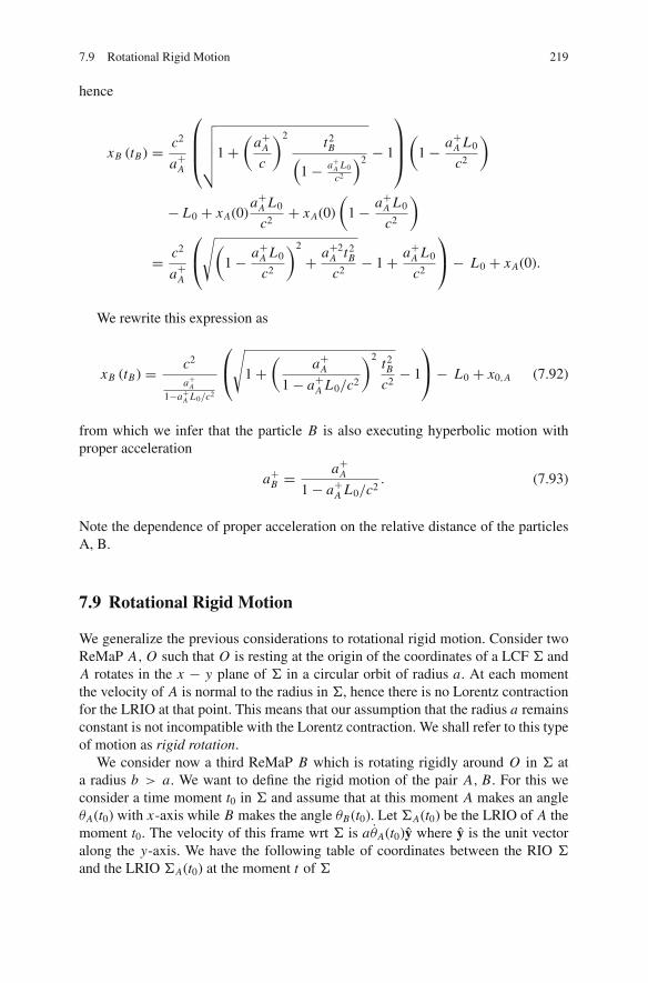
7.9 Rotational Rigid Motion 219
hence
xB (tB) = c2
a+A
⎛
⎜⎜⎝
√√√√√1+(
a+Ac
)2t2B(
1− a+A L0
c2
)2 − 1
⎞
⎟⎟⎠
(1− a+A L0
c2
)
− L0 + xA(0)a+A L0
c2+ xA(0)
(1− a+A L0
c2
)
= c2
a+A
⎛
⎝√(
1− a+A L0
c2
)2
+ a+2A t2
B
c2− 1+ a+A L0
c2
⎞
⎠− L0 + xA(0).
We rewrite this expression as
xB (tB) = c2
a+A1−a+A L0/c2
⎛
⎝√
1+(
a+A1− a+A L0/c2
)2t2B
c2− 1
⎞
⎠− L0 + x0,A (7.92)
from which we infer that the particle B is also executing hyperbolic motion withproper acceleration
a+B =a+A
1− a+A L0/c2. (7.93)
Note the dependence of proper acceleration on the relative distance of the particlesA, B.
7.9 Rotational Rigid Motion
We generalize the previous considerations to rotational rigid motion. Consider twoReMaP A, O such that O is resting at the origin of the coordinates of a LCF Σ andA rotates in the x − y plane of Σ in a circular orbit of radius a. At each momentthe velocity of A is normal to the radius in Σ, hence there is no Lorentz contractionfor the LRIO at that point. This means that our assumption that the radius a remainsconstant is not incompatible with the Lorentz contraction. We shall refer to this typeof motion as rigid rotation.
We consider now a third ReMaP B which is rotating rigidly around O in Σ ata radius b > a. We want to define the rigid motion of the pair A, B. For this weconsider a time moment t0 in Σ and assume that at this moment A makes an angleθA(t0) with x-axis while B makes the angle θB(t0). Let ΣA(t0) be the LRIO of A themoment t0. The velocity of this frame wrt Σ is aθA(t0)y where y is the unit vectoralong the y-axis. We have the following table of coordinates between the RIO Σ
and the LRIO ΣA(t0) at the moment t of Σ
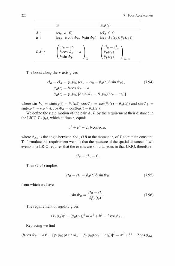
220 7 Four-Acceleration
Σ ΣA(t0)
A : (ct0, a, 0) (ctA, 0, 0B : (ctB, b cosΦB, b sinΦB) (ctB, xB(tB), yB(tB))
B Ai :
⎛
⎝ctB − ct0b cosΦB − ab sinΦB
⎞
⎠
Σ
⎛
⎝ctB − ctA
xB(tB)yB(tB)
⎞
⎠
ΣA(t0)
The boost along the y-axis gives
ctB − ctA = γA(t0) (ctB − ct0 − βA(t0)b sinΦB) , (7.94)
xB(t) = b cosΦB − a,
yB(t) = γA(t0) [b sinΦB − βA(t0)(ctB − ct0)] ,
where sinΦA = sin(θA(t) − θA(t0)), cosΦA = cos(θA(t) − θA(t0)) and sinΦB =sin(θB(t)− θA(t0)), cosΦB = cos(θB(t)− θA(t0)).
We define the rigid motion of the pair A, B by the requirement their distance inthe LRIO ΣA(t0), which at time t0 equals
a2 + b2 − 2ab cosφAB,
where φAB is the angle between O A, O B at the moment t0 of Σ to remain constant.To formulate this requirement we note that the measure of the spatial distance of twoevents in a LRIO requires that the events are simultaneous in that LRIO, therefore
ctB − ctA = 0.
Then (7.94) implies
ctB − ct0 = βA(t0)b sinΦB (7.95)
from which we have
sinΦB = ctB − ct0bβA(t0)
. (7.96)
The requirement of rigidity gives
(xB(tA))2 + (yB(tA))2 = a2 + b2 − 2 cosφAB .
Replacing we find
(b cosΦB − a)2 + [γA(t0) (b sinΦB − βA(t0)(ctB − ct0))]2 = a2 + b2 − 2 cosφAB .

7.9 Rotational Rigid Motion 221
The first term
(b cosΦB − a)2 = b2 cos2 ΦB − 2ab cosΦB + a2
= b2
[1−
(c(tB − t0)
βA(t0)b
)2]− 2ab cosΦB + a2
= a2 + b2 − c2(tB − t0)2
β2A(t0)
− 2ab cosΦB,
where in the second step we have used (7.95).The second term gives
[γA(t0) (b sinΦB − βA(t0)(ctB − ct0))]2 = γ 2A(t0)
[ctB − ct0βA(t0)
− βA(t0)(ctB − ct0)
]2
= γ 2A(t0)
c2(tB − t0)2
β2A(t0)
(1− β2A(t0))2
= c2(tB − t0)2
β2A(t0)
.
Replacing in the rigidity condition we find
a2 + b2 − c2(tB − t0)2
β2A(t0)
− 2ab cosΦB + c2(tB − t0)2
β2A(t0)γ 2(t0)
= a2 + b2 − 2ab cosφAB ⇒
c2
2ab(tB − t0)2 + cosΦB = cosφAB . (7.97)
Conditions (7.95) and (7.97) are the two equations quantifying the rotationalrigid motion. The first equation gives the time tB in Σ of the event B so that whenthe event A occurs at time t0 in Σ both events occurring at the same moment in theLRIO ΣA(t0). Given θA(t) the second equation determines the angle θB(t) of B sothat the spatial distance of A, B will be constant for the LRIO ΣA(t0) of A at thetime moment t0. Note that for this motion the angle φAB is constant and equals theangle AOB at the moment t0.
From the rigidity relation we get by differentiating wrt tB
c2
2ab2(tB − t0)− dΦB
dtBsinΦB = 0⇒
c2
ab(tB − t0)− dΦB
dtB
ctB − ct0βA(t0)b
= 0⇒dθ (tB)
dtB= βA(t0)
ac⇒
dθ (tB)
dtB= dθA(t0)
dt0, (7.98)

222 7 Four-Acceleration
that is, the angular velocity of B in Σ at the moment tB equals the angular velocityof A at the time moment t0 in Σ. This means that the instantaneous rest frame forB at the moment tB coincides with the instantaneous rest frame of A at the momentt0, hence what we have said for the second automatically applies for the first. Weconclude that the definition of rigidity we gave is independent of which particlewe consider as a reference particle. We also note that if dθA(t0)
dt0is a monotonically
increasing function of time, then so is dθ(tB )dtB
.A special case occurs when the two particles are on the same radius at the times
t0 and tB , respectively. In this case φAB is either 0 or π and for any given θA(tA) the
θB(tB) = θA(tA)+ φAB . (7.99)
In order to write the rigidity conditions with reference to the particle B we inter-change A ↔ B and a ↔ b. Let tA be the time moment of Σ for which the eventcorresponding to particle A and the event corresponding to particle B are simulta-neous at the LRIO of B at the moment tB . Then the rotational rigidity conditions forparticle B read
ctA − ctB = βB(tB)a sin[θA(tA)− θB(tB)], (7.100)
c2
2ab(tA − tB)2 + cos[θA(tA)− θB(tB)] = cosφAB . (7.101)
7.9.1 The Transitive Property of the Rigid Rotational Motion
We consider four ReMaP A, B, D, O which are moving so that A, B are in rigidrotation about O , and B, D are also in rigid rotation about O . We define the tran-sitive property of the rigid rotational motion by the requirement that the ReMaPsA, D execute rigid rotational motion about O . Let us examine if this kinematicrequirement can be satisfied and under what conditions.
The fact that the particles A, B are in rigid rotation about O implies that for giventA, θA(tA) of the particle A there are tB, θB(tB) (time in the RIO Σ with origin at O)satisfying the following two equations:
dθ (tB)
dtB= dθA(tA)
dtA, (7.102)
ctB − ctA = βA(tA)b sin[θB(tB)− θA(tA)]. (7.103)
Similarly for the pair B, D we have the equations
dθ (tD)
dtD= dθB(tB)
dtB, (7.104)
ctD − ctB = βB(tB)d sin[θD(tD)− θB(tB)]. (7.105)

7.9 Rotational Rigid Motion 223
The transitive property will be satisfied if the following two conditions aresatisfied:
dθ (tD)
dtD= dθA(tA)
dtA, (7.106)
ctD − ctA = βA(tA)d sin[θD(tD)− θA(tA)]. (7.107)
From (7.102) and (7.104) follows
dθ (tD)
dtD= dθA(tA)
dtA.
Because θ (tD) is uniquely defined in terms of θA(tA) and also dθ(tD )dtD
is a mono-tonic function, we infer that the first condition (7.106) is satisfied provided tD = tD .It remains the second condition to be checked. From condition (7.107) settingtD = tD we have
ctD − ctA = βA(tA)d sin[θD(tD)− θA(tA)]. (7.108)
Subtracting (7.105) and (7.106) we obtain
ctD − ctA = βB(tB)d sin[θD(tD)− θB(tB)]− βA(tA)b sin[θB(tB)− θA(tA)].
The last two relations and (7.103) imply
βB(tB)d sin[θD(tD) − θB(tB)]− βA(tA)b sin[θD(tD)− θA(tA)]
= βA(tA)d sin[θB(tB)− θA(tA)]
or replacing βB(tB) = bc
dθB (tB )dtB
, βA(tA) = ac
dθA(tA)dtA= a
cdθB (tB )
dtB:
bd sin[θD(tD)− θB(tB)]− ab sin[θB(tB)− θA(tA)] = ad sin[θD(tD)− θA(tA)].(7.109)
This condition is satisfied automatically in Newtonian Physics but not in SpecialRelativity, in which it serves as an additional condition/constraint. This conditionrestricts severely the possible cases in Special Relativity. Indeed (7.109) has thefollowing solutions:Solution 1
θD(tD) = θB(tB) = θA(tA) and any values of the constants a, b, d. This solutionforces the three points along the same radius on the plane of rotation, therefore therigid rotation of a rigid rod normal to the pivot at one of its ends.Solution 2
θB(tB) = θA(tA) �= θD(tD), d �= 0. In this case condition (7.109) reduces toa = b that is the points A, B coincide hence we are forced back to the two pointsrigid rotational motion.

224 7 Four-Acceleration
We conclude that the only possibility for rigid rotational motion in Special Rel-ativity is the rotation of a rigid rod about one of its points. This implies that if wehave a disk of radius R then the disk can rotate rigidly if the points in each radiusstay at all times in the same radius, i.e., they have the same angular velocity.
7.10 The Rotating Disk
We come to the final case of our considerations that is the rigid motion of a rotatingdisk. This is a complex problem which appears to be still unsolved in the currentliterature, something to be expected because it requires so many conventions that thechoice of a unique approach is not feasible. In any case it is an interesting problemand in this section we shall follow the rather standard and widely accepted – but notunique! – approach of Grøn.
7.10.1 The Kinematics of Relativistic Observers
Before we enter into the discussion of the rotating disk problem we have to advancea little our knowledge of relativistic kinematics. Let us see why. The kinematics ofSpecial Relativity developed in the previous sections was concerned mainly with therelativistic mass point (ReMaP). This kinematics has been extended with the Born’srigid motion to cover the rigid body of Newtonian Physics. However the problemin Special (and General) Relativity is that one does not have solids, therefore onehas to define the relativistic body, and then develop a kinematics appropriate for thistype of body. This will become apparent from the discussion of the rotating disk.
Kinematics is a comparative study which requires two observers. In Special Rel-ativity there are two different cases to consider:
(a) Kinematics between two relativistic inertial observers (RIO)(b) Kinematics between a RIO and an accelerating observer.
In the first case the kinematics is determined by the Lorentz transformation relat-ing the observers. That is, the choice of the second observer is equivalent to thechoice of the appropriate Lorentz transformation (via the β-factor). In the secondcase the choice of the accelerating observer is at will because the Lorentz transfor-mation does not relate a RIO with an accelerating observer, therefore in this casethe kinematics is defined. This is done by the definition of a metric (of Lorentziancharacter) for the accelerated observer by means of two actions:
(a) The definition of a coordinate transformation which relates the coordinates ofthe RIO with those of the accelerated observer.
(b) By assuming that this transformation leaves the form of the metric the same(ds2 = ds ′2) , that is, the new metric is found from the Minkowski metric (ofthe RIO) if one replaces the RIO coordinates in terms of the coordinates of the

7.10 The Rotating Disk 225
accelerated observer. Using this new metric one determines the relation of thetime and the spatial intervals between the two observers.
One may consider the proposed coordinate transformation as “a generalizedLorentz transformation.” However, this transformation is very different from thestandard Lorentz transformation. Indeed the proposed transformation is as follows:
(a) It is specific to the two observers involved(b) It is not an isometry of Minkowski space, that is, it is not represented with a
Lorentz matrix6
(c) It does not necessarily generates a (Lie) group, hence it is possible that onecannot define a covariance property7
We note that the metric ds2 is still flat because with a coordinate transformationit is not possible to create new tensors.8
Having a metric for the relativistic observer it is possible to define coordinatetime and the space intervals. This is important and it is done as explained below.9
7.10.2 Chronometry and the Spatial Line Element
The coordinatization in spacetime by a relativistic observer (inertial or not) isdone by means of chronometry. Let us recall briefly this procedure. The relativisticobserver is equipped with a photongun (a torch) and a clock. In order to determinethe coordinates of an event the observer emits a light beam toward the point in spacewhere the event takes place and in the direction e such that the beam is reflected ata “mirror,” placed at the point of space and returns along the same direction back tothe observer. The observer notes the reading of his clock for the event of emittancete and the event of reception tr . He also reads from the scale of the photongun thedirection (angles) of the beam in his coordinate frame, Σ say. Subsequently theobserver defines the following coordinates for the event in Σ
6 For those who have a knowledge of geometry, it is not generated by a Killing vector of theMinkowski metric.7 For example the standard Lorentz transformations do form a group and the tensors which trans-form covariantly under this group are the Lorentz tensors. These tensors describe covariantly(within Special Relativity) the physical quantities of the theory.8 Flat means the curvature tensor vanishes. This means that the coordinate functions are definedeverywhere in the space. Under a coordinate transformation it is possible to have new quantities,which are not tensors, (e.g., the connection coefficients Γa
bc), such as the curvature tensor. Thereason for this is that the curvature tensor is covariant wrt the group of the general coordinatetransformations (manifold mapping group) which includes whatever coordinate transformationswe introduce between the coordinates of the RIO and the coordinates of the accelerated observer.9 See also Ref: Landau and Lipsitz The classical theory of fields 5th Edition p. 234.

226 7 Four-Acceleration
( te+tr2 c
te−tr2 ce
)
Σ
. (7.110)
Using the chronometric coordinatization one can determine geometrically if agiven relativistic observer Σ is a RIO or an accelerating observer. This is done asfollows (see Fig. 7.13). Let P be an arbitrary spacetime event whose coordinateshave being determined by Σ. Draw from P the normal plane to the world line of theobserver. Let tP be the intersection of that plane with the world line of the observer.If tP−te = tr−tP for all spacetime events P then the observer Σ is a RIO, otherwiseit is an accelerating observer.
Let us assume now that the metric of the relativistic observer – defined in theway explained above – in his coordinate frame, Σ say, has the form
ds2 = gμνdxμdxν + 2g0μdx0dxμ + g00(dx0)2. (7.111)
The emitted and the received light rays by the observer performing the chrono-metric measurement of the coordinates of an event P belong to the light cone of thepoint P . The equation of this cone is
gμνdxμdxν + 2g0μdx0dxμ + g00(dx0)2 = 0, (7.112)
where dx0 is to be taken as the time of traveling of the light beam to and from Pand dxμ are the coordinates defining the space axes of the coordinate system of theobserver. Considering (7.112) as a quadratic equation in dx0 and solving in termsof dx0 we find
dx0± =
1
g00
[−g0μdxμ ±√|(g0μg0ν − gμνg00)|dxμdxν
]. (7.113)
These values of dx0 concern the bidirectional propagation of light, one value forthe “go” and the other for the “return” trip of the light ray. The difference of the two
PP
et
Pt
rt
AcceleratedObserver
Inertialet
PtPt
rt
Observer
Fig. 7.13 The coordination of an accelerating and an inertial observer

7.10 The Rotating Disk 227
roots gives the total traveling (coordinate) time of the beam. We find
dx0C D = dx0
+ − dx0− =
2
g00
√|(g0μg0ν − gμνg00)|dxμdxν, (7.114)
where (C) is the event of emittance and (D) the event of reception.The proper time between the events C, D is obtained if we set dxμ = 0 in (7.111)
ds2 = −c2dτ 2 = g00(dx0AB)2 (7.115)
from which follows
dτ = 1
c
√|g00|dx0. (7.116)
This equation relates the proper time interval of the relativistic observer (that is,the time period measured by its proper clock) with the coordinate time determinedby the chronometric procedure.
Concerning the spatial distance of the event P we have
dlP = 1
2dx0
C D =√∣∣∣∣
g0μg0ν
g00− gμν
∣∣∣∣ dxμdxν . (7.117)
This leads us to consider the three-dimensional line element
dl2 =∣∣∣∣g0μg0ν
g00− gμν
∣∣∣∣ dxμdxν (7.118)
as a positive definite line element, which defines the spatial metric of the relativisticobserver10 Σ.
Relations (7.116) and (7.118) describe the kinematics of a relativistic (inertialor accelerating) observer. The quantities dτ, dlμ are the units of time and spatialdistance determined from the accelerating observer and dx0, dxμ the coordinatevalues of these quantities determined by the chronometric coordinatization. Theserelations provide us all the necessary equipment to discuss the rigid motion of therotating disk.
(1) In the derivation we have considered dx0+ > 0, dx0
− < 0 but this is not neces-sary; dx0
+, dx0− can have any sign. The fact that in this case the value of x0(D)
at the moment of arrival of the light signal in D might be less than the valuex0(C) at the moment of departure from C contains no contradiction since therate of clocks at different points in space are not assumed to be synchronized inany way.
10 Not of spacetime! Each relativistic observer has its own spatial geometry!

228 7 Four-Acceleration
(2) If we wish to find the spatial length dlμ along the coordinate xμ say, we simplywrite
dlμ =√∣∣∣∣
g0μg0μ
g00− gμμ
∣∣∣∣dxμ (7.119)
In this equation dxμ is the coordinate spatial length, that is the spatial lengthdetermined by the chronometric coordinatization. The above equation meansthat the spatial distance of the point P along the coordinate line xμ attributed
by the observer is
√∣∣∣ g0μg0μ
g00− gμμ
∣∣∣ times the coordinate length (i.e., coordinate
unit) along that coordinate line.(3) If the observer is inertial then the metric has components diag(−1, 1, 1, 1) and
we find dτ = t, dl2 = δμνdxμdxν , which are the expected answers.
7.10.3 The Rotating Disk
A circular disk of radius R lying on the plane x, y of a RIO Σ rotates with constantangular velocity ω about the z-axis. The center of the disk is assumed to be at thepoint (−R, 0, 0). This description, although perfectly alright in Newtonian Physics,is meaningless in Special Relativity if we do not define(!) precisely for Σ what wemean by a rotating disk. Indeed in Newtonian Physics the disk is a solid, thereforewe do not expect any change in the disk when it is resting and when it is set inrotation. However, in Special (and General) Relativity there do not exist solid bodiesand one has to define the moving body.
There is not a unique or “the correct” definition of the rotating disk and one candefine it as one wishes. Then the theory produces the consequences of the specificdefinition and the “experiment” tests the validity or not of the results. This meansthat all approaches/assumptions concerning the rotating disk are acceptable untilexperiment will select “the one,” if it exists. It is to be noted that the outcome doesnot prove or disprove Special Relativity, but concerns only the specific assumptions,which have been made in the definition of the moving body. If the experiment ver-ifies these assumptions then Special Relativity is extended to apply to this type ofmoving body and all is well done. If not, then the assumptions are abandoned butSpecial Relativity stays!
In the following we will consider a “standard” approach due to Grøn.11 For fur-ther information on the problem of the rotating disk and other approaches the readeris referred to the work of R. Klauber.12
Following the previous analysis we consider three types of observers. The RIOΣ for whom the rotating disk is defined (this is the reference RIO), a Locally
11 Grøn “Relativistic description of a rotating disk” Am. J. Physics 43, 869–876, (1975).12 R. Klauber “Relativistic rotation: A comparison of theories” gr-qc /0604118 16 December 2006.

7.10 The Rotating Disk 229
Relativistic Inertial Observer (LRIO) defined by an accelerating point at the rimof the rotating disk and the accelerated observer rotating together with the rotatingdisk (say the “proper” observer of the disk).
The kinematics between the two RIO is determined by the Lorentz transforma-tion corresponding to the velocity of the second RIO. The kinematics between thestandard RIO and the rotating observer requires
(a) The definition of the rotating disk for the accelerated, i.e., (rotating) observerand through this.
(b) The definition of the coordinate transformation, relating the coordinate systemsof the two observers. This transformation determines a metric for the rotatingobserver via relations (7.115) and (7.117) and determines the kinematics of theaccelerated observer in terms of the kinematics of the RIO.
7.10.4 Definition of the Rotating Disk for a RIO
When the disk rotates
(a) It preserves its shape (that is it remains as a plane circular disk).(b) The disk rotates with constant angular velocity about the fixed direction of z-
axis.(c) There is no relative rotation of the parts of the disk. Kinematically this means
that the points on a radius remain on the radius during the rotation of the disk.As we have seen in Sect. 7.9 this is necessary if the transitivity property of therigid rotational motion is to be satisfied.
(d) The radius R of the disk when at rest and after it is made to rotate does notchange.13
It is obvious that under the above assumptions for Σ, the disk is assumed to rotateas a solid (Born conditions are satisfied). Due to the above assumptions the angle abetween two radii of the disk before and during the motion remains constant. Thisimplies for the arc length across the rotating disk
ds
r= dθ 0 < r ≤ R. (7.120)
13 These assumptions can be stated in a more advanced language. Here we state without furthercomment the geometric significance of each of the four assumptions in terms of the fluid ofobservers defined by the disk:
(a) The fluid defined by the disk has zero shear σab = 0(b) ωab;c = 0(c) ua = 0(d) θ = 0. The Born rigidity conditions σab = 0, θ = 0 are satisfied.

230 7 Four-Acceleration
The angular velocity of the disk for the observer Σ is defined as follows:
ω = dθ
dt, (7.121)
where t is time in Σ. Replacing in (7.120) we find
ds/dt
r= ω.
But ds/dt = v is the speed of rotation (at distance r form the axis of rotation),therefore
v = ωr. (7.122)
The condition
v < c⇒ ωR < c⇒ ω <c
R
restricts the values of the angular velocity ω.The above exhaust the assumptions defining the rotating disk for the RIO Σ.
7.10.5 The Locally Relativistic Inertial Observer (LRIO)
We consider the disk at rest and divide its rim in a large number n (say) of lineelements of length 2π R/n each. Then at one of these line elements, the k say, weconsider the comoving LRIO Σk whose velocity (in Σ!) is v = ωRj, where j isthe unit along the y-axis (see Fig. 7.14). We consider a point P at the rim of thedisk and write the components of the position four-vector, the four-velocity, and thefour-acceleration of P in Σ14:
xiP =
⎛
⎜⎜⎝
tp
−R(1− cos θP )R sin θP
0
⎞
⎟⎟⎠
Σ
, uiP = γ
dxiP
dt=
⎛
⎜⎜⎝
γ
−βγ sin θP
βγ cos θP
0
⎞
⎟⎟⎠
Σ
,
aiP = γ
duiP
dt=
⎛
⎜⎜⎝
γ γ
−βγ (γ sin θP + ωγ cos θP )βγ (γ cos θP − ωγ sin θP )
0
⎞
⎟⎟⎠
Σ
.
Assume that in Σk
14 t is time in Σ. We set c = 1.

7.10 The Rotating Disk 231
Fig. 7.14 Definition ofcoordinates for the LRIO Σk
P
ObserverInertial
X
y
O
ω
A
Sk
xik,P =
⎛
⎜⎜⎝
tk,p
xk,P
yk,P
0
⎞
⎟⎟⎠
Σk
, uik,P =
⎛
⎜⎜⎝
γk,p
γk,pvk,x
γk,pvk,y
0
⎞
⎟⎟⎠
Σk
, (7.123)
where γk,p is the γ -factor of the point P in Σk . Σk is related to Σ with a boost alongthe y-axis with β = ωR/c. For the four-position vector the boost gives
tp = γ (tk,p + βyk,P ), (7.124)
xk,P = −R(1− cos θP ), (7.125)
yk,P = γ (R sin θP − βtp). (7.126)
Replacing tp from (7.124) in (7.126) we get
yk,P = γ[R sin θP − βγ (tk,p + βyk,P )
]⇒
yk,P = R
(1
γsin θP − ωtk,p
). (7.127)
Replacing yk,P from (7.127) in (7.124) follows that
tp = 1
γtk,p + βR sin θP , (7.128)
which relates the time of Σ,Σk for the point P along the rim of the disk. (Obviouslyall the above go through if we assume instead of the rim a point P at a distancer < R from the center of the rotating disk).
From the above relations we compute
(1+ xk,P
R
)2+
(ωγ tk,p + γ yk,P
R
)2= 1. (7.129)
It follows that for the observer Σk at time tk,p = 0 the points at the rim of thedisk (that is, the shape of the disk) are on an ellipse centered at the point (−R, 0)

232 7 Four-Acceleration
whose minor semi-axis is R/γ (along the y-axis) and its major semi-axis is R (alongthe x-axis) (see Fig. 7.14).
Let us assume now the initial condition
At time tp = 0 the point P is at the point A of Σk .
This implies
tk,A = −βR sin θA ⇔ ωtk,A = −β2 sin θA. (7.130)
The point A arrives at the point P after time tP , therefore the angle
θP = θA + ωtp. (7.131)
Then
xk,P = −R(1− cos(θA + ωtp)
), (7.132)
yk,P = R
(1
γsin(θA + ωtp)− ωtk,p
).
We infer that for the observer Σk the point P describes a cycloid. The sametrajectory (i.e., a cycloid) describes the point P for the RIO Σ but with equations(see Fig. 7.15):
xP = −R(1− cos(θA + ωtp)
),
yP = R(sin(θA + ωtp)− ωtP
). (7.133)
Equations (7.133) can be written in terms of the coordinates in Σk if we substitutetp from (7.124)
xP = −R[1− cos(θA + ωγ (tk,p + βyk,P ))
],
yP = R[sin(θA + ωγ (tk,p + βyk,P ))− ωtk,p
].
Fig. 7.15 The cycloid for theRIO Σ and the rotatingobserver Σk
Sk
X
y
X
y
ObserverInertial S ObserverInertial

7.10 The Rotating Disk 233
In (7.131) the angle θA is measured in Σ. To compute it in Σk we use the trans-formation formulae
sin θA = sin θk,A√1− β2 cos2 θk,A
, cos θA = cos θk,A
γ√
1− β2 cos2 θk,A
(7.134)
7.10.5.1 Transformation of Angles
Let θk,P the angle between the x-axis and the direction of the radius of the disk fromthe center of the disc to the point P . Then we have for the center of the disk
In Σ : xcenter = −R, ycenter = 0.In Σk the boost gives: xk,center = xcenter = −R, yk,center = −βγ tk,p.We have then for θk,P
tan θk,P = yk,P − yk,A
xk,P − xk,A=
R(
1γ
sin θP − ωtk,p
)− 0
−R (1− cos θP )+ R(7.135)
= 1
γtan
[ωγ (βyk + tk,p)
]+ ω(γ − 1)tk,p
Grøn seems to miss the term ω(γ − 1)tk,p. See relation (17) of his paper. Notethat θP = ωtP .
7.10.5.2 The Four-Velocities
We compute first the relative velocity of the point P in Σk . The four-velocity of Σk
in Σ is (c = 1)
uik =
⎛
⎜⎜⎝
γ
0γβ
0
⎞
⎟⎟⎠
Σ
.
Therefore the relative four-velocity of the point P in Σk is
uik,P = ui
P − uik =
⎛
⎜⎜⎝
γ
−βγ sin θP
βγ cos θP
0
⎞
⎟⎟⎠
Σ
−
⎛
⎜⎜⎝
γ
0γβ
0
⎞
⎟⎟⎠
Σ
=
⎛
⎜⎜⎝
0−βγ sin θP
−βγ (1− cos θP )0
⎞
⎟⎟⎠
Σ
.
The invariant uiP uki = −γk,P where γk,P is the γ -factor of P in Σk . Replacing
we find
γk,P = γ 2(1− β2 cos θP ). (7.136)

234 7 Four-Acceleration
This is an invariant therefore its value is the same for all RIO, including Σ!We note that the point P ′ of the disk opposite to the point P (i.e., θP = π ) has
γ -factor
γk,P ′ = γ 2(1+ β2) = 2γ 2 − 1.
We consider now the boost relating Σ,Σk applied to the four-velocity vector of
the point P . We have the components
⎛
⎜⎜⎝
γk,p
γk,pvk,x
γk,pvk,y
0
⎞
⎟⎟⎠
Σk
and
⎛
⎜⎜⎝
γ
−βγ sin θP
βγ cos θP
0
⎞
⎟⎟⎠
Σ
.
For the zeroth component we find
γk,p = γ (γ − ββγ cos θP ) = γ 2(1− β2 cos θP )
which coincides with the previous result (7.136). For the other two components weget
γk,pvk,x = −βγ sin θP ,
γk,pvk,y = γ (βγ cos θP − βγ ) = βγ 2(cos θP − 1).
or, replacing γk,p
vk,x = − βγ sin θP
γ 2(1− β2 cos θP )= − β sin θP
γ (1− β2 cos θP ),
vk,y = βγ 2(cos θP − 1)
γ 2(1− β2 cos θP )= β(cos θP − 1)
1− β2 cos θP.
If we replace further (θA = 0)
θP = ωγ (tk,p + βyk,P ),
we compute the velocity of the point P in the RIO Σk .Concerning the direction of motion we have
tan θk,P = vk,y
vk,x⇒ vk,y = vk,x tan θP = − β sin θP
γ (1− β2 cos θP )tan θP
= −β tan θP√
1+tan2 θP
γ
(1− β2 1√
1+tan2 θP
) tan θP = − β tan2 θP
γ(√
1+ tan2 θP − β2) .
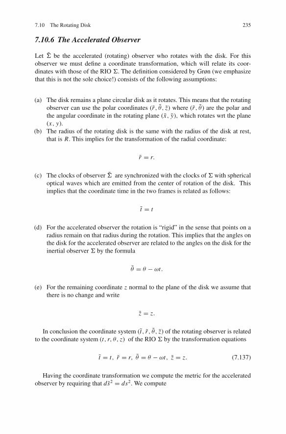
7.10 The Rotating Disk 235
7.10.6 The Accelerated Observer
Let Σ be the accelerated (rotating) observer who rotates with the disk. For thisobserver we must define a coordinate transformation, which will relate its coor-dinates with those of the RIO Σ. The definition considered by Grøn (we emphasizethat this is not the sole choice!) consists of the following assumptions:
(a) The disk remains a plane circular disk as it rotates. This means that the rotatingobserver can use the polar coordinates (r , θ , z) where (r , θ ) are the polar andthe angular coordinate in the rotating plane (x, y), which rotates wrt the plane(x, y).
(b) The radius of the rotating disk is the same with the radius of the disk at rest,that is R. This implies for the transformation of the radial coordinate:
r = r.
(c) The clocks of observer Σ are synchronized with the clocks of Σ with sphericaloptical waves which are emitted from the center of rotation of the disk. Thisimplies that the coordinate time in the two frames is related as follows:
t = t
(d) For the accelerated observer the rotation is “rigid” in the sense that points on aradius remain on that radius during the rotation. This implies that the angles onthe disk for the accelerated observer are related to the angles on the disk for theinertial observer Σ by the formula
θ = θ − ωt.
(e) For the remaining coordinate z normal to the plane of the disk we assume thatthere is no change and write
z = z.
In conclusion the coordinate system (t, r , θ , z) of the rotating observer is relatedto the coordinate system (t, r, θ, z) of the RIO Σ by the transformation equations
t = t, r = r, θ = θ − ωt, z = z. (7.137)
Having the coordinate transformation we compute the metric for the acceleratedobserver by requiring that ds2 = ds2. We compute
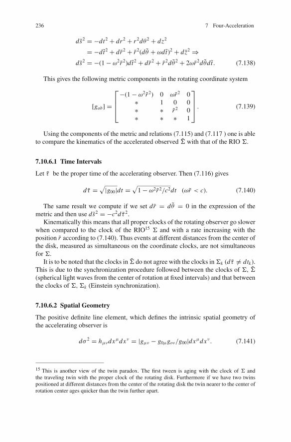
236 7 Four-Acceleration
ds2 = −dt2 + dr2 + r2dθ2 + dz2
= −dt2 + dr2 + r2(d θ + ωdt)2 + dz2 ⇒ds2 = −(1− ω2r2)dt2 + dr2 + r2d θ2 + 2ωr2d θdt . (7.138)
This gives the following metric components in the rotating coordinate system
[gab] =
⎡
⎢⎢⎣
−(1− ω2r2) 0 ωr2 0∗ 1 0 0∗ ∗ r2 0∗ ∗ ∗ 1
⎤
⎥⎥⎦ . (7.139)
Using the components of the metric and relations (7.115) and (7.117 ) one is ableto compare the kinematics of the accelerated observed Σ with that of the RIO Σ.
7.10.6.1 Time Intervals
Let τ be the proper time of the accelerating observer. Then (7.116) gives
d τ =√|g00|dt =
√1− ω2r2/c2dt (ωr < c). (7.140)
The same result we compute if we set dr = d θ = 0 in the expression of themetric and then use ds2 = −c2d τ 2.
Kinematically this means that all proper clocks of the rotating observer go slowerwhen compared to the clock of the RIO15 Σ and with a rate increasing with theposition r according to (7.140). Thus events at different distances from the center ofthe disk, measured as simultaneous on the coordinate clocks, are not simultaneousfor Σ.
It is to be noted that the clocks in Σ do not agree with the clocks in Σk (d τ �= dtk).This is due to the synchronization procedure followed between the clocks of Σ, Σ
(spherical light waves from the center of rotation at fixed intervals) and that betweenthe clocks of Σ,Σk (Einstein synchronization).
7.10.6.2 Spatial Geometry
The positive definite line element, which defines the intrinsic spatial geometry ofthe accelerating observer is
dσ 2 = hμνdxμdxν = |gμν − g0μgoν/g00|dxμdxν . (7.141)
15 This is another view of the twin paradox. The first tween is aging with the clock of Σ andthe traveling twin with the proper clock of the rotating disk. Furthermore if we have two twinspositioned at different distances from the center of the rotating disk the twin nearer to the center ofrotation center ages quicker than the twin further apart.

7.10 The Rotating Disk 237
From the components of the metric for the rotating observer we compute (see(7.139))
dσ 2 = dr2 + r2
1− ω2r2d θ2. (7.142)
It follows that the line element along the radial coordinate is (set d θ = 0)
dσr = dr (7.143)
and the tangential line element along the θ-direction is (set dr = 0)
dσθ = r√1− ω2r2
d θ . (7.144)
The fact that the proper spatial length depends on r shows that the disk cannotpass from rest to rotation in such a way that both the radial and the tangential lineelements remain unchanged.
In order to compute the length of the periphery of the disk in Σ we take in (7.144)d θ = 2π and r = R and get
S = 2π R√1− ω2 R2
< S, (7.145)
where S is the length of the periphery of the disk for the RIO Σ. The difference isdue to the fact that the unit of spatial length for the observer Σ changes along theperiphery of the disk.
7.10.6.3 The Velocity of Light for the Accelerating Observer Σ
From (7.141) we have that the line element along the coordinate direction l is foundby setting μ = ν = l
dσl =√
(gll − g0l g0l/g00)dxl .
The velocity of a particle in Σ along the direction l is (we do not take c = 1 inorder to show the differentiation from the value c)
cl = dσl
dx0c =
√(gll − g0l g0l/g00)
dxl
dx0c. (7.146)
The line element between two points with coordinates (x0, xl ) and (x0+dx0, xl+dxl ) (which are related with velocity dxl
dx0 ) is
ds2 = gll(dxl )2 + 2gl0dxldx0 + g00(dx0)2.

238 7 Four-Acceleration
If these points are along the trajectory of a light ray, then ds2 = 0 and we obtain
gll(dxl )2 + 2gl0dxldx0 + g00(dx0)2 = 0.
Dividing with (dx0)2 we find
dxl
dx0= g00√|g2
l4 − gll g00| + gl4
.
Substituting in (7.146) we obtain the velocity of light in the direction l
cl = dσl
dx0c =
√|gll − g0l g0l/g00| g00c√
|g2l0 − gll g00| + gl0
=√|g00|gl0√
|g2l0−gll g00|
+ 1c.
(7.147)Let us see what we get for the two characteristic coordinate directions. Along the
radial direction r we have g0r = 0, g00 = −(1− ω2r2), grr = 1 therefore
cr =√
1− ω2r2c < c.
For the tangential velocity of light we have g0θ = ωr2, g00 = −(1 − ω2r2),gθθ = r2. Hence
cθ =√
1− ω2r2
ωr2√|ωr2−r2[−(1−ω2r2)]
+ 1c =√
1− ω2r2
1+ ωrc =
√1− ωr
1+ ωrc < c.
Exercise 25 Compute the spatial length of the velocity of light that is the quantityc2
r + r2c2θ and compare it with c.
The reason that the velocity of light is locally different from c is due to the factthat the clocks of the rotating disk are synchronized with light signals from thecenter of the disk, whereas the clocks of the RIO Σ are synchronized by the Einsteinconvention (i.e., the Lorentzian kinematics).
Exercise 26 Show that the time Δtr required by a light ray to reach from the centerof the disk to the periphery of a circle of radius r1 is given by
Δtr = 1
c
∫ r1
0
dr√1− ω2r2/c2
= 1
ωarcsin
ωr12
c. (7.148)

7.11 The Generalization of Lorentz Transformation and the Accelerated Observers 239
7.11 The Generalization of Lorentz Transformationand the Accelerated Observers
The Lorentz transformation contains all the mathematical structure of Special Rel-ativity. Indeed being linear relates the characteristic observers of the theory (theRIO) and, by means of the Lorentz group, defines the Lorentz tensors, which arethe mathematical objects describing the physical quantities of the theory. Thereforewithin the framework setup by the Lorentz transformation it is possible to studyall problems involving relativistic inertial motions. However, in practice the ruleis accelerated motions whereas inertial motions are the exception. Therefore it isnatural to ask
Is it possible to study accelerated motions by means of a (generalized) Lorentz transforma-tion?
One answer to this question has been given in Sect. 7.2 by the introduction of theLocally Relativistic Inertial Observers (LRIO). In that approach one approximatesthe world line of an accelerated observer (which of course is not a straight line) witha continuous sequence of straight lines each line being the tangent at each and everypoint of the world line. This continuous sequence of straight lines is parameterizedby the proper time τ (say) of the accelerated observer and can be considered equiv-alently as a continuous sequence of Lorentz transformations whose parameter β(τ )is again a function of the proper time τ . This approach has been used in the study ofthe Thomas phenomenon.
In the last sections we considered a different approach, that is, we induceda metric for the accelerated observer using the metric of the inertial observerη = diag(−1, 1, 1, 1) and the transformation relating the coordinates of the twoobservers. Then we were able to calculate temporal and spatial distances for theaccelerated observer. In the present section we wish to take (7.116) and (7.119) onestep further and answer the question
Is it possible to determine a transformation which relates a RIO with a given acceleratedobserver in the same way the Lorentz transformation relates a RIO with a RIO?
As we shall show this is possible, and the resulting transformation – which isnot universal as the Lorentz transformation, but depends on the particular acceler-ated observer – we call generalized Lorentz transformation. We shall consider onlysimple configurations, because in more general situations one has to go directly toGeneral Relativity. This “generalization” of the Lorentz transformation will takeus to the limits of Special Relativity and furthermore indicates the direction oneshould take in order to extend the theory. Indeed, as will be shown, the extension –generalization of Special Relativity is not of a simple academic interest but it is anecessity emerging from physical reality. That is to say, there are relativistic phe-nomena which cannot be answered within the scenario of Special Relativity, becausethey are not due to relative motion.

240 7 Four-Acceleration
7.11.1 The Generalized Lorentz Transformation
We seek a generalization of Lorentz transformation which will meet the followingdemands:
(1) The assumptions which will be made shall be minimal(2) In the limit, when the acceleration vanishes the “generalized” Lorentz transfor-
mation will reduce to the standard Lorentz transformation
We recall that the standard Lorentz transformation has the following basicfutures:
(1) It is an isometry, that is, preserves the Lorentz length ds2 = ds ′2.(2) It is linear(3) Preserves the canonical form of the Lorentz metric diag(−1, 1, 1, 1).
The generalization we are looking for must defy some of these assumptions. Butwhich one(s)?
The assumption of isometry is essential because it concerns fundamental physicalprinciples of the theory. For example, the particles are classified into photons andparticles with mass according to the (Lorentz) length of the momentum or posi-tion four-vector. Therefore a transformation which will not preserve the length offour-vectors it is possible to change the nature of a particle. This would imply that,by means of a transformation, a photon could become a particle with mass andconversely, a situation which cannot be accepted.
There remain the other two assumptions. The property of linearity must be defied,because the world-line of an accelerated observer is not a straight line and a lineartransformation cannot relate a straight line with a non-straight line. Concerning thelast property this must also be abandoned because the Lorentz metric for an accel-erated observer cannot have the canonical form.
Based on the above remarks we demand that the generalized Lorentz transforma-tion must satisfy the following requirements:
• Must be an isometry, that is ds2 = ds ′2
• Will not be linear except when acceleration vanishes• Will apply in general only locally, that is, around every point of the world line
of the (specific) accelerated observer and not globally (i.e., in the whole ofMinkowski space) as it is the case with the standard Lorentz transformation.Furthermore in general the set of all “generalized” Lorentz transformations asso-ciated with an accelerated motion cannot be a subgroup of the Lorentz group andneed not form a group
Consider a RIO Σ with coordinates (l, x, y, z) and let (l ′, x ′, y′, z′) be the coor-dinates of an accelerated observer E . The distance of two “adjacent” points in

7.11 The Generalization of Lorentz Transformation and the Accelerated Observers 241
Minkowski space for Σ is16
ds2 = −dl2 + dx2 + dy2 + dz2 (7.149)
while for E let us assume that it has the general form17
ds ′2 = −u20dl ′2 + u2
1dx ′2 + u22dy′2 + u2
3dz′2, (7.150)
where u0, u1, u2, u3 are real, smooth functions of the coordinates (l ′, x ′, y′, z′). Thedemand of isometry gives
−dl2 + dx2 + dy2 + dz2 = −u20dl ′2 + u2
1dx ′2 + u22dy′2 + u2
3dz′2. (7.151)
In order to simplify the mathematics we consider motion along the x-directiononly and set y = y′, z = z′. Then the transformation we are looking for is of theform
x = x(l ′, x ′), l = l(l ′, x ′), (7.152)
where the functions are such that the transformation will be non-singular, that is, itwill be reversible. The condition for this is that the Jacobian shall be non-zero. Wecompute
dx = ∂x
∂l ′dl′ + ∂x
∂x ′dx ′ = a(l ′, x ′)dl ′ + b(l ′, x ′)dx ′
dl = ∂l
∂l ′dl ′ + ∂l
∂x ′dx
′ = c(l ′, x ′)dl ′ + d(l ′, x ′)dx ′
from which follows
ds2 = −dl2 + dx2 = −(cdl ′ + ddx ′)2 + (adl ′ + bdx ′)2
= (−c2 + a2)dl ′2 + (b2 − d2)dx ′2 + 2(ab − cd)dl ′dx ′.
But
ds ′2 = −u20dl ′2 + u2
1dx ′2
hence isometry implies
16 The concept “adjacent” is outside the scope of this book and requires more advanced mathe-matics (topology). We simply mention that “adjacent” is modulated according to the curvature (=measure of acceleration) at each point of the world line of the accelerated observer.17 This form is general, because it can be shown that every (non-singular) metric can be put in thisform by an appropriate choice of the coordinate system. Note that the quantities u0, u1, u2, u3 arefunctions of the coordinates and not constants.

242 7 Four-Acceleration
c2 − a2 = u20, (7.153)
b2 − d2 = u21, (7.154)
ab − cd = 0. (7.155)
Because the functions u0, u1 are real we demand | c |>| a |, | b |>| d |. Fromthe continuity of the transformation we also have the conditions
∂2x
∂l ′∂x ′= ∂2x
∂x ′∂l ′=⇒ a,x ′ = b,l ′ , (7.156)
∂2l
∂l ′∂x ′= ∂2l
∂x ′∂l ′=⇒ c,x ′ = d,l ′ , (7.157)
where “,” indicates partial derivative wrt the value that follows. Relations (7.154),(7.155), (7.156), (7.157), and (7.158) are the relations among the coefficientsa, b, c, d of the required transformation and the components u0, u1 of the metric.
We note that if we demand the transformation to be linear the coefficientsa, b, c, d must be constants. In this case from (7.154), (7.155), and (7.156) followsthat the coefficients u0, u1 are also constants, hence if we consider the change ofunits x ′ ⇒ u1x ′, l ′ ⇒ u0l ′ the metric takes its canonical form diag(−1, 1, 1, 1) andwe return to the standard Lorentz transformation. We infer that in order to have ageneralized Lorentz transformation the coefficients a, b, c, d or, equivalently, thefunctions u0(l ′, x ′), u1(l ′, x ′) must be non-constants.
Obviously the general solution of the system of equations (7.154), (7.155),(7.156), (7.157), and (7.158) is difficult to find – and perhaps it is of no interest –therefore we are looking for special solutions, which have a profound kinematicand/or geometric significance.
7.11.2 The Special Case u0(l ′, x′) = u1(l ′, x′) = u(x′)
We consider the accelerated (one-dimensional) motion which is defined by the con-ditions
u0(l ′, x ′) = u1(l ′, x ′) = u(x ′), (7.158)
where u(x ′) is a real smooth function. We note that for this choice the metric forthe accelerated observer is conformal18 to the canonical form of the Lorentz metricdiag(−1, 1, 1, 1):
ds ′2 = u2(x ′)(−dl2 + dx2).
18 Two metrics g1(xi ), g2(xi ) are said to be conformal if there exists a smooth function φ(xi ) suchthat g2(xi ) = φ(xi )g1(xi ). The conformally related metrics have important applications in physicsand especially in electromagnetism and General Relativity. A metric which is conformal to theLorentz metric is called conformally flat.
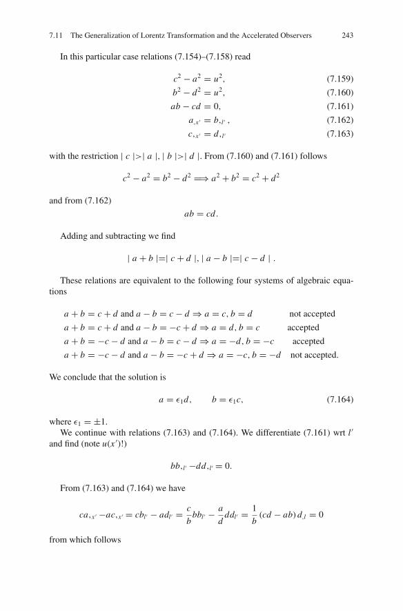
7.11 The Generalization of Lorentz Transformation and the Accelerated Observers 243
In this particular case relations (7.154)–(7.158) read
c2 − a2 = u2, (7.159)
b2 − d2 = u2, (7.160)
ab − cd = 0, (7.161)
a,x ′ = b,l ′ , (7.162)
c,x ′ = d,l ′ (7.163)
with the restriction | c |>| a |, | b |>| d |. From (7.160) and (7.161) follows
c2 − a2 = b2 − d2 =⇒ a2 + b2 = c2 + d2
and from (7.162)
ab = cd.
Adding and subtracting we find
| a + b |=| c + d |, | a − b |=| c − d | .
These relations are equivalent to the following four systems of algebraic equa-tions
a + b = c + d and a − b = c − d ⇒ a = c, b = d not accepted
a + b = c + d and a − b = −c + d ⇒ a = d, b = c accepted
a + b = −c − d and a − b = c − d ⇒ a = −d, b = −c accepted
a + b = −c − d and a − b = −c + d ⇒ a = −c, b = −d not accepted.
We conclude that the solution is
a = ε1d, b = ε1c, (7.164)
where ε1 = ±1.We continue with relations (7.163) and (7.164). We differentiate (7.161) wrt l ′
and find (note u(x ′)!)
bb,l ′ −dd,l ′ = 0.
From (7.163) and (7.164) we have
ca,x ′ −ac,x ′ = cbl ′ − adl ′ = c
bbbl ′ − a
dddl ′ = 1
b(cd − ab) d,l = 0
from which follows

244 7 Four-Acceleration
(a
c
)
,x ′= 0⇒ a = Φ(l ′)c, (7.165)
where Φ(l ′) is a smooth function. Replacing a in (7.160) we find (ε2 = ±1)
c = ε2u√1−Φ2
, | Φ |< 1.
and from (7.165) follows
d = ε1Φ(l ′)c.
Finally the solution is
a = ε1d = ε1ε2uΦ√1−Φ2
,
b = ε1c = ε1ε2u√1−Φ2
. (7.166)
This solution is determined in terms of the functions u(x ′), Φ(l ′) (| Φ |< 1),which have to be determined. In order to do that we consider (7.163) from whichfollows
a,x ′ = b,l ′ ⇒ Φ√1−Φ2
u,x ′ = uΦΦ,l ′(1−Φ2
)3/2 ⇒u,x ′
u= Φ,l ′
1−Φ2.
The lhs is a function of x ′ and the rhs is a function of l ′. Therefore each side ofthe equation must equal a constant p, say
1
u
du
dx ′= p, (7.167)
1
1−Φ2
dΦ
dl ′= p. (7.168)
Integration of the first gives
u(x′) = Aepx ′ , A = constant (7.169)
and integration of the second
1+Φ
1−Φ= e2pl ′+2B ⇒ Φ(l ′) = tanh(pl ′ + B), B = constant. (7.170)
Eventually we have the solution

7.11 The Generalization of Lorentz Transformation and the Accelerated Observers 245
a(l ′, x ′) = ε1d(l′, x′) = ε1ε2 Aepx ′ tanh(pl ′ + B)√
1− tanh2(pl ′ + B)= ε1ε2 Aepx ′ sinh(pl ′ + B)
b(l ′, x ′) = ε1c(l ′, x ′) = ε1ε2 Aepx ′ cosh(pl ′ + B).
In order to compute the constant B we assume the initial condition: the motionstarts from rest. Then dx ′
dl ′ (0) = dxdl (0) = 0 and follows
0 = dx
dl |0= a(0)dl
′ + b(0)dx′
c(0)dl ′ + d(0)dx ′ |0= a(0)+ b(0) dx
′
dl ′ (0)
c(0)+ d(0) dx ′
dl ′ (0)⇒ a(0) = 0⇒ B = 0.
This implies the final expression for the coordinates of the metric
a(l ′, x ′) = ε1d(l ′, x ′) = ε1ε2 Aepx ′ sinh pl ′, (7.171)
b(l ′, x ′) = ε1c(l ′, x ′) = ε1ε2 Aepx ′ cosh pl ′. (7.172)
Having the expression of the coordinates of the metric we are in a position todetermine the “generalized” Lorentz transformation for this particular case we dis-cuss (not for every accelerated motion!). We find
x =∫
adl ′ + bdx ′ = ε1ε2A
p
∫d[epx ′ cosh pl ′] = ε1ε2
A
pepx ′ cosh pl ′ + B1
(7.173)and similarly
l = ε1ε2A
pepx ′ sinh pl ′ + B2. (7.174)
We determine the constants B1, B2 by demanding the initial conditions: l =l ′ = 0, x ′ = 0, x = k, that is, the motion starts from the point x = k of Σ andwith the clocks synchronized at the origin of the coordinates. We compute easilyB1 = −ε1ε2
Ap + k, B2 = 0, hence
l = ε1ε2A
pepx ′ sinh pl ′, (7.175)
x = ε1ε2A
p(epx ′ cosh pl ′ − 1)+ k. (7.176)
It remains to compute the constant A which concerns initial conditions for u. Werequire that when x ′ = 0 then dx ′ = 0, that is, at the origin of E the coordinatel ′ = τ where τ is the proper time of the accelerated observer. This demand restrictsthe motion of the origin of the accelerated frame to be the hyperbolic motion westudied in Sect. 7.4.
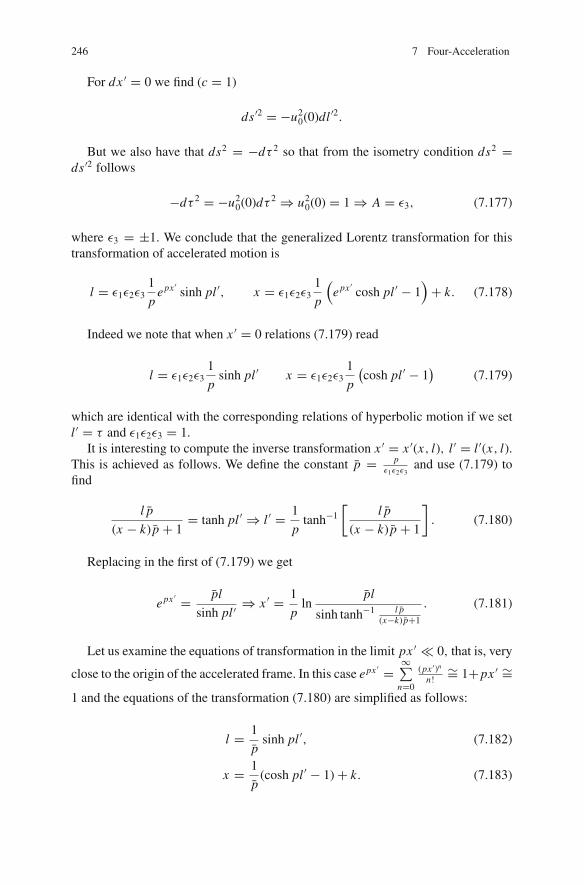
246 7 Four-Acceleration
For dx ′ = 0 we find (c = 1)
ds ′2 = −u20(0)dl ′2.
But we also have that ds2 = −dτ 2 so that from the isometry condition ds2 =ds ′2 follows
−dτ 2 = −u20(0)dτ 2 ⇒ u2
0(0) = 1⇒ A = ε3, (7.177)
where ε3 = ±1. We conclude that the generalized Lorentz transformation for thistransformation of accelerated motion is
l = ε1ε2ε31
pepx ′ sinh pl ′, x = ε1ε2ε3
1
p
(epx ′ cosh pl ′ − 1
)+ k. (7.178)
Indeed we note that when x ′ = 0 relations (7.179) read
l = ε1ε2ε31
psinh pl ′ x = ε1ε2ε3
1
p
(cosh pl ′ − 1
)(7.179)
which are identical with the corresponding relations of hyperbolic motion if we setl ′ = τ and ε1ε2ε3 = 1.
It is interesting to compute the inverse transformation x ′ = x ′(x, l), l ′ = l ′(x, l).This is achieved as follows. We define the constant p = p
ε1ε2ε3and use (7.179) to
find
l p
(x − k) p + 1= tanh pl ′ ⇒ l ′ = 1
ptanh−1
[l p
(x − k) p + 1
]. (7.180)
Replacing in the first of (7.179) we get
epx ′ = pl
sinh pl ′⇒ x ′ = 1
pln
pl
sinh tanh−1 l p(x−k) p+1
. (7.181)
Let us examine the equations of transformation in the limit px ′ � 0, that is, very
close to the origin of the accelerated frame. In this case epx ′ =∞∑
n=0
(px ′)n
n!∼= 1+px ′ ∼=
1 and the equations of the transformation (7.180) are simplified as follows:
l = 1
psinh pl ′, (7.182)
x = 1
p(cosh pl ′ − 1)+ k. (7.183)

7.11 The Generalization of Lorentz Transformation and the Accelerated Observers 247
We infer that very close to the origin of the accelerated frame the equationsof transformation tend to the equations of hyperbolic motion, a result which wasexpected.
7.11.2.1 Conclusion
It is possible to find a non-linear isometry which relates the coordinates (l, x) of aRIO with the coordinates of an accelerated observer E (l ′, x ′). Therefore we arriveat the important conclusion that
The accelerated motion can be “absorbed” into the generalization of the metric, that is theGeometry.
Although we proved this for the simple case we considered above, there is no reasonwhy we should not assume the validity of this conclusion in general. This conclusionis of fundamental importance for the following reason. According to the Principle ofEquivalence the massive bodies (and, as we shall see, the photons) suffer the sameacceleration in a gravitational field independently of their internal structure. Con-sider a RIO Σ in which there exists a gravitational field whose strength is g. Thenaccording to the Equivalence Principle all particles with mass (and the photons),when moving freely in Σ, attain acceleration g. According to the generalization wehave considered it is possible to alter the metric diag(−1, 1, 1, 1) to a new metric,which will be determined from the form of the gravitational field. Therefore
The gravitational field is “absorbed” into Geometry (i.e. the metric) of spacetime (notMinkowski space anymore) and in the new metric the effect of the gravity does not exist.
This type of motion is called free fall. It exists in Newtonian Physics. However,it is not attributed to the change of the background geometry of (absolute) space andone simply ignores the gravitational field as a force in Newton’s Second Law. Thegeometrization of the gravitational field started with Special Relativity and finallyfound its natural place in General Relativity, which is also a geometric theory ofphysics.
7.11.3 Equation of Motion in a Gravitational Field
An important application of the generalized Lorentz transformation, which takesus very close to General Relativity, is the Principle of Least Action for acceleratedmotions.
Let A, B two events along the world line of a ReMaP P . If P moves inertiallythen the world line of P is a straight line in Minkowski space and it is defined bythe requirement that the integral
∫ B
A
√|ds2|

248 7 Four-Acceleration
is extremum wrt the metric η = diag(−1, 1, 1, 1). This requirement is equivalentto the demand that the variation of the action integral vanishes (Principle of LeastAction)
δ
∫ B
A
√|ds2| = 0.
Because for an accelerated motion we have assumed that the metric remains thesame, that is ds2 = ds ′2, whereas the components change we stipulate that the worldline of an accelerated relativistic mass point is given by the condition
δ
∫ B
A
√|ds ′2| = 0, (7.184)
that is, it is a geodesic (curve of extremum length defined by the points A, B) wrtthe metric gi j . Therefore the straight lines of an inertial motion become geodesics ofa proper Riemannian metric of Lorentzian character. In case the acceleration is dueto gravitational forces only, (7.184) defines the world line of a relativistic particle infree fall in the gravitational field.
We conclude that the effect of accelerated motion in Special Relativity is twofold:
• “Changes” the Lorentz metric from its canonical form η = diag(−1, 1, 1, 1) toanother general form gi j . The theory does not say how this new metric is to bedefined and one if free to do it as one considers best. General Relativity givesfield equations for the determination of this metric.
• The world line of a relativistic particle in free motion is a (timelike) straight linein Minkowski space when the gravitational field vanishes and (timelike) geodesicof the Riemannian space with metric gi j when there exists a gravitational field.
The above conclusions lead us to the following generalization of the EquivalencePrinciple of Newtonian gravity in General Relativity (as we shall see Special Rela-tivity cannot accommodate the gravitational field):
Accelerated motions which are caused by the gravitational field only (free fall) take placealong geodesics of the metric which corresponds to the particular gravitational field.19
7.12 The Limits of Special Relativity
In Sect. 7.11 we showed that accelerated motions, and consequently the gravitationalfield, can be absorbed in the geometry of spacetime without introducing new prin-ciples but the Principle of Equivalence, which is borrowed from Newtonian theory.Therefore it is logical to expect that with this differentiation–generalization SpecialRelativity can become a theory of gravity. The first attempts toward this direction
19 This metric is computed (partially) from Einstein field equations.

7.12 The Limits of Special Relativity 249
were done by Einstein himself (and others followed). However, it became clear thatSpecial Relativity cannot accommodate the gravitational field. However, it offersmany of its elements for such a theory to be constructed. This road led eventually tothe Theory of General Relativity. In the following we present some thought exper-iments which justify these remarks. The common characteristic of these “experi-ments” is that they consider photons interacting with the gravitational field and showthat this interaction leads to new phenomena which cannot be explained within theframework of Special Relativity and require a new relativistic theory of gravitation.
7.12.1 Experiment 1: The Gravitational Redshift
Consider a positron and one electron which rest within a gravitational field at thepotential level V in some RIO Σ. At some moment the particles are left to fall freelyin the gravitational field. At the potential level V +ΔV (ΔV < 0) the two particlesannihilate producing two photons of frequency ν (why the two photons must havethe same frequency?). Subsequently the photons are reflected elastically on a largemirror and return to the potential level V where they interact creating again a pairpositron – electron which are left to fall again and so on. This thought experimentwas suggested by Einstein.20
We discuss this thought experiment with the sole restriction that it does not giverise to a perpetual mobile, that is, the Second Principle of Thermodynamics is notviolated. Because the particles have equal masses, at the potential level V+ΔV theywill have equal kinetic energies 1
2 mv2 = m | ΔV |. At the first event of annihilationof the particles conservation of energy implies for the frequency of the photons (inthe following we assume c = 1)
2hν = −2mΔV + 2m. (7.185)
Let ν the frequency of the photons when they reach the potential level V . If thephotons do not interact with the gravitational field their frequency at the potentiallevel V will again be ν, hence the produced pair of particles must have non-zerokinetic energy, which contradicts the Second Principle of Thermodynamics. There-fore the photons must interact with the gravitational field and more specificallythey must loose energy (i.e., they must be redshifted) as they propagate to higherpotential levels. In order to compute the amount of redshift we assume that the pairof electron – positron at the potential level V is produced at rest, therefore
2hν = 2m. (7.186)
20 See A. Einstein “Uber den Einfluss der Schwerkraft auf die Ausbreitung des Lichtes” Ann. Phys.898–908, (1911). Translation of this paper can be found in Lorentz H. A, Einstein A, Minkowski Hand Weyl H “The Principle of Relativity: A Collection of Original Memoirs” Mathewen, London,(1923). Paperback reprint Dover (1952) New York.

250 7 Four-Acceleration
From relations (7.186) and (7.187) follows
ν − ν
ν= ΔV < 0. (7.187)
The redshift of an electromagnetic wave is measured with the quantity z = λ−λλ
or, in terms of the frequency z = Δνν
. It follows that
z = ΔV . (7.188)
The phenomenon of variation of the frequency of a photon as it propagates ina non-homogeneous gravitational field we call gravitational redshift. This phe-nomenon is neither Newtonian nor it can be explained within the framework ofSpecial Relativity. Indeed the gravitational redshift has served as one of the firstexperimental facts toward the justification of General Relativity. It has been ver-ified by astronomical observations (with the shift of the line D1 of the spec-trum of Na in the solar spectrum21 as well as with relevant observations in thelaboratory.
Concerning the latter the best available measurements have been done by Poundand Rebka22 and Pound and Snider.23 In these experiments γ radiation of 14.4 KeVproduced from the radioactive source 57Co, was made to propagate opposite to thegravitational field into a tube of length 22.5 m filled up with helium, which wasplaced along the tower of Harvard in the campus of the University of Harvard. Atthe reception of the photons it was placed an absorber enriched with 57Fe, whichwas connected with a proportional counter. If the photons do not interact with thegravitational field the energy of the photons is proportional to the square of the speedu of the emitter (this velocity can change as we shall see below in this book whenwe study the relativistic reactions). If we consider various speeds of the emitter thenthe distribution of the number of photons in terms of speed must be a Gaussiansymmetric around the value u = 0.
In the experiment, the distribution of photons for two ranges of the velocity wasmeasured and the existence of asymmetry was examined. The first range was thevelocities VD ± u and the second range the velocities −VD ± u. The asymmetrywas observed and the calculations agreed with the value given by the gravitationalredshift (that is z = −mgh). Therefore the gravitational redshift is indeed a physicalphenomenon, which must satisfy every theory of gravity. One of these theories isGeneral Relativity.
21 See Brault J. W. “Gravitational redshift of solar lines” in Bull Amer Phys Soc 8, 28, (1963).22 See Pound R. V. and Rebka G. A. “Apparent weight of photons” Phys Rev 4, 337–341, (1960).23 See Pound R. V. and Snider J. L. “Effect of gravity on gamma radiation” Phys Rev B140,788–803, (1965).
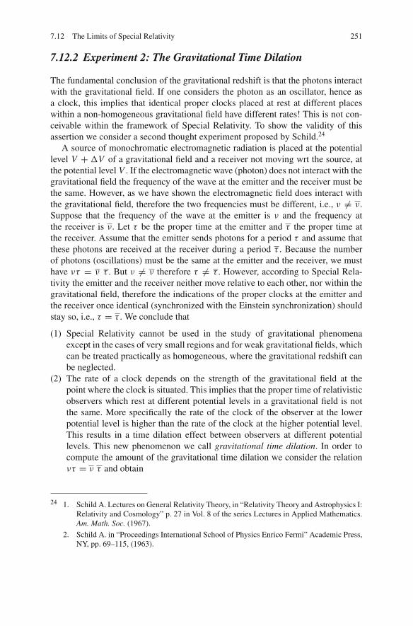
7.12 The Limits of Special Relativity 251
7.12.2 Experiment 2: The Gravitational Time Dilation
The fundamental conclusion of the gravitational redshift is that the photons interactwith the gravitational field. If one considers the photon as an oscillator, hence asa clock, this implies that identical proper clocks placed at rest at different placeswithin a non-homogeneous gravitational field have different rates! This is not con-ceivable within the framework of Special Relativity. To show the validity of thisassertion we consider a second thought experiment proposed by Schild.24
A source of monochromatic electromagnetic radiation is placed at the potentiallevel V + ΔV of a gravitational field and a receiver not moving wrt the source, atthe potential level V . If the electromagnetic wave (photon) does not interact with thegravitational field the frequency of the wave at the emitter and the receiver must bethe same. However, as we have shown the electromagnetic field does interact withthe gravitational field, therefore the two frequencies must be different, i.e., ν �= ν.Suppose that the frequency of the wave at the emitter is ν and the frequency atthe receiver is ν. Let τ be the proper time at the emitter and τ the proper time atthe receiver. Assume that the emitter sends photons for a period τ and assume thatthese photons are received at the receiver during a period τ . Because the numberof photons (oscillations) must be the same at the emitter and the receiver, we musthave ντ = ν τ . But ν �= ν therefore τ �= τ . However, according to Special Rela-tivity the emitter and the receiver neither move relative to each other, nor within thegravitational field, therefore the indications of the proper clocks at the emitter andthe receiver once identical (synchronized with the Einstein synchronization) shouldstay so, i.e., τ = τ . We conclude that
(1) Special Relativity cannot be used in the study of gravitational phenomenaexcept in the cases of very small regions and for weak gravitational fields, whichcan be treated practically as homogeneous, where the gravitational redshift canbe neglected.
(2) The rate of a clock depends on the strength of the gravitational field at thepoint where the clock is situated. This implies that the proper time of relativisticobservers which rest at different potential levels in a gravitational field is notthe same. More specifically the rate of the clock of the observer at the lowerpotential level is higher than the rate of the clock at the higher potential level.This results in a time dilation effect between observers at different potentiallevels. This new phenomenon we call gravitational time dilation. In order tocompute the amount of the gravitational time dilation we consider the relationντ = ν τ and obtain
24 1. Schild A. Lectures on General Relativity Theory, in “Relativity Theory and Astrophysics I:Relativity and Cosmology” p. 27 in Vol. 8 of the series Lectures in Applied Mathematics.Am. Math. Soc. (1967).
2. Schild A. in “Proceedings International School of Physics Enrico Fermi” Academic Press,NY, pp. 69–115, (1963).
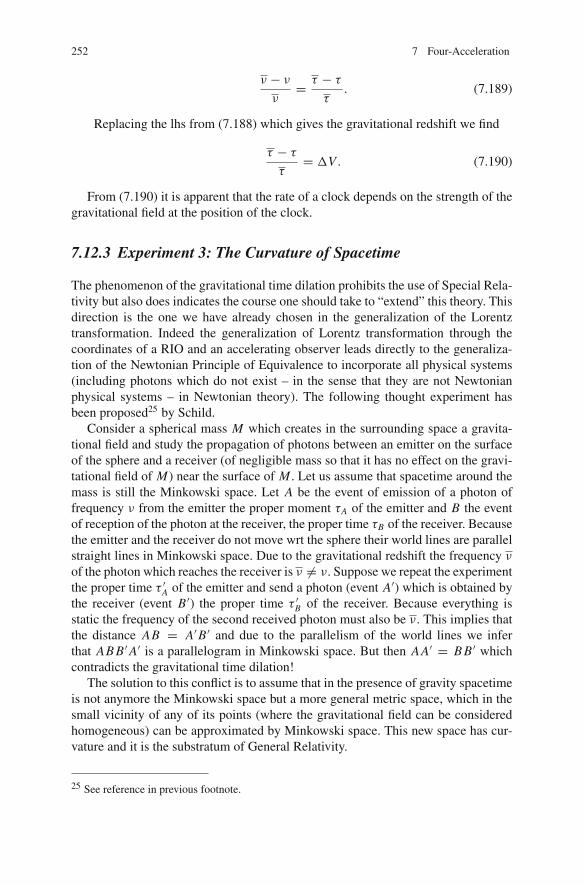
252 7 Four-Acceleration
ν − ν
ν= τ − τ
τ. (7.189)
Replacing the lhs from (7.188) which gives the gravitational redshift we find
τ − τ
τ= ΔV . (7.190)
From (7.190) it is apparent that the rate of a clock depends on the strength of thegravitational field at the position of the clock.
7.12.3 Experiment 3: The Curvature of Spacetime
The phenomenon of the gravitational time dilation prohibits the use of Special Rela-tivity but also does indicates the course one should take to “extend” this theory. Thisdirection is the one we have already chosen in the generalization of the Lorentztransformation. Indeed the generalization of Lorentz transformation through thecoordinates of a RIO and an accelerating observer leads directly to the generaliza-tion of the Newtonian Principle of Equivalence to incorporate all physical systems(including photons which do not exist – in the sense that they are not Newtonianphysical systems – in Newtonian theory). The following thought experiment hasbeen proposed25 by Schild.
Consider a spherical mass M which creates in the surrounding space a gravita-tional field and study the propagation of photons between an emitter on the surfaceof the sphere and a receiver (of negligible mass so that it has no effect on the gravi-tational field of M) near the surface of M . Let us assume that spacetime around themass is still the Minkowski space. Let A be the event of emission of a photon offrequency ν from the emitter the proper moment τA of the emitter and B the eventof reception of the photon at the receiver, the proper time τB of the receiver. Becausethe emitter and the receiver do not move wrt the sphere their world lines are parallelstraight lines in Minkowski space. Due to the gravitational redshift the frequency ν
of the photon which reaches the receiver is ν �= ν. Suppose we repeat the experimentthe proper time τ ′A of the emitter and send a photon (event A′) which is obtained bythe receiver (event B ′) the proper time τ ′B of the receiver. Because everything isstatic the frequency of the second received photon must also be ν. This implies thatthe distance AB = A′B ′ and due to the parallelism of the world lines we inferthat AB B ′A′ is a parallelogram in Minkowski space. But then AA′ = B B ′ whichcontradicts the gravitational time dilation!
The solution to this conflict is to assume that in the presence of gravity spacetimeis not anymore the Minkowski space but a more general metric space, which in thesmall vicinity of any of its points (where the gravitational field can be consideredhomogeneous) can be approximated by Minkowski space. This new space has cur-vature and it is the substratum of General Relativity.
25 See reference in previous footnote.

Chapter 8Paradoxes
8.1 Introduction
As has been remarked repeatedly in the previous chapters, the theory of SpecialRelativity is not based on direct sensory experience, as it is the case with NewtonianPhysics. This leads to situations which contradict the “common sense”1 in the sensethat the theory gives different results depending on the observer describing a givenphenomenon. This contradicts the fundamental hypothesis of physics that “reality”is observer independent. If this was true, then that would be a real problem for thetheory.
As it is expected, after the introduction of Special Relativity and indeed afterits early success, many people (who react to the new) posed several “hypothetical”experiments with the purpose to prove the confrontation of the “new” theory with thecommon sense, hence its invalidation. Most of these suggestions involve the lengthcontraction and the time dilation, because both (Euclidean) space and (Newtonian)time are fundamental to our perception of the world. All these “experiments” withone name are referred to as “paradoxes.”
All paradoxes concern Newtonian Physical situations (“common sense”), whichare transferred over to Special Relativity without checking if this is possible andin what way. All paradoxes can be explained if one considers the problem from atrue relativistic point of view. We believe that whatever paradoxes will be proposedthey will be explained by Special Relativity. Since if Special Relativity had even asmall “bag” it is rather unreal that this has not yet shown after the everyday routineapplication of the theory in the laboratory for more than 100 years.
However, paradoxes are useful because they help us understand better the theoryand it is possible that they reveal facets of the theory that we have not noticed yet.A similar case is the contribution of Einstein to quantum theory. Indeed Einstein
1 Einstein in order to show the insufficiency of the “common sense” in various projections ofthe human mind has remarked that “Common sense is the aggregate of prejudices acquiredby the age of eighteen.” However, many years before him Heraclitus has remarked that“T oυ λoγ oυ δεoντoς ξυνoυ ζωoυσ ιν oι πoλλoι ως ιδιαν εχoντες φρoνησ ιν” which means“Although common sense is common, most people consider it as if it is their own.”
M. Tsamparlis, Special Relativity, DOI 10.1007/978-3-642-03837-2 8,C© Springer-Verlag Berlin Heidelberg 2010
253

254 8 Paradoxes
was very sceptical about quantum theory (“The God does not play dice”) and pro-posed many paradoxes and arguments in order to disprove that theory. The searchfor answers to these arguments greatly helped quantum mechanics, to the degree thatlater these arguments were considered to be Einstein’s contribution in the develop-ment of quantum mechanics.
One of the most well-known paradoxes, for which many papers and argumentshave been put forward, is the tween paradox according to which two twins in relativenon-uniform motion age differently. Today, this paradox should be considered asrather trivial and shall not be considered here.2 Instead in the following we shalldiscuss more advanced and relatively unknown paradoxes.
8.2 Various Paradoxes
In this section we discuss a number of paradoxes which concern the length contrac-tion, the time dilation, and other Newtonian Physical quantities.
Example 30 In Fig. 8.1 the H-shaped slider C DE Z slides with constant velocity βcalong the ends of the circuit Σ. We assume that the current can flow only along thesides C E and DZ and that the distance of the points C D equals the distance ofthe points AB when the slider C DE Z rests in the circuit Σ. Let Σ′ be the properobserver of the slider. According to Σ as the slider moves the distance of the pointsC, D is shortened due to length contraction; therefore the lamp will be off for aperiod of time Toff (say). According to the proper observer Σ′ of the slider for thesame reason the distance of the points AB is shorter than that of the points C D,therefore the lamp will be always on. Prove that the two views, however radical, canbe explained and hence do not lead to a paradox.Solution
Before we consider the solution of the paradox3 we note that when we close aswitch the current develops in the conductor with speed βsc where βsc is the speed
Fig. 8.1 The paradox of thelamp ∑
A B
C D
E
β
Z
2 For literature relevant to this paradox see for example D. Greenberger “The reality of the twinparadox effect” Am. J. Phys. 40, 750–754, (1972).3 For a different approach see G. Sastry “Is length contraction really paradoxical?” Am. J. Phys. 55,943–46, (1987).

8.2 Various Paradoxes 255
of propagation of the electromagnetic field in the conductor. This implies that for aninterruption of the development of a current in a conductor there is a “dead” time.We use this effect in order to explain the paradox.
The circuit is open when the following events take place:
(a) The point C leaves contact A.(b) The electric pulse which is created when the point B comes in contact with
point D travels along the part AB of the circuit.
Assuming that the lamp is at the end A of the conductor we have for each of theobservers the following time intervals concerning the events (a) and (b):Observer Σ
The time period that the circuit stays “off” due to dissociation of the points A,C(Lorentz contraction, event a) equals
l0 − l0γ
βc.
The time required by the current to develop in the circuit after point D closes thecircuit at the point B (event b) is
AB
βsc= l0
βsc.
Therefore for Σ the time period for which the lamp is off equals
Toff =l0 − l0
γ
βc+ l0
βsc= lo
c
(1
β+ 1
βs
)− l0
βγ c. (8.1)
Observer Σ′
Assume that the observer Σ′ counts time zero when the end D coincides with thepoint B. The moment that the end point C disassociates from the end point A is4
(event a)
t ′1 =Difference of length AB in Σ′ and in Σ
βc=
l0 − l0γ
βc.
4 We note that t ′2 > t ′1, therefore it is possible that for observer Σ′ the circuit remains open andtherefore the lamp will be turned off. The proof that t ′2 > t ′1 is as follows. It is enough to show that
γ l0
cβs+ γβl0
c>
l0
βc− l0
γβc⇔ γ
βs>
1
β− 1
γβ− γβ = − γ
1+ γ,
which is true.

256 8 Paradoxes
Assuming that the speed of the pulse for observer Σ′ is β ′sc the distance AB,which for Σ′ has length l0
γand speed −βc, is covered in the interval (event b)
t ′2 =l0
γ (β ′s − β)c.
(β ′s − β)c is the speed of propagation of the pulse in the “moving” circuit AB.The time period for which the circuit stays off for Σ′ is
T ′off = t ′2 − t ′1 =l0
γ (β ′s − β)c− l0 − (l0/γ )
βc.
From the relativistic rule of composition of three-velocities we have
β ′s =βs + β
1+ βsβ⇒ β ′s − β = β
γ 2(1+ βsβ).
Replacing we calculate T ′off:
T ′off =γ l0
βsc+ γ
l0β
c− l0
βc+ l0
γβc= γ Toff.
This relation proves that if the lamp turns off for Σ then it does so for Σ′ for timeperiods related by the time dilation formula
T ′off = γ Toff.
Example 31 A source of monochromatic light is moving in the LCF Σ with constantvelocity u in the plane x−z parallel to the x-axis at a height hs along the z-axis. Awall of negligible thickness and of height hw (hw < hs) is placed parallel to theplane y−z and in front of the light source. Due to the presence of the wall a shadowis created in the rear part of the wall along the x-axis (see Fig. 8.2). From NewtonianPhysics we expect that
(a) The shadow will be continuous.(b) As the source approaches the wall the length of the shadow on the x-axis will
diminish and will vanish when the source is exactly over the wall (that is at thez-axis according to Fig. 8.2).
(c) First the most distant points from the wall will be lighted.
Show that in Special Relativity the behavior of the shadow is different than theNewtonian one, if the velocity u is such that u
c > 1− hw
hs. Specifically, show that the

8.2 Various Paradoxes 257
Fig. 8.2 The shadow paradox
PP’
S S’ R
T
O
shadow vanishes before the light source reaches the wall. Calculate the distance ofthe light source from the wall when the shadow vanishes.5
SolutionFirst we discuss the phenomenon qualitative. We consider a point S along the
orbit of the light source and let P be the point along the x-axis which is lightedfrom the light ray emitted from the source at the point S and greases the wall at thepoint T (see Fig. 8.2). The shadow at the point P disappears when this ray reachesthe x-axis. Since light propagates with constant finite velocity, when this light rayreaches the point P , the light source will emit a new light ray from another point S′.This light ray will reach another point P ′ at which the shadow will disappear (seeFig. 8.2). Depending on the velocity of the source it is possible that the time requiredfor the light ray to cover the distance S P is larger than the sum of the time intervalsrequired by the source to cover the distance SS′ and the light ray emitted from thepoint S′ to cover the distance S′P ′. If this is the case the shadow disappears firstat the point P ′ and later at the point P! This behavior is different than the expectedNewtonian behavior and it is due to the finite speed of light.
Let us come now to the quantitative discussion. Let Σ be the rest frame of thewall and Σ′ the rest frame of the light source. Let tS be the moment of Σ at whichthe light source is at the point S and tP the moment at which the light ray reachesthe point P , which we assume to be situated at a distance xP from the wall. Fromthe geometry of Fig. 8.2 we have
xP = hw tanφ, (8.2)
(S P) = hS
cosφ= k
√h2
w + x2P , (8.3)
where we have set k = hwhs
< 1. We note that when the light source is infinitely farfrom the wall the angle φ = π
2 and xP →∞ hence the shadow covers all the partsof the x-axis at the other side of the wall.
5 For a different approach see H.-M. Lai “Extraordinary shadow appearance due to fast movinglight” Am. J. Phys. 43, 818–820, (1975).
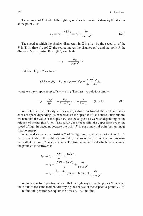
258 8 Paradoxes
The moment of Σ at which the light ray reaches the x-axis, destroying the shadowat the point P , is
tP = tS + (S P)
c= tS + hS
c cosφ. (8.4)
The speed at which the shadow disappears in Σ is given by the speed vP of theP in Σ. In time dtS (of Σ) the source moves the distance udtS and the point P thedistance dxP = vP dtS . From (8.2) we obtain
dxP = − hw
cos2 φdφ.
But from Fig. 8.2 we have
(S R) = (hs − hw) tanφ =⇒ dφ = u cos2 φ
hs − hwdtS,
where we have replaced d(SR) = −udt S . The last two relations imply
vP = dxP
dtS= − hw
hs − hwu = − u
k − 1(k > 1). (8.5)
We note that the velocity vP has always direction toward the wall and has aconstant speed depending (as expected) on the speed u of the source. Furthermore,we note that the value of the speed vP can be as great as we wish depending on therelation of the heights hs, hw. This result does not conflict the upper limit set by thespeed of light in vacuum, because the point P is not a material point but an image(has no energy).
We consider now a new position S′ of the light source after the point S and let P ′
be the point where the light ray emitted by the source at the point S′ and greasingthe wall at the point T hits the x-axis. The time moment tP ′ at which the shadow atthe point P ′ is destroyed is
tP ′ = tS + (SS′)u+ (S′P ′)
c
= tS + (S R)− (S′R)
u+ hS
c cosφ′
= tS + hs − hw
u(tanφ − tanφ′)+ hS
c cosφ′.
We look now for a position S′ such that the light rays from the points S, S′ reachthe x-axis at the same moment destroying the shadow at the respective points P, P ′.
To find this position we equate the times tP , tP ′ and find
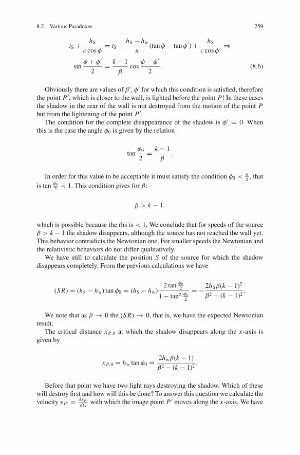
8.2 Various Paradoxes 259
tS + hS
c cosφ= tS + hS − hw
u(tanφ − tanφ′)+ hS
c cosφ′⇒
sinφ + φ′
2= k − 1
βcos
φ − φ′
2. (8.6)
Obviously there are values of β ′, φ′ for which this condition is satisfied, thereforethe point P ′, which is closer to the wall, is lighted before the point P! In these casesthe shadow in the rear of the wall is not destroyed from the motion of the point Pbut from the lightening of the point P ′.
The condition for the complete disappearance of the shadow is φ′ = 0. Whenthis is the case the angle φ0 is given by the relation
tanφ0
2= k − 1
β.
In order for this value to be acceptable it must satisfy the condition φ0 < π2 , that
is tan φ0
2 < 1. This condition gives for β:
β > k − 1,
which is possible because the rhs is < 1. We conclude that for speeds of the sourceβ > k − 1 the shadow disappears, although the source has not reached the wall yet.This behavior contradicts the Newtonian one. For smaller speeds the Newtonian andthe relativistic behaviors do not differ qualitatively.
We have still to calculate the position S of the source for which the shadowdisappears completely. From the previous calculations we have
(S R) = (hS − hw) tanφ0 = (hS − hw)2 tan φ0
2
1− tan2 φ0
2
= − 2hSβ(k − 1)2
β2 − (k − 1)2.
We note that as β → 0 the (S R)→ 0, that is, we have the expected Newtonianresult.
The critical distance xP,0 at which the shadow disappears along the x-axis isgiven by
xP,0 = hw tanφ0 = 2hwβ(k − 1)
β2 − (k − 1)2.
Before that point we have two light rays destroying the shadow. Which of thesewill destroy first and how will this be done? To answer this question we calculate thevelocity vP ′ = dxP′
dtSwith which the image point P ′ moves along the x-axis. We have

260 8 Paradoxes
vP ′ = dxP ′
dtS= d
dtS(hw tanφ′) = − hw
cos2 φ
dφ
dtS
cos2 φ
cos2 φ′dφ′
dφ
= vPcos2 φ
cos2 φ′dφ′
dφ.
Because π2 > φ > φ′, cos2 φ
cos2 φ′ < 1. Also from (8.6) one can show that −1
<dφ′dφ < 0.We note that the velocity vP ′ has direction opposite to that of vP and smaller
magnitude. This is expected as the point P ′ is closer to the wall hence it must moveopposite to the point P in order to destroy the shadow in the interval xP−xP ′ .
Finally, we note that the length of the shadow along the x-axis equals
xP − xP ′ = hw(tanφ − tanφ′) = hwsin(φ − φ′)cosφ cosφ′
> 0.
This is always positive, therefore the shadow is constantly diminishing.
Example 32 In the LCF Σ a right angle lever B AC with equal lengths AB = BC =L is resting under the influence of a pair of forces f as shown in Fig. 8.3. Atsome moment, the lever starts sliding along the x-axis with constant speed u whileremaining under the action of the same couple of forces in its rest frame. Obviously,the proper observer, Σ′ say, of the lever will observe no change (because nothingchanges concerning the couple of forces). However, the observer Σ will “see” theangle to rotate, because due to length contraction of the side AB a net moment willapply to the lever. Explain the above paradox.
It is given that the transformation of the four-force under a boost along thex-axis is
f ′x =1
(1− u·vc2 )
( fx − u
c2f · v),
f ′y =1
γ (u)(1− u·vc2 )
fy,
f ′z =1
γ (u)(1− u·vc2 )
fz .
Fig. 8.3 The paradox of theL-shaped object
A B
C
L f
L
f

8.2 Various Paradoxes 261
SolutionIn the proper frame Σ′ of the rod the velocity vanishes, therefore the inverse boost
from Σ to Σ′ of the components of the four-force gives
fx = f ′x ,fy = f ′y/γ (u),
fz = f ′z/γ (u).
The forces which act on the lever angle in the LCF Σ′ are f′B = f j and f′C = f i.These forces in Σ transform to
fB = (0, f/γ (u), 0) = f
γ (u)j,
fC = ( f, 0, 0) = f i.
We take moments in Σ wrt the point A of the lever angle:
fB(AB)Σ − fC (AC)Σ = 1
γ (u)f
1
γ (u)L − f L = −β2 f L < 0.
We note that the total moment about the point A in Σ does not vanish, hencethe lever angle will rotate about A for the one observer (the Σ) and will not for theproper observer Σ′. The source of this paradoxical behavior is due to the assumptionthat the angle is a solid body. In Relativity (both Special and General) there are nosolid bodies, because their existence relies in the Euclidean metric of the three-dimensional space.6
Example 33 An equilateral triangle of side a slides with speed u along the x-axis ofthe LCF Σ. Compute the perimeter of the triangle when it slides
(a) Along one of its heights(b) Along one of its sides
Comment on the results in the limit β → 0 (Newtonian limit) and β → 1 (relativis-tic limit).
Solution
(a) We consider the events A, B,C to be the position of the tips of the triangle ateach moment. We know the coordinates of these events in the proper frame Σ′
6 To find more on this paradox which has a long history in Special Relativity the reader can checkthe following articles:
1. J. C. Nockerson and R. McAdory “Right-angle lever paradox” Am. J. Phys. 43, 615, (1975).2. D. Jensen “The paradox of the L-shaped object” Am. J. Phys. 57, 553, (1989).

262 8 Paradoxes
A
B
C
D
0
300
0,
Fig. 8.4 Motion of an equilateral triangle
say of the triangle and we compute them in the frame Σ using the appropriateboost. With the help of Fig. 8.4 we obtain the following table of coordinates:
Σ Σ′
A : (ctA, xA, 0, 0)Σ (ct ′A, 0, 0, 0)Σ′
B : (ctB , xB , yB , 0)Σ (ct ′A,a√
32 , a
2 , 0)Σ′
C : (ctC , xC , yC , 0)Σ (ct ′A,a√
32 ,− a
2 , 0)Σ′
B Ai (cΔtB A, xB − xA, yB , 0)Σ (0, a√
32 , a
2 , 0)Σ′
C Ai (cΔtC A, xC − xA, yC , 0)Σ (0, a√
32 ,− a
2 , 0)Σ′C Bi (cΔtC B , xC − xB , yC − yC , 0)Σ (0, 0,−a, 0)Σ′
xB − xA = xC − xA = (AD)Σ = a′ cosφ where a′ is the side (AB)Σ = (AC)Σin Σ and φ is the angle B AD in Σ. From the triangle ADB we obtain sinφ =(B D)Σ(AB)Σ
= a2a′ , hence
xB − xA = a′√
1− a2
4a′2=
√a′2 − a2
4.
The boost gives xB − xA = 1γ
a√
32 . Replacing xB − xA we find
a′ =√
1+ 3γ 2
2a.
Obviously in the LCF Σ the triangle ABC is isosceles with perimeter
T = 2a′ + a =[1+
√4− 3β2
]a.

8.2 Various Paradoxes 263
Second SolutionSince the side (BC) is normal to the relative velocity it will stay normal and
with the same length, that is (BC)Σ = a. The points B,C are symmetric aboutthe x-axis which coincides with the direction of the relative velocity, hence theywill stay symmetric in Σ. This implies that the point D is the middle point of(BC)Σ and in Σ. The side (AD)Σ due to length contraction in Σ has length a
√3
2γ .Therefore
(AB)Σ =√
(B D)2Σ′ + (AD)2
Σ′ =√
a2
4+ 3a2
4γ 2= a
2
√4− 3β2
from which the perimeter follows easily.(b) This case is described in Fig. 8.5. We give only the “practical” solution and
leave the coordinate solution for the reader. We consider the height AD and forobvious reasons we write
(B D)Σ′ = (B D)Σ = a√
3
2,
(AD)Σ = 1
γ(AD)Σ′ = a
2γ.
Therefore
(BC)Σ = (AB)Σ =√
(AD)2Σ + (B D)2
Σ =a
2
√4− β2.
The perimeter of the triangle ABC for Σ is
T = 2(AB)Σ + (AC)Σ = a[√
1− β2 +√
4− β2].
Concerning the Newtonian and the relativistic limits of the perimeter we see thatin both cases the Newtonian limit (β → 0) of the perimeter of the triangle equals 3a,that is, the triangle behaves as a solid body and its angles and the lengths of its sides
0
600
A
B
CD 0,Fig. 8.5 Motion of an isosceles triangle

264 8 Paradoxes
do not change. In the relativistic limit (β → 1) in the first case, the perimeter ofthe triangle becomes 2a, the angle B AC → 180◦ and the triangle degenerates to astraight line. In the second case the perimeter equals a
√3 and the angle ABC → 0◦,
that is the triangle degenerates again to a straight line of length twice the height B D.We see that the perimeter of a triangle in Σ depends on the way the triangle
moves in Σ. This shows clearly that there are no rigid bodies (in the Newtoniansense!) in Relativity.

Chapter 9Mass – Four-Momentum
9.1 Introduction
In the previous sections we considered the kinematics of Special Relativity, whichconcerns the study of the four vectors of position, velocity, and acceleration. Themajor result of this study was the geometric description/definition of the RelativisticMass Particle (ReMaP) as a set of four-vectors, which at each point along the worldline of the particle have common proper frame or characteristic frame if they aretimelike or spacelike, respectively.
With the three four-vectors of four-position, four-velocity, and four-accelerationone is able to study the geometric properties of the world line of the ReMaP but notthe individual characteristics of the ReMaP and its interaction with the environment.For example, it is not possible to say if a given world line concerns an electronmoving in an electromagnetic field or a ReMaP which is mechanically accelerated.Furthermore it is not possible to predict the world line of ReMaP moving under theaction of a given dynamical field. In conclusion kinematics studies the world lineonly as a geometric result independently of the cause and the internal structure ofthe system.
The situation is the same with Newtonian Physics in which the three correspond-ing quantities of Newtonian kinematics do not suffice for the study of Newtonianmotion. As we do in Newtonian Physics we introduce in Special Relativity new rel-ativistic physical quantities, the Dynamical Relativistic Physical Quantities, whichcharacterize the world lines with more information. The set of all these quantitiestogether with the “laws” which govern them comprises the field of RelativisticDynamics.
We recall that the relativistic physical quantities are Lorentz tensors which in theproper frame of the ReMaP must satisfy the following two conditions:
• They must attain their reduced or canonical form• Either their components must be directly related to corresponding Newtonian
physical quantities or their physical meaning must be defined by a relativisticprinciple.
M. Tsamparlis, Special Relativity, DOI 10.1007/978-3-642-03837-2 9,C© Springer-Verlag Berlin Heidelberg 2010
265

266 9 Mass – Four-Momentum
These two conditions must be satisfied by all dynamic physical quantities intro-duced in the following.
The simplest tensors are the invariants. Furthermore from the invariants we areable to construct new tensors using the rules of Proposition 2, that is, either bymultiplying or by differentiating wrt an invariant.
The first invariant we introduce is the (relativistic) mass and, using this, the four-vectors of four-momentum, four-force, etc.
We emphasize that the photons, and in general the particles with speed c are notReMaP, therefore they do not have a proper frame. This implies that the definition ofthe dynamical quantities for these particles, hence their dynamics, is different thanthe dynamics of ReMaP and must be treated accordingly.
9.2 The (Relativistic) Mass
Before we define the (Lorentz) invariant dynamical physical quantity (relativistic)mass we refer some general comments which concern all invariant dynamical phys-ical quantities.
• Any (Lorentz) invariant is a potential relativistic physical quantity and it is char-acterized by the fact that it has the same (arithmetic) value in all LCF. Thereforeit suffices to know the value of an invariant in one LCF.
• In order a potentially invariant physical quantity to become a relativistic physicalquantity its value in the proper frame of the ReMaP must coincide with a cor-responding Newtonian physical quantity. If there is no such a quantity, then itsrelativistic physical role will be defined by means of a principle (for example, theinvariant c).
• Every invariant relativistic physical quantity of a ReMaP, say the A0+, defines inthe proper frame Σ+ of the ReMaP a new potential relativistic physical quantityby means of the timelike four-vector (A0+, 0)Σ+ . One such four-vector we havealready defined in kinematics by the invariant c, and it is the four-velocity whosecomponents in Σ+ are (c, 0)Σ+ .
• In addition to the four-vector (A0+, 0)Σ+ the invariant defines more dynamicalrelativistic physical quantities by means of the rules 1, 2 of Proposition 2.
The first invariant quantity we introduce is the (relativistic) mass m of theReMaP. In order to make the mass a relativistic physical quantity we stipulate thatin the proper frame of the ReMaP its value will be identical with the value of theNewtonian mass of the ReMaP in that frame.1
1 Usually in the literature the relativistic mass of a ReMaP is referred as rest mass and it is writtenas m0. This is due to the fact that its value is defined in the proper frame of the ReMaP where theReMaP is at rest. However, it is important to become clear that the relativistic mass is an invarianthence its value is the same in all LCF and does not change “with the velocity” as it is erroneouslyclaimed. Therefore the term “rest mass” is misleading and should be abandoned.

9.3 The Four-Momentum of a ReMaP 267
The mass of a ReMaP need not be a constant. For example, in the case of a rel-ativistic rocket the mass of the rocket changes along the world line, i.e., m = m(τ )where τ is the proper time of the rocket. In this case every value m(τ ) is a (Lorentz)invariant and the mass of the rocket is a continuous sequence of relativistic invari-ants parameterized by the proper time of the rocket. In this sense we consider therate of change dm/dτ of the proper mass of the rocket and whatever consequencesthis has.
As we have already remarked the luxons (photons) do not have proper frametherefore for those we cannot define the relativistic physical quantity mass as we didfor ReMaP. However, we can define a “mass” which will be common for all luxonsas a limiting case of the (relativistic) mass of the ReMaP. Indeed we note that themass of a ReMaP is not possible to equal zero because no Newtonian particle hasmass zero. However, the mass can approach zero as closely as one wishes, hencezero is the minimum (lowest limit) of the mass of the ReMaP. Furthermore theLorentz transformation being homogeneous preserves zero. Therefore we define therelativistic mass of luxons to be zero. As we shall see this choice is compatible withthe dynamic physical quantities of photons, to be considered further on.
9.3 The Four-Momentum of a ReMaP
Consider a ReMaP P of mass m and four-velocity ui . By means of Rule 1 of Propo-sition 2 we define the potential relativistic physical quantity
pi = m ui . (9.1)
pi is a timelike four-vector with length
p2 = m2 ui ui = −m2 c2 < 0. (9.2)
In the proper frame Σ+ of P the reduced form of the four-velocity is (c, 0)Σ+hence the four-momentum pi = (mc, 0)Σ+. The zeroth component mc of pi inthe proper frame has physical meaning (by definition, not by Newtonian analogue!)because both m and c are relativistic physical quantities. Therefore the four-vectorpi is a relativistic physical quantity. In Special Relativity the four-vector of (linear)momentum is as important as the linear momentum vector in Newtonian Physics.As it will be shown in the following, its components encounter both for the energyand the three-momentum of the ReMaP in a LCF.
To find the components of pi we recall that in Σ the four-velocity ui has compo-
nents ui = γ
(cu
)
Σ
hence the four-momentum
pi = γ
(mcmu
)
Σ
. (9.3)

268 9 Mass – Four-Momentum
In order to reveal the physical meaning of the components of the four-momentumin the LCF Σ, we consider the Taylor expansion of γ around the value 1 andcompare the result with known Newtonian quantities. For the spatial componentswe have
mγ u = mu + O(u2/c2)u. (9.4)
mu is the “Newtonian” linear momentum of the ReMaP P in Σ. Therefore it islogical to assume that the quantity
p = m γ u (9.5)
is the (linear) three-momentum of P in Σ.Working in a similar fashion we find for the zeroth component of the four-
momentum
mγ c2 = mc2 + 1
2mu2 + O(u4/c2) . (9.6)
The quantity 12 mu2 is the Newtonian kinetic energy of P in Σ, therefore the
terms mγ c2 and mc2 must be related to energy quantities. The term mc2 involvesonly the ReMaP P and it is independent of its motion. This term we identify withthe internal energy of the ReMaP P and the term mγ c2 with the total energy E ofP in Σ
E = mγ c2. (9.7)
With these identifications the four-momentum of P in Σ has the following rep-resentation:
pi =(
E/cp
)
Σ
. (9.8)
Using (9.7) and (9.8) and replacing in (9.2) we obtain the following fundamentalformula which relates E, p,m:
E =√
p2c2 + m2c4. (9.9)
This relation is possible to be displayed on the Euclidean plane by means of anorthogonal triangle (see Fig. 9.1). T is the kinetic energy of P in Σ.
Exercise 27 Prove that the angle φ in Fig. 9.1 is given by the relation
sinφ = pc
E= β.
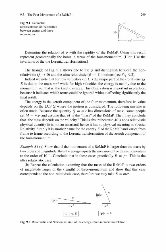
9.3 The Four-Momentum of a ReMaP 269
Fig. 9.1 Geometricrepresentation of the relationbetween energy and three-momentum
T
mc 2
φ
|p| c
mc2
Determine the relation of φ with the rapidity of the ReMaP. Using this resultrepresent geometrically the boost in terms of the four-momentum. [Hint: Use theinvariants of the the Lorentz transformation.]
The triangle of Fig. 9.1 allows one to use φ and distinguish between the non-relativistic (β → 0) and the ultra relativistic (β → 1) motions (see Fig. 9.2).
Indeed we note that for low velocities (in Σ!) the major part of the (total) energyE is due to the mass mc2 while for high velocities the energy is mainly due to themomentum pc, that is, the kinetic energy. This observation is important in practice,because it indicates which terms could be ignored without affecting significantly thefinal result.
The energy is the zeroth component of the four-momentum, therefore its valuedepends on the LCF Σ where the motion is considered. The following mistake isoften made. Because the quantity E
c2 = mγ has dimensions of mass, some peopleset M = mγ and assume that M is the “mass” of the ReMaP. Then they concludethat “the mass depends on the velocity.” This is absurd because M is not a relativisticphysical quantity (it is not an invariant) hence it has no physical meaning in SpecialRelativity. Simply it is another name for the energy E of the ReMaP and varies fromframe to frame according to the Lorentz transformation of the zeroth component ofthe four-momentum.
Example 34 (a) Show that if the momentum of a ReMaP is larger than the mass bytwo orders of magnitude, then the energy equals the measure of the three-momentumto the order of 10−4. Conclude that in these cases practically E = pc. This is theultra relativistic case.
(b) Repeat the calculation assuming that the mass of the ReMaP is two ordersof magnitude larger of the (length) of three-momentum and show that this casecorresponds to the non-relativistic case, therefore we may take E = mc2.
2
|p|
|p| � |p| ≈
2
|p|
Fig. 9.2 Relativistic and Newtonian limit of the energy–three-momentum relation
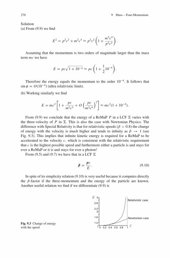
270 9 Mass – Four-Momentum
Solution(a) From (9.9) we find
E2 = p2c2 + m2c4 ≈ p2c2
(1+ m2c4
p2c2
).
Assuming that the momentum is two orders of magnitude larger than the massterm mc we have
E = pc√
1+ 10−4 ≈ pc
(1+ 1
210−4
).
Therefore the energy equals the momentum to the order 10−4. It follows thatsinφ = O(10−4) (ultra relativistic limit).
(b) Working similarly we find
E = mc2
[1+ pc
m2c4+ O
( pc
m2c4
)2]≈ mc2(1+ 10−4).
From (9.9) we conclude that the energy of a ReMaP P in a LCF Σ varies withthe three-velocity of P in Σ. This is also the case with Newtonian Physics. Thedifference with Special Relativity is that for relativistic speeds (β > 0.8) the changeof energy with the velocity is much higher and tends to infinity as β → 1 (seeFig. 9.3). This implies that infinite kinetic energy is required for a ReMaP to beaccelerated to the velocity c, which is consistent with the relativistic requirementthat c is the highest possible speed and furthermore either a particle is and stays forever a ReMaP or it is and stays for ever a photon!
From (9.5) and (9.7) we have that in a LCF Σ
β = pc
E. (9.10)
In spite of its simplicity relation (9.10) is very useful because it computes directlythe β-factor if the three-momentum and the energy of the particle are known.Another useful relation we find if we differentiate (9.9) is
Fig. 9.3 Change of energywith the speed
Relativistic case
Newtonian case

9.3 The Four-Momentum of a ReMaP 271
Ed E = pd pc = | p|d| p|c (why?)
from which follows
β = d E
d| p|c . (9.11)
Exercise 28 Let Σ, Σ′ be two LCF which are related with a boost in the standardconfiguration with velocity factor β. Let P be a ReMaP with mass m which in Σ,
Σ′ has linear momentum p, p′ and energies E, E ′, respectively. Prove the relations
E ′ = γ (E − βpx c), (9.12)
p′x = γ (px − βE/c), (9.13)
p′y = py, p′z = pz . (9.14)
Example 35 P, Σ, Σ′ as in Exercise 28. Prove the relations
(p′x −
√1+ β
1− βpx
)(p′x −
√1− β
1+ βpx
)= β2γ 2(p2
y + p2z + m2c2),
(E ′ −
√1+ β
1− βE
)(E ′ −
√1− β
1+ βE
)= β2γ 2c2(p2
y + p2z + m2c2).
Plot these relations when p2y + p2
z = constant. What happens when P is a photon?Solution
The four-momentum of P in Σ and Σ′ is pi = (E/c, p)Σ and pi = (E ′/c, p′)Σ′ ,respectively. The two expressions of the four-momentum are related by a boostalong the common x, x ′ axis. Relation (9.13) gives
(p′x − γ px )2 = γ 2β2 E2
c2= γ 2β2(p2
x + a2),
where a2 = p2y + p2
z + m2c2. This relation can be written as
(p′x − γ px )2 − (γβpx )2 = γ 2β2a2
or
[p′x − (γ + γβ)px ][p′x − (γ − γβ)px ] = γ 2β2a2.
But
γ ± βγ = γ (1± β) =√
1± β
1∓ β.

272 9 Mass – Four-Momentum
Replacing we find
(p′x −
√1+ β
1− βpx
)(p′x −
√1− β
1+ βpx
)= β2γ 2a2. (9.15)
Working similarly for the energy we show
(E ′ −
√1+ β
1− βE
)(E ′ −
√1− β
1+ βE
)= β2γ 2a2. (9.16)
If a2 = constant these equations describe hyperbolae with asymptotes thestraight lines
p′x =√
1+ β
1− βp′x p′x =
√1− β
1+ βpx
and, respectively,
E ′ =√
1+ β
1− βE ′ =
√1− β
1+ β
The plotting is left to the reader. In case P is a photon relations (9.15) and (9.16)become identical and furthermore the mass m = 0.
Exercise 29 The LCF Σ and Σ′ are moving with parallel axes and relative velocity u.A ReMaP P has four-momentum (E/c,p)Σ and (E ′/c,p′)Σ′ in Σ, Σ′, respectively.
(a) Show that the components of the four-momentum in Σ and Σ′ are related asfollows:
E ′ = γu (E − u·p) , (9.17)
p′ = p+ u[
u·pu2
(γu − 1)− γuE
c
]. (9.18)
Show that in the case of a boost these relations reduce to (9.12) – (9.14).
(b) Show that the angles θ, θ ′ of the three-momenta p,p′ with the relative velocityu of Σ and Σ′ are related as follows:
cot θ ′ =(
cot θ − β
B ′1
sin θ
), (9.19)
where B ′ is the speed factor of P in Σ′. Relation (9.19) is called the particleaberration formula. It is used in the focussing of beams of particles.
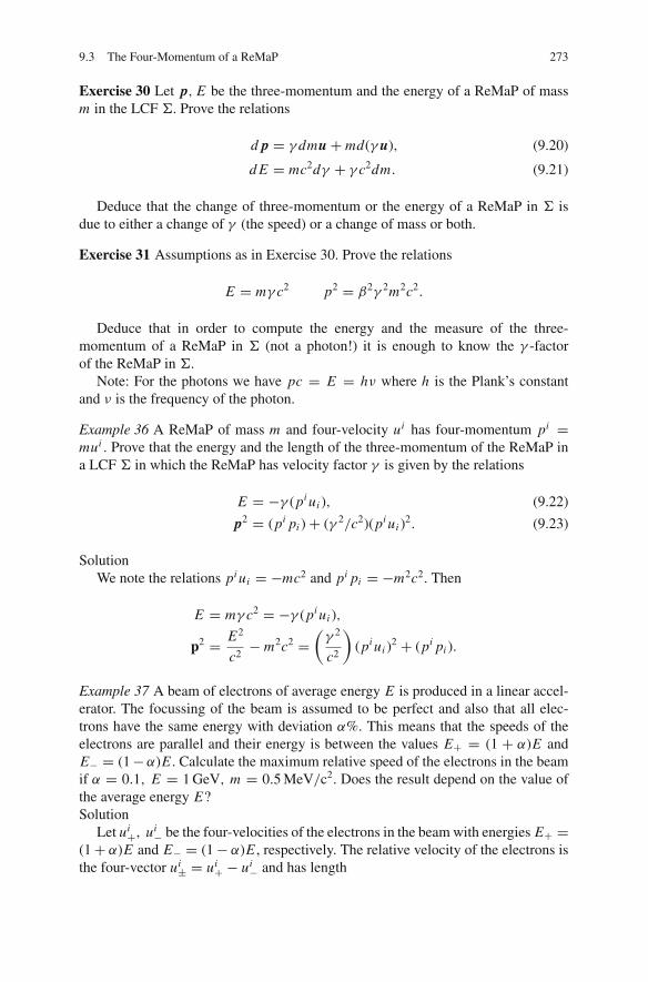
9.3 The Four-Momentum of a ReMaP 273
Exercise 30 Let p, E be the three-momentum and the energy of a ReMaP of massm in the LCF Σ. Prove the relations
d p = γ dmu + md(γ u), (9.20)
d E = mc2dγ + γ c2dm. (9.21)
Deduce that the change of three-momentum or the energy of a ReMaP in Σ isdue to either a change of γ (the speed) or a change of mass or both.
Exercise 31 Assumptions as in Exercise 30. Prove the relations
E = mγ c2 p2 = β2γ 2m2c2.
Deduce that in order to compute the energy and the measure of the three-momentum of a ReMaP in Σ (not a photon!) it is enough to know the γ -factorof the ReMaP in Σ.
Note: For the photons we have pc = E = hν where h is the Plank’s constantand ν is the frequency of the photon.
Example 36 A ReMaP of mass m and four-velocity ui has four-momentum pi =mui . Prove that the energy and the length of the three-momentum of the ReMaP ina LCF Σ in which the ReMaP has velocity factor γ is given by the relations
E = −γ (pi ui ), (9.22)
p2 = (pi pi )+ (γ 2/c2)(pi ui )2. (9.23)
SolutionWe note the relations pi ui = −mc2 and pi pi = −m2c2. Then
E = mγ c2 = −γ (pi ui ),
p2 = E2
c2− m2c2 =
(γ 2
c2
)(pi ui )
2 + (pi pi ).
Example 37 A beam of electrons of average energy E is produced in a linear accel-erator. The focussing of the beam is assumed to be perfect and also that all elec-trons have the same energy with deviation α%. This means that the speeds of theelectrons are parallel and their energy is between the values E+ = (1 + α)E andE− = (1−α)E . Calculate the maximum relative speed of the electrons in the beamif α = 0.1, E = 1 GeV, m = 0.5 MeV/c2. Does the result depend on the value ofthe average energy E?Solution
Let ui+, ui
− be the four-velocities of the electrons in the beam with energies E+ =(1+ α)E and E− = (1− α)E , respectively. The relative velocity of the electrons isthe four-vector ui
± = ui+ − ui
− and has length

274 9 Mass – Four-Momentum
ui±u±i = (ui
+ − ui−)(u+i − u−i ) = −2c2 − 2ui
+u−i . (9.24)
We calculate the inner product ui+u−i in the proper frame of ui
−. In that frame
ui− =
(c0
)
−, ui+ =
(γ±cγ±v±
)
−where γ± is the γ -factor of the relative velocity
v±. The product ui+u−i = −γ±c2. Replacing in (9.24) we find
ui±u±i = 2(γ± − 1)c2. (9.25)
We note that the length of the four-vector ui± is positive hence ui
± is not a four-velocity!
We calculate γ± in the laboratory where the four-velocities ui+, ui
− are given.
From the relations ui+ = pi
+m , ui
− = pi−
m and the relation ui+u−i = −γ±c2 we find
γ± = − 1
m2c2pi+ p−i .
We also calculate the inner product in the laboratory. We have the components
pi+ =
(E+/cpe+
)
L
, pi− =
(E−/cpe−
)
L
from which follows
γ± = − 1
m2c4(−E+E− + p+ p−c2). (9.26)
The length
p+c =√
E2+ − m2c4 = E+
√
1− m2c4
E2+
≈ E+
[1− 1
2
(mc2
E+
)2
+ O
((mc2
E+
)4)]
and similarly
p−c =√
E2− − m2c4 ≈ E−
[1− 1
2
(mc2
E−
)2
+ O
((mc2
E−
)4)]
.
Therefore the product
p+ p−c2 ≈ E+E−
[1− 1
2
(mc2
E+
)2
− 1
2
(mc2
E−
)2
+ O
((mc2
E−
)4
,
(mc2
E−
)4)]
.
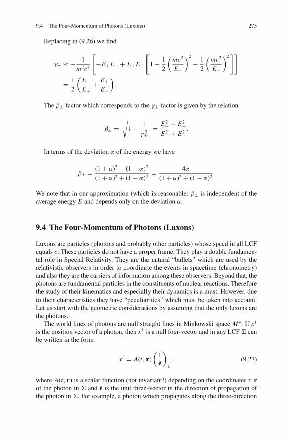
9.4 The Four-Momentum of Photons (Luxons) 275
Replacing in (9.26) we find
γ± ≈ − 1
m2c4
[−E+E− + E+E−
[1− 1
2
(mc2
E+
)2
− 1
2
(mc2
E−
)2]]
= 1
2
(E−E++ E+
E−
).
The β±-factor which corresponds to the γ±-factor is given by the relation
β± =√
1− 1
γ 2±= E2
+ − E2−
E2+ + E2−.
In terms of the deviation α of the energy we have
β± = (1+ α)2 − (1− α)2
(1+ α)2 + (1− α)2= 4α
(1+ α)2 + (1− α)2.
We note that in our approximation (which is reasonable) β± is independent of theaverage energy E and depends only on the deviation α.
9.4 The Four-Momentum of Photons (Luxons)
Luxons are particles (photons and probably other particles) whose speed in all LCFequals c. These particles do not have a proper frame. They play a double fundamen-tal role in Special Relativity. They are the natural “bullets” which are used by therelativistic observers in order to coordinate the events in spacetime (chronometry)and also they are the carriers of information among these observers. Beyond that, thephotons are fundamental particles in the constituents of nuclear reactions. Thereforethe study of their kinematics and especially their dynamics is a must. However, dueto their characteristics they have “peculiarities” which must be taken into account.Let us start with the geometric considerations by assuming that the only luxons arethe photons.
The world lines of photons are null straight lines in Minkowski space M4. If xi
is the position vector of a photon, then xi is a null four-vector and in any LCF Σ canbe written in the form
xi = A(t, r)
(1e
)
Σ
, (9.27)
where A(t, r) is a scalar function (not invariant!) depending on the coordinates t, rof the photon in Σ and e is the unit three-vector in the direction of propagation ofthe photon in Σ. For example, a photon which propagates along the three-direction

276 9 Mass – Four-Momentum
(1, 1, 1)t in Σ and the moment t = 0 of Σ passes through the origin has positionvector
xi = ct
(1,
1√3,
1√3,
1√3
)t
Σ
. (9.28)
The four-velocity of a photon cannot be defined by the relation dxi/dτ becausephotons do not have proper time. The same holds for the four-acceleration, whichalso has the additional constraint that the speed in all LCF equals c. We also have aproblem with the four-momentum because one cannot consider mass with the stan-dard connotation for the photons, except as a minimum of the mass of the ReMaP.
In order to circumvent these difficulties and be consistent with what we havedone already, we continue using the process of the limit. We start with the four-momentum.
Because we have assumed the “mass” of photons to equal 0 the four-momentumpi pi = −m2c2 = 0 must also be a zero four-vector. This means that in any LCF Σ
pi can be written in the form
pi = A(t, r)(1, e)Σ, (9.29)
where A(t, r) is a scalar (but not an invariant!) quantity and the three-vector edefines the direction of propagation of the photon in the three-space of Σ. FromNewtonian Physics we know that a photon of frequency ν, which propagates alongthe direction e, has energy E and momentum p given by
E = hν, (9.30)
p = hν
ce = E
ce. (9.31)
Based on the above analysis we define the four-momentum of a photon in a LCFΣ in which the photon has energy E(= hν) and three-momentum p(= hν
c e) withthe relation
pi =(
E/c(E/c)e
)
Σ
. (9.32)
This definition connects the two natures of the photon, that is, the wave and theparticle nature.
Example 38 In the LCF Σ a photon has energy E and three-momentum p. Calculatethe energy E ′ and the direction of propagation e′ of the photon in an LCF Σ′, whichmoves relative to Σ with velocity u. Express the angle θ ′ between e′ and u in termsof the angle θ between e and u. Comment on the result.Solution
Suppose the four-momentum pi of the photon in Σ and Σ′ has representationpi = (E/c,p)Σ and pi = (E ′/c,p′)Σ′ , respectively. The Lorentz transformation

9.4 The Four-Momentum of Photons (Luxons) 277
parallel and normal to the relative velocity u gives (recall that p‖ = p·uu2 ):
E ′/c = γ (u)(E/c − β · p‖), (9.33)
E ′
ce′⊥ = p⊥, (9.34)
E ′
ce′‖ = γ (u)
(p‖ − β
E
c
). (9.35)
From (9.33) we have for the energy E ′ in Σ′
E ′ = γ (u)(E − p·u). (9.36)
The other two equations give
(E ′/c)e′ = p⊥ +[γ (u)
p·uu2− γ (u)
E
c2
]u
= p[
(γ (u)− 1)p·uu2− γ (u)
E
c2
]u
from which follows
e′ = c
γ (u)(E − p·u)
{p+
[(γ (u)− 1)
p·uu2− γ (u)
E
c2
]u}. (9.37)
Relation (9.37) is known as light aberration formula. [Prove (9.37) by directapplication of the Lorentz transformation].
Concerning the angle θ we consider θ �= kπ/2, k = 0, 1, 2, 3 and |pc| = E(because we have photons) hence |p‖| = E
c cos θ, |p⊥| = Ec sin θ . It follows
cot θ ′ = |e′‖||e′⊥|= γ (u)
(E/c) cos θ − (E/c)β
(E/c) sin θ
= γ (u)cos θ − β
sin θ= γ (u)
(cot θ − β
sin θ
). (9.38)
[Compare this relation with (9.19). What are their similarities and differences?]We consider next the special cases θ = kπ/2, k = 0, 1, 2, 3. When θ = 0
from (9.34) we have p⊥ = 0 =⇒ e′⊥ = 0 hence θ ′ = 0, that is, the directions ofpropagation of the photon on Σ and Σ′ coincide. The same result we find if we workdirectly with (9.37). Indeed we have (u = ue)
e′ = c
γ (u)(E − βE)
[E
ce+
[(γ (u)− 1)
βE
u2− γ (u)
E
c2
]e]= e.

278 9 Mass – Four-Momentum
When θ = π2 then p·u = 0 and (9.37) gives
e′ = 1
γ(e⊥ − βγ e‖).
The cot θ ′ = −βγ < 0 hence θ ′ε (π2 , π ).Working similarly we show that when θ = π the θ ′ = π and when θ = 3π/2
the θ ′ε (−π/2, π/2).
9.5 The Four-Momentum of Particles
In the previous sections we defined the four-momentum of the ReMaP and the pho-tons in a different way. The necessity for this approach was due to the different char-acter of this four-vector for each class of particles, that is, timelike for the ReMaPand null for the photons. However, in nuclear reactions both types of particles areinvolved therefore it would be useful to have a unified approach. This leads us to theintroduction of particle four-vector which is a four-vector whose (Lorentz) lengthis either negative or zero. This approach gives us the possibility to give a dynamicdefinition for the elementary particles.
Definition 13 Particle in the Theory of Special Relativity is any physical systemwhose four-momentum is a particle four-vector.
This definition allows us to use all the results on particle four-vectors in the studyof relativistic collisions. However, it is to be noted that the results of that sectionapply to all particle four-vectors not only to the four-momentum.
9.6 The System of Natural Units
In Newtonian Physics the physical quantities spatial length (L), time (T) and mass(M) are absolute (i.e., Euclidean invariants) therefore it is logical to develop a systemof units whose fundamental elements are the [L,T,M]. This system is the Interna-tional System of Units (SI units) which is an evolution (in 1960) of the well-knownMKSA system with the addition of the units of Kelvin, Candela, and (later on)the mole.
In the Theory of Special Relativity the quantities T, L are not relativistic physicalquantities hence the SI, although it can still be used, is not anymore inherent in thattheory.
In order to find a new system of units suitable for Special Relativity we considerthe new fundamental invariant relativistic quantities. The first such quantity is thevalue c, therefore in the “relativistic” system the universal constant c will equal thepure number 1. The new system we call the System of Natural Units (NU).

9.6 The System of Natural Units 279
In this system the unit of spatial length 1 m is related to the unit of time 1 s withthe relation
1 s = 3× 10⁸ m. (9.39)
The independent dimensions in the System of Natural Units are (among other) the[L, M].
In order to convert the value of a quantity from the SI system in the system ofNatural Units we apply the following simple rule:
Multiply the value of the physical quantity in the SI units with the quantity c = [c]m/swhere [c] = 3 × 10⁸ in the same power as the time T appears in the units of the physicalquantity in the SI system.
Let us see some applications of this rule.Spatial length (L in SI)
The dimensions are the same in both systems of units, i.e., 1 m. Indeed, accordingto the rule
1 m in SI = [c]0 (m/s)0 m = 1 m in NU.
Time (T in SI)The unit of time in NU is the spatial length m. Indeed according to the rule
1 s in SI = [c]1 (m/s)1 s in NU = [c] m
which is in agreement with (9.39).Velocity(L/T in SI)
1 m/s in SI = [c]−1 (m/s)−1 (m/s) = [c]−1in NU.
We note that in NU the velocity is a pure number, as expected.Acceleration (L/T 2 in SI)
1 m/s2 in SI = [c]−2 (m/s)−2 m/s2 = [c]−2 m−1in NU.
Force (M L/T 2 in SI)
1N in SI = 1 kg m/s2 = [c]−2(m/s)−2kg m/s2 = [c]−2kg m−1 in NU.
Exercise 32 Show the validity of the following transformations between the valuesof the physical quantities in the SI and the NU system.Energy (Nm)
1J in SI = [c]−2 kg in NU.

280 9 Mass – Four-Momentum
(Note that the dimensions of energy in NU is mass (kg) which is compatible withthe relation E = mc2 and allows us to measure energy in kg and conversely massin kJ.)Pressure
1 N/m2 in SI = [c]−2 kg/m3 in NU
Energy density
1 J/m3 in SI = [c]−2 kg/m3 in NU
Mass density
1 kg/m3 in SI = 1 kg/m3 in NU
Momentum
1 kg m/s1 in SI = [c]−1 kg in NU
(Note that in the NU system the dimensions of energy are identical with those oflinear momentum).
Plank’s constant:
h = 6.63× 10⁻³⁴ J s in SI = 6.63× 10⁻³⁴[c]−2kg× [c] m
= 2.21× 10−42 kg m in NU.
Except the introduction of the NU system, there is also the necessity to adjust therelativistic units of measurement to the relativistic reality. Indeed as it is nonsenseto measure the speed of a car in mm/days, similarly it makes no sense to measurethe energy of an elementary particle in J. The basic physical quantity in the studyof elementary particles (at the level we are dealing with) is the energy. Since inNU the units of energy are identical with the units of mass (because c = 1 andE = mc2), we measure the mass of elementary particles in units of energy. Forreasons we mentioned above these units are not the erg (C.G.S.) or the Joule (S.I.)but the eV and its multiples. By definition 1 eV is the kinetic energy acquired by anelectron which starts from rest and moves in empty space between two points whosepotential difference is 1 V. Let us calculate how much energy is in 1 eV.
The charge of the electron equals 1.6021× 10⁻¹⁹ Cb, therefore,
1 eV = 1.6021× 10⁻¹⁹ J = 1.602× 10⁻¹² erg.
Inverting this relation we find
1 J = 6.24× 10¹⁸ eV.
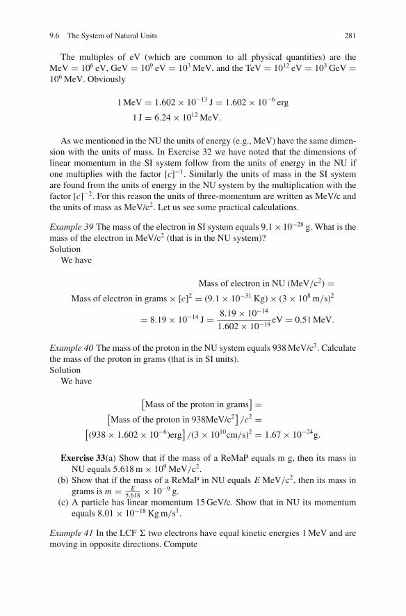
9.6 The System of Natural Units 281
The multiples of eV (which are common to all physical quantities) are theMeV = 106 eV, GeV = 109 eV = 103 MeV, and the TeV = 1012 eV = 103 GeV =106 MeV. Obviously
1 MeV = 1.602× 10⁻¹³ J = 1.602× 10⁻⁶ erg
1 J = 6.24× 10¹² MeV.
As we mentioned in the NU the units of energy (e.g., MeV) have the same dimen-sion with the units of mass. In Exercise 32 we have noted that the dimensions oflinear momentum in the SI system follow from the units of energy in the NU ifone multiplies with the factor [c]−1. Similarly the units of mass in the SI systemare found from the units of energy in the NU system by the multiplication with thefactor [c]−2. For this reason the units of three-momentum are written as MeV/c andthe units of mass as MeV/c2. Let us see some practical calculations.
Example 39 The mass of the electron in SI system equals 9.1× 10⁻²⁸ g. What is themass of the electron in MeV/c2 (that is in the NU system)?Solution
We have
Mass of electron in NU (MeV/c2) =Mass of electron in grams× [c]2 = (9.1× 10⁻³¹ Kg)× (3× 10⁸ m/s)2
= 8.19× 10⁻¹⁴ J = 8.19× 10⁻¹⁴
1.602× 10⁻¹⁹eV = 0.51 MeV.
Example 40 The mass of the proton in the NU system equals 938 MeV/c2. Calculatethe mass of the proton in grams (that is in SI units).Solution
We have
[Mass of the proton in grams
] =[Mass of the proton in 938MeV/c2
]/c2 =
[(938× 1.602× 10−6)erg
]/(3× 1010cm/s)2 = 1.67× 10⁻²⁴g.
Exercise 33(a) Show that if the mass of a ReMaP equals m g, then its mass inNU equals 5.618 m× 109 MeV/c2.
(b) Show that if the mass of a ReMaP in NU equals E MeV/c2, then its mass ingrams is m = E
5.618 × 10⁻⁹ g.(c) A particle has linear momentum 15 GeV/c. Show that in NU its momentum
equals 8.01× 10⁻¹⁸ Kg m/s1.
Example 41 In the LCF Σ two electrons have equal kinetic energies 1 MeV and aremoving in opposite directions. Compute

282 9 Mass – Four-Momentum
(a) The speed of each electron in Σ
(b) The relative velocity of the electrons
(It is given that the mass of the electron in NU is m = 0.51 MeV/c2).Solution
(a) If T is the kinetic energy of the electron then the total energy E = T + mc2.
But E = mγ c2. Therefore
γ = T + mc2
mc2= 1+ T
mc2=⇒ γ = 2.96 and β = 0.94.
(b) The relative velocity of the electrons equals the velocity of one of them in therest frame of the other. The relativistic rule for spatial velocities gives
|vrel| = u + u
1+ uu/c2= 2β
1+ β2c,
where β = u/c is the β-factor of each electron in Σ. Replacing, we find |vrel| =0.998c.
Example 42 Calculate to the order of the third decimal digit the β-factor of a pionof momentum 10.0 GeV/c. It is given that the mass of the pion is 1.40 GeV/c2.Solution
It is given that |pc| = 10.0 GeV and mc2 = 1.40 GeV. Then
β = |pc|E= |pc|
mγ c2⇒ βγ = |pc|
mc2= 7.14
therefore
γ =√
1+ (βγ )2 = 7.21,
β =√
1− 1
γ 2= 0.990.
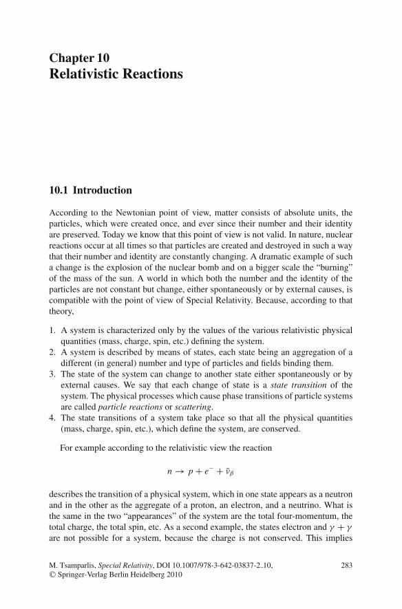
Chapter 10Relativistic Reactions
10.1 Introduction
According to the Newtonian point of view, matter consists of absolute units, theparticles, which were created once, and ever since their number and their identityare preserved. Today we know that this point of view is not valid. In nature, nuclearreactions occur at all times so that particles are created and destroyed in such a waythat their number and identity are constantly changing. A dramatic example of sucha change is the explosion of the nuclear bomb and on a bigger scale the “burning”of the mass of the sun. A world in which both the number and the identity of theparticles are not constant but change, either spontaneously or by external causes, iscompatible with the point of view of Special Relativity. Because, according to thattheory,
1. A system is characterized only by the values of the various relativistic physicalquantities (mass, charge, spin, etc.) defining the system.
2. A system is described by means of states, each state being an aggregation of adifferent (in general) number and type of particles and fields binding them.
3. The state of the system can change to another state either spontaneously or byexternal causes. We say that each change of state is a state transition of thesystem. The physical processes which cause phase transitions of particle systemsare called particle reactions or scattering.
4. The state transitions of a system take place so that all the physical quantities(mass, charge, spin, etc.), which define the system, are conserved.
For example according to the relativistic view the reaction
n→ p + e− + νβ
describes the transition of a physical system, which in one state appears as a neutronand in the other as the aggregate of a proton, an electron, and a neutrino. What isthe same in the two “appearances” of the system are the total four-momentum, thetotal charge, the total spin, etc. As a second example, the states electron and γ + γ
are not possible for a system, because the charge is not conserved. This implies
M. Tsamparlis, Special Relativity, DOI 10.1007/978-3-642-03837-2 10,C© Springer-Verlag Berlin Heidelberg 2010
283

284 10 Relativistic Reactions
that the Newtonian distinction of systems, in simple and complex according to thenumber of particles they involve, does not apply. Indeed, as we have seen in theabove example, the same system in one state appears as a single particle (the n)and in another as the aggregate of three particles (the p, e−, νβ). Furthermore, itis possible that each particle is by itself a system and in some states can appear asmore particles and so on.
If in a reaction (or scattering) of particles the number and the identity of particlesare preserved, we call the reaction elastic. In all other cases, the reaction is calledinelastic.
In practice, particle reactions are achieved by the collision of beams of fastmoving particles either with targets at rest in the laboratory or with other travel-ing beams. These beams of particles (the mother particles) are created in specialman-made machines (particle colliders, linear accelerators, synchrotrons, etc.) orin interstellar space, e.g., by magnetic fields of strongly magnetized stellar bodies.The particles which emerge from a reaction (the daughter particles) are observedwith special machines, which measure their distribution in space (number densityand energy density in a specified direction and a small solid angle) in some LCFs.For a long time the experimental measurements involved photographing and count-ing the particle trajectories (bubble chamber), but today there are more accurateand powerful electronic methods employing computers and photosensitive materi-als (scintillator, etc.). In every case, what we observe in a particle reaction is a setof orbits, whose study provides us with information concerning the values of thephysical quantities of the system in the LCF we are working. The experimentallymeasured quantities we observe are
1. The identity of the particles (partially)2. The distribution of the space velocities of the particles (i.e., the number of
trajectories per given direction and unit solid angle)3. The distribution of energies and three-momenta (curvatures and other geometric
elements of the orbits in given electromagnetic fields)
The “metamorphosis” of a physical system from one state to another can bestudied in two stages. The first stage considers the initial and the final states andit is concerned only with the conservation of the physical quantities characterizingthe system. The second stage studies the dynamics, that is the mechanism, whichbrings the initial state to the final state. In the following, we shall be concerned withthe first study, sometimes called the kinetics of the reaction. The second approachrequires the methods of quantum physics and it is outside the scope of this book.
10.2 Representation of Particle Reactions
The spacetime representation of a particle reaction is shown in Fig. 10.1. This rep-resentation simply shows the particles which react and the particles which are pro-duced. The dark circle represents the mechanism of the reaction (the “dynamics”

10.3 Relativistic Reactions 285
Fig. 10.1 Spacetimerepresentation of a reaction
12
1′
2′
′···
···
of the reaction) and, as we remarked above, concerns the study of the reaction bymeans of quantum field theory.
The study of the kinetics of a particle reaction is also done in two stages, as it isdone with conventional chemistry. In the first stage, the reaction is studied stoichio-metrically, that is, we consider a small number of individual reacting particles andwrite
A + B + · · · → A′ + B ′ + · · ·1 2 + · · · 1′ 2′ + · · ·
This defines the initial and the final states of the system. Then one considersthe conservation equations of the physical quantities of the system in one or morestates and draws conclusions with the purpose to explain or foresee the experimentaldata. In the second stage, the reaction is studied qualitatively, that is, one considersthe distributions of particles (not individual particles) and subsequently studies theconservation of the various physical quantities of the system. In the following, weshall be concerned with the stoichiometric study only, because the quantitative studyrequires special knowledge beyond the scope of this book.
10.3 Relativistic Reactions
In Special Relativity the basic physical quantity, which characterizes a system ofparticles is the four-momentum. The four-momentum of a relativistic system in acertain state is the vector sum of the four-momenta of all components compris-ing the system. If the state of the system consists only of free particles, then thefour-momentum of the system equals the sum of four-momenta of all individualparticles. If the state of the system contains fields of interaction among the particles,then the four-momentum of the system contains the four-momenta of the particlesplus the four-momenta of the fields of interaction. For example, the four-momentumof an atom includes the four-momenta of the nucleus, and the electrons plus themomentum of the electromagnetic field coupling the nucleus and the electrons. Fur-thermore, the nucleus itself is a system whose four-momentum is the sum of themomenta of the nucleons which make it up and the hadronic and the electromag-netic fields which couple them. Moreover, each nucleon is a relativistic system andso on. We note that there is an endless process, which does not allow for a clear-cutdistinction between particle momentum and field momentum. Therefore, what isexperimentally measured is the total momentum of an experimentally identifiablesystem.

286 10 Relativistic Reactions
Fig. 10.2 Schematicrepresentation of the reacting(mother) momenta
Fig. 10.3 Schematicrepresentation of theproduced (daughter)momenta reaction point
2
1 ···
m
Consider a set of particles P1, P2, . . . , Pn with corresponding four-momenta p1,p2, . . ., pn . We say that these particles react or collide if their world lines have acommon point as shown in Fig. 10.2.
The reaction is a common event for all particles involved. As a result of the reac-tion, suppose that new particles Q1, Q2, . . ., Qm are produced with four-momentumq1, q2, . . ., qm respectively. The new particles are in general different both in identity(P(α) �= Q(β)) and in number (see Fig. 10.3).
The world lines of the daughter particles have again a common spacetime event,which is the same as the event of reaction/collision of the mother particles. There-fore, at the spacetime event of the reaction we have the following sets of timelike ornull four-vectors:
p1, p2, . . . , pn and q1, q2, . . . , qm .
These vectors are elements of Minkowski space, therefore they must comply withthe geometry of that space. In Chap. 1 we stated Proposition 4, which concerns thesum of particle four-vectors and the triangle inequality in Minkowski space. Let ussee the effect of each of these geometric results on the four-momenta.
10.3.1 The Sum of Particle Four-Vectors
According to Proposition 4, the sum of a finite number of future/past-directed time-like or null four-vectors (particle four-vectors) is a future/past-directed timelikefour-vector except, if and only if, all vectors are null and parallel, in which case thesum is a null vector parallel to the individual vectors. Let us see the significance of

10.3 Relativistic Reactions 287
Fig. 10.4 Relativisticreaction Particles Particles
Reaction
this result in the case of spacetime collisions. The second part assures that in SpecialRelativity the light beams exist and are geometrically sound quantities. Indeed, alight beam is defined by a bunch of parallel null straight world lines and accordingto Proposition 4, the sum of such an aggregate of lines is again a parallel null linecorresponding to the beam. Furthermore, it is easy to show that if two photons (ornull straight world lines) are parallel in Minkowski space, then their directions ofpropagation in Euclidean three-space are also parallel. Therefore, a light beam inNewtonian space is also a light beam in spacetime. This is an important conclu-sion otherwise we would not be able to coordinate spacetime by means of lightrays (i.e., to do chronometry in Special Relativity) working within our Newtonianenvironment.
Concerning the first part of the proposition we have that – excluding the casethat all four-momenta are future/past-directed null and parallel – the sums Pi =∑n
B=1 piB and Qi =∑m
α=1 qiα are timelike four-vectors. This geometric result, when
transferred to the relativistic reactions, means that they must be of the general form(Fig. 10.4)
Certainly, geometry does not (and should not!) say which particles are producedwhen certain particles are involved in a relativistic reaction. This is the work ofphysics and its laws. However, what it does say is that in a relativistic reaction par-ticles produce particles and only particles. This is not a self-evident fact and showsthat our belief of how a relativistic reaction occurs is justified by the mathematicalmodel we employ.
Because four-momentum is a relativistic physical quantity, we demand that dur-ing a relativistic reaction the total four-momentum is conserved, that is, the follow-ing equation holds:
Pi = Qi . (10.1)
The understanding of this law is different from the usual point of view of thecorresponding law of conservation of three-momentum (and energy) of NewtonianPhysics, the difference being in the absolute character of the particles of the latter.Indeed, in Special Relativity it is assumed that during the reaction, the reactingparticles form a new unstable (or virtual) particle with four-momentum Pi whichsubsequently, with some kind of esoteric mechanism, brakes up into the productsof the reaction. This virtual particle is called center of momentum particle and isindicated as shown in Fig. 10.5. Such an assumption is clearly incompatible withthe Newtonian point of view.
The law of conservation of four-momentum is a pillar of contemporary physicsand appears to hold exactly without exception. For example, an apparent violationin radioactive beta decay back in the 1930s led Pauli to the speculative hypothesisthat in that reaction there is also an undetected neutral particle of small proper mass,

288 10 Relativistic Reactions
Fig. 10.5 The center ofmomentum particle 1
2
·1
2··
···
Fig. 10.6 The closed polygonof linear four-momenta 1
2
1
2
3
which was later named “neutrino.” This speculation was established1 23 years later,beyond any doubt, by its detection in a nuclear reaction.
Geometrically the law of conservation of four-momentum in spacetime is rep-resented as in Newtonian three-space, that is, with two closed polygons with onecommon side (the four-vector Pi ) the rest of the sides being the four-momentap1, p2, . . . , pn and q1, q2, . . . , qm as shown in Fig. 10.6.
Algebraically, this law is described by the equation
p1 + p2 + · · · + pn = q1 + q2 + · · · + qm . (10.2)
10.3.2 The Relativistic Triangle Inequality
Let us consider now the second geometric result of Proposition 4 concerning therelativistic triangle inequality. Let O Ai , O Bi , and ABi be the position four-vectorsof three spacetime points O, A, B in the interior of the (future) light cone. Then forthe spacetime triangle (O AB) it is true that the Lorentz lengths (not the Euclideanlengths!) satisfy the relation
(Lorentz length of OB) > (Lorentz length of OA)+ (Lorentz length of AB).
1 C. L. Cowan Jr and F. Reines Phys. Rev. 92, 830, (1953); F. Reines and C. L. Cowan Jr Phys.Rev. 113, 273, (1959).

10.4 Working with Four-Momenta 289
This relation is opposite to the one of Euclidean geometry and can be extendedeasily to any spacetime polygon, whose sides are timelike and/or null four-vectors.The physical meaning of this geometric result is the following:
Consider a closed spacetime polygon with sides the four-momentum vectors piA
(A = 1, 2, . . . , n) and let Pi be their sum. The length of each side equals m Ac,where m A is the mass of the particle A with four-momentum pi
A (A = 1, 2, . . . , n).The geometric result implies that the mass of the center of mass particle is morethan (and in extreme cases equal to) the sum of the masses of the individual reactingparticles. Because the mass is directly related to energy, this result can be understoodas follows.
A relativistic system in every state consists of a set of particles and has totalenergy E , which includes the masses of the constituting particles, their kinetic ener-gies, and the energy of the dynamical fields among the particles:
[Mass of the system] =[Masses of particles]+ [Kinetic energy of particles]
+ [Energy of dynamical fields].
At every moment, these three types of energy are in dynamic equilibrium so thatit is possible, e.g., to reduce the mass of the individual particles while increasingthe kinetic energy in order to keep the total mass of the system constant. This phe-nomenon happens in nuclear reactors (e.g., in the sun), where a part of the mass ofthe system is transformed into kinetic energy of the products which, accordingly, isdissipated as radiation and heat.
10.4 Working with Four-Momenta
Having given the basic definitions and notions concerning the four-momentum wecontinue with practical examples, which show how one works in practice with four-momenta.
Example 43 Show that there are no relativistic reactions, whose product will be asingle photon. Also show that the photon does not decay.
SolutionAssume that particles 1, 2 with masses m1,m2, respectively, interact and produce
a photon according to the reaction 1+ 2→ γ .Conservation of four-momentum gives
pi1 + pi
2 = piγ .
Squaring and using the relation pi pi = −m2c4 we find
− m21c2 − m2
2c2 + 2pi1 p2i = 0. (10.3)

290 10 Relativistic Reactions
Relation (10.3) contains invariant quantities, therefore its value can be computedin any LCF. We choose the proper system Σ1 of particle 1, in which p1 = 0 and let
pi2 =
(E ′2/c
p′2
)
Σ1
. Then relation (10.3) gives
(m1 + m2)2c2 + 2m1(E ′2 − m2c2) = 0.
In this relation all terms are ≥ 0, therefore it vanishes only if each term vanishes.The vanishing of the first term gives m1 = m2 = 0, which means that the tworeacting particles must be photons.
Conservation of energy in Σ gives
E1 + E2 = E3,
p1 + p2 = p3.
Squaring the second and using relation p2i = E2
i (i = 1, 2, 3) for the reactingphotons, we find that one of the energies E1, E2 must vanish which is impossible.We conclude that a single photon cannot be the result of a relativistic reaction.
Considering the reaction in the equivalent form
(−γ )→ (−1)+ (−2),
we conclude that a photon cannot decay.
The following example shows the connection of the relativistic law of conser-vation of four-momentum with the conservation of energy and three-momentum ofNewtonian Physics.
Example 44 a. Show that if the time component of a four-vector vanishes in allLCFs, then the four-vector is the zero four-vector. (This result is known as the The-orem of the zeroth component).
b. Show that in the Theory of Special Relativity the conservation of energyimplies the conservation of three-momentum and conversely. This result shows thatthe Newtonian laws of conservation of energy and three-momentum are containedas a set in the conservation law of four-momentum.
Solution
a. Consider the four-vector Ai , which in the LCFs Σ and Σ′ has components Ai =(0A
)
Σ
and Ai =(
0A′
)
Σ′, respectively. If the relative velocity of Σ, Σ′ is β,
then the Lorentz transformation gives
0 = γ (0− β · A),
A′ = γ (A− β · 0)

10.5 Special Coordinate Frames in the Study of Relativistic Collisions 291
from which follows
β · A = 0, A′ = γA.
Because β is arbitrary, the first relation gives A = 0 and then from the secondrelation A′ = 0 follows. In both cases we have Ai = 0.
b. Let Pi be the four-momentum of a physical system, which undergoes an inter-action. Let ΔPi be the change in the four-momentum of the system duringthis interaction and let an arbitrary LCF be Σ, in which the four-vector ΔPi
has components ΔPi =(
ΔEc
Δp
)
Σ
. If the energy is conserved during the inter-
action ΔE = 0 in all LCFs then by the Theorem of the zeroth componentΔPi = 0 ⇒ Δp = 0, that is the three-momentum of the physical system isalso conserved during the interaction. Working in a similar manner we show thatΔp = 0⇒ ΔE = 0.
10.5 Special Coordinate Frames in the Studyof Relativistic Collisions
The quantitative study of a relativistic reaction involves calculations with compo-nents, therefore it requires the decomposition of the four-vectors involved in someLCF. In practice, we use the following three LCFs:
• The proper frame of the center of momentum particle. This frame is called thecenter of momentum (CM) frame and denoted as Σ∗ or ΣC M .
• The proper frames of the reacting and the product particles (excluding of coursethe photons). We call these LCFs target frame of the relevant particle.
• The laboratory frame, which as a rule coincides with one of the target framesbut in the case of colliding beams it can be the proper frame of the measuringapparatus. The laboratory frame is denoted with (L).
It is useful to compute the B, Γ-factors of the CM frame in the L frame. To dothat we decompose the four-vector Pi in both systems:
Pi =(
Mc0
)
C M
=(
E L/cPL
)
L
.
From the relation E L = MΓc2, or from the time component of the Lorentztransformation, we have
Γ = E L
Mc2. (10.4)
The space component of the Lorentz transformation gives
292 10 Relativistic Reactions
B = PLc
E L. (10.5)
In words the above relations are [see also (9.10)]
B = Total momentum of system of particles in L
Total energy of system of particles in L, (10.6)
Γ = Total energy of system of particles in L
Mass of CM Particle. (10.7)
In order to compute the quantities B,Γ in terms of the energies and the three-momenta of the reacting particles, we decompose in the lab frame (or in any other
frame we desire) the four-momenta of the particles piA =
(E L
A/cpL
A
)
L
, A =1, 2, . . . , n, and have the relations
E L =∑
A
E LA, PL =
∑
A
pLA. (10.8)
We recall that the four-momentum of a photon is piA = E
c
(1e
)
Σ
, where e is
the direction of propagation of the photon in the LCF Σ and E is the energy of thephoton in Σ.
10.6 The Generic Reaction A + B → C
Let us consider the reaction
1+ 2+ · · · → 1′ + 2′ + · · · .
According to our previous considerations this reaction expresses two differentappearances of the same physical system. Furthermore, the particles themselves canbe complex physical systems consisting of more particles. This point of view allowsus to consider the reaction
A + B → C,
where A, B are hypothetical (virtual) “particles” which consist of some particles,1, 2, . . . and C is the particle 1′ + 2′ + · · · . With this approach we can think of anyrelativistic reaction as a sequence of reactions of the form A + B → C . We remarkthat the reaction (decay) A→ B + C is the same with A + B → C because it canbe written as A + (−B)→ C . We conclude that the reaction

10.6 The Generic Reaction A + B → C 293
A + B → C
is the generic reaction in terms of which all reactions can be studied. In the follow-ing, we study the generic reaction and apply the results to specific problems.
In order to facilitate the writing of the results and show their cyclical property,we introduce the following notation. Let the physical quantity be A, which refers tothe particle N in the LCF Σ. We shall write
NΣ A.
For example, the energy of particle 1 in the proper frame Σ2 of particle 2 iswritten as 1
Σ2E . If the LCF Σ is obvious it shall be omitted. For the CM frame Σ∗
we shall write 1Σ∗E or 1 E∗.
10.6.1 The Physics of the Generic Reaction
Consider an arbitrary LCF Σ, in which the four-momenta of particles A, B, C aredecomposed as follows:
(AΣE/c
AΣp
),
(BΣE/c
BΣp
),
(CΣE/c
CΣp
).
Conservation four-momentum gives
(AΣE/c
AΣp
)+
(BΣE/c
BΣp
)=
(CΣE/c
CΣp
)(10.9)
or in terms of components
AΣE +B
Σ E =CΣ E, (10.10)
AΣp+B
Σp =CΣ p. (10.11)
To these equations we must add the corresponding equations, which define themasses:
IΣE =
√IΣp2c2 + m2
I c4 I = A, B, C. (10.12)
We end up with a system of seven equations in 15 quantities. Usually, the massesare assumed to be given, therefore the unknown quantities reduce to five. As weshow below, the masses suffice in order to fix the energies and the lengths of three-momenta, therefore the remaining five unknowns involve the directions of the three-momenta.

294 10 Relativistic Reactions
In order to compute the energies in terms of the masses we square (10.9) andevaluate the Lorentz product of the four-momenta in the proper frame of one of theinvolved particles, as we did in Example 43. We have
−m2Ac2 − m2
Bc2 + 2(−A
ΣAE B
ΣAE/c2 +A
ΣAp·BΣA
p) = −m2
C c2. (10.13)
In the proper frame ΣA of particle A we have AΣA
pA = 0, AΣA
E = m Ac2 and let
piB =
(BA E/c
BAp
)
ΣA
. Then (10.13) gives
BΣA
E = m2C − m2
A − m2B
2m Ac2. (10.14)
In order to compute the energy AΣB
E , we simply interchange in (10.14) A, B andfind
AΣB
E = m2C − m2
B − m2A
2m Bc2. (10.15)
Finally, in order to compute the energy AΣC
E , we write the reaction as
A + (−C)→ (−B)
and apply (10.14) with the following change of letters:
A↔ A, B ↔ −C, C ↔ −B,
namely,
pA ↔ pA, pB ↔ −pC , pC ↔ −pB .
We write the result leaving the squares of the four-momenta (the masses) thesame and changing the sign of the energy:
CΣA
E = −m2B + m2
A + m2C
2m Ac2. (10.16)
We note that the relations giving the energies are cyclical and independent ofthe nature of the particles, therefore there must exist a purely geometric method forthe calculation of the energies. This observation leads us to look for a geometricdescription of the reaction as a collision of four-vectors, a point of view which weshall develop in Sect. 16.3.
Concerning the computation of the length of the three-momenta, we have

10.6 The Generic Reaction A + B → C 295
|BΣAp |2c2 = B
ΣAE2 − m2
Bc4 = c4
[m2
C − m2A − m2
B
2m A
]2
− m2Bc4
= c4
4m2A
(m A + m B + mC ) (m A + m B − mC )
(m A − m B + mC ) (m A − m B − mC ) .
It follows:
|BΣAp |= c
2m Aλ(m A,m B,mC ), (10.17)
where the function λ is defined by the relation
λ(m A,m B,mC ) =√
(m A + m B + mC ) (m A + m B − mC )√
(m A − m B + mC ) (m A − m B − mC ) > 0 (10.18)
and has dimensions [M2 L0 T 0]. The function λ(m A, m B, mC ) is symmetric in allits arguments, therefore the only difference between the length of the three-momentaof the particles is the mass in the denominator of relation (10.17). The function λ ischaracteristic in the study of the relativistic reactions/collisions and it is called thetriangle function.
Exercise 34 In general, the λ function for three variables is defined as follows:
λ(x, y, z) =√(
x2 + y2 − z2)2 − 4x2 y2. (10.19)
Show that the function λ(x, y, z) has the following algebraic and geometricproperties.
A. Algebraic
1.
λ(x, y, z) = λ(x, y, z) = λ(z, y, x) = λ(y, z, x). (10.20)
λ(x, y, z) = [x − (√
y +√z)2] 1
2[x − (√
y −√z)2] 1
2 . (10.21)
λ(x, y, y) =√
x2(x2 − 4y2). (10.22)
λ(x, y, 0) = ‖x − y‖. (10.23)
λ(x, y, z) =√
(z − x − y)(z − x + y)(z + x − y)(z − x + y). (10.24)
2. λ(x, y, z) ≥ 0 if z ≥ x + y (relativistic case) and λ(x, y, z) < 0 if z < x + y(Newtonian case).

296 10 Relativistic Reactions
B. Geometric
The quantity 14
√−λ(x, y, z) equals the area of a Euclidean triangle with sidesx, y, z. The negative sign is needed because in the Euclidean case z < x + yand the function λ(x, y, z) < 0. It is this property that gave λ(x, y, z) its name.λ(x, y, z) is the formula of Heron2 for the area of a triangle in terms of its sides(see Example 79).
One could forward the question: How much information is contained in the aboveequations? To answer this question we consider an arbitrary LCF Σ, which is notthe proper frame of any of the particles A, B, C . Then relation (10.13) allows us tocompute the (Euclidean) inner products of the three-momenta of the particles in Σ
(note that these products are not Lorentz invariant, therefore they depend on the LCFΣ). The inner products give the (Euclidean) angles among the three-momenta in Σ,hence the triangle of the three-momenta is fully determined in Σ. In case Σ coin-cides with the proper frame of any of the particles A, B, C , then the triangle of thethree-momenta degenerates into a straight line segment. We conclude that assumingthat the masses of the particles are given, we have the following information in anarbitrary LCF Σ:
1. Complete knowledge of the triangle (or straight line segment) of the three-momenta
2. Complete knowledge of the energies of the particles
Therefore the remaining five parameters concern the positioning of the triangle ofthe three-momenta in the three-space of Σ (more precisely in the momentum spaceof Σ). This positioning requires three parameters for fixing one of the vertices of thetriangle and two parameters (two angles) for the determination of the orientation ofthe plane of the triangle.
A different way to study the effect of the masses on the “internal” structure ofthe system of particles is via the geometric representation of the relation E2 =| p |2c2 +m2c4. In the proper space of one of the particles it is easy to check the validityof the triangles of Fig. 10.7.
K
EEAΣB A
EΣB
A
λ
m
B
λ
m
m cA2
Bm c2 HD Z
Fig. 10.7 Representation of the reaction A + B → C
2 See http://mathpages.com/home/kmath196.htm.

10.6 The Generic Reaction A + B → C 297
We note that the masses m A, m B fix the point Z of the projection of the vertex Kof the Euclidean triangles (K Z H ) and (K Z D), the height in each case being fixedby the function λ(m A, m B, mC ) and the masses m A, m B .
Consequently, the three masses fix the figure completely and what remains is itspositioning in the three-dimensional Euclidean space of the particle C .
The following example shows the application of the above discussion in practice.
Example 45 Show that in the decay 1 → 2 + 3 the factors β2, β3 in the CM areconstant, depending only on the masses of the particles and the energy in the CM.
SolutionRelation (10.17) gives the length of the three-momenta of particles 2, 3:
| p∗2 |=| p∗3 |=λ(m1,m2,m3)
2Mc,
where M is the mass of the CM particle. The energies of the particles 2, 3 in theCM frame, according to (10.16), are
E∗2 =M2 + m2
2 − m23
2Mc2, E∗3 =
M2 − m22 + m2
3
2Mc2.
From (10.6) the factor β∗2 of particle 2 in the CM frame is
β∗2 =| p∗2 | c
E∗2= λ(m1,m2,m3)
M2 + m22 − m2
3
. (10.25)
We note that β∗2 depends only on the masses of the particles and the mass of theCM particle, which in the CM frame equals the energy of the particles in that frame.We work similarly for particle 3.
10.6.2 Threshold of a Reaction
An interesting limiting case occurs when the triangle of the three-momenta degener-ates to a straight line segment. This happens when the height of the triangle vanishes,that is, when the function λ(m A, m B, mC ) = 0. In this case, all the three particlesA, B, C are at rest in the proper frame of C (which is also the CM frame) and wesay that this limiting case is the threshold of the reaction. Conservation of energy inthe proper frame of C gives
AΣC
E + BΣC
E = mC c2 ⇒ mC ≥ m A + m B,

298 10 Relativistic Reactions
where equality holds only at the threshold of the reaction.3 This result is the physicalexplanation of the triangle inequality we mentioned in Sect. 10.3 or, equivalently,the geometric interpretation of the function λ, as the area of a Euclidean trianglewith sides m A, m B, mc. In practice, this means that in case the two particles collidetotally inelastically, so that after collision they become one particle, their kineticenergy (in the proper frame of the daughter particle) transforms into the mass ofthe new particle. Conversely, when a particle decays, a part of its mass becomeskinetic energy of the produced particles. At the threshold of a reaction, there is notransformation of mass into kinetic energy.
Exercise 35 Show that the necessary and sufficient condition for the particles A andB of non-zero mass to react at the threshold is
piA
m A= pi
B
m B⇔ ui
A = uiB,
where ui is the four-velocity of the particles.
Exercise 36 Consider the case m A = m B = m and show that in this case thetriangle of the reaction is isosceles with height (= length of three-momentum)
| p |= c2
√m2
C − 4m2 and common side (= energy) E = mc2 c2. Deduce that at
the threshold of the reaction, the mass m = mc2 and the triangle degenerates to a
straight line segment.
In case one of the particles A, B is a photon, only one of the triangles (K Z H ),(K Z D) of Fig. 10.7 survives. We infer that it is not possible that both particles arephotons, because in that case there does not exist a triangle (see also Example 43).
Exercise 37 Assume that one of the particles, the A say, is a photon and that m B �=0. Show that in this case, the energies of A, B in the proper frame of C are thefollowing:
AΣC
E = m2C − m2
B
2mC, B
ΣCE = m2
C + m2B
2mC. (10.26)
What can you say about the lengths of the three-momenta without any furthercalculations?
Consider that the mass m B → 0 and show that the mass cannot take the valuezero, because then the sum of the angles of the triangle of reaction becomes greaterthan 2π . Conclude that it is not possible for one particle to decay to two photons ortwo photons to react and produce a single particle (decay in two particles is possi-ble!).
3 The vanishing of the function λ(m A, m B , mC ) implies the condition(m2
C + m2A − m2
B
)2 −4m2
C m2B = 0, from which follows mC = m B ± m A. But the function λ is symmetric in all
its arguments, therefore the result must not change if we interchange the masses m A,m B . Thisproperty selects only the case mC = m B + m A.

10.6 The Generic Reaction A + B → C 299
The threshold energy of a reaction is the energy of the bullet particle in the CMframe at the threshold of the reaction. The threshold energy is different for differentbullet particles. Let us see how the threshold energy is computed in practice.
Example 46 Consider the reaction π− + p → K 0 + Λ0, where the proton rests inthe laboratory.
(a) Compute the threshold energy of the pion.(b) In an experiment, in which the pions have three-momentum 2.50 GeV/c, it is
observed that the Λ0 particles have momentum 0.60 GeV/c and they emerge atan angle of 45◦ with the direction of motion of the pions. Compute the γ ∗-factorof the CM frame.
(c) Compute the three-momentum of the kaons K 0 in the laboratory frame and inthe CM frame.It is given that mπ− = 140 MeV/c2, m p = 938 MeV/c2, mK 0 = 498 MeV/c2,mΛ0 = 1116 MeV/c2.
Solution
(a) The reaction is
π− + p → K 0 + Λ0
1 2 3 4.
Conservation of four-momentum gives
pi1 + pi
2 = pi3 + pi
4.
At the threshold of the reaction at the CM frame the total three-momentum of thedaughter particles vanishes. Therefore
pi3 + pi
4 =(
(m3 + m4)c0
)
C M
.
Squaring the conservation equation we find
−m21c2 − m2
2c2 + 2pi1 p2i = −(m3 + m4)2c2. (10.27)
The term pi1 p2i is invariant, therefore it can be computed in any LCF. We choose
the lab frame, where p is at rest, and assume that at the threshold we have thecomponents
pi1 =
(E1,th/c
pth
)
L
, pi2 =
(m2c
0
)
L
.
Replacing in (10.27) and solving for E1, th we find

300 10 Relativistic Reactions
E1, th = (m3 + m4)2 − m21 − m2
2
2m2c2.
A second solution, which is based in the previous considerations, is the following.The energy of particle 1 in the lab frame is (see (10.14))
1L E = M2 − m2
1 − m22
2m2c2,
where M is the mass of the CM particle. At the threshold of the reaction
M = m3 + m4
from which follows
1L Eth = (m3 + m4)2 − m2
1 − m22
2m2c2.
(b) In the experiment, the four-momentum of the CM particle in the lab frame is
PiK O = pi
1 + pi2 =
(E/cP
)
L
,
where
E = E1 + E2 =√
p21c2 + m2
1c4 + m2c2 = 3.44 GeV,
P = p1 + p2 = 2.50 i GeV/c.
The β∗-factor of the CM frame in the lab frame is given by
β∗ = | P | cE= 0.727
from which we compute γ ∗ = 1.456.(c) Conservation of three-momentum in the lab frame gives
p3 = p1 + p2 − p4 = 2.50 i− 0.60(cos 45 i+ sin 45 j) = (2.08 i−0.42 j) GeV/c
from which we compute | p3 |= 2.12 GeV/c and
tan θ3 = −0.42
2.08= −0.2019⇒ θ3 = −110 24′ 57′′.
The energy of K 0 in the lab is

10.6 The Generic Reaction A + B → C 301
E3 =√
p23c2 + m2
3c4 ≈ 2.18 GeV/c.
In order to compute the three-momentum of the kaons in the CM frame we usethe Lorentz transformation, which connects the lab and the CM frames. We have
p∗3x = γ ∗(p3x − β∗E3/c),
p∗3y = p3y,
E∗3/c = γ ∗(E3/c − β∗ p3x ).
Replacing we compute
p∗3 = (0.721 i−0.42 j) GeV/c.
It follows that the length | p∗3 |= 0.834 GeV/c and the angle
tan θ∗3 =−0.42
0.721= −0.5825⇒ θ∗3 = −300 13′ 19′′.
Example 47 A particle A of mass m1 �= 0, which in the lab frame has energy E1,decays into two particles B,C with masses m2, m3, respectively.
a. Show that m1 ≥ m2 + m3, where the equal sign holds at the threshold of thereaction.
b. Calculate the range of energies of particle A (in the lab) and the conditions thatthe masses must satisfy in order for the reaction to be possible.
Solution
a. The reaction is
A→ B + C1 2 3
.
Conservation of four-momentum pi1 = pi
2 + pi3 in the proper frame of A, ΣA
gives
m1
(c0
)
ΣA
= m2γ21
(cv2
)
ΣA
+ m3γ31
(cv3
)
ΣA
,
where γ21, γ31 are the γ -factors of particles 2, 3 in ΣA. From the zeroth compo-nent we have
m1 = m2γ21 + m3γ31 ≥ m2 + m3.

302 10 Relativistic Reactions
The “=” holds when γ21 = γ31 = 1, that is at the threshold of the reaction.b. Square the conservation equation to get
−m22c2 = −m2
1c2 − m23c2 − 2pi
1 p3i . (10.28)
We compute the product pi1 p3i in the lab frame. We have
pi1 · p3i =
(E1/cp1
)
L
·(
E3/cp3
)
L
= − E1 E3
c2+ p1 p3 cos θ,
where p1 = |p1|, p3 = |p3| and θ is the angle between p1, p3 in the lab. Replac-ing in (10.28) we find
E1 E3 − c2 p1 p3 cos θ = 1
2(m2
1 + m23 − m2
2)c4 ⇒
cp1 cos θ√
E23 − m2
3c4 = −Xc2 + E1 E3, (10.29)
where X = 12 (m2
1 + m23 − m2
2)c2 > 0. Squaring we find
c2 p21 cos2 θ (E2
3 − m23c4) = X2c4 + E2
1 E23 − 2Xc2 E1 E3 ⇒
(E21 − c2 p2
1 cos2 θ )E23 − 2Xc2 E1 E3 + X2c4 + c6 p2
1m23 cos2 θ = 0.
This is a quadratic equation in E3, therefore it obtains the extreme values whenthe discriminant Δ = 0. We compute
Δ = (Xc2 E1)2 − (E21 − c2 p2
1 cos2 θ )(X2c4 + c6 p21m2
3 cos2 θ )
= X2 E21c4 − [E2
1 X2c4 + (c6 E21 p2
1m23 − c6 p2
1 X2) cos2 θ − c8 p41m2
3 cos4 θ ]
and find the equation
[c2 p2
1m23 cos2 θ − (E2
1m23 − X2)
]cos2 θ = 0 .
The roots of this equation are
cos θ = 0, cos2 θ = E21m2
3 − X2
m23 p2
1c2.
We examine each root separately.When the first root cos θ = 0 is replaced in the original equation (10.29) it givesE1 E3 = Xc2, hence E1 E3 is an invariant.The second root gives

10.6 The Generic Reaction A + B → C 303
cos2 θ = E21
p21c2− X2
m23 p2
1c2= 1+ m2
1c2
p21
− X2
m23 p2
1c2⇒
sin2 θ = X2
m23 p2
1c2− m2
1c2
p21
.
Therefore, we have the condition
0 ≤ X2
m23 p2
1c2− m2
1c2
p21
≤ 1⇔ 0 ≤ X2
m23
− m21c4 ≤ p2
1c2 ⇔
0 ≤ X2
m23
− m21c4 ≤ E2
1 − m21c4.
The left-hand side gives the following condition for the energy:
X2 − m21m2
3c4 ≥ 0⇔(X − m1m3c2) (X + m1m3c2) ≥ 0⇔
((m1 − m3)2 − m22) ((m1 + m3)2 − m2
2) ≥ 0 .
Because m1 ≥ m2 and m1 ≥ m3, this inequality has the solution
m1 ≥ m2
(as well as the condition m1 ≥ m2 + m3, which we already know). The othercondition for the energy of the mother particle is
E21 ≥
X2
m23
⇒ E1 ≥ |X |m3= 1
2
|m21 + m2
3 − m22|
m3c2.
Because in the proper frame of the mother particle, the daughter particles ingeneral have energies E2 ≥ m2c2, E3 ≥ m3c2, it must be true that m1 ≥ m2+m3,which we already know.(Examine the case that one of the daughter particles is a photon.)
Example 48 In the generic reaction A + B → C define the invariants
sAB = 1
c2(pi
A + piB)2, tAB = 1
c2(pi
A − piB)2. (10.30)
The first of these invariants gives the mass of the CM particle and the secondthe three-momentum transfer (equivalently the percentage of energy of the system,which is transformed into kinetic energy of the CM particle). Show that the quanti-ties sAB, tAB attain their extreme values simultaneously and that this is happening at

304 10 Relativistic Reactions
the threshold of the reaction. Also show that in that case the mass of the CM particlehas its minimum value m A + m B .
SolutionWe note that the sum sAB + tAB = 1
c2
[(pi
A)2 + (piB)2
] = −m2A − m2
B= constant.Therefore, when sAB is maximum, tAB becomes minimum and conversely. BecausesAB is an invariant, its value is the same in all LCFs. We compute it in the properframe of the particle B. In that frame, the inner product pi
A pBi = −AB Em B , therefore
sAB = −m2A − m2
B − 2 AB Em B . The maximum value of the right-hand side occurs
when AB E = m Ac2, namely at the threshold of the reaction. For this energy, the value
sAB, max = −(m A+m B)2 and the corresponding minimum value of the quantity tAB
at that energy is tAB, min = (m A − m B)2. The last question is left to the reader.
10.7 Transformation of Angles
In the last section we have shown that, given the masses, the remaining unknown ele-ments of the reaction are (a) the angles between the three-momenta of the reactingparticles and (b) the orientation of the plane of the triangle of the three-momentain the LCF, in which the reaction is studied. Because in practice the angular datain general are given in different LCF, it is necessary to study the transformation ofangles under Lorentz transformation. This study will be done between the CM frame(Σ∗) and the lab frame (ΣL ), because these are the frames mostly used in practice.
Exercise 38 Consider a particle with four-momentum pi , which in the LCF Σ∗ andΣL has components
pi =(
E L/cpL
)
ΣL
,
(E∗/c
p∗
)
Σ∗.
Assume that the velocity factor of Σ∗ in ΣL is β and show that between thethree-vectors pL and p∗ the following relation holds:
pL = p∗ + (γ − 1)p∗ · ββ2
β + γ E∗β. (10.31)
Furthermore, show that the factors BL ,B∗ of the particle in the frames ΣL andΣ∗, respectively, are given by the relations
BL = cpL
E L, B∗ = cp∗
E∗. (10.32)
Using relations (10.31), (10.32) we are able to compute the components of thefour-momentum in ΣL when they are known in Σ∗ and conversely.
Without loss of generality (why?) we direct the axes of Σ∗ and ΣL in such a waythat they are related by a boost along the z-axis with velocity factor β. Then the

10.7 Transformation of Angles 305
Fig. 10.8 Sphericalcoordinates in momentumspace
Lorentz transformation gives
E∗/c = γ (E L/c − βpLz ),
p∗x = pLx ,
p∗y = pLy , (10.33)
p∗z = γ (pLz − βEL/c).
We consider in each of the frames Σ∗, ΣL spherical coordinates (see Fig. 10.8)and have the relations
pLx = P L sin θ L cosφL , p∗x = P∗ sin θ∗ cosφ∗,
pLy = P L sin θ L sinφL , p∗y = P∗ sin θ∗ sinφ∗,
pLz = P L cos θ L , p∗z = P∗ cos θ∗.
In the new coordinates the equations of the transformation (10.33) are written asfollows:
E∗/c = γ (E L/c − βP L cos θ L ), (10.34)
P∗ sin θ∗ cosφ∗ = P L sin θ L cosφL , (10.35)
P∗ sin θ∗ sinφ∗ = P L sin θ L sinφL , (10.36)
P∗ cos θ∗ = γ (P L cos θ L − βE L/c). (10.37)
Dividing (10.35) by (10.36) we find
tanφL = tanφ∗. (10.38)
Because 0 < φL, φ∗ < π it follows:
φL = φ∗. (10.39)

306 10 Relativistic Reactions
Then the equations of the transformation are written as
E∗/c = γ (E L/c − βP L cos θ L ), (10.40)
P∗ sin θ∗ = P L sin θ L , (10.41)
φ∗ = φL , (10.42)
P∗ cos θ∗ = γ (P L cos θ L − βE L/c). (10.43)
In order to derive the transformation between the angles θ L , θ∗ we divide rela-tions (10.43), (10.41) and find (compare with (9.38))
cot θ∗ = γ
(cot θ L − r L
sin θ L
), (10.44)
where the quantity r L is the quotient of the β-factor of ΣL and Σ∗, and BL theβ-factor of the particle in the lab frame:
r L = β
BL. (10.45)
We have the following result illustrated below.
Exercise 39 Show that when r L > 1, the angle θ L has a maximum, which occursfor the value
θ Lmax = cos−1
(− 1
r L
)(10.46)
and equals
sin θ Lmax =
B∗Γ∗
BLΓL, (10.47)
where Γ∗ = 1/√
1− B∗2 is the γ -factor of the particle in Σ∗.
Exercise 40 Using the inverse Lorentz transformation, show that the following rela-tion holds:
cot θ L = γ
(cot θ∗ + r∗
sin θ∗
), (10.48)
where the quantity r∗ is defined as follows:
r∗ = β
B∗. (10.49)

10.7 Transformation of Angles 307
Show that when r∗ > 1, the angle θ∗ has a maximum for the value
θ∗max = cos−1
(− 1
r∗
)(10.50)
and this maximum equals
sin θ∗max =BLΓL
B∗Γ∗. (10.51)
The length P L =| pL | of the three-momentum of the particle remains to be com-puted in the laboratory frame ΣL in terms of the components of the four-momentumin the CM frame Σ∗. From the transformation of energy – see (10.40) – we have
γ E L = E∗ + γβcP L cos θ L .
Replacing this in E L =√
(PL )2c2 + m2c4 and squaring we find
γ 2(1− β2 cos2 θ L )(cP L )2 − 2βγ E∗ cos θ LcP L + γ 2m2c4 − (E∗)2 = 0. (10.52)
The term
1− β2 cos2 θ L = 1− β2(1− sin2 θ L ) = 1
γ 2(1+ β2γ 2 sin2 θ L )
and similarly the term
γ 2m2c4 − (E∗)2 = γ 2m2c4 − (cP∗)2 − m2c4 = −(cP∗)2 + β2γ 2m2c4.
Replacing in (10.52) we find a quadratic equation in terms of P L :
(1+β2γ 2 sin2 θ L )(cP L )2−2βγ E∗ cos θ LcP L−(cP∗)2+β2γ 2m2c4 = 0, (10.53)
whose solution is
cP L = 1
1+ β2γ 2 sin2 θ LX, (10.54)
where
X = βγ E∗ cos θ L ±√
(βγ E∗ cos θ L )2 − (1+ β2γ 2 sin2 θL)(β2γ 2m2c4 − (cP∗)2).(10.55)
The term in square root can be written as
γ 2[(cP∗)2 − β2γ 2m2c4 sin2 θL
].

308 10 Relativistic Reactions
Therefore, finally, we have
cPL = 1
1+ β2γ 2 sin2 θ L
[βγ E∗ cos θ L ± γ
√(cP∗)2 − β2γ 2m2c4 sin2 θL
].
(10.56)From relation (10.48) one computes sin θ L , cos θ L in terms of the trigonometric
functions of θ∗, therefore relation (10.56) gives the three-momentum of the particlein the lab frame ΣL , if the four-momentum is known in the CM frame Σ∗.
10.7.1 Radiative Transitions
One important application of the results of the last section occurs, when one of theproduced particles is a photon. These reactions are of the general form4
A→ B + γ,
where A, B are some sets of particles or a single particle. Such reactions are theexcitation and de-excitation of atoms, various decay reactions of particles (e.g.,Σ0 → Λ + γ, π+ → μ+ + νμ), etc. The study of these reactions is done inthe CM frame, which coincides with the proper frame of the mother particle, or inthe lab frame, in which the mother particle A has three-momentum p. The three-dimensional schematic representation of the reaction is shown in Fig. 10.9.
Without making any further calculations, we use relations (10.14), (10.15),(10.16), and (10.17) and write the energies of the particle B and the photon in theCM frame:
γ
A E = m2A − m2
B
2m Ac2, B
A E = m2A + m2
B
2m Ac2, (10.57)
γ
A P =BA P = c
2m Aλ(m A,m B,mγ ) =γ
A E/c = m2A − m2
B
2m Ac. (10.58)
From the above relations it is clear that for the reaction to be possible, the mass ofthe mother particle A must be greater than the mass of the daughter particle B. Thedifference of the masses Δm = m A − m B is called proper mass loss and equals thekinetic energy of the products in the CM frame. Indeed, we calculate for particle B
Fig. 10.9 Decay in the labframe and in the CM frame ∑∑
∗∗
∗
4 m A �= 0, see Example 43.

10.7 Transformation of Angles 309
BAT =B
A E − m Bc2 = c2
2m A(m A − m B)2
and for the photon
γ
AT =γ
A E = m2A − m2
B
2m Ac2.
Therefore, the total kinetic energy ATtotal of the products in the CM frame is
ATtotal =BA T +γ
A T = c2
2m A
[(m A − m B)2 + m2
A − m2B
] = (m A − m B)c2. (10.59)
Finally, concerning the factor BAβ of the particle B in the CM frame we have
BAβ =
BA PcBA E= m2
A − m2B
m2A + m2
B
. (10.60)
In order to compute the corresponding quantities in the laboratory frame weapply the boost relating the two frames with velocity factor A
Lβ = βA of the particleA in the lab frame. For particle B we have
BL E = γA
(BA E + βA
BA Pc cos θ∗
).
But BA Pc =γ
A Pc =γ
A E , therefore
BL E = γA
(BA E + βA
γ
A E cos θ∗). (10.61)
For the photon,
γ
L E = γA(γ
A E − βcγA P cos θ∗) = γA
γ
A E(1− β cos θ∗
). (10.62)
Using the energy BL E we compute the three-momentum
BL Pc =
√BL E2 − m2
Bc4
while for the photon we have
γ
L Pc =γ
L E .
The angular quantities of the daughter particles remains to be computed. In orderto compute the total angle θ+φ in the lab frame, we square the conservation relation:
m2Ac2 = m2
Bc2 − 2(−B
L E γ
L E +BL P γ
L Pc2 cos(θ + φ))

310 10 Relativistic Reactions
and solve for cos (θ + φ). The result is
cos (θ + φ) =[
BL E γ
L E − m2A − m2
B
2c2
] (BL P γ
L Pc2)−1.
This relation calculates the angle θ + φ in terms of the energies and the three-momenta of the daughter particles in the lab frame.
In order to compute the angles in the lab frame, we apply relations (10.48) and(10.49). For particle B we have
cot θ L = γA
(cot θ∗ + r∗B
sin θ∗
),
where r∗ = βA/BAβ. Similarly, for the photon we find
cotφL = γA
(cotφ∗ + r∗γ
sinφ∗
)= γA
(cotφ∗ − βA
sinφ∗
).
The maximum angle between the direction of emission of the photon and thedirection of motion of the mother particle in the lab frame is given by the relation(10.51):
sinφLmax =
γ
A Pγ
L P=
γ
A Eγ
L E= 1
γA (1− β cos θ∗).
Example 49 An excited atom of mass m∗ makes a transition from the excited stateto the ground state of mass m by the emission of a photon. Subsequently, this photoncollides with a similar atom, which is in the ground state. Determine the conditionon the energy of the second particle in the ground state in order to make a transitionto the excited state.
SolutionThe reactions are 1→ γ + 2 and 3+ γ → 4 where 1, 4 are the atoms of mass
m∗ in the excited state and 2, 3 are the atoms of mass m in the ground state. If wedenote by pI , I = 1, 2, 3, 4, the four-momenta of the corresponding particles, wehave the conservation equations
pi1 = pi
γ + pi2, pi
γ + pi3 = pi
4.
The energy of the photon in the proper frame of atom 1 is (see (10.16) or writethe reaction in the form pi
1 − piγ = pi
2 and square)
Eγ = m∗2 − m2
2m∗c2. (10.63)

10.7 Transformation of Angles 311
Squaring the second conservation equation and using (10.63) we find
2piγ p3i = (m2 − m∗2)c2 = −2m∗Eγ . (10.64)
Assume that in the proper frame Σ1 of particle 1 the four-momenta piγ =
Eγ
c
(1e
)
Σ1
, pi3 =
(E3/cp3
)
Σ1
, where e is the direction of propagation of the photon
in Σ1. Then (10.64) gives
e · p3 = 1
c(E3 − m∗c2). (10.65)
Let p3⊥ be the component of p3 normal to e and p3‖ = 1c (E3 − m∗c2) the com-
ponent parallel to the direction e. We have
E23 − p2
3⊥c2 − p23‖c
2 − m2c2 = 0⇒E2
3 − p23‖c
2 − m2c2 � 0.
Replacing p3‖ we find the required condition:
E3 � m∗2 + m2
2m∗c2.
We conclude that the transition is possible only if the atom 3 has a non-vanishingspeed in the proper frame of the initial excited atom 1. To find the γ -factor of thismotion we write E3 = mγ3c2 and have
γ3 � m∗2 + m2
2mm∗.
The corresponding β-factor is computed to be
β >(m∗ − m)(m∗ + m)
m∗2 + m2.
To obtain a physical estimate of the result, we consider the excitation energyΔE = (m∗ − m)c2 and have
β >(ΔE/c2)(m∗ + m)
m∗2 + m2.
If the excitation energy ΔE � mc2, we can approximate m∗ � m and the aboverelation reduces to

312 10 Relativistic Reactions
β >ΔE
mc2= hν
mc2,
where ν is the frequency of the emitted photon.
10.7.2 Reactions With Two-Photon Final State
The reactions with two-photon final state5 are important in practice and include thepositron–electron annihilation e+ + e− → γ + γ , the two-photon decay of thepion π0 → γ + γ , which is used in experimental particle research to recognizephotons from π0 or η0 decay against a background of uncorrected photons. In thecase of two-photon final state, the results of Sect. 10.7.1 do not apply and we haveto consider this case as a new one.
We consider the reaction
A→ γ + γ
1 2 3,
where A is the CM particle. For example, we consider the reaction e++e− → γ+γin the following two stages:
e+ + e− → A→ γ + γ
and assume that in the lab frame the CM particle A describes the system of theparticles e+, e−. This consideration is not obligatory but, as a rule, it is the onerecommended, because it leads to the result with the use of the general results onthe generic reaction A + B → C .
We consider the electron to be at rest in the lab frame when a positron of energyE1 (in the lab frame ) interacts producing two photons. Let us assume that in the CMframe the direction of propagation of photons creates an angle θ∗ with the commondirection of e+, e− (see Fig. 10.9). First we compute the various parameters of theCM particle and then the angle between the directions of the photons in the labframe.
We consider the first part of the reaction (i.e., e++ e− → A) and we have for themass M of the CM particle
pi1 + p2i = pi
A ⇒ pi1 pi
2 =1
2
(−M2 + 2m2) c2.
5 Reactions with products ν + γ and ν + ν have not been observed and seem to be forbidden by aquantal conservation law.
10.7 Transformation of Angles 313
Because the electron rests in the lab we have pi1 p2i = −E1m. Replacing we find
M = m√
2(1+ γ1),
where γ1 = E1mc2 is the γ -factor of the positron in the lab frame.
Next we compute the β∗-factor of the CM particle in the lab frame. We have
β∗ = | p1 + p2 | cE1 + mc2
= mβ1γ1c2
mγ1c2 + mc2= β1γ1
1+ γ1=
√γ1 − 1
γ1 + 1.
Also
γ ∗ = 1/√
1− β∗2 =√
γ1 + 1
2.
The energies E∗3 , E∗4 of the photons in the CM frame are equal (to show thissimply consider the projection of the three-momentum of the photons normal to thedirection of motion of the mother particle in the CM frame). Let E∗3 = E∗4 = E∗ bethe common value of the energy. To compute E∗, we consider relation (10.14) forthe right part of the reaction (i.e., A→ γ + γ ) and write
E∗ = E∗3 =M2 − 0− 0
2Mc2 = Mc2
2= mc2
√γ1 + 1
2.
To calculate the energies of the photons in the lab frame we consider the x-axisalong the direction of motion of the positron and use the boost from the CM frameto the lab frame. We find
E3
c= γ ∗
(E∗3c+ β∗ p3,x
)= γ ∗
E∗
c
(1+ β∗ cos θ∗
).
Similarly, for the other photon we compute
E4
c= γ ∗
E∗
c
(1− β∗ cos θ∗
).
We note that the ratio of the energies is
E∗
E3= 1
γ ∗ (1+ β∗ cos θ∗), (10.66)
E∗
E4= 1
γ ∗ (1− β∗ cos θ∗). (10.67)
The angle θ L between the directions of the photons in the lab frame remains to becomputed. For this, we write the four-momenta pi
3, pi4 in the lab frame and compute

314 10 Relativistic Reactions
the inner product pi3 p4i . We have
pi3 =
E3
c
(1e3
)
L
, pi4 =
E4
c
(1e4
)
L
,
pi3 p4i = E3 E4
c2
(−1+ cos θL).
In the CM frame we have
pi3 p4i = E∗2
c2(−1+ cosπ ) = −2E∗2
c2.
Equating the two results and solving for θ L we get
−2 sin2 θ L
2= − 2E∗2
E3 E4⇒ sin
θ L
2=
√E∗2
E3 E4.
We replace the ratios E∗E3, E∗
E4from (10.66) and (10.67) and have the final answer:
sinθ L
2= 1
γ ∗√(
1− β∗2 cos2 θ∗) . (10.68)
We note that when θ∗ = π/2 (that is, in the CM frame the directions of thephotons are perpendicular to the direction of motion of the electron and the positron)
sinθ L
2= 1
γ ∗=
√2
1+ γ1. (10.69)
In this special case, we also have E3 = E4 (why?) so that the photons are emittedin the lab symmetrically to the direction of motion of the positrons and with equalfrequency (color). Finally for the value γ1 = 3, the angle θ L = π/2 and the photonsin the lab frame are propagating at 45◦ to the direction of motion of the positrons inthe lab frame.
Fig. 10.10 Annihilatione+–e−

10.7 Transformation of Angles 315
Example 50 (Isotropy and constancy of c) A beam of positrons of energy E hits atarget of electrons, which is resting in the lab. From the scattering, photons are pro-duced, which are detected with two counters A, B placed in the plane x–y at equaldistances from the target and making an angle φ with the axes x and y, respectively(see Fig. 10.10).
1. Calculate the energy E as a function of the angle φ (and the mass m of theelectron). What happens when the detectors A, B are placed at an angle φ =45◦?
2. Consider the pair e+ , e− as a source of photons and show how it is possible todemonstrate that the speed of light is isotropic and independent of the speed ofthe emitter.
Solution
1. The reaction is
e+ + e− → γ + γ
1 + 2 3 4.
In the lab frame (= proper frame of the electron) the energy of particle 1 is
1L E = E1 = M2 − 2m2
2mc2, (10.70)
where M is the mass of the CM particle. Squaring the conservation equation offour-momentum, we find the mass M in terms of the scalar product pi
3 · pi4:
− M2c2 = 2pi3 · pi
4. (10.71)
Conservation of three-momentum along the y-axis gives
E3 sinφ = E4 cosφ ⇒ E4 = E3 tanφ. (10.72)
Conservation of energy in the lab frame gives
E1 + mc2 = E3 + E4 ⇒ E3 = E1 + mc2
1+ tanφ. (10.73)
In order to compute M we decompose pi3, pi
4 in the lab frame:
pi3 = (E3/c)
⎛
⎜⎜⎝
1cosφsinφ
0
⎞
⎟⎟⎠
L
, pi4 = (E4/c)
⎛
⎜⎜⎝
1− sinφ
− cosφ0
⎞
⎟⎟⎠
L
316 10 Relativistic Reactions
and replace the unknown energies E3, E4 from relations (10.72), (10.73). Theresult is
pi3 · pi
4 = −E2
3
c2tanφ(1+ sin 2φ) = − 1
2c2sin 2φ
(E1 + mc2)2
.
We replace the inner product pi3 · pi
4 in (10.71) and find the mass:
M2 = sin 2φ
(E1 + mc2
)2
c4.
Therefore, the energy of the photons in the lab frame in terms of the angle φ is
E1 = 2− sin 2φ
sin 2φmc2. (10.74)
The factor γ (φ) of the positrons in the lab frame is
γ (φ) = E1
mc2= 2− sin 2φ
sin 2φ.
For φ = 45◦ we find γ (45◦) = 1, that is, the positron reacts at rest in the labframe (threshold of the reaction) and the energy has its minimal value E1 = mc2.[Exercise: Compute the derivative d E1
dφ and verify that the minimum value of theenergy E1 occurs for the value φ = 45◦.]
From (10.72), (10.73) we compute E3(45◦) = E4(45◦) = mc2, which meansthat the emitted photons have the same frequency, which is determined by themass of the electron only. Kinematically the angle φ measures the β-factor ofthe positron in the lab frame and the value 45◦ corresponds to the threshold ofthe reaction.
2. We consider the pair e+, e− as a source of photons (photon emitter), whosevelocity is the velocity of the CM particle. Then we have the following situation:
• For the various values of the angle φ the detectors A, B detect photons withenergies E3, E4, which are fixed uniquely by the value of the angle φ and theenergy E1 of the positrons in the lab frame.
• The speed of the photon emitter in the lab is determined by the energy E1.• The detectors A, B are at equal distances from the photon emitter, therefore, if
the speed of light is constant, the photons will be detected simultaneously at thedetectors A, B (for all angles φ).
From the above, we conclude that in order to prove the independence of thespeed of light from the velocity of the photon emitter, it is enough to measure thetime difference between the photons received at the detectors.
This leads to the following experimental procedure. For a given energy E1 ofthe positrons, we measure the frequency of events registered by the detectors and

10.7 Transformation of Angles 317
Fig. 10.11 Sandeh’sexperimental curves
determine the time difference for each event. If the speed of light is independent ofthe speed of the photon emitter, then most events for each energy E1 (and angle φ)will occur at the value Δt = 0 (simultaneous events). The value φ = 45◦ has nospecial significance, besides the fact that it corresponds to the minimum value ofthe energy E1, therefore it is meaningless to continue the measurements for angleslarger than 45◦.
This experiment has been realized by Sandeh6 for various values of the positronenergy in the lab. The experimental measurements (see Fig. 10.11) did indeed showthat most events occur for simultaneous events (Δt = 0). If we rotate the wholemeasuring apparatus around the z-axis and repeat the experimentation, then we findthe same result. This proves the isotropy of the speed of light.
10.7.3 Elastic Collisions – Scattering
We say that a reaction or particle collision is elastic if the number and the identityof the reacting particles are preserved. The most well-known elastic scattering isthe Compton scattering, in which a beam of X-rays is scattered on a source of freeelectrons according to the reaction
e− + γ → γ + e−.
Other well-known reactions of elastic scattering are
• Rutherford scattering:
a + nucleus→ a + nucleus at the same state.
6 D. Sandeh Phys. Rev. Lett. 10, 271, (April 1983).

318 10 Relativistic Reactions
• Proton–proton scattering without the production of other particles:
p + p→ p + p.
In this reaction it is not possible to relate a given mother proton with a specificdaughter proton, that is which initial proton corresponds to which final. We canonly say that two protons are reacting and two protons are emerging from thereaction.
• Elastic collision of pion with proton:
π− + p→ π− + p.
The physical quantities we wish to find in an elastic collision are the energyand the angle of scattering of the daughter particles in the laboratory, in terms ofthe energy of the bullet beam of particles. In an elastic scattering, as a rule, the labframe coincides with the proper frame of the target particle. However, in the study ofelastic collisions in space, the lab frame is the frame of distant stars. Such collisionsare the elastic scattering of particles of cosmic radiation of very high energy onthermal photons, which are radiated from stellar objects. During these collisions it ispossible that these particles lose most of their energy, whereas the scattered photonsincrease, respectively, their energy with the result of increase in their frequency fromthe visible to γ -ray frequencies. Similar scattering phenomena occur in acceleratorswith the head-on collision of laser beams with a beam of accelerating electrons.
In order to study the elastic scattering, we write the reaction in two stages withthe intermediate CM particle (Fig. 10.12):
A + B → P → A + B1 2 3 4
and assume that the lab frame coincides with the proper frame of particle 2. Wecompute first the quantities of the CM particle P . For the mass M we have
12 E = E1 = M2 − m2
1 − m22
2m2c2 ⇒ M =
√m2
1 + m22 + 2m2 E1/c2.
The β∗-factor of P in the lab frame is
Fig. 10.12 Elastic collisionin the lab frame and the CMframe
θ
φ
ΣL
1 2
3
4
θ∗
Σ∗θ∗
1
2
34

10.7 Transformation of Angles 319
β∗ =√
E21 − m2
1c4
E1 + m2c2i
and the γ ∗-factor
γ ∗ = E1 + m2c2
Mc2.
Next, we compute the energy and the scattering angle of the daughter particle 3of mass m1. From the conservation of four-momentum we have
(pi
4
)2 = (pi
1 + pi2 − pi
3
)2. (10.75)
In the lab frame, the decomposition of the four-vectors is
pi1 =
(E1/cp1
)
L
, pi2 =
(m2c
0
)
L
, pi3 =
(E3/cp3
)
L
, pi4 =
(E4/cp4
)
L
.
We note that the angle θ13 is given by the expression
p1 · p3 = P1 P3 cos θ13,
where P1, P3 are the lengths of the three-momenta of the particles 1, 3 in the labframe. Replacing in Eq. (10.75) and solving for cos θ13 we find
cos θ13 = −2m21c4 + (E3 − E1) m2c2 + E1 E3
P1 P3c2.
The unknown quantities in this equation are the quantities P1, P3. The length P1
is computed from the relation
P1c =√
E21 − m2
1c4
while for the calculation of P3 we need to know the energy E3 of particle 3 in thelab frame. This is computed as follows:
The length P∗3 of the three-momentum and the energy E∗3 of particle 3 in the CMframe are given by the relations
P∗3 =|3P p |= 1
2M
√λ(M,m1,m2), E∗3 =
√P∗23 c2 + m2
1c4.
The boost relating the lab and the CM frame gives for the energy E3 of particle3 in the lab: E3 =3
L E = γ ∗(E∗3 + β∗cP∗3 cos θ∗13
), where θ∗13 is the scattering angle
in the CM frame and β∗, γ ∗ are the velocity factors of the CM frame in the lab.

320 10 Relativistic Reactions
A different method to compute the scattering angle in the lab frame is by the useof the transformation equation (10.48) for the angles or, equivalently, to work asfollows.
We decompose the three-momentum of particle 3 along and normal to the direc-tion of motion of particle 1 in the lab frame. Then the boost between the lab frameand the CM frame gives
cot θ13 =3Lp‖3Lp⊥= Γ∗3
(P∗3 cos θ∗13 + β∗E∗3/c
)
P∗3 sin θ∗13
= Γ∗3
(cot θ∗13 +
β∗
B∗3 sin θ∗13
),
where B∗3 , Γ∗
3 are the β, γ -factors of particle 3 in the CM frame and are computedas follows:
B∗3 =P∗3E∗3
(cos θ∗13i+ sin θ∗13j
), Γ ∗3 =
E∗3m1
.
Exercise 41 Consider two particles of non-zero mass, which collide elastically, andshow that in the CM frame the speeds of particles remain unchanged after the colli-sion.
Example 51 (Compton scattering) A photon is scattered elastically on an electron,which rests in the laboratory. Calculate the energy of the scattered particles in thelaboratory as functions of the energy of the incident photon and the scattering angleof the photon in the lab frame (Fig. 10.13).
SolutionThe reaction is
γ + e− → γ + e−
1 2 3 4.
Conservation of four-momentum gives pi4 = pi
1+ pi2 − pi
3, which after squaringbecomes
pi1 p2i − pi
1 p3i − pi2 p3i = 0.
Fig. 10.13 Comptonscattering in the lab frameand the CM frame

10.7 Transformation of Angles 321
The decomposition of the four-momenta in the lab frame is
pi1 =
E1
c
(1i
)
L
, pi2 =
(mc0
)
L
, pi3 =
E3
c
(1e3
)
L
, pi4 =
(E4/cp4
)
L
.
We compute the inner products in the last equation and solving in terms of E3,we find
E3 = mc2
E1(1− cos θ13)+ mc2E1,
where θ13 is the scattering angle. This relation gives the energy E3 in terms of therequired quantities E1, θ13. We introduce the quantity E = mc2/E1 and have thedimensionless ratio
E3
E1= E
1+ E − cos θ13= E
E + 2 sin2 12θ13
. (10.76)
For the energy E4 of the scattered electron in the lab frame we have
E4 = E1 + mc2 − E3 =(E1 + mc2
) [E1(1− cos θ13)+ mc2
]− mc2 E1
E1(1− cos θ13)+ mc2.
We note that the ratio
E4
E3= −1+ (E + 1)(1+ E − cos θ13)
E . (10.77)
The angle θ34 between the scattered particles remains to be computed in termsof the quantities E1, θ13 or E, θ13. We consider the equation of conservation offour-momentum in the form
pi1 + pi
2 = pi3 + pi
4
and squaring we get
pi1 p2i = pi
3 p4i .
We calculate the inner products in the lab and find
−E1m = − E3 E4
c2+ E3
cP4 cos θ34.
We solve this equation in terms of cos θ34 and we write the result in terms of theratios E3
E4and E3
E1:

322 10 Relativistic Reactions
cos θ34 = E3 E4 − E1mc2
E3
√E2
4 − m2c4= E4/E3 − (E1/E3)2E
√E2
4
E23− E2
E23/E2
1
.
Replacing E3E4, E3
E1from (10.76) and (10.77) we calculate the angle θ34 in terms of
the quantities E, θ13.A different way to compute the angle θ34 is to compute the recoil angle φ of the
electron. This is done as follows.First we note that the three-momenta of the involved particles are coplanar
(why?). Then, conservation of three-momentum along and normal to the directionof the incident photon gives the equations
|p3| sin θ13 = |p4| sinφ,
|p1| = |p3| cos θ13 + |p4| cosφ.
Dividing these equations we find
tanφ = |p3| sin θ13
|p1| − |p3| cos θ13=
E3E1
sin θ13
1− E3E1
cos θ13,
where we have used the fact that |p1| = E1c , |p3| = E3
c . Replacing E3E1
from (10.76)and applying standard trigonometry we find (Fig. 10.13)
tanφ = cot 12θ13
1+ 1+EE
.
We note that tanφ is always positive, therefore the electron is always thrownforward.
Finally, let us compute the electron’s recoil speed. Conservation of energy gives
E4 = E1 + mc2 − E3 = mc2
E + mc2 − EE + 2 sin2 1
2θ13
mc2
E
= 1+ 2(1+E)E2 sin2 1
2θ13
1+ 2E sin2 1
2θ13mc2.
But E4 = mc2γ4, where γ4 is the γ -factor of the recoil electron in the lab frame.Therefore
γ4 =1+ 2
E(1+ 1
E)
sin2 12θ13
1+ 2E sin2 1
2θ13. (10.78)

10.7 Transformation of Angles 323
From this the β-factor is computed as
β4 =2E sin 1
2θ13
√1+ 2E+1
E2 sin2 12θ13
1+ 2(1+E)E2 sin2 1
2θ13
.
Exercise 42 Determine the conditions for which the photon is scattered opposite toits initial direction (back scattering). Note that in this case θ13 = θ34 = π . Similarlystudy the forward scattering for which θ13 = θ34 = 0. Show that in the forwardscattering the energy of the scattered photon is maximum and equal to E1, whereasfor the backward scattering it has the minimum value E
2+E E1. Also show that thevelocity of the recoil electron ranges from zero for the forward scattering to themaximum value β4, max = 2(1+E)
E2+2E+2 .
Example 52 A particle of mass m and kinetic energy T in the laboratory is scatteredelastically on another similar particle which rests in the laboratory. Calculate thekinetic energy of the scattered particle in terms of the kinetic energy of the bulletparticle and the scattering angle. Determine the maximal value of the scatteringangle.Solution
The reaction is
A + B → A + B1 2 3 4
.
Conservation of four-momentum gives
pi4 = pi
1 + pi2 − pi
3
and upon squaring
m2c2 = pi1 p2i − pi
1 p3i − pi2 p3i .
We calculate the inner products in the lab frame and find the equation
m2c2 = −E1m − p1 · p3 + E3
c
(E1
c+ mc
)=⇒
p1 · p3 = (E3 − mc2)(E1 + mc2)/c2.
But
c2p1 · p3 = p1 p3c2 cos θ13 =√
E21 − m2c4
√E2
3 − m2c4 cos θ13.
Replacing in the last relation, we find
(E2
1 − m2c4) (
E23 − m2c4
)cos2 θ13 =
(E1 + mc2
)2 (E3 − mc2
)2 ⇒(E1 − mc2
) (E3 + mc2
)cos2 θ13 =
(E3 − mc2
) (E1 + mc2
).

324 10 Relativistic Reactions
The kinetic energies of the initial and the scattered particles in the lab frame are
T1 = E1 − mc2, T3 = E3 − mc2.
Replacing in the last relation, we find
T3 = 2mc2T1 cos2 θ13
2mc2 + T1 sin2 θ13. (10.79)
We note that the maximal value of the scattering angle θ13 occurs when T1 = T3,that is, when the kinetic energy of the bullet particle is transferred to the scatteredparticle. Setting T1 = T3 in (10.79) we find
(T1 + 2mc2
)sin2 θ13 = 0⇒ θ13 = 0◦.

Chapter 11Four-Force
11.1 Introduction
In the previous chapters we considered four-vectors, which describe the evolutionof a relativistic system in spacetime without taking into account the environment,which modulates motion. In the present chapter, we develop the dynamics of SpecialRelativity by introducing the four-vector of four-force. However, the real power ofrelativistic dynamics is via the introduction of the Lagrangian and the Hamiltonianformalism, which we shall also consider briefly. In what follows, we present a num-ber of solved problems, which will familiarize the reader with simple applicationsof relativistic dynamics.
11.2 The Four-Force
Consider a ReMaP P with four-velocity ui and mass m(τ ), where τ is the propertime of P . We define the four-vector (= potential relativistic physical quantity)
Fi = d
dτ(m(τ )ui ) = dpi
dτ, (11.1)
where pi = m(τ )ui is the four-momentum of P . The four-vector Fi we namefour-force acting on P . Because P has only mass, the only reaction it can have isthe change of the mass dm
dτ . The remaining dynamical fields (electromagnetic field,forces due to other mechanical systems, e.g., springs) demand a “charge,” thereforethey have an effect on the four-acceleration only. This is the reason that gravity hasa different role from the rest of the dynamical fields, i.e., interacts with the mass.1
This becomes clear if we write the four-force as follows:
1 Recall that gravity interacts with the gravitational mass, whereas the mass which enters Newton’ sSecond Law is the inertial mass. However, due to Eotwos experiments we identify these two masses(Equivalence Principle) in Newtonian Gravity. The same Principle is assumed to hold in GeneralRelativity.
M. Tsamparlis, Special Relativity, DOI 10.1007/978-3-642-03837-2 11,C© Springer-Verlag Berlin Heidelberg 2010
325

326 11 Four-Force
Fi = dm
dτui + mai . (11.2)
The first term is parallel to the four-velocity and the second normal to it. Eachpart we associate with a different Newtonian physical quantity. Indeed, as it will beshown, the timelike part concerns the total variation of the energy of P due to theaction of an inertial three-force f (that is a force which changes the kinematics of P)and the spacelike part is defined in terms of f.
Before we continue with the study of the four-force, we must prove that it corre-sponds to a relativistic physical quantity and it is not simply a four-vector withoutphysical significance. To do this, we consider the proper frame Σ+ of P and from(11.2) we obtain
Fi = dm
dτ
(c0
)
Σ++ m
(0
a+
)
Σ+=
(c dm
dτma+
)
Σ+. (11.3)
If in Σ+ we identify the invariant dmdτ with the Newtonian physical quantity
( dmdt )Σ+ and the space part ma+ with the Newtonian three-force fΣ+ then the com-
ponents of the four-vector Fi attain physical significance, therefore this four-vectorrepresents a relativistic physical quantity.
In order to understand the physical meaning of the two parts of the four-force in an arbitrary frame Σ, we consider the decomposition of Fi in Σ. If the
four-momentum pi in Σ is
(E/c
p
)
Σ
, we have
Fi = dpi
dτ= dt
dτ
d
dt
(E/c
p
)
Σ
= γ
( .
E/cf
)
Σ
, (11.4)
where f = dpdt is the three-force in Σ and E = d E
dt . The quantity E is possible to becomputed in two ways. Either from the relation
E =√
p2c2 + m2c4 ⇒.
E = 1
2E
(2f · pc2 + 2m
.mc4
) = f · u+ c2
γ 2
dm
dτ(11.5)
or by using the invariant Fi ui . In this case we have
Fi ui =(
dm
dτui + mai
)ui = −dm
dτc2. (11.6)
In Σ the value of the invariant is
Fi ui = γ
( 1c E
f
)· γ
(c
u
)= γ 2(−E + f · u). (11.7)

11.2 The Four-Force 327
Equating the two expressions and solving in terms of E we obtain again
E = c2
γ 2
dm
dτ+ f · u. (11.8)
Verbally, the above equation can be stated as follows:
⎡
⎣Change of the
total energy of Pin Σ
⎤
⎦ = c2
γ 2
⎡
⎢⎢⎣
Change ofthe internal energy
(mass) of Pin its proper frame
⎤
⎥⎥⎦+
⎡
⎢⎢⎣
Rate of productionof work in Σ by
the external forcesacting on P in Σ.
⎤
⎥⎥⎦
(11.9)
Equation (11.9) is the conservation of energy in Special Relativity. The new ele-ment is the relation of the (proper) mass of P with the work produced by the externalforce f acting on P in Σ.
From (11.2) follows that one is possible to classify the four-forces in a covariantmanner using the vanishing or not of the quantity Fi ui = − dm
dτ c2. The four-forcesFi , for which dm
dτ = 0, we call pure or inertial four-forces and are the ones thatcreate motion in three-dimensional space and correspond to the Newtonian forces.The second type of four-forces is defined by the requirement ai = 0 and correspondsto four-forces which do not produce motion in the three-dimensional space. Thesefour-forces we call thermal. The general expression of a thermal four-force is
Fi = dm
dτui . (11.10)
To understand this type of force consider a ReMaP P , whose four-velocity is ui
and in its proper frame it is heated (e.g., by means of the flame of a candle) or isloosing mass as it is the case, e.g., with a rocket. Then dm
dτ �= 0 and on P acts athermal force Fi . The three-momentum of P varies as follows:
dp = dmu
which implies that on P acts the three-force
f = dm
dτu. (11.11)
The change of the energy E of P in Σ is given by (11.8). For a pure force wecompute
E = f · u, (11.12)
that is, we recover the corresponding expression of Newtonian Physics.

328 11 Four-Force
For a thermal force
E = c2
γ 2
dm
dτ+ f · u = c2
γ 2
dm
dτ+ dm
dτu2 = dm
dτc2,
that is, the rate of change of energy is independent of Σ. In this case, the energy
E(t) =∫
dm
dτc2dt + constant. (11.13)
Let us discuss an example with a thermal four-force.
Example 53 A black (i.e., absolutely absorbing) surface is resting in the laboratory.At what rate photons of wavelength λ cm must fall normally to the surface in orderto exert a three-force F N/m2 normal to the surface?Numerical application: λ = 5× 10⁻⁷ m, F = 10−5 N, h = 6.63× 10⁻³⁴ Js, S =0.01 m2.First Solution
Let J be the number of photons that fall on the surface S per second and squaremeter. Because the surface is black, all photons are absorbed. This implies that pers and m2 on the surface the photons transfer momentum
J · hν
c= J
h
λ.
The force F due to change of the three-momentum is
F = Jh
λS ⇒ J = Fλ
hS.
Numerical application:
J = 10−5N× 5× 10−7m
6.63× 10⁻³⁴J s× 0.01 m2= 7.54× 10²³photons.
Second Solution [with the use of (11.13)].Per unit of time (s) and surface (m2) on the surface fall J photons of energy
E = hν = hcλ
. Therefore, the increase of the mass of the surface per s and m2 is
dm
dt= J
hc
λc2= J
h
λc.
The thermal force, which is produced from this increase of proper mass equals
f = dm
dτu = Jc
hS
λcz = J
hS
λz,

11.2 The Four-Force 329
where z is the unit normal to the surface and parallel to the direction of the fallingphotons.
In the following we shall consider pure forces only, because these are the onesthat interest this book. This implies that in the sequel the following relations areassumed to hold:
Fi = m ai (11.14)
Fi = γ
(1c f · u
f
)
Σ
(11.15)
E = f · u = mγ c2. (11.16)
If we replace in (11.14) Fi and ai in terms of their components in an arbitraryLCF Σ, we find (11.16) and the equation
f = mγu+ mγ a (11.17)
which defines the three-force f in terms of the three-acceleration a. This expressioncan be simplified significantly. Indeed, from (7.4) we have
.γ = 1
c2 γ3(v · a) therefore
replacing in (11.17) we find
f = mγ
(1
c2γ 2(v · a)v+ a
)= mγ
(1
c2γ 2va‖ve‖+a‖ + a⊥
)
= mγ[(γ 2β2 + 1)a‖ + a⊥
]=mγ (γ 2a‖ + a⊥). (11.18)
Exercise 43
(a) Show that (11.17) is compatible with (11.16).[Hint: Make use of (11.8)].
(b) Show that (11.17) can be written as f = dpdt , where p = mγu, (m = constant)
and t is time in Σ. This result is used in the solution of problems, when theforce f is given.
From (11.17) we note that, although the form of the four-force Fi = mai hasthe form of Newton’s Second Law, the corresponding three-force is related to three-acceleration in a different manner due to the presence of the extra term mγu, whichis an “apparent” force related to the three-velocity of P . This term never vanishesexcept if γ = 0, in which case (prove this result) ai = 0, therefore f = 0. Further-more, the three three-vectors f, u, a are coplanar, but the direction of f is differentfrom that of a.
This fact has led people to consider for the relativistic inertial three-forces two“masses” with reference to the direction of three-velocity. The parallel mass (m‖)and the perpendicular mass (m⊥.) The calculation of these masses is as follows:

330 11 Four-Force
Projecting (11.17) along u we find
f‖ = f · u = mγ u2 + mγ a · u
= mγ
(u2γ 2
c2+ 1
)a · u
= mγ 3a · u (11.19)
therefore
m‖ = mγ 3. (11.20)
Working similarly we find for m⊥
m⊥ = mγ. (11.21)
A useful observation concerning the one-dimensional problems is the following.In these cases the three-force is collinear to the three-velocity, therefore from (11.19)we have for any type of force the condition
f = mγ 3 dv
dt= mγ 3v
dv
dx= 1
2mc2γ 3 dβ2
dx= 1
2mc2γ 3 d
dx
(1− 1
γ 2
)= mc2 dγ
dx
hence
2∫
1
f (x)dx = mc2(γ2 − γ1), (11.22)
that is, for a one-dimensional motion under the action of any type of (smooth) forcef (x) the speed is given by the first integral (11.22).
Exercise 44 (Conservation of mechanical energy) Consider two events 1, 2 alongthe world line cP of a ReMaP P . By making use of (11.16) show that for a pureforce in an arbitrary LCF Σ
E2 − E1 =∫ c2
c1
f · vdt, (11.23)
where v is the three-velocity of P in Σ. Making use of the relation E = mc2 + T ,where T is the kinetic energy of P in Σ, show that the change of kinetic energy inΣ is given by the expression
T2 − T1 =∫ c2
c1
f · vdt. (11.24)

11.2 The Four-Force 331
Conclude that in case m = constant, then in any LCF Σ the following Law ofConservation of Energy holds
⎡
⎢⎢⎣
Change of theKinetic energy of P in Σ
between the events1, 2 along its worldline
⎤
⎥⎥⎦ =
⎡
⎢⎢⎣
Work done bythe external inertial
three-forces on P in Σ betweenthe events 1, 2
⎤
⎥⎥⎦ . (11.25)
Prove that in the case of one-dimensional motion relation (11.22) follows as aspecial case of (11.24).
Exercise 45 A ReMaP P is moving in the LCF Σ under the action of the three-forcef. Let Σ′ be another LCF, whose axes are parallel to those of Σ and its velocity is u.Prove that the three-force f and the rate of change of energy of P in Σ′ are given bythe following relations:
f′ = 1
γu Q
{f+
[(γu − 1)
u · fu2− 1
c2γu (f · v)
]u}, (11.26)
d E ′
dt ′= 1
Q
(d E
dt− u · f
), (11.27)
where Q = (1− u·v
c2
)and v is the velocity of P in Σ.
In the special case Σ,Σ′ are related with a boost along the direction of the com-mon x-axis then the above relations read
f ′x =1
Q
{fx − u
c2(f · v)u
}, (11.28)
f ′y =fy
γu Q, (11.29)
f ′z =fz
γu Q. (11.30)
[Hint: Apply the general Lorentz transformation (1.51) and (1.52) to the four-force].
A direct application of Exercise 45 is the following example:
Example 54 Let Σ and Σ′ be two LCF with parallel axes and relative velocity u.A ReMaP P is moving in Σ under the action of the three-force f, which is alwaysnormal to the direction of the three-velocity of P in Σ.
(a) Show that the total energy of P in Σ is a constant of motion.(b) Show that the energy E ′ of P in Σ′ is not in general a constant of motion.(c) Apply the result of (a) in order to show that the total energy of an electric
charge, which moves in a LCF Σ under the action of a magnetic field only is aconstant of motion.

332 11 Four-Force
Solution
(a) Let v be the velocity of P in Σ. From (11.16) we have in Σ
E = f · v = 0⇒ E = constant in Σ.
(b) Equation (11.27) gives
d E ′
dt ′= 1
Q(−u · f) �= 0 (except if u · f = 0).
(c) When an electric charge q moves in a LCF Σ, in which there is a magneticfield B only, the force on the charge is the Lorentz force f = kqv × B (k is aconstant depending on the units). This force is always normal to the velocity ofthe charge, therefore according to (a) the energy of the charge is a constant ofmotion in Σ. In Σ′ the electromagnetic field will have in general and electricfield2 hence in Σ′ the Lorentz force on the charge is f′ = q(E′ +v′ ×B′), whichis not normal to the velocity of the charge in Σ′. Therefore (in general), thetotal energy of the charge is not a constant of motion in Σ′. (Does this resultcontradicts (b)?)
In the following examples we show how one studies the motion of a ReMaP,which moves under the action of a given three-force.
Example 55 A particle P of mass m is moving along the x-axis of the LCF Σ underthe action of the three-force (a > 0)
f = 2mc2a
(a − x)2,
where a is a positive constant. Assuming that the motion starts from rest at the originof Σ, prove that P is at the position x (x < a) along the x-axis of Σ after a timeinterval
t = 1
3c
√x
a(x + 3a).
[Hint: It is given that
∫xdx√ax + b
= 2(ax − 2b)
3a2
√ax + b + C ].
2 This will be shown in Chap. 13.

11.2 The Four-Force 333
SolutionThe motion of P is one-dimensional, therefore (11.22) applies,3 which gives in
Σ taking into consideration the initial condition
x∫
0
f (x)dx = mc2(γ − 1). (11.31)
Replacing f (x) in the lhs we compute
⎛
⎝ 1√1− v2
c2
⎞
⎠2
=(
a + x
a − x
)2
⇒ v = 2c
√ax
a + x.
Concerning the calculation of x(t) we have
dx
dt= 2c
√ax
a + x⇒
∫ x
0
a + x√ax
dx = 2c∫ t
0dt ⇒
t = 1
3c
√x
a(x + 3a).
Example 56 A particle of mass m is moving in the xy plane of the LCF Σ under theaction of the constant force F = f j. If at t = 0 the particle starts to move from theorigin with three-momentum p(0) = p0i, show that the equation of motion of theparticle in Σ is
y = E0
f
(−1+ cosh
f x
cp0
),
where E0 =√
(p20c2 + m2c4).
Compute the Newtonian limit. How this result is related to the projectile motionof Newtonian Physics in a constant gravitational field?Solution
The equation of motion of the particle in Σ is
F = dpdt
from which follows
dpx
dt= 0,
dpy
dt= f,
dpz
dt= 0.
3 The same result we find if we consider the conservation of energy given by relation (11.24).

334 11 Four-Force
The first and the last equation give
px (t) = px (0) = p0
pz(t) = pz(0) = 0.
The second
py = f t + p0(y) = f t.
Hence, the three-momentum is
p = (p0, f t, 0).
The three-velocity of the particle in Σ is
u = pmγ= c2
Ep = c2
c√
m2c2 + p2p
= c2
c√
m2c2 + p20 + f 2t2
(p0, f t, 0)
= c2
√E2
0 + f 2t2c2(p0, f t, 0),
where E0 is the total energy of the particle at t = 0. From this relation follows
drdt= c2
√E2
0 + f 2t2c2(p0, f t, 0) ⇒
r− r0 = ((x − x0), (y − y0), (z − z0)) =∫ t
0
c2
√E2
0 + f 2t2c2(p0, f t, 0)dt.
Using the initial condition r(0) = 0 we find
x(t) =∫ t
0
p0c2
√E2
0 + f 2t2c2dt = p0c
fsinh−1 c f t
E0
y(t) =∫ t
0
f tc2
√E2
0 + f 2t2c2dt = E0
f
⎡
⎣−1+√
1+(
c f t
E0
)2⎤
⎦
z(t) = 0.

11.2 The Four-Force 335
The orbit of the particle is in the plane xy. Eliminating t we find the equation ofthe orbit
y = E0
f
(−1+ cosh
f x
p0c
).
In order to find the Newtonian limit, we expand cosh around the point x = 0 andfind
y = E0
f
[−1+ 1+ f 2x2
2p20c2+ O(x4)
]= E0 f
2p20c2
x2 + · · · .
Ignoring x4 terms, we obtain the result
y = E0 f
2p20c2
x2 = mγ0c2 f
2m2γ 20 c2u2
0
x2 = f
2mγ0u20
x2,
which coincides with the orbit of a Newtonian projectile in a constant force fieldf = f j with initial velocity u0 � c.
Example 57 (Hyperbolic motion) A particle of mass m is moving along the x-axis of the LCF Σ under the action of the constant three-force f = f i ( f =constant in Σ).
(1) Assume that the particle starts its motion from rest at the origin of Σ and showthat its position x(t) is given by the expression
x(t) = c
k(√
1+ k2t2 − 1).
Display the quantities kc v(t) and k
c x(t) in terms of t , where v(t) is the velocityof the particle.
(2) If τ is the proper time of the particle show that
x(τ ) = c
k(cosh kτ − 1) , t = 1
ksinh kτ.
Making use of the above results, show that the length of the position four-vectorx2 − c2t2 is a constant of motion (hyperbolic motion, see Sect. 7.4).
Solution
(1) The equation of motion of the particle in Σ is
f
m= d
dt
v√1− v2
c2
.

336 11 Four-Force
Fig. 11.1 Velocity and speedin one-dimensionalhyperbolic motion
1( )
( )
Integrating and taking into consideration the initial condition v(0) = 0 we find
v(t) = f
m
t√1+ ( f
mc t)2.
We introduce the constant k (with dimensions [T−1]) k = fmc and write
v(t) = ckt√1+ k2t2
.
Integrating again and using the initial condition x(0) = 0 follows
x(t) = c
k(√
1+ k2t2 − 1). (11.32)
The graph of the quantities 1c v(kt), k
c x(t) in terms of t is shown in Fig. 11.1.(2) Let τ be the proper time of the particle. Then
dτ = 1
γdt = dt√
1+ k2t2⇒ t = 1
ksinh kτ.
Replacing t in x(t) we find
x(τ ) = c
k(cosh kτ − 1). (11.33)
The last part is obvious.
In the next example we show that the three-force is not necessarily collinear withthe three-acceleration, a characteristic which differentiates drastically the relativisticdynamics from the Newtonian. In general, the accelerated motions (for large andpersistent accelerations) give rise to paradoxes, which are not easy to understand orexplain and must be considered with great care.
Example 58 A particle of mass m moves in the xy plane of a LCF Σ under the actionof the three-force f = fx i + fyj. If a = ax i + ayj is the three-acceleration of theparticle in Σ, show that

11.2 The Four-Force 337
fx = m[ax (1− β2
y )+ ayβxβy]
(1− β2x − β2
y )3/2, (11.34)
fy = m[ay(1− β2
x )+ axβxβy]
(1− β2x − β2
y )3/2. (11.35)
These relations show that the three-force acting on the particle and the resultingthree-acceleration are not collinear (both in Σ!)
Using these relations prove that in order ax = 0, the three-force must have com-ponent along the x-axis. Compute this component and give a physical interpretationof this “paradox.”
In order to study the relation between the components of the three-force and thethree-acceleration introduce the quantity R = fx
fyand show that
ay
ax= k1 − Rk2
Rk3 − k2, (11.36)
where k1 ≡ 1− u2y
c2 , k2 ≡ ux uy
c2 , k3 ≡ 1− u2x
c2 . Consider the special case βx (t) = βy(t)and show that
k1 = k3 = 1− k2.
Display ay
axas a function of k2 for the values R ∈ {1.0, 1.1, 2.0, 10.0,∞}. Com-
ment on the result.4
[Hint: γ = u·ac2 γ
3].Solution
Because the motion is in the plane xy the component uz = 0. We compute
fx = d
dt(mγ ux ) = mux
dγ
dt+ mγ ax = 1
c2muxγ
3(ux ax + uyay)+ mγ ax
= mβxγ3
(βx ax + βyay + 1
γ 2
ax
βx
)
= mβxγ3
(βx ax + βyay +
1− β2x − β2
y
βxax
),
fx = mγ 3[(1− β2
y )ax + βxβyay].
4 The reader can find more information on this interesting approach in the following references:
1. G. W. Ficken “A relativity paradox: The negative acceleration component” Am. J. Phys. 44,1136–1137, (1976).
2. P. F. Gonzalez Diaz “Some additional results on the directional relationship between forcesand acceleration in Special Relativity” IL NUOVO CIMENTO 51B, 104–116, (1979).

338 11 Four-Force
Similarly we show the result for fy .We set ax = 0 in the last relations and we get
fx = mγ 3ayβxβy and fy = mγ 3ay(1− β2x )
from which follows
fx = fyβxβy
1− β2x
.
The component fx of the three-force along the x-axis when the three-accelerationvanishes is explained as follows. Condition ax = 0 implies ux = constant. However,the time derivative of the momentum px = mγ (u2
x + u2y)ux does not vanish because
γ �= 0, therefore the component fx �= 0.
We define R = fx
fyand replacing in the expressions which give fx , fy we find
R = ax k1 + ayk2
ax k2 + ayk3=
k1 + k2ay
ax
k2 + k3ay
ax
⇒
ay
ax= k1 − Rk2
Rk3 − k2,
where k1 ≡ 1− β2y , k2 ≡ βxβy , k3 ≡ 1− β2
x .In case βx (t) = βy(t) follows easily that k1 = k3 = 1− k2, β
2x = 1
2β2.
Furthermore, γ = 1√−1+2k1hence
ay
ax= 1− (1+ R)k2
R − (1+ R)k2. (11.37)
The graph of ay
ax(k2) is shown in Fig. 11.2.
Since k2 = 12β
2 the deviation from the Newtonian result appears when the speed
u has large values. For small speeds k2 −→ 0 and ay
ax−→ 1
R =fy
fx, which is the
expected Newtonian expression. It is to be noted that when fy = 0 and fx �= 0, thatis, when there is force only along the x-axis the R = ∞ and from the graph followsthat ay
ax< 0 hence the quantity ax measures retardation. In this case (11.35) gives
ax = −k3
k2ay =
(1− 1
k2
)ay < 0,
fx = mγ 3 k22 − k1k3
k2ay = mγ 3
(2− 1
k2
)ay > 0.
When fx = 0 then (11.34) gives ax = − k21−k2
ay , which means that ax < 0 andax < ay because 0 ≤ k2 < 1/2 as it can be seen from Fig. 11.2. From this relationfollows

11.2 The Four-Force 339
Fig. 11.2 ay
axwhen
vx (t) = vy(t)
fy = mγ 3(1− k2)
(1− k2
1− k22
)ay .
We note that as k2 −→ 1/2 the fy −→∞ because γ −→∞.If the component fx has small value, e.g., fx = fy/10, then from Fig. 11.2
follows that for this value of R the quotient ay
ax> 0. The vanishing of ay
axoccurs
when k2 � 0.1 which implies that the component fx of the three-force “finishes” atthe value k2 � 0.1. Finally, when R = 1 from (11.37) follows ay
ax= 1−2k2
1−2k2= 1, that
is, the quotient ay
axis independent of k2. This is a limiting case.
Exercise 46
(a) Using the identity of the (Euclidean) three-dimensional vector calculus
A×(B× C) = (A · C)B− (A · B)C
show that
A = 1
B2(A · B)B− B×(B× A)
B2. (11.38)
This relation decomposes the vector A normal and parallel to the vector B.(b) Take B to be the unit vector e‖ along the direction of the velocity and show the
relation
f′ = 1
γu Qf⊥+
[f‖ − u×(v× u)
Quc2· f]
e‖. (11.39)

340 11 Four-Force
Subsequently, show that when f⊥ �= 0 the f′ can be written as a Lorentz force asfollows5
f′ = f⊥γu
Q
[e⊥+ 1
c2V× h
], (11.40)
where h = u × e⊥ is the “magnetic field” and V = u + c2 Rf⊥γu
e⊥ is the “corrected”
velocity in the LCF Σ and R = Q[f‖ − u×(v×u)
Quc2 · f].
[Hint: Use (11.26)].
11.3 Inertial Four-Force and Four-Potential
In order to develop the dynamics of Special Relativity along the analytic formalismof Lagrange and Hamilton, we have to introduce potential functions for four-forces.It is obvious that we shall consider only inertial four-forces because analytic dynam-ics concerns inertial motion and not, e.g., thermal forces.
The first type of potential functions we look for are the (Lorentz) invariants.6
Consider a ReMaP with four-velocity ui which is moving under the action of theinertial four-force Fi . Suppose φ(l, r) (l = ct) is an invariant such that
Fi = −qφ,i , (11.41)
where q is a constant. The spacelike character of Fi implies the constraint
Fi ui = −qφ,i u
i = 0
for all four-velocities ui . The geometric meaning of this constraint is that the“equipotential surfaces” φ = constant are (Lorentz) orthogonal to the four-velocityui , hence they are spacelike hypersurfaces. Since the four-velocity is arbitrary, thisimplies φ,i = 0 (why?). Clearly this is impossible, therefore it is not possible toconsider an invariant four-potential.
Our next choice is a vector four-potential Φi (l, r) say. In this case, we assumethat the four-potential is related with the four-force Fi as follows
Fi = q
c(Φi, j −Φ j,i )u
j . (11.42)
5 A special case of this result can be found in D. Bedford and P. Krumm Am. J. Phys 53, 889,(1985).6 The potential is a relativistic physical quantity, therefore must be expressed in terms of a Lorentztensor.
11.3 Inertial Four-Force and Four-Potential 341
We note that the constraint Fi ui = 0 is satisfied identically for all ui , thereforeit is possible that we shall consider such a four-potential. In the more general case,that is, when there does not exist a four-potential, it is still possible to write the(inertial) four-force in the form Fj = Ωi j ui , where Ωi j is an antisymmetric tensor.Such four-forces are due to various dynamical fields.
Now we come to the question: Suppose one is given a three-force f, which inthe LCF Σ is conservative (that is, it can be expressed as the derivative of a scalarthree-potential – not Lorentz invariant in general). How one will compute a four-potential for the four-force defined by this three-force in Σ and subsequently in allother LCF via the appropriate Lorentz transformation? Furthermore the transformedthree-force in the other LCF is conservative and, if it is, does there exist a transfor-mation law between the two three-potentials?
In order to answer these questions we note that the Lorentz transformation ofthe three-force does not necessarily preserve the conservative character of the force,that is, in general the transformed three-force will not be conservative. However, ifwe manage to define for the three-force f a four-potential in Σ then this will give afour-potential in any other LCF via the Lorentz transformation of the first. This isshown clearly by the following example.
Example 59 Show that a three-force which is central in the LCF Σ is not (in general)central in another LCF Σ′. Because the central forces are conservative conclude thatthe property of a three-force to be conservative is not (in general) Lorentz covariant.Solution
Let f(r) = f (r )r be a central force in the LCF Σ where r = r r is the positionvector in Σ. As we know from Newtonian Mechanics, this force is conservative withpotential function U (r) = − ∫
f · dr = − ∫f (r )dr . Let P be a ReMaP which in
Σ has velocity v, position vector r while moves under the action of the three-forcef(r). Then the four-force on P in Σ is
Fi = γ
(f · v/c
f
)
Σ
.
Let Σ′ be another LCF in which P has velocity v′ and position vector r′ whileis moving under the action of the same three-force, which in Σ′ we denote by f′. Inorder to compute f′, we consider the Lorentz transformation of the four-vector Fi
from Σ to Σ′ and have ((Q = 1− u·vc2 ), see Exercise 45)
f′ = 1
γu Q
{f (r )r+
[(γu − 1)
u·ru2
f (r )− γu
c2f (r )(r·v)
]u}
= f (r )
γu Q
{r+
[(γu − 1)
u·ru2− γu
c(ct)
]u+γu
c(ct)u− γu
c2(r·v)u
}.
The first two terms in brackets equal r′ and the quantity ct − r·vc = 1
γvdτ , where
dτ is the proper time of P . Finally, we find

342 11 Four-Force
f′ = f (r )
γu Q
(r′ + γu
γvcdτu
). (11.43)
Obviously the three-force f′ is not central (due to the term f (r )dτγv Qc u) in Σ′ hence,
in general, f′ is not conservative.
Exercise 47 In Example 59 calculate ∇′ × f′ and find the conditions (if they exist)for which the three-force f′ is conservative.
11.3.1 The Vector Four-Potential
Consider an LCF Σ in which there exists a conservative three-force field f withpotential7 φ(l, r) ( l = ct) so that f = −q∇φ. We define the four-potential of thefour-force which is defined by the three-force f with the timelike four-vector Φi ,which in Σ has components
Φi = (φ, 0, 0, 0) (11.44)
and require that the inertial four-force Fi on an arbitrary ReMaP P which in Σ
moves under the action of the three-force f is given by
Fi = q
c(Φi, j −Φ j,i )v
i . (11.45)
Before we continue, we have to check that this definition of the four-potential iscompatible with the decomposition of the four-force in Σ, that is, that the definition
(11.45) leads to the expression Fi = γ
(1c f · v
f
)
Σ
.8
In order to show this, we write f = −∇φ and assume that in Σ vi = γ
(cv
)
Σ
. We
compute the components of the four-force defined by f by considering the definition(11.45). For the temporal component we have9
F0 = q
c(Φ0, j −Φ j.0)v j = q
c(Φ0,μ −Φμ,0)γ vμ = q
cΦ0,μγ v
μ (11.46)
= q
cγ∇φ · v = −1
cγ f · v. (11.47)
7 The scalar potential φ(r, t) corresponds to the three-force f not the four-force Fi defined by f!As we have shown, there does not exist an invariant four-potential.8 One could work in the opposite direction, that is consider the decomposition of the four-force inΣ and derive the definition (11.45).9 Care! F0 = −F0.

11.4 The Lagrangian Formalism for Inertial Four-Forces 343
Similarly, for the spatial components we have
Fμ = q
c(Φμ, j −Φ j, μ)v j = −q
cΦ0, μv
0 = −q
cφ, μγ c = γ f
which completes the proof.Concerning the physical meaning of the four-potential, we note that it is a four-
vector which is determined by the motion of P , therefore must be expressible interms of the invariants associated with the ReMaP P . The only such quantity (inthe absence of dynamical fields) is the mass of P . Therefore, there must exist arelation between the mass m of P , which is moving under the action of the inertialfour-force, and the four-potential of the four-force. Obviously, this relation must besought in the conservation of energy.
We consider the condition Fivi = 0 which gives in Σ
E = f · v⇒d E = f · dr = −q∇φ · dr = −qdφ
hence in Σ
E + qφ = constant.
But E = T + mc2 where T is the kinetic energy of P in Σ. Hence
T + qφ = constant− mc2.
The lhs is the same with the corresponding Newtonian expression whereas the rhsdiffers by the term mc2, which indicates the different dynamics of the two theories.Indeed, the common appearance of this term with the quantities T and qφ indicatesthat the mass m of P can change by the kinetic energy and/or the potential energyof the dynamical field, which modulates the motion. Therefore, if E1 = M1c2 andE2 = M2c2 (Mi = γmi where i = 1, 2) are the energies of P at the events 1, 2 ofits world line and φ1, φ2 the corresponding values of the potential of the three-forcein Σ, then
(M2 − M1)c2 = q(φ2 − φ1),
that is, the energy of the field changes the “inertial” mass of P and conversely.
11.4 The Lagrangian Formalism for Inertial Four-Forces
The Lagrangian and the Hamiltonian formulations of dynamics of Special Relativityare equally important as it is in Newtonian Physics. However, it presents “peculiar-ities” and it is more obscure due to the hyperbolic geometry of spacetime and the

344 11 Four-Force
possibility of null four-vectors. In the following, we shall discuss only the rudimentsof these formalisms and advise the interested reader to consult books whose subjectis the relativistic field theory.
The main role of Lagrange equations is to produce the equations of motion ofa ReMaP moving under the action of an inertial dynamical field. The Lagrangeequations involve a scalar (not invariant!) function, the Lagrangian and the equationsof motion (for conservative dynamical fields) have the well-known form
d
dθ
∂L
∂ x i− ∂L
∂xi= 0, (11.48)
where a dot over a symbol indicates derivation along the parameter θ . The functionL cannot be arbitrary. Indeed, the equations of motion (11.48) must be covariantwrt the Lorentz group (see Covariance Principle in Sect. 4.8) therefore, the quantityLdθ must be a (Lorentz) invariant. This requirement restricts L depending on thetype of the parameter θ . A significant difference from Newtonian Physics is thatθ need not be the time but it can be any (increasing and smooth) parameter alongthe world line of the ReMaP. From the variational calculus it is known that (11.48)follows from the stationary integral
δ
∫Ldθ = 0. (11.49)
In case θ is the time in a LCF Σ then the integral∫
Ldt is the action integral andthe Lagrangian function L is called the relativistic Lagrangian of the ReMaP in Σ.
We start our study by computing the Lagrangian of a free relativistic particle ofmass m and four-velocity ui . In Newtonian Physics the Lagrangian L0, N for a freeNewtonian particle is
L0, N = 2T = mv2
and the Principle of Least Action10 is
δ
∫L0, N dt = 0,
where t is time along the orbit of the moving particle in space. This leads us toconsider11 in Special Relativity as the Lagrangian of the free particle the LagrangianL0, M :
10 It is not always least. The correct is to say stationary action. But this is what prevailed in theliterature and we shall follow it.11 As a matter of fact this choice is unique, because m and the proper time are the only invariantsassociated with a free particle.

11.4 The Lagrangian Formalism for Inertial Four-Forces 345
L0, M = m(ui ui ) = −mc2 (11.50)
and write for the (relativistic) Principle of Least Action
δ
∫ 2
1L0, M dτ = 0, (11.51)
where 1, 2 are events along the world line of the particle and τ is the proper timeof the particle. Equation (11.51) does not apply to photons, because photons do nothave proper time. However, the formalism can be extended to include the photons,by considering a different parameter along the null world line of a photon. In orderfor the function L0, M to be accepted must lead to the equation of motion of a freeparticle
dpi
dτ= 0. (11.52)
As we assume the four-force to be inertial (Fi ui = 0) the mass m of the particleis constant, hence (11.52) is written
dui
dτ= 0⇒ d2xi
dτ 2= 0 (11.53)
and has solution
xi = uiτ + Bi . (11.54)
This is consistent with the assumption that the world line of a free particle is atimelike straight line.
Let us examine the Lagrangian we considered in more detail. Replacing L0,M in(11.51) we find
− mc2δ
∫ 2
1dτ = 0 =⇒ δ
∫ 2
1dτ = 0. (11.55)
Equation (11.55) is the equation of geodesics, which in Minkowski space areindeed the straight lines (11.54). By definition, the world lines of photons are nullstraight lines in Minkowski space, therefore, the formalism we developed is ampleand consistent with the assumptions we have made so far.
It remains to prove that the variation (11.51) leads to the equation of motion(11.52) when Ldθ = L0, M dτ and θ is a smooth function of τ such that the deriva-tive dθ
dτ between two events 1, 2 of the world line of the particle does not changesign. Without restriction of generality we assume dθ
dτ > 0.The necessity of consideration of the parameter θ comes from the necessity to
cover the case of photons, which do not have proper time as well as the need to

346 11 Four-Force
compute the equations of motion in an LCF other than the proper frame of theparticle. For example, if we consider θ = t where t is time in Σ, then the equationswhich follow from the variation of the action integral are the equations of motion inΣ. With the introduction of the parameter θ the Lagrangian becomes
L0M = mui ui = −mc√−ui ui = −mc
√−ηi j
dxi
dτ
dx j
dτ
= −mc
√−ηi j
dxi
dθ
dx j
dθ
dθ
dτ
hence
L0M dτ = −mc√−ηi j x i x j dθ, (11.56)
where xi = dxi
dθ . The Principle of Least Action reads for the parameter θ :
δ
∫Λdθ = 0, (11.57)
where
Λ = −mc√−ηi j x i x j . (11.58)
In the following, we shall show that indeed the Lagrangian Λ leads to the correctequations of motion.
Consider an inertial four-force field Fi which is described by the four-vectorpotential Φi according to the relation
Fi = k(Φi, j −Φ j,i )xj dθ
dτ, (11.59)
where k = qc is a constant. As we have said, the equation of motion of a ReMaP P
of mass m and four-velocity ui in the four-force field Fi is
dpi
dτ= Fi , (11.60)
where pi = mui and τ is the proper time of P . This relation in terms of the param-eter θ is written as follows:
dpi
dθ
dθ
dτ= Fi = k(Φi, j −Φ j,i )x
j dθ
dτ=⇒
dpi
dθ= k(Φi, j −Φ j,i )x
j . (11.61)

11.4 The Lagrangian Formalism for Inertial Four-Forces 347
Equation (11.61) must follow from Lagrange equations for the Lagrangian Λ,that is, from the equation
d
dθ
∂Λ
∂ x i− ∂Λ
∂xi= 0. (11.62)
The Lagrangian Λ besides the term −mc√−ηi j x i x j which is the Lagrangian of
the free particle, must have a second term which will take into account the potentialfield Fi . In analogy with Newtonian Physics we define the relativistic Lagrangianas follows:
Λ = −mc√−ηi j x i x j − kΦi x
i (11.63)
and compute the Lagrange equation (11.62). We set for convenience A = √−ηi j x i x j
and get
∂Λ
∂ x i= −mc
∂ A
∂ x i− kΦi
But
∂ A
∂ x i= − 1
Aηi j x
j .
hence
∂Λ
∂ x i= mc
Aηi j x
j − kΦi .
The derivative
d
dθ
∂Λ
∂ x i= −mcA
A2ηi j x
j − mc
Aηi j x
j − kΦi = −mc
A2ηi j [ Ax j − Ax j ]− kΦi .
The term
Φi = dΦi
dθ= dΦi
dx jx j = Φi
j xj
so that
d
dθ
∂Λ
∂ x i= −mc
A2ηi j
(Ax j − Ax j
)− kΦi, j xj .
We also compute
∂Λ
∂xi= −kΦ j,i x
j .
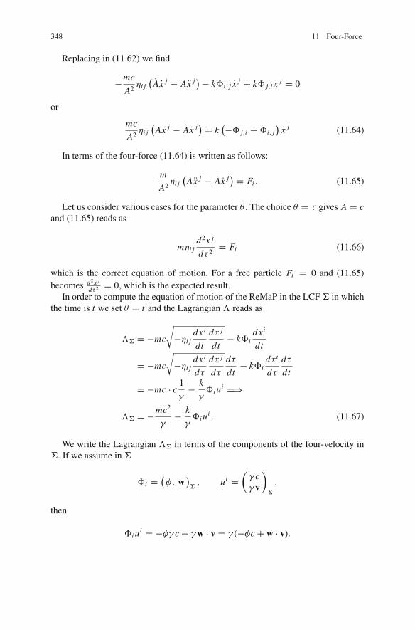
348 11 Four-Force
Replacing in (11.62) we find
−mc
A2ηi j
(Ax j − Ax j
)− kΦi, j xj + kΦ j,i x
j = 0
or
mc
A2ηi j
(Ax j − Ax j
) = k(−Φ j,i +Φi, j
)x j (11.64)
In terms of the four-force (11.64) is written as follows:
m
A2ηi j
(Ax j − Ax j
) = Fi . (11.65)
Let us consider various cases for the parameter θ . The choice θ = τ gives A = cand (11.65) reads as
mηi jd2x j
dτ 2= Fi (11.66)
which is the correct equation of motion. For a free particle Fi = 0 and (11.65)becomes d2x j
dτ 2 = 0, which is the expected result.In order to compute the equation of motion of the ReMaP in the LCF Σ in which
the time is t we set θ = t and the Lagrangian Λ reads as
ΛΣ = −mc
√−ηi j
dxi
dt
dx j
dt− kΦi
dxi
dt
= −mc
√−ηi j
dxi
dτ
dx j
dτ
dτ
dt− kΦi
dxi
dτ
dτ
dt
= −mc · c 1
γ− k
γΦi u
i =⇒
ΛΣ = −mc2
γ− k
γΦi u
i . (11.67)
We write the Lagrangian ΛΣ in terms of the components of the four-velocity inΣ. If we assume in Σ
Φi =(φ, w
)Σ, ui =
(γ cγ v
)
Σ
.
then
Φi ui = −φγ c + γw · v = γ (−φc + w · v).

11.4 The Lagrangian Formalism for Inertial Four-Forces 349
Replacing in (11.67) we find
ΛΣ = −mc2
γ− k(−φc + w · v). (11.68)
Exercise 48
(a) Let vρ = dxρ
dt be the three-velocity of a ReMaP P in a LCF Σ. Prove the identity
∂
∂vρ
1
γ= − 1
c2γ vρ (11.69)
[Hint: ∂∂vρ
v2 = 2vρ].(b) Show that the three-momentum pρ of P in Σ can be written as
pρ = ∂
∂vρ
(−mc2
γ
), (11.70)
where m = constant.[Hint: pρ = mγ vρ].
(c) Prove the relations
dpρ
dt= d
dt
(∂L0,Σ
∂vρ
)− ∂L0,Σ
∂xρ,
dp0
dt= d E
d(ct)= ∂L0,Σ
∂(ct),
where L0, Σ = −mc2
γand vρ = dxρ
dt . Finally show that
dpi
dt= d
dt
(∂L
∂ x i
)− ∂L0,Σ
∂xi,
where x i = dxi
dt . Conclude that the Lagrangian of a free particle in Σ is the
function L0, Σ = −mc2
γ.
Exercise 49
(a) Let θ be a parameter along the world line of a ReMaP P such that dθdτ > 0 where
τ is the proper time of P . Show that the Lagrangian Lθ which corresponds to theparameter θ is related to the Lagrangian Lτ which corresponds to the parameterτ , with the relation
Lτ = Lθ
dθ
dτ(11.71)
[Hint: δ∫
Lθdθ = δ∫
Lτdτ ].

350 11 Four-Force
(b) Consider θ = t where t is the time in a LCF Σ and show that
LΣ+ = γ Lt, Σ, (11.72)
where LΣ+ is the Lagrangian in the proper frame of P and Lt, Σ the Lagrangianin Σ.
(c) Let Σ, Σ′ be two LCF with parallel axes and relative velocity u. Prove that theLagrangians of an inertial conservative four-vector field in Σ, Σ′ are related asfollows:
LΣγΣ = LΣ′γΣ′ , (11.73)
where γΣ = 1√1−β2
, γΣ′ = 1√1−(β ′)2
, and β, β ′ are the speeds of P in Σ, Σ′,
respectively.
Making use of the relation γΣ′ = γuγΣ Q, where Q = 1− u·vc2 , prove that
LΣ′(q′,
dq ′
dt ′, t ′) = 1
γu QLΣ(q,
dq
dt, t). (11.74)
This relation gives the transformation law of the Lagrangian function under aLorentz transformation.
11.5 Motion in a Central Potential
As an application of the Lagrange formalism in Special Relativity we consider themotion of a ReMaP P of mass m �= 0 (not a photon!) in the LCF Σ, in whichthere exists a central potential given by the function U (r ). Recall (see Example 59)that the motion of P in another LCF which moves wrt Σ is not in general central.Therefore, whatever results we derive in this section are valid in Σ only. If onewishes to find these results in another LCF, the Σ′ say, then the results must betransformed by the Lorentz transformation relating Σ and Σ′.
According to the previous considerations the four-potential defined by the three-potential U (r ) in Σ is the timelike four-vector (U (r ), 0, 0, 0). The motion in Σ istaking place on a plane as in Newtonian Mechanics. Indeed, in Σ the three-force onP is F = − dV
dr er , therefore the angular momentum L of P wrt the origin of Σ isconstant:
dLdt= r× F = 0.
In addition L·r = 0, that is, the position vector r is always normal to the constantvector L consequently the orbit of P in Σ is on a plane.

11.5 Motion in a Central Potential 351
The Lagrangian of P equals the sum of the Lagrangian L0(τ ) = −mc2, whereτ is the proper time of P and the potential function U (r ). In order to express L0 interms of the parameter t the time in Σ, we use the relation
L0(τ )dτ = L0(t)dt
from which follows
L0(t) = − 1
γmc2. (11.75)
Consequently the Lagrangian of P in Σ is12
LΣ(r, t) = −m
γc2 −U (r ). (11.76)
We consider polar coordinates r, θ so that the speed v2 = .r
2+ r2.
θ2
and the finalform of the Lagrangian reads
LΣ(r , t) = −mc2
√
1−.r
2 + r2.
θ2
c2−U (r ). (11.77)
The angle θ is a cyclic coordinate, therefore, the generalized momentum Pθ ≡ Lz
is a constant of motion. We compute
Lz = ∂L
∂.
θ= mγ r2
.
θ . (11.78)
The Lagrange equation for the r -coordinate is
d
dt
∂L
∂.r− ∂L
∂r= 0
from which follows
d
dt(γ
.r )− γ r
.
θ2 + 1
m
dU
dr= 0. (11.79)
Because the Lagrangian is independent of time (and there are no non-holonomicconstraints) the energy is a constant of motion or, equivalently a first integral of(11.79). This implies E + U = C where C is a constant. Solving in terms of γ wefind
12 This Lagrangian follows directly from (11.67) if we change LΣ → ΛΣ.
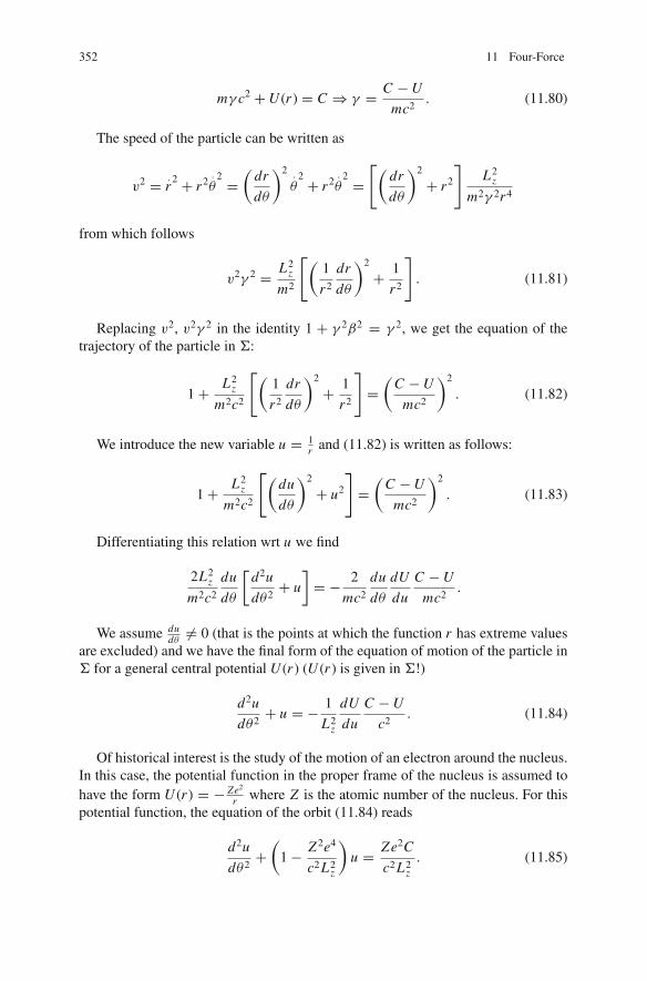
352 11 Four-Force
mγ c2 +U (r ) = C ⇒ γ = C −U
mc2. (11.80)
The speed of the particle can be written as
v2 = .r
2 + r2.
θ2 =
(dr
dθ
)2 .
θ2 + r2
.
θ2 =
[(dr
dθ
)2
+ r2
]L2
z
m2γ 2r4
from which follows
v2γ 2 = L2z
m2
[(1
r2
dr
dθ
)2
+ 1
r2
]. (11.81)
Replacing v2, v2γ 2 in the identity 1 + γ 2β2 = γ 2, we get the equation of thetrajectory of the particle in Σ:
1+ L2z
m2c2
[(1
r2
dr
dθ
)2
+ 1
r2
]=
(C −U
mc2
)2
. (11.82)
We introduce the new variable u = 1r and (11.82) is written as follows:
1+ L2z
m2c2
[(du
dθ
)2
+ u2
]=
(C −U
mc2
)2
. (11.83)
Differentiating this relation wrt u we find
2L2z
m2c2
du
dθ
[d2u
dθ2+ u
]= − 2
mc2
du
dθ
dU
du
C −U
mc2.
We assume dudθ �= 0 (that is the points at which the function r has extreme values
are excluded) and we have the final form of the equation of motion of the particle inΣ for a general central potential U (r ) (U (r ) is given in Σ!)
d2u
dθ2+ u = − 1
L2z
dU
du
C −U
c2. (11.84)
Of historical interest is the study of the motion of an electron around the nucleus.In this case, the potential function in the proper frame of the nucleus is assumed tohave the form U (r ) = − Ze2
r where Z is the atomic number of the nucleus. For thispotential function, the equation of the orbit (11.84) reads
d2u
dθ2+
(1− Z2e4
c2 L2z
)u = Ze2C
c2L2z
. (11.85)

11.5 Motion in a Central Potential 353
If we introduce the new constant λ2 = 1− Z2e4
c2 L2z
this equation is written as
d2u
dθ2+ λ2u = Ze2C
c2 L2z
. (11.86)
This equation describes a forced harmonic oscillation with proper frequency λ
and driving force Ze2Cc2 L2
z. The solution is
u = A cos λθ + B sin λθ + 1
λ2
Ze2C
c2 L2z
, (11.87)
where the constants A, B are determined from the initial conditions. We assume thatθ = 0 when the electron is at the perihelion (see Fig. 11.3) and have
(dr
dθ
)
θ=0
= u2
(du
dθ
)
θ=0
= 0⇒(
du
dθ
)
θ=0
= 0.
Then (11.87) gives B = 0 and the general solution reads
1
r= A cos λθ + 1
λ2
Ze2C
c2 L2z
. (11.88)
We infer that in the proper frame of the nucleus Σ, the orbit of the electron is an
ellipse with one focal point at the origin of Σ and eccentricity Ac2 L2z
Ze2c . The constant1A is the distance of the directrix from the focal point (see Fig. 11.3).
The Newtonian limit of the orbit occurs when c→∞ that is, λ = 1. This orbit isthe well-known circular orbit assumed by Bohr in his model of the atom. For finitevalues of c, λ �= 1 and the orbit is precessing between two enveloping circles, whichare defined by the maximum and the minimum values of r , as shown in Fig. 11.4.The precession is due to the fact that after a change of θ by 2π the factor λθ doesnot change 2π except iff λ = 1, which is the Newtonian orbit. After a completerotation the ellipsis “closes” by an angle 2π +Δθ where per complete rotation Δθ
is defined by the relation
Fig. 11.3 Specifying thecoordinates r, θ
1
directrix

354 11 Four-Force
Fig. 11.4 Precession of theorbit
Nucleus
∆ φ
λ(2π +Δθ ) = 2π =⇒ Δθ = 2π1− λ
λ.
Because 1 − λ deviates from 1 in terms of the order 1c2 its value is close to 1,
hence the deviation Δθ per rotation is very small. Kinematically this means that thethe orbit precesses along the enveloping circles with very small angular velocity.
Sommerfeld used the precession of the relativistic orbit in the old Quantum The-ory in order to determine the quantum conditions for the energy levels and the prob-ability for the transition between stable orbits of the hydrogen atom. As it is wellknown, in the old Quantum Theory for every periodicity of a stable classical orbit,there corresponds a quantum number. For example, Bohr had used the periodicityof the Newtonian orbit in order to introduce the quantum number (= quantize) ofangular momentum and, based on that, to compute the energy levels of the hydrogenatom. By using the relativistic orbit, Sommerfeld calculated in addition the fineenergy levels of the energy spectrum of the hydrogen atom.
If we assume that the angular momentum Lz is quantized in multiples of � = h2π
then we find that the minimum value of Lz = � gives the minimum value of λ,which is
λ2min = 1−
(Ze2
�c
)2
= 1− Z2α2,
where
α = e2
�c= 7, 2972× 10−3 = 1
134, 04
is a universal constant known as the fine structure constant.The constant α determines the strength of the electromagnetic interaction among
the fundamental particles by relating the quantum of the electric charge (e) with thequantum of the angular momentum � and the speed of light c. The deviation of λmin
from 1 is of the order of(
Z134
)2. For H2 (Z = 1) hence the quotient 1
134 = 5.6×10⁻⁵,

11.6 Motion of a Rocket 355
which can be observed in spectroscopy The fine lines in the spectrum of hydrogenwere observed and that was one of the most accurate tests of relativistic dynamics.
However, when the dynamics of Special Relativity is applied to the gravitationalfield fails to justify the observational results.
Let us consider the gravitational field of the sun U (r ) = −G Mr . Then all previous
relations hold if one replaces Ze2 with G Mm where m is the mass of the particlewhich moves under the action of the gravitational field. If we compute from theserelations the precession of Mercury we find that it precesses 7′′ per century, whilethe measured value (with accuracy 5′′ ) is 43′′ per century. Therefore, when dealingwith the gravitational field we should apply the dynamics of General and not ofSpecial Relativity.13
11.6 Motion of a Rocket
The motion of a rocket is a motion in which the mass changes. In the study of thismotion, the rocket is considered to be a ReMaP with proper time τ , four-velocity ui ,four-acceleration ai whose mass is changing at a rate dm/dτ , e.g., by the emissionof exhaust gases. The physical variables are the ones which can be measured by theobserver inside the rocket (the proper frame). These are
• The rate of reduction of (proper) mass dm/dτ (an invariant) and• The relative speed of emitted gases w′.
In the following, we assume one-dimensional motion so that the velocity of theexhausted gases is antiparallel to the (constant ) direction of the velocity of therocket. To determine the equation of motion of the rocket we consider the changeof the four-momentum between the proper time moments τ and τ + dτ . Supposethat the proper moment τ the mass of the rocket is m(τ ), its four-velocity is ui (τ )and that the proper moment τ + dτ these quantities are (assuming a continuousvariation) m(τ + dτ ) = m(τ )− dm and ui (τ + dτ ) = ui (τ )+ dui .
Let dm ′ the mass of the gases (we do not have conservation of mass!) and letwi their four-velocity. Conservation of four-momentum of the system between theproper time moments τ and τ + dτ gives
mui = (m − dm)(ui + dui )+ dm ′wi ⇒ mdui − dmui + dmwi = 0, (11.89)
where we have ignored the term dmdui .This equation is covariant, that is, it is valid in all LCF. We write it in the LCF
Σ+ of the IRIO of the rocket and compute it in any other LCF using the appropriateLorentz transformation. The ui ui = −c2 ⇒ ui dui = 0, that is, dui is a spacelikefour-vector.
13 For a different view of this topic see T. E. Philips Jr., “Mercury precession according to SpecialRelativity” Am. J. Phys. 54, 245–247, (1986).
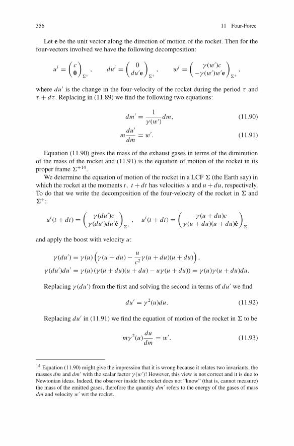
356 11 Four-Force
Let e be the unit vector along the direction of motion of the rocket. Then for thefour-vectors involved we have the following decomposition:
ui =(
c0
)
Σ+, dui =
(0
du′e
)
Σ+, wi =
(γ (w′)c
−γ (w′)w′e
)
Σ+,
where du′ is the change in the four-velocity of the rocket during the period τ andτ + dτ . Replacing in (11.89) we find the following two equations:
dm ′ = 1
γ (w′)dm, (11.90)
mdu′
dm= w′. (11.91)
Equation (11.90) gives the mass of the exhaust gases in terms of the diminutionof the mass of the rocket and (11.91) is the equation of motion of the rocket in itsproper frame Σ+14.
We determine the equation of motion of the rocket in a LCF Σ (the Earth say) inwhich the rocket at the moments t, t + dt has velocities u and u+ du, respectively.To do that we write the decomposition of the four-velocity of the rocket in Σ andΣ+:
ui (t + dt) =(
γ (du′)cγ (du′)du′e
)
Σ+, ui (t + dt) =
(γ (u + du)c
γ (u + du)(u + du)e
)
Σ
and apply the boost with velocity u:
γ (du′) = γ (u)(γ (u + du)− u
c2γ (u + du)(u + du)
),
γ (du′)du′ = γ (u) (γ (u + du)(u + du)− uγ (u + du)) = γ (u)γ (u + du)du.
Replacing γ (du′) from the first and solving the second in terms of du′ we find
du′ = γ 2(u)du. (11.92)
Replacing du′ in (11.91) we find the equation of motion of the rocket in Σ to be
mγ 2(u)du
dm= w′. (11.93)
14 Equation (11.90) might give the impression that it is wrong because it relates two invariants, themasses dm and dm ′ with the scalar factor γ (w′)! However, this view is not correct and it is due toNewtonian ideas. Indeed, the observer inside the rocket does not “know” (that is, cannot measure)the mass of the emitted gases, therefore the quantity dm ′ refers to the energy of the gases of massdm and velocity w′ wrt the rocket.

11.6 Motion of a Rocket 357
Equation (11.93) makes possible for the observer in the rocket, to be able todetermine his motion in Σ by looking at the indication (a) of the instrument whichmeasures dm/dt , that is, the rate of consumption of fuel and (b) a second instru-ment which measures the relative velocity of the exhausted gases w′ wrt the rocket.Indeed, if these two quantities are known then by integrating (11.93) the traveleris able to compute the speed and the position of the rocket in Σ. If we consideran approximation of the order O(β2) then (11.93) reduces to the correspondingequation of Newtonian Physics, as it is expected.
In order to solve the equation of motion (11.93) we have to make certain assump-tions, which have a sound physical basis. We assume w′ = constant, which meansthat the engines of the rocket work steadily. Furthermore we consider the initialconditions m(0) = M, u(0) = u0. Then (11.93) gives
∫ u
u0
du
1− u2
c2
=∫ m
Mw′
dm
m
from which follows
c
2
[ln
(1+ u
c
1− uc
)− ln
(1+ u0
c
1− u0c
)]= − ln
( m
M
)w′
.
Solving for u(t) we find
u(t) = A − (mM
)B
A + (mM
)B c, (11.94)
where A = 1+ u0c
1− u0c
and B = 2w′c . For initial speeds u0 � c the term u0/c can be
ignored (A = 1) and the solution (11.94) is written as
u(t) = 1− (mM
)B
1+ (mM
)B c. (11.95)
We note that always u < c and u → c only when the quotient m/M → 0.Furthermore, the rate of change of the mass dm/dt does not enter the calculations.For u0/c � 1 (and also for m/M = 1) we recover again the well-known Newtonianresult. In general, the Newtonian behavior appears when the parameter
(mM
)B � 1.This happens at two phases of the motion:
• At the beginning of the motion, when m/M = 1 (and small velocities)• When 2w′/c � 1 approximately for all the duration of motion.
Practically, we have Newtonian behavior for w′/c = 0.1. In Fig. 11.5 we displaythe quotient u/c as a function of the ratio m/M and for the values A = 1 andB = 0.1 (Newtonian limit) and B = 0.4 (relativistic limit).

358 11 Four-Force
Fig. 11.5 Newtonian(B = 0.1) and relativistic(B = 0.4) motion of therocket
0 4
0 6
0 8
1 0
Newtonian limit
Relativistic limit
0 0 0 4 0 6 0 8 1 00 2
0 2
[Question: What one can say for photonic fuel, that is fuel for which the exhaustedgases are photons? What is the mass dm ′ in that case?].
Example 60 A spacecraft departs from the Earth and moves along a constant direc-tion toward the center of galaxy, which is a distance of 30,000 ly as measured fromthe Earth. The engines of the spacecraft work steadily and create a constant properacceleration g for the first half of the trip and a constant retardation g for the returntrip.
(1) How long will the trip last according to the proper clock of the spacecraft?(2) What distance has the spacecraft covered as estimated by the crew in the space-
craft?(3) What fraction of the initial mass of the spacecraft will be used if we assume that
the engines of the spacecraft transform the mass of the spacecraft into photons(photonic fuel) with an efficiency of 100% and the radiation is emitted in theopposite direction to the direction of the velocity of the spacecraft? Assumec = 1.
Solution
(1) Assume that the x ′-axis joins the Earth with the center of galaxy (this is possiblebecause the three-dimensional space in Special Relativity is flat, i.e., has zerocurvature). Then y = z = 0 during all the duration of the trip. For the four-velocity and the four-acceleration of the rocket in the frame Σ of the Earth wehave the decomposition
ui =(
u0
u1
)
Σ
, ai =(
a0
a1
)
Σ
.
The orthogonality relation is
ui ai = 0⇒ −a0u0 + a1u1 = 0⇒ a0 = λu1, a1 = λu0,
where λ �= 0 is a constant. It is given that ai ai = g2. Because the length of afour-vector is invariant we compute it in Σ and find
−(a0)2 + (a1)2 = g2 ⇒ λ = ±g,

11.6 Motion of a Rocket 359
where λ = +g is for the first part of the trip and λ = −g for the return trip backto Earth. Finally, for the departure trip we have the equations of motion
du0
dτ= gu1,
du1
dτ= gu0.
Differentiating the first wrt τ and replacing du1
dτ from the second we find
d2u0
dτ 2= g
du1
dτ= g2u0 ⇒ d2u0
dτ 2− g2u0 = 0.
The solution of this equation is
u0 = A sinh gτ + B cosh gτ,
where A, B are constants. In a similar manner we compute
u1 = A′ sinh gτ + B ′ cosh gτ.
The initial conditions are
τ = t = 0, u1(0) = 0,du1
dt(0) = g, u0(0) = 1
from which follows
u1(τ ) = sinh gτ, u0(τ ) = cosh gτ. (11.96)
Concerning the position we have from (11.96)
dt
dτ= u0(τ ) = cosh gτ,
dx
dτ= dx
dt
dt
dτ= 1
γu1(τ )γ = sinh gτ.
Assuming the initial conditions τ = t = x = 0 we end up with
t(τ ) = 1
gsinh gτ, x(τ ) = 1
g(cosh gτ − 1)
which is (as it should be expected!) the expression of hyperbolic motion (seeExample 27).
In order to get an idea of the result let us make some calculations. To dothat we have to express g in units of distance and time. We note that 1 ly =

360 11 Four-Force
lightyear ≈ 9.5×10¹⁵ m and 1 year ≈ 3.15×10¹⁷ s. Moreover we have assumedc = 1⇒ 1 s = 3× 10⁸ m. Using these, we compute in units of distance
g = 10 m/s2 = 10× 1
(3× 10⁸)2m−1
= 10× 1
(3× 10⁸)2× (9.5× 1015) ly−1 ≈ 1 (ly)−1.
Similarly in units of time we have
g = 10 m/s2 = 10× 1
3× 10⁸s−1 = 10
1
3× 108×(3×107)(years)−1 ≈ 1 (years)−1.
Using these units we find that for the first part of the trip, that is, x = 15, 000 ly,the time
τ = 1
gcosh−1(gx + 1)⇒ τ = [(1 year)−1]−1 cosh−1[(ly)−1(15000 ly)+ 1]
= cosh−1(15001) years = 10.31 years.
Obviously for the whole trip it is required twice this time period, that is
τtotal = 2 τ = 20.62 years.
The time period between the events of departure and arrival of the spacecraftfor the observer on Earth is
t = 1
gsinh gτ = sinh 20.62 = 4.5× 10⁸ years.
Observe the difference between t and τ and appreciate the well-known twinparadox.
(2) In order to compute the distance covered by the spacecraft from the Earth, asestimated by the crew at the spacecraft, we consider coordinates (cT, X ) in theproper frame of the spacecraft and apply the boost with velocity u1/γ where u1
is the x-component of the four-velocity. We find
X = γ
(x − u1
γt
), (11.97)
T = γ
(t − u1
γx
). (11.98)
But
γ = u0 = cosh gτ.

11.6 Motion of a Rocket 361
therefore (11.97) and (11.98) give
X = 1
g(1− cosh gτ ) = −x .
This result is important because it proves that the distance of the spacecraft fromthe Earth is the same as estimated either by the observer at the Earth or by thecrew in the spacecraft.
(3) Let M0 be the initial mass of the spacecraft and M(τ ) the mass after proper timeτ . Then the energy E(τ ) = M(τ )γ (τ ) = M(τ )u0 and the three-momentumP(τ ) = M(τ )γ (τ )u = M(τ )u1. The proper moment τ + dτ the change of theenergy and the momentum of the spacecraft, d E and d P , respectively, equal thecorresponding quantities d Ephotons and d Pphotons of the emitted photons, respec-tively. But for photons we have that d Ephotons = d Pphotons hence we have thefollowing equation of motion:
−d P = d E ⇒ d(E + P) = 0⇒ E + P = constant.
From the initial conditions E(0) = M0, P(0) = 0 we compute that the value ofthe constant is M0, therefore we have finally
M(τ )u0 + M(τ )u1 = M0 ⇒ M(τ ) = M0
u0 + u1.
We replace u0, u1 from (11.96) and get
M(τ ) = M0e−gτ .
For proper time τtotal = 20.62 years we find that the percentage of the masswhich has been used equals
ΔM =(
1− M(τ )
M0
)× 100 ≈ (1− e−20.26) = 99.999%.
Example 61 A particle of mass m and velocity u moves along the x-axis of the LCFΣ.
(1) Show that the three-momentum and the energy of the particle are given by therelations P = mc sinhχ, E = mc2 coshχ where χ is the rapidity of theparticle in Σ. Deduce that the speed and the rapidity of the particle in Σ arerelated as follows u(t) = c tanhχ .
(2) Consider a second LCF Σ′ which moves wrt Σ in the standard configurationalong the x-axis with speed v. Show that in Σ′ the three-momentum P ′, E ′,and the energy E ′ of the particle are given by the following formulae:
P ′ = mc sinh(χ + ψ), E ′ = mc2 cosh(χ + ψ),

362 11 Four-Force
where tanhψ = v/c. Explain the geometric meaning of this result. Assume thatthe speed u changes to u + du. Prove that
duγ 2(u) = cdχ.
If du′ is the corresponding change of the velocity in Σ′ show that
du′2/(u′2(u) = cdχ.
(3) Application.A rocket moves freely by exhausting gases with a constant rate μ = d M/dτand velocity −w′e, where e is the (constant) direction of motion of the rocket.If the rocket starts from a space platform A with initial mass M0 and movesalong the x-axis calculate the velocity u(t) of the rocket wrt the platform whenits mass is M(τ ).
Solution(2) The speed u and the rapidity χ of a particle in a LCF Σ are related as followsu = c tanhχ . Differentiating we find
du = 1
cosh2 χcdχ = 1
γ 2(u)cdχ ⇒ γ 2(u)du = cdχ. (11.99)
From the relativistic rule of composing velocities we have that the rapidity χ ′ ofthe particle in Σ′ is
χ ′ = χ + ψ,
where ψ is the rapidity of Σ′ wrt Σ (v = c tanhψ). If v′ is the velocity of the particlein Σ′, then applying relation (11.99) for the velocity u′ we find
du′ = 1
cosh2 χ ′cdχ ′ = γ 2(u′)du′ = cdχ = γ 2(u)du (11.100)
because dψ = 0. From (11.99) and (11.100) we infer
γ 2(u′)du′ = γ 2(u)du.
which means that the quantity γ 2(u)du is an invariant (but depends on the time t inΣ).Application
The equation of motion of the rocket in Σ is (see (11.93)):
mγ 2(u)du
dm= w′,

11.7 The Frenet–Serret Frame in Minkowski Space 363
where w′ is the speed of the exhausted gases wrt the rocket. In order to write thisequation in terms of the rapidity χ we use (11.99) and find
cdχ = w′dm
m.
The solution of this equation is
χ − χ0 = ln
(M
M0
) w′c
.
From the initial conditions we have χ0 = tanh−1 0 = 0, hence
χ = ln
(M0
M
)w′/c
. (11.101)
From the relation which gives the rapidity we find eχ =√
c+uc−u . Replacing in
(11.101)
u(t) = 1− (M/M0)2β ′
1+ (M/M0)2β ′ c,
where β ′ = w′c .
11.7 The Frenet–Serret Frame in Minkowski Space
In classical vector calculus the Frenet–Serret equations define at each point alonga smooth curve an orthonormal basis – or a “moving frame” – which is called theFrenet–Serret frame. The usefulness of the Frenet–Serret frame is that it charac-terizes and is characterized uniquely by the curve. In this section, we define theFrenet–Serret frame along a curve in Minkowski space and demonstrate its applica-tion in the definition of a generic four-force vector. It is apparent that in Minkowskispace the equations defining the Frenet–Serret frame along a given curve must befour and the orthonormal tetrad defining the frame will involve Lorentz orthogonalvectors.
The first difference between the Euclidean and the Lorentzian Frenet–Serretframe is that in the first case one has one type of curves whereas the second onehas three types of curves, the timelike, the spacelike, and the null.15 Furthermore,the null curves are degenerate in the sense that their tangent vector is also normal to
15 Besides these curves there are infinite other curves in Minkowski space which, however, do notinterest us in relativity.

364 11 Four-Force
the curve. Therefore, the Frenet–Serret frame applies only to non-null (i.e., timelikeand spacelike) curves.
Let ci (r ) be a smooth non-null curve in Minkowski space and let r be an affineparameter16 so that the tangent vector to the curve is Ai = dci/dr :
Ai Ai = ε(A), (11.102)
ε(A) being the sign of Ai , that is, ε(A) = +1/ − 1 if Ai is spacelike/timelike,respectively.
In the following, we shall denote the covariant differentiation along Ai with adot, e.g.,
T i1...irj1... js= T i1...ir
j1... js ,kAk . (11.103)
Because Ai is unit Ai Ai = 0.Let Bi be the unit vector along Ai so that
Ai = bBi (b > 0). (11.104)
Then
Bi Ai = 0, Bi Bi = ε(B). (11.105)
We consider the derivative Bi and decompose it parallel and normal to the planedefined by Ai , Bi . We write
Bi = a Ai + cCi , (11.106)
where a, c are coefficients and Ci is a unit vector normal to both Ai and Bi and sothat the quantity ηi jk Ai B j Ck > 0 (this defines the positive orientation of the frame).Then we have
Ci Ci = ε(C) (11.107)
and
Ai Ci = Bi Ci = 0. (11.108)
In order to compute the coefficients a, c we differentiate (11.105) and use(11.104) to get
16 Recall that a parameter along a non-null parameterized curve is called affine if the tangent vectoralong the curve (for this parametrization) has unit length, i.e., ±1. If r is an affine parameter thenar + b where a, bεR is also an affine parameter.

11.7 The Frenet–Serret Frame in Minkowski Space 365
Bi Ai = −Bi Ai = −bε(B).
But from (11.106) we have
Bi Ai = aε(A)⇒ a = −ε(A)ε(B)b. (11.109)
Replacing in (11.106) we obtain finally
Bi = −ε(A)ε(B)bAi + cCi . (11.110)
We apply the same procedure to the unit vector C i and write
C i = βAi + γ Bi + d Di , (11.111)
where Di is the unit normal to the trihedral defined by the four-vectors Ai , Bi , Ci ,i.e.,
Di Di = ε(D) (11.112)
and
Ai Di = Bi Di = Ci Di = 0. (11.113)
In order to compute the coefficients β, γ we contract (11.111) with Ai , Bi anduse (11.108) to find
βε(A) = C i Ai = −Ci Ai = −Ci bBi = 0
and
γ ε(B) = C i Bi = −Ci Bi = −ε(C)c.
Hence
β = 0, γ = −ε(B)ε(C)c
and (11.111) is written as follows:
C i = −ε(B)ε(C)cBi + d Di . (11.114)
We decompose similarly Di = δAi + εBi + nCi and making use of (11.113) wefind δ = ε = 0 and n = −dε(C)ε(D), so that17
17 The four-vector Di is determined uniquely from the “outer product” of the three four-vectorsAi , Bi ,Ci , i.e., Di = ηi
jkl A j BkCl where ηijkl =
√−gεijkl and εi jkl is the Levi-Civita symbol

366 11 Four-Force
Di = −ε(C)ε(D)dCi . (11.115)
From the above analysis we reach at the following conclusion:
Proposition 7 At every point along a smooth non-null curve in Minkowski space,affinely parameterized with the parameter r = arc length it is possible to constructan orthonormal tetrad Ai , Bi ,Ci , Di such that the four-vector Ai is tangent to thecurve and the rest three spacelike mutually perpendicular four-vectors Bi ,Ci , Di
to follow from the solution of the system of differential equations
Ai = bBi , (11.116)
Bi = −ε(A)ε(B)bAi + cCi , (11.117)
C i = −ε(B)ε(C)cBi + d Di , (11.118)
Di = −ε(C)ε(D)dCi , (11.119)
where a dot over a symbol indicates differentiation wrt r .
The four-vectors Bi , Ci , Di we call the first, second, and third normal, respec-tively, of the curve ci and the parameters b, c, d the first, second and third curvatureof ci . The geometric significance of the Frenet–Serret curvatures is that they defineuniquely the curve ci (for given initial conditions).18 If we denote the curvaturesb, c, d of the curve by κ1, κ2, κ3, respectively, the Serret–Frenet relations are writ-ten in the following matrix notation:
⎛
⎜⎜⎝
Ai
Bi
C i
Di
⎞
⎟⎟⎠ = S
⎛
⎜⎜⎝
Ai
Bi
Ci
Di
⎞
⎟⎟⎠ , (11.120)
where the 4× 4 matrix
S =
⎛
⎜⎜⎝
0 κ1 0 0−ε(A)ε(B)κ1 0 κ2 0
0 −ε(B)ε(C)κ2 0 κ3
0 0 −ε(C)ε(D)κ3 0
⎞
⎟⎟⎠ . (11.121)
(εi jkl = +1 if i jkl is an even permutation of 0123 and εi jkl = −1 otherwise). This implies thatthe parameter d is possible to be expressed in terms of the parameters a, b, c and their deriva-tives. Therefore, in Minkowski space we have three four-vectors and three parameters associateduniquely with a given smooth curve and the associated Frenet–Serret frame. The orientation of thisframe is positive or negative according the sign of the determinant of the 4 × 4 matrix defined bythe four-vectors Ai , Bi , Ci , Di or equivalently from the sign of the quantity η jkls A j BkCl Ds .18 We note that the same relations hold in the case of General Relativity with the differencethat the partial derivative is replaced with the covariant Riemannian derivative. Moreover if weset ε(A) = 1, Di = 0 we recover the Frenet–Serret formulae of the Euclidean three-dimensionalgeometry.

11.7 The Frenet–Serret Frame in Minkowski Space 367
In case the curve ci is timelike ε(A) = −1, ε(B) = ε(C) = ε(D) = +1 and(11.116), (11.117), (11.118) and (11.119) become
Ai = κ1 Bi , (11.122)
Bi = κ1 Ai + κ2Ci , (11.123)
C i = −κ2 Bi + κ3 Di , (11.124)
Di = −κ3Ci . (11.125)
Consequently the matrix S:
S =
⎛
⎜⎜⎝
0 κ1 0 0κ1 0 κ2 00 −κ2 0 κ3
0 0 −κ3 0
⎞
⎟⎟⎠ . (11.126)
In case ci is a spacelike curve then ε(A) = 1, ε(B) = −1 (say) ε(C) = ε(D) = 1and relations (11.116), (11.117), (11.118) and (11.119) are
Ai = κ1 Bi , (11.127)
Bi = κ1 Ai + κ2Ci , (11.128)
C i = κ2 Bi + κ3 Di , (11.129)
Di = −κ3Ci (11.130)
Exercise 50 Prove that the Frenet–Serret coefficients can be written in covariantform as follows:
κ1 = Ai Bi κ2 = Bi Ci κ3 = C i Di . (11.131)
Deduce that the curvatures b, c, d are invariants – being inner products of four-vectors – and characterize a curve in an intrinsic manner (that is, independent of thechoice of coordinate system). As we have already remarked, it is this result whichmakes the Frenet–Serret formalism a useful geometric tool in the study of worldlines.
Exercise 51 The straight line in Minkowski space is defined by the conditionAi =constant. Use the Frenet–Serret equations (11.116), (11.117), (11.118) and(11.119) to show that for a straight line the curvatures κ1 = κ2 = κ3 = 0. Converselyusing the values κ1 = κ2 = κ3 = 0 in the same equations prove that the curve theydescribe is a straight line. This result makes possible the definition of the straightline in a algebraic and covariant manner.
In order to show how one computes the Frenet–Serret basis along a world line(i.e., a timelike curve) we consider a ReMaP P , which starts to move from the origin

368 11 Four-Force
of an LCF Σ along the x-axis with constant proper acceleration a > 0 (hyperbolicmotion). As we have shown (see equation (7.47)) the world line of P is (c = 1)
x = 1
a(cosh(aτ )− 1) y = 0, z = 0,
where τ is the proper time of P (related to the time t of Σ with the relationt = 1
a (sinh(aτ )). The four-vector Ai is the four-velocity ui with componentsui = (u0, u1, 0, 0)t
Σ where u0 = cosh(aτ ), u1 = sinh(aτ ). The four-vectorAi is the four-acceleration of P , which in Σ is given by ai = (a0, a1, 0, 0)t
Σ
where a0 = a sinh(aτ ) = au1, a1 = a cosh(aτ ) = au0. The length of the four-acceleration is a, hence the unit vector along the direction of ai , which is also thefirst normal to the curve, is Bi = (u1, u0, 0, 0)Σ. In order to compute the secondnormal to the curve we differentiate Bi and find
Bi = (u1, u0, 0, 0)t = (au0, au1, 0, 0)t = aui .
From (11.123) follows κ2 = 0. For this value of κ2 (11.124) and (11.125) areindependent of the remaining two and are satisfied by infinitely many pairs offour-vectors Ci , Di . This is due to the fact the the motion takes place in the planex − ct , which can be embedded in infinitely many ways into the four-dimensionalMinkowski space.
11.7.1 The Physical Basis
The Frenet–Serret frame has a special physical significance in the case of timelikecurves. Indeed in this case the vector Ai is the four-velocity of the ReMaP P , thefirst normal is the direction of the four-acceleration while the first curvature κ1 isthe measure of the four-acceleration. Therefore, the Frenet–Serret frame covers thebasic physical quantities of kinematics. There still remains a part which containshigher than the first derivatives of the four-velocity. This extra part must be related tothe dynamics of motion, that is, the external four-force which modulates the motionof P .
It is speculated that the four-force depends on the higher derivatives of the four-velocity when a charge accelerates. Indeed, it is assumed that an accelerating chargeradiates an electromagnetic field which exerts a force back on the charge. This forceis not a Lorentz force. Up to now, many formulae for this type of force have beenproposed but it appears that “the force” has not yet been found. Although we donot know the actual expression of this type of force, nonetheless it is possible bythe use of the Frenet–Serret frame, to give the generic expression for this four-force in terms of the “physical” kinematic quantities ua, ua, ua,
...u
a. That is, we
give a parameterized geometric expression which contains all possible four-forcesone could conceive. The role of physics is to select the appropriate values of theparameters!

11.7 The Frenet–Serret Frame in Minkowski Space 369
In the following, we assume that the generic four-force is a pure four-force, thatis a spacelike four-vector normal to the four-velocity. Summarizing we have to solvethe following problem:
Compute the generic form of a spacelike four-vector along a smooth non-null curve – whichis not a straight line – in a basis which consists of the unit tangent to the curve and its higherderivatives, assuming that they do not vanish. We call this new (not in general orthonormal)basis the physical basis along the curve.
This means that we are looking – if it exists! – for an expression of the form
r i = f 0i (xi , ui , ui , ...)ui + f 1
i (xi , ui , ui , ...)ui + · · · , (11.132)
where r i is an arbitrary four-vector (null or non-null) defined along the curve.Let ci be a non-null, smooth, affinely parameterized curve in Minkowski space
with unit tangent vector Ai . From the Frenet–Serret relations we have
Ai , Ai = bBi , (11.133)
where
Ai Ai = ε(A), Bi Ai = 0, Bi Bi = ε(B).
Differentiating twice Ai along the curve we find19
Ai = −ε(A)ε(B)b2 Ai + bBi + bcCi . (11.134)...
Ai = [−3ε(A)ε(B)bb]Ai + [b − ε(A)ε(B)b3 − ε(B)ε(C)bc2]Bi
+[2cb + bc]Ci + bcd Di . (11.135)
We conclude that in general the tangent and the Frenet–Serret bases are relatedas follows:
⎡
⎢⎢⎢⎢⎣
Ai.
Ai..
Ai...
Ai
⎤
⎥⎥⎥⎥⎦= R
⎡
⎢⎢⎣
Ai
Bi
Ci
Di
⎤
⎥⎥⎦ , (11.136)
where the 4× 4 matrix
19 The three four-vectors Ai , Ai , Ai are sufficient (provided they are independent) in order to com-pute the fourth by the formula T i = ηi
jkl A j Ak Al . This means that, in general, the physical basisrequires only up to the second derivative of the vector Ai along the curve.

370 11 Four-Force
R =
⎡
⎢⎢⎣
1 0 0 00 b 0 0
−ε(A)ε(B)b2.
b bc 0−3ε(A)ε(B)bb b − ε(A)ε(B)b3 − ε(B)ε(C)bc2 bc + 2cb bcd
⎤
⎥⎥⎦ .
The matrix R defines a change of bases (not necessarily change of coordinates20)if its determinant does not vanish. We compute
det (R) = b3c2d (11.137)
from which we infer that R defines a change of basis provided bcd �= 0. Kinemat-ically this means that the physical basis is possible only for non-planar acceleratedmotions (see Exercise 51). In case one of the curvatures b, c, d vanishes we canconsider higher derivatives of Ai until we obtain a basis along the curve.
In the following we assume bcd �= 0 and express the four-vectors of the Frenet–Serret tetrahedron in terms of the four-vectors of the physical basis using the matrixR. We have
⎡
⎢⎢⎣
Ai
Bi
Ci
Di
⎤
⎥⎥⎦ = R−1
⎡
⎢⎢⎢⎢⎣
Ai.
Ai..
Ai...
Ai
⎤
⎥⎥⎥⎥⎦. (11.138)
We compute
R−1 =
⎡
⎢⎢⎣
1 0 0 00 1
b 0 0ε(A)ε(B)b
c − bb2c
1bc 0
Λ M N Ξ
⎤
⎥⎥⎦ , (11.139)
where
Λ = (R−1)41 = −ε(A)ε(B)(cb − bc)
c2d, (11.140)
M= (R−1)42 = ε(A)ε(B)cb4 + ε(B)ε(C)c3b2 − b(bc − bc)+ 2cb2
c2b3d, (11.141)
20 A basis in a linear space does not necessarily follow from a system of coordinate functions, thatis, the basis vectors cannot be written as tangent vectors to a system of coordinate lines. A criterionthat a set of vectors is generated by a coordinate system is that the vectors commute. If this is thecase, we call the basis holonomic, otherwise unholonomic.

11.7 The Frenet–Serret Frame in Minkowski Space 371
N = (R−1)43 = −cb − 2bc
b2c2d, (11.142)
Ξ = (R−1)44 = 1
bcd. (11.143)
Exercise 52 Verify that the matrix R−1 is the inverse of the matrix R. Then showthat
Ai = ui ,
Bi = 1
bui ,
Ci = ε(A)ε(B)b
cui − b
b2cui + 1
bcui ,
Di = Λui + Mui + Nui +Ξ...u
i.
Consider now an arbitrary four-vector which in the Frenet–Serret basis has thefollowing analysis:
r i = a Ai + βBi + γCi + δDi . (11.144)
Replacing Ai , Bi , Ci , Di in terms of the vectors of the physical basis we find
r i =[α + γ
ε(A)ε(B)b
c− δ
ε(A)ε(B)(cb − bc)
c2d
]Ai+
+[β
1
b− γ
b
b2c+ δ
ε(A)ε(B)cb4 + ε(B)ε(C)c3b2 − b(bc − bc)+ 2cb2
c3b2d
]Ai+
+[γ
1
bc− δ
cb + 2bc
b2c2d
]Ai + δ
1
bcd
...
Ai . (11.145)
Equation (11.145) is the answer to our problem, that is, gives the generic formof an arbitrary four-vector in terms of the tangent vector to the curve and its deriva-tives. If we denote the curvatures b, c, d as κ1, κ2, κ3 then expression (11.145) reads
r i =[α + γ
ε(A)ε(B)κ1
κ2− δ
ε(A)ε(B)(κ2κ1 − κ1κ2)
κ22κ3
]Ai+
+[β
1
κ1− γ
κ1
κ21κ2+ δ
ε(A)ε(B)κ2κ14 + ε(B)ε(C)κ3
2κ21 + κ1(κ2κ1 − κ1κ2)+ 2κ2κ
21
κ32κ
21κ3
].
Ai+
+[γ
1
κ1κ2− δ
κ2κ1 + 2κ1κ2
κ12κ2
2κ3
]..
Ai + δ
1
κ1κ2κ3
...
Ai (11.146)

372 11 Four-Force
11.7.2 The Generic Inertial Four-Force
We are now ready to compute the generic expression of a pure four-force whichmodulates the motion of a ReMaP P . Let ci be the world line of P which we assumeto be such that κ1κ2κ3 �= 0 and let ui be the four-velocity of P . The physical framealong ci consists of the four-vectors
Ai = ui , Ai = ui , Ai = ui ,...
Ai = ...
ui.
A pure four-force Fi on P is defined by the condition Fi ui = 0. The generalexpression (11.146) reads for ε(A) = −1, ε(B) = ε(C) = +1
r i =[α − γ
κ1
κ2+ δ
κ2κ1 − κ1κ2
κ22κ3
]ui
+[β
1
κ1− γ
κ1
κ21κ2+ δ−κ2κ1
4 + κ32κ
21 + κ1(κ2κ1 − κ1κ2)+ 2κ2κ
21
κ32κ
21κ3
]ui
+[γ
1
κ1κ2− δ
κ2κ1 + 2κ1κ2
κ12κ2
2κ3
]ui
+ δ1
κ1κ2κ3
...u
i. (11.147)
Condition r i ui = 0 implies α = 0 (due to (11.144)), therefore, the genericexpression of a pure (or inertial) four-force acting on P (and in general of a spacelikevector normal to the four-velocity ui !) is
Fi =[−γ κ1
κ2+ δ
κ2κ1 − κ1κ2
κ22κ3
]ui
+[β
1
κ1− γ
κ1
κ21κ2+ δ−κ2κ1
4 + κ32κ
21 + κ1(κ2κ1 − κ1κ2)+ 2κ2κ
21
κ32κ
21κ3
]ui
+[γ
1
κ1κ2− δ
κ2κ1 + 2κ1κ2
κ12κ2
2κ3
]ui + δ
1
κ1κ2κ3
...u
i. (11.148)
Note that this expression contains ui although Fi ui = 0! This is due to the factthat the basis {ui , ui , ui ,
...u
i } is not orthonormal. For example
ui ui = (ui ui ). − ui ui = −u2 = −b2 �= 0. (11.149)
Exercise 53 Prove the relations
ui ui = −κ12, (11.150)
ui ui = κ1κ1, (11.151)

11.7 The Frenet–Serret Frame in Minkowski Space 373
...u
iui = −3κ1κ1. (11.152)
[Hint: Use (11.136) to write ui = b2 Ai + bBi + bcCi ]
During the many years of Special Relativity there have been proposed many typesof pure four-forces. Each of these satisfies a physical “need” and follows from somephysical considerations or inspirations. All the proposed four-forces must followfrom the generic expression (11.148) for an appropriate set of values of the parame-ters β, γ , δ, otherwise they are exempted mathematically. In the following, we shallexamine a few types of pure four-forces proposed over the years and will decide ontheir geometric acceptance.
11.7.2.1 Newtonian Type Four-Force
This force has the general expression Fi = mui and is the generalization of New-ton’s Second Law in Special Relativity. To prove that this type of force is acceptable,we have to prove that it follows from the generic expression (11.148) for a specialset of values of the parameters β, γ , δ. For this, we examine if the following systemof equations has a unique solution:
−γ κ1
κ2+ δ
κ2κ1 + 2κ1κ2
κ22κ3
= 0,
β1
κ1− γ
κ1
κ21κ2+ δ−κ2κ1
4 + κ32κ
21 + κ1(κ2κ1 − κ1κ2)+ 2κ2κ
21
κ32κ
21κ3
= m,
γ1
κ1κ2− δ
κ2κ1 + 2κ1κ2
κ12κ2
2κ3= 0,
δ = 0.
The solution of the system is γ = δ = 0, β = κ1m where κ1 is the first curvature(= the measure of the four-acceleration) of the world line. We conclude that theproposed Newtonian four-force is geometrically acceptable. This does not mean ofcourse that it is also physically acceptable. Only experiment can establish this.
11.7.2.2 The Lorentz–Dirac Four-Force
Dirac suggested that the four-force on a particle of mass m and charge q, whichaccelerates under the action of a three-force is given by the following formula(Lorentz–Dirac force):
Fi = mui − 2
3q2[ui − (ui ui )u
i ]. (11.153)

374 11 Four-Force
The second term is assumed to describe the self interaction of the charge with itsown radiation field.
We examine if this type of force is geometrically acceptable. For that we checkif it is normal to the four-velocity. We find
Fi ui = −2
3q2[ui ui − (u j u j )(u
i ui )] = −2
3q2(−ui ui + ui ui ) = 0
therefore, Fi is a pure four-force. We continue with the computation of the param-eters β, γ , δ. We note that ui ui = k2
1, hence (11.153) can be written as
Fi = mui + 2
3q2κ1
2ui − 2
3q2ui . (11.154)
Comparing (11.154) with the generic expression (11.148) we find the followingalgebraic system of four-equations in the three unknowns β, γ , δ
−γ κ1
κ2+ δ
κ2κ1 + 2κ1κ2
κ22 d
= 2
3κ2
1 q2,
β1
κ1− γ
κ1
κ21 c+ δ−κ2κ
41 + κ3
2κ21 + κ1(κ2κ1 − κ1κ2)+ 2κ2κ
21
κ21 c3d
= m,
γ1
κ1κ2− δ
κ2κ1 + 2κ1κ2
κ21κ
22 d
= −2
3q2,
δ = 0.
The solution of this system is
β = mκ1 − 2
3κ1q2,
γ = −2
3κ1κ2q2,
δ = 0. (11.155)
We conclude that the Lorentz–Dirac four-force is geometrically acceptable and,furthermore in the Frenet–Serret basis can be written as
Fi =(
m −−2
3q2 κ1
κ1
)κ1 Bi − 2
3κ1κ2q2Ci . (11.156)
Note that the case Fi = 0 is impossible, because
κ1κ2 �= 0.

11.7 The Frenet–Serret Frame in Minkowski Space 375
11.7.2.3 Bonnor Four-Force
Bonnor21 assumed that the four-force on an accelerating charged particle depends(i) on the ui , ui and (ii) the amount of radiated energy is measured by the change mof the mass of the particle. Then he gave the expression
Fi = mui +[
m − 2
3q2(ui ui )
]ui . (11.157)
As we have seen ui ui = κ12 hence this can be written as
Fi = mui +(
m − 2
3κ2
1 q2
)ui . (11.158)
We demand the condition Fi ui = 0 (pure four-force) and find from (11.158)
Fi ui = −(
m − 2
3κ1
2q2
)= 0⇔ m = 2
3κ1
2q2. (11.159)
Replacing this back in (11.157) follows Fi = mui , that is, the Newtonian typeof force but with varying mass. We do not expect that the Newtonian type of forcewill be possible to describe the self force on the charge, therefore, it appears that theBonnor four-force does not serve its purpose. Indeed, it was soon abandoned.
The conclusion is
When geometry is used properly becomes a great tool to make good physics!
21 See W. B. Bonnor “A new equation of motion for a radiating charged particle” Proc. R. Soc.Lond. A, 337, 591–598, (1974). Also A. Schild “On the radiation emitted by an accelerated pointcharge” J. Math. Analysis. Appl. 1, 127–131, (1960).

Chapter 12Irreducible Decompositions
12.1 Decompositions
In order to understand the concept of decomposition it is best to start with a well-known example. Consider a two-index tensor Tab and write it in terms of the sym-metric and antisymmetric parts as follows:
Tab = 1
2(Tab + Tba)+ 1
2(Tab − Tba) = T(ab) + T[ab]. (12.1)
This breaking (=decomposition) of the tensor into two parts has the advantagethat under a change of coordinates, each part transforms independently of the other.Hence, one is possible to study the behavior of the tensor under coordinate trans-formations by studying the behavior of each part independently, thus facilitating thestudy. Since (12.1) is an identity, no information is lost. Behind this obvious remarkthere is a general conclusion as follows. The coordinate transformations of a space(i.e., all differentiable coordinate transformations) form a group known as the man-ifold mapping group (MMG). As we have said, a group of transformations definesa type of tensors, i.e., the geometric objects which transform covariantly under thisgroup. The tensors defined by the MMG are the most general ones defined on aspace. This is so because the MMG requires no other structure on the space but thetransformations themselves, which are inherent in the definition of the space. Thedecomposition of the tensor Tab we considered in symmetric and antisymmetricparts is covariant wrt the MMG group in the sense that (a) each part is a tensor ofthe same type as Tab and (b) each part transforms independently under the action ofthe MMG (i.e., under coordinate transformations).
What has been said for the MMG applies to any other group of transformations.In particular, let us consider the Lorentz group which is the group of Special Rela-tivity. The tensors of this group are the Lorentz tensors. A covariant decompositionof a Lorentz tensor in irreducible parts is the decomposition (via an identity) of thistensor in a sum of Lorentz tensors each with fewer components, which transformindependently under the action of the Lorentz group. In the present chapter, wediscuss the irreducible decomposition of vectors and tensors wrt a general vectorand wrt a pair of vectors. We apply the results in Minkowski space and produce the
M. Tsamparlis, Special Relativity, DOI 10.1007/978-3-642-03837-2 12,C© Springer-Verlag Berlin Heidelberg 2010
377

378 12 Irreducible Decompositions
well-known and important 1+3 and 1+1+2 decompositions. These decompositionsare usually hidden behind the discussions in Special Relativity; however, they haveto be considered explicitly when one considers the energy momentum tensor, therelativistic fluids, and other relevant material.
12.1.1 Writing a Tensor of Valence (0,2) as a Matrix
The calculations involving tensors with two indices are simplified significantly ifwe write them as square matrices. In order to do that, we must follow a definiteconvention which will secure the validity of the results. For the vectors in a linearspace V 3 (we use V 3 for economy of space, the same apply to any finite n) we havemade the convention to represent the contravariant vectors with n × 1 (or column)matrices and the covariant vectors with 1×n (or row) matrices. For the tensors withtwo covariant indices we make the following convention:
The first index counts rows and the second counts columns.
According to this convention we write
Ti j =⎛
⎝T11 T12 T13
T21 T22 T23
T31 T32 T33
⎞
⎠ .
A special case of tensors with two indices are the products of two vectors AμBν .According to the definition of tensor product, the components of the tensor AμBν( inthe coordinate system in which the components of the vectors Aμ and Bν are given)are found by multiplying each component of Aμ with all the components of Bν andsetting the result as a row in the resulting matrix. For example, if we are given
Aμ =⎛
⎝120
⎞
⎠ , Bν =⎛
⎝111
⎞
⎠
then the tensor product
Aμ ⊗ Bν =⎛
⎝1 1 12 2 20 0 0
⎞
⎠ .
It is easy to show that the matrix which is defined by the product Aν ⊗ Bμ is thetranspose of the matrix corresponding to the product Bμ ⊗ Aν .
Another case which we meet frequently in practice is the computation of thecomponents of the tensor Ti j A j if we are given the components of the tensors Ti j , A j

12.2 The Irreducible Decomposition wrt a Non-null Vector 379
(in the same coordinate system!). According to the convention above, this is foundas follows:
Ti j A j =⎛
⎝T11 T12 T13
T21 T22 T23
T31 T32 T33
⎞
⎠
⎛
⎝A1
A2
A3
⎞
⎠ =⎛
⎝T11 A1 + T12 A2 + T13 A3
T21 A1 + T22 A2 + T23 A3
T31 A1 + T32 A2 + T33 A3
⎞
⎠
and
Ti j Ai =⎛
⎝A1
A2
A3
⎞
⎠t ⎛
⎝T11 T12 T13
T21 T22 T23
T31 T32 T33
⎞
⎠
= (A1, A2, A3
)⎛
⎝T11 T12 T13
T21 T22 T23
T31 T32 T33
⎞
⎠
=(
A1T11 + A2T21 + A3T31, A1T12 + A2T22 + A3T32,
A1T13 + A2T23 + A3T33
).
In the following, we shall apply extensively the above conventions. However, it isadvised that before one accepts a result as final, one should check it at least partiallyusing the standard analytical method of components. Of course the best is to do thecalculations by means of an algebraic computer program.
12.2 The Irreducible Decomposition wrt a Non-null Vector
With every non-null vector we associate a unique projection operator which projectsin a plane normal to the vector. This operator can be defined in any metrical space(positive definite or not) and especially in the Euclidean space. In this section, weshall study this projective tensor and we shall define a covariant decomposition ofany tensor in irreducible parts. We call this decomposition the 1 + (n − 1) decom-position and it is used extensively in relativistic Physics (however, not in NewtonianPhysics).
In order to emphasize the concept and the generality of the projection operatorin the following we shall consider initially a Euclidean space of dimension n(≥ 2)and subsequently we shall consider the 1+3 decomposition in Minkowski space.
12.2.1 Decomposition in a Euclidean Space En
12.2.1.1 Decomposition of a Euclidean Vector
Consider a Euclidean space of dimension n(≥ 2) endowed with a metric gEμν . Inan ECF the components of the metric are δμν . Let Aμ be a vector in space whose

380 12 Irreducible Decompositions
length A2 = gEμν Aμ Aν > 0. We define the projective tensor hμν associated withthe vector Aμ as follows:
hμν(A) = gEμν − 1
A2Aμ Aν . (12.2)
It is easy to prove the following identities:
hμν(A) = hνμ(A) (symmetric tensor), (12.3)
hμν(A)δμν = hμμ(A) = n − 1 (trace), (12.4)
hμν(A)Aν = 0 (projects normal to the vector Aμ). (12.5)
Exercise 54 Show that the components of the projection tensor hμν(A) in an ECF Π
and for an arbitrary vector Aμ are diag(1− 1A2 (A1)2, . . . , 1− 1
A2 (An)2). Furthermoreshow that if Aμ is unit (i.e., A2 = 1) then hμν(A) = δμν − Aμ Aν .
Using hμν(A) we can decompose any other vector Bμ along and normal to thevector Aμ as follows:
Bμ = δμν Bν =(
hμν +
1
A2Aμ Aν
)Bν = hμ
ν Bν + 1
A2(Aν Bν)Aμ. (12.6)
We call the vector B⊥ ≡ hμν Bν the normal component of Bμ wrt Aμ and the
vector 1A2 (Aν Bν)Aμ the parallel component of Bμ wrt Aμ. In the following, we
assume that we work in an ECF, therefore the components of the metric are δμν .
Example 62 Decompose the vector Bν =⎛
⎝111
⎞
⎠ normal and parallel to the vector
Aμ =⎛
⎝120
⎞
⎠.
SolutionWe compute |A|2 = 5. Hence
h(A)μν = δμν − 1
A2Aμ Aν =
⎛
⎝1 0 00 1 00 0 1
⎞
⎠− 1
5
⎛
⎝1 2 02 4 00 0 0
⎞
⎠ = 1
5
⎛
⎝4 −2 0−2 1 00 0 5
⎞
⎠ .
(Check that h(A)μν Aν = 0!) Then for the normal and parallel parts of Bμ we have
Bμ
⊥ = h(A)μ
νBν = 1
5
⎛
⎝2−15
⎞
⎠ , Bμ
‖ = Bμ − Bμ
⊥ =1
5
⎛
⎝360
⎞
⎠ .
(Check that Bμ = Bμ
⊥ + Bμ
‖ ).

12.2 The Irreducible Decomposition wrt a Non-null Vector 381
12.2.1.2 Decomposition of a Euclidean Second-Order Tensor
The 1+3 decomposition of an arbitrary tensor Tμν in a Euclidean space of dimensionn wrt the vector Aμ of (Euclidean) length A2 is done by means of the followingidentity:
Tμν = δμαδν
βTαβ =(
hμα + 1
A2Aμ Aα
)(hν
β + 1
A2Aν Aβ
)Tαβ
=[
1
A4Aα Aβ Aμ Aν + 1
A2hμ
α Aβ Aν + 1
A2hν
β Aα Aμ + hμαhν
β
]Tαβ
= 1
A4
(Tαβ Aα Aβ
)Aμ Aν (12.7)
+ 1
A2hμ
α AβTαβ Aν + 1
A2hν
β AαTαβ Aμ + hμαhν
βTαβ.
We note that the irreducible parts of the tensor Tμν are the following tensors:
• An invariant: 1A4 Tαβ Aα Aβ
• Two vectors normal to Aμ: 1A2 hμ
α AβTαβ and 1A2 hν
β AαTαβ
• A tensor with two indices but with components only in the space which is normalto the vector Aμ: hμ
αhνβTαβ
The above result is written conveniently in the form of the following blockmatrix:
⎛
⎝1
A4 Tαβ Aα Aβ 1A2 hμ
α AβTαβ
1A2 hν
β AαTαβ hμαhν
βTαβ
⎞
⎠ , (12.8)
where the blocks (1,2) and (2,1) are matrices of order 1× n and n× 1, respectively,and the block (2,2) is a square matrix of dimension (n−1)× (n−1). The 1+ (n−1)decomposition (12.8) is used extensively in the study of the energy momentum ten-sor and the kinematics of Special Relativity. Strange enough it appears that it is notused in Newtonian Physics!
Example 63 Decompose the tensor of order (0, 2) Tμν =⎛
⎝1 0 11 2 10 0 1
⎞
⎠ wrt the
Euclidean vector Aμ =⎛
⎝120
⎞
⎠.
SolutionIn Example 62 we computed the projection operator
h(A)μν = 1
5
⎛
⎝4 −2 0−2 1 00 0 5
⎞
⎠ .

382 12 Irreducible Decompositions
We are ready to compute the irreducible parts of the decomposition as givenin (12.7). Since the purpose of the example is to present practices of calculationwe shall follow the intermediate steps and show how they are computed usingmatrices. We denote by [h], [T ], [A] the matrices which correspond to the tensorshαβ, Tαβ, Aα and give the answer as a product of matrices. We emphasize that thecalculation is done in a Euclidean space. In a Lorentz space, we have to take intoaccount the signs which can be positive or negative. We also note that the compo-nents of the metric are δμν , therefore when we raise or lower indices we observe nochange in the coordinates. For example, we have [hαβ] = [hβ
.α] = [hα.β]. This is not
the case with the Lorentz metric.For the invariant part we have
1
A4(Tαβ Aα Aβ) = 1
A4[A]t [T ][A]
= 1
25
(1 2 0
)⎛
⎝1 0 11 2 10 0 1
⎞
⎠
⎛
⎝120
⎞
⎠ = 11
25.
The second irreducible part is a 3 × 1 matrix. We recall that the lower indices(covariant) count rows and the upper indices (contravariant) count columns. Wehave
1
A2hμα AβTαβ = 1
A2(hμ1 AβT1β + hμ2 AβT2β + hμ3 AβT3β)
= 1
A2
(hμ1 hμ2 hμ3
)⎛
⎝AβT1β
AβT2β
AβT3β
⎞
⎠
= 1
A2[h][T ][A]
= 1
25
⎛
⎝4 −2 0−2 1 00 0 5
⎞
⎠
⎛
⎝1 0 11 2 10 0 1
⎞
⎠
⎛
⎝120
⎞
⎠ = 1
25
⎛
⎝−630
⎞
⎠ .
Similarly, for the 1× 3 irreducible part we have
1
A2hμ
α AβTβα = 1
A2(hμ
1 AβTβ1 + hμ2 AβTβ2 + hμ
3 AβTβ3)
= 1
A2
(AβTβ1 AβTβ2 AβTβ3
)⎛
⎝hμ
1
hμ2
hμ3
⎞
⎠ = 1
A2[A]t [T ][h]

12.2 The Irreducible Decomposition wrt a Non-null Vector 383
= 1
25
(1 2 0
)⎛
⎝1 0 11 2 10 0 1
⎞
⎠
⎛
⎝4 −2 0−2 1 0
0 0 5
⎞
⎠
= 1
25
(4 −2 15
).
Finally, for the 3× 3 irreducible part we compute
hαμhβ
ν Tαβ = [h][T ][h] = 1
25
⎛
⎝4 −2 0−2 1 0
0 0 5
⎞
⎠
⎛
⎝1 0 11 2 10 0 1
⎞
⎠
⎛
⎝4 −2 0−2 1 0
0 0 5
⎞
⎠
= 1
25
⎛
⎝16 −8 10−8 4 −5
0 0 25
⎞
⎠ .
It would be a good exercise to check that the above results are correct. To do thisone must add the computed irreducible parts and get the original tensor. Let us dothis. We have
Aμ Aν =(
1 2 0)⊗ (
1 2 0) =
⎛
⎝1 2 02 4 00 0 0
⎞
⎠ ,
(1
A2hμ
α AβTαβ
)Aν = 1
25
(−6 3 0)⊗ (
1 2 0) = 1
25
⎛
⎝−6 −12 0
3 6 00 0 0
⎞
⎠ ,
(1
A2hμ
α AβTβα
)Aν = 1
25
(1 2 0
)⊗ (4 −2 15
) = 1
25
⎛
⎝4 −2 158 −4 300 0 0
⎞
⎠ .
It is easy to show that the sum of these three matrices and the matrix
hμαhν
βTαβ = 1
25
⎛
⎝16 −8 10−8 4 −5
0 0 25
⎞
⎠
give indeed the original tensor Tμν .
12.2.2 1 + 3 Decomposition in Minkowski Space
The main difference between the decomposition of a tensor in Minkowski space andin Euclidean space is that in the former when we change an index from covariant(lower index) to contravariant (upper index) in the computations we have to changethe sign of the zeroth component. Furthermore, in Minkowski space we have vectors

384 12 Irreducible Decompositions
with zero length for which the projection operator is not defined. Finally, for thetimelike vectors Ai Ai < 0, therefore we have to replace Ai Ai with sign(A)A2 whereA2 > 0 (A ∈ R) and sign(A) = −1,+1 for timelike and spacelike four-vectors,respectively.
The first application of the 1+3 decomposition in Minkowski space is in the kine-matics. For this reason, we consider the 1+3 decomposition wrt the four-velocity,that is a unit timelike vector1 ua (ui ui = −1) . In this case, relations (12.6),(12.7) we computed for the Euclidean metric apply and taking into account thatsign(u) < 0 we write2
• Projection operator:
h(u)ab = ηab + uaub. (12.9)
• 1+3 decomposition of a four-vector:
wa = −(wbub)ua + h(u)abub. (12.10)
Decomposition of a tensor of type (0, 2):
Tab =(Tcducud
)uaub − h(u) c
a ud Tcdub − h(u)bducTcdua + h(u) c
a h(u) db Tcd .
(12.11)
We note that these formulae coincide with those of the last section when wereplaced A2 with −1. However, the calculation of the components is another story.This will become clear from the following example which we advise the reader tofollow through step by step.
Example 64 1+3 decompose the four-vector
wi =
⎛
⎜⎜⎝
√3
210
⎞
⎟⎟⎠
and the Lorentz tensor
Tab =
⎛
⎜⎜⎝
1 0 0 10 1 0 10 1 2 10 0 0 1
⎞
⎟⎟⎠
1 We consider c = 1. Otherwise we have uaua = −c2.2 Relations (12.10), (12.11) can be proved directly by using the identity Tab = ηa
cηbd Tcd and then
replace ηab = h(u)ab + uaub.

12.2 The Irreducible Decomposition wrt a Non-null Vector 385
wrt the four-vector ua =
⎛
⎜⎜⎝
√3
110
⎞
⎟⎟⎠.
It is assumed that the components of all tensors are in the same LCF system.Solution
Since we work in an LCF system the Lorentz metric has components η =diag(−1, 1, 1, 1). We compute3
ua ⊗ ub =
⎛
⎜⎜⎝
3 −√3 −√3 0−√3 1 1 0−√3 1 1 0
0 0 0 0
⎞
⎟⎟⎠ .
uaua = −1 (Unit timelike four-vector).
h(u)ab =
⎛
⎜⎜⎝
2 −√3 −√3 0−√3 2 1 0−√3 1 2 0
0 0 0 1
⎞
⎟⎟⎠ .
Concerning the raising and the lowering of the indices we have
h(u)ab = ηbch(u)ac =
⎛
⎜⎜⎝
−2 −√3 −√3 0√3 2 1 0√3 1 2 0
0 0 0 1
⎞
⎟⎟⎠
and
h(u)ab = ηach(u)cb =
⎛
⎜⎜⎝
−2√
3√
3 0−√3 2 1 0−√3 1 2 0
0 0 0 1
⎞
⎟⎟⎠ .
Note that [h(u)ab] = [h(u)b
a]t . We are ready to apply the 1+3 decomposition.For the four-vector wa we have
wa|| = waua = 0,
wa⊥ = h(u)a
bwb =
⎛
⎜⎜⎝
√3
210
⎞
⎟⎟⎠ .
3 Recall: First index row, second index column!

386 12 Irreducible Decompositions
We verify that wa = wa|| + wa
⊥ =
⎛
⎜⎜⎝
√3
210
⎞
⎟⎟⎠.
Similarly, for the tensor Tab we compute
Tabuaub = 7,
h(u)acTcdud = [h(u)a
c][Tcd ][ud ]
=
⎛
⎜⎜⎝
−2 −√3 −√3 0√3 2 1 0√3 1 2 0
0 0 0 1
⎞
⎟⎟⎠
⎛
⎜⎜⎝
1 0 0 10 1 0 10 1 2 10 0 0 1
⎞
⎟⎟⎠
⎛
⎜⎜⎝
√3
110
⎞
⎟⎟⎠
= − (6√
3,−8,−10, 0).
h(u)daTcduc = [uc]t [Tcd ][h(u)d
a]
=(√
3, 1, 1, 0)⎛
⎜⎜⎝
1 0 0 10 1 0 10 1 2 10 0 0 1
⎞
⎟⎟⎠
⎛
⎜⎜⎝
−2√
3√
3 0−√3 2 1 0−√3 1 2 0
0 0 0 1
⎞
⎟⎟⎠
= −(
6√
3, −9, −9, −√
3− 2).
h(u)ach(u)b
d Tcd = [h(u)ac][Tcd ][h(u)b
d ]
=
⎡
⎢⎢⎣
−2 −√3 −√3 0√3 2 1 0√3 1 2 0
0 0 0 1
⎤
⎥⎥⎦
⎛
⎜⎜⎝
1 0 0 10 1 0 10 1 2 10 0 0 1
⎞
⎟⎟⎠
⎡
⎢⎢⎣
−2√
3√
3 0−√3 2 1 0−√3 1 2 0
0 0 0 1
⎤
⎥⎥⎦
=
⎡
⎢⎢⎣
16 −8√
3 −8√
3 −2√
3− 2−7√
3 11 10√
3+ 3−9√
3 13 14√
3+ 30 0 0 1
⎤
⎥⎥⎦ .
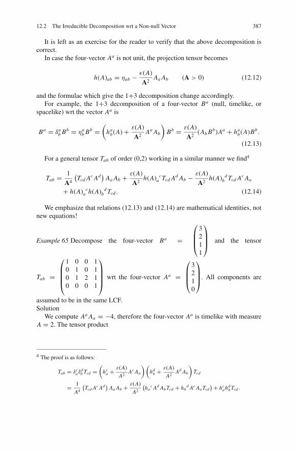
12.2 The Irreducible Decomposition wrt a Non-null Vector 387
It is left as an exercise for the reader to verify that the above decomposition iscorrect.
In case the four-vector Aa is not unit, the projection tensor becomes
h(A)ab = ηab − ε(A)
A2Aa Ab (A > 0) (12.12)
and the formulae which give the 1+3 decomposition change accordingly.For example, the 1+3 decomposition of a four-vector Ba (null, timelike, or
spacelike) wrt the vector Aa is
Ba = δab Bb = ηa
b Bb =(
hab(A)+ ε(A)
A2Aa Ab
)Bb = ε(A)
A2(Ab Bb)Aa + ha
b(A)Bb.
(12.13)
For a general tensor Tab of order (0,2) working in a similar manner we find4
Tab = 1
A4
(Tcd Ac Ad
)Aa Ab + ε(A)
A2h(A) c
a Tcd Ad Ab − ε(A)
A2h(A) d
b Tcd Ac Aa
+ h(A) ca h(A) d
b Tcd . (12.14)
We emphasize that relations (12.13) and (12.14) are mathematical identities, notnew equations!
Example 65 Decompose the four-vector Ba =
⎛
⎜⎜⎝
3211
⎞
⎟⎟⎠ and the tensor
Tab =
⎛
⎜⎜⎜⎝
1 0 0 10 1 0 10 1 2 10 0 0 1
⎞
⎟⎟⎟⎠ wrt the four-vector Aa =
⎛
⎜⎜⎝
3210
⎞
⎟⎟⎠. All components are
assumed to be in the same LCF.Solution
We compute Aa Aa = −4, therefore the four-vector Aa is timelike with measureA = 2. The tensor product
4 The proof is as follows:
Tab = δcaδ
db Tcd =
(hc
a +ε(A)
A2Ac Aa
)(hd
b +ε(A)
A2Ad Ab
)Tcd
= 1
A4
(Tcd Ac Ad
)Aa Ab + ε(A)
A2
(ha
c Ad AbTcd + hbd Ac Aa Tcd
)+ hcahd
b Tcd .

388 12 Irreducible Decompositions
Aa ⊗ Ab =
⎛
⎜⎜⎝
9 6 3 06 4 2 03 2 1 00 0 0 0
⎞
⎟⎟⎠
and the projection operator
h(A)ab =
⎛
⎜⎜⎜⎜⎜⎜⎜⎜⎜⎜⎜⎜⎝
5
4
−3
2
−3
40
−3
22
1
20
−3
4
1
2
5
40
0 0 0 1
⎞
⎟⎟⎟⎟⎟⎟⎟⎟⎟⎟⎟⎟⎠
.
For the four-vector Ba we have
Ba Aa = −4,
h(A)ab Bb =
⎛
⎜⎜⎝
0001
⎞
⎟⎟⎠ ,
therefore Ba = Aa + h(A)ab Bb.
For the tensor Tab we compute
1
A4Tab Aa Ab = 17
16,
1
A2h(A)c
aTcb Ab =(
39
16,−21
8,−33
16, 0
),
1
A2h(u)b
aTcb Ac =(
39
16, −23
8, −25
16, −3
2
),
h(A)cah(A)d
b Tcd =
⎛
⎜⎜⎜⎜⎜⎜⎜⎜⎜⎜⎜⎜⎝
97
16
−57
8
−63
16
−7
2
−51
8
31
4
29
84
−87
16
47
8
73
16
5
2
0 0 0 1
⎞
⎟⎟⎟⎟⎟⎟⎟⎟⎟⎟⎟⎟⎠
.
Verify the above result using relation (12.14).
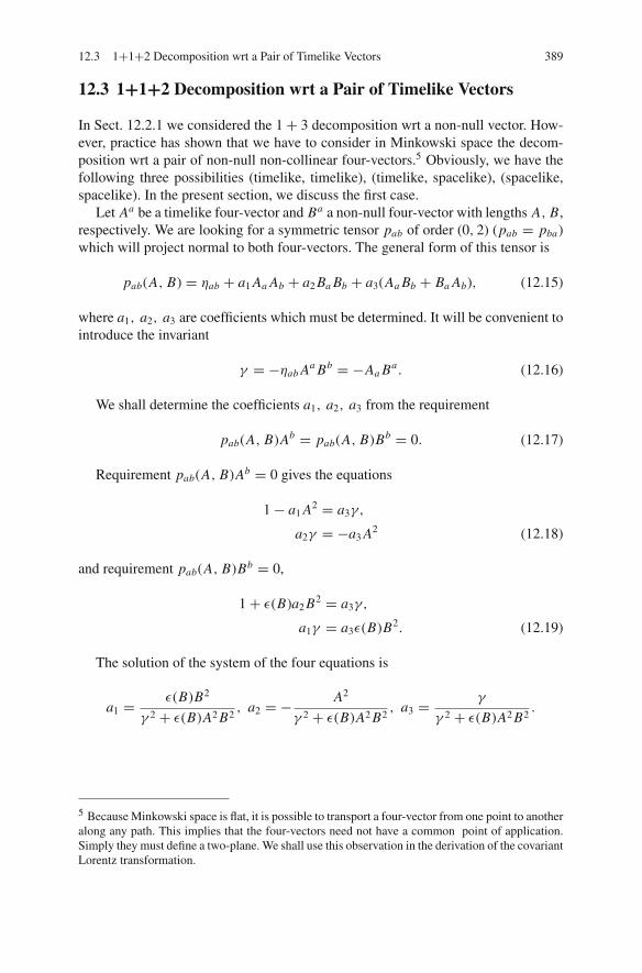
12.3 1+1+2 Decomposition wrt a Pair of Timelike Vectors 389
12.3 1+1+2 Decomposition wrt a Pair of Timelike Vectors
In Sect. 12.2.1 we considered the 1+ 3 decomposition wrt a non-null vector. How-ever, practice has shown that we have to consider in Minkowski space the decom-position wrt a pair of non-null non-collinear four-vectors.5 Obviously, we have thefollowing three possibilities (timelike, timelike), (timelike, spacelike), (spacelike,spacelike). In the present section, we discuss the first case.
Let Aa be a timelike four-vector and Ba a non-null four-vector with lengths A, B,respectively. We are looking for a symmetric tensor pab of order (0, 2) (pab = pba)which will project normal to both four-vectors. The general form of this tensor is
pab(A, B) = ηab + a1 Aa Ab + a2 Ba Bb + a3(Aa Bb + Ba Ab), (12.15)
where a1, a2, a3 are coefficients which must be determined. It will be convenient tointroduce the invariant
γ = −ηab Aa Bb = −Aa Ba . (12.16)
We shall determine the coefficients a1, a2, a3 from the requirement
pab(A, B)Ab = pab(A, B)Bb = 0. (12.17)
Requirement pab(A, B)Ab = 0 gives the equations
1− a1 A2 = a3γ,
a2γ = −a3 A2 (12.18)
and requirement pab(A, B)Bb = 0,
1+ ε(B)a2 B2 = a3γ,
a1γ = a3ε(B)B2. (12.19)
The solution of the system of the four equations is
a1 = ε(B)B2
γ 2 + ε(B)A2 B2, a2 = − A2
γ 2 + ε(B)A2 B2, a3 = γ
γ 2 + ε(B)A2 B2.
5 Because Minkowski space is flat, it is possible to transport a four-vector from one point to anotheralong any path. This implies that the four-vectors need not have a common point of application.Simply they must define a two-plane. We shall use this observation in the derivation of the covariantLorentz transformation.
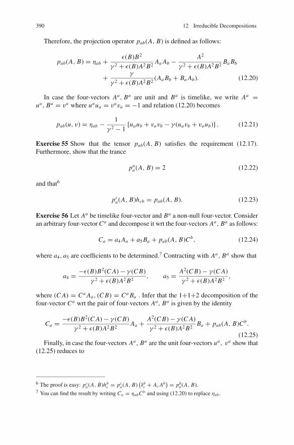
390 12 Irreducible Decompositions
Therefore, the projection operator pab(A, B) is defined as follows:
pab(A, B) = ηab + ε(B)B2
γ 2 + ε(B)A2 B2Aa Ab − A2
γ 2 + ε(B)A2 B2Ba Bb
+ γ
γ 2 + ε(B)A2 B2(Aa Bb + Ba Ab). (12.20)
In case the four-vectors Aa, Ba are unit and Ba is timelike, we write Aa =ua, Ba = va where uaua = vava = −1 and relation (12.20) becomes
pab(u, v) = ηab − 1
γ 2 − 1[uaub + vavb − γ (uavb + vaub)] . (12.21)
Exercise 55 Show that the tensor pab(A, B) satisfies the requirement (12.17).Furthermore, show that the trance
paa (A, B) = 2 (12.22)
and that6
pca(A, B)hcb = pab(A, B). (12.23)
Exercise 56 Let Aa be timelike four-vector and Ba a non-null four-vector. Consideran arbitrary four-vector Ca and decompose it wrt the four-vectors Aa, Ba as follows:
Ca = a4 Aa + a5 Ba + pab(A, B)Cb, (12.24)
where a4, a5 are coefficients to be determined.7 Contracting with Aa, Ba show that
a4 = −ε(B)B2(C A)− γ (C B)
γ 2 + ε(B)A2 B2, a5 = A2(C B)− γ (C A)
γ 2 + ε(B)A2 B2,
where (C A) = Ca Aa, (C B) = Ca Ba . Infer that the 1+1+2 decomposition of thefour-vector Ca wrt the pair of four-vectors Aa, Ba is given by the identity
Ca = −ε(B)B2(C A)− γ (C B)
γ 2 + ε(B)A2 B2Aa + A2(C B)− γ (C A)
γ 2 + ε(B)A2 B2Ba + pab(A, B)Cb.
(12.25)Finally, in case the four-vectors Aa, Ba are the unit four-vectors ua, va show that
(12.25) reduces to
6 The proof is easy: pca(A, B)hb
c = pca(A, B)
(δb
c + Ac Ab) = pb
a (A, B).7 You can find the result by writing Ca = ηabCb and using (12.20) to replace ηab.

12.3 1+1+2 Decomposition wrt a Pair of Timelike Vectors 391
Ca = (Cu)− γ (Cv)
γ 2 − 1ua + (Cv)− γ (Cu)
γ 2 − 1va + pab(u, v)Cb. (12.26)
In example 66, we derive the standard decomposition of a timelike four-vectorwrt a pair of another two timelike four-vectors. It would be an instructive exerciseto derive the same result using the 1+1+2 decomposition.
Example 66 Consider the timelike four-vector pi , of length p2 = −M2. Determinetwo timelike four-vectors pi
1, pi2 such that
pi = pi1 + pi
2 (12.27)
assuming that the lengths
p21 = −m2
1, p22 = −m2
2, (12.28)
where M,m1 > m2 > 0 are given and that the following conditions are satisfied8:
pi1 pi < 0 , pi
2 pi < 0. (12.29)
SolutionLet pi
1, pi2 be the required four-vectors. We consider the parallel projection
piA‖ =
piA pi
−p2pi
and the normal projection
piA,⊥ = pi
A − piA‖
of the vectors piA (A = 1, 2) wrt the four-vector pi . Then (12.27) projected parallel
and normal to pi gives
pi = pi1‖ + pi
2‖, (12.30)
0 = pi1⊥ + pi
2⊥. (12.31)
Let ni be a unit four-vector normal to the four-vector pi . We define the invariantsλ,μ in terms of pi
1 with the relations
pi1⊥ = μni , pi
1‖ = λpi .
8 The last requirement means that all three four-vectors have the same sign of their zero component,that is, they point in the same part of the light cone.

392 12 Irreducible Decompositions
From (12.30), (12.31) we have
pi2⊥ = −μni , pi
2‖ = (1− λ)pi .
We compute the lengths of pi1, pi
2 in terms of λ,μ. We find
−λ2 M2 + μ2 = −m21, (12.32)
−(1− λ)2 M2 + μ2 = −m22. (12.33)
The solution of the system of equations (12.32), (12.33) is
λ = M2 + m21 − m2
2
2M2= 1
M1M E, (12.34)
μ2 = [M2 − (m1 + m2)2][M2 − (m1 − m2)2]
2M= 1
4M2λ2(M,m1,m2), (12.35)
where 2M E is the energy of “particle” pi
2 in the proper frame of pi and μ is the lengthof the three-momentum of 1 in the same frame. We note that we recover the resultsof the reaction pi → pi
1+ pi1. The invariants λ,μ satisfy certain restrictions. Indeed,
from the inequalities (12.29) and because μ2 ≥ 0, one has9
M2 + m21 − m2
2 > 0,
[(M − m1)2 − m22][(M + m1)2 − m2
2] ≥ 0.
The first inequality gives
M ≥ m1 + m2
and the second inequality is trivially satisfied.Therefore, the condition is
M ≥ m1 + m2 (12.36)
as expected.Conversely, we note that if M > m1 + m2 and ni is a unit normal four-vector to
pi , then the equations give a solution to the problem. Therefore, condition (12.36)is sufficient for the solution of the problem and the general solution is given from(12.34), (12.35). We note that the general solution is determined completely in termsof the data of the problem modulo the spacelike unit four-vector ni . Therefore wehave∞2 solutions.
9 The first two conditions mean that the energy is positive. The third is the restriction that themeasure of the three-momentum is non-negative.

12.3 1+1+2 Decomposition wrt a Pair of Timelike Vectors 393
Exercise 57 Let Aa be a unit timelike four-vector (Aa Aa = −1) and Ba be a unitspacelike unit four-vector (Ba Ba = 1) and let φ = Aa Ba be their inner product.Define the quantity Δ = 1+φ2 and prove that the tensor of order (0, 2) pab(A, B) =ηab + 1
Δ[Aa Ab − Ba Bb − φ(Aa Bb + Ab Ba)] has the following properties
1. Is symmetric.2. Projects normal to both Aa, Ba , that is
pab(A, B)Ab = pab(A, B)Bb = 0. (12.37)
3. Its trace
paa (A, B) = 2. (12.38)
4.
pab(A, B)hbc (A) = pac(A, B). (12.39)
pca(A, B)hb
c = pba(A, B). (12.40)
We call the projection tensor pab(A, B) the screen projection operator associatedwith the four-vectors A, B. This tensor is used in the study of spacelike congruences,e.g., the field lines of the electric filed.

Chapter 13The Electromagnetic Field
13.1 Introduction
The Theory of Special Relativity (and consequently the Theory of GeneralRelativity) would have never been discovered if Maxwell had not formulated thetheory of electrodynamics.
Before Maxwell, the electric and the magnetic fields were considered to be inde-pendent physical fields and as such had been studied for many years by a number ofpioneer physicists who discovered many laws concerning the physics of these fields.Maxwell was the first to foresee the common origin of these fields and introducedthe electromagnetic field as the underlying physical entity. Subsequently he statedthe basic equations governing the evolution of the electromagnetic field and repro-duced all the then known physical laws concerning the electric and the magneticfields.
However, Maxwell’s field equations had a stoning property: They were notcovariant under the classical Galileo transformations,1 that is, their form was depen-dent on the particular Newtonian inertial frame they were written!
The non-covariance of Maxwell equations wrt the Galileo group of transforma-tions was a serious defect. Indeed according to the covariance principle the physicalquantities as well as the physical laws of a theory of physics must be covariantunder the fundamental group of transformations of the theory. Therefore the non-covariance of the electromagnetic field wrt the group of Galileo transformationsmeant that the electromagnetic field was not a Newtonian physical quantity! Butthen the electric field and the magnetic field are not Newtonian physical quantities,a fact that one could hardly understand and accept easily.
Furthermore it was found that these equations were covariant under another moregeneral group of transformations, which today we call the Lorentz group. But at thetime there was not a theory of physics covariant wrt the Lorentz group, therefore thesituation appeared to be impossible!
In addition to this theoretical – but important – aspect came a number of experi-ments involving light, which could not be explained in terms of Newtonian Physics.
1 That is, three-space rotation and translation or equivalently rigid body motion.
M. Tsamparlis, Special Relativity, DOI 10.1007/978-3-642-03837-2 13,C© Springer-Verlag Berlin Heidelberg 2010
395

396 13 The Electromagnetic Field
These experiments were performed mainly by Michelson and Morley and were indi-cating that the speed of light in vacuum was independent of the speed of the sourceand the speed of the receiver and in fact was a universal constant.
As it is the case with such revolutionary and “out of the current line” situations,experts reacted with “wisdom” and tried to find “generalizations” or “hidden” fieldsin the well-established Newtonian Theory, which could explain the peculiar behav-ior of light. They invented a new “substance” to replace the absolute character ofspace and time, the ether, whose properties were postulated to be just enough toexplain the new experimental facts. However, at that very moment the Theory ofSpecial Relativity had been born and it was a matter of time who will present it first.
Again as it is the case with great ideas the development was slow and gradual.An eminent physicist of the time, H. Lorentz (see Footnote 1, Sect. 4.1), who wasworking on the effects of the electromagnetic field formulated a theory for the elec-tron and introduced (in an artificial way) for the first time the Lorentz contraction.Another great theoretician H. Poincare discussed the theoretical aspects of relativemotion and practically stated what we call today the Einstein Relativity Principle.However, the birth of the new theory required a young and very special man, not yetestablished, and therefore able to think outside the current trend. That was AlbertEinstein, who starting from the invariance of Maxwell equations derived the Lorentztransformations and rewrote Maxwell equations in their intrinsic four-dimensionalform. Then taking a step further he postulated the Einstein Principle of Relativity(see Footnote 1, Sect. 4.1) claiming that in addition to the electromagnetic field thereare many more physical fields which are covariant wrt the Lorentz transformation.These fields are the physical quantities of a new theory of physics and together withthe laws which govern their behavior constitute what we call today the Theory ofSpecial Relativity.2
In the following sections of this chapter we discuss the relativistic form ofMaxwell equations and we solve some well-known problems indicating the appli-cation of the four-dimensional formalism in standard electrodynamics.
13.2 Maxwell Equations in Newtonian Physics
The theory of the electromagnetic field developed by Maxwell is a macroscopictheory, that is, it does not enter into the structure of matter as we understand ittoday. According to that theory the electromagnetic field in an arbitrary medium isdescribed by means of four-vector fields: the electric field E, the magnetic field H,the electric induction D, and the magnetic induction B.
2 Sometimes it is stated erroneously that this principle concerns all physical phenomena – seephysical quantities. It does not. All Newtonian physical quantities do not obey Einstein’s Relativ-ity Principle whereas they do obey the Galileo Relativity Principle. For this reason a Newtonianphysical quantity (velocity for example) is not a relativistic physical quantity, etc. Every theory ofphysics has a separate domain of application which comprises a “subset” of physical phenomena.See Chap. 2 for details.

13.2 Maxwell Equations in Newtonian Physics 397
As we have remarked in the introduction Maxwell’s equations are not covariantunder the Galileo group, therefore their form depends on the Newtonian inertialsystem, K say, we write them. If in K there are all four fields E,H,D,B then Maxwellequations for the electromagnetic field (in K only!) in SI units3 are the following:
∇ × E+ ∂B∂t= 0, (13.1)
∇ ×H−∂D∂t= j , (13.2)
∇j+ ∂ρ
∂t= 0. (13.3)
In these equations j is the electric current density in K , which is defined by therelation4 j = ρv, where ρ, v is the density and the velocity of the electric charge inthe frame K . Equation (13.3) expresses the conservation of electric current and it iscalled the continuity equation (for electric charge).
In empty space these equations are known with various names. The first is knownas Faraday’s Law and the second in the static case (that is when ∂D
∂t = 0) as Ampere’sLaw.
An immediate consequence of (13.1)5 is
∇ · B = 0. (13.4)
This equation implies that there is no magnetic charge and therefore magneticcurrent.
From (13.2) and (13.3) it follows:
∇ · D = ρ. (13.5)
Equation (13.5) (or one of its versions) is known as Gauss Law.Equations (13.1), (13.2), (13.4), and (13.5) constitute Maxwell equations for a
general electromagnetic field in a general medium. In practice we consider specialcases depending on the particular physical problem. In these cases Maxwell equa-tions take a simplified form. A standard method to obtain such simplified formsis by considering relations among the fields D,B and E,H known as constitutive
3 Electromagnetism is an old subject with applications in the most diverse areas of science andengineering. As a result there is a number of units in terms of which Maxwell equations have beenwritten. In this book we shall use the SI system. In Sect. 13.16 we show how one writes theseequations in other systems and especially in the Gauss system.4 The current j is more general than this but for the time being the conduction current suffices.5 To be precise (13.1) implies that ∇ · B = constant in K. The requirement that the value of thisconstant is 0 is an extra assumption whose discussion is outside the scope of this book. For thisreason this equation is considered as an extra independent equation compatible with the rest ofMaxwell equations.

398 13 The Electromagnetic Field
relations. The first such simplifying assumption we do is that the medium is homo-geneous and isotropic (that is invariant under the Galileo group). For such mediumswe assume that the constitutive relations are
D = εE, B = μH. (13.6)
The quantities ε dielectric constant and μ magnetic permeability are character-istic quantities of a medium and satisfy the relation
εμ = 1/u2, (13.7)
where u is the speed of the electromagnetic field in the medium.6 Because the elec-tromagnetic field propagates in empty space we must consider the empty space as amedium. In Special Relativity (but not in General Relativity!) empty three-space isconsidered to be a homogeneous and isotropic medium with dielectric constant ε0
and magnetic permeability μ0.7 Because in empty space the electromagnetic fieldpropagates with speed c (13.7) implies the relation
ε0μ0 = 1/c2. (13.9)
We note that (13.9) relates the constancy of the speed of light with the electro-magnetic properties of empty space.
For a homogeneous but not isotropic medium the fields D and H are related withthe fields E and B by the relations
D = εE+ P, B = μ(H+M), (13.10)
where we have introduced two new vector fields, the polarization vector P and themagnetization vector M to count for the anisotropy. Obviously in empty spaceP =M =0.
The first question to pose in the relativistic study of the electromagnetic fieldis if there exists a “generalized” potential in K (which cannot be a scalar) which,with proper derivations, produces both the electric and the magnetic fields in K . Weaddress this question in the next section.
6 The quantities ε, μ are scalar only for homogeneous and isotropic media. For anisotropic andnon-homogeneous materials these quantities are described by second-order symmetric tensors.7 The values assigned to these constants are the following:
ε0 = 8.85× 10⁻¹² Farad/m, μ0 = 1.26× 10⁻⁶ Henry/m. (13.8)

13.3 The Electromagnetic Potential 399
13.3 The Electromagnetic Potential
Equation (13.4) implies that (provided certain mathematical assumptions are ful-filled, which we assume to be the case) there exists a differentiable vector fieldA(r, t) such that
B = ∇ × A. (13.11)
Replacing in (13.1) we find
∇ ×[
E+ ∂A∂t
]= 0. (13.12)
In the derivation of (13.12) we have used the fact that the operators ∂∂t and ∇
commute8:
∂
∂t∇ = ∇ ∂
∂t.
From a well-known proposition of classical vector calculus, (13.12) implies thatthere exists a scalar function φ(r, t) such that
E+ ∂A∂t= −∇φ,
hence
E = −∇φ − ∂A∂t
. (13.13)
The functions φ and A are the potentials for the electric and the magnetic fields,because they produce these fields by proper derivations.
Up to this point the functions φ and A are general. To determine them we areusing the remaining two Maxwell equations. In order to make things simpler (with-out restricting seriously the generality, since the same hold in the case of a homoge-neous and isotropic medium) we consider Maxwell equations in empty space9 andwrite the constitutive equations:
D = ε0E, B = μ0H.
If we replace E and B in terms of φ and A in (13.2) and (13.5) it follows:
8 The operators ∇ and ddt do not commute, because the operator d
dt includes variations in space.9 In order to write Maxwell equations for a homogeneous and isotropic medium it is enough toreplace c2 with the product εμ or with the speed u2 of the electromagnetic field in the medium.

400 13 The Electromagnetic Field
∇2φ + ∂
∂t(∇ · A) = − ρ
ε0, (13.14)
∇ × (∇ × A)+ 1
c2
∂
∂t
(∇φ + ∂
∂tA)= μ0j. (13.15)
Equation (13.14) does not simplify further. Equation (13.15) can be written dif-ferently. Using the identity
∇ × (∇ × A) = ∇(∇ · A)−∇2A
and the fact that ∇ ∂φ
∂t = ∂∂t∇φ after a simple calculation we find the equation
∇2A− 1
c2
∂2A∂t2−∇
[∇ · A+ 1
c2
∂φ
∂t
]= −μ0j. (13.16)
Equations (13.14) and (13.16) are the dynamical equations determining thepotentials φ and A.
We note that these equations do not determine the potentials φ,A completely.Indeed if we replace A with A′ = A + ∇Λ where Λ(r, t) is an arbitrary (butdifferentiable) function, then
∇ × A′ = ∇ × A = B
because ∇ × (∇Λ) = 0 for every function Λ(r, t).Therefore the transformation A′ = A + ∇Λ leaves the magnetic field invariant.
However, this is not so for the electric field, which under the transformation A′ =A+∇Λ transforms as follows:
E = −∇φ − ∂A∂t= −∇φ − ∂A′
∂t+∇
(∂Λ
∂t
)=⇒
E = −∇(φ − ∂Λ
∂t
)− ∂A′
∂t.
In order that the electric field remain invariant we have to consider the followingtransformation of the scalar field φ:
φ −→ φ′ = φ − ∂Λ
∂t.
The transformation of the potentials, which leave the dynamical fields E,Binvariant, is called a gauge transformation. This type of transformations is veryimportant in physics.
The indeterminacy in the determination of the potentials gives us the freedom todefine the function Λ by means of a scalar relation among the potentials φ,A andselect the pair of potentials which is most convenient to our purposes. The basic

13.3 The Electromagnetic Potential 401
criterion for this relation is that it must be tensorial, that is covariant under thefundamental group of the theory. Otherwise the relation will be frame dependent. Itis evident that in the Theory of Special Relativity this condition must be covariantunder the Lorentz group, whereas in Newtonian Physics under the Galileo group.A second criterion, however of less importance, is that the condition which will beconsidered must lead to potential functions which simplify (13.14) and (13.16).
In the Theory of Special Relativity the condition which fulfils both requirementsis the Lorentz gauge, which for empty space is defined as follows:
∇ · A+ 1
c2
∂φ
∂t= 0. (13.17)
We note that with the Lorentz gauge the field equations (in empty space!) become
∇2φ − 1
c2
∂2φ
∂t2= − ρ
ε0or �φ = − ρ
ε0, (13.18)
∇2A− 1
c2
∂2A∂t2= −μ0j or �A = −μ0j, (13.19)
where
� = ∇2 − 1
c2
∂2
∂t2(13.20)
is the D’Alembert operator.10 As we have seen in Exercise 11 D’Alembert’s operatoris Lorentz covariant. Therefore with the use of the Lorentz gauge the equations ofthe electromagnetic potentials become similar and are written in Lorentz covariantform in terms of the D’Alembert operator. This observation leads us in a natural wayto the four-potential and enables us to write Maxwell equations in four-dimensionalformalism.
Another aspect of the Lorentz gauge is that it implies the equation of continuity.Indeed from (13.18) and (13.19) we have
∇(�A) = −μ0∇ · j , ∂
∂t(�φ) = − 1
ε0
∂ρ
∂t=⇒
�(
∇ · A+ 1
c2
∂φ
∂t
)= −μ0
(∇ · j+∂ρ
∂t
),
which proves this assertion.
10 It is interesting to read about the life and the work of D’Alembert. The interested reader canvisit the web site http://www-history.mcs.st-andrews.ac.uk/Biographies/D’Alembert.html

402 13 The Electromagnetic Field
Because the dynamical equations for the potentials are covariant wrt the gaugetransformation of the fields, we demand that the Lorentz gauge also will be invari-ant under the gauge transformation. This condition determines the gauge functionΛ(r, t). Indeed the condition ∇ · A′ + 1
c2∂φ′∂t = 0 gives
0 = ∇ · A′ + 1
c2
∂φ′
∂t= ∇ · (A+∇Λ)+ 1
c2
∂
∂t
(φ − ∂Λ
∂t
)
= ∇ · A+ 1
c2
∂φ
∂t+∇2Λ− 1
c2
∂2Λ
∂t2
= ∇2Λ− 1
c2
∂2Λ
∂t2= �Λ.
We conclude that the function Λ must be a solution of the wave equation inempty space.
There are gauge conditions for the potentials φ,A other than the Lorentz condi-tion. However, they are not Lorentz covariant and/or they do not imply the continuityequation for the charge. For example in Newtonian Physics the gauge conditionfor the electromagnetic potentials is the Coulomb gauge, which is defined by therelation
∇ · A = 0. (13.21)
The name of this gauge is due to the fact that by its use the field equation (13.18)becomes
∇2φ = − ρ
ε0, (13.22)
which is the well-known Poisson equation whose solution is
φ(r, t) =∫
Ω
ρ(r′, t)
|r′ − r|d3r′, (13.23)
where ρ(r′, t) is the charge density (in the Newtonian inertial system K whereMaxwell equations are considered). This relation means that the scalar potentialis the instantaneous Coulomb potential due to the charge density ρ(r, t) distributedin the space Ω (and measured in K ).
Collecting the above results we state that Maxwell equations in empty space inthe Lorentz gauge are as follows:
a. For the fields:
B = ∇ × A, (13.24)
E = −∇φ − ∂A∂t
. (13.25)

13.3 The Electromagnetic Potential 403
b. For the potentials:
�φ = − ρ
ε0, (13.26)
�A = −μ0j. (13.27)
c. Equation of continuity:
∇ · j+ ∂ρ
∂t= 0. (13.28)
d. Lorentz gauge:
∇ · A+ 1
c2
∂φ
∂t= 0. (13.29)
The main result which follows from the above equations is that if we solve thewave equation for scalar and vector waves, then we have solved completely Maxwellequations and we have determined the electromagnetic field.
The difference between the Lorentz gauge and the Coulomb gauge is that thefirst is covariant wrt the Lorentz group whereas the second wrt the Euclidean group.This becomes clear from the following example.
Example 67 a. In the LCF Σ consider the four-quantity
(− 1c
∂∂t∇)
Σ
and show that
it defines a four-vector. Show that the length of this four-vector is the D’Alembertoperator � = ∇2 − 1
c2∂2
∂t2 and conclude that the D’Alembert operator is covariantwrt the Lorentz group.b. Show that in an LCF Σ′ moving with parallel axes wrt the LCF Σ with velocityu, the ∇ transforms as follows:
∇′ = ∇ +{
(γ − 1)u ·∇
u2+ γ
c2
∂
∂t
}u. (13.30)
Solution
a. We consider an LCF Σ′ moving in the standard configuration relative to the LCFΣ with parameter β. The Lorentz transformation relating Σ′ and Σ is
x = γ (x ′ + βct ′), ct = γ (ct ′ + βx ′), y = y′, z = z′.

404 13 The Electromagnetic Field
We have then
∂
∂x ′= ∂
∂x
∂x
∂x ′+ ∂
∂y
∂y
∂x ′+ ∂
∂z
∂z
∂x ′+ ∂
∂(ct)
∂(ct)
∂x ′= γ
∂
∂x+ βγ
∂
∂(ct),
∂
∂y′= ∂
∂y,
∂
∂z′= ∂
∂z,
∂
∂(ct ′)= ∂
∂x
∂x
∂(ct ′)+ ∂
∂y
∂y
∂(ct ′)+ ∂
∂z
∂z
∂(ct ′)+ ∂
∂(ct)
∂(ct)
∂(ct ′)= γ
∂
∂(ct)+ βγ
∂
∂x.
Therefore
⎛
⎜⎜⎜⎜⎜⎝
− ∂c∂t ′
∂∂x ′
∂∂y′
∂∂z′
⎞
⎟⎟⎟⎟⎟⎠=
⎛
⎜⎜⎝
γ −βγ 0 0−βγ γ 0 0
0 0 1 00 0 0 1
⎞
⎟⎟⎠
⎛
⎜⎜⎜⎜⎜⎝
− ∂c∂t
∂∂x
∂∂y
∂∂z
⎞
⎟⎟⎟⎟⎟⎠, (13.31)
where in the rhs the multiplication is matrix multiplication. This equation means
that the quantity ∇i ≡(
∂∂(ct) ,∇
)(note the lowering of the index and the conse-
quent change in the sign of the zeroth component!11) is a four-vector.The length of this four-vector is
ηi j∇i∇ j = ∇2 − 1
c2
∂2
∂t2≡ �.
This quantity is invariant, that is
∇′2 − 1
c2
∂2
∂t ′2= ∇2 − 1
c2
∂2
∂t2. (13.32)
b. We consider the LCF Σ′ whose axes are parallel to the ones of the LCF Σ andmoves with velocity u. Then the general Lorentz transformation (1.52) whichrelates Σ and Σ′ gives for the three-vector ∇
11 We recall at this point the rule for signs of the components when we lower and raise theindex of a four-vector. To the contravariant four-vector Ai we correspond the covariant four-vector Ai with the relation Ai = ηi j A j where ηi j is the Lorentz metric. In case we have Lorentzorthonormal frames (which we assume to be the rule) the Lorentz metric has its canonical form
ηi j = diag(−1, 1, 1, 1). Therefore in such frames (and only there!) the four-vector Ai =(
BA
)
Σ
corresponds to the four-vector Ai = (−B,A)Σ, that is, the sign of the zeroth component changesand the matrix from column becomes row. If the frames are not Lorentz orthonormal then theabove simple rule does not apply and one has to (a) compute the components of the Lorentz metricand then (b) multiply the resulting 4 × 4 matrix with the column (or row) matrix defined by thecomponents of the four-vector in the same frame.

13.4 The Equation of Continuity 405
∇′ = ∇ +{
(γ − 1)u ·∇
u2+ 1
c2γ
∂
∂t
}u.
13.4 The Equation of Continuity
The equations of continuity appear in all theories of physics and express the conser-vation of a current. In the Theory of Special Relativity the equations of continuityhave a special significance which we show in this section.
In an LCF Σ we consider a Euclidean vector field A and a Euclidean invariant Bwhich satisfy an equation of continuity, that is
∇ · A+ ∂B
∂t= 0. (13.33)
This relation can be written as follows:(− ∂
c∂t
∇
)·(
BcA
)= 0, (13.34)
where the dot indicates Lorentz inner product. This equation attains a physicalmeaning in Special Relativity only when it is covariant under the action of Lorentztransformations, which we assume to be the case. What does this assumption imply
on the four-quantity
(BcA
)
Σ
?
If the rhs was not zero then by the quotient theorem the four-quantity Ai ≡(BcA
)
Σ
should be a four-vector, because the operator(
∂c∂t , ∇)
Σis a four-vector.
But the rhs vanishes and the quotient theorem does not apply because zero is covari-ant wrt any homogeneous transformation (the Lorentz transformation included!).
However, although the equation of continuity does not determine the Lorentz
covariance of the four-quantity
(BcA
)
Σ
it does say that the assumption Ai four-
vector is acceptable. In this case the equation of continuity is written as Ai,i = 0; it
is Lorentz covariant and has a physical meaning in Special Relativity. The physicalmeaning we give it is that the four-vector Ai represents a “physical current” and theequation of continuity expresses the lack of charge for this current or, equivalently,the lack of sinks and sources for this physical field.
The consideration Ai four-vector is not the only possible way and of course itneed not be compatible with other transformations12 which the Euclidean quantitiesA, Bc may obey.
12 Indeed let us assume that the four-quantity (Bc,A)Σ transforms from an LCF Σ to the LCF Σ′
according to the rule

406 13 The Electromagnetic Field
In electromagnetism the equation of continuity is the following:
∇ · j+ ∂ρ
∂t= 0,
where j = ρu is the conduction current in an LCF Σ, ρ the density of the charge inΣ, and u the velocity of the charge in Σ. This equation gives in Σ the four-quantity
j i =(ρcj
)
Σ
=(ρcρu
)
Σ
= ρ
γγ
(cu
)
Σ
= ρ
γui , (13.35)
where ui is the four-velocity of the charge. Therefore the requirement j i to be a four-vector implies that the quantity ρ0 = ρ
γmust be Lorentz invariant. The invariant ρ0
is called proper density of the charge and we assume that it measures the density ofthe charge in the rest frame of the charge. The ρ = ρ0γ is the density of the chargein the LCF Σ. We note that ρ > ρ0, that is, we have “charge dilation.” We call thefour-vector j i conduction four-current and we define it covariantly as follows:
j i = ρ0ui . (13.36)
The equation of continuity in electromagnetism reads
j i,i = 0. (13.37)
We assume the electric charge to be Lorentz invariant and define it in the LCF Σ
with the relation
d Q = ρdV, (13.38)
where dV is an elementary volume at the point of three-space of Σ where the chargedensity is ρ. In the proper frame of the charge, d Q = ρ0dV0 from which followsthe well-known transformation of three-volume:
dV = 1
γdV0. (13.39)
(B ′cA′
)
Σ′= κ(υ)
(BcA
)
Σ
,
where κ(υ) is a function of relative velocity v of the frames Σ, Σ′. Then relation (13.34) ispreserved in the new frame. Indeed
Ai −→ Ai ′ = κ(υ)Ai ,
thereforeAi ′
,i ′ = Q(υ)(κ(υ)Ai ),i = Q(υ)κ(υ)Ai,i ,
where Q(υ) is some function of the relative velocity resulting from the Lorentz transformation.This condition is not Lorentz covariant except if and only if Q(υ)κ(υ) = 1.

13.4 The Equation of Continuity 407
Example 68 a. Show that the elementary three-volume dV under a Lorentz trans-formation with parameter γ transforms as follows: dV = 1
γdV+ where dV+ is
the three-volume in the proper frame.b . Let A be an invariant physical quantity (e.g., mass, charge) with density ρA.
Show that under the same Lorentz transformation the density transforms with therelation ρA = γρ+A where ρ+A is the density in the proper frame of the volume.
c. Suppose the quantity A of question (b) satisfies an equation of continuity, that is,in an arbitrary LCF Σ:
∇ · j+ ∂ρA
∂t= 0,
where j is a current which is related to A and ρA is the density of A in Σ. Thisequation is written as
(∂∂ct∇
)(cρA
jA
)= 0.
Assume that the four-quantity J aA =
(cρA
jA
)is a four-vector and find a covariant
relation among J a and the four-velocity ua of the elementary volume dV in Σ.Finally show that in this case the equation of continuity of the quantity A is writtencovariantly as J a
,a = 0.Solution
a. We consider the elementary surface d S normal to the three-velocity u of theelementary volume in the LCF Σ and we have dV = d Sdl. Under the actionof the Lorentz transformation d S = d S+ and dl = 1
γdl+ from which follows
dV = 1γ
dV+.b. Because A is invariant we have
ρAdV = ρ+A dV+ =⇒ ρA = γρ+A .
c. Considering that the quantity
(cρA
jA
)is a four-vector we have
(cρA
jA
)= ρA
(c
jA/ρA
)= ρ+A
(γ c
γ jA/ρA
).
The only four-vector whose zeroth component equals γ c in the arbitrary LCFΣ is the four-velocity ua of the elementary volume dV . It follows that jA = ρAuwhere u is the three-velocity of the elementary volume dV in Σ. We infer that thefour-current of the quantity A is defined covariantly with the relation J a
A = ρ+A ua
where ua is the four-velocity of every elementary volume dV of A. In terms of thefour-current the equation of continuity is written as the Lorentz product:

408 13 The Electromagnetic Field
0 = ∂ρ
∂ct+∇ · jA = ∂ J 0
A
∂x0+∇ · Jμ
A = J aA,a .
Example 69 a. A current I flows through a straight conductor of infinite length.Calculate the magnetic field in a distance r from the conductor.
b. A straight conductor of infinite length is charged homogeneously with a positivecharge of density ρ. Calculate the electric field at a distance r from the conductor.
c. In the LCF Σ the current I flows through a straight conductor of infinite lengthwhile a charge q moves parallel to the direction of the conductor with constantspeed u at a distance r from the conductor. Study the motion of the charge in theproper frame of the conductor and the proper frame of the charge.(It is given that ε0 = 8.85418 × 10⁻¹² Cb2
N m2 (the useful quantity is 14πε0= 9.0×
109 N m2
Cb2 ) and μ0 = 4π × 10−7 WeberA m .)
Solution
a. According to Ampere’s Law the magnetic field B which is created from a currentI is given (in the SI system) by the relation
∮B · dl =μ0 I, (13.40)
where the integral is computed over a smooth closed curve in the space of themagnetic field and dl is the element of length along this curve (see Fig. 13.1).In the case of a straight conductor of infinite length, due to symmetry, themagnetic field at a point P in space must have a direction normal to the directionof the conductor and a strength depending on the distance r of the P from theconductor. In order to compute the magnetic field at the point P we consider theplane through P which is normal to the conductor and in that plane we considera circle centered at the conductor with radius r . Then B = Beφ and dl = dl eφ ,hence
∮B · dl =
∮Brdφ=2πr B.
Fig. 13.1 Ampere’s Law
l
B
magnetic fieldlines

13.4 The Equation of Continuity 409
Ampere’s Law gives
B = μ0 I
2πreφ,
where (er , eφ, eθ ) is the right-handed system of spherical coordinates.b. If a charge, Q say, is enclosed in the interior of a smooth closed surface S, then
the electric field E on the surface is given by Gauss Law, which in the SI systemof units is as follows:
∮E · dS = 1
ε0Q,
where dS is the elementary surface at a point P of S and E is the value of theelectric field at the point P .In the case of a straight conductor of infinite length with charge density ρ weconsider a cylindrical surface with axis the conductor, radius r , and length 2l andhave
∮E · dS =
∫ l
−lE2πrdl.
The E ‖ dS due to symmetry, that is, E = E er , S = d Ser . Gauss Law gives
E = ρ
2πrε0,
where ρ = Ql is the linear density of charge. The direction of E depends on the
sign of the charge density.c. In the proper frame of the conductor, Σ say, the current flowing through the
conductor creates a magnetic field. There does not exist an electric field becausethe metallic conductor is electrically neutral. Indeed the conductor consists ofpositive ions of charge density ρ+, which have velocity zero and free electronsof density ρ− = ρ+ which move with small velocity v, opposite to the directionof the current. In the frame Σ we consider a charge q which moves with velocityu parallel to the direction of the current in the conductor, therefore it suffers theLorentz force
F = qu× B.
As we saw in (a) the magnetic field B = μ0 I2πr eφ , therefore
F = quμ0 I
2πreθ ×eφ = −quμ0 I
2πrer ,

410 13 The Electromagnetic Field
where er is the unit normal with direction from the conductor to the charge. Wenote that the charge is attracted from the conductor.13
We consider now the motion in the proper frame of the charge, Σ′ say. In thatframe the densities of the positive ions ρ ′+ and the free electrons ρ ′− are not equaland they must be calculated from the Lorentz transformation relating Σ, Σ′. Supposethat in Σ′ the four-current of the positive ions j i
+ and that of the free electronsj i− are
j i− =
⎛
⎜⎜⎝
ρ ′−cρ ′−v
′
00
⎞
⎟⎟⎠
Σ′
, j i+ =
⎛
⎜⎜⎝
ρ ′+c−ρ ′+u
00
⎞
⎟⎟⎠
Σ′
.
We know that in the proper frame Σ of the conductor these four-vectors are
j i− =
⎛
⎜⎜⎝
ρ−cρ−v
00
⎞
⎟⎟⎠
Σ
, j i+ =
⎛
⎜⎜⎝
ρ+c000
⎞
⎟⎟⎠
Σ
.
The Lorentz transformation gives
ρ ′−c = γu
(ρ−c − u
cρ−v
)= γuρ−c
(1− uv
c2
),
ρ ′+c = γuρ+c = γuρ−c
(because in Σ ρ+ = ρ−). The overall charge density in Σ′ is
ρ ′ = ρ ′+ − ρ ′− = γuρ−uv
c2.
This means that the conductor appears to be charged in Σ′ although it is neutralin Σ! This fact is completely at odds with the Newtonian point of view and it isdue to the fact that the charge density (not the charge!) is not Lorentz invariant inSpecial Relativity.
This charge of the conductor creates at the position of the moving charge theelectric field
13 From this result we can compute the force between two straight parallel conductors of infinitelength carrying currents I1 and I2. Indeed the first conductor (the I1 say) exerts to the elementarylength dl2 of the second conductor the force F21 = − dq2uμ0 I1
2πr er . But the length dl2 carries chargedq2 = I2dt so that dq2u = I2dl2, therefore the force per unit length on the current I2 due tothe current I1 is F21
dl2= −μ0 I1 I2
2πr er . This force is obviously attractive. If the currents have oppositedirection of flow that force is repulsive, a phenomenon with important practical applications.

13.4 The Equation of Continuity 411
E′ = ρ ′
2πr ′ε0er ′ = γuρ−uv
2πr ′ε0c2er .
But r ′ = r because r is measured normal to the velocity u. Also ε0c2 = 1μ0
.Replacing we find
E′ = γuμ0(ρ−v)u
2πrer .
Now ρ−v = j− = −I where I is the current through the conductor. Therefore
E′ = −γuμ0uI
2πrer = −γuE.
The force which is exerted on the moving charge in Σ′ is due to this electric fieldand equals
F+ = qE′ = −γuqE =− γuF,
where F is the force in the charge in Σ, which is due to the magnetic field createdby the current I .
This result is compatible with the transformation of the four-force. Indeed in Σ
the product F · u = 0, hence the four-force on the charge q has components
Fi =⎛
⎝0
γuF‖ = 0γuF⊥ = −γuF
⎞
⎠
Σ
.
In the LCF Σ′ the four-force is
Fi =⎛
⎝0
F′‖F′⊥
⎞
⎠
Σ′
.
The Lorentz transformation relating Σ, Σ′ gives
F′‖ = γu(0− βγuF‖) = 0,
F′⊥ = −γuF,
which coincides with the previous result.We note that in the proper frame Σ′ of the moving charge there does exist
magnetic field created by the current flowing through the conductor, but this fielddoes not exert a force on the charge because in Σ′ the charge is at rest.
In order to compute in Σ′ the current which flows through the conductor weconsider the currents of the positive ions and the free electrons and we have for thenet total current I ′

412 13 The Electromagnetic Field
I ′ = I ′− + I ′+ = −ρ ′−v′ + ρ ′+v = −γuρ−(v − u)− γuρ−u = −γuρ−v = γu I,
where I is the current flowing through the conductor in Σ.Question: Is this result compatible with the Lorentz transformation of the four-current?
13.5 The Electromagnetic Four-Potential
In the last section we wrote Maxwell equations for empty three-space in an arbitraryLCF Σ in terms of the potentials A, φ. In the present section we shall write theseequations in terms of the four-vector formalism.
For convenience we collect the obtained results in the following table:
Maxwell equations Electromagnetic potentials
∇ · E = ρ
ε0E = −∇φ − ∂A
∂t (13.13)
∇ · B = 0 B = ∇ × A (13.11)
∇ × B = μ0j+ 1c2
∂E∂t ∇2φ − 1
c2∂2φ
∂t2 = − ρ
ε0(13.18)
∇ × E = − ∂B∂t ∇2A− 1
c2∂2A∂t2 = −μ0j (13.19)
Lorentz gauge ∇ · A+ 1c2
∂φ
∂t = 0 (13.17)
We note that the equations giving the potentials A, φ in Σ are written (μ0ε0 =1/c2) as
Lorentz gauge :
(− ∂c∂t∇
)
Σ
·(
φ
cA
)
Σ
= 0, (13.41)
Maxwell equations : �(
φ
cA
)
Σ
= −⎛
⎝ρ
cε0
μ0j
⎞
⎠
Σ
= −μ0 j i . (13.42)
Equation (13.41) is a continuity equation with “current”
(φ
cA
)
Σ
, which is com-
patible with the assumption (−φ/c,A) four-vector. Equation (13.42) implies (dueto the quotient theorem) that (−φ/c,A) must be a four-vector, because the operator� ≡ ∇2 − 1
c2∂2
∂t2 is Lorentz covariant and the rhs is the four-current. We concludethat there exists a new four-vector, which we denote Ω i and call the electromagneticfour-potential which in the LCF Σ has components

13.5 The Electromagnetic Four-Potential 413
Ω i =(
φ
cA
)
Σ
⇔ Ωi =(−φ
c,A
)
Σ
. (13.43)
In terms of the electromagnetic four-potential Ω i Maxwell equations are writtenin covariant form as follows:
Ω i,i = 0, (13.44)
�Ω i ≡ Ωi, j
, j = −μ0 j i . (13.45)
It is apparent that the knowledge of Ω i is sufficient to determine the electromag-netic field. Indeed let us compute the fields E,B in Σ in terms of the components ofΩ i (in Σ!). If in (13.13) we consider
ct = x0, x = x1, y = x2, z = x3
and write for the partial derivative Ωi, j = ∂Ωi∂x j it follows easily that14
1
cEx = Ω0,1 −Ω1,0,
1
cEy = Ω0,2 −Ω2,0,
1
cEz = Ω0,3 −Ω3,0.
Similarly from (13.11) we have
Bx = Ω3,2 −Ω2,3,
By = Ω1,3 −Ω3,1,
Bz = Ω2,1 −Ω1,2.
14 In a compact formalism (13.13) is written as
Eμ = −φ,μ−cAμ,0.
Now (13.43) gives
Ω0 = −φ
c, Ωμ = Aμ
from which we compute
Ω0,μ = −1
cφ,μ , Ωμ,0 = Aμ,0 ⇒ Ω0,μ −Ωμ,0 = −1
c(φ,μ+cAμ,0) = 1
cEμ.
For the magnetic field we have from (13.11)
Bμ = −εμνρ A[νρ] = −εμνρΩ[νρ].

414 13 The Electromagnetic Field
The above relations can be written collectively in the form of a matrix asfollows15:
⎛
⎜⎜⎝
0 −Ex/c −Ey/c −Ez/cEx/c 0 Bz − By
Ey/c − Bz 0 Bx
Ez/c By − Bx 0
⎞
⎟⎟⎠
Σ
= Ω j,i −Ωi, j . (13.46)
The rhs of (13.46) is an antisymmetric tensor Fi j of order (0,2) which we namethe electromagnetic field tensor and define as follows:
Fi j = Ω j,i −Ωi, j . (13.47)
The components of Fi j in the LCF Σ are
Fi j =
⎛
⎜⎜⎝
0 −Ex/c −Ey/c −Ez/cEx/c 0 Bz − By
Ey/c − Bz 0 Bx
Ez/c By − Bx 0
⎞
⎟⎟⎠
Σ
. (13.48)
From the above we infer the following conclusions:
a. In an LCF Σ the fields E,B are parts (components) of a more general field whichis the electromagnetic field tensor Fi j . This is similar to the Newtonian space andNewtonian time which are parts (components) of the relativistic spacetime.
b. The components of a tensor depend on the LCF where they are computed. There-fore it is possible that the electromagnetic field in an LCF is expressed in terms ofan electric field, in another in terms of a magnetic field, and in another in termsof an electric and a magnetic field. For example the electromagnetic field of acharge in the proper frame of the charge is expressed by an electric field and ina frame where the charge is moving in terms of an electric and a magnetic field.This fact cannot be explained in terms of Newtonian Physics because there thesevector fields are covariant, therefore if they vanish/do not vanish in one framethey vanish/do not vanish in all Newtonian frames.
In the following the electromagnetic field tensor due to the fields E,B shall beindicated as Fi j ≡ (E/c,B). Because the units of the components of a tensor mustbe the same, the magnetic field B must always be related to E/c.
Exercise 58 Show that the potentials φ and A under a Lorentz transformation trans-form as follows:
15 According to our convention the first index of a matrix counts rows and the second columns.

13.6 The Electromagnetic Field Tensor Fi j 415
A′⊥ = A⊥,
A′|| = γ[A|| − u
c2φ],
φ′ = γ (φ − u · A||).
[Hint: Consider the electromagnetic four-potential Ω i .]
13.6 The Electromagnetic Field Tensor Fi j
The electromagnetic field tensor is a powerful tool which enables us to use geo-metric methods and the Lorentz transformation to answer a number of fundamentalquestions concerning the electromagnetic field. In this section we shall deal with thefollowing questions:
(a) Consider an electromagnetic field Fi j which in the LCF Σ is represented withthe fields (E/c,B) and in the LCF Σ′ with the fields (E′/c,B′). What is thetransformation between the fields (E/c,B) and (E′/c,B′)?
(b) How can one write the electromagnetic field equations (13.44), (13.45) in termsof the electromagnetic field tensor Fi j ?
(c) What are the invariants of the electromagnetic field?
13.6.1 The Transformation of the Fields
The electric field E and the magnetic field B are not parts of four-vectors, there-fore one cannot use the Lorentz transformation relating Σ and Σ′ to compute theirtransformation. Instead one must use the electromagnetic field tensor Fi j in whichthese fields are components. If Li ′
i is the Lorentz transformation relating Σ and Σ′
the components of Fi j are transformed as follows:
Fi ′ j ′ = Lii ′L
jj ′Fi j . (13.49)
Let us compute the transformation of the fields for the case of a boost along thecommon axis x, x ′ with velocity u. For a boost we have the matrices
Lii ′ =
⎛
⎜⎜⎝
γ βγ 0 0βγ γ 0 00 0 1 00 0 0 1
⎞
⎟⎟⎠ , Li ′i =
⎛
⎜⎜⎝
γ −βγ 0 0−βγ γ 0 0
0 0 1 00 0 0 1
⎞
⎟⎟⎠ , (13.50)
hence

416 13 The Electromagnetic Field
− Ex ′
c= F0′1′ = Li
0′Lj1′Fi j = L0
0′L11′F01 +L1
0′L01′F10 = −γ 2 Ex
c+γ 2β2 Ex
c= − Ex
c,
Bz′ = F1′2′ = Li1′L
j2′Fi j = Li
1′L22′Fi2 = L0
1′F02 + L11′F12 = γ
(Bz − β
Ey
c
),
−By′ = F1′3′ = Li1′L
j3′Fi j = Li
1′L33′Fi3 = L0
1′F03 + L11′F13 = −γ
(By + β
Ez
c
).
Similarly we compute the remaining elements of the transformed matrix Fi ′ j ′ .A practical method to compute the transformation of the components of the ten-
sor Fi j in Σ′ is the following.16 The tensor Fi j in the LCFs Σ and Σ′ is representedwith the following matrices:
[Fi j ] =
⎛
⎜⎜⎝
0 −Ex/c −Ey/c −Ez/cEx/c 0 Bz − By
Ey/c − Bz 0 Bx
Ez/c By − Bx 0
⎞
⎟⎟⎠
Σ
,
[Fi ′ j ′ ] =
⎛
⎜⎜⎝
0 −Ex ′/c −Ey′/c −Ez′/cEx ′/c 0 Bz′ − By′
Ey′/c − Bz′ 0 Bx ′
Ez′/c By′ − Bx ′ 0
⎞
⎟⎟⎠
Σ′
.
Then the Lorentz transformation of the tensor Fi j is written as the followingmatrix equation:
[Fi ′ j ′ ]Σ′ = [Lii ′]
t [Fi j ]Σ[L jj ′], (13.51)
where the upper index t indicates transpose. The Lorentz metric for a boost is sym-metric, therefore in the rhs we have to consider only the matrix Li
i ′ . Introducing thematrices in the rhs we find
Fi ′ j ′ =
⎛
⎜⎜⎜⎜⎜⎜⎜⎜⎜⎝
0 −Ex/c −γ ( Ey
c − βBz) −γ ( Ez
c + βBy)
Ex/c 0 γ (Bz − βEy
c ) −γ (By + βEz
c )
γ ( Ey
c − βBz) −γ (Bz − βEy
c ) 0 Bx
γ ( Ez
c + βBy) γ (By + βEz
c ) −Bx 0
⎞
⎟⎟⎟⎟⎟⎟⎟⎟⎟⎠
.
(13.52)
16 See also Exercise 6. This practical rule applies to tensors of type (0,2) and (2,0)! It is possibleto be generalized to tensors with more indices; however, this is outside our interest.

13.6 Maxwell Equations in Terms of Fi j 417
If we replace Fi ′ j ′ in terms of E′,B′ we obtain the transformation equations ofthe electric and the magnetic fields:
Ex ′/c = Ex/c, Bx ′ = Bx ,
Ey′/c = γ (Ey/c − βBz), By′ = γ (By + βEz/c),Ez′/c = γ (Ez/c + βBy), Bz′ = γ (Bz − βEy/c).
(13.53)
Another useful relation among the pairs (E/c,B), (E′/c,B′) relates the paralleland the normal projection of the fields along the direction of the relative velocity uof Σ and Σ′. Indeed by writing u = ui we have from (13.53)
E′|| = Ex ′ i′ = Ex i = E||,
E′⊥ = Ey′ j′ + Ez′k′ = γ (Ey − u Bz)j+ γ (Ez + u By) k
= γ (Eyj+ Ezk)+ γ u(−Bzj+ Byk) = γ [E⊥ + (u× B)⊥] .
Similarly we work with B′||,B′⊥. Finally we obtain the relations
E′|| = E||,
E′⊥ = γ [E⊥ + u× B] , (13.54)
B′|| = B||,
B′⊥ = γ
[B⊥ − 1
c2u× E
].
It follows that the projections of the fields E,B along the direction of the veloc-ity u do not change whereas the normal projections are changing by the factoru×B,−u×E, respectively. Relations (13.54) are more general than (13.53) becausethey apply to a general relative velocity u and not only a boost.
Exercise 59 Prove that the transformation equations (13.54) can be written equiva-lently as follows:
E′ = γE+ 1− γ
u2(u · E)u+γ (u× B), (13.55)
B′ = γB+ 1− γ
u2(u · B)u− 1
c2γ (u× E). (13.56)
13.6.2 Maxwell Equations in Terms of Fi j
From the definition Fi j,k = −Ωi, jk + Ω j,ik we have by cyclic permutation of theindices
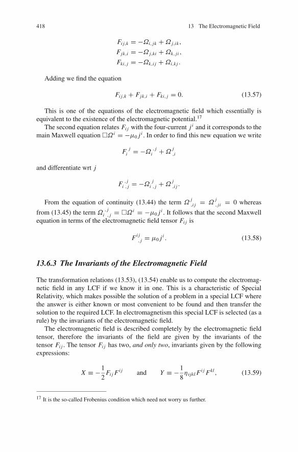
418 13 The Electromagnetic Field
Fi j,k = −Ωi, jk +Ω j,ik,
Fjk,i = −Ω j,ki +Ωk, j i ,
Fki, j = −Ωk,i j +Ωi,k j .
Adding we find the equation
Fi j,k + Fjk,i + Fki, j = 0. (13.57)
This is one of the equations of the electromagnetic field which essentially isequivalent to the existence of the electromagnetic potential.17
The second equation relates Fi j with the four-current j i and it corresponds to themain Maxwell equation �Ω i = −μ0 j i . In order to find this new equation we write
F ji = −Ω , j
i +Ωj,i
and differentiate wrt j
F , ji , j = −Ω j
i , j +Ωj,i j .
From the equation of continuity (13.44) the term Ωj,i j = Ω
j, j i = 0 whereas
from (13.45) the term Ω, j
i , j = �Ω i = −μ0 j i . It follows that the second Maxwellequation in terms of the electromagnetic field tensor Fi j is
Fi j, j = μ0 j i . (13.58)
13.6.3 The Invariants of the Electromagnetic Field
The transformation relations (13.53), (13.54) enable us to compute the electromag-netic field in any LCF if we know it in one. This is a characteristic of SpecialRelativity, which makes possible the solution of a problem in a special LCF wherethe answer is either known or most convenient to be found and then transfer thesolution to the required LCF. In electromagnetism this special LCF is selected (as arule) by the invariants of the electromagnetic field.
The electromagnetic field is described completely by the electromagnetic fieldtensor, therefore the invariants of the field are given by the invariants of thetensor Fi j . The tensor Fi j has two, and only two, invariants given by the followingexpressions:
X ≡ −1
2Fi j Fi j and Y ≡ −1
8ηijkl Fi j Fkl, (13.59)
17 It is the so-called Frobenius condition which need not worry us further.

13.6 Maxwell Equations in Terms of Fi j 419
where ηijkl is the completely antisymmetric tensor with four indices.18
In an LCF Σ these invariants are computed in terms of the electric and the mag-netic fields. Indeed considering the components of Fi j in Σ we have
X = −1
2Fi j Fi j = −(F01 F01+ F02 F02+ F03 F03+F12 F12+ F13 F13+ F23 F23)
= − 1
c2[Ex (−Ex )+ Ey(−Ey)+ Ez(−Ez)]− [B2
x + B2y + B2
z ]
= 1
c2E2 − B2, (13.60)
Y = −1
8ηijkl Fi j Fkl = 4
[η0123 F01 F23 + η1230 F12 F30 + η2301 F23 F01
]
= −4
[Ex
c(−Bx )+ Ey
c(−By)+ Ez
c(Bz)
]
= 1
cE · B. (13.61)
In the next example we show that the quantities 1c2 E2−B2 and 1
c E · B are indeedinvariant under Lorentz transformations.
Example 70 Consider two LCFs Σ and Σ′ which are moving in the standard way andlet E,B and E′,B′ be the electric and the magnetic fields in Σ and Σ′, respectively.Prove that
E · B = E′ · B′ and B2 − 1
c2E2 = B′2 − 1
c2E′2.
First Solution
From the transformation equations (13.53) we have
1
cE′ · B′ = 1
c
[E ′x B ′x + E ′y B ′y + E ′z B ′z
]
= 1
c[Ex Bx + γ 2
(Ey/c − βBz
) (By + βEz
)
+ γ 2(Ez/c + βBy
) (Bz − βEy/c
)]
= 1
c
[Ex Bx +
(γ 2 − γ 2β2
)Ey By +
(γ 2 − γ 2β2
)Ez Bz
]
18 ηijkl i, j, k, l = 0, 1, 2, 3 equals zero if two of the indices have the same value and±1 if (i jkl)is an even or an odd permutation of (0123). See Sect. 13.10.1.

420 13 The Electromagnetic Field
= 1
c
(Ex Bx + Ey By + Ez Bz
)
= 1
cE · B.
Also
1
c 2(E′)2 − (B′) 2 = 1
c 2(E ′ 2x + E ′ 2y + E ′ 2z )− (B ′ 2x + B ′ 2y + B ′ 2z )
= 1
c 2E2
x + γ 2
(1
cEy − βBz
)2
+ γ 2
(1
cEz + βBy
)2
− B2x − γ 2
(By + β
1
cEz
)2
− γ 2
(Bz − β
1
cEy
)2
+ 2γ 2β1
cEz By − 2γ 2β
1
cEz By
= 1
c 2E2
x +(γ 2 − γ 2β2
) 1
c 2E2
y +(γ 2 − γ 2β2
) 1
c 2E2
z
− B2x −
(γ 2 − γ 2β2
)B2
y −(γ 2 − γ 2β2
)B2
z
= 1
c 2(E2
x + E2y + E2
z )− (B2x + B2
y + B2z )
= 1
c 2E2 − B2.
Second SolutionIn this solution we use the transformation equations (13.54) which define the
general Lorentz transformation, therefore the proof is completely general. We have
E′ · B′ = [E‖ + γ (E⊥+v× B)
] ·[
B‖ + γ (B⊥ − 1
c 2v× E)
]
= E‖ · B‖ + γ 2E⊥ · B⊥ − γ 2 1
c 2(v× B)·(v× E).
From classical vector calculus we have the identity
(A× B) · (C× D) = (A · C)(B · D)− (A · D)(B · C).
Using the above identity we compute
1
c2(v× B)·(v× E) =β2(E · B)−β2E‖ · B‖.
Replacing we find

13.7 The Physical Significance of the Electromagnetic Invariants 421
E′ · B′ = (1+ γ 2β2)E‖ · B‖ + γ 2E⊥ · B⊥ − γ 2β2(E · B)
= γ 2(E‖ · B‖ + E⊥ · B⊥)− γ 2β2(E · B) = (γ 2 − γ 2β2)(E · B)
= E · B.
In the same manner one proves the second relation.
13.7 The Physical Significance of the Electromagnetic Invariants
The invariants of the electromagnetic field contain significant information concern-ing the character of the electromagnetic field and can be used to classify the electro-magnetic fields in sets with similar dynamical properties.
As we have seen the electromagnetic field has two invariants, the quantitiesX = 1
c2 E2 − B2 and Y = 1c E · B. X measures the difference of the strengths of
the fields and Y their angle. Therefore we consider the following four cases:
(i) X = Y = 0:The electromagnetic fields with vanishing invariants are characterized by theproperties
1
c| E |=| B | and E⊥B,
that is, in all LCFs the electric and the magnetic fields have the same strengthand they are normal to each other. These electromagnetic fields are callednull electromagnetic fields and we assume that they describe electromagneticwaves.
(ii) X �= 0, Y = 0:The electromagnetic fields with invariants X �= 0, Y = 0 are characterized bythe fact that in an arbitrary LCF either the electric and the magnetic fields areperpendicular and have different strengths or one of them vanishes. Which ofthem vanishes we find from the sign of the invariant X . If X > 0 then only themagnetic field is possible to vanish and if X < 0 then only the electric field ispossible to vanish.
(iii) X = 0, Y �= 0:The electric and the magnetic fields of these electromagnetic fields have equalstrength in all LCFs ( 1
c |E| = |B|) and they are perpendicular in no LCFs. IfY > 0 then (in all LCFs!) their directions make an acute angle and if Y < 0this angle is obtuse. In both cases there exists always a family of LCFs in whichE ‖ B.
(iv) X �= 0, Y �= 0:This case is similar to (iii) with the difference that the strengths of the fieldsE, B are different in all LCFs.

422 13 The Electromagnetic Field
From the above analysis we conclude that we should consider three types ofelectromagnetic fields:
(a) Electromagnetic waves (X = Y = 0)(b) Electromagnetic fields with electric or magnetic field only or both fields per-
pendicular and with different strength (X �= 0, Y = 0)(c) Electromagnetic fields with both electric and magnetic fields (X = 0 or X �=
0 and Y �= 0) for which there exists a family of LCFs in which E ‖ B
Because the invariant Y determines whether the electric and the magnetic fieldsare perpendicular or parallel, in our study we consider the cases Y = 0 and Y �= 0.
13.7.1 The Case Y = 0
Consider an electromagnetic field whose invariant Y = 0. We prove that there existfamilies of LCF in which the electromagnetic field has only electric field (if X > 0)or only magnetic field (if X < 0).
Suppose that in some LCF Σ the electromagnetic field has E = 0 (respectively,B = 0). Then in all LCFs Σ′ with velocities ‖ B (respectively, ‖ E) it has onlymagnetic (respectively, electric) field.
Consider now an arbitrary LCF Σ, in which E �= 0 and B �= 0, and assume thatX < 0. We consider the LCF Σ′ with velocity
u = α(E× B),
where α is a parameter which has to be determined. Because the velocity is perpen-dicular to the fields we have
E‖ = B‖ = 0.
From the transformation equations (13.54) we find for the field E′ in Σ′
E′‖ = B′‖ = 0,
E′⊥ = γ {E⊥+u× B}= γ {E+α [(E× B)× B]} = γ (1− αB2)E,
where we have taken into consideration Y = 1c E ·B = 0. Because we have assumed
X < 0 we can define the LCF Σ′ with the condition E′ = 0, that is, there exists onlymagnetic field. Then the last equation gives
α = 1/B2 ⇒ u = 1
B2(E× B).
The magnetic field B′ in Σ′ is given from the relation (13.54):

13.7 The Physical Significance of the Electromagnetic Invariants 423
B′ = γu
{B− 1
c2u× E
}= γu
(1− E2
c2 B2
)B
and it is B′ ‖ B and also B′⊥u.The LCF Σ′ belongs to the LCF in which there exists only magnetic field and–
as we have shown – in all LCFs Σ′′
with velocities u′ = λB′ relative to Σ′, whereλ is a real parameter, the electromagnetic field has only magnetic part. In order tocompute the velocity v say, of Σ
′′wrt Σ, we apply the relativistic rule of composition
of three-velocities. From Example 20 we have
v = 1
γu Q
{λB′ + u
[u · λB′
u2(γu − 1)+ γu
]},
where Q = 1− u·λBc2 = 1. Replacing we find
v = u+ λ
(1− E2
c2 B2
)B = 1
B2(E× B)+ λ
(1− E2
c2 B2
)B.
In case the invariant X > 0 then working in a similar manner we find
B′ = γ
{B− 1
c2v× E
}= γ
(1− α
E2
c2
)B
and requiring that B′ = 0 we find the velocity
u = c2
E2(E× B).
The electromagnetic field in Σ′ has only electric field, which is given by therelation
E′ = γ (E+ v× B) = γ
(1− c2 B2
E2
)E.
In this case the LCF Σ′ is not unique and all LCFs Σ′′ with velocities
u = c2
E2 (E× B)+ λ(
1− B2c2
E2
)E have the same property.
13.7.2 The Case Y �= 0
In this case the electric and the magnetic fields do not vanish and they are notperpendicular in any LCF. We shall show that in this case there exists a family ofLCFs in which E ‖ B.
We consider a LCF Σ′, which relative to the LCF Σ has velocity u normal to theplane defined by the fields E, B in Σ. We write
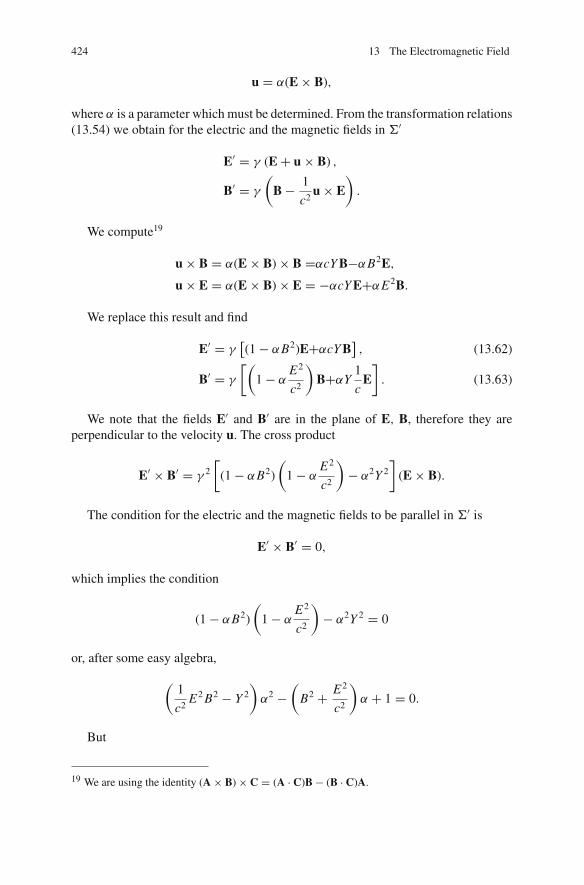
424 13 The Electromagnetic Field
u = α(E× B),
where α is a parameter which must be determined. From the transformation relations(13.54) we obtain for the electric and the magnetic fields in Σ′
E′ = γ (E+ u× B) ,
B′ = γ
(B− 1
c2u× E
).
We compute19
u× B = α(E× B)× B =αcY B−αB2E,
u× E = α(E× B)× E = −αcY E+αE2B.
We replace this result and find
E′ = γ[(1− αB2)E+αcY B
], (13.62)
B′ = γ
[(1− α
E2
c2
)B+αY
1
cE]. (13.63)
We note that the fields E′ and B′ are in the plane of E, B, therefore they areperpendicular to the velocity u. The cross product
E′ × B′ = γ 2
[(1− αB2)
(1− α
E2
c2
)− α2Y 2
](E× B).
The condition for the electric and the magnetic fields to be parallel in Σ′ is
E′ × B′ = 0,
which implies the condition
(1− αB2)
(1− α
E2
c2
)− α2Y 2 = 0
or, after some easy algebra,
(1
c2E2 B2 − Y 2
)α2 −
(B2 + E2
c2
)α + 1 = 0.
But
19 We are using the identity (A× B)× C = (A · C)B− (B · C)A.

13.7 The Physical Significance of the Electromagnetic Invariants 425
Y = 1
cB · E =1
cB E cosϕ ⇒ 1
c2E2 B2 − Y 2 = 1
c2E2 B2 sin2 ϕ =
∣∣∣∣1
cE× B
∣∣∣∣2
.
Also α = β
| 1c E×B| . Replacing we find the following equation for the parameter β:
β2 − B2 + E2
c2
| 1c E× B |β + 1 = 0.
The allowable solution (β < 1) of this equation is
β = 1
2
[A −
√A2 − 4
], (13.64)
where A = B2+ E2
c2
| 1c E×B| ≥ 2. We conclude that the velocity of Σ′ relative to Σ is
u = βc1c E× B
| 1c E× B | ,
where β is given in (13.64).It remains to compute the proportionality factor relating the strengths of the two
fields. We write
B′ = λ1
cE′ ⇒ λ = E′ · cB′
E′2= c2Y
E′2.
For the length E′2 we have from (13.62)
E′2 = γ 2[E2 − 2αB2 E2 + 2αc2Y 2 + α2 E2 B4 − α2c2Y 2 B2
]
= γ 2 E2[1− 2αB2 sin2 ϕ + α2 B4 sin2 ϕ
],
hence
λ = cB cosφ
γ 2 E[1− 2αB2 sin2 ϕ + α2 B4 sin2 ϕ
] .
Σ′ is not the unique LCF in which the electric and the magnetic fields are parallel.Indeed it can be shown easily that the same holds in any other LCF in which therelative velocity of Σ′ is u′ = κ e′, where κ is a real parameter and e′ is the unitvector in the common direction of the fields in Σ′. In order to compute the velocity,u say, of these LCFs relative to Σ we consider the relativistic rule of composition ofthree-velocities and have

426 13 The Electromagnetic Field
u = 1
γv Q
{u′+v
[v · u′v2
(γv − 1)+ γv
]},
where Q = 1 − u·v′c2 . But v · u′ = 0 because the vector e′ is normal to the vectors
E′, B′, hence Q = 1, and
u = 1
γv
(κ
E′
E ′+ vγv
)= v+ κ
γv
E′
E ′.
13.8 Motion of a Charge in an ElectromagneticField – The Lorentz Force
Consider a charge q and assume that in the proper frame of the charge Σ+ thereexists an electric and a magnetic field given by the vectors 1
c E+, B+. We define thethree-force on the charge in Σ+ due to this electromagnetic field to be f+ = qE+.This definition coincides with the Newtonian force on a charge resting in a electricand a magnetic field.20 Then in the proper frame of the charge the four-force Fi =(
0qE+
)
Σ+is completely determined and can be computed in any other LCF using
the appropriate Lorentz transformation.However, instead of using the Lorentz transformation to compute the three-force
in an arbitrary LCF, Σ say, it is more fundamental to write the four-force Fi covari-antly in an arbitrary LCF and then compute the three-force on the charge in Σ bytaking the components of the quantities involved in Σ.
In order to do that we note that the four-velocity ui of the charge q in Σ+ has
components [ui ] =(
c0
)
Σ+and similarly the electromagnetic field tensor in Σ+
[Fi j ] =
⎛
⎜⎜⎝
0 −E+x /c −E+y /c −E+z /cE+x /c 0 B+z − B+yE+y /c − B+z 0 B+xE+z /c B+y − B+x 0
⎞
⎟⎟⎠
Σ+
.
Then using the definition of the four-force in Σ+ we have (in Σ+) the relation
Fi = q Fi j uj . (13.65)
20 Recall that the definitions of physical quantities in Special Relativity are made in the properframe and coincide with the corresponding Newtonian quantities (provided they exist). This is thegeneral rule – strategy – for defining physical quantities in Special Relativity and it is justified bythe facts that (a) the physical quantities are understood and manipulated in the Newtonian worldand (b) Special Relativity must be understood physically in the Newtonian world. The differenceintroduced by Special Relativity is in the transformation of these quantities from LCF to LCF.

13.8 Motion of a Charge in an Electromagnetic Field – The Lorentz Force 427
But j i = qui is the four-current due to the charge. Therefore the four-force actingon the charge q (in Σ+!) is written covariantly as
Fi = Fi j J j . (13.66)
This relation has been proved in Σ+ but because it is covariant it is valid in anyother LCF, therefore it defines the four-force on the charge due to the electromag-netic field.21
In order to compute the force on a charge moving with velocity u in an electro-magnetic field E/c,B in an LCF Σ we work as follows. In Σ the electromagneticfield tensor is
[Fi j ] =
⎛
⎜⎜⎝
0 −Ex/c −Ey/c −Ez/cEx/c 0 Bz − By
Ey/c − Bz 0 Bx
Ez/c By − Bx 0
⎞
⎟⎟⎠
Σ
and let the four-velocity of the charge ui =(γucγuu
)
Σ
. We know that the four-force
Fi due to a three-force f in Σ is given by the expression Fi =(γu
1c E
γuf
)
Σ
, where Eis the rate of change of the energy of the charge in Σ under the action of the force f(in Σ!). Replacing this in the lhs of (13.65) we find
(γu
1c E
γuf
)
Σ
= q
⎛
⎜⎜⎝
0 −Ex/c −Ey/c −Ez/cEx/c 0 Bz − By
Ey/c − Bz 0 Bx
Ez/c By − Bx 0
⎞
⎟⎟⎠
Σ
(γucγuu
)
Σ
= qγu
(1c E · u
E+ u× B
)
Σ
.
From this result follow two important conclusions:
• The magnetic field does not change the energy of the charge (does not producework). Work is produced only by the electric field E and it is given by the relation
dEdt= qE · u. (13.67)
• The three-force on the charge q in Σ due to the electromagnetic field E/c,B (inΣ!) is given by the formula
21 In case we have a charge density ρ instead of a single charge, then the four-vector Fi is the
density of four-force and J i is the density of the four-current of the charge J i =(ρcj
)
Σ
.

428 13 The Electromagnetic Field
f = q (E+ u× B) . (13.68)
This force is known as the Lorentz force to remind Lorentz who first gave thisformula prior to the invention of Special Relativity. We note that this equation doesnot contain the factor γu and this fact sometimes obscures its relativistic origin.However, as we have shown this is a purely relativistic formula.
The equation of motion of a relativistic point, P say, under the action of a four-force Fi is given by the relativistic generalization of the Second Law of Newton:
Fi = dpi
dτ, (13.69)
where pi is the four-momentum of the mass point and τ is its proper time. In an
LCF Σ Fi =(γ 1
c Eγ f
)
Σ
, pi =(E/cp
)
Σ
and this equation gives
(γu
1c E
γuf
)
Σ
= γd
dt
(E/cp
)
Σ
,
where t is time in Σ and γ = dtdτ . The zeroth coordinate gives
E = f · v (13.70)
and the space coordinate gives the equation of motion
f = dpdt
. (13.71)
The first relation expresses the conservation of kinetic energy, that is, a motion inwhich the three-force is always normal to the velocity, the energy – and consequentlythe speed – is a constant of motion. The second equation is the equation of motionand constitutes the generalization of Newton’s Second Law in Special Relativity.
In accordance with the above the equation of motion of a charge q with velocityv in an LCF Σ in which the electromagnetic field is given by the vectors ( 1
c E, B) is
dpdt= q (E+ v× B) . (13.72)
The equation of motion (13.72) can be written using the results of Exercise 43:
q (E+ v× B) = mγ v+ mγ a = mγ (γ 2a|| + a⊥). (13.73)

13.9 Motion of a Charge in a Homogeneous Electromagnetic Field 429
Another equivalent form of this equation is in terms of the proper time of thecharge. In this case we use the relation γ = dt
dτ and find
dpdτ= γ f =q
(dt
dτE+ dr
dτ× B
). (13.74)
13.9 Motion of a Charge in a HomogeneousElectromagnetic Field
In this section we study the motion of a charge q of mass m in an LCF Σ, in whichthere exists a homogeneous electromagnetic field with (constant) 1
c E, B. The equa-tion of motion of the charge is (13.72) or (13.74), whose solution gives the orbit ofthe charge in Σ. In general the solution of the equations of motion is difficult andone looks for simplifications and shortcuts which could make the solution possible.This is indeed the case and will be shown below.
As we have shown in Sect. 13.7 for every electromagnetic field there are LCFsin which the electric and the magnetic vectors of the field have one of the followingforms, depending on the values of the invariants of the field:
a. Only electric field (X > 0, Y = 0)b. Only magnetic field (X < 0, Y = 0)c. Electric and magnetic fields perpendicular and of equal strength (X = 0, Y = 0)d. Electric and magnetic fields parallel and with different strength (X �= 0, Y �= 0)
This means that it is enough to solve the equations of motion of the charge in oneof these cases in order to cover all possible homogeneous electromagnetic fields.
In practice the algorithm for studying the motion of a charge in an arbitraryhomogeneous electromagnetic field consists of the following steps:
• Calculate the invariants.• Determine the type of the electromagnetic field, determine the appropriate LCF,
and calculate the electromagnetic field in that LCF.• Write and solve the equations of motion in that LCF.• Transfer the solution by means of the appropriate Lorentz transformation to the
original LCF.
In the following we solve the equations of motion for every one of the specialcases (a)–(d) above.
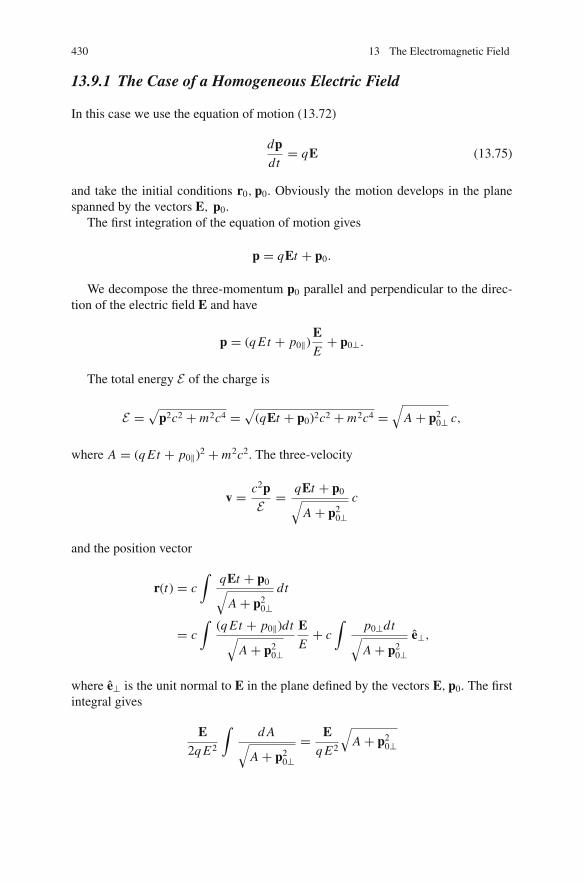
430 13 The Electromagnetic Field
13.9.1 The Case of a Homogeneous Electric Field
In this case we use the equation of motion (13.72)
dpdt= qE (13.75)
and take the initial conditions r0,p0. Obviously the motion develops in the planespanned by the vectors E, p0.
The first integration of the equation of motion gives
p = qEt + p0.
We decompose the three-momentum p0 parallel and perpendicular to the direc-tion of the electric field E and have
p = (q Et + p0‖)EE+ p0⊥.
The total energy E of the charge is
E =√
p2c2 + m2c4 =√
(qEt + p0)2c2 + m2c4 =√
A + p20⊥ c,
where A = (q Et + p0‖)2 + m2c2. The three-velocity
v = c2pE =
qEt + p0√A + p2
0⊥c
and the position vector
r(t) = c∫
qEt + p0√A + p2
0⊥dt
= c∫
(q Et + p0‖)dt√A + p2
0⊥
EE+ c
∫p0⊥dt√A + p2
0⊥e⊥,
where e⊥ is the unit normal to E in the plane defined by the vectors E,p0. The firstintegral gives
E2q E2
∫d A√
A + p20⊥= E
q E2
√A + p2
0⊥

13.9 Motion of a Charge in a Homogeneous Electromagnetic Field 431
and the second
∫p0⊥dt√A + p2
0⊥= p0⊥
q Eln
[q Et + p0‖ +
√(q Et + p0‖)2 + p2
0⊥ + m2c2
].
Replacing we find
r(t) = Ec
q E2
√(q Et + p0‖)2 + m2c2 + p2
0⊥ (13.76)
+ p0⊥c
q Eln
∣∣∣∣q Et + p0‖ +√
(q Et + p0‖)2 + p20⊥ + m2c2
∣∣∣∣ e⊥ + C.
Taking into account the initial conditions we compute for the constant C
C = r0 − c
q E
(E0EEc+ p0⊥ln
∣∣∣∣E0
c+ p0‖
∣∣∣∣ e⊥
).
Second SolutionWithout restricting generality we consider the x-axis along the direction of the
electric field and the y-axis in the plane spanned by the vectors E,p0. Then E = E iand the initial conditions become
x(0) = y(0) = z(0) = 0,
dct
dτ= E0
mc,
dx
dτ= p0x
m,
dy
dτ= p0y
m,
where E0 =√
p20c2 + m2c4 is the initial energy of the charge and τ its proper time.
We consider the equations of motion in the form (13.69) and write
mdxi2
dτ 2= Fi =
(γ dE
cdt
γ qE
).
But
γdEdt= γ f · v = γ q E
dx
dt= q E
dx
dτ,
hence the equations of motion in the LCF we are working become

432 13 The Electromagnetic Field
d2ct
dτ 2= q E
mc
dx
dτ,
d2x
dτ 2= q E
mc
dct
dτ, (13.77)
d2 y
dτ 2= 0,
d2z
dτ 2= 0.
The solution of these equations, with the initial conditions we have considered,is
x(τ ) = E0
q E
(cosh
q Eτ
mc− 1
)+ cp0x
q Esinh
q Eτ
mc,
y(τ ) = p0yτ
m, (13.78)
z(τ ) = 0,
ct(τ ) = E0
q Esinh
q Eτ
mc+ cp0x
q E
(cosh
q Eτ
mc− 1
).
In order to calculate the motion of the particle in Σ we express the proper timeτ in terms of the time t of Σ. This is done as follows. The x-component of thethree-momentum is
px = mux = mdx
dτ= E0
csinh
q Eτ
mc+ p0x cosh
q Eτ
mc.
Similarly the energy (=zeroth coordinate of the four-momentum) is
Ec= mu0 = 1
c
(E0 cosh
q Eτ
mc+ cp0x sinh
q Eτ
mc
).
We add
E + cpx = (E0 + cp0x ) expq Eτ
mc⇒
τ = mc
q Eln
∣∣∣∣E + cpx
E0 + cp0x
∣∣∣∣ . (13.79)
In detail this relation is written as follows:
τ = mc
q Eln
∣∣∣∣∣∣
p0x + q Et +√
(p0x + q Et)2 + m2c2 + p20y
p0x + E0/c
∣∣∣∣∣∣. (13.80)

13.9 Motion of a Charge in a Homogeneous Electromagnetic Field 433
Replacing τ in (13.78) the motion of the particle in Σ is found to be
x(t) = c
q E
(√(p0x + q Et)2 + m2c2 + p2
0y −E0
c
), (13.81)
y(t) = cp0y
q Eln
∣∣∣∣∣∣
p0x + q Et +√
(p0x + q Et)2 + m2c2 + p20y
p0x + E0/c
∣∣∣∣∣∣,
z(t) = 0.
It is of interest to examine the Newtonian and the relativistic limit of this result.In the Newtonian limit p0 � mc and t � mc
q E from which follows easily that themotion of the charge in Σ is given by the classical solution
x(t) = p0x t
m+ q E
2mt2,
y(t) = p0yt
m,
z(t) = 0.
In the relativistic limit for large times t � mcq E the speed of the charge approaches
the value c even if originally small. In this limit the motion of the charge is
x(t) = ct − mc2
q E,
y(t) = cp0y
q Eln
2|q|Et
mc, (13.82)
z(t) = 0.
In Fig. 13.2 it is shown the distance x(t) for the initial conditions p0x = p0y = 0and in addition the Newtonian (t � mc
q E ) and the relativistic limit (t � mcq E ) of
motion are indicated.
Fig. 13.2 Motion of a Charge in a Homogeneous Electric Field

434 13 The Electromagnetic Field
In order to compute the equation of the trajectory of the charge in Σ we eliminatethe proper time τ from (13.78) and find
x = E0
q E
(cosh
q Ey
cp0y− 1
)+ cp0x
q Esinh
q Ey
cp0y. (13.83)
In the Newtonian limit E0 = mc2 , p0 � mc and |q|Eycp0y� 1 because the momen-
tum of the charge must be small compared to mc. Using these results one obtainsthe well-known Newtonian result
x = mq Ey2
2p20y
+ p0x
p0yy.
13.9.2 The Case of a Homogeneous Magnetic Field
The equation of motion of a charge in a homogeneous magnetic field is
dpdt= qv× B. (13.84)
Multiplying with p we find
dpdt
p = 0⇒ p2 = constant⇒ E =√
p20 + m2c4 = constant.
The speed v = |p0|c2
E = constant. Using the constant energy we rewrite theequation of motion as follows:
Ec2
.v = qv× B
and we study the motion parallel and perpendicular to the magnetic field. Integrat-ing (13.84) parallel to the magnetic field we find
r‖ = v‖(0)t + r‖(0).
The speed22
22 It is possible to integrate the equations of motion directly and not use the first integrals. This isdone as follows. Without restricting the generality we consider the z-axis along the direction of themagnetic field (B = Bk) in which case the equations of motion in the direction perpendicular tothe magnetic field give

13.9 Motion of a Charge in a Homogeneous Electromagnetic Field 435
v2 = v2⊥ + v2
‖ ⇒ |v⊥(t)| = constant = |v⊥(0)| .
This result is an additional integral of motion and implies that
v⊥(t) = v⊥(0)eωt ,
where ω is a real parameter. In order to determine ω we differentiate v⊥(t) and usethe equation of motion. We find
.v⊥(t) = v⊥(0)ωeωt = ωv⊥(t),
therefore
Ec2
ωv⊥(t) = qv⊥(t)B ⇒ ω = qc2 B
E = q B
mγ.
The parameter ω is called the cyclotronic frequency and it is known from New-tonian Physics. Integrating once more we find the motion perpendicular to the mag-netic field:
r⊥(t) = v⊥(0)
ωeωt + r⊥(0).
From the solution of the equations of motion we conclude that the motion of acharge in a constant magnetic field is a combination of two motions: a translational
mγ0υx = q Bυy
mγ0υy = −q Bυx
}⇒ υx = ωυy
υy = −ωυx,
where ω = q Bmγ0
. To solve this system of simultaneous equations we multiply the second with i andadd. It follows:
(υx + i υy
) = −iω(υx + iυy
)⇒w(t) = w(0)e−iωt , where w(t) = υx + iυy .
Equating the real and the imaginary parts we find
υx (t) = υx (0) cosωt + υy(0) sinωt,
υy(t) = υx (0) sinωt − υy(0) cosωt.
Let us assume for simplicity the initial conditions υx (0) = υ, υy(0) = 0. Then υx (t) =υ cosωt, υy(t) = υ sinωt . Integrating these last relations we find for the motion perpendicularto the direction of the magnetic field
x(t) = x0 + υ
ωsinωt,
y(t) = y0 − υ
ωcosωt.

436 13 The Electromagnetic Field
motion with constant speed parallel to the magnetic field and a uniform circularmotion in the normal plane to the magnetic field with frequency ω.
In the Newtonian limit ω = q Bm .
13.9.3 The Case of Two Homogeneous Fields of Equal Strengthand Perpendicular Directions
This case concerns the motion of a charge in an electromagnetic field in which theelectric and the magnetic fields are related as follows: E
c = B and E · B=0. Withoutrestricting generality we consider E = E j and B = E
c k. Then the equations ofmotion
.p = q(E+ v× B)
become
.px =
q
cvy E,
.py = q E
(1− vx
c
),
.pz = 0.
The last equation gives
Pz = p0z = constant.
In order to solve the remaining two equations we are looking for first integrals.We note that the energy E is written as
E2 − p2x c2 = p2
yc2 + C21 , (13.85)
where C21 = p2
z c2 + m2c4. But
E = f · v =q Evy = px c⇒ E − px c = a = constant,
where in the first step we have used the equation of motion for py . Combining thisresult with (13.85) we find
E + px c = p2yc2 + C2
1
a. (13.86)
From the last two relations we find by adding and subtracting

13.9 Motion of a Charge in a Homogeneous Electromagnetic Field 437
E = a
2+ p2
yc2 + C21
2a, (13.87)
px = − a
2c+ p2
yc2 + C21
2ac. (13.88)
The second equation of motion gives for the quantity.py
.py = q E
(1− px c
E)= q E
E (E − px c) = q Ea
E ⇒ E .py = qEa.
Replacing E from (13.87) we have
∫ (a2 + C2
1
2a+ c2
2ap2
y
)dpy = qEat
and finally
c2
3a2p3
y +(
1+ C21
a2
)py = 2q Et + constant. (13.89)
In order to compute the motion (that is the functions x(t), y(t), z(t)) we use(13.89) and replace time with the variable py . This is done as follows.
We consider initially the coordinate x(t) and note that the velocity vx can beexpressed in two ways, either as
vx = px c2
Eor as
vx = dx
dt= dx
dpy
dpy
dt= dx
dpy
qaE
E .
Equating these two expressions we find the differential equation
dx
dpy= px c2
qaE= c2
qaE
(− a
2c+ p2
yc2 + C21
2ac
)= c
2q E
(−1+ p2
yc2 + C21
a2
),
whose solution is
x(py) = c
2q E
[(−1+ C2
1
a2
)py + c2
3a2p3
y
]+ x(0). (13.90)
Similarly for the y(t) coordinate we compute

438 13 The Electromagnetic Field
vy = pyc2
E ,
vy = dy
dt= dy
dpy
dpy
dt= dy
dpy
qaE
E
from which follows
dy
dpy= c2
qaEpy ⇒ y(py) = c2
2qaEp2
y + y(0). (13.91)
Finally for the z(t) coordinate we have
dz
dpy= pz0c2
qaE⇒ z(py) = pz0c2
qaEpy + z(0). (13.92)
13.9.4 The Case of Homogeneous and Parallel Fields E ‖ B
In this case the electric and the magnetic fields are parallel and affect indepen-dently the motion of the charge, the electric field along the common direction ofthe fields, and the magnetic field normal to this direction. Therefore the motion canbe considered as a combination of two motions: one motion under the action of ahomogeneous electric field and a second motion under the action of a homogeneousmagnetic field. These two motions are related via the energy of the charge, whichdepends on its speed (contrary to the Newtonian case).
Without restricting generality we assume the z-axis along the common directionof the fields and write E = Ek, B = Bk. The equations of motion are
px = qvy B, py = −qvx B, pz = q E . (13.93)
Because vx = px c2
E and similarly for vy , the equations of motion become
px = q Bc2
E py, py = −q Bc2
E px , pz = q E . (13.94)
The third equation concerns the motion under the action of a homogeneous elec-tric field and has been studied in Sect. 13.9.1. The solution is (see (13.81))
z(t) = c
q E
(√(p0z + q Et)2 + m2c2 + p2
0⊥ −E0
c
), (13.95)
where p0⊥ = p0x i + p0yj and E0 is the energy of the charge at the moment t = 0.We also have
pz(t) = q Et.

13.9 Motion of a Charge in a Homogeneous Electromagnetic Field 439
Differentiating E2 = p2c2+m2c4 wrt time and using the equations of motion wefind EE = pz pz from which follows
E =√
p2z c2 + E2
0 =√
(q Ect)2 + E20 . (13.96)
Concerning the solution of the remaining two equations we cannot apply theprevious study dealing with the motion of a charge in a homogeneous magneticfield because now the energy of the charge is not constant. From the equations ofmotion we have
px px + py py = 0 ⇒ p2x + p2
y = constant = p2⊥ = p2
⊥, (13.97)
therefore we have the first integral
px + i py = p⊥e−iφ, (13.98)
where φ is a real parameter. Differentiating (13.98) wrt t and replacing px , py fromthe equations of motion we find for the parameter φ the equation
φ = q Bc2
E = q Bc2
√(q Ect)2 + E2
0
. (13.99)
Integrating wrt t we find eventually (φ(0) = 0)
ct = E0
q Esinh
φE
Bc.
Using this equation we can change the variable t with φ facilitating the integra-tion of the equations of motion. Indeed we have
px + i py = Ec2
(vx + ivy) = Ec2
d(x + iy)
dt= E
c2
dφ
dt
d(x + iy)
dφ
= Ec2
q Bc2
Ed(x + iy)
dφ= q B
d(x + iy)
dφ.
Integrating wrt φ
x + iy = p⊥q B
∫
0e−iφdφ = i
p⊥q B
(e−iφ − 1)+ x(0)+ iy(0)
from which follows
x(φ) = p⊥q B
sinφ + x(0), y(φ) = p⊥q B
(cosφ − 1)+ y(0).

440 13 The Electromagnetic Field
Concerning the z(t) coordinate we find in a similar fashion
q Et = Ec2
z = E
c2
dφ
dt
dz
dφ⇒ dz
dφ= E0
q Bcsinh
φE
Bc.
Integrating
z(φ) = E0
q E
(cosh
φE
Bc− 1
)+ z(0).
The orbit of the charge is a helix with constant radius p⊥q B and a pace which
increases monotonically. The angular speed of rotation equals dφdt = q Bc2
E and dimin-ishes with time whereas the speed of the translational motion along the commondirection of the fields increases continually with limiting value c.
13.10 The Relativistic Electric and Magnetic Fields
In the previous sections we developed the theory of the electromagnetic field usingthe three-vector notation. This formulation, although it is more tangible to the new-comer in Special Relativity, lacks the consistency and the power of the four-vectorformalism. Furthermore it cannot be used in General Relativity in which the four-formalism is a must. For these reasons in the present and the following sectionswe discuss the theory of the electromagnetic field using the four-formalism. In par-ticular we consider the case of a homogeneous and isotropic material, the emptyspace being the extreme particular case. Although it is not necessary, we shall keepc in the formulae in order to make them applicable to numerical calculations. Thismeans that the four-velocity of a comoving observer is ua = cδa
0 (ua = −cδ0a). All
frames are assumed to be Lorentz orthonormal frames (i.e., LCF) so that the metricηab = (−1, 1, 1, 1).
13.10.1 The Levi-Civita Tensor Density
In the following we shall use the antisymmetric tensor Fab, hence it is necessary thatwe shall discuss concisely the basic tool in the manipulation of such tensors, that isthe Levi-Civita tensor density.
In Minkowski space the alternating tensor is defined as follows:
ηabcd = η[abcd], η0123 = (−g)−1/2 = −η0123, (13.100)
where g = det(gab). It has the following properties:

13.10 The Relativistic Electric and Magnetic Fields 441
ηcabdηcmnr = −3!δ[am δb
nδd]r
= − (δa
mδbnδ
dr − δa
mδdn δ
br + δb
mδdn δ
ar − δb
mδanδ
dr + δd
mδanδ
br − δd
mδbnδ
ar
),
(13.101)
ηabcdηabst = −4δ[cs δ
d]t = −2(δc
s δdt − δd
s δct ), (13.102)
ηabcdηabct = −3!δdt , (13.103)
ηabcdηabcd = −4!. (13.104)
In the Euclidean three-dimensional space the alternating tensor is defined as fol-lows:
ημνρ = η[μνρ], η123 = h−1/2,
where h = det(hμν) and satisfies the properties
ημνρημστ = 2δ[νσ δρ]
τ , ημνρημντ = 2δρτ . (13.105)
Usually in Euclidean space ημνρ is written as εμνρ because the determinant of theEuclidean metric equals 1, therefore the tensor density becomes a tensor. However,we should not worry about that and we shall keep the notation ημνρ for uniformity.Examples
1. Consider the Euclidean vectors u = uμeμ, v = vμeμ where {e} is an orthonormalbasis, e.g., the {i, j,k}. Then the cross product
u× v = ημνρuνvρ eμ or (u × v)μ = ημνρuνvρ.
2. Let us prove the well-known identity of vector calculus:
A× (B× C) = (A · C)B− (A · B)C.
We have
[A× (B× C)]μ = ημνρ Aν(B× C)ρ = ημνρ Aνηρστ BσCτ
= ημνρηρστ Aν BσCτ
= (δμσ δντ − δνσ δ
μτ )Aν BσCτ = (AνCν)Bμ − (Aν Bν)Cμ
= [(A · C)B− (A · B)C]μ .
3. For every antisymmetric tensor Aμν = 12
(Aμν − Aνμ
)we define the vector
Rμ = 1
2ημνρ Aνρ. (13.106)
Conversely for every vector Rμ we define the antisymmetric tensor
442 13 The Electromagnetic Field
Aμν = ημνρ Rρ. (13.107)
4. The curl of a vector field Bμ is the antisymmetric tensor Aμν = B[μ,ν].
In Minkowski space the above remain the same except that we have more termsand changes of sign. The relation which we shall use frequently is the definition ofa vector from an antisymmetric tensor:
ωa = 1
2c2ηabcdωbcud , (13.108)
where ud is the four-velocity. The four-vector ωa is spacelike, that is ωaua = 0. Theinverse relation is
ωab = ηabcdωcud . (13.109)
These are the basics one should know in order to be able to follow the subsequentcalculations. It is strongly advised that the reader read and understand these conceptsproperly before he/she continues.
13.10.2 The Case of Vacuum
As we have seen the electromagnetic field in vacuum for a given LCF Σ is describedby the three-electric and the three-magnetic fields E, B (in Σ). These fields are thecomponents of the electromagnetic field tensor Fab in Σ. The tensor Fab, althoughdetermined in Σ, is independent of Σ and characterizes the electromagnetic fieldonly. This means that the vector fields E, B essentially require two tensors to bedefined, i.e., the tensor Fab and the (relativistic) observer with four-velocity ua
observing the electromagnetic field. Using this observation we introduce a (rela-tivistic) electric and a (relativistic) magnetic induction field Ea, Ba , respectively,as follows:
Ea = Fabub, Ba = 1
2cηabcd Fbcud , (13.110)
where ηabcd is the Levi-Civita density ηabcd . For reasons which we shall explainsoon we name these new four-vectors the four-electric field and the four-magneticinduction. The following relations are obvious:
Eaua = Baua = 0, (13.111)
that is, the four-vectors Ea, H a are spacelike.Let us compute the components of Ea, Ba in the proper frame of the observer,
Σ+ say, in which we assume that the electromagnetic field tensor is given by

13.10 The Relativistic Electric and Magnetic Fields 443
[Fi j ] =
⎛
⎜⎜⎝
0 −E+x /c −E+y /c −E+z /cE+x /c 0 B+z − B+yE+y /c − B+z 0 B+xE+z /c B+y − B+x 0
⎞
⎟⎟⎠
Σ+
while ua =(
c0
)
Σ+. Replacing these coordinate expressions in (13.110) we com-
pute easily23
Ea =(
0E+
)
Σ+, Ba =
(0
B+
)
Σ+.
What is the difference among the fields Ea, H a and E, B? The difference is thatthey coincide only in the proper frame Σ+ of the observer while in the frame ofany other LCF Σ the Ea, H a are computed by the proper Lorentz transformationrelating Σ,Σ+ while the E, B are computed from the transformed components ofthe tensor Fi j via the relations
E = c
⎛
⎝F01
F02
F03
⎞
⎠ , B =⎛
⎝−F23
−F31
−F12
⎞
⎠ . (13.112)
We remark that the fields Ea, H a depend on the observer ui while the tensor Fab
is the same for all observers and characterizes the electromagnetic field only.We consider the LCF Σ in which there exists the electromagnetic field Fab given
by the following matrix:
[Fi j ] =
⎛
⎜⎜⎝
0 −Ex/c −Ey/c −Ez/cEx/c 0 Bz − By
Ey/c − Bz 0 Bx
Ez/c By − Bx 0
⎞
⎟⎟⎠
Σ
. (13.113)
In order to compute the components of the electric field observed by an observer
ua whose four-velocity in Σ is ua =(γ cγ v
)
Σ
we multiply the matrices
[Ea] = [Fab][ub]
23 It will help if we demonstrate the computation of the components of the four-vector for themagnetic field. For example for the Bx coordinate we have
Bx = 1
2cηxjkl F jkul = 1
2cc ηxtjk F jk = −1
2ηtxyz (F yz − Fzy) = F yz = B+x .

444 13 The Electromagnetic Field
from which follows
Ea =(γ
E · vc
, γ (E+ v× B)
)
Σ
. (13.114)
Exercise 60 Show that the components of the magnetic field Ba in Σ are as follows:
Ba =(γ
B · vc
, γ
(B− 1
c2v× E
))
Σ
. (13.115)
Are these results compatible with the ones we found in (13.55) and (13.56)?
It is possible to express the tensor Fab in terms of the vector fields Ea, Ba . Thesimplest way to do this is to consider the fields Ea, Ba in the proper frame of theobserver ui and show that
Fab = − 1
c2(Eaub − Ebua)+ 1
cηabcd Bcud . (13.116)
This equation although proved in one frame holds in all frames because it is atensor equation.
Exercise 61 Verify (13.116) by replacing Fi j in (13.110).
The four-force Fa on a four-current J a which is moving under the action of theelectromagnetic field Fab is given by the expression (see Sect. 13.8)
Fa = Fab jb, (13.117)
hence the equation of motion of a charge of mass m is
d
dτ(mua) = Fa
b jb, (13.118)
where ua is the four-velocity of the proper observer of the charge and τ is the propertime of that observer.
Exercise 62 An observer with four-velocity ua =(γ cγ v
)
Σ
observes the electric
field Ea =(
γE · v/cγ (E+ v× B)
)
Σ
. Show that the equation of motion of a charge q in
Σ is as follows:
γ γ = q
mγ
E · vc2⇔ dγ
dτ= q
mγ
E · vc2
, (13.119)
vγ + γ a = q
mγ (E+ v× B)⇔d(γ v)
dτ= q
mγ (E+ v× B) , (13.120)
where τ is the proper time of the charge.

13.10 The Relativistic Electric and Magnetic Fields 445
[Hint: Use that the four-acceleration of the observer in Σ is given by aa =(γ γ
vγ + γ a
)
Σ
where γ = dγdt , a = dv
dt , and t is time in Σ.]
In Sect. 13.6.2 we have seen that Maxwell equations in vacuum in terms of theelectromagnetic field tensor Fab are written as follows:
F{ab,c} = 0, (13.121)
Fab,b = μ0 J a, (13.122)
where {ab, c} means cyclic sum in all enclosed indices. Furthermore the continuityequation for the charge is expressed by the equation
J a,a = 0. (13.123)
The above equations are the basic equations of the electromagnetic field for thevacuum in the four-formalism.
13.10.3 The Electromagnetic Theory for a General Medium
As it has been said at the beginning of this chapter the electromagnetic field for anLCF Σ in a general medium is specified by the following four three-vectors:
1. Electric field E2. Magnetic field B3. Electric displacement field D4. Magnetic displacement field H
As the vectors E,B define in Σ the antisymmetric tensor Fab (13.113), in thesame manner the fields D,H define in Σ the antisymmetric tensor Kab as follows:
Kab =
⎛
⎜⎜⎝
0 −Dx −Dy −Dz
Dx 0 Hz/c − Hy/cDy − Hz/c 0 Hx/cDz Hy/c − Hx/c 0
⎞
⎟⎟⎠
Σ
. (13.124)
Therefore in a general medium the electromagnetic field is expressed by twodifferent (antisymmetric) tensors, the electromagnetic field tensor Fab and the induc-tion field tensor Kab. This means that for a general material an observer with four-velocity ua defines the following four spacelike four-vectors:
1. The electric field:
Ea = Fabub. (13.125)

446 13 The Electromagnetic Field
2. The electric displacement field:
Da = 1
cK abub. (13.126)
3. The magnetic induction field:
Ba = 1
2cηabcd Fbcud . (13.127)
4. The magnetic field strength:
Ha = 1
2ηabcd K bcud . (13.128)
These four-vector fields express the “interaction” of the observer with the electro-magnetic field and they are in general different for the same electromagnetic fieldand different observers. In order to compute the components of these fields in an
LCF Σ in which the four-velocity of the observes ua =(γ cγ v
)
Σ
we use (13.124)
and multiply with the matrix representation of ua . For example the components ofthe electric induction Da in Σ are computed from the multiplication of the matrices:
[Da] = [Kab][ub].
Replacing we find
Da =(γD · v, γ c
(D+ 1
c2v×H
))
Σ
. (13.129)
Exercise 63 Show that the components of the magnetic field H a in Σ are as follows:
H a =(γ
H · vc
, γ (H− v× D)
)
Σ
. (13.130)
Relations (13.125) to (13.128) can be inverted to express Fab and Kab in termsof the vector fields Ea, Ba, Da, H a as follows:
Fab = 1
c2(−Eaub + Ebua)+ 1
cηabcd Bcud , (13.131)
Kab = 1
c(−Daub + Dbua)+ 1
c2ηabcd H cud . (13.132)
Exercise 64 Prove (13.132) by replacing the expressions of Kab in (13.128). SeeExercise 61.

13.10 The Relativistic Electric and Magnetic Fields 447
In the literature use is made of the dual form of the tensors Fab and Kab byapplying the theory of bivectors. A bivector is any second-order antisymmetrictensor Xab = −Xba. A bivector is called simple if it can be written in the formXab = A[a Bb] where Aa, Ba are vectors.
The dual bivector X∗ab of a bivector Xab is defined as follows:
X∗ab = 1
2ηabcd Xcd ⇔ Xab = −1
2ηabcd X∗cd . (13.133)
It is easy to show that in the LCF Σ the components of the dual bivectorsF∗ab, K ∗ab are
[F∗ab ] =
⎛
⎜⎜⎝
0 −Bx/c −By/c −Bx/cBx/c 0 Ez − Ey
By/c − Ez 0 Ex
Bx/c Ey − Ex 0
⎞
⎟⎟⎠
Σ
, (13.134)
[K ∗ab ] =
⎛
⎜⎜⎝
0 −Hx/c −Hy/c −Hz/cHx/c 0 Dz − Dy
Hy/c − Dz 0 Dx
Hz/c Dy − Dx 0
⎞
⎟⎟⎠
Σ
. (13.135)
Exercise 65 Show that in the comoving frame the magnetic induction and the mag-netic field intensity are given by the relation
F∗abub = (0, Bx , By, Bz)Σ+ , K ∗abub = (0, Hx , Hy, Hz)Σ+ .
Then prove that the dual bivectors F∗ab, K ∗ab in terms of the vector fields of theelectromagnetic field are written as follows:
F∗ab = −1
cBaub + 1
cBbua − 1
c2ηabcd Ecud , (13.136)
K ∗ab = −1
c2Haub + 1
c2Hbua − 1
cηabcd Dcud . (13.137)
Exercise 66 Prove the following formulae:
Ba = F∗abub, H a = K ∗abub, (13.138)
Ea = −1
2ηabcd F∗bcud , Da = 1
2cηabcd K ∗bcud . (13.139)
448 13 The Electromagnetic Field
13.10.4 The Electric and Magnetic Moments
Consider an electromagnetic field which is described by the tensors Fab, Kab. Wedefine the magnetization tensor
Mab = −√
ε0
μ0Fab + Kab. (13.140)
If ua is the four-velocity of an observer we define the four-vectors
Pa = 1
cMabub, (13.141)
Ma = 1
2ηabcd Mbcud . (13.142)
Pa is called the polarization four-vector and Ma the magnetization four-vector.
Exercise 67 a. Show that for a general medium
Pa = Da − ε0 Ea, (13.143)
Ma = Ha − 1
μ0Ba . (13.144)
Deduce that in empty space Pa = Ma = 0, hence the polarization and themagnetization fields measure properties of matter.
b. Show that in a homogeneous and isotropic medium the polarization and the mag-netization vectors are given by the following formulae:
Pa = (ε − ε0)Ea, (13.145)
Ma =(
1− μ
μ0
)H a . (13.146)
c. Making use of (13.114),(13.115),(13.129),(13.130) show that:
Pa = γ
((D−ε0
cE)·v, c
(D−ε0
cE)+ v×
(1
cH−ε0E
))
Σ
, (13.147)
Ma = 1
cγ
(1
c
(H− 1
μ0B)·v,H− 1
μ0B− v×
(D−ε0
cE))
Σ
. (13.148)
13.10.5 Maxwell Equations for a General Medium
For a general medium Maxwell equations take the form
K ab;b = J a, (13.149)
F∗ab;b = 0, (13.150)

13.10 The Relativistic Electric and Magnetic Fields 449
where J a is the four-current density and F∗ab = 12η
abcd Fcd is the dual bivector ofthe electromagnetic field tensor Fab.
Exercise 68 Show that (13.149), (13.150) reduce to the three-dimensional Maxwellequations (13.1), (13.2), and (13.3) in the proper frame of the material. More specif-ically show that
F∗ab;b = 0 reduces to the equations divB = 0, curlE = − ∂B
∂t ,
K ab;b = J a reduces to the equations divD = ρ, curlH = J+ ∂D
∂t .
Exercise 69 Prove that the field equation (13.150) can be written as follows:
F∗ab;b = 0⇔ F{ab;c} = 0, (13.151)
where {ab; c} means cyclic sum in all indices enclosed.[Hint: F∗ab
;b = 0 ⇒ ηabcd Fcd;b = 0. Multiply with ηarst and expand the productηarstη
abcd to get the result. The inverse is obvious.]
The four-current by means of the four-velocity ua is decomposed as follows:
J a = 1
c2ρua + j a, (13.152)
where
ρ = −ua Ja, j a = hab J b. (13.153)
ρ is the charge density and j a is the conduction current. The current ρua is calledthe convection current. More on the 1+3 decomposition of the conduction currentis discussed in Sect. 13.11.
The antisymmetry of K ab implies K ab,ab = 0 which leads to the continuity equa-
tion for the charge
J a;a = 0. (13.154)
13.10.6 The 1 + 3 Decomposition of Maxwell Equations
In order to write Maxwell equations in terms of the various vector fields wemust decompose them wrt the four-velocity ua of the observer who observes theelectromagnetic field. These equations are the relativistic covariant generalizationof the three-dimensional Newtonian equations and consist of two sets of equa-tions, called the constraint and the propagation equations for the electromagneticfield.

450 13 The Electromagnetic Field
Before we proceed with the computation of these equations we need to recall the1+3 decomposition of the tensor ui ; j . This is given by the identity (not equation!)24
ui ; j = ωi j + σi j + 1
3θhi j − 1
c2ui ;kuku j , (13.155)
where the (symmetric) tensor hi j = ηi j + 1c2 ui u j is the standard tensor which
projects perpendicular to ui , that is hi j u j = 0, and the various tensors involvedare defined as follows:
ωi j = hri hs
j u[r ;s], ωi = 1
2cηi jklu jωkl, θ = ua
;a, σi j = hri hs
j u(r ;s) − 1
3θhi j .
(13.156)
Proposition 8 The 1+3 decomposition of the equation F∗ab;b = 0 gives the equa-
tions
hab Bb
;a =2
cωa Ea, (13.157)
hab Bb = ua
;b Bb − θBa + I a(E) =(σ a
b + ωab −
2
3θha
b
)Bb + I a(E), (13.158)
where the “current”
I a(E) = ηabcdub(uc Ed − Ec;d ) (13.159)
and a dot over a symbol denotes covariant differentiation wrt ua.The 1+3 decomposition of the equation K ab
;b = J a gives the equations
hab Db
;a =ρ
c+ 2
cωa Ha, (13.160)
hab Db=ua
;b Db − θDa + I a(H )− J a=(σ a
b + ωab −
2
3θha
b
)Db + I a(H )− J b,
(13.161)
where the “current”
I a(H ) = 1
cηabcdub
(1
c2uc Hd − Hc;d
). (13.162)
24 We use ; to indicate the partial derivative and not, as we do for the rest of the book. The reason isthat the results we derive hold also in General Relativity where we have the Riemannian covariantderivative, which is indicated with semicolon. These results are important, therefore we see noreason for not giving them in all their generality. If the reader finds it hard to follow he/she canreplace semicolon with comma and all results go through without any change.

13.10 The Relativistic Electric and Magnetic Fields 451
ProofWe make extensive use of the formulae (13.138) and (13.139).
Equation F∗ab;b = 0
ua-projection
ua F∗ab;b = 0.
We compute
ua F∗ab;b =
(ua F∗ab
);b−ua;b F∗ab = −cBb
;b − F∗abωab + 1
c2F∗abuaub
= −cBb;b − F∗abωab + c
1
c2Baua . (13.163)
The vorticity vector ωa is defined by the relation (see (13.108), (13.109))
ωa = 1
2c2ηabcdubωcd ⇔ ωab = ηabcdω
cud .
This gives
F∗abωab = −ηabrsηabcd Er usωcud = 2
(δr
cδsd − δs
cδrd
)Er usω
cud = −2c2 Eaωa .
Also the term
Bb;b −
1
c2Baua = Bb
;b +1
c2Bbub = Ba,b
(ηab + 1
c2uaub
)= ha
b Bb; a .
Replacing in (13.163) we find the constraint equation for Ba :
hab Bb
;a =2
cωa Ea . (13.164)
Spatial Projection
hab F∗bc
;c = 0.
We compute
2hab F∗bc
;c = habη
bcde Fcd;e
= habη
bcde[−2(Ecud );e − ηcdrs(ur Bs);e]
= −2habη
bcde(Ec;eud + Ecud;e)− habη
bcdeηcdrs(ur;e Bs + ur Bs
;e).

452 13 The Electromagnetic Field
The first two terms give
Aa ≡ −2habη
bcde(Ec;eud + Ecud;e) =
= −2habη
bcde Ec;eud − 2habη
bcde Ec
(ωde − 1
c2udue
)
= −2ηacde Ec;eud − 2habη
bcde Ecωde + 2
c2ha
bηbcde Ecudue.
= 2ηabcd Ec;dub − 2
c2ηabcdubuc Ed = −2ηabcdub
(1
c2uc Ed − Ec;d
).
where we have used that
2hab Ec(−2)(δb
r δcs − δc
r δbs )urωs = 0.
The last term gives
Ca ≡ −habη
bcdeηcdrs(ur;e Bs + ur Bs
;e) == 2ha
b(δbr δ
es − δe
r δbs )(ur
;e Bs + ur Bs;e)
= 2hab(ub
;e Be + ub Be;e − ur
;r Bb − ue Bb;e)
= 2hab
(σ b
e + ωbe + 1
3θhb
e − 1
c2ubue
)Be − 2θBa − 2ha
b Bb
= 2
(σ a
e + ωae − 2
3θa
e
)Be − 2ha
b Bb.
Combining the last two results we have the propagation equation for Ba :
hab Bb = (σ a
c + ωac − 2
3θha
c)Bc + I a(E), (13.165)
where the E-current is given by the relation
I a(E) ≡ ηabcdub
(1
c2uc Ed − Ec;d
). (13.166)
Equation K ab;b = J a
ua-projection
ua K ab;b = −ρ.
We compute

13.10 The Relativistic Electric and Magnetic Fields 453
ua K ab;b =
(ua K ab
);b − ua;b K ab =
= −cDb;b −
(ωab − 1
c2uaub
)K ab = −cDb
;b − ωab K ab + 1
cua Da .
The term
K abωab = K abηabcdωcud = 2H bωb.
Therefore we have the constraint equation for Da :
Da;a − 1
c2Daua = ρ
c+ 2
cωa Ha . (13.167)
Spatial projection
hab K bc
;c = hab J b = j a .
The lhs of the equation gives
hab
[1
c(−Dbuc + Dcub);c − 1
c2ηbcde(ud He);c
]=
= 1
cha
b
[−Db − Dbuc
;c + Dc;cub + Dcub
;c −1
cηbcde(ud;c He + ud He;c)
]
= −1
cha
b Db − Dauc;c + Dc
(σ a
c + 1
3ha
cθ + ωac − 1
c2uauc
)− 1
cha
bηbcdeωdc He
+ 1
c3ηacdeud uc He − 1
cηacdeud He;c
= 1
c
[−ha
b Db + Dc
(σ a
c + ωac − 2
3θha
c
)− 1
cηacdeωdc He − ua2ωb Hb
+ 1
c3ηacdeucud He − 1
cηabcd ub Hc;d
].
The term
−ηacdeωdc He = ηabcdωbc Hd = −cηabcdηbcrsurωs Hdurωs Hd
= 2c(δa
r δds − δd
r δas
) = 2cuaωb Hb.
Replacing in the last relation we find the propagation equation for Da :
hab Db = ua
;b Db − θDa + I a(H )− j a =(σ a
c + ωac −
2
3θha
c
)Dc + I a(H )− j a,
(13.168)where the H -current is defined as follows:
I a(H ) ≡ 1
cηabcdub
(1
c2uc Hd − Hc;d
). (13.169)

454 13 The Electromagnetic Field
Equations (13.157) and (13.160) are called the constraint equations (becausethey contain divergences) and (13.158) and (13.161) the propagation equations(because they express the derivative of the fields along ua) for the electric and themagnetic fields.
13.11 The Four-Current of Conductivity and Ohm’s Law
We consider a charge q moving with four-velocity ua in a region of space wherethere exists an electromagnetic field Fab. The charge “sees” an electric field Ea anda magnetic field Ba given by (13.110)
Ea = Fabub, (13.170)
Ba = 1
2cηabcdub Fcd (13.171)
while the tensor Fab in terms of the fields Ea, Ba , and ua is given by relation(13.117):
Fab = 1
c2(ua Eb − ub Ea)− 1
cηabcduc Bd . (13.172)
Finally we recall the equation of continuity for charge:
J a;a = 0. (13.173)
In order to study the four-vector J a we 1+3 decompose it along the four-velocityua of the charge and then we give a physical meaning to each irreducible part. Fromthe standard analysis of 1+3 decomposition we have
J a = − 1
c2(J bub)ua + ha
b J b, (13.174)
where hab is the tensor projecting perpendicularly to ua . It follows that in every LCFthe four-current J a determines and it is determined by one invariant (the J bub) andone spacelike vector (the ha
b J b). Consequently in order to give a physical interpre-tation to the four-current J a we must give an interpretation to the invariant J bub andthe spacelike vector ha
b J b. As we have emphasized the physical interpretation ofa relativistic quantity is made by its identification with a corresponding Newtonianphysical quantity in the proper frame of the observer. We consider the followinginterpretation/identification:
• The invariant −J aua is the charge density of the charge in the proper frame ofthe charge.
• The spacelike four-vector hab J b is the three-vector of electrical conductivity in
the proper frame of the charge.

13.11 The Four-Current of Conductivity and Ohm’s Law 455
Let us compute the components of the four-current J a in an LCF Σ in which the
four-velocity ua =(γ cγ v
)
Σ
. We write
J a =(
j0
j
)
Σ
, (13.175)
where the components j0 and j have to be computed. From the definition of thetensor hab we have
hab J b = (ηab + 1
c2uaub)J b = Ja + J cuc
c2ua
= (− j0, j)Σ + 1
c2(−γ cj0 + γ j · v)(−γ c, γ v)Σ
=(
(γ 2 − 1) j0 − γ 2 j · vc
, j− γ 2
cj0v+ γ 2
c2(j · v)v
)
Σ
=(β2γ 2 j0 − γ 2 j · v
c, j− γ 2
cj0v+ γ 2
c2(j · v)v
)
Σ
.
Here we have exhausted all our assumptions. Essentially all equations we haveobtained up to now are mathematical identities because we have not used anyphysical law. In order to continue we consider Ohm’s Law which is stated as follows:
hab J b = kab Fbcuc. (13.176)
kab is a tensor which we call the electric conductivity tensor. For a homogeneousand isotropic medium the tensor kab = kδab where k is a constant called the electricconductivity of the medium. Subsequently for such a medium Ohm’s Law reads
hab J b = k Fa
bub = k Ea . (13.177)
Ohm’s Law makes possible the calculation of the charge density and the conduc-tion current in Σ. Indeed replacing in (13.177) the components in Σ of the variousquantities involved we find
k
(γ
E · vc
, γ (E+ v× B)
)
Σ
=(β2γ 2 j0 − γ 2 j · v
c, j− γ 2
cj0v+ γ 2
c2(j · v)v
)
Σ
.
(13.178)The zeroth component gives
j · vc= β2 j0 − k
γ
E · vc
(13.179)

456 13 The Electromagnetic Field
and the spatial component
j =(γ 2
cj0 − γ 2
c2(j · v)
)v+ kγ (E+ v× B). (13.180)
We note that the zeroth component follows from the spatial part if the later isscalar multiplied with v, hence the zeroth component is included in the spatial partand we ignore it.
We continue with the spatial part of the four-vector. We note that the quantity inparenthesis gives
γ 2
cj0 − γ 2
c2(j · v) = γ 2
c
(j0 − 1
c(j · v)
)= γ 2
c
(j0 − β2 j0 + k
γ
E · vc
)
= 1
c
(j0 + kγ
E · vc
).
Replacing in (13.180) we find
j =1
cj0v+kγ
(E+ v× B+ E · v
c2v). (13.181)
We conclude that in a charged homogeneous and isotropic medium the three-current j in an LCF Σ has two parts:
1. The convection current:
jconv = 1
cj0v, (13.182)
which depends on the motion of the charged medium and it is due to the chargedensity in Σ.
2. The conduction current:
jcond = kγ
(E+ v× B+ E · v
c2v), (13.183)
which is due to the fields E, B in Σ and depends on the electric conductivity kof the charged medium.
The physical meaning of this result is that if a conductor is not charged (that isJ aua = 0) and moves in an LCF with velocity v, it appears to be charged withcharge E·v
c2 . (More on this aspect can be found in Exercise 69.)We compute next the components of the four-vector J a in Σ in terms of the
zeroth component j0 in Σ.25 From the previous considerations we have
25 Note that the components are not the same with the coefficients of the 1+3 decompositionbecause the former are just components whereas the second tensors.

13.11 The Four-Current of Conductivity and Ohm’s Law 457
J aua = −γ cj0 + γ j · v
= γ c
(− j0 + β2 j0 − k
γ
E · vc
)
= − c
γj0 − kE · v.
Therefore the component j0 of the four-vector J a in Σ is
j0 = γ
c
(−J aua)− kγ
E · vc
. (13.184)
Concerning the spatial part of the four-current J a in Σ we have from (13.181)
j = 1
cj0v+kγ
(E+ v× B+ E · v
c2v)
= 1
c
(j0 + kγ
E · vc
)v+ kγ (E+ v× B)
= γ
c2
(−J aua)
v+ kγ (E+ v× B).
The conduction current can be written in an alternative form which helps usunderstand its physical meaning. We project (13.183) along and perpendicularlyto the three-velocity vector v of the charged medium in Σ and find
kγ
(E+ v× B− E · v
c2v)· v = kγ
(E · v− E · v
c2v2
)
= k
γE · v = kv
γE‖ = kv
γE′‖
and
kγ (E⊥+v× B) = kγE′⊥,
that is, the two currents are expressed in terms of the corresponding parts of theelectric field in the proper frame of the charged medium. We conclude that theconduction current in Σ is
jcond = kv
γE′‖ + kγE′⊥. (13.185)
From this relation it becomes clear that the conduction current is due to the elec-tromagnetic field and not due to the charge density of the medium.
Example 71 A charged isotropic and homogeneous medium with electric conductiv-ity k moves in an LCF O with velocity u. In “Newtonian” electrodynamics Ohm’sLaw states that j = kE, where j is the conduction current in Σ and E the electric

458 13 The Electromagnetic Field
field in Σ. Assuming that the scalar quantity k is Lorentz invariant prove that theLorentz covariant form of Ohm’s Law in Special Relativity is hab J b = k Ea where
a. ua is the four-velocity of the charge defined by the three-velocity u in Σ, that is
ua =(γ cγ v
)
Σ
.
b. J a is a four-vector with components J a =(ρ/c2
j
)
Σ
where ρ is the charge
density in Σ.c. Ea = Fa
b ub is the relativistic electric field which corresponds to the four-velocityua .
SolutionIt is enough to prove that the covariant expression holds in one LCF and specifi-
cally in the proper frame Σ+ of the charged medium. In this frame the four-velocity
ua =(
c0
)
Σ+and the electric field Ea = Fabub =
(0
E+
)
Σ+. Suppose that in this
frame J a =(ρ+/c2
j+
)
Σ+. We replace in the given expression the various quan-
tities in terms of their components and find j+ = kE+ which coincides with the“Newtonian” j = kE written in Σ+.
13.11.1 The Continuity Equation J a;a = 0 for an Isotropic Material
The equation J a;a = 0 is a direct consequence of Maxwell equations, therefore it
does not give information which is not already included in Maxwell equations. How-ever, it can be used in order to express the electric conductivity through Maxwellequations.
We have
J a;a =
(ρ0
c2ua + k Ea
)
;a= 0 (13.186)
from which follows
1
c2(ρ0 + ρ0ua
;a)+ k;a Ea + k Ea;a = 0, (13.187)
where ρ0 = ρ,aua and have assumed that the material is isotropic but not homoge-neous so that k need not be constant. We compute the divergence of the field Ea .We have
Ea;a = (Fabub);a = Fab
;aub + Fabub;a . (13.188)
But Maxwell equations give
Fab;aub = −μJ bub = μρ0. (13.189)

13.12 The Electromagnetic Field in a Homogeneous and Isotropic Medium 459
Also from the decomposition (13.155) of ua;b and the antisymmetry of Fab wehave
Fabub;a = Fab
(ωba − 1
c2ubua
)= Fabωba + 1
c2ub Eb. (13.190)
Replacing in (13.188) we find
Ea;a = μρ0 − Fabωab + 1
c2ub Eb. (13.191)
Finally the conservation equation (13.186) gives
k,a Ea + k
(μρ0 − Fabωab + 1
c2ua Ea
)+ 1
c2(ρ0 + ρ0θ ) = 0. (13.192)
Equation (13.192) holds for a general velocity and a general electromagneticfield. It is a differential equation which determines the electric conductivity alongthe direction of the field Ea .
13.12 The Electromagnetic Field in a Homogeneousand Isotropic Medium
The fields Ea, Ba, Da, H a and (13.157), (13.160), (13.158), (13.161) describe theelectromagnetic field in a general medium. Since it is impossible to solve theseequations for an arbitrary medium we consider special cases by assuming relationsamongst these fields. We call these relations constitutive relations. We used one suchrelation at the beginning of this chapter to define (in the rest frame of the materialonly!) the homogeneous and isotropic material by the requirements
D =εE, B = μH, (13.193)
where the coefficients ε, μ are constants, characteristic of the material, and satisfythe relation
εμ = 1
v2, (13.194)
where v is the (phase) velocity of the electromagnetic field within the material. Forvacuum these coefficients are the ε0, μ0, and satisfy the relation (13.9):
ε0μ0 = 1
c2. (13.195)
The refraction index n of the material is defined by the ratio
n = c
v> 1 (13.196)

460 13 The Electromagnetic Field
and it is given by the relation
n =√
εμ
ε0μ0= c√εμ. (13.197)
The index of refraction is the physical quantity which differentiates a homoge-neous and isotropic material from the vacuum (the extreme of such material).
This definition of the homogeneous and isotropic material is not suitable in Spe-cial Relativity because it is given in the proper frame only and in terms of three-vectors in that frame. The proper way to state a constitutive relation in relativityis in terms of the four-vectors Ea, Ba, Da, H a . Indeed in that case this relation iscovariant, hence observer independent. Following this remark we define a (rela-tivistic) homogeneous and isotropic material as one in which the electromagneticfield vectors Ea, Ba, Da, H a , which are assigned by some observers ua , satisfy thefollowing requirements:
Da = εEa, Ba = μH a, J a = k H a, (13.198)
where the constants ε, μ are the dielectric constant and the magnetic permeabilityof the material, respectively, and k is the electric conductivity of the material.
Example 72 i. Show that condition (13.198) implies the following conditions onthe tensors Fab, Kab of the electromagnetic field:
1
cKabub = εFabub, (13.199)
μK{abuc} = 1
cF{abuc}. (13.200)
ii. Define the tensor
eabcd = 1
μc
(ηac − χ
c2uauc
) (ηbd − χ
c2ubud
), (13.201)
where χ = n2 − 1 is the electric susceptibility of the material and n is therefraction index of the material. Show that for a homogeneous and isotropicmaterial the induction tensor Kab is related to the electromagnetic field tensorFab as follows:
Kab = eabcd Fcd . (13.202)

13.12 The Electromagnetic Field in a Homogeneous and Isotropic Medium 461
Proofii.
1
μc
(ηac − χ
c2uauc
) (ηbd − χ
c2ubud
)Fcd
= 1
μc
(F d
a +χ
c2ua Ed
) (ηbd − χ
c2ubud
)
= 1
μc
(Fab + χ
c2ua Eb − χ
c2ub Ea
)
= 1
μc
[1
c2(−Eaub + Ebua)+ 1
cηabcd Bcud + χ
c2ua Eb − χ
c2ub Ea
]
= 1
μc
[1
c2(1+ χ ) (−Eaub + Ebua)+ μ
cηabcd H cud
]
= 1
μc
n2
c2(−Eaub + Ebua)+ 1
c2ηabcd H cud
= 1
μc
εμc2
c2(−Eaub + Ebua)+ 1
c2ηabcd H cud
= 1
c(−Daub + Dbua)+ 1
c2ηabcd H cud
= Kab.
In order to express (13.198) in terms of the three-vector fields we consider anLCF Σ in which the four-vectors Ea, Ba, Da, H a are given by (13.114),(13.115)and (13.129), (13.130), respectively, and find
D+ 1
c2v×H=ε
c(E+ v× B) (13.203)
μ
c(H− v× D) = B− 1
c2v× E. (13.204)
Replacing B into the first equation we find
D+ 1
c2v×H=ε
cE+εμ
cv×H−εμ
cv× (v× D)+ 1
c3εv× (v× E). (13.205)
Using the identity of vector calculus
A× (B× C) = (A · C)B− (A · B)C
and relations (13.194), (13.195) we end up with the conditions
D‖ = ε
cE‖ (13.206)
(1− n2β2
c2
)D⊥ = ε
cγ 2E⊥ +
(n2
c− 1
)ε0μ0(v×H). (13.207)

462 13 The Electromagnetic Field
We see that in Σ condition (13.193) does not hold for a homogeneous andisotropic material (except if n = 1, i.e., in empty space!).
Exercise 70 Show that for a homogeneous and isotropic material
B‖ = μ
cH‖ (13.208)
(1− n2β2
c2
)B⊥ = μ
cγ 2H⊥ + 1
c2
(1− n2
c
)v× E. (13.209)
For β � 1 the above expressions (13.206), (13.207) and (13.208), (13.209)reduce to
D = εE⊥ + n2 − 1
c2v×H, (13.210)
B=μH+ n2 − 1
c2v× E. (13.211)
These relations are used widely in the study of the electromagnetic field in ahomogeneous and isotropic medium.
Exercise 71 Show that the polarization four-vector and the magnetization four-vector under a Lorentz transformation transform as follows:
P‖ = P0‖, P⊥ = γ
(P0− 1
c2v×M0
), (13.212)
M‖ =M0‖, M⊥ = γ
(M0−v× P0) , (13.213)
where P0,M0 are these vectors in the proper frame Σ+ of the medium and ua =(γ cγ v
)
Σ
is the four-velocity in Σ+. Deduce that a medium which is polarized but
not magnetized in one LCF is polarized and magnetized for another LCF.
For small velocities β → 0 relations (13.212), (13.213) give
P = P0, M = P0 × v, (13.214)
which means that polarized material appears magnetized.Let us consider a magnet resting in Σ+ so that P0 = 0, M0 �= 0. Then in another
LCF Σ (13.212), (13.213) give
P = −γ 1
c2v×M0, M =M0. (13.215)
This means that a moving permanent magnet carries an electric moment givingrise to the phenomenon of homopolar induction utilized widely in electrical engi-neering.

13.13 Electric Conductivity and the Propagation Equation for Ea 463
There remain the propagation and the constraint equations for a homogeneousand isotropic material.
From the corresponding equations for a general medium, i.e., (13.157), (13.158),(13.160), (13.161), it follows:
hab H b
;a =1
μc2ωa Ea, (13.216)
hab Eb
;a =ρ
εc+ 1
εc2ωa Ha, (13.217)
hab H b = ua
;b H b − θH a + 1
μI a(E) =
(σ a
b + ωab −
2
3θha
b
)H b + 1
μI a(E),
(13.218)
hab Eb = ua
;b Eb − θEa + 1
εI a(H )− 1
εj a
=(σ a
b + ωab −
2
3θha
b
)Eb + 1
εI a(H )− 1
εj a, (13.219)
where
I a(E) = ηabcdub
(1
c2uc Ed − Ec;d
), (13.220)
I a(H ) = ηabcdub
(1
c2uc Hd − Hc;d
)(13.221)
are the electric field and the magnetic field currents. The constraint and the propaga-tion equations correspond to the three-dimensional equations of the electromagneticfield as follows:
hab Ea;b − 1εc 2ωa Ha = ρ
εc ⇔ divE = ρ/εc
hab Ha;b − 1μc 2ωa Ea = 0 ⇔ divH = 0
hab Eb = (
σ ab + ωa
b − 23θha
b
)Eb + 1
ε(I a(H )− j a) ⇔ ∂E
∂t = − 1εj+ 1
ε∇ ×H
hab H b = (
σ ab + ωa
b − 23θha
b
)H b + 1
μI a(E) ⇔ ∂H
∂t = − 1μ∇ × E.
13.13 Electric Conductivity and the Propagation Equationfor Ea
The electric conductivity is defined by Ohm’s Law which in its simplest form isstated as follows:
hab J b = j a = k Ea . (13.222)

464 13 The Electromagnetic Field
We consider the propagation equation of Da:
hab Db =
(σ a
b + ωab −
2
3θha
b
)Db + I a(H )− j a
and contract with Da to get
Da Da =(σ a
b + ωab −
2
3θha
b
)Db Da + Da I a(H )− kεE2.
Solving this for k we find
k = 1
εE2
[−1
2D2 + σab Da Db − 2
3θD2 + εEa I a(H )
].
The term
Ea I a(H ) = 1
cηabcdub
[1
c2uc Hd − Hc;d
]Ea
= 1
c3ηabcdubuc Hd Ea − 1
cηabcdub Hc;d Ea
= − 1
c2ua Sa − 1
cηabcdub Hc;d Ea,
where Sa = 1cη
abcdub Ec Hd is the Poynting vector. We conclude that according toOhm’s Law the electric conductivity is given by
k = 1
εE2
[−1
2D2 + σab Da Db − 2
3θD2 − 1
c2ua Sa − 1
cηabcdub Hc;d Ea
].
(13.223)Assuming a homogeneous and isotropic medium we write Da = εEa and
(13.223) reduces to
k = −(ε + 2
3θε
)+ 1
εE2
[−ε2
2(E2). + ε2σab Ea Eb − 1
c2ua Sa − ηabcdub Hc;d Ea
].
(13.224)This relation can be written differently. Indeed
ηabcdub Hc;d Ea =(ηabcdub Hc Ea
);d − ηabcdub;d Hc Ea − ηabcdub Hc Ea;d
= −cSd;d − ηabcd
(ωbd − 1
c2u[bud]
)Hc Ea − ηabcdub Hc Ea;d
= −cSd;d − ηabcdωbd Ea Hc − 1
cSbub − ηabcdub Hc Ea;d .
The term
ηabcdωbd Ea Hc = ηabcdηbdrsurωs Ea Hc = 2(δa
r δcs − δc
r δas
)urωs Ea Hc = 0.

13.14 The Generalized Ohm’s Law 465
Replacing in (13.224) we obtain the final result:
k = −(ε + 2
3θε
)− 1
εE2
[1
2ε2(E2). − ε2σab Ea Eb + Sd
;d +1
cηabcdub Hc Ea;d
].
13.14 The Generalized Ohm’s Law
Ohm’s Law concerns the current due to the motion of a charge in a medium inwhich there exists an electromagnetic field. The standard form of this law in ahomogeneous and isotropic medium is
jμ = k Eμ, (13.225)
where the scalar quantity k is the electric conductivity of the medium and E is theelectric field. This expression of Ohm’s Law is not general in Newtonian Physicsbecause it takes account only of the conduction and the convection currents, whereasit is known that in a conducting medium there are more types of electric current. Onesuch current is the Hall current.
In Newtonian Physics Ohm’s Law which incorporates the conduction current andthe Hall current is defined by the following relation:
j = kE+ λj× B. (13.226)
The new coefficient λ is called the transverse conductivity.In this section we determine the relativistic form of Ohm’s Law when the Hall
current is taken into consideration.The technique we follow in our calculations is a good working example of how
one can transfer an expression of Newtonian Physics into a corresponding expres-sion of Relativistic physics. This technique consists of two steps:
a. Write the Newtonian equation in tensor form.b. Develop a correspondence between the Newtonian and the relativistic tensors and
transfer this expression in covariant form in Special Relativity. There is a (small)possibility that the relativistic expression is not determined uniquely from thecorresponding Newtonian, hence before one accepts the result it is advisable toexamine its physical significance.
The tensor form of the Newtonian expression (13.226) is
jμ = k Eμ + λεμνρ jν Bρ. (13.227)
We note that the current jμ is involved in two terms, therefore we have to solvethis relation in terms of jμ. We multiply with the Levi-Civita antisymmetric tensorand get

466 13 The Electromagnetic Field
εμστ jμ = εμστ k Eμ + λεμστ εμνρ jν Bρ.
The term (see (13.105))
εμστ εμνρ = δνσ δ
ρτ − δρσ δ
ντ ,
thus
εμστ jμ = εμστ k Eμ + λ( jσ Bτ − jτ Bσ ).
We multiply with the magnetic field Bτ and find the expression
εμστ jμBτ = εμστ k EμBτ − λ[(j · B)Bσ − B2 jσ
]. (13.228)
Replacing in the original equation (13.227) we find
1
λ( jσ − k Eσ ) = kεμστ EμBτ + λ
[(j · B)Bσ − B2 jσ
]. (13.229)
We note that in this expression the current appears in the inner product j · B. Wemultiply (13.229) with Bσ and find
j · B = k(E · B). (13.230)
Replacing we get the required Newtonian tensor expression26:
(1+ λ2B2) jμ = k Eμ − λkεμστ Eσ Bτ + λ2k(E · B)Bμ. (13.231)
Having found the tensor form of the law in Newtonian Physics we continue withits relativistic generalization. The first step to take is to find the corresponding four-vectors. For the current we have the four-current J a . Concerning the coordinatesystem we consider a relativistic observer ua , who interacts with (observes) theelectromagnetic field. We 1+3 decompose J a wrt ua and get
J a = 1
c2ρua + ha
b J b (13.232)
where ρ is the charge density as measured by the observer ua . Subsequently
26 A proof using the classical vector calculus is the following. We take the cross and the innerproduct of (13.226) with B:
j× B = k(E× B)+ λ(j · B)B− λB2j, j · B =k(E · B).
Subsequently we replace in (13.226) and get the required expression.

13.15 The Energy Momentum Tensor of the Electromagnetic Field 467
a. We consider the correspondence:
εμστ → 1
cηabcdud
b. We identify the spatial part hab J b with the three-current jμ which we calculated
above.
Finally we obtain the required27 relativistic form of the generalized Ohm’s Law :
J a = ρ
c2ua + 1
(1+ λ2 Bc Bc)
[k Ea + 1
cλkηabcd Ebuc Bd + λ2k(Ec Bc)Ba
].
(13.233)Equation (13.233) gives the four-current in terms of the (relativistic) electric and
magnetic fields and takes into account the conduction current as well as the Halleffect.
13.15 The Energy Momentum Tensorof the Electromagnetic Field
Consider an electromagnetic field described by the tensors F∗ab, Kab which satisfythe field equations (13.149), (13.150):
K ab,b = J a, (13.234)
F∗ab,b = 0, (13.235)
where J a is the four-current density vector and F∗ab = 12η
abcd Fcd is the dual bivec-tor of Fab. The four-force on the current J a due to the electromagnetic field is
Fa = Fab Jb = Fab K cb..,c =
1
c
(Fab K c
b
),c − Fab
,c K cb .
We consider the tensor
Tab = −1
c
[Fac K c
.b +1
4gab
(Fcd K cd
)](13.236)
and compute its divergence. We have
T ba ,b = −
1
c
[(Fac K cb
),b +
1
4
(Fcd K cd
),a
]
= −1
cFa − 1
cFab
,c K cb −
1
4c
(Fcd K cd
),a . (13.237)
27 See Bekenstein and Oron Phys. Rev. D. 18, 1809 (1978).

468 13 The Electromagnetic Field
The term
1
cFab
,c K cb =
1
2c
[Fa
b,c − Fac,b
]K bc = 1
2cK bc
[Fab,c + Fca,b
]
= − 1
2cK bc Fbc,a (13.238)
where in the last step we have used Maxwell equation in the form (13.151).We specialize our study to a homogeneous and isotropic material. In this case
Da = εEa ⇒ 1
cKabub = εFabub ⇔ 1
cKa0 = εFa0, (13.239)
Ba = μH a ⇒ ηabcd
(1
cFcd − μK cd
)ub ⇔ Fbν = μcKbν . (13.240)
Replacing in (13.238) we find
− 1
2cK bc Fbc,a = − 1
2cK b0 Fb0,a − 1
2cK bμ Fbμ,a
= − 1
2cK b0 1
cεKb0,a − 1
2cK bμμcKbμ,a
= − 1
4c
[1
cε
(K b0 Kb0
),a + μc
(K bν Kbν
),a
]
= − 1
4c
[(K b0 Fb0
),a+ (
K bν Fbν),a
]
= − 1
4c
(K bc Fbc
),a .
Replacing in (13.237) we obtain the final result
T ab,b =
1
cFa (13.241)
that is, for a homogeneous and isotropic material the divergence of the tensor T ab isthe four-force on the current J a . Because the vacuum is a special homogeneous andisotropic material this relation holds also in vacuum. However, there is a differencebetween the vacuum and a homogeneous and isotropic material. Indeed in vacuumthe tensor T ab is symmetric whereas for a homogeneous and isotropic material thistensor is not symmetric.
Let us compute the expression of T ab in terms of the vector fields of the electro-magnetic field in a homogeneous and isotropic material. The invariant
Fab Kab =[
1
c2(−Eaub + Ebua)+ 1
cηabcd Bcud
]

13.15 The Energy Momentum Tensor of the Electromagnetic Field 469
×[
1
c(−Daub + Dbua)+ 1
c2ηabrs Hr us
]
= 2
c3(Ea Da)(ubub)+ 1
c3ηabcdηabrs Bcud Hr us
= −2
c(Ea Da)− 2
c3
(δc
r δds − δd
r δcs
)Bcud Hr us
= −2
c(Ea Da)− 2
c3(Bc H c)(udud )
= 2
c
[Ba H a − Ea Da
]. (13.242)
The term
Fac K c.b =
[1
c2(−Eauc + Ecua)+ 1
cηacde Bdue
]
[1
c
(−Dcub + Dbuc)+ 1
c2ηc
brs Hr us
]
= 1
c3
[−Ea Db(−c2)− (Ec Dc)uaub]
− 1
c4ηbcrs Ec Hr usua − 1
c2ηacde Dc Bdueub
+ 1
c3ηacdeη
cfrsη f b Hr us Bdue.
The term
ηacdeηc f rsη f b Hr us Bdue = −ηcadeη
c f rsη f b Hr us Bdue
=[δ f
a δrdδ
se−δ f
a δsdδ
re+δr
aδsdδ
fe −δr
aδf
d δse+δs
aδf
d δre−δs
aδrdδ
fe
]η f b Hr us Bdue
= ηab(Hr Br )(−c2)− Ha Bb(−c2)− (Hr Br )uaub
= c2[−hab(Hc Bc)+ Ha Bb
].
We introduce the Poynting four-vector and the polarization four-vector by theformulae
Sa = 1
cηabcd Eb H cud , (13.243)
Pa = 1
cηabcd Db Bcud (13.244)
and have
Fac K c.b =
1
c
[Ea Db + Ha Bb − 1
c2(Ec Dc)uaub − hab(Hc Bc)− 1
c3Sbub − Paub
].

470 13 The Electromagnetic Field
Adding these results we find
Tab = −1
c
[Fac K c
b +1
4ηab
(Fcd K cd
)]
= − 1
c2
[Ea Db + Ha Bb − 1
c2(Ec Dc)uaub − hab(Hc Bc)− 1
c3Sbua − Paub
]
− 1
2c2ηab
[Bc H c − Ec Dc
].
This can be written differently as follows:
Tab = − 1
c2
[(Ea Db + Ha Bb)− 1
c2(Ec Dc)uaub − ηab(Hc Bc)− 1
c2(Hc Bc)uaub
+ 1
2ηab
[Bc H c − Ec Dc]− 1
c3Saub − Paub
]
= − 1
c2
[(Ea Db + Ha Bb)− 1
c2
(Hc Bc + Ec Dc
)uaub
− 1
2ηab
(Hc Bc + Ec Dc
)− 1
c3Saub − Paub
],
hence
Tab = 1
c2
[−(Ea Db + Ha Bb)+ 1
2
(hab + 1
c2uaub
)(Hc Bc + Ec Dc)+ 1
c3Sbua + Paub
].
(13.245)
This tensor has the following irreducible parts wrt the four-velocity ua (see(12.11):
w = Tabuaub = 1
2
(Hc Bc + Ec Dc
), (13.246)
Sa = −chca Tbcub, (13.247)
Pa = −hba Tbcuc, (13.248)
Πab = hcahd
b Tcd = − 1
c2
[Ea Db + Ha Bb − 1
2hab
(Hc Bc + Ec Dc
)]. (13.249)
It is obvious that the tensor Tab is not symmetric. In order to find the physicalsignificance of each of the irreducible parts we consider the proper frame of theobserver, Σ+ say, in which the four-velocity ua = cδa
0 . Let us assume that in thisframe the electromagnetic field is given by the three-vectors E,B,D,H so that from(13.114 ),(13.115),(13.129),(13.130) we have
Ea = (0,E)Σ+ , Ba = (0,B)Σ+ , Da = (0,D)Σ+ , H a = (0,H)Σ+ ,

13.15 The Energy Momentum Tensor of the Electromagnetic Field 471
whereas from (13.243), (13.244) we compute28 for the spacelike four-vectors Sa, Pa :
Sa = (0,1
cηa.bc0 Eb H cu0) = (0,E×H)Σ+ , (13.250)
Pa = (0,1
cηa.bc0 Db Bcu0) = (0,D× B)Σ+ . (13.251)
Replacing the expressions of Ea, Ba, Da, H a in (13.246) and (13.249) we find
w = 1
2(H · B+ E · D), (13.252)
Πab = − 1
c2
[EμDν + HμBν − wδμν
]δμa δ
νb , (13.253)
where in (13.253) we have assumed a Cartesian coordinate system. The quantity w
expresses the energy density of the electromagnetic field in Σ+, the vectors Sa, Pa
measure the momentum transfer, and the tensor Πab is the stress tensor for the elec-tromagnetic field when considered as a “fluid”.
Exercise 72 Show that for a homogeneous and isotropic material of dielectric con-stant ε and magnetic permeability μ
i. The polarization vector:
Pa = εμSa . (13.254)
ii. The energy density:
w = 1
2(μH 2 + εE2). (13.255)
iii. The stress tensor:
Πab = − 1
c2
[εEμEν + μHμHν − wδμν
]δμa δ
νb . (13.256)
iv. The energy momentum tensor:
Tab = 1
c2
[−(εEa Eb + μHa Hb) + 1
2
(hab + 1
c2uaub
) (μH 2 + εE2
)
+ 1
c3Sbua + εμSaub
]. (13.257)
28 Recall that u0 = c, u0 = −c.

472 13 The Electromagnetic Field
Exercise 73 The energy conservation law for charges and the electromagnetic fieldin a homogeneous and isotropic material (c = 1).
i. Consider the vector identity
div(A× B) = A · (∇ × B)+ B · (∇ × A) (13.258)
and using Maxwell equations for a general medium show that
div(E×H) = −(∂B∂t·H+ ∂D
∂t· E
)− j · E. (13.259)
ii. Show that for a homogeneous and isotropic medium of dielectric constant ε andmagnetic permeability μ
div S = −∂w
∂t− j · E, (13.260)
where w = 12 (μH 2+ εE2) is the energy density of the electromagnetic field and
S = E×H is the Poynting vector.iii. Consider the current to be a conduction current j =ρu where ρ is the charge
density and u is the velocity of the charges. Then j · E =ρE · u = F · u where Fis the force density on the charge. The quantity F · u = ∂T
∂t where T is the kineticenergy density of the charges, so that (13.260) reads
div S = −∂(w + T )
∂t. (13.261)
iv. Consider a volume V in which the charge has kinetic energy T and the electro-magnetic field energy density w. Then integrate (13.261) to obtain
∫
V
∂(w + T )
∂tdV = −
∫
V
div SdV .
Apply Gauss Theorem to write this equation as
w + T = −∮
S·dσ . (13.262)
In this form this equation expresses the conservation of energy for charges andthe electromagnetic field. As a consequence of (13.262) we may interpret thePoynting vector as the flux of energy per unit time through a unit area orientednormally to the Poynting vector. However, this interpretation is not fully justi-fied by Maxwell equations because if we add to the vector S another vector S′
satisfying the condition div S′ = 0 the above result does not change.

13.15 The Energy Momentum Tensor of the Electromagnetic Field 473
Exercise 74 The momentum conservation law for charges and the electromagneticfield in a homogeneous and isotropic material.
i. Consider the following identity of vector calculus:
grad(A · B) = (A ·∇)B+ (B ·∇)A+ A× curl B+ B× curl A (13.263)
and take A = B to find
1
2∇A2 = (A ·∇)A+ A× curl A. (13.264)
Show next that the term
(A ·∇)A = ∂
∂xa (Aa Ab)eb − A · div A, (13.265)
where A = Aa ea in the basis {ea}. Conclude that identity (13.264) is written as
A · div A− A× curl A = ∂
∂xa
(Aa Ab − 1
2A2δab
)eb. (13.266)
ii. Consider Maxwell equations for a general medium and show that
B× (∇ ×H)+ D× (∇ × E) = B× j+ ∂
∂t(B× D).
From Maxwell equations we also have div D =ρ, div B =0 where ρ is thecharge density. Use these and the last relation to show that for a homogeneousand isotropic material of dielectric constant ε and magnetic permeability μ
∂
∂xa
(Ea Db + Ha Bb + 1
2(H · B+ E · D)δab
)eb = ρE+ j× B+ P,
where P is the polarization vector. The term ρE + j× B = F where F is theLorentz force density.
iii. Show that the last relation can be written as
∂Πab
∂xbeb = F+∂P
∂t, (13.267)
where the tensor
Πab = Ea Db + Ha Bb − wδab. (13.268)

474 13 The Electromagnetic Field
iv. Consider a volume V and integrate (13.267) over the volume V to find
∫
V
∂Πab
∂xbebdV =
∫
V
FdV + ∂
∂t
∫
V
PdV . (13.269)
The term∫
V
FdV = ∂p∂t where p is the linear momentum density of the charges
enclosed in the volume V .29 Write (13.269) in the form
∮
S
∂Πab
∂xbeb · dσ = ∂
∂t
∫
V
(p+ P)dV (13.270)
and conclude that (a) the quantity ∂Πab∂xb eb · dσ represents the force acting on an
infinitesimal surface area dσ normal to the vector eb and (b) the quantity P isthe field momentum density.
v. Show that for a homogeneous and isotropic material the polarizationP =εμS = n2
c S where n is the index of refraction of the medium. Note that inthis case the Poynting vector has also the interpretation of the field momentumdensity. Furthermore
Πab = εEa Eb + μHa Hb − wδab,
i.e., Πab is symmetric. Note that even in this case the energy momentum tensorTab is not symmetric (it is symmetric only for vacuum).
The energy momentum tensor for the electromagnetic field we have consideredis due to H. Minkowski. Its derivation is based on the assumption T ab
;b = 1c Fa and
not to symmetry (i.e., T ab = T ba). Because in general we “assume” the energymomentum tensor to be symmetric, soon after Minkowski, M. Abraham suggestedanother energy momentum tensor which was similar to Minkowski – in fact it isbased on the Minkowski energy momentum tensor – and is supposed to hold withina medium only (in the empty space they coincide). Both tensors are correct and stilltoday there is a discussion going on as to which energy momentum tensor should beconsidered as more appropriate. Abraham uses the equation T ab
;b = 1c Fa to define
the four-force, which inevitably is different from the Lorentz force 1c Fabub.
Closing we should remark that the four-dimensional formulation of electromag-netism is not an academic luxury but a practical necessity because this formalismleads safely to correct and consistent results which can always be translated intopractical working equations (i.e., written in terms of three-dimensional quantities)for a given LCF.
29 The partial derivative ∂∂t indicates that the volume V is comoving, that is does not change in
time.

13.16 The Electromagnetic Field of a Moving Charge 475
13.16 The Electromagnetic Field of a Moving Charge
The determination of the electromagnetic field produced by a moving charge in anLCF Σ is an important problem with many applications. The solution of this prob-lem with Newtonian methods is difficult and the results cannot be checked reliably.On the contrary the solution within the relativistic formalism gives a complete andsubstantiated answer and exhibits the power and the usefulness of this formalism.
We consider a charge q with world line Q whose equation is ci (τ ), where τ isthe proper time of the charge. We wish to determine the electromagnetic field due tothe charge at proper time τ at the spacetime point P with coordinates xi . Supposethat at the moment τ the position vector of the point P relative to the charge is Ri .Then (see Fig. 13.3)
Ri = xi − ci (τ ). (13.271)
We make the following two assumptions:
1. The electromagnetic field created by the charge propagates with speed c.This implies that the point P is on the light cone of the point ci (τ ) of the worldline. Therefore the position vector Ri is a null four-vector:
Ri Ri = 0. (13.272)
2. The electromagnetic field created by the charge in the proper frame of the chargeconsists only of an electric field, which is spherically symmetric with center atthe charge.This means that in the proper frame of the charge, Σ′ say, the potentials of theelectromagnetic field are (SI system of units)
φ′ = 1
4πε0
q
r ′, A′ = 0.
Then the four-potential Ω i in Σ′ is given by
Fig. 13.3 Theelectromagnetic field of amoving charge
( )τ

476 13 The Electromagnetic Field
Ω i =( 1
4πε0
qcr ′
0
)
Σ′, Ωi =
(− 1
4πε0
q
cr ′, 0
)
Σ′.
Suppose that in Σ′ the position vector Ri of the spacetime point P has compo-
nents Ri =(
ct ′
r′
)
Σ′. Because Ri is null we have
−c2t′2 + r
′2 = 0⇒ ct ′ = r ′, thus Ri =(
r ′
r′
)
Σ′,
where r ′ is the length of r′. The four-velocity of the charge in Σ′ is ui =(
c0
)
Σ′and a simple calculation shows that Ωi can be written covariantly as follows:
Ωi = 1
4πε0
qui
cD, (13.273)
where in order to save writing we have set D = R j u j = −r ′c.Having computed the four-potential we have practically solved the problem,
because the tensor Fi j is given by
Fi j = −Ωi, j +Ω j,i .
In order to compute the derivative Ωi, j at the point P we note that
∂
∂xi |P= ∂τ
∂xi |c(τ )
d
dτ= τi
d
dτ.
The quantity τi is computed from Ri as follows. From (13.271) we have Ri, j =ηi j − uiτ j so that
R j R j = 0⇒ R j R j,i = 0⇒ R j (ηi j − u jτi ) = 0⇒ τ j = R j
D.
Accordingly the derivative of the four-velocity
ui, j = τ jdui
dτ= τ j ui = 1
DR j ui
and that of the quantity D
D, j = u j + c2
D
(1+ 1
c2Rkuk
)R j .

13.16 The Electromagnetic Field of a Moving Charge 477
Using these expressions we compute
Ωi, j = − 1
4πε0
q
cD2ui u j − 1
4πε0
qc
D3Si R j ,
where
Si =(
1+ 1
c2Rkuk
)ui − D
c2
.ui . (13.274)
Finally
Fi j = −Ωi, j +Ω j,i = 1
4πε0
qc
D3
(Si R j − Sj Ri
). (13.275)
The tensor Fi j contains all the information concerning the electromagnetic fielddue to the charge. Let us see why.
13.16.1 The Invariants
From (13.59) we have for the invariant X
X = −1
2Fi j Fi j = −1
2
1
(4πε0)2
q2c2
D6
[Si R j − Sj Ri
] [Si R j − S j Ri
]
= − 1
(4πε0)2
q2c2
D6
[S2 R2 − (Si Ri )
2] = 1
(4πε0)2
q2c2
D6
(Si Ri
)2
(because R2 = 0). But
(Si Ri
)2 = D2
(1+ 1
c2Rk .
uk
)2
− D2
c4
(Rkuk
)2 = D2,
hence
X = 1
(4πε0)2
q2c2
D4. (13.276)
Similarly from (13.59) we have for the invariant Y
4Y = −1
2ηijkl Fi j Fkl = 1
(4πη0)2
2q2c2
D6ηijkl S
i R j Sk Rl = 0.

478 13 The Electromagnetic Field
From the values of the invariants we conclude that the electromagnetic field pro-duced by a moving charge in an LCF Σ, say, either consists of an electric field Eand a magnetic field B which are normal to each other and with different strength,or an electric field only (as it is the case in Σ′).
13.16.2 The Fields Ei, Bi
The fields Ei , Bi are computed from the tensor Fi j using the relations (13.110). Wefind
Ei = Fi j uj = 1
4πε0
qc
D3
[Si D − (Sj u
j )Ri].
But
Sj uj = −c2
(1+ 1
c2Rkuk
),
therefore
Ei = 1
4πε0
qc
D3
[(1+ 1
c2Rkuk
) (Dui + c2 Ri
)− D2
c2ui
]. (13.277)
For the magnetic field we have
Bi = 1
2cηijkl F jkul = 1
2c
1
4πε0
2qc
D3ηijkl S
j Rkul = 1
4πε0
q
D2c2ηijkl R j ukul .
(13.278)It is easy to prove that the fields Ei , Bi are (Lorentz!) perpendicular:
Ei Bi = 0.
This result was expected because in the proper frame of the charge the fieldsEi , Bi coincide with the fields E+, B+, whose inner product vanishes, therefore inthis system Ei Bi = 0. However, this relation is covariant hence it is valid in allLCFs.
13.16.3 The Lienard–Wiechert Potentials and the Fields E, B
Consider an arbitrary LCF Σ in which the charge has velocity u and acceleration a.We calculate in Σ the scalar and the vector potentials as well as the fields E, B.

13.16 The Electromagnetic Field of a Moving Charge 479
In the LCF Σ we have the following components of the involved four-vectors:
Ri =(
rr
)
Σ
, ui =(γ cγu
)
Σ
, ui =(
a0ca0u+ γ 2a
)
Σ
,
where ui is the four-acceleration of the charge and a0 = γ γ . We compute
D = Ri ui = −γ (cr − r · u),
Rkuk = −a0(cr − r · u)+γ 2(r · a) = a0 D
γ+ γ 2(r · a).
The four-potential is given from the covariant expression (13.273)
Ωi = 1
4πε0
qui
cD.
The zeroth component and the spatial part of the four-potential are the scalar andthe vector potentials, respectively. We call these potentials the Lienard–Wiechertpotentials. In order to compute these potentials it is enough to calculate the compo-nents of Ω i = 1
4πε0
qui
Dc . Using the above results we find easily that
φ = − 1
4πε0
q
r(1− ur
c
) , A = − 1
4πε0
qu
c2r(1− ur
c
) , (13.279)
where ur = u·rr is the component of the velocity in the direction r.
From the Lienard–Wiechert potentials we cannot compute (directly) the fieldsE, B from the relations
B = ∇ × A, E = −∇φ + ∂A∂t
and we must work with the relativistic formalism. From the components of the four-vectors in Σ we compute30
Si =(−γ
c
[c2 + γ 2(r · a)
],γ
c2
{[c2 + γ 2(r · a)
]u+γ 2(cr − r · u)a
}).
For the electric field E we have (see footnote 14)
30 Si is defined in (13.274).

480 13 The Electromagnetic Field
1
cE = F0μ = − 1
4πε0
qc
γ 3(cr − r · u)3
(S0 Rμ − R0Sμ
)
= − 1
4πε0
qc
γ 3(cr − r · u)3
[−γ
c
[c2 + γ 2(r · a)
]r
−(−r )γ
c2
{[c2 + γ 2(r · a)
]u+ γ 2(cr − r · u)a
}].
After some simple algebra we find
E = 1
4πε0
q
cγ 2(cr − r · u)3
{[c2 + γ 2(r · a)
](cr−ru)−γ 2r (cr − r · u)a
}.
(13.280)This relation can be written in a form which singles out completely the part of the
field which is due to acceleration. Indeed using the identity A× (B× C) = (A · C)B− (A · B)C we write the electric field as follows:
E = 1
4πε0
q
(cr − r · u)3
[c2
γ 2(cr−ru)+ r× [(cr−ru)× a]
]. (13.281)
For the magnetic field we have
B = (−F23,−F31,−F12)
= qc/4πε0
γ 3(cr − r · u)3 (S2 R3 − S3 R2, S3 R1 − S1 R3, S1 R2 − R1S2)
= qc/4πε0
γ 3(cr − r · u)3 (S× R)
= qc/4πε0
γ 3(cr − r · u)3
( γ
c2
{[c2 + γ 2(r · a)
]u+γ 2(cr − r · u)a
}× r)
= 1
cr(r× E),
that is
B = 1
c
rr× E. (13.282)
A special case with much interest is the motion of a charge with constant velocity(a = 0), e.g., the motion of free electrons within a conductor. In this case relations(13.281) and (13.282) give
E = 1
4πε0
qc3
γ 2(c2t − r · u)3 (r− ut), (13.283)
B = 1
4πε0
qc
γ 2(c2t − r · u)3 (u× r), (13.284)

13.16 The Electromagnetic Field of a Moving Charge 481
where we have used that r = ct .These expressions have an easier physical interpretation if they are written in
terms of the angle θ of the vectors u, r in Σ. Indeed we have
cr − r · u = cr − ru cos θ = cr (1− β cos θ ),
hence (ε0μ0 = 1/c2)
E = 1
4πε0
qr′
γ 2r3(1− β cos θ )3, (13.285)
B = μ0
4π
q(u× r′)γ 2r3(1− β cos θ )3
, (13.286)
where r′ = r− ut is the vector in the three-space of Σ connecting the charge withthe point in three-space where the electromagnetic field is created.
In order to draw geometric conclusions from (13.285) we have to express the rhsin terms of the vector r′. If we call φ the angle between the vectors r′, u in Σ wehave |r′‖| = r ′ cosφ, |r′⊥| = r ′ sinφ (see Fig. 13.4).
We note that ut = ur/c = βr and calculate the quantity
γ 2r′2‖ + r′2⊥ = γ 2
[(r · uu− ut
)2+ 1
γ 2r2⊥
]
= γ 2[(r cos θ − ut)2 + (1− β2)r2 sin2 θ
]
= γ 2r2[1+ β2(1− sin2 θ )− 2β cos θ
]
= γ 2r2(1− β cos θ )2.
But in the proper frame of the charge
γ 2r′2‖ + r′2⊥ = γ 2r ′2 cos2 φ + r ′2 sin2 φ
= γ 2r ′2[cos2 φ + (1− β2) sin2 φ]
= γ 2r ′2(1− β2 sin2 φ)
Fig. 13.4 Angles in theproper frame of the chargeand in Σ u
rr ′

482 13 The Electromagnetic Field
and finally
r (1− β cos θ ) = r ′√
1− β2 sin2 φ.
The electric and the magnetic fields are written in terms of the elements of r′:
E = 1
4πε0
qr′
γ 2r ′3(1− β2 sin2 φ)3/2, (13.287)
B = μ0
4π
q u× r′
γ 2r ′3(1− β2 sin2 φ)3/2. (13.288)
From these relations we infer the following:
1. The electric field is not isotropic (consequently spherically symmetric) and (aswe show below) its strength is largest normal to the direction of the velocityand takes the smallest value along the direction of the velocity. Consequently thelines of force of the electric field are denser in the plane perpendicular to thevelocity.
2. The magnetic field which is produced from an electric current in Σ is normalto the plane defined by the current and the point at which we are looking for thefield. Furthermore its strength is proportional to the value of the current (j = qu).
3. In the Newtonian limit γ ≈ 1, β ≈ 0, and also ut � ct so that r ≈ r ′ andrelations (13.285) and (13.286) reduce to
E = 1
4πε0
qr′
r ′3, (13.289)
B = μ0
4π
j× r′
r ′3. (13.290)
The first gives the electric field of the Newtonian approach and the second is thecelebrated Biot–Savart Law.31
Fig. 13.5 Biot–Savart Law
l
r0 B
31 We recall that in the Newtonian approach the magnetic field of a current i satisfies two laws:the Ampere Law
∮B · dl = μ0i and the Biot–Savart Law dB = μ0
4πi
r3 dl × r where dl is anelementary length along the conductor and r is the point where one calculates the magnetic field(see Fig. 13.5). Ampere’s Law is used in the cases where the magnetic field has high (geometric)symmetry whereas the Biot–Savart Law is used in more general cases in which the magnetic fieldis computed by integration along the conductor.

13.16 The Electromagnetic Field of a Moving Charge 483
In order to study in depth the anisotropy of the electric field, which is a purelyrelativistic phenomenon, we write (13.287) as follows:
E = 1
4πε0
qr′
r ′31
γ 2(1− β2 sin2 φ)3/2. (13.291)
The first term in the rhs
E(q) = 1
4πε0
qr′
r ′3
is the electric field which is created at the point P in Σ by the charge q. The secondterm is due to the effect of anisotropy and it is of the order β2, hence absent in theNewtonian limit.
In order to estimate the effect of anisotropy we introduce the quantity f (β, φ) =1
γ 2(1−β2 sin2 φ)32
which we plot as a function of φ for various values of β. This plot
is shown in Fig. 13.6 where the anisotropy of the quantity f (β, φ) in Σ and itsdependence on the factor β (the speed of the charge in Σ) are apparent.
We note that when β → 0 the curve tends to a straight line parallel to the x-axis,which means that in the Newtonian limit there is no dependence on the angle φ
and the field becomes isotropic. For relativistic β the strength of the field in theequatorial plane tends to zero whereas it tends to infinity near the value φ = ±π
2(δ-function).
In the following we discuss two examples of motion of a charge in an LCF andcalculate the resulting electromagnetic field. The first example concerns uniformmotion and the second uniform circular motion.
Example 73 A charge q is moving in an LCF Σ with constant velocity u. If thecharge is at the origin O of Σ at the moment t = 0 of Σ calculate the electromag-netic field at the point P of Σ.
Fig. 13.6 The anisotropy ofthe electric field
0 10 30 5
0 80 9
15050-50-100
1 4
1 0
φ

484 13 The Electromagnetic Field
SolutionLet r be the position vector of P in Σ. Because the electromagnetic field propa-
gates with speed c, the field created by the charge when it was at the origin O of Σ
will reach P at the moment t = r/c of Σ. But then the charge will be at the positionut in Σ and the point P will have position vector wrt the charge r′Σ = r− ut .32
Obviously
| r |=r = ct.
In the proper frame Σ′ of the charge the electromagnetic field has only electricfield which is given from the relation
EΣ′ = 1
4πε0
qr′Σ′r ′3Σ′
. (13.292)
In order to calculate the electric field in Σ we consider the Lorentz transforma-tion. However, we do not need to do that because we have already computed thisfield in (13.283), i.e.,
E = 1
4πε0
qc3
γ 2(cr − r · u)3 (r− ut). (13.293)
As an instructive exercise let us compute the electric field directly. We have in anobvious notation
E‖Σ = E‖Σ′ = 1
4πε0
q
r ′3Σ′r′‖Σ′ =
1
4πε0
q
r ′3Σ′γ r′‖Σ,
E⊥Σ = γE⊥Σ′ = γ1
4πε0
q
r ′3Σ′r′⊥Σ′ =
1
4πε0
q
r ′3Σ′γ r′⊥Σ.
The electric field in Σ is
EΣ = E‖Σ + E⊥Σ = 1
4πε0
q
r ′3Σ′γ r′Σ.
The length r′2Σ′ in Σ remains to be computed. We have
r′2Σ′ = r′2‖Σ′ + r′2⊥Σ′ = γ 2r′2‖Σ + r′2⊥Σ = γ 2
[(r · uu− ut
)2+ 1
γ 2r′2⊥Σ
]= γ 2
∼R
2
,
32 For the observer on the charge the field at the point P at the moment t appears to come fromthe origin O of Σ. Because in the standard non-relativistic approach to electromagnetism timeis understood in the Newtonian approach, the origin O is referred to as the retarding point. Thisterminology has no place in the relativistic approach where time is a mere coordinate and can takeany value depending on the frame.

13.16 The Electromagnetic Field of a Moving Charge 485
where∼R
2
= ( r·uu − ut
)2 + 1γ 2 r′2⊥Σ. Finally
EΣ = 1
4πε0
q
γ 2∼R
3 r′Σ. (13.294)
This expression appears to differ from (13.283) but this is not true. Indeed wenote that
∼R
2
= (r‖ − ut)2 + (1− β2)r2⊥ = (r cos θ − ut)2 + (1− β2)r2 sin2 θ
= r2[cos2 θ − 2β cos θ + β2 + sin2 θ − β2 sin2 θ ]
= r2(1− β cos θ )2,
therefore
∼R = r (1− β cos θ ) = 1
c(rc − r · u).
Replacing in (13.294) we recover (13.293).We see once more that the anisotropy of the electric field increases as the angle
φ tends to ±π/2. For the limiting values φ = 0, π2 we have
E‖ = 1
4πε0
q
γ 2r ′3Σr′Σ, E⊥ = 1
4πε0
qγ
r ′3Σr′Σ. (13.295)
The magnetic field in Σ must satisfy the relation (why?)
B = 1
c2u× E
from which follows again relation (13.290).
Example 74 A charge q moves in the LCF Σ along the periphery of a circle of radiusR with constant angular velocity ω. Calculate the electromagnetic field in Σ at thecenter P of the orbit.Solution
We consider the origin of Σ to be at the center of the orbit, so that the coordinatesof the point P we are interested in for the electromagnetic field are xi (t) = 0 and
ci (t) =(
ctRer
)
Σ
. The four-vector Ri is Ri =(
rr
)
Σ
where r = ct, r = − Rer .
But Ri is null, therefore r = R. The three-velocity of the charge in Σ is u =ωReθ and the three-acceleration a = −ω2 Rer . These give for the four-velocity ui =(
γ cγωReθ
)
Σ
and for the invariant D = Ri ui = −Rγ c. We replace these in (13.273)
and calculate the four-potential
Ω i = 1
4πε0
qui
Dc= − q
4πε0 Rc2
(c
ωReθ
)
Σ
. (13.296)

486 13 The Electromagnetic Field
Having found the four-potential one calculates the antisymmetric tensor Fi j andsubsequently the electric and the magnetic fields. However, one is possible to workdirectly, by replacing
r =− Rer , u =ωReθ , a = −ω2 Rer
in the general relation (13.281). Indeed doing that we find for the electric field
E = − 1
4πε0
q
γ 2c3 R3
[c3 Rer + Rω(c2 + γ 2β2ω2)eθ
]
= − 1
4πε0
q
γ 2 R2
[er + β(1+ β2γ 2)eθ
]
= − 1
4πε0
q
γ 2 R2
[er + βγ 2eθ
].
In order to find the Newtonian limit we set γ = 1, β = 0 and find the Coulombfield:
E = − 1
4πε0
q
R2er .
Concerning the magnetic field we have from (13.282)
B = 1
cer × E =− 1
4πε0
q
γ 2 R2
1
cer ×
[er + βγ 2eθ
]
= − 1
4πε0c
q
γ 2 R2βγ 2ek
= −μ0qω
4π Rek,
which coincides with the previous result.This expression can be compared with the well-known result concerning the elec-
tromagnetic field of a circular conductor if we consider the charge as the current:
i = q
T= qω
2π.
Then
B = −μ0
2
i
Rek,
which is the well-known result of non-relativistic electromagnetism. If we introducethe magnetic dipole moment of the loop
μ = π R2i ek, (13.297)

13.16 The Electromagnetic Field of a Moving Charge 487
we have for the magnetic field the expression:
B = − μ0
2π R3μ. (13.298)
Example 75 In an LCF Σ two charges q1 and q2 start moving uniformly along paral-lel directions with the same speed u. Calculate (in Σ!) the force between the chargeswhen they are moving (a) along the same direction and (b) in opposite directions.Solution
From Fig. 13.7(A) we have r′21(t) = r′21(0) = l21 = constant and φ = π2 .
Replacing in (13.291) we find for the electric field which is due to the charge q1 atthe position of the charge q2
E21 = 1
4πε0
q1
γ 2l312
(1− β2
)3/2 l21 = 1
4πε0
q1γ
l321
l21 = Al21,
where A = 14πε0
q1γ
l312
.
The magnetic field at the position of the charge q2 is
B21 = 1
c2u× E21 = A
c2u× l21.
The force on the charge q2 is the Lorentz force:
F21 = q2
[E21 + 1
c2u× B21
]= q2 A
[l21 + 1
c2u× (u× l21)
]
= q2 A(1− β2)l21
= 1
4πε0
q1q2
γ l321
l21.
Fig. 13.7 The force between parallel currents

488 13 The Electromagnetic Field
Second SolutionIn the proper frame Σ1 of charge q1 the charge q2 is fixed, therefore the applied
force is
F21,Σ1 =1
4πε0
q1q2
l321
l21
(the l21 does not suffer Lorentz contraction because it is normal to the relative veloc-ity u). Obviously F21,Σ1⊥u thus F21,Σ1 · u = 0 and the four-force on the charge q2
is
Fi21 =
(0
γF21,Σ1
)
Σ1
.
In order to calculate the force F21,Σ in Σ we use the Lorentz transformation withspeed u. It is left as an exercise to the reader to show that one finds the result of thefirst solution.(b) From Fig. 13.5(B) we have for the counter parallel motion
r′21(t) = l21 − 2ut, r ′12 =√
l212 + 4u2t2, sinφ = 2ut√
l212 + 4u2t2
.
The electric field created by the charge q1 at the position of charge q2 is
E21 = 1
4πε0
q1
γ 2[l212 + 4u2t2
]3(
1− β2 4u2t2
l212+4u2t2
)3/2 (l21 − 2ut) = A(l21 − 2ut),
where A = 14πε0
q1
γ 2[l212+4u2t2]3
(1−β2 4u2 t2
l212+4u2 t2
)3/2 . The magnetic field is given by
B21 = 1
c2u× E21 = A
c2u× l21.
The force on the charge q2 is (see (13.291))
F21 = q2[E21 + (−u)× B21] = q2 A[l21 − β2l21] = q2 A
γ 2l21
or, replacing A,
F21 = 1
4πε0
q1q2
γ 4[l212 + 4u2t2
]3(
1− β2 4u2t2
l212+4u2t2
)3/2 l21.

13.17 Special Relativity and Practical Applications 489
In this case too it is possible to calculate the force in the proper frame of thecharge q1 and then transfer the result in Σ using the appropriate Lorentz transfor-mation. The details are left to the reader.
13.17 Special Relativity and Practical Applications
The Theory of Special Relativity is not a luxurious exercise of the mind which“helps” us to understand the world satisfying our metaphysical agonies. It is a the-ory for the engineer, a theory which leads us to construct new medical devices, newmeasuring instruments, and certainly new energy production plants and (unfortu-nately) new weapons. In order to just touch at this aspect of Special Relativity, inthis section we discuss an application, which is used directly or indirectly in thedesign of counters of charged particles in the laboratory using the electromagneticfield they produce. The requirements we set for the performance of this machine are
• The reaction time (that is the time interval in which the instrument can distinguishbetween two particles) must be small in order to be possible to measure fastmoving (i.e., relativistic) particles.
• The sensitivity of the instrument (that is the output which is produced for themaximum velocity and the minimum charge) must be adequate so that it will bepossible to count various kinds of particles.
• The instrument must be capable to “see” small regions in space, because theradioactive sources used in the laboratory are of small size.
The above conditions are satisfied if we use the magnetic field created by themoving charged particles to produce electrical pulses. In practice this is achievedif we place a loop near the orbit of the particle. Indeed the passing of the particlecreates a change in the flux of the magnetic field through the loop (zero–maximum–zero) which produces an electromotive force Eδ = − dΦ
dt at the ends of the loop. Wecan measure this potential relatively easily.
Based on the above analysis we design the following construction. We consider asmall plane loop of area d S which we place near the radioactive source (consideredto be a point) and in such a way so that the source is in the plane of the loop. Weconsider an LCF Σ with origin the source, we assign the plane x − z to be the planeof the loop and assume the velocity of the charged particles to be along the z-axis.We also place the center of the loop on the x-axis and at a distance x0 from thesource.
The change of the magnetic flux Φ is due to the normal component of the mag-netic field to the plane of the loop, which according to our arrangement is the com-ponent By . In order to compute By we use the relation B = 1
c2 u×E and taking intoaccount that u = (0, 0, u) we have
B = u
c2(Ex j− Ey i)⇒ By = u
c2Ex .

490 13 The Electromagnetic Field
Hence
Φ = By(x0)d S = u
c2Ex (x0)d S,
where Ex (x0) is the x-component of the electric field at the position (x0, 0, 0). Theelectromotive force which is created in the loop due to the passing of the charge is
Eδ = −dΦ
dt= − u
c2
∂Ex
∂td S.
But we have computed (see (13.295))
Ex (x0) = γq
4πε0
x0(x2
0 + u2t2)3/2
so that
∂Ex (x0)
∂t= −γ 3q
4πε0
u2x0t(x2
0 + u2t2)5/2 .
Therefore the electromotive force per unit of loop surface is
ΔEδ = γ3qβ2u
4πε0
x0t(x2
0 + u2t2)5/2 .
We compute that ΔEδ has an extremum at the moments
t0 = ± |x0|2γ u
.
Without restricting generality we consider x0 < 0. Then we have that at themoment t0,1 = − x0
2γ u appears the maximum electromotive force and the momentt0,2 = x0
2γ u the minimum. (If x0 > 0 the role of these time moments is interchanged.)These values are symmetric about the value t = 0. Therefore at the ends of the loopwe have the voltage of Fig. 13.8 where we have assumed that the voltage pulse hasthe form of a Gaussian.
Having discussed the basic structure and operation of the instrument counter wecontinue with its precision. A Gaussian pulse is characterized by two parameters:the time interval ρ between the maximum and the minimum of the pulse and thetime interval d between two successive pulses (Fig. 13.9).
Observation has shown that an instrument can distinguish two successive pulsesif d > ρ (see Fig. 13.9A), whereas in the case (d ≤ ρ) it considers the pulses asone (see Fig. 13.9B). In the counter under consideration the maximum occurs at themoment t0,1 and the minimum the moment t0,2. If we consider that the particle isradiated at the moment t = 0 = 1
2 (t0,2 + t0,1) then we have that ρ = |t0,1| = |x0|2γ u .

13.17 Special Relativity and Practical Applications 491
x0 < 0
d
t02t01 t
ΣδΔ
x0 > 0
tt02
t01
ΣδΔ
Fig. 13.8 The form of the voltage pulse
( ) ( )
Fig. 13.9 Precision of an instrument
Using this result and the fact that the speed of the electromagnetic field covers thedistance x0 with finite speed c, we define the precision of the instrument as follows:
Δt = x0
2γ u.
We note that the precision depends
a. On the speed of the radiated particles (as the speed increases the precision isreduced, which is logical and expected)
b. On the distance of the loop from the source (as the loop moves away from thesource the precision increases, assuming that the signal of the source remainsdetectable and not influenced from other interferences)
The above analysis must be given to an industrial physicist who will explain it tothe designing engineers and together will start the designing of the instrument. Thisactivity involves the construction design, the development of the construction plans,the construction of the prototype, the evaluation of the prototype with reference toprototype sources or other similar reference instruments, its precision, etc. Whenthis procedure has been completed the project is passed on to the team of design-ing the appearance of the instrument and after cost analysis, market research it ispossible that the instrument will appear in the market.
Physics of the “thinking room” is not possible today. We all must be activelyinvolved in the process of economy and the development of society. However dif-ficult and disappointing such an action may be for a traditional physicist, it is anecessity which has to be faced.

492 13 The Electromagnetic Field
13.18 The Systems of Units SI and Gauss in Electromagnetism
The main systems of units which are used in the (non-industrial) applications ofelectromagnetism are the SI and the Gauss system. The use of two different systemsdifferentiates the constants in Maxwell equations causing confusion as to whichform corresponds to which system of units and how an equation given in one sys-tem can be taken over to the other. In this book we have used the SI system only,therefore this confusion is not possible. However, it is possible that one will wishfor some reason to write an equation in the Gauss system of units. In the presentsection we give simple rules to how this can be done.
There are two approaches. One, which is the most reliable, is to carry out thedimensional analysis of an equation and then apply the necessary “factors” as forexample we do with the speed of light when we set c = 1 and then we add therequired c at the end, so that the dimensions of all factors match properly. Thesecond, and easier, method is to use the basic equations of electromagnetism andfind the correspondence in the two systems between the fundamental quantities.Because this correspondence is independent of the equation used to derive it, it mustbe applicable to all equations, therefore one can use it to transfer any equation fromone system to the other by transferring term by term. We note that the correspon-dence between the electric and the magnetic quantities is done by the fundamentalrelation ε0μ0 = 1
c2 .We shall work with the second method and start with the correspondence of the
quantity ε0. For this we consider the Coulomb Law, which in the two systems ofunits has the form
SI System: F = 1
4πε0
Q2
r2r,
Gauss System: F = Q2
r2r.
It follows that in order to write an expression involving ε0 from SI to the Gausssystem we must set
ε0 ↔ 1
4π.
We find the transformation of the electric field from the equation F = QE. Thisrelation is identical in both systems of units, therefore the correspondence is
E↔ E.
We find the correspondence of the magnetic field H and the electric induction Dfrom Ampere’s Law. We have

13.18 The Systems of Units SI and Gauss in Electromagnetism 493
SI system: ∇ ×H = j+ ∂D∂t
,
Gauss system: ∇ ×H = 4π
cj+ ∂D
c∂t,
therefore
4π
cH↔ H,
4πD↔ D.
We compute the correspondence between the other basic physical quantities fromthe catastatic equations:
SI system: D = ε0E+ P ; B = μ0H+ μ0M,
Gauss system: D = E+ 4πP; B = H+ 4πM.
The first gives
P↔ P
and the second
cB↔ B,
where we have used the relation ε0μ0 = 1c2 .
We compute the correspondence for the vector potential A from its definitionA = ∇ × B, from which follows
cA↔ A.
Similarly for the scalar potential we find (φ = −∇E)
φ ↔ φ.
For easy reference we collect these results in Table 13.1.
Example 76 In the SI system the magnetic moment of a current j at the point r isdefined as follows: m = 1
2
∫r × j. Write the corresponding equation in the Gauss
system of units given that the energy W of the current j in an external field B isdefined by the relation W = m · B.

494 13 The Electromagnetic Field
Table 13.1 Table for the transformation of equations between the SI and the Gauss system of units
QuantitySI
GaussSI Gauss
ε0 4πε0 1 F = 14πε0
Q2
r2 r F = Q2
r2 rE E E F = QE F = QEH 4π
c H H �×H = j+ ∂D∂t �×H = 4π
c j+ 1c∂D∂t
D 4πD D �×H = j+ ∂D∂t �×H = 4π
c j+ 1c∂D∂t
P P P D = ε0E+ P D = E+ 4πPB cB B B =μ0H+ μ0M B =H+ 4πMM M/c M B =μ0H+ μ0M B =H+ 4πMA cA A A = �× B A = �× Bφ φ φ φ = −�E φ = −�E
SolutionBecause the energy has the same units in both systems of units and because the
correspondence of B is cB↔ B it follows that the correspondence for m is
1
cm↔ m.
Hence in the Gauss system the magnetic moment is defined with the relationm = 1
2c
∫r× j dV .
Example 77 In the SI system of units the magnetic induction of a coil of length l,small radius r , and n turns per unit of length is given by the formula
L = μμ0n2lπr2.
Write this formula in the Gauss system of units given that the inductance L istransformed as the quantity B.Solution
In the SI system we have
L = μ1
ε0c2n2lπr2 = 4πμ
c2n2lπr2.
The correspondence of L is cL ↔ L , therefore in the Gauss system this relationbecomes
cL → L = 4πμ
cn2lπr2.

Chapter 14Relativistic Angular Momentum
14.1 Introduction
In the previous chapters we considered in Special Relativity concepts which corre-sponded to Newtonian vector quantities. In this chapter we deal with the angularmomentum tensor of Newtonian Physics, which is a physical quantity describedby an antisymmetric second-order tensor. This necessitates the introduction ofnew mathematical concepts and tools, the main one being the bivector. We shallalso make use of the basics of the antisymmetric tensor analysis discussed inSect. 13.10.1. The reader should consult this section before attempting to read thepresent chapter.
14.2 Mathematical Preliminaries
A bivector is any second-order antisymmetric tensor Xab = −Xba. A bivector iscalled simple if it can be written in the form Xab = A[a Bb] where Aa, Ba are vectors.The dual bivector X∗ab of a bivector Xab is defined as follows:
X∗ab = 1
2ηabcd Xcd ⇔ Xab = −1
2ηabcd X∗cd . (14.1)
Bivectors, being tensors, can be 1+3 decomposed wrt any timelike vector.
14.2.1 1 + 3 Decomposition of a Bivector Xab
We consider a timelike vector field pa (pa pa = −p2, p2 > 0) and the associatedprojection operator
hab = gab + 1
p2pa pb.
M. Tsamparlis, Special Relativity, DOI 10.1007/978-3-642-03837-2 14,C© Springer-Verlag Berlin Heidelberg 2010
495

496 14 Relativistic Angular Momentum
The 1+3 decomposition1 of a general second-order tensor Tab in Minkowskispace has been computed in (12.11) as follows:
Tab = 1
p4(Tcd pc pd )pa pb − 1
p2(ha
cTcd pd )pb − 1
p2(hb
d Tcd pc)pa + hachb
d Tcd
or in matrix form
⎛
⎝1p4 (Tcd pc pd ) − 1
p2 (hbcTcd pd )
− 1p2 (hbd Tdc pc) ha
chbd Tcd
⎞
⎠ . (14.2)
This is a mathematical identity which expresses covariantly the tensor in termsof one scalar, two vectors, and one second-order tensor of order (2, 2) in the properspace of pa . In the special case that the tensor Tab = Xab where Xab is a bivector,formula (14.2) simplifies. Indeed the term
Xcd pc pd = 0. (14.3)
Next we define the vector
Ea = 1
p2ha
c Xcd pd = 1
p2Xab pb. (14.4)
This vector is called the electric part of the bivector Xab. Then the terms in(14.2), which contain once the projection tensor, give
− Ea pb + Eb pa . (14.5)
Concerning the last term which contains twice the projection tensor, we defineanother vector H a as follows:
hachb
d Xcd = −ηabcd pc H d (14.6)
and have the final 1+3 decomposition of Xab along pa :
Xab = −Ea pb + Eb pa − ηabcd pc H d . (14.7)
We call the vector H a the magnetic part of the bivector Xab. We emphasize that(14.7) is a mathematical identity, therefore all information of Xab is contained in thepair of vector fields Ea, H a .
In order to compute the vector Ha in terms of the bivector Xab we contract (14.6)with ηabcd and get
1 This result is general and holds for the 1+ (n − 1) decomposition of a second-order tensor.

14.2 Mathematical Preliminaries 497
ηabcd pb Xcd = ηabcd pb(−Ec pd + Ed pc − ηcdrs pr Hs
)
= −ηabcdηcdrs pb pr Hs
= 2(δr
aδsb − δs
aδrb
)pb pr Hs
= −2(pc pc)Ha = 2p2 Ha
from which follows
Ha = 1
2p2ηabcd pb Xcd , p2 > 0. (14.8)
We note that both vectors Ea, H a are spacelike:
Ea pa = H a pa = 0. (14.9)
Let Σp be the proper frame of pa and suppose that in this frame Ea =(E1, E2, E3)t
and H a = (H 1, H 2, H 3)t . Then in Σp the components of Xab are
[Xab] =
⎛
⎜⎜⎝
0 −p2 E1 −p2 E2 −p2 E3
p2 E1 0 pH 3 −pH 2
p2 E2 −pH 3 0 pH 1
p2 E3 pH 2 −pH 1 0
⎞
⎟⎟⎠
Σp
. (14.10)
Finally we compute the invariants of the bivector Xab in terms of the vectorsEa, H a . We have
2X ≡ −Xab Xab = −(−Ea pb + Eb pa − ηabcd pc H d )
(−Ea pb + Eb pa − ηabcd pc Hd )
= −2(Ea Ea)(−p2)− ηabcdηabmn pc pm H d Hn
= 2p2 E2 + 2(δmc δn
d − δmd δn
c )pc pm H d Hn
= 2p2 E2 − 2p2 H 2 = 2p2(E2 − H 2) (14.11)
and
−8Y = ηabcd Xab Xcd
= ηabcd (−Ea pb + Eb pa − ηabrs pr Hs)(−Ec pd + Ed pc − ηcdmn pm Hn)
= 2ηabcdηcdmn Ea pb pm Hn + 2ηabcdη
abrs pr Hs Ec pd
= −4(δma δn
b − δnaδ
mb )Ea pb pm Hn − 4(δr
cδsd − δs
cδrd pr Hs Ec pd ) (14.12)
= −8p2(Ea Ha). (14.13)

498 14 Relativistic Angular Momentum
Therefore
X = −1
2Xab Xab = p2(E2 − H 2), (14.14)
Y = −1
8ηabcd Xab Xcd = p2(Ea Ha). (14.15)
Exercise 75 Consider the bivector Fab of the electromagnetic field tensor and letpa = ua , where ua is the four-velocity of the observer. Show that the electric partand the magnetic part of this bivector defined in (14.4) and (14.8) as well as theinvariants defined in (14.11) and (14.13), respectively, coincide with the correspond-ing quantities considered in Sect. 13.1.
14.3 The Derivative of Xab Along the Vector pa
Let s be an affine parameter along the trajectory of a particle and let ua = dxa
ds = pa
pbe the four-velocity of the particle. We find from (14.7)
d Xab
ds≡ Xab = −Ea pb − Ea pb + Eb pa + Eb pa − ηabcd pc H d − ηabcd pc H d ,
where a dot over a symbol indicates derivation wrt s. The tensor Xab is also abivector, therefore it can be decomposed as above in terms of a new pair of vectors(ea, ha). We compute the electric and the magnetic parts assuming pa pa = 0, i.e.,the proper mass is constant. We find using (14.4), (14.8) that
ea = 1
p2X ab pb = hab Eb − 1
p2ηabcd pb pc Hd . (14.16)
Also
ha = 1
2p2ηabcd pb Xcd
= 1
2p2ηabcd pb
(−Ec pd − Ec pd + Ed pc + Ed pc − ηcdrs pr H s − ηcdrs pr H s)
= 1
2p2ηabcd pb
(2Ed pc − ηcdrs pr H s − ηcdrs pr H s
)
= 1
2p2ηabcd pb2Ed pc − 1
2p2ηabcd pbηcdrs pr H s − 1
2p2ηabcd pbηcdrs pr H s .

14.3 The Derivative of Xab Along the Vector pa 499
The terms
ηabcd pbηcdrs pr H s = −2(δar δ
bs − δb
r δas )pb pr H s = 0,
ηabcd pbηcdrs pr H s = −2(δar δ
bs − δb
r δas )pb pr H s = −2p2ha
b H b,
therefore finally
ha = hab H b + 1
p2ηabcd pb pc Ed . (14.17)
We consider now the orthonormal frame2 {ua, N (ρ)a} where ua = pa/|p| andN (ρ)a N (ρ)b = δa
b . In this frame we set
Ea =3∑
ρ=1
pρ N (ρ)a, H a =3∑
ρ=1
(−1)ρ p3+ρ N (ρ)a, (14.18)
where pρ, p3+ρ are components. Then the derivative of Ea, H a along ua is
Ea =3∑
ρ=1
(pρ N (ρ)a + pρ N (ρ)a
), H a =
3∑
ρ=1
(−1)ρ(
p3+ρ N (ρ)a + p3+ρ N (ρ)a),
(14.19)
that is, they are expressed in terms of the derivatives N (ρ)a . Let us assume that thevectors N (ρ)a are propagated along the particle trajectory according to the “law”
N (ρ)a = S0ρua +
3∑
μ=1
Sμρ N (μ)a . (14.20)
Then we obtain
Ea =3∑
ρ=1
⎛
⎝ pρ N (ρ)a + pρ
˙⎛
⎝S0ρua +
3∑
μ=1
Sμρ N (μ)a
⎞
⎠
⎞
⎠
=3∑
ρ=1
⎡
⎣pρS0ρua +
⎛
⎝ pρδμρ + pρ
3∑
μ=1
Sμρ
⎞
⎠ N (μ)a
⎤
⎦ , (14.21)
H a =3∑
ρ=1
(−1)ρ
⎡
⎣p3+ρS0ρua +
⎛
⎝ p3+ρδμρ + p3+ρ3∑
μ=1
Sμρ
⎞
⎠ N (μ)a
⎤
⎦ . (14.22)
2 The calculations are general and hold for n dimensions.

500 14 Relativistic Angular Momentum
These relations give us the propagation equation of the vectors Ea, H a asso-ciated with the bivector Xab relative to the unit four-vector ua . The transport lawof the frame {ua, N a} is general and can be established in practice by means of a“parallel” transport law of the frame {ua Nμ}, that is by a derivation.3 If we replacethe expressions (14.21) and (14.22) into (14.16) and (14.17) we find
ea =⎡
⎣3∑
ρ=1
pρδμρ + pρ
3∑
μ=1
Sμρ − κ1η
01μν p3+ν
⎤
⎦ N (μ)a, (14.23)
ha =⎡
⎣3∑
ρ=1
(−1)ρ
⎛
⎝ p3+ρδμρ + p3+ρ3∑
μ=1
Sμρ
⎞
⎠+ κ1η01μν pν
⎤
⎦ N (μ)a, (14.24)
where κ1 is the first (principal) normal of the trajectory defined by the equation
∣∣∣∣dua
ds
∣∣∣∣ = κ1. (14.25)
Kinematically κ1 is the length of the four-acceleration and geometrically theinverse of the radius of curvature of the orbit at the point where it is computed.
14.4 The Angular Momentum in Special Relativity
Having presented the basics of the theory of bivectors we are in a position to pro-ceed with the generalization of the concept of Newtonian angular momentum inSpecial Relativity. The relativistic form of this concept is necessary because angularmomentum is a fundamental quantity of Newtonian Physics and, as will be seen,leads to the important concept of spin, which is a purely relativistic physical quantitywith no Newtonian analogue.
14.4.1 The Angular Momentum in Newtonian Theory
The Newtonian angular momentum of a particle with linear momentum pμ withreference to a point with position vector aμ is the (0, 2) tensor lμν defined as follows:
lμν = (xμ − aμ)pν − pμ(xν − aν). (14.26)
We note that lμν is the same for all points with position vector aμ + kxμ (kεR).Definition (14.26) can be written as follows:
3 E.g., a Fermi-propagated frame.

14.4 The Angular Momentum in Special Relativity 501
lμ(a) = ημνρ(r ν − aν)pρ, (14.27)
where lρ is a 1-form or pseudovector with components the three componentsl12,l13, l23 of the antisymmetric tensor lμν of angular momentum.
In the following we consider the angular momentum wrt the origin (i.e., we takethe point with aμ = 0 and k = 0). Then relations (14.26) and (14.27) read
lμν = ημνρlρ, (14.28)
lμ = ημνρr ν pρ. (14.29)
In three-vector notation we write lρ = l and it is easy to show that l can be writtenas the cross product:
l = r× p, (14.30)
where r,p are the position vector and the linear momentum of the particle.Newton’s Second Law gives
dlμνdt= xμ fν − fμxν, (14.31)
where f μ = dpμ
dt is the three-force on the particle. The three-vector form of thisformula is
dldt= r× f. (14.32)
The bivector
Mμν = xμ fν − fμxν (14.33)
is called the net moment or the net torque of the force acting on the particle. It canbe represented by a 1-form Mρ according to the formula
Mμν = ημνρ Mρ. (14.34)
Then the equation of motion of the angular momentum reads
dlμνdt= Mμν (14.35)
and in terms of the corresponding 1-forms
ημνρ
(Mρ − dlρ
dt
)= 0.

502 14 Relativistic Angular Momentum
Contracting with ημνσ we find
Mρ = dlρ
dt. (14.36)
The three-vector notation of the above is as follows. If F is the three-force on theparticle Newton’s Second Law gives for the moment of force or the pseudovector(=1-form) of torque about the point with position vector a
N(a) = (r− a)× f = r×dpdt− (a× f) = d
dt(r× p)− L(a) =dL
dt− L(a),
where L = r× p is the angular momentum of the particle wrt the origin, whichwe call the net angular momentum. When we take the point to be the origin,then L(a) = 0 and the net angular momentum L is related to the net torque N asfollows:
N =dLdt
. (14.37)
From this relation it follows that if the net torque vanishes, the net angularmomentum remains constant. This result is known as the conservation of angularmomentum.
14.4.2 The Angular Momentum of a Particle in Special Relativity
Before we proceed, we remark that in the generalization of the angular momentumin Special Relativity we have a new situation. Indeed up to now all the physicalquantities we have considered and generalized were vectors (e.g., the velocity, theacceleration, the momentum) whereas now we generalize a bivector or equivalentlya pseudovector. This means that we do not anymore have the rather easy physicalintuition of the vector quantities and we must rely more on the mathematical manip-ulations and “similarities,” rather than on “plausible” physical grounds. Because ofthis we must be prepared to meet “strange” situations in the sense that we mayend up with relativistic physical quantities with no Newtonian analogue. However,this is not news. Indeed, we recall that the four-velocity in the proper frame of theparticle has one component only, the quantity c, a purely relativistic quantity with noNewtonian analogue. A more drastic situation is the case with the four-accelerationwhich in the proper frame was defined solely by the proper acceleration a+, againwithout Newtonian analogue. In both these cases, we postulated the physical natureof the new relativistic quantities. Therefore, it is reasonable to expect that in theproper frame of the particle, the angular momentum is possible to be reduced toan antisymmetric (0, 2) tensor with no Newtonian analogue, whose physical signif-icance will have to be postulated.

14.4 The Angular Momentum in Special Relativity 503
Let us consider a particle with position four-vector xa and four-momentum pa
and let a spacetime point with position four-vector Aa . We define the RelativisticAngular Momentum of the particle wrt the point Aa to be the bivector
Lab(A) = (xa − Aa)pb − pa(xb − Ab) = ηabcd (xc − Ac)pd . (14.38)
The bivector
Lab = xa pb − pa xb = ηabcd xc pd (14.39)
is called the net angular momentum of the particle. We have
Lab(A) = Lab − (Aa pb − pa Ab), (14.40)
that is Lab(A) equals Lab minus the constant term Aa pb − pa Ab. This formal def-inition takes us to a situation analogue to that of Newtonian Physics, where theangular momentum depends on the point at which it is defined. Note that if Aa
is replaced with Aa + kpa then Lab(A) does not change. This means that if thereference point “moves” along the world line of the instantaneous inertial observerof the particle, the angular momentum Lab(A) does not change. In the following weconsider the angular momentum wrt the origin (i.e., we take Aa = 0) and we discussthe relativistic net angular momentum.
We compute the electric and magnetic four-vectors associated with the bivectorLab in its 1+3 decomposition wrt the four-momentum pa . For the electric part wehave from (14.4)
Ea = 1
p2ha
c Lcd pd = 1
p2ha
c(xc pd − pcxd )pd = 1
p2(−p2)ha
cxc = −hacxc,
(14.41)
that is, Ea is the spatial part of the position vector xa . Concerning the magnetic partwe find using (14.8)
Ha = − 1
2p2ηabcd pb Lcd = − 1
2p2ηabcd pb(xc pd − pcxd ) = 0. (14.42)
We conclude that the angular momentum tensor with reference to the four-momentum pa has “electric” part only and this equals −ha
cxx . It is remarkablethat the mass does not enter into the vector fields defined by the four-momentum.
Concerning the invariants of Lab we compute using the general formulae (14.14),(14.15)
X = p2 E2, Y = 0. (14.43)
Next we consider the propagation of the net angular momentum along the worldline of the particle, that is the derivative d Lab
dτ = Lab. This is also a bivector whose

504 14 Relativistic Angular Momentum
electric and magnetic parts are given by (14.16), (14.17), respectively. Assumingthat the proper mass of the particle is constant (i.e., the particle does not radiate) wecompute
ea(L) = hab Eb = −hab d
dτ(hc
bxc) = −hab(hcbxc + hc
buc)
= −hab
[d
dτ
(δc
b +1
c2ucub
)xc
]= − 1
c2hab(ucub + ucub)xc
= −(
1
c2
)ua(ucxc) = − 1
mc2(ucxc)Fa, (14.44)
ha(L) = 1
p2ηabcd pb pc Ed = − 1
m2c2ηabcd pb Fche
d xe = − 1
m2c2ηabcd pb Fcxd
= − 1
mc2ηabcdub Fcxd , (14.45)
where ua is the four-velocity of the particle and we have applied Newton’s general-ized Second Law to write Fa = dpa
dτ = pa . We note that both ea, ha are spacelikefour-vectors:
ea = habeb, ha = ha
bhb. (14.46)
We define the (net relativistic) torque tensor of the four-force Fa by the formula
Mab = xa Fb − Fa xb.
This is also a bivector, hence it has an “electric” and a “magnetic” part. Wecompute
Ea(M) = 1
p2ha
c Mcd pd = − 1
m2c2(xb pb)Fa = − 1
mc2(xbub)Fa,
H a(M) = 1
2p2ηabcd pb(xc Fd − Fcxd ) = 1
2mc2ηabcdub(xc Fd − xd Fc)
= 1
mc2ηabcdubxc Fd .
We note that Ea(M) = ea(L) and H a(M) = ha(L), therefore4
4 This equation is computed directly as follows:
d Lab
dτ= dxa
dτpb + xa dpb
dτ− dxb
dτpa − xb dpa
dτ= ua pb + xa Fb − ub pa − xb Fa
= xa Fb − Fa xb
= Mab. (14.47)

14.4 The Angular Momentum in Special Relativity 505
d Lab
dτ= Mab. (14.48)
This is the equation of propagation (i.e., equation of motion) of the (relativistic)angular momentum Lab of the particle.
We compute the invariant ucxc in the proper frame of the particle. In that framexa = (cτ
0
)Σ+ , ua = (c
0
)Σ+ , hence ucxc = −c2τ . Therefore
ea(L) = τ
mFa . (14.49)
The components of the angular momentum in the frame of an LCF Σ in whichxa = (ct
rμ
)Σ
, pa = (γmcγmvμ
)Σ
are computed as follows5:
[Lab]Σ =(
ctrμ
)
Σ
⊗(
mγ c
mγ vν
)
Σ
−(
mγ c
mγ vμ
)
Σ
⊗(
ctr ν
)
Σ
= (ct rμ
)Σ⊗
(mγ c
mγ vν
)
Σ
− (mγ c mγ vμ
)Σ⊗
(ctr ν
)
Σ
=(
ct( mγ c
mγ vν
)rμ
( mγ cmγ vν
) )
Σ−
(mγ c
(ctr ν
)mγ vμ
(ctr ν
))
Σ
=⎛
⎝c2tmγ c mγ crμ
mγ ctv ν mγ rμvν
⎞
⎠−⎛
⎝c2tmγ c mγ ctvμ
mγ cr ν mγ vμr ν
⎞
⎠
=⎛
⎝0 −mγ c(tvμ − rμ)
mγ c(tvν − r ν) mγ (rμvν − vμrν)
⎞
⎠ ,
i.e., the components of Lab in the frame Σ are
L00 = 0, (14.50)
L0μ = −mγ c(tvμ − rμ), (14.51)
Lμ0 = mγ c(tvμ − rμ) = −L0μ, (14.52)
Lμν = mγ (rμvν − vμr ν) = mγ μν, (14.53)
where μν = m(rμvν − vμr ν) is identified with the net Newtonian angularmomentum.
5 Note the method we use to compute the components by the tensor product of the correspondingmatrices.

506 14 Relativistic Angular Momentum
We note that for a particle at rest μν = 0, but L0ν = −mcr ν �= 0, i.e., the four-angular momentum does not vanish. However, in the proper frame of the particle– and only there because only there rμ = 0 – both Lab = 0 and Mab = 0. Weconclude that it is possible to define the proper frame, i.e., the requirement L0μ = 0,by the condition
Lab pb = 0. (14.54)
This observation is important and will be used subsequently.
14.5 The Intrinsic Angular Momentum – The Spin Vector
The angular momentum we considered in Sect. 14.4.2 is due to the motion of theparticle, that is, it is of a kinematic nature. For this reason we call it the orbitalangular momentum, mainly because originally it was used in the early model ofthe atom to study the motion of the rotating electrons around the nucleus. Its maincharacteristic is that it vanishes at the proper frame of the particle. Physical obser-vations have shown that this type of angular momentum is not sufficient to cover thephysical phenomena and one has to consider an additional type of angular momen-tum, however, of a dynamic nature. The sum of the orbital and the dynamic angularmomentum makes the total angular momentum of the particle, which is the quantityone should consider in the study of motion of a particle in a magnetic field.
It is to be noted that the definition of the intrinsic angular momentum (and conse-quently the spin) given below does not apply to the photon and the neutrino, becauseboth do not have proper frame. However, it is possible to define spin for these par-ticles by a limiting process (m → 0). It turns out that for these particles the spin iseither parallel or antiparallel to the three-velocity in all frames.6
14.5.1 The Magnetic Dipole
To obtain a feeling of the physics of the “dynamic” angular momentum, we dis-cuss briefly some well-known experiments of classical electromagnetism. It is wellknown that when an electric current i moves in a magnetic field B, it suffers a forceF = idl× B where dl is a differential element of length along the conductor (moregeneral along the path of the current). Consider a rectangular loop ABC D of wireof length AB = C D = a and width BC = D A = b which is placed in a uniformmagnetic field B, so that the plane of the loop is always normal to the direction of themagnetic field (see Fig. 14.1(a)). The current is provided into the loop by a pair ofwires which are twisted tightly together so that there will be no net magnetic forceon the twisted pair, because the currents in the two wires are in opposite directions.
6 See E. P. Wigner Rev. Mod. Phys. 29, 255, (1957).

14.5 The Intrinsic Angular Momentum – The Spin Vector 507
0
( )
F 3
F 1
B
1
2
3
F 1
B
F 2
F 3
F 4
0
( )
1
2
34 A
B C
D
Fig. 14.1 Rectangular coil carrying current in a uniform magnetic field
Thus the lead wires may be ignored. The loop is suspended from a long inextensiblestring at its center of mass, so that it is free to turn, at least through a small angle.
The net force on the loop is the resultant of the forces on the four sides of theloop. Let us determine the force on side C D (see Fig. 14.1(b)). On the side C Dthe vector dl points in the direction of the current and has magnitude b. The anglebetween C D and B is 90− θ , hence the magnitude of the force on this side is
FC D = ibB cos θ
and its direction is out of the plane of Fig. 14.1(b). Working in a similar way, weshow that the force on the opposite side AB has the same magnitude FAB = FC D
and points in the opposite direction to FC D . Thus FC D + FAB = 0 and these twoforces taken together have no effect on the motion of the loop. The remaining forcesFBC ,FD A have equal magnitude iaB and opposite directions, but they have differentline of action. As a result the total force FBC + FD A = 0 but they produce a nettorque which tends to rotate the loop about the axis xx ′ as shown in Fig. 14.1(a).This torque can be represented with a vector pointing along the xx ′ axis from rightto left in Fig. 14.1(a). The magnitude of this torque, τ ′ say, equals twice the torquecaused by FBC , that is
τ ′ = 2(iaB )
(b
2
)sin θ = iabB sin θ = iSB sin θ, (14.55)
where S = ab is the area of the loop. It can be shown that this result holds forall plane loops of area S, whether they are rectangular or not. If we have N loopstogether, as in a coil, then the total torque on the coil is τcoil = Nτ ′ = iNSB sin θ .The quantity
μ = iNS e, (14.56)
where e is the unit vector along the direction xx ′, is called the magnetic dipolemoment of the coil and the coil itself is called a magnetic dipole. In general by a
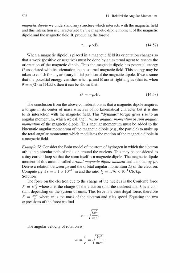
508 14 Relativistic Angular Momentum
magnetic dipole we understand any structure which interacts with the magnetic fieldand this interaction is characterized by the magnetic dipole moment of the magneticdipole and the magnetic field B, producing the torque
τ = μ×B. (14.57)
When a magnetic dipole is placed in a magnetic field its orientation changes sothat a work (positive or negative) must be done by an external agent to restore theorientation of the magnetic dipole. Thus the magnetic dipole has potential energyU associated with its orientation in an external magnetic field. This energy may betaken to vanish for any arbitrary initial position of the magnetic dipole. If we assumethat the potential energy vanishes when μ and B are at right angles (that is, whenθ = π/2) in (14.55), then it can be shown that
U = −μ·B. (14.58)
The conclusion from the above considerations is that a magnetic dipole acquiresa torque in its center of mass which is of no kinematical character but it is dueto its interaction with the magnetic field. This “dynamic” torque gives rise to anangular momentum, which we call the intrinsic angular momentum or spin angularmomentum of the magnetic dipole. This angular momentum must be added to thekinematic angular momentum of the magnetic dipole (e.g., the particle) to make upthe total angular momentum which modulates the motion of the magnetic dipole ina magnetic field.
Example 78 Consider the Bohr model of the atom of hydrogen in which the electronorbits in a circular path of radius r around the nucleus. This may be considered asa tiny current loop so that the atom itself is a magnetic dipole. The magnetic dipolemoment of this atom is called orbital magnetic dipole moment and denoted by μl .Derive a relation between μl and the orbital angular momentum Ll of the electron.Compute μI if r = 5.1× 10⁻¹¹ m and the ratio e
m = 1.76× 10¹¹ Cb/kg.Solution
The force on the electron due to the charge of the nucleus is the Coulomb forceF = k e2
r2 where e is the charge of the electron (and the nucleus) and k is a con-stant depending on the system of units. This force is a centrifugal force, thereforeF = mv2
r where m is the mass of the electron and v its speed. Equating the twoexpressions of the force we find
v =√
ke2
mr.
The angular velocity of rotation is
ω = v
r=
√ke2
mr3.

14.5 The Intrinsic Angular Momentum – The Spin Vector 509
The current produced by the rotation of the electron is the rate at which it passesthrough any given point of the orbit, hence
i = eν = e( ω
2π
)= e2
2π
√k
mr3.
The orbital dipole moment μI is given by (14.56) if we put N = 1 and A = πr2,that is
μI = e2
2π
√k
mr3πr2 = e2
2
√kr
m. (14.59)
The orbital angular momentum L I of the electron is
L I = mvr = mωr2 = m
√ke2
mr3r2 = 2m
eμI ,
which shows that the orbital angular momentum of the electron is proportional tothe magnetic dipole moment.
Introducing the data in (14.59) and taking k = 14πε0
(MKS system) we compute
μI = 9.1× 10⁻²⁴A m2.
It is an experimental fact that the elementary particles are magnetic dipoles, thatis, they have an intrinsic angular momentum. Originally this was confirmed for theelectron and then it was established for all other particles. This means that an elec-tron in its proper frame creates an electric field due to its charge and a magnetic fielddue to its magnetic dipole moment. The field lines of these two fields are shown inFig. 14.2 where the intrinsic angular momentum LI is also shown. The fact thatthe elementary particles are magnetic dipoles, and not simply charged or neutralunits of mass, indicates that they consist of “smaller” more “elementary” particlesin the same way the atom is a magnetic dipole due to the rotation of the rotatingelectron. This is true even for the particles with zero intrinsic angular momentum,
E
(a) (b)
B
LI
Fig. 14.2 Electric and magnetic field lines of electron

510 14 Relativistic Angular Momentum
in the sense that the parts it consists of cancel the effects of each other. The follow-ing exercise could be an extreme mechanistic physical explanation of the magneticdipole moment of the electron.
Exercise 76 Assume that the electron is a small sphere of radius R, its charge andmass being distributed uniformly throughout its volume. It has been measured thatsuch an electron has an intrinsic angular momentum L I = 0.53 × 10⁻³⁴J s anda magnetic dipole moment μI = 9.1 × 10⁻²⁴A m2. Show that the ratio e/m =2μI /L I . To justify this result divide the spherical electron into infinitesimal currentloops and find an expression for the magnetic dipole moment by integration.
14.5.2 The Relativistic Spin
In the last section we have shown that besides the kinematic angular momentumbivector and the torque tensor which correspond directly to the relevant concepts ofNewtonian theory, and both vanish in the particle’s proper frame, there is anotherangular momentum of non-kinematic nature which must be taken into account.Although the appropriate place to discuss this topic is quantum electrodynamics,7 inthe following we shall attempt a classic treatment which we find is of some physicalvalue.
The question we have to answer is
How could one incorporate the two types of angular momentum, kinematic and dynamic,in one, the total angular momentum?
The answer to this question is necessary because experiment has shown that theelementary particles are magnetic dipoles, therefore their motion in magnetic fields(which is a routine in experimental physics) will be modulated by the total angularmomentum and not by the orbital angular momentum alone.
Looking for the answer we note that the orbital angular momentum bivector Lab
has only electric part. Therefore if we add a bivector Sab to Lab, which has onlymagnetic part, then we have the total angular momentum while we preserve thekinematic and the dynamic characters apart. The requirement that the electric partEa(S) of Sab vanishes is (use (14.4) to see this)
Sab pb = 0⇔ Saua = 0, (14.60)
7 The reader may wonder why we bother to discuss the concept of spin within the limits of thenon-quantum theory when we know that only a quantal description can be correct. The answer liesin the quantal theorem which states that the classical equation of motion of a dynamical variableis the quantal equation of motion of the mean value of that variable averaged over an ensemble ofidentical systems. Therefore the conclusions we shall draw, with the classical treatment, will applyto averages over many identical particles prepared in the same way, like the electrons or muons ina beam or the valence electrons in a gas of atoms in a glow tube.
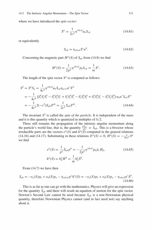
14.5 The Intrinsic Angular Momentum – The Spin Vector 511
where we have introduced the spin vector:
Sa = 1
2c2ηabcdub Scd (14.61)
or equivalently
Sab = ηabcd Scud . (14.62)
Concerning the magnetic part H a(S) of Sab from (14.8) we find
H a(S) = 1
2p2ηabcd pb Scd = 1
mSa . (14.63)
The length of the spin vector Sa is computed as follows:
S2 = Sa Sa = 1
4c4ηabcdub Scdηarst u
r Sst
= − 1
4c4
(δb
r δcs δ
dt − δb
r δds δ
ct + δc
r δds δ
bt − δc
r δbs δ
dt + δd
r δbs δ
ct − δd
r δcs δ
bt
)ubur Scd Sst
= − 1
4c42(−c2)Sab Sab = 1
2c2Sab Sab. (14.64)
The invariant S2 is called the spin of the particle. It is independent of the massand it is this quantity which is quantized in multiples of �/2.
There still remains the propagation of the intrinsic angular momentum alongthe particle’s world line, that is, the quantity d Sab
dτ = Sab. This is a bivector whoseirreducible parts are the vectors ea(S) and ha(S) computed in the general relations(14.16) and (14.17). Substituting in these relations Ea(S) = 0, H a(S) = − 1
2mc2 Sa
we find
ea(S) = 1
p2Sab pb = − 1
2p2ηabcd pb pc Hd , (14.65)
ha(S) = hab H b = 1
mha
b Sb.
From (14.7) we have then
Sab = −ea(S)pb + eb(S)pa − ηabcd pcha(S) = −ea(S)pb + eb(S)pa − ηabcduc Sd .
(14.66)
This is as far as one can go with the mathematics. Physics will give an expressionfor the quantity Sab and there will result an equation of motion for the spin vector.Newton’s Second Law cannot be used because Sab is a non-Newtonian physicalquantity, therefore Newtonian Physics cannot (and in fact need not) say anythingabout it.

512 14 Relativistic Angular Momentum
In order for physics to make a statement it goes over to experiment and observa-tion. Because Sab is an angular momentum Sab must be a torque. We have seen thatwith each magnetic dipole there is associated a magnetic dipole moment μI and ifa magnetic dipole is placed in a magnetic field B it suffers a torque τ = μI × B(see (14.57)). Furthermore, experiment has shown that the elementary particles (inthe standard sense of the term) behave as magnetic dipoles. These and the expectedapplication of the theory of relativity to elementary particles lead us to relate themagnetic dipole moment with the magnetic part of the tensor Sab, and subsequentlyvia (14.66), with the spin vector Sa .
Now, let τab(S) be the torque tensor corresponding to the intrinsic angularmomentum Sab. Then we assume the equation of motion
Sab = τab(S). (14.67)
The torque tensor has an “electric” part (which vanishes) and a “magnetic” partH a(τ ) which equals the magnetic part of Sab, that is we have
H a(τ ) = ha(S) = 1
mha
b Sb.
In analogy with the Newtonian result (14.57), we define H a(τ ) by the formula
H a(τ ) = 1
mηabcdubμI c Bd , (14.68)
where μI c is the magnetic dipole moment of the particle. Then the equation ofmotion of the spin vector is
hab Sb = ηabcdubμI c Bd (14.69)
or using (14.79) (see below)
hab Sb = g
|q|2mc
ηabcdub Sc Bd . (14.70)
In the proper frame of the particle the equation of motion (14.70) is written as
dS∗
dτ&= g|q|
2mcS∗ × B∗, (14.71)
where the ∗ besides a symbol indicates that the quantity is computed in the properframe of the particle and the & sign above the equality indicates that the equationholds in the proper frame of the particle only.
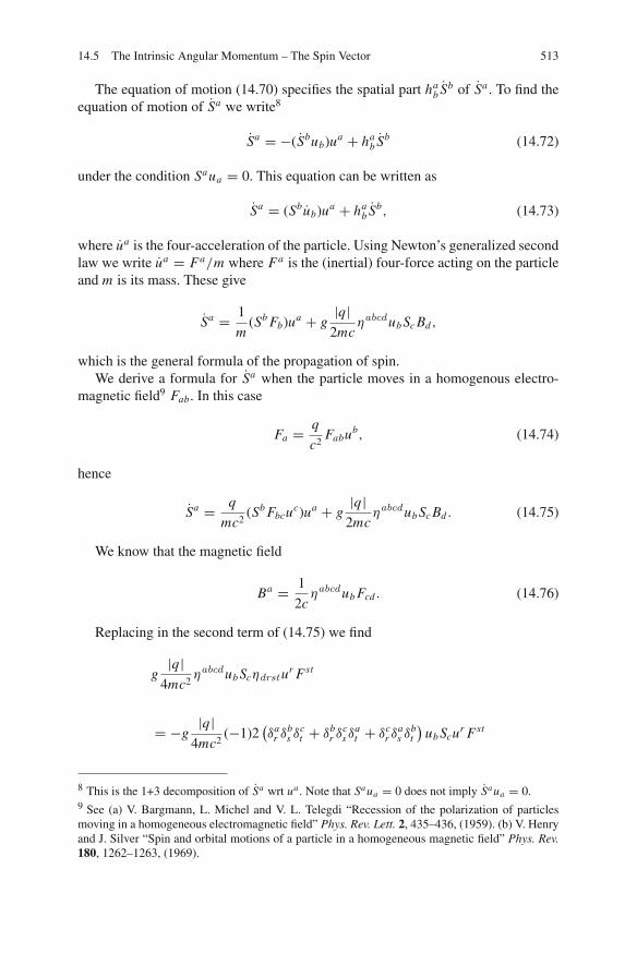
14.5 The Intrinsic Angular Momentum – The Spin Vector 513
The equation of motion (14.70) specifies the spatial part hab Sb of Sa . To find the
equation of motion of Sa we write8
Sa = −(Sbub)ua + hab Sb (14.72)
under the condition Saua = 0. This equation can be written as
Sa = (Sbub)ua + hab Sb, (14.73)
where ua is the four-acceleration of the particle. Using Newton’s generalized secondlaw we write ua = Fa/m where Fa is the (inertial) four-force acting on the particleand m is its mass. These give
Sa = 1
m(Sb Fb)ua + g
|q|2mc
ηabcdub Sc Bd ,
which is the general formula of the propagation of spin.We derive a formula for Sa when the particle moves in a homogenous electro-
magnetic field9 Fab. In this case
Fa = q
c2Fabub, (14.74)
hence
Sa = q
mc2(Sb Fbcuc)ua + g
|q|2mc
ηabcdub Sc Bd . (14.75)
We know that the magnetic field
Ba = 1
2cηabcdub Fcd . (14.76)
Replacing in the second term of (14.75) we find
g|q|
4mc2ηabcdub Scηdrstur Fst
= −g|q|
4mc2(−1)2
(δa
r δbs δ
ct + δb
r δcs δ
at + δc
r δas δ
bt
)ub Scur Fst
8 This is the 1+3 decomposition of Sa wrt ua . Note that Saua = 0 does not imply Saua = 0.9 See (a) V. Bargmann, L. Michel and V. L. Telegdi “Recession of the polarization of particlesmoving in a homogeneous electromagnetic field” Phys. Rev. Lett. 2, 435–436, (1959). (b) V. Henryand J. Silver “Spin and orbital motions of a particle in a homogeneous magnetic field” Phys. Rev.180, 1262–1263, (1969).

514 14 Relativistic Angular Momentum
= g|q|
4mc22(ua Fbc + ub Fca + uc Fab
)ub Sc
= g|q|/m
2c2(Fbcub Scua − c2 Fca Sc)
= g|q|/m
2Fac Sc + g
|q|/m
2c2(Fbcub Sc)ua .
Therefore
Sa = q
mc2(Sb Fbcuc)ua + g
|q|/m
2Fac Sc + g
|q|/m
2c2(Fbcub Sc)ua ⇒
(14.77)
Sa = |q|m
g
2Fac Sc + |q|
mc2
(g
2− q
|q|)
(Sb Fcbuc)ua . (14.78)
The experiments which confirm the proportionality of the magnetic dipole momentand the change of the intrinsic angular momentum are called “gyromagnetic” exper-iments. Relation (14.78) has been confirmed by such experiments on many differentsystems. The constant of proportionality is one of the parameters characterizingthe particular system. It is normally specified by giving the gyromagnetic ratio org-factor, defined by the relation
μaI = g
|q|2mc
Sa, (14.79)
where |q|/m is the (measure of) charge to mass ratio of the particle. The first suc-cessful experiments to show this have been performed by Einstein and de Hass asearly as 1915 and later on (1935) by Barnett.10 It has been found that for the electronge− = −2 and for the positron ge+ = 2. Pion has gπ = 0. The magnetic dipolemoment of the hydrogen atom results from both the electron orbital motion and theelectron spin. These two interact and the value of the g-factor for the atom is between−1 (pure electron orbit) and −2 (pure electron spin). For electrons, positrons, andmuons experiment has given the following values:
ge− = −2(1+ 1.1596× 10⁻³),
ge+ = +2(1+ 1.17× 10⁻³),
gμ− = −2(1+ 1.166× 10⁻³),
gμ+ = +2(1+ 1.16× 10⁻³),
10 A. Einstein and W. J. de Haas Verhandl. Deut. Phys. Ges. 17, 152, (1915); S.J. Barnett Rev.Mod. Phys. 7, 129, (1935)
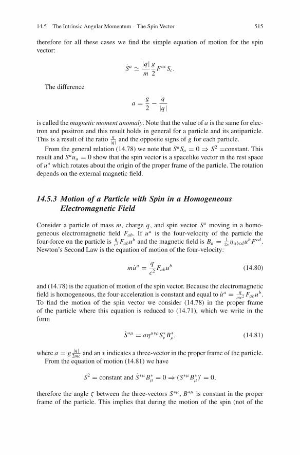
14.5 The Intrinsic Angular Momentum – The Spin Vector 515
therefore for all these cases we find the simple equation of motion for the spinvector:
Sa � |q|m
g
2Fac Sc.
The difference
a = g
2− q
|q|is called the magnetic moment anomaly. Note that the value of a is the same for elec-tron and positron and this result holds in general for a particle and its antiparticle.This is a result of the ratio q
|q| and the opposite signs of g for each particle.
From the general relation (14.78) we note that Sa Sa = 0⇒ S2 =constant. Thisresult and Saua = 0 show that the spin vector is a spacelike vector in the rest spaceof ua which rotates about the origin of the proper frame of the particle. The rotationdepends on the external magnetic field.
14.5.3 Motion of a Particle with Spin in a HomogeneousElectromagnetic Field
Consider a particle of mass m, charge q , and spin vector Sa moving in a homo-geneous electromagnetic field Fab. If ua is the four-velocity of the particle thefour-force on the particle is q
c2 Fabub and the magnetic field is Ba = 12cηabcdub Fcd .
Newton’s Second Law is the equation of motion of the four-velocity:
mua = q
c2Fabub (14.80)
and (14.78) is the equation of motion of the spin vector. Because the electromagneticfield is homogeneous, the four-acceleration is constant and equal to ua = q
mc2 Fabub.To find the motion of the spin vector we consider (14.78) in the proper frameof the particle where this equation is reduced to (14.71), which we write in theform
S∗μ = aημνρS∗ν B∗ρ, (14.81)
where a = g |q|2mc and an ∗ indicates a three-vector in the proper frame of the particle.From the equation of motion (14.81) we have
S2 = constant and S∗μB∗μ = 0⇒ (S∗μB∗μ)· = 0,
therefore the angle ζ between the three-vectors S∗μ, B∗μ is constant in the properframe of the particle. This implies that during the motion of the spin (not of the

516 14 Relativistic Angular Momentum
particle!) the vector S∗μ traces the surface of a right circular cone with axis alongthe magnetic field B∗μ with opening angle ζ . The solution of (14.81) is written asfollows:
S∗μ(τ ) = S∗ sin ζ (cosω∗τeμ(1) + sinω∗τeμ(2))+ cos ζ S∗eμ(3), (14.82)
where e(1)μ, e(2)μ, e(3)ρ is an orthonormal basis and B∗μ = B∗e(3)μ. To determine theangular speed ω∗ we compute the derivative S∗μ and then use the equation of motion(14.81). We find
ω∗(− sinω∗τeμ(1) + cosω∗τeμ(2)
)= aημνρ(cosω∗τeμ(1) + sinω∗τeμ(2))B∗eμ(3).
Taking μ = 1 we find easily that ω∗ = aB∗, hence
ω∗μ = −aB∗eμ(3). (14.83)
Therefore the solution of the equation of motion in the proper frame is
S∗μ = S∗ sin ζ (e(1)μ cos aB∗τ + e(2)μ sin aB∗τ )+ cos ζ S∗e(3)μ. (14.84)
This represents a regular precession in which the spin vector traces out a rightcircular cone with the direction of the magnetic field as axis and constant angularvelocity ω∗ = g
2|q|B∗
mc . The quantity ω∗c = −|q|B∗
mc is the cyclotronic frequency11 inthe proper frame of the particle (see Fig. 14.3).
Fig. 14.3 Spin precession ina uniform magnetic field
S ¤
B ¤
sin
τ
11 This is the angular speed of a particle of charge q which is introduced at right angles to a uniformmagnetic field of magnetic induction B∗.

14.5 The Intrinsic Angular Momentum – The Spin Vector 517
14.5.4 Transformation of Motion in Σ
In order to find the motion of spin in another coordinate frame, the Σ say, we haveto apply the appropriate Lorentz transformation to the various quantities involved.However, this is not enough. Indeed in the proper frame the spin precesses aroundthe magnetic field with angular velocity ω∗ = − g
2 ω∗c whereas the particle acceler-ates (i.e., a+ �= 0) as it moves. This means that the spatial directions in the properframe of the particle suffer the Thomas rotation which (in Σ!) is given by the angularvelocity ωT = − γu−1
u2 u × a, where u, a are the velocity and the acceleration of theparticle in Σ (see (14.70)). Therefore in Σ the spin vector executes two independentrotational motions with angular velocity ω∗ and ωT , the net angular velocity beingthe composition of the two angular velocities. Let us compute the motion of the spinin Σ.
Choose the coordinates in Σ so that the z-axis is along the direction of the homo-geneous magnetic field B and assume that the initial velocity of the particle is normalto the magnetic field so that the motion takes place in the plane x, y with basis vec-tors e1,e2. The electromagnetic field induced in the proper frame (=local rest frame!)of the particle at each position along its trajectory is given by the transformationformulae
E∗ = E|| + γu [E⊥ + u× B] = γuu Be2, (14.85)
B∗ = B|| + γu
[B⊥ − 1
c2u× E
]= −γu Be3, (14.86)
where u = ue1 is the velocity of the particle in Σ. We see that in the proper framethe direction of the magnetic field is along the z-axis whereas the electric field isuniform and along the direction of the radius. The force due to the electric field is
F∗ = qE∗ = qγuu Be2 (14.87)
and it is a centripetal force (otherwise the particle would not rotate12) with acceler-ation
a∗ = ω∗c u. (14.88)
From the above we find
ω∗c = γu|q|Bmc= γuω0, (14.89)
where ω0 = |q|Bmc is the Newtonian cyclotronic angular speed in Σ. Therefore in theproper frame we have that the spin precesses with angular velocity
12 We can always make that force centripetal by changing the direction of the speed u.

518 14 Relativistic Angular Momentum
ω∗ = −g
2γuω0e3. (14.90)
From the transformation of the angular velocity13 we have that in Σ
ω = −g
2ω0e3. (14.91)
Concerning the Thomas precession we have shown in (6.72) that for a circularmotion
ωT = −(γu − 1)ωce3, (14.92)
where ωc is the angular (i.e., the cyclotronic) speed of rotation given by
ωc = |q|Bγumc
= 1
γuω0. (14.93)
Eventually we have that in Σ the spin precesses around the direction of B withtotal angular velocity
ωS = ω + ωT = −(
g
2+ 1− 1
γu
)ω0e3. (14.94)
One important (and well-known) conclusion is that the difference
ωD ≡ ωS − ωc = −(g
2+ 1
)ω0e3, (14.95)
which is possible to be measured directly, is independent of the speed of the particle.This fact facilitates the measurement of the factor g because one can use beams ofthe same particles but different initial speeds.
In case the velocity of the particles is not normal to the magnetic field, we decom-pose it into two components, one parallel to the field and one normal to it. The aboveconsiderations hold for the normal component. Concerning the parallel componentthis stays constant (the magnetic field has no effect parallel to its direction) hencethe motion parallel to the magnetic field is with uniform velocity. In conclusionthe motion of the particle (not the spin!) is the combination of two motions: onemotion with uniform velocity (drifting) parallel to the direction of B and a planarcircular motion with uniform angular velocity ωS with axis along the direction ofB. The combination of the two motions results in a helical motion with axis along
13 Note that the angular velocity equals 2π/T , therefore its transformation is like T−1, that is
ω∗ = γuω,
where ω is the angular speed in Σ and ω∗ is the angular speed in Σ∗.

14.5 The Intrinsic Angular Momentum – The Spin Vector 519
the direction of B. This means that the frame Σ we considered is drifting along thedirection of B with constant speed u||, therefore in order to find the motion in theoriginal frame, the Σ′ say, we have to apply the appropriate boost along the z-axis.This means that the circular frequencies we have found above must be multipliedwith the factor 1
γ||. For example in Σ′ the spin precesses with angular velocity
ω′S = −(
g
2+ 1− 1
γu
)1
γ||ω0e3. (14.96)

Chapter 15The Covariant Lorentz Transformation
15.1 Introduction
It can hardly be emphasized that one of the most important elements of SpecialRelativity is the Lorentz transformation. This is the reason why we have spent somuch space and effort to derive and study the Lorentz transformation in the earlychapters of the book. One could naturally ask “After all these different derivationsof the Lorentz transformation why are we not yet finished with it?” The reason is thefollowing. Special Relativity is a geometric theory of physics, which can be writtenand studied covariantly in terms of Lorentz tensors (four-vectors, etc.) without theneed to consider a coordinate system until the very end, when one has to computeexplicitly the components of the physical quantities of a problem for some observer.
All derivations of the Lorentz transformations so far used either coordinatesor three-vectors, that is, they were not covariant. This does not mean that thesetransformations are not the general ones or that they are insufficient to deal withall relativistic problems. The point is that, although the covariant Lorentz transfor-mation is not necessary for the development and the application of the theory, incases where one has to deal with general problems of a qualitative character or withinvolved problems, the covariant formalism significantly simplifies the calculationsbecause one is able to apply geometric techniques to get answers which would notbe feasible to get with the standard form of the transformation. Furthermore, if onedescribes a problem in covariant formalism then it is possible to use one of thewell-known algebraic computing programs to perform the calculations. This is ofpractical importance because it makes easy (or even possible) complex calculations,which would be unbearable to be carried out by hand and, most important, withoutmistakes. Finally, we emphasize the aesthetic side of the matter and claim that sincethe Theory of Special Relativity is a geometric theory of motion, its description inany but the covariant formalism hides much of the power and the elegance of thetheory.
In this chapter we derive the covariant form of Lorentz transformation and werefer to some of its applications. As it might be expected this chapter is of a moreadvanced level, therefore it is advisable to be studied after the reader has someexperience with Special Relativity.
M. Tsamparlis, Special Relativity, DOI 10.1007/978-3-642-03837-2 15,C© Springer-Verlag Berlin Heidelberg 2010
521

522 15 The Covariant Lorentz Transformation
Before we get into the details, let us take a quick promenade into the relevant lit-erature. Based on the vector form of the Lorentz transformation, Fahnline1 gave thecovariant expression of the (proper) Lorentz transformation and the correspondingcovariant transformation of a four-vector. He used this form of the transformationto compute the composition of successive Lorentz transformations in a brute yetdirect way. This problem is not easy. Indeed, it is well known2 that in order tocompute the covariant form of the Euclidean rotation of this decomposition onehas to invoke the homomorphism between the restricted Lorentz group SO(3,1) andSL(2,C). Fahnline showed that this is not necessary, provided that the covariant formof the transformation is used.
Finally, a different and very interesting approach to the covariant Lorentz trans-formation has been given by Krause3 who expressed the Lorentz transformationin terms of two unit timelike vectors ua, va corresponding to the four-velocitiesof inertial observers related by the transformation. He considered only the properLorentz transformation, whose covariant form he derived using the orthonormaltetrads associated with the observers ua, va . He followed a similar technique devel-oped by Basanski4 who used null tetrads to express the Lorentz transformation interms of spacetime rotations. The approach of Krause is more fundamental than thatof Fahnline.
Finally, in a more recent work, Jantzen et al.5 have introduced a covariant formof Lorentz transformation based on relative velocity and the fact that under aLorentz transformation between two observers the timelike plane defined by thefour-velocities of the observers and the normal two-plane to that plane are preserved.They obtained the proper Lorentz transformation (they call it “relative observerboost”) and they discuss some of its properties, however again in a form whichobscures the simple geometric significance of the Lorentz transformation. In a sim-ilar approach Urbantke6 studied the Lorentz transformation and considered someapplications of the proper Lorentz transformation in terms of spacetime reflections.
Before we present our approach, we emphasize once more that the Lorentz trans-formation (in vector or in covariant form) is of a pure mathematical origin and hasnothing to do with Special Relativity or any other theory of physics. Its connectionwith physics is introduced by the Principle of Special Relativity, which demandsthat all physical quantities in Special Relativity must be covariant under the Lorentz
1 D. Fahnline Am. J. Phys. 50, 50, 818–821, (1982).2 See F. R. Halpern (1968) “Special Relativity and Quantum Mechanics” (Prentice Hall,Englewood Cliffs, NJ and Goldstein Herbert “Classical Mechanics” Second Edition (1980)Addison-Wesley, chapter 73 J. Krause “Lorentz transformations as space-time reflections” J. Math. Physics 18, 879–893,(1977).4 S. L. Basanski “Decomposition of the Lorentz Transformation Matrix into Skew – SymmetricTensors” J. Math. Phys. 6,1201–1202, (1965).5 R. Jantzen, P. Capini, D. Bini Ann Phys. 215, (1992) 1 and gr-qc/0106043.6 H. K. Urbantke Found. Phys. Lett. 16, 111, (2003).

15.2 The Covariant Lorentz Transformation 523
transformation (that is, they must be Lorentz tensors). This point is justified by thefact that we are able to derive/study the Lorentz transformation based on geometricassumptions only without making reference to any physical concepts or systems.
15.2 The Covariant Lorentz Transformation
In Chap. 1 we derived the Lorentz transformation L : M4 → M4 as an endomor-phism of Minkowski space satisfying the following two requirements:
(1) L is a linear transformation.(2) L is an isometry of M4 which in addition preservers the canonical form
η = diag(−1, 1, 1, 1) of the Lorentz metric, that is, it satisfies the equationLtηL = η.
The derivation of the covariant Lorentz transformation will be based on geomet-ric assumptions which are hidden in the above requirements. Indeed the linearityof the transformation means that L preserves the linear geometric elements (straightlines, two-planes and three-planes or hyperplanes) in M4. The first part of the secondassumption means that it also preserves the character of these linear elements, thatis, a timelike straight line goes to a timelike straight line, a spacelike two-planeto a spacelike two-plane, etc. Since a timelike straight line is characterized by itsunit tangent vector, let ua, va be two unit timelike vectors related by the Lorentztransformation.
Then the preservation of the canonical form η of the Lorentz metric implies thatL preserves the Euclidean planes normal to the four-vectors ua, va . Equivalently,the Lorentz transformation relates the LCF associated with the four-vectors ua, va .The above observations are sufficient in order to define the covariant form of theLorentz transformation.
In the following we shall need the projection tensors hab and pab we defined in(12.2) and (12.21).
15.2.1 Definition of the Lorentz Transformation
Definition 14 Let ua, va be two unit, non-collinear, timelike vectors, correspondingto the four-velocities of two (inertial) observers, which define a timelike two-plane.The (planar) Lorentz transformation defined by ua, va is the map7 L : M4 → M4
specified by the following requirements:
(1) L is a linear transformation and preserves the timelike two-plane spanned bythe vectors ua, va and the spacelike two-plane normal to the ua, va two-plane.
(2) L is an isometry of M4.
7 To be precise this is a transformation in the tangent space of M4 but due to the flatness of M4 itcan be reduced unambiguously to a transformation in M4.

524 15 The Covariant Lorentz Transformation
(3) L is defined on an equal footing in terms of ua, va (this is the so-calledreciprocity principle8). This is formulated by the requirement that the inverseLorentz transformation is the same with the direct but with ua, va interchanged.
Let us write the verbal requirements of the definition in terms of equations.Requirement 1 implies for the timelike two-plane spanned by the vectors ua, va
the equations
Lva = Aua + Bva, Lua = Cua + Dva, (15.1)
where A, B,C, D are quantities independent of the spacetime coordinates such thatAB − C D �= 0 (because ua, va are not collinear) and AD �= 0 (otherwise thetransformation is singular).For the spacelike two-plane normal to that plane the same requirement implies theequation
Lpab(u, v) = pab(u, v), (15.2)
where pab is the projection tensor which projects normal to the timelike plane ofua, va . Requirement 2 means that the inner products of vectors are preserved. Forthe two vectors ua, va this requirement implies the equations
(Lua, Lua) = (Lva, Lva) = −1, (Lua, Lva) = (ua, va). (15.3)
Requirement 3 means that the inverse transformation applied to ua has the sameresult as the direct transformation applied to the vector va and vice versa. Thisimplies the equations
L−1ua = Ava + Bua, L−1va = Cva + Dua . (15.4)
We conclude that
(a) In order to specify the (planar) Lorentz transformation defined by the vectorsua, va it is enough to compute the unknown coefficients A, B,C, D describingthe transformation.
(b) The transformation is defined by (15.1), (15.2), (15.3), and (15.4).
15.2.2 Computation of the Covariant Lorentz Transformation
We introduce the quantity (we consider c = 1 in what follows)
γ = −uava (15.5)
8 The interested reader can find more information on this principle in V. Bruzzi and V. Gorini“Reciprocity principle and the Lorentz transformation” J. Math. Phys. 10, 1518–1524, (1989).

15.2 The Covariant Lorentz Transformation 525
(this is the gamma-factor relating the two observers) and use (15.3) to get
(Lua, Lva) = (ua, va) = −γ ⇒ (AC + B D)+ (BC + AD − 1)γ = 0.
From the lengths of the four-vectors we have
vava = −1⇒ A2 + 2γ AB + B2 = 1
and
uaua = −1⇒ C2 + 2γC D + D2 = 1.
The first equation of relation (15.4) gives
ua = L L−1ua = L(Ava + Bua) = (A2 + BC)ua + (AB + B D)va,
hence
A2 + BC = 1,
AB + B D = 0.
Similarly the second part of (15.4) gives
D2 + BC = 1,
AC + C D = 0.
Finally, after some simple manipulations, we have the following system of sevennon-linear algebraic equations in the four unknowns A, B, C, D:
B(2γ A + B − C) = 0, (15.6)
C(2γ D + C − B) = 0, (15.7)
B(A + D) = 0, (15.8)
C(A + D) = 0, (15.9)
A2 − D2 = 0, (15.10)
A2 + BC = 1, (15.11)
(AC + B D)+ (BC + AD − 1)γ = 0. (15.12)
We expect that the system has many solutions, therefore there are more thanone Lorentz transformations satisfying the conditions of Definition 14. A simpleanalysis shows that the solutions of the system can be classified by the vanishing ornot of the quantities A + D, A − D. It is an easy exercise to show that the systemadmits the following families of solutions (AD �= 0):

526 15 The Covariant Lorentz Transformation
(1) A − D = 0, A + D �= 0⇐⇒ A = D �= 0.
A B C D±1 0 0 ±1
(2) A + D = 0, A − D �= 0⇐⇒ A = −D �= 0.
A B C D±1 0 ±2γ ∓1±1 ∓2γ 0 ∓1
We end up with a total of 2+ 4 = 6 solutions. Replacing the values of the coef-ficients A, B,C, D we find the action of the Lorentz transformation (not the trans-formation per se!) on the four-vectors ua, va . The results are collected in Table 15.1.
We observe that cases V, V I are identical with cases I V, III , respectively, ifwe interchange ua ↔ va . This is to be expected because cases V, V I expressthe inverse transformation from ua to va and we have assumed that ua, va arecompletely equivalent. Therefore, without loss of generality we may restrict ourconsiderations to the first four cases I − I V only. By doing so, we introduce anasymmetry, which, however, can be ignored if we assume that the direct Lorentztransformation is from va → ua . This implies then that the coefficient B = 0, thatis, we define the generic Lorentz transformation by the relations
Lva = ±ua, Lua = Cua + Dva . (15.13)
The coefficient ±1 in the rhs of the first equation (15.13) is due to the factthat the Lorentz transformation preserves the magnitude and the direction of thefour-vectors but not necessarily the sense of direction.
Table 15.1 The action of the generic Lorentz transformation
A B C DLorentz transformation and theinverse
I. 1 0 0 1Lua = va, Lva = ua
L−1ua = va, L−1va = ua
II. −1 0 0 −1Lua = −va, Lva = −ua
L−1ua = −va, L−1va = −ua
III. 1 0 2γ −1Lua = 2γ ua − va, Lva = ua
L−1ua = va, L−1va = 2γ va − ua
IV. −1 0 −2γ 1Lua = −2γ ua + va, Lva = −ua
L−1ua = −va, L−1va = −2γ va + ua
V. 1 −2γ 0 −1Lua = −va, Lva = −2γ va + ua
L−1ua = −2γ ua + va, L−1va = −ua
VI. −1 2γ 0 1Lua = va, Lva = 2γ va − ua
L−1ua = 2γ ua − va, L−1va = ua

15.2 The Covariant Lorentz Transformation 527
We compute now the Lorentz transformation itself. From (15.13) we expect thatthe generic expression of the Lorentz transformation in terms of the four-vectorsua, va will be of the form
Lab = I a
b + A1uavb + B1uaub + C1vavb + D1v
aub, (15.14)
where I ab is the identity transformation and the coefficients A1, B1, C1, D1 are
computed in terms of A, B, C, D by means of the action of the transformationon ua, va . For example, the action of L (on the left) on ua gives
Lua = ua + A1ua(−γ )+ B1ua(−1)+ C1va(−γ )+ D1v
a(−1)
= (1− A1γ − B1)ua − (C1γ + D1)va .
Comparing this with the second of (15.13) we find the equations
1− A1γ − B1 = C, (15.15)
C1γ + D1 = −D. (15.16)
Similarly, the action of L on va gives the equations
1− D1γ − C1 = B, (15.17)
A1 + B1γ = −A. (15.18)
The solution of the system of (15.15), (15.16), (15.17), and (15.18) is
A1 = 1
1− γ 2(γC − γ − A) ,
B1 = 1
1− γ 2(γ A + 1− C) ,
C1 = 1
1− γ 2(γ D + 1− B) , (15.19)
D1 = 1
1− γ 2(γ B − γ − D) .
Using the values of the coefficients A, B, C, D for each solution we computethe value of the coefficients A1, B1, C1, D1 and consequently the Lorentz trans-formation for each case. The result of the calculations are collected in Table 15.2.
We conclude that the covariant expression of the generic Lorentz transformation(that is, the one which covers all possible cases!) and its inverse in terms of the

528 15 The Covariant Lorentz Transformation
Table 15.2 The generic Lorentz transformation
A B C D A1 B1 C1 D1
I. 1 0 0 1 − 1
1− γ
1
1− γ
1
1− γ− 1
1− γ
II. −1 0 0 −11
1+ γ
1
1+ γ
1
1+ γ
1
1+ γ
III. 1 0 2γ −1 −1+ 2γ
1+ γ
1
1+ γ
1
1+ γ
1
1+ γ
IV. −1 0 −2γ 11− 2γ
1− γ
1
1− γ
1
1− γ
1
1− γV. Same as I V if u ←→ v
VI. Same as I I I if u ←→ v
initial coefficients A, B, C, D are
Lab = δa
b +1
1− γ 2(γC − γ − A) uavb + 1
1− γ 2(γ A + 1− C) uaub
+ 1
1− γ 2(γ D + 1− B) vavb + 1
1− γ 2(γ B − γ − D) vaub, (15.20)
(L−1)ab = δa
b +1
1− γ 2(γ B − γ − D) uavb + 1
1− γ 2(γ D + 1− B) uaub
+ 1
1− γ 2(γ A + 1− C) vavb + 1
1− γ 2(γC − γ − A) vaub. (15.21)
We note that the transformation is defined solely in terms of the four-vectorsua, va as requested. The expressions are important because
(1) They are fully covariant (independent of any coordinate frame)(2) They depend only on the four-vectors ua, va , that is, the four-velocities of the
observers defining the transformation.
Exercise 77 (a) Prove that the generic Lorentz transformation does satisfy theisometry condition (L−1)c
aηcd Ldb = ηab where ηab is the Lorentz metric.
(b) Prove that the inverse generic Lorentz transformation is found from the directby interchanging ua ←→ va .
Replacing in these expressions the values of the coefficients A, B, C, D ofTable 15.1 for each case (or using Table 15.2) we find the covariant expression forthe corresponding Lorentz transformation. The results are given9 in Table 15.3.
Exercise 78 (a) Prove that in cases I, I I the Lorentz transformation L satisfies theproperty L = L−1, i.e., L2 = I . Such operators are called spacetime reflections.
In the last column of Table 15.3 we give the characterization of each type ofLorentz transformation with the one we computed in Chap. 1. The justification ofthis will be given below when we derive the action of each type of Lorentz transfor-mation in terms of coordinates.
9 The expression of the proper Lorentz transformation given in Table 15.2 coincides (after somerearrangements) with that of Krause.

15.2 The Covariant Lorentz Transformation 529
Table 15.3 The covariant Lorentz transformations
Lorentz transformation Type
I.La
b = δab +
1
1− γ(ua − va)(ub − vb)
L−1ab = δa
b +1
1− γ(va − ua)(vb − ub)
Space inversion
II.La
b = δab +
1
1+ γ(ua + va)(ub + vb)
L−1ab = δa
b +1
1+ γ(va + ua)(vb + ub)
Time inversion
III.La
b = δab +
1
1+ γ(ua + va)(ub + vb)− 2uavb
L−1ab = δa
b +1
1+ γ(va + ua)(vb + ub)− 2vaub
Proper
IV.La
b = δab +
1
1− γ(ua − va)(ub − vb)+ 2uavb
L−1ab = δa
b +1
1− γ(va − ua)(vb − ub)+ 2vaub
Spacetime inversion
15.2.3 The Action of the Covariant Lorentz Transformationon the Coordinates
The expression of the generic Lorentz transformation we found treats the transfor-mation on an equal footing wrt the four-vectors ua, va . However, this is not thestandard practice where one considers the Lorentz transformation from one LCFto another. To reconcile the two approaches we consider the action of the Lorentztransformation on the components of a four-vector. Indeed, using the expression(15.20) it is a straightforward matter to write the transformation equation and theinverse of any four-vector xa in generic and covariant form (recall that B = 0):
xa = xa + 1
1− γ 2
{[(γC − γ − A) vb + (γ A + 1− C) ub] xb
}ua
+ 1
1− γ 2
{[(γ D + 1) vb − (γ + D) ub] xb
}va, (15.22)
xa = xa + 1
1− γ 2
{[(γC − γ − A) ub + (γ A + 1− C) vb] xb
}va
+ 1
1− γ 2
{[(γ D + 1) ub − (γ + D) vb] xb
}ua . (15.23)
From this, we calculate in Table 15.4 the covariant expression of the action ofeach type of Lorentz transformation and its inverse on an arbitrary four-vector xa .
In order to find the standard vector expression of the Lorentz transformation, wehave to consider the proper frame of one of the defining four-vectors. Take ua as thereference vector and denote its proper frame by Σu . Then we have

530 15 The Covariant Lorentz Transformation
Table 15.4 The action of the covariant Lorentz transformation on a four-vector
Transformation of four-vector Type
I .La
b xb = xa + 1
1− γ
[(ub − vb)xb
](ua − va)
(L−1)ab xb = xa + 1
1− γ
[(vb − ub)xb
](va − ua)
SI
I I .La
b xb = xa + 1
1+ γ
[(ub + vb)xb
](ua + va)
(L−1)ab xb = xa + 1
1+ γ
[(vb + ub)xb
](va + ua)
TI
III .La
b xb = xa + 1
1+ γ
[(ub + vb)xb
](ua + va)− 2
(vbxb
)ua
(L−1)ab xb = xa + 1
1+ γ
[(vb + ub)xb
](va + ua)− 2
(ubxb
)va
PLT
I V .La
b xb = xa + 1
1− γ
[(ub − vb)xb
](ua − va)+ 2
(vbxb
)ua
(L−1)ab xb = xa + 1
1− γ
[(vb − ub)xb
](va − ua)+ 2
(ubxb
)va
STI
Notation: SI = space inversion, TI = time inversion, PLT = proper Lorentz transformation,STI = spacetime inversion.
ua =(
10
)
Σu
, va =(
γ
γ v
)
Σu
. (15.24)
Let us consider xa to be the position four-vector10 and let us assume that xa =(lr
)
Σu
. Then from (15.22) we have
(l ′
r′
)
Σv
=(
lr
)
Σu
+ 1
1− γ 2
{(γC − γ − A)
(γ
γ v
)
Σu
·(
lr
)
Σu
}(10
)
Σu
+ 1
1− γ 2
{(γ A + 1− C)
(10
)
Σu
·(
lr
)
Σu
}(10
)
Σu
+ 1
1− γ 2
{(γ D + 1)
(γ
γ v
)
Σu
·(
lr
)
Σu
}(γ
γ v
)
Σu
− 1
1− γ 2
{(γ + D)
(10
)
Σu
·(
lr
)
Σu
}(γ
γ v
)
Σu
,
which leads to the following generic transformation equations
10 This is not necessary but it will help the reader to associate the new approach with the standardformalism.
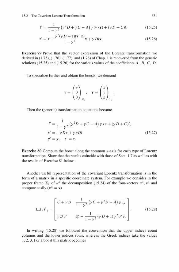
15.2 The Covariant Lorentz Transformation 531
l ′ = 1
1− γ 2
(γ 2 D + γC − A
)γ (v · r)+ (γ D + C)l, (15.25)
r′ = r+ γ 2(γ D + 1)(v · r)
1− γ 2v+ γ Dlv. (15.26)
Exercise 79 Prove that the vector expression of the Lorentz transformation wederived in (1.75), (1.76), (1.77), and (1.78) of Chap. 1 is recovered from the genericrelations (15.25) and (15.26) for the various values of the coefficients A, B, C, D.
To specialize further and obtain the boosts, we demand
v =⎛
⎝v
00
⎞
⎠
Σu
, r =⎛
⎝xyz
⎞
⎠
Σu
.
Then the (generic) transformation equations become
l ′ = 1
1− γ 2
(γ 2 D + γC − A
)γ xv + (γ D + C)l,
x ′ = −γ Dx + γ vDl, (15.27)
y′ = y, z′ = z.
Exercise 80 Compute the boost along the common x-axis for each type of Lorentztransformation. Show that the results coincide with those of Sect. 1.7 as well as withthe results of Exercise 81 below.
Another useful representation of the covariant Lorentz transformation is in theform of a matrix in a specific coordinate system. For example we consider in theproper frame Σu of ua the decomposition (15.24) of the four-vectors ua, va andcompute easily (vμ = v)
Lu(v)ij =
⎡
⎢⎢⎢⎣
C + γ D1
1− γ 2
(γC + γ 2 D − A
)γ vμ
γ Dvμ δμν +1
1− γ 2(γ D + 1) γ 2vμvν
⎤
⎥⎥⎥⎦ . (15.28)
In writing (15.28) we followed the convention that the upper indices countcolumns and the lower indices rows, whereas the Greek indices take the values1, 2, 3. For a boost this matrix becomes

532 15 The Covariant Lorentz Transformation
Lu(v)ij =
⎡
⎢⎢⎢⎢⎢⎣
C + γ Dγ v
1− γ 2
(γC + γ 2 D − A
)0
γ Dv −γ D 0
0 0 δLK
⎤
⎥⎥⎥⎥⎥⎦, (15.29)
where the indices K , L take the values 1, 2.
Exercise 81 Prove that the determinant of the generic boost (15.29) equals
det Lu(v) = −AD. (15.30)
Conclude that in the cases I, I I (spatial and temporal inversion) the detLu(v) = −1 whereas for the cases III , I V (proper transformation and spacetimereflection) det Lu(v) = +1. This shows which types of Lorentz transformationdo not constitute (by themselves only!) a group (because they do not contain theidentity).11
Exercise 82 Show that the matrix representation of each of the four types of Lorentztransformation is the following:Case I (space inversion) (C = 0, D = 1, A = 1).General:
L(u)ij =
⎡
⎢⎢⎣
γ −γ vμ
γ vμ δμν +γ 2
1− γvμvν
⎤
⎥⎥⎦ . (15.31)
Boost:
L(u)ij =
⎡
⎢⎢⎣
γ −γ v 0 0γ v −γ 0 00 0 1 00 0 0 1
⎤
⎥⎥⎦ . (15.32)
Case I I (time inversion) (C = 0, A = 1, D = 1).General:
L(u)ij =
⎡
⎢⎢⎣
−γ γ vμ
−γ vμ δμν +γ 2
1+ γvμvν
⎤
⎥⎥⎦ . (15.33)
11 The set of all types of Lorentz transformations constitutes a group. This group has four com-ponents. Of those, only the subset of the proper Lorentz transformations form a group, which is asubgroup of the Lorentz group.

15.2 The Covariant Lorentz Transformation 533
Boost:
L(u)ij =
⎡
⎢⎢⎣
−γ γ v 0 0−γ v γ 0 00 0 1 00 0 0 1
⎤
⎥⎥⎦ . (15.34)
Case I I I (proper Lorentz transformation) (C = 2γ, A = 1, D = −1).General:
Lu(v)ij =
⎡
⎢⎢⎣
γ −γ vμ
−γ vμ δμν +γ 2
1+ γvμvν
⎤
⎥⎥⎦ . (15.35)
Boost:
Lu(v)ij =
⎡
⎢⎢⎣
γ −γ v 0 0−γ v γ 0 00 0 1 00 0 0 1
⎤
⎥⎥⎦ . (15.36)
Case I V (spacetime inversion) ( C = −2γ, A = −1, D = 1).General:
L(u)ij =
⎡
⎢⎢⎣
−γ γ vμ
γ vμ δμν +γ 2
1− γvμvν
⎤
⎥⎥⎦ . (15.37)
Boost:
L(u)ij =
⎡
⎢⎢⎣
−γ γ v 0 0γ v −γ 0 00 0 1 00 0 0 1
⎤
⎥⎥⎦ . (15.38)
We note that all four types of Lorentz transformation can be written in covariantform. This means that it is not necessary to study the relativistic problems with theproper Lorentz transformation only, and one can use equally well all other typesof Lorentz transformation. However, this is not done in practice and rarely in theexisting literature.12
12 See for example the book R. Sachs “The Physics of the Time Reversal” The University ofChicago Press, Chicago, (1987).

534 15 The Covariant Lorentz Transformation
In the following sections we shall consider various simple but important applica-tions of the covariant Lorentz transformation, keeping always in mind the level ofthe present book.
15.2.4 The Invariant Length of a Four-Vector
Consider a four-vector wa and the Lorentz transformation L(u, v) defined by theunit timelike (non-collinear) four-vectors ua, va . Consider the decomposition
wa = a1ua + a2va + wa
⊥,
where wa⊥ = p(u, v)a
bwb is the normal projection of wa on the two-plane of ua, va .
We introduce the invariants Au = waua , Av = wava (and γ = −uava) and computeeasily
Au = −a1 − a2γ, Av = −a1γ − a2.
Reversing these relations we compute a1, a2 in terms of Au, Av and find that
wa = 1
1− γ 2
{(γ Av − Au)ua + (γ Au − Av) va
}+ wa⊥. (15.39)
It follows that the length w2 = −wawa of wa is given by the relation
w2 = 1
1− γ 2
(−A2u − A2
v + 2γu Av Au)+ wa
⊥w⊥a . (15.40)
This result is important because w2 is Lorentz invariant. This means that to anyfour-vector we have associated a Lorentz invariant quantity written in covariantform. In later sections we shall discuss the use of this invariant.
For later reference we note that the action of the generic Lorentz transformationon the (arbitrary) four-vector wa reads
Labw
b = 1
1− γ 2{(γ A − C)Au + (γC − A) Av} ua+ 1
1− γ 2D (γ Av − Au) va+wa
⊥.
(15.41)
15.3 The Four Types of the Lorentz Transformation Viewedas Spacetime Reflections
We have already pointed out that the first two types of the Lorentz transformationsatisfy the property L2 = I , that is their action twice produces no change. Suchoperations are called spacetime reflections. In this section, we take the subject fur-ther and show that all four types of the Lorentz transformation can be described interms of spacetime reflections.

15.3 The Four Types of the Lorentz Transformation Viewed as Spacetime Reflections 535
Let na be a unit vector so that ε(n) = ±1. Then the tensor
Nε(n)ab(n) = δa
b − 2ε(n)nanb (15.42)
reflects na , that is, Nε(n)ab(n)nb = −na .
From the two vectors ua, va we can define two new vectors. The spacelike unitvector wa = 1√
2(γ−1)(ua − va) and the timelike unit vector sa = 1√
2(γ+1)(ua + va).
Then it is easy to see that the spacetime reflection along wa , i.e., N+ab(w), is the
space inversion Lorentz transformation and that the spacetime reflection along sa ,i.e., N−a
b(s), is the time inversion Lorentz transformation. This explains the space-time reflection property L2 = I of these two types of transformation.
The proper Lorentz transformation cannot be described by means of a singlespacetime reflection operator. To see this, let us denote this transformation as L3
ab
and assume that it can be written in the form
L3ab = δa
b + kmamb (15.43)
for some unit vector ma and some factor k. Writing ma = αua + βva +⊥ ma anddemanding that the resulting form of the transformation coincides with the onegiven in Table 15.3 we arrive at a contradiction. However, we can represent L3
ab
as the product of two spacetime reflections. Indeed, it is easy to show that L3 can bewritten as
L3ab = (δa
c + 2uauc)
(δc
b +1
1+ γ(uc + vc)(ub + vb)
), (15.44)
that is13
L3ab = N−a
b(u)N−ab(s). (15.45)
It is interesting to note that the product N−ab(v)N−a
b(s) produces the type VLorentz transformation we have neglected and corresponds to the inverse L−1
3a
b .Working similarly with the spacetime inversion L4
ab we show that
L4ab = (δa
c + 2uauc)
(δc
b +1
1− γ(uc − vc)(ub − vb)
), (15.46)
which implies
L4ab = N−a
b(u)N+ab(w). (15.47)
13 See J. Krause “Lorentz transformations as space-time reflections” J. Math. Phys. 18, 879–893,(1977).

536 15 The Covariant Lorentz Transformation
Therefore, we have described all four types of the Lorentz transformation interms of spacetime reflections along the reference vector ua and the characteristicvectors wa, sa .
One application of this result (see Krause ibd) is to compute the transformationmatrix S(L) corresponding to the Lorentz transformation L in the Dirac four-spinortransformation law. We consider the Dirac 4 × 4 γ matrices which are defined bythe condition
γ aγ b + γ bγ a = 2ηab. (15.48)
We introduce as usual the matrix γ 5 = γ 0γ 1γ 2γ 3 which satisfies the well-knownproperties
γ 5γ a + γ aγ 5 = 0, (γ 5)2 = −I. (15.49)
The invariance of Dirac’s equation under a Lorentz transformation Lab implies
the condition
γ a = Lab S(L)γ b S−1(L), (15.50)
where S(L) is a non-singular matrix associated with the transformation Lab . Tak-
ing Lab to be a spacetime reflection Nε(n)
ab(n) = δa
b − 2ε(n)nanb, we compute thecommutator:
[γ a, S(L)] = −2ε(n)na S(L) � n, (15.51)
where � n = naγa . Multiplying (15.48) with nb we get the anticommutator
{γ a � n, � nγ a} = 2na . (15.52)
To make (15.52) a commutator we multiply with γ 5 and use (15.49) to get
[γ a, γ 5 � n] = −2ε(n)γ 5na, (15.53)
which by virtue of the identity � n � n = ε(n) is written as
[γ a, γ 5 � n] = −2na(γ 5 � n) � n. (15.54)
Comparison of (15.51) and (15.54) gives
S(L) = γ 5 � n (15.55)
up to a constant. Let us denote the space (time) reflection Lorentz transformationalong the vector wa , (resp. sa) by L1, (resp. L2). Then we have

15.4 Relativistic Composition Rule of Four-Vectors 537
S(L1) = γ 5 � w = 1√2(γ − 1)
γ 5(� u− � v), (15.56)
S(L2) = γ 5 � s = 1√2(γ + 1)
γ 5(� u+ � v). (15.57)
Concerning the proper Lorentz transformation we have from (15.45)
S(L3) = S(N−(u))S(N−(s)) = γ 5 � u 1√2(γ + 1)
γ 5(� u+ � v)
= 1√2(γ + 1)
(−1+ � u � v). (15.58)
Similarly for the spacetime reflection we use (15.47) to find
S(L4) = S(N−(u))S(N−(w)) = γ 5 � u 1√2(γ − 1)
γ 5(� u− � v)
= − 1√2(γ − 1)
(1+ � u � v). (15.59)
These results are manifestly covariant.
15.4 Relativistic Composition Rule of Four-Vectors
In this section, we employ the covariant Lorentz transformation to discuss the rel-ativistic composition rule of four-vectors. Usually we refer to the relativistic com-position rule for three-velocities and three-acceleration but as we shall show, thecomposition rule is general and applies to all four-vectors and of course to all typesof Lorentz transformation.
The reason why we pay so much attention to the composition rule of three-velocities is historic and is due to the fact that this rule was used to prove that thevelocity of light was incompatible with the Newtonian composition rule of three-vectors and therefore a new theory of physics had to be introduced (of course none isso unwise to say that Newtonian Physics has to be abandoned!). Furthermore, it wasshown that the behavior of the velocity of light was compatible with the compositionrule proposed by Special Relativity, a fact that contributed to the acceptance and thefurther development of that theory.
Before we discuss the relativistic composition rule for four-vectors we examinethe corresponding rule of Newtonian Physics.14 Let us start with the Galileo trans-formation for the position vector15:
14 See also Sect. 6.3.15 Many times this transformation is written as

538 15 The Covariant Lorentz Transformation
rP ′ = Γv(O, O ′)rP . (15.61)
As we know there are two ways to look at a transformation: the passive and theactive view. According to the first view we consider one vector (more generallytensor) and two coordinate systems and the transformation transfers the componentsof the vector (respectively, tensor) from one system to the other leaving the vector(respectively, tensor) the same. In the second point of view, we consider one coordi-nate system and two vectors (respectively, tensors) and the transformation connectsone vector (respectively, tensor) with another in the same coordinate system (seeFig. 15.1).
For example, the passive view of the Galileo transformation is
x ′ = x − vx t, y′ = y − vyt, z′ = z − vz t (15.62)
and the active view is equation (15.61). The active view contains more of the math-ematical information of the transformation whereas the passive view is necessary inthe computations. Concerning the Lorentz transformation in a similar manner, thepassive view of a boost along the common x-axis is
l ′ = γ (l − vt), x ′ = γ (x − vl), y′ = y, z′ = z (15.63)
and the active view for the general Lorentz transformation is (see (15.22))
(a) Passive view
′
′
( = 3 = 3)( ′ = 3 ′ = 1)
(b) Active view
3i + 3 j
3i + j
Fig. 15.1 Passive and active interpretation of a transformation
r′ = Ar− vt, (15.60)
where A is a Euclidean (orthogonal) rotation matrix and v is the velocity of Σ′ wrt Σ. This relationis not more general than (15.61), and the matrix A is not needed because relation (15.60) is a vectorequation. The matrix A is needed only when (15.61) is written in a coordinate system in which caseit describes the relative rotation of the three-axes.

15.4 Relativistic Composition Rule of Four-Vectors 539
x ′i = xi + 1
1− γ 2
{[(γC − γ − A) v j + (γ A + 1− C) u j
]x j
}ui
+ 1
1− γ 2
{[(γ D + 1) v j − (γ + D) u j
]x j
}vi . (15.64)
After this detour into the two views of a transformation, let us return to theEuclidean three-space where we describe Newtonian motion and let us considera moving point mass. Let O , O ′ be the origins of the coordinate systems of twoNewtonian observers Π and Π′ and let vΠ and vΠ′ be the velocities of a point masswrt Π and Π′, respectively. The Newtonian law of composition of velocities requires
vΠ′ = vΠ − vO,O ′ , (15.65)
where vO,O ′ is the relative velocity of the observer Π wrt Π′. We can regard equa-tion (15.65) as a transformation in a linear three-dimensional space whose vectorsare the velocities (this is the tangent space of the Newtonian three-dimensionalspace). In this space the transformation (15.65) is the Galileo transformation! Thatis we have
vΠ′ = Γu(O, O ′)vΠ, (15.66)
where u is the relative velocity of Π′ wrt Π.A similar result holds for the acceleration, that is Newton’s composition rule for
acceleration is
aΠ′ = Γa(O, O ′)aΠ (15.67)
and similarly for any other vector. This is expected as according to the Galileo Prin-ciple of Covariance, the Galileo transformation concerns all Newtonian vectors (andtensors) and not only the position vector.
From the above analysis we conclude that
The Newtonian composition rule of Euclidean vectors (respectively, tensors) is equivalentto the active view of the Galileo transformation in the corresponding linear space of therelevant vector (velocity space, momentum space, acceleration space, etc.) (respectively,tensor).
Based on this conclusion we define the Law of Composition of four-vectors inSpecial Relativity as follows:
Definition 15 Consider the LCFs Σ and Σ′ with four-velocities ua and va , respec-tively (uaua = vava = −1, ua �= ± va) and let Li
j (u, v) be the Lorentz transforma-tion defined by the four-vectors ua, va . Let wi
P ′ be a four-vector in the tangent spaceof Σ′ at the point P ′, with position vector xi ′
P ′ , on the straight line (=the cosmic lineof Σ′) defined by the four-vector va (see Fig. 15.2). We define the point P on thestraight line (=the cosmic line of Σ) defined by the four-vector ua , by the positionvector

540 15 The Covariant Lorentz Transformation
Fig. 15.2 Composition ofLorentz transformations
xiP = (L−1
u,v)ij x
jP ′ . (15.68)
The tangent vector wiP in the tangent space TP M which is defined by the relation
wiP = (L−1
u,v)ijw
jP ′ (15.69)
is called the composite vector under the Lorentz transformation Lij (u, v) and we
postulate that it defines the Composition Rule of four-vectors in spacetime.
In the following when the four-vectors ui , vi are understood we shall omit them,that is, instead of writing L−1
u,v we shall simply write L−1.
15.4.1 Computation of the Composite Four-Vector
Using relation (15.23), which gives the inverse Lorentz transformation, we computethe generic form of the composite four-vector wi
P :
wiP = wi
P ′ +1
1− γ 2
{[(γC − γ − A) u j + (γ A + 1− C) v j
]w
jP ′
}vi
+ 1
1− γ 2
{[(γ D + 1) u j − (γ + D) v j
]w
jP ′
}ui
= wiP ′ +
1
1− γ 2
{(γC − γ − A) A′u + (γ A + 1− C) A′v
}vi
+ 1
1− γ 2
{(γ D + 1) A′u − (γ + D) A′v
}ui , (15.70)
where we have introduced the quantities
A′u = wiP ′ui , A′v = wi
P ′vi . (15.71)

15.4 Relativistic Composition Rule of Four-Vectors 541
Special attention must be paid to the computation of the quantity A′v = wiP ′vi .
Indeed, this quantity involves the four-vectors wiP ′ , vi which are defined at differ-
ent points of M4, therefore their contraction is meaningless. However, M4 is a flatspace, therefore we can transport parallel the four-vector wi
P ′ from the point P ′ tothe point P along any path we wish, the parallel transport being independent of thepath taken.16 This parallel transport is not possible in a curved space in which trans-portation is path dependent. This is the reason why we do not use the compositionof four-vectors in General Relativity. This does not mean of course that people havenot tried to do so17 however, as expected, without any success.
We continue with the computation of the zeroth component (Au = wiP ui ) and
the spatial part (hij (u)w j
P ) of the composite four-vector in the proper frame of ui . Asimple computation gives for the first
Au = 1
1− γ 2
[(γ A − γ 2C − Dγ )A′u + (D − γ 2 A + γC)A′v
]. (15.72)
Concerning the spatial part we have
hij (u)w j
P = hij (u)wi
P ′ +1
1− γ 2
[(γC − γ − A) A′u + (γ A + 1− C) A′v
]hi
j (u)v j .
(15.73)Replacing hi
j (u) = δij + ui u j we find
hij (u)w j
P = wiP ′ + A′uui
+ 1
1− γ 2
{(γC − γ − A) A′u + (γ A + 1− C) A′v
}(vi − γ ui )
= wiP ′ +
1
1− γ 2
{(1+ γ A − γ 2C
)A′u − γ (γ A + 1− C) A′v
}ui
+ 1
1− γ 2
{(γC − γ − A) A′u + (γ A + 1− C) A′v
}vi . (15.74)
The length of the spatial part is hi j (u)wiPw
jP and it is computed to be
hi j (u)wiPw
jP = wPiw
iP + (wi
P ui )2
= wP ′iwiP ′ +
1
(1− γ 2)2
[(γ 2 A − γC − D)A′v + (γ D + γ 2C − γ A)A′u
]2,
(15.75)
16 The parallel transport is defined by the requirement that the transported vector at the point Phas the same components with the original vector at the point P ′ in the same (global) coordinatesystem of M4.17 For example see F. Felice “On the velocity composition law in General Relativity” Lettere alNuovo Cimento 25, 531–532 (1979).

542 15 The Covariant Lorentz Transformation
where we have replaced the quantity wiP ui from (15.72) and used the fact that the
Lorentz transformation is an isometry, therefore wPiwiP = wP ′iw
iP ′ . We note that
the rhs contains only wiP ′ and not wi
P .Relations (15.72) and (15.75) are general and hold for an arbitrary four-vector
(null, timelike, or spacelike) and all types of Lorentz transformation. Therefore, theycontain all possible rules of composition of all four-vectors in Special Relativity.
15.4.2 The Relativistic Composition Rule for Three-Velocities
In order to convince the reader that the general relations derived in the last sectioncontain all known results as special cases, we derive in the following the well-knownrelativistic rules for the composition of three-velocities and three-accelerations forthe proper Lorentz transformation.
From Table 15.1 we have that the proper Lorentz transformation is defined bythe values A = 1, C = 2γ, D = −1. Therefore, in the case of proper Lorentztransformation, relations (15.72), (15.73), and (15.75) become
Au = 2γ A′u − A′v, (15.76)
hij (u)w j
P = hij (u)wi
P ′ +1
1+ γ
{− (2γ + 1) A′u + A′v}
hij (u)v j , (15.77)
and
hi j (u)wiPw
jP = wP ′iw
iP ′ +
[2γ A′u − A′v
]2. (15.78)
Suppose that the components of the four-vectors wiP , wi
P ′ in the proper frame Σu
are
wiP =
(γwγww
)
Σu
, wiP ′ =
(γw′
γw′w′
)
Σu
(15.79)
and those of the four-vectors ui , vi which define the transformation
ui =(
10
)
Σu
, vi =(
γvγvv
)
Σu
.
We compute
Au = wi ui = −γw,A′v = wi
P ′vi = −γvγw′ + γvγw′v · w′,A′u = wi
P ′ui = −γw′ ,
where for emphasis we have replaced γ with γv .

15.4 Relativistic Composition Rule of Four-Vectors 543
Replacing in (15.76) we find for the zeroth coordinate the well-known transfor-mation rule for γ ′s:
γw = γvγw′(1+ v · w′). (15.80)
Concerning the spatial coordinate we find from (15.77)
γww = γw′w′ + 1
1+ γv
{−(2γv + 1)(−γw′)− γvγw′ + γvγw′v · w′}γvv.
Making use of (15.80)18 follows the well-known formula (c.f. with (6.33))
w = 1
γv(1+ v · w′){
w′ + γv
(1+ γv
1+ γvv · w′
)v}. (15.81)
Exercise 83 Consider the boost along the x-axis of Σu with velocity v and assume
that the decomposition of the three-velocity w in Σu is w =⎛
⎝wx
wy
wz
⎞
⎠
Σu
. Then prove
that the relativistic composition rule for the three-velocities is given by the well-known relations
wx = w′x + v
1+ vw′x, wy =
w′yγv(1+ vw′x )
, wz =w′z
γv(1+ vw′x ). (15.82)
Furthermore show that
w′x =wx − v
1− vw′x, w′y =
wy
γv(1− vw′x ), w′z =
wz
γv(1− vwx )(15.83)
and verify the correspondence v←→−v, w′ ←→ w.
18 An equivalent expression is (see Ar Ben-Menahem, Am. J. Phys 53, 62–66, (1985).
w = 1
(1+ v · w′){
w′
γv+
(1+ γv − 1
γv
v · w′v2
)}v.
The proof is simple. We have
1+ γv
1+ γv(vw′) = 1+ γ 2
v v2
γv(1+ γv)
(vw′)v2= 1+ γ 2
v − 1
γv(1+ γv)(vw′)v2 = 1+ γv − 1
γv(vw′)v2.

544 15 The Covariant Lorentz Transformation
15.4.3 Riemannian Geometry and Special Relativity
It is generally believed that Riemannian geometry has no place in Special Relativitysince Minkowski space M4 is flat (=has zero curvature). This is true but it is not thewhole story. Indeed, as we have seen in Special Relativity, besides the spacetime,other linear spaces with physical significance are involved such as the three-velocityspace, the three-momentum space. Using the length of the spatial part of the four-vectors one can define in any of these spaces a Lorentz covariant, positive definite,and symmetric (that is Riemannian) metric whose curvature does not (in general)vanish.
In the current section we study the case of the three-velocity space and obtainresults which have been around for a long time. One can use the same approach tostudy the three-space of other four-vectors and obtain new results. From (15.78) wehave for the length of the spatial part of the composite four-velocity19
γ 2ww2 = −1+ (
2γv(−γw′)+ γvγw′ − γvγw′v · w′)2
= −1+ [γvγw′(1+ v · w′)]2
= −1+ γ 2w,
where for emphasis we write γv in place of γ and we have used (15.80) for thetransformation of the time component. This implies the relation
w2 = 1− 1
γ 2w
. (15.84)
Exercise 84 (a) Prove that w2 can be written as follows:
w2 = 1− 1
γ 2v γ
2w′Q
2w′, (15.85)
where Qw′ = 1+ v · w′.(b) Using (a) justify the following calculation:
w2 = 1
Q2w′
[(1+ v · w′)2 − (1− v2)(1− w′2)
]
= 1
Q2w′
[(v2 + w′2 + 2vw′)+ (v · w′)2 − v2w′2
]
= 1
Q2w′
[(v+ w′)2 − (v× w′)2] . (15.86)
[Hint: Use the identity |a× b|2 = a2b2 − (a · b)2.]
19 Note that wi is a four-velocity, hence wiwi = −1.

15.4 Relativistic Composition Rule of Four-Vectors 545
(c) Using the correspondence w′ ←→ w, v←→−v show that
(w′)2 = 1− 1
γ 2w′, (15.87)
hence
(w′)2 = 1− 1
γ 2v γ
2wQ2
w
, (15.88)
where Qw = 1− v · w. Finally show that
(w′)2 = 1
Q2w
[(1− v · w)2 − (1− v2)(1− w2)
]
= 1
Q2w
[(v2 + w2 − 2vw)+ (v · w)2 − v2w2]
= 1
Q2w
[(v− w)2 − (v× w)2
]. (15.89)
The quantity (w′)2 is positive definite and most important it is Lorentz invariant(because the quantity γw′ = −w′aua is Lorentz invariant). Therefore, it can be usedas a Lorentz invariant, positive definite distance in the space of three-velocities. Thisdistance leads to a Lorentz covariant Riemannian metric which is not flat. Let us findthis metric.
In the space of three-velocities we consider an “infinitesimal” change w = v+dvand have20
(v− w)2 = (dv)2,
(v× w)2 = |v× (v+dv)|2 = |v× dv|2 = v2(dv)2 − (v·dv)2,
Qw = 1− v · w = 1− v · (v+ dv) = 1−v2 − v·dv.
Replacing the result in (15.89) we find
w′2 = 1(1−v2 − v·dv
)2
[(dv)2 − v2(dv)2 + (v·dv)2
]
= 1(1−v2 − v·dv
)2
[(1− v2
)(dv)2 + (v·dv)2
]. (15.90)
20 Note that v·dv = vdv.

546 15 The Covariant Lorentz Transformation
The term
1(1− v2 − v·dv
)2 =1
(1− v2
)2
1[
1− (v·dv)2
(1−v2)2
]2
= 1(1− v2
)2
[1+ 2(v · dv)
1− v2+ 3(v · dv)2
(1− v2)2+ · · ·
].
Replacing in (15.90) we find
(1− v2
)(dv)2 + (v·dv)2
(1−v2
)2 + O((dv)3).
We introduce in the space of three-velocities spherical coordinates (v, θ, φ) withthe standard relation v = v(sin θ cosφ, sin θ sinφ, cos θ ). In these coordinates
(dv)2 = (dv)2 + v2dθ2 + v2 sin2 θdφ2,
hence
−v2(dv)2 + (v·dv)2 = −v4(dθ2 + sin2 θdφ2).
Replacing the results in (15.90) we find
w′2 = (dv)2
(1−v2
)2 −1
(1−v2
)2 v4(dθ2 + sin2 θdφ2)+ O((dv)3)
= (dv)2 + v2dθ2 + v2 sin2 θdφ2
(1− v2
)2 − v4
(1− v2)2(dθ2 + sin2 θdφ2)+ O((dv)3)
= (dv)2
(1−v2
)2 +v2
1−v2(dθ2 + sin2 θdφ2)+ O((dv)3). (15.91)
The quantity w′2 is the required distance in the space of three-velocities if weneglect third-order terms in dv. Then, the rhs defines a Riemannian metric ds2 inthat space as follows:
ds2 = (dv)2
(1−v2
)2 +v2
1−v2(dθ2 + sin2 θdφ2) (15.92)
or, in more standard notation,
gi j = diag
(1
(1−v2
)2 ,v2
1− v2,
v2
1− v2sin2 θ
). (15.93)

15.4 Relativistic Composition Rule of Four-Vectors 547
The contravariant metric is
gi j = diag((
1−v2)2
,1− v2
v2,
1− v2
v2 sin2 θ
). (15.94)
It can be shown that the space of three-velocities endowed with this metricbecomes a Riemannian space of constant negative curvature. If we introduce therapidity χ with the relation γ = coshχ we have
1− v2 = 1
cosh2 χ,
v2
1− v2= sinh2 χ, dv = dχ
cosh2 χ
from which follows
ds2 = dχ2 + sinh2 χ (dθ2 + sin2 θdφ2). (15.95)
For small χ the sinhχ ∼ χ ∼ v and the space of three-velocities is flat, asexpected at the Newtonian level of small velocities.21
Exercise 85 Consider the metric (15.93) and define the Lagrangian
L =.v
2
(1−v2
)2 +v2
1−v2(.
θ2 + sin2 θ
.
φ2), (15.96)
where dot means derivation wrt an affine parameter along a geodesic in three-velocity space.
(a) Show that Lagrange equations are
..
θ + 2
v(1− v2).v
.
θ − sin θ cos θ.
φ2 = 0, (15.97)
..
φ + 2 cot θ.
φ.
θ + 2
v(1− v2).v
.
φ = 0, (15.98)
..v + 2v
1− v2
.v
2 − v(.
θ2 + sin2 θ
.
φ2) = 0. (15.99)
(b) From Lagrange equations conclude that the non-vanishing connection coeffi-cients22 are
21 More information on the geometry of the three-velocity space can be found in V. Fock “Thetheory of space, time and gravitation” 2nd Revised Edition, Pergamon Press, (1976).22 One can also compute the connection coefficients directly from the metric by means of theformulae

548 15 The Covariant Lorentz Transformation
Γ212 =
1
v(1− v2), Γ2
33 = − sin θ cos θ,
Γ313 =
1
v(1− v2), Γ3
23 = cot θ,
Γ111 =
2v
1− v2, Γ1
33 = −v sin2 θ, Γ122 = −v.
(c) The Ricci tensor Ri j is defined by the relation
Ri j = Γki j,k − Γk
ik, j − Γkl jΓ
lik + Γk
lkΓli j . (15.100)
Show that
Ri j = −2gi j . (15.101)
(d) The scalar curvature R is defined by the relation
R = gi j Ri j . (15.102)
Prove that R = −6.(e) The curvature tensor Rijkl is defined by the relation
Rijkl = gik R jl − g jk Ril − gil R jk + g jl Rik − 1
2(gik g jl − gil g jk)R. (15.103)
Show that
Rijlk = −(gik g jl − gil g jk). (15.104)
Conclude that the space of three-velocities endowed with the metric w′ is aspace of constant negative curvature (R = −6).
15.4.4 The Relativistic Rule for the Compositionof Three-Accelerations
We recall that the components of the four-acceleration ai of a relativistic particle inan LCF Σ are (c = 1)
Γii j =
∂
∂xllog
√|gii |, Γi
i i =∂
∂xilog
√|gii |, Γi
j j = −1
2gii
∂g j j
∂xi,
Γijk = 0 when all indices are different.

15.4 Relativistic Composition Rule of Four-Vectors 549
aiP =
(a0
a0u+ γ 2u w
)
Σu
,
where u is the three-velocity of the particle in Σ, a = dudt is the three-acceleration of
the particle in Σ, and a0 = γ 4u (u · a).
Let P, P ′ be the points in Minkowski space related by the Lorentz transformationand let ai
P and aiP ′ the corresponding four-acceleration vectors resulting from the
transformation. We consider an LCF Σu (the same for both accelerations!) in whichwe shall relate the components of the accelerations. In Σu we have the components
aiP =
(a0
a0w+ γ 2wa
)
Σu
, aiP ′ =
(a′0
a′0w′ + γ 2w′a′
)
Σu
,
where a0 = γ 4w(w · a), a′0 = γ 4
w′(w′ · a′), a = dw
dt , a′ = dw′dt ′ (all quantities referring
to Σu). We compute (see (15.71))
Au′ = −a′0,Au = −a0,
Av′ = −a′0γv + γvv·(a′0w′ + γ 2w′a′).
To find the transformation of the zeroth coordinate we replace in (15.76)
a0 = γv(1+ v · w′)[
a′0 +γ 2w′
1+ v · w′ (v · a′)]. (15.105)
Concerning the spatial part, from (15.77) we have
a0w+ γ 2wa = a′0w′ + γ 2
w′a′
+ 1
1+ γv
{− (2γv + 1) (−a′0)+ (−a′0)γv + γvv·(a′0w′ + γ 2w′a′)}γvv.
Replacing w from (15.81) and remembering that Qw′ = (1+ v · w′) we find
γ 2wa = a′0w′ − a0
γv Qw′
[w′ + γv
(1+ γv
1+ γvv · w′
)v]+ γ 2
w′a′
+ γv
1+ γv
[(1+ γv)a′0 + γva′0v · w′ + γvγ
2w′v · a′
]v
=(
a′0 −a0
γv Qw′
)w′ + γ 2
w′a′
+ γv
1+ γv
{a′0 + γv Qw′a
′0 + γvγ
2w′v · a′ −
a0
γv Qw′(1+ γv Qw′)
}v.
(15.106)

550 15 The Covariant Lorentz Transformation
The term multiplying w′ reads if we use (15.105):
a′0 −a0
γv Qw′= − γ 2
w′
Qw′(v · a′). (15.107)
Similarly the term multiplying v gives if we replace a0 from (15.107):
γv
1+ γv
{a′0 + γv Qw′a
′0 + γvγ
2w′v · a′ −
(a′0 +
γ 2w′
Qw′(v · a′)
)(1+ γv Qw′)
}
= − γv
1+ γv
γ 2w′
Qw′(v · a′).
Replacing these in (15.106) we obtain after some tedious yet standard calcula-tions the result
a = 1
γ 2v Q3
w′
[Qw′a′ − (v · a′)w′ − γv
1+ γv(v · a′)v
]. (15.108)
It is easy to check that (15.108) coincides with the transformation rule for three-acceleration (7.20) derived in Sect. 7.
15.5 The Composition of Lorentz Transformations
Another application of the composite four-vector is the computation of productsof successive Lorentz transformations. We consider three linearly independent unitfour-vectors (that is, the velocities of three relativistic observers in relative motion)ui , vi , w′i and the Lorentz transformations they define:
Lv = L(u, v), Lw′ = L(u, w′), Lw = L(u, w).
From the defining equations (15.13) of the Lorentz transformation we have
Lvvi = Aui , (15.109)
Lvui = Cvui + Dvvi , (15.110)
L−1v ui = Avv
i , (15.111)
L−1v vi = Cvv
i + Dvui , (15.112)
where Av, Cv, Dv are constants given in Table 15.1. We recall that Av = ±1.Similar relations hold for the rest two Lorentz transformations Lw′ , Lw. Of coursein each case we have to change the index in the coefficients and write Aw′ , Cw′ , Dw′
for Lw′ and Aw, Cw, Dw for Lw. Let wi be the composite four-vector of w′i underthe transformation Lv . Then

15.5 The Composition of Lorentz Transformations 551
wi = L−1v w′i , w′i = Lv wi . (15.113)
Let Lw be the Lorentz transformation defined by the four-vectors ui , wi . Weconsider the product of transformations Lw′LvL−1
w and study its effect on the four-vector ui . We have
Lw′LvL−1w ui = Lw′Lv Awui (Use (15.111))
= AwLw′LvL−1v w′i (Use (15.113))
= AwLw′w′i (Use(15.109))
= Aw Aw′ui .
We conclude that the action of the composite transformation leaves the lengthand the direction of the four-vector ui invariant but not the sense of direction (thischanges when Aw Aw′ = −1). This means that the effect of the composite transfor-mation is a spatial rotation in the spatial plane normal to the four-vector ua (that is,the rest space of the observer ua). The set of all these transformations constitutes agroup known as the little group or isotropic group of ui . The dimension of this groupequals 3 and it is this group which makes possible the covariant 1+3 decompositionof a four-vector in temporal and spatial parts. We write
Lw′LvL−1w = R(u). (15.114)
The computation of the composite transformation R(u) is difficult and involved,especially if one follows the standard vector form of the Lorentz transforma-tion. However, using the covariant Lorentz transformation one computes rela-tively easily R(u) and certainly in covariant form! Furthermore the method ofcomputation can be extended formally to the remaining three types of Lorentztransformation.
In the following, we compute R(u) for proper Lorentz transformations (definedby Aw = Aw′ = 1). First, we write R(u) in the form of a block matrix as follows:
R(u) =(
1 00 A
), (15.115)
where A is a Euclidean 3 × 3 matrix, that is At A = I3, generating a rotation in thespatial plane normal to the four-vector ui .
From Table 15.3 we have for the proper Lorentz transformation and its inversethe expressions
Lij = δi
j +1
1+ γ(ui + vi )(u j + v j )− 2uiv j , (15.116)
L−1ij = δi
j +1
1+ γ(vi + ui )(v j + u j )− 2vi u j . (15.117)

552 15 The Covariant Lorentz Transformation
From (15.113) and (15.117) it follows:
wi = w′i + 1
1+ γv[(1+ γv)γw′ − ψ] vi − γw′ + ψ
1+ γvui , (15.118)
where we have set ψ = −w′ivi .We express γw in terms of γw′ .From the transformation equation (see 15.76)
Au = 2γ A′u − A′v (15.119)
of the zeroth component of the composite four-vector we have in the current notation
γw = 2 γvγw′ − ψ
wi = wi ′ + γw + γw′
1+ γvvi − γw′ + ψ
1+ γvui (15.120)
Now we are ready to work with the transformation R(u). We have
Rij (u) = Lw′LvL−1
w
= Lw′Lv
[δi
j +1
1+ γw
(ui + wi )(u j + w j
)− 2wi u j
](15.121)
= (Lw′Lv)ij +
1
1+ γw[Lw′Lv(u + w)]i (u j + w j )− 2 [Lw′Lvw]i u j .
The term
− 2Lw′Lvwi = −2Lw′w
′i = −2ui . (15.122)
The term
Lw′Lv(ui + wi ) = Lw′i Lvui + Lw′i Lvwi = Lw′(−vi + 2γvui )+ ui
= −Lw′vi + 2γvLw′u
i + ui
= −Lw′vi + 2γv(−w′i + 2γw′i u
i )+ ui
= −Lw′vi − 2γvw
′i + (1+ 4γvγw′i )ui . (15.123)
Using (15.116) we compute for the four-vector w′i
Lw′vi = vi + 1
1+ γw′(ψ + 2ψγw′ − γv)ui − 1
1+ γw′(γv + ψ)w′i . (15.124)
Replacing we find that the term
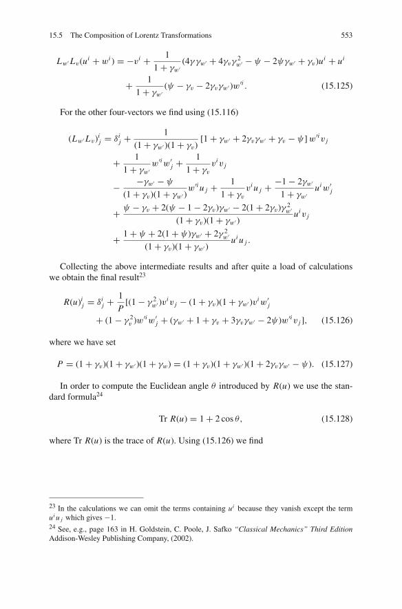
15.5 The Composition of Lorentz Transformations 553
Lw′Lv(ui + wi ) = −vi + 1
1+ γw′(4γ γw′ + 4γvγ
2w′ − ψ − 2ψγw′ + γv)ui + ui
+ 1
1+ γw′(ψ − γv − 2γvγw′)w
′i . (15.125)
For the other four-vectors we find using (15.116)
(Lw′Lv)ij = δi
j +1
(1+ γw′)(1+ γv)[1+ γw′ + 2γvγw′ + γv − ψ]w′iv j
+ 1
1+ γw′w′iw′j +
1
1+ γvviv j
− −γw′ − ψ
(1+ γv)(1+ γw′)w′i u j + 1
1+ γvvi u j + −1− 2γw′
1+ γw′uiw′j
+ ψ − γv + 2(ψ − 1− 2γv)γw′ − 2(1+ 2γv)γ 2w′
(1+ γv)(1+ γw′)uiv j
+ 1+ ψ + 2(1+ ψ)γw′ + 2γ 2w′
(1+ γv)(1+ γw′)ui u j .
Collecting the above intermediate results and after quite a load of calculationswe obtain the final result23
R(u)ij = δi
j +1
P[(1− γ 2
w′)viv j − (1+ γv)(1+ γw′)v
iw′j
+ (1− γ 2v )w′iw′j + (γw′ + 1+ γv + 3γvγw′ − 2ψ)w′iv j ], (15.126)
where we have set
P = (1+ γv)(1+ γw′)(1+ γw) = (1+ γv)(1+ γw′)(1+ 2γvγw′ − ψ). (15.127)
In order to compute the Euclidean angle θ introduced by R(u) we use the stan-dard formula24
Tr R(u) = 1+ 2 cos θ, (15.128)
where Tr R(u) is the trace of R(u). Using (15.126) we find
23 In the calculations we can omit the terms containing ui because they vanish except the termui u j which gives −1.24 See, e.g., page 163 in H. Goldstein, C. Poole, J. Safko “Classical Mechanics” Third EditionAddison-Wesley Publishing Company, (2002).

554 15 The Covariant Lorentz Transformation
cos θ = 1
2(Rμ
μ − 1) = 1
2P[(1− γ 2
w′)vμvμ − (1+ γv)(1+ γw′)v
μw′μ
+ (1− γ 2v )w′μw′μ + (γw′ + 1+ γv + 3γvγw′ − 2ψ)w′μvμ]+ 1.
For the terms involved in this relation we compute
vμvμ = −1+ γ 2v ,
w′μw′μ = −1+ γ 2w′ ,
w′μvμ =√−1+ γ 2
w′
√−1+ γ 2
v cosφ,
ψ = −w′ivi = w′μvμ − v0w′0 = γvγw′ −√−1+ γ 2
w′
√−1+ γ 2
v cosφ.
Replacing we find the cosine of the angle θ :
cos θ = 1− (γv − 1)(γw′ − 1) sin2 φ
1+ γvγw′ +√−1+ γ 2
w′√−1+ γ 2
v cosφ. (15.129)
To compare this result with existing results in the literature we introduce the
quantity τ =√
(1+ γw)(1+ γw′)
(γw − 1)(γw′ − 1). Then it can be shown that (15.129) reads
cos θ = 1− 2 sin2 φ
1+ τ 2 + 2τ cosφ, (15.130)
which coincides with the existing result in the literature.25
25 See equation (10) of the paper “Wigner’s rotation revisited” Ar Ben-Menahem, Am. J. Phys. 53,62–66, (1985).

Chapter 16Geometric Description of RelativisticInteractions
16.1 Collisions and Geometry
There is a fundamental difference concerning the concept of particle in Newtonianand in relativistic physics. In Newtonian Physics a particle is a “thing” which hasbeen created once and since then exists as an absolute unit for ever. Concerningthe physical quantities associated with a particle they are divided into two classes:the ones which are inherent in the structure of the particle such as mass, chargeand characterize the identity of the Newtonian particle and those which depend onthe motion of the particle in a reference system such as velocity, linear momentum.Newtonian particles are assumed to interact by collisions creating larger systems.This interaction of particles happens in a way that the overall inherent quantities ofthe particles are conserved (i.e., mass, charge) while some of the motion dependentphysical quantities such as energy, mass, and linear momentum are also conserved.Finally the systems consisting of many particles have more macroscopic physicalquantities such as temperature, pressure.
In Special Relativity the scenario is drastically different. A relativistic particle isnot a “thing” but a set of physical quantities which share the same frame as properor as characteristic frame depending if they are timelike or spacelike, respectively.In this sense a “particle” can appear as a n or as three particles p, e−, νβ accordingto the reaction n → p + e− + νβ . In this sense, for example, an electron is a setof two scalars (mass, charge), one vector (spin), and other physical fields makingup a catalogue which is not necessarily complete. That is, it is possible that anexperiment will indicate that the electron has associated a new physical propertywhich we did not know and which we have to consider. This new quantity will notchange the concept of the electron; however, it might lead us to consider more typesof electron (as we do with the positron) but this is it. In the relativistic approach wehave discovered only partially the entities of creation and we should be open to newdiscoveries.
As in Newtonian theory in Special (and General) Relativity the relativistic parti-cles, besides their inherent physical quantities, also have physical quantities whichdepend on their motion in a LCF. These quantities are the four-velocity, four-momentum, etc. Furthermore they are allowed to interact creating larger systems
M. Tsamparlis, Special Relativity, DOI 10.1007/978-3-642-03837-2 16,C© Springer-Verlag Berlin Heidelberg 2010
555

556 16 Geometric Description of Relativistic Interactions
which, as in Newtonian Physics, introduce new physical quantities such as (rela-tivistic) temperature. During their interaction we assume that some of the inherentand the non-inherent physical quantities of the particles are conserved. For example,the total charge and the total four-momentum are conserved.
It becomes clear that in Special Relativity one is possible to look upon a relativis-tic interaction as a transformation of a set of Lorentz tensors (scalars, four-vectors,tensors) to another set of Lorentz tensors (scalars, four-vectors, etc.) which maydiffer both in number and in type. This view is useful and important because itmakes possible to geometrize particle interactions. One might ask
Why should we want to geometrize relativistic interactions?
The answer is simpleBecause if we manage to do so, then we gain twofold, that is,
(a) We shall be able to “explain” various relativistic results and show that whatis new is not their mathematical expression but the physical explanation wehave given to mathematical expressions. In this sense we let “physics justifygeometry”.
(b) It would be possible to produce new results which will be consistent mathemat-ically and possibly lead to new physical phenomena we have not thought of yet.In a sense we let “geometry propose physics”.
In this chapter we discuss relativistic reactions in the above sense. However, weshall restrict our considerations to systems of four-momentum only, mainly becauseat the level we work this is the physical quantity we are most interested. How-ever, the approach is otherwise general so we shall speak of interacting four-vectorswhich need not be four-momenta!
16.2 Geometric Description of Collisions in Newtonian Physics
From the previous discussion it is clear that behind the physics of relativistic col-lisions there exists a geometry, which would be interesting and useful to be recog-nized and studied. The same holds for Newtonian collisions, although this is notwidely known. In this section we discuss briefly the Newtonian case for a simplemodel and in the next section we consider the relativistic counterpart.
We consider two similar smooth (solid) spheres with masses m1, m2 which aremoving along the same direction along the x-axis with velocities v1, v2, respec-tively. We assume that at some moment the spheres collide centrally and after theircollision they move again along the x-axis with corresponding velocities v′1, v
′2.
Newtonian conservation laws of linear momentum and energy give
m1(v1 − v′1) = −m2(v2 − v′2) (conservation of momentum), (16.1)
m1(v21 − v′21 ) = −m2(v2
2 − v′22 ) (conservation of energy). (16.2)

16.2 Geometric Description of Collisions in Newtonian Physics 557
Combining these two equations we find
v1 − v2 = v′2 − v′1, (16.3)
that is, the relative velocity of the spheres is preserved during the elastic collision.Solving (16.1) and (16.2) with respect to v′1, v
′2 we find
v′1 =1− k
1+ kv1 + 2k
1+ kv2, (16.4)
v′2 =2
1+ kv1 + k − 1
1+ kv2, (16.5)
where k = m2/m1. These equations can be written in the following form:
(v′1v′2
)=
⎛
⎜⎜⎜⎝
1− k
1+ k
2k
1+ k
2
1+ k
−1+ k
1+ k
⎞
⎟⎟⎟⎠
(v1
v2
)(16.6)
or
(v′1v′2
)= M
(v1
v2
), (16.7)
where M is the matrix:
M =
⎛
⎜⎜⎜⎝
1− k
1+ k
2k
1+ k
2
1+ k
−1+ k
1+ k
⎞
⎟⎟⎟⎠ . (16.8)
The matrix M contains all the information concerning the collision and it is thegeometric expression of the laws of conservation of linear momentum and energy.In order to understand the geometric significance of the matrix M (equivalently,of the laws of conservation of linear momentum and energy), we consider M asa transformation matrix in a linear space in which we interpret geometrically thecollision. We assume that in the specific example this space is an Euclidean two-
dimensional space, whose vectors are of the form
(v1
v2
). In this space the state of
the system of masses is described by the position vector
(v1
v2
), which after the
collision is transformed to the vector
(v′1v′2
). Therefore, in that space, the collision
is described by the linear transformation

558 16 Geometric Description of Relativistic Interactions
(v1
v2
)M−→
(v′1v′2
).
We note that geometrically the collision is not characterized by the velocities, butwith the matrix M which is defined in terms of the ratio k = m2
m1of the masses. This
observation is very important and has many consequences among which we note thefollowing:
(1) If
(−v1−v2
)is another initial point (i.e., different initial velocities), then for the
same masses we can write the result of a central collision without any furthercalculations, as the image point under the linear transformation M , that is,
(−v′1−v′2
)= M
(−v1−v2
)
(2) It is possible to study qualitatively the collision without any reference to veloc-ities, by studying the geometric properties of the transformation matrix M .
The second point is more important, because it geometrizes the physical processof collision and allows us to employ the powerful mathematical methods of differ-ential geometry in the study of the problem. Of course the problem we consideredis simple but the method can be generalized to more complex problems and makepossible the study of physical problems, which otherwise would be very difficultto do. More generally, the geometrization of mechanics is a long-standing studywhich recently has been extended to the study of dynamical systems, which involvepractically most branches of modern science ranging from physics to economics andmedicine (chaos, Hamiltonian dynamics, etc.).
Exercise 86 Show that the transformation matrix M satisfies the following geomet-ric properties.
(1) M is symmetric, if and only if m1 = m2.(2) traceM = 0(3) det M = −1(4) M2 = I or M−1 = M (M is a projective operator)(5) diag(m1,m2) = Mtdiag(m1,m2)M .
16.3 Geometric Description of Relativistic Reactions
The geometric description of Newtonian collisions cannot be transferred to SpecialRelativity as such, for the following two reasons:
(1) The photons have zero mass, therefore their description is not possible in acollision matrix containing masses.
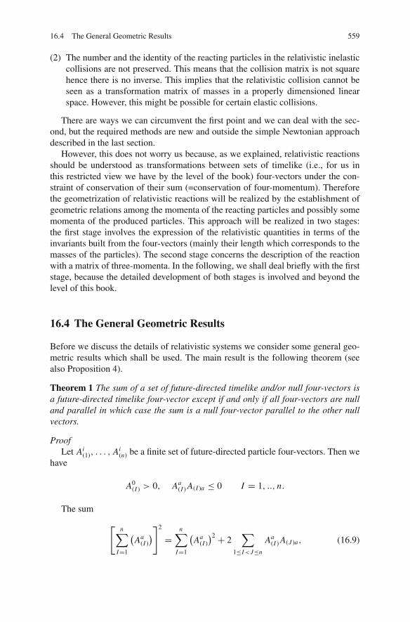
16.4 The General Geometric Results 559
(2) The number and the identity of the reacting particles in the relativistic inelasticcollisions are not preserved. This means that the collision matrix is not squarehence there is no inverse. This implies that the relativistic collision cannot beseen as a transformation matrix of masses in a properly dimensioned linearspace. However, this might be possible for certain elastic collisions.
There are ways we can circumvent the first point and we can deal with the sec-ond, but the required methods are new and outside the simple Newtonian approachdescribed in the last section.
However, this does not worry us because, as we explained, relativistic reactionsshould be understood as transformations between sets of timelike (i.e., for us inthis restricted view we have by the level of the book) four-vectors under the con-straint of conservation of their sum (=conservation of four-momentum). Thereforethe geometrization of relativistic reactions will be realized by the establishment ofgeometric relations among the momenta of the reacting particles and possibly somemomenta of the produced particles. This approach will be realized in two stages:the first stage involves the expression of the relativistic quantities in terms of theinvariants built from the four-vectors (mainly their length which corresponds to themasses of the particles). The second stage concerns the description of the reactionwith a matrix of three-momenta. In the following, we shall deal briefly with the firststage, because the detailed development of both stages is involved and beyond thelevel of this book.
16.4 The General Geometric Results
Before we discuss the details of relativistic systems we consider some general geo-metric results which shall be used. The main result is the following theorem (seealso Proposition 4).
Theorem 1 The sum of a set of future-directed timelike and/or null four-vectors isa future-directed timelike four-vector except if and only if all four-vectors are nulland parallel in which case the sum is a null four-vector parallel to the other nullvectors.
ProofLet Ai
(1), . . . , Ai(n) be a finite set of future-directed particle four-vectors. Then we
have
A0(I ) > 0, Aa
(I ) A(I )a ≤ 0 I = 1, .., n.
The sum
[n∑
I=1
(Aa
(I )
)]2
=n∑
I=1
(Aa
(I )
)2 + 2∑
1≤I<J≤n
Aa(I ) A(J )a, (16.9)
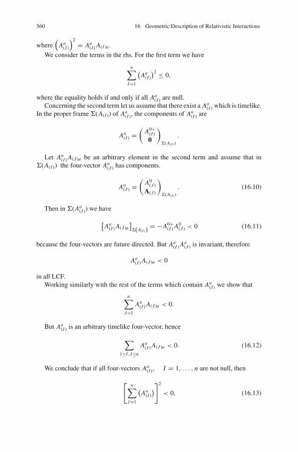
560 16 Geometric Description of Relativistic Interactions
where(
Aa(I )
)2= Aa
(I ) A(I )a .
We consider the terms in the rhs. For the first term we have
n∑
I=1
(Aa
(I )
)2 ≤ 0,
where the equality holds if and only if all Aa(I ) are null.
Concerning the second term let us assume that there exist a Aa(I ) which is timelike.
In the proper frame Σ(A(I )) of Aa(I ), the components of Aa
(I ) are
Aa(I ) =
(A0+
(I )0
)
Σ(A(I ))
.
Let Aa(I ) A(J )a be an arbitrary element in the second term and assume that in
Σ(A(I )) the four-vector Aa(J ) has components.
Aa(J ) =
(A0
(J )A(J )
)
Σ(A(I ))
. (16.10)
Then in Σ(Aa(I )) we have
[Aa
(I ) A(J )a]Σ(A(I )) = −A0+
(I ) A0(J ) < 0 (16.11)
because the four-vectors are future directed. But Aa(I ) Aa
(J ) is invariant, therefore
Aa(I ) A(J )a < 0
in all LCF.Working similarly with the rest of the terms which contain Aa
(I ) we show that
n∑
J=1
Aa(I ) A(J )a < 0.
But Aa(I ) is an arbitrary timelike four-vector, hence
∑
1≤I,J≤n
Aa(I ) A(J )a < 0. (16.12)
We conclude that if all four-vectors Aa(I ), I = 1, . . . , n are not null, then
[n∑
I=1
(Aa
(I )
)]2
< 0, (16.13)
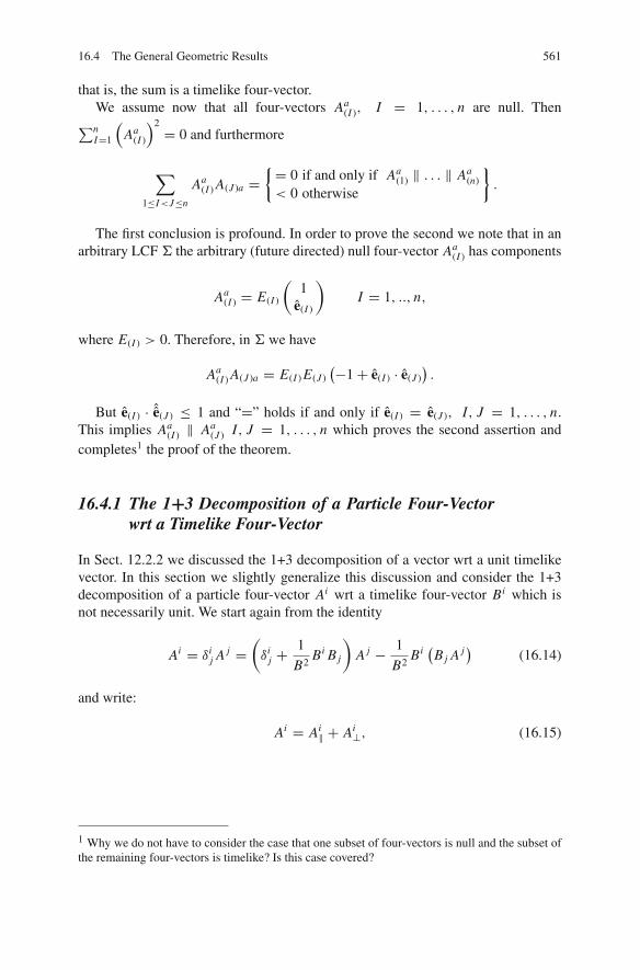
16.4 The General Geometric Results 561
that is, the sum is a timelike four-vector.We assume now that all four-vectors Aa
(I ), I = 1, . . . , n are null. Then∑n
I=1
(Aa
(I )
)2= 0 and furthermore
∑
1≤I<J≤n
Aa(I ) A(J )a =
{= 0 if and only if Aa(1) ‖ . . . ‖ Aa
(n)< 0 otherwise
}.
The first conclusion is profound. In order to prove the second we note that in anarbitrary LCF Σ the arbitrary (future directed) null four-vector Aa
(I ) has components
Aa(I ) = E(I )
(1
e(I )
)I = 1, .., n,
where E(I ) > 0. Therefore, in Σ we have
Aa(I ) A(J )a = E(I ) E(J )
(−1+ e(I ) · e(J )).
But e(I ) · ˆe(J ) ≤ 1 and “=” holds if and only if e(I ) = e(J ), I, J = 1, . . . , n.This implies Aa
(I ) ‖ Aa(J ) I, J = 1, . . . , n which proves the second assertion and
completes1 the proof of the theorem.
16.4.1 The 1+3 Decomposition of a Particle Four-Vectorwrt a Timelike Four-Vector
In Sect. 12.2.2 we discussed the 1+3 decomposition of a vector wrt a unit timelikevector. In this section we slightly generalize this discussion and consider the 1+3decomposition of a particle four-vector Ai wrt a timelike four-vector Bi which isnot necessarily unit. We start again from the identity
Ai = δij A j =
(δi
j +1
B2Bi B j
)A j − 1
B2Bi
(B j A j
)(16.14)
and write:
Ai = Ai‖ + Ai
⊥, (16.15)
1 Why we do not have to consider the case that one subset of four-vectors is null and the subset ofthe remaining four-vectors is timelike? Is this case covered?

562 16 Geometric Description of Relativistic Interactions
where:
Ai‖ = −
1
B2
(B j A j
)Bi , (16.16)
Ai⊥ =
(δi
j +1
B2Bi B j
)A j . (16.17)
The four-vector Ai‖ is the parallel component and the four-vector Ai
⊥ the normalprojection of Ai along Bi . The tensor
hij (B) = δi
j +1
B2Bi B j (16.18)
is the projection tensor associated with the four-vector Bi . We have:
Ai⊥ = hi
j (B)A j . (16.19)
As we have seen the two-tensor hij (B) is very important in Relativity and it is
used extensively in all calculations. In the rest frame ΣB of Bi the components ofhi
j (B) are
hij (B) = diag(0, 1, 1, 1)ΣB (16.20)
and can be thought as the Euclidean metric of the rest space of Bi . It satisfies theproperties:
hi j (B) = h ji (B), hij (B)h j
k (B) = hik(B), hi
i (B) = 3. (16.21)
Summarizing we have
Aa = −1
B2(Ab Bb)Ba + ha
b(B)Ab (16.22)
and in matrix form2:
Aa =⎛
⎝− Ab Bb
B
h(B)ab Ab
⎞
⎠
ΣB
.
Having given the basic facts about the decomposition of four-vectors we areready to discuss the geometry of systems of particle four-vectors. It will help ifwe keep in mind that the results we shall obtain hold for the four-momentum, but
2 The unit in the direction of Ba is Ba/B hence the B in the denominator.

16.5 The System of Two to One Particle Four-Vectors 563
they apply to any set of interacting four-vectors. In the rest of the chapter we shallconsider two special four-vector systems. The system A + B → C , which is thegeneric reaction, and the system A + B → C + D, which is more general thatthe first. The results we shall obtain will be generic in the sense that they applyto all reactions of the type we consider. We shall illustrate the results by specificexamples, which demonstrate how one applies the general ideas in practice. Finally,it should be remarked that the results we derive are covariant, therefore, it is possibleto develop proper software (for algebraic computing), which will give the answer toany problem for sufficiently given data!
16.5 The System of Two to One Particle Four-Vectors
The simpler system of particle four-vectors is the system consisting of two future-directed particle four-vectors Aa, Ba and corresponds to the generic reaction A +B → C . From these two four-vectors we define another two four-vectors the Aa +Ba , Aa − Ba . The four-vector Aa + Ba is a future-directed particle four-vector, theCenter System (CS) four-vector (see Sect. 1.12). In case Aa, Ba are four-momentathe four-vector Aa + Ba is the center of momenta four-vector and the particle itdefines is the center of momentum particle.
We shall express the inner products between the four-vectors Aa, Ba in terms oftheir lengths. The results will be used to compute the zeroth component of Aa in theproper frame of one of the rest four-vectors. The zeroth component, equivalently theinner product Aa Ba , is computed from the identity
(Aa + Ba)2 = (Aa)2 + (Ba)2 + 2Aa Ba . (16.23)
If we replace the lengths
(Aa + Ba)2 = −M2, (Aa)2 = −A2, (Ba)2 = −B2 (M, A, B > 0) (16.24)
we find
Aa Ba = 1
2
(−M2 + A2 + B2). (16.25)
Concerning the spatial part of Aa in ΣB we have
hab(B)Ab = Aa + (Ab Bb)
B2Ba = Aa + 1
2B2
(−M2 + A2 + B2)
Ba . (16.26)
The spatial part can be decomposed further in the direction A(B) and the lengthof A(B) in ΣB :
A(B) =√
hab(B)Aa AbA(B). (16.27)

564 16 Geometric Description of Relativistic Interactions
Finally for the four-vector Aa we have the decomposition
Aa =⎛
⎝M2−A2−B2
2B
√hab(B)Aa Ab A(B)
⎞
⎠
ΣB
. (16.28)
We see that the four-vector Aa is determined from the invariants A, B, M and thespatial direction A(B).
Exercise 87 For every non-null four-vector Ai the symmetric tensor hi j (A) = ηi j −1
Ak AkAi A j projects normal to the vector Ai , that is, hi j (A)A j = 0.
(a) Let pi the four-momentum of a particle and pi1 the four-momentum of another
particle. Show the identity
pi1 =
p j1 p j
pk pkpi + hi
j (p)p j1 .
This identity defines the 1+ 3 decomposition of the four-vector pi1 wrt the four-
vector pi . The part pi1‖ ≡ p j
1 p j
pk pkpi is the parallel part and the part pi
1⊥ ≡ hij (p)p j
1 is
the normal part. Show that the inner product p j1 p j = 1
2 {(pi + pi1)2− pi pi − pi
1 p1i },that is, it is expressed in terms of the length of the four-vectors. In order to give theabove a physical interpretation we consider the masses pi pi = −m2c2, pi
1 p1i =−m2
1c2 and then the inner product p j1 p j = −m EΣ
1 , where EΣ1 is the energy of
the particle of four-momentum pi1 in the proper frame Σ of the particle with four-
momentum pi . Define pi2 = pi − pi
1 and show that
EΣ1 =
m1 + m22 − m2
1
2mc2,
where pi2 p2i = −m2
2c2. Also show that the length of the normal part pi1⊥ · pi
1⊥ isgiven by the relation
pi1⊥ · pi
1⊥ ≡ p12c2 = E∗21 − m2
1c4 = [m2 − (m1 + m2)2][m2 − (m1 − m2)2]
2Mc2.
Finally collect the results of the 1+3 decomposition of the four-vector pi1 in Σ as
follows:
pi1 =
(E∗1/c
p1
)
Σ
=
⎛
⎜⎜⎜⎝
m2 + m22 − m2
1
2mc
[m2 − (m1 + m2)2][m2 − (m1 − m2)2]
2MceΣ
⎞
⎟⎟⎟⎠
Σ
,
where eΣ is the unit of the spatial part of pi1 in Σ.

16.5 The System of Two to One Particle Four-Vectors 565
16.5.1 The Triangle Function of a System of Two ParticleFour-Vectors
The length hab(B)Aa Ab of A(B) is an invariant therefore it is a characteristic quantityof the system of the four-vectors Aa, Ba . In order to determine the exact dependenceof this quantity on the four-vectors Aa, Ba we compute it. From (16.26) we have
hab(B)Aa Ab =[
Aa + 1
2B2
[−M2 + A2 + B2]
Ba
]Aa
= 1
4B2λ2(M2, A2, B2), (16.29)
where
λ(M2, A2, B2) =√[−M2 + A2 + B2
]2 − 4A2 B2 (16.30)
=√
M4 + A4 + B4 − 2M2 A2 − 2M2 B2 − 2A2 B2.
We conclude the following:
(1) The function λ(M2, A2, B2) is an invariant depending only on the lengths of thevectors (A + B)a, Aa, Ba .
(2) The function λ(M2, A2, B2) is symmetric in all its arguments.
We have met the function λ before, when we were studying the collisionA + B → C . Here we simply recover it in a more general set up and, furthermore,we give its covariant geometric meaning. The properties of the function λ are givenin Exercise 34.
Example 79 Show that the quantity
E = 1
4
√−λ(x, y, z) (16.31)
equals the area of an Euclidean triangle of sides√
x,√
y,√
z. Prove that the tri-angle inequality of Euclidean geometry assures that in a Euclidean space λ(x, y,z) < 0.Solution
The semi-perimeter τ of a Euclidean triangle of sides α = √x, β = √y, γ =√z equals τ = (α + β + γ )/2 and the area is given by the Heron’s formula
E = √τ (τ − α)(τ − β)(τ − γ ). We find

566 16 Geometric Description of Relativistic Interactions
E2 = 1
16(α + β + γ )(−α + β + γ )(α − β + γ )(α + β − γ )
= 1
16
(−a2 + (β + γ )2) (a2 − (β − γ )2)
= − 1
16
(x − (√
y +√z)2) (
x − (√
y −√z)2)
= − 1
16λ(x, y, z).
Because in Euclidean geometry the area E ≥ 0 it follows that λ(x, y, z) ≤ 0.This creates a contradiction because in Minkowski space λ(x, y, z) equals the mea-sure |A∗| which is positive, hence in Minkowski space λ(x, y, z) ≥ 0! How-ever, there is no problem because in Euclidean geometry the triangle inequalityimplies that λ(x, y, z) ≤ 0 and in Minkowski space the same inequality assures thatλ(x, y, z) ≥ 0. To prove the latter, we consider the four-vectors Aa, Ba, (A + B)a
and from (10.21) we have for x = (A + B)2, y = A2, z = B2
[(A + B)2 −
(√A2 +
√B2
)] [(A + B)2 −
(√A2 −
√B2
)]≥ 0
(A + B)2 ≥(√
A2 +√
B2)2
, (A + B)2 ≥(√
A2 −√
B2)2
or
(A + B)2 ≤(√
A2 +√
B2)2
, (A + B)2 ≤(√
A2 −√
B2)2
.
But√
A2 +√
B2 ≥√
A2 −√
B2 because A, B > 0. Hence
(A + B) ≥√
A2 +√
B2 (16.32)
for all pairs of particle four-vectors Aa, Ba . Therefore the condition
λ(M2, A2, B2) ≥ 0
is satisfied and it is equivalent to the triangle inequality in Minkowski space.In words relation (16.32) means that the particle four-vector (A + B)a is some-
thing “more” than the aggregate of the particle four-vectors Aa, Ba . This “some-thing” is the structure which couples the two four-vectors into the system – par-ticle four-vector (A + B)a . To see what this implies we examine its effect in onewell-known issue of relativistic physics, the mass loss. We assume the four-vectorsAa, Ba to be four-momenta. Then (A+ B)a represents the center momentum parti-cle whose mass is M . Then inequality (16.32) implies that M is larger than the sumof the masses m A,m B of the individual particles Aa, Ba , the difference counting forthe potential (or internal) energy of the particle (A + B)a .

16.5 The System of Two to One Particle Four-Vectors 567
An interesting special case is λ(x, y, z) = 0. Then M = A + B and |AM | =|BM | = 0, which implies that the proper frame of the four-vectors Aa, Ba coin-cides with the proper frame of Ma . We call the condition λ(x, y, z) = 0 thethreshold of the interaction of the four-vectors Aa, Ba . Note that the above do notapply only to four-momentum but to interacting triplets of four-vectors Aa, Ba,
(A + B)a .
16.5.2 Extreme Values of the Four-Vectors (A ± B)2
The lengths (A + B), (A − B) of a system of two particle four-vectors Aa, Ba oflength A, B find application in many cases and especially in relativistic reactions(collisions) ((A+ B) is the mass of the center of momentum particle and (A− B) isthe amount of transfer of four-momenta). It is of interest to determine the extremevalues of the quantities (A + B), (A − B) when the direction of Aa, Ba changeswhile their length remains constant.
From (16.23) we have−(A± B)2 = −A2− B2∓2Aa Ba therefore the extremumof −(A ± B)2 occurs when the term Aa Ba is an extremum. The term Aa Ba isinvariant therefore it is possible to be computed in any LCF. We choose the properframe ΣA of Aa and write
Aa =(
A0
)
ΣA
, Ba =(
B0(A)
B(A)
)
ΣA
from which follows
Aa Ba = −AB0(A).
But B0(A) =
√B2 + B2
(A) hence
Aa Ba = −A√
B2 + B2(A). (16.33)
We note that in the rhs the only quantity which changes is B2(A), therefore the
extremum (maximum) of Aa Ba occurs if
∂(Aa Ba)
∂(B2(A))= 0.
This condition gives
−AB(A)√
B2 + B2(A)
= 0⇒ B(A) = 0

568 16 Geometric Description of Relativistic Interactions
hence
(Aa Ba)max = −AB.
It follows
(A + B)2max = A2 + B2 + 2AB = (A + B)2,
(A − B)2min = A2 + B2 − 2AB = (A − B)2.
Condition B(A) = 0 means that the proper frames of the four-vectors Aa, Ba
coincide or Aa = αBa , where α is an invariant. To compute a we multiply thisequation with Aa and find
−A2 = α(Aa Ba) = −αAB ⇒ α = A
B.
Therefore, the condition for the extremum is3 Aa
A = Ba
B or Aa ‖ Ba .
16.5.3 The System Aa, Ba, (A + B)a of Particle Four-Vectors inCS
Let Aa, Ba be two particle four-vectors, which are not null and parallel and let Σ∗ bethe CS of the system of Aa, Ba . We shall denote the components of the four-vectorsin CS with an asterisk, e.g., for the vector Aa we write
Aa =(
A0∗
A∗
)
Σ∗. (16.34)
In order to compute A0∗ we note that in Σ∗ (A + B)a =(
M0
)
Σ∗, hence
Aa(A + B)a = −A0∗M. (16.35)
But from (16.25) we have, if we replace B with M (why we can do this?)
Aa(A + B)a = 1
2
(−M2 − A2 + B2)
3 It is possible to compute the extremals of the quantity (16.33) without any calculations if we notethat the quantity under the square root is non-negative. Therefore the maximum value occurs forthe minimum value of the denominator which is B2
(A) = 0 and the minimum when the denominatoris maximum, that is, when B2
(A) is infinite.

16.5 The System of Two to One Particle Four-Vectors 569
from which follows
− A0∗M = 1
2
(−M2 − A2 + B2)⇒ A0∗ = 1
2M
(M2 + A2 − B2
). (16.36)
Concerning the length of the spatial part A∗ from (16.29) we have
(A∗)2 = hab(A + B)Aa Ab = 1
4M2λ2(M2, A2, B2). (16.37)
It is instructive to compute the components of the four-vector Aa in the CSdirectly by making use of the decomposition (16.28). To do this we write (A+B)a =Aa + Ba as −Ba = Aa − (A + B)a , which shows that −Ba is the CS of thefour-vectors Aa and −(A + B)a . Therefore relation (16.28) applies if we make thecorrespondence
M ←→ B,
ΣB ←→ Σ∗,
A(B) ←→−A∗,
A0(B) ←→−A0∗
It follows
Aa =
⎛
⎜⎜⎝
M2 + A2 − B2
2M
12M
√λ(M2, A2, B2)A∗
⎞
⎟⎟⎠
Σ∗
. (16.38)
Concerning the decomposition of Ba we have from (16.38), if we interchangeA←→ B and note that A∗ + B∗ = 0
Ba =
⎛
⎜⎜⎝
M2 − A2 + B2
2M
− 12M
√λ(M2, A2, B2)A∗
⎞
⎟⎟⎠
Σ∗
. (16.39)
In order to check our results we compute the angle θ∗AB between the vectorsA∗, B∗ in Σ∗. Obviously we expect to find θ∗AB = π since A∗ = −B∗. We compute
A∗ · B∗ = hab(A + B)Aa Ba = − 1
4M2λ2(M2, A2, B2) = |A∗||B∗| cos θ∗AB .
But |A∗| = |B∗| = 12M
√λ(M2, A2, B2) therefore cos θ∗AB = −1⇒ θ∗AB = π .

570 16 Geometric Description of Relativistic Interactions
16.5.4 The System Aa, Ba, (A + B)a in the Lab
The LCF in which we study the “motion” of systems of particle four-vectors are
(a) The CS(b) The proper frame of one of the particle four-vectors, which we call the target
system(c) The Laboratory System (lab) which usually coincides with the proper frame of
one of the particle four-vectors
In Sect. 16.5.3 we studied the system of two particle four-vectors Aa, Ba in theCS. In this section we study the same system in the lab which we assume that itcoincides with the proper frame of particle Ba .
We denote the components of a four-vector in the lab with an L and write
Aa =(
A0L
AL
)
ΣL
, Ba =(
B0
)
ΣL
, (A + B)a =(
(A + B)0L
(A+ B)L
)
ΣL
. (16.40)
In order to compute the components A0L , (AL )2 we apply relations (16.36) and(16.37) provided we change A + B with B. From (16.36) we find
A0L = − 1
2B
(−B2 − A2 + M2) = 1
2B
(B2 + A2 − M2
)(16.41)
and from (16.37)
(AL )2 = hab(B)Aa Ab = 1
4B2λ2(M2, A2, B2), (16.42)
where we have used the fact the triangle function is symmetric in all its arguments.Let us assume that Σ∗ is moving wrt ΣL = ΣB with velocity β∗. Then we have
Ba =(
B0
)
ΣL
=
⎛
⎜⎜⎝
M2 − A2 + B2
2M
12M
√λ(M2, A2, B2)B∗
⎞
⎟⎟⎠
Σ∗
.
The two expressions are related with the Lorentz transformation which relatesΣ∗, ΣL . Therefore (see (1.75)).
M2 − A2 + B2
2M= γ B ⇒ γ = M2 − A2 + B2
2B M(16.43)
1
2M
√λ(M2, A2, B2)B∗ = γβ ⇒ β =
√λ(M2, A2, B2)
2Mγ BB∗. (16.44)

16.5 The System of Two to One Particle Four-Vectors 571
Let us consider the application of the above general results in special two particlesystems.
Example 80 Consider an electron and a positron with four-momenta pae− , pa
e+ ,respectively. Assume c = 1.
(1) Determine the energy of each particle in the CS.(2) Show that in the CS the spatial momenta are antiparallel.(3) Assume that the positron rests in the lab and compute the velocity of the CS in
the lab.
SolutionLet me− = me+ = m the masses of the particles involved. The four-momentum
of the center of momentum particle is (pe− + pe+ )a = pae− + pa
e+ and let its mass beM . Identifying Aa , Ba with pa
e− , pae+ , respectively, we find from (16.38)
pae− =
⎛
⎜⎜⎝
M2 − m2 + m2
2M
12M
√λ(M2,m2,m2)p∗e−
⎞
⎟⎟⎠
Σ∗
=
⎛
⎜⎜⎝
M2
2
12
√M2 − 4m2p∗e−
⎞
⎟⎟⎠
Σ∗
(16.45)
pae+ =
⎛
⎜⎜⎝
M2 + m2 − m2
2M
12M
√λ(M2,m2,m2)p∗e+
⎞
⎟⎟⎠
Σ∗
=
⎛
⎜⎜⎝
M2
2
− 12
√M2 − 4m2p∗e−
⎞
⎟⎟⎠
Σ∗
. (16.46)
The energy is the zeroth component of the four-momentum, hence
E∗e− = E∗e+ =M2
2.
The three-momenta are the spatial part of the four-momentum. It follows
|p∗e−| = |p∗e+| =1
2
√M2 − 4m2.
Concerning the angle θ∗e−e+ between the two three-momenta in the CS we findθ∗e−e+ = π .
From (16.43) we find that the γ−factor of the CS in the lab (=proper frame ofpe+ ) is
γ = M2 − m2 + m2
2m M= M
2m.

572 16 Geometric Description of Relativistic Interactions
Finally from (16.44) we find for the β∗-factor (c = 1)
β∗ =√λ(M2,m2,m2)
2Mγmp∗e− =
√M2 − 4m2
Mp∗e− .
The three-vector p∗e− is a space direction in the lab which shall be defined fromthe initial conditions (it is the direction of the bullet particle in the lab).
In the next exercise we compute the same results using direct calculation, so thatthe reader will gain experience with this type of problems.
Exercise 88 Assume pae− = Aa, pa
e+ = Ba, A2 = B2 = m2 and that the lengthof the momentum of the center of momenta particle is M . Verify the followingcalculations:
(a) Energies:
E∗e− =M2 − m2 + m2
2Mc2c4 = M
2c2 = E∗e+ .
(b) three-momenta:
hab(pe− + pe+)pae− pb
e− = −m2c2 + 1
4M2
[M2 − m2 + m2
]c2 =
(M2
4− m2
)c2
p∗2
e− = p∗2e+ =1
4(M2 − 4m2)c2.
(c) Angle:
hab(pe− + pe+ )pae− pb
e+ = −1
4M2
[M4 − 4m2 M2
]c2 = −1
4
[M2 − 4m2
]c2
= −|p∗e− ||p∗e+| = |p∗e−||p∗e+| cosπ.
Example 81 In the LCF Σ the null four-vectors Aa, Ba have components Aa =A (1, 1, 0, 0)Σ , Ba = B (1, 0, 1, 0)Σ.
(1) If Aa, Ba are four-momenta of photons determine the energy and the directionof motion (the speed is known!) of the photons in the LCF Σ.
(2) A particle Γ of mass√
3 moves in the plane x, y of Σ with factor β = 12 in a
direction which makes an angle 450 with the x-axis. Determine the energy andthe four-momentum of particle Γ in Σ.
(3) Compute the angle between the direction of motion of the photons Aa, Ba inthe proper frame of the particle Γ.

16.5 The System of Two to One Particle Four-Vectors 573
Solution
(1) The energy of the photon Aa in Σ is
AΣE/c = A⇒A
Σ E = Ac
and the three-momentum is
AΣp = A
⎛
⎝100
⎞
⎠ .
The direction of motion of the photon Aa in Σ is
AΣp =
⎛
⎝100
⎞
⎠ .
Prove that the photon Ba moves in Σ in a direction normal to the directionof Aa .
(2) The γ -factor of the particle Γ in Σ is
γ = 1√1− β2
= 2√3, β = 1
2.
Therefore the energy and the three-momentum of Γ in Σ are
ΓΣE = mγ c2 = 2c2,
ΓΣp = mγβc
1√2
⎛
⎝110
⎞
⎠ = c√2
⎛
⎝110
⎞
⎠ .
The four-momentum of Γ in Σ is
paΓ =
⎛
⎝ΓΣE/c
ΓΣp
⎞
⎠
Σ
=
⎛
⎜⎜⎝
2cc√2
c√2
0
⎞
⎟⎟⎠
Σ
.
We check the results by showing that paΓ pΓa = −mΓc2. Indeed
paΓ pΓa = −4c2 + c2
2+ c2
2= −3c2.
(3) To find the angle of the space directions of motion of the photons Aa, Ba in theproper frame of Γ we consider the inner product

574 16 Geometric Description of Relativistic Interactions
hab(Γ)Aa Bb =(ηab + 1
3c2pΓa pΓb
)Aa Bb
= Aa Ba + 1
3c2
(pΓa Aa
) (pΓb Bb
)
= 0+ 1
3c2c2
(−2+ 1√
2
)2
= 1
3
(−2+ 1√
2
)2
.
But
hab(Γ)Aa Bb = |AΣp||BΣp| cos θAB,Σ.
The |AΣp| = |BΣp| = 1 therefore θAB,Σ = cos−1{ 13 (−2+ 1√2)2}.
16.6 The Relativistic System Aa + Ba → Ca + Da
Let M be the length of the common Center System four-vector of the pairs (Aa, Ba),(Ca, Da). From (16.25) we have
−M2 = −A2 − B2 + 2(AB) = −C2 − D2 + 2(C D), (16.47)
where (AB) = Aa Ba, (C D) = Ca Da . We assume that the lengths A, B,C, D ofthe particle four-vectors are given (e.g., they are the masses of the correspondingparticles) and also that we are given enough data to compute one of the innerproducts (AB) or (C D). We shall show that with these data we can compute theremaining quantities involved.
In order to do that we consider the decomposition of the four-vectors
(a) In the lab, which we assume that it coincides with the proper frame of the(non-null!) particle four-vector Ba and
(b) In the CS.
Before we continue our discussion we recall that if we are given the four-vectorsof one pair, e.g., the pair (Aa, Ba) in a LCF Σ then the β∗-factor and the γ ∗-factorof the CS in Σ are given by the relations
β∗Σ =AΣ + BΣ
A0Σ + B0
Σ
, γ ∗Σ =A0
Σ + B0Σ
M. (16.48)

16.6 The Relativistic System Aa + Ba → Ca + Da 575
In case Σ is the proper frame of Ba (=lab) then these relations read
β∗L =AL
AL0 + B, γ ∗L =
A0L + B
M. (16.49)
In the calculations it will be useful to write relations (16.48) and (16.49) incovariant form, that is, in terms of tensor quantities. If Σ is determined by the unittimelike four-vector sa (sasa = −1) which is the unit in the direction of the centerfour-vector Aa + B2, then (16.48) is written as
β∗Σ =hab(s)(Ab + Bb)
−sb(Ab + Bb), γ ∗Σ = −
sb(Ab + Bb)
M. (16.50)
In the lab these relations give
β∗L =hab(B)(Ab + Bb)
− 1B Bb(Ab + Bb)
=1
2B
√λ(M2, A2, B2)
− 1B
(Ab Bb − B2
) A = 1
2
√λ(M2, A2, B2)
M2 − A2 + B2A,
(16.51)
γ ∗L = −Bb(Ab + Bb)
B M= −Bb Ab + B2
B M= M2 − A2 + B2
2B M, (16.52)
where A is the unit of the spatial direction of Aa in the proper frame of Ba .From relations (16.43) and (16.44) we have the following decompositions of the
four-vectors in the lab (ΣL ) and in the CS (Σ∗).4
Aa =
⎛
⎜⎜⎝
M2 + A2 − B2
2M
12M
√λ(M2, A2, B2)A∗
⎞
⎟⎟⎠
Σ∗
=
⎛
⎜⎜⎝
M2 − A2 − B2
2B
12B
√λ(M2, A2, B2)AB
⎞
⎟⎟⎠
ΣL
, (16.53)
Ba =
⎛
⎜⎜⎝
M2 − A2 + B2
2M
− 12M
√λ(M2, A2, B2)A∗
⎞
⎟⎟⎠
Σ∗
=⎛
⎝B
0
⎞
⎠
ΣL
, (16.54)
Ca =
⎛
⎜⎜⎝
M2 + C2 − D2
2M
12M
√λ(M2,C2, D2)C∗
⎞
⎟⎟⎠
Σ∗
=
⎛
⎜⎝− (C B)
B
hab(B)Cb
⎞
⎟⎠
ΣL
, (16.55)
4 The “=” does not mean that we can equate the corresponding components of the four-vectorsbecause the decompositions/components refer to different coordinate frames. It simply indicatesthat they refer to the decomposition of the same four-vector in different LCF. The components ofeach vector are related to the other via the Lorentz transformation which relates the correspondingLCF frames.

576 16 Geometric Description of Relativistic Interactions
Da =
⎛
⎜⎜⎝
M2 − C2 + D2
2M
− 12M
√λ(M2,C2, D2)C∗
⎞
⎟⎟⎠
Σ∗
=
⎛
⎜⎝− (DB)
B
hab(B)Db
⎞
⎟⎠
ΣL
. (16.56)
In order to calculate the zeroth component (i.e., (C B)) of the four-vector Ca inthe lab, we note that the inner product is invariant, therefore we can compute it inany frame we wish. We choose the CS Σ∗ where we know the components of thefour-vectors. We have
(C B) = − 1
4M2[(M2 − A2 + B2
) (M2 + C2 − D2
)
+√λ(M2, A2, B2)
√λ(M2,C2, D2)(A∗ · C∗)]. (16.57)
Similarly for the four-vector Da we have
(DB) = − 1
4M2[(M2 − A2 + B2
) (M2 − C2 + D2
)
−√λ(M2, A2, B2)
√λ(M2,C2, D2)(A∗ · C∗)]. (16.58)
We conclude that in order to determine the zeroth components of the “ daughter”four-vectors Ca, Da in lab we need to know the angle between A∗, C∗ in the CS Σ∗.
In the following we compute the various angles which enter in the geometry ofthe interaction.
(a) Computation of the angle θ LC D between the spatial parts of the four-vectors
Ca, Da in the lab frame.We have
hab(B)Ca Db =(ηab + 1
B2Ba Bb
)Ca Db
= (C D)+ 1
B2(C B)(DB) = 1
2(−M2 + C2 + D2)
+ 1
B2(C B)(DB)
= |CL ||DL | cos θ LC D ⇒
cos θ LC D =
1
|CL ||DL |[
1
2(−M2 + C2 + D2)+ 1
B2(C B)(DB)
], (16.59)

16.6 The Relativistic System Aa + Ba → Ca + Da 577
where
|CL | =√
hab(B)CaCb =√[−C2 + 1
B2(C B)2
], (16.60)
|DL | =√
hab(B)Da Db =√[−D2 + 1
B2(DB)2
]. (16.61)
(b) Computation of the angle θ LAC between the spatial part of the four-vectors Ca
and Aa in the lab frame.The spatial part of the four-vectors Aa, Ca in the lab is given by the relationshab(B)Ab , hcd (B)Cd , respectively. Therefore the angle cos θ L
AC of the spatialparts in the lab is
|CL ||AL | cos θ LAC = hab(B)Aahb
d (B)Cd = hab(B)AaCb. (16.62)
The term
hab(B)Ca Ab = (C A)+ 1
B2(AB)(C B)
= (C A)+ −M2 + A2 + B2
2B2(C B).
In order to compute the inner product (C A) we use the conservation equationAa + Ba = Ca + Da which we multiply with Ca and get
(AC)+ (C B) = −C2 + (C D)⇒(AC) = −(C B)− C2 + 1
2(−M2 + C2 + D2)
= −(C B)− 1
2(M2 + C2 − D2). (16.63)
Replacing we find
hab(B)Ca Ab = −1
2
[(M2 + C2 − D2)+ 1
B2
(M2 − A2 + B2
)(C B)
].
(16.64)
The term |CL | has been calculated in (16.60) and the term |AL | in (16.42).Introducing the above results in (16.62) we find

578 16 Geometric Description of Relativistic Interactions
cos θ LC A = −
B2
√λ(M2, A2, B2)
√−B2C2 + (C B)2
[(M2 + C2 − D2)+ 1
B2
(M2 − A2 + B2
)(C B)
]. (16.65)
(c) Computation of the angle θ∗AC of the spatial part of the four-vector Ca with thespatial part of the four-vector Aa in the CS.
We note that normal to the direction of β∗L the CL does not change. The conditionfor this is
CL × β∗L = C∗ × β∗L (16.66)
which gives
|CL | sin θ LAC = |C∗| sin θ∗AC ⇒
sin θ LAC =
|C∗||CL | sin θ∗AC =
√λ(M2,C2, D2)
2M√−C2 + 1
B2 (C B)2sin θ∗AC , (16.67)
where we have made use of (16.60).With the calculation of the angle sin θ∗AC we have completed the various quanti-
ties concerning the interaction A + B −→ C + D.Obviously it is necessary that we organize the above results in order to make
clear their internal coherence and, most important, to make them usable in practice.
(A) Data We take as data the quantities A, B,C, D, A0L , A, which practicallymeans the masses of the particles A, B,C, D the energy E L
A of A in the lab(=proper frame of B) and the direction of motion of particle A in the lab.
(B) Computed quantities
(1) The mass M of the center of momentum particle:
M2 = A2 + B2 + 2B E LA . (16.68)
(2) The λ functions of the mother and the daughter particles:
λ2(M2, A2, B2) = M4 + A4 + B4 − 2M2 A2 − 2M2 B2 − 2A2 B2, (16.69)
λ2(M2,C2, D2) = M4 + C4 + D4 − 2M2C2 − 2M2 D2 − 2C2 D2. (16.70)
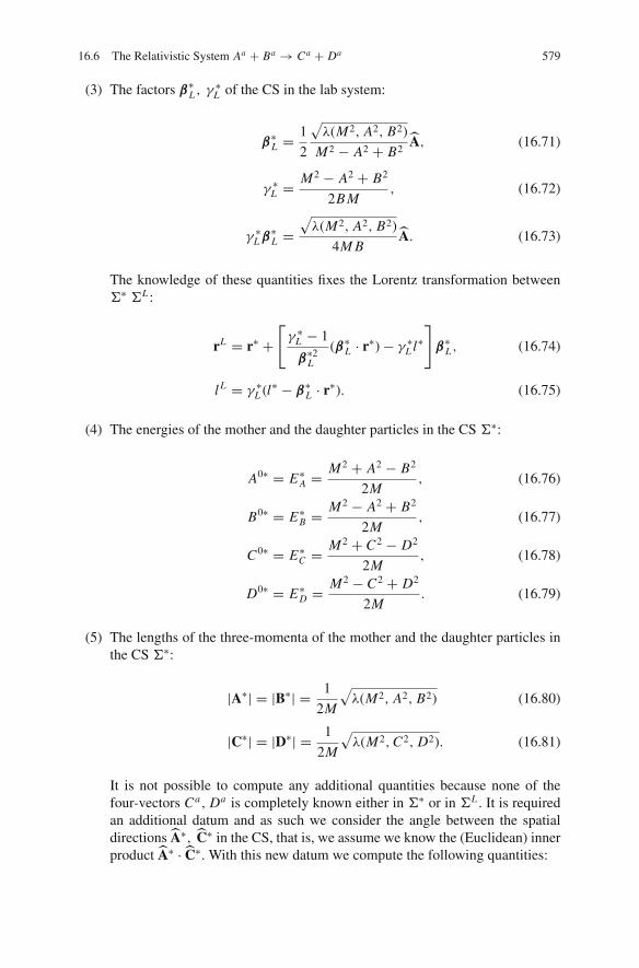
16.6 The Relativistic System Aa + Ba → Ca + Da 579
(3) The factors β∗L , γ∗L of the CS in the lab system:
β∗L =1
2
√λ(M2, A2, B2)
M2 − A2 + B2A, (16.71)
γ ∗L =M2 − A2 + B2
2B M, (16.72)
γ ∗L β∗L =√λ(M2, A2, B2)
4M BA. (16.73)
The knowledge of these quantities fixes the Lorentz transformation betweenΣ∗ ΣL :
rL = r∗ +[γ ∗L − 1
β∗2L
(β∗L · r∗)− γ ∗L l∗]
β∗L , (16.74)
l L = γ ∗L (l∗ − β∗L · r∗). (16.75)
(4) The energies of the mother and the daughter particles in the CS Σ∗:
A0∗ = E∗A =M2 + A2 − B2
2M, (16.76)
B0∗ = E∗B =M2 − A2 + B2
2M, (16.77)
C0∗ = E∗C =M2 + C2 − D2
2M, (16.78)
D0∗ = E∗D =M2 − C2 + D2
2M. (16.79)
(5) The lengths of the three-momenta of the mother and the daughter particles inthe CS Σ∗:
|A∗| = |B∗| = 1
2M
√λ(M2, A2, B2) (16.80)
|C∗| = |D∗| = 1
2M
√λ(M2,C2, D2). (16.81)
It is not possible to compute any additional quantities because none of thefour-vectors Ca, Da is completely known either in Σ∗ or in ΣL . It is requiredan additional datum and as such we consider the angle between the spatialdirections A∗, C∗ in the CS, that is, we assume we know the (Euclidean) innerproduct A∗ · C∗. With this new datum we compute the following quantities:

580 16 Geometric Description of Relativistic Interactions
(6) The invariants (C B), (DB), (C A), (D A):
(C B) = − 1
4M2
[(M2 − A2 + B2
) (M2 + C2 − D2
)]
− 1
4M2
[√λ(M2, A2, B2)
√λ(M2,C2, D2)(A∗ · C∗)
], (16.82)
(DB) = −(C B)− 1
2
(M2 + B2 − A2
), (16.83)
(C A) = −(C B)− 1
2(M2 + C2 − D2), (16.84)
(D A) = −(C B)+ 1
2
(M2 + B2 − A2
)+ 1
2(M2 − C2 + D2). (16.85)
(7) The energies of the daughter particles in the lab ΣL :
E LC = −
1
B(C B) [(C B) < 0 because E L
C > 0], (16.86)
E LD = −
1
B(DB) [(DB) < 0 because E L
D > 0]. (16.87)
(8) The length of the three-momentum of the daughter particles in the lab ΣL :
|CL | =√−C2 + 1
B2(C B)2, (16.88)
|DL | =√−D2 + 1
B2(DB)2. (16.89)
(9) The angle θ LC D between the direction of motion of the daughter particles in the
lab ΣL :
cos θ LC D =
1
|CL ||DL |[
1
2(−M2 + C2 + D2)+ 1
B2(C B)(DB)
]. (16.90)
(10) The angle θ LAC of the three-momentum CL of the daughter particle C and the
direction of motion of the mother particle A in the LAB ΣL :
cos θ LAC = −
B
|CL |√λ(M2, A2, B2)[
(M2 + C2 − D2)+ 1
B2
(M2 − A2 + B2
)(C B)
], (16.91)
sin θ LAC =
|C∗||CL | sin θ∗AC =
√λ(M2,C2, D2)
2M |CL | sin θ∗AC . (16.92)

16.6 The Relativistic System Aa + Ba → Ca + Da 581
The above general relations can be used directly in an algebraic computing pro-gram to develop software that would solve automatically collision problems pro-vided the correct data have been introduced. A hint on how this can be done we givein the examples below.
Example 82 An electron with four-momentum Aa interacts with a positron of four-momentum Ba producing two photons with four-momenta Ca and Da , respectively.Given that (a) the positron rests in the laboratory; and (b) the electron moves in thelaboratory along the direction specified by the unit vector eA, with speed factor γA
compute
(1) The mass M of the center of momentum particle(2) The factor β∗L of the CS in the lab system lab(3) The energy of the particles and the measure of their three-momenta in
the CS(4) The energy of the photons and the measure of their three-momenta in the lab if
the angle of direction of the photon with the direction of motion of the electronin the CS is θ∗AC = π
2(5) The angle θ L
AC of the direction of motion of the photon with that of the electronin the lab
(6) The angle between the direction of motion of the photons in the lab
SolutionFrom the data of the problem we have A = B = m, C = D = 0. Furthermore
it is given that the energy of the photon A in the lab is (c = 1)
E L = AL = mγA
and its direction A = eA. Finally it is given that in the CS the direction or prop-agation of the emitted photon is perpendicular to the direction of motion of theelectron, therefore A∗ · C∗ = cos π
2 = 0. Using these data we compute directly fromthe previous formulae the required quantities.
(1) From (16.68) we find M
M = m√
2(1+ γA).
(2) From (16.69) and (16.70) we find the λ function:
λ2(M2, A2, B2) = M4 + 2m4 − 4M2m2 − 2m4 = M2(M2 − 4m2),
λ2(M2,C2, D2) = M4.

582 16 Geometric Description of Relativistic Interactions
(3) From (16.71), (16.72), and (16.73) the velocity factors of the CS in the lab:
β∗L =1
2
M√
M2 − 4m2
M2= 1
2
√1− 4
( m
M
)2
= 1
2
√
1− 41
2(1+ γA)= γA − 1
γA + 1eA,
γ ∗L =M2 − m2 + m2
2m M= 1
2
M
m=
√1+ γA
2.
(4) From (16.76) to (16.79) the energy of the particles in the CS:
E∗A = E∗B =M2 + m2 − m2
2M= M
2= m
√(1+ γA
2,
E∗C = E∗D =M2
2M= M
2= m
√(1+ γA
2.
(5) From (16.80) we have for the length of the three-momentum of the electronand the positron in the CS:
|A∗| = |B∗| = 1
2Mλ(M2, A2, B2) = m
2
√(M
m
)2
− 4 = m
√γA − 1
2
and from relation (16.81)
E∗C = E∗D =M
2= m
√1+ γA
2.
Since Ca, Da are null vectors the energy equals the measure of the three-
momenta, that is, |C∗| = |D∗| = m√
1+γA
2 .(6) In order to compute the energy and the measure of the three-momenta of the
daughter particles in the lab we have to compute the inner product of the four-vectors involved. Equations (16.82) and (16.83) give for the inner products(C B), (DB)
(C B) = (DB) = − 1
4M2
[M2 M2] = −M2
4
and (16.84) and (16.91) give for the inner products (AC), (AD)
(C A) = M2
4− M2
2= −M2
4,
(D A) = −M2
4+ M2
2+ M2
2= 3M2
4.

16.6 The Relativistic System Aa + Ba → Ca + Da 583
From relations (16.86) and (16.87) we compute
E LC = E L
D = −1
m
−M2
4= 1+ γA
2m.
Since Ca, Da are null |pLC | = |pL
D| = m 1+γA
2 .(7) Using (16.88) and (16.89) we compute the magnitude of the three-momentum
of the daughter particles in the lab:
|CL | = |DL | = M2
4m.
(8) Relation (16.90) gives the angle between the daughter particles in the lab:
cos θ LC D =
16m2
M4
[−M2
2+ 1
m2
M4
16
]= 1− 8
(Mm
)2 =γA − 3
1+ γA.
(9) From (16.91) we compute the angle θ LAC :
cos θ LAC = −
m2
M√
M2 − 4m2 M2
4
[M2 + 1
m2M2 − M2
4
]=
√(Mm
)2 − 4Mm
=√
γA − 1
γA + 1.
(10) Finally from (16.92) we compute the angle θ LAC :
sin θ LAC =
M2
2M M2
4m
sinπ
2=
√2
1+ γA.
Example 83 (Compton scattering) A photon is scattered by an electron which restsin the laboratory. If the energy of the scattered photon in the laboratory is E A andthe scattering angle (in the laboratory) is θ L , calculate the energy of the scatteredphoton in the laboratory.5
SolutionThe reaction is
γ + e− −→ γ + e−.
Considering the reaction A + B −→ C + D we identify the following data forthe present problem:
5 For the standard treatment see Example 51

584 16 Geometric Description of Relativistic Interactions
A = C = 0, B = D = m, E LA = E A, θ
LAC = θ L .
From relation (16.68) we compute
M2 = m2 + 2m E A. (16.93)
For the triangle function λ(M2, 0,m2) we have from (16.30)
λ(M2, 0,m2) = (−M2 + m2)2.
Replacing the data in (16.91) we end up with one equation with unknown innerproduct (C B):
cosθ L = −m2[M2 − m2 + 1
m2 (M2 + m2)(C B)]
(M2 − m2)(C B).
We solve in terms of (C B) and find
(C B) = − (M2 − m2)m2
M2 + m2 − (M2 − m2) cos θ L.
Replacing M2 from (16.93) we find finally
(C B) = − m2 E A
m + E A(1− cos θ L ). (16.94)
Having computed (C B) we replace in the general relations and calculate the restof the elements of the reaction. For example, the energy of C in the laboratory isfrom (16.86)
E LC = −
(C B)
m= E Am
m + (1− cos θ L )E A. (16.95)
If the data of the problem are different then we work in a similar manner (seeExample 84).
Exercise 89 In Example 83 consider as given the energies E A, EC in the lab systemof the falling and the scattered photon and prove that the angle of scattering θ L
AC isgiven by the expression
sin2 θ LAC
2= 1
2m
(1
EC− 1
E A
). (16.96)
[Hint: In the expression EC = −(C B)m replace (C B) from (16.94) and solve for
cos θ LAC ].

16.6 The Relativistic System Aa + Ba → Ca + Da 585
Example 84 Study the reaction A + B −→ C + D considering as data the lengthsA, B,C, D of the particle four-vectors and the scattering angles θ L
AC , θLAD . Apply
your results to the case of final state of two photons.Solution
Normal to the direction of motion of the particle A we have
|CL | sin θ LAC = |DL | sin θ L
AD ⇒ |DL | = sin θ LAC
sin θ LAD
|CL |. (16.97)
The inner products give
AL · CL = |AL ||CL | cos θ LAC ,
AL · DL = |AL ||DL | cos θ LAD,
AL · (CL + DL ) = |A|L [|CL | cos θ LAC + |DL | cos θ L
AD
].
From the conservation of four-momentum we have AL = CL + DL . Replacingwe find
|A|L = sin(θ LAC + θ L
AD)
sin θ LAD
|CL |. (16.98)
We conclude that we can express the measure of the spatial parts of the four-momenta Aa, Da in terms of the spatial part of the four-momentum Ca .
Conservation of four-momentum gives for the zeroth component
E LA + B = E L
C + E LD. (16.99)
On the other hand for the particle A we have
−A2 = −(E LA)2 + (|A|L)2 ⇒ (E L
A)2 = A2 + (|A|L)2
= A2 + sin2(θ LAC + θ L
AD)
sin2 θ LAD
|CL |2
and for the particles C, D
(E LC )2 = C2 + (|C|L)2
,
(E LD)2 = D2 + (|D|L)2 = D2 + sin2 θ L
AC
sin2 θ LAD
|CL |2.

586 16 Geometric Description of Relativistic Interactions
Replacing in (16.99) we find the equation
√
A2 + sin2(θ LAC + θ L
AD)
sin2 θ LAD
|CL |2 + B =√
C2 + (|C|L)2 +√
D2 + sin2 θ LAC
sin2 θ LAD
|CL |2
(16.100)
which we solve and determine |CL |. From (16.97) we determine |DL |. Then from(16.88)
|CL |2 = −C2 + (C B)2
B2
we determine the inner product (C B) and from (16.89) the inner product (DB).Then (16.86) and (16.87) give the energies E L
C , E LD of the daughter particles in
the laboratory. Finally from (16.90) we compute M2 and consequently any otherquantity we wish. Obviously the calculations are involved and this indicates theusefulness of the covariant study of the relativistic collisions which makes possiblethe solution of a problem with the use of algebraic computing programmes.Application
Final state of two photons means that the daughter particles are photons. Thisimplies C = D = 0 and from the above analysis we find
|C|L = E LC ,
E LD = |D|L =
sin θ LAC
sin θ LAD
E LC ,
E LA =
√
A2 + sin2(θ LAC + θ L
AD)
sin2 θ LAD
(E L
C
)2.
Replacing in (16.100) we find an equation with sole unknown the energy E LC :
[sin2(θ L
AC + θ LAD)
sin2 θ LAD
−(
1+sin θ LAC
sin θ LAD
)2](E L
C
)2+2B
(1+sin θ L
AC
sin θ LAD
)E L
C+A2−B2 = 0.
Solving we determine E LC and from this all the quantities of the reaction.
The above solution is crude. We present a second solution in accordance to theprevious considerations. We replace the data in (16.91) and find an equation withunknowns the quantities (C B) and M2:
cos θ LC = −
B2[M2 + 1
B2 (M2 − A2 + B2)(C B)]
√λ(M2, A2, B2)(C B)
. (16.101)

16.6 The Relativistic System Aa + Ba → Ca + Da 587
We solve in terms of (C B):
(C B) = − M2 B2
M2 − A2 + B2 +√λ(M2, A2, B2) cos θ L
C
. (16.102)
If we replace C with D in the above relation we find without any further calcu-lations
(DB) = − M2 B2
M2 − A2 + B2 +√λ(M2, A2, B2) cos θ L
D
. (16.103)
From the conservation equation we have if we contract with Ba
(AB)− B2 = (C B)+ (DB) =⇒ −M2 + A2 − B2
2= (C B)+ (DB). (16.104)
Replacing in this last equation the inner products (C D), (DB) from (16.102) and(16.103) we end up with one equation which contains only M2.
16.6.1 The Reaction B −→ C + D
The reaction B −→ C+D is a special case of A+ B −→ C+D if A “disappears.”This means two conditions:
(a) Aa = 0 and(b) The energies EC
A = E DA of the daughter particles in the “proper” frame of A
vanish.
We conclude that in order to study reactions of the form B −→ C+D we have touse simply the general formulae we have derived and consider as data A = 0, E L
A =EC
A = E DA = 0.
Condition: E LA = − 1
B (AB) = 0⇒ M = B.Condition: EC
A = − 1B (AC) = 0⇒ (AC) = 0. Then from (16.82) follows that
(C B) = − 1
4B2(B2 + B2)(B2 − C2 + D2) = −1
2(B2 − C2 + D2).
Working similarly we see that condition E DA implies
(DB) = −1
2(B2 + C2 − D2).
Concerning the energies of the daughter particles in the laboratory from relations(16.86) and (16.87) we have

588 16 Geometric Description of Relativistic Interactions
E LC =
1
2B(B2 + C2 − D2),
E LC =
1
2B(B2 − C2 + D2).
From relations (16.88) and (16.89) we have that the magnitude of the three-momentum of the daughter particles is the same and equal to
|CL | = |DL | = 1
2B
√λ(B2,C2, D2).
We conclude that the reactions 1 + 2 → 3 and 1 → 2 + 3 are completelycharacterized by five parameters. One set of such parameters is the three masses ofthe particles and the angles of motion of one particle in the proper frame of someother. Obviously, there are other sets of five parameters.
To check the above we replace the above results in (16.90) and find cos θ LC D=−1,
hence θ LC D = π as expected.
Bibliography
1. H. Weyl, A. Einstein, H. A. Lorentz, and H. Minkowski. The Principle of Relativity. Dover,New York, 1924.
2. J. Aharoni. The Special Theory of Relativity. Oxford at the Clarendon Press, Oxford, 1965.3. A. Das. The Special Theory of Relativity: A Mathematical Exposition. Springer, New York,
1996.4. W. C. Dixon. Special Relativity: The Foundation of Macroscopic Physics. Cambridge Univer-
sity Press, Cambridge, 1978.5. A. P. Lightman et al. Problem Book in Relativity and Gravitation. Princeton University Press,
Princeton, 1975.6. V. V. Batygin et al. Problems in Electrodynamics. Academic Press, New York, 1978.7. A. P. French. Special Relativity. M.I.T. Introductory Physics Series, Massachusetts, 1968.8. R. Hagedorn. Relativistic Kinematics. W. A. Bemjamen INC., New York, 1964.9. J. D. Jackson. Classical Electrodynamics. John Wiley and Sons, New York, 1998.
10. D. F. Lawden. An Introduction to Tensor Calculus and Relativity Third Edition. John Wileyand Sons, New York, 1982.
11. H. Muirhead. The Special Theory of Relativity. The MacMillen Press Ltd., London, 1973.12. R. Resnick. Introduction to Special Relativity. John Wiley and Sons, New York, 1968.13. W. Rindler. Essential Relativity Special, General, and Cosmological Revised Second Edition.
Springer -Verlag, New York, 1969.14. W. Rindler. Introduction to Special Relativity. Oxford University Press, Oxford, 1982.15. R. D. Sard. Relativistic Mechanics Special Relativity and Classical Particle Dynamics.
Springer, New York, 1970.16. J. L. Synge. Relativity: The Special Theory. North Holland Publishing Company, Amsterdam,
1965.17. V. A. Ugarov. Special Theory of Relativity. MIR Publishers, Moscow, 1979.18. J. VanBladel. Relativity and Engineering. W. A. Benjamin, New York, 1984.
M. Tsamparlis, Special Relativity, DOI 10.1007/978-3-642-03837-2,C© Springer-Verlag Berlin Heidelberg 2010
589


Index
AAbberation, 143Acceleration time dilatation, 209Action integral, 344Active transformation, 6Affine parametrization, 99Affine space, 95Algebraic method, 146Arrow of time, 103Axiom
realtivistic inertia, 103
BBasic sensors, 56Basis
g-Cartesian, 7g-orthonormal, 7
Biot-Savart, 482Bivector, 495
simple, 447, 495dual, 447, 495
Boosts, 20, 28, 31, 35Born acceleration, 207Born rigid motion, 206, 207Born rigidity, 206Bradyons, 98
CCanonical form, 7, 48Cartesian coordinate system, 63Cartesian frames
Euclidean, 9Lorentz, 9
Center of momentum particle, 287, 563Center System, 52Character of inner product, 7Characteristic quantity of a theory, 59Chronometry, 92, 103, 104
of two events, 118
Clock, 72Closed system, 84Comoving observers, 133Composite vector, 540Composition law
Newtonian vectors, 82Composition rule for 3-vectors
Newtonian, 160relativistic, 161
Composition Rule of four-vectors, 540Conduction current, 406, 449, 456Conduction four-current, 406Conformal, 242Conformally flat, 242Conservation
of angular momentum, 502mechanical energy, 330
Constancy of c, 315Constitutive relations, 398, 459Constraint equations, 449, 454Continuity equation, 397, 449Contravariant indices, 4Convection current, 449, 456Coordinate functions, 2Coulomb gauge, 402Covariance Principle, 63
Galileo, 79–81Lorentz, 108, 109
Covariant indices, 4Curvature, 252
a curve, 366worldline, 157
Cyclotronic frequency, 435, 516
DD’Alembert operator, 401, 403Decomposition 1+3, 561Dielectric constant, 398Dielectric permittivity constant, 459
591

592 Index
Dual space, 5Dummy index, 4
EECF, 9, 14Elastic collision, 284Electric conductivity, 455, 460, 465
tensor, 455Electric part, 496Electric susceptibility, 460Electromagnetic field tensor, 414, 445Electromagnetic four-potential, 412Electromagnetic waves, 421Energy
internal, 268total , 268
EOT, 14Equation of continuity, 405
electormagetism, 406Ether, 88Euclidean inner product, 7, 8Euler angles, 16Event, 94Event horizon, 97
FFine structure constant, 354Focussing of beams of particles, 272Foliation, 95Force
Lorentz force, 428Four-acceleration, 157, 186Four-electric field, 442Four-force
Bonnor, 375definition, 325generic, 372inertial, 327Lorentz-Dirac, 373Newtonian, 373pure, 327thermal, 327
Four-force on a charge, 427Four-magnetic induction, 442Four-momentum, 267
photon, 276Four-vectors, 17
center of momentum, 563future directed, 26null, 17past directed, 26spacelike, 17timelike, 17
future directed, 96past directed, 96
Four-velocity, 156Frame
center of momentum, 291laboratory, 291target, 291
Frame Frenet-Serret, 363Free fall, 247Frenet-Serret frame, 363Fundamental equation of isometry, 10Future, 103Future directed, 48
GG-basis, 11G-factor, 514G-isometries, 9G-orthogonal transformations, 9Gauge Lorentz, 401Gauge transformation, 400General linear group, 6Generalized Lorentz transformation, 239Generalized Ohm Law, 467Generic reaction, 293Geometric description of collissions
Newtonian, 556Gravitational red-shift, 215, 250Gravitational time dilation, 251Gyromagnetic ratio, 514
HHall current, 465Hamilton formalism, 343Heron, 565Holonomic basis, 2Homogeneous and isotropic material, 460Homopolar induction, 462Hyperbolic motion, 197, 335
IImage of physical phenomenon, 57Index of refraction, 459Induction field tensor, 445Inelastic collision, 284Inertial motion, 76Inner product, 6
character, 7Euclidean, 7, 8Lorentz, 8non-degenerate, 7representation, 7
Instantaneous inertial direction, 76Internal energy, 268International System of Units (SI), 278Intrinsic angular momentum, 508Isotropic group, 551

Index 593
LLaboratory System, 570Lagrange formalism, 343Lagrangian
relativistic, 344Laue, 139Law
conservation of four-momentum, 287conservation of linear momentum, 84
LCF, 9, 104Length contraction, 46, 127Levi Civita tensor density, 440Lienard - Wiechert potentials, 479Light aberration formula, 277Light cone, 96
future, 96past, 96
Linear transformations, 5Little group, 551Local Relativistic Inertial Observer, 188Lorentz
gauge, 401, 412vector form, 26
Lorentz Cartesian Frame, 104Lorentz force, 428Lorentz inner product, 8Lorentz transformation
boost, 35Luxons, 275
MMagnetic dipole, 508Magnetic dipole moment, 486, 507Magnetic moment anomaly, 515Magnetic part, 496Magnetic permeability, 398Magnetic permeability constant, 459Magnetization four-vector, 448Magnetization Vector, 398Mass, 266
inertial, 83photon, 276
Maxwell equations, 412Ampere Law, 397Faraday Law, 397Gauss Law, 397Newtonian form, 397
Measuring sensors, 56Metric
Euclidean, 9Lorentz, 9space, 7
Minkowski, 93Minkowski space, 8
NNet angular momentum, 502, 503Net moment, 501Net torque, 501NIO, 78Normal
first, second, third, 366Normal component, 380Null cone, 18Null curves, 98Null electromagnetic fields, 421Null vectors, 96
OObservation, 59Observers, 59
inetrial, 63Newtonian, 63Newtonian inertial, 103Newtonian observers, 75relativistic , 63relativistic accelerated, 103relativistic inertial, 103
Optical image, 135Orbital angular momentum, 506Orbital magnetic dipole moment, 508Oscillator, 195
PParadox, 118, 253Parallel component, 380Particle abberation formula, 272Particle four-vector, 50, 278Particle reactions, 283Passive transformation, 6Past, 103Past directed, 48Photongun, 102Physical quantity, 61
Newtonian, 81Poincare transformations, 99Poisson equation, 402Polarization four-vector, 448Polarization Vector, 398Position four-vector, 107Position vector, 59Potential
electric, 399magnetic, 399Newtonian Physical quantity, 81, 84relativistic physical quantity, 110

594 Index
Poynting vector, 464Prediction, 66Principle
Covariance, 63, 64Inertia, 64of Inertia, 63
Principle of Communicationof Einstein , 107
Principle of Least Action, 248Principle of Relativity, 62
Galileo, 79, 84Projection tensor, 562Propagation equations, 449, 454Proper
clock, 102Proper frame, 48, 101
instantaneous, 100Proper length, 207Proper mass loss, 308Proper space, 101Proper time, 100, 155Proper transformation
Lorentz, 20
RRapidity, 20, 38, 43, 101, 122, 197Reactions
excitation reactions, 308radiative transitions, 308
Reality of a physical theory, 61Reciprocity of motion, 114Reciprocity principle, 524Redshift
acceleration, 215Reduced form, 48Relative 3-velocity, 169Relative four-acceleration, 167Relative four-vector, 167Relative four-velocity, 167Relative position vector, 166Relativistic
Light Frame, 104observation, 92observers, 92physical quantity, 110
Relativistic angular momentum, 503Relativistic composition rule
3-velocities, 161Relativistic electric field, 442Relativistic inertial directions, 103Relativistic inertial motion, 95Relativistic Inertial Observers, 99Relativistic magnetic field, 442
Relativistic mass, 266Relativistic mass point (ReMaP), 155, 157Relativistic measurement
spatial distance, 120temporal difference, 120
Relativistically parallel axes, 41ReMaP, 155Rest frame, 49Rest length
proper length, 132Retarding point, 484Rigid body motion, 212Rigid motion, 207Rigid rod, 132
characteristic observers, 133relativistic length, 133rest length, 132rest observer, 134
Rigid rotation, 219Rocket motion, 355
SSandeh D, 317Scattering, 283
Compton, 320, 583elastic, 317
Screen projection operator, 393Space, 69
homogeneity, 71isotropy, 71
Spacelike curves, 98Spacetime, 8, 59, 93
reflections, 528Speed of light, 92Spin angular momentum, 508Spin of a particle, 511Spin vector, 511Standard configuration, 25State transition, 283Straight line of time, 72Synchronization, 74, 102, 204
Einstein, 205of LRIO, 208
Synchronization of chronometry, 209System of Natural Units, 278
TTachyons, 98Tangent basis of a curve, 369Target system, 570Tensorial transformation, 9Tensors, 11
Euclidean, 12Lorentz, 12, 265

Index 595
Theorem of the zeroth component, 290Thomas phenomenon, 177Thomas precession, 177Threshold, 297, 567Threshold energy, 299Time, 71
“arrow” of time, 73Time dilation, 46, 123Torque tensor, 504Total energy, 268Transformation
coordinates, 1Galileo, 160Lorentz
generalized, 240of fields E,B, 415similarity, 7
Transformation matrix, 3Transformations
improper g-orthogonal, 10proper g-orthogonal, 10
Transverse conductivity, 465Triangle function, 295
VVector four-potential , 3403-Velocity space, 1743-Velocity triangle, 175Vorticity vector, 451
WWigner angle, 170World line, 97