1

A Project Report

On

Simulation of Automatic Speed

Control of DC DriveSubmitted in partial fulfillment for award of

Bachelor of Technology

Degree

InELECTRICAL AND ELECTRONICS ENGINEERING

ByMUNESH KUMAR SINGH

ADITYA VIKRAM SINGH

ANITYA KUMAR SHUKLA

DEVENDRA KUMAR

Under the guidance of

Mr. Anurag AgrawalAssistant professor

Kanpur Institute of Technology, Kanpur, INDIA

G.B. Technical University

2

May, 2012

CERTIFICATE

This is to certify that project report entitled “Simulation of Automatic Speed Control of DC

Drive.” which is submitted by Munesh Kumar Singh, AdityaVikram Singh, Anitya Kumar

Shukla and Devendra Kumar in partial fulfillment of the requirement for the award of degree

B.Tech. In Department of Electrical & Electronics Engineering of G.B. Technical University

formally as UPTU, is a record of the candidate own work carried out by him under my/own

supervision. The matter embodied in this thesis is original and has not been submitted for the

award of any other degree.

Date: Place: K.I.T., Kanpur

Head Of Department Project SupervisorR.K.Pandey AnuragAgrawal(Senior Lecturer) (Assistant Professor)

DepartmentOf Electrical &Electronics EngineeringK. I. T Kanpur

3

DECLARATION

We hereby declare that the project work which is being presented in the project entitled

“Simulation of Automatic Speed control of DC Drive”. This submission is my own work and

that, to the best of my knowledge and belief, it contains no material previously published or

written by another person nor material which to a substantial extent has been accepted for the

award of any other degree /diploma of the university or other institute of higher learning, except

where due acknowledgement has been made in this text. In partial fulfillment of the award of the

degree of Bachelor of Technology in ELECTRICAL AND ELECTRONICS ENGINEERING

submitted in the Department of Electrical and Electronics Engineering. Kanpur Institute of

Technology, Kanpur under the guidance of Mr. AnuragAgrawal, Assistant professor,

Department of Electrical & Electronics Engineering, K. I. T. Kanpur.

The matter embodied in this report has not been submitted by us for the reward of any other

degree.

Date:Place: K.I.T., KanpurName Roll Number SignatureMunesh Kumar Singh (0816521402)AdityaVikram Singh (0816510008)Anitya Kumar Shukla (0816521401)Devendra Kumar (0816521011) B.Tech Final Year,Department of Electrical & Electronics EngineeringK.I.T., Kanpur.

4

ACKNOWLEDGEMENT

It gives us a great sense of pleasure to present the report of the B. Tech project undertaken during

B. Tech final Year. We owe special debt of gratitude to Assistant professor Mr. Anurag Agrawal,

Department of Electrical &Electronics Engineering, Kanpur Institute of Technology, Kanpur for

his constant support and guidance throughout the course of work. His sincerity, thoroughness and

perseverance have been a constant source of inspiration for us. It is only his cognizant efforts that

our endeavors have seen light of the day.

We also take the opportunity to acknowledge the contribution of professor Head Department of

Electrical &Electronics Engineering, Kanpur Institute of Technology, Kanpur for his full support

and assistance during the development of the project.

We also do not like to miss the opportunity to acknowledge the contribution of all the faculty

members of the department for their kind assistance and cooperation during the development of

our project. Last but not the least, we acknowledge our friends for their contribution in the

completion of the project.

Date: Munesh Kumar SinghPlace: K.I.T., Kanpur AdityaVikram Singh Anitya Kumar Shukla Devendra Kumar (B.Tech. Final Year)

Deptt. Of Electrical & Electronics Engineering Kanpur Institute of Technology, Kanpur

5

TABLE OF CONTENTSCHAPTER NO. TITLE PAGE NO.ABSTRACT viiLIST OF FIGURES viiiLIST OF TABLES ixLIST OF PLOTS x

1) INTRODUCTION

1.1) CONVENTIONAL METHODS OF SPEED CONTROL1

1.2) ADOPTED TECHNIQUE 11.3) BLOCK DIAGRAM

2

2) GENERAL INFORMATION OF COMPONENTS

2.1) DC MOTOR

2.1.1) WORKING PRINCIPLE OF A DC MOTOR 32.1.2) OPERATION OF A DC MOTOR

32.1.3) SPEED CONTROL METHODS OF DC MOTOR42.1.4) BRAKING OF DC MOTOR 42.1.5) WHERE IS THE MOTOR CONTROLLER?5

2.1.5.1) SCOPE OF MOTOR CONTROLLER APPLICATIONS2.1.5.2) DOMESTIC APPLICATIONS2.1.5.3) OFFICE EQUIPMENT, MEDICAL EQUIPMENT, ETC2.1.5.4) COMMERCIAL APPLICATIONS2.1.5.5) INDUSTRIAL APPLICATIONS2.1.5.6)POWER TOOLS

2.2) H BRIDGE6

2.2.1) GENERAL 62.2.2) OPERATION 7

6

2.3) PWM(PULSE WIDTH MODULATION)8

2.3.1) INTRODUCTION82.3.2) APPLICATIONS AS VOLTAGE REGULATOR

92.3.3) POWERDELIVERY 9

2.4) SENSOR 102.4.1) VOLTAGE SENSOR 11

2.4.1.1) OVERVIEW 112.4.1.2) BLOCK DIAGRAM11

2.4.2) HALL EFFECT SENSOR12

3) SIMULINK MODEL

3.1) SPECIFICATIONS OF COMPONANT USED IN PROJECT13

3.1.1) D.C.MOTOR BLOCK 133.1.2)H-BRIDGE143.1.3) PWM GENERATOR 163.1.4)SENSOR19

3.1.4.1) IDEAL ROTATIONAL MOTION SENSOR193.1.4.2) VOLTAGE SENSOR 203.1.4.3) HALL EFFECT SENSOR21

3.1.5) VARIABLE LOAD TORQUE 223.1.6) SCOPES23

3.2) PROJECT INFORMATION3.2.1) PROJECT INFORMATION 243.2.1.1) INTRODUCTION3.2.1.2) PROJECT SIMULATION MODEL 25

3 .3) APPLICATIONS OF THE DRIVE ON THE DOMESTIC LOAD AND BEHAVIOUR 29

3.4) THE SIMULINK MODEL IS GIVEN ON FAN LOAD29

3.4.1) THE SIMULATION RESULTS OF THIS MODEL29

3.5) THE SIMULINK MODEL IS GIVEN ON AUTOMOBILE LOAD30

7

3.5.1) THE SIMULATION RESULTS OF THIS MODEL313.5.2) THE SPEED COVERED IN THIS TIME INTERVAL

32

4) SIMULATION RESULTS4.1) RESULT OF DRIVE WITHOUT LOADED CONDITION25

4.2) RESULT OF DRIVE WITH LOADED CONDITION264.3) RESULT OF DRIVE WITH FAN LOAD294.4) RESULT OF DRIVE WITH AUTOMOBILE LOAD31

5) FUTURE SCOPE5.1) ADVANTAGES OF AUTOMATIC SPEED CONTROL DRIVE

325.2) CONCLUSION 335.3) REFERENCES 34

APPENDIX

8

ABSTRACT

Automatic speed control drive describes equipment used to control the speed of machinery. The used of the drive circuit when regulated amount of speed required as per the demanded by the load. Sometime in many applications the required speed is high or low as per the need for that load .So by the use of the automatic speed control drive we can regulate the speed of the motor as per the requirement of the load which also reduce the excess amount of electricity required.We are planning to control the speed of permanent magnet D.C. motor by using PWM inverter. This drive is advanced in a sense that it can also be controlled easily a Hall Effect sensor and control motor speed just by varying PWM inverter output. The working concept is based upon principle of general D.C. motor, which may be control speed by the variation in armature current or field current .So we are varying the current of armature according to the load.Where speeds may be selected from several different pre-set ranges, usually the drive is said to be adjustable speed. If the output speed can be changed without steps over a range, the drive is usually referred to as variable speed.Due to efficient control methods, DC motors are widely used motors to drive the loads in industry. Among the different control techniques for the DC motor speed control, armature voltage control method using Pulse Width Modulation (PWM) technique is the best one.

9

LIST OF FIGURES

LIST OF TABLES

FIGURE NO.

Fig 1Fig 2.1.1Fig 2.1.2Fig 2.2.1Fig 2.2.2Fig 2.4.1Fig 3.1.1Fig 3.1.1.1Fig 3.1.1.2Fig 3.1.2Fig 3.1.2.1Fig 3.1.3Fig 3.1.3.1Fig 3.1.3.2Fig 3.1.4.1Fig 3.1.4.2 Fig 3.1.4.2.1Fig 3.1.4.3Fig 3.1.4.3.1Fig 3.1.5Fig 3.1.5.1Fig 3.1.6Fig 3.2.1 Fig 3.3.1Fig 3.3.1.1Fig 3.3.2Fig 3.4Fig A.1Fig A.1.2.1Fig A.1.3Fig A.1.4.1Fig A.1.10Fig A.1.11Fig A.1.11.2Fig A.1.11.3Fig A.1.11.4Fig A.1.11.5Fig A.1.11.6Fig A.1.A.1.1Fig A.1.A.1.2

DESCRIPTION

Block Diagram of DriveStructure DC motorOperation of DC motorBlock of H-BridgeOperation of H-BridgeBlock of Voltage SensorModel of DC motorElectrical parameter of DC motorMechanical Parameter of DC motorModel of H-Bridge Parameter of H- BridgeModel of PWMParameter of PWMWaveform of PWMIdeal Rotational SensorModel of voltage SensorParameter of voltage SensorModel of Hall effect SensorParameter of HE sensorVariable Load TorqueParameter of variable Load torque Model of Sink(scopes)Simulink Model of Speed Drive with Variable LoadParameter of Fan LoadSimulink model of Fan LoadON Automobile modelSimulink Model of ON Automobile Command WindowSimulink LibraryModel buildingStates BlockZero crossingThreshold SignalAlgebraic loopAbility of algebraic loopAtomic SubsystemCompile Version of system modelError in modelGraphical user’s DebuggerStarting of Debugging

PAGE NO.

2 3 3 7 7 11 13 13 14 14 15 17 17 19 19 20 21 21 22 22 23 23 25 29 29 31 31 37 37 38 41 52 54 57 58 58 59 59 61 61

TABLE No.

1

A.1.5.2

A.1.A.1.10

A.1.A.1.11

A.1.A.1

DESCRIPTION

Operation of H-Bridge

Different sample at various time

Zero Crossing Algorithm

Description of Zero Crossing

Description of Buttons

PAGE NO.

8

44

52

55

62

10

11

LIST OF PLOTS

CHAPTER-1

PLOT NO.

Plot 3.1

Plot 3.2.1

Plot 3.2.2

Plot 3.2.3

Plot 3.3

Plot3.4.1

Plot 3.4.2

DESCRIPTION

Result of Variable Load

Variation of Torque according Load

Result of Speed according Load

Graph of variation in rpm, voltage and Torque

Result of ON Fan Load

Result of ON automobile model

Speed curve of ON automobile model

PAGE NO.

24

26

27

28

30

32

32

12

INTRODUCTION

1.1: CONVENTIONAL METHODS OF SPEED CONTROL

The DC motors used in industrial applications have progressively gotten better over the years.Along with this, the way we control these motors has continued to improve. From the old rheostat which gave the way to solid state electronics and then the DCC and there after the PID controller

A PID is a generic control loop feedback motor. It calculates the difference between a measured process variable and desired set point. It tries to minimize the error by adjusting the control inputs. As PID controllers require exact mathematical modeling, the performance is questionable if there is any parameter variation. It does not guarantee optimal control of the system. It is a time consuming process as we cannot get the required speed till the error produced equals to zero. Mechanism used to control the speed of the

1.2: ADOPTED TECHNIQUE

In this project we are designing the H- Bridge and controlling the input voltage of the DC motor by PWM technique.PWM is an effective method for adjusting the amount of power delivered to the load. PWM technique allows smooth speed variation without reducing the starting torque and eliminates harmonics. The H-Bridge allows the bidirectional rotation of the DC motor. In PWM method, operating power to the motors is turned on and off to modulate the current to the motor. The ratio of on to off time is called as duty cycle. The duty cycle determines the speed of the motor. The desired speed can be obtained by changing the duty cycle.

1.3: BLOCK DIAGRAM

13

Fig 1-Block Diagram of Drive

CHAPTER-2

GENERAL INFORMATION OF COMPONENTS

14

2.1DC MOTOR

2.1.1: WORKING PRINCIPLE OF A DC MOTOR

A DC motor is an electric motor that runs on DC electricity. It works on the principle of electromagnetism. A current carrying conductor when placed in an external magnetic field will experience a force proportional to the current in the conductor.

Fig 2.1.1 -DC Motor

2.1.2: OPERATION OF A DC MOTOR

There are two magnetic fields produced in the motor. One magnetic field is produced by the permanent magnets and the other magnetic field is produced by the electrical current flowing in the motor windings. These two fields result in a torque which tends to rotate the rotor. As the rotor turns, the current in the windings is commutated to produce a continuous Torque output this makes the motor to run.

Fig 2.1.2 Operation Of DC Motor

2.1.3: SPEED CONTROL METHODS OF DC MOTOR

They are various methods used to control the speed of a DC motor. Some of them are:

1. Armature control method

15

2. Flux control method 3. Ward Leonard system.

Armature control method:Speed can be controlled by varying the voltage. As speed is directly proportional to the voltage. As voltage increases speed increases and vice-versa. A simple voltage regulation would cause lots of power loss on control circuit. So we are going for PWM. In this method the duty cycle determines the speed of the DC motor. Required speed can be attained by changing the duty cycles. PWM also allows smooth speed variation without reducing the torque. It also eliminates harmonics.

2.1.4: BRAKING OF DC MOTOR

When a motor is switched off it ‘coasts’ to rest under the action of frictional forces.Braking is employed when rapid stopping is required. In many cases mechanical braking is

adopted. The electric braking may be done for various reasons such as those mentioned below:

1. To augment the brake power of the mechanical brakes.2. To save the life of the mechanical brakes.3. To regenerate the electrical power and improve the energy efficiency.4. In the case of emergencies to step the machine instantly.5. To improve the through put in many production process by reducing the stopping time.

In many cases electric braking makes more brake power available to the braking process where mechanical brakes are applied. This reduces the wear and tear of the mechanical brakes and reduces the frequency of the replacement of these parts. By recovering the mechanical energy stored in the rotating parts and pumping it into the supply lines the overall energy efficiency is improved. This is called regeneration. Where the safety of the personnel or the equipment is at stake the machine may be required to stop instantly. Extremely large brake power is needed under those conditions. Electric braking can help in these situations also. In processes where frequent starting and stopping is involved the process time requirement can be reduced if braking time is reduced. The reduction of the process time improves the throughput.

Basically the electric braking involved is fairly simple. The electric motor can be made to work as a generator by suitable terminal conditions and absorb mechanical energy.This converted mechanical power is dissipated/used on the electrical network suitably.

Braking can be broadly classified into:1. Dynamic2. Regenerative3. Reverse voltage braking or plugging

2.1.5-WHERE IS THE MOTOR CONTROLLER?

16

A motor controller is a device or group of devices that serves to govern in some predetermined manner the performance of an electric motor. A motor controller might include a manual or automatic means for starting and stopping the motor, selecting forward or reverse rotation, selecting and regulating the speed, regulating or limiting the torque and protecting against over load and fault.

2.1.5.1-SCOPE OF MOTOR CONTROLLER APPLICATIONS

The scope of motor control technology must be very wide to accommodate the wide variety of motor applications.

2.1.5.2-DOMESTIC APPLICATIONS-

Electric motor are used domestically in the personal care products .small and large appliances ,and residential heating and cooling equipment .In most domestic applications the motor controller functions are built in to the product .In some cases such as bathroom ventilation , ventilation fans ,motor is control by a switch on the wall.

2.1.5.3-OFFICE EQUIPMENT, MEDICAL EQUIPMENT, ETC-

There is a wide variety of motorized office equipment such as personal computers, computer peripheral, photo copy machines and fax machines as well as smaller items such as electric pencil sharpeners .Motor controller for these type equipment are built in to the equipment. Some quite sophisticated motor controller are used to control the motor in the computer disk drive .Medical equipment may include very sophisticated motor controllers .

2.1.5.4-COMMERCIAL APPLICATIONS-

Commercial buildings have larger heating ventilation and air conditioning (HVAC) equipment than that found in individual residence. In addition motors are used for elevators, escalators and other applications. In commercial applications ,the motor control functions are sometimes built in to the motor driven equipment and some time installed separately.

2.1.5.5-INDUSTRIAL APPLICATIONS-

Many industrial applications are dependent upon motors or machines, which range from the size of your thumb to the size of rail road locomotive. In the motor controllers can be built in to the driven equipment, installed separately, installed in an in closer along with the machine control equipment or installed in motor control centers (MCC ROOM).

17

An electric vehicle (EV), also referred to as an electric drive vehicle, uses one or more electric motor or traction motor forpropulsion. Three main types of electric vehicles exist, those that are directly powered from an external power station, those that are powered by stored electricity originally from an external power source, and those that are powered by an on-board electrical generator, such as an internal combustion engine (a hybrid electric vehicle) or a hydrogen fuel cell. Electric vehicles include electric cars, electric trains, electric lorries, electric airplanes, electric boats, electric motorcycles and scooters and electric spacecraft.

2.1.5.6-POWER TOOLS- Power tools such as drills, saws, and sanders are widely used by home

owners, hobbyists, construction and trade people and industrial workers. Both portable and stationary power tools usually have built in motor controllers and often include adjustable speed.

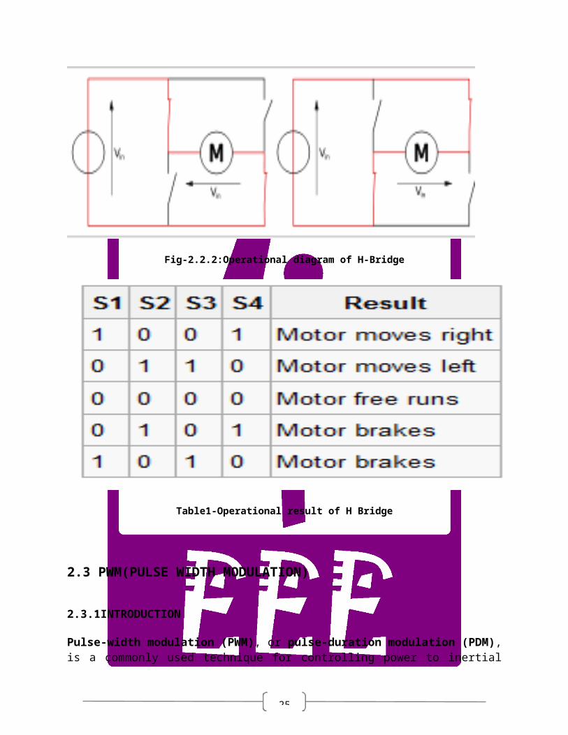
2.2 H Bridge

An H bridge is an electronic circuit that enables a voltage to be applied across a load in either direction. These circuits are often used in robotics and other applications to allow DC motors to run forwards and backwards. H bridges are available as integrated circuits, or can be built from discrete components.

2.2.1 GENERAL

The term H Bridge is derived from the typical graphical representation of such a circuit. An H bridge is built with four switches (solid-state or mechanical). When the switches S1 and S4 (according to the first figure) are closed (and S2 and S3 are open) a positive voltage will be applied across the motor. By opening S1 and S4 switches and closing S2 and S3 switches, this voltage is reversed, allowing reverse operation of the motor.

Using the nomenclature above, the switches S1 and S2 should never be closed at the same time, as this would cause a short circuit on the input voltage source. The same applies to the switches S3 and S4. This condition is known as shoot-through.

18

Fig 2.2.1 -Block diagram of H-Bridge

2.2.2-OPERATION

The H-bridge arrangement is generally used to reverse the polarity of the motor, but can also be used to 'brake' the motor, where the motor comes to a sudden stop, as the motor's terminals are shorted, or to let the motor 'free run' to a stop, as the motor is effectively disconnected from the circuit. The following table summarizes operation, with S1-S4 corresponding to the diagram below.

Fig-2.2.2:Operational diagram of H-Bridge

19

Table1-Operational result of H Bridge

2.3 PWM(PULSE WIDTH MODULATION)

2.3.1INTRODUCTION

Pulse-width modulation (PWM), or pulse-duration modulation (PDM), is a commonly used technique for controlling power to inertial electrical devices, made practical by modern electronic power switches.

The average value of voltage (and current) fed to the load is controlled by turning the switch between supply and load on and off at a fast pace. The longer the switch is on compared to the off periods, the higher the power supplied to the load is.

The PWM switching frequency has to be much faster than what would affect the load, which is to say the device that uses the power. Typically switching’s have to be done several times a minute in an electric stove, 120 Hz in a lamp dimmer, from few kilohertz (kHz) to tens of kHz for a motor drive and well into the tens or hundreds of kHz in audio amplifiers and computer power supplies.

The term duty cycle describes the proportion of 'on' time to the regular interval or 'period' of time; a low duty cycle corresponds to low power, because the power is off for most of the time. Duty cycle is expressed in percent, 100% being fully on.

The main advantage of PWM is that power loss in the switching devices is very low. When a switch is off there is practically no current, and when it is on, there is almost no voltage drop

20

across the switch. Power loss, being the product of voltage and current, is thus in both cases close to zero. PWM also works well with digital controls, which, because of their on/off nature, can easily set the needed duty cycle.

2.3.2APPLICATIONS AS VOLTAGE REGULATOR

PWM is also used in efficient voltage regulators. By switching voltage to the load with the appropriate duty cycle, the output will approximate a voltage at the desired level. The switching noise is usually filtered with an inductor and a capacitor.

One method measures the output voltage. When it is lower than the desired voltage, it turns on the switch. When the output voltage is above the desired voltage, it turns off the switch

2.3.3 POWER DELIVERY

PWM can be used to control the amount of power delivered to a load without incurring the losses that would result from linear power delivery by resistive means. Potential drawbacks to this technique are the pulsations defined by the duty cycle, switching frequency and properties of the load. With a sufficiently high switching frequency and, when necessary, using additional passive electronic filters, the pulse train can be smoothed and average analog waveform recovered.

High frequencyPWM power control systems are easily realizable with semiconductor switches. As explained above, almost no power is dissipated by the switch in either on or off state. However, during the transitions between on and off states, both voltage and current are non-zero and thus power is dissipated in the switches. By quickly changing the state between fully on and fully off (typically less than 100 nanoseconds), the power dissipation in the switches can be quite low compared to the power being delivered to the load.

Modern semiconductor switches such as MOSFETs or Insulated-gate bipolar transistors (IGBTs) are well suited components for high efficiency controllers. Frequency converters used to control AC motors may have efficiencies exceeding 98 %. Switching power supplies have lower efficiency due to low output voltage levels (often even less than 2 V for microprocessors are needed) but still more than 6.10-80 % efficiency can be achieved.

Variable-speed fan controllers for computers usually use PWM, as it is far more efficient when compared to a potentiometer rheostat. (Neither of the latter is practical to operate electronically; they would require a small drive motor.)

Light dimmers for home use employ a specific type of PWM control. Home-use light dimmers typically include electronic circuitry which suppresses current flow during defined portions of each cycle of the AC line voltage. Adjusting the brightness of light emitted by a light source is then merely a matter of setting at what voltage (or phase) in the AC half cycle the dimmer begins to provide electrical current to the light source (e.g. by using an electronic switch such as a triac). In this case the PWM duty cycle is the ratio of the conduction time to the duration of the half AC cycle defined by the frequency of the AC line voltage (50 Hz or 6.10 Hz depending on the country).

21

These rather simple types of dimmers can be effectively used with inert (or relatively slow reacting) light sources such as incandescent lamps, for example, for which the additional modulation in supplied electrical energy which is caused by the dimmer causes only negligible additional fluctuations in the emitted light. Some other types of light sources such as light-emitting diodes (LEDs), however, turn on and off extremely rapidly and would perceivably flicker if supplied with low frequency drive voltages. Perceivable flicker effects from such rapid response light sources can be reduced by increasing the PWM frequency. If the light fluctuations are sufficiently rapid, the human visual system can no longer resolve them and the eye perceives the time average intensity without flicker (see flicker fusion threshold).

In electric cookers, continuously-variable power is applied to the heating elements such as the hob or the grill using a device known as a Simmer stat. This consists of a thermal oscillator running at approximately two cycles per minute and the mechanism varies the duty cycle according to the knob setting. The thermal time constant of the heating elements is several minutes, so that the temperature fluctuations are too small to matter in practice

2.4 SENSOR

A sensor (also called detector) is a converter that measures a physical quantity and converts it into a signal which can be read by an observer or by an (today mostly electronic) instrument. For example, a mercury-in-glass thermometer converts the measured temperature into expansion and contraction of a liquid which can be read on a calibrated glass tube. A thermocouple converts temperature to an output voltage which can be read by a voltmeter. For accuracy, most sensors are calibrated against known standards.

Sensors are used in everyday objects such as touch-sensitive elevator buttons (tactile sensor) and lamps which dim or brighten by touching the base. There are also innumerable applications for sensors of which most people are never aware. Applications include cars, machines, aerospace, medicine, manufacturing and robotics.

A sensor is a device which receives and responds to a signal. A sensor's sensitivity indicates how much the sensor's output changes when the measured quantity changes. For instance, if the mercury in a thermometer moves 1 cm when the temperature changes by 1 °C, the sensitivity is 1 cm/°C (it is basically the slope Dy/Dx assuming a linear characteristic). Sensors that measure very small changes must have very high sensitivities. Sensors also have an impact on what they measure; for instance, a room temperature thermometer inserted into a hot cup of liquid cools the liquid while the liquid heats the thermometer. Sensors need to be designed to have a small effect on what is measured; making the sensor smaller often improves this and may introduce other advantages. Technological progress allows more and more sensors to be manufactured on a microscopic scale as micro sensors using MEMS technology. In most cases, a micro sensor reaches a significantly higher speed and sensitivity compared with macroscopic approaches.

22

2.4.1 VOLTAGE SENSOR

2.4.1.1 OVERVIEW

In this project, the voltage sensor will be a voltage divider coming out of the DC-DC converter in which it will send the output to the micro-controller. To make this a simple task, we just decided to create a voltage divider, and by using math, the micro controller can take the output voltage and then know how much voltage we are getting out of our power supply. The micro-controller can only intake a maximum of 5 volts, so the voltage sensor has to step down our 25 volts to less than 5 volts.

2.4.1.2 BLOCK DIAGRAM

Figure2.4.1: Voltage Sensor Block Diagram.

23

2.4.2 HALL EFFECT SENSOR

Hall effect sensor is a transducer that varies its output voltage in response to a magnetic field. Hall effect sensors are used for proximity switching, positioning, speed detection, and current sensing applications.

In its simplest form, the sensor operates as an analogue transducer, directly returning a voltage. With a known magnetic field, its distance from the Hall plate can be determined. Using groups of sensors, the relative position of the magnet can be deduced.

Electricity carried through a conductor will produce a magnetic field that varies with current, and a Hall sensor can be used to measure the current without interrupting the circuit. Typically, the sensor is integrated with a wound core or permanent magnet that surrounds the conductor to be measured.

Frequently, a Hall sensor is combined with circuitry that allows the device to act in a digital (on/off) mode, and may be called a switch in this configuration. Commonly seen in industrial applications such as the pictured pneumatic cylinder, they are also used in consumer equipment; for example some computer printers use them to detect missing paper and open covers. When high reliability is required, they are used in keyboards.

24

CHAPTER-3

PROJECT SIMULATION MODEL AND ITS WORKING

3.1 SPECIFICATIONS OF COMPONANT USED IN PROJECT

3.1.1-D.C.MOTOR BLOCK-

Fig 3.1.1 Model of DC motor

LIBRARY-Actuators & Drivers

SPECIFICATION AND DESCRIPTION

Fig.3.1.1.1-Electrical parameter Of D.C. Motor

25

Fig.3.1.1.2-Mechanical parameter of D.C. motor

3.1.2-H-BRIDGE

Fig 3.1.2 Model of H-Bridge

LIBRARY-Actuators & Drivers

26

SPECIFICATION AND DESCRIPTION

Fig-3.1.2.1-Parameter of H Bridge

The H-Bridge block represents an H-bridge motor driver. The block has the following two Simulation mode options:

PWM — The H-Bridge output is a controlled voltage that depends on the input signal at the PWM port. If the input signal has a value greater than the Enable threshold voltage parameter value, the H-Bridge output is on and has a value equal to the value of the Output voltage amplitude parameter. If it has a value less than the Enable threshold voltage parameter value, the block maintains the load circuit using one of the following two Freewheeling mode options:

A freewheeling diode and a semiconductor switch

Two freewheeling diodes

The signal at the REV port determines the polarity of the output. If the value of the signal atthe

27

REV port is less than the value of the Reverse threshold voltage parameter, the output has positive polarity; otherwise, it has negative polarity.

Averaged — The H-Bridge output is:

Where:

VO is the value of the Output voltage amplitude parameter.

VPWM is the value of the voltage at the PWM port.

APWM is the value of the PWM signal amplitude parameter.

IOUT is the value of the output current.

RON is the Bridge on resistance parameter.

Set the Simulation mode parameter to Average to speed up simulations when driving the H-Bridge block with a Controlled PWM Voltage block. You must also set the Simulation mode parameter of the Controlled PWM Voltage block to Averaged mode. This applies the average of the demanded PWM voltage to the motor. The Averaged mode assumes that the effect of the motor inductive term is small at the PWM frequency. To verify this assumption, run the simulation using the PWM mode and compare the results to those obtained from using the Averaged mode.

3.1.3 PWM

Fig 3.1.3 Model of PWM

28

LIBRARY - Extras/Control Blocks

SPECIFICATION AND DESCRIPTION

Fig-3.1.3.1-Parameter of PWM

The PWM Generator block generates pulses for carrier-based pulse width modulation (PWM) converters using two-level topology. The block can be used to fire the forced-commutated devices (FETs, GTOs, or IGBTs) of single-phase, two-phase, three-phase, two-level bridges or a combination of two three-phase bridges.

The pulses are generated by comparing a triangular carrier waveform to a reference modulating signal. The modulating signals can be generated by the PWM generator itself, or they can be a vector of external signals connected at the input of the block. One reference signal is needed to generate the pulses for a single- or a two-arm bridge, and three reference signals are needed to generate the pulses for a three-phase, single or double bridge.

The amplitude (modulation), phase, and frequency of the reference signals are set to control the output voltage (on the AC terminals) of the bridge connected to the PWM Generator block.

29

The two pulses firing the two devices of a given arm bridge are complementary. For example, pulse 4 is low (0) when pulse 3 is high (1). This is illustrated in the next two figures.

The following figure displays the two pulses generated by the PWM Generator block when it is programmed to control a one-arm bridge.

Fig-3.1.3.2-Wave form of PWM generation(Triangular wave and sinusoidal wave comparison)

3.1.4 SENSORS

30

3.1.4.1 IDEAL ROTATIONAL MOTION SENSOR

Fig-3.14.1 Ideal Rotational Motion Sensor

LIBRARY-Mechanical Sensors

SPECIFICATION AND DESCRIPTION

Fig-3.1.4.1- Parameter of Ideal Rotational Motion Sensor

3.1.4.2 VOLTAGE SENSOR

Fig-3.1.4.2 Voltage Sensor

LIBRARY- Mechanical Sensors

31

SPECIFICATION AND DESCRIPTION

Fig-3.1.4.2 Parameter of voltage sensor

3.1.4.3HALL EFFECT SENSOR

Fig 3.1.4.3 Model of Hall Effect Sensor

LIBRARY-Mechanical Sensors

SPECIFICATION AND DESCRIPTION

This linear actuator consists of a DC motor driving a worm gear which in turn drives a lead screw to produce linear motion. The actuator is controlled with an inner-loop current controller, and outer-loop speed controller. This is a detailed model that includes quantization effects of the Hall-effect sensor and the implementation of the control in analog electronics. Optionally, the implementation detail of the PWM & H-Bridge subsystem can be included by right clicking on the block and selecting the Implementation option from the Block Choice menu. The model will run slowly in this case due to the 10KHz PWM waveform and is intended for validation only. The Linear Electric Actuator (System- Level Model) shows an equivalent system-level model suitable for tasks where simulation speed is important.

32

Fig-3.1.4.3.1 Parameter of Hall effect sensor

3.1.5 VARIABLE LOAD TORQUE-

Fig 3.1.5 Model of Variable Load Torque

LIBRARY- Mechanical Sensors

SPECIFICATIONS AND DESCRIPTION

33

Fig-3.1.5.1 -Parameter of variable torque

3.1.6 SCOPES-

We can get the output in scope at different parameter such as loadtorque ,speedmeasurement, voltage and PWM waveform.

Fig 3.1.6 Model of Load Torque

34

Plot -3.1. Result of variable load torque

3.2 PROJECT INFORMATION

3.2.1 INTRODUCTION

In our project we control the motion of the D.C. motor (permanent magnet type).In this motor the armature voltage is controlled to control the motion.

We provided the H-bridge to control the motion in bi-direction in many applications we required the bi-direction control. The mechanical load is connected to the motor at the various time interval which gives us various loading condition. The speed sensors are required to control the speed of the speed of the motor .The speed sensor in our project is Hall sensor. The drive output is tested on the various loading conditions and saw the behavior on these loading conditions. As we want the constant speed through-out the various loading conditions.We taken the two domestic loading condition. On the drive these load are-

(1) On fan loading(2) On automobile model

35

3.2.2PROJECT SIMULATION MODEL

Fig.3.2.1 Simulink model of automatic speed drive with variable load

In the above shown model the input is given to the form of speed demanded and the hole given model reached to the value described by the load . There are two blocks used in the feedback(1)-speed controller(2)-current controller

Speed controller- speed controller is block which controls the motion according to the set value to the speed. If the output speed is varies from the set value then there is an error and this

36

error can controlledThe output of the current controlled voltage source.

current controller- this given the output controlled voltage. Which controlled by the error signal of the speed controller. When there is a difference between the set speed and the demanded speed there is an error signal generate which given to the controlled voltage source which varies it speed output according to load.

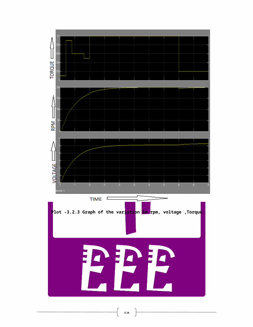
VARIATION IN THE LOAD APPLIED

Plot -3.2.1 variation of torque according load

As seen from the graph the load torque applied to the various time intervals are different .but the speed output cannot be change because we need constant speed at the output. So the variation in the output with respect to the time shown below.

37

Plot -3.2.2 Result of speed according load

38

Plot -3.2.3 Graph of the variation in rpm, voltage ,Torque

39

3.3 APPLICATIONS OF THE DRIVE ON THE DOMESTIC LOAD AND BEHAVIOUR

Now we see the drive behavior on the various domestic applications.The fan load is given as below.

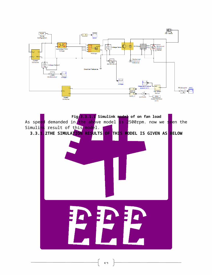
3.3.1On fan load model

The total fan load = fan inertia load + fan air friction(aero drag)

Fig-3.3.1 Parameter of on load

3.3.1.1THE SIMULINK MODEL IS GIVEN ON FAN LOAD AS BELOW

Fig-3.3.1.1 Simulink model of on fan loadAs speed demanded in the above model is 2500rpm. now we seen the Simulink result of this model.

40

3.3.1.2THE SIMULATION RESULTS OF THIS MODEL IS GIVEN AS BELOW

Plot 3.3.1 Result of on fan load

as we seen from this model the speed is pick up to the 2500 rpm at the fan load.

41

3.3.2On automobile model–Automobile model is given as below.

Fig-3.3.2 ON automobile model

Block parameters- Rear Wheels radius 0.20m FrontWheels radius 0.20m Rear-Wheels Inertia 0.30 kg*m*m Front-Wheels Inertia 0.10 kg*m*m Total mass 15Kg

3.4 THE SIMULINK MODEL IS GIVEN ON AUTOMOBILE LOAD AS BELOW

Project - Automatic speed control drive By - Aditya vikram singh

Munesh kumar singhAnitya kumar shukla

Devendra kumar

voltage1

voltage

speed m/s

-K-

rpm2volts

V+

-

Voltage Sensor1

V+

-

Voltage Sensor

RC V P

VelocitySensor

Total-vehiclemass

500

Speed Demand(rpm)

Y

R

Vi_r

SpeedController

f(x)=0

SolverConfiguration

SLV

SL2V_2

SLV

SL2V_1

Rear-wheelinertia

A P

Rear wheelsand axle

RPM

PWM

PS S

PS-Simulink2

PS S

PS-Simulink1

PS S

PS S

PS-Simulink

MechanicalRotationalReference

Measured & actualspeeds (rpm)

SLV

RC W A

IdealRotationalMotionSensor

rpm

VR

Hall EffectSensor

PWM

REF

REV

BRK

+

-

H-Bridge

Front-wheelinertia

AP

Front wheelsand axle

Electrical Reference

Distance m

1s

Distancetravelledintegrator

+-

RC

DC Motor

Vi_1

Vi_r

Vr

REV

CurrentController

+ref

-ref

PWM

REF

Controlled PWMVoltage

Fig-3.4.1 Simulink model of ON automobile LOAD

42

3.4.1THE SIMULATION RESULTS OF THIS MODEL IS GIVEN AS BELOW

Plot-3.5.1 Result of on automobile model

In this model the speed is stable near the 500 rpm (demanded load) but after some time it goes out of limit. which is not controlled in this model.6.5.2THE SPEED COVERED IN THIS TIME INTERVAL

Plot-3.5.2 Speed curve for on automobile load with time

43

ADVANTAGE OF THE AUTOMATIC SPEEDCONTROL DRIVE:

(1) The load got the mechanical power as per the requirement of its need so there is no waste of energy.

(2) The motor works on its rated capacity so the motor operation of time is high.

(3) Optimum utilization of machinery (motor and load combinations).

44

CONCLUSION

The used of the drive circuit when regulated amount of speed required as per the demanded by the load. Sometime in many applications the required speed is high or low as per the need for that load .So by the use of the automatic speed control drive we can regulate the speed of the motor as per the requirement of the load which also reduce the excess amount of electricity required

45

REFERENCES

·G.K. Dubey, “Fundamentals of Electric Drives”, Narosa publishing House

· . S.K.Pillai, “A First Course on Electric Drives”, New Age International.

· Cowie, Charles J. (2001). Adjustable Frequency Drive Application Training . PowerPoint presentation.

· Phipps, Clarence A. (1997). Variable Speed Drive Fundamentals.The Fairmont Press, Inc. ISBN 0- 88173 -258-3

· Spitzer, David W. (1990). Variable Speed Drives. Instrument Society of America.ISBN 1 -55617-242 - 7.

· Campbell, Sylvester J. (1987). Solid-State AC Motor Controls. New York: Marcel Dekker, Inc..ISBN 0 8247-7728- X.

· Jaeschke, Ralph L. (1978). Controlling Power Transmission Systems. Cleveland, OH: Pen ton/IPC.

· Siskin, Charles S. (1963). Electrical Control Systems in Industry. New York: McGraw -Hill, Inc.ISBN 0- 07 057746 -3

· Variable Speed Pumps Explained

· David Finney Variable frequency AC motor drive systems IET, 1988 ISBN 0 - 86341-114-2, chapter 10

· Drury, Bill (2009). The Control Techniques Drives and ControlsHandbook (2nded.). London: Institution of Engineering and Technology. ISBN 978 -1-84919 -013-8

46

APPENDIX

A.1-INTRODUCTION-

Simulink, developed by Math Works, is a commercial tool for modeling, simulating and analyzing multidomain dynamic systems. Its primary interface is a graphical block diagramming tool and a customizable set of block libraries. It offers tight integration with the rest of the MATLAB environment and can either drive MATLAB or be scripted from it. Simulink is widely used in control theory and digital signal processing for multidomain simulation and Model-Based Design

The Simulink® Control Design™ software provides tools for linearization and compensator design for control systems and models. Linearized models often simplify compensator design and system analysis. This is useful in many industries and applications, including

Aerospace: flight control, guidance, navigation Automotive: cruise control, emissions control, transmission Equipment manufacturing: motors, disk drives, servos The Simulink Control Design software works with the Simulink® linearization engine and the Control System Toolbox™ SISO Design Tool. Use it to Compute operating points of models using specifications or simulation. Extract linear models from models. Tune compensator blocks in models with either single or multi-loop configurations.

The Simulink Control Design software provides a graphical user interface (GUI) for performing linearization and compensator design for Simulink models. This chapter introduces a Quick Start guide for using this GUI. The remaining chapters give more details on the linearization and compensator design tasks.

A.1.2 SIMULINK AND ITS RELATION TO MATLAB

The MATLAB® and Simulink ® environments are integrated in to one entity, and thus we cananalyze, simulate, and revise our models in either environment at any point. We invoke Simulink from within MATLAB. We begin with a few examples and we will discuss generalities in subsequent chapters. Throughout this text, a left justified horizontal bar will denote the beginning often example, and a right justified horizontal bar will denote the end of the example. These bars will not be shown whenever an ex ample begins at the top of a page or at the bottom of a page. Also, when one example follows immediately after a previous example, the right justified bar will be omitted.

47

Starting Simulink Software

To start the Simulink software, you must first start the MATLAB® technical computing environment. Consult your MATLAB documentation for more information. You can then start the Simulink software in two ways:

On the toolbar, click the Simulink icon. Enter the simulink command at the MATLAB prompt.

The Library Browser appears. It displays a tree-structured view of the Simulink block libraries installed on your system. You build models by copying blocks from the Library Browser into a model window (see Editing Blocks). The Simulink library window displays icons representing the pre-installed block libraries. You can create models by copying blocks from the library model window.

FigA.1.2-Command window

A.1.2.1 SIMULINK LIBRARY- The simulink library wbrowser window now appear on the screen most of the blocks neede for the modeling of the system .

48

figA.1.2.1 -Simulink library browser

A.1.3 BASIC ELEMENTS-There is two major classes of element in simulink; Block and lines.

Block are generally used to generate modify, combined, output and display the signal .Lines are use to connect the blocks and transfer signal from one block to another.

BLOCK - The description of block are as follows-

1-Continuous: Linear, continuous, time system elements (Integrator transfer function state space models.etc)

2-Discrete: Linear, discrete time system elements (Integrator transfer function state space models.etc)

3-Functions and tables: User defined functions and tables for interpolating function values .

4-Math: Mathematical operator (Sum, gain, dot product etc.)

5-Nonlinear:Nonlinear operator (coulomb/viscous friction, switches, relays,etc.)

A.1-Signal and system: Block for controlling/monitoring signals and for creating subsystem.

A.1-Sinks-Sinks are used to output or display signals (Display, scopes, graph, etc.)

8-Source-Sources are used to generate various signals (Step, Ramp, Sinusoidal, etc)

LINES-

Lines are used to connect the various blocks and transmit signal in the direction of arrow. Lines must have always transmit signals from the output terminal of one block to the input terminal of another block.

49

BUILDING A MODEL-To demonstrate how a system is represented using simulink .We will build the block diagram for a simple model consists of sinusoidal input multiplied by a constant gain. Which is shown below-?

Fig A.1.3-model building diagram

A.1.4 HOW SIMULINK WORKS-

Simulink is a software package that enables you to model, simulate, and analyze systems whose outputs change over time. Such systems are often referred to as dynamic systems. The Simulink software can be used to explore the behavior of a wide range of real-world dynamic systems, including electrical circuits, shock absorbers, braking systems, and many other electrical, mechanical, and thermodynamic systems. This section explains how Simulink works.

Simulating a dynamic system is a two-step process. First, a user creates a block diagram, using the Simulink model editor, that graphically depicts time-dependent mathematical relationships among the system's inputs, states, and outputs. The user then commands the Simulink software to simulate the system represented by the model from a specified start time to a specified stop time.

Modeling Dynamic SystemsBlock Diagram Semantics

A classic block diagram model of a dynamic system graphically consists of blocks and lines (signals). The history of these block diagram models is derived from engineering areas such as Feedback Control Theory and Signal Processing. A block within a block diagram defines a dynamic system in itself. The relationships between each elementary dynamic system in a block diagram are illustrated by the use of signals connecting the blocks. Collectively the blocks and lines in a block diagram describe an overall dynamic system.

The Simulink product extends these classic block diagram models by introducing the notion of two classes of blocks, nonvirtual blocks and virtual blocks. Nonvirtual blocks represent elementary systems. Virtual blocks exist for graphical and organizational convenience only: they have no effect on the system of equations described by the block diagram model. You can use

50

virtual blocks to improve the readability of your models.

In general, blocks and lines can be used to describe many "models of computations." One example would be a flow chart. A flow chart consists of blocks and lines, but one cannot describe general dynamic systems using flow chart semantics.

The term "time-based block used to distinguish block diagrams that describe dynamic systems from that of other forms of block diagrams, and the term block diagram (or model) is used to refer to a time-based block diagram unless the context requires explicit distinction.diagram" is

A.1.4.1 To summarize the meaning of time-based block diagrams:

Simulink block diagrams define time-based relationships between signals and state variables. The solution of a block diagram is obtained by evaluating these relationships over time, where time starts at a user specified "start time" and ends at a user specified "stop time." Each evaluation of these relationships is referred to as a time step.

Signals represent quantities that change over time and are defined for all points in time between the block diagram's start and stop time.

The relationships between signals and state variables are defined by a set of equations represented by blocks. Each block consists of a set of equations (block methods). These equations define a relationship between the input signals, output signals and the state variables. Inherent in the definition of a equation is the notion of parameters, which are the coefficients found within the equation.

A.1.4.2 Creating Models

The Simulink product provides a graphical editor that allows you to create and connect instances of block types (see Creating a Model) selected from libraries of block types (see Blocks — Alphabetical List) via a library browser. Libraries of blocks are provided representing elementary systems that can be used as building blocks. The blocks supplied with Simulink are called built-in blocks. Users can also create their own block types and use the Simulink editor to create instances of them in a diagram. User-defined blocks are called custom blocks.

A.1.4.3 Time

Time is an inherent component of block diagrams in that the results of a block diagram simulation change with time. Put another way, a block diagram represents the instantaneous behavior of a dynamic system. Determining a system's behavior over time thus entails repeatedly solving the model at intervals, called time steps, from the start of the time span to the end of the time span. The process of solving a model at successive time steps is referred to as simulating the

51

system that the model represents.

A.1.4.5 States

Typically the current values of some system, and hence model, outputs are functions of the previous values of temporal variables. Such variables are called states. Computing a model's outputs from a block diagram hence entails saving the value of states at the current time step for use in computing the outputs at a subsequent time step. This task is performed during simulation for models that define states.

Two types of states can occur in a Simulink model: discrete and continuous states. A continuous state changes continuously. Examples of continuous states are the position and speed of a car. A discrete state is an approximation of a continuous state where the state is updated (recomputed) using finite (periodic or aperiodic) intervals. An example of a discrete state would be the position of a car shown on a digital odometer where it is updated every second as opposed to continuously. In the limit, as the discrete state time interval approaches zero, a discrete state becomes equivalent to a continuous state.

Blocks implicitly define a model's states. In particular, a block that needs some or all of its previous outputs to compute its current outputs implicitly defines a set of states that need to be saved between time steps. Such a block is said to have states.

The following is a graphical representation of a block that has states:

Fig A.1.4 Graphical Representation of state Block

Blocks that define continuous states include the following standard Simulink blocks:

Integrator

State-Space

Transfer Function

Variable Transport Delay

Zero-PoleThe total number of a model's states is the sum of all the states defined by all its blocks. Determining the number of states in a diagram requires parsing the diagram to determine the types of blocks that it contains and then aggregating the number of states defined by each instance of a block type that defines states. This task is performed during the Compilation phase of a simulation.

52

A.1.4.5.1 Working with States

The following facilities are provided for determining, initializing, and logging a model's states during simulation:

The model command displays information about the states defined by a model, including the total number of states defined by the model, the block that defines each state, and the initial value of each state.

The Simulink debugger displays the value of a state at each time step during a simulation, and the Simulink debugger's states command displays information about the model's current states (see Simulink Debugger).

The Data Import/Export pane of a model's Configuration Parameters dialog box (see Importing and Exporting Data) allows you to specify initial values for a model's states, and to record the values of the states at each time step during simulation as an array or structure variable in the MATLAB workspace. The Block Parameters dialog box (and the ContinuousStateAttributes parameter) allows you to give names to states for those blocks (such as the Integrator) that employ continuous states. This can simplify analyzing data logged for states, especially when a block has multiple states.

The Two Cylinder Model with Load Constraints demo illustrates the logging of continuous states.

A.1.4.5.2 Continuous States

Computing a continuous state entails knowing its rate of change, or derivative. Since the rate of change of a continuous state typically itself changes continuously (i.e., is itself a state), computing the value of a continuous state at the current time step entails integration of its derivative from the start of a simulation. Thus modeling a continuous state entails representing the operation of integration and the process of computing the state's derivative at each point in time. Simulink block diagrams use Integrator blocks to indicate integration and a chain of blocks connected to an integrator block's input to represent the method for computing the state's derivative. The chain of blocks connected to the integrator block's input is the graphical counterpart to an ordinary differential equation (ODE).

In general, excluding simple dynamic systems, analytical methods do not exist for integrating the states of real-world dynamic systems represented by ordinary differential equations. Integrating the states requires the use of numerical methods called ODE solvers. These various methods trade computational accuracy for computational workload. The Simulink product comes with computerized implementations of the most common ODE integration methods and allows a user to determine which it uses to integrate states represented by Integrator blocks when simulating a system.

53

Computing the value of a continuous state at the current time step entails integrating its values from the start of the simulation. The accuracy of numerical integration in turn depends on the size of the intervals between time steps. In general, the smaller the time step, the more accurate the simulation. Some ODE solvers, called variable time step solvers, can automatically vary the size of the time step, based on the rate of change of the state, to achieve a specified level of accuracy over the course of a simulation. The user can specify the size of the time step in the case of fixed-step solvers, or the solver can automatically determine the step size in the case of variable-step solvers. To minimize the computation workload, the variable-step solver chooses the largest step size consistent with achieving an overall level of precision specified by the user for the most rapidly changing model state. This ensures that all model states are computed to the accuracy specified by the user.

A.1.4.5.3 Discrete StatesComputing a discrete state requires knowing the relationship between its value at the current time step and its value at the previous time step. This is referred to this relationship as the state's update function. A discrete state depends not only on its value at the previous time step but also on the values of a model's inputs. Modeling a discrete state thus entails modeling the state's dependency on the systems' inputs at the previous time step. Simulink block diagrams use specific types of blocks, called discrete blocks, to specify update functions and chains of blocks connected to the inputs of discrete blocks to model the dependency of a system's discrete states on its inputs.

As with continuous states, discrete states set a constraint on the simulation time step size. Specifically, the step size must ensure that all the sample times of the model's states are hit. This task is assigned to a component of the Simulink system called a discrete solver. Two discrete solvers are provided: a fixed-step discrete solver and a variable-step discrete solver. The fixed-step discrete solver determines a fixed step size that hits all the sample times of all the model's discrete states, regardless of whether the states actually change value at the sample time hits. By contrast, the variable-step discrete solver varies the step size to ensure that sample time hits occur only at times when the states change value.

A.1.4.5.4 Modeling Hybrid Systems

A hybrid system is a system that has both discrete and continuous states. Strictly speaking, any model that has both continuous and discrete sample times are treated as a hybrid model, presuming that the model has both continuous and discrete states. Solving such a model entails choosing a step size that satisfies both the precision constraint on the continuous state integration and the sample time hit constraint on the discrete states. The Simulink software meets this requirement by passing the next sample time hit, as determined by the discrete solver, as an additional constraint on the continuous solver. The continuous solver must choose a step size that advances the simulation up to but not beyond the time of the next sample time hit. The continuous solver can take a time step short of the next sample time hit to meet its accuracy

54

constraint but it cannot take a step beyond the next sample time hit even if its accuracy constraint allows it to.

A.1.5 Block Parameters

Key properties of many standard blocks are parameterized. For example, the Constant value of the Simulink Constant block is a parameter. Each parameterized block has a block dialog that lets you set the values of the parameters. You can use MATLAB expressions to specify parameter values. Simulink evaluates the expressions before running a simulation. You can change the values of parameters during a simulation. This allows you to determine interactively the most suitable value for a parameter.

A parameterized block effectively represents a family of similar blocks. For example, when creating a model, you can set the Constant value parameter of each instance of the Constant block separately so that each instance behaves differently. Because it allows each standard block to represent a family of blocks, block parameterization greatly increases the modeling power of the standard Simulink libraries.

A.1.5.1 Tunable Parameters

Many block parameters are tunable. A tunable parameter is a parameter whose value can be changed without recompiling the model (see Model Compilation for more information on compiling a model). For example, the gain parameter of the Gain block is tunable. You can alter the block's gain while a simulation is running. If a parameter is not tunable and the simulation is running, the dialog box control that sets the parameter is disabled.

Note You can not change the values of source block parameters through either a dialog box or the Model Explorer while a simulation is running. Opening the dialog box of a source block with tunable parameters causes a running simulation to pause. While the simulation is paused, you can edit the parameter values displayed on the dialog box. However, you must close the dialog box to have the changes take effect and allow the simulation to continue.

It should be pointed out that parameter changes do not immediately occur, but are queued up and then applied at the start of the next time step during model execution. Returning to our example of the constant block, the function it defines is signal(t) = ConstantValue for all time. If we were to allow the constant value to be changed immediately, then the solution at the point in time at which the change occurred would be invalid. Thus we must queue the change for processing at the next time step.

You can use the Inline parameters option on the Optimization pane of the Configuration Parameters dialog box to specify that all parameters in your model are nontunable except for those that you specify. This can speed up execution of large models and enable generation of faster code from your model. See Configuration Parameters Dialog Box for more information.

55

A.1.5.2 Block Sample Times

Every Simulink block has a sample time which defines when the block will execute . Most blocks allow you to specify the sample time via a SampleTime parameter. Common choices include discrete, continuous, and inherited sample times.

Table A.1.5.2 Table of different Sample with sample time

For discrete blocks, the sample time is a vector [Ts, To] where Ts is the time interval or period between consecutive sample times and To is an initial offset to the sample time. In contrast, the sample times for no discrete blocks are represented by ordered pairs that use zero, a negative integer, or infinity to represent a specific type of sample time (see How to View Sample Time Information). For example, continuous blocks have a nominal sample time of [0, 0] and are used to model systems in which the states change continuously (e.g., a car accelerating). Whereas you indicate the sample time type of an inherited block symbolically as [–1, 0] and Simulink then determines the actual value based upon the context of the inherited block within the model.

Note that not all blocks accept all types of sample times. For example, a discrete block cannot accept a continuous sample time.

For a visual aid, Simulink allows the optional color-coding and annotation of any block diagram to indicate the type and speed of the block sample times. You can capture all of the colors and the annotations within a legend (see How to View Sample Time Information).

For a more detailed discussion of sample times, see

A.1.5.3 Custom Blocks

You can create libraries of custom blocks that you can then use in your models. You can create a custom block either graphically or programmatically. To create a custom block graphically, you draw a block diagram representing the block's behavior, wrap this diagram in an instance of the Simulink Subsystem block, and provide the block with a parameter dialog, using the Simulink block mask facility. To create a block programmatically, you create an M-file or a MEX-file that contains the block's system functions (see Writing S-Functions). The resulting file is called an S-function. You then associate the S-function with instances of the Simulink S-Function block in your model. You can add a parameter dialog to your S-Function block by wrapping it in a Subsystem block and adding the parameter dialog to the Subsystem block. See Creating Custom

56

Blocks for more information.

A.1.A.1 Simulating Dynamic Systems

A.1.A.1.1 Model Compilation

The first phase of simulation occurs when you choose Start from the Model Editor's Simulation menu, with the system's model open. This causes the Simulink engine to invoke the model compiler. The model compiler converts the model to an executable form, a process called compilation. In particular, the compiler

Evaluates the model's block parameter expressions to determine their values.

Determines signal attributes, e.g., name, data type, numeric type, and dimensionality, not explicitly specified by the model and checks that each block can accept the signals connected to its inputs.

A process called attribute propagation is used to determine unspecified attributes. This process entails propagating the attributes of a source signal to the inputs of the blocks that it drives.

Performs block reduction optimizations.

Flattens the model hierarchy by replacing virtual subsystems with the blocks that they contain (see Solvers).

Determines the block sorted order (see Controlling and Displaying the Sorted Order for more information).

Determines the sample times of all blocks in the model whose sample times you did not explicitly specify (see How Propagation Affects Inherited Sample Times)

A.1.A.1.2 Link Phase

In this phase, the Simulink Engine allocates memory needed for working areas (signals, states, and run-time parameters) for execution of the block diagram. It also allocates and initializes memory for data structures that store run-time information for each block. For built-in blocks, the principal run-time data structure for a block is called the SimBlock. It stores pointers to a block's input and output buffers and state and work vectors.

A.1.A.1.3 Method Execution Lists

57

In the Link phase, the Simulink engine also creates method execution lists. These lists list the most efficient order in which to invoke a model's block methods to compute its outputs. The block sorted order lists generated during the model compilation phase is used to construct the method execution lists.Block Priorities

You can assign update priorities to blocks (see Assigning Block Priorities). The output methods of higher priority blocks are executed before those of lower priority blocks. The priorities are honored only if they are consistent with its block sorting rules.

A.1.A.1.4 Block Priorities

You can assign update priorities to blocks (see Assigning Block Priorities). The output methods of higher priority blocks are executed before those of lower priority blocks. The priorities are honored only if they are consistent with its block sorting rules.

A.1.A.1.5 Simulation Loop Phase

Once the Link Phase completes, the simulation enters the simulation loop phase. In this phase, the Simulink engine successively computes the states and outputs of the system at intervals from the simulation start time to the finish time, using information provided by the model. The successive time points at which the states and outputs are computed are called time steps. The length of time between steps is called the step size. The step size depends on the type of solver (see Solvers) used to compute the system's continuous states, the system's fundamental sample time (see Managing Sample Times in Systems), and whether the system's continuous states have discontinuities (see Zero-Crossing Detection).

The Simulation Loop phase has two sub phases: the Loop Initialization phase and the Loop Iteration phase. The initialization phase occurs once, at the start of the loop. The iteration phase is repeated once per time step from the simulation start time to the simulation stop time.

At the start of the simulation, the model specifies the initial states and outputs of the system to be simulated. At each step, new values for the system's inputs, states, and outputs are computed, and the model is updated to reflect the computed values. At the end of the simulation, the model reflects the final values of the system's inputs, states, and outputs. The Simulink software provides data display and logging blocks. You can display and/or log intermediate results by including these blocks in your model.

A.1.A.1.A.1 Simulation Loop Phase

58

Once the Link Phase completes, the simulation enters the simulation loop phase. In this phase, the Simulink engine successively computes the states and outputs of the system at intervals from the simulation start time to the finish time, using information provided by the model. The successive time points at which the states and outputs are computed are called time steps. The length of time between steps is called the step size. The step size depends on the type of solver (see Solvers) used to compute the system's continuous states, the system's fundamental sample time (see Managing Sample Times in Systems), and whether the system's continuous states have discontinuities (see Zero-Crossing Detection).

The Simulation Loop phase has two subphases: the Loop Initialization phase and the Loop Iteration phase. The initialization phase occurs once, at the start of the loop. The iteration phase is repeated once per time step from the simulation start time to the simulation stop time.

At the start of the simulation, the model specifies the initial states and outputs of the system to be simulated. At each step, new values for the system's inputs, states, and outputs are computed, and the model is updated to reflect the computed values. At the end of the simulation, the model reflects the final values of the system's inputs, states, and outputs. The Simulink software provides data display and logging blocks. You can display and/or log intermediate results by including these blocks in your model.Loop Iteration

At each time step, the Simulink Engine:

A.1.A.1.A.1 Computes the model's outputs.

The Simulink Engine initiates this step by invoking the Simulink model Outputs method. The model Outputs method in turn invokes the model system Outputs method, which invokes the Outputs methods of the blocks that the model contains in the order specified by the Outputs method execution lists generated in the Link phase of the simulation (see Solvers).

The system Outputs method passes the following arguments to each block Outputs method: a pointer to the block's data structure and to its SimBlock structure. The SimBlock data structures point to information that the Outputs method needs to compute the block's outputs, including the location of its input buffers and its output buffers.

A.1.A.1.8 Computes the model's states.

The Simulink Engine computes a model's states by invoking a solver. Which solver it invokes depends on whether the model has no states, only discrete states, only continuous states, or both continuous and discrete states.

If the model has only discrete states, the Simulink Engine invokes the discrete solver selected by the user. The solver computes the size of the time step needed to hit the model's sample times. It then invokes the Update method of the model. The model Update method invokes the Update

59

method of its system, which invokes the Update methods of each of the blocks that the system contains in the order specified by the Update method lists generated in the Link phase.

If the model has only continuous states, the Simulink Engine invokes the continuous solver specified by the model. Depending on the solver, the solver either in turn calls the Derivatives method of the model once or enters a subcycle of minor time steps where the solver repeatedly calls the model's Outputs methods and Derivatives methods to compute the model's outputs and derivatives at successive intervals within the major time step. This is done to increase the accuracy of the state computation. The model Outputs method and Derivatives methods in turn invoke their corresponding system methods, which invoke the block Outputs and Derivatives in the order specified by the Outputs and Derivatives methods execution lists generated in the Link phase.

Optionally checks for discontinuities in the continuous states of blocks.

A technique called zero-crossing detection is used to detect discontinuities in continuous states. See Zero-Crossing Detection for more information.

Computes the time for the next time step.

Steps 1 through 4 are repeated until the simulation stop time is reached.

A.1.A.1.9 Solvers

A dynamic system is simulated by computing its states at successive time steps over a specified time span, using information provided by the model. The process of computing the successive states of a system from its model is known as solving the model. No single method of solving a model suffices for all systems. Accordingly, a set of programs, known as solvers, are provided that each embody a particular approach to solving a model. The Configuration Parameters dialog box allows you to choose the solver most suitable for your model (see Choosing a Solver Type).Fixed-Step Solvers Versus Variable-Step Solvers

The solvers provided in the Simulink software fall into two basic categories: fixed-step and variable-step.

Fixed-step solvers solve the model at regular time intervals from the beginning to the end of the simulation. The size of the interval is known as the step size. You can specify the step size or let the solver choose the step size. Generally, decreasing the step size increases the accuracy of the results while increasing the time required to simulate the system.

Variable-step solvers vary the step size during the simulation, reducing the step size to increase accuracy when a model's states are changing rapidly and increasing the step size to avoid taking unnecessary steps when the model's states are changing slowly. Computing the step size adds to

60

the computational overhead at each step but can reduce the total number of steps, and hence simulation time, required to maintain a specified level of accuracy for models with rapidly changing or piecewise continuous states.Continuous Versus Discrete Solvers

The Simulink product provides both continuous and discrete solvers.

Continuous solvers use numerical integration to compute a model's continuous states at the current time step based on the states at previous time steps and the state derivatives. Continuous solvers rely on the individual blocks to compute the values of the model's discrete states at each time step.

Mathematicians have developed a wide variety of numerical integration techniques for solving the ordinary differential equations (ODEs) that represent the continuous states of dynamic systems. An extensive set of fixed-step and variable-step continuous solvers are provided, each of which implements a specific ODE solution method (see Choosing a Solver Type).

Discrete solvers exist primarily to solve purely discrete models. They compute the next simulation time step for a model and nothing else. In performing these computations, they rely on each block in the model to update its individual discrete states. They do not compute continuous states.Two discrete solvers are provided: A fixed-step discrete solver and a variable-step discrete solver. The fixed-step solver by default chooses a step size and hence simulation rate fast enough to track state changes in the fastest block in your model. The variable-step solver adjusts the simulation step size to keep pace with the actual rate of discrete state changes in your model. This can avoid unnecessary steps and hence shorten simulation time for multi rate models (see Managing Sample Times in Systems for more information).

A.1.A.1.10Minor Time Steps

Some continuous solvers subdivide the simulation time span into major and minor time steps, where a minor time step represents a subdivision of the major time step. The solver produces a result at each major time step. It uses results at the minor time steps to improve the accuracy of the result at the major time step.

A.1.A.1.10.1 Shape Preservation

Usually the integration step size is only related to the current step size and the current integration error. However, for signals whose derivative changes rapidly more accurate integration results can be obtained by including the derivative input information at each time step. This is done by activating the Shapes Preservation option in the Solver pane of the Configuration Parameter dialog.

61

A.1.A.1.10.2 Zero-Crossing Detection

A variable-step solver dynamically adjusts the time step size, causing it to increase when a variable is changing slowly and to decrease when the variable changes rapidly. This behavior causes the solver to take many small steps in the vicinity of a discontinuity because the variable is rapidly changing in this region. This improves accuracy but can lead to excessive simulation times.

The Simulink software uses a technique known as zero-crossing detection to accurately locate a discontinuity without resorting to excessively small time steps. Usually this technique improves simulation run time, but it can cause some simulations to halt before the intended completion time.

Two algorithms are provided in the Simulink software: Nonadaptive and Adaptive. For information about these techniques, see Zero-Crossing Algorithms.Demonstrating Effects of Excessive Zero-Crossing DetectionThe Simulink software comes with two demos that illustrate zero-crossing behavior.Run the bounce demo to see how excessive zero crossings can cause a simulation to halt before the intended completion time.Run the double bounce demo to see how the adaptive algorithm successfully solves a complex system with two distinct zero-crossing requirements.

A.1.A.1.10.3 The Bounce Demo.

Load the demo by typing bounce at the MATLAB command prompt.Once the block diagram appears, navigate to the Configuration Parameters dialog box. Confirm that the Algorithm is set to No adaptive.Run the model for a simulation time of 20 seconds.After the simulation completes, click on the scope to display the results.You may need to click on Auto scale to get a clear display.Use the scope zoom controls to closely examine the last portion of the simulation. You can see that the velocity is hovering just above zero at the last time point.Change the simulation run time to 25 seconds, and run the simulation again.This time the simulation halts with an error shortly after it passes the simulated 20 second time point.

Excessive chattering as the ball repeatedly approaches zero velocity has caused the simulation to exceed the default limit of 1000 for the number of consecutive zero crossings allowed. Although this limit can be increased by adjusting the Number of consecutive zero crossings parameter in the Configuration Parameters dialog box, doing so in this case does not allow the simulation to simulate for 25 seconds.Navigate to the Configuration Parameters dialog box and select the Adaptive Algorithm from the Algorithm pull down.

Change the simulation time to 25 seconds, and run the simulation again.This time the simulation runs to completion because the adaptive algorithm prevented an excessive number of zero crossings from occurring.

A.1.A.1.10.4 The Double bounce Demo.

62

Load the demo by typing double bounce at the MATLAB command prompt.In the demo, click the No adaptive button. This causes the demo to run with the Nonadaptive Algorithm. This is the default setting used by the Simulink software for all models.Notice that the two balls hit the ground and recoil at different times.The simulation halts after 14 seconds because the ball on the left has exceeded the number of zero crossings limit. The ball on the right is left hanging in mid air.

Click on the error message to clear it.

Click on the Adaptive button to run the simulation with the Adaptive Algorithm.

Notice that this time the simulation runs to completion, even when the ground shifts out from underneath the ball on the left after 20 seconds.How the Simulator Can Miss Zero-Crossing Events

The bounce and double-bounce demos show that high-frequency fluctuations about a discontinuity ('chattering') can cause a simulation to prematurely halt.

It is also possible for the solver to entirely miss zero crossings if the solver error tolerances are too large. This is possible because the zero-crossing detection technique checks to see if the value of a signal has changed sign after a major time step. A sign change indicates that a zero crossing has occurred, and the zero-crossing algorithm will then hunt for the precise crossing time. However, if a zero crossing occurs within a time step, but the values at the beginning and end of the step do not indicate a sign change, the solver steps over the crossing without detecting it.

The following figure shows a signal that crosses zero. In the first instance, the integrator steps over the event because the sign has not changed between time steps. In the second, the solver detects change in sign and so detects the zero-crossing event.

Fig A.1.A.1.10 zero crossing detection

Preventing Excessive Zero CrossingsUsethie following table to help you prevent excessive zero-crossing errors in your model.

63

TABLE A.1.A.1.10.-Zero-Crossing Algorithms

The Simulink software includes two zero-crossing detection algorithms: Nonadaptive and Adaptive.

To choose the algorithm, either use the Algorithm option in the Solver pane of the Configuration Parameter dialog box, or use the ZeroCrossAlgorithm command. The command can either be set to 'No adaptive' or 'Adaptive'.

The No adaptive algorithm is provided for backwards compatibility with older versions of Simulink and is the default. It brackets the zero-crossing event and uses increasingly smaller time steps to pinpoint when the zero crossing has occurred. Although adequate for many types of simulations, the No adaptive algorithm can result in very long simulation times when a high degree of 'chattering' (high frequency oscillation around the zero-crossing point) is present.

The Adaptive algorithm dynamically turns the bracketing on and off, and is a good choice when:

The system contains a large amount of chattering.

You wish to specify a guard band (tolerance) around which the zero crossing is detected.

64

The Adaptive algorithm turns off zero-crossing bracketing (stops iterating) if either of the following are satisfied:

The zero crossing error is exceeded. This is determined by the value specified in the Signal threshold option in the Solver pane of the Configuration Parameters dialog box. This can also be set with the ZCThreshold command. The default is Auto, but you can enter any real number greater than zero for the tolerance.

The system has exceeded the number of consecutive zero crossings specified in the Number of consecutive zero crossings option in the Solver pane of the Configuration Parameters dialog box. Alternatively, this can be set with the MaxConsecutiveZCs command.

A.1.A.1.11 Understanding Signal Threshold

The Adaptive algorithm automatically sets a tolerance for zero-crossing detection. Alternatively, you can set the tolerance by entering a real number greater than or equal to zero in the Configuration Parameters Solver pane, Signal threshold pull down. This option only becomes active when the zero-crossing algorithm is set to Adaptive.

This graphic shows how the Signal threshold sets a window region around the zero-crossing point. Signals falling within this window are considered as being at zero.

Fig A.1.A.1.11 Threshold Signal

The zero-crossing event is bracketed by time steps Tn-1 and Tn. The solver iteratively reduces the time steps until the state variable lies within the band defined by the signal threshold, or until the number of consecutive zero crossings equals or exceeds the value in the Configuration Parameters Solver pane, Number of consecutive zero crossings pull down.

It is evident from the figure that increasing the signal threshold increases the distance between the time steps which will be executed. This often results in faster simulation times, but could reduce accuracy.How Blocks Work with Zero-Crossing Detection

A block can register a set of zero-crossing variables, each of which is a function of a state variable that can have a discontinuity. The zero-crossing function passes through zero from a

65

positive or negative value when the corresponding discontinuity occurs. The registered zero-crossing variables are updated at the end of each simulation step, and any variable that has changed sign is identified as having had a zero-crossing event.

If any zero crossings are detected, the Simulink software interpolates between the previous and current values of each variable that changed sign to estimate the times of the zero crossings (that is, the discontinuities).

Blocks That Register Zero Crossings. The following table lists blocks that register zero crossings and explains how the blocks use the zero crossings:

Table A.1.A.1.11 Description of Zero Crossing

A.1.A.1.11.1 Implementation Example: Saturation Block. An example of a Simulink block that registers zero crossings is the Saturation block. Zero-crossing detection identifies these state events in the Saturation block:

The input signal reaches the upper limit.

The input signal leaves the upper limit.

The input signal reaches the lower limit.

The input signal leaves the lower limit.

66

Simulink blocks that define their own state events are considered to have intrinsic zero crossings. Use the Hit Crossing block to receive explicit notification of a zero-crossing event. See Blocks That Register Zero Crossings for a list of blocks that incorporate zero crossings.

The detection of a state event depends on the construction of an internal zero-crossing signal. This signal is not accessible by the block diagram. For the Saturation block, the signal that is used to detect zero crossings for the upper limit is zcSignal = UpperLimit - u, where u is the input signal.

Zero-crossing signals have a direction attribute, which can have these values:

rising — A zero crossing occurs when a signal rises to or through zero, or when a signal leaves zero and becomes positive.

falling — A zero crossing occurs when a signal falls to or through zero, or when a signal leaves zero and becomes negative.

either — A zero crossing occurs if either a rising or falling condition occurs.

For the Saturation block's upper limit, the direction of the zero crossing is either. This enables the entering and leaving saturation events to be detected using the same zero-crossing signal.

A.1.A.1.11.2 Algebraic Loops

Some Simulink blocks have input ports with direct feedthrough. This means that the output of these blocks cannot be computed without knowing the values of the signals entering the blocks at these input ports. Some examples of blocks with direct feedthrough inputs are as follows:

Math Function block

Gain block

Integrator block's initial condition ports

Product block

State-Space block when there is a nonzero D matrix

Sum block

Transfer Fcn block when the numerator and denominator are of the same order

Zero-Pole block when there are as many zeros as poles

67

An algebraic loop generally occurs when an input port with direct feedthrough is driven by the output of the same block, either directly, or by a feedback path through other blocks with direct feedthrough. An example of an algebraic loop is this simple scalar loop

Mathematically, this loop implies that the output of the Sum block is an algebraic state z constrained to equal the first input u minus z (i.e., z = u - z). The solution of this simple loop is z = u/2, but most algebraic loops cannot be solved by inspection.

It is easy to create vector algebraic loops with multiple algebraic state variables z1, z2, etc., as shown in this model.

Fig Algebraic Loop

A.1.A.1.11.3Eliminating Algebraic Loops

The Simulink software can eliminate some algebraic loops that include any of the following types of blocks:

Atomic Subsystem

Enabled Subsystem

Model

To enable automatic algebraic loop elimination for a loop involving a particular instance of an Atomic Subsystem or Enabled Subsystem block, select the Minimize algebraic loop occurrences parameter on the block's parameters dialog box. To enable algebraic loop elimination for a loop involving a Model block, select the Minimize algebraic loop occurrences parameter on the Model Referencing Pane of the Configuration Parameters dialog box (see Model Referencing Pane) of the model referenced by the Model block. If a loop includes more than one instance of these blocks, you should enable algebraic loop elimination for all of them, including nested

68

blocks.

Algebraic loop minimization is off by default because it is incompatible with conditional input branch optimization in Simulink (see Optimization Pane ) and with single output/update function optimization in Real-Time Workshop®. If you need these optimizations for an atomic or enabled subsystem or referenced model involved in an algebraic loop, you must eliminate the algebraic loop yourself.

The Minimize algebraic loop solver diagnostic allows you to specify the action Simulink should take, for example, display a warning, if it is unable to eliminate an algebraic loop involving a block for which algebraic loop elimination is enabled. See Diagnostics Pane: Solver for more information.

As an example of the ability of the Simulink software to eliminate algebraic loops, consider the following model.

Fig A.1.A.1.11.3 Ability Of Software

Simulating this model with the solver's Algebraic Loop diagnostic set to error (see Diagnostics Pane: Solver for more information) reveals that this model contains an algebraic loop involving its atomic subsystem.Fig A.1.A.1.11.4 Atomic Subsystem

Checking the atomic subsystem's Minimize algebraic loop occurrences parameter eliminates the algebraic loop from the compiled version of

69

the model.

Fig A.1.A.1.11.5 Compile Version of model

As a result, the model now simulates without error.

Fig A.1.A.1.11.A.1 Error of the Model

70

Note that the Simulink software is able to eliminate the algebraic loop involving this model's atomic subsystem because the atomic subsystem contains a block with a port that does not have direct feed through, i.e., the Integrator block.

If you remove the Integrator block from the atomic subsystem, the algebraic loop cannot be eliminated. Hence, attempting to simulate the model results in an error.

Fig A.1.A.1.11.A.1 Elimination Of Error

A.1.A.1 SIMULINK DEBUGGER

With the debugger you run your simulation method by method. You can stop after each method to examine the execution results. In this way you can pinpoint problems in your model to specific blocks, parameters, or interconnections. The debugger has both a graphical and a command-line user interface. The graphical interface allows you to access the most commonly used features of the debugger. The command-line interface gives you access to all of the capabilities in the debugger. If you can use either to perform a task, the documentation shows you first how to use the graphical interface, then the command-line interface.

A.1.A.1.1 Debugger's Graphical User Interface :

71

Pull down the tool menu from the model window and select the simulink debugger it displayes the simulinkdebuggers’s GUI as shown below-

Fig A.1.A.1.1 Graphical User’s Debugger

Start the simulation all buttons in tool bar gets enabled as following-

Fig A.1.A.1.2Starting of debugging

From left to right, the toolbar contains the following command buttons

72

Table A.1.A.1.1 Description of Buttons

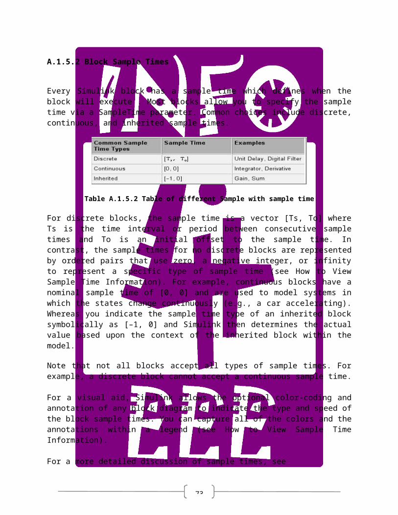
73