Solving Large-Scale Machine Learning Problemsin a Distributed Way

Martin Takac

Cognitive Systems Institute Group Speaker Series

June 09 2016

1 / 28

Outline

1 Machine Learning - Examples and Algorithm

2 Distributed Computing

3 Learning Large-Scale Deep Neural Network (DNN)

2 / 28

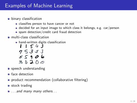
Examples of Machine Learning

binary classification

classifies person to have cancer or notdecided for an input image to which class it belongs, e.g. car/personspam detection/credit card fraud detection

multi-class classification

hand-written digits classification

speech understanding

face detection

product recommendation (collaborative filtering)

stock trading

. . . and many many others. . .

3 / 28

Support Vector Machines (SVM)

blue: healthy person

green: e.g. patient with lung cancer

Exhaled breath analysis for lung cancer: predict if patient has cancer or not

4 / 28

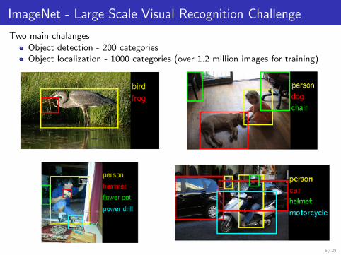
ImageNet - Large Scale Visual Recognition Challenge

Two main chalangesObject detection - 200 categoriesObject localization - 1000 categories (over 1.2 million images for training)

5 / 28

ImageNet - Large Scale Visual Recognition Challenge

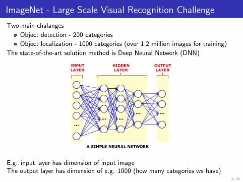
Two main chalanges

Object detection - 200 categories

Object localization - 1000 categories (over 1.2 million images for training)

The state-of-the-art solution method is Deep Neural Network (DNN)

E.g. input layer has dimension of input imageThe output layer has dimension of e.g. 1000 (how many categories we have)

5 / 28

Deep Neural Network

we have to learn the weights between neurons (blue arrows)

the neural network is defining a non-linear and non-convex function (ofweights w) from input x to output y :

y = f (w ; x)

6 / 28

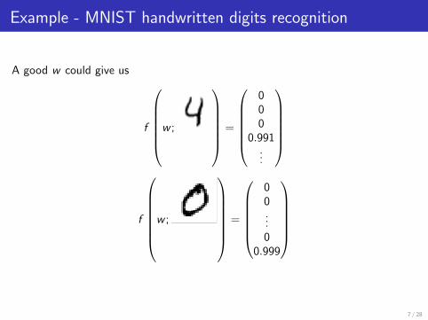
Example - MNIST handwritten digits recognition

A good w could give us

f

w ;

=

000

0.991...

f

w ;

=

00...0

0.999

7 / 28

Mathematical Formulation

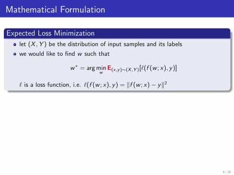
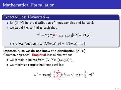
Expected Loss Minimization

let (X ,Y ) be the distribution of input samples and its labels

we would like to find w such that

w∗ = arg minw

E(x,y)∼(X ,Y )[`(f (w ; x), y)]

` is a loss function, i.e. `(f (w ; x), y) = ‖f (w ; x)− y‖2

Impossible, as we do not know the distribution (X ,Y )Common approach: Empirical loss minimization:

we sample n points from (X ,Y ): {(xi , yi )}ni=1

we minimize regularized empirical loss

w∗ = arg minw

1

n

n∑i=1

`(f (w ; xi ), yi ) +λ

2‖w‖2

8 / 28

Mathematical Formulation

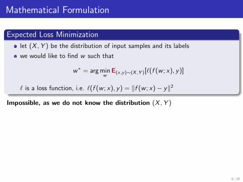
Expected Loss Minimization

let (X ,Y ) be the distribution of input samples and its labels

we would like to find w such that

w∗ = arg minw

E(x,y)∼(X ,Y )[`(f (w ; x), y)]

` is a loss function, i.e. `(f (w ; x), y) = ‖f (w ; x)− y‖2

Impossible, as we do not know the distribution (X ,Y )

Common approach: Empirical loss minimization:

we sample n points from (X ,Y ): {(xi , yi )}ni=1

we minimize regularized empirical loss

w∗ = arg minw

1

n

n∑i=1

`(f (w ; xi ), yi ) +λ

2‖w‖2

8 / 28

Mathematical Formulation

Expected Loss Minimization

let (X ,Y ) be the distribution of input samples and its labels

we would like to find w such that

w∗ = arg minw

E(x,y)∼(X ,Y )[`(f (w ; x), y)]

` is a loss function, i.e. `(f (w ; x), y) = ‖f (w ; x)− y‖2

Impossible, as we do not know the distribution (X ,Y )Common approach: Empirical loss minimization:

we sample n points from (X ,Y ): {(xi , yi )}ni=1

we minimize regularized empirical loss

w∗ = arg minw

1

n

n∑i=1

`(f (w ; xi ), yi ) +λ

2‖w‖2

8 / 28

Stochastic Gradient Descent (SGD) Algorithm

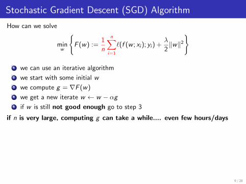
How can we solve

minw

{F (w) :=

1

n

n∑i=1

`(f (w ; xi ); yi ) +λ

2‖w‖2

}

1 we can use an iterative algorithm

2 we start with some initial w

3 we compute g = ∇F (w)

4 we get a new iterate w ← w − αg5 if w is still not good enough go to step 3

if n is very large, computing g can take a while.... even few hours/daysTrick:

choose i ∈ {1, . . . , n} randomly

define gi = ∇(`(f (w ;wi ); yi ) + λ

2 ‖w‖2)

use gi instead of g in the algorithm (step 4)

Note: E[gi ] = g , so in expectation, the ”direction” the algorithm is going is thesame as if we use the true gradient, but we can compute it n times faster!

9 / 28

Stochastic Gradient Descent (SGD) Algorithm

How can we solve

minw

{F (w) :=

1

n

n∑i=1

`(f (w ; xi ); yi ) +λ

2‖w‖2

}

1 we can use an iterative algorithm

2 we start with some initial w

3 we compute g = ∇F (w)

4 we get a new iterate w ← w − αg5 if w is still not good enough go to step 3

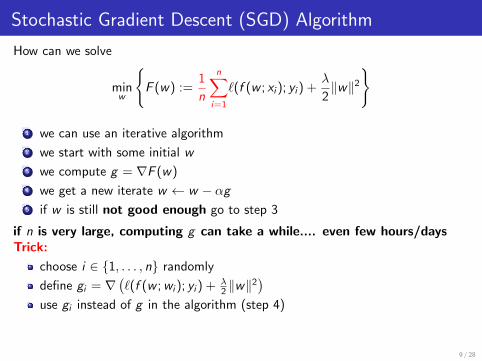
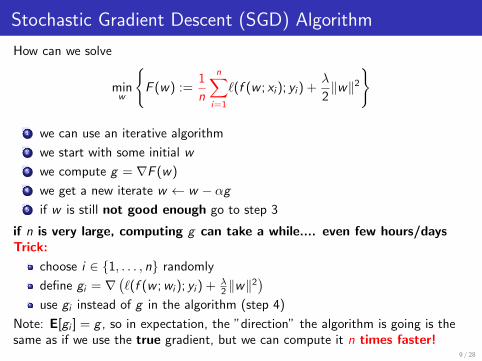
if n is very large, computing g can take a while.... even few hours/days

Trick:

choose i ∈ {1, . . . , n} randomly

define gi = ∇(`(f (w ;wi ); yi ) + λ

2 ‖w‖2)

use gi instead of g in the algorithm (step 4)

Note: E[gi ] = g , so in expectation, the ”direction” the algorithm is going is thesame as if we use the true gradient, but we can compute it n times faster!

9 / 28

Stochastic Gradient Descent (SGD) Algorithm

How can we solve

minw

{F (w) :=

1

n

n∑i=1

`(f (w ; xi ); yi ) +λ

2‖w‖2

}

1 we can use an iterative algorithm

2 we start with some initial w

3 we compute g = ∇F (w)

4 we get a new iterate w ← w − αg5 if w is still not good enough go to step 3

if n is very large, computing g can take a while.... even few hours/daysTrick:

choose i ∈ {1, . . . , n} randomly

define gi = ∇(`(f (w ;wi ); yi ) + λ

2 ‖w‖2)

use gi instead of g in the algorithm (step 4)

Note: E[gi ] = g , so in expectation, the ”direction” the algorithm is going is thesame as if we use the true gradient, but we can compute it n times faster!

9 / 28

Stochastic Gradient Descent (SGD) Algorithm

How can we solve

minw

{F (w) :=

1

n

n∑i=1

`(f (w ; xi ); yi ) +λ

2‖w‖2

}

1 we can use an iterative algorithm

2 we start with some initial w

3 we compute g = ∇F (w)

4 we get a new iterate w ← w − αg5 if w is still not good enough go to step 3

if n is very large, computing g can take a while.... even few hours/daysTrick:

choose i ∈ {1, . . . , n} randomly

define gi = ∇(`(f (w ;wi ); yi ) + λ

2 ‖w‖2)

use gi instead of g in the algorithm (step 4)

Note: E[gi ] = g , so in expectation, the ”direction” the algorithm is going is thesame as if we use the true gradient, but we can compute it n times faster!

9 / 28

Outline

1 Machine Learning - Examples and Algorithm

2 Distributed Computing

3 Learning Large-Scale Deep Neural Network (DNN)

10 / 28

The Architecture

What if the size of data {(xi , yi )} exceeds the memory of a singlecomputing node?

each node can store portion of the data {(xi , yi )}each node is connected to the computer network

they can communicate with any other node (over maybe 1 or more switches)

Fact: every communication is much more expensive then accessing local data(can be even 100,000 times slower).

11 / 28

The Architecture

What if the size of data {(xi , yi )} exceeds the memory of a singlecomputing node?

each node can store portion of the data {(xi , yi )}each node is connected to the computer network

they can communicate with any other node (over maybe 1 or more switches)

Fact: every communication is much more expensive then accessing local data(can be even 100,000 times slower).

11 / 28

Outline

1 Machine Learning - Examples and Algorithm

2 Distributed Computing

3 Learning Large-Scale Deep Neural Network (DNN)

12 / 28

Using SGD for DNN in Distributed Way

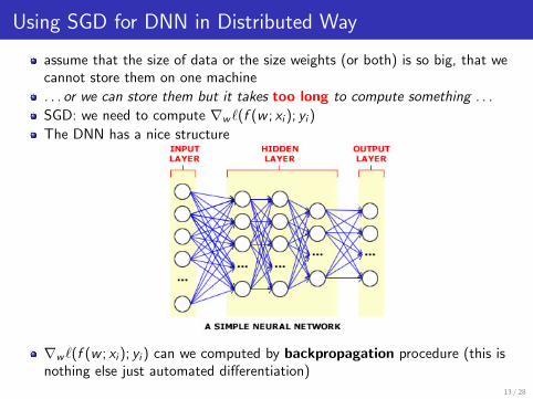
assume that the size of data or the size weights (or both) is so big, that wecannot store them on one machine

. . . or we can store them but it takes too long to compute something . . .

SGD: we need to compute ∇w `(f (w ; xi ); yi )

The DNN has a nice structure

∇w `(f (w ; xi ); yi ) can we computed by backpropagation procedure (this isnothing else just automated differentiation)

13 / 28

Why is SGD a Bad Distributed Algorithm

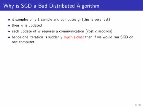
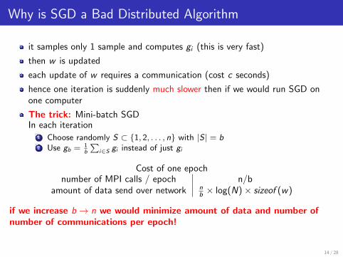
it samples only 1 sample and computes gi (this is very fast)

then w is updated

each update of w requires a communication (cost c seconds)

hence one iteration is suddenly much slower then if we would run SGD onone computer

The trick: Mini-batch SGDIn each iteration

1 Choose randomly S ⊂ {1, 2, . . . , n} with |S | = b2 Use gb = 1

b

∑i∈S gi instead of just gi

Cost of one epochnumber of MPI calls / epoch n/b

amount of data send over network nb × log(N)× sizeof (w)

if we increase b → n we would minimize amount of data and number ofnumber of communications per epoch! Caveat: there is no free lunch!Very large b means slower convergence!

14 / 28

Why is SGD a Bad Distributed Algorithm

it samples only 1 sample and computes gi (this is very fast)

then w is updated

each update of w requires a communication (cost c seconds)

hence one iteration is suddenly much slower then if we would run SGD onone computer

The trick: Mini-batch SGDIn each iteration

1 Choose randomly S ⊂ {1, 2, . . . , n} with |S | = b2 Use gb = 1

b

∑i∈S gi instead of just gi

Cost of one epochnumber of MPI calls / epoch n/b

amount of data send over network nb × log(N)× sizeof (w)

if we increase b → n we would minimize amount of data and number ofnumber of communications per epoch! Caveat: there is no free lunch!Very large b means slower convergence!

14 / 28

Why is SGD a Bad Distributed Algorithm

it samples only 1 sample and computes gi (this is very fast)

then w is updated

each update of w requires a communication (cost c seconds)

hence one iteration is suddenly much slower then if we would run SGD onone computer

The trick: Mini-batch SGDIn each iteration

1 Choose randomly S ⊂ {1, 2, . . . , n} with |S | = b2 Use gb = 1

b

∑i∈S gi instead of just gi

Cost of one epochnumber of MPI calls / epoch n/b

amount of data send over network nb × log(N)× sizeof (w)

if we increase b → n we would minimize amount of data and number ofnumber of communications per epoch!

Caveat: there is no free lunch!Very large b means slower convergence!

14 / 28

Why is SGD a Bad Distributed Algorithm

it samples only 1 sample and computes gi (this is very fast)

then w is updated

each update of w requires a communication (cost c seconds)

hence one iteration is suddenly much slower then if we would run SGD onone computer

The trick: Mini-batch SGDIn each iteration

1 Choose randomly S ⊂ {1, 2, . . . , n} with |S | = b2 Use gb = 1

b

∑i∈S gi instead of just gi

Cost of one epochnumber of MPI calls / epoch n/b

amount of data send over network nb × log(N)× sizeof (w)

if we increase b → n we would minimize amount of data and number ofnumber of communications per epoch! Caveat: there is no free lunch!Very large b means slower convergence!

14 / 28

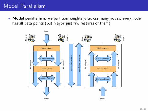
Model Parallelism

Model parallelism: we partition weights w across many nodes; every nodehas all data points (but maybe just few features of them)

Hidden Layer 1

Hidden Layer 2

Output

Input

Forward Propagation

Hidden Layer 1

Hidden Layer 2

Output

Backward Propagation

Node

1

Node

1

Node

2

Node

2

All S

ampl

es

All S

ampl

es

All S

ampl

es

All S

ampl

es

Exchange Activation

Exchange Activation

Exchange Deltas

Exchange Deltas

15 / 28

Data Parallelism

Data parallelism: we partition data-samples across many nodes, each nodehas a fresh copy of w

Hidden Layer 1

Hidden Layer 2

Output

Input

Forward Propagation

Hidden Layer 1

Hidden Layer 2

Output

Backward Propagation

Node

1

Node

1

Node

2

Node

2

Parti

al S

ampl

es

Parti

al S

ampl

es

Parti

al S

ampl

es

Parti

al S

ampl

es

Hidden Layer 1

Hidden Layer 2

Hidden Layer 1

Hidden Layer 2

Exchange Gradient

16 / 28

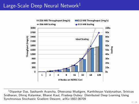
Large-Scale Deep Neural Network1

1Dipankar Das, Sasikanth Avancha, Dheevatsa Mudigere, Karthikeyan Vaidynathan, SrinivasSridharan, Dhiraj Kalamkar, Bharat Kaul, Pradeep Dubey: Distributed Deep Learning UsingSynchronous Stochastic Gradient Descent, arXiv:1602.06709

17 / 28

There is almost no speedup for large b

18 / 28

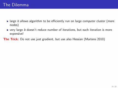
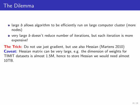
The Dilemma

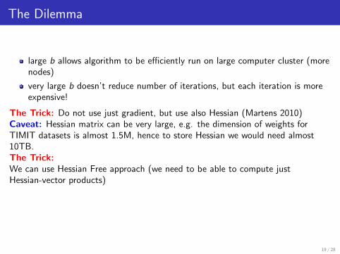
large b allows algorithm to be efficiently run on large computer cluster (morenodes)

very large b doesn’t reduce number of iterations, but each iteration is moreexpensive!

The Trick: Do not use just gradient, but use also Hessian (Martens 2010)

Caveat: Hessian matrix can be very large, e.g. the dimension of weights forTIMIT datasets is almost 1.5M, hence to store Hessian we would need almost10TB.The Trick:We can use Hessian Free approach (we need to be able to compute justHessian-vector products)Algorithm:

w ← w − α[∇2F (w)]−1∇F (w)

19 / 28

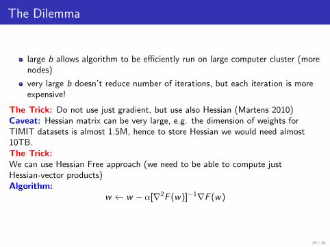
The Dilemma

large b allows algorithm to be efficiently run on large computer cluster (morenodes)

very large b doesn’t reduce number of iterations, but each iteration is moreexpensive!

The Trick: Do not use just gradient, but use also Hessian (Martens 2010)Caveat: Hessian matrix can be very large, e.g. the dimension of weights forTIMIT datasets is almost 1.5M, hence to store Hessian we would need almost10TB.

The Trick:We can use Hessian Free approach (we need to be able to compute justHessian-vector products)Algorithm:

w ← w − α[∇2F (w)]−1∇F (w)

19 / 28

The Dilemma

large b allows algorithm to be efficiently run on large computer cluster (morenodes)

very large b doesn’t reduce number of iterations, but each iteration is moreexpensive!

The Trick: Do not use just gradient, but use also Hessian (Martens 2010)Caveat: Hessian matrix can be very large, e.g. the dimension of weights forTIMIT datasets is almost 1.5M, hence to store Hessian we would need almost10TB.The Trick:We can use Hessian Free approach (we need to be able to compute justHessian-vector products)

Algorithm:w ← w − α[∇2F (w)]−1∇F (w)

19 / 28

The Dilemma

large b allows algorithm to be efficiently run on large computer cluster (morenodes)

very large b doesn’t reduce number of iterations, but each iteration is moreexpensive!

The Trick: Do not use just gradient, but use also Hessian (Martens 2010)Caveat: Hessian matrix can be very large, e.g. the dimension of weights forTIMIT datasets is almost 1.5M, hence to store Hessian we would need almost10TB.The Trick:We can use Hessian Free approach (we need to be able to compute justHessian-vector products)Algorithm:

w ← w − α[∇2F (w)]−1∇F (w)

19 / 28

Non-convexity

We want to minimizemin

wF (w)

∇2F (w) is NOT positive semi-definite at any w !

20 / 28

Computing Step

recall the algorithm

w ← w − α[∇2F (w)]−1∇F (w)

we need to compute p = [∇2F (w)]−1∇F (w), i.e. to solve

∇2F (w)p = ∇F (w) (1)

we can use few iterations of CG method to solve it(CG assumes that ∇2F (w) � 0)

In our case it may not be true, hence, it is suggested to stop CG sooner, if itis detected during CG that ∇2F (w) is indefinite

We can use a Bi-CG algorithm to solve (1) and modify the algorithm2 asfollows

w ← w − α

{p, if pT∇F (x) > 0,

−p, otherwise

PS: we use just b samples to estimate ∇2∇F (w)2Xi He, Dheevatsa Mudigere, Mikhail Smelyanskiy and Martin Takac: Large Scale Distributed

Hessian-Free Optimization for Deep Neural Network, arXiv:1606.00511, 2016.21 / 28

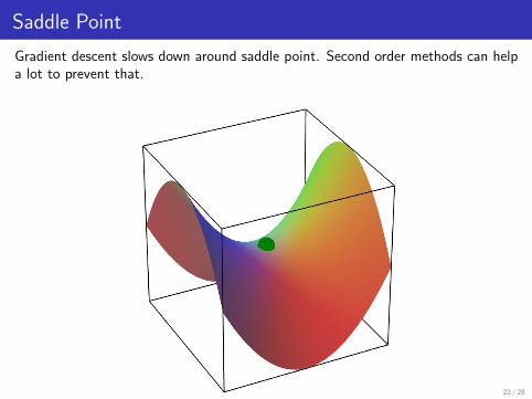
Saddle Point

Gradient descent slows down around saddle point. Second order methods can helpa lot to prevent that.

22 / 28

50 100 150 200 250 300 350 400

10−3

10−2

10−1

100

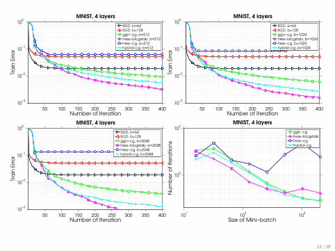
MNIST, 4 layers

Number of iteration

Tra

in E

rro

r

SGD, b=64

SGD, b=128

ggn−cg, b=512

hess−bicgstab, b=512

hess−cg, b=512

hybrid−cg, b=512

50 100 150 200 250 300 350 400

10−3

10−2

10−1

100

MNIST, 4 layers

Number of iteration

Tra

in E

rro

r

SGD, b=64

SGD, b=128

ggn−cg, b=1024

hess−bicgstab, b=1024

hess−cg, b=1024

hybrid−cg, b=1024

50 100 150 200 250 300 350 400

10−3

10−2

10−1

100

MNIST, 4 layers

Number of iteration

Tra

in E

rro

r

SGD, b=64

SGD, b=128

ggn−cg, b=2048

hess−bicgstab, b=2048

hess−cg, b=2048

hybrid−cg, b=2048

101

102

103

102

103

MNIST, 4 layers

Size of Mini−batch

Nu

mb

er

of

Ite

ratio

ns

ggn−cg

hess−bicgstab

hess−cg

hybrid−cg

23 / 28

1 1.5 2 2.5 3 3.5 4 4.5 5

100

101

102

103

TIMIT, T=18, b=512

log2(Number of Nodes)

Ru

n T

ime

pe

r It

era

tio

n

Gradient

CG

Linesearch

1 1.5 2 2.5 3 3.5 4 4.5 5

100

101

102

103

TIMIT, T=18, b=1024

log2(Number of Nodes)

Ru

n T

ime

pe

r It

era

tio

n

Gradient

CG

Linesearch

1 1.5 2 2.5 3 3.5 4 4.5 5

100

101

102

103

TIMIT, T=18, b=4096

log2(Number of Nodes)

Ru

n T

ime

pe

r It

era

tio

n

Gradient

CG

Linesearch

1 1.5 2 2.5 3 3.5 4 4.5 5

101

102

103

TIMIT, T=18, b=8192

log2(Number of Nodes)

Ru

n T

ime

pe

r It

era

tio

n

Gradient

CG

Linesearch

24 / 28

1 1.5 2 2.5 3 3.5 4 4.5 5

100

101

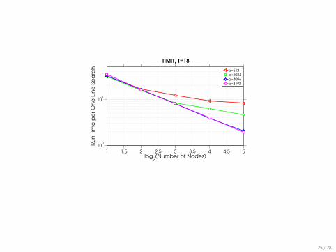
TIMIT, T=18

log2(Number of Nodes)

Ru

n T

ime

pe

r O

ne

Lin

e S

ea

rch

b=512

b=1024

b=4096

b=8192

25 / 28

Learning Artistic Style by Deep Neural Network3

3Joint work with Jiawei Zhang, based on Leon A. Gatys, Alexander S. Ecker, Matthias Bethge, A Neural Algorithm of Artistic Style, arxiv 1508.06576

26 / 28

Learning Artistic Style by Deep Neural Network3

3Joint work with Jiawei Zhang, based on Leon A. Gatys, Alexander S. Ecker, Matthias Bethge, A Neural Algorithm of Artistic Style, arxiv 1508.06576

26 / 28

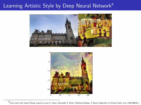
Learning Artistic Style by Deep Neural Network4

4Joint work with Jiawei Zhang, based on Leon A. Gatys, Alexander S. Ecker, Matthias Bethge, A Neural Algorithm of Artistic Style, arxiv 1508.0657627 / 28

Learning Artistic Style by Deep Neural Network4

4Joint work with Jiawei Zhang, based on Leon A. Gatys, Alexander S. Ecker, Matthias Bethge, A Neural Algorithm of Artistic Style, arxiv 1508.0657627 / 28

References

1 Albert Berahas, Jorge Nocedal and Martin Takac: A Multi-Batch L-BFGS Method for MachineLearning, arXiv:1605.06049, 2016.

2 Xi He, Dheevatsa Mudigere, Mikhail Smelyanskiy and Martin Takac:Large Scale Distributed Hessian-Free Optimization for Deep Neural Network, arXiv:1606.00511, 2016.

3 Chenxin Ma and Martin Takac: Partitioning Data on Features or Samples in Communication-EfficientDistributed Optimization?, OptML@NIPS 2015.

4 Chenxin Ma, Virginia Smith, Martin Jaggi, Michael I. Jordan, Peter Richtarik and Martin Takac: Addingvs. Averaging in Distributed Primal-Dual Optimization, ICML 2015.

5 Martin Jaggi, Virginia Smith, Martin Takac, Jonathan Terhorst, Thomas Hofmann and Michael I.Jordan: Communication-Efficient Distributed Dual Coordinate Ascent, NIPS 2014.

6 Richtarik, P. and Takac, M.: Distributed coordinate descent method for learning with big data, JournalPaper Journal of Machine Learning Research (to appear), 2016

7 Richtarik, P. and Takac, M.: On optimal probabilities in stochastic coordinate descent methods,Optimization Letters, 2015.

8 Richtarik, P. and Takac, M.: Parallel coordinate descent methods for big data optimization,Mathematical Programming, 2015.

9 Richtarik, P. and Takac, M.: Iteration complexity of randomized block-coordinate descent methods forminimizing a composite function, Mathematical Programming, 2012.

10 Takac, M., Bijral, A., Richtarik, P. and Srebro, N.: Mini-batch primal and dual methods for SVMs, InICML, 2013.

11 Qu, Z., Richtarik, P. and Zhang, T.: Randomized dual coordinate ascent with arbitrary sampling,arXiv:1411.5873, 2014.

12 Qu, Z., Richtarik, P., Takac, M. and Fercoq, O.: SDNA: Stochastic Dual Newton Ascent for EmpiricalRisk Minimization, arXiv:1502.02268, 2015.

13 Tappenden, R., Takac, M. and Richtarik, P., On the Complexity of Parallel Coordinate Descent, arXiv:1503.03033, 2015.

28 / 28