Aeroacoustic simulation of bluff body noise using a hybrid statistical method

School of Mechanical Engineering

Tuesday, November 10, 2009

Life Impact The University of Adelaide

Aeroacoustic simulation of bluff body noise using a hybrid statistical

method

Con DoolanSchool of Mechanical EngineeringUniversity of Adelaide, SA, 5005

ACOUSTICS 2009

Summary

• Bluff Body Noise - What is it?

• Why is it important?

• Physics controlling flow and noise

• Simulation methods - limitations for engineers

• Statistical Correction

• Results

Bluff Body - Dipole Noise

!v =

Uc

f0

= Dk

St0

U0

Streamlined Body - 3/2 Pole Noise

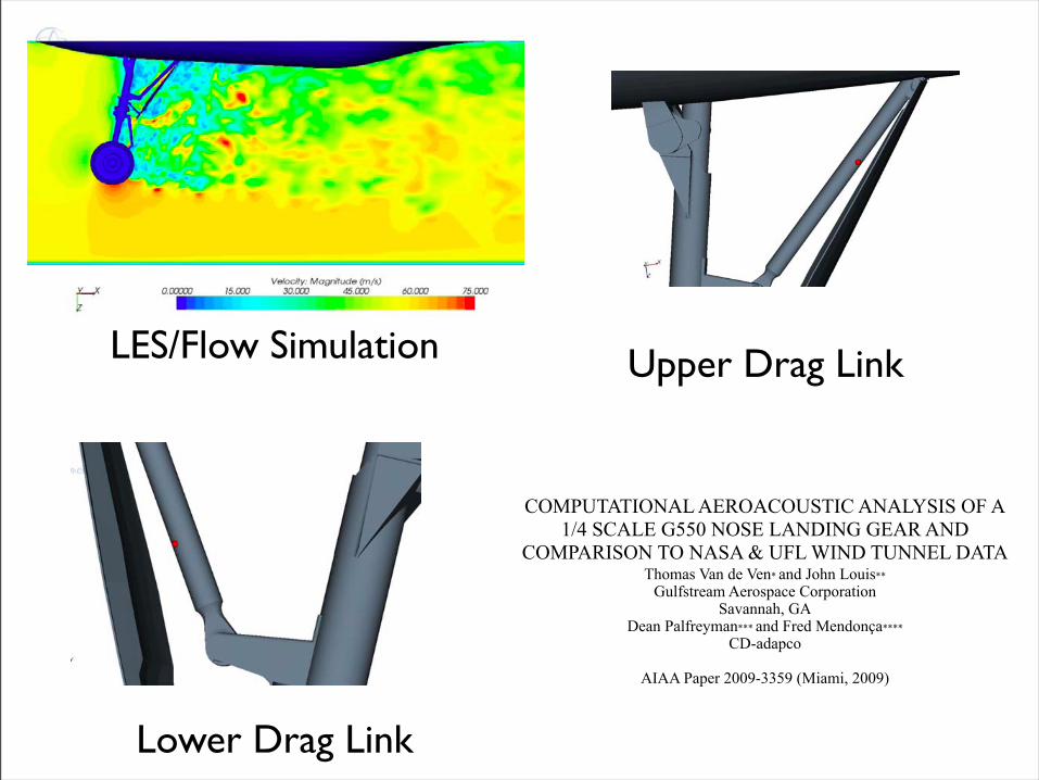
Lower Drag Link

Upper Drag LinkLES/Flow Simulation

COMPUTATIONAL AEROACOUSTIC ANALYSIS OF A1/4 SCALE G550 NOSE LANDING GEAR AND

COMPARISON TO NASA & UFL WIND TUNNEL DATAThomas Van de Ven* and John Louis**

Gulfstream Aerospace CorporationSavannah, GA

Dean Palfreyman*** and Fred Mendonça****

CD-adapco

AIAA Paper 2009-3359 (Miami, 2009)

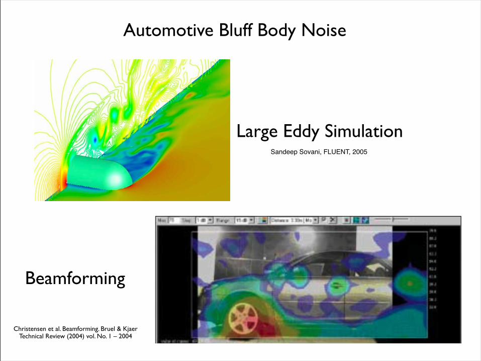
Automotive Bluff Body Noise

Christensen et al. Beamforming. Bruel & Kjaer Technical Review (2004) vol. No. 1 – 2004

Beamforming

Large Eddy SimulationSandeep Sovani, FLUENT, 2005

Subs and Trains

Proceedings of ACOUSTICS 2009 23–25 November 2009, Adelaide, Australia

(a) Entire grid

(b) Region about cylinder

Figure 2: Computational grid used for aerodynamic simulation

flow-through times. This corresponds to 434,783 time steps andcaptures 100 vortex shedding cycles with 439 non-dimensionaltime steps per shedding period.

ACOUSTIC SIMULATION METHOD

Compact Acoustic Assumption

It is pertinent to examine the limits of acoustic compactnessbefore describing the general acoustic simulation methodology.An assumption of acoustic compactness is valid if the wave-length of sound is greater than the dimensions of the object orsource region producing it. Strictly, it is difficult to determinedefinite frequency limits on when compactness can be assured.This is because as the wavelength to source dimension ratio(λ/d) is increased, true compactness is achieved only asymp-totically as λ/d → ∞. Practically however, a nearly compactsound field is achieved before that and, as will be shown below,the error in this assumption is limited to a ∼ 1 dB if the Machnumber is small.

Consider a cylinder of diameter d in cross flow whose freestreamvelocity is U0 and Mach number M. The sound above the cylin-der is mainly controlled by the dipole sound field whose sourcestrength is governed by the surface pressure fluctuations. If thesound is measured directly above the cylinder, a distance Rfrom its centre, then Curle’s theory can be used to approximateits value (p�(ω))

p�(ω)∼ −iωA(c0R)

�pue

−iω(R−d/2)c − ple

−iω(R+d/2)c e−iξ

�(1)

∼ −iωA(c0R)

|p|e−iωR/c�

eiωd

2 − e−iωd

2 e−iξ�

(2)

where pu and pl are the pressures on the upper and lower surfaceof the cylinder, |p|∼ |pu|∼ |pl |, A is a reference area and ξ isthe phase between pu and pl . If a compact assumption is made,

then the propagation time between points on the surface is zero,or in the above equation d → 0. Therefore, an estimate of theerror due to a compact assumption can be made by dividingEq. 2 by itself but with d = 0. In dB, this expression is (takingthe real component)

E = 20log10 cos(πStM) (3)

For the case considered here, the maximum frequency is limitedto a Strouhal number, St = f d/U0 = 2 and a Mach number of0.06. This results in an error E < 1 dB. Therefore the assump-tion of compactness is appropriate for the present work. Notethat the error becomes very large when M > 0.15.

Curle’s Theory

The acoustically compact form of Curle’s equation (Curle 1955)can be simplified to predict the acoustic far field (representedas a density fluctuation ρ �) generated at an observation point bya fluctuating point force F̃ applied on a compressible fluid thatis initially at rest

4πc20ρ �(x̃, t) =− ∂

∂xi

�Fir

�=

1c0

xir2

�∂Fi∂ t

�(4)

where Fi are the three vector components of the resulting forceapplied on the fluid and c0 is the speed of sound of the medium(air) at rest. The observation point is x̃ measured with respectto the compact body (in this case, the centre of the cylinder).The distance between the body and the observation point isdescribed by the distance r. The square brackets denote a valuetaken at the retarded time Θ = t− r/c0.

A URANS simulation can provide unsteady sectional force data(Fi(t), used to calculate the acoustic source terms in Curle’scompact acoustic analogy, Eq. 4) in a straightforward manner.However, it is well known that transient force data from thesetypes of simulations are extremely tonal and tend to overesti-mate the vortex shedding frequency, and its harmonics, result-ing in poor noise predictions. The reasons behind these defi-ciencies results from the two-dimensionality of the simulationand, to some extent, the nature of the turbulence model em-ployed (Casalino et al. 2003). The frequency change is mainlydue to the over-prediction of Reynolds stresses in the near wakeartificially constraining the size of the re-circulation bubbleformed immediately behind the bluff body (Roshko 1993).

To use a URANS simulation to calculate noise, the simulatedbody forces need to be modified to take into account the effectof wake three-dimensionality on the cylinder unsteady sectionalforce coefficients. This is done in a two-step method. First, therandom, low frequency beating is introduced using a tempo-ral model. Second, the effects of spanwise decorrelation areincorporated using a modified form of the model originallydeveloped by Casalino and Jacob (2003). These models aresummarised below.

Temporal Model

It is assumed that the true force Ftrue(t) is convoluted over asignal of time length T to the URANS simulated force signalFURANS(t) using an impulse response function h(t)

Ftrue(t) =� T

0h(τ)FURANS(t) dτ (5)

If the impulse response function can be described as

h(t) = e−iφτ (6)

Australian Acoustical Society 3


(a) Entire grid









�pue



�(1)

∼ −iωA(c0R)

|p|e−iωR/c�

eiωd

2 − e−iωd

2 e−iξ�

(2)





Curle’s Theory


4πc20ρ �(x̃, t) =− ∂

∂xi

�Fir

�=

1c0

xir2

�∂Fi∂ t

�(4)




Temporal Model


Ftrue(t) =� T



h(t) = e−iφτ (6)


If a body is compact, then the noise (density fluctuation )is a function of the force acting on it ( )

Compact Aeroacoustic Noise: Curle’s Theory


(a) Entire grid









�pue



�(1)

∼ −iωA(c0R)

|p|e−iωR/c�

eiωd

2 − e−iωd

2 e−iξ�

(2)





Curle’s Theory


4πc20ρ �(x̃, t) =− ∂

∂xi

�Fir

�=

1c0

xir2

�∂Fi∂ t

�(4)




Temporal Model


Ftrue(t) =� T



h(t) = e−iφτ (6)



(a) Entire grid









�pue



�(1)

∼ −iωA(c0R)

|p|e−iωR/c�

eiωd

2 − e−iωd

2 e−iξ�

(2)





Curle’s Theory


4πc20ρ �(x̃, t) =− ∂

∂xi

�Fir

�=

1c0

xir2

�∂Fi∂ t

�(4)




Temporal Model


Ftrue(t) =� T



h(t) = e−iφτ (6)


The error (dB) associated with the compact assumption is:


(a) Entire grid









�pue



�(1)

∼ −iωA(c0R)

|p|e−iωR/c�

eiωd

2 − e−iωd

2 e−iξ�

(2)





Curle’s Theory


4πc20ρ �(x̃, t) =− ∂

∂xi

�Fir

�=

1c0

xir2

�∂Fi∂ t

�(4)




Temporal Model


Ftrue(t) =� T



h(t) = e−iφτ (6)


Brief Article

The Author

November 10, 2009

M = 0.06

1

This work:


(a) Entire grid









�pue



�(1)

∼ −iωA(c0R)

|p|e−iωR/c�

eiωd

2 − e−iωd

2 e−iξ�

(2)





Curle’s Theory


4πc20ρ �(x̃, t) =− ∂

∂xi

�Fir

�=

1c0

xir2

�∂Fi∂ t

�(4)




Temporal Model


Ftrue(t) =� T



h(t) = e−iφτ (6)


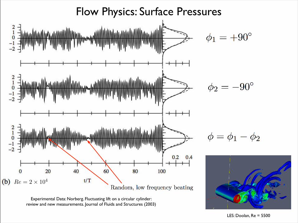
!1 = +90!

!2 = !90!

! = !1 ! !2

Random, low frequency beating4

Re = 2 ! 104

Flow Physics: Surface Pressures

Experimental Data: Norberg. Fluctuating lift on a circular cylinder: review and new measurements. Journal of Fluids and Structures (2003)

LES: Doolan, Re = 5500

Flow Physics: Spanwise Phase Dispersion

1. Direct Numerical Simulation (DNS)Most Accurate, no assumptions, impossible for engineering flows

2. Large Eddy Simulation (LES)Very good accuracy, a few assumptions, possible for engineering flows, but difficult for engineering design

3. Unsteady Reynolds Averaged Navier Stokes (URANS)Reasonably accurate when time averaged, many assumptions, only way to do engineering design for most engineers.

CFD Comparison

New Methodology:

Use a statistical model to correct URANS flow simulations in order to correctly model far-field noise

URANS SIGNALS ADD STATISTICS “TRUE”

SIGNALS

220 240 260 280 300 320

−0.6

−0.4

−0.2

0

0.2

0.4

0.6

0.8

1

1.2

tU0 /d

C l, Cd

Cd

Cl

0.1 0.2 0.4 0.8 1 1.4 2−10

0

10

20

30

40

50

60

70

80

St

PSD

[dB/

Hz]

With Spanwise Effects

Pure Tone

Temporal Statistics


(a) Entire grid









�pue



�(1)

∼ −iωA(c0R)

|p|e−iωR/c�

eiωd

2 − e−iωd

2 e−iξ�

(2)





Curle’s Theory


4πc20ρ �(x̃, t) =− ∂

∂xi

�Fir

�=

1c0

xir2

�∂Fi∂ t

�(4)




Temporal Model


Ftrue(t) =� T



h(t) = e−iφτ (6)



(a) Entire grid









�pue



�(1)

∼ −iωA(c0R)

|p|e−iωR/c�

eiωd

2 − e−iωd

2 e−iξ�

(2)





Curle’s Theory


4πc20ρ �(x̃, t) =− ∂

∂xi

�Fir

�=

1c0

xir2

�∂Fi∂ t

�(4)




Temporal Model


Ftrue(t) =� T



h(t) = e−iφτ (6)



(a) Entire grid









�pue



�(1)

∼ −iωA(c0R)

|p|e−iωR/c�

eiωd

2 − e−iωd

2 e−iξ�

(2)





Curle’s Theory


4πc20ρ �(x̃, t) =− ∂

∂xi

�Fir

�=

1c0

xir2

�∂Fi∂ t

�(4)




Temporal Model


Ftrue(t) =� T



h(t) = e−iφτ (6)


23–25 November 2009, Adelaide, Australia Proceedings of ACOUSTICS 2009

then the true signal can be considered as a composite of anumber of original simulated signals, each with a randomlydispersed phase difference φτ = φτ (τ).

In the same manner as the spatial case (Casalino and Jacob2003, see next section), it is assumed that the autocorrelationcoefficient (ρτ ) can be distributed according to Laplacian statis-tics

ρτ (τ) = exp�− τt

τc

�(7)

so that τt = τ/T is the time delay normalised by the time baseT and τc = ∆tc/T is a normalised time scale associated with therandomness of the time signal. Note, Gaussian statistics couldequally be applied.

The Laplacian model calls for a linear distribution of varianceover 0≤ τt ≤ 1

wτ (τt) = wτ,maxτt (8)

where wτ,max = 1/τc. This variance distribution is used to gen-erate a random dispersion of phase (φτ ) over 0 ≤ τt ≤ 1 thatmodulates the retarded time of the URANS signal used to cal-culate noise in Eq. 4 using

Θτ = Θ+φτ2π

dU0

(9)

This modulation is performed as a pre-processing step be-fore the spanwise decorrelation of the signals. Practically, 100URANS unsteady force data records, each with a randomly dis-persed phase, are used to create a single temporally decorrelatedforce signal.

Spatial Model

Recently, Casalino and Jacob (2003) have developed an ad-hoc technique to overcome some of the problems associatedwith URANS solutions in noise prediction. It accounts for thethree-dimensional nature of the flow by randomly dispersing thephase of surface pressure fluctuations across the span of a cylin-der (or any other extruded two-dimensional shape) accordingto a statistical model based on an estimate of the spanwise co-herence. The random phase is then used to perturb the retardedtime of surface pressure fluctuations across the span, which arethen used in an FWH solver to calculate far-field noise.

Following Casalino and Jacob (2003) and consistent with thetemporal model of the last section, random phase distributionsare determined using a linear variance distribution (w) acrossthe span

w(η) = 2wmax|η | (10)

where η is the the spanwise coordinate along the cylinder span(Lz). A linear variance distribution results in a Laplacian corre-lation coefficient, giving

wmax = 1/Ll (11)

where Ll is Laplacian spanwise correlation length scale. Hence,the model describing the correlation coefficient ρ(η) across thespan is (for Laplacian statistics)

ρ(η) = exp�− |η |

Ll

�(12)

Using the spanwise statistical model, a random dispersion inphase (φη ) is created along the span of the cylinder.

The phase distribution is then used to modulate the retardedtime

Θη = Θ+φη2π

dU0

(13)

This procedure is equivalent to introducing a spanwise lossof coherency along the span of a cylinder. It is a convenientway of introducing some of the features of a three-dimensionalflowfield to a noise calculation that uses a two-dimensional flowsimulation.

To estimate the spanwise correlation length scale, empiricalrelations (Norberg 2003) can be used. For this paper, the exper-imental measurements of Casalino and Jacob (2003) are usedinstead.

Frequency Compensation

The experimental data has been shifted in frequency so thatthe main tone occurs at an identical Strouhal number to theURANS simulation. According to Curle’s theory (Eq. 4), linearfrequency scaling also necessitates a small scaling in amplitude.The frequency and amplitude were scaled according to

fshi f t = fStnumStexp

(14)

∆SPL(dB) = 20log10StnumStexp

(15)

RESULTS

Aerodynamic Results

Figure 3 shows the instantaneous spanwise vorticity in the nearwake of the cylinder over one vortex shedding cycle. The simu-lation successfully recreates the major features of the unsteadyflow. These are boundary layer separation, shear layer growthand instability and the creation of discrete vorticies that laterform the von Karman vortex street. While the URANS mod-elling procedure filters most of the high frequency turbulencefluctuations, small vorticial structures form in the shear layersand these may be attributed to the Kelvin-Helmholtz instabilitymechanism. The periodic nature of the shedding process ob-served in Fig. 3 is responsible for the creation of unsteady forceon the cylinder and hence noise.

Table 1 compares mean flow measurements from the literaturewith the numerical simulations. As shown, the URANS simula-tion recreate the mean force coefficients well. The fundamentalStrouhal number (Sto) is slightly over-predicted and the reasonsfor this are discussed earlier.

Equispaced contours of root-mean-square (RMS) pressure coef-ficient about the cylinder are shown in Fig. 4. The highest levelof pressure fluctuation is present in the flow itself, in the regionof the near wake associated with vortex formation. However,this pressure variation does not contribute significantly to thefarfield noise. This is because it is not near a solid boundary andhence cannot support a dipole (Curle 1955). In fact, the acoustic

4 Australian Acoustical Society

...





τc

�(7)





Θτ = Θ+φτ2π

dU0

(9)


Spatial Model



w(η) = 2wmax|η | (10)


wmax = 1/Ll (11)


ρ(η) = exp�− |η |

Ll

�(12)



Θη = Θ+φη2π

dU0

(13)






(14)


(15)

RESULTS

Aerodynamic Results





Autocorrelation function for phase





τc

�(7)





Θτ = Θ+φτ2π

dU0

(9)


Spatial Model



w(η) = 2wmax|η | (10)


wmax = 1/Ll (11)


ρ(η) = exp�− |η |

Ll

�(12)



Θη = Θ+φη2π

dU0

(13)






(14)


(15)

RESULTS

Aerodynamic Results





Time “shift”

Spatial Statistics





τc

�(7)





Θτ = Θ+φτ2π

dU0

(9)


Spatial Model



w(η) = 2wmax|η | (10)


wmax = 1/Ll (11)


ρ(η) = exp�− |η |

Ll

�(12)



Θη = Θ+φη2π

dU0

(13)






(14)


(15)

RESULTS

Aerodynamic Results









τc

�(7)





Θτ = Θ+φτ2π

dU0

(9)


Spatial Model



w(η) = 2wmax|η | (10)


wmax = 1/Ll (11)


ρ(η) = exp�− |η |

Ll

�(12)



Θη = Θ+φη2π

dU0

(13)






(14)


(15)

RESULTS

Aerodynamic Results





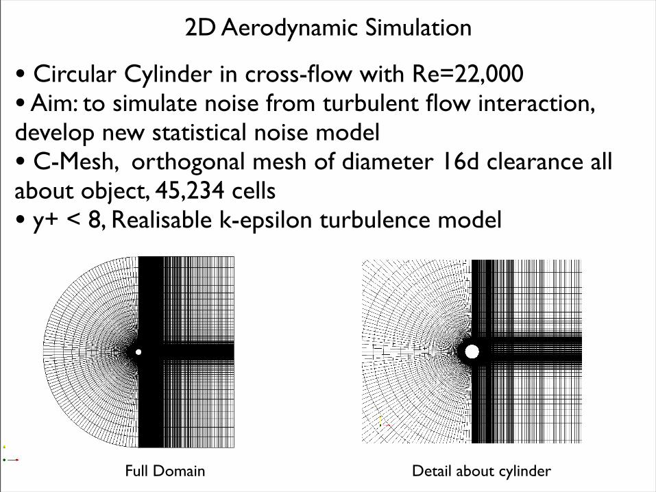
2D Aerodynamic Simulation

• Circular Cylinder in cross-flow with Re=22,000• Aim: to simulate noise from turbulent flow interaction, develop new statistical noise model• C-Mesh, orthogonal mesh of diameter 16d clearance all about object, 45,234 cells• y+ < 8, Realisable k-epsilon turbulence model

Full Domain Detail about cylinder

x/d

y/d

−0.5 0 0.5 1 1.5 2 2.5

−1

−0.5

0

0.5

1

x/d

y/d

−0.5 0 0.5 1 1.5 2 2.5

−1

−0.5

0

0.5

1

x/d

y/d

−0.5 0 0.5 1 1.5 2 2.5

−1

−0.5

0

0.5

1

x/d

y/d

−0.5 0 0.5 1 1.5 2 2.5

−1

−0.5

0

0.5

1

Instantaneous Vorticity


(a) tU0/D = 321

(b) tU0/D = 322

(c) tU0/D = 323

(d) tU0/D = 324

Figure 3: Instantaneous spanwise vorticity contours over onevortex shedding cycle. Levels: −15 ≤ ωzd

U∞≤ 15 with intervals

|∆ω|dU∞

= 5

Table 1: Comparison between mean experimental data andURANS simulation data.

Experiment URANSSt0 0.2∗ 0.239C�

l 0.354∗∗ 0.367Cd 1.1∗∗ 0.98

Source: ∗(Casalino and Jacob 2003),∗∗(Schewe 1983)

Figure 4: RMS pressure coefficient contours about the cylin-der in turbulent flow. Levels: 0 ≤ prms/(ρ0U2

0 ) ≤ 0.225 withintervals ∆prms/(ρ0U2

0 ) = 0.025

source associated with the wake is of quadrupole form and istherefore very inefficient compared with pressure variations onthe surface of the cylinder (Lighthill 1952).

For this case, the unsteady pressure that is the major contributorto noise is that on the surface of the cylinder. From Fig. 4, thelargest unsteady pressure amplitudes occur on the top and bot-tom surfaces of the cylinder, hence it is the lift dipole that is thelargest source of noise. This is consistent with the conventionalmodel for the production of the Aeolian tone (Phillips 1956).However, the unsteady drag, while lower in amplitude, can stillprovide a significant component to the measured noise spectraif the measurement microphone is placed away from the verticalaxis (Casalino and Jacob 2003, Lockard et al. 2008)

Time-series unsteady sectional lift and drag coefficient dataobtained from the URANS aerodynamic simulation are pre-sented in Fig. 5 over a non-dimensional time of ∆tU0/D = 100.The force signals are periodic and statistically stationary. It isinteresting to observe that the drag force oscillates at twicethe frequency of the lift force. This is due to the fact that thesign of the resolved vertical (lift) forces depends on the sign ofthe shed vorticity, but the resolved horizontal (drag) forces areindependent of the sign of the vorticity.

Figure 6 displays the power spectra of the simulated forcecoefficients. The spectra are extremely tonal, with significantharmonic components. If these are used to calculate noise, theywill give unrealistically tonal noise spectra. The acoustic simu-lation method described earlier will be used in the next sectionto obtain acoustic spectra that contain the correct amount ofspectral broadening.

Acoustic Results

Before effective acoustic simulation can be performed, esti-mates of the time and space correlation scales are required forthe statistical analysis.



(a) tU0/D = 321

x/d

y/d

−0.5 0 0.5 1 1.5 2 2.5

−1

−0.5

0

0.5

1

(b) tU0/D = 322

(c) tU0/D = 323

(d) tU0/D = 324



|∆ω|dU∞

= 5



l 0.354∗∗ 0.367Cd 1.1∗∗ 0.98




0 ) = 0.025





Acoustic Results




(a) tU0/D = 321

(b) tU0/D = 322

x/d

y/d

−0.5 0 0.5 1 1.5 2 2.5

−1

−0.5

0

0.5

1

(c) tU0/D = 323

(d) tU0/D = 324



|∆ω|dU∞

= 5



l 0.354∗∗ 0.367Cd 1.1∗∗ 0.98




0 ) = 0.025





Acoustic Results




(a) tU0/D = 321

(b) tU0/D = 322

(c) tU0/D = 323

x/dy/d

−0.5 0 0.5 1 1.5 2 2.5

−1

−0.5

0

0.5

1

(d) tU0/D = 324



|∆ω|dU∞

= 5



l 0.354∗∗ 0.367Cd 1.1∗∗ 0.98




0 ) = 0.025





Acoustic Results



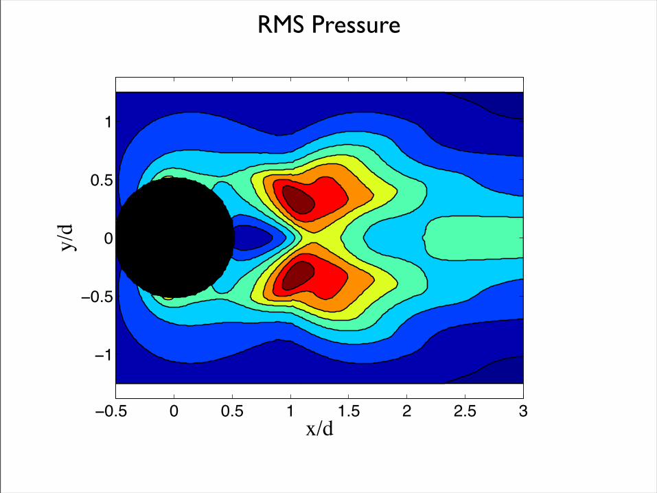
RMS Pressure

x/d

y/d

−0.5 0 0.5 1 1.5 2 2.5 3

−1

−0.5

0

0.5

1

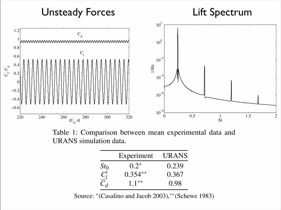
Unsteady Forces

220 240 260 280 300 320

−0.6

−0.4

−0.2

0

0.2

0.4

0.6

0.8

1

1.2

tU0 /d

C l, Cd

Cd

Cl

Lift Spectrum

0 0.5 1 1.5 210−8

10−6

10−4

10−2

100

102

St

1/Hz


(a) tU0/D = 321

(b) tU0/D = 322

(c) tU0/D = 323

(d) tU0/D = 324



|∆ω|dU∞

= 5



l 0.354∗∗ 0.367Cd 1.1∗∗ 0.98




0 ) = 0.025





Acoustic Results



Time Series Acoustic Pressure

0 50 100 150 200 250 300 350 400−1

−0.5

0

0.5

1 x 10−4

tU0/D

pʹ′/ρ

U02

Assumed characteristic time ~60 vortex shedding periods and spanwise correlation length of 0.27 x span.

Acoustic PSD at 86.25D above centre of cylinder

0.1 0.2 0.4 0.8 1 1.4 20

10

20

30

40

50

60

70

80

St

PSD

[dB/

Hz]

URANS + StatisticsURANSExperiment

100 statistical acoustic signal PSD’s were averaged.

Application to the NASA Tandem Cylinder Case

x/d

y/d

−1 0 1 2 3 4 5 6−1.5

−1

−0.5

0

0.5

1

1.5

−15

−10

−5

0

5

10

15

0.1 0.2 0.4 0.8 1 1.4 240

50

60

70

80

90

100

110

120

St

PSD

[dB/

Hz]

URANS + Statistics2D URANSExperiment (NASA QFF)

Grid

Flow: vorticity

Acoustics

Conclusions

• A methodology for correcting URANS CFD data to appropriate noise source terms has been presented

• When applied to cylinder flows, the method correctly recreates the spectral broadening about the main tone

• At this stage, the method has difficulty in recreating the harmonics

Technology

Aeroacoustic simulation of bluff body noise using a hybrid statistical method