2013 第2回数理生物学サマーレクチャーコース@RIKEN CDB 2013/7/30

確率的に表わされる過程柴田達夫

理化学研究所発生・再生科学総合研究センター

数理生物学サマーレクチャーコース第２回2013/7/30

数理生物学サマーレクチャーコース第２回 2013/7/30

Fig. 2. Recorded random walk trajectories by Jean Baptiste Perrin [72]. Left part: three designs obtained by tracinga small grain of putty (mastic, used for varnish) at intervals of 30 s. One of the patterns contains 50 single points. Rightpart: the starting point of each motion event is shifted to the origin. The "gure illustrates the pdf of the travelled distancer to be in the interval (r, r#dr), according to (2!!!)"# exp(!r!/[2!!])2!rdr, in two dimensions, with the length variance!!. These "gures constitute part of the measurement of Perrin, Dabrowski and Chaudesaigues leading to the determina-tion of the Avogadro number. The result given by Perrin is 70.5!10!!. The remarkable wuvre of Perrin discusses allpossibilities of obtaining the Avogadro number known at that time. Concerning the trajectories displayed in the left partof this "gure, Perrin makes an interesting statement: `Si, en e!et, on faisait des pointeH s de seconde en seconde, chacun deces segments rectilignes se trouverait remplaceH par un contour polygonal de 30 co( teH s relativement aussi compliqueH que ledessin ici reproduit, et ainsi de suitea. [If, veritably, one took the position from second to second, each of these rectilinearsegments would be replaced by a polygonal contour of 30 edges, each itself being as complicated as the reproduceddesign, and so forth.] This already anticipates LeH vy's cognisance of the self-similar nature, see footnote 9, as well as of thenon-di!erentiability recognised by N. Wiener.

$ In the historical context, note that the theory of the continuum formulation of #uid dynamics had already been fullydeveloped at that time. Thus, some of its milestones date back to the 18th and "rst half of the 19th century, such asBernoulli's equation (1738); Euler's equation (1755); Navier's (1827) use as a phenomenological model and Stokes' (1845)derivation of the Navier}Stokes equation. Maxwells' dynamical theory of gases dates back to 1867 and Boltzmann'stransport equation was published in 1872 for the description of collision processes. The latter is the footing for theatomistic random walk approach to Brownian motion.

A. Fick set up the di!usion equation in 1855 [68].$ Subsequently, the detailed experiments by Gouyproved the kinetic theory explanation given by C. Weiner in 1863. After attempts of "ndinga stochastic footing like the collision model by von NaK geli and John William Strutt, LordRayleigh's results, it was Albert Einstein who, in 1905, uni"ed the two approaches in his treatises onthe Brownian motion, a name coined by Einstein although he reportedly did not have access toBrown's original work. Note that a similar description of di!usion was presented by the French

8 R. Metzler, J. Klafter / Physics Reports 339 (2000) 1}77

Nobel Prizes Alfred Nobel Educational Video Player Nobel Organizations Search

About the Nobel Prizes

Facts and Lists

Nobel Prize in PhysicsAll Nobel Prizes in Physics

Facts on the Nobel Prize inPhysics

Prize Awarder for the NobelPrize in Physics

Nomination and Selection ofPhysics Laureates

Nobel Medal for Physics

Articles in Physics

Video Nobel Lectures

Nobel Prize in Chemistry

Nobel Prize in Medicine

Nobel Prize in Literature

Nobel Peace Prize

Prize in Economic Sciences

Nobel Laureates Have Their Say

Nobel Prize Award Ceremonies

Nomination and Selection ofNobel Laureates

1901 2010

Sort and list Nobel Prizes and Nobel Laureates Prize category:

1926

Jean Baptiste Perrin

Physics

The Nobel Prize in Physics 1926Jean Baptiste Perrin

The Nobel Prize in Physics 1926

Jean Baptiste Perrin

The Nobel Prize in Physics 1926 was awarded to Jean Baptiste Perrin "for hiswork on the discontinuous structure of matter, and especially for his discovery ofsedimentation equilibrium".

Photos: Copyright © The Nobel Foundation

TO CITE THIS PAGE:MLA style: "The Nobel Prize in Physics 1926". Nobelprize.org. 10 Jun 2011http://nobelprize.org/nobel_prizes/physics/laureates/1926/

RELATED DOCUMENTS:

ARTICLE

PHYSICS

The Nobel Prize inPhysics

Read more about theNobel Prize in Physics 1901-2000.

RECOMMENDED:

FACTS AND LISTS

NOBEL PRIZESWho Are the 2010Nobel Laureates?

See a list of the elevenNobel Laureates of 2010.

HAVE YOUR SAY!

What invention has mostaffected your life?

FACTS AND LISTS

NOBEL PRIZESNobel Prize Facts

Find out more aboutthe oldest, youngest, most

awarded Nobel Laureates.

SIGN UP

FOLLOW US

Youtube

Facebook

Twitter

Nobelprize.org Monthly

RSS

About Nobelprize.org Privacy Policy Terms of Use Technical Support Copyright © Nobel Media AB 2011

Home A-Z Index FAQ Press Contact Us

Home A-Z Index FAQ Press Contact Us

Home / Nobel Prizes / Nobel Prize in Physics / The Nobel Prize in Physics 1926

! Metzler, R. & Klafter, J. The random walk's guide to anomalous diffusion: a fractional dynamics approach. Phys Rep 339, 1–77 (2000).

米沢富美子「ブラウン運動」共立出版


Fig. 2. Recorded random walk trajectories by Jean Baptiste Perrin [72]. Left part: three designs obtained by tracinga small grain of putty (mastic, used for varnish) at intervals of 30 s. One of the patterns contains 50 single points. Rightpart: the starting point of each motion event is shifted to the origin. The "gure illustrates the pdf of the travelled distancer to be in the interval (r, r#dr), according to (2!!!)"# exp(!r!/[2!!])2!rdr, in two dimensions, with the length variance!!. These "gures constitute part of the measurement of Perrin, Dabrowski and Chaudesaigues leading to the determina-tion of the Avogadro number. The result given by Perrin is 70.5!10!!. The remarkable wuvre of Perrin discusses allpossibilities of obtaining the Avogadro number known at that time. Concerning the trajectories displayed in the left partof this "gure, Perrin makes an interesting statement: `Si, en e!et, on faisait des pointeH s de seconde en seconde, chacun deces segments rectilignes se trouverait remplaceH par un contour polygonal de 30 co( teH s relativement aussi compliqueH que ledessin ici reproduit, et ainsi de suitea. [If, veritably, one took the position from second to second, each of these rectilinearsegments would be replaced by a polygonal contour of 30 edges, each itself being as complicated as the reproduceddesign, and so forth.] This already anticipates LeH vy's cognisance of the self-similar nature, see footnote 9, as well as of thenon-di!erentiability recognised by N. Wiener.

$ In the historical context, note that the theory of the continuum formulation of #uid dynamics had already been fullydeveloped at that time. Thus, some of its milestones date back to the 18th and "rst half of the 19th century, such asBernoulli's equation (1738); Euler's equation (1755); Navier's (1827) use as a phenomenological model and Stokes' (1845)derivation of the Navier}Stokes equation. Maxwells' dynamical theory of gases dates back to 1867 and Boltzmann'stransport equation was published in 1872 for the description of collision processes. The latter is the footing for theatomistic random walk approach to Brownian motion.

A. Fick set up the di!usion equation in 1855 [68].$ Subsequently, the detailed experiments by Gouyproved the kinetic theory explanation given by C. Weiner in 1863. After attempts of "ndinga stochastic footing like the collision model by von NaK geli and John William Strutt, LordRayleigh's results, it was Albert Einstein who, in 1905, uni"ed the two approaches in his treatises onthe Brownian motion, a name coined by Einstein although he reportedly did not have access toBrown's original work. Note that a similar description of di!usion was presented by the French

8 R. Metzler, J. Klafter / Physics Reports 339 (2000) 1}77

x(t1), y(t1)( ), x(t2 ), y(t2 )( ),, x(tn ), y(tn )( )位置の観測値

確率論的 ↔ 決定論的

x, y( )確率変数 (stochastic variable)

確率過程 (stochastic process)

=確率変数の系列 (時系列)

! Metzler, R. & Klafter, J. The random walk's guide to anomalous diffusion: a fractional dynamics approach. Phys Rep 339, 1–77 (2000).


1次元ランダムウォーク

1. 各分子は速度vでτ秒毎に距離δ=vτだけ右か左に移動する

2. 各ステップで右に行く確率は1/2であり、左に行く確率は1/2 分子は水の分子と相互作用をすると、最後のステップでどちらへ動いたのか忘れてしまう

3. 各分子は他の全ての粒子と無関係に動く

-3δ -2δ -δ 0 δ 2δ 3δ


0

20

40

60

80

100

-10 -5 0 5 10

time

step

position

x(t)

x(0)



-3δ -2δ -δ 0 δ 2δ 3δ離散時刻t=nτ x(t) = �

n�

i=1

�i位置：

x(t) = �n�

i=1

�i = 0位置の期待値：

�i = �1, or 1ただし，確率1/2 1/2

• 粒子は平均としては動かない



離散時刻t=nτ x(t) = �n�

i=1

�i位置：

x(t) = �n�

i=1


�i = �1, or 1ただし，確率1/2 1/2

01

平均２乗変位：（時刻tにおける位置の分散）

x(t)2 =��

n⇤

i=1

�i

⇥2= �2

� n⇤

i=1

�2i + 2n⇤

i=1

n⇤

j=i+1

�i� j

⇥2

= �2n⇤

i=1

�2i + 2n⇤

i=1

n⇤

j=i+1

�i� j2

= n�2 =�2

⇥t

-3δ -2δ -δ 0 δ 2δ 3δ



離散時刻t=nτ x(t) = �n�

i=1

�i位置：

x(t) = �n�

i=1


�i = �1, or 1ただし，確率1/2 1/2

平均２乗変位： x(t)2 =�2

⇥t

x(t)2 = 2Dt D =�2

2⇥拡散係数

-3δ -2δ -δ 0 δ 2δ 3δ


0

20

40

60

80

100

-10 -5 0 5 10

time

step

position

|x(t)� x(0)|2 = 2Dt

x(t)

x(0)

�|x(t)� x(0)|2 =

⇤2Dt

平均２乗変位

確率過程の中の法則性

Mean Square DisplacementMSD

• 粒子の分布の広がりは時間の平方根に比例して大きくなる。


米沢富美子「ブラウン運動」共立出版


中心極限定理

0.45

0.5

0.55

0.6

0.65

0.7

0.75

0.8

-1 -0.5 0 0.5 1

g(x,1)

0.45

0.5

0.55

0.6

0.65

0.7

0.75

0.8

-1 -0.5 0 0.5 1

g(x,1)


中心極限定理

0.2

0.25

0.3

0.35

0.4

0.45

0.5

0.55

0.6

-2 -1.5 -1 -0.5 0 0.5 1 1.5 2 0.2

0.25

0.3

0.35

0.4

0.45

0.5

0.55

0.6

-2 -1.5 -1 -0.5 0 0.5 1 1.5 2


中心極限定理

0.05

0.1

0.15

0.2

0.25

0.3

0.35

0.4

-4 -3 -2 -1 0 1 2 3 4 0.05

0.1

0.15

0.2

0.25

0.3

0.35

0.4

-4 -3 -2 -1 0 1 2 3 4


中心極限定理

0

0.05

0.1

0.15

0.2

0.25

0.3

-8 -6 -4 -2 0 2 4 6 8 0

0.05

0.1

0.15

0.2

0.25

0.3

-8 -6 -4 -2 0 2 4 6 8


中心極限定理

0

0.02

0.04

0.06

0.08

0.1

0.12

0.14

0.16

0.18

0.2

-15 -10 -5 0 5 10 15 0

0.02

0.04

0.06

0.08

0.1

0.12

0.14

0.16

0.18

0.2

-15 -10 -5 0 5 10 15


中心極限定理

0

0.02

0.04

0.06

0.08

0.1

0.12

0.14

0.16

-30 -20 -10 0 10 20 30 0

0.02

0.04

0.06

0.08

0.1

0.12

0.14

0.16

-30 -20 -10 0 10 20 30


中心極限定理

0

0.01

0.02

0.03

0.04

0.05

0.06

0.07

0.08

0.09

0.1

-60 -40 -20 0 20 40 60 0

0.01

0.02

0.03

0.04

0.05

0.06

0.07

0.08

0.09

0.1

-60 -40 -20 0 20 40 60


中心極限定理

0

0.05

0.1

0.15

0.2

0.25

0.3

0.35

0.4

0 5 10 15 20

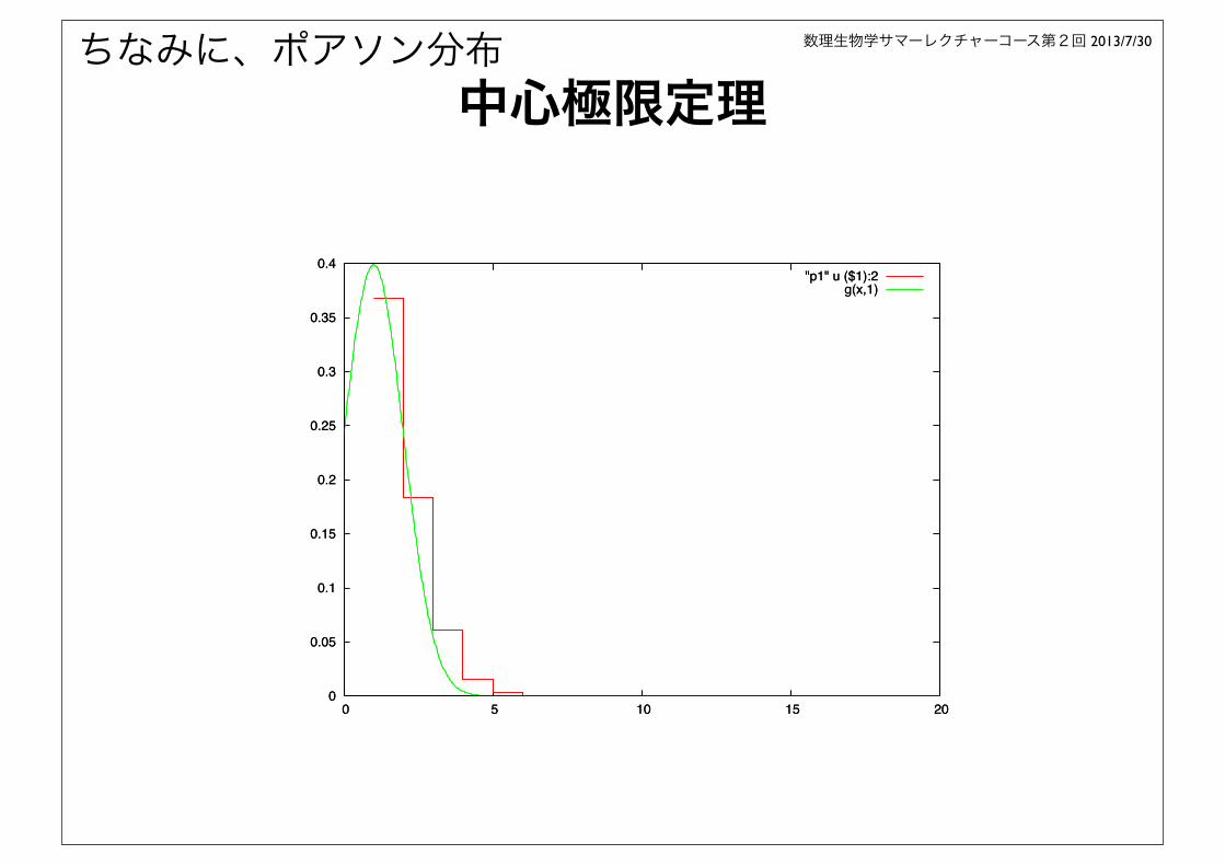
"p1" u ($1):2g(x,1)

0

0.05

0.1

0.15

0.2

0.25

0.3

0.35

0.4

0 5 10 15 20

"p1" u ($1):2g(x,1)

ちなみに、ポアソン分布


中心極限定理

0

0.02

0.04

0.06

0.08

0.1

0.12

0.14

0.16

0.18

0 5 10 15 20

"p5" u ($1):2g(x,5)

0

0.02

0.04

0.06

0.08

0.1

0.12

0.14

0.16

0.18

0 5 10 15 20

"p5" u ($1):2g(x,5)



中心極限定理

0

0.02

0.04

0.06

0.08

0.1

0.12

0.14

0.16

0.18

0 5 10 15 20

"p5" u ($1):2g(x,5)

0

0.02

0.04

0.06

0.08

0.1

0.12

0.14

0.16

0.18

0 5 10 15 20

"p5" u ($1):2g(x,5)



中心極限定理

0

0.005

0.01

0.015

0.02

0.025

0.03

0.035

0.04

60 80 100 120 140

"p100" u ($1):2g(x,100)

0

0.005

0.01

0.015

0.02

0.025

0.03

0.035

0.04

60 80 100 120 140

"p100" u ($1):2g(x,100)



中心極限定理

Xn = x1 + x2 ++ xn

確率変数 xi

ただし、平均 m, 分散 s2 の同じ確率分布に従うとする

n が十分に大きいとき、Xnは平均 µ=nm, 分散σ2=ns2 のガウス分布に近づく

P(Xn ) =12πσ 2

e− (Xn−µ )

2

2σ 2



P(x,t x = 0,t = 0) = 14πDt

e− x2

4Dt

|x(t)� x(0)|2 = 2Dt平均２乗変位

D =�2

2⇥を一定に保って、δとτを小さくする

-3δ -2δ -δ 0 δ 2δ 3δ

t秒後の位置xはガウス分布に従う


1次元ランダムウォークを確率分布で考える

P(i,n) 粒子が離散時刻t=nτに位置x=δiにある確率

P(i,n +1) = P(i,n)+ 12P(i −1,n)+ 1

2P(i +1,n)− 2 1

2P(i,n)

P(x,t +τ ) = P(x,t)+ 12P(x −δ ,t)+ 1

2P(x +δ ,t)− 2 1

2P(x,t)

∂P(x,t)∂t

= δ 2

2τ∂2P(x,t)∂x2

時刻t+τ=(n+1)τの確率を時刻t=nτの確率で表わす

τ,δの十分小さい連続

-3δ -2δ -δ 0 δ 2δ 3δ


• 分子が細胞内にすっかり行き渡るのにかかる時間

tmix=L2/D L : 細胞サイズ(1~10μm)

tmix~10~0.1 sec• L : 胚サイズ(100~1000μm)

tmix~103~105 sec• 粒子が2倍の距離を動こうとすれば4倍、10倍の距離を動こうとすれば100倍の時間がかかる。

細胞中のタンパク分子の拡散定数

水中バクテリア真核細胞ミトコンドリア

細胞外マトリックス

拡散定数D

μm2/sec100程度 10程度 30程度 20~30程度 10~30程度

Xenopus early embryo, (inomata, et al. 2013)


拡散 VS 輸送

! Howard, J., Grill, S. W. & Bois, J. S. Turing's next steps: the mechanochemical basis of morphogenesis. Nature Reviews Molecular Cell Biology 12, 392–398 (2011).

• 輸送 (移流、advection)

- 典型的なモーターのスピード: v=1μm/sec

• 拡散- D=5 μm2/s; D=10 μm2/s; D=50 μm2/s

• 輸送が拡散を追い越すのは!

- D/v~ 5μm; D/v~ 10μm; D/v~50μm

• Péclet number : Pe=vL/D ; L=distance

- Pe << 1: 拡散

- Pe >> 1: 輸送


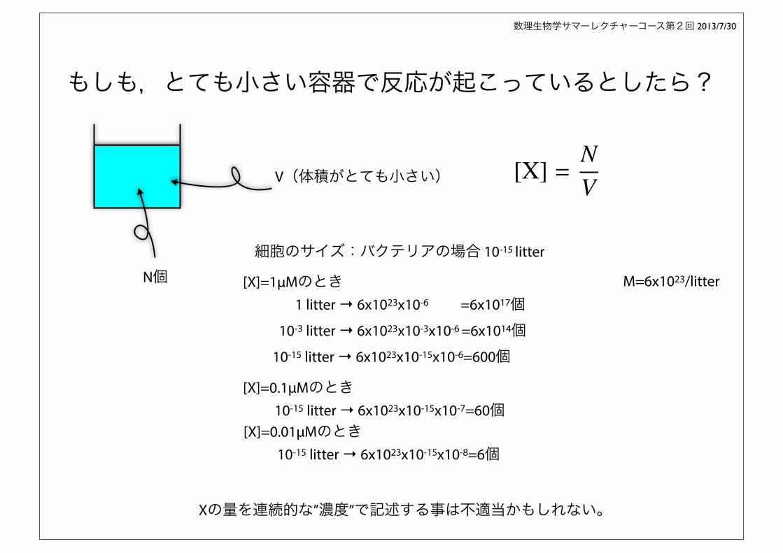
もしも，とても小さい容器で反応が起こっているとしたら？

Xの量を連続的な”濃度”で記述する事は不適当かもしれない。

N個

V（体積がとても小さい） [X] =NV

細胞のサイズ：バクテリアの場合 10-15 litter

[X]=1μMのとき 1 litter → 6x1023x10-6 =6x1017個 10-3 litter → 6x1023x10-3x10-6 =6x1014個10-15 litter → 6x1023x10-15x10-6=600個

[X]=0.1μMのとき10-15 litter → 6x1023x10-15x10-7=60個

10-15 litter → 6x1023x10-15x10-8=6個[X]=0.01μMのとき

M=6x1023/litter


濃度、分子数

体積体積体積体積

1 µm3

(E. coli)100 µm3

(核) 1,000 µm3

()10,000 µm3

(Fibroblast)

10 µM 6,000 600,000 6,000,000 60,000,0001 µM 600 60,000 600,000 6,000,000

100 nM 60 6000 60,000 600,00010 nM 6 600 6000 60,0001 nM 0.6 60 600 6,0001 pM 0.06 0.6 6


細胞中の化学反応は確率であらわされる• 化学反応は確率過程で記述される

• 反応速度定数 k:単位時間、分子あたりの反応確率

• 細胞中の反応確率 (単位時間あたり)

• その結果、濃度は時間的に確率的変動を示すV

E

A B

A+E k�⇥ B+E

200

250

300

350

400

0 100 200 300 400 500 600

濃度はゆらぐ平均値: X

ゆらぎ＝分散: σ2

k

VNANE


濃度の変化は体積に依存する

• 十分大きな体積中の化学反応と、極めて小さい体積中の化学反応は性質が大きく異なる

0 20 40 60 80

100

0 10 20 30 40 50

0 200 400 600 800

1000

0 10 20 30 40 50

0 2000 4000 6000 8000

10000

0 10 20 30 40 50

0 2 4 6 8 10

0 10 20 30 40 50time (s)

V=10

V=100

V=1000

V =∞

確率的

決定論的

ある化学反応を体積を変えながら調べた（ブリュッセレーター）


Single channel recording

216

directly the amplitude of current pulses

(about 3 :aA), and hence the conductance

of a singh: open ion channel, which is com-

monly about 30 pS (i.e. resistance about

33 000 rsegohms; one Sicmen = one

reciproca ohm). This is information that

cannot be obtained by the 'relaxation'

methods though it can be estimated h'om

noise analysis.

( 4 ) O b s e r r a t i o n s o f noise , o r f l~tf tualions,

in the r e s t ~ n s e to agonis~v.

When many ion channels are simulta-

neoasly open, the individual step-like tran.

sitions shown in Fig. 3 may (depending on

the recmding method) not be distinguish-

abl¢~ But they are there, and they give rise

to the nc,isiness of the record in the pres-

ence of a;gonists shown in Fig. 4A and B.

it has already been mentioned above

that the term equilibrium refers only to

arerage be,~¢iour. Imagine that there are

one million ion channels in the experimen-

tal preparation, and that we apply enough

agonist to open, at equilibrium, one chan-

nel in a thousand, Therefore at equilibrium

the~e art', on a r e r a g e . 1000 ion channels

open. But all of the channels are opening

and shutting at random and there is not

exact ly o n e thousand open at any pa~licular

moment. Suppose that an instantaneous

picture c~uld be taken of all the channels at

a partic~lar instant, and the state (open or

shut) of each one noted. This would he

e x ~ l y analogou[ to t~ssing a penny a mil-

lion times and noting, each time whether it

came do~vn "heads" (channel open) or tails

(channel shut). (In this case it is a very

b l a n d penny, that comes down heads o.~iy

once in 1000 throws on average.) Clearly

every time the experiment was repeated

(an instantaneous picture taken, or a mil-

lion tosses performed), we would not

expect to see exac t l y 1000 open channels

(or to get exactly 1000 'heads'). The prob-

lem can be treated by standard coin tossing

theory*, and the expected distribution of

the number of open channels is shown in

Fig. 4C. it has a standard deviation of 31.6

and a roughly Gaussian form. Sowe expect

that 95% of the time, the number of open

channels will be within two standard devia-

tions (i.e. 63.2) of the mean and we, should

therefore say, not that there are 1000

channels open at equilibrium, but that

there are 1000 ± 63.2. These

momeut- to-moment fluctuations (of

about +6 percent in this example) in the

number of open ion channels are quite big

"The binomia!_distribution with N = IO~channels.p = U.OOI ( p m b a b i l i l y Of being open ). gives the mean

numherofopenchannelsasNp = 1000. withstandard det-ialion ¢ ~ = 31.6.

enough to see, and they are what gives rise

to the fluctuations, o, noise, shown in Fig.

4A, B'.

Holy, then. can usehtl informatior

ext;actcd from the rather unpromis

looking signals shown in Fig. 4A, B? T .e

are two things that we can measure, the

amplitude of the noise, and its frequency.

Let us deal with these in turn.

N o i s e amplitud,~,. A conventional way to

measure the amplitude of a fluctuating cur-

rent (e.g. the alternating mains supply) is to

specify the rms ( : ~ t mean square) current,

which i~ ~:othi~: other than the standard

deviatioo of thc cerrent, calculated in the

ordinary way from a series of values of the

current measured at different instants. This

amplitude (standard deviation) is, for

example, clearly bigger for the record in

Fig. 4B than for that in Fig. 4A. The stan-

dasd dc~ia~a~, ~.~[ t i ~ current is a direct

measure of the standard deviation of the

number of open channels which was dis-

cussed above. If wc divide the square of the

observed standard deviation by the mean

current, we obtain an estimate of tbe cur-

rent through a single ion channel (around

3pA) and hence an estimate of the channel

conductance (as long as few channels are

open and a mechanism like equation 4 is

valid*).

N o i s e f r e q u e n c y . It is obvious by eye that

the noise in Fig. 4A contains higher fre-

quencies than that in Fig. 4B. it is therefore

natural to ask whet~ter anything interesting

can be learned from the frequency, and, if

~ , how it can be treasured. The answer to

the first question is yes; we can learn about

the rate at which channels open and shut.

The answer to the ~ccond question follows.

Fig. 5A shows, sehematically, the opening

and shutting of five: individual ion channels

(mean channel lifetime = 5 ms, say), and

Fig. 5B shows tht ~, sum of these records.

"l~e fluctuating record in Fig. 5B is jus,~ the

~ r l of noise illustrated in Fig. 4A,B

(~lhough the individual steps are too small

to be distinguished in the latter). Now a~

tiime zero it is seen that there are four ion

channels open (channels ~umber 1, 2, 4

and 5). If we look a bit later on, say ! .0 ms

later (as marked in Fig. 5B), there are still

~ u r channels open; not surprisingly, they

~ e the same four as were open originally,

I~¢cause, in a short time like 1.0 ms it is

¢!uite likely that none of these channels will

+ Under these conditions Np(I - p) ~- Np so the var- ianc~ o f the total conductance is approximalely y'Np (wl~m y is the conductance o f a single channel) whereas the mean conductance is 1/Np. Their ratio i~ simply 3/.

T I P S - A u g u s t 1981

have shut yet (and that no others will have

opened), it is therefore to be expected that

the current at any given moment will be

very similar to the current at a short time

later if, by short, we mean shor t relative to

the c h a n n e l l i f e t i m e . In other words the cur-

rent at any given moment will be highly

correlated with the current i .0 ms later, If

we calculate an ordinary correlation coef-

ficient between t h e ~ two quantities we

expect that it will be very good, i.e. near

unity, as shown in Fig. 5C. Now consider

what happens if, rather than waiting 1.0

ms, we wait 15 ms (see Fig. 5B). This is

quite long compared with the mean open

¢hem~ • Sins ~ .moan ~ l i f l~me

I I

~[ - L . _ Y ~ r ~ ' L . L Y - - - - ' L Y - ,

I', ~l --L÷+ ~ _ _ _ J -

I t Or t~ ~ ,

~.0 t -$ml l-ISmt

C. D

io 5 f t i m d d ~ m l t e sm~ll~t~.O~l frequency ll'lzJ tiog ~ b t

Fig. 5. Explanation o] the analysis o f the frequency

characteristics o f flucmations in the current elicited (i.e.

in the number orlon channels opened) by agonist~'.

A. Simulatedhehariourof~veindividuMionchannels

(opening is pirated downwards). They are opening and

shutting at random with a mean open li~time o f 5 ms.

B. Sum o f the fire r~'cords shown in A. The total

number open (and hence the tmal currenO shows fluc-

tuations o f the sort that gis'e rise to observations like

those in Fig. 4A,B. An arbiwarily chosen line marks

zero time, and the timex !. 5 and 15 ms later are also

marked with rertical lines.

C. The correlation analysis o fnoise. Two obsert'aCions

separated by I ms are likely to he highly correlated (ns

shown by the dot). The correlation wil' be less when dw

separation is 5 ms, and there is hardly any correlation

with a separation o f 15 ms. The correlation (according

to the mechanism in equation 4) dies out along the

exponential curre shown, with a lime constant o f • =

l / (a + 13'), The time constant is 3 ms in the ¢:'ample

shown; it is less than Ihe mean open channel lifetime (5

ms). because, as is clear from A, the channeh" are open

for a substantial pan o f the lime• (From e~iuation 5 it

follows that the equilil~ium fraction o f shut channels is

0.6. o f open channels is 0.4. ¢i = 1#5 ms) = 200 s -~

and 13' = 133.3 s-~" thus r = i 1333.3 = 3 ms),

D. Presemation o f the same analysis o f noise as a

power spectrum. The ordinate is normally in units o f

AmpllHz, but is giren in arbitrary uni~ here. The

amoum o f noiw is hah'ed (from I00 to 50) at 53.1 H: .

so v = 11(2n ! 53.D = 3 ms. e.mctly ns found in C.

ひとつのチャンネルが開いている時間の分布は指数関数にしたがっている

p(t) ⇥ e��t

1.! Sakmann, B. & Neher, E. Single-channel Recording. (Springer, 2009).


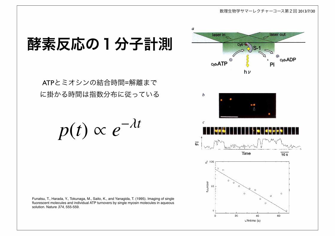
酵素反応の１分子計測

Funatsu, T., Harada, Y., Tokunaga, M., Saito, K., and Yanagida, T. (1995). Imaging of single fluorescent molecules and individual ATP turnovers by single myosin molecules in aqueous solution. Nature 374, 555-559.

ATPとミオシンの結合時間=解離までに掛かる時間は指数分布に従っている

p(t) ⇥ e��t


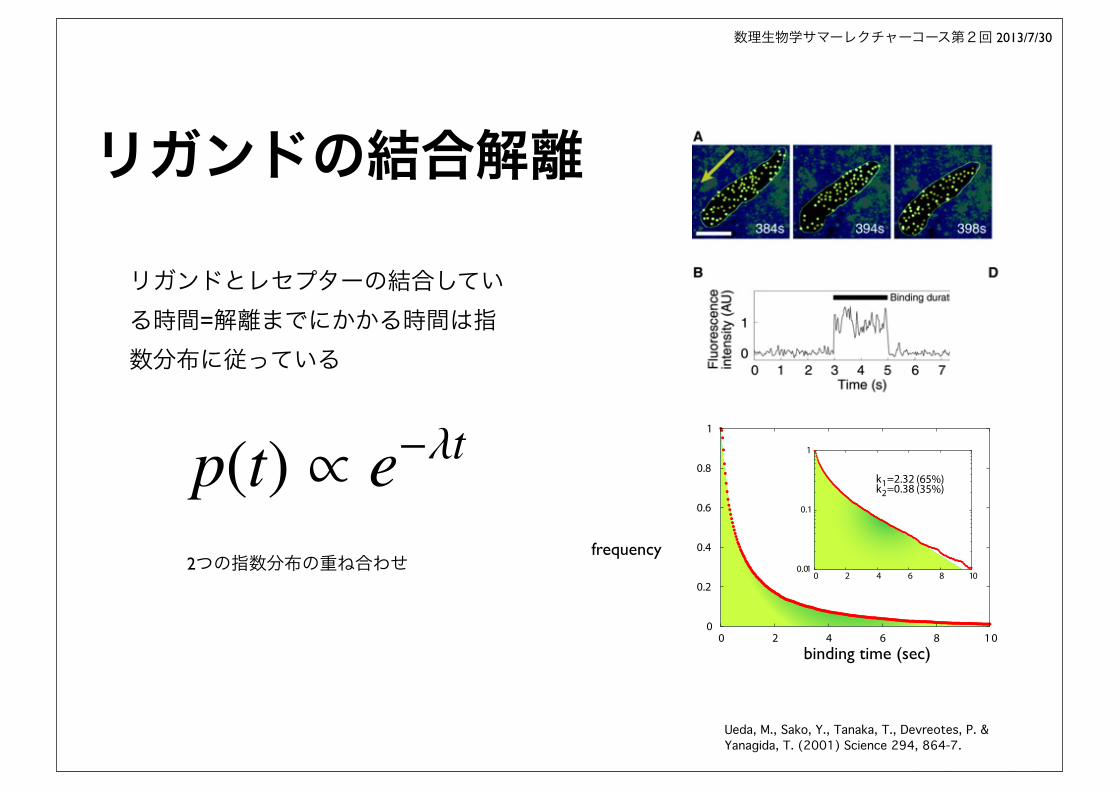
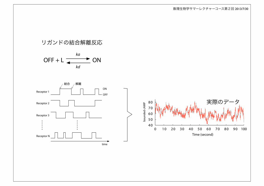
リガンドの結合解離

Ueda, M., Sako, Y., Tanaka, T., Devreotes, P. & Yanagida, T. (2001) Science 294, 864-7.

2つの指数分布の重ね合わせ

binding time (sec)

binding time (sec)

frequency

リガンドとレセプターの結合している時間=解離までにかかる時間は指数分布に従っている

p(t) ⇥ e��t


ON

OFFReceptor 1

結合解離

time

4 0

5 0

6 0

7 0

8 0

0 1 0 2 0 3 0 4 0 5 0 6 0 7 0 8 0 9 0 100Time (second)

boun

ded

cAM

P 実際のデータ

ON

OFF

time

Receptor 1

Receptor 2

Receptor 3

Receptor N

結合解離

OFF + L ONka

kd

リガンドの結合解離反応


１次反応を考えよう：分解反応

d[X]dt= ��[X]

[X]t = [X]0e��t

X��⇥

0.0 0.5 1.0 1.5 2.0

0.2

0.4

0.6

0.8

1.0

[X]t

t


１つの分子の反応を考えるたとえば，，

t=0

いつ反応するか？

X��⇥ いつ消滅するか？例1

Xk�⇥ Y いつＹに変化するか？例2


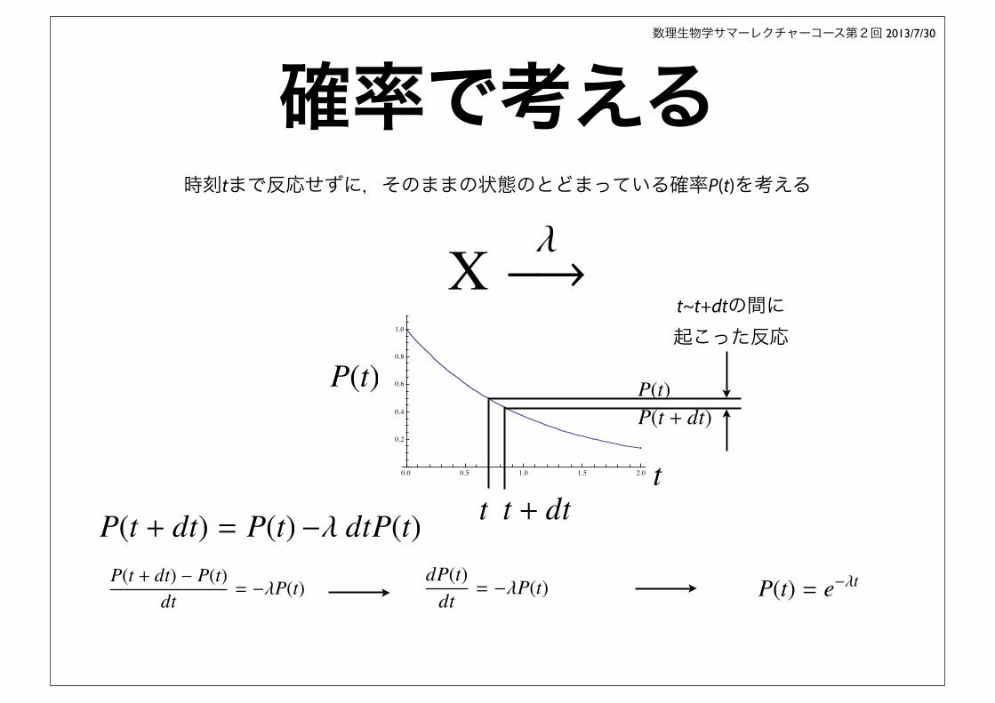
確率で考える時刻tまで反応せずに，そのままの状態のとどまっている確率P(t)を考える

0.0 0.5 1.0 1.5 2.0

0.2

0.4

0.6

0.8

1.0

t

P(t)

t t + dt

t~t+dtの間に起こった反応

P(t + dt) = P(t)

X��⇥

�� dtP(t)P(t + dt) � P(t)

dt= ��P(t)

dP(t)dt= ��P(t) P(t) = e��t

P(t)P(t + dt)


0 = t0 < t1 < t2 << tn−1 < tn = T

x(t1), x(t2 ),, x(tn )

観測時刻

ti = i × Δt

観測値

x =01⎧⎨⎩

(off)

(on)

216

directly the amplitude of current pulses

(about 3 :aA), and hence the conductance

of a singh: open ion channel, which is com-

monly about 30 pS (i.e. resistance about

33 000 rsegohms; one Sicmen = one

reciproca ohm). This is information that

cannot be obtained by the 'relaxation'

methods though it can be estimated h'om

noise analysis.

( 4 ) O b s e r r a t i o n s o f noise , o r f l~tf tualions,

in the r e s t ~ n s e to agonis~v.

When many ion channels are simulta-

neoasly open, the individual step-like tran.

sitions shown in Fig. 3 may (depending on

the recmding method) not be distinguish-

abl¢~ But they are there, and they give rise

to the nc,isiness of the record in the pres-

ence of a;gonists shown in Fig. 4A and B.

it has already been mentioned above

that the term equilibrium refers only to

arerage be,~¢iour. Imagine that there are

one million ion channels in the experimen-

tal preparation, and that we apply enough

agonist to open, at equilibrium, one chan-

nel in a thousand, Therefore at equilibrium

the~e art', on a r e r a g e . 1000 ion channels

open. But all of the channels are opening

and shutting at random and there is not

exact ly o n e thousand open at any pa~licular

moment. Suppose that an instantaneous

picture c~uld be taken of all the channels at

a partic~lar instant, and the state (open or

shut) of each one noted. This would he

e x ~ l y analogou[ to t~ssing a penny a mil-

lion times and noting, each time whether it

came do~vn "heads" (channel open) or tails

(channel shut). (In this case it is a very

b l a n d penny, that comes down heads o.~iy

once in 1000 throws on average.) Clearly

every time the experiment was repeated

(an instantaneous picture taken, or a mil-

lion tosses performed), we would not

expect to see exac t l y 1000 open channels

(or to get exactly 1000 'heads'). The prob-

lem can be treated by standard coin tossing

theory*, and the expected distribution of

the number of open channels is shown in

Fig. 4C. it has a standard deviation of 31.6

and a roughly Gaussian form. Sowe expect

that 95% of the time, the number of open

channels will be within two standard devia-

tions (i.e. 63.2) of the mean and we, should

therefore say, not that there are 1000

channels open at equilibrium, but that

there are 1000 ± 63.2. These

momeut- to-moment fluctuations (of

about +6 percent in this example) in the

number of open ion channels are quite big

"The binomia!_distribution with N = IO~channels.p = U.OOI ( p m b a b i l i l y Of being open ). gives the mean

numherofopenchannelsasNp = 1000. withstandard det-ialion ¢ ~ = 31.6.

enough to see, and they are what gives rise

to the fluctuations, o, noise, shown in Fig.

4A, B'.

Holy, then. can usehtl informatior

ext;actcd from the rather unpromis

looking signals shown in Fig. 4A, B? T .e

are two things that we can measure, the

amplitude of the noise, and its frequency.

Let us deal with these in turn.

N o i s e amplitud,~,. A conventional way to

measure the amplitude of a fluctuating cur-

rent (e.g. the alternating mains supply) is to

specify the rms ( : ~ t mean square) current,

which i~ ~:othi~: other than the standard

deviatioo of thc cerrent, calculated in the

ordinary way from a series of values of the

current measured at different instants. This

amplitude (standard deviation) is, for

example, clearly bigger for the record in

Fig. 4B than for that in Fig. 4A. The stan-

dasd dc~ia~a~, ~.~[ t i ~ current is a direct

measure of the standard deviation of the

number of open channels which was dis-

cussed above. If wc divide the square of the

observed standard deviation by the mean

current, we obtain an estimate of tbe cur-

rent through a single ion channel (around

3pA) and hence an estimate of the channel

conductance (as long as few channels are

open and a mechanism like equation 4 is

valid*).

N o i s e f r e q u e n c y . It is obvious by eye that

the noise in Fig. 4A contains higher fre-

quencies than that in Fig. 4B. it is therefore

natural to ask whet~ter anything interesting

can be learned from the frequency, and, if

~ , how it can be treasured. The answer to

the first question is yes; we can learn about

the rate at which channels open and shut.

The answer to the ~ccond question follows.

Fig. 5A shows, sehematically, the opening

and shutting of five: individual ion channels

(mean channel lifetime = 5 ms, say), and

Fig. 5B shows tht ~, sum of these records.

"l~e fluctuating record in Fig. 5B is jus,~ the

~ r l of noise illustrated in Fig. 4A,B

(~lhough the individual steps are too small

to be distinguished in the latter). Now a~

tiime zero it is seen that there are four ion

channels open (channels ~umber 1, 2, 4

and 5). If we look a bit later on, say ! .0 ms

later (as marked in Fig. 5B), there are still

~ u r channels open; not surprisingly, they

~ e the same four as were open originally,

I~¢cause, in a short time like 1.0 ms it is

¢!uite likely that none of these channels will

+ Under these conditions Np(I - p) ~- Np so the var- ianc~ o f the total conductance is approximalely y'Np (wl~m y is the conductance o f a single channel) whereas the mean conductance is 1/Np. Their ratio i~ simply 3/.

T I P S - A u g u s t 1981

have shut yet (and that no others will have

opened), it is therefore to be expected that

the current at any given moment will be

very similar to the current at a short time

later if, by short, we mean shor t relative to

the c h a n n e l l i f e t i m e . In other words the cur-

rent at any given moment will be highly

correlated with the current i .0 ms later, If

we calculate an ordinary correlation coef-

ficient between t h e ~ two quantities we

expect that it will be very good, i.e. near

unity, as shown in Fig. 5C. Now consider

what happens if, rather than waiting 1.0

ms, we wait 15 ms (see Fig. 5B). This is

quite long compared with the mean open

¢hem~ • Sins ~ .moan ~ l i f l~me

I I

~[ - L . _ Y ~ r ~ ' L . L Y - - - - ' L Y - ,

I', ~l --L÷+ ~ _ _ _ J -

I t Or t~ ~ ,

~.0 t -$ml l-ISmt

C. D

io 5 f t i m d d ~ m l t e sm~ll~t~.O~l frequency ll'lzJ tiog ~ b t

Fig. 5. Explanation o] the analysis o f the frequency

characteristics o f flucmations in the current elicited (i.e.

in the number orlon channels opened) by agonist~'.

A. Simulatedhehariourof~veindividuMionchannels

(opening is pirated downwards). They are opening and

shutting at random with a mean open li~time o f 5 ms.

B. Sum o f the fire r~'cords shown in A. The total

number open (and hence the tmal currenO shows fluc-

tuations o f the sort that gis'e rise to observations like

those in Fig. 4A,B. An arbiwarily chosen line marks

zero time, and the timex !. 5 and 15 ms later are also

marked with rertical lines.

C. The correlation analysis o fnoise. Two obsert'aCions

separated by I ms are likely to he highly correlated (ns

shown by the dot). The correlation wil' be less when dw

separation is 5 ms, and there is hardly any correlation

with a separation o f 15 ms. The correlation (according

to the mechanism in equation 4) dies out along the

exponential curre shown, with a lime constant o f • =

l / (a + 13'), The time constant is 3 ms in the ¢:'ample

shown; it is less than Ihe mean open channel lifetime (5

ms). because, as is clear from A, the channeh" are open

for a substantial pan o f the lime• (From e~iuation 5 it

follows that the equilil~ium fraction o f shut channels is

0.6. o f open channels is 0.4. ¢i = 1#5 ms) = 200 s -~

and 13' = 133.3 s-~" thus r = i 1333.3 = 3 ms),

D. Presemation o f the same analysis o f noise as a

power spectrum. The ordinate is normally in units o f

AmpllHz, but is giren in arbitrary uni~ here. The

amoum o f noiw is hah'ed (from I00 to 50) at 53.1 H: .

so v = 11(2n ! 53.D = 3 ms. e.mctly ns found in C.

確率変数

確率過程


P(x0 )

P(x1, x0 )

P(xn ,, x1, x0 )

経路の確率

遷移確率 P(x1 x0 ) =P(x1, x0 )P(x0 )

P(xn ,, x1 x0 ) =

P(xn ,, x1, x0 )P(x0 )

P(xn xn−1,, x1, x0 ) =

P(xn ,, x1, x0 )P(xn−1,, x1, x0 )


P(x2, x1 x0 ) = P(x2 x1)P(x1 x0 )

P(x2, x1, x0 ) = P(x2 x1)P(x1 x0 )P(x0 )

P(xn xn−1,, x1, x0 ) = P(xn xn−1)

マルコフ過程 (Markov process)

P(x2 x0 ) = P(x2 x1)P(x1 x0 )x1∑

(Chapman-Kolmogorov equation)


0.0 0.5 1.0 1.5 2.0

0.2

0.4

0.6

0.8

1.0

t

時刻tにXである確率p(t) = e−λt q(t) = 1− p(t) = 1− e−λt

時刻tにYである確率

X λ⎯ →⎯ Y

P(Y,t X,0) = 1− e−λtP(X,t X,0) = e−λt

P(Y,2t;X,t X,0) = (1− e−λt )e−λt = P(Y,2t X,t)P(X,t X,0)P(Y,2t;Y,t X,0) = 1− e−λt = P(Y,2t Y,t)P(Y,t X,0)

P(Y,2t X,0) = 1− e−λ (2t ) (Chapman-Kolmogorov equation)


• 位置Xはマルコフ過程ではない

• なぜなら、時刻tの位置Xは、t-1, t-2,,に依存する

• 位置Xと速度Vはマルコフ過程になる

��

��

��

��

��

��

��

�� i

��

��

��

��

��

�� i

� ��

��

�

��

��

��

� ��

i

A

B濃度の増加

濃度の増加

-1 0 1-2 2

C

D

・・・・・・・・

Fig.3

E

通常の運動

q>pp0 適応

濃度の減少

適応濃度減少時の運動濃度増加時の運動

濃度の減少

方向転換の確率

v -vv


X λ0⎯ →⎯ X' λ1⎯ →⎯ Y

直接観測できない中間状態X’がある

X λ⎯ →⎯ Y

2 4 6 8 10

0.6

0.7

0.8

0.9

1.0

時刻tにX or X’である確率時刻tにYでない確率

2 4 6 8 10

0.05

0.10

0.15

0.20

0.25

Yになるまでの時間tの確率分布関数

p(t) = e−λ0t − e−λ1t

λ1 − λ0

1−0

t

∫ p(s)ds


P(Y,t X,0) =0

t

∫ p(s)dsP(X,t X,0) = 1−

0

t

∫ p(s)ds

P(Y,2t;X,t X,0) = 1−0

t

∫ p(s)ds( ) 0

t

∫ p(s)dsP(Y,2t;Y,t X,0) = 1−

0

t

∫ p(s)ds

P(Y,2t;X,t X,0)+ P(Y,2t;Y,t X,0) =0

t

∫ p(s)ds( )2≠ P(Y,2t X,0)

p(t) = e−λ0t − e−λ1t

λ1 − λ0Yになるまでの時間tの確率分布関数

XとX’は区別ができないとする。それらをまとめてXと書く


生成，分解反応/ birth-and-death process

k�⇥ X, X��⇥

転写，翻訳分解例えば，遺伝子発現

N個ある確率をP(N,t)とおく。

P(N) = (k/�)N

N! e�k� ポアソン分布

N = k�

平均： ⇥2 = N2 � N2= k�分散：

定常分布� dPdt = 0

⇥

dP(N, t)dt

= k�P(N � 1, t) � P(N, t)

⇥+ ��(N + 1)P(N + 1, t) � NP(N, t)

⇥

生成反応分解反応

N � �2


組織中の細胞の多様性はどのように維持されているか

1.! Klein, A. M. & Simons, B. D. Universal patterns of stem cell fate in cycling adult tissues. Development 138, 3103–3111 (2011).


Single-proliferative compartment model of IFE maintenance

With this background, we turn now to the consideration of the novel single-proliferative

compartment model introduced in the main text. When formulated as a non-equilibrium

process, the model is described by the set of non-equilibrium rate equations

A��!

8>>>><

>>>>:

A + A Prob. r

A + B Prob. 1� 2r

B + B Prob. r

B��! C,

(5)

where, as usual, A denote EPCs, B represent post-mitotic cells in the basal layer, and C

specify the suprabasal layer cells. To maintain the total basal layer cell population, we

must impose the condition that � = ⇢1�⇢�, i.e. the net rate at which post-mitotic cells are

generated in the basal layer, ⇢�, is compensated by the rate at which they are removed,

(1 � ⇢)�. By neglecting processes involving the shedding of cells from the surface of the

epidermis, the model is restricted to the consideration of the total clone size distribution

at appropriately short time scales. However, if we focus only on the clone size distribution

associated with those cells which occupy the basal layer, the model can be applied up to

arbitrary time scales. For this case, the transfer process must be replaced by one in which

B type cells are lost from the distribution at a rate �, i.e. B��! ;. In either case, the

time evolution associated with (5) can be cast in the form of a Master equation. Defining

PnA,nB(t) as the probability of finding nA type A cells and nB type B cells in a given clone

after some time t, the basal layer cell probability distribution evolves according to the Master

equation

@tPnA,nB = r� [(nA � 1)PnA�1,nB � nAPnA,nB ] + r�[(nA + 1)PnA+1,nB�2 � nAPnA,nB ]

+(1� 2r)�[nAPnA,nB�1 � nAPnA,nB ] + �[(nB + 1)PnA,nB+1 � nBPnA,nB ],

6

pn (t) ~τtexp −n τ

t⎛⎝⎜

⎞⎠⎟

十分に時間が経てば

τ = ρrλ

Γ = ρ1− ρ

λただし、

ρは、Aの割合

スケーリング則

パラメータフィッティングの結果

比較的簡単なマルコフモデルが実験結果をよく説明する

実験とモデルの比較

1.! Clayton, E. et al. A single type of progenitor cell maintains normal epidermis. Nature 446, 185–189 (2007).2.! Klein, A. M., Doupé, D. P., Jones, P. H. & Simons, B. D. Kinetics of cell division in epidermal maintenance. Phys Rev E 76, 021910 (2007).

まとめ/キーワード• 確率変数

• 確率過程

• ランダムウォーク、拡散

• 平均二乗変位 (mean

square displacement, MSD)

• 中心極限定理、ガウス分布、正規分布

• 指数分布

• 経路の確率

• 遷移確率

• マルコフ過程、非マルコフ過程

• 生成消滅過程, birth-and-

death process


• ハーケン「Synergetics, 共同現象の数理」東海大学出版

• W. フェラー「確率論とその応用」紀伊国屋書店

• ハワードバーグ「生物学におけるランダムウォーク」法政大学出版局

• 寺本英「ランダムな現象の数学」、吉岡書店

• Van Kampen, “Stochastic Processes in Physics and Chemistry”, North Holland

Technology

2013 第2回数理生物学サマーレクチャーコース@RIKEN CDB 2013/7/30