1

I am not OEM savvy ! The notes sections in this presentation also provide links to some of my blog posts

2

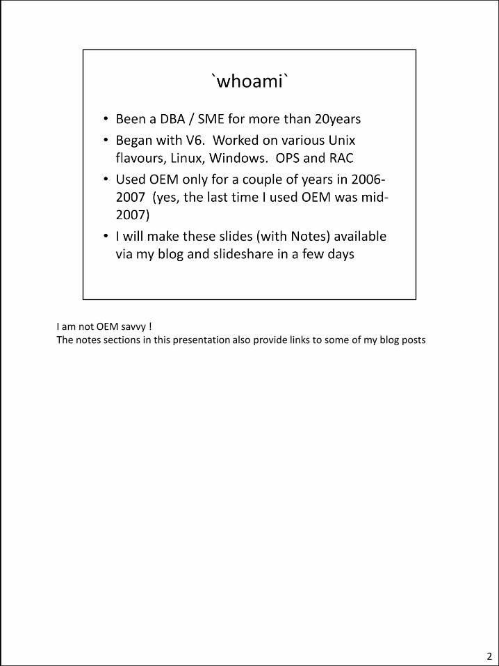
Only a small set of privileges are really required. Also look at the OEM_MONITOR role that has ANALYZE ANY , SELECT ANY, SELECT ANY DICTIONARY and ADVISOR privileges, none of which I use (although ADVISOR may be useful). For a short note on the difference between SELECT ANY DICTIONARY and SELECT_CATALOG_ROLE see http://hemantoracledba.blogspot.com/2014/02/the-difference-between-select-any.html SELECT ANY can be useful if you need to query data (e.g. To identify distribution patterns and skew) in a schema – but the owner might prefer to grant you SELECT privileges on only a subset of tables --- that sort of requirement comes in handy when doing Performance Tuning, which is outside of the scope of this presentation. If you plan to use PLSQL (e.g. to schedule jobs to collect this monitoring information), you *will* need direct privileges on the underlying views. For example, on V_$SESSION, V_$SQL etc. There are many System Privileges and Object level privileges that can be granted to Junior DBAs, Performance Analysts etc without having to grant the DBA role.

3

These are the privileges I need. I don’t use ADVISORs but do use AWR.

4

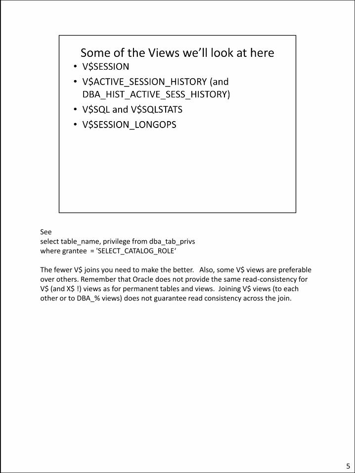
See select table_name, privilege from dba_tab_privs where grantee = 'SELECT_CATALOG_ROLE‘ The fewer V$ joins you need to make the better. Also, some V$ views are preferable over others. Remember that Oracle does not provide the same read-consistency for V$ (and X$ !) views as for permanent tables and views. Joining V$ views (to each other or to DBA_% views) does not guarantee read consistency across the join.

5

Columns that have been retrieved from V$SESSION_WAIT are now available in V$SESSION. V$SQL preferred over V$SQLAREA because the latter does an aggregation (across all Child Cursors). When I join V$SESSION to V$SQL, I join on both SQL_ID and CHILD_NUMBER. Similarly, I prefer V$SEGSTAT over V$SEGMENT_STATISTICS – the former is faster. If you don’t have the Diagnostic Pack for V$ASH, you could sample V$SESSION quickly with custom code.

6

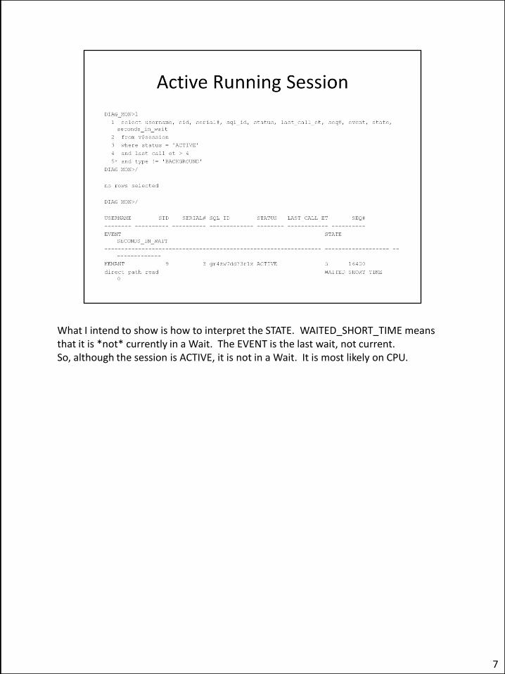
What I intend to show is how to interpret the STATE. WAITED_SHORT_TIME means that it is *not* currently in a Wait. The EVENT is the last wait, not current. So, although the session is ACTIVE, it is not in a Wait. It is most likely on CPU.

7

Note the change to the WAITING on “free buffer waits”. That *is* the CURRENT Wait as at the time of the snapshot. (Similarly, the “db file scattered read” wait after that). So, at the bottom of this slide, the session’s current SQL has been active for 55 seconds and is currently in a multiblock read wait.

8

Note how the *current* wait status can keep changing. Have you noted SEQ# incrementing ? That indicates that the Wait Events *are* changing.

9

Recursive SQLs called by DBMS_STATS (or any PLSQL procedure) are are at a depth level below. The top level is dep=0, the succeeding levels are 1 and beyond.

10

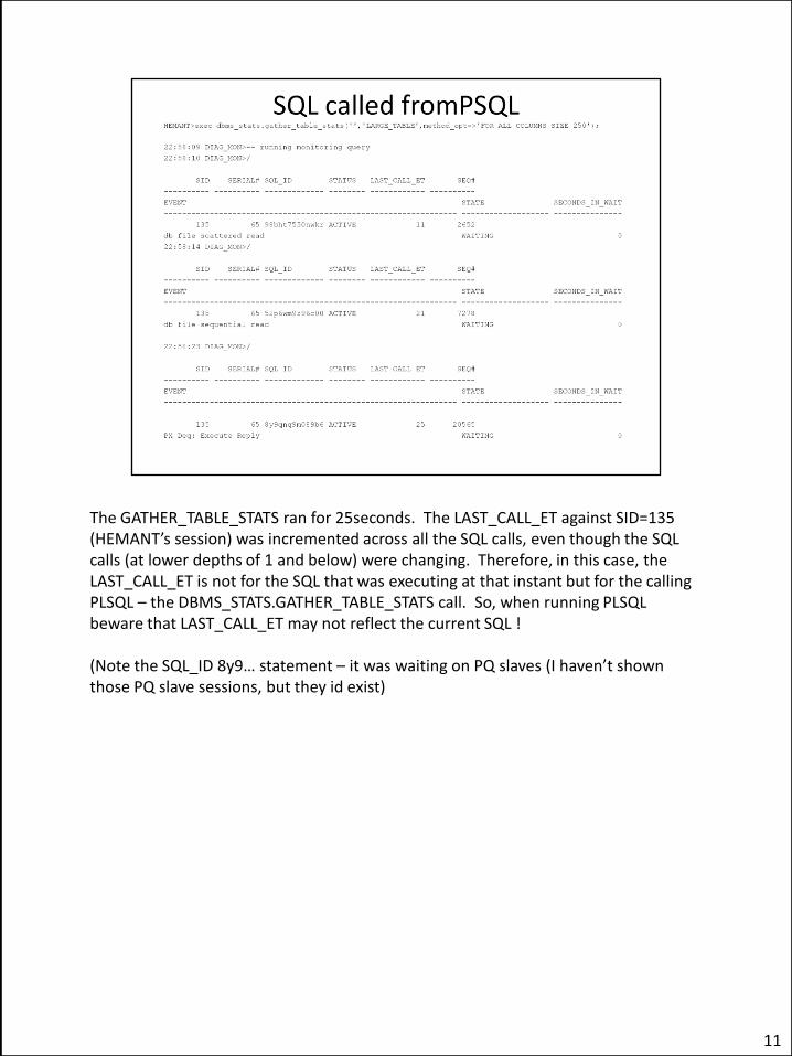
The GATHER_TABLE_STATS ran for 25seconds. The LAST_CALL_ET against SID=135 (HEMANT’s session) was incremented across all the SQL calls, even though the SQL calls (at lower depths of 1 and below) were changing. Therefore, in this case, the LAST_CALL_ET is not for the SQL that was executing at that instant but for the calling PLSQL – the DBMS_STATS.GATHER_TABLE_STATS call. So, when running PLSQL beware that LAST_CALL_ET may not reflect the current SQL ! (Note the SQL_ID 8y9… statement – it was waiting on PQ slaves (I haven’t shown those PQ slave sessions, but they id exist)

11

This slide is not necessarily part of this presentation. It is just to demonstrate that a PLSQL (the DBMS_STATS.GATHER_TABLE_STATS in this case) can call multiple SQLs, at different recursive depth levels. (From dep=0 to dep=4 in this case). So, when you are monitoring V$SQL_ID in V$SESSION, you might get a statement that is at a much lowe depth.

12

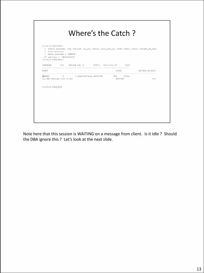
Note here that this session is WAITING on a message from client. Is it Idle ? Should the DBA ignore this ? Let’s look at the next slide.

13

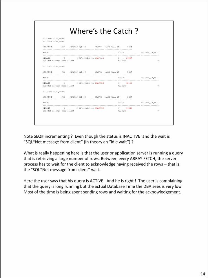
Note SEQ# incrementing ? Even though the status is INACTIVE and the wait is “SQL*Net message from client” (In theory an “idle wait”) ? What is really happening here is that the user or application server is running a query that is retrieving a large number of rows. Between every ARRAY FETCH, the server process has to wait for the client to acknowledge having received the rows – that is the “SQL*Net message from client” wait. Here the user says that his query is ACTIVE. And he is right ! The user is complaining that the query is long running but the actual Database Time the DBA sees is very low. Most of the time is being spent sending rows and waiting for the acknowledgement.

14

Note the last wait at SEQ#34020. It is now 4 seconds ! Let’s see the next slide.

15

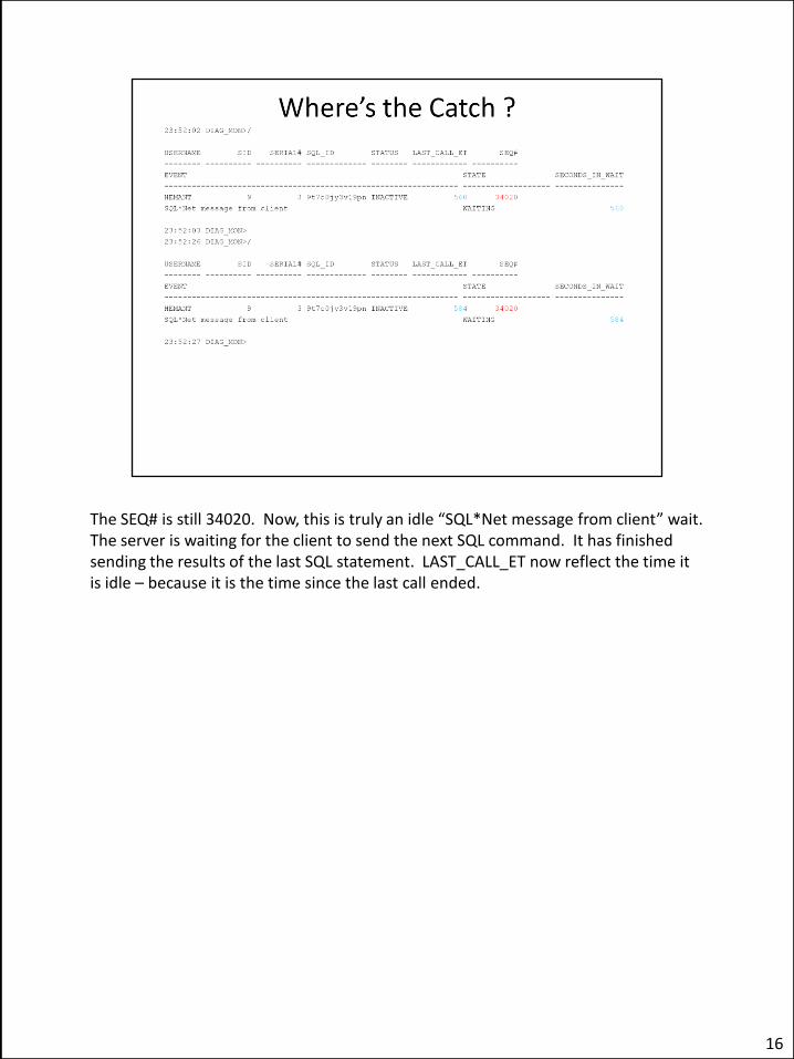
The SEQ# is still 34020. Now, this is truly an idle “SQL*Net message from client” wait. The server is waiting for the client to send the next SQL command. It has finished sending the results of the last SQL statement. LAST_CALL_ET now reflect the time it is idle – because it is the time since the last call ended.

16

I don’t have SELECT privilege on the underlying table in the HEMANT schema. Yet, I can get the execution plan. I don’t need the SELECT privilege on the underlying table(s) or the SELECT ANY privilege or the DBA role to be able to do this.

17

Because I have SELECT_CATALOG_ROLE, I can query the underlying statistics.

18

I can create AWR snapshots because I have EXECUTE on DBMS_WORKLOAD_REPOSITORY. I don’t need to be granted the DBA role. I can use SQLDeveloper 4.0.1 to generate an AWR report without logging in to the server as “oracle”

19

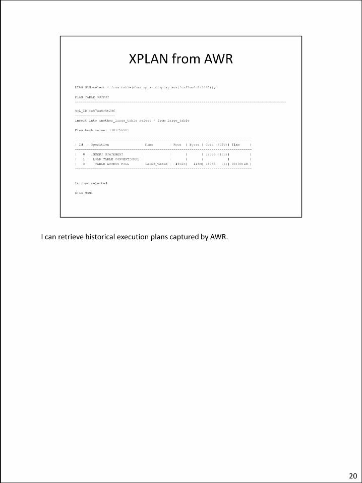
I can retrieve historical execution plans captured by AWR.

20

Too many people on the Internet think that this view shows how long the query is running and how long it is expected to continue. It shows the *current operation* not the whole SQL. An SQL Query can consist of multiple operations. Even Parallel Query can run different block ranges using multiple passes, each pass is a separate operation (and each PQ slave a separate session, so a separate row in this view).

21

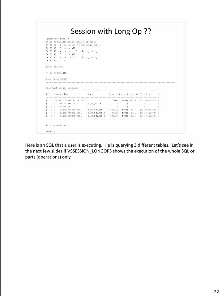
Here is an SQL that a user is executing. He is querying 3 different tables. Let’s see in the next few slides if V$SESSION_LONGOPS shows the execution of the whole SQL or parts (operations) only.

22

Look a the SQL_PLAN_LINE_ID. This extract from V$SESSION_LONGOPS is for only one step in the Execution Plan. The SOFAR, ELAPSED_SECONDS and TIME_REMAINING are for that one operation – reading table HEMANT.LARGE_TABLE_2 The estimated time for this operation is 15+26 = 41seconds.

23

The operation has been running for 32seconds and still needs another 30seconds (i.e. 62seconds in all, not the 42seconds estimated earlier). Oracle is continously revising the estimated.

24

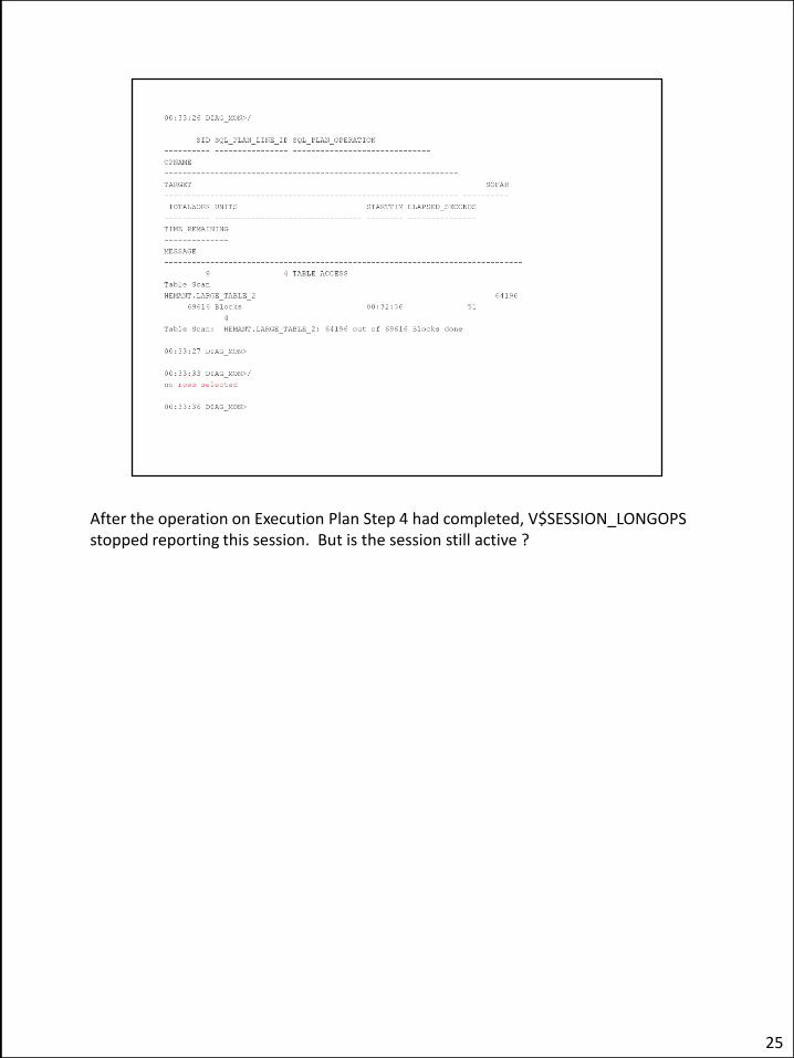
After the operation on Execution Plan Step 4 had completed, V$SESSION_LONGOPS stopped reporting this session. But is the session still active ?

25

The session is still active. It is now on Execution Plan Step 5 – the next table in the SQL operation. A database server process can do only 1 thing at a time. If it is querying LARGE_TABLE_2, it cannot also be querying LARGE_TABLE_3 at the same time. The retrieval of rows from LARGE_TABLE_3 is sequentially done later ! (Parallel Query is a way around the fundamental rule that a process can be doing only one thing at any time – PQ spawns multiple processes to do multiple things (reads from different block ranges and/or partitions of the same table) concurrently)

26

In the previous slide, the estimate for the read from HEMANT.LARGE_TABLE_3 was (12 + 51) 63seconds. It is now 53seconds.

27

The estimate has now changed to 65seconds. For another example of misreading V$SESSION_LONGOPS on a DML that does a Full Table Scan see http://hemantoracledba.blogspot.com/2009/01/when-not-to-use-vsessionlongops.html

28

I had mentioned earlier that a query that sends multiple rows to a client / application server sends the rows in batches – based on the ARRAY Size. Search my blog for examples of ARRAYSIZE (and LINESIZE and PAGESIZE if using an SQLPlus Client) {I have a few different blogposts on this} I have shown earlier how the “SQL*Net message from client” isn’t always an Idle Event. The presence of this wait event, with increasing SEQ# can indicate array fetches.

29

Note the two queries retrieved the same number of rows. The elapsed time reported by the client would have included the “SQL*Net message wait from client” wait event on the server for the multiple round trips. The FETCHES count indicates the round-trips. The first SQL used an ARRAYSIZE of 100, the second was doing a Row-By-Row FETCH. (The extra 1 FETCH is always present when you run an SQL, you’ll even see it in the trace file as a FETCH with 0 rows executed first).

30

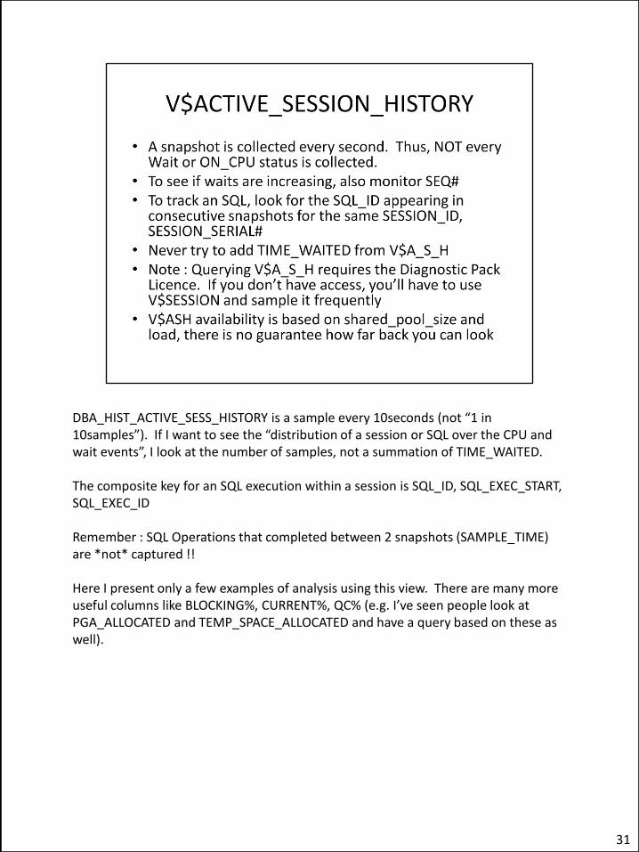
DBA_HIST_ACTIVE_SESS_HISTORY is a sample every 10seconds (not “1 in 10samples”). If I want to see the “distribution of a session or SQL over the CPU and wait events”, I look at the number of samples, not a summation of TIME_WAITED. The composite key for an SQL execution within a session is SQL_ID, SQL_EXEC_START, SQL_EXEC_ID Remember : SQL Operations that completed between 2 snapshots (SAMPLE_TIME) are *not* captured !! Here I present only a few examples of analysis using this view. There are many more useful columns like BLOCKING%, CURRENT%, QC% (e.g. I’ve seen people look at PGA_ALLOCATED and TEMP_SPACE_ALLOCATED and have a query based on these as well).

31

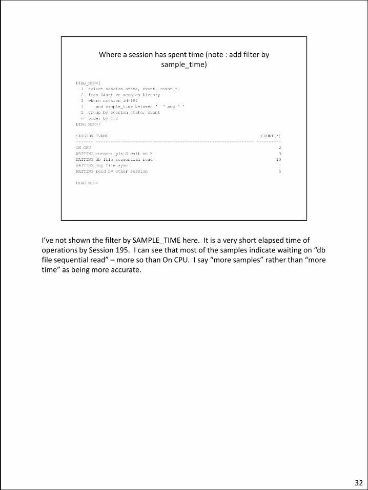
I’ve not shown the filter by SAMPLE_TIME here. It is a very short elapsed time of operations by Session 195. I can see that most of the samples indicate waiting on “db file sequential read” – more so than On CPU. I say “more samples” rather than “more time” as being more accurate.

32

Here, the session ran multiple SQL statements. I can see the distribution of CPU and Wait Events amongst the different SQL.

33

Here, I filter for a MODULE, rather than a SESSION (I’ve not shown the filter by SAMPLE_TIME). (Note : “log file sync” wait may not always show which the SQL_ID was that was waiting on the Event).

34

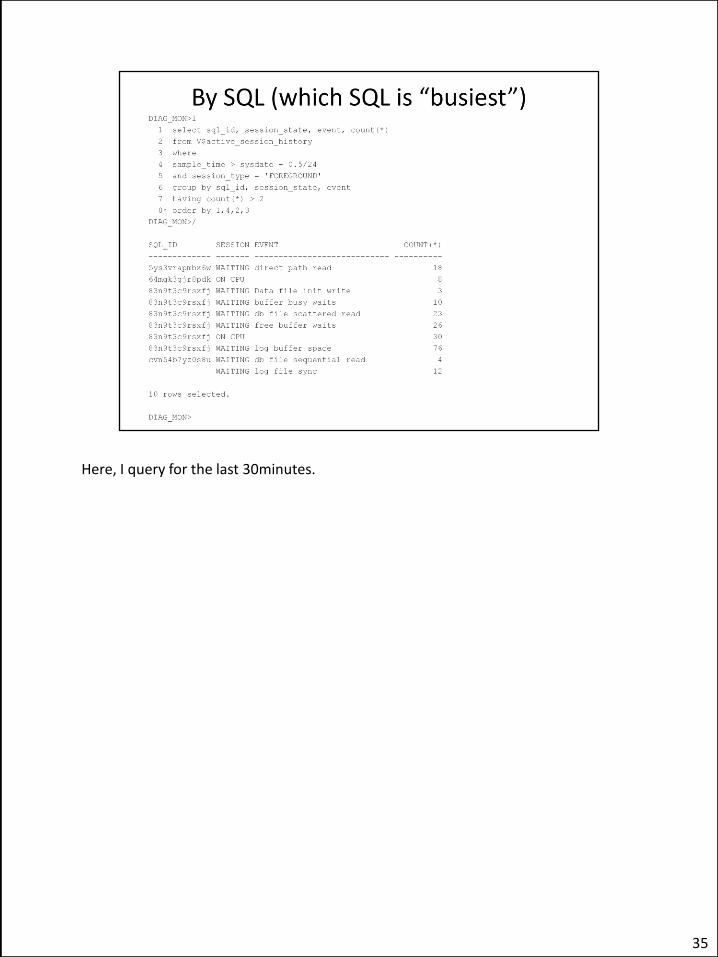
Here, I query for the last 30minutes.

35

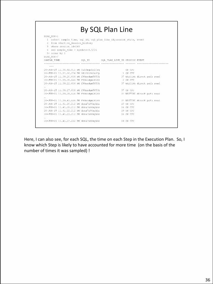
Here, I can also see, for each SQL, the time on each Step in the Execution Plan. So, I know which Step is likely to have accounted for more time (on the basis of the number of times it was sampled) !

36

Distribution of CPU Usage (this is an approximation because it is based on a sample taken every 10seconds only !) This is based on number of occurrences in samples, not actual time spent on CPU. But we could approximate the one for the other.

37

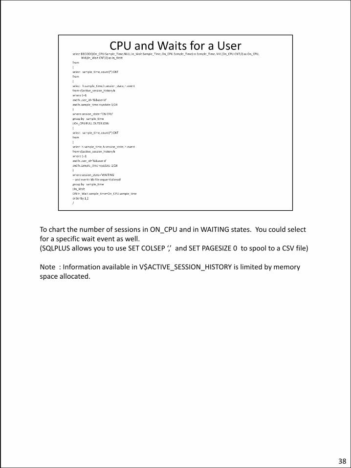
To chart the number of sessions in ON_CPU and in WAITING states. You could select for a specific wait event as well. (SQLPLUS allows you to use SET COLSEP ‘,’ and SET PAGESIZE 0 to spool to a CSV file) Note : Information available in V$ACTIVE_SESSION_HISTORY is limited by memory space allocated.

38

This is another way to represent Active Sessions.

39

Extract previous occurrences of an SQL from AWR history

40

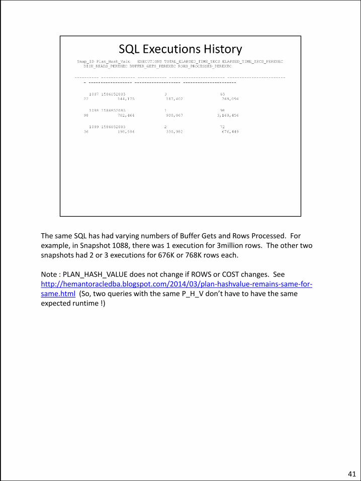
The same SQL has had varying numbers of Buffer Gets and Rows Processed. For example, in Snapshot 1088, there was 1 execution for 3million rows. The other two snapshots had 2 or 3 executions for 676K or 768K rows each. Note : PLAN_HASH_VALUE does not change if ROWS or COST changes. See http://hemantoracledba.blogspot.com/2014/03/plan-hashvalue-remains-same-for-same.html (So, two queries with the same P_H_V don’t have to have the same expected runtime !)

41

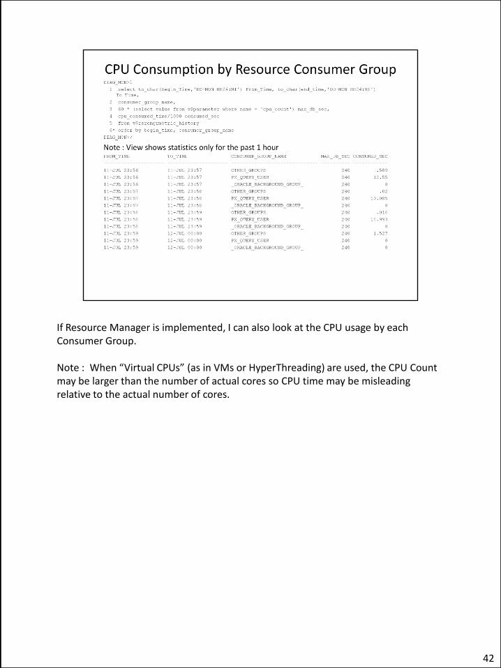
If Resource Manager is implemented, I can also look at the CPU usage by each Consumer Group. Note : When “Virtual CPUs” (as in VMs or HyperThreading) are used, the CPU Count may be larger than the number of actual cores so CPU time may be misleading relative to the actual number of cores.

42

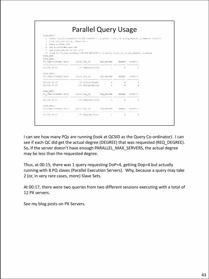
I can see how many PQs are running (look at QCSID as the Query Co-ordinator). I can see if each QC did get the actual degree (DEGREE) that was requested (REQ_DEGREE). So, if the server doesn’t have enough PARALLEL_MAX_SERVERS, the actual degree may be less than the requested degree. Thus, at 00:15, there was 1 query requesting DoP=4, getting Dop=4 but actually running with 8 PQ slaves (Parallel Execution Servers). Why, because a query may take 2 (or, in very rare cases, more) Slave Sets. At 00:17, there were two queries from two different sessions executing with a total of 12 PX servers. See my blog posts on PX Servers.

43

Very important : UNDO RECORDS is NOT the same (or same size) as Table Rows or Index Entries.

44

You can check the distribution of transactions across different Undo Segments. Remember : The SQL_ID is only the current SQL. A transaction can consist of multiple DMLs, including SELECT queries ! The current SQL may be a SELECT but the transaction may have 1 or 100 or 1000 INSERT/UPDATE/DELETE statements before this. The transaction started rolling back after 00:28:15. (Also note that Current SQL_ID is not always available)

45

I can compare CPU time with Wait Events time. I can identify the top Wait. I can filter for statistics or waits that I am particularly interested in.

46

I can select which Statistics and which Wait Events are of interest to me for this particular database instance. (Different application profiles may have different interesting Statistics and Waits !) This gives me a “Profile” view of the Instance

47

Note : Time_Waited and CPU used are both in Centi-seconds. Here I can compare CPU time with time on major wait events. I can also look at major statistics that I can filter.

48