Contents

1 From Microscopic to Macroscopic Behavior 11.1 Introduction . . . . . . . . . . . . . . . . . . . . . . . . . . . . . . . . . . . . . . . . 11.2 Some qualitative observations . . . . . . . . . . . . . . . . . . . . . . . . . . . . . . 31.3 Doing work . . . . . . . . . . . . . . . . . . . . . . . . . . . . . . . . . . . . . . . . 41.4 Quality of energy . . . . . . . . . . . . . . . . . . . . . . . . . . . . . . . . . . . . . 51.5 Some simple simulations . . . . . . . . . . . . . . . . . . . . . . . . . . . . . . . . . 61.6 Work, heating, and the first law of thermodynamics . . . . . . . . . . . . . . . . . 141.7 Measuring the pressure and temperature . . . . . . . . . . . . . . . . . . . . . . . . 151.8 *The fundamental need for a statistical approach . . . . . . . . . . . . . . . . . . . 181.9 *Time and ensemble averages . . . . . . . . . . . . . . . . . . . . . . . . . . . . . . 201.10 *Models of matter . . . . . . . . . . . . . . . . . . . . . . . . . . . . . . . . . . . . 20

1.10.1 The ideal gas . . . . . . . . . . . . . . . . . . . . . . . . . . . . . . . . . . . 211.10.2 Interparticle potentials . . . . . . . . . . . . . . . . . . . . . . . . . . . . . . 211.10.3 Lattice models . . . . . . . . . . . . . . . . . . . . . . . . . . . . . . . . . . 21

1.11 Importance of simulations . . . . . . . . . . . . . . . . . . . . . . . . . . . . . . . . 221.12 Summary . . . . . . . . . . . . . . . . . . . . . . . . . . . . . . . . . . . . . . . . . 23Additional Problems . . . . . . . . . . . . . . . . . . . . . . . . . . . . . . . . . . . . . . 24Suggestions for Further Reading . . . . . . . . . . . . . . . . . . . . . . . . . . . . . . . 25

2 Thermodynamic Concepts 262.1 Introduction . . . . . . . . . . . . . . . . . . . . . . . . . . . . . . . . . . . . . . . . 262.2 The system . . . . . . . . . . . . . . . . . . . . . . . . . . . . . . . . . . . . . . . . 272.3 Thermodynamic Equilibrium . . . . . . . . . . . . . . . . . . . . . . . . . . . . . . 272.4 Temperature . . . . . . . . . . . . . . . . . . . . . . . . . . . . . . . . . . . . . . . 282.5 Pressure Equation of State . . . . . . . . . . . . . . . . . . . . . . . . . . . . . . . 312.6 Some Thermodynamic Processes . . . . . . . . . . . . . . . . . . . . . . . . . . . . 332.7 Work . . . . . . . . . . . . . . . . . . . . . . . . . . . . . . . . . . . . . . . . . . . . 34

i

CONTENTS ii

2.8 The First Law of Thermodynamics . . . . . . . . . . . . . . . . . . . . . . . . . . . 372.9 Energy Equation of State . . . . . . . . . . . . . . . . . . . . . . . . . . . . . . . . 392.10 Heat Capacities and Enthalpy . . . . . . . . . . . . . . . . . . . . . . . . . . . . . . 402.11 Adiabatic Processes . . . . . . . . . . . . . . . . . . . . . . . . . . . . . . . . . . . 432.12 The Second Law of Thermodynamics . . . . . . . . . . . . . . . . . . . . . . . . . . 472.13 The Thermodynamic Temperature . . . . . . . . . . . . . . . . . . . . . . . . . . . 492.14 The Second Law and Heat Engines . . . . . . . . . . . . . . . . . . . . . . . . . . . 512.15 Entropy Changes . . . . . . . . . . . . . . . . . . . . . . . . . . . . . . . . . . . . . 562.16 Equivalence of Thermodynamic and Ideal Gas Scale Temperatures . . . . . . . . . 602.17 The Thermodynamic Pressure . . . . . . . . . . . . . . . . . . . . . . . . . . . . . . 612.18 The Fundamental Thermodynamic Relation . . . . . . . . . . . . . . . . . . . . . . 622.19 The Entropy of an Ideal Gas . . . . . . . . . . . . . . . . . . . . . . . . . . . . . . 632.20 The Third Law of Thermodynamics . . . . . . . . . . . . . . . . . . . . . . . . . . 642.21 Free Energies . . . . . . . . . . . . . . . . . . . . . . . . . . . . . . . . . . . . . . . 65Appendix 2B: Mathematics of Thermodynamics . . . . . . . . . . . . . . . . . . . . . . 70Additional Problems . . . . . . . . . . . . . . . . . . . . . . . . . . . . . . . . . . . . . . 73Suggestions for Further Reading . . . . . . . . . . . . . . . . . . . . . . . . . . . . . . . 80

3 Concepts of Probability 823.1 Probability in everyday life . . . . . . . . . . . . . . . . . . . . . . . . . . . . . . . 823.2 The rules of probability . . . . . . . . . . . . . . . . . . . . . . . . . . . . . . . . . 843.3 Mean values . . . . . . . . . . . . . . . . . . . . . . . . . . . . . . . . . . . . . . . . 893.4 The meaning of probability . . . . . . . . . . . . . . . . . . . . . . . . . . . . . . . 91

3.4.1 Information and uncertainty . . . . . . . . . . . . . . . . . . . . . . . . . . . 933.4.2 *Bayesian inference . . . . . . . . . . . . . . . . . . . . . . . . . . . . . . . . 97

3.5 Bernoulli processes and the binomial distribution . . . . . . . . . . . . . . . . . . . 993.6 Continuous probability distributions . . . . . . . . . . . . . . . . . . . . . . . . . . 1093.7 The Gaussian distribution as a limit of the binomial distribution . . . . . . . . . . 1113.8 The central limit theorem or why is thermodynamics possible? . . . . . . . . . . . 1133.9 The Poisson distribution and should you fly in airplanes? . . . . . . . . . . . . . . 1163.10 *Tra!c flow and the exponential distribution . . . . . . . . . . . . . . . . . . . . . 1173.11 *Are all probability distributions Gaussian? . . . . . . . . . . . . . . . . . . . . . . 119Additional Problems . . . . . . . . . . . . . . . . . . . . . . . . . . . . . . . . . . . . . . 128Suggestions for Further Reading . . . . . . . . . . . . . . . . . . . . . . . . . . . . . . . 136

CONTENTS iii

4 Statistical Mechanics 1384.1 Introduction . . . . . . . . . . . . . . . . . . . . . . . . . . . . . . . . . . . . . . . . 1384.2 A simple example of a thermal interaction . . . . . . . . . . . . . . . . . . . . . . . 1404.3 Counting microstates . . . . . . . . . . . . . . . . . . . . . . . . . . . . . . . . . . . 150

4.3.1 Noninteracting spins . . . . . . . . . . . . . . . . . . . . . . . . . . . . . . . 1504.3.2 *One-dimensional Ising model . . . . . . . . . . . . . . . . . . . . . . . . . . 1504.3.3 A particle in a one-dimensional box . . . . . . . . . . . . . . . . . . . . . . 1514.3.4 One-dimensional harmonic oscillator . . . . . . . . . . . . . . . . . . . . . . 1534.3.5 One particle in a two-dimensional box . . . . . . . . . . . . . . . . . . . . . 1544.3.6 One particle in a three-dimensional box . . . . . . . . . . . . . . . . . . . . 1564.3.7 Two noninteracting identical particles and the semiclassical limit . . . . . . 156

4.4 The number of states of N noninteracting particles: Semiclassical limit . . . . . . . 1584.5 The microcanonical ensemble (fixed E, V, and N) . . . . . . . . . . . . . . . . . . . 1604.6 Systems in contact with a heat bath: The canonical ensemble (fixed T, V, and N) 1654.7 Connection between statistical mechanics and thermodynamics . . . . . . . . . . . 1704.8 Simple applications of the canonical ensemble . . . . . . . . . . . . . . . . . . . . . 1724.9 A simple thermometer . . . . . . . . . . . . . . . . . . . . . . . . . . . . . . . . . . 1754.10 Simulations of the microcanonical ensemble . . . . . . . . . . . . . . . . . . . . . . 1774.11 Simulations of the canonical ensemble . . . . . . . . . . . . . . . . . . . . . . . . . 1784.12 Grand canonical ensemble (fixed T, V, and µ) . . . . . . . . . . . . . . . . . . . . . 1794.13 Entropy and disorder . . . . . . . . . . . . . . . . . . . . . . . . . . . . . . . . . . . 181Appendix 4A: The Volume of a Hypersphere . . . . . . . . . . . . . . . . . . . . . . . . 183Appendix 4B: Fluctuations in the Canonical Ensemble . . . . . . . . . . . . . . . . . . . 184Additional Problems . . . . . . . . . . . . . . . . . . . . . . . . . . . . . . . . . . . . . . 185Suggestions for Further Reading . . . . . . . . . . . . . . . . . . . . . . . . . . . . . . . 188

5 Magnetic Systems 1905.1 Paramagnetism . . . . . . . . . . . . . . . . . . . . . . . . . . . . . . . . . . . . . . 1905.2 Thermodynamics of magnetism . . . . . . . . . . . . . . . . . . . . . . . . . . . . . 1945.3 The Ising model . . . . . . . . . . . . . . . . . . . . . . . . . . . . . . . . . . . . . 1945.4 The Ising Chain . . . . . . . . . . . . . . . . . . . . . . . . . . . . . . . . . . . . . 195

5.4.1 Exact enumeration . . . . . . . . . . . . . . . . . . . . . . . . . . . . . . . . 1955.4.2 !Spin-spin correlation function . . . . . . . . . . . . . . . . . . . . . . . . . 1995.4.3 Simulations of the Ising chain . . . . . . . . . . . . . . . . . . . . . . . . . . 2015.4.4 *Transfer matrix . . . . . . . . . . . . . . . . . . . . . . . . . . . . . . . . . 2035.4.5 Absence of a phase transition in one dimension . . . . . . . . . . . . . . . . 205

5.5 The Two-Dimensional Ising Model . . . . . . . . . . . . . . . . . . . . . . . . . . . 206

CONTENTS iv

5.5.1 Onsager solution . . . . . . . . . . . . . . . . . . . . . . . . . . . . . . . . . 2065.5.2 Computer simulation of the two-dimensional Ising model . . . . . . . . . . 211

5.6 Mean-Field Theory . . . . . . . . . . . . . . . . . . . . . . . . . . . . . . . . . . . . 2115.7 *Infinite-range interactions . . . . . . . . . . . . . . . . . . . . . . . . . . . . . . . 216Additional Problems . . . . . . . . . . . . . . . . . . . . . . . . . . . . . . . . . . . . . . 224Suggestions for Further Reading . . . . . . . . . . . . . . . . . . . . . . . . . . . . . . . 228

6 Noninteracting Particle Systems 2306.1 Introduction . . . . . . . . . . . . . . . . . . . . . . . . . . . . . . . . . . . . . . . . 2306.2 The Classical Ideal Gas . . . . . . . . . . . . . . . . . . . . . . . . . . . . . . . . . 2306.3 Classical Systems and the Equipartition Theorem . . . . . . . . . . . . . . . . . . . 2386.4 Maxwell Velocity Distribution . . . . . . . . . . . . . . . . . . . . . . . . . . . . . . 2406.5 Occupation Numbers and Bose and Fermi Statistics . . . . . . . . . . . . . . . . . 2436.6 Distribution Functions of Ideal Bose and Fermi Gases . . . . . . . . . . . . . . . . 2456.7 Single Particle Density of States . . . . . . . . . . . . . . . . . . . . . . . . . . . . 247

6.7.1 Photons . . . . . . . . . . . . . . . . . . . . . . . . . . . . . . . . . . . . . . 2496.7.2 Electrons . . . . . . . . . . . . . . . . . . . . . . . . . . . . . . . . . . . . . 250

6.8 The Equation of State for a Noninteracting Classical Gas . . . . . . . . . . . . . . 2526.9 Black Body Radiation . . . . . . . . . . . . . . . . . . . . . . . . . . . . . . . . . . 2556.10 Noninteracting Fermi Gas . . . . . . . . . . . . . . . . . . . . . . . . . . . . . . . . 259

6.10.1 Ground-state properties . . . . . . . . . . . . . . . . . . . . . . . . . . . . . 2606.10.2 Low temperature thermodynamic properties . . . . . . . . . . . . . . . . . . 263

6.11 Bose Condensation . . . . . . . . . . . . . . . . . . . . . . . . . . . . . . . . . . . . 2676.12 The Heat Capacity of a Crystalline Solid . . . . . . . . . . . . . . . . . . . . . . . . 272

6.12.1 The Einstein model . . . . . . . . . . . . . . . . . . . . . . . . . . . . . . . 2726.12.2 Debye theory . . . . . . . . . . . . . . . . . . . . . . . . . . . . . . . . . . . 273

Appendix 6A: Low Temperature Expansion . . . . . . . . . . . . . . . . . . . . . . . . . 275Suggestions for Further Reading . . . . . . . . . . . . . . . . . . . . . . . . . . . . . . . 286

7 Thermodynamic Relations and Processes 2887.1 Introduction . . . . . . . . . . . . . . . . . . . . . . . . . . . . . . . . . . . . . . . . 2887.2 Maxwell Relations . . . . . . . . . . . . . . . . . . . . . . . . . . . . . . . . . . . . 2907.3 Applications of the Maxwell Relations . . . . . . . . . . . . . . . . . . . . . . . . . 291

7.3.1 Internal energy of an ideal gas . . . . . . . . . . . . . . . . . . . . . . . . . 2917.3.2 Relation between the specific heats . . . . . . . . . . . . . . . . . . . . . . . 291

7.4 Applications to Irreversible Processes . . . . . . . . . . . . . . . . . . . . . . . . . . 2927.4.1 The Joule or free expansion process . . . . . . . . . . . . . . . . . . . . . . 293

CONTENTS v

7.4.2 Joule-Thomson process . . . . . . . . . . . . . . . . . . . . . . . . . . . . . 2947.5 Equilibrium Between Phases . . . . . . . . . . . . . . . . . . . . . . . . . . . . . . . 296

7.5.1 Equilibrium conditions . . . . . . . . . . . . . . . . . . . . . . . . . . . . . . 2977.5.2 Clausius-Clapeyron equation . . . . . . . . . . . . . . . . . . . . . . . . . . 2987.5.3 Simple phase diagrams . . . . . . . . . . . . . . . . . . . . . . . . . . . . . . 3007.5.4 Pressure dependence of the melting point . . . . . . . . . . . . . . . . . . . 3017.5.5 Pressure dependence of the boiling point . . . . . . . . . . . . . . . . . . . . 3027.5.6 The vapor pressure curve . . . . . . . . . . . . . . . . . . . . . . . . . . . . 302

7.6 Vocabulary . . . . . . . . . . . . . . . . . . . . . . . . . . . . . . . . . . . . . . . . 303Additional Problems . . . . . . . . . . . . . . . . . . . . . . . . . . . . . . . . . . . . . . 303Suggestions for Further Reading . . . . . . . . . . . . . . . . . . . . . . . . . . . . . . . 305

8 Classical Gases and Liquids 3068.1 Introduction . . . . . . . . . . . . . . . . . . . . . . . . . . . . . . . . . . . . . . . . 3068.2 The Free Energy of an Interacting System . . . . . . . . . . . . . . . . . . . . . . . 3068.3 Second Virial Coe!cient . . . . . . . . . . . . . . . . . . . . . . . . . . . . . . . . . 3098.4 Cumulant Expansion . . . . . . . . . . . . . . . . . . . . . . . . . . . . . . . . . . . 3138.5 High Temperature Expansion . . . . . . . . . . . . . . . . . . . . . . . . . . . . . . 3158.6 Density Expansion . . . . . . . . . . . . . . . . . . . . . . . . . . . . . . . . . . . . 3198.7 Radial Distribution Function . . . . . . . . . . . . . . . . . . . . . . . . . . . . . . 323

8.7.1 Relation of thermodynamic functions to g(r) . . . . . . . . . . . . . . . . . 3268.7.2 Relation of g(r) to static structure function S(k) . . . . . . . . . . . . . . . 3278.7.3 Variable number of particles . . . . . . . . . . . . . . . . . . . . . . . . . . . 3298.7.4 Density expansion of g(r) . . . . . . . . . . . . . . . . . . . . . . . . . . . . 331

8.8 Computer Simulation of Liquids . . . . . . . . . . . . . . . . . . . . . . . . . . . . 3318.9 Perturbation Theory of Liquids . . . . . . . . . . . . . . . . . . . . . . . . . . . . . 333

8.9.1 The van der Waals Equation . . . . . . . . . . . . . . . . . . . . . . . . . . 3348.9.2 Chandler-Weeks-Andersen theory . . . . . . . . . . . . . . . . . . . . . . . . 335

8.10 *The Ornstein-Zernicke Equation . . . . . . . . . . . . . . . . . . . . . . . . . . . . 3368.11 *Integral Equations for g(r) . . . . . . . . . . . . . . . . . . . . . . . . . . . . . . . 3378.12 *Coulomb Interactions . . . . . . . . . . . . . . . . . . . . . . . . . . . . . . . . . . 339

8.12.1 Debye-Huckel Theory . . . . . . . . . . . . . . . . . . . . . . . . . . . . . . 3408.12.2 Linearized Debye-Huckel approximation . . . . . . . . . . . . . . . . . . . . 3418.12.3 Diagrammatic Expansion for Charged Particles . . . . . . . . . . . . . . . . 342

8.13 Vocabulary . . . . . . . . . . . . . . . . . . . . . . . . . . . . . . . . . . . . . . . . 343Appendix 8A: The third virial coe!cient for hard spheres . . . . . . . . . . . . . . . . . 3448.14 Additional Problems . . . . . . . . . . . . . . . . . . . . . . . . . . . . . . . . . . . 347

CONTENTS vi

9 Critical Phenomena 3509.1 A Geometrical Phase Transition . . . . . . . . . . . . . . . . . . . . . . . . . . . . 3509.2 Renormalization Group for Percolation . . . . . . . . . . . . . . . . . . . . . . . . . 3549.3 The Liquid-Gas Transition . . . . . . . . . . . . . . . . . . . . . . . . . . . . . . . . 3589.4 Bethe Approximation . . . . . . . . . . . . . . . . . . . . . . . . . . . . . . . . . . 3619.5 Landau Theory of Phase Transitions . . . . . . . . . . . . . . . . . . . . . . . . . . 3639.6 Other Models of Magnetism . . . . . . . . . . . . . . . . . . . . . . . . . . . . . . . 3699.7 Universality and Scaling Relations . . . . . . . . . . . . . . . . . . . . . . . . . . . 3719.8 The Renormalization Group and the 1D Ising Model . . . . . . . . . . . . . . . . . 3729.9 The Renormalization Group and the Two-Dimensional Ising Model . . . . . . . . . 3769.10 Vocabulary . . . . . . . . . . . . . . . . . . . . . . . . . . . . . . . . . . . . . . . . 3829.11 Additional Problems . . . . . . . . . . . . . . . . . . . . . . . . . . . . . . . . . . . 382Suggestions for Further Reading . . . . . . . . . . . . . . . . . . . . . . . . . . . . . . . 385

10 Introduction to Many-Body Perturbation Theory 38710.1 Introduction . . . . . . . . . . . . . . . . . . . . . . . . . . . . . . . . . . . . . . . . 38710.2 Occupation Number Representation . . . . . . . . . . . . . . . . . . . . . . . . . . 38810.3 Operators in the Second Quantization Formalism . . . . . . . . . . . . . . . . . . . 38910.4 Weakly Interacting Bose Gas . . . . . . . . . . . . . . . . . . . . . . . . . . . . . . 390

A Useful Formulae 397A.1 Physical constants . . . . . . . . . . . . . . . . . . . . . . . . . . . . . . . . . . . . 397A.2 SI derived units . . . . . . . . . . . . . . . . . . . . . . . . . . . . . . . . . . . . . . 397A.3 Conversion factors . . . . . . . . . . . . . . . . . . . . . . . . . . . . . . . . . . . . 398A.4 Mathematical Formulae . . . . . . . . . . . . . . . . . . . . . . . . . . . . . . . . . 398A.5 Approximations . . . . . . . . . . . . . . . . . . . . . . . . . . . . . . . . . . . . . . 398A.6 Euler-Maclaurin formula . . . . . . . . . . . . . . . . . . . . . . . . . . . . . . . . . 399A.7 Gaussian Integrals . . . . . . . . . . . . . . . . . . . . . . . . . . . . . . . . . . . . 399A.8 Stirling’s formula . . . . . . . . . . . . . . . . . . . . . . . . . . . . . . . . . . . . . 400A.9 Constants . . . . . . . . . . . . . . . . . . . . . . . . . . . . . . . . . . . . . . . . . 401A.10 Probability distributions . . . . . . . . . . . . . . . . . . . . . . . . . . . . . . . . . 402A.11 Fermi integrals . . . . . . . . . . . . . . . . . . . . . . . . . . . . . . . . . . . . . . 402A.12 Bose integrals . . . . . . . . . . . . . . . . . . . . . . . . . . . . . . . . . . . . . . . 403

Chapter 1

From Microscopic to MacroscopicBehavior

c©2006 by Harvey Gould and Jan Tobochnik28 August 2006

The goal of this introductory chapter is to explore the fundamental differences between micro-scopic and macroscopic systems and the connections between classical mechanics and statisticalmechanics. We note that bouncing balls come to rest and hot objects cool, and discuss how thebehavior of macroscopic objects is related to the behavior of their microscopic constituents. Com-puter simulations will be introduced to demonstrate the relation of microscopic and macroscopicbehavior.

1.1 Introduction

Our goal is to understand the properties of macroscopic systems, that is, systems of many elec-trons, atoms, molecules, photons, or other constituents. Examples of familiar macroscopic objectsinclude systems such as the air in your room, a glass of water, a copper coin, and a rubber band(examples of a gas, liquid, solid, and polymer, respectively). Less familiar macroscopic systemsare superconductors, cell membranes, the brain, and the galaxies.

We will find that the type of questions we ask about macroscopic systems differ in importantways from the questions we ask about microscopic systems. An example of a question about amicroscopic system is “What is the shape of the trajectory of the Earth in the solar system?”In contrast, have you ever wondered about the trajectory of a particular molecule in the air ofyour room? Why not? Is it relevant that these molecules are not visible to the eye? Examples ofquestions that we might ask about macroscopic systems include the following:

1. How does the pressure of a gas depend on the temperature and the volume of its container?

2. How does a refrigerator work? What is its maximum efficiency?

1

CHAPTER 1. FROM MICROSCOPIC TO MACROSCOPIC BEHAVIOR 2

3. How much energy do we need to add to a kettle of water to change it to steam?

4. Why are the properties of water different from those of steam, even though water and steamconsist of the same type of molecules?

5. How are the molecules arranged in a liquid?

6. How and why does water freeze into a particular crystalline structure?

7. Why does iron lose its magnetism above a certain temperature?

8. Why does helium condense into a superfluid phase at very low temperatures? Why do somematerials exhibit zero resistance to electrical current at sufficiently low temperatures?

9. How fast does a river current have to be before its flow changes from laminar to turbulent?

10. What will the weather be tomorrow?

The above questions can be roughly classified into three groups. Questions 1–3 are concernedwith macroscopic properties such as pressure, volume, and temperature and questions related toheating and work. These questions are relevant to thermodynamics which provides a frameworkfor relating the macroscopic properties of a system to one another. Thermodynamics is concernedonly with macroscopic quantities and ignores the microscopic variables that characterize individualmolecules. For example, we will find that understanding the maximum efficiency of a refrigeratordoes not require a knowledge of the particular liquid used as the coolant. Many of the applicationsof thermodynamics are to thermal engines, for example, the internal combustion engine and thesteam turbine.

Questions 4–8 relate to understanding the behavior of macroscopic systems starting from theatomic nature of matter. For example, we know that water consists of molecules of hydrogenand oxygen. We also know that the laws of classical and quantum mechanics determine thebehavior of molecules at the microscopic level. The goal of statistical mechanics is to begin withthe microscopic laws of physics that govern the behavior of the constituents of the system anddeduce the properties of the system as a whole. Statistical mechanics is the bridge between themicroscopic and macroscopic worlds.

Thermodynamics and statistical mechanics assume that the macroscopic properties of thesystem do not change with time on the average. Thermodynamics describes the change of amacroscopic system from one equilibrium state to another. Questions 9 and 10 concern macro-scopic phenomena that change with time. Related areas are nonequilibrium thermodynamics andfluid mechanics from the macroscopic point of view and nonequilibrium statistical mechanics fromthe microscopic point of view. Although there has been progress in our understanding of nonequi-librium phenomena such as turbulent flow and hurricanes, our understanding of nonequilibriumphenomena is much less advanced than our understanding of equilibrium systems. Because un-derstanding the properties of macroscopic systems that are independent of time is easier, we willfocus our attention on equilibrium systems and consider questions such as those in Questions 1–8.

CHAPTER 1. FROM MICROSCOPIC TO MACROSCOPIC BEHAVIOR 3

1.2 Some qualitative observations

We begin our discussion of macroscopic systems by considering a glass of water. We know that ifwe place a glass of hot water into a cool room, the hot water cools until its temperature equalsthat of the room. This simple observation illustrates two important properties associated withmacroscopic systems – the importance of temperature and the arrow of time. Temperature isfamiliar because it is associated with the physiological sensation of hot and cold and is importantin our everyday experience. We will find that temperature is a subtle concept.

The direction or arrow of time is an even more subtle concept. Have you ever observed a glassof water at room temperature spontaneously become hotter? Why not? What other phenomenaexhibit a direction of time? Time has a direction as is expressed by the nursery rhyme:

Humpty Dumpty sat on a wallHumpty Dumpty had a great fallAll the king’s horses and all the king’s menCouldn’t put Humpty Dumpty back together again.

Is there a a direction of time for a single particle? Newton’s second law for a single particle,F = dp/dt, implies that the motion of particles is time reversal invariant, that is, Newton’s secondlaw looks the same if the time t is replaced by −t and the momentum p by −p. There is nodirection of time at the microscopic level. Yet if we drop a basketball onto a floor, we know that itwill bounce and eventually come to rest. Nobody has observed a ball at rest spontaneously beginto bounce, and then bounce higher and higher. So based on simple everyday observations, we canconclude that the behavior of macroscopic bodies and single particles is very different.

Unlike generations of about a century or so ago, we know that macroscopic systems such as aglass of water and a basketball consist of many molecules. Although the intermolecular forces inwater produce a complicated trajectory for each molecule, the observable properties of water areeasy to describe. Moreover, if we prepare two glasses of water under similar conditions, we wouldfind that the observable properties of the water in each glass are indistinguishable, even thoughthe motion of the individual particles in the two glasses would be very different.

Because the macroscopic behavior of water must be related in some way to the trajectories of itsconstituent molecules, we conclude that there must be a relation between the notion of temperatureand mechanics. For this reason, as we discuss the behavior of the macroscopic properties of a glassof water and a basketball, it will be useful to discuss the relation of these properties to the motionof their constituent molecules.

For example, if we take into account that the bouncing ball and the floor consist of molecules,then we know that the total energy of the ball and the floor is conserved as the ball bouncesand eventually comes to rest. What is the cause of the ball eventually coming to rest? Youmight be tempted to say the cause is “friction,” but friction is just a name for an effective orphenomenological force. At the microscopic level we know that the fundamental forces associatedwith mass, charge, and the nucleus conserve the total energy. So if we take into account themolecules of the ball and the floor, their total energy is conserved. Conservation of energy doesnot explain why the inverse process does not occur, because such a process also would conservethe total energy. So a more fundamental explanation is that the ball comes to rest consistent withconservation of the total energy and consistent with some other principle of physics. We will learn

CHAPTER 1. FROM MICROSCOPIC TO MACROSCOPIC BEHAVIOR 4

that this principle is associated with an increase in the entropy of the system. For now, entropy isonly a name, and it is important only to understand that energy conservation is not sufficient tounderstand the behavior of macroscopic systems. (As for most concepts in physics, the meaningof entropy in the context of thermodynamics and statistical mechanics is very different than theway entropy is used by nonscientists.)

For now, the nature of entropy is vague, because we do not have an entropy meter like we dofor energy and temperature. What is important at this stage is to understand why the concept ofenergy is not sufficient to describe the behavior of macroscopic systems.

By thinking about the constituent molecules, we can gain some insight into the nature ofentropy. Let us consider the ball bouncing on the floor again. Initially, the energy of the ballis associated with the motion of its center of mass, that is, the energy is associated with onedegree of freedom. However, after some time, the energy becomes associated with many degreesof freedom associated with the individual molecules of the ball and the floor. If we were to bouncethe ball on the floor many times, the ball and the floor would each feel warm to our hands. So wecan hypothesize that energy has been transferred from one degree of freedom to many degrees offreedom at the same time that the total energy has been conserved. Hence, we conclude that theentropy is a measure of how the energy is distributed over the degrees of freedom.

What other quantities are associated with macroscopic systems besides temperature, energy,and entropy? We are already familiar with some of these quantities. For example, we can measurethe air pressure in a basketball and its volume. More complicated quantities are the thermalconductivity of a solid and the viscosity of oil. How are these macroscopic quantities related toeach other and to the motion of the individual constituent molecules? The answers to questionssuch as these and the meaning of temperature and entropy will take us through many chapters.

1.3 Doing work

We already have observed that hot objects cool, and cool objects do not spontaneously becomehot; bouncing balls come to rest, and a stationary ball does not spontaneously begin to bounce.And although the total energy must be conserved in any process, the distribution of energy changesin an irreversible manner. We also have concluded that a new concept, the entropy, needs to beintroduced to explain the direction of change of the distribution of energy.

Now let us take a purely macroscopic viewpoint and discuss how we can arrive at a similarqualitative conclusion about the asymmetry of nature. This viewpoint was especially importanthistorically because of the lack of a microscopic theory of matter in the 19th century when thelaws of thermodynamics were being developed.

Consider the conversion of stored energy into heating a house or a glass of water. The storedenergy could be in the form of wood, coal, or animal and vegetable oils for example. We know thatthis conversion is easy to do using simple methods, for example, an open fireplace. We also knowthat if we rub our hands together, they will become warmer. In fact, there is no theoretical limit1

to the efficiency at which we can convert stored energy to energy used for heating an object.What about the process of converting stored energy into work? Work like many of the other

concepts that we have mentioned is difficult to define. For now let us say that doing work is1Of course, the efficiency cannot exceed 100%.

CHAPTER 1. FROM MICROSCOPIC TO MACROSCOPIC BEHAVIOR 5

equivalent to the raising of a weight (see Problem 1.18). To be useful, we need to do this conversionin a controlled manner and indefinitely. A single conversion of stored energy into work such as theexplosion of a bomb might do useful work, such as demolishing an unwanted football stadium, buta bomb is not a useful device that can be recycled and used again. It is much more difficult toconvert stored energy into work and the discovery of ways to do this conversion led to the industrialrevolution. In contrast to the primitiveness of the open hearth, we have to build an engine to dothis conversion.

Can we convert stored energy into work with 100% efficiency? On the basis of macroscopicarguments alone, we cannot answer this question and have to appeal to observations. We knowthat some forms of stored energy are more useful than others. For example, why do we bother toburn coal and oil in power plants even though the atmosphere and the oceans are vast reservoirsof energy? Can we mitigate global warming by extracting energy from the atmosphere to run apower plant? From the work of Kelvin, Clausius, Carnot and others, we know that we cannotconvert stored energy into work with 100% efficiency, and we must necessarily “waste” some ofthe energy. At this point, it is easier to understand the reason for this necessary inefficiency bymicroscopic arguments. For example, the energy in the gasoline of the fuel tank of an automobileis associated with many molecules. The job of the automobile engine is to transform this energyso that it is associated with only a few degrees of freedom, that is, the rolling tires and gears. Itis plausible that it is inefficient to transfer energy from many degrees of freedom to only a few.In contrast, transferring energy from a few degrees of freedom (the firewood) to many degrees offreedom (the air in your room) is relatively easy.

The importance of entropy, the direction of time, and the inefficiency of converting storedenergy into work are summarized in the various statements of the second law of thermodynamics.It is interesting that historically, the second law of thermodynamics was conceived before the firstlaw. As we will learn in Chapter 2, the first law is a statement of conservation of energy.

1.4 Quality of energy

Because the total energy is conserved (if all energy transfers are taken into account), why do wespeak of an “energy shortage”? The reason is that energy comes in many forms and some forms aremore useful than others. In the context of thermodynamics, the usefulness of energy is determinedby its ability to do work.

Suppose that we take some firewood and use it to “heat” a sealed room. Because of energyconservation, the energy in the room plus the firewood is the same before and after the firewoodhas been converted to ash. But which form of the energy is more capable of doing work? Youprobably realize that the firewood is a more useful form of energy than the “hot air” that existsafter the firewood is burned. Originally the energy was stored in the form of chemical (potential)energy. Afterward the energy is mostly associated with the motion of the molecules in the air.What has changed is not the total energy, but its ability to do work. We will learn that an increasein entropy is associated with a loss of ability to do work. We have an entropy problem, not anenergy shortage.

CHAPTER 1. FROM MICROSCOPIC TO MACROSCOPIC BEHAVIOR 6

1.5 Some simple simulations

So far we have discussed the behavior of macroscopic systems by appealing to everyday experienceand simple observations. We now discuss some simple ways that we can simulate the behavior ofmacroscopic systems, which consist of the order of 1023 particles. Although we cannot simulatesuch a large system on a computer, we will find that even relatively small systems of the order ofa hundred particles are sufficient to illustrate the qualitative behavior of macroscopic systems.

Consider a macroscopic system consisting of particles whose internal structure can be ignored.In particular, imagine a system of N particles in a closed container of volume V and suppose thatthe container is far from the influence of external forces such as gravity. We will usually considertwo-dimensional systems so that we can easily visualize the motion of the particles.

For simplicity, we assume that the motion of the particles is given by classical mechanics,that is, by Newton’s second law. If the resultant equations of motion are combined with initialconditions for the positions and velocities of each particle, we can calculate, in principle, thetrajectory of each particle and the evolution of the system. To compute the total force on eachparticle we have to specify the nature of the interaction between the particles. We will assumethat the force between any pair of particles depends only on the distance between them. Thissimplifying assumption is applicable to simple liquids such as liquid argon, but not to water. Wewill also assume that the particles are not charged. The force between any two particles must berepulsive when their separation is small and weakly attractive when they are reasonably far apart.For simplicity, we will usually assume that the interaction is given by the Lennard-Jones potential,whose form is given by

u(r) = 4ε

[(σ

r

)12−

(σ

r

)6]. (1.1)

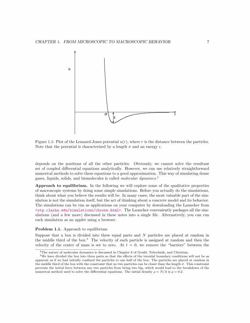
A plot of the Lennard-Jones potential is shown in Figure 1.1. The r−12 form of the repulsive partof the interaction is chosen for convenience only and has no fundamental significance. However,the attractive 1/r6 behavior at large r is the van der Waals interaction. The force between anytwo particles is given by f(r) = −du/dr.

Usually we want to simulate a gas or liquid in the bulk. In such systems the fraction ofparticles near the walls of the container is negligibly small. However, the number of particles thatcan be studied in a simulation is typically 103–106. For these relatively small systems, the fractionof particles near the walls of the container would be significant, and hence the behavior of sucha system would be dominated by surface effects. The most common way of minimizing surfaceeffects and to simulate more closely the properties of a bulk system is to use what are known astoroidal boundary conditions. These boundary conditions are familiar to computer game players.For example, a particle that exits the right edge of the “box,” re-enters the box from the left side.In one dimension, this boundary condition is equivalent to taking a piece of wire and making itinto a loop. In this way a particle moving on the wire never reaches the end.

Given the form of the interparticle potential, we can determine the total force on each particledue to all the other particles in the system. Given this force, we find the acceleration of eachparticle from Newton’s second law of motion. Because the acceleration is the second derivativeof the position, we need to solve a second-order differential equation for each particle (for eachdirection). (For a two-dimensional system of N particles, we would have to solve 2N differentialequations.) These differential equations are coupled because the acceleration of a given particle

CHAPTER 1. FROM MICROSCOPIC TO MACROSCOPIC BEHAVIOR 7

u

rε

σ

Figure 1.1: Plot of the Lennard-Jones potential u(r), where r is the distance between the particles.Note that the potential is characterized by a length σ and an energy ε.

depends on the positions of all the other particles. Obviously, we cannot solve the resultantset of coupled differential equations analytically. However, we can use relatively straightforwardnumerical methods to solve these equations to a good approximation. This way of simulating densegases, liquids, solids, and biomolecules is called molecular dynamics.2

Approach to equilibrium. In the following we will explore some of the qualitative propertiesof macroscopic systems by doing some simple simulations. Before you actually do the simulations,think about what you believe the results will be. In many cases, the most valuable part of the sim-ulation is not the simulation itself, but the act of thinking about a concrete model and its behavior.The simulations can be run as applications on your computer by downloading the Launcher from<stp.clarku.edu/simulations/choose.html>. The Launcher conveniently packages all the sim-ulations (and a few more) discussed in these notes into a single file. Alternatively, you can runeach simulation as an applet using a browser.

Problem 1.1. Approach to equilibriumSuppose that a box is divided into three equal parts and N particles are placed at random inthe middle third of the box.3 The velocity of each particle is assigned at random and then thevelocity of the center of mass is set to zero. At t = 0, we remove the “barriers” between the

2The nature of molecular dynamics is discussed in Chapter 8 of Gould, Tobochnik, and Christian.3We have divided the box into three parts so that the effects of the toroidal boundary conditions will not be as

apparent as if we had initially confined the particles to one half of the box. The particles are placed at random inthe middle third of the box with the constraint that no two particles can be closer than the length σ. This constraintprevents the initial force between any two particles from being two big, which would lead to the breakdown of thenumerical method used to solve the differential equations. The initial density ρ = N/A is ρ = 0.2.

CHAPTER 1. FROM MICROSCOPIC TO MACROSCOPIC BEHAVIOR 8

three parts and watch the particles move according to Newton’s equations of motion. We saythat the removal of the barrier corresponds to the removal of an internal constraint. What doyou think will happen? The applet/application at <stp.clarku.edu/simulations/approach.html> implements this simulation. Give your answers to the following questions before you do thesimulation.

(a) Start the simulation with N = 27, n1 = 0, n2 = N , and n3 = 0. What is the qualitativebehavior of n1, n2, and n3, the number of particles in each third of the box, as a function ofthe time t? Does the system appear to show a direction of time? Choose various values of Nthat are multiples of three up to N = 270. Is the direction of time better defined for larger N?

(b) Suppose that we made a video of the motion of the particles considered in Problem 1.1a. Wouldyou be able to tell if the video were played forward or backward for the various values of N?Would you be willing to make an even bet about the direction of time? Does your conclusionabout the direction of time become more certain as N increases?

(c) After n1, n2, and n3 become approximately equal for N = 270, reverse the time and continuethe simulation. Reversing the time is equivalent to letting t → −t and changing the signs ofall the velocities. Do the particles return to the middle third of the box? Do the simulationagain, but let the particles move for a longer time before the time is reversed. What happensnow?

(d) From watching the motion of the particles, describe the nature of the boundary conditionsthat are used in the simulation.

The results of the simulations in Problem 1.1 might not seem very surprising until you startto think about them. Why does the system as a whole exhibit a direction of time when the motionof each particle is time reversible? Do the particles fill up the available space simply because thesystem becomes less dense?

To gain some more insight into these questions, we consider a simpler simulation. Imaginea closed box that is divided into two parts of equal volume. The left half initially contains Nidentical particles and the right half is empty. We then make a small hole in the partition betweenthe two halves. What happens? Instead of simulating this system by solving Newton’s equationsfor each particle, we adopt a simpler approach based on a probabilistic model. We assume that theparticles do not interact with one another so that the probability per unit time that a particle goesthrough the hole in the partition is the same for all particles regardless of the number of particlesin either half. We also assume that the size of the hole is such that only one particle can passthrough it in one unit of time.

One way to implement this model is to choose a particle at random and move it to the otherside. This procedure is cumbersome, because our only interest is the number of particles on eachside. That is, we need to know only n, the number of particles on the left side; the number onthe right side is N − n. Because each particle has the same chance to go through the hole in thepartition, the probability per unit time that a particle moves from left to right equals the numberof particles on the left side divided by the total number of particles; that is, the probability of amove from left to right is n/N . The algorithm for simulating the evolution of the model is givenby the following steps:

CHAPTER 1. FROM MICROSCOPIC TO MACROSCOPIC BEHAVIOR 9

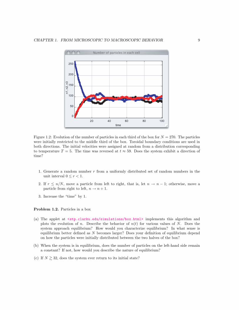
Figure 1.2: Evolution of the number of particles in each third of the box for N = 270. The particleswere initially restricted to the middle third of the box. Toroidal boundary conditions are used inboth directions. The initial velocities were assigned at random from a distribution correspondingto temperature T = 5. The time was reversed at t ≈ 59. Does the system exhibit a direction oftime?

1. Generate a random number r from a uniformly distributed set of random numbers in theunit interval 0 ≤ r < 1.

2. If r ≤ n/N , move a particle from left to right, that is, let n → n − 1; otherwise, move aparticle from right to left, n→ n + 1.

3. Increase the “time” by 1.

Problem 1.2. Particles in a box

(a) The applet at <stp.clarku.edu/simulations/box.html> implements this algorithm andplots the evolution of n. Describe the behavior of n(t) for various values of N . Does thesystem approach equilibrium? How would you characterize equilibrium? In what sense isequilibrium better defined as N becomes larger? Does your definition of equilibrium dependon how the particles were initially distributed between the two halves of the box?

(b) When the system is in equilibrium, does the number of particles on the left-hand side remaina constant? If not, how would you describe the nature of equilibrium?

(c) If N & 32, does the system ever return to its initial state?

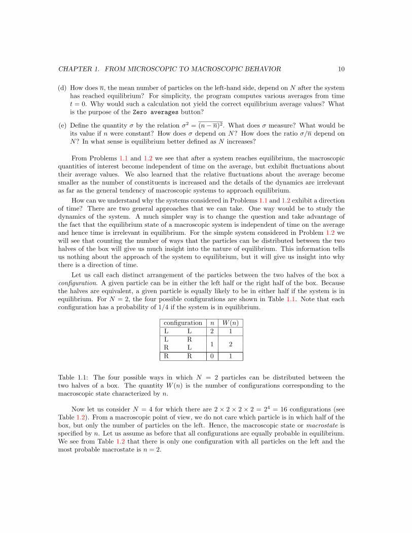
CHAPTER 1. FROM MICROSCOPIC TO MACROSCOPIC BEHAVIOR 10

(d) How does n, the mean number of particles on the left-hand side, depend on N after the systemhas reached equilibrium? For simplicity, the program computes various averages from timet = 0. Why would such a calculation not yield the correct equilibrium average values? Whatis the purpose of the Zero averages button?

(e) Define the quantity σ by the relation σ2 = (n− n)2. What does σ measure? What would beits value if n were constant? How does σ depend on N? How does the ratio σ/n depend onN? In what sense is equilibrium better defined as N increases?

From Problems 1.1 and 1.2 we see that after a system reaches equilibrium, the macroscopicquantities of interest become independent of time on the average, but exhibit fluctuations abouttheir average values. We also learned that the relative fluctuations about the average becomesmaller as the number of constituents is increased and the details of the dynamics are irrelevantas far as the general tendency of macroscopic systems to approach equilibrium.

How can we understand why the systems considered in Problems 1.1 and 1.2 exhibit a directionof time? There are two general approaches that we can take. One way would be to study thedynamics of the system. A much simpler way is to change the question and take advantage ofthe fact that the equilibrium state of a macroscopic system is independent of time on the averageand hence time is irrelevant in equilibrium. For the simple system considered in Problem 1.2 wewill see that counting the number of ways that the particles can be distributed between the twohalves of the box will give us much insight into the nature of equilibrium. This information tellsus nothing about the approach of the system to equilibrium, but it will give us insight into whythere is a direction of time.

Let us call each distinct arrangement of the particles between the two halves of the box aconfiguration. A given particle can be in either the left half or the right half of the box. Becausethe halves are equivalent, a given particle is equally likely to be in either half if the system is inequilibrium. For N = 2, the four possible configurations are shown in Table 1.1. Note that eachconfiguration has a probability of 1/4 if the system is in equilibrium.

configuration n W (n)L L 2 1L RR L 1 2

R R 0 1

Table 1.1: The four possible ways in which N = 2 particles can be distributed between thetwo halves of a box. The quantity W (n) is the number of configurations corresponding to themacroscopic state characterized by n.

Now let us consider N = 4 for which there are 2 × 2 × 2 × 2 = 24 = 16 configurations (seeTable 1.2). From a macroscopic point of view, we do not care which particle is in which half of thebox, but only the number of particles on the left. Hence, the macroscopic state or macrostate isspecified by n. Let us assume as before that all configurations are equally probable in equilibrium.We see from Table 1.2 that there is only one configuration with all particles on the left and themost probable macrostate is n = 2.

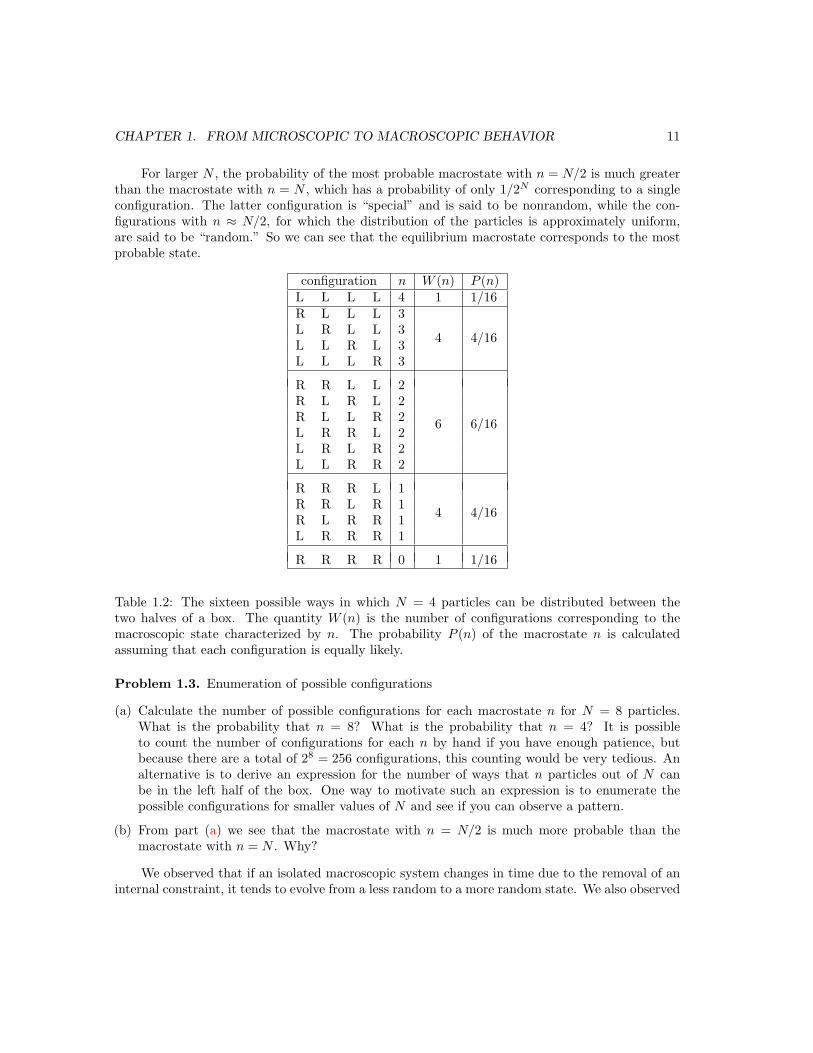
CHAPTER 1. FROM MICROSCOPIC TO MACROSCOPIC BEHAVIOR 11

For larger N , the probability of the most probable macrostate with n = N/2 is much greaterthan the macrostate with n = N , which has a probability of only 1/2N corresponding to a singleconfiguration. The latter configuration is “special” and is said to be nonrandom, while the con-figurations with n ≈ N/2, for which the distribution of the particles is approximately uniform,are said to be “random.” So we can see that the equilibrium macrostate corresponds to the mostprobable state.

configuration n W (n) P (n)L L L L 4 1 1/16R L L L 3L R L L 3L L R L 3L L L R 3

4 4/16

R R L L 2R L R L 2R L L R 2L R R L 2L R L R 2L L R R 2

6 6/16

R R R L 1R R L R 1R L R R 1L R R R 1

4 4/16

R R R R 0 1 1/16

Table 1.2: The sixteen possible ways in which N = 4 particles can be distributed between thetwo halves of a box. The quantity W (n) is the number of configurations corresponding to themacroscopic state characterized by n. The probability P (n) of the macrostate n is calculatedassuming that each configuration is equally likely.

Problem 1.3. Enumeration of possible configurations

(a) Calculate the number of possible configurations for each macrostate n for N = 8 particles.What is the probability that n = 8? What is the probability that n = 4? It is possibleto count the number of configurations for each n by hand if you have enough patience, butbecause there are a total of 28 = 256 configurations, this counting would be very tedious. Analternative is to derive an expression for the number of ways that n particles out of N canbe in the left half of the box. One way to motivate such an expression is to enumerate thepossible configurations for smaller values of N and see if you can observe a pattern.

(b) From part (a) we see that the macrostate with n = N/2 is much more probable than themacrostate with n = N . Why?

We observed that if an isolated macroscopic system changes in time due to the removal of aninternal constraint, it tends to evolve from a less random to a more random state. We also observed

CHAPTER 1. FROM MICROSCOPIC TO MACROSCOPIC BEHAVIOR 12

that once the system reaches its most random state, fluctuations corresponding to an appreciablynonuniform state are very rare. These observations and our reasoning based on counting thenumber of configurations corresponding to a particular macrostate allows us to conclude that

A system in a nonuniform macrostate will change in time on the average so as toapproach its most random macrostate where it is in equilibrium.

Note that our simulations involved watching the system evolve, but our discussion of thenumber of configurations corresponding to each macrostate did not involve the dynamics in anyway. Instead this approach involved the enumeration of the configurations and assigning themequal probabilities assuming that the system is isolated and in equilibrium. We will find that it ismuch easier to understand equilibrium systems by ignoring the time altogether.

In the simulation of Problem 1.1 the total energy was conserved, and hence the macroscopicquantity of interest that changed from the specially prepared initial state with n2 = N to themost random macrostate with n2 ≈ N/3 was not the total energy. So what macroscopic quantitychanged besides n1, n2, and n3 (the number of particles in each third of the box)? Based on ourearlier discussion, we tentatively say that the quantity that changed is the entropy. This statementis no more meaningful than saying that balls fall near the earth’s surface because of gravity. Weconjecture that the entropy is associated with the number of configurations associated with agiven macrostate. If we make this association, we see that the entropy is greater after the systemhas reached equilibrium than in the system’s initial state. Moreover, if the system were initiallyprepared in a random state, the mean value of n2 and hence the entropy would not change. Hence,we can conclude the following:

The entropy of an isolated system increases or remains the same when an internalconstraint is removed.

This statement is equivalent to the second law of thermodynamics. You might want to skip toChapter 4, where this identification of the entropy is made explicit.

As a result of the two simulations that we have done and our discussions, we can make someadditional tentative observations about the behavior of macroscopic systems.

Fluctuations in equilibrium. Once a system reaches equilibrium, the macroscopic quantities ofinterest do not become independent of the time, but exhibit fluctuations about their average values.That is, in equilibrium only the average values of the macroscopic variables are independent oftime. For example, for the particles in the box problem n(t) changes with t, but its average valuen does not. If N is large, fluctuations corresponding to a very nonuniform distribution of theparticles almost never occur, and the relative fluctuations, σ/n become smaller as N is increased.

History independence. The properties of equilibrium systems are independent of their history.For example, n would be the same whether we had started with n(t = 0) = 0 or n(t = 0) = N .In contrast, as members of the human race, we are all products of our history. One consequenceof history independence is that it is easier to understand the properties of equilibrium systems byignoring the dynamics of the particles. (The global constraints on the dynamics are important.For example, it is important to know if the total energy is a constant or not.) We will find thatequilibrium statistical mechanics is essentially equivalent to counting configurations. The problemwill be that this counting is difficult to do in general.

CHAPTER 1. FROM MICROSCOPIC TO MACROSCOPIC BEHAVIOR 13

Need for statistical approach. Systems can be described in detail by specifying their microstate.Such a description corresponds to giving all the information that is possible. For a system ofclassical particles, a microstate corresponds to specifying the position and velocity of each particle.In our analysis of Problem 1.2, we specified only in which half of the box a particle was located,so we used the term configuration rather than microstate. However, the terms are frequently usedinterchangeably.

From our simulations, we see that the microscopic state of the system changes in a complicatedway that is difficult to describe. However, from a macroscopic point of view, the description ismuch simpler. Suppose that we simulated a system of many particles and saved the trajectoriesof the particles as a function of time. What could we do with this information? If the number ofparticles is 106 or more or if we ran long enough, we would have a problem storing the data. Dowe want to have a detailed description of the motion of each particle? Would this data give usmuch insight into the macroscopic behavior of the system? As we have found, the trajectories ofthe particles are not of much interest, and it is more useful to develop a probabilistic approach.That is, the presence of a large number of particles motivates us to use statistical methods. InSection 1.8 we will discuss another reason why a probabilistic approach is necessary.

We will find that the laws of thermodynamics depend on the fact that the number of particles inmacroscopic systems is enormous. A typical measure of this number is Avogadro’s number whichis approximately 6 × 1023, the number of atoms in a mole. When there are so many particles,predictions of the average properties of the system become meaningful, and deviations from theaverage behavior become less and less important as the number of atoms is increased.

Equal a priori probabilities. In our analysis of the probability of each macrostate in Prob-lem 1.2, we assumed that each configuration was equally probable. That is, each configuration ofan isolated system occurs with equal probability if the system is in equilibrium. We will make thisassumption explicit for isolated systems in Chapter 4.

Existence of different phases. So far our simulations of interacting systems have been restrictedto dilute gases. What do you think would happen if we made the density higher? Would a systemof interacting particles form a liquid or a solid if the temperature or the density were chosenappropriately? The existence of different phases is investigated in Problem 1.4.

Problem 1.4. Different phases

(a) The applet/application at <stp.clarku.edu/simulations/lj.html> simulates an isolatedsystem of N particles interacting via the Lennard-Jones potential. Choose N = 64 and L = 18so that the density ρ = N/L2 ≈ 0.2. The initial positions are chosen at random except thatno two particles are allowed to be closer than σ. Run the simulation and satisfy yourself thatthis choice of density and resultant total energy corresponds to a gas. What is your criterion?

(b) Slowly lower the total energy of the system. (The total energy is lowered by rescaling thevelocities of the particles.) If you are patient, you might be able to observe “liquid-like”regions. How are they different than “gas-like” regions?

(c) If you decrease the total energy further, you will observe the system in a state roughly corre-sponding to a solid. What is your criteria for a solid? Explain why the solid that we obtain inthis way will not be a perfect crystalline solid.

CHAPTER 1. FROM MICROSCOPIC TO MACROSCOPIC BEHAVIOR 14

(d) Describe the motion of the individual particles in the gas, liquid, and solid phases.

(e) Conjecture why a system of particles interacting via the Lennard-Jones potential in (1.1) canexist in different phases. Is it necessary for the potential to have an attractive part for thesystem to have a liquid phase? Is the attractive part necessary for there to be a solid phase?Describe a simulation that would help you answer this question.

It is fascinating that a system with the same interparticle interaction can be in differentphases. At the microscopic level, the dynamics of the particles is governed by the same equationsof motion. What changes? How does such a phase change occur at the microscopic level? Whydoesn’t a liquid crystallize immediately when its temperature is lowered quickly? What happenswhen it does begin to crystallize? We will find in later chapters that phase changes are examplesof cooperative effects.

1.6 Measuring the pressure and temperature

The obvious macroscopic variables that we can measure in our simulations of the system of particlesinteracting via the Lennard-Jones potential include the average kinetic and potential energies, thenumber of particles, and the volume. We also learned that the entropy is a relevant macroscopicvariable, but we have not learned how to determine it from a simulation.4 We know from oureveryday experience that there are at least two other macroscopic variables that are relevant fordescribing a macrostate, namely, the pressure and the temperature.

The pressure is easy to measure because we are familiar with force and pressure from coursesin mechanics. To remind you of the relation of the pressure to the momentum flux, consider Nparticles in a cube of volume V and linear dimension L. The center of mass momentum of theparticles is zero. Imagine a planar surface of area A = L2 placed in the system and orientedperpendicular to the x-axis as shown in Figure 1.3. The pressure P can be defined as the force perunit area acting normal to the surface:

P =Fx

A. (1.2)

We have written P as a scalar because the pressure is the same in all directions on the average.From Newton’s second law, we can rewrite (1.2) as

P =1A

d(mvx)dt

. (1.3)

From (1.3) we see that the pressure is the amount of momentum that crosses a unit area ofthe surface per unit time. We could use (1.3) to determine the pressure, but this relation usesinformation only from the fraction of particles that are crossing an arbitrary surface at a giventime. Instead, our simulations will use the relation of the pressure to the virial, a quantity thatinvolves all the particles in the system.5

4We will find that it is very difficult to determine the entropy directly by making either measurements in thelaboratory or during a simulation. Entropy, unlike pressure and temperature, has no mechanical analog.

5See Gould, Tobochnik, and Christian, Chapter 8. The relation of the pressure to the virial is usually consideredin graduate courses in mechanics.

CHAPTER 1. FROM MICROSCOPIC TO MACROSCOPIC BEHAVIOR 15

not done

Figure 1.3: Imaginary plane perpendicular to the x-axis across which the momentum flux is eval-uated.

Problem 1.5. Nature of temperature

(a) Summarize what you know about temperature. What reasons do you have for thinking thatit has something to do with energy?

(b) Discuss what happens to the temperature of a hot cup of coffee. What happens, if anything,to the temperature of its surroundings?

The relation between temperature and energy is not simple. For example, one way to increasethe energy of a glass of water would be to lift it. However, this action would not affect thetemperature of the water. So the temperature has nothing to do with the motion of the center ofmass of the system. As another example, if we placed a container of water on a moving conveyorbelt, the temperature of the water would not change. We also know that temperature is a propertyassociated with many particles. It would be absurd to refer to the temperature of a single molecule.

This discussion suggests that temperature has something to do with energy, but it has missedthe most fundamental property of temperature, that is, the temperature is the quantity that becomesequal when two systems are allowed to exchange energy with one another. (Think about whathappens to a cup of hot coffee.) In Problem 1.6 we identify the temperature from this point ofview for a system of particles.

Problem 1.6. Identification of the temperature

(a) Consider two systems of particles interacting via the Lennard-Jones potential given in (1.1). Se-lect the applet/application at <stp.clarku.edu/simulations/thermalcontact.html>. Forsystem A, we take NA = 81, εAA = 1.0, and σAA = 1.0; for system B, we have NB = 64,εAA = 1.5, and σAA = 1.2. Both systems are in a square box with linear dimension L = 12. Inthis case, toroidal boundary conditions are not used and the particles also interact with fixedparticles (with infinite mass) that make up the walls and the partition between them. Initially,the two systems are isolated from each other and from their surroundings. Run the simulationuntil each system appears to be in equilibrium. Does the kinetic energy and potential energyof each system change as the system evolves? Why? What is the mean potential and kineticenergy of each system? Is the total energy of each system fixed (to within numerical error)?

CHAPTER 1. FROM MICROSCOPIC TO MACROSCOPIC BEHAVIOR 16

(b) Remove the barrier and let the two systems interact with one another.6 We choose εAB = 1.25and σAB = 1.1. What quantity is exchanged between the two systems? (The volume of eachsystem is fixed.)

(c) Monitor the kinetic and potential energy of each system. After equilibrium has been establishedbetween the two systems, compare the average kinetic and potential energies to their valuesbefore the two systems came into contact.

(d) We are looking for a quantity that is the same in both systems after equilibrium has beenestablished. Are the average kinetic and potential energies the same? If not, think about whatwould happen if you doubled the N and the area of each system? Would the temperaturechange? Does it make more sense to compare the average kinetic and potential energies or theaverage kinetic and potential energies per particle? What quantity does become the same oncethe two systems are in equilibrium? Do any other quantities become approximately equal?What do you conclude about the possible identification of the temperature?

From the simulations in Problem 1.6, you are likely to conclude that the temperature isproportional to the average kinetic energy per particle. We will learn in Chapter 4 that theproportionality of the temperature to the average kinetic energy per particle holds only for asystem of particles whose kinetic energy is proportional to the square of the momentum (velocity).

Another way of thinking about temperature is that temperature is what you measure with athermometer. If you want to measure the temperature of a cup of coffee, you put a thermometerinto the coffee. Why does this procedure work?

Problem 1.7. ThermometersDescribe some of the simple thermometers with which you are familiar. On what physical principlesdo these thermometers operate? What requirements must a thermometer have?

Now lets imagine a simulation of a simple thermometer. Imagine a special particle, a “demon,”that is able to exchange energy with a system of particles. The only constraint is that the energyof the demon Ed must be non-negative. The behavior of the demon is given by the followingalgorithm:

1. Choose a particle in the system at random and make a trial change in one of its coordinates.

2. Compute ∆E, the change in the energy of the system due to the change.

3. If ∆E ≤ 0, the system gives the surplus energy |∆E| to the demon, Ed → Ed + |∆E|, andthe trial configuration is accepted.

4. If ∆E > 0 and the demon has sufficient energy for this change, then the demon gives thenecessary energy to the system, Ed → Ed − ∆E, and the trial configuration is accepted.Otherwise, the trial configuration is rejected and the configuration is not changed.

6In order to ensure that we can continue to identify which particle belongs to system A and system B, we haveadded a spring to each particle so that it cannot wander too far from its original lattice site.

CHAPTER 1. FROM MICROSCOPIC TO MACROSCOPIC BEHAVIOR 17

Note that the total energy of the system and the demon is fixed.We consider the consequences of these simple rules in Problem 1.8. The nature of the demon

is discussed further in Section 4.9.

Problem 1.8. The demon and the ideal gas

(a) The applet/application at <stp.clarku.edu/simulations/demon.html> simulates a demonthat exchanges energy with an ideal gas of N particles moving in d spatial dimensions. Becausethe particles do not interact, the only coordinate of interest is the velocity of the particles.In this case the demon chooses a particle at random and changes its velocity in one of its ddirections by an amount chosen at random between −∆ and +∆. For simplicity, the initialvelocity of each particle is set equal to +v0x, where v0 = (2E0/m)1/2/N , E0 is the desiredtotal energy of the system, and m is the mass of the particles. For simplicity, we will chooseunits such that m = 1. Choose d = 1, N = 40, and E0 = 10 and determine the mean energyof the demon Ed and the mean energy of the system E. Why is E 6= E0?

(b) What is e, the mean energy per particle of the system? How do e and Ed compare for variousvalues of E0? What is the relation, if any, between the mean energy of the demon and themean energy of the system?

(c) Choose N = 80 and E0 = 20 and compare e and Ed. What conclusion, if any, can you make?7

(d) Run the simulation for several other values of the initial total energy E0 and determine how edepends on Ed for fixed N .

(e) From your results in part (d), what can you conclude about the role of the demon as athermometer? What properties, if any, does it have in common with real thermometers?

(f) Repeat the simulation for d = 2. What relation do you find between e and Ed for fixed N?

(g) Suppose that the energy momentum relation of the particles is not ε = p2/2m, but is ε = cp,where c is a constant (which we take to be unity). Determine how e depends on Ed for fixedN and d = 1. Is the dependence the same as in part (d)?

(h) Suppose that the energy momentum relation of the particles is ε = Ap3/2, where A is a constant(which we take to be unity). Determine how e depends on Ed for fixed N and d = 1. Is thisdependence the same as in part (d) or part (g)?

(i) The simulation also computes the probability P (Ed)δE that the demon has energy betweenEd and Ed +δE. What is the nature of the dependence of P (Ed) on Ed? Does this dependencedepend on the nature of the system with which the demon interacts?

7There are finite size effects that are order 1/N .

CHAPTER 1. FROM MICROSCOPIC TO MACROSCOPIC BEHAVIOR 18

1.7 Work, heating, and the first law of thermodynamics

If you watch the motion of the individual particles in a molecular dynamics simulation, you wouldprobably describe the motion as “random” in the sense of how we use random in everyday speech.The motion of the individual molecules in a glass of water would exhibit similar motion. Supposethat we were to expose the water to a low flame. In a simulation this process would roughlycorrespond to increasing the speed of the particles when they hit the wall. We say that we havetransferred energy to the system incoherently because each particle would continue to move moreor less at random.

You learned in your classical mechanics courses that the change in energy of a particle equalsthe work done on it and the same is true for a collection of particles as long as we do not changethe energy of the particles in some other way at the same time. Hence, if we squeeze a plasticcontainer of water, we would do work on the system, and we would see the particles near the wallmove coherently. So we can distinguish two different ways of transferring energy to the system.That is, heating transfers energy incoherently and doing work transfers energy coherently.

Lets consider a molecular dynamics simulation again and suppose that we have increased theenergy of the system by either compressing the system and doing work on it or by increasing thespeed of the particles that reach the walls of the container. Roughly speaking, the first way wouldinitially increase the potential energy of interaction and the second way would initially increasethe kinetic energy of the particles. If we increase the total energy by the same amount, could wetell by looking at the particle trajectories after equilibrium has been reestablished how the energyhad been increased? The answer is no, because for a given total energy, volume, and number ofparticles, the kinetic energy and the potential energy would have unique equilibrium values. (SeeProblem 1.6 for a demonstration of this property.) We conclude that the energy of the gas canbe changed by doing work on it or by heating it. This statement is equivalent to the first law ofthermodynamics and from the microscopic point of view is simply a statement of conservation ofenergy.

Our discussion implies that the phrase “adding heat” to a system makes no sense, becausewe cannot distinguish “heat energy” from potential energy and kinetic energy. Nevertheless, wefrequently use the word “heat ” in everyday speech. For example, we might way “Please turn onthe heat” and “I need to heat my coffee.” We will avoid such uses, and whenever possible avoidthe use of the noun “heat.” Why do we care? Because there is no such thing as heat! Once upona time, scientists thought that there was a fluid in all substances called caloric or heat that couldflow from one substance to another. This idea was abandoned many years ago, but is still used incommon language. Go ahead and use heat outside the classroom, but we won’t use it here.

1.8 *The fundamental need for a statistical approach

In Section 1.5 we discussed the need for a statistical approach when treating macroscopic systemsfrom a microscopic point of view. Although we can compute the trajectory (the position andvelocity) of each particle for as long as we have patience, our disinterest in the trajectory of anyparticular particle and the overwhelming amount of information that is generated in a simulationmotivates us to develop a statistical approach.

CHAPTER 1. FROM MICROSCOPIC TO MACROSCOPIC BEHAVIOR 19

(a) (b)

Figure 1.4: (a) A special initial condition for N = 11 particles such that their motion remainsparallel indefinitely. (b) The positions of the particles at time t = 8.0 after the change in vx(6).The only change in the initial condition from part (a) is that vx(6) was changed from 1 to 1.000001.

We now discuss why there is a more fundamental reason why we must use probabilistic meth-ods to describe systems with more than a few particles. The reason is that under a wide variety ofconditions, even the most powerful supercomputer yields positions and velocities that are mean-ingless! In the following, we will find that the trajectories in a system of many particles dependsensitively on the initial conditions. Such a system is said to be chaotic. This behavior forces usto take a statistical approach even for systems with as few as three particles.

As an example, consider a system of N = 11 particles moving in a box of linear dimensionL (see the applet/application at <stp.clarku.edu/simulations/sensitive.html>). The initialconditions are such that all particles have the same velocity vx(i) = 1, vy(i) = 0, and the particlesare equally spaced vertically, with x(i) = L/2 for i = 1, . . . , 11 (see Fig. 1.4(a)). Convince yourselfthat for these special initial conditions, the particles will continue moving indefinitely in the x-direction (using toroidal boundary conditions).

Now let us stop the simulation and change the velocity of particle 6, such that vx(6) =1.000001. What do you think happens now? In Fig. 1.4(b) we show the positions of the particlesat time t = 8.0 after the change in velocity of particle 6. Note that the positions of the particlesare no longer equally spaced and the velocities of the particles are very different. So in this case,a small change in the velocity of one particle leads to a big change in the trajectories of all theparticles.

Problem 1.9. IrreversibilityThe applet/application at <stp.clarku.edu/simulations/sensitive.html> simulates a systemof N = 11 particles with the special initial condition described in the text. Confirm the results thatwe have discussed. Change the velocity of particle 6 and stop the simulation at time t and reverse

CHAPTER 1. FROM MICROSCOPIC TO MACROSCOPIC BEHAVIOR 20

all the velocities. Confirm that if t is sufficiently short, the particles will return approximately totheir initial state. What is the maximum value of t that will allow the system to return to itsinitial positions if t is replaced by −t (all velocities reversed)?

An important property of chaotic systems is their extreme sensitivity to initial conditions,that is, the trajectories of two identical systems starting with slightly different initial conditionswill diverge exponentially in a short time. For such systems we cannot predict the positionsand velocities of the particles because even the slightest error in our measurement of the initialconditions would make our prediction entirely wrong if the elapsed time is sufficiently long. Thatis, we cannot answer the question, “Where is particle 2 at time t?” if t is sufficiently long. It mightbe disturbing to realize that our answers are meaningless if we ask the wrong questions.

Although Newton’s equations of motion are time reversible, this reversibility cannot be realizedin practice for chaotic systems. Suppose that a chaotic system evolves for a time t and all thevelocities are reversed. If the system is allowed to evolve for an additional time t, the system willnot return to its original state unless the velocities are specified with infinite precision. This lackof practical reversibility is related to what we observe in macroscopic systems. If you pour milkinto a cup of coffee, the milk becomes uniformly distributed throughout the cup. You will neversee a cup of coffee spontaneously return to the state where all the milk is at the surface becauseto do so, the positions and velocities of the milk and coffee molecules must be chosen so that themolecules of milk return to this very special state. Even the slightest error in the choice of positionsand velocities will ruin any chance of the milk returning to the surface. This sensitivity to initialconditions provides the foundation for the arrow of time.

1.9 *Time and ensemble averages

We have seen that although the computed trajectories are meaningless for chaotic systems, averagesover the trajectories are physically meaningful. That is, although a computed trajectory mightnot be the one that we thought we were computing, the positions and velocities that we computeare consistent with the constraints we have imposed, in this case, the total energy E, the volumeV , and the number of particles N . This reasoning suggests that macroscopic properties such asthe temperature and pressure must be expressed as averages over the trajectories.

Solving Newton’s equations numerically as we have done in our simulations yields a timeaverage. If we do a laboratory experiment to measure the temperature and pressure, our mea-surements also would be equivalent to a time average. As we have mentioned, time is irrelevant inequilibrium. We will find that it is easier to do calculations in statistical mechanics by doing anensemble average. We will discuss ensemble averages in Chapter 3. In brief an ensemble average isover many mental copies of the system that satisfy the same known conditions. A simple examplemight clarify the nature of these two types of averages. Suppose that we want to determine theprobability that the toss of a coin results in “heads.” We can do a time average by taking onecoin, tossing it in the air many times, and counting the fraction of heads. In contrast, an ensembleaverage can be found by obtaining many similar coins and tossing them into the air at one time.

It is reasonable to assume that the two ways of averaging are equivalent. This equivalenceis called the quasi-ergodic hypothesis. The use of the term “hypothesis” might suggest that theequivalence is not well accepted, but it reminds us that the equivalence has been shown to be

CHAPTER 1. FROM MICROSCOPIC TO MACROSCOPIC BEHAVIOR 21

rigorously true in only a few cases. The sensitivity of the trajectories of chaotic systems to initialconditions suggests that a classical system of particles moving according to Newton’s equations ofmotion passes through many different microstates corresponding to different sets of positions andvelocities. This property is called mixing, and it is essential for the validity of the quasi-ergodichypothesis.

In summary, macroscopic properties are averages over the microscopic variables and givepredictable values if the system is sufficiently large. One goal of statistical mechanics is to givea microscopic basis for the laws of thermodynamics. In this context it is remarkable that theselaws depend on the fact that gases, liquids, and solids are chaotic systems. Another importantgoal of statistical mechanics is to calculate the macroscopic properties from a knowledge of theintermolecular interactions.

1.10 *Models of matter

There are many models of interest in statistical mechanics, corresponding to the wide range ofmacroscopic systems found in nature and made in the laboratory. So far we have discussed asimple model of a classical gas and used the same model to simulate a classical liquid and a solid.

One key to understanding nature is to develop models that are simple enough to analyze, butthat are rich enough to show the same features that are observed in nature. Some of the morecommon models that we will consider include the following.

1.10.1 The ideal gas

The simplest models of macroscopic systems are those for which the interaction between the indi-vidual particles is very small. For example, if a system of particles is very dilute, collisions betweenthe particles will be rare and can be neglected under most circumstances. In the limit that theinteractions between the particles can be neglected completely, the model is known as the idealgas. The classical ideal gas allows us to understand much about the behavior of dilute gases, suchas those in the earth’s atmosphere. The quantum version will be useful in understanding black-body radiation (Section 6.9), electrons in metals (Section 6.10), the low temperature behavior ofcrystalline solids (Section 6.12), and a simple model of superfluidity (Section 6.11).

The term “ideal gas” is a misnomer because it can be used to understand the properties ofsolids and other interacting particle systems under certain circumstances, and because in manyways the neglect of interactions is not ideal. The historical reason for the use of this term is thatthe neglect of interparticle interactions allows us to do some calculations analytically. However,the neglect of interparticle interactions raises other issues. For example, how does an ideal gasreach equilibrium if there are no collisions between the particles?

CHAPTER 1. FROM MICROSCOPIC TO MACROSCOPIC BEHAVIOR 22

1.10.2 Interparticle potentials

As we have mentioned, the most popular form of the potential between two neutral atoms is theLennard-Jones potential8 given in (1.1). This potential has an weak attractive tail at large r,reaches a minimum at r = 21/6σ ≈ 1.122σ, and is strongly repulsive at shorter distances. TheLennard-Jones potential is appropriate for closed-shell systems, that is, rare gases such as Ar or Kr.Nevertheless, the Lennard-Jones potential is a very important model system and is the standardpotential for studies where the focus is on fundamental issues, rather than on the properties of aspecific material.

An even simpler interaction is the hard core interaction given by

V (r) =

∞ (r ≤ σ)0. (r > σ)

(1.4)

A system of particles interacting via (1.4) is called a system of hard spheres, hard disks, or hardrods depending on whether the spatial dimension is three, two, or one, respectively. Note thatV (r) in (1.4) is purely repulsive.

1.10.3 Lattice models

In another class of models, the positions of the particles are restricted to a lattice or grid and themomenta of the particles are irrelevant. In the most popular model of this type the “particles”correspond to magnetic moments. At high temperatures the magnetic moments are affected byexternal magnetic fields, but the interaction between moments can be neglected.

The simplest, nontrivial model that includes interactions is the Ising model, the most impor-tant model in statistical mechanics. The model consists of spins located on a lattice such thateach spin can take on one of two values designated as up and down or ±1. The interaction energybetween two neighboring spins is −J if the two spins are in the same state and +J if they arein opposite states. One reason for the importance of this model is that it is one of the simplestto have a phase transition, in this case, a phase transition between a ferromagnetic state and aparamagnetic state.

We will focus on three classes of models – the ideal classical and quantum gas, classical systemsof interacting particles, and the Ising model and its extensions. These models will be used in manycontexts to illustrate the ideas and techniques of statistical mechanics.

1.11 Importance of simulations

Only simple models such as the ideal gas or special cases such as the two-dimensional Ising modelcan be analyzed by analytical methods. Much of what is done in statistical mechanics is to establishthe general behavior of a model and then relate it to the behavior of another model. This way ofunderstanding is not as strange as it first might appear. How many different systems in classicalmechanics can be solved exactly?

8This potential is named after John Lennard-Jones, 1894–1954, a theoretical chemist and physicist at CambridgeUniversity.

CHAPTER 1. FROM MICROSCOPIC TO MACROSCOPIC BEHAVIOR 23

Statistical physics has grown in importance over the past several decades because powerfulcomputers and new computer algorithms have allowed us to explore the consequences of more com-plex systems. Simulations play an important intermediate role between theory and experiment. Asour models become more realistic, it is likely that they will require the computer for understandingmany of their properties. In a simulation we start with a microscopic model for which the variablesrepresent the microscopic constituents and determine the consequences of their interactions. Fre-quently the goal of our simulations is to explore these consequences so that we have a better ideaof what type of theoretical analysis might be possible and what type of laboratory experimentsshould be done. Simulations allow us to compute many different kinds of quantities, some of whichcannot be measured in a laboratory experiment.

Not only can we simulate reasonably realistic models, we also can study models that are im-possible to realize in the laboratory, but are useful for providing a deeper theoretical understandingof real systems. For example, a comparison of the behavior of a model in three and four spatialdimensions can yield insight into why the three-dimensional system behaves the way it does.

Simulations cannot replace laboratory experiments and are limited by the finite size of thesystems and by the short duration of our runs. For example, at present the longest simulations ofsimple liquids are for no more than 10−6 s.

Not only have simulations made possible new ways of doing research, they also make it possibleto illustrate the important ideas of statistical mechanics. We hope that the simulations that wehave already discussed have already convinced you of their utility. For this reason, we will considermany simulations throughout these notes.

1.12 Summary

This introductory chapter has been designed to whet your appetite, and at this point it is not likelythat you will fully appreciate the significance of such concepts as entropy and the direction of time.We are reminded of the book, All I Really Need to Know I Learned in Kindergarten.9 In principle,we have discussed most of the important ideas in thermodynamics and statistical physics, but itwill take you a while before you understand these ideas in any depth.

We also have not discussed the tools necessary to solve any problems. Your understanding ofthese concepts and the methods of statistical and thermal physics will increase as you work withthese ideas in different contexts. You will find that the unifying aspects of thermodynamics andstatistical mechanics are concepts such as the nature of equilibrium, the direction of time, andthe existence of cooperative effects and different phases. However, there is no unifying equationsuch as Newton’s second law of motion in mechanics, Maxwell’s equations in electrodynamics, andSchrodinger’s equation in nonrelativistic quantum mechanics.

There are many subtleties that we have glossed over so that we could get started. For example,how good is our assumption that the microstates of an isolated system are equally probable? Thisquestion is a deep one and has not been completely answered. The answer likely involves thenature of chaos. Chaos seems necessary to insure that the system will explore a large number ofthe available microstates, and hence make our assumption of equal probabilities valid. However,we do not know how to tell a priori whether a system will behave chaotically or not.

9Robert Fulghum, All I Really Need to Know I Learned in Kindergarten, Ballantine Books (2004).

CHAPTER 1. FROM MICROSCOPIC TO MACROSCOPIC BEHAVIOR 24

Most of our discussion concerns equilibrium behavior. The “dynamics” in thermodynamicsrefers to the fact that we can treat a variety of thermal processes in which a system moves fromone equilibrium state to another. Even if the actual process involves non-equilibrium states, wecan replace the non-equilibrium states by a series of equilibrium states which begin and end atthe same equilibrium states. This type of reasoning is analogous to the use of energy argumentsin mechanics. A ball can roll from the top of a hill to the bottom, rolling over many bumps andvalleys, but as long as there is no dissipation due to friction, we can determine the ball’s motionat the bottom without knowing anything about how the ball got there.

The techniques and ideas of statistical mechanics are now being used outside of traditionalcondensed matter physics. The field theories of high energy physics, especially lattice gauge theo-ries, use the methods of statistical mechanics. New methods of doing quantum mechanics convertcalculations to path integrals that are computed numerically using methods of statistical mechan-ics. Theories of the early universe use ideas from thermal physics. For example, we speak aboutthe universe being quenched to a certain state in analogy to materials being quenched from highto low temperatures. We already have seen that chaos provides an underpinning for the need forprobability in statistical mechanics. Conversely, many of the techniques used in describing theproperties of dynamical systems have been borrowed from the theory of phase transitions, one ofthe important areas of statistical mechanics.

Thermodynamics and statistical mechanics have traditionally been applied to gases, liquids,and solids. This application has been very fruitful and is one reason why condensed matter physics,materials science, and chemical physics are rapidly evolving and growing areas. Examples of newmaterials include high temperature superconductors, low-dimensional magnetic and conductingmaterials, composite materials, and materials doped with various impurities. In addition, scientistsare taking a new look at more traditional condensed systems such as water and other liquids,liquid crystals, polymers, crystals, alloys, granular matter, and porous media such as rocks. Andin addition to our interest in macroscopic systems, there is growing interest is mesoscopic systems,systems that are neither microscopic nor macroscopic, but are in between, that is, between ∼ 102

to ∼ 106 particles.Thermodynamics might not seem to be as interesting to you when you first encounter it.

However, an understanding of thermodynamics is important in many contexts including societalissues such as global warming, electrical energy production, fuel cells, and other alternative energysources.

The science of information theory uses many ideas from statistical mechanics, and recently, newoptimization methods such as simulated annealing have been borrowed from statistical mechanics.

In recent years statistical mechanics has evolved into the more general field of statisticalphysics. Examples of systems of interest in the latter area include earthquake faults, granular mat-ter, neural networks, models of computing, genetic algorithms, and the analysis of the distributionof time to respond to email. Statistical physics is characterized more by its techniques than by theproblems that are its interest. This universal applicability makes the techniques more difficult tounderstand, but also makes the journey more exciting.

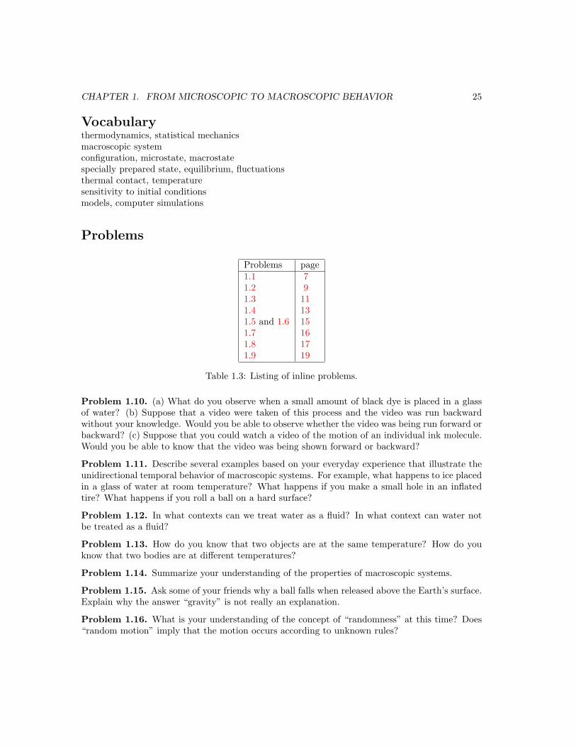
CHAPTER 1. FROM MICROSCOPIC TO MACROSCOPIC BEHAVIOR 25

Vocabularythermodynamics, statistical mechanicsmacroscopic systemconfiguration, microstate, macrostatespecially prepared state, equilibrium, fluctuationsthermal contact, temperaturesensitivity to initial conditionsmodels, computer simulations

Problems

Problems page1.1 71.2 91.3 111.4 131.5 and 1.6 151.7 161.8 171.9 19

Table 1.3: Listing of inline problems.

Problem 1.10. (a) What do you observe when a small amount of black dye is placed in a glassof water? (b) Suppose that a video were taken of this process and the video was run backwardwithout your knowledge. Would you be able to observe whether the video was being run forward orbackward? (c) Suppose that you could watch a video of the motion of an individual ink molecule.Would you be able to know that the video was being shown forward or backward?

Problem 1.11. Describe several examples based on your everyday experience that illustrate theunidirectional temporal behavior of macroscopic systems. For example, what happens to ice placedin a glass of water at room temperature? What happens if you make a small hole in an inflatedtire? What happens if you roll a ball on a hard surface?

Problem 1.12. In what contexts can we treat water as a fluid? In what context can water notbe treated as a fluid?

Problem 1.13. How do you know that two objects are at the same temperature? How do youknow that two bodies are at different temperatures?

Problem 1.14. Summarize your understanding of the properties of macroscopic systems.

Problem 1.15. Ask some of your friends why a ball falls when released above the Earth’s surface.Explain why the answer “gravity” is not really an explanation.

Problem 1.16. What is your understanding of the concept of “randomness” at this time? Does“random motion” imply that the motion occurs according to unknown rules?

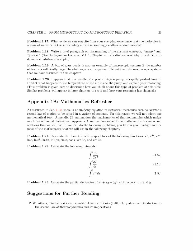
CHAPTER 1. FROM MICROSCOPIC TO MACROSCOPIC BEHAVIOR 26

Problem 1.17. What evidence can you cite from your everyday experience that the molecules ina glass of water or in the surrounding air are in seemingly endless random motion?

Problem 1.18. Write a brief paragraph on the meaning of the abstract concepts, “energy” and“justice.” (See the Feynman Lectures, Vol. 1, Chapter 4, for a discussion of why it is difficult todefine such abstract concepts.)

Problem 1.19. A box of glass beads is also an example of macroscopic systems if the numberof beads is sufficiently large. In what ways such a system different than the macroscopic systemsthat we have discussed in this chapter?

Problem 1.20. Suppose that the handle of a plastic bicycle pump is rapidly pushed inward.Predict what happens to the temperature of the air inside the pump and explain your reasoning.(This problem is given here to determine how you think about this type of problem at this time.Similar problems will appear in later chapters to see if and how your reasoning has changed.)

Appendix 1A: Mathematics Refresher

As discussed in Sec. 1.12, there is no unifying equation in statistical mechanics such as Newton’ssecond law of motion to be solved in a variety of contexts. For this reason we will not adopt onemathematical tool. Appendix 2B summarizes the mathematics of thermodynamics which makesmuch use of partial derivatives. Appendix A summarizes some of the mathematical formulas andrelations that we will use. If you can do the following problems, you have a good background formost of the mathematics that we will use in the following chapters.

Problem 1.21. Calculate the derivative with respect to x of the following functions: ex, e3x, eax,lnx, lnx2, ln 3x, ln 1/x, sinx, cos x, sin 3x, and cos 2x.

Problem 1.22. Calculate the following integrals:∫ 2

1

dx

2x2(1.5a)∫ 2

1

dx

4x(1.5b)∫ 2

1

e3xdx (1.5c)

Problem 1.23. Calculate the partial derivative of x2 + xy + 3y2 with respect to x and y.

Suggestions for Further Reading

P. W. Atkins, The Second Law, Scientific American Books (1984). A qualitative introduction tothe second law of thermodynamics and its implications.

CHAPTER 1. FROM MICROSCOPIC TO MACROSCOPIC BEHAVIOR 27

J. G. Oliveira and A.-L. Barabasi, “Darwin and Einstein correspondence patterns,” Nature 437,1251 (2005). The authors found the probability that Darwin and Einstein would respond toa letter in τ days is well approximated by a power law, P (τ) ∼ τ−a with a ≈ 3/2. Whatis the explanation for this power law behavior? How long does it take you to respond to anemail?

Manfred Eigen and Ruthild Winkler, How the Principles of Nature Govern Chance, PrincetonUniversity Press (1993).

Richard Feynman, R. B. Leighton, and M. Sands, Feynman Lectures on Physics, Addison-Wesley(1964). Volume 1 has a very good discussion of the nature of energy and work.

Harvey Gould, Jan Tobochnik, and Wolfgang Christian, An Introduction to Computer SimulationMethods, third edition, Addison-Wesley (2006).

F. Reif, Statistical Physics, Volume 5 of the Berkeley Physics Series, McGraw-Hill (1967). Thistext was the first to make use of computer simulations to explain some of the basic propertiesof macroscopic systems.

Jeremy Rifkin, Entropy: A New World View, Bantom Books (1980). Although this popular bookraises some important issues, it, like many other popular books articles, misuses the conceptof entropy. For more discussion on the meaning of entropy and how it should be introduced,see <www.entropysite.com/> and <www.entropysimple.com/>.

Chapter 2

Thermodynamic Concepts andProcesses

c©2005 by Harvey Gould and Jan Tobochnik29 September 2005

The study of temperature, energy, work, heating, entropy, and related macroscopic concepts com-prise the field known as thermodynamics.

2.1 Introduction

In this chapter we will discuss ways of thinking about macroscopic systems and introduce the basicconcepts of thermodynamics. Because these ways of thinking are very different from the ways thatwe think about microscopic systems, most students of thermodynamics initially find it difficultto apply the abstract principles of thermodynamics to concrete problems. However, the study ofthermodynamics has many rewards as was appreciated by Einstein:

A theory is the more impressive the greater the simplicity of its premises, the moredifferent kinds of things it relates, and the more extended its area of applicability.Therefore the deep impression that classical thermodynamics made to me. It is the onlyphysical theory of universal content which I am convinced will never be overthrown,within the framework of applicability of its basic concepts.1

The essence of thermodynamics can be summarized by two laws: (1) Energy is conservedand (2) entropy increases. These statements of the laws are deceptively simple. What is energy?You are probably familiar with the concept of energy from other courses, but can you define it?Abstract concepts such as energy and entropy are not easily defined nor understood. However, asyou apply these concepts in a variety of contexts, you will gradually come to understand them.

1A. Einstein, Autobiographical Notes, Open Court Publishing Company (1991).

26

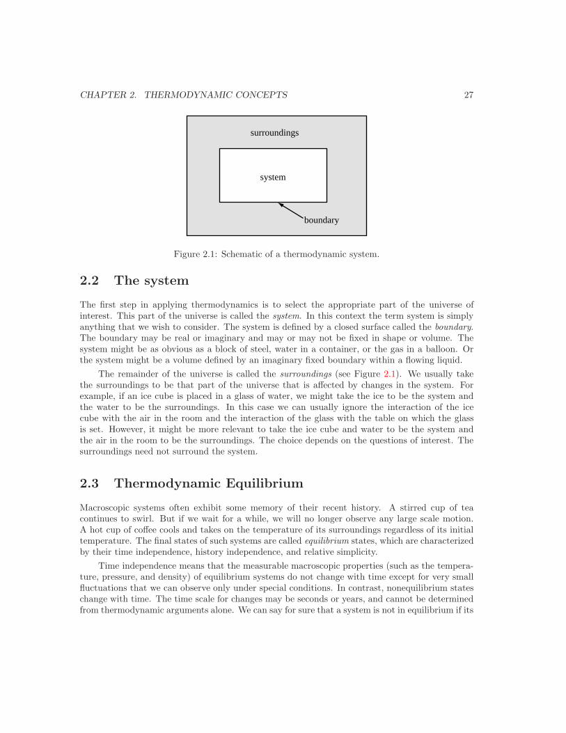
CHAPTER 2. THERMODYNAMIC CONCEPTS 27

system

surroundings

boundary

Figure 2.1: Schematic of a thermodynamic system.

2.2 The system

The first step in applying thermodynamics is to select the appropriate part of the universe ofinterest. This part of the universe is called the system. In this context the term system is simplyanything that we wish to consider. The system is defined by a closed surface called the boundary.The boundary may be real or imaginary and may or may not be fixed in shape or volume. Thesystem might be as obvious as a block of steel, water in a container, or the gas in a balloon. Orthe system might be a volume defined by an imaginary fixed boundary within a flowing liquid.

The remainder of the universe is called the surroundings (see Figure 2.1). We usually takethe surroundings to be that part of the universe that is affected by changes in the system. Forexample, if an ice cube is placed in a glass of water, we might take the ice to be the system andthe water to be the surroundings. In this case we can usually ignore the interaction of the icecube with the air in the room and the interaction of the glass with the table on which the glassis set. However, it might be more relevant to take the ice cube and water to be the system andthe air in the room to be the surroundings. The choice depends on the questions of interest. Thesurroundings need not surround the system.

2.3 Thermodynamic Equilibrium

Macroscopic systems often exhibit some memory of their recent history. A stirred cup of teacontinues to swirl. But if we wait for a while, we will no longer observe any large scale motion.A hot cup of coffee cools and takes on the temperature of its surroundings regardless of its initialtemperature. The final states of such systems are called equilibrium states, which are characterizedby their time independence, history independence, and relative simplicity.

Time independence means that the measurable macroscopic properties (such as the tempera-ture, pressure, and density) of equilibrium systems do not change with time except for very smallfluctuations that we can observe only under special conditions. In contrast, nonequilibrium stateschange with time. The time scale for changes may be seconds or years, and cannot be determinedfrom thermodynamic arguments alone. We can say for sure that a system is not in equilibrium if its

CHAPTER 2. THERMODYNAMIC CONCEPTS 28

properties change with time, but time independence during our observation time is not sufficientto determine if a system is in equilibrium. It is possible that we just did not observe the systemlong enough.

As in Chapter 1 the macrostate of a system refers to its macroscopic bulk properties such as itstemperature and pressure. Only a relatively few quantities are needed to specify the macrostate ofa system in equilibrium. For example, if you drop an ice cube into a cup of coffee, the temperatureimmediately afterward will vary throughout the coffee until the coffee reaches equilibrium. Beforeequilibrium is reached, we must specify the temperature at every point in the coffee to fully specifyits state. Once equilibrium is reached, the temperature will be uniform throughout and only onenumber is needed to specify the temperature.

History independence implies that a system can come to the same final equilibrium statethrough an infinity of possible ways. The final state has lost all memory of how it was produced. Forexample, if we put several cups of coffee in the same room, they will all reach the final temperature,regardless of their different initial temperatures or how much milk was added. However, there aremany examples where the history of the system is important. For example, a metal cooled quicklymay contain defects that depend on the detailed history of how the metal was cooled. Such asystem is not in equilibrium.

It is difficult to know for certain whether a system is in equilibrium because the time ittakes the system to reach equilibrium may be very long and our measurements might not indicatewhether a system’s macroscopic properties are changing. In practice, the criterion for equilibriumis circular. Operationally, a system is in equilibrium if its properties can be consistently describedby the laws of thermodynamics.

The circular nature of thermodynamics is not fundamentally different than that of other fieldsof physics. For example, the law of conservation of energy can never be disproved, because wecan always make up new forms of energy to make it true. If we find that we are continuallymaking up new forms of energy for every new system we find, then we would discard the law ofconservation of energy as not being useful. As an example, if we were to observe a neutron at restdecay into an electron and proton (beta decay) and measure the energy and momentum of thedecay products, we would find an apparent violation of energy conservation in the vast majority ofdecays. Historically, Pauli did not reject energy conservation, but instead suggested that a thirdparticle (the neutrino) is also emitted. Pauli’s suggestion was made in 1930, but the (anti)neutrinowas not detected until 1956. In this example our strong belief in conservation of energy led to anew prediction and discovery.

The same is true for thermodynamics. We find that if we use the laws of thermodynamics forsystems that experimentally appear to be in equilibrium, then everything works out fine. In somesystems such as glasses that we suspect are not in thermal equilibrium, we must be very careful ininterpreting our measurements according to the laws of thermodynamics.

2.4 Temperature

The concept of temperature plays a central role in thermodynamics and is related to the physiolog-ical sensation of hot and cold. Because such a sensation is an unreliable measure of temperature,we will develop the concept of temperature by considering what happens when two bodies are

CHAPTER 2. THERMODYNAMIC CONCEPTS 29

placed in thermal contact. The most important property of the temperature is its tendency tobecome equal. For example, if we put a hot and a cold body into thermal contact, the temperatureof the hot body decreases and the temperature of the cold body increases until both bodies are atthe same temperature and the two bodies are in thermal equilibrium.

Problem 2.1. (a) Suppose you are blindfolded and place one hand in a pan of warm water andthe other hand in a pan of cold water. Then your hands are placed in another pan of water at roomtemperature. What temperature would each hand perceive? (b) What are some other examplesof the subjectivity of our perception of temperature?

To define temperature more carefully, consider two systems separated by an insulating wall.2

A wall is said to be insulating if the thermodynamic variables of one system can be changed withoutinfluencing the thermodynamic variables of the other system. For example, if we place one systemunder a flame, the temperature, pressure, and the volume of the second system would remainunchanged. If the wall between the two systems were conducting, then the other system would beaffected. Of course, insulating and conducting walls are idealizations. A good approximation tothe former is the wall of a thermos bottle; a thin sheet of copper is a good approximation to thelatter.

Now consider two systems surrounded by insulating walls, except for a common conductingwall. For example, suppose that one system is a cup of coffee in a vacuum flask and the othersystem is mercury enclosed in a glass tube. (That is, the glass tube is in thermal contact withthe coffee.) We know that the height of the mercury column will reach a time-independent value,and hence the coffee and the mercury are in equilibrium. Now suppose that we dip the mercurythermometer into a cup of tea in another vacuum flask. If the height of the mercury column isthe same as it was when placed into the coffee, we say that the coffee and tea are at the sametemperature. This conclusion can be generalized as

If two bodies are in thermal equilibrium with a third body, they are in thermal equi-librium with each other (zeroth law of thermodynamics).

This conclusion is sometimes called the zeroth law of thermodynamics. The zeroth law implies theexistence of some universal property of systems in thermal equilibrium and allows us to obtain thetemperature of a system without a direct comparison to some standard. Note that this conclusionis not a logical necessity, but an empirical fact. If person A is a friend of B and B is a friend of C,it does not follow that A is a friend of C.

Problem 2.2. Describe some other measurements that also satisfy a law similar to the zerothlaw.

Any body whose macroscopic properties change in a well-defined manner can be used tomeasure temperature. A thermometer is a system with some convenient macroscopic property thatchanges with the temperature in a known way. Examples of convenient macroscopic propertiesinclude the length of an iron rod, and the magnitude of the electrical resistance of gold. In allthese cases we need to measure only a single quantity to indicate the temperature.

2An insulating wall is sometimes called an adiabatic wall.

CHAPTER 2. THERMODYNAMIC CONCEPTS 30

Problem 2.3. Why are thermometers relatively small devices in comparison to the system ofinterest?

To use different thermometers quantitatively, we need to make them consistent with oneanother. To do so, we choose a standard thermometer that works over a wide range of temperaturesand define reference temperatures which correspond to physical processes that always occur at thesame temperature. The familiar gas thermometer is based on the fact that the temperature T ofa dilute gas is proportional to its pressure P at constant volume. The temperature scale that isbased on the gas thermometer is called the ideal gas temperature scale. The unit of temperatureis called the kelvin (K). We need two points to define a linear function. We write

T (P ) = aP + b, (2.1)

where a and b are constants. We may choose the magnitude of the unit of temperature in anyconvenient way. The gas temperature scale has a natural zero — the temperature at which thepressure of an ideal gas vanishes — and hence we take b = 0. The second point is establishedby the triple point of water, the unique temperature and pressure at which ice, water, and watervapor coexist. The temperature of the triple point is defined to be 273.16K exactly. Hence, thetemperature of a fixed volume gas thermometer is given by

T = 273.16P

Ptp, (ideal gas temperature scale) (2.2)

where P is the pressure of the ideal gas thermometer, and Ptp is its pressure at the triple point.Equation (2.2) holds for a fixed amount of matter in the limit P → 0. From (2.2) we see that thekelvin is defined as the fraction 1/273.16 of the temperature of the triple point of water.

Note that the gas scale of temperature is based on experiment, and there is no a priori reason toprefer this scale to any other. However, we will show in Section 2.16 that the ideal gas temperaturedefined by (2.2) is consistent with the thermodynamic temperature scale.

At low pressures all gas thermometers read the same temperature regardless of the gas thatis used. The relation (2.2) holds only if the gas is sufficiently dilute that the interactions betweenthe molecules can be ignored. Helium is the most useful gas because it liquefies at a temperaturelower than any other gas.

The historical reason for the choice of 273.16K for the triple point of water is that it gave, tothe accuracy of the best measurements then available, 100K for the difference between the ice point(the freezing temperature at standard pressure3) and the steam point (the boiling temperature atstandard pressure of water). However, more accurate measurements now give the difference as99.97K (see Table 2.1).

The centigrade temperature scale is defined as

Tcentigrade = (T − Tice) × 100Tsteam − Tice

, (2.3)

3Standard atmospheric pressure is the pressure of the earth’s atmosphere under normal conditions at sea leveland is defined to be 1.013 × 105 N/m2. The SI unit of pressure is N/m2; this unit has been given the name pascal(Pa).

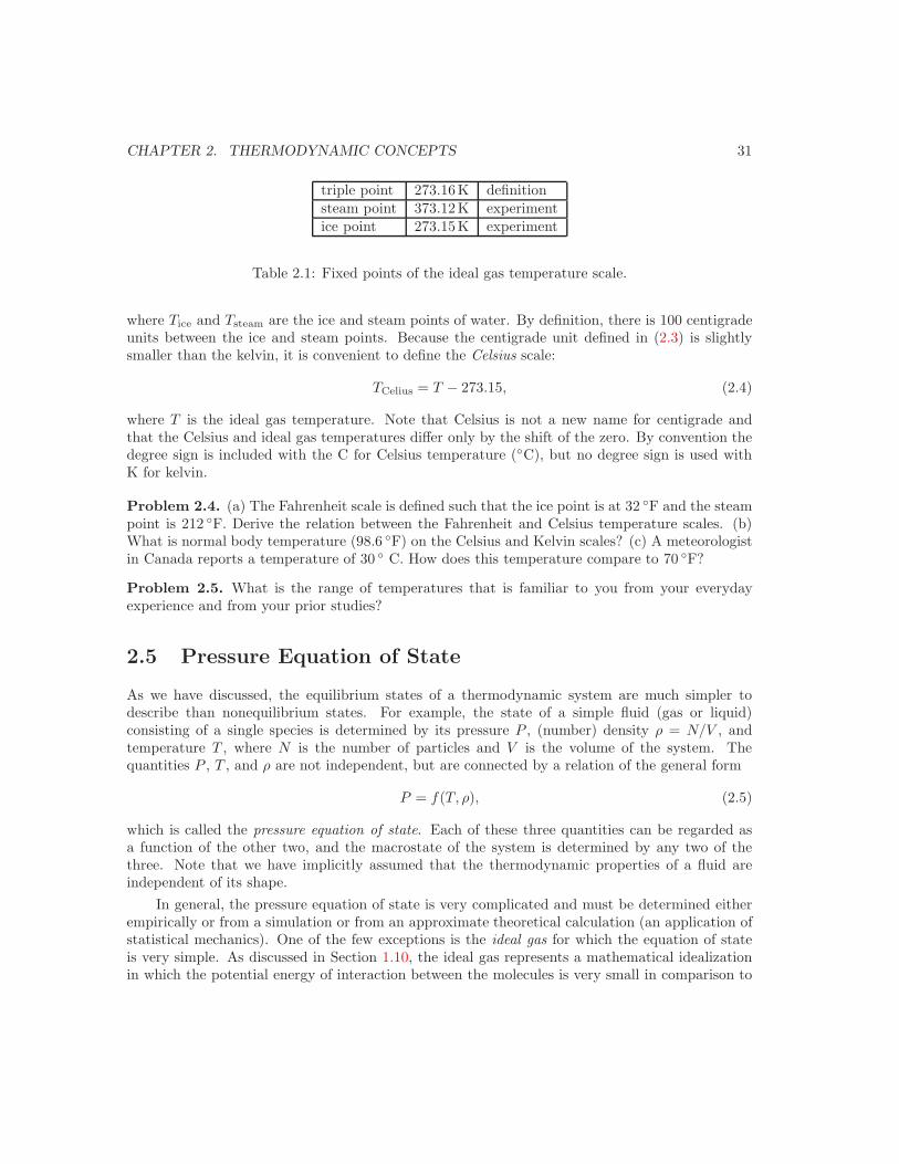
CHAPTER 2. THERMODYNAMIC CONCEPTS 31

triple point 273.16K definitionsteam point 373.12K experimentice point 273.15K experiment

Table 2.1: Fixed points of the ideal gas temperature scale.

where Tice and Tsteam are the ice and steam points of water. By definition, there is 100 centigradeunits between the ice and steam points. Because the centigrade unit defined in (2.3) is slightlysmaller than the kelvin, it is convenient to define the Celsius scale:

TCelius = T − 273.15, (2.4)

where T is the ideal gas temperature. Note that Celsius is not a new name for centigrade andthat the Celsius and ideal gas temperatures differ only by the shift of the zero. By convention thedegree sign is included with the C for Celsius temperature (C), but no degree sign is used withK for kelvin.

Problem 2.4. (a) The Fahrenheit scale is defined such that the ice point is at 32 F and the steampoint is 212 F. Derive the relation between the Fahrenheit and Celsius temperature scales. (b)What is normal body temperature (98.6 F) on the Celsius and Kelvin scales? (c) A meteorologistin Canada reports a temperature of 30 C. How does this temperature compare to 70 F?

Problem 2.5. What is the range of temperatures that is familiar to you from your everydayexperience and from your prior studies?

2.5 Pressure Equation of State

As we have discussed, the equilibrium states of a thermodynamic system are much simpler todescribe than nonequilibrium states. For example, the state of a simple fluid (gas or liquid)consisting of a single species is determined by its pressure P , (number) density ρ = N/V , andtemperature T , where N is the number of particles and V is the volume of the system. Thequantities P , T , and ρ are not independent, but are connected by a relation of the general form

P = f(T, ρ), (2.5)

which is called the pressure equation of state. Each of these three quantities can be regarded asa function of the other two, and the macrostate of the system is determined by any two of thethree. Note that we have implicitly assumed that the thermodynamic properties of a fluid areindependent of its shape.

In general, the pressure equation of state is very complicated and must be determined eitherempirically or from a simulation or from an approximate theoretical calculation (an application ofstatistical mechanics). One of the few exceptions is the ideal gas for which the equation of stateis very simple. As discussed in Section 1.10, the ideal gas represents a mathematical idealizationin which the potential energy of interaction between the molecules is very small in comparison to

CHAPTER 2. THERMODYNAMIC CONCEPTS 32

their kinetic energy and the system can be treated classically. For an ideal gas, we have for fixedtemperature the empirical relation:

P ∝ 1V

. (fixed temperature) (2.6)

orPV = constant. (2.7)

The relation (2.7) is sometimes called Boyle’s law and was published by Robert Boyle in 1660.Note that the relation (2.7) is not a law of physics, but an empirical relation. An equation such as(2.7), which relates different states of a system all at the same temperature, is called an isotherm.

We also have the empirical relation

V ∝ T. (fixed pressure) (2.8)

Some textbooks refer to (2.8) as Charles’s law, but it should be called the law of Gay-Lussac.We can express the two empirical relations, (2.7) and (2.8), as P ∝ T/V . In addition, if we

hold T and P constant and introduce more gas into the system, we find that the pressure increasesin proportion to the amount of gas. If N is the number of gas molecules, we can write

PV = NkT, (ideal gas pressure equation of state) (2.9)

where the constant of proportionality k in (2.9) is found experimentally to have the same value forall gases in the limit P → 0. The value of k is

k = 1.38 × 10−23 J/K, (Boltzmann’s constant) (2.10)

and is called Boltzmann’s constant. The relation (2.9) will be derived using statistical mechanicsin Section 4.5.

Because the number of particles in a typical gas is very large, it sometimes is convenient tomeasure this number relative to the number of particles in one mole of gas. A (gram) mole ofany substance consists of Avogadro’s number, NA = 6.022 × 1023, of that substance. Avogadro’snumber is defined so that 12.0 g of 12C atoms contain exactly one mole of these atoms. If thereare ν moles, then N = νNA, and the ideal gas equation of state can be written as

PV = νNAkT = νRT, (2.11)

whereR = NAk = 8.314 J/K mole (2.12)

is the gas constant.Real gases do not satisfy the ideal gas equation of state except in the limit of low density. For

now we will be satisfied with considering a simple phenomenological4 equation of state of a realgas with an interparticle interaction similar to the Lennard-Jones potential (see Figure 1.1). The

4Phenomenological is a word that we will use often. It means a description of the phenomena; such a descriptionis not derived from fundamental considerations.

CHAPTER 2. THERMODYNAMIC CONCEPTS 33

simplest phenomenological pressure equation of state that describes the behavior of real gases atmoderate densities is due to van der Waals and has the form

(P +N2

V 2a)(V − Nb) = NkT, (van der Waals equation of state) (2.13)

where a and b are empirical constants characteristic of the particular gas. The parameter b takesinto account the finite size of the molecules by decreasing the effective available volume to any givenmolecule. The parameter a is associated with the attractive interactions between the molecules.We will derive this approximate equation of state in Section 8.2.

2.6 Some Thermodynamic Processes

A change from one equilibrium state of the system to another is called a thermodynamic process.Thermodynamics cannot determine how much time such a process will take, and the final stateis independent of the amount of time it takes to reach equilibrium. It is convenient to considerthermodynamic processes where a system is taken from an initial to a final state by a continuoussuccession of intermediate states. To describe a process in terms of thermodynamic variables, thesystem must be in thermodynamic equilibrium. However, for the process to occur, the system can-not be exactly in thermodynamic equilibrium because at least one of the thermodynamic variablesis changing. However, if the change is sufficiently slow, the process is quasistatic, and the systemcan be considered to be in a succession of equilibrium states. A quasistatic process is an idealizedconcept. Although no physical process is quasistatic, we can imagine real processes that approachthe limit of quasistatic processes.

Some thermodynamic processes can go only in one direction and others can go in eitherdirection. For example, a scrambled egg cannot be converted to a whole egg. Processes that cango only in one direction are called irreversible. A process is reversible if it is possible to restore thesystem and its surroundings to their original condition. (The surroundings include any body thatwas affected by the change.) That is, if the change is reversible, the status quo can be restoredeverywhere.

Processes such as stirring the milk in a cup of coffee or passing an electric current through aresistor are irreversible because once the process is done, there is no way of reversing the process.But suppose we make a small and very slow frictionless change of a constraint such as an increasein the volume, which we then reverse. Because there is no friction, we do no net work in thisprocess. At the end of the process, the constraints and the energy of the system return to theiroriginal values and the state of the system is unchanged. In this case we can say that this processis reversible. Of course, no real process is truly reversible because it would require an infinite timeto occur. The relevant question is whether the process approaches reversibility.

Consider a gas in a closed, insulated container that is divided into two chambers by an imper-meable partition. The gas is initially confined to one chamber and then allowed to expand freelyinto the second chamber to fill the entire container. What is the nature of this process? The processis certainly not quasistatic. But we can imagine this process to be performed quasistatically. Wecould divide the second chamber into many small chambers separated by partitions and punctureeach partition in turn, allowing the expanded gas to come into equilibrium. So in the limit of an

CHAPTER 2. THERMODYNAMIC CONCEPTS 34

infinite number of partitions, such a process would be quasistatic. However this process would notbe reversible, because the gas would never return to its original volume.

Problem 2.6. Are the following processes reversible or irreversible?

(a) Air is pumped into a tire.

(b) Air leaks out of a tire.

2.7 Work

During a process the surroundings can do work on the system of interest or the system can dowork on its surroundings. We now obtain an expression for the mechanical work done on a systemin a quasistatic process. For simplicity, we assume the system to be a fluid. Because the fluid isin equilibrium, we can characterize it by a uniform pressure P . For simplicity, we assume that thefluid is contained in a cylinder of cross-sectional area A fitted with a movable piston. The pistonis girded by rings so that no gas or liquid can escape (see Figure 2.2). We can add weights to thepiston causing it to compress the fluid. Because the pressure is defined as the force per unit area,the magnitude of the force exerted by the fluid on the piston is given by PA, which also is theforce exerted by the piston on the fluid. If the piston is displaced quasistatically by an amount dx,then the work done on the fluid by the piston is given by5

dW = −(PA) dx = −P (Adx) = −PdV. (2.15)

The negative sign in (2.15) is present because if the volume of the fluid is decreased, the work doneby the piston is positive.

If the volume of the fluid changes quasistatically from a initial volume V1 to a final volume V2,the system remains very nearly in equilibrium, and hence its pressure at any stage is a function ofits volume and temperature. Hence, the total work is given by the integral

W1→2 = −∫ V2

V1

P (T, V ) dV. (quasistatic process) (2.16)

Note that the work done on the fluid is positive if V2 < V1 and is negative if V2 > V1.For the special case of an ideal gas, the work done on a gas that is compressed at constant

temperature is given by

W1→2 = −NkT

∫ V2

V1

dV

V

= −NkT lnV2

V1. (ideal gas at constant temperature) (2.17)

5Equation (2.15) can be written asdW

dt= −P

dV

dt, (2.14)

if the reader does not like the use of differentials. See Appendix 2B.

CHAPTER 2. THERMODYNAMIC CONCEPTS 35

F = PA

P

∆x

Figure 2.2: Example of work done on a fluid enclosed within a cylinder fitted with a piston whenthe latter moves a distance ∆x.

Figure 2.3: A block on an frictionless incline. The figure is taken from Loverude et al.

We have noted that the pressure P must be uniform throughout the fluid. But compressioncannot occur if pressure gradients are not present. To move the piston from its equilibrium position,we must add (remove) a weight from it. Then for a moment, the total weight on the piston will begreater than PA. This difference is necessary if the piston is to move downward and do work onthe gas. If the movement is sufficiently slow, the pressure departs only slightly from its equilibriumvalue. What does “sufficiently slow” mean? To answer this question, we have to go beyond themacroscopic reasoning of thermodynamics and consider the molecules that comprise the fluid. Ifthe piston is moved downward a distance ∆x, then the density of the molecules near the pistonbecomes greater than the bulk of the fluid. Consequently, there is a net movement of moleculesaway from the piston until the density again becomes uniform. The time τ for the fluid to return toequilibrium is given by τ ≈ ∆x/vs, where vs is the mean speed of the molecules (see Section 6.4).For comparison, the characteristic time τp for the process is τp ≈ ∆x/vp, where vp is the speed ofthe piston. If the process is to be quasistatic, it is necessary that τ τp or vp vs. That is, thespeed of the piston must be much less than the mean speed of the molecules, a condition that iseasy to satisfy in practice.

Problem 2.7. To refresh your understanding of work in the context of mechanics, look at Fig. 2.3and explain whether the following quantities are positive, negative, or zero: (a) The work done onthe block by the hand. (b) The work done on the block by the earth. (c) The work done on thehand by the block (if there is no such work, state so explicitly).

Work depends on the path. The solution of the following example illustrates that the work

CHAPTER 2. THERMODYNAMIC CONCEPTS 36

P

P2

P1

V1 V2 V

A B

CD

Figure 2.4: A simple cyclic process. What is the net work done on the gas?

done on a system depends not only on the initial and final states, but also on the intermediatestates, that is, on the path.

Example 2.1. Cyclic processesFigure 2.4 shows a cyclic path ABCDA in the PV diagram of an ideal gas. How much work isdone on the gas during this cyclic process? (Look at the figure before you attempt to answer thequestion.)

Solution. During the isobaric expansion A → B, the work done on the gas is

WAB = −P2(V2 − V1). (2.18)

No work is done from B → C and from D → A. The work done on the gas from C → D is

WCD = −P1(V1 − V2). (2.19)

The net work done on the gas is then

Wnet = WAB + WCD = −P2(V2 − V1) − P1(V1 − V2)= −(P2 − P1)(V2 − V1) < 0. (2.20)

The result is that the net work done on the gas is the negative of the area enclosed by the path.If the cyclic process were carried out in the reverse order, the net work done on the gas would bepositive.

Because the system was returned to its original pressure and volume, why is the net amountof work done not zero? What would be the work done if the gas were taken from V2 to V1 alongthe diagonal path connecting C and A?

CHAPTER 2. THERMODYNAMIC CONCEPTS 37

2.8 The First Law of Thermodynamics

If we think of a macroscopic system as consisting of a large number of interacting particles, weknow that it has a well defined total energy which satisfies a conservation principle. This simplejustification of the existence of a thermodynamic energy function is very different from the histor-ical development because thermodynamics was developed before the atomic theory of matter waswell accepted. Historically, the existence of a macroscopic conservation of energy principle wasdemonstrated by purely macroscopic observations as outlined in the following.6

Consider a system enclosed by insulating walls – walls that prevent the system from beingheated by the environment. Such a system is thermally isolated. A process in which the state of thesystem is changed only by work done on the system is called adiabatic. We know from overwhelmingempirical evidence that the amount of work needed to change the state of a thermally isolatedsystem depends only on the initial and final states and not on the intermediate states throughwhich the system passes. This independence of the path under these conditions implies that wecan define a function E such that for a change from state 1 to state 2, the work done on a thermallyisolated system equals the change in E:

W = E2 − E1 = ∆E. (adiabatic process) (2.21)

The quantity E is called the (internal) energy of the system.7 The internal energy in (2.21) ismeasured with respect to the center of mass.8 The energy E is an example of a state function,that is, it characterizes the state of a macroscopic system and is independent of the path.

Problem 2.8. What the difference between the total energy and the internal energy?

If we choose a convenient reference state as the zero of energy, then E has an unique value foreach state of the system because W is independent of the path for an adiabatic process. (Rememberthat in general W depends on the path.)

If we relax the condition that the change be adiabatic and allow the system to interact withits surroundings, we would find in general that ∆E = W . (The difference between ∆E and W iszero for an adiabatic process.) In general, we know that we can increase the energy of a systemby doing work on it or by heating it as a consequence of a temperature difference between it andits surroundings. In general, the change in the internal energy of a closed system (fixed number ofparticles) is given by

∆E = W + Q. (first law of thermodynamics) (2.22)

The quantity Q is the change in the system’s energy due to heating (Q > 0) or cooling (Q < 0) andW is the work done on the system. Equation (2.22) expresses the law of conservation of energyand is known as the first law of thermodynamics. This equation is equivalent to saying that thereare two macroscopic ways of changing the internal energy of a system: doing work and heating.

6These experiments were done by Joseph Black (1728–1799), Benjamin Thompson (Count Rumford) (1753–1814), especially Robert Mayer (1814–1878), and James Joule (1818–1889). Mayer and Joule are now recognized asthe co-discovers of the first law of thermodynamics, but Mayer received little recognition at the time of his work.

7Another common notation for the internal energy is U .8Microscopically, the internal energy of a system of particles is the sum of the kinetic energy in a reference frame

in which the center of mass velocity is zero and the potential energy arising from the forces of the particles on eachother.

CHAPTER 2. THERMODYNAMIC CONCEPTS 38

One consequence of the first law of thermodynamics is that ∆E is independent of the path,even though the amount of work W does depend on the path. And because W depends on thepath and ∆E does not, the amount of heating also depends on the path.

Problem 2.9. A cylindrical pump contains one mole of a gas. The piston fits tightly so that no airescapes and friction in negligible between the piston and the cylinder walls. The pump is thermallyinsulated from its surroundings. The piston is quickly pressed inward. What will happen to thetemperature of the gas? Explain your reasoning.

So far we have considered two classes of thermodynamic quantities. One class consists of statefunctions because they have a specific value for each macroscopic state of the system. An exampleof such a function is the internal energy E. As we have discussed, there are other quantities, suchas work and energy transfer due to heating, that do not depend on the state of the system. Theselatter quantities depend on the thermodynamic process by which the system changed from onestate to another.

Originally, many scientists thought that there was a fluid called heat in all substances whichcould flow from one substance to another. This idea was abandoned many years ago, but is stillused in everyday language. Thus, people talk about adding heat to a system. We will avoid this useand whenever possible we will avoid the use of the noun “heat” altogether. Instead, we will referto a process as heating or cooling if it changes the internal energy of a system without changingany external parameters (such as the external pressure, electric field, magnetic field, etc). Heatingoccurs whenever two solids at different temperatures are brought into thermal contact. In everydaylanguage we would say that heat flows from the hot to the cold body. However, we prefer to saythat energy is transferred from the hotter to the colder body. There is no need to invoke the noun“heat,” and it is misleading to say that heat “flows” from one body to another.

To understand better that there is no such thing as the amount of heat in a body, considerthe following simple analogy adapted from Callen.9 A farmer owns a pond, fed by one stream anddrained by another. The pond also receives water from rainfall and loses water by evaporation.The pond is the system of interest, the water within it is analogous to the internal energy, theprocess of transferring water by the streams is analogous to doing work, the process of addingwater by rainfall is analogous to heating, and the process of evaporation is analogous to cooling.The only quantity of interest is the water, just as the only quantity of interest is energy in thethermal case. An examination of the change in the amount of water in the pond cannot tell ushow the water got there. The terms rain and evaporation refer only to methods of water transfer,just as the terms heating and cooling refer only to methods of energy transfer.

Another example is due to Bohren and Albrecht.10 Take a small plastic container and addjust enough water to it so that its temperature can be conveniently measured. Then let the waterand the bottle come into equilibrium with their surroundings. Measure the temperature of thewater, cap the bottle, and shake the bottle until you are too tired to continue further. Then uncapthe bottle and measure the water temperature again. If there were a “whole lot of shaking goingon,” you would find the temperature had increased a little.

In this example, the temperature of the water increased without heating. We did work onthe water, which resulted in an increase in its internal energy as manifested by a rise in the

9See page 20.10See page 25.

CHAPTER 2. THERMODYNAMIC CONCEPTS 39

temperature. The same increase in temperature could have been obtained by bringing the waterinto contact with a body at a higher temperature. But it would be impossible to determine bymaking measurements on the water whether shaking or heating had been responsible for takingthe system from its initial to its final state. (To silence someone who objects that you heated thewater with “body heat,” wrap the bottle with an insulating material.)

Problem 2.10. How could the owner of the pond distinguish between the different types of watertransfer assuming that the owner has flow meters, a tarpaulin, and a vertical pole?

Problem 2.11. Convert the following statement to the language used by physicists, “I am cold,please turn on the heat.”

Before the equivalence of heating and energy transfer was well established, a change in energyby heating was measured in calories. One calorie is the amount of energy needed to raise thetemperature of one gram of water from 14.5 C to 15.5 C. We now know that one calorie isequivalent to 4.186 J, but the use of the calorie for energy transfer by heating and the joule forwork still persists. Just to cause confusion, the calorie we use to describe the energy content offoods is actually a kilocalorie.

2.9 Energy Equation of State

In (2.9) we gave the pressure equation of state for an ideal gas. Now that we know that the internalenergy also determines the state of a system of particles, we need to know how E depends on twoof the three variables, T and P or V . The form of the energy equation of state for an ideal gasmust also be determined empirically or calculated from first principles using statistical mechanics(see Section 4.5). From these considerations the energy equation of state for a monatomic gas isgiven by

E =32NkT. (ideal gas energy equation of state) (2.23)

Note that the energy of an ideal gas is independent of its volume.Similarly, the approximate thermal equation of state of a real gas corresponding to the pressure

equation of state (2.13) is given by

E =32NkT − N

N

Va. (van der Waals energy equation of state) (2.24)

Note that the energy depends on the volume if the interactions between particles is included.

Example 2.2. Work is done on an ideal gas at constant temperature. (a) What is the change inthe energy11 of the gas?Solution.

Because the energy of an ideal gas depends only on the temperature (see (2.23)), there is nochange in its internal energy for an isothermal (constant temperature) process. Hence, ∆E = 0 =Q + W , and

Q = −W = NkT lnV2

V1. (isothermal process for an ideal gas) (2.25)

11We actually mean the internal energy, but the meaning should be clear from the context.

CHAPTER 2. THERMODYNAMIC CONCEPTS 40

We see that if work is done on the gas (V2 < V1), then the gas must give energy to its surroundingsso that its temperature does not change.

Extensive and intensive variables. The thermodynamic variables that we have introduced sofar may be divided into two classes. Quantities such as the density ρ, the pressure P , and thetemperature T are intensive variables and are independent of the size of the system. Quantitiessuch as the volume V and the internal energy E are extensive variables and are proportional tothe number of particles in the system (at fixed density). As we will see in Section 2.10, it oftenis convenient to convert extensive quantities to a corresponding intensive quantity by defining theratio of two extensive quantities. For example, the energy per particle and the energy per per unitmass are intensive quantities.

2.10 Heat Capacities and Enthalpy

We know that the temperature of a macroscopic system usually increases when we transfer energyto it by heating.12 The magnitude of the increase in temperature depends on the nature of thebody and how much of it there is. The amount of energy transfer due to heating required toproduce a unit temperature rise in a given substance is called the heat capacity of that substance.Here again we see the archaic use of the word “heat.” But because the term “heat capacity” iscommon, we are forced to use it. If a body undergoes an increase of temperature from T1 to T2

accompanied by an energy transfer due to heating Q, then the average heat capacity is given bythe ratio

average heat capacity =Q

T2 − T1. (2.26)

The value of the heat capacity depends on what constraints are imposed. We introduce the heatcapacity at constant volume by the relation

CV =(∂E

∂T

)V

. (2.27)

Note that if the volume V is held constant, the change in energy of the system is due only tothe energy transferred by heating. We have adopted the common notation in thermodynamics ofenclosing partial derivatives in parentheses and using subscripts to denote the variables that areheld constant. In this context, it is clear that the differentiation in (2.27) is at constant volume,and we will write CV = ∂E/∂T if there is no ambiguity.13 (See Appendix 2B for a discussion ofthe mathematics of thermodynamics.)

Equation (2.27) together with (2.23) can be used to obtain the heat capacity at constantvolume of a monatomic ideal gas:

CV =32Nk. (monatomic ideal gas) (2.28)

Note that the heat capacity at constant volume of an ideal gas is independent of the temperature.12Can you think of an counterexample?13Although the number of particles also is held constant, we will omit the subscript N in (2.27) and in other

partial derivatives to reduce the number of subscripts.

CHAPTER 2. THERMODYNAMIC CONCEPTS 41

The heat capacity is an extensive quantity, and it is convenient to introduce the specificheat which depends only on the nature of the material, not on the amount of the material. Theconversion to an intensive quantity can be achieved by dividing the heat capacity by the amountof the material expressed in terms of the number of moles, the mass, or the number of particles.We will use lower case c for specific heat; the distinction between the various kinds of specific heatswill be clear from the context and the units of c.

The enthalpy. The combination of thermodynamic variables, E + PV , occurs sufficiently oftento acquire its own name. The enthalpy H is defined as

H = E + PV. (enthalpy) (2.29)

We can use (2.29) to find a simple expression for CP , the heat capacity at constant pressure. From(2.15) and (2.22), we have dE = dQ − PdV or dQ = dE + PdV (at constant pressure). From theidentity, d(PV ) = PdV + V dP , we can write dQ = dE + d(PV ) − V dP . At constant pressuredQ = dE + d(PV ) = d(E + PV ) = dH . Hence, we can define the heat capacity at constantpressure as

CP =∂H

∂T, (2.30)

where we have suppressed noting that the pressure P is held constant during differentiation. Wewill learn that the enthalpy is another state function that often makes the analysis of a systemsimpler. At this point, we can only see that CP can be expressed more simply in terms of theenthalpy.

Problem 2.12. (a) Give some of examples of materials that have a relatively low and relativelyhigh heat capacity. (b) Why do we have to distinguish between the heat capacity at constantvolume and the heat capacity at constant pressure?

Example 2.3. A water heater holds 150kg of water. How much energy is required to raise thewater temperature from 18 C to 50 C?Solution. The (mass) specific heat of water is c = 4184J/kg K. (The difference between the specificheats of water at constant volume and constant pressure is negligible at room temperatures.) Theenergy required to raise the temperature by 32 C is

Q = mc(T2 − T1) = 150 kg × (4184 J/kgK) × (50 C − 18 C)

= 2 × 107 J.

We have assumed that the specific heat is constant in this temperature range.

Note that because the kelvin is exactly the same magnitude as a degree Celsius, it often ismore convenient to express temperature differences in degrees Celsius.

Example 2.4. A 1.5 kg glass brick is heated to 180 C and then plunged into a cold bath containing10 kg of water at 20 C. Assume that none of the water boils and that there is no heating of thesurroundings. What is the final temperature of the water and the glass? The specific heat of glassis approximately 750 J/kgK.

CHAPTER 2. THERMODYNAMIC CONCEPTS 42

Solution. Conservation of energy implies that

∆Eglass + ∆Ewater = 0,

ormglasscglass(T − Tglass) + mwatercwater(T − Twater) = 0.

The final equilibrium temperature T is the same for both. We solve for T and obtain

T =mglasscglassTglass + mwatercwaterTwater

mglasscglass + mwatercwater

=(1.5 kg)(750 J/kgK)(180 C) + (10 kg)(4184 J/kgK)(20 C)

(1.5 kg)(750 J/kgK) + (10 kg)(4184 J/kgK)= 24.2 C.

Example 2.5. The temperature of one mole of helium gas is increased from 20 C to 40 C atconstant volume. How much energy is needed to accomplish this temperature change?Solution. Because the amount of He gas is given in moles, we need to know the molar specificheat. From (2.28) and (2.12), we have that cV = 3R/2 = 1.5× 8.314 = 12.5 J/moleK. Because cV

is constant (an excellent approximation), we have

∆E = Q =∫

CV dT = νcV

∫dT = 1 mole× 12.5

Jmole K

× 20 K = 250 J.

Example 2.6. At very low temperatures the heat capacity of an insulating solid is proportional toT 3. If we take C = AT 3 for a particular solid, what is the energy needed to raise the temperaturefrom T1 to T2? The difference between CV and CP can be ignored at low temperatures. (InSection 6.12, we use the Debye theory to express the constant A in terms of the speed of soundand other parameters and find the range of temperatures for which the T 3 behavior is a reasonableapproximation.)Solution. Because C is temperature-dependent, we have to express the energy added as an integral:

Q =∫ T2

T1

C(T ) dT. (2.31)

In this case we have

Q = A

∫ T2

T1

T 3 dT =A

4(T 4

2 − T 41 ). (2.32)

General relation between CP and CV . The first law can be used to find the general relation (2.36)between CP and CV . The derivation involves straightforward, but tedious manipulations of ther-modynamic derivatives. We give it here to give a preview of the general nature of thermodynamicarguments.

From (2.29) and (2.30), we have

CP =(∂H

∂T

)P

=(∂E

∂T

)P

+ P(∂V

∂T

)P

. (2.33)

CHAPTER 2. THERMODYNAMIC CONCEPTS 43

If we consider E to be a function of T and V , we can write

dE =(∂E

∂T

)V

dT +(∂E

∂V

)T

dV, (2.34)

and hence (by dividing by ∆T and taking the limit ∆T → 0 at constant P )

(∂E

∂T

)P

= CV +(∂E

∂V

)T

(∂V

∂T

)P

. (2.35)

If we eliminate (∂E/∂T )P in (2.33) by using (2.35), we obtain our desired result:

CP = CV +∂E

∂V

∂V

∂T+ P

∂V

∂T. (general result) (2.36)

Equation (2.36) is a general relation that depends only on the first law. A more useful generalrelation between CP and CV that depends on the second law of thermodynamics will be derivedin Section 7.3.2.

For the special case of an ideal gas, ∂E/∂V = 0 and ∂V/∂T = Nk/P , and hence

CP = CV + Nk (ideal gas) (2.37)

Note that CP is bigger than CV , a general result for any macroscopic body. Note that we usedthe two equations of state for an ideal gas, (2.9) and (2.23), to obtain CP , and we did not have tomake an independent measurement or calculation.

Why is CP bigger than CV ? Unless we prevent it from doing so, a system normally expandsas its temperature increases. The system has to do work on its surroundings as it expands. Hence,when a system is heated at constant pressure, energy is needed both to increase the temperatureof the system and to do work on its surroundings. In contrast, if the volume is kept constant, nowork is done on the surroundings and the heating only has to supply the energy required to raisethe temperature of the system.

The result (2.37) for CP for an ideal gas illustrates the power of thermodynamics. We useda general principle, the first law, and one equation of state to determine CP , a quantity thatwe did not know directly. In Chapter 7 we will derive the general relation CP > CV for anythermodynamic system.

2.11 Adiabatic Processes

So far we have considered processes at constant temperature, constant volume, and constant pres-sure.14 We have also considered adiabatic processes which occur when the system does not exchangeenergy with its surroundings due to a temperature difference. Note that an adiabatic process neednot be isothermal. For example, a chemical reaction that occurs within a container that is wellinsulated is not isothermal.

Problem 2.13. Give an example of an isothermal process that is not adiabatic.14These processes are called isothermal, isochoric, and isobaric, respectively.

CHAPTER 2. THERMODYNAMIC CONCEPTS 44

We now show that the pressure of an ideal gas changes more rapidly for a given change ofvolume in a quasistatic adiabatic process than it does in an isothermal process. For an adiabaticprocess the first law reduces to

dE = dW. (adiabatic process) (2.38)

For an ideal gas we have ∂E/∂V = 0, and hence (2.34) reduces to

dE = CV dT = −PdV, (ideal gas only) (2.39)

where we have used (2.38). The easiest way to proceed is to eliminate P in (2.39) using the idealgas law PV = NkT :

CV dT = −NkTdV

V(2.40)

We next eliminate Nk in (2.40) in terms of CP − CV and express (2.40) as

CV

CP − CV

dT

T=

1γ − 1

dT

T= −dV

V, (2.41)

where the symbol γ is the ratio of the heat capacities:

γ =CP

CV. (2.42)

For an ideal gas CV and CP and hence γ are independent of temperature, and we can integrate(2.41) to obtain

TV γ−1 = constant. (quasistatic adiabatic process) (2.43)

For an ideal monatomic gas, we have from (2.28) and (2.37) that CV = 3Nk/2 and CP =5Nk/2, and hence

γ = 5/3. (ideal monatomic gas) (2.44)

Problem 2.14. Use (2.43) and the ideal gas pressure equation of state in (2.9) to show that in aquasistatic adiabatic processes P and V are related as

PV γ = constant. (2.45)

Also show that T and P are related asTP (1−γ)/γ = constant. (2.46)

The relations (2.43)–(2.46) hold for a quasistatic adiabatic process of an ideal gas; the relation(2.45) is the easiest relation to remember. Because γ > 1, the relation (2.45) implies that fora given volume change, the pressure changes more for an adiabatic process than it does for acomparable isothermal process for which PV = constant. We can understand the reason for thisdifference as follows. For an isothermal compression the pressure increases and the internal energyof the gas does not change. For an adiabatic compression the energy increases because we havedone work on the gas and no energy can be transferred to the surroundings. The increase in theenergy causes the temperature to increase. Hence in an adiabatic compression, both the decreasein the volume and the increase in the temperature cause the pressure to increase faster.

CHAPTER 2. THERMODYNAMIC CONCEPTS 45

V

Ti

Tf

adiabatic

isotherm

isothermP

Figure 2.5: A P -V diagram for adiabatic and isothermal processes. The two processes begin atthe same initial temperature, but the adiabatic process has a steeper slope and ends at a highertemperature.

In Figure 2.5 we show the P -V diagram for both isothermal and adiabatic processes. Theadiabatic curve has a steeper slope than the isothermal curves at any point. From (2.45) we seethat the slope of an adiabatic curve for an ideal gas is

(∂P

∂V

)adiabatic

= −γP

V, (2.47)

in contrast to the slope of an isothermal curve for an ideal gas:

(∂P

∂V

)T

= −P

V. (2.48)

How can the ideal gas relations PV γ = constant and PV = NkT both be correct? The answeris that PV = constant only for an isothermal process. A quasistatic ideal gas process cannot beboth adiabatic (Q = 0) and isothermal (no temperature change). During an adiabatic process, thetemperature of an ideal gas must change.

Problem 2.15. Although we do work on an ideal gas when we compress it isothermally, why doesthe energy of the gas not increase?

CHAPTER 2. THERMODYNAMIC CONCEPTS 46

Example 2.7. Adiabatic and isothermal expansion. Two identical systems each contain ν =0.06mole of an ideal gas at T = 300K and P = 2.0 × 105 Pa. The pressure in the two systems isreduced by a factor of two allowing the systems to expand, one adiabatically and one isothermally.What are the final temperatures and volumes of each system? Assume that γ = 5/3.Solution. The initial volume V1 is given by

V1 =νRT1

P1=

0.060 mole× 8.3 J/(K mole)× 300 K2.0 × 105 Pa

= 7.5 × 10−4 m3.

For the isothermal system, PV remains constant, so the volume doubles as the pressuredecreases by a factor of two and hence V2 = 1.5× 10−3 m3. Because the process is isothermal, thetemperature remains at 300K.

For adiabatic compression we have

V γ2 =

P1Vγ1

P2,

orV2 =

(P1

P2

)1/γV1 = 23/5 × 7.5 × 10−4 m3 = 1.14 × 10−3 m3.

In this case we see that for a given pressure change, the volume change for the adiaabatic processis greater. We leave it as an exercise to show that T2 = 250K.

Problem 2.16. Air initially at 20C is compressed by a factor of 15. (a) What is the finaltemperature assuming that the compression is adiabatic and γ = 1.4, the value of γ for air atthe relevant range of temperatures? By what factor does the pressure increase? (b) What is thefinal pressure assuming the compression is isothermal? (c) In which case does the pressure changemore?

How much work is done in a quasistatic adiabatic process? Because Q = 0, ∆E = W . For anideal gas, ∆E = CV ∆T for any process. Hence for a quasistatic adiabatic process

W = CV (T2 − T1). (quasistatic adiabatic process for an ideal gas) (2.49)

We leave it to Problem 2.17 to show that (2.49) can be expressed in terms of the pressure andvolume as

W =P2V2 − P1V1

γ − 1. (2.50)

Problem 2.17. Another way to derive (2.50), the work done in a quasistatic adiabatic process,is to use the relation (2.45). Work out the steps.

Example 2.8. Compression in a Diesel engine occurs quickly enough so that very little heatingof the environment occurs and thus the process may be considered adiabatic. If a temperature of500 C is required for ignition, what is the compression ratio? Assume that γ = 1.4 for air and thetemperature is 20 C before compression.

CHAPTER 2. THERMODYNAMIC CONCEPTS 47

Solution. Equation (2.43) gives the relation between T and V for a quasistatic adiabatic process.We write T1 and V1 and T2 and V2 for the temperature and volume at the beginning and the endof the piston stroke. Then (2.45) becomes

T1Vγ−11 = T2V

γ−12 . (2.51)

Hence the compression ratio V1/V2 is

V1

V2=

(T2

T1

)1/(γ−1)

=(773 K

293 K

)1/0.4

= 11.

Of course it is only an approximation to assume that the compression is quasistatic.

2.12 The Second Law of Thermodynamics

The consequences of the first law of thermodynamics can be summarized by the statements that(a) energy is conserved in thermal processes and (b) heating is a form of energy transfer. We alsonoted that the internal energy of a system can be identified with the sum of the potential andkinetic energies of the particles (in a reference frame in which the center of mass velocity is zero.)

There are many processes that do not occur in nature, but whose occurrence would be consis-tent with the first law. For example, the first law does not prohibit energy from being transferredspontaneously from a cold body to a hot body, yet it has never been observed. There is anotherproperty of systems that must be taken into account, and this property is called the entropy.15

Entropy is another example of a state function. One of the remarkable achievements of thenineteenth century was the reasoning that such a state function must exist without any idea ofhow to measure its value directly. In Chapter 4 we will learn about the relationship between theentropy and the number of possible microscopic states, but for now we will follow a logic that doesnot depend on any knowledge of the microscopic behavior.

It is not uncommon to use heating as a means of doing work. For example, power plants burnoil or coal to turn water into steam which in turn turns a turbine in a magnetic field creatingelectricity which then can do useful work in your home. Can we completely convert all the energycreated by chemical reactions into work? Or more simply can we cool a system and use all theenergy lost by the system to do work? Our everyday experience tells us that we cannot. If itwere possible, we could power a boat to cross the Atlantic by cooling the sea and transferringenergy from the sea to drive the propellers. We would need no fuel and travel would be muchcheaper. Or instead of heating a fluid by doing electrical work on a resistor, we could considera process in which a resistor cools the fluid and produces electrical energy at its terminals. Thefact that these processes do not occur is summarized in one of the statements of the second law ofthermodynamics:

No process is possible whose sole result is the complete conversion of energy transferredby heating into work (Kelvin statement).

The second law implies that a perpetual motion machine of the second kind does not exist. Sucha machine would convert heat completely into work (see Figure 2.6).

15This thermodynamic variable was named by Rudolf Clausius, who wrote in 1850 that he formed the wordentropy (from the Greek word for transformation) so as to be as similar as possible to the word energy.

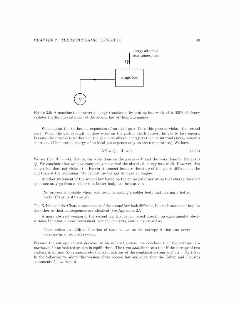
CHAPTER 2. THERMODYNAMIC CONCEPTS 48

magic box

Q

energy absorbedfrom atmosphere

light

Figure 2.6: A machine that converts energy transferred by heating into work with 100% efficiencyviolates the Kelvin statement of the second law of thermodynamics.

What about the isothermal expansion of an ideal gas? Does this process violate the secondlaw? When the gas expands, it does work on the piston which causes the gas to lose energy.Because the process is isothermal, the gas must absorb energy so that its internal energy remainsconstant. (The internal energy of an ideal gas depends only on the temperature.) We have

∆E = Q + W = 0. (2.52)

We see that W = −Q, that is, the work done on the gas is −W and the work done by the gas isQ. We conclude that we have completely converted the absorbed energy into work. However, thisconversion does not violate the Kelvin statement because the state of the gas is different at theend than at the beginning. We cannot use the gas to make an engine.

Another statement of the second law based on the empirical observation that energy does notspontaneously go from a colder to a hotter body can be stated as

No process is possible whose sole result is cooling a colder body and heating a hotterbody (Clausius statement).

The Kelvin and the Clausius statements of the second law look different, but each statement impliesthe other so their consequences are identical (see Appendix 2A).

A more abstract version of the second law that is not based directly on experimental obser-vations, but that is more convenient in many contexts, can be expressed as

There exists an additive function of state known as the entropy S that can neverdecrease in an isolated system.

Because the entropy cannot decrease in an isolated system, we conclude that the entropy is amaximum for an isolated system in equilibrium. The term additive means that if the entropy of twosystems is SA and SB, respectively, the total entropy of the combined system is Stotal = SA + SB.In the following we adopt this version of the second law and show that the Kelvin and Clausiusstatements follow from it.

CHAPTER 2. THERMODYNAMIC CONCEPTS 49

The statement of the second law in terms of the entropy is applicable only to isolated systems(a system enclosed by insulating, rigid, and impermeable walls). In general, the system of interestcan exchange energy with its surroundings. In many cases the surroundings may be idealized asa large body that does not interact with the rest of the universe. For example, we can take thesurroundings of a cup of hot water to be the atmosphere in the room. In this case we can treatthe composite system, system plus surroundings, as isolated. For the composite system, we havefor any process

∆Scomposite ≥ 0, (2.53)

where Scomposite is the entropy of the system plus its surroundings.If a change is reversible, we cannot have ∆Scomposite > 0, because if we reverse the change we

would have ∆Scomposite < 0, a violation of the Clausius statement. Hence, the only possibility isthat

∆Scomposite = 0. (reversible process) (2.54)

To avoid confusion, we will use the term reversible to be equivalent to a constant entropy process.The condition for a process to be reversible requires only that the total entropy of a closed systembe constant; the entropies of its parts may either increase or decrease.

2.13 The Thermodynamic Temperature

The Clausius and Kelvin statements of the second law arose from the importance of heat enginesto the development of thermodynamics. A seemingly different purpose of thermodynamics is todetermine the conditions of equilibrium. These two purposes are linked by the fact that wheneverthere is a difference of temperature, work can be extracted. So the possibility of work and theabsence of equilibrium are related.

In the following, we derive the properties of the thermodynamic temperature from the sec-ond law. In Section 2.16 we will show that this temperature is the same as the ideal gas scaletemperature.

Consider an isolated composite system that is partitioned into two subsystems A and B by afixed, impermeable, insulating wall. For the composite system we have

E = EA + EB = constant, (2.55)

V = VA + VB = constant, and N = NA + NB = constant. Because the entropy is additive, we canwrite the total entropy as

S(EA, VA, NA, EB, VB , NB) = SA(EA, VA, NA) + SB(EB , VB, NB). (2.56)

Most divisions of energy, EA and EB, between subsystems A and B do not correspond to thermalequilibrium.

For thermal equilibrium to be established, we replace the fixed, impermeable, insulating wallby a fixed, impermeable, conducting wall so that the two subsystems are in thermal contact andenergy transfer by heating or cooling can occur. We say that we have relaxed an internal constraint.According to our statement of the second law, the values of EA and EB will be such that the entropy

CHAPTER 2. THERMODYNAMIC CONCEPTS 50

of the system becomes a maximum. To find the value of EA that maximizes S as given by (2.56),we calculate

dS =( ∂SA

∂EA

)VA,NA

dEA +( ∂SB

∂EB

)VB ,NB

dEB. (2.57)

Because the total energy of the system is conserved, we have dEB = −dEA, and hence

dS =[( ∂SA

∂EA

)VA,NA

−( ∂SB

∂EB

)VB ,NB

]dEA. (2.58)

The condition for equilibrium is that dS = 0 for arbitrary values of dEA, and hence( ∂SA

∂EA

)VA,NA

=( ∂SB

∂EB

)VB ,NB

. (2.59)

Because the temperatures of the two systems are equal in thermal equilibrium, we conclude thatthe derivative ∂S/∂E must be associated with the temperature. We will find that it is convenientto define the thermodynamic temperature T as

1T

=( ∂S

∂E

)V,N

, (thermodynamic definition of temperature) (2.60)

which implies that the condition for thermal equilibrium is1

TA=

1TB

. (2.61)

Of course we can rewrite (2.61) as TA = TB.We have found that if two systems are separated by a conducting wall, energy will be trans-

ferred until each of the systems reaches the same temperature. We now suppose that the twosubsystems are initially separated by an insulating wall and that the temperatures of the two sub-systems are almost equal with TA > TB. If this constraint is removed, we know that energy willbe transferred across the conducting wall and the entropy of the composite system will increase.From (2.58) we can write the change in entropy as

∆S ≈ [ 1TA

− 1TB

]∆EA > 0, (2.62)

where TA and TB are the initial values of the temperatures. The condition that TA > TB, requiresthat ∆EA < 0 in order for ∆S > 0 in (2.62) to be satisfied. Hence, we conclude that the definition(2.60) of the thermodynamic temperature implies that energy is transferred from a system witha higher value of T to a system with a lower value of T . We can express (2.62) as: No processexists in which a cold body cools off while a hotter body heats up and the constraints on the bodiesand the state of its surroundings are left unchanged. We recognize this statement as the Clausiusstatement of the second law.

The definition (2.60) of T is not unique, and we could have replaced 1/T by other functionsof temperature such as 1/T 2 or 1/

√T . However, we will find in Section 2.16 that the definition

(2.60) implies that the thermodynamic temperature is identical to the ideal gas scale temperature.Note that the inverse temperature can be interpreted as the response of the entropy to a

change in the energy of the system. In Section 2.17, we will derive the condition for mechanicalequilibrium, and in Section 4.5 we will derive the condition for chemical equilibrium. These twoconditions complement the condition for thermal equilibrium. All three conditions must be satisfiedfor thermodynamic equilibrium to be established.

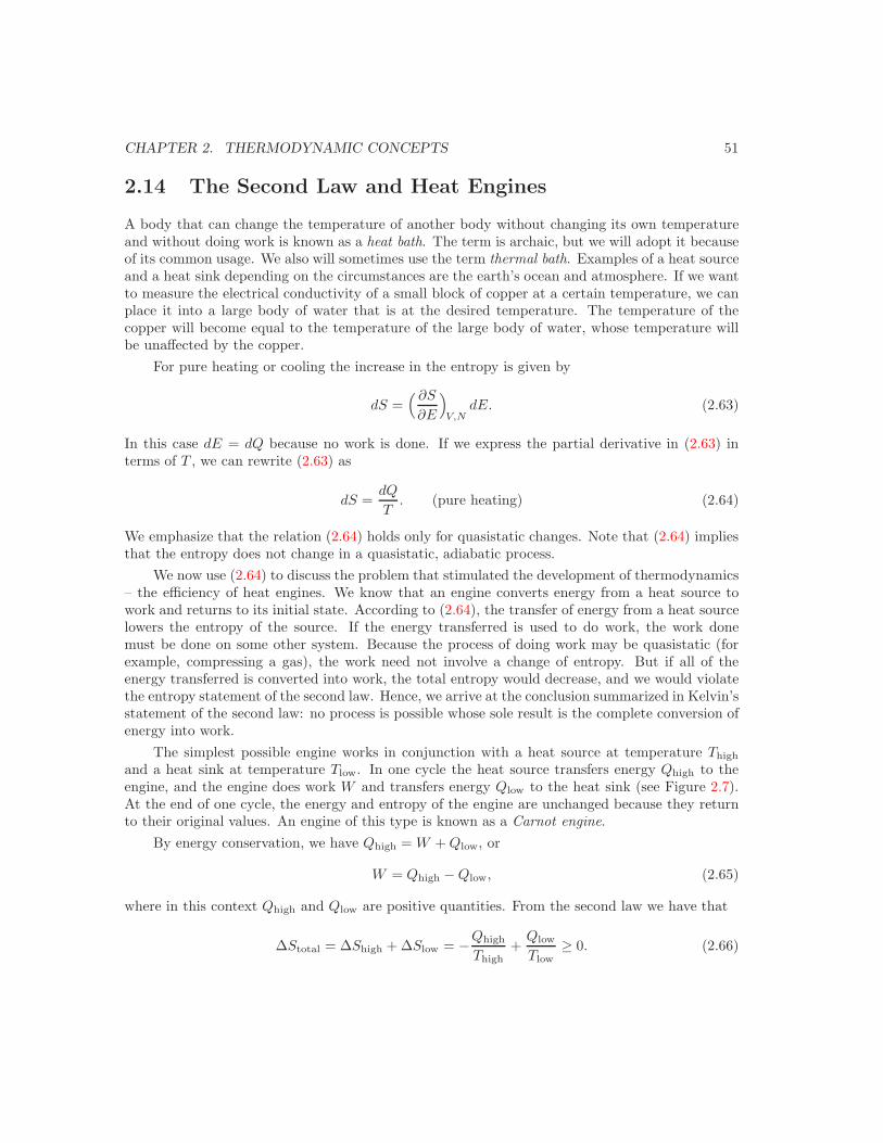
CHAPTER 2. THERMODYNAMIC CONCEPTS 51

2.14 The Second Law and Heat Engines

A body that can change the temperature of another body without changing its own temperatureand without doing work is known as a heat bath. The term is archaic, but we will adopt it becauseof its common usage. We also will sometimes use the term thermal bath. Examples of a heat sourceand a heat sink depending on the circumstances are the earth’s ocean and atmosphere. If we wantto measure the electrical conductivity of a small block of copper at a certain temperature, we canplace it into a large body of water that is at the desired temperature. The temperature of thecopper will become equal to the temperature of the large body of water, whose temperature willbe unaffected by the copper.

For pure heating or cooling the increase in the entropy is given by

dS =( ∂S

∂E

)V,N

dE. (2.63)

In this case dE = dQ because no work is done. If we express the partial derivative in (2.63) interms of T , we can rewrite (2.63) as

dS =dQ

T. (pure heating) (2.64)

We emphasize that the relation (2.64) holds only for quasistatic changes. Note that (2.64) impliesthat the entropy does not change in a quasistatic, adiabatic process.

We now use (2.64) to discuss the problem that stimulated the development of thermodynamics– the efficiency of heat engines. We know that an engine converts energy from a heat source towork and returns to its initial state. According to (2.64), the transfer of energy from a heat sourcelowers the entropy of the source. If the energy transferred is used to do work, the work donemust be done on some other system. Because the process of doing work may be quasistatic (forexample, compressing a gas), the work need not involve a change of entropy. But if all of theenergy transferred is converted into work, the total entropy would decrease, and we would violatethe entropy statement of the second law. Hence, we arrive at the conclusion summarized in Kelvin’sstatement of the second law: no process is possible whose sole result is the complete conversion ofenergy into work.

The simplest possible engine works in conjunction with a heat source at temperature Thigh

and a heat sink at temperature Tlow. In one cycle the heat source transfers energy Qhigh to theengine, and the engine does work W and transfers energy Qlow to the heat sink (see Figure 2.7).At the end of one cycle, the energy and entropy of the engine are unchanged because they returnto their original values. An engine of this type is known as a Carnot engine.

By energy conservation, we have Qhigh = W + Qlow, or

W = Qhigh − Qlow, (2.65)

where in this context Qhigh and Qlow are positive quantities. From the second law we have that

∆Stotal = ∆Shigh + ∆Slow = −Qhigh

Thigh+

Qlow

Tlow≥ 0. (2.66)

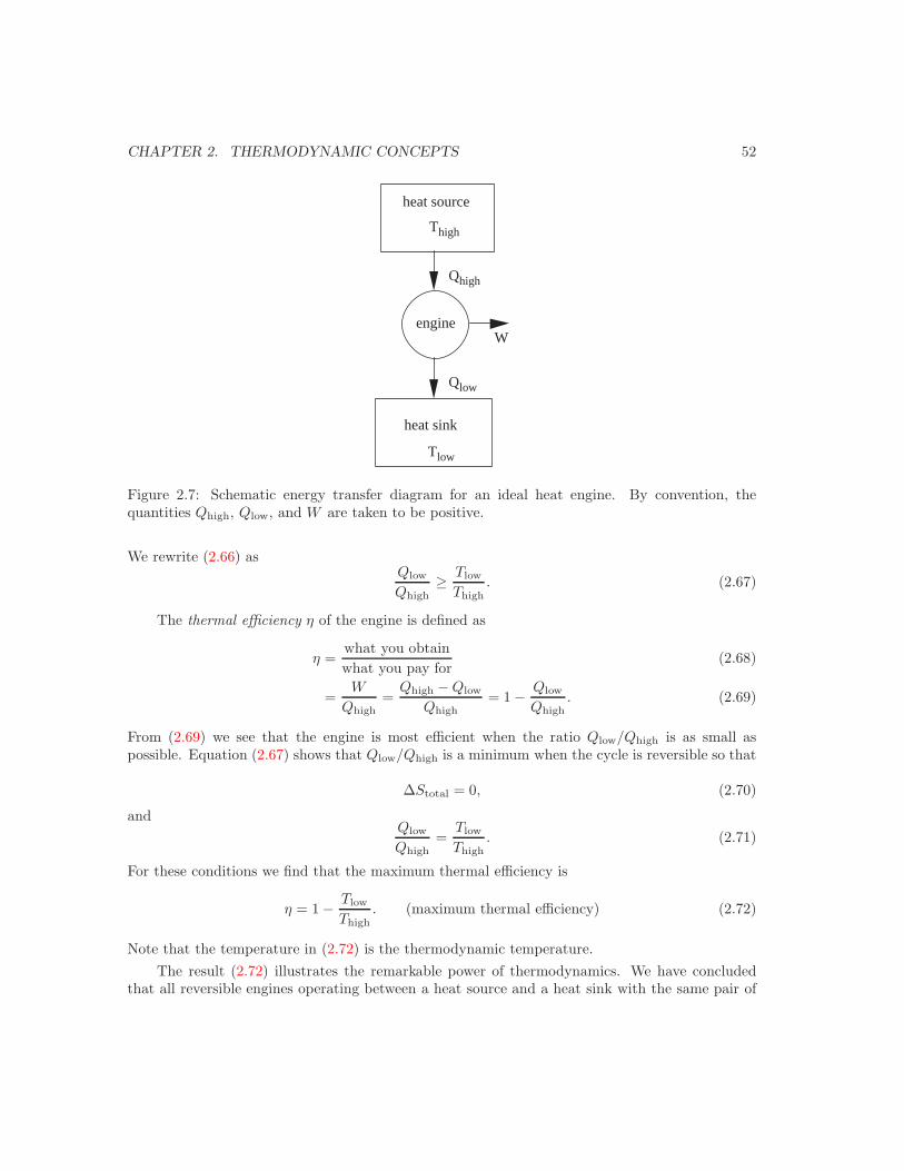
CHAPTER 2. THERMODYNAMIC CONCEPTS 52

heat source

Thigh

engine

heat sink

Tlow

Qhigh

Qlow

W

Figure 2.7: Schematic energy transfer diagram for an ideal heat engine. By convention, thequantities Qhigh, Qlow, and W are taken to be positive.

We rewrite (2.66) asQlow

Qhigh≥ Tlow

Thigh. (2.67)

The thermal efficiency η of the engine is defined as

η =what you obtainwhat you pay for

(2.68)

=W

Qhigh=

Qhigh − Qlow

Qhigh= 1 − Qlow

Qhigh. (2.69)

From (2.69) we see that the engine is most efficient when the ratio Qlow/Qhigh is as small aspossible. Equation (2.67) shows that Qlow/Qhigh is a minimum when the cycle is reversible so that

∆Stotal = 0, (2.70)

andQlow

Qhigh=

Tlow

Thigh. (2.71)

For these conditions we find that the maximum thermal efficiency is

η = 1 − Tlow

Thigh. (maximum thermal efficiency) (2.72)

Note that the temperature in (2.72) is the thermodynamic temperature.The result (2.72) illustrates the remarkable power of thermodynamics. We have concluded

that all reversible engines operating between a heat source and a heat sink with the same pair of

CHAPTER 2. THERMODYNAMIC CONCEPTS 53

temperatures have the same efficiency and that no irreversible engine working between the samepair of temperatures can have a greater efficiency. This statement is known as Carnot’s principle.That is, based on general principles, we have been able to determine the maximum efficiency of areversible engine without knowing anything about the details of the engine.

Of course, real engines never reach the maximum thermodynamic efficiency because of thepresence of mechanical friction and because the processes cannot really be quasistatic. For thesereasons, real engines seldom attain more than 30–40% of the maximum thermodynamic efficiency.Nevertheless, the basic principles of thermodynamics are an important factor in their design. Wewill discuss other factors that are important in the design of heat engines in Chapter 7.

Example 2.9. A Carnot engineA Carnot engine extracts 240 J from a heat source and rejects 100 J to a heat sink at 15 C duringeach cycle. How much work does the engine do in one cycle? What is its efficiency? What is thetemperature of the heat source?Solution. From the first law we have

W = 240 J− 100 J = 140 J.

The efficiency is given by

η =W

Qhigh=

140240

= 0.583 = 58.3%.

We can use this result for η and the general relation (2.72) to solve for Thigh:

Thigh =Tlow

1 − η=

288 K1 − 0.583

= 691 K.

Note that to calculate the efficiency, we must work with the thermodynamic temperature.

Example 2.10. The cycle of a hypothetical engine is illustrated in Figure 2.8. Let P1 = 1 × 106

Pa, P2 = 2 × 106 Pa, V1 = 5 × 10−3 m3, and V2 = 25 × 10−3 m3. If the energy absorbed byheating the engine is 5 × 104 J, what is the efficiency of the engine?Solution. The work done by the engine equals the area enclosed:

W =12(P2 − P1)(V2 − V1).

Confirm that W = 1 × 104 J. The efficiency is given by

η =W

Qabsorbed=

1 × 104

5 × 104= 0.20.

The maximum efficiency of a heat engine depends on the temperatures Thigh and Tlow ina simple way and not on the details of the cycle or working substance. The Carnot cycle is aparticular sequence of idealized processes of an ideal gas that yields the maximum thermodynamicefficiency given in (2.72). The four steps of the Carnot cycle (two adiabatic and two isothermalsteps) are illustrated in Figure 2.9. The initial state is at the point A. The gas is in contact with ahot heat bath at temperature Thigh so that the temperature of the gas also is Thigh. The piston ispushed in as far as possible so the volume is reduced. As a result of the relatively high temperatureand small volume, the pressure of the gas is high.

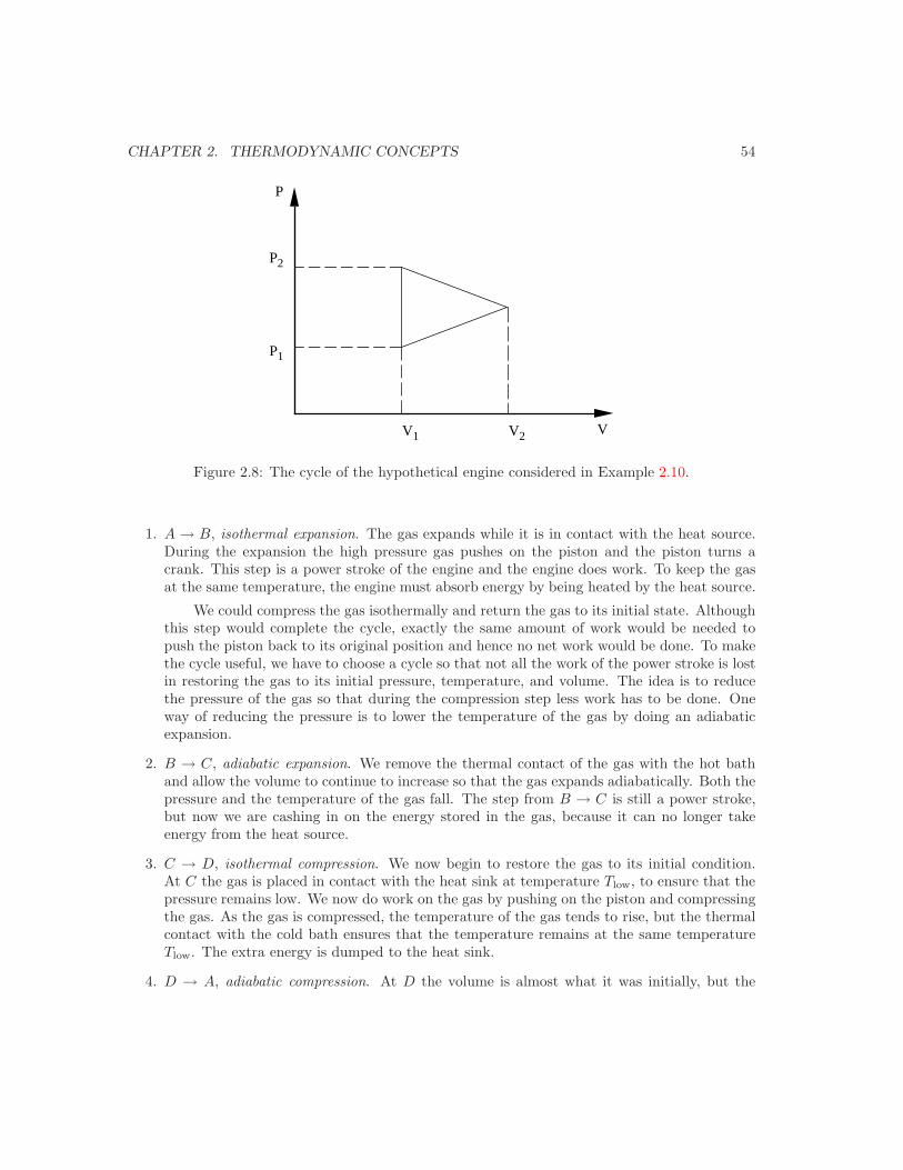
CHAPTER 2. THERMODYNAMIC CONCEPTS 54

P

P2

P1

V1 V2 V

Figure 2.8: The cycle of the hypothetical engine considered in Example 2.10.

1. A → B, isothermal expansion. The gas expands while it is in contact with the heat source.During the expansion the high pressure gas pushes on the piston and the piston turns acrank. This step is a power stroke of the engine and the engine does work. To keep the gasat the same temperature, the engine must absorb energy by being heated by the heat source.

We could compress the gas isothermally and return the gas to its initial state. Althoughthis step would complete the cycle, exactly the same amount of work would be needed topush the piston back to its original position and hence no net work would be done. To makethe cycle useful, we have to choose a cycle so that not all the work of the power stroke is lostin restoring the gas to its initial pressure, temperature, and volume. The idea is to reducethe pressure of the gas so that during the compression step less work has to be done. Oneway of reducing the pressure is to lower the temperature of the gas by doing an adiabaticexpansion.

2. B → C, adiabatic expansion. We remove the thermal contact of the gas with the hot bathand allow the volume to continue to increase so that the gas expands adiabatically. Both thepressure and the temperature of the gas fall. The step from B → C is still a power stroke,but now we are cashing in on the energy stored in the gas, because it can no longer takeenergy from the heat source.

3. C → D, isothermal compression. We now begin to restore the gas to its initial condition.At C the gas is placed in contact with the heat sink at temperature Tlow, to ensure that thepressure remains low. We now do work on the gas by pushing on the piston and compressingthe gas. As the gas is compressed, the temperature of the gas tends to rise, but the thermalcontact with the cold bath ensures that the temperature remains at the same temperatureTlow. The extra energy is dumped to the heat sink.

4. D → A, adiabatic compression. At D the volume is almost what it was initially, but the

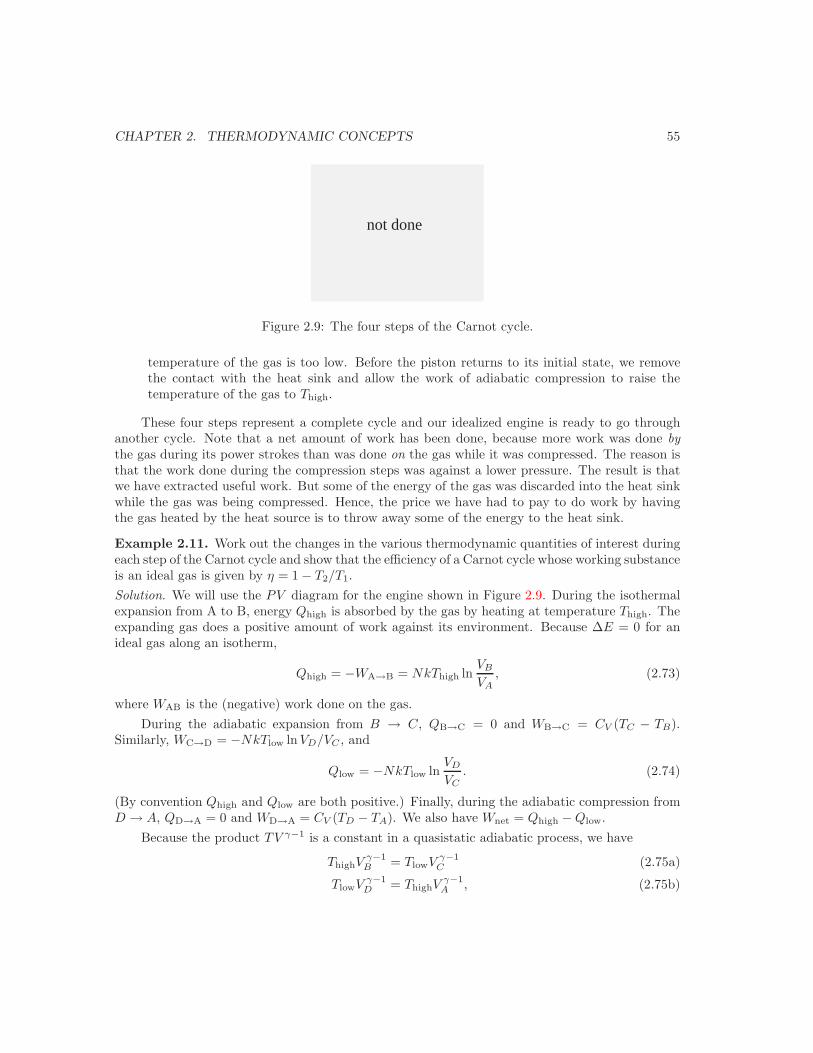
CHAPTER 2. THERMODYNAMIC CONCEPTS 55

not done

Figure 2.9: The four steps of the Carnot cycle.

temperature of the gas is too low. Before the piston returns to its initial state, we removethe contact with the heat sink and allow the work of adiabatic compression to raise thetemperature of the gas to Thigh.

These four steps represent a complete cycle and our idealized engine is ready to go throughanother cycle. Note that a net amount of work has been done, because more work was done bythe gas during its power strokes than was done on the gas while it was compressed. The reason isthat the work done during the compression steps was against a lower pressure. The result is thatwe have extracted useful work. But some of the energy of the gas was discarded into the heat sinkwhile the gas was being compressed. Hence, the price we have had to pay to do work by havingthe gas heated by the heat source is to throw away some of the energy to the heat sink.

Example 2.11. Work out the changes in the various thermodynamic quantities of interest duringeach step of the Carnot cycle and show that the efficiency of a Carnot cycle whose working substanceis an ideal gas is given by η = 1 − T2/T1.Solution. We will use the PV diagram for the engine shown in Figure 2.9. During the isothermalexpansion from A to B, energy Qhigh is absorbed by the gas by heating at temperature Thigh. Theexpanding gas does a positive amount of work against its environment. Because ∆E = 0 for anideal gas along an isotherm,

Qhigh = −WA→B = NkThigh lnVB

VA, (2.73)

where WAB is the (negative) work done on the gas.During the adiabatic expansion from B → C, QB→C = 0 and WB→C = CV (TC − TB).

Similarly, WC→D = −NkTlow ln VD/VC , and

Qlow = −NkTlow lnVD

VC. (2.74)

(By convention Qhigh and Qlow are both positive.) Finally, during the adiabatic compression fromD → A, QD→A = 0 and WD→A = CV (TD − TA). We also have Wnet = Qhigh − Qlow.

Because the product TV γ−1 is a constant in a quasistatic adiabatic process, we have

ThighVγ−1B = TlowV γ−1

C (2.75a)

TlowV γ−1D = ThighV

γ−1A , (2.75b)

CHAPTER 2. THERMODYNAMIC CONCEPTS 56

which implies thatVB

VA=

VC

VD. (2.76)

The net work is given by

Wnet = Qhigh − Qlow = Nk(Thigh − Tlow) lnVB

VC. (2.77)

The efficiency is given by

η =Wnet

Qhigh=

Thigh − Tlow

Thigh, (2.78)

as was found earlier by general arguments.

2.15 Entropy Changes

As we have mentioned, the impetus for developing thermodynamics was the industrial revolutionand the efficiency of engines. However, similar reasoning can be applied to other macroscopicsystems to calculate the change in entropy.

Example 2.12. A solid with heat capacity C is taken from an initial temperature T1 to a finaltemperature T2. What is its change in entropy? (Ignore the small difference in the heat capacitiesat constant volume and constant pressure.)Solution. We assume that the temperature of the solid is increased by putting the solid in contactwith a succession of heat baths at temperatures separated by a small amount ∆T . Then theentropy change is given by

S2 − S1 =∫ T2

T1

dQ

T=

∫ T2

T1

C(T )dT

T. (2.79)

Because the heat capacity C is a constant, we find

∆S = S2 − S1 = C

∫ T2

T1

dT

T= C ln

T2

T1. (2.80)

Note that if T2 > T1, the entropy has increased.

How can we measure the entropy of a solid? We know how to measure the temperature andthe energy, but we have no entropy meter. Instead we have to determine the entropy indirectly. Ifthe volume is held constant, we can determine the temperature dependence of the entropy by doingmany successive measurements of the heat capacity and by doing the integral in (2.79). In practice,such an integral can be done numerically. Note that such a determination gives only an entropydifference. We will discuss how to determine the absolute value of the entropy in Section 2.20.

Entropy changes due to thermal contact

A solid with heat capacity CA at temperature TA is placed in contact with another solid with heatcapacity CB at a lower temperature TB. What is the change in entropy of the system after the

CHAPTER 2. THERMODYNAMIC CONCEPTS 57

two bodies have reached thermal equilibrium? Assume that the heat capacities are independent oftemperature and the two solids are isolated from their surroundings.

From Example 2.4 we know that the final equilibrium temperature is given by

T =CATA + CBTB

CA + CB. (2.81)

Although the process is irreversible, we can calculate the entropy change by considering any processthat takes a body from one temperature to another. For example, we can imagine that a body isbrought from its initial temperature TB to the temperature T in many successive infinitesimal stepsby placing it in successive contact with a series of reservoirs at infinitesimally greater temperatures.At each contact the body is arbitrarily close to equilibrium and has a well defined temperature.For this reason, we can apply the result (2.80) which yields ∆SA = CA ln T/TA. The total changein the entropy of the system is given by

∆S = ∆SA + ∆SB = CA lnT

TA+ CB ln

T

TB, (2.82)

where T is given by (2.81). Substitute real numbers for TA, TB, and C and convince yourself that∆S ≥ 0. Does the sign of ∆S depend on whether TA > TB or TA < TB?

Example 2.13. Entropy changesOne kilogram of water at 0 C is brought into contact with a heat bath at 50 C. What is thechange of entropy of the water, the bath, and the combined system consisting of both the waterand the heat bath?Solution. The change in entropy of the water is given by

∆SH20 = C lnT2

T1= 4184 ln

273 + 50273 + 0

= 703.67 J/K. (2.83)

Why does the factor of 273 enter in (2.83)? The amount of energy transferred to the water fromthe heat bath is

Q = C(T2 − T1) = 4184 × 50 = 209, 200 J. (2.84)

The change in entropy of the heat bath is

∆SB =−Q

T2= −209200

323= −647.68 J/K. (2.85)

Hence the total change in the entropy is

∆S = ∆SH20 + ∆SB = 703.67− 647.68 = 56 J/K. (2.86)

Problem 2.18. The temperature of one kilogram of water at 0 C is increased to 50 C by firstbringing it into contact with a heat bath at 25 C and then with a heat bath at 50 C. What is thechange in entropy of the entire system?

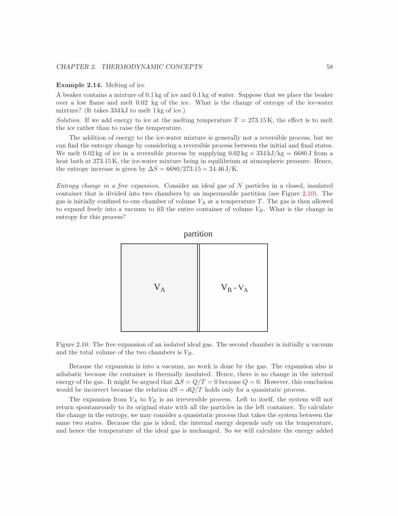
CHAPTER 2. THERMODYNAMIC CONCEPTS 58

Example 2.14. Melting of iceA beaker contains a mixture of 0.1 kg of ice and 0.1 kg of water. Suppose that we place the beakerover a low flame and melt 0.02 kg of the ice. What is the change of entropy of the ice-watermixture? (It takes 334kJ to melt 1 kg of ice.)Solution. If we add energy to ice at the melting temperature T = 273.15K, the effect is to meltthe ice rather than to raise the temperature.

The addition of energy to the ice-water mixture is generally not a reversible process, but wecan find the entropy change by considering a reversible process between the initial and final states.We melt 0.02 kg of ice in a reversible process by supplying 0.02 kg × 334 kJ/kg = 6680 J from aheat bath at 273.15K, the ice-water mixture being in equilibrium at atmospheric pressure. Hence,the entropy increase is given by ∆S = 6680/273.15 = 24.46J/K.

Entropy change in a free expansion. Consider an ideal gas of N particles in a closed, insulatedcontainer that is divided into two chambers by an impermeable partition (see Figure 2.10). Thegas is initially confined to one chamber of volume VA at a temperature T . The gas is then allowedto expand freely into a vacuum to fill the entire container of volume VB. What is the change inentropy for this process?

VA VB - VA

partition

Figure 2.10: The free expansion of an isolated ideal gas. The second chamber is initially a vacuumand the total volume of the two chambers is VB .

Because the expansion is into a vacuum, no work is done by the gas. The expansion also isadiabatic because the container is thermally insulated. Hence, there is no change in the internalenergy of the gas. It might be argued that ∆S = Q/T = 0 because Q = 0. However, this conclusionwould be incorrect because the relation dS = dQ/T holds only for a quasistatic process.

The expansion from VA to VB is an irreversible process. Left to itself, the system will notreturn spontaneously to its original state with all the particles in the left container. To calculatethe change in the entropy, we may consider a quasistatic process that takes the system between thesame two states. Because the gas is ideal, the internal energy depends only on the temperature,and hence the temperature of the ideal gas is unchanged. So we will calculate the energy added

CHAPTER 2. THERMODYNAMIC CONCEPTS 59

during an isothermal process to take the gas from volume VA to VB ,

Q = NkT lnVB

VA, (2.87)

where we have used (2.25). Hence, from (2.79), the entropy change is given by

∆S =Q

T= Nk ln

VB

VA. (2.88)

Note that VB > VA and the entropy change is positive as expected.Alternatively, we can argue that the work needed to restore the gas to its original state is

given by

W = −∫ VA

VB

P dV = NkT lnVB

VA, (2.89)

where we have used the fact that the process is isothermal. Hence, in this case W = T∆S, andthe entropy increase of the universe requires work on the gas to restore it to its original state.

The discussion of the free expansion of an ideal gas illustrates two initially confusing aspects ofthermodynamics. One is that the name thermodynamics is a misnomer because thermodynamicstreats only equilibrium states and not dynamics. Nevertheless, thermodynamics discusses processesthat must happen over some interval of time. Also confusing is that we can consider processesthat did not actually happen. In this case no energy by heating was transferred to the gas andthe process was adiabatic. The value of Q calculated in (2.87) is the energy transferred in anisothermal process. Of course, no energy is transferred by heating in an adiabatic process, but theentropy change is the same. For this reason we calculated the entropy change as if an isothermalprocess had occurred.

Quasistatic adiabatic processes. We have already discussed that quasistatic adiabatic processeshave the special property that the entropy does not change, but we repeat this statement here toemphasize its importance. Because the process is adiabatic, Q = 0, and because the process isquasistatic, ∆S = Q/T = 0, and there is no change in the entropy.

Maximum work. When two bodies are placed in thermal contact, no work is done, that is,∆W = 0 and ∆E = QA + QB = 0. What can we do to extract the maximum work possible fromthe two bodies? From our discussion of heat engines, we know that we should not place them inthermal contact. Instead we run a Carnot (reversible) engine between the two bodies. However,unlike the reservoirs considered in the Carnot engine, the heat capacities of the two bodies arefinite, and hence the temperature of each body changes as energy is transferred from one body tothe other.

Because the process is assumed to be reversible, we have

∆S = ∆SA + ∆SB = 0, (2.90)

from which it follows using (2.79) that

CA lnT

TA+ CB ln

T

TB= 0. (2.91)

CHAPTER 2. THERMODYNAMIC CONCEPTS 60

If we solve (2.91) for T , we find that

T = TCA/(CA+CB)A T

CB/(CA+CB)B . (2.92)

We see that the final temperature for a reversible process is the geometrical average of TA and TB

weighted by their respective heat capacities.

Problem 2.19. (a) Suppose T1 = 256K and TB = 144K. What are the relative values of the finaltemperatures in (2.81) and (2.92) assuming that the heat capacities of the two bodies are equal?(b) Show that the work performed by the heat engine in the reversible case is given by

W = ∆E = CA(T − TA) + CB(T − TB). (2.93)

Are all forms of energy equivalent? If you were offered 100J of energy, would you choose tohave it delivered as compressed gas at room temperature or as a hot brick at 400K? The answermight depend on what you want to do with the energy. If you want to lift a block of ice, the bestchoice would be to take the energy in the compressed gas. If you want to keep warm, the 400Kobject would be acceptable.

If you are not sure what you want to do with the energy, it is clear from the second law ofthermodynamics that we should take the form of the energy that can be most directly convertedinto work, because there is no restriction on using stored energy for heating. What is different isthe quality of the energy, which we take to be a measure of its ability to do a variety of tasks. Wecan readily convert energy from higher to lower quality, but the second law of thermodynamicsprevents us from going in the opposite direction with 100% efficiency.

We found in our discussion of the adiabatic free expansion of a gas that the entropy increases.Because the system has lost ability to do work, we can say that there has been a deterioration ofthe quality of energy. Suppose that we had let the gas undergo a quasistatic isothermal expansioninstead of an adiabatic free expansion. Then the work done by the gas would have been (see(2.25)):

W = NkT lnVB

VA. (2.94)

After the adiabatic free expansion, the gas can no longer do this work, even though its energy isunchanged. If we compare (2.94) with (2.88), we see that the energy that becomes unavailable todo work in an adiabatic free expansion is

Eunavailable = T∆S. (2.95)

Equation (2.95) indicates that entropy is a measure of the quality of energy. Given two systemswith the same energy, the one with the lower entropy has the higher quality energy. An increasein entropy implies that some energy has become unavailable to do work.

2.16 Equivalence of Thermodynamic and Ideal Gas ScaleTemperatures

So far we have assumed that the ideal gas scale temperature which we introduced in Section 2.4is the same as the thermodynamic temperature defined by (2.60). We now show that the twotemperatures are proportional and can be made equal if we choose the units of S appropriately.

CHAPTER 2. THERMODYNAMIC CONCEPTS 61

The gas scale temperature, which we denote as θ in this section to distinguish it from thethermodynamic temperature T , is defined by the relation

θ = PV/Nk. (2.96)

That is, θ is proportional to the pressure of a gas at a fixed low density and is equal to 273.16Kat the triple point of water. The fact that θ ∝ P is a matter of definition. Another importantproperty of ideal gases is that the internal energy depends only on θ and is independent of thevolume.

One way to show that T is proportional to θ is to consider a Carnot cycle (see Figure 2.9)with an ideal gas as the working substance. At every stage of the cycle we have

dQ

θ=

dE − dW

θ=

dE + PdV

θ,

ordQ

θ=

dE

θ+ Nk

dV

V. (2.97)

The first term on the right-hand side of (2.97) depends only on θ and the second term dependsonly on the volume. If we integrate (2.97) around one cycle, both θ and V return to their startingvalues, and hence the loop integral of the right-hand side of (2.97) is zero. We conclude that∮

dQ

θ=

Qcold

θcold− Qhot

θhot= 0. (2.98)

In Section 2.14 we showed that Qcold/Qhot = Tcold/Thot for a Carnot engine (see (2.71)). If wecombine this result with (2.98), we find that

Tcold

Thot=

θcold

θhot. (2.99)

It follows that the thermodynamic temperature T is proportional to the ideal gas scale temperatureθ. From now on we shall assume that we have chosen suitable units for S so that T = θ.

2.17 The Thermodynamic Pressure

In Section 2.13 we showed that the thermodynamic definition of temperature follows by consideringthe condition for the thermal equilibrium of two subsystems. In the following, we show that thepressure can be defined in an analogous way and that the pressure can be interpreted as a responseof the entropy to a change in the volume.

As before, consider an isolated composite system that is partitioned into two subsystems. Thesubsystems are separated by a movable, insulating wall so that the energies and volumes of thesubsystems can adjust themselves, but NA and NB are fixed. For simplicity, we assume that EA

and EB have already changed so that thermal equilibrium has been established. For fixed totalvolume V , we have one independent variable which we take to be VA; VB is given by VB = V −VA.The value of VA that maximizes Stotal is given by

dStotal =∂SA

∂VAdVA +

∂SB

∂VBdVB = 0. (2.100)

CHAPTER 2. THERMODYNAMIC CONCEPTS 62

Because dVA = −dVB, we can use (2.100) to write the condition for mechanical equilibrium as

∂SA

∂VA=

∂SB

∂VB. (2.101)

We define the thermodynamic pressure P as

P

T=

( ∂S

∂V

)E,N

. (thermodynamic definition of the pressure) (2.102)

For completeness, we also define the chemical potential as the response of the entropy to achange in the number of particles:

µ

T= −

( ∂S

∂N

)E,V

. (thermodynamic definition of the chemical potential) (2.103)

We will discuss the interpretation of µ in Section 4.12. You probably won’t be surprised to learnthat if two systems can exchange particles, then µ1 = µ2 is the condition for chemical equilibrium.

We will sometimes distinguish between thermal equilibrium, mechanical equilibrium, andchemical equilibrium for which the temperatures, pressures, and chemical potentials are equal,respectively.

2.18 The Fundamental Thermodynamic Relation

The first law of thermodynamics implies that the internal energy E is a function of state. For anychange of state, the change in E is given by (2.21):

∆E = Q + W. (any process) (2.104)

To separate the contributions to E due to heating and work, the constraints on the system haveto be known. If the change is quasistatic, then the infinitesimal work done is

dW = −PdV, (quasistatic process) (2.105)

anddQ = TdS. (quasistatic process) (2.106)

Thus, for an infinitesimal change in energy, we obtain

dE = TdS − PdV. (2.107)

There are two ways of thinking about (2.107). As our derivation suggests this equation tells us therelationship between changes in energy, entropy, and volume in a quasistatic process. However,because S, V , and E are functions of state, we can view (2.107) as the differential form (for fixedN) of the fundamental equation E = E(S, V, N) which describes the relationship between E, S,V , and N for all equilibrium states. We can also understand (2.107) by considering S as a functionof E, V , and N , and writing dS as

dS =∂S

∂EdE +

∂S

∂VdV +

∂S

∂NdN. (2.108)

CHAPTER 2. THERMODYNAMIC CONCEPTS 63

If we use the definitions (2.60), (2.102), and (2.103) of the various partial derivatives of S(E, V, N),we can write

dS =1T

dE +P

TdV − µ

TdN, (2.109)

which is equivalent to (2.107) for a fixed number of particles.If we know the entropy S as a function of E, V and N , we can immediately determine the

corresponding responses T, P , and µ. For this reason we shall refer to E, V and N as the naturalvariables in which S should be expressed. In this context S can be interpreted as a thermodynamicpotential because its various partial derivatives yield the equations of state of the system. InSection 2.21 we shall discuss thermodynamic potentials that have different sets of natural variables.

We can alternatively consider E as a function of S, V , and N and rewrite (2.109) as

dE = TdS − PdV + µdN. (fundamental thermodynamic relation) (2.110)

Equation (2.110) is a mathematical statement of the combined first and second laws of thermo-dynamics. Although there are few equations in physics that are necessary to memorize, (2.110) isone of the few equations of thermodynamics that you should know without thinking.

Many useful thermodynamic relations can be derived using (2.110). For example, if we regardE as a function of S, V , and N , we can write

dE =∂E

∂SdS +

∂E

∂VdV +

∂E

∂NdN. (2.111)

If we compare (2.110) and (2.111), we see that

T =(∂E

∂S

)V,N

P = −(∂E

∂V

)S,N

µ =( ∂E

∂N

)S,V

. (2.112)

Note that E(S, V, N) also can be interpreted as a thermodynamic potential. Or we can start with(2.110) and easily obtain (2.109) and the thermodynamics definitions of T , P , and µ.

2.19 The Entropy of an Ideal Gas

Because we know two equations of state of an ideal gas, (2.9) and (2.23), we can find the entropy ofan ideal gas as a function of various combinations of E, T , P , and V (for fixed N). If we substitute1/T = 3Nk/(2E) and P/T = Nk/V into (2.109), we obtain

dS =32Nk

dE

E+ Nk

dV

V. (2.113)

We can integrate (2.113) to obtain the change in the entropy from state E1, V1 to state E2, V2:

∆S =32Nk ln

E2

E1+ Nk ln

V2

V1. (2.114)

We see that S is an additive quantity as we assumed; that is, S is proportional to N ,

CHAPTER 2. THERMODYNAMIC CONCEPTS 64

Frequently it is more convenient to express S in terms of T and V or T and P . To obtainS(T, V ) we substitute E = 3NkT/2 into (2.114) and obtain

∆S =32Nk ln

T2

T1+ Nk ln

V2

V1. (2.115)

Problem 2.20. (a) Find ∆S(T, P ) for an ideal gas. (b) Use (2.115) to derive the relation (2.45)for a quasistatic adiabatic process.

2.20 The Third Law of Thermodynamics

We can calculate only differences in the entropy using purely thermodynamic relations as we didin Section 2.19. We can determine the absolute value of the entropy by using the third law ofthermodynamics which states that

limT→0

S = 0. (third law of thermodynamics) (2.116)

A statement equivalent to (2.116) was first proposed by Nernst in 1906 on the basis of empiricalobservations.16 The statistical basis of this law is discussed in Section 4.6. In the context ofthermodynamics, the third law can be understood only as a consequence of empirical observations.

The most important consequence of the third law is that all heat capacities must go to zeroas the temperature approaches zero. For changes at constant volume, we know that

S(T2, V ) − S(T1, V ) =∫ T2

T1

CV (T )T

dT. (2.117)

The condition (2.116) implies that in the limit T1 → 0, the integral in (2.117) must go to afinite limit, and hence we require that CV (T ) → 0 as T → 0. Similarly, we can argue thatCP → 0 as T → 0. Note that these conclusions about the low temperature behavior of CV andCP are independent of the nature of the system. Such is the power of thermodynamics. This lowtemperature behavior of the heat capacity was first established experimentally in 1910–1912.

As we will find in Section 4.6, the third law is a consequence of the fact that the mostfundamental description of nature at the microscopic level is quantum mechanical. We have alreadyseen that the heat capacity is a constant for an ideal classical gas. Hence, the thermal equationof state, E = 3NkT/2, as well as the pressure equation of state, PV = NkT , must cease to beapplicable at sufficiently low temperatures.

Example 2.15. At very low temperature T , the heat capacity C of an insulating solid is pro-portional to T 3. If we take C = AT 3 for a particular solid, what is the entropy of the solid attemperature T ?Solution. As before, the entropy is given by (see (2.79)):

S(T ) =∫ T

0

CV (T )T

dT, (2.118)

16Walther Nernst (1864–1943) was awarded the 1920 Nobel prize in chemistry for his discovery of the third lawand related work.

CHAPTER 2. THERMODYNAMIC CONCEPTS 65

where we have used the fact that S(T = 0) = 0. We can integrate the right-hand side of (2.118)from T = 0 to the desired value of T to find the absolute value of S. The result in this case isS = AT 3/3.

Problem 2.21. Is the expression (2.115) applicable at very low temperatures? Explain.

2.21 Free Energies

We have seen that the entropy of an isolated system can never decrease. However, an isolatedsystem is not of much experimental interest, and we wish to consider the more typical case where thesystem of interest is connected to a much larger system whose properties do not change significantly.As we have discussed on page 51, this larger system is called a heat bath.

If a system is connected to a heat bath, then the entropy of the system may increase ordecrease. The only thing we can say for sure is that the entropy of the system plus the heat bathmust increase. Because the entropy is additive, we have17

Scomposite = S + Sbath, (2.119)

and∆Scomposite = ∆S + ∆Sbath ≥ 0, (2.120)

where the properties of the system of interest are denoted by the absence of a subscript. Our goalis to determine if there is a property of the system alone (not the composite system) that is amaximum or a minimum. We begin by writing the change ∆Sbath in terms of the properties ofthe system. Because energy can be transferred between the system and heat bath, we have

∆Sbath =−Q

Tbath, (2.121)

where Q is the amount of energy transferred by heating the system, and −Q is the amount of energytransferred to the heat bath. If we use (2.121) and the fundamental thermodynamic relation,(2.110), we can rewrite (2.120) as

∆Scomposite = ∆S − Q

Tbath. (2.122)

The application of the first law to the system gives

∆E = Q + W, (2.123)

where ∆E is the change in the energy of the system and W is the work done on it. If the workdone on the system is due to the heat bath, then W = −Pbath∆V , where ∆V is the change involume of the system. Then we can write

∆Scomposite = ∆S − ∆E − W

Tbath= ∆S − ∆E + Pbath∆V

Tbath≥ 0. (2.124)

17The following discussion is adapted from Mandl, pp. 89–92.

CHAPTER 2. THERMODYNAMIC CONCEPTS 66

A little algebra leads to∆E + Pbath∆V − Tbath∆S ≤ 0. (2.125)

This result suggests that we define the availability by

A = E + PbathV − TbathS, (2.126)

so that (2.125) becomes∆A = ∆E + Pbath∆V − Tbath∆S ≤ 0. (2.127)

The availability includes properties of both the system and the heat bath. The significance of theavailability will be discussed below.

We now look at some typical experimental situations, and introduce a quantity that dependsonly on the properties of the system. As before, we assume that its volume and number of particlesis fixed, and that its temperature equals the temperature of the heat bath, that is, Tbath = T and∆V = 0. In this case we have

∆A = ∆E − T∆S ≡ ∆F ≤ 0, (2.128)

where we have defined the Helmholtz free energy as

F = E − TS. (2.129)

The inequality in (2.128) implies that if a constraint within the system is removed, then the system’sHelmholtz free energy will decrease. At equilibrium the left-hand side of (2.128) will vanish, andF will be a minimum. Thus, F plays the analogous role for systems at constant T and V that wasplayed by the entropy for an isolated system (constant E and V ).

The entropy of an isolated system is a function of E, V , and N . What are the natural variablesfor F? From our discussion it should be clear that these variables are T , V , and N . The answercan be found by taking the differential of (2.129) and using (2.110). The result is

dF = dE − SdT − TdS (2.130a)= (TdS − PdV + µdN) − SdT − TdS (2.130b)= −SdT − PdV + µdN. (2.130c)

We substituted dE = TdS − PdV + µdN to go from (2.130a) to (2.130b).From (2.130c) we see that F = F (T, V, N) and that S, P , and µ can be obtained by taking

appropriate partial derivatives of F . For example,

S = −(∂F

∂T

)V,N

, (2.131)

and

P = −(∂F

∂V

)T,N

(2.132)

Hence, we conclude that the Helmholtz free energy is a minimum for a given T , V , and N .The Helmholtz free energy is only one example of a free energy or thermodynamic potential.

We can relax the condition of a fixed volume by requiring that the pressure be specified. In this

CHAPTER 2. THERMODYNAMIC CONCEPTS 67

case mechanical equilibrium requires that the pressure of the system equal the pressure of thebath. This case is common in experiments using fluids where the pressure is fixed at atmosphericpressure. We write Pbath = P and express (2.125) as

∆A = ∆E + P∆V − T∆S ≡ ∆G ≤ 0, (2.133)

where we have defined the Gibbs free energy as

G = E − TS + PV = F + PV. (2.134)

The natural variables of G can be found in the same way as we did for F . We find that G =G(T, P, N) and

dG = dE − SdT − TdS + PdV + V dP

= (TdS − PdV + µdN) − SdT − TdS + PdV + V dP

= −SdT + V dP + µdN. (2.135)

We can use similar reasoning to conclude that G is a minimum at fixed temperature, pressure, andnumber of particles.

We can also relate G to the chemical potential using the following argument. Note that Gand N are extensive variables, but T and P are not. Thus, G must be proportional to N :

G = Ng(T, P ), (2.136)

where g(T, P ) is the Gibb’s free energy per particle. This function must be the chemical potentialbecause ∂G/∂N = g(T, P ) from (2.136) and ∂G/∂N = µ from (2.135). Thus, the chemicalpotential is the Gibbs free energy per particle:

µ(T, P ) =G

N= g(T, p). (2.137)

Because g depends only on T and P , we have

dg =( ∂g

∂P

)T

dP +( ∂g

∂T

)P

dT (2.138)

= vdP − sdT, (2.139)

where v = V/N and s = S/N . The properties of G and the relation (2.139) will be importantwhen we discuss processes involving a change of phase (see Section 7.5).

Another common thermodynamic potential is the enthalpy H which we defined in (2.29). Thispotential is similar to E(S, V, N) except for the requirement of fixed P rather than fixed V .

Problem 2.22. Show thatdH = TdS + V dP + µdN, (2.140)

and

T =(∂H

∂S

)P,N

(2.141)

V =(∂H

∂P

)S,N

(2.142)

µ =(∂H

∂N

)S,P

. (2.143)

CHAPTER 2. THERMODYNAMIC CONCEPTS 68

Problem 2.23. Show that H is a minimum for an equilibrium system at fixed entropy.

Landau potential. As we have seen, we can define many thermodynamic potentials dependingon which variables we constrain. A very useful thermodynamic potential that has no generallyrecognized name or symbol is sometimes called the Landau potential and is denoted by Ω. Anothercommon name is simply the grand potential. The Landau potential is the thermodynamic potentialfor which the variables T, V , and µ are specified and is given by

Ω(T, V, µ) = F − µN. (2.144)

If we take the derivative of Ω and use the fact that dF = −SdT − PdV + µdN (see (2.130c)), weobtain

dΩ = dF − µdN − Ndµ (2.145a)= −SdT − PdV − Ndµ. (2.145b)

From (2.145a) we have

S = −(∂Ω

∂T

)V,µ

. (2.146)

P = −( ∂Ω

∂V

)T,µ

. (2.147)

N = −(∂Ω

∂µ

)T,V

. (2.148)

Because G = Nµ, we can write Ω = F −G. Hence, if we use the definition G = F +PV , we obtain

Ω(T, V, µ) = F − µN = F − G = −PV. (2.149)

The relation (2.149) will be very useful for obtaining the equation of state of various systems (seeSection 6.10).

*Useful work and availability. The free energies that we have introduced are useful for under-standing the maximum amount of useful work, Wuseful, that can be done by a system when it isconnected to a heat bath. The system is not necessarily in thermal or mechanical equilibrium withits surroundings. In addition to the system of interest and its surroundings (the bath), we includea third body, namely, the body on which the system does useful work. The third body is thermallyinsulated. The total work Wby done by the system is the work done against its surroundings,Pbath∆V plus the work done on the body, Wuseful:

Wby = Pbath∆V + Wuseful. (2.150)

Because Wby is the work done by the system when its volume changes by ∆V , the first term in(2.150) does not contain a negative sign. This term is the work that is necessarily and uselesslyperformed by the system in changing its volume and thus also the volume of its surroundings. Thesecond term is the useful work done by the system. In (2.125) we replace the work done on theheat bath, Pbath∆V , by the total work done by the system Pbath∆V + Wuseful to obtain

∆E + Pbath∆V + Wuseful − Tbath∆S ≤ 0, (2.151)

CHAPTER 2. THERMODYNAMIC CONCEPTS 69

or the useful work done is

Wuseful ≤ −(∆E + Pbath∆V − Tbath∆S) = −∆A, (2.152)

Note that the maximum amount of useful work that can be done by the system is equal to −∆A.This relation explains the meaning of the terminology availability because only −∆A is availablefor useful work. The rest of the work is wasted on the surroundings.

Problem 2.24. (a) Show that if the change in volume of the system is zero, ∆V = 0, and theinitial and final temperature are that of the heat bath, then the maximum useful work is −∆F . (b)Show that if the initial and final temperature and pressure are that of the bath, then the maximumuseful work is −∆G.

Vocabulary

thermodynamics, system, boundary, surroundings

insulator, conductor, adiabatic wall

thermal contact, thermal equilibrium, temperature, thermodynamic equilibrium

thermometer, Celsius temperature scale, ideal gas temperature scale, thermodynamic tem-perature

heating, work

internal energy E, entropy S, state function, laws of thermodynamics

ideal gas, ideal gas equation of state, van der Waals equation of state

Boltzmann’s constant, universal gas constant

intensive and extensive variables

heat capacity, specific heat

quasistatic, reversible, irreversible, isothermal, constant volume, adiabatic, quasistatic, andcyclic processes

heat bath, heat source, heat sink

Carnot engine, refrigerator, heat pump efficiency, coefficient of performance

thermodynamic potential, Helmholtz free energy F , Gibbs free energy G, enthalpy H , Landaupotential Ω, availability A

Notation

volume V , number of particles N , thermodynamic temperature T , pressure P , chemicalpotential µ

CHAPTER 2. THERMODYNAMIC CONCEPTS 70

total work W , total energy transferred due to a temperature difference alone Q

kelvin K, Celsius C, Fahrenheit F

heat capacity C, specific heat c

thermal efficiency η

Boltzmann’s constant k, gas constant R

Appendix 2A: Equivalence of Different Statements of the Sec-ond Law

[xx not done xx]

Appendix 2B: The Mathematics of Thermodynamics

Because the notation of thermodynamics can be cumbersome, we have tried to simplify it wheneverpossible. However, one common simplification can lead to initial confusion.

Consider the functional relationships:

y = f(x) = x2, (2.153)

andx = g(z) = z1/2. (2.154)

If we write x in terms of z, we can write y as

y = h(z) = f(g(z)) = z. (2.155)

We have given the composite function a different symbol h because it is different from both f andg. But we would soon exhaust the letters of the alphabet, and we frequently write y = f(z) = z.Note that f(z) is a different function than f(x).

The notation is even more confusing in thermodynamics. Consider for example, the entropy Sas a function of E, V , and N , which we write as S(E, V, N). However, we frequently consider E asa function of T from which we would obtain another functional relationship: S(E(T, V, N), V, N).A mathematician would write the latter function with a different symbol, but we don’t. In so doingwe confuse the name of a function with that of a variable and use the same name (symbol) for thesame physical quantity. This sloppiness can cause problems when we take partial derivatives. Ifwe write ∂S/∂V , is E or T to be held fixed? One way to avoid confusion is to write (∂S/∂V )E or(∂S/∂V )T , but this notation can become cumbersome.

Another confusing aspect of the mathematics of thermodynamics is the use of differentials.Many authors, including Bohren and Albrecht,18 have criticized their use. These authors and

18See Bohren and Albrecht, pp. 93–99.

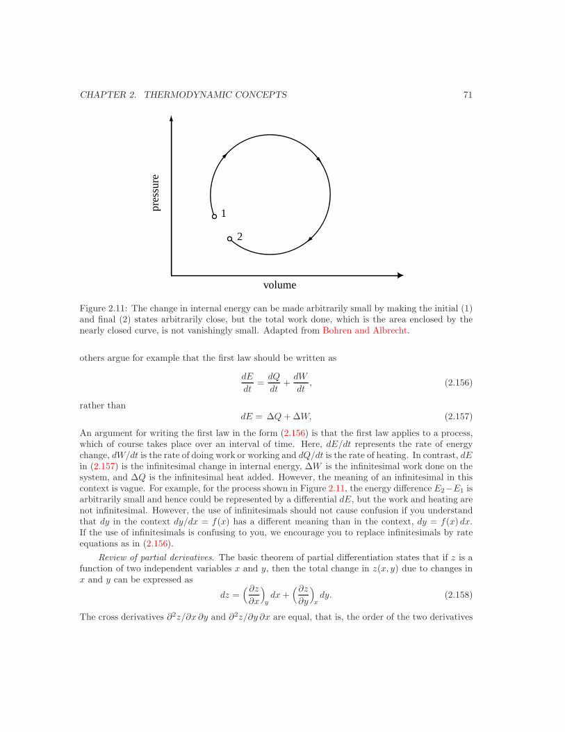
CHAPTER 2. THERMODYNAMIC CONCEPTS 71

1

2

volume

pres

sure

Figure 2.11: The change in internal energy can be made arbitrarily small by making the initial (1)and final (2) states arbitrarily close, but the total work done, which is the area enclosed by thenearly closed curve, is not vanishingly small. Adapted from Bohren and Albrecht.

others argue for example that the first law should be written as

dE

dt=

dQ

dt+

dW

dt, (2.156)

rather thandE = ∆Q + ∆W, (2.157)

An argument for writing the first law in the form (2.156) is that the first law applies to a process,which of course takes place over an interval of time. Here, dE/dt represents the rate of energychange, dW/dt is the rate of doing work or working and dQ/dt is the rate of heating. In contrast, dEin (2.157) is the infinitesimal change in internal energy, ∆W is the infinitesimal work done on thesystem, and ∆Q is the infinitesimal heat added. However, the meaning of an infinitesimal in thiscontext is vague. For example, for the process shown in Figure 2.11, the energy difference E2−E1 isarbitrarily small and hence could be represented by a differential dE, but the work and heating arenot infinitesimal. However, the use of infinitesimals should not cause confusion if you understandthat dy in the context dy/dx = f(x) has a different meaning than in the context, dy = f(x) dx.If the use of infinitesimals is confusing to you, we encourage you to replace infinitesimals by rateequations as in (2.156).

Review of partial derivatives. The basic theorem of partial differentiation states that if z is afunction of two independent variables x and y, then the total change in z(x, y) due to changes inx and y can be expressed as

dz =(∂z

∂x

)ydx +

(∂z

∂y

)xdy. (2.158)

The cross derivatives ∂2z/∂x ∂y and ∂2z/∂y ∂x are equal, that is, the order of the two derivatives

CHAPTER 2. THERMODYNAMIC CONCEPTS 72

does not matter. We will use this property to derive what are known as the Maxwell relations inSection 7.2.

The chain rule for differentiation holds in the usual way if the same variables are held constantin each derivative. For example, we can write

(∂z

∂x

)y

=( ∂z

∂w

)y

(∂w

∂x

)y. (2.159)

We also can derive a relation whose form is superficially similar to (2.159) when different variablesare held constant in each term. From (2.158) we set dz = 0 and obtain

dz = 0 =(∂z

∂x

)ydx +

(∂z

∂y

)xdy. (2.160)

We divide both sides of (2.160) by dx:

0 =(∂z

∂x

)y

+(∂z

∂y

)x

(∂y

∂x

)z, (2.161)

and rewrite (2.161) as (∂z

∂x

)y

= −(∂z

∂y

)x

(∂y

∂x

)z. (2.162)

Note that (2.162) involves a relation between the three possible partial derivatives which involvex, y, and z.

Problem 2.25. Consider the function

z(x, y) = x2y + 2x4y6.

Calculate ∂z/∂x, ∂z/∂y, ∂2z/∂x ∂y, and ∂2z/∂y ∂x and show that ∂2z/∂x ∂y = ∂2z/∂y ∂x.

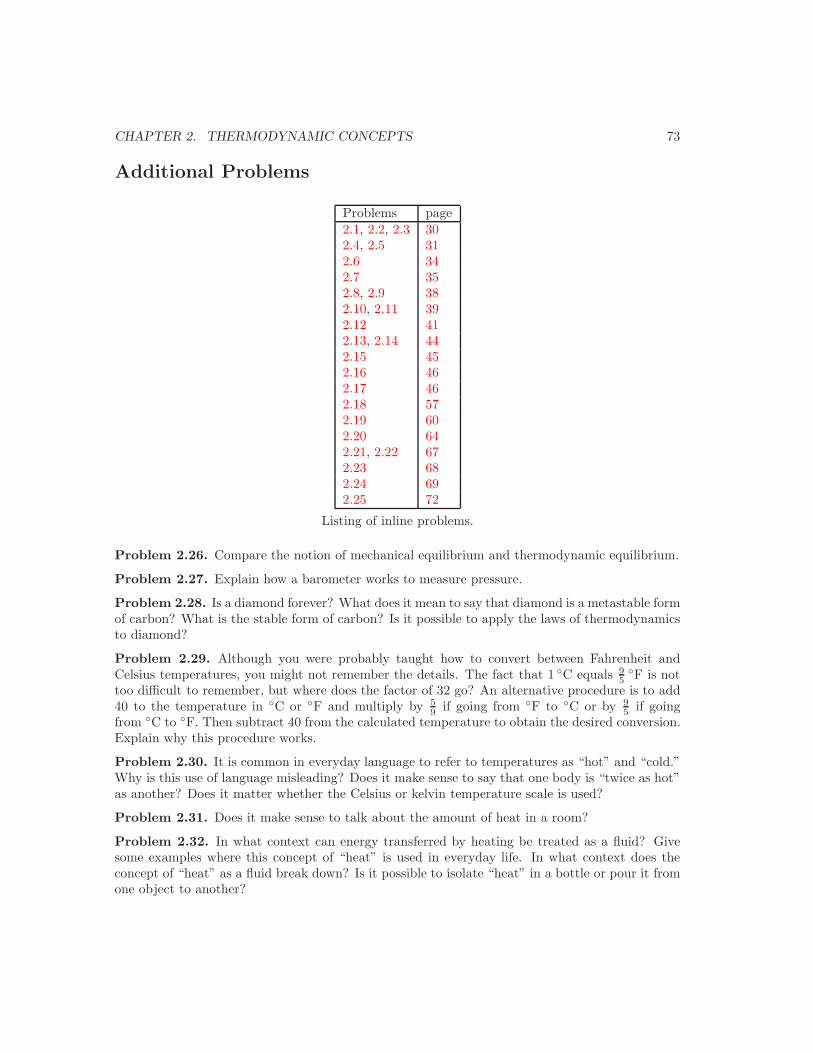
CHAPTER 2. THERMODYNAMIC CONCEPTS 73

Additional Problems

Problems page2.1, 2.2, 2.3 302.4, 2.5 312.6 342.7 352.8, 2.9 382.10, 2.11 392.12 412.13, 2.14 442.15 452.16 462.17 462.18 572.19 602.20 642.21, 2.22 672.23 682.24 692.25 72

Listing of inline problems.

Problem 2.26. Compare the notion of mechanical equilibrium and thermodynamic equilibrium.

Problem 2.27. Explain how a barometer works to measure pressure.

Problem 2.28. Is a diamond forever? What does it mean to say that diamond is a metastable formof carbon? What is the stable form of carbon? Is it possible to apply the laws of thermodynamicsto diamond?

Problem 2.29. Although you were probably taught how to convert between Fahrenheit andCelsius temperatures, you might not remember the details. The fact that 1 C equals 9

5F is not

too difficult to remember, but where does the factor of 32 go? An alternative procedure is to add40 to the temperature in C or F and multiply by 5

9 if going from F to C or by 95 if going

from C to F. Then subtract 40 from the calculated temperature to obtain the desired conversion.Explain why this procedure works.

Problem 2.30. It is common in everyday language to refer to temperatures as “hot” and “cold.”Why is this use of language misleading? Does it make sense to say that one body is “twice as hot”as another? Does it matter whether the Celsius or kelvin temperature scale is used?

Problem 2.31. Does it make sense to talk about the amount of heat in a room?

Problem 2.32. In what context can energy transferred by heating be treated as a fluid? Givesome examples where this concept of “heat” is used in everyday life. In what context does theconcept of “heat” as a fluid break down? Is it possible to isolate “heat” in a bottle or pour it fromone object to another?

CHAPTER 2. THERMODYNAMIC CONCEPTS 74

Problem 2.33. Why should we check the pressure in a tire when the tire is cold?

Problem 2.34. Suppose that we measure the temperature of a body and then place the body ona moving conveyer belt. Does the temperature of the body change?

Problem 2.35. Why do we use the triple point of water to calibrate thermometers? Why not usethe melting point or the boiling point?

Problem 2.36. In the text we discussed the analogy of the internal energy to the amount ofwater in a pond. The following analogy due to Dugdale might also be helpful.19 Suppose that astudent has a bank account with a certain amount of money. The student can add to this amountby either depositing or withdrawing cash and by writing or depositing checks from the accountsof others. Does the total amount of money in his account distinguish between cash and checktransfers? Discuss the analogies to internal energy, work, and heating.

Problem 2.37. The following excerpt is taken from a text used by one of the author’s childrenin the sixth grade. The title and the author will remain anonymous. Find the conceptual errorsin the text.A. What is heat?

You have learned that all matter is made up of atoms. Most of these atoms combine to form molecules.These molecules are always moving—they have kinetic energy. Heat is the energy of motion (kinetic energy)of the particles that make up any piece of matter.

The amount of heat a material has depends on how many molecules it has and how fast the moleculesare moving. The greater the number of molecules and the faster they move, the greater the number ofcollisions between them. These collisions produce a large amount of heat.

How is heat measured? Scientists measure heat by using a unit called a calorie. A calorie is theamount of heat needed to raise the temperature of 1 gram of 1 water 1 degree centigrade (Celsius).

A gram is a unit used for measuring mass. There are about 454 grams in 1 pound.

Scientists use a small calorie and a large Calorie. The unit used to measure the amount of heat neededto raise the temperature of 1 gram of water 1 degree centigrade is the small calorie. The large calorie isused to measure units of heat in food. For example, a glass of milk when burned in your body producesabout 125 Calories.

Questions:

1. What is heat?

2. What two things does the amount of heat a substance has depend on?

3. What is a calorie?

4. Explain the following: small calorie; large calorie.

B. What is temperature?

The amount of hotness in an object is called its temperature. A thermometer is used to measuretemperature in units called degrees. Most thermometers contain a liquid.

C. Expansion and Contraction

Most solids, liquids and gases expand when heated and contract when cooled. When matter is heated,its molecules move faster. As they move, they collide with their neighbors very rapidly. The collisionsforce the molecules to spread farther apart. The farther apart they spread, the more the matter expands.

19See Dugdale, pp. 21–22.

CHAPTER 2. THERMODYNAMIC CONCEPTS 75

Air, which is a mixture of gases, expands and becomes lighter when its temperature rises. Warm airrises because the cold, heavier air sinks and pushes up the lighter warm air.

What happens when solids or gases are cooled? The molecules slow down and collide less. The

molecules move closer together, causing the material to contract.

Problem 2.38. Why are the terms heat capacity and specific heat poor choices of names? Suggestmore appropriate names. Criticize the statement: “The heat capacity of a body is a measure ofhow much heat the body can hold.”

Problem 2.39. The atmosphere of Mars has a pressure that is only 0.007 times that of the Earthand an average temperature of 218K. What is the volume of 1 mole of the Martian atmosphere?

Problem 2.40. Discuss the meaning of the statement that one of the most important contributionsof 19th century thermodynamics was the development of the understanding that heat (and work)are names of methods not names of things.

Problem 2.41. Gasoline burns in an automobile engine and releases energy at the rate of 160kW.Energy is exhausted through the car’s radiator at the rate of 51 kW and out the exhaust at 50 kW.An additional 23 kW goes to frictional heating within the machinery of the car. What fraction ofthe fuel energy is available for moving the car?

Problem 2.42. Two moles of an ideal gas at 300K occupying a volume of 0.10m3 is compressedisothermally by a motor driven piston to a volume of 0.010m3. If this process takes places in 120 s,how powerful a motor is needed?

Problem 2.43. Give an example of a process in which a system is not heated, but its temperatureincreases. Also give an example of a process in which a system is heated, but its temperature isunchanged.

Problem 2.44. (a) Suppose that a gas expands adiabatically into a vacuum. What is the workdone by the gas? (b) Suppose that the total energy of the gas is given by (see (2.24))

E =32NkT − N

N

Va, (2.163)

where a is a positive constant. Initially the gas occupies a volume VA at a temperature TA. Thegas then expands adiabatically into a vacuum so that it occupies a total volume VB . What is thefinal temperature of the gas?

Problem 2.45. Calculate the work done on one mole of an ideal gas in an adiabatic quasistaticcompression from volume VA to volume VB . The initial pressure is PA.

Problem 2.46. Consider the following processes and calculate W , the total work done on thesystem and Q, the total energy absorbed by heating the system when it is brought quasistaticallyfrom A to C (see Figure 2.12). Assume that the system is an ideal gas. (This problem is adaptedfrom Reif, p. 215.)

(a) The volume is changed quasistatically from A → C while the gas is kept thermally isolated.

CHAPTER 2. THERMODYNAMIC CONCEPTS 76

(b) The system is compressed from its original volume of VA = 8 m3 to its final volume VC = 1 m3

along the path A → B and B → C. The pressure is kept constant at PA = 1 Pa and the systemis cooled to maintain constant pressure. The volume is then kept constant and the system isheated to increase the pressure to PB = 32 Pa.

(c) A → D and D → C. The two steps of the preceding process are performed in opposite order.

(d) A → C. The volume is decreased and the system is heated so that the pressure is proportionalto the volume.

V

AB

C D

1

32

P

1 8

P ∝ V-5/3

Figure 2.12: Illustration of various thermodynamic processes discussed in Problem 2.46. The unitsof the pressure P and the volume V are Pa and m3, respectively.

Problem 2.47. A 0.5 kg copper block at 80 C is dropped into 1 kg of water at 10 C. What isthe final temperature? What is the change in entropy of the system? The specific heat of copperis 386 J/(kgK).

Problem 2.48. (a) Surface temperatures in the tropical oceans are approximately 25 C, whilehundreds of meters below the surface the temperature is approximately 5 C. What would be theefficiency of a Carnot engine operating between these temperatures? (b) What is the efficiency ofa Carnot engine operating between the normal freezing and boiling points of water?

Problem 2.49. A small sample of material is taken through a Carnot cycle between a heat sourceof boiling helium at 1.76 K and a heat sink at an unknown lower temperature. During the process,7.5 mJ of energy is absorbed by heating from the helium and 0.55 mJ is rejected at the lowertemperature. What is the lower temperature?

CHAPTER 2. THERMODYNAMIC CONCEPTS 77

Problem 2.50. Positive change in total entropy

(a) Show that the total entropy change in Example 2.13 can be written as

∆S = Cf(T2

T1), (2.164)

wheref(x) = lnx +

1x− 1. (2.165)

and x > 1 corresponds to heating. Calculate f(x = 1) and df/dx and show that the entropyof the universe increases for a heating process.

(b) If the total entropy increases in a heating process, does the total entropy decrease in a coolingprocess? Use similar considerations to show that the total entropy increases in both cases.

(c) Plot f(x) as a function of x and confirm that its minimum value is at x = 1 and that f > 0for x < 1 and x > 1.

Problem 2.51. Show that the enthalpy, H ≡ E + PV , is the appropriate free energy for the casewhere the entropy and number of particles is fixed, but the volume can change. In this case weconsider a system connected to a larger body such that the pressure of the system equals that ofthe large body with the constraint that the larger body and the system do not exchange energy.An example of this situation would be a gas confined to a glass container with a movable piston.

Problem 2.52. Find the Landau potential for the case where the temperature is fixed by a heatbath, the volume is fixed, and particles can move between the systems and the heat bath. You willneed to extend the definition of the availability to allow for the number of particles to vary withinthe system. Use the same argument about extensive variables to show that the Landau potentialequals −PV .

Problem 2.53. One kilogram of water at 50 C is brought into contact with a heat bath at 0 C.What is the change of entropy of the water, the bath, and the combined system consisting of boththe water and the heat bath? Given that the total entropy increased in Example 2.13, should theentropy increase or decrease in this case?

Problem 2.54. Calculate the changes in entropy due to various methods of heating:

(a) One kilogram of water at 0 C is brought into contact with a heat bath at 90 C. What isthe change in entropy of the water? What is the change in entropy of the bath? What is thechange in entropy of the entire system consisting of both water and heat bath? (The specificheat of water is approximately 4184 J/kgK.)

(b) The water is heated from 0 C to 90 C by first bringing it into contact with a heat bath at45 C and then with a heat bath at 90 C. What is the change in entropy of the entire system?

(c) Discuss how the water can be heated from 0 C to 90 C without any change in entropy of theentire system.

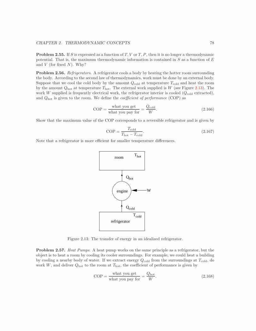
CHAPTER 2. THERMODYNAMIC CONCEPTS 78

Problem 2.55. If S is expressed as a function of T, V or T, P , then it is no longer a thermodynamicpotential. That is, the maximum thermodynamic information is contained in S as a function of Eand V (for fixed N). Why?

Problem 2.56. Refrigerators. A refrigerator cools a body by heating the hotter room surroundingthe body. According to the second law of thermodynamics, work must be done by an external body.Suppose that we cool the cold body by the amount Qcold at temperature Tcold and heat the roomby the amount Qhot at temperature Thot. The external work supplied is W (see Figure 2.13). Thework W supplied is frequently electrical work, the refrigerator interior is cooled (Qcold extracted),and Qhot is given to the room. We define the coefficient of performance (COP) as

COP =what you get

what you pay for=

Qcold

W. (2.166)

Show that the maximum value of the COP corresponds to a reversible refrigerator and is given by

COP =Tcold

Thot − Tcold. (2.167)

Note that a refrigerator is more efficient for smaller temperature differences.

room

refrigerator

Qcold

Qhot

W

Tcold

Thot

engine

Figure 2.13: The transfer of energy in an idealized refrigerator.

Problem 2.57. Heat Pumps. A heat pump works on the same principle as a refrigerator, but theobject is to heat a room by cooling its cooler surroundings. For example, we could heat a buildingby cooling a nearby body of water. If we extract energy Qcold from the surroundings at Tcold, dowork W , and deliver Qhot to the room at Thot, the coefficient of performance is given by

COP =what you get

what you pay for=

Qhot

W. (2.168)

CHAPTER 2. THERMODYNAMIC CONCEPTS 79

What is the maximum value of COP for a heat pump in terms of Tcold and Thot? What is the COPwhen the outside temperature is 0 C and the interior temperature is 23 C? Is it more effectiveto operate a heat pump during the winters in New England where the winters are cold or in thePacific Northwest where the winters are relatively mild?

Problem 2.58. Use (2.115) to derive the relation (2.43) between V and T for an ideal gas in aquasistatic adiabatic process.

Problem 2.59. The Otto cycle. The Otto cycle is the idealized prototype of most present-dayinternal combustion engines. The cycle was first described by Beau de Rochas in 1862. NicholasOtto independently conceived of the same cycle in 1876 and then constructed an engine to imple-ment it. The idealization makes two basic assumptions. One is that the working substance is takento be air rather than a mixture of gases and vapor whose composition changes during the cycle.For simplicity, we assume that CV and CP are constant and that γ = CP /CV = 1.4, the valuefor air. The more important approximation is that the changes are assumed to be quasistatic. Anidealized cycle that represents the six parts of this cycle is known as the air standard Otto cycleand is illustrated in Figure 2.14.

5 → 1. Intake stroke. The mixture of gasoline and air is drawn into the cylinder through theintake valve by the movement of the piston. Idealization: A quasistatic isobaric intake of airat pressure P0 to a volume V1.

1 → 2. Compression stroke. The intake valve closes and air-fuel mixture is rapidly com-pressed in the cylinder. The compression is nearly adiabatic and the temperature rises.Idealization: A quasistatic adiabatic compression from V1 to V2; the temperature rises fromT1 to T2.

2 → 3. Explosion. The mixture explodes such that the volume remains unchanged and a veryhigh temperature and pressure is reached. Idealization: A quasistatic and constant volumeincrease of temperature and pressure due to the absorption of energy from a series of heatbaths between T2 and T3.

3 → 4. Power stroke. The hot combustion products expand and do work on the piston.The pressure and temperature decrease considerably. Idealization: A quasistatic adiabaticexpansion produces a decrease in temperature.

4 → 1. Valve exhaust. At the end of the power stroke the exhaust valve opens and the com-bustion products are exhausted to the atmosphere. There is a sudden decrease in pressure.Idealization: A quasistatic constant volume decrease in temperature to T1 and pressure P0

due to a exchange of energy with a series of heat baths between T4 and T1.

1 → 5. Exhaust stroke. The piston forces the remaining gases into the atmosphere. Theexhaust valve then closes and the intake valve opens for the next intake stroke. Idealization:A quasistatic isobaric expulsion of the air.

Show that the efficiency of the Otto cycle is

η = 1 − (V2

V1

)γ−1. (2.169)

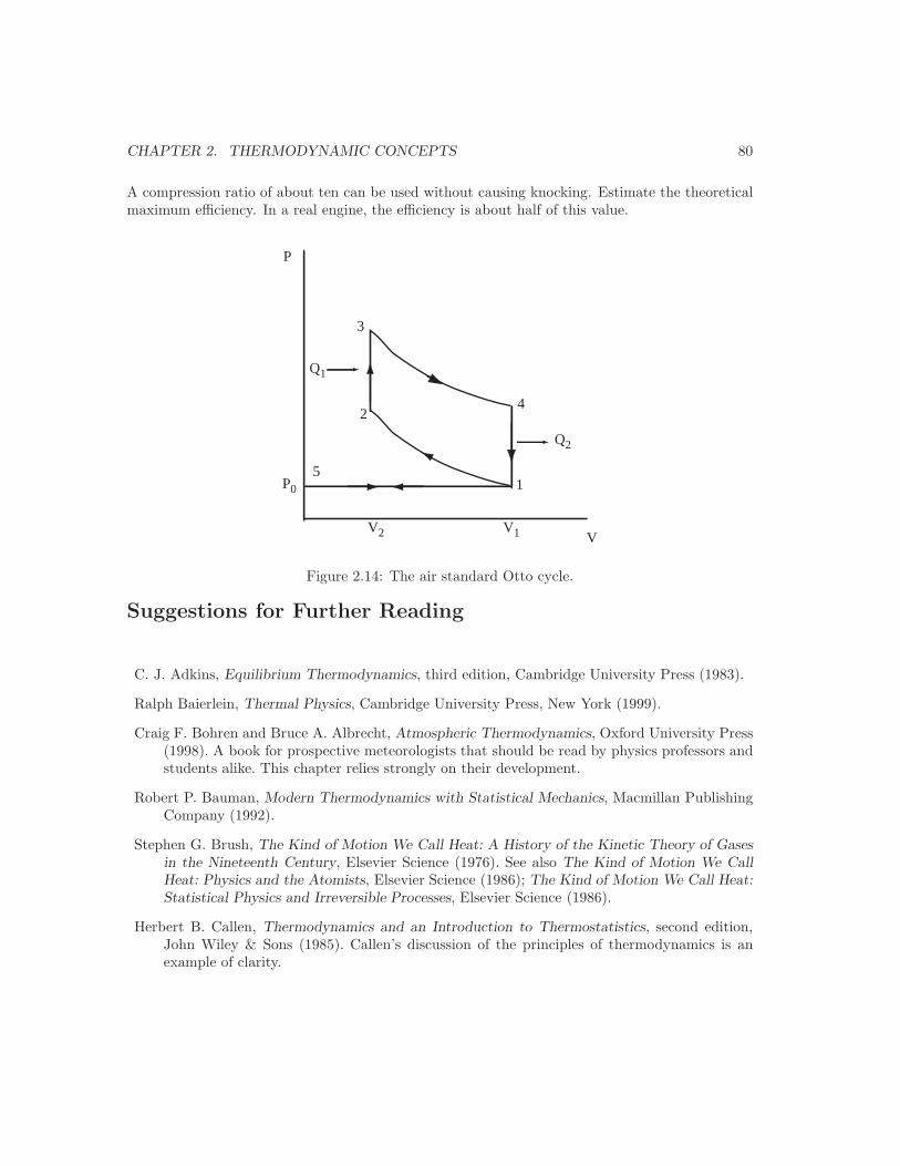
CHAPTER 2. THERMODYNAMIC CONCEPTS 80

A compression ratio of about ten can be used without causing knocking. Estimate the theoreticalmaximum efficiency. In a real engine, the efficiency is about half of this value.

3

P

V

42

15

P0

Q1

Q2

V2 V1

Figure 2.14: The air standard Otto cycle.

Suggestions for Further Reading

C. J. Adkins, Equilibrium Thermodynamics, third edition, Cambridge University Press (1983).

Ralph Baierlein, Thermal Physics, Cambridge University Press, New York (1999).

Craig F. Bohren and Bruce A. Albrecht, Atmospheric Thermodynamics, Oxford University Press(1998). A book for prospective meteorologists that should be read by physics professors andstudents alike. This chapter relies strongly on their development.

Robert P. Bauman, Modern Thermodynamics with Statistical Mechanics, Macmillan PublishingCompany (1992).

Stephen G. Brush, The Kind of Motion We Call Heat: A History of the Kinetic Theory of Gasesin the Nineteenth Century, Elsevier Science (1976). See also The Kind of Motion We CallHeat: Physics and the Atomists, Elsevier Science (1986); The Kind of Motion We Call Heat:Statistical Physics and Irreversible Processes, Elsevier Science (1986).

Herbert B. Callen, Thermodynamics and an Introduction to Thermostatistics, second edition,John Wiley & Sons (1985). Callen’s discussion of the principles of thermodynamics is anexample of clarity.

CHAPTER 2. THERMODYNAMIC CONCEPTS 81

J. S. Dugdale, Entropy and its Physical Meaning, Taylor & Francis (1996). A very accessibleintroduction to thermodynamics.

E. Garber, S. G. Brush, and C. W. F. Everitt, eds., Maxwell on Heat and Statistical Mechanics,Lehigh University Press (1995).

Michael E. Loverude, Christian H. Kautz, and Paula R. L. Henon, “Student understanding of thefirst law of thermodynamics: Relating work to the adiabatic compression of an ideal gas,”Am. J. Phys. 70, 137–148 (2002).

F. Reif, Statistical Physics, Volume 5 of the Berkeley Physics Series, McGraw-Hill (1965).

F. Mandl, Statistical Physics, second edition, John Wiley & Sons (1988).

David E. Meltzer, “Investigation of students’ reasoning regarding heat, work, and the first lawof thermodynamics in an introductory calculus-based general physics course,” Am. J. Phys.72, 1432–1446 (2004).

Daniel V. Schroeder, An Introduction to Thermal Physics, Addison-Wesley (2000).

Richard Wolfson and Jay M. Pasachoff, Physics, second edition, HarperCollins College Publishers(1995). Chapters 19–22 are a good introduction to the laws of thermodynamics.

Chapter 3

Concepts of Probabilityc©2005 by Harvey Gould and Jan Tobochnik

5 December 2005

We introduce the basic concepts of probability and apply it to simple physical systems and everydaylife. We will discover the universal nature of the central limit theorem and the Gaussian distributionfor the sum of a large number of random processes and discuss its relation to why thermodynamicsis possible. Because of the importance of probability in many contexts and the relatively littletime it will take us to cover more advanced topics, our discussion goes beyond what we will needfor most applications of statistical mechanics.

3.1 Probability in everyday life

Chapter 2 provided an introduction to thermodynamics using macroscopic arguments. Our goal,which we will consider again in Chapter 4, is to relate the behavior of various macroscopic quantitiesto the underlying microscopic behavior of the individual atoms or other constituents. To do so, wewill need to introduce some ideas from probability.

We all use the ideas of probability in everyday life. For example, every morning many of usdecide what to wear based on the probability of rain. We cross streets knowing that the probabilityof being hit by a car is small. We can even make a rough estimate of the probability of being hitby a car. It must be less that one in a thousand, because you have crossed streets thousands oftimes and hopefully you have not been hit. Of course you might be hit tomorrow, or you mighthave been hit the first time you tried to cross a street. These comments illustrate that we havesome intuitive sense of probability and because it is a useful concept for survival, we know how toestimate it. As expressed by Laplace (1819),

Probability theory is nothing but common sense reduced to calculation.

Another interesting thought is due to Maxwell (1850):

The true logic of this world is the calculus of probabilities . . .

82

CHAPTER 3. CONCEPTS OF PROBABILITY 83

However, our intuition only takes us so far. Consider airplane travel. Is it safe to fly? Supposethat there is a one chance in 100,000 of a plane crashing on a given flight and that there are a1000 flights a day. Then every 100 days or so there would be a reasonable likelihood of a planecrashing. This estimate is in rough accord with what we read. For a given flight, your chances ofcrashing are approximately one part in 105, and if you fly five times a year for 80 years, it seemsthat flying is not too much of a risk. However, suppose that instead of living 80 years, you couldlive 20,000 years. In this case you would take 100,000 flights, and it would be much more risky tofly if you wished to live your full 20,000 years. Although this last statement seems reasonable, canyou explain why?

Much of the motivation for the mathematical formulation of probability arose from the profi-ciency of professional gamblers in estimating gambling odds and their desire to have more quanti-tative measures. Although games of chance have been played since history has been recorded, thefirst steps toward a mathematical formulation of games of chance began in the middle of the 17thcentury. Some of the important contributors over the following 150 years include Pascal, Fermat,Descartes, Leibnitz, Newton, Bernoulli, and Laplace, names that are probably familiar to you.

Given the long history of games of chance and the interest in estimating probability in a varietyof contexts, it is remarkable that the theory of probability took so long to develop. One reasonis that the idea of probability is subtle and is capable of many interpretations. An understandingof probability is elusive due in part to the fact that the probably depends on the status of theinformation that we have (a fact well known to poker players). Although the rules of probability aredefined by simple mathematical rules, an understanding of probability is greatly aided by experiencewith real data and concrete problems. To test your current understanding of probability, try tosolve Problems 3.1–3.6 before reading the rest of this chapter. Then in Problem 3.7 formulate thelaws of probability as best as you can based on your solutions to these problems.

Problem 3.1. A jar contains 2 orange, 5 blue, 3 red, and 4 yellow marbles. A marble is drawnat random from the jar. Find the probability that (a) the marble is orange, (b) the marble is red,(c) the marble is orange or blue.

Problem 3.2. A piggy bank contains one penny, one nickel, one dime, and one quarter. It isshaken until two coins fall out at random. What is the probability that at least $0.30 falls out?

Problem 3.3. A girl tosses a pair of dice at the same time. Find the probability that (a) bothdice show the same number, (b) both dice show a number less than 5, (c) both dice show an evennumber, (d) the product of the numbers is 12.

Problem 3.4. A boy hits 16 free throws out of 25 attempts. What is the probability that he willmake a free throw on his next attempt?

Problem 3.5. Consider an experiment in which a die is tossed 150 times and the number of timeseach face is observed is counted. The value of A, the number of dots on the face of the die and thenumber of times that it appeared is shown in Table 3.1. What is the predicted average value of Aassuming a fair die? What is the average value of A observed in this experiment?

Problem 3.6. A coin is taken at random from a purse that contains one penny, two nickels, fourdimes, and three quarters. If x equals the value of the coin, find the average value of x.

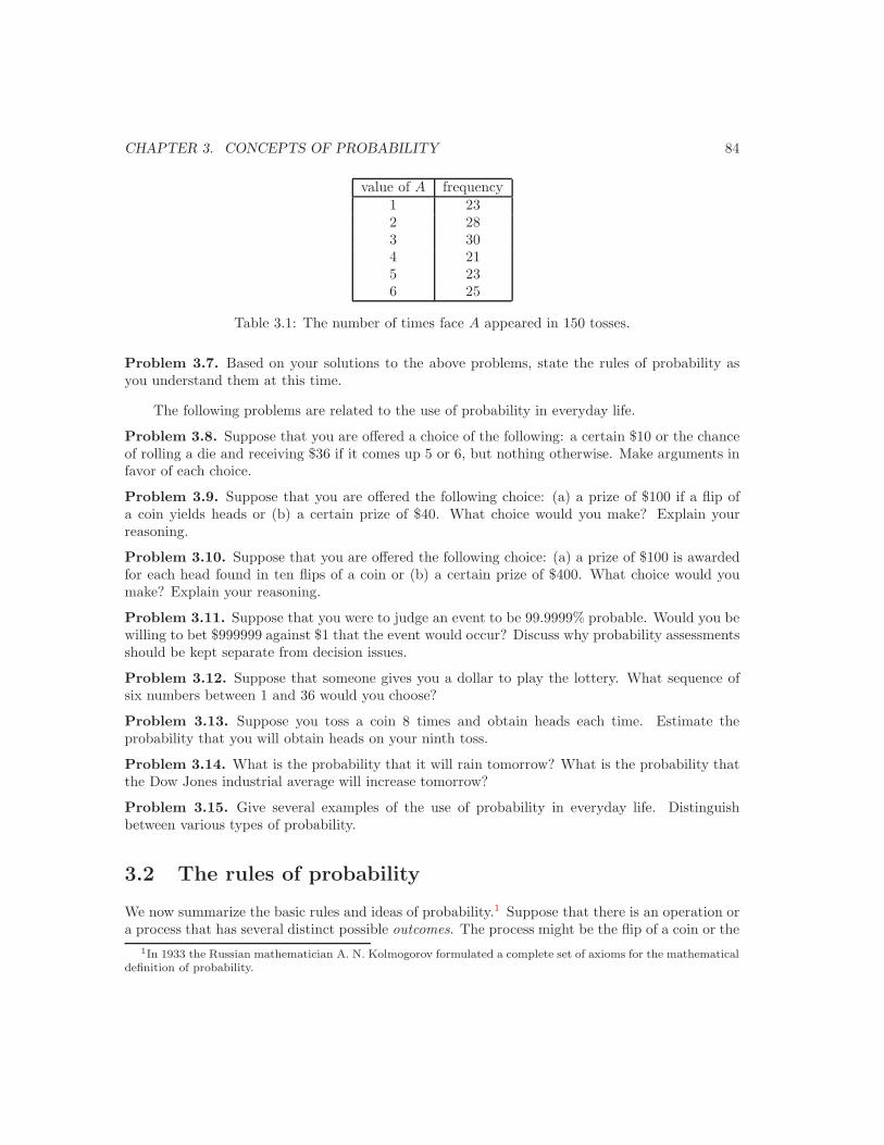
CHAPTER 3. CONCEPTS OF PROBABILITY 84

value of A frequency1 232 283 304 215 236 25

Table 3.1: The number of times face A appeared in 150 tosses.

Problem 3.7. Based on your solutions to the above problems, state the rules of probability asyou understand them at this time.

The following problems are related to the use of probability in everyday life.

Problem 3.8. Suppose that you are offered a choice of the following: a certain $10 or the chanceof rolling a die and receiving $36 if it comes up 5 or 6, but nothing otherwise. Make arguments infavor of each choice.

Problem 3.9. Suppose that you are offered the following choice: (a) a prize of $100 if a flip ofa coin yields heads or (b) a certain prize of $40. What choice would you make? Explain yourreasoning.

Problem 3.10. Suppose that you are offered the following choice: (a) a prize of $100 is awardedfor each head found in ten flips of a coin or (b) a certain prize of $400. What choice would youmake? Explain your reasoning.

Problem 3.11. Suppose that you were to judge an event to be 99.9999% probable. Would you bewilling to bet $999999 against $1 that the event would occur? Discuss why probability assessmentsshould be kept separate from decision issues.

Problem 3.12. Suppose that someone gives you a dollar to play the lottery. What sequence ofsix numbers between 1 and 36 would you choose?

Problem 3.13. Suppose you toss a coin 8 times and obtain heads each time. Estimate theprobability that you will obtain heads on your ninth toss.

Problem 3.14. What is the probability that it will rain tomorrow? What is the probability thatthe Dow Jones industrial average will increase tomorrow?

Problem 3.15. Give several examples of the use of probability in everyday life. Distinguishbetween various types of probability.

3.2 The rules of probability

We now summarize the basic rules and ideas of probability.1 Suppose that there is an operation ora process that has several distinct possible outcomes. The process might be the flip of a coin or the

1In 1933 the Russian mathematician A. N. Kolmogorov formulated a complete set of axioms for the mathematicaldefinition of probability.

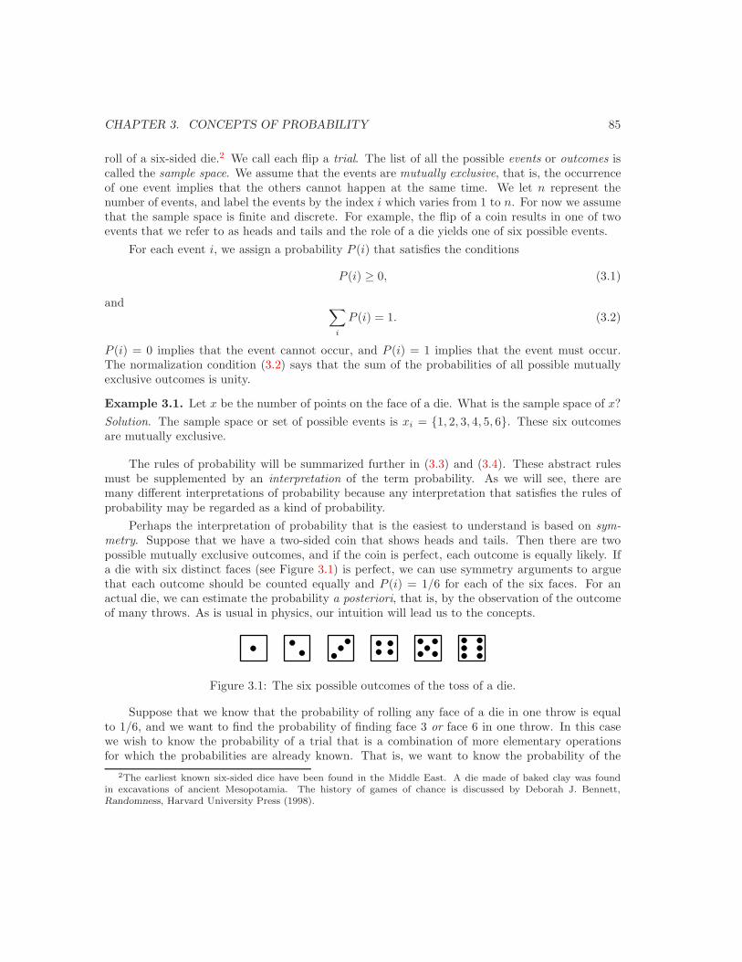
CHAPTER 3. CONCEPTS OF PROBABILITY 85

roll of a six-sided die.2 We call each flip a trial. The list of all the possible events or outcomes iscalled the sample space. We assume that the events are mutually exclusive, that is, the occurrenceof one event implies that the others cannot happen at the same time. We let n represent thenumber of events, and label the events by the index i which varies from 1 to n. For now we assumethat the sample space is finite and discrete. For example, the flip of a coin results in one of twoevents that we refer to as heads and tails and the role of a die yields one of six possible events.

For each event i, we assign a probability P (i) that satisfies the conditions

P (i) ≥ 0, (3.1)

and ∑i

P (i) = 1. (3.2)

P (i) = 0 implies that the event cannot occur, and P (i) = 1 implies that the event must occur.The normalization condition (3.2) says that the sum of the probabilities of all possible mutuallyexclusive outcomes is unity.

Example 3.1. Let x be the number of points on the face of a die. What is the sample space of x?Solution. The sample space or set of possible events is xi = 1, 2, 3, 4, 5, 6. These six outcomesare mutually exclusive.

The rules of probability will be summarized further in (3.3) and (3.4). These abstract rulesmust be supplemented by an interpretation of the term probability. As we will see, there aremany different interpretations of probability because any interpretation that satisfies the rules ofprobability may be regarded as a kind of probability.

Perhaps the interpretation of probability that is the easiest to understand is based on sym-metry. Suppose that we have a two-sided coin that shows heads and tails. Then there are twopossible mutually exclusive outcomes, and if the coin is perfect, each outcome is equally likely. Ifa die with six distinct faces (see Figure 3.1) is perfect, we can use symmetry arguments to arguethat each outcome should be counted equally and P (i) = 1/6 for each of the six faces. For anactual die, we can estimate the probability a posteriori, that is, by the observation of the outcomeof many throws. As is usual in physics, our intuition will lead us to the concepts.

Figure 3.1: The six possible outcomes of the toss of a die.

Suppose that we know that the probability of rolling any face of a die in one throw is equalto 1/6, and we want to find the probability of finding face 3 or face 6 in one throw. In this casewe wish to know the probability of a trial that is a combination of more elementary operationsfor which the probabilities are already known. That is, we want to know the probability of the

2The earliest known six-sided dice have been found in the Middle East. A die made of baked clay was foundin excavations of ancient Mesopotamia. The history of games of chance is discussed by Deborah J. Bennett,Randomness, Harvard University Press (1998).

CHAPTER 3. CONCEPTS OF PROBABILITY 86

outcome, i or j, where i is distinct from j. According to the rules of probability, the probabilityof event i or j is given by

P (i or j) = P (i) + P (j). (addition rule) (3.3)

The relation (3.3) is generalizable to more than two events. An important consequence of (3.3) isthat if P (i) is the probability of event i, then the probability of event i not occurring is 1 − P (i).

Example 3.2. What is the probability of throwing a three or a six with one throw of a die?Solution. The probability that the face exhibits either 3 or 6 is 1

6 + 16 = 1

3 .

Example 3.3. What is the probability of not throwing a six with one throw of die?Solution. The answer is the probability of either “1 or 2 or 3 or 4 or 5.” The addition rule givesthat the probability P (not six) is

P (not six) = P (1) + P (2) + P (3) + P (4) + P (5)

= 1 − P (6) =56,

where the last relation follows from the fact that the sum of the probabilities for all outcomes sumsto unity. Although this property of the probability is obvious, it is very useful to take advantageof this property when solving many probability problems.

Another simple rule is for the probability of the joint occurrence of independent events. Theseevents might be the probability of throwing a 3 on one die and the probability of throwing a 4 ona second die. If two events are independent, then the probability of both events occurring is theproduct of their probabilities

P (i and j) = P (j)P (j). (multiplication rule) (3.4)

Events are independent if the occurrence of one event does not change the probability for theoccurrence of the other.

To understand the applicability of (3.4) and the meaning of the independence of events,consider the problem of determining the probability that a person chosen at random is a femaleover six feet tall. Suppose that we know that the probability of a person to be over six feet tallis P (6+) = 1

5 , and the probability of being female is P (female) = 12 . We might conclude that

the probability of being a tall female is P (female) × P (6+) = 12 × 1

5 = 110 . The same probability

would hold for a tall male. However, this reasoning is incorrect, because the probability of beinga tall female differs from the probability of being a tall male. The problem is that the two events– being over six feet tall and being female – are not independent. On the other hand, considerthe probability that a person chosen at random is female and was born on September 6. Wecan reasonably assume equal likelihood of birthdays for all days of the year, and it is correct toconclude that this probability is 1

2 × 1365 (not counting leap years). Being a woman and being born

on September 6 are independent events.

Problem 3.16. Give an example from your solutions to Problems 3.1–3.6 where you used theaddition rule or the multiplication rule.

CHAPTER 3. CONCEPTS OF PROBABILITY 87

Example 3.4. What is the probability of throwing an even number with one throw of a die?Solution. We can use the addition rule to find that

P (even) = P (2) + P (4) + P (6) =16

+16

+16

=12.

Example 3.5. What is the probability of the same face appearing on two successive throws of adie?Solution. We know that the probability of any specific combination of outcomes, for example,(1,1), (2,2), . . . (6,6) is 1

6 × 16 = 1

36 . Hence, by the addition rule

P (same face) = P (1, 1) + P (2, 2) + . . . + P (6, 6) = 6 × 136

=16.

Example 3.6. What is the probability that in two throws of a die at least one six appears?Solution. We have already established that

P (6) =16

P (not 6) =56.

There are four possible outcomes (6, 6), (6, not 6), (not 6, 6), (not 6, not 6) with the probabilities

P (6, 6) =16× 1

6=

136

P (6, not 6) = P (not 6, 6) =16× 5

6=

536

P (not 6, not 6) =56× 5

6=

2536

.

All outcomes except the last have at least one six. Hence, the probability of obtaining at least onesix is

P (at least one 6) = P (6, 6) + P (6, not 6) + P (not 6, 6)

=136

+536

+536

=1136

.

A more direct way of obtaining this result is to use the normalization condition. That is,

P (at least one six) = 1 − P (not 6, not 6) = 1 − 2536

=1136

.

Example 3.7. What is the probability of obtaining at least one six in four throws of a die?Solution. We know that in one throw of a die, there are two outcomes with P (6) = 1

6 andP (not 6) = 5

6 . Hence, in four throws of a die there are sixteen possible outcomes, only one ofwhich has no six. That is, in the fifteen mutually exclusive outcomes, there is at least one six. Wecan use the multiplication rule (3.3) to find that

P (not 6, not 6, not 6, not 6) = P (not 6)4 =(56)4

,

CHAPTER 3. CONCEPTS OF PROBABILITY 88

and hence

P (at least one six) = 1 − P (not 6, not 6, not 6, not 6)

= 1 − (56)4 =

6711296

≈ 0.517.

Frequently we know the probabilities only up to a constant factor. For example, we might knowP (1) = 2P (2), but not P (1) or P (2) separately. Suppose we know that P (i) is proportional to f(i),where f(i) is a known function. To obtain the normalized probabilities, we divide each functionf(i) by the sum of all the unnormalized probabilities. That is, if P (i) ∝ f(i) and Z =

∑f(i),

then P (i) = f(i)/Z. This procedure is called normalization.

Example 3.8. Suppose that in a given class it is three times as likely to receive a C as an A,twice as likely to obtain a B as an A, one-fourth as likely to be assigned a D as an A, and nobodyfails the class. What are the probabilities of getting each grade?Solution. We first assign the unnormalized probability of receiving an A as f(A) = 1. Thenf(B) = 2, f(C) = 3, and f(D) = 0.25. Then Z =

∑i f(i) = 1 + 2 + 3 + 0.25 = 6.25. Hence,

P (A) = f(A)/Z = 1/6.25 = 0.16, P (B) = 2/6.25 = 0.32, P (C) = 3/6.25 = 0.48, and P (D) =0.25/6.25 = 0.04.

The normalization procedure arises again and again in different contexts. We will see thatmuch of the mathematics of statistical mechanics can be formulated in terms of the calculation ofnormalization constants.

Problem 3.17. Find the probability distribution P (n) for throwing a sum n with two dice andplot P (n) as a function of n.

Problem 3.18. What is the probability of obtaining at least one double six in twenty-four throwsof a pair of dice?

Problem 3.19. Suppose that three dice are thrown at the same time. What is the probabilitythat the sum of the three faces is 10 compared to 9?

Problem 3.20. What is the probability that the total number of spots shown on three dice thrownat the same time is 11? What is the probability that the total is 12? What is the fallacy in thefollowing argument? The number 11 occurs in six ways: (1,4,6), (2,3,6), (1,5,5), (2,4,5), (3,3,5),(3,4,4). The number 12 also occurs in six ways: (1,5,6), (2,4,6), (3,3,6), (2,5,5), (3,4,5), (4,4,4) andhence the two numbers should be equally probable.

Problem 3.21. In two tosses of a single coin, what is the probability that heads will appearat least once? Use the rules of probability to show that the answer is 3

4 . However, d’Alembert,a distinguished French mathematician of the eighteenth century, reasoned that there are only 3possible outcomes: heads on the first throw, heads on the second throw, and no heads at all. Thefirst two of these three outcomes is favorable. Therefore the probability that heads will appear atleast once is 2

3 . What is the fallacy in this reasoning?

CHAPTER 3. CONCEPTS OF PROBABILITY 89

3.3 Mean values

The specification of the probability distribution P (1), P (2), . . . P (n) for the n possible values of thevariable x constitutes the most complete statistical description of the system. However, in manycases it is more convenient to describe the distribution of the possible values of x in a less detailedway. The most familiar way is to specify the average or mean value of x, which we will denote asx. The definition of the mean value of x is

x ≡ x1P (1) + x2P (2) + . . . + xnP (n) (3.6a)

=n∑

i=1

xiP (i), (3.6b)

where P (i) is the probability of xi, and we have assumed that the probability is normalized. Iff(x) is a function of x, then the mean value of f(x) is defined by

f(x) =n∑

i=1

f(xi)P (i). (3.7)

If f(x) and g(x) are any two functions of x, then

f(x) + g(x) =n∑

i=1

[f(xi) + g(xi)]P (i)

=n∑

i=1

f(xi)P (i) +n∑

i=1

g(xi)P (i),

orf(x) + g(x) = f(x) + g(x). (3.8)

Problem 3.22. Show that if c is a constant, then

cf(x) = cf(x). (3.9)

In general, we can define the mth moment of the probability distribution P as

xm ≡n∑

i=1

ximP (i), (3.10)

where we have let f(x) = xm. The mean of x is the first moment of the probability distribution.

Problem 3.23. Suppose that the variable x takes on the values −2, −1, 0, 1, and 2 with proba-bilities 1/4, 1/8, 1/8, 1/4, and 1/4, respectively. Calculate the first two moments of x.

The mean value of x is a measure of the central value of x about which the various values ofxi are distributed. If we measure x from its mean, we have that

∆x ≡ x − x, (3.11)

and

CHAPTER 3. CONCEPTS OF PROBABILITY 90

∆x = (x − x) = x − x = 0. (3.12)

That is, the average value of the deviation of x from its mean vanishes.If only one outcome j were possible, we would have P (i) = 1 for i = j and zero otherwise, that

is, the probability distribution would have zero width. In general, there is more than one outcomeand a possible measure of the width of the probability distribution is given by

∆x2 ≡ (x − x

)2. (3.13)

The quantity ∆x2 is known as the dispersion or variance and its square root is called the standarddeviation. It is easy to see that the larger the spread of values of x about x, the larger the variance.The use of the square of x−x ensures that the contribution of x values that are smaller and largerthan x enter with the same sign. A useful form for the variance can be found by letting

(x − x

)2 =(x2 − 2xx + x2

)(3.14)

= x2 − 2x x + x2,

or (x − x

)2 = x2 − x2. (3.15)

Because ∆x2 is always nonnegative, it follows that x2 ≥ x2.The variance is the mean value of the square (x − x)2 and represents the square of a width.

We will find that it is useful to interpret the width of the probability distribution in terms of thestandard deviation. The standard deviation of the probability distribution P (x) is given by

σx =√

∆x2 =√(

x2 − x2). (3.16)

Example 3.9. Find the mean value x, the variance ∆x2, and the standard deviation σx for thevalue of a single throw of a die.Solution. Because P (i) = 1

6 for i = 1, . . . , 6, we have that

x =16(1 + 2 + 3 + 4 + 5 + 6) =

72

= 3.5

x2 =16(1 + 4 + 9 + 16 + 25 + 36) =

463

∆x2 = x2 − x2 =463

− 494

=3712

≈ 3.08

σx ≈ √3.08 = 1.76

Example 3.10. On the average, how many times must a die be thrown until a 6 appears?Solution. Although it might seem obvious that the answer is six, it is instructive to confirm thisanswer. Let p be the probability of a six on a given throw. The probability of success for the firsttime on trial i is given in Table 3.2.

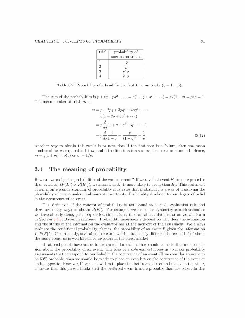
CHAPTER 3. CONCEPTS OF PROBABILITY 91

trial probability ofsuccess on trial i

1 p2 qp3 q2p4 q3p

Table 3.2: Probability of a head for the first time on trial i (q = 1 − p).

The sum of the probabilities is p + pq + pq2 + · · · = p(1 + q + q2 + · · · ) = p/(1− q) = p/p = 1.The mean number of trials m is

m = p + 2pq + 3pq2 + 4pq3 + · · ·= p(1 + 2q + 3q2 + · · · )= p

d

dq(1 + q + q2 + q3 + · · · )

= pd

dq

11 − q

=p

(1 − q)2=

1p

(3.17)

Another way to obtain this result is to note that if the first toss is a failure, then the meannumber of tosses required is 1 + m, and if the first toss is a success, the mean number is 1. Hence,m = q(1 + m) + p(1) or m = 1/p.

3.4 The meaning of probability

How can we assign the probabilities of the various events? If we say that event E1 is more probablethan event E2 (P (E1) > P (E2)), we mean that E1 is more likely to occur than E2. This statementof our intuitive understanding of probability illustrates that probability is a way of classifying theplausibility of events under conditions of uncertainty. Probability is related to our degree of beliefin the occurrence of an event.

This definition of the concept of probability is not bound to a single evaluation rule andthere are many ways to obtain P (Ei). For example, we could use symmetry considerations aswe have already done, past frequencies, simulations, theoretical calculations, or as we will learnin Section 3.4.2, Bayesian inference. Probability assessments depend on who does the evaluationand the status of the information the evaluator has at the moment of the assessment. We alwaysevaluate the conditional probability, that is, the probability of an event E given the informationI, P (E|I). Consequently, several people can have simultaneously different degrees of belief aboutthe same event, as is well known to investors in the stock market.

If rational people have access to the same information, they should come to the same conclu-sion about the probability of an event. The idea of a coherent bet forces us to make probabilityassessments that correspond to our belief in the occurrence of an event. If we consider an event tobe 50% probable, then we should be ready to place an even bet on the occurrence of the event oron its opposite. However, if someone wishes to place the bet in one direction but not in the other,it means that this person thinks that the preferred event is more probable than the other. In this

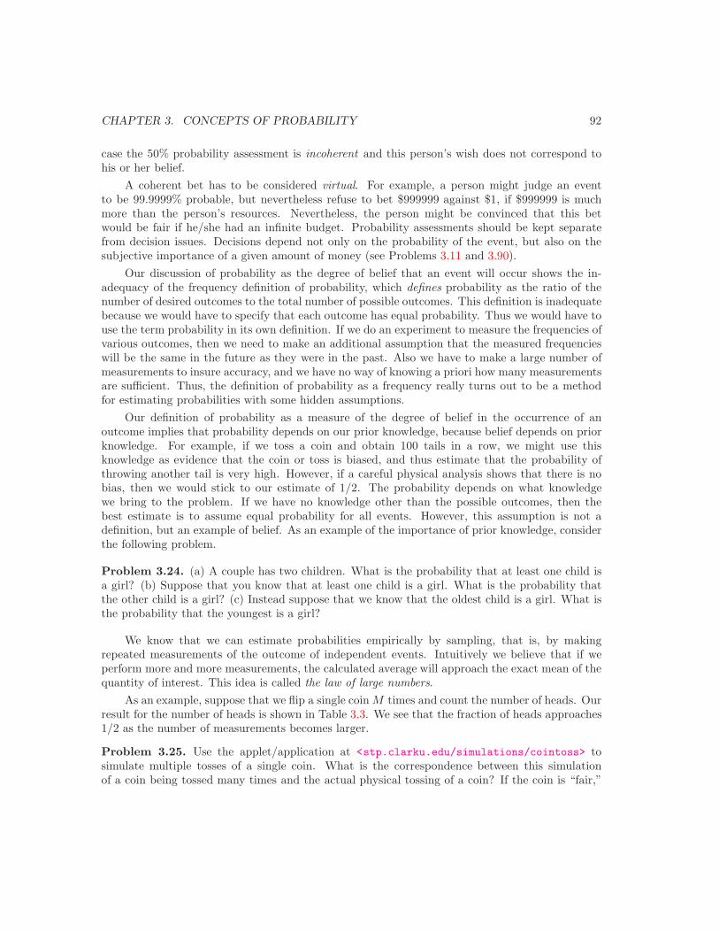
CHAPTER 3. CONCEPTS OF PROBABILITY 92

case the 50% probability assessment is incoherent and this person’s wish does not correspond tohis or her belief.

A coherent bet has to be considered virtual. For example, a person might judge an eventto be 99.9999% probable, but nevertheless refuse to bet $999999 against $1, if $999999 is muchmore than the person’s resources. Nevertheless, the person might be convinced that this betwould be fair if he/she had an infinite budget. Probability assessments should be kept separatefrom decision issues. Decisions depend not only on the probability of the event, but also on thesubjective importance of a given amount of money (see Problems 3.11 and 3.90).

Our discussion of probability as the degree of belief that an event will occur shows the in-adequacy of the frequency definition of probability, which defines probability as the ratio of thenumber of desired outcomes to the total number of possible outcomes. This definition is inadequatebecause we would have to specify that each outcome has equal probability. Thus we would have touse the term probability in its own definition. If we do an experiment to measure the frequencies ofvarious outcomes, then we need to make an additional assumption that the measured frequencieswill be the same in the future as they were in the past. Also we have to make a large number ofmeasurements to insure accuracy, and we have no way of knowing a priori how many measurementsare sufficient. Thus, the definition of probability as a frequency really turns out to be a methodfor estimating probabilities with some hidden assumptions.

Our definition of probability as a measure of the degree of belief in the occurrence of anoutcome implies that probability depends on our prior knowledge, because belief depends on priorknowledge. For example, if we toss a coin and obtain 100 tails in a row, we might use thisknowledge as evidence that the coin or toss is biased, and thus estimate that the probability ofthrowing another tail is very high. However, if a careful physical analysis shows that there is nobias, then we would stick to our estimate of 1/2. The probability depends on what knowledgewe bring to the problem. If we have no knowledge other than the possible outcomes, then thebest estimate is to assume equal probability for all events. However, this assumption is not adefinition, but an example of belief. As an example of the importance of prior knowledge, considerthe following problem.

Problem 3.24. (a) A couple has two children. What is the probability that at least one child isa girl? (b) Suppose that you know that at least one child is a girl. What is the probability thatthe other child is a girl? (c) Instead suppose that we know that the oldest child is a girl. What isthe probability that the youngest is a girl?

We know that we can estimate probabilities empirically by sampling, that is, by makingrepeated measurements of the outcome of independent events. Intuitively we believe that if weperform more and more measurements, the calculated average will approach the exact mean of thequantity of interest. This idea is called the law of large numbers.

As an example, suppose that we flip a single coin M times and count the number of heads. Ourresult for the number of heads is shown in Table 3.3. We see that the fraction of heads approaches1/2 as the number of measurements becomes larger.

Problem 3.25. Use the applet/application at <stp.clarku.edu/simulations/cointoss> tosimulate multiple tosses of a single coin. What is the correspondence between this simulationof a coin being tossed many times and the actual physical tossing of a coin? If the coin is “fair,”

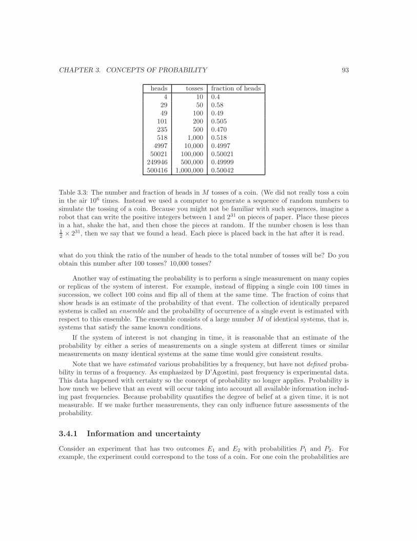
CHAPTER 3. CONCEPTS OF PROBABILITY 93

heads tosses fraction of heads4 10 0.4

29 50 0.5849 100 0.49

101 200 0.505235 500 0.470518 1,000 0.518

4997 10,000 0.499750021 100,000 0.50021

249946 500,000 0.49999500416 1,000,000 0.50042

Table 3.3: The number and fraction of heads in M tosses of a coin. (We did not really toss a coinin the air 106 times. Instead we used a computer to generate a sequence of random numbers tosimulate the tossing of a coin. Because you might not be familiar with such sequences, imagine arobot that can write the positive integers between 1 and 231 on pieces of paper. Place these piecesin a hat, shake the hat, and then chose the pieces at random. If the number chosen is less than12 × 231, then we say that we found a head. Each piece is placed back in the hat after it is read.

what do you think the ratio of the number of heads to the total number of tosses will be? Do youobtain this number after 100 tosses? 10,000 tosses?

Another way of estimating the probability is to perform a single measurement on many copiesor replicas of the system of interest. For example, instead of flipping a single coin 100 times insuccession, we collect 100 coins and flip all of them at the same time. The fraction of coins thatshow heads is an estimate of the probability of that event. The collection of identically preparedsystems is called an ensemble and the probability of occurrence of a single event is estimated withrespect to this ensemble. The ensemble consists of a large number M of identical systems, that is,systems that satisfy the same known conditions.

If the system of interest is not changing in time, it is reasonable that an estimate of theprobability by either a series of measurements on a single system at different times or similarmeasurements on many identical systems at the same time would give consistent results.

Note that we have estimated various probabilities by a frequency, but have not defined proba-bility in terms of a frequency. As emphasized by D’Agostini, past frequency is experimental data.This data happened with certainty so the concept of probability no longer applies. Probability ishow much we believe that an event will occur taking into account all available information includ-ing past frequencies. Because probability quantifies the degree of belief at a given time, it is notmeasurable. If we make further measurements, they can only influence future assessments of theprobability.

3.4.1 Information and uncertainty

Consider an experiment that has two outcomes E1 and E2 with probabilities P1 and P2. Forexample, the experiment could correspond to the toss of a coin. For one coin the probabilities are

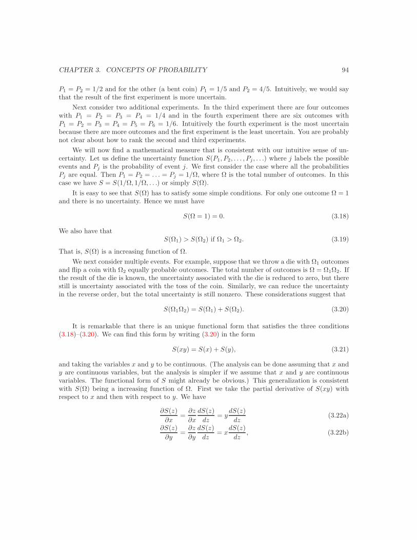
CHAPTER 3. CONCEPTS OF PROBABILITY 94

P1 = P2 = 1/2 and for the other (a bent coin) P1 = 1/5 and P2 = 4/5. Intuitively, we would saythat the result of the first experiment is more uncertain.

Next consider two additional experiments. In the third experiment there are four outcomeswith P1 = P2 = P3 = P4 = 1/4 and in the fourth experiment there are six outcomes withP1 = P2 = P3 = P4 = P5 = P6 = 1/6. Intuitively the fourth experiment is the most uncertainbecause there are more outcomes and the first experiment is the least uncertain. You are probablynot clear about how to rank the second and third experiments.

We will now find a mathematical measure that is consistent with our intuitive sense of un-certainty. Let us define the uncertainty function S(P1, P2, . . . , Pj , . . .) where j labels the possibleevents and Pj is the probability of event j. We first consider the case where all the probabilitiesPj are equal. Then P1 = P2 = . . . = Pj = 1/Ω, where Ω is the total number of outcomes. In thiscase we have S = S(1/Ω, 1/Ω, . . .) or simply S(Ω).

It is easy to see that S(Ω) has to satisfy some simple conditions. For only one outcome Ω = 1and there is no uncertainty. Hence we must have

S(Ω = 1) = 0. (3.18)

We also have thatS(Ω1) > S(Ω2) if Ω1 > Ω2. (3.19)

That is, S(Ω) is a increasing function of Ω.We next consider multiple events. For example, suppose that we throw a die with Ω1 outcomes

and flip a coin with Ω2 equally probable outcomes. The total number of outcomes is Ω = Ω1Ω2. Ifthe result of the die is known, the uncertainty associated with the die is reduced to zero, but therestill is uncertainty associated with the toss of the coin. Similarly, we can reduce the uncertaintyin the reverse order, but the total uncertainty is still nonzero. These considerations suggest that

S(Ω1Ω2) = S(Ω1) + S(Ω2). (3.20)

It is remarkable that there is an unique functional form that satisfies the three conditions(3.18)–(3.20). We can find this form by writing (3.20) in the form

S(xy) = S(x) + S(y), (3.21)

and taking the variables x and y to be continuous. (The analysis can be done assuming that x andy are continuous variables, but the analysis is simpler if we assume that x and y are continuousvariables. The functional form of S might already be obvious.) This generalization is consistentwith S(Ω) being a increasing function of Ω. First we take the partial derivative of S(xy) withrespect to x and then with respect to y. We have

∂S(z)∂x

=∂z

∂x

dS(z)dz

= ydS(z)

dz(3.22a)

∂S(z)∂y

=∂z

∂y

dS(z)dz

= xdS(z)

dz, (3.22b)

CHAPTER 3. CONCEPTS OF PROBABILITY 95

where z = xy. But from (3.21) we have

∂S(z)∂x

=dS(x)

dx(3.23a)

∂S(z)∂y

=dS(y)

dy. (3.23b)

By comparing the right-hand side of (3.22) and (3.23), we have

dS

dx= y

dS

dz(3.24a)

dS

dy= x

dS

dz. (3.24b)

If we multiply (3.24a) by x and (3.24b) by y, we obtain

zdS(z)

dz= x

S(x)dx

= yS(y)dy

. (3.25)

Note that the second part of (3.25) depends only on x and the third part depends only on y.Because x and y are independent variables, the three parts of (3.25) must be equal to a constant.Hence we have the desired condition

xS(x)dx

= yS(y)dy

= A, (3.26)

where A is a constant. The differential equation in (3.26) can be integrated to give

S(x) = A ln x + B. (3.27)

The integration constant B must be equal to zero to satisfy the condition (3.18). The constant Ais arbitrary so we choose A = 1. Hence for equal probabilities we have that

S(Ω) = ln Ω. (3.28)

What about the case where the probabilities for the various events are unequal? We will showin Appendix 3A that the general form of the uncertainty S is

S = −∑

j

Pj ln Pj . (3.29)

Note that if all the probabilities are equal then

Pj =1Ω

(3.30)

for all j. In this case

S = −∑

j

1Ω

ln1Ω

= Ω1Ω

ln Ω = ln Ω, (3.31)

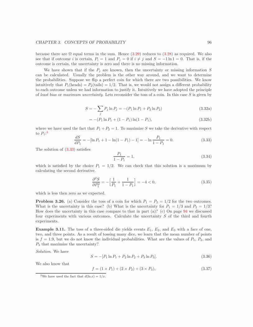
CHAPTER 3. CONCEPTS OF PROBABILITY 96

because there are Ω equal terms in the sum. Hence (3.29) reduces to (3.28) as required. We alsosee that if outcome i is certain, Pi = 1 and Pj = 0 if i = j and S = −1 ln 1 = 0. That is, if theoutcome is certain, the uncertainty is zero and there is no missing information.

We have shown that if the Pj are known, then the uncertainty or missing information Scan be calculated. Usually the problem is the other way around, and we want to determinethe probabilities. Suppose we flip a perfect coin for which there are two possibilities. We knowintuitively that P1(heads) = P2(tails) = 1/2. That is, we would not assign a different probabilityto each outcome unless we had information to justify it. Intuitively we have adopted the principleof least bias or maximum uncertainty. Lets reconsider the toss of a coin. In this case S is given by

S = −∑

j

Pj ln Pj = −(P1 ln P1 + P2 ln P2) (3.32a)

= −(P1 ln P1 + (1 − P1) ln(1 − P1), (3.32b)

where we have used the fact that P1 + P2 = 1. To maximize S we take the derivative with respectto P1:3

dS

dP1= −[lnP1 + 1 − ln(1 − P1) − 1] = − ln

P1

1 − P1= 0. (3.33)

The solution of (3.33) satisfiesP1

1 − P1= 1, (3.34)

which is satisfied by the choice P1 = 1/2. We can check that this solution is a maximum bycalculating the second derivative.

∂2S

∂P 21

= −[ 1P1

+1

1 − P1

]= −4 < 0, (3.35)

which is less then zero as we expected.

Problem 3.26. (a) Consider the toss of a coin for which P1 = P2 = 1/2 for the two outcomes.What is the uncertainty in this case? (b) What is the uncertainty for P1 = 1/3 and P2 = 1/3?How does the uncertainty in this case compare to that in part (a)? (c) On page 94 we discussedfour experiments with various outcomes. Calculate the uncertainty S of the third and fourthexperiments.

Example 3.11. The toss of a three-sided die yields events E1, E2, and E3 with a face of one,two, and three points. As a result of tossing many dice, we learn that the mean number of pointsis f = 1.9, but we do not know the individual probabilities. What are the values of P1, P2, andP3 that maximize the uncertainty?

Solution. We haveS = −[P1 ln P1 + P2 ln P2 + P3 ln P3]. (3.36)

We also know thatf = (1 × P1) + (2 × P2) + (3 × P3), (3.37)

3We have used the fact that d(ln x) = 1/x.

CHAPTER 3. CONCEPTS OF PROBABILITY 97

and P1 + P2 + P3 = 1. We use the latter condition to eliminate P3 using P3 = 1 − P1 − P2, andrewrite (3.37) as

f = P1 + 2P2 + 3(1 − P1 − P2) = 3 − 2P1 − P2. (3.38)

We then use (3.38) to eliminate P2 and P3 from (3.36) using P2 = 3−f −2P1 and P3 = f −2+P1:

S = −[P1 ln P1 + (3 − f − 2P1) ln(3 − f − 2P1) + (f − 2 + P1) ln(f − 2 + P1)]. (3.39)

Because S in (3.39) depends on only P1, we can simply differentiate S with respect P1 to find itsmaximum value:

dS

dP1= −

[ln P1 − 1 − 2[ln(3 − f − 2P1) − 1] + [ln(f − 2 + P1) − 1]

]

= lnP1(f − 2 + P1)(3 − f − 2P1)2

= 0. (3.40)

We see that for dS/dP1 to be equal to zero, the argument of the logarithm must be one. The resultis a quadratic equation for P1.

Problem 3.27. Fill in the missing steps in Example 3.11 and solve for P1, P2, and P3.

In Appendix 3B we maximize the uncertainty for a case for which there are more than threeoutcomes.

3.4.2 *Bayesian inference

Let us define P (A|B) as the probability of A occurring given that we know B. We now discuss afew results about conditional probability. Clearly,

P (A) = P (A|B) + P (A|B), (3.41)

where B means B does not occur. Also, it is clear that

P (A and B) = P (A|B)P (B) = P (B|A)P (A), (3.42)

Equation (3.42) means that the probability that A and B occur equals the probability that A occursgiven B times the probability that B occurs, which is the same as the probability that B occursgiven A times the probability A that occurs. If we are interested in various possible outcomes Ai

for the same B, we can rewrite (3.42) as

P (Ai|B) =P (B|Ai)P (Ai)

P (B). (3.43)

If all the Ai are mutually exclusive and if at least one of the Ai must occur, then we can also write

P (B) =∑

i

P (B|Ai)P (Ai). (3.44)

CHAPTER 3. CONCEPTS OF PROBABILITY 98

If we substitute (3.44) for P (B) into (3.43), we obtain the important result:

P (Ai|B) =P (B|Ai)P (Ai)∑i P (B|Ai)P (Ai)

. (Bayes’ theorem) (3.45)

Equation 3.45 is known as Bayes’ theorem.Bayes’ theorem is very useful for choosing the most probable explanation of a given data set.

In this context Ai represents the possible explanations and B represents the data. As more databecomes available, the probabilities P (B|Ai)P (Ai) change.

As an example, consider the following quandary known as the Monty Hall Problem.4 In thisshow a contestant is shown three doors. Behind one door is an expensive gift such as a car andbehind the other two doors are inexpensive gifts such as a tie. The contestant chooses a door.Suppose she chooses door 1. Then the host opens door 2 containing the tie. The contestant nowhas a choice – should she stay with her original choice or switch to door 3? What would you do?

Let us use Bayes’ theorem to determine her best course of action. We want to calculate

P (A1|B) = P (car behind door 1|door 2 open after door 1 chosen),

andP (A3|B) = P (car behind door 3|door 2 open after door 1 chosen),

where Ai denotes car behind door i. We know that all the P (Ai) equal 1/3, because with noinformation we must assume that the probability that the car is behind each door is the same.Because the host can open door 2 or 3 if the car is behind door 1, but can only open door 2 if thecar is behind door 3 we have

P (door 2 open after door 1 chosen|car behind 1) = 1/2 (3.46a)P (door 2 open after door 1 chosen|car behind 2) = 0 (3.46b)P (door 2 open after door 1 chosen|car behind 3) = 1. (3.46c)

Using Bayes’ theorem we have

P (car behind 1|door 2 open after door 1 chosen) =(1/2)(1/3)

12

13 + 0 1

3 + 1 13

= 1/3 (3.47a)

P (car behind 3|door 2 open after door 1 chosen) =(1)(1/3)

12

13 + 0 1

3 + 1 13

= 2/3. (3.47b)

The results in (3.47) suggest the contestant has a higher probability of winning the car if sheswitches doors and chooses door 3. The same logic suggests that she should always switch doorsindependently of which door she originally chose. A search of the internet for Monty Hall willbring you to many sites that discuss the problem in more detail.

Example 3.12. Even though you have no symptoms, your doctor wishes to test you for a raredisease that only 1 in 10,000 people of your age contract. The test is 98% accurate, which meansthat if you have the disease, 98% of the times the test will come out positive, and 2% negative.

4This question was posed on the TV game show, “Let’s Make A Deal,” hosted by Monty Hall.

CHAPTER 3. CONCEPTS OF PROBABILITY 99

We will also assume that if you do not have the disease, the test will come out negative 98% ofthe time and positive 2% of the time. You take the test and it comes out positive. What is theprobability that you have the disease? Is this test useful?Solution. Let P (+|D) = 0.98 represent the probability of testing positive and having the disease.If D represents not having the disease and − represents testing negative, then we are given:P (−|D) = 0.02, P (−|D) = 0.98, P (+|D) = 0.02, P (D) = 0.0001, and P (D) = 0.9999. FromBayes’ theorem we have

P (D|+) =P (+|D)P (D)

P (+|D)P (D) + P (+|D)P (D)

=(0.98)(0.0001)

(0.98)(0.0001) + (0.02)(0.9999)= 0.0047 = 0.47%. (3.48)

Problem 3.28. Imagine that you have a sack of 3 balls that can be either red or green. Thereare four hypotheses for the distribution of colors for the balls: (1) all are red, (2) 2 are red, (3) 1is red, and (4) all are green. Initially, you have no information about which hypothesis is correct,and thus you assume that they are equally probable. Suppose that you pick one ball out of thesack and it is green. Use Bayes’ theorem to determine the new probabilities for each hypothesis.

Problem 3.29. Make a table that determines the necessary accuracy for a test to give the prob-ability of having a disease if tested positive equal to at least 50% for diseases that occur in 1 in100, 1 in 1000, 1 in 10,000, and 1 in 100,000 people.

We have emphasized that the definition of probability as a frequency is inadequate. If youare interesting in learning more about Bayesian inference, read Problem 3.92 and the reference byD’Agostini.

3.5 Bernoulli processes and the binomial distribution

Because most physicists spend little time gambling,5 we will have to develop our intuitive under-standing of probability in other ways. Our strategy will be to first consider some physical systemsfor which we can calculate the probability distribution by analytical methods. Then we will usethe computer to generate more data to analyze.

Noninteracting magnetic momentsConsider a system of N noninteracting magnetic moments of spin 1

2 , each having a magneticmoment µ in an external magnetic field B. The field B is in the up (+z) direction. Spin 1

2implies that a spin can point either up (parallel to B) or down (antiparallel to B). The energyof interaction of each spin with the magnetic field is E = ∓µB, according to the orientation ofthe magnetic moment. As discussed in Section 1.10, this model is a simplification of more realisticmagnetic systems.

5After a Las Vegas hotel hosted a meeting of the American Physical Society in March, 1986, the physicists wereasked never to return.

CHAPTER 3. CONCEPTS OF PROBABILITY 100

We will take p to be the probability that the spin (magnetic moment) is up and q the probabilitythat the spin is down. Because there are no other possible outcomes,we have p+q = 1 or q = 1−p.If B = 0, there is no preferred spatial direction and p = q = 1/2. For B = 0 we do not yet knowhow to calculate p and for now we will assume that p is a known parameter. In Section 4.8 we willlearn how to calculate p and q when the system is in equilibrium at temperature T .

We associate with each spin a random variable si which has the values ±1 with probabilityp and q, respectively. One of the quantities of interest is the magnetization M , which is the netmagnetic moment of the system. For a system of N spins the magnetization is given by

M = µ(s1 + s2 + . . . + sN ) = µ

N∑i=1

si. (3.49)

In the following, we will take µ = 1 for convenience whenever it will not cause confusion. Alterna-tively, we can interpret M as the net number of up spins.

We will first calculate the mean value of M , then its variance, and finally the probabilitydistribution P (M) that the system has magnetization M . To compute the mean value of M , weneed to take the mean values of both sides of (3.49). If we use (3.8), we can interchange the sumand the average and write

M =( N∑

i=1

si

)=

N∑i=1

si. (3.50)

Because the probability that any spin has the value ±1 is the same for each spin, the mean valueof each spin is the same, that is, s1 = s2 = . . . = sN ≡ s. Therefore the sum in (3.50) consists ofN equal terms and can be written as

M = Ns. (3.51)

The meaning of (3.51) is that the mean magnetization is N times the mean magnetization of asingle spin. Because s = (1 × p) + (−1 × q) = p − q, we have that

M = N(p − q). (3.52)

Now let us calculate the variance of M , that is, (M − M)2. We write

∆M = M − M =N∑

i=1

∆si, (3.53)

where∆si ≡ si − s. (3.54)

As an example, let us calculate (∆M)2 for N = 3 spins. In this case (∆M)2 is given by

(∆M)2 = (∆s1 + ∆s2 + ∆s3)(∆s1 + ∆s2 + ∆s3)

=[(∆s1)2 + (∆s2)2 + (∆s3)2

]+ 2

[∆s1∆s2 + ∆s1∆s3 + ∆s2∆s3

]. (3.55)

We take the mean value of (3.55), interchange the order of the sums and averages, and write

(∆M)2 =[(∆s1)2 + (∆s2)2 + (∆s3)2

]+ 2

[∆s1∆s2 + ∆s1∆s3 + ∆s2∆s3

]. (3.56)

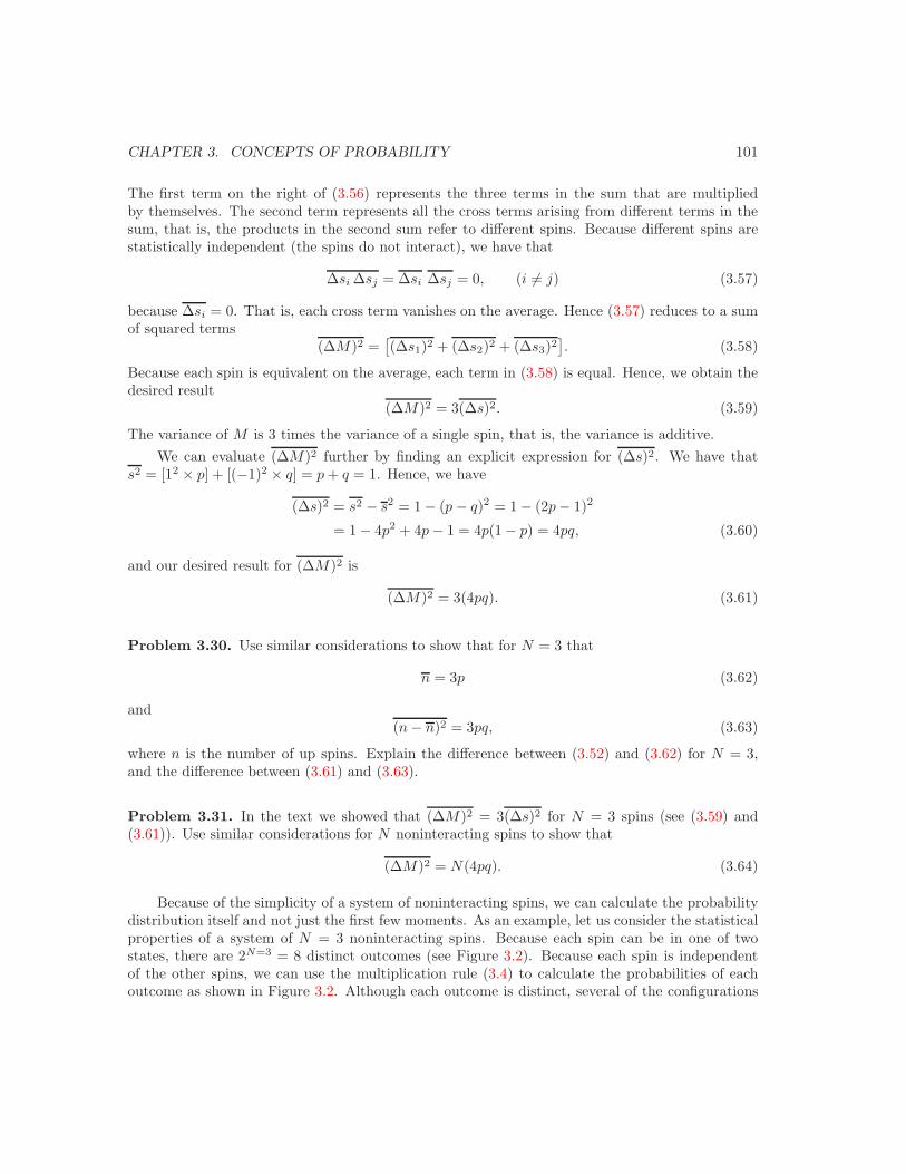
CHAPTER 3. CONCEPTS OF PROBABILITY 101

The first term on the right of (3.56) represents the three terms in the sum that are multipliedby themselves. The second term represents all the cross terms arising from different terms in thesum, that is, the products in the second sum refer to different spins. Because different spins arestatistically independent (the spins do not interact), we have that

∆si ∆sj = ∆si ∆sj = 0, (i = j) (3.57)

because ∆si = 0. That is, each cross term vanishes on the average. Hence (3.57) reduces to a sumof squared terms

(∆M)2 =[(∆s1)2 + (∆s2)2 + (∆s3)2

]. (3.58)

Because each spin is equivalent on the average, each term in (3.58) is equal. Hence, we obtain thedesired result

(∆M)2 = 3(∆s)2. (3.59)

The variance of M is 3 times the variance of a single spin, that is, the variance is additive.We can evaluate (∆M)2 further by finding an explicit expression for (∆s)2. We have that

s2 = [12 × p] + [(−1)2 × q] = p + q = 1. Hence, we have

(∆s)2 = s2 − s2 = 1 − (p − q)2 = 1 − (2p − 1)2

= 1 − 4p2 + 4p − 1 = 4p(1 − p) = 4pq, (3.60)

and our desired result for (∆M)2 is

(∆M)2 = 3(4pq). (3.61)

Problem 3.30. Use similar considerations to show that for N = 3 that

n = 3p (3.62)

and(n − n)2 = 3pq, (3.63)

where n is the number of up spins. Explain the difference between (3.52) and (3.62) for N = 3,and the difference between (3.61) and (3.63).

Problem 3.31. In the text we showed that (∆M)2 = 3(∆s)2 for N = 3 spins (see (3.59) and(3.61)). Use similar considerations for N noninteracting spins to show that

(∆M)2 = N(4pq). (3.64)

Because of the simplicity of a system of noninteracting spins, we can calculate the probabilitydistribution itself and not just the first few moments. As an example, let us consider the statisticalproperties of a system of N = 3 noninteracting spins. Because each spin can be in one of twostates, there are 2N=3 = 8 distinct outcomes (see Figure 3.2). Because each spin is independentof the other spins, we can use the multiplication rule (3.4) to calculate the probabilities of eachoutcome as shown in Figure 3.2. Although each outcome is distinct, several of the configurations

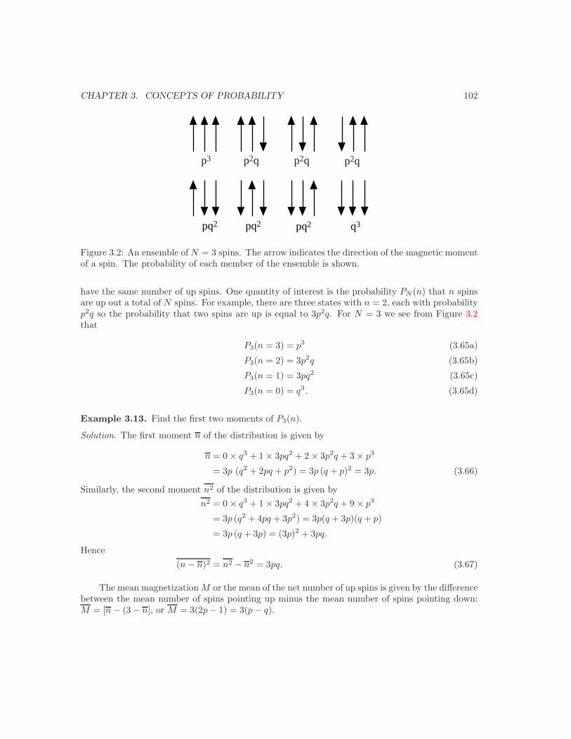
CHAPTER 3. CONCEPTS OF PROBABILITY 102

p3 p2q p2q p2q

pq2 pq2 pq2 q3

Figure 3.2: An ensemble of N = 3 spins. The arrow indicates the direction of the magnetic momentof a spin. The probability of each member of the ensemble is shown.

have the same number of up spins. One quantity of interest is the probability PN (n) that n spinsare up out a total of N spins. For example, there are three states with n = 2, each with probabilityp2q so the probability that two spins are up is equal to 3p2q. For N = 3 we see from Figure 3.2that

P3(n = 3) = p3 (3.65a)

P3(n = 2) = 3p2q (3.65b)

P3(n = 1) = 3pq2 (3.65c)

P3(n = 0) = q3. (3.65d)

Example 3.13. Find the first two moments of P3(n).

Solution. The first moment n of the distribution is given by

n = 0 × q3 + 1 × 3pq2 + 2 × 3p2q + 3 × p3

= 3p (q2 + 2pq + p2) = 3p (q + p)2 = 3p. (3.66)

Similarly, the second moment n2 of the distribution is given byn2 = 0 × q3 + 1 × 3pq2 + 4 × 3p2q + 9 × p3

= 3p (q2 + 4pq + 3p2) = 3p(q + 3p)(q + p)

= 3p (q + 3p) = (3p)2 + 3pq.

Hence(n − n)2 = n2 − n2 = 3pq. (3.67)

The mean magnetization M or the mean of the net number of up spins is given by the differencebetween the mean number of spins pointing up minus the mean number of spins pointing down:M = [n − (3 − n], or M = 3(2p− 1) = 3(p − q).

CHAPTER 3. CONCEPTS OF PROBABILITY 103

Problem 3.32. The outcome of N coins is identical to N noninteracting spins, if we associate thenumber of coins with N , the number of heads with n, and the number of tails with N − n. For afair coin the probability p of a head is p = 1

2 and the probability of a tail is q = 1− p = 1/2. Whatis the probability that in three tosses of a coin, there will be two heads?

Problem 3.33. One-dimensional random walk. The original statement of the random walk prob-lem was posed by Pearson in 1905. If a drunkard begins at a lamp post and takes N steps of equallength in random directions, how far will the drunkard be from the lamp post? We will consideran idealized example of a random walk for which the steps of the walker are restricted to a line(a one-dimensional random walk). Each step is of equal length a, and at each interval of time,the walker either takes a step to the right with probability p or a step to the left with probabilityq = 1− p. The direction of each step is independent of the preceding one. Let n be the number ofsteps to the right, and n′ the number of steps to the left. The total number of steps N = n + n′.(a) What is the probability that a random walker in one dimension has taken three steps to theright out of four steps?

From the above examples and problems, we see that the probability distributions of nonin-teracting magnetic moments, the flip of a coin, and a random walk are identical. These exampleshave two characteristics in common. First, in each trial there are only two outcomes, for example,up or down, heads or tails, and right or left. Second, the result of each trial is independent of allprevious trials, for example, the drunken sailor has no memory of his or her previous steps. Thistype of process is called a Bernoulli process.6

Because of the importance of magnetic systems, we will cast our discussion of Bernoulli pro-cesses in terms of the noninteracting magnetic moments of spin 1

2 . The main quantity of interest isthe probability PN (n) which we now calculate for arbitrary N and n. We know that a particularoutcome with n up spins and n′ down spins occurs with probability pnqn′

. We write the probabilityPN (n) as

PN (n) = WN (n, n′) pnqn′, (3.68)

where n′ = N − n and WN (n, n′) is the number of distinct configurations of N spins with n upspins and n′ down spins. From our discussion of N = 3 noninteracting spins, we already know thefirst several values of WN (n, n′).

We can determine the general form of WN (n, n′) by obtaining a recursion relation betweenWN and WN−1. A total of n up spins and n′ down spins out of N total spins can be found byadding one spin to N − 1 spins. The additional spin is either

(a) up if there are (n − 1) up spins and n′ down spins, or

(b) down if there are n up spins and n′ down spins.

Because there are WN (n − 1, n′) ways of reaching the first case and WN (n, n′ − 1) ways in thesecond case, we obtain the recursion relation

WN (n, n′) = WN−1(n − 1, n′) + WN−1(n, n′ − 1). (3.69)

6These processes are named after the mathematician Jacob Bernoulli, 1654 – 1705.

CHAPTER 3. CONCEPTS OF PROBABILITY 104

1

1

1 1

11

1 1

2

3 3

4 46 1

Figure 3.3: The values of the first few coefficients WN (n, n′). Each number is the sum of the twonumbers to the left and right above it. This construction is called a Pascal triangle.

If we begin with the known values W0(0, 0) = 1, W1(1, 0) = W1(0, 1) = 1, we can use the recursionrelation (3.69) to construct WN (n, n′) for any desired N . For example,

W2(2, 0) = W1(1, 0) + W1(2,−1) = 1 + 0 = 1. (3.70a)W2(1, 1) = W1(0, 1) + W1(1, 0) = 1 + 1 = 2. (3.70b)W2(0, 2) = W1(−1, 2) + W1(0, 1) = 0 + 1. (3.70c)

In Figure 3.3 we show that WN (n, n′) forms a pyramid or (a Pascal) triangle.It is straightforward to show by induction that the expression

WN (n, n′) =N !

n! n′!=

N !n!(N − n)!

(3.71)

satisfies the relation (3.69). Note the convention 0! = 1. We can combine (3.68) and (3.71) to findthe desired result

PN (n) =N !

n! (N − n)!pnqN−n . (binomial distribution) (3.72)

The form (3.72) is called the binomial distribution. Note that for p = q = 1/2, PN (n) reduces to

PN (n) =N !

n! (N − n)!2−N . (3.73)

The probability PN (n) is shown in Figure 3.4 for N = 16.

Problem 3.34. (a) Calculate the distribution PN (n) that n spins are up out of a total of N forN = 4 and N = 16 and put your results in the form of a table. Calculate the mean values of nand n2 using your tabulated values of PN (n). (b) Plot your tabulated results that you calculatedin part (a) (see Figure 3.4). Assume p = q = 1/2. Visually estimate the width of the distribution

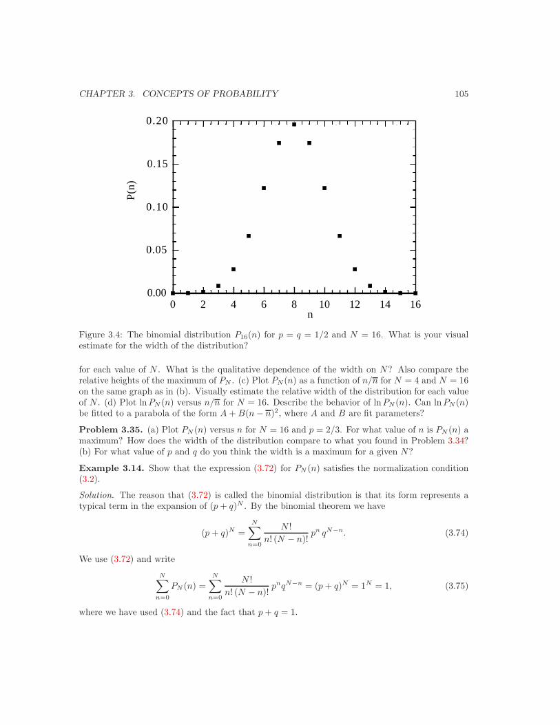
CHAPTER 3. CONCEPTS OF PROBABILITY 105

0.00

0.05

0.10

0.15

0.20

0 2 4 6 8 10 12 14 16

P(n

)

n

Figure 3.4: The binomial distribution P16(n) for p = q = 1/2 and N = 16. What is your visualestimate for the width of the distribution?

for each value of N . What is the qualitative dependence of the width on N? Also compare therelative heights of the maximum of PN . (c) Plot PN (n) as a function of n/n for N = 4 and N = 16on the same graph as in (b). Visually estimate the relative width of the distribution for each valueof N . (d) Plot lnPN (n) versus n/n for N = 16. Describe the behavior of lnPN (n). Can lnPN (n)be fitted to a parabola of the form A + B(n − n)2, where A and B are fit parameters?

Problem 3.35. (a) Plot PN (n) versus n for N = 16 and p = 2/3. For what value of n is PN (n) amaximum? How does the width of the distribution compare to what you found in Problem 3.34?(b) For what value of p and q do you think the width is a maximum for a given N?

Example 3.14. Show that the expression (3.72) for PN (n) satisfies the normalization condition(3.2).

Solution. The reason that (3.72) is called the binomial distribution is that its form represents atypical term in the expansion of (p + q)N . By the binomial theorem we have

(p + q)N =N∑

n=0

N !n! (N − n)!

pn qN−n. (3.74)

We use (3.72) and write

N∑n=0

PN (n) =N∑

n=0

N !n! (N − n)!

pnqN−n = (p + q)N = 1N = 1, (3.75)

where we have used (3.74) and the fact that p + q = 1.

CHAPTER 3. CONCEPTS OF PROBABILITY 106

Calculation of the mean value

We now find an analytical expression for the dependence of n on N and p. From the definition(3.6) and (3.72) we have

n =N∑

n=0

n PN (n) =N∑

n=0

nN !

n! (N − n)!pnqN−n. (3.76)

We evaluate the sum in (3.76) by using a technique that is useful in a variety of contexts.7 Thetechnique is based on the fact that

pd

dppn = npn. (3.77)

We use (3.77) to rewrite (3.76) as

n =N∑

n=0

nN !

n! (N − n)!pnqN−n (3.78)

=N∑

n=0

N !n! (N − n)!

(p

∂

∂ppn

)qN−n. (3.79)

We have used a partial derivative in (3.79) to remind us that the derivative operator does not acton q. We interchange the order of summation and differentiation in (3.79) and write

n = p∂

∂p

[ N∑n=0

N !n! (N − n)!

pnqN−n

](3.80)

= p∂

∂p(p + q)N , (3.81)

where we have temporarily assumed that p and q are independent variables. Because the operatoracts only on p, we have

n = pN(p + q)N−1. (3.82)

The result (3.82) is valid for arbitrary p and q, and hence it is applicable for p + q = 1. Thus ourdesired result is

n = pN. (3.83)

The dependence of n on N and p should be intuitively clear. Compare the general result (3.83) tothe result (3.66) for N = 3. What is the dependence of n′ on N and p?

Calculation of the relative fluctuations7The integral

R ∞0 xn e−ax2

for a > 0 is evaluated in Appendix A using a similar technique.

CHAPTER 3. CONCEPTS OF PROBABILITY 107

To determine ∆n2 we need to know n2 (see the relation (3.15)). The average value of n2 can becalculated in a manner similar to that for n. We write

n2 =N∑

n=0

n2 N !n! (N − n)!

pnqN−n (3.84)

=N∑

n=0

N !n! (N − n)!

(p

∂

∂p

)2pnqN−n

=(p

∂

∂p

)2N∑

n=0

N !n! (N − n)!

pnqN−n =(p

∂

∂p

)2 (p + q)N

=(p

∂

∂p

)[pN(p + q)N−1

]

= p[N(p + q)N−1 + pN(N − 1)(p + q)N−2

]. (3.85)

Because we are interested in the case p + q = 1, we have

n2 = p [N + pN(N − 1)]

= p [pN2 + N(1 − p)] = (pN)2 + p (1 − p)N

= n2 + pqN, (3.86)

where we have used (3.83) and let q = 1 − p. Hence, from (3.86) we find that the variance of n isgiven by

σn2 = (∆n)2 = n2 − n2 = pqN. (3.87)

Compare the calculated values of σn from (3.87) with your estimates in Problem 3.34 and to theexact result (3.67) for N = 3.

The relative width of the probability distribution of n is given by (3.83) and (3.87)

σn

n=

√pqN

pN=

(q

p

)12

1√N

. (3.88)

We see that the relative width goes to zero as 1/√

N .Frequently we need to evaluate ln N ! for N 1. A simple approximation for lnN ! known as

Stirling’s approximation is

ln N ! ≈ N ln N − N. (Stirling’s approximation) (3.89)

A more accurate approximation is given by

ln N ! ≈ N ln N − N +12

ln(2πN). (3.90)

A simple derivation of Stirling’s approximation is given in Appendix A.

CHAPTER 3. CONCEPTS OF PROBABILITY 108

Problem 3.36. (a) What is the largest value of ln N ! that you can calculate exactly using atypical hand calculator? (b) Compare the approximations (3.89) and (3.90) to each other and tothe exact value of lnN ! for N = 5, 10, 20, and 50. If necessary, compute lnN ! directly using therelation

ln N ! =N∑

m=1

ln m. (3.91)

(c) Use the simple form of Stirling’s approximation to show that

d

dxln x! = lnx for x 1. (3.92)

Problem 3.37. Consider the binomial distribution PN (n) for N = 16 and p = q = 1/2. What isthe value of PN (n) for n = σn/2? What is the value of the product PN (n = n)σn?

Problem 3.38. A container of volume V contains N molecules of a gas. We assume that the gasis dilute so that the position of any one molecule is independent of all other molecules. Althoughthe density will be uniform on the average, there are fluctuations in the density. Divide the volumeV into two parts V1 and V2, where V = V1 + V2. (a) What is the probability p that a particularmolecule is in each part? (b) What is the probability that N1 molecules are in V1 and N2 moleculesare in V2? (c) What is the average number of molecules in each part? (d) What are the relativefluctuations of the number of particles in each part?

Problem 3.39. Suppose that a random walker takes n steps to the right and n′ steps to the leftand each step is of equal length a. Denote x as the net displacement of a walker. What is the meanvalue x for a N -step random walk? What is the analogous expression for the variance (∆x)2?

Problem 3.40. Monte Carlo simulation. We can gain more insight into the nature of the Bernoullidistribution by doing a Monte Carlo simulation, that is, by using a computer to “flip coins” andaverage over many measurements.8 In the context of random walks, we can implement a N -stepwalk by the following pseudocode:

do istep = 1,Nif (rnd <= p) thenx = x + 1

elsex = x - 1

end ifend do

The function rnd generates a random number between zero and one. The quantity x is the netdisplacement assuming that the steps are of unit length. It is necessary to save the value ofx after N steps and average over many walkers. Write a simple program or use the applet at<stp.clarku.edu/simulations/OneDimensionalWalk> to compute PN (x). First choose N = 4and p = 1/2 and make a sufficient number of measurements so that the various quantities ofinterest are known to a good approximation. Then take N = 100 and describe the qualitativex-dependence of PN (x).

8The name “Monte Carlo” was coined by Nicolas Metropolis in 1949.

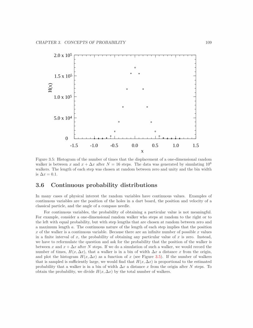
CHAPTER 3. CONCEPTS OF PROBABILITY 109

0

5.0 x 104

-1.5 -1.0 -0.5 0.0 0.5 1.0 1.5x

1.0 x 105

1.5 x 105

2.0 x 105H

(x)

Figure 3.5: Histogram of the number of times that the displacement of a one-dimensional randomwalker is between x and x + ∆x after N = 16 steps. The data was generated by simulating 106

walkers. The length of each step was chosen at random between zero and unity and the bin widthis ∆x = 0.1.

3.6 Continuous probability distributions

In many cases of physical interest the random variables have continuous values. Examples ofcontinuous variables are the position of the holes in a dart board, the position and velocity of aclassical particle, and the angle of a compass needle.

For continuous variables, the probability of obtaining a particular value is not meaningful.For example, consider a one-dimensional random walker who steps at random to the right or tothe left with equal probability, but with step lengths that are chosen at random between zero anda maximum length a. The continuous nature of the length of each step implies that the positionx of the walker is a continuous variable. Because there are an infinite number of possible x valuesin a finite interval of x, the probability of obtaining any particular value of x is zero. Instead,we have to reformulate the question and ask for the probability that the position of the walker isbetween x and x + ∆x after N steps. If we do a simulation of such a walker, we would record thenumber of times, H(x, ∆x), that a walker is in a bin of width ∆x a distance x from the origin,and plot the histogram H(x, ∆x) as a function of x (see Figure 3.5). If the number of walkersthat is sampled is sufficiently large, we would find that H(x, ∆x) is proportional to the estimatedprobability that a walker is in a bin of width ∆x a distance x from the origin after N steps. Toobtain the probability, we divide H(x, ∆x) by the total number of walkers.

CHAPTER 3. CONCEPTS OF PROBABILITY 110

In practice, the choice of the bin width is a compromise. If ∆x is too big, the features ofthe histogram would be lost. If ∆x is too small, many of the bins would be empty for a givennumber of walkers. Hence, our estimate of the number of walkers in each bin would be lessaccurate. Because we expect the number to be proportional to the width of the bin, we can writeH(x, ∆x) = p(x)∆x. The quantity p(x) is the probability density. In the limit that ∆x → 0,H(x, ∆x) becomes a continuous function of x, and we can write the probability that a walker is inthe range between a and b as

P (a to b) =∫ b

a

p(x) dx. (3.93)

Note that the probability density p(x) is nonnegative and has units of one over the dimension ofx.

The formal properties of the probability density p(x) are easily generalizable from the discretecase. For example, the normalization condition is given by

∫ ∞

−∞p(x) dx = 1. (3.94)

The mean value of the function f(x) in the interval a to b is given by

f =∫ b

a

f(x) p(x) dx. (3.95)

Problem 3.41. The random variable x has the probability density

p(x) =

Ae−λx if 0 ≤ x ≤ ∞0 x < 0.

(3.96)

(a) Determine the normalization constant A in terms of λ. (b) What is the mean value of x?What is the most probable value of x? (c) What is the mean value of x2? (d) Choose λ = 1 anddetermine the probability that a measurement of x yields a value less than 0.3.

Problem 3.42. Consider the probability density function p(v) = (a/π)3/2 e−av2for the velocity

v of a particle. Each of the three velocity components can range from −∞ to +∞ and a is aconstant. (a) What is the probability that a particle has a velocity between vx and vx + dvx, vy

and vy + dvy, and vz and vz + dvz? (b) Show that p(v) is normalized to unity. Use the fact that

∫ ∞

0

e−au2du =

12

√π

a. (3.97)

Note that this calculation involves doing three similar integrals that can be evaluated separately.(c) What is the probability that vx ≥ 0, vy ≥ 0, vz ≥ 0 simultaneously?

Problem 3.43. (a) Find the first four moments of the Gaussian probability density

p(x) = (2π)−12 e−x2/2. (−∞ < x < ∞) (3.98)

CHAPTER 3. CONCEPTS OF PROBABILITY 111

Guess the dependence of the kth moment on k for k even. What are the odd moments of p(x)?(b) Calculate the value of C4, the fourth-order cumulant, defined by

C4 = x4 − 4x3 x − 3 x22

+ 12 x2 x2 − 6 x4. (3.99)

Problem 3.44. Consider the probability density given by

p(x) =

(2a)−1 for |x| ≤ a

0 for |x| > a(3.100)

(a) Sketch the dependence of p(x) on x. (b) Find the first four moments of p(x). (c) Calculate thevalue of the fourth-order cumulant C4 defined in (3.99)). What is C4 for the probability densityin (3.100)?

Problem 3.45. Not all probability densities have a finite variance. Sketch the Lorentz or Cauchydistribution given by

p(x) =1π

γ

(x − a)2 + γ2. (−∞ < x < ∞) (3.101)

Choose a = 0 and γ = 1 and compare the form of p(x) in (3.101) to the Gaussian distribution givenby (3.98). Give a simple argument for the existence of the first moment of the Lorentz distribution.Does the second moment exist?

3.7 The Gaussian distribution as a limit of the binomialdistribution

In Problem 3.34 we found that for large N , the binomial distribution has a well-defined maximumat n = pN and can be approximated by a smooth, continuous function even though only integervalues of n are physically possible. We now find the form of this function of n.

The first step is to realize that for N 1, PN (n) is a rapidly varying function of n nearn = pN , and for this reason we do not want to approximate PN (n) directly. However, becausethe logarithm of PN (n) is a slowly varying function (see Problem 3.34), we expect that the powerseries expansion of ln PN (n) to converge. Hence, we expand ln PN (n) in a Taylor series about thevalue of n = n at which lnPN (n) reaches its maximum value. We will write p(n) instead of PN (n)because we will treat n as a continuous variable and hence p(n) is a probability density. We find

ln p(n) = ln p(n = n) + (n − n)d ln p(n)

dn

∣∣n=n

+12(n − n)2

d2 ln p(n)d2n

∣∣n=n

+ · · · (3.102)

Because we have assumed that the expansion (3.102) is about the maximum n = n, the first deriva-tive d ln p(n)/dn

∣∣n=n

must be zero. For the same reason the second derivative d2 ln p(n)/dn2∣∣n=n

must be negative. We assume that the higher terms in (3.102) can be neglected and adopt thenotation

ln A = ln p(n = n), (3.103)

and

CHAPTER 3. CONCEPTS OF PROBABILITY 112

B = −d2 ln p(n)dn2

∣∣n=n

. (3.104)

The approximation (3.102) and the notation in (3.103) and (3.104) allows us to write

ln p(n) ≈ ln A − 12B(n − n)2, (3.105)

orp(n) ≈ Ae−

12B(n−n)2 . (3.106)

We next use Stirling’s approximation to evaluate the first two derivatives of ln p(n) and thevalue of ln p(n) at its maximum to find the parameters A, B, and n. We write

ln p(n) = lnN ! − ln n! − ln(N − n)! + n ln p + (N − n) ln q. (3.107)

It is straightforward to use the relation (3.92) to obtain

d(ln p)dn

= − lnn + ln(N − n) + ln p − ln q. (3.108)

The most probable value of n is found by finding the value of n that satisfies the conditiond ln p/dn = 0. We find

N − n

n=

q

p, (3.109)

or (N − n)p = nq. If we use the relation p + q = 1, we obtain

n = pN. (3.110)

Note that n = n, that is, the value of n for which p(n) is a maximum is also the mean value of n.The second derivative can be found from (3.108). We have

d2(ln p)dn2

= − 1n− 1

N − n. (3.111)

Hence, the coefficient B defined in (3.104) is given by

B = −d2 ln p

dn2=

1n

+1

N − n=

1Npq

. (3.112)

From the relation (3.87) we see that

B =1σ2

, (3.113)

where σ2 is the variance of n.If we use the simple form of Stirling’s approximation (3.89) to find the normalization constant

A from the relation ln A = ln p(n = n), we would find that lnA = 0. Instead, we have to use themore accurate form of Stirling’s approximation (3.90). The result is

A =1

(2πNpq)1/2=

1(2πσ2)1/2

. (3.114)

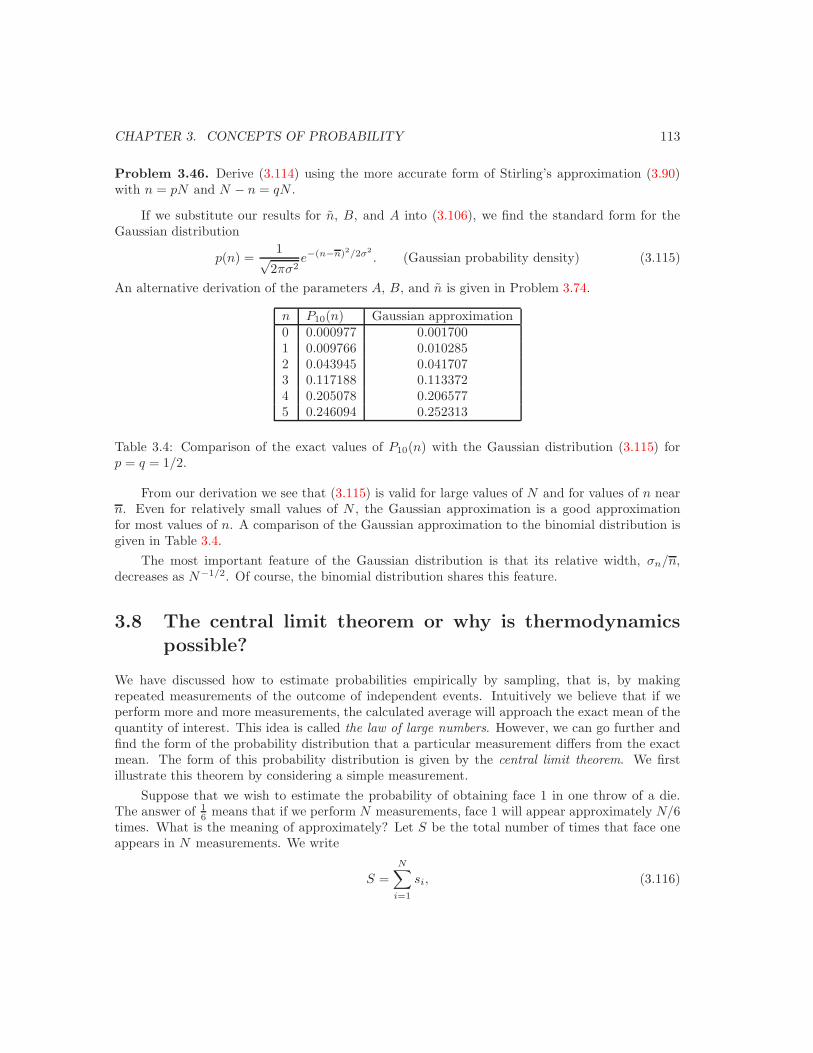
CHAPTER 3. CONCEPTS OF PROBABILITY 113

Problem 3.46. Derive (3.114) using the more accurate form of Stirling’s approximation (3.90)with n = pN and N − n = qN .

If we substitute our results for n, B, and A into (3.106), we find the standard form for theGaussian distribution

p(n) =1√

2πσ2e−(n−n)2/2σ2

. (Gaussian probability density) (3.115)

An alternative derivation of the parameters A, B, and n is given in Problem 3.74.

n P10(n) Gaussian approximation0 0.000977 0.0017001 0.009766 0.0102852 0.043945 0.0417073 0.117188 0.1133724 0.205078 0.2065775 0.246094 0.252313

Table 3.4: Comparison of the exact values of P10(n) with the Gaussian distribution (3.115) forp = q = 1/2.

From our derivation we see that (3.115) is valid for large values of N and for values of n nearn. Even for relatively small values of N , the Gaussian approximation is a good approximationfor most values of n. A comparison of the Gaussian approximation to the binomial distribution isgiven in Table 3.4.

The most important feature of the Gaussian distribution is that its relative width, σn/n,decreases as N−1/2. Of course, the binomial distribution shares this feature.

3.8 The central limit theorem or why is thermodynamicspossible?

We have discussed how to estimate probabilities empirically by sampling, that is, by makingrepeated measurements of the outcome of independent events. Intuitively we believe that if weperform more and more measurements, the calculated average will approach the exact mean of thequantity of interest. This idea is called the law of large numbers. However, we can go further andfind the form of the probability distribution that a particular measurement differs from the exactmean. The form of this probability distribution is given by the central limit theorem. We firstillustrate this theorem by considering a simple measurement.

Suppose that we wish to estimate the probability of obtaining face 1 in one throw of a die.The answer of 1

6 means that if we perform N measurements, face 1 will appear approximately N/6times. What is the meaning of approximately? Let S be the total number of times that face oneappears in N measurements. We write

S =N∑

i=1

si, (3.116)

CHAPTER 3. CONCEPTS OF PROBABILITY 114

where

si =

1, if the ith throw gives 10 otherwise.

(3.117)

If N is large, then S/N approaches 1/6. How does this ratio approach the limit? We can empiricallyanswer this question by repeating the measurement M times. (Each measurement of S consists ofN throws of a die.) Because S itself is a random variable, we know that the measured values ofS will not be identical. In Figure 3.6 we show the results of M = 10, 000 measurements of S forN = 100 and N = 800. We see that the approximate form of the distribution of values of S is aGaussian. In Problem 3.47 we calculate the absolute and relative width of the distributions.

Problem 3.47. Estimate the absolute width and the relative width of the distributions shown inFigure 3.6 for N = 100 and N = 800. Does the error of any one measurement of S decreases withincreasing N as expected? How would the plot change if M were increased to M = 10, 000?

In Appendix 3A we show that in the limit of large N , the probability density p(S) is given by

p(S) =1√

2πσ2S

e−(S−S)2/2σ2S , (3.118)

where

S = Ns (3.119)

σ2S = Nσ2, (3.120)

with σ2 = s2 − s2. The quantity p(S)∆S is the probability that the value of∑N

i=1 si is between Sand S + ∆S. Equation (3.118) is equivalent to the central limit theorem. Note that the Gaussianform in (3.118) holds only for large N and for values of S near its most probable (mean) value. Thelatter restriction is the reason that the theorem is called the central limit theorem; the requirementthat N be large is the reason for the term limit.

The central limit theorem is one of the most remarkable results of the theory of probability.In its simplest form, the theorem states that the sum of a large number of random variableswill approximate a Gaussian distribution. Moreover, the approximation steadily improves as thenumber of variables in the sum increases.

For the throw of a die, s = 16 , s2 = 1

6 , and σ2 = s2 − s2 = 16 − 1

36 = 536 . For N throws of a

die, we have S = N/6 and σ2S = 5N/36. Hence, we see that in this case the most probable relative

error in any one measurement of S decreases as σS/S =√

5/N .Note that if we let S represent the displacement of a walker after N steps, and let σ2 equal

the mean square displacement for a single step, then the result (3.118)–(3.120) is equivalent toour results for random walks in the limit of large N . Or we can let S represent the magnetizationof a system of noninteracting spins and obtain similar results. That is, a random walk and itsequivalents are examples of an additive random process.

The central limit theorem shows why the Gaussian distribution is ubiquitous in nature. If arandom process is related to a sum of a large number of microscopic processes, the sum will bedistributed according to the Gaussian distribution independently of the nature of the distributionof the microscopic processes.

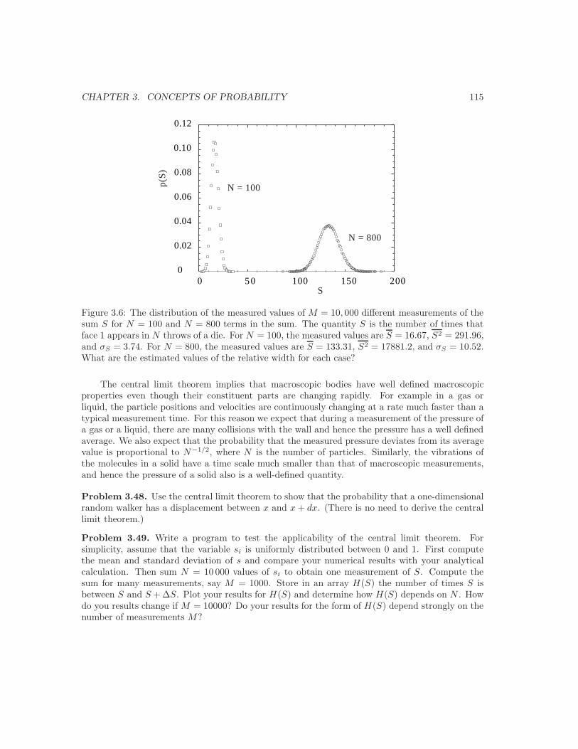
CHAPTER 3. CONCEPTS OF PROBABILITY 115

0

0.02

0.04

0.06

0.08

0.10

0.12

0 50 100 150 200S

N = 100

N = 800

p(S

)

Figure 3.6: The distribution of the measured values of M = 10, 000 different measurements of thesum S for N = 100 and N = 800 terms in the sum. The quantity S is the number of times thatface 1 appears in N throws of a die. For N = 100, the measured values are S = 16.67, S2 = 291.96,and σS = 3.74. For N = 800, the measured values are S = 133.31, S2 = 17881.2, and σS = 10.52.What are the estimated values of the relative width for each case?

The central limit theorem implies that macroscopic bodies have well defined macroscopicproperties even though their constituent parts are changing rapidly. For example in a gas orliquid, the particle positions and velocities are continuously changing at a rate much faster than atypical measurement time. For this reason we expect that during a measurement of the pressure ofa gas or a liquid, there are many collisions with the wall and hence the pressure has a well definedaverage. We also expect that the probability that the measured pressure deviates from its averagevalue is proportional to N−1/2, where N is the number of particles. Similarly, the vibrations ofthe molecules in a solid have a time scale much smaller than that of macroscopic measurements,and hence the pressure of a solid also is a well-defined quantity.

Problem 3.48. Use the central limit theorem to show that the probability that a one-dimensionalrandom walker has a displacement between x and x + dx. (There is no need to derive the centrallimit theorem.)

Problem 3.49. Write a program to test the applicability of the central limit theorem. Forsimplicity, assume that the variable si is uniformly distributed between 0 and 1. First computethe mean and standard deviation of s and compare your numerical results with your analyticalcalculation. Then sum N = 10 000 values of si to obtain one measurement of S. Compute thesum for many measurements, say M = 1000. Store in an array H(S) the number of times S isbetween S and S + ∆S. Plot your results for H(S) and determine how H(S) depends on N . Howdo you results change if M = 10000? Do your results for the form of H(S) depend strongly on thenumber of measurements M?

CHAPTER 3. CONCEPTS OF PROBABILITY 116

3.9 The Poisson distribution and should you fly in airplanes?

We now return to the question of whether or not it is safe to fly. If the probability of a planecrashing is p = 10−5, then 1 − p is the probability of surviving a single flight. The probabilityof surviving N flights is then PN = (1 − p)N . For N = 400, PN ≈ 0.996, and for N = 105,PN ≈ 0.365. Thus, our intuition is verified that if we lived eighty years and took 400 flights, wewould have only a small chance of crashing.

This type of reasoning is typical when the probability of an individual event is small, butthere are very many attempts. Suppose we are interested in the probability of the occurrence of nevents out of N attempts such that the probability p of the event for each attempt is very small.The resulting probability is called the Poisson distribution, a distribution that is important in theanalysis of experimental data. We discuss it here because of its intrinsic interest.

To derive the Poisson distribution, we begin with the binomial distribution:

P (n) =N !

n! (N − n)!pn(1 − p)N−n. (3.121)

(As before, we suppress the N dependence of P .) As in Section (3.7, we will approximate lnP (n)rather than P (n) directly. We first use Stirling’s approximation to write

lnN !

(N − n)!= lnN ! − ln(N − n)! (3.122)

≈ N ln N − (N − n) ln(N − n)≈ N ln N − (N − n) ln N

= N ln N − N ln N + n lnN

= n ln N. (3.123)

From (3.123) we obtainN !

(N − n)!≈ en ln N = Nn. (3.124)

For p 1, we have ln(1 − p) ≈ −p, eln(1−p) = 1 − p ≈ e−p, and (1 − p)N−n ≈ e−p(N−n) ≈ e−pN .If we use the above approximations, we find

P (n) ≈ Nn

n!pne−pN =

(Np)n

n!e−pN , (3.125)

or

P (n) =nn

n!e−n, (Poisson distribution) (3.126)

wheren = pN. (3.127)

The form (3.126) is the Poisson distribution.Let us apply the Poisson distribution to the airplane survival problem. We want to know the

probability of never crashing, that is, P (n = 0). The mean N = pN equals 10−5 × 400 = 0.004 for

CHAPTER 3. CONCEPTS OF PROBABILITY 117

N = 400 flights and N = 1 for N = 105 flights. Thus, the survival probability is P (0) = e−N ≈0.996 for N = 400 and P (0) ≈ 0.368 for N = 105 as we calculated previously. We see that if wefly 100,000 times, we have a much larger probability of dying in a plane crash.

Problem 3.50. Show that the Poisson distribution is properly normalized, and calculate the meanand variance of n. Because P (n) for n > N is negligibly small, you can sum P (n) from n = 0to n = ∞ even though the maximum value of n is N . Plot the Poisson distribution P (n) as afunction of n for p = 0.01 and N = 100.

3.10 *Traffic flow and the exponential distribution

The Poisson distribution is closely related to the exponential distribution as we will see in thefollowing. Consider a sequence of similar random events and let t1, t2, . . . be the time at whicheach successive event occurs. Examples of such sequences are the successive times when a phonecall is received and the times when a Geiger counter registers a decay of a radioactive nucleus.Suppose that we determine the sequence over a very long time T that is much greater than anyof the intervals ti − ti−1. We also suppose that the average number of events is λ per unit time sothat in a time interval t, the mean number of events is λt.

Assume that the events occur at random and are independent of each other. Given λ, themean number of events per unit time, we wish to find the probability distribution w(t) of theinterval t between the events. We know that if an event occurred at time t = 0, the probabilitythat another event occurs within the interval [0, t] is

∫ t

0

w(t)∆t, (3.128)

and the probability that no event occurs in the interval t is

1 −∫ t

0

w(t)∆t. (3.129)

Thus the probability that the duration of the interval between the two events is between t andt + ∆t is given by

w(t)∆t = probability that no event occurs in the interval [0, t]× probability that an event occurs in interval [t, t + ∆t]

=[1 −

∫ t

0

w(t)dt]λ∆t. (3.130)

If we cancel ∆t from each side of (3.130) and differentiate both sides with respect to t, we find

dw

dt= −λw,

so thatw(t) = Ae−λt. (3.131)

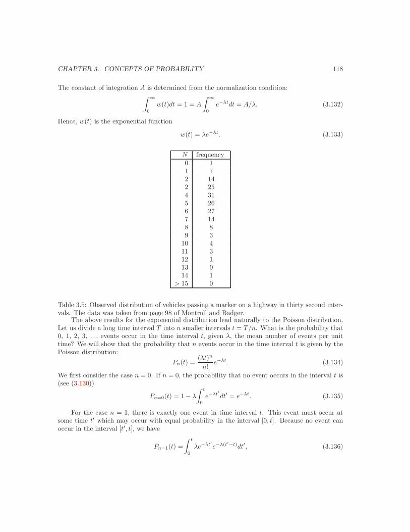
CHAPTER 3. CONCEPTS OF PROBABILITY 118

The constant of integration A is determined from the normalization condition:∫ ∞

0

w(t)dt = 1 = A

∫ ∞

0

e−λtdt = A/λ. (3.132)

Hence, w(t) is the exponential function

w(t) = λe−λt. (3.133)

N frequency0 11 72 142 254 315 266 277 148 89 3

10 411 312 113 014 1

> 15 0

Table 3.5: Observed distribution of vehicles passing a marker on a highway in thirty second inter-vals. The data was taken from page 98 of Montroll and Badger.

The above results for the exponential distribution lead naturally to the Poisson distribution.Let us divide a long time interval T into n smaller intervals t = T/n. What is the probability that0, 1, 2, 3, . . . events occur in the time interval t, given λ, the mean number of events per unittime? We will show that the probability that n events occur in the time interval t is given by thePoisson distribution:

Pn(t) =(λt)n

n!e−λt. (3.134)

We first consider the case n = 0. If n = 0, the probability that no event occurs in the interval t is(see (3.130))

Pn=0(t) = 1 − λ

∫ t

0

e−λt′dt′ = e−λt. (3.135)

For the case n = 1, there is exactly one event in time interval t. This event must occur atsome time t′ which may occur with equal probability in the interval [0, t]. Because no event canoccur in the interval [t′, t], we have

Pn=1(t) =∫ t

0

λe−λt′e−λ(t′−t)dt′, (3.136)

CHAPTER 3. CONCEPTS OF PROBABILITY 119

where we have used (3.135) with t → (t′ − t). Hence,

Pn=1(t) =∫ t

0

λe−λtdt = (λt)e−λt. (3.137)

In general, if n events are to occur in the interval [0, t], the first must occur at some time t′

and exactly (n − 1) must occur in the time (t − t′). Hence,

Pn(t) =∫ t

0

λe−λt′Pn−1(t − t′). (3.138)

Equation (3.138) is a recurrence formula that can be used to derive (3.134) by induction. It is easyto see that (3.134) satisfies (3.138) for n = 0 and 1. As is usual when solving recursion formula byinduction, we assume that (3.134) is correct for (n− 1). We substitute this result into (3.138) andfind

Pn(t) = λne−λt

∫ t

0

(t − t′)n−1dt′/(n − 1)! =(λt)b

n!e−λt. (3.139)

An application of the Poisson distribution is given in Problem 3.51.

Problem 3.51. In Table 3.5 we show the number of vehicles passing a marker during a thirtysecond interval. The observations were made on a single lane of a six lane divided highway. Assumethat the traffic density is so low that passing occurs easily and no platoons of cars develop. Is thedistribution of the number of vehicles consistent with the Poisson distribution? If so, what is thevalue of the parameter λ?

As the traffic density increases, the flow reaches a regime where the vehicles are very close toone another so that they are no longer mutually independent. Make arguments for the form of theprobability distribution of the number of vehicles passing a given point in this regime.

3.11 *Are all probability distributions Gaussian?

We have discussed the properties of random additive processes and found that the probabilitydistribution for the sum is a Gaussian. As an example of such a process, we discussed a one-dimensional random walk on a lattice for which the displacement x is the sum of N random steps.

We now discuss random multiplicative processes. Examples of such processes include thedistributions of incomes, rainfall, and fragment sizes in rock crushing processes. Consider thelatter for which we begin with a rock of size w. We strike the rock with a hammer and generatetwo fragments whose sizes are pw and qw, where q = 1 − p. In the next step the possible sizesof the fragments are p2w, pqw, qpw, and q2w. What is the distribution of the fragments after Nblows of the hammer?

To answer this question, consider a binary sequence in which the numbers x1 and x2 appearindependently with probabilities p and q respectively. If there are N elements in the product Π, wecan ask what is Π, the mean value of Π. To compute Π, we define P (n) as the probability that theproduct of N independent factors of x1 and x2 has the value x1

nx2N−n. This probability is given

CHAPTER 3. CONCEPTS OF PROBABILITY 120

by the number of sequences where x1 appears n times multiplied by the probability of choosing aspecific sequence with x1 appearing n times:

P (n) =N !

n! (N − n)!pnqN−n. (3.140)

The mean value of the product is given by

Π =N∑

n=0

P (n)x1nx2

N−n (3.141)

= (px1 + qx2)N . (3.142)

The most probable event is one in which the product contains Np factors of x1 and Nq factors ofx2. Hence, the most probable value of the product is

Π = (x1px2

q)N . (3.143)

We have found that the average value of the sum of random variables is a good approximationto the most probable value of the sum. Let us see if there is a similar relation for a randommultiplicative process. We first consider x1 = 2, x2 = 1/2, and p = q = 1/2. Then Π =[(1/2) × 2 + (1/2)× (1/2)]N = (5/4)N = eN ln 5/4. In contrast Π = 21/2 × (1/2)1/2 = 1.

The reason for the large discrepancy between Π and Π is the relatively important role playedby rare events. For example, a sequence of N factors of x1 = 2 occurs with a very small probability,but the value of this product is very large in comparison to the most probable value. Hence, thisextreme event makes a finite contribution to Π and a dominant contribution to the higher momentsΠ

m.

∗Problem 3.52. (a) Confirm the above general results for N = 4 by showing explicitly all thepossible values of the product. (b) Consider the case x1 = 2, x2 = 1/2, p = 1/3, and q = 2/3, andcalculate Π and Π.∗Problem 3.53. (a) Show that Π

mreduces to (pxm

1 )N as m → ∞. This result implies thatfor m 1, the mth moment is determined solely by the most extreme event. (b) Based on theGaussian approximation for the probability of a random additive process, what is a reasonableguess for the continuum approximation to the probability of a random multiplicative process?Such a distribution is called the log-normal distribution. Discuss why or why not you expect thelog-normal distribution to be a good approximation for N 1. (c) More insight can be gained byrunning the applet at <stp.clarku.edu/simulations/product> which simulates the distributionof values of the product x1

nx2N−n. Choose x1 = 2, x2 = 1/2, and p = q = 1/2 for which we have

already calculated the analytical results for Π and Π. First choose N = 4 and estimate Π andΠ. Do your estimated values converge more or less uniformly to the exact values as the numberof measurements becomes large? Do a similar simulation for N = 40. Compare your results witha similar simulation of a random walk and discuss the importance of extreme events for randommultiplicative processes. An excellent discussion is given by Redner (see references).

Vocabulary

sample space, events, outcome

CHAPTER 3. CONCEPTS OF PROBABILITY 121

uncertainty, principle of least bias or maximum uncertainty

probability distribution, probability density

mean value, moments, variance, standard deviation

conditional probability, Bayes’ theorem

binomial distribution, Gaussian distribution, Poisson distribution

random walk, random additive processes, central limit theorem

Stirling’s approximation

Monte Carlo sampling

Notation

probability distribution P (i), mean value f(x), variance ∆x2, standard deviation σ

conditional probability P (A|B), probability density p(x)

Appendix 3A: The uncertainty for unequal probabilities

Consider a loaded die for which the probabilities Pj are not equal. We wish to motivate the form(3.29) for S. Imagine that we roll the die a large number of times N . Then each outcome wouldoccur Nj = NPj times and there would be Nj = NP1 outcomes of face 1, NP2 outcomes of face2, . . . These outcomes could occur in many different orders. Thus the original uncertainty aboutthe outcome of one roll of a die is converted into an uncertainty about order. Because all thepossible orders that can occur in an experiment of N rolls are equally likely, we can use (3.28) forthe associated uncertainty SN :

SN = ln Ω = ln[ N !∏

jNj !

], (3.144)

The right-hand side of (3.144) equals the total number of possible sequences.To understand the form (3.144) suppose that we know that if we toss a coin four times, we

will obtain 2 heads and 2 tails. What we don’t know is the sequence. In Table 3.6 we show the sixpossible sequences. It is easy to see that this number is given by

M =N !∏jNj

=4!

2! 2!= 6. (3.145)

Now that we understand the form of SN in (3.144), we can find the desired form of S. Theuncertainty SN in (3.144) is the uncertainty associated with all N rolls. The uncertainty associatedwith one roll is

S = limN→∞

1N

SN = limN→∞

1N

ln[ N !∏

jNj!

]= lim

N→∞1N

[ln N ! −

∑j

ln Nj !]. (3.146)

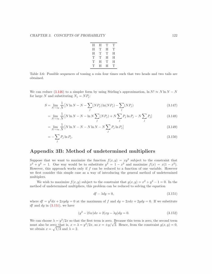
CHAPTER 3. CONCEPTS OF PROBABILITY 122

H H T TH T H TH T T HT T H HT H T HT H H T

Table 3.6: Possible sequences of tossing a coin four times such that two heads and two tails areobtained.

We can reduce (3.146) to a simpler form by using Stirling’s approximation, lnN ! ≈ N ln N − Nfor large N and substituting Nj = NPj :

S = limN→∞

1N

[N ln N − N −

∑j

(NPj) ln(NPj) −∑

j

(NPj) (3.147)

= limN→∞

1N

[N ln N − N − ln N

∑j

(NPj) + N∑

j

Pj ln Pj − N∑

j

Pj ] (3.148)

= limN→∞

1N

[N ln N − N − N ln N − N

∑j

Pj ln Pj

](3.149)

= −∑

j

Pj ln Pj . (3.150)

Appendix 3B: Method of undetermined multipliers

Suppose that we want to maximize the function f(x, y) = xy2 subject to the constraint thatx2 + y2 = 1. One way would be to substitute y2 = 1 − x2 and maximize f(x) = x(1 − x2).However, this approach works only if f can be reduced to a function of one variable. Howeverwe first consider this simple case as a way of introducing the general method of undeterminedmultiplers.

We wish to maximize f(x, y) subject to the constraint that g(x, y) = x2 + y2 − 1 = 0. In themethod of undetermined multipliers, this problem can be reduced to solving the equation

df − λdg = 0, (3.151)

where df = y2dx + 2xydy = 0 at the maximum of f and dg = 2xdx + 2ydy = 0. If we substitutedf and dg in (3.151), we have

(y2 − 2λx)dx + 2(xy − λy)dy = 0. (3.152)

We can choose λ = y2/2x so that the first term is zero. Because this term is zero, the second termmust also be zero; that is, x = λ = y2/2x, so x = ±y/

√2. Hence, from the constraint g(x, y) = 0,

we obtain x =√

1/3 and λ = 2.

CHAPTER 3. CONCEPTS OF PROBABILITY 123

In general, we wish to maximize the function f(x1, x2, . . . , xN ) subject to the constraintsgj(x1, x2, . . . , xN ) = 0 where j = 1, 2, . . . , M with M < N . The maximum of f is given by

df =N∑

i=1

( ∂f

∂xi

)dxi = 0, (3.153)

and the constraint can be expressed as

dg =N∑

i=1

(∂gj

∂xi

)dxi = 0. (3.154)

As in our example, we can combine (3.153) and (3.154) and write df − ∑Mj=1 λjdgj = 0 or

N∑i=1

[( ∂f

∂xi

)−

M∑i=1

λj

(∂gj

∂xi

)]dxi = 0. (3.155)

We are free to choose all M values of αj such that the first M terms in the square brackets arezero. For the remaining N −M terms, the dxi can be independently varied because the constraintshave been satisfied. Hence, the remaining terms in square brackets must be independently zeroand we are left with N − M equations of the form

( ∂f

∂xi

)−

M∑i=1

λj

(∂gj

∂xi

)= 0. (3.156)

In Example 3.11 we were able to obtain the probabilities by reducing the uncertainty S toa function of a single variable P1 and then maximizing S(P1). We now consider a more generalproblem where there are more outcomes, the case of a loaded die for which there are six outcomes.Suppose that we know that the average number of points on the face of a die if f . Then we wishto determine P1, P2, . . . , P6 subject to the constraints

6∑j=1

Pj = 1, (3.157)

6∑j=1

jPj = f. (3.158)

For a perfect die f = 3.5. Equation (3.156) becomes

6∑j=1

[(1 + lnPj) + α + βj]dPj = 0, (3.159)

where we have used dS = −∑6j=1 d(Pj ln Pj) = −∑6

j=1(1 + lnPj)dPj ; α and β are the undeter-mined (Lagrange) multipliers. We choose α and β so that the first two terms in the brackets (withj = 1 and j = 2 are independently zero. We write

α = ln P2 − 2 ln P1 − 1 (3.160a)β = ln P1 − ln P2. (3.160b)

CHAPTER 3. CONCEPTS OF PROBABILITY 124

We can solve (3.160b) for lnP2 = ln P1 − β and use (3.160a) to find lnP1 = −1 − α − β and usethis result to write P2 = −1 − α − β2. We can independently vary dP3, . . . dP6 because the twoconstraints are satisfied by the values of P1 and P2. We let

ln Pj = −1 − α − jβ, (3.161)

orPj = e−1−αe−βj . (3.162)

We can eliminate the constant α by the normalization condition (3.157):

Pj =e−βj∑j e−βj

. (3.163)

The constant β is determined by the constraint (3.38):

f =e−β + 2e−β2 + 3e−β3 + 4e−β4 + 5e−β5 + 6e−β6

e−β + e−β2 + e−β3 + e−β4 + e−β5 + e−β6. (3.164)

In general, (3.164) must be solved numerically.

Problem 3.54. Show that the solution to (3.164) is β = 0 for f = 7/2, β = +∞ for f = 2,β = −∞ for f = 6, and β = −0.1746 for f = 4.

Appendix 3C: Derivation of the central limit theorem

To discuss the derivation of the central limit theorem, it is convenient to introduce the characteristicfunction φ(k) of the probability density p(x). The main utility of the characteristic function is thatit simplifies the analysis of the sums of independent random variables. We define φ(k) as the Fouriertransform of p(x):

φ(k) = eikx =∫ ∞

−∞dx eikxp(x). (3.165)

Because p(x) is normalized, it follows that φ(k = 0) = 1. The main property of the Fouriertransform that we need is that if φ(k) is known, we can find p(x) by calculating the inverse Fouriertransform:

p(x) =12π

∫ ∞

−∞dk e−ikxφ(k). (3.166)

Problem 3.55. Calculate the characteristic function of the Gaussian probability density.

One useful property of φ(k) is that its power series expansion yields the moments of p(x):

φ(k) =∞∑

n=0

kn

n!dnφ(k)

dkn

∣∣k=0

, (3.167)

= eikx =∞∑

n=0

(ik)nxn

n!. (3.168)

CHAPTER 3. CONCEPTS OF PROBABILITY 125

By comparing coefficients of kn in (3.167) and (3.168), we see that

x = −idφ

dk

∣∣k=0

. (3.169)

In Problem 3.56 we show that

x2 − x2 = − d2

dk2ln φ(k)

∣∣k=0

(3.170)

and that certain convenient combinations of the moments are related to the power series expansionof the logarithm of the characteristic function.

Problem 3.56. The characteristic function generates the cumulants Cm defined by

ln φ(k) =∞∑

m=1

(ik)m

m!Cm. (3.171)

Show that the cumulants are combinations of the moments of x and are given by

C1 = x (3.172a)

C2 = σ2 = x2 − x2 (3.172b)

C3 = x3 − 3 x2x + 2 x3 (3.172c)

C4 = x4 − 4 x3 x − 3 x22

+ 12 x2 x2 − 6 x4. (3.172d)

Now let us consider the properties of the characteristic function for the sums of independentvariables. For example, let p1(x) be the probability density for the weight x of adult males and letp2(y) be the probability density for the weight of adult females. If we assume that people marryone another independently of weight, what is the probability density p(z) for the weight z of anadult couple? We have that

z = x + y. (3.173)

How do the probability densities combine? The answer is

p(z) =∫

dx dy p1(x)p2(y) δ(z − x − y). (3.174)

The integral in (3.174) represents all the possible ways of obtaining the combined weight z asdetermined by the probability density p1(x)p2(y) for the combination of x and y that sums toz. The form (3.174) of the integrand is known as a convolution. An important property of aconvolution is that its Fourier transform is a simple product. We have

φz(k) =∫

dz eikzp(z) (3.175)

=∫

dz

∫dx

∫dy eikzp1(x)p2(y) δ(z − x − y)

=∫

dx eikxp1(x)∫

dy eikyp2(y)

= φ1(k)φ2(k). (3.176)

CHAPTER 3. CONCEPTS OF PROBABILITY 126

It is straightforward to generalize this result to a sum of N random variables. We write

z = x1 + x2 + . . . + xN . (3.177)

Then

φz(k) =N∏

i=1

φi(k). (3.178)

That is, for independent variables the characteristic function of the sum is the product of theindividual characteristic functions. If we take the logarithm of both sides of (3.178), we obtain

ln φz(k) =N∑

i=1

ln φi(k). (3.179)

Each side of (3.179) can be expanded as a power series and compared order by order in powersof ik. The result is that when random variables are added, their associated cumulants also add.That is, the nth order cumulants satisfy the relation:

Czn = C1

n + C2n + . . . + CN

n . (3.180)

We conclude see that if the random variables xi are independent (uncorrelated), their cumulantsand in particular, their variances, add.

If we denote the mean and standard deviation of the weight of an adult male as x and σrespectively, then from (3.172a) and (3.180) we find that the mean weight of N adult males isgiven by Nx. Similarly from (3.172b) we see that the standard deviation of the weight of N adultmales is given by σ2

N = Nσ2, or σN =√

Nσ. Hence, we find the now familiar result that the sumof N random variables scales as N while the standard deviation scales as

√N .

We are now in a position to derive the central limit theorem. Let x1, x2, . . ., xN be N mutuallyindependent variables. For simplicity, we assume that each variable has the same probabilitydensity p(x). The only condition is that the variance σ2

x of the probability density p(x) must befinite. For simplicity, we make the additional assumption that x = 0, a condition that always canbe satisfied by measuring x from its mean. The central limit theorem states that the sum S hasthe probability density

p(S) =1√

2πNσx2

e−S2/2Nσx2

(3.181)

From (3.172b) we see that S2 = Nσ2x, and hence the variance of S grows linearly with N . However,

the distribution of the values of the arithmetic mean S/N becomes narrower with increasing N :

(x1 + x2 + . . . xN

N

)2

=Nσ2

x

N2=

σ2x

N. (3.182)

From (3.182) we see that it is useful to define a scaled sum:

z =1√N

(x1 + x2 + . . . + xN ), (3.183)

CHAPTER 3. CONCEPTS OF PROBABILITY 127

and to write the central limit theorem in the form

p(z) =1√

2πσ2e−z2/2σ2

. (3.184)

To obtain the result (3.184), we write the characteristic function of z as

φz(k) =∫

dx eikz

∫dx1

∫dx2 · · ·

∫dxN δ

(z − [x1 + x2 + . . . + xN

N1/2

])× p(x1) p(x2) . . . p(xN )

=∫

dx1

∫dx2 . . .

∫dxN eik(x1+x2+...xN )/N1/2

p(x1) p(x2) . . . p(xN )

= φ( k

N1/2

)N. (3.185)

We next take the logarithm of both sides of (3.185) and expand the right-hand side in powers ofk to find

ln φz(k) =∞∑

m=2

(ik)m

m!N1−m/2Cm. (3.186)

The m = 1 term does not contribute in (3.186) because we have assumed that x = 0. Moreimportantly, note that as N → ∞, the higher-order terms are suppressed so that

ln φz(k) → −k2

2C2, (3.187)

orφz(k) → e−k2σ2/2 + . . . (3.188)

Because the inverse Fourier transform of a Gaussian is also a Gaussian, we find that

p(z) =1√

2πσ2e−z2/2σ2

. (3.189)

The leading correction to φ(k) in (3.189) gives rise to a term of order N−1/2, and therefore doesnot contribute in the limit N → ∞.

The conditions for the rigorous applicability of the central limit theorem can be found intextbooks on probability. The only requirements are that the various xi be statistically independentand that the second moment of p(x) exists. Not all probabilities satisfy this latter requirement asdemonstrated by the Lorentz distribution (see Problem 3.45). It is not necessary that all the xi

have the same distribution.

CHAPTER 3. CONCEPTS OF PROBABILITY 128

Figure 3.7: Representation of a square lattice of 16×16 sites. The sites are represented by squaresand are either occupied (shaded) or empty (white).

Additional Problems

Problems page3.1, 3.2, 3.3, 3.4, 3.5, 3.6 833.7, 3.8, 3.9, 3.10, 3.11, 3.12, 3.13, 3.14, 3.15 843.16 863.17, 3.18, 3.19, 3.20, 3.21 883.22, 3.23 893.24 923.26, 3.27 963.28, 3.29 993.30, 3.31 1013.32, 3.33 1033.34, 3.35 1043.36 1083.37, 3.38, 3.39, 3.40 1083.41 1103.42, 3.43, 3.44, 3.45 1113.46 1133.47 1143.48, 3.49 1153.50 1173.51 1193.52, 3.53 1203.54 1243.55, 3.56 125

Listing of inline problems.

Problem 3.57. In Figure 3.7 we show a square lattice of 162 sites each of which is either occupiedor empty. Estimate the probability that a site in the lattice is occupied.

Problem 3.58. Three coins are tossed in succession. Assume that the simple events are equiprob-able. Find the probabilities of the following: (a) the first coin is a heads, (b) exactly two headshave occurred, (c) not more than two heads have occurred.

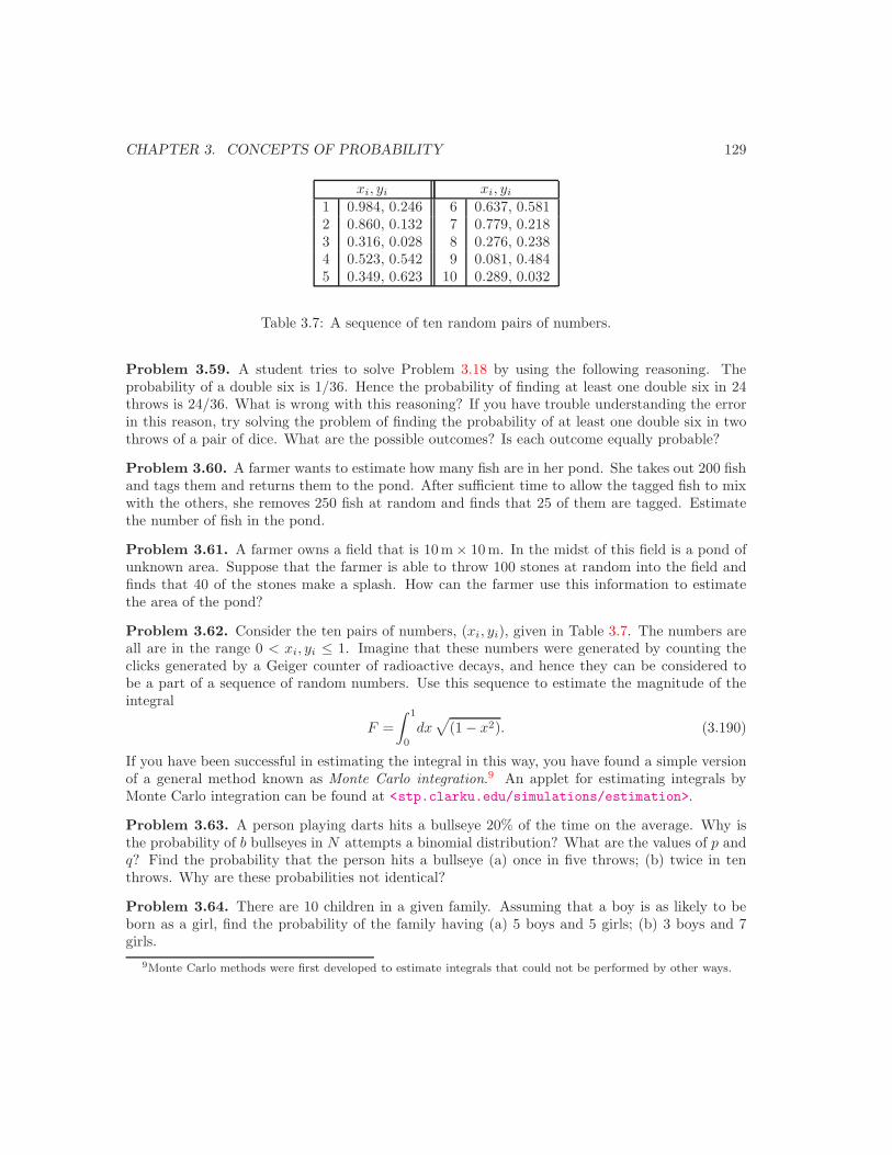
CHAPTER 3. CONCEPTS OF PROBABILITY 129

xi, yi xi, yi

1 0.984, 0.246 6 0.637, 0.5812 0.860, 0.132 7 0.779, 0.2183 0.316, 0.028 8 0.276, 0.2384 0.523, 0.542 9 0.081, 0.4845 0.349, 0.623 10 0.289, 0.032

Table 3.7: A sequence of ten random pairs of numbers.

Problem 3.59. A student tries to solve Problem 3.18 by using the following reasoning. Theprobability of a double six is 1/36. Hence the probability of finding at least one double six in 24throws is 24/36. What is wrong with this reasoning? If you have trouble understanding the errorin this reason, try solving the problem of finding the probability of at least one double six in twothrows of a pair of dice. What are the possible outcomes? Is each outcome equally probable?

Problem 3.60. A farmer wants to estimate how many fish are in her pond. She takes out 200 fishand tags them and returns them to the pond. After sufficient time to allow the tagged fish to mixwith the others, she removes 250 fish at random and finds that 25 of them are tagged. Estimatethe number of fish in the pond.

Problem 3.61. A farmer owns a field that is 10 m× 10 m. In the midst of this field is a pond ofunknown area. Suppose that the farmer is able to throw 100 stones at random into the field andfinds that 40 of the stones make a splash. How can the farmer use this information to estimatethe area of the pond?

Problem 3.62. Consider the ten pairs of numbers, (xi, yi), given in Table 3.7. The numbers areall are in the range 0 < xi, yi ≤ 1. Imagine that these numbers were generated by counting theclicks generated by a Geiger counter of radioactive decays, and hence they can be considered tobe a part of a sequence of random numbers. Use this sequence to estimate the magnitude of theintegral

F =∫ 1

0

dx√

(1 − x2). (3.190)

If you have been successful in estimating the integral in this way, you have found a simple versionof a general method known as Monte Carlo integration.9 An applet for estimating integrals byMonte Carlo integration can be found at <stp.clarku.edu/simulations/estimation>.

Problem 3.63. A person playing darts hits a bullseye 20% of the time on the average. Why isthe probability of b bullseyes in N attempts a binomial distribution? What are the values of p andq? Find the probability that the person hits a bullseye (a) once in five throws; (b) twice in tenthrows. Why are these probabilities not identical?

Problem 3.64. There are 10 children in a given family. Assuming that a boy is as likely to beborn as a girl, find the probability of the family having (a) 5 boys and 5 girls; (b) 3 boys and 7girls.

9Monte Carlo methods were first developed to estimate integrals that could not be performed by other ways.

CHAPTER 3. CONCEPTS OF PROBABILITY 130

Problem 3.65. What is the probability that five children produced by the same couple will consistof (a) three sons and two daughters? (b) alternating sexes? (c) alternating sexes starting with ason? (d) all daughters? Assume that the probability of giving birth to a boy and a girl is the same.

Problem 3.66. A good hitter in baseball has a batting average of 300 or more, which means thatthe hitter will be successful 3 times out of 10 tries on the average. Assume that on average a hittergets three hits for each 10 times at bat and that he has 4 times at bat per game. (a) What is theprobability that he gets zero hits in one game? (b) What is the probability that he will get twohits or less in a three game series? (c) What is the probability that he will get five or more hitsin a three game series? Baseball fans might want to think about the significance of “slumps” and“streaks” in baseball.

Problem 3.67. In the World Series in baseball and in the playoffs in the National BasketballAssociation and the National Hockey Association, the winner is determined by a best of sevenseries. That is, the first team that wins four games wins the series and is the champion. Doa simple statistical calculation assuming that the two teams are evenly matched and the win-ner of any game might as well be determined by a coin flip and show that a seven game se-ries should occur 31.25% of the time. What is the probability that the series lasts n games?More information can be found at <www.mste.uiuc.edu/hill/ev/seriesprob.html> and at<www.insidescience.org/reports/2003/080.html>.

Problem 3.68. The Galton board (named after Francis Galton (1822–1911)), is a triangular arrayof pegs. The rows are numbered 0, 1, . . . from the top row down such that row n has n + 1 pegs.Suppose that a ball is dropped from above the top peg. Each time the ball hits a peg, it bounces tothe right with probability p and to the left with probability 1− p, independently from peg to peg.Suppose that N balls are dropped successively such that the balls do not encounter one another.How will the balls be distributed at the bottom of the board? Links to applets that simulate theGalton board can be found in the references.

Problem 3.69. (a) What are the chances that at least two people in your class have the samebirthday? Assume that the number of students is 25. (b) What are the chances that at least oneother person in your class has the same birthday as you? Explain why the chances are less in thesecond case.

Problem 3.70. Many analysts attempt to select stocks by looking for correlations in the stockmarket as a whole or for patterns for particular companies. Such an analysis is based on the beliefthat there are repetitive patterns in stock prices. To understand one reason for the persistenceof this belief do the following experiment. Construct a stock chart (a plot of stock price versustime) showing the movements of a hypothetical stock initially selling at $50 per share. On eachsuccessive day the closing stock price is determined by the flip of a coin. If the coin toss is a head,the stock closes 1/2 point ($0.50) higher than the preceding close. If the toss is a tail, the priceis down by 1/2 point. Construct the stock chart for a long enough time to see “cycles” and otherpatterns appear. The moral of the charts is that a sequence of numbers produced in this manneris identical to a random walk, yet the sequence frequently appears to be correlated.

Problem 3.71. Suppose that a random walker takes N steps of unit length with probability pof a step to the right. The displacement m of the walker from the origin is given by m = n − n′,where n is the number of steps to the right and n′ is the number of steps to the left. Show thatm = (p − q)N and σ2

m = (m − m)2 = 4Npq.

CHAPTER 3. CONCEPTS OF PROBABILITY 131

Problem 3.72. The result (3.61) for (∆M)2 differs by a factor of four from the result for σ2n in

(3.87). Why? Compare (3.61) to the result of Problem 3.39.

Problem 3.73. A random walker is observed to take a total of N steps, n of which are to theright. (a) Suppose that a curious observer finds that on ten successive nights the walker takesN = 20 steps and that the values of n are given successively by 14, 13, 11, 12, 11, 12, 16, 16, 14,8. Compute n, n2, and σn. Use this information to estimate p. If your reasoning gives differentvalues for p, which estimate is likely to be the most accurate? (b) Suppose that on another tensuccessive nights the same walker takes N = 100 steps and that the values of n are given by 58,69, 71, 58, 63, 53, 64, 66, 65, 50. Compute the same quantities as in part (a) and estimate p. Howdoes the ratio of σn to n compare for the two values of N? Explain your results. (c) Compute mand σm, where m = n− n′ is the net displacement of the walker. This problem inspired an articleby Zia and Schmittmann (see the references).

Problem 3.74. In Section 3.7 we evaluated the derivatives of P (n) to determine the parametersA, B, and n in (3.106). Another way to determine these parameters is to assume that the binomialdistribution can be approximated by a Gaussian and require that the first several moments of theGaussian and binomial distribution be equal. We write

P (n) = Ae−12B(n−n)2 , (3.191)

and require that ∫ N

0

P (n) dn = 1. (3.192)

Because P (n) depends on the difference n− n, it is convenient to change the variable of integrationin (3.192) to x = n − n. We have ∫ N−n

−n

P (x) dx = 1, (3.193)

whereP (x) = Ae−

12Bx2

. (3.194)

In the limit of large N , we can extend the upper and lower limits of integration in (3.193) andwrite ∫ ∞

−∞P (x) dx = 1, (3.195)

The first moment of P (n) is given by

n =∫ N

0

nP (n) dn = pN. (3.196)

Make a change of variables and show that∫ ∞

−∞xP (x) dx = n − n. (3.197)

Because the integral in (3.197) is zero, we can conclude that n = n. We also have that

(n − n)2 =∫ N

0

(n − n)2 P (n) dn = pqN. (3.198)

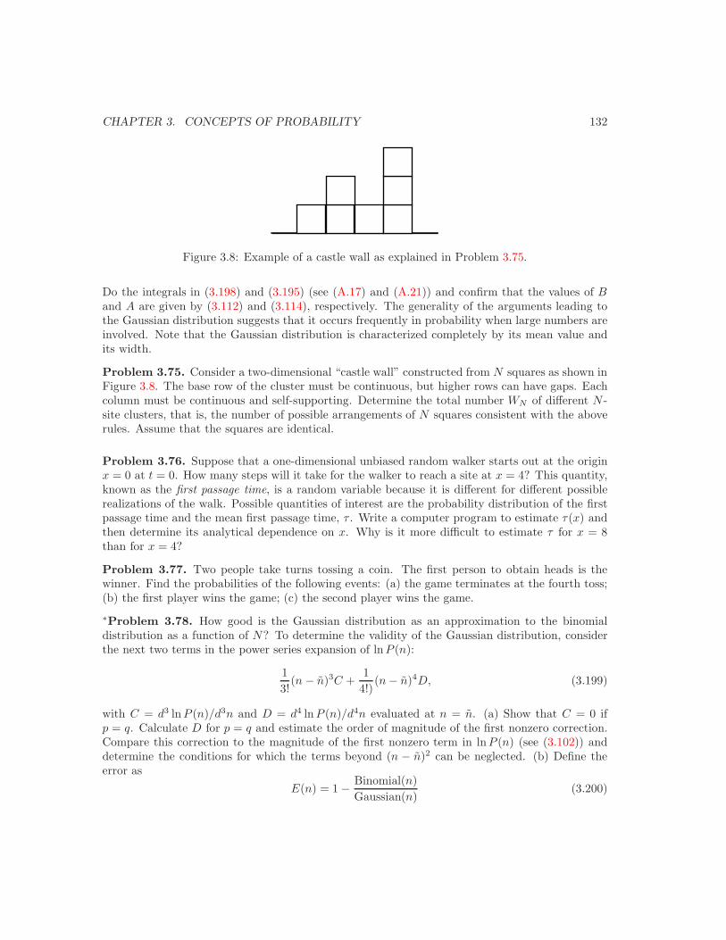
CHAPTER 3. CONCEPTS OF PROBABILITY 132

Figure 3.8: Example of a castle wall as explained in Problem 3.75.

Do the integrals in (3.198) and (3.195) (see (A.17) and (A.21)) and confirm that the values of Band A are given by (3.112) and (3.114), respectively. The generality of the arguments leading tothe Gaussian distribution suggests that it occurs frequently in probability when large numbers areinvolved. Note that the Gaussian distribution is characterized completely by its mean value andits width.

Problem 3.75. Consider a two-dimensional “castle wall” constructed from N squares as shown inFigure 3.8. The base row of the cluster must be continuous, but higher rows can have gaps. Eachcolumn must be continuous and self-supporting. Determine the total number WN of different N -site clusters, that is, the number of possible arrangements of N squares consistent with the aboverules. Assume that the squares are identical.

Problem 3.76. Suppose that a one-dimensional unbiased random walker starts out at the originx = 0 at t = 0. How many steps will it take for the walker to reach a site at x = 4? This quantity,known as the first passage time, is a random variable because it is different for different possiblerealizations of the walk. Possible quantities of interest are the probability distribution of the firstpassage time and the mean first passage time, τ . Write a computer program to estimate τ(x) andthen determine its analytical dependence on x. Why is it more difficult to estimate τ for x = 8than for x = 4?

Problem 3.77. Two people take turns tossing a coin. The first person to obtain heads is thewinner. Find the probabilities of the following events: (a) the game terminates at the fourth toss;(b) the first player wins the game; (c) the second player wins the game.

∗Problem 3.78. How good is the Gaussian distribution as an approximation to the binomialdistribution as a function of N? To determine the validity of the Gaussian distribution, considerthe next two terms in the power series expansion of lnP (n):

13!

(n − n)3C +1

4!)(n − n)4D, (3.199)

with C = d3 ln P (n)/d3n and D = d4 ln P (n)/d4n evaluated at n = n. (a) Show that C = 0 ifp = q. Calculate D for p = q and estimate the order of magnitude of the first nonzero correction.Compare this correction to the magnitude of the first nonzero term in lnP (n) (see (3.102)) anddetermine the conditions for which the terms beyond (n − n)2 can be neglected. (b) Define theerror as

E(n) = 1 − Binomial(n)Gaussian(n)

(3.200)

CHAPTER 3. CONCEPTS OF PROBABILITY 133

Plot E(n) versus n and determine the approximate width of E(n). (c) Show that if N is sufficientlylarge and neither p nor q is too small, the Gaussian distribution is a good approximation for nnear the maximum of P (n). Because P (n) is very small for large (n−n), the error in the Gaussianapproximation for larger n is negligible.

Problem 3.79. Consider a random walk on a two-dimensional square lattice where the walkerhas an equal probability of taking a step to one of four possible directions, north, south, east, orwest. Use the central limit theorem to find the probability that the walker is a distance r to r + drfrom the origin, where r2 = x2 + y2 and r is the distance from the origin after N steps. There isno need to do an explicit calculation.

Problem 3.80. One of the first continuum models of a random walk is due to Rayleigh (1919).In the Rayleigh model the length a of each step is a random variable with probability density p(a)and the direction of each step is random. For simplicity consider a walk in two dimensions andchoose p(a) so that each step has unit length. Then at each step the walker takes a step of unitlength at a random angle. Use the central limit theorem to find the asymptotic form of p(r, N) dr,the probability that the walker is in the range r to r + dr, where r is the distance from the originafter N steps.

Problem 3.81. Suppose there are three boxes each with two balls. The first box has two greenballs, the second box has one green and one red ball, and the third box has two red balls. Supposeyou choose a box at random and find one green ball. What is the probability that the other ballis green?

Problem 3.82. Open a telephone directory to an random page and make a list corresponding tothe last digit n of the first 100 telephone numbers. Find the probability P (n) that the number nappears. Plot P (n) as a function of n and describe its n-dependence. Do you expect that P (n)should be approximately uniform?

∗Problem 3.83. A simple model of a porous rock can be imagined by placing a series of overlap-ping spheres at random into a container of fixed volume V . The spheres represent the rock andthe space between the spheres represents the pores. If we write the volume of the sphere as v, itcan be shown the fraction of the space between the spheres or the porosity φ is φ = exp(−Nv/V ),where N is the number of spheres. For simplicity, consider a two-dimensional system, and writea program to place disks of diameter unity into a square box. The disks can overlap. Divide thebox into square cells each of which has an edge length equal to the diameter of the disks. Find theprobability of having 0, 1, 2, or 3 disks in a cell for φ = 0.03, 0.1, and 0.5.

∗Problem 3.84. Do a search of the Web and find a site that lists the populations of various citiesin the world (not necessarily the largest ones) or the cities of your state or region. The quantityof interest is the first digit of each population. Alternatively, scan the first page of your localnewspaper and record the first digit of each of the numbers you find. (The first digit of a numbersuch as 0.00123 is 1.) What is the probability P (n) that the first digit is n, where n = 1, . . . , 9?Do you think that P (n) will be the same for all n?

It turns out that the form of the probability P (n) is given by

P (n) = log10

(1 +

1n

). (3.201)

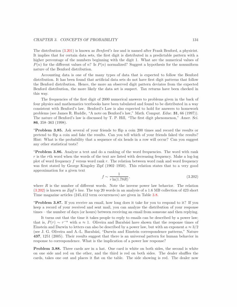
CHAPTER 3. CONCEPTS OF PROBABILITY 134

The distribution (3.201) is known as Benford’s law and is named after Frank Benford, a physicist.It implies that for certain data sets, the first digit is distributed in a predictable pattern with ahigher percentage of the numbers beginning with the digit 1. What are the numerical values ofP (n) for the different values of n? Is P (n) normalized? Suggest a hypothesis for the nonuniformnature of the Benford distribution.

Accounting data is one of the many types of data that is expected to follow the Benforddistribution. It has been found that artificial data sets do not have first digit patterns that followthe Benford distribution. Hence, the more an observed digit pattern deviates from the expectedBenford distribution, the more likely the data set is suspect. Tax returns have been checked inthis way.

The frequencies of the first digit of 2000 numerical answers to problems given in the back offour physics and mathematics textbooks have been tabulated and found to be distributed in a wayconsistent with Benford’s law. Benford’s Law is also expected to hold for answers to homeworkproblems (see James R. Huddle, “A note on Benford’s law,” Math. Comput. Educ. 31, 66 (1997)).The nature of Benford’s law is discussed by T. P. Hill, “The first digit phenomenon,” Amer. Sci.86, 358–363 (1998).

∗Problem 3.85. Ask several of your friends to flip a coin 200 times and record the results orpretend to flip a coin and fake the results. Can you tell which of your friends faked the results?Hint: What is the probability that a sequence of six heads in a row will occur? Can you suggestany other statistical tests?

∗Problem 3.86. Analyze a text and do a ranking of the word frequencies. The word with rankr is the rth word when the words of the text are listed with decreasing frequency. Make a log-logplot of word frequency f versus word rank r. The relation between word rank and word frequencywas first stated by George Kingsley Zipf (1902–1950). This relation states that to a very goodapproximation for a given text

f ∼ 1r ln(1.78R)

, (3.202)

where R is the number of different words. Note the inverse power law behavior. The relation(3.202) is known as Zipf’s law. The top 20 words in an analysis of a 1.6 MB collection of 423 shortTime magazine articles (245,412 term occurrences) are given in Table 3.8.

∗Problem 3.87. If you receive an email, how long does it take for you to respond to it? If youkeep a record of your received and sent mail, you can analyze the distribution of your responsetimes – the number of days (or hours) between receiving an email from someone and then replying.

It turns out that the time it takes people to reply to emails can be described by a power law;that is, P (τ) ∼ τ−a with a ≈ 1. Oliveira and Barabasi have shown that the response times ofEinstein and Darwin to letters can also be described by a power law, but with an exponent a ≈ 3/2(see J. G. Oliveira and A.-L. Barabasi, “Darwin and Einstein correspondence patterns,” Nature437, 1251 (2005). Their results suggest that there is an universal pattern for human behavior inresponse to correspondence. What is the implication of a power law response?

Problem 3.88. Three cards are in a hat. One card is white on both sides, the second is whiteon one side and red on the other, and the third is red on both sides. The dealer shuffles thecards, takes one out and places it flat on the table. The side showing is red. The dealer now

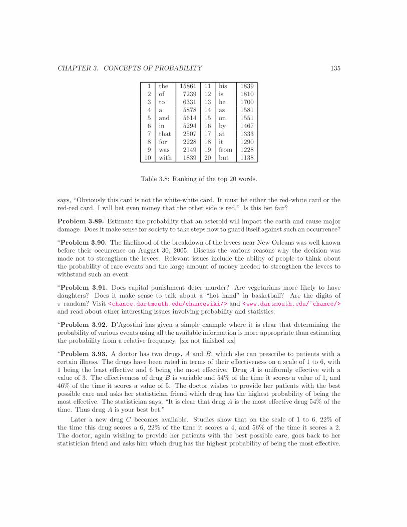
CHAPTER 3. CONCEPTS OF PROBABILITY 135

1 the 15861 11 his 18392 of 7239 12 is 18103 to 6331 13 he 17004 a 5878 14 as 15815 and 5614 15 on 15516 in 5294 16 by 14677 that 2507 17 at 13338 for 2228 18 it 12909 was 2149 19 from 1228

10 with 1839 20 but 1138

Table 3.8: Ranking of the top 20 words.

says, “Obviously this card is not the white-white card. It must be either the red-white card or thered-red card. I will bet even money that the other side is red.” Is this bet fair?

Problem 3.89. Estimate the probability that an asteroid will impact the earth and cause majordamage. Does it make sense for society to take steps now to guard itself against such an occurrence?

∗Problem 3.90. The likelihood of the breakdown of the levees near New Orleans was well knownbefore their occurrence on August 30, 2005. Discuss the various reasons why the decision wasmade not to strengthen the levees. Relevant issues include the ability of people to think aboutthe probability of rare events and the large amount of money needed to strengthen the levees towithstand such an event.

∗Problem 3.91. Does capital punishment deter murder? Are vegetarians more likely to havedaughters? Does it make sense to talk about a “hot hand” in basketball? Are the digits ofπ random? Visit <chance.dartmouth.edu/chancewiki/> and <www.dartmouth.edu/~chance/>and read about other interesting issues involving probability and statistics.

∗Problem 3.92. D’Agostini has given a simple example where it is clear that determining theprobability of various events using all the available information is more appropriate than estimatingthe probability from a relative frequency. [xx not finished xx]

∗Problem 3.93. A doctor has two drugs, A and B, which she can prescribe to patients with acertain illness. The drugs have been rated in terms of their effectiveness on a scale of 1 to 6, with1 being the least effective and 6 being the most effective. Drug A is uniformly effective with avalue of 3. The effectiveness of drug B is variable and 54% of the time it scores a value of 1, and46% of the time it scores a value of 5. The doctor wishes to provide her patients with the bestpossible care and asks her statistician friend which drug has the highest probability of being themost effective. The statistician says, “It is clear that drug A is the most effective drug 54% of thetime. Thus drug A is your best bet.”

Later a new drug C becomes available. Studies show that on the scale of 1 to 6, 22% ofthe time this drug scores a 6, 22% of the time it scores a 4, and 56% of the time it scores a 2.The doctor, again wishing to provide her patients with the best possible care, goes back to herstatistician friend and asks him which drug has the highest probability of being the most effective.

CHAPTER 3. CONCEPTS OF PROBABILITY 136

The statistician says, ”Because there is this new drug C on the market, your best bet is now drugB, and drug A is your worst bet.” Show that the statistician is right.

Suggestions for Further Reading

Vinay Ambegaokar, Reasoning About Luck, Cambridge University Press (1996). A book devel-oped for a course intended for non-science majors. An excellent introduction to statisticalreasoning and its uses in physics.

Peter L. Bernstein, Against the Gods: The Remarkable Story of Risk, John Wiley & Sons (1996).The author is a successful investor and an excellent writer. The book includes an excellentsummary of the history of probability.

David S. Betts and Roy E. Turner, Introductory Statistical Mechanics, Addison-Wesley (1992).Section 3.4 is based in part on Chapter 3 of this text.

The <www.dartmouth.edu/~chance/> Chance database encourages its users to apply statisticsto everyday events.

Giulio D’Agostini, “Teaching statistics in the physics curriculum: Unifying and clarifying role ofsubjective probability,” Am. J. Phys. 67, 1260–1268 (1999). The author, whose main researchinterest is in particle physics, discusses subjective probability and Bayes’ theorem. Section 3.4is based in part on this article.

See <www.math.uah.edu/stat/objects/> for an excellent simulation of the Galton board.

Gene F. Mazenko, Equilibrium Statistical Mechanics, John Wiley & Sons (2000). Sections 1.7 and1.8 of this graduate level text discuss the functional form of the missing information.

Elliott W. Montroll and Michael F. Shlesinger, “On the wonderful world of random walks,” inStudies in Statistical Mechanics, Vol. XI: Nonequilibrium Phenomena II, J. L. Lebowitz andE. W. Montroll, eds., North-Holland (1984).

Elliott W. Montroll and Wade W. Badger, Introduction to Quantitative Aspects of Social Phenom-ena, Gordon and Breach (1974). The applications of probability that are discussed includetraffic flow, income distributions, floods, and the stock market.

Richard Perline, “Zipf’s law, the central limit theorem, and the random division of the unitinterval,” Phys. Rev. E 54, 220–223 (1996).

S. Redner, “Random multiplicative processes: An elementary tutorial,” Am. J. Phys. 58, 267–273(1990).

Charles Ruhla, The Physics of Chance, Oxford University Press (1992).

B. Schmittmann and R. K. P. Zia, “‘Weather’ records: Musings on cold days after a long hotIndian summer,” Am. J. Phys. 67, 1269–1276 (1999). A relatively simple introduction to thestatistics of extreme values. Suppose that some breaks the record for the 100 meter dash.How long do records typically survive before they are broken?

CHAPTER 3. CONCEPTS OF PROBABILITY 137

Kyle Siegrist at the University of Alabama in Huntsville has developed many applets to illustrateconcepts in probability and statistics. See <www.math.uah.edu/stat/> and follow the linkto Bernoulli processes.

G. Troll and P. beim Graben, “Zipf’s law is not a consequence of the central limit theorem,”Phys. Rev. E 57, 1347–1355 (1998).

Charles A. Whitney, Random Processes in Physical Systems: An Introduction to Probability-Based Computer Simulations, John Wiley & Sons (1990).

R. K. P. Zia and B. Schmittmann, “Watching a drunkard for 10 nights: A study of distributionsof variances,” Am. J. Phys. 71, 859 (2003). See Problem 3.73.

Chapter 4

The Methodology of StatisticalMechanics

c©2006 by Harvey Gould and Jan Tobochnik11 January 2006

We develop the basic methodology of statistical mechanics and provide a microscopic foundationfor the concepts of temperature and entropy.

4.1 Introduction

We first discuss a simple example to make explicit the probabilistic assumptions and types ofcalculations that we do in statistical mechanics.

Consider an isolated system of N = 5 noninteracting with magnetic moment µ and spin 1/2in a magnetic field B. If the total energy E = −µB, what is the mean magnetic moment of agiven spin in the system? The essential steps needed to analyze this system can be summarized asfollows.1. Specify the macrostate and accessible microstates of the system. The macroscopic state ormacrostate of the system corresponds to the information that we know. For this example theobservable quantities are the total energy E, the magnetization M , the number of spins N , andthe external magnetic field B. (Because the spins are noninteracting, it is redundant to specifyboth M and E.)

The most complete specification of the system corresponds to a enumeration of the microstatesor configurations of the system. For N = 5, there are 25 = 32 microstates, each specified by theorientation of each spin. However, not all of the 32 microstates are consistent with the informationthat E = −µB. For example, E = −5µB for the microstate shown in Figure 4.1a is not allowed,that is, such a state is inaccessible. The accessible microstates of the system are those that areconsistent with the macroscopic conditions. In this example, ten of the thirty-two total microstatesare accessible (see Figure 4.1b).

138

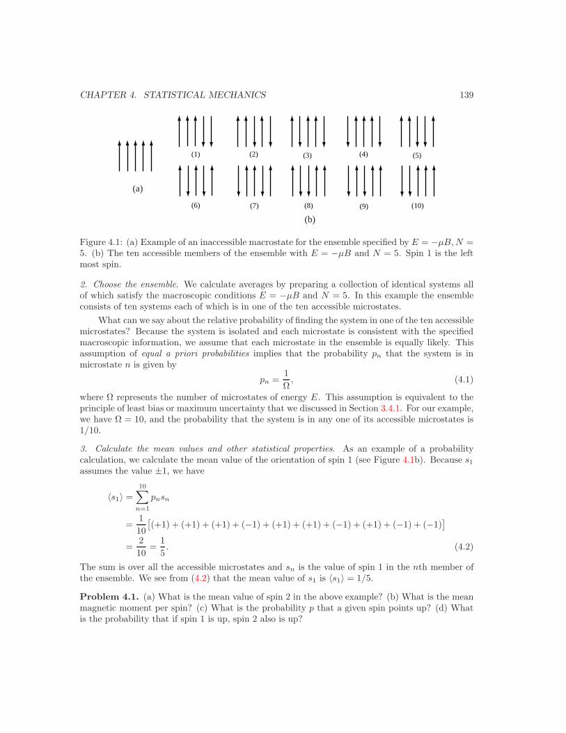
CHAPTER 4. STATISTICAL MECHANICS 139

(a)

(b)

(1) (2) (3) (4) (5)

(6) (7) (8) (9) (10)

Figure 4.1: (a) Example of an inaccessible macrostate for the ensemble specified by E = −µB, N =5. (b) The ten accessible members of the ensemble with E = −µB and N = 5. Spin 1 is the leftmost spin.

2. Choose the ensemble. We calculate averages by preparing a collection of identical systems allof which satisfy the macroscopic conditions E = −µB and N = 5. In this example the ensembleconsists of ten systems each of which is in one of the ten accessible microstates.

What can we say about the relative probability of finding the system in one of the ten accessiblemicrostates? Because the system is isolated and each microstate is consistent with the specifiedmacroscopic information, we assume that each microstate in the ensemble is equally likely. Thisassumption of equal a priori probabilities implies that the probability pn that the system is inmicrostate n is given by

pn =1Ω

, (4.1)

where Ω represents the number of microstates of energy E. This assumption is equivalent to theprinciple of least bias or maximum uncertainty that we discussed in Section 3.4.1. For our example,we have Ω = 10, and the probability that the system is in any one of its accessible microstates is1/10.

3. Calculate the mean values and other statistical properties. As an example of a probabilitycalculation, we calculate the mean value of the orientation of spin 1 (see Figure 4.1b). Because s1

assumes the value ±1, we have

〈s1〉 =10∑

n=1

pnsn

=110

[(+1) + (+1) + (+1) + (−1) + (+1) + (+1) + (−1) + (+1) + (−1) + (−1)

]

=210

=15. (4.2)

The sum is over all the accessible microstates and sn is the value of spin 1 in the nth member ofthe ensemble. We see from (4.2) that the mean value of s1 is 〈s1〉 = 1/5.

Problem 4.1. (a) What is the mean value of spin 2 in the above example? (b) What is the meanmagnetic moment per spin? (c) What is the probability p that a given spin points up? (d) Whatis the probability that if spin 1 is up, spin 2 also is up?

CHAPTER 4. STATISTICAL MECHANICS 140

Of course there is a more direct way of calculating s1 in this case. Because M = 1, six out ofthe ten spins are up. The equivalency of the spins implies that the probability of a spin being upis 6/10. Hence, s = (3/5)(1)+ (2/5)(−1) = 1/5. What is the implicit assumption that we made inthe more direct method?

Problem 4.2. (a) Consider N = 4 noninteracting spins with magnetic moment µ and spin 1/2in a magnetic field B. If the total energy E = −2µB, what are the accessible microstates and theprobabilities that a particular spin has a magnetic moment ±µ? (b) Consider N = 9 noninteractingspins with total energy E = −µB. What is the net number of up spins, the number of accessiblemicrostates, and the probabilities that a particular spin has magnetic moment ±µ? Compare theseprobabilities to the analogous ones calculated in part (a).

Problem 4.3. Consider a one-dimensional ideal gas consisting of N = 5 particles each of whichhas the same speed v, but velocity ±v. The velocity of each particle is independent. What is theprobability that all the particles are moving in the same direction?

The model of noninteracting spins that we have considered is an example of an isolated system,that is, a system with fixed E, B, and N . In general, an isolated system cannot exchange energyor matter with its surroundings nor do work on another system. The macrostate of such a systemis specified by E, V , and N (B instead of V for a magnetic system). Our strategy is to firstunderstand how to treat isolated systems. Conceptually, isolated systems are simpler because allthe accessible microstates have the same probability (see Section 4.5).

4.2 A simple example of a thermal interaction

We will now consider some model systems that can exchange energy with another system. Thisexchange has the effect of relaxing one of the internal constraints and, as we will see, imposinganother. We will see that for nonisolated systems, the probability of each microstate will not bethe same.

We know what happens when we place two bodies at different temperatures into thermalcontact with one another – energy is transferred from the hotter to the colder body until thermalequilibrium is reached and the two bodies have the same temperature. We now consider a simplemodel that illustrates how statistical concepts can help us understand the transfer of energy andthe microscopic nature of thermal equilibrium.

Consider a model system of N noninteracting distinguishable particles such that the energyof each particle is given by integer values, εn = 0, 1, 2, 3, . . . We can distinguish the particlesby their colors. (Or we can assume that the particles have the same color, but are fixed on latticesites.) For reasons that we will discuss in Section 6.12, we will refer to this model system as anEinstein solid.1

Suppose that we have an Einstein solid with N = 3 particles (with color red, white, and blue)in an isolated box and that their total energy is E = 3. For these small values of N and E, we canenumerate the accessible microstates by hand. The ten accessible microstates of this system are

1These particles are equivalent to the quanta of the harmonic oscillator, which have energy En = (n + 12)ω. If

we measure the energies from the lowest energy state, 12

ω, and choose units such that ω = 1, we have εn = n.

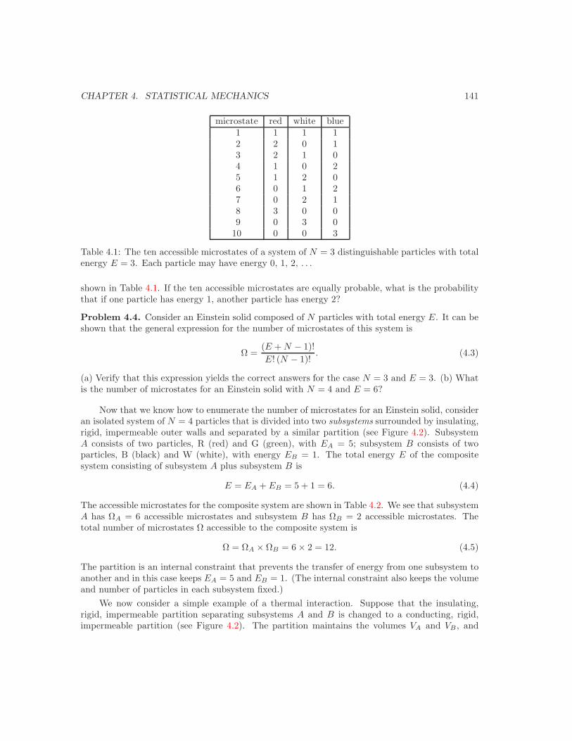
CHAPTER 4. STATISTICAL MECHANICS 141

microstate red white blue1 1 1 12 2 0 13 2 1 04 1 0 25 1 2 06 0 1 27 0 2 18 3 0 09 0 3 0

10 0 0 3

Table 4.1: The ten accessible microstates of a system of N = 3 distinguishable particles with totalenergy E = 3. Each particle may have energy 0, 1, 2, . . .

shown in Table 4.1. If the ten accessible microstates are equally probable, what is the probabilitythat if one particle has energy 1, another particle has energy 2?

Problem 4.4. Consider an Einstein solid composed of N particles with total energy E. It can beshown that the general expression for the number of microstates of this system is

Ω =(E + N − 1)!E! (N − 1)!

. (4.3)

(a) Verify that this expression yields the correct answers for the case N = 3 and E = 3. (b) Whatis the number of microstates for an Einstein solid with N = 4 and E = 6?

Now that we know how to enumerate the number of microstates for an Einstein solid, consideran isolated system of N = 4 particles that is divided into two subsystems surrounded by insulating,rigid, impermeable outer walls and separated by a similar partition (see Figure 4.2). SubsystemA consists of two particles, R (red) and G (green), with EA = 5; subsystem B consists of twoparticles, B (black) and W (white), with energy EB = 1. The total energy E of the compositesystem consisting of subsystem A plus subsystem B is

E = EA + EB = 5 + 1 = 6. (4.4)

The accessible microstates for the composite system are shown in Table 4.2. We see that subsystemA has ΩA = 6 accessible microstates and subsystem B has ΩB = 2 accessible microstates. Thetotal number of microstates Ω accessible to the composite system is

Ω = ΩA × ΩB = 6 × 2 = 12. (4.5)

The partition is an internal constraint that prevents the transfer of energy from one subsystem toanother and in this case keeps EA = 5 and EB = 1. (The internal constraint also keeps the volumeand number of particles in each subsystem fixed.)

We now consider a simple example of a thermal interaction. Suppose that the insulating,rigid, impermeable partition separating subsystems A and B is changed to a conducting, rigid,impermeable partition (see Figure 4.2). The partition maintains the volumes VA and VB , and

CHAPTER 4. STATISTICAL MECHANICS 142

subsystem A subsystem B

EA = 5 EB = 1

insulating, rigid, impermeable wall

RWG

B

(a)

subsystem A subsystem B

EA + EB = 6

conducting, rigid, impermeable wall

RWG

B

(b)

Figure 4.2: Two subsystems, each with two distinguishable particles, surrounded by (a) insulating,rigid, and impermeable outer walls and (b) separated by a conducting, rigid, and impermeablewall. The other walls remain the same.

EA accessible microstates EB accessible microstates5,0 0,5 1,0 0, 1

5 4,1 1,4 13,2 2,3

Table 4.2: The 12 equally probable microstates accessible to subsystems A and B before theremoval of the internal constraint. The conditions are NA = 2, EA = 5, NB = 2, and EB = 1.

hence the single particle energy eigenvalues are not changed. Because the partition is impermeable,the particles cannot penetrate the partition and go from one subsystem to the other. However,energy can be transferred from one subsystem to the other, subject only to the constraint thatthe total energy of subsystems A and B is constant, that is, E = EA + EB = 6. The microstatesof subsystems A and B are listed in Table 4.3 for all the possible values of EA and EB. Thetotal number of microstates Ω(EA, EB) accessible to the composite system whose subsystems haveenergy EA and EB is

Ω(EA, EB) = ΩA(EA) × ΩB(EB). (4.6)

For example. if EA = 4 and EB = 2, then subsystem A can be in any one of five microstates andsubsystem B can be in any of three microstates. These two sets of microstates of subsystems Aand B can be combined to give 5 × 3 = 15 microstates of the composite system.

The total number of microstates Ω accessible to the composite system can be found by sum-ming ΩA(EA)ΩB(EB) over the possible values of EA and EB consistent with the condition thatEA + EB = 6. Hence, Ω can be expressed as

Ω =∑EA

ΩA(EA)ΩB(E − EA). (4.7)

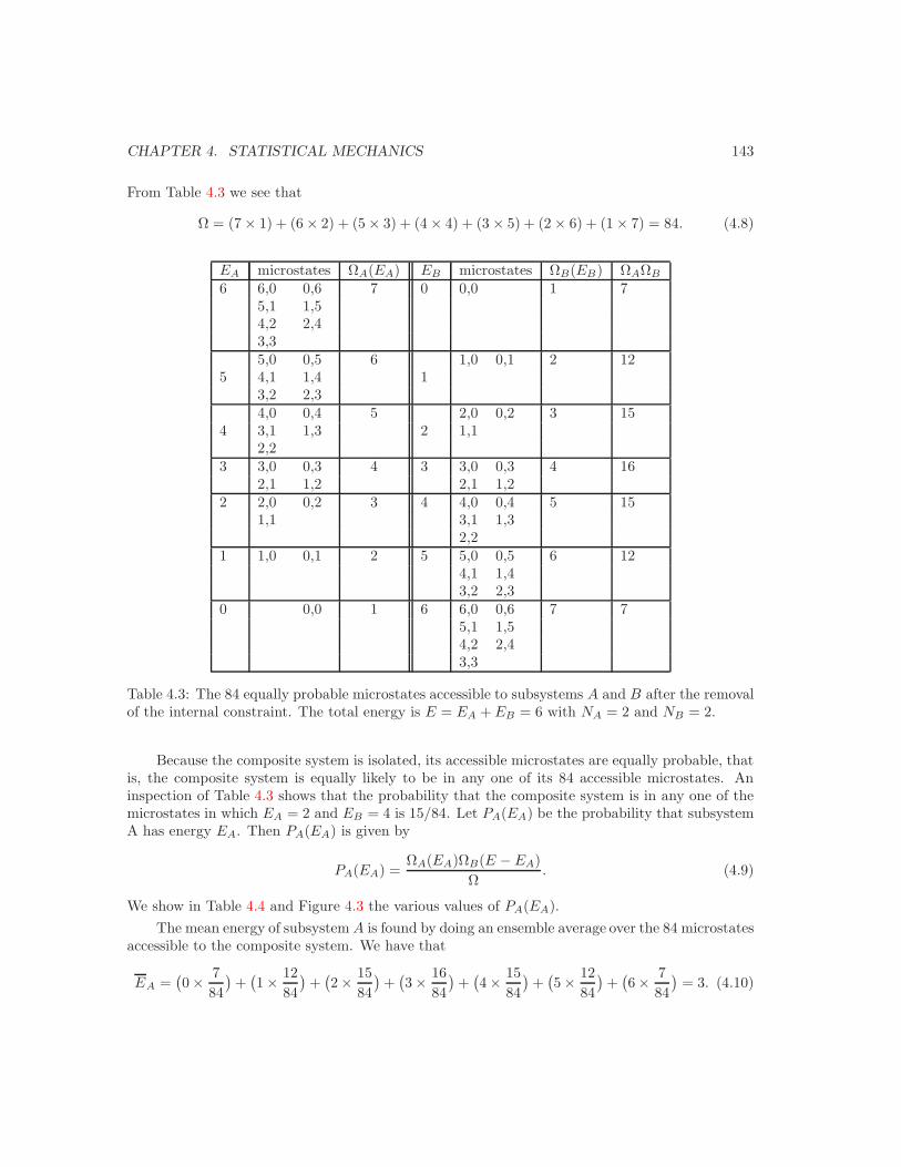
CHAPTER 4. STATISTICAL MECHANICS 143

From Table 4.3 we see that

Ω = (7 × 1) + (6 × 2) + (5 × 3) + (4 × 4) + (3 × 5) + (2 × 6) + (1 × 7) = 84. (4.8)

EA microstates ΩA(EA) EB microstates ΩB(EB) ΩAΩB

6 6,0 0,6 7 0 0,0 1 75,1 1,54,2 2,43,35,0 0,5 6 1,0 0,1 2 12

5 4,1 1,4 13,2 2,34,0 0,4 5 2,0 0,2 3 15

4 3,1 1,3 2 1,12,2

3 3,0 0,3 4 3 3,0 0,3 4 162,1 1,2 2,1 1,2

2 2,0 0,2 3 4 4,0 0,4 5 151,1 3,1 1,3

2,21 1,0 0,1 2 5 5,0 0,5 6 12

4,1 1,43,2 2,3

0 0,0 1 6 6,0 0,6 7 75,1 1,54,2 2,43,3

Table 4.3: The 84 equally probable microstates accessible to subsystems A and B after the removalof the internal constraint. The total energy is E = EA + EB = 6 with NA = 2 and NB = 2.

Because the composite system is isolated, its accessible microstates are equally probable, thatis, the composite system is equally likely to be in any one of its 84 accessible microstates. Aninspection of Table 4.3 shows that the probability that the composite system is in any one of themicrostates in which EA = 2 and EB = 4 is 15/84. Let PA(EA) be the probability that subsystemA has energy EA. Then PA(EA) is given by

PA(EA) =ΩA(EA)ΩB(E − EA)

Ω. (4.9)

We show in Table 4.4 and Figure 4.3 the various values of PA(EA).The mean energy of subsystem A is found by doing an ensemble average over the 84 microstates

accessible to the composite system. We have that

EA =(0 × 7

84)

+(1 × 12

84)

+(2 × 15

84)

+(3 × 16

84)+

(4 × 15

84)

+(5 × 12

84)

+(6 × 7

84)

= 3. (4.10)

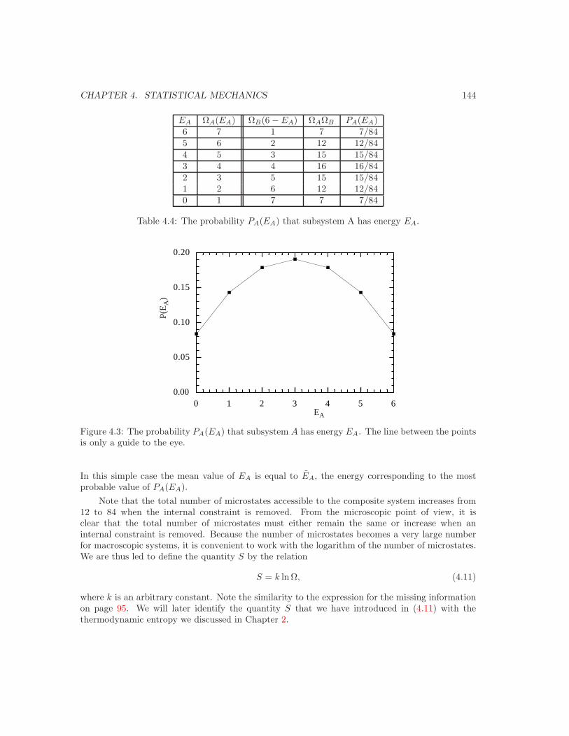
CHAPTER 4. STATISTICAL MECHANICS 144

EA ΩA(EA) ΩB(6 − EA) ΩAΩB PA(EA)6 7 1 7 7/845 6 2 12 12/844 5 3 15 15/843 4 4 16 16/842 3 5 15 15/841 2 6 12 12/840 1 7 7 7/84

Table 4.4: The probability PA(EA) that subsystem A has energy EA.

0.00

0.05

0.10

0.15

0.20

0 1 2 3 4 5 6EA

P(E

A)

Figure 4.3: The probability PA(EA) that subsystem A has energy EA. The line between the pointsis only a guide to the eye.

In this simple case the mean value of EA is equal to EA, the energy corresponding to the mostprobable value of PA(EA).

Note that the total number of microstates accessible to the composite system increases from12 to 84 when the internal constraint is removed. From the microscopic point of view, it isclear that the total number of microstates must either remain the same or increase when aninternal constraint is removed. Because the number of microstates becomes a very large numberfor macroscopic systems, it is convenient to work with the logarithm of the number of microstates.We are thus led to define the quantity S by the relation

S = k ln Ω, (4.11)

where k is an arbitrary constant. Note the similarity to the expression for the missing informationon page 95. We will later identify the quantity S that we have introduced in (4.11) with thethermodynamic entropy we discussed in Chapter 2.

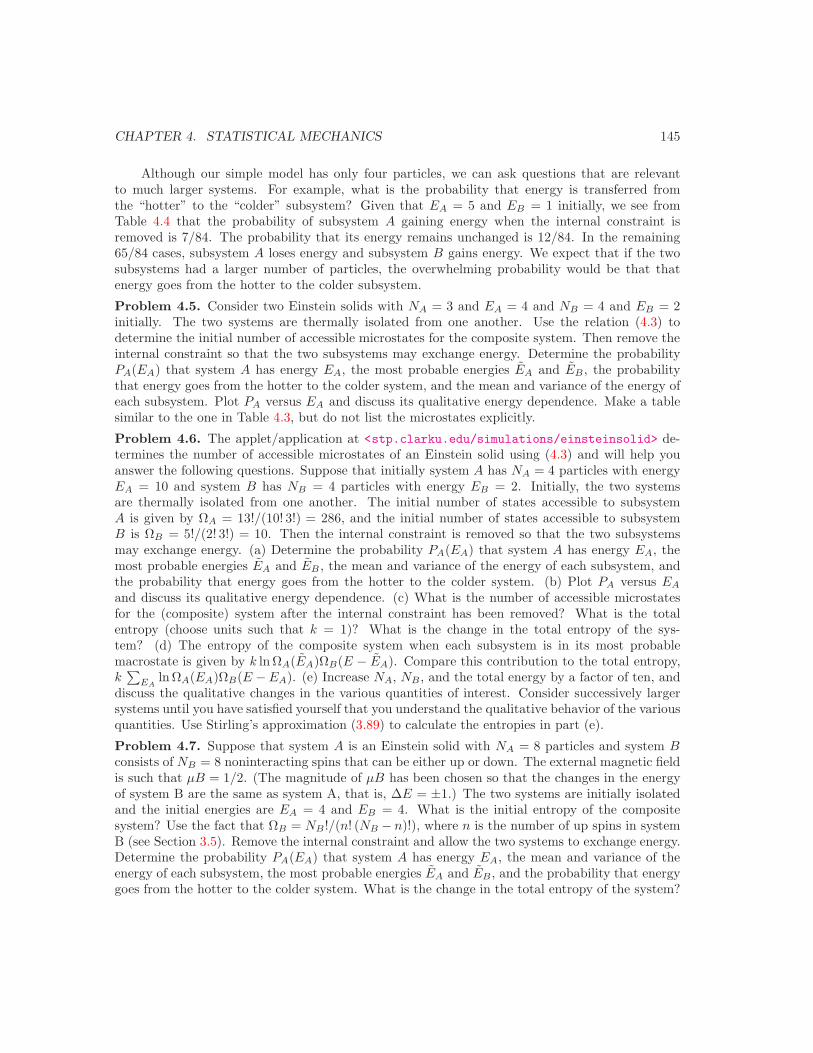
CHAPTER 4. STATISTICAL MECHANICS 145

Although our simple model has only four particles, we can ask questions that are relevantto much larger systems. For example, what is the probability that energy is transferred fromthe “hotter” to the “colder” subsystem? Given that EA = 5 and EB = 1 initially, we see fromTable 4.4 that the probability of subsystem A gaining energy when the internal constraint isremoved is 7/84. The probability that its energy remains unchanged is 12/84. In the remaining65/84 cases, subsystem A loses energy and subsystem B gains energy. We expect that if the twosubsystems had a larger number of particles, the overwhelming probability would be that thatenergy goes from the hotter to the colder subsystem.

Problem 4.5. Consider two Einstein solids with NA = 3 and EA = 4 and NB = 4 and EB = 2initially. The two systems are thermally isolated from one another. Use the relation (4.3) todetermine the initial number of accessible microstates for the composite system. Then remove theinternal constraint so that the two subsystems may exchange energy. Determine the probabilityPA(EA) that system A has energy EA, the most probable energies EA and EB, the probabilitythat energy goes from the hotter to the colder system, and the mean and variance of the energy ofeach subsystem. Plot PA versus EA and discuss its qualitative energy dependence. Make a tablesimilar to the one in Table 4.3, but do not list the microstates explicitly.

Problem 4.6. The applet/application at <stp.clarku.edu/simulations/einsteinsolid> de-termines the number of accessible microstates of an Einstein solid using (4.3) and will help youanswer the following questions. Suppose that initially system A has NA = 4 particles with energyEA = 10 and system B has NB = 4 particles with energy EB = 2. Initially, the two systemsare thermally isolated from one another. The initial number of states accessible to subsystemA is given by ΩA = 13!/(10! 3!) = 286, and the initial number of states accessible to subsystemB is ΩB = 5!/(2! 3!) = 10. Then the internal constraint is removed so that the two subsystemsmay exchange energy. (a) Determine the probability PA(EA) that system A has energy EA, themost probable energies EA and EB , the mean and variance of the energy of each subsystem, andthe probability that energy goes from the hotter to the colder system. (b) Plot PA versus EA

and discuss its qualitative energy dependence. (c) What is the number of accessible microstatesfor the (composite) system after the internal constraint has been removed? What is the totalentropy (choose units such that k = 1)? What is the change in the total entropy of the sys-tem? (d) The entropy of the composite system when each subsystem is in its most probablemacrostate is given by k ln ΩA(EA)ΩB(E − EA). Compare this contribution to the total entropy,k

∑EA

ln ΩA(EA)ΩB(E − EA). (e) Increase NA, NB, and the total energy by a factor of ten, anddiscuss the qualitative changes in the various quantities of interest. Consider successively largersystems until you have satisfied yourself that you understand the qualitative behavior of the variousquantities. Use Stirling’s approximation (3.89) to calculate the entropies in part (e).

Problem 4.7. Suppose that system A is an Einstein solid with NA = 8 particles and system Bconsists of NB = 8 noninteracting spins that can be either up or down. The external magnetic fieldis such that µB = 1/2. (The magnitude of µB has been chosen so that the changes in the energyof system B are the same as system A, that is, ∆E = ±1.) The two systems are initially isolatedand the initial energies are EA = 4 and EB = 4. What is the initial entropy of the compositesystem? Use the fact that ΩB = NB!/(n! (NB − n)!), where n is the number of up spins in systemB (see Section 3.5). Remove the internal constraint and allow the two systems to exchange energy.Determine the probability PA(EA) that system A has energy EA, the mean and variance of theenergy of each subsystem, the most probable energies EA and EB, and the probability that energygoes from the hotter to the colder system. What is the change in the total entropy of the system?

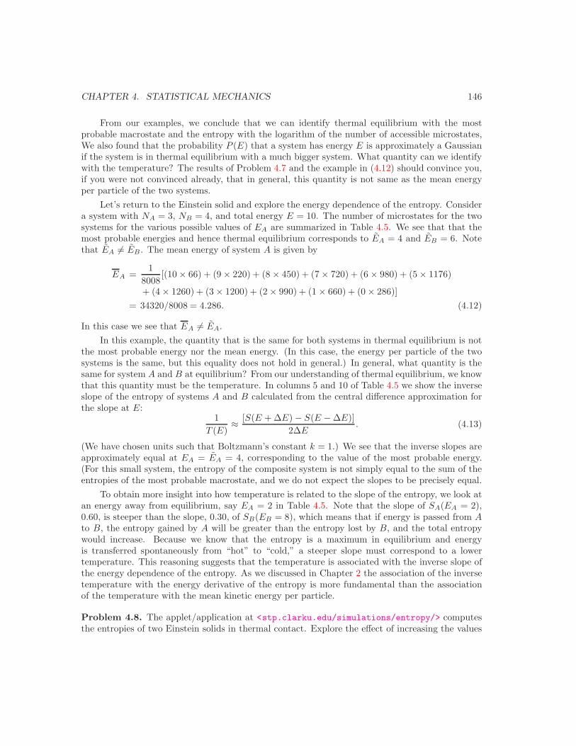
CHAPTER 4. STATISTICAL MECHANICS 146

From our examples, we conclude that we can identify thermal equilibrium with the mostprobable macrostate and the entropy with the logarithm of the number of accessible microstates,We also found that the probability P (E) that a system has energy E is approximately a Gaussianif the system is in thermal equilibrium with a much bigger system. What quantity can we identifywith the temperature? The results of Problem 4.7 and the example in (4.12) should convince you,if you were not convinced already, that in general, this quantity is not same as the mean energyper particle of the two systems.

Let’s return to the Einstein solid and explore the energy dependence of the entropy. Considera system with NA = 3, NB = 4, and total energy E = 10. The number of microstates for the twosystems for the various possible values of EA are summarized in Table 4.5. We see that that themost probable energies and hence thermal equilibrium corresponds to EA = 4 and EB = 6. Notethat EA = EB. The mean energy of system A is given by

EA =1

8008[(10 × 66) + (9 × 220) + (8 × 450) + (7 × 720) + (6 × 980) + (5 × 1176)

+ (4 × 1260) + (3 × 1200) + (2 × 990) + (1 × 660) + (0 × 286)]= 34320/8008 = 4.286. (4.12)

In this case we see that EA = EA.In this example, the quantity that is the same for both systems in thermal equilibrium is not

the most probable energy nor the mean energy. (In this case, the energy per particle of the twosystems is the same, but this equality does not hold in general.) In general, what quantity is thesame for system A and B at equilibrium? From our understanding of thermal equilibrium, we knowthat this quantity must be the temperature. In columns 5 and 10 of Table 4.5 we show the inverseslope of the entropy of systems A and B calculated from the central difference approximation forthe slope at E:

1T (E)

≈ [S(E + ∆E) − S(E − ∆E)]2∆E

. (4.13)

(We have chosen units such that Boltzmann’s constant k = 1.) We see that the inverse slopes areapproximately equal at EA = EA = 4, corresponding to the value of the most probable energy.(For this small system, the entropy of the composite system is not simply equal to the sum of theentropies of the most probable macrostate, and we do not expect the slopes to be precisely equal.

To obtain more insight into how temperature is related to the slope of the entropy, we look atan energy away from equilibrium, say EA = 2 in Table 4.5. Note that the slope of SA(EA = 2),0.60, is steeper than the slope, 0.30, of SB(EB = 8), which means that if energy is passed from Ato B, the entropy gained by A will be greater than the entropy lost by B, and the total entropywould increase. Because we know that the entropy is a maximum in equilibrium and energyis transferred spontaneously from “hot” to “cold,” a steeper slope must correspond to a lowertemperature. This reasoning suggests that the temperature is associated with the inverse slope ofthe energy dependence of the entropy. As we discussed in Chapter 2 the association of the inversetemperature with the energy derivative of the entropy is more fundamental than the associationof the temperature with the mean kinetic energy per particle.

Problem 4.8. The applet/application at <stp.clarku.edu/simulations/entropy/> computesthe entropies of two Einstein solids in thermal contact. Explore the effect of increasing the values

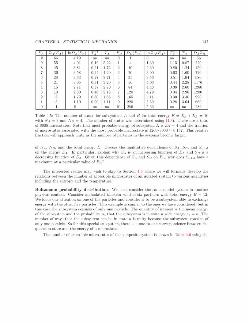
CHAPTER 4. STATISTICAL MECHANICS 147

EA ΩA(EA) ln ΩA(EA) T−1A TA EB ΩB(EB) ln ΩA(EA) T−1

B TB ΩAΩB

10 66 4.19 na na 0 1 0 na na 669 55 4.01 0.19 5.22 1 4 1.39 1.15 0.87 2208 45 3.81 0.21 4.72 2 10 2.30 0.80 1.24 4507 36 3.58 0.24 4.20 3 20 3.00 0.63 1.60 7206 28 3.33 0.27 3.71 4 35 3.56 0.51 1.94 9805 21 3.05 0.31 3.20 5 56 4.03 0.44 2.28 11764 15 2.71 0.37 2.70 6 84 4.43 0.38 2.60 12603 10 2.30 0.46 2.18 7 120 4.79 0.34 2.96 12002 6 1.79 0.60 1.66 8 165 5.11 0.30 3.30 9901 3 1.10 0.90 1.11 9 220 5.39 0.28 3.64 6600 1 0 na na 10 286 5.66 na na 286

Table 4.5: The number of states for subsystems A and B for total energy E = EA + EB = 10with NA = 3 and NB = 4. The number of states was determined using (4.3). There are a totalof 8008 microstates. Note that most probable energy of subsystem A is ES = 4 and the fractionof microstates associated with the most probable macrostate is 1260/8008 ≈ 0.157. This relativefraction will approach unity as the number of particles in the systems become larger.

of NA, NB, and the total energy E. Discuss the qualitative dependence of SA, SB, and Stotal

on the energy EA. In particular, explain why SA is an increasing function of EA and SB is adecreasing function of EA. Given this dependence of SA and SB on EA, why does Stotal have amaximum at a particular value of EA?

The interested reader may wish to skip to Section 4.5 where we will formally develop therelations between the number of accessible microstates of an isolated system to various quantitiesincluding the entropy and the temperature.

Boltzmann probability distribution. We next consider the same model system in anotherphysical context. Consider an isolated Einstein solid of six particles with total energy E = 12.We focus our attention on one of the particles and consider it to be a subsystem able to exchangeenergy with the other five particles. This example is similar to the ones we have considered, but inthis case the subsystem consists of only one particle. The quantity of interest is the mean energyof the subsystem and the probability pn that the subsystem is in state n with energy εn = n. Thenumber of ways that the subsystem can be in state n is unity because the subsystem consists ofonly one particle. So for this special subsystem, there is a one-to-one correspondence between thequantum state and the energy of a microstate.

The number of accessible microstates of the composite system is shown in Table 4.6 using the

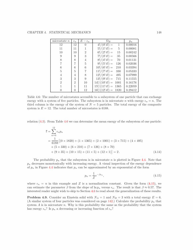
CHAPTER 4. STATISTICAL MECHANICS 148

microstate n εn E − εn ΩB pn

12 12 0 4!/(0! 4!) = 1 0.0001611 11 1 5!/(1! 4!) = 5 0.0008110 10 2 6!/(2! 4!) = 15 0.002429 9 3 7!/(3! 4!) = 35 0.005668 8 4 8!/(4! 4!) = 70 0.011317 7 5 9!/(5! 4!) = 126 0.020366 6 6 10!/(6! 4!) = 210 0.033945 5 7 11!/(7! 4!) = 330 0.053334 4 8 12!/(8! 4!) = 495 0.079993 3 9 13!/(9! 4!) = 715 0.115552 2 10 14!/(10! 4!) = 1001 0.161761 1 11 15!/(11! 4!) = 1365 0.220590 0 12 16!/(12! 4!) = 1820 0.29412

Table 4.6: The number of microstates accessible to a subsystem of one particle that can exchangeenergy with a system of five particles. The subsystem is in microstate n with energy εn = n. Thethird column is the energy of the system of N = 5 particles. The total energy of the compositesystem is E = 12. The total number of microstates is 6188.

relation (4.3). From Table 4.6 we can determine the mean energy of the subsystem of one particle:

ε =12∑

n=0

εnpn

=1

6188[(0 × 1820) + (1 × 1365) + (2 × 1001) + (3 × 715) + (4 × 495)

+ (5 × 330) + (6 × 210) + (7 × 126) + (8 × 70)

+ (9 × 35) + (10 × 15) + (11 × 5) + (12 × 1)]

= 2 . (4.14)

The probability pn that the subsystem is in microstate n is plotted in Figure 4.4. Note thatpn decreases monotonically with increasing energy. A visual inspection of the energy dependenceof pn in Figure 4.4 indicates that pn can be approximated by an exponential of the form

pn =1Z

e−βεn , (4.15)

where εn = n in this example and Z is a normalization constant. Given the form (4.15), wecan estimate the parameter β from the slope of ln pn versus εn. The result is that β ≈ 0.57. Theinterested reader might wish to skip to Section 4.6 to read about the generalization of these results.

Problem 4.9. Consider an Einstein solid with NA = 1 and NB = 3 with a total energy E = 6.(A similar system of four particles was considered on page 142.) Calculate the probability pn thatsystem A is in microstate n. Why is this probability the same as the probability that the systemhas energy εn? Is pn a decreasing or increasing function of εn?

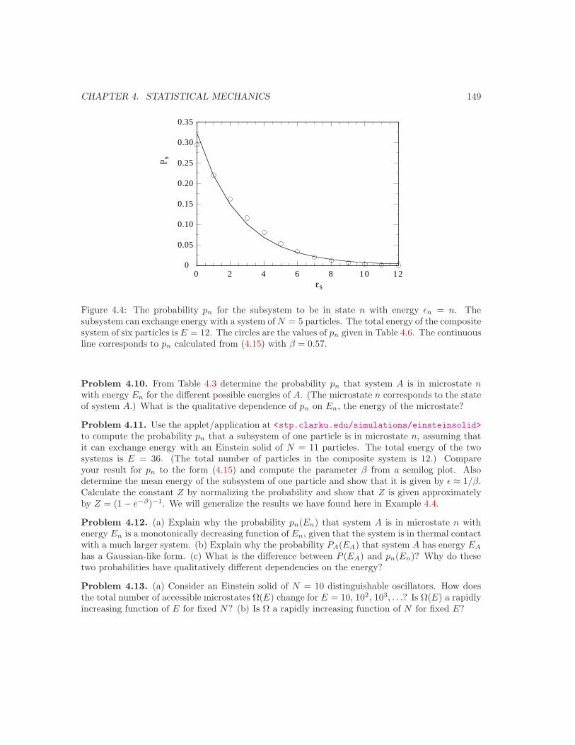
CHAPTER 4. STATISTICAL MECHANICS 149

0

0.05

0.10

0.15

0.20

0.25

0.30

0.35

0 2 4 6 8 10 12εs

P s

Figure 4.4: The probability pn for the subsystem to be in state n with energy εn = n. Thesubsystem can exchange energy with a system of N = 5 particles. The total energy of the compositesystem of six particles is E = 12. The circles are the values of pn given in Table 4.6. The continuousline corresponds to pn calculated from (4.15) with β = 0.57.

Problem 4.10. From Table 4.3 determine the probability pn that system A is in microstate nwith energy En for the different possible energies of A. (The microstate n corresponds to the stateof system A.) What is the qualitative dependence of pn on En, the energy of the microstate?

Problem 4.11. Use the applet/application at <stp.clarku.edu/simulations/einsteinsolid>to compute the probability pn that a subsystem of one particle is in microstate n, assuming thatit can exchange energy with an Einstein solid of N = 11 particles. The total energy of the twosystems is E = 36. (The total number of particles in the composite system is 12.) Compareyour result for pn to the form (4.15) and compute the parameter β from a semilog plot. Alsodetermine the mean energy of the subsystem of one particle and show that it is given by ε ≈ 1/β.Calculate the constant Z by normalizing the probability and show that Z is given approximatelyby Z = (1 − e−β)−1. We will generalize the results we have found here in Example 4.4.

Problem 4.12. (a) Explain why the probability pn(En) that system A is in microstate n withenergy En is a monotonically decreasing function of En, given that the system is in thermal contactwith a much larger system. (b) Explain why the probability PA(EA) that system A has energy EA

has a Gaussian-like form. (c) What is the difference between P (EA) and pn(En)? Why do thesetwo probabilities have qualitatively different dependencies on the energy?

Problem 4.13. (a) Consider an Einstein solid of N = 10 distinguishable oscillators. How doesthe total number of accessible microstates Ω(E) change for E = 10, 102, 103, . . .? Is Ω(E) a rapidlyincreasing function of E for fixed N? (b) Is Ω a rapidly increasing function of N for fixed E?

CHAPTER 4. STATISTICAL MECHANICS 150

4.3 Counting microstates

In the examples we have considered so far, we have seen that the most time consuming task isenumerating (counting) the number of accessible microstates for a system of fixed energy andnumber of particles. We now discuss how to count the number of accessible microstates for severalother systems of interest.

4.3.1 Noninteracting spins

We first reconsider an isolated system of N noninteracting spins with spin 1/2 and magneticmoment µ in an external magnetic field B. Because we can distinguish spins at different latticesites, a particular state or configuration of the system is specified by giving the orientation (upor down) of each of the N spins. We want to find the total number of accessible microstatesΩ(E, B, N) for particular values of E, B, and N .

We know that if n spins are parallel to B and N − n spins are antiparallel to B, the energyof the system is

E = n(−µB) + (N − n)(µB) = −(2n − N)µB. (4.16)

For a given N and B, n specifies the energy and vice versa. If we solve (4.16) for n, we find

n =N

2− E

2µB. (4.17)

As we found in (3.71), the total number of microstates with energy E is given by the number ofways n spins out of N can be up. This number is given by

Ω(n, N) =N !

n! (N − n)!, (4.18)

where n is related to E by (4.17). We will apply this result in Example 4.2 on page 163.

4.3.2 *One-dimensional Ising model

It is instructive to discuss the number of states for the one-dimensional Ising model. For smallN we can determine Ω(E, N) by counting on our fingers. For example, it is easy to verify thatΩ(−2, 2) = 2 and Ω(0, 2) = 2 and Ω(−3, 3) = 2 and Ω(1, 3) = 6 using periodic boundary conditions.It turns out that the general expression for Ω(E, N) for the one-dimensional Ising model for evenN is

Ω(E, N) = 2(

N

i

)= 2

N !i! (N − i)!

, (i = 0, 2, 4, . . . , N) (4.19)

where E = 2i − N . We will discuss the Ising model in more detail in Chapter 5.

Problem 4.14. Verify that (4.19) gives the correct answers for N = 2 and 4.

CHAPTER 4. STATISTICAL MECHANICS 151

pmax

L

x

p

Figure 4.5: The phase space for a single particle of mass m and energy E in a one-dimensionalbox of length L. The maximum value of the momentum is pmax =

√2mE. Any point within the

shaded rectangle corresponds to a microstate with energy less than or equal to E.

4.3.3 A particle in a one-dimensional box

Classical calculation. Consider the microstates of a single classical particle of mass m confinedto a one-dimensional box of length L. We know that the microstate of a particle is specified byits position x and momentum p.2 We say that the microstate (x, p) is a point in phase space (seeFigure 4.5).

As in Section 4.3.1, we want to calculate the number of microstates of the system with energyE. Because the values of the position and momenta of a particle are continuous variables, thisquestion is not meaningful and instead we will determine the quantity g(E)∆E, the number ofmicrostates between E and E + ∆E; the quantity g(E) is the density of states. However, it iseasier to first calculate Γ(E), the number of microstates of the system with energy less than orequal to E. Then the number of microstates between E and E + ∆E, g(E)∆E, is related to Γ(E)by

g(E)∆E = Γ(E + ∆E) − Γ(E) ≈ dΓ(E)dE

∆E. (4.20)

If the energy of the particle is E and the dimension of the box is L, then the microstates ofthe particle with energy less than or equal to E are restricted to the rectangle shown in Figure 4.5,where pmax =

√2mE. However, because the possible values of x and p are continuous, there are

an infinite number of microstates within the rectangle! As we discussed in Section 3.6, we haveto group or bin the microstates so that we can count them, and hence we divide the rectangle inFigure 4.5 into bins or cells of area ∆x∆p.

The area of phase space occupied by the trajectory of a particle whose position x is less thanor equal to L and whose energy is less than or equal to E is equal to 2pmaxL. Hence, the number

2We could equally well specify the velocity v rather than p, but the momentum p is the appropriate conjugatevariable to x in the formal treatment of classical mechanics.

CHAPTER 4. STATISTICAL MECHANICS 152

of cells or microstates equals

Γcl(E) =2pmaxL

∆x∆p= 2

L

∆x∆p(2mE)1/2, (4.21)

where the values of ∆x and ∆p are arbitrary. What is the corresponding density of states?

Quantum calculation. The most fundamental description of matter at the microscopic level isgiven by quantum mechanics. Although the quantum mechanical description is more abstract, wewill find that it makes counting microstates more straightforward.

As before, we consider a single particle of mass m in a one-dimensional box of length L.According to de Broglie, a particle has wave properties associated with it, and the correspondingstanding wave has a node at the boundaries of the box. The wave function of the wave with oneantinode can be represented as in Figure 4.6; the corresponding wavelength is given by

λ = 2L. (4.22)

In general, the greater the number of antinodes of the wave, the greater the energy associated withthe particle. The possible wavelengths that are consistent with the boundary conditions at x = 0and x = L are given by

λn =2L

n, (n = 1, 2, 3, . . .) (4.23)

where the index n labels the quantum state of the particle and can be any nonzero, positive integer.From the de Broglie relation,

p =h

λ, (4.24)

and the nonrelativistic relation between the energy E and the momentum p, we find that theeigenvalues of the particle are given by

En =p2

n

2m=

h2

2m λ2n

=n2h2

8mL2. (4.25)

It is now straightforward to count the number of microstates with energy less than or equalto E. The value of n for a given E is (see (4.25))

n =2L

h(2mE)1/2. (4.26)

Because successive microstates correspond to values of n that differ by unity, the number of stateswith energy less than or equal to E is given by

Γqm(E) = n =2L

h(2mE)1/2. (4.27)

Unlike the classical case, the number of states Γqm(E) for a quantum particle in a one-dimensional box has no arbitrary parameters such as ∆x and ∆p. If we require that the classicaland quantum enumeration of microstates agree in the semiclassical limit,3 we see that the number

3Note that the semiclassical limit is not equivalent to simply letting → 0.

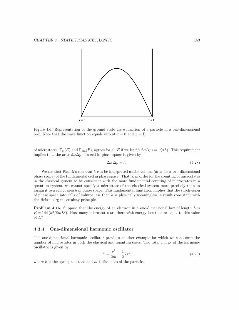
CHAPTER 4. STATISTICAL MECHANICS 153

x = 0 x = L

Figure 4.6: Representation of the ground state wave function of a particle in a one-dimensionalbox. Note that the wave function equals zero at x = 0 and x = L.

of microstates, Γcl(E) and Γqm(E), agrees for all E if we let 2/(∆x∆p) = 1/(π). This requirementimplies that the area ∆x∆p of a cell in phase space is given by

∆x∆p = h. (4.28)

We see that Planck’s constant h can be interpreted as the volume (area for a two-dimensionalphase space) of the fundamental cell in phase space. That is, in order for the counting of microstatesin the classical system to be consistent with the more fundamental counting of microstates in aquantum system, we cannot specify a microstate of the classical system more precisely than toassign it to a cell of area h in phase space. This fundamental limitation implies that the subdivisionof phase space into cells of volume less than h is physically meaningless, a result consistent withthe Heisenberg uncertainty principle.

Problem 4.15. Suppose that the energy of an electron in a one-dimensional box of length L isE = 144 (h2/8mL2). How many microstates are there with energy less than or equal to this valueof E?

4.3.4 One-dimensional harmonic oscillator

The one-dimensional harmonic oscillator provides another example for which we can count thenumber of microstates in both the classical and quantum cases. The total energy of the harmonicoscillator is given by

E =p2

2m+

12kx2, (4.29)

where k is the spring constant and m is the mass of the particle.

CHAPTER 4. STATISTICAL MECHANICS 154

Classical calculation. The shape of the phase space area traversed by the trajectory x(t), p(t)can be determined from (4.29) by dividing both sides by E and substituting ω2 = k/m:

x(t)2

2E/mω2+

p(t)2

2mE= 1. (4.30)

where the total energy E is a constant of the motion.From the form of (4.30) we see that the shape of phase space of a one-dimensional harmonic

oscillator is an ellipse,x2

a2+

p2

b2= 1, (4.31)

with a2 = 2E/(mω2) and b2 = 2mE. Because the area πab = 2πE/ω, the number of states withenergy less than or equal to E is given by

Γcl(E) =πab

∆x∆p=

2πE

ω ∆x∆p. (4.32)

Quantum mechanical calculation. The energy eigenvalues of the harmonic oscillator are givenby

En = (n +12) ω. (n = 0, 1, 2, . . .) (4.33)

Hence the number of microstates is given by

Γqm(E) = n =E

ω− 1

2→ E

ω. (4.34)

We see that Γqm(E) = Γcl(E) for all E, if 2π/(∆x∆p) = or ∆x∆p = h as before.

4.3.5 One particle in a two-dimensional box

Consider a single particle of mass m in a rectangular box of sides Lx and Ly. The wave functiontakes the form of a standing wave in two dimensions. The energy of the particle is given by

E =p2

2m=

12m

(px2 + py

2), (4.35)

where p = k. The wave vector k satisfies the conditions for a standing wave:

kx =π

Lxnx, ky =

π

Lyny. (nx, ny = 1, 2, 3, . . .) (4.36)

The corresponding eigenvalues are given by

Enx,ny =h2

8m

[nx

2

Lx2 +

ny2

Ly2

]. (4.37)

The states of the particle are labeled by the two integers nx and ny with nx, ny > 0. Thepossible values of nx, ny lie at the centers of squares of unit area as shown in Figure 4.7. For

CHAPTER 4. STATISTICAL MECHANICS 155

not done

Figure 4.7: The points represent possible values of nx and ny such that R2 = n2x + n2

y = 102 andnx > 0 and ny > 0. The number of states for R = 10 is 69. The corresponding number from theasymptotic relation is Γ(E) = π 102/4 ≈ 78.5.

simplicity, we assume that the box is square so that Lx = Ly. The values of (nx, ny) for a given Esatisfy the condition

R2 = nx2 + ny

2 =(2L

h

)2

(2mE). (4.38)

For large values of nx and ny, the values of nx and ny that correspond to states with energy lessthan or equal to E lie inside the positive quadrant of a circle of radius R, where

R =2L

h(2mE)1/2. (4.39)

Recall that nx and ny are both positive. Hence, the number of states with energy less than orequal to E is given by

Γ(E) =14πR2 = π

L2

h2(2mE). (4.40)

Note that V = L2 in this case.

Problem 4.16. The expression (4.40) for Γ(E) is valid only for large E because the area of aquadrant of a circle overestimates the number of lattice points nx, ny inside a circle of radiusR. Explore how the relation Γ = πR2/4 approximates the actual number of microstates bywriting a program that computes the number of nonzero, positive integers that satisfy the conditionn2

x + n2y ≤ R2. Pseudocode for such a program is listed in the following:

R = 10R2 = R*Rstates = 0do nx = 1,Rdo ny = 1,R

if ((nx*nx + ny*ny) <= R2) thenstates = states + 1

end ifend do

end do

CHAPTER 4. STATISTICAL MECHANICS 156

What is the minimum value of R for which the difference between the asymptotic relation and theexact count is less than 1%?

4.3.6 One particle in a three-dimensional box

The generalization to three dimensions is straightforward. If we assume that the box is a cubewith linear dimension L, we have

E =h2

8mL2[n2

x + n2y + n2

z]. (4.41)

The values of nx, ny, and nz that correspond to microstates with energy less than or equal to Elie inside the positive octant of a sphere of radius R given by

R2 = n2x + n2

y + n2z =

(2L

h

)2

(2mE). (4.42)

HenceΓ(E) =

18

(43πR3

)=

π

6

(2L

h

)3

(2mE)3/2 =4π

3V

h3(2mE)3/2, (4.43)

where we have let V = L3.

Problem 4.17. The expression (4.43) for Γ(E) is valid only for large E because the area of anoctant of a sphere overestimates the number of lattice points nx, ny, nz. Explore how the relationΓ = πR3/6 approximates the total number of microstates by writing a program that computes thenumber of nonzero, positive integers that satisfy the condition n2

x + n2y + n2

z ≤ R2.

Problem 4.18. Estimate the number of microstates accessible to a gas molecule at typical roomtemperatures and pressures. We can proceed by estimating the mean energy E of a gas moleculesuch as nitrogen at room temperature by using the relation E = 3NkT/2. Calculate the number ofmicrostates Γ(E) with energy less than E accessible to such a molecule enclosed in a box having avolume of one liter (103 cm3). Consider a small energy interval ∆E = 10−27 J that is much smallerthan E itself, and calculate the number of microstates g(E)∆E accessible to the molecule in therange between E and E + ∆E.

4.3.7 Two noninteracting identical particles and the semiclassical limit

Consider two noninteracting particles of mass m of the same species in a one-dimensional box oflength L. The total energy is given by

En1,n2 =h2

8mL2[n2

1 + n22], (4.44)

where the quantum numbers n1 and n2 are positive nonzero integers. However, to count themicrostates correctly, we need to take into account that particles of the same species are indistin-guishable, one of the fundamental principles of quantum mechanics.

As an example of how we would count the microstates of this two particle system, suppose thatthe total energy is such that n2

1 + n22 ≤ 25. The values of n1 and n2 that satisfy this constraint are

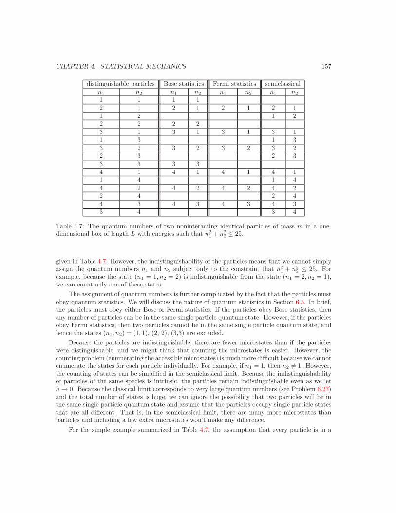
CHAPTER 4. STATISTICAL MECHANICS 157

distinguishable particles Bose statistics Fermi statistics semiclassicaln1 n2 n1 n2 n1 n2 n1 n2

1 1 1 12 1 2 1 2 1 2 11 2 1 22 2 2 23 1 3 1 3 1 3 11 3 1 33 2 3 2 3 2 3 22 3 2 33 3 3 34 1 4 1 4 1 4 11 4 1 44 2 4 2 4 2 4 22 4 2 44 3 4 3 4 3 4 33 4 3 4

Table 4.7: The quantum numbers of two noninteracting identical particles of mass m in a one-dimensional box of length L with energies such that n2

1 + n22 ≤ 25.

given in Table 4.7. However, the indistinguishability of the particles means that we cannot simplyassign the quantum numbers n1 and n2 subject only to the constraint that n2

1 + n22 ≤ 25. For

example, because the state (n1 = 1, n2 = 2) is indistinguishable from the state (n1 = 2, n2 = 1),we can count only one of these states.

The assignment of quantum numbers is further complicated by the fact that the particles mustobey quantum statistics. We will discuss the nature of quantum statistics in Section 6.5. In brief,the particles must obey either Bose or Fermi statistics. If the particles obey Bose statistics, thenany number of particles can be in the same single particle quantum state. However, if the particlesobey Fermi statistics, then two particles cannot be in the same single particle quantum state, andhence the states (n1, n2) = (1, 1), (2, 2), (3,3) are excluded.

Because the particles are indistinguishable, there are fewer microstates than if the particleswere distinguishable, and we might think that counting the microstates is easier. However, thecounting problem (enumerating the accessible microstates) is much more difficult because we cannotenumerate the states for each particle individually. For example, if n1 = 1, then n2 = 1. However,the counting of states can be simplified in the semiclassical limit. Because the indistinguishabilityof particles of the same species is intrinsic, the particles remain indistinguishable even as we leth → 0. Because the classical limit corresponds to very large quantum numbers (see Problem 6.27)and the total number of states is huge, we can ignore the possibility that two particles will be inthe same single particle quantum state and assume that the particles occupy single particle statesthat are all different. That is, in the semiclassical limit, there are many more microstates thanparticles and including a few extra microstates won’t make any difference.

For the simple example summarized in Table 4.7, the assumption that every particle is in a

CHAPTER 4. STATISTICAL MECHANICS 158

different microstate implies that we can ignore the microstates (1, 1), (2, 2), and (3, 3). Hence, inthe semiclassical limit, we are left with six states (2, 1), (3, 1), (3, 2), (4, 1), (4, 2), and (4, 3) thatsatisfy the criterion n2

1 + n22 ≤ 25.

This example illustrates how we can simplify the counting of the microstates in the semiclas-sical limit. We first count the total number of microstates of the N identical particles assumingthat the particles are distinguishable. For N = 2 and the constraint that n2

1 + n22 ≤ 25, we would

find 12 microstates, assuming that the two particles are in different single particle states (see thelast column of Table 4.7). We then correct for the overcounting of the microstates due to theindistinguishability of the particles by dividing by N !, the number of permutations of the differentsingle particle states. For our example we would correct for the overcounting by dividing by the2! ways of permuting two particles, and we obtain a total of 12/2! = 6 states.

4.4 The number of states of N noninteracting particles: Semi-classical limit

We now apply these considerations to count the number of microstates of N noninteracting particlesin a three-dimensional box in the semiclassical limit. A simpler way to do so that yields the correctE and V dependence is given in Problem 4.19, but the numerical factors will not be identical tothe result of the more accurate calculation that we discuss here.

The idea is to first count the microstates assuming that the N particles are distinguishableand then divide by N ! to correct for the overcounting. We know that for one particle in a three-dimensional box, the number of microstates with energy less than or equal to E is given bythe volume of the positive part of the three-dimensional sphere of radius R (see (4.39)). For Ndistinguishable particles in a three-dimensional box, the number of microstates with energy lessthan or equal to E is given by the volume of the positive part of the 3N -dimensional hypersphereof radius R = (2mE)1/2(2L/h). To simplify the notation, we consider the calculation of Vn(R),the volume of a n-dimensional hypersphere of radius R and write Vn(R) as

Vn(R) =∫

r21+r2

2+···+r2n<R2

dr1 dr2 · · · drn. (4.45)

It is shown in Appendix 4A that Vn(R) is given by (for integer n)

Vn(R) =2πn/2

nΓ(n/2)Rn, (4.46)

where the Gamma function Γ(n) = (n−1)!, Γ(n+1) = nΓ(n) if n is an integer, and Γ(1/2) =√

π/2.The cases n = 2 and n = 3 yield the expected results, V2 = 2πR2/(2Γ(1)) = πR2 because Γ(1) = 1,and V3 = 2π3/2R3/(3Γ(3/2)) = 4

3πR3 because Γ(3/2) = Γ(1/2) = π1/2/2. The volume of thepositive part of a n-dimensional sphere of radius R is given by

Γ(R) =(1

2

)n

Vn(R). (4.47)

(The volume Γ(R) should not be confused with the Gamma function Γ(n).)

CHAPTER 4. STATISTICAL MECHANICS 159

We are interested in the case n = 3N and R = (2mE)1/2(2L/h). In this case the volumeΓ(E, V, N) is given by

Γ(E, V, N) =(1

2

)3N 2π3N/2

3N(3N/2− 1)!R3N/2 (4.48a)

=(1

2

)3N π3N/2

(3N/2)!R3N/2 (4.48b)

=(1

2

)3N(2L

h

)3N/2 π3N/2

(3N/2)!(2mE)3N/2 (4.48c)

=( V

h3

)N (2πmE)3N/2

(3N/2)!. (4.48d)

If we include the factor of 1/N ! to correct for the overcounting of microstates in the semiclassicallimit, we obtain the desired result:

Γ(E, V, N) =1

N !

( V

h3

)N (2πmE)3N/2

(3N/2)!. (semiclassical limit) (4.49)

A more convenient expression for Γ can be found by using Stirling’s approximation for N 1.We have

ln Γ = − ln N ! + N lnV

h3+

32N ln(2πmE) − ln

(3N

2

)! (4.50a)

= −N ln N + N + N ln V − 3N

2ln h2 +

32N ln(2πmE) − 3

2N ln

3N

2+

3N

2(4.50b)

= N lnV

N+

32N ln

4πmE

3Nh2+

52N (4.50c)

= N lnV

N+

32N ln

mE

3Nπ2+

52N, (4.50d)

where we have let h = 2π to obtain (4.50d) from (4.50c) .

Problem 4.19. We can obtain an equivalent expression for Γ(E, V, N) using simpler physicalconsiderations. We write

Γ(E, V, N) ≈ 1N !

Γ1(E

N, V )Γ1(

E

N, V ) . . .Γ1(

E

N, V ), (4.51)

where Γ1(E, V ) is the number of states for a particle with energy less than E in a three-dimensionalbox of volume V . We have assumed that on the average each particle has an energy E/N . Findthe form of Γ(E, V, N) using the relation (4.43) for Γ1. Compare the V and E-dependencies ofΓ(E, V, N) obtained from this simple argument to (4.49). What about the N -dependence?

Problem 4.20. Calculate g(E, V, N) and verify that Γ(E, V, N) and g(E, V, N) are rapidly in-creasing functions of E, V , and N .

CHAPTER 4. STATISTICAL MECHANICS 160

4.5 The microcanonical ensemble (fixed E, V, and N)

So far, we have learned how to count the number of microstates of an isolated system. Sucha system of particles is specified by the energy E, volume V , and number of particles N . Allmicrostates that are consistent with these conditions are assumed to be equally probable. Thecollection of systems in different microstates and specified values of E, V , and N is called themicrocanonical ensemble. In general, the energy E is a continuous variable, and the energy isspecified to be in the range E to E + ∆E.4

In the following we show how the quantities that correspond to the usual thermodynamicquantities, for example, the entropy, temperature, and pressure, are related to the number ofmicrostates. We will then use these relations to derive the ideal gas equation of state and otherwell known results using (4.50d) for the number of microstates of an ideal gas of N particles in avolume V with energy E.

We first establish the connection between the number of accessible microstates to various ther-modynamic quantities by using arguments that are similar to our treatment of the simple modelsthat we considered in Section 4.2. Consider two isolated systems A and B that are separated by aninsulating, rigid, and impermeable wall. The macrostate of each system is specified by EA, VA, NA

and EB , VB, NB, respectively, and the corresponding number of microstates is ΩA(EA, VA, NA)and ΩB(EB , VB, NB). Equilibrium in this context means that each accessible microstate is equallyrepresented in our ensemble. The number of microstates of the composite system consisting of thetwo isolated subsystems A and B is

Ω = ΩA(EA, VA, NA)ΩB(EB , VB , NB). (4.52)

We want a definition of the entropy that is a measure of the number of microstates and thatis additive. It was assumed by Boltzmann that S is related to Ω by the famous formula, firstproposed by Planck:

S = k ln Ω. (4.53)

Note that if we substitute (4.52) in (4.53), we find that S = SA +SB, and S is an additive functionas it must be.

Next we modify the wall between A and B so that it becomes conducting, rigid, and im-permeable. We say that we have relaxed the internal constraint of the composite system. Thetwo subsystems are now in thermal contact so that the energies EA and EB can vary, subject tothe condition that the total energy E = EA + EB is fixed; the volumes VA and VB and particlenumbers NA and NB remain unchanged. What happens to the number of accessible microstatesafter we relax the internal constraint? In general, we expect that there are many more microstatesavailable after the constraint is removed. If subsystem A has energy EA, it can be in any one ofits Ω(EA) microstates. Similarly, subsystem B can be in any one of its ΩB(E − EA) microstates.Because every possible state of A can be combined with every possible state of B to give a differentstate of the composite system, it follows that the number of distinct microstates accessible to the

4For a quantum system, the energy E must always be specified in some range. The reason is that if the energywere specified exactly, the system would have to be in an eigenstate of the system. If it were, the system wouldremain in this eigenstate indefinitely, and a statistical treatment would be meaningless.

CHAPTER 4. STATISTICAL MECHANICS 161

composite system when A has energy EA is the product ΩA(EA)ΩB(E − EA). Hence, the totalnumber of accessible microstates after the subsystems are in thermal equilibrium is

Ω(E) =∑EA

ΩA(EA)ΩB(E − EA). (4.54)

The probability that system A has energy EA is given by

P (EA) =ΩA(EA)ΩB(E − EA)

Ω(E). (4.55)

Note that the logarithm of (4.54) does not yield a sum of two functions. However, the dominantcontribution to the right-hand side of (4.54) comes from the term with EA = EA, where EA is themost probable value of EA. With this approximation we can write

Ω ≈ ΩA(EA)ΩB(E − EA). (4.56)

The approximation (4.56) becomes more and more accurate as the thermodynamic limit (N, V →∞, ρ = N/V = constant) is approached and allows us to write

S = k ln Ω = SA + SB (4.57)

before and after the constraint is removed.The relation S = k ln Ω is not very mysterious. It is simply a matter of counting the number

of accessible microstates and assuming that they are all equally probable. We see immediatelythat one consequence of this definition is that the entropy increases or remains unchanged after aninternal constraint is relaxed. Given the definition (4.53) of S as a function of E, V , and N , it isnatural to adopt the thermodynamic definitions of temperature, pressure, and chemical potential:

1T

=∂S

∂E. (4.58)

P

T=

∂S

∂V. (4.59)

µ

T= − ∂S

∂N. (4.60)

We have made the connection between statistical mechanics and thermodynamics.How should we define the entropy for a system in which the energy is a continuous variable?

Three possibilities are

S = k ln Γ (4.61a)S = k ln g(E)∆E (4.61b)S = k ln g(E). (4.61c)

It is easy to show that in the limit N → ∞, the three definitions yield the same result (seeProblem 4.21). The reason is that Γ(E) and g(E) are such rapidly increasing functions of E thatit makes no difference whether we include the microstates with energy less than or equal to E orjust the states between E and E + ∆E.

CHAPTER 4. STATISTICAL MECHANICS 162

Example 4.1. Find the pressure and thermal equations of state of an ideal classical gas.Solution. If we use any of the definitions of S given in (4.61), we find that the entropy of an idealgas in the semiclassical limit for N → ∞ is given by

S(E, V, N) = Nk[ln

V

N+

32

lnmE

3Nπ2+

52]. (4.62)

Problem 4.21. (a) Justify the statement made in the text that any of the definitions of S givenin (4.61) yield the result (4.62). (b) Verify the result (4.62) for the entropy S of an ideal gas.

Problem 4.22. Compare the form of S given in (4.62) with the form of S determined fromthermodynamic considerations in Section 2.19.

We now use the result (4.62) for S to obtain the thermal equation of state of an ideal classicalgas. From (4.62) we see that

1T

=( ∂S

∂E

)V,N

=32

Nk

E, (4.63)

and hence we obtain the familiar result

E =32NkT. (4.64)

The pressure equation of state follows from (4.59) and (4.62) and is given by

P

T=

( ∂S

∂V

)E,N

=Nk

V,

and hencePV = NkT. (4.65)

We have finally derived the equations of state of an ideal classical gas from first principles! We seethat we can calculate the thermodynamic information for an isolated system by counting all theaccessible microstates as a function of the total energy E, volume V , and number of particles N .Do the equations of state depend on and the various constants in (4.49)?

Note that we originally defined the ideal gas temperature scale in Section 2.4 by assumingthat T ∝ P . We then showed that the ideal gas temperature scale is consistent with the thermo-dynamic temperature defined by the relation 1/T = (∂S/∂E)V,N . Finally, we have shown that theassociation of S with the logarithm of the number of accessible microstates is consistent with therelation P ∝ T for an ideal classical gas.

Problem 4.23. Use the relations (4.62) and (4.64) to obtain S as a function of T , V , and Ninstead of E, V , and N . This relation is known as the Sackur-Tetrode equation.

Problem 4.24. Use (4.60) and (4.62) to derive the dependence of the chemical potential µ onE, V , and N for a ideal classical gas. Then use (4.64) to determine µ(T, V, N). (We will deriveµ(T, V, N) for the ideal classical gas more simply in Section 6.8.)

CHAPTER 4. STATISTICAL MECHANICS 163

Example 4.2. Consider a system of N noninteracting spins and find the dependence of its tem-perature T on the total energy E. What is the probability that a given spin is up?Solution. First we have to find the dependence of the entropy S on the energy E of the system.As discussed in Sec. 4.3.1, the energy E for a system with n spins up out of N in a magnetic fieldB is given by

E = −(n−n′)µB = −[n−(N −n)]µB = −(2n−N)µB, (4.16)

where n′ = N − n is the number of down spins and µ is the magnetic moment of the spins. Thecorresponding number of microstates is given by (4.18):

Ω(n) =N !

n!(N − n)!. (4.18)

From (4.16), we find that the value of n corresponding to a given E is given by

n =12

(N − E

µB

). (4.66)

The thermodynamic temperature T is given by

1T

=∂S

∂E=

dS(n)dn

dn

dE= − 1

2µB

dS

dn. (4.67)

It is understood that the magnetic field B is held fixed.To calculate dS/dn, we use the approximation (3.92) for large n:

d

dnln n! = lnn, (4.68)

and finddS(n)

dn= k[− ln n + ln(N − n)], (4.69)

where S(n) = k ln Ω(n) from (4.18). Hence

1T

= −k1

2µBln

N − n

n. (4.70)

Equation (4.70) yields T as a function of E by eliminating n using (4.66).The natural variables in the microcanonical ensemble are E, V , and N . Hence, T is a derived

quantity and is found as a function of E. As shown in Problem 4.25, we can rewrite this relationto express E as a function T . The result is

E = −NµB tanhµB

kT= −NµB tanhβµB, (4.71)

where β = 1/kT .

CHAPTER 4. STATISTICAL MECHANICS 164

ensemble macrostate probability distribution thermodynamics

microcanonical E, V, N pn = 1/Ω S(E, V, N) = k ln Ω

canonical T, V, N pn = e−βEn/Z F (T, V, N) = −kT ln Z

grand canonical T, V, µ pn = e−β(En−µNn)/Z Ω(T, V, µ) = −kT lnZ

Table 4.8: Summary of the three common ensembles. Note that Ω is the number of accessible mi-crostates in the microcanonical ensemble and the thermodynamic potential in the grand canonicalensemble.

The probability p that a given spin is up is equal to the ratio n/N . We can solve (4.70) forn/N and obtain (see Problem 4.25)

p =n

N=

11 + e−2µB/kT

, (4.72a)

=eµB/kT

eµB/kT + e−µB/kT=

eβµB

eβµB + e−βµB, (4.72b)

We have obtained the result for p that we promised in Section 3.5.

Note we have had to consider all N spins even though the spins do not interact with eachanother. The reason is that the N spins have a definite energy and hence we cannot assign theorientation of the spins independently. We will obtain the result (4.72) by a more straightforwardmethod in Section 4.6.

Problem 4.25. Solve (4.70) for n/N and verify (4.72). Then use (4.16) to solve for E as a functionof T for a system of N noninteracting spins.

Although the microcanonical ensemble is conceptually simple, it is not the most practical en-semble. The major problem is that because we must satisfy the constraint that E is specified, wecannot assign energies to each particle individually, even if the particles do not interact. Anotherproblem is that because each microstate is as important as any other, there are no obvious ap-proximation methods that retain only the most important microstates. Moreover, isolated systemsare very difficult to realize experimentally, and the temperature rather than the energy is a morenatural independent variable.

Before we discuss the other common ensembles, we summarize their general features in Ta-ble 4.8. The internal energy E is fixed in the microcanonical ensemble and hence only the meantemperature is specified and the temperature fluctuates. In the canonical ensemble the temper-ature T and hence the mean energy is fixed, but the energy fluctuates. Similarly, the chemicalpotential and hence the mean number of particles is fixed in the grand canonical ensemble, andthe number of particles fluctuates. In all of these ensembles, the volume V is fixed which impliesthat the pressure fluctuates. We also can choose an ensemble in which the pressure is fixed andthe volume fluctuates.

Problem 4.26. Consider a collection of N distinguishable, harmonic oscillators with total energyE. The oscillators are distinguishable because they are localized on different lattice sites. In one

CHAPTER 4. STATISTICAL MECHANICS 165

dimension the energy of each particle is given by εn = (n+ 12 )ω, where ω is the angular frequency.

Hence, the total energy can be written as E = (Q + 12N)ω, where Q is the number of quanta.

Calculate the dependence of the temperature T on the total energy E in the microcanonicalensemble using the result that the number of accessible microstates in which N distinguishableoscillators can share Q indistinguishable quanta is given by Ω = (Q + N − 1)!/Q!(N − 1)! (see(4.3)). Use this relation to find E(T ). The thermodynamics of this system is calculated muchmore simply in the canonical ensemble as shown in Example 4.52.

4.6 Systems in contact with a heat bath: The canonicalensemble (fixed T, V, and N)

We now assume that the system of interest can exchange energy with a much larger system knownas the heat bath. The heat bath is sufficiently large that it is not significantly affected by thesmaller system. For example, if we place a glass of cold water into a room, the temperature of thewater will eventually reach the temperature of the air in the room. Because the volume of the glassis small compared to the volume of the room, the cold water does not cool the air appreciably andthe air is an example of a heat bath.

The composite system, the system of interest plus the heat bath, is an isolated system. Wecan characterize the macrostate of the composite system by E, V, N . The accessible microstatesof the composite system are equally probable. If the system of interest is in a microstate withenergy En, then the energy of the heat bath is Ebath = E − En. Because the system of interestis much smaller than the heat bath, we know that En E. For small systems it is not clearhow we should assign the potential energy of interaction of particles at the interface of the systemand the heat bath. However, if the number of particles is large, the number of particles near theinterface is small in comparison to the number of particles in the bulk so that the potential energyof interaction of particles near the surface can be ignored. Nevertheless, these interactions areessential in order for the system to come into thermal equilibrium with the heat bath.

For a given microstate of the system, the heat bath can be in any one of a large number ofmicrostates such that the total energy of the composite system is E. The probability pn that thesystem is in microstate n with energy En is given by (see (4.52))

pn =1 × Ω(E − En)∑

n Ω(E − En), (4.73)

where Ω(E − En) is the number of microstates of the heat bath for a given microstate n of thesystem of interest. As En increases, Ω(E − En), the number of accessible microstates available tothe heat bath, decreases. We conclude that pn is a decreasing function of En, because the largerthe value of En, the less energy is available to the heat bath.

We can simplify the form of pn by using the fact that En E. However, we cannot approxi-mate Ω(E −En) directly because Ω is a rapidly varying function of the energy. For this reason we

CHAPTER 4. STATISTICAL MECHANICS 166

take the logarithm of (4.73) and write

ln pn = C + ln Ω(Ebath = E − En) (4.74a)

≈ C + ln Ω(E) − En

(∂ ln Ω(Ebath)∂Ebath

)Ebath=E

(4.74b)

= C + ln Ω(E) − En

kT, (4.74c)

where C is related to the denominator of (4.73) and does not depend on En. We have used therelation

β ≡ 1kT

=(∂ ln Ω(Ebath)

∂Ebath

)N,V

. (4.75)

As can be seen from (4.75), β is proportional to the inverse temperature of the heat bath. From(4.74c) we obtain

pn =1Z

e−βEn . (Boltzmann distribution) (4.76)

The function Z is found from the normalization condition∑

n pn = 1 and is given by

Z =∑

n

e−βEn . (partition function) (4.77)

The “sum over states” Z(T, V, N) is known as the partition function. (In German Z is known asthe Zustandsumme, a more descriptive term.) Note that pn applies to a system in equilibrium witha heat bath at temperature T . The nature of the system has changed from Section 4.5.

Problem 4.27. Discuss the relation between the qualitative results that we obtained in Table 4.6and the Boltzmann distribution in (4.76).

Problem 4.28. The hydrocarbon 2-butene, CH3-CH = CH-CH3 occurs in two conformations(geometrical structures) called the cis- and trans-conformations. The energy difference ∆E betweenthe two conformations is approximately ∆E/k = 4180K,with the trans conformation lower thanthe cis conformation. Determine the relative abundance of the two conformations at T = 300Kand T = 1000K.

In the canonical ensemble the temperature T is fixed by the heat bath, and a macrostate isspecified by the temperature T , volume V , and the number of particles N . The mean energy E isgiven by

E =∑

n

pnEn =1Z

∑n

En e−βEn , (4.78)

where we have substituted the Boltzmann form (4.76) for the probability distribution. We use atrick similar to that used in Section 3.5 to obtain a simpler form for E. First we write

E = − 1Z

∂

∂β

∑n

e−βEn, (4.79)

CHAPTER 4. STATISTICAL MECHANICS 167

where we have used the fact that derivative ∂∂β (e−βEn) = −Ene−βEn . Because

∂Z

∂β= −

∑n

Ene−βEn , (4.80)

we can writeE = − 1

Z

∂Z

∂β= − ∂

∂βln Z. (4.81)

We see that E is a function of T for fixed V and N and can be expressed as a derivative of Z.In the same spirit, we can express CV , the heat capacity at constant volume, in terms of Z.

We have

CV =∂E

∂T=

dβ

dT

∂E

∂β, (4.82)

=1

kT 2

[ 1Z

∂2Z

∂β2− 1

Z2

(∂Z

∂β

)2], (4.83)

where ∂E/∂β has been calculated from (4.81). Because

E2 =1Z

∑n

E2n e−βEn =

1Z

∂2Z

∂β2, (4.84)

we obtain the relationCV =

1kT 2

[E2 − E2]. (4.85)

Equation (4.85) relates the response of the system to a change in energy to the equilibrium energyfluctuations. Note that we can calculate the variance of the energy, a measure of the magnitude ofthe energy fluctuations, from the heat capacity. We will later find other examples of the relationof the linear response of an equilibrium system to the equilibrium fluctuations of an associatedquantity.5

∗Problem 4.29. The isothermal compressibility of a system is defined as κ = −(1/V )(∂V/∂P

)T.

In what way is κ a linear response? In analogy to the relation of CV to the fluctuations in theenergy, how do you think κ is related to the fluctuations in the volume of the system at fixed T ,P , and N?

Because the energy is restricted to a very narrow range in the microcanonical ensemble andcan range anywhere between zero and infinity in the canonical ensemble, it is not obvious thatthe two ensembles give the same results for the thermodynamic properties of a system. One wayto understand why the thermodynamic properties are independent of the choice of ensemble isto use the relation (4.85) to estimate the range of energies in the canonical ensemble that have asignificant probability. Because both E and CV are extensive quantities, they are proportional toN . Hence, the relative fluctuations of the energy in the canonical ensemble is given by√

E2 − E2

E=

√kT 2CV

E∼ N1/2

N∼ N−1/2. (4.86)

5The relation (4.85) is important conceptually and is useful for simulations at a given temperature (see Sec-tion 4.11). However, it is almost always more convenient to calculate CV from its definition in (4.82).

CHAPTER 4. STATISTICAL MECHANICS 168

From (4.86) we see that in the limit of large N , the relative fluctuations in the values of E thatwould be observed in the canonical ensemble are vanishingly small. For this reason the meanenergy in the canonical ensemble is a well defined quantity just like it is in the microcanonicalensemble. However, the fluctuations in the energy are qualitatively different in the two ensembles(see Appendix 4B).

Problem 4.30. The Boltzmann probability given by (4.76) is the probability that the system isin a particular microstate with energy En. On the basis of what you have learned so far, what doyou think is the form of the probability p(E)∆E that the system has energy E between E andE + ∆E?

In addition to the relation of the mean energy to ∂ ln Z/∂β, we can express the mean pressureP in terms of ∂ ln Z/∂V . If the system is in microstate n, then a quasistatic change dV in thevolume produces the energy change

dEn =dEn

dVdV = −Pn dV. (4.87)

The quantity dEn in (4.87) is the work done on the system in state n to produce the volume changedV . The relation (4.87) defines the pressure Pn of the system in state n. Hence, the mean pressureof the system is given by

P = −∑n

pndEn

dV. (4.88)

From (4.77) and (4.88) we can express the mean pressure as

P = kT(∂ ln Z

∂V

)T,N

. (4.89)

Note that in defining the pressure, we assumed that a small change in the volume does notchange the probability distribution of the microstates. In general, a perturbation of the system willinduce transitions between the different microstates of the system so that if initially the system isin a microstate n, it will not stay in that state as the volume is changed. However, if the changeoccurs sufficiently slowly so that the system can adjust to the change, then the system will remainin its same state. As discussed in Chapter 2, such a change is called quasistatic.

We can use the relation E =∑

n pnEn to write the total change in the energy as

dE =∑

n

dpnEn +∑

n

pndEn . (4.90)

The second term in (4.90) can be written as

∑n

pn dEn =∑

n

pndEn

dVdV. (4.91)

The identification of the second term in (4.90) with the work done on the system allows us to write

dE =∑

n

En dpn − PdV. (4.92)

CHAPTER 4. STATISTICAL MECHANICS 169

If we use the fundamental thermodynamic relation (2.110), dE = TdS − PdV (for fixed N), wecan identify the first term in (4.92) with the change in entropy of the system. Hence, we have

TdS =∑

n

En dpn. (4.93)

From (4.93) we see that a change in entropy of the system is related to a change in the probabilitydistribution.

We can use (4.93) to obtain an important conceptual expression for the entropy. We rewritepn = e−βEn/Z as En = −kT (lnZ + ln pn), and substitute this relation for En into (4.93):

TdS =∑

n

En dpn = −kT∑

n

ln Z dpn − kT∑

n

ln pn dpn. (4.94)

The first term in (4.94) is zero because the total change in the probability must sum to zero. From(4.94) we write

dS = −k∑

n

ln pn dpn, (4.95)

or= −k

∑n

d(pn ln pn). (4.96)

We can integrate both sides of (4.96) to obtain the desired result:

S = −k∑

n

pn ln pn . (4.97)

We have assumed that the constant of integration is zero. The quantity defined by (4.11) and(4.97) is known as the statistical entropy in contrast to the thermodynamic entropy introduced inChapter 2. Note the similarity of (4.97) to (3.29).

The relation (4.97) for S is also applicable to the microcanonical ensemble. If there are Ωaccessible microstates, then pn = 1/Ω for each state because each state is equally likely. Hence,

S = −k

Ω∑n=1

1Ω

ln1Ω

= −kΩ1Ω

ln1Ω

= k ln Ω. (4.98)

Note that the constant of integration in going from (4.96) to (4.97) must be set to zero so thatS reduces to its form in the microcanonical ensemble. We see that we can interpret (4.97) as thegeneralization of its microcanonical form with the appropriate weight for each state.

It is remarkable that the statistical entropy defined by (4.11) and (4.97) is equivalent to itsthermodynamic definition which can be expressed as

dS =∫

dQ

T. (4.99)

The relation (4.97) is of fundamental importance and shows that the entropy is uniquelydetermined by the probability distribution pn of the different possible states. Note that complete

CHAPTER 4. STATISTICAL MECHANICS 170

predictability (only one accessible microstate) implies the vanishing of the entropy. Also as thenumber of accessible microstates increases, the greater the value of S and hence the higher thedegree of unpredictability of the system.

The idea of entropy has come a long way. It was first introduced into thermodynamics as a statefunction to account for the irreversible behavior of macroscopic systems under certain conditions.The discovery of the connection between this quantity and the probability distribution of thesystem’s microstates was one of the great achievements of Ludwig Boltzmann, and the equationS = k ln Γ (his notation) appears on his tombstone.6 Since then, our understanding of entropy hasbeen extended by Shannon and Jaynes and others to establish a link between thermodynamics andinformation theory (see Section 3.4.1). In this context we can say that S is a measure of the lackof information, because the greater the number of microstates that are available to a system in agiven macrostate, the less we know about which microstate the system is in.

Although the relation (4.11) is of fundamental importance, we will not be able to use it tocalculate the entropy in any of the applications that we consider. The calculation of the entropywill be discussed in Section 4.7.

The third law of thermodynamics. One statement of the third law of thermodynamics is

The entropy approaches a constant value as the temperature approaches zero.

The third law was first formulated by Nernst in 1906 based on experimental observations. We caneasily see that the law follows simply from the statistical definition of the entropy. At T = 0, thesystem is in the ground state which we will label by 0. From (4.97) we see that if pn = 1 for state 0and is zero for all other microstates, then S = 0. We conclude that S → 0 as T → 0 if the systemhas an unique ground state. This behavior is the type that we would expect for simple systems.

If there are g(0) microstates with the same ground state energy, then the corresponding entropyis S(T = 0) = k ln g(0). As an example, because an electron has spin 1

2 , it has two quantum statesfor each value of its momentum. Hence, an electron in zero magnetic field has degeneracy7 gn = 2,because its energy is independent of its spin orientation, and the ground state entropy of a systemof electrons would be kN ln 2. However, there are some complex systems for which g(0) ∼ N . Inany case, we can conclude that the heat capacities must go to zero as T → 0 (see Problem 4.45).

4.7 Connection between statistical mechanics and thermo-

dynamics

We have seen that the statistical quantity that enters into the calculation of the mean energy andthe mean pressure is not Z, but lnZ (see (4.81) and (4.89)). We also learned in Section 2.21 thatthe Helmholtz free energy F = E−TS is the thermodynamic potential for the variables T , V , andN . Because this set of variables corresponds to the variables specified by the canonical ensemble,it is natural to look for a connection between lnZ and F , and we define the latter as

F = −kT ln Z . (statistical mechanics definition of the free energy) (4.100)

6See www.lecb.ncifcrf.gov/~toms/icons/aust2002/photos-by-tds/all/index.105.html .7An energy level is said to be degenerate if there are two or more microstates with the same energy.

CHAPTER 4. STATISTICAL MECHANICS 171

At this stage the quantity defined in (4.100) has no obvious relation to the thermodynamic potentialF = E − TS that we defined earlier.

We now show that F as defined by (4.100) is equivalent to the thermodynamic definitionF = E − TS. The relation (4.100) gives the fundamental relation between statistical mechanicsand thermodynamics for given values of T , V , and N , just as S = k ln Ω gives the fundamentalrelation between statistical mechanics and thermodynamics for given values of E, V , and N (seeTable 4.8).

We write the total change in the quantity βF = − ln Z as

d(βF ) = − 1Z

∂Z

∂βdβ − 1

Z

∂Z

∂VdV

= Edβ − βPdV, (4.101)

where we have used (4.81) and (4.88). We add and subtract βdE to the right-hand side of (4.101)to find

d(βF ) = Edβ + βdE − βdE − βPdV

= d(βE) − β(dE + PdV ). (4.102)

Hence, we can writed(βF − βE) = −β(dE + PdV ). (4.103)

From the thermodynamic relation dE = TdS − PdV (for fixed N), we can rewrite (4.103) as

d(βF − βE) = −β(dE + PdV ) = −βTdS = −dS/k. (4.104)

If we integrate (4.104), we find

S/k = β(E − F ) + constant, (4.105)

orF = E − TS + constant. (4.106)

If we make the additional assumption that the free energy should equal the internal energy of thesystem at T = 0, we can set the constant in (4.106) equal to zero, and we obtain

F = E − TS. (4.107)

Equation (4.107) is equivalent to the thermodynamic definition of the Helmholtz free energy withE replaced by E. In the following, we will write E instead of E because the distinction will beclear from the context.

In Section 2.21 we showed that the Helmholtz free energy F is the natural thermodynamicpotential for given values of T , V , and N and that

S = −(∂F

∂T

)V,N

. (4.108)

P = −(∂F

∂V

)T,N

(4.109)

µ =( ∂F

∂N

)T,V

. (4.110)

CHAPTER 4. STATISTICAL MECHANICS 172

These relations still hold with F = −kT ln Z.In the above we started with the statistical mechanical relation F = −kT ln Z (see (4.100))

and found that it was consistent with the thermodynamic relation F = E − TS (see (4.107)). Itis instructive to start with the latter and show that it implies that F = −kT ln Z. We substituteE = −∂ ln Z/∂β and the relation S = kβ2(∂F/∂β) (see (4.108)) and find

F = E − TS = −∂ ln Z

∂β− β

(∂F

∂β

)V,N

. (4.111)

We rewrite (4.111) as

F + β(∂F

∂β

)V,N

= −∂ ln Z

∂β=

(∂βF

∂β

)V,N

. (4.112)

If we integrate both sides of (4.112), we find (up to a constant) that

F = −kT ln Z. (4.113)

4.8 Simple applications of the canonical ensemble

To gain experience with the canonical ensemble, we consider some relatively simple examples. In allthese examples, the goal is to calculate the sum over microstates in the partition function. Thenwe can calculate the free energy using (4.100), the entropy from (4.108), and the mean energyfrom (4.81). (In these simple examples, the volume of the system will not be relevant, so we willnot calculate the pressure.) In principle, we can follow this “recipe” for any physical systems.However, we will find that summing over microstates to evaluate the partition function is usuallya formidable task.

Example 4.3. Consider a system consisting of two distinguishable particles. Each particle has twostates with single particle energies 0 and ∆. The quantity ∆ is called the energy gap. The systemis in equilibrium with a heat bath at temperature T . What are the thermodynamic properties ofthe system?Solution. The states of this two-particle system are (0, 0), (0, ∆), (∆, 0), and (∆, ∆). The partitionfunction Z2 is given by

Z2 =4∑

n=1

e−βEn

= 1 + 2e−β∆ + e−2β∆ (4.114)

= (1 + e−β∆)2. (4.115)

As might be expected, we can express Z2 in terms of Z1, the partition function for one particle:

Z1 =2∑

n=1

e−βεn = 1 + e−β∆. (4.116)

By comparing the forms of (4.115) and (4.116), we find that

Z2 = Z21 . (4.117)

CHAPTER 4. STATISTICAL MECHANICS 173

What do you expect the relation is between ZN , the partition function for N noninteractingdistinguishable particles, and Z1?

Note that if the two particles were indistinguishable, there would be three microstates if theparticles were bosons and one microstate if the particles are fermions, and the relation (4.117)would not hold.

Because Z2 is simply related to Z1, we can consider the statistical properties of a systemconsisting of one particle with Z1 given by (4.116). From (4.76) we find the probability that thesystem is in each of its two possible states is given by:

p1 =1Z1

=1

1 + e−β∆(4.118a)

p2 =e−β∆

Z1=

e−β∆

1 + e−β∆. (4.118b)

The average energy is given by

e =2∑

n=1

pnεn

=∆ e−β∆

1 + e−β∆. (4.119)

Of course, e could also be found from the relation e = −∂ ln Z/∂β. (We have used the symbol ε todenote the energy of a single particle.) The energy of N noninteracting, distinguishable particlesof the same type is given by E = Ne.

It is easy to calculate the various thermodynamic quantities directly from the partition functionin (4.115). The free energy per particle, f , is given by

f = −kT ln Z1 = −kT ln[1 + e−β∆], (4.120)

and s, the entropy per particle, is given by

s = −( ∂f

∂T

)V

= k ln[1 + e−β∆] + kβ∆

1 + eβ∆. (4.121)

If we had not already calculated the average energy e, we could also obtain it from the relatione = f − Ts. (As before, we have used lower case symbols to denote that the results are for oneparticle.) Confirm that the various ways of determining e yield the same results as found in (4.119).The behavior of the various thermodynamic properties of this system are explored in Problem 4.49.

Example 4.4. Determine the thermodynamic properties of a one-dimensional harmonic oscillatorin equilibrium with a heat bath at temperature T .Solution. The energy levels of a single harmonic oscillator are given by

εn = (n +12)ω. (n = 0, 1, 2, . . .) (4.122)

CHAPTER 4. STATISTICAL MECHANICS 174

The partition function is given by

Z =∞∑

n=0

e−βω(n+1/2) = e−βω/2∞∑

n=0

e−nβω (4.123)

= e−βω/2(1 + e−βω + e−2βω + · · · ) = e−βω/2(1 + x + x2 + · · · ), (4.124)

where x = e−βω. The infinite sum in (4.124) is a geometrical series in x and can be summed usingthe result that 1 + x + x2 + . . . = 1/(1 − x) (see Appendix A). The result is

Z =e−βω/2

1 − e−βω, (4.125)

and

ln Z = −12βω − ln(1 − e−βω). (4.126)

We leave it as an exercise for the reader to show that

f =12

ω + kT ln(1 − e−βω) (4.127)

s = k[ βω

eβω − 1− ln(1 − e−βω)

](4.128)

e = ω[12

+1

eβω − 1]. (4.129)

Equation (4.129) is Planck’s formula for the mean energy of an oscillator at temperature T . Theheat capacity is discussed in Problem 4.52.

Problem 4.31. What is the mean energy of a system of N harmonic oscillators in equilibrium witha heat bath at temperature T ? Compare your result with the result for the energy of N harmonicoscillators calculated in the microcanonical ensemble in Problem 4.26. Do the two ensembles giveidentical answers?

Equation (4.77) for Z is a sum over all the microstates of the system. Because the energiesof the different microstates may be the same, we can group together microstates with the sameenergy and write (4.77) as

Z =∑levels

g(En) e−βEn , (4.130)

where g(En) is the number of microstates of the system with energy En. The sum in (4.130) isover all the energy levels of the system.

Example 4.5. Consider a three level single particle system with five microstates with energies0, ε, ε, ε, and 2ε. What is g(εn) for this system? What is the mean energy of the system if it isequilibrium with a heat bath at temperature T ?Solution. The partition function is given by (see (4.130))

Z1 = 1 + 3e−βε + e−2βε.

CHAPTER 4. STATISTICAL MECHANICS 175

Hence, the mean energy of a single particle is given by

e = ε3e−βε + 2e−2βε

1 + 3e−βε + e−2βε.

What is the energy of N such particles?

Problem 4.32. In Section 4.3.2 we were given the number of states with energy E for the one-dimensional Ising model. Use the result (4.19) to calculate the free energy of the one-dimensionalIsing model for N = 2 and 4.

4.9 A simple thermometer

Consider a system of one particle which we will call a demon that can exchange energy with anothersystem (see page 17). The demon obeys the following rules or algorithm:

1. Set up an initial microstate of the system with the desired total energy and assign an initialenergy to the demon. (The initial demon energy is usually set to zero.)

2. Make a trial change in the microstate. For the Einstein solid, choose a particle at randomand randomly increase or decrease its energy by unity. For a system of particles, change theposition of a particle by a small random amount. For the Ising model, flip a spin chosen atrandom. Compute the change in energy of the system, ∆E. If ∆E ≤ 0, accept the change,and increase the energy of the demon by |∆E|. If ∆E > 0, accept the change if the demonhas enough energy to give to the system, and reduce the demon’s energy by ∆E. If a trialchange is not accepted, the existing microstate is counted in the averages. In either case thetotal energy of the system plus the demon remains constant.

3. Repeat step 2 many times choosing particles (or spins) at random.

4. Compute the averages of the quantities of interest once the system and the demon havereached equilibrium.

The demon can trade energy with the system as long as its energy remains greater than its lowerbound, which we have chosen to be zero. The demon is a facilitator that allows the particles inthe system to indirectly trade energy with one another.

Problem 4.33. The demon can be considered to be a small system in equilibrium with a muchlarger system. Because the demon is only one particle, its microstate is specified by its energy.Given these considerations, what is the form of the probability that the demon is in a particularmicrostate?

In Problems 4.34 and 4.35 we use the demon algorithm to determine the probability that thedemon is in a particular microstate.

Problem 4.34. Consider a demon that exchanges energy with an ideal classical gas of N identicalparticles of mass m in one dimension. Because the energy of a particle depends only on its speed,the positions of the particles are irrelevant in this case. Choose a particle at random and change

CHAPTER 4. STATISTICAL MECHANICS 176

its velocity by an amount, δ, chosen at random between −∆ and ∆. The change in energy of thesystem is the difference ∆E = 1

2 [(v + δ)2 − v2], where we have chosen units so that m = 1. Theparameter ∆ is usually chosen so that the percentage of accepted changes is between 30% to 50%.The applet/application at <stp.clarku.edu/simulations/demon> implements this algorithm.(a) First consider a small number of particles, say N = 10. The applet chooses the specialmicrostate for which all the velocities of the particles in the system are identical such that thesystem has the desired initial energy. After the demon and the system have reached equilibrium,what is the mean kinetic energy per particle, the mean velocity per particle, and the mean energyof the demon? (b) Compare the initial mean velocity of the particles in the system to the meanvalue after equilibrium has been established and explain the result. (c) Compute the probability,p(Ed)dEd, that the demon has an energy between Ed and Ed + dEd. Fit your results to the formp(Ed) ∝ exp(−βEd), where β is a parameter. Given the form of p(Ed), determine analyticallythe dependence of the mean demon energy on β and compare your prediction with your numericalresults. (d) What is form of the distribution of the velocities and the kinetic energies of the systemafter it has reached equilibrium? (e) How would your results change for an ideal gas in two andthree dimensions? (f) For simplicity, the initial demon energy was set to zero. Would your resultsbe different if the demon had a non-zero initial energy if the total energy of the demon plus thesystem was the same as before?

Problem 4.35. Consider a demon that exchanges energy with an Einstein solid of N particles.First do the simulation by hand choosing N = 4 and E = 8. For simplicity, choose the initialdemon energy to be zero. Choose a particle at random and randomly raise or lower its energyby one unit consistent with the constraint that the energy of the demon Ed ≥ 0. In this casethe energy of the particle chosen also must remain nonnegative. Note that if a trial change is notaccepted, the existing microstate is counted in all averages.

After you are satisfied that you understand how the algorithm works, use the applet at<stp.clarku.edu/simulations/demon/einsteinsolid> and choose N = 20 and E = 40. DoesEd eventually reach a well defined average value? If so, what is the mean energy of the demon afterequilibrium between the demon and the system has been established? What is the probability thatthe demon has energy Ed? What is the mean and standard deviation of the energy of the system?What are the relative fluctuations of the energy in the system? Compute the probability, P (Ed),that the demon has an energy Ed. Fit your results to the form P (Ed) ∝ exp(−βEd), where β isa parameter. Then increase E to E = 80. How do the various averages change? If time permits,increase E and N and determine any changes in Pd.

Example 4.6. A demon exchanges energy with a system of N quantized harmonic oscillators (seeProblem 4.35). What is the mean energy of the demon?Solution. The demon can be thought of as a system in equilibrium with a heat bath at temperatureT . For simplicity, we will choose units such that the harmonic oscillators have energy 0, 1, 2, . . .,and hence, the energy of the demon is also restricted to integer values. Because the probability ofa demon microstate is given by the Boltzmann distribution, the demon’s mean energy is given by

Ed =∑∞

n=0 ne−βn∑∞n=0 e−βn

. (4.131)

Explain why the relation (4.131) for the demon energy is reasonable, and do the sums in (4.131)

CHAPTER 4. STATISTICAL MECHANICS 177

to determine the temperature dependence of Ed. (It is necessary to only do the sum in thedenominator of (4.131).)

Example 4.7. A demon exchanges energy with an ideal classical gas of N particles in one dimen-sion (see Problem 4.34). What is the mean energy of the demon?Solution. In this case the demon energy is a continuous variable. Hence,

Ed =

∫ ∞0 Ed e−βEd∫ ∞

0e−βEd

. (4.132)

Explain why the relation (4.132) for the demon energy is reasonable and determine the temperaturedependence of Ed. Would this temperature difference be different if the gas were three-dimensional?Compare the temperature dependence of Ed for a demon in equilibrium with an ideal classical gas toa demon in equilibrium with a system of harmonic oscillators. Why is the temperature dependencedifferent?

4.10 Simulations of the microcanonical ensemble

How can we implement the microcanonical ensemble on a computer? One way to do so for aclassical system of particles is to use the method of molecular dynamics (see Section 1.5). Inthis method we choose initial conditions for the positions and velocities of each particle that areconsistent with the desired values of E, V , and N . The numerical solution of Newton’s equationsgenerates a trajectory in 3N -dimensional phase space. Each point on the trajectory represents amicrostate of the microcanonical ensemble with the additional condition that the momentum ofthe center of mass is fixed. The averages over the phase space trajectory represent a time average.

To do such a simulation we need to be careful to choose a representative initial condition.For example, suppose that we started with the particles in one corner of the box. Even though amicrostate with all the particles in one corner is as likely to occur as other microstates with sameenergy, there are many more microstates for which the particles are spread throughout the boxthan there are those with particles in one corner.

As we will justify further in Section 6.3, we can identify the temperature of a system ofinteracting particles with the kinetic energy per particle using the relation (4.64). (For the idealgas the total energy is simply the kinetic energy.) If we were to do a molecular dynamics simulation,we would find that the total energy is (approximately) constant, but the kinetic energy and hencethe temperature fluctuates. The mean temperature of the system becomes well defined if the systemis in equilibrium, the number of particles in the system is sufficiently large, and the simulation isdone for a sufficiently long time.

Our assumption that a molecular dynamics simulation generates microstates consistent withthe microcanonical ensemble is valid as long as a representative sample of the accessible microstatescan be reached during the duration of the simulation. Such a system is said to be quasi-ergodic.

What if we have a system of fixed total energy for which Newton’s equations of motion isnot applicable? For example, there is no dynamics for the model introduced in Section 4.2 inwhich the particles have only integer values of the energy. Another general way of generatingrepresentative microstates is to use a Monte Carlo method. As an example, consider a system

CHAPTER 4. STATISTICAL MECHANICS 178

of N noninteracting distinguishable particles whose single particle energies are 0, 1, 2, . . . For thismodel the relevant variables are the quantum numbers of each particle such that their sum equalsthe desired total energy E. Given a set of quantum numbers, how do we generate another set ofquantum numbers with the same energy? Because we want to generate a representative sampleof the accessible states, we need to make all changes at random. One possibility is to choose a(distinguishable) particle at random and make a trial change in its energy by ±1. However, sucha trial change would change the total energy of the system and hence not be acceptable. (For thissimple example of noninteracting particles, we could choose two particles at random and maketrial changes that would leave the total energy unchanged.)

A more interesting example is a system of particles interacting via the Lennard-Jones potentialwhich has the form

u(r) = 4ε[(σ

r)12 − (

σ

r)6

], (4.133)

where r is the separation between two particles, σ is a measure of the diameter of a particle, andε is a measure of the depth of the attractive part of the force. Note that u(r) is repulsive at shortdistances and attractive at large distances. The 12-6 potential describes the interaction of themonatomic atoms of the noble gases and some diatomic molecules such as nitrogen and oxygenreasonably well. The parameters ε and σ can be determined from experiments or approximate cal-culations. The values ε = 1.65×10−21 J and σ = 3.4 A yield good agreement with the experimentalproperties of liquid Argon.

As we will see in Chapter 6, we can ignore the velocity coordinates and consider only thepositions of the particles and their potential energy. If we were to choose one particle at random,and make a random displacement, the potential energy of the system would almost certainly change.The only way we could keep the energy constant (or within a fixed interval ∆E) as required by themicrocanonical ensemble is to displace two particles chosen at random and hope that their randomdisplacements would somehow keep the potential energy constant. Very unlikely!

The condition that the total energy is fixed makes sampling the accessible microstates difficult.This difficulty is analogous to the difficulty that we have already found doing calculations in themicrocanonical ensemble. We can get around this difficulty by relaxing the condition that the totalenergy be fixed. One way is to add to the system of N particles an extra degree of freedom calledthe demon, as we discussed in Sec. 4.9. The total energy of the demon plus the original system isfixed. Because the demon is one particle out of N +1, the fluctuations in the energy of the originalsystem are order 1/N , which goes to zero as N → ∞. Another way of relaxing the condition thatthe total energy is fixed is to use the canonical ensemble.

4.11 Simulations of the canonical ensemble

Suppose that we wish to simulate a system that is in equilibrium with a heat bath at temperatureT . One way to do so is to start with an arbitrary microstate of energy E and weight it by itsrelative probability e−βE . For example, for the Einstein solid considered in Section 4.10, we couldgenerate another microstate by choosing a particle at random and changing its energy by ±1 atrandom. A new microstate would be generated and the mean energy of the system would be

CHAPTER 4. STATISTICAL MECHANICS 179

estimated by

E(T ) =∑M

n=1 Ene−βEn∑Mn=1 e−βEn

, (4.134)

where En is the energy of microstate n and the sum is over the M states that have been sampled.However, this procedure would be very inefficient because the M states would include many stateswhose weight in averages such as (4.134) would be very small.

To make the sampling procedure effective, we need to generate microstates with probabilitiesproportional to their weight, that is, proportional to e−βEn . In this way we would generate stateswith the highest probability. Such a sampling procedure is known as importance sampling. Thesimplest and most common method of importance sampling in statistical mechanics is known asthe Metropolis algorithm. The method is based on the fact that the ratio of the probability thatthe system is in state j with energy Ej to the probability of being in state i with energy Ei ispj/pi = e−β(Ej−Ei) = e−β∆E, where ∆E = Ej −Ei. We then interpret this ratio as the probabilityof making a transition from state i to state j. If ∆E < 0, the quantity e−β∆E is greater thanunity, and the probability is unity. The Metropolis algorithm can be summarized as follows:

1. Choose an initial microstate, for example, choose random initial energies for each particle inan Einstein solid or random positions in a system of particles interacting via the Lennard-Jones potential.

2. Make a trial change in the microstate. For the Einstein solid, choose a particle at randomand increase or decrease its energy by unity. For a system of particles, change the positionof a particle by a small random amount. Compute the change in energy of the system, ∆E,corresponding to this change. If ∆E < 0, then accept the change. If ∆E > 0, accept thechange with probability w = e−β∆E. To do so, generate a random number r uniformlydistributed in the unit interval. If r ≤ w, accept the new microstate; otherwise, retain theprevious microstate.

3. Repeat step 2 many times.

4. Compute the averages of the quantities of interest once the system has reached equilibrium.

Problem 4.36. Use the Metropolis probability to simulate an Einstein solid of N particles. ChooseN = 20 and β = 1. Choose a particle at random and randomly lower or raise its energy by oneunit. If the latter choice is made, generate a number at random in the unit interval and acceptthe change if r ≤ e−β. If a trial change is not accepted, the existing microstate is counted in allaverages. Does the energy of the system eventually reach a well defined average? If so, vary β anddetermine E(T ). Compare your results to the analytical results you found in Example 4.4.

4.12 Grand canonical ensemble (fixed T, V, and µ)

In Section 4.6 we derived the Boltzmann probability distribution for a system in equilibrium witha heat bath at temperature T . The role of the heat bath is to fix the mean energy of the system.We now generalize this derivation and find the probability distribution for a system in equilibrium

CHAPTER 4. STATISTICAL MECHANICS 180

with a heat bath at temperature T = 1/kβ and a particle reservoir with chemical potential µ. Inthis case the role of the particle reservoir is to fix the mean number of particles. This ensemble isknown as the grand canonical ensemble.

As before, the composite system is isolated with total energy E, total volume V , and totalnumber of particles N . The probability that the (sub)system is in microstate n with Nn particlesis given by (see (4.73))

pn =1 × Ω(E − En, N − Nn)∑

n Ω(E − En, N − Nn). (4.135)

The difference between (4.73) and (4.135) is that we have allowed both the energy and the numberof particles of the system of interest to vary. As before, we take the logarithm of both sides of(4.135) and exploit the fact that En E and Nn N . We have

ln pn ≈ constant − En∂ ln Ω(E)

∂E− Nn

∂ ln Ω(N)∂N

. (4.136)

The derivatives in (4.136) are evaluated at Ebath = E and Nreservoir = N , respectively. If wesubstitute β = ∂ ln Ω/∂E and βµ = −∂ ln Ω/∂N , we obtain

ln pn = constant − En

kT+

µNn

kT, (4.137)

or

pn =1Z e−β(En−µNn) . (Gibbs distribution) (4.138)

Equation (4.138) is the Gibbs distribution for a variable number of particles. That is, pn is theprobability that the system is in state n with energy En and Nn particles. The grand partitionfunction Z in (4.138) is found from the normalization condition

∑n

pn = 1. (4.139)

Hence, we obtainZ =

∑n

e−β(En−µNn). (4.140)

In analogy to the relations we found in the canonical ensemble, we expect that there is asimple relation between the Landau potential defined in (2.144) and the grand partition function.Because the derivation of this relation proceeds as in Sec. 4.6, we simply give the relation:

Ω = −kT lnZ. (4.141)

Example 4.8. Many impurity atoms in a semiconductor exchange energy and electrons with theelectrons in the conduction band. Consider the impurity atoms to be in thermal and chemicalequilibrium with the conduction band, which can be considered to be an energy and particlereservoir. Assume that ∆ is the ionization energy of the impurity atom. Find the probability thatan impurity atom is ionized.Solution. Suppose that one and only one electron can be bound to an impurity atom. Becausean electron has a spin, both spin orientations ↑ and ↓ are possible. An impurity atom has three

CHAPTER 4. STATISTICAL MECHANICS 181

allowed states: state 1 without an electron (atom ionized), state 2 with an electron attached withspin ↑, and state 3 with an electron attached with spin ↓. We take the zero of energy to correspondto the two bound states. The microstates of the system are summarized below.

state n description N εn

1 electron detached 0 −∆2 electron attached, spin ↑ 1 03 electron attached, spin ↓ 1 0

The grand partition function of the impurity atom is given by

Z = eβ∆ + 2eβµ. (4.142)

Hence, the probability that an atom is ionized (state 1) is given by

P (ionized) =eβ∆

eβ∆ + 2eβµ=

11 + e−β(∆−µ)

. (4.143)

4.13 Entropy and disorder

Many texts and articles for the scientifically literate refer to entropy as a measure of “disorder” or“randomness.” This interpretation is justified by the relation, S = k ln Ω. The argument is that anincrease in the disorder in a system corresponds to an increase in Ω. Usually a reference is madeto a situation such as the tendency of students’ rooms to become messy. There are two problemswith this interpretation – it adds nothing to our understanding of entropy and is inconsistent withour naive understanding of structural disorder.

We have already discussed the interpretation of entropy in the context of information theoryas a measure of the uncertainity or lack of information. Thus, we already have a precise definitionof entropy and can describe a student’s messy room as having a high entropy because of our lackof information about the location of a particular paper or article of clothing. We could definedisorder as lack of information, but such a definition does not help us to understand entropy anybetter because it would not provide an independent understanding of disorder.

The other problem with introducing the term disorder to describe entropy is that it can leadus to incorrect conclusions. In the following we will describe two examples where the crystallinephase of a given material has a higher entropy than the liquid phase. Yet you would probablyagree that a crystal is more ordered than a liquid. So how can a crystal have a higher entropy?

Suppose that we are going on a short trip and need to pack our suitcase with only a fewarticles.8 In this case the volume of the suitcase is much greater than the total volume of the articleswe wish to pack, and we would probably just randomly throw the articles into the suitcase. Placingthe articles in an ordered arrangement would require extra time and the ordered arrangement wouldprobably be destroyed during transport. In statistical mechanics terms we say that there are manymore ways in which the suitcase can be packed in a disordered arrangement than the ordered one.Hence, we could include that the disordered state has a higher entropy than the ordered state.This low density case is consistent with the usual association of entropy and disorder.

8This example is due to Laird.

CHAPTER 4. STATISTICAL MECHANICS 182

Now suppose that we are going on a long trip and need to pack many articles in the samesuitcase, that is, the total volume of the articles to be packed is comparable to the volume of thesuitcase. In this high density case we know from experience that randomly throwing the articlesinto the suitcase won’t allow us to shut the suitcase. Such a configuration is incompatible with thevolume constraints of the suitcase. If we randomly throw the articles in the suitcase many times,we might find a few configurations that would allow us to close the suitcase. In contrast, if we packthe articles in a neat and ordered arrangement, the suitcase can be closed. Also there are manysuch configurations that would satisfy the constraints. We conclude that the number of orderedarrangements (of the suitcase articles) is greater than the number of corresponding disorderedarrangements. Therefore an ordered arrangement in the high density suitcase has a higher entropythan a structurally disordered state. The association of disorder with entropy is not helpful here.

The suitcase example is an example of an entropy-driven transition because energy did notenter into our considerations at all. Another example of an entropy-drived transition is a system ofhard spheres or hard disks. In this seemingly simple model the interaction between two particlesis given by

u(r) =

∞ r < σ

0 r ≥ σ.(4.144)

In Chapter 8 we will learn that the properties of a liquid at high density are determined mainy bythe repulsive part of the interparticle potential. For this model only non-overlapping configurationsare allowed and so the potential energy is zero. Hence, the internal energy is solely kinetic andthe associated contribution to the free energy is the ideal gas part which depends only on thetemperature and the density. Hence, the difference in the free energy ∆F = ∆E − T∆S betweena hard sphere crystal and a hard sphere fluid at the same density and temperature must equal−T∆S.

In Chapter 8 we will do simulations that indicate that a transition from a fluid at low densityto a crystal at high density exists (at fixed temperature). (More extensive simulations and theoryshow the the crystal has fcc symmetry and that the co-existence densities of the crystal and fluidare between ρσ3 = 0.945 and 1.043.) Thus at some density ∆F must become negative, which canoccur only if ∆S = Scrystal − Sfluid is positive. We conclude that at high density the entropy ofthe crystal must be greater than that of a fluid at equal temperature and density for a fluid-solid(freezing) transition to exist.

Vocabulary

composite system, subsystem

equal a priori probabilities

microcanonical ensemble, canonical ensemble, grand canonical ensemble

Boltzmann distribution, Gibbs distribution

entropy S, Helmholtz free energy F , Gibbs free energy G, Landau potential Ω

demon algorithm, Metropolis algorithm

CHAPTER 4. STATISTICAL MECHANICS 183

Appendix 4A: The volume of a hypersphere

We derive the volume of a hypersphere of n dimensions given in (4.46). As in (4.45), the volumeis given by

Vn(R) =∫

x21+x2

2+···+x2n<R2

dx1 dx2 · · ·dxn. (4.145)

Because Vn(R) ∝ Rn for n = 2 and 3, we expect that Vn is proportional to Rn. Hence, we write

Vn = CnRn, (4.146)

where Cn is the (unknown) constant of proportionality that depends only on n. We rewrite thevolume element dVn = dx1 dx2 · · ·dxn as

dVn = dx1 dx2 · · ·dxn = Sn(R) dR = nCnRn−1dR, (4.147)

where Sn = nCnRn−1 is the surface area of the hypersphere. As an example, for n = 3 we havedV3 = 4πR2 dR and S3 = 4πR2. To find Cn for general n, consider the identity (see Appendix A)

In =∫ ∞

−∞dx1 · · ·

∫ ∞

−∞dxn e−(x2

1+···+x2n) =

[∫ ∞

−∞dx e−x2]n = πn/2. (4.148)

The left-hand side of (4.148) can be written as

In =∫ ∞

−∞dx1 · · ·

∫ ∞

−∞dxn e−(x2

1+···+x2n) =

∫ ∞

0

dR Sn(R) e−R2

= nCn

∫ ∞

0

dR Rn−1 e−R2. (4.149)

We can relate the integral in (4.149) to the Gamma function Γ(n) defined by the relation

Γ(n) =∫ ∞

0

dxxn−1 e−x. (4.150)

The relation (4.150) holds for n > −1 and whether or not n is an integer. We make the change ofvariables x = R2 so that

In =12nCn

∫ ∞

0

dxxn/2−1 e−x =12nCn Γ(n/2). (4.151)

A comparison of (4.151) with (4.148) yields the relation

Cn =2πn/2

nΓ(n/2)=

πn/2

(n/2)Γ(n/2). (4.152)

It follows that

Vn(R) =2πn/2

nΓ(n/2)Rn. (4.153)

CHAPTER 4. STATISTICAL MECHANICS 184

Appendix 4B: Fluctuations in the canonical ensemble

To gain more insight into the spread of energies that are actually observed in the canonical en-semble, we calculate the probability P (E)∆E that a system in equilibrium with a heat bath attemperature T has a energy E in the range ∆E. In most macroscopic systems, the number ofmicrostates with the same energy is large. In such a case the probability that the system is in anyof the microstates with energy En can be written as

pn =g(En)e−βEn∑n g(En)e−βEn

, (4.154)

where g(En) is the number of microstates with energy En. In the thermodynamic limit N , V → ∞,the spacing between consecutive energy levels becomes very small and we can regard E as acontinuous variable. We write P (E)dE for the probability that the system in the range E andE +dE and let g(E) dE be the number of microstates between E and E +dE. (The function g(E)is the density of states and is the same function discussed in Section 4.3.) Hence, we can rewrite(4.154) as

P (E) dE =g(E)e−βEdE∫ ∞

0g(E)e−βEdE

. (4.155)

As we did in Section 3.7, we can find an approximate form of P (E) by expanding P (E) aboutE = E, the most probable value of E. To do so, we evaluate the derivatives ∂ ln P/∂E and∂2 ln P/∂E2 using (4.155):

(∂ ln P

∂E

)E=E

=(∂ ln g

∂E

)E=E

− β = 0. (4.156)

and (∂2 ln P

∂E2

)E=E

=(∂2 ln g

∂E2

)E=E

. (4.157)

We have (∂2 ln g

∂E2

)E=E

=∂

∂E

(∂ ln g

∂E

)E=E

=∂β

∂E. (4.158)

Finally, we obtain∂β

∂E= − 1

kT 2

∂T

∂E= − 1

kT 2CV. (4.159)

We can use the above results to expand ln P (E) about E = E through second order in (E−E)2.The result is

ln P (E) = lnP (E) − (E − E)2

2kT 2CV+ . . . (4.160)

orP (E) = P (E)e−(E−E)2/2kT 2CV . (4.161)

If we compare (4.161) to the standard form of a Gaussian distribution (3.115), we see that E = Eand σ2

E = kT 2CV as expected.

CHAPTER 4. STATISTICAL MECHANICS 185

Additional Problems

Problems page4.1 1394.2, 4.3 1404.4, 4.5, 4.6, 4.7 1454.8 1464.9, 4.10 1484.11, 4.12, 4.13 1494.14 1504.15 1534.16 1554.17, 4.18 1564.19, 4.20 1594.21, 4.22, 4.23, 4.24 1624.25, 4.26 1644.27, 4.28 1664.29, 4.30 1674.31, 4.32 1754.34, 4.35 1754.33 1754.36 179

Table 4.9: Listing of inline problems.

Problem 4.37. Discuss the statistical nature of the Clausius statement of the second law thatenergy cannot go spontaneously from a colder to a hotter body. Under what conditions is thestatement applicable? In what sense is this statement incorrect?

Problem 4.38. Given our discussion of the second law of thermodynamics from both the macro-scopic and microscopic points of view, discuss the following quote due to Arthur Stanley Eddington:

The law that entropy always increases, the Second Law of Thermodynamics, holds . . .the supreme position among the laws of Nature. If someone points out to you thatyour pet theory of the universe is in disagreement with Maxwell’s equations, then somuch the worse for Maxwell’s equations. . . But if your theory is found to be againstthe second law of thermodynamics, I can give you no hope; there is nothing for it butto collapse in deepest humiliation.

Problem 4.39. Consider an isolated composite system consisting of subsystems 1 and 2 that canexchange energy with each other. Subsystem 1 consists of three noninteracting spins, each havingmagnetic moment µ. Subsystem 2 consists of two noninteracting spins each with a magneticmoment 2µ. A magnetic field B is applied to both systems. (a) Suppose that the total energy isE = −3µB. What are the accessible microstates of the composite system? What is the probabilityP (M) that system 1 has magnetization M? (b) Suppose that systems 1 and 2 are initially separated

CHAPTER 4. STATISTICAL MECHANICS 186

from each other and that the net magnetic moment of 1 is −3µ and the net magnetic moment of2 is +4µ. The systems are then placed in thermal contact with one another and are allowed toexchange energy. What is the probability P (M) that the net magnetic moment of system 1 hasone of its possible values M? What is the mean value of the net magnetic moment of system 1?

Problem 4.40. Consider two isolated systems of noninteracting spins with NA = 4 and NB = 16.If their initial energies are EA = −2µB and EB = −2µB, what is the total number of microstatesavailable to the composite system? If the two systems are now allowed to exchange energy withone another, what is the probability that system 1 has energy EA? What is the mean value of EA

and its relative fluctuations of EA? Calculate the analogous quantities for system B. What is themost probable macrostate for the composite system?

Problem 4.41. Show that the relations (4.58)–(4.60) follow from the thermodynamic relationdE = TdS − PdV + µdN (see (2.110)).

Problem 4.42. Suppose that the number of states between energy E and E + ∆E of an isolatedsystem of N particles in a volume V is given by

g(E)∆E = c(V − bN)N(E +N2a

V)3N/2∆E, (4.162)

where a, b, and c are constants. What is the entropy of the system? Determine the temperatureT as a function of E. What is the energy in terms of T , the density ρ = N/V , and the parametersa and b? What is the pressure as a function of T and ρ? What are the units of the parameters aand b?

Problem 4.43. Discuss the assumptions that are needed to derive the classical ideal gas equationsof state, (4.64) and (4.65).

Problem 4.44. Assume that g(E) = E3N/2 for a classical ideal gas. Plot g(E), e−βE , and theproduct g(E) e−βE versus E for N = 6 and β = 1. What is the qualitative behavior of the threefunctions? Show that the product g(E)e−βE has a maximum at E = 3N/(2β). Compare this valueto the mean value of E given by

E =

∫ ∞0 Eg(E)e−βEdE∫ ∞0 g(E)e−βEdE

. (4.163)

Problem 4.45. Explain why the various heat capacities must go to zero as T → 0.

Problem 4.46. The partition function of a hypothetical system is given by

ln Z = aT 4V, (4.164)

where a is a constant. Evaluate the mean energy E, the pressure P , and the entropy S.

Problem 4.47. (a) Suppose that you walk into a store with little money in your pocket (and nocredit card). Would you care about the prices of the articles you wished to purchase? Would youcare about the prices if you had just won the lottery? (b) Suppose that you wish to purchase acar that costs $20,000 but have no money. You then find a dollar bill on the street. Has your“capacity” for purchasing the car increased? Suppose that your uncle gives you $8000. Has yourcapacity for purchasing the car increased substantially? How much money would you need beforeyou might think about buying the car?

CHAPTER 4. STATISTICAL MECHANICS 187

Problem 4.48. Show that the partition function Z12 of two independent distinguishable systems1 and 2 both in equilibrium with a heat bath at temperature T equals the product of the partitionfunctions of the separate systems:

Z12 = Z1Z2. (4.165)

Problem 4.49. (a) Consider a system of N noninteracting, distinguishable particles each of whichcan be in single particle states with energy 0 and ∆ (see Example 4.3). The system is in equilibriumwith a beat bath at temperature T . Sketch the probabilities that a given particle is in the groundstate and the excited state with energy ∆, and discuss the limiting behavior of the probabilitiesfor low and high temperatures. What does high and low temperature mean in this case? Sketchthe T -dependence of the mean energy E(T ) and give a simple argument for its behavior. Fromyour sketch of E(T ) sketch the T -dependence of the heat capacity C(T ) and describe its qualitativebehavior. Give a simple physical argument why C has a maximum and estimate the temperature atwhich the maximum occurs. (b) Calculate C(T ) explicitly and verify that its behavior is consistentwith the qualitative features illustrated in your sketch. The maximum in the heat capacity of a twostate system is called the Schottky anomaly, but the characterization of this behavior as anomalyis a misnomer because many systems behave as two level systems at low temperatures.

Problem 4.50. Consider a system of N noninteracting, distinguishable particles. Each particlecan be in one of three states with energies 0, ∆, and 10∆. Without doing an explicit calculation,sketch the temperature dependence of the heat capacity at low temperatures.

Problem 4.51. Consider a system of one particle in equilibrium with a heat bath. The particlehas two microstates of energy ε1 = 0 and ε2 = ∆. Find the probabilities p1 and p2 when the meanenergy of the system is 0.2∆, 0.4∆, 0.5∆, 0.6∆, and ∆, respectively. What are the correspondingtemperatures? (Hint: Write the mean energy as x∆ and express your answers in terms of x.)

Problem 4.52. (a) Calculate the heat capacity CV of a system of N one-dimensional harmonicoscillators (see Example 4.4). (b) Plot the T -dependence of the mean energy E and the heatcapacity C = dE/dT . (c) Show that E → kT at high temperatures for which kT ω. Thisresult corresponds to the classical limit and will be shown in Section 6.3 to be a consequence ofthe equipartition theorem. In this limit the thermal energy kT is large in comparison to ω, theseparation between energy levels. Hint: expand the exponential function in (4.129). (d) Showthat at low temperatures for which ω kT , E = ω(1

2 + e−βω). What is the value of theheat capacity? Why is the latter so much smaller than it is in the high temperature limit? (e)Verify that S → 0 as T → 0 in agreement with the third law of thermodynamics, and that at highT , S → kN ln(kT/ω). The latter result implies that the effective number of microstates overwhich the probability is nonzero is ekT/ω. This result is reasonable because the width of theBoltzmann probability distribution is kT , and hence the number of microstates that are occupiedat high temperature is kT/ω.

Problem 4.53. In the canonical ensemble the temperature is fixed and the constant volume heatcapacity is related to the variance of the energy fluctuations (see (4.85)). As discussed on page 177,the temperature fluctuates in the microcanonical ensemble. Guess how the constant volume heatcapacity might be expressed in the microcanonical ensemble.

Problem 4.54. Consider the system illustrated in Figure 4.8. The system consists of two dis-tinguishable particles, each of which can be in either of two boxes. Assume that the energy of a

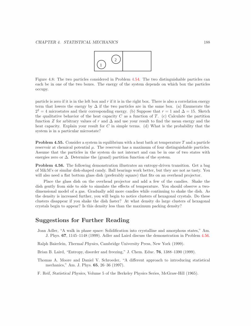
CHAPTER 4. STATISTICAL MECHANICS 188

12

Figure 4.8: The two particles considered in Problem 4.54. The two distinguishable particles caneach be in one of the two boxes. The energy of the system depends on which box the particlesoccupy.

particle is zero if it is in the left box and r if it is in the right box. There is also a correlation energyterm that lowers the energy by ∆ if the two particles are in the same box. (a) Enumerate the22 = 4 microstates and their corresponding energy. (b) Suppose that r = 1 and ∆ = 15. Sketchthe qualitative behavior of the heat capacity C as a function of T . (c) Calculate the partitionfunction Z for arbitrary values of r and ∆ and use your result to find the mean energy and theheat capacity. Explain your result for C in simple terms. (d) What is the probability that thesystem is in a particular microstate?

Problem 4.55. Consider a system in equilibrium with a heat bath at temperature T and a particlereservoir at chemical potential µ. The reservoir has a maximum of four distinguishable particles.Assume that the particles in the system do not interact and can be in one of two states withenergies zero or ∆. Determine the (grand) partition function of the system.

Problem 4.56. The following demonstration illustrates an entropy-driven transition. Get a bagof M&M’s or similar disk-shaped candy. Ball bearings work better, but they are not as tasty. Youwill also need a flat bottom glass dish (preferably square) that fits on an overhead projector.

Place the glass dish on the overhead projector and add a few of the candies. Shake thedish gently from side to side to simulate the effects of temperature. You should observe a two-dimensional model of a gas. Gradually add more candies while continuing to shake the dish. Asthe density is increased further, you will begin to notice clusters of hexagonal crystals. Do theseclusters disappear if you shake the dish faster? At what density do large clusters of hexagonalcrystals begin to appear? Is this density less than the maximum packing density?

Suggestions for Further Reading

Joan Adler, “A walk in phase space: Solidification into crystalline and amorphous states,” Am.J. Phys. 67, 1145–1148 (1999). Adler and Laird discuss the demonstration in Problem 4.56.

Ralph Baierlein, Thermal Physics, Cambridge University Press, New York (1999).

Brian B. Laird, “Entropy, disorder and freezing,” J. Chem. Educ. 76, 1388–1390 (1999).

Thomas A. Moore and Daniel V. Schroeder, “A different approach to introducing statisticalmechanics,” Am. J. Phys. 65, 26–36 (1997).

F. Reif, Statistical Physics, Volume 5 of the Berkeley Physics Series, McGraw-Hill (1965).

CHAPTER 4. STATISTICAL MECHANICS 189

W. G. V. Rosser, An Introduction to Statistical Physics, Ellis Horwood Limited (1982).

Daniel V. Schroeder, An Introduction to Thermal Physics, Addison-Wesley (1999).

Ruth Chabay and Bruce Sherwood, Matter & Interactions, John Wiley & Sons (2002), Vol. 1,Modern Mechanics.

Chapter 5

Magnetic Systems

c©2005 by Harvey Gould and Jan Tobochnik7 December 2005

In Chapter 4 we developed the general formalism of statistical mechanics. We now apply this for-malism to several magnetic systems for which the interactions between the magnetic moments areimportant. We will discover that these interactions lead to a wide range of phenomena, includingthe existence of phase transitions and other cooperative phenomena. We also introduce severalother quantities of physical interest.

5.1 Paramagnetism

We first review the behavior of a system of noninteracting magnetic moments with spin 1/2 inequilibrium with a thermal bath at temperature T . We discussed this system in Section 4.3.1 andin Example 4.2 using the microcanonical ensemble. We will find that this system is much easier totreat in the canonical ensemble.

Because the magnetic moments or spins are noninteracting, the only interaction is that ofthe spins with an external magnetic field B in the z direction. The magnetic field due to thespins themselves is assumed to be negligible. The energy of interaction of a spin with the externalmagnetic field B is given by

E = −µ · B = −µzB = −µBs, (5.1)

where µz is the component of the magnetic moment in the direction of the magnetic field B. Wewrite µz = sµ, where s = ±1.

We assume that the spins are fixed on a lattice so that they are distinguishable even thoughthe spins are intrinsically quantum mechanical (because of the association of a magnetic momentwith a spin angular momentum). What would we like to know about the properties of a systemof noninteracting spins? In the absence of an external magnetic field, there are not many physicalquantities of interest. The spins point randomly up or down because there is no preferred direction,

190

CHAPTER 5. MAGNETIC SYSTEMS 191

and the mean internal energy is zero. However, in the presence of an external magnetic field, thenet magnetic moment and the energy of the system are nonzero.

Because each spin is independent of the others, we can find the partition function for onespin, Z1, and use the relation ZN = ZN

1 to obtain ZN , the partition function for N spins. We canderive this relation by writing the energy of the N spins as E = −µB

∑Ni=1 si and expressing the

partition function ZN for the N -spin system as

ZN =∑

s1=±1

∑s2=±1

. . .∑

sN =±1

eβµBΣNi=1si (5.2)

=∑

s1=±1

∑s2=±1

. . .∑

sN =±1

eβµBs1eβµBs2 . . . eβµBsN

=∑

s1=±1

eβµBs1∑

s2=±1

eβµBs2 . . .∑

sN=±1

eβµBsN

=[ ∑s1=±1

eβµBs1]N = ZN

1 . (5.3)

To find Z1 we write

Z1 =∑

s=±1

e−βµBs = eβµB(−1) + eβµB(+1) = 2 coshβµB, (5.4)

where we have performed the sum over s = ±1. The partition function for N spins is simply

ZN = (2 coshβµB)N . (5.5)

We now use the canonical ensemble formalism that we developed in Section 4.6 to find thethermodynamic properties of the system for a given T and B. In the following, we will use thenotation 〈A〉 instead of A to designate an ensemble average. We will also frequently omit thebrackets 〈. . .〉, because it will be clear from the context when an average is implied.

The free energy is given by

F = −kT ln ZN = −NkT ln Z1 = −NkT ln(2 coshβµB). (5.6)

The mean energy E is

E = −∂ ln ZN

∂β=

∂(βF )∂β

= −NµB tanhβµB. (5.7)

Note that we have omitted the brackets because it is clear that E is the mean energy in the presentcontext. From (5.7) we see that E → 0 as T → ∞ (β → 0).

Problem 5.1. Compare the result (5.7) for the mean energy in the canonical ensemble to thecorresponding result that you found in Problem 4.25 in the microcanonical ensemble.

The heat capacity C is a measure of the change of the temperature due to the addition ofenergy at constant magnetic field. The heat capacity at constant magnetic field can be expressedas

C =∂E

∂T= −kβ2 ∂E

∂β. (5.8)

CHAPTER 5. MAGNETIC SYSTEMS 192

(We will write C rather than CB because no confusion will result.) From (5.7) and (5.8), we findthat the heat capacity of a system of N noninteracting spins is given by

C = N(βµB)2 sech2 βµB. (5.9)

Note that the heat capacity is always positive, goes to zero as T → 0 consistent with the third lawof thermodynamics, and goes to zero at high T .

Magnetization and Susceptibility. Two additional macroscopic quantities of interest arethe mean magnetic moment or magnetization (in the z direction)

〈M〉 = µ

N∑i=1

〈si〉, (5.10)

and the isothermal susceptibility χ:

χ =(∂M

∂B

)T

. (5.11)

The susceptibility χ is a measure of the change of the magnetization due to a change in the externalmagnetic field and is another example of a linear response function. We can express M and χ interms of derivatives of lnZ by noting that the total energy can be written in the general form as

E = E0 − MB, (5.12)

where E0 is the energy of interaction of the spins with themselves and −MB is the energy ofinteraction of the spins with the magnetic field. (For noninteracting spins E0 = 0.) This form ofE implies that we can write Z in the form

Z =∑

s

e−β(E0,s−MsB), (5.13)

where Ms and E0,s are the values of M and E0 in microstate s. From (5.13) we have

∂Z

∂B=

∑s

βMs e−β(E0,s−MsB), (5.14)

and hence the mean magnetization is given by

〈M〉 =1Z

∑s

Mse−β(E0,s−MsB) (5.15a)

=1

βZ

∂Z

∂B(5.15b)

= kT∂ ln ZN

∂B. (5.15c)

If we substitute the relation F = −kT ln Z, we obtain

〈M〉 = −∂F

∂B. (5.16)

CHAPTER 5. MAGNETIC SYSTEMS 193

Often we are more interested in the mean magnetization per spin 〈m〉, which is simply

〈m〉 =1N

〈M〉. (5.17)

We leave it as an exercise for the reader to show that in the limit B → 0 (see Problem 5.31)

χ =1

kT[〈M2〉 − 〈M〉2]. (5.18)

The quantity χ in (5.18) is the zero-field susceptibility.1 Note the similarity of the form (5.18) withthe form (4.85) for the heat capacity CV . That is, the response functions CV and χ are related tothe corresponding equilibrium fluctuations in the system.

From (5.6) and (5.16) we find that the magnetization of a system of noninteracting spins is

M = Nµ tanhβµB. (5.19)

The susceptibility can be calculated using (5.11) and (5.19) and is given by

χ = Nµ2β sech2 βµB. (5.20)

For high temperatures (small β), sech βµB → 1, and the leading behavior of χ is given by

χ → Nµ2β =Nµ2

kT. (high temperature) (5.21)

The result (5.21) is known as the Curie form for the isothermal susceptibility and is commonlyobserved for magnetic materials at high temperatures (kT µB).

We see that M is zero at B = 0 for all T implying that the system is paramagnetic. ForB = 0, we note that M → 0 as β → 0 (high T ), which implies that χ → 0 as T → ∞. Because asystem of noninteracting spins is paramagnetic, such a model is not applicable to materials such asiron that can have a nonzero magnetization even when the magnetic field is zero. Ferromagnetismis due to the interactions between the spins.

Problem 5.2. (a) Plot the magnetization per spin as given by (5.19) and the heat capacity Cas given by (5.9) as a function of T . Give a simple argument why C must have a broad maximumsomewhere between T = 0 and T = ∞. (b) Plot the isothermal susceptibility χ versus T for fixedB and describe its limiting behavior for low and high T .

Problem 5.3. Calculate the entropy of a system of N noninteracting spins and discuss its limitingbehavior at low and high temperatures.

Problem 5.4. (a) Consider a solid containing N noninteracting paramagnetic atoms whosemagnetic moments can be aligned either parallel or antiparallel to the magnetic field B. The systemis in equilibrium with a thermal bath at temperature T . The magnetic moment is µ = 9.274×10−24

J/tesla. If B = 4 tesla, at what temperature are 75% of the spins oriented in the +z direction? (b)Assume that N = 1023, T = 1 K, and that B is increased quasistatically from 1 tesla to 10 tesla.What is the magnitude of the energy transfer from the thermal bath? (c) If the system is nowthermally isolated at T = 1 K and B is quasistatically decreased from 10 tesla to 1 tesla, what isthe final temperature of the system? This process is known as adiabatic demagnetization.

1We will use the same notation for the zero-field isothermal susceptibility and the isothermal susceptibility in anonzero field because the distinction will be clear from the context.

CHAPTER 5. MAGNETIC SYSTEMS 194

5.2 Thermodynamics of magnetism

Note that the free energy F defined by the relation F = −kT ln Z implies that F is a functionof T , B, and N . The magnetization M fluctuates. It can be shown (see Appendix 5B) that themagnetic work done on a magnetic system with magnetization M in an external magnetic field Bis given by dW = −MdB. For fixed N , we have the thermodynamic relation

dF (T, B) = −SdT − MdB. (5.22)

From (5.22) we obtain (5.16) for the magnetization in terms of the free energy. As an aside, wenote that if M is a constant and B is allowed to vary, we can define G = F + MH so that

dG(T, M) = −SdT + BdM. (5.23)

5.3 The Ising model

As we saw in Section 5.1, the absence of interactions between the spins implies that the systemcan only be paramagnetic. The most important model of a system that exhibits a phase transitionis the Ising model, the harmonic oscillator (or fruit fly) of statistical mechanics.2 The model wasproposed by Wilhelm Lenz (1888–1957) in 1920 and was solved exactly for the one-dimensionalcase by his student Ernest Ising in 1925.3 Ising was very disappointed because the one-dimensionalcase does not have a phase transition. Lars Onsager solved the Ising model exactly in 1944 fortwo dimensions in the absence of an external magnetic field and showed that there was a phasetransition in two dimensions.4 The two-dimensional Ising model is the simplest model of a phasetransition.

In the Ising model the spin at every site is either up (+1) or down (−1). Unless otherwisestated, the interaction is between nearest neighbors only and is given by −J if the spin are paralleland +J if the spins are antiparallel. The total energy can be expressed in the form5

E = −J

N∑i,j=nn(i)

sisj − B

N∑i=1

si , (Ising model) (5.24)

where si = ±1 and J is known as the exchange constant. In the following, we will refer to s itselfas the spin.6 The first sum in (5.24) is over all pairs of spins that are nearest neighbors. Theinteraction between two nearest neighbor spins is counted only once. We have implicitly assumed

2Each year hundreds of papers are published that apply the Ising model to problems in such diverse fields asneural networks, protein folding, biological membranes and social behavior.

3A biographical note about Ising’s life is at <www.bradley.edu/las/phy/personnel/isingobit.html> .4The model is sometimes known as the Lenz-Ising model. The history of the Ising model is discussed by

Stephen Brush.5If we interpret the spin as a operator, then the energy is really a Hamiltonian. The distinction is unimportant

in the present context.6Because the spin S is a quantum mechanical object, we expect that the commutator of the spin operator with

the Hamiltonian is nonzero. However, because the Ising model retains only the component of the spin along thedirection of the magnetic field, the commutator of the spin S with the Hamiltonian is zero, and we can treat thespins in the Ising model as if they were classical.

CHAPTER 5. MAGNETIC SYSTEMS 195

that the external magnetic field is in the up or positive z direction. The factors of µ0 and g havebeen incorporated into the quantity B which we will refer to as the magnetic field. In the samespirit the magnetization becomes the net number of positive spins rather than the net magneticmoment. A discussion of how magnetism occurs in matter in given in Appendix 5A.

In addition to the conceptual difficulties of statistical mechanics, there is no standard procedurefor calculating the partition function. In spite of the apparent simplicity of the Ising model, we canfind exact solutions only in one dimension and in two dimensions in the absence of a magnetic field.In other cases we need to use approximation methods and computer simulations.7 In the followingsection we will discuss the one-dimensional Ising model for which we can find an exact solution. InSection 5.5 we will briefly discuss the nature of the exact solutions for the two-dimensional Isingmodel. We will find that the two-dimensional Ising model exhibits a continuous phrase transition.We will also consider some straightforward simulations of the Ising model to gain more insight intothe behavior of the Ising model. In Section 5.6 we will discuss a simple approximation known asmean-field theory that is applicable to a wide variety of systems. A more advanced treatment ofthe Ising model is given in Chapter 9.

5.4 The Ising Chain

In the following we describe several methods for obtaining exact solutions of the one-dimensionalIsing model and introduce an additional physical quantity of interest.

5.4.1 Exact enumeration

The canonical ensemble is the natural choice for calculating the thermodynamic properties of theIsing model. Because the spins are interacting, we no longer have the relation ZN = ZN

1 , andwe have to calculate ZN directly. The calculation of the partition function ZN is straightforwardin principle. The goal is to enumerate all the microstates of the system and the correspondingenergies, calculate ZN for finite N , and then take the limit N → ∞. The difficulty is that the totalnumber of states, 2N , is too many for N large. However, for the one-dimensional Ising model orIsing chain, we can calculate ZN for small N and quickly see how to generalize to arbitrary N .

For a finite chain we need to specify the boundary condition for the spin at each end. Onepossibility is to choose free ends so that the spin at each end has only one interaction (see Fig-ure 5.1a). Another choice is toroidal boundary conditions as shown in Figure 5.1b. This choiceimplies that the Nth spin is connected to the first spin so that the chain forms a ring. The choiceof boundary conditions does not matter in the thermodynamic limit, N → ∞.

In the absence of an external magnetic field, we will find that it is more convenient to choosefree boundary conditions when calculating Z directly. The energy of the Ising chain in the absence

7In three dimensions it has been shown that the Ising model is NP-complete, that it is computationally intractable.That is, the three-dimensional Ising model (and the two-dimensional Ising model with next nearest-neighbor in-teractions in addition to the nearest-neighbor kind) falls into the same class as other hard problems such as thetraveling salesman problem.

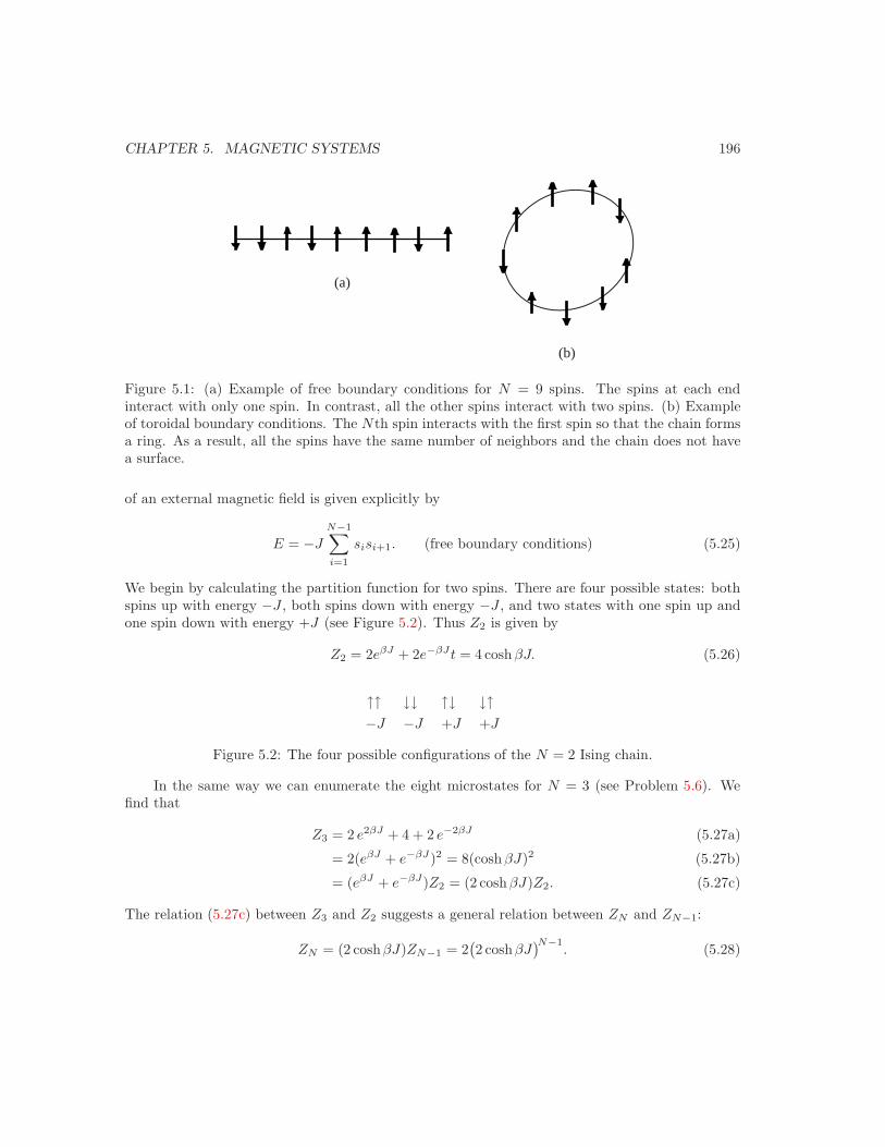
CHAPTER 5. MAGNETIC SYSTEMS 196

(a)

(b)

Figure 5.1: (a) Example of free boundary conditions for N = 9 spins. The spins at each endinteract with only one spin. In contrast, all the other spins interact with two spins. (b) Exampleof toroidal boundary conditions. The Nth spin interacts with the first spin so that the chain formsa ring. As a result, all the spins have the same number of neighbors and the chain does not havea surface.

of an external magnetic field is given explicitly by

E = −J

N−1∑i=1

sisi+1. (free boundary conditions) (5.25)

We begin by calculating the partition function for two spins. There are four possible states: bothspins up with energy −J , both spins down with energy −J , and two states with one spin up andone spin down with energy +J (see Figure 5.2). Thus Z2 is given by

Z2 = 2eβJ + 2e−βJt = 4 coshβJ. (5.26)

↑↑ ↓↓ ↑↓ ↓↑−J −J +J +J

Figure 5.2: The four possible configurations of the N = 2 Ising chain.

In the same way we can enumerate the eight microstates for N = 3 (see Problem 5.6). Wefind that

Z3 = 2 e2βJ + 4 + 2 e−2βJ (5.27a)

= 2(eβJ + e−βJ)2 = 8(coshβJ)2 (5.27b)

= (eβJ + e−βJ)Z2 = (2 coshβJ)Z2. (5.27c)

The relation (5.27c) between Z3 and Z2 suggests a general relation between ZN and ZN−1:

ZN = (2 coshβJ)ZN−1 = 2(2 coshβJ

)N−1. (5.28)

CHAPTER 5. MAGNETIC SYSTEMS 197

We can derive the recursion relation (5.28) directly by writing ZN for the Ising chain in theform

ZN =∑

s1=±1

· · ·∑

sN =±1

eβJPN−1

i=1 sisi+1 . (5.29)

The sum over the two possible states for each spin yields 2N microstates. To understand themeaning of the sums in (5.29), we write (5.29) for N = 3:

Z3 =∑

s1=±1

∑s2=±1

∑s3=±1

eβJs1s2+βJs2s3 . (5.30)

The sum over s3 can be done independently of s1 and s2, and we have

Z3 =∑

s1=±1

∑s2=±1

eβJs1s2[eβJs2 + e−βJs2

](5.31a)

=∑

s1=±1

∑s2=±1

eβJs1s22 coshβJs2 = 2∑

s1=±1

∑s2=±1

eβJs1s2 coshβJ. (5.31b)

We have used the fact that the cosh function is even and hence coshβJs2 = cosh βJ , independentlyof the sign of s2. The sum over s1 and s2 in (5.31b) is straightforward, and we find,

Z3 = (2 coshβJ)Z2, (5.32)

in agreement with (5.27c).The analysis of (5.29) proceeds similarly. Note that spin N occurs only once in the exponential

and we have, independently of the value of sN−1,∑

sN =±1

eβJsN−1sN = 2 coshβJ. (5.33)

Hence we can write ZN asZN = (2 coshβJ)ZN−1. (5.34)

Problem 5.5. Use the recursion relation (5.34) and the result (5.32) for Z2 to confirm the result(5.28) for ZN .

We can use the general result (5.28) for ZN to find the Helmholtz free energy:

F = −kT ln ZN = −kT[ln 2 + (N − 1) ln(2 coshβJ)

]. (5.35)

In the thermodynamic limit N → ∞, the term proportional to N in (5.35) dominates, and we havethe desired result:

F = −NkT ln(2 coshβJ

). (5.36)

Problem 5.6. Enumerate the 2N microstates for the N = 4 Ising chain and find the correspond-ing contributions to Z4 for free boundary conditions. Then show that Z4 satisfies the recursionrelation (5.34) for free boundary conditions.

CHAPTER 5. MAGNETIC SYSTEMS 198

0

0.1

0.2

0.3

0.4

0.5

0 1 2 3 4 5 6 7 8kT/J

spec

ific

hea

t

Figure 5.3: The temperature dependence of the heat capacity C of an Ising chain in the absenceof an external magnetic field. At what value of kT/J does C exhibit a maximum? Explain.

Problem 5.7. (a) What is the ground state of the Ising chain? (b) What is the behavior of S inthe limits T → 0 and T → ∞? The answers can be found without doing an explicit calculation.(c) Use (5.36) for F to verify the following results for the entropy S, the mean energy E, and theheat capacity C of the Ising chain:

S = Nk[ln(e2βJ + 1) − 2βJ

1 + e−2βJ

]. (5.37)

E = −NJ tanhβJ. (5.38)

C = Nk(βJ)2(sechβJ)2. (5.39)

Verify your answers for the limiting behavior of S given in part (b). A plot of the T -dependenceof the heat capacity in the absence of a magnetic field is given in Figure 5.3.

∗Problem 5.8. In Problem 4.19 the density of states was given (without proof) for the one-dimensional Ising model for even N and toroidal boundary conditions:

Ω(E, N) = 2(

N

i

)= 2

N !i! (N − 1)!

, (i = 0, 2, 4, . . . , N) (4.19)

with E = 2 i − N . Use this form of Ω and the relation

ZN =∑E

Ω(E, N)e−βE (5.40)

to find the free energy for small values of (even) N . (b) Use the results for ZN that you found byexact enumeration to find Ω(E, N) for small values of N .

CHAPTER 5. MAGNETIC SYSTEMS 199

5.4.2 ∗Spin-spin correlation function

We can gain further insight into the properties of the Ising model by calculating the spin-spincorrelation function G(r) defined as

G(r) = 〈sksk+r〉 − 〈sk〉 〈sk+r〉. (5.41)

Because the average of sk is independent of the choice of the site k and equals m, the magnetizationper spin m = M/N and G(r) can be written as

G(r) = 〈sksk+r〉 − m2. (5.42)

The average denoted by the brackets 〈. . .〉 is over all spin configurations. Because all lattice sitesare equivalent, G(r) is independent of the choice of k and depends only on the separation r (fora given T and B), where r is the separation between spins in units of the lattice constant. Notethat for r = 0, G(r) = 〈m2〉 − 〈m〉2 ∝ χ (see (5.18)).

The spin-spin correlation function tells us the degree to which a spin at one site is correlatedwith a spin at another site. If the spins are not correlated, then G(r) = 0. At high temperaturesthe interaction between spins is unimportant, and hence the spins are randomly oriented in theabsence of an external magnetic field. Thus in the limit kT J , we expect that G(r) → 0 forfixed r. For fixed T and B, we expect that if spin k is up, then the two adjacent spins will have agreater probability of being up than down. Why? As we move away from spin k, we expect thatthe probability that spin k + r is up will decrease. Hence, we expect that G(r) → 0 as r → ∞.

We will show in the following that G(r) can be calculated exactly for the Ising chain. Theresult is

G(r) =(tanhβJ

)r. (5.43)

A plot of G(r) for βJ = 2 is shown in Figure 5.4. Note that G(r) → 0 for increasing r as expected.We will find it useful to define the correlation length ξ by writing G(r) in the form

G(r) = e−r/ξ. (5.44)

For the one-dimensional Ising model

ξ = − 1ln(tanh βJ)

. (5.45)

At low temperatures, tanh βJ ≈ 1 − 2e−2βJ , and

ln(tanhβJ

) ≈ −2e−2βJ . (5.46)

Hence

ξ =12e2βJ . (βJ 1) (5.47)

From (5.47) we see that the correlation length becomes very large for low temperatures (βJ 1).The correlation length gives the length scale for the decay of correlations between the spins.

Problem 5.9. What is the maximum value of tanhβJ? Show that for finite values of βJ , G(r)given by (5.43) decays with increasing r.

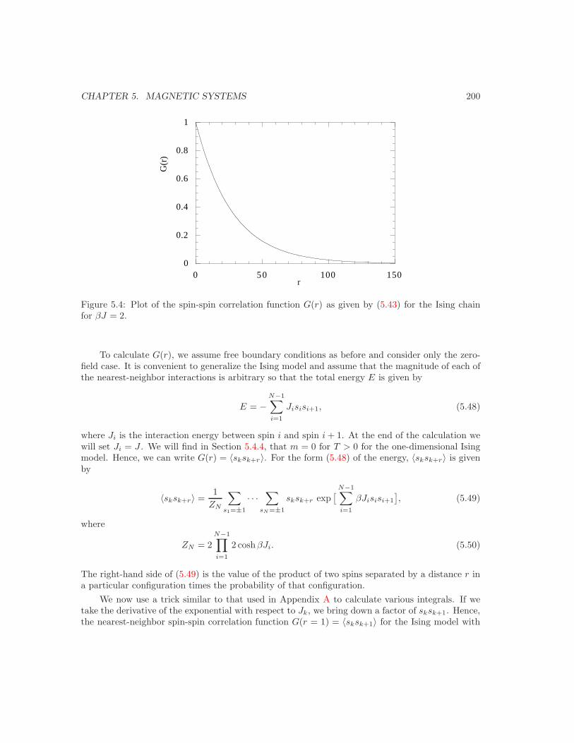
CHAPTER 5. MAGNETIC SYSTEMS 200

0

0.2

0.4

0.6

0.8

1

0 50 100 150

G(r

)

r

Figure 5.4: Plot of the spin-spin correlation function G(r) as given by (5.43) for the Ising chainfor βJ = 2.

To calculate G(r), we assume free boundary conditions as before and consider only the zero-field case. It is convenient to generalize the Ising model and assume that the magnitude of each ofthe nearest-neighbor interactions is arbitrary so that the total energy E is given by

E = −N−1∑i=1

Jisisi+1, (5.48)

where Ji is the interaction energy between spin i and spin i + 1. At the end of the calculation wewill set Ji = J . We will find in Section 5.4.4, that m = 0 for T > 0 for the one-dimensional Isingmodel. Hence, we can write G(r) = 〈sksk+r〉. For the form (5.48) of the energy, 〈sksk+r〉 is givenby

〈sksk+r〉 =1

ZN

∑s1=±1

· · ·∑

sN =±1

sksk+r exp[ N−1∑

i=1

βJisisi+1

], (5.49)

where

ZN = 2N−1∏i=1

2 coshβJi. (5.50)

The right-hand side of (5.49) is the value of the product of two spins separated by a distance r ina particular configuration times the probability of that configuration.

We now use a trick similar to that used in Appendix A to calculate various integrals. If wetake the derivative of the exponential with respect to Jk, we bring down a factor of sksk+1. Hence,the nearest-neighbor spin-spin correlation function G(r = 1) = 〈sksk+1〉 for the Ising model with

CHAPTER 5. MAGNETIC SYSTEMS 201

Ji = J can be expressed as

〈sksk+1〉 =1

ZN

∑s1=±1

· · ·∑

sN =±1

sksk+1 exp[ N−1∑

i=1

βJisisi+1

], (5.51)

=1

ZN

1β

∂

∂Jk

∑s1=±1

· · ·∑

sN =±1

exp[ N−1∑

i=1

βJisisi+1

],

=1

ZN

1β

∂ZN(J1, · · · , JN−1)∂Jk

∣∣∣∣Ji=J

=sinh βJ

coshβJ= tanhβJ, (5.52)

where we have used the form (5.50) for ZN . To obtain G(r = 2), we use the fact that s2k+1 = 1 to

write sksk+2 = sksk+1sk+1sk+2 and

G(r = 2) =1

ZN

∑sj

sksk+1sk+1sk+2 exp[ N−1∑

i=1

βJisisi+1

], (5.53)

=1

ZN

1β2

∂2ZN (J1, · · · , JN−1)∂Jk ∂Jk+1

= [tanhβJ ]2. (5.54)

It is clear that the method used to obtain G(r = 1) and G(r = 2) can be generalized toarbitrary r. We write

G(r) =1

ZN

1βr

∂

∂Jk

∂

Jk+1· · · ∂

Jk+r−1ZN , (5.55)

and use (5.50) for ZN to find that

G(r) = tanhβJk tanhβJk+1 · · · tanhβJk+r−1,

=r∏

k=1

tanhβJk+r−1. (5.56)

For a uniform interaction, Ji = J , and (5.56) reduces to the result for G(r) in (5.43).

Problem 5.10. Consider an Ising chain of N = 4 spins and calculate G(r) by exact enumerationof the 24 microstates. What are the possible values of r for free and toroidal boundary conditions?Choose one of these boundary conditions and calculate G(r = 1) and G(r = 2) using the microstatesthat were enumerated in Problem 5.6. Assume that the system is in equilibrium with a thermalbath at temperature T and in zero magnetic field. (For convenience choose k = 1.)

5.4.3 Simulations of the Ising chain

Although we have found an exact solution for the one-dimensional Ising model, we can gain addi-tional physical insight by doing simulations. As we will see, simulations are essential for the Isingmodel in higher dimensions.

CHAPTER 5. MAGNETIC SYSTEMS 202

As we discussed in Section 4.11, the Metropolis algorithm is the simplest and most commonMonte Carlo algorithm for a system in equilibrium with a thermal bath at temperature T . In thecontext of the Ising model, the Metropolis algorithm can be implemented as follows:

1. Choose an initial microstate of N spins. The two most common initial states are the groundstate with all spins parallel or the T = ∞ state where each spin is chosen to be ±1 at random.

2. Choose a spin at random and make a trial flip. Compute the change in energy of the system,∆E, corresponding to the flip. The calculation is straightforward because the change inenergy is determined by only the nearest neighbor spins. If ∆E < 0, then accept the change.If ∆E > 0, accept the change with probability p = e−β∆E. To do so, generate a randomnumber r uniformly distributed in the unit interval. If r ≤ p, accept the new microstate;otherwise, retain the previous microstate.

3. Repeat step (2) many times choosing spins at random.

4. Compute the averages of the quantities of interest such as 〈E〉, 〈M〉, C, and χ after thesystem has reached equilibrium.

In the following two problems we explore some of the qualitative properties of the Ising chain.

Problem 5.11. Use the applet/application at <stp.clarku.edu/simulations/ising1d> to sim-ulate the one-dimensional Ising model. It is convenient to measure the temperature in units suchthat J/k = 1. For example, a temperature of T = 2 really means that T = 2J/k. The “time”is measured in terms of Monte Carlo steps per spin, where in one Monte Carlo step per spin, Nspins are chosen at random for trial changes. (On the average each spin will be chosen equally,but during any finite interval, some spins might be chosen more than others.) Choose B = 0.

(a) Choose N = 500 spins and start the system at T = 2 and observe the evolution of themagnetization and energy per spin to equilibrium. The initial state is chosen to be the groundstate. What is your criterion for equilibrium? What is the approximate relaxation time forthe system to reach equilibrium? What is the mean energy, magnetization, heat capacity, andsusceptibility? Estimate the mean size of the domains of parallel spins.

(b) Consider T = 1.0 and T = 0.5 and observe the size of the domains of parallel spins. Estimatethe mean size of the domains at these temperatures.

(c) Approximately how many spins should you choose to avoid finite size effects at T = 0.5?

Problem 5.12. The thermodynamic quantities of interest for the Ising model include the meanenergy E, the specific heat C, and the isothermal susceptibility χ. We are especially interested inthe temperature-dependence of these quantities near T = 0.

(a) Why is the mean value of the magnetization of little interest for the one-dimensional Isingmodel?

(b) How can the specific heat and susceptibility be computed during the simulation at a giventemperature?

CHAPTER 5. MAGNETIC SYSTEMS 203

(c) Use the applet at <stp.clarku.edu/simulations/ising1d> to estimate these quantities anddetermine the qualitative-dependence of χ and the correlation length ξ on T at low tempera-tures.

(d) Why does the Metropolis algorithm become inefficient at low temperatures?

5.4.4 *Transfer matrix

So far we have considered the Ising chain only in zero external magnetic field. As might be expected,the solution for B = 0 is more difficult. We now apply the transfer matrix method to solve forthe thermodynamic properties of the Ising chain in nonzero magnetic field. The transfer matrixmethod is very general and can be applied to various magnetic systems and to seemingly unrelatedquantum mechanical systems. The transfer matrix method also is of historical interest because itled to the exact solution of the two-dimensional Ising model in the absence of a magnetic field.

To apply the transfer matrix method to the one-dimensional Ising model, it is necessary toadopt toroidal boundary conditions so that the chain becomes a ring with sN+1 = s1. Thisboundary condition enables us to write the energy as:

E = −J

N∑i=1

sisi+1 − 12B

N∑i=1

(si + si+1). (toroidal boundary conditions) (5.57)

The use of toroidal boundary conditions implies that each spin is equivalent.The transfer matrix T is defined by its four matrix elements which are given by

Ts,s′ = eβ[Jss′+ 12 B(s+s′)]. (5.58)

The explicit form of the matrix elements is

T++ = eβ(J+B) (5.59a)

T−− = eβ(J−B) (5.59b)

T−+ = T+− = e−βJ , (5.59c)

or

T =(

T++ T+−T−+ T−−

)

=(

eβ(J+B) e−βJ

e−βJ eβ(J−B)

). (5.60)

The definition (5.58) of T allows us to write ZN in the form

ZN(T, B) =∑s1

∑s2

· · ·∑sN

Ts1,s2Ts2,s3 · · ·TsN ,s1 . (5.61)

The form of (5.61) is suggestive of our interpretation of T as a transfer function.

CHAPTER 5. MAGNETIC SYSTEMS 204

The rule for matrix multiplication that we need for the transfer matrix method is

(T2)s1,s3 =∑s2

Ts1,s2Ts2,s3 . (5.62)

If we multiply N matrices together, we obtain:

(TN )s1,sN+1 =∑s2

∑s3

· · ·∑sN

Ts1,s2Ts2,s3 · · ·TsN ,sN+1 . (5.63)

This result is very close to what we have in (5.61). To make it identical, we use periodic boundaryconditions and set sN+1 = s1, and sum over s1:

∑s1

(TN )s1,s1 =∑s1

∑s2

∑s3

· · ·∑sN

Ts1,s2Ts2,s3 · · ·TsN ,s1 = ZN . (5.64)

Because∑

s1(TN )s1,s1 is the definition of the trace (the sum of the diagonal elements) of (TN ),

we haveZN = trace(TN ). (5.65)

Because the trace of a matrix is independent of the representation of the matrix, the trace in(5.65) may be evaluated by bringing T into diagonal form:

T =(

λ+ 00 λ−

). (5.66)

The matrix TN is diagonal with the diagonal matrix elements λN+ , λN

− . If we choose the diagonalrepresentation fo T in (5.66), we have

trace (TN ) = λN+ + λN

− , (5.67)

where λ+ and λ− are the eigenvalues of T. Hence, we can express ZN as

ZN = λN+ + λN

− . (5.68)

The fact that ZN is the trace of the Nth power of a matrix is a consequence of our assumption oftoroidal boundary conditions.

The eigenvalues λ± are given by the solution of the determinant equation∣∣∣∣e

β(J+B) − λ e−βJ

e−βJ eβ(J−B) − λ

∣∣∣∣ = 0. (5.69)

The roots of (5.69) are

λ± = eβJ coshβB ± [e−2βJ + e2βJ sinh2 βB

]1/2. (5.70)

It is easy to show that λ+ > λ− for all B and β, and consequently (λ−/λ+)N → 0 as N → ∞. Inthe thermodynamic limit (N → ∞), we obtain from (5.68) and (5.70)

1N

ln ZN (T, B) = lnλ+ + ln[1 +

(λ−λ+

)N ] →N→∞ ln λ+, (5.71)

CHAPTER 5. MAGNETIC SYSTEMS 205

and the free energy per spin is given by

1N

F (T, B) = −kT ln[eβJ coshβJ +

(e2βJ sinh2 βB + e−2βJ

)1/2]. (5.72)

We can use (5.72) to find the magnetization M at nonzero T and B:

M =∂F

∂B= N

sinh βB

(sinh2 βB + e−4βJ)1/2. (5.73)

We know that a system is paramagnetic if M = 0 only for B = 0, and is ferromagnetic if M = 0for B = 0. For the one-dimensional Ising model, we see from (5.73) that M = 0 for B = 0, andthere is no spontaneous magnetization at nonzero temperature. (Recall that sinhx ≈ x for smallx.) That is, the one-dimensional Ising model undergoes a phase transition from the paramagneticto the ferromagnetic state only at T = 0. In the limit of low temperature (βJ 1 and βB 1),sinh βB ≈ 1

2eβB e−2βJ and m = M/N ≈ 1 for B = 0. Hence, at low temperatures only a smallfield is needed to produce saturation, corresponding to m = 1.

Problem 5.13. More insight into the properties of the Ising chain in nonzero magnetic field can befound by calculating the isothermal susceptibility χ. Calculate χ using (5.73). What is the limitingbehavior of χ in the limit T → 0? Express this limiting behavior in terms of the correlation lengthξ.

5.4.5 Absence of a phase transition in one dimension

We learned in Section 5.4.4 that the one-dimensional Ising model does not have a phase transitionexcept at T = 0. We now argue that a phase transition in one dimension is impossible if theinteraction is short-range, that is, if only a finite number of spins interact with one another.

At T = 0 the energy is a minimum with E = −(N − 1)J (for free boundary conditions), andthe entropy S = 0.8 Consider all the excitations at T > 0 obtained by flipping all the spins to theright of some site (see Figure 5.5(a)). The energy cost of creating such a domain wall is 2J . Becausethere are N − 1 sites where the wall may be placed, the entropy increases by ∆S = k ln(N − 1).Hence, the free energy cost associated with creating one domain wall is

∆F = 2J − kT ln(N − 1). (5.74)

We see from (5.74) that for T > 0 and N → ∞, the creation of a domain wall lowers the freeenergy. Hence, more domain walls will be created until the spins are completely randomized andthe net magnetization is zero. We conclude that M = 0 for T > 0 in the limit N → ∞.

Problem 5.14. Compare the energy of the configuration in Figure 5.5(a) with the energy of theconfiguration shown in Figure 5.5(b) and discuss why the number of spins in a domain in onedimension can be changed without the cost of energy.

8The ground state for B = 0 corresponds to all spins up or all spins down. It is convenient to break this symmetryby assuming that B = 0+ and letting T → 0 before setting B = 0.

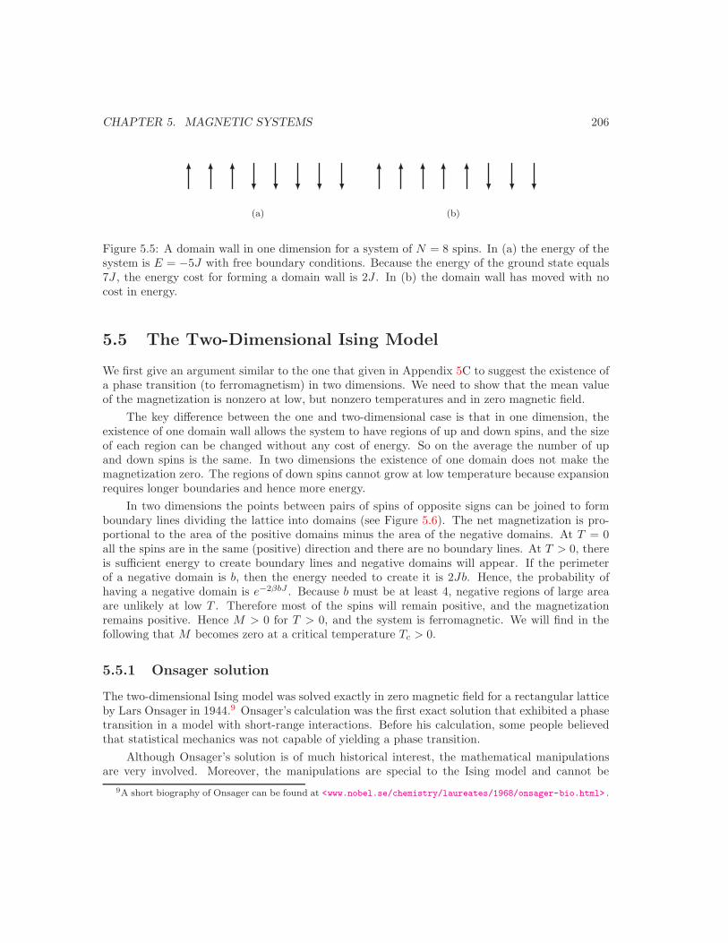
CHAPTER 5. MAGNETIC SYSTEMS 206

(a) (b)

Figure 5.5: A domain wall in one dimension for a system of N = 8 spins. In (a) the energy of thesystem is E = −5J with free boundary conditions. Because the energy of the ground state equals7J , the energy cost for forming a domain wall is 2J . In (b) the domain wall has moved with nocost in energy.

5.5 The Two-Dimensional Ising Model

We first give an argument similar to the one that given in Appendix 5C to suggest the existence ofa phase transition (to ferromagnetism) in two dimensions. We need to show that the mean valueof the magnetization is nonzero at low, but nonzero temperatures and in zero magnetic field.

The key difference between the one and two-dimensional case is that in one dimension, theexistence of one domain wall allows the system to have regions of up and down spins, and the sizeof each region can be changed without any cost of energy. So on the average the number of upand down spins is the same. In two dimensions the existence of one domain does not make themagnetization zero. The regions of down spins cannot grow at low temperature because expansionrequires longer boundaries and hence more energy.

In two dimensions the points between pairs of spins of opposite signs can be joined to formboundary lines dividing the lattice into domains (see Figure 5.6). The net magnetization is pro-portional to the area of the positive domains minus the area of the negative domains. At T = 0all the spins are in the same (positive) direction and there are no boundary lines. At T > 0, thereis sufficient energy to create boundary lines and negative domains will appear. If the perimeterof a negative domain is b, then the energy needed to create it is 2Jb. Hence, the probability ofhaving a negative domain is e−2βbJ . Because b must be at least 4, negative regions of large areaare unlikely at low T . Therefore most of the spins will remain positive, and the magnetizationremains positive. Hence M > 0 for T > 0, and the system is ferromagnetic. We will find in thefollowing that M becomes zero at a critical temperature Tc > 0.

5.5.1 Onsager solution

The two-dimensional Ising model was solved exactly in zero magnetic field for a rectangular latticeby Lars Onsager in 1944.9 Onsager’s calculation was the first exact solution that exhibited a phasetransition in a model with short-range interactions. Before his calculation, some people believedthat statistical mechanics was not capable of yielding a phase transition.

Although Onsager’s solution is of much historical interest, the mathematical manipulationsare very involved. Moreover, the manipulations are special to the Ising model and cannot be

9A short biography of Onsager can be found at <www.nobel.se/chemistry/laureates/1968/onsager-bio.html> .

CHAPTER 5. MAGNETIC SYSTEMS 207

Figure 5.6: Example of a domain wall in the two-dimensional Ising model.

generalized to other systems. For these reasons few workers in statistical mechanics have gonethrough the Onsager solution in great detail. (It is probably true that fewer people understand theOnsager solution of the two-dimensional Ising model than understand Einstein’s theory of generalrelativity.) In the following, we give only the results of the two-dimensional solution for a squarelattice and concentrate on approximation methods of more general applicability.

The critical temperature Tc is given by

sinh2J

kTc= 1, (5.75)

orkTc/J =

2ln(1 +

√2)

≈ 2.269. (5.76)

It is convenient to express the mean energy in terms of the dimensionless parameter κ defined as

κ = 2sinh 2βJ

(cosh 2βJ)2. (5.77)

A plot of the parameter κ versus βJ is given in Figure 5.7. Note that κ is zero at low and hightemperatures and has a maximum of unity at T = Tc.

The exact solution for the energy E can be written in the form

E = −2NJ tanh 2βJ − NJsinh2 2βJ − 1

sinh 2βJ cosh 2βJ

[ 2π

K1(κ) − 1], (5.78)

where

K1(κ) =∫ π/2

0

dφ√1 − κ2 sin2 φ

. (5.79)

K1 is known as the complete elliptic integral of the first kind. The first term in (5.78) is similar tothe result (5.38) for the energy of the one-dimensional Ising model with a doubling of the exchange

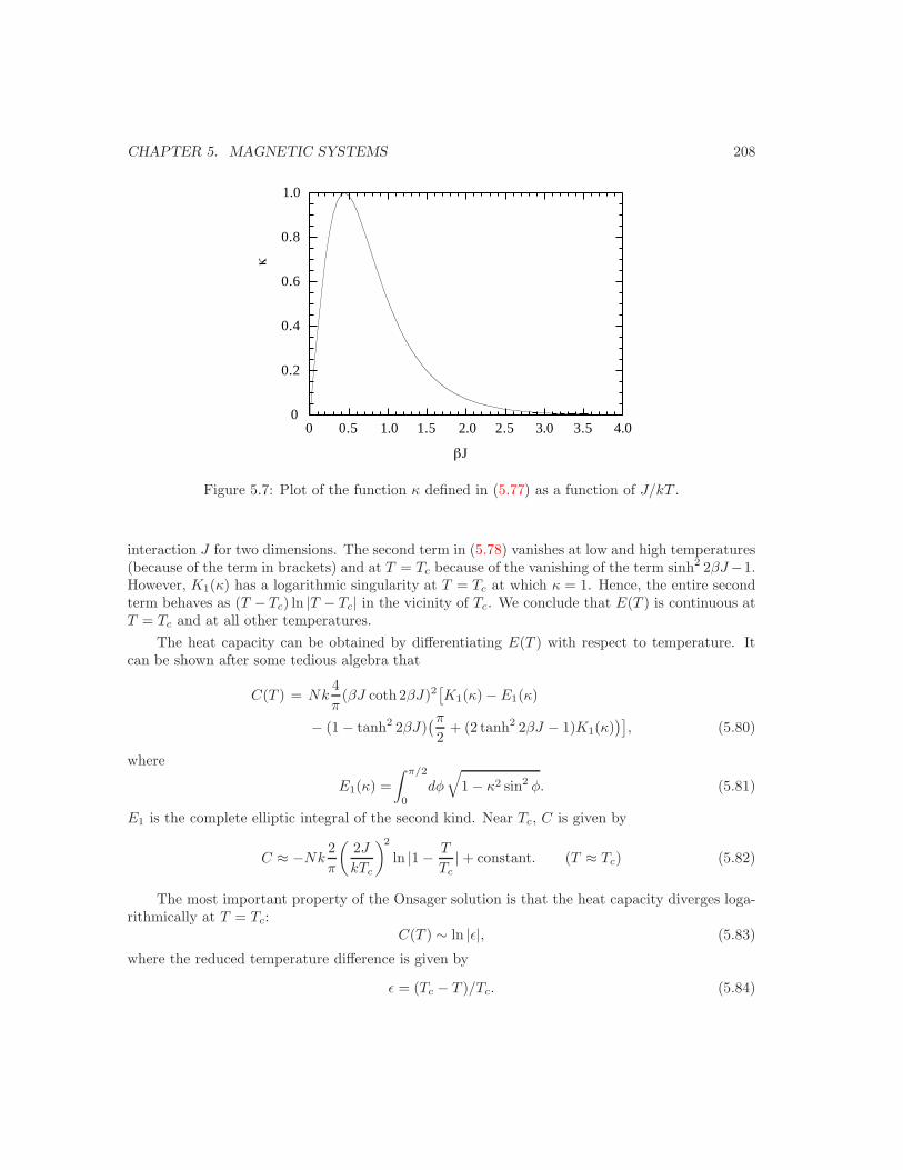
CHAPTER 5. MAGNETIC SYSTEMS 208

0

0.2

0.4

0.6

0.8

1.0

0 0.5 1.0 1.5 2.0 2.5 3.0 3.5 4.0

βJ

κ

Figure 5.7: Plot of the function κ defined in (5.77) as a function of J/kT .

interaction J for two dimensions. The second term in (5.78) vanishes at low and high temperatures(because of the term in brackets) and at T = Tc because of the vanishing of the term sinh2 2βJ−1.However, K1(κ) has a logarithmic singularity at T = Tc at which κ = 1. Hence, the entire secondterm behaves as (T − Tc) ln |T − Tc| in the vicinity of Tc. We conclude that E(T ) is continuous atT = Tc and at all other temperatures.

The heat capacity can be obtained by differentiating E(T ) with respect to temperature. Itcan be shown after some tedious algebra that

C(T ) = Nk4π

(βJ coth 2βJ)2[K1(κ) − E1(κ)

− (1 − tanh2 2βJ)(π

2+ (2 tanh2 2βJ − 1)K1(κ)

)], (5.80)

where

E1(κ) =∫ π/2

0

dφ

√1 − κ2 sin2 φ. (5.81)

E1 is the complete elliptic integral of the second kind. Near Tc, C is given by

C ≈ −Nk2π

(2J

kTc

)2

ln |1 − T

Tc| + constant. (T ≈ Tc) (5.82)

The most important property of the Onsager solution is that the heat capacity diverges loga-rithmically at T = Tc:

C(T ) ∼ ln |ε|, (5.83)

where the reduced temperature difference is given by

ε = (Tc − T )/Tc. (5.84)

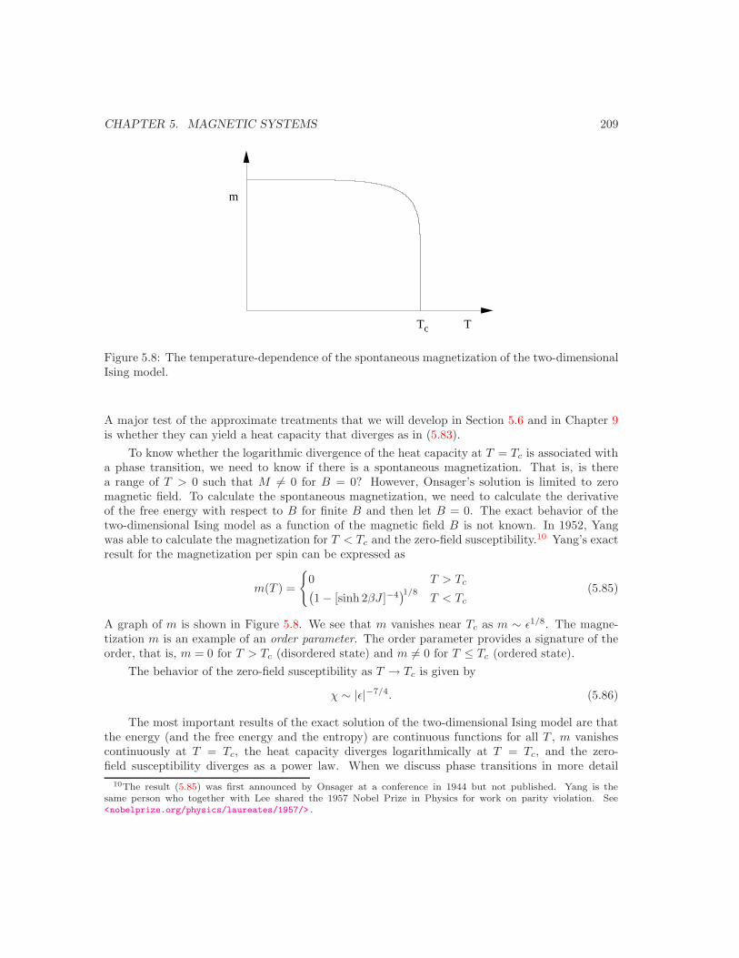
CHAPTER 5. MAGNETIC SYSTEMS 209

m

TTc

Figure 5.8: The temperature-dependence of the spontaneous magnetization of the two-dimensionalIsing model.

A major test of the approximate treatments that we will develop in Section 5.6 and in Chapter 9is whether they can yield a heat capacity that diverges as in (5.83).

To know whether the logarithmic divergence of the heat capacity at T = Tc is associated witha phase transition, we need to know if there is a spontaneous magnetization. That is, is therea range of T > 0 such that M = 0 for B = 0? However, Onsager’s solution is limited to zeromagnetic field. To calculate the spontaneous magnetization, we need to calculate the derivativeof the free energy with respect to B for finite B and then let B = 0. The exact behavior of thetwo-dimensional Ising model as a function of the magnetic field B is not known. In 1952, Yangwas able to calculate the magnetization for T < Tc and the zero-field susceptibility.10 Yang’s exactresult for the magnetization per spin can be expressed as

m(T ) =

0 T > Tc(1 − [sinh 2βJ ]−4

)1/8T < Tc

(5.85)

A graph of m is shown in Figure 5.8. We see that m vanishes near Tc as m ∼ ε1/8. The magne-tization m is an example of an order parameter. The order parameter provides a signature of theorder, that is, m = 0 for T > Tc (disordered state) and m = 0 for T ≤ Tc (ordered state).

The behavior of the zero-field susceptibility as T → Tc is given by

χ ∼ |ε|−7/4. (5.86)

The most important results of the exact solution of the two-dimensional Ising model are thatthe energy (and the free energy and the entropy) are continuous functions for all T , m vanishescontinuously at T = Tc, the heat capacity diverges logarithmically at T = Tc, and the zero-field susceptibility diverges as a power law. When we discuss phase transitions in more detail

10The result (5.85) was first announced by Onsager at a conference in 1944 but not published. Yang is thesame person who together with Lee shared the 1957 Nobel Prize in Physics for work on parity violation. See<nobelprize.org/physics/laureates/1957/> .

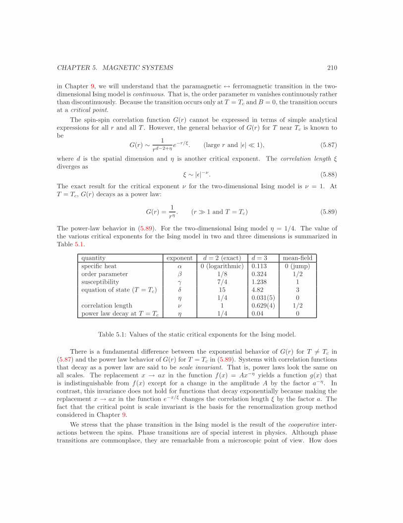
CHAPTER 5. MAGNETIC SYSTEMS 210

in Chapter 9, we will understand that the paramagnetic ↔ ferromagnetic transition in the two-dimensional Ising model is continuous. That is, the order parameter m vanishes continuously ratherthan discontinuously. Because the transition occurs only at T = Tc and B = 0, the transition occursat a critical point.

The spin-spin correlation function G(r) cannot be expressed in terms of simple analyticalexpressions for all r and all T . However, the general behavior of G(r) for T near Tc is known tobe

G(r) ∼ 1rd−2+η

e−r/ξ. (large r and |ε| 1), (5.87)

where d is the spatial dimension and η is another critical exponent. The correlation length ξdiverges as

ξ ∼ |ε|−ν . (5.88)

The exact result for the critical exponent ν for the two-dimensional Ising model is ν = 1. AtT = Tc, G(r) decays as a power law:

G(r) =1rη

. (r 1 and T = Tc) (5.89)

The power-law behavior in (5.89). For the two-dimensional Ising model η = 1/4. The value ofthe various critical exponents for the Ising model in two and three dimensions is summarized inTable 5.1.

quantity exponent d = 2 (exact) d = 3 mean-fieldspecific heat α 0 (logarithmic) 0.113 0 (jump)order parameter β 1/8 0.324 1/2susceptibility γ 7/4 1.238 1equation of state (T = Tc) δ 15 4.82 3

η 1/4 0.031(5) 0correlation length ν 1 0.629(4) 1/2power law decay at T = Tc η 1/4 0.04 0

Table 5.1: Values of the static critical exponents for the Ising model.

There is a fundamental difference between the exponential behavior of G(r) for T = Tc in(5.87) and the power law behavior of G(r) for T = Tc in (5.89). Systems with correlation functionsthat decay as a power law are said to be scale invariant. That is, power laws look the same onall scales. The replacement x → ax in the function f(x) = Ax−η yields a function g(x) thatis indistinguishable from f(x) except for a change in the amplitude A by the factor a−η. Incontrast, this invariance does not hold for functions that decay exponentially because making thereplacement x → ax in the function e−x/ξ changes the correlation length ξ by the factor a. Thefact that the critical point is scale invariant is the basis for the renormalization group methodconsidered in Chapter 9.

We stress that the phase transition in the Ising model is the result of the cooperative inter-actions between the spins. Phase transitions are of special interest in physics. Although phasetransitions are commonplace, they are remarkable from a microscopic point of view. How does

CHAPTER 5. MAGNETIC SYSTEMS 211

the behavior of the system change so remarkably with a small change in the temperature eventhough the interactions between the spins remain unchanged and short-range? The study of phasetransitions in relatively simple systems such as the Ising model has helped us begin to under-stand phenomena as diverse as the distribution of earthquakes, the shape of snow flakes, and thetransition from a boom economy to a recession.

5.5.2 Computer simulation of the two-dimensional Ising model

The implementation of the Metropolis algorithm for the two-dimensional model proceeds as in onedimension. The only difference is that an individual spin interacts with four nearest neighborson a square lattice rather than only two as in one dimension. Simulations of the Ising modelin two dimensions allow us to compare our approximate results with the known exact results.Moreover, we can determine properties that cannot be calculated analytically. We explore some ofthe properties of the two-dimensional Ising model in Problem 5.15.

Problem 5.15. Use the applet at <stp.clarku.edu/simulations/ising2d/> to simulate thetwo-dimensional Ising model at a given temperature. First choose N = L2 = 322. Set the externalmagnetic field B = 0 and take T = 10. (Remember that we are measuring T in terms of J/k.) Forsimplicity, the initial orientation of the spins is all spins parallel.

(a) Is the orientation of the spins random, that is, is the mean magnetization equal to zero? Isthere a slight tendency for a spin to align with its neighbors?

(b) Next choose a low temperature such as T = 0.5. Are the spins still random or do a majoritychoose a preferred direction?

(c) Choose L = 4 and T = 2.0. Does the sign of the magnetization change during the simulation?Choose a larger value of N and observe if the sign of the magnetization changes.

(d) You probably noticed that M = 0 for sufficient high T and is nonzero for sufficiently low T .Hence, there is an intermediate value of T at which M first becomes nonzero. Choose L = 32and start with T = 4 and gradually lower the temperature. Note the groups of aligned spinsthat grow as T is decreased. Estimate the value of T at which the mean magnetization firstbecomes nonzero.

Problem 5.16. We can use the applet at <stp.clarku.edu/simulations/ising2d/> to obtainmore quantitative information. Choose N = 322 and set B = 0. Start from T = 4 and determinethe temperature-dependence of the magnetization M , the zero-field susceptibility χ, the meanenergy E, and the specific heat C. Decrease the temperatures in intervals of ∆T = 0.2 until aboutT = 1.6. Describe the qualitative behavior of these quantities.

5.6 Mean-Field Theory

Because we cannot solve the thermodynamics of the Ising model exactly in three dimensions andthe exact solution of the two-dimensional Ising model is limited to zero external magnetic field, weneed to develop approximate theories. In this section we develop an approximate theory known

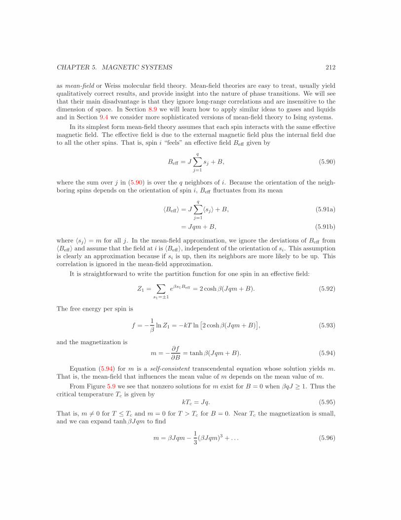
CHAPTER 5. MAGNETIC SYSTEMS 212

as mean-field or Weiss molecular field theory. Mean-field theories are easy to treat, usually yieldqualitatively correct results, and provide insight into the nature of phase transitions. We will seethat their main disadvantage is that they ignore long-range correlations and are insensitive to thedimension of space. In Section 8.9 we will learn how to apply similar ideas to gases and liquidsand in Section 9.4 we consider more sophisticated versions of mean-field theory to Ising systems.

In its simplest form mean-field theory assumes that each spin interacts with the same effectivemagnetic field. The effective field is due to the external magnetic field plus the internal field dueto all the other spins. That is, spin i “feels” an effective field Beff given by

Beff = J

q∑j=1

sj + B, (5.90)

where the sum over j in (5.90) is over the q neighbors of i. Because the orientation of the neigh-boring spins depends on the orientation of spin i, Beff fluctuates from its mean

〈Beff〉 = J

q∑j=1

〈sj〉 + B, (5.91a)

= Jqm + B, (5.91b)

where 〈sj〉 = m for all j. In the mean-field approximation, we ignore the deviations of Beff from〈Beff〉 and assume that the field at i is 〈Beff〉, independent of the orientation of si. This assumptionis clearly an approximation because if si is up, then its neighbors are more likely to be up. Thiscorrelation is ignored in the mean-field approximation.

It is straightforward to write the partition function for one spin in an effective field:

Z1 =∑

s1=±1

eβs1Beff = 2 coshβ(Jqm + B). (5.92)

The free energy per spin is

f = − 1β

ln Z1 = −kT ln[2 coshβ(Jqm + B)

], (5.93)

and the magnetization is

m = − ∂f

∂B= tanhβ(Jqm + B). (5.94)

Equation (5.94) for m is a self-consistent transcendental equation whose solution yields m.That is, the mean-field that influences the mean value of m depends on the mean value of m.

From Figure 5.9 we see that nonzero solutions for m exist for B = 0 when βqJ ≥ 1. Thus thecritical temperature Tc is given by

kTc = Jq. (5.95)

That is, m = 0 for T ≤ Tc and m = 0 for T > Tc for B = 0. Near Tc the magnetization is small,and we can expand tanh βJqm to find

m = βJqm − 13(βJqm)3 + . . . (5.96)

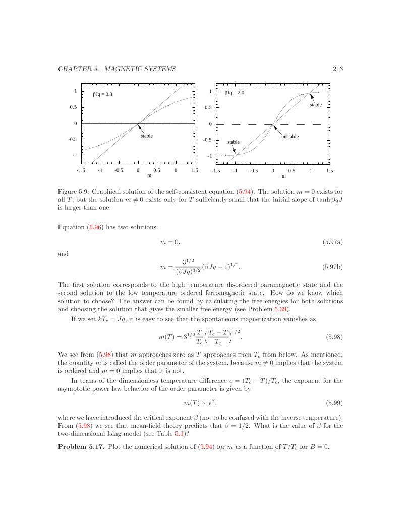
CHAPTER 5. MAGNETIC SYSTEMS 213

-1

-0.5

0

0.5

1

-1.5 -1 -0.5 0 0.5 1 1.5m

βJq = 0.8

stable

-1

-0.5

0

0.5

1

-1.5 -1 -0.5 0 0.5 1 1.5m

unstable

stable

stable

βJq = 2.0

Figure 5.9: Graphical solution of the self-consistent equation (5.94). The solution m = 0 exists forall T , but the solution m = 0 exists only for T sufficiently small that the initial slope of tanh βqJis larger than one.

Equation (5.96) has two solutions:

m = 0, (5.97a)

and

m =31/2

(βJq)3/2(βJq − 1)1/2. (5.97b)

The first solution corresponds to the high temperature disordered paramagnetic state and thesecond solution to the low temperature ordered ferromagnetic state. How do we know whichsolution to choose? The answer can be found by calculating the free energies for both solutionsand choosing the solution that gives the smaller free energy (see Problem 5.39).

If we set kTc = Jq, it is easy to see that the spontaneous magnetization vanishes as

m(T ) = 31/2 T

Tc

(Tc − T

Tc

)1/2

. (5.98)

We see from (5.98) that m approaches zero as T approaches from Tc from below. As mentioned,the quantity m is called the order parameter of the system, because m = 0 implies that the systemis ordered and m = 0 implies that it is not.

In terms of the dimensionless temperature difference ε = (Tc − T )/Tc, the exponent for theasymptotic power law behavior of the order parameter is given by

m(T ) ∼ εβ . (5.99)

where we have introduced the critical exponent β (not to be confused with the inverse temperature).From (5.98) we see that mean-field theory predicts that β = 1/2. What is the value of β for thetwo-dimensional Ising model (see Table 5.1)?

Problem 5.17. Plot the numerical solution of (5.94) for m as a function of T/Tc for B = 0.

CHAPTER 5. MAGNETIC SYSTEMS 214

Problem 5.18. Determine m(T ) from the numerical solution of (5.94) for B = 1 and compareyour values with the exact solution in one dimension (see (5.73)).

We next find the behavior of other important physical properties near Tc. The zero-fieldisothermal susceptibility (per spin) is given by

χ = limB→0

∂m

∂B=

β(1 − tanh2 βJqm)1 − βJq(1 − tanh2 βJqm)

. (5.100)

Note that for very high temperatures, βJ → 0, and χ from (5.100) approaches the Curie law fornoninteracting spins as expected. For T above and close to Tc, we find (see Problem 5.19)

χ ∼ T

T − Tc. (5.101)

The result (5.101) for χ is known as the Curie-Weiss law. We characterize the divergence of thezero-field susceptibility as the critical point is approached from either the low or high temperatureside as

χ ∼ |ε|−γ . (T near Tc) (5.102)

The mean-field prediction for the critical exponent γ is γ = 1.

Problem 5.19. (a) Use the relation (5.100) to show that χ = (1/k)(T − Tc)−1 for T → T +c . (b)

It is more difficult to show that χ = (1/2k)(Tc− T )−1 for T → T−c .

The magnetization at Tc as a function of B can be calculated by expanding (5.94) to thirdorder in B with β = βc = 1/qJ :

m = m + βcB − 13(m + βcB)3 + . . . (5.103)

For m and B very small, we can assume that βcB m. This assumption yields

m = (3βcB)1/3, (T = Tc) (5.104)

which is consistent with this assumption. In general, we write

m ∼ B1/δ. (T = Tc) (5.105)

The mean-field prediction is δ = 3.The energy per spin in the mean-field approximation is simply

E = −12Jqm2, (5.106)

which is the average value of the interaction energy divided by two to account for double counting.Because m = 0 for T > Tc, the energy vanishes for all T > Tc and thus the heat capacity alsovanishes according to mean-field theory. Below Tc the energy is given by

E = −12Jq

[tanh(β(Jqm + B))

]2. (5.107)

The specific heat can be calculated from (5.107) for T < Tc. As shown in Problem 5.20, C → 3k/2for T → Tc from below. Hence, mean-field theory predicts predicts that there is a jump in thespecific heat.

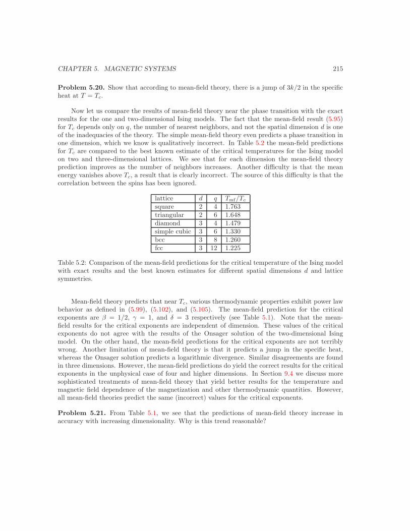
CHAPTER 5. MAGNETIC SYSTEMS 215

Problem 5.20. Show that according to mean-field theory, there is a jump of 3k/2 in the specificheat at T = Tc.

Now let us compare the results of mean-field theory near the phase transition with the exactresults for the one and two-dimensional Ising models. The fact that the mean-field result (5.95)for Tc depends only on q, the number of nearest neighbors, and not the spatial dimension d is oneof the inadequacies of the theory. The simple mean-field theory even predicts a phase transition inone dimension, which we know is qualitatively incorrect. In Table 5.2 the mean-field predictionsfor Tc are compared to the best known estimate of the critical temperatures for the Ising modelon two and three-dimensional lattices. We see that for each dimension the mean-field theoryprediction improves as the number of neighbors increases. Another difficulty is that the meanenergy vanishes above Tc, a result that is clearly incorrect. The source of this difficulty is that thecorrelation between the spins has been ignored.

lattice d q Tmf/Tc

square 2 4 1.763triangular 2 6 1.648diamond 3 4 1.479simple cubic 3 6 1.330bcc 3 8 1.260fcc 3 12 1.225

Table 5.2: Comparison of the mean-field predictions for the critical temperature of the Ising modelwith exact results and the best known estimates for different spatial dimensions d and latticesymmetries.

Mean-field theory predicts that near Tc, various thermodynamic properties exhibit power lawbehavior as defined in (5.99), (5.102), and (5.105). The mean-field prediction for the criticalexponents are β = 1/2, γ = 1, and δ = 3 respectively (see Table 5.1). Note that the mean-field results for the critical exponents are independent of dimension. These values of the criticalexponents do not agree with the results of the Onsager solution of the two-dimensional Isingmodel. On the other hand, the mean-field predictions for the critical exponents are not terriblywrong. Another limitation of mean-field theory is that it predicts a jump in the specific heat,whereas the Onsager solution predicts a logarithmic divergence. Similar disagreements are foundin three dimensions. However, the mean-field predictions do yield the correct results for the criticalexponents in the unphysical case of four and higher dimensions. In Section 9.4 we discuss moresophisticated treatments of mean-field theory that yield better results for the temperature andmagnetic field dependence of the magnetization and other thermodynamic quantities. However,all mean-field theories predict the same (incorrect) values for the critical exponents.

Problem 5.21. From Table 5.1, we see that the predictions of mean-field theory increase inaccuracy with increasing dimensionality. Why is this trend reasonable?

CHAPTER 5. MAGNETIC SYSTEMS 216

5.7 *Infinite-range interactions

We might expect that mean-field theory would become exact in a system for which every spininteracts equally strongly with every other spin. We will refer to this model as the infinite-rangeIsing model, although the interaction range becomes infinite only in the limit N → ∞. We willleave it as a problem to show that for such a system of N spins, the energy is given by

E =JN

2(N − M2), (5.108)

where M is the magnetization and JN is the interaction between any two spins. Note that Edepends only on M . We also leave it as a problem to show that the number of states withmagnetization M is given by

g(M) =N !

n!(N − n)!, (5.109)

where n is the number of up spins. As before, we have n = N/2 + M/2 and N − n = N/2−M/2.

Problem 5.22. (a) Show that the energy of a system for which every spin interacts with everyother spin is given by (5.108). One way to do so is to consider a small system, say N = 9 andto work out the various possibilities. As you do so, you will see how to generalize your results toarbitrary N . (b) Use similar considerations as in part (a) to find the number of states as in (5.109).

We have to scale the energy of interaction JN to obtain a well-behaved thermodynamic limit.If we did not, the energy change associated with the flip of a spin would grow linearly with N anda well-defined thermodynamic limit would not exist. We will choose

JN =qJ

N, (5.110)

so that kTc/J = q when N → ∞.Given the energy in (5.108) and the number of states in (5.109), we can write the partition

function asZN =

∑M

N !(N

2 + M2 )!(N

2 − M2 )!

e−βJN(N−M2)/2e−βBM , (5.111)

where we have included the interaction with an external magnetic field. For N not too large, wecan evaluate the sum over M numerically. For N very large we can convert the sum to an integral.We write

Z =∫ ∞

−∞dMZ(M), (5.112)

whereZ(M) =

N !n!(N − n)!

e−βEe−βBM , (5.113)

where n = (M + N)/2. A plot of Z(M) shows that it is peaked about some value of M . So letus do our usual trick of expanding lnZM about its maximum. For simplicity, we will first find thevalue of M for which Z(M) is a maximum. We write

ln Z(M) = lnN ! − ln n! − ln(N − n)! − βE + βhM. (5.114)

CHAPTER 5. MAGNETIC SYSTEMS 217

Then we use that the fact that ddx(ln x!) = lnx, dn/dM = 1/2, and d(N − n)/dM = −1/2 and

obtain

d ln Z(M)dM

= −12

ln n +12

ln(N − n) + βJNM + βB (5.115a)

= −12

lnN

2(1 + m) +

12

lnN

2(1 − m) + qβJm + βB (5.115b)

= −12

ln(1 + m) +12

ln(1 − m) + qβJm + βB = 0. (5.115c)

We set d(ln Z(M))/dM = 0 because we wish to find the value of M that maximizes Z(M). Wehave

12

ln1 − m

1 + m= −β(qJm + B), (5.116)

so that1 − m

1 + m= e−2β(qJm+B) = x (5.117)

Finally we solve (5.117) for m in terms of x and obtain

1 − m = x(1 + m) (5.118a)m(−1 − x) = −1 + x (5.118b)

m =1 − x

1 + x=

1 − e−2β(Jqm+B)

e−2β(Jqm+B) + 1(5.119a)

=eβ(Jqm+B) − e−β(qm+B)

e−β(Jqm+B) + eβ(qm+B)(5.119b)

= tanh(β(Jqm + B). (5.119c)

Note that (5.119c) is identical to the previous mean-field result in (5.94).

∗Problem 5.23. Show that Z(M) can be written as a Gaussian and then do the integral over Min (5.112) to find the mean-field form of Z. Then use this form of Z to find the mean-field resultfor the free energy F .

Appendix 5A. How does magnetism occur in matter?

Classical electromagnetic theory tells us that magnetic fields are due to electrical currents andchanging electric fields, and that the magnetic fields far from the currents are described by amagnetic dipole. It is natural to assume that magnetic effects in matter are due to microscopiccurrent loops created by the motion of electrons in atoms. However, it was shown by Niels Bohrin his doctoral thesis of 1911 and independently by Johanna H. van Leeuwen in her 1919 doctoralthesis that the phenomena of diamagnetism does not exist in classical physics (see Problem 6.76).Hence, magnetism can be understood only by using quantum mechanics.

The most obvious new physics due to quantum mechanics is the existence of an intrinsicmagnetic moment. The intrinsic magnetic moment is proportional to the intrinsic spin, another

CHAPTER 5. MAGNETIC SYSTEMS 218

quantum mechanical property. The interaction energy between a single spin and an externallyapplied magnetic field B is given by

E = −µ ·B. (5.120)

There is a distinction between the magnetic field produced by currents external to the materialand the field produced internally by the magnetic moments within the material. The applied fieldis denoted as H, and the total field is denoted as B. The fields B and H are related to themagnetization per unit volume, m = M/V , by

B = µ0(H + m). (5.121)

The energy due to the external magnetic field H coupled to M is

E = −M · H. (5.122)

The origin of the interaction energy between magnetic moments must be due to quantummechanics. Because the electrons responsible for magnetic behavior are localized near the atoms ofa regular lattice in most magnetic materials, we consider the simple case of two localized electrons.Each electron has a spin 1/2 which can point either up or down along the axis that is specified bythe applied magnetic field. The electrons interact with each other and with nearby atoms and aredescribed in part by the spatial wavefunction ψ(r1, r2). This wavefunction must be multiplied bythe spin eigenstates to obtain the actual state of the two electron system. We denote the basis forthese states as

|↑↑〉, |↓↓〉, |↑↓〉, |↓↑〉, (5.123)

where the arrows corresponds to the spin of the electrons. These states are eigenstates of thez-component of the total spin angular momentum, Sz, such that Sz operating on any of thestates in (5.123) has an eigenvalue equal to the sum of the spins in the z direction. For example,Sz| ↑↑〉 = 1| ↑↑〉 and Sz| ↑↓〉 = 0| ↑↓〉. Similarly, Sx or Sy give zero if either operator acts on thesestates. Because electrons are fermions, the basis states in (5.123) are not physically meaningful,because if two electrons are interchanged, the new wavefunction must either be the same or differby a minus sign. The simplest normalized linear combinations of the states in (5.123) that satisfythis condition are

1√2(|↑↓〉 − |↓↑〉) (5.124a)

|↑↑〉 (5.124b)1√2(|↑↓〉 + |↓↑〉) (5.124c)

|↓↓〉 (5.124d)

The state in (5.124a) is antisymmetric, because interchanging the two electrons leads to minus theoriginal state. This state has a total spin, S = 0, and is called the singlet state. The collectionof the last three states is called the triplet state and has S = 1. Because the states of fermionsmust be antisymmetric, the spin state is antisymmetric when the spatial part of the wavefunctionψ(r1, r2) is symmetric and vice versa. That is, if the spins are parallel, then ψ(r1, r2) = −ψ(r2, r1).Similarly, if the spins are antiparallel, then ψ(r1, r2) = +ψ(r2, r1). Hence, when r1 = r2, ψ is zerofor parallel spins and is nonzero for antiparallel spins. We conclude that if the spins are parallel,

CHAPTER 5. MAGNETIC SYSTEMS 219

the separation between the two electrons will rarely be small and their average electrostatic energywill be less than it is for antiparallel spins. We denote Etriplet and Esinglet as the triplet energy andthe singlet energy, respectively, and write the interaction energy in terms of the spin operators.We write

(S1 + S2)2 = S12 + S2

2 + 2S1 ·S2. (5.125)

For spin 1/2, S12 = S1(S1 +1) = 3/4 = S2

2. The total spin, S = S1 +S2 equals zero for the singletstate and unity for the triplet state. Hence, S2 = S(S + 1) = 0 for the singlet state and S2 = 2 forthe triplet state. These results lead to S1 · S2 = −3/4 for the singlet state and S1 · S2 = 1/4 forthe triplet state and allows us to write

E =14(Esinglet + 3Etriplet) − JS1 · S2, (5.126)

where J = Esinglet −Etriplet. The first part of (5.126) is a constant and can be omitted by suitablydefining the zero of energy. The second term represents a convenient form of the interactionbetween two spins.

Can we write the total effective interaction of a system of three spins as −J12 S1 · S2 −J23 S2 ·S3−J13 S1 ·S3? In general, the answer is no, and we can only hope that this simple form isa reasonable approximation. The total energy of the most common model of magnetism is basedon the form (5.126) for the spin-spin interaction and is expressed as

H = −N∑

i<j=1

Jij Si · Sj − gµ0H·N∑

i=1

Si, (Heisenberg model) (5.127)

where gµ0 is the magnetic moment of the electron. The exchange interaction Jij can be positiveor negative. The form (5.127) of the interaction energy is known as the Heisenberg model. Notethat S as well as the Hamiltonian H is an operator, and that the Heisenberg model is quantummechanical in nature. The distinction between the operator H and the magnetic field H will beclear from the context.

As we have seen, the Heisenberg model assumes that we can treat all interactions in terms ofpairs of spins. This assumption means that the magnetic ions in the crystal must be sufficientlyfar apart that the overlap of their wavefunctions is small. We also have neglected any orbitalcontribution to the total angular momentum. In addition, dipolar interactions can be importantand lead to a coupling between the spin degrees of freedom and the relative displacements of themagnetic ions. In general, it is very difficult to obtain the exact Hamiltonian from first principles,and the Heisenberg form of the Hamiltonian should be considered as a reasonable approximationwith the details buried into the exchange constant J .

The Heisenberg model is the starting point for most microscopic models of magnetism. Wecan go to the classical limit S → ∞, consider spins with one, two, or three components, place thespins on lattices of any dimension and any crystal structure, and allow J to be positive, negative,random, nearest-neighbor, long-range, etc. In addition, we can include other interactions such asthe interaction of an electron with an ion. The theoretical possibilities are very rich as are thetypes of magnetic materials of interest experimentally.

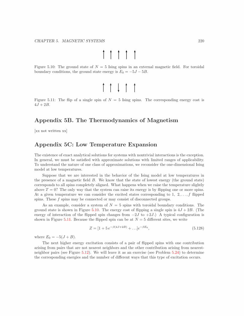
CHAPTER 5. MAGNETIC SYSTEMS 220

Figure 5.10: The ground state of N = 5 Ising spins in an external magnetic field. For toroidalboundary conditions, the ground state energy is E0 = −5J − 5B.

Figure 5.11: The flip of a single spin of N = 5 Ising spins. The corresponding energy cost is4J + 2B.

Appendix 5B. The Thermodynamics of Magnetism

[xx not written xx]

Appendix 5C: Low Temperature Expansion

The existence of exact analytical solutions for systems with nontrivial interactions is the exception.In general, we must be satisfied with approximate solutions with limited ranges of applicability.To understand the nature of one class of approximations, we reconsider the one-dimensional Isingmodel at low temperatures.

Suppose that we are interested in the behavior of the Ising model at low temperatures inthe presence of a magnetic field B. We know that the state of lowest energy (the ground state)corresponds to all spins completely aligned. What happens when we raise the temperature slightlyabove T = 0? The only way that the system can raise its energy is by flipping one or more spins.At a given temperature we can consider the excited states corresponding to 1, 2, . . . , f flippedspins. These f spins may be connected or may consist of disconnected groups.

As an example, consider a system of N = 5 spins with toroidal boundary conditions. Theground state is shown in Figure 5.10. The energy cost of flipping a single spin is 4J + 2B. (Theenergy of interaction of the flipped spin changes from −2J to +2J .) A typical configuration isshown in Figure 5.11. Because the flipped spin can be at N = 5 different sites, we write

Z = [1 + 5 e−β(4J+2B) + . . .]e−βE0, (5.128)

where E0 = −5(J + B).The next higher energy excitation consists of a pair of flipped spins with one contribution

arising from pairs that are not nearest neighbors and the other contribution arising from nearest-neighbor pairs (see Figure 5.12). We will leave it as an exercise (see Problem 5.24) to determinethe corresponding energies and the number of different ways that this type of excitation occurs.

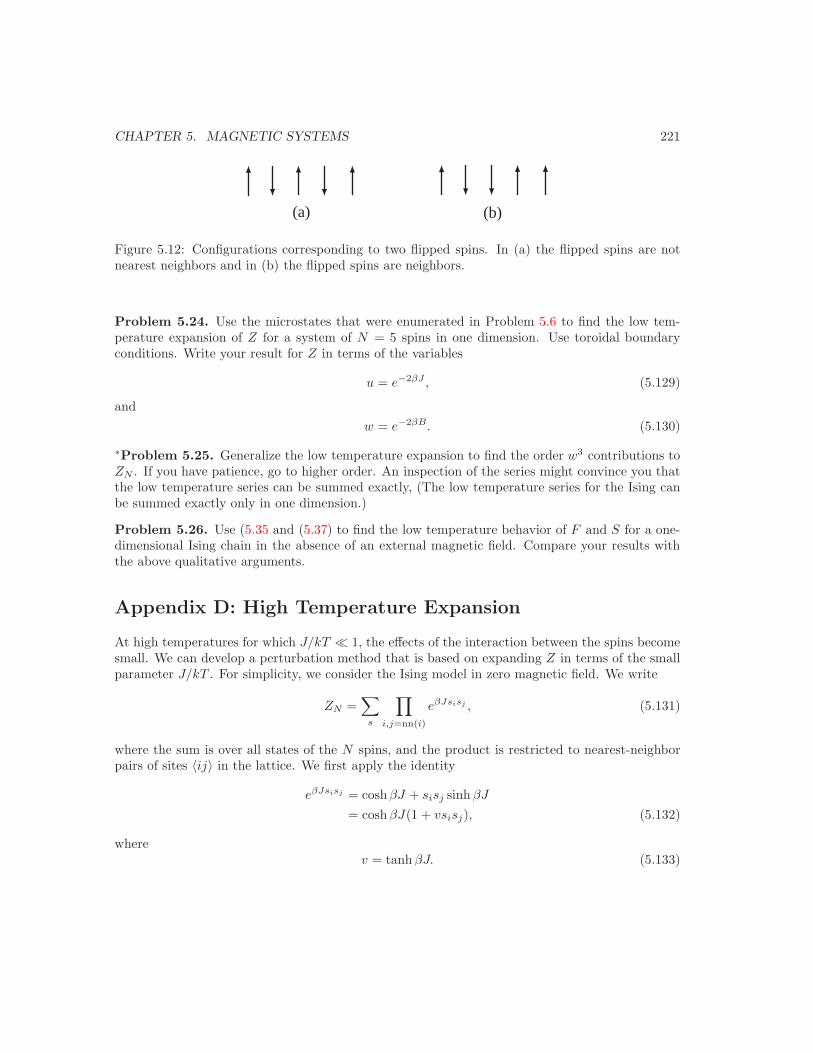
CHAPTER 5. MAGNETIC SYSTEMS 221

(a) (b)

Figure 5.12: Configurations corresponding to two flipped spins. In (a) the flipped spins are notnearest neighbors and in (b) the flipped spins are neighbors.

Problem 5.24. Use the microstates that were enumerated in Problem 5.6 to find the low tem-perature expansion of Z for a system of N = 5 spins in one dimension. Use toroidal boundaryconditions. Write your result for Z in terms of the variables

u = e−2βJ , (5.129)

andw = e−2βB. (5.130)

∗Problem 5.25. Generalize the low temperature expansion to find the order w3 contributions toZN . If you have patience, go to higher order. An inspection of the series might convince you thatthe low temperature series can be summed exactly, (The low temperature series for the Ising canbe summed exactly only in one dimension.)

Problem 5.26. Use (5.35 and (5.37) to find the low temperature behavior of F and S for a one-dimensional Ising chain in the absence of an external magnetic field. Compare your results withthe above qualitative arguments.

Appendix D: High Temperature Expansion

At high temperatures for which J/kT 1, the effects of the interaction between the spins becomesmall. We can develop a perturbation method that is based on expanding Z in terms of the smallparameter J/kT . For simplicity, we consider the Ising model in zero magnetic field. We write

ZN =∑

s

∏i,j=nn(i)

eβJsisj , (5.131)

where the sum is over all states of the N spins, and the product is restricted to nearest-neighborpairs of sites 〈ij〉 in the lattice. We first apply the identity

eβJsisj = coshβJ + sisj sinh βJ

= coshβJ(1 + vsisj), (5.132)

wherev = tanhβJ. (5.133)

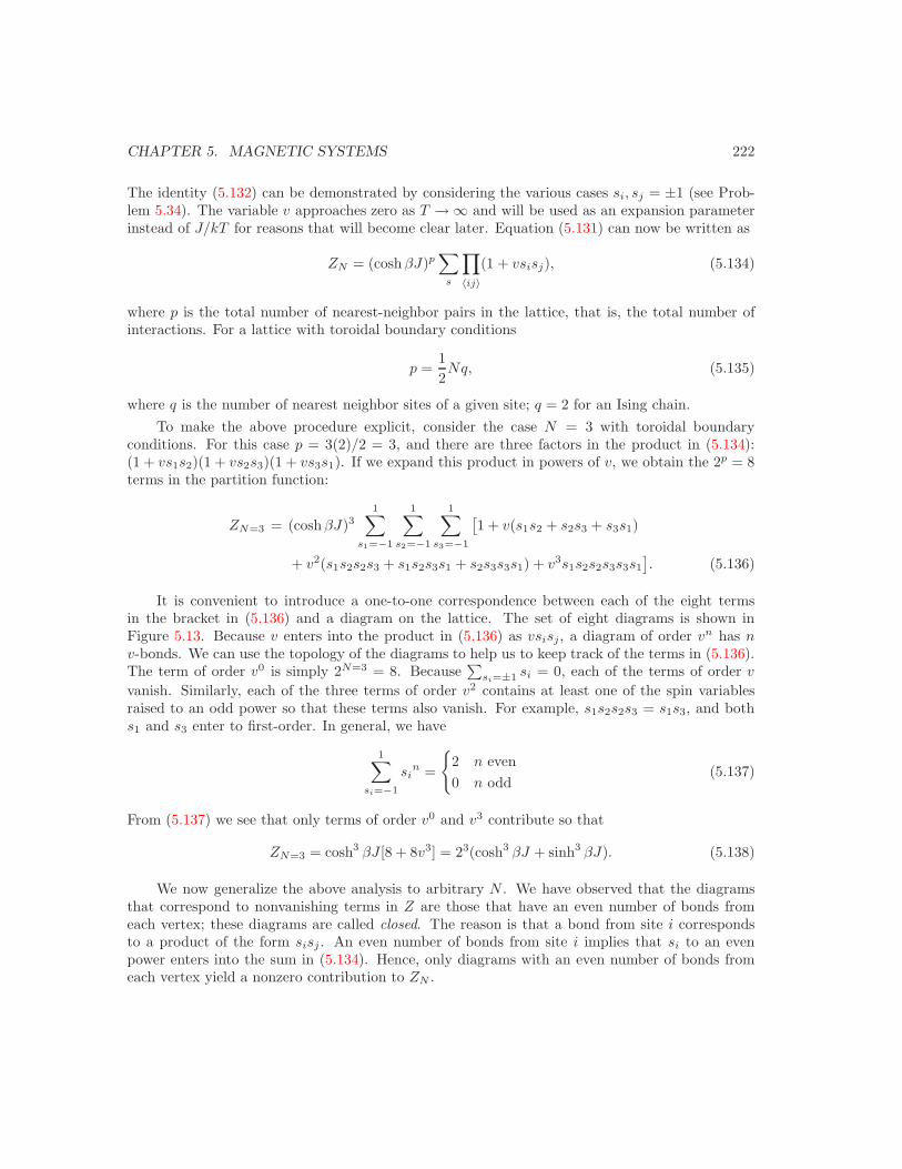
CHAPTER 5. MAGNETIC SYSTEMS 222

The identity (5.132) can be demonstrated by considering the various cases si, sj = ±1 (see Prob-lem 5.34). The variable v approaches zero as T → ∞ and will be used as an expansion parameterinstead of J/kT for reasons that will become clear later. Equation (5.131) can now be written as

ZN = (cosh βJ)p∑

s

∏〈ij〉

(1 + vsisj), (5.134)

where p is the total number of nearest-neighbor pairs in the lattice, that is, the total number ofinteractions. For a lattice with toroidal boundary conditions

p =12Nq, (5.135)

where q is the number of nearest neighbor sites of a given site; q = 2 for an Ising chain.To make the above procedure explicit, consider the case N = 3 with toroidal boundary

conditions. For this case p = 3(2)/2 = 3, and there are three factors in the product in (5.134):(1 + vs1s2)(1 + vs2s3)(1 + vs3s1). If we expand this product in powers of v, we obtain the 2p = 8terms in the partition function:

ZN=3 = (cosh βJ)31∑

s1=−1

1∑s2=−1

1∑s3=−1

[1 + v(s1s2 + s2s3 + s3s1)

+ v2(s1s2s2s3 + s1s2s3s1 + s2s3s3s1) + v3s1s2s2s3s3s1

]. (5.136)

It is convenient to introduce a one-to-one correspondence between each of the eight termsin the bracket in (5.136) and a diagram on the lattice. The set of eight diagrams is shown inFigure 5.13. Because v enters into the product in (5.136) as vsisj, a diagram of order vn has nv-bonds. We can use the topology of the diagrams to help us to keep track of the terms in (5.136).The term of order v0 is simply 2N=3 = 8. Because

∑si=±1 si = 0, each of the terms of order v

vanish. Similarly, each of the three terms of order v2 contains at least one of the spin variablesraised to an odd power so that these terms also vanish. For example, s1s2s2s3 = s1s3, and boths1 and s3 enter to first-order. In general, we have

1∑si=−1

sin =

2 n even0 n odd

(5.137)

From (5.137) we see that only terms of order v0 and v3 contribute so that

ZN=3 = cosh3 βJ [8 + 8v3] = 23(cosh3 βJ + sinh3 βJ). (5.138)

We now generalize the above analysis to arbitrary N . We have observed that the diagramsthat correspond to nonvanishing terms in Z are those that have an even number of bonds fromeach vertex; these diagrams are called closed. The reason is that a bond from site i correspondsto a product of the form sisj . An even number of bonds from site i implies that si to an evenpower enters into the sum in (5.134). Hence, only diagrams with an even number of bonds fromeach vertex yield a nonzero contribution to ZN .

CHAPTER 5. MAGNETIC SYSTEMS 223

1

3

v0

v1

v2

v3

2

Figure 5.13: The eight diagrams that correspond to the eight terms in the Ising model partitionfunction for the N = 3 Ising chain. The term sisj is represented by a line is represented by a linebetween the neighboring sites i and j.

For the Ising chain, only two bonds can come from a given site. Hence, we see that althoughthere are 2N diagrams for a Ising chain of N spins with toroidal boundary conditions, only thediagrams of order v0 (with no bonds) and of order vN will contribute to ZN . We conclude that

ZN = (coshβJ)N [2N + 2NvN ]. (5.139)

Problem 5.27. Draw the diagrams that correspond to the terms in the high temperature expan-sion of the Ising model partition function for the N = 4 Ising chain.

Problem 5.28. The form of ZN in (5.139) is not identical to the form of ZN given in (5.28). Usethe fact that v < 1 and take the thermodynamic limit N → ∞ to explain the equivalence of thetwo results for ZN .

Vocabulary

magnetization m, zero field susceptibility χ

Ising model, exchange constant J

correlation function G(r), correlation length ξ, domain wall

order parameter, continuous phase transition, critical point

critical temperature Tc, critical exponents α, β, δ, γ, ν, η

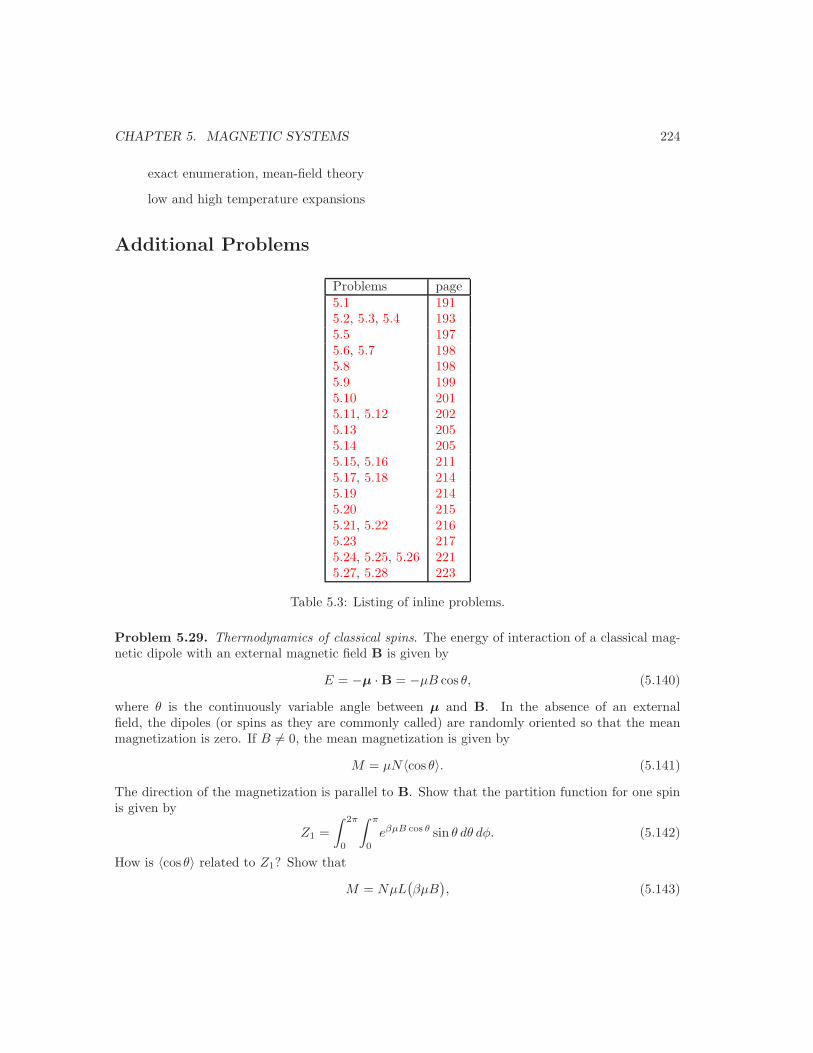
CHAPTER 5. MAGNETIC SYSTEMS 224

exact enumeration, mean-field theory

low and high temperature expansions

Additional Problems

Problems page5.1 1915.2, 5.3, 5.4 1935.5 1975.6, 5.7 1985.8 1985.9 1995.10 2015.11, 5.12 2025.13 2055.14 2055.15, 5.16 2115.17, 5.18 2145.19 2145.20 2155.21, 5.22 2165.23 2175.24, 5.25, 5.26 2215.27, 5.28 223

Table 5.3: Listing of inline problems.

Problem 5.29. Thermodynamics of classical spins. The energy of interaction of a classical mag-netic dipole with an external magnetic field B is given by

E = −µ ·B = −µB cos θ, (5.140)

where θ is the continuously variable angle between µ and B. In the absence of an externalfield, the dipoles (or spins as they are commonly called) are randomly oriented so that the meanmagnetization is zero. If B = 0, the mean magnetization is given by

M = µN〈cos θ〉. (5.141)

The direction of the magnetization is parallel to B. Show that the partition function for one spinis given by

Z1 =∫ 2π

0

∫ π

0

eβµB cos θ sin θ dθ dφ. (5.142)

How is 〈cos θ〉 related to Z1? Show that

M = NµL(βµB

), (5.143)

CHAPTER 5. MAGNETIC SYSTEMS 225

where the Langevin function L(x) is given by

L(x) =ex + e−x

ex − e−x− 1

x= coth x − 1

x. (5.144)

For |x| < π, L(x) can be expanded as

L(x) =x

3− x3

45+ . . . +

22nB2n

(2n)!+ . . . , (x 1) (5.145)

where Bn is the Bernoulli number of order n (see Appendix A). What is M and the susceptibilityin the limit of high T ? For large x, L(x) is given by

L(x) ≈ 1 − 1x

+ 2e−2x. (x 1) (5.146)

What is the behavior of M in the limit of low T ?

Problem 5.30. Arbitrary spin. The magnetic moment of an atom or nucleus is associated withits angular momentum which is quantized. If the angular momentum is J , the magnetic momentalong the direction of B is restricted to (2J +1) orientations. We write the energy of an individualatom as

E = −gµ0 J ·B = −gµ0JzB. (5.147)

The values of µ0 and g depend on whether we are considering a nucleus, an atom, or an electron.The values of Jz are restricted to −J,−J + 1,−J + 2, . . . , J − 1, J . Hence, the partition functionfor one atom contains (2J + 1) terms:

Z1 =J∑

m=−J

e−β(−gµ0mB). (5.148)

The summation index m ranges from −J to J in integral steps.To simplify the notation, we let α = βgµ0B, and write Z1 as a finite geometrical series:

Z1 =J∑

m=−J

emα, (5.149a)

= e−αJ(1 + eα + e2α + . . . + e2Jα). (5.149b)

The sum of a finite geometrical series is given by

Sn =n∑

p=0

xp =xn+1 − 1

x − 1. (5.150)

Given that there are (2J + 1) terms in (5.149b), show that

Z = e−αJ e(2J+1)α − 1eα − 1

= e−αJ [1 − e(2J+1)α]1 − eα

. (5.151)

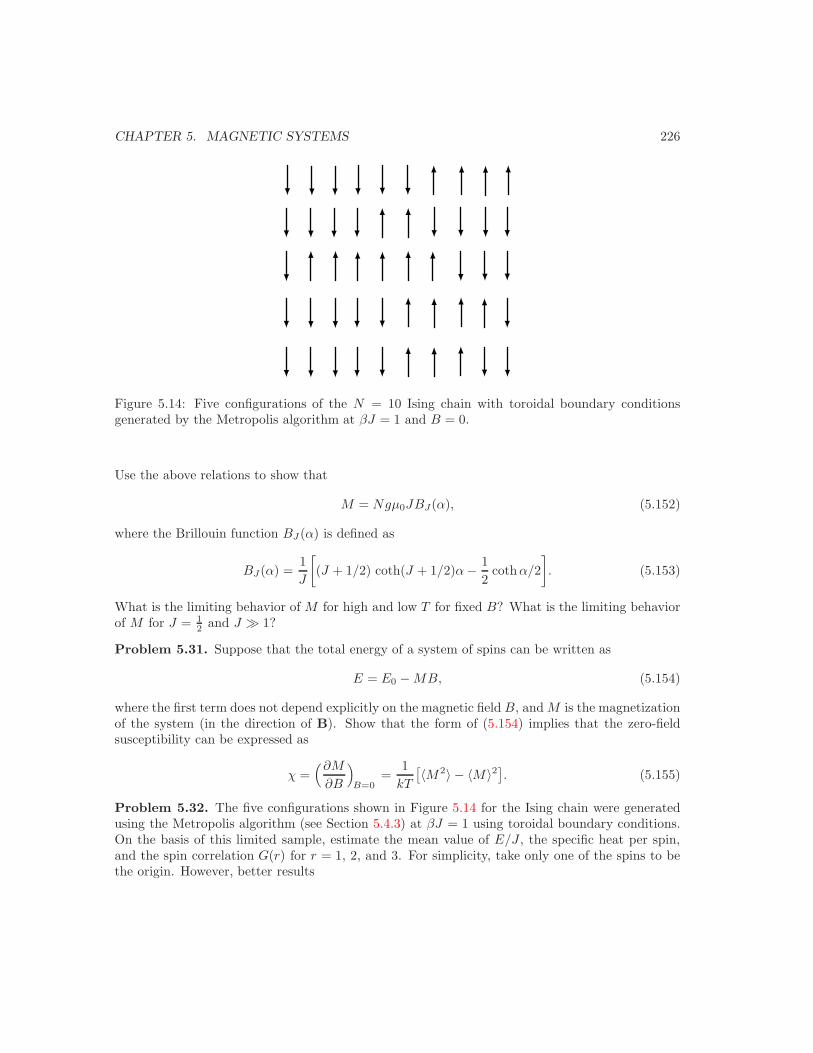
CHAPTER 5. MAGNETIC SYSTEMS 226

Figure 5.14: Five configurations of the N = 10 Ising chain with toroidal boundary conditionsgenerated by the Metropolis algorithm at βJ = 1 and B = 0.

Use the above relations to show that

M = Ngµ0JBJ(α), (5.152)

where the Brillouin function BJ (α) is defined as

BJ(α) =1J

[(J + 1/2) coth(J + 1/2)α− 1

2cothα/2

]. (5.153)

What is the limiting behavior of M for high and low T for fixed B? What is the limiting behaviorof M for J = 1

2 and J 1?

Problem 5.31. Suppose that the total energy of a system of spins can be written as

E = E0 − MB, (5.154)

where the first term does not depend explicitly on the magnetic field B, and M is the magnetizationof the system (in the direction of B). Show that the form of (5.154) implies that the zero-fieldsusceptibility can be expressed as

χ =(∂M

∂B

)B=0

=1

kT

[〈M2〉 − 〈M〉2]. (5.155)

Problem 5.32. The five configurations shown in Figure 5.14 for the Ising chain were generatedusing the Metropolis algorithm (see Section 5.4.3) at βJ = 1 using toroidal boundary conditions.On the basis of this limited sample, estimate the mean value of E/J , the specific heat per spin,and the spin correlation G(r) for r = 1, 2, and 3. For simplicity, take only one of the spins to bethe origin. However, better results

CHAPTER 5. MAGNETIC SYSTEMS 227

Problem 5.33. Use the applet at <stp.clarku.edu/simulations/ising/> to determine P (E),the probability that the system has energy E, for the two-dimensional Ising model. (For theIsing model the energy is a discrete variable.) What is the approximate form of the probabilitydistribution at T = 4? What is its width? Then take T = Tc ≈ 2.269. Is the form of P (E) similar?If not, why?

Problem 5.34. Verify the validity of the identity (5.132) by considering the different possiblevalues of sisj and using the identities 2 coshx = ex + e−x and 2 sinhx = ex − e−x.

Problem 5.35. Explore the analogy between the behavior of the Ising model and the behaviorof a large group of people. Under what conditions would a group of people act like a collectionof individuals doing their “own thing?” Under what conditions might they act as a group? Whatfactors could cause such a transition?

∗Problem 5.36. Ising chain. Write a program that uses the demon algorithm to generate arepresentative sample of microstates for the Ising chain at fixed energy. The energy for a particularconfiguration of spins is given by

E = −J

N∑i=1

sisi+1, (5.156)

where si = ±1 and sN+1 = s1. The easiest trial change is to flip a spin from +1 to −1 or viceversa. For such a flip the possible changes in energy are ∆E = Etrial−Eold = 0 and ±4J . Confirmthat the possible energies of the spins are E = −NJ,−NJ + 4J,−NJ + 8J . . . + NJ , and thatthe possible demon energies are Ed = 4nJ , where n = 0, 1, 2, . . . The most difficult part of thesimulation is choosing the initial state so that it has the desired energy. Choose N = 20 andEd = 0 initially. Write a subroutine that begins with all spins down and randomly flips spinsuntil the desired energy is reached. Choose J to be the unit of energy. Collect data for the meanenergy of the system and the mean demon energy for about ten different energies and plot yourresults. Equilibrate the spins for about 100 flips per spin before taking averages for each value ofthe total energy. Average over approximately 1000 flips per spin. Increase the number of flips perspin until you obtain reasonable results. Compute the probability density, P (Ed), and determineits dependence on Ed by making a semilog plot.

∗Problem 5.37. Consider a one-dimensional Ising-type model defined by the usual Hamiltonianwith B = 0, but with si = 0,±1. Use the transfer matrix method to calculate the dependence ofthe energy on T . The solution requires the differentiation of the root of a cubic equation that youmight wish to do numerically.

Problem 5.38. Calculate the partition function for the Ising model on a square lattice for N = 4and N = 9 in the presence of an external magnetic field. Assume that the system is in equilibriumwith a thermal bath at temperature T . You might find it easier to write a short program toenumerate all the microstates. Choose either toroidal or open boundary conditions. Calculate thecorresponding values of the mean energy, the heat capacity, and the zero field susceptibility.

Problem 5.39. It can be shown that the free energy per spin in the mean-field approximation isgiven by

f = −(q/2)Jm2 − Bm + kTs(m), (5.157)

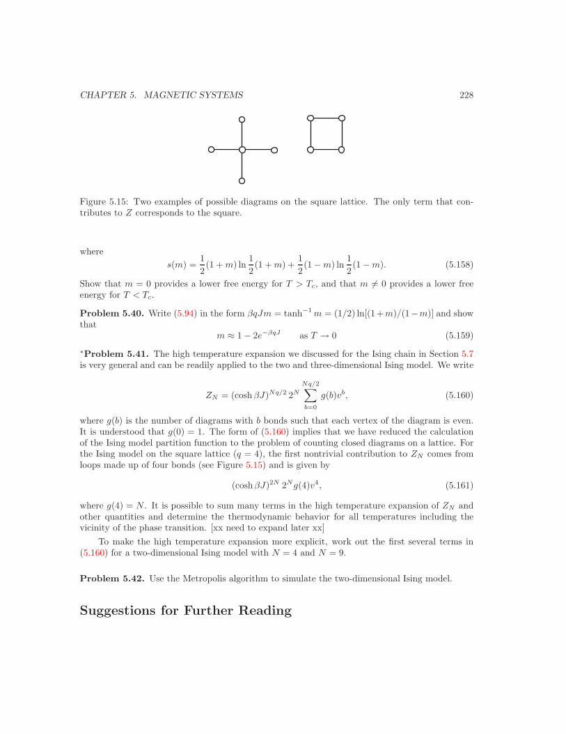
CHAPTER 5. MAGNETIC SYSTEMS 228

Figure 5.15: Two examples of possible diagrams on the square lattice. The only term that con-tributes to Z corresponds to the square.

wheres(m) =

12(1 + m) ln

12(1 + m) +

12(1 − m) ln

12(1 − m). (5.158)

Show that m = 0 provides a lower free energy for T > Tc, and that m = 0 provides a lower freeenergy for T < Tc.

Problem 5.40. Write (5.94) in the form βqJm = tanh−1 m = (1/2) ln[(1+m)/(1−m)] and showthat

m ≈ 1 − 2e−βqJ as T → 0 (5.159)

∗Problem 5.41. The high temperature expansion we discussed for the Ising chain in Section 5.7is very general and can be readily applied to the two and three-dimensional Ising model. We write

ZN = (coshβJ)Nq/2 2N

Nq/2∑b=0

g(b)vb, (5.160)

where g(b) is the number of diagrams with b bonds such that each vertex of the diagram is even.It is understood that g(0) = 1. The form of (5.160) implies that we have reduced the calculationof the Ising model partition function to the problem of counting closed diagrams on a lattice. Forthe Ising model on the square lattice (q = 4), the first nontrivial contribution to ZN comes fromloops made up of four bonds (see Figure 5.15) and is given by

(coshβJ)2N 2Ng(4)v4, (5.161)

where g(4) = N . It is possible to sum many terms in the high temperature expansion of ZN andother quantities and determine the thermodynamic behavior for all temperatures including thevicinity of the phase transition. [xx need to expand later xx]

To make the high temperature expansion more explicit, work out the first several terms in(5.160) for a two-dimensional Ising model with N = 4 and N = 9.

Problem 5.42. Use the Metropolis algorithm to simulate the two-dimensional Ising model.

Suggestions for Further Reading

CHAPTER 5. MAGNETIC SYSTEMS 229

Stephen G. Brush, “History of the Lenz-Ising Model,” Rev. Mod. Phys. 39, 883–893 (1967).

M. E. J. Newman and G. T. Barkema, Monte Carlo Methods in Statistical Physics, ClarendonPress (1999).

H. Eugene Stanley, Introduction to Phase Transitions and Critical Phenomena, Oxford UniversityPress (1971).

Chapter 6

Noninteracting Particle Systems

c©2006 by Harvey Gould and Jan Tobochnik21 July 2006

The goal of this chapter is to apply the general formalism of statistical mechanics to classicaland quantum systems of noninteracting particles.

6.1 Introduction

Noninteracting systems are important for several reasons. For example, the interaction betweenthe atoms in a gas can be ignored in the limit of low densities. In the limit of high temperatures,the interaction between the spins in an Ising model can be neglected because the thermal energyis much larger than the potential energy of interaction. Another reason for studying systemsof noninteracting particles is that there are many cases for which the equilibrium properties ofa system of interacting particles can be reformulated as a collection of noninteracting modes orquasiparticles. We will see such an example when we study the harmonic model of a crystal.

6.2 The Classical Ideal Gas

Consider an ideal gas of N identical particles of mass m confined within a cube of volume V = L3.1

If the gas is in thermal equilibrium with a heat bath at temperature T , it is natural to treat theideal gas in the canonical ensemble. However, because the particles are not localized, they cannotbe distinguished from each other as were the harmonic oscillators considered in Example 4.4 andthe spins in Chapter 5. Hence, we cannot simply focus our attention on one particular particle.

On the other hand, if the temperature is sufficiently high, we expect that we can treat a systemof particles semiclassically. To do so, the de Broglie wavelength associated with the particles must

1An ideal gas is a good approximation to a real gas at low densities where the mean interparticle distance ismuch larger than the range of the interparticle interactions.

230

CHAPTER 6. NONINTERACTING PARTICLE SYSTEMS 231

be small. That is, for the semiclassical description to be valid, the mean de Broglie wavelengthλ must be smaller than any other length in the system. For an ideal gas, the only two lengthsare L, the linear dimension of the system, and ρ−1/3, the mean distance between particles (inthree dimensions). Because we are interested in the thermodynamic limit for which L λ, thesemiclassical limit requires that

λ ρ−1/3 or ρλ3 1. (semiclassical limit) (6.1)

Problem 6.1. Mean distance between particles

(a) Consider a system of N particles confined to a line of length L. What is the mean distancebetween the particles?

(b) Consider a similar system of N particles confined to a square of linear dimension L. What isthe mean distance between the particles?

To estimate the magnitude of λ, we need to know the typical value of the momentum of aparticle. If the kinematics of the particles can be treated nonrelativistically, we know from (4.64)that p2/2m = 3kT/2. (We will rederive this result in Section 6.3.) Hence, we have p2 ∼ mkT andλ ∼ h/

√mkT . We will find it is convenient to define the thermal de Broglie wavelength λ as

λ =h

(2πmkT )1/2=

( h2

2πmkT

)1/2

=(2π~

2

mkT

)1/2

. (thermal de Broglie wavelength) (6.2)

The calculation of the partition function of an ideal gas in the semiclassical limit proceedsas follows. First, we assume that λ ρ−1/3 so that we could pick out one particle from anotherif the particles were distinguishable. (If λ ∼ ρ−1/3, the wave functions of the particles wouldoverlap.) Of course, identical particles are intrinsically indistinguishable, so we will have to correctfor overcounting later.

With these considerations we now calculate Z1, the partition function for one particle, in thesemiclassical limit. As we found in (4.41), the energy eigenvalues of a particle in a cube of side Lare given by

εn =h2

8mL2(nx

2 + ny2 + nz

2), (6.3)

where the subscript n represents the set of quantum numbers nx, ny, and nz, each of which canbe any nonzero, positive integer. The corresponding partition function is given by

Z1 =∑

n

e−βεn =

∞∑

nx=1

∞∑

ny=1

∞∑

nz=1

e−βh2(nx2+ny

2+nz2)/8mL2

. (6.4)

Because the sum over each quantum number is independent of the other two quantum numbers,we can rewrite (6.4) as

Z1 =(

∞∑

nx=1

e−αnx2)(

∞∑

ny=1

e−αny2)(

∞∑

nz=1

e−αnz2)

(6.5a)

= ZxZyZz = Z3x, (6.5b)

CHAPTER 6. NONINTERACTING PARTICLE SYSTEMS 232

where

α =βh2

8mL2, (6.6)

and

Zx =∞∑

nx=1

e−αnx2

. (6.7)

The functions Zy and Zz have the same form as Zx. Of course, we could have guessed beforehandthat Z1 in (6.5b) would factor into three terms. Why? Note that the magnitude of α in (6.7) isthe order of λ2/L2 1.

We found in Problem 4.18 that the quantum numbers are order 1010 for a macroscopic systemat room temperature. Thus we can convert the sum in (6.7) to an integral:

Zx =

∞∑

nx=1

e−αnx2

=

∞∑

nx=0

e−αnx2 − 1 →

∫ ∞

0

e−αn2

x dnx − 1. (6.8)

We have accounted for the fact that the sum over nx in (6.7) is from nx = 1 rather than nx = 0.We make a change of variables and write x2 = αn2

x. The Gaussian integral can be easily evaluated(see Appendix A), and we have that

Zx = L(23m

βh2

)1/2∫ ∞

0

e−x2

dx− 1 = L(2πm

βh2

)1/2

− 1. (6.9)

Because the first term in (6.9) is order L/λ 1, we can ignore the second term. The expressionsfor Zy and Zz are identical, and hence we obtain

Z1 = ZxZyZz = V(2πm

βh2

)3/2. (6.10)

The result (6.10) is the partition function associated with the translational motion of one particlein a box. Note that Z1 can be conveniently expressed as

Z1 =V

λ3. (6.11)

It is straightforward to find the mean pressure and energy for one particle in a box. We takethe logarithm of both sides of (6.10) and find

lnZ1 = lnV − 3

2lnβ +

3

2ln

2πm

h2. (6.12)

Hence the mean pressure is given by

p1 =1

β

∂ lnZ1

∂V

∣

∣

∣

T,N=

1

βV=kT

V, (6.13)

and the mean energy is

CHAPTER 6. NONINTERACTING PARTICLE SYSTEMS 233

e1 = −∂ lnZ1

∂β

∣

∣

∣

V,N=

3

2β=

3

2kT. (6.14)

The mean energy and pressure of an ideal gas of N particles is N times that of the correspondingquantities for one particle. Hence, we obtain for an ideal classical gas2 the equations of state

PV = NkT, (6.15)

and

E =3

2NkT. (6.16)

The heat capacity at constant volume of an ideal gas of N particles is

CV =∂E

∂T

∣

∣

∣

V=

3

2Nk. (6.17)

We have derived the mechanical and thermal equations of state for a classical ideal gas fora second time! The derivation of the equations of state is much easier in the canonical ensemblethan in the microcanonical ensemble. The reason is that we were able to consider the partitionfunction of one particle because the only constraint is that the temperature is fixed instead of thetotal energy.

Problem 6.2. The volume dependence of Z1 should be independent of the shape of the box. Showthat the same result for Z1 is obtained if the box has linear dimensions Lx, Ly, and Lz.

Problem 6.3. We obtained the semiclassical limit of the partition function Z1 for one particle ina box by writing it as a sum over single particle states and then converting the sum to an integral.Show that the semiclassical partition Z1 for a particle in a one-dimensional box can be expressedas

Z1 =

∫

dp dx

he−βp2/2m. (one dimension) (6.18)

Remember that the integral over p in (6.18) extends from −∞ to +∞.

The entropy of a classical ideal gas of N particles. Although it is straightforward to calculatethe mean energy and pressure of an ideal classical gas, the calculation of the entropy is more subtle.To understand the difficulty, consider the calculation of the partition function of an ideal gas ofthree particles. Because there are no interactions between the particles, we can write the totalenergy as a sum of the single particle energies: Es = ε1 + ε2 + ε3, where εi is the energy of the ithparticle. We write the partition function Z3 as

Z3 =∑

all states

e−β(ε1+ε2+ε3). (6.19)

The sum over all states in (6.19) is over the states of the three particle system. If the three particleswere distinguishable, there would be no restriction on the number of particles that could be in any

2If this section had a musical theme, the theme music for this section would be found at www.classicalgas.com/ .

CHAPTER 6. NONINTERACTING PARTICLE SYSTEMS 234

single particle state, and we could sum over the possible states of each particle separately. Hence,the partition function for a system of three distinguishable particles has the form

Z3 = Z31 . (distinguishable particles) (6.20)

It is instructive to show the origin of the relation (6.20) for an specific example. Suppose thethree particles are red, white, and blue and are in equilibrium with a heat bath at temperature T .For simplicity, we assume that each particle can be in one of only three states with energy ε1, ε2,or ε3. The partition function for one particle is given by

Z1 = e−βε1 + e−βε2 + e−βε3 . (6.21)

In Table 6.2 we show the twenty-seven possible states of the system of three distinguishable par-ticles. The corresponding partition function is given by

Z3 = e−3βε1 + e−3βε2 + e−3βε3

+ 3[

e−β(2ε1+ε2) + e−β(ε1+2ε2) + e−β(2ε1+ε3)

+ e−β(2ε2+ε3) + e−β(ε1+2ε3) + e−β(ε2+2ε3)]

+ 6 e−β(ε1+ε2+ε3). (three distinguishable particles) (6.22)

It is easy to see that Z3 in (6.22) can be factored and expressed as

Z3 = Z31 . (6.23)

If the three particles are indistinguishable, many of the microstates shown in Table 6.2 wouldbe impossible. In this case we cannot assign the states of the particles independently, and the sumover all states in (6.19) cannot be factored as in (6.20). For example, the state 1, 2, 3 could notbe distinguished from the state 1, 3, 2.

As discussed in Section 4.3.7, the semiclassical limit assumes that states with multiple occu-pancy such as 1, 1, 2 and 1, 1, 1 can be ignored because there are many more single particle statesthan there are particles (see Problem 4.18). (In our simple example, each particle can be in oneof only three states and the number of states is comparable to the number of particles.) If weassume that the particles are indistinguishable and that microstates with multiple occupancy canbe ignored, then Z3 is simply given by

Z3 = e−β(E1+E2+E3). (indistinguishable, multiple occupancy ignored) (6.24)

However, if the particles are distinguishable, there are 3! states (states 22–27 in Table 6.2) withenergy ε1 + ε2 + ε3 (again ignoring states with multiple occupancy). Thus if we count microstatesassuming that the three particles are distinguishable, we overcount the number of states by thenumber of permutations of the particles. Hence, in the semiclassical limit we can write

Z3 =Z3

1

3!. (correction for overcounting) (6.25)

In general, if we begin with the fundamental quantum mechanical description of matter, thenidentical particles are indistinguishable at all temperatures. However, if we make the assumption

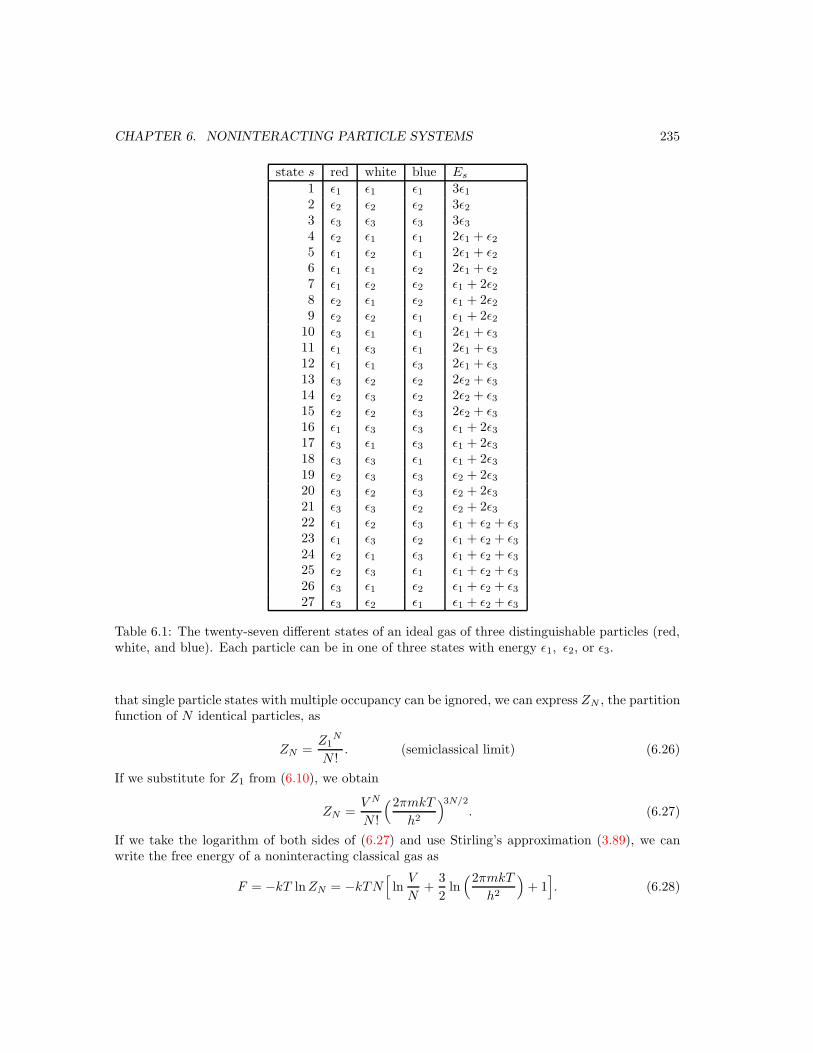
CHAPTER 6. NONINTERACTING PARTICLE SYSTEMS 235

state s red white blue Es

1 ε1 ε1 ε1 3ε12 ε2 ε2 ε2 3ε23 ε3 ε3 ε3 3ε34 ε2 ε1 ε1 2ε1 + ε25 ε1 ε2 ε1 2ε1 + ε26 ε1 ε1 ε2 2ε1 + ε27 ε1 ε2 ε2 ε1 + 2ε28 ε2 ε1 ε2 ε1 + 2ε29 ε2 ε2 ε1 ε1 + 2ε2

10 ε3 ε1 ε1 2ε1 + ε311 ε1 ε3 ε1 2ε1 + ε312 ε1 ε1 ε3 2ε1 + ε313 ε3 ε2 ε2 2ε2 + ε314 ε2 ε3 ε2 2ε2 + ε315 ε2 ε2 ε3 2ε2 + ε316 ε1 ε3 ε3 ε1 + 2ε317 ε3 ε1 ε3 ε1 + 2ε318 ε3 ε3 ε1 ε1 + 2ε319 ε2 ε3 ε3 ε2 + 2ε320 ε3 ε2 ε3 ε2 + 2ε321 ε3 ε3 ε2 ε2 + 2ε322 ε1 ε2 ε3 ε1 + ε2 + ε323 ε1 ε3 ε2 ε1 + ε2 + ε324 ε2 ε1 ε3 ε1 + ε2 + ε325 ε2 ε3 ε1 ε1 + ε2 + ε326 ε3 ε1 ε2 ε1 + ε2 + ε327 ε3 ε2 ε1 ε1 + ε2 + ε3

Table 6.1: The twenty-seven different states of an ideal gas of three distinguishable particles (red,white, and blue). Each particle can be in one of three states with energy ε1, ε2, or ε3.

that single particle states with multiple occupancy can be ignored, we can express ZN , the partitionfunction of N identical particles, as

ZN =Z1

N

N !. (semiclassical limit) (6.26)

If we substitute for Z1 from (6.10), we obtain

ZN =V N

N !

(2πmkT

h2

)3N/2

. (6.27)

If we take the logarithm of both sides of (6.27) and use Stirling’s approximation (3.89), we canwrite the free energy of a noninteracting classical gas as

F = −kT lnZN = −kTN[

lnV

N+

3

2ln

(2πmkT

h2

)

+ 1]

. (6.28)

CHAPTER 6. NONINTERACTING PARTICLE SYSTEMS 236

In Section 6.8 we will use the grand canonical ensemble to obtain the entropy of an idealclassical gas without any ad hoc assumptions such as introducing the factor of N ! and assumingthat the particles are distinguishable. That is, in the grand canonical ensemble we will be able toautomatically satisfy the condition that the particles are indistguishable.

Problem 6.4. Use the result (6.28) to find the pressure equation of state and the mean en-ergy of an ideal gas. Do these relations depend on whether the particles are indistinguishable ordistinguishable?

Problem 6.5. Entropy of an ideal gas

(a) The entropy can be found from the relations, F = E − TS or S = −∂F/∂T . Show that

S(T, V,N) = Nk[

lnV

N+

3

2ln

(2πmkT

h2

)

+5

2

]

. (6.29)

The form of S in (6.29) is known as the Sackur-Tetrode equation (see Problem 4.24). Is thisform of S applicable in the limit of low temperatures?

(b) Express kT in terms of E and show that S(E, V,N) can be expressed as

S(E, V,N) = Nk[

lnV

N+

3

2ln

(4πmE

3Nh2

)

+5

2

]

, (6.30)

in agreement with the result (4.62) found by using the microcanonical ensemble. The form(6.30) of S in terms of its natural variables E, V , and N is known as the fundamental relation

for an ideal classical gas.

Problem 6.6. Order of magnitude estimates

Calculate the entropy of one mole of helium gas at standard temperature and pressure. TakeV = 2.24× 10−2 m3, N = 6.02× 1023, m = 6.65× 10−27 kg, and T = 273K.

Problem 6.7. Use the relation µ = ∂F/∂N and the result (6.28) to show that the chemicalpotential of an ideal classical gas is given by

µ = −kT ln[ V

N

(2πmkT

h2

)3/2]

. (6.31)

We will see in Problem 6.49 that if two systems are placed into contact with different initial chemicalpotentials, particles will go from the system with high chemical potential to the system with lowchemical potential. (This behavior is analogous to energy going from high to low temperatures.)Does “high” chemical potential for an ideal classical gas imply “high” or “low” density?

Problem 6.8. Entropy as an extensive quantity

(a) Because the entropy is an extensive quantity, we know that if we double the volume and doublethe number of particles (thus keeping the density constant), the entropy must double. Thiscondition can be written formally as S(T, λV, λN) = λS(T, V,N). Although this behavior ofthe entropy is completely general, there is no guarantee that an approximate calculation of Swill satisfy this condition. Show that the Sackur-Tetrode form of the entropy of an ideal gasof identical particles, (6.29), satisfies this general condition.

CHAPTER 6. NONINTERACTING PARTICLE SYSTEMS 237

(b) Show that if the N ! term were absent from (6.27) for ZN , S would be given by

S = Nk[

lnV +3

2ln

(2πmkT

h2

)

+3

2

]

. (6.32)

Is this form of S proportional to N for V/N constant?

(c) The fact that (6.32) yields an entropy that is not extensive does not indicate that identicalparticles must be indistinguishable. Instead the problem arises from our identification of Swith lnZ as discussed in Section 4.6. Recall that we considered a system with fixed N andmade the identification (see (4.104))

dS/k = d(lnZ + βE). (6.33)

It is straightforward to integrate (6.33) and obtain

S = k(lnZ + βE) + g(N), (6.34)

where g(N) is an arbitrary function of N only. Although we usually set g(N) = 0, it isimportant to remember that g(N) is arbitrary. What must be the form of g(N) in order thatthe entropy of an ideal classical gas be extensive?

Entropy of mixing. Consider two identical ideal gases at the same temperature T in separateboxes each with the same density. What is the change in entropy of the combined system after thegases are allowed to mix? We can answer this question without doing any calculations. Becausethe particles in each gas are identical, there would be no change in the total entropy. Why? Whatif the gases were not identical? In this case, there would be a change in entropy because removingthe partition between the two boxes is an irreversible process. (Reinserting the partition wouldnot separate the two gases.) In the following we calculate the change in both cases.

Consider two ideal gases at the same temperature T with N1 and N2 particles in boxes ofvolume V1 and V2, respectively. The gases are initially separated by a partition. If we use (6.29)for the entropy, we find

S1 = N1k[

lnV1

N1+ f(T )

]

, (6.35a)

S2 = N2k[

lnV2

N2+ f(T )

]

, (6.35b)

where the function f(T ) = 3/2 ln(2πmkT/h2) + 5/2. We then allow the particles to mix so thatthey fill the entire volume V = V1 + V2. If the particles are identical, the total entropy after theremoval of the partition is given by

S = k(N1 +N2)[

lnV1 + V2

N1 +N2+ f(T )

]

, (6.36)

and the change in the value of S, the entropy of mixing, is given by

∆S = k[

(N1 +N2) lnV1 + V2

N1 +N2−N1 ln

V1

N1−N2 ln

V2

N2

]

. (identical gases) (6.37)

CHAPTER 6. NONINTERACTING PARTICLE SYSTEMS 238

Problem 6.9. For the special case of equal densities of the two gases before separation, use (6.37)to show that ∆S = 0 as expected. (Use the fact that N1 = ρV1 and N2 = ρV2.) Why is theentropy of mixing nonzero for N1 6= N2 and/or V1 6= V2 even though the particles are identical?

If the two gases are not identical, the total entropy after mixing is

S = k[

N1 lnV1 + V2

N1+N2 ln

V1 + V2

N2+ (N1 +N2)f(T )

]

. (6.38)

Then the entropy of mixing becomes

∆S = k[

N1 lnV1 + V2

N1+N2 ln

V1 + V2

N2−N1 ln

V1

N1−N2 ln

V2

N2

]

. (non-identical gases) (6.39)

For the special case of N1 = N2 = N and V1 = V2 = V , we find

∆S = 2Nk ln 2. (6.40)

Explain the result (6.40) in simple terms.

Problem 6.10. What would be the result for the entropy of mixing if we had used the result(6.32) for S instead of (6.29)? Consider the special case of N1 = N2 = N and V1 = V2 = V .

6.3 Classical Systems and the Equipartition Theorem

We have used the microcanonical and canonical ensembles to show that the mean energy of anideal classical gas in three dimensions is given by E = 3kT/2. Similarly, we have found that themean energy of a one-dimensional harmonic oscillator is given by E = kT in the limit of hightemperatures. These results are special cases of the equipartition theorem which can be stated asfollows:

For a classical system in equilibrium with a heat bath at temperature T , the mean value

of each contribution to the total energy that is quadratic in a coordinate equals 12kT .

Note that the equipartition theorem holds regardless of the coefficients of the quadratic terms.

To derive the equipartition theorem, we consider the canonical ensemble and express theaverage of any physical quantity f(r,p) in a classical system by

f =

∫

f(r1, . . . , rN ,p1, . . . ,pN) e−βE(r1,...,rN ,p1,...,pN ) dr1 . . . drN dp1 . . . dpN∫

e−βE(r1,...,rN ,p1,...,pN ) dr1 . . . drN dp1 . . . dpN, (6.41)

where we have used the fact that the probability density of a particular microstate is proportionalto e−βE(r1,...,rN ,p1,...,pN ). Remember that a microstate is defined by the positions and momenta ofevery particle. Classically, the sum over quantum states has been replaced by an integration overphase space.

Suppose that the total energy can be written as a sum of quadratic terms. The most commoncase is the kinetic energy in the nonrelativistic limit. For example, the kinetic energy of one particle

CHAPTER 6. NONINTERACTING PARTICLE SYSTEMS 239

in three dimensions can be expressed as (p2x+p2

y+p2z)/2m. Another example is the one-dimensional

harmonic oscillator for which the total energy is p2x/2m+kx2/2. Let us consider a one-dimensional

system for simplicity, and suppose that the energy of the system can be written as

E = ε1(p1) + E(x1, . . . , xN , p2, . . . , pN ), (6.42)

where ε1 = ap21. We have separated out the quadratic dependence of the energy of particle 1 on

its momentum. We use (6.41) and express the mean value of ε1 in one dimension as

ε1 =

∫ ∞

−∞ε1 e

−βE(x1,...,xN ,p1,...,pN ) dx1 . . . dxN dp1 . . . dpN∫ ∞

−∞e−βE(x1,...,xN ,p1,...,pN ) dx1 . . . dxN dp1 . . . dpN

(6.43a)

=

∫ ∞

−∞ ε1 e−β[ε1+E(x1,...,xN ,p2,...,pN )] dx1 . . . dxN dp1 . . . dpN

∫ ∞

−∞e−β[ε1+E(x1,...,xN ,p2,...,pN )] dx1 . . . dxNdp1 . . . dpN

(6.43b)

=

∫ ∞

−∞ ε1 e−βε1dp1

∫

e−βE dx1 . . . dxN dp2 . . . dpN∫ ∞

−∞e−βε1dp1

∫

e−βE dx1 . . . dxN dp2 . . . dpN

. (6.43c)

The integrals over all the coordinates except p1 cancel, and we have

ε1 =

∫ ∞

−∞ ε1 e−βε1 dp1

∫ ∞

−∞e−βε1 dp1

. (6.44)

Note that we could have written ε1 in the form (6.44) directly without any intermediate steps

because the probability density can be written as a product of two terms – one term that depends

only on p1 and another term that depends on all the other coordinates. As we have done in other

contexts, we can write ε1 as

ε1 = − ∂

∂βln

(

∫ ∞

−∞

e−βε1 dp1

)

. (6.45)

If we substitute ε1 = ap21, the integral in (6.45) becomes

Z =

∫ ∞

−∞

e−βε1dp1 =

∫ ∞

−∞

e−βap2

1 dp1 (6.46a)

= (βa)−1/2

∫ ∞

−∞

e−x2

dx, (6.46b)

where we have let x2 = βap2. Note that the integral in (6.46b) is independent of β. Hence

ε1 = − ∂

∂βlnZ(β) =

1

2kT. (6.47)

Equation (6.47) is an example of the equipartition theorem of classical statistical mechanics.

Problem 6.11. Explain why we could have written (6.44) directly. What is the physical inter-pretation of the integrand in the numerator?

CHAPTER 6. NONINTERACTING PARTICLE SYSTEMS 240

The equipartition theorem is not a theorem and is not a new result. It is applicable only whenthe system can be described classically and is applicable only to each term in the energy that isproportional to a coordinate squared. This coordinate must take on a continuum of values from−∞ to +∞.

Applications of the equipartition theorem. A system of particles in three dimensions has3N quadratic terms in the kinetic energy, three for each particle. From the equipartition theorem,we know that the mean kinetic energy is 3NkT/2, independent of the nature of the interactions,if any, between the particles. Hence, the heat capacity at constant volume of an ideal classicalmonatomic gas is given by CV = 3Nk/2 as found previously.

Another application of the equipartition function is to the one-dimensional harmonic oscillatorin the classical limit. In this case there are two quadratic contributions to the total energy and hencethe mean energy of a classical harmonic oscillator in equilibrium with a heat bath at temperatureT is kT . In the harmonic model of a crystal each atom feels a harmonic or spring-like force dueto its neighboring atoms. The N atoms independently perform simple harmonic oscillations abouttheir equilibrium positions. Each atom contributes three quadratic terms to the kinetic energy andthree quadratic terms to the potential energy. Hence, in the high temperature limit the energy ofa crystal of N atoms is E = 6NkT/2 and the heat capacity at constant volume is

CV = 3Nk. (law of Dulong and Petit) (6.48)

The result (6.48) is known as the law of Dulong and Petit. This result was first discovered empir-ically, is not a law, and is valid only at sufficiently high temperatures. At low temperatures theindependence of CV on T breaks down and a quantum treatment is necessary. The heat capacityof an insulating solid at low temperatures is discussed in Section 6.12.

The result (6.47) implies that the heat capacity of a monatomic classical ideal gas is 3NkT/2.Let us consider a gas consisting of diatomic molecules. Its equation of state is still given byPV = NkT assuming that the molecules do not interact. Why? However, its heat capacitydiffers in general from that of a monatomic gas because a diatomic molecule has additional energyassociated with vibrational and rotational motion. We expect that the two atoms of a diatomicmolecule can vibrate along the line joining them and rotate about their center of mass, in additionto the translational motion of their center of mass. Hence, we would expect that CV for an idealdiatomic gas is greater than CV for a monatomic gas. The heat capacity of a diatomic molecule isexplored in Problem 6.51.

We have seen that it is convenient to do calculations for a fixed number of particles forclassical systems. For this reason we usually calculate the heat capacity of a N particle system orthe specific heat per particle. Experimental chemists usually prefer to give the specific heat as theheat capacity per mole and experimental physicists frequently prefer to give the specific heat asthe heat capacity per kilogram or gram. All three quantities are known as the specific heat andtheir precise meaning is clear from their units and the context.

6.4 Maxwell Velocity Distribution

We now find the distribution of particle velocities in a classical system that is in equilibrium witha heat bath at temperature T . We know that the total energy can be written as the sum of

CHAPTER 6. NONINTERACTING PARTICLE SYSTEMS 241

two parts: the kinetic energy K(p1, . . . ,pN ) and the potential energy U(r1, . . . , rN ). The kineticenergy is a quadratic function of the momenta p1, . . . ,pN (or velocities), and the potential energyis a function of the positions r1, . . . , rN of the particles. We write the total energy as E = K +U .The probability density of a configuration of N particles defined by r1, . . . , rN ,p1, . . . ,pN is givenin the canonical ensemble by

p(r1, . . . , rN ;p1, . . . ,pN) = Ae−[K(p1,p2,...,pN)+U(r1,r2,...,rN )]/kT (6.49a)

= Ae−K(p1,p2,...,pN )/kT e−U(r1,r2,...,rN )/kT , (6.49b)

where A is a normalization constant. Note that the probability density p is a product of twofactors, one that depends only on the particle positions and the other that depends only on theparticle momenta. This factorization implies that the probabilities of the momenta and positionsare independent. For example, the momentum of a particle is not influenced by its position andvice versa. The probability of the positions of the particles can be written as

f(r1, . . . , rN ) dr1 . . . drN = B e−U(r1,...,rN )/kT dr1 . . . drN , (6.50)

and the probability of the momenta is given by

f(p1, . . . ,pN ) dp1 . . . dpN = C e−K(p1,...,pN )/kT dp1 . . . dpN . (6.51)

For simplicity, we have denoted the two probability densities by f , even though their functionalform is different in (6.50) and (6.51). The constants B and C in (6.51) and (6.50) can be found byrequiring that each probability is normalized.

We emphasize that the probability distribution for the momenta does not depend on thenature of the interaction between the particles and is the same for all classical systems at thesame temperature. This statement might seem surprising at first because it might seem that thevelocity distribution should depend on the density of the system. An external potential also doesnot affect the velocity distribution. These statements are not true for quantum systems, because inthis case the position and momentum operators do not commute. That is, e−β(K+U) 6= e−βKe−βU

for quantum systems.

Because the total kinetic energy is a sum of the kinetic energy of each of the particles, theprobability density f(p1, . . . ,pN ) is a product of terms that each depend on the momenta of onlyone particle. This factorization implies that the momentum probabilities of the various particlesare independent, that is, the momentum of one particle does not affect the momentum of anyother particle. These considerations imply that we can write the probability that a particle hasmomentum p in the range dp as

f(px, py, pz) dpxdpydpz = c e−(p2

x+p2

y+p2

z)/2mkT dpxdpydpz . (6.52)

The constant c is given by the normalization condition

c

∫ ∞

−∞

∫ ∞

−∞

∫ ∞

−∞

e−(p2

x+p2

y+p2

z)/2mkT dpxdpydpz = c[

∫ ∞

−∞

e−p2/2mkT dp]3

= 1. (6.53)

If we use the fact that∫ ∞

−∞ e−αx2

dx = (π/α)1/2 (see Appendix A), we find that c = (2πmkT )−3/2.Hence the momentum probability distribution can be expressed as

f(px, py, pz) dpxdpydpz =1

(2πmkT )3/2e−(p2

x+p2

y+p2

z)/2mkT dpxdpydpz. (6.54)

CHAPTER 6. NONINTERACTING PARTICLE SYSTEMS 242

The corresponding velocity probability distribution is given by

f(vx, vy, vz) dvxdvydvz = (m

2πkT)3/2 e−m(v2

x+v2

y+v2

z)/2kT dvxdvydvz . (6.55)

Equation (6.55) is called the Maxwell velocity distribution. Note that it is a Gaussian. Theprobability distribution for the speed is derived in Problem 6.23.

Because f(vx, vy, vz) is a product of three independent factors, the probability of the velocityof a particle in a particular direction is independent of the velocity in any other direction. Forexample, the probability that a particle has a velocity in the x-direction in the range vx to vx +dvx

isf(vx) dvx = (

m

2πkT)1/2 e−mv2

x/2kT dvx. (6.56)

Many textbooks derive the Maxwell velocity distribution for an ideal classical gas and give themistaken impression that the distribution applies only if the particles are noninteracting. We stressthat the Maxwell velocity (and momentum) distribution applies to any classical system regardlessof the interactions, if any, between the particles.

Problem 6.12. Is there an upper limit to the velocity?

The upper limit to the velocity of a particle is the velocity of light. Yet the Maxwell velocitydistribution imposes no upper limit to the velocity. Is this contradiction likely to lead to difficulties?

Problem 6.13. Alternative derivation of the Maxwell velocity distribution

We can also derive the Maxwell velocity distribution by making some plausible assumptions. Wefirst assume that the probability density f(v) for one particle is a function only of its speed |v|or equivalently v2. We also assume that the velocity distributions of the components vx, vy, vz areindependent of each other.

(a) Given these assumptions, explain why we can write

f(v2x + v2

y + v2z) = f(v2

x)f(v2y)f(v2

z). (6.57)

(b) Show that the only mathematical function that satisfies the condition (6.57) is the exponentialfunction

f(v2) = c e−αv2

, (6.58)

where c and α are independent of v.

(c) Determine c in terms of α using the normalization condition 1 =∫ ∞

−∞ f(v)dv for each compo-nent. Why must α be positive?

(d) Use the fact that 12kT = 1

2mv2x to find the result (6.55).

CHAPTER 6. NONINTERACTING PARTICLE SYSTEMS 243

6.5 Occupation Numbers and Bose and Fermi Statistics

We now develop the formalism for calculating the thermodynamic properties of ideal quantumsystems. The absence of interactions between the particles of an ideal gas enables us to reducethe problem of determining the energy levels Es of the gas as a whole to determining εk, theenergy levels of a single particle. Because the particles are indistinguishable, we cannot specifythe microstate of each particle. Instead a microstate of an ideal gas is specified by the occupation

numbers nk, the number of particles in each of the single particle energies εk. If we know the valueof the occupation number for each state, we can write the total energy of the system as

Es =∑

k

nk εk. (6.59)

The set of nk completely specifies a microstate of the system. The partition function for an idealgas can be expressed in terms of the occupation numbers as

Z(V, T,N) =∑

nk

e−βP

k nkεk , (6.60)

where the occupation numbers nk satisfy the condition

N =∑

k

nk. (6.61)

As discussed in Section 4.3.7 one of the fundamental results of relativistic quantum mechanicsis that all particles can be classified into two groups. Particles with zero or integral spin such as 4Heare bosons and have wave functions that are symmetric under the exchange of any pair of particles.Particles with half-integral spin such as electrons, protons, and neutrons are fermions and havewave functions that are antisymmetric under particle exchange. The Bose or Fermi character ofcomposite objects can be found by noting that composite objects that have an even number offermions are bosons and those containing an odd number of fermions are themselves fermions.3 Forexample, an atom of 3He is composed of an odd number of particles: two electrons, two protons,and one neutron each of spin 1

2 . Hence, 3He has half-integral spin making it a fermion. An atomof 4He has one more neutron so there are an even number of fermions and 4He is a boson. Whattype of particle is a hydrogen molecule, H2?

It is remarkable that all particles fall into one of two mutually exclusive classes with differentspin. It is even more remarkable that there is a connection between the spin of a particle andits statistics. Why are particles with half-integral spin fermions and particles with integral spinbosons? The answer lies in the requirements imposed by Lorentz invariance on quantum fieldtheory. This requirement implies that the form of quantum field theory must be the same in allinertial reference frames. Although most physicists believe that the relation between spin andstatistics must have a simpler explanation, no such explanation yet exists.4

3You might have heard of the existence of Bose-like bound pairs of electrons (Cooper pairs) in what is known asthe BCS theory of superconductivity. However such pairs are not composite objects in the usual sense.

4In spite of its fundamental importance, it is only a slight exaggeration to say that “everyone knows the spin-statistics theorem, but no one understands it.”

CHAPTER 6. NONINTERACTING PARTICLE SYSTEMS 244

n1 n2 n3 n4

0 1 1 11 0 1 11 1 0 11 1 1 0

Table 6.2: Possible states of a three particle fermion system with four single particle energy states.The quantity nk represents the number of particles in a single particle state k. Note that we havenot specified which particle is in a particular state.

The difference between fermions and bosons is specified by the possible values of nk. Forfermions we have

nk = 0 or 1. (fermions) (6.62)

The restriction (6.62) states the Pauli exclusion principle for noninteracting particles – two identicalfermions cannot be in the same single particle state. In contrast, the occupation numbers nk foridentical bosons can take any positive integer value:

nk = 0, 1, 2, · · · (bosons) (6.63)

We will see in the following sections that the fermion or boson nature of a many particle systemcan have a profound effect on its properties.

Example 6.1. Calculate the partition function of an ideal gas of N = 3 identical fermions inequilibrium with a heat bath at temperature T . Assume that each particle can be in one of fourpossible states with energies, ε1, ε2, ε3, and ε4.

Solution. The possible microstates of the system are summarized in Table 6.2 with four singleparticle states. The spin of the fermions is neglected. Is it possible to reduce this problem to a onebody problem as we did for a classical noninteracting system?

The partition function is given by

Z3 = e−β(ε2+ε3+ε4) + e−β(ε1+ε3+ε4) + e−β(ε1+ε2+ε4) + e−β(ε1+ε2+ε3). (6.64)

Problem 6.14. Calculate n1, the mean number of fermions in the state with energy ε1, for thesystem in Example 6.1.

Problem 6.15. Calculate the mean energy of an ideal gas of N = 3 identical bosons in equilibriumwith a heat bath at temperature T , assuming that each particle can be in one of three states withenergies, 0, ∆, and 2∆. Is it possible to reduce this problem to a one body problem as we did fora classical noninteracting system?

∗Problem 6.16. Consider a single particle of mass m in a one-dimensional harmonic oscillatorpotential given by V (x) = 1

2kx2. As we found in Example 4.4, the partition function is given by

Z1 = e−x/2/(1 − e−x), where x = β~ω.

(a) What is the partition function Z2d for two noninteracting distinguishable particles in the samepotential?

CHAPTER 6. NONINTERACTING PARTICLE SYSTEMS 245

(b) What is the partition function Z2f,S=0 for two noninteracting fermions in the same potentialassuming the fermions have no spin?

(c) What is the partition function Z2b for two noninteracting bosons in the same potential? Assumethe bosons have spin zero.

∗Problem 6.17. Calculate the mean energy and entropy in the four cases considered in Prob-lem 6.16. Plot E and S as a function of T and compare the behavior of E and S in the limitingcases of T → 0 and T → ∞.

6.6 Distribution Functions of Ideal Bose and Fermi Gases

The calculation of the partition function for an ideal gas in the semiclassical limit was straightfor-ward because we were able to choose a single particle as the system. This choice is not possiblefor an ideal gas at low temperatures where the quantum nature of the particles cannot be ignored.So we need a different strategy. The key idea is that it is possible to distinguish the set of allparticles in a given single particle state from the particles in any other single particle state. Forthis reason we choose the system of interest to be the set of all particles that are in a given single

particle state. Because the number of particles in a given quantum state varies, we need to usethe grand canonical ensemble and assume that each system is populated from a particle reservoirindependently of the other single particle states.

Because we have not used the grand canonical ensemble until now, we briefly review itsnature. The thermodynamic potential in the grand canonical ensemble is denoted by Ω(T, V, µ)and is equal to −PV (see (2.149)). The connection of thermodynamics to statistical mechanics isgiven by Ω = −kT lnZ , where the grand partition function Z is given by

Z =∑

n

e−β(En−µNn). (6.65)

In analogy to the procedure for the canonical ensemble, our goal is to calculate Z , then Ω and thepressure equation of state −PV (in terms of T , V , and µ), and then determine S from the relation

S = −(∂Ω

∂T

)

V,µ, (6.66)

and the mean number of particles from the relation

N = −(∂Ω

∂µ

)

T,V(6.67)

The probability of a particular microstate is given by

pn =1

Z e−β(En−µNn). (Gibbs distribution) (6.68)

We will use all these relations in the following.

CHAPTER 6. NONINTERACTING PARTICLE SYSTEMS 246

The first step in our application of the grand canonical ensemble is to calculate the grandpartition function Zk for all particles in the kth single particle state. Because the energy of the nk

particles in the kth state is nk εk, we can write Zk as

Zk =∑

nk

e−βnk(εk−µ), (6.69)

where the sum is over the possible values of nk. For fermions this sum is straightforward becausenk = 0 and 1 (see (6.62)). Hence

Zk = 1 + e−β(εk−µ). (6.70)

The corresponding thermodynamic or Landau potential, Ωk, is given by

Ωk = −kT lnZk = −kT ln[1 + e−β(εk−µ)]. (6.71)

We can use the relation nk = −∂Ωk/∂µ (see (6.67)) to find the mean number of particles in thekth quantum state. The result is

nk = −∂Ωk

∂µ=

e−β(µ−εk)

1 + e−β(µ−εk), (6.72)

or

nk =1

eβ(εk−µ) + 1. (Fermi-Dirac distribution) (6.73)

The result (6.73) for the mean number of particles in the kth state is known as the Fermi-Dirac

distribution.

The integer values of nk are unrestricted for bosons. We write (6.69) as

Zk = 1 + e−β(εk−µ) + e−2β(εk−µ) + · · · =

∞∑

nk=0

[

e−β(εk−µ)]nk . (6.74)

The geometrical series in (6.74) is convergent for e−β(εk−µ) < 1. Because this condition must besatisfied for all values of εk, we require that eβµ < 1 or

µ < 0. (bosons) (6.75)

In contrast, the chemical potential may be either positive or negative for fermions. The summationof the geometrical series in (6.74) gives

Zk =1

1 − e−β(εk−µ), (6.76)

and hence we obtainΩk = kT ln

[

1 − e−β(εk−µ)]

. (6.77)

The mean number of particles in the kth state is given by

nk = −∂Ωk

∂µ=

e−β(εk−µ)

1 − e−β(εk−µ)(6.78)

or

CHAPTER 6. NONINTERACTING PARTICLE SYSTEMS 247

nk =1

eβ(εk−µ) − 1. (Bose-Einstein distribution) (6.79)

The form (6.79) is known as the Bose-Einstein distribution.

It is frequently convenient to group the Fermi-Dirac and Bose-Einstein distributions togetherand to write

nk =1

eβ(εk−µ) ± 1.

+ Fermi-Dirac distribution

− Bose-Einstein distribution(6.80)

The convention is that the upper sign corresponds to Fermi statistics and the lower sign to Bosestatistics.

The classical limit. The Fermi-Dirac and Bose-Einstein distributions must reduce to the classicallimit under the appropriate conditions. In the classical limit nk 1 for all k, that is, the meannumber of particles in any single particle state must be small. Hence εβ(εk−µ) 1 and in this limitboth the Fermi-Dirac and Bose-Einstein distributions reduce to

nk = e−β(εk−µ) (Maxwell-Boltzmann distribution) (6.81)

This result (6.81) is known as the Maxwell-Boltzmann distribution.

6.7 Single Particle Density of States

If we sum (6.80) over all single particle states, we obtain the mean number of particles in thesystem:

N(T, V, µ) =∑

k

nk =∑

k

1

eβ(εk−µ) ± 1. (6.82)

For a given temperature T and volume V , (6.82) is an implicit equation for the chemical potentialµ in terms of the mean number of particles. That is, the chemical potential determines the meannumber of particles just as the temperature determines the mean energy. Similarly, we can writethe mean energy of the system as

E(T, V, µ) =∑

k

εk nk. (6.83)

Because the (grand) partition function Z is a product, Z =∏

k Zk, the Landau potential for theideal gas is given by

Ω(T, V, µ) =∑

k

Ωk = ∓kT∑

k

ln[

1 ± e−β(εk−µ)]

. (6.84)

For a macroscopic system the number of particles and the energy are well defined, and we willusually replace n and E by N and E respectively.

Because we have described the microscopic states at the most fundamental level, that is, byusing quantum mechanics, we see that the macroscopic averages of interest such as (6.82), (6.83)and (6.84) involve sums rather than integrals over the microscopic states. However, because our

CHAPTER 6. NONINTERACTING PARTICLE SYSTEMS 248

systems of interest are macroscopic, the volume of the system is so large that the energies of thediscrete microstates are very close together and for practical purposes indistinguishable from acontinuum. Because it is easier to do integrals than to do sums over a very large number of states,we wish to replace the sums in (6.82)–(6.84) by integrals. For example, we wish to write for anarbitrary function f(ε)

∑

k

f(εk) →∫ ∞

0

f(ε) g(ε)dε, (6.85)

where g(ε) dε is the number of single particle states between ε and ε + dε. The quantity g(ε) isknown as the density of states, although a better term would be the density of single particle states.

Although we already have calculated the density of states g(ε) for a single particle in a box(see Section 4.3), we review the calculation here to emphasize its generality and the commonaspects of the calculation for black body radiation, elastic waves in a solid, and electron waves.For convenience, we choose the box to be a cube of linear dimension L and assume that the wavefunction vanishes at the faces of the cube. This condition ensures that we will obtain standingwaves. The condition for a standing wave in one dimension is that the wavelength satisfies thecondition

λ =2L

nn = 1, 2, . . . (6.86)

where n is a nonzero positive integer. It is useful to define the wave number k as

k =2π

λ, (6.87)

and write the standing wave condition as k = nπ/L. Because the waves in the x, y, and z directionssatisfy similar conditions, we can treat the wave number as a vector whose components satisfy

k = (nx, ny, nz)π

L, (6.88)

where nx, ny, nz are positive integers. Not all values of k are permissible and each combinationof nx, ny, nz corresponds to a different state. In the “number space” defined by the threeperpendicular axes labeled by nx, ny, and nz, the possible values of states lie at the centersof cubes of unit edge length. These quantum numbers are usually very large for a macroscopicbox, and hence the integers nx, ny, nz and k can be treated as continuous variables.

Because the energy of a wave depends only on the magnitude of k, we want to know thenumber of states between k and k+ dk. As we did in Section 4.3, it is easier to first find Γ(k), thenumber of states with wave number less than or equal to k. We know that the volume in n-spaceof a single state is unity, and hence the number of states in number space that are contained inthe positive octant of a sphere of radius n is given by Γ(n) = 1

8 (4πn3/3), where n2 = n2x +n2

y +n2z.

Because k = πn/L, the number of states with wave vector less than or equal to k is

Γ(k) =1

8

4πk3/3

(π/L)3. (6.89)

If we use the relation

g(k) dk = Γ(k + dk) − Γ(k) =dΓ(k)

dkdk, (6.90)

CHAPTER 6. NONINTERACTING PARTICLE SYSTEMS 249

we obtain

g(k) dk = Vk2dk

2π2, (6.91)

where the volume V = L3. Equation (6.91) gives the density of states in k-space between k andk + dk.

Although we obtained the result (6.91) for a cube, the result is independent of the shape ofthe enclosure and the nature of the boundary conditions (see Problem 6.47). That is, if the box issufficiently large, the surface effects introduced by the box do not affect the physical properties ofthe system.

Problem 6.18. Find the form of the density of states in k-space for standing waves in a two-dimensional and in a one-dimensional box.

6.7.1 Photons

The result (6.91) for the density of states in k-space holds for any wave in a three-dimensionalenclosure. Now we wish to find the number of states g(ε) dε as a function of the energy ε. Weadopt the same symbol to represent the density of states in k-space and in ε-space because theinterpretation of g will be clear from the context.

The form of g(ε) depends on how the energy depends on k. For electromagnetic waves offrequency ν, we know that λν = c, ω = 2πν, and k = 2π/λ. Hence, ω = 2πc/λ or

ω = ck. (6.92)

The energy ε of a photon of frequency ω is

ε = ~ω = ~ck. (6.93)

Because k = ε/~c, we find that

g(ε) dε = Vε2

2π2~3c3dε. (6.94)

The result (6.94) requires one modification. The state of an electromagnetic wave or photondepends not only on its wave vector or momentum, but also on its polarization. There are twomutually perpendicular directions of polarization (right circularly polarized and left circularlypolarized) for each electromagnetic wave of wave number k.5 Thus the number of photon statesin which the photon has a energy in the range ε to ε+ dε is given by

g(ε) dε = Vε2dε

π2~3c3. (photons) (6.95)

5In the language of quantum mechanics we say that the photon has spin one and two helicity states. The factthat the photon has spin S = 1 and two rather than (2S +1) = 3 helicity states is a consequence of special relativityfor massless particles.

CHAPTER 6. NONINTERACTING PARTICLE SYSTEMS 250

6.7.2 Electrons

For a nonrelativistic particle of mass m, we know that

ε =p2

2m. (6.96)

From the relations p = h/λ and k = 2π/λ, we find that the momentum p of a particle is related toits wave vector k by p = ~k. Hence, the energy can be expressed as

ε =~

2k2

2m, (6.97)

and

dε =~

2k

mdk. (6.98)

If we use the relations (6.97) and (6.98), we find that the number of states in the interval ε to ε+dεis given by

g(ε) dε = nsV

4π2~3(2m)3/2 ε1/2 dε. (6.99)

We have included a factor of ns, the number of spin states for a given value of k or ε. Becauseelectrons have spin 1/2, ns = 2, and we can write (6.99) as

g(ε) dε =V

2π2~3(2m)3/2 ε1/2 dε. (electrons) (6.100)

Because it is common to choose units such that ~ = 1, we will express most of our results in theremainder of this chapter in terms of ~ instead of h.

Problem 6.19. Calculate the energy density of states for a nonrelativistic particle of mass m ind = 1 and d = 2 spatial dimensions (see Problem 6.18). Sketch g(ε) on one graph for d = 1, 2,and 3 and comment on the dependence of g(ε) on ε for different spatial dimensions.

Problem 6.20. Calculate the energy density of states for a relativistic particle of rest mass m forwhich ε2 = p2c2 +m2c4.

Problem 6.21. The relation between the energy and equation of state for an ideal gas

The mean energy E is given by

E =

∫ ∞

0

εn(ε) g(ε) dε (6.101a)

= nsV

4π2~3(2m)3/2

∫ ∞

0

ε3/2dε

eβ(ε−µ) ± 1. (6.101b)

Use (6.84) for the Landau potential and (6.99) for the density of states of nonrelativistic particlesin three dimensions to show that Ω can be expressed as

Ω = ∓kT∫ ∞

0

g(ε) ln[1 ± e−β(ε−µ)] dε, (6.102a)

= ∓kT nsV

4π2~3(2m)3/2

∫ ∞

0

ε1/2 ln[1 ± e−β(ε−µ)] dε. (6.102b)

CHAPTER 6. NONINTERACTING PARTICLE SYSTEMS 251

Integrate (6.102b) by parts with u = ln[1 ± e−β(ε−µ)] and dv = ε1/2 dε and show that

Ω = −2

3ns

V

4π2~3(2m)3/2

∫ ∞

0

ε3/2 dε

eβ(ε−µ) ± 1. (6.103)

The form (6.101b) for E is the same as the general result (6.103) for Ω except for the factor of − 23 .

Because Ω = −PV (see (2.149)), we obtain

PV =2

3E. (6.104)

The relation (6.104) is exact and holds for an ideal gas with any statistics at any temperature T ,and depends only on the nonrelativistic relation, ε = p2/2m.

Problem 6.22. The relation between the energy and equation of state for photons

Use similar considerations as in Problem 6.21 to show that for photons:

PV =1

3E. (6.105)

Equation (6.105) holds at any temperature and is consistent with Maxwell’s equations which impliesthat the pressure due to an electromagnetic wave is related to the energy density by P = u(T )/3.

The distribution of speeds in a classical system of particles can be found from (6.55). As wedid previously, we need to know the number of states between v and v+dv. This number is simply4π(v + ∆v)3/3 − 4πv3/3 → 4πv2∆v in the limit ∆v → 0. Hence, the probability that a particlehas a speed between v and v + dv is given by

f(v)dv = 4πAv2e−mv2/2kT dv, (6.106)

where A is a normalization constant which we obtain in Problem 6.23.

Problem 6.23. Maxwell speed distribution

(a) Compare the form of (6.106) with (6.91).

(b) Use the fact that∫ ∞

0 f(v) dv = 1 to calculate A and show that

f(v)dv = 4πv2(m

2πkT)3/2e−mv2/2kT dv. (Maxwell speed distribution) (6.107)

(c) Calculate the mean speed v, the most probable speed v, and the root-mean square speed vrms

and discuss their relative magnitudes.

Make the change of variables u = v/√

(2kT/m) and show that

f(v)dv = f(u)du = (4/√π)u2e−u2

du, (6.108)

where again we have used same the same notation for two different, but physically relatedprobability densities. The (dimensionless) speed probability density f(u) is shown in Figure 6.1.

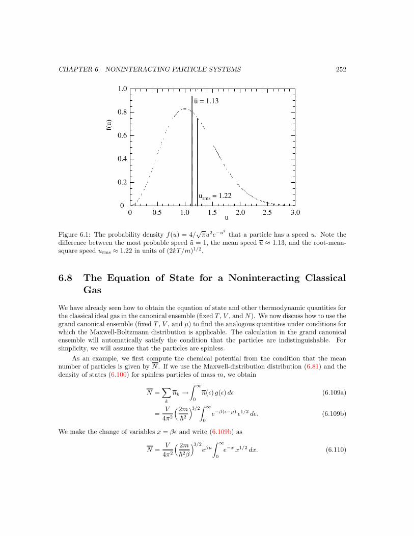
CHAPTER 6. NONINTERACTING PARTICLE SYSTEMS 252

0

0.2

0.4

0.6

0.8

1.0

0 0.5 1.0 1.5 2.0 2.5 3.0u

f(u)

u = 1.13

urms = 1.22

Figure 6.1: The probability density f(u) = 4/√πu2e−u2

that a particle has a speed u. Note thedifference between the most probable speed u = 1, the mean speed u ≈ 1.13, and the root-mean-square speed urms ≈ 1.22 in units of (2kT/m)1/2.

6.8 The Equation of State for a Noninteracting Classical

Gas

We have already seen how to obtain the equation of state and other thermodynamic quantities forthe classical ideal gas in the canonical ensemble (fixed T , V , andN). We now discuss how to use thegrand canonical ensemble (fixed T , V , and µ) to find the analogous quantities under conditions forwhich the Maxwell-Boltzmann distribution is applicable. The calculation in the grand canonicalensemble will automatically satisfy the condition that the particles are indistinguishable. Forsimplicity, we will assume that the particles are spinless.

As an example, we first compute the chemical potential from the condition that the meannumber of particles is given by N . If we use the Maxwell-distribution distribution (6.81) and thedensity of states (6.100) for spinless particles of mass m, we obtain

N =∑

k

nk →∫ ∞

0

n(ε) g(ε) dε (6.109a)

=V

4π2

(2m

~2

)3/2∫ ∞

0

e−β(ε−µ) ε1/2 dε. (6.109b)

We make the change of variables x = βε and write (6.109b) as

N =V

4π2

( 2m

~2β

)3/2

eβµ

∫ ∞

0

e−x x1/2 dx. (6.110)

CHAPTER 6. NONINTERACTING PARTICLE SYSTEMS 253

The integral in (6.110) can be done analytically (make the change of variables x = y2) and has the

value π1

2 /2 (see Appendix A). Hence, the mean number of particles is given by

N(T, V, µ) = V( m

2π~2β

)3/2eβµ. (6.111)

Because we cannot easily measure µ, we are not satisfied with knowing the function N(T, V, µ).Instead, we can find the value of µ that yields the desired value of N by solving (6.111) for thechemical potential:

µ = kT ln[N

V

(2π~2β

m

)3/2]. (6.112)

What is the difference, if any, between (6.111) and the result (6.31) for µ found in the canonicalensemble?

Problem 6.24. Estimate the chemical potential of a monatomic ideal gas at room temperature.

As we saw in Section 2.21, the chemical potential is the change in each of the thermodynamicpotentials when one particle is added. It might be expected that µ > 0, because it should costenergy to add a particle. On the other hand, because the particles do not interact, perhaps µ = 0?So why is µ 0 for a classical ideal gas? The reason is that we have to determine how muchenergy must be added to the system to keep the entropy and the volume fixed. Suppose that weadd one particle with zero kinetic energy. Because the gas is ideal, there is no potential energy ofinteraction. However, because V is fixed, the addition of an extra particle leads to an increase inS. (S is an increasing function of N and V .) Because S also is an increasing function of the totalenergy, we have to reduce the energy.

The calculation of N(T, V, µ) leading to (6.111) was not necessary because we can calculatethe equation of state and all the thermodynamic quantities from the Landau potential Ω. Wecalculate Ω from (6.84) by noting that eβµ 1 and approximating the argument of the logarithmby ln (1 ± x) ≈ ±x. We find that

Ω = ∓kT∑

k

ln[

1 ± e−β(εk−µ)]

(6.113a)

→ −kT∑

k

e−β(εk−µ). (semiclassical limit) (6.113b)

As expected, the form of Ω in (6.113b) is independent of whether we started with Bose or Fermistatistics.

As usual, we replace the sum over the single particle states by an integral over the density ofstates and find

Ω = −kT eβµ

∫ ∞

0

g(ε) e−βε dε (6.114a)

= −kT V

4π2~3

(2m

β

)3/2eβµ

∫ ∞

0

x1/2 e−x dx (6.114b)

= −k V

β5/2

( m

2π~2

)3/2eβµ. (6.114c)

CHAPTER 6. NONINTERACTING PARTICLE SYSTEMS 254

If we substitute λ = (2πβ~2/m)1/2, we find

Ω = −kT Vλ3

eβµ. (6.115)

From the relation Ω = −PV (see (2.149)), we obtain

P =kT

λ3eβµ. (6.116)

If we use the thermodynamic relation (6.67), we obtain

N = −∂Ω

∂µ

∣

∣

∣

V,T=V

λ3eβµ. (6.117)

The usual classical equation of state, PV = NkT , is obtained by using (6.117) to eliminate µ. Thesimplest way of finding the energy is to use the relation (6.104).

We can find the entropy S(T, V, µ) using (6.115) and (6.66):

S(T, V, µ) = −∂Ω

∂T

∣

∣

∣

V,µ= kβ2 ∂Ω

∂β(6.118a)

= V kβ2[ 5

2β7/2− µ

β6/2

]

( m

2π~2

)3/2eβµ. (6.118b)

If we eliminate µ from (6.118b), we obtain the Sackur-Tetrode expression for the entropy of anideal gas:

S(T, V,N) = Nk[5

2− ln

N

V− ln

(2π~2

mkT

)3/2]. (6.119)

We have written N rather than N in (6.119). Note that we did not have to introduce any ex-tra factors of N ! as we did in Section 6.2, because we already correctly counted the number ofmicrostates.

Problem 6.25. Complete the missing steps and derive the ideal gas equations of state.

Problem 6.26. Show that N can be expressed as

N =V

λ3eβµ, (6.120)

and hence

µ(T, V ) = −kT ln1

ρλ3, (6.121)

where ρ = N/V .

Problem 6.27. In Section 6.2 we argued that the semiclassical limit λ ρ−1/3 (see (6.1)) impliesthat nk 1, that is, the mean number of particles that are in any single particle energy state isvery small. Use the expression (6.121) for µ and (6.81) for nk to show that the condition nk 1implies that λ ρ−1/3.

CHAPTER 6. NONINTERACTING PARTICLE SYSTEMS 255

6.9 Black Body Radiation

We can regard electromagnetic radiation as equivalent to a system of noninteracting bosons (pho-tons), each of which has an energy hν, where ν is the frequency of the radiation. If the radiation isin an enclosure, equilibrium will be established and maintained by the interactions of the photonswith the atoms of the wall in the enclosure. Because the atoms emit and absorb photons, the totalnumber of photons is not conserved.

One of the important observations that led to the development of quantum theory was theconsideration of the frequency spectrum of electromagnetic radiation from a black body. If a bodyin thermal equilibrium emits electromagnetic radiation, then this radiation is described as blackbody radiation and the object is said to be a black body. This statement does not mean thatthe body is actually black. The word “black” indicates that the radiation is perfectly absorbedand re-radiated by the object. The spectrum of light radiated by such an idealized black bodyis described by a universal spectrum called the Planck spectrum, which we will derive in thefollowing (see (6.129)). The nature of the spectrum depends only on the absolute temperature Tof the radiation.

The physical system that most closely gives the spectrum of a black body is the spectrumof the cosmic microwave background.6 The observed cosmic microwave background spectrum fitsthe theoretical spectrum of a black body better than the best black body spectrum that we canmake in a laboratory! In contrast, a piece of hot, glowing firewood, for example, is not really inthermal equilibrium, and the spectrum of glowing embers is only a crude approximation to blackbody spectrum. The existence of the cosmic microwave background spectrum and its fit to theblack body spectrum is compelling evidence that the universe experienced a Big Bang.

We can derive the Planck radiation law using either the canonical or grand canonical ensemblebecause the photons are continuously absorbed and emitted by the walls of the container and hencetheir number is not conserved. Let us first consider the canonical ensemble, and consider a gas ofphotons in equilibrium with a heat bath at temperature T . The total energy of the system is givenby E = n1ε1 + n2ε2 + . . ., where nk is the number of photons with energy εk. Because there is no

6The universe is filled with electromagnetic radiation with a distribution of frequencies given by (6.129) withT ≈ 2.73 K. The existence of this background radiation is a remnant from a time when the universe was composedprimarily of electrons and protons at a temperature of about 4000 K. This plasma of electrons and protons interactedstrongly with the electromagnetic radiation over a wide range of frequencies, so that the matter and the radiationreached thermal equilibrium. By the time that the universe had cooled to 3000 K, the matter was primarily inthe form of atomic hydrogen, which interacts with radiation only at the frequencies of the hydrogen spectral lines.As a result most of the radiation energy was effectively decoupled from matter. Electromagnetic radiation, suchas starlight, radiated by matter since the decoupling, is superimposed on the cosmic black body radiation. Moreinformation about the cosmic microwave background can be found at <www.astro.ubc.ca/people/scott/cmb.html>and at many other sites.

CHAPTER 6. NONINTERACTING PARTICLE SYSTEMS 256

constraint on the total number of photons, we can write the canonical partition function as

Z(T, V ) =∑

s

e−βEs =

∞∑

n1,n2,...=0

e−β(n1ε1+n2ε2+ ...) (6.122a)

=

∞∑

n1=0

e−βn1ε1

∞∑

n2=0

e−βn2ε2 . . . (6.122b)

=∏

k

[

∞∑

nk=0

e−βnkεk

]

. (6.122c)

The lack of a constraint means that we can do the sum over each occupation number separately.Because the term in brackets in (6.122c) is a geometrical series, we obtain

Z(T, V ) =∏

k

[ 1

1 − e−βεk

]

. (photon gas) (6.123)

A quantity of particular interest is the mean number of photons in state k. In the canonicalensemble we have

nk =

∑

s nk e−βEs

∑

s e−βEs

=

∑

n1,n2,... nk e−β(n1ε1+n2ε2+...+nkεk+...)

Z(6.124a)

=1

Z

[ ∂

∂(−βεk)

∑

n1,n2,...

e−β(n1ε1+n2ε2+···+nkεk+...)]

(6.124b)

=∂ lnZ

∂(−βεk). (6.124c)

Because the logarithm of a product of terms equals the sum of the logarithms of each term, wehave from (6.123) and (6.124c)

nk =∂

∂(−βεk)

[

∑

k′

− ln (1 − e−βεk′ )]

(6.125a)

=e−βεk

1 − e−βεk, (6.125b)

or

nk =1

eβεk − 1. (Planck distribution) (6.125c)

If we compare the form of (6.125c) with the general Bose-Einstein distribution in (6.79), wesee that the two expressions agree if we set µ = 0. This result can be understood by simple con-siderations. As we have mentioned, equilibrium is established and maintained by the interactionsbetween the photons and the atoms of the wall in the enclosure. The number N of photons in thecavity cannot be imposed externally on the system and is fixed by the temperature T of the wallsand the volume V enclosed. Hence, the free energy F for photons cannot depend on N becausethe latter is not a thermodynamic variable, and we have µ = ∂F/∂N = 0. If we substitute µ = 0

CHAPTER 6. NONINTERACTING PARTICLE SYSTEMS 257

into the general result (6.79) for noninteracting bosons, we find that the mean number of photonsin state k is given by

nk =1

eβhν − 1, (6.126)

in agreement with (6.125c). That is, the photons in blackbody radiation are bosons whose chemicalpotential is zero. The role of the chemical potential is to set the mean number of particles, justas the temperature sets the mean energy. However, the chemical potential has no role to play fora system of photons in black body radiation. So we could have just started with (6.79) for nk inthe grand canonical ensemble and set µ = 0.

Planck’s theory of black body radiation follows from the form of the density of states forphotons found in (6.95). The number of photons with energy in the range ε to ε+ dε is given by

N(ε) dε = n(ε)g(ε) dε =V

π2~3c3ε2 dε

eβε − 1. (6.127)

(For simplicity, we have ignored the polarization of the electromagnetic radiation, and hence thespin of the photons.) If we substitute ε = hν in the right-hand side of (6.127), we find that thenumber of photons in the frequency range ν to ν + dν is given by

N(ν) dν =8πV

c3ν2 dν

eβhν − 1. (6.128)

The distribution of radiated energy is obtained by multiplying (6.128) by hν:

E(ν)dν = hνN(ν) dν =8πhV ν3

c3dν

eβhν − 1. (6.129)

Equation (6.129) gives the energy radiated by a black body of volume V in the frequency rangebetween ν and ν + dν. The energy per unit volume u(ν) is given by

u(ν) =8πhν3

c31

eβhν − 1. (Planck’s radiation law) (6.130)

We can change variables to ε = hν and write the energy density as

u(ε) =8π

(hc)3ε3

eε/kT − 1. (6.131)

The temperature dependence of u(ε) is shown in Figure 6.2.

Problem 6.28. Wien’s displacement law

The maximum of u(ν) shifts to higher frequencies with increasing temperature. Show that themaximum of u can be found by solving the equation

(3 − x)ex = 3, (6.132)

where x = βhνmax. Solve (6.132) numerically for x and show that

hνmax

kT= 2.822. (Wien’s displacement law) (6.133)

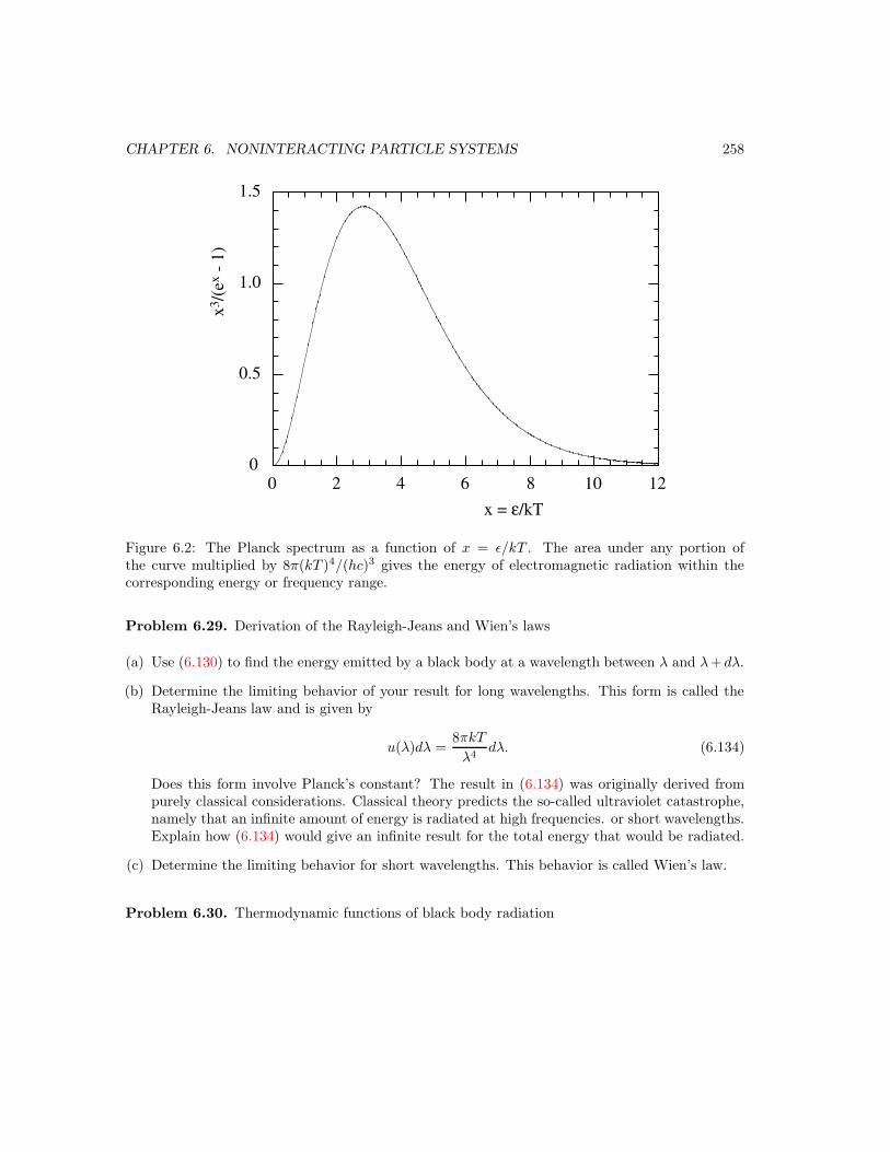
CHAPTER 6. NONINTERACTING PARTICLE SYSTEMS 258

0

0.5

1.0

1.5

0 2 4 6 8 10 12 x = ε/kT

x3/(

ex -

1)

Figure 6.2: The Planck spectrum as a function of x = ε/kT . The area under any portion ofthe curve multiplied by 8π(kT )4/(hc)3 gives the energy of electromagnetic radiation within thecorresponding energy or frequency range.

Problem 6.29. Derivation of the Rayleigh-Jeans and Wien’s laws

(a) Use (6.130) to find the energy emitted by a black body at a wavelength between λ and λ+ dλ.

(b) Determine the limiting behavior of your result for long wavelengths. This form is called theRayleigh-Jeans law and is given by

u(λ)dλ =8πkT

λ4dλ. (6.134)

Does this form involve Planck’s constant? The result in (6.134) was originally derived frompurely classical considerations. Classical theory predicts the so-called ultraviolet catastrophe,namely that an infinite amount of energy is radiated at high frequencies. or short wavelengths.Explain how (6.134) would give an infinite result for the total energy that would be radiated.

(c) Determine the limiting behavior for short wavelengths. This behavior is called Wien’s law.

Problem 6.30. Thermodynamic functions of black body radiation

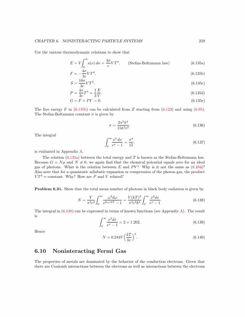
CHAPTER 6. NONINTERACTING PARTICLE SYSTEMS 259

Use the various thermodynamic relations to show that

E = V

∫ ∞

0

u(ν) dν =4σ

cV T 4. (Stefan-Boltzmann law) (6.135a)

F = −4σ

3cV T 4. (6.135b)

S =16σ

3cV T 3. (6.135c)

P =4σ

3cT 4 =

1

3

E

V. (6.135d)

G = F + PV = 0. (6.135e)

The free energy F in (6.135b) can be calculated from Z starting from (6.123) and using (6.95).The Stefan-Boltzmann constant σ is given by

σ =2π5k4

15h3c2. (6.136)

The integral∫ ∞

0

x3 dx

ex − 1=π4

15. (6.137)

is evaluated in Appendix A.

The relation (6.135a) between the total energy and T is known as the Stefan-Boltzmann law.Because G = Nµ and N 6= 0, we again find that the chemical potential equals zero for an idealgas of photons. What is the relation between E and PV ? Why is it not the same as (6.104)?Also note that for a quasistatic adiabatic expansion or compression of the photon gas, the productV T 3 = constant. Why? How are P and V related?

Problem 6.31. Show that the total mean number of photons in black body radiation is given by

N =V

π2c3

∫ ∞

0

ω2dω

e~ω/kT − 1=V (kT )3

π2c3~3

∫ ∞

0

x2dx

ex − 1. (6.138)

The integral in (6.138) can be expressed in terms of known functions (see Appendix A). The resultis

∫ ∞

0

x2dx

ex − 1= 2 × 1.202. (6.139)

Hence

N = 0.244V(kT

~c

)3

. (6.140)

6.10 Noninteracting Fermi Gas

The properties of metals are dominated by the behavior of the conduction electrons. Given thatthere are Coulomb interactions between the electrons as well as interactions between the electrons

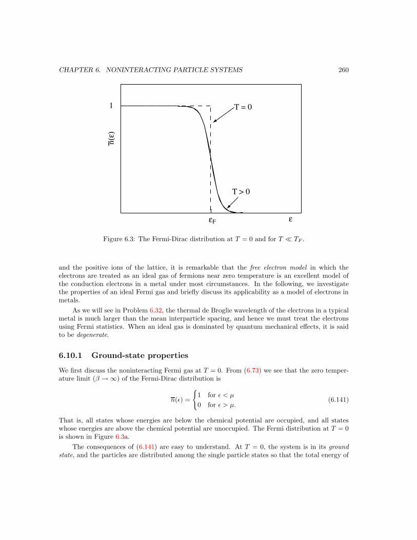
CHAPTER 6. NONINTERACTING PARTICLE SYSTEMS 260

εF ε

n(ε)

T = 0

T > 0

1

Figure 6.3: The Fermi-Dirac distribution at T = 0 and for T TF .

and the positive ions of the lattice, it is remarkable that the free electron model in which theelectrons are treated as an ideal gas of fermions near zero temperature is an excellent model ofthe conduction electrons in a metal under most circumstances. In the following, we investigatethe properties of an ideal Fermi gas and briefly discuss its applicability as a model of electrons inmetals.

As we will see in Problem 6.32, the thermal de Broglie wavelength of the electrons in a typicalmetal is much larger than the mean interparticle spacing, and hence we must treat the electronsusing Fermi statistics. When an ideal gas is dominated by quantum mechanical effects, it is saidto be degenerate.

6.10.1 Ground-state properties

We first discuss the noninteracting Fermi gas at T = 0. From (6.73) we see that the zero temper-ature limit (β → ∞) of the Fermi-Dirac distribution is

n(ε) =

1 for ε < µ

0 for ε > µ.(6.141)

That is, all states whose energies are below the chemical potential are occupied, and all stateswhose energies are above the chemical potential are unoccupied. The Fermi distribution at T = 0is shown in Figure 6.3a.

The consequences of (6.141) are easy to understand. At T = 0, the system is in its ground

state, and the particles are distributed among the single particle states so that the total energy of

CHAPTER 6. NONINTERACTING PARTICLE SYSTEMS 261

the gas is a minimum. Because we may place no more than one particle in each state, we needto construct the ground state of the system by adding a particle, one at a time, into the lowestavailable energy state until we have placed all the particles. To find the value of µ(T = 0) ≡ εF ,we write

N =

∫ ∞

0

n(ε) g(ε) dε →T→0

∫ µ(T=0)

0

g(ε) dε = V

∫ εF

0

(2m)3/2

2π2~3ε1/2 dε. (6.142)

We have substituted the electron density of states (6.100) in (6.142). The upper limit εF in (6.142)is equal to µ(T = 0) and is determined by requiring the integral to give the desired number ofparticles N . We find that

N =V

3π2

(2mεF~2

)3/2

. (6.143)

The energy of the highest occupied state is called the Fermi energy εF and the correspondingFermi momentum is pF =

√2mεF . From (6.143) we have that

εF =~

2

2m(3π2ρ)2/3, (6.144)

where the density ρ = N/V . It follows that the Fermi momentum is given by

pF = (3π2ρ)1/3~. (6.145)

At T = 0 all the states with momentum less that pF are occupied and all the states above thismomentum are unoccupied. The boundary in momentum space between occupied and unoccupiedstates at T = 0 is called the Fermi surface. For an ideal Fermi gas, the Fermi surface is the surfaceof a sphere with radius pF . Note that the Fermi momentum can be estimated by assuming the deBroglie relation p = h/λ and taking λ ∼ ρ−1/3, the mean distance between particles. That is, theparticles are “localized” within a box of order ρ−1/3.

The chemical potential at T = 0 equals εF and is positive. On the other hand, in Section 6.8 weargued in that µ should be a negative quantity for a classical ideal gas, because we have to subtractenergy to keep the entropy from increasing when we add a particle to the system. However, thisargument depends on the possibility of adding a particle with zero energy. In a Fermi system atT = 0, no particle can be added with energy less than µ(T = 0), and hence µ(T = 0) > 0.

We will find it convenient in the following to introduce a characteristic temperature, the Fermitemperature TF , by

TF = εF /k. (6.146)

The order of magnitude of TF for typical metals is estimated in Problem 6.32.

A direct consequence of the fact that the density of states in three dimensions is proportionalto ε1/2 is that the mean energy per particle is 3εF/5:

E

N=

∫ εF

0 ε g(ε) dε∫ εF

0g(ε) dε

=

∫ εF

0 ε3/2dε∫ εF

0ε1/2dε

(6.147a)

=25ε

5/2F

23ε

3/2F

=3

5εF . (6.147b)

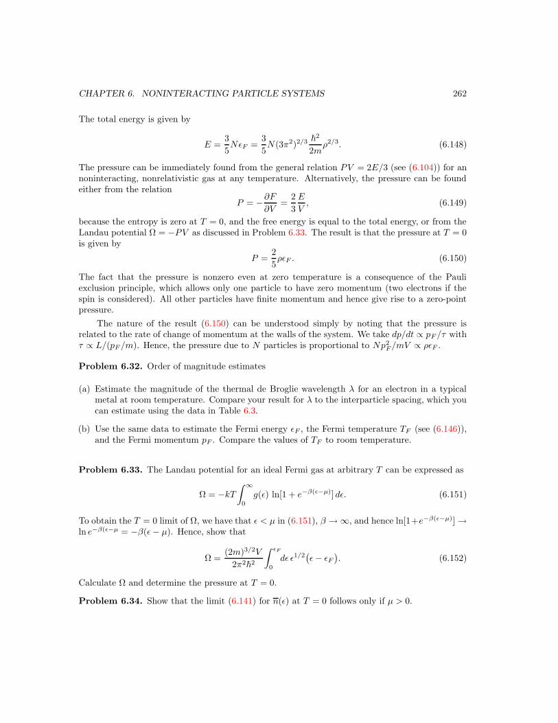
CHAPTER 6. NONINTERACTING PARTICLE SYSTEMS 262

The total energy is given by

E =3

5NεF =

3

5N(3π2)2/3 ~

2

2mρ2/3. (6.148)

The pressure can be immediately found from the general relation PV = 2E/3 (see (6.104)) for annoninteracting, nonrelativistic gas at any temperature. Alternatively, the pressure can be foundeither from the relation

P = −∂F∂V

=2

3

E

V, (6.149)

because the entropy is zero at T = 0, and the free energy is equal to the total energy, or from theLandau potential Ω = −PV as discussed in Problem 6.33. The result is that the pressure at T = 0is given by

P =2

5ρεF . (6.150)

The fact that the pressure is nonzero even at zero temperature is a consequence of the Pauliexclusion principle, which allows only one particle to have zero momentum (two electrons if thespin is considered). All other particles have finite momentum and hence give rise to a zero-pointpressure.

The nature of the result (6.150) can be understood simply by noting that the pressure isrelated to the rate of change of momentum at the walls of the system. We take dp/dt ∝ pF /τ withτ ∝ L/(pF /m). Hence, the pressure due to N particles is proportional to Np2

F/mV ∝ ρεF .

Problem 6.32. Order of magnitude estimates

(a) Estimate the magnitude of the thermal de Broglie wavelength λ for an electron in a typicalmetal at room temperature. Compare your result for λ to the interparticle spacing, which youcan estimate using the data in Table 6.3.

(b) Use the same data to estimate the Fermi energy εF , the Fermi temperature TF (see (6.146)),and the Fermi momentum pF . Compare the values of TF to room temperature.

Problem 6.33. The Landau potential for an ideal Fermi gas at arbitrary T can be expressed as

Ω = −kT∫ ∞

0

g(ε) ln[1 + e−β(ε−µ)] dε. (6.151)

To obtain the T = 0 limit of Ω, we have that ε < µ in (6.151), β → ∞, and hence ln[1+e−β(ε−µ)] →ln e−β(ε−µ = −β(ε− µ). Hence, show that

Ω =(2m)3/2V

2π2~2

∫ εF

0

dε ε1/2(

ε− εF)

. (6.152)

Calculate Ω and determine the pressure at T = 0.

Problem 6.34. Show that the limit (6.141) for n(ε) at T = 0 follows only if µ > 0.

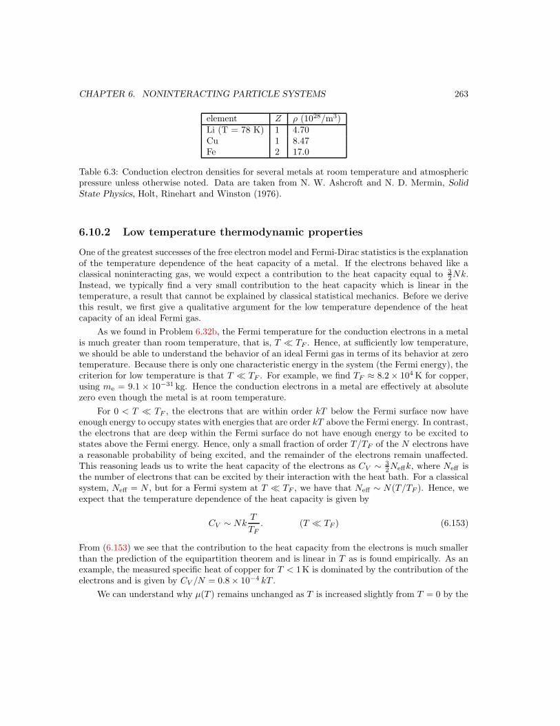
CHAPTER 6. NONINTERACTING PARTICLE SYSTEMS 263

element Z ρ (1028/m3)Li (T = 78 K) 1 4.70Cu 1 8.47Fe 2 17.0

Table 6.3: Conduction electron densities for several metals at room temperature and atmosphericpressure unless otherwise noted. Data are taken from N. W. Ashcroft and N. D. Mermin, Solid

State Physics, Holt, Rinehart and Winston (1976).

6.10.2 Low temperature thermodynamic properties

One of the greatest successes of the free electron model and Fermi-Dirac statistics is the explanationof the temperature dependence of the heat capacity of a metal. If the electrons behaved like aclassical noninteracting gas, we would expect a contribution to the heat capacity equal to 3

2Nk.Instead, we typically find a very small contribution to the heat capacity which is linear in thetemperature, a result that cannot be explained by classical statistical mechanics. Before we derivethis result, we first give a qualitative argument for the low temperature dependence of the heatcapacity of an ideal Fermi gas.

As we found in Problem 6.32b, the Fermi temperature for the conduction electrons in a metalis much greater than room temperature, that is, T TF . Hence, at sufficiently low temperature,we should be able to understand the behavior of an ideal Fermi gas in terms of its behavior at zerotemperature. Because there is only one characteristic energy in the system (the Fermi energy), thecriterion for low temperature is that T TF . For example, we find TF ≈ 8.2 × 104 K for copper,using me = 9.1 × 10−31 kg. Hence the conduction electrons in a metal are effectively at absolutezero even though the metal is at room temperature.

For 0 < T TF , the electrons that are within order kT below the Fermi surface now haveenough energy to occupy states with energies that are order kT above the Fermi energy. In contrast,the electrons that are deep within the Fermi surface do not have enough energy to be excited tostates above the Fermi energy. Hence, only a small fraction of order T/TF of the N electrons havea reasonable probability of being excited, and the remainder of the electrons remain unaffected.This reasoning leads us to write the heat capacity of the electrons as CV ∼ 3

2Neffk, where Neff isthe number of electrons that can be excited by their interaction with the heat bath. For a classicalsystem, Neff = N , but for a Fermi system at T TF , we have that Neff ∼ N(T/TF ). Hence, weexpect that the temperature dependence of the heat capacity is given by

CV ∼ NkT

TF. (T TF ) (6.153)

From (6.153) we see that the contribution to the heat capacity from the electrons is much smallerthan the prediction of the equipartition theorem and is linear in T as is found empirically. As anexample, the measured specific heat of copper for T < 1K is dominated by the contribution of theelectrons and is given by CV /N = 0.8 × 10−4 kT .

We can understand why µ(T ) remains unchanged as T is increased slightly from T = 0 by the

CHAPTER 6. NONINTERACTING PARTICLE SYSTEMS 264

not done

Figure 6.4: The area under the step function is approximately equal to the area under the contin-uous function, that is, the areas of the two cross-hatched areas are approximately equal.

following reasoning. The probability that a state is empty is

1 − n(ε) = 1 − 1

eβ(ε−µ) + 1=

1

eβ(µ−ε) + 1. (6.154)

We see from (6.154) that for a given distance from µ, the probability that a particle is lost from apreviously occupied state below µ equals the probability that an previously empty state is occupied:n(ε− µ) = 1 − n(µ− ε). This property implies that the area under the step function at T = 0 isnearly the same as the area under n(ε) for T TF (see Figure 6.4). That is, n(ε) is symmetricalabout ε = µ. If we make the additional assumption that the density of states changes very littlein the region where n departs from a step function, we see that the mean number of particles lost

from the previously occupied states just balances the mean number gained by the previously emptystates. Hence, we conclude that for T TF , we still have the correct number of particles withoutany need to change the value of µ.

Similar reasoning implies that µ(T ) must decrease slightly as T is increased from zero. Supposethat µ were to remain constant as T is increased. Because the density of states is an increasingfunction of ε, the number of electrons we would add at ε > µ would be greater than the numberwe would lose from ε < µ. As a result, we would increase the number of electrons by increasing T .To prevent such an nonsensical increase, µ has to reduce slightly. We will show in the followingthat µ(T )− µ(T = 0) ∼ (T/TF )2 and hence to first order in T/TF , µ is unchanged. Note that theform of n(ε) shown in Figure 6.3b is based on the assumption that µ(T ) ≈ εF for T TF .

Problem 6.35. Numerical evaluation of the chemical potential

To find the chemical potential for T > 0, we need to find the value of µ that yields the desirednumber of particles. We have

N =

∫ ∞

0

n(ε)g(ε)dε =V (2m)3/2

2π2~3

∫ ∞

0

ε1/2dε

eβ(ε−µ) + 1, (6.155)

where we have used (6.100) for g(ε). It is convenient to let ε = xεF , µ = µ∗εF , and T ∗ = kT/εFand rewrite (6.155) as

ρ =N

V=

(2m)3/2

2π2~3ε3/2F

∫ ∞

0

x1/2 dx

e(x−µ∗)/T∗ + 1, (6.156)

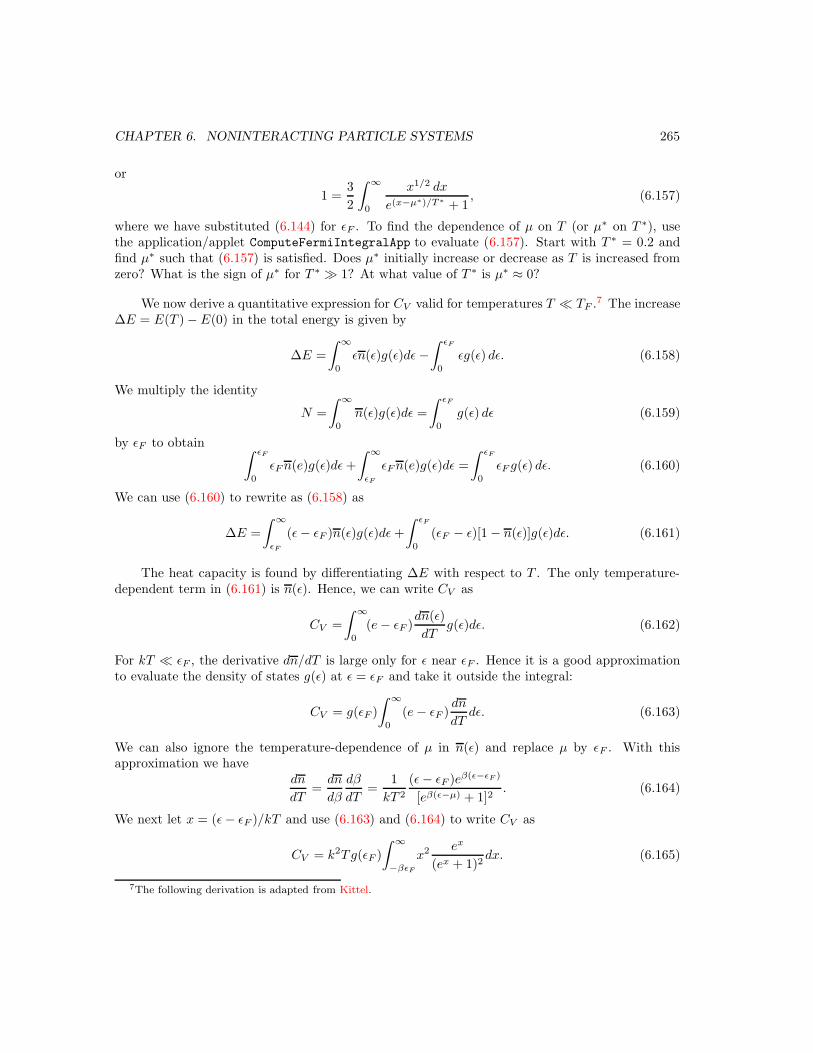
CHAPTER 6. NONINTERACTING PARTICLE SYSTEMS 265

or

1 =3

2

∫ ∞

0

x1/2 dx

e(x−µ∗)/T∗ + 1, (6.157)

where we have substituted (6.144) for εF . To find the dependence of µ on T (or µ∗ on T ∗), usethe application/applet ComputeFermiIntegralApp to evaluate (6.157). Start with T ∗ = 0.2 andfind µ∗ such that (6.157) is satisfied. Does µ∗ initially increase or decrease as T is increased fromzero? What is the sign of µ∗ for T ∗ 1? At what value of T ∗ is µ∗ ≈ 0?

We now derive a quantitative expression for CV valid for temperatures T TF .7 The increase∆E = E(T ) −E(0) in the total energy is given by

∆E =

∫ ∞

0

εn(ε)g(ε)dε−∫ εF

0

εg(ε) dε. (6.158)

We multiply the identity

N =

∫ ∞

0

n(ε)g(ε)dε =

∫ εF

0

g(ε) dε (6.159)

by εF to obtain∫ εF

0

εFn(e)g(ε)dε+

∫ ∞

εF

εFn(e)g(ε)dε =

∫ εF

0

εF g(ε) dε. (6.160)

We can use (6.160) to rewrite as (6.158) as

∆E =

∫ ∞

εF

(ε− εF )n(ε)g(ε)dε+

∫ εF

0

(εF − ε)[1 − n(ε)]g(ε)dε. (6.161)

The heat capacity is found by differentiating ∆E with respect to T . The only temperature-dependent term in (6.161) is n(ε). Hence, we can write CV as

CV =

∫ ∞

0

(e− εF )dn(ε)

dTg(ε)dε. (6.162)

For kT εF , the derivative dn/dT is large only for ε near εF . Hence it is a good approximationto evaluate the density of states g(ε) at ε = εF and take it outside the integral:

CV = g(εF )

∫ ∞

0

(e− εF )dn

dTdε. (6.163)

We can also ignore the temperature-dependence of µ in n(ε) and replace µ by εF . With thisapproximation we have

dn

dT=dn

dβ

dβ

dT=

1

kT 2

(ε− εF )eβ(ε−εF )

[eβ(ε−µ) + 1]2. (6.164)

We next let x = (ε− εF )/kT and use (6.163) and (6.164) to write CV as

CV = k2Tg(εF )

∫ ∞

−βεF

x2 ex

(ex + 1)2dx. (6.165)

7The following derivation is adapted from Kittel.

CHAPTER 6. NONINTERACTING PARTICLE SYSTEMS 266

We can replace the lower limit by −∞ because the factor ex in the integrand is negligible atx = −βεF for low temperatures. If we use the integral

∫ ∞

−∞

x2 ex

(ex + 1)2dx =

π2

3, (6.166)

we can write the heat capacity of an ideal Fermi gas as

CV =1

3π2g(εF )k2T. (6.167)

It is straightforward to show that

g(εF ) =3N

2εF=

3N

2kTF, (6.168)

and we finally arrive at our desired result

CV =π2

2Nk

T

TF. (T TF ) (6.169)

A more detailed discussion of the low temperature properties of an ideal Fermi gas is given inAppendix 6A. For convenience, we summarize the main results here:

Ω = −2

3

21/2V m3/2

π2~3

[2

5µ5/2 +

π2

4(kT )2µ1/2

]

. (6.170)

N = −∂Ω

∂µ=V (2m)3/2

3π2~3

[

µ3/2 +π2

8(kT )2µ−1/2

]

. (6.171)

The results (6.170) and (6.171) are in the grand canonical ensemble in which the chemical potentialis fixed. However, most experiments are done on a sample with a fixed number of electrons, andhence µ must change with T to keep N fixed. To find this dependence we rewrite (6.171) as

3π2~

3ρ

(2m)3/2= µ3/2

[

1 +π2

8(kT )2µ−2

]

, (6.172)

where ρ = N/V . If we raise both sides of (6.172) to the 2/3 power and use (6.144), we have

µ =32/3π4/3

~2ρ2/3

2m

[

1 +π2

8(kT )2µ−2

]−2/3, (6.173a)

= εF[

1 +π2

8(kT )2µ−2

]−2/3. (6.173b)

In the limit of T → 0, µ = εF as expected. From (6.173b) we see that the first correction for lowtemperatures is given by

µ(T ) = εF[

1 − 2

3

π2

8

(kT )2

µ2

]

= εF[

1 − π2

12

( T

TF

)2], (6.174)

where we have made the expansion (1 + x)n ≈ 1 + nx and replaced µ on the right-hand side byεF = kTF .

CHAPTER 6. NONINTERACTING PARTICLE SYSTEMS 267

From (6.174), we see that the chemical potential decreases with temperature to keep N fixed,but the decrease is second order in T/TF (rather than first-order), consistent with our earlierqualitative considerations. The explanation for the decrease in µ(T ) is that more particles movefrom low energy states below the Fermi energy to energy states above the Fermi energy as thetemperature rises. Because the density of states increases with energy, it is necessary to decreasethe chemical potential to keep the number of particles constant. In fact, as the temperaturebecomes larger than the Fermi temperature, the chemical potential changes sign and becomesnegative.

Problem 6.36. Use (6.170) and (6.174) to show that the mean pressure for T TF is given by

P =2

5ρεF

[

1 +5π2

12

( T

TF

)2+ . . .

]

. (6.175)

Use the general relation between E and PV to show that

E =3

5NεF

[

1 +5π2

12

( T

TF

)2+ . . .

]

. (6.176)

Also show that the low temperature behavior of the heat capacity at constant volume is given by

CV =π2

2Nk

T

TF. (6.177)

For completeness, show that the low temperature behavior of the entropy is given by

S =π2

2Nk

T

TF. (6.178)

Why is it not possible to calculate S by using the relations Ω = −PV and S = −∂Ω/∂T , with Pgiven by (6.175)?

We see from (6.177) that the conduction electrons of a metal contribute a linear term to theheat capacity. In Section 6.12 we shall see that the contribution from lattice vibrations contributesa term proportional to T 3 to CV at low T . Thus for sufficiently low temperature, the linear termdominates.

Problem 6.37. In Problem 6.32b we found that TF = 8.5×104 K for Copper. Use (6.177) to findthe predicted value of C/NkT for Copper. How does this value compare with the experimentalvalue C/NkT = 8 × 10−5? It is remarkable that the theoretical prediction agrees so well withthe experimental result based on the free electron model. Show that the small discrepancy can beremoved by defining an effective mass m∗ of the conduction electrons equal to 1.3me, where me isthe mass of an electron. What factors might account for the effective mass being greater than me?

Problem 6.38. Consider a system of electrons restricted to a two-dimensional surface of area A.Show that the mean number of electrons can be written as

N =mA

π~2

∫ ∞

0

dε

eβ(ε−µ) + 1. (6.179)

The integral in (6.179) can be evaluated in closed form using

∫

dx

1 + aebx=

1

bln

ebx

1 + aebx+ constant. (6.180)

CHAPTER 6. NONINTERACTING PARTICLE SYSTEMS 268

Show thatµ(T ) = kT ln

[

eρπ~2/mkT − 1

]

, (6.181)

where ρ = N/A. What is the value of the Fermi energy εF = µ(T = 0)? What is the value of µ forT TF ? Plot µ versus T and discuss its qualitative dependence on T .

6.11 Bose Condensation

The historical motivation for discussing the noninteracting Bose gas is that this idealized systemexhibits Bose-Einstein condensation. The original prediction of Bose-Einstein condensation bySatyendra Nath Bose and Albert Einstein in 1924 was considered by some to be a mathematicalartifact or even a mistake. In the 1930’s Fritz London realized that superfluid liquid helium couldbe understood in terms of Bose-Einstein condensation. However, the analysis of superfluid liquidhelium is complicated by the fact that the helium atoms in a liquid strongly interact with oneanother. For many years scientists tried to create a Bose condensate in less complicated systems.In 1995 several groups used laser and magnetic traps to create a Bose-Einstein condensate of alkaliatoms at approximately 10−6 K. In these systems the interaction between the atoms is very weakso that the ideal Bose gas is a good approximation and is no longer only a textbook example.8

Although the form of the Landau potential for the ideal Bose gas and the ideal Fermi gasdiffers only superficially (see (6.84)), the two systems behave very differently at low temperatures.The main reason is the difference in the ground states, that is, for a Bose system there is no limitto the number of particles in a single particle state.

The ground state of an ideal Bose gas is easy to construct. We can minimize the total energyby putting all the particles into the single particle state of lowest energy:

ε1 =π2

~2

2mL2(12 + 12 + 12) = 3

π2~

2

2mL2. (6.182)

Note that ε1 is a very small energy for a macroscopic system. The energy of the ground state isgiven by Nε1. For convenience, we will choose the energy scale such that the ground state energyis zero. The behavior of the system cannot depend on the choice of the zero of energy.

The behavior of an ideal Bose gas can be understood by calculating N(T, V, µ):

N =∑

k

1

eβ(εk−µ) − 1→

∫ ∞

0

n(ε)g(ε)dε (6.183)

=V

4π2~3(2m)3/2

∫ ∞

0

ε1/2 dε

eβ(ε−µ) − 1= g V

∫ ∞

0

ε1/2 dε

eβ(ε−µ) − 1. (6.184)

For simplicity, we will assume that our gas of bosons has zero spin, the same value of the spin asthe helium isotope 4He.

8The 2001 Nobel Prize for Physics was awarded to Eric Cornell, Wolfgang Ketterle, and Carl Wieman for achievingBose-Einstein condensation in dilute gases of alkali atoms and for early fundamental studies of the properties of thecondensate.

CHAPTER 6. NONINTERACTING PARTICLE SYSTEMS 269

To understand the nature of an ideal Bose gas at low temperatures, suppose that the meandensity of the system is fixed and consider the effect of lowering the temperature. The correctchoice of µ gives the desired value of ρ when substituted into (6.185).

ρ =N

V= g

∫ ∞

0

ε1/2 dε

eβ(ε−µ) − 1. (6.185)

We study the behavior of µ as a function of the temperature in Problem 6.39.

Problem 6.39. We know that in the high temperature limit, the chemical potential µ must begiven by its classical value given in (6.112). As we saw in Problem 6.24, µ is negative and largein magnitude. Let us investigate numerically how µ changes as we decrease the temperature.The application/applet ComputeBoseIntegralApp evaluates the integral on the right-hand side of(6.185) for a given value of β and µ. The goal is to find the value of µ for a given value of T thatyields the desired value of ρ.

Let ρ∗ = ρ/g = 1 and begin with T = 10. First choose µ = −10 and find the computed valueof the right-hand side. Do you have to increase or decrease the value of µ to make the computedvalue of the integral closer to ρ∗ = 1? By using trial and error, you should find that µ ≈ −33.4.Next choose T = 5 and find the value of µ needed to keep ρ∗ fixed at ρ∗ = 1. Does µ increase ordecrease in magnitude? Note that you can generate a plot of µ versus T by clicking on the Accept

parameters button.

We found numerically in Problem 6.39 that as T is decreased at constant density, |µ| mustdecrease. Because µ is negative for Bose-Einstein statistics, this dependence implies that µ becomesless negative. However, this behavior implies that there would be a lower bound for the temperatureat which µ = 0 (the upper bound for µ for Bose systems). We can find the value of this temperatureby solving (6.185) with µ = 0:

ρ = g

∫ ∞

0

ε1/2 dε

eβcε − 1= g(kTc)

3/2

∫ ∞

0

x1/2 dx

ex − 1, (6.186)

where Tc is the value of T at which µ = 0. The definite integral in (6.186) can be written in termsof known functions (see Appendix A) and has the value:

∫ ∞

0

x1/2 dx

ex − 1= 2.612

π1/2

2= C. (6.187)

We have

kTc =( ρ

gC

)2/3

=(4π

C

)2/3 ~2

2ma2, (6.188)

where a = ρ−1/3 is the mean interparticle spacing. We thus obtain the temperature Tc thatsatisfies (6.186) for fixed density. Note that the energy ~

2/2ma2 in (6.188) can be interpreted asthe zero-point energy associated with localizing a particle of mass m in a volume a3.

Similarly we can find the maximum density for a given temperature:

ρc =2.612

λ3. (6.189)

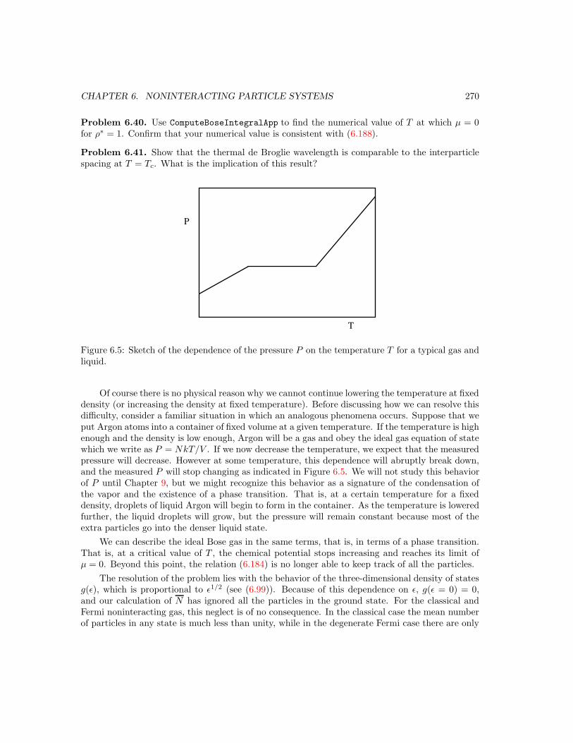
CHAPTER 6. NONINTERACTING PARTICLE SYSTEMS 270

Problem 6.40. Use ComputeBoseIntegralApp to find the numerical value of T at which µ = 0for ρ∗ = 1. Confirm that your numerical value is consistent with (6.188).

Problem 6.41. Show that the thermal de Broglie wavelength is comparable to the interparticlespacing at T = Tc. What is the implication of this result?

P

T

Figure 6.5: Sketch of the dependence of the pressure P on the temperature T for a typical gas andliquid.

Of course there is no physical reason why we cannot continue lowering the temperature at fixeddensity (or increasing the density at fixed temperature). Before discussing how we can resolve thisdifficulty, consider a familiar situation in which an analogous phenomena occurs. Suppose that weput Argon atoms into a container of fixed volume at a given temperature. If the temperature is highenough and the density is low enough, Argon will be a gas and obey the ideal gas equation of statewhich we write as P = NkT/V . If we now decrease the temperature, we expect that the measuredpressure will decrease. However at some temperature, this dependence will abruptly break down,and the measured P will stop changing as indicated in Figure 6.5. We will not study this behaviorof P until Chapter 9, but we might recognize this behavior as a signature of the condensation ofthe vapor and the existence of a phase transition. That is, at a certain temperature for a fixeddensity, droplets of liquid Argon will begin to form in the container. As the temperature is loweredfurther, the liquid droplets will grow, but the pressure will remain constant because most of theextra particles go into the denser liquid state.

We can describe the ideal Bose gas in the same terms, that is, in terms of a phase transition.That is, at a critical value of T , the chemical potential stops increasing and reaches its limit ofµ = 0. Beyond this point, the relation (6.184) is no longer able to keep track of all the particles.

The resolution of the problem lies with the behavior of the three-dimensional density of statesg(ε), which is proportional to ε1/2 (see (6.99)). Because of this dependence on ε, g(ε = 0) = 0,and our calculation of N has ignored all the particles in the ground state. For the classical andFermi noninteracting gas, this neglect is of no consequence. In the classical case the mean numberof particles in any state is much less than unity, while in the degenerate Fermi case there are only

CHAPTER 6. NONINTERACTING PARTICLE SYSTEMS 271

two electrons in the zero kinetic energy state. However, for the noninteracting Bose gas, the meannumber of particles in the ground state is given by

N0 =1

e−βµ − 1, (6.190)

(Remember that we have set ε0 = 0.) When T is sufficiently low, N0 will be very large. Hence, thedenominator of (6.190) must be very small, which implies that e−βµ ≈ 1 and the argument of theexponential −βµ must be very small. Therefore, we can approximate e−βµ as 1− βµ and N0 1becomes

N0 = −kTµ. (6.191)

The chemical potential must be such that the number of particles in the ground state approachesits maximum value which is order N . Hence, if we were to use the integral (6.184) to calculate Nfor T < Tc, we would have ignored the particles in the ground state. We have resolved the problem– the missing particles are in the ground state. The phenomena we have described, macroscopic

occupation of the ground state, is called Bose-Einstein condensation. That is for T < Tc, N0/N isnonzero in the limit of N → ∞.

Now that we know where to find the missing particles, we can calculate the thermodynamicsof the ideal Bose gas. For T < Tc, the chemical potential is zero in the thermodynamic limit, andthe number of particles not in the ground state is given by (6.184):

Nε =V

4π2~3(2m)3/2

∫ ∞

0

ε1/2dε

eβε − 1= N

( T

Tc

)3/2

, (T < Tc) (6.192)

where Tc is defined by (6.188). All of the remaining particles, which we denote as N0, are inthe ground state, that is, have energy ε = 0. Another way of understanding (6.192) is that forT < Tc, µ must be zero because the number of particles not in the ground state is determined bythe temperature. Thus

N0 = N −Nε = N[

1 −( T

Tc

)3/2]. (T < Tc) (6.193)

Note that for T < Tc, a finite fraction of the particles are in the ground state.

Because the energy of the gas is determined by the particles with ε > 0, we have for T < Tc

E =

∫ ∞

0

ε g(ε) dε

eβε − 1=V (mkT )3/2 kT

21/2π2~3

∫ ∞

0

x3/2 dx

ex − 1. (6.194)

The definite integral in (6.194) is given in Appendix A:

∫ ∞

0

x3/2 dx

ex − 1= 1.341

3π1/2

4. (6.195)

If we substitute (6.195) into (6.194), we can write the energy as

E = 31.341

25/2π3/2

V (mkT )3/2kT

~3= 0.1277V

m3/2(kT )5/2

~3. (6.196)

CHAPTER 6. NONINTERACTING PARTICLE SYSTEMS 272

Note that E ∝ T 5/2 for T < Tc. The heat capacity at constant volume is

CV =∂E

∂T= 3.2V

(mkT )3/2k

~3, (6.197)

or

CV = 1.9Nεk. (6.198)

Note that the heat capacity has a form similar to an ideal classical gas for which CV = 1.5Nk.

The pressure of the Bose gas for T < Tc can be obtained easily from the general relationPV = 2

3E for a nonrelativistic ideal gas. From (6.196) we obtain

P =1.341

23/2π3/2

m3/2(kT )5/2

~3= 0.085

m3/2(kT )5/2

~3. (6.199)

Note that the pressure is proportional to T 5/2 and is independent of the density. This behavior isa consequence of the fact that the particles in the ground state do not contribute to the pressure.If additional particles are added to the system at T < Tc, the number of particles in the state ε = 0increases, but the pressure does not increase.

What is remarkable about the phase transition in an ideal Bose gas is that it occurs at all.That is, unlike all other known transitions, its occurrence has nothing to do with the interactionsbetween the particles and has everything to do with the nature of the statistics. Depending onwhich variables are being held constant, the transition in an ideal Bose gas is either first-order orcontinuous. We postpone a discussion of the nature of the phase transition of an ideal Bose gasuntil Chapter 9 where we will discuss phase transitions in more detail. It is sufficient to mentionhere that the order parameter in the ideal Bose gas can be taken to be the fraction of particlesin the ground state, and this fraction goes continuously to zero as T → Tc from below at fixeddensity.

What makes the Bose condensate particular interesting is that for T < Tc, a finite fractionof the atoms are described by the same quantum wavefunction, which gives the condensate manyunusual properties. In particular, Bose condensates have been used to produce atom lasers – laser-like beams in which photons are replaced by atoms – and to study fundamental processes such assuperfluidity.

Problem 6.42. Show that the ground state contribution to the pressure is given by

P0 =kT

Vln(N0 + 1). (6.200)

Explain why P0 can be regarded as zero and why the pressure of an Bose gas for T < Tc isindependent of the volume.

Problem 6.43. What is the approximate value of Tc for a noninteracting Bose gas at a densityof ρ = 0.14 gmcm−3, the density of liquid 4He? Take m = 6.65× 10−27 kg.

6.12 The Heat Capacity of a Crystalline Solid

The free electron model of a metal successfully explains the temperature dependence of the con-tribution to the heat capacity from the electrons. What about the contribution from the ions?

CHAPTER 6. NONINTERACTING PARTICLE SYSTEMS 273

In a crystal each ion is localized about its lattice site and oscillates due to spring-like forces be-tween nearest-neighbor atoms. Classically, we can regard each atom of the solid as having threedegrees of freedom, each of which contributes 1

2kT to the mean kinetic energy and 12kT to the

mean potential energy. Hence, the heat capacity at constant volume of a homogeneous isotropicsolid is given by CV = 3Nk, independent of the nature of the solid. This behavior of CV agreeswith experiment remarkably well at high temperatures, where the meaning of high temperaturewill be defined later in terms of the parameters of the solid. At low temperatures, the classicalbehavior is an overestimate of the experimentally measured heat capacity, and CV is found to beproportional to T 3. To understand this behavior, we first consider the Einstein model and thenthe more sophisticated Debye model of a solid.

6.12.1 The Einstein model

The reason why the heat capacity starts to decrease at low temperature is that the oscillations ofthe crystal must be treated quantum mechanically rather than classically. The simplest model ofa solid, proposed by Einstein in 1906, is that each atom behaves like three independent harmonicoscillators each of frequency ω and possible energies ε = (n + 1

2 )~ω. Because the 3N identicaloscillators are independent and are associated with distinguishable sites, we need only to find thethermodynamic functions of one of them. The partition function for one oscillator in one dimensionis

Z1 = e−β~ω/2∞∑

n=0

[

e−β~ω]n

(6.201a)

=e−β~ω/2

1 − e−β~ω. (6.201b)

(We considered this calculation in Example 4.4.) Other thermodynamic properties of one oscillatorare given by

f = −kT lnZ1 =~ω

2+ kT ln[1 − e−β~ω]. (6.202)

s = − ∂f

∂T= −k ln[1 − e−β~ω] + β~ω

1

eβ~ω − 1. (6.203)

e = f + Ts = (n+1

2)~ω, (6.204)

where

n =1

eβ~ω − 1. (6.205)

Note the form of n. To obtain the extensive quantities such as F , S, and E, we multiply the singleparticle values by 3N . For example, the heat capacity of an Einstein solid is given by

CV =(∂E

∂T

)

V= 3N

( ∂e

∂T

)

V(6.206)

= 3Nk(β~ω)2eβ~ω

[eβ~ω − 1]2. (6.207)

CHAPTER 6. NONINTERACTING PARTICLE SYSTEMS 274

It is convenient to introduce the Einstein temperature

kTE = ~ω, (6.208)

and rewrite CV as

CV = 3Nk(TE

T

)2 eTE/T

[eTE/T − 1]2. (6.209)

The limiting behavior of CV from (6.207) or (6.209) is

CV → 3Nk. (T TE) (6.210)

and

CV → 3Nk(~ω

kT)2e−~ω/kT . (T TE) (6.211)

The calculated heat capacity is consistent with the third law of thermodynamics and is not verydifferent from the heat capacity actually observed for insulating solids. However, it decreases tooquickly at low temperatures and is not consistent with the observed low temperature behaviorsatisfied by all solids:

CV ∝ T 3. (6.212)

Problem 6.44. Explain the form of n in (6.205). Why is the chemical potential zero in this case?

Problem 6.45. Derive the limiting behavior in (6.210) and (6.211).

6.12.2 Debye theory

The Einstein model is based on the idea that each atom behaves like an harmonic oscillator whosemotion is independent of the other atoms. A better approximation was made by Debye (1912) whoobserved that solids can carry sound waves. Because waves are inherently a collective phenomenaand are not associated with the oscillations of a single atom, it is better to think of a crystallinesolid in terms of the collective rather than the independent motions of the atoms. The collectiveor cooperative motions correspond to normal modes of the system, each with its own frequency.

There are two independent transverse modes and one longitudinal mode corresponding totransverse and longitudinal sound waves with speeds, ct and cl, respectively. (Note that ct and clare speeds of sound, not light.) Given that the density of states of each mode is given by (6.94),the density of states of the system is given by

g(ω)dω = (2gt + gl)dω =V ω2dω

2π2

( 2

c3t+

1

c3l

)

. (6.213)

It is convenient to define a mean speed of sound c by the relation

3

c3=

2

c3t+

1

c3l. (6.214)

Then the density of states can be written as

g(ω) dω =3V ω2dω

2π2c3. (6.215)

CHAPTER 6. NONINTERACTING PARTICLE SYSTEMS 275

The total energy is given by

E =

∫

~ω n(ω)g(ω) dω, (6.216a)

=3V ~

2π2c3

∫

ω3 dω

eβ~ω − 1. (6.216b)

Equation (6.216b) does not take into account the higher frequency modes that do not satisfy thelinear relation ω = kc. However, we do not expect that the higher frequency modes will contributemuch to the heat capacity. After all, we already know that the Einstein model gives the correcthigh temperature behavior. Because the low temperature heat capacity depends only on the lowfrequency modes, which we have treated correctly using (6.215), it follows that we can obtain agood approximation to the heat capacity by extending (6.215) beyond its range of validity up to acutoff frequency chosen to give the correct number of modes. That is, we assume that g(ω) ∝ ω2

up to a maximum frequency ωD such that

3N =

∫ ωD

0

g(ω) dω. (6.217)

If we substitute (6.215) into (6.217), we find that

ωD = 2πc( 3ρ

4π

)1/3. (6.218)

It is convenient to relate the maximum frequency ωD to a characteristic temperature, the Debyetemperature TD, by the relation

~ωD = kTD. (6.219)

The thermal energy can now be expressed as

E =3V ~

2π2c3

∫ kTD/~

0

ω3 dω

eβ~ω − 1, (6.220a)

= 9NkT( T

TD

)3∫ TD/T

0

x3 dx

ex − 1. (6.220b)

In the high temperature limit, TD/T → 0, and the important contribution to the integral in(6.220b) comes from small x. Because the integrand is proportional x2 for small x, the integral isproportional to (T/TD)−3, and hence the energy is proportional to T . Thus in the high temperaturelimit, the heat capacity is independent of the temperature, consistent with the law of Dulong andPetit. In the low temperature limit TD/T → ∞, and the integral in (6.220b) is independent oftemperature. Hence in the limit T → 0, the energy is proportional to T 4 and the heat capacity isproportional to T 3, consistent with experimental results at low temperature.

Vocabulary

thermal de Broglie wavelength, λ

CHAPTER 6. NONINTERACTING PARTICLE SYSTEMS 276

equipartition theorem

Maxwell velocity and speed distribution

occupation numbers, spin and statistics, bosons and fermions

Bose-Einstein distribution, Fermi-Dirac distribution, Maxwell-Boltzmann distribution

single particle density of states, g(ε)

Fermi energy εF , temperature TF , and momentum pF

macroscopic occupation, Bose-Einstein condensation

Einstein and Debye theories of a crystalline solid, law of Dulong and Petit

Appendix 6A: Low Temperature Expansion

For convenience, we repeat the formal expressions for the thermodynamic properties of a nonin-teracting Fermi gas at temperature T . The mean number of particles is given by

N =21/2V m3/2

π2~3

∫ ∞

0

ε1/2 dε

eβ(ε−µ) + 1. (6.221)

After an integration by parts, the Landau potential Ω is given by the expression (see (6.103))

Ω = −2

3

21/2Vm3/2

π2~3

∫ ∞

0

ε3/2 dε

eβ(ε−µ) + 1. (6.222)

The integrals in (6.221) and (6.222) cannot be expressed in terms of familiar functions forall T . However, in the limit T TF (as is the case for almost all metals), it is sufficient toapproximate the integrals. To understand the approximations, we express the integrals (6.221)and (6.222) in the form

I =

∫ ∞

0

f(ε) dε

eβ(ε−µ) + 1, (6.223)

where f(ε) = ε1/2 and e3/2, respectively.

The expansion procedure is based on the fact that the Fermi distribution function n(ε) differsfrom its T = 0 form only in a small range of width kT about µ. We let ε−µ = kTx and write I as

I = kT

∫ ∞

−βµ

f(µ+ kTx)

ex + 1dx (6.224)

= kT

∫ 0

−βµ

f(µ+ kTx)

ex + 1dx+ kT

∫ ∞

0

f(µ+ kTx)

ex + 1dx. (6.225)

In the first integrand in (6.225) we let x → −x so that

I = kT

∫ βµ

0

f(µ− kTx)

e−x + 1dx+ kT

∫ ∞

0

f(µ+ kTx)

ex + 1dx. (6.226)

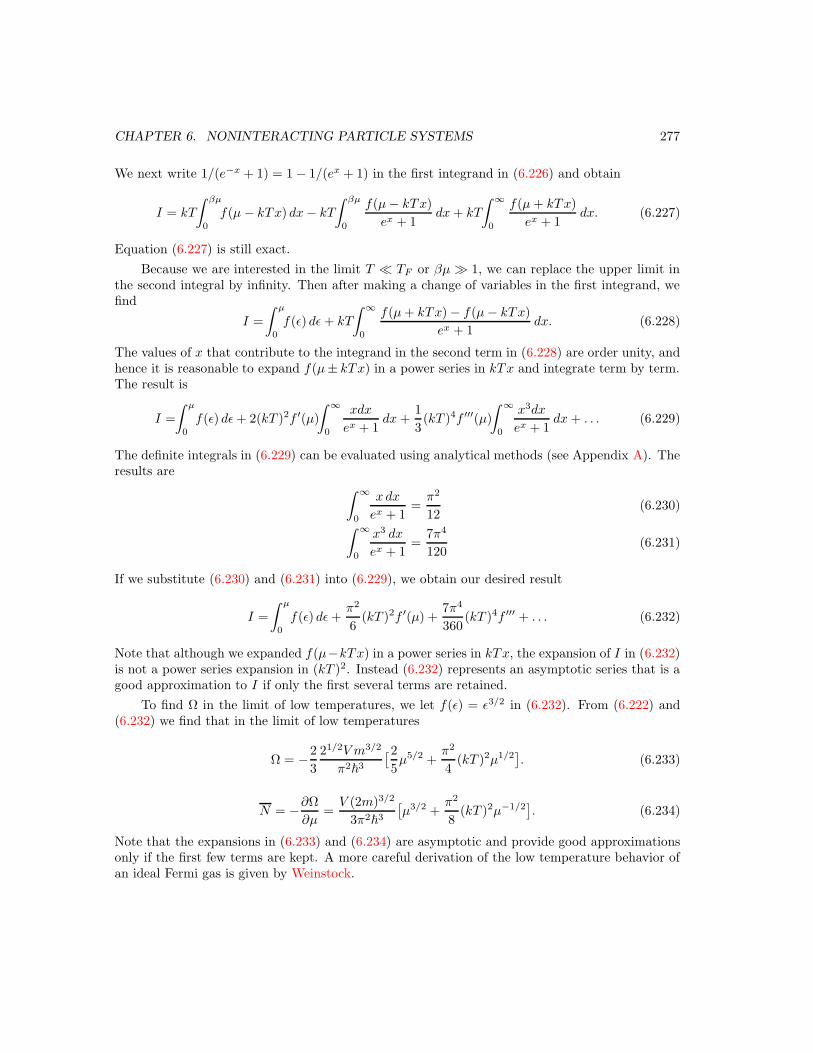
CHAPTER 6. NONINTERACTING PARTICLE SYSTEMS 277

We next write 1/(e−x + 1) = 1 − 1/(ex + 1) in the first integrand in (6.226) and obtain

I = kT

∫ βµ

0

f(µ− kTx) dx− kT

∫ βµ

0

f(µ− kTx)

ex + 1dx+ kT

∫ ∞

0

f(µ+ kTx)

ex + 1dx. (6.227)

Equation (6.227) is still exact.

Because we are interested in the limit T TF or βµ 1, we can replace the upper limit inthe second integral by infinity. Then after making a change of variables in the first integrand, wefind

I =

∫ µ

0

f(ε) dε+ kT

∫ ∞

0

f(µ+ kTx) − f(µ− kTx)

ex + 1dx. (6.228)

The values of x that contribute to the integrand in the second term in (6.228) are order unity, andhence it is reasonable to expand f(µ± kTx) in a power series in kTx and integrate term by term.The result is

I =

∫ µ

0

f(ε) dε+ 2(kT )2f ′(µ)

∫ ∞

0

xdx

ex + 1dx+

1

3(kT )4f ′′′(µ)

∫ ∞

0

x3dx

ex + 1dx+ . . . (6.229)

The definite integrals in (6.229) can be evaluated using analytical methods (see Appendix A). Theresults are

∫ ∞

0

x dx

ex + 1=π2

12(6.230)

∫ ∞

0

x3 dx

ex + 1=

7π4

120(6.231)

If we substitute (6.230) and (6.231) into (6.229), we obtain our desired result

I =

∫ µ

0

f(ε) dε+π2

6(kT )2f ′(µ) +

7π4

360(kT )4f ′′′ + . . . (6.232)

Note that although we expanded f(µ−kTx) in a power series in kTx, the expansion of I in (6.232)is not a power series expansion in (kT )2. Instead (6.232) represents an asymptotic series that is agood approximation to I if only the first several terms are retained.

To find Ω in the limit of low temperatures, we let f(ε) = ε3/2 in (6.232). From (6.222) and(6.232) we find that in the limit of low temperatures

Ω = −2

3

21/2V m3/2

π2~3

[2

5µ5/2 +

π2

4(kT )2µ1/2

]

. (6.233)

N = −∂Ω

∂µ=V (2m)3/2

3π2~3

[

µ3/2 +π2

8(kT )2µ−1/2

]

. (6.234)

Note that the expansions in (6.233) and (6.234) are asymptotic and provide good approximationsonly if the first few terms are kept. A more careful derivation of the low temperature behavior ofan ideal Fermi gas is given by Weinstock.

CHAPTER 6. NONINTERACTING PARTICLE SYSTEMS 278

Additional Problems

Problems page6.1 2316.2, 6.3 2336.4, 6.5, 6.6, 6.7, 6.8 2366.10 2386.11 2396.12, 6.13 2426.14, 6.15, 6.16 2446.17 2456.18 2496.19, 6.20, 6.21, 6.22, 6.23 2516.24 2536.25, 6.26, 6.27 2546.28, 6.29 2586.30, 6.31 2596.32 2626.33, 6.34 2626.36, 6.37, 6.38 2676.41 2706.42, 6.43 2726.44, 6.45 274

Listing of inline problems.

Problem 6.46. We can write the total energy of a system of N particles in the form

E =

N∑

i=1

p2i

2m+

N∑

i=j+1

N∑

j=1

uij (6.235)

where uij = u(|ri − rj |) is the interaction energy between particles i and j. Discuss why thepartition function of a classical system of N particles can be written in the form

ZN =1

N !h3N

∫

d3Np d3Nr e−βP

i p2

i /2m e−βP

i<juij . (6.236)

∗Problem 6.47. Assume periodic boundary conditions so that the wave function ψ satisfies thecondition (in one dimension)

ψ(x) = ψ(x+ L). (6.237)

The form of the one particle eigenfunction consistent with (6.237) is given by

ψ(x) ∝ eikxx. (6.238)

What are the allowed values of kx? How do they compare with the allowed values of kx for a particlein a one-dimensional box? Generalize the form (6.238) to a cube and determine the allowed valuesof k. Find the form of the density of states and show that the same result (6.91) is obtained.

CHAPTER 6. NONINTERACTING PARTICLE SYSTEMS 279

Problem 6.48. Estimate the chemical potential of one mole of helium gas at STP.

Problem 6.49. Suppose that two systems are initially in thermal and mechanical equilibrium,but not in chemical equilibrium, that is, T1 = T2, P1 = P2, but µ1 6= µ2. Use reasoning similar tothat used in Section 2.12 to show that particles will move from the system with higher density tothe system at lower density.

Problem 6.50. Explain in simple terms why the mean kinetic energy of a classical particle inequilibrium with a heat bath at temperature T is 1

2kT per quadratic contribution to the kineticenergy, independent of the mass of the particle.

Problem 6.51. The atoms we discussed in Section 6.3 were treated as symmetrical, rigid struc-tures capable of only undergoing translation motion, that is, their internal motion was ignored.Real molecules are neither spherical nor rigid, and rotate about two or three axes and vibratewith many different frequencies. For simplicity, consider a linear rigid rotator with two degrees offreedom. The rotational energy levels are given by

ε(j) = j(j + 1)~

2

2I, (6.239)

where I is the moment of inertia and j = 0, 1, 2, . . . The degeneracy of each rotational level is(2j + 1).

(a) Find the partition function Zrot for the rotational states of one molecule.

(b) For T Tr = ~2/(2kI), the spectrum of the rotational states may be approximated by a

continuum and the sum over j can be replaced by an integral. Show that the rotational heatcapacity is given by CV,rot = Nk in the high temperature limit. Compare this result with theprediction of the equipartition theorem.

(c) A more accurate evaluation of the sum for Zrot can be made using the Euler-Maclaurin formula(see Appendix A)

∞∑

i=0

f(x) =

∫ ∞

0

f(x) dx+1

2f(0) − 1

12f ′(0) +

1

720f ′′′(0) + . . . (6.240)

Show that the corresponding result for CV,rot is

CV,rot = Nk[1 +1

45

(Tr

T

)2+ . . .]. (6.241)

(d) Show that the leading contribution to CV,rot for T Tr s is

CV,rot = 12Nk(Tr

T

)2e−2Tr/T + . . . (6.242)

CHAPTER 6. NONINTERACTING PARTICLE SYSTEMS 280

not done

Figure 6.6: A schematic representation of a diatomic molecule.

Problem 6.52. In Section 6.3 we found the specific heat of monatomic gases using the equipar-tition theorem. In this problem we consider the specific heat of a diatomic gas. A monatomicgas is described by three independent coordinates and is said to have three degrees of freedom perparticle. The total energy of a diatomic gas is a sum of three terms, a translational, rotational,and vibrational part, and hence the total specific heat of the gas can be written as

cv = ctr + crot + cvib. (6.243)

The last two terms in (6.243) arise from the internal degrees of freedom, two for rotation and onefor vibration. (Some textbooks state that there are two vibrational degrees of freedom because thevibrational energy is part kinetic and part potential.) What is the high temperature limit of cv fora diatomic gas? The values of ~

2/2kI and ~ω/k for H2 are 85.5K and 6140K, respectively, whereω is the vibrational frequency. What do you expect the value of cv to be at room temperature?Sketch the T -dependence of cv in the range 10 K ≤ T ≤ 10000K.

Problem 6.53. What is the probability that a classical nonrelativistic particle has kinetic energyin the range ε to ε+ dε?

Problem 6.54. Consider a classical ideal gas in equilibrium at temperature T in the presence ofan uniform gravitational field. Find the probability P (z)dz that an atom is at a height between zand z + dz above the earth’s surface. How do the density and the pressure depend on z?

Problem 6.55. A system of glass beads or steel balls is an example of a granular system. Insuch system the beads are macroscopic objects and the collisions between the beads is inelastic.(Think of the collision of two basketballs.) Because the collisions in such a system are inelastic,a gas-like steady state is achieved only by inputting energy, usually by shaking or vibrating thewalls of the container. Suppose that the velocities of the particles are measured in a directionperpendicular to the direction of shaking. Do you expect the distribution of the velocities tobe given by a Gaussian distribution as in (6.56)? See for example, the experiments by DanielL. Blair and Arshad Kudrolli, “Velocity correlations in dense granular gases,” Phys. Rev. E 64,050301(R) (2001) and the theoretical arguments by J. S. van Zon and F. C. MacKintosh, “Velocitydistributions in dissipative granular gases,” Phys. Rev. Lett. 93, 038001 (2004).

∗Problem 6.56. In one of his experiments on gravitational sedimentation, Perrin observed thenumber of particles in water at T = 293K and found that when the microscope was raised by

CHAPTER 6. NONINTERACTING PARTICLE SYSTEMS 281

100µm, the mean number of particles in the field of view decreased from 203 to 91. Assume thatthe particles have a mean volume of 9.78×10−21 m3 and a mass density of 1351kg/m3. The densityof water is 1000kg/m3. Use this information to estimate the magnitude of Boltzmann’s constant.

Problem 6.57.

(a) What is the most probable kinetic energy of an atom in a classical system in equilibrium witha heat bath at temperature T ? Is it equal to 1

2mv2, where v is the most probable

(b) Find the following mean values for the same system: vx, v2x, v

2xv

2y, and vxv2

y. Try to do aminimum of calculations.

Problem 6.58. Consider a classical one-dimensional oscillator whose energy is given by

ε =p2

2m+ ax4, (6.244)

where x, p, and m have their usual meanings; the parameter a is a constant.

(a) If the oscillator is in equilibrium with a heat bath at temperature T , calculate the mean kineticenergy, the mean potential energy, and the mean total energy of the oscillator.

(b) Consider a classical one-dimensional oscillator whose energy is given by

ε =p2

2m+

1

2kx2 + ax4. (6.245)

In this case the anharmonic contribution ax4 is very small. What is the leading contributionof this term to the mean potential energy?

Problem 6.59. Consider a system consisting of two noninteracting particles connected to a heatbath at temperature T . Each particle can be in one of three states with energies 0, ε1, and ε2.Find the partition function for the following cases:

(a) The particles obey Maxwell-Boltzmann statistics and can be considered distinguishable.

(b) The particles obey Fermi-Dirac statistics.

(c) The particles obey Bose-Einstein statistics.

(d) Find the probability in each case that the ground state is occupied by one particle.

(e) What is the probability that the ground state is occupied by two particles?

(f) Estimate the probabilities in (d) and (e) for kT = ε2 = 2ε1.

Problem 6.60. Show that the grand partition function Z can be expressed as

Z =

∞∑

N=0

eβµNZN (6.246)

where ZN is the partition function for a system of N particles. Consider a system of noninteracting(spinless) fermions such that each particle can be a single particle state with energy 0, ∆, and 2∆.Find an expression for Z . Show how the mean number of particles depends on µ for T = 0,kT = ∆/2, and kT = ∆.

CHAPTER 6. NONINTERACTING PARTICLE SYSTEMS 282

Problem 6.61. A system contains N identical noninteracting fermions with 2N distinct singleparticle states. Suppose that 2N/3 of these states have energy zero, 2N/3 have energy ∆, and2N/3 have energy 2∆. Show that µ is independent of T . Calculate and sketch the T -dependenceof the energy and heat capacity.

Problem 6.62. Find general expressions for N , Ω, and E for a highly relativistic ideal gas andfind a general relation between PV and E.

Problem 6.63. Calculate the chemical potential µ(T ) of a noninteracting Fermi gas at low tem-peratures T TF for a one-dimensional ideal Fermi gas. Use the result for µ(T ) found for thetwo-dimensional case in Problem 6.38 and compare the qualitative behavior of µ(T ) in one, two,and three dimensions.

Problem 6.64. Discuss the meaning of the Fermi temperature TF . Why is it not the temperatureof the Fermi gas?

Problem 6.65. High temperature limit for ideal Fermi gas

If T TF at fixed density, quantum effects can be neglected and the thermal properties of anideal Fermi gas reduces to the ideal classical gas. Does the pressure increase or decrease when thetemperature is lowered (at constant density)? That is, what is the first quantum correction to theclassical equation of state? The pressure is given by (see (6.103))

P =(2m)3/2

3π2~3

∫ ∞

0

ε3/2 dε

eβ(x−µ) + 1. (6.247)

In the high temperature limit, eβµ 1, and we can make the expansion

1

eβ(ε−µ) + 1= eβ(µ−ε) 1

1 + e−β(ε−µ)(6.248a)

≈ eβ(µ−ε)[1 − e−β(ε−µ)]. (6.248b)

If we use (6.248b), we obtain

eβµ

∫ ∞

0

x3/2e−x(1 − eβµe−x) dx =3

4π1/2eβµ[1 − 1

25/2eβµ]. (6.249)

Use (6.249) to show that P is given by

P =m3/2(kT )5/2

21/2 π3/2~3eβµ

[

1− 1

25/2eβµ

]

. (6.250)

Find a similar expression for N . Eliminate µ and show that the leading order correction to theequation of state is given by

PV = NkT[

1 +π3/2

4

ρ~3

(mkT )3/2

]

, (6.251a)

= NkT[

1 +1

27/2ρλ3

]

. (6.251b)

CHAPTER 6. NONINTERACTING PARTICLE SYSTEMS 283

What is the condition for the correction term in (6.251b) to be small? Note that as the temperatureis lowered at constant density, the pressure increases. This dependence implies that quantum effectsdue to Fermi statistics lead to an effective “repulsion” between the particles. What do you thinkwould be the effect of Bose statistics in this context (see Problem 6.69)?

Mullin and Blaylock have emphasized that it is misleading to interpret the sign of the cor-rection term in (6.251b) in terms of an effective repulsive exchange “force,” and stress that thepositive sign is a consequence of the symmetrization requirement for same spin fermions.

∗Problem 6.66. Numerical calculation of the chemical potential for the ideal Fermi gas

Although it is not possible to do integrals of the type (6.223) analytically for all T , we can performthese integrals numerically. From (6.227) show that we can express I in the form

I =

∫ µ

0

f(ε) dε+ kT

∫ ∞

0

f(µ+ kTx) − f(µ− kTx)

ex + 1dx+ kT

∫ ∞

βµ

f(µ− kTx)

ex + 1dx. (6.252)

To calculate N we choose f(ε) = 21/2V m3/2ε1/2/π2~

3 (see (6.221)). We also introduce the dimen-sionless variables u and t defined by the relations µ = uεF and T = tTF . As a result, show thatwe find the following implicit equation for u:

1 = u3/2 +3

2t

∫ ∞

0

(u+ tx)1/2 − (u− tx)1/2

ex + 1dx+

3

2t

∫ ∞

t−1

(u+ tx)1/2

ex + 1dx (6.253)

Show that if the dimensionless “temperature” t is zero, then the dimensionless chemical potentialu = 1. Use Simpson’s rule or a similar integration method to find u for t = 0.1, 0.2, 0.5, 1.0, 1.2, 2,and 4. Plot µ/εF versus T/TF and discuss its qualitative T dependence. At approximately whattemperature does u = 0?

Problem 6.67. In the text we gave a simple argument based on the assumption that CV ∼ Neffkto obtain the qualitative T -dependence of CV at low temperatures for an ideal Bose and Fermi gas.Use a similar argument based on the assumption that PV = NeffkT to obtain the T -dependenceof the pressure at low temperatures.

∗Problem 6.68. Consider a system of N noninteracting fermions with single particle energiesgiven by εn = n∆, where n = 1, 2, 3, . . . Find the mean energy and heat capacity of the system.Although this problem can be treated exactly, it is not likely that you will be able to solve theproblem by thinking about the case of general N . The exact partition function for general Nhas been found by several authors including Peter Borrmann and Gert Franke, “Recursion for-mulas for quantum statistical partition functions,” J. Chem. Phys. 98, 2484–2485 (1993) and K.Schonhammer, “Thermodynamics and occupation numbers of a Fermi gas in the canonical ensem-ble,” Am. J. Phys. 68, 1032–1037 (2000).

Problem 6.69. High temperature limit for ideal Bose gas

If T Tc at fixed density, quantum effects can be neglected and the thermal properties of anideal Bose gas reduces to the ideal classical gas. Does the pressure increase or decrease when thetemperature is lowered (at constant density)? That is, what is the first quantum correction to theclassical equation of state? The pressure is given by (see (6.103))

P =21/2m3/2(kT )5/2

3π2~3

∫ ∞

0

x3/2 dx

ex−βµ − 1. (6.254)

CHAPTER 6. NONINTERACTING PARTICLE SYSTEMS 284

Follow the same procedure as in Problem 6.65 and show that

PV = NkT[

1 − π3/2

2

ρ~3

(mkT )3/2

]

. (6.255)

We see that as the temperature is lowered at constant density, the pressure becomes less than itsclassical value. We can interpret this change due to an effective “attraction” between the particlesdue to the Bose statistics.

Problem 6.70. Does Bose condensation occur for a one and two-dimensional ideal Bose gas? Ifso, find the transition temperature. If not, explain.

Problem 6.71. Discuss why Bose condensation does not occur in a gas of photons in thermalequilibrium (black body radiation).

∗Problem 6.72. Effect of boundary conditions

(a) Assume that N noninteracting bosons are enclosed in a cube of edge length L with rigid walls.What is the ground state wave function? How does the density of the condensate vary inspace?

(b) Assume instead the existence of periodic boundary conditions. What is the spatial dependenceof the ground state wave function on this case?

(c) Do the boundary conditions matter in this case? If so, why?

∗Problem 6.73. Bose-Einstein condensation in low-dimensional traps

As we found in Problem 6.70, Bose-Einstein condensation does not occur in ideal one and two-dimensional systems. However, this result holds only if the system is confined by rigid walls. Inthe following, we will show that Bose-Einstein condensation can occur if a system is confined by aspatially varying potential. For simplicity, we will treat the system semiclassically

Let us assume that the confining potential has the form

V (r) ∼ rn. (6.256)

Then the region accessible to a particle with energy ε has a radius L ∼ ε1/n. Show that thecorresponding density of states behaves as

g(ε) ∼ Ldε1

2d−1 ∼ εd/nε

1

2d−1 ∼ εα, (6.257)

where

α =d

n+d

2− 1 (6.258)

What is the range of values of n for which Tc > 0 for d = 1 and 2? More information aboutexperiments on Bose-Einstein condensation can be found in the references.

∗Problem 6.74. Numerical evaluation of the chemical potential of an ideal Bose gas

CHAPTER 6. NONINTERACTING PARTICLE SYSTEMS 285

Make the change of variables µ = kT u and βε = x+u and show that (6.184) for ρ = N(T, V, µ)/Vcan be written as

ρ =(2mkT )3/2

4π2~3

∫ ∞

0

dx (x + u)1/2

ex − 1. (6.259)

Use the expression (6.188) for Tc to find the implicit equation for u:

2.31 =( T

Tc

)3/2∫ ∞

0

dx (x + u)1/2

ex − 1. (6.260)

Evaluate the integral in (6.260) numerically and find the value of u and hence µ for T = 4Tc,T = 2Tc, T = 1.5Tc, and T = 1.1Tc.

Problem 6.75. (a) Show that if the volume of the crystal is Na3, where a is the equilibriumdistance between atoms, then the Debye wave number, kD = ωD/c, is about π/a.

(b) Evaluate the integral in (6.220b) numerically and plot the heat capacity versus T/TD over theentire temperature range.

∗Problem 6.76. Show that the probability P (N) of finding a system in the T, V, µ ensemble withexactly N particles, regardless of their positions and momenta, is given by

P (N) =1

Z eβNµZN(V, T ). (6.261)

Use (6.261) to show that

N =∞∑

N=0

NP (N) =z

Z∂Z∂z

=∂ lnZ∂βµ

, (6.262)

where the activity z is defined asz = eβµ. (6.263)

Also show that the variance of the number of particles is given by

N2 −N2

= kT∂N

µ. (6.264)

∗Problem 6.77. Number fluctuations in a noninteracting classical gas

Show that the grand partition function of a noninteracting classical gas can be expressed as

Z =

∞∑

N=0

(zZ1)N

N != ezZ1 . (6.265)

Show that the mean value of N is given by

N = zZ1, (6.266)

and that the probability that there are N particles in the system is given by a Poisson distribution:

PN =zNZN

Z =(zZ1)

N

N !Z =N

N

N !e−N . (6.267)

What is the variance, (N −N)2, and the N -dependence of the relative root mean square deviation,

[〈N2〉 −N2]1/2/N?

CHAPTER 6. NONINTERACTING PARTICLE SYSTEMS 286

∗Problem 6.78. Number fluctuations in a degenerate noninteracting Fermi gas

Use the relation

(N −N)2 = kT∂N

∂µ(6.268)

to find the number fluctuations in the noninteracting Fermi gas for fixed T, V and µ. Show that

(N −N)2 =kT

2

V (2m)3/2

2π2~3

∫ ∞

0

ε−1/2 dε

eβ(ε−µ) + 1, (6.269a)

→ 3NT

2TF. (T TF ) (6.269b)

Explain why the fluctuations in a degenerate Fermi system are much less than in the correspondingclassical system.

∗Problem 6.79. Absence of classical magnetism

As mentioned in Chapter 5, van Leeuwen’s theorem states that the phenomena of diamagnetismdoes not exist in classical physics. Hence, magnetism is an intrinsically quantum mechanicalphenomena. Prove van Leeuwen’s theorem using the following hints.

The proof of this theorem requires the use of classical Hamiltonian mechanics for which theregular momentum p is replaced by the canonical momentum p − A/c, where the magnetic fieldenters through the vector potential, A. Then make a change of variables that eliminates A, andthus the electric and magnetic fields from the Hamiltonian. Because the local magnetic fields areproportional to the velocity, they too will vanish when the integral over momenta is done in thepartition function.

∗Problem 6.80. The Fermi-Pasta-Ulam (FPU) problem

The same considerations that make the Debye theory of solids possible also suggest that a moleculardynamics simulation of a solid at low temperatures will fail. As we noted in Section 6.12, a systemof masses linked by Hooke’s law springs can be represented by independent normal modes. Theimplication is that a molecular dynamics simulation of a system of particles interacting via theLennard-Jones potential will fail at low temperatures because the simulation will not be ergodic.The reason is that at low energies, the particles will undergo small oscillations, and hence thesystem can be represented by a system of masses interacting via Hooke’s law springs. A initialset of positions and velocities would correspond to a set of normal modes. Because the systemwould remain in this particular set of modes indefinitely, a molecular dynamics simulation wouldnot sample the various modes and the simulation would not be ergodic.

In 1955 Fermi, Pasta, and Ulam did a simulation of a one-dimensional chain of springs con-nected by springs. If the force between the springs is not linear, for example, V (x) = kx2/2+κx4/4,the normal modes will not be an exact representation of the system for κ > 0. Would a molecu-lar dynamics simulation be ergodic for κ > 0? The answer to this question is nontrivial and hasinterested physicists and mathematicians ever since. A good place to start is the book by Weissert.

Suggestions for Further Reading

CHAPTER 6. NONINTERACTING PARTICLE SYSTEMS 287

More information about Bose-Einstein condensation can be found at <jilawww.colorado.edu/bec/>,<bec.nist.gov/>, and <cua.mit.edu/ketterle_group/>.

Vanderlei Bagnato and Daniel Kleppner, “Bose-Einstein condensation in low-dimensional traps,”Phys. Rev. A 44, 7439 (1991).

Ian Duck and E. C. G. Sudarshan, Pauli and the Spin-Statistics Theorem, World Scientific (1998).This graduate level book simplifies and clarifies the formal statements of the spin-statisticstheorem, and corrects the flawed intuitive explanations that are frequently given.

David L. Goodstein, States of Matter, Prentice Hall (1975). An excellent text whose emphasis ison the applications of statistical mechanics to gases, liquids and solids. Chapter 3 on solidsis particularly relevant to this chapter.

J. D. Gunton and M. J. Buckingham, “Condensation of ideal Bose gas as cooperative transition,”Phys. Rev. 166, 152 (1968).

F. Herrmann and P. Wurfel, “Light with nonzero chemical potential,” Am. J. Phys. 73, 717–721(2005). The authors discuss thermodynamic states and processes involving light in which thechemical potential of light is nonzero.

Charles Kittel, Introduction to Solid State Physics, seventh edition, John Wiley & Sons (1996).See Chapters 5 and 6 for a discussion of the Debye model and the free electron gas.

W. J. Mullin and G. Blaylock, “Quantum statistics: Is there an effective fermion repulsion orboson attraction?,” Am. J. Phys. 71, 1223–1231 (2003).

Jan Tobochnik, Harvey Gould, and Jonathan Machta, “Understanding temperature and chemicalpotential using computer simulations,” Am. J. Phys. 73, 708–716 (2005).

Donald Rogers, Einstein’s Other Theory: The Planck-Bose-Einstein of Heat Capacity, PrincetonUniversity Press (2005).

Robert Weinstock, “Heat capacity of an ideal free electron gas: A rigorous derivation,” Am. J.Phys. 37, 1273 (1969).

Thomas P. Weissert, The Genesis of Simulation in Dynamics: Pursuing the Fermi-Pasta-Ulam

Problem, Springer-Verlag (1998).

Chapter 7

Thermodynamic Relations andProcesses

c©2005 by Harvey Gould and Jan Tobochnik20 November 2005

7.1 Introduction

All thermodynamic measurements can be expressed in terms of partial derivatives.1 For example,the pressure P can be expressed as P = −∂F/∂V . Suppose that we make several thermodynamicmeasurements, for example, CV , CP , and KT , the isothermal compressibility. The latter is definedas

KT = − 1V

(∂V

∂P

)T

. (isothermal compressibility) (7.1)

Now suppose that we wish to know the (isobaric) coefficient of thermal expansion α, which isdefined as

α =1V

(∂V

∂T

)P

. (thermal expansion coefficient) (7.2)

(The number of particles N is assumed to be held constant in the above derivatives.) Do we need tomake an independent measurement of α or can we determine α by knowing the values of CV , CP ,and KT ? To answer this question and related ones, we first need to know how to manipulatepartial derivatives. This aspect of thermodynamics can be confusing when first encountered.

Thermodynamic systems normally have two or more independent variables. For example, thecombination E, V, N or T, P, N . Because there are many choices of combinations of independentvariables, it is important to be explicit about which variables are independent and which variablesare being held constant in any partial derivative. We suggest that you reread Appendix 2B for areview of some of the properties of partial derivatives. The following example illustrates the powerof purely thermodynamic arguments based on the manipulation of thermodynamic derivatives.

1This point has been emphasized by Styer.

288

CHAPTER 7. THERMODYNAMIC RELATIONS AND PROCESSES 289

Example 7.1. The thermodynamics of black body radiation. We can derive the relation u(T ) ∝ T 4

(see (6.135a)) for u, the energy per unit volume of blackbody radiation, by using thermodynamicarguments and two reasonable assumptions.Solution. The two assumptions are that u depends only on T and the radiation exerts a pressureon the walls of the cavity given by

P =13u(T ). (7.3)

Equation (7.3) follows directly from Maxwell’s electromagnetic theory and was obtained in Sec-tion 6.9 from first principles (see Problem 6.30).

We start from the fundamental thermodynamic relation dE = TdS − PdV , and write it as

dS =dE

T+

P

TdV. (7.4)

We let E = V u, substitute dE = V du + udV and the relation (7.3) into (7.4), and write

dS =V

Tdu +

u

TdV +

13

u

TdV =

V

T

du

dTdT +

43

u

TdV. (7.5)

From (7.5) we have( ∂S

∂V

)T

=43

u

T(7.6a)

(∂S

∂T

)V

=V

T

du

dT. (7.6b)

Because the order of the derivatives is irrelevant, ∂2S/∂V ∂T and ∂2S/∂T∂V are equal. Hence, weobtain:

43

∂

∂T

( u

T

)=

∂

∂V

(V

T

) du

dT. (7.7)

Next we assume that u depends only on T and perform the derivatives in (7.7) to find

43

[ 1T

du

dT− u

T 2

]=

1T

du

dT, (7.8)

which reduces todu

dT= 4

u

T. (7.9)

If we substitute the form u(T ) = aT n in (7.9), we find that this form is a solution for n = 4:

u(T ) = aT 4. (7.10)

The constant a in (7.10) cannot be determined by thermodynamic arguments.

We can obtain the entropy by using the first partial derivative in (7.6). The result is

S =4

3TV u(T ) + constant. (7.11)

The constant of integration in (7.11) must be set equal to zero to make S proportional to V .Hence, we conclude that S = 4aV T 3/3. The above thermodynamic argument was first given byBoltzmann in 1884.

CHAPTER 7. THERMODYNAMIC RELATIONS AND PROCESSES 290

7.2 Maxwell Relations

Example 7.1 illustrates the power of thermodynamic arguments and indicates that it would beuseful to relate various thermodynamic derivatives to one another. The Maxwell relations, whichwe derive in the following, relate the various thermodynamic derivatives of E, F , G, and H to oneanother and are useful for eliminating quantities that are difficult to measure in terms of quantitiesthat can be measured directly. We will see that the Maxwell relations can be used to show that theinternal energy and enthalpy of an ideal gas depend only on the temperature. More im portantly,we also will answer the question posed in Section 7.1 and relate the coefficient of thermal expansionto other thermodynamic derivatives.

We start with E(S, V, N) and write

dE = TdS − PdV + µdN. (7.12)

In the following we will assume that N is a constant. From (7.12) we have that

T =(∂E

∂S

)V

. (7.13)

and

P = −(∂E

∂V

)S

. (7.14)

Because the order of differentiation should be irrelevant, we obtain from (7.13) and (7.14)

∂2E

∂V ∂S=

∂2E

∂S∂V, (7.15)

or ( ∂T

∂V

)S

= −(∂P

∂S

)V

. (7.16)

Equation (7.16) is our first Maxwell relation. The remaining Maxwell relations are obtained inProblem 7.1.

Problem 7.1. From the differentials of the thermodynamic potentials:

dF = −SdT − PdV, (7.17)dG = −SdT + V dP, (7.18)dH = TdS + V dP, (7.19)

derive the Maxwell relations:( ∂S

∂V

)T

=(∂P

∂T

)V

, (7.20)( ∂S

∂P

)T

= −(∂V

∂T

)P

, (7.21)(∂T

∂P

)S

=(∂V

∂S

)P

. (7.22)

CHAPTER 7. THERMODYNAMIC RELATIONS AND PROCESSES 291

Also consider a variable number of particles to derive the Maxwell relations

( ∂V

∂N

)P

=( ∂µ

∂P

)N

(7.23)

and ( ∂µ

∂V

)N

= −( ∂P

∂N

)V

. (7.24)

7.3 Applications of the Maxwell Relations

The Maxwell relations depend on our identification of (∂E/∂S)V with the temperature, a relationthat follows from the second law of thermodynamics. The Maxwell relations are not purely math-ematical in content, but are different expressions of the second law. In the following, we use theserelations to derive some useful relations between various thermodynamic quantities.

7.3.1 Internal energy of an ideal gas

We first show that the internal energy E of an ideal gas is a function only of T given the pressureequation of state, PV = NkT . That is, if we think of E as a function of T and V , we want toshow that (∂E/∂V )T = 0. From the fundamental thermodynamic relation, dE = TdS − PdV , wesee that (∂E/∂V )T can be expressed as

(∂E

∂V

)T

= T( ∂S

∂V

)T− P. (7.25)

To show that E is a function of T only, we need to show that the right-hand side of (7.25) is zero.The term involving the entropy in (7.25) can be rewritten using the Maxwell relation (7.20):

(∂E

∂V

)T

= T(∂P

∂T

)V

− P. (7.26)

Because (∂P/∂T )V = P/T for an ideal gas, we see that the right-hand side of (7.26) is zero.

Problem 7.2. Show that the enthalpy of an ideal gas is a function of T only.

7.3.2 Relation between the specific heats

As we have seen, it is much easier to calculate the heat capacity at constant volume than atconstant pressure. However, it is usually easier to measure the heat capacity at constant pressure.For example, most solids expand when heated, and hence it is easier to make measurements atconstant pressure. In the following, we derive a thermodynamic relation that relates CV and CP .First recall that

CV =(∂E

∂T

)V

= T(∂S

∂T

)V

(7.27a)

and

CHAPTER 7. THERMODYNAMIC RELATIONS AND PROCESSES 292

CP =(∂H

∂T

)P

= T(∂S

∂T

)P

. (7.27b)

We consider S as a function of T and P and write

dS =∂S

∂TdT +

∂S

∂PdP, (7.28)

and take the partial derivative with respect to temperature at constant volume of both sides of(7.28): (∂S

∂T

)V

=(∂S

∂T

)P

+( ∂S

∂P

)T

(∂P

∂T

)V

. (7.29)

We then use (7.27) to rewrite (7.29) as

CV

T=

( ∂S

∂P

)T

(∂P

∂T

)V

+CP

T. (7.30)

Because we would like to express CP −CV in terms of measurable quantities, we use the Maxwellrelation (7.21) to eliminate (∂S/∂P ) and rewrite (7.30) as:

CP − CV = T(∂V

∂T

)P

(∂P

∂T

)V

. (7.31)

We next use the identity (see (2.162)),(∂V

∂T

)P

(∂T

∂P

)V

(∂P

∂V

)T

= −1, (7.32)

to eliminate (∂P/∂T )V and write:

CP − CV = −T(∂P

∂V

)T

(∂V

∂T

)P

2

. (7.33)

If we substitute the definitions (7.1) of the isothermal compressibility KT and (7.2) for the thermalexpansion coefficient α, we obtain the desired general relation:

CP − CV = VT

KTα2. (7.34)

Note that (7.34) is more general that the relation (2.36) which depends on only the first law.For an ideal gas we have KT = 1/P and α = 1/T and (7.34) reduces to the familiar result

(see (2.37))CP − CV = Nk. (7.35)

Although we will not derive these conditions here, it is plausible that the heat capacity andcompressibility of equilibrium thermodynamic systems must be positive. Given these assumptions,we see from (7.34) that CP > CV in general.

7.4 Applications to Irreversible Processes

Although the thermodynamic quantities of a system can be defined only when the system is inequilibrium, we found in Chapter 2 that it is possible to obtain useful results for systems that passthrough nonequilibrium states if the initial and final states are in equilibrium. In the following, wewill consider some well known thermodynamic processes.

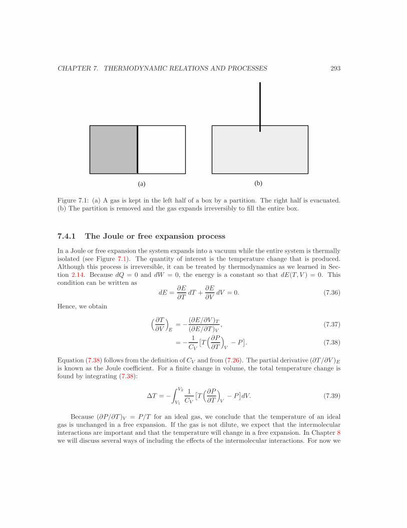
CHAPTER 7. THERMODYNAMIC RELATIONS AND PROCESSES 293

(a) (b)

Figure 7.1: (a) A gas is kept in the left half of a box by a partition. The right half is evacuated.(b) The partition is removed and the gas expands irreversibly to fill the entire box.

7.4.1 The Joule or free expansion process

In a Joule or free expansion the system expands into a vacuum while the entire system is thermallyisolated (see Figure 7.1). The quantity of interest is the temperature change that is produced.Although this process is irreversible, it can be treated by thermodynamics as we learned in Sec-tion 2.14. Because dQ = 0 and dW = 0, the energy is a constant so that dE(T, V ) = 0. Thiscondition can be written as

dE =∂E

∂TdT +

∂E

∂VdV = 0. (7.36)

Hence, we obtain

( ∂T

∂V

)E

= − (∂E/∂V )T

(∂E/∂T )V, (7.37)

= − 1CV

[T

(∂P

∂T

)V

− P]. (7.38)

Equation (7.38) follows from the definition of CV and from (7.26). The partial derivative (∂T/∂V )E

is known as the Joule coefficient. For a finite change in volume, the total temperature change isfound by integrating (7.38):

∆T = −∫ V2

V1

1CV

[T

(∂P

∂T

)V

− P]dV. (7.39)

Because (∂P/∂T )V = P/T for an ideal gas, we conclude that the temperature of an idealgas is unchanged in a free expansion. If the gas is not dilute, we expect that the intermolecularinteractions are important and that the temperature will change in a free expansion. In Chapter 8we will discuss several ways of including the effects of the intermolecular interactions. For now we

CHAPTER 7. THERMODYNAMIC RELATIONS AND PROCESSES 294

will be satisfied a simple modification of the ideal gas equation of state due to van der Waals (see(2.13):

(P +N2

V 2a)(V − Nb) = NkT. (van der Waals equation of state) (7.40)

Problem 7.3. Calculate (∂T/∂V )E for the van der Waals equation of state (7.40) and show thata free expansion results in cooling.

The physical reason for the cooling of a real gas during a free expansion can be understood asfollows. The derivative (∂E/∂V )T depends only on the potential energy of the particles becausethe temperature is held constant. As shown in Figure 1.1, the intermolecular potential is repulsivefor small separations r and is attractive for large r. For a dilute gas the mean separation betweenthe particles is greater than r0 = 21/6σ, the distance at which the potential is a minimum. As thevolume increases, the mean separation between the molecules increases and hence the energy ofinteraction becomes less negative, that is, increases. Hence we conclude that (∂E/∂V )T increases.Because the heat capacity is always positive, we find that (∂T/∂V )E is negative and that realgases always cool in a free expansion.

7.4.2 Joule-Thomson process

The Joule-Thomson (or Joule-Kelvin2 or porous plug) process is a steady state flow process inwhich a gas is forced through a porous plug or expansion value from a region of high pressure P1 toa region of lower pressure P2 (see Figure 7.2). The gas is thermally isolated from its surroundings.The process is irreversible because the gas is not in equilibrium. We will see that a real gas iseither cooled or heated in passing through the plug.

Consider a given amount (for example, one mole) of a gas that occupies a volume V1 at pressureP1 on the left-hand side of the valve and a volume V2 at pressure P2 on the right-hand side. Thework done on the gas is given by

W = −∫ 0

V1

PdV −∫ V2

0

PdV. (7.41)

The pressure on each side of the porous plug is constant, and hence we obtain

W = P1V1 − P2V2. (7.42)

Because the process talks place in an isolated cylinder, there is no energy transfer due to heating,and the change in the internal energy is given by

∆E = E2 − E1 = W = P1V1 − P2V2. (7.43)

Hence, we obtain

E2 + P2V2 = E1 + P1V1, (7.44)

which can be written as2William Thomson was later awarded a peerage and became Lord Kelvin.

CHAPTER 7. THERMODYNAMIC RELATIONS AND PROCESSES 295

P1 P2

Figure 7.2: Schematic representation of the Joule-Thomson process. The two pistons ensureconstant pressures on each side of the porous plug. The porous plug can be made by packing glasswool into a pipe. The process can be made continuous by using a pump to return the gas from theregion of low pressure to the region of high pressure.

H2 = H1. (7.45)

That is, the Joule-Thomson process occurs at constant enthalpy. All we can say is that the finalenthalpy equals the initial enthalpy; the intermediate states of the gas are nonequilibrium statesfor which the enthalpy is not defined.

The calculation of the temperature change in the Joule-Thomson effect is similar to our treat-ment of the Joule effect. Because the process occurs at constant enthalpy, it is useful to write

dH(T, P ) =∂H

∂TdT +

∂H

∂PdP = 0. (7.46)

As before, we assume that the number of particles is a constant. From (7.46) we have

dT = − (∂H/∂P )T

(∂H/∂T )P. (7.47)

From the relation, dH = TdS +V dP , we have (∂H/∂P )T = T (∂S/∂P )T +V . If we substitute thisrelation in (7.47), use the Maxwell relation (7.21), and the definition CP = (∂H/∂T )P , we obtain

(∂T

∂P

)H

=V

CP(Tα − 1) , (7.48)

where the thermal expansion coefficient α is defined by (7.2). Note that the change in pressure dPis negative, that is, the gas goes from a region of high pressure to a region of low pressure. To findthe temperature change produced in a finite pressure drop, we integrate (7.48) and find

∆T = T2 − T1 =∫ P2

P1

V

CP(Tα − 1) dP. (7.49)

For an ideal gas, α = 1/T and ∆T = 0 as expected.To understand the nature of the temperature change in a real gas, we calculate α for the van

der Waals equation of state (7.40). We write the latter in the form

P + aρ2 =ρkT

1 − bρ, (7.50)

CHAPTER 7. THERMODYNAMIC RELATIONS AND PROCESSES 296

and take the derivative with respect to T at constant P :

2aρ( ∂ρ

∂T

)P

=ρk

1 − bρ+

( ∂ρ

∂T

)P

kT

(1 − bρ)2. (7.51)

If we express α as

α = −1ρ

( ∂ρ

∂T

)P

, (7.52)

we can write (7.51) in the form:

[ kT

(1 − bρ)2− 2aρ

]α =

k

(1 − bρ). (7.53)

For simplicity, we consider only low densities in the following. In this limit we can write α as

α =k(1 − bρ)

kT − 2aρ(1 − bρ)2, (7.54a)

≈ 1T

(1 − bρ)[1 + 2aβρ(1 − bρ)2

], (7.54b)

≈ 1T

[1 − ρ(b − 2aβ)]. (7.54c)

From (7.54c) we obtain (Tα − 1) = ρ(2aβ − b) at low densities.We can define an inversion temperature Ti at which the derivative (∂T/∂P )H changes sign.

From (7.54) and (7.48), we see that kTi = 2a/b for a low density gas. For T > Ti, the gas warmsas the pressure falls in the Joule-Thomson expansion. However, for T < Ti, the gas cools as thepressure falls.

For most gases Ti is well above room temperatures. Although the cooling effect is small, theeffect can be made cumulative by using the cooled expanded gas in a heat exchanger to precoolthe incoming gas.

7.5 Equilibrium Between Phases

Every substance can exist in qualitatively different forms, called phases. For example, most sub-stances exist in the form of a gas, liquid, or a solid. The most familiar substance of this type iswater which exists in the form of water vapor, liquid water, and ice.3 The existence of differentphases depends on the pressure and temperature and the transition of one phase to another occursat particular temperatures and pressures. For example, water is a liquid at room temperature andatmospheric pressure, but if it is cooled below 273.15K, it solidifies eventually, and if heated about373.15K it vaporizes.4 At each of these temperatures, water undergoes dramatic changes in itsproperties, and we say that a phase transition occurs. The existence of distinct phases must bethe result of the intermolecular interactions, yet these interactions are identical microscopically in

3All of the natural ice on earth is hexagonal, as manifested in six-cornered snow flakes. At lower temperaturesand at pressures above about 108 Pa, many other ice phases with different crystalline structures exist.

4If you were to place a thermometer in a perfectly pure boiling water, the thermometer would not read 100 C.A few degrees of superheating is almost inevitable. Superheating and supercooling are discussed in Section xx.

CHAPTER 7. THERMODYNAMIC RELATIONS AND PROCESSES 297

all phases. Why is the effect of the interactions so different macroscopically? The answer is theexistence of cooperative effects, which we discussed briefly in Section 5.5.1 and will discuss in moredetail in Chapter 8.

7.5.1 Equilibrium conditions

Before we discuss the role of intermolecular interactions, we obtain the conditions for equilibriumbetween two phases of a substance consisting of a single type of molecule. We discuss mixturesof more than one substance in Section ??. For example, the phases might be a solid and a liquidor a liquid and a gas. We know that as for any two bodies in thermodynamic equilibrium, thetemperatures T1 and T2 of the two phases must be equal:

T1 = T2. (7.55)

We also know that the pressure on the two phases must be equal,

P1 = P2, (7.56)

because the forces exerted by the two phases on each other at their surface of contact must beequal and opposite.

We show in the following that because the number of particles N1 and N2 of each species canvary, the chemical potentials of the two phases must be equal:

µ1 = µ2. (7.57)

Because the temperatures and pressures are uniform, we can write (7.57) as

µ1(T, P ) = µ2(T, P ). (7.58)

Note that because µ(T, P ) = g(T, P ), where g is the Gibbs free energy per particle, we canequivalently write the equilibrium condition (7.58) as

g1(T, P ) = g2(T, P ). (7.59)

We now derive the equilibrium condition (7.58) for the chemical potential. Because T and Pare well defined quantities for a system of two phases, the natural thermodynamic potential is theGibbs free energy G = E − TS + PV . Let Ni be the number of particles in phase i and gi(T, P )be the Gibbs free energy per particle in phase i. Then G can be written as

G = N1g1 + N2g2. (7.60)

Conservation of matter implies that the total number of particles remains constant:

N = N1 + N2 = constant. (7.61)

Suppose we let N1 vary. Because G is a minimum in equilibrium, we have

dG = 0 = g1dN1 + g2dN2 = (g1 − g2)dN1, (7.62)

with dN2 = −dN1. Hence, we find that a necessary condition for equilibrium is

g1(T, P ) = g2(T, P ). (7.63)

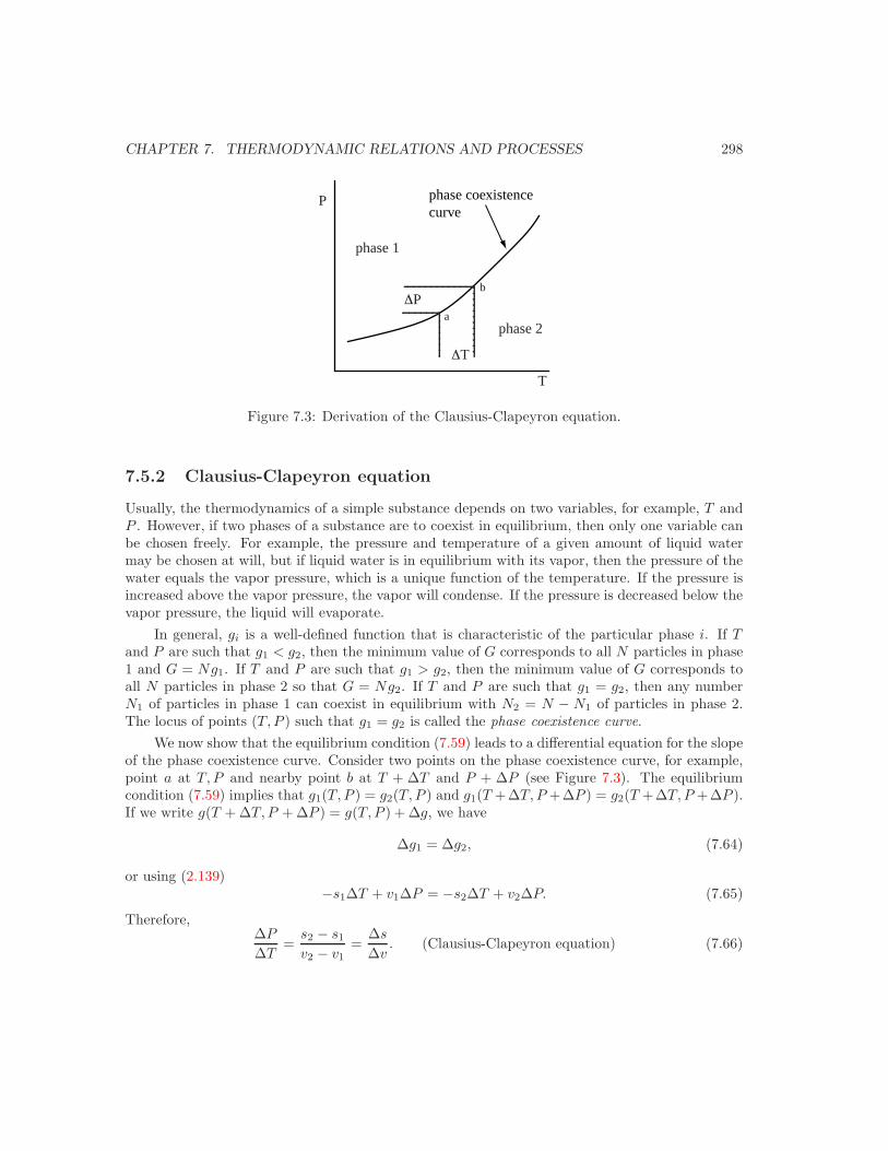
CHAPTER 7. THERMODYNAMIC RELATIONS AND PROCESSES 298

P

T

phase 1

phase 2

∆T

∆Pa

b

phase coexistencecurve

Figure 7.3: Derivation of the Clausius-Clapeyron equation.

7.5.2 Clausius-Clapeyron equation

Usually, the thermodynamics of a simple substance depends on two variables, for example, T andP . However, if two phases of a substance are to coexist in equilibrium, then only one variable canbe chosen freely. For example, the pressure and temperature of a given amount of liquid watermay be chosen at will, but if liquid water is in equilibrium with its vapor, then the pressure of thewater equals the vapor pressure, which is a unique function of the temperature. If the pressure isincreased above the vapor pressure, the vapor will condense. If the pressure is decreased below thevapor pressure, the liquid will evaporate.

In general, gi is a well-defined function that is characteristic of the particular phase i. If Tand P are such that g1 < g2, then the minimum value of G corresponds to all N particles in phase1 and G = Ng1. If T and P are such that g1 > g2, then the minimum value of G corresponds toall N particles in phase 2 so that G = Ng2. If T and P are such that g1 = g2, then any numberN1 of particles in phase 1 can coexist in equilibrium with N2 = N − N1 of particles in phase 2.The locus of points (T, P ) such that g1 = g2 is called the phase coexistence curve.

We now show that the equilibrium condition (7.59) leads to a differential equation for the slopeof the phase coexistence curve. Consider two points on the phase coexistence curve, for example,point a at T, P and nearby point b at T + ∆T and P + ∆P (see Figure 7.3). The equilibriumcondition (7.59) implies that g1(T, P ) = g2(T, P ) and g1(T +∆T, P +∆P ) = g2(T +∆T, P +∆P ).If we write g(T + ∆T, P + ∆P ) = g(T, P ) + ∆g, we have

∆g1 = ∆g2, (7.64)

or using (2.139)−s1∆T + v1∆P = −s2∆T + v2∆P. (7.65)

Therefore,∆P

∆T=

s2 − s1

v2 − v1=

∆s

∆v. (Clausius-Clapeyron equation) (7.66)

CHAPTER 7. THERMODYNAMIC RELATIONS AND PROCESSES 299

The relation (7.66) is called the Clausius-Clapeyron equation. It relates the slope of the phasecoexistence curve at the point T, P to the entropy change ∆s per particle and the volume change∆v per particle when the curve is crossed at this point. For N particles we have ∆S = N∆s and∆V = N∆v, and hence (7.66) can be expressed as

dP

dT=

∆S

∆V. (7.67)

From the relation (7.25), we can write

T∂S

∂V=

∂E

∂V+ P. (7.68)

At the phase coexistence curve for a given T and P , we can write

TS2 − S1

V2 − V1=

E2 − E1

V2 − V1+ P, (7.69)

orT (S2 − S1) = (E2 − E1) + P (V2 − V1). (7.70)

Because the enthalpy H = U + PV , it follows that

L2→1 = T (S2 − S1) = H2 − H1. (7.71)

The energy L required to melt a given amount of a solid is called the enthalpy of fusion.5 Theenthalpy of fusion is related to the difference in entropies of the liquid and the solid phase and isgiven by

Lfusion = Hliquid − Hsolid = T (Sliquid − Ssolid), (7.72)

where T is the melting temperature at the given pressure. Similarly, the equilibrium of a vaporand liquid leads to the enthalpy of vaporization

vaporization = hvapor − hliquid. (7.73)

where h is the specific enthalpy. The enthalpy of sublimation associated with the equilibrium ofvapor and solid is given by

sublimation = hvapor − hsolid. (7.74)

We say that if there is a discontinuity in the entropy and the volume at the transition, thetransition is discontinuous or first-order and L = ∆H = T∆S. Thus the Clausius-Clapeyronequation can be expressed in the form

dP

dT=

L

T∆V=

T∆v. (7.75)

5The more familiar name is latent heat of fusion. As we discussed in Chapter 2, latent heat is an archaic termand is a relic from the time it was thought that there were two kinds of heat: sensible heat, the kind you can feel,and latent heat, the kind you cannot.

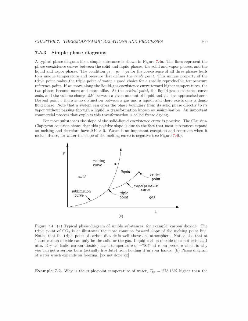
CHAPTER 7. THERMODYNAMIC RELATIONS AND PROCESSES 300

7.5.3 Simple phase diagrams

A typical phase diagram for a simple substance is shown in Figure 7.4a. The lines represent thephase coexistence curves between the solid and liquid phases, the solid and vapor phases, and theliquid and vapor phases. The condition g1 = g2 = g3 for the coexistence of all three phases leadsto a unique temperature and pressure that defines the triple point. This unique property of thetriple point makes the triple point of water a good choice for a readily reproducible temperaturereference point. If we move along the liquid-gas coexistence curve toward higher temperatures, thetwo phases become more and more alike. At the critical point, the liquid-gas coexistence curveends, and the volume change ∆V between a given amount of liquid and gas has approached zero.Beyond point c there is no distinction between a gas and a liquid, and there exists only a densefluid phase. Note that a system can cross the phase boundary from its solid phase directly to itsvapor without passing through a liquid, a transformation known as sublimination. An importantcommercial process that exploits this transformation is called freeze drying.

For most substances the slope of the solid-liquid coexistence curve is positive. The Clausius-Clapeyron equation shows that this positive slope is due to the fact that most substances expandon melting and therefore have ∆V > 0. Water is an important exception and contracts when itmelts. Hence, for water the slope of the melting curve is negative (see Figure 7.4b).

T

P

meltingcurve

solid

gas

liquidcriticalpoint

triplepoint

sublimationcurve

vapor pressurecurve

(a)

Figure 7.4: (a) Typical phase diagram of simple substances, for example, carbon dioxide. Thetriple point of CO2 is at illustrates the more common forward slope of the melting point line.Notice that the triple point of carbon dioxide is well above one atmosphere. Notice also that at1 atm carbon dioxide can only be the solid or the gas. Liquid carbon dioxide does not exist at 1atm. Dry ice (solid carbon dioxide) has a temperature of −78.5 at room pressure which is whyyou can get a serious burn (actually frostbite) from holding it in your hands. (b) Phase diagramof water which expands on freezing. [xx not done xx]

Example 7.2. Why is the triple-point temperature of water, Ttp = 273.16K higher than the

CHAPTER 7. THERMODYNAMIC RELATIONS AND PROCESSES 301

ice-point temperature, Tice = 273.15 K, especially given that at both temperatures ice and waterare in equilibrium?Solution. The triple-point temperature T3 is the temperature at which water vapor, liquid water,and ice are in equilibrium. At T = T3, the vapor pressure of water equals the sublimation pressureof ice which is equal to P3 = 611Pa. The ice point is defined as the temperature at which pure iceand air-saturated liquid water are in equilibrium under a total pressure of 1 atm = 1.013× 105 Pa.Hence, the triple-point temperature and the ice point temperature differ for two reasons – the totalpressure is different and the liquid phase is not pure water.

Let us find the equilibrium temperature of ice and pure water when the pressure is increasedfrom the triple point to a pressure of 1 atm. From (7.75), we have for liquid-solid equilibrium

∆T =T (vsolid − vliquid)

fusion∆P. (7.76)

Because the changes in T and P are very small, we can assume that all the terms in the coefficientof ∆P are very small. Let Tice be the equilibrium temperature of ice and pure water. If we integratethe left-hand side of (7.76) from T3 to Tice and the right side from P3 to atmospheric pressure P ,we obtain

Tice − T3 =T (vsolid − vliquid)

lfusion(P − P3). (7.77)

To three significant figures, T = 273K, P − P3 = 1.01 × 105 Pa, vsolid = 1.09 × 10−3 m3/kg,vliquid = 1.00 × 10−3 m3/kg, and fusion = 3.34 × 105 J/kg. If we substitute these values into(7.77), we find Tice −T3 = −0.0075K. That is, the ice point temperature of pure water is 0.0075Kbelow the temperature of the triple point. Hence, the effect of the dissolved air is to lower thetemperature by 0.0023K at which the liquid phase is in equilibrium with pure ice at atmosphericpressure below the equilibrium temperature for pure water.

7.5.4 Pressure dependence of the melting point

We consider the equilibrium between ice and water as an example of the pressure dependence ofthe melting point. The enthalpy of fusion of water at 0C is

fusion = 3.35 × 105 J/kg. (7.78)

The specific volumes in the solid and liquid phase are

vsolid = 1.09070× 10−3 m3/kg, and vliquid = 1.00013× 10−3 m3/kg, (7.79)

so that ∆v = vliquid − vsolid = −0.0906 × 10−3 m3/kg. If we substitutes these values of and ∆vin (7.75), we find

dP

dT= − 3.35 × 105

273.2× 9.06 × 10−5= −1.35 × 107 Pa/K. (7.80)

From (7.80) we see that an increase in pressure of 1.35 × 107 Pa or 133 atmospheres lowers themelting point by 1C.

CHAPTER 7. THERMODYNAMIC RELATIONS AND PROCESSES 302

The lowering of the melting point of ice under pressure is responsible for the motion of glaciers.The deeper parts of a glacier melt under the weight of ice on top allowing the bottom of a glacierto flow. The bottom freezes again when the pressure decreases.

Some textbooks state that ice skaters are able to skate freely because the pressure of the iceskates lowers the melting point of the ice and allows ice skaters to skate on a thin film of waterbetween the blade and the ice. As soon as the pressure is released, the water refreezes. From theabove example we see that if the ice is at −1C, then the pressure due to the skates must be 135atmospheres for bulk melting to occur. However, even for extremely narrow skates and a largeperson, the skates do not exert enough pressure to cause this phenomenon. As an example, wetake the contact area of the blades to be 10−4 m2 and the mass of the skater to be 100 kg. Thenthe pressure is given by

P =F

A=

mg

A≈ 107 Pa ≈ 100 atm. (7.81)

Given that on many winter days, the temperature is lower than a fraction of a degree belowfreezing, there must a mechanism different than pressure-induced melting that is responsible forice skating. And how do we explain the slide of a hockey puck, which has a large surface area anda small weight? The answer appears to be the existence of surface melting, that is, the existenceof a layer of liquid water on the surface of ice that exists independently of the pressure of an iceskate (see the references).

7.5.5 Pressure dependence of the boiling point

Because ∆v is always positive for the transformation of liquid to gas, increasing the pressure on aliquid always increases the boiling point. For water the enthalpy of vaporization is

vaporization = 2.257 × 106 J/kg. (7.82)

The specific volumes in the liquid and gas phase at T = 373.15K and P = 1atm are

vliquid = 1.043× 10−3 m3/kg and vgas = 1.673 m3/kg. (7.83)

Hence from (7.75) we have

dP

dT=

2.257 × 106

373.15× 1.672= 3.62 × 103 Pa/K. (7.84)

7.5.6 The vapor pressure curve

The Clausius-Clapeyron equation for the vapor pressure curve can be approximated by neglectingthe specific volume of the liquid in comparison to the gas, ∆v = vgas − vliquid ≈ vgas. From (7.83)we see that for water at its normal boiling point, this approximation introduces an error of less than0.1 per cent. If we assume that the vapor behaves like an ideal gas, we have that vgas = RT/P forone mole of the gas. With these approximations, the Clausius-Clapeyron equation can be writtenas

dP

P=

dT

RT 2. (7.85)

CHAPTER 7. THERMODYNAMIC RELATIONS AND PROCESSES 303

If we also assume that is approximately temperature independent, we can integrate (7.85) to find

ln P (T ) = −

RT+ constant (7.86)

orP (T ) ≈ P0e

−/RT , (7.87)

where P0 is a constant.

Example 7.3. In the vicinity of the triple point the liquid-vapor coexistence curve of liquidammonia can be represented by ln P = 24.38 − 3063/T , where the pressure is given in Pascals.The vapor pressure of solid ammonia is lnP = 27.92 − 3754/T . What are the temperature andpressure at the triple point? What are the enthalpies of sublimation and vaporization? What isthe enthalpy of fusion at the triple point?Solution. At the triple point, Psolid = Pliquid or 24.38 − 3063/T = 27.92 − 3754/T . The solutionis T = 691/3.54 = 195.2K. The corresponding pressure is 8.7Pa. The relation (7.86), lnP =−/RT + constant, can be used to find the enthalpy of sublimation and vaporization of ammoniaat the triple point. We have sublimation = 3754R = 3.12 × 104 J/mol and vaporization = 3063R =2.55 × 104 J/mol. The enthalpy of melting satisfies the relation sublimation = vaporization + fusion.Hence, fusion = (3.12 − 2.55)× 104 = 5.74 × 103 J/mol.

7.6 Vocabulary

Maxwell relationsfree expansion, Joule-Thomson processphase coexistence curve, phase diagramtriple point, critical pointClausius-Clapeyron equationenthalpy of fusion, vaporization, and sublimation

Additional Problems

Problems page7.1 2907.2 2917.3 294

Table 7.1: Listing of inline problems.

Problem 7.4. Show that the three enthalpy (differences) are not independent, but are related by

fusion + vaporization = sublimation. (7.88)

Interpret this relation in physical terms.

CHAPTER 7. THERMODYNAMIC RELATIONS AND PROCESSES 304

Problem 7.5. Show that(∂CP

∂P

)T

= −T(∂2V

∂T 2

)P

, (7.89)

and (∂CV

∂V

)T

= T(∂2P

∂T 2

)V

. (7.90)

Problem 7.6. Show thatKT

KS=

CP

CV, (7.91)

where

KT = − 1V

(∂V

∂P

)T

(7.92a)

KS = − 1V

(∂V

∂P

)S

. (7.92b)

KS is the adiabatic compressibility. Use (7.92b) and (7.34) to obtain the relation

KT − KS =TV

CPα2. (7.93)

Problem 7.7. The inversion temperature for the Joule-Thomson effect is determined by therelation (∂T/∂V )P = T/V (see (7.48))). In Section 7.4.2 we showed that for low densities andhigh temperatures (low pressures) the inversion temperature is given by kTinv = 2a/b. Show thatat high pressures, Tinv is given by

kTinv =2a

9b(2 ±

√1 − 3b2P/a)2. (7.94)

Show that as P → 0, kTinv = 2a/b. For P < a/3b2, there are two inversion points between whichthe derivative (∂T/∂P )H is positive. Outside this temperature interval the derivative is negative.For P > a/3b2 there are no inversion points and (∂T/∂P )H < 0 is negative everywhere. Find thepressure dependence of the inversion temperature for the Joule-Thomson effect.

Problem 7.8. Use the result (7.84) to estimate the boiling temperature of water at the height ofthe highest mountain in your geographical region.

Problem 7.9. A particular liquid boils at 127C at a pressure of 1.06 × 105 Pa. Its enthalpy ofvaporization is 5000J/mol. At what temperature will it boil if the pressure is raised to 1.08×105 Pa?

Problem 7.10. A particular liquid boils at a temperature of 105C at the bottom of a hill and at95C at the top of the hill. The enthalpy of vaporization is 1000J/mol. What is the approximateheight of the hill?

CHAPTER 7. THERMODYNAMIC RELATIONS AND PROCESSES 305

Suggestions for Further Reading

David Lind and Scott P. Sanders, The Physics of Skiing: Skiing at the Triple Point, Springer(2004). See Technote 1 for a discussion of the thermodynamics of phase changes.

Daniel F. Styer, “A thermodynamic derivative means an experiment,” Am. J. Phys. 67, 1094–1095 (1999).

James D. White, “The role of surface melting in ice skating,” Phys. Teacher 30, 495 (1992).

Chapter 8

Theories of Classical Gases andLiquids

c©2005 by Harvey Gould and Jan Tobochnik15 November 2005

8.1 Introduction

Because there are few problems in statistical physics that can be solved exactly, we need to developtechniques for obtaining approximate solutions. In this chapter we introduce perturbation methodsthat are applicable whenever there is a small expansion parameter, for example, low density. Asan introduction to the nature of many-body perturbation theory, we first consider the classicalmonatomic gas. The discussion in Section 8.4 involves many of the considerations and difficultiesencountered in quantum field theory. For example, we will introduce diagrams that are analogous toFeynman diagrams and find divergences analogous to those found in quantum electrodynamics. Wealso will derive what is known as the linked cluster expansion, a derivation that is straightforwardin comparison to its quantum counterpart.

8.2 The Free Energy of an Interacting System

Consider a gas of N identical particles of mass m at density ρ = N/V and temperature T . Ifwe make the assumption that the total potential energy U is a sum of two-body interactionsu(|ri − rj |) = uij , we can write U as

U =N∑

i<j

uij . (8.1)

306

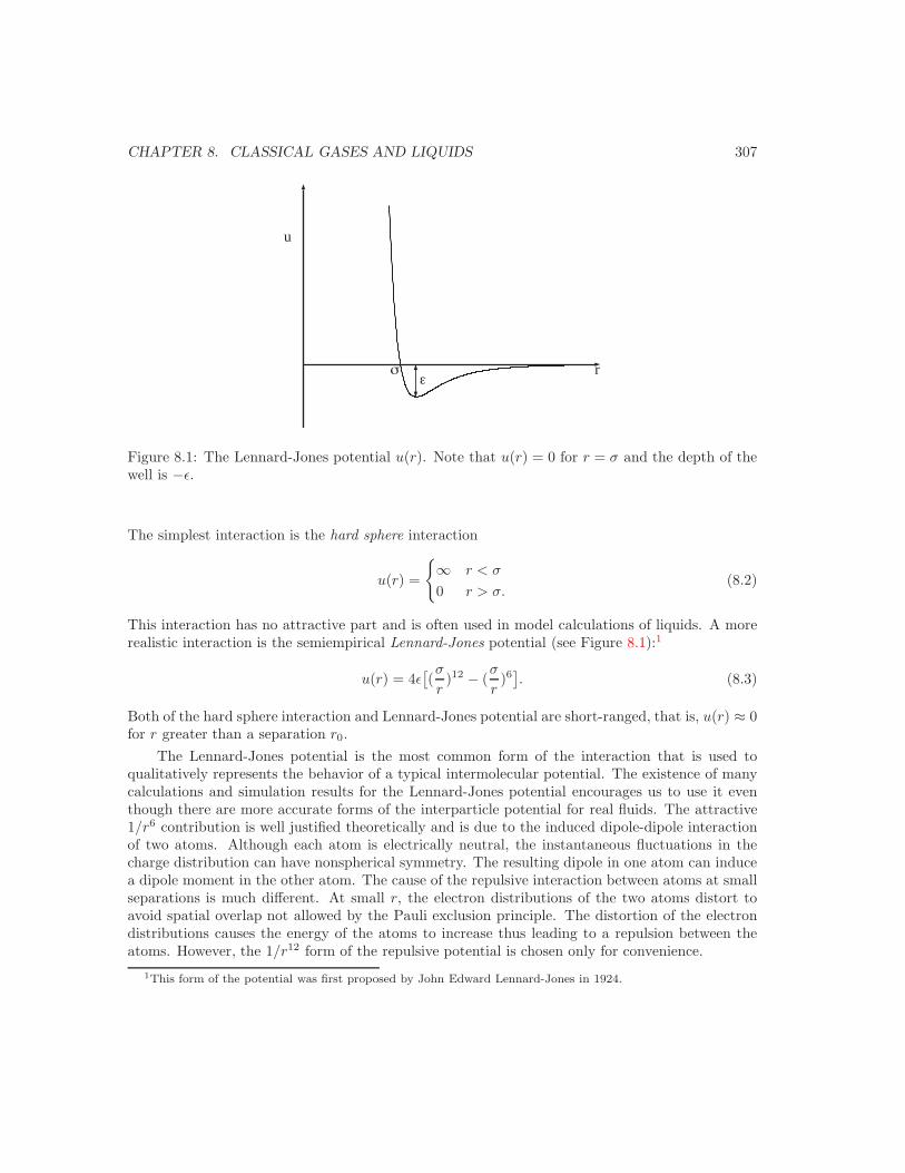
CHAPTER 8. CLASSICAL GASES AND LIQUIDS 307

u

rσε

Figure 8.1: The Lennard-Jones potential u(r). Note that u(r) = 0 for r = σ and the depth of thewell is −ε.

The simplest interaction is the hard sphere interaction

u(r) =

∞ r < σ

0 r > σ.(8.2)

This interaction has no attractive part and is often used in model calculations of liquids. A morerealistic interaction is the semiempirical Lennard-Jones potential (see Figure 8.1):1

u(r) = 4ε[(σ

r)12 − (

σ

r)6

]. (8.3)

Both of the hard sphere interaction and Lennard-Jones potential are short-ranged, that is, u(r) ≈ 0for r greater than a separation r0.

The Lennard-Jones potential is the most common form of the interaction that is used toqualitatively represents the behavior of a typical intermolecular potential. The existence of manycalculations and simulation results for the Lennard-Jones potential encourages us to use it eventhough there are more accurate forms of the interparticle potential for real fluids. The attractive1/r6 contribution is well justified theoretically and is due to the induced dipole-dipole interactionof two atoms. Although each atom is electrically neutral, the instantaneous fluctuations in thecharge distribution can have nonspherical symmetry. The resulting dipole in one atom can inducea dipole moment in the other atom. The cause of the repulsive interaction between atoms at smallseparations is much different. At small r, the electron distributions of the two atoms distort toavoid spatial overlap not allowed by the Pauli exclusion principle. The distortion of the electrondistributions causes the energy of the atoms to increase thus leading to a repulsion between theatoms. However, the 1/r12 form of the repulsive potential is chosen only for convenience.

1This form of the potential was first proposed by John Edward Lennard-Jones in 1924.

CHAPTER 8. CLASSICAL GASES AND LIQUIDS 308

Problem 8.1. Show that the minimum of the Lennard-Jones potential is at r0 = 21/6σ and thatu(r0) = −ε. At what value of r is u(r) a minimum?

We assume that the condition λ n−1/3 is satisfied so that the system can be treatedsemiclassically. In this limit the partition function for N identical particles is given by

ZN =1

N ! h3N

∫d3Np d3Nr e−βK e−βU , (8.4)

where the kinetic energy K =∑

i p2i /2m. The partition function for an ideal classical gas of N

particles, Zideal, is given by

Zideal =1

N !h3NV N

∫d3Np e−βK . (8.5)

We have already seen in Section 6.8 that Zideal can be evaluated exactly. The corresponding freeenergy of a classical ideal gas is Fideal = −kT ln Zideal.

Because the potential energy does not depend on the momenta of the particles, the kineticenergy part of the integrand in (8.4) can be integrated separately, and ZN can be written in theform

ZN

Zideal=

1V N

∫d3r1d

3r2 . . . d3rN e−βU , (8.6)

We adopt the notation 〈· · ·〉0 to denote an average over the microstates of the ideal gas. That is,each particle in (8.6) has a probability d3r/V of being in a volume d3r. Using this notation wewrite

ZN

Zideal= 〈e−βU 〉0. (8.7)

The contribution to the free energy from the correlations between the particles due to their inter-actions, Fc, has the form

Fc = −kT lnZ

Zideal= −kT ln 〈e−βU 〉0. (8.8)

We see that the calculation of the free energy of a classical system of interacting particles can bereduced to the evaluation of the ensemble average in (8.8). The evaluation of Fc for a classicalsystem of interacting particles is the overall goal of this chapter.

Because we do not expect to be able to calculate Fc exactly for arbitrary densities, we firstseek an approximation for Fc for low densities where we expect that the interactions between theparticles are not too important. We know that the ideal gas equation of state, PV/NkT = 1, isa good approximation to a gas in the dilute limit where the intermolecular interactions can beignored. If the interactions are short-range, we assume that we can make an expansion of thepressure in powers of the density. This expansion is known as the virial expansion and is writtenas

PV

NkT= 1 + ρB2(T ) + ρ2B3(T ) + . . . (8.9)

CHAPTER 8. CLASSICAL GASES AND LIQUIDS 309

The quantities Bn are known as virial coefficients and involve the interaction of n particles. Thefirst four virial coefficients are given by the integrals (B1 = 1)

B2(T ) = − 12V

∫d3r1d

3r2 f12, (8.10a)

B3(T ) = − 13V

∫d3r1d

3r2d3r3 f12f13f23, (8.10b)

B4(T ) = − 18V

∫d3r1d

3r2d3r3d

3r4

(3f12f23f34f41

+ 6f12f23f34f41f13 + f12f23f34f41f13f24

), (8.10c)

where fij = f(|ri − rj |), andf(r) = e−βu(r) − 1. (8.11)

The function f(r) defined in (8.11) is known as the Mayer f -function.

Problem 8.2. The density expansion of the free energy Fc is usually written as

−βFc

N=

∞∑p=1

bpρp

p + 1, (8.12)

where the bp are known as cluster integrals. Use the thermodynamic relation between the pressureand the free energy to show that Bn and bn−1 are related by

Bn = −n − 1n

bn−1 (8.13)

Problem 8.3. Plot the Mayer function f(r) for a hard sphere interaction and a Lennard-Jonespotential. Does f(r) depend on T for hard spheres?

8.3 Second Virial Coefficient

We can find the form of the second virial coefficient B2 by simple considerations. For simplicity,we first consider the partition function for N = 2 particles:

Z2

Zideal=

1V 2

∫d3r1 d3r2 e−βu12 . (8.14)

We can simplify the integrals in (8.14) by choosing particle 1 as the origin and specifying particle2 relative to particle 1. This choice of coordinates gives a factor of V because particle 1 can beanywhere in the box. Hence, we can write (8.26) as

Z2

Zideal=

1V

∫d3r e−βu(r), (8.15)

where r = r2 − r1 and r = |r|. The function e−βu(r) that appears in the integrand for Z2 has theundesirable property that it approaches unity rather than zero as r → ∞. Because we want to

CHAPTER 8. CLASSICAL GASES AND LIQUIDS 310

obtain an expansion in the density, we want to write the integrand in (8.15) in terms of a functionof r which is significant only if two particles are close to each other. Such a function is the Mayerfunction f(r) defined in (8.11). We write e−βu(r) = 1 + f(r) and express (8.15) as

Z2

Zideal=

1V

∫d3r [1 + f(r)]. (8.16)

Note that f(r) → 0 for sufficiently large r. The first term in the integrand in (8.16) correspondsto no interactions and the second term corresponds to the second virial coefficient B2 defined in(8.10a). To see this correspondence, we choose particle 1 as the origin as before, and rewrite (8.10a)for B2 as

B2 = −12

∫d3rf(r). (8.17)

If we compare the form (8.16) and (8.17), we see that we can express Z2/Zideal in terms of B2:

Z2

Zideal= 1 − 2

VB2. (8.18)

We next evaluate ZN for N = 3 particles. We have

Z3

Zideal=

1V 3

∫d3r1 d3r2 d3r3 e−β

Puij (8.19)

=1

V 3

∫d3r1 d3r2 d3r3

∏i<j

(1 + fij), (8.20)

=1

V 3

∫d3r1 d3r2 d3r3

[(1 + f12)(1 + f13)(1 + f23)

](8.21)

=1

V 3

∫d3r1 d3r2 d3r3

[1 + (f12 + f13 + f23)

+ (f12f13 + f12f23 + f13f23) + f12f13f23)]

(8.22)

We see that we can group terms of products of f ’s. If we neglect all but the first term in theexpansion (8.22), we recover the ideal gas result Z/Zideal = 1. It is plausible that in the limit oflow density, only the second sum in (8.22) involving pairs of particles is important, and we canignore the remaining terms involving products of two and three f ’s. Because the three terms f12,f13, and f23 give the same contribution, we have

Z3

Zideal≈ 1 +

3V

∫d3rf(r) = 1 − 6

VB2 (8.23)

We will see in Section 8.5 that the term in (8.22) involving a product of three f ’s is related to thethird virial coefficient.

For arbitrary N we write

ZN

Zideal=

1V N

∫d3r1 d3r2 . . . d3rNe−β

Puij

=1

V N

∫d3r1 d3r2 . . . d3rN

∏i<j

(1 + fij). (8.24)

CHAPTER 8. CLASSICAL GASES AND LIQUIDS 311

We have ∏i<j

(1 + fij) = 1 +∑k<l

fkl +∑

k<l, m<n

fklfmn + . . . (8.25)

We keep only the ideal gas contribution and the terms involving pairs of particles, and we ignorethe remaining terms involving products of two or more f ’s. There are a total of 1

2N(N − 1) termsin the sum

∑fkl corresponding to the number of ways of choosing pairs of particles. These terms

are all equal because they differ only in the way the variables of integration are labeled. Hence,we can write the integral of the first sum in (8.25) as

1V N

∫d3r1 . . . d3rN

∑k<l

fkl =1

V N

N(N − 1)2

∫d3r1 . . . d3rNf(r12). (8.26)

The integration with respect to r3 . . . rN over the volume of the system gives a factor of V N−2.As before, we can simplify the remaining integration over r1 and r2 by choosing particle 1 as

the origin and specifying particle 2 relative to particle 1. Hence, we can write the right-hand sideof (8.26) as

N(N − 1)2V

∫d3rf(r) → N2

2V

∫d3rf(r), (8.27)

where we have replaced N − 1 by N because N 1. If we identify the integral in (8.27) with B2,we see that we can write

ZN

Zideal≈ 1 − NρB2. (8.28)

If the interparticle potential u(r) ≈ 0 for r > r0, then f(r) differs from zero only for r < r0

and the integral B2 is bounded and is order r03 in three dimensions (see Problem 8.4). Hence B2

is independent of V and is an intensive quantity. However, this well-behaved nature of B2 impliesthat the second term in (8.28) is proportional to N and in the limit N → ∞, this term is largerthan the first — not a good omen for a perturbation theory.

The reason we have obtained this apparent divergence in ZN/Zideal is that we have calculatedthe wrong quantity. The quantity of physical interest is F rather than Z. Because F is proportionalto N , it follows from the relation F ∝ ln Z that ZN must depend on the Nth power of an intensivequantity. Thus Z must have the form

ZN

Zideal=

(1 − ρB2 + . . .

)N, (8.29)

so that F will be proportional to N . Hence, the leading contribution to Z/Zideal should be writtenas

ZN

Zideal= 1 − NρB2 → (1 − ρB2)N . (8.30)

The corresponding free energy is given by

F = Fideal − NkT ln(1 − ρB2),≈ Fideal + NkTρB2, (8.31)

CHAPTER 8. CLASSICAL GASES AND LIQUIDS 312

where we have used the fact that ln(1 + x) ≈ x for x 1. The corresponding equation of state isgiven by

PV

NkT= 1 + ρB2. (8.32)

The second term in (8.32) represents the first density correction to the ideal gas equation of state.The properties of B2 and the approximate equation of state (8.32) are explored in Problems 8.4–8.7.

Problem 8.4. To calculate B2 we need to first perform the angular integrations in (8.17). Showthat because u(r) depends only on r, B2 can be written as

B2(T ) = −12

∫d3r f(r) = 2π

∫ ∞

0

drr2 (1 − e−βu(r)). (8.33)

Show that B2 = 2πσ3/3 for a system of hard spheres of diameter σ.

Problem 8.5. Qualitative temperature behavior of B2(T ). Suppose that u(r) has the qualitativebehavior shown in Figure 8.1. Take r0 to be the value of r at which u(r) is a minimim (seeProblem 8.1). Interpret r0 in terms of the effective diameter of the atoms.

For high temperatures (kT ε), u(r)/kT 1 for r > r0. Explain why the value of the integralin (8.33) is determined by the contributions from the integrand for r < r0 where u(r)/kT is largeand positive. Show that in this limit B2(T ) ≈ b, where b = 2πr3

0/3. What is the interpretation ofthe parameter b?

For low temperatures (kT ε), the dominant contributions to the integral are determined bythe contributions from the integrand for r > r0. What is the sign of u(r) for r > r0? What is thesign of B2(T ) at low T ? Show that in this limit B2 ≈ −a/kT , where

a = −2π

∫ ∞

r0

u(r)r2dr. (8.34)

Show that this reasoning implies that B2 can be written in the approximate form

B2 = b − a

kT, (8.35)

where b = 2πr30/3 and a is given by (8.34). Why does B2(T ) pass through zero at some intermediate

temperature? The temperature at which B2(T ) = 0 is known at the Boyle temperature.

Problem 8.6. Use a simple numerical method such as Simpson’s rule (see Appendix Bxx) todetermine the T -dependence of B2 for the Lennard-Jones potential. At what temperature doesB2 vanish? How does this temperature compare with that predicted by (8.35)? Compare yournumerical result with the approximate result found in Problem 8.5.

Problem 8.7. Inversion temperature of Argon. In Section 7.4.2 we discussed the porous plug orJoule-Thompson process in which a gas is forced from a high pressure chamber through a porousplug into a lower pressure chamber. The process occurs at constant enthalpy and the change intemperature of the gas is given by dT = (∂T/∂P )H dP for small changes in pressure. We knowthat (see (7.48)) (∂T

∂P

)H

=1

CP

[T

(∂V

∂T

)P,N

− V]. (8.36)

CHAPTER 8. CLASSICAL GASES AND LIQUIDS 313

The locus of points (∂T/∂P )H = 0 is called the Joule-Thompson inversion curve. Assume theapproximate equation of state V = NkT/P + NB2 and use your numerical results for B2 fromProblem 8.6 for the Lennard-Jones potential to compute the inversion temperature at which theinversion curve is a maximum. Use σ = 3.4 Aand ε/k = 120 K and compare your result with theexperimental value of 780 K.

Problem 8.8. Assume that u(r) has the form u(r) ∼ r−n for large r. What is the condition onn such that the integral in (8.33) for B2 exists? Why is it plausible that the density expansion(8.8) is not applicable to a system of particles with an interaction proportional to 1/r (a Coulombsystem)?

∗Problem 8.9. Show that if the last term in (8.22) is neglected, Z3/Zideal = 1 − 6B2/V +12B2

2/V 2 ≈ (1 − 2ρB2)3, where ρ = 3/V . Also show that the last term in (8.22) is related to B3.

In Problem 8.5 we found that B2 can be written in the approximate form (8.35). This ap-proximate form of B2 allows us to write the equation of state as (see (8.32))

PV = NkT[1 + ρb − ρa

kT

]or

P ≈ ρkT [1

1 − ρb− ρa

kT]

=ρkT

1 − ρb− ρ2a2. (8.37)

Note that we have made the approximation 1 + ρb ≈ 1/(1 − ρb), which is consistent with ourassumption that ρb 1. The approximate equation of state in (8.37) is known as the van derWaals equation of state as discussed on page 33. Note that the parameter a takes into account thelong-range attraction of the molecules and the parameter b takes into account their short-rangerepulsion. A more systematic derivation of the van der Waals equation of state will be given inSection 8.9.1.

8.4 Cumulant Expansion

In Section 8.2 we had to make some awkward assumptions to obtain the form of B2 from anexpansion of Z/Zideal. To find the form of the higher order virial coefficients, we introduce what isknown as the cumulant expansion. In Section 8.5 we apply this formalism to obtain an expansionof lnZ/Zideal in powers of β. Finally, we rearrange this expansion so that it becomes an expansionof lnZ/Zideal in powers of ρ.

The form (8.8) for Fc is similar to that frequently encountered in probability theory. Weintroduce the function φ(t) defined as

φ(t) ≡ 〈etx〉, (8.38)

where the random variable x occurs according to the probability distribution p(x), that is, theaverage denoted by 〈. . .〉 is over p(x). The function φ(t) is an example of a moment generating

CHAPTER 8. CLASSICAL GASES AND LIQUIDS 314

function because a power series expansion in t yields

φ(t) = 〈[1 + tx +12!

t2x2 + · · · ]〉, (8.39)

= 1 + t〈x〉 +t2

2!〈x2〉 + · · · ,

=∞∑

n=0

tn〈xn〉n!

. (8.40)

In the present case the physical quantity of interest is proportional to lnZ, so we will want toconsider the series expansion of lnφ rather than φ. (The correspondence is t → −β and x → U .)The series expansion of lnφ(t) can be written in the form

ln φ = ln 〈etx〉 =∞∑

n=1

tnMn(x)n!

, (8.41)

where the coefficients Mn are known as cumulants or semi-invariants. The first four cumulantsare

M1 = 〈x〉, (8.42a)M2 = 〈x2〉 − 〈x〉2, (8.42b)M3 = 〈x3〉 − 3〈x2〉〈x〉 + 2〈x〉3, (8.42c)M4 = 〈x4〉 − 4〈x3〉〈x〉 − 3〈x2〉2 + 12〈x2〉〈x〉2 − 6〈x〉4. (8.42d)

Problem 8.10. Use the first few terms in the Taylor expansion of ln(1 + x) (see Appendix A) toobtain the expressions for Mn given in (8.42).

Because ln φ(x) is an extensive or additive quantity, the independent random variables x andy satisfy the condition that

ln 〈et(x+y)〉 = ln〈etx〉〈ety〉 = ln〈etx〉 + ln〈ety〉. (8.43)

Because

ln 〈et(x+y)〉 =∞∑

n=0

tn

n!Mn(x + y), (8.44)

we have the resultMn(x + y) = Mn(x) + Mn(y). (8.45)

The relation (8.45) implies that all cross terms in Mn involving independent variables vanish.

Problem 8.11. As an example of the cancellation of cross terms, consider M3(x + y). From(8.42c) we know that M3(x + y) is given by

M3(x + y) = (x + y)3 − 3(x + y)2 (x + y) + 2(x + y)3

(8.46)

Show explicitly that all cross terms cancel and that M3(x + y) = M3(x) + M3(y).

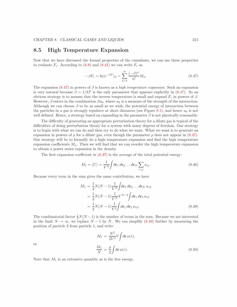
CHAPTER 8. CLASSICAL GASES AND LIQUIDS 315

8.5 High Temperature Expansion

Now that we have discussed the formal properties of the cumulants, we can use these propertiesto evaluate Fc. According to (8.8) and (8.41) we can write Fc as

−βFc = ln〈e−βU 〉0 =∞∑

n=1

(−β)n

n!Mn. (8.47)

The expansion (8.47) in powers of β is known as a high temperature expansion. Such an expansionis very natural because β = 1/kT is the only parameter that appears explicitly in (8.47). So anobvious strategy is to assume that the inverse temperature is small and expand Fc in powers of β.However, β enters in the combination βu0, where u0 is a measure of the strength of the interaction.Although we can choose β to be as small as we wish, the potential energy of interaction betweenthe particles in a gas is strongly repulsive at short distances (see Figure 8.1), and hence u0 is notwell defined. Hence, a strategy based on expanding in the parameter β is not physically reasonable.

The difficulty of generating an appropriate perturbation theory for a dilute gas is typical of thedifficulties of doing perturbation theory for a system with many degrees of freedom. Our strategyis to begin with what we can do and then try to do what we want. What we want is to generate anexpansion in powers of ρ for a dilute gas, even though the parameter ρ does not appear in (8.47).Our strategy will be to formally do a high temperature expansion and find the high temperatureexpansion coefficients Mn. Then we will find that we can reorder the high temperature expansionto obtain a power series expansion in the density.

The first expansion coefficient in (8.47) is the average of the total potential energy:

M1 = 〈U〉 =1

V N

∫dr1 dr2 . . . drN

∑i<j

uij . (8.48)

Because every term in the sum gives the same contribution, we have

M1 =12N(N − 1)

1V N

∫dr1 dr2 . . . drN u12

=12N(N − 1)

1V N

V N−2

∫dr1 dr2 u12

=12N(N − 1)

1V 2

∫dr1 dr2 u12. (8.49)

The combinatorial factor 12N(N −1) is the number of terms in the sum. Because we are interested

in the limit N → ∞, we replace N − 1 by N . We can simplify (8.49) further by measuring theposition of particle 2 from particle 1, and write

M1 =N2

2V 2V

∫dru(r),

orM1

N=

ρ

2

∫dru(r). (8.50)

Note that M1 is an extensive quantity as is the free energy.

CHAPTER 8. CLASSICAL GASES AND LIQUIDS 316

Before we proceed further, we note that we have implicitly assumed that the integral in (8.50)converges. However, the integral diverges for small r for a system of hard spheres or the Lennard-Jones potential. So what can we do? The answer might seem strange at first, but we will let ourintuition rather than mathematical rigor guide us. So let us assume that we can overcome theseproblems later. Or if this assumption seems unacceptable, we can equally well assume that thepotential energy of interaction is not strongly repulsive at small separations and is short-range.Examples of such potentials include the step potential u(r) = u0 for r < a and u(r) = 0 for r > a,and the Gaussian potential u(r) = u0 e−r2/a2

.We next consider M2 which is given by

M2 = 〈U2〉 − 〈U〉2, (8.51)

where〈U〉 =

∑i<j

∑j

〈uij〉. (8.52)

and〈U2〉 =

∑i<j

∑j

∑k<l

∑l

〈uij ukl〉, (8.53)

The various terms in (8.53) and (8.52) may be classified according to the number of subscripts incommon. As an example, suppose that N = 4. We have

U =4∑

i<j=1

uij = u12 + u13 + u14 + u23 + u24 + u34, (8.54)

and

U2 = [u212 + u2

13 + u214 + u2

23 + u224 + u2

34]+ 2[u12u13 + u12u14 + u12u23 + u12u24 + u13u14 + u13u23

+ u13u34 + u14u24 + u14u34 + u23u24 + u23u34 + u24u34]+ 2[u12u34 + u13u24 + u14u23] (8.55)

An inspection of (8.55) shows that the 36 terms in (8.55) can be grouped into three classes:No indices in common (disconnected terms). A typical disconnected term is 〈u12u34〉.Because the variables r12 and r34 are independent, u12 and u34 are independent, and we can write

〈u12u34〉 = 〈u12〉〈u34〉. (8.56)

From (8.45) we know that every disconnected term such as the one in (8.56) is a cross term thatis canceled if all terms in M2 are included.One index in common (reducible terms). An example of a reducible term is 〈u12u23〉. Wecan see that such a term also factorizes because of the homogeneity of space. Suppose we choose

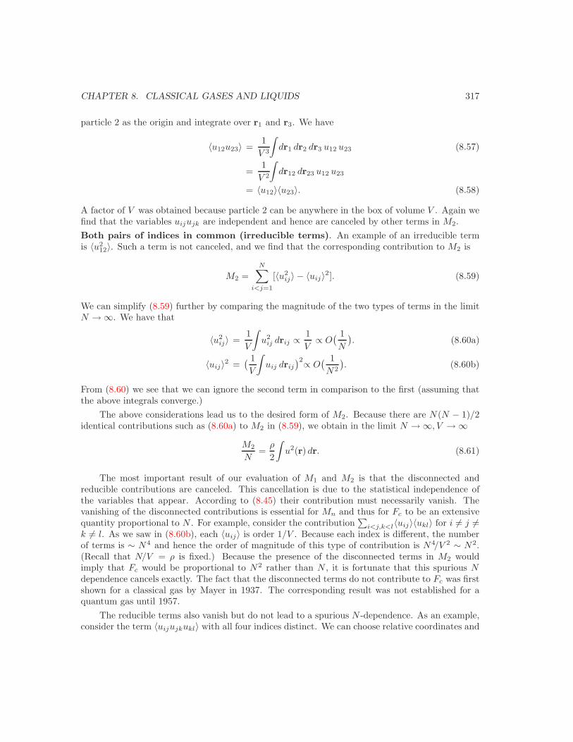
CHAPTER 8. CLASSICAL GASES AND LIQUIDS 317

particle 2 as the origin and integrate over r1 and r3. We have

〈u12u23〉 =1

V 3

∫dr1 dr2 dr3 u12 u23 (8.57)

=1

V 2

∫dr12 dr23 u12 u23

= 〈u12〉〈u23〉. (8.58)

A factor of V was obtained because particle 2 can be anywhere in the box of volume V . Again wefind that the variables uijujk are independent and hence are canceled by other terms in M2.Both pairs of indices in common (irreducible terms). An example of an irreducible termis 〈u2

12〉. Such a term is not canceled, and we find that the corresponding contribution to M2 is

M2 =N∑

i<j=1

[〈u2ij〉 − 〈uij〉2]. (8.59)

We can simplify (8.59) further by comparing the magnitude of the two types of terms in the limitN → ∞. We have that

〈u2ij〉 =

1V

∫u2

ij drij ∝ 1V

∝ O( 1N

). (8.60a)

〈uij〉2 =( 1V

∫uij drij

)2∝ O( 1N2

). (8.60b)

From (8.60) we see that we can ignore the second term in comparison to the first (assuming thatthe above integrals converge.)

The above considerations lead us to the desired form of M2. Because there are N(N − 1)/2identical contributions such as (8.60a) to M2 in (8.59), we obtain in the limit N → ∞, V → ∞

M2

N=

ρ

2

∫u2(r) dr. (8.61)

The most important result of our evaluation of M1 and M2 is that the disconnected andreducible contributions are canceled. This cancellation is due to the statistical independence ofthe variables that appear. According to (8.45) their contribution must necessarily vanish. Thevanishing of the disconnected contributions is essential for Mn and thus for Fc to be an extensivequantity proportional to N . For example, consider the contribution

∑i<j,k<l〈uij〉〈ukl〉 for i = j =

k = l. As we saw in (8.60b), each 〈uij〉 is order 1/V . Because each index is different, the numberof terms is ∼ N4 and hence the order of magnitude of this type of contribution is N4/V 2 ∼ N2.(Recall that N/V = ρ is fixed.) Because the presence of the disconnected terms in M2 wouldimply that Fc would be proportional to N2 rather than N , it is fortunate that this spurious Ndependence cancels exactly. The fact that the disconnected terms do not contribute to Fc was firstshown for a classical gas by Mayer in 1937. The corresponding result was not established for aquantum gas until 1957.

The reducible terms also vanish but do not lead to a spurious N -dependence. As an example,consider the term 〈uijujkukl〉 with all four indices distinct. We can choose relative coordinates and

CHAPTER 8. CLASSICAL GASES AND LIQUIDS 318

(a) (b) (c)

Figure 8.2: Examples of disconnected diagrams with three bonds. For (a) the volume dependence isV −3, the number of terms in the sum is O(N6) and the magnitude of the contribution is O(N3). For(b) the volume dependence is V −3, the number of terms in the sum is O(N5), and the magnitude ofthe contribution is O(N2). For (c) the volume dependence is V −2, the number of terms is O(N4),and magnitude is O(N2).

show that this term factorizes, 〈uijujkukl〉 = 〈uij〉〈ujk〉〈ukl〉, and hence is canceled for a classicalgas. However, the N -dependence of this term is N4/V 3 ∼ N . This fact that the reducible termsare proportional to N is fortunate because the reducible terms do not cancel for a quantum gas.

Problem 8.12. Consider a system of N = 4 particles and obtain the explicit form of the firstthree cumulants. Show that the disconnected and reducible contributions cancel.

To consider the higher-order cumulants, we introduce a graphical notation that correspondsto the various contributions to Mn. As we have seen, we do not need to consider products ofexpectation values because they either cancel or are O(1/N) relative to the irreducible termsarising from the first term in Mn. The rules for the calculation of Mn are

a. For each particle (subscript on u) draw a vertex (a point).b. Draw a bond (dotted line) between two vertices. There is a total of n bonds among pvertices, where 2 ≤ p ≤ n.

c. If the diagram contains two or more pieces not joined by a bond, then the diagram is disconnected;If the diagram can be separated into two disconnected pieces by removing one vertex, then thediagram is reducible. The remaining diagrams are irreducible and are the only ones that need tobe considered.

Examples of the various types of disconnected and reducible diagrams are shown in Figs. 8.2–8.4corresponding to Mn=3. What are the corresponding contributions to M3?

It is straightforward to find the contributions to M3 corresponding to the two types of irre-ducible diagrams shown in Figure 8.4. There are 1

2N(N − 1) identical contributions of type (a)and N(N − 1)(N − 2) of the type shown in (b). Hence, the form of M3 in the limit N → ∞ is

M3

N=

ρ

2

∫u3(r) dr + ρ2

∫u12 u23 u31 dr12 dr23. (8.62)

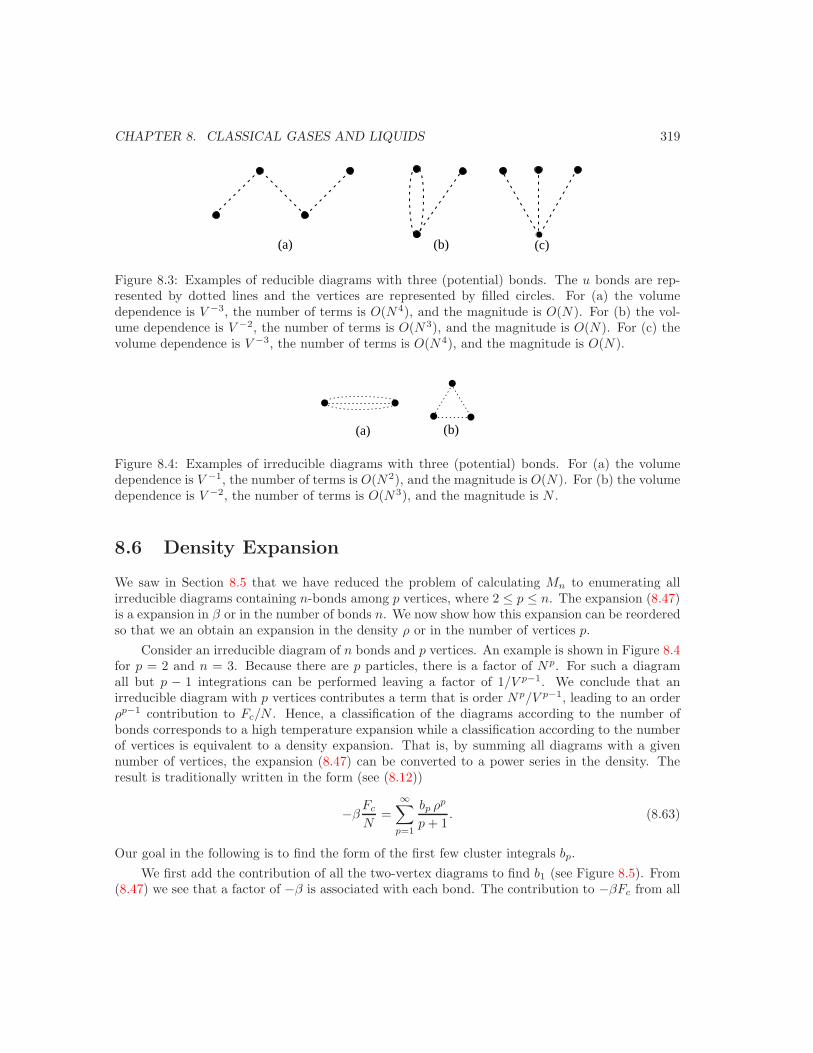
CHAPTER 8. CLASSICAL GASES AND LIQUIDS 319

(a) (b) (c)

Figure 8.3: Examples of reducible diagrams with three (potential) bonds. The u bonds are rep-resented by dotted lines and the vertices are represented by filled circles. For (a) the volumedependence is V −3, the number of terms is O(N4), and the magnitude is O(N). For (b) the vol-ume dependence is V −2, the number of terms is O(N3), and the magnitude is O(N). For (c) thevolume dependence is V −3, the number of terms is O(N4), and the magnitude is O(N).

(a) (b)

Figure 8.4: Examples of irreducible diagrams with three (potential) bonds. For (a) the volumedependence is V −1, the number of terms is O(N2), and the magnitude is O(N). For (b) the volumedependence is V −2, the number of terms is O(N3), and the magnitude is N .

8.6 Density Expansion

We saw in Section 8.5 that we have reduced the problem of calculating Mn to enumerating allirreducible diagrams containing n-bonds among p vertices, where 2 ≤ p ≤ n. The expansion (8.47)is a expansion in β or in the number of bonds n. We now show how this expansion can be reorderedso that we an obtain an expansion in the density ρ or in the number of vertices p.

Consider an irreducible diagram of n bonds and p vertices. An example is shown in Figure 8.4for p = 2 and n = 3. Because there are p particles, there is a factor of Np. For such a diagramall but p − 1 integrations can be performed leaving a factor of 1/V p−1. We conclude that anirreducible diagram with p vertices contributes a term that is order Np/V p−1, leading to an orderρp−1 contribution to Fc/N . Hence, a classification of the diagrams according to the number ofbonds corresponds to a high temperature expansion while a classification according to the numberof vertices is equivalent to a density expansion. That is, by summing all diagrams with a givennumber of vertices, the expansion (8.47) can be converted to a power series in the density. Theresult is traditionally written in the form (see (8.12))

−βFc

N=

∞∑p=1

bp ρp

p + 1. (8.63)

Our goal in the following is to find the form of the first few cluster integrals bp.We first add the contribution of all the two-vertex diagrams to find b1 (see Figure 8.5). From

(8.47) we see that a factor of −β is associated with each bond. The contribution to −βFc from all

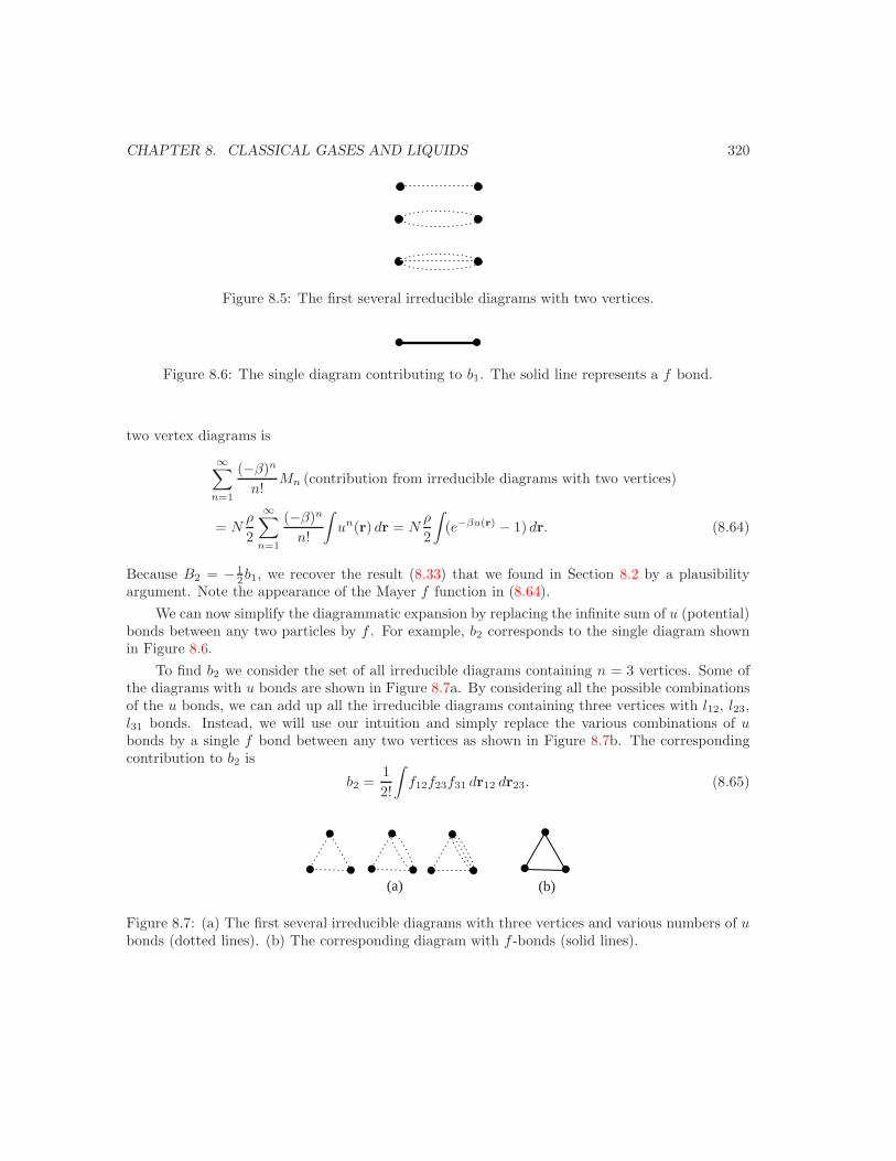
CHAPTER 8. CLASSICAL GASES AND LIQUIDS 320

Figure 8.5: The first several irreducible diagrams with two vertices.

Figure 8.6: The single diagram contributing to b1. The solid line represents a f bond.

two vertex diagrams is

∞∑n=1

(−β)n

n!Mn (contribution from irreducible diagrams with two vertices)

= Nρ

2

∞∑n=1

(−β)n

n!

∫un(r) dr = N

ρ

2

∫(e−βu(r) − 1) dr. (8.64)

Because B2 = − 12b1, we recover the result (8.33) that we found in Section 8.2 by a plausibility

argument. Note the appearance of the Mayer f function in (8.64).We can now simplify the diagrammatic expansion by replacing the infinite sum of u (potential)

bonds between any two particles by f . For example, b2 corresponds to the single diagram shownin Figure 8.6.

To find b2 we consider the set of all irreducible diagrams containing n = 3 vertices. Some ofthe diagrams with u bonds are shown in Figure 8.7a. By considering all the possible combinationsof the u bonds, we can add up all the irreducible diagrams containing three vertices with l12, l23,l31 bonds. Instead, we will use our intuition and simply replace the various combinations of ubonds by a single f bond between any two vertices as shown in Figure 8.7b. The correspondingcontribution to b2 is

b2 =12!

∫f12f23f31 dr12 dr23. (8.65)

(b)(a)

Figure 8.7: (a) The first several irreducible diagrams with three vertices and various numbers of ubonds (dotted lines). (b) The corresponding diagram with f -bonds (solid lines).

CHAPTER 8. CLASSICAL GASES AND LIQUIDS 321

1

23

4 1 2

3 4

1 4

2 3

1 2

3 4

1 2

3 4

1 4 1 4 1 4 1

3 2 2 3 3 2 3 4

21 4

2 3

Figure 8.8: The four-vertex diagrams with all the possible different labelings. Note that the bondsare f bonds.

In general, it can be shown that

bp =1p!

∑∫ ∏fij dr1 . . . drp, (8.66)

where the sum is over all irreducible topologically distinct diagrams among p + 1 vertices. Forexample, b3 corresponds to the four-vertex diagrams shown in Figure 8.8. The correspondingresult for b3 is

b3 =13!

∫(3f12f23f34f41 + 6f12f23f34f41f13 + f12f23f34f41f13f24) dr2dr3dr4. (8.67)

We see that we have converted the original high temperature expansion to a density expansionby summing what are known as ladder diagrams. These diagrams corresponding to all the possibleu bonds between any two particles (vertices). The result of this sum is the Mayer f function. Theresultant density expansion for the free energy and the pressure equation of state is one of the fewexpansions known in physics that is convergent for sufficiently small densities. In contrast, mostexpansions in physics are asymptotic.

The procedure for finding higher order terms in the density expansion of the free energy isstraightforward in principle. To find the contribution of order ρp−1, we enumerate all the diagramswith p vertices and various numbers of f bonds such that the diagrams are irreducible. There isonly one f bond between any two vertices. However, the enumeration of the cluster integrals bp

becomes more and more difficult for larger p. Even more difficult is the calculation of the clusterintegrals even for hard spheres.

The results for the known virial coefficients for hard spheres are summarized in Table 8.1 interms of the parameter

η = πρσ3/6, (8.68)

where σ is the diameter of the spheres. The parameter η can be expressed as

η = ρ(4π/3)(σ/2)3. (8.69)

The form of (8.69) shows that η is the fraction of the space occupied by N spheres. For this reasonη is often called the packing fraction.

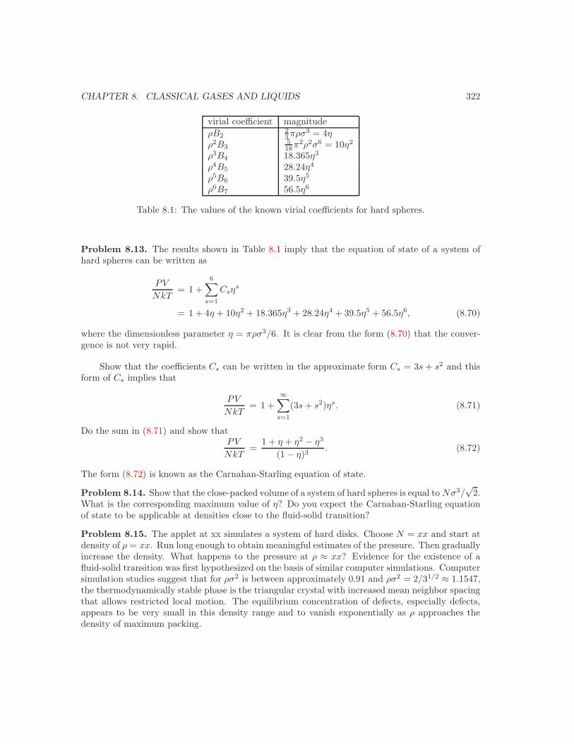
CHAPTER 8. CLASSICAL GASES AND LIQUIDS 322

virial coefficient magnitudeρB2

23πρσ3 = 4η

ρ2B3518π2ρ2σ6 = 10η2

ρ3B4 18.365η3

ρ4B5 28.24η4

ρ5B6 39.5η5

ρ6B7 56.5η6

Table 8.1: The values of the known virial coefficients for hard spheres.

Problem 8.13. The results shown in Table 8.1 imply that the equation of state of a system ofhard spheres can be written as

PV

NkT= 1 +

6∑s=1

Csηs

= 1 + 4η + 10η2 + 18.365η3 + 28.24η4 + 39.5η5 + 56.5η6, (8.70)

where the dimensionless parameter η = πρσ3/6. It is clear from the form (8.70) that the conver-gence is not very rapid.

Show that the coefficients Cs can be written in the approximate form Cs = 3s + s2 and thisform of Cs implies that

PV

NkT= 1 +

∞∑s=1

(3s + s2)ηs. (8.71)

Do the sum in (8.71) and show thatPV

NkT=

1 + η + η2 − η3

(1 − η)3. (8.72)

The form (8.72) is known as the Carnahan-Starling equation of state.

Problem 8.14. Show that the close-packed volume of a system of hard spheres is equal to Nσ3/√

2.What is the corresponding maximum value of η? Do you expect the Carnahan-Starling equationof state to be applicable at densities close to the fluid-solid transition?

Problem 8.15. The applet at xx simulates a system of hard disks. Choose N = xx and start atdensity of ρ = xx. Run long enough to obtain meaningful estimates of the pressure. Then graduallyincrease the density. What happens to the pressure at ρ ≈ xx? Evidence for the existence of afluid-solid transition was first hypothesized on the basis of similar computer simulations. Computersimulation studies suggest that for ρσ2 is between approximately 0.91 and ρσ2 = 2/31/2 ≈ 1.1547,the thermodynamically stable phase is the triangular crystal with increased mean neighbor spacingthat allows restricted local motion. The equilibrium concentration of defects, especially defects,appears to be very small in this density range and to vanish exponentially as ρ approaches thedensity of maximum packing.

CHAPTER 8. CLASSICAL GASES AND LIQUIDS 323

Problem 8.16. Use the Carnahan-Starling equation of state (8.72) to derive analytical expressionsfor the excess entropy Sex, excess energy ESex, excess Helmholtz free energy for a hard-sphere fluid.The excess entropy Sex is defined by S − −NK ln P − Nk ln βλ3 + 5Nk/2 + Sex and the excessenergy is defined by E = 3NkT + Eex.

Problem 8.17. Consider a one-dimensional gas of particles confined to a box of length L. Supposethat the interparticle interaction is given by

u(x) =

∞ x < a

0 x ≥ a(8.73)

Such a system of hard rods is known as a Tonks gas. (a) Evaluate the virial coefficients B2 andB3. It is possible to do the integrals analytically. (b) Note that the form of the interaction (8.73)prevents particles from exchanging places, that is, from changing their order. What is the available“volume” in which the particles can move? Use this consideration to guess the form of the equationof state. (c∗) Calculate the partition function and the equation of state exactly and show thatyour results are consistent with part (a).

8.7 Radial Distribution Function

Now that we know how to include the interactions between particles to obtain the equation of state,we can consider how these interactions lead to correlations between the particles. We know that ifthe interactions are neglected, the positions of the particles are uncorrelated and the probability offinding a particle a distance r away from a particular particle is proportional to ρ. In the following,we define a quantity that is a measure of the correlations between particles and determine itsdependence on r in the limit of low density.

The probability of a configuration of N particles in a volume V is given in the canonicalensemble by

PN (r1, r2, . . . , rN ) dr1dr2 . . . drN =e−βUdr1dr2 . . . drN∫e−βUdr1dr2 . . . drN

=e−βUdr1dr2 . . . drN

QN, (8.74)

where U is the total potential energy of the configuration. The quantity PN dr1dr2 . . . drN is theprobability that particle 1 is in the range dr1 about r1, particle 2 is in the range dr2 about r2, etc.

The configurational integral QN is defined as

QN =∫

dr1dr2 . . . drN e−βU . (8.75)

Note that QN is related to the partition function ZN for a classical system by QN = ZN/(N ! λ3N ).QN is defined so that QN = V N for an ideal gas.

The probability that particle 1 is in the range dr1 about r1 and particle 2 is in the range dr2

about r2 is obtained by integrating (8.74) over the positions of particles 3 through N :

P2(r1, r2) dr1dr2 =∫

e−βUdr3 . . . drN

QNdr1dr2. (8.76)

CHAPTER 8. CLASSICAL GASES AND LIQUIDS 324

The probability that any particle is in the range dr1 about r1 and any other particle is in the rangedr2 about r2 is N(N − 1)P2. In general, we define the n-particle density function for a system ofN particles as

ρn(r1, . . . , rn) =N !

(N − n)!

∫e−βUdrN−n . . . drN

QN. (8.77)

It is easy to see that ρ2 = N(N − 1)P2. The normalization condition for ρn is∫

ρn(r1, . . . , rn) dr1 . . . drn =N !

(N − n)!. (8.78)

For n = 1, we have ∫ρ1(r) dr = N. (8.79)

If the system is homogeneous, then ρ1(r) is independent of r, and it follows from (8.79) that

ρ1(r) =N

V= ρ. (8.80)

We define the pair distribution function g(r1, r2) as

ρ2g(r1, r2) = ρ2 = N(N − 1)P2 = N(N − 1)∫e−βUdr3 . . . drN

QN, (8.81)

or

g(r1, r2) = (1 − 1N

)V 2

∫e−βUdr3 . . . drN

QN. (8.82)

If the interparticle interaction is spherically symmetric and the system is a liquid, then g(r1, r2)depends only on the relative separation r12 = |r1 − r2| between particles 1 and 2. We adopt thenotation g(r) = g(r12) in the following; g(r) is called the radial distribution function.

Note that g(r) is defined so that g(r) = 1 for an ideal gas. (Actually g(r) = 1 − 1/N , but wecan ignore the 1/N correction in the thermodynamic limit.) The quantity ρg(r)dr is related to theprobability of observing a second particle in the range dr a distance r away from a particle at theorigin. The normalization for ρg(r) is given by

ρ

∫g(r) 4πr2dr = ρ(1 − 1

N)V 2 1

V= N − 1. (8.83)

From (8.83) we see that ρg(r) 4πr2dr is the number of particles between r and r + dr about aparticular particle, that is, the product ρg(r) can be interpreted as the local density about aparticular particle.

The qualitative features of g(r) for a Lennard-Jones fluid are shown in Figure 8.9. We seethat g → 0 as r → 0 because the interaction between the particles does not allow the particles tobecome too close. Similarly at large r the other particles are not correlated with the fixed particleand g(r) → 1 as r → ∞.

It is easy to find the form of g(r) in the limit of low densities. In the limit N → ∞, g(r) isgiven by (see (8.82))

g(r) =V 2

∫e−βUdr3 . . . drN

QN. (8.84)

CHAPTER 8. CLASSICAL GASES AND LIQUIDS 325

not done

Figure 8.9: Dependence of g(r) on r for a three-dimensional Lennard-Jones liquid at kT/ε = xxand ρσ3 = xx.

At low densities, we may integrate over particles 3, 4, . . . , N , assuming that these particles aredistant from particles 1 and 2 and also distant from each other. Also for almost all configurations,we can replace U by u12 in the numerator. Similarly, the denominator can be approximated byV N . Hence we have

g(r) ≈ V 2 e−βu12V N−2

V N= e−βu(r). (8.85)

Another way of defining g(r) is in terms of the local particle density. Consider the sum∑Ni=1 δ(r − ri). Given the properties of the delta function, we know that the integral of this sum

about r over the volume element d3r yields the number of particles in the volume element. Hence,we can define the local particle density as

ρ(r) =N∑

i=1

δ(r − ri). (8.86)

We have

ρ1(r) =⟨ N∑

i=1

δ(r − ri)⟩, (8.87)

where 〈δ(r − ri)〉 is given by

⟨δ(r − ri)

⟩=

1QN

∫δ(r − r1) e−βU(r1,...,rN ) dr1 . . . drN (8.88)

=1

QN

∫e−βU(r,r2,...,rN ) dr2 . . . drN . (8.89)

For a homogeneous system ρ1(r1) = ρ.

Problem 8.18. Use (8.89) and the definition (8.87) to show that ρ1(r1) = ρ for a homogeneoussystem.

We can define ρ2(r1, r2) as

ρ2(r1, r2) =∑i=j

⟨δ(r1 − ri)δ(r2 − rj)

⟩(8.90)

CHAPTER 8. CLASSICAL GASES AND LIQUIDS 326

We can use the same reasoning as in (8.89) to show that

ρ2(r1, r2) = N(N − 1)∫

d3r3d3r4 . . . d3rNe−βU(r1,r2,r3...rN )∫

d3r1d3r2d3r3d3r4 . . . d3rNe−βU(r1,r2,r3...rN )(8.91)

If we compare (8.91) and (8.81), we see that we can also define g(r1, r2) as

ρ2g(r1, r2) =∑i=j

⟨δ(r1 − ri)δ(r2 − rj)

⟩(8.92)

Hence, we see that g(r) is related to the spatial correlation of the density fluctuations in the system.

8.7.1 Relation of thermodynamic functions to g(r)

We first derive a relation for the mean energy E in terms of g(r). We write

E =32NkT + U, (8.93)

whereU =

1QN

∫· · ·

∫Ue−βU dr1dr2 . . . drN . (8.94)

The two terms in (8.93) are the mean kinetic energy and the mean potential energy U , respectively.If we assume that U is given by (8.1), we can write U as

U =N(N − 1)

21

QN

∫e−βUu(r12) dr1 . . . drN , (8.95)

=N(N − 1)

2

∫u(r12)

[∫e−βU dr3 . . . drN

QN

]dr1dr2,

=12

∫u(r12) ρ2g(r1, r2) dr1dr2. (8.96)

Hence

U =N2

2V

∫u(r)g(r)d3r = N

ρ

2

∫u(r)g(r) 4πr2dr, (8.97)

and the total energy E per particle is given by

E

N=

32kT +

ρ

2

∫ ∞

0

u(r)g(r) 4πr2 dr. (8.98)

The form of the second term in (8.98) for the mean potential energy is clear from physicalconsiderations. The potential energy of interaction between a particular particle and all the otherparticles between r and r + dr is u(r)ρg(r)4πr2dr, where we have interpreted ρg(r) as the localdensity. The total potential energy is found by integrating over all values of r and multiplying byN/2. The factor of N is included because any of the N particles can be chosen as the particle atthe origin; the factor of 1/2 is included so that each pair interaction is counted only once.

CHAPTER 8. CLASSICAL GASES AND LIQUIDS 327

We can derive a similar relation between the mean pressure and an integral over the productof g(r) and the force −du(r)/dr. The pressure is related to the configurational part of the partitionfunction by

P = −∂F

∂V= kT

∂ ln QN

∂V. (8.99)

For large V the pressure is independent of the shape of the container. For convenience, we assumethat the container is a cube of linear dimension L, and we write the configuration integral QN as

QN =∫ L

0

· · ·∫ L

0

e−βU dx1dy1dz1 . . . dxNdyNdzN . (8.100)

We first change variables so that the limits of integration are independent of L and let xi = xi/L,etc. Then

QN = V N

∫ 1

0

. . .

∫ 1

0

e−βUdx1dy1dz1 . . . dxNdyNdzN , (8.101)

where U depends on the separation rij = L[(xi − xj)2 + (yi − yj)2 + (xi − zj)2]1/2. This change ofvariables allows us to take the derivative of QN with respect to V . We have

∂QN

∂V= NV N−1

∫ 1

0

· · ·∫ 1

0

e−βUdx1 . . . dzN

− V N

kT

∫ 1

0

· · ·∫ 1

0

e−βU ∂U

∂Vdx1 . . . dzN , (8.102)

where∂U

∂V=

∑i<j

du(rij)drij

drij

dL

dL

dV=

∑i<j

du(rij)drij

rij

L

13L2

. (8.103)

Now that we have differentiated QN with respect to V , we transform back to the original variablesx1, . . . , zN . In the second term of (8.103) we also can use the fact that there are N(N − 1)/2identical contributions. We obtain

∂ ln QN

∂V=

1QN

∂QN

∂V=

N

V− ρ2

6V kT

∫r12

du(r12)dr12

g(r12) dr1 dr2, (8.104)

and hence

PV

NkT= 1 − ρ

6kT

∫ ∞

0

rdu(r)

drg(r) 4πr2dr. (virial equation of state) (8.105)

The integrand in (8.105) is related to the virial in classical mechanics and is the mean value of theproduct r · F (cf. Goldstein).

8.7.2 Relation of g(r) to static structure function S(k)

A measurement of the radial distribution function g(r) probes distances on the order of the meaninterparticle spacing, which is the order of Angstroms or 10−10 m. Such wavelengths can be ob-tained with neutrons or x-rays. To understand how an elastic scattering experiment can probe the

CHAPTER 8. CLASSICAL GASES AND LIQUIDS 328

structure, we consider x-ray scattering. A typical x-ray wavelength is 1 A, and the correspondingenergy per photon is ω = hc/λ ≈ 104 eV. This energy is very large in comparison to the ther-mal energy of the particles in a liquid that is the order of kT or approximately 0.1 eV at roomtemperatures. Hence, collisions with the particles in a liquid will leave the photon energies almostunaltered and to a good approximation, the scattering can be treated as elastic.

In Appendix 8A, we show that the scattered intensity of the x-rays is given by

I(θ) = NI1S(k), (8.106)

where the wave vector k is related to the scattering angle θ. The static structure function S(k) isgiven by

S(k) =1N

⟨ N∑i,j=1

eik·(ri−rj)⟩. (8.107)

It is easy to show that S(k) is N if the particles are not correlated because in this case the onlycontribution to the sum in (8.107) is for i = j.

The static structure function S(k) is a measure of the correlations between the positions ofthe atoms in the liquid and is related to the Fourier transform of g(r) as we show in the following.We first divide the sum over i and j in (8.107) into self, i = j, and distinct, i = j, contributions.There are N of the former and N(N − 1) of the latter. We write

S(k) = 1 +1N

N(N − 1)〈eik·(r1−r2)〉 (8.108)

= 1 +N(N − 1)

N

∫dr1 . . . drN eik·(r1−r2) e−βU∫

dr1 . . . drN e−βU. (8.109)

If we use the definition (8.81) of g(r1, r2), we can write (8.109) as

S(k) = 1 +1N

∫dr1dr2 ρ2g(r1, r2) eik·(r1−r2). (8.110)

For a homogeneous liquid, g(r1, r2) depends only on |r1 − r2|, and we obtain

S(k) = 1 + ρ

∫dr g(r)eik·r. (8.111)

It is customary to rewrite (8.111) as

S(k) − 1 = ρ

∫dr [g(r) − 1] eik·r + ρ

∫dr eik·r

= ρ

∫dr [g(r) − 1] eik·r + ρ(2π)3δ(k). (8.112)

The contribution of the δ(k) term in (8.112) is unimportant because it is identically zero exceptwhen k = 0, that is, for radiation not scattered by the atoms in the fluid. Hence, we can rewrite(8.112) in the desired form:

S(k) − 1 = ρ

∫dr [g(r) − 1] eik·r. (8.113)

CHAPTER 8. CLASSICAL GASES AND LIQUIDS 329

From (8.113) we see that S(k) − 1 is the Fourier transform of g(r) − 1, and a measurement ofthe intensity of elastically scattered radiation yields the Fourier transform of the radial correlationfunction.

8.7.3 Variable number of particles

In a scattering experiment the beam samples a subset of the total volume. Because the numberof particles in the subset fluctuates, we need to use the grand canonical ensemble to describe themeasured value of S(k). The energy and pressure equations (8.98) and (8.105) are identical in bothensembles, but the compressibility equation, which we derive in the following, can only be derivedin the grand canonical ensemble because it relates the integral of g(r) − 1 and hence S(k = 0) tofluctuations in the density.

The compressibility KT is defined as (see (7.1))

KT = − 1V

∂V

∂P=

1ρ

∂ρ

∂P. (8.114)

We will use thermodynamic arguments in the following to show that

ρKT =1N

(∂N

∂µ

)T,V

. (8.115)

If we combine (8.115) with (6.262), we see that the compressibility is related to the density fluc-tuations:

ρKT =1

kT

〈N2〉 − 〈N〉2〈N〉 . (8.116)

The thermodynamic argument proceeds as follows. We have that

dΩ = −PdV − SdT − Ndµ = −PdV − V dP. (8.117)

We cancel the PdV term on both sides of (8.117) and solve for dµ:

dµ =V

NdP − S

NdT. (8.118)

We let v = V/N ; v is the volume per particle or specific volume. Because µ is an intensive quantity,we can express µ as µ(v, T ) and obtain

(∂µ

∂v

)T

= v(∂P

∂v

)T

. (8.119)

We can change v by changing either V or N :

(∂µ

∂v

)T,V

=∂N

∂v

∂µ

∂N= −N2

V

∂µ

∂N(8.120)

(∂µ

∂v

)T,N

=∂V

∂v

∂µ

∂V= −N

∂µ

∂V. (8.121)

CHAPTER 8. CLASSICAL GASES AND LIQUIDS 330

However, the way in which v is changed cannot affect (8.119). Hence,

−N2

V

( ∂µ

∂N

)T,V

= V(∂P

∂V

)T,N

. (8.122)

We leave it as an exercise to the reader to use (8.122) and (8.114) to obtain the desired relation(8.115).

We now relate the integral over g(r) to the density fluctuations. In the grand canonicalensemble the probability density of finding n particular particles with positions r1, . . . , rn in therange dr1, . . . , drn is given by

Pn(r1, . . . , rn) =∞∑

N=0

zN

N !Z∫

e−βUN drn+1 . . . drN , (8.123)

where z = eβµ. There are N(N − 1) . . . (N −n + 1) = N !/(N −n)! different sets of particles whichcan correspond to the n particles. Hence, the total probability that any n particles occupy thesevolume elements is given by

Pn(r1, . . . , rn) ≡ ρng(r1, . . . , rn), (8.124a)

=∞∑

N=0

zN

N − n)!Z∫· · ·

∫e−βUN drN+1, . . . drN . (8.124b)

As before, the main quantity of interest is g(r1, r2).From the definition of P1 and P2, it follows that

∫P1(r1) dr1 = 〈N〉, (8.125)

and ∫ ∫P2(r1, r2) dr1dr2 = 〈N(N − 1)〉. (8.126)

We can use (8.126) and (8.125) to obtain∫ ∫ [

P2(r1, r2) − P1(r1)P1(r2)]dr1dr2 = 〈N2〉 − 〈N〉2 − 〈N〉. (8.127)

The left-hand side of (8.127) is equal to V ρ2∫

[g(r) − 1] d3r for a homogeneous system. Hence weobtain

Nρ

∫[g(r) − 1] d3r = 〈N2〉 − 〈N〉2 − 〈N〉, (8.128)

or

1 + ρ

∫[g(r) − 1] d3r =

〈N2〉 − 〈N〉2〈N〉 . (8.129)

If we use the relation (8.115), we find the desired relation

1 + ρ

∫[g(r) − 1] d3r = ρkTKT . (compressibility equation) (8.130)

CHAPTER 8. CLASSICAL GASES AND LIQUIDS 331

The relation (8.130), known as the compressibility equation, expresses KT as an integral over g(r)and holds only in the grand canonical ensemble. From the relation (8.113), we have

S(k = 0) − 1 = ρ

∫[g(r) − 1] d3r,

and henceS(k = 0) = ρkTKT . (8.131)

As mentioned, the condition (8.131) on S(k = 0) only applies in the grand canonical ensemble.What is S(k = 0) in the canonical ensemble? Why is the value of S(k = 0 different in these twoensembles?

8.7.4 Density expansion of g(r)

The density expansion of g(r) is closely related to the density expansion of the free energy. Insteadof deriving the relation here, we show the first few diagrams corresponding to the first two densitycontributions. We write

g(r) = e−βu(r)y(r), (8.132)

and

y(r) =∞∑

n=0

ρnyn(r). (8.133)

The function y(r) has the convenient property that y(r) → 1 in the limit of low density. Thediagrams for y(r) have two fixed points represented by open circles corresponding to particles 1and 2. The other particles are integrated over the volume of the system. The diagrams for y1(r)and y2(r) are shown in Figure 8.10. The corresponding integrals are

y1(r) =∫

f(r13)f(r23) dr3, (8.134)

andy2(r) =

12

∫[2f13f34f42 + 4f13f34f42f32 + f13f42f32f14

+ f13f34f42f32f14] dr3dr4. (8.135)

Note that the diagrams in Figure 8.10 and hence the integrals in (8.134) and (8.135) are closelyrelated to the diagrams for the virial coefficients.

8.8 Computer Simulation of Liquids

We have already discussed several models that can be solved analytically and be used to increaseour understanding of gases and crystalline solids. For example, the ideal gas can be used as thestarting point for a density expansion, and the harmonic model provides an idealized model of asolid. For liquids no simple model exists. The closest candidate is the hard sphere model, the

CHAPTER 8. CLASSICAL GASES AND LIQUIDS 332

(a)

1 2

3

1 2

3 4

1 2

3 4

1 2

3 4

1 2

3 4

(b)

Figure 8.10: The diagrams contributing to (a) y1(r) and (b) y2(r).

properties of which can be calculated approximately using the various methods described in thefollowing sections.

The development of a microscopic theory of liquids was hampered for many years by the lackof a convenient small expansion parameter. One of the first successes of the computer simulationsof simple liquids is that they lead to the development of a microscopic theory of liquids basedon the realization that the details of the weak attractive part of the interparticle interaction areunimportant. The implication of this realization is that g(r) does not depend strongly on thetemperature. As we will find in Problem 8.19, simulations have also taught us that the behaviorof g(r) is also insensitive to the details of the repulsive part of the interaction. Hence g(r) for asystem of system of hard spheres is a good approximation to g(r) for Lennard-Jones systems atthe same density. Moreover, we can simulate hard sphere systems and obtain essentially exactsolutions for g(r) and the equation of state.

In the Monte Carlo implementation of the canonical ensemble, a particle is chosen at randomand is moved randomly to a new position, and the change in energy of the system, ∆E, is calculated.Why are the velocities of the particles irrelevant? As discussed in Section 4.11, we can do a MonteCarlo simulation of the equilibrium properties of a system of particles by using the Metropolisalgorithm. In this algorithm, a particle is chosen at random and randomly displaced. The moveis accepted if the change is energy ∆E < 0; otherwise a random number r between 0 and 1 isgenerated and the move is accepted if r ≤ e−β∆E. Otherwise, the move is rejected, and the newconfiguration is identical to the old configuration.

For a system of hard spheres, the rules are even simpler. If the trial position of a particle doesnot overlap another sphere, the trial position is accepted; otherwise it is rejected.

Problem 8.19. Use the applet at xx to determine the behavior of g(r) by doing Monte Carlosimulations for different interactions, densities, and temperatures. (a) For a given interaction,describe qualitatively how g(r) changes with the density ρ at a given temperature T . (b) How doesg(r) change with T for a given ρ? (c) Consider the Lennard-Jones and hard sphere interactionsand confirm that the form of g(r) depends more on the repulsive part of the interaction and onlyweakly on the attractive part. (d) Confirm that the function y(r) introduced in (8.132) dependsless sensitively on the interaction than does g(r) itself.

CHAPTER 8. CLASSICAL GASES AND LIQUIDS 333

8.9 Perturbation Theory of Liquids

The physical picture of a liquid that we developed in Section 8.8 from several computer simulationssuggests that the repulsive part of the interaction dominates the structure of a liquid, and theattractive part of the interaction can be treated as a perturbation. In the following we develop aperturbation theory of liquids in which the unperturbed or reference system is taken to be a systemof hard spheres rather than an ideal gas. The idea is that the effect of the difference between thehard sphere interaction and the real interaction should be small. We will see that if we choose theeffective diameter of the hard spheres in a clever way, the difference can be minimized.

We begin by writing the potential energy as

U = Uref + U1, (8.136)

where Uref is the potential energy of the reference system, and U1 will be treated as a perturbation.The configurational integral QN can be written as

QN =∫· · ·

∫e−β(Uref+U1) dr1 . . . drN . (8.137)

We multiply and divide the right-hand side of (8.137) by

Qref =∫· · ·

∫e−βUref dr1 . . . drN , (8.138)

and write

QN =∫· · ·

∫e−βUref dr1 . . . drN

∫ · · · ∫ e−β(Uref+U1)dr1 . . . drN

Qref,

= Qref

∫· · ·

∫Pref e−βU1 dr1 . . . drN , (8.139)

where

Pref =e−βUref

Qref. (8.140)

We see that we have expressed QN in (8.139) as the average of exp(−βU1) over the referencesystem. We write

QN = Qref 〈e−βU1〉ref , (8.141)

and

− βF1 = ln〈e−βU1〉ref , (8.142)

=∞∑

n=1

(−β)nMn

n!. (8.143)

The brackets 〈. . .〉ref denote an average over the microstates of the reference system. That is,the microstates are weighted by the probability Pref . Note that in Section 8.2, the brackets 〈. . .〉included a factor 1/V with each integral over r. This factor is omitted in this section and in thefollowing.

CHAPTER 8. CLASSICAL GASES AND LIQUIDS 334

Problem 8.20. Show that if we choose the reference system to be an ideal gas, the above expres-sions reduce to formal expressions similar to those considered in Section 8.2.

The leading term in (8.143) is

M1 = 〈U1〉ref =N∑

i<j=1

〈u1(rij)〉ref ,

=N(N − 1)

21

Qref

∫· · ·

∫e−βUref u1(r12) dr1 . . . drN . (8.144)

The radial distribution function of the reference system is given by

ρ2gref(r12) = N(N − 1)∫e−βUref dr3 . . . drN

Qref. (8.145)

Hence

M1 =ρ2

2

∫u1(r12)gref(r12) dr1dr2

=ρN

2

∫u1(r)gref(r) d3r, (8.146)

andF = Fref +

ρN

2

∫u1(r)gref(r) d3r. (8.147)

Note that Fref in (8.147) is the free energy of the reference system. We evaluate (8.147) withincreasing sophistication in the following two subsections.

8.9.1 The van der Waals Equation

As we have mentioned, the reason for the success of the reference theory of liquids is that thestructure of a simple liquid is determined primarily by the repulsive part of the potential. Themain effect of the remaining part of the potential is to provide a uniform potential in which theparticles move. This idea is not new and is the basis of the van der Waals equation of state. Wenow show how the van der Waals equation of state can be derived from the perturbation theorydeveloped in Section 8.9 about the hard sphere reference potential.

If we assume that gref(r) has the simple form

gref(r) =

0 r < σ

1 r ≥ σ,(8.148)

then M1 in (8.146) can be written as

M1 = 2πρN

∫ ∞

σ

u1(r) r2dr = −ρaN, (8.149)

where

CHAPTER 8. CLASSICAL GASES AND LIQUIDS 335

a = −2π

∫ ∞

σ

u1(r) r2dr. (8.150)

Our next job is to approximate Fref . Until recently, the equation of state of hard spheres wasnot known very accurately. A simple way of approximating Fref is based on the assumption thatthe effective volume available to a particle in a fluid is smaller than the volume available in an idealgas. In this spirit we assume that Fref has the same form as it does for an ideal gas (see (6.28)),but with V replaced by Veff . We write

Fref

NkT= 3 ln λ − 1 − ln Veff + lnN, (8.151)

whereVeff = V − V0, (8.152)

and

V0 = Nb =12N

4πσ3

3. (8.153)

In (8.153) we have accounted for the fact that only half of the volume of a sphere can be assignedto a given particle. The corresponding equation of state with the above approximations for M1,Fref , and Veff is given by

PV

NkT=

11 − bρ

− aρ

kT. (van der Waals equation) (8.154)

Equation (8.154) is the familiar van der Waals equation of state and gives results that are in pooragreement with experimental data, especially if a is calculated using (8.150). Better results canbe obtained by regarding a and b as free parameters chosen to fit a measured equation of state.However, agreement with experimental data is only qualitative. Nevertheless, the van der Waalsequation of state predicts a liquid-gas transition as we will discuss in Section xx.

8.9.2 Chandler-Weeks-Andersen theory

We now develop a more systematic way of choosing the reference potential. The most appropriateway of dividing the interparticle potential into a reference part and a perturbative part is notobvious. One way is to separate the potential into positive and negative contributions. This choiceimplies that we should separate the Lennard-Jones potential at r = σ. Another way is to separatethe potential into a part containing all the repulsive forces and a part containing all the attractiveforces. This choice is the one adopted by the Chandler-Weeks-Andersen theory. We write theLennard-Jones potential as

u(r) = uref(r) + u1(r), (8.155)

and add and subtract a factor of ε to write:

uref(r) =

u(r) + ε r < 21/6σ

0 r ≥ 21/6σ(8.156)

u1(r) =

−ε r < 21/6σ

u(r) r ≥ 21/6σ(8.157)

Note that we have added and subtracted a factor of ε to u(r) for r < 21/6σ.

CHAPTER 8. CLASSICAL GASES AND LIQUIDS 336

Problem 8.21. (a) Plot the dependence of u1(r) on r and confirm that u1(r) is a slowly varyingfunction of r.

Because the reference system in the Chandler-Weeks-Andersen theory is not a hard sphereinteraction, the properties of the reference system are not well known and further approximationsare necessary. In the Chandler-Weeks-Andersen approach, the reference system is approximated byhard spheres with a temperature and density-dependent diameter d. As we have seen, the functiony(r) = eβu(r)g(r) is a slowly varying function whose shape does not depend sensitively on the formof the interaction. In the Chandler-Weeks-Andersen theory y(r) and the reference free energy areapproximated by their hard sphere forms:

gref(r) ≈ e−βuref (r)yhs(r, d), (8.158)

andFref = Fhs(d). (8.159)

Fhs and yhs are the free energy and the distribution functions for hard spheres of diameter d.The value of d at a given value of ρ and T is found by requiring that the compressibility of thereference system equal the compressibility of a hard sphere system of diameter d via the relation(see (8.130)):

kT∂ρ

∂P= 1 + ρ

∫[g(r) − 1] dr. (8.160)

We write ∫[e−βuref yhs(r, d) − 1] dr =

∫e−βuhs [yhs(r, d) − 1] dr, (8.161)

where uhs is the hard sphere interaction. The numerical solution of (8.161) yields a unique valueof d as a function of T and ρ.

8.10 *The Ornstein-Zernicke Equation

We have seen that we can derive a density expansion for the pressure and for the radial distributionfunction g(r). However, we do not expect to obtain very accurate results by keeping only the firstseveral terms. An alternative procedure is to express g(r) in terms of the direct correlation functionc(r). The latter function is generally a more slowly varying of r. An approximation for c(r) thenyields a better approximation for g(r) than would be found by approximating g(r) directly.

Because g(r) → 1 for r 1, it is convenient to define the function h(r) by the relation

h(r) = g(r) − 1 (8.162)

so that h(r) → 0 for sufficiently large r and h(r) = 0 for an ideal gas. The function h(r) describesthe correlations between two particles. It also is convenient to introduce a third correlation func-tion, c(r), known as the direct correlation function. We can think of the total correlation betweenparticles 1 and 2 as due to the direct correlation between them and the indirect correlation dueto the presence of increasingly larger numbers of intermediate particles. We define c(r) by therelation (for a homogeneous and isotropic system):

h(r) = c(r) + ρ

∫c(|r − r′|)h(r′) dr. (Ornstein-Zernicke equation) (8.163)

CHAPTER 8. CLASSICAL GASES AND LIQUIDS 337

The relation (8.163) was first proposed in 1914 and is known as the Ornstein-Zernicke equation. Itis plausible that the range of c(r) is comparable to the range of the potential u(r), and that h(r)is longer ranged than u(r) due to the effects of the indirect correlations. That is, in general, c(r)has a much shorter range than h(r). To lowest order in the density, c(r) = f(r) and for large r,c(r) = −βu(r) as expected.

We can find c(r) from h(r) by introducing the Fourier transforms

c(k) =∫

c(r) eik·r dr, (8.164)

andh(k) =

∫h(r) eik·r dr. (8.165)

If we take the Fourier transform of both sides of (8.163), we find that

h(k) = c(k) + ρ c(k)h(k), (8.166)

or

c(k) =h(k)

1 + ρh(k), (8.167)

andh(k) =

c(k)1 − ρc(k)

. (8.168)

8.11 *Integral Equations for g(r)

The Ornstein-Zernicke equation can be used to motivate several approximate integral equationsfor g(r) that are applicable to dense liquids. The most useful of these equations for systems withshort-range repulsive interactions is known as the Percus-Yevick equation. Although this equationcan be derived using graph theory and corresponds to ignoring an (infinite) subset of diagramsfor c(r), the derivation does not add much physical insight. Instead we will only summarize thenature of the equation.

Percus-Yevick equation. It is convenient to consider the function y(r) defined by (8.132) insteadof the function g(r) because y(r) is more slowly varying. One way to motivate the Percus-Yevickequation is to note that to lowest order in the density, y(r) = ρy1(r), where y1 is given by (8.134).Similarly, the lowest order density contributions to c(r) are c0(r) = f(r) and c1(r) = f(r)y1(r).We generalize this relation between c(r) and y(r) and assume that

c(r) = f(r)y(r) = [1 − eβu(r)] g(r). (8.169)

Equation (8.169) is correct to first order in the density. Note that the c(r) as given by (8.169) is ashort-range function, that is, the same range as f(r) or u(r). If we substitute the approximation(8.169) into the Ornstein-Zernicke equation, we find

y(r12) = 1 + ρ

∫f(r13)y(r13)h(r23) dr3. (Percus-Yevick equation) (8.170)

CHAPTER 8. CLASSICAL GASES AND LIQUIDS 338

Equation (8.170) is an example of a nonlinear integral equation. In general, the Percus-Yevickmust be solved numerically, but it can be solved analytically for hard spheres (see Appendix 8C).The analytical solution of the Percus-Yevick equation for hard spheres can be expressed as

c(r) =

−(1 − η)−4

[(1 − 2η)2 − 6η(1 + 1

2η)2(r/σ) + 12η(1 + 2η)2(r/s)2

]r < σ

0, r > σ.(8.171)

Given c(r), we can find g(r). Because the derivation is tedious, we will omit it and give onlythe result for g(r) at contact:

g(σ) = limε→0+

g(r = σ + ε) =1 + 1

2η

(1 − η)2. (8.172)

Given the Percus-Yevick result for g(σ) we can find the corresponding approximate equationof state for hard spheres from the virial equation of state (8.105). For a discontinuous potentialwe can simplify the form of (8.105). We write

du

drg(r) =

du

dre−βu(r)y(r) = − 1

β

d

dre−βu(r)y(r). (8.173)

For hard spheres we know that e−βu(r) = 0 for r < σ and e−βu(r) = 1 for r > σ. Hence, we canwrite e−βu(r) = Θ(r − σ) and de−βu(r)/dr = δ(r − σ). Using this result we have that the pressureof a hard sphere fluid is given by

P = ρkT[1 +

2π

3ρσ3g(σ)

]. (8.174)

If we substitute (8.172) into (8.174), we find the virial equation of state for a hard sphere fluid

P = ρkT1 + 2η + 3η2

(1 − η)2, (virial equation of state) (8.175)

where η = πρσ3/6.An alternative way of calculating the pressure is to use the compressibility relation (8.130).

We can write (8.130) in terms of c(r) rather than g(r)−1 by using the Ornstein-Zernicke equation:

g(r) − 1 = c(r) + ρ

∫c(|r − r′|)[g(r′) − 1]d3r′. (8.176)

We multiply both sides of this equation by d3r and integrate noting that∫

c(|r−r′|) d3r =∫c(r) d3r

and rearranging the results to find∫

[g(r) − 1]d3r =∫

c(r) d3r

1 − ρ∫

c(r) d3r. (8.177)

Finally we combine (8.177) with (8.130) to find

(kT∂ρ

∂P)−1 = 1 − ρ

∫c(r) d3r. (8.178)

CHAPTER 8. CLASSICAL GASES AND LIQUIDS 339

If we substitute the Percus-Yevick result (8.171) into (8.178) and integrate, we find

P = ρkT[1 + η + η2

(1 − η)3]. (compressibility equation of state) (8.179)

If the Percus-Yevick equation were exact, the two ways of obtaining the equation of state wouldyield identical results.

The Percus-Yevick equation gives reasonable predictions for g(r) and the equation of state forfluid densities. However, it predicts finite pressures for η < 1 even though the maximum densityis ρmax =

√2/σ3 or ηmax =

√2π/6 ≈ 0.74.

Mean spherical approximation. Another simple closure approximation for the Ornstein-Zernicke equation can be motivated by the following considerations. Consider a fluid whose parti-cles interact via a pair potential of the form

u(r) =

∞ r < σ

v(r) r > σ(8.180)

where v(r) is a continuous function of r. Because of the hard sphere cutoff, g(r) = 0 for r < σ.For large r the Percus-Yevick approximation for c(r) reduces to

c(r) = −βv(r). (8.181)

The mean spherical approximation is based on the assumption that (8.181) holds not just for larger, but for all r. Hence, the mean spherical approximation is

c(r) = −βv(r) r > σ (8.182a)

andg(r) = 0 r < σ (8.182b)

together with the Ornstein-Zernicke equation.The hypernetted-netted chain approximation is another useful integral equation for g(r). It is

equivalent to setting

c(r) = f(r)y(r) + y(r) − 1 − ln y(r). (hyper-netted chain equation) (8.183)

If we analyze the Percus-Yevick and the hypernetted-chain approximations in terms of a virialexpansion (see Problem 8.32), we find that the hypernetted-chain approximation appears to bemore accurate than the Percus-Yevick approximation. However, it turns out that the Percus-Yevick approximation works better for hard spheres and other short-range potentials. In contrast,the hypernetted-chain approximation works better for the one-component plasma and other long-range potentials.

8.12 *Coulomb Interactions

The virial or density expansion of the free energy and other thermodynamic quantities is notapplicable to a gas consisting of charged particles interacting via the Coulomb potential. For

CHAPTER 8. CLASSICAL GASES AND LIQUIDS 340

example, we found in Problem 8.8 that the second virial coefficient does not exist if the interparticlepotential u(r) decreases less rapidly than 1/r3 at large distances. This divergence is symptomatic ofthe fact that a density expansion is meaningless for a system of particles interacting via long-rangeforces.

8.12.1 Debye-Huckel Theory

The simplest model of a system of particles interacting via the Coulomb potential is a gas ofmobile electrons moving in a fixed, uniform, positive background. The charge density of thepositive background is chosen to make the system overall neutral. Such a system is known as anelectron gas or a one-component plasma.

Debye and Huckel developed a theory that includes the interactions between charged particlesin an approximate, but very clever way. Consider an electron at r = 0. The average electricpotential φ(r) in the neighborhood of r = 0 is given by Poisson’s equation:

∇2φ(r) = −4π[(negative point charge at origin)+ (density of positive uniform background)+ (density of negative electron gas charge)] (8.184)

or∇2φ(r) = −4π[−eδ(r) + eρ − eρ(r)], (8.185)

where ρ is the mean number density of the electrons and the uniform positive background, andρ(r) is the number density of the electrons in the vicinity of r = 0. We assume that to a goodapproximation ρ(r) is given by the Boltzmann factor

ρ(r) = ρ eeφ(r)/kT . (8.186)

If we combine (8.185) and (8.186), we obtain the Poisson-Boltzmann equation for φ(r):

∇2φ(r) = 4πe[δ(r) − ρ + ρeφ(r)/kT

]. (8.187)

Equation (8.187) is a nonlinear differential equation for φ(r). For φ/kT 1, we can writeeβφ(r) ≈ 1 + βφ(r). In this way we obtain the linear Poisson-Boltzmann equation

(∇2 − κ2)φ(r) = 4πe δ(r), (8.188)

where κ2 is given by

κ2 =4πρe2

kT. (8.189)

We look for solutions to (8.187) that are spherically symmetric. The solution of (8.189) can beshown to be

φ(r) = −ee−κr

r. (8.190)

The energy of the other elections in the potential φ is u = −eφ so that the effective energy ofinteraction is given by

ueff(r) = e2 e−κr

r. (8.191)

CHAPTER 8. CLASSICAL GASES AND LIQUIDS 341

The result (8.190) or (8.191) shows that the electrons collaborate in such a way as to screen thepotential of a given electron over a distance λD = 1/κ. The quantity λD is called the Debye length.Note that to use statistical arguments, it is necessary that many particles have approximatelythe same potential energy, that is, many particles need to be within the range λD of φ. Thisrequirement can be written as ρλ3

D 1 or

ρλ3D =

( kT

4πe2ρ1/3

)3/2. (8.192)

The condition (8.192) holds in the limit of low density and high temperature.

Problem 8.22. Show that (8.192) is equivalent to the condition that the mean interaction energyis much smaller than the mean kinetic energy.

8.12.2 Linearized Debye-Huckel approximation

The Ornstein-Zernicke is exact, but h(r) and c(r) are not known in general and some type ofclosure approximation must be made. The simplest approximation is to assume that c(r) is givenby

c(r) = −βu(r) (8.193)

for all r. For the one component plasma, u(r) = e2/r, u(k) = 4πe2/k2, and (8.193) implies that

c(k) = −β4πe2

k2. (8.194)

If we substitute (8.194) into (8.168), we find

h(k) = − 4πβe2

k2 + κ2, (8.195)

where κ2 = 4πβρe2. Hence, we have

h(r) = −βe2

re−κr, (8.196)

and

g(r) = 1 − βe2

re−κr. (8.197)

Note that in this approximation g(r) becomes negative at small r. This failure can be correctedby letting

g(r) = exp(−βe2

re−κr

). (8.198)

Equation (8.198) is the Debye-Huckel form of g(r).

CHAPTER 8. CLASSICAL GASES AND LIQUIDS 342

Figure 8.11: The first several diagrams for the high temperature expansion of g(r). The bondsrepresent the Coulomb interaction u(r) = e2/r.

8.12.3 Diagrammatic Expansion for Charged Particles

Recall that we derived the density expansion of the free energy by first doing a high temperatureexpansion. Although individual terms in this expansion diverge at short separations for systemswith a strongly repulsive interaction, the divergence can be removed by rearranging the expansionso that all terms of a given density were grouped together and summed. However, an expansion interms of the density and the interaction of small numbers of particles makes no sense if the inter-action is long-range. We now discuss how to group the individual terms in the high temperatureexpansion so that the divergence at large separations for the Coulomb potential is removed.

Instead of considering the diagrammatic expansion for the free energy, we consider the dia-grammatic expansion for g(r), because the latter is easier to interpret physically. It is convenientto write g(r) in the form

g(r) = e−βψ(r), (8.199)

where ψ(r) is the potential of mean force. Instead of deriving the high temperature or low densityexpansion for ψ(r), we will use our intuition to write down what we think are the relevant diagrams.Some typical diagrams for ψ(r) are shown in Figure 8.11. It is easy to show that the contributionof the individual diagrams diverges for the Coulomb potential. Recall that we obtained the lowdensity expansion by first summing up all possible u bonds between two particles. Because theCoulomb interaction is long-range, it is plausible that we should first sum up the infinite class ofdiagrams corresponding to the maximum number of particles for a given number of bonds. Thefirst several ring diagrams are shown in Figure 8.12 and are called ring diagrams. Because we knowthat the Coulomb interaction is screened, we expect that we should add up the contributions ofall the ring diagrams before we include the contributions of other diagrams.

The contribution of the ring diagrams to ψ(r) is given by

− βψ(r) = −βu(r) + ρ

∫[−βu(r13)][−βu(r32)] d3r3

+ ρ2

∫[−βu(r13)][−βu(r34)][−βu(r42)] d3r3d

3r4 + . . . , (8.200)

where r = r12. The structure of the integrals in (8.200) is the same as the convolution integraldiscussed in Appendix 8A. We follow the same procedure and take the spatial Fourier transformof both sides of (8.200). The result can be written as

−βψ(k) = −βu(k) + ρ[−βu(k)]2 + ρ2[−βu(k)]3 + . . . , (8.201)

where u(k) is the Fourier transform of u(r) = e2/r. In Problem 8.34 it is shown that

u(k) =4πe2

k2. (8.202)

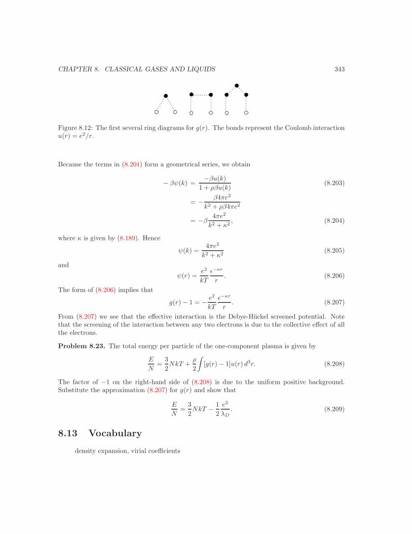
CHAPTER 8. CLASSICAL GASES AND LIQUIDS 343

Figure 8.12: The first several ring diagrams for g(r). The bonds represent the Coulomb interactionu(r) = e2/r.

Because the terms in (8.201) form a geometrical series, we obtain

− βψ(k) =−βu(k)

1 + ρβu(k)(8.203)

= − β4πe2

k2 + ρβ4πe2

= −β4πe2

k2 + κ2, (8.204)

where κ is given by (8.189). Hence

ψ(k) =4πe2

k2 + κ2(8.205)

and

ψ(r) =e2

kT

ε−κr

r. (8.206)

The form of (8.206) implies that

g(r) − 1 = − e2

kT

ε−κr

r. (8.207)

From (8.207) we see that the effective interaction is the Debye-Huckel screened potential. Notethat the screening of the interaction between any two electrons is due to the collective effect of allthe electrons.

Problem 8.23. The total energy per particle of the one-component plasma is given by

E

N=

32NkT +

ρ

2

∫[g(r) − 1]u(r) d3r. (8.208)

The factor of −1 on the right-hand side of (8.208) is due to the uniform positive background.Substitute the approximation (8.207) for g(r) and show that

E

N=

32NkT − 1

2e2

λD. (8.209)

8.13 Vocabulary

density expansion, virial coefficients

CHAPTER 8. CLASSICAL GASES AND LIQUIDS 344

Mayer f function

cumulant, high temperature expansion

disconnected, reducible, and irreducible diagrams

ladder diagrams, ring diagrams

radial distribution function g(r)

static structure function S(k)

reference theory of liquids

Debye-Huckel theory

Appendix 8A: The third virial coefficient for hard spheres

In Problem 8.4 we showed that B2 = 2πσ3/3 for hard spheres. The form of the third virialcoefficient B3 is (see (8.10b))

B3 = − 13V

∫f(|r1 − r2|)f(|r1 − r3|)f(|r2 − r3|) dr1dr2dr3. (8.210)

B3 also can be calculated by geometrical considerations, but these considerations test one’s geo-metrical intuition. An easier way to proceed is to take advantage of the fact that (8.210) is anexample of a convolution integral which can be expressed more simply in terms of the Fouriertransform of f(r). We introduce the Fourier transform of f(r) as

f(k) =∫

f(r) e−ik·rd3r

= 4π

∫ ∞

0

r2f(r)sin kr

krdr (8.211)

The form (8.211) follows from (8.211) by choosing k to be along the z-axis of a spherical coordinatesystem. This choice allows us to write k · r = kr cos θ and d3r = r2dr sin θdθ dφ and do theintegration over θ and φ (see Problem 8.35). Because f(r) = −1 for 0 < r < 1 and f(r) = 0 forr > 1, we can do the integral in (8.211) to find

f(k) = 4πσ3

[cos kσ

(kσ)2− sinkσ

(kσ)3

]. (8.212)

The term in brackets in (8.212) can be related to a half-integer Bessel Function.The main trick is to express B3 in (8.210) in terms of f(k). To do so, we introduce the inverse

transform

f(r) =∫

d3k

(2π)3f(k)eik·r (8.213)

CHAPTER 8. CLASSICAL GASES AND LIQUIDS 345

for any function f(r). If we substitute (8.213) into (8.210), we find

B3 = − 13V

∫dk1

(2π)3dk2

(2π)3dk3

(2π)3eik1·(r2−r1)eik2·(r3−r1)eik3·(r3−r2)

f(k1)f(k2)f(k3) dr1dr2dr3. (8.214)

We first group the exponentials in (8.214) so that we can do the integrals over r1 and r2 by usingthe property that ∫

d3r eik·r = (2π)3δ(k). (8.215)

The result is that k1 = k3 = −k2. The integral over r3 gives a factor of V . Because f dependsonly on |k|, we can write (8.214) as

B3 = −13

∫d3k

(2π)3f(k)3, (8.216)

where f(k) is given by (8.212). It is straightforward to evaluate the resultant integral by numericalmethods. The resultant integral can also be evaluated analytically (see Problem 8.35). The resultis

B3 =5π2

18σ6. (8.217)

B4 can also be evaluated analytically, but higher order virial coefficients have to be evaluated byMonte Carlo methods (see Problem 8.38).

Appendix 8B: Relation of Scattered Intensity of X-Rays to

g(r)

Consider a plane wave of the form a0eiq·r incident on a fluid sample that contains N atoms of

atomic number Z. We want to know the intensity of the scattered radiation at an angle θ relativeto the incident beam (see Figure 8.13). The scattering is the result of the interaction of the incidentbeam with the atomic electrons. We let ri be the position of the ith atom and r(n)

i the positionof the nth electron of the ith atom. The amplitude at a distance r of the wave scattered by anelectron at the origin is

A(θ) = f(θ)eiq′r

r, (8.218)

where q′ is the magnitude of the wave vector of the scattered wave. Note that (8.218) has the formof a spherical wave. The atomic scattering form factor depends on the polarization of the incidentbeam according to Thomson’s formula:

f(θ) = a0e2

mc2cos θ (polarization vector in the scattering plane) (8.219a)

= a0e2

mc2(polarization is orthogonal) (8.219b)

CHAPTER 8. CLASSICAL GASES AND LIQUIDS 346

not done

Figure 8.13: The geometry of elastic scattering.

An electron at r(n)i scatters in the direction θ (wave vector q′) with a phase difference such that

q′ · r(n)i − q · r(n)

i = k · r(n)i , (8.220)

wherek = q′ − q (8.221)

is the scattering vector. The amplitude of the wave scattered by the electron r(n)i is given by

A(n)i (θ) = f(θ)

eiq′r

reik·r(n)

i . (8.222)

Because the scattering is elastic, |q| = |q′|, and the magnitude of k is

k = |k| = 2|q| sin θ

2. (8.223)

The amplitude of the wave scattering by the ith atom is the sum of the amplitudes scattered byeach of the Z electrons:

Ai(θ) = f(θ)eiq′r

r

Z∑n=1

eik·r(n)i (8.224a)

= f(θ)eiq′r

reik·ri

Z∑n=1

eik·(r(n)i −ri). (8.224b)

Note that r(n)i − ri is the position of the nth electron of the ith atom relative to its own nucleus.

The amplitude of the wave scattered by the fluid is given by

A(θ) =N∑

i=1

Ai(θ). (8.225)

The intensity of the radiation that is scattered in the direction θ is given by 〈|A(θ)|2〉, wherethe average represents the quantum average over the electronic states of each atom and an ensembleaverage over the positions of the atoms in the fluid. We have

I(θ) = 〈|A(θ)|2〉 =〈a(θ)2〉

r2NF (k)S(k), (8.226)

CHAPTER 8. CLASSICAL GASES AND LIQUIDS 347

where 〈a(θ)2〉 is an average over the two polarization states:

〈a(θ)2〉 = a20

e4

m2c4

1 + cos2 θ

2. (8.227)

The form factor F (k) is the same for each atom and is given by

F (k) = 〈|Z∑

n=1

eik·(r(n)i −ri)|2〉, (8.228)

where the average in (8.228) denotes a quantum average. The structure function S(k) is definedby the statistical average:

S(k) =1N

〈∣∣N∑

i=1

eik·ri∣∣2〉. (8.229)

We see that the scattered intensity is proportional to S(k), the quantity of interest.

Appendix 8C: Solution of the Percus-Yevick Equation

[xx not finished xx]

8.14 Additional Problems

Problem 8.24. Why is the method that we have used to obtain the virial expansion for a classicalfluid not applicable to a quantum system?

Problem 8.25. Show that the virial coefficient B2 given in (8.33) can be written in the form

B2 = − 16kT

∫ ∞

0

rdu(r)

dre−βu(r)4πr2dr. (8.230)

What is the condition on u(r) for this form to be meaningful?

Problem 8.26. Calculate ZN/Zideal for a system of N = 3 particles using (8.24). Express B3 interms of Z3/Zideal and Z2/Zideal.

Problem 8.27. Assume that g(r) can be written in the form

g(r) = g0 + ρg1(r) + ρ2g2(r) + · · · (8.231)

Use the virial equation of state (8.105) to obtain

PV

NkT= 1 − ρ

6kT

∞∑n=0

ρn

∫ ∞

0

rdu

drgn(r) 4πr2dr. (8.232)

CHAPTER 8. CLASSICAL GASES AND LIQUIDS 348

Compare the density expansion (8.9) of PV/NkT with (8.231) and show that

Bn+2 = − 16kT

∫ ∞

0

rdu

drgn(r)4πr2dr. (8.233)

From the result of Problem 8.25 show that

g0(r) = e−βu(r). (8.234)

Problem 8.28. Show that a system of hard disks attains its maximum packing density in aregular triangular lattice with each disk touching six neighbors. In this arrangement ρ0σ

2 =2/31/2 ≈ 1.1547.2

∗Problem 8.29. Use the applet at xx to find the pressure of the hard disk crystal as a function ofthe density ρ. It is generally accepted that the pressure exhibits a simple-pole divergence at closepacking:

βPσ2 =4/31/2

1 − ρ/ρ0. (8.235)

Problem 8.30. Use the relation (8.105) to find the form of B2 implied by (8.85).

Problem 8.31. Use the fact that the Fourier transform of the density ρ(r) is

ρk =∫

e−ik·rρ(r) dr =N∑

i=1

e−ik·ri (8.236)

to show that S(k) can be expressed as

S(k) =1N

〈ρkρ−k〉. (8.237)

From (8.237) is straightforward to show that S(k) can be written as

S(k) =1N

〈N∑

i=1

N∑j=1

e−ik·rieik·rj 〉 (8.238)

=1N

〈|N∑

i=1

e−ik·ri |2〉. (8.239)

Problem 8.32. Write y(r) in the form of a density expansion

y(r) = eβug(r) = 1 + ρy1(r) + ρ2y2(r) + · · · (8.240)

What is the form of y1 and y2 implied by the Percus-Yevick and hyper-netted chain approximations?

Problem 8.33. Pade approximation for the equation of state. [xx not finished xx]

Problem 8.34. Derive the form of the Fourier transform of the Coulomb potential u(r) = e2/r.2See for example, C. A. Rogers, Packing and Covering, Cambridge University Press (1964), Chapter 1.

CHAPTER 8. CLASSICAL GASES AND LIQUIDS 349

Problem 8.35. Do the integral (8.211) in Appendix 8A.

Problem 8.36. Use the approximate results (8.175) and (8.179) for the Percus-Yevick equationof state of hard spheres to compare the exact virial coefficients summarized in Table 8.1 with thosepredicted by (8.175) and (8.179). Which equation of state gives better results?

Problem 8.37. Show that the mean spherical approximation (8.182) is equivalent to the Percus-Yevick equation (8.170) for hard spheres.

Problem 8.38. (a) Use a Monte Carlo method to evaluate the integrals associated with B3 fora hard core interaction. Your estimate should be consistent with the result B3 = 5πσ6/18 (see(8.73)). Choose units such that σ = 1. One simple procedure is to generate points [xx not finishedxx] Higher order virial coefficients are given by Rhee.

Suggestions for Further Reading

Earlier work on hard disks was done by B. J. Alder and T. E. Wainwright, Phys. Rev. 127,349 (1962). See also A. C. Mitus, H. Weber, and D. Marx, Phys. Rev. E 55, 6855 (1997).

John A. Barker and Douglas Henderson, “What is “liquid”? Understanding the states ofmatter,” Rev. Mod. Phys. 48, 587 (1976).

R. Brout and P. Carruthers, Lectures on the Many-Electron Problem, Interscience Publishers(1963). Chapter 1 has an excellent introduction to the cumulant expansion.

David Chandler, Introduction to Modern Statistical Mechanics, Oxford University Press (1987).Herbert Goldstein, Classical Mechanics, second edition, Addison-Wesley (1980).Jean-Pierre Hansen and Ian R. McDonald, Theory of Simple Liquids, second edition, Academic

Press (1986).Joseph Kestin and J. R. Dorfman, A Course in Statistical Thermodynamics, Academic Press

(1971). Chapter 7 in this senior/graduate text has a good discussion of the properties of real gases.

Chapter 9

Critical Phenomena and theRenormalization Group

c©2005 by Harvey Gould and Jan Tobochnik14 December 2005

One of the greatest recent achievements of theoretical physics has been the development of therenormalization group. This development has had a major impact on our understanding of phasetransitions, quantum field theory, turbulence, and the emerging science of dynamical systems. Wefirst introduce the renormalization group in the context of a simple geometrical model that exhibitsa continuous transition. We then discuss some of the ideas associated with critical phenomena bydiscussing the van der Waals equation of state and introducing more sophisticated versions ofmean-field theory. Finally, we discuss two renormalization group methods for the Ising model.

9.1 A Geometrical Phase Transition

We first consider a simple geometrical model that exhibits a continuous phase transition. Themodel, known as percolation, does not involve the temperature or the evaluation of a partitionfunction. Although this transition is easy to imagine, especially by implementing the model on acomputer, the questions that are raised by the model are as profound as they are for more complexsystems such as the Ising model.

The applications of percolation are more difficult to understand than percolation in the contextof a well-defined mathematical problem. The flow of oil through porous rock, the behavior of arandom resistor network, and the spread of a forest fire are just a few of the many applications.

The problem of percolation is easiest to formulate on a lattice. Consider a large lattice andassume that every site in the lattice can be in one of two states, “occupied” or “empty.” Each siteis occupied independently of its neighbors with probability p. This model of percolation is calledsite percolation. The nature of percolation is related to the connectivity properties of the lattice.We define a cluster as a group of occupied sites that are connected by nearest-neighbor distances

350

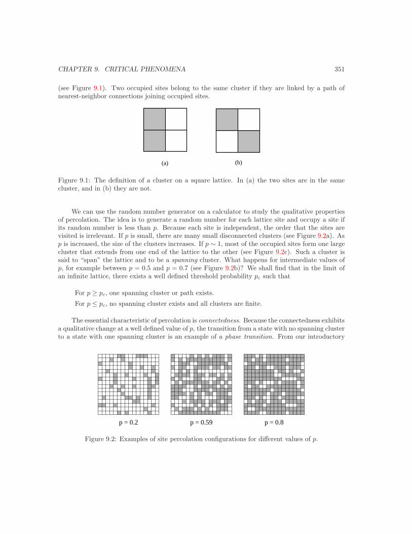
CHAPTER 9. CRITICAL PHENOMENA 351

(see Figure 9.1). Two occupied sites belong to the same cluster if they are linked by a path ofnearest-neighbor connections joining occupied sites.

(a) (b)

Figure 9.1: The definition of a cluster on a square lattice. In (a) the two sites are in the samecluster, and in (b) they are not.

We can use the random number generator on a calculator to study the qualitative propertiesof percolation. The idea is to generate a random number for each lattice site and occupy a site ifits random number is less than p. Because each site is independent, the order that the sites arevisited is irrelevant. If p is small, there are many small disconnected clusters (see Figure 9.2a). Asp is increased, the size of the clusters increases. If p ∼ 1, most of the occupied sites form one largecluster that extends from one end of the lattice to the other (see Figure 9.2c). Such a cluster issaid to “span” the lattice and to be a spanning cluster. What happens for intermediate values ofp, for example between p = 0.5 and p = 0.7 (see Figure 9.2b)? We shall find that in the limit ofan infinite lattice, there exists a well defined threshold probability pc such that

For p ≥ pc, one spanning cluster or path exists.

For p ≤ pc, no spanning cluster exists and all clusters are finite.

The essential characteristic of percolation is connectedness. Because the connectedness exhibitsa qualitative change at a well defined value of p, the transition from a state with no spanning clusterto a state with one spanning cluster is an example of a phase transition. From our introductory

p = 0.2 p = 0.59 p = 0.8

Figure 9.2: Examples of site percolation configurations for different values of p.

CHAPTER 9. CRITICAL PHENOMENA 352

discussion of critical phenomena in Chapter 5, we know that it is convenient to define an orderparameter, a quantity that vanishes for p < pc and is nonzero for p ≥ pc. The order parameter forpercolation is P∞, the probability that an occupied site is part of the spanning cluster. We canestimate P∞ for a given configuration from its definition:

P∞ =number of sites in the spanning cluster

total number of occupied sites. (9.1)

To calculate P∞ exactly we need to average over all configurations. For p < pc, P∞ = 0 becausethere is no spanning cluster. At p = 1, P∞ has its maximum value of unity because only thespanning cluster exists. These properties suggest that P∞ is a reasonable choice for the orderparameter.

Because p can be varied continuously, we expect that the phase transition at pc is continuous.In the critical region near and above pc, we assume that P∞ vanishes as

P∞ ∼ (p − pc)β , (9.2)

where β is an example of a critical exponent.More information can be obtained from the cluster size distribution ns(p) defined as

ns(p) =mean number of clusters of size s

total number of lattice sites. (9.3)

For p ≥ pc, the spanning cluster is excluded from ns. To get an idea of how we can calculate ns,we consider ns(p) for small s on the square lattice. The probability of finding a single isolatedoccupied site (s = 1) is

n1(p) = p(1 − p)4, (9.4)

because the probability that one site is occupied is p and the probability that all of its fourneighboring sites are empty is (1 − p)4. Similarly, n2(p) is given by

n2(p) = 4p2(1 − p)6. (9.5)

The factor of 4 in (9.5) is due to the four possible orientations of a cluster of two particles. BecauseN

∑s sns is the total number of occupied sites not in the spanning cluster (N is the total number

of lattice sites), we have the relation∑

s

sns(p) + P (p) = p, (9.6)

where the sum is over all non-spanning clusters.Similarly, because Nsns is the number of occupied sites in clusters of size s, the quantity

ws =sns∑s sns

, (9.7)

is the probability that an occupied site chosen at random is part of an s-site cluster.At p = pc, ns scales as

ns ∼ s−τ . (9.8)

CHAPTER 9. CRITICAL PHENOMENA 353

The meaning of the power law relation (9.8) is that at p = pc on an infinite lattice, clusters of allsizes exist.

Many of the properties of interest are related to moments of ns. For example, the mean size(number of particles) of the clusters is defined as

S(p) =∑

s

sws =∑

s s2ns∑s sns

. (9.9)

The sum in (9.9) is over the finite clusters. The quantity S(p) behaves near pc as

S(p) ∼ (p − pc)−γ . (9.10)

It is convenient to associate a characteristic length ξ with the clusters. One way to do so isto introduce the radius of gyration Rs of a single cluster of s particles:

Rs2 =

1s

s∑i=1

(ri − r)2, (9.11)

where

r =1s

s∑i=1

ri, (9.12)

and ri is the position of the ith site in the cluster. The correlation length ξ is defined as a weightedaverage over the radius of gyration of all the finite clusters.1 The statistical weight of the clustersof size s is the probability ws that a given site is a member of such a cluster times the number ofsites s in the cluster, that is, s2 ns(p). Hence, the average radius of gyration of all the non-spanningclusters is given by ξ as

ξ2 =∑

s s2ns Rs2∑

s s2ns. (9.13)

Near pc we assume that the correlation length ξ diverges as

ξ ∼ |pc − p|−ν . (9.14)

Why do systems exhibit power law behavior as the critical point is approached? For example,the order parameter goes to zero as a power of (pc − p)/pc for percolation and as a power ofε = (Tc − T )/Tc for thermal systems. In the limit that (pc − p)/pc or ε becomes small, there isno other quantity to set the scale for ε or (pc − p)/pc. For example, we cannot have functionssuch as sin ε, because as ε goes to zero, sin ε reduces to ε. The simplest functions without acharacteristic scale are powers. Hence, we should not be surprised that various quantities showpower law behavior near the critical points.

How can we determine the values of pc and the critical exponents

Problem 9.1. Run the applet at xxx to simulate percolation of the square and triangular lattices.Define a spanning cluster as one that connects the top and bottom of the lattice and the leftand right. Visually estimate the value of pc at which a spanning cluster first occurs. Chooseprogressively larger lattices and try to extrapolate your estimated values of pc for various latticedimensions L to L → ∞.

1More precisely, ξ should be called the connectedness length.

CHAPTER 9. CRITICAL PHENOMENA 354

lattice d q pc (site) pc (bond)linear chain 1 2 1 1square 2 4 0.59275 1

2

triangular 2 6 12 0.3473

honeycomb 2 3 0.698(3) 0.6527diamond 3 4 0.4299(8) 0.3886(5)simple cubic 3 6 0.3117(3) 0.2492(2)bcc 3 8 0.24674(7) 0.1795(3)fcc 3 12 0.1998 0.1198(3)

Table 9.1: Summary of known results for the percolation threshold. The figure in parentheses isthe probable error in the last figure.

quantity functional form exponent d = 2 d = 3order parameter P∞ ∼ (p − pc)β β 5/36 0.403(8)mean size of finite clusters S(p) ∼ |p − pc|−γ γ 43/18 1.73(3)connectedness length ξ(p) = |p − pc|−ν ν 4/3 0.89(1)cluster distribution ns ∼ s−τ (p = pc) τ 187/91 2.2

Table 9.2: Summary of known results for the static critical exponents associated with the percola-tion transition. The number in parentheses is the probable error in the last figure.

The values of the percolation threshold depend on the symmetry of the lattice and are summa-rized in Table 9.1. A summary of the known values of the various critical exponents for percolationis given in Table 9.2. For two dimensions, the static exponents are known exactly. For three dimen-sions no exact results are known, and the exponents have been estimated using various approximatemethods. The accuracy of the numerical values for the critical exponents is consistent with theassumption that the exponents are independent of the symmetry of the lattice and depend onlyon d.

The critical exponents for percolation satisfy a set of relations that are identical to the scalingrelations for thermal systems (see Table 9.3). For example, we will find that

2β + γ = dν, (9.15)

where d is the spatial dimension.We would like to be able to understand these results on a deeper level than the qualitative

description we have given. To do this end we next introduce a renormalization group method forpercolation.

9.2 Renormalization Group for Percolation

The important idea that is incorporated into the renormalization group is that all length scalesare important at the critical point. For percolation this idea implies that clusters of all sizes exist

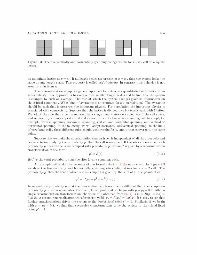
CHAPTER 9. CRITICAL PHENOMENA 355

Figure 9.3: The five vertically and horizontally spanning configurations for a 2× 2 cell on a squarelattice.

on an infinite lattice at p = pc. If all length scales are present at p = pc, then the system looks thesame on any length scale. This property is called self-similarity. In contrast, this behavior is notseen for p far from pc.

The renormalization group is a general approach for extracting quantitative information fromself-similarity. The approach is to average over smaller length scales and to find how the systemis changed by such an average. The rate at which the system changes gives us information onthe critical exponents. What kind of averaging is appropriate for site percolation? The averagingshould be such that it preserves the important physics. For percolation the important physics isassociated with connectivity. Suppose that the lattice is divided into b× b cells each with b2 sites.We adopt the rule that a cell is replaced by a single renormalized occupied site if the cell spans,and replaced by an unoccupied site if it does not. It is not clear which spanning rule to adopt, forexample, vertical spanning, horizontal spanning, vertical and horizontal spanning, and vertical orhorizontal spanning. In the following, we will adopt horizontal and vertical spanning. In the limitof very large cells, these different rules should yield results for pc and ν that converge to the samevalue.

Suppose that we make the approximation that each cell is independent of all the other cells andis characterized only by the probability p′ that the cell is occupied. If the sites are occupied withprobability p, then the cells are occupied with probability p′, where p′ is given by a renormalizationtransformation of the form

p′ = R(p). (9.16)

R(p) is the total probability that the sites form a spanning path.An example will make the meaning of the formal relation (9.16) more clear. In Figure 9.3

we show the five vertically and horizontally spanning site configurations for a b = 2 cell. Theprobability p′ that the renormalized site is occupied is given by the sum of all the possibilities:

p′ = R(p) = p4 + 4p3(1 − p). (9.17)

In general, the probability p′ that the renormalized site is occupied is different than the occupationprobability p of the original sites. For example, suppose that we begin with p = p0 = 0.5. After asingle renormalization transformation, the value of p obtained from (9.17) is p1 = R(p0 = 0.5) =0.3125. A second renormalization transformation yields p2 = R(p1) = 0.0934. It is easy to see thatfurther transformations drives the system to the trivial fixed point p∗ = 0. Similarly, if we beginwith p = p0 = 0.8, we find that successive transformations drive the system to the trivial fixedpoint p∗ = 1.

CHAPTER 9. CRITICAL PHENOMENA 356

To find the nontrivial fixed point associated with the critical threshold pc, we need to find thespecial value of 0 < p < 1 such that

p∗ = R(p∗). (9.18)

For the recursion relation (9.17) we find that the solution of the fourth degree polynomial equationfor p∗ yields the two trivial fixed points p∗ = 0 and p∗ = 1, and the nontrivial fixed pointp∗ = 0.7676 that we associate with pc. This calculated value of p∗ for a 2 × 2 cell should becompared with the best known estimate pc = 0.5927 for the square lattice. Note that p∗ is anexample of an unstable fixed point because the iteration of (9.17) for p arbitrarily close to p∗ willdrive p to one of the stable fixed points.

To calculate the critical exponent ν from the renormalization transformation, we note that onthe renormalized lattice all lengths are reduced by a factor of b in comparison to all lengths in theoriginal system. Hence ξ′, the connectedness length in the renormalized lattice, is related to ξ, theconnectedness length in the original lattice, by

ξ′ =ξ

b. (9.19)

Because ξ(p) = const|p − pc|−ν for p ∼ pc and pc corresponds to p∗, we have

|p′ − p∗|−ν =1b|p − p∗|−ν . (9.20)

To find the relation between p′ and p near pc, we expand the renormalization transformation (9.16)about p = p∗ and obtain to first order

p′ − p∗ = R(p) − R(p∗) ≈ λ (p − p∗), (9.21)

where

λ =dR

dp

∣∣∣∣p=p∗

. (9.22)

We need to do a little algebra to obtain an explicit expression for ν. We first raise the leftand right sides of (9.21) to the −ν power and write

|p′ − p∗|−ν = λ−ν |p − p∗|−ν . (9.23)

We compare (9.20) and (9.23) and obtain

λ−ν = b−1. (9.24)

Finally, we take the logarithm of both sides of (9.24) and obtain the desired relation for the criticalexponent ν:

ν =ln b

ln λ. (9.25)

As an example, we calculate ν for b = 2 using (9.17). We write R(p) = p4 + 4p3(1 − p) =−3p4 + 4p3 and find λ = dR/dp|p=p∗ = 12p2(1 − p)|p=0.7676 = 1.6432. We then use the relation(9.25) to obtain

ν =ln 2

ln 1.6432= 1.40. (9.26)

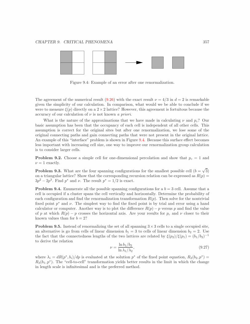
CHAPTER 9. CRITICAL PHENOMENA 357

Figure 9.4: Example of an error after one renormalization.

The agreement of the numerical result (9.26) with the exact result ν = 4/3 in d = 2 is remarkablegiven the simplicity of our calculation. In comparison, what would we be able to conclude if wewere to measure ξ(p) directly on a 2×2 lattice? However, this agreement is fortuitous because theaccuracy of our calculation of ν is not known a priori.

What is the nature of the approximations that we have made in calculating ν and pc? Ourbasic assumption has been that the occupancy of each cell is independent of all other cells. Thisassumption is correct for the original sites but after one renormalization, we lose some of theoriginal connecting paths and gain connecting paths that were not present in the original lattice.An example of this “interface” problem is shown in Figure 9.4. Because this surface effect becomesless important with increasing cell size, one way to improve our renormalization group calculationis to consider larger cells.

Problem 9.2. Choose a simple cell for one-dimensional percolation and show that pc = 1 andν = 1 exactly.

Problem 9.3. What are the four spanning configurations for the smallest possible cell (b =√

3)on a triangular lattice? Show that the corresponding recursion relation can be expressed as R(p) =3p2 − 2p3. Find p∗ and ν. The result p∗ = 1/2 is exact.

Problem 9.4. Enumerate all the possible spanning configurations for a b = 3 cell. Assume that acell is occupied if a cluster spans the cell vertically and horizontally. Determine the probability ofeach configuration and find the renormalization transformation R(p). Then solve for the nontrivialfixed point p∗ and ν. The simplest way to find the fixed point is by trial and error using a handcalculator or computer. Another way is to plot the difference R(p)− p versus p and find the valueof p at which R(p) − p crosses the horizontal axis. Are your results for pc and ν closer to theirknown values than for b = 2?

Problem 9.5. Instead of renormalizing the set of all spanning 3×3 cells to a single occupied site,an alternative is go from cells of linear dimension b1 = 3 to cells of linear dimension b2 = 2. Usethe fact that the connectedness lengths of the two lattices are related by ξ(p2)/ξ(p1) = (b1/b2)−1

to derive the relationν =

ln b1/b2

ln λ1/λ2, (9.27)

where λi = dR(p∗, bi)/dp is evaluated at the solution p∗ of the fixed point equation, R2(b2, p∗) =

R3(b1, p∗). The “cell-to-cell” transformation yields better results in the limit in which the change

in length scale is infinitesimal and is the preferred method.

CHAPTER 9. CRITICAL PHENOMENA 358

9.3 The Liquid-Gas Transition

Experimentally we know that a simple system of say, Argon atoms, is a gas at high temperaturesand a liquid at low temperatures. The van der Waals equation of state is the simplest equation ofstate that exhibits a gas-liquid transition. We derived its form in Section 8.9.1 and obtained:

P =NkT

V − Nb− ρ2a2. (9.28)

The parameter a is a measure of the attractive interactions among the particles and the parameterb is a measure of the repulsive interactions. The latter become important when two particles cometoo close to each other. In the following we rederive the van der Waals equation to emphasize itsmean-field nature.

Let us assume that the intermolecular interaction consists of a hard-core repulsion and a weaklong-range interaction:

u(r) = uhc + uattr. (9.29)

The partition function can be expressed as

Z

Zideal=

∫dr1 · · ·drNe−β

Pi<j u(|ri−rj |). (9.30)

We assume that uattr has the special form, uattr ∝ λdφ(λr) such that∫

uattrddr is a constant as

λ → 0 and d is the spatial dimension. This form implies that as the range of uattr increases, itsstrength decreases. An example of such an interaction is

uattr = −caλde−λr, (9.31)

where a will be associated with the van der Waals parameter. The constant c is chosen so that

−∫

uattr(r) dr = a. (9.32)

The basic assumption of mean-field theory is that the fluctuating field experienced by anindividual particle can be replaced by its average. This assumption is reasonable if a large numberof particles contribute to the fluctuating field and can be shown to be rigorously correct for apotential of the form λdφ(λr) in the limit λ → 0.

This assumption allows us to replace the potential∑

j

∫uattr(|ri − rj |) seen by particle i by

its averageN

V

∫uattr(r) dr = −N

Va. (9.33)

Note that the average in (9.33) is independent of ri. We now sum over all i < j and obtain

⟨∑i<j

uattr(|ri − rj |)⟩

= −12aN2

V. (9.34)

The factor one-half enters because of the condition i < j. Hence, we can rewrite (9.30) as

Z = Zhc eβaN2/2V , (9.35)

CHAPTER 9. CRITICAL PHENOMENA 359

where Zhc represents the partition function for a system of hard core particles. The free energy isgiven by

F = −kT ln Z(T, V, N) = Fhc − 12aN2

V, (9.36)

and the pressure is given by

P = −(∂F

∂V

)T

= Phc − ρ2a. (9.37)

As we discussed in Section 8.9.1, van der Waals assumed that Zhc is given by

Zhc =1

N !1

λ3N(V − Nb)N . (9.38)

It is straightforward to use (9.38) to obtain (9.28).We now consider the isotherms predicted by (9.28). For fixed T , P approaches infinity as

V/N → b. In contrast, for an ideal gas, P becomes infinite only in the limit V/N → 0. ForV/N b, the van der Waals equation of state reduces to the ideal gas equation. Between thesetwo limits, the van der Waals equation exhibits behavior very different from the ideal gas. Forexample, both the first and second derivatives of P may vanish (see Problem 9.6).

Problem 9.6. Sketch several isotherms (P versus V at constant T and N) of the van der Waalsequation of state (9.28). The isotherms above T = Tc are monotonic, but those below Tc developa region of positive slope, (∂P/∂V )T > 0. Explain why the latter behavior is nonphysical. Findthe value of Tc by solving the equations

(∂P

∂V

)T

= 0, (9.39)

and (∂2P

∂V 2

)T

= 0. (9.40)

These two conditions together with (9.28) give three conditions for the three unknowns Tc, Pc, andVc in terms of the parameters a and b. To obtain the solution, rewrite (9.28) as a cubic equationin V . Confirm that

V 3 − (Nb +NkT

P)V 2 +

aN2

PV − a2bN3

P= 0. (9.41)

On any isotherm, there should be three solutions for any value of P . At the critical point, thesethree solutions merge so that

(V − Vc)3 = V 3 − 3VcV2 + 3V 2

c V − V 3c = 0. (9.42)

Compare the coefficients of each power of V in (9.41) and (9.42) and confirm that

Vc = 3Nb, Pc =a2

27b2, kTc =

8a

27b. (9.43)

Problem 9.7 shows that the van der Waals equation can be written in the same form for allsubstances.

CHAPTER 9. CRITICAL PHENOMENA 360

-0.5

0.0

0.5

1.0

1.5

2.0

0.0 0.5 1.0 1.5 2.0 2.5 3.0 3.5V/Vc

0.8Tc

0.9Tc

Tc

1.1Tc

1.2TcP/

P c

Figure 9.5: The van der Waals isotherms near the critical temperature. Note that for T > Tc, theisotherms have no minima or maxima.

Problem 9.7. Define the dimensionless quantities

T =T

Tc, P =

P

Pc, V =

V

Vc, (9.44)

and confirm that all van der Waals fluids have the same form of the equation of state

(P +3

V 2)(3V − 1) = 8T . (9.45)

Equation (9.45) implies that the equation of state is the same form for all gases, which is calledthe law of corresponding states. In reality, such a statement is only approximately true.

Now let us examine the conditions for which a van der Waals isotherm has minima andmaxima. For ∂P /∂V to vanish, we must have

f(V ) =(3V − 1)2

4V 3= T . (9.46)

The function f(V ) vanishes at V = 1/3 and in the limit V → ∞. The derivative of f vanishesfor V = 1 and hence the maximum value of f(V ) is f(1) = 1. This behavior implies that (9.46)cannot be satisfied for T > 1 or equivalently T > Tc. For T > Tc, the van der Waals isothermshave no minima or maxima.

CHAPTER 9. CRITICAL PHENOMENA 361

Now let us consider the van der Waals isobars. From (9.45), we obtain

T =(3V − 1

8)(

P +3

V 2

). (9.47)

For T to have a maximum or minimum requires that

3V 2

− 2V 3

= P (9.48)

Because the values of the left-hand side of (9.48) are less than or equal to one, we conclude that Thas no extrema if P > 1 (P > Pc).

For T < Tc the isotherms have one maximum and one minimum between which the slope ispositive. What is the significance of a positive slope?

9.4 Bethe Approximation

In Section 5.6 we introduced a simple mean-field approach in the context of the Ising model. Thebasic approximation was to ignore all correlations between the spins, including nearest neighbors,and approximate 〈sisj〉 as 〈sisj〉 ≈ 〈si〉〈sj〉 = m2. In the following, we discuss how to improve thisapproximation. This approximation method is due to Bethe.2

The idea is that instead of considering the effective field felt by a single spin, we considerthe effective field felt by a group of spins. In particular, consider a central spin and its nearestneighbors (see Figure 9.6). The interactions of the nearest neighbors with the central spin iscalculated exactly, and the rest of the spins in the system are assumed to act on the nearestneighbors through an effective field that we calculate self-consistently. The energy of the centralcluster is

Hc = −Js0

q∑j=1

sj − Bs0 − Beff

q∑j=1

sj (9.49a)

= −(Js0 + Beff)∑

j

sj − Bs0, (9.49b)

where q is the coordination number of the lattice. (For a square lattice q = 4.) Note that thefluctuating field acting on the nearest neighbor spins s1, . . . , sq has been replaced by the effectivefield Beff .

The cluster partition function Zc is given by

Zc =∑

s0=±1,sj=±1

e−βHc . (9.50)

We first do the sum over s0 = ±1 and write

Zc = eβB∑

sj=±1

eβ(J+Beff )Pq

j sj + e−βB∑

sj=±1

eβ(−J+Beff )Pq

j sj . (9.51)

2Bethe is probably better known for his work in nuclear physics and other areas. The reference is H. Bethe,Proc. Royal Society A 150, 552 (1935).

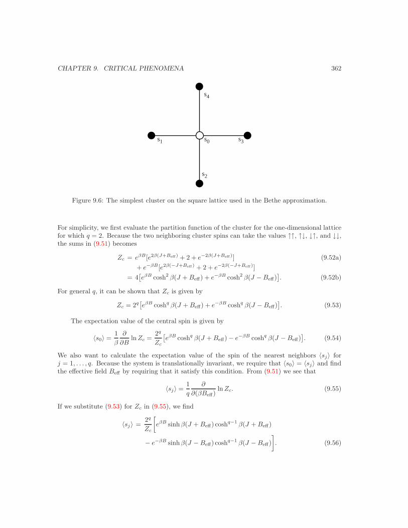
CHAPTER 9. CRITICAL PHENOMENA 362

s1

s4

s3

s2

s0

Figure 9.6: The simplest cluster on the square lattice used in the Bethe approximation.

For simplicity, we first evaluate the partition function of the cluster for the one-dimensional latticefor which q = 2. Because the two neighboring cluster spins can take the values ↑↑, ↑↓, ↓↑, and ↓↓,the sums in (9.51) becomes

Zc = eβB[e2β(J+Beff ) + 2 + e−2β(J+Beff )] (9.52a)+ e−βB[e2β(−J+Beff ) + 2 + e−2β(−J+Beff )]

= 4[eβB cosh2 β(J + Beff) + e−βB cosh2 β(J − Beff)

]. (9.52b)

For general q, it can be shown that Zc is given by

Zc = 2q[eβB coshq β(J + Beff) + e−βB coshq β(J − Beff)

]. (9.53)

The expectation value of the central spin is given by

〈s0〉 =1β

∂

∂Bln Zc =

2q

Zc

[eβB coshq β(J + Beff) − e−βB coshq β(J − Beff)

]. (9.54)

We also want to calculate the expectation value of the spin of the nearest neighbors 〈sj〉 forj = 1, . . . , q. Because the system is translationally invariant, we require that 〈s0〉 = 〈sj〉 and findthe effective field Beff by requiring that it satisfy this condition. From (9.51) we see that

〈sj〉 =1q

∂

∂(βBeff)ln Zc. (9.55)

If we substitute (9.53) for Zc in (9.55), we find

〈sj〉 =2q

Zc

[eβB sinh β(J + Beff) coshq−1 β(J + Beff)

− e−βB sinhβ(J − Beff) coshq−1 β(J − Beff)]. (9.56)

CHAPTER 9. CRITICAL PHENOMENA 363

To find the critical temperature, we set B = 0. The requirement 〈s0〉 = 〈sj〉 yields theequation

coshq β(J + Beff) − coshq β(J − Beff) = sinh β(J + Beff) coshq−1 β(J + Beff)− sinh β(J − Beff) coshq−1 β(J − Beff). (9.57)

Equation (9.57) can be simplified by writing sinhx = coshx − e−x with x = β(J ± Beff):

coshq−1 β(J + Beff)coshq−1 β(J − Beff)

= e2βBeff . (9.58)

Equation (9.58) always has the solution Beff = 0 corresponding to the disordered high tem-perature phase. As Beff → ∞, the left-hand side of (9.58) approaches e2βJ(q−1), a constantindependent of Beff , and the right-hand side diverges. Therefore, if the slope of the function onthe left at Beff = 0 is greater than 2β, the two functions must intersect again at finite Beff . If wetake the derivative of the left-hand side of (9.58) with respect to Beff and set it equal to 2β, wefind that the condition for a solution to exist is

cothβcJ = q − 1, (9.59)

where cothx = coshx/ sinh x. Because (9.58) is invariant under Beff → −Beff , there will be twosolutions for T ≤ Tc.

On the square lattice, (9.59) yields kTc/J = 2.888 . . . in comparison to the exact resultkTc/J = 2.269 . . . (see (5.76)) and the result of simple mean-field theory, kTc/J = 4. Notethat for the one-dimensional Ising model, q = 2 and the Bethe approximation predicts Tc = 0 inagreement with the exact result.

Better results can be found by considering larger clusters. However, although such an approachyields more accurate phase diagrams, it always yields the same mean-field exponents because itdepends on the truncation of correlations beyond a certain distance. This approximation mustbreak down in the vicinity of a critical point where the correlations become infinite.

Problem 9.8. Work out the details of the Bethe approximation, an improved mean-field methoddiscussed in Section 9.4, for the Ising chain. Show that the effective three spin Hamiltonian canbe written as

H3 = −J(s1 + s2 + s3) − mJ(s1 + s3), (9.60)

where m = 〈s〉. (Explain why the effective field Beff is given by Beff = Jm.) Evaluate the partitionfunction for the cluster Z3 by summing over the possible values of s1, s2 and s3. The magnetizationper spin, m, can be found by evaluating 〈s2〉. Expand your result for m near m = 0 and show thatTc = 0.

9.5 Landau Theory of Phase Transitions

As we have discussed, the key idea of mean-field theory is the neglect of correlations between thespins or other relevant coordinates. For the Ising model we can write the spin at lattice point r as

CHAPTER 9. CRITICAL PHENOMENA 364

m(r) = m + φ(r) and express the interaction term in the energy as

m(r)m(r′) = [m + φ(r)][m + φ(r′)]

= m2 + m[φ(r) + φ(r′)] + φ(r)φ(r′). (9.61)

If we assume that φ(r) m, we may neglect the last term in (9.61) and obtain

m(r)m(r′) ≈ m2 + m[φ(r) + φ(r′)] = m2 + m[m(r) + m(r′) − 2m], (9.62a)= m[φ(r) + φ(r′)] − m2. (9.62b)

Using this approximation, we write the total energy as

− J∑r,r′

m(r)m(r′) − B∑r

m(r)≈−J∑r,r′

(m[m(r) + m(r′)] − m2

) − B∑r

m(r) (9.63a)

=12NJm2 − (Jm + B)

∑r

m(r). (9.63b)

Note that the spin m(r) enters only linearly in (9.63b). We evaluate the partition function as inChapter 5 and find

Z ≈ Zmf = e−12NβJm2

[2 coshβ(Jm + B)]N . (9.64)

The free energy for a given value of m in this simple mean-field approximation is proportional to−kT ln Zmf and can be expressed as

Fmf =12NJm2 − Nβ ln coshβ(Jm + B), (9.65)

apart from an irrelevant constant. Because the equilibrium free energy must be a minimum for agiven value of T and B, we can determine m by requiring that it minimize Fmf . The result is

m = tanhβ(Jm + B), (9.66)

as we found in (5.94).

Problem 9.9. (a) Derive (9.66) from the requirement that F in (9.65) is a minimum in equilibrium.(b) Expand Fmf in a power series in m and show that Fmf can be written in the Landau form(9.67).

Landau realized that the qualitative features of mean-field theory can be summarized by asimple expression for the free energy. Because m is small near the critical point, it is reasonableto assume that the free energy density (free energy per unit volume) can be written in the form

f(m, T ) = a +b

2m2 +

c

4m4 − Bm, (9.67)

where the parameters a, b, and c depend on T . The assumption underlying the form (9.67) is thatf can be expanded in a power series in m about m = 0 near the critical point. Although thisassumption is not correct, Landau theory, like mean-field theory in general, is still a useful tool.For the Ising model, Landau also assumed that f(m) is symmetrical about m = 0 so that the m3

CHAPTER 9. CRITICAL PHENOMENA 365

not done

Figure 9.7: The dependence of the Landau form of the free energy on the order parameter m.

term can be omitted. The quantity m is called the order parameter because it is zero for T > Tc,is nonzero for T ≤ Tc, and characterizes the nature of the transition.

The equilibrium value of m is the value that minimizes the free energy. In Figure 9.7 we showthe dependence of f on m for B = 0. We see that if b > 0 and c > 0, then the minimum of f is atm = 0. However if b < 0 and c > 0, then the minimum of f is at m = 0. We have for B = 0 that

∂f

∂m= bm + cm3 = 0. (9.68)

If we assume that b = b0(T − Tc) and c > 0, we find

m = ±(b0

c

)1/2(Tc − T )1/2. (9.69)

The behavior of the specific heat can be found from the relation C = T∂s/∂T . The entropy densityis given by

s = − ∂f

∂T= −a′ − b′

2m2 − b

2(m2)′ − c

4(m4)′, (9.70)

where the primes in (9.70) denote the derivative with respect to T . From (9.70) we have

C = Tds

dT= −Ta′′ − Tb′(m2)′ − cT

4(m4)′′, (9.71)

where we have used the fact that b′′ = 0, and have assumed that c is independent of T . Becausem = 0 for T ≥ Tc, we have C → −Ta′′ as T → Tc from above. For T → Tc from below, we have(m2)′ = b0/c, b′ = b0, and (m4)′′ → 2(b0/c)2. Hence, we obtain

C →−Ta′′ T → T +

c

−Ta′′ + Tb20/2c T → T−

c

(9.72)

We see that the order parameter m and the specific heat C have the same behavior near Tc as wepreviously obtained in our simple mean-field treatment of the Ising model.

Problem 9.10. The susceptibility per spin can be found from the relation

χ =∂m

∂B.

CHAPTER 9. CRITICAL PHENOMENA 366

(a) Show that if B = 0, bm+ cm3−B = 0 in the Landau theory, and hence χ−1 = (b+3cm2). ForT > Tc, m = 0 and χ−1 = b = b0(T − Tc). For T < Tc, m2 = −b/c, and hence χ−1 = 2b0(Tc − T ).Hence Landau theory predicts that γ = γ′ = 1. (b) Show that at the critical point cm3 = B, andhence δ = 3.

We can generalize Landau theory to incorporate spatial fluctuations by writing

f(r) = a +b

2m2(r) +

c

4m4(r) +

g

2[∇m(r)]2 − B m(r), (9.73)

where the parameter g > 0. This form of the free energy density is commonly known as theLandau-Ginzburg form. The gradient term in (9.73) expresses the fact that the free energy israised by spatial fluctuations in the order parameter. The total free energy is given by

F =∫

f(r) d3r, (9.74)

and the total magnetization is

M =∫

m(r) d3r. (9.75)

We follow the same procedure as before and minimize the total free energy:

δF =∫

δm(r)[b m(r) + c m3(r) − B] + g∇δm(r) · ∇m(r)d3r = 0. (9.76)

The last term in the integrand of (9.76) can be simplified by integrating by parts and requiringthat δm(r) = 0 at the surface. In this way we obtain

B(r) = b m(r) + c m(r)3 − g∇2m(r). (9.77)

It is clear that (9.77) reduces to the usual Landau theory by letting B(r) = B and ∇m(r) = 0.If we imagine that a localized perturbation B(r) = B0δ(r) is applied to the system, we can

use (9.77) to calculate its effect. We write

m(r) = m0 + φ(r), (9.78)

and assume that the spatially varying term φ(r) is small so that m(r)3 ≈ m30 + 3m2

0φ(r). Wesubstitute (9.78) into (9.77) and obtain

∇2φ(r) − b

gφ(r) − 3

c

gm2

0 φ(r) − b

gm0 − c

gm3

0 = −B0

gδ(r). (9.79)

If we substitute m0 = 0 for T > Tc and m20 = −b/c for T < Tc into (9.79), we obtain

∇2φ − b

gφ = −B0

gδ(r) (T > Tc) (9.80a)

∇2φ + 2b

gφ = −B0

gδ(r). (T < Tc) (9.80b)

CHAPTER 9. CRITICAL PHENOMENA 367

Note that φ in (9.80) satisfies an equation of the same form as the one we found in the Debye-Huckel theory (see Section 8.12). The solution of (9.80) can be written in spherical coordinates as

φ(r) =B0

4πg

1re−r/ξ, (9.81)

with

ξ(T ) =[ g

b(T )]1/2 (T > Tc) (9.82a)

and

ξ(T ) =[ −g

2b(T )]1/2

. (T < Tc) (9.82b)

We will see that the quantity ξ(T ) can be interpreted as the correlation length. Because b(T ) =b0(T − Tc), we see that ξ diverges from both above and below Tc as

ξ(T ) ∼ |T − Tc|−ν . (9.83)

In general, ξ ∼ |T − Tc|−ν ; mean-field theory predicts that ν = 1/2.The correlation function of the order parameter is given by

G(r) = 〈m(r)m(0)〉 − 〈m〉2. (9.84)

We can relate φ(r) to G(r) by the following considerations. Because we can write the total energyin the form

H = H0 −∫

m(r)B(r) d3r, (9.85)

we have

〈m(r)〉 =∑

s ms(r)e−β[H0,s−R

B(r′)ms(r′)d3r′]∑s e−β[H0,s−

RB(r′)ms(r′)d3r′]

, (9.86)

where H0 is the part of H that is independent of B(r), and H0,s and ms(r) denote the values ofH0 and m(r) in state s. We see that

δ〈m(r)〉δB(0)

= β[〈m(r)m(0)〉 − 〈m(r)〉〈m(0)〉] = βG(r). (9.87)

Because m(r) = m0 + φ(r), we also have δ〈m(r)〉/δB(0) = φ(r)/B0. Hence, G(r) = kTφ(r)/B0

and we find using (9.81) that

G(r) =kT

4πg

1re−r/ξ. (9.88)

From the form of (9.88) we recognize ξ as the correlation length in the neighborhood of Tc. AtT = Tc, b = 0, and we find from (9.88) that G(r) ∼ 1/r. For arbitrary spatial dimension d we canwrite this spatial dependence as

G(r) ∼ 1rd−2+η

, (T = Tc) (9.89)

where we have introduced another critical exponent η. We see that Landau theory yields η = 0.

CHAPTER 9. CRITICAL PHENOMENA 368

Problem 9.11. Derive the relation (9.87) between the linear response δ〈m(r)〉/δB(0) and thespin correlation function G(r).

The existence of long-range correlations in the correlation function of the order parameter G(r)is associated with the divergence of χ, the susceptibility per spin. As we showed in Chapter 5, χis related to the fluctuations in M (see (5.18)):

χ =1

NkT[〈M2〉 − 〈M〉2] (9.90a)

=1

NkT〈[M − 〈M〉]2〉. (9.90b)

(We have defined χ as the isothermal susceptibility per spin.) We write

M − 〈M〉 =N∑

i=1

[si − 〈si〉], (9.91)

and

χ =1

NkT

N∑i,j=1

[〈sisj〉 − 〈si〉〈sj〉] (9.92a)

=1

kT

N∑j=1

G1j , (9.92b)

where Gij = 〈sisj〉 − 〈si〉〈sj〉. We have used the definition of Gij and the fact that all lattice sitesare equivalent. The generalization of (9.92b) to a continuous system is

χ =1

kT

∫G(r) d3r. (9.93)

From (9.93) we see that the divergence of the susceptibility is associated with the existence oflong-range correlations.

Problem 9.12. Show that the relation (9.93) and the form (9.88) implies that χ ∼ |T − Tc|−1.

Range of Validity of Mean-Field Theory. It is interesting that mean-field theory carrieswith it the seeds of its own destruction and must break down when the system is sufficiently closeto its critical point. That is, mean-field theory should be applicable if the fluctuations in theorder parameter are much smaller than its mean value so that the fluctuations can be ignored.Conversely, if fluctuations are larger than the mean value, mean-field theory should break down.∫

[〈m(r)m(0)〉 − 〈m(r)〉〈m(0)〉] d3r∫m2 d3r

1. (9.94)

The condition (9.94) is known as the Ginzburg criterion and gives a criterion for the self-consistencyof mean-field theories. If we substitute G(r) from (9.88) into (9.94) and integrate over a sphere ofradius ξ, we find

kT

4πg

∫ ξ

0

e−r/ξ 4πrdr =kT ξ2

g(1 − 2

e) =

0.264kT ξ2

g. (9.95)

CHAPTER 9. CRITICAL PHENOMENA 369

The Ginzburg criterion for the validity of mean-field theory becomes

0.264kT ξ2

g 4π

3ξ3m2 (9.96)

or0.063

g ξm2. (Ginzburg criterion) (9.97)

Because ξ ∼ |T − Tc|−1/2 and m2 ∼ (T − Tc), we see that the magnitude of the product ξm20

approaches zero as T → Tc and the Ginzburg criterion will not be satisfied for T sufficiently closeto Tc. Hence, mean-field theory contains the seeds of its own destruction and must break downwhen the system is sufficiently close to its critical point. However, there exist some systems, forexample, superconductivity as described by BCS theory, for which ξ is very large and (9.97) issatisfied in practice down to temperature differences as small as |T − Tc| ∼ 10−14.

Problem 9.13. We can generalize the results of mean-field theory to arbitrary spatial dimensiond. Equation (9.80) can be generalized to arbitrary d by replacing the operator ∇2 by the analogousd-dimensional operator. The general solution is not as simple as (9.5), but has the asymptotic form

G(r) ∼ e−r/ξ

rd−2. (9.98)

Generalize the Ginzburg criterion (9.94) to arbitrary d and show the inequality is satisfied ifdν − 2β − 2ν, or

d > 2 + 2β/ν. (9.99)

Ignore all numerical factors. Because mean-field theory yields β = 12 and ν = 1

2 , we find thatmean-field theory is valid for all T near Tc if d > dc = 4. At d = dc, the upper critical dimension,there are small logarithmic corrections to the mean-field critical exponents. That is, near thecritical point, mean-field theory is only reliable for dimensions greater than four.

9.6 Other Models of Magnetism

The Ising model is an excellent model for testing methods of statistical mechanics, and there arestill aspects of the model that are of much current interest.3 Many variations of the Ising modeland the Heisenberg model provide the basis for models of magnetic phenomena. One interestinglimit is S → ∞, corresponding to classical spins. In this limit the direction of S is not quantized. Itis convenient to replace the spin S by a unit vector s = S/S and redefine the coupling constant suchthat the old J is replaced by J/S2. The factor of S2 cancels, and we are left with the Hamiltonian

H = −J∑

si · sj . (classical Heisenberg model) (9.100)

If the spins can point in any direction in three-dimensional space, this model is referred to asthe classical Heisenberg model or sometimes the O(2) model from group theory. If the spins arerestricted to stay in a plane, then the model is called the planar or x-y model. The properties

3The existence of many papers on the Ising model has led some workers in statistical mechanics to dub the Isingmodel as the “fruit-fly” of statistical mechanics.

CHAPTER 9. CRITICAL PHENOMENA 370

of these models depends on the dimension of the lattice. For example, in three dimensions theclassical Heisenberg model has a phase transition between a low temperature ferromagnetic stateand a high temperature paramagnetic state. However, on a two-dimensional lattice the classicalHeisenberg model has no phase transition and is always in the disordered paramagnetic state exceptat T = 0. This result is related to the issue of confinement of quarks in the theory of quantumchromodynamics.

The planar model has some very interesting properties on a two-dimensional lattice. Althoughthere is no spontaneous magnetization, there nevertheless is a phase transition between a lowtemperature quasi-ordered phase and a high temperature disordered phase. The phase transitionis caused by the unbinding of spin vortex pairs.

We also can include the effects of anisotropy by replacing JSi ·Sj by JxSx,iSx,j +JySy,iSy,j +JzSz,iSz,j , and giving Jx, Jy, and Jz different values. An important special case is Jx = Jy = Jz.Interesting models can be created by extending the interactions between the spins beyond nearestneighbors, and adjusting the interaction to be different for different neighbors and for differentdistances. An example is the ANNNI model or antiferromagnetic next-nearest neighbor model. Inthis model the nearest neighbors have ferromagnetic couplings, but next-nearest neighbors haveantiferromagnetic couplings. We also can give the coupling Ji,j for each pair of spins, i and j, arandom value. Such a model is called a spin glass and is currently an area of active research. Otherextensions include adding a random magnetic field at each site to favor a particular direction ofthe spin (the random field Ising model).

In addition to magnetic systems, the above models are useful for studying other systems. Forexample, “up” and “down” in the Ising model can represent A and B atoms in an AB alloy. Inthis case the model is referred to as a lattice gas. The principal difference is that is that the netspin or magnetization (or total number of A atoms or total number of gas particles) is fixed. Thisdistinction means that a different ensemble is appropriate.

Superfluids can be modeled by the planar model near the superfluid phase transition. Thereason is that the spin-spin interaction in the planar model can be expressed as cos(θi − θj), whereθi is an angle that goes from 0 to 2π. In superfluids the order parameter is described by a quantummechanical phase that also is an angle.

Another extension to the Heisenberg model is the q-state Potts model for which there are qdiscrete states at each site; the energy is −J if two neighboring sites are in the same state andzero otherwise. A related extension is the q-state clock model, where the spin is restricted to pointin a two-dimensional plane at q equally spaced angles. These models are useful for modeling thebehavior of atoms absorbed on surfaces, when there are q possible types of sites on the surface atwhich the atom can stick.

Similar spin models are being extended to understand the field theories used in high energyphysics. The principal difference is that the interactions are typically four spin interactions betweenspins located at the corners of the square plaquettes of the lattice. The planar model turns out torepresent electromagnetism. We can obtain the other fundamental interactions by invoking morecomplicated spins that become matrices instead of simple vectors.

CHAPTER 9. CRITICAL PHENOMENA 371

9.7 Universality and Scaling Relations

For convenience, we summarize the standard static critical exponents in Table 9.3. The quantityε = (Tc − T )/Tc. The notation C ∼ |ε|−α means that C has a singular contribution proportionalto |ε|−α.

heat capacity C ∼ |ε|−α

order parameter m ∼ εβ

susceptibility χ ∼ |ε|−γ

equation of state (ε = 0) m ∼ B−1/δ

correlation length ξ ∼ |ε|−ν

power law decay at ε = 0 G(r) ∼ 1/rd−2+η

Table 9.3: Summary of the definition of the standard critical exponents expressed in the languageof magnetic systems.

The above definitions of the critical exponents implicitly assume that the singularities are thesame whether the critical point is approached from above or below. (The exception is m which iszero for T > Tc.) In the following, we will not bother to write |ε| instead of ε.

The importance of the critical exponents is that they are universal, that is, they depend onlyon the spatial dimension of the lattice d and the number of components of the order parameter,and do not depend on the details of the interactions. For example, the critical exponents for theIsing model are the same as those for the liquid-gas critical point. The standard universality classescorrespond to the scalar, planar, and three-dimensional vector order parameter for which n = 1,n = 2, and n = 3, respectively. Examples of n = 1 are the Ising model, the lattice gas model,and the liquid-gas transition. Examples of n = 2 are planar ferromagnets, the superfluid, andordinary superconductivity. The latter two cases correspond to n = 2 because the order parameteris complex. The case n = 3 corresponds to the Heisenberg model.

We will find in the following that only two of the above six critical exponents are independent.The exponents are related by the scaling relations which are summarized in Table 9.4.

Fisher γ = ν(2 − η)Rushbrooke α + 2β + γ = 2Widom γ = β(d − 1)Josephson νd = 2 − α

Table 9.4: Examples of simple scaling relations between the critical exponents.

The essential physics of the critical point is that the correlation length ξ is the only char-acteristic length of the system. This assumption is known as the “scaling hypothesis,” althoughnow it is more than a hypothesis. A simple way to obtain the above scaling relations is to usedimensional analysis and assume that a quantity that has dimension L−d is proportional to ξ−d

near the critical point.

CHAPTER 9. CRITICAL PHENOMENA 372

Because the quantity βF is dimensionless and proportional to N , we have that βF/V hasdimensions

[βf ] = L−d. (9.101)

Similarly the correlation function G(r) depends on L according to

[G(r)] = L2−d−η. (9.102)

By definition G(r) has the same dimension as m2 so

[m] = L(2−d−η)/2. (9.103)

If we use the relation (9.90b), we have

[kTχ] = L2−η. (9.104)

Finally, because M = −∂F/∂B (see (5.16)), we have

[B/kT ]− L(2+d−η)/2. (9.105)

We now replace the L in the above formulae by ξ and let ξ ∼ ε−ν . Because the dimensions ofthe heat capacity are the same as βf in (9.101), we obtain 2 − α = νd. We leave it as an exercisefor the reader to obtain the other scaling relations (see Problem 9.14).

Problem 9.14. Use the above dimensional analysis arguments to obtain the relations −ν(2− d−η)/2 = β, −ν(2 − η) = −γ, and ν(2 + d − η)/2 = βδ. Then do some simple algebra to derive theRushbrooke and Widom scaling laws.

9.8 The Renormalization Group and the 1D Ising Model

Although the one-dimensional Ising model does not have a critical point, the application of therenormalization group method has much pedagogical value and is the only case in which a simplegrouping of spins can be carried out analytically. The Hamiltonian for the Ising chain with periodicboundary conditions is (see (5.57))

H = −J

N∑i=1

sisi+1 − 12B

N∑i=1

(si + si+1). (9.106)

It is convenient to define the dimensionless parameters K = βJ and B = βB. For periodicboundary conditions the partition function can be written as

Z =∑s

exp[ N∑

i=1

(Ksisi+1 +

12B(si + si+1)

)]. (9.107)

The sum in (9.107) is over all possible spin configurations. For simplicity, we first consider B = 0.

CHAPTER 9. CRITICAL PHENOMENA 373

One way to obtain a renormalized lattice is to group sites into cells. Another way to reducethe number of degrees of freedom is to average or sum over them. For example, for the d = 1 Isingmodel we can write Z as

Z(K, N) =∑s

eK(s1s2+s2s3)eK(s3s4+s4s5).... (9.108)

The form (9.108) suggests that we sum over even spins:

Z(K, N) =∑

odd spins

[eK(s1+s3) + e−K(s1+s3)

] × [eK(s3+s5) + e−K(s3+s5)

] × · · · (9.109)

This method of reducing the degrees of freedom is called decimation.We next try to write the partially averaged partition function (9.109) in its original form with

N/2 spins and, in general, a different interaction K ′. If such a rescaling were possible, we couldobtain a recursion relation for K ′ in terms of K. We require that

eK(s1+s3) + e−K(s1+s3) = A(K) eK′s1s3 , (9.110)

where the function A does not depend on s1 or s3. If the relation (9.110) exists, we can write

Z(K, N) =∑

s1,s3,s5...

A(K) eK′s1s3A(K) eK′s3s5 . . . , (9.111a)

= [A(K)]N/2Z(K ′, N/2). (9.111b)

In the limit N → ∞, we know that lnZ is proportional to N , that is,

ln Z = Nf(K), (9.112)

where f(K) depends on K and is independent of N . From (9.111b) and (9.112) we obtain

ln Z = Nf(K) =N

2ln A(K) + lnZ(K ′,

N

2) (9.113a)

=N

2ln A(K) +

N

2f(K ′), (9.113b)

orf(K ′) = 2f(K)− ln A(K). (9.114)

We can find the form of A(K) from (9.110). Recall that (9.110) holds for all values of s1 ands3. We first consider the cases s1 = s3 = 1 and s1 = s3 = −1 for which

e2K + e−2K = AeK′. (9.115)

For the case s1 = 1 and s3 = −1 or s1 = −1 and s3 = 1, we have

2 = Ae−K′. (9.116)

From (9.116) we have A = 2eK′, and hence from (9.115), we obtain

e2K + e−2K = 2e2K′, (9.117)

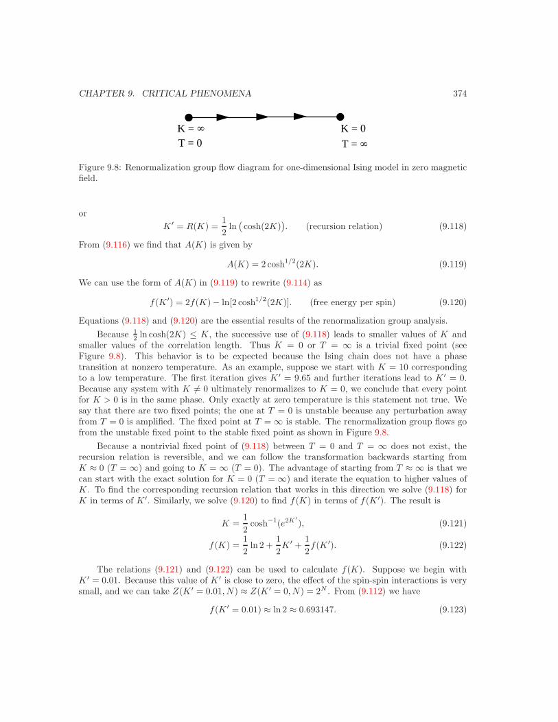
CHAPTER 9. CRITICAL PHENOMENA 374

K = ∞T = 0

K = 0

T = ∞

Figure 9.8: Renormalization group flow diagram for one-dimensional Ising model in zero magneticfield.

orK ′ = R(K) =

12

ln(cosh(2K)

). (recursion relation) (9.118)

From (9.116) we find that A(K) is given by

A(K) = 2 cosh1/2(2K). (9.119)

We can use the form of A(K) in (9.119) to rewrite (9.114) as

f(K ′) = 2f(K)− ln[2 cosh1/2(2K)]. (free energy per spin) (9.120)

Equations (9.118) and (9.120) are the essential results of the renormalization group analysis.Because 1

2 ln cosh(2K) ≤ K, the successive use of (9.118) leads to smaller values of K andsmaller values of the correlation length. Thus K = 0 or T = ∞ is a trivial fixed point (seeFigure 9.8). This behavior is to be expected because the Ising chain does not have a phasetransition at nonzero temperature. As an example, suppose we start with K = 10 correspondingto a low temperature. The first iteration gives K ′ = 9.65 and further iterations lead to K ′ = 0.Because any system with K = 0 ultimately renormalizes to K = 0, we conclude that every pointfor K > 0 is in the same phase. Only exactly at zero temperature is this statement not true. Wesay that there are two fixed points; the one at T = 0 is unstable because any perturbation awayfrom T = 0 is amplified. The fixed point at T = ∞ is stable. The renormalization group flows gofrom the unstable fixed point to the stable fixed point as shown in Figure 9.8.

Because a nontrivial fixed point of (9.118) between T = 0 and T = ∞ does not exist, therecursion relation is reversible, and we can follow the transformation backwards starting fromK ≈ 0 (T = ∞) and going to K = ∞ (T = 0). The advantage of starting from T ≈ ∞ is that wecan start with the exact solution for K = 0 (T = ∞) and iterate the equation to higher values ofK. To find the corresponding recursion relation that works in this direction we solve (9.118) forK in terms of K ′. Similarly, we solve (9.120) to find f(K) in terms of f(K ′). The result is

K =12

cosh−1(e2K′), (9.121)

f(K) =12

ln 2 +12K ′ +

12f(K ′). (9.122)

The relations (9.121) and (9.122) can be used to calculate f(K). Suppose we begin withK ′ = 0.01. Because this value of K ′ is close to zero, the effect of the spin-spin interactions is verysmall, and we can take Z(K ′ = 0.01, N) ≈ Z(K ′ = 0, N) = 2N . From (9.112) we have

f(K ′ = 0.01) ≈ ln 2 ≈ 0.693147. (9.123)

CHAPTER 9. CRITICAL PHENOMENA 375

K ′ K f(K ′) f(K)0.01 0.100334 0.693147 0.6981470.100334 0.327447 0.698147 0.745814

Table 9.5: Summary of the first few steps of the calculation of f , the free energy per spin, for thed = 1 Ising model from the recursion relations (9.121) and (9.122). The function f is related tothe partition function Z by lnZ = Nf (see (9.112)).

Given K ′ = 0.01, we calculate K from (9.121) and obtain the result K = 0.100334. The value off(K) for this value of K is found from (9.122) to be 0.698147. This calculation of f(K) and K isthe first step in an iterative procedure that can be repeated indefinitely with K ′ chosen to be thevalue of K from the prior iteration and f(K ′) chosen to be the value of f(K) from the previousiteration. The first few iterations are shown in Table 9.5.

Problem 9.15. Extend the calculation of f(k) in Table 9.5 to larger values of K by doing severalmore iterations of (9.121) and (9.122). Also calculate the exact value of the free energy for thecalculated values of K using (5.28) and compare your results to f(K). Because the recursionrelations (9.121) and (9.122) are exact, the only source of error is the first value of f . Does theerror increase or decrease as the calculation proceeds?

∗Problem 9.16. For nonzero magnetic field show that the function A(K, B) satisfies the relation:

2eB(s1+s3)/2 cosh[K(s1 + s3) + B] = A(K, B) e2f+K′s1s3+ 12B′(s1+s3), (9.124)

Show that the recursion relations for nonzero magnetic field are

K ′ =14

lncosh(2K + B) cosh(2K − B)

cosh2 B, (9.125a)

B′ = B +12

lncosh(2K + B)cosh(2K − B)

, (9.125b)

and

f(K, B) =18

ln[16 cosh(2K + B) cosh(2K − B) cosh2 B

](9.125c)

The recursion relations (9.125) have a line of trivial fixed points satisfying K∗ = 0 and arbitraryB∗, corresponding to the paramagnetic phase, and an unstable ferromagnetic fixed point at K∗ =0, B∗ = 0.

Justify the relation

Z(K, B, N) = eNf(K,B)Z(K ′, B′,12N). (9.126)

∗Problem 9.17. Transfer matrix method. As shown in Section 5.4.4, the partition function forthe N -spin Ising chain can be written as the trace of the Nth power of the transfer matrix T. Wecan reduce the number of degrees of freedom by describing the system in terms of two-spin cells.We write Z as

Z = traceTN = trace (T2)N/2

= traceT′N/2. (9.127)

CHAPTER 9. CRITICAL PHENOMENA 376

The transfer matrix for two-spin cells, T2, can be written as

T2 = TT =(

e2K+2B + e−2K eB + e−B

e−B + eB e2K−2B + e−2K .

)(9.128)

In (9.128) we have written K = βJ and B represents the product βB as we did earlier. We requirethat T′ have the same form as T:

T′ = C

(eK′+B′

e−K′

e−K′eK′−B .

)(9.129)

A parameter C must be introduced because matching (9.128) with (9.129) requires matchingthree matrix elements, which in general is impossible with only two variables, K ′ and h′. We havethree unknowns to satisfy the three conditions:

CeK′eB′

= e−2K + e2Ke2B (9.130a)

Ce−K′= e−B + e−B (9.130b)

CeK′e−B′

= e−2K + e2Ke−2B. (9.130c)

Show that the solution can be written as

e−2K′=

e−B + eB

e−2K−B + e2K+B, (9.131a)

e−2B′=

e−2K + e2K−2B

e−2K + e2K+2B, (9.131b)

4C = (e4K + e−4K + e−2B + e2B)(2 + e−2B + e2B). (9.131c)

Also show that the recursion relations in (9.131) reduce to (9.118) for B = 0. For B = 0, startfrom some initial state K0, B0 and calculate a typical renormalization group trajectory. To whatphase (paramagnetic or ferromagnetic) does the fixed point correspond?

9.9 The Renormalization Group and the Two-DimensionalIsing Model

For simplicity, we consider B = 0 so that there is only one coupling constant K = βJ . Aspointed out by Wilson, there is no recipe for constructing a renormalization group transformation,and we will consider only one possible approach. In particular, we consider the majority ruletransformation developed by Niemeijer and van Leeuwen for the ferromagnetic Ising model on thetriangular lattice. This approach is known as a real-space method, because the renormalizationgroup transformation is applied directly to the spins on the lattice.

The idea is to divide the original lattice into cells and replace the site spins si = ±1 by therenormalized cell spins µα = ±1. The Latin indices i and j denote the original lattice sites andthe Greek indices α and β denote the renormalized cell spins. As shown in Figure 9.9, we takethe sites of the original triangular lattice and group them into cells or blocks of three. The cells

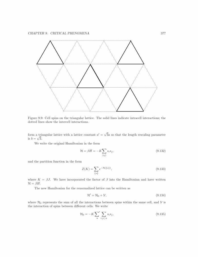
CHAPTER 9. CRITICAL PHENOMENA 377

Figure 9.9: Cell spins on the triangular lattice. The solid lines indicate intracell interactions; thedotted lines show the intercell interactions.

form a triangular lattice with a lattice constant a′ =√

3a so that the length rescaling parameteris b =

√3.

We write the original Hamiltonian in the form

H = βH = −K∑〈ij〉

sisj , (9.132)

and the partition function in the form

Z(K) =∑s

e−H(s), (9.133)

where K = βJ . We have incorporated the factor of β into the Hamiltonian and have writtenH = βH .

The new Hamiltonian for the renormalized lattice can be written as

H′ = H0 + V , (9.134)

where H0 represents the sum of all the interactions between spins within the same cell, and V isthe interaction of spins between different cells. We write

H0 = −K∑′

α

∑i,j⊂α

sisj , (9.135)

CHAPTER 9. CRITICAL PHENOMENA 378

where the sum over α represents the sum over cells. The restricted sum in (9.135) (denoted by aprime) is over configurations of the original lattice that are consistent with a given set of cell spinsµ. For b =

√3, the Hamiltonian for cell α has the form

H0,α = −K(s1,αs2,α + s1,αs3,α + s2,αs3,α). (9.136)

We write V asV = −K

∑α,β

α =β

∑′

i⊂α

∑′

j⊂β

sisj . (9.137)

The replacement of the original site spins by cell spins leads in general to a Hamiltonian thatdoes not have the same form as (9.132). That is, the new Hamiltonian involves interactions betweencell spins that are not nearest neighbors. Nevertheless, we assume that the new Hamiltonian hasthe same form:

Fr + H′ = −K ′∑′

〈αβ〉µαµβ. (9.138)

The term Fr in (9.138) is independent of the cell spin configurations. The representation (9.134)–(9.137) is exact.

In the following, we treat the interactions of the spins within the cells exactly and the inter-actions between the cells approximately. We will obtain a recursion relation

K ′ = R(K), (9.139)

and a nontrivial fixed point K∗ such that

λK =∂K ′

∂K

∣∣∣∣K∗

, (9.140)

and

ν =ln λK

ln b, (9.141)

where b is the length rescaling parameter.The renormalized Hamiltonian is given formally by

e−Fr−H′=

∑s

P (µ, s) e−(H0+V), (9.142)

where the operator P (µ, s) transforms the original three spins to the cell spin and implements themajority rule so that the renormalized cell spin equals the sign of the sum of the site spins in thecell. Formally, we can write P for cell spin α as

P (µα, s) = δ(µα − sgn(s1 + s2 + s3)

). (9.143)

Because we need to treat the interaction between the cell spins approximately, we introducean average over the original spin variables with respect to H0:

〈A〉0 =

∑′s A(s)P (µ, s) e−H0(s)

∑′s P (µ, s) e−H0(s)

. (9.144)

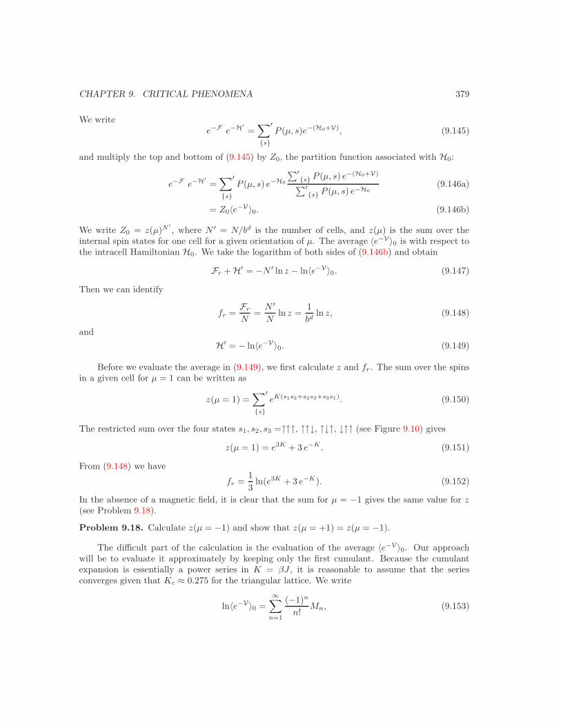
CHAPTER 9. CRITICAL PHENOMENA 379

We writee−Fre−H′

=∑′

sP (µ, s)e−(H0+V), (9.145)

and multiply the top and bottom of (9.145) by Z0, the partition function associated with H0:

e−Fre−H′=

∑′

sP (µ, s) e−H0

∑′s P (µ, s) e−(H0+V)

∑′s P (µ, s) e−H0

(9.146a)

= Z0〈e−V〉0. (9.146b)

We write Z0 = z(µ)N ′, where N ′ = N/bd is the number of cells, and z(µ) is the sum over the

internal spin states for one cell for a given orientation of µ. The average 〈e−V〉0 is with respect tothe intracell Hamiltonian H0. We take the logarithm of both sides of (9.146b) and obtain

Fr + H′ = −N ′ ln z − ln〈e−V〉0. (9.147)

Then we can identify

fr =Fr

N=

N ′

Nln z =

1bd

ln z, (9.148)

andH′ = − ln〈e−V〉0. (9.149)

Before we evaluate the average in (9.149), we first calculate z and fr. The sum over the spinsin a given cell for µ = 1 can be written as

z(µ = 1) =∑′

seK(s1s2+s2s3+s3s1). (9.150)

The restricted sum over the four states s1, s2, s3 =↑↑↑, ↑↑↓, ↑↓↑, ↓↑↑ (see Figure 9.10) gives

z(µ = 1) = e3K + 3 e−K . (9.151)

From (9.148) we have

fr =13

ln(e3K + 3 e−K). (9.152)

In the absence of a magnetic field, it is clear that the sum for µ = −1 gives the same value for z(see Problem 9.18).

Problem 9.18. Calculate z(µ = −1) and show that z(µ = +1) = z(µ = −1).

The difficult part of the calculation is the evaluation of the average 〈e−V〉0. Our approachwill be to evaluate it approximately by keeping only the first cumulant. Because the cumulantexpansion is essentially a power series in K = βJ , it is reasonable to assume that the seriesconverges given that Kc ≈ 0.275 for the triangular lattice. We write

ln〈e−V〉0 =∞∑

n=1

(−1)n

n!Mn, (9.153)

CHAPTER 9. CRITICAL PHENOMENA 380

Figure 9.10: Three spin cluster on the triangular lattice.

and keep only the first cumulantM1 = 〈V〉0. (9.154)

The first approximation to the intercell interaction V can be written as (see Figure 9.11)

Vαβ = −Ks1,α[s2,β + s3,β]. (9.155)

Note that V(1) in (9.155) includes only the interaction of two nearest neighbor cells and that thisapproximation does not preserve the symmetry of the triangular lattice. However, this approxi-mation is consistent with our assumption that the renormalized Hamiltonian has the same formas the original Hamiltonian. Because H0 does not couple different cells, we have

〈Vαβ〉0 = −2K〈s1,αs2,β〉0, (9.156a)= −2K〈s1,α〉0〈s2,β〉0. (9.156b)

(The factor of 2 in (9.156) arises from the fact that 〈s2,β〉 = 〈s3,β〉.)From (9.156b) we see that we need to find 〈s1,α〉0. Suppose that µα = 1. The four states

consistent with this condition are shown in Figure 9.10. It is easy to see that

〈s1,α〉0 =1z

∑′

ss1e

K(s1s2+s2s3+s3s1) (9.157a)

=1z

[+ 1e3K + 1e−K + 1e−K − 1e−K

](9.157b)

=1z[e3K + e−K ]. (µα = +1). (9.157c)

Similarly, we can show that

〈s1,α〉0 =1z[−e3K − e−K ] = −1

z[e3K + e−K ] (µα = −1) (9.158)

Hence, we can write

〈s1,α〉0 =1z[e3K + e−K ]µα. (9.159)

From (9.156b) and (9.159) we have

〈Vαβ〉0 = −2Kf(K)2µαµβ , (9.160)

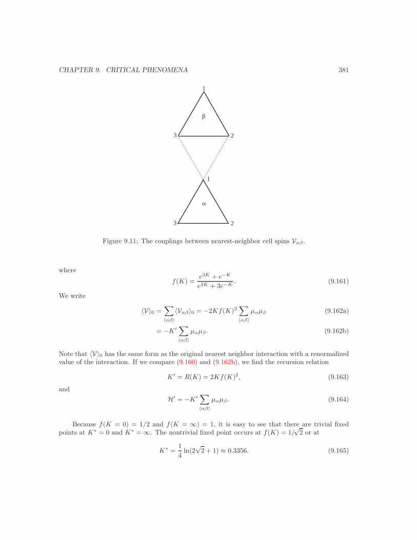
CHAPTER 9. CRITICAL PHENOMENA 381

1

3 2

1

3 2

α

β

Figure 9.11: The couplings between nearest-neighbor cell spins Vαβ .

where

f(K) =e3K + e−K

e3K + 3e−K. (9.161)

We write

〈V〉0 =∑〈αβ〉

〈Vαβ〉0 = −2Kf(K)2∑〈αβ〉

µαµβ (9.162a)

= −K ′ ∑〈αβ〉

µαµβ . (9.162b)

Note that 〈V〉0 has the same form as the original nearest neighbor interaction with a renormalizedvalue of the interaction. If we compare (9.160) and (9.162b), we find the recursion relation

K ′ = R(K) = 2Kf(K)2, (9.163)

andH′ = −K ′ ∑

〈αβ〉µαµβ . (9.164)

Because f(K = 0) = 1/2 and f(K = ∞) = 1, it is easy to see that there are trivial fixedpoints at K∗ = 0 and K∗ = ∞. The nontrivial fixed point occurs at f(K) = 1/

√2 or at

K∗ =14

ln(2√

2 + 1) ≈ 0.3356. (9.165)

CHAPTER 9. CRITICAL PHENOMENA 382

The exact answer for Kc for the triangular lattice is Kc = 13 ln 3 = 0.2747. We also have

λK =dK ′

dK

∣∣K=K∗ = 1.624, (9.166)

and hence

ν =ln 1.624ln√

3≈ 0.882. (9.167)

For comparison, the exact result is ν = 1.

Problem 9.19. Confirm the above results for K∗, λK , and ν.

We can extend the renormalization group analysis by considering higher order cumulants. Thesecond order cumulant introduces two new interactions that are not in the original Hamiltonian.That is, the cell spins interacts not only with nearest-neighbor cell spins, but also with second andthird neighbor cell spins. Hence, for consistency we have to include in our original Hamiltoniansecond and third neighbor interactions also. Fortunately, good results can usually be found bystopping at the second cumulant. More details can be found in the references.

9.10 Vocabulary

Landau theory

mean-field critical exponents

Ginzburg criterion

scaling relations, universality

percolation, connectivity

cluster, spanning cluster

recursion relation

decimation

cell spins

real space renormalization group approach

9.11 Additional Problems

Problem 9.20. Calculate the temperature and density dependence of the compressibility of a gasassuming that it satisfies the van der Waals equation of state (8.154).

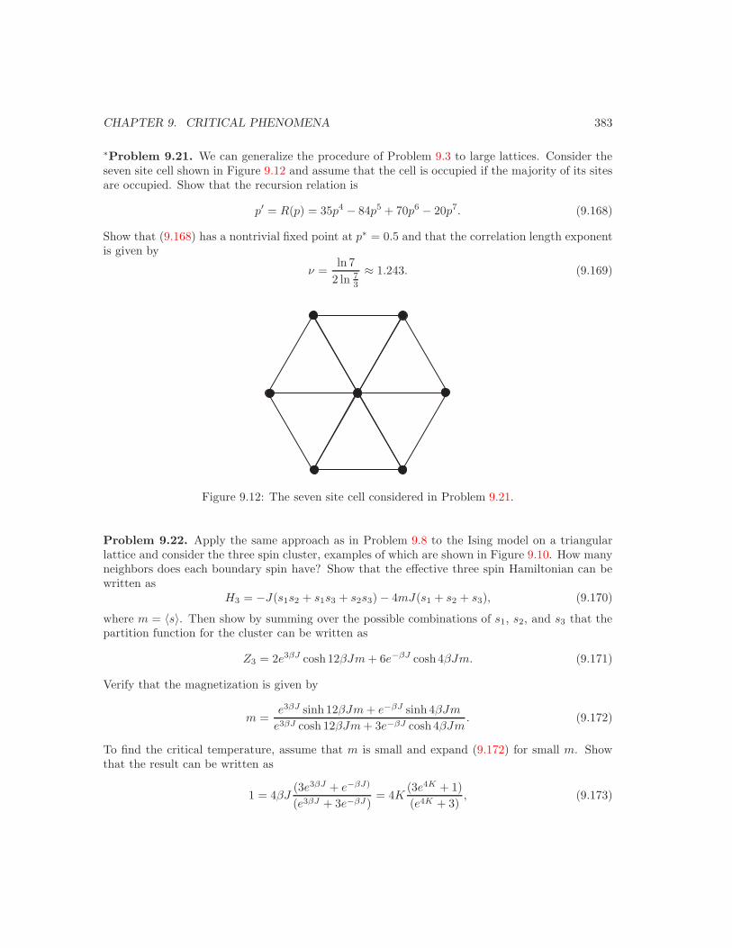
CHAPTER 9. CRITICAL PHENOMENA 383

∗Problem 9.21. We can generalize the procedure of Problem 9.3 to large lattices. Consider theseven site cell shown in Figure 9.12 and assume that the cell is occupied if the majority of its sitesare occupied. Show that the recursion relation is

p′ = R(p) = 35p4 − 84p5 + 70p6 − 20p7. (9.168)

Show that (9.168) has a nontrivial fixed point at p∗ = 0.5 and that the correlation length exponentis given by

ν =ln 7

2 ln 73

≈ 1.243. (9.169)

Figure 9.12: The seven site cell considered in Problem 9.21.

Problem 9.22. Apply the same approach as in Problem 9.8 to the Ising model on a triangularlattice and consider the three spin cluster, examples of which are shown in Figure 9.10. How manyneighbors does each boundary spin have? Show that the effective three spin Hamiltonian can bewritten as

H3 = −J(s1s2 + s1s3 + s2s3) − 4mJ(s1 + s2 + s3), (9.170)

where m = 〈s〉. Then show by summing over the possible combinations of s1, s2, and s3 that thepartition function for the cluster can be written as

Z3 = 2e3βJ cosh 12βJm + 6e−βJ cosh 4βJm. (9.171)

Verify that the magnetization is given by

m =e3βJ sinh 12βJm + e−βJ sinh 4βJm

e3βJ cosh 12βJm + 3e−βJ cosh 4βJm. (9.172)

To find the critical temperature, assume that m is small and expand (9.172) for small m. Showthat the result can be written as

1 = 4βJ(3e3βJ + e−βJ)

(e3βJ + 3e−βJ)= 4K

(3e4K + 1)(e4K + 3)

, (9.173)

CHAPTER 9. CRITICAL PHENOMENA 384

where K = βJ . Show numerically that the value of K that solves (9.173) is K = Kc ≈ 0.177.Compare this value of βcJ to the exact value βcHTc = 1

3 ln 3 ≈ 0.366 for the triangular latticeand the simple mean-field value (see Table 5.2). As an example of the fact that all mean-fieldapproximations give the same critical exponents, show that β = 1

2 .

Problem 9.23. Another way to express the scaling hypothesis is to assume that for B = 0, G(r)near ε = 0 has the form

G(r) ∼ 1rd−2+η

ψ±(r/ξ), (9.174)

where ψ± is an unspecified scaling function. Use (9.174) and the relation (9.93) to obtain Fisher’sscaling law, γ = ν(2 − η).

∗Problem 9.24. Develop an improved mean-field theory for the Ising model on a square latticebased on a four spin cluster.

∗Problem 9.25. We can apply mean-field ideas to percolation. It is easier to do so in the contextof bond percolation. In bond percolation we place bonds between lattice sites with probability pand we call any set of sites that are connected to one another by bonds a cluster. The criticalbond probability pc occurs when there is a spanning cluster.

Let P∞ be the probability that a randomly chosen bond forms part of the infinite cluster. Agiven bond will form part of such a cluster only if it has at least one neighboring bond. That is,a bond will not form part of an infinite cluster if its neighboring bonds are themselves not partof the cluster. This requirement gives us a relation connecting the probabilities that neighboringbonds are part of the infinite cluster. If we assume that these probabilities are the same for allbonds (a mean-field assumption), we require that

1 − P∞,i =q∏

j=1

(1 − pP∞,j), (9.175)

where P∞,i is the probability that bond i belongs to the infinite cluster. However, because we haveassumed that all bonds see the same local environment, we have that P∞,i = P∞ and hence

1 − P∞ = (1 − pP∞)q. (9.176)

Work out the graphical solution of (9.176) and show that pc = 1/q. If we set P∞ ∼ (p−pc)β , whatis the mean-field value of β for percolation?

∗Problem 9.26. The method we used in Section 9.8 for the one-dimensional Ising model is anexample of a decimation method. In this problem, we apply another decimation method to thetwo-dimensional Ising model on the square lattice in the absence of an external magnetic field. TheMigdal-Kadanoff approximation consists of two steps that are illustrated in Figure 9.13. First thesites denoted by an × in Figure 9.13a are removed. To compensate for this removal, the remainingbonds are doubled in strength so that the new Hamiltonian becomes

βH = −2K∑′

〈i,j〉sisj . (9.177)

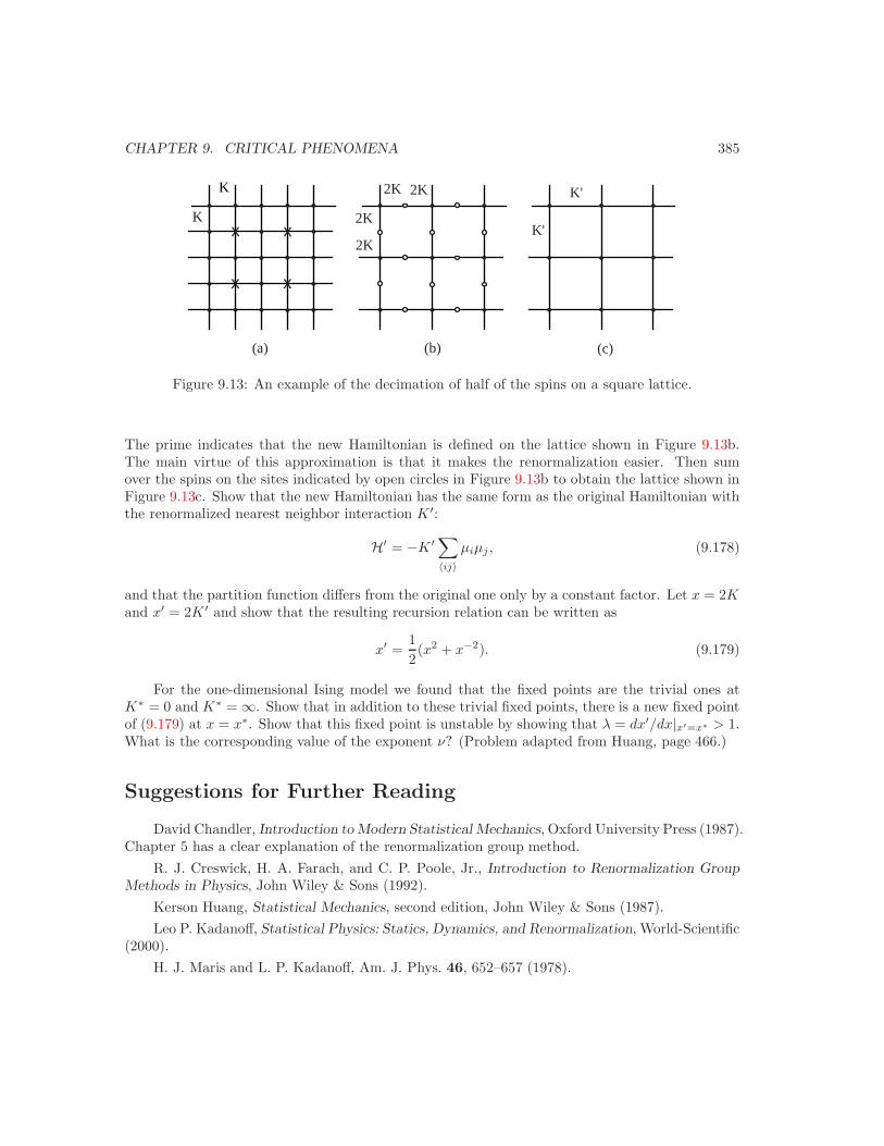
CHAPTER 9. CRITICAL PHENOMENA 385

K

K

2K

2K

2K

2K K'

K'x x

xx

(a) (b) (c)

Figure 9.13: An example of the decimation of half of the spins on a square lattice.

The prime indicates that the new Hamiltonian is defined on the lattice shown in Figure 9.13b.The main virtue of this approximation is that it makes the renormalization easier. Then sumover the spins on the sites indicated by open circles in Figure 9.13b to obtain the lattice shown inFigure 9.13c. Show that the new Hamiltonian has the same form as the original Hamiltonian withthe renormalized nearest neighbor interaction K ′:

H′ = −K ′ ∑〈ij〉

µiµj , (9.178)

and that the partition function differs from the original one only by a constant factor. Let x = 2Kand x′ = 2K ′ and show that the resulting recursion relation can be written as

x′ =12(x2 + x−2). (9.179)

For the one-dimensional Ising model we found that the fixed points are the trivial ones atK∗ = 0 and K∗ = ∞. Show that in addition to these trivial fixed points, there is a new fixed pointof (9.179) at x = x∗. Show that this fixed point is unstable by showing that λ = dx′/dx|x′=x∗ > 1.What is the corresponding value of the exponent ν? (Problem adapted from Huang, page 466.)

Suggestions for Further Reading

David Chandler, Introduction to Modern Statistical Mechanics, Oxford University Press (1987).Chapter 5 has a clear explanation of the renormalization group method.

R. J. Creswick, H. A. Farach, and C. P. Poole, Jr., Introduction to Renormalization GroupMethods in Physics, John Wiley & Sons (1992).

Kerson Huang, Statistical Mechanics, second edition, John Wiley & Sons (1987).Leo P. Kadanoff, Statistical Physics: Statics, Dynamics, and Renormalization, World-Scientific

(2000).H. J. Maris and L. P. Kadanoff, Am. J. Phys. 46, 652–657 (1978).

CHAPTER 9. CRITICAL PHENOMENA 386

Michael Plischke and Birger Bergersen, Equilibrium Statistical Physics, second edition, WorldScientific (1994). An excellent text for an introductory graduate level course.

Chapter 10

Introduction to Many-BodyPerturbation Theory

c©2006 by Harvey Gould and Jan Tobochnik2 January 2006

We introduce the language of second quantization in the context of quantum many body systemsand treat the weakly interacting Bose gas at low temperatures.

10.1 Introduction

As we saw in Chapter 8, it is difficult to treat the interparticle interactions in a classical manybody system of particles. As might be expected, the analysis of the analogous quantum system iseven more difficult.

Just as we developed the density expansion of a classical gas by doing perturbation theoryabout the ideal gas, we will first treat an interacting many-body quantum system by starting fromthe single particle approximation. We know that the wave function Ψ(r1, r2, . . . , rN ) for a system ofN identical interacting particles can be expanded in terms of the wave function Φ(r1, r2, . . . , rN ) ofthe noninteracting system. The wave function Φ is given in terms of suitably symmetrized productsof the single particle eigenfunctions φ(ri). If we adopt periodic boundary conditions, φk(r) is givenby

φk(r) =1

L3/2eik·r, (10.1)

where L is the linear dimension of the system. Note that φ is a eigenfunction of the momentump = k.

If the particles are bosons, the wave function Ψ and hence Φ must be symmetric with respect tothe interchange of any two particles. If the particles are fermions, Ψ and Φ must be antisymmetricwith respect to the interchange of any two particles. The latter condition is the generalization ofthe Pauli exclusion principle.

387

CHAPTER 10. INTRODUCTION TO MANY-BODY PERTURBATION THEORY 388

Because of the impossibility of distinguishing identical particles, it is useful to describe non-interacting quantum systems by specifying only the number of particles in each single particlestate (see Section 6.5). That is, instead of working in coordinate space, we can represent the basisfunctions of the many-body wave functions by

|n1n2 . . .〉, (10.2)

where nk is the number of particles in the single particle state φk. For fermions nk equals 0 or 1;there is no restriction for bosons. For a system with a fixed number of particles N , the occupationnumbers nk satisfy the condition

N =∑

k

nk. (10.3)

We also learned in Section 6.5 that it is convenient to treat quantum mechanical systems in thegrand canonical ensemble in which the number of particles in a particular single particle quantumstate may vary. For this reason we next introduce a formalism that explicitly allows us to writethe energy of the system in terms of operators that change the number of particles in a given state.

10.2 Occupation Number Representation

If we specify a state of the system in the occupation number representation, it is convenient tointroduce the operators ak and a†

k that act on states such as in (10.2). For bosons we define ak

and a†k by

ak| . . . nk . . .〉 =√

nk| . . . nk − 1 . . .〉, (10.4a)

anda†

k| . . . nk . . .〉 =√

nk + 1| . . . nk + 1 . . .〉 (10.4b)

From the definition (10.4a) we see that ak reduces the number of particles in state k and leaves theother occupation numbers unchanged. For this reason ak is called the annihilation or destructionoperator. Similarly, from (10.4b) we that a†

k increases the occupation number of state k by unityand is called the creation operator. The factor of

√nk is included in (10.4a) to normalize the N

and N − 1 particle wave functions and to make the definitions consistent with the assertion thatak and a†

k are Hermitian conjugates. The factor√

1 + nk is included for the latter reason.From the definitions in (10.4), it is easy to show that

aka†k|nk〉 = (nk + 1)|nk〉 (10.5a)

a†kak|nk〉 = nk|nk〉. (10.5b)

We have written |nk〉 for | . . . , nk, . . .〉. By subtracting (10.5b) from (10.5a), we have

(aka†k − a†

kak)|nk〉 = |nk〉. (10.6)

In general, we may write that[ak, a†

k] ≡ aka†k − a†

kak = 1, (10.7)

CHAPTER 10. INTRODUCTION TO MANY-BODY PERTURBATION THEORY 389

and show that

[ak, a†k] = δkk′ , (10.8)

and[ak, ak′ ] = [a†

k, a†k′ ] = 0. (10.9)

The commutation relations (10.8) and (10.9) define the creation and destruction operators a†k and

ak.The appropriate definition of ak and a†

k is a little more tedious for fermions, and we shallsimply define them by the anticommutation relations:

ak, a†k ≡ aka†

k + a†kak = 1, (10.10)

andak, ak′ = a†

k, a†k′ = 0. (10.11)

Equation (10.11) is equivalent to the statement that it is not possible to create two particles in thesame single particle state.

10.3 Operators in the Second Quantization Formalism

It is easy to show that for both Bose and Fermi statistics, the number operator Nk is given by

Nk = a†kak. (10.12)

The eigenvalues of Nk acting on |nk〉 are zero or unity for fermions and either zero or any positiveinteger for bosons.

We now wish to write other operators in terms of ak and a†k. To do so, we note that a†

k andak are the creation and destruction operators for a free particle with momentum p = k describedby the wave function (10.1). The kinetic energy is an example of a one-particle operator

T = − 2

2m

N∑i=1

∇2i . (10.13)

The form (10.13) in which the momentum p is expressed as an operator is an example of what iscalled first quantization. Note that the sum in (10.13) is over the indistinguishable particles in thesystem. A more convenient form for T in the second quantization formalism is given by

T =∑p

εp a†pap, (10.14)

where εp = p2/2m and p = k. Note that the kinetic energy is diagonal in p. The form of (10.14)is suggestive and can be interpreted as the sum of the kinetic energy in state p times the numberof particles in this state.

CHAPTER 10. INTRODUCTION TO MANY-BODY PERTURBATION THEORY 390

The form of the two-particle potential energy operator U can be obtained from straightforwardbut tedious arguments. The result can be written as

U =12

∑k′

1,k′1,k1,k2

〈k′1k

′2|u|k1k2〉 a†

k′1a†k′

2ak1 ak2 . (10.15)

The summation in (10.15) is over all values of the momenta (wave vectors) of a pair of particlessuch that the total momentum is conserved in the interaction:

k1 + k2 = k′1 + k′

2. (10.16)

The matrix element 〈k′1k

′2|u|k1k2〉 is given by

〈k′1k

′2|u|k1k2〉 =

1V 2

∫∫ei(k′

1−k1)·r1+i(k′2−k2)·r2 u(|r2 − r1|) dr1dr2. (10.17)

We next make the change of variables, R = (r1 + r2)/2 and r = r1 − r2, and write

〈k′1k

′2|u|k1k2〉 =

1V 2

∫∫ei(k1−k′

1+k2−k′2)·R ei(k1−k′

1−k2+k′2)·r/2u(r) dR dr. (10.18a)

Because of the homogeneity of space, the integral over R can be done yielding a Dirac delta functionand the condition (10.16). We thus obtain obtain

〈k′1k

′2|u|k1k2〉 = u(k) =

∫e−ik·ru(r) dr, (10.18b)

where k = k′2 − k2 = −(k′

1 − k1) is the momentum (wave vector) transferred in the interaction.With these considerations we can write the Hamiltonian in the form

H =∑

p

p2

2ma†pap +

12V

∑k,p1,p2

u(k)a†p1+ka†

p2−kap2 ap1 . (10.19)

We have written p1 and p2 instead of k1 and k2 in (10.19) and chosen units such that = 1.The order of the operators in (10.15) and (10.19) is important for fermions because the fermionoperators anticommute. The order is unimportant for bosons. The form of the interaction term in(10.19) can be represented as in Figure 10.1.

10.4 Weakly Interacting Bose Gas

A calculation of the properties of the dilute Bose gas was once considered to have no direct physicalrelevance because the gases that exist in nature condense at low temperatures. However, such acalculation was interesting because the properties of the weakly interacting Bose gas are similarto liquid 4He. In particular, a dilute Bose gas can be a superfluid even though an ideal Bose gascannot. Moreover, in recent years, the dilute Bose gas at low temperatures has been created inthe laboratory (see references).

The condition for a gas to be dilute is that the range of interaction σ should be small incomparison to the mean distance between the particles, ρ−1/3, that is ρσ3 1. Because the gas is

CHAPTER 10. INTRODUCTION TO MANY-BODY PERTURBATION THEORY 391

not done

Figure 10.1: Representation of the matrix element in (10.15).

dilute, we need to consider only binary interactions between particles using quantum perturbationtheory. The difficulty is that because of the rapid increase in the interparticle potential u(r) atsmall r, ordinary perturbation theory (the Born approximation) cannot be directly applied.

We can circumvent the lack of applicability of the Born approximation by the following argu-ment. The scattering cross section is given by |f |2, where f is the scattering amplitude. In theBorn approximation, f is given by

f(k) = − m

4π2

∫u(r)e−ik·r dr, (10.20)

where k is the momentum transferred in the interaction. In the limit of low temperatures, theparticle momenta are small, and we can set k = 0 in (10.20). If we set f(k = 0) = −a, where a isthe scattering amplitude, we obtain

a = mU0/4π2 (10.21)

whereU0 =

∫u(r) dr. (10.22)

In the following, we will set u(k = 0) = U0 = 4π2a/m, so that we will be able to mimic the result

of doing a true perturbation theory calculation.1

If we assume that u(k) = U0 for al k, a constant, we can write the Hamiltonian as

H =∑p

p2

2ma†pap +

U0

2V

∑k,p1,p2

a†p1−ka†

p2+kap2 ap1 . (10.23)

The form of (10.23) is the same for Bose or Fermi statistics. Only the commutation relations forthe creation and destruction operators are different.

We now follow the approximation method developed by Bogolyubov (1947). In the limitU0 → 0, H reduces to the Hamiltonian of the ideal Bose gas. We know that the latter has

1In the language of quantum mechanics, we need to replace the bare interaction u by the t matrix. Thisreplacement is the quantum mechanical generalization of replacing −βu by the Mayer f function. Not surprisingly,this replacement can be represented by an infinite sum of ladder-type diagrams. Note that if we interpret the Mayerf function as the effective interaction between particles, the first cumulant in a high temperature expansion wouldyield the same result as the first term in the classical virial expansion.

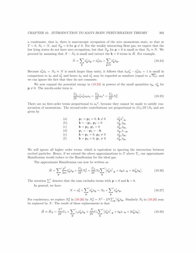
CHAPTER 10. INTRODUCTION TO MANY-BODY PERTURBATION THEORY 392

a condensate, that is, there is macroscopic occupation of the zero momentum state, so that atT = 0, N0 = N , and Np = 0 for p = 0. For the weakly interacting Bose gas, we expect that thelow lying states do not have zero occupation, but that Np for p > 0 is small so that N0 ≈ N . Weproceed by assuming that N − N0 is small and extract the k = 0 terms in H . For example,

N =∑p

a†pap = a†

0a0 +∑p =0

a†pap. (10.24)

Because a†0a0 = N0 ≈ N is much larger than unity, it follows that a0a

†0 − a†

0a0 = 1 is small incomparison to a0 and a†

0 and hence a0 and a†0 may be regarded as numbers (equal to

√N0), and

we can ignore the fact that they do not commute.We now expand the potential energy in (10.23) in powers of the small quantities ap, a†

p forp = 0. The zeroth-order term is

U0

2Va†0a

†0a0a0 =

U0

2Va0

4 =U0

2VN2

0 . (10.25)

There are no first-order terms proportional to a03, because they cannot be made to satisfy con-

servation of momentum. The second-order contributions are proportional to (U0/2V )N0 and aregiven by

(a) p1 = p2 = 0, k = 0 a†ka†

−k

(b) k = −p1, p2 = 0 a†p1

ap1

(c) k = p2, p1 = 0 a†p2

ap2

(d) p1 = −p2 = −k ap1 a−p1

(e) k = p1 = 0, p2 = 0 a†p2

ap2

(f) k = p2 = 0, p1 = 0 a†p1

ap1

We will ignore all higher order terms, which is equivalent to ignoring the interaction betweenexcited particles. Hence, if we extend the above approximations to T above Tc, our approximateHamiltonian would reduce to the Hamiltonian for the ideal gas.

The approximate Hamiltonian can now be written as

H =∑p

′ p2

2ma†pap +

U0

2VN2

0 +U0

2VN0

∑k

′[a†ka†

−k + aka−k + 4a†kak

]. (10.26)

The notation∑′ denotes that the sum excludes terms with p = 0 and k = 0.

In general, we haveN = a2

0 +∑p

′a†pap = N0 +

∑p

′a†pap. (10.27)

For consistency, we replace N20 in (10.26) by N2

0 = N2−2N∑

p′a†

pap. Similarly N0 in (10.26) maybe replaced by N . The result of these replacements is that

H ≈ HB =N2

2VU0 +

∑p

′εpa

†pap +

N

2VU0

∑k

′[a†ka†

−k + aka−k + 2a†kak

]. (10.28)

CHAPTER 10. INTRODUCTION TO MANY-BODY PERTURBATION THEORY 393

Note that HB only allows excitation of pairs of momentum k and −k from the condensate andre-entry of such pairs into the condensate.

The approximate Hamiltonian HB is bilinear in a and a†. This form is similar to that of aharmonic oscillator. This similarity suggests that we can diagonalize HB by making an appropriatelinear transformation of the operators a and a†. If HB is put into diagonal form, then HB wouldhave the same form as an ideal gas, and we could easily calculate the energy eigenvalues.

We define new operators b† and b by

ak = ukbk + vk b†−k (10.29a)

a†k = ukb†k + vk b−k, (10.29b)

and require them to satisfy the Bose commutation relations

bkb†k′ − b†k′ bk = δkk′ and bkbk′ = bk′ bk. (10.30)

As shown in Problem 10.1, b† and b satisfy the Bose commutation relations only if the relation(10.31) between uk and vk is satisfied:

u2k − v2

k = 1. (10.31)

Problem 10.1. (a) Use (10.29) to express b† and b in terms of a† and a. (b) Show that thecommutation relations (10.30) are satisfied only if (10.31) is satisfied.

If we substitute the above expressions for a† and a into (10.28), we obtain

HB = E0 + HD + HI (10.32a)

where

E0 =N2U0

2V+

∑k

′[(εp +

NU0

V

)vk

2 +NU0

Vukvk

](10.32b)

HD =∑k

′[(εp +

NU0

V)(uk

2 + vk2)2NU0

Vukvk

]b†kbk (10.32c)

HI =∑k

′[(εk +

NU0

V

)(ukvk +

12vk(u2

k + v2k)

)](b†kb†−k + bkb−k

). (10.32d)

From the form of (10.32), we see that HB would be diagonal if HI = 0. This condition is satisfiedif

2(εk +

NU0

V

)(ukvk + vk(u2

k + v2k

)= 0, (10.33)

and the relation (10.31) is satisfied. Note that we have two equations for the two unknown uk andvk. We can satisfy the relation (10.31) automatically by letting

uk = cosh θk (10.34a)vk = sinh θk. (10.34b)

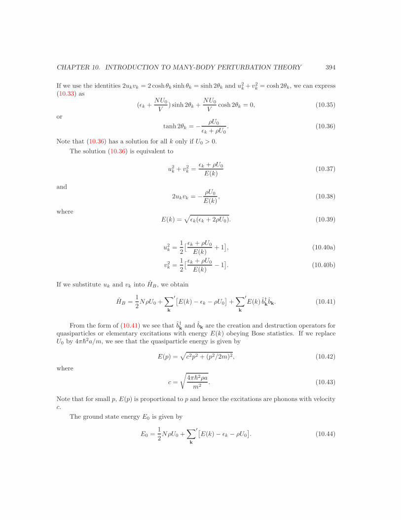
CHAPTER 10. INTRODUCTION TO MANY-BODY PERTURBATION THEORY 394

If we use the identities 2ukvk = 2 cosh θk sinh θk = sinh 2θk and u2k + v2

k = cosh 2θk, we can express(10.33) as

(εk +NU0

V) sinh 2θk +

NU0

Vcosh 2θk = 0, (10.35)

ortanh 2θk = − ρU0

εk + ρU0. (10.36)

Note that (10.36) has a solution for all k only if U0 > 0.The solution (10.36) is equivalent to

u2k + v2

k =εk + ρU0

E(k)(10.37)

and2ukvk = − ρU0

E(k), (10.38)

whereE(k) =

√εk(εk + 2ρU0). (10.39)

u2k =

12[ εk + ρU0

E(k)+ 1

], (10.40a)

v2k =

12[ εk + ρU0

E(k)− 1

]. (10.40b)

If we substitute uk and vk into HB, we obtain

HB =12NρU0 +

∑k

′[E(k) − εk − ρU0

]+

∑k

′E(k) b†kbk. (10.41)

From the form of (10.41) we see that b†k and bk are the creation and destruction operators forquasiparticles or elementary excitations with energy E(k) obeying Bose statistics. If we replaceU0 by 4π

2a/m, we see that the quasiparticle energy is given by

E(p) =√

c2p2 + (p2/2m)2, (10.42)

where

c =

√4π2ρa

m2. (10.43)

Note that for small p, E(p) is proportional to p and hence the excitations are phonons with velocityc.

The ground state energy E0 is given by

E0 =12NρU0 +

∑k

′[E(k) − εk − ρU0

]. (10.44)

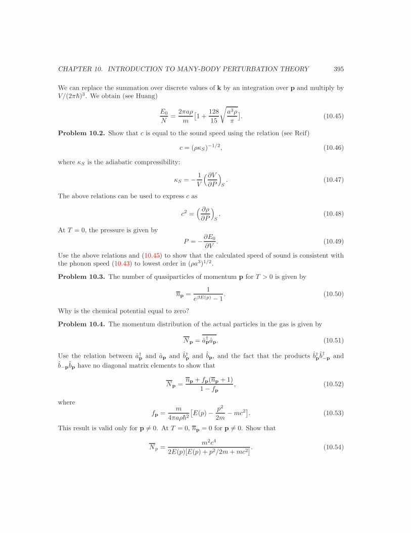
CHAPTER 10. INTRODUCTION TO MANY-BODY PERTURBATION THEORY 395

We can replace the summation over discrete values of k by an integration over p and multiply byV/(2π)3. We obtain (see Huang)

E0

N=

2πaρ

m

[1 +

12815

√a3ρ

π

]. (10.45)

Problem 10.2. Show that c is equal to the sound speed using the relation (see Reif)

c = (ρκS)−1/2, (10.46)

where κS is the adiabatic compressibility:

κS = − 1V

(∂V

∂P

)S

. (10.47)

The above relations can be used to express c as

c2 =( ∂ρ

∂P

)S

. (10.48)

At T = 0, the pressure is given by

P = −∂E0

∂V. (10.49)

Use the above relations and (10.45) to show that the calculated speed of sound is consistent withthe phonon speed (10.43) to lowest order in (ρa3)1/2.

Problem 10.3. The number of quasiparticles of momentum p for T > 0 is given by

np =1

eβE(p) − 1. (10.50)

Why is the chemical potential equal to zero?

Problem 10.4. The momentum distribution of the actual particles in the gas is given by

Np = a†pap. (10.51)

Use the relation between a†p and ap and b†p and bp, and the fact that the products b†pb†−p and

b−pbp have no diagonal matrix elements to show that

Np =np + fp(np + 1)

1 − fp, (10.52)

where

fp =m

4πaρ2

[E(p) − p2

2m− mc2

]. (10.53)

This result is valid only for p = 0. At T = 0, np = 0 for p = 0. Show that

Np =m2c4

2E(p)[E(p) + p2/2m + mc2]. (10.54)

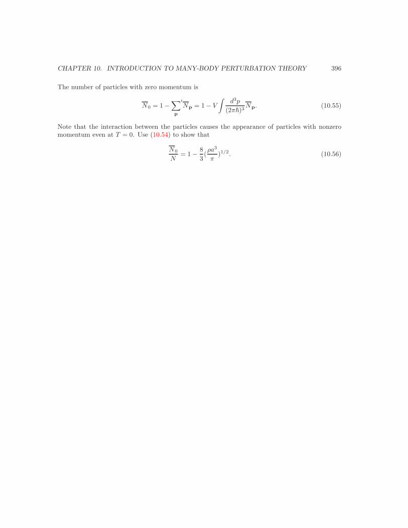
CHAPTER 10. INTRODUCTION TO MANY-BODY PERTURBATION THEORY 396

The number of particles with zero momentum is

N0 = 1 −∑p

′Np = 1 − V

∫d3p

(2π)3Np. (10.55)

Note that the interaction between the particles causes the appearance of particles with nonzeromomentum even at T = 0. Use (10.54) to show that

N0

N= 1 − 8

3(ρa3

π)1/2. (10.56)

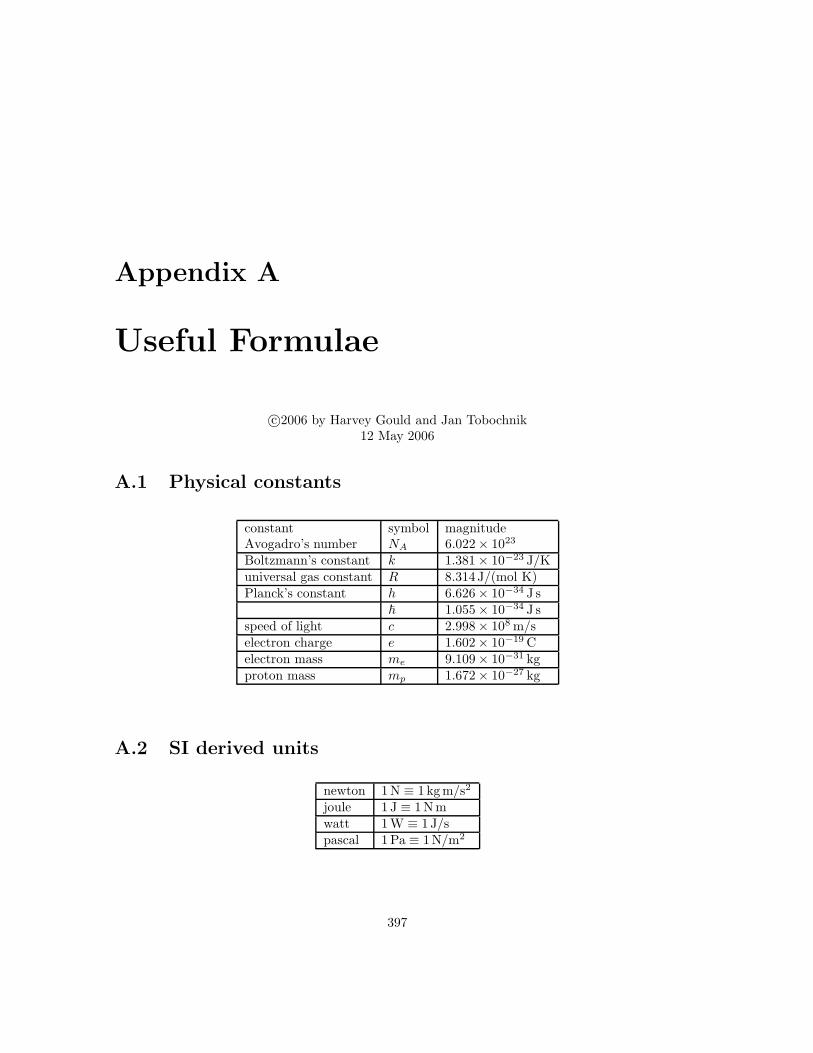
Appendix A

Useful Formulae

c©2006 by Harvey Gould and Jan Tobochnik12 May 2006

A.1 Physical constants

constant symbol magnitudeAvogadro’s number NA 6.022× 1023

Boltzmann’s constant k 1.381× 10−23 J/Kuniversal gas constant R 8.314J/(mol K)Planck’s constant h 6.626× 10−34 J s

~ 1.055× 10−34 J sspeed of light c 2.998× 108 m/selectron charge e 1.602× 10−19 Celectron mass me 9.109× 10−31 kgproton mass mp 1.672× 10−27 kg

A.2 SI derived units

newton 1 N ≡ 1 kgm/s2

joule 1 J ≡ 1N mwatt 1 W ≡ 1 J/spascal 1 Pa ≡ 1N/m2

397

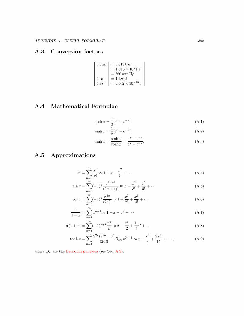
APPENDIX A. USEFUL FORMULAE 398

A.3 Conversion factors

1 atm = 1.013bar= 1.013× 105 Pa= 760 mm Hg

1 cal = 4.186J1 eV = 1.602× 10−19 J

A.4 Mathematical Formulae

coshx =1

2[ex + e−x]. (A.1)

sinhx =1

2[ex − e−x]. (A.2)

tanhx =sinh x

coshx=

ex − e−x

ex + e−x. (A.3)

A.5 Approximations

ex =

∞∑

n=0

xn

n!≈ 1 + x +

x2

2!+ · · · (A.4)

sin x =∞∑

n=0

(−1)n x2n+1

(2n + 1)!≈ x − x3

3!+

x5

5!+ · · · (A.5)

cosx =

∞∑

n=0

(−1)n x2n

(2n)!≈ 1 − x2

2!+

x4

4!+ · · · (A.6)

1

1 − x=

∞∑

n=1

xn−1 ≈ 1 + x + x2 + · · · (A.7)

ln (1 + x) =

∞∑

n=1

(−1)n+1 xn

n≈ x − x2

2+

1

3x3 + · · · (A.8)

tanh x =

∞∑

n=1

22n(22n − 1)

(2n)!B2n x2n−1 ≈ x − x3

3+

2x5

15+ · · · , (A.9)

where Bn are the Bernoulli numbers (see Sec. A.9).

APPENDIX A. USEFUL FORMULAE 399

A.6 Euler-Maclaurin formula

∞∑

i=0

f(x) =

∫ ∞

0

f(x) dx +1

2f(0) − 1

12f ′(0) +

1

720f ′′′(0)+ (A.10)

A.7 Gaussian Integrals

In =

∫ ∞

−∞

dx xne−ax2

. (n ≥ 0, a > 0) (A.11)

I0 = (π

a)1/2 (A.12)

I1 = 0 (A.13)

I2 =1

2(

π

a3)1/2 (A.14)

Derivation:

I0 =

∫ +∞

−∞

e−ax2

dx. (A.15)

We note that x in the integrand in (A.15) is a dummy variable. Hence, we may write I0 equallywell as

I0 =

∫ +∞

−∞

e−ay2

dy.

To convert the integrand to a form we can integrate, we multiply I by itself and write

I20 =

∫ +∞

−∞

e−ax2

dx

∫ +∞

−∞

e−ay2

dy =

∫ +∞

−∞

∫ +∞

−∞

e−(x2+y2) dx dy. (A.16)

The double integral in (A.16) extends over the entire xy-plane. We introduce the polar coordinatesr and θ, where r2 = x2 + y2. The element of area in polar coordinates is rdr dθ. Hence, I2

0 can berewritten in the form

I20 =

∫ 2π

0

∫ ∞

0

e−ar2

rdr dθ = 2π

∫ ∞

0

e−ar2

rdr.

We let z = ar2, dz = 2ardr, and write

I20 =

π

a

∫ ∞

0

e−z dz =π

a

[

− e−z]∞

0=

π

a.

Hence, we obtain the desired result

I0 =

∫ +∞

−∞

e−ax2

dx =(π

a

)1/2. (A.17)

Clearly the values of In for n odd are zero by symmetry. For odd values of n, let us redefineIn as

In =

∫ ∞

0

dxxne−ax2

. (n odd) (A.18)

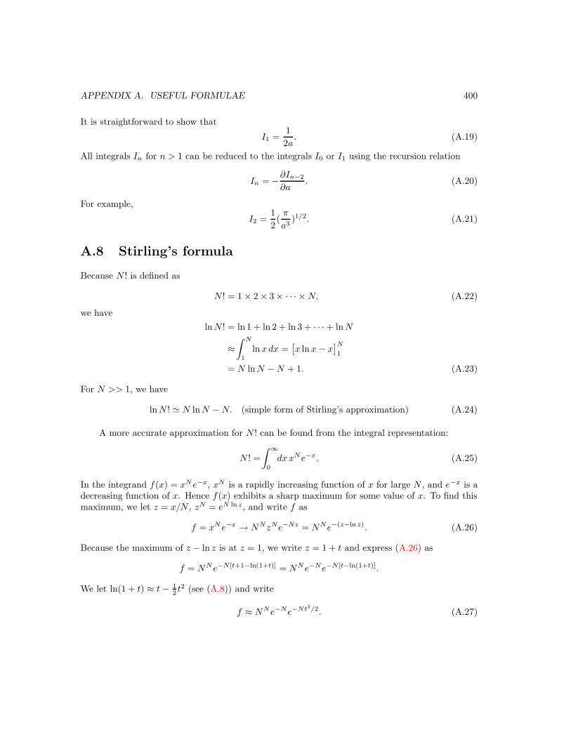
APPENDIX A. USEFUL FORMULAE 400

It is straightforward to show that

I1 =1

2a. (A.19)

All integrals In for n > 1 can be reduced to the integrals I0 or I1 using the recursion relation

In = −∂In−2

∂a. (A.20)

For example,

I2 =1

2(

π

a3)1/2. (A.21)

A.8 Stirling’s formula

Because N ! is defined as

N ! = 1 × 2 × 3 × · · · × N, (A.22)

we have

ln N ! = ln 1 + ln 2 + ln 3 + · · · + ln N

≈∫ N

1

ln x dx =[

x ln x − x]N

1

= N ln N − N + 1. (A.23)

For N >> 1, we have

ln N ! ' N ln N − N. (simple form of Stirling’s approximation) (A.24)

A more accurate approximation for N ! can be found from the integral representation:

N ! =

∫ ∞

0

dx xNe−x. (A.25)

In the integrand f(x) = xNe−x, xN is a rapidly increasing function of x for large N , and e−x is adecreasing function of x. Hence f(x) exhibits a sharp maximum for some value of x. To find thismaximum, we let z = x/N , zN = eN ln z, and write f as

f = xNe−x → NNzNe−Nz = NNe−(z−ln z). (A.26)

Because the maximum of z − ln z is at z = 1, we write z = 1 + t and express (A.26) as

f = NNe−N [t+1−ln(1+t)] = NNe−Ne−N [t−ln(1+t)].

We let ln(1 + t) ≈ t − 12 t2 (see (A.8)) and write

f ≈ NNe−Ne−Nt2/2. (A.27)

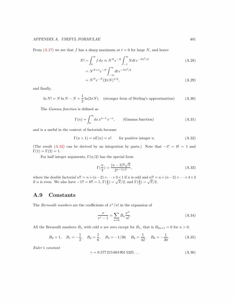
APPENDIX A. USEFUL FORMULAE 401

From (A.27) we see that f has a sharp maximum at t = 0 for large N , and hence

N ! =

∫ ∞

0

f dx ≈ NNe−N

∫ ∞

−1

Ndt e−Nt2/2 (A.28)

= NN+1e−N

∫ ∞

−∞

dt e−Nt2/2

= NNe−N(2πN)1/2, (A.29)

and finally,

ln N ! = N ln N − N +1

2ln(2πN). (stronger form of Stirling’s approximation) (A.30)

The Gamma function is defined as

Γ(n) =

∫ ∞

0

dx xn−1 e−x, (Gamma function) (A.31)

and is a useful in the context of factorials because

Γ(n + 1) = nΓ(n) = n! for positive integer n. (A.32)

(The result (A.32) can be derived by an integration by parts.) Note that −1! = 0! = 1 andΓ(1) = Γ(2) = 1.

For half integer arguments, Γ(n/2) has the special form

Γ(n

2) =

(n − 2)!!√

π

2n−1)/2, (A.33)

where the double factorial n!! = n× (n−2)×· · ·×3×1 if n is odd and n!! = n× (n−2)×· · ·×4×2if n is even. We also have −1!! = 0!! = 1, Γ( 1

2 ) =√

π/2, and Γ( 32 ) =

√π/2.

A.9 Constants

The Bernoulli numbers are the coefficients of xn/n! in the expansion of

x

ex − 1=

∑

n=0

Bnxn

n!. (A.34)

All the Bernoulli numbers Bn with odd n are zero except for B1, that is B2n+1 = 0 for n > 0.

B0 = 1, B1 = −1

2, B2 =

1

6, B4 = −1/30, B6 =

1

42, B8 = − 1

30. (A.35)

Euler’s constant

γ = 0.577 215 664 901 5325 . . . (A.36)

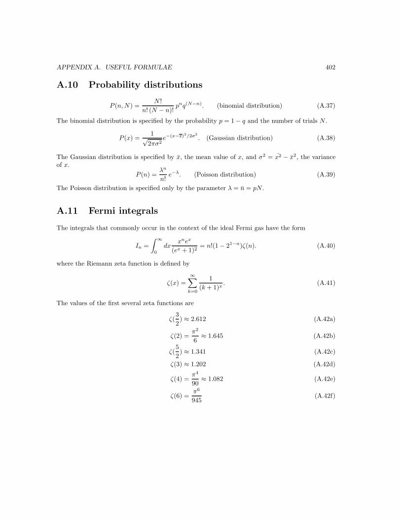
APPENDIX A. USEFUL FORMULAE 402

A.10 Probability distributions

P (n, N) =N !

n! (N − n)!pnq(N−n). (binomial distribution) (A.37)

The binomial distribution is specified by the probability p = 1 − q and the number of trials N .

P (x) =1√

2πσ2e−(x−x)2/2σ2

. (Gaussian distribution) (A.38)

The Gaussian distribution is specified by x, the mean value of x, and σ2 = x2 − x2, the varianceof x.

P (n) =λn

n!e−λ. (Poisson distribution) (A.39)

The Poisson distribution is specified only by the parameter λ = n = pN .

A.11 Fermi integrals

The integrals that commonly occur in the context of the ideal Fermi gas have the form

In =

∫ ∞

0

dxxnex

(ex + 1)2= n!(1 − 21−n)ζ(n). (A.40)

where the Riemann zeta function is defined by

ζ(x) =

∞∑

k=0

1

(k + 1)x. (A.41)

The values of the first several zeta functions are

ζ(3

2) ≈ 2.612 (A.42a)

ζ(2) =π2

6≈ 1.645 (A.42b)

ζ(5

2) ≈ 1.341 (A.42c)

ζ(3) ≈ 1.202 (A.42d)

ζ(4) =π4

90≈ 1.082 (A.42e)

ζ(6) =π6

945(A.42f)

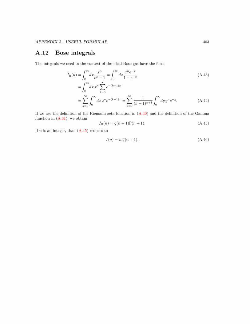
APPENDIX A. USEFUL FORMULAE 403

A.12 Bose integrals

The integrals we need in the context of the ideal Bose gas have the form

IB(n) =

∫ ∞

0

dxxn

ex − 1=

∫ ∞

0

dxxne−x

1 − e−x(A.43)

=

∫ ∞

0

dx xn∞∑

k=0

e−(k+1)x

=

∞∑

k=0

∫ ∞

0

dx xne−(k+1)x =

∞∑

k=0

1

(k + 1)n+1

∫ ∞

0

dy yne−y. (A.44)

If we use the definition of the Riemann zeta function in (A.40) and the definition of the Gammafunction in (A.31), we obtain

IB(n) = ζ(n + 1)Γ(n + 1). (A.45)

If n is an integer, than (A.45) reduces to

I(n) = n!ζ(n + 1). (A.46)