Adaptive multi-element polynomial chaos with discrete measure: Algorithms and application to

SPDEs Mengdi Zheng and George Karniadakis

Content: 1. computing SPDE by MEPCM 2. motivations 3. numerical integration on discrete measure 4. numerical example on KdV equation 5. future work

1.What computational SPDE is about? (MEPCM)

Xt(!) E[y(x, t;!)]Xt(!)

Xt(⇠1, ⇠2, ...⇠n)

...

⇠n

⇠3⇠2

⇠1

⌦

E[ym(x, t;!)]

E[ym(x, t; ⇠1, ⇠2, ..., ⇠n)]

fix x, t, integration over a finite dimensional sample space

MEPCM=FEM on sample space

⇠1

⇠2

⌦

⇡ ⇡

Gauss quadratures

So it’s all about integration on the sample space...Gauss integration

I =

Z b

ad�(x)f(x) ⇡

Z b

ad�(x)

dX

i=1

f(xi)hi(x)

=dX

i=1

f(xi)

Z b

ad�(x)hi(x)

Generate {P_i(x)} orthogonal to this measure

zeros of P_d(x) Lagrange interpolation on the zeros

dX

i=1

y(x, t; ⇠1,i)wionly run deterministic solver

on quadrature points, no need to run propagator

exactness of integration m=2d-1

2. Three motivations of dealing with discrete measure

Gaussian process Levy

process

Hermite polynomial chaos

Levy-Sheffer polynomial chaos ?

jump

current work

Analysis of historical stock prices shows that simple models with randomness provided by pure jump Levy processes often capture the statistical behavior of observed stock prices better than similar models with randomness provided by a Brownian motion.

Mathematical finance

1

2

3

4

5

3. J. Foo proved this on continuous measure

J. Foo, X. Wan, G. E. Karniadakis, A multi-element probabilistic col- location method for PDEs with parametric uncertainty: error anal- ysis and applications, Journal of Computational Physics 227 (2008), pp. 9572–9595.

3. Can we prove it on discrete measure? for discrete measure

�" =NX

i=1

�i⌘"⌧i ,

lim"!0

⌘"⌧i = �⌧i , lim"!0

�" = �.

�����

Z

�f(x)�(dx)�

NeX

i=1

QBi

m f

����� ����Z

�f(x)�(dx)�

Z

�f(x)�"(dx)

����

+

�����

Z

�f(x)�"(dx)�

NeX

i=1

Q",Bi

m f

����� +

�����

NeX

i=1

Q",Bi

m f �NeX

i=1

QBi

m f

����� ,

h / N�1es N�(m+1)

es

m = 2d� 1N�2d

es

� =NX

i=1

�i�⌧i ⌦⌧1 ⌧2 ⌧3

Generating orthogonal polynomials for discrete measure

Vandermonde matrix method

µk =

Z

Rx

k�(dx)

0

BBBB@

µ0 µ1 . . . µk

µ1 µ2 . . . µk+1

. . . . . . . . . . . .µk�1 µk . . . µ2k�1

0 0 . . . 1

1

CCCCA

0

BBBB@

p0p1. . .pk�1

pk

1

CCCCA=

0

BBBB@

00. . .01

1

CCCCA

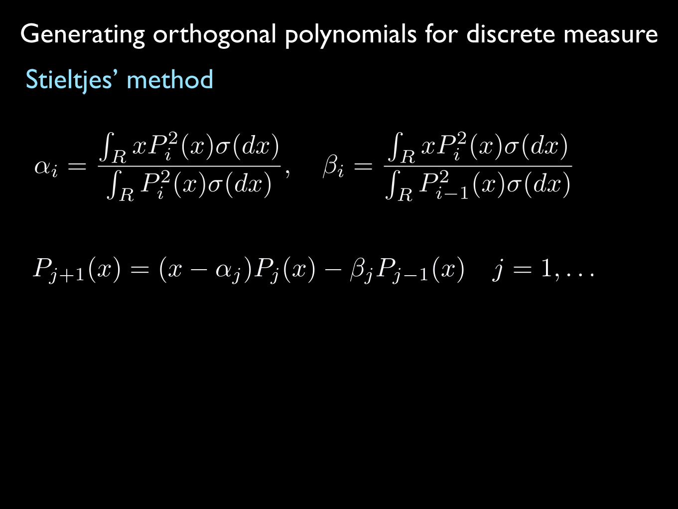
Generating orthogonal polynomials for discrete measure

Stieltjes’ method

↵i =

RR xP

2i (x)�(dx)R

R P

2i (x)�(dx)

, �i =

RR xP

2i (x)�(dx)R

R P

2i�1(x)�(dx)

Pj+1(x) = (x� ↵j)Pj(x)� �jPj�1(x) j = 1, . . .

Generating orthogonal polynomials for discrete measureFischer’s method

� =NX

i=1

�i�⌧i ⌫ = � + ��⌧

↵⌫i = ↵i + �

�2i Pi(⌧)Pi+1(⌧)

1 + �Pi

j=0 �2jP

2j (⌧)

� ��2i�1Pi(⌧)Pi�1(⌧)

1 + �Pi�1

j=0 �2jP

2j (⌧)

�⌫i = �i

[1 + �Pi�2

j=0 �2jP

2j (⌧)][1 + �

Pij=0 �

2jP

2j (⌧)]

[1 + �Pi�1

j=0 �2jP

2j (⌧)]

2

Generating orthogonal polynomials for discrete measure

Modified Chebyshev method

⌫r =

Z

⌦pr(⇠)d�(⇠)

�kl =

Z

⌦Pk(⇠)pl(⇠)d�(⇠)

↵k = ak +�k,k+1

�kk� �k�1,k

�k�1,k�1,�k =

�k,k

�k�1,k�1

Generating orthogonal polynomials for discrete measure

Lanczos’ method0

BBBB@

1pw1

pw2 . . .

pwNp

w1 ⌧1 0 . . . 0pw2 0 ⌧2 . . . 0. . . . . . . . . . . . . . .pwN 0 0 . . . ⌧N

1

CCCCA

0

BBBB@

1p�1 0 . . . 0p

�0 ↵0p�1 . . . 0

0p�1 ↵1 . . . 0

. . . . . . . . . . . . . . .0 0 0 . . . ↵N�1

1

CCCCA

�(x) =NX

i=1

wi�⌧i

QBi

mgenerating orthogonal polynomials w.r.t.

discrete measure

QBi

mgenerating orthogonal polynomials w.r.t.

discrete measure

QBi

mgenerating orthogonal polynomials w.r.t.

discrete measure

3. Numerical integration on discrete measure test theorem on discrete measure by GENZ functions

in 1D

3. Numerical integration on discrete measure

in 1Dtest theorem on discrete measure by GENZ functions

Sparse grid for discrete measure in higher dimensions

A(k +N,N) =X

k+1|i|k+N

(�1)k+N�|i|✓

k +N � 1k +N � |i|

◆(U i1 ⌦ ...⌦ U iN )

‘finite difference method along dimensions’

3. Numerical integration on discrete measure

in 2D by sparse grid

test theorem on discrete measure by GENZ functions

Numerical example on KdV equationu

t

+ 6uux

+ u

xxx

= �⇠, x 2 R

u(x, 0) =a

2sech

2(

pa

2(x� x0))

< u

m(x, T ;!) >=

Z

Rd⇢(⇠)[

a

2sech

2(

pa

2(x� 3�⇠T 2 � x0 � aT )) + �⇠T ]m

L2u1 =

qRdx(E[u

num

(x, T ;!)]� E[uex

(x, T ;!)])2qR

dx(E[uex

(x, T ;!)])2

L2u2 =

qRdx(E[u2

num

(x, T ;!)]� E[u2ex

(x, T ;!)])2qR

dx(E[u2ex

(x, T ;!)])2

p-convergence

h-convergence

MEPCM on an adapted mesh

⇠1

⇠2

⌦

Gauss quadratures

Criterion: divide integration

domain s.t. we minimize the difference in

variance

‘local variance’ criterion

MEPCM on an adapted mesh

2 discrete R.V.s by sparse grid

Discrete R.V. + Continuous R.V. by sparse grid

4 discrete R.V.s by sparse grid

Future work before I graduate1. represent Levy process by independent R.V.s and solve SPDE w/ Levy by MEPCM 2. try LDP on SPDE w/ Levy 3. try Levy-Sheffer system on SPDE w/ Levy 4. application in mathematical finance 5. simulate NS equation with jump processes 6. solve SPDE w/ non-Gaussian processes 7. simulate NS equation with non-Gaussian processes