MAPPING ENERGY STATES ON

CU(775) USING ANGLE-RESOLVED

TWO-PHOTON PHOTOEMISSION

Advisor: Prof. R.M. Osgood, Prof. K. Bergman

Kevin Knox, Jerry Dadap

Speaker: Po-Chun Yeh

OUTLINE

Goal –Understanding the band structure of

Cu.

Understanding of Cu Band structure - bulk state

Simulation

AR2PPE

Ultra-fast Laser with

OPA-SHG

A. ANGLE RESOLVED TWO PHOTON

PHOTOEMISSION - ENVIRONMENT

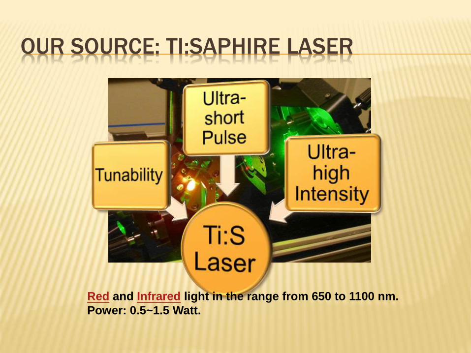
OUR SOURCE: TI:SAPHIRE LASER

Red and Infrared light in the range from 650 to 1100 nm.

Power: 0.5~1.5 Watt.

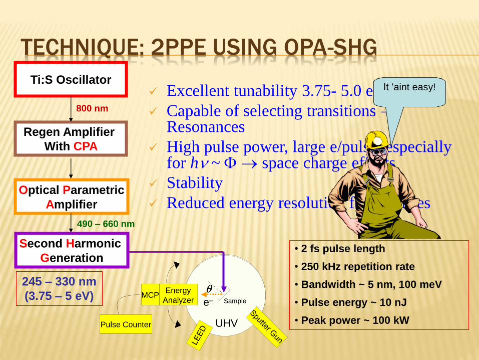
490 – 660 nm

• 2 fs pulse length

• 250 kHz repetition rate

• Bandwidth ~ 5 nm, 100 meV

• Pulse energy ~ 10 nJ

• Peak power ~ 100 kW

Ti:S Oscillator

Regen Amplifier

With CPA

Optical Parametric

Amplifier

800 nm

245 – 330 nm

(3.75 – 5 eV)

Second Harmonic

Generation

q

e–

UHV

Energy

Analyzer

Pulse Counter

MCPSample

q

e–

UHV

Energy

Analyzer

Pulse Counter

MCPSample

TECHNIQUE: 2PPE USING OPA-SHG

Excellent tunability 3.75- 5.0 eV

Capable of selecting transitions Resonances

High pulse power, large e/pulse especially for h ~ space charge effects

Stability

Reduced energy resolution for fs pulses

It ‘aint easy!

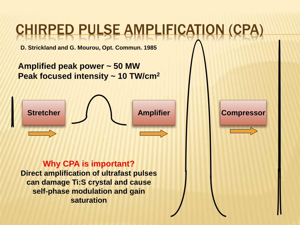
D. Strickland and G. Mourou, Opt. Commun. 1985

Stretcher Amplifier Compressor

Why CPA is important? Direct amplification of ultrafast pulses

can damage Ti:S crystal and cause

self-phase modulation and gain

saturation

Amplified peak power ~ 50 MW

Peak focused intensity ~ 10 TW/cm2

CHIRPED PULSE AMPLIFICATION (CPA)

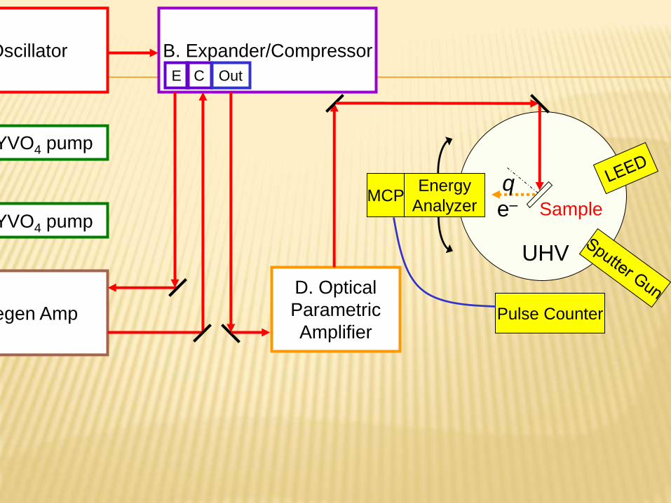
A. Ti:S Oscillator

Nd:YVO4 pump

C. Ti:S Regen Amp

B. Expander/Compressor

D. Optical

Parametric

Amplifier

Nd:YVO4 pump

E C Out

LAYOUT

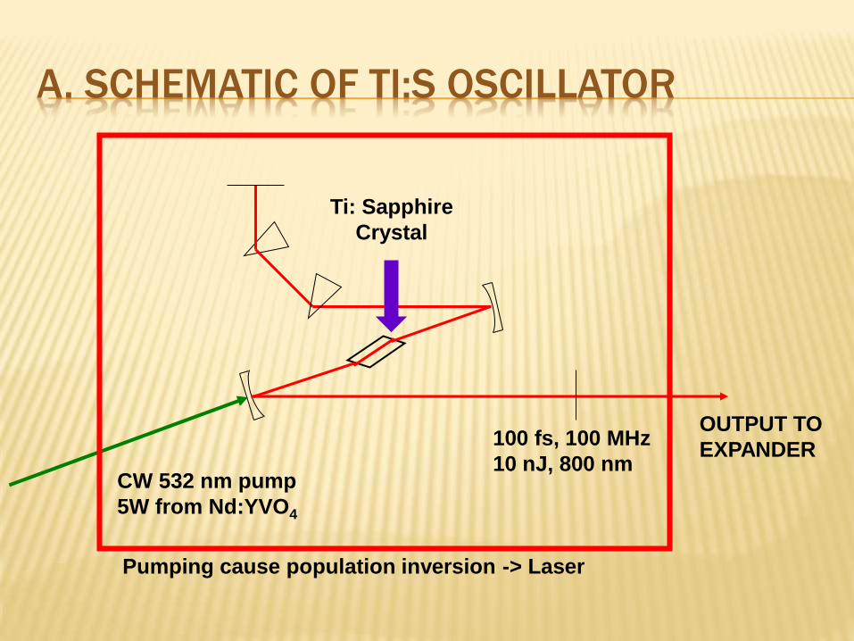
CW 532 nm pump

5W from Nd:YVO4

100 fs, 100 MHz

10 nJ, 800 nm

OUTPUT TO

EXPANDER

A. SCHEMATIC OF TI:S OSCILLATOR

Ti: Sapphire

Crystal

Pumping cause population inversion -> Laser

FROM

OSCILLATOR

TO

REGEN

FROM

REGEN

TO

OPA

GRATING

GRATING

B. EXPANDER/COMPRESSOR LAYOUT

EXPANDER

COMPRESSOR

GATE

INPUT FROM EXPANDER

OUTPUT TO COMPRESSOR

10W PUMP

Nd:YVO4

C. SCHEMATIC OF TI:S REGEN AMPLIFIER

1 2 1 2

1: Inject Seed

Pulse

2: Eject

Amplified Pulse

Population

Inversion –

Gain > Loss

~25 rounds

in resonator

- AMPLIFY

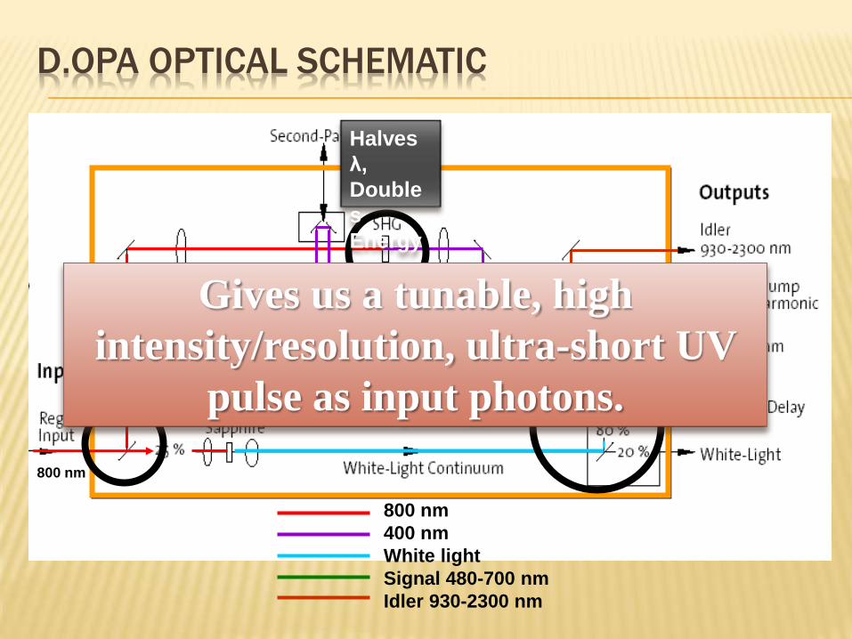
800 nm

800 nm

400 nm

White light

Signal 480-700 nm

Idler 930-2300 nm

D.OPA OPTICAL SCHEMATIC

Split

pulse

Halves

λ,

Double

s

Energy

Combine,

Amplify

Specific Freq.

Gives us a tunable, high

intensity/resolution, ultra-short UV

pulse as input photons.

B. AR2PPE

THEORY AND EXPERIMENT

EF

E

k||0

Evac

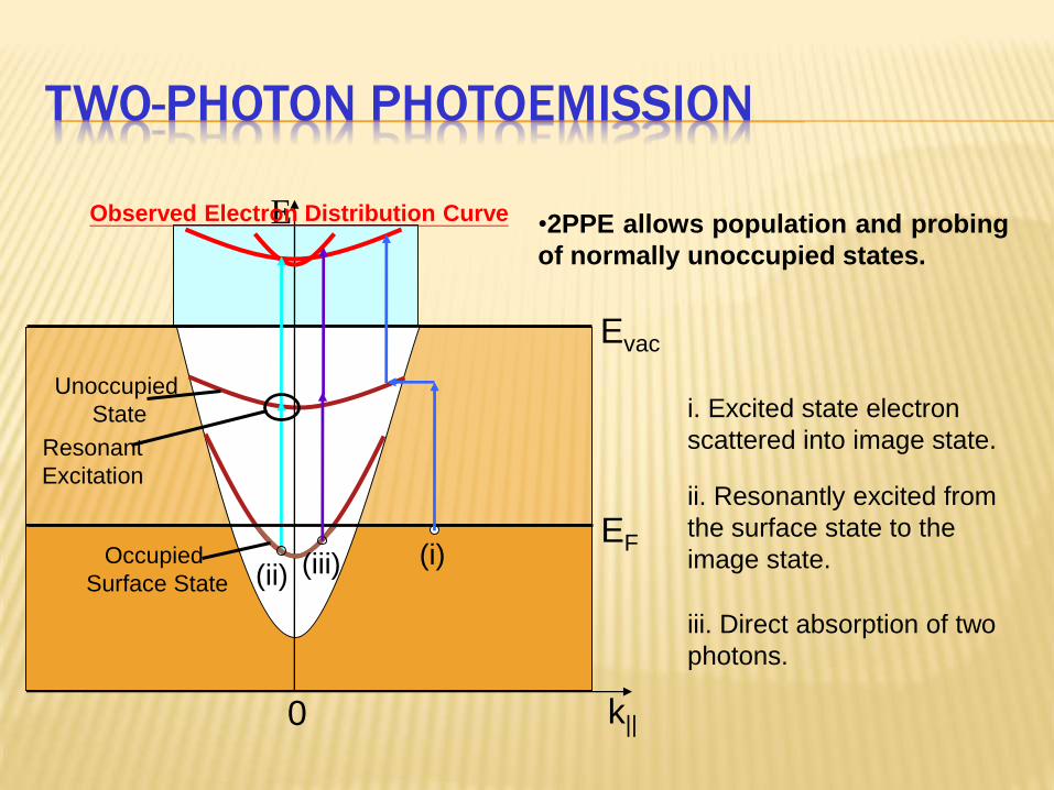
Observed Electron Distribution Curve

Unoccupied

State

Occupied

Surface State

Resonant

Excitation

(ii) (iii) (i)

•2PPE allows population and probing

of normally unoccupied states.

i. Excited state electron

scattered into image state.

ii. Resonantly excited from

the surface state to the

image state.

iii. Direct absorption of two

photons.

TWO-PHOTON PHOTOEMISSION

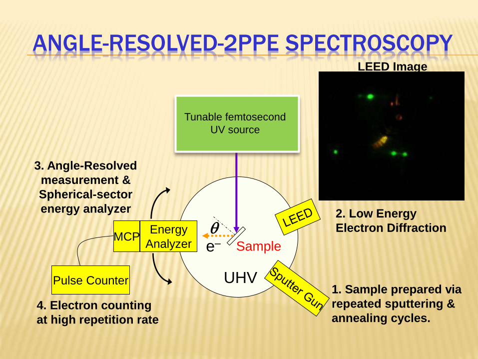
ANGLE-RESOLVED-2PPE SPECTROSCOPY

qe–

UHVPulse Counter

Energy

AnalyzerMCP

Sample

Tunable femtosecond

UV source

3. Angle-Resolved

measurement &

Spherical-sector

energy analyzer

4. Electron counting

at high repetition rate

1. Sample prepared via

repeated sputtering &

annealing cycles.

2. Low Energy

Electron Diffraction

LEED Image

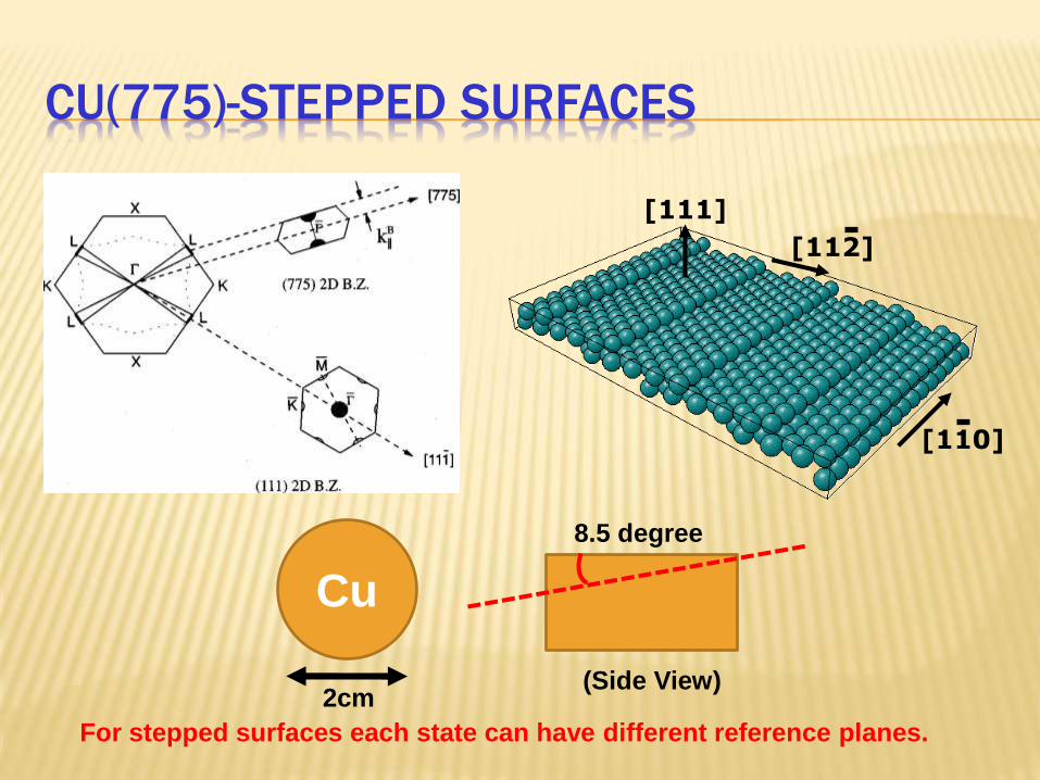
For stepped surfaces each state can have different reference planes.

[112]

[110]

[111]

CU(775)-STEPPED SURFACES

Cu

2cm

8.5 degree

(Side View)

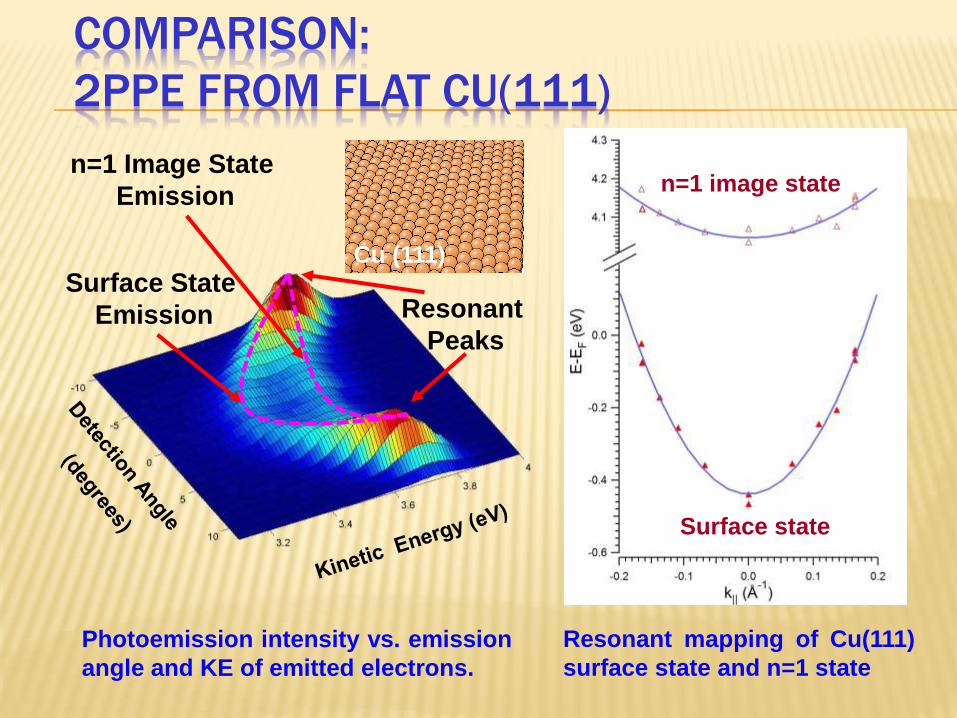
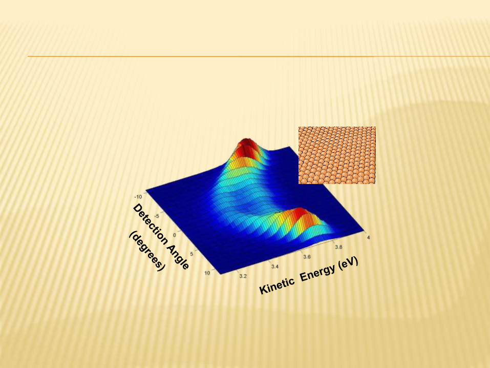
COMPARISON:

2PPE FROM FLAT CU(111)

Resonant mapping of Cu(111)

surface state and n=1 state

Photoemission intensity vs. emission

angle and KE of emitted electrons.

Resonant

Peaks

Surface State

Emission

n=1 Image State

Emission

Surface state

n=1 image state

Cu (111)

Surface state

n=1 image state

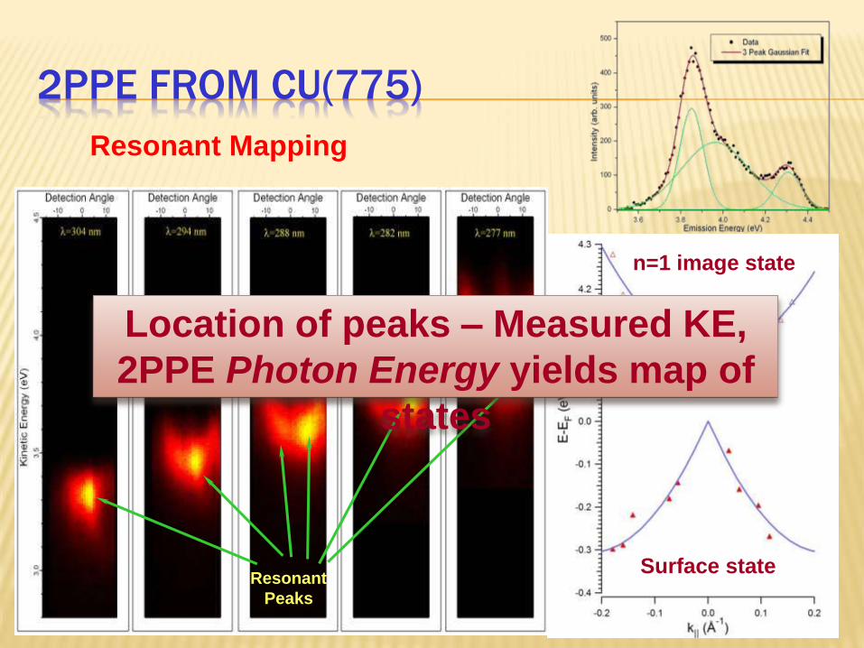
2PPE FROM CU(775)

Resonant

Peaks

Resonant Mapping

Location of peaks – Measured KE,

2PPE Photon Energy yields map of

states

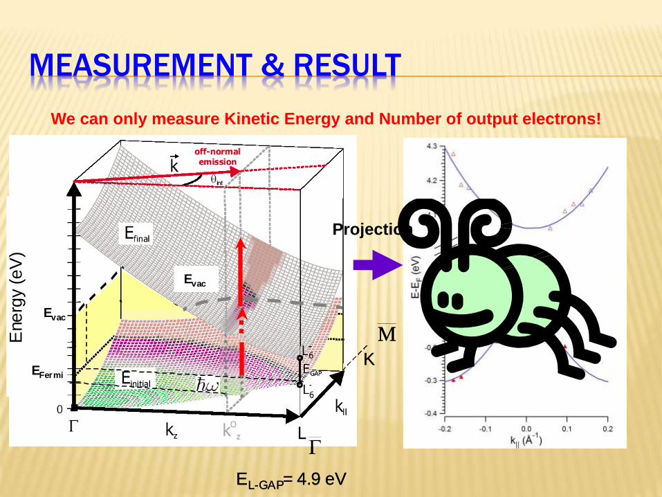
MEASUREMENT & RESULT

We can only measure Kinetic Energy and Number of output electrons!

Evac

EFermi

Evac

Ene

rgy (

eV

)

K

M

EL-GAP= 4.9 eV

Evac

EFermi

Evac

Ene

rgy (

eV

)

K

M

EL-GAP= 4.9 eV

Projection

C. BAND STRUCTURE SIMULATION

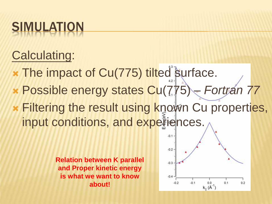
SIMULATION

Calculating:

The impact of Cu(775) tilted surface.

Possible energy states Cu(775) – Fortran 77

Filtering the result using known Cu properties,

input conditions, and experiences.

Relation between K parallel

and Proper kinetic energy

is what we want to know

about!

STEP1 MODIFICATION OF TILTED SURFACE

K Parallel

K

Perpendicular

K

Tilted?

K’

CACULATION

Define variable (R, n) for K parallel and K

perpendicular!

Proof: Orthogonal Coordinates – Product

Rule

Get tilted K(Kx, Ky, Kz)Kx = Ky = (SQRT(3))/2 *1.74*R - 0.01*n*0.7/1.407

Kz = (SQRT(3))/2 *1.74*1.4*R + 0.01*n*1/1.407

R = Testing number from 0.100~0.900

n = +50 to -50

When R=0.5, |K| = 1.5 ± 0.5 / A (Amstrong), matching

the flat Cu(111) experimental range.

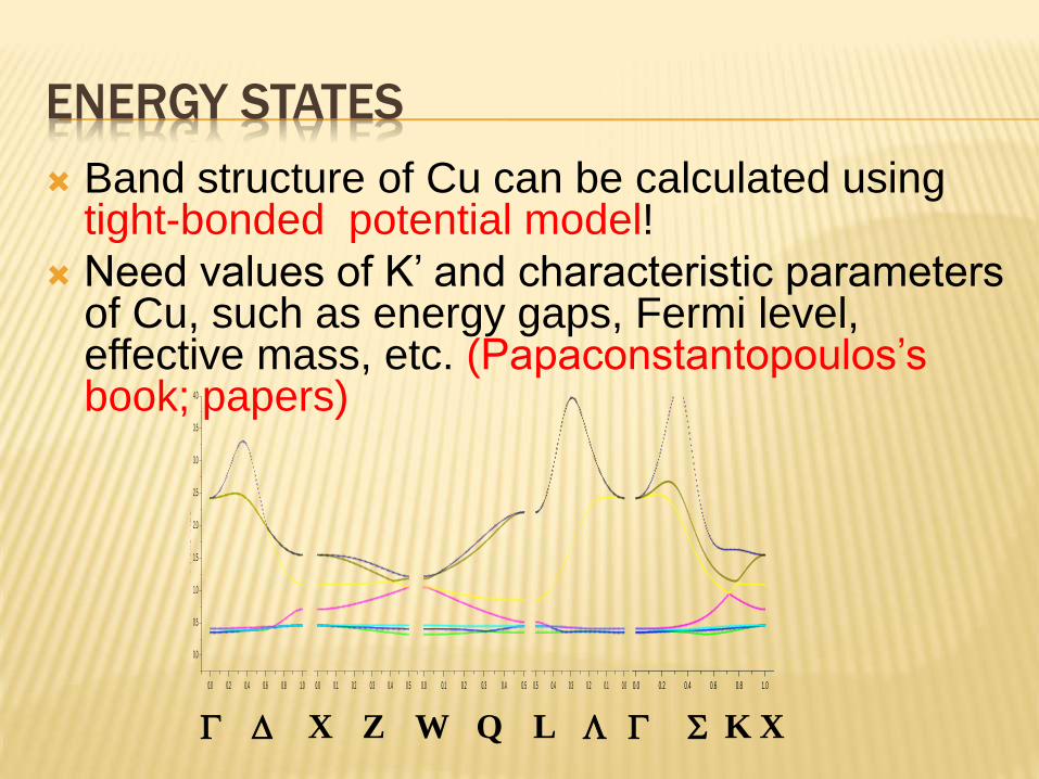
ENERGY STATES

Band structure of Cu can be calculated using tight-bonded potential model!

Need values of K’ and characteristic parameters of Cu, such as energy gaps, Fermi level, effective mass, etc. (Papaconstantopoulos’sbook; papers)

0.0 0.2 0.4 0.6 0.8 1.0

0.0

0.5

1.0

1.5

2.0

2.5

3.0

3.5

4.0

Y A

xis T

itle

X Axis Title

0.0 0.1 0.2 0.3 0.4 0.5

0.0

0.5

1.0

1.5

2.0

2.5

3.0

3.5

4.0

Y A

xis T

itle

X Axis Title

0.0 0.1 0.2 0.3 0.4 0.5

0.0

0.5

1.0

1.5

2.0

2.5

3.0

3.5

4.0Y

A

xis T

itle

X Axis Title

0.5 0.4 0.3 0.2 0.1 0.0

0.0

0.5

1.0

1.5

2.0

2.5

3.0

3.5

4.0

Y A

xis T

itle

X Axis Title

0.0 0.2 0.4 0.6 0.8 1.0

0.0

0.5

1.0

1.5

2.0

2.5

3.0

3.5

4.0

Y A

xis T

itle

X Axis Title

X L XKSD LWZ Q

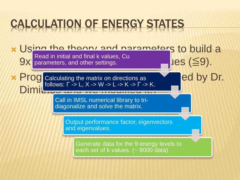
CALCULATION OF ENERGY STATES

Using the theory and parameters to build a

9x9 Matrix, solving the eigenvalues (≦9).

Program on Fortran 77 (Was created by Dr.

Dimitrios and we modified it.)

Read in initial and final k values, Cu parameters, and other settings.

Calculating the matrix on directions as follows: Γ -> L, X -> W -> L -> K -> Γ -> K.

Call in IMSL numerical library to tri-diagonalize and solve the matrix.

Output performance factor, eigenvectors and eigenvalues.

Generate data for the 9 energy levels to each set of k values. (~ 9000 data)

CALCULATE THE RIGHT RESULT

If not interpreted and modified properly, the result is useless.

Conditions:

1. Transition happens between E7 & E6

2. Cu work function: 4.9eV

3. Proper energy shifting should make E7 > 0 and E6 < 0 while Zero Point Energy = Fermi Energy

4. Given Photon Energy hv

5. 1st PPE: E7 – E6 = hv, error < 0.02 eV

6. 2nd PPE: E7 + hv – Work Func. = Kinetic Energy

In short, 2PPE happens between precise energy

states. Also, the energy of 1st PPE should lower

than work function; otherwise we will get the

wrong states.

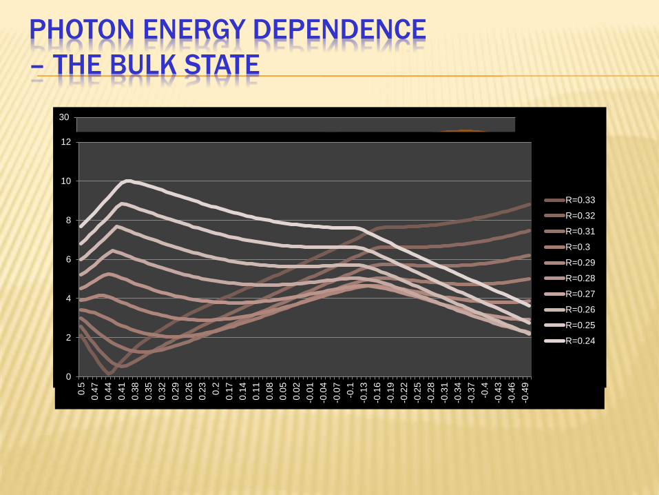
PHOTON ENERGY DEPENDENCE

– THE BULK STATE

0

5

10

15

20

25

30

0.5

0.4

7

0.4

4

0.4

1

0.3

8

0.3

5

0.3

2

0.2

9

0.2

6

0.2

3

0.2

0.1

7

0.1

4

0.1

1

0.0

8

0.0

5

0.0

2

-0.0

1

-0.0

4

-0.0

7

-0.1

-0.1

3

-0.1

6

-0.1

9

-0.2

2

-0.2

5

-0.2

8

-0.3

1

-0.3

4

-0.3

7

-0.4

-0.4

3

-0.4

6

-0.4

9

ΔE(R=0.6)

ΔE(R=0.55)

ΔE(R=0.5)

ΔE(R=0.45)

ΔE(R=0.4)

ΔE(R=0.35)

ΔE(R=0.3)

ΔE(R=0.25)

ΔE(R=0.2)

ΔE(R=0.15)

0

2

4

6

8

10

12

0.5

0.4

7

0.4

4

0.4

1

0.3

8

0.3

5

0.3

2

0.2

9

0.2

6

0.2

3

0.2

0.1

7

0.1

4

0.1

1

0.0

8

0.0

5

0.0

2

-0.0

1

-0.0

4

-0.0

7

-0.1

-0.1

3

-0.1

6

-0.1

9

-0.2

2

-0.2

5

-0.2

8

-0.3

1

-0.3

4

-0.3

7

-0.4

-0.4

3

-0.4

6

-0.4

9

R=0.33

R=0.32

R=0.31

R=0.3

R=0.29

R=0.28

R=0.27

R=0.26

R=0.25

R=0.24

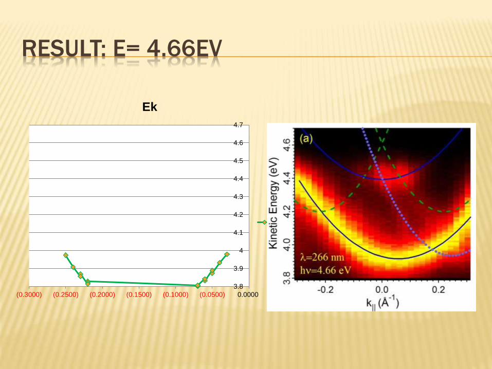
RESULT: E= 4.66EV

3.8

3.9

4

4.1

4.2

4.3

4.4

4.5

4.6

4.7

(0.3000) (0.2500) (0.2000) (0.1500) (0.1000) (0.0500) 0.0000

Ek

Ek

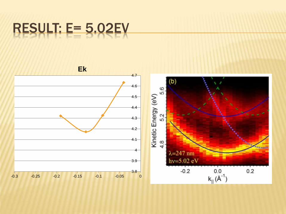
RESULT: E= 5.02EV

3.8

3.9

4

4.1

4.2

4.3

4.4

4.5

4.6

4.7

-0.3 -0.25 -0.2 -0.15 -0.1 -0.05 0

Ek

DISCUSSION

2 Good 2 Bad

Slope and shape is pretty near!

Built up a standard procedure to do

calculation fast.

Energy shift problem.

n all negative/positive – need further study.

FUTURE PLAN

Need more data, especially with energies

close to boundary (work func.)

Using higher photon energy.

Different approach on the calculation (New

model, different length, etc.)

Re-program it on other languages with a

more user-friendly interface.

REFERENCES

Nonequilibrium Band Mapping of Unoccupied Bulk States Below the VaccumLevel by Two-Photon Photoemission, by Zhaofeng Hao, J. I. Dadap, K. Knox, M. Yilmaz, N. Zaki, P. D. Johnson, and R. M. Osgood. (Pending on PRL)

Electronic structure of a Co-decorated vicinal Cu(775) surface: High-resolution photoemission spectroscopy, by S.-C. Wang, M. B. Yilmaz, K. R. Knox, N. Zaki, J. I. Dadap, T. Valla, P. D. Johnson, and R. M. Osgood, Phys. Rev. B 77, 115448 (2008).

Scattering of Surface States at Step Edges in Nanostripe Arrays, by F. Schiller, M. Ruiz-Dses, J. Cordon, and J. E. Ortega, Phy. Rev. Lett. 95, 066805 (2005).

Observation of a one-dimensional state on stepped Cu(775), by X. J. Shen, H. Kwak, D. Mocuta, A. M. Radojevic, S. Smadici, and R. M. Osgood, Phys. Rev. B 63, 165403 (2001).

Surface electron motion near monatomic steps: Two-photon photoemission studies on stepped Cu(111), by X. Y. Wang, X. J. Shen, and R. M. Osgood, Phys. Rev. B 56, 7665 (1997).

Book: S. Hufner, Photoelectron Specstropy, 3rd ed. (Springer, Berlin, 2003)

Book: Hai-Lung Dai, Wilson Ho, Laser Spectroscopy and Photo-Chemistry on Metal Surfaces. (World Scientific, 1995)

Book: Harald Ibach, Hans Luth, Solid State Physics. (Springer, 1991)

~FIN~

Q&A time

Thank you for

your patience!

qe–

UHV

Pulse Counter

Energy

AnalyzerMCP

Sample

Oscillator

Nd:YVO4 pump

Regen Amp

B. Expander/Compressor

D. Optical

Parametric

Amplifier

Nd:YVO4 pump

E C Out