AINL 2016: Filchenkov

Deep Neural Networks Tutorial

Andrey Filchenkov Computer Technology Chair

Computer Technologies Lab

ITMO University

[email protected]

AINL FRUCT’ 6. No , 6, “t. Peters urg, Russia

Tutorial topics

Very brief introduction to AI, ML and ANN

What is ANN and how to learn it

DNN and standard DNN architectures

Beyond discriminative models

2 / 64

Next topic





3 / 64

Artificial intelligence

Strong AI (A general I): functionality is similar to the human

brain or better.

Weak AI: good in solving certain well-formulated tasks.

Machine learning is a part of Weak AI

Many people have been thinking that artificial neural

networks are a path to Strong AI

Many people are thinking that deep learning networks are a

path to Strong AI

4 / 64

Neural networks as a machine learning algorithm

Neural paradigm is not only about machine learning

(computer architecture, computations, etc.)

Machine learning is about creating algorithms which can learn

patterns, regularities and rules from given data.

The biggest part of machine learning is supervised learning:

we are given a set of objects, each has a label, and we want to

learn how to find these label for objects we have never seen.

5 / 64

Biological neuron

6 / 64

Brief early history of artificial neural networks

1943 Artificial neuron by McCulloch and Pitts

1949 Neuron learning rule by Hebb

1957 Perceptron by Rosenblatt

1960 Perceptron learning rule by Widrow and Hoff

1968 Group Method of Data Handling to learn multilayered

networks by Ivakhnenko

1969 Perceptrons by Minski and Papert

1974 Back propagation algorithm by Webros and by Galushkin

7 / 64

Brief modern history of ANN

1980 Convolutional NN by Fukushima

1982 Recurrent NN by Hopfield

1991 Va ishi g gradient pro le was identified by Hochreiter

1997 Long short term memory network by Hochreiter and

Schmidhuber

1998 Gradient descent for convolutional NN by LeCun et al.

2006 Deep model by Hinton, Osindero and Teh

2012 DNN started to become mainstream in ML and AI

8 / 64

Next topic





9 / 64

Two sources of knowledge

Experts

we need to ask wisely and process

Data

we need to process and apply machine learning algorithms

How do we obtain knowledge?

10 / 64

Algorithms, performance of which grows with experience

The most popular task is prediction

Algorithms require data and labels (for predicting)

Learning of these algorithms is to minimize error rate in

prediction or maximize similar to the known answer

Machine learning

11 / 64

Each object is represented

as a feature vector. Each

object thus is a point in a

multidimensional space.

Vector representation of objects

12 / 64

Linear discriminant surface

Linear model (neuron)

13 / 64

Non-linear case

14 / 64

Multilayer neural network

We just build a composition of

neurons (as functions)

15 / 64

Next topic




• Deep learning introduction and best practices

• Deep Boltzmann Machines (DBM) and Deep Belief Network (DBN)

• Convolution Neural Network (CNN)

• Autoencoders

• Recurrental Neural Network (RNN) and Long-Short Term Memory (LSTM)


16 / 64

Deep architecture

Definition: Deep architectures are composed of multiple levels of

non-linear operations, such as neural nets with many hidden

layers

Most machine learning algorithms have shallow (1–3 layers)

architecture (SVM, PCA, kNN, Logistic Regression, etc.)

Goal: Deep learning methods aim at:

Learning feature hierarchies, no more feature engineering!

Where features from higher levels of the hierarchy are formed

by lower level features.

17 / 64

Why to go deep?

Some functions cannot be efficiently represented (in terms of

number of tunable elements) by architectures that are too shallow

Functions that can be compactly represented by a depth k

architecture might require an exponential number of computational

elements to be represented by a depth k− ar hite ture

Deep Representations might allow non-local generalization and

comprehensibility

Deep learning gets state of the art results in many fields (vision,

audio, NLP, etc.)!

18 / 64

DNN best practices: ReLU, PReLU

ReLU

19 / 64

PReLU

Sigmoid, hyperbolic tangent activation functions have a problem

with vanishing of gradients and tend to overfitting

DNN best practices: Data augmentation

The easiest and most common method to reduce overfitting on

image data is to artificially enlarge the dataset using label-

preserving transformations.

Types of data augmentation:

Image translation

Horizontal/vertical reflections + cropping

Changing RGB intensities

20 / 64

DNN best practices: Dropout

Dropout: set the output of each hidden neuron to zero w.p. 0.5

The euro s hi h are dropped out i this a do ot o tri ute to the forward pass and do not participate in backpropagation

So every time an input is presented, the neural network samples a different architecture, but all these architectures share weights

This technique reduces complex co-adaptations of neurons, since a neuron cannot rely on the presence of particular other neurons

It is, therefore, forced to learn more robust features that are useful in conjunction with many different random subsets of the other neurons

Without dropout, a network exhibits substantial overfitting

Dropout roughly doubles the number of iterations required to converge

21 / 64

Greedy Layer-Wise Training (1/2)

1. Train first layer using your data without the labels (unsupervised)

• Since there are no targets at this level, labels don't help. Could also use the more abundant unlabeled data which is not part of the training set (i.e. self-taught learning).

2. Then freeze the first layer parameters and start training the second layer using the output of the first layer as the unsupervised input to the second layer

3. Repeat this for as many layers as desired

• This builds our set of robust features

4. Use the outputs of the final layer as inputs to a supervised layer/model and train the last supervised layer(s) (leave early weights frozen)

5. Unfreeze all weights and fine tune the full network by training with a supervised approach, given the pre-processed weight settings

22 / 64

Greedy Layer-Wise Training (2/2)

Greedy layer-wise training avoids many of the problems of trying to train a deep net in a supervised fashion:

• Each layer gets full learning focus in its turn since it is the only current "top" layer

• Can take advantage of unlabeled data

• When you finally tune the entire network with supervised training the network weights have already been adjusted so that you are in a good error basin and just need fine tuning. This helps with problems of:

• Ineffective early layer learning

• Deep network local minima

23 / 64

Restricted Boltzmann machine

Two types of nodes: hidden and visible.

We are minimizing system energy which is not to converge by

updating its weights with propagating new objects. Probability

distribution on visible and hidden layers is Gibbs distribution.

24 / 64

Deep Belief Network

25 / 64

First train unsupervisedly with several

(two) levels of RBM (or autoencoders).

Then train next layers supervisedly and

consecutively.

Hinton, G. E. and Salakhutdinov, R. R. (2006). Reducing the dimensionality of data with neural networks. Science, 313:504-507.

Deep Boltzmann machine

26 / 64

Convolution Neural Network (CNN)

Core concepts:

Local perception – each neuron sees a small part of the

object. Use kernels (filters) to capture 1-D or 2-D structure of

objects. For instance, capture all pixel neighbors for an image.

Weight sharing – use small and the same sets of kernels for all

objects, this leads to reduction of number of adjusting

parameters in comparison with MLP

Subsampling/pooling – use dimensionality reduction for

images in order to provide invariance to scale

27 / 64

Discrete convolution

28 / 64

What can kernels do?

29 / 64

*

*

*

=

=

=

blur

edge

detection

sharpen

Discrete convolution

30 / 64

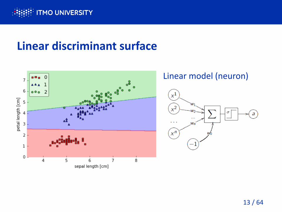
How do trained kernels look like?

31 / 64

low feature medium feature high feature

Each kernel composes a local patch of lower-level features

into high level representation

Levels of abstraction

Hierarchical Learning:

Natural progression from low level to high level structure as seen in natural complexity

Easier to monitor what is being learnt and to guide the machine to better subspaces

A good lower level representation can be used for many distinct tasks

32 / 64

LeNet

33 / 64

LeCun, Yann, et al. "Gradient-based learning applied to document recognition." Proceedings of the

IEEE 86.11 (1998): 2278-2324.

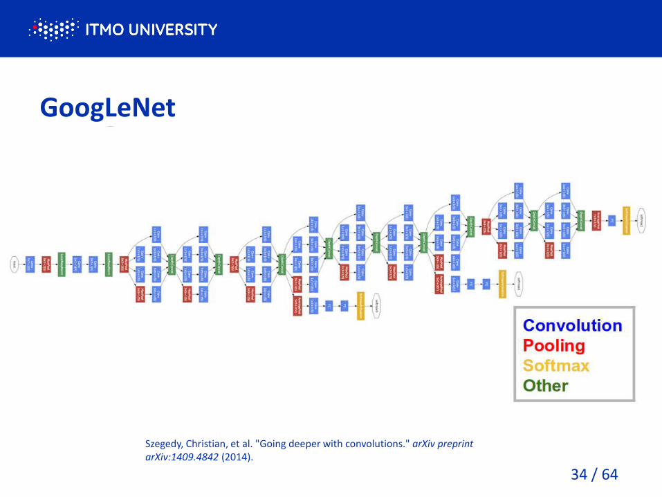
GoogLeNet

34 / 64

Szegedy, Christian, et al. "Going deeper with convolutions." arXiv preprint

arXiv:1409.4842 (2014).

Application of CNN

Image Recognition

Image Search (enhance search engine)

Visual Question Answering

NLP (Sentence Classification, etc.)

Speech Recognition

…

35 / 64

Visual question answering (1/2)

36 / 64

Visual question answering (2/2)

37 / 64

Application of CNN: Visual question answering

38 / 64

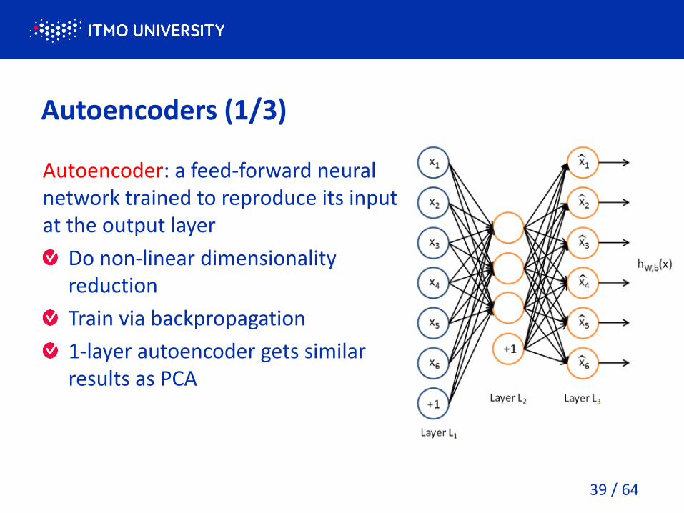
Autoencoders (1/3)

Autoencoder: a feed-forward neural

network trained to reproduce its input

at the output layer

Do non-linear dimensionality

reduction

Train via backpropagation

1-layer autoencoder gets similar

results as PCA

39 / 64

Autoencoders (2/3)

40 / 64

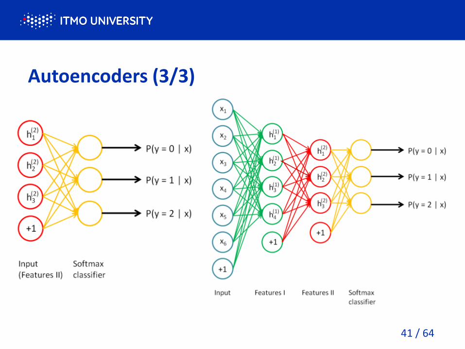
Autoencoders (3/3)

41 / 64

Autoencoders in bioinformatics

42 / 64 Fakoor, Rasool, et al. "Using deep learning to enhance cancer diagnosis and classification." Proceedings of the International

Conference on Machine Learning. 2013.

Deep autoencoders: document processing

We can use an autoencoder to find low-dimensional codes for

documents that allow fast and accurate retrieval of similar

documents from a large set.

We start with o erti g ea h do u e t i to a ag of ords . This is a 2000 dimensional vector that contains the

counts for each of the 2000 commonest words.

43 / 64

Deep autoencoders: document retrieval

We train the neural network to reproduce its input vector as its output

This forces it to compress as much information as possible into the 10 numbers in the central bottleneck.

These 10 numbers are then a good way to compare documents.

44 / 64

2000 reconstructed counts

500 neurons

250 neurons

10

250 neurons

500 neurons

2000 word counts

Deep autoencoders: document visualization (1/2)

Instead of using codes to

retrieve documents, we can

use 2-D codes to visualize sets

of documents.

This works much better than

2-D PCA

45 / 64

2000 reconstructed counts

500 neurons

250 neurons

2

250 neurons

500 neurons

2000 word counts

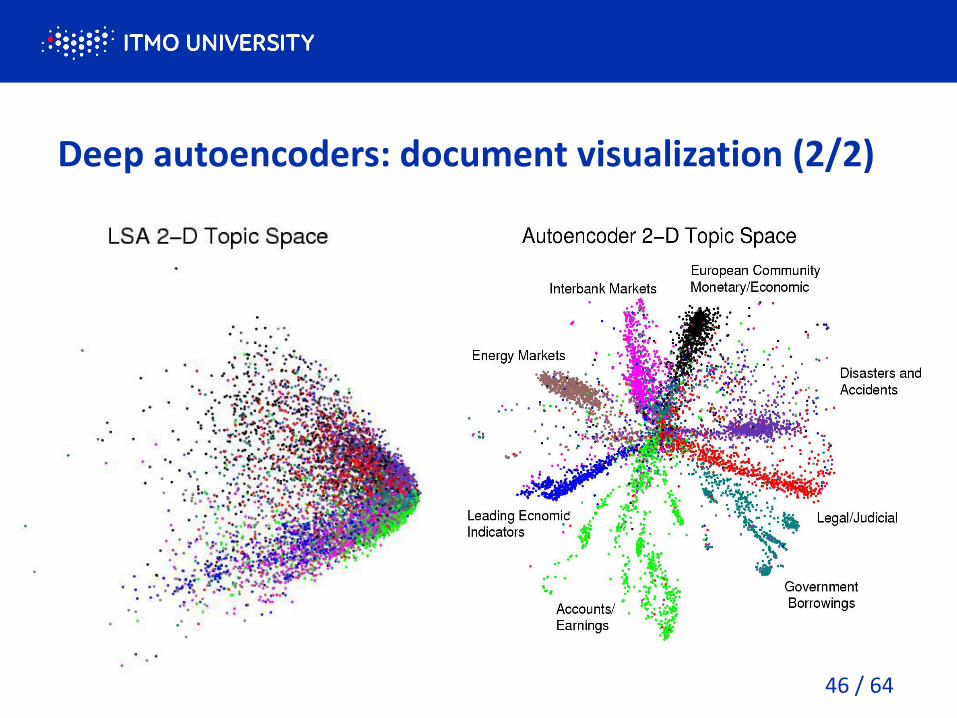
Deep autoencoders: document visualization (2/2)

46 / 64

Recurrent Neural Network (RNN)

RNN: a neural network with recurrent connections

Good for sequence data: time series, text, audio

47 / 64

Recurrent Neural Network (RNN): scheme

48 / 64

Long Short-Term Memory (LSTM)

LSTM: a special case of RNN capable of learning long-term

dependencies

There are four neural network layers in repeating module

49 / 64 Hochreiter, Sepp, and Jürgen Schmidhuber. "Long short-term memory." Neural computation 9.8 (1997): 1735-1780.

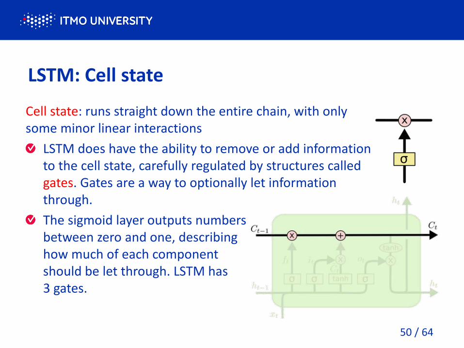
LSTM: Cell state

Cell state: runs straight down the entire chain, with only

some minor linear interactions

LSTM does have the ability to remove or add information

to the cell state, carefully regulated by structures called

gates. Gates are a way to optionally let information

through.

The sigmoid layer outputs numbers

between zero and one, describing

how much of each component

should be let through. LSTM has

3 gates.

50 / 64

LSTM: Forget gate layer

It looks at ℎt−1 and �t, and outputs a number between 0 and

1 for each number in the cell state �t−1. 1 represents

o pletel keep this hile 0 represe ts o pletel get rid of this .

51 / 64

LSTM: Input gate layer (1/2)

How to decide what new information to store in the cell state?

First, a sig oid la er alled the i put gate la er de ides which values should be updated.

Next, a tanh layer creates a vector of new candidate values, �t, that ould e added to the state. I the e t step, e’ll combine these two to create an update to the state

52 / 64

LSTM: Input gate layer (2/2)

It’s o ti e to update the old ell state, ��−1, into the new

cell state ��. The previous steps already decided what to do,

we just need to actually do it

We multiply the old state by ��, forgetting the things we

decided to forget earlier. Then we add �� ⋅ ��−1. This is the

new candidate values, scaled by how much we decided to

update each state value

53 / 64

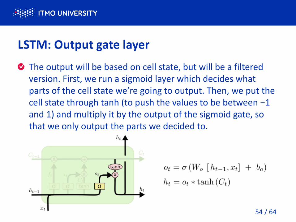
LSTM: Output gate layer

The output will be based on cell state, but will be a filtered

version. First, we run a sigmoid layer which decides what

parts of the ell state e’re goi g to output. The , e put the cell state through tanh to push the alues to e et ee − and 1) and multiply it by the output of the sigmoid gate, so

that we only output the parts we decided to.

54 / 64

Visual question answering: LSTM

55 / 64

Deep learning analysis: advantages

Extremely strong model, which can potentially solve any problem of machine learning.

Already learnt model can be reused: multi-task support

Many good models are already known which are state-of-the-art for many tasks:

• image recognition;

• speech recognition;

• natural language processing;

• etc.

56 / 64

Deep learning analysis: disadvantages

The deeper the net is

• the more data you need;

• the more time you need;

• the stronger processors you need.

Usually no intuition how it works exactly;

Usually you work with DNN as a black box;

Prone to overfitting: regularization must be used.

57 / 64

Next topic





58 / 64

Reverse the network and make it predict images given labels

Image synthesis

Dosovitskiy, A., Tobias Springenberg, J., & Brox, T. (2015). Learning to generate chairs with convolutional neural networks. In Proceedings of the IEEE

Conference on Computer Vision and Pattern Recognition (pp. 1538-1546). 59 / 64

Keep i er represe tatio of a i age (Gram matrix �� for convolutional layers)

Then create a new random network and

learn it no have similar inner

representation as the one we have kept.

Texture synthesis

Gatys, L., Ecker, A. S., & Bethge, M. (2015). Texture synthesis using convolutional neural networks. In Advances in Neural Information Processing

Systems (pp. 262-270). 60 / 64

Style = texture.

Image = content and

is represented with

the last

convolutional layer.

We will learn an

image that is similar

both to image and

content.

Style transmission

Gatys, L. A., Ecker, A. S., & Bethge, M. (2015). A neural algorithm of artistic style. arXiv preprint arXiv:1508.06576.

61 / 64

DeetArt was created in 2015:

https://deepart.io/

They implemented the algorithm

described before.

DeepArt and Prisma

62 / 64

Prisma was created in June,

2016.

They made it optimized,

mobiles and with preselected

filters (instead of styles)

https://deepart.io/

https://deepart.io/

Materials

Presentation was prepared using:

1. http://avisingh599.github.io/deeplearning/visual-qa/

2. http://colah.github.io/posts/2015-08-Understanding-LSTMs/

3. https://class.coursera.org/ml-003/lecture

4. K. Vorontsov Ma hi e lear i g ourse i Russia

63 / 64

http://avisingh599.github.io/deeplearning/visual-qa/




http://colah.github.io/posts/2015-08-Understanding-LSTMs/








https://class.coursera.org/ml-003/lecture



Thanks for attention!

Questions?