The Structure of Pay Changes at the Local Level

199THE STRUCTUREOF PAY CHANGESAT THE LOCAL

LEVEL

Kenneth Snellman

PALKANSAAJIEN TUTKIMUSLAITOS •TYÖPAPEREITALABOUR INSTITUTE FOR ECONOMIC RESEARCH • DISCUSSION PAPERS

This working paper is a part of the project ”Rules of the game in the labour market:Industrial relations, the bargaining system and income policies in the 2000s”

(Työmarkkinoiden pelisäännöt: työelämän suhteet, sopimustoiminta ja tulopolitiikka 2000-luvulla), which is funded by the Finnish Work Environment Fund. This working paper hasbenefitted from comments from Reija Lilja and participants in the seminar at the Labour

Institute for Economic Research.

**Labour Institute for Economic Research, Pitkänsillanranta 3 A, FIN-00530 Helsinki.E-mail: [email protected]

Helsinki 2004

199

THE STRUCTUREOF PAYCHANGES ATTHE LOCALLEVEL*

Kenneth Snellman**

ISBN 952−5071−93−6ISSN 1795−1801

Abstract

In this paper the distribution of pay changes in the Finnish industry 1997–2000across employees and plants is examined. The study supports the hypothesisthat such pay measures that are more closely dependent on contracts exhibit lessvariation in pay. It is also shown that pay cuts and pay rises are concentratedto certain plants and to a rather large extent to the same plants.

1 Introduction

The institutions of the labour market and the bargaining system are of greatimportance for wage formation. Rather than being a spot market the Finnishlabour market is characterised by long-term relations and collective agreements.This limits the possibilities of firms to implement pay cuts but the collectiveagreements also prevent trade unions from demanding wage rises at the locallevel in excess of those agreed on at the industry level. The issue examined inthis paper is to what extent deviations from the general pay rise prescribed bythe collective agreements occurs. It is also tested whether the distribution ofsuch pay changes can be explained by plant-specific needs for renegotiations ofcontracts.

For wage changes to deviate from the general pay rise, given that the joband employee characteristics remain the same, it is necessary that both the firmand the local union accept it. One reason for employees and local unions toaccept wage cuts is that they reduce the risk for dismissals. For an employee toget a pay rise in excess of the general pay rise, it may be enough that a superioragrees to it. Raising the pay of individual workers may be in the interest ofthe firm, because it improves incentives or prevents the exit of a productiveemployee.

This study takes the contracts as its starting point. For an internationalsurvey of wage changes that takes the contracts of the individuals as its startingpoint, see Malcomson [1999]. Although wage formation on the Finnish labourmarket is characterised by the collective bargaining, it has been shown thatthere are large individual deviations from what is agreed on in the collectiveagreements. For example a large proportion of the employees experience wagecuts from one year to the next [Vartiainen, 2000], although the general pay risehas never been negative. Se also Vartiainen [1996, 1994] for earlier empiricalstudies of wage formation, wage drift and wage cuts and Bockerman et al. [2003]for a contemporary study of wage cuts with a wider perspective on the Finnishlabour market. This study goes further than these studies by investigating theconcentration of pay changes. Above all I examine the hypothesis that wagecuts are concentrated to certain plants.

The second section includes a presentation of the institutional frameworkand an examination of the possibilities it and the theory suggest there are fordeviations from the pay changes stipulated by collective agreements. In thethird section follows a short presentation of the data used in the study. The

3

fourth section provides a general characterisation of the pay changes of theindividuals according to different measures of pay. In the fifth section the plant-wise concentration of the pay changes of wage earners is examined. The sixthsection provides an examination of the same issue for salaried employees. In theseventh section follows an investigation of whether pay cuts of wage earners andsalaried employees take place in the same plants. Section eight is the conclusion.

2 The institutional framework in Finland andthe concept of rigidity

Because the large majority of employees continue to work in the same plantfrom one year to the next, the change in the wage level in the economy to arather large extent depends on pay changes of employees who stay in the sameplant. This study concentrates on this component of the change in wage costand disregard changes in average pay associated with reallocation of workersfrom one employer to another or changes in the workers’ employment status.

The pay of the employees is regulated by collective agreements, which deter-mine minimum wages, and unless the firm and its employees (the local union)agree on something else, the minimum change in the pay employees actually re-ceive. Because employees usually do not object to pay rises to other employees,firms are in general allowed to rise the pay of employees more than the generalpay rise. Reasons for doing this may be that managers want to motivate emplo-yees to be productive or prevent productive employees from quitting.1 However,unless there are changes in the job characteristics on which pay is based, a firmmust not lower the employees’ pay without approval of the local union branch.Because there is extra compensation associated with such job characteristics asovertime work and working Sundays for wage earners, less overtime and work-ing fewer Sundays should clearly in accordance with the contracts be associatedwith a reduction in total pay for them. Job changes inside a plant can also takeplace or, alternatively, what is required in the job can change. Such changescan also affect what should be paid according to the contract.

The alternative way for wage changes to take place is through changes in thecontracts. This includes the possibility that the local union agrees to pay beingcut, even though there should be a general pay rise in the industry accordingto the collective agreement. This can take place, if the employees in the firmaccept it and the pay does not fall below the minimum wage level in the collectiveagreement. In consequence, how much wages exceed the minimum wage levelsets an upper limit to how large wage cuts firms can implement at the locallevel.

It is uncertain to what extent these types of changes take place. It has oftenbeen claimed that wages are rigid, meaning that they do not change frequently

1To the explanations categorised under increased motivation I also include rent-sharing,which is likely to be, at least partly, a consequence of firms paying employees higher wages toprevent strikes and other protests among employees against the firm.

4

and especially that wages are rarely cut. Earlier studies have mostly beenconcerned with whether there exist any rigidity and wage cuts. Since this studyis aimed at examining the occurrence of pay changes of different origin andespecially of those not in accordance with the general pay rises, this study takesa slightly different perspective on the issue.

The contractual framework suggests that the general pay rises should formstarting points for any negotiations concerning deviations. It therefore seemsuseful to define rigidity in this paper as a tendency to not deviate from the ge-neral pay rises. The discussion above suggests that one should use observationsfor which there are no changes in the observable job characteristics, becausethen there are no extra pay changes in accordance with contracts the rigidityeffects of collective agreements should be most visible. Reasons for employeesand local unions to accept a wage cut by changing the contracts might be badperformance of the firm or redesign of jobs that change job characteristics, whichpossibly are not included in the contracts.

If firms are more free to set pay in response to changes in their needs, itseems likely that they are more able to maximise profit and productivity andthat the allocation on the labour market also is more efficient. Some studies haveargued the opposite, pointing to the positive effect of closing down inefficientplants and supplying inexpensive labour to more efficient plants [Hibbs andLocking, 2000, Moene and Wallerstein, 1997, Agell and Lommerud, 1993]. Lessresponsiveness of wages to productivity might also raise the firms’ return oninvestments [Teulings and Hartog, 1998]. However, examining the extent towhich wage flexibility increases productivity or profitability is beyond the aimof this paper.

Because the changes stipulated by the collective agreements are poorly known,this study concentrates on the occurrence of wage cuts and the concentration ofthese to certain plants. As nominal wage cuts are examined, the study is closelyrelated to studies concerned with nominal pay rigidities.

The theoretical framework gives a number of hypothesis to test. Since labourdemand and the performance of the employees is likely to vary over time, paymore directly related to output should be less rigid also when measured as payper hour. This gives the following hypothesis.

H1: Variation in pay is larger and pay cuts more frequent for types of paydirectly dependent on variables not determined by the collective agreements.

One type of pay which is dependent on a variable not determined by contracts ispiece rate pay. A part of a reduced demand for labour input should be reflectedin a somewhat slower working pace of the employees, as it is not necessary tofinish the work so fast. This should also mean that decreases in pay occur morefrequently for piece rate pay. Also overtime pay should clearly be more variable,as overtime hours are rather easily adjusted.

For the change in pay to be different from what the collective agreementprescribes, both parties have to accept the deviation. Pay cuts are possibleonly if the local union branch accepts that wages are cut, for example because

5

it saves jobs. Such circumstances are likely to be plant- and firm-specific. Inconsequence, pay cuts not in accordance with collective agreements should bea plant-specific (or possibly firm-specific) phenomenon. This observation givesthe following hypothesis.

H2: Pay cuts should be concentrated to certain plants.

The null hypothesis then is that wage cuts occur with the same relative fre-quency in all plants. According to the theory the management’s decision toraise an employee’s pay is more related to the characteristics of the individual.The local union should not resist such pay changes, since it does not make anyemployee worse off. Moreover, even a poorly performing plant could be willingto raise the pay of individual employees to keep productive employees motivated.In consequence, pay rises above what is prescribed by the collective agreementshould be less of a plant-specific phenomenon than pay cuts.

H3: Pay rises higher than the general rise should be less concentrated thanpay cuts.

In addition to the hypothesis that firms manage to negotiate down the wagesof employees in some plants, one could further hypothesise that some plantshave more wage flexibility with both high pay rises and pay cuts. Alternatively,there are more measurement errors in the data for for some plants. Then thefollowing should be observed.

H4: Pay cuts occur in plants which also have a high frequency of large pay rises.

Finally it seems likely that wage earners and salaried employees are treatedin the same way by firms so that wage cuts among wage earners is more com-mon when there also are some cuts in the pay of salaried employees. Ths givesHypothesis H5.

H5: Cuts in the pay of salaried employees occur in plants in which also thepay of wage earners is cut.

In the next section there is a short presentation of the data.

3 The data and possibilities of examining thehypotheses

The data sets used in this study have been obtained from the Confederationof Finnish Industry and Employers. For each year there is one data set whichcomprises wage earners in the manufacturing sector and another one that com-prises salaried employees in this sector. For every year the data sets contain

6

more than 200000 observations on wage earners and somewhat less than 200000observations on salaried employees. For both categories data from the years1997–2000 are used. In consequence, there are observations on changes in payfrom three years.

Only ordinary employees who have started to work in the plant before thebeginning of the year are included. Everyone who has been employed in morethan one plant is also excluded. As are wage earners for whom there is given anending date for the employment relationship (value different from zero or missingfor the variable) or who do not work between 1400 and 2200 hours. For salariedemployees there are usually no data on working hours but salaried employeesearning less than 60000 markkas are excluded, since full time employees do notearn so little. Wage earners who do not get any pay according to the data arealso dropped from the data set. All these criteria should be satisfied in twoconsecutive years for an employee in a given plant to give an observation of achange in pay. The majority of observations dropped are dropped because of theemployee’s mobility or failure to meet the requirements of full-time employment.However, observations on employees who change jobs inside the plant are alsodeleted. Finally to avoid influence from extreme observations and measurementerrors, all observations in which total pay rises by more than 50 percent or fallby more than 33 percent are deleted. As are observations on each pay typewhen it rises by more than 50 percent or falls by more than 33 percent. Suchhuge changes should not usually take place and are likely to indicate some kindof measurement error in the data.

To get a thorough description of the changes in pay, a number of differentconcepts of pay are used in the analysis. Payment schemes do not exclude eachother; some employees are paid according to one system a part of their workingtime and according to a different system for other working hours. The number ofobservations in the tables varies as only some employees are remunerated usingmore than one payment scheme. Categories of payment schemes are time rate,partial piece rate and pure piece rate. Pure piece rate means individual piecerate and that pay depends completely on output. Partial piece rate is oftenassociated with teamwork and then partly relates pay to the joint output of anumber of persons. In addition to these types of pay there is also performance-related-pay which gives bonuses to employees whose firm, plant or team hasreached certain aims. These bonuses are not included in this analysis.

Data from the same source have been used earlier by Juhana Vartiainen toexamine wage changes and cuts. See Vartiainen [2000] for a more extensivepresentation of the data. Although the data set for the years 1997–2000 issomewhat different from that in earlier years, there are no differences of anygreater significance for this study.

7

4 The distribution of changes in pay for wageearners

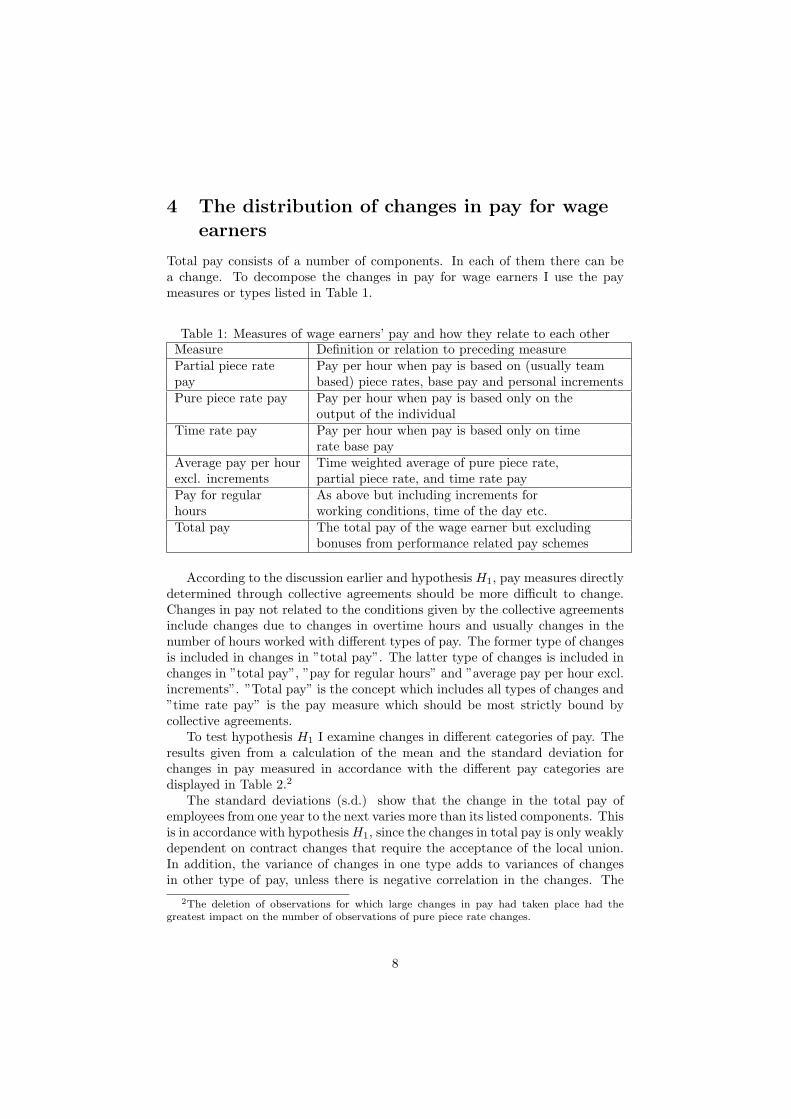
Total pay consists of a number of components. In each of them there can bea change. To decompose the changes in pay for wage earners I use the paymeasures or types listed in Table 1.

Table 1: Measures of wage earners’ pay and how they relate to each otherMeasure Definition or relation to preceding measurePartial piece rate Pay per hour when pay is based on (usually teampay based) piece rates, base pay and personal incrementsPure piece rate pay Pay per hour when pay is based only on the

output of the individualTime rate pay Pay per hour when pay is based only on time

rate base payAverage pay per hour Time weighted average of pure piece rate,excl. increments partial piece rate, and time rate payPay for regular As above but including increments forhours working conditions, time of the day etc.Total pay The total pay of the wage earner but excluding

bonuses from performance related pay schemes

According to the discussion earlier and hypothesis H1, pay measures directlydetermined through collective agreements should be more difficult to change.Changes in pay not related to the conditions given by the collective agreementsinclude changes due to changes in overtime hours and usually changes in thenumber of hours worked with different types of pay. The former type of changesis included in changes in ”total pay”. The latter type of changes is included inchanges in ”total pay”, ”pay for regular hours” and ”average pay per hour excl.increments”. ”Total pay” is the concept which includes all types of changes and”time rate pay” is the pay measure which should be most strictly bound bycollective agreements.

To test hypothesis H1 I examine changes in different categories of pay. Theresults given from a calculation of the mean and the standard deviation forchanges in pay measured in accordance with the different pay categories aredisplayed in Table 2.2

The standard deviations (s.d.) show that the change in the total pay ofemployees from one year to the next varies more than its listed components. Thisis in accordance with hypothesis H1, since the changes in total pay is only weaklydependent on contract changes that require the acceptance of the local union.In addition, the variance of changes in one type adds to variances of changesin other type of pay, unless there is negative correlation in the changes. The

2The deletion of observations for which large changes in pay had taken place had thegreatest impact on the number of observations of pure piece rate changes.

8

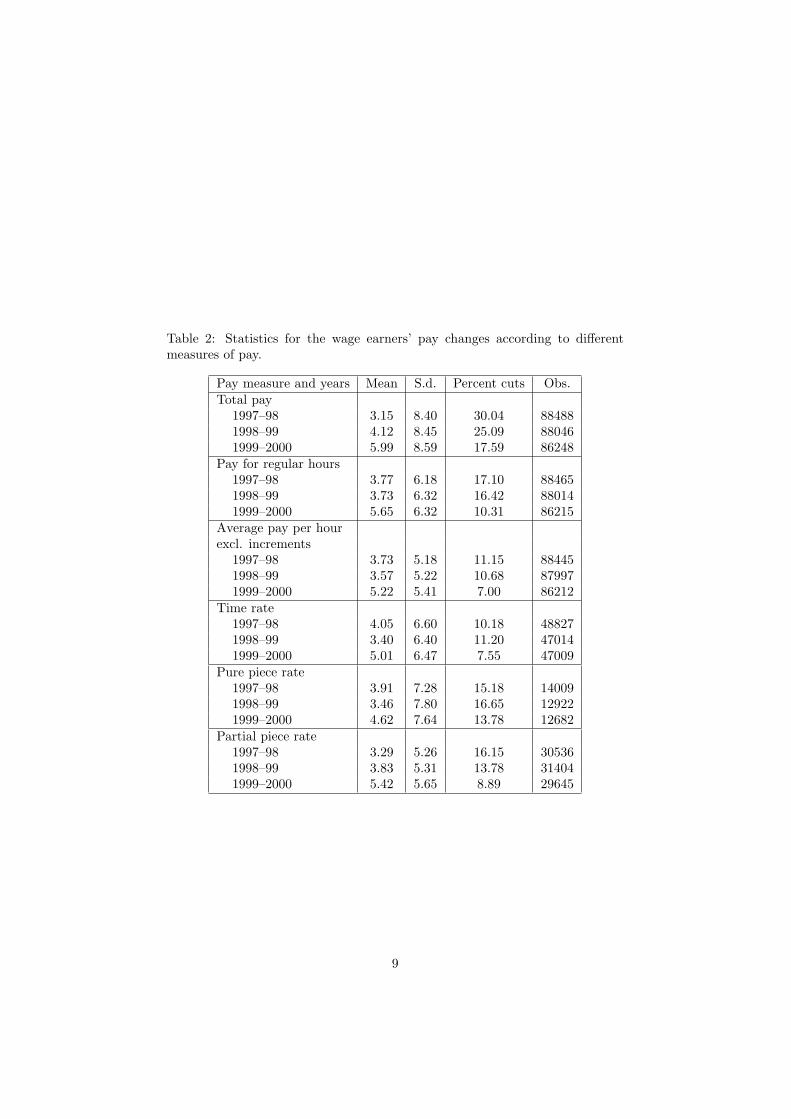
Table 2: Statistics for the wage earners’ pay changes according to differentmeasures of pay.

Pay measure and years Mean S.d. Percent cuts Obs.Total pay

1997–98 3.15 8.40 30.04 884881998–99 4.12 8.45 25.09 880461999–2000 5.99 8.59 17.59 86248

Pay for regular hours1997–98 3.77 6.18 17.10 884651998–99 3.73 6.32 16.42 880141999–2000 5.65 6.32 10.31 86215

Average pay per hourexcl. increments

1997–98 3.73 5.18 11.15 884451998–99 3.57 5.22 10.68 879971999–2000 5.22 5.41 7.00 86212

Time rate1997–98 4.05 6.60 10.18 488271998–99 3.40 6.40 11.20 470141999–2000 5.01 6.47 7.55 47009

Pure piece rate1997–98 3.91 7.28 15.18 140091998–99 3.46 7.80 16.65 129221999–2000 4.62 7.64 13.78 12682

Partial piece rate1997–98 3.29 5.26 16.15 305361998–99 3.83 5.31 13.78 314041999–2000 5.42 5.65 8.89 29645

9

same conclusions also applies to the difference in standard deviation betweenchanges in ”pay for regular hours” and ”average pay per hour excl. increments”.However, a bit surprising is that the standard deviation for changes in ”averagepay per hour excl. increments” is smaller than for changes in time rate, purepiece rate, and partial pece rate pay.

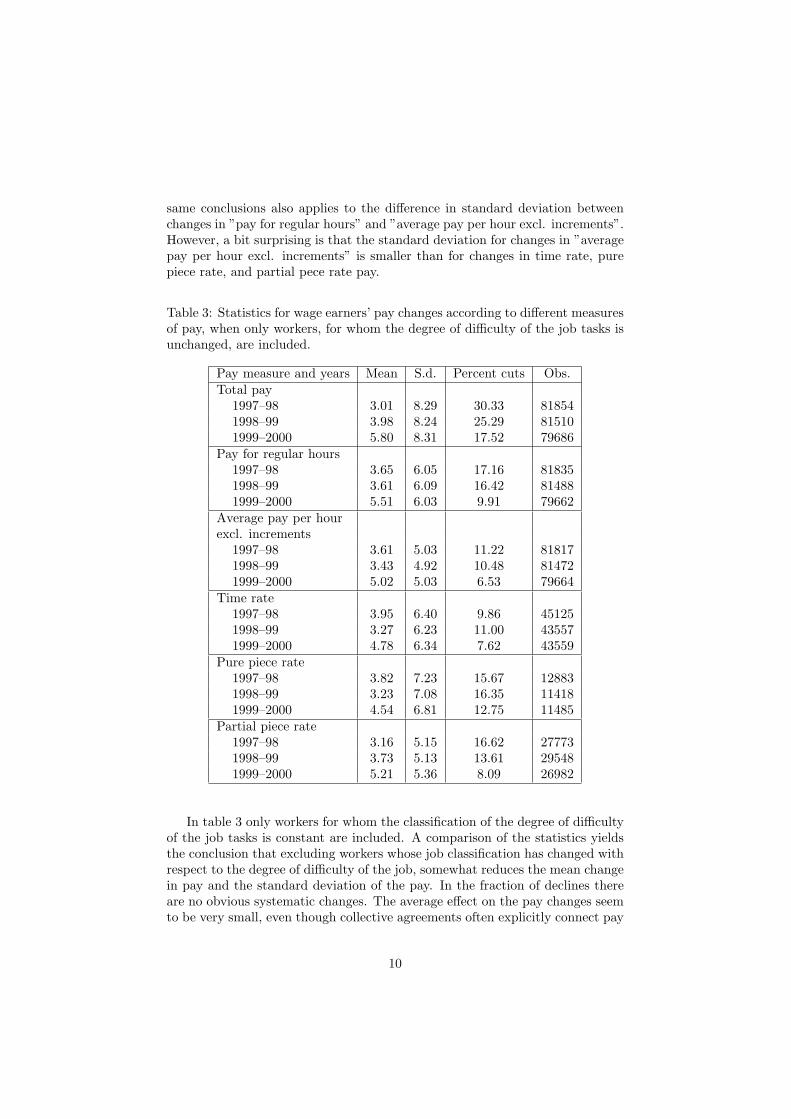
Table 3: Statistics for wage earners’ pay changes according to different measuresof pay, when only workers, for whom the degree of difficulty of the job tasks isunchanged, are included.

Pay measure and years Mean S.d. Percent cuts Obs.Total pay

1997–98 3.01 8.29 30.33 818541998–99 3.98 8.24 25.29 815101999–2000 5.80 8.31 17.52 79686

Pay for regular hours1997–98 3.65 6.05 17.16 818351998–99 3.61 6.09 16.42 814881999–2000 5.51 6.03 9.91 79662

Average pay per hourexcl. increments

1997–98 3.61 5.03 11.22 818171998–99 3.43 4.92 10.48 814721999–2000 5.02 5.03 6.53 79664

Time rate1997–98 3.95 6.40 9.86 451251998–99 3.27 6.23 11.00 435571999–2000 4.78 6.34 7.62 43559

Pure piece rate1997–98 3.82 7.23 15.67 128831998–99 3.23 7.08 16.35 114181999–2000 4.54 6.81 12.75 11485

Partial piece rate1997–98 3.16 5.15 16.62 277731998–99 3.73 5.13 13.61 295481999–2000 5.21 5.36 8.09 26982

In table 3 only workers for whom the classification of the degree of difficultyof the job tasks is constant are included. A comparison of the statistics yieldsthe conclusion that excluding workers whose job classification has changed withrespect to the degree of difficulty of the job, somewhat reduces the mean changein pay and the standard deviation of the pay. In the fraction of declines thereare no obvious systematic changes. The average effect on the pay changes seemto be very small, even though collective agreements often explicitly connect pay

10

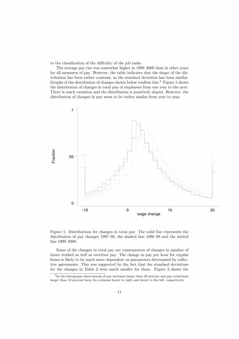
to the classification of the difficulty of the job tasks.The average pay rise was somewhat higher in 1999–2000 than in other years

for all measures of pay. However, the table indicates that the shape of the dis-tribution has been rather constant, as the standard deviation has been similar.Graphs of the distribution of changes shown below confirm this.3 Figure 1 showsthe distribution of changes in total pay of employees from one year to the next.There is much variation and the distribution is positively sloped. However, thedistribution of changes in pay seem to be rather similar from year to year.

Fra

ctio

n

wage change-10 0 10 20

0

.05

.1

Figure 1: Distributions for changes in total pay. The solid line represents thedistribution of pay changes 1997–98, the dashed line 1998–99 and the dottedline 1999–2000.

Some of the changes in total pay are consequences of changes in number ofhours worked as well as overtime pay. The change in pay per hour for regularhours is likely to be much more dependent on parameters determined by collec-tive agreements. This was supported by the fact that the standard deviationsfor the changes in Table 2 were much smaller for them. Figure 2 shows the

3In the histograms observations of pay increases larger than 20 percent and pay reductionslarger than 10 percent form the columns farest to right and farest to the left, respectively.

11

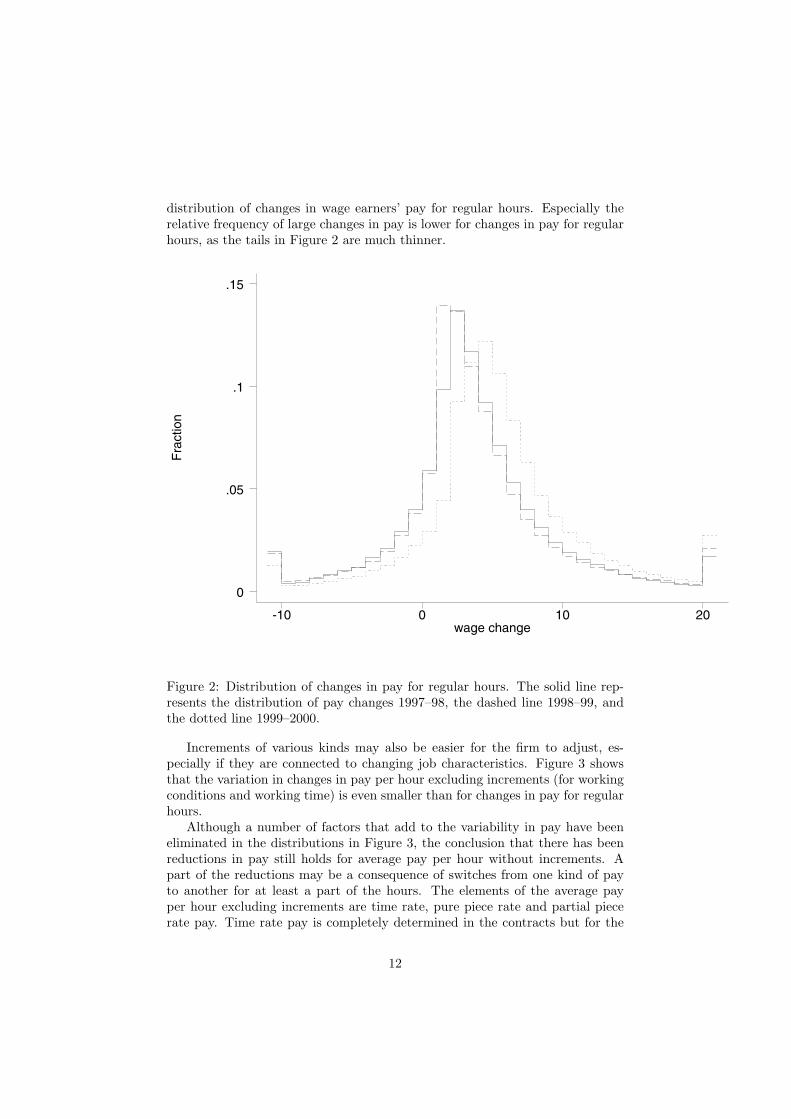
distribution of changes in wage earners’ pay for regular hours. Especially therelative frequency of large changes in pay is lower for changes in pay for regularhours, as the tails in Figure 2 are much thinner.

Fra

ctio

n


0

.05

.1

.15

Figure 2: Distribution of changes in pay for regular hours. The solid line rep-resents the distribution of pay changes 1997–98, the dashed line 1998–99, andthe dotted line 1999–2000.

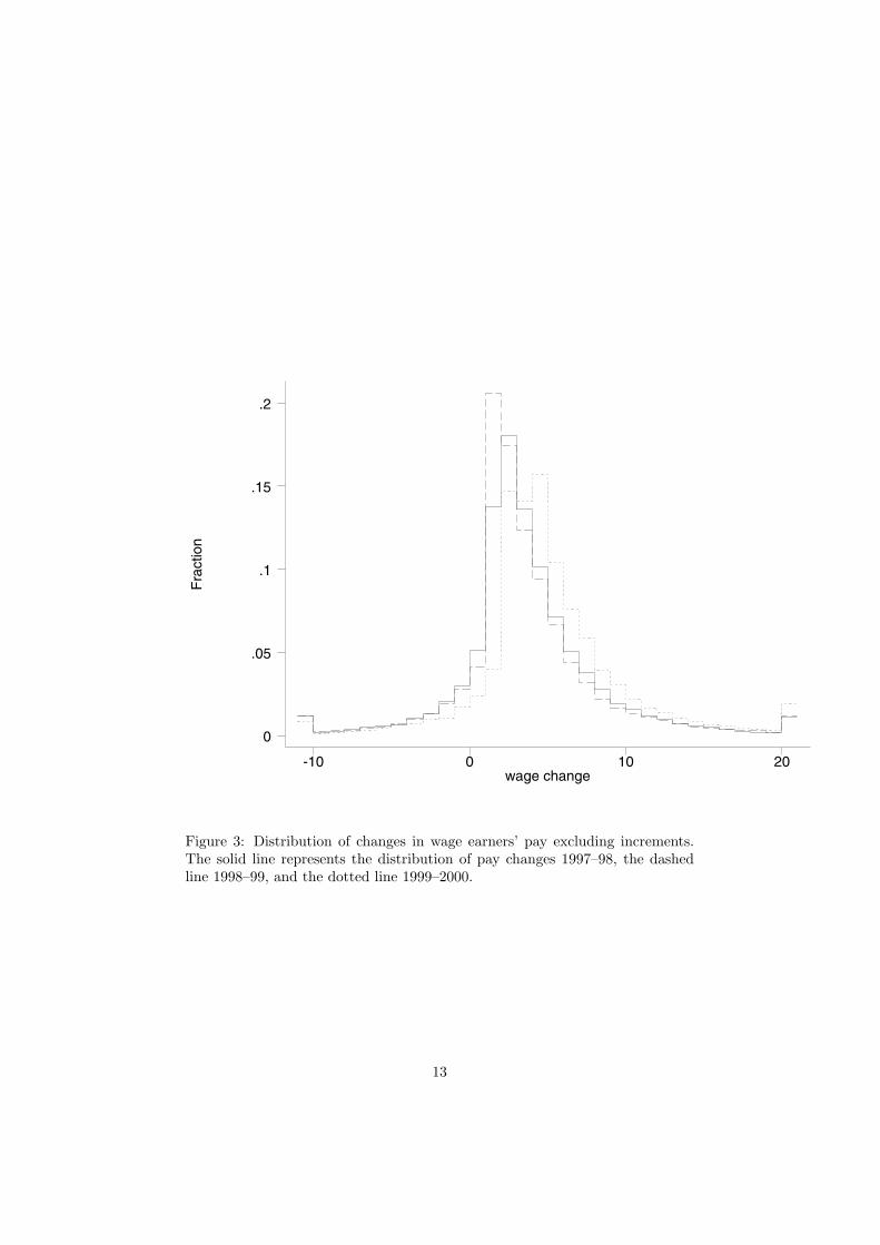
Increments of various kinds may also be easier for the firm to adjust, es-pecially if they are connected to changing job characteristics. Figure 3 showsthat the variation in changes in pay per hour excluding increments (for workingconditions and working time) is even smaller than for changes in pay for regularhours.

Although a number of factors that add to the variability in pay have beeneliminated in the distributions in Figure 3, the conclusion that there has beenreductions in pay still holds for average pay per hour without increments. Apart of the reductions may be a consequence of switches from one kind of payto another for at least a part of the hours. The elements of the average payper hour excluding increments are time rate, pure piece rate and partial piecerate pay. Time rate pay is completely determined in the contracts but for the

12

Fra

ctio

n


0

.05

.1

.15

.2

Figure 3: Distribution of changes in wage earners’ pay excluding increments.The solid line represents the distribution of pay changes 1997–98, the dashedline 1998–99, and the dotted line 1999–2000.

13

other pay types pay partly depends on the output of the employees. HypothesisH1 means that piece rate pay should be more variable than time rate pay. Thestandard deviations in Table 2 gave support to the hypothesis, but only forpure piece rates and not for partial piece rates. The graph of the distributionof the changes in pure piece rate pay in Figure 4 also show that the tails ofthe distribution are much fatter and the top lower than for the average pay perhour without increments in Figure 3 and time rate pay in Figure 5.4

Fra

ctio

n


0

.05

.1

.15

Figure 4: Distribution of changes in wage earners’ pay per hour for hours withpure piece rate pay. The solid line represents the distribution of pay changes1997–98, the dashed line 1998–99, and the dotted line 1999–2000.

The distribution for changes in pay based on partial piece rates in Figure 6seems to have a broad top but thinner tails than the distribution for changes inpay based on pure piece rates. Large changes in pay per hour are rather rarefor partial piece rate pay.

Hypothesis H1 thus receives support except for that partial piece rates seem4A problem might be that the there are larger measurement errors in the pay per hour for

pure piece rates than for the other kinds of pay, since the number of hours worked is of lessimportance.

14

Fra

ctio

n


0

.1

.2

.3

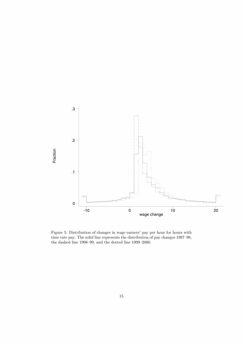
Figure 5: Distribution of changes in wage earners’ pay per hour for hours withtime rate pay. The solid line represents the distribution of pay changes 1997–98,the dashed line 1998–99, and the dotted line 1999–2000.

15

Fra

ctio

n


0

.05

.1

.15

Figure 6: Distribution of changes in wage earners’ pay per hour for hours withpartial piece rate pay. The solid line represents the distribution of pay changes1997–98, the dashed line 1998–99, and the dotted line 1999–2000.

16

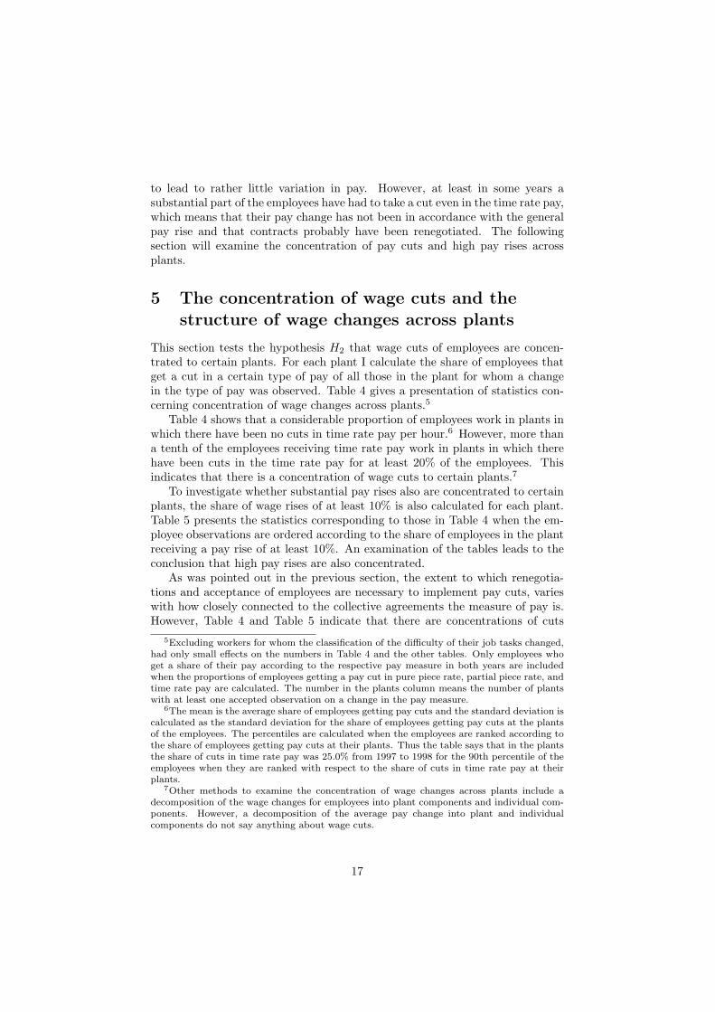
to lead to rather little variation in pay. However, at least in some years asubstantial part of the employees have had to take a cut even in the time rate pay,which means that their pay change has not been in accordance with the generalpay rise and that contracts probably have been renegotiated. The followingsection will examine the concentration of pay cuts and high pay rises acrossplants.

5 The concentration of wage cuts and thestructure of wage changes across plants

This section tests the hypothesis H2 that wage cuts of employees are concen-trated to certain plants. For each plant I calculate the share of employees thatget a cut in a certain type of pay of all those in the plant for whom a changein the type of pay was observed. Table 4 gives a presentation of statistics con-cerning concentration of wage changes across plants.5

Table 4 shows that a considerable proportion of employees work in plants inwhich there have been no cuts in time rate pay per hour.6 However, more thana tenth of the employees receiving time rate pay work in plants in which therehave been cuts in the time rate pay for at least 20% of the employees. Thisindicates that there is a concentration of wage cuts to certain plants.7

To investigate whether substantial pay rises also are concentrated to certainplants, the share of wage rises of at least 10% is also calculated for each plant.Table 5 presents the statistics corresponding to those in Table 4 when the em-ployee observations are ordered according to the share of employees in the plantreceiving a pay rise of at least 10%. An examination of the tables leads to theconclusion that high pay rises are also concentrated.

As was pointed out in the previous section, the extent to which renegotia-tions and acceptance of employees are necessary to implement pay cuts, varieswith how closely connected to the collective agreements the measure of pay is.However, Table 4 and Table 5 indicate that there are concentrations of cuts

5Excluding workers for whom the classification of the difficulty of their job tasks changed,had only small effects on the numbers in Table 4 and the other tables. Only employees whoget a share of their pay according to the respective pay measure in both years are includedwhen the proportions of employees getting a pay cut in pure piece rate, partial piece rate, andtime rate pay are calculated. The number in the plants column means the number of plantswith at least one accepted observation on a change in the pay measure.

6The mean is the average share of employees getting pay cuts and the standard deviation iscalculated as the standard deviation for the share of employees getting pay cuts at the plantsof the employees. The percentiles are calculated when the employees are ranked according tothe share of employees getting pay cuts at their plants. Thus the table says that in the plantsthe share of cuts in time rate pay was 25.0% from 1997 to 1998 for the 90th percentile of theemployees when they are ranked with respect to the share of cuts in time rate pay at theirplants.

7Other methods to examine the concentration of wage changes across plants include adecomposition of the wage changes for employees into plant components and individual com-ponents. However, a decomposition of the average pay change into plant and individualcomponents do not say anything about wage cuts.

17

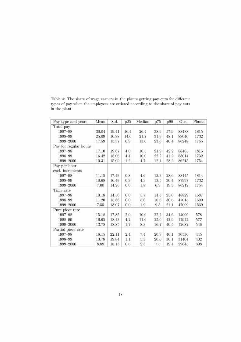
Table 4: The share of wage earners in the plants getting pay cuts for differenttypes of pay when the employees are ordered according to the share of pay cutsin the plant.

Pay type and years Mean S.d. p25 Median p75 p90 Obs. PlantsTotal pay

1997–98 30.04 19.41 16.4 26.4 38.9 57.9 88488 18151998–99 25.09 16.88 14.6 21.7 31.9 48.1 88046 17321999–2000 17.59 15.37 6.9 13.0 23.6 40.4 86248 1755

Pay for regular hours1997–98 17.10 19.67 4.0 10.5 21.9 42.2 88465 18151998–99 16.42 18.06 4.4 10.0 22.2 41.2 88014 17321999–2000 10.31 15.09 1.2 4.7 12.4 28.2 86215 1754

Pay per hourexcl. increments

1997–98 11.15 17.43 0.8 4.6 13.3 28.6 88445 18141998–99 10.68 16.43 0.3 4.3 13.5 30.4 87997 17321999–2000 7.00 14.26 0.0 1.8 6.9 19.3 86212 1754

Time rate1997–98 10.18 14.56 0.0 5.7 14.3 25.0 48829 15871998–99 11.20 15.86 0.0 5.6 16.6 30.6 47015 15091999–2000 7.55 13.07 0.0 1.9 9.5 21.1 47009 1539

Pure piece rate1997–98 15.18 17.85 2.0 10.0 22.2 34.6 14009 5781998–99 16.65 18.43 4.2 11.6 25.0 42.9 12922 5771999–2000 13.78 18.85 1.7 8.3 16.7 40.5 12682 546

Partial piece rate1997–98 16.15 22.11 2.4 7.4 20.9 46.1 30536 4451998–99 13.78 19.84 1.1 5.3 20.0 36.1 31404 4021999–2000 8.89 18.13 0.6 2.3 7.5 19.4 29645 398

18

Table 5: The concentration of wage earners getting pay rises ≥ 10% for differenttypes of pay. Employees ordered according to the share of employees in theirplant receiving such a pay rise.


1997–98 15.32 13.24 6.5 12.1 20.9 31.3 88488 18151998–99 17.78 16.26 7.2 12.8 23.9 38.9 88046 17321999–2000 23.48 17.73 11.4 18.0 31.8 47.4 86248 1755

Pay for regular hours1997–98 10.66 13.17 2.2 6.3 13.7 28.7 88465 18151998–99 10.79 15.99 1.9 4.9 12.0 26.7 88014 17321999–2000 16.18 17.85 3.8 10.6 21.3 38.5 86215 1754


1997–98 7.59 11.97 1.0 3.5 8.4 19.3 88445 18141998–99 7.32 12.56 0.7 3.1 8.3 18.2 87997 17321999–2000 11.40 16.06 1.6 5.5 13.3 30.8 86212 1754

Time rate1997–98 10.26 13.10 1.5 6.0 13.2 25.0 48829 15871998–99 8.72 12.51 0.2 5.0 11.4 22.2 47015 15091999–2000 11.79 14.33 2.2 6.6 16.2 31.2 47009 1539

Pure piece rate1997–98 11.16 16.65 1.6 6.1 12.7 30.2 14009 5781998–99 9.64 14.68 0.0 4.8 12.2 25.0 12922 5771999–2000 12.60 16.25 2.1 6.5 17.4 33.3 12682 546

Partial piece rate1997–98 7.54 12.32 0.3 3.0 9.5 19.2 30536 4451998–99 8.84 14.82 1.1 3.7 10.8 21.4 31404 4021999–2000 13.83 18.95 1.6 7.0 14.0 40.8 29645 398

19

and rises for all types of pay, although the numbers may to some extent reflectthat small plants exhibiting either no cuts at all or a rather large share of cutswhen the work force is small and the number of plants was too great to allowtests of significance of the concentrations. To reduce the number of plants (toenable a statistical test) and avoid concentrations that reflect differences be-tween industries, I take the metal industry and test for whether the pay cuts ofindividuals are randomly distributed between plants in which there are at least20 observations. Pearson’s χ2-test for the distribution of pay cuts yields theresult that the null hypothesis (independently distributed observations) can berejected for all pay measures, which is shown in Table 6. The pay cuts are thusconcentrated to certain plants.

Table 6: A test for whether pay cuts are independently distributed across plantswith at least 20 employees in the metal industry.

Pay type and years χ2 p(χ2 | H0) Plants (=df+1) Obs.Total pay

1997–98 5620.43 0.0000 249 292271998–99 4778.54 0.0000 247 290821999–2000 4825.07 0.0000 259 28088

Pay for regular hours1997–98 8010.82 0.0000 249 292231998–99 6786.80 0.0000 247 290741999–2000 7513.14 0.0000 259 28084


1997–98 9953.32 0.0000 249 292221998–99 7719.17 0.0000 247 290711999–2000 12735.15 0.0000 259 28082

Time rate1997–98 3790.62 0.0000 234 187641998–99 5367.06 0.0000 232 184301999–2000 5560.15 0.0000 245 18339

Pure piece rate1997–98 463.61 0.0000 86 27561998–99 474.24 0.0000 68 21311999–2000 602.07 0.0000 73 2193

Partial piece rate1997–98 5200.06 0.0000 128 125251998–99 3619.26 0.0000 120 127931999–2000 6799.80 0.0000 115 11603

The tests in table 6 thus confirm the hypothesis H2. To enable a check ofthe hypothesis H3, that high pay rises should be less concentrated, I also make

20

the corresponding examination of the independence of the distribution of payrises higher than or equal to 10% in Table 7. The results show that pay risesare also significantly concentrated to certain plants, although the χ2-values forthe tests concerning the concentration of wage rises are lower than for pay cuts.

Table 7: A test for whether pay rises ≥ 10% are independently distributedacross plants with at least 20 employees in the metal industry.

Pay type and years χ2 p(χ2 | H0) Plants (=df+1) Obs.Total pay

1997–98 3715.08 0.0000 249 292271998–99 6484.57 0.0000 247 290821999–2000 4374.58 0.0000 259 28088

Pay for regular hours1997–98 4527.85 0.0000 249 292231998–99 8814.11 0.0000 247 290741999–2000 6220.47 0.0000 259 28084


1997–98 5247.87 0.0000 249 292221998–99 6533.96 0.0000 247 290711999–2000 4449.94 0.0000 259 28082

Time rate1997–98 3639.61 0.0000 234 187641998–99 3078.61 0.0000 232 184301999–2000 2839.74 0.0000 245 18339

Pure piece rate1997–98 424.82 0.0000 86 27561998–99 288.51 0.0000 68 21311999–2000 360.36 0.0000 73 2193

Partial piece rate1997–98 3382.98 0.0000 128 125251998–99 4318.69 0.0000 120 127931999–2000 2186.93 0.0000 115 11603

Finally to test Hypothesis H4 I cross tabulate plants according to the shareof wage cuts and high increases (≥ 10%) in wages. The plants are categorisedinto three groups according to the share of wage cuts and high wage increasesrespectively: Those in which none have taken place, those in which a small sharehave received a wage cut and high pay rise respectively, and those in which alarge share have received it.

The χ2-values are so high that the test strongly reject that pay cuts and highpay rises would be independently distributed across firms. The Tables 8 and 9show that there is a tendency that there in plants, in which there are no wage

21

Table 8: Cross tabulation of plants when they are categorised according toshare of cuts in the total pay of wage earners and share of wage earners gettingincreases ≥ 10% in total pay.

Plants categorised Share of wage cuts χ2 (4df)/by share of wage rises ≥ 10% No cuts Small Large All plants Prob.

1997–98Large 39.43 49.47 23.71 37.09Small 11.43 38.38 45.69 37.18 157.64No rises ≥ 10% 49.14 12.15 30.60 25.72 0.00000Number of plants 175 469 464 1108



22

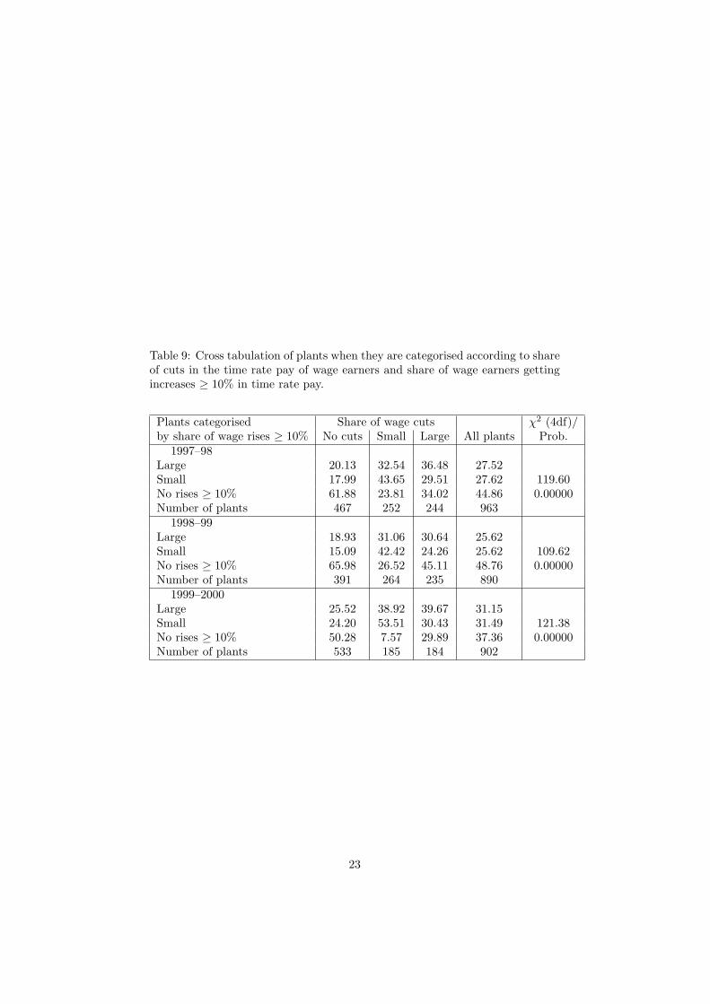
Table 9: Cross tabulation of plants when they are categorised according to shareof cuts in the time rate pay of wage earners and share of wage earners gettingincreases ≥ 10% in time rate pay.

Plants categorised Share of wage cuts χ2 (4df)/by share of wage rises ≥ 10% No cuts Small Large All plants Prob.




23

cuts, also are no high wage increases. This applies both for changes in the totalpay of the wage earners and for changes in the time rate pay. This supportsthe hypothesis H4 and that the wage flexibility varies across plants. However, acomparison of the numbers in the tables also yields the conclusion that plantsin which there is a large share pay cuts have a larger probability of having nowage rises at all than those with only a small share of pay cuts. However, thismay also indicate that the random distribution of cuts and increases in plantswith only few workers have affected the categorisation.

To eliminate the influence of random categorisation due to few workers inthe plant I also tested with excluding all plants with less than 25 observationsof pay changes. This had some effect on the distribution for changes in thetotal pay. Nevertheless, the results indicated that there was a division betweena group of plants with both many pay cuts and high pay increases and a groupwith many cuts but no high pay rises.

The results thus largely support Hypothesis H2, that is there is a concen-tration of pay cuts to certain plants. The support for Hypothesis H3 is weak.The results in Tables 8 and 9 suggest that pay cuts and pay rises to a largeextent coexist in the plants and the concentration to certain plants may be aconsequence of higher flexibility in these plants, or alternatively measurementerrors. This result supports the hypothesis H4. Although this last result pointsin a somewhat different direction in explaining the concentration of wage cuts,the results do not contradict the claim that plant-specific needs are importantfor explaining the concentration of wage cuts to certain plants. However, it in-dicates that these to a rather large extent are related to a higher wage flexibilityinside the plants.

Characteristics of pay changes and cuts amongsalaried employees

The data for salaried employees is not as detailed as for wage earners, sincesalaries are not dependent on the number of hours actually worked and thereis no information on hours worked. The pay of salaried employees consists ofa fixed monthly salary to which bonuses are added. It is natural to comparethe changes in total pay of the salaried employees to the changes in total payof wage earners. Because the salary in the short run is fixed and independentof the performance of the employee, it seems most appropriate to compare thechanges in the fixed monthly salary of the salaried employees to changes in thetime rate pay per hour of the wage earners.

The mean pay changes are somewhat larger for salaried employees thanfor wage earners. Much of the variation is accounted for by increments andbonuses (not including bonuses from profit sharing schemes), which leads to amuch higher standard deviation for changes in total pay than for changes thefixed monthly salary. The proportion of salaried employees who get a cut inthe fixed salary is also much smaller than the proportion getting a cut in the

24

Table 10: Statistics for the pay changes of salaried employees.

Pay type and years Mean S.d. Percent decl. Percent rises ≥ 10% Obs.Total pay

1997–98 6.14 9.31 17.44 25.01 735701998–99 4.25 9.29 25.34 19.30 756661999–2000 6.75 9.47 15.99 27.78 74057

Fixed monthly salary1997–98 4.71 5.13 1.13 11.78 750571998–99 4.01 5.45 3.82 10.17 771261999–2000 6.14 5.66 1.61 16.65 75951

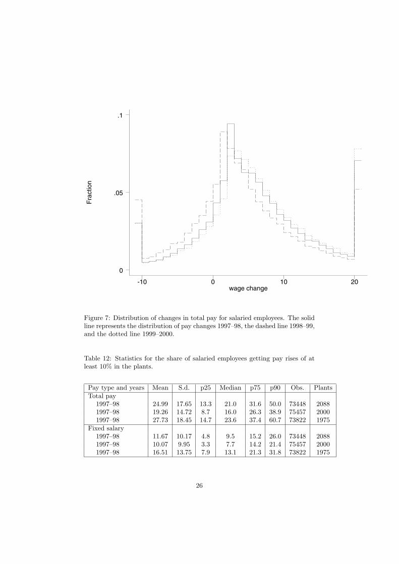
total pay. This is in accordance with the theory since the increments are likelyto change with the state of the world and the performance of the individual inaccordance with contracts. The fixed salary is likely to be much more rigid sincechanging the contract requires the acceptance of both parties. The distributionof changes in total pay and monthly salaries are shown graphically in Figures 7and 8 respectively. The graphs confirm the rigidity of fixed salaries comparedto total pay.

The proportion of salaries being cut is very small even compared to theproportion of cuts in the time rate pay of wage earners. An investigation of thedistribution of pay cuts show that there is some concentration of them to certainplants. See Table 11 for statistics concerning the distribution of pay cuts.

Table 11: Statistics for the share of salaried employees getting lower pay in theplants.


1997–98 17.42 13.00 8.7 14.6 23.1 34.3 73448 20881997–98 25.29 18.51 12.5 20.7 31.5 50.0 75457 20001997–98 15.93 13.18 7.9 12.8 20.0 29.1 73822 1975

Fixed salary1997–98 1.12 3.82 0.0 0.0 0.9 2.7 73448 20881997–98 3.82 10.05 0.0 0.4 3.1 8.2 75457 20001997–98 1.58 5.32 0.0 0.0 1.3 3.6 73822 1975

Similarly there is some concentration of high pay increases (≥ 10%). Thestatistics concerning the distribution of these are shown in Table 12.

To test the hypothesis H4 concerning the coexistence of pay rises and paycuts also for salaried employees I cross tabulate the plants according to the

25

Fra

ctio

n


0

.05

.1

Figure 7: Distribution of changes in total pay for salaried employees. The solidline represents the distribution of pay changes 1997–98, the dashed line 1998–99,and the dotted line 1999–2000.

Table 12: Statistics for the share of salaried employees getting pay rises of atleast 10% in the plants.


1997–98 24.99 17.65 13.3 21.0 31.6 50.0 73448 20881997–98 19.26 14.72 8.7 16.0 26.3 38.9 75457 20001997–98 27.73 18.45 14.7 23.6 37.4 60.7 73822 1975

Fixed salary1997–98 11.67 10.17 4.8 9.5 15.2 26.0 73448 20881997–98 10.07 9.95 3.3 7.7 14.2 21.4 75457 20001997–98 16.51 13.75 7.9 13.1 21.3 31.8 73822 1975

26

Fra

ctio

n


0

.2

.4

.6

Figure 8: Distribution of changes in fixed monthly pay for salaried employees.The solid line represents the distribution of pay changes 1997–98, the dashedline 1998–99, and the dotted line 1999–2000.

27

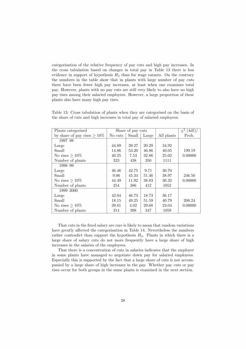
categorisation of the relative frequency of pay cuts and high pay increases. Inthe cross tabulation based on changes in total pay in Table 13 there is lessevidence in support of hypothesis H4 than for wage earners. On the contrarythe numbers in the table show that in plants with large number of pay cutsthere have been fewer high pay increases, at least when one examines totalpay. However, plants with no pay cuts are still very likely to also have no highpay rises among their salaried employees. However, a large proportion of theseplants also have many high pay rises.

Table 13: Cross tabulation of plants when they are categorised on the basis ofthe share of cuts and high increases in total pay of salaried employees.

Plants categorised Share of pay cuts χ2 (4df)/by share of pay rises ≥ 10% No cuts Small Large All plants Prob.




That cuts in the fixed salary are rare is likely to mean that random variationshave greatly affected the categorisation in Table 14. Nevertheless the numbersrather contradict than support the hypothesis H4. Plants in which there is alarge share of salary cuts do not more frequently have a large share of highincreases in the salaries of the employees.

That there is a concentration of cuts in salaries indicates that the employerin some plants have managed to negotiate down pay for salaried employees.Especially this is supported by the fact that a large share of cuts is not accom-panied by a large share of high increases in the pay. Whether pay cuts or payrises occur for both groups in the same plants is examined in the next section.

28

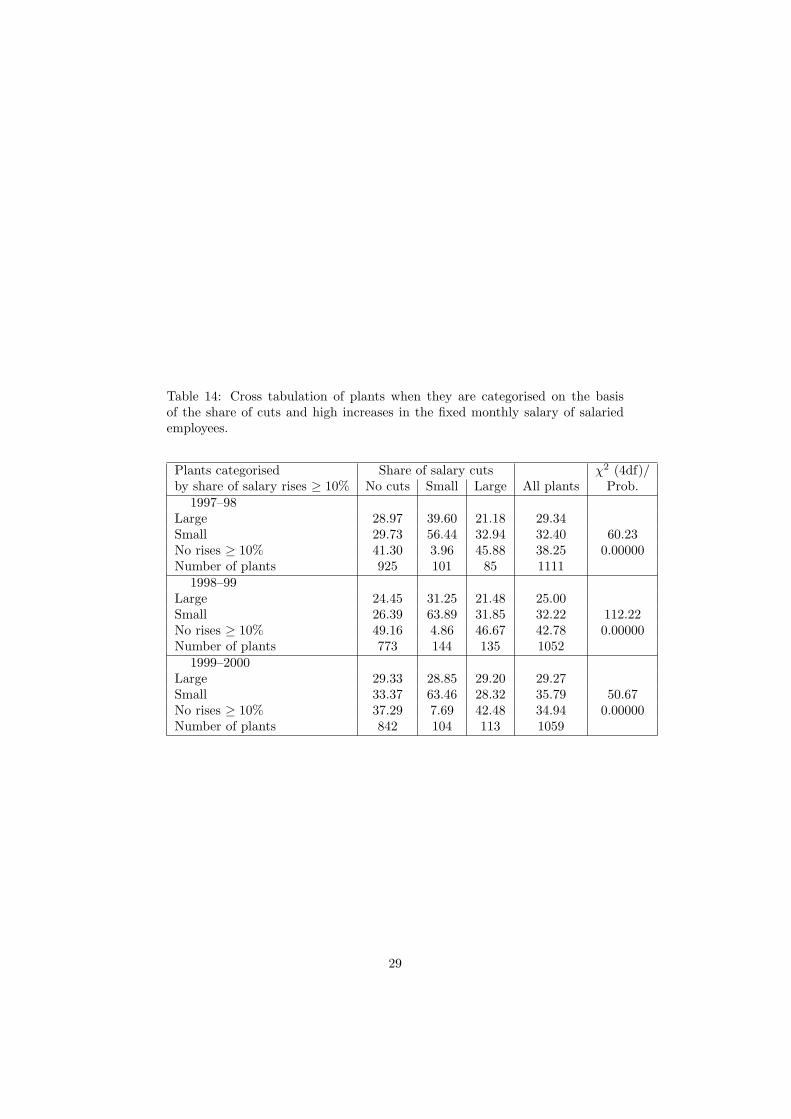
Table 14: Cross tabulation of plants when they are categorised on the basisof the share of cuts and high increases in the fixed monthly salary of salariedemployees.

Plants categorised Share of salary cuts χ2 (4df)/by share of salary rises ≥ 10% No cuts Small Large All plants Prob.




29

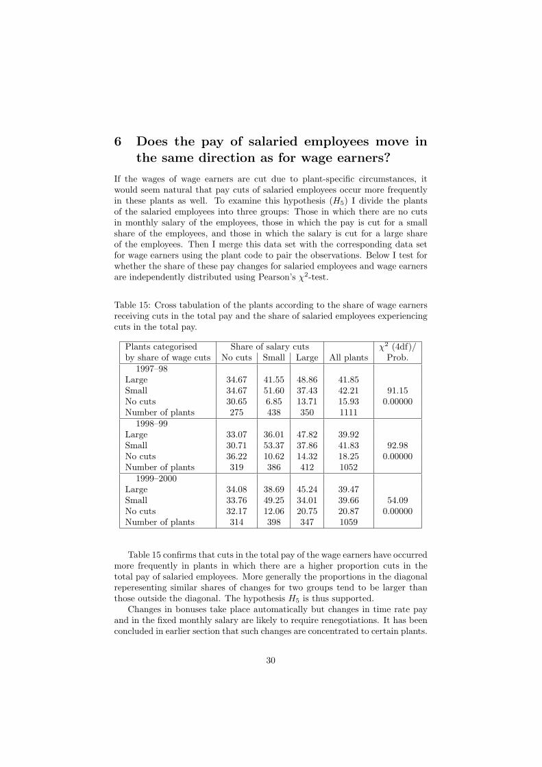
6 Does the pay of salaried employees move inthe same direction as for wage earners?

If the wages of wage earners are cut due to plant-specific circumstances, itwould seem natural that pay cuts of salaried employees occur more frequentlyin these plants as well. To examine this hypothesis (H5) I divide the plantsof the salaried employees into three groups: Those in which there are no cutsin monthly salary of the employees, those in which the pay is cut for a smallshare of the employees, and those in which the salary is cut for a large shareof the employees. Then I merge this data set with the corresponding data setfor wage earners using the plant code to pair the observations. Below I test forwhether the share of these pay changes for salaried employees and wage earnersare independently distributed using Pearson’s χ2-test.

Table 15: Cross tabulation of the plants according to the share of wage earnersreceiving cuts in the total pay and the share of salaried employees experiencingcuts in the total pay.

Plants categorised Share of salary cuts χ2 (4df)/by share of wage cuts No cuts Small Large All plants Prob.

1997–98Large 34.67 41.55 48.86 41.85Small 34.67 51.60 37.43 42.21 91.15No cuts 30.65 6.85 13.71 15.93 0.00000Number of plants 275 438 350 1111



Table 15 confirms that cuts in the total pay of the wage earners have occurredmore frequently in plants in which there are a higher proportion cuts in thetotal pay of salaried employees. More generally the proportions in the diagonalreperesenting similar shares of changes for two groups tend to be larger thanthose outside the diagonal. The hypothesis H5 is thus supported.

Changes in bonuses take place automatically but changes in time rate payand in the fixed monthly salary are likely to require renegotiations. It has beenconcluded in earlier section that such changes are concentrated to certain plants.

30

In Table 16 it is tested whether also cuts in these pay measures are concentratedto the same plants for salaried employees and wage earners.

Table 16: Cross tabulation of the plants according to the share of wage earnersreceiving cuts in the time rate pay and the share of salaried employees experi-encing cuts in the fixed salary.

Plants categorised by Share of salary cuts χ2 (4df)share of wage cuts No cuts Small Large All plants Prob.




Table 16 shows that the relation between cuts in fixed salaries and cuts intime rate pay is significant but weaker than for cuts in total pay. However, dueto the rareness of cuts in fixed salaries small plants with cut in the pay of onlyone person are strongly over-represented among the plants with a large shareof cuts in fixed salaries. The results may therefore reflect effects related to thesize of the plants. To avoid this problem and compare the distribution of cutsin time rate pay with less random cuts in the total pay of salaried employees, inTable 17 I cross-tabulate plants according to the share of cuts in the time ratepay and the share of cuts in the total pay of the salaried employees. The totalpay of salaried employees is also more likely to respond to the performance ofthe plant.

Table 17 confirms that the frequency of wage cuts are related to the shareof cuts in the total pay of salaried employees. However, in large proportions ofthose plants with a large share of salary cuts there are no cuts in wages. Thismight be a consequence of the small size of the plants.

To test whether the same relation exists for pay rises I also cross tabulateplants according to the share of pay rises of at least 10%. The categorisation ofthe plants are made on the basis of the proportion of pay rises relative to thosein other plants and the cross tabulations are made for the same pay measures

31

Table 17: Cross tabulation of the plants according to the share of wage earnersreceiving cuts in the time rate pay and the share of salaried employees receivingcuts in the total pay.

Plants categorised by Share of salary cuts χ2 (4df)share of wage cuts No cuts Small Large All plants Prob.




as for cuts. The three categories are plants with no pay rises of at least 10%,plants with a low share of pay rises of at least 10%, and plants with a high shareof pay rises ≥ 10%. Table 18 shows that there are significant relationships forpay rises as well.

To enable an examination of the corresponding distribution for high increasesin the time rate pay and fixed monthly salary the corresponding statistics forthese are displayed in Table 19. There is once again a concentration to thediagonal meaning that wages have tended to rise to the same extent as salaries.

When the share of high rises in the total pay of salaried employees andthe share of high rises in time rate pay are used for the categorisation of theplants for the cross tabulation in Table 20, the results are very similar to thecorresponding results for cuts in Table 17.

There are other variables which might affect changes in pay. One such is thesize of the plants. Especially one could imagine that the division of plants onthe basis of their rank concerning the share of cuts in the salaried employees’pay leads to an underrepresentation of small plants among those plants with asmall share of pay cuts. To test whether this has affected the results I maketests corresponding to those in cross tables above for plants in which there are atleast 50 observations of pay changes for salaried employees and 50 observationsof pay changes of wage earners (see Table 21). The main result of deletingsmall plants is such a large elimination of plants that the differences become

32

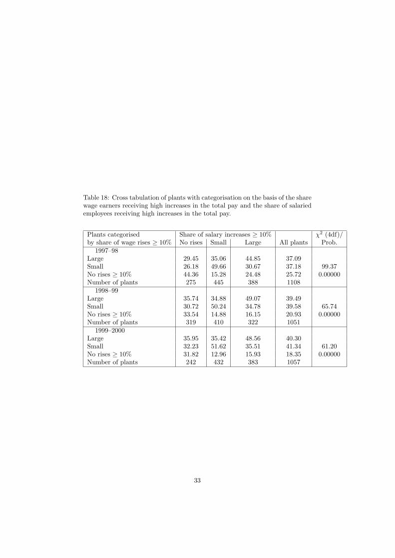
Table 18: Cross tabulation of plants with categorisation on the basis of the sharewage earners receiving high increases in the total pay and the share of salariedemployees receiving high increases in the total pay.

Plants categorised Share of salary increases ≥ 10% χ2 (4df)/by share of wage rises ≥ 10% No rises Small Large All plants Prob.




33

Table 19: Cross tabulation of plants with categorisation on the basis of theshare wage earners receiving high increases in the time rate pay and the shareof salaried employees receiving high increases in the monthly salary.

Plants categorised by Share of pay increases ≥ 10% χ2 (4df)share of wage rises ≥ 10% No rises Small Large All plants Prob.




34

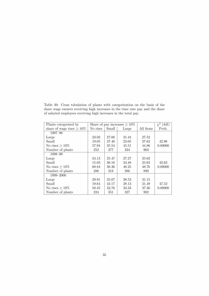
Table 20: Cross tabulation of plants with categorisation on the basis of theshare wage earners receiving high increases in the time rate pay and the shareof salaried employees receiving high increases in the total pay.

Plants categorised by Share of pay increases ≥ 10% χ2 (4df)share of wage rises ≥ 10% No rises Small Large All firms Prob.




35

insignificant. However, overall Hypothesis H5 receives support from the crosstabulations of the wage changes for wage earners and the changes in salary forsalaried employees.

Table 21: Cross tabulation of plants with categorisation on the basis of theshare wage earners receiving cuts in the time rate pay and the share of salariedemployees receiving cuts in the monthly salary. Only plants with at least 50salaried employees and 50 wage earners included.

Firms categorised by Share of salary cuts χ2 (4df)share of wage cuts No cuts Small Large All plants Prob.




Conclusion

The results indicate that there is a concentration of pay cuts to certain plantsbut also a concentration of high pay increases. Moreover, these cuts and risesare for wage earners to some extent concentrated to the same plants. The studythus supports the claim that there are some flexibility in wages but that theytend to be concentrated to certain plants.

These observations form a basis for other examinations of changes in pay.Further studies are required to identify the characteristics of the plants whichimplement pay cuts as well as of the employees, whose pay is cut in such wide-ranging pay cuts. One can also examine to what extent minimum wages blockpay cuts for those employees with the lowest pay in the plants.

Further examinations should also include an investigation of the persistenceof changes in pay. It seems likely that pay changes are less persistent in plantsin which there is a larger variation in pay changes.

36

References

Jonas Agell and Kjell Erik Lommerud. Egalitarism and growth. ScandinavianJournal of Economics, 95:59–79, 1993.

Petri Bockerman, Seppo Laaksonen, and Jari Vainionmaki. Who bear the bur-den of wage cuts? Evidence from Finland during the 1990s. Discussion Papers191, Labour Institute for Economic Research, Helsinki, 2003.

Douglas A. Hibbs and Hakan Locking. Wage dispersion and productive effi-ciency: Evidence for sweden. Journal of Labor Economics, 18:755–782, 2000.

James M. Malcomson. Individual employment contracts. In Orley C. Ashenfelterand David Card, editors, Handbook of Labor Economics, volume 3B, pages2291–2372. Elsevier Science, 1999.

Karl Ove Moene and Michael Wallerstein. Pay inequality. Journal of LaborEconomics, 15:403–30, 1997.

Coen Teulings and Joop Hartog. Corporatism or Competition? Labour Con-tracts, Institutions and Wage Structures in International Comparison. Cam-bridge, UK: Cambridge University Press, 1998.

Juhana Vartiainen. Palkkaliukumat Suomen teollisuudessa: yksilotason ana-lyysi. Tutkimuksia 44. Labour Institute of Economic Research, Helsinki, 1994.

Juhana Vartiainen. Palkkasopimusjarjestelmat, liukuma ja suomen kansan-talouden inflaatioalttius. In Tuovi Allen and Kaitila Ville, editors, Tyomarkki-nat EMU:ssa, B127. The Research Institute of the Finnish Economy, Helsinki,1996.

Juhana Vartiainen. Palkkarakenne ja tyourat. Tutkimuksia 78. Labour Instituteof Economic Research, Helsinki, 2000.

37

Government & Nonprofit

The Structure of Pay Changes at the Local Level