The impact of inequality on the municipal income tax in Finland

275

The impact ofinequality onthe municipalincome tax in

Finland

Eero Lehto

PALKANSAAJIEN TUTKIMUSLAITOS • TYÖPAPEREITA

LABOUR INSTITUTE FOR ECONOMIC RESEARCH • DISCUSSION PAPERS

Helsinki 2012

275The impact of inequality on the municipal income tax in Finland*

Eero Lehto**

*This study is funded by Employee’s Foundation and The Foundation for Municipal Development. I am grateful for this fi nancial support. I am also grateful for

Petri Böckerman and Jukka Pirttilä for very useful comments.

**Labour Institute for Economic Research, Helsinki

TYÖPAPEREITA 275DISCUSSION PAPERS 275

Palkansaajien tutkimuslaitosPitkänsillanranta 3 A00530 HelsinkiPuh. 09−2535 7330Faksi 09−2535 7332www.labour.fi

ISBN 978–952–209–101–7 (pdf)ISSN 1795–1801 (pdf)

1

ABSTRACT

This study addresses the determination of the municipal income tax rate. In the theoretical public

choice model introduced in this study we specify the central hypothesis, which says that low-income

earners using their voting power tend to take advantage of high-income taxpayers. Our findings

indicate that the median income earner will raise the municipal income tax rate the harder, the larger

the difference is between the mean income and the median income. The evidence for this impact

becomes stronger when it is conditioned on the voting rate. According to this, only if the voting rate

exceeds a certain limit – which is quite close to the average voting rate – does inequality start to work

in the direction expected. The larger inequality then raises the municipal income tax rate.

Keywords: income inequality, municipal income tax rate, median voter

JEL classification: D31, D72, H22, H24

TIIVISTELMÄ

Tämä tutkimus keskittyy analysoimaan ensisijaisesti kunnallisveroasteen määräytymistä. Tarkastelu

ulottuu koskemaan myös kiinteistöverojen määräytymistä. Tähän tutkimukseen sisältyvä tilas-

tollinen analyysi testaa teoreettista hypoteesia, jonka mukaan enemmistöasemaan päässeen mediaa-

nituloisten tuloluokan edut vaikuttavan kunnallisveron asettamiseen. Mediaanitulo saadaan, kun

kaikki tulonsaajat laitetaan tulojen mukaan suuruusjärjestykseen. Mediaanitulo on tällöin keskim-

mäisen tulonsaajan tulo. Näin ollen mediaanituloinen ja kaikki, joiden tulot ovat mediaanituloja

pienemmät, ovat kunnassa enemmistönä. Keskitulo taas saadaan laskemalla yhteen kaikkien tulon-

saajien tulot ja jakamalla näin saatu summa tulonsaajien määrällä. On huomionarvoista, että kai-

kissa kunnissa mediaanituloisen tulot ovat keskituloja pienemmät. Niinpä jos kuntalaiset äänestävät

oman tuloluokkansa edustajia ja jos äänestysprosentti olisi sata, mediaanituloinen pääsisi enem-

mistöasemaan päättämään kunnallisverosta. Meltzerin ja Richardin (1981) ovat osoittaneet, että

mediaanituloisen kannattaa tuolloin nostaa (kunnallis)veroprosenttia sitä enemmän, mitä suurempi

on keskitulon ja mediaanitulojen erotus eli mitä vinompi on tulojakauma. Tässä tutkimuksessa

näkökulmaa laajennetaan ottamaan huomioon myös äänestyskäyttäytyminen. On ilmeistä, että mitä

alempi on äänestysprosentti, sitä suurempituloisille siirtyy äänivalta kunnissa. Tämä pohjautuu

havaintoihin siitä, että pienituloiset ovat keskimääräistä laiskempia äänestäjiä. Niinpä, jos äänes-

tysprosentti on matala, on ilmeistä, ettei mediaanituloinen pääse enemmistöasemaan ja siten vaikut-

tamaan kunnallisveroprosenttiin haluamallaan tavalla.

2

Tutkimuksen keskeisin tulos on, että tuloerot kunnallisverotuksen alaisissa tuloissa, joita mitataan

joko keski- ja mediaanitulojen erotuksella tai gini-kertoimella, pyrkivät nostamaan kunnallisvero-

prosenttia, mutta taas laskemaan vakituisen asuinrakennuksen kiinteistöveroprosenttia. Tällainen

vaikutus syntyy, koska silloin, kun kaikki äänestävät, enemmistövalta kunnanvaltuustossa pyrkii

keskittymään niille, joiden tulot yltävät korkeintaan mediaanitasolle. Tämä ryhmä on tulonjaon

vinouden vuoksi suurempi kuin se ryhmä, jonka tulot ylittävät esimerkiksi keskitulot. Tutkimus

vahvistaa tältä osin Meltzerin and Richardin (1981)1 jo aiemmin esittämän hypoteesin, jonka

mukaan tuloerojen kasvaessa enemmistövaltaa käyttävä mediaanituloinen nostaa veroastetta.

Kunnallisverotukseenkin tämä pätee, koska erilaiset vähennykset tekevät siitä progressiivisen.

Niinpä tuloerojen kasvaessa yhä suurempi osa veroista koituu suurempituloisten maksettavaksi. Se,

että vakituisen asuinrakennuksen kiinteistövero reagoi tuloerojen kasvuun päinvastaisella tavalla,

kertonee siitä, että kunnallisveron muutoksen vaikutuksia pyritään vaimentamaan verolla, jota ei

kerätä ansiotulojen perusteella.

Tuloerojen vaikutuksen osalta edellä saadut tulokset olivat tilastollisesti verraten vahvoja, mutteivät

tilastollisin kriteerein aivan kiistattomia. Muun muassa tämän vuoksi tutkittiin erikseen sitä,

riippuuko tuloerojen vaikutus kunnallisvero- ja vakituisen asunnon kiinteistöveroprosenttiin

äänestysaktiivisuudesta. Tämän tutkimista motivoi tieto siitä, että pienempituloiset ovat laiskempia

äänestämään. Onkin ilmeistä, että äänestysprosentin aleneminen siirtää enemmistövaltaa kunnassa

suurempituloisille. Niinpä osoittautuikin, että mainitut tulonjaon vaikutukset kunnallisveroprosent-

tiin riippuvat keskeisesti äänestysprosentista. Tyypillisesti tuloerojen kasvu alkaa nostaa kunnallis-

veroprosenttia vasta silloin, kun äänestysprosentti ylittää runsaat 60 prosenttia. Tämän mukaan noin

puolet väestöstä elää kunnissa, joissa äänestysprosentti jää tämän rajan alapuolelle. Vakinaisen

asuinrakennuksen kiinteistöveron määräytyminen ei ole yhtä selvästi ehdollinen äänestyskäyttäy-

tymiselle.

Ennakko-olettamusta, jonka mukaan äänestysprosentin nousu vahvistaa pienituloisten ja siten medi-

aanituloisen valtaan pääsyä, tukevat havainnot äänestysprosentin suorasta vaikutuksesta veropro-

sentteihin. Saatujen tulosten mukaan äänestysprosentin nousu nostaa kunnallisveroprosenttia ja taas

laskee vakituisen asuinrakennuksen kiinteistöveroprosenttia.

1 Katso myös Persson and Tabellini, 2002.

3

1. INTRODUCTION

This study addresses the determination of the municipal income tax rate. In the theoretical public

choice model introduced in this study we specify the central hypothesis, which says that low-

income earners using their voting power tend to take advantage of high-income taxpayers. This

hypothesis was originally introduced by Meltzer and Richard (1981), who considered the linkage

between the income distribution in a majority voting and the level of redistributive government

spending. This study also empirically tests whether the municipal level mean and medium incomes

affect the municipal income tax rate in a presumed way. The data covers the years 1995–2006 of

431 Finnish municipalities.

In the public choice model considered, individuals are assumed to maximize their utility with

respect to their consumption and mortgage investments regarding the level of income as given. In

this respect, our model is close to the approach of Borge and Rattsö (2004). In the model

considered, individuals optimize their behaviour in the first phase, and in the second phase the

medium voter fixes the communal income and mortgage tax rates, subject to individuals’

optimizing behaviour. In these respects, this study follows a standard public choice approach which

is introduced, for example, in Persson and Tabellini (2002).2

Empirical support for the Meltzer-Richard hypothesis has been rather vague. Meltzer and Richard

(1983), who used US state level times series data themselves, could show that in accordance with

the hypothesis the ratio of mean income to median income is positively related to governmental

spending for redistribution. Later, Perotti (1996), using cross-country data, and Rodriguez (1999),

using panel data across US states, found hardly any support for the consistent relationship between

inequality and redistribution. Neither did Basset at al. (1999) obtain evidence for the Meltzer-

Richard hypothesis. Alesina et al. (2000), however, discovered that, in the United States, public

employment is significantly higher in cities where income inequality and ethnic fragmentation are

higher. Recently, Khan et al. (2009) also obtained support for the Meltzer-Richard hypothesis, using

human capital inequality as a measure of inequality. The data set of their study includes 108

countries from 1960-2000.

The results obtained using the municipalities data are, in that sense, more reliable in that

municipalities of a given country resemble the same socio-economic background which limits

2

Unlike us, Person and Tabellini (2002) assume that leisure is included in the utility function and that labour-input and

leisure are fixed in the first-phase decision.

4

omitted-variable bias. This makes the findings of Borge and Rattsö (2004) especially interesting.

They discovered that unequal income distribution makes an upward shift in the property tax rate in

the model in which Norwegian municipalities also finance their economy via a fixed utility charge.

The rather weak evidence for the Meltzer-Richard hypothesis is seen to reflect low-income

individuals’ problems in political participation. Firstly, low-income earners are probably inefficient

in participation, as Frey (1971) states. From this it follows that the low-income median voter does

not necessarily capture the majority position in a democratically chosen city council. In addition,

relatively high participation costs, for example high costs to acquire relevant information, lower the

voting rates of low-income individuals (Jones and Cullis, 1986). Barnes (2005) also focuses on this

point. Owing to all this, the median voter’s income tends to be above the median income. In

addition, in the municipal context at least, the preferences for municipal services are not necessarily

homogeneous. The wealthier have possibly acquired voluntary accident and health insurances

relatively frequently, which have made them independent of municipally financed services.

Heterogeneousness in this respect could have its own impact on the determination of the municipal

income tax rate, the sign of this impact being conditional on the nature of the majority position as to

whether it is either a median-income individual or a higher-income individual who is in power.

Using panel data on 431 Finnish municipalities from 1995–2006, this study investigates the validity

of the Meltzer-Richard hypothesis. The estimation results of the econometric model verify, to some

degree, the standard hypothesis, according to which an uneven income distribution within a

municipality creates an upward bias in a municipal tax rate. But more specifically, according to the

results obtained in this study an increase in the difference between mean and medium incomes

(inequality measure) on the communal tax rate is conditional on voting behaviour. The increasing

income dispersion starts to create upward pressure on the municipal income tax rate only if the

voting rate exceeds a certain limit. This indicates that on the average the medium voter’s income is

higher than a medium income or that the actual decision-making power is in the hands of

individuals with higher incomes than a median voter’s income.

5

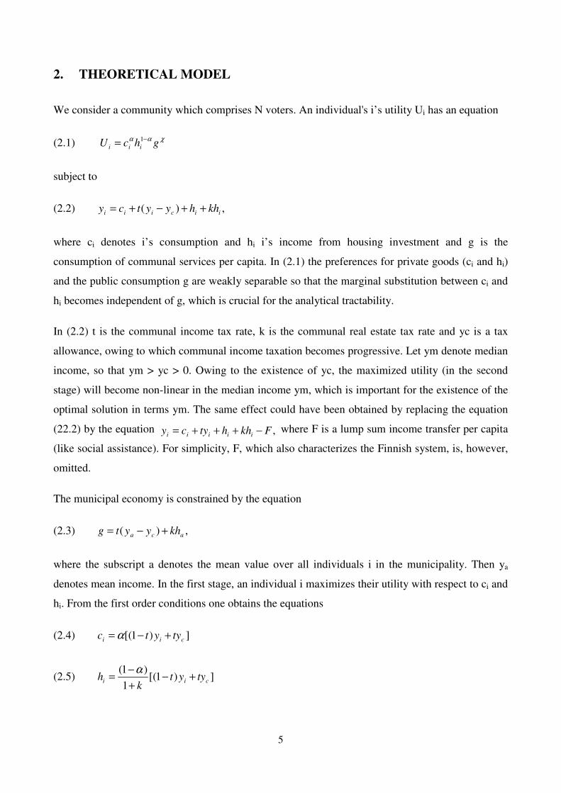
2. THEORETICAL MODEL

We consider a community which comprises N voters. An individual's i’s utility Ui has an equation

(2.1) χααghcU iii

−= 1

subject to

(2.2) ,)( iiciii khhyytcy ++−+=

where ci denotes i’s consumption and hi i’s income from housing investment and g is the

consumption of communal services per capita. In (2.1) the preferences for private goods (ci and hi)

and the public consumption g are weakly separable so that the marginal substitution between ci and

hi becomes independent of g, which is crucial for the analytical tractability.

In (2.2) t is the communal income tax rate, k is the communal real estate tax rate and yc is a tax

allowance, owing to which communal income taxation becomes progressive. Let ym denote median

income, so that ym > yc > 0. Owing to the existence of yc, the maximized utility (in the second

stage) will become non-linear in the median income ym, which is important for the existence of the

optimal solution in terms ym. The same effect could have been obtained by replacing the equation

(22.2) by the equation where F is a lump sum income transfer per capita

(like social assistance). For simplicity, F, which also characterizes the Finnish system, is, however,

omitted.

The municipal economy is constrained by the equation

(2.3) ,)( aca khyytg +−=

where the subscript a denotes the mean value over all individuals i in the municipality. Then ya

denotes mean income. In the first stage, an individual i maximizes their utility with respect to ci and

hi. From the first order conditions one obtains the equations

(2.4) ])1[( cii tyytc +−= α

(2.5) ])1[(1

)1(cii tyyt

kh +−

+

−=

α

,Fkhhtycy iiiii −+++=

6

for ci and hi. Using (2.3), (2.4) and 2.5) and assuming that the median-income individual – whose

income is ym – is the median voter whose preferences become the collective choice. The maximized

utility Wmax

can then be written in the form

(2.6) χααα ααα ]

)1(

)1)()1(()(][()1[()1()1( )1()1(max

k

tyytkyyttyytkW ca

cacm+

−+−+−+−+−= −− .

Maximizing Wmax

in (2.6) with respect to tax rates t and k, the following first order conditions are

obtained:

(2.7) 0)()1(

)1())1(()])1((

)1(

)1()()[( =−

+

++−++−

+

−+−−− cacmcacacm yy

k

ktyyttyyt

k

kyytyy

αχ

α

(2.8) 0))1(())1)((1()1()( =+−++−−−+−− cacaca tyyttyytkktyy χα

It is noteworthy that the income distribution (in the data considered) implies that ya > ym. Analysing

(2.7) and (2.8) it can be proved (the proof is presented in Appendix 1) that

(2.9) 0<mdy

dt and .0>

ady

dt

These results already imply that a decrease in ym given ya or an increase in (ya – ym ) given ya

increases income tax rate t. In other words, an increase in an inequality (the Meltzer-Richard

hypothesis) raises the tax rate. The fact that 0>ady

dt follows from the implicitly assumed positive

income elasticity of public services.

It also follows from (2.7) and (2.8) that

(2.10) 0>mdy

dk and 0<

ady

dk.

In the model considered, the real estate rate reacts in the opposite way to the change in ym to what

income tax rate t does. If inequality increases, the majority voter benefits from the shifting of the

tax burden from real estate taxation to income taxation.

7

Let yv denote the majority voter’s income. Insofar as, it has been assumed that yv = ym, where ym

is the medium income. Owing to a low voting rate, however, yv can be remarkably higher than ym.

Yet our theoretical model produces the following results

and ,

even if ym < ya < yv. According to this, an increase in yv or in yv – ya given ya would lead to a

decrease in the tax rate. In this case, an increase in yv does not necessarily reflect the fact that

income distribution (given the voting rate) becomes more dispersed. The lowering of the voting rate

alone may also raise yv. So, a decrease in tax rate t can be related to an increase in the voting power

of the wealthiest. So the original Meltzer-Richard hypothesis becomes revised.

In the empirical analysis of this study yv is unobservable. If ym is, however, close to yv, the

Meltzer-Richard hypothesis is valid. The larger the difference between ya and ym, the more the

majority voter shifts the burden of taxes onto the shoulders of the higher income community

members. Therefore the sign of dt/dym is negative. That yv may, however, differ remarkably from

ym creates a major problem of the empirical analysis. It is possible that, instead, ya is close to yv. In

this situation the hypothesis derived cannot then be necessarily verified when one uses ya and ym as

explanatory variables. It is then possible that the more ya rises in relation to ym, the more the

majority voter tends to decrease the tax rate in order to lighten his or her own tax burden. This could

turn the sign of dt/dya negative. To cope with this problem in the empirical analysis we control the

municipal voting rate, too. One can expect that the higher the voting rate is, the closer the observed

ym is to the unobserved yv so that the results (2.9) are valid.

Insofar as, we have assumed that municipalities are homogeneous in their preferences. This reflects

more or less a situation in which municipalities differ from each other only in the income distributions

but not so much in mean incomes. In fact, the differences in mean incomes are, however, remarkable.

This is relevant, because in Finland, too, the wealthiest citizens tend to rely more on private services –

especially in healthcare – which make them more reluctant to support the provision of public services.

This could reflect in the behaviour of majority voters in two ways. The higher the majority voter’s

income is, the less they prefer public services, which would lower the tax rate. In addition to that, the

higher the income of the other members in a municipality is, the less they demand public services. For

the self-interested majority this would create an opportunity for cost savings and the lowering of

income tax. The mean income represents the income level of others. Abstracted from income

0<vdy

dt0>

ady

dt

8

distribution effects, the municipalities with higher means would then fail to lower the municipal tax

rate. Suppose that an increase in ya decreasing χ in (2.1) could capture this effect. In Appendix 1 it is

shown that dt/dχ > 0 and that the sign of dk/dχ is ambiguous. In principal, it could then be possible

that an increase in the mean income makes the medium voter decrease the municipal tax rate, given

the income distribution (mean income minus median income).

3. DATA AND THE ESTIMATED MODEL

This study uses the panel data for 431 Finnish communes from the years 1995–2006. The income

distribution statistics of Statistics Finland provides information about the municipal level median

and mean income and gini coefficients. From the statistics for the economy of municipalities

provided by Statistics Finland (Finances and activities of municipalities and joint municipal boards)

we have obtained information about the municipal tax rates and income sources. Information about

municipalities’ population structure has been extracted from the population statistics of Statistics

Finland. In addition, various items of information about municipal features – such as population

density, industrial structure, and geographic characteristics – have been acquired from the statistics

provided by the Association of Finnish Local and Regional Authorities.3

In this study we focus on the determination of the municipal income tax rate (ctax). Being aware

that this tax interacts with real estate tax and its income, we control some municipal-level variables

which are thought to have an impact on real estate taxes. We also report estimates from a model

which includes three real estate tax tariffs, which determine taxes for land, permanent residence and

other buildings (mostly summer cottages). Municipalities can set these tariffs within certain limits.

These variables are regarded as endogenous.

For the municipal income rate tax (ctax) the simultaneous equation system (2.7)–(2.8) produces a

reduced form equation

(3.1) ia Xmedycctax 1111 )log( Π+++= βα .

Taking into account the impact of the voting rate we also estimate an enlarged equation

(3.2) ia Xvrvrmedmedycctax 132111 )*()log( Π+++++= βββα .

3

The data also includes information about households’ consumption habits at the municipal level which is obtained

from the consumption surveys of Statistics Finland. The municipal level variables from this data, however, were not

considered reliable.

9

Above

ya = mean income

ym = median income

med = log(ya) – log(ym )

vr = municipal voting rate

Xi = the vector of controlling variables

Estimating this model one can test whether inequality lowers the municipal tax rate. According to

the basic Meltzer-Richards hypothesis it is hypothesized that in (3.1) β1 > 0 and that α1 + β1 > 0. In

(3.2) these effects are contingent on the voting rate. So it is expected that if vr exceeds a certain

limit, β1 + β2vr > 0 and α1 + β1 + β2vr > 0.

To investigate the robustness of the results and to clarify the possible ambiguousness of the results

an alternative measure of inequality is also used. The variable med above is then replaced by

municipality-level gini coefficient (gini).

Out of the three real estate tax tariffs, the one that concerns permanent residence is analogous to the

housing tax which is analysed in the theoretical model. The tax is collected directly from the

community member on the basis of this tariff, unlike the rest of the real estate taxes. So we also

empirically investigate the determination of this tariff – denoted below restax – in the following

models:

(3.3) ia Xmedydrestax 1111 )log( Λ+++= λδ

(3.4) ia Xvrvrmedmedydrestax 132111 )*()log( Λ+++++= φλλδ .

On the basis of the theoretical analysis, we expect that in (3.3) δ1 < 0 and δ1 + λ1 < 0. It is possible

that the voting rate plays a central role here, too. If the medium income earner can use the majority

power only when the voting is high enough, it is possible that in model (3.4) λ1 + λ1vr < 0 and δ1 +

λ1 + λ1vr < 0 only if vr exceeds a certain limit.

In the basic models (3.1)–(3.2)4 the following variables are included in the vector Xi:

log of debt per inhabitant, euros

log of a municipality’s share of corporate tax revenue per inhabitant, euros

log of state aid per inhabitant, euros

4 Estimating models (3.3.) and (3.4.) the set of controllers is almost the same as in models (3.1.9 and (3.2).

10

log of mean of capital income in state taxation, euros

the share of population under 15 years

log of the size of population

YEAR = year dummies.

The first three financial variables above describe the municipality’s financial situation and are thus

closely linked to the needs to set the municipal income tax rate on an appropriate level. Indebtedness

is directly related to the municipality’s need to strengthen its economy by means of a high income tax

rate. Therefore the expected impact of this variable on ctax is positive. The municipality’s share of the

corporate tax income (collected by the state) variable tells us about substitutive incomes from other

sources. Its impact on ctax is assumed to be negative. The standards for state aid are determined by

the municipality’s age, income and industrial structure, being independent of the chosen income tax

rate. A large amount of state aid tells us that a municipality has economic problems and so has a need

to keep ctax on a high level. But, on the other hand, state aid as an income source is a substitute for

income tax revenue. Therefore the sign of its estimated effect on ctax is ambiguous.

The social assistance expenditure per inhabitant, whose standard is set by the state and which is

therefore primarily out of municipal-level control, was also included in the controlling variables.

Owing to a non-significant explanation, this variable was, however, omitted.

The hypothesized effect from the income distribution on the municipal tax rate was solved from the

two-equation model which included the setting of both the municipal tax rate and the municipal

level estate tax tariffs. Therefore it is relevant to also take into account the factors which impact on

the real estate tax income. The municipal level mean of capital income – which is not part of the tax

base in municipal income taxation – is a good proxy for the real estate tax base. The real estate tax

revenues are a substitute for income tax revenue and therefore it is expected that the impact of the

average capital income on ctax will be negative.

The underage population increases communal expenses and generates upward pressure on taxes.

The anticipated effect of the share of the population under 15 years on ctax is therefore positive.

The larger size of population is assumed to represent a greater potential to internalize the economies

of scope, which is thought to create an opportunity for savings on expenditure and therefore for a

lower municipal tax rate.

In the basic case, variables ya, med (= ya – ym) and the voting rate and all the other controlling

variables are treated as being exogenous. In this approach it is thus assumed that the mean income

11

and income distribution in a municipality and the municipality’s economy do not react in a

remarkable way to the municipal tax rate. The possible endogeneity of municipal level income

variables and fiscal variables concerning the municipality’s economy addresses the feed-back

mechanism which arises if a change in a municipal income tax rate affects income or fiscal

variables directly or indirectly, for example, through in- or out-commuting.

The fact that one does not regard the impact of in- and out-immigration on the municipality’s

economy as being remarkable in Finland (see Helin et al., 1998) supports the exogeneity assumption.

On the other hand, Kangasharju and Moisio (2006) have obtained a result according to which

neighbouring tax rates have a positive impact on a municipality’s income tax rate in Finland. This and

even more profound evidence of mimicking in tax-setting and spending decisions in England (see

Revelli, 2002) shows that the municipalities, however, in their decisions, take into account the

existence of some kind of feedback mechanism, which may work out through immigration. This

justifies the use of the method of instrumental variables in the estimation of models (3.1.) and (3.2). In

their empirical study concerning tax and fee setting in Norway Borge and Rattsö (2004) thought that

tax decisions had a response on other fiscal variables which had an effect on immigration and finally

on income distribution and mean income. To tackle the endogeneity problem, we estimate the model

with the instrumental variables approach using the two-stage GLS random effects estimator. To check

the robustness the results are also reported from OLS, fixed effects and GMM regression.

The choice of instruments was dictated by the nature of the variables. Describing geography, the

age structure of the population and the industrial structure, the variables are thought of as being

exogenous. Such variables were chosen as instruments which had an influence on endogenous

variables in the first stage estimation but whose direct impact on the explained tax rate in the second

stage was not remarkable. In the GMM estimation the validity of the over-identification restriction

was a central criterion for the choice of instruments.

Estimating models (3.1) and (3.2) with random effect IV regression the following instruments are

then used:

the share of population of 75 years and over

the share of population between 65 and 74 years

the number of summer cottages per permanent inhabitant

concentration rate (the share of those who live in population centres)

log of population density

workplace self-sufficiency

12

the share of industrial production and construction

the share of service production.

It turned out that, for example, the share of population of 75 years and over, which had a statistically

significant impact on some endogenous explanatory variables, had no impact on the tax rate. So this

variable as well as the share of population between 65 and 74 years is used as an instrument. Part of

the real estate taxes are collected from those who own summer cottages. In fact, summer cottages are

used as an instrument because they have a remarkable impact on real estate tariffs and real estate

income, which is an alternative income source for municipal income tax revenue. The instruments

mentioned so far vary within time, while the latter five instruments include only a cross-sectional

variation corresponding to the situation in the year 2004. These instruments describe a municipality’s

regional and industrial structure. These variables are thought to shape the municipalities’ income

structure and voting behaviour without having any impact on the taxing behaviour. It is remarkable

that the concentration rate variable may have high values, even if the density is low.

The with-one-year lagged dependent variable and endogenous explanatory variables are also used

as instruments.

Models (3.3) and (3.4) are estimated only with the instrumental variable approach. The summer

cottages are then regarded as an exogenous variable, but the other instruments are the same as in the

models in Table 2. The dependent variable is then the real estate tariff for the permanent resident.

The method is basically the same as in the estimation of models (3.1.) and (3.2).

4. RESULTS

The data which is used in the analysis is described in Table A1 in Appendix 2. The income distribution

is typically skewed to the right so that the income inequality variable (med) has positive values in

almost all cases. In fact, out of 4 925 observations only in four cases has med a negative value.

The results from the random effects panel data estimation – in which all the municipal level income

and financial variables are regarded as exogenous – are reported in Table 1. The estimation results

from the models – which do not include voting behaviour – in the first and fourth columns of Table

1 show that the difference between mean and median income (med) has an anticipated positive

impact on the municipal tax rate. The impact of mean income is, however, negative and not positive

as the theoretical model would suggest. The results can be interpreted to show that the municipal

13

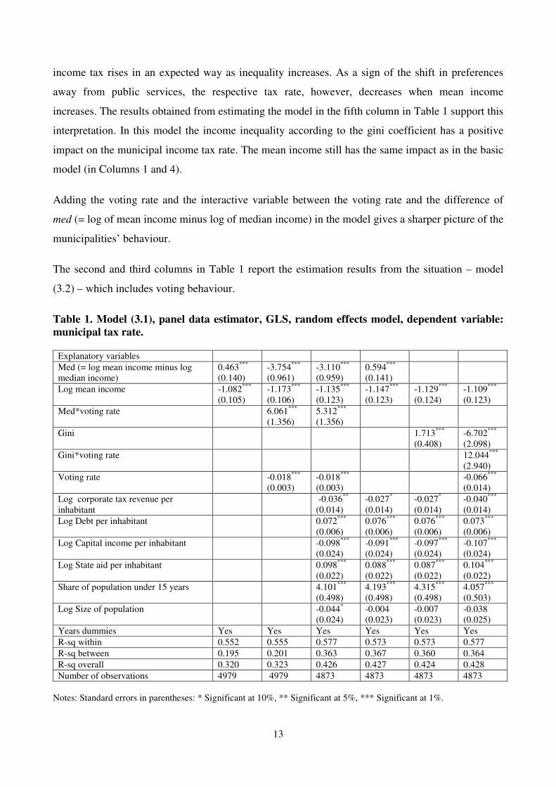
income tax rises in an expected way as inequality increases. As a sign of the shift in preferences

away from public services, the respective tax rate, however, decreases when mean income

increases. The results obtained from estimating the model in the fifth column in Table 1 support this

interpretation. In this model the income inequality according to the gini coefficient has a positive

impact on the municipal income tax rate. The mean income still has the same impact as in the basic

model (in Columns 1 and 4).

Adding the voting rate and the interactive variable between the voting rate and the difference of

med (= log of mean income minus log of median income) in the model gives a sharper picture of the

municipalities’ behaviour.

The second and third columns in Table 1 report the estimation results from the situation – model

(3.2) – which includes voting behaviour.

Table 1. Model (3.1), panel data estimator, GLS, random effects model, dependent variable: municipal tax rate.

Explanatory variables

Med (= log mean income minus log

median income)

0.463***

(0.140)

-3.754***

(0.961)

-3.110***

(0.959)

0.594***

(0.141)

Log mean income -1.082***

(0.105)

-1.173***

(0.106)

-1.135***

(0.123)

-1.147***

(0.123)

-1.129***

(0.124)

-1.109***

(0.123)

Med*voting rate 6.061***

(1.356)

5.312***

(1.356)

Gini 1.713***

(0.408)

-6.702***

(2.098)

Gini*voting rate 12.044***

(2.940)

Voting rate -0.018***

(0.003)

-0.018***

(0.003)

-0.066***

(0.014)

Log corporate tax revenue per

inhabitant

-0.036**

(0.014)

-0.027*

(0.014)

-0.027*

(0.014)

-0.040***

(0.014)

Log Debt per inhabitant 0.072***

(0.006)

0.076***

(0.006)

0.076***

(0.006)

0.073***

(0.006)

Log Capital income per inhabitant -0.098***

(0.024)

-0.091***

(0.024)

-0.097***

(0.024)

-0.107***

(0.024)

Log State aid per inhabitant 0.098***

(0.022)

0.088***

(0.022)

0.087***

(0.022)

0.104***

(0.022)

Share of population under 15 years 4.101***

(0.498)

4.193***

(0.498)

4.315***

(0.498)

4.057***

(0.503)

Log Size of population -0.044*

(0.024)

-0.004

(0.023)

-0.007

(0.023)

-0.038

(0.025)

Years dummies Yes Yes Yes Yes Yes Yes

R-sq within 0.552 0.555 0.577 0.573 0.573 0.577

R-sq between 0.195 0.201 0.363 0.367 0.360 0.364

R-sq overall 0.320 0.323 0.426 0.427 0.424 0.428

Number of observations 4979 4979 4873 4873 4873 4873

Notes: Standard errors in parentheses: * Significant at 10%, ** Significant at 5%, *** Significant at 1%.

14

The impact from the median incomes (ym) is then the sum of the coefficients of the med and the

interactive variable med*voting rates. For example, in the model in which the coefficients are

reported in the second column, log Ym has a negative impact on the municipal tax rate, if –

3.754*med + 6.061*(voting rate*med) > 0, which requires that the voting rate exceeds 61.9 per

cent. In the third column model the corresponding limit is 58.5 per cent. The model in the sixth

column includes an interactive variable between the gini coefficient and the voting rate. The gini

coefficient has an anticipated positive impact on the municipal income tax rate, if the voting rate

exceeds 55.6 per cent.

The average voting rate (from the years 1992, 1996, 2000 and 2004) has been 66.7 per cent, but the

population size weighted average has been only 61.7 per cent. This means that in several

municipalities, especially in larger municipalities, the medium income earner is not the majority

voter. In the models with an interactive variable the impact of the log of mean income could also

turn out to be positive (as we originally expected), if the voting rate is high enough. But the voting

rate should then exceed 78.4 per cent (second column model) or 79.9 per cent (third column model).

On average, the voting rate is above 78.3% in only 15 municipalities out of 431.

According to the coefficient estimates of the model in the third column of Table 1, the rise in the

voting rate will increase the municipal income tax rate, if 5.312*meds – 0.018 > 0. This requires

that meds > 0.003, which is almost always true in our data. This condition is not valid in only a few

cases out of almost five thousand. In the model in Column 2 this condition is even less restricted. In

the model which includes a gini-coefficient (Column 6) the voting rate raises the municipal income

tax rate, if the gini-coefficient is above 0.005, which is always true.

The impacts of financial variables correspond to our expectations. The corporate tax revenue

collected by the state is partly paid to municipalities. The obtained negative coefficient of this

variable corresponds to our expectations. If these revenues grow, the need to collect taxes by raising

the income tax rate is reduced. Capital income is not part of the income tax base, but it is a good

proxy for financial wealth and also for the real estate tax base. So, in municipalities with a high

mean of capital income the real estate tax revenues are also relatively large, which reduces the need

to collect income tax revenue. The negative coefficient of the capital income variable is thus rather

anticipated. State aid is a substitute income source for income taxes, which could lead one to expect

that the coefficient of this variable is negative. The positive coefficient may tell us that state aid is

not too generous and that the municipalities who are aided have financial problems. The negative

15

impact of debt on the income tax rate shows that highly indebted municipalities have to keep the

income tax rate at a high level.

The size of the population under 15 years of age increases expenditures and so also the tax rate.

That the size of the population has a negative impact points to the existence of scale economies in

producing municipal services.

Table 2 reports the results from the instrumental variables regression. Income variables, financial

variables about the municipality’s economy and the voting rate – variables from the 2nd to the tenth

rows in Table 2 – have been endogenized. The exogenous variables which, by their nature, are

thought as being independent of other variables in the model are the share of the population under

15 years of age and the log of the population size. The other population age variables did not turn

out to have statistically significant explanatory power in the second stage estimation. In the first

stage, endogenous variables were explained by exogenous variables and by additional instruments

which are the lagged values of endogenous explanatory variables and some variables about the

population and the industrial structure. The relevance of the first-stage instruments is satisfied

because each of them is statistically significant in several first-stage equations.

The results from the models in Table 2 are parallel with the results reported in Table 1. The mean

income still has a negative impact on the municipal income tax rate. That the impact from the

median income on the municipal income tax rate is negative – as expected – in the models in Table

2 (second and third columns) requires that the voting rate exceeds 68.2 and 61.4 per cent. Limits are

then a little higher than in the standard random effects regression in Table 1. The respective limit

for the log of mean income to have a positive impact on the tax rate is now 78.4 and 73.3 and so a

little lower than in the models reported in Table 1. The gini coefficient still has a positive impact

and with the respective interactive variable its positiveness rate hinges on the voting activity. It (the

model in the 6th column) now requires the voting rate to exceed 59.0 per cent. The IV regression

also yields the finding that the voting rate has a positive impact on the municipal income tax rate.

16

Table 2. Models (3.1) and (3.2.), second stage regression, G2SLS random effect IV regression, dependent variable: municipal tax rate, Income and financial variables instrumented.


Med (= log mean income minus log

median income)

-0.038

(0.256)

-10.161***

(2.134)

-6.698***

(2.145)

0.723**

(0.263)


(0.164)

-1.524***

(0.166)

-1.299***

(0.198)

-1.262***

(0.195)

-1.144***

(0.213)

-1.149***

(0.214)


(3.067)

10.915***

(3.085)

Gini 2.445***

(0.805)

-17.647***

(4.811)

Gini*voting rate 29.926***

(7.001)


(0.006)

-0.027***

(0.006)

-0.153***

(0.034)


inhabitant

-0.064**

(0.031)

-0.067**

(0.031)

-0.066**

(0.031)

-0.083***

(0.032)

Log debt per inhabitant 0.139***

(0.011)

0.143***

(0.011)

0.144***

(0.011)

0.139***

(0.011)

Log capital income per inhabitant -0.357***

(0.071)

-0.373***

(0.071)

-0.419***

(0.076)

-0.418***

(0.076)

Log state aid per inhabitant 0.019

(0.045)

0.004

(0.045)

-0.003

(0.045)

0.034

(0.045)

Share of population under 15 years 4.090***

(0.548)

4.046***

(0.548)

4.152***

(0.546)

3.825***

(0.556)

Log size of population -0.065**

(0.029)

-0.025

(0.026)

-0.020

(0.026)

-0.071**

(0.029)


R-sq within 0.554 0.554 0.562 0.556 0.552 0.557

R-sq between 0.223 0.222 0.420 0.435 0.430 0.416

R-sq overall 0.338 0.337 0.451 0.458 0.454 0.449



In the models in Table 2 the impacts of other controllers is almost the same as in the random effects

regression. Exceptionally, the positive impact of the state aid variable has disappeared.

Table A2 in the Appendix includes the estimation results from pooled data OLS regression and

panel data fixed effects regression. The results are mainly in line with the results reported in Tables

1 and 2. In the OLS models (2nd

column) the negativity of the median income variable, however,

requires that the voting rate exceeds 76.7 per cent, which is more than in the models in Table 1 and

2. In the fixed effects model (4th

column) the respective voting rate limit is 52.5 per cent and so

even lower than in the other models. On the whole, it is a little surprising that the fixed effect

estimates are so close to the previous estimates (reported in Table 1 and 2), because one could have

believed a priori that the within time variation of the fixed effects regression would not alone

specify the hypothesized effects of income distribution.

17

The estimation results from a dynamic model have been reported in Table A3 in appendices. In this

model it is thought that the municipal tax rate adjusts slowly. The inclusion of a lagged dependent

variable creates an endogeneity problem, and so the model is estimated using a dynamic panel

estimator known as a system GMMM estimator (see Roodman, 2009). This estimator is designed

for a situation with a small number of time periods and a great number of observed groups

(municipalities). The System GMM creates an equation system in levels and in first differences.5

The contemporaneous values of the municipal-level financial variables (log of corporate tax

revenue, log of debt, log of capital income and log of state aid) are specified as being endogenous,

while with one period lagged income variables and the voting rate (med, log mean income,

med*voting rate and voting rate) are classified as being predetermined variables independent of

current disturbances but influenced by past ones. Year dummies, the share of population under 15

years and the log size of population are considered as strictly exogenous variables which serve as

standard IV instruments. The choice of endogenous and predetermined variables is dictated by the

need to increase the significance of the model (F-test) without violating the joint validity of

instruments (according to the Sargent/Hansen test for over-identifying restrictions). For equations in

differences, the specified model uses, as instruments, exogenous variables and the lags of other

regressors (GMM instruments) in levels dated from t-1 up to t-3 (to restrict the number of

instruments). In the equations in levels the instruments are the respective first differences and also

the contemporaneous value of differenced predetermined variables. The results that are reported in

Table A3 show that the income variable med is insignificant in the model which does not include

voting behaviour. In the model with voting the central results are close to the results which are

reported in Tables 1 and 2. The median income decreases the municipal income tax rate when the

voting rate exceeds 66.4 per cent. For the mean income to have a hypothised positive impact on the

tax rate, the voting rate must be over 69.5 per cent. According to the AR tests, the presence of the

first-order autocorrelation cannot be rejected (as is expected) but, more importantly, the absence of

the second-order autocorrelation cannot be rejected either, which suggests that no residual serial

correlation is present in the models. The other test statistics of the model in the second column of

Table A3 indicate that the GMM and IV instrument subsets are valid jointly and apart6. The

5 The use of forward orthogonal deviations rather than first differences is motivated by the need to save observations

(see Roodman, 2009). 6 The Hansen test about ”excluding group” shows dropping out either GMM-instruments (the lagged values of

endogenous variables) or IV-instruments deteriorates the over-identification restrictions, so the instruments in question

can be regarded as valid. Similarly, the other test difference-in-Hansen test called “difference” shows that redefining

GMM- or IV-instruments as endogenous would create a loss to the over-identification restrictions (see Baum et al.,

2003).

18

instruments can be considered as relevant owing to their significance in the first-stage equations in

the G2SLS random effect IV regression whose results are reported in Table 2.

Table 3 reports the estimation results of models (3.3) and (3.4) in which the dependent variable is

the real estate tax tariff for permanent residence. The hypotheses derived would suggest that median

income had a positive impact and mean income a negative impact on the real estate tax rate. The

estimation results largely support this hypothesis, although in the IV regression the inclusion of

other controllers makes the impact of median income on the real estate tax tariff statistically not

different from zero. The behavioural pattern of the real estate rate tax for permanent residence

mirrors that of the municipal income tax rate as far as the impact of voting activity is concerned.

The voting rate thus seems to lower the real estate tax rate in question.

Table 3. Models (3.3) and (3.4), regular GLS random effect and IV (G2SLS) random effect regression, dependent variable: real estate tax tariff for permanent residence.

Explanatory variables Random effects (GLS) IV (G2SLS)

Med (= median income minus mean

income)

-3.351**

(1.140)

-0.580

(9.667)

-2.718*

(1.456)

-5.463**

(2.473)

-5.157

(20.791)

0.240

(2.669)


(0.944)

-7.473***

(0.955)

-6.799***

(1.238)

-7.913***

(1.219)

-9.671***

(1.265)

-9.241***

(1.979)

Med*voting rate -3.681

(13.656)

2.429

(2.992)


(0.028)

-1.898***

(0.544)

Log corporate tax revenue per inhabitant

-0.044

(0.149)

-0.855***

(0.316)

Log debt per inhabitant 0.341***

(0.066)

0.609***

(0.108)

Log capital income per inhabitant -0.095

(0.244)

-1.028

(0.708)

Log state aid per inhabitant 0.198

(0.229)

-0.687

(0.108)

Share of population under 15 years -2.969

(5.068)

-2.791

(5.563)

Log size of population 0.775***

(0.258)

0.953***

(0.207)

Log number of summer cottages

per inhabitant

0.378*

(0.201)

0.385*

(0.207)


R-sq within 0.535 0.541 0.539 0.538 0.542 0.537

R-sq between 0.086 0.086 0.158 0.085 0.090 0.171

R-sq overall 0.312 0.315 0.341 0.305 0.306 0.338



19

5. CONCLUSION

On the whole, the results obtained are finally in line with the results suggested by the theoretical literature

(see for example, Persson and Tabellini, 2002). Insofar as the tax setting is conditioned on the voting

performance, our results are, however, novel in the empirical literature. Although the theoretical

model of this study is, in some respect, similar to the model introduced by Borge and Rattsö (2004),

the empirical findings are not comparable. In their model, property tax plays the same role as the

municipal income tax in our model. Borge and Rattsö (2004) discovered that unequal income

distribution created a standard upwards impact on the property tax in their model in which the

Norwegian municipalities also finance their economy via a fixed utility charge. Our findings

indicate that in the Finnish system the median income earner tends to raise the municipal income

tax rate the harder, the larger the difference is between the mean income and the median income.

This is partly mirrored by the setting of the real estate tax tariff, which is, however, fiscally far less

important than income tax. We discovered that the validity of the Meltzer-Richard hypothesis in the

communal framework is, however, conditional on the voting rate. According to this, only if the

voting rate exceeds a certain limit – which is quite close to the average voting rate – does inequality

start to work in the direction expected. The larger inequality then raises the municipal income tax

rate. Furthermore, we found that increasing voting activity has a tendency to raise the municipal

income tax rate and lower the real estate tax rate for permanent residence.

LITERATURE

Alesina, A., Baqir, R. and Easterly, W. (2000), Redistributive public employment, Journal of

Urban Economics 48, 219–241.

Barnes, L. (2005), the Income distribution of voters – literature review and research plan,

Manuscript 21.12.2005.

Basset, W., Burkett, J. and Putterman, L. (1999), Income distribution, government transfers, and the

problem of unequal influence. European Journal of Political Economy 15, 207–228.

Baum, C., Schaffer, M. and Stillman, S. (2003), Instrumental variables and GMM: Estimation and

testing, Working Paper No. 545, Boston College.

Borge, L-E. and Rattsö, J. (2004), Income distribution and tax structure: Empirical test of Meltzer-

Richard hypothesis, European Economic Review 48, 805–826.

20

Frey, B.S. (1971), Why do high income people participate more in politics?, Public Choice 11, 101–

105.

Helin, H., Laakso, D., Lankinen, M. and Susiluoto, I. (1998), Migration and municipalities (in

Finnish: Muuttoliike ja kunnat), Kunnallisalan kehittämissäätiön tutkimusjulkaisut nro 15, Vam-

mala.

Jones, P.R. ja Cullis, J.G. (1986), Is democracy regressive?: A comment on political participation,

Public Choice 51, 101–107.

Kangasharju, A. and Moisio, A. (2006), Tax competition among municipalities in Finland, Urban

Economic Review numero 005, Universidade de Santiago de Compostela, 12–23.

Khan, M.J., Javid, A., Ahmed, U. and Farooq, S. (2009), Size of government spending and human

capital inequality: evidence from cross sectional and panel data analysis, European Journal of

Social Sciences 9, 300–322.

Meltzer, A.H. and Richard, S.F. (1981), A rational theory of the size of government. Journal of

Political Economy 89, 914–927.

Meltzer, A.H. and Richard, S.F. (1983), Tests of a rational theory of the size of government. Public

Choice 41, 403–418.

Perotti, R. (1996), Growth, income distribution and democracy: What the data say. Journal of

Economic Growth 1, 149–188.

Persson, T. and Tabellini, G. (2002), Political economics and public finance, in Auerbach, A. and

Feldstein, M. (eds.) Handbook of public economics – volume 3, Elsevier, New-York.

Revel, F. (2002), Testing the taxmimicking versus expenditure spill-over hypotheses using English

data, Applied Economic 34, 1723–1731.

Rodriguez, F.C. (1999), Does distributional skewness lead to redistribution? Evidence from the

United States, Economics and Politics 11, 171–199.

Roodman, D. (2009). How to Do xtabond2: An Introduction to "Difference" and "System" GMM in

Stata. Stata Journal 9(1): 86–136.

21

APPENDIX 1.

Let A denote the left hand side of the equation (2.7). Then

(a1) 0)()1(

)1()1)(( <−

+

++−−=

∂

∂cacm yy

k

kyy

t

A αχ

and

.0)1(

))(1(])1[(])(1[(

)1(

)1()(

22<

+

−−+−−+−

+

−−−=

∂

∂

k

yytyyttyyt

kyy

k

A ca

cmcacm

αχ

α

Using (2.7) the latter equation transforms into

(a2) .0)1)(1(

)1()(<

++

−−−=

∂

∂

kk

yyy

k

A acm

α

α

From (2.7.) one also obtains

(a3) 0)1(

)1(])1[()( <

+

−+−−−−=

∂

∂

k

kytyytyyyt

y

Accacca

m

α

and

(a4) .0)1)((

)1()( >

+−

−−=

∂

∂

kyy

kyyy

y

A

c

a

c

cm

a

α

The left hand side of the equation (2.8) is denoted by B; then

(a5) ,0])1[(

])1(1)[((<

+−

+−+−−=

∂

∂

ca

caca

tyyt

ktyytkyy

t

B

(a6) ,0])1)[(1()( <+−−−−−=∂

∂caca tyyttyy

k

Bα

(a6) 0=∂

∂

my

B

and

(a7) .0)1(2 <+−=∂

∂c

a

ykty

B

22

The necessary second-order conditions for this optimization problem – which maximizes Wmax

in

(2.6) – requires that 0<∂

∂

t

A, 0<

∂

∂

k

B and that .0>

∂

∂

∂

∂−

∂

∂

∂

∂

t

B

k

A

k

B

t

A The expressions (a1) and (a6)

show that the two first-mentioned conditions are valid. To prove that 0>∂

∂

∂

∂−

∂

∂

∂

∂

t

B

k

A

k

B

t

A is also

valid, we write this condition in the form

(a8)

.0)1)(1()(

])1(

)1())[(()(

)1)(1(

)]2(1[)1())((

>+−−+

++

+−−−+

++

+++−−−

γα

αα

α

αχααα

ccma

ccacmca

a

cacm

yyyy

yk

kyyyytyy

kk

kkkyyyyy

The inequality (a8) is valid and so the necessary second-order conditions are met.

Let us then explore the sign of mdy

dt and .

ady

dt These expressions can be written in the form

(a9)

t

B

k

A

k

B

t

A

k

B

y

A

y

B

k

A

dy

dt mm

m

∂

∂

∂

∂−

∂

∂

∂

∂

∂

∂

∂

∂−

∂

∂

∂

∂

=

and

(a10) .

t

B

k

A

k

B

t

A

k

B

y

A

y

B

k

A

dy

dt aa

a

∂

∂

∂

∂−

∂

∂

∂

∂

∂

∂

∂

∂−

∂

∂

∂

∂

=

The sign of the left-hand side in the equations (a1) – (a7) and the validity of (a8) guarantee that

0<mdy

dt in (a9) and that 0>

ady

dt in (a10).

The derivatives mdy

dk and

ady

dk have the expressions

(a11)

t

B

k

A

k

B

t

A

y

B

t

A

t

B

y

A

dy

dk mm

m

∂

∂

∂

∂−

∂

∂

∂

∂

∂

∂

∂

∂−

∂

∂

∂

∂

=

and

23

(a12) .

t

B

k

A

k

B

t

A

y

B

t

A

t

B

y

A

dy

dk aa

a

∂

∂

∂

∂−

∂

∂

∂

∂

∂

∂

∂

∂−

∂

∂

∂

∂

=

The sign of the left-hand side in the equations (a1) – (a7) and the fact that the denominator is

positive make us conclude that 0>mdy

dk in (a11) and that 0<

ady

dk in (a12).

Let us then explore the sign of χd

dt, which has an expression

(a13) .

t

B

k

A

k

B

t

A

k

BAB

k

A

d

dt

∂

∂

∂

∂−

∂

∂

∂

∂

∂

∂

∂

∂−

∂

∂

∂

∂

=χχ

χ

Above

(a14) 0)1(

)1())()1(( >

+

+−+−=

∂

∂

k

kyytyyt

Acacm

α

χ

and

(a15) .0)1( >+−=∂

∂ca tyyt

B

χ

Using the equation (2.8) it is obtained from (2.7) that

)1(

))1(()(

)1(

)1())()1(

kt

tyytyy

k

kyytyyt ca

cmcacm+

+−−=

+

+−+−

α.

Using this result and expressions (a14) and (a15), the numerator of (a13) can be written in the form

.0))())(1(()1)(1(

))1)(((>−+−−

++

+−−caca

cacm yykyytkk

tyytyyα

α

Because the denominator is positive as well, .0>χd

dt

It will turn out that the sign of χd

dkis ambiguous. With reasonable assumptions it will become

negative. The details of this analysis are not reported.

24

APPENDIX 2.

Data description and auxiliary estimations

Table A1. Descriptive statistics.

Variable (and explanation) Mean Stand. v. M Max

Municipal income tax rate 18.28 0.72 15.0 21.0

Median of nominal taxable income in municipal taxation 10453 2805 4393 23596

Mean of nominal taxable income in municipal taxation 12123 2861 6644 40562

Med (= log mean income – log median income) 0.159 0.077 -0.022 0.772

Gini coefficient of nominal taxable income in municipal taxation 0.477 0.037 0.390 0.719

Voting rate (Municipal elections were held in years 1992, 1996, 2000

and 2004. The voting rate e.g. in year 2000 is given also for years 2001,

2002 and 2003.)

65.1 6.8 45.6 89.5

Municipality’s share of the nominal corporate taxes per inhabitant, €

(These taxes are collected by the state.)

230 173 3 2809

Nominal debt stock per inhabitant, € (at the end of the year) 973 722 0.3 8650

Capital income per inhabitant (in state .ation), € 1334 986 232 26839

Nominal state aid per inhabitant, € (State aid is determined by the

commune’s geographical and economical characteristics and it also

implements the levelling of the commune’s computational (not real) tax

revenue)

1327

613 0.2 5689

Real estate tax tariff for permanent residence, % (This tariff is fiscally the

second most important.)

0.255

0.062 0.1 0.5

Size of population (at the end of the year) 11894 31098 233 564521

Share of population under 15 years 1

(Corresponds to the situation at the

end of the year.)

0.185 0.032 0.099 0.336

Share of population 75 years and over1 0.082 0.025 0.016 0.167

Share of population between 65 and 74 years1 0.101 0.022 0.030 0.180

Number of summer cottages per inhabitant 1042 892 0 6196

Urbanization rate (the share of those who live in population centres) 2 59.8 21.3 0 99.0

Log Population density2 2.61 1.38 -1.60 8.01

Share of industrial production and construction2

26.6 11.0 4.0 56.5

Share of service production2 56.3 10.2 29.1 90.3

Workplace self-sufficiency2 85.0 18.3 41.1 147.9

1The data includes information about the municipal age structure only from the years 1995, 1998, 2001 and 2006. The

missing observations for the rest of the years are obtained by linear interpolation.

2The same value, corresponding to the situation at the end of 2005, for all years

25

Table A2. Model (3.1) and (3.2), OLS and panel data fixed effects estimator, dependent variable: municipal tax rate.

Explanatory variables OLS OLS GLS, fixed effects GLS, fixed effects

Med (= log mean income

minus log median income)

-0.413***

(0.137)

-5.130***

(0.972)

0.775***

(0.157)

-2.262**

(1.003)


(0.083)

-1.015***

(0.087)

-0.886***

(0.181)

-0.801***

(0.180)


(1.395)

4.308***

(1.413)

Voting rate -0.003

(0.003)

-0.020***

(0.003)


inhabitant

-0.021

(0.017)

-0.004

(0.016)

-0.032**

(0.015)

-0.042***

(0.015)

Log Debt per inhabitant 0.173***

(0.008)

0.150***

(0.008)

0.066***

(0.006)

0.063***

(0.006)

Log Capital income per

inhabitant

-0.248***

(0.022)

-0.234***

(0.021)

-0.035

(0.025)

-0.050*

(0.025)

Log State aid per inhabitant 0.227***

(0.024)

0.184***

(0.023)

0.054**

(0.023)

0.064***

(0.023)

Share of population under 15

years

1.559***

(0.295)

2.233***

(0.295)

5.631***

(0.830)

5.521***

(0.829)

Log Size of population -0.054***

(0.010)

-0.051***

(0.011)

-0.156

(0.150)

-0.184

(0.149)

Years dummies Yes Yes Yes Yes

R-sq within 0.575 0.579

R-sq between 0.244 0.251

R-sq overall (adjusted R-sq) (0.487) (0.527) 0.353 0.360

Number of observations 4873 4873 4873 4873


26

Table A3. Model (3.2), system GMM estimators, dependent variable: municipal tax rate.


Municipal tax rate t-1 0.797***

(0.045)

0.737***

(0.047)

Medt-1 (= log mean income minus log median income) -0.048

(0.415)

-6.156*

(3.161)

Log mean incomet-1 -0.521***

(0.173)

-0.289

(0.198)

(med*voting rate)t-1 9.268*

(4.870)

Voting ratet-1 -0.001

(0.009)

Log Share of corporate tax revenuet per inhabitant -0.107**

(0.050)

-0.022

(0.053)

Log corporate tax revenuet-1 per inhabitant 0.002

(0.052)

-0.026

(0.051)

Log Debtt per inhabitant -0.027

(0.050)

-0.013

(0.059)

Log Debtt-1 per inhabitant 0.055

(0.051)

0.052

(0.056)

Log Capital incomet per inhabitant -0.282***

(0.093)

-0.289***

(0.095)

Log Capital incomet-1 per inhabitant 0.075

(0.100)

-0.033

(0.097)

Log State aid t per inhabitant 0.082

(0.104)

0.082

(0.104)

Log State aidt-1 per inhabitant -0.228**

(0.103)

-0.227**

(0.103)

Years dummies Yes Yes

AR(1), pr > z 0.000 0.000

AR(2), pr > z 0.462 0.749

Hansen test for over-identifying restrictions, prob > chi2 0.140 0.405

Difference-in-Hansen tests of exogeneity of instrument subsets:

GMM instruments for levels

Hansen test excluding group, Prob > chi2

Difference (null = instruments are exogeneous), Prob > chi2

0.459

0.012

0.558

0.144

IV instruments

Hansen test excluding group, Prob > chi2

Difference (null = instruments are exogeneous), Prob > chi2

0.117

0.433

0.216

0.915

Number of observations 4431 4431


Government & Nonprofit

The impact of inequality on the municipal income tax in Finland