Eleftherios GiovanisUniversity of Verona, Department of Economics, Italy

Oznur OzdamarAdnan Menderes University, Aydın Faculty of Economics, Department of Econometrics, Aydın, TurkeyBologna University, Department of Economics, Italy

Empirical Applications of Collective Household Labour Supply Models in Iraq

• Motivation and Aim of the Study• Previous Research• Data and Methodology• Empirical Results• Conclusion and policy implications

Outline

• Household resource allocation and labour supply have been always a subjectof economics and have been long studied. Various theories have beendeveloped in an attempt to identify the patterns where household membersparticipate in the labour market and share the resources maximising theirutilities.

• Previous theoretical studies initiated with Chiappori (1988; 1992), employ theconceptual framework of utility in order to analyse the process of choosingthe labour supply level by the household members.

• The primary idea is that the labour-working hours supplied by each memberis that it depends its own age, education, wage and other characteristics ordistribution factors.

Motivation and Aim

• Household is often used as the main unit of analysis in many economic andpolicy studies, including labour supply, inequality and poverty.

• The unitary model treats the household in the analysis like an individual whomaximises his/her utility. In this case the household is considered as oneentity which interacts only with the outside world economy and society.

• The unitary model therefore, does not meet the condition of theindividualism because the household members are not characterised only bytheir own utility functions or preferences, but their choices and utilitiesdepend also on the characteristics of the other household members.

Motivation and Aim

• This can be harmful for policy making, especially for the welfareindicators and policies targeting inequality and poverty which may havecontradictory results and consequences when they are based on theunitary model analysis.

• Chiappori (1988) proposed a household collective model, where thedecisions and choices of the individuals depend also on the preferences,choices and characteristics of the remained household members.

Motivation and Aim

• However, there is still a small relatively number of empirical studiesespecially in the countries of the MENA region. This project attempts tocontribute to the previous research in the field of the householdcollective labour supply and intra-household resource allocation in Iraq.

• More specifically, the study aims to answer how the household choicesof labour supply and resource allocation are made, based on thespouses’ characteristics, household characteristics and distributionfactors.

Motivation and Aim

• The limitation of the previous studies is the assumption made that the time outside the market is pure leisure (Chiappori, 1988; 1992, Fortin and Lacroix, 1997; Chiappori et al., 2002). The exception is the study by Rapoport et al. (2011) who have included also the household domestic production by examining the sharing rule on household decision making regarding both time allocation and sharing on market and household time.

• Moreover, this study expands the empirical findings of Rapoport et al.(2011) by exploring the disability as an additional distribution factor

Motivation and Aim

• The second aim of this project is to apply the innovative approach by Kalugina et al., (2009) where the model takes into consideration the household production and the self-reported life satisfaction in relation with the sharing rule that governs the bargaining process in the household.

• Using self-reported data can be useful to derive not only the derivatives of the sharing rulebut also the individual share of the household full income Kalugina et al., (2009). The studyby Mangiavacchi and Rapallini (2009) employed self-reported life satisfaction data in Italiancouples, and they found that it is possible to derive the sharing rule and to explore therelevance of the spouses’ wages in the bargaining process.

• A similar approach is followed in this study; however the life satisfaction is treated as alatent variable since it is an unobservable and various other self-reported satisfactionvariables will be included in order to estimate a structural equation model (SEM) to accountfor the plausible measurement error of the life satisfaction and the simultaneity process inthe labour supply.

Motivation and Aim

• In the first category, the studies are based on the “added worker effect” where the mainidea is that the unemployment of the husband raises the probability that the wife will enterthe labour market. In a study by Lundberg (1988) employment transition probabilitiesestimation for the sample 1,081 families from the Seattle and Denver Income MaintenanceExperiments (SIME/DIME) using monthly frequency are employed. Lundberg (1988) foundthat the husband’s unemployment raises the probability of the average wife to enter thelabour market by 25 per cent, while it lowers the probability that she will leave the job by33 per cent compared to the case when the husband is employed.

• Maloney (1991) used data derived by the Panel Study of Income Dynamics (PSID) in 1982for 1,958 married couples in USA. The main findings show that husband’s unemployment,on average, is not significantly associated with the probability that his partner will enter thelabour market. However, on the other hand, in the case where the husband is permanentlyunemployed, the reservation wage of the wife is reduced and the probability for her toswitch to employment is increased.

• In another study by Duguet and Simonnet (2004) it is argued that the “added worker effect”can be an issue related to demographical factors, such as the number of the children, ratherthan being associated to unemployment characteristics. Using data from 5,425 couples inFrance they found that the labours supply of the husband is increased when a child is born,while the wife tends to reduce the working hours.

Previous Research

• The second group includes studies that are based on the unitary model. Beforeproceeding to the previous literature review it is important to notice that Becker(1981) was probably the first that formalized the household behaviour within theextension of the neoclassical consumer demand models to families.

• Nevertheless, Samuelson (1956) before Becker has already employed the householdwelfare function to express social indifference curves. Therefore, considering andcombining the frameworks by Samuelson and Becker, the household is assumedthat attempts to maximise a joint welfare function where the marginal rate ofsubstitution is equal across all the pairs of the goods.

• The unitary model treats the household to behave in the same way as individualdoes implying that the neoclassical consumer theory axioms and assumptions canbe applied (Vermeulen, 2002). However, neoclassical consumer theory applies onlyto individuals and not to groups.

• Moreover, according to the Arrow’s Impossibility Theorem group preferencerelations do not necessarily behave in the same way as those for the individuals andtherefore they cannot be modelled in the same fashion (Browning and Chiappori,1998).

Previous Research

• In terms of formal theory, the unitary model of household behaviour resultsin the testable restrictions of Slutsky symmetry, income pooling and thenegativity of price responses on demand systems (Browning et al, 1994).

• The Slutsky symmetry requires that there is symmetry in the compensatedcross wage effects of the different household members in terms of laboursupply (Fortin and Lacroix, 1997).

• The income pooling hypothesis, is a condition where the household resourcesincluding the non-labour income, labour, capital and land are pooled togetherand this condition states that the source of the non-labour income has notabsolutely influence in the household allocation maximization problem .TheIncome Pooling Hypothesis has been strongly questioned in this literaturesince several studies have found empirical evidence against it (Bourguignon etal., 1993; Fortin and Lacroix, 1997).

Previous Research

• Many studies have been employed using collective models in order toexamine the consumption allocation and to test the income pooling(see for examples Chiappori , 1988, 1992; Lundberg et al., 1997;Chiappori et al., 2002; Attanasio and Lechene, 2002; Blundell at al.,2005, 2007).

• The study by Lundberg et al. (1997) exploited a policy change in theUnited Kingdom that essentially redistributed a substantial child benefitfrom husbands to wives in the late 1970’s. Under the income poolinghypothesis, a change in the nominal recipient of a transfer should haveno effect on household demands. However, the authors found a greaterexpenditure on women’s and children’s clothing after the change,rejecting the income pooling hypothesis.

Previous Research

• Another study is by Blundell et al. (2007) who estimated a collectivelabour supply model of married couples without children, using datafrom UK Family Expenditure Survey during the period 1978-2001. Theauthors developed a model in which women choose whether to work ornot and how many hours, while for men is assumed that they chooseonly whether to work or not. The study rejects the unitary model andthe main findings suggest that the labour supply of female depends onthe male wage when the husband is not working which is consistentwith the bargaining interpretation. An increase in male’s wage when heis working, is associated with reductions in the female’s labour supply,which is consistent with the income effect because increases in themale wage increase also the total household income and the wife’s non-labour income.

Previous Research

• To what extent do individual preferences, characteristics anddistribution factors affect the household labour supply and what is thesharing rule in married couples in Iraq?

• Is the collective model applicable for the prediction of household labour supply choices relatively to the unitary model in Iraq?

• How the intra-household resource allocation is mapped with disabled family members?

• How the sharing rule is derived using self-reported life satisfaction data?

Main questions

Methodology

z 'lnlnlnln 543210 asayawwawawaah mfmff

z'lnlnlnln 543210 bsbybwwbwbwbbh mfmfm

(1)

(2)

• For this study, the Iraq Household Socio-Economic Survey (IHSES) that tookplace in Iraq during the period 2012-2013 is used.

• IHSES is a household survey programme which aims to produce high qualitydata, improved survey methods and it has been risen from the need toimprove the statistical data at the household level which are required fordesign, analysis, implementation and evaluation of the social policies indeveloping countries.

• The first survey has been taken place in 2007; however is not employed inthis study for the main reason that time use on labour supply and householdproduction, as well as, on life satisfaction is not available.

• The IHSES sample has been explicitly stratified by Gadah (district) and asample size of 216 households per Gadah was proposed, equivalent to a totalsample of 25,488 households for the country. The final sample size is 24,944households and 176,042 individuals.

Data

Variables Average Standard Deviation Minimum Maximum

Panel A: Spouses characteristics

Female Wage (in 1,000 ID) 17.317 37.268 0.16 1,220

Male Wage (in 1,000 ID) 19.639 36.884 0.24 1,360

Female Age 35.840 9.938 18 68

Male Age 38.372 10.435 18 70

Female Education 3.592 1.066 1 5

No-certificate -Illiterate 6.44% Elementary school 13.20%

High School 7.25% University Degree 60.85%

Postgraduate and Higher Education 12.26%

Male Education 2.458 2.312 1 5

No-certificate -Illiterate 25.29% Elementary school 41.17%

High School 6.81% University Degree 15.89%

Postgraduate and Higher Education 10.84%

Female Time Use on Household Chores 3.391 1.608 0 8

Male Time Use on Household Chores 0.226 0.6586 0 6

Female Time Use on Caring of Children and Elderly 1.945 1.791 0 7

Male Time Use on Caring of Children and Elderly 0.479 0.8917 0 5

Female Time Use on Labour Market 3.749 2.719 0 12

Male Time Use on Labour Market 6.889 2.977 0 13

Female Time Use on Leisure 1.4440 2.272 0 7

Male Time Use on Leisure 1.5204 2.492 0 8

Panel B: Household Characteristics

Non-Labour Income 2,769.971 10.862,33 0 240,000

Number of Children 0-5 years old 3.6231 2.261 0 9

Number of Children 6-15 years old 0.3941 0.6330 0 5

Urban Area 0.4677 0.4989 0 1

Has the household experienced shock (i.e. income, assets, weather) 0.0160 0.1258 0 1

Table 1. Summary Statistics

Labour Supply Domestic Production Labour Supply and Domestic Production

Variables Men Women Men Women Men WomenLog of female rate ln wf 3.7103

(2.4079)2.4102**(1.156)

0.5973(0.3881)

-1.1169*(0.5611)

0.2388(1.7957)

1.3461*(0.0722)

Log of male wage ln wm 2.1684*(1.1089)

-3.2497**(1.5261)

-1.1671***(0.0557)

3.9352 (3.1776)

1.0679**(0.4820)

3.8798(4.4483)

Interaction of spouse’ wages ln wmln wf 0.7036**(0.3461)

0.7246**(0.3407)

0.7304**(0.3493)

0.8698*(0.4671)

0.2200(0.5870)

0.7668**(0.3454)

Non-labour income (y) -0.0250(0.0210)

-0.0381**(0.0178)

0.0282**(0.0139)

0.0580*(0.0302)

-0.0210(0.0560)

0.0220**(0.0102)

Age difference between male and female 0.0330***(0.0114)

-0.0327***(0.0109)

0.0148*(0.0086)

0.0203**(0.0092)

0.0432**(0.0213)

0.0316**(0.0137)

Difference in male and female education 0.2969***(0.1050)

-0.0767(0.0970)

0.0380(0.2983)

0.3252** (0.1537)

-0.0437(0.0832)

-0.0055(0.0170)

Number of children 0-5 years old -0.2037**(0.0992)

-0.4098***(0.1410)

0.6351**(0.2960)

1.5618*(0.8143)

-0.1072(0.1413)

1.4020**(0.6332)

Number of children 6-15 years old 1.1099**(0.0539)

-0.4504(0.3342)

-1.0525**(0.5258)

-0.3068(0.2686)

-1.1239**(0.5025)

-0.1656(0.1835)

Non-Disabled Female 2.9634(1.8824)

2.3189**(1.1034)

-3.5039*(2.0677)

3.1701*(1.6622)

-2.0336*(1.1562)

6.0435**(2.9093)

Non-Disabled Male 1.6070**(0.0752)

1.7837(2.1931)

3.8894**(1.6438)

0.2576(0.4250)

5.3521**(2.5642)

-5.4160(4.2073)

Income-Asset Shock (No) -2.1257***(0.7111)

0.2073(1.300)

-0.6431(0.8012)

0.8965(1.7724)

-1.2839(1.1822)

0.3894(1.4223)

Urban Area 1.7789 (1.3463)

-3.490***(1.176)

-0.8840(1.3947)

0.8440(2.2107)

-1.9645(1.2421)

1.1593(0.8903)

No. observations 986 986 986 986 986 986

Endogeneity test 5.4083[0.2303]

5.8157[0.1209]

2.6673 [0.4458]

Table 2. GMM Estimates of the Labour Supply and Domestic Production Equations (1)-(2)

Standard errors within brackets, p-values within square brackets, ***, ** and * denote significance at 1%, 5% and 10%.

Labour Supply Labour Supply and Domestic Production

φ/x φ/x

wf 0.1290*(0.0652)

0.2130(0.1556)

wm 0.3242**(0.1410)

0.3953**(0.1751)

Non labour income 0.3521**(0.1594)

0.3862**(0.1701)

Age difference between male and female

0.0062*(0.0034)

0.1003**(0.0434)

Difference in male and female education

0.2163*(0.1162)

0.4944(0.3885)

Collective rationality chi-square test 1.514[0.690]

1.7322[0.546]

Table 3. Estimation of the Sharing Rule

Standard errors within brackets, p-values within square brackets, ***, ** and * denote significance at 1%, 5% and 10%.

.4.4

5.5

.55

.6La

bour

Sup

ply

Shar

e H

ours

0 .2 .4 .6 .8 1Women Wage Share

Women Share Men Share

Figure 1. Labour Supply Share in Hours and Women Wage Share

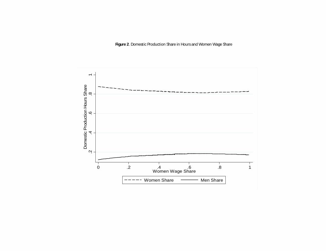
Figure 2. Domestic Production Share in Hours and Women Wage Share

.2.4

.6.8

1D

omes

tic P

rodu

ctio

n H

ours

Sha

re

0 .2 .4 .6 .8 1Women Wage Share

Women Share Men Share

• Regarding the number of the children, both men and women are more likely to reduce thelabour supply for children who are 0-5 years old which may be associated with the fact thatthe spouses devote more time for their caring and less time on labour market.

• On the other hand, the effect of the number of children 6-15 years old is positive andsignificant on the labour supply for males.

• For those households that have not experienced any income or assets shocks because of anexogenous event, such as economic crisis, drought, livestock loss and others, men spendless time on labour market.

• Regarding disability, the results show that non-disabled men have no effect on female’slabour market supply, while the non-disabled women are more likely to work more hoursper day than the disabled women.

• Similarly, non-disabled men spend more hours in the labour market than their disabledcounterparts, while the non-disability status of females does not influence males’ labourmarket supply.

Empirical Results

• Non-disabled spouses spend on average more time on domesticproduction on average more by 3 and 4 hours respectively for womenand men.

• On the other hand, the disability status of men does not influencewomen domestic production supply, while men whose spouse is non-disabled spend less time on domestic production, since their spouse ishealthy can capable to contribute to household production.

Empirical Results

• The sharing rule of a one ID increase in the non-labour income, increases the share of female by 0.35 and 0.38 considering respectively the labour supply and the total working supply-labour market plus the domestic production.

• The partial derivative of male’s wage is 0.2130 but it is statistically insignificant.

• On the other hand, the partial derivative of the female’s wage is 0.3953 and significant, indicating that the female can claim the 39 per cent of the non-income.

Empirical Results

• Non-disabled men spend on average 5 more hours than their disabledcounterparts on the total labour supply, similar to the non-disabledwomen- are able to work more hours on labour market and at the sametime to contribute more in the domestic production.

• The share of women on the full income who are non-disabled is higherby 0.3 than the disabled women.

Empirical Results

);,,()1();,,(max,,,,,

zz mmmmffffYCLYCLYCLUYCLU

mmmfff

),,( pwwyTwTwpYpYCCwLwL fmfmfmfmmff

s.t

The household production technology function for Y is characterised by:

);,( zkm

kf

kk ttFY

mmfftttwtwpY

mf

,

max

mfiforzYCLU iiiYLC

iiii

,);,,(max,,

iiiii pYCwL

TthL iii

s.t

zz ;,,,,, sywwwLL mffff

zz ;,,,,, sywwwLL mffmmm

The Marshallian demand functions can be defined similarly to the labour supply functions in sections 3.3 as:

Following the definition by Mangiavacchi and Rapallini (2009) it will be:

mfmff ifyTww 21

mfmff ifyTww 21

mfmff ifyTww 21

The index of inequality I is defined as:

kif

kkif

kif

I

f

f

f

*

2*

1

1*

,2

,1

,0

The index I will take value 0 I=0 if φf< φm, I=1 if φf = φm and I=2 if φf > φm .

The sub-sample of the couples who declare the same level of the life satisfaction and thus assuming the partners share the same amount of the total full income, it will become:

yTww mfmf 21

Structural Equations LS: Women LS: Men Index of InequalityDifference in Wages Between Male and Female -0.0084***

(0.0003)Log of Female Wage -0.8561***

(0.0171)0.6101

(0.0079)Log of Male Wage 1.1782**

(0.4578)-1.1279**(0.4553)

Male Age 0.0133***(0.0023)

Male Age Square -0.00013***(2.13e-06)

Female Age -0.0194***(0.0021)

Female Age Square 0.0003(0.0032)

Difference in Education between Male and Female 0.0378**(0.0164)

-0.0035**(0.0016)

-0.0291***(0.0017)

Difference in Age between Male and Female -0.0166***(0.0002)

Non-Household Labour Income 1.11e-03*(5.77e-04)

Time Use of Female’s Leisure 0.0307***(0.0024)

Time Use of Male’s Leisure -0.0087***(0.0024)

Number of Children 0-5 years old 0.0339***(0.0107)

0.0211***(0.0074)

0.2443**(0.1185)

Number of Children 6-15 years old -0.0089**(0.0044)

-0.0404(0.0871)

-0.1077***(0.0125)

Disabled Female Partner (No) 0.1971***(0.0710)

-0.0687**(0.0342)

0.0643***(0.0086)

Disabled Male Partner (No) 0.2245**(0.1022)

0.0318(0.0236)

-0.1251***(0.0071)

Urban Area -0.0320(0.0479)

0.0082(0.0100)

-0.0123(0.0090)

Income-Asset Shock (No) -0.1148(0.1865)

-0.0108(0.0264)

0.0114(0.0358)

No. Observations 976Standard errors within brackets, p-values within square brackets, ***, ** and * denote significance at 1%, 5% and 10%.

Table 4. Three-Stage Least Squares for Partners’ Total Labour Supply Equations

Structural Equations Log of Sharing RatioVariables Coefficients

Log of Female Wage 0.0177***(0.0016)

Log of Male Wage -0.0207***(0.0016)

Non-Labour Income 0.0110*(0.0058)

Age Difference Between Male and Female -0.0014***(0.0003)

Education Level Difference Between Male and Female -0.0076***(0.0021)

Number of Children 0-5 years old 0.0032***(0.0010)

Number of Children 6-15 years old -0.0064**(0.0028)

Disabled Female Partner (No) 0.0774***(0.0162)

Disabled Male Partner (No) -0.0831***(0.0092)

Urban Area 0.0315***(0.0041)

Income-Asset Shock (No) -0.0843***(0.0127)

No. Observations 986R Square 0.5037

Standard errors within brackets, p-values within square brackets, *** and * denote significance at 1%, and 10%.

Table 5. Weighted OLS estimation of the Sharing Rule

• An increase of one percent in the female wage rate results to woman’sshare increase by 1,500 ID, while the respective percentage pointincrease in male’s wage decreases her share by 1,800 ID.

• Regarding the disability, the women who are not disabled enjoy a highershare by 0.2974 more than their disabled counterparts, while the menhave a share of 0.6198 more than the disabled men.

• An increase of 1 ID in non-labour income results to increases onwoman’s share by 0.395. On the other hand, increases in the number ofchildren 6-15 years old and the age and education difference betweenmales and females decreases the woman’s share on full income.

Empirical Results

• The income share is an important distribution factor, because policy can alter this variable.

• However, one can easily conceive of a model in which resources are pooledbut the allocation of expenditures between household members depends onsome DF’s other than income.

• The collective model is important for policy implications. The bargainingmodel can be tested using policy reforms that target transfers, like childbenefits or allowances, towards mothers.

• Individual preferences over private and public consumption is crucial for thepurposes of analyzing the welfare implications of policy reforms and forunderstanding issues such as child poverty.

• This is also important in the policy agenda both in developed and indeveloping countries since governments are particularly concerned aboutdelivering benefits to children, such as schooling or nutrition subsidies

Policy Implications