Difference-in-Difference

MethodsDay 2, Lecture 1

By Ragui Assaad

Training on Applied Micro-Econometrics and Public Policy Evaluation

July 25-27, 2016

Economic Research Forum

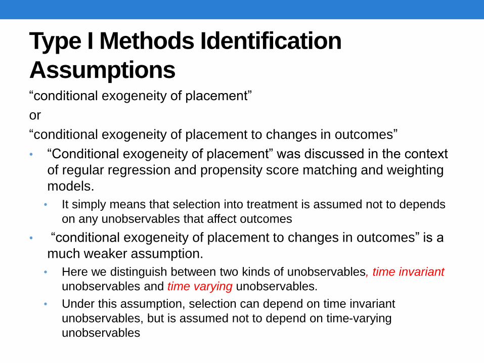
Type I Methods Identification

Assumptions“conditional exogeneity of placement”

or

“conditional exogeneity of placement to changes in outcomes”

• “Conditional exogeneity of placement” was discussed in the context

of regular regression and propensity score matching and weighting

models.

• It simply means that selection into treatment is assumed not to depends

on any unobservables that affect outcomes

• “conditional exogeneity of placement to changes in outcomes” is a

much weaker assumption.

• Here we distinguish between two kinds of unobservables, time invariant

unobservables and time varying unobservables.

• Under this assumption, selection can depend on time invariant

unobservables, but is assumed not to depend on time-varying

unobservables

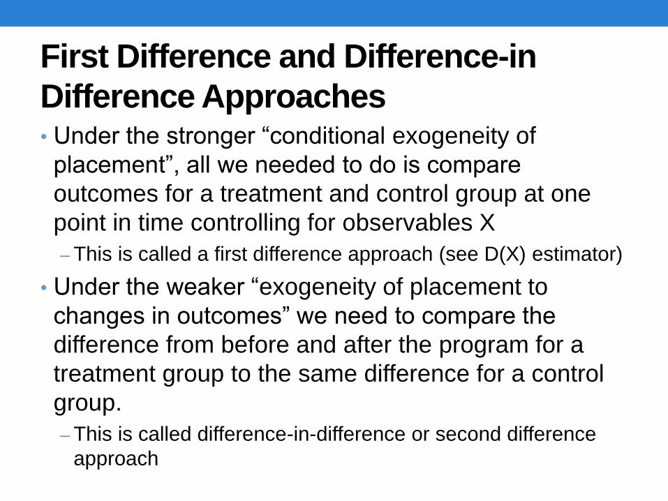
First Difference and Difference-in

Difference Approaches• Under the stronger “conditional exogeneity of

placement”, all we needed to do is compare

outcomes for a treatment and control group at one

point in time controlling for observables X

– This is called a first difference approach (see D(X) estimator)

• Under the weaker “exogeneity of placement to

changes in outcomes” we need to compare the

difference from before and after the program for a

treatment group to the same difference for a control

group.

– This is called difference-in-difference or second difference

approach

The Identification Assumption

Graphically

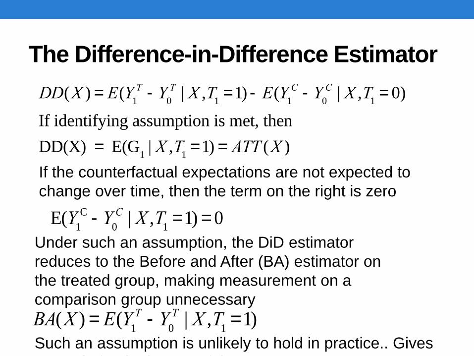
The Difference-in-Difference Estimator

DD(X ) = E(Y1

T -Y0

T | X ,T1=1) - E(Y

1

C -Y0

C | X ,T1= 0)

If identifying assumption is met, then

DD(X) = E(G1| X ,T

1=1) = ATT (X )

If the counterfactual expectations are not expected to

change over time, then the term on the right is zero

E(Y1

C -Y0

C | X ,T1=1) = 0

Under such an assumption, the DiD estimator

reduces to the Before and After (BA) estimator on

the treated group, making measurement on a

comparison group unnecessary

BA(X ) = E(Y1

T -Y0

T | X ,T1=1)

Such an assumption is unlikely to hold in practice.. Gives

you only for the impact of the program

Data Structures for DiD Estimation

When we have multiple observations on the same units, we

effectively have panel data

• Panel data can come in a number of different shapes

• Let’s talk about shapes with a person-time period

structure (say, before and after)

• “Long” data: an individual shows up twice, once in time period 0

and once in time period 1. An observation is an individual in a time

period

• “Wide” data: an observation is a person, and there are different

variables for each time period

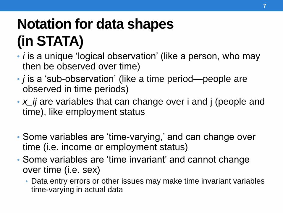
Notation for data shapes

(in STATA)• i is a unique ‘logical observation’ (like a person, who may

then be observed over time)

• j is a ‘sub-observation’ (like a time period—people are observed in time periods)

• x_ij are variables that can change over i and j (people and time), like employment status

• Some variables are ‘time-varying,’ and can change over time (i.e. income or employment status)

• Some variables are ‘time invariant’ and cannot change over time (i.e. sex)• Data entry errors or other issues may make time invariant variables

time-varying in actual data

7

Long Data: An Example

• An observation is a

person (id=i) in a

year(=j)

• A person has multiple

observations (multiple

years)

• inc (income) is time

varying (x_ij)

• Sex is time invariant

8

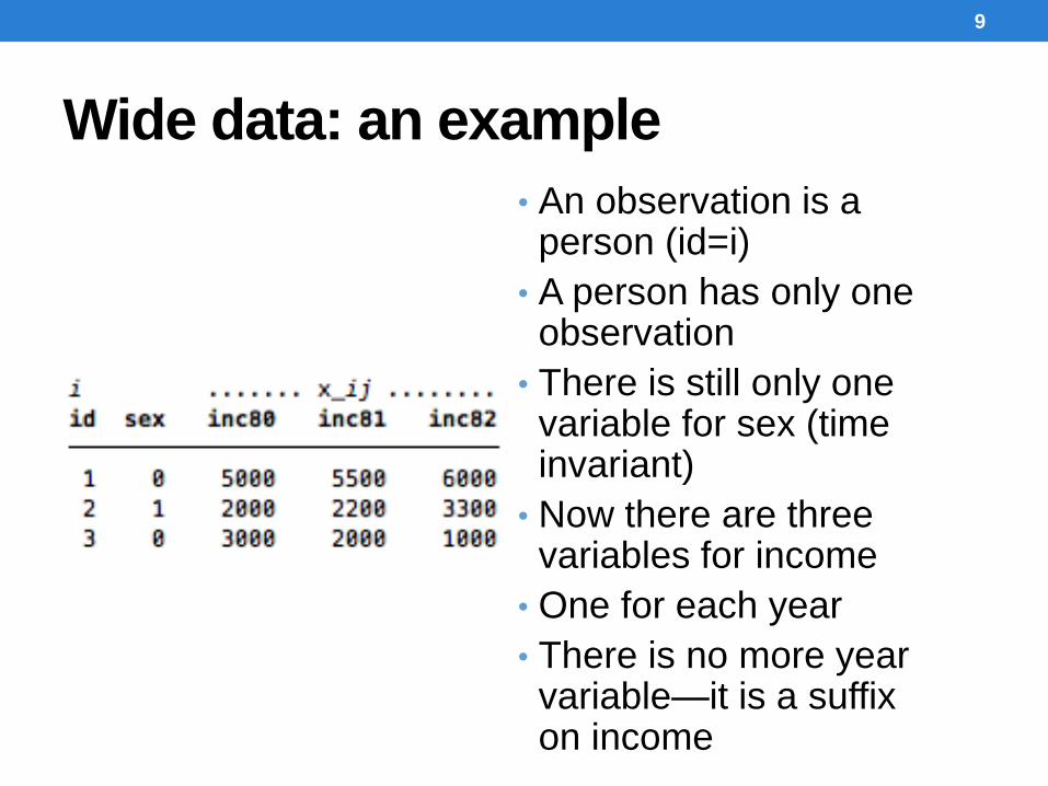
Wide data: an example

• An observation is a person (id=i)

• A person has only one observation

• There is still only one variable for sex (time invariant)

• Now there are three variables for income

• One for each year

• There is no more year variable—it is a suffix on income

9

Reshaping Data from Long to Wide

and vice versa

• You can use the “reshape” command in STATA

to reshape data from long to wide and vice

versa.

• However before you do that, you need to know

what form your data is in.

• The “duplicate report” command on the unique

individual identifier can allow you to do that.

Estimating the DD Estimator in Practice:

The Regression Approach

• Shape the data up as “long”, with each observation being an individual i time

period t

• Run a regression of the outcome (Yit) on the treatment status (Ti1), a time

dummy (t) (t=0, before, t=1, after) (Ti0 = 0, by definition)

Yit

=a +bTi1t +gT

i1+dt +e

it

Calculate the following expectations:

E(Yi0

|Ti1

= 0) =a

E(Yi1

|Ti1

= 0) =a +d

E(Yi0

|Ti1

=1) =a +g

Note: We can ignore the X’s since this regression does not et have

covariates. I also dropped the T and C superscripts since we only

observed treatment for treated observations and non-treatment for

comparison observations

E(Yi1

|Ti1

=1) =a +b +g +d

SD1 = E(Yi1

|Ti1

=1)-E(Yi1

|Ti1

= 0) = (a +b +g +d)- (a +d) = b +g

SD0= E(Y

i0|Ti1

=1)-E(Yi0

|Ti1

= 0) = (a +g)- (a) =g

Estimating the DD Estimator in Practice:

The Regression Approach

The Single Difference Estimator after Treatment is given by:

The Single Difference Estimator before Treatment is given by:

You can think of this estimator as measuring the effect of

selection – the difference between treatment and

comparisons observations before any treatment is applied.

• The Difference-in-Difference Estimator or the Double

Difference estimators is given by:

Estimating the DD Estimator in Practice:

The Regression Approach

DD = SD1-SD

0= b

Thus, under the weaker Type I identification assumptions,

the effect of the treatment on the treated (ATT) is given by

the regression coefficient β, which is the coefficient of the

interaction term between the treatment dummy and the

time dummy.

SD1 is an unbiased measured of ATT if and only if ϒ=0,

which means there is no selection.

Introducing Covariates

• It is easy to introduce covariates in DiD estimation

Yit

=a + bTi1

t +g Ti1

+dt + qjX

itjj

å +eit

All the expectations can now be written given X.

ATT is still equal to β.

To obtain heterogeneous effects, all you ned to

do is interact β & ϒ with the Xs.

An Example: Wahba and Assaad (2014). Flexible

Labor Regulations and Informality in Egypt

• Studies the effects of the 2003/04 labor law on informality of employment in Egypt

• Research Design• Two observation periods

• 1998-2002 pre-intervention P=0 (P=post)

• 2004-2008 post-intervention P=1

• Two groups of private non-agricultural wage workers who would be differentially affected are observed over a 5-yer period, either pre-or post-intervention

• Workers initially non-contracted working for formal/semiformal enterprises (F) (T=1)

• Workers initially non-contracted working in informal enterprises (I) (T=0)

• Contention is that second group of workers unlikely to be affected by new labor law

Wahba and Assaad (2014)

• Estimation Equation

Where:

Cit is a dummy indicating the contract status of the worker

Tit is a dummy indicating belonging to F (versus i)

Pit is a dummy indicating post

Xit is a vector of observables including individual characteristics, such as gender, education and region, GDP growth rates, annual unemployment rates, a time trend variable capturing the time since the job started

We posit that δ captures he effect of the law.

C

it=a +bT

it+g P

it+dT

itP

it+jX

it+e

it

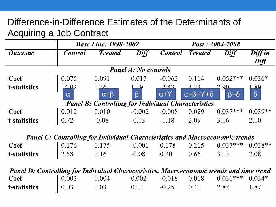
Difference-in-Difference Estimates of the Determinants of

Acquiring a Job Contract

α α+β β α+ϒ α+β+ϒ+δ β+δ δ

Falsification Tests

• The identifying assumption for DiD means that the trend

in the outcome variable between treated and control

observations (conditional on observables) should not be

different absent treatment.

• To check on this, one can check whether the trend is the

same in the pre-treatment period.

• To do this, you will need two points in time prior to treatment

begins.

• The same regression is carried out for that pre-treatment period.

The coefficient β needs to be statistically insignificant in this case to

pass the falsification test.

Cross-Sectional Difference-in-

Difference• DiD estimators do not have to involve measurements

across time.

• Can be done across groups of individuals, with one group not expected to be affected by treatment.

• E.g.• Target and non-target villages for micro-credit programs

• Participating and non-participating households

• Non-targeted villages are not expected to be affected, so difference between participating and non-participating HH in such villages could be a measure of selection into participation• DiD: difference between participants and non-participants in

targeted villages, minus the same difference in non-targeted villages

Difference-in-Difference and PSM

• One can use DiD in the context of PSM as well

• Matching is still done along pre-treatment characteristics

ATT = (1/NT

) [(Y1 j

T -Y0 j

t )j=1

NT

å - wij

iÎC

å (Y1ij

C -Y0ij

C )]

Using “wide” data, calculate Y1j - Y0j at the individual

level and then carry out PSM on that outcome

variable

Wahba and Assaad (2014)

PSM Robustness check:

• Treatment: (as before) is belonging to a formal

firm or informal firm at the beginning of the perio

T=1 in formal firm

T=0 in informal firm

• Outcome: whether individual with no contract in

2002-2004 moved to a contract job in 2004-2008.

Y=1 obtained contract

Y=0 did not obtain contract

• Falsification test

• Do it again for period 1996-98 to 1998-2002

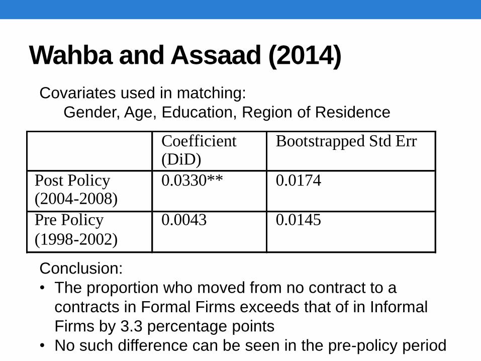
Wahba and Assaad (2014)

Coefficient (DiD)

Bootstrapped Std Err

Post Policy (2004-2008)

0.0330** 0.0174

Pre Policy

(1998-2002)

0.0043 0.0145

Covariates used in matching:

Gender, Age, Education, Region of Residence

Conclusion:

• The proportion who moved from no contract to a

contracts in Formal Firms exceeds that of in Informal

Firms by 3.3 percentage points

• No such difference can be seen in the pre-policy period