Categorical dependent variables:Application using WVS data from selected Arab countries

Irina Vartanova

Institute for Futures Studies, Stockholm

ERF Workshop – May 11, 2015

1 / 25

Example: Income and Happiness

• Positive but diminishing association between income andhappiness (see Clark, et al., 2007 for a review)

• The association can be partially explained by reversecausation and by unobserved individual characteristics, suchas personality traits.

• Relative income is more important than actual income, besidescomparisons of relative position are made across nations.

2 / 25

Variables

Taking all things together, would you say you are

• Very happy

• Rather happy

• Not very happy

• Not at all happy

1

0

On this card is an income scale on which 1 indicates the lowestincome group and 10 the highest income group in your country.We would like to know in what group your household is.

1 - Lowest group 10 - Highest group

3 / 25

Data

• WVS, 6th wave

• 12 MENA countries: Algeria, Egypt, Iraq, Jordan, Kuwait,Lebanon, Libya, Morocco, Palestine, Qatar, Yemen

• Bahrain excluded

• Pool sample: 9928 after listwize deletion of missing cases

4 / 25

Raw Probabilities

5 / 25

Logit Model

logΩ(X ) = 0.525 + 0.047β

6 / 25

Income Distribution

7 / 25

Model Summary

Model 1 Model 2

s.income 0.267∗∗∗ (0.010) 0.252∗∗∗ (0.011)Palestine −0.308∗∗∗ (0.106)Iraq −0.786∗∗∗ (0.100)Jordan 0.367∗∗∗ (0.113)Kuwait 0.825∗∗∗ (0.135)Lebanon −0.353∗∗∗ (0.105)Libya 0.507∗∗∗ (0.103)Morocco 0.014 (0.106)Qatar 2.084∗∗∗ (0.231)Tunisia 0.011 (0.106)Egypt −2.482∗∗∗ (0.097)Yemen −0.132 (0.106)Constant −0.102∗∗ (0.047) 0.260∗∗∗ (0.089)N 14617 14617Log Likelihood −7558.220 −6399.145

8 / 25

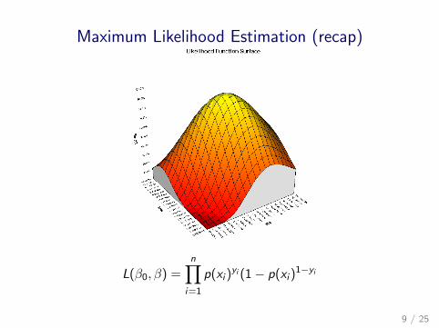
Maximum Likelihood Estimation (recap)

L(β0, β) =n∏

i=1

p(xi )yi (1− p(xi )

1−yi

9 / 25

(Relatively) full model of happinessBased on the extensive review of existing factors of subjectivewell-being (Dolan et. all, 2008), we control for:

• Gender - women tend to report higher happiness.• Age squared - younger and older generations are happier.• Marital status, being married is associated with the highest

happiness and being divorced with the lowest.• Having children, the effect is mixed. Positive effect on life

satisfaction, but not on happiness. Negative consequences ofadditional children, also culturally dependant.• Health.• Education has positive effect, especially in low income

countries.• Unemployment is detrimental for happiness especially among

men.• Religiosity have positive effect on happiness.• General trust positively associated with happiness.

10 / 25

(Relatively) full model of happiness - 2

Happiness

s.income 0.198∗∗∗ (0.013)female 0.307∗∗∗ (0.054)poly(age, 2)1 5.221 (3.915)poly(age, 2)2 21.006∗∗∗ (3.252)education Middle −0.057 (0.060)education High −0.055 (0.081)marital.st Divorced −0.661∗∗∗ (0.148)marital.st Widowed −0.396∗∗∗ (0.125)marital.st Single −0.366∗∗∗ (0.109)children 1 child 0.278∗∗ (0.125)children 2 or more 0.113 (0.100)to be continued

11 / 25

(Relatively) full model of happiness - 3

s.health Good −0.649∗∗∗ (0.069)s.health Fair −1.765∗∗∗ (0.076)s.health Poor −2.767∗∗∗ (0.112)imp.religion Rather important −0.474∗∗∗ (0.089)imp.religion Not very important −0.895∗∗∗ (0.166)imp.religion Not at all important −1.164∗∗∗ (0.214)general.trust 0.325∗∗∗ (0.065)unemployed −0.494∗∗∗ (0.103)Female:unemployed 0.158 (0.175)Constant 1.712∗∗∗ (0.155)N 13750Log Likelihood −5302.329

12 / 25

Country Effect: All Pairwise Comparisons

Pal

estin

e

Iraq

Jord

an

Kuw

ait

Leba

non

Liby

a

Mor

occo

Qat

ar

Tuni

sia

Egy

pt

Yem

en

Egypt

Tunisia

Qatar

Morocco

Libya

Lebanon

Kuwait

Jordan

Iraq

Palestine

Algeria 0.570.12

0.930.11

0.060.12

−0.600.16

0.040.13

−0.070.12

0.260.12

−1.660.24

0.140.12

2.850.11

0.540.12

0.360.11

−0.510.12

−1.160.16

−0.530.13

−0.640.12

−0.310.12

−2.230.24

−0.420.12

2.280.11

−0.020.12

−0.870.12

−1.520.15

−0.890.12

−1.000.11

−0.670.11

−2.590.24

−0.780.11

1.920.10

−0.390.11

−0.660.16

−0.020.13

−0.130.12

0.200.12

−1.720.25

0.080.12

2.790.11

0.480.13

0.630.16

0.530.15

0.850.16

−1.070.26

0.740.16

3.440.15

1.140.16

−0.110.13

0.220.13

−1.700.25

0.110.13

2.810.12

0.510.14

0.330.12

−1.590.24

0.210.11

2.920.10

0.610.12

−1.920.24

−0.110.12

2.590.11

0.290.12

1.810.24

4.510.24

2.210.25

2.700.11

0.400.12

−2.300.11

Significantly < 0Not SignificantSignificantly > 0

bold = brow − bcol

ital = SE(brow − bcol)13 / 25

Multiplicity Correction

• Since we test 66hypothesissimultaneously,around 3 of themcould be significantby chance

• There are severalways to correct formultiple testing. HereI use the Holmcorrection which setsthe α for the entireset of tests equal toαn .

Pal

estin

e

Iraq

Jord

an

Kuw

ait

Leba

non

Liby

a

Mor

occo

Qat

ar

Tuni

sia

Egy

pt

Yem

en

Egypt

Tunisia

Qatar

Morocco

Libya

Lebanon

Kuwait

Jordan

Iraq

Palestine

Algeria 0.570.12

0.930.11

0.060.12

−0.600.16

0.040.13

−0.070.12

0.260.12

−1.660.24

0.140.12

2.850.11

0.540.12

0.360.11

−0.510.12

−1.160.16

−0.530.13

−0.640.12

−0.310.12

−2.230.24

−0.420.12

2.280.11

−0.020.12

−0.870.12

−1.520.15

−0.890.12

−1.000.11

−0.670.11

−2.590.24

−0.780.11

1.920.10

−0.390.11

−0.660.16

−0.020.13

−0.130.12

0.200.12

−1.720.25

0.080.12

2.790.11

0.480.13

0.630.16

0.530.15

0.850.16

−1.070.26

0.740.16

3.440.15

1.140.16

−0.110.13

0.220.13

−1.700.25

0.110.13

2.810.12

0.510.14

0.330.12

−1.590.24

0.210.11

2.920.10

0.610.12

−1.920.24

−0.110.12

2.590.11

0.290.12

1.810.24

4.510.24

2.210.25

2.700.11

0.400.12

−2.300.11

Significantly < 0Not SignificantSignificantly > 0

bold = brow − bcol

ital = SE(brow − bcol)

14 / 25

Interpretation: Odds Ratios

• Odds ratios describe the factor by which odds change as onevariable changes holding other constant. They are easilycalculated:

ebs.income = 1.22

• Interpretation: For all of the people who live in the sameMENA country, have the same gender, age, education and soon and with 5 score on subjective income - for every 100 ofthem we would expect to be happy, we would expect 122 ofthe same types of people, but who had 6 score on subjectiveincome, be happy.

• Odds ratios remain only relative comparisons due tounobserved heterogeneity (Mood, 2010).

15 / 25

Alternatives: Types of Marginal Effects

• Average Marginal Effects - takes the average of the marginaleffect across all cases used to estimate the model.

• Marginal Effect at the Mean - takes the marginal effect ofeach variable holding all other variables constant at theirmean values.

• Marginal Effect at Representative values - take the marginaleffect of each variable holding all others constant atsubstantively/theoretically interesting values

16 / 25

Predicted Probabilities

s.income effect plot

s.income

happ

y

0.70

0.75

0.80

0.85

0.90

2 4 6 8 10

17 / 25

Model Fit, Evaluation and Comparison

• Specification tests: Wald test, Likelihood ratio test

• Pseudo-R2

• Information criteria: AIC, BIC

18 / 25

Testing: Wald and Likelihood-Ratio Test

• A Wald test is base on the assumption that B N(β,V (B))and tests whether β = 0

• A likelihood-ratio test compares two models, a full one (MF )with coefficients BF and a nested model (MR) which places qlinear restrictions on the coefficients in BF :

LLR = −2(LL(MR)− (LL(MF ) χ2q

19 / 25

Hypothesis Test for Subjective Income

Wald test

Res.Df Df χ2 Pr(> χ2)1 137182 13718 1 229.48 < 2.2e − 16 ∗ ∗∗

LR test

Df LogLik Df χ2 Pr(> χ2)1 32 -5302.32 31 -5420.2 -1 235.69 < 2.2e − 16 ∗ ∗∗

20 / 25

Pseudo-R2

• Pseudo-R2 rely on analogous to the linear model, but none ofthem can be interpreted as the proportion of variation in thedependent variable explained by the independent variables.

• Many different types, each of them produce different results

21 / 25

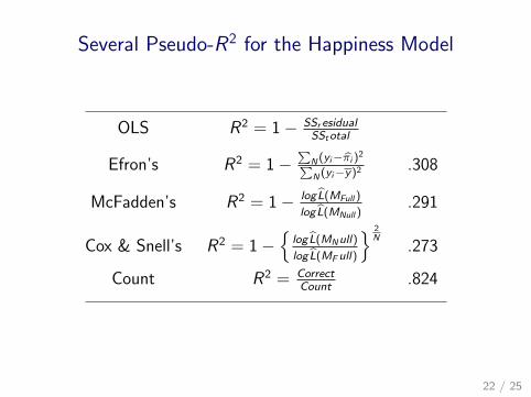
Several Pseudo-R2 for the Happiness Model

OLS R2 = 1− SSr esidualSStotal

Efron’s R2 = 1−∑

N(yi−πi )2∑

N(yi−y)2.308

McFadden’s R2 = 1− logL(MFull )

logL(MNull ).291

Cox & Snell’s R2 = 1−

logL(MNull)

logL(MFull)

2N

.273

Count R2 = CorrectCount

.824

22 / 25

AIC and BIC

Akaike’s Information Criterion

AIC = −2log(L(Θ‖data)) + 2K

Bayesian Information Criterion

BIC = −2log(L) + Klog(n)

• Whether to use AIC or BIC depends on how much one wantsto penalize additional model parameters.

23 / 25

AIC and BIC for the Happiness Model

Base model Without Gender*Unemployment

Log Likelihood −5302.329 −5302.867AIC 10668.66 10667.73BIC 10909.58 10901.13

24 / 25