Download pdf - Understanding mean transit times in Andean tropical montane cloud forest catchments: combining tracer data, lumped parameter models and uncertainty analysis

HESSD10, 15871–15914, 2013

Understanding meantransit times in

Andean catchments

E. Timbe et al.

Title Page

Abstract Introduction

Conclusions References

Tables Figures

J I

J I

Back Close

Full Screen / Esc

Printer-friendly Version

Interactive Discussion

Discussion

Paper

|D

iscussionP

aper|

Discussion

Paper

|D

iscussionP

aper|

Hydrol. Earth Syst. Sci. Discuss., 10, 15871–15914, 2013www.hydrol-earth-syst-sci-discuss.net/10/15871/2013/doi:10.5194/hessd-10-15871-2013© Author(s) 2013. CC Attribution 3.0 License.

Hydrology and Earth System

Sciences

Open A

ccess

Discussions

This discussion paper is/has been under review for the journal Hydrology and Earth SystemSciences (HESS). Please refer to the corresponding final paper in HESS if available.

Understanding mean transit times inAndean tropical montane cloud forestcatchments: combining tracer data,lumped parameter models anduncertainty analysis

E. Timbe1,2, D. Windhorst2, P. Crespo1, H.-G. Frede2, J. Feyen1, and L. Breuer2

1Departamento de Recursos Hídricos y Ciencias Ambientales, Dirección de Investigación(DIUC), Universidad de Cuenca, Cuenca, Ecuador2Institute for Landscape Ecology and Resources Management (ILR), Research Centre for BioSystems, Land Use and Nutrition (IFZ), Justus-Liebig-Universität Gießen, Gießen, Germany

Received: 27 November 2013 – Accepted: 3 December 2013 – Published: 23 December 2013

Correspondence to: E. Timbe ([email protected])

Published by Copernicus Publications on behalf of the European Geosciences Union.

15871

http://www.hydrol-earth-syst-sci-discuss.net

http://www.hydrol-earth-syst-sci-discuss.net/10/15871/2013/hessd-10-15871-2013-print.pdf

http://www.hydrol-earth-syst-sci-discuss.net/10/15871/2013/hessd-10-15871-2013-discussion.html

http://creativecommons.org/licenses/by/3.0/

HESSD10, 15871–15914, 2013


Andean catchments

E. Timbe et al.

Title Page



Tables Figures

J I

J I

Back Close

Full Screen / Esc



Discussion

Paper

|D

iscussionP

aper|

Discussion

Paper

|D

iscussionP

aper|

Abstract

Weekly samples from surface waters, springs, soil water and rainfall were collectedin a 76.9 km2 mountain rain forest catchment and its tributaries in southern Ecuador.Time series of the stable water isotopes δ18O and δ2H were used to calculate meantransit times (MTTs) and the transit time distribution functions (TTDs) solving the con-5

volution method for seven lumped parameter models. For each model setup, the Gen-eralized Likelihood Uncertainty Estimation (GLUE) methodology was applied to findthe best predictions, behavioral solutions and parameter identifiability. For the studybasin, TTDs based on model types such as the Linear-Piston Flow for soil watersand the Exponential-Piston Flow for surface waters and springs performed better than10

more versatile equations such as the Gamma and the Two Parallel Linear Reservoirs.Notwithstanding both approaches yielded a better goodness of fit for most sites, butwith considerable larger uncertainty shown by GLUE. Among the tested models, cor-responding results were obtained for soil waters with short MTTs (ranging from 3 to 12weeks). For waters with longer MTTs differences were found, suggesting that for those15

cases the MTT should be based at least on an intercomparison of several models.Under dominant baseflow conditions long MTTs for stream water≥ 2 yr were detected,a phenomenon also observed for shallow springs. Short MTTs for water in the top soillayer indicate a rapid exchange of surface waters with deeper soil horizons. Differencesin travel times between soils suggest that there is evidence of a land use effect on flow20

generation.

1 Introduction

The mean transit time (MTT) of waters provides a valuable primary description of thehydrologic (Fenicia et al., 2010) and biochemical systems (Wolock et al., 1997) ofa catchment and its sensitivity to anthropogenic factors (Landon et al., 2000; Turner25

et al., 2006; Tetzlaff et al., 2007; Darracq et al., 2010). The transit time distribution

15872





HESSD10, 15871–15914, 2013


Andean catchments

E. Timbe et al.

Title Page



Tables Figures

J I

J I

Back Close

Full Screen / Esc



Discussion

Paper

|D

iscussionP

aper|

Discussion

Paper

|D

iscussionP

aper|

function (TTD) describes the probability that water was at some point in the catchmenta given amount of time ago (McDonnell et al., 2010). Together with the physical char-acteristics of the catchment, the MTT and TTD allow inferring the recharge of aquifers(Rose et al., 1996), the bulk water velocities through its compartments (Rinaldo et al.,2011), and the interpretation of the water chemistry (Maher, 2011); all of which sup-5

ports the design of prevention, control, remediation and restoration techniques. Addi-tionally, MTT and TTD data are useful to reduce the uncertainty of results and improveinput parameter identifiability for either hydrologic modeling studies (Weiler et al., 2003;Vache and McDonnell, 2006; McGuire et al., 2007; Capell et al., 2012) or solute move-ment analyses through soil and aquifers using mixing models (Iorgulescu et al., 2007;10

Barthold et al., 2010).The stable water isotopes δ18O and δ2H are commonly used as environmental trac-

ers for a preliminary assessment of the transport of water in watersheds with transittimes less than 5 yr (Soulsby et al., 2000, 2009; Rodgers et al., 2005; Viville et al.,2006). For longer MTTs, up to 12 yr, tritium radioisotopes are used to analyze the stor-15

age and flow behavior in surface water and shallow groundwater systems (Kendall andMcDonnell, 1998), while carbon isotopes are employed for analyzing the dynamics ofdeep groundwater with ages of hundreds to thousands of years (Leibundgut et al.,2009).

Traditionally, researchers in tracer hydrology apply quasi distributed and conceptual20

models to encompass the non-linearity of the processes related to the transit statesof the soil moisture dynamics (Botter et al., 2010; Fenicia et al., 2010). However, theuse of such modeling approaches is only advisable after a basic inference of the MTTsusing simpler TTDs as the lumped-parameter models proposed by Maloszewski andZuber (1982, 1993), models that are based on quasi-linearity and steady state condi-25

tions. These models include the exponential (EM), piston (PM), or linear (LM) models,in which the MTT of the tracer is the only unknown variable, and also combinationsof models such as the exponential-piston flow (EPM) and the linear-piston flow (LPM)models. Among the two-parameter lumped models, the dispersion model (DM), that

15873





HESSD10, 15871–15914, 2013


Andean catchments

E. Timbe et al.

Title Page



Tables Figures

J I

J I

Back Close

Full Screen / Esc



Discussion

Paper

|D

iscussionP

aper|

Discussion

Paper

|D

iscussionP

aper|

considers simplifications of the general advection-dispersion equation, has been ap-plied in environmental tracer studies (Maloszewski et al., 2006; Viville et al., 2006;Kabeya et al., 2006). More recently, new lumped models are being exploited such asthe two parameter Gamma model (GM) proposed by Kirchner et al. (2000), which isa more general and flexible version of the exponential model; and the Two Parallel5

Linear Reservoirs model (TPLR), a three-parameter function that combines two paral-lel reservoirs, each one represented by a single exponential distribution (Weiler et al.,2003). The use of these models for estimating the MTT in the compartments of a catch-ment has become a standard practice for the preliminary assessment of the catchmentfunctioning. McGuire and McDonnell (2006) presented in their study a compilation of10

the most frequently used lumped parameter models for deriving MTTs. Under the con-dition that a particular model ought to be concordant with the physical characteristics ofthe aquifer system, this condition hinders the applicability of lumped parameter modelsto poor gauged catchments with scarce or no information on the physical character-istics of the system. For these cases the authors believe that it is better to use an15

ensemble of models in order to be certain that the results or the inferences point inthe same direction, or if not, to have a better idea of the uncertainties. In accordance,seven lumped parameter models to infer the MTTs for diverse water stores (stream,springs, creeks and soil water) were applied in this study. Results were evaluated onthe basis of the best matches to a predefined objective function, their magnitude of20

uncertainty and the number of observations in the range of behavioral solutions.Particular for tropical zones the knowledge of hydrological functioning is still limited

and investigation of system descriptors such as MTT and TTD are keys to improveour understanding of catchment responses (Murphy and Bowman, 2012; Brehm et al.,2008). This is especially the case for tropical mountain rainforest systems. In this study25

we focus on the San Francisco river basin, a mesoscale headwater catchment of theAmazon in Ecuador. Notwithstanding the recent characterization of the climate (Bendixet al., 2006), soils (Wilcke et al., 2002), water chemistry (Buecker et al., 2011) andhydrology (Plesca et al., 2012) of the basin, we are still lacking a perceptual model that

15874





HESSD10, 15871–15914, 2013


Andean catchments

E. Timbe et al.

Title Page



Tables Figures

J I

J I

Back Close

Full Screen / Esc



Discussion

Paper

|D

iscussionP

aper|

Discussion

Paper

|D

iscussionP

aper|

explains the observations of chemical, hydrometric and isotopic variables and relatedprocesses (Crespo et al., 2012).

To enhance the understanding of the hydrological functioning of the San Franciscobasin, this study focuses on the (i) estimation of the MTT in the different compartmentsof the catchment; (ii) characterization of the dominant TTD functions; and (iii) evaluation5

of the performance and uncertainty of the models used to derive the MTTs and TTDs.Translated into hypotheses the study reported in this paper aimed to confirm or reject,respectively, that

1. the used tracers are conservative, there are no stagnant flows in the system, andthe tracer mean transit time τ represents the MTT of water;10

2. stationary conditions are dominant in the basin and lumped equations based onlinear or quasi-linear behaviors are applicable;

3. given the steepness of the topography and the shallow depth of the soil layers thetransit times of the sampling sites are less than 5 yr, making it possible to use δ2Hand δ18O as tracers;15

4. the diversity of the sampling sites allows evaluating the spatial variability in catch-ment hydrology, identifying the dominant processes, and screen the performanceof the TTD models;

5. the multi-model approach and the identifiability of their parameters enable identi-fication of the respective TTDs and MTTs.20

2 Materials and methods

2.1 Study area

The San Francisco tropical mountain cloud forest catchment, 76.9 km2 in size, is lo-cated in the foothills of the Andean cordillera in South Ecuador, between Loja and

15875





HESSD10, 15871–15914, 2013


Andean catchments

E. Timbe et al.

Title Page



Tables Figures

J I

J I

Back Close

Full Screen / Esc



Discussion

Paper

|D

iscussionP

aper|

Discussion

Paper

|D

iscussionP

aper|

Zamora (Fig. 1), and drains into the Amazonian river system. Hourly meteorologi-cal data recorded at the Estación Científica San Francisco (ECSF, 1957 m a.s.l.), ElTiro (2825 m a.s.l.), Antenas (3150 m a.s.l.) and TS1 (2660 m a.s.l.) climate stations areavailable from the DFG funded Research Unit FOR816 (www.tropicalmountainforest.org). Monthly averages of the main meteorological parameters for the period 1998–5

2012 allow a description of their spatial and interannual variation. Mean annual tem-perature ranges from 15 ◦C in the lower part of the study area (1957 m a.s.l.) to 10 ◦Con the ridge (3150 m a.s.l.), with an altitude gradient of −0.57 ◦C per 100 m, withoutmarked monthly variability. The wind velocities of the prevailing south-easterlies reachaverage maximum daily values of 10 ms−1 between June and September, while wind10

velocities in the middle and lower catchment areas are fairly constant, equal to 1 ms−1.The humid regime of the catchment is comparatively constant with the relative hu-midity varying between 84.5 % in the lower parts and 95.5 % at the ridges. Among allmeteorological parameters, precipitation shows the largest spatial variability, with anaverage gradient of 220 mm per 100 m−1 (Bendix et al., 2008b). However, this gradi-15

ent is not constant throughout the catchment and shows substantial spatial variability(Breuer et al., 2013). Recent estimation of horizontal rainfall revealed its significance,contributing 5–35 % of measured tipping bucket rainfall, respectively to the lower andridge areas of the catchment (Rollenbeck et al., 2011). Rainfall is marked by low rainfallintensities, generally less than 10 mmh−1 and high spatial variability. Annual rainfall is20

uni-modal distributed with a peak in the period April–June. Using the Thiessen methodand considering horizontal rainfall, the precipitation depth amounted 2321 mm in theperiod August 2010–July 2011, and 2505 mm in the period August 2011–July 2012.A more detailed descriptions of the weather and climate of the study area is given inBendix et al. (2008a).25

In line with findings of Crespo et al. (2012) baseflow in the same area accounts for85 % of the total volume runoff (Table 2), notwithstanding the rapid and marked re-sponse of flows to extreme rainfall events. In just a few hours peak discharge is several

15876





www.tropicalmountainforest.org



HESSD10, 15871–15914, 2013


Andean catchments

E. Timbe et al.

Title Page



Tables Figures

J I

J I

Back Close

Full Screen / Esc



Discussion

Paper

|D

iscussionP

aper|

Discussion

Paper

|D

iscussionP

aper|

times higher than baseflow (Fig. 2c), carrying considerable amounts of sediment andaccompanied by drastic changes in the cross section.

Mayor soil types are Histosols associated with Stagnasols, Cambisols and Regosols,while Umbrisols and Leptosols are present to a lesser degree (Liess et al., 2009). Thegeology is reasonable similar throughout the study area, consisting of sedimentary5

and metamorphic Paleozoic rocks of the Chiguinda unit with contacts to the Zamorabatholith (Beck et al., 2008). The topography is characterized by steep valleys with anaverage slope of 63 %, situated in the altitudinal range of 1725–3150 m a.s.l. (Table 2).Protected by the Podocarpus National Park, the southern part of the catchment iscovered by pristine primary forest and sub-páramo. In the northern part, particular10

during the last two decades, land is being converted to grassland. Presently 68 % ofthe catchment is covered by forest, 20 % is sub-páramo, 6.5 % is used as pastureand 3 % is degraded grassland covered with shrubs (Goettlicher et al., 2009; Plescaet al., 2012). Landslides are present in the catchment, especially along the paved roadbetween the cities Loja and Zamora.15

2.2 Catchment composition and discharge measurements

The San Francisco catchment is composed of seven sub-catchments with areas rang-ing between 0.7 and 34.9 km2, characterized by different land uses varying from pris-tine forest and sub-páramo to pasture areas (Fig. 1 and Table 2). Since August 2010,water level and temperature sensors (mini-diver, Schlumberger Water Services, Delft,20

NL) with a 5 min resolution are installed at 4 tributaries of the catchment: FH, QN,QM, QC (Fig. 1) and in the main outlet (PL). As explained later in this section, specificdischarges derived of these sites were used to account for the hydrological behaviorof the remaining sub-catchments. In the QC cross section a 90◦ V-notch weir is in-stalled for measuring the discharge. At PL a Doppler radar RQ-24 (Sommer Messtech-25

nik, Koblach, AT) records water level and surface water velocity in 15 min resolution.Fortnightly, discharge is measured by the salt dilution method (Boiten, 2000) usingportable electric conductivity probes (pH/cond 340i, WTW, Weilheim, DE) to develop

15877





HESSD10, 15871–15914, 2013


Andean catchments

E. Timbe et al.

Title Page



Tables Figures

J I

J I

Back Close

Full Screen / Esc



Discussion

Paper

|D

iscussionP

aper|

Discussion

Paper

|D

iscussionP

aper|

stage-discharge curves for each gauge station. The Manning method based on mea-surements of the wetted area and the stream velocity was used to complement andcrosscheck manual measurements. For this purpose periodically the cross section inevery gauge station was measured using a total station (SET650X, Sokkia, Olathe,Kansas, US). Figure 2 shows the hourly hydrograph for the main outlet (PL); similar5

hydrographs were calculated for the sections FH, QN, QC and QM.

2.3 Isotope sampling and analyses

Weekly isotope data were collected in the main river, its tributaries, creeks and springsin the period August 2010–mid August 2012 (Table 1), using 2 mL amber glass bottles.Soil water was sampled in the lower part of the catchment along two altitudinal tran-10

sects covered by pasture and forest, respectively in 6 sites and 3 depths (0.10, 0.25and 0.40 m) using wick-samplers. The soil water collectors were designed and installedas described by Mertens et al. (2007). Woven and braided 3/8 fiberglass wicks (Ama-tex Co. Norristown, PA, US) were unraveled over a length of 0.75 m and spread overa 0.30m×0.30m×0.01m square plastic plate. The plate enveloped with fiberglass was15

covered with fine soil particles of the parent material and then set in contact with theundisturbed soil, respectively at the bottom of the organic horizon (0.10 m below sur-face), a transition horizon (0.25 m below surface) and a lower mineral horizon (0.40 mbelow surface). The low constant tension in the wick-samplers guarantees that the mo-bile phase of the soil water is sampled, avoiding isotope fractionation (Landon et al.,20

1999). Event based rainfall samples for isotope analyses were collected from mid-August 2010 until mid-August 2012, in an open area (1900 m a.s.l.) at ECSF (Fig. 1).The end of a single rainfall event was marked by a time span of 30 min without rainfall.

The stable isotopes signatures of δ18O and δ2H are reported in per mil relative tothe Vienna Standard Mean Ocean Water (VSMOW) (Craig, 1961). The water isotopic25

analyzes were performed using a compact wavelength-scanned cavity ring down spec-troscopy based isotope analyzer (WS-CRDS) with a precision of 0.1 per mil for δ18Oand 0.5 for δ2H (Picarro L1102-i, CA, US).

15878





HESSD10, 15871–15914, 2013


Andean catchments

E. Timbe et al.

Title Page



Tables Figures

J I

J I

Back Close

Full Screen / Esc



Discussion

Paper

|D

iscussionP

aper|

Discussion

Paper

|D

iscussionP

aper|

2.4 Isotopic gradient of rainfall

Given the large altitudinal gradient in the San Francisco basin, it is to be expectedthat the input isotopic signal of rainfall for every sub-catchment varies according to itselevation (Dansgaard, 1964). In this regard, Windhorst et al. (2013) estimated this vari-ation for the main transect of the catchment: −0.22 ‰ δ18O, −1.12 ‰ δ2H and 0.6 ‰5

deuterium excess per 100 m elevation gain. Applying this altitude gradient under theassumption that the incoming rainfall signal is the sole source of water, thereby exclud-ing any unlikely source of water from outside the topographic catchment boundarieswith a different isotope signal, it was possible to derive the recharge elevation and lo-calized input signal in each sub-catchment. The derived recharge elevations were used10

to crosscheck that they are inside the topographic boundaries of every sub-catchment(Table 5) and comparable to their mean elevations (Table 2).

Since no marked fractionation was observed for all analyzed waters it is highly prob-able that similar estimations of MTT are derived using either δ18O or δ2H (Fig. 3).Therefore, in this study δ18O was selected for further analysis.15

2.5 Mean transit time estimation and transit time distribution

Mean transit times were calculated based on stationary conditions. In the case ofstream water this condition was fulfilled by considering only baseflow conditions (Heid-büchel et al., 2012), which were dominant in the catchment during the 2 yr observationperiod, accounting for 85 % of total runoff volume. Baseflow separations for streamflow20

were obtained through parameter fitting to the slope of the recessions in the observedhourly flows using the Water Engineering Time Series PROcessing tool (WETSPRO),developed by Willems (2009). To account for samples taken at baseflow conditionsin sites where hydrometric records were not available, the specific discharges of thecloser catchments with similar characteristics in terms of land use, size, and observed25

hydrologic behavior were used. In this sense, QZ, QR and QP were considered similar

15879





HESSD10, 15871–15914, 2013


Andean catchments

E. Timbe et al.

Title Page



Tables Figures

J I

J I

Back Close

Full Screen / Esc



Discussion

Paper

|D

iscussionP

aper|

Discussion

Paper

|D

iscussionP

aper|

to QN, QM and QC (Table 2). Soil and spring waters are less influenced by particularrain events and therefore all samples were included in the analysis.

For the calculation of MTTs, the authors used the lumped parameter approach. Inthis, the aquifer system is treated as an integral unit and the flow pattern is assumedto be constant as outlined in Maloszewski and Zuber (1982) for the special case of5

constant tracer concentration in time-invariant systems. In this case the transport ofa tracer through a catchment is expressed mathematically by the convolution integral.The tracer output Cout(t) and input Cin(t) are related in function of time:

Cout(t) =

t∫−∞

Cin(t′) exp[−λ(t− t′)

]g(t− t′)dt′ (1)

10

In the convolution integral, the stream outflow composition Cout at a time t (time of exit)consists of a tracer Cin that falls uniformly on the catchment in a previous time step t′

(time of entry), Cin becomes lagged according to its transit time distribution g(t− t′);the factor exp[−λ(t− t′)] is used to correct for decay if a radioactive tracer is used(λ = tracer’s radioactive decay constant). For stable tracers (λ = 0), and considering15

that the time span t− t′ is the tracer’s transit time τ, the Eq. (1) can be simplified andre-expressed as:

Cout(t) =

t∫−∞

Cin(t′)g(τ)dt′ (2)

where the weighting function g(τ) or tracer’s transit time distribution (TTD), describes20

the normalized distribution function of the tracer injected instantaneously over an entirearea (McGuire and McDonnell, 2006). As it is hard to obtain this function by experimen-tal means, the most common way to apply this lumped approach is to adopt a theo-retical distribution function that better fits to the studied system. In general meaning,any type of a weighting function is understood as a model. The equations for each of25

15880





HESSD10, 15871–15914, 2013


Andean catchments

E. Timbe et al.

Title Page



Tables Figures

J I

J I

Back Close

Full Screen / Esc



Discussion

Paper

|D

iscussionP

aper|

Discussion

Paper

|D

iscussionP

aper|

the lumped parameter models used in this study are shown in Table 3. EM and LMreflect simpler transitions where the tracer’s mean transit time τ is the only unknownvariable. More flexible models consider a mixture of two different types of distribution.EPM includes piston and exponential flows, while the LPM accounts for piston andlinear flows. In both cases the equations are integrated by the parameter η indicating5

the percentage contribution of each flow type distribution. The DM, derived from thegeneral equation of advection-dispersion, is also one of the common models used inhydrologic systems (Maloszewski et al., 2006). In this model the fitting parameter Dpis related to the transport process of the tracer (Kabeya et al., 2006). In the GM, theproduct of the two shape parameters α and β equals τ. This method was successfully10

applied by Dunn et al. (2010) and Hrachowitz et al. (2010). The TPLR model (Weileret al., 2003) is based on the parallel combination of two single exponential reservoirs(despite of its name TPLR follows exponential and not linear assumption), representingfast τf and slow flows τs, respectively. The flow partition between the two reservoirs isdenoted by the parameter ϕ.15

2.6 Convolution equation resolution

The conventional resolution of the convolution equation requires the continuity of datafor each time step of the input function. Weekly data of the isotopic composition of allsampled waters were therefore used in this study. Available sub-daily rainfall data wereweighed according to the daily volume registered at the nearest meteorological station20

(ECSF, Figs. 1 and 2a). For the 2 yr sampling period, only 5 weeks without rainfall wereregistered. For these cases, average values considering the antecedent and precedentweekly isotopic signatures were used.

Due to the similarities between the seasonal isotopic fluctuations of the sampledeffluents and rainfall signal, a constant interannual recharge of the aquifers was as-25

sumed. For each sampling site, the 2 yr isotopic data series were used as input forthe models. To get stable results between two consecutive periods, these input isotopetime series were repeated 20 times in a loop; an approach similar to the methodology

15881





HESSD10, 15871–15914, 2013


Andean catchments

E. Timbe et al.

Title Page



Tables Figures

J I

J I

Back Close

Full Screen / Esc



Discussion

Paper

|D

iscussionP

aper|

Discussion

Paper

|D

iscussionP

aper|

presented by Munoz-Villers and McDonnell (2012) resulting in an artificial time seriesof 40 yr. Data of the last loop were considered for statistical treatment and analysis.The repetition of the input isotopic signal implies that interannual variation of rain isnegligible; an acceptable assumption for the San Francisco catchment considering thehigh degree of similarity between the same months along the analyzed 2 yr period5

(Fig. 4). Comparable monthly isotopic seasonality of rainfall has been described byGoller et al. (2005) for the same study area and for nearby regions with similar climaticconditions, e.g., Amaluza GNIP station (http://www.iaea.org/water).

2.7 Evaluation of model performance

The search for acceptable model parameters for each site was conducted through sta-10

tistical comparisons of 10 000 simulations based on the Monte-Carlo method, consider-ing a uniform random distribution of the variables involved in each model. For each siteand model its performance was calculated using the Nash–Sutcliffe Efficiency (NSE).Quantification of errors and deviations from the observed data were respectively calcu-lated by the root mean square error (RMSE) and the bias. MatLab version 7 was used15

for data handling and solving the convolution equation.The Generalized Likelihood Uncertainty Estimation (GLUE, Beven and Freer, 2001),

was used to find uncertainty ranges of possible or behavioral parameter solutions. TheGLUE approach considers that several likely solutions are valid as long as efficiencyof a particular simulation is above a pre-set, but subjective threshold. Due to the diver-20

sity of sampling sites, multiple models and the expected range of variability for NSEamong sites, a fixed confidence interval of 5–95 % of the top 5 % of the best NSE wasapplied as a lower threshold for every case. Besides, a prediction was considered poorwhenever the best NSE was below 0.45.

The following three criteria were used to select the best solutions of MTTs and TTDs:25

(1) NSE; (2) magnitude of the uncertainty of the prediction, expressed as a percent ofthe predicted MTT value; and (3) percentage of observations covered by the range ofbehavioral solutions defined according to the second criteria.

15882





http://www.iaea.org/water

HESSD10, 15871–15914, 2013


Andean catchments

E. Timbe et al.

Title Page



Tables Figures

J I

J I

Back Close

Full Screen / Esc



Discussion

Paper

|D

iscussionP

aper|

Discussion

Paper

|D

iscussionP

aper|

3 Results

3.1 Soil water

Of all predictions the best matches of the models with respect to the NSE objectivefunction ranged between 0.64 and 0.91 (Fig. 5a). When only the best goodness of fitis considered, the GM and the EPM models performed best in 13 of the 18 sampled5

sites, the DM model in 3 sites, and the LM and LPM models in one location (Fig. 5b).Only these models were considered for further mutual comparison. The TPLR and EMapproaches performed worst in 17 of the 18 sites (Fig. 5a), and were therefore not fur-ther considered. Even when the derived MTT values were similar among the modelsthat best fitted the objective function (Fig. 6a), the LPM model performed best taking10

into consideration additional selection criteria, as shown in Fig. 6b and c. Figure 8 de-picts for the LPM model, applied to site C2, the uncertainty and the range of behavioralsolutions for the two model parameters. Uncertainties, expressed on average valuesfor all soil sites (Fig. 6b), were lower for LM (32 %), LPM (35 %) and GM (37 %) modelsthan for DM (51 %) and EPM (44 %) models. The percentage of observations described15

inside the range of behavioral solutions according to their uncertainty ranges (Fig. 6c)was bigger for LPM (68 %) and EPM (59 %) models compared to the DM (47 %), GM(41 %) and LM (33 %) models.

According to the standard deviations (σ) of the observed δ18O, the amplitude ofseasonality between sites and horizons, varied from 2.57 to 3.98 ‰ (Table 4), very20

similar to the σ of weekly rainfall data (4.3 ‰). Except for the A3 and D2 sites, σshowed a decreasing pattern according to the sampling depth. Besides, they areinverse linearly correlated to the estimated MTTs (for LPM model results were τ =−2.4474σ +12.954,r2 = 0.60), indicating a distinctive decrease in the pattern of MTTwith soil depth (0.10, 0.25 and 0.40 m).25

Considering results from the LPM model (Table 4), differences between observedand predicted values described by the RMSE are up to 1.72 ‰ and the larger absolutebias accounts for 0.181 ‰ (Table 4). Bearing in mind the ranges of behavioral solution,

15883





HESSD10, 15871–15914, 2013


Andean catchments

E. Timbe et al.

Title Page



Tables Figures

J I

J I

Back Close

Full Screen / Esc



Discussion

Paper

|D

iscussionP

aper|

Discussion

Paper

|D

iscussionP

aper|

MTT results were between 2.3 and 6.3 weeks for pastures soils and between 3.7 and9.2 weeks for forested soils, while parameterizations for η (ratio of the total volume tothe volume in which linear flow applies) ranged from 0.84 to 2.23 and from 0.76 to 1.61respectively.

3.2 River and tributaries5

Considering all sites and models the criteria NSE> 0.45 was exceeded in 41 of the 63predictions (9 sites per 7 models, Fig. 5a). Among the analyzed sites the TPLR modelyielded the best matches for PL, SF, FH, QZ, QN, QM and QC, while the EPM modelfor the QR and QP sites (Fig. 5b). The GM model reached closest efficiencies whencompared to the best match for every site. Consequently only the TPLR, EPM and10

GM models were further considered. Although the best NSEs were reached using theTPLR model (0.61 on average for all sites) compared to the GM (0.57 on average) orthe EPM (0.55 on average) model, TPLR predictions showed the largest uncertainties(115 % on average of predicted MTTs, Fig. 7b) and at the same time depicted thelowest number of observations inside the predicted range of behavioral solutions (29 %15

on average, Fig. 7c). Considering these additional selection criteria, EPM performedbetter: uncertainty of MTT was on average 16 % (66 % on average for GM model) andthe number of observation inside this range was 72 % (33 % on average for GM model).Differences between MTT predictions for a particular site are depicted in Fig. 7a. Forstream water at the main outlet, Figs. 9–11 show the parameter uncertainties and20

behavioral solutions for the TPLR, GM and EPM models, respectively.Considering the results from the EPM model (Table 5, Fig. 7a), the low seasonal am-

plitudes described by the observed data of the effluents (σ between 0.30 and 0.59 ‰)resulted in small errors and deviations when simulated and observed data were com-pared (RMSE up to 0.41 ‰ and larger absolute bias of 0.005 ‰). But at the same25

time, the fitting efficiencies were lower than for soil waters, with a maximum NSE of0.56 for the main stream, and NSEs between 0.48 and 0.58 for the main tributaries(Fig. 5a). The predicted MTT at catchment outlet was 2.0 yr with a η parameter of 1.84

15884





HESSD10, 15871–15914, 2013


Andean catchments

E. Timbe et al.

Title Page



Tables Figures

J I

J I

Back Close

Full Screen / Esc



Discussion

Paper

|D

iscussionP

aper|

Discussion

Paper

|D

iscussionP

aper|

(a similar value was estimated for the main river at the SF sampling site, MTT=2.0 yrand η = 1.85) and varied from 2.0 (QM, η = 1.85) to 3.9 yr (QC, η = 1.97) for the maintributaries. As in the case of water from soils, results of MTT followed an inverse lin-ear correlation with amplitude of observed data (σ): τ = −7.3152σ +5.9893; r2 = 0.91.Independent of the amplitude of the isotope signal between sampled sites (σ), uncer-5

tainties for each site were similar with a maximum range between 14.1 % and 20.4 %of the predicted MTT as derived for the FH and QM sites (Table 5). Similarly, η rangedfrom 1.61 (QZ) to 2.21 (QP), the average value of η = 1.85 implies a 54 % of volumeportion of exponential flow and a 46 % volume of piston flow; the uncertainty for the ηparameter was 25 % on average.10

3.3 Springs and creeks

Of 35 predictions (5 sites per 7 models) the criteria NSE> 0.45 was fulfilled in 20cases. Sites with reduced isotope signal yielded lower efficiencies (Fig. 5a); i.e. for theTP site only two models provided NSE values higher than 0.45: EPM (NSE=0.49)and TPLR (NSE=0.51). For the QRS site only the DM model (NSE=0.68) qualified,15

while for the remaining sites the criteria NSE> 0.45 was reached at least by 5 models.Except for the QRS site, the remaining sites showed similarities to stream waters inthe sense of best models to describe the data when only the best fits to the objectivefunction were considered: TP, PLS and SFS sites were best described using a TPLRdistribution function while Q3 was best described by a GM distribution. GM was also20

the second best model for the PLS and SFS sites. At the same time, EPM was thesecond best model for the TP site and the third one for the Q3 and PLS sites. TheDM model performed best only for the QRS site (Fig. 5a). As for stream waters, whencomparing the EPM model to the TPLR or GM models (Fig. 7), this one performedbest when considering two additional selection criteria: an uncertainty equal or less25

than 17 % on the predicted MTTs (45 and 77 % for GM and TPLR models) and 73 % ofobserved data inside the range of behavioral solutions (27 % for GM or TPLR models).

15885





HESSD10, 15871–15914, 2013


Andean catchments

E. Timbe et al.

Title Page



Tables Figures

J I

J I

Back Close

Full Screen / Esc



Discussion

Paper

|D

iscussionP

aper|

Discussion

Paper

|D

iscussionP

aper|

Among the analyzed sites (detailed results are shown in Table 5), the amplitudes ofobserved δ18O data described by σ, ranged from 0.25 to 0.54 ‰ for the small creeksTP and Q3; while values of 0.17, 0.29 and 0.50 ‰ for the springs QRS, SFS andPLS, respectively. Similar to stream water, the damped amplitudes yielded lower effi-ciencies than for soil waters but at the same time lower errors and bias. Considering5

EPM, MTTs of 4.5 yr (NSE=0.49, η = 1.74) for TP and 2.1 yr (NSE=0.65, η = 1.84) forQ3 were estimated; while for springs, 2.0 yr (NSE=0.69, η = 1.85) for PLS and 3.3 yr(NSE=0.47, η = 1.42) for SFS. Results for the QRS site showed poor reliability due tothe reduced amplitude of δ18O in the observed data, the lowest among the observedsites (σ = 0.17). For this site, using the EPM model a maximum NSE of 0.28 was10

reached, vs. an efficiency of 0.25 for the TPLR and GM models. Estimations for MTTswere larger than 5 yr, and therefore beyond the level of applicability of the method fornatural isotopic tracers.

4 Discussion

For soil waters, similar MTT results of a few weeks to months were obtained regardless15

the lumped parameter models used (Fig. 6a). Although the LPM model did not yieldpredictions with the highest efficiencies, the predicted TTD yielded smaller ranges ofuncertainty (Fig. 6b) and a larger number of observations inside them (Fig. 6c), advan-tages that could not be inferred by using only the best matches to NSE, for which GMand EPM models performed better than others (Fig. 5b). Using a LPM model, suitable20

to describe a partially confined aquifer with increasing thickness (Maloszewski and Zu-ber, 1982), we found MTTs varying from 2.3 to 6.3 weeks for pastures sites and from3.7 to 9.2 weeks for forested soils. If we consider that only the top soil horizon wassampled (maximum sampled depth was 0.4 m), these results are comparable to valuesbetween 7.5 and 31 weeks found in 2.0 m soil columns of typical Bavarian soil using25

the DM model (Maloszewski et al., 2006).

15886





HESSD10, 15871–15914, 2013


Andean catchments

E. Timbe et al.

Title Page



Tables Figures

J I

J I

Back Close

Full Screen / Esc



Discussion

Paper

|D

iscussionP

aper|

Discussion

Paper

|D

iscussionP

aper|

For larger MTTs (> 1 yr), as derived for sampled surface waters and shallow springs,there were differences when predicted results among models were compared (Fig. 7a),especially for sites with strong damped signals of measured δ18O (e.g. QRS and TPsites). Similarly to soil waters, when considering uncertainties, the EPM model per-formed significantly better when compared to the TPLR or GM models, although the5

latter two performed best for most of the sampled surface waters according to the NSEobjective function (Fig. 5a and b).

When analyzing results from different models, dotty plots of model parameter un-certainty are very useful to display not only the magnitude of uncertainty but also itstendency. Similarly, the uncertainty bands of behavioral solutions can help to account10

for the sensitivity of the parameter uncertainty on δ18O modeled results. For example,when predicted results for the PL site are compared, larger parameter uncertainty andskewness are notorious for TPLR than for EPM or GM models (Figs. 9a–c for TPLR,10a–c for GM and 11a and b for EPM). At the same time EPM shows the highest sen-sitivity in modeled results (Figs. 9d, 10d, 11c). In order to contrast the signature of the15

effluent with younger waters such as rainfall, Figs. 9e, 10e, or 11d show the dampedobserved (and predicted) δ18O signatures at the main outlet; a characteristic presentin all analyzed surface waters. Considering the efficiencies reached by the predictions,we should keep in mind that ranges of behavioral solutions derived from a fixed 5 %of the top NSE are generally smaller than a predefined lower limit for all waters, e.g.,20

a predefined lower efficiency limit of 0.30 and 0.45 were used by Speed et al. (2010)and Capell et al. (2012), respectively.

Considering the LPM results for MTTs of soil water from pastures (4.3 weeks onaverage) and forest sites (5.9 weeks on average) as independent data sets, a twotailed p value of 0.0075 for a Student’s t test was calculated, meaning that the differ-25

ence between the two groups was statistically significant, although physical character-istics, like length, slope and altitude and meteorological conditions of the respective hillslopes were more or less similar. Land use effects affecting soil hydraulic propertiescontrolling the infiltration and flow of water were detected in previous studies within

15887





HESSD10, 15871–15914, 2013


Andean catchments

E. Timbe et al.

Title Page



Tables Figures

J I

J I

Back Close

Full Screen / Esc



Discussion

Paper

|D

iscussionP

aper|

Discussion

Paper

|D

iscussionP

aper|

the research area (Huwe et al., 2008). Confirming findings in other tropical catchmentswere published by Zimmermann et al. (2006), who stated that under grazing the hy-draulic conductivity decreased, overland and near surface flows increased, the storagecapacity of the soil matrix declined, with feedbacks on the MTT of soil water. Similarinsights were found by Tetzlaff et al. (2007) comparing two small catchments in Central5

Scotland Highlands of different land use.The variation range between the fitting efficiencies and corresponding results of

MTTs for stream water among the 7 models for a given site was higher when com-pared to the ones for soil water. This was somehow to be expected, since the damp-ening effect on a catchment to sub-catchment scale generates a smoother signal fil-10

tering/averaging the heterogeneity observed at a single point along a precise transect.Since for most of the cases the calculated MTT for soil waters showed an increasingpattern according to soil depth, longer MTTs corresponding to longer distances to thestream were to be expected due to the seepage of water from the deeper soil layer. Soilwater below 0.4 m was not monitored within this study, given the shallow soil depth and15

the increasing fraction of rock material with depth, preventing the use of wick samplers.The similarities and differences between models for sites with MTTs> 1 yr, as for

stream and spring waters, gave insights about the importance to account for a properTTD, defined according to the conceptual knowledge of the catchment’s functioning,before calculating MTT. In this regard, the use of a multi-model approach and uncer-20

tainty analysis is believed essential as to be able of defining which functions describesin a better way the parameter identifiability and bounds of behavioral solutions. By con-sidering best matches to NSE for stream waters, best predictions were obtained withthe TPLR, EPM and GM models; being more flexible versions of a pure exponential dis-tribution function (i.e. EM model) that helps to account for non-linearities of the system.25

The same distribution functions were identified as good predictors of observed datain a related study by Weiler et al. (2003). Nevertheless, the damped isotopic signalof all surface and spring waters compared to the rainfall input function provided lowerefficiencies of predictions than for soil waters. Among these models and considering

15888





HESSD10, 15871–15914, 2013


Andean catchments

E. Timbe et al.

Title Page



Tables Figures

J I

J I

Back Close

Full Screen / Esc



Discussion

Paper

|D

iscussionP

aper|

Discussion

Paper

|D

iscussionP

aper|

the uncertainties of the estimations, EPM can be considered the most reliable for thesurface waters of the San Francisco catchment. When comparing the TPLR to EPMor GM models, the latter two take the non-linearity of the flow without splitting it in tworeservoirs with different exponential behaviors into account, therefore yielding moreidentifiable results. Larger uncertainties for the TPLR three parameter model was also5

found by Hrachowitz et al. (2009b). However, findings by Weiler et al. (2003) suggestthat the TPLR distribution function could achieve better predictions for runoff eventsgenerated by mixed fast and slow flows. On the other hand, in related studies the EPMmodel yielded better predictions for surface and spring waters (Viville et al., 2006). Inthe San Francisco catchment, the average η = 1.85 value for surface waters (similar10

values were found for creeks: η = 1.79 and springs: η = 1.64) implies that a significantportion of old water (46 %) is released previous to the new one (54 %). The η value inthis study is larger than the η value found in studies for stream water in temperate smallheadwaters catchments (η = 1.09, Kabeya et al., 2006; η = 1.28, McGuire et al., 2002;η = 1.37, Asano et al., 2002), and close to results published by Katsuyama et al. (2009)15

for two riparian groundwater systems (η = 1.6 and 1.7).The Gamma model, identified as the second best model for surface waters and

springs in the San Francisco catchment, was also identified as an applicable distribu-tion function in headwater montane catchments with dominant baseflow in temperateclimate (Hrachowitz et al., 2009a, 2010; Dunn et al., 2010). For our study area, a char-20

acteristic shape parameter α < 1 (e.g. Fig. 10b) was found in all stream and spring sitesmeaning that an initial peak or a significant part of the flow was quickly transported tothe river. Similar results were found recently for mountain catchments of comparablesize in Scotland by Kirchner et al. (2010), who also stated the importance for account-ing the best distribution shape, which is usually assumed as purely exponential (α = 1).25

MTTs derived without the use of observed data using a purely exponential model fre-quently led to an overestimation of α and consequently an underestimation of MTTs.The higher flexibility of the GM model permits to account for the non-linearity in thebehavior of a catchment system (Hrachowitz et al., 2010).

15889





HESSD10, 15871–15914, 2013


Andean catchments

E. Timbe et al.

Title Page



Tables Figures

J I

J I

Back Close

Full Screen / Esc



Discussion

Paper

|D

iscussionP

aper|

Discussion

Paper

|D

iscussionP

aper|

5 Conclusions

The research revealed that looking for the best TTD and its derived MTT is not onlymatter of accounting for the best fit to a predefined objective function, instead, it isrecommended to (1) include in the analysis several potential TTD models, (2) assessthe uncertainty range of predictions and (3) account for the parameter identifiability.5

Although the uncertainty range increases for MTTs larger than 1–2 yr, using simplermodels that still yield acceptable fits to an objective function can help to reduce theuncertainty associated to the predictions. In this sense, using the best predictions frommodels like LPM for soil waters and EPM for surface and spring waters yielded a morereliable range of MTT inferences through lowering the uncertainty associated in the10

predictions of certain models. Sites that showed substantial differences in predictionsbetween models (e.g. QRS or TP) were related to a strong reduction of the isotopicsignal yielding larger uncertainties and extended MTT predictions getting close to thelimitations of the used method. It is recommended to interpret these results with care,even to not consider them until longer time series of isotopic data are available.15

The diversity of sampling sites and uncertainty analysis, based on the best fits to theobjective function NSE and the identifiability of the parameters of the convolution equa-tions of 7 conceptual models, allowed to define with adequate accuracy the ranges ofvariation of the mean transit times (MTTs) and the proper distributions functions (TTDs)for the main hydrological compartments of the San Francisco catchment. Pure expo-20

nential distributions (i.e. EM) provided the poorest predictions in all sites, suggestingnon-linearities of the processes, as produced by preferential or bypass flow. On theother hand, models such as EPM or GM which have a better performance in terms ofconsidering the non-linearity, in most cases yielded better fits to the observed data andat the same time better identifiability of its variables (τ, η or α).25

For baseflow conditions, which are annually dominant in the catchment area, streamwater at the main outlet (PL) and five tributaries (FH, QZ, QN, QR, QM) yielded sim-ilar MTT estimations, ranging from 1.8 to 2.5 yr, including uncertainty ranges; while

15890





HESSD10, 15871–15914, 2013


Andean catchments

E. Timbe et al.

Title Page



Tables Figures

J I

J I

Back Close

Full Screen / Esc



Discussion

Paper

|D

iscussionP

aper|

Discussion

Paper

|D

iscussionP

aper|

the MTT estimation for two tributaries (QP and QC) were between 3.5 and 4.4 yr. De-spite the similar contribution areas, 2 small creeks described contrasting transit times,TP between 4.2 and 5.1 yr, and Q3 between 1.9 and 2.2 yr. Springs showed a longervariation range, from 2.0 yr for PLS to larger than 5 yr for QRS. Considering the pre-dominance of the stream water characteristics of the larger sub-catchments and the5

higher variability of smaller tributaries (creeks and springs), there is a clear indicationthat the heterogeneity of the small scale aquifers is averaged in large areas. In thissense, an in depth analysis on individual functioning or intercomparison between ana-lyzed sites, which was beyond the scope of this paper, should be performed in selectedareas using longer time series.10

Two transects based on land cover characteristics showed differences in MTTs. Pas-tures have shorter ranges (2.3–6.3 weeks) than forested (3.7–9.2 weeks) areas. Con-sidering the characteristics of the sampling sites (Table 2), results suggest a possibleregulatory effect of land use on water movement. Although the representativeness ofthe sampled sites is low in comparison to the total catchment area, findings point out15

the potential of environmental tracer methods for estimating the effects of changes invegetation, a task usually difficult to accomplish by conventional hydrometric methods.

Acknowledgements. The authors are very grateful for the support provided by Karina Feijoduring the field sampling campaign which most of the times was conducted in harsh climaticconditions. Thanks are due to the German students spending throughout the research short-20

stays at the San Francisco Research Station helping with the realization of the aims of theproject and more importantly for providing a friendly working environment. In this regard welike to acknowledge especially the dedication of Caroline Fries, Thomas Waltz and DorotheeHucke. Furthermore, special thanks are due to Irene Cardenas for her unconditional supportwith the vast amount of lab analyses. Thanks are also due to Thorsten Peters of the University25

of Erlangen for providing meteorological data and the logistic support offered by Felix Matt andJorg Zeilinger, and the administrative and technical staff of the San Francisco Research Sta-tion. Last but not least, the authors recognize that this research would not have been possiblewithout the financial support of the German Research Foundation (DFG, BR2238/4-2) and theSecretaria Nacional de Ciencia, Tecnología e Innovación (SENESCYT).30

15891





HESSD10, 15871–15914, 2013


Andean catchments

E. Timbe et al.

Title Page



Tables Figures

J I

J I

Back Close

Full Screen / Esc



Discussion

Paper

|D

iscussionP

aper|

Discussion

Paper

|D

iscussionP

aper|

References

Asano, Y., Uchida, T., and Ohte, N.: Residence times and flow paths of water in steep un-channelled catchments, Tanakami, Japan, J. Hydrol., 261, 173–192, doi:10.1016/S0022-1694(02)00005-7, 2002.

Barthold, F. K., Wu, J., Vache, K. B., Schneider, K., Frede, H.-G., and Breuer, L.: Identification of5

geographic runoff sources in a data sparse region: hydrological processes and the limitationsof tracer-based approaches, Hydrol. Process., 24, 2313–2327, doi:10.1002/hyp.7678, 2010.

Beck, E., Makeschin, F., Haubrich, F., Richter, M., Bendix, J., and Valerezo, C.: The ecosys-tem (Reserva Biológica San Francisco), in: Gradients in a Tropical Mountain Ecosystem ofEcuador, edited by: Beck, E., Bendix, J., Kottke, I., Makeschin, F., and Mosandl, R., Springer,10

Berlin, 1–13, 2008.Bendix, J., Homeier, J., Ortiz, E. C., Emck, P., Breckle, S.-W., Richter, M., and Beck, E.: Sea-

sonality of weather and tree phenology in a tropical evergreen mountain rain forest, Int. J.Biometeorol., 50, 370–384, doi:10.1007/s00484-006-0029-8, 2006.

Bendix, J., Rollenbeck, R., Fabian, P., Emck, P., Richter, M., and Beck, E.: Climate variability,15

in: Gradients in a Tropical Mountain Ecosystem of Ecuador, edited by: Beck, E., Bendix, J.,Kottke, I., Makeschin, F., and Mosandl, R., Springer, Berlin, 281–290, 2008a.

Bendix, J., Rollenbeck, R., Richter, M., Fabian, P., and Emck, P.: Climate, in: Gradients in a Trop-ical Mountain Ecosystem of Ecuador, edited by: Beck, E., Bendix, J., Kottke, I., Makeschin, F.,and Mosandl, R., Springer, Berlin, 63–73, 2008b.20

Beven, K. and Freer, J.: Equifinality, data assimilation, and uncertainty estimation in mechanisticmodelling of complex environmental systems using the GLUE methodology, J. Hydrol., 249,11–29, doi:10.1016/S0022-1694(01)00421-8, 2001.

Boiten, W.: Hydrometry, Taylor & Francis, The Netherlands, 2000.Botter, G., Bertuzzo, E., and Rinaldo, A.: Transport in the hydrologic response: travel time25

distributions, soil moisture dynamics, and the old water paradox, Water Resour. Res., 46,W03514, doi:10.1029/2009WR008371, 2010.

Brehm, G., Homeier, J., Fiedler, K., Kottke, I., Illig, J., Nöske, N. M., Werner, F. A., andBreckle, S. W.: Mountain rain forests in southern Ecuador as a hotspot of biodiversity –limited knowledge and diverging patterns, in: Gradients in a Tropical Mountain Ecosystem of30

Ecuador, edited by: Beck, E., Bendix, J., Kottke, I., Makeschin, F., and Mosandl, R., Springer,Berlin, 15–23, 2008.

15892





http://dx.doi.org/10.1016/S0022-1694(02)00005-7

http://dx.doi.org/10.1016/S0022-1694(02)00005-7

http://dx.doi.org/10.1016/S0022-1694(02)00005-7

http://dx.doi.org/10.1002/hyp.7678

http://dx.doi.org/10.1007/s00484-006-0029-8

http://dx.doi.org/10.1016/S0022-1694(01)00421-8

http://dx.doi.org/10.1029/2009WR008371

HESSD10, 15871–15914, 2013


Andean catchments

E. Timbe et al.

Title Page



Tables Figures

J I

J I

Back Close

Full Screen / Esc



Discussion

Paper

|D

iscussionP

aper|

Discussion

Paper

|D

iscussionP

aper|

Breuer, L., Windhorst, D., Fries, A., and Wilcke, W.: Supporting, regulating, and provisioninghydrological services, in ecosystem services, biodiversity and environmental change, in:A Tropical Mountain Ecosystem of South Ecuador, edited by: Bendix, J., Beck, E., Bräun-ing, A., Makeschin, F., Mosandl, R., Scheu, S., and Wilcke, W., Springer, Berlin, 107–116,2013.5

Buecker, A., Crespo, P., Frede, H.-G., and Breuer, L.: Solute behaviour and export rates inneotropical montane catchments under different land-uses, J. Trop. Ecol., 27, 305–317,doi:10.1017/S0266467410000787, 2011.

Capell, R., Tetzlaff, D., Hartley, A. J., and Soulsby, C.: Linking metrics of hydrological functionand transit times to landscape controls in a heterogeneous mesoscale catchment, Hydrol.10

Process., 26, 405–420, doi:10.1002/hyp.8139, 2012.Craig, H.: Standard for reporting concentrations of deuterium and oxygen-18 in natural waters,

Science, 133, 1833, doi:10.1126/science.133.3467.1833, 1961.Crespo, P., Buecker, A., Feyen, J., Vache, K. B., Frede, H.-G., and Breuer, L.: Preliminary

evaluation of the runoff processes in a remote montane cloud forest basin using mixing model15

analysis and mean transit time, Hydrol. Process., 26, 3896–3910, doi:10.1002/hyp.8382,2012.

Dansgaard, W.: Stable isotopes in precipitation, Tellus, 16, 436–468, doi:10.1111/j.2153-3490.1964.tb00181.x, 1964.

Darracq, A., Destouni, G., Persson, K., Prieto, C., and Jarsjo, J.: Scale and model resolution20

effects on the distributions of advective solute travel times in catchments, Hydrol. Process.,24, 1697–1710, doi:10.1002/hyp.7588, 2010.

Dunn, S. M., Birkel, C., Tetzlaff, D., and Soulsby, C.: Transit time distributions of a con-ceptual model: their characteristics and sensitivities, Hydrol. Process., 24, 1719–1729,doi:10.1002/hyp.7560, 2010.25

Fenicia, F., Wrede, S., Kavetski, D., Pfister, L., Hoffmann, L., Savenije, H. H. G., and McDon-nell, J. J.: Assessing the impact of mixing assumptions on the estimation of streamwatermean residence time, Hydrol. Process., 24, 1730–1741, doi:10.1002/hyp.7595, 2010.

Goettlicher, D., Obregon, A., Homeier, J., Rollenbeck, R., Nauss, T., and Bendix, J.: Land-coverclassification in the Andes of southern Ecuador using Landsat ETM plus data as a basis for30

SVAT modelling, Int. J. Remote Sens., 30, 1867–1886, doi:10.1080/01431160802541531,2009.

15893





http://dx.doi.org/10.1017/S0266467410000787


http://dx.doi.org/10.1126/science.133.3467.1833


http://dx.doi.org/10.1111/j.2153-3490.1964.tb00181.x






http://dx.doi.org/10.1080/01431160802541531

HESSD10, 15871–15914, 2013


Andean catchments

E. Timbe et al.

Title Page



Tables Figures

J I

J I

Back Close

Full Screen / Esc



Discussion

Paper

|D

iscussionP

aper|

Discussion

Paper

|D

iscussionP

aper|

Goller, R., Wilcke, W., Leng, M. J., Tobschall, H. J., Wagner, K., Valarezo, C., andZech, W.: Tracing water paths through small catchments under a tropical montanerain forest in south Ecuador by an oxygen isotope approach, J. Hydrol., 308, 67–80,doi:10.1016/j.jhydrol.2004.10.022, 2005.

Heidbüchel , I., Troch, P. A., Lyon, S. W., and Weiler, M.: The master transit time distribution5

of variable flow systems, Water Resour. Res., 48, W06520, doi:10.1029/2011WR011293,2012.

Hrachowitz, M., Soulsby, C., Tetzlaff, D., Dawson, J. J. C., Dunn, S. M., and Malcolm, I. A.: Us-ing long-term data sets to understand transit times in contrasting headwater catchments, J.Hydrol., 367, 237–248, doi:10.1016/j.jhydrol.2009.01.001, 2009a.10

Hrachowitz, M., Soulsby, C., Tetzlaff, D., Dawson, J. J. C., and Malcolm, I. A.: Regionalizationof transit time estimates in montane catchments by integrating landscape controls, WaterResour. Res., 45, W05421, doi:10.1029/2008WR007496, 2009b.

Hrachowitz, M., Soulsby, C., Tetzlaff, D., Malcolm, I. A., and Schoups, G.: Gamma distribu-tion models for transit time estimation in catchments: physical interpretation of parameters15

and implications for time-variant transit time assessment, Water Resour. Res., 46, W10536,doi:10.1029/2010WR009148, 2010.

Huwe, B., Zimmermann, B., Zeilinger, J., Quizhpe, M., and Elsenbeer, H.: Gradients and pat-terns of soil physical parameters at local, field and catchment scales, in: Gradients in a Tropi-cal Mountain Ecosystem of Ecuador, edited by: Beck, E., Bendix, J., Kottke, I., Makeschin, F.,20

and Mosandl, R., Springer, Berlin, 375–386, 2008.Iorgulescu, I., Beven, K. J., and Musy, A.: Flow, mixing, and displacement in using a data-based

hydrochemical model to predict conservative tracer data, Water Resour. Res., 43, W03401,doi:10.1029/2005WR004019, 2007.

Kabeya, N., Katsuyama, M., Kawasaki, M., Ohte, N., and Sugimoto, A.: Estimation of mean25

residence times of subsurface waters using seasonal variation in deuterium excess in a smallheadwater catchment in Japan, Hydrol. Process., 21, 308–322, doi:10.1002/hyp.6231, 2006.

Katsuyama, M., Kabeya, N., and Ohte, N.: Elucidation of the relationship between geographicand time sources of stream water using a tracer approach in a headwater catchment, WaterResour. Res., 45, W06414, doi:10.1029/2008WR007458, 2009.30

Kendall, C. and McDonnell, J. J.: Isotope Tracers in Catchment Hydrology, Elsevier, Amsterdam,The Netherlands, 1998.

15894





http://dx.doi.org/10.1016/j.jhydrol.2004.10.022

http://dx.doi.org/10.1029/2011WR011293


http://dx.doi.org/10.1029/2008WR007496

http://dx.doi.org/10.1029/2010WR009148

http://dx.doi.org/10.1029/2005WR004019


http://dx.doi.org/10.1029/2008WR007458

HESSD10, 15871–15914, 2013


Andean catchments

E. Timbe et al.

Title Page



Tables Figures

J I

J I

Back Close

Full Screen / Esc



Discussion

Paper

|D

iscussionP

aper|

Discussion

Paper

|D

iscussionP

aper|

Kirchner, J. W., Feng, X. H., and Neal, C.: Fractal stream chemistry and its implications forcontaminant transport in catchments, Nature, 403, 524–527, doi:10.1038/35000537, 2000.

Kirchner, J. W., Tetzlaff, D., and Soulsby, C.: Comparing chloride and water isotopesas hydrological tracers in two Scottish catchments, Hydrol. Process., 24, 1631–1645,doi:10.1002/hyp.7676, 2010.5

Landon, M. K., Delin, G. N., Komor, S. C., and Regan, C. P.: Comparison of the stable-isotopiccomposition of soil water collected from suction lysimeters, wick samplers, and cores ina sandy unsaturated zone, J. Hydrol., 224, 45–54, doi:10.1016/S0022-1694(99)00120-1,1999.

Landon, M. K., Delin, G. N., Komor, S. C., and Regan, C. P.: Relation of pathways and transit10

times of recharge water to nitrate concentrations using stable isotopes, Ground Water, 38,381–395, doi:10.1111/j.1745-6584.2000.tb00224.x, 2000.

Leibundgut, C., Maloszewski, P., and Külls, C.: Environmental tracers, in: Tracers in Hydrology,John Wiley & Sons, Ltd., Chichester, UK, 13–56, doi:10.1002/9780470747148.ch3, 2009.

Liess, M., Glaser, B., and Huwe, B.: Digital soil mapping in southern ecuador, Erdkunde, 63,15

309–319, doi:10.3112/erdkunde.2009.04.02, 2009.Maher, K.: The role of fluid residence time and topographic scales in determining chemical

fluxes from landscapes, Earth Planet. Sci. Lett., 312, 48–58, doi:10.1016/j.epsl.2011.09.040,2011.

Maloszewski, P. and Zuber, A.: Determining the turnover time of groundwater systems with the20

aid of environmental tracers, 1. models and their applicability, J. Hydrol., 57, 207–231, 1982.Maloszewski, P. and Zuber, A.: Principles and practice of calibration and validation of

mathematical-models for the interpretation of environmental tracer data, Adv. Water Resour.,16, 173–190, doi:10.1016/0309-1708(93)90036-F, 1993.

Maloszewski, P., Maciejewski, S., Stumpp, C., Stichler, W., Trimborn, P., and Klotz, D.: Modelling25

of water flow through typical Bavarian soils: 2. environmental deuterium transport, Hydrol.Sci. J.-J. Sci. Hydrol., 51, 298–313, doi:10.1623/hysj.51.2.298, 2006.

McDonnell, J. J., McGuire, K., Aggarwal, P., Beven, K. J., Biondi, D., Destouni, G., Dunn, S.,James, A., Kirchner, J., Kraft, P., Lyon, S., Maloszewski, P., Newman, B., Pfister, L., Ri-naldo, A., Rodhe, A., Sayama, T., Seibert, J., Solomon, K., Soulsby, C., Stewart, M., Tet-30

zlaff, D., Tobin, C., Troch, P., Weiler, M., Western, A., Worman, A., and Wrede, S.: How oldis streamwater?, open questions in catchment transit time conceptualization, modelling andanalysis, Hydrol. Process., 24, 1745–1754, doi:10.1002/hyp.7796, 2010.

15895





http://dx.doi.org/10.1038/35000537


http://dx.doi.org/10.1016/S0022-1694(99)00120-1


http://dx.doi.org/10.1002/9780470747148.ch3

http://dx.doi.org/10.3112/erdkunde.2009.04.02

http://dx.doi.org/10.1016/j.epsl.2011.09.040

http://dx.doi.org/10.1016/0309-1708(93)90036-F

http://dx.doi.org/10.1623/hysj.51.2.298


HESSD10, 15871–15914, 2013


Andean catchments

E. Timbe et al.

Title Page



Tables Figures

J I

J I

Back Close

Full Screen / Esc



Discussion

Paper

|D

iscussionP

aper|

Discussion

Paper

|D

iscussionP

aper|

McGuire, K. J. and McDonnell, J. J.: A review and evaluation of catchment transit time model-ing, J. Hydrol., 330, 543–563, doi:10.1016/j.jhydrol.2006.04.020, 2006.

McGuire, K. J., DeWalle, D. R., and Gburek, W. J.: Evaluation of mean residence timein subsurface waters using oxygen-18 fluctuations during drought conditions in the mid-Appalachians, J. Hydrol., 261, 132–149, doi:10.1016/S0022-1694(02)00006-9, 2002.5

McGuire, K. J., Weiler, M., and McDonnell, J. J.: Integrating tracer experiments with model-ing to assess runoff processes and water transit times, Adv. Water Resour., 30, 824–837,doi:10.1016/j.advwatres.2006.07.004, 2007.

Mertens, J., Diels, J., Feyen, J., and Vanderborght, J.: Numerical analysis of passivecapillary wick samplers prior to field installation, Soil Sci. Soc. Am. J., 71, 35–42,10

doi:10.2136/sssaj2006.0106, 2007.Munoz-Villers, L. E. and McDonnell, J. J.: Runoff generation in a steep, tropical montane

cloud forest catchment on permeable volcanic substrate, Water Resour. Res., 48, W09528,doi:10.1029/2011WR011316, 2012.

Murphy, B. P. and Bowman, D. M. J. S.: What controls the distribution of tropical forest and15

savanna?, Ecol. Lett., 15, 748–758, doi:10.1111/j.1461-0248.2012.01771.x, 2012.Plesca, I., Timbe, E., Exbrayat, J.-F., Windhorst, D., Kraft, P., Crespo, P., Vache, K. B.,

Frede, H.-G., and Breuer, L.: Model intercomparison to explore catchment function-ing: results from a remote montane tropical rainforest, Ecol. Model., 239, 3–13,doi:10.1016/j.ecolmodel.2011.05.005, 2012.20

Rinaldo, A., Beven, K. J., Bertuzzo, E., Nicotina, L., Davies, J., Fiori, A., Russo, D., and Bot-ter, G.: Catchment travel time distributions and water flow in soils, Water Resour. Res., 47,W07537, doi:10.1029/2011WR010478, 2011.

Rodgers, P., Soulsby, C., and Waldron, S.: Stable isotope tracers as diagnostic tools in up-scaling flow path understanding and residence time estimates in a mountainous mesoscale25

catchment, Hydrol. Process., 19, 2291–2307, doi:10.1002/hyp.5677, 2005.Rollenbeck, R., Bendix, J., and Fabian, P.: Spatial and temporal dynamics of atmospheric wa-

ter inputs in tropical mountain forests of South Ecuador, Hydrol. Process., 25, 344–352,doi:10.1002/hyp.7799, 2011.

Rose, T. P., Davisson, M. L., and Criss, R. E.: Isotope hydrology of voluminous cold springs in30

fractured rock from an active volcanic region, northeastern California, J. Hydrol., 179, 207–236, doi:10.1016/0022-1694(95)02832-3, 1996.

15896






http://dx.doi.org/10.1016/S0022-1694(02)00006-9

http://dx.doi.org/10.1016/j.advwatres.2006.07.004

http://dx.doi.org/10.2136/sssaj2006.0106

http://dx.doi.org/10.1029/2011WR011316

http://dx.doi.org/10.1111/j.1461-0248.2012.01771.x

http://dx.doi.org/10.1016/j.ecolmodel.2011.05.005

http://dx.doi.org/10.1029/2011WR010478



http://dx.doi.org/10.1016/0022-1694(95)02832-3

HESSD10, 15871–15914, 2013


Andean catchments

E. Timbe et al.

Title Page



Tables Figures

J I

J I

Back Close

Full Screen / Esc



Discussion

Paper

|D

iscussionP

aper|

Discussion

Paper

|D

iscussionP

aper|

Soulsby, C., Malcolm, R., Helliwell, R., Ferrier, R. C., and Jenkins, A.: Isotope hydrologyof the Allt a’ Mharcaidh catchment, Cairngorms, Scotland: implications for hydrologicalpathways and residence times, Hydrol. Process., 14, 747–762, doi:10.1002/(SICI)1099-1085(200003)14:4<747::AID-HYP970>3.0.CO;2-0, 2000.

Soulsby, C., Tetzlaff, D., and Hrachowitz, M.: Tracers and transit times: windows for viewing5

catchment scale storage?, Hydrol. Process., 23, 3503–3507, doi:10.1002/hyp.7501, 2009.Speed, M., Tetzlaff, D., Soulsby, C., Hrachowitz, M., and Waldron, S.: Isotopic and geochem-

ical tracers reveal similarities in transit times in contrasting mesoscale catchments, Hydrol.Process., 24, 1211–1224, doi:10.1002/hyp.7593, 2010.

Tetzlaff, D., Malcolm, I. A., and Soulsby, C.: Influence of forestry, environmental change and10

climatic variability on the hydrology, hydrochemistry and residence times of upland catch-ments, J. Hydrol., 346, 93–111, doi:10.1016/j.jhydrol.2007.08.016, 2007.

Turner, J., Albrechtsen, H. J., Bonell, M., Duguet, J. P., Harris, B., Meckenstock, R., McGuire, K.,Moussa, R., Peters, N., Richnow, H. H., Sherwood-Lollar, B., Uhlenbrook, S., and vanLanen, H.: Future trends in transport and fate of diffuse contaminants in catchments,15

with special emphasis on stable isotope applications, Hydrol. Process., 20, 205–213,doi:10.1002/hyp.6074, 2006.

Vache, K. B. and McDonnell, J. J.: A process-based rejectionist framework for evaluating catch-ment runoff model structure, Water Resour. Res., 42, W02409, doi:10.1029/2005WR004247,2006.20

Viville, D., Ladouche, B., and Bariac, T.: Isotope hydrological study of mean transit time in thegranitic Strengbach catchment (Vosges massif, France): application of the FlowPC modelwith modified input function, Hydrol. Process., 20, 1737–1751, doi:10.1002/hyp.5950, 2006.

Weiler, M., McGlynn, B. L., McGuire, K. J., and McDonnell, J. J.: How does rainfall becomerunoff?, a combined tracer and runoff transfer function approach, Water Resour. Res., 39,25

1315–1327, doi:10.1029/2003WR002331, 2003.Wilcke, W., Yasin, S., Abramowski, U., Valarezo, C., and Zech, W.: Nutrient storage and turnover

in organic layers under tropical montane rain forest in Ecuador, Eur. J. Soil Sci., 53, 15–27,doi:10.1046/j.1365-2389.2002.00411.x, 2002.

Willems, P.: A time series tool to support the multi-criteria performance evaluation of rainfall-30

runoff models, Environ. Model. Softw., 24, 311–321, doi:10.1016/j.envsoft.2008.09.005,2009.

15897





http://dx.doi.org/10.1002/(SICI)1099-1085(200003)14:4<747::AID-HYP970>3.0.CO;2-0







http://dx.doi.org/10.1029/2005WR004247


http://dx.doi.org/10.1029/2003WR002331

http://dx.doi.org/10.1046/j.1365-2389.2002.00411.x

http://dx.doi.org/10.1016/j.envsoft.2008.09.005

HESSD10, 15871–15914, 2013


Andean catchments

E. Timbe et al.

Title Page



Tables Figures

J I

J I

Back Close

Full Screen / Esc



Discussion

Paper

|D

iscussionP

aper|

Discussion

Paper

|D

iscussionP

aper|

Windhorst, D., Waltz, T., Timbe, E., Frede, H.-G., and Breuer, L.: Impact of elevation andweather patterns on the isotopic composition of precipitation in a tropical montane rainforest,Hydrol. Earth Syst. Sci., 17, 409–419, doi:10.5194/hess-17-409-2013, 2013.

Wolock, D. M., Fan, J., and Lawrence, G. B.: Effects of basin size on low-flow stream chemistryand subsurface contact time in the Neversink River Watershed, New York, Hydrol. Process.,5

11, 1273–1286, doi:10.1002/(SICI)1099-1085(199707)11:9<1273:AID-HYP557>3.0.CO;2-S, 1997.

Zimmermann, B., Elsenbeer, H., and De Moraes, J. M.: The influence of land-use changes onsoil hydraulic properties: implications for runoff generation, Forest Ecol. Manag., 222, 29–38,doi:10.1016/j.foreco.2005.10.070, 2006.10

15898





http://dx.doi.org/10.5194/hess-17-409-2013

http://dx.doi.org/10.1002/(SICI)1099-1085(199707)11:9%3C1273:AID-HYP557%3E3.0.CO;2-S



http://dx.doi.org/10.1016/j.foreco.2005.10.070

HESSD10, 15871–15914, 2013


Andean catchments

E. Timbe et al.

Title Page



Tables Figures

J I

J I

Back Close

Full Screen / Esc



Discussion

Paper

|D

iscussionP

aper|

Discussion

Paper

|D

iscussionP

aper|

Table 1. Applied sampling strategy in the San Francisco catchment.

Sample type Collection Sampled Site Name Site code Altitude Samples Numbermethod sincea ma.s.l. (Weeks)

Rainfall Collector Aug 2010 Estación San Francisco ECSF 1900 99

Main river Manually Aug 2010 Planta (outlet) PL 1725 104San Francisco SF 1825 104

Tributaries Manually Aug 2010 Francisco Head FH 1917 98Zurita QZ 2047 103Navidades QN 2050 104Ramon QR 1726 104Pastos QP 1925 103Milagro QM 1878 104Cruces QR 1978 102

Creeks Manually Dec 2010 Pastos tributary TP 1950 88Q3 Q3 1907 88

Springs Manually Aug 2010 PL Spring PLS 1731 98SF Spring SFS 1826 100QR Spring QRS 1900 100

Pastures soil water Wick-sampler Nov 2010 Pastos altob A1/A2/A3 2025 60/58/45Pastos mediob B1/B2/B3 1975 70/70/63Pastos bajob C1/C2/C3 1925 67/71/55

Forest soil water Wick-sampler Sep 2010 Bosque altob D1/D2/D3 2000 78/74/62Bosque mediob E1/E2/E3 1900 86/80/62Bosque bajob F1/F2/F3 1825 55/53/36

aSampling campaign was completed until mid-Aug 2012.b There are three wick-samplers per site (i.e. A1=0.10 m, A2=0.25 m and A3=0.40 m below surface).

15899





HESSD10, 15871–15914, 2013


Andean catchments

E. Timbe et al.

Title Page



Tables Figures

J I

J I

Back Close

Full Screen / Esc



Discussion

Paper

|D

iscussionP

aper|

Discussion

Paper

|D

iscussionP

aper|

Table 2. Main characteristics of the San Francisco catchment and its tributaries.

Parameter Units Outlet Subcatchment

PL FH QZ QN QR QP QM QC

Catchment physical characteristics

Drainage area [km2] 76.9 34.9 11.2 9.8 4.7 3.4 1.3 0.7Mean elevation [m a.s.l.] 2531 2615 2615 2591 2472 2447 2274 2290Altitude range [m] 1325 1133 991 975 1424 975 772 516Mean slope [%] 63 63 63 60 69 67 57 56

Hydrological parameters

Discharge [mm] 2959 2691 – 1291 – – 3.315 2742Baseflow [mm] 2520 2152 – 1044 – – 2118 2268

[%] 85.2 80.0 – 80.8 – – 63.9 82.7

Land use

Forest [%] 68 67 72 65 80 63 90 22Sub-páramo [%] 21 29 15 17 18 10 9 10Pasture/Bracken [%] 9 3 12 16 2 26 1 67Others [%] 2 1 1 2 0 1 0 1

Soil type

Histosols [%] 74 74 70 71 70 62 57 54Regosols [%] 15 15 18 16 18 21 25 24Cambisols [%] 7 7 8 8 8 11 13 14Stagnasols [%] 4 4 4 5 4 6 5 8

15900





HESSD10, 15871–15914, 2013


Andean catchments

E. Timbe et al.

Title Page



Tables Figures

J I

J I

Back Close

Full Screen / Esc



Discussion

Paper

|D

iscussionP

aper|

Discussion

Paper

|D

iscussionP

aper|

Table 3. Lumped parameter models used for the calculation of the transit time distribution.

Model Transit time distribution g(τ) Parameter(s)

Exponential Model (EM) 1τ exp

(−tτ

)τ

Linear Model (LM) 12τ for t ≤ 2τ τ0 for t > 2τ

Exponential Piston flow Model (EPM) ητ exp

(−η

τ +η−1)

for t ≥ τ(1−η−1) τ,η0 for t < τ(1−η−1)

Linear Piston flow Model (LPM) η2τ for τ − τ

η ≤ t ≤ τ + τη τ,η

0 for other t

Dispersion Model (DM)(

4πDptτ

)−1/2t−1 exp

[−(1− t

τ

)2(

τ4Dpt

)]τ,Dp

Gamma Model (GM) τα−1

βαΓ(α) exp−τ/β α,β

Two Parallel Linear Reservoirs (TPLR) φτf

exp(− t

τf

)+ 1−φ

τsexp

(−tτs

)τf,τs,φ

15901





HESSD10, 15871–15914, 2013


Andean catchments

E. Timbe et al.

Title Page



Tables Figures

J I

J I

Back Close

Full Screen / Esc



Discussion

Paper

|D

iscussionP

aper|

Discussion

Paper

|D

iscussionP

aper|

Table 4. Main statistical parameters of observed δ18O and predicted results for soil waters us-ing a LPM distribution function. Statistical parameters of modeled results: RMSE, bias, meanand σ correspond to the best matching value of the objective function NSE. Uncertainty boundsof modeled parameters (τ and η), calculated through Generalized Likelihood Uncertainty Esti-mation (GLUE) are showed in parenthesis.

Site Sampling Observed Modeled δ18O, ‰, VSMOWdepth

δ18O, ‰, VSMOW Mean σa NSEa RMSEa Bias τ ηm Mean Na σa ‰ ‰ – ‰ ‰ weeks –

Pastures transect

A1 0.10 −6.70 60 3.65 −6.80 3.06 0.87 1.32 −0.099 3.5 (2.8–4.4) 1.40 (0.93–2.23)A2 0.35 −6.79 58 3.33 −6.87 2.46 0.73 1.72 −0.084 5.3 (4.6–6.3) 0.99 (0.90–1.28)A3 0.60 −7.13 45 3.98 −7.31 3.18 0.86 1.46 −0.181 4.9 (3.6–5.3) 1.11 (0.88–1.37)B1 0.10 −6.84 70 3.71 −6.91 3.01 0.83 1.52 −0.069 4.7 (3.4–5.1) 1.10 (0.93–1.47)B2 0.35 −7.03 70 3.41 −7.02 2.71 0.78 1.57 0.007 4.3 (3.9–5.3) 0.98 (0.90–1.33)B3 0.60 −6.76 63 3.41 −6.77 2.97 0.79 1.54 −0.006 4.5 (3.4–5.2) 1.03 (0.89–1.45)C1 0.10 −6.65 67 3.66 −6.74 3.15 0.84 1.44 −0.090 3.3 (2.3–4.2) 0.96 (0.87–1.82)C2 0.35 −7.06 71 3.49 −7.10 3.11 0.87 1.27 −0.043 3.1 (2.7–4.4) 0.89 (0.84–1.55)C3 0.60 −6.52 55 3.07 −6.53 2.56 0.80 1.36 −0.015 5.4 (4.4–5.8) 1.09 (0.88–1.32)Forest transect

D1 0.10 −7.38 78 3.12 −7.26 2.56 0.78 1.44 0.122 5.7 (4.8–6.4) 1.27 (0.97–1.60)D2 0.35 −7.06 74 2.59 −6.97 2.56 0.78 1.19 0.087 6.8 (5.5–9.2) 1.04 (0.86–1.19)D3 0.60 −6.80 62 2.75 −6.73 2.56 0.80 1.22 0.062 6.0 (4.8–6.7) 0.99 (0.86–1.28)E1 0.10 −6.65 86 3.14 −6.58 2.56 0.80 1.40 0.070 5.1 (4.8–6.3) 1.15 (0.93–1.61)E2 0.35 −6.63 78 2.94 −6.64 2.56 0.78 1.37 −0.016 6.4 (5.7–7.3) 1.01 (0.93–1.45)E3 0.60 −6.44 62 2.57 −6.48 2.56 0.76 1.24 −0.036 8.3 (7.2–9.2) 1.03 (0.88–1.18)F1 0.10 −6.75 55 3.16 −6.79 2.56 0.89 1.05 −0.039 4.3 (3.8–5.5) 0.96 (0.87–1.38)F2 0.35 −6.45 53 3.15 −6.54 2.56 0.89 1.03 −0.089 4.3 (3.7–5.5) 0.94 (0.83–1.58)F3 0.60 −8.09 36 2.56 −8.05 2.56 0.66 1.46 0.045 6.0 (6.0–7.8) 0.80 (0.76–0.94)

a N =number of samples, σ = standard deviation, RMSE=Root Mean Square Error, NSE=Nash–Sutcliffe Efficiency.

15902





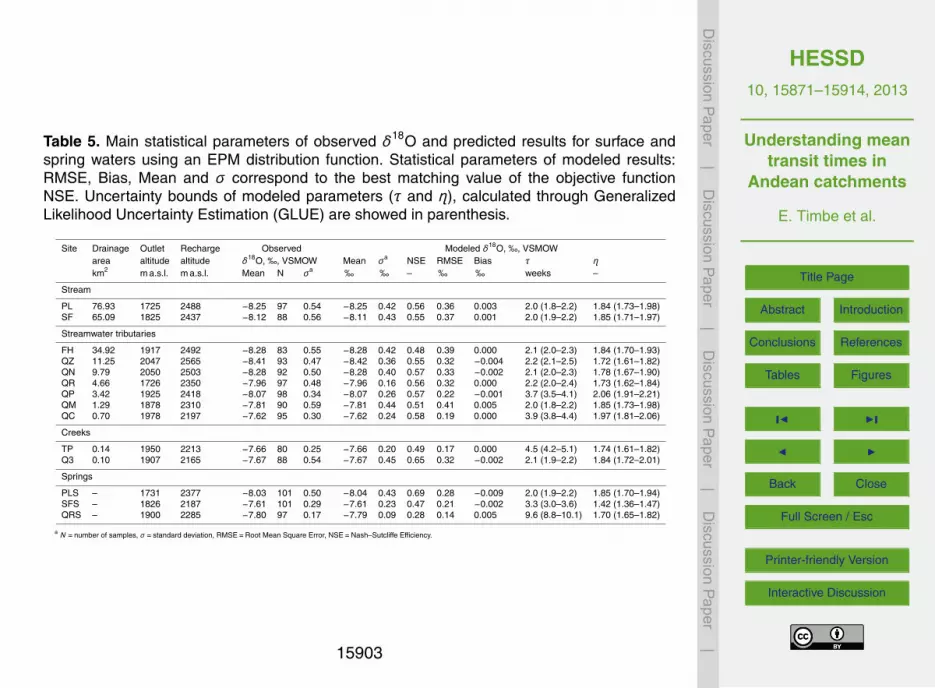
HESSD10, 15871–15914, 2013


Andean catchments

E. Timbe et al.

Title Page



Tables Figures

J I

J I

Back Close

Full Screen / Esc



Discussion

Paper

|D

iscussionP

aper|

Discussion

Paper

|D

iscussionP

aper|

Table 5. Main statistical parameters of observed δ18O and predicted results for surface andspring waters using an EPM distribution function. Statistical parameters of modeled results:RMSE, Bias, Mean and σ correspond to the best matching value of the objective functionNSE. Uncertainty bounds of modeled parameters (τ and η), calculated through GeneralizedLikelihood Uncertainty Estimation (GLUE) are showed in parenthesis.

Site Drainage Outlet Recharge Observed Modeled δ18O, ‰, VSMOWarea altitude altitude δ18O, ‰, VSMOW Mean σa NSE RMSE Bias τ ηkm2 m a.s.l. m a.s.l. Mean N σa ‰ ‰ – ‰ ‰ weeks –

Stream

PL 76.93 1725 2488 −8.25 97 0.54 −8.25 0.42 0.56 0.36 0.003 2.0 (1.8–2.2) 1.84 (1.73–1.98)SF 65.09 1825 2437 −8.12 88 0.56 −8.11 0.43 0.55 0.37 0.001 2.0 (1.9–2.2) 1.85 (1.71–1.97)

Streamwater tributaries

FH 34.92 1917 2492 −8.28 83 0.55 −8.28 0.42 0.48 0.39 0.000 2.1 (2.0–2.3) 1.84 (1.70–1.93)QZ 11.25 2047 2565 −8.41 93 0.47 −8.42 0.36 0.55 0.32 −0.004 2.2 (2.1–2.5) 1.72 (1.61–1.82)QN 9.79 2050 2503 −8.28 92 0.50 −8.28 0.40 0.57 0.33 −0.002 2.1 (2.0–2.3) 1.78 (1.67–1.90)QR 4.66 1726 2350 −7.96 97 0.48 −7.96 0.16 0.56 0.32 0.000 2.2 (2.0–2.4) 1.73 (1.62–1.84)QP 3.42 1925 2418 −8.07 98 0.34 −8.07 0.26 0.57 0.22 −0.001 3.7 (3.5–4.1) 2.06 (1.91–2.21)QM 1.29 1878 2310 −7.81 90 0.59 −7.81 0.44 0.51 0.41 0.005 2.0 (1.8–2.2) 1.85 (1.73–1.98)QC 0.70 1978 2197 −7.62 95 0.30 −7.62 0.24 0.58 0.19 0.000 3.9 (3.8–4.4) 1.97 (1.81–2.06)

Creeks

TP 0.14 1950 2213 −7.66 80 0.25 −7.66 0.20 0.49 0.17 0.000 4.5 (4.2–5.1) 1.74 (1.61–1.82)Q3 0.10 1907 2165 −7.67 88 0.54 −7.67 0.45 0.65 0.32 −0.002 2.1 (1.9–2.2) 1.84 (1.72–2.01)

Springs

PLS – 1731 2377 −8.03 101 0.50 −8.04 0.43 0.69 0.28 −0.009 2.0 (1.9–2.2) 1.85 (1.70–1.94)SFS – 1826 2187 −7.61 101 0.29 −7.61 0.23 0.47 0.21 −0.002 3.3 (3.0–3.6) 1.42 (1.36–1.47)QRS – 1900 2285 −7.80 97 0.17 −7.79 0.09 0.28 0.14 0.005 9.6 (8.8–10.1) 1.70 (1.65–1.82)

a N =number of samples, σ = standard deviation, RMSE=Root Mean Square Error, NSE=Nash–Sutcliffe Efficiency.

15903





HESSD10, 15871–15914, 2013


Andean catchments

E. Timbe et al.

Title Page



Tables Figures

J I

J I

Back Close

Full Screen / Esc



Discussion

Paper

|D

iscussionP

aper|

Discussion

Paper

|D

iscussionP

aper|

Fig. 1. San Francisco catchment with sampling locations and delineation of drainage area.Acronyms in bold are defined in Table 1. Isotope rainfall sampling was conducted at ECSFfacilities.

15904





HESSD10, 15871–15914, 2013


Andean catchments

E. Timbe et al.

Title Page



Tables Figures

J I

J I

Back Close

Full Screen / Esc



Discussion

Paper

|D

iscussionP

aper|

Discussion

Paper

|D

iscussionP

aper|

Fig. 2. (a) Weekly δ18O and δ2H at the ECSF rainfall sampling collector; light blue bubblesindicate daily δ18O and relative volume of daily rainfall; (b) weekly δ18O and δ2H of streamwaterat catchment’s main outlet (PL) for baseflow and high flow conditions; and (c) time series ofrainfall for ECSF meteorological station, hourly discharge and baseflows at the catchment outlet(PL).

15905





HESSD10, 15871–15914, 2013


Andean catchments

E. Timbe et al.

Title Page



Tables Figures

J I

J I

Back Close

Full Screen / Esc



Discussion

Paper

|D

iscussionP

aper|

Discussion

Paper

|D

iscussionP

aper|

Fig. 3. Shaded area depicts the expected variation range of the Local Meteorological WaterLine of rainfall (LMWL) considering the altitudinal range of the catchment (1725–3150 m a.s.l.)and estimated d-excess gradient. Symbols in colors depict weekly values of some of the catch-ment’s waters. Acronyms are defined in Table 1.

15906





HESSD10, 15871–15914, 2013


Andean catchments

E. Timbe et al.

Title Page



Tables Figures

J I

J I

Back Close

Full Screen / Esc



Discussion

Paper

|D

iscussionP

aper|

Discussion

Paper

|D

iscussionP

aper|

Fig. 4. Monthly isotopic δ18O signals between two consecutive years (2010–2012) at ECSF(1900 m a.s.l.) and averaged monthly values (1992–1994) at Amaluza GNIP station (latitude−2.61, longitude −78.57, altitude 2378 m a.s.l.).

15907





HESSD10, 15871–15914, 2013


Andean catchments

E. Timbe et al.

Title Page



Tables Figures

J I

J I

Back Close

Full Screen / Esc



Discussion

Paper

|D

iscussionP

aper|

Discussion

Paper

|D

iscussionP

aper|

Fig. 5. (a) Best NSE for each of the seven lumped parameter models; (b) MTT estimationaccording the best NSE per site: symbols represent MTT corresponding to the best matchingresult among 7 models considering the NSE criteria showed in (a), vertical line representsuncertainty bounds according the GLUE methodology for the selected model.

15908





HESSD10, 15871–15914, 2013


Andean catchments

E. Timbe et al.

Title Page



Tables Figures

J I

J I

Back Close

Full Screen / Esc



Discussion

Paper

|D

iscussionP

aper|

Discussion

Paper

|D

iscussionP

aper|

Fig. 6. Intercomparison of models for soil sites according to their: (a) estimated mean transittimes; (b) uncertainty ranges expressed in percentage of its respective MTT estimation; and(c) number of observations inside the range of behavioral solutions.

15909





HESSD10, 15871–15914, 2013


Andean catchments

E. Timbe et al.

Title Page



Tables Figures

J I

J I

Back Close

Full Screen / Esc



Discussion

Paper

|D

iscussionP

aper|

Discussion

Paper

|D

iscussionP

aper|

Fig. 7. Intercomparison of models for surface waters and springs according to their: (a) es-timated mean transit times; (b) uncertainty ranges expressed in percentage of its respectiveMTT estimation; and (c) number of observations inside the range of behavioral solutions.

15910





HESSD10, 15871–15914, 2013


Andean catchments

E. Timbe et al.

Title Page



Tables Figures

J I

J I

Back Close

Full Screen / Esc



Discussion

Paper

|D

iscussionP

aper|

Discussion

Paper

|D

iscussionP

aper|

Fig. 8. Fitted results of the LPM model compared to observed data for soil water of a pasturessite (C2). Sub-plots (a) and (b) show the uncertainty analysis of 10 000 simulations and thefeasible range of behavioral solutions of model parameters as a 5 % of the top best prediction.Black filled circles in sub-plot (c) represents the observed data; the black line and the shadedarea represent the best possible solution and its range of variation according to the 5–95 %confidence limits of the behavioral solutions shown in (a); and the gray dashed line with crossesrepresents the weekly rainfall variation as input function for the model.

15911





HESSD10, 15871–15914, 2013


Andean catchments

E. Timbe et al.

Title Page



Tables Figures

J I

J I

Back Close

Full Screen / Esc



Discussion

Paper

|D

iscussionP

aper|

Discussion

Paper

|D

iscussionP

aper|

Fig. 9. Uncertainty ranges for outlet stream water (PL site) using a TPLR distribution function.Sub-plots (a), (b) and (c) show the modeled parameter uncertainties of 10 000 random simu-lations and the feasible range of behavioral solutions taking a lower limit of 5 % from the bestsolution. Black filled circles in the sub-plots (d) and (e) represents the observed data, the blackline and shaded area depict the best possible solution and its range of variation according to the5–95 % confidence limits of the behavioral solutions shown in sub-plot (b); and the gray dashedline with crosses in sub-plot (e) represents the weekly rainfall variation as input function for themodel.

15912





HESSD10, 15871–15914, 2013


Andean catchments

E. Timbe et al.

Title Page



Tables Figures

J I

J I

Back Close

Full Screen / Esc



Discussion

Paper

|D

iscussionP

aper|

Discussion

Paper

|D

iscussionP

aper|

Fig. 10. Uncertainty ranges for outlet stream water (PL site) using a GM distribution function.Sub-plots (a), (b) and (c) show the modeled parameters uncertainties of 10 000 simulationsand the feasible range of behavioral solutions taking a lower limit of 5 % from the best solution.Black filled circles in the sub-plots (d) and (e) represents the observed data, the black line andthe shaded area represent the best possible solution and its range of variation according to the5–95 % confidence limits of the behavioral solutions shown in sub-plot (a); and the gray dashedline with crosses in sub-plot (e) represents the weekly rainfall variation as input function for themodel.

15913





HESSD10, 15871–15914, 2013


Andean catchments

E. Timbe et al.

Title Page



Tables Figures

J I

J I

Back Close

Full Screen / Esc



Discussion

Paper

|D

iscussionP

aper|

Discussion

Paper

|D

iscussionP

aper|

Fig. 11. Uncertainty ranges for outlet stream water (PL site) using an EPM distribution function.Sub-plots (a) and (b) show the modeled parameters uncertainties of 10 000 simulations andthe feasible range of behavioral solutions taking a lower limit of 5 % from the best solution.Black filled circles in the sub-plots (c) and (d) represent the observed data, the black line andthe shaded area represent the best possible solution and its range of variation according the5–95 % confidence limits of the behavioral solutions shown in sub-plot (a); and the gray dashedline with crosses in sub-plot (d) represents the weekly rainfall variation as input function for themodel.

15914



