METAGENOMICS TO
EXPLORE THE
BIOTECHNOLOGICAL
POTENTIAL OF CRYOSPHERIC
BACTERIA
by
Melanie Claire Hay
Department of Geography and Earth Sciences
and
Institute of Biological, Environmental and Rural Sciences
Aberystwyth University
This dissertation is submitted for the degree of Doctor of Philosophy
September 2020


i
To my parents, siblings, and niece

ii rd
Te
mp
lat
e b
yF
rie
dm an
&
M
or
gan
2
01 4
DECLARATION
Word Count of thesis: 84 690
DECLARATION
This work has not previously been accepted in substance for any degree and is not
being concurrently submitted in candidature for any degree.
Candidate name Melanie Claire Hay
Signature:
Date 14 September 2020
STATEMENT 1
This thesis is the result of my own investigations, except where otherwise stated.
Where *correction services have been used, the extent and nature of the correction is
clearly marked in a footnote(s).
Other sources are acknowledged by footnotes giving explicit references. A
bibliography is appended.
Signature:
Date 14 September 2020
STATEMENT 2
I hereby give consent for my thesis, if accepted, to be available for photocopying and
for inter-library loan, and for the title and summary to be made available to outside
organisations.
Signature:
Date 14 September 2020

The Biotechnological Potential of Cryospheric Bacteria
iii
SUMMARY
Bioprospecting is the process by which organisms are investigated for natural products
(NPs) that can be of societal benefit. The cryosphere is a prime region for bioprospecting
because it has extreme environmental conditions that increase the probability of NP
novelty, it is underexplored, and it is threatened by global climate change. Initially, 16S
rRNA gene amplicon analysis was used to identify environments with high
bioprospecting potential in a Svalbard glacier system (Chapter 3). Bacteria showed
strong habitat preference, suggesting niche specialisation and subsequent vulnerability to
climate change. Phylotypes do not provide functional information about microbes,
therefore, shotgun metagenomics was used to understand the high potential environments
better. Following the construction and testing of a bioinformatics workflow (Chapter 8),
a collection of 74 metagenome assembled genomes (MAGs) from Svalbard cryoconite,
soil and seawater (Chapter 4) and 121 MAGs from the Scărișoara Ice Cave (Chapter 7)
were constructed. These MAGs were taxonomically classified, revealing several novel
species. The spatial distribution of MAGs across several sites, together with identification
of genes in major biogeochemical pathways was explored to understand microbe nutrient
needs and look for signs of cooperation between co-occurring MAGs. Genome-mining
was used to screen the MAGs for potentially useful secondary metabolites (Chapter 5).
The MAGs were rich in biosynthetic gene clusters (BGCs) for exopolysaccharides (EPS),
carotenoids, and non-ribosomal peptide synthases (NRPS), all of which find utility in the
food, cosmetic and pharmaceutical industries. Bioinformatics predictions are limited by
information in databases, and functional studies are needed to describe novel functions.
Therefore, a functional metagenomic screen was conducted to search for novel cold-
active polymerases by cloning soil and cryoconite environmental DNA into cold-sensitive
E. coli mutants (Chapter 6). This thesis confirmed enormous diversity and novelty in
cryospheric bacteria. Furthermore, adaptations that enable survival in the extreme
conditions lend themselves to biotechnological applications.
Chapter 1
iv
ACKNOWLEDGEMENTS
This research was funded by a Marie Curie MicroArctic ITN grant. I am eternally grateful for the generous
financial support as well as the many incredible opportunities that being part of this network has afforded
me. I treasure the memories created at training events and meetings, and hope to stay connected to the
wonderful group of ESRs and PIs.
I am incredibly grateful to my supervisors, Dr Arwyn Edwards and Dr Andy Mitchell for their mentorship.
This was a wonderful adventure. Thank you for indulging my ideas, giving me so much independence, and
providing advice, calm, reason, motivation, and support over all the years, as well as some genuinely fun
fieldwork trips and discussions.
I am thankful to several people who were generous with their time, expertise, and equipment. Thank you
to Dr Matt Hegarty for assisting with shotgun and 16S rRNA amplicon sequencing, Prof Luis Muir, Dr
Manfred Beckmann, Dr Sumana Bhowmick, and Dr Jason Finch for all the help with metabolomics, Pauline
Rees Stevens for letting me use equipment for DNA extraction and Dr Karen Reed and Shelley Rundle at
Wales Gene Park for answering questions and assisting with shotgun metagenome sequencing. I would like
to acknowledge those who assisted with sample collection or provided me with samples and data. Thanks
to Diana Carolina Mogrovejo, Nora Els, Andy Mitchell, and Arwyn Edwards for your assistance with
sample collection in Ny Ålesund, Svalbard in June/ July 2017 and Aliyah Debbonaire and Arwyn Edwards
for sample collection in June / July 2018. Special thank you to Nick Cox and the NERC Arctic Research
station for hosting me in the summers of 2017 and 2018. I would also like to thank Dr Cristina Purcarea for
providing the Scărișoara Ice Cave metagenome sequences. I would like to acknowledge the help I received
from Andre Soares conducting bioinformatics analyses, and Pallavee Srivastava, who taught this non-
microbiologist how to culture bacteria. I would also like to acknowledge Meren, (of anvi’o) and Kai Blin
(of MIBiG) who responded to GitHub issues and tweets, but more than that, created incredible tools, and
created excellent resources on how to use their tools.
I had two secondments during my PhD that were both wonderful experiences. Thank you to Prof Tim
Vogel, Dr Catherine Larose, Dr Laure Franqueville and Benoit Bergk Pinto at the Environmental Microbial
Genomics Group at École Centrale de Lyon, who hosted me in their lab, trained me in new techniques and
made me feel absolutely welcome and at home. I would also like to sincerely thank Dr David Rooke, Colin
Bright, Sandeep, and Karl for making my visit to Dynamic Extractions in Tredegar such a warm,
informative, and friendly experience.
The daily reality of the PhD, with all is highs and lows, has been navigated with the best lab mates, and
dear friends that a person could hope to find. My eternal gratitude, love, and loyalty to the ‘Four
Musketeers’, which includes André Soares, Aliyah Debbonaire and Pallavee Srivastava. Thanks for the
coffees, beers, wines (and whines), work talk, life talk, silly talk, and serious advice. I learned and gained
and grew so much from knowing you. I would also like to thank the other members of F36 who provided
friendship, a few good nights out and serious laughs, Karen Cameron, Alvaro Garcia, Eleanor Furness, and
Joe Dean.
To Morgan Commins, my wonderful friend- it is impossible not to acknowledge your role in my life and
academic journey over the 14 years since we met. Thank you for believing in me, encouraging me, regularly
feeding me great food, and all the adventures.
Finally, I would like to thank my family. My father, Malcolm Hay, encouraged my love of science from a
young age, and financially supported much of my studies. You believed in me and instilled in me the belief
that I can do anything. I also want to thank my mother, Wendy Hay, who is kindness, gentleness, and
acceptance personified. I would not have completed this PhD without my twin sister, Michelle Hay (Shelly).
You have been there through literally everything. Your support, in academics and life is constant and
absolute. Thank you to Michelle and my brother-in-law, Andrew Bowman for the cosiest, happiest, most
encouraging space a person could hope for during a combined pandemic/ PhD write-up. Likewise, I had
shelter from my youngest sister, Kirsten Hay and my brother-in-law, Timothy Fischer, during December
and January 2019. Kirst, it has been a long time since you sent me handwritten and decorated letters at
Rhodes, but your support, thoughtfulness and generosity over the years has not wavered. Finally, my
brother Alastair Hay, and my sister-in-law Mai, your messages never fail to make me smile, especially
since Alexandra Ida Hay joined the world last year.

The Biotechnological Potential of Cryospheric Bacteria
Melanie Hay –September 2020 v
TABLE OF CONTENTS
DECLARATION ................................................................................................................ II
SUMMARY ..................................................................................................................... III
ACKNOWLEDGEMENTS ..................................................................................................IV
TABLE OF CONTENTS ..................................................................................................... V
LIST OF TABLES ......................................................................................................... XIII
LIST OF FIGURES ......................................................................................................... XV
LIST OF ABBREVIATIONS AND ACRONYMS ............................................................... XXIV
1 LITERATURE REVIEW ....................................................................................... 1
1.1 BIOPROSPECTING ............................................................................................... 1
1.1.1 Bioprospecting encourages biodiversity conservation ................................. 1
1.1.2 Bioprospecting provides solutions to emerging global challenges............... 2
1.1.3 Bioprospecting in the cryosphere ................................................................. 2
1.2 THE HABITATS OF THE GLOBAL CRYOSPHERE ..................................................... 3
1.2.1 Glacial ecosystems ........................................................................................ 3
1.2.2 Cryoconite ..................................................................................................... 4
1.2.3 Soil ................................................................................................................ 8
1.2.4 Seawater ...................................................................................................... 10
1.3 INVESTIGATED REGIONS .................................................................................. 11
1.3.1 Svalbard ...................................................................................................... 11
1.3.2 Scărișoara Ice Cave .................................................................................... 12
1.4 EXTREME ENVIRONMENTAL PARAMETERS ....................................................... 13
1.4.1 Low temperatures ........................................................................................ 13
1.4.2 High UV radiation ...................................................................................... 13
1.4.3 Low liquid water availability ...................................................................... 14
1.5 BIOTECHNOLOGY ............................................................................................. 14
1.5.1 Cold-active enzymes .................................................................................... 15
1.5.2 Anti-freeze proteins (AFPs) and ice-binding proteins (IBPs) ..................... 20
1.5.3 Polyunsaturated fatty acids ......................................................................... 22
1.5.4 UV screens, pigments, and antioxidants ..................................................... 25
1.5.5 Exopolysaccharides/ extra cellular polymeric substances (EPS) ............... 27
1.6 NOVEL ANTIMICROBIAL COMPOUNDS ............................................................... 29
1.6.1 Advantages and challenges ......................................................................... 29
1.6.2 Drugs from polar organisms ....................................................................... 30

Chapter 1
vi
1.7 BIOMINING, BIOREMEDIATION AND PLASTIC DEGRADATION ............................. 34
1.7.1 Bioremediation: degradation of contaminants ........................................... 34
1.7.2 Plastic Degradation .................................................................................... 36
1.8 METAGENOMICS .............................................................................................. 39
1.8.1 Challenges ................................................................................................... 39
1.8.2 Sequence-based methods ............................................................................. 42
1.8.3 Functional screening methods .................................................................... 43
1.8.4 Strategic cultivation and expression ........................................................... 47
1.9 AIMS AND OBJECTIVES ..................................................................................... 48
2 MATERIALS AND METHODS ......................................................................... 49
2.1 SAMPLING SITES, SAMPLE COLLECTION, TRANSPORTATION, AND STORAGE ...... 49
2.1.1 Soil sample collection ................................................................................. 49
2.1.2 Cryoconite sample collection ...................................................................... 49
2.1.3 Glacial water and seawater sample collection ........................................... 51
2.1.4 Storage and transport ................................................................................. 51
2.2 DNA EXTRACTION........................................................................................... 51
2.2.1 DNA Extraction for 16S rRNA gene amplicon analysis ............................. 52
2.2.2 Qiagen DNEasy PowerWater ..................................................................... 53
2.2.3 Qiagen DNeasy PowerSoil .......................................................................... 54
2.2.4 FastDNA™ Spin Kit for Soil ....................................................................... 55
2.2.5 MasterPure Complete DNA & RNA Purification Kit ................................. 56
2.2.6 Ludox Density Gradient centrifugation ...................................................... 58
2.2.7 MO BIO PowerMax Soil DNA Isolation Kit ............................................... 60
2.2.8 ZymoBIOMICS DNA Minikit ...................................................................... 61
2.3 DNA QUALITY AND CONCENTRATION ............................................................. 62
2.3.1 Agarose gel electrophoresis for DNA visualisation .................................... 62
2.3.2 Qubit to assess DNA concentration ............................................................ 62
2.4 POLYMERASE CHAIN REACTION (PCR) ........................................................... 62
2.4.1 Optimisation of 16S rRNA gene PCR ......................................................... 62
2.5 DNA CLEAN-UP AND PURIFICATION ................................................................ 63
2.5.1 Ampure bead clean-up ................................................................................ 63
2.6 DNA SEQUENCING ........................................................................................... 64
2.6.1 Illumina MiSeq of 16S rRNA gene Amplicons ............................................ 64
2.6.2 Illumina Nextera shotgun sequencing ......................................................... 65

The Biotechnological Potential of Cryospheric Bacteria
Melanie Hay –September 2020 vii
2.6.3 Sanger sequencing ...................................................................................... 66
3 HABITAT PREFERENCE OF BACTERIA FROM A HIGH ARCTIC
GLACIAL ECOSYSTEM INDICATES CLIMATE VULNERABILITY .............. 67
3.1 INTRODUCTION................................................................................................. 67
3.1.1 Aims and objectives ..................................................................................... 70
3.2 METHODS ......................................................................................................... 71
3.2.1 Sample collection ........................................................................................ 71
3.2.2 DNA extraction............................................................................................ 72
3.2.3 Library preparation and sequencing .......................................................... 73
3.2.4 Bioinformatics analysis ............................................................................... 73
3.2.5 Statistical analysis and plotting of 16S rRNA abundance data .................. 75
3.2.6 Co-occurrence network analysis ................................................................. 75
3.3 RESULTS .......................................................................................................... 76
3.3.1 Sequencing results ....................................................................................... 76
3.3.2 Taxonomic assignment ................................................................................ 76
3.3.1 Decontamination ......................................................................................... 76
3.3.1 Phylogenetic diversity of different environments ........................................ 81
3.3.2 Community composition by environment .................................................... 86
3.3.3 Comparison/ Relationship between environments ...................................... 99
3.4 DISCUSSION ................................................................................................... 104
3.4.1 The Decontam tool was able to successfully remove contaminants ......... 104
3.4.2 There is a continuum between the snowpack, slush, meltwater, and
proglacial water. ................................................................................................... 104
3.4.3 Proglacial water is an intersection of multiple environment inputs ......... 106
3.4.4 Soil is extremely heterogenous .................................................................. 106
3.4.5 Seawater does not share ASVs with other environments .......................... 107
3.4.6 Cryoconite communities on VB and ML are similar ................................. 107
3.4.7 High bioprospecting potential due to rare and specialist taxa ................. 108
3.4.8 Recommendations ..................................................................................... 109
3.5 CONCLUSIONS ................................................................................................ 109
4 METAGENOME ASSEMBLED GENOMES FROM SVALBARD
CRYOCONITE, SOIL, AND SEAWATER ARE PHYLOGENETICALLY AND
FUNCTIONALLY DIVERSE ................................................................................... 110
4.1 INTRODUCTION............................................................................................... 110

Chapter 1
viii
4.1.1 Aims and Objectives .................................................................................. 112
4.2 MATERIALS AND METHODS ............................................................................ 113
4.2.1 Sample collection ...................................................................................... 113
4.2.2 DNA extraction.......................................................................................... 114
4.2.3 Library preparation and sequencing ........................................................ 114
4.2.4 Reads processing and quality control ....................................................... 115
4.2.5 Taxonomic assignment .............................................................................. 116
4.2.6 Metagenome-assembled genomes (MAGs) ............................................... 116
4.2.7 Binning and refinement of MAGs .............................................................. 116
4.2.8 Phylogenomic Tree.................................................................................... 117
4.2.9 Spatial distribution of the MAGs across sample sites ............................... 118
4.2.10 Biogeochemical cycles .......................................................................... 118
4.2.11 Phormidesmis pangenome .................................................................... 118
4.3 RESULTS ........................................................................................................ 120
4.3.1 Library Statistics ....................................................................................... 120
4.3.2 Reads-based taxonomy .............................................................................. 121
4.3.3 Assembly statistics ..................................................................................... 127
4.3.4 Metagenome Assembled Genomes ............................................................ 129
4.3.5 Phylogenomic tree of Svalbard MAGs ...................................................... 135
4.3.6 Spatial distribution of MAGs .................................................................... 141
4.3.7 Major biogeochemical cycles .................................................................... 145
4.3.8 Phormidesmis and Leptolyngba pangenome ............................................ 149
4.4 DISCUSSION ................................................................................................... 155
4.4.1 Effect of environment complexity on ability to resolve MAGs .................. 155
4.4.2 Phylogenomics of Svalbard MAGs............................................................ 156
4.4.3 Spatial distribution of MAGs across different sites .................................. 157
4.4.4 Cyanobacteria ........................................................................................... 158
4.4.5 Biogeochemical cycling in different environments ................................... 159
4.4.6 Advantages to this study ............................................................................ 164
4.4.7 Limitations of this study ............................................................................ 165
4.4.8 Future work ............................................................................................... 166
4.5 CONCLUSION .................................................................................................. 166

The Biotechnological Potential of Cryospheric Bacteria
Melanie Hay –September 2020 ix
5 THE SECONDARY METABOLITES OF SOIL AND CRYOCONITE HAVE
A RANGE OF BIOTECHNOLOGICAL APPLICATIONS .................................. 167
5.1 INTRODUCTION............................................................................................... 167
5.1.1 Aims and objectives ................................................................................... 169
5.2 METHODS ....................................................................................................... 170
5.2.1 Samples ..................................................................................................... 170
5.2.2 Bioinformatics detection of BGCs ............................................................. 171
5.2.3 Metabolomics ............................................................................................ 172
5.3 RESULTS ........................................................................................................ 174
5.3.1 Assembly .................................................................................................... 174
5.3.2 Screening MAGs for BGCs ....................................................................... 176
5.3.3 Network analysis of BGCs from MAGs ..................................................... 179
5.3.4 Cyanobacterial secondary metabolites ..................................................... 185
5.3.5 Actinobacterial MAG DA_MAG_007_Iso899 .......................................... 187
5.3.6 Screening contigs by environment ............................................................ 191
5.3.7 The metabolomes of cryoconite from different glaciers are similar ......... 194
5.4 DISCUSSION ................................................................................................... 197
5.4.1 Biosynthetic gene clusters are modular .................................................... 197
5.4.2 Secondary metabolites reflect adaptations to environmental stressors .... 198
5.4.3 The NRPS metabolites of Cyanobacteria .................................................. 200
5.4.4 Talented Actinobacterial MAGs ................................................................ 202
5.4.5 Sequencing depth and metabolite detection .............................................. 202
5.4.6 Linking detected metabolites and predictions based on BGCs ................. 203
5.4.7 Future work ............................................................................................... 203
5.5 CONCLUSION .................................................................................................. 204
6 SCREENING OF ARCTIC SOIL AND CRYOCONITE METAGENOMES
FOR COLD-ACTIVE POLYMERASES ................................................................. 205
6.1 INTRODUCTION............................................................................................... 205
6.1.1 Aims and objectives ................................................................................... 207
6.2 MATERIALS AND METHODS ........................................................................... 208
6.2.1 Samples and environmental DNA extraction ............................................ 208
6.2.2 Bacterial strains ........................................................................................ 208
6.2.3 PCR of polA gene ...................................................................................... 209
6.2.4 Cloning and transformation ...................................................................... 211

Chapter 1
x
6.2.5 Glycerol stocks .......................................................................................... 220
6.2.6 Bioinformatics ........................................................................................... 220
6.3 RESULTS ........................................................................................................ 221
6.3.1 Sanger sequencing to confirm mutation .................................................... 221
6.3.2 Transformation of DH10B with soil and cryoconite eDNA ...................... 223
6.3.3 Size of cryoconite and soil eDNA inserts .................................................. 225
6.3.4 Cold complementation .............................................................................. 227
6.4 DISCUSSION ................................................................................................... 229
6.4.1 Difficulties encountered ............................................................................ 229
6.4.2 The clones reflect the most abundant taxa in cryoconite and soil ............ 231
6.4.3 The clones from the cold-complementation assay tended to have DNA-
binding activity ...................................................................................................... 231
6.4.4 Future work ............................................................................................... 232
6.5 CONCLUSION .................................................................................................. 233
7 A METAGENOMIC ANALYSIS OF THE FUNCTIONAL POTENTIAL OF
THE SCĂRIȘOARA ICE CAVE .............................................................................. 234
7.1 INTRODUCTION............................................................................................... 234
7.1.1 Aims and objectives ................................................................................... 235
7.2 MATERIALS AND METHODS ............................................................................ 236
7.2.1 Site description .......................................................................................... 236
7.2.2 Sequencing and bioinformatics ................................................................. 238
7.2.3 Metagenome assembled genomes (MAGs)................................................ 238
7.3 RESULTS ........................................................................................................ 240
7.3.1 Sequencing results ..................................................................................... 241
7.3.2 Taxonomy .................................................................................................. 241
7.3.3 Assembly .................................................................................................... 244
7.3.4 Metagenome assembled genomes ............................................................. 244
7.3.5 Phylogenomics .......................................................................................... 249
7.3.6 Spatial distribution of MAGs throughout the Ice-Cave ............................ 255
7.3.7 Biogeochemical cycles .............................................................................. 257
7.3.8 Antimicrobial secondary metabolites ........................................................ 262
7.4 DISCUSSION ................................................................................................... 267
7.4.1 Phylogeny and novel species ..................................................................... 267
7.4.2 Spatial distribution of the MAGs .............................................................. 268

The Biotechnological Potential of Cryospheric Bacteria
Melanie Hay –September 2020 xi
7.4.3 Biogeochemical cycling ............................................................................ 269
7.4.4 Secondary metabolites .............................................................................. 272
7.5 CONCLUSION .................................................................................................. 272
8 BIOINFORMATICS WORKFLOW FOR BIOPROSPECTING FROM
METAGENOMES ...................................................................................................... 274
8.1 INTRODUCTION............................................................................................... 274
8.1.1 Aims and Objectives .................................................................................. 275
8.2 METHODS ....................................................................................................... 276
8.2.1 Environmental sample types ..................................................................... 276
8.2.2 Quality control .......................................................................................... 276
8.2.3 Assembly .................................................................................................... 276
8.2.4 Metagenome-assembled genomes (MAGs) using anvi’o .......................... 277
8.2.5 Binning and refinement of MAGs .............................................................. 279
8.2.6 Screening MAGs and contigs .................................................................... 282
8.2.7 Workflow steps .......................................................................................... 283
8.3 RESULTS ........................................................................................................ 284
8.3.1 Identification of bioprospecting targets .................................................... 284
8.3.2 Datasets ..................................................................................................... 284
8.3.3 Assembly comparisons .............................................................................. 287
8.3.4 Read Mapping ........................................................................................... 295
8.3.5 The performance of different binning tools ............................................... 297
8.3.6 Manual refinement in anvi’o ..................................................................... 301
8.3.7 Genome completeness and quality ............................................................ 306
8.3.8 Databases and tools for the annotation of reads, contigs and MAGs ...... 306
8.4 DISCUSSION ................................................................................................... 311
8.4.1 The effect of environment on assembly size .............................................. 311
8.4.2 The advantages and disadvantages of reads, contigs and metagenome-
assembled genomes ............................................................................................... 312
8.4.3 Optimisation and benchmarking are necessary ........................................ 312
8.4.4 Long-read technologies will improve MAG quality .................................. 314
8.4.5 Contigs and MAGs are a catalogue of diversity that can be explored ..... 314
8.4.6 MAGs enable strategic bioprospecting ..................................................... 316
8.5 CONCLUSION .................................................................................................. 317

Chapter 1
xii
9 DISCUSSION ...................................................................................................... 320
9.1 BIOPROSPECTING AND GLOBAL CLIMATE CHANGE ......................................... 320
9.2 GENOME-CENTRED METAGENOMICS ENABLES STRATEGIC BIOPROSPECTING.. 321
9.2.1 MAGs vs phylotypes from previous 16S rRNA gene analysis ................... 322
9.2.2 Environment choice for bioprospecting .................................................... 324
9.3 ENVIRONMENTAL PRESSURES SELECT FOR SPECIFIC GENES AND PRODUCTS ... 325
9.3.1 Same genes, but with a twist ..................................................................... 326
9.4 THE CHOICE OF APPROPRIATE METHODS AND MULTIPLE LINES OF EVIDENCE . 328
9.4.1 Functional studies are vital to ground-truth bioinformatics predictions.. 328
9.4.2 Non-representative samples ...................................................................... 329
9.5 MICROBIAL COMMUNITIES ARE COOPERATIVE ............................................... 330
9.5.1 Co-cultivation to investigate ‘uncultivatable’ species .............................. 331
9.6 APPLICATIONS OF THE RESULTS OF THIS THESIS ............................................. 331
9.6.1 Strategic cultivation .................................................................................. 331
9.6.2 Host engineering ....................................................................................... 332
9.7 GENETIC NOVELTY IN THE CRYOSPHERE ........................................................ 332
9.8 CONCLUSION .................................................................................................. 333
10 REFERENCES .................................................................................................... 334
VOLUME 2: APPENDIX

The Biotechnological Potential of Cryospheric Bacteria
Melanie Hay –September 2020 xiii
LIST OF TABLES
Table 1-1 Table of common Bacterial phyla in Svalbard cryoconite ............................... 8
Table 1-2 Table of common Bacterial phyla in Svalbard soil ........................................ 10
Table 1-3 Table of common Bacterial phyla in Svalbard seawater ................................ 10
Table 1-4. The potential uses of psychrophilic microorganisms in biotechnology ........ 15
Table 1-5: Sources of cold-active enzymes from Arctic microorganisms ...................... 17
Table 1-6 Table of ice-nucleation-active bacteria ........................................................... 21
Table 1-7 Potential sources of PUFA from Cryospheric microorganisms ..................... 24
Table 1-8 Microbial sources of antioxidants, pigments and UV screens ........................ 26
Table 1-9 The use of EPSs in biotechnology .................................................................. 28
Table 1-10 Antimicrobial products from cryospheric microorganisms .......................... 31
Table 1-11 Bacteria with ability to grow on hydrocarbon sources, with potential
application for bioremediation ................................................................................ 35
Table 1-12 Bacteria capable of plastic degradation ........................................................ 38
Table 2-1 Table of DNA Extraction Kits used in different chapters .............................. 52
Table 3-1 Table of contaminants and true ASVs in environmental subsets ................... 78
Table 3-2 Table of alpha diversity measure for different environment groups .............. 85
Table 4-1 Table of sample type, collection date and GPS coordinates ......................... 113
Table 4-2 Characteristics of the Svalbard Soil, Seawater and Cryoconite datasets after
trimming ................................................................................................................ 120
Table 4-3 Assembly Statistics for the Svalbard metagenomes ..................................... 128
Table 4-4 Table of high quality MAGS (completion >90%, redundancy < 10%)........ 131
Table 4-5 Table of medium quality MAGS (completion >70%. Redundancy < 10%) 133
Table 4-6 Table of MAGS classified to species level using FastANI .......................... 136
Table 4-7 Classification of MAGS using GTDB-Tk .................................................... 137
Table 4-8 Full GTDB classification of Cyanobacterial MAGs included in the Leptolyngba
pangenome analysis .............................................................................................. 149
Table 4-9 Table of publicly available genomes included in the Leptolyngbya Pangenome
............................................................................................................................... 150
Table 4-10 COG Functional categories of accessory gene clusters in Leptolyngbya MAGs
............................................................................................................................... 154
Table 5-1 Table of sample sites for metabolite extractions and shotgun metagenome
sequencing ............................................................................................................. 170
Table 5-2 Table comparing Assembly statistics and contig size distribution of sea, soil
and cryoconite assemblies. .................................................................................... 175
Table 5-3 BGCs from Actinobacterial MAG DA_MAG_007_Iso899 ......................... 187
Table 5-4 Types of secondary metabolites detected by antiSMASH ........................... 191

Chapter 1
xiv
Table 5-5 Table of rare secondary metabolites detected in cryoconite, soil and seawater
............................................................................................................................... 192
Table 6-1 Tables of environments and DNA extraction methods ................................. 208
Table 6-2 Table of bacterial strains used in this thesis ................................................. 209
Table 6-3 Table of Media Supplements ........................................................................ 209
Table 6-4 Table of primers used to amplify the polA gene. .......................................... 211
Table 6-5 Components and volumes for DNA Blunting reaction ................................ 215
Table 6-6 Components and volumes for ligation Reaction ........................................... 215
Table 6-7 Table of glycerol stocks of different strains with different supplements ..... 220
Table 6-8 Table of blastx hits of randomly selected soil and cryoconite clones in DH10B
cells. ...................................................................................................................... 224
Table 7-1. A table describing the age, location and characteristics of samples collected in
the Scărișoara Ice Cave. ........................................................................................ 236
Table 7-2 Ice-cave library shotgun library statistics ..................................................... 240
Table 7-3 Table comparing Ice Cave assemblies .......................................................... 243
Table 7-4 Table of MAG characteristics ....................................................................... 246
Table 7-5 Table of MAGS classified to species level using FastANI .......................... 249
Table 7-6 GTDB-Yk classification of Ice Cave MAGS ............................................... 251
Table 8-1 Bioprospecting targets for cryospheric environments .................................. 284
Table 8-2 Characteristics of the Svalbard Soil, Seawater and Cryoconite datasets that
contributed to the design and implementation of the bioinformatics workflow ... 285
Table 8-3 Characteristics of the Scărișoara Ice-Cave dataset that contributed to the design
and implementation of the bioinformatics workflow ............................................ 286
Table 8-4: Comparison of cryoconite metagenome assembly statistics using QUAST 289
Table 8-5 Table comparing Assembly statistics and contig distribution of sea, soil and
cryoconite assemblies. .......................................................................................... 292
Table 8-6 Table comparing BGCs detected from contigs form the MEGAHIT,
metaSPAdes and IDBA-UD assemblies. .............................................................. 293
Table 8-7 Alignment rate of reads mapped back to assembly ...................................... 295
Table 8-8 Binning tool comparison for the Svalbard and Ice-Cave datasets ................ 297
Table 8-9 Table of tool and databases........................................................................... 310
Table 8-10 Table of tools used in the workflow. .......................................................... 318
Table 8-11 List of databases used in the workflow....................................................... 319
Table 8-12: Table of high performance and cloud computing facilities ....................... 319

The Biotechnological Potential of Cryospheric Bacteria
Melanie Hay –September 2020 xv
LIST OF FIGURES
Figure 1-1: Factors that make the cryosphere attractive for bioprospecting. The
cryosphere is an extreme environment and relatively unexplored, which increases
the chances of novel NPs. The cryosphere is seriously threatened because of global
climate change, and there is therefore an urgent need to explore these environments
soon. .......................................................................................................................... 3
Figure 1-2: Diagram showing the some of the habitats of a glacier ecosystem. ............... 5
Figure 1-3 Map of Svalbard. Svalbard is a Norwegian archipelago, situated between 74°
- 81° N and 10° - 35° E. The largest island of the Svalbard archipelago is Spitsbergen.
Figure by (Räisänen, 2008) ..................................................................................... 11
Figure 1-4 Map of the Scărișoara Ice Cave location in Romania. The cave is located in
the Bihor Mountains of North West Romania (46°29’23”N, 22°48’35”E) at an
altitude of 1165m. ................................................................................................... 12
Figure 1-5 Simplified and general overview of culture-dependent and metagenomic
methods for bioprospecting. Bioprospecting is an innovative field, beset by many
challenges that are being imaginatively overcome by technological advances. ..... 40
Figure 2-1 Map of sampling sites included in this thesis. Samples of cryoconite were
collected from four glaciers (ML, VB, VL and AB). Soil was collected from the ML
glacier forefield in three transects of five time points. Snow, slush, and meltwater
was collected from ML, and seawater was collected from Kongsfjorden ford. ..... 50
Figure 2-2 Gel of High Molecular Weight DNA extracted using Ludox HS-40. PL is
Phage DNA (47 kb). CL is Cleaver Scientific Broad Range Ladder. The numbered
lanes 1-20 refer to 1st, 2nd and 3rd 100 mL aliquots of soil slurry). Gel is 0.8% agarose
in 0.5 X TBE. .......................................................................................................... 59
Figure 2-3 Comparison of different polymerases on amplification of a range of
environment types. The High-Fidelity polymerases (Accuzyme and Platinum High
Fidelity) were completely inhibited by samples that amplified robustly using
Platinum Green Hot Start. ....................................................................................... 63
Figure 3-1 Map showing sampling sites in Ny-Ålesund, Spitsbergen, Svalbard. .......... 72
Figure 3-2 Decontamination of the Svalbard dataset. ASVs coloured red are contaminants
due to their high prevalence in negative controls, and low prevalence in
environmental samples. Blue points are true ASVs, detected in a high proportion of
samples, and in a low proportion of the negative controls. Boxplots showing the
proportion of reads remaining in samples vs controls after decontamination. ....... 80
Figure 3-3 The phylogenetic diversity of different environment types in Svalbard. A) Bar
plot showing the RA of phyla in the different environments. Samples were merged
by environment, and ASVs were agglomerated to Class level and only the top 50
classes are shown. Colours represent the different phyla. The thin horizontal lines
represent different classes within each phylum. RA does not equal 1, because only
the top 50 of 117 classes are plotted. B) Line graph showing the number of phyla,
classes, orders, families, and genera in each environment type. C) Table of phyla,
classes, order, families, and genera across different environments, and also showing
the totals for the combined soil (soil-0, soil-1, soil-2, soil3 and soil4), glacial waters
(snow, slush and meltwater), and the merged proglacial and cryoconite samples from
ML and VB. ............................................................................................................ 82

Chapter 1
xvi
Figure 3-4 Alpha Diversity of environment groups from Svalbard cryospheric
environments. See details in Table 3-2. .................................................................. 84
Figure 3-5 MDS Ordination showing Beta Diversity using Bray Curtis distance. ......... 86
Figure 3-6 Relative abundance of the most abundant taxa in cryoconite samples from
Midtre Lovénbreen and Vestre Brøggerbreen. (A) Proportion of reads remaining
after filtering out ASVs with less than (x > 20) in at least 6 samples. (B) Relative
abundance of filtered samples by class. (C) Relative abundance of filtered samples
by Genus. ................................................................................................................ 87
Figure 3-7 Scatter plot of the most prevalent and abundant ASVs in cryoconite, by Order.
X-axis is the prevalence of each ASV (number of samples in which each ASV
occurs). Y-axis is log10 of the mean RA of the ASVs across all samples in the
cryoconite dataset. Points are coloured by Order. .................................................. 88
Figure 3-8 Relative abundance of the most abundant taxa in snow, slush and meltwater
samples from Midtre Lovénbreen (A) Proportion of reads remaining after filtering
out ASVs without at least 10 reads in 5 or more samples. (B) Boxplot of number of
reads in included libraries. (C) Relative abundance of filtered samples by Genus. 90
Figure 3-9 Scatter plot of the most prevalent and abundant ASVs in supraglacial habitats)
snow, slush and meltwater, by Genus. X-axis is the prevalence of each ASV (number
of samples in which each ASV occurs). Y-axis is log10 of the mean relative
abundance of the ASVs across all samples in the glacial water (snow, slush,
meltwater) dataset. Points are coloured by Genus. ................................................. 91
Figure 3-10 Relative abundance of bacterial genera in proglacial water from Midtre
Lovénbreen and Vestre Brøggerbreen. (A) Proportion of reads remaining after
filtering out ASVs without at least 4 reads in 2 or more samples. (B) Boxplot of
number of reads in included libraries. (C) Relative abundance of filtered samples by
Genus. ..................................................................................................................... 92
Figure 3-11 Scatter plot of the most prevalent and abundant ASVs in proglacial water by
Family. X-axis is the prevalence of each ASV (number of samples in which each
ASV occurs). Y-axis is log10 of the mean relative abundance of the ASVs across all
samples in proglacial water. Points are coloured by Family. .................................. 93
Figure 3-12 Relative abundance of genera in glacier forefield soil samples. (A) Proportion
of reads remaining after filtering out ASVs without at least 10 reads in 3 or more
samples. (B) Boxplot of number of reads in included libraries. (C) Relative
Abundance of filtered samples by Genus. .............................................................. 94
Figure 3-13 Scatter plot of the most prevalent and abundant ASVs in glacial forefield soil
(n=45), by order. X-axis is the prevalence of each ASV (number of samples in which
each ASV occurs) The axis is shortened from 45 to 35, and there were 0 ASVs
present in all 45 samples. Y-axis is log10 of the mean relative abundance of the
ASVs across all samples. Points are coloured by Order. ........................................ 95
Figure 3-14 Relative abundance of bacterial families in sea water samples collected from
1m and 15m depth from the Kongsfjorden, in front of ML. (A) Proportion of reads
remaining after filtering out ASVs without at least 10 reads in 2 or more samples.
(B) Boxplot of number of reads in included libraries. (C) Relative Abundance of
filtered samples by Genus. ...................................................................................... 97
Figure 3-15 Scatter plot of the most prevalent and abundant ASVs in seawater (n=6), by
order. X-axis is the prevalence of each ASV (number of samples in which each ASV

The Biotechnological Potential of Cryospheric Bacteria
Melanie Hay –September 2020 xvii
occurs). Y-axis is log10 of the mean relative abundance of the ASVs across all
samples. Points are coloured by Order. ................................................................... 98
Figure 3-16 Bar plot showing effect of filtering on library size. The removal of ASVs
without ≧ 5 copies in at least two samples resulted in a reduction in library size
across the different samples. Environments with high heterogeneity and greater
diversity (like soil) suffered the greatest reduction in size. .................................. 100
Figure 3-17 UpSetR Diagram showing number of unique and shared ASVs between
different environments. Each environment group is a set (Barplot A). The number
of ASVs in each set and intersection of sets are shown in Barplot B above the matrix.
The black circles indicate the environments sharing ASVs. Sets are arranged in an
environmental gradient and reflect proximity between environments. Only
intersections involving 13 or more ASVs are shown. ........................................... 101
Figure 3-18 Network analysis of samples based on Bray-Curtis distances. Network
created using a maximum distance threshold of 0.7 for connecting vertices with an
edge. The network layout method is Fruchterman Reingold. The colour of groups is
based on environment subgroup, shape is based on glacier of origin and points are
labelled. ................................................................................................................. 102
Figure 3-19 Co-occurrence network of ASVs in Svalbard. The decontaminated dataset
(ASVs = 58 880) was filtered to include only ASVs with more than 40 reads in six
or more samples (ASVs = 526). A correlation analysis was run based on Spearman's
co-efficient, with a correlation coefficient cut-off of 0.5 and P-value cut-off of 0.05.
Network visualisation performed in Gephi, layout is Fruchterman Reingold. Node
colour refers to Phylum membership, Size of node reflects Degree, and edge colour
shows weight. There are four clusters main clusters detected, (modularity = 0.592),
which correspond roughly to sea, cryoconite, soil, and glacial surface communities.
............................................................................................................................... 103
Figure 4-1 Map of sampling sites for shotgun libraries included in this study. Orange
points are the soil sites, yellow points are the sea samples and green points are
cryoconite samples. ............................................................................................... 114
Figure 4-2 Reads-based taxonomic assignment of cryoconite libraries at the Phylum level
using Kaiju. Cryoconite libraries are listed on the x-axis. A dashed lined separates
the combined cryoconite library from the individual libraries. ............................ 121
Figure 4-3 Reads-based taxonomic assignment of cryoconite libraries at the Genus level
using Kaiju. ........................................................................................................... 122
Figure 4-4 Reads-based taxonomic assignment of soil libraries at the Phylum level using
Kaiju. Soil libraries are listed on the x-axis. A dashed lined separates the combined
soil library from the individual libraries. .............................................................. 123
Figure 4-5 Reads-based taxonomic assignment of soil libraries at the Genus level using
Kaiju. Soil libraries are listed on the x-axis. A dashed line separates the combined
soil library. ............................................................................................................ 124
Figure 4-6 Reads-based taxonomic assignment of seawater libraries at the Phylum level
using Kaiju. ........................................................................................................... 125
Figure 4-7 Reads-based taxonomic assignment of seawater libraries at the Species level
using Kaiju. ........................................................................................................... 126
Figure 4-8 Comparison of cryoconite, soil and seawater co-assemblies and combined
Svalbard co-assembly. .......................................................................................... 127

Chapter 1
xviii
Figure 4-9 Figure showing the MAGS included in the dataset. Figure is generated using
anvi-interactive from anvi’o. MAGS are ordered using mean-coverage and viewed
using ‘detection’ which shows proportion of the MAG which has at least 1 X
coverage. ............................................................................................................... 130
Figure 4-10 Phylogeny of MAGs created by Fast Tree of Muscle alignment of 71 single
copy core genes. .................................................................................................... 135
Figure 4-11 Heatmap showing distribution of MAGs across different environments and
sites using a MAG-centric view. This view is useful to see in which environment
each MAG is the most abundant. It compares each MAG to the same MAG in other
environments. ........................................................................................................ 142
Figure 4-12 The distribution of Svalbard MAGS based on Abundance. Colour guide:
Green: MAGs close to sample mean coverage; Blue: MAGs are highly abundant
(10- 40x the sample mean); wheat: rare MAGs (0.1 of the sample mean); white:
MAGs recruited zero reads in that sample. The phylum membership of MAGs is
displayed using a colour legend and environments were forced to cluster together.
............................................................................................................................... 144
Figure 4-13 Figure 1 showing the detection of key genes in Svalbard MAGS involved in
biogeochemical cycling. ........................................................................................ 147
Figure 4-14 Figure 2 showing the detection of key genes in Svalbard MAGS involved in
biogeochemical cycling. ........................................................................................ 148
Figure 4-15 The Pangenome of Phormidesmis and Leptolyngba species and MAGs .. 152
Figure 5-1 Ideal workflow for the exploring the metabolites of Svalbard soil and
cryoconite using a mix of metabolomics and metagenomics. .............................. 173
Figure 5-2 Secondary metabolite clusters in MAGs from the Acidobacteriota,
Actinobacteriota, Armatimonadota, Bacteroidota, Bdellovibrionota, Chloroflexota,
Chloroflexota_A phyla. Table showing the number and types of clusters detected by
antiSMASH 5. The MAGs are arranged by taxonomic clade, and the relative
abundance in each sample (expressed as max-normalised-abundance) is shown per
MAG. .................................................................................................................... 177
Figure 5-3 Secondary metabolite clusters in MAGs from the Cyanobacteria,
Eremiobacterota, Fibrobacterota, Gemmatimonadota, Myxococcota, Patescibacteria
and Proteobacteria phyla. Table showing the number and types of clusters detected
by antiSMASH 5. The MAGs are arranged by taxonomic clade, and the relative
abundance in each sample (expressed as max-normalised-abundance) is shown per
MAG. .................................................................................................................... 178
Figure 5-4 BiG-SCAPE network of 1742 BGCs from the Svalbard MAG collection and
1830 known biosynthetic gene clusters from the MiBIG database (v1.4). Total
BGCs: 2649 (1096 singleton/s), links: 13454, families: 1433. Network generated
using cutoff distance of 0.7. Clusters with a blue border represent BGCs with known
compounds from the MiBIG database. Nodes without borders represent BGCs
detected in the MAGs. .......................................................................................... 179
Figure 5-5 A Family of BGC s that synthesize carotenoid clusters similar to BGC0000646
and BGC0000647 are widely distributed across several phyla. Figure shows the
contig id, MAG id and phyla membership of different tree branches. The molecules
synthesized by the known BGCs are shown below. The * next to CC_MAG_026
because it does not belong to the same phylum (Armatimonadota) as the surrounding
MAGs. ................................................................................................................... 180

The Biotechnological Potential of Cryospheric Bacteria
Melanie Hay –September 2020 xix
Figure 5-6 Family of BGCs that synthesize Astaxanthin dideoxyglycoside
(BGC0001086) and Zeaxanthin (BGC0000656) gene clusters are all from the family
Sphingomonadaceae. Figure shows the contig id and MAG id. The compound
synthesized by the known BGCs are shown below. ............................................. 181
Figure 5-7 Family of BGCs similar to Hopene (BGC0000663) all from the
Alphaproteobacteria. Figure shows the contig id and MAG id. The compound
synthesized by the known BGCs are shown below the tree. ................................ 182
Figure 5-8 Several NRPs with similarity to anabaenopeptin NZ857 / nostamide A were
identified in Chloroflexota and Cyanobacterial MAGs. ....................................... 184
Figure 5-9 Several Actinobacterial MAGs contain a polyketide BGC for alkylresorcinol.
............................................................................................................................... 185
Figure 5-10 KnownClusterBlast results of A NRPS from cc_MAG_Nostoc_71: The
highly modular nature of NRPS gene clusters means that small reorganisations can
result in a large number of different compounds. ................................................. 186
Figure 5-11 Cluster 27.1 has high similarity to several Polyketide: Enediyene type I
BGCs. A Map of the location of the different clusters detected by antiSMASH on
this contig. B shows the detailed NRPS/ PKS domain annotation. C shows known
BGCs identified by KnownClusterBlast. D shows the accessions of similar clusters
using SubClusterBlast. ......................................................................................... 189
Figure 5-12 A Map of the location of the different clusters detected by antiSMASH on
this contig. B shows the detailed NRPS/ PKS domain annotation. C shows known
BGCs identified by KnownClusterBlast. D shows the accessions of similar clusters
using SubClusterBlast. .......................................................................................... 190
Figure 5-13 The number of biosynthetic gene clusters (BGCs) belonging to the most
common types of secondary metabolite detected in cryoconite, soil and seawater.
Figure shows only the most common secondary metabolite types (n> 10 in at least
one environment). A) shows the absolute number of clusters detected in each
environment. B) shows the relative proportion of the metabolites in each
environment. ......................................................................................................... 193
Figure 5-14 Principle Component Analysis (PCA), Principal Component- Linear
Discriminant Analysis (PC-LDA) and Unsupervised Random Forest MDS of
cryoconite of metabolites from four glaciers. Each point on the graph represents
metabolites from a separate cryoconite hole. ........................................................ 194
Figure 5-15 Heat map of explanatory features for metabolite differences between four
Svalbard glaciers, and their KEGG categories . .................................................... 196
Figure 6-1. Position of primer binding sites for the E.coli polA gene. The location of the
mutation and the codon that is affected is indicated in yellow. A G(346) -> A
transition causes Asp(116) (aspartic acid D) to be changed to a Asn (Asparagine N).
The different primer pairs that were tested are indicated on the figure. FWD primers
are in pink and REV primers are in orange. .......................................................... 210
Figure 6-2 DNA size selection via agarose gel electrophoresis. An example of gel used
to size select DNA fragments for clone library construction. BR is Cleaver Scientific
Broad Range DNA Ladder, 1Kb is the NEB 1kb DNA Ladder. 5ul of cryoconite and
soil respectively was added to the second and second last columns for visualization
of the pool fragment sizes. .................................................................................... 212

Chapter 1
xx
Figure 6-3 Vector map of the pJET1.2/blunt plasmid. The vector contains the (bla(ApR))
sequence which confers resistance to ampicillin (and carbenicillin) and the eco47IR
gene which is lethal unless disrupted by an insert. ............................................... 214
Figure 6-4 A Map of the pUC19 plasmid used as a transformation control in all cloning
experiments. The pUC19 plasmid has high transformation efficiency, is resistant to
carbenicillin antibiotics and is a similar size to empty pJET1.2/blunt. It was therefore
used as transformation efficiency control. ............................................................ 214
Figure 6-5 Cloning strategy to identify cold-active polymerases. The pJET2.1/blunt
plasmids were first transformed into chemically competent E. coli DH10B. Clones
were washed off, amplified in an O/N culture, midiprepped and then transformed
into the mutant E.coli HCS1 and cs2-29 strains. The E.coli HCS1 and cs2-29 were
grown at 15°C to identify clones with potential polymerases. ............................. 216
Figure 6-6. A: Agarose gel of E. coli cs2-29 and HCSI genomic DNA. Lane numbers
refer to the glycerol stock number. LH: Thermo ScientificTM MassRuler DNA
Ladder Mix. LM: Thermo ScientificTM MassRuler DNA Ladder High Range. B:
Agarose gel of polA PCR products. The polA gene was amplified using three
different primer pairs [1, 3, 8] that contained the mutation site. L: The DNA ladder
is the NEB 100 bp ladder. C: is a PCR negative control. ..................................... 221
Figure 6-7. Alignment of polA amplicons and polA gene showing the position of the
mutation conferring cold sensitivity. There is a G>A transition in the sc2-29 and
HCS1 mutant strains at position 346. .................................................................... 222
Figure 6-8. Alignment of translated polA gene showing the position of the amino acid
change causing cold sensitivity. The G>A transition in the cs2-29 and HCS1 mutant
strains at position results in an amino acid change from D (Aspartic acid) to be
changed to a N (Asparagine) at position 116. ....................................................... 222
Figure 6-9 Examples of clones obtained by transformation into DH10B. A shows clones
derived from soil DNA. B shows clones obtained from cryoconite DNA. C is a
PUC19 control to check transformation efficiency and D is a PCR product control
to check ligation efficiency. Plates are LB, supplemented with carbenicillin. ..... 223
Figure 6-10 Agarose gel of PCR of pJET1.2/blunt inserts from randomly selected DH10B
cryoconite and soil clones. .................................................................................... 224
Figure 6-11 A: Example of an agarose gel of undigested plasmids extracted from Batch
2 cryoconite and soil clone libraries. S: soil, C: cryoconite, (n-n) refer to the mixed
ligation batches. B: Restriction digestion of Batch 1 plasmids to check linear size. C
Cryoconite library. S: soil library. P: PCR ligation control. BR: Cleaver Scientific
Broad Range Ladder. +/– reflects whether the library was (+) or was not (-)
incubated with Xho1 restriction enzyme. ............................................................. 226
Figure 6-12 Agarose gel of PCR of pJET1.2/blunt inserts from randomly selected cs2-29
cryoconite and soil clones. .................................................................................... 227
Figure 6-13 Agarose gel of PCR of pJET1.2/blunt inserts from randomly selected HCS1
cryoconite and soil clones. .................................................................................... 228
Figure 7-1 A schematic diagram of the Scărișoara Ice Cave showing the locations of the
sample collection. .................................................................................................. 237
Figure 7-2 Phylum-level taxonomic profile of individual samples from various locations
in the Scărișoara Ice Cave. .................................................................................... 241
The Biotechnological Potential of Cryospheric Bacteria
Melanie Hay –September 2020 xxi
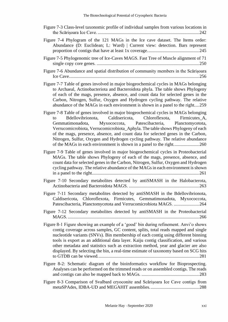
Figure 7-3 Class-level taxonomic profile of individual samples from various locations in
the Scărișoara Ice Cave. ........................................................................................ 242
Figure 7-4 Phylogram of the 121 MAGs in the Ice cave dataset. The Items order:
Abundance (D: Euclidean; L: Ward) | Current view: detection. Bars represent
proportion of contigs that have at least 1x coverage. ............................................ 245
Figure 7-5 Phylogenomic tree of Ice-Caves MAGS. Fast Tree of Muscle alignment of 71
single copy core genes. ......................................................................................... 250
Figure 7-6 Abundance and spatial distribution of community members in the Scărișoara
Ice Cave. ................................................................................................................ 256
Figure 7-7 Table of genes involved in major biogeochemical cycles in MAGs belonging
to Archaeal, Actinobacteriota and Bacteroidota phyla. The table shows Phylogeny
of each of the mags, presence, absence, and count data for selected genes in the
Carbon, Nitrogen, Sulfur, Oxygen and Hydrogen cycling pathway. The relative
abundance of the MAGs in each environment is shown in a panel to the right. ... 259
Figure 7-8 Table of genes involved in major biogeochemical cycles in MAGs belonging
to Bdellovibrionota, Caldisericota, Chloroflexota, Firmicutes_A,
Gemmatimonadota, Myxococcota, Patescibacteria, Planctomycetota,
Verrucomicrobiota, Verrucomicrobiota_Aphyla. The table shows Phylogeny of each
of the mags, presence, absence, and count data for selected genes in the Carbon,
Nitrogen, Sulfur, Oxygen and Hydrogen cycling pathway. The relative abundance
of the MAGs in each environment is shown in a panel to the right. ..................... 260
Figure 7-9 Table of genes involved in major biogeochemical cycles in Proteobacterial
MAGs. The table shows Phylogeny of each of the mags, presence, absence, and
count data for selected genes in the Carbon, Nitrogen, Sulfur, Oxygen and Hydrogen
cycling pathway. The relative abundance of the MAGs in each environment is shown
in a panel to the right. ............................................................................................ 261
Figure 7-10 Secondary metabolites detected by antiSMASH in the Halobacterota,
Actinobacteria and Bacteroidota MAGS. ............................................................. 263
Figure 7-11 Secondary metabolites detected by antiSMASH in the Bdellovibrionota,
Caldisericota, Chloroflexota, Firmicutes, Gemmatimonadota, Myxococcota,
Patescibacteria, Planctomycetota and Verrucomicrobiota MAGS. ...................... 264
Figure 7-12 Secondary metabolites detected by antiSMASH in the Proteobacterial
MAGS. .................................................................................................................. 266
Figure 8-1 Figure showing an example of a ‘good’ bin during refinement. Anvi’o shows
contig coverage across samples, GC content, splits, total reads mapped and single
nucleotide variants (SNVs). Bin membership of each contig using different binning
tools is export as an additional data layer. Kaiju contig classification, and various
other metadata and statistics such as extraction method, year and glacier are also
displayed. By selecting the bin, a real-time estimate of taxonomy based on SCG hits
to GTDB can be viewed. ....................................................................................... 281
Figure 8-2: Schematic diagram of the bioinformatics workflow for Bioprospecting.
Analyses can be performed on the trimmed reads or on assembled contigs. The reads
and contigs can also be mapped back to MAGs. .................................................. 283
Figure 8-3 Comparison of Svalbard cryoconite and Scărișoara Ice Cave contigs from
metaSPAdes, IDBA-UD and MEGAHIT assemblies. .......................................... 288

Chapter 1
xxii
Figure 8-4 Testing single assembly vs co-assembly on the Scărișoara Ice Cave libraries.
Scărișoara Ice cave assemblies were assembled individually in a single assembly,
and in a co-assembly. ............................................................................................ 290
Figure 8-5 Comparison of assembly of different environments. All three assemblies were
performed using MEGAHIT with the default parameters. ................................... 291
Figure 8-6: Comparison of the choice of assembler on the number and type of secondary
metabolite clusters detected by antismash5. ......................................................... 294
Figure 8-7: The percentage of reads aligned to the contigs reflects the complexity of the
communities in each environment type and at each site. ...................................... 296
Figure 8-8: Comparison of different CONCOCT, MaxBin2, MetaBAT2 and DAS Tool
binning methods on the Svalbard and Ice Cave datasets. ..................................... 298
Figure 8-9 Comparison of binning tools for refining MAGs from the Svalbard dataset.
Scatterplot showing percent redundancy (x-axis) and percent completion (y-axis) for
the bins resolved using CONCOCT, MaxBin2, MetaBAT2 and DAS Tool, as well
as the final MAG collection. The binning tool is shown represented by colour, and
the size of the bin is represented by point size. A horizontal line at 5% and 90% on
the x- and y-axis respectively represent the criteria for high quality MAGs. The grey
dashed line at 10% and 70% on the x- and y-axis respectively represent the criteria
for inclusion in this study. Four outlier bins from CONCOCT with redundancy >
350% are not shown. ............................................................................................. 299
Figure 8-10 Comparison of binning tools for refining MAGs from the Ice-Cave dataset.
Scatterplot showing percent redundancy (x-axis) and percent completion (y-axis) for
the bins resolved using CONCOCT, MaxBin2, MetaBAT2 and DAS Tool, as well
as the final MAG collection. The binning tool is shown represented by colour, and
the size of the bin is represented by point size. A horizontal line at 5% and 90% on
the x- and y-axis respectively represent the criteria for high quality MAGs. The grey
dashed line at 10% and 70% on the x- and y-axis respectively represent the criteria
for inclusion in this study. Two outlier bins from CONCOCT with redundancy >
350% are not shown. ............................................................................................. 300
Figure 8-11 Example A: Bin that is not complete across a single sample, and has varying
levels of coverage in different samples ................................................................. 302
Figure 8-12: Example B: This bin has high consensus between binning methods and
consistent coverage cross a single site. ................................................................. 303
Figure 8-13: Example C: Bin with low consensus between binning methods, and variable
coverage across contigs and across samples. ........................................................ 304
Figure 8-14 Scatterplot showing the effect of the manual refinement step on bin quality
(completion and redundancy). A red horizontal line at 5% and 90% on the x- and y-
axis respectively represent the criteria for high quality MAGs. The grey dashed line
at 10% and 70% on the x- and y-axis respectively represent the criteria for inclusion
in this study. .......................................................................................................... 305
Figure 8-15 Scatterplot showing the effect of the manual refinement step on bin quality
(completion and redundancy). A red horizontal line at 5% and 90% on the x- and y-
axis respectively represent the criteria for high quality MAGs. The grey dashed line
at 10% and 70% on the x- and y-axis respectively represent the criteria for inclusion
in this study. .......................................................................................................... 305

The Biotechnological Potential of Cryospheric Bacteria
Melanie Hay –September 2020 xxiii
Figure 8-16 Example of a summary of carbohydrate-active enzymes hits in contigs from
the cryoconite MEGAHIT assembly, using each of the tools: HMMER, DIAMOND
and HotPep. A total of 8349 of the detected enzymes were detected by more than
one tool, while 4501 of the enzymes were detected using all three tools. ............ 307
Figure 8-17 Relative abundance of carbohydrate active families in seawater, cryoconite,
soil and Ice-Cave contigs. ..................................................................................... 308
Figure 8-18 Sunburst plots of the major carbohydrate active enzyme classes and the most
abundant enzyme families within each class. ....................................................... 309
Chapter 1
xxiv
LIST OF ABBREVIATIONS AND ACRONYMS
MEASUREMENTS AND UNITS
° degrees
µL microlitre
µm micrometer
µM micromolar
Da dalton
g Relative Centrifugal Force
km² Square kilometers
C Celsius
L Litres
M Molar (Mole per Litre)
m metres
m/z mass to charge ratio
mg milligrams
min minutes
mL millilitres
mM milliMolar
mm millimetres
ng nanograms
nm nanometers
nM nanoMolar
pM picoMolar
s second
E East/Eastings
N North/Northings
ACRONYMS
AA Amino acid
AB Austre Brøggerbreen
AFP Anti-Freeze Protein
Amp Ampicillin
ANI Average Nucleotide Identity
ANOVA Analysis of Variance
antiSMASH Antimicrobial Secondary Metabolite Analysis Shell
AP Anabaenopeptin
ASV Amplicon Sequence Variant
BSC Biological Soil Crust
BGC Biosynthetic Gene Cluster
BLAST Basic Local Alignment Search Tool
BP Bioplastics
bp base pairs
Ca2+ Calcium ion

The Biotechnological Potential of Cryospheric Bacteria
Melanie Hay –September 2020 xxv
CaCl2 Calcium chloride
CAP Canonical Analysis of Principal co-ordinates
cDNA complimentary Deoxyribonucleic Acid
CER Closest Environmental Relative
Chl a Chlorophyll a
Cl- Chloride ion
CLIMB Cloud Infrastructure for Microbial Bioinformatics
CNR Closest Named Relative
CO Carbon monoxide
CO2 Carbon dioxide
COG Cluster of Orthologous Groups
coxLMS Carbon monoxide dehydrogenase (L, M and S subunits)
CP Cyanopeptolin
CPR Candidate Phyla Radiation
DEM Digital Elevation Model
DHA Docosahexaenoic acid
DNA Deoxyribonucleic Acid
dNTP deoxynucleotide triphosphate
EB Elution Buffer
eDNA Environmental (metagenomic) DNA
eggNOG Evolutionary genealogy of genes: Non-supervised Orthologous
Groups
EPA Eicosapentaenoic acid
EPS Extracellular Polymeric Substances
FA Fatty acid
FDR False Discovery Rate
Fe2+ Ferrous ion (Iron)
FI-ESI-MS Flow Infusion Electrospray Ionisation Mass Spectrometry
GNPS Global Natural Products Social Molecular Networking
GPS Global Positioning System
GTDB Genome Taxonomy Database
GTDB-tk Genome Taxonomy Database toolkit
H2O Water
HCl Hydrochloric acid
HMM Hidden Markov Model
HPLC High Performance Liquid Chromatography
IBP Ice-Binding Protein
KEGG Kyoto Encyclopaedia of Genes and Genomes
LB Luria-Bertani broth
LAP Linear azol(in)e-containing peptides
LC-MS Liquid chromatography–mass spectrometry
MAG Metagenome assembled genome
MAA Mycosporine-like amino acids
MC Microcystin
MDS Multidimensional scaling

Chapter 1
xxvi
MG Microginin
Mg2+ Magnesium ion
MIBiG Minimum Information about a Biosynthetic Gene Cluster database
ML Midtre Lovénbreen
N Nitrogen
NCBI National Centre for Biotechnology Information
NGS Next Generation Sequencing
NH3 Ammonia
nifDHK Nitrogenase genes
nmda NDMA-dependent methanol dehydrogenase
NO2- Nitrite ion
NO3- Nitrate ion
NP Natural Product
NRPS Non-ribosomal peptide synthetase cluster
O2 Oxygen
OD Optical density
O/N Overnight
ORF Open Reading Frame
OTU Operational Taxonomic Unit
PBS Phosphate Buffered Saline
PCA Principal Components Analysis
PCB Polychlorinated biphenyls
PCO Principal Co-Ordinates Analysis
PCR Polymerase Chain Reaction
PERMANOVA Permutational Analysis of Variance
PKS Polyketide Synthase
PolA DNA Polymerase A
POP Persistent organic pollutant
PpyS-KS PPY-like pyrone cluster
PUFA Polyunsaturated fatty acid
QIIME Quantitative Insights into Microbial Ecology
RA Relative Abundance
Rbs ribosome binding site
RED Relative evolutionary divergence
rRNA Ribosomal Ribonucleic Acid
RiPP Ribosomally synthesised and post-translationally modified peptide
product
Rpf Resuscitation promotion factor
Rpm Revolutions per minute
S2 Disulphide
SCG Single-copy Core Gene
SD Standard Deviation
smdh S-(hydroxymethyl)mycothiol dehydrogenase
SO42- Sulphate ion
T1PKS Type I Polyketide synthase

The Biotechnological Potential of Cryospheric Bacteria
Melanie Hay –September 2020 xxvii
T2PKS Type II Polyketide synthase
T3PKS Type III Polyketide synthase
TBE Tris-borate-EDTA
TBP Toxic Bioactive Peptides
TCA Tricarboxylic Acid
TE Tris-EDTA
Thy Thymine
TNF Tetranucleotide frequencies
UV Ultraviolet
VB Vestre Brøggerbreen
VL Vestre Lovénbreen


The Biotechnological Potential of Cryospheric Bacteria
Melanie Hay –September 2020 1
1 LITERATURE REVIEW
“It was for the best, so Nature had no choice but to do it.” -Marcus Aurelius
1.1 Bioprospecting
Bioprospecting is the process by which organisms are investigated for natural products (NPs)
that can be of societal benefit. These benefits range from bioactive compounds that can act
as life-saving drugs in the pharmaceutical industry (Lo Giudice and Fani, 2016; Lyutskanova
et al., 2009) to freeze-resistant genes in genetically modified crops (Muñoz et al., 2017), to
cold-active enzymes in large-scale industrial processes (Ferrer et al., 2016; Santiago et al.,
2016). NPs are especially attractive to the pharmaceutical industry because they have
evolved over millions of years to fulfil a variety of roles in diverse organisms, and therefore
offer unrivalled chemical diversity, structural complexity and proven biological potency
(Knight et al., 2003).
1.1.1 Bioprospecting encourages biodiversity conservation
While bioprospecting is usually done for commercial profit, recent agreements such as the
Nagoya Protocol (https://www.cbd.int/abs/), have done much to ensure that this is not
synonymous with exploitation or biopiracy (Buck and Hamilton, 2011). Instead,
bioprospecting is frequently cited as a possible solution to natural resource degradation and
biodiversity loss because it promotes investment in biodiversity conservation (Ding et al.,
2006).

Chapter 1
2
1.1.2 Bioprospecting provides solutions to emerging global challenges
There has been an increase in bioprospecting worldwide as scientists turn to microorganisms
to try solve many of the worlds emerging challenges, such as the rise of anti-microbial
resistance (Ventola, 2015), global climate change and the need for green energy (Cavicchioli
et al., 2019), the accumulation of plastic waste (Wei and Zimmermann, 2017), and
environmental contamination (Grannas et al., 2013) to name but a few. The utility of
microorganisms as solutions to these problems may lie in their use as communities as a
whole (Bell et al., 2013; Yergeau et al., 2009) in pure culture as cell factories (Hauksson et
al., 2000; Muñoz et al., 2017), or by the heterologous expression of the products of single
genes (like enzymes) (De Santi et al., 2014; Jeon et al., 2009; Vester et al., 2014) or gene
clusters (secondary metabolites) (Feng et al., 2012; Komatsu et al., 2013; Owen et al., 2015;
Zhang et al., 2010).
1.1.3 Bioprospecting in the cryosphere
While all environments are explored, from deep sea hydrothermal vents (Stokke et al., 2020),
to the Amazon rainforest (Pereira et al., 2017) to the stomachs of various ruminants (Hess et
al., 2011; Singh et al., 2019), several factors are contributing to increased bioprospecting
interest in the Arctic cryosphere (Figure 1-1). Firstly, the Arctic is an extremely harsh
environment with several unique environmental stressors that prove challenging to life, such
as low temperatures, high summer UV radiation, low winter light and low liquid water
availability (Maccario et al., 2015) (Section 1.4). The organisms that inhabit this icy
environment therefore warrant our attention because their metabolic, physiological and
structural adaptations to these inhospitable conditions may offer unique solutions (Section
1.5). Secondly, the Arctic is a relatively unexplored environment due to logistical difficulty
and expense in accessing this region (Edwards et al., 2016; Gowers et al., 2019). One of the
great balancing acts in bioprospecting is to maximise novelty, while minimising redundancy
and the rediscovery of strains and NPs (Demain and Sanchez, 2009). Therefore, the relative
lack of research in this region bodes well for novel discoveries. Thirdly, global climate
change is rapidly altering this environment (Barry, 2017; Fountain, 2012), at a rate that twice
the global average (Graversen et al., 2008). There is therefore a sense of urgency to explore
the environment before it is irrevocably altered.

The Biotechnological Potential of Cryospheric Bacteria
Melanie Hay –September 2020 3
1.2 The habitats of the global cryosphere
The cryosphere is defined as regions of the Earth where water is in its solid form and includes
glaciers, icecaps and ice-sheets, as well as sea ice, frozen inland water bodies, snow and
permafrost (Margesin and Collins, 2019). The cryosphere is one of the Earth’s largest
biomes, covering approximately 10% of the Earth’s surface, and is home to an enormous
variety of microorganisms from all domains of life (Anesio et al., 2017; Anesio and
Laybourn-Parry, 2012; Boetius et al., 2015; Hodson et al., 2008). In the following section
the characteristics of some of the major cryospheric environment types and the
microorganisms that inhabit them are reviewed.
Figure 1-1: Factors that make the cryosphere attractive for bioprospecting. The
cryosphere is an extreme environment and relatively unexplored, which increases the
chances of novel NPs. The cryosphere is seriously threatened because of global climate
change, and there is therefore an urgent need to explore these environments soon.
1.2.1 Glacial ecosystems
Ice sheets, ice caps and glaciers are large bodies of frozen freshwater. Glaciers are defined
by their underlying topography while ice caps and sheets override their underlying
topography, with a 50,000 km2 cut-off between cap and sheet. The types and densities of
microbial life supported by different glaciers will be shaped by environmental and physical
attributes, such as water content, nutrient abundance, ionic strength, solar radiation and pH
conditions, which can differ regionally, such as between different glacier sites or within
different glacial zones (Hodson et al., 2008).

Chapter 1
4
Glaciers themselves can be divided into three main glacial ecosystems: the supraglacial,
englacial and subglacial systems (Figure 1-2) (Hodson et al., 2008). The supraglacial system
consists of the surface habitats of the glacier, such as snow, meltwater streams and
cryoconite holes (Anesio and Laybourn-Parry, 2012; Hodson et al., 2008). The englacial
system consists of deep ice and the moulins and crevasses that bring meltwater from the
glacier surface to the subglacial system and is unlikely to support the diversity and
abundance of life of the other glacial zones (Hodson et al., 2008). The subglacial system
occurs at the interface of the ice-bed with the underlying geology and may consist of basal
ice, till mixtures and subglacial lakes.
It is estimated that 1025 – 1029 microbial cells are trapped in glacial ice world-wide (Irvine-
Fynn and Edwards, 2014), and it has been suggested that 1017 – 1021 viable microorganisms
are liberated annually by global glacier melt (Hodson et al., 2008). All three domains of life
are represented; bacteria, archaea and eukarya; with bacteria and eukarya making up the vast
majority, and archaea detected less frequently in surface habitats (Cook et al., 2016b;
Hodson et al., 2008; Zarsky et al., 2013), but more commonly in subglacial habitats
(Hamilton et al., 2013; Stibal et al., 2012). The supraglacial zone itself contains a series of
distinct surface habitats such as clean snow, green snow, red snow, biofilms, clean ice, dirty
ice and cryoconite holes (Lutz et al., 2016). In a summary of cell density in several different
cryosphere habitats, supraglacial and permafrost habitats had the highest cell density, at 104
- 108 per ml and 105 - 108 per ml respectively (Boetius et al., 2015). Of these supraglacial
habitats, cryoconite holes are the most biodiverse and active (Hodson et al., 2008).
1.2.2 Cryoconite
Cryoconite is a dark, granular sediment comprising biotic (organic) and abiotic (inorganic)
material that commonly discolours the surface of glacial ice (Cook et al., 2016b; Hodson et
al., 2008). The dark colour of cryoconite granules lowers the albedo of the ice, resulting in
localised warming and melting (Box et al., 2012). This melting causes the formation of
cylindrical holes, filled with meltwater, which can be tens of centimetres deep (Cook et al.,
2016b; Hodson et al., 2008). The most common location of these cryoconite holes is in the
ablation zone of glaciers (Cook et al., 2016b; Hodson et al., 2008), however they can also be
found in glacial streams (hydroconite) and in a thickened, anoxic form, termed a cryoconite
‘mantle’, which differs substantially from open cryoconite holes (Hodson et al., 2008).

The Biotechnological Potential of Cryospheric Bacteria
5
Figure 1-2: Diagram showing some of the habitats of a glacier ecosystem.

Chapter 1
6
Cryoconite granules can be of varying size and comprise a variety of different minerals and
organisms in various proportions, depending on local factors (Cook et al., 2016a). In addition
to living cyanobacteria and heterotrophic bacteria, granules contain organic matter from
decomposition of dead bacteria and biogenic material from local and distant sources (Cook et
al., 2016a, 2016b). The amount of organic matter in cryoconite is likely a combination of
primary production via photosynthesis, supplemented by windblown allochthonous organic
material from surrounding environments, autochthonous material washed-in from the glacier
surface or remnants of organic matter from the past, when primary production was much
higher, are all possible sources (Telling et al., 2012). The source of living organisms is unclear,
but there is strong evidence for the deposition of organisms from an Aeolian biome (Cameron
et al., 2020a; Cook et al., 2016b; Cuthbertson et al., 2017).
The microstructure of cryoconite consists of many internal layers, surrounded by filamentous
cyanobacteria (Hodson et al., 2010a). The filamentous cyanobacteria are important organisms
in establishing cryoconite granules because they weave around smaller particles and bind them
together physically, as well as secrete extra cellular polymeric substances (EPS) that act as a
glue between particles (Chrismas et al., 2016a; Hodson et al., 2010a). Inorganic mineral
fragments are usually present and often consist of phyllosilicate, tectosilicate and quartz, with
some variations due to local geology (Cook et al., 2016b). The source of inorganic solutes is
likely to be from marine aerosol, which supplies Na+, Cl-, K+ and NO3- and carbonate
weathering of debris, which provides minerals such as Ca2+ and Mg2+(Hodson et al., 2010a).
Other sources of inorganic minerals, pollutants and black carbon is via the deposition of wind-
blown fine dusts.
1.2.2.1 Spatial and temporal variation
Both spatial and temporal (seasonal) differences in environmental factors affect the activity
and structure of microbial communities (Cameron et al., 2012a; Hell et al., 2013). Cameron et
al showed that the microbial community structure at various glaciers in the Arctic (Svalbard
and Greenland) and the Antarctic were significantly different, suggesting local environmental
differences shape community structure (Cameron et al., 2012a); while Edwards et al. showed
that the bacterial communities of cryoconite are distinct and differ compared to nearby ice-
marginal habitats (Edwards et al., 2013b). This suggests that site-specific environmental
variables selects for the types of microbial communities that flourish (Cameron et al., 2012a).
However, there is additional complexity because the microbial community can also change
the local environment. For example, cryoconite hole morphology responds to environmental

The Biotechnological Potential of Cryospheric Bacteria
7
changes such as changes in light intensity and sediment deposition (Cook et al., 2016a, 2010).
Specifically, cryoconite holes deepen in response to increased sunlight and broaden in
response to additional sediment deposit (Cook et al., 2016a).
There is also evidence of succession of microbial communities over time. Edwards et al
demonstrated a reciprocal relationship between Alphaproteobacteria and Betaproteobacteria
classes and hypothesises that early-colonizing opportunistic Betaproteobacteria that reproduce
quickly and prolifically, are replaced by the Alphaproteobacteria, which establish equilibrium
(Edwards et al., 2014). The bacterial communities that initially establish themselves may alter
the local environment via their metabolic activities; resulting in an increase or decrease in
certain nutrients, or a change in pH, that makes it more suitable for other organisms. For
example, numerous studies have shown that the pH of water inside cryoconite holes is
increased when there is net autotrophy (Stibal et al., 2008; Stibal and Tranter, 2007).
1.2.2.2 Cryoconite-associated bacteria
Previous studies have shown that there are both inter-regional (Cameron et al., 2012a) and
interglacial (Edwards et al., 2011) differences in cryoconite bacterial communities. Early
studies on microbial biodiversity on Svalbard relied on techniques such as microscopy and
spectroscopy to identify organisms (Hodson et al., 2010a; Kaštovská et al., 2007, 2005;
Langford et al., 2010; Säwström et al., 2002, 2002; Stibal et al., 2008, 2006; Stibal and Tranter,
2007; Takeuchi, 2002). As such, all early studies tended to characterise the cyanobacteria as
the most abundant species. With the single exception of Kaštovská, 2007, who used fatty acid
analysis to identify Actinobacteria (Kaštovská et al., 2007), there were no other phyla of
bacteria recognised until after 2010 (Table 1-1). Edwards et al were the first to use 16S rRNA
terminal restriction fragment length polymorphisms (tRFLP) to classify bacterial species
(Edwards et al., 2011). Studies of cryoconite consistently report Cyanobacteria and
Proteobacteria as the most abundant phyla (Cameron et al., 2012a; Edwards et al., 2011, 2014;
Gokul et al., 2016). Recently, Gokul et al sampled 37 sites on the Foxfonna ice-cap in central
Svalbard and demonstrated that cryoconite bacterial communities are strongly dominated by
a small number of core taxa which are both ubiquitous and abundant (Gokul et al., 2016). The
core taxa include representatives of Actinobacteria, Cyanobacteria, Proteobacteria,
Bacteroidetes, Chloroflexi and Gemmatimonadetes (Gokul et al., 2016). Notably, an OTU
belonging to the filamentous cyanobacterial genus Leptolyngbya was present at all of the sites
at a mean relative abundance four times greater than the next most dominant OTUs, which
corroborates the hypothesis that filamentous bacteria are important ecosystem engineers, and
play a vital role in the formation of granules. Archaea are very rarely detected in Svalbard,

Chapter 1
8
however, Nitrososphaera from the ammonia-oxidising archaeal phylum Thaumarchaeota
(Zarsky et al., 2013), as well as Nitrosophaerales and Methanobacteriales have been detected
in Svalbard cryoconite (Lutz et al., 2016). Table 1-1 shows common bacterial phyla in
Svalbard cryoconite. There have been a few reviews that have tried to summarise the
biodiversity of cryoconite across all geographic locations (Kaczmarek et al., 2016).
Table 1-1 Table of common Bacterial phyla in Svalbard cryoconite
1.2.3 Soil
Soil is considered to harbour the most diverse communities of bacteria of any environment on
Earth (Roesch et al., 2007), and this diversity can vary dramatically across micro-, meso- and
macro scales (Bach et al., 2018). A review of the biogeography of Arctic soils showed large
scale differences in community structure across Alaska, Canada, Greenland, Svalbard, Finland
and Siberia (Malard and Pearce, 2018). In a study of 200 independent Arctic soil samples from
43 sites, including Svalbard, the most abundant phyla were the Proteobacteria (20%),
Planctomycetes (15%) and Acidobacteria (13%) while Actinobacteria, Bacteroidetes,
Study Method
Aci
do
bac
teri
a
Act
ino
bac
teri
a
Bac
tero
ide
tes
Ch
loro
fle
xi
Cya
no
bac
teri
a
Firm
icu
tes
Ge
mm
atim
on
ade
tes
Pla
nto
myc
ete
s
Proteobacteria
Ve
rru
com
icro
bia
α
β
γ δ
ε ζ
(Säwström et al., 2002) M
(Takeuchi, 2002) M
(Kaštovská et al., 2005) M
(Stibal et al., 2006) M
(Kaštovská et al., 2007) M, FA
(Stibal and Tranter, 2007) M
(Stibal et al., 2008) M
(Hodson et al., 2010a) M
(Langford et al., 2010) M
(Edwards et al., 2011) TRFLP, C
(Cameron et al., 2012b) PCR, N+C
(Cameron et al., 2012a) TRFLP, C
(Edwards et al., 2013c) TRFLP
(Zarsky et al., 2013) qPCR 16S
(Edwards et al., 2014) TRFLP, 454 16S
(Singh et al., 2014a) I, 16S
(Singh et al., 2014b) I, 16S
(Gokul et al., 2016) TRFLP, 16S PCR
(Lutz et al., 2016)
Methods of classification is denoted as follows: M, microscopy, R, 16S rRNA RFLP, C, clone library, I- isolates from clones. The phyla with > 1% abundance are indicated in each study. cL-cbbL, aA- amoA, nG narG/ napA, NS- NirS

The Biotechnological Potential of Cryospheric Bacteria
9
Chloroflexi and Verrucomicrobia each accounted for 4–6% of the community (Malard et al.,
2019). However, the specific species within these phyla differed between samples and sites,
suggesting significant heterogeneity and endemism in Arctic soils. The major factors driving
soil biogeography are pH and vegetation cover (Malard et al., 2019; Malard and Pearce, 2018).
Vegetation in turn can be established only when nutrients are available to support plant growth.
One of the major processes in the Arctic is the exposure of new soils as glaciers lose volume
and retreat (Bradley et al., 2014; Yoshitake et al., 2018). These recently exposed soils are
generally extremely oligotrophic and contain few bacteria. It takes years to decades for
communities to take hold and flourish and there is a development of the community over time
as well as succession of the bacterial taxa that make up that community (Schulz et al., 2013).
The initial source of nutrients in recently exposed glacier forefields is established by
allochthonous inputs from the supraglacial and subglacial environments, precipitation and
aerial deposition (Hodson et al., 2010b), mammal and bird droppings and adjacent ecosystems
such as marine systems and vegetated soils (Bradley et al., 2014).
In a study of the Austre Brøggerbreen (AB) glacier forefield, changes in microbial community
were found to be rapid in the first few years after deglaciation, and then stabilise and change
much more slowly (Yoshitake et al., 2018). The first colonizers in newly exposed soils tend
to be Cyanobacteria, green algae, lichens, mosses and fungi, which often conglomerate and
form biological soil crusts (BSCs) (Schulz et al., 2013). These early colonisers change the soil
nutrient content and increase the availability of biologically available carbon and nitrogen. A
study of four sites in Svalbard found that filamentous cyanobacteria belonging to the
Leptolyngbyaceae family were the most abundant cyanobacteria in BSCs (Pushkareva et al.,
2015). When two sites from the forefield of Midtre Lovénbreen (ML) glacier, Svalbard were
investigated using shotgun metagenomics, they were found to contain 28 different phyla, the
most dominant phyla of which were the Proteobacteria and Actinobacteria with
Planctomycetes, Firmicutes, Verrucomicrobia, Acidobacteria, Cyanobacteria, Bacteroidetes,
Chloroflexi making up less abundant community members (Seok et al., 2016). Studies of
microbial communities of Svalbard soil is shown in Table 1-2.
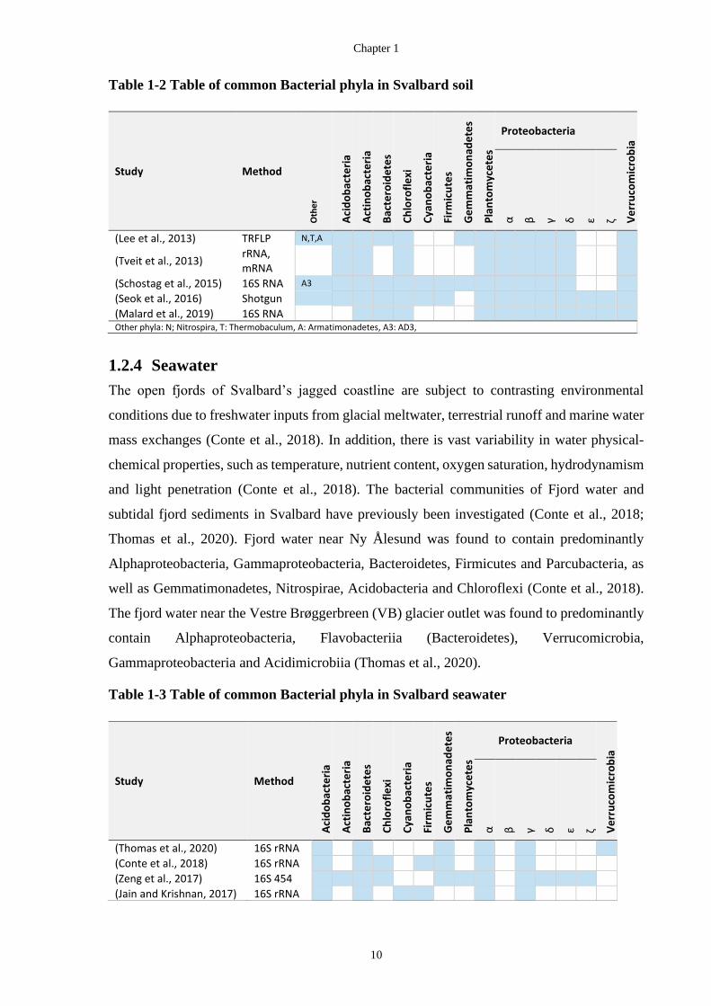
Chapter 1
10
Table 1-2 Table of common Bacterial phyla in Svalbard soil
1.2.4 Seawater
The open fjords of Svalbard’s jagged coastline are subject to contrasting environmental
conditions due to freshwater inputs from glacial meltwater, terrestrial runoff and marine water
mass exchanges (Conte et al., 2018). In addition, there is vast variability in water physical-
chemical properties, such as temperature, nutrient content, oxygen saturation, hydrodynamism
and light penetration (Conte et al., 2018). The bacterial communities of Fjord water and
subtidal fjord sediments in Svalbard have previously been investigated (Conte et al., 2018;
Thomas et al., 2020). Fjord water near Ny Ålesund was found to contain predominantly
Alphaproteobacteria, Gammaproteobacteria, Bacteroidetes, Firmicutes and Parcubacteria, as
well as Gemmatimonadetes, Nitrospirae, Acidobacteria and Chloroflexi (Conte et al., 2018).
The fjord water near the Vestre Brøggerbreen (VB) glacier outlet was found to predominantly
contain Alphaproteobacteria, Flavobacteriia (Bacteroidetes), Verrucomicrobia,
Gammaproteobacteria and Acidimicrobiia (Thomas et al., 2020).
Table 1-3 Table of common Bacterial phyla in Svalbard seawater
Study Method
Oth
er
Aci
do
bac
teri
a
Act
ino
bac
teri
a
Bac
tero
ide
tes
Ch
loro
fle
xi
Cya
no
bac
teri
a
Firm
icu
tes
Ge
mm
atim
on
ade
tes
Pla
nto
myc
ete
s
Proteobacteria
Ve
rru
com
icro
bia
α
β
γ δ
ε ζ
(Lee et al., 2013) TRFLP N,T,A
(Tveit et al., 2013) rRNA, mRNA
(Schostag et al., 2015) 16S RNA A3
(Seok et al., 2016) Shotgun
(Malard et al., 2019) 16S RNA
Other phyla: N; Nitrospira, T: Thermobaculum, A: Armatimonadetes, A3: AD3,
Study Method
Aci
do
bac
teri
a
Act
ino
bac
teri
a
Bac
tero
ide
tes
Ch
loro
fle
xi
Cya
no
bac
teri
a
Firm
icu
tes
Ge
mm
atim
on
ad
ete
s
Pla
nto
myc
ete
s
Proteobacteria
Ve
rru
com
icro
bia
α
β
γ δ
ε ζ
(Thomas et al., 2020) 16S rRNA
(Conte et al., 2018) 16S rRNA
(Zeng et al., 2017) 16S 454
(Jain and Krishnan, 2017) 16S rRNA
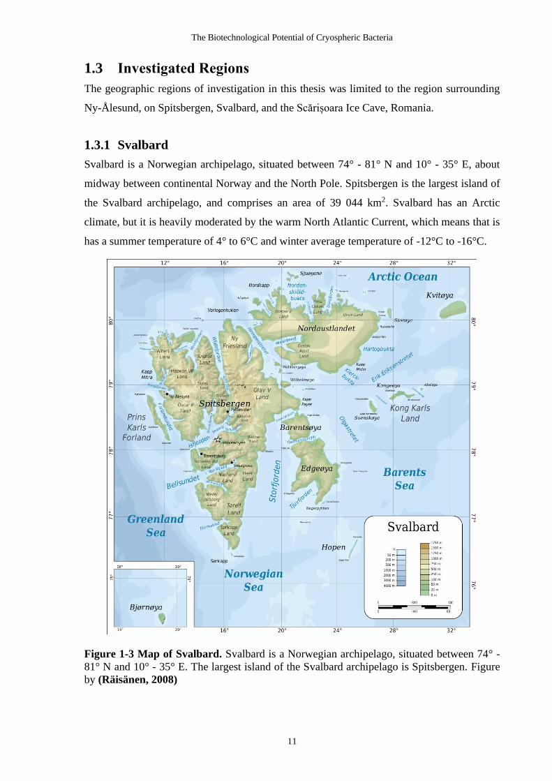
The Biotechnological Potential of Cryospheric Bacteria
11
1.3 Investigated Regions
The geographic regions of investigation in this thesis was limited to the region surrounding
Ny-Ålesund, on Spitsbergen, Svalbard, and the Scărișoara Ice Cave, Romania.
1.3.1 Svalbard
Svalbard is a Norwegian archipelago, situated between 74° - 81° N and 10° - 35° E, about
midway between continental Norway and the North Pole. Spitsbergen is the largest island of
the Svalbard archipelago, and comprises an area of 39 044 km2. Svalbard has an Arctic
climate, but it is heavily moderated by the warm North Atlantic Current, which means that is
has a summer temperature of 4° to 6°C and winter average temperature of -12°C to -16°C.
Figure 1-3 Map of Svalbard. Svalbard is a Norwegian archipelago, situated between 74° -
81° N and 10° - 35° E. The largest island of the Svalbard archipelago is Spitsbergen. Figure
by (Räisänen, 2008)

Chapter 1
12
1.3.2 Scărișoara Ice Cave
The Scărișoara ice cave in Romania is an example of a non-Arctic cryospheric environment
and is included in this thesis because it embodies an example of a habitat that is extremely
unique, isolated form other cryospheric habitats and severely threatened by both climate
change and anthropogenic activity (tourism). The Scărișoara Ice Cave is one of the oldest and
largest perennial underground ice-blocks in the world, being older than 3500 years and greater
than 100 000 m3 in volume. The cave is located in the Bihor Mountains of North West Romania
(46°29’23”N, 22°48’35”E) at an altitude of 1165m (Iţcuş et al., 2016). The Scărișoara ice
block differs from surface glaciers and glacier caves because it is not formed by snow
accumulation (Holmlund et al., 2005). Rather it grows via the annual freezing of a layer of
water that trickles into the cave during summer months, forming a shallow lake on top of the
existing ice block. This layer, which can be up to 20 cm deep, freezes every winter, trapping
at its bottom a layer of sediment deposited during the summer. The ice block therefore consists
of sequential layers of ice of variable thickness, separated by organic- and organic-rich
sediment layers.
Figure 1-4 Map of the Scărișoara Ice Cave location in Romania. The cave is located in the
Bihor Mountains of North West Romania (46°29’23”N, 22°48’35”E) at an altitude of 1165m.

The Biotechnological Potential of Cryospheric Bacteria
13
1.4 Extreme environmental parameters
The cryosphere is considered an ‘extreme environment’ because it has several environmental
parameters considered limiting for the development of life (Maccario et al., 2015). These life-
limiting parameters include low temperatures, high UV radiation and low liquid water
availability (Maccario et al., 2015). However, microorganisms have displayed significant
resilience in adapting to these environments.
1.4.1 Low temperatures
The cryosphere, from the Greek work cryos meaning “cold” or “ice” consists of regions where
temperatures are sufficiently low that water is in a frozen state. Although air temperatures can
rise above 0°C, temperatures in the ice tend to range from 0°C as a maximum in the
summertime during melting, to - 50°C in the Arctic winter (Maccario et al., 2015). The
temperature range is therefore extremely variable, and can differ significantly depending on
other conditions, such as wind, which tends to lower the surface temperature, or snow cover,
which tends to increase the temperature by insulating the ice (Maccario et al., 2015).
Generally, organisms are classified into two groups according to the cardinal (minimum,
optimal and maximum growth) temperatures of the organism (Casanueva et al., 2010). Some
organisms, called psychrophiles, clearly prefer or require cold environments; and have
cardinal temperatures in the range <0°C, 15°C and 20°C (Casanueva et al., 2010). While other
organisms, called psychrotrophs, could more accurately be described as “cold-adapted
mesophiles” and have cardinal temperature ranges of >0°C, >20°C and >30°C (Casanueva et
al., 2010). Some psychrophiles may need to adapt to enormous temperature fluctuations, and
will require mechanisms to do so, while others will be exposed to constant low temperature
(Casanueva et al., 2010). Among the adaptations to low temperatures, are: cold active enzymes
that are active at low temperature (Section 1.5.1), an increase in unsaturated fatty acids,
(including polyunsaturated fatty acids), which help maintain membrane fluidity in the cold
(Section 1.5.3), and anti-freeze proteins and ice-nucleation proteins that help protect
organisms from ice-injury (Section 1.5.2).
1.4.2 High UV radiation
The polar regions are subjected to continuous light in the summer, and continuous dark in the
winter. During summer, the polar regions experience continuous daylight and receive
increased ultraviolet (UV) exposure due to ozone depletion (Maccario et al., 2015). UV
radiation is generally known to be damaging to cells. The type of damage that is caused is

Chapter 1
14
wavelength dependent. UV-B (290-320 nm) results in direct damage to DNA, where it causes
the formation of thymine dimers (Setlow et al., 1963). In addition, there is a scattering effect
in the ice and snow, which results in photolysis of compounds in the snow, and the release of
reactive gases in the snow-boundary layer (Maccario et al., 2015). These highly reactive gases
tend to raise the levels of reactive oxygen species (ROS), making this a highly reactive
environment (Maccario et al., 2015). Among the adaptations to the high UV radiation are UV
screens, pigments, and antioxidants (Section 1.5.4).
1.4.3 Low liquid water availability
Liquid water is vital for all living organisms, as it the medium in which the metabolic reactions
of the cell take place. Due to the low temperature of glacial environments, water is mainly
found in solid form (ice), with the exception of meltwater streams, water films, or veins and
pockets (Hodson et al., 2008). These veins and pockets tend to be hypersaline or hyper-acidic,
because they contain all the elements that are excluded from the ice-crystals as freezing takes
place (Barletta et al., 2012; Dani et al., 2012; Maccario et al., 2015). Microorganisms in ice
may, therefore, undergo desiccation as a consequence of low liquid water availability and high
osmotic pressure (Maccario et al., 2015). Adaptations to this environmental stress includes the
formation of EPS (Section 1.5.5) and compatible solutes.
1.5 Biotechnology
The focus of Section 1.5 will be how innovative physiological and metabolic adaptations to
the environmental stressors highlighted in (Section 1.4) may be harnessed in biotechnology to
create products and solutions that are useful to industry (Casanueva et al., 2010; D’Amico et
al., 2006; Santiago et al., 2016, Maccario et al., 2015). According to a report by the United
Nations University of Advanced Studies (UNU-IAS), in 2008, there were already 43
companies involved in the development of biotechnology products based on Arctic genetic
resources (Leary, 2008). In addition, there were 31 patents or pending patents based on these
Arctic microbial resources in 2008 (Leary, 2008); this number is undoubtedly much higher in
2020. The potential use of psychrophilic organisms in biotechnology has been reviewed
previously (see (Arrigo, 2014; Casanueva et al., 2010; Larose et al., 2013a; Maccario et al.,
2015; Margesin and Miteva, 2011; Miteva, 2008)).

The Biotechnological Potential of Cryospheric Bacteria
15
Table 1-4. The potential uses of psychrophilic microorganisms in biotechnology
Product Microorganism source Application Section
Cold-active enzymes Psychrophilic bacteria
and fungi
Food industry, detergents 1.5.1 Cold-active enzymes
Polyunsaturated
fatty acids
Cold-adapted bacteria Dietary supplements for
humans, livestock, and fish
1.5.3 Polyunsaturated Fatty
acids
Ice nucleation
proteins
Psychrophilic bacteria
and fungi
Food industry, synthetic
snow
1.5.2 Anti-freeze proteins
(AFPs) and ice-binding
proteins (IBPs) Antifreeze proteins
and solutes
Psychrophilic bacteria
and fungi
Cryoprotectants, food
industry
UV screens,
pigments, and
antioxidants
Psychrophilic bacteria
and fungi
Biomedical, pharmaceutical,
food technology and
cosmetics
1.5.4 UV screens, pigments
and UV screens, pigments,
and antioxidants
Exopolysaccharide Psychrophilic bacteria
(cyanobacteria)
Biomedical, pharmaceutical,
food technology and
cosmetics
1.5.5 Exopolysaccharides/
extra cellular polymeric
substances
The following subsections discuss (i) the various challenges posed by the environment, (ii) the
biological adaptations to these challenges that make life possible, and (iii) the potential
applications of these adaptive strategies in biotechnology.
1.5.1 Cold-active enzymes
Recently, the World Enzymes to 2017 Report forecast that enzyme demand would rise by 6.4
% to 6.9 billion p.a. in 2017 (http://www.rnrmarketresearch.com/world-enzymes-to-2017-
market-report.html). There are several advantages to the use of enzymes to catalyse chemical
reactions as opposed to purely chemical and physical methods. Cold-active enzymes have
utility in many industries, and help to reduce carbon emmisions in large-scale industrial
processes (Casanueva et al., 2010; Cavicchioli et al., 2002; D’Amico et al., 2006; Maccario et
al., 2015; Santiago et al., 2016). Biological enzymes are efficient and highly selective
catalysts, and they are generally more energy efficient, safer, and better for the environment
(Santiago et al., 2016). The heating of reactants, which is a requirement of many chemical
reactions, is an energy-intensive process that is both financially undesirable to businesses and
environmentally unsustainable (Santiago et al., 2016). The enzymes of psychrophiles allow
reactions to take place at lower temperatures, reducing the need for heating. In a time of
growing concern over environmental sustainability, this makes low-temperature enzymes an
attractive solution for industry. In fact, it has been estimated that by 2030, up to 40% of the
bulk chemical synthesis processes requiring environmentally damaging substances, and high
energy inputs could be replaced by enzymatic catalysts (Ferrer et al., 2016).

Chapter 1
16
Low-temperature enzymes have several additional advantages in industry. The low
temperature of the reaction may reduce or prevent many undesirable chemical reactions that
occur spontaneously at higher temperatures. This allows a greater specificity of reaction and
potentially a higher yield. Finally, low-temperature enzymes are unstable or denatured at
higher temperatures. This enables reactions to be terminated by heat-inactivation, allowing for
the sequencing of reactions through multi-stage chemical transformations without the need for
purification steps, and removing the need for chemical inactivation methods (Santiago et al.,
2016).
The Arrhenius law suggests that reaction rates should decrease with temperature, due to the
decreased kinetic energy of the reacting molecules, which results in fewer interactions of the
substrate with the active site (Casanueva et al., 2010; Santiago et al., 2016). Therefore, to
maintain high activity, psychrophilic organisms must compensate for the reduced number of
active site-substrate collisions, by increasing the likelihood of successful collisions. The
structural and functional differences between thermophilic, mesophilic, and psychrophilic
enzymes are due to changes in the amino acids that make up the enzyme. These changes can
be in the form of amino acid substitutions, insertions and deletions (Santiago et al., 2016). The
type of change, as well as the location of the change, have different consequences for the
thermal stability of the molecule. As a general rule, it appears that there is a trade-off between
protein thermostability and conformational flexibility, with high conformational rigidity
resulting in the high thermostability seen in thermophiles, and the high conformational
flexibility in psychrophiles leading to decreased thermostability (Casanueva et al., 2010;
Santiago et al., 2016; Siddiqui and Cavicchioli, 2006). There is evidence that the increased
flexibility occurs mainly at the active site, and is not necessarily present throughout the whole
protein (Casanueva et al., 2010). Some structural features of cold-adapted proteins include
fewer ion pairs resulting in fewer salt bridges, fewer polar, H-bond-forming residues, fewer
arginine residues, fewer proline residues in protein loops, and fewer aromatic interactions than
those in mesophilic proteins (Grzymski et al., 2006).
Several cold-active enzymes isolated from Arctic bacteria are described in Table 1-5 and cold-
active enzymes from Antarctic bacteria are listed in Appendix Table A-1. These include
several lipases, esterases and β-galactosidases which lend themselves to applications from
laundry and detergent industry, to bioremediation, to biofuel production to the food and
pharmaceutical industries (Table 1-5, and references therein).

The Biotechnological Potential of Cryospheric Bacteria
17
Table 1-5: Sources of cold-active enzymes from Arctic microorganisms
Target Product
Location Environment source
Phylum Source Organism
Discovery approach Application Reference
Esterase Spitsbergen island, Svalbard
Soil Gammaproteobacteria
Pseudomonas sp. S9
Genomic DNA library, phenotype screening, specific primers, followed by heterologous expression
Additives in food processes, laundry detergents, and bioremediation.
(Wicka et al., 2016)
Protease Spitsbergen, Svalbard
Seawater Gammaproteobacteria
Shewanella arctica
Genomic DNA library, phenotype screening, specific primers, followed by heterologous expression
Chemical, cosmetics, and pharmaceutical industries.
(Qoura et al., 2015)
Pullunase Spitsbergen, Svalbard
Seawater Gammaproteobacteria
Shewanella arctica
Genomic DNA library, phenotype screening, specific primers, followed by heterologous expression
Starch degradation for ethanol-based biofuel production.
(Elleuche et al., 2015)
β-galacto-sidase
South-West Greenland
Ikka columns Firmicutes Alkalilactibacillus ikkense
Genomic DNA library, phenotype screening, specific primers, followed by heterologous expression
Production of lactose-free dairy products as yogurt, sour cream, and some cheeses.
(Schmidt and Stougaard, 2010)
Esterase Kolyma lowland region, Siberia
Cryopeg within Permafrost
Gammaproteobacteria
*Psychrobacter cryohalolentis K5(T)
Genome mining and specific primers followed by heterologous expression
Detergent preparations and bioremediation of polluted soils and waters in cold regions.
(Novototskaya-Vlasova et al., 2012)
Esterase Kolyma lowland region, Siberia
Permafrost Gammaproteobacteria
*Psychrobacter cryohalolentis K5(T).
Genome mining and specific primers followed by heterologous expression
Whole cell biocatalysts in organic synthesis and bioremediation at low temperatures, cell surface display platform.
(Petrovskaya et al., 2015)
Lipase Kolyma lowland region, Siberia
Cryopeg within Permafrost
Gammaproteobacteria
*Psychrobacter cryohalolentis K5(T)
Genome mining and specific primers followed by heterologous expression
Production of pharmaceuticals, food, detergents, and fine organic synthesis.
(Novototskaya-Vlasova et al., 2013)
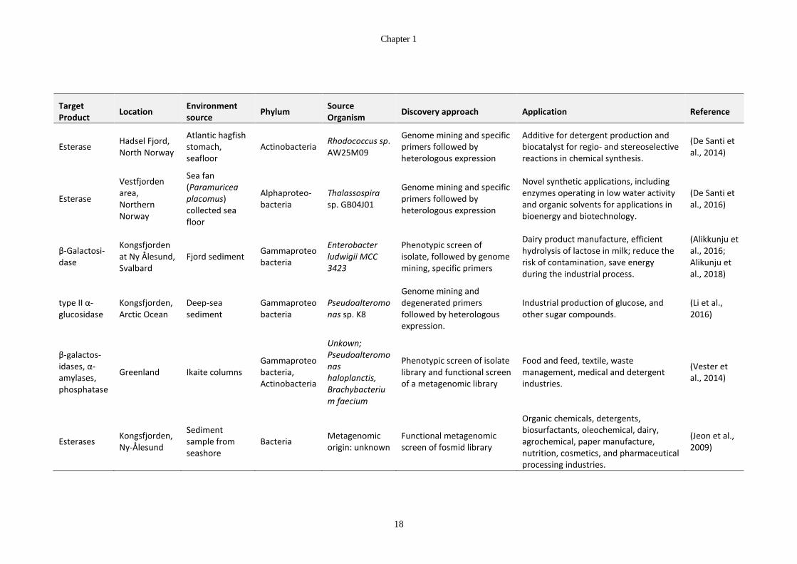
Chapter 1
18
Target Product
Location Environment source
Phylum Source Organism
Discovery approach Application Reference
Esterase Hadsel Fjord, North Norway
Atlantic hagfish stomach, seafloor
Actinobacteria Rhodococcus sp. AW25M09
Genome mining and specific primers followed by heterologous expression
Additive for detergent production and biocatalyst for regio- and stereoselective reactions in chemical synthesis.
(De Santi et al., 2014)
Esterase
Vestfjorden area, Northern Norway
Sea fan (Paramuricea placomus) collected sea floor
Alphaproteo-bacteria
Thalassospira sp. GB04J01
Genome mining and specific primers followed by heterologous expression
Novel synthetic applications, including enzymes operating in low water activity and organic solvents for applications in bioenergy and biotechnology.
(De Santi et al., 2016)
β-Galactosi-dase
Kongsfjorden at Ny Ålesund, Svalbard
Fjord sediment Gammaproteobacteria
Enterobacter ludwigii MCC 3423
Phenotypic screen of isolate, followed by genome mining, specific primers
Dairy product manufacture, efficient hydrolysis of lactose in milk; reduce the risk of contamination, save energy during the industrial process.
(Alikkunju et al., 2016; Alikunju et al., 2018)
type II α-glucosidase
Kongsfjorden, Arctic Ocean
Deep-sea sediment
Gammaproteobacteria
Pseudoalteromonas sp. K8
Genome mining and degenerated primers followed by heterologous expression.
Industrial production of glucose, and other sugar compounds.
(Li et al., 2016)
β-galactos-idases, α-amylases, phosphatase
Greenland Ikaite columns Gammaproteobacteria, Actinobacteria
Unkown; Pseudoalteromonas haloplanctis, Brachybacterium faecium
Phenotypic screen of isolate library and functional screen of a metagenomic library
Food and feed, textile, waste management, medical and detergent industries.
(Vester et al., 2014)
Esterases Kongsfjorden, Ny-Ålesund
Sediment sample from seashore
Bacteria Metagenomic origin: unknown
Functional metagenomic screen of fosmid library
Organic chemicals, detergents, biosurfactants, oleochemical, dairy, agrochemical, paper manufacture, nutrition, cosmetics, and pharmaceutical processing industries.
(Jeon et al., 2009)

The Biotechnological Potential of Cryospheric Bacteria
19
Target Product Location Environment source
Phylum Source Organism Discovery approach Application Reference
Esterase Kapp Wijk, Svalbard
Intertidal zone sediment
Bacteria Unknown (similarity to Vibrio caribbenthicus)
Functional metagenomic screen of fosmid library
Detergent, food, pharmaceutical, paper, textile, leather, and fine chemicals industries
(Fu et al., 2013)
Serine hydroxymethyl transferase
Arctic Ocean Sea ice Gammaproteobacteria
Psychromonas ingrahamii
Genome mining of isolate, synthesis of gene and heterologous expression.
Catalyse reactions in the synthesis of pharmaceuticals, agrochemicals, and food additives.
(Angelaccio et al., 2012)
Alkaline phosphatase
Reykjavik, Iceland
Seawater Gammaproteobacteria
Vibrio sp. G15-21 Isolate screen, followed by enzyme purification by affinity-resin column.
Molecular biology tool. (Hauksson et al., 2000)
DNA Polymerases
Northern Schneeferner, Germany
Glacial ice Bacteroidetes, Gammaproteobacteria, Actinobacteria
Algoriphagus, Pedobacter, Microscilla, Thermus, Acinetobacter, Rhodococcus
Functional metagenomic screen of fosmid library on cold-sensitive E. coli mutant.
Molecular biology tool (Simon et al., 2009a)
* Example of a single genome being mined for multiple enzymes Abbreviations: Thin Layer Chromatography (TLC), Eicosapentaenoic Acid (EPA), Liquid Chromatography-Mass Spectrometry (LC-MS), Minimum Inhibitory Concentration (MIC)

Chapter 1
20
1.5.2 Anti-freeze proteins (AFPs) and ice-binding proteins (IBPs)
The formation of ice crystals in cells can cause rupture of cell membranes and the death of
the organism (Lorv et al., 2014). Psychrophiles have had to establish ways to lower the
freezing point of the cytoplasm and prevent the formation of ice-crystals at temperatures at
which water is usually frozen. Adaptations that prevent ice crystal formation include the
accumulation of antifreeze proteins (AFPs) and ice-binding proteins (IBPs) and the synthesis
of highly soluble poly-hydroxyl solutes, such as glycine, betaine, glycerol, trehalose,
mannitol and sorbitol, which reduce the freezing point of the cytoplasm and act as
cryoprotectant (Casanueva et al., 2010).
AFPs and IBPs find many uses in industry. For example, they are used in the
cryopreservation of biological tissues (Bar Dolev et al., 2016), a common process in fertility
treatment, where sperm, oocytes and embryos may be frozen for storage, and thawed at the
appropriate time. They also have the potential for use in cryosurgery, where ice-nucleation
proteins may be used to ablate cancer cells, by forming the characteristic ice spicules that
puncture and shear cells during freezing (Bar Dolev et al., 2016). The food industry also has
a multitude of uses for AFPs and IBPs, where they are used to prevent the unfavourable
changes and loss of quality in food when it is frozen and thawed.
AFPs and IBPs both play a role in ice-crystal development; however, each protein class is
involved in a different stage of the freezing process (Lorv et al., 2014). IBPs trigger ice-
nucleation events, while AFPs inhibit growth of ice-crystals by binding to the ice-crystal
nucleation centres and preventing the further accretion of ice (Bar Dolev et al., 2016; Lorv
et al., 2014). AFPs have already been used with some success by Unilver to keep ice-cream
from losing its creamy texture (Bar Dolev et al., 2016; Muñoz et al., 2017). AFPs may also
be used in agriculture to improve crops resilience to frost and prevent the accumulation of
ice on surfaces, such as roads, aircraft, air turbine blades, air-conditioners and freezers (Bar
Dolev et al., 2016). Genes from Arctic bacteria that have potential biotechnological
applications are listed in Table 1.6.

The Biotechnological Potential of Cryospheric Bacteria
21
Table 1-6 Table of ice-nucleation-active bacteria
Antifreeze proteins
Product Location Environment type
Domain Microorganism Approach Reference
Antifreeze protein Antarctica Sediment and ice samples
Bacteria Sphingomonas, Plantibacter and Pseudomonas
Phenotypic screening of isolates for freeze-thaw tolerance, TH measurement, protein purification, WGS and annotation, food preservation tests.
(Muñoz et al., 2017)
Antifreeze protein Midre Lovénbreen glacier, Ny-Ålesund, Svalbard
Cryoconite holes Bacteria
Cryobacterium. psychrotolerans, Cryobacterium. psychrophilum, Pseudomonas ficuserectae, Subtercola frigoramans)
Phenotypic screening of isolates for anti-freeze activity, protein purification and activity assays
(Singh et al., 2014a)
Antifreeze protein (extracellular ice-binding glycoprotein)
Tvillingvatnet Pond, Ny-Ålesund, Svalbard
Ice core from frozen freshwater pond
Yeast Leucosporidium sp
Phenotypic screen, followed by genome sequencing, specific primers, cloning and sequence confirmation
(Lee et al., 2010)
Antifreeze protein with ice-nucleation activity
Canadian High Arctic Plant roots in soil Bacteria Pseudomonas putida GR12-2 Amino acid sequencing, followed by PCR and expression in a heterologous host
(Muryoi et al., 2004)
Antifreeze protein
Ace Lake, Pendant Lake, Triple Lake, Deep Lake and Club Lake, Vestfold Hills and Larsemann Hills, Antarctica
Water from lakes with range of salinity and nutrients
Bacteria
Mar. protea, Pseudoalteromonas, Pseudomonas fluorescens, Stenotrophomonas maltophilia, Sphingomonas
Phenotypic screen of isolates, Splat assay, sequencing of 16S rRNA gene.
(Gilbert et al., 2004)
TH: thermal hysteresis, Splat assay ((Knight et al., 1988)), WGS: whole genome sequencing

Chapter 1
22
1.5.3 Polyunsaturated fatty acids
Cellular membranes are vital components of all cells, as they control the internal
composition of the cytoplasm by selectively allowing the transport of molecules into and out
of the cell via passive, facilitated and active transport. Membrane-fluidity generally
decreases with temperature, which decreases membrane permeability (D’Amico et al.,
2006). The lower the density of fatty acid (FA) chains in the membrane, the lower the
temperature at which the membrane transitions from the liquid crystalline, to the gel phase
(Casanueva et al., 2010). Generally, microorganisms have adapted membranes that reduce
the packing efficiency of FA chains by means of an increased proportion of unsaturated FAs,
decreased average FA chain length, increased methyl branching and an increased antesio:
iso branching ratio (Casanueva et al., 2010; Chattopadhyay, 2006). For example, an analysis
of the FA profiles of Cryobacterium and Micrococcus isolates from cryoconite holes in
Svalbard showed a higher concentration of branched fatty acids than saturated or unsaturated
fatty acids (Singh et al., 2014b).
Genes involved in increasing the fluidity of cell membranes; that may have biotechnological
potential include: polyunsaturated fatty acid (PUFA) synthesis genes, desaturases and
dioxygen lipid desaturases (Casanueva et al., 2010). PUFA can be divided into ω6 and ω3
FAs, depending on whether the first double bond is at the 3rd or 6th carbon position, from
the methyl end group of the FA chain. Mammals, including humans, are unable to synthesize
the ω6 FA, linoleic acid (LA), and the ω3 FA, α-linoleic acid (ALA), and so they rely on
dietary sources of the essential fatty acids. Furthermore, several of the other biologically
important PUFA such as eicosapentaenoic acid (EPA) and docosahexaenoic acid (DHA) can
be synthesised from ALA; however, the conversion from ALA to EPA and DHA Is low, and
it is still preferable to obtain EPA and DHA from dietary sources. ALA is used in the
biosynthesis of arachidonic acid (AA), which is in turn used in the biosynthesis of some
prostaglandins, prostacyclin, leukotrienes, and thromboxane (Abedi and Sahari, 2014).
PUFA are essential to optimal human health and play a role in maintaining several important
body functions. For example, long-chain PUFA help to regulate the immune system, and
may help prevent autoimmune diseases such as rheumatoid arthritis, ulcerative colitis, and
Crohn’s disease, while ω3 fatty acids are beneficial in the management of skin disease,
asthma, arthritis, lupus erythematosus and multiple sclerosis (Abedi and Sahari, 2014). DHA
is essential for proper brain function, and directly influences the activity of serotonergic and
cholinergic neurotransmitters (Abedi and Sahari, 2014; Bazinet and Layé, 2014). PUFA

The Biotechnological Potential of Cryospheric Bacteria
23
have traditionally been sourced from fish oils; however, as fish stocks plummet worldwide,
other alternative and more sustainable sources of PUFAs are required (Abedi and Sahari,
2014). PUFA form aquatic species also carry other risks, such as contamination with
teratogenic, carcinogenic, and mutagenic chemicals such as DDT and dioxin-like
polychlorinated biphenyls (Abedi and Sahari, 2014). Aquatic species also tend to accumulate
methyl mercury and heavy metals such as Pb, Cr, Hg, Cd, and As, and antibiotics (Abedi
and Sahari, 2014).
The production of PUFA from bacteria is therefore a promising avenue for investigation
(Ochsenreither et al., 2016; Ratledge, 2004). There are two main lineages of marine bacteria
appear to produce PUFA, the Gammaproteobacteria genera (Shewanella (EPA), Colwellia
(DHA), Moritella (DHA), Psychromonas and Photobacterium (EPA)) and several species
within two genera of the Cytophaga-Flavobacterium-Bacteroides (CFB) grouping
(Flexibacter (EPA) and Psychroserpens) (Allen and Bartlett, 2002; Nichols, 2003; Nichols
and McMeekin, 2002). EPA might be a vital component of the cell membrane in selected
cold-adapted bacteria, as disruption of the EPA synthesis genes in the halophilic,
psychrophilic strain Shewanella livingstonensis Ac10 resulted in a cold-sensitive mutant
with decreased growth rate and filamentous cells (Dai et al., 2012; Sato et al., 2008).
A survey of metabolites produced by the microorganisms of several surface glacial habitats
revealed that several algal species were positively correlated with the presence of PUFAs,
and PUFAs were especially high in red snow (Lutz et al., 2016).
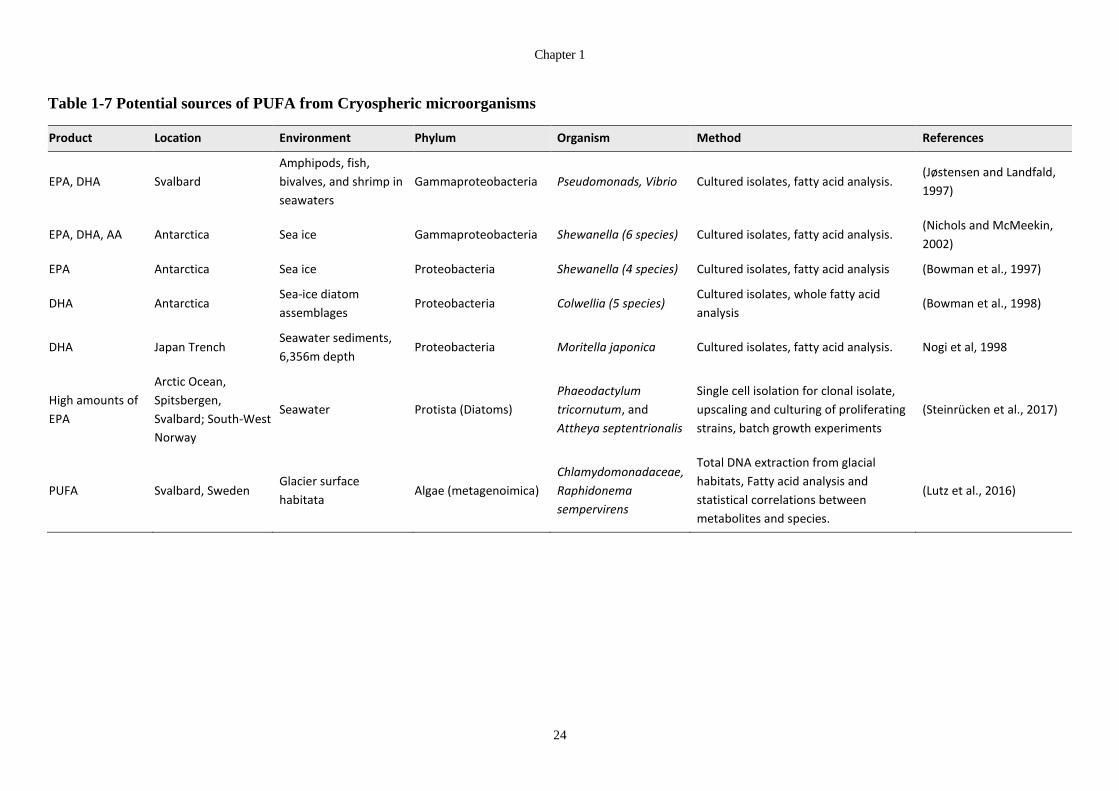
Chapter 1
24
Table 1-7 Potential sources of PUFA from Cryospheric microorganisms
Product Location Environment Phylum Organism Method References
EPA, DHA Svalbard
Amphipods, fish,
bivalves, and shrimp in
seawaters
Gammaproteobacteria Pseudomonads, Vibrio Cultured isolates, fatty acid analysis. (Jøstensen and Landfald,
1997)
EPA, DHA, AA Antarctica Sea ice Gammaproteobacteria Shewanella (6 species) Cultured isolates, fatty acid analysis. (Nichols and McMeekin,
2002)
EPA Antarctica Sea ice Proteobacteria Shewanella (4 species) Cultured isolates, fatty acid analysis (Bowman et al., 1997)
DHA Antarctica Sea-ice diatom
assemblages Proteobacteria Colwellia (5 species)
Cultured isolates, whole fatty acid
analysis (Bowman et al., 1998)
DHA Japan Trench Seawater sediments,
6,356m depth Proteobacteria Moritella japonica Cultured isolates, fatty acid analysis. Nogi et al, 1998
High amounts of
EPA
Arctic Ocean,
Spitsbergen,
Svalbard; South-West
Norway
Seawater Protista (Diatoms)
Phaeodactylum
tricornutum, and
Attheya septentrionalis
Single cell isolation for clonal isolate,
upscaling and culturing of proliferating
strains, batch growth experiments
(Steinrücken et al., 2017)
PUFA Svalbard, Sweden Glacier surface
habitata Algae (metagenoimica)
Chlamydomonadaceae,
Raphidonema
sempervirens
Total DNA extraction from glacial
habitats, Fatty acid analysis and
statistical correlations between
metabolites and species.
(Lutz et al., 2016)

The Biotechnological Potential of Cryospheric Bacteria
25
1.5.4 UV screens, pigments, and antioxidants
At low temperatures, oxygen is more soluble in water, which means that there is a greater
threat from reactive oxygen species (ROS). In addition, Arctic environments experience high
UV radiation, which can be directly damaging to DNA, as well as causing increased ROS
via photolysis (Casanueva et al., 2010). To prevent potentially lethal DNA damage from UV
radiation and ROS, microorganisms have adapted a range of DNA repair mechanisms, UV
screens and antioxidants (enzymes and metabolites) (Maccario et al., 2015; Mandelli et al.,
2012; Sajjad et al., 2020). These antioxidant enzymes and metabolites may be useful in the
cosmetic pharmaceutical and biomedical fields (Mandelli et al., 2012; Sajjad et al., 2020;
Yabuzaki, 2017).
For example, psychrophilic bacteria have an increase in the number of catalases, superoxide
dismutases (SODs) as well as other antioxidants such as rubreyrythrin, and rubredoxin
oxidoreductase and dioxygen-consuming lipid desaturases (Casanueva et al., 2010).
Microbial mats, dominated by Cyanobacteria, in the Canadian High Arctic, produce several
natural UV-absorbing/screening compounds like carotenoids, mycosporine-like amino acids
(MAAs) and phycobiliproteins (PBPs)(Mueller et al., 2005). Scytonemin is a Cyanobacterial
indole alkaloid compound that has UV protectant, anti-inflammatory, anti-proliferative, and
antioxidant activity. MAAs act as sunscreens, and antioxidants and can be used as UV
protectors in skin-care products, or as photo-stabilizing additives in paints, plastics, and
varnishes (Fuentes-Tristan et al., 2019; Pathak et al., 2020).
A survey of supraglacial habitats revealed that carotenoids were abundant (Lutz et al., 2016),
and are a probably responsible for the darkening of snow and ice that causes melting.
Cyanobacterial mats in the Canadian High Arctic were also a source of abundant
chlorophylls, carotenoids, scytonemins, MAAs and phycobiliproteins and MAA metabolites
(Mueller et al., 2005; Quesada et al., 1999).
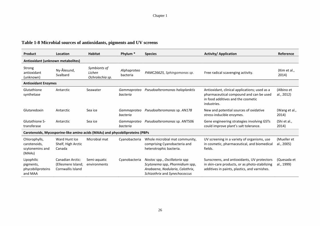
Chapter 1
26
Table 1-8 Microbial sources of antioxidants, pigments and UV screens
Product Location Habitat Phylum * Species Activity/ Application Reference
Antioxidant (unknown metabolites)
Strong antioxidant (unknown)
Ny-Ålesund, Svalbard
Symbionts of Lichen Ochrolechia sp.
Alphaproteo bacteria
PAMC26625, Sphingomonas sp. Free radical scavenging activity. (Kim et al., 2014)
Antioxidant Enzymes
Glutathione synthetase
Antarctic Seawater Gammaproteobacteria
Pseudoalteromonas haloplanktis Antioxidant, clinical applications; used as a pharmaceutical compound and can be used in food additives and the cosmetic industries.
(Albino et al., 2012)
Glutaredoxin Antarctic Sea ice Gammaproteobacteria
Pseudoalteromonas sp. AN178 New and potential sources of oxidative stress-inducible enzymes.
(Wang et al., 2014)
Glutathione S-transferase
Antarctic Sea ice Gammaproteobacteria
Pseudoalteromonas sp. ANT506 Gene engineering strategies involving GSTs could improve plant’s salt tolerance.
(Shi et al., 2014)
Carotenoids, Mycosporine-like amino acids (MAAs) and phycobiliproteins (PBPs
Chlorophylls, carotenoids, scytonemins and (MAAs)
Ward Hunt Ice Shelf, High Arctic Canada
Microbial mat Cyanobacteria Whole microbial mat community, comprising Cyanobacteria and heterotrophic bacteria.
UV screening in a variety of organisms, use in cosmetic, pharmaceutical, and biomedical fields.
(Mueller et al., 2005)
Lipophilic pigments, phycobiliproteins and MAA
Canadian Arctic: (Ellesmere Island; Cornwallis Island
Semi-aquatic environments
Cyanobacteria Nostoc spp., Oscillatoria spp Scytonema spp, Phormidium spp, Anabaena, Nodularia, Calothrix, Schizothrix and Synechococcus
Sunscreens, and antioxidants, UV protectors in skin-care products, or as photo-stabilizing additives in paints, plastics, and varnishes.
(Quesada et al., 1999)

The Biotechnological Potential of Cryospheric Bacteria
27
1.5.5 Exopolysaccharides/ extra cellular polymeric substances (EPS)
As mentioned in Section 1.4.3, microorganisms in ice environments are subject to
desiccation stress due to low water availability and high osmotic pressure. Adaptation to
these stressors include the use of osmoprotectants and exopolysaccharides (EPS). EPS are
high molecular weight carbohydrate polymers that constitute a significant component of the
extracellular polymers surrounding most microbial cells, where they are usually found as
capsular polysaccharides (covalently bound to the cell surface), and or as slime
polysaccharides (loosely attached to the cell surface or in the extracellular medium) (Poli et
al., 2010). Most EPS are heteropolysaccharides, consisting of three or four different
monosaccharides arranged in groups of 10 or less to form repeating units (Poli et al., 2010).
The material properties of these EPSs make them useful in the food industry as a thickening
agent, in the pharmaceutical industry, and in the cosmetic industry (Poli et al., 2010). In
addition to their ability to produce slime and biofilms, exopolysaccharides also have
potential applications as anticoagulant, antithrombotic, immunomodulation, anticancer and
as bioflocculants due to their interactions with the immune system (Nwodo et al., 2012). In
cold environments EPSs may have a role in freeze-thaw tolerance (Kim and Yim, 2007),
and also provide a site for the localisation of UV protective compounds such as scytonemin
and MAAs and allow for the scavenging of metal cations in oligotrophic conditions
(Chrismas et al., 2016a; Pereira et al., 2009).
EPS is likely to play an important role in the formation of cryoconite granules (Chrismas et
al., 2016a; Hodson et al., 2010a; Langford et al., 2010), therefore, the cyanobacteria of
cryoconite is particularly interesting as a source of novel EPS.

Chapter 1
28
Table 1-9 The use of EPSs in biotechnology
Product Location Habitat Phylum Species Properties Industrial use References
EPS: N-acetyl glucosamine, mannose
and glucuronic acid residues bound
by heterogeneous linkages.
Arctic Brown alga
Laminaria Bacteriodetes
Polaribacter sp.
SM1127
Antioxidant, UV
protection and extreme
moisture-retaining
properties.
Food, cosmetic,
pharmaceutical, and
biomedical fields.
(Sun et al.,
2015,
2020)
EPS: galactose and glucose, at a ratio
of 1:1.5.
King George
Island,
Antarctica
Sediment Gammaproteo
bacteria
Pseudoalteromonas
arctica
Confers protection against
free-thaw cycles.
Cryoprotectant in
medical applications and
food industries.
(Kim and
Yim, 2007)
EPS: highly complex α-mannan
polysaccharide. Arctic Sea ice
Gammaproteo
bacteria
Pseudoalteromonas
sp. SM20310
Protection against high
salinity and freeze-thaw
injury.
Use as cryoprotectant. (Liu et al.,
2013)
Structure not described. Greenland Ice
Sheet. Cryoconite Cyanobacteria
Phormidesmis
priestleyi BC1401
(Chrismas
et al.,
2016a)

The Biotechnological Potential of Cryospheric Bacteria
29
1.6 Novel antimicrobial compounds
Since the discovery of penicillin by Alexander Fleming in 1928, more than 23 000 NPs have
been characterised (Katz and Baltz, 2016). NPs have also been developed into a great number
of drugs, able to treat infection and disease in plants, animals and humans (Katz and Baltz,
2016; Knight et al., 2003). The majority of drugs are bioactive secondary metabolites, which
have obscure functions in the organisms which produce them, but which have may have
evolved in response to competition between microbes (Bérdy, 2005; van Bergeijk et al.,
2020).
1.6.1 Advantages and challenges
NP-based drug-discovery has several advantages over its synthetic chemistry counterpart.
NP resources remain largely unexplored and as new discovery strategies are developed, and
new environments are sampled, many novel bioactive compounds may emerge (Knight et
al., 2003; Zhang and Demain, 2005). NPs have been selected by nature for specific biological
interactions; therefore, they have evolved to bind to proteins and have drug-like properties.
Because NPs have evolved over billions of years to fulfil a variety of roles in diverse
organisms, natural products offer unrivalled chemical diversity, structural complexity, and
proven biological potency. However, there are several challenges that have hindered the true
potential of discovery antimicrobial compounds from environments from being realised
(Knight et al., 2003). Firstly, much of the environmental sampling has consisted of random
sampling and has missed the true potential of many regions. Secondly, the major barriers to
a truly systematic evaluation of environmental microbes is the difficulty in isolating and
cultivation of up to 99% of the microbes present in any sample (Head et al., 1998; Pham and
Kim, 2012; Stewart, 2012). Despite the massive number of uncultivated microbes, the easily
cultured microbes have been characterised a number of times, resulting in a redundancy of
strains and compounds within many NP extract libraries (Demain and Sanchez, 2009). In
addition, the entire process from characterization and isolation of the active compounds from
NP extracts are extremely labour intensive and time-consuming; and once a compound has
been discovered; the production of adequate amounts of the compound generally requires
massive scale-up.
The drug discovery process has always been limited by the technological and biological
knowledge of the time. From the late 1930s to the 1970’s, drug discovery was mainly
conducted via phenotypic screening (Katz and Baltz, 2016). In this technique, fermentation

Chapter 1
30
broths and purified products were deposited on filter paper discs and placed on agar plates
seeded with a test organism (Katz and Baltz, 2016). Areas that showed growth inhibition
(bacteriostatic) and cell death (bactericidal) activity indicates the presence of a potential
antimicrobial (Katz and Baltz, 2016). In this way, more than 20 novel classes of antibiotics
were discovered between 1930 and 1962 (Coates et al., 2011). From the 1970’s onwards, the
approach shifted to “knowledge-based approaches”, as knowledge of molecular biology
grew, and specific targets for drugs were identified (Katz and Baltz, 2016). Despite the many
advances in the field, only two new classes of antimicrobials have made it to market since
1962, a startlingly low figure (Coates et al., 2011). Recently, genome- and metagenome-
mining techniques have heralded another paradigm shift in drug discovery, and been used to
discover several new antibiotics, such as haloduracin (McClerren et al., 2006), lactocillin
(Donia et al., 2014) and taromycin A (Yamanaka et al., 2014). Halduracin, a complex
comprising two separate ribosomally encoded and post-translationally modified peptides
(RiPPs), prevents transglycosylation and inhibits cell wall biosynthesis in Gram-positive
bacteria by binding to lipid II4 (Oman et al., 2011). Lactocillin is also a RiPP that targets
Gram-positive organisms. Taromycin A is a nonribosomal peptide derived from a marine
actinomycete Saccharomonospora sp. CNQ-490(Yamanaka et al., 2014). The screening of
soil environmental DNA in heterologous hosts has also resulted in the discovery of the
antibiotics Fasamycin A and B (Feng et al., 2012), Tetarimycin A (Kallifidas et al., 2012)
and Utahmycins A and B (Bauer et al., 2010).
1.6.2 Drugs from polar organisms
The cryosphere is an excellent environment to search for antimicrobials because there is a
high amount of competition in nutrient-poor environments and they have not been fully
explored. Furthermore, bioprospecting using metagenomics approaches is ideal because the
cultivation of polar organisms is especially time-consuming and difficult. Table 1.10 details
some of the potential antimicrobials isolated from polar organisms. To date, antimicrobial
compounds have been identified from Arctic (Al-Zereini et al., 2007; Kim et al., 2014;
Lyutskanova et al., 2009; Macherla et al., 2005; Wietz et al., 2012; Yuan et al., 2014; Zhang
et al., 2004) and Antarctic (Asthana et al., 2009; Bruntner et al., 2005; Learn-Han Lee et al.,
2012; L.-H. Lee et al., 2012; Mojib et al., 2010; O’Brien et al., 2004; Tedesco et al., 2016;
Wong et al., 2011) environments (Table 10). These antimicrobial producing bacteria were
isolated from soil (Lyutskanova et al., 2009; O’Brien et al., 2004), seawater (Tedesco et al.,
2016; Wietz et al., 2012), and freshwater (Mojib et al., 2010).

The Biotechnological Potential of Cryospheric Bacteria
31
Table 1-10 Antimicrobial products from cryospheric microorganisms
Product Location Environment Organisms Approach Reference
Three main antimicrobial compounds with activity against Gram-positive and Gram-negative bacteria, yeasts, and fungi
Spitsbergen, Svalbard
Permafrost soils
Streptomyces spp. SB9, SB72 and SB81, Streptomyces spp. SB33 andSB47
Screening of isolates for antimicrobial activity, followed by TLC of extracts.
(Lyutskanova et al., 2009)
Arthrobacilins A, B and C. Antibacterial activity against Vibrio anguillarum and S. aureus
Arctic Ocean (Above 80°N)
Sea ice surface and deep water
Pseudoalteromonas sp. (4), Arthrobacter (7), Psychrobacter sp. (2), Vibrio sp. (3)
Ethanol and ethyl acetate extracts, antibacterial screening, and LC-MS total ion chromatogram.
(Wietz et al., 2012)
Antibacterial and/or antifungal activity (11 strains), activity against Bacillus subtilis and C. albicans (7 strains)
Chukchi Shelf, Arctic Ocean
deep-sea sediments
Streptomyces, Nocardiopsis and Microlunatus.strains
PCR-based screening biosynthetic pathway genes, Antimicrobial Activity Testing by Agar Diffusion (Inhibition Zones).
(Yuan et al., 2014)
2-Nitro-4-(2’-nitroethenyl)-phenol with antimicrobial and cytotoxic activity
Arctic Ocean Arctic sea-ice floe
Salegentibacter sp. T436
Isolation and purification of the Compounds from fermentation of isolates, Antimicrobial activities, determined in the serial dilution assay, and inhibition of germination and growth.
(Al-Zereini et al., 2007)
Antibacterial activities against Gram positive (S. aureus, B. subtilis, and M. luteus) and Gram negative (E. cloacae, P. aeruginosa, and E. coli)
Ny-Ålesund, Svalbard, Dasan Korean Arctic Station
Bacterial symbionts of Lichen Ochrolechia sp.
26605 Sphingomonas sp., 26606 Burkholderia sp., 26607 Burkholderia sp., 26608 Burkholderia sp. 26625 Sphingomonas sp.
Metabolite extraction from isolates, antimicrobial screens against test organisms, paper disk diffusion test, MIC.
(Kim et al., 2014)
Three new pyrrolosesquiterpenes Moderately cytotoxic glyciapyrroles A, B, and C;
Alaska Marine sediments
Streptomyces sp. (NPS008187) Analytical HPLC with photodiode array (PDA) detection.
(Macherla et al., 2005)
Cyclic acylpeptides Mixirin A, Mixirin B, Mixirin C Cytotoxic against human colon tumour cells (HCT-116)
Arctic ocean Sea mud Bacillus sp Silica gel, Sephadex LH-20 column chromatography and reversed-phase HPLC.
(Zhang et al., 2004)

Chapter 1
32
Product Location Environment Organisms Approach Reference
Violacein and flexirubin, with antimycobacterial against M. tuberculosis
Schirmacher Oasis, East Antarctica
Freshwater lakes
Janthinobacterium sp. Ant5-2 (J-PVP), Flavobacterium sp. Ant342 (F-YOP)
Pigments were extracted from isolates, purified by liquid chromatograph, concentrated then purified using reverse phase flash column reverse phase HPLC column
(Mojib et al., 2010)
Three rhamnolipids with antimicrobial activity against Bcc (Burkholderia cepacia complex) strains
Ross Sea, Antarctica
Sub-sea sediments
Pseudomonas BNT1 Bioassay-guided purification employing SPE and HPLC. Finally, LC-MS and NMR
(Tedesco et al., 2016)
4-[(5-carboxy-2-hydroxy)-benzyl]-1,10-dihydroxy-3,4,7,11,11-pentamethyl- octahydro cyclopenta <a> naphthalene antibacterial against M. tuberculosis, S.aureus, S. typhi, P. aeruginosa, E. coli, E. aerogenes
Antarctica unknown Nostoc CCC 537 HPLC, UV, IR, 1H NMR, EIMS, and ESIMS (Asthana et al., 2009)
Metabolites active against C. albicans and S. aureus and P. aeruginosa.
Barrientos Island, Antarctica
Soil
Brevibacterium casei (2), Brevibacterium sanguinis (2), Demetria terragena (2), Gordonia sputi (2), Janibacter melonis, Kocuria palustris, Lapillicoccus jejuensis, Micromonospora marina, Micromonospora tulbaghiae, Nocardioides ganghwensis, Rhodococcus yunnanensis
Isolates were grown in fermentation broth, and aliquots of the of the fermentation supernatant were tested against C. albicans; S. aureus and P. aeruginosa.
(Learn-Han Lee et al., 2012)
Metabolites active against C. albicans and S. aureus
Barrientos Island, Antarctica
Soil Bradyrhizobium (9), Paracoccus (1), Sphingomonas (1), Methylobacterium (2)
Isolates were grown in fermentation broth, and aliquots of the of the fermentation supernatant were tested against C. albicans; S. aureus and P. aeruginosa.
(L.-H. Lee et al., 2012)
Angucyclinone, Frigocyclinone, antibacterial against Gram-positive bacteria
Antarctica (Terra Nova Bay at Edmundson Point
Soil Streptomyces griseus strain NTK 97
Amberlite XAD-16 column, adsorption chromatography using a column of silica gel 60, purification on a Sephadex LH-20 column, ESI-TOF MS spectrum, NMR data including DEPT-135, 1D and 2D NMR data
(Bruntner et al., 2005)
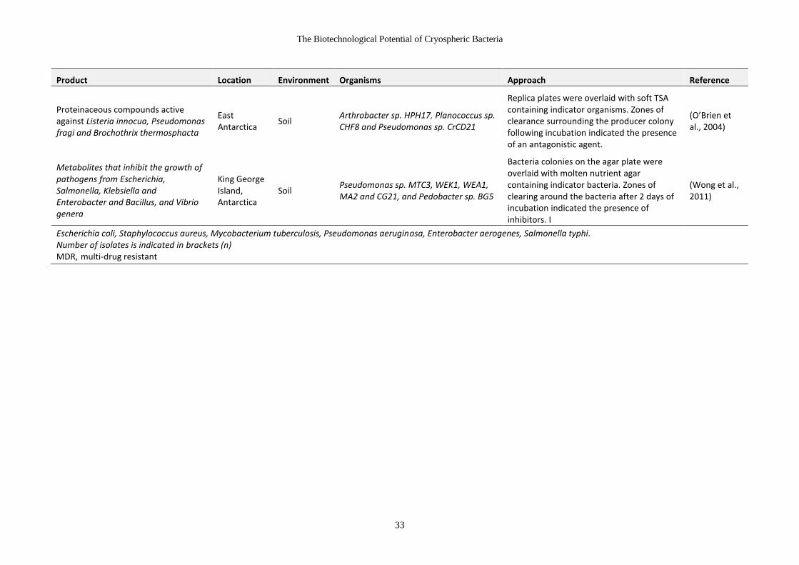
The Biotechnological Potential of Cryospheric Bacteria
33
Product Location Environment Organisms Approach Reference
Proteinaceous compounds active against Listeria innocua, Pseudomonas fragi and Brochothrix thermosphacta
East Antarctica
Soil Arthrobacter sp. HPH17, Planococcus sp. CHF8 and Pseudomonas sp. CrCD21
Replica plates were overlaid with soft TSA containing indicator organisms. Zones of clearance surrounding the producer colony following incubation indicated the presence of an antagonistic agent.
(O’Brien et al., 2004)
Metabolites that inhibit the growth of pathogens from Escherichia, Salmonella, Klebsiella and Enterobacter and Bacillus, and Vibrio genera
King George Island, Antarctica
Soil Pseudomonas sp. MTC3, WEK1, WEA1, MA2 and CG21, and Pedobacter sp. BG5
Bacteria colonies on the agar plate were overlaid with molten nutrient agar containing indicator bacteria. Zones of clearing around the bacteria after 2 days of incubation indicated the presence of inhibitors. I
(Wong et al., 2011)
Escherichia coli, Staphylococcus aureus, Mycobacterium tuberculosis, Pseudomonas aeruginosa, Enterobacter aerogenes, Salmonella typhi. Number of isolates is indicated in brackets (n) MDR, multi-drug resistant

Chapter 1
34
1.7 Biomining, bioremediation and plastic degradation
In low nutrient glacial environments, microorganisms play a vital role in recycling nutrients to
ensure the sustained availability of a variety of nutrients (Bradley et al., 2014; Cameron et al.,
2012b). Adaptation to extreme, nutrient-poor conditions, may have selected for innovative
metabolic processes for metabolising non-conventional compounds in efficient ways. These
unique metabolic pathways may lead to novel means of storage, transformation or export of
minerals and nutrients (Cook et al., 2016b).
1.7.1 Bioremediation: degradation of contaminants
The successful bioremediation of contaminated soils requires that there are microorganisms
that can degrade the offending pollutants, and that the environmental conditions at the site of
contamination are conducive to the growth of those bacteria (Aislabie et al., 2006). The isolated
polar regions have experienced pollution at or near scientific and military bases, due to the
reliance of these human settlements on petroleum for power and heat generation and the
operation of transport vehicles (Aislabie et al., 2006). A second cause of pollution in polar
regions is the result of industrial activity and the emission of pollutants which can travel vast
distances in the atmosphere and be deposited with snow into Arctic environments (Papale et
al., 2017). In addition, persistent organic pollutants (POPs) with mutagenic and carcinogenic
potential can be incorporated into cryoconite (Cook et al., 2016b).
It was recently shown that microbial communities in Greenland cryoconite have resistance to,
and the potential to degrade several anthropogenic pollutants, such as the heavy metals mercury
and lead, persistent toxic compounds such as polychlorinated biphenyls (PCB) and dichloro-
diphenyl-trichloroethane as well as polyaromatic hydrocarbons (PAH) (Hauptmann et al.,
2017). Isolates from seawater and sediment from the Kongsfjorden fjord, Svalbard belonging
to the genera Algoriphagus, Devosia, Salinibacterium and Gelidibacter were also efficient at
degrading PCBs (Papale et al., 2017). Bacteria able to degrade alkanes are typically from
Rhodococcus or Pseudomonas genera, while Sphingomonas and Pseudomonas tend to degrade
aromatic compounds (Baraniecki et al., 2002) (Table 1.11).

The Biotechnological Potential of Cryospheric Bacteria
35
Table 1-11 Bacteria with ability to grow on hydrocarbon sources, with potential application for bioremediation
Origin/ Source Phylum/ Class Organism Hydrocarbon growth substrates Reference
Antarctic soil, Jubany Station (King George Island, South Shetland Islands)
Gammaproteobacteria Acinetobacter ADH-1 Crude oil, aromatic gas oil, hydrogenated gas oil, kerosene, dodecane, hexadecane, cyclohexane
(Cormack and Fraile, 1997)
Antarctic soil Actinobacteria Arthrobacter protophormiae MTCC 688
Hexadecane (Pruthi and Cameotra, 1997)
Arctic tundra, northern coast of Ellesmere Island
Alphaproteobacteria Sphingomonas DhA-95 Jet A-1 jet fuel, dodecane, pristane
(Yu et al., 2000) Gammaproteobacteria
Pseudomonas DhA-91 Jet A-1 jet fuel, octane, dodecane Pseudomonas IpA-92 Toluene Pseudomonas IpA-93 Toluene, benzene
Scott Base, Antarctica Actinobacteria Rhodococcus 5/1, 5/14, 7/1 JP8 jet fuel, C6–C20n-alkanes, pristane (Bej et al., 2000)
Northeastern tip of Ellesmere Island Gammaproteobacteria Pseudomonas Ps 8 Jet A-1 fuel, hexadecane, pristane
(Thomassin-Lacroix et al., 2001) Actinobacteria Rhodococcus Rho10 Jet A-1 jet fuel, dodecane
Marble Point, Antarctica Gammaproteobacteria Pseudomonas sp.5B JP-8 jet fuel¹, hexane
(Eckford et al., 2002) Pseudomonas stutzeri 5A JP-8 jet fuel¹, benzene, toluene, m-xylene
Scott Base, Ross Island, Antarctica Actinobacteria Rhodococcus 43/02 JP5 jet fuel, dodecane, hexadecane, pristane
(Saul et al., 2005) Alphaproteobacteria Sphingomonas 43/03, 44/02 Phenanthrene
Saglek, Labrador, Canada Gammaproteobacteria Pseudomonas PK4 Pyrene, dodecane, hexadecane (Eriksson et al.,
2002) Pseudomonas K319 Pyrene
Wright Valley, Antarctica Gammaproteobacteria Pseudomonas 30-3 JP8 jet fuel, C8–C13n-alkanes, toluene, m- and p-xylene, 1,2,4-trimethyl benzene
(Panicker et al., 2002)
Coastal soils of the Ross Sea region of Antarctica
Gammaproteobacteria
Pseudomonas Ant 5 JP8 jet fuel, NAH, 2MNAH
(Aislabie et al., 2000)
Pseudomonas Ant 7 JP8 jet fuel, p-xylene, 1,2,4-trimethyl benzene naphthalene, 1-methyl naphthalene and 2-methyl naphthalene
Pseudomonas 7/22 JP8 jet fuel, toluene, m- and p-xylene, 1,2,4-trimethyl benzene
Alphaproteobacteria Sphingomonas Ant 20 JP8 jet fuel, 1-methyl naphthalene, phenanthrene
Alphaproteobacteria Sphingomonas Ant 17 JP8 jet fuel, m-xylene, 1-methyl naphthalene and 2-methyl naphthalene, dimethylnaphthalene, 2-ethylnaphthalene, fluorene, phenanthrene
(Baraniecki et al., 2002)
¹ Pseudomonas 5A and 5B could only metabolise JP-8 jet fuel in the presence of NH4Cl (Eckford et al., 2002)

Chapter 1
36
1.7.2 Plastic Degradation
Petroleum-based plastics are ubiquitous and are used in virtually all areas of human life
(Wei and Zimmermann, 2017). Unfortunately, many of these plastics are recalcitrant to
degradation and persist in the environment for many years, leading to the massive
accumulation of plastic in landfills and oceans (Danso et al., 2019). It was estimated that
192 coastal countries generated 275 million metric tons (MT) of plastic waste in 2010,
which resulted in 4.8 to 12.7 million MT entering the ocean (Jambeck et al., 2015). That
number is only expected to have grown. Unfortunately, nearly 60% of the plastic waste
generated in Europe is from packaging materials, single-use disposable plastic and other
short-lived items that are discarded within a year (Wei and Zimmermann, 2017).
Together, Polyethylene (PE), polypropylene (PP), polystyrene (PS), polyvinyl chloride
(PVC), polyethylene terephthalate (PET) and polyurethane (PUR) account for over 80%
of the Europe’s plastic demand (Wei and Zimmermann, 2017). Plastics also use 8% of
the total global fossil fuel production to provide the raw materials or energy for their
manufacture (Wei and Zimmermann, 2017). There is virtually no location on the planet
untouched by the problem of plastic waste. Even as far north as Spitsbergen, Svalbard,
there is human debris in the form of wood, glass, plastic bottles, tins, bulbs, clothing,
bags, plastic tape fishing nets and rope (Bergmann et al., 2019; Urbanek et al., 2017).
Conventional plastics are extremely resistant to biodegradation. What biodegradation
does take place is incredibly slow and relies on the presence of various abiotic factors
such as UV irradiation, the presence/ absence of oxygen, temperature and the presence of
chemical oxidants (Wei and Zimmermann, 2017). Chemical and structural factors
affecting the biodegradability of plastics include their hydrophobicity, degree of
crystallinity, surface topography and the molecular size of the synthetic polymers (Wei
and Zimmermann, 2017).
A study of the microbiomes associated with different sized plastic debris types and sizes
used a network building approach to define the core taxa associated with the plastic
surface of each debris category (Debroas et al., 2017). Interestingly, although samples
were collected from the North Atlantic Ocean (subtropical gyre), most of the species
present were associated with non-marine ecosystems, suggesting that they are hitchhikers.
Keystone species came from the Rhodobacterales, Rhizobiales, Streptomycetales and
Cyanobacteria. The colonization also appeared to be polymer specific, with poly(ethylene
terephthalate) (PET) and polystyrene (PS) mesoplastics being significantly dominated by

The Biotechnological Potential of Cryospheric Bacteria
37
Alphaproteobacterial and Gammaproteobacteria. Polyethylene (PE) mesoplastics were
dominated by Alphaproteobacteria, Gammaproteobacteria and Actinobacteria, and the
majority of polyethylene microplastics were dominated by Betaproteobacteria (Debroas
et al., 2017).
Enzymes capable of degrading PE include certain laccases, manganese peroxidase and
lignin peroxidase. A thermostable laccase from the actinomycete, Rhodococcus ruber
C208 was able to degrade PE films in culture supernatants and cell-free extracts in the
presence of copper and when UV-irradiated (Santo et al., 2013). Polyurethane (PUR) can
be enzymatically depolymerised by microbial ureases, esterases and proteases (Wei and
Zimmermann, 2017).
Bioplastics (BP) are an alternative to the non-degradable conventional plastics. BPs
contributed roughly 2 million tons or approximately 1% of the world’s annual plastic
production in 2014 (Urbanek et al., 2017). However, this is expected to increase four-fold
to approximately 8 million tons by 2019 (Urbanek et al., 2017). BPs can be divided into
two types: renewable resource-based BPs and petroleum-based BPs. Renewable resource-
based BPs can be obtained from organic waste material, crops, microorganisms, or
genetically modified plants. Examples include polyhydroxyalkanoates (PHAs) and
poly(lactic acid) (PLA). Alternatively, three examples of petroleum-based BPs are
poly(butylene succinate-co-adipate) (PBSA), poly(butylene succinate) (PBS) and poly(ε-
caprolactone) (PCL). Recently, 121/313 isolates from 52 soil samples from Spitsbergen
were shown to degrade BPs (Urbanek et al., 2017). The number of isolates that could
clear PBSA, PBS and PCL were 116, 73 and 102, respectively. Moreover, 56 of the
isolates were able to grow on PLA agar plates. The bacterial strains with the highest
ability for biodegradation were Pseudomonas and Rhodococcus species (Urbanek et al.,
2017).
There is some thought that the use of living microorganisms rather than isolated enzymes
may be better for plastic degradation. Even more promising is the use of bacterial
communities, made up of defined microbial strains, which have shown better
performance than single organisms (Wei and Zimmermann, 2017).

Chapter 1
38
Table 1-12 Bacteria capable of plastic degradation
Type of plastic
Environment Enzyme Phylum Organism Study Type Reference
PE Soil Laccase Actinobacteria Rhodococcus ruber
Isolate. (Santo et al., 2013)
Crude-oil contaminated beach soil
Alkane Hydroxylase (AH)
Proteobacteria (Gammaproteobacteria)
Pseudomonas sp. E4, Pseudomonas aeruginosa E7
Alkane hydroxylase gene (alkB) expressed in Escherichia coli BL21
(Jeon and Kim, 2015; Yoon et al., 2012)
PS Hydroquinone peroxidase
Proteobacteria (Gammaproteobacteria)
Azotobacter beijerinckii
Two-phase system- dichloromethane and water. Rapid conversion to soluble products in 5 minutes at 30°C organic phase containing hydrogen peroxide and tetramethylhydroquinone
Nakamiya et al, 1997
PBs (PBSA, PBS and PCL)
Soil samples Unknown Gammaproteobacteria, Actinobacteria
Pseudomonas and Rhodococcus species
Isolates capable of clear zone formation on emulsified PBSA, PBS and PCL and PLA agar plates.
(Urbanek et al., 2017)
PE: Polyethylene: Made up of monomers of ethylene with the formula (C2H4) n and is the most common plastic containing a C-C backbone. PS: polystyrene: An aromatic polymer made up of monomers of styrene. PBSA: poly(butylene succinate-co-adipate), PBS: poly(butylene succinate), PCL: poly(ε-caprolactone),PLA: poly(lactic acid)
The Biotechnological Potential of Cryospheric Bacteria
39
1.8 Metagenomics
It is well established that only a small fraction of the species in environmental microbial
communities can be cultivated in the laboratory using traditional cultivation techniques
(Culligan et al., 2014; Head et al., 1998; Yarza et al., 2014; Yu et al., 2000). This
discrepancy has previously been termed “The Great Plate Count Anomaly” (Staley and
Konopka, 1985) and the uncultivatable organisms have earned the monicker “microbial
dark matter”. The field of metagenomics is a field of study and a set of techniques
(Culligan et al., 2014) that were developed to address this problem of “microbial dark
matter”. Currently, there are several different methods and techniques that can be used to
identify genes, enzymes, and bioactive molecules. Metagenomics typically consist of the
following steps: DNA extraction from an environmental sample, sequencing of the
metagenome, bioinformatics analyses and annotate of genes and/or the expression of
selected genes in a heterologous host to confirm function (Thomas et al., 2012; Vester et
al., 2015) (Figure 1-5). Each strategy has advantages and disadvantages, and the approach
depends on the type of sample, the resources available and the question that is being
asked. This thesis will use a mix of bioinformatics and functional screening approaches.
1.8.1 Challenges
The following section will highlight several major challenges in microbiology research
that metagenomics helps to address.
1.8.1.1 Organisms not yet cultivated
Since the arrival of next-generation sequencing (NGS), and now third-generation
sequencing, 16S rRNA sequences representing several hundred thousand new species
have been deposited annually into databases (Yarza et al., 2014). An analysis, based on
thresholds for 16S rRNA sequence similarity, suggest that there as many as ~ 1350 phyla,
~2200 classes, ~4200 orders, ~9600 families and ~61 000 genera (Yarza et al., 2014).
This is vastly more than the number of taxa that have currently been described. For
example, approximately 2000 genera have currently been described, of the more than 60
000 genera that are suspected to exist (Yarza et al., 2014). Additionally, although there
are more than 1000 estimated phyla, the bacteria cultivated to date are almost completely
dominated by just four phyla, the Actinobcteria, Bacteriodetes, Firmicutes and
Proteobacteria (Culligan et al., 2014), although debate still exists over whether the
Proteobacteria are just one phyla, or several (Yarza et al., 2014).

Chapter 1
40
Figure 1-5 Simplified and general overview of culture-dependent and metagenomic
methods for bioprospecting. Bioprospecting is an innovative field, beset by many
challenges that are being imaginatively overcome by technological advances.
Even prior to the revelation provided by the dawn of metagenomics, a clear mismatch
existed between what has been observed under the microscope, and what grows in culture.
A study of cryoconite on Svalbard glaciers experienced difficulty isolating cyanobacterial
and algal species observed under the microscope, yet managed to culture species that had

The Biotechnological Potential of Cryospheric Bacteria
41
not been directly observed (Stibal et al., 2006). This highlights the problem that what is
cultured in the lab is very seldom the most abundant or ecologically important species,
and the cultivation of strains from an environmental sample is therefore a poor
representation of community structure (Vester et al., 2015).
Although many organisms have not yet been cultivated, this doesn’t mean that it won’t
one day be possible. Organisms may be uncultivatable due to a difference between the
original environment and the laboratory conditions (Mu et al., 2020). For example,
temperature, pH, nutrients, salinity or any number of other factors may inhibit growth.
Additionally, many microorganisms are in symbiotic relationships with each other, and
are dependent on the presence of other microbes, (and the secondary metabolites they
secrete/produce)(Brown et al., 2015).
1.8.1.2 Unexpressed or undetectable proteins
In 2017, the (2017_01) UniProt database contains more than 73 million sequence entries,
of which only 0.17 % have evidence at the protein level, and only 1.44% have evidence
at the trancript level (http://www.ebi.ac.uk/uniprot/TrEMBLstats) (accessed 24/01/2017).
This suggests that a significant number of proteins may not be expressed, or are present
at levels below detection (Vester et al., 2015). In addition, the number of hypothetical
proteins and proteins of unknown function form the majority of many organisms’
genomes (Vanni et al., 2020). Where functions have been ascribed, these are themselves
based on predictions using homology to known genes (El-Gebali et al., 2019; Galperin et
al., 2015; Huerta-Cepas et al., 2017; Mistry et al., 2013).
1.8.1.3 Undetectable secondary metabolites
As mentioned in Section 1.6, bioactive secondary metabolites are an excellent source of
novel drugs to treat a myriad of human, animal, and crop diseases. Recent advances have
enabled the complex chemical structure of a secondary metabolite to be discerned from
the enzymes encoded by a particular set of genomic sequences (McAlpine et al., 2005).
A cryptic biosynthetic gene cluster (BGC) is a cluster of genes that synthesise an
unknown compound (Butler et al., 2016). An analysis of the genomes of 1154 archaeal
and bacterial organisms predicted 33 351 putative BGCs, many of which encode
secondary metabolites that have never been detected (Cimermancic et al., 2014). In
addition, it is suspected that the current list of BGCs currently vastly underestimates the
true number present. Not only are there many non-detectable BGCs, but those that are
detected using bioinformatics may not be expressed in culture. Systematic surveys of

Chapter 1
42
thousands of sequenced microbial genomes showed that silent clusters outnumber
expressed clusters in laboratory cultures suggesting enormous untapped potential in the
genomes of cultured microbes (Butler, 2004). Metagenome mining studies have revealed
that BGCs encoding compound classes that are commonly found in the genomes of
uncultivated bacteria are rarely found in the genomes of cultivatable bacteria (Butler et
al., 2016). Therefore, there has been a rise in genome mining and metagenome mining as
strategies for drug discovery, as the discovery paradigm has shifted from “microbial
metabolites” discovered via metabolite detection to “biosynthetic gene cluster” detection
together with predictions of their potential products (Butler, 2004).
1.8.2 Sequence-based methods
1.8.2.1 Comparative genomics
When dealing with small datasets it is difficult to interpret whether changes in amino
acids in proteins have occurred as an adaptive response to the cold, or whether the changes
are purely the result of evolution and genetic drift. However, the use of large
metagenomic datasets to compare psychrophilic, mesophilic and thermophilic organisms
from cold, moderate and hot environments respectively, can highlight common trends in
cold-adapted organisms that are more likely to be due to adaptations to the extreme
environment, as opposed to the random background noise of evolution (Casanueva et al.,
2010; Siddiqui and Cavicchioli, 2006). For this reason, metagenomic sequence datasets
derived from snow and ice habitats have provided a wealth of information about
adaptations to the cryospheric conditions (Edwards et al., 2013a; Simon et al., 2009b).
1.8.2.2 Metagenome-assembled genomes (MAGs)
Metagenome-assembled genomes (MAGs) are reconstructed genomes from
metagenomic DNA and represent a major advancement in the understanding of
uncultivated bacteria because MAGs can be annotated and mined using the same tools as
those previously restricted to cultivated organisms. Thanks to a rise in third generation
sequencers, such as the MinION™ Nanopore, reads are longer than ever (B. L. Brown et
al., 2017). Longer reads not only mean that assembly is less time consuming, as some
contigs can span entire genome lengths; but hybrid assembly of long reads from Nanopore
and short-reads from Illumina data are enabling the construction of closed, complete
genomes from metagenomic data (Moss et al., 2020; Overholt et al., 2019; Singleton et
al., 2020).

The Biotechnological Potential of Cryospheric Bacteria
43
1.8.3 Functional screening methods
Functional metagenomics refers to the study of a metagenome via the construction of a
clone library and the expression of individual genes (or clusters of genes) in a foreign
host to asses activity (Vester et al., 2015). However, genes from a library will not
automatically be expressed, and the low hit rate achieved to date may be less to do with
the low prevalence of these enzymes and products in the environment, and more to do
with inappropriate lysis methods, choices of vectors and choice of expression host. There
are minimum requirements for gene transcription to occur, including the presence of a
promoter, and the appropriate transcription factors to recognise the promoter (Gabor et
al., 2004). In addition, successful transcription, does not guarantee translation. The
minimum requirements for translation include a ribosome binding site (rbs) in the -20 to
-1 region upstream of the start codon for initiation of translation, as well as an initiation
codon that is recognisable in the host. Assuming translation at the ribosome, the peptide
may require chaperones, cofactors, and various modifications to ensure proper folding,
and then an appropriate secretion machinery in order to express the enzyme and prevent
the formation of inclusion bodies (Ferrer et al., 2016).
1.8.3.1 Vectors
There are several types of cloning vectors, such as plasmids, fosmids, cosmids and
bacterial artificial chromosomes (BACs). The choice of vector depends on the length of
the genomic fragments that are obtained from the environmental sample, which in turn
depends largely on the extraction method. Plasmids can accept inserts of up to 15kb,
fosmids can accept 25-35 kb, cosmids can accept 25 – 40kb fragments and BACs can
accept fragments from 100-200kb in size (Rashid and Stingl, 2015; Vester et al., 2015).
The advantage of using plasmids to construct small-insert libraries, is that the plasmids
can have a high copy number, containing many copies of the insert per cell. In addition,
the plasmids typically contain strong promoters, which result in good transcription
(Rashid and Stingl, 2015). Together, this makes the detection of even weakly expressed
proteins and enzymes possible. In addition, because the insert sizes are smaller, fewer
genes will be expressed in each clone (Rashid and Stingl, 2015), which is useful when
wanting to screen single enzymes or proteins. An advantage of using BACS, is that large
inserts can contain multiple genes or entire operons (Rashid and Stingl, 2015), which is
useful when looking for biosynthetic gene clusters that produce novel secondary
metabolites (Gabor et al., 2004). However, successful screening of these libraries may be
more difficult because they single-copy, and therefore may express products in extremely
Chapter 1
44
low, or undetectable amounts. In addition, unlike the promoters in plasmids, the genes in
a BAC insert are usually still under the control of their native promoters. This means that
these inserts rely on the transcription factors, cofactors and signalling pathways of the
host, which may result in many genes remaining unexpressed.
1.8.3.2 Expression-hosts
To amplify, synthesise, purify, and characterise enzymes, a host is transformed with the
vectors containing genomic fragments, and then expressed. The selection of both vector
and host are non-trivial matters, as successful expression relies on the transcriptional
regulators encoded in the metagenome fragment being recognised by and compatible with
the RNA polymerases in the host. In recognition of the need to consider host compatibility
and silenced gene clusters, a number of heterologous hosts have been engineered, with
the specific intention of maximising secondary metabolite production (Zhang et al.,
2010). These include strains of Streptomyces coelicolor (Gomez-Escribano and Bibb,
2014), S. albus (Seipke, 2015), S. lividans, S avermitillis (Komatsu et al., 2013), S.
antibioticus, and S. parvalus, from the Actinobacteria, as well as engineered organisms
from other phyla, such as Escherichia coli, Bacillus subtilis, Pseudomonas putida,
Saccharomyces cerevisiae and Apergillus nidulans (Gomez-Escribano and Bibb, 2014;
Park et al., 2020; Zhang et al., 2010).
One of the most common hosts is Escherichia coli (E. coli). The optimum growth
temperature of E. coli is 37°C, which is significantly higher than the optimum temperature
of psychrophiles, and thus also significantly warmer than the ideal temperature for cold-
active enzymes, which presents a number of problems for heterologous expression. If the
optimum temperature of the E. coli host is used, there may be misfolding or denaturation
and a loss of functional ability of the enzymes. However, if the optimum temperature of
the enzyme is used, the metabolic reactions of E.coli may be 16–80 times lower (Vester
et al., 2015). Agilent Technologies have attempted to address this problem, by
engineering a strain of E.coli (Arctic Express) to include chaperones from a psychrophilic
bacterial strain, Oleispira antarctica (Vester et al., 2015). An alternative to genetically
engineering E. coli, is to simply use a psychrophiles as an expression host.
Pseudoalteromonas haloplanktis TAC125 is an Antarctic bacterium that is used as a
system for expression and secretion of proteins (Cusano et al., 2006; Parrilli et al., 2008).
P. haloplanktis TAC125 has increased solubility and secretion of protein products due to
disruption of its gspE gene (Parrilli et al., 2008).

The Biotechnological Potential of Cryospheric Bacteria
45
1.8.3.2.1 Multiple hosts
The use of a few alternative screening hosts from a variety of taxa may also increase the
number of positive clones that can be detected. In a study to try quantify the accessibility
of the metagenome by random expression cloning techniques, statistical models were
used to assess the percentage of genes from a variety of bacterial taxa that would be
detectable in E.coli (Gabor et al., 2004). Three scenarios for successful gene expression
were defined, (i) independent gene expression where both promoter and ribosome binding
site (rbs) are provided by the insert (IND), expression where only the rbs, but not the
promoter, is located on the insert (TRANSC) and (iii) expression dependent on both a
promoter and rbs provided by the vector (DEP). They found that about 40% of the genes
from 32 analysed genomes would be recoverable via the IND method if expressed in
E.coli (Gabor et al., 2004). However, this varied widely by phyla, with only 7%
recoverable from Actinobacteria, and up to 73% recoverable from Firmicutes. The
TRANSC fraction of genes required an optimum insert size of only 15 kb, and this was
the largest fraction in Actinobacteria (~58%), and Proteobacteria (~38%). The DEP
fraction represents DNA that is virtually inaccessible and represents approximately 48%
of Actinobacterial genes are dependent on this expression type.
This theoretical prediction has been verified experimentally by testing the expression of
the same metagenomic library in different hosts. In a screen for secondary metabolites, a
library was expressed in both E. coli and Streptomyces lividans via the creation of a
cosmid vector that could be conjugated between E. coli and S. lividans. They found that
the library hosted in S. lividans contained 12 functionally active clones, none of which
had been detected when using E.coli as the host (McMahon et al., 2012). Even more
illuminating, Craig et al., screened a metagenomic library in six proteobacterial hosts, E.
coli and five others; Agrobacterium tumefaciens, Burkholderia graminis, Caulobacter
vibrioides, Pseudomonas putida, and Ralstonia metallidurans and found that there was
only one case where the same small-molecule-producing clone (containing a six-gene
operon for the production of the carotenoid β-carotene) was identified using two different
host species (R. metallidurans and A. tumefaciens) (Craig et al., 2010). Interestingly, R.
metallidurans belongs to the Betaproteobacteria class and A. tumefaciens belongs to the
Betaproteobacteria class, yet other Alpha- and Betaproteobacteria hosts in this
experiment did not express this operon (Craig et al., 2010).

Chapter 1
46
1.8.3.3 Screening methods
Once a clone library has been constructed, the clones need to be screened for the activity
of interest. The hit rate of these screens is notoriously low (Culligan et al., 2014). The
following methods have been developed to attempt to either improve expression of
psychrophilic NPs or increase the number of positive hits and screen for a larger variety
of functions and activities than previously possible.
One possibility is to use traditional chromogenic and substrate-based assays, but simply
but incubate the plates at a low temperature (Vester et al., 2015). A second approach is
heterologous complementation screening, which involves the use of an expression host
that has a mutation such that only clones containing genes that complement or restore that
function will be able to grow (Rashid and Stingl, 2015; Vester et al., 2015). This approach
was used to identify several cold-active polymerases from glacial ice in Germany (Simon
et al., 2009b).
Substrate-induced expression screening (SIGEX) is a means to screen libraries for clones
that are able to catabolise a substrate (compound) of interest (Uchiyama and Watanabe,
2008). In this method, a cloning vector is used that contains a fluorescence gene such as
green fluorescing protein (GFP), located immediately downstream of the cloning site.
Upon the induction of gene(s) in the insert by the substrate of interest, the GPF is co-
expressed, signifying the presence of an induced gene (Uchiyama and Watanabe, 2008).
Positive clones can then be selected by fluorescence-activated cell sorting
(FACS)(Uchiyama and Watanabe, 2008).
Product-induced gene expression (PIGEX) extends the work of SIGEX. Rather than
relying on the presence of a substrate to induce GFP expression, PIGEX relies on the
presence of the product to induce expression (Uchiyama and Miyazaki, 2010). This is
achieved by pairing a product-responsive transcriptional regulator, with a reporter gene
like GFP (Uchiyama and Miyazaki, 2010). A huge advantage of this method is that it
identifies clones that have the enzyme activity of interest. However, the selection of a
sensor gene that is sensitive to the product, and not the substrate or precursor is
challenging. Likewise, this assay will only work on those products that are not produced
as part of the normal metabolism of the host cell.

The Biotechnological Potential of Cryospheric Bacteria
47
1.8.4 Strategic cultivation and expression
Challenges in the field of metagenomics-based bioprospecting from natural environments
are therefore (i) trying to get an accurate representation of the species that exist, in their
correct proportions, (ii) characterising the enzymes and proteins these organisms are
capable of synthesising, and (iii) designing an expression system that can successfully
express the NP of interest. The use of bioinformatics to reconstruct uncultivated bacteria
from diverse environments, will open new avenues to address each of these challenges,
and will pave the way for strategic cultivation and heterologous expression.
Chapter 1
48
1.9 Aims and objectives
The aims of this thesis are:
1. Conduct a taxonomic survey of a range of cryospheric environments to prioritise
environments for further research (Chapter 3).
2. Construct high quality metagenome-assembled genomes (MAGs) from Svalbard
soil, cryoconite and soil metagenomes (Chapter 4) and the Scărișoara Ice cave
(Chapter 7) which will form the basis for:
2.1.1. Identifying novel species from these environments,
2.1.2. Describing the distribution of these MAGs across different sites,
2.1.3. Identifying nutrient sources of the MAGs by looking for key genes
in major biogeochemical cycles
2.1.4. Exploring the MAGs for BGCs capable of synthesising novel
secondary metabolites
3. Explore the secondary metabolites of the Svalbard metagenomes by linking the
metabolome (detected using LC-MS) in soil and cryoconite to the predicted
metabolic profiles of the MAGs (Chapter 6).
4. Use functional metagenomics to look for cold-active enzymes by cloning soil and
cryoconite DNA into cold-sensitive E.coli mutants (Chapter 7).
5. Develop and optimise a Bioinformatics workflow for bioprospecting from
shotgun metagenomic data (Chapter 8).
In addition, there are three outputs of this thesis, in the form of data and a clone library,
that form the basis of further research in this area.
1) A collection of MAGs from Svalbard.
2) A collection of MAGs from the Scărișoara Ice Cave.
3) Clone libraries of soil and cryoconite DNA, in DH10B and HCS1 and cs2-29 that
can be screened for Natural Products.

The Biotechnological Potential of Cryospheric Bacteria
49
2 MATERIALS AND
METHODS
2.1 Sampling sites, sample collection, transportation, and storage
The samples included in this thesis were collected from locations in Ny-Ålesund,
Svalbard in late June and early July 2017 and 2018 (See Appendix B-1 for sample
name, type, collection date, GPS coordinates and chapter inclusion). The environments
sampled included cryoconite, snow, slush and meltwater from glacial surfaces,
proglacial water from the glacier snout, soil from a glacial forefield, and seawater from
the fjord in front of Midtre Lovénbreen (ML). Most samples were collected from the
ML glacier and its surrounds. However, cryoconite was also collected from Vestre
Brøggerbreen (VB), Austre Brøggerbreen (AB) and Vestre Lovénbreen (VL). The
locations of sample sites are shown in Figure 2-1.
2.1.1 Soil sample collection
Soil from the forefield of the ML glacier was collected over three days. Sample sites were
arranged in three transects of five time points for a total of 15 unique samples. Samples
were collected into sterile Whirl-Pak® bags (Nasco) using a shovel or scoop that was pre-
contaminated by soil immediately adjacent to the sample site by scooping and discarding
the adjacent soil multiple times before sample collection.
2.1.2 Cryoconite sample collection
Cryoconite was collected from ML and VB in 2017 and ML, VB, AB and VL in 2018.
Cryoconite was aspirated into sterile 15 mL or 50 mL Falcon Tubes or Whirl-Pak® bags
(Nasco) using a turkey baster pre-contaminated with nearby cryoconite. The granules
were allowed to settle, and the excess water poured off until the tube was full. For
cryoconite collected in 2018, GPS co-ordinates, photos and hole and water depth
measurements were taken on site.

Chapter 2
50
Figure 2-1 Map of sampling sites included in this thesis. Samples of cryoconite were collected from four glaciers (ML, VB, VL and AB). Soil was collected
from the ML glacier forefield in three transects of five time points. Snow, slush, and meltwater was collected from ML, and seawater was collected from
Kongsfjorden ford.

The Biotechnological Potential of Cryospheric Bacteria
51
2.1.3 Glacial water and seawater sample collection
Snow and slush samples from the ML glacier surface were aseptically collected into 2 L
sterile Whirl-Pak® bags (Nasco) using a scoop pre-contaminated with snow or slush.
Water from glacial meltwater streams on ML and proglacial water from ML and VB was
collected in 2L Nalgene bottles that had been bleached, rinsed in HCl, and autoclaved in
the lab. Each Nalgene was also pre-contaminated by filling and completely emptying the
Nalgene in the stream water five times before taking the sample. Seawater was collected
from open water in front of the ML forefield at two depths using a Niskin bottle. The
Niskin bottle was cast three times at 1 m and 15 m depth at each sampling location, and
2 L of water was collected in two sterile 1 L Nalgenes after each sampling event.
2.1.3.1 Filtering of liquid samples
Snow and slush samples were left in the sealed bags to melt in the dark in the NERC
Arctic Station lab before filtering. All liquid samples were filtered into Sterivex GP 0.22
µm polyethersulfone filters (Millipore, MA, USA) using a peristatic pump. The Sterivex
filters were filled with RNAlater ™ Stabilization Solution (Invitrogen, Catalog AM7020),
the ports sealed and placed at -20°C at the NERC Arctic Station.
2.1.4 Storage and transport
Cryoconite and soil samples were returned to the NERC Arctic station and stored at -
20°C together with Sterivex filters from the filtered liquid samples. Samples were
transported to the UK in insulated chilled containers. All samples were then placed at -
20°C for long-term storage.
2.2 DNA Extraction
Extraction from complex environments such as soil only recovers a fraction of the cells
present (Busi et al., 2020; Trevors and van Elsas, 1995). For example, certain groups of
organisms resist separation from soil, such as methanotrophic bacteria from peat, and
ammonium-oxidising bacteria in clay loam soils (Bakken and Lindahl, 1995). In addition,
DNA purified from soil microorganisms often contains humic and fulvic acids which can
inhibit enzymes, such as Taq DNA polymerase, used in downstream assays. Numerous
DNA extraction kits and methods were therefore tested to optimise yield and minimise
PCR inhibitors. The Extraction methods used for different samples types, and different
analyses are listed in Table 2-1.

Chapter 2
52
Table 2-1 Table of DNA Extraction Kits used in different chapters
Kit Section Chapter Application Samples
Qiagen DNEasy PowerWater 2.2.2 3 16S rRNA gene
amplicon Analysis
Snow, slush,
meltwater,
proglacial
water,
seawater
4 Metagenomes Seawater
Qiagen DNeasy PowerSoil 2.2.3 4 Metagenomes Cryoconite
MP Biomedicals FastDNA Spin Kit
for Soil
2.2.4 3 16 Amplicon
analysis
Soil, Cryoconite
4 Metagenomes Soil (F3T3_FD)
MO BIO PowerMax Soil DNA
Isolation Kit
2.2.7 4 Metagenomes Soil (F3T3_PM)
6 Cloning Soil
MasterPure Complete DNA &
RNA Purification Kit
2.2.5 6 Cloning
optimisation
Soil
Ludox Density Gradient
centrifugation
2.2.6 4 Metagenomes Soil (F3T3_Lud)
6 Cloning
optimisation
Soil
ZymoBIOMICS DNA Minikit 2.2.8 6 Strain
confirmation
E.coli isolates
Table listing different DNA Extraction kits, the chapters, and samples for which each kit was used and
the purpose for which the DNA was extracted.
2.2.1 DNA Extraction for 16S rRNA gene amplicon analysis
A survey of the taxonomic diversity of a range of cryospheric environment types was
conducted using16S rRNA gene amplicon-based analysis (Chapter 3). This study
included liquid and solid environment samples; therefore, more than one DNA
extraction kit was required due to the differing quantities and properties of the samples
collected. DNA from all liquid samples, such as snow, slush, meltwater, proglacial
water and seawater were extracted using the DNEasy PowerWater Kit (Section 2.2.2) in
a clean room, while wearing a Tyvek suit to minimise contamination of low biomass
samples. Some experimentation was required to select the DNA extraction kit for the
solid samples because some of the soil sites, particularly those with high clay content,
yielded extremely low DNA concentrations. Various kits and modified buffers were
tested to optimise DNA yield from these sites. The FastDNA Spin Kit for Soil (MP
Biomedicals) resulted in the highest yield from clay soils, which is in agreement with
previous published studies (Dineen et al., 2010). Therefore, to reduce bias from using

The Biotechnological Potential of Cryospheric Bacteria
53
different kits, all solid samples, including cryoconite, were extracted using the FastDNA
Spin Kit for Soil (Section 2.2.4). Extractions from each sample site were performed in
triplicate in randomised batches so that DNA from no sample site was extracted twice in
a single batch and a control extraction was included in each extraction batch.
2.2.2 Qiagen DNEasy PowerWater
The Qiagen DNeasy® PowerWater® Sterivex™ Kit was used to extract DNA from
snow, slush, glacial meltwater, proglacial water, and seawater samples that had been
filtered through Sterivex filters (Millipore cat. no. SVGPL10RC).
Prior to use, Solution ST1A was added to Solution ST1B, and mixed well. Inlet and
outlet caps were removed to extract the RNAlater™ Stabilization Solution
(ThermoFischer Scientific) which had been added to the Sterivex filters for storage.
Liquid was removed using a syringe with a tubing connector that had been washed in
bleach, HCl and ddH2O. The outlet cap was replaced and 0.9 mL of Solution ST1B was
added using a pipette tip. Thereafter, the inlet was recapped and the Sterivex filter were
secured horizontally to a vortex adapter, with the inlet facing outwards. The filters were
vortexed at minimum speed for 5 min, after which they were rotated 180 degrees from
the original position, while maintaining their orientation with inlet facing outwards, and
vortexed for an additional 5 minutes. The Sterivex filter units were positioned with the
inlet facing up, the inlet caps were removed, and 0.9 mL of Solution MBL (prewarmed
to 65℃) was added to each unit using a pipette tip. The inlets were recapped, and the
Sterivex filter units were incubated at 90ºC for 5 minutes. The filters were cooled for 2
minutes and then secured horizontally, with the inlet facing outwards to a vortex adapter
and vortexed at maximum speed for 5 minutes. The lysate was removed from the
Sterivex filters by pulling back the plunger of a 3 mL syringe to fill the barrel with 1
mL of air, and then attaching it to the inlet of Sterivex filter unit. The air was pushed
into the unit until there was resistance, and then the plunger was released and slowly
pulled back to remove as much of the lysate as possible. The syringe was detached from
the Sterivex filter unit and the lysate added to 5 mL glass PowerBead Tubes. The
PowerBead Tubes were secured horizontally to a vortex adapter and vortexed at
maximum speed for 5 minutes. The tubes were centrifuged at 4000 x g for 1 minute and
the supernatants transferred to clean 2.2 mL collection tubes. Thereafter, 300 µL of
Solution IRS was added to the tubes, which were vortexed briefly to mix, and then
incubated in an ice-bucket (approximately 4 °C) for 5 minutes. The tubes were

Chapter 2
54
centrifuged at 13,000 x g for 1 minute and the supernatants were transferred to clean 5
mL collection tubes.
For each sample, a tube extender was placed firmly into an MB Spin Column and the
tube extender/MB Spin Column unit was attached to a VacConnector and VacValve
(VV) on the QIAvac 24 Plus Manifold. Solution MR, which had been prewarmed to 65
℃, was retrieved and 3 mL was immediately added to the Collection Tubes containing
supernatant and vortexed to mix. The entire 4.5 mL of supernatant was then loaded into
the tube extender/MB Spin Column. The vacuum source was turned on and the VV of
the port opened, allowing the lysate to pass through. Once the lysate had passed through
completely, the VV was closed. While keeping the MB Spin Column attached to the
VV the tube extenders were removed and discarded. Following this, 0.8 mL of ethanol
was added to the MB Spin Column, the VV was opened and the ethanol allowed to pass
through the column completely. The VV was closed and then 0.8 mL of Solution PW
(mixed thoroughly by shaking) was added to the MB Spin Column. The VV was opened
and Solution PW allowed to pass through the column completely. The vacuum was
maintained for another minute to dry the membrane. The VV was closed and 0.8 mL of
ethanol was added to the MB Spin Column. The VV was opened and a vacuum was
applied until the ethanol had passed through the MB Spin Column completely. The
vacuum was maintained for another minute to dry the membrane, then closed. The
vacuum source was turned off and an unused port as opened to vent the manifold. The
MB Spin Column was removed and placed in a 2.2 mL collection tube. The tube was
centrifuged at 13,000 x g for 2 min to completely dry the membrane. The MB Spin
Column was transferred to a new 2.2 mL collection tube and 100 µL of Solution EB
was added to the centre of the white filter membrane. Finally, the tubes were
centrifuged at 13,000 x g for 1 minute at room temperature to elute the DNA and the
MB Spin Columns were discarded. DNA concentration and quality were tested using
Qubit and agarose gel electrophoresis before long-term storage at -20 ℃.
2.2.3 Qiagen DNeasy PowerSoil
The Qiagen DNeasy® PowerSoil® Kit was used to extract DNA from soil and
cryoconite. Cryoconite DNA from these extractions were used for the shotgun
metagenomes (Chapter 4) and clone libraries (Chapter 6).
Briefly, approximately 0.25 g of soil or cryoconite was added to PowerBead tubes and
vortexed briefly to mix. Solution C1 was pre-warmed to 60 ℃ and 60 µL was added to

The Biotechnological Potential of Cryospheric Bacteria
55
each tube. The tubes were then secured horizontally to a Vortex Adapter and vortexed at
maximum speed for 15 minutes. The samples were centrifuged at 10 000 x g for 30
seconds and the supernatant transferred to 2 mL collection tubes to which 250 µL of
Solution C2 had been pre-aliquoted. The samples were vortexed for 5 seconds and then
incubated in an ice-bucket (4 ℃) for 5 minutes. The samples were centrifuged at 10 000
x g for 1 minute and 600 µL of the supernatants were added to a 2 mL collection tube to
which 200 µL of Solution C3 had been pre-aliquoted. The tubes were vortexed to mix,
incubated in an ice-bucket (4 ℃) for 5 minutes and then centrifuged at 10 000 x g for 1
minute. Carefully avoiding the pellet, 750 µL of supernatant was transferred to 2 mL
collection tubes to which 1200 µL of vigorously mixed Solution C4 had been pre-
aliquoted. The samples were vortexed briefly to mix and then 675 µL was added onto
an MB Spin Column and centrifuged at 10 000 x g for 1 minute. The throughflow was
discarded and the same step repeated twice more until all the sample had been
processed. Thereafter, 500 µL of Solution C5 was added to the Spin Column and the
samples were centrifuged for 30 seconds at 10 000 x g. The flow through was discarded
and the Spin Column was centrifuged for a further minute at 10 000 x g. Following this,
the Spin Column was carefully transferred to a clean 2 mL collection tube and 100 µL
of Solution C6 (10 mM Tris-HCl, pH 8.5) was added to the centre of the filter
membrane and left for 5 minutes at room temperature. The DNA was eluted by
centrifugation for 30 seconds at 10 000 x g. The Spin columns were discarded, and the
DNA concentration and quality were tested using Qubit and agarose gel electrophoresis
before long-term storage at -20 ℃.
2.2.4 FastDNA™ Spin Kit for Soil
The FastDNA™ Spin Kit for Soil (MP Biomedicals) was used to extract DNA from
glacier forefield soils and cryoconite collected in July 2017. The DNA extracted using
this kit was used to create the 16S rRNA gene amplicon Libraries in Chapter 3
(Appendix Figure C-1). The Kit was selected because it yielded higher concentrations
of DNA than the Qiagen DNEasy PowerSoil, particularly for the high clay-content soils
close to the glacier snout.
Extractions from forefield soil were performed following the manufacturer’s
instructions with small modifications. Approximately 500 mg of soil was weighed and
added to Lysing Matrix E tubes, to which 978 µL of Sodium Phosphate Buffer and 122
µL of MT Buffer was added. The samples were then put on ice and homogenized in the

Chapter 2
56
FastPrep24 Instrument for three cycles of 30 seconds at a speed setting of 6.0, with 30
seconds of cooling on ice between cycles. The tubes were centrifuged for 15 minutes at
14 000 x g to pellet debris. Following this, the supernatant was transferred to a clean
2mL microcentrifuge tube, to which 250 µL PPS (Protein Precipitation Solution) was
added. The tubes were inverted 10 times to mix, followed by 5 minutes centrifugation at
14 000 x g to pellet the precipitate. The supernatant was then carefully transferred to
15ml flacon tubes. The Binding Matrix suspension was mixed thoroughly using a
vortex, and 1 mL was added to the supernatant in each 15 mL tube. Tubes were inverted
by hand for 2 minutes, and then placed in a rack for 3 minutes for the silica matrix to
settle. Thereafter, 500 µL of supernatant was removed and discarded, avoiding the silica
pellet. The Binding Matrix was gently resuspended in the remaining supernatant and
approximately 600 µL was added to Spin™ Filter. The Spin™ Filter was centrifuged at
14 000 x g for 1 minute, and the catchment tube was emptied. The remaining
supernatant was added to the Spin™ Filter, and the centrifugation and emptying step
was repeated. The pellet on the filter was gently resuspended using 500 µL SEWS-M
(to which ethanol had been added at first use). The Spin™ Filter tube was then
centrifuged at 14 000 x g for 1 minute, the catchment tube was emptied and replaced,
followed by a second centrifugation of 2 minutes at 14 000 x g to dry the matrix. The
catch tube was discarded and replaced with a new catch tube. The Spin™ Filter was
then allowed to air dry at room temperature for 5 minutes. Finally, the Binding Matrix
was gently resuspended in 100 µL DES (DNase/ Pyrogen-Free Water) and the tubes
were centrifuged for 1 minute at 14 000 x g to elute the DNA, after which the Spin™
Filters were discarded. The DNA concentration and quality were tested using Qubit and
agarose gel electrophoresis before long-term storage at -20 ℃.
2.2.5 MasterPure Complete DNA & RNA Purification Kit
The MasterPure™ Complete DNA & RNA Purification Kit was selected to try to extract
high molecular weight DNA for cloning because this extraction method does not rely on
bead beating, which shears genomic DNA.
2.2.5.1 Extraction
Each extraction used 50 mL of PBS with 0.1% Tween 20 per sample. After sifting soil to
remove large stones, 1 g of wet soil was placed in a 50 mL screw-cap conical tube to
which 10 mL of PBS with 0.1% Tween 20 was added. The tubes were mixed by vortexing
at maximum speed for 1 minute to disperse and dissociate the soil particles. The soil

The Biotechnological Potential of Cryospheric Bacteria
57
suspension was centrifuged at 1,600 x g for 4 minutes and the supernatant was poured
into a new 50-mL tube. An additional 20 mL of PBS with 0.1% Tween 20 was added to
the original soil pellet and mixed by vortexing at maximum speed for 1 minute. The soil
suspension was centrifuged at exactly 900 x g for 3 minutes in a tabletop centrifuge and
the supernatant was combined with the previously collected supernatant. The soil pellet
was extracted again with an additional 20 mL of PBS + 0.1% Tween and centrifugation.
The pooled supernatant was centrifuged at 900 x g for 2 minutes in a tabletop centrifuge
and the supernatant was transferred to a fresh 50-mL tube.
2.2.5.2 Filtration
The entire collected supernatant (50 mL) was poured through four layers of bleached
and autoclaved Miracloth filtration material (Calbiochem). The sample was then
prefiltered through a 1.2-µm filter membrane using a Nalgene® 300-4000 250mL
Vacuum Filter Holder with Funnel and Receiver (Thermo Scientific™) with a handheld
vacuum pump. The filtrate was collected then passed through a 0.22-μm filter
membrane to trap the microbial mass on the filter. Using forceps and scissors pre-
soaked in 70% ethanol, the membrane was removed from the filter apparatus, cut in
half, and each half placed rounded side down along the side near the bottom of a 50-mL
sterile conical tube. The upper surface of the filter faced the centre of the tube and was
not allowed to dry out. Filter Wash Buffer was prepared immediately before use (by
adding 1.5 μL of Tween20 to 1.5 mL of PBS), and 1.5 mL was added to the filter pieces
in the tube. The tube was vortexed at the low speed setting to rewet the filter pieces,
then the setting was increased to the highest speed. The 1.5 mL cell suspension was
transferred to a clean microcentrifuge tube, then centrifuged at 14,000 x g for 2 minutes
to pellet the cells.
2.2.5.3 Lysis, and Protein Precipitation
The supernatant was discarded, and the cell pellet resuspended in 300 μL of TE Buffer,
to which 2 μL of Ready-Lyse Lysozyme Solution and 1 μL of RNase A was added. The
suspension was mixed, centrifuge briefly then incubated at 37°C for 30 minutes. After
incubation, 300 μL of 2x Tissue and Cell Lysis Solution and 1 μL of Proteinase K was
added to the tube and mixed by vortexing. After a brief pulse-centrifuge to ensure that
all the solution is in the bottom of the tube, the suspension was incubated at 65°C for 15
minutes. The tubes were cooled on ice for 3-5 minutes, then 350 μL of MPC Protein
Precipitation Reagent was added to the tube and mixed by vortexing vigorously for 10

Chapter 2
58
seconds. The cell debris was pelleted by centrifugation for 10 minutes at 20,000 x in a
microcentrifuge at 4°C. The supernatant was transferred to a clean 1.7-mL
microcentrifuge tube and 570 μL of isopropanol was added. The contents of the tube
were mixed by inverting the tube several times. Thereafter the DNA was pelleted by
centrifugation for 10 minutes at 20,000 x g at 4°C. The isopropanol was removed with a
pipette tip, being careful not to dislodge the DNA pellet. Once dry, 500 μL of 70%
ethanol was added to the pellet, followed by centrifugation for 5 minutes at 20,000 x g
at 4°C.21. A pipet tip was used to remove the ethanol without dislodging the DNA
pellet. The DNA pellet was then air-dried for 8 minutes at room temperature. Finally,
the DNA pellet was resuspended in 40 μL of TE Buffer. The quality (size) and
concentration of the isolated DNA was checked by gel electrophoresis on a 1% agarose
gel and Qubit, respectively.
2.2.6 Ludox Density Gradient centrifugation
To scale up the number of cells that could be separated for lysis, density gradient
centrifugation was tried instead of filtering. The method was based on the protocol
described by Bakken who separated cells using a colloidal silica gradient (Percoll)
(Bakken and Lindahl, 1995). The size of Percoll particles is approximately 35 nm,
whilst the size of Ludox HS 40 particles is approximately 12 nm. Although high losses
of cells from clay loam cells due to sedimentation through the gradient were reported
(Bakken and Lindahl, 1995), the large amount of soil that could be processed might
compensate for a relative increase in cell loss. Moreover, although Bakken reported that
the direct loading of cell homogenate on top of a Percoll density gradient was not
promising, as the cell yield was low, and the gradient contained many contaminating
substances; it was speculated that the greater size difference between Ludox HS
particles and bacterial cells would allow for easier removal of the silica particles from
the bacterial cell pellet.
According to procedures recommended by Bakken & Lindahl, 1995, 60 – 72 g of soil
was added to PBS with 0.1% Tween20 or distilled water and homogenized in a waring-
type blender for 3 x 1 minute at maximum speed. The slurry was then poured into two
sterile 50 mL Falcon Tubes. Thereafter, 100 mL was added, and the process repeated two
more times for a total of 6 x 50 mL Falcon Tubes containing 300 mL of slurry. The Tubes
were centrifuged at 900 x g for 2 minutes to pellet large soil particles and transferred to a

The Biotechnological Potential of Cryospheric Bacteria
59
new tube. The Falcon tubes were then centrifuged at 3857 x g for 30 minutes and the
supernatant was discarded. The pellet was resuspended in 3.5 mL PBS.
The microbial cell fraction was separated from soil particles using density gradient
centrifugation with LUDOX HS 40. Exactly 30 mL of Ludox HS 40 was added to sterile
50 mL Falcon Tubes. The supernatant from three Tubes was loaded onto a single column
and the Falcon Tube was centrifuged for 30 minutes at 3857 x g. At this point, the cell
fraction formed a visible layer on within the Ludox column, which was collected by
pipetting and transferred into a new 50 mL Falcon Tube.
Up to 40 mL of PBS was added to the Tubes, which were then centrifuged for 15 minutes
at maximum speed (3857 x g). The supernatant was poured off and the step repeated five
times to try and dilute and remove the LUDOX silica particles. After the fifth
centrifugation, the supernatant was poured off and the pellet was resuspended in 2 mL
PBS and added to a 2 mL microcentrifuge tube. The tube was centrifuged at 10 000 x g
for 2 minutes and the supernatant poured off. The pellet was finally resuspended in 300
μL TE. The DNA was then extracted followed the method described in Section 2.2.5.3.
This method was successful at extracting high molecular weight DNA of the right size
for fosmid packaging but did not yield the concentration of DNA expected from the mass
of starting material.
Figure 2-2 Gel of High Molecular Weight DNA extracted using Ludox HS-40. PL is
Phage DNA (47 kb). CL is Cleaver Scientific Broad Range Ladder. The numbered lanes
1-20 refer to 1st, 2nd and 3rd 100 mL aliquots of soil slurry). Gel is 0.8% agarose in 0.5 X
TBE.
Chapter 2
60
2.2.7 MO BIO PowerMax Soil DNA Isolation Kit
The DNA extracted using the MO BIO PowerMax Soil Kit was used in the Soil Shotgun
metagenome library in Chapter 4 and was also used to construct the soil clone library in
Chapter 6.
Solution C1 was warmed to 60 °C before starting. Fifteen mL of PowerBead Solution
was added to a PowerBead Tube followed by10 g of soil sample (from which large
stones had been removed). After vortexing for 1 minute, 1.2 mL of Solution C1 was
added to the PowerMax® Bead Solution Tube and vortexed vigorously for 30 seconds.
The PowerMax® Bead Solution Tubes were then secured horizontally to a vortex and
vortexed for 10 minutes at the highest speed, then centrifuged at 2500 x g for 3 minutes
at room temperature. The supernatants were transferred to a clean Collection Tube, to
which 5 mL of Solution C2 was added, inverted twice to mix, and incubated at 4°C for
10 minutes. The tubes were centrifuged at 2500 x g for 4 minutes at room temperature,
then the supernatant was transferred to a clean Collection Tube, avoiding the pellet.
Four mL of Solution C3 was added and the mixture was inverted twice to mix, followed
by incubation at 4°C for 10 minutes. The tubes were centrifuged at 2500 x g for 4
minutes at room temperature and the supernatant was transferred to a clean Collection
Tube. Solution C4 was mixed by shaking and 30 mL was added to the supernatant and
inverted twice. The Spin Filter was filled with the Solution C4/ supernatant mix and
centrifuged at 2500 x g for 2 minutes at room temperature. The flow through was
discarded and the previous step was repeated twice more with the remaining
supernatant. Once the final through-flow has been discarded, 10 mL of Solution C5 was
added to Spin Filter and centrifuged at 2500 x g for 3 minutes at room temperature and
the flow through discarded. The Spin Filter was centrifuged at 2500 x g for 5 minutes at
room temperature, then carefully placed in a new Collection Tube. To elute, 5 mL of
sterile Solution C6 was added to the centre of Spin Filter membrane and centrifuged at
2500 x g for 3 minutes at room temperature. The Spin Filter was discarded, and the
DNA was further concentrated. To concentrate the DNA, 0.2 mL of 5M NaCl was
added and the tube was inverted 3-5 times to mix. Next, 10.4 mL of 100% cold ethanol
was added and inverted 3-5 times to mix. The solution was centrifuged at 2500 x g for
30 minutes at room temperature. All liquid was decanted. The DNA pellet was then
washed with 70% cold ethanol, the liquid decanted, and the residual ethanol allowed to
evaporate in ambient air. Finally, the precipitated DNA was resuspended in sterile 10
mM Tris.

The Biotechnological Potential of Cryospheric Bacteria
61
2.2.8 ZymoBIOMICS DNA Minikit
The ZymoBIOMICS DNA Minikit (ZymoResearch, Catalog No. D4300) was used to
extract DNA from E. coli HCS1 and cs2-29 colonies prior to PCR to confirm the fcsA29
mutation in the polA gene.
DNA was extracted from E.coli colonies by scraping single colonies into ZR
BashingBead™ Lysis Tubes (0.1 & 0.5 mm) to which 750 µL ZymoBIOMICS™ Lysis
Solution was added. The tubes were secured to a vortex adapter with a 2 mL tube holder
and vortexed at maximum speed for 5 minutes. The ZR BashingBead™ Lysis Tubes
were then centrifuged at ≥ 10,000 x g for 1 minute. Up to 400 µL of the supernatant was
transferred to a Zymo-Spin™ IV Spin Filter (Orange Top) in a clean Collection Tube
and centrifuged at 7,000 x g for 1 minute. Thereafter, 1,200 µL of ZymoBIOMICS™
DNA Binding Buffer was added to the filtrate. Up to 800 µL at a time of the mixture
was added to a Zymo-Spin™ IIIC-Z Column in a Collection Tube, centrifuged at
10,000 x g for 1 minute, and the through-flow discarded, until all the filtrate had been
processed. The Zymo-Spin™ IIIC-Z Column was placed in a new Collection Tube to
which 400 µL ZymoBIOMICS™ DNA Wash Buffer 1 was added. The Tube was
centrifuge at 10,000 x g for 1 minute, the flow-through was discarded and 700 µL
ZymoBIOMICS™ DNA Wash Buffer 2 was added to the Zymo-Spin™ IIIC-Z Column
in the same Collection Tube. The tube was centrifuged at 10,000 x g for 1 minute, the
flow-through discarded and 200 µL ZymoBIOMICS™ DNA Wash Buffer 2 was added
to the Zymo-Spin™ IIIC-Z Column and centrifuged at 10,000 x g for 1 minute. The
Zymo-Spin™ IIIC-Z Column was transferred to a clean 1.5 mL microcentrifuge tube
and 100 µL ZymoBIOMICS™ DNase/RNase Free Water was added directly to the
column matrix and incubated for 1 minute. The Tube was centrifuged at 10,000 x g for
1 minute to elute the DNA. In a final step to remove PCR inhibitors, a Zymo-Spin™
IV-HRC Spin Filter (Green Top) was prepared by snapping off the base of the Zymo-
Spin™ IV-HRC Spin Filter (Green Top) and placing it into a clean Collection Tube.
The tube was centrifuged at 8,000 x g for 3 mins and the flow-through discarded. The
cap was removed and 400 µL DNase/RNase Free Water was added to the Zymo-Spin™
IV-HRC Spin Filter and centrifuged at 8,000 x g for 2 minutes. Finally, the eluted DNA
was transferred to a prepared Zymo-Spin™ IV-HRC Spin Filter in a clean 1.5 mL
microcentrifuge tube. The Zymo-Spin™ IV-HRC Spin Filter was loosely capped and
centrifuged at exactly 8,000 x g for 1 minute.

Chapter 2
62
2.3 DNA Quality and concentration
2.3.1 Agarose gel electrophoresis for DNA visualisation
Agarose gel electrophoresis was used for the visualisation of DNA from genomic and
metagenomic DNA extraction, PCR amplifications, plasmid minipreps and restriction
digestions. Briefly, agarose gels were made using agarose and 0.5X TBE (Tris Borate-
EDTA) Buffer. Agarose concentrations ranged from 0.8% (for very large DNA
fragments) to 1.5 % for small amplicons. Gels were run in a gel tank for variable lengths
of time, depending on fragment size, gel concentration and required band resolution for
visualisation. The most used stain was SybrSafe, in a concentration between 2 and 8 μL
per 100 mL gel. Appropriate ladders were used, depending on the DNA fragment sizes
and resolution required.
2.3.2 Qubit to assess DNA concentration
DNA concentration of samples was measured using the Qubit® dsDNA HS (High
Sensitivity) Assay (Invitrogen™, Catalog no. Q32854) and the Qubit® 2.0 Fluorometer
(Invitrogen™, Catalog no. Q32866). Samples were prepared in Qubit® assay tubes
(Invitrogen™, Catalog. no. Q32856). The working solution was prepared by diluting the
Qubit® dsDNA HS Reagent 1:200 in Qubit® dsDNA HS Buffer. Standards were
prepared and calibration done for each batch of samples. Working solution (190 – 199
μL) and sample DNA (10 – 1 μL) was mixed to a final volume of 200 μL and briefly
vortexed to mix. Calibration was performed with the standards and samples were
measured following the Qubit® 2.0 instructions.
2.4 Polymerase Chain Reaction (PCR)
2.4.1 Optimisation of 16S rRNA gene PCR
In the extraction and amplification of DNA from Svalbard, habitats there were several
obstacles to overcome. In a comparative study, it is best to minimise the number of
potential confounding factors introduced by methodological differences that may
introduce bias. However, in a survey of these many diverse habitat types, there is no
method that is optimal for all sample types. The samples from different environment
types had different starting concentrations of DNA, different inhibitors, and different
taxonomic profiles.
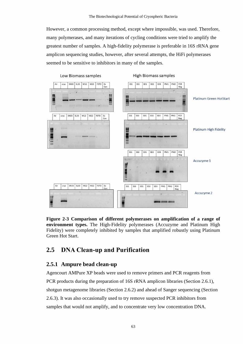
The Biotechnological Potential of Cryospheric Bacteria
63
However, a common processing method, except where impossible, was used. Therefore,
many polymerases, and many iterations of cycling conditions were tried to amplify the
greatest number of samples. A high-fidelity polymerase is preferable in 16S rRNA gene
amplicon sequencing studies, however, after several attempts, the HiFi polymerases
seemed to be sensitive to inhibitors in many of the samples.
Figure 2-3 Comparison of different polymerases on amplification of a range of
environment types. The High-Fidelity polymerases (Accuzyme and Platinum High
Fidelity) were completely inhibited by samples that amplified robustly using Platinum
Green Hot Start.
2.5 DNA Clean-up and Purification
2.5.1 Ampure bead clean-up
Agencourt AMPure XP beads were used to remove primers and PCR reagents from
PCR products during the preparation of 16S rRNA amplicon libraries (Section 2.6.1),
shotgun metagenome libraries (Section 2.6.2) and ahead of Sanger sequencing (Section
2.6.3). It was also occasionally used to try remove suspected PCR inhibitors from
samples that would not amplify, and to concentrate very low concentration DNA.

Chapter 2
64
Briefly, the AMPure XP solution was vortexed to mix and left for 30 minutes at room
temperature. AMPure XP solution was added in a ratio of 1.8 μL AMPure XP: 1 μL of
sample. The sample and beads were pipetted to mix and incubated for a few minutes to
allow the DNA fragments to bind to the paramagnetic beads. The 96 well plate was then
placed on a magnetic plate holder to allow the separation of beads and DNA fragments
from contaminants. While the beads + DNA were attached to the tube wall by the
magnet, the liquid was removed from the wells, and then the washed twice with 200 μL
freshly-made 70 - 80% ethanol to remove contaminants All of the ethanol was removed
and the beads allowed to air-dry for a few minutes. The 96 well plate was removed from
the magnetic rack and 10mM Tris was added and the beads gently washed into solution
and allowed to incubate at room temperature for 5 minutes. The plate was then placed
back on the rack and the purified DNA fragments could be removed from the wells and
transferred to a new plate.
2.6 DNA Sequencing
2.6.1 Illumina MiSeq of 16S rRNA gene Amplicons
The v3-v4 region of the 16S rRNA gene was amplified because it has been evaluated as
the most promising bacterial primer pair for bacterial diversity studies (Klindworth et
al., 2013). PCR amplification was performed using the recommended Illumina 16S
rRNA PCR Forward 5' [TCGTCGGCAGCGTCAGATGTGTATAAGAGACAGCCT
ACGGGNGGCWGCAG] 3’ and Reverse Primers 5' [GTCTCGTGGGCTCGGAGATG
TGTATAAGAGACAGGACTACHVGGGTATCTAATCC] 3’. The PCR reaction was
performed in two 96 well plates. Samples were split between high and low
concentration plates based on the starting concentration of the samples (Appendix
Figure C-5 and Figure C-6). This was done to lower the risk of cross contamination of
extremely low biomass samples by highly concentrated samples. The PCR reactions
were set up in a volume of 50 μL as follows: 25μL Invitrogen Platinum HotStart Green
PCR Mix (2x), 10 μL PCR FWD primer (1 μM), 10 μL PCR REV primer (1 μM), 1-5
μL environmental DNA and 0-4 μL PCR water to volume. The amount of DNA added
depended on the starting concentration of the extracted DNA and the suspected presence
of inhibitors.
Samples were then amplified on a thermal cycler using the following program: 95ºC for
3min, 34 cycles of: 95ºC for 30s, 55ºC for 30s and 72ºC for 30s, followed by a final

The Biotechnological Potential of Cryospheric Bacteria
65
72ºC step for 5min. In addition, eight PCR controls were run, in which ultra-pure Milli-
Q water was added instead of sample. Amplification success was confirmed by running
5µL of product on a 1% agarose gel (Appendix Figure C-2). Amplification products
were then cleaned-up with Ampure® beads (Section 2.5.1) followed by agarose gel
electrophoresis to confirm successful clean-up (Appendix Figure C-3).
Using a multichannel pipette, 5 µL from each well was transferred to a new 96‐well plate.
The Index 1 and 2 primers were arranged in a rack (TruSeq Index Plate Fixture) using the
arrangements described in Appendix Table C-1. The second stage PCR reaction to add
indexes was set up in a total volume of 25 μL with 2.5 μL DNA, 2.5 μL Nextera XT Index
Primer 1 (N7xx), 2.5 µL Nextera XT Index Primer 2 (S5xx), 12.5 µL Accuzyme Mix (2x)
and 5 μL PCR-grade water. The PCR was run on a thermal cycler using the following
program: 95°C for 3 minutes, followed by 8 cycles of: 95°C for 30 seconds, 55°C for 30
seconds, 72°C for 30 seconds and final elongation step at 72°C for 5 minutes, followed
by hold at 4°C. The second stage PCR products were run on a gel and compared to first
stage PCR products to confirm the size shift from approximately 550 bp to 630 bp
(Appendix Figure C-4). The second stage PCR products were once again cleaned up using
AmpureBeads (Section 2.5.1) and 3 μL was run on an agarose gel to check for PCR
product with no remaining primers. The samples were then measured using an EPOCH
(BioTek Instruments, Inc) or Qubit to determine exact concentrations for pooling.
2.6.2 Illumina Nextera shotgun sequencing
The environmental DNA was tagmented by adding 10 μL Tagment DNA buffer (TD) to
the 5ul of normalised DNA and then adding 5μl of Amplicon Tagment Mix (ATM) to the
wells and mixing well. The PCR plate was then centrifuged at 280 x g at room temperature
for 1 minute to make sure all sample was in the bottom of the well. The mix was then
rapidly transferred to a pre-programmed and pre-warmed thermocycler set at 55° C and
incubated for 5 minutes exactly, followed by rapid cooling to 10 °C. As soon as the
thermocycler reached 10 °C the plate was removed and 5 μL of Neutralize Tagment (NT)
Buffer was added to stop the tagmentation reaction. The plate was then centrifuged at 280
x g at room temperature for 1 minute, then incubated for an additional 5 minutes at room
temperature.
The libraries were amplified and indexed using a limited-cycle PCR. The indexes for each
library (Appendix Table D-1) were arranged in a 96-well PCR plate; 5 μL of Index 1 (i7)
was added down each column using a multichannel pipette, followed by the addition of 5
Chapter 2
66
μL of Index2 (i5) across each row. Thereafter, 15 μL of Nextera PCR Master Mix (NPM)
was added to each well and mixed by pipetting, followed by a brief centrifugation at 280
x g for 1 minute at room temperature. The libraries were then amplified in a thermocycler
set to the following cycle conditions: 72 °C for 3 minutes, 95 °C for 30 seconds, followed
by 15 cycles of 95 °C for 10 seconds, 55°C for 30 seconds and 72 °C for 30 seconds,
followed by a final elongation step of 5 minutes at 72 °C. A 1.5% agarose gel was run to
confirm successful amplification of metagenomic libraries (Appendix Figure D-1). The
resulting indexed libraries were cleaned up using Ampure beads (Section 2.5.1) and
resuspended in 37.5µL of Resuspension Buffer. Cleaned, indexed metagenomic libraries
were equimolarly pooled to 40 nM in a final volume of 50µL. To provide a final library
concentration of 4nM, 5µL of the previous solution were diluted in 10mM Tris 0.05%
TWEEN. The pooled libraries were sequenced at Wales Gene Park (Cardiff University)
in an Illumina NextSeq® in High Output mode, generating 2 x 150bp paired end reads.
2.6.3 Sanger sequencing
The PCR products from amplification of pJET2.1/blunt vector inserts, the 16S rRNA gene
and polA gene sequences were sent for Sanger Sequencing. Briefly, the PCR products
were cleaned up using Ampure beads. Thereafter, 5- 25 ng DNA in 6 µL was added to 4
µL BigDye™ Terminator Ready Reaction Mix (Applied Biosystems™) and 1.6 pmol of
FWD primer and sent for sequencing on an ABI 3730 DNA analyser (Applied
Biosystems™).

The Biotechnological Potential of Cryospheric Bacteria
67
3 HABITAT PREFERENCE OF
BACTERIA FROM A HIGH
ARCTIC GLACIAL
ECOSYSTEM INDICATES
CLIMATE VULNERABILITY
3.1 Introduction
The cryosphere is one of the Earth’s largest biomes, covering approximately 10% of the
Earth’s surface, and includes glaciers, icecaps and ice-sheets, as well as sea ice, frozen
inland water bodies, snow and permafrost (Margesin and Collins, 2019). This biome has
been identified an attractive region for bioprospecting (Cavicchioli et al., 2002; Leary,
2008) because it is an extreme environment (Maccario et al., 2015), difficult to access
and therefore relatively unexplored (Edwards et al., 2016; Gowers et al., 2019) and under
threat from global warming (Stibal et al., 2020). The potential loss of biodiversity due to
climate change represents a tragic squandering of undiscovered biological novelty and
identifying the most vulnerable environments is therefore an urgent priority.
Within the cryosphere, glaciers and glacial systems are attractive ecosystems for
bioprospecting because they contain within them different habitat types (snow, slush,
cryoconite, meltwater, proglacial water) and are adjacent to influencing environments
such as moraines, marine systems and freshwater lakes (Cameron et al., 2020b; Lutz et
al., 2016; Thomas et al., 2020). Each habitat contains distinct microbial communities
(bacterial, fungal, and algal) adapted to specific local conditions (Anesio and Laybourn-
Parry, 2012; Boetius et al., 2015; Hodson et al., 2008). These microbial communities vary
in complexity and heterogeneity, and this heterogeneity can be present at the micro, meso
and macroscales (Bay et al., 2020; Edwards et al., 2020; Malard et al., 2019). This system
is therefore subject to strong gradients in local selection pressures and has high
heterogeneity, which makes it a likely biodiversity hotspot.

Chapter 3
68
The microbial communities of glacial systems are also responsive and dynamic, with
spatial and temporal variation demonstrated in forefield soil (Bradley et al., 2014; Rime
et al., 2016, 2015), snow (Hell et al., 2013; Larose et al., 2013a; Lutz et al., 2014, 2016),
slush (Lutz et al., 2014), meltwater (Cameron et al., 2020b; Kohler et al., 2020) and
cryoconite (Cook et al., 2016a; Edwards et al., 2013c; Gokul et al., 2016) communities.
The high sensitivity and adaptability of some microorganisms to changing environmental
conditions suggest that communities contain specialists that thrive or dominate only under
specific conditions (Allison and Martiny, 2008). Alternatively, some taxa are relatively
stable both spatially and temporally due to an ability to adapt to a wide range of
conditions. These highly prevalent and stable taxa can be considered the core ‘keystone’
taxa because they persist either in a wide range of spatially separate environments of the
same type, or over seasonal changes. Keystone taxa have been identified in cryoconite
(Gokul et al., 2016) and soil (Malard et al., 2019) and likely represent highly adaptable
generalists. However, in addition to the highly abundant and prevalent keystone taxa,
there is a long tail of low abundance taxa. This long tail of low abundance species may
represent a reservoir of biodiversity, with specialist taxa that may either thrive and
become the new keystone species under different conditions, or go extinct should
conditions change beyond the habitable range for that species. Alas, due to practices in
dataset processing, the rare tail is often removed during a decontamination step, when
rarefying libraries to equal library sizes (McMurdie and Holmes, 2014), or is obscured by
OTU clustering (Bay et al., 2020).
With the threat of climate change, understanding the biogeography of the region, as well
as the factors that influence it, is a race against time. Specialists, with narrow
environmental windows are the most threatened , as perturbations caused by climate
change could lead to local extinctions (Stibal et al., 2020). One of the easiest ways to
identify specialist species is to determine their prevalence across different sites and
environmental gradients. In glacial ecosystems, there is a constant spread or inoculation
of taxa from one environment to downstream environments. The seeding and succession
of microbial community members into new environments can occur over long time scales,
such as the development of a glacier forefield soils (Bradley et al., 2014; Rime et al.,
2016), or over shorter time period, such as the flow of microbial assemblages from
supraglacial habitats to subglacial, proglacial (Kohler et al., 2020), forefield and marine
(Thomas et al., 2020) environments via meltwater (Cameron et al., 2020b; Kohler et al.,
2020) or aeolian transfer. In light of the vast amount of meltwater being lost annually due

The Biotechnological Potential of Cryospheric Bacteria
69
to climate change, several studies on the consequences of the release of glacial microbial
assemblages on downstream environments have been conducted in Arctic environments,
from Disco Island, Greenland (Cameron et al., 2020) to Ny Ålesund Svalbard (Thomas
et al., 2020). In particular, there has been a focus on the seeding of downstream
ecosystems and determining the ‘directionality’ of the flow of microbial species from
glacial surface snow and bare ice to meltwater, to downstream soil, freshwater and marine
ecosystems (Cameron et al., 2020b). Environment-agnostic species that can survive in
physically linked environments despite harsh ‘environmental’ boundaries, such as sharp
changes in pH, salinity, or light exposure tend to be generalists, and will likely dominate
more and more as global climate change continues to alter environments. The habitat or
site-specific species represent a vulnerable group that may soon be lost due to climate
change.
One of the requirements for this study is a high level of resolution of individual
community members within and across sites. As technology has improved, the resolution
to which we can resolve community structure has improved from microscopy (Stibal et
al., 2006; Takeuchi, 2002), to RFLP analysis (Cameron et al., 2012a; Edwards et al., 2011,
2013c), to cloning amplicons (Cameron et al., 2012a), and finally to the arrival of NGS
sequencing (Cameron et al., 2020b; Gokul et al., 2016; Thomas et al., 2020) and soon 3rd
Generation sequencing (Edwards et al., 2016; Gowers et al., 2019). However, it has been
shown that not just sequencing technology, but also bioinformatics methodologies can
weaken the ability to detect biogeographical patterns (Bay et al., 2020). In particular, the
clustering of sequences at 97% identity threshold (OTUs) and/or filtering the rare
biosphere (sequences lower than 0.05% relative abundance) were both found to obscure
biogeographic patterns (Bay et al., 2020). In this study, we describe the biogeography of
an Arctic glacier system at a fine resolution, by using amplicon sequence variants (ASVs)
rather than OTUs and by retaining the rare microbiome.
In this chapter, samples from a range of cryospheric environments surrounding Ny-
Ålesund, Spitsbergen, Svalbard were collected over two weeks. The environment types
included snow, slush, glacial meltwater, proglacial water, forefield soil, seawater and
cryoconite.

Chapter 3
70
3.1.1 Aims and objectives
The aims of this study were as follows:
1. Increase the resolution for investigating biogeographic trends by using ASVs
rather than OTUs and using statistical methods to remove contaminants.
2. Determine the phylogenetic diversity and species-richness of each sampled
environment.
3. Identify whether here are ‘keystone’ taxa which are highly abundant and prevalent
members of an environment type.
4. Identify community members that are unique to, or shared between, different
environments.
5. Create a co-occurrence network to determine the extent to which ASVs co-occur
and visualise how these occur within or across environment types.

The Biotechnological Potential of Cryospheric Bacteria
71
3.2 Methods
3.2.1 Sample collection
Sampling was conducted on, and in the vicinity of, the Midtre Lovénbreen (ML) and
Vestre Brøggerbreen (VB) glaciers in the Kongsfjorden area of Spitzbergen, Svalbard in
late June to early July 2017 (Figure 1). Many cryospheric environment types were
sampled including air, snow, slush, meltwater, cryoconite, proglacial water, soil, and
seawater. GPS co-ordinates are available in Appendix Table B-1.
3.2.1.1 Snow and slush
The snow and slush were collected on 29 June, 3 July, and 7 July, from mid-way between
stake 4 and stake 5 on ML. Two litres of snow and two litres of slush were collected from
three pits, located approximately three meters apart on each of the three days. The snow
and slush from each pit were melted overnight in the dark and filtered through a Millipore
Sterivex filter within 36 hours.
3.2.1.2 Meltwater
Six litres of water were collected in sterile 1 litre Nalgene’s from a flowing meltwater
stream in line with stake 3 on ML on the 29 June, 3 July, and 7 July. Two Nalgene’s (2
litres) were filtered through a Millipore Sterivex using a peristaltic pump within 24 hours
of collection. The Sterivex filter was filled with DNA Later, sealed, and stored at -20 °C
until DNA extraction. A 50 mL falcon tube of filtered meltwater was collected, without
any air bubbles, and stored at 4°C until chemical analysis could be done.
3.2.1.3 Proglacial water
Proglacial water was collected in six sterile 1 L Nalgene’s from flowing streams at the
snout of each of ML and VB glaciers. Two litres of water were filtered through a single
Sterivex to get 3 replicates for each proglacial stream.
3.2.1.4 Seawater
Seawater was collected from open water in front of the ML glacier forefield at two depths
using a Niskin bottle. The Niskin bottle was dropped three times at 1m and 15 meters
each, and 2 litres of water was collected in sterile 1L Nalgenes after each sampling event.

Chapter 3
72
3.2.1.5 Soil
Soil from the forefield of the ML glacier was collected in three transects perpendicular to
the snout of the glacier. Samples were collected into Whirl Pak bags at five time points
for a total of 15 unique samples, which were extracted in triplicate.
3.2.1.6 Cryoconite
Cryoconite was collected from ML by Nora Els and from VB by Dr Arwyn Edwards and
Nora Els. GPS coordinates for cryoconite on the map are approximate, based on
descriptions of the collection points relative to landmarks.
Figure 3-1 Map showing sampling sites in Ny-Ålesund, Spitsbergen, Svalbard.
3.2.2 DNA extraction
The high clay content of soils from the ML Glacier forefield proved challenging for DNA
extraction. Several kits and protocols with various modifications were attempted to
optimise yield (Section 2.2.1). Based on yield comparisons, the DNA from soil and
cryoconite samples were extracted using the MP Biomedicals FastDNA kit for soil
according to manufacturer’s instructions, with a few modifications (Section 2.2.4). The
air, snow, slush, meltwater, proglacial water and sea water was filtered through Sterivex
filters, topped with RNA Later and stored at -20 °C. DNA extractions were done using
the Qiagen PowerWater Kit according to manufacturer’s instructions (Section 2.2.2).
Because the samples were low biomass, extractions were performed in a clean room,

The Biotechnological Potential of Cryospheric Bacteria
73
while wearing sterile Tyvek suits and masks. All samples from the FastDNA and
PowerWater extractions were eluted in 100 μL. DNA quality and quantity were checked
by running 4µL- 8µL of genomic DNA on a 1.5% agarose gel and using Qubit (Section
2.3.2) to determine concentration. DNA was aliquoted and stored at -20°C.
3.2.3 Library preparation and sequencing
Samples were prepared for 16S rRNA amplicon sequencing using the Illumina 16S rRNA
metagenomic sequencing library preparation protocol (Section 2.6.1). The 16S rRNA
PCR was performed using Invitrogen’s Platinum Green Mastermix because it succeeded
at amplifying more samples in the dataset than the High Fidelity Polymerases we tested
(Section 2.4.1). Briefly, a first-stage PCR was performed using the Illumina
recommended FWD (5’ TCGTCGGCAGCGTCAGATGTGTATAAGAGACAGCC
TACGGGNGGCWGCAG 3’) and REV (5' GTCTCGTGGGCTCGGAGATGTGTATA
AGAGACAGGACTAC HVGGGTATCTAATCC 3’) primers for the V3-V4 region of
the 16S rRNA gene. Samples were then amplified on a thermal cycler using the following
program: 95ºC for 3 min, 34 cycles of: 95ºC for 30s, 55ºC for 30s and 72ºC for 30s,
followed by a final 72ºC step for 5 min. Amplicons were cleaned-up with Ampure® beads
at a 1.8x ratio (Section 2.5.1) before a second PCR to add indexes (Appendix Table C-1).
The conditions for the second stage PCR were: 95ºC for 3 min, 8 cycles of: 95ºC for 30s,
55ºC for 30s and 72ºC for 30s, followed by a final 72ºC step for 5 min. The second stage
PCR products were cleaned up using a 1.8x Ampure® beads ratio, and the sample
concentrations were quantified on an EPOCH machine. Finally, cleaned-up indexed
amplicons pooled in equimolar concentrations in a solution of 10mM Tris-HCl (pH 8)
and 0.1% TWEEN® and sequenced using an Illumina MiSeq® at Aberystwyth
University. The sequencing run was done using 2 x 300 bp paired-end sequencing, to
sequence the entire ~460bp V3-V4 region with enough overlap to merge samples.
3.2.4 Bioinformatics analysis
3.2.4.1 Removing adapters and quality trimming
Raw reads were demultiplexed on Illumina BaseSpace. Various parameters were tested
during quality control to optimise read quality and number. Adapters and primer
sequences were removed from raw reads using Cutadapt (version 2.4:
https://cutadapt.readthedocs.io/en/v2.4/) (Martin, 2011) using pair-ended trimming to
remove linked adapters. The 5’ adapter + 16S FWD primer and the reverse complement
Chapter 3
74
of the 16S REV primer + adapter were used to trim forward reads and the 5’ adapter +
16S REV primer and reverse complement of the 16S FWD primer and adapter were
used to trim the reverse reads. The 3’ ends were trimmed using a Phred score of 10 (-q
10) and paired reads in which at least one of the paired reads was shorter than 150bp
were removed (-m 150).
3.2.4.2 Taxonomic assignment using DADA2
Reads were assigned to amplicon sequence variants (ASVs) using DADA2 (v. 1.14.0)
(Callahan et al., 2016). After checking the QualityProfile plots (Appendix Section C-1),
FilterAndTrim() was used to truncate the R1 reads to 270 bp and the R2 reads to 220 bp.
Reads that had been trimmed shorter than these lengths by Cutadapt were lost at this stage.
The learnErrors() function was run with randomize=TRUE, as samples were ordered by
environment type and the error model needed to be based on a range of samples types.
The Error Plots can be viewed in Appendix Section C-2. The sample inference was run
using pool=”pseudo”. Pooling allows information to be shared across samples, which
makes it easier to resolve rare variants that were seen just once or twice in one sample but
many times across samples (https://benjjneb.github.io/dada2/pseudo.html#Pseudo-
pooling). Pooling is computationally expensive, therefore “pseudo-pooling” was used.
Pseudo-pooling is a two-step process in which independent processing is performed first
on the raw data alone, and then on the raw data a second time, informed by priors
generated from the first round of processing. The R1 and R2 reads were merged using
mergePairs() with the default overlap settings. Chimeras were removed using
removeBimeraDenovo(). Thereafter, taxonomic assignment was performed to genus level
using training fasta files derived from the Silva Project's version 132 release (Quast et al.,
2013).
3.2.4.3 Decontamination
Previous studies have shown that contamination can be a major factor in low biomass
samples (de Goffau et al., 2018; Salter et al., 2014). Sources of contamination range from
DNA extraction kit reagents, to PCR water, PCR reagents (Iulia et al., 2013) or
contaminants introduced by human error. To check for contamination, DNA extraction
controls and PCR negative controls were sequenced together with samples and used to
infer contamination. Contaminants were identified and removed from the samples using
the Decontam (v.1.6.0) package in R (Davis et al., 2018) which takes into account the
DNA concentrations of samples because contamination is more likely in low

The Biotechnological Potential of Cryospheric Bacteria
75
concentration samples (Details in Appendix Table C-2, Section C-5 and Section C-6).
Prior to decontam, the dataset was split into subsets containing all samples of a specific
environment type, relevant extraction controls and all the PCR negative controls used in
each plate. Data was split because the Decontam package recognises outliers, and
sequences in low biomass samples as contaminants. Due to the vast differences in DNA
concentration, and community diversity in different environment types, the samples were
split to compare like with like. The samples were processed using a prevalence of 0.5
(except for the glacial waters, which also made use of frequency). The frequency
parameter was omitted because the dataset contained samples of different environment
types, some of which were low biomass. The frequency parameter therefore mistakenly
excludes real taxa.
3.2.5 Statistical analysis and plotting of 16S rRNA abundance data
The 16S rRNA abundance data was filtered and analysed and using Phyloseq (V. 1.30.0)
(McMurdie and Holmes, 2013) in R (R-3.6.1), available at
(https://github.com/joey711/phyloseq). Rarefaction was avoided as far as possible to
avoid the loss of information or the loss of samples (McMurdie and Holmes, 2014). To
account for library size differences, the abundance values were converted to relative
abundance (RA) wherever doing so was justified. Occasionally filtering steps were
required to see trends in abundant taxa. Wherever filtering steps were applied, the relative
effect of the filtering step on library size is recorded. For measures of alpha diversity, the
unrarefied and rarefied data is compared. Common taxa shared between environment
types were plotted using UpSetR (Conway et al., 2017; Lex et al., 2014) available at
(https://github.com/hms-dbmi/UpSetR). Taxa belonging to each environment were
considered sets, and intersections between sets reflect shared taxa between groups.
3.2.6 Co-occurrence network analysis
Co-occurrence network analysis was performed using modified R and Python scripts as
described in (Hu et al., 2017; Ju et al., 2014; Ju and Zhang, 2015) and available at
https://github.com/RichieJu520/Co-occurrence_Network_Analysis. Networks were
visualised in Gephi 0.9.2 (https://gephi.org/) (Bastian et al., 2009; Jacomy et al., 2014)
using Java V8 (build 1.8.0_241-b07).

Chapter 3
76
3.3 Results
3.3.1 Sequencing results
There were 12,957,386 paired reads sequenced by the MiSeq run. However, 1 629 793
paired reads from the Illumina MiSeq run could not be demultiplexed and assigned to a
sample. This represents a significant fraction of the dataset (12.6%) and analysis of the
undetermined reads shows these reads either contained unexpected index combinations
(evidence of index-switching) or belonged to the PhiX Control. There was a large
variation in the library size of different samples (Appendix Section C-3), and potential
explanatory factors such as extraction method (Appendix Section C 4-1), environment
(Appendix Section C 4-2), extraction batch (Appendix Section C 4-3) and PCR plate,
column and row (Appendix Section C 4-4) were explored.
3.3.2 Taxonomic assignment
Prior to decontamination there were 59 135 unique sequence variants detected by DADA2
in 138 samples made up of 116 environmental samples and 22 controls.
3.3.1 Decontamination
One of the main aims of this study was to investigate the extremely rare specialist
community. We therefore wanted to retain low abundance ASVs, while removing true
contaminants. Simply removing ASVs that occur in negative controls from the dataset
risks removing true ASVs because high abundance members of adjacent samples are the
most likely source of contamination, and some of the species likely to contaminate
laboratory reagents (kitome) are similar to those found in the highly oligotrophic snow,
slush and meltwater environments (oligotrophic, stored in the fridge or freezer) (Edwards
et al., 2020; Salter et al., 2014). Decontam identifies contaminants based on their
prevalence in samples vs negative controls, and/or by their higher frequency in samples
with low starting concentrations, such as low biomass samples, which are more likely to
be contaminated (Davis et al., 2018).
The snow, slush and meltwater samples were especially tricky to decontaminate because
they were both low biomass and most likely to be contaminated by kitome contaminants,
but also the environment most likely to legitimately contain common kitome species. To
address this concern, the snow, slush, and meltwater samples were combined into a subset
(glacial waters) and decontaminated using the combined method, (threshold = 0,5) which
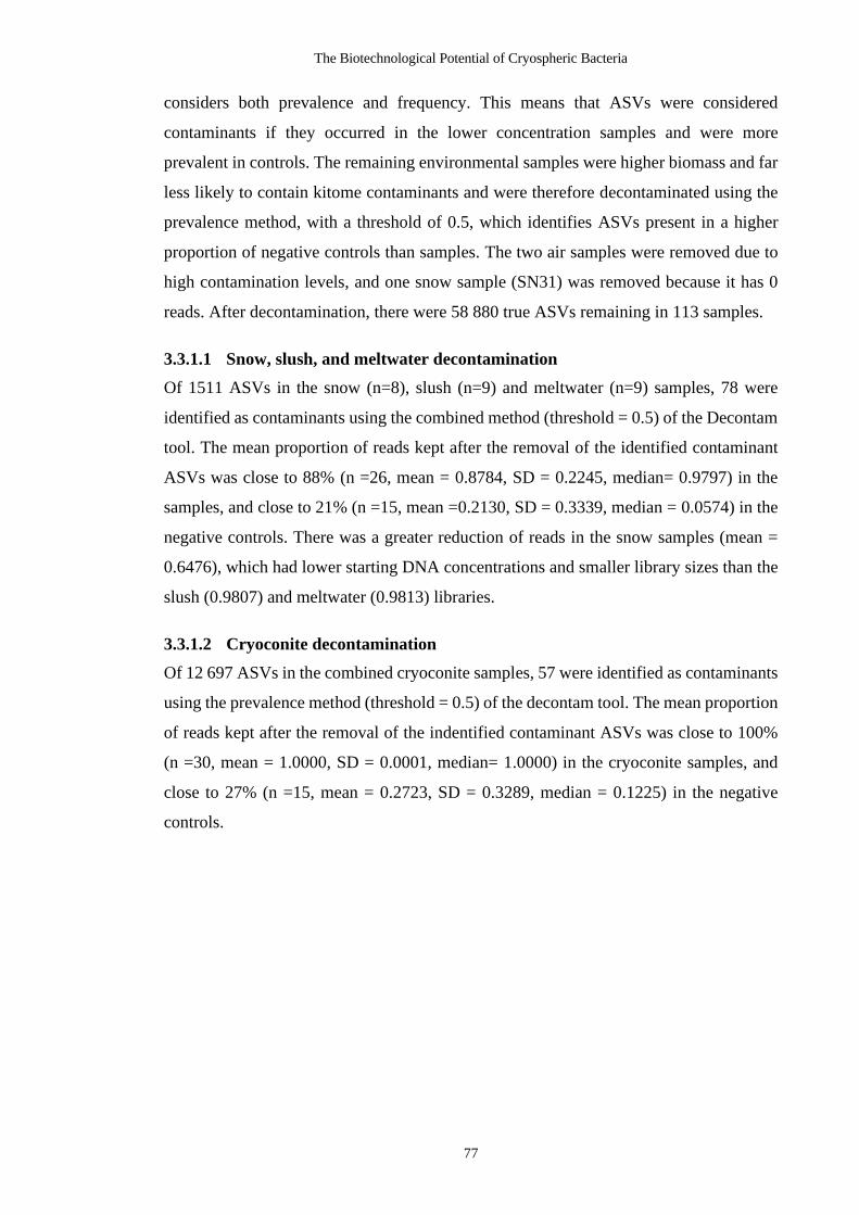
The Biotechnological Potential of Cryospheric Bacteria
77
considers both prevalence and frequency. This means that ASVs were considered
contaminants if they occurred in the lower concentration samples and were more
prevalent in controls. The remaining environmental samples were higher biomass and far
less likely to contain kitome contaminants and were therefore decontaminated using the
prevalence method, with a threshold of 0.5, which identifies ASVs present in a higher
proportion of negative controls than samples. The two air samples were removed due to
high contamination levels, and one snow sample (SN31) was removed because it has 0
reads. After decontamination, there were 58 880 true ASVs remaining in 113 samples.
3.3.1.1 Snow, slush, and meltwater decontamination
Of 1511 ASVs in the snow (n=8), slush (n=9) and meltwater (n=9) samples, 78 were
identified as contaminants using the combined method (threshold = 0.5) of the Decontam
tool. The mean proportion of reads kept after the removal of the identified contaminant
ASVs was close to 88% (n =26, mean = 0.8784, SD = 0.2245, median= 0.9797) in the
samples, and close to 21% (n =15, mean =0.2130, SD = 0.3339, median = 0.0574) in the
negative controls. There was a greater reduction of reads in the snow samples (mean =
0.6476), which had lower starting DNA concentrations and smaller library sizes than the
slush (0.9807) and meltwater (0.9813) libraries.
3.3.1.2 Cryoconite decontamination
Of 12 697 ASVs in the combined cryoconite samples, 57 were identified as contaminants
using the prevalence method (threshold = 0.5) of the decontam tool. The mean proportion
of reads kept after the removal of the indentified contaminant ASVs was close to 100%
(n =30, mean = 1.0000, SD = 0.0001, median= 1.0000) in the cryoconite samples, and
close to 27% (n =15, mean = 0.2723, SD = 0.3289, median = 0.1225) in the negative
controls.

Chapter 3
78
Table 3-1 Table of contaminants and true ASVs in environmental subsets
Subsets Samples and controls Number of ASVs Decontam Final Dataset
Environment type
Controls No of samples
No. of controls
Combined Sample ASVs
Control ASVs
Combined ASVs
Shared ASVs
Method Threshold Contaminant ASVs
True ASVs
True ASVs in samples
Difference
Glacial waters (snow, slush, and meltwater)
[1] [3] 26 15 41 1323 272 1511 84 Comb 0.5 78 1433 1245 78
Proglacial - ML [1] [3] 3 15 18 2593 272 2846 19 Prev 0.5 64 2782 2587 6
Proglacial - VB [1] [3] 3 15 18 3163 272 3395 40 Prev 0.5 57 3338 3150 13
Seawater [1] [3] 6 15 21 1658 272 1920 10 Prev 0.5 67 1853 1657 1
Soil [1] [2] 45 15 60 40122 226 40257 91 Prev 0.5 88 40169 40045 77
Cryoconite [1] [2] 30 15 45 12483 226 12697 12 Prev 0.5 57 12622 12478 5
Subset: the dataset was divided into subsets for decontamination. Several combinations were tested. Controls: [1] PCR negative controls (n=8), [2] Fast DNA extraction controls (n=7), [3] Sterivex DNA extraction controls (n=7). Combined ASVs: ASVs in the combined subset. Combined ASVs is less than the sum of the ASVs in samples and controls because several ASVs occur in both the samples and controls. Shared ASVs: The number of ASVs that are present in both samples and controls. Method: The method used in the Decontam tool. Prev: uses ASV prevalence in samples and controls to distinguish contaminants. Comb: combined method uses prevalence and frequency. Frequency takes account of the starting concentration of samples in which ASVs are detected because low concentration samples are more likely to contain contaminants. True ASVs in samples: The number of ASVs in the decontaminated dataset (minus the controls). Difference: The number of ASVs that have been removed from the subset [Sample ASVs -True ASVs in samples].

The Biotechnological Potential of Cryospheric Bacteria
79
3.3.1.3 Proglacial water decontamination
The proglacial water samples from VB and ML were decontaminated together and
separately to test the effect of combined and separate decontamination. When combining
samples, 21 ASVs were removed, whereas separate decontamination resulted in the
removal of 6 and 13 ASVs from ML and VB, respectively. Samples from each glacier
were therefore decontaminated separately. Of 2864 ASVs in the ML proglacial water
samples (n=3), 64 were identified as contaminants using the prevalence method
(threshold = 0.5) of the Decontam tool. Of 3395 ASVs in the VB proglacial water samples
(n=3), 57 were identified as contaminants using the prevalence method (threshold = 0.5)
of the Decontam tool. The mean proportion of reads kept after the removal of the
identified contaminant ASVs was close to 100% (n =6, mean = 0.9983, SD = 0.0016,
median = 0.9983) in the proglacial water samples, and approximately 20% (n =15, mean
= 0.2036, SD = 0.3384, median = 0.0513) in the negative controls.
3.3.1.4 Soil decontamination
Of 40257 ASVs in the combined forefield soil samples, 88 were identified as
contaminants using the prevalence method (threshold = 0.5) of the Decontam tool. The
mean proportion of reads kept after the removal of the identified contaminant ASVs was
close to 91% (n =45, mean = 0.9096, SD = 0.2410, median = 0.9989) in the soil samples,
and approximately 12% (n =15, mean = 0.1247, SD = 0.1873, median = 0.0292) in the
negative controls. Notably, the largest proportional drop in reads occurred in the Soil-0
samples (n=9), collected closest to the glacier snout, which had the lowest starting DNA
concentrations and were most likely to suffer contamination.
3.3.1.5 Seawater decontamination
Of 1920 ASVs in the seawater samples, 67 were identified as contaminants using the
prevalence method (threshold = 0.5) of the decontam tool. The mean proportion of reads
kept after the removal of the identified contaminant ASVs was 100% (n =6, mean = 1.00,
SD = 0.00, median = 1.00) in the seawater samples, and approximately 16.25% (n =15,
mean = 0.1625, SD =0.2606, median =0.0513) in the negative controls. Interestingly, only
one of the identified contaminants was present in any seawater samples.

Chapter 3
80
Figure 3-2 Decontamination of the Svalbard dataset. ASVs coloured red are contaminants
due to their high prevalence in negative controls, and low prevalence in environmental samples. Blue points
are true ASVs, detected in a high proportion of samples, and in a low proportion of the negative controls.
Boxplots showing the proportion of reads remaining in samples vs controls after decontamination.
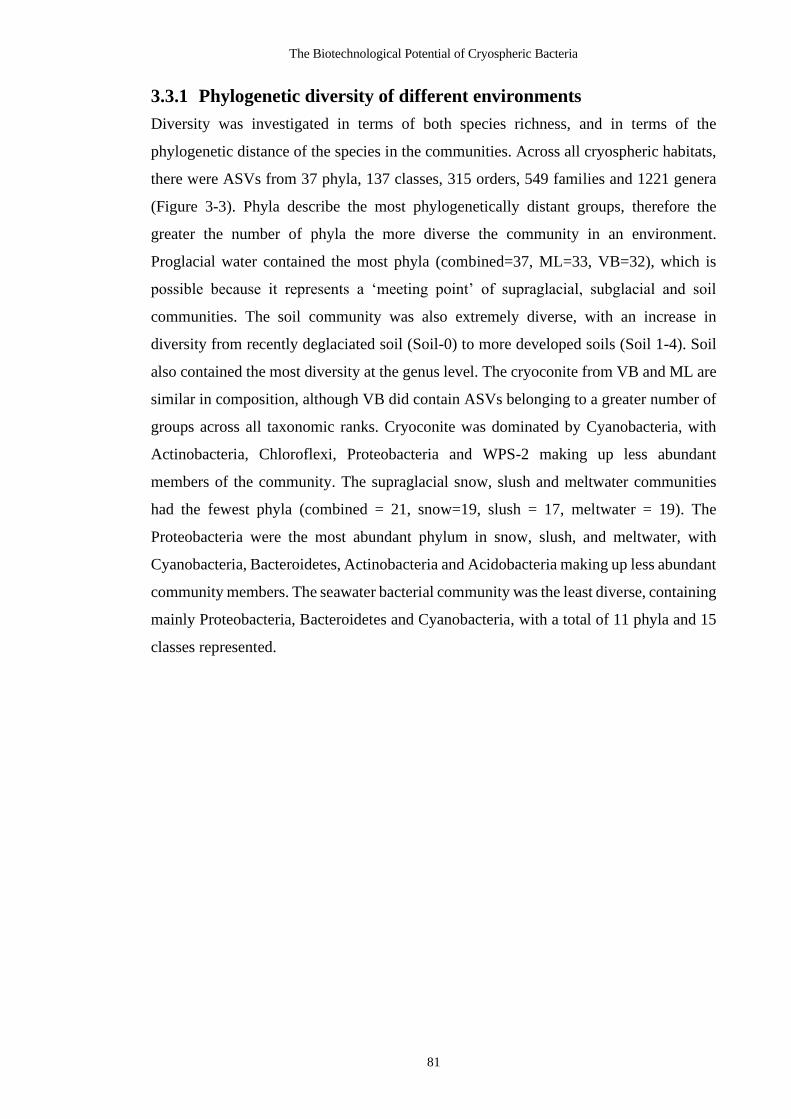
The Biotechnological Potential of Cryospheric Bacteria
81
3.3.1 Phylogenetic diversity of different environments
Diversity was investigated in terms of both species richness, and in terms of the
phylogenetic distance of the species in the communities. Across all cryospheric habitats,
there were ASVs from 37 phyla, 137 classes, 315 orders, 549 families and 1221 genera
(Figure 3-3). Phyla describe the most phylogenetically distant groups, therefore the
greater the number of phyla the more diverse the community in an environment.
Proglacial water contained the most phyla (combined=37, ML=33, VB=32), which is
possible because it represents a ‘meeting point’ of supraglacial, subglacial and soil
communities. The soil community was also extremely diverse, with an increase in
diversity from recently deglaciated soil (Soil-0) to more developed soils (Soil 1-4). Soil
also contained the most diversity at the genus level. The cryoconite from VB and ML are
similar in composition, although VB did contain ASVs belonging to a greater number of
groups across all taxonomic ranks. Cryoconite was dominated by Cyanobacteria, with
Actinobacteria, Chloroflexi, Proteobacteria and WPS-2 making up less abundant
members of the community. The supraglacial snow, slush and meltwater communities
had the fewest phyla (combined = 21, snow=19, slush = 17, meltwater = 19). The
Proteobacteria were the most abundant phylum in snow, slush, and meltwater, with
Cyanobacteria, Bacteroidetes, Actinobacteria and Acidobacteria making up less abundant
community members. The seawater bacterial community was the least diverse, containing
mainly Proteobacteria, Bacteroidetes and Cyanobacteria, with a total of 11 phyla and 15
classes represented.

Chapter 3
82
Figure 3-3 The phylogenetic diversity of different environment types in Svalbard.
A) Bar plot showing the RA of phyla in the different environments. Samples were merged
by environment, and ASVs were agglomerated to Class level and only the top 50 classes
are shown. Colours represent the different phyla. The thin horizontal lines represent
different classes within each phylum. RA does not equal 1, because only the top 50 of
117 classes are plotted. B) Line graph showing the number of phyla, classes, orders,
families, and genera in each environment type. C) Table of phyla, classes, order, families,
and genera across different environments, and also showing the totals for the combined
soil (soil-0, soil-1, soil-2, soil3 and soil4), glacial waters (snow, slush and meltwater), and
the merged proglacial and cryoconite samples from ML and VB.

The Biotechnological Potential of Cryospheric Bacteria
83
3.3.1.1 Alpha Diversity
Alpha diversity (species richness) was determined by counts of the number of observed
species, Shannon Index (H) and Simpson’s Diversity index (D). These measures were
applied to decontaminated, but unfiltered data (ASVs = 58880) (Figure 3-4 A), to data
that had been filtered to remove ASVs not present in at least three samples (ASVs = 3647)
(Figure 3-4 B) and to rarefied data (reads=3483, ASVs=27643, samples = 95) (Figure 3-
4 C).
The use of rarefaction in microbiome analysis is growing increasingly controversial
(McMurdie and Holmes, 2014), and since the focus of this study is on the rare
microbiome, a rarefaction step would almost certainly obscure the very patterns we are
trying to identify (Bay et al., 2020). However, the effect of library size/sampling depth is
a serious confounding factor because large libraries are likely to have more ASVs than
small libraries. In this study, we chose to use the unfiltered dataset because we had already
observed that libraries of the lowest number of reads (Soil) had the highest diversity of
ASVs (Appendix Section C-7). Therefore, skipping the rarefying skip was unlikely to
introduce a confounding factor for species richness, except maybe to underestimate
diversity in soil. The significant drop in number of observed species in the filtered data
reflects the heterogeneity of the environment, particularly evident in soil. Rarefying to
3483 reads resulted in the loss of 18 samples, and 53% of the ASVs.
Diversity indexes were used to understand species richness in these samples, but also to
understand whether sampling depth adequately captured representative diversity.
Simpson's Diversity Index (D) was selected as a diversity measure because it considers
species richness, as well as the RA of each species. As species richness and evenness
increase, so diversity increases. The value of D is close to 1 (representing infinite
diversity) for almost all environment types, except for cryoconite (Cryoconite-ML,
D=0.663 ± 0.043, Cryoconite-VB, D=0.663 ± 0.145) and Meltwater (D=0.881 ± 0.030).
The high D values suggest that sampling depth failed to capture true diversity. The
cryoconite samples on the other hand (except for cryoconite from a specific site on VB)
had D values close to 0.6, due to the dominance of this environment type by a single
species (low evenness).

Chapter 3
84
Figure 3-4 Alpha Diversity of environment groups from Svalbard cryospheric
environments. See details in Table 3-2.

The Biotechnological Potential of Cryospheric Bacteria
85
Table 3-2 Table of alpha diversity measure for different environment groups
Observed Shannon Simpson (D)
X12_group Mean Sd Mean Sd Mean Sd n
Cryoconite-ML 270.33 50.55 2.483 0.153 0.633 0.043 6
Cryoconite-VB 360.58 118.99 2.765 0.960 0.663 0.145 24
Meltwater 142.50 44.85 3.075 0.128 0.881 0.030 8
Proglacial Water-ML
1009.00 NA 6.036 NA 0.992 NA 1
Proglacial Water-VB 651.67 68.09 4.932 0.045 0.969 0.003 3
Sea Water 277.50 34.52 3.990 0.280 0.922 0.029 6
Slush 129.44 35.11 3.181 0.476 0.909 0.037 9
Snow 125.75 59.82 3.580 0.386 0.943 0.020 4
Soil-0 162.00 112.98 3.952 0.712 0.954 0.031 4
Soil-1 720.88 175.00 5.659 0.426 0.990 0.006 8
Soil-2 877.57 346.07 5.725 0.717 0.980 0.025 7
Soil-3 1181.00 272.54 6.481 0.244 0.996 0.001 7
Soil-4 1001.38 328.09 6.037 0.754 0.987 0.016 8
NA: There were only 3 Proglacial Water-ML samples to start with. After rarefying, there were not enough samples to calculate mean and sd.
3.3.1.2 Beta Diversity
Beta diversity refers to the ratio between local or alpha diversity and regional diversity.
This is the diversity of species between two habitats or regions. Similar patterns of beta
diversity were observed using a range of distance measures (Appendix Figure C-23). Beta
diversity is shown using MDS ordination of Bray Curtis distance (Figure 3-5). The
seawater samples cluster closely together in the centre of the plot, having no overlap with
any other environment types and being equally different to all other environment types.
There are three main branches on the plot: cryoconite, soil and a cluster of snow, slush,
and meltwater. Cryoconite almost always forms a tight cluster, whereas soil forms a long
gradient. Most of the snow, slush and meltwater samples cannot be distinguished from
each other and form a cluster together. Habitat type is more important, than glacial origin
for explaining distance, which can be seen in the clustering of proglacial water from VB
and ML clustering together, and cryoconite from VB and VL clustering together.

Chapter 3
86
Figure 3-5 MDS Ordination showing Beta Diversity using Bray Curtis distance.
3.3.2 Community composition by environment
3.3.2.1 Cryoconite
Cryoconite was collected from VB (n=24) and ML (n=6) glaciers. In addition, the
samples from VB were collected from both open (n=6) and closed (n=6) cryoconite holes.
After decontamination, there were 12 478 unique ASVs in cryoconite samples. Technical
replicates (ACVBO3-1 and ACVB03-2) from one of the VB open cryoconite holes
(ACVB03) was particularly abundant in rare taxa. This species richness is not a
consequence of differences in library size (Appendix Figure C-22). To detect large scale
trends in community structure, and identify keystone taxa, the cryoconite samples were
filtered to include on those ASV with more than 20 reads in at least 6 (>20%) or more of
the samples. After filtering, 350 ASVs were retained in the dataset. Filtering out rare taxa
reduced the dataset to just 2.8% of the original ASV diversity, and reduced the mean
library size to 0.949 ± 0.006 for ML and 0.8819004 ± 0.157291348 for VB (Figure 3-6
A). This suggest that about 10% of the cryoconite community consist of rare taxa.
The ASVs in the filtered dataset was agglomerated at the genus level to identify the most
abundant genera (Figure 3-6). The most common genera by far was
Phormidesmis_ANT.L52.6 which had a mean RA of 79.89% across the cryoconite
samples.

The Biotechnological Potential of Cryospheric Bacteria
87
Figure 3-6 Relative abundance of the most abundant taxa in cryoconite samples from Midtre Lovénbreen and Vestre Brøggerbreen. (A)
Proportion of reads remaining after filtering out ASVs with less than (x > 20) in at least 6 samples. (B) Relative abundance of filtered samples by class.
(C) Relative abundance of filtered samples by Genus.

Chapter 3
88
Other abundant genera were Solitalea (1.21%), Salinibacterium (0.93%), Acidiphilium
(0.72%) Tychonema_CCAP_1459-11B (0.59%), Pseudanabaena_PCC-7429 (0.25%)
and Granulicella (0.22%). However, 15.04% of the ASVs were unassigned at the genus
level. At the class level, Ktednobacteria, Actinobacteria, Alphaproteobacteria and
Bacteroidia were common. Finally, the cryoconite keystone taxa was analysed at the
highest resolution by looking at the abundance and prevalence of particular ASVs across
all cryoconite samples (Figure 3-7). There were 64 ASVs in the filtered cryoconite dataset
of 350 ASVs that were present in 90% of samples. (Appendix Table C-12).
Figure 3-7 Scatter plot of the most prevalent and abundant ASVs in cryoconite, by
Order. X-axis is the prevalence of each ASV (number of samples in which each ASV
occurs). Y-axis is log10 of the mean RA of the ASVs across all samples in the cryoconite
dataset. Points are coloured by Order.
A single ASV, (ASV1) was present across all 30 of the samples belonged to the genus
Phormidesmis_ANT.L52.6 at a mean RA of 59.98%. There were two additional
Phormidesmis_ANT.L52.6 ASVs that were present in all samples at a mean RA of more
than 3% (ASV9 (5.142%) and ASV 13 (3.584%)). Other highly prevalent and abundant
ASVs include ASV27 (1.094%), genus Solitalea and ASV40 (0.900) belonging to the
family Microbacteriaceae. We also identified several ASVs that highly abundant
members of the community at a specific site (Appendix Table C-13). Examples include
ASVs from the order Nostocales (ASV319 and ASV539) were detected only in VB
cryoconite, and were not found in ML cryoconite.
3.3.2.2 Glacial waters
Three biological replicates of snow, slush, and meltwater were collected from ML on
three separate days during the summer melt season. After decontamination, there were
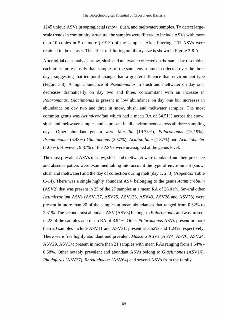
The Biotechnological Potential of Cryospheric Bacteria
89
1245 unique ASVs in supraglacial (snow, slush, and meltwater) samples. To detect large-
scale trends in community structure, the samples were filtered to include ASVs with more
than 10 copies in 5 or more (>19%) of the samples. After filtering, 231 ASVs were
retained in the dataset. The effect of filtering on library size is shown in Figure 3-8 A.
After initial data analysis, snow, slush and meltwater collected on the same day resembled
each other more closely than samples of the same environment collected over the three
days, suggesting that temporal changes had a greater influence than environment type
(Figure 3.8). A high abundance of Pseudomonas in slush and meltwater on day one,
decreases dramatically on day two and three, concomitant with an increase in
Polaromonas. Glaciimonas is present in low abundance on day one but increases in
abundance on day two and three in snow, slush, and meltwater samples. The most
common genus was Actimicrobium which had a mean RA of 34.51% across the snow,
slush and meltwater samples and is present in all environments across all three sampling
days. Other abundant genera were Massilia (19.73%), Polaromonas (13.19%),
Pseudomonas (5.43%) Glaciimonas (2.37%), Acidiphilium (1.87%) and Acinetobacter
(1.63%). However, 9.87% of the ASVs were unassigned at the genus level.
The most prevalent ASVs in snow, slush and meltwater were tabulated and their presence
and absence patters were examined taking into account the type of environment (snow,
slush and meltwater) and the day of collection during melt (day 1, 2, 3) (Appendix Table
C-14). There was a single highly abundant ASV belonging to the genus Actimicrobium
(ASV2) that was present in 25 of the 27 samples at a mean RA of 26.01%. Several other
Actimicrobium ASVs (ASV137, ASV25, ASV133, ASV49, ASV28 and ASV73) were
present in more than 20 of the samples at mean abundances that ranged from 0.32% to
2.31%. The second most abundant ASV (ASV3) belongs to Polaromonas and was present
in 23 of the samples at a mean RA of 8.94%. Other Polaromonas ASVs present in more
than 20 samples include ASV11 and ASV31, present at 3.52% and 1.24% respectively.
There were five highly abundant and prevalent Massilia ASVs (ASV4, ASV6, ASV24,
ASV29, ASV34) present in more than 21 samples with mean RAs ranging from 1.64% -
8.58%. Other notably prevalent and abundant ASVs belong to Glaciimonas (ASV16),
Rhodoferax (ASV37), Rhodanbacter (ASV64) and several ASVs from the family

Chapter 3
90
Figure 3-8 Relative abundance of the most abundant taxa in snow, slush and meltwater samples from Midtre Lovénbreen (A) Proportion of reads
remaining after filtering out ASVs without at least 10 reads in 5 or more samples. (B) Boxplot of number of reads in included libraries. (C) Relative
abundance of filtered samples by Genus.

The Biotechnological Potential of Cryospheric Bacteria
91
Burkholderiaceae (ASV21, ASV41). ASV7, belonging to the order Chloroplast was present at 3.65%
in 20 of the samples, and is likely an algae species. Of note, there is a Burkholderiaceae ASV (ASV159)
that is present in just 1/9 of the snow samples, but in 9/9 and 6/9 of the slush and meltwater samples,
respectively.
Figure 3-9 Scatter plot of the most prevalent and abundant ASVs in supraglacial habitats) snow,
slush and meltwater, by Genus. X-axis is the prevalence of each ASV (number of samples in which
each ASV occurs). Y-axis is log10 of the mean relative abundance of the ASVs across all samples in
the glacial water (snow, slush, meltwater) dataset. Points are coloured by Genus.
3.3.2.3 Proglacial water
Proglacial water was collected from both ML on day two of the snow, slush, meltwater collection
(n=3) and from VB (n=3). After decontamination, there were 5224 ASVs remaining in the proglacial
samples. The libraries from samples collected from VB were significantly larger than those collected
from ML. Both PM2 and PM3 were less than 1000 sequences before filtering. Therefore the number
of reads required in each library was reduced to a minumum of 4 reads in two or more libraries. After
filtering the dataset to include only ASVs with four or more copies in two or more samples, there were
945 ASVs remaing in the dataset. The effect of filtering on library size was much more significant in
the ML samples than in the VB samples.
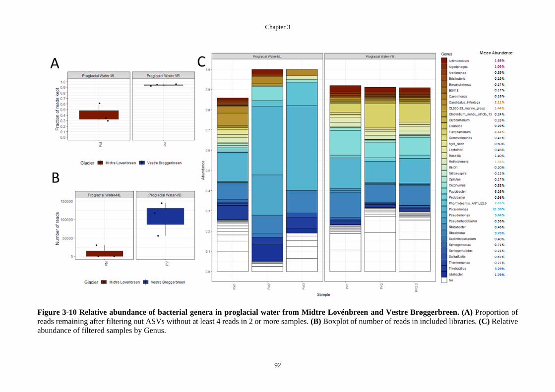
Chapter 3
92
Figure 3-10 Relative abundance of bacterial genera in proglacial water from Midtre Lovénbreen and Vestre Brøggerbreen. (A) Proportion of
reads remaining after filtering out ASVs without at least 4 reads in 2 or more samples. (B) Boxplot of number of reads in included libraries. (C) Relative
abundance of filtered samples by Genus.

The Biotechnological Potential of Cryospheric Bacteria
93
Figure 3-11 Scatter plot of the most prevalent and abundant ASVs in proglacial water by
Family. X-axis is the prevalence of each ASV (number of samples in which each ASV occurs). Y-
axis is log10 of the mean relative abundance of the ASVs across all samples in proglacial water.
Points are coloured by Family.
In the proglacial samples, there is evidence of ASV sharing between environments. The highly
abundant Polaromonas ASV (ASV11) from snow, slush and meltwater is the most abundant ASV
in proglacial water, occurring in all six samples at a mean RA of 9.29% (Appendix Table C-15).
Five of the proglacial water samples also contained the Phormidesmis_ANT.L52.6 ASV (ASV1) at
a mean RA of 2.33%. In addition, there were several highly prevalent ASVs belonging to the genus
Candidatus_Nitrotoga (ASV219, ASV395, ASV1026) and Thiobacillus (ASV26, ASV2425) that
hint at a subglacial community input. There were also some site-specific ASVs that occurred in
high abundance at a specific site. Although ML had smaller library sizes than VB, there we several
ASVs at relatively high abundance in ML samples only, such as Pseudomonas (ASV17, 10.31%),
Ulvibacter (ASV86, 5.38%) and Sediminibacterium (ASV5130, 1.05%) (Appendix Table C-16).
3.3.2.4 Soil
After decontamination, there were 40045 ASVs remaining in the forefield soil samples. This
enormous species richness is despite relatively small library sizes compared to other environment
types (Appendix Figure C-22 and Figure 3-4). To detect large-scale trends in community structure,
the samples were filtered to include ASVs with more than 10 reads in three or more of the samples.
After filtering, only 1281 ASVs were retained in the dataset.

Chapter 3
94
Figure 3-12 Relative abundance of genera in glacier forefield soil samples. (A) Proportion of reads remaining after filtering out ASVs without at
least 10 reads in 3 or more samples. (B) Boxplot of number of reads in included libraries. (C) Relative Abundance of filtered samples by Genus.

The Biotechnological Potential of Cryospheric Bacteria
95
The dramatic effect of filtering on library size is shown in Figure 3-8 A. With three replicates
from each site, the loss of such a large proportion of ASVs and reads from each library suggest
enormous heterogeneity, not only between glacial forefield sites, but even replicates from the
same site). The heterogeneity of soil samples in the glacial forefield is further illustrated by
plotting the prevalence and abundance of ASVs in the dataset (Figure 3-13).
The most abundant genus was the Oryzihumus from the Actinobacteria, with a mean RA of
15.36%, which was more abundant in developed soils (Soil -2, -3, -4). The second most
abundant genus was the Sphingomonas (5.22 %), present to some degree across all time points.
The four genera Thiobacillus (5.08%), Arenimonas (2.00%), Candidatus_Nitrotoga (2.61%)
and Sulfuricurvum (2.71%) were present mainly in the recently deglaciated Soil-0. There was a
large proportion of ASVs that could not be resolved to genus level.
Figure 3-13 Scatter plot of the most prevalent and abundant ASVs in glacial forefield soil
(n=45), by order. X-axis is the prevalence of each ASV (number of samples in which each ASV
occurs) The axis is shortened from 45 to 35, and there were 0 ASVs present in all 45 samples.
Y-axis is log10 of the mean relative abundance of the ASVs across all samples. Points are
coloured by Order.
The most prevalent ASVs in the soil samples, by time point and by transect, are tabulated in
Appendix Table C-17 and the most abundant ASVs in Appendix Table C-18. From a total of 45
samples and 40 045 ASVs, there were only five ASVs present in 30 or more of the samples. A
Sphingomonas ASV (ASV69) was present in 35 of the samples at a mean RA of 1.58%, and two
more Sphingomonas ASVs (ASV76 and ASV152) were present in 30 of the samples at a mean
RA of 1.92% and 0.68% respectively. The other ASVs in more than 30 of the samples were

Chapter 3
96
Oryzihumus ASVs (ASV48 and ASV114) from the family Micrococcales, which were present
at a mean RA of 7.99% and 1.94%, respectively. Of the remaining 26 ASVs present in more
than 20 of the samples, there were an additional three Oryzihumus ASVs (ASV150, ASV83 and
ASV334), three Sphingomonas ASVs (ASV340, ASV301, ASV460). The remainder were from
family Rhizobiales (ASV135, ASV154, ASV45), Frankiales (ASV157, ASV257),
Propionibacteriales (ASV101, ASV129, ASV411, ASV363), Betaproteobacteriales (ASV1359,
ASV229, ASV403, ASV65, ASV45).
To further investigate soil heterogeneity across the forefield, the ASVs that were prevalent at a
single site were examined (Appendix Table C-19). This was done by looking for ASVs that
occurred in all three replicates of a single site, and not in any other samples. Site specific ASVs
were identified at 6 of 15 sample sites: F1T1 (5), F2T1 (13), F1T2 (1), F1T3 (3), F2T3 (1), and
F3T4 (2). Many of the taxa that appeared ‘unique to one site’ came from the site F2T1. The
libraries from this site were much larger in size than the libraries from different sites. This
suggests that perhaps the presence of these ASVs in all three replicates are a result of greater
sampling depth at this site. Site-specific ASVs were occasionally abundant community members
at those sites. For example, ASV39, belonging to genus Ellin6067, which was present at a mean
RA of 4.371% at F2T2, an Oryzihumus ASV (ASV393) was present at a mean RA of 2.11% at
site F1T2, and two ASVs from the order Chloroplast (ASV797, ASV976), which may be algal
species, were present at 2.96% and 2.53% ate sites F2T3 and F3T4 respectively.
It is unclear whether the clay samples collected from the glacier snout are low in diversity or
whether the low diversity reflects the difficulty inherent in extracting DNA from clay soils,
which adsorb DNA. Interestingly the library sizes, made from extraction replicates from each
site are similar in size, despite each replicate being extracted in different batches on different
days.

The Biotechnological Potential of Cryospheric Bacteria
97
Figure 3-14 Relative abundance of bacterial families in sea water samples collected from 1m and 15m depth from the Kongsfjorden, in front of
ML. (A) Proportion of reads remaining after filtering out ASVs without at least 10 reads in 2 or more samples. (B) Boxplot of number of reads in included
libraries. (C) Relative Abundance of filtered samples by Genus.
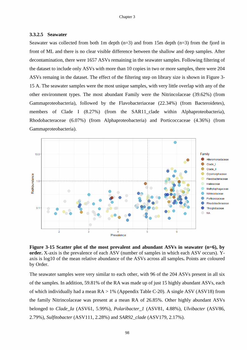
Chapter 3
98
3.3.2.5 Seawater
Seawater was collected from both 1m depth (n=3) and from 15m depth (n=3) from the fjord in
front of ML and there is no clear visible difference between the shallow and deep samples. After
decontamination, there were 1657 ASVs remaining in the seawater samples. Following filtering of
the dataset to include only ASVs with more than 10 copies in two or more samples, there were 204
ASVs remaing in the dataset. The effect of the filtering step on library size is shown in Figure 3-
15 A. The seawater samples were the most unique samples, with very little overlap with any of the
other environment types. The most abundant Family were the Nitrincolaceae (39.62%) (from
Gammaproteobacteria), followed by the Flavobacteriaceae (22.34%) (from Bacteroidetes),
members of Clade I (8.27%) (from the SAR11_clade within Alphaproteobacteria),
Rhodobacteraceae (6.07%) (from Alphaproteobacteria) and Porticoccaceae (4.36%) (from
Gammaproteobacteria).
Figure 3-15 Scatter plot of the most prevalent and abundant ASVs in seawater (n=6), by
order. X-axis is the prevalence of each ASV (number of samples in which each ASV occurs). Y-
axis is log10 of the mean relative abundance of the ASVs across all samples. Points are coloured
by Order.
The seawater samples were very similar to each other, with 96 of the 204 ASVs present in all six
of the samples. In addition, 59.81% of the RA was made up of just 15 highly abundant ASVs, each
of which individually had a mean RA > 1% (Appendix Table C-20). A single ASV (ASV18) from
the family Nitrincolaceae was present at a mean RA of 26.85%. Other highly abundant ASVs
belonged to Clade_Ia (ASV61, 5.99%), Polaribacter_1 (ASV81, 4.88%), Ulvibacter (ASV86,
2.79%), Sulfitobacter (ASV111, 2.28%) and SAR92_clade (ASV179, 2.17%).

The Biotechnological Potential of Cryospheric Bacteria
99
There was an apparent trend with ASV88 and ASV126, both of which were of the order
Chloroplast, were present at a higher RA in shallow samples than in deep samples, likely due to
the greater penetration of sunlight at 1m vs 15m depth. The opposite was true of ASV81 and
ASV287 belonging to the genus Polaribacter_1, which were present at a higher RA in deep
samples vs shallow samples. There were eight ASVs present in of the shallow samples and none
of the deep samples, and one ASV present only in the deep samples (Appendix Table C-21).
Considering the smaller library sizes of deep-sea samples, the presence of ASV 5401 (f_
Nitrincolaceae) in deep sea libraries only suggests that this may be a specialist species with a
narrow tolerance for depth/pressure or sunlight or a correlated environmental pressure.
3.3.3 Comparison/ Relationship between environments
3.3.3.1 Unique taxa and shared taxa between environments
UpsetR was used to show the number of ASVs that are unique to each environment or shared
between environment types (Figure 3-17). The plot is based on a filtered dataset (ASVs = 3958) in
which ASVs with ≧ 5 copies in at least two samples are included. The requirement for ASVs to
occur in at least two samples will result in an underestimation of unique ASVs in heterogenous and
complex environments but gives better resolution for understanding shared ASVs. This filtering
step results in a proportionally larger decrease in soil library size compared to cryoconite for
example (Figure 3-16).

Chapter 3
100
Figure 3-16 Bar plot showing effect of filtering on library size. The removal of ASVs without
≧ 5 copies in at least two samples resulted in a reduction in library size across the different samples.
Environments with high heterogeneity and greater diversity (like soil) suffered the greatest
reduction in size.
The UpsetR plot shows how several ASVs are shared between environments that are adjacent
and/or similar (Figure 3-17). Even though they are physically distant, the largest set is intersection
of the cryoconite from VB and ML (n=539). Several sets describe direct flow from one habitat to
another, such as the 52 ASVs shared only between VB cryoconite and VB proglacial water, and 23
shared ASVs between proglacial water from ML and Soil-0 from the ML forefield (near the glacier
snout). From this plot, large intersections occur between adjacent environments such as the
supraglacial habitats of snow, slush and meltwater (65 ASVs), some of which also flow into ML
proglacial water (23), or chronological soil sites (soil 1,2,3,4 (169), Soil 2,3,4 (151), Soil-3,4 (148)
or soil-1,2 (111)), or from snow, slush, meltwater and cryoconite (14 ASVs). Of note is also a
number of sets of ASVs that occur in a single site. They are important because they represent ASVs
that are prevalent within a single site (and therefore part of this dataset), but not between sites.
Therefore, although they are not rare taxa, they likely represent specialists. Examples include the
248 ASVs unique to Soil-0 and 127 ASVs unique to VB proglacial water and 319 ASVs present
only in cryoconite from VB. Seawater is the only environment type that shares 0 ASVs with any
other environment.

The Biotechnological Potential of Cryospheric Bacteria
101
Figure 3-17 UpSetR Diagram showing number of unique and shared ASVs between different environments. Each environment group is a set
(Barplot A). The number of ASVs in each set and intersection of sets are shown in Barplot B above the matrix. The black circles indicate the
environments sharing ASVs. Sets are arranged in an environmental gradient and reflect proximity between environments. Only intersections involving
13 or more ASVs are shown.

Chapter 3
102
3.3.3.2 Network analysis between samples
For network analysis, samples with n < 100 reads after decontamination were removed, leaving a
dataset of 108 samples containing 58870 ASVs. The data was then filtered to contain only taxa that
had >15 reads in three or more samples (ASVs = 2431).
Figure 3-18 Network analysis of samples based on Bray-Curtis distances. Network created using
a maximum distance threshold of 0.7 for connecting vertices with an edge. The network layout method
is Fruchterman Reingold. The colour of groups is based on environment subgroup, shape is based on
glacier of origin and points are labelled.
Samples clearly cluster based on environment type, with environment type playing a more prominent
role than proximity. The proglacial water samples from VB are more like proglacial water from ML
than they are to cryoconite collected from VB. The snow, slush and meltwater samples form a cluster,
with a potential gradient (light-coloured samples from day 1 tend to cluster closely regardless of
environment type). The cryoconite samples are similar and tightly clustered, whereas the soil samples
are more distributed.
3.3.3.3 Network analysis between taxa
The decontaminated dataset (ASVs = 58 880) was filtered to include only ASVs with more than 40
reads in six or more samples (ASVs = 526). A co-occurrence network described the probability of taxa
being found together. There are four main clusters detected, (modularity = 0.592), which correspond
roughly to sea, cryoconite, soil, and glacial surface communities.

The Biotechnological Potential of Cryospheric Bacteria
103
Figure 3-19 Co-occurrence network of ASVs in Svalbard. The decontaminated dataset (ASVs = 58 880) was filtered to include only ASVs with more than 40 reads
in six or more samples (ASVs = 526). A correlation analysis was run based on Spearman's co-efficient, with a correlation coefficient cut-off of 0.5 and P-value cut-
off of 0.05. Network visualisation performed in Gephi, layout is Fruchterman Reingold. Node colour refers to Phylum membership, Size of node reflects Degree, and
edge colour shows weight. There are four clusters main clusters detected, (modularity = 0.592), which correspond roughly to sea, cryoconite, soil, and glacial surface
communities.

Chapter 3
104
3.4 Discussion
In this study, the taxonomic profiles of several environment habitats of a glacial system in Ny
Ålesund, Svalbard were investigated, with a focus on identifying specialist members of Arctic
microbial communities. Specialists are adapted to an extremely narrow environmental niche and
are therefore spatially constrained and most threatened by the consequences of global climate
change. The use of ASVs was preferred over the use of OTUs (Callahan et al., 2017), as this precise
level of resolution improves the ability to detect community members unique to specific
environmental niches, regardless of close relatedness to species in nearby environments.
3.4.1 The Decontam tool was able to successfully remove contaminants
Two common methods used to remove contaminants from 16S rRNA amplicon datasets are i) the
removal of all sequences present in control samples and ii) the removal of very rare taxa that fall
below a certain threshold. Both methods have their drawbacks; in the first case, removal of all
ASVs that occur in negative controls can inadvertently remove legitimate environmental ASVs that
are also present in the kitome due to similar conditions. In addition, one of the most likely sources
of contaminants in negative controls is cross-contamination from environmental samples: the
ASVs most likely to contaminate negative controls are the most abundant ASVs in the high biomass
environmental samples. The second strategy of removing rare taxa is also flawed as it skews
downstream analyses of species richness, particularly in microbially diverse and heterogenous
samples. Since specialist species are likely to be rare and low-abundance members of a community,
some effort was spent on decontaminating the dataset to preserve the rare microbiome. In this study,
the Decontam tool was able to remove most sequences from control samples, whilst having
minimal effect on environmental samples (Appendix Figure C-21). As expected, the low
abundance samples (snow and clay soil from the glacier snout) were most effected by
decontamination, likely due to legitimately high levels of contamination in samples with low
starting concentrations.
3.4.2 There is a continuum between the snowpack, slush, meltwater, and proglacial
water.
Using a variety of methods, the supraglacial environments of snow, slush and meltwater were
similar in community structure (Figure 3-17, Figure 3-18, Figure 3-19). An UpsetR plot (Figure
3-17) showed that there are more shared ASVs between snow, slush and meltwater (n=65) than
there are sets of ASVs unique to any of those environment types. However, multivariate analysis

The Biotechnological Potential of Cryospheric Bacteria
105
of variance revealed that differences in community structure between environments was still
significant, and explained up to 16.5% of the variation (Adonis, F.model = 1.9819, R2= 0.16541,
Pr(>F) 0.0161). There was no significant difference between the bacterial diversity of snow, slush
and meltwater samples collected on the same day. However, there was a small change in
community composition due to time. Using Adonis to perform multivariate analysis of variance,
there were significant differences in environmental communities due to sampling date (Date of
collection, F.model= 2.6792, R2 = 0.21131, Pr(>F) =0.0014). In fact, time explained more of the
variance than environment type, which is similar to previous studies of supraglacial habitat
communities (Hell et al., 2013).
A microbial community associated with snow environments is increasingly recognized (Carpenter
et al., 2000; Amato et al., 2007; Xiang et al., 2009a; Larose et al., 2010; Chuvochina et al., 2011;
Harding et al., 2011). Snow bacterial abundance in Svalbard ranges between 2 x 10⁴ cells·ml-1 in
the accummulation snow layer of glaciers, 6 x 10⁴ cells mL−1 in seasonal snow bordering the sea,
and 2 x 10⁵ cells mL−1 in the summer layer, where higher temperatures enables rapid mutiplication
(Amato et al., 2007). Previous studies of snow show the presence of Alphaproteobacteria,
Betaproteobacteria and Gammaproteobacteria, Firmicutes and Actinobacteria (Amato et al.,
2007), with one genus, Polaromonas, showing a particularly high abundance (Hell et al., 2013).
Although the bacterial communities of surface snow, snow, slush and near-surface ice are distinct,
they have a significant capacity for rapid change in response to changing environmental conditions
(Hell et al., 2013). This study corroborates these findings, with members of Actimicrobium,
Polaromonas, Glaciimonas and Massilia making up a core community of abundant and prevalent
ASVs in snow, slush, and meltwater (Appendix Table C-14, Figure 3-8). Massilia was previously
found to be specific to glacial snow, and is thus highlighted as a vulnerable species due to glacier
and snowpack loss induced by climate change (Zhang et al., 2015). The most abundant genus and
ASV was Actimicrobium (ASV1), which has previously been found in a glacial snowpack
(Terashima et al., 2017). Interestingly, there is only one characterised species of Actimocrobium,
Actimicrobium antarcticum, discovered in Antarctic sea water in 2011 (Kim et al., 2011). The
presence of this genus in such high abundance, and the number of ASVs related to this genus
suggest an opportunity to investigate the possibility of new species of this genus. The high
abundance of chloroplast sequences is potentially derived from green algae in the snow.

Chapter 3
106
3.4.3 Proglacial water is an intersection of multiple environment inputs
Proglacial water is expected to be an amalgam of subsurface, surface and forefield communities,
and was the most biodiverse habitat type in the dataset, with the greatest number of phyla (Figure
3-3). In the UpSetR plot, the proglacial water from ML was more like forefield samples (65 ASVs),
and the proglacial water from VB was more like the glacial surface communities. Strikingly, the
proglacial water from ML most resembled the proglacial water from VB, which is agreement with
several other sources that identify a similar microbial communities in subglacial environments
globally (Dubnick et al., 2017). Phylotypes unique to the subglacial outflow samples were
dominated by bacteria in the phyla Bacteroidetes, Actinobacteria, Firmicutes, Acidobacteria and
Proteobacteria (Dubnick et al., 2017).
3.4.4 Soil is extremely heterogenous
The glacial forefield soil was extremely heterogenous, but there is evidence of gradients affecting
species composition. The number of singleton ASVs in soil shows that it is potentially both a
heterogeneous and under-sampled environment (Figure 3-4, Figure 3-12, Appendix Figure C-22).
In addition, ASVs present at high abundance, but only in specific sites (Appendix Table C-19),
suggest that sampling deeply (i.e. large library sizes at a single site) and widely (lots of different
sites across the forefield) would be necessary to accurately describe microbial communities. Early-
stage glacial soil sampled from the ML glacier snout was extremely different to soil at all other
time points (Figure 3-12 and Appendix Table C-17). The forefields of glaciers often show signs of
succession, with soils closer to the glacier snout having lower biodiversity and little plant life, and
later successional stage soils have significantly more biodiversity and plant life. The co-occurrence
network Figure 3-19 shows that the soil co-occurrence network has two ‘arms’, possibly related to
soil development and the presence of plants. Although the microbial communities that dominate in
Arctic soils can be influenced by a variety of factors, including the local geology, the presence or
absence of seasonal or permanent permafrost and their location in relation to glaciers; pH and
vegetation of soils has been shown to have the greatest influence on biodiversity (Malard and
Pearce, 2018). A recent study of the biogeography of Arctic sites which took into account 200
independent Arctic soil samples from 43 sites, found that of the 48 147 bacterial taxa, a core
microbiome composed of only 13 taxa that were ubiquitously distributed and present within 95%
of samples was identified (Malard et al., 2019). Together, the high heterogeneity across the ML
forefield in this study, and the vast heterogeneity across multiple Arctic sites suggests high levels
of endemism in Arctic soils. A review of Arctic soils found that Proteobacteria and, specifically,
Nitrogen-fixing Rhizobiales (Alphaproteobacteria), Burkholderiales (Betaproteobacteria),

The Biotechnological Potential of Cryospheric Bacteria
107
Xanthomonadales (Gamma-proteobacteria) and Myxococcales (Deltaproteobacteria) dominated
Arctic soil bacterial communities. The dominant phyla in the ML forefield belonged to the
Proteobacteria, Cyanobacteria, Actinobacteria, Acidobacteria, Bacteroidetes and
Gemmatimonadetes. Specific genera included Oryzihumus, Sphingomonas, Thiobacillus,
Arenimonas, Candidatus_Nitrotoga and Sulfuricurvum.
3.4.5 Seawater does not share ASVs with other environments
Seawater has various gradients, such as temperature, pressure, oxygen saturation and light
penetration which can all affect bacterial community structure. A study of free-living and particle-
associated bacterial communities and their spatial variation in Kongsfjorden, found that all samples
were dominated by Proteobacteria, followed by Bacteroidetes, Firmicutes and Actinobacteria (Jain
and Krishnan, 2017) and Fjord water near Ny Ålesund as found to contain predominantly
Alphaproteobacteria, Gammaproteobacteria, Bacteroidetes, Firmicutes and Parcubacteria, as well
as Gemmatimonadetes, Nitrospirae, Acidobacteria and Chloroflexi (Conte et al., 2018). The high
prevalence of Nitrincolaceae (39.62%) (from Gammaproteobacteria), followed by the
Flavobacteriaceae (22.34%) (from Bacteroidetes), members of Clade I (8.27%) (from the
SAR11_clade within Alphaproteobacteria), Rhodobacteraceae (6.07%) (from
Alphaproteobacteria) and Porticoccaceae (4.36%) (from Gammaproteobacteria) is similar to the
community structure described in the fjord waters near the VB glacier snout (Thomas et al., 2020).
There was absolutely no evidence that ASVs from the glacier or forefield were present in seawater
(Figure 3-17, Figure 3-19). However, this may differ in glacial ecosystems that end in marine
outlets.
3.4.6 Cryoconite communities on VB and ML are similar
Cryoconite is a dark, granular sediment comprising biotic (organic) and abiotic (inorganic) material
that commonly discolours the surface of glacial ice (J. Cook et al., 2016; Hodson et al., 2008).
Previous studies have shown that there are both inter-regional (Cameron et al., 2012a) and
interglacial (Edwards et al., 2011) differences in cryoconite bacterial communities. Proteobacteria
and Cyanobacteria are consistently the most abundant phyla detected in cryoconite (Edwards et al.,
2011) (Cameron et al., 2012a; Edwards et al., 2014; Gokul et al., 2016). Cryoconite bacterial
communities from the nearby Foxfanna glacier are strongly dominated by a small number of core
taxa, include representatives of Actinobacteria, Cyanobacteria, Proteobacteria, Bacteroidetes,
Chloroflexi and Gemmatimonadetes which are both ubiquitous and abundant (Gokul et al., 2016).
Notably, an OTU belonging to the filamentous cyanobacterial genus Leptolyngbya was present at

Chapter 3
108
all of the sites at a mean RA four times greater than the next most dominant OTUs, which
corroborates the hypothesis that filamentous bacteria are important ecosystem engineers, and play
a vital role in the formation of granules. In this study, we found the same, a single ASV (ASV1)
was found in all the cryoconite samples at mean RA of 59.98%, and a core microbiome of bacteria
common to all cryoconite sites included in the study could be identified (Appendix Table C-12).
The dominance of the habitat type by a single ASV resulted in a lower Simpson index compared
to the other environments (Table 3-2). The cryoconite communities of ML and VB were more
similar to each other (UpsetR, 539 ASVs) than supraglacial, meltwater and glacial forefield
samples upstream and downstream respectively (Figure 3-17). This suggests that the cryoconite
community is a unique supraglacial habitat type, and corroborates previous studies showing that
the bacterial communities of cryoconite are distinct and differ compared to nearby ice-marginal
habitats (Edwards et al., 2013b). Although robust and diverse, it does not spread easily beyond the
supraglacial environment.
3.4.7 High bioprospecting potential due to rare and specialist taxa
It has been suggested that the cryospheric biome is attractive for bioprospecting because it is
extreme, difficult to access and therefore relatively unexplored and under threat from global
warming. In this chapter, the enormous breadth of diversity in this glacial environment has been
highlighted (Figure 3-3). The rare microbiome is enormous, with a significant proportion of
communities being composed of rare taxa endemic to specific environments or even specific sites.
As a result, sampling depth was inadequate to describe the community completely (Figure 3-4,
Figure 3-16, Appendix Figure C-22). This biodiversity is hypothesized to translate to novelty
because even in communities that are functionally similar, a greater number of species represents
more biological variations in the enzymes and pathways that undertake those functions. Therefore,
the more species, the more potential for biological novelty and unique biotechnological tools. In
addition, analysis revealed that many of these environments are unique, where ‘uniqueness’ in this
case is determined by how many bacterial species occur exclusively in that environment and not in
any others. By filtering out ASVs that occur at only a single site, it was shown that soil is extremely
heterogenous, with many ASVs that are not shared even between samples extracted from the same
site (Figure 3-16). Cryoconite was remarkable for how many ASVs were shared between different
sites on the same and different glaciers; nonetheless it did not share ASVs with adjacent
environments (Figure 3-6, Figure 3-17, Figure 3-19, Appendix Table C-12). In terms of
bioprospecting, environments that share many species represent redundancy and duplication of
sampling effort. There are several environments in this study that are especially attractive because

The Biotechnological Potential of Cryospheric Bacteria
109
they occur only in and around glaciers. Examples include cryoconite and recently exposed
deglaciated soils (Soil-0). Bacterial adaptation to new environmental conditions is also much
slower in the cryosphere, because of longer generation times at lower temperatures.
3.4.8 Recommendations
This study attempted to increase the resolution at which the biogeography of glacial environmental
habitats in Svalbard was analysed, but using ASVs rather than OTUs, and preserving the rare taxa
in the analysis. However, there are several ways in which the data could be improved in future
investigations. Firstly, the library size distribution in this study was quite varied (Appendix Figure
C-10). There are two ways to decrease variance in library size- the first is using Illumina indexed
adapters attached to PCR primers, which removes the need for a second-stage PCR entirely, and
ensures that DNA concentration calculations are only measuring indexed reads. It also has the
added benefit of decreasing opportunities for contamination because if the index is added in the
first PCR, the cross-contamination of wells during further steps and processing has no bearing on
the library membership of the amplicon. A second approach is a qPCR of the indexes to determine
index concentrations prior to pooling. A qPCR of indexes, rather than amplicons, will prevent the
overestimation of library size based on a high DNA concentration library that contains unindexed
amplicons. Secondly, the calculation of absolute abundance measures, can help in data preparation,
sequencing, and results interpretation. Finally, the sequencing technology can be improved- the use
of Nanopore to sequence the entire 16S rRNA operon will allow even better identification of unique
ASVs and will also allow a more rapid sampling.
3.5 Conclusions
The extent to which glacial habitat types, and the communities therein, may change because of
global climate change is currently a matter of intense research and great concern (Cauvy-Fraunié
and Dangles, 2019; Stibal et al., 2020). This study reveals an extensive rare microbiome consisting
of highly specialist bacterial communities that have a narrow ecological niche. In addition, some
dominant and abundant community members, such as the communities that colonise cryoconite,
are widespread across different glaciers, but do not spread easily to adjacent habitats. The
implication of this is that glacial communities do not survive outside of glacial conditions, and that
glacier loss means the irrevocable loss of these community members. This is additional evidence
that changes wrought by climate change may have enormous, unknowable, and potentially
irreversible changes on community structure. There may well be a bacterial extinction event
decimating rare species of bacteria that are delimited to extremely narrow environmental windows.

Chapter 4
110
4 METAGENOME ASSEMBLED
GENOMES FROM SVALBARD
CRYOCONITE, SOIL, AND
SEAWATER ARE
PHYLOGENETICALLY AND
FUNCTIONALLY DIVERSE
4.1 Introduction
The cryosphere has been identified as a region with exceptional bioprospecting potential because
it is considered an extreme environment (Cavicchioli et al., 2002; Santiago et al., 2016; Vester et
al., 2015), it is relatively unexplored, and it is under threat from global climate change (Graham et
al., 2017; Graversen et al., 2008). Svalbard is located 74° - 81° N and 10° - 35° E and experiences
extreme cold, as well as continuous summer light and winter dark due to its far North latitude.
These unique environmental stressors increase the likelihood of novel species and natural products.
Numerous studies have attempted to describe the community profiles of various cryospheric
habitats using amplicon sequencing of the 16S rRNA gene (Chapter 3) (Anesio et al., 2017).
However, amplicon-based studies have numerous pitfalls, including amplification bias, the fact that
bacterial, fungal, archaeal, and algal communities need to be sequenced separately, and the failure
of primers to amplify divergent 16S rRNA sequences, such as those present in much of the
candidate phyla radiation (CPR) (Brown et al., 2015). Perhaps most importantly, phylotypes are
unable to provide reliable functional predictions that would help tell us the putative metabolic
potential of the microbial community (Edwards et al., 2020). MAGs are reconstructed genomes
that inevitably represent the most abundant members of a community, because they are constructed
from the longest contigs with the deepest coverage, proportional to their abundance in the original
sample. The MAGs allow the identification of novel species that are unique to the environment,

The Biotechnological Potential of Cryospheric Bacteria
111
can then be mined in same was as traditional genomes for genes and genomes clusters that
synthesise useful and novel secondary metabolite clusters.
This thesis suggests that resolving metagenomes from these environments in a vital step that
provides insight into the ecology of the region and establishes a foundation on which strategic
bioprospecting can be based. There are several advantages of genome-centric metagenomics.
Firstly, genome-level resolution and classification provides information about novel species and
their phylogenetic relationships to known species (Parks et al., 2018). Secondly, mapping reads
back to contigs (and MAGs) can be used to estimate the abundance of the species of interest across
several sites. This is useful in its own right for providing ecological insights but is also a useful
tool as to prioritise locations when a specific target is identified. Finally, functional information,
provided by the annotation of metabolic functions and biogeochemical pathways, and co-
occurrence at various sites, allows inferences to be made about symbiotic relationships which in
turn can inform decision making about co-culturing.
To date, there have been numerous attempts to reconstruct genomes from rare environments in
order to gain insights into phylogenetic diversity (Vavourakis et al., 2016), biogeochemical cycling
potential (Anantharaman et al., 2016; Linz et al., 2018; Yaxin Xue et al., 2020), contaminant
degradation potential (Hauptmann et al., 2017) and even secondary metabolites with antimicrobial
potential (Cuadrat et al., 2018). The Arctic is still underexplored, but it has not been neglected.
MAGs have been reconstructed from Greenland cryoconite (Hauptmann et al., 2017), Svalbard
permafrost (Yaxin Xue et al., 2020) and Canadian glacier metagenomes (Trivedi et al., 2020). For
example, 29 MAGS were identified from 34 cryoconite samples collected from five different
locations around Greenland (Hauptmann et al., 2017). These genomes showed potential resistance
to and degradation of contaminants such as polychlorinated biphenyls (PCB), polycyclic aromatic
hydrocarbons (PAHs), and the heavy metals mercury and lead. In addition, the presence of the
resistance and degradation genes was spatially variable, which the authors hypothesized may
indicate local contamination at specific sites.
Cyanobacteria are important ecosystem engineers in cryoconite on the glacial surface (Gokul et al.,
2016; Hodson et al., 2010a) and in the development of soils in glacial forefield (Pushkareva et al.,
2015). Indeed, Phormidesmis Priestleyi is the major species present in cryoconite from Midtre
Lovénbreen and Austre Brøggerbreen (Takeuchi et al., 2019), Foxfanna in Svalbard (Gokul et al.,
2016), and is also found in cryoconite in Greenland (Chrismas et al., 2016b) and elsewhere (Segawa
et al., 2017). Although the single cultured isolate resembling the Phormidesmis Priestleyi in
Svalbard was isolated in Greenland (Chrismas et al., 2016a), this specific Cyanobacterial MAG
Chapter 4
112
was notably missing from the Greenland cryoconite metagenome, which had Nostoc as its only
cyanobacterial bin (Hauptmann et al., 2017). Several closely related bacteria has been sequenced
from non-axenic cultures from several sub-polar habitats (Cornet et al., 2018), but abundance and
highly prevalent species Phormidesmis Priestleyi has not yet been sequenced from metagenomic
samples.
4.1.1 Aims and Objectives
The aims of this chapter are as follows:
1. Construct high quality metagenome-assembled genomes (MAGs) from soil,
cryoconite and soil metagenomes.
2. Classify the MAGs using phylogenomic methods and identify novel species from
these environments.
3. Use read mapping and coverage information to visualise the distribution of these
species across different sample sites and identify species that co-occur at specific
locations.
4. Use HMMER to detect the presence of genes involved in biogeochemical recycling
of major nutrients at specific sites.
5. Create a pangenome of related Cyanobacterial MAGs to evaluate their relatedness
to reference sequences, and to each other, and determine whether their accessory
genome has genes involved in habitat adaptation.

The Biotechnological Potential of Cryospheric Bacteria
113
4.2 Materials and methods
4.2.1 Sample collection
Samples were collected as previously described: seawater from Kongsfjorden Fjord (Section
3.2.1.4), cryoconite from Austre Brøggerbreen (AB), Midtre Lovénbreen (MB), Vestre
Brøggerbreen (VB) and Vestre Lovénbreen (VL) (Section 3.2.1.6) and soil from the moraines in
front of ML (Section 3.2.1.5). The location and types of samples included in this study are shown
in Figure 4-1 and Table 4-1.
Table 4-1 Table of sample type, collection date and GPS coordinates
Sample name Environment Year Date Glacier NORTH Y EAST X
AB1804 Cryoconite 2018 06/07/2018 Austre Brøggerbreen 78d 53' 44" 11d 49' 54"
VL1801 Cryoconite 2018 07/07/2018 Vestre Lovénbreen 78d 54' 14 11d 56' 27
VB1802 Cryoconite 2018 09/07/2018 Vestre Brøggerbreen 78d 54' 40 11d 43' 60
ML1802 Cryoconite 2018 11/07/2018 Midtre Lovénbreen 78d 53' 17 12d 02' 49
CRML21 Cryoconite 2017 12/07/2017 Midtre Lovénbreen 78d 53' 32 12d 03' 18
NCRVB211 Cryoconite 2017 10/07/2017 Vestre Brøggerbreen 78d 54' 41 11d 43' 58
F1T3 Soil 2017 07/07/2017 ML Forefield 78d 53' 54 12d 03' 58
F1T41 Soil 2017 07/07/2017 ML Forefield 78d 53' 57 12d 04' 0
F2T21 Soil 2017 03/07/2017 ML Forefield 78d 53' 49 12d 04' 05
F2T41 Soil 2017 07/07/2017 ML Forefield 78d 53' 57 12d 04' 14
F3T11 Soil 2017 01/07/2017 ML Forefield 78d 53' 44 12d 04' 05
F3T31 Soil 2017 07/07/2017 ML Forefield 78d 53' 53 12d 04' 17
SS1 Seawater 2017 05/07/2017 Fjord 78d 55' 27 12d 03' 59
SS2 Seawater 2017 05/07/2017 Fjord 78d 55' 24 12d 04' 10
SS3 Seawater 2017 05/07/2017 Fjord 78d 55' 22 12d 04' 53
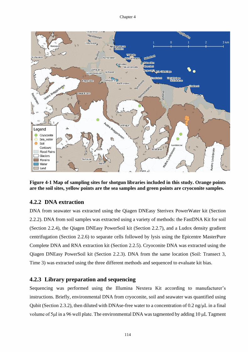
Chapter 4
114
Figure 4-1 Map of sampling sites for shotgun libraries included in this study. Orange points
are the soil sites, yellow points are the sea samples and green points are cryoconite samples.
4.2.2 DNA extraction
DNA from seawater was extracted using the Qiagen DNEasy Sterivex PowerWater kit (Section
2.2.2). DNA from soil samples was extracted using a variety of methods: the FastDNA Kit for soil
(Section 2.2.4), the Qiagen DNEasy PowerSoil kit (Section 2.2.7), and a Ludox density gradient
centrifugation (Section 2.2.6) to separate cells followed by lysis using the Epicentre MasterPure
Complete DNA and RNA extraction kit (Section 2.2.5). Cryoconite DNA was extracted using the
Qiagen DNEasy PowerSoil kit (Section 2.2.3). DNA from the same location (Soil: Transect 3,
Time 3) was extracted using the three different methods and sequenced to evaluate kit bias.
4.2.3 Library preparation and sequencing
Sequencing was performed using the Illumina Nextera Kit according to manufacturer’s
instructions. Briefly, environmental DNA from cryoconite, soil and seawater was quantified using
Qubit (Section 2.3.2), then diluted with DNAse-free water to a concentration of 0.2 ng/μL in a final
volume of 5μl in a 96 well plate. The environmental DNA was tagmented by adding 10 μL Tagment

The Biotechnological Potential of Cryospheric Bacteria
115
DNA buffer (TD) to the 5uL of normalised DNA and then adding 5μL of Amplicon Tagment Mix
(ATM) to the wells and mixing well. The PCR plate was then centrifuged at 280 x g at room
temperature for 1 minute to make sure all sample was in the bottom of the well. The mix was then
rapidly transferred to a pre-programmed and pre-warmed thermocycler set at 55° C and incubated
for 5 minutes exactly, followed by rapid cooling to 10 °C. As soon as the thermocycler reached 10
°C the plate was removed and 5 μL of Neutralize Tagment (NT) Buffer was added to stop the
tagmentation reaction. The plate was then centrifuged at 280 x g at room temperature for 1 minute,
then incubated for an additional 5 minutes at room temperature.
The libraries were amplified and indexed using a limited-cycle PCR. The indexes for each library
(Appendix Table D-1) were arranged in a 96-well PCR plate; 5 μL of Index 1 (i7) was added to
each column using a multichannel pipette, followed by the addition of 5 μL of Index2 (i5) across
each row. Thereafter, 15 μL of Nextera PCR Master Mix (NPM) was added to each well and mixed
by pipetting, followed by a brief centrifugation at 280 x g for 1 minute at room temperature. The
libraries were then amplified in a thermocycler set to the following cycle conditions: 72 °C for 3
minutes, 95 °C for 30 seconds, followed by 15 cycles of 95 °C for 10 seconds, 55°C for 30 seconds
and 72 °C for 30 seconds, followed by a final elongation step of 5 minutes at 72 °C.
A 1.5% agarose gel was run to confirm successful amplification of metagenomic libraries
(Appendix Figure D-1). The resulting indexed libraries were cleaned up using Ampure beads
(Section 2.5.1) and resuspended in 37.5µL of Resuspension Buffer. Cleaned, indexed metagenomic
libraries were equimolarly pooled to 40 nM in a final volume of 50µL. To provide a final library
concentration of 4nM, 5µL of the previous solution were diluted in 10mM Tris 0.05% TWEEN.
The pooled libraries were sequenced at Wales Gene Park (Cardiff University) in an Illumina
NextSeq® in High Output mode, generating 2 x 150bp paired end reads.
4.2.4 Reads processing and quality control
Paired end libraries were uploaded to KBase (https://www.kbase.us/) (Arkin et al., 2018), assessed
using FastQC (J. Brown et al., 2017), trimmed using Trimmomatic (Bolger et al., 2014) to remove
adapters and low-quality reads and the checked using FastQC a second time. The quality-controlled
libraries for each environment type were combined and co-assembled on KBase using MEGAHIT
(D. Li et al., 2015). MEGAHIT was selected as the assembly tool because it was computationally
efficient and performed on par with other assemblers, as determined by optimisation, described in
Chapter 8 Section 8.3.3.1. The assembly and the trimmed libraries for individual samples were then
downloaded for further analysis.

Chapter 4
116
4.2.5 Taxonomic assignment
Reads-based taxonomic assignment was performed on KBase on individual libraries and on pooled
environmental libraries using Kaiju (v.15.0) in Greedy mode, against the NCBI BLAST nr + EUK
database (Menzel et al., 2016).
4.2.6 Metagenome-assembled genomes (MAGs)
Most analysis was conducted on instances hosted on servers at CLIMB (https://www.climb.ac.uk/)
(Connor et al., 2016). Metagenome assembled genomes were constructed using anvi’o (v 6.1 –
Esther) (Eren et al., 2015). A contigs database was created from the assembly fasta file by running
anvi-gen-contigs-database which and identifies open reading frames (ORFs) using Prodigal (Hyatt
et al., 2010). To estimate the number of bacterial genomes in the metagenome, anvi’o runs
HMMER against a series of single-copy gene databases. In anvi’o-6.1, these include HMM profiles
for Archaea (76 genes), Protista (83 genes), Bacteria (71 genes). The scripts to detect candidate
phyla radiation (CPR) rely on the single copy gene HMM dataset from Campbell et al, therefore,
we included this dataset, together with the three profiles with anvio-6.1 in the HMMer scan
(Campbell et al., 2013). The contigs were also functionally annotated with ncbi COG functions
(Section 8.2.4.1.2), KEGG pathway information (Section 8.2.4.1.3) and eggNOG information
(Section8.2.4.1.4). Taxonomy information for each gene call and contig was also classified using
Kaiju (Section 8.2.4.2.1).
4.2.7 Binning and refinement of MAGs
The contigs database of 162,105 contigs (divided into 163,249 splits) was too large to run anvi-
interactive with hierarchical clustering and run manual binning. Therefore, the contigs were binned
using anvi-cluster-contigs as part of the anvi’o workflow using CONCOCT, MaxBin2 and
MetaBAT2 (Section 8.2.5.1). The DAS Tool was then run on all three collections, using
DIAMOND as a search engine. The taxonomic classification of the bins from each binning method
(collection) were checked using anvi-estimate-scg-taxonomy, using the contigs database, merged
profile, and each of the collections. The SCG taxonomy is a courtesy of The Genome Taxonomy
Database (GTDB), which is the new gold standard taxonomy for bacterial classification (Parks et
al., 2018).The bins from the DAS Tool collection were then refined using anvi-refine. The resulting
bins from each tool were exported as collections, merged to create a data-frame of bin-association
per contig and exported as a data layer into anvi’o. Anvi-interactive was run with the collection
DAS Tool, ordered by mean-coverage, and viewed using ‘detection’ which shows proportion of
the contig (or bin) which has at least 1 X coverage.

The Biotechnological Potential of Cryospheric Bacteria
117
4.2.7.1 Screen for Candidate Phyla Radiation genomes
To screen for candidate phyla radiation (CPR), which often contain reduced genomes (Brown et
al., 2015), anvi-script-gen-CPR-classifier was run on the Campbell taxonomy (Campbell et al.,
2013).
4.2.7.2 Criteria for inclusion as a MAG
The dataset was trimmed to contain high quality MAGs. The genomes had to be larger than 1.8
MB, have greater 80% completion and less than 10% redundancy (Bowers et al., 2017).
4.2.7.3 Check genome quality with CheckM and GTDB-Tk
The refined MAGs were exported and the contigs were uploaded as assemblies to KBase for quality
checking using CheckM (https://github.com/Ecogenomics/CheckM) (Parks et al., 2015). The
MAGs were also submitted to GTDB-Tk on KBase for taxonomic assignment. The Genome
Taxonomy Database Toolkit (GTDB-Tk) (https://ecogenomics.github.io/GTDBTk/), provides
taxonomic classification of bacterial and archaeal genomes by placing them into domain-specific,
concatenated protein reference trees (Chaumeil et al., 2020). GTDB-Tk uses the same criteria of
relative evolutionary divergence (RED) and average nucleotide identity (ANI) for establishing
taxonomic ranks as the recently proposed rank-normalized taxonomy in GTDB (Parks et al., 2018).
4.2.8 Phylogenomic Tree
The phylogenomic relationship of the MAGs was compared by following the tutorial:
http://merenlab.org/tutorials/infant-gut/#chapter-iii-phylogenomics. Briefly, using the HMM hits
from a curated collection of single copy core genes (Bacteria_71, Appendix Table D-10) for the
GToTree workflow (Lee, 2019) were compared in a phylogenomic analysis. To do this, the selected
genes from each MAG in the collection were concatenated, translated and aligned by running anvi-
get-sequences-for-hmm-hits with default settings plus the additional parameters: (--concatenate-
genes --return-best-hit --get-aa-sequences). The anvi-get-sequences command uses MUSCLE to
align the genes (Edgar, 2004). The phylogenomic tree was calculated using anvi-gen-
phylogenomic-tree, which infers approximately-maximum-likelihood phylogenetic trees from
FASTA files using FastTree (Price et al., 2010).
Chapter 4
118
4.2.9 Spatial distribution of the MAGs across sample sites
The spatial distribution of MAGs was visualised using heatmaps of max-normalised ratio (number
of reads recruited to a contig divided by the maximum number of reads recruited to that contig in
any sample) and abundance (mean coverage of each MAG divided by that sample’s overall mean
coverage across all the MAGs). The heatmaps were created using the R package ComplexHeatmap
(http://www.bioconductor.org/packages/devel/bioc/html/ComplexHeatmap.html) (Gu et al.,
2016). Max-normalised ratio considers one contig across all samples, where the value is normalized
to the single maximum value for that contig. The sample containing the contig that contributed the
max value will always equal 1, and the value for that contig in the other samples will be the fraction
of that max.
4.2.10 Biogeochemical cycles
The fasta files from the MAGs were analysed for major metabolic pathways using MetabolisHMM
(https://github.com/elizabethmcd/metabolisHMM) (McDaniel et al., 2019). In this analysis, the
fasta files of the genomes are formatted, annotated using prodigal and then a HMMER search is
run against a curated list of genes involved in important biogeochemical pathways. The list of
genes, their HMM profiles and their accessions are available in Appendix Table D-15.
4.2.11 Phormidesmis pangenome
A pangenome of Phormidesmis genomes was constructed using nine genomes downloaded from
NCBI genbank and refseq by searching for complete Phormidesmis genomes on the GTDB
database (https://gtdb.ecogenomic.org/). These were compared to the MAGs resolved in this
dataset using a workflow described (http://merenlab.org/2016/11/08/pangenomics-v2/) and
(http://merenlab.org/tutorials/infant-gut/#chapter-iv-pangenomics). The phylogenetic
relationships of genera and families are constantly being shuffled with new information (See
Appendix Table D-13 comparing ncbi and GTDB-Tk phylogeny). Therefore, all six cyanobacterial
genomes and their closest hits (Appendix Table D-12) were compared in a pangenome analysis
(Appendix Figure D-3). Based on this initial analysis, three cyanobacterial bins:
CC_mag_060_Nodoslinea. MB_mag_047 and CC_mag_055, were investigated further.
The external genomes (Table 4.9) were downloaded from ncbi, and the fasta files were converted
to contigs.db in the anvi’o workflow using anvi-script-FASTA-to-contigs-db. The scripts anvi-run-
hmms and anvi-run-ncbi-cogs was then run to make the external genomes comparable to the
MAGS. The internal MAGs and external genomes downloaded from GTDB were made into a
The Biotechnological Potential of Cryospheric Bacteria
119
genomes storage database that stores information about genomes using anvi-gen-genomes-storage.
The pangenome was generated by running anvi-pan-genome, which makes used of DIAMOND
(Buchfink et al., 2015) and MCL (Enright et al., 2002). The pangenome was also generated using
blastp (--use-ncbi-blast), which is slower than DIAMOND, but which gives better annotation. The
average nucleotide identity (ANI) of the MAGs and external genomes was calculated within anvi’o
using PyANI (Pritchard et al., 2015). Inkscape (available from https://inkscape.org/) was used to
finalize figures.

Chapter 4
120
4.3 Results
4.3.1 Library Statistics
Table 4-2 Characteristics of the Svalbard Soil, Seawater and Cryoconite datasets after trimming
Read Length Duplicate reads Quality
Environment Sample Reads No Bases mean std dev Number % mean std dev GC%
Soil F3T3_Lud 40,079,596 5,866,959,800 146.38 17.23 595,443 1.49 34.05 4.75 57.43
Soil F3T3_PM 44,915,524 6,576,965,385 146.43 17.22 43,387 0.10 34.05 4.76 62.47
Soil F3T3_FD 113,754,008 16,645,206,349 146.33 17.43 594,826 0.52 34.04 4.77 61.04
Soil F1T3-3 37,684,166 5,477,450,552 145.35 18.97 121,309 0.32 33.89 5.01 61.17
Soil F1T4-2 38,762,496 5,660,342,037 146.03 17.92 881,337 2.27 34.00 4.85 57.65
Soil F2T2-1 29,116,044 4,232,776,792 145.38 19.00 310,829 1.07 33.88 5.02 56.75
Soil F3T1-3 35,482,472 5,166,716,509 145.61 18.70 336,628 0.95 33.92 4.97 58.63
Soil F2T4-2 35,085,040 5,124,389,299 146.06 17.92 74,333 0.21 34.00 4.83 58.69
Sea SS1 51,330,724 7,191,372,496 140.10 25.89 1,100,183 2.14 34.20 4.54 50.69
Sea SS2 55,019,496 7,445,759,578 135.33 32.31 1,412,286 2.57 33.89 5.02 49.25
Sea SS3 35,985,822 4,971,626,677 138.16 29.48 775,768 2.16 33.96 4.92 49.01
Cryoconite ML-17 28,795,356 4,194,553,943 145.67 18.57 441,991 1.53 33.89 5.02 55.16
Cryoconite VB-17 34,504,862 5,049,762,759 146.35 17.40 601,414 1.74 34.05 4.77 54.68
Cryoconite ML-18 28,471,672 4,149,307,242 145.73 18.46 471,631 1.66 33.94 4.93 54.46
Cryoconite VB-18 29,787,650 4,347,438,702 145.95 18.08 384,887 1.29 33.94 4.93 55.41
Cryoconite AB-18 64,909,032 9,494,783,816 146.28 17.54 131,932 0.20 34.02 4.81 56.75
Cryoconite VL-18 14,939,536 2,184,519,311 146.22 17.69 78,246 0.52 34.04 4.78 54.47
Library statistics are reported after quality trimming using Trimmomatic. The untrimmed library information can be viewed in Appendix Table D-2.

The Biotechnological Potential of Cryospheric Bacteria
121
4.3.2 Reads-based taxonomy
The taxonomy of reads from each library was determined using Kaiju.
4.3.2.1 Cryoconite
Approximately 60% of the reads in the cryoconite libraries could be classified. A small minority of
these reads could not be assigned at the phylum level. The majority of reads belonged to bacterial
phyla. The Cyanobacteria were the most abundant, followed by Proteobacteria, Actinobacteria and
Bacteroidetes. Other phyla present across all the samples include the Acidobacteria, Chloroflexi,
Firmicutes, Plantomycetes and Gemmatimonadetes. The Ascomycota were the most abundant phylum
from the Fungal kingdom and Chlorophyta were the most abundant phylum from the Viridiplantae
(Green Algae). There were also viruses detected in all samples.
Figure 4-2 Reads-based taxonomic assignment of cryoconite libraries at the Phylum level using
Kaiju. Cryoconite libraries are listed on the x-axis. A dashed lined separates the combined cryoconite
library from the individual libraries.

Chapter 4
122
At the genus level, the VB library and ML library from 2017 and 2018 resemble each other closely.
Phormidesmis is the most abundant genus in the ML-17 (33.92%), ML-18 (33.81%), VB-17 (33.69%)
and VB-18 (24.12%) samples. Although members of Phormidesmis are present in AB (6.23%) and
VL (6.00%), they represent a smaller fraction of the community. Other genera present in significant
numbers include Ktedonobacter which were found in ML-17, ML-18, VB-17, and VB-18. VL is
notable for its high proportion of Nostoc (7.28%) which was present at higher abundance than
Phormidesmis (6.00%).
Figure 4-3 Reads-based taxonomic assignment of cryoconite libraries at the Genus level using
Kaiju.
At the genus level, approximately 20% of the reads were unassigned, 40% of reads belonged to rare
taxa, present at less than 0.5%, and the remaining 40% could be classified.

The Biotechnological Potential of Cryospheric Bacteria
123
4.3.2.2 Soil
Approximately 60% of the reads in the soil libraries could be classified. The soil libraries were
dominated by Bacterial phyla, of which the Proteobacteria, Actinobacteria and Bacteroidetes were the
most abundant, followed by Acidobacteria, Cyanobacteria, Chloroflexi, Plantomycetes,
Verrucomicrobia, Firmicutes, Gemmatimonadetes and Nitrospirae (Figure 4-4). Reads belonging to
the fungal phyla Ascomycota made up a small proportion of the libraries.
Figure 4-4 Reads-based taxonomic assignment of soil libraries at the Phylum level using Kaiju.
Soil libraries are listed on the x-axis. A dashed lined separates the combined soil library from
the individual libraries.
Although phylum-level diversity is similar across different soil samples, there is greater diversity at
lower taxonomic ranks (Figure 4-5). There is a long tail of genera present at less than 0.5% relative
abundance. The most abundant genera, which was also common to all sample sites were
Sphingomonas, Nocardioides, Streptomyces and Bradyrhizobium. However, some genera are present
at relatively high abundance at specific sites or when DNA was extracted using specific methods.
Notably high abundance at the genus level include Cecembia (4.52 %), a genus that was not detected
above 0.5% in either F3T3_PM or F3T3_FD, despite being from the same site. Other notable examples
include Nostoc, present at 7.76% in F2T2, and at lower abundance in F1T3, F3T1, F2T4. The genus
Leptolyngba was also found in all samples where Nostoc was identified.

Chapter 4
124
Figure 4-5 Reads-based taxonomic assignment of soil libraries at the Genus level using Kaiju.
Soil libraries are listed on the x-axis. A dashed line separates the combined soil library.

The Biotechnological Potential of Cryospheric Bacteria
125
4.3.2.3 Seawater
The SS1 library was slightly different to SS2 and SS3 in number of reads classified and in the
composition of classified reads. In particular, the SS1 library had more classified reads overall, with a
large proportion of sequences belonging to members of the Firmicutes and Actinobacteria, which was
a relatively minor constituent of the SS2 and SS3 communities. The seawater libraries had the lowest
percentage of classified reads of any environment type, with only 46.56%, 11.02% and 11.14% of
reads classified in the SS1, SS2 and SS3 libraries, respectively.
Figure 4-6 Reads-based taxonomic assignment of seawater libraries at the Phylum level using
Kaiju.
Viruses were abundant in the SS2 (6.53%) and SS3 (3.96%) samples, and less abundant in SS1
(0.38%). The most abundant bacterial phyla in all samples were the Proteobacteria, (range 36.56% to
42.28%), with a high abundance of Bacteroidetes in SS2 (19.25%) and SS3 (22.36%) and a lower
proportion in SS1 (1.13%). There was also notable number of Chlorophya (Green Algae),
Bacillariophyta (Diatoms), Archaea (Euryarchaeota and Crenarchaeota), Fungi (Ascomycota,
Basidiomycota), Apicomplexa and Euglenida.

Chapter 4
126
Figure 4-7 Reads-based taxonomic assignment of seawater libraries at the Species level using
Kaiju.
At the species level, SS1 differs from SS2 and SS3. SS1 contained a high abundance of species
commonly associated with sewerage. Methanosarcina mazei (1.88%), an anærobic archaeobacter is
found in semi aquatic environments such as sewage receptacles and anoxygenic, moist soil.
Campylobacter jejuni (1.60) is commonly found in animal faeces and is a leading cause of food-borne
illness in humans.

The Biotechnological Potential of Cryospheric Bacteria
127
4.3.3 Assembly statistics
The soil, cryoconite and seawater shotgun libraries were assembled by environment, and in a co-
assembly of all environments. This was done to see whether co-assembly would increase library depth
sufficiently to assemble additional/ longer contigs for bacterial species present in more than one of the
Svalbard environments types. The co-assembly was similar in size to the sum of each of the soil,
cryoconite and sea assemblies (Table 4-3). This suggests that co-assembly did not result in additional
recruitment of reads into contigs or deeper coverage. This is likely because of little overlap in
community members between soil, cryoconite and seawater (Chapter 3, Figure 3-17, Figure 3-19). As
a result, a co-assembly of libraries from all Svalbard environments was used. The co-assembly
provides extra information about the identity of genomes that are shared between environments, with
minimal loss of information about genomes that are unique to one environment (or even one sample)
in particular. The only assembly tool able to cope with the size of the library was MEGAHIT.
Figure 4-8 Comparison of cryoconite, soil and seawater co-assemblies and combined Svalbard
co-assembly.

Chapter 4
128
Table 4-3 Assembly Statistics for the Svalbard metagenomes
Assembly
Longest contig
Nx (Lx)
Length Num
Contigs Sum
Length Contig Length
Histogram Contig Length
Histogram Contig Length Histogram
(bp) (bp) (bp) (1bp <= len <
10Kbp) (10Kbp <= len <
100Kbp) (len >= 100Kbp)
cryoconite- MEGAHIT
315846
N50: 5126 >= 106 0 0
L50: (24906) >= 105 18 2524410
N75: 2995 >= 104 8246 154707901
L75: (60198) >= 103 115949 538521980
N90: 2329 >= 500 115949 538521980
L90: (90952) >= 1 115949 538521980
soil-MEGAHIT
300154
N50: 4111 >= 106 0 0
L50: (10133) >= 105 45 6597658
N75: 2616 >= 104 2366 59047038
L75: (26569) >= 103 49641 208560096
N90: 2199 >= 500 49641 208560096
L90: (39681) >= 1 49641 208560096
sea-MEGAHIT
115659
N50: 4236 >= 106 0 0
L50: (1450) >= 105 2 221424
N75: 2686 >= 104 321 6766634
L75: (3510) >= 103 6451 26970110
N90: 2225 >= 500 6451 26970110
L90: (5171) >= 1 6451 26970110
Svalbard MEGAHIT
554015
N50: 4739 >= 106 0 0
L50: (34565) >= 105 51 7820617
N75: 2833 >= 104 10130 201062657
L75: (85286) >= 103 162105 720998358
N90: 2268 >= 500 162105 720998358
L90: (128180) >= 1 162105 720998358
The Biotechnological Potential of Cryospheric Bacteria
129
4.3.4 Metagenome Assembled Genomes
The contigs from the MEGAHIT assembly were clustered into 151 bins using CONCOCT (v 1.1.0)
(Appendix Table D-5), 180 bins using MaxBin2 (version 2.2.7) (Appendix Table D-6), and 225 bins
using metaBAT2 (v 2.12.1) (Appendix Table D-7). The bins in each collection were compared using
DAS Tool (v 1.1.2) (Appendix Table D-8) and a refined collection of 95 bins with completion > 50%
was created. The taxonomic classification of the bins from each binning method (collection) were
checked using anvi-estimate-scg-taxonomy, using the contigs database, merged profile, and collection
(Appendix Table D-4).
4.3.4.1 Manual Bin Refining
The bins were refined multiple times using anvi-refine and the method described in Chapter 8 (Section
8.2.5). A final collection consisting of 74 MAGs was kept for the remainder of the study. The final
collection consists of 41 high quality draft genomes (completion > 90 % (prefix MAG) and 32 medium
quality draft genomes (completion >70%, redundancy < 10% (prefix mag)). This collection of MAGS
recruited 262,080,978 nucleotides, which represent only 36.35% of all nucleotides stored in the contigs
and profile databases. The remaining contigs belonged to species present in too low abundance to
properly be resolved into genomes by this sampling effort.

Chapter 4
130
Figure 4-9 Figure showing the MAGS included in the dataset. Figure is generated using anvi-interactive from anvi’o. MAGS are ordered using
mean-coverage and viewed using ‘detection’ which shows proportion of the MAG which has at least 1 X coverage.
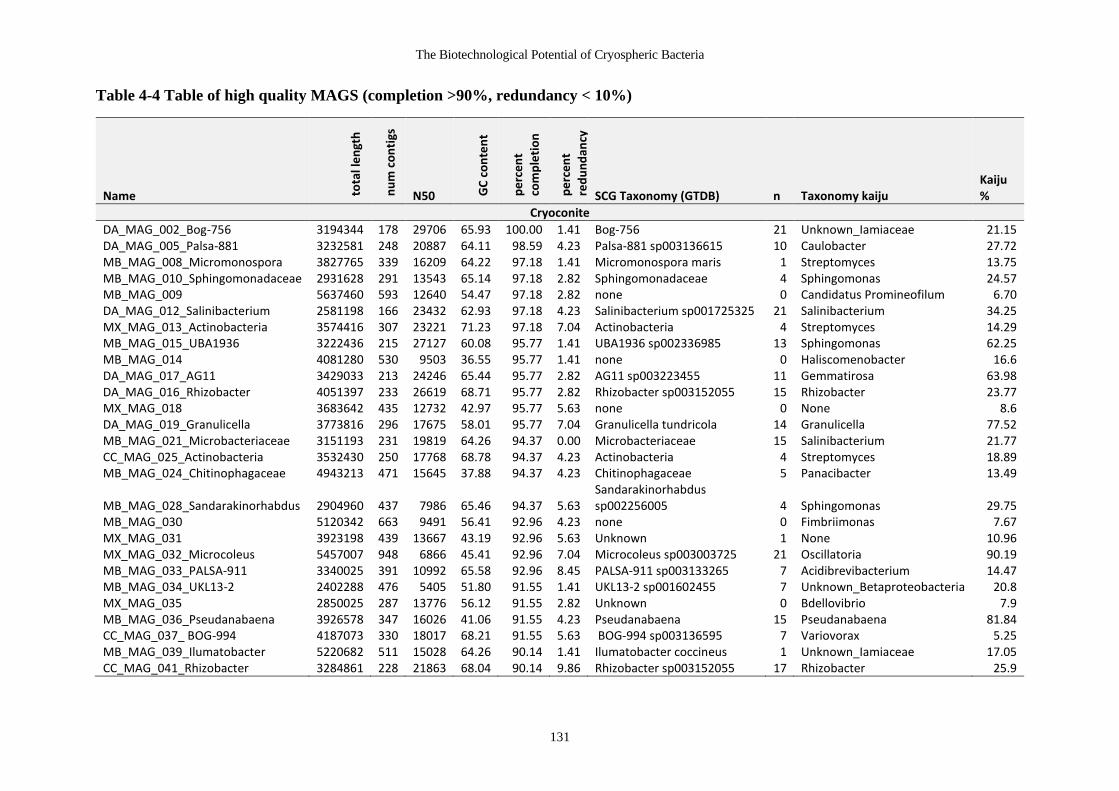
The Biotechnological Potential of Cryospheric Bacteria
131
Table 4-4 Table of high quality MAGS (completion >90%, redundancy < 10%)
Name tota
l le
ngt
h
nu
m c
on
tigs
N50 GC
co
nte
nt
pe
rce
nt
com
ple
tio
n
pe
rce
nt
red
un
dan
cy
SCG Taxonomy (GTDB) n Taxonomy kaiju Kaiju %
Cryoconite
DA_MAG_002_Bog-756 3194344 178 29706 65.93 100.00 1.41 Bog-756 21 Unknown_Iamiaceae 21.15 DA_MAG_005_Palsa-881 3232581 248 20887 64.11 98.59 4.23 Palsa-881 sp003136615 10 Caulobacter 27.72 MB_MAG_008_Micromonospora 3827765 339 16209 64.22 97.18 1.41 Micromonospora maris 1 Streptomyces 13.75 MB_MAG_010_Sphingomonadaceae 2931628 291 13543 65.14 97.18 2.82 Sphingomonadaceae 4 Sphingomonas 24.57 MB_MAG_009 5637460 593 12640 54.47 97.18 2.82 none 0 Candidatus Promineofilum 6.70 DA_MAG_012_Salinibacterium 2581198 166 23432 62.93 97.18 4.23 Salinibacterium sp001725325 21 Salinibacterium 34.25 MX_MAG_013_Actinobacteria 3574416 307 23221 71.23 97.18 7.04 Actinobacteria 4 Streptomyces 14.29 MB_MAG_015_UBA1936 3222436 215 27127 60.08 95.77 1.41 UBA1936 sp002336985 13 Sphingomonas 62.25 MB_MAG_014 4081280 530 9503 36.55 95.77 1.41 none 0 Haliscomenobacter 16.6 DA_MAG_017_AG11 3429033 213 24246 65.44 95.77 2.82 AG11 sp003223455 11 Gemmatirosa 63.98 DA_MAG_016_Rhizobacter 4051397 233 26619 68.71 95.77 2.82 Rhizobacter sp003152055 15 Rhizobacter 23.77 MX_MAG_018 3683642 435 12732 42.97 95.77 5.63 none 0 None 8.6 DA_MAG_019_Granulicella 3773816 296 17675 58.01 95.77 7.04 Granulicella tundricola 14 Granulicella 77.52 MB_MAG_021_Microbacteriaceae 3151193 231 19819 64.26 94.37 0.00 Microbacteriaceae 15 Salinibacterium 21.77 CC_MAG_025_Actinobacteria 3532430 250 17768 68.78 94.37 4.23 Actinobacteria 4 Streptomyces 18.89 MB_MAG_024_Chitinophagaceae 4943213 471 15645 37.88 94.37 4.23 Chitinophagaceae 5 Panacibacter 13.49
MB_MAG_028_Sandarakinorhabdus 2904960 437 7986 65.46 94.37 5.63 Sandarakinorhabdus sp002256005 4 Sphingomonas 29.75
MB_MAG_030 5120342 663 9491 56.41 92.96 4.23 none 0 Fimbriimonas 7.67 MX_MAG_031 3923198 439 13667 43.19 92.96 5.63 Unknown 1 None 10.96 MX_MAG_032_Microcoleus 5457007 948 6866 45.41 92.96 7.04 Microcoleus sp003003725 21 Oscillatoria 90.19 MB_MAG_033_PALSA-911 3340025 391 10992 65.58 92.96 8.45 PALSA-911 sp003133265 7 Acidibrevibacterium 14.47 MB_MAG_034_UKL13-2 2402288 476 5405 51.80 91.55 1.41 UKL13-2 sp001602455 7 Unknown_Betaproteobacteria 20.8 MX_MAG_035 2850025 287 13776 56.12 91.55 2.82 Unknown 0 Bdellovibrio 7.9 MB_MAG_036_Pseudanabaena 3926578 347 16026 41.06 91.55 4.23 Pseudanabaena 15 Pseudanabaena 81.84 CC_MAG_037_ BOG-994 4187073 330 18017 68.21 91.55 5.63 BOG-994 sp003136595 7 Variovorax 5.25 MB_MAG_039_Ilumatobacter 5220682 511 15028 64.26 90.14 1.41 Ilumatobacter coccineus 1 Unknown_Iamiaceae 17.05 CC_MAG_041_Rhizobacter 3284861 228 21863 68.04 90.14 9.86 Rhizobacter sp003152055 17 Rhizobacter 25.9

Chapter 4
132
Table 4.5 continued…
Name tota
l le
ngt
h
nu
m c
on
tigs
N50 GC
co
nte
nt
pe
rce
nt
com
ple
tio
n
pe
rce
nt
red
un
dan
cy
SCG taxonomy (GTDB) n Taxonomy kaiju Kaiju %
Seawater
MB_MAG_023_ASP10-02a 2563445 129 32893 45.24 94.37 2.82 ASP10-02a sp002335115 20 Candidatus Thioglobus 6.75 MB_MAG_038_UBA10364 1841681 133 18813 41.70 90.14 0.00 UBA10364 sp002430755 21 Owenweeksia 21.43
Soil
MB_MAG_001 3997738 152 39686 69.07 100.00 1.41 none 0 Luteitalea 5.8 MB_MAG_003_BK-30 3001625 147 29296 65.34 100.00 2.82 Burkholderiaceae_BK-30 21 Hydrogenophaga 45.35 MB_MAG_004 4947466 409 16841 68.99 98.59 1.41 none 0 Ferrovibrio 7.49
DA_MAG_006_Cytophagales 3673287 48 136173 42.04 97.18 0.00 Sporocytophaga myxococcoides 3 Cytophaga 33.53
DA_MAG_007_Iso899 4713114 185 33034 69.61 97.18 1.41 Iso899 sp000421445 11 Streptomyces 18.83
DA_MAG_011_Sphningosinicella 3477485 118 42505 66.66 97.18 4.23 Sphningosinicella sp003012735 12 Sphingosinicella 86.05
MB_MAG_020_ Cyclobacteriaceae 4845095 302 22910 38.78 94.37 0.00 Cyclobacteriaceae 4 Unknown_Flammeovirgaceae 18.15
MX_MAG_022_Pararhodobacter 3720906 603 7696 70.98 94.37 2.82 Pararhodobacter sp001314715 10 Rhodobaca 13.27
CC_MAG_026 3384069 404 11587 35.24 94.37 4.23 none 0 Haliscomenobacter 15.02 MB_MAG_027_UBA11741 4420110 372 16213 54.65 94.37 5.63 UBA11741 sp002427845 6 Chloracidobacterium 12.93
CC_MAG_029_HLUCCA01 2523900 60 69398 45.16 92.96 0.00 HLUCCA01 6 Candidatus Cyclonatronum 81.15
MB_MAG_040 3254196 446 8589 36.52 90.14 4.23 none 0 Flavobacterium 7.4

The Biotechnological Potential of Cryospheric Bacteria
133
Table 4-5 Table of medium quality MAGS (completion >70%. Redundancy < 10%)
Name tota
l le
ngt
h
nu
m c
on
tigs
N50 GC
co
nte
nt
pe
rce
nt
com
ple
tio
n
pe
rce
nt
red
un
dan
cy
SCG Taxonomy (GTDB) n Taxonomy kaiju Kaiju %
Cryoconite
MX_mag_042_Ktedonobacteraceae 4685611 848 6700 53.2 88.73 1.41 Ktedonobacteraceae 4 Unknown_Ktedonobacteria 66.35 MB_mag_045 3183126 474 7727 47.61 87.32 4.23 none 0 Unknown_Ktedonobacteria 25.32 MB_mag_047_ULC077BIN1 3491281 719 5103 48.58 87.32 9.86 ULC077BIN1 sp003249025 18 Leptolyngbya 19.47 MX_mag_044_UBA5184 2744076 427 8453 62.42 87.32 2.82 Palsa-1515 sp003158195 4 Unknown_Bacteria 3.49 MB_mag_046_UBA2376 6278991 987 7373 66.04 87.32 9.86 UBA2376 sp002344285 2 Haliangium 27.86 MB_mag_048_Xanthomonadaceae 4060943 245 25552 62.82 85.92 0 Xanthomonadaceae 8 Lysobacter 15.77 MB_mag_051 3703043 665 6064 63.99 85.92 4.23 conflict 2 Fimbriimonas 5.86 MB_mag_050_Sphingomonadaceae 2515818 320 10297 67.47 85.92 2.82 Sphingomonadaceae 3 Sphingomonas 24.61 MX_mag_058_Chitinophagaceae 4091667 812 6024 37.06 84.51 9.86 Chitinophagaceae 6 Panacibacter 11.58 MB_mag_055_Phormidesmis 3621916 480 8841 49.44 84.51 2.82 Phormidesmis priestleyi 18 Leptolyngbya 55.49 CC_mag_053_UKL13-2 2993940 633 5373 52.59 84.51 1.41 UKL13-2 sp001602455 6 Unknown_Betaproteobacteria 19.75 MX_mag_054 4076001 831 5585 57.29 84.51 2.82 none 0 Unknown_Ktedonobacteria 19.86 CC_mag_052_Bradyrhizobium 5766360 626 13724 62.24 84.51 1.41 Bradyrhizobium 18 Bradyrhizobium 80.79 MB_mag_057_Polyangiaceae 5712704 946 6896 64.77 84.51 7.04 Polyangiaceae Labilithrix 4 Labilithrix 44.61 MB_mag_056 4563212 885 5536 67.99 84.51 4.23 none 0 Streptomyces 4.86 CC_mag_059_Dermatophilaceae 3256706 382 10773 69.57 83.1 1.41 Dermatophilaceae 10 Intrasporangium 18.85 MB_CPR_001 1237930 82 22880 39.7 81.69 4.23 none 0 None 11.36 MB_mag_061 2915558 669 4501 63.5 80.28 4.23 conflict 2 Fimbriimonas 4.63 MX_mag_063_Sphingomonas 1824331 443 4446 64.65 80.28 7.04 Sphingomonas 9 Sphingomonas 70.88 MB_bin_064_Microbacteriaceae 2485453 163 20769 66.28 78.87 1.41 Microbacteriaceae 9 Lysinimonas 44.63 MB_bin_065_Fimbriimonas 2967189 515 6437 51.23 77.46 0 Fimbriimonas 3 Fimbriimonas 64.47 MB_bin_066_BOG-944 4204385 780 5915 65.14 76.06 0 BOG-944 sp003134215 1 Fimbriimonas 5.51 MB_bin_067_Sandarakinorhabdus 2323251 375 7206 66.66 76.06 1.41 Sandarakinorhabdus 6 Sphingomonas 33.6 MB_CPR_002 1175402 195 7155 34.97 73.24 2.82 none 0 None 11.79 MB_bin_069_Bryobacteraceae 3840205 557 8316 57.14 73.24 2.82 Bryobacteraceae 2 Candidatus Solibacter 59.78 CC_bin_071_Nostoc 5614383 1271 4836 41.94 70.42 9.86 Nostoc sp002949735 11 Nostoc 91.82

Chapter 4
134
Table 4.6 continued…
Name tota
l le
ngt
h
nu
m c
on
tigs
N50 GC
co
nte
nt
pe
rce
nt
com
ple
tio
n
pe
rce
nt
red
un
dan
cy
SCG Taxonomy (GTDB) n Taxonomy kaiju Kaiju %
Seawater
MX_mag_062_Ascidiaceihabitans 2223744 556 4225 50.99 80.28 4.23 Ascidiaceihabitans sp002478745 18 Sulfitobacter 32.37
Soil
MB_mag_043_UBA4742 2225260 392 6786 66.48 87.32 1.41 UBA4742 sp002403895 1 Unknown_Iamiaceae 21.43 MB_mag_049_Aquiflexum 4067355 204 34607 41.04 85.92 1.41 Aquiflexum balticum 17 Belliella 66.53 CC_mag_060_Nodosilinea 2559317 740 3583 57.28 83.1 2.82 Nodosilinea 19 Halomicronema 21.89 MB_bin_068 2134956 206 13635 56.75 74.65 2.82 none 0 Fimbriimonas 46.19
MB_CPR_003 763139 102 9802 44.66 73.24 4.23 none 0 Unknown_Candidatus_Saccharibacteria 45.1
MB_bin_070_QHBO01 2957152 263 15831 67.08 73.24 4.23 QHBO01 sp003243965 2 Streptomyces 6.39

The Biotechnological Potential of Cryospheric Bacteria
135
4.3.5 Phylogenomic tree of Svalbard MAGs
Figure 4-10 Phylogeny of MAGs created by Fast Tree of Muscle alignment of 71 single copy core
genes.

Chapter 4
136
4.3.5.1 GTDB-Tk Classification of MAGS
The MAGs were classified taxonomically using two different methods. A phylogenomic tree was
constructed using a curated list of 71 genes (Lee, 2019) (Figure 4-10) and MAGs were classified using
the GTDB-Tk (Table 4-7). Both methods gave similar results and clades within the phylogenomic tree
(Figure 4-10) related to the 14 different phyla identified using GTDB-Tk (Table 4-7). In order of
abundance, these were the Proteobacteria (α = 13, γ =8), Actinobacteriota (11), Bacteroidota (10) and
the Cyanobacteria (6). The Chloroflexota (5) and Chloroflexota_A (1), Armatimonadota (6),
Acidobacteriota (4) and Patescibacteria (3) also had several members. Finally, we resolved two MAGs
each from the Myxococcota and Fibrobacterota, and a single MAG member from Bdellovibrionota,
Eremiobacterota and Gemmatimonadota.
Two of the MAGs, MB_mag_055_Phormidesmis and MB_MAG_023_ASP10-02a were assigned to
species-level using FastANI (Jain et al., 2018) within the GTDB-TK (Chaumeil et al., 2020) with ANI
> 95% and an alignment fraction >65% (Table 4-6). MB_mag_055_Phormidesmis is very similar to
the Phormidesmis priestleyi strain BC1401, isolated from cryoconite in a Greenland glacier.
MB_MAG_023_ASP10-02a is very similar to an Oceanospirillaceae bacterium UBA2001 isolated
from subsurface seawater marine metagenome from the North Sea (Parks et al., 2017). The remainder
of the MAGS were assigned to novel species within their genus.
Table 4-6 Table of MAGS classified to species level using FastANI
User Genome Classification FastANI Reference
Fast
AN
I Re
fere
nce
Rad
ius
Fast
AN
I AN
I
Fast
AN
I A
lign
men
t
Frac
tio
n
Location Reference
MB_mag_055
_
Phormidesmis
p__Cyanobacteria;
c__Cyanobacteriia;
o__Leptolyngbyales;
f__Leptolyngbyaceae;
g__Phormidesmis_A;
s__Phormidesmis_A
priestleyi_B
GCF_001650195.1 95 99.29 0.97 Cryoconite,
Greenland
(Chrismas et
al., 2016a)
MB_MAG_023
_ ASP10-02a
p__Proteobacteria;
c__Gammaproteobacteria;
o__Pseudomonadales;
f__Nitrincolaceae;
g__ASP10-02a; s__ASP10-
02a sp002335115
GCA_002335115.1 95 95.44 0.86 Subsurface
seawater,
North Sea
(Parks et al.,
2017)

The Biotechnological Potential of Cryospheric Bacteria
137
Table 4-7 Classification of MAGS using GTDB-Tk
Phylum Genus MAG
Cla
ssif
icat
ion
Me
tho
d
No
te
AA
Pe
rce
nt
RED
Val
ue Closest Placement
Reference
Closest Placement Taxonomy
Clo
sest
Pla
cem
en
t
AN
I
Clo
sest
Pla
cem
en
t
Alig
nm
en
t Fr
acti
on
Acidobacteriota
Granulicella DA_MAG_019_Granulicella P C: TOP 89.15 0.961 GCF_000178975.2 Granulicella tundricola
78.41 0.23
BOG-234 MB_bin_069_Bryobacteraceae P N: RED 70.56 0.891
UBA11741 MB_MAG_027_UBA11741 P C: TOP 90.91 0.94
MB_MAG_001 P N: RED 95.02 0.703
Actinobacteriota
MB_mag_043_UBA4742 P N: RED 76.59 0.598
Bog-756 DA_MAG_002_Bog-756 P C: TOP 89.92 0.939
MB_MAG_039_Ilumatobacter P N: RED 87.76 0.82
MB_MAG_008_Micromonospora P C: TOP 96.69 0.604
GCA-2748155 CC_mag_059_Dermatophilaceae P N: RED 78.93 0.861
Salinibacterium DA_MAG_012_Salinibacterium P C: TOP 94.03 0.967 GCF_900230175.1 Salinibacterium xinjiangense
77.83 0.26
UBA10887 MB_MAG_021_Microbacteriaceae P N: RED 87.02 0.966 GCA_003454135.1 UBA10887 sp003454135
79.23 0.43
UBA1487 MB_bin_064_Microbacteriaceae P C: TOP 84.62 0.944 GCA_002325245.1 UBA1487 sp002325245
78.91 0.36
CC_MAG_025_Actinobacteria P N: RED 89.31 0.704
MX_MAG_013_Actinobacteria P N: RED 94.42 0.712
Iso899 DA_MAG_007_Iso899 P N: RED 93.19 0.93
Armatimonadota
MB_bin_066_BOG-944 P N: RED 69.05 0.694
MB_mag_051 P N: RED 69.8 0.693
MB_mag_061 P N: RED 47.62 0.707
MB_MAG_030 P N: RED 90.22 0.734
MB_bin_065_Fimbriimonas P N: RED 74.48 0.888
MB_bin_068 P C: TOP 79.37 0.775

Chapter 4
138
Table 4-7 continued…
Phylum Genus MAG
Cla
ssif
icat
ion
M
eth
od
No
te
AA
Pe
rc e
nt
RED
Val
ue Closest Placement
Reference
Closest Placement Taxonomy
Clo
sest
Pla
cem
en
t A
NI
Clo
sest
P
lace
me
nt
Alig
nm
en
t Fr
acti
on
Bacteroidota
Ferruginibacter MB_MAG_024_Chitinophagaceae P C: TOP 95.36 0.902
MX_mag_058_Chitinophagaceae P C: TOP 78.41 0.901 MB_MAG_014 P C: TOP 85.97 0.714
UBA3362 CC_MAG_026 P N: RED 88.51 0.881 MB_MAG_020_Cyclobacteriaceae P N: RED 97.16 0.808
Cecembia MB_mag_049_Aquiflexum P C: TOP 83.12 0.98 GCF_003014575.1 Cecembia rubra 82.37 0.69 DA_MAG_006_Cytophagales P N: RED 98 0.845
UBA10364 MB_MAG_038_UBA10364 P C: TOP 91.96 0.993 GCA_003487785.1 UBA10364 sp003487785
87.14 0.83
MB_MAG_040 P N: RED 83.23 0.848
UBA11400 CC_MAG_029_HLUCCA01 P N: RED 91.45 0.879
Bdellovibrionota UBA1018 MX_MAG_035 P N: RED 89.23 0.854
Chloroflexota
MB_MAG_009 P N: RED 91.19 0.797 MB_mag_045 P N: RED 78.99 0.609 MX_mag_054 P N: RED 72.24 0.608 MX_mag_042_Ktedonobacteraceae P C: TOP 85.36 0.869
MB_mag_056 P N: RED 76.37 0.519
Chloroflexota_A MB_bin_070_QHBO01 P N: RED 83.59 0.842 GCA_003243965.1 QHBO01 sp003243965
77.35 0.29
Cyanobacteria
Microcoleus MX_MAG_032_Microcoleus P C: TOP 85.69 0.982 GCF_003003725.1 Microcoleus sp003003725
89.64 0.81
Phormidesmis_A MB_mag_055_Phormidesmis ANI/P
F: TOP+ ANI
80.42 GCF_001650195.1 Phormidesmis_A priestleyi_B
99.29 0.97
ULC077BIN1 MB_mag_047_ULC077BIN1 P N: RED 70.79 0.971 GCA_003249025.1 ULC077BIN1 sp003249025
83.83 0.8
Nodosilinea CC_mag_060_Nodosilinea P C: TOP 64.13 0.969
Pseudanabaena MB_MAG_036_Pseudanabaena P C: TOP 91.17 0.978 GCA_003242085.1 Pseudanabaena frigida
80.5 0.68
Nostoc CC_bin_071_Nostoc P C: TOP 65.77 0.96

The Biotechnological Potential of Cryospheric Bacteria
139
Table 4-7 continued…
Phylum Genus MAG
Cla
ssif
i
cati
on
M
eth
od
No
te
AA
P
erc
en
t RED
Val
ue Closest Placement
Reference
Closest Placement Taxonomy C
lose
st
Pla
cem
en
t A
NI
Clo
sest
P
lace
m
en
t A
lign
me
nt
Frac
tio
n
Eremiobacterota Palsa-1515 MX_mag_044_UBA5184 P N: RED 80.12 0.893
Fibrobacterota MX_MAG_018 P N: RED 87.7 0.787 MX_MAG_031 P N: RED 92.6 0.783
Gemmatimonadota
2013-60CM-65-52
DA_MAG_017_AG11 P N: RED 84.44 0.929 GCA_002215645.1 2013-60CM-65-52 sp002215645
78.45 0.34
Myxococcota MB_mag_046_UBA2376 P N: RED 80.62 0.829 GCA_002344285.1
UBA2376 sp002344285
76.62 0.31
MB_mag_057_Polyangiaceae P N: RED 70.63 0.831
Patescibacteria
MB_CPR_002 P C: TOP 55.38 0.806
PJMF01 MB_CPR_001 P N: RED 64.76 0.895 MB_CPR_003 P C: TOP 57.52 0.761
Proteobacteria
BOG-908 MB_MAG_033_PALSA-911 P N: RED 85.1 0.858
Palsa-881 DA_MAG_005_Palsa-881 P C: TOP 93.61 0.961 GCA_003161535.1 Palsa-881 sp003161535
77.07 0.31
MB_MAG_004 P N: RED 93.63 0.749
Bradyrhizobium CC_mag_052_Bradyrhizobium P C: TOP 81.43 0.987 GCA_001464035.1 Bradyrhizobium sp001464035
84.13 0.61
Ascidiaceihabitans
MX_mag_062_Ascidiaceihabitans P C: TOP 72.22 0.998 GCA_002478745.1 Ascidiaceihabitans sp002478745
89.75 0.78
Pararhodobacter MX_MAG_022_Pararhodobacter P C: TOP 87.62 0.944 MB_bin_067_Sandarakinorhabdus P N: RED 58.47 0.86 MB_MAG_010_Sphingomonadaceae P N: RED 93.35 0.846 MB_MAG_028_Sandarakinorhabdus P N: RED 84.17 0.859 MB_mag_050_Sphingomonadaceae P C: TOP 78.97 0.812
Sphingomonas_A MX_mag_063_Sphingomonas P C: TOP 55.46 0.944 GCF_000585415.1 Sphingomonas_A jaspsi
78.74 0.51
Sphningosinicella DA_MAG_011_Sphningosinicella P C: TOP 93.13 0.947 GCF_003012735.1 Sphningosinicella sp003012735
79.26 0.48

Chapter 4
140
Table 4-6 continued…
Phylum Genus MAG
Cla
ssif
icat
ion
Me
tho
d
No
te
AA
Pe
rce
nt
RED
Val
ue
Closest Placement Reference
Closest Placement Taxonomy
Clo
sest
Pla
cem
en
t A
NI
Clo
sest
Pla
cem
en
t A
lign
me
nt
Frac
tio
n
Proteobacteria
UBA1936 MB_MAG_015_UBA1936 P C: TOP 96.37 0.956 GCA_002336985.1 UBA1936 sp002336985
77.31 0.24
MB_MAG_003_BK-30 P C: TOP 96.61 0.95
BOG-994 CC_MAG_037_BOG-994 P N: RED 84.54 0.893
Rhizobacter CC_MAG_041_Rhizobacter P C: TOP 89.25 0.974 GCA_003152055.1 Rhizobacter sp003152055
80.99 0.61
Rhizobacter DA_MAG_016_Rhizobacter P C: TOP 91.67 0.973 GCA_003152055.1 Rhizobacter sp003152055
82.36 0.61
UKL13-2 CC_mag_053_UKL13-2 P N: RED 80.63 0.898
MB_MAG_034_UKL13-2 P N: RED 84.58 0.899
ASP10-02a MB_MAG_023_ASP10-02a ANI/P
F: TOP+ANI: 92.24
GCA_002335115.1 ASP10-02a sp002335115
95.44 0.86
MB_mag_048_Xanthomonadaceae P C: TOP 86.59 0.855
P: Placement C: TOP: taxonomic classification fully defined by topology N: RED: taxonomic novelty determined using RED F: T+ANI: topological placement and ANI have congruent species assignments

The Biotechnological Potential of Cryospheric Bacteria
141
4.3.6 Spatial distribution of MAGs
Reads from each library (site) were mapped back to contigs by anvi’o to create a profile. High
read coverage at a site reflects high abundance, whereas low coverage indicates the absence of
the genome at the site. In this way it is possible to map relative abundance of the MAGs across
different sites. By clustering the MAGs by site, groups of commonly co-occurring bacteria can
be identified. The spatial distribution of the MAGs was plotted using MAG-centric (Figure 4-
11; max-normalised ratio) and sample-centric (Figure 4-12; abundance) values. Both methods
compare the coverage of each genome at each site but are normalised in different ways.
4.3.6.1 Max-normalized ratio to identify sites where MAG is most abundant
The max-normalised-ratio of coverage for the MAGs were clustered using the default
hierarchical clustering withing the ComplexHeatmap package, and then divided into groups
using k-means clustering into k=9 groups of MAGs and k=5 environments (set.seed=5).
Groups of MAGs that are similar within sea, cryoconite and soil were identified. Notably, the
MAGs in the VL cryoconite sample were very different to those in the cryoconite from ML,
VB, and AB. The VL community was missing many of the members that make up the
communities on VL, VB and VL, and instead, contained community members more commonly
found in glacial forefield soil. The MAGs found in the seawater samples had absolutely no
overlap with any of the other environments. Clustering in this way also revealed several MAGs
that were present in a single sample or site. This was particularly true of MAGS present only
in the F3T3_Ludox soil sample and the cryoconite from AB.

Chapter 4
142
Figure 4-11 Heatmap showing distribution of MAGs across different environments and
sites using a MAG-centric view. This view is useful to see in which environment each MAG
is the most abundant. It compares each MAG to the same MAG in other environments.

The Biotechnological Potential of Cryospheric Bacteria
143
4.3.6.2 The Abundance of MAGs across different sites.
Abundance values in anvi’o are calculated as the mean coverage of each MAG divided by that
sample’s overall mean coverage across all the MAGs. Abundance values therefore represent
the ratio of a MAGs mean coverage to the mean coverage of all the MAGs in the sample.
Therefore, MAGs with larger abundance values are more represented in that sample (i.e.
recruited more reads) than those contigs with smaller abundance values. This is a useful view
for highlighting abundant and rare taxa. Figure 4-12 shows the plotted abundance values of
each of the MAGs across the different sites. This visualisation is particularly useful for
highlighting the highly abundant (green to blue) MAGs compared to the rare MAGs (wheat
and white).
Overall patterns are immediately evident. Firstly, the seawater has the fewest MAGs and these
MAGs are not found in the other environments. Secondly, the cryoconite sample from VL is
missing a large portion of the community that is present in AB, ML and VB samples. The ML
and VB samples are very similar to each other and the VL and AB samples have several species
in common that are not found on VB or ML. There are several MAGs, mainly belonging to the
Actinobacteria and Proteobacteria that are highly abundant community members in cryoconite,
and low abundance members of the soil community. There are also members of the soil
community that were not detected in the cryoconite habitats.
There are several MAGs (dark blue) that are highly dominant community members at specific
sites. MB_mag_055_Phormidesmis is the most abundant MAG in the cryoconite samples,
especially from ML and VB, however it is also found in high abundance on AB and VL and is
present at low abundance in soil samples. VL has three highly abundant cyanobacterial MAGs
that are absent or extremely rare in the VB and ML samples. Two of these MAGs,
CC_mag_071_Nostoc and MX_MAG_032_Microleus are also present in AB, however
MB_mag_047_ULC077BIN1, is not found in any of the other cryoconite samples, but is found
in all of the soil except F3T3_Lud.
The Cyanobacterial MAG, CC_mag_Nodoslinea_60, is not found in any of the cryoconite
samples, but is highly abundant in the two early soil samples (F3T1 and F3T2) and is present,
though less abundant, in later soils. The five MAGs belonging to the Chloroflexota are found
exclusively in cryoconite, except for MX_mag_042_Ktedonobacteraceae, which is a low
abundance member in all the soil samples.

Chapter 4
144
Figure 4-12 The distribution of Svalbard MAGS based on Abundance. Colour guide:
Green: MAGs close to sample mean coverage; Blue: MAGs are highly abundant (10- 40x the
sample mean); wheat: rare MAGs (0.1 of the sample mean); white: MAGs recruited zero reads
in that sample. The phylum membership of MAGs is displayed using a colour legend and
environments were forced to cluster together.

The Biotechnological Potential of Cryospheric Bacteria
145
The Soil_S1_F3T3_Lud sample is different from all other soil samples, even though the library
was extracted from the same soil site as (F3T3). This sample has several highly abundant
Bacteroidota MAGs that are present only in this sample. This likely represent an extraction
bias and further discussion of this sample will take place in the discussion.
4.3.7 Major biogeochemical cycles
The tool metabolisHMM was run to look for the presence of major genes involved in Carbon,
Nitrogen, Sulfur, Oxygen and Hydrogen cycling (Figure 4-13, Figure 4-14).
4.3.7.1 Carbon cycling
Several MAGs had copies of form I RubisCO, including an Actinobacteria,
CC_MAG_025_Actinobacteria, from the family Frankiaceae, two Alphaproteobacterial
MAGs, MB_MAG_033_PALSA_911 and CC_mag_052_Bradyrhizobium belonging to the
family Acetobacteraceae and Xanthobacteraceae respectively as well as a
Gammaproteobacterial MAG CC_MAG_037_BOG_994, family Burkholderiaceae. The MAG
MB_bin_070_QHBO01 from the phylum Chloroflexota_A and MX_mag_044_UBA5184
from the phylum Eremiobacterota also contained copies.
There were also Form I RubisCO genes in all the cyanobacterial MAGs, except for
cc_mag_071_Nostoc_ and CC_mag_060_Nodoslinea. Of note, the cyanobacterial MAGs in
this study had <90% completion, and therefore their absence may just reflect the incomplete
bins. Interestingly, all MAGs harbouring RubisCO form I genes were most abundant in
cryoconite, with the sole exception of MB_bin_070_QHBO01, which was more abundant in
soil. Several methylotrophs were identified that had NDMA-dependent methanol
dehydrogenase (nmda) and S-(hydroxymethyl)mycothiol dehydrogenase (smdh) genes in two
and seven Actinobacterial MAGs, respectively. The smdh enzyme was found in seven of the
ten Actinobacterial MAGs. Most of the Actinobacterial MAGs are more prevalent in
cryoconite, but DA_MAG_007_Iso899 was more abundant in soil. There is evidence of carbon
monoxide (CO) oxidation via carbon monoxide dehydrogenase (coxSML) genes in several
Acidobacteria (3/4), Actinobacteria (5/11), Alphaproteobacteria (8/15) and
Gammaproteobacteria (4/8) MAGs.

Chapter 4
146
4.3.7.2 Nitrogen cycling
There was only one MAG capable of nitrogen fixation from the resolved genomes. The
CC_bin_071_Nostoc had nifD and nifH genes (Figure 4-14), responsible for nitrogen fixation.
Soil had a high number of genomes that has nosD and nosZ genes in involved in denitrification.
An Alphaproteobacterial MAG, CC_mag_052_Brazyrhizobium, from the order Rhizobiales
with a copy of the napA (nitrate reductase) gene was present in all soil and cryoconite samples.
A second MAG, MB_MAG_020_Cyclobacteriaceae from the Bacteroidota had a copy of the
napA gene but was present only in the F3T3_Ludox samples, which is believed to have been
enriched (Section ). The narG gene (respiratory nitrate reductase) was present in two
Actinobacterial MAGs, CC_MAG_025_Actinobacteria and
MB_MAG_008_Micromonospora and two Alphaproteobacterial MAGs, MB_MAG_004 and
MX_MAG_022_Pararhodobacter (Figure 4-14). Both Actinobacterial MAGs were common in
cryoconite samples, however the proteobacterial MAGs were from the F3T3_Ludox samples.
4.3.7.3 Sulfur cycling
The most common gene detected for sulfur cycling was sulfur dioxygenas (sdo). Sdo oxidizes
the sulfane sulfur in GSSH to sulfite, and there were 39 MAGs that had at least one of these
genes. The second most abundant gene was sulfate adenylyltransferase (sat), gene, which forms
adenosine 5'-phosphosulfate (APS) from ATP and free sulfate, the first step in the formation
of the activated sulfate donor 3'-phosphoadenylylsulfate (PAPS). Sat was found in the majority
of Cyanobacterial (5/6) and Chloroflexota genomes (4/5) as well as in a few Acidobacteriota
(2/5), Alphaproteobacteria (2/13) and Gammaproteobacteria (1/8).

The Biotechnological Potential of Cryospheric Bacteria
147
Figure 4-13 Figure 1 showing the detection of key genes in Svalbard MAGS involved in biogeochemical cycling.

Chapter 4
148
Figure 4-14 Figure 2 showing the detection of key genes in Svalbard MAGS involved in biogeochemical cycling.

The Biotechnological Potential of Cryospheric Bacteria
149
4.3.8 Phormidesmis and Leptolyngba pangenome
A pangenome which included five MAGS: MB_mag_055_Phormidesmis,
MB_mag_047_ULC077BIN1, MX_MAG_032_Microcoleus, MB_MAG_036_Pseudanabaena and
CC_mag_060_Nodosilinea was created in order to confirm the correct taxonomic placement of the
MAGs compared to well classified publicly available genomes (Appendix Figure D-3). Following
this initial confirmation, a subsequent pangenome of more closely related species was created
(Figure 4-15). The old NCBI taxonomy of the organisms has been rewritten by improved
taxonomical classification by GTDB (Parks et al., 2018). This has resulted in the refinement and
reclassification of the old Leptolyngba family into two new families, the Phormidesmiaceae and
Leptolyngbyaceae, and the inclusion of several species previously classified as Synechococcaceae
(Table 4-9). There have been rearrangements of genera within these families; Phormidesmis has been
split into Phormidesmis and Phormidesmis_A, with Phormidesmis_A being classified within
Leptolyngba rather than Phormidesmiaceae. Therefore, the old genus Phormidesmis has been split
into different taxonomic orders. The genus Nodoslinea is now classified within Phormidesmiaceae.
Based on the close relatedness of species within the Phormidesmiaceae and Leptolyngbyaceae
families, and the presence of MAGs, within both families, a pangenome was created using MAGS
(Table 4-8) and publicly available genomes (Table 4-9).
Table 4-8 Full GTDB classification of Cyanobacterial MAGs included in the Leptolyngba
pangenome analysis
MAG name Full GTDB-Tk Classification Sequences for comparison in pangenome
MB_mag_055_Phormidesmis p__Cyanobacteria; c__Cyanobacteriia; o__Leptolyngbyales; f__Leptolyngbyaceae; g__Phormidesmis_A; s__Phormidesmis_A priestleyi_B
GCF_001650195.1 GCF_001895925.1
MB_mag_047_ULC077BIN1 p__Cyanobacteria; c__Cyanobacteriia; o__Leptolyngbyales; f__Leptolyngbyaceae; g__ULC077BIN1
GCA_003249025.1
CC_mag_060_Nodosilinea p__Cyanobacteria; c__Cyanobacteriia; o__Phormidesmiales; f__Phormidesmiaceae; g__Nodosilinea; s__
GCA_003249105.1
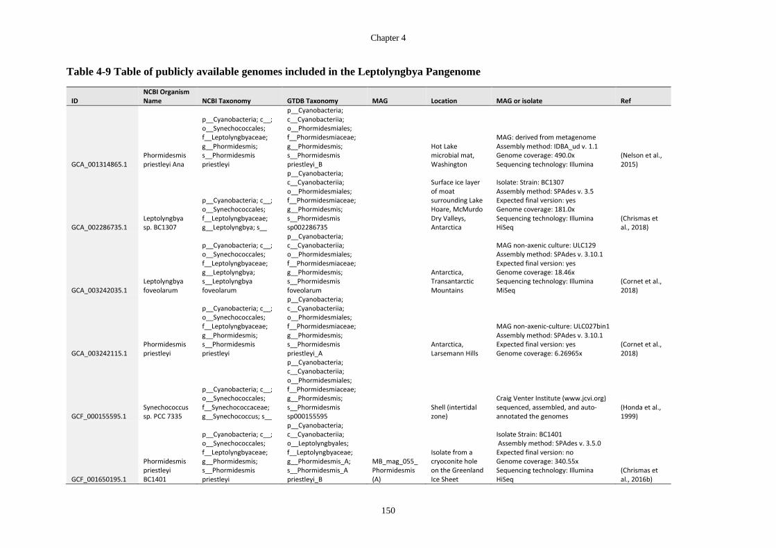
Chapter 4
150
Table 4-9 Table of publicly available genomes included in the Leptolyngbya Pangenome
ID NCBI Organism Name NCBI Taxonomy GTDB Taxonomy MAG Location MAG or isolate Ref
GCA_001314865.1 Phormidesmis priestleyi Ana
p__Cyanobacteria; c__; o__Synechococcales; f__Leptolyngbyaceae; g__Phormidesmis; s__Phormidesmis priestleyi
p__Cyanobacteria; c__Cyanobacteriia; o__Phormidesmiales; f__Phormidesmiaceae; g__Phormidesmis; s__Phormidesmis priestleyi_B
Hot Lake microbial mat, Washington
MAG: derived from metagenome Assembly method: IDBA_ud v. 1.1 Genome coverage: 490.0x Sequencing technology: Illumina
(Nelson et al., 2015)
GCA_002286735.1 Leptolyngbya sp. BC1307
p__Cyanobacteria; c__; o__Synechococcales; f__Leptolyngbyaceae; g__Leptolyngbya; s__
p__Cyanobacteria; c__Cyanobacteriia; o__Phormidesmiales; f__Phormidesmiaceae; g__Phormidesmis; s__Phormidesmis sp002286735
Surface ice layer of moat surrounding Lake Hoare, McMurdo Dry Valleys, Antarctica
Isolate: Strain: BC1307 Assembly method: SPAdes v. 3.5 Expected final version: yes Genome coverage: 181.0x Sequencing technology: Illumina HiSeq
(Chrismas et al., 2018)
GCA_003242035.1 Leptolyngbya foveolarum
p__Cyanobacteria; c__; o__Synechococcales; f__Leptolyngbyaceae; g__Leptolyngbya; s__Leptolyngbya foveolarum
p__Cyanobacteria; c__Cyanobacteriia; o__Phormidesmiales; f__Phormidesmiaceae; g__Phormidesmis; s__Phormidesmis foveolarum
Antarctica, Transantarctic Mountains
MAG non-axenic culture: ULC129 Assembly method: SPAdes v. 3.10.1 Expected final version: yes Genome coverage: 18.46x Sequencing technology: Illumina MiSeq
(Cornet et al., 2018)
GCA_003242115.1 Phormidesmis priestleyi
p__Cyanobacteria; c__; o__Synechococcales; f__Leptolyngbyaceae; g__Phormidesmis; s__Phormidesmis priestleyi
p__Cyanobacteria; c__Cyanobacteriia; o__Phormidesmiales; f__Phormidesmiaceae; g__Phormidesmis; s__Phormidesmis priestleyi_A
Antarctica, Larsemann Hills
MAG non-axenic-culture: ULC027bin1 Assembly method: SPAdes v. 3.10.1 Expected final version: yes Genome coverage: 6.26965x
(Cornet et al., 2018)
GCF_000155595.1 Synechococcus sp. PCC 7335
p__Cyanobacteria; c__; o__Synechococcales; f__Synechococcaceae; g__Synechococcus; s__
p__Cyanobacteria; c__Cyanobacteriia; o__Phormidesmiales; f__Phormidesmiaceae; g__Phormidesmis; s__Phormidesmis sp000155595
Shell (intertidal zone)
Craig Venter Institute (www.jcvi.org) sequenced, assembled, and auto-annotated the genomes
(Honda et al., 1999)
GCF_001650195.1
Phormidesmis priestleyi BC1401
p__Cyanobacteria; c__; o__Synechococcales; f__Leptolyngbyaceae; g__Phormidesmis; s__Phormidesmis priestleyi
p__Cyanobacteria; c__Cyanobacteriia; o__Leptolyngbyales; f__Leptolyngbyaceae; g__Phormidesmis_A; s__Phormidesmis_A priestleyi_B
MB_mag_055_Phormidesmis (A)
Isolate from a cryoconite hole on the Greenland Ice Sheet
Isolate Strain: BC1401 Assembly method: SPAdes v. 3.5.0 Expected final version: no Genome coverage: 340.55x Sequencing technology: Illumina HiSeq
(Chrismas et al., 2016b)

The Biotechnological Potential of Cryospheric Bacteria
151
ID NCBI Organism Name NCBI Taxonomy GTDB Taxonomy MAG Location MAG or isolate Ref
GCF_001895925.1
Phormidesmis priestleyi ULC007
p__Cyanobacteria; c__; o__Synechococcales; f__Leptolyngbyaceae; g__Phormidesmis; s__Phormidesmis priestleyi
p__Cyanobacteria; c__Cyanobacteriia; o__Leptolyngbyales; f__Leptolyngbyaceae; g__Phormidesmis_A; s__Phormidesmis_A priestleyi_A
MB_mag_055_Phormidesmis (B)
Antarctica, Larsemann Hills
MAG non-axenic-culture: ULC007bin1 Assembly method: SPAdes v. 3.10.1 Expected final version: yes Genome coverage: 26.62x Sequencing technology: Illumina MiSeq
(Cornet et al., 2018)
GCA_003249025.1 Leptolyngbya sp.
p__Cyanobacteria; c__; o__Synechococcales; f__Leptolyngbyaceae; g__Leptolyngbya; s__
p__Cyanobacteria; c__Cyanobacteriia; o__Leptolyngbyales; f__Leptolyngbyaceae; g__ULC077BIN1; s__ULC077BIN1 sp003249025
MB_mag_047_ULC077BIN1 (A)
Canada microbial mat
derived from metagenome Assembly method: SPAdes v. 3.10.1 Expected final version: yes Genome coverage: 15.08x Sequencing technology: Illumina MiSeq
(Cornet et al., 2018)
GCA_003249105.1 Leptolyngbya sp.
p__Cyanobacteria; c__; o__Synechococcales; f__Leptolyngbyaceae; g__Leptolyngbya; s__
p__Cyanobacteria; c__Cyanobacteriia; o__Phormidesmiales; f__Phormidesmiaceae; g__Nodosilinea; s__Nodosilinea sp003249105
CC_mag_060_Nodosilinea
Belgium, Renipont lake
MAG non-axenic culture: ULC186bin1 Assembly method: SPAdes v. 3.10.1 Expected final version: yes Genome coverage: 21.11x Sequencing technology: Illumina MiSeq
(Cornet et al., 2018)

Chapter 4
152
Figure 4-15 The Pangenome of Phormidesmis and Leptolyngba species and MAGs. Public genomes (black) are compared to MAGs (colour).
Regions of overlap represent common gene clusters, and non-overlapping regions represent a unique accessory genome. An ANI results matrix
(purple) reflects the relatedness of the MAGs and public genomes to each other.

The Biotechnological Potential of Cryospheric Bacteria
153
4.3.8.1 Functional Enrichment analysis
Functional enrichment analysis based on geographic location, environment type and GTDB
classification (Appendix Table D-14) was performed using the tool anvi-get-enriched-functions-
per-pan-group. This tool creates a frequency table of functions in genomes and uses a Generalized
Linear Model with the logit linkage function to compute an enrichment score and p-value for each
function with False Detection Rate (FDR) correction to p-values to account for multiple tests is
done using the package qvalue. The tool identifies groups within genomes, and then identifies
functions that are enriched within those groups. In this way it is possible to identify functions that
are characteristic of the genomes within a group, and absent from genomes from outside this group.
There was no functional enrichment identified between groups of genomes based on Environment
type, geographic location or GDTB classification. The non-significant results are likely due to a
lack of statistical power, as the number of samples per group were not large enough to reach
significance.
4.3.8.2 The functions of accessory genes in CC_mag_047 and cc_mag_055
After ordering the pangenome by gene cluster frequency and presence/ absence, the singleton gene
clusters (accessory genome) of the MAGs included in this pangenome were identified (Figure 4-
15). The identity and function of the singleton genes were analysed. MB_mag_047 had 472,
CC_mag_060 had 407 and CC_mag_055 had 102 gene clusters that were unique and not shared
with any other genome in the pangenome. Of these, 164 of the clusters were assigned to a COG
functional category. The accessory genes were not known to be specific to cold-adaptation.

Chapter 4
154
Table 4-10 COG Functional categories of accessory gene clusters in Leptolyngbya MAGs
COG Category CC_mag_055
CC_mag_060
MB_mag_047
Information Storage and Processing
[K] Transcription 0 19 5
[L] Replication, recombination, and repair 2 15 14
Cellular Processes and Signalling
[D] Cell cycle control, cell division, chromosome partitioning 1 0 2
[V] Defence mechanisms 3 3 6
[T] Signal transduction mechanisms 0 15 19
[M] Cell wall/membrane/envelope biogenesis 1 17 9
[U] Intracellular trafficking, secretion, and vesicular transport 1 0 6
[O] Posttranslational modification, protein turnover, chaperones 0 10 9
Metabolism
[C] Energy production and conversion 0 7 2
[G] Carbohydrate transport and metabolism 1 4 5
[E] Amino acid transport and metabolism 0 11 5
[F] Nucleotide transport and metabolism 0 3 1
[H] Coenzyme transport and metabolism 0 2 0
[I] Lipid transport and metabolism 0 1 0
[P] Inorganic ion transport and metabolism 0 4 6
[Q] Secondary metabolites biosynthesis, transport, and catabolism
0 6 5
Poorly Characterized
[S] Function unknown 12 64 70
Mixed
E, G 0 2 0
E, T 0 1 0
G, M 0 1 0
I, Q 0 3 0
N, T 0 1 0
Grand Total 21 189 164

The Biotechnological Potential of Cryospheric Bacteria
155
4.4 Discussion
The chapter describes 74 metagenome-assembled-genomes (MAGs) recovered from sea, soil and
cryoconite metagenomes from Ny-Ålesund, Svalbard. By their nature, reconstructed genomes
represent the most abundant members of a community, because they are constructed from the
longest contigs with the deepest coverage, proportional to their abundance in the original sample.
They are therefore useful to understand the functional and metabolic potential of the most abundant
members of a community. Using read mapping, the resolved genomes could be traced to exact
environments types and geographical locations to provide additional ecological insights.
4.4.1 Effect of environment complexity on ability to resolve MAGs
Deep shotgun sequencing of these environments confirmed the presence of fungal, algal, and viral
species in the sampled environments (Figure 4-4, Figure 4-6, and Figure 4-8). The higher the
relative proportion of non-bacterial taxa, the greater the difficulty in resolving genomes. Seawater
had a particularly high viral load. The relatively small assembly from seawater can be accounted
for by the fact that many reads belonged to abundant, but non-bacterial sources, such as viruses,
algae, and fungi. There were relatively fewer high quality MAGs reconstructed from soil, with
fewer of their reads being aligned to the final assembly which reflects the enormous diversity of
bacteria in the sample (Chapter 8, Table 8-7, Figure 8-7), which were not present in high enough
abundance to assemble into contigs > 2000 bp or groups of contigs large enough to form bins. The
high number of MAGs assembled from cryoconite libraries is due to a combination of (1) similarity
across sites, relatively high bacterial population relative to eukaryotes, and a small core community
of highly abundant species (Chapter 3). There was a good correlation between the taxonomy of the
reconstructed MAGs and the taxonomic classification of reads. For example, the most abundant
species from the reads-based taxonomic assignment in cryoconite were Phormidesmis,
Sphingomonas, Ktedonobacteria, Nostoc, Bradyrhizobium, Leptolyngba, Microbacteria,
Pseudanabaena, Granulicella, Illumatobacter and Rhizobacter which were all present in the MAG
collection. In soil, abundant reads-based taxa with MAG representatives include Sphingomonas,
Nostoc, several Actinobacteria, Leptolyngbya, Bradyrhizobium, Cecembia, Aquiflexum and
Sphingosinicella. Finally, the MAGs from seawater were from the most abundant phyla, the
Proteobacteria and Bacteroidetes.

Chapter 4
156
4.4.2 Phylogenomics of Svalbard MAGs
The vast majority of cultured isolates belong to just four phyla: Proteobacteria, Actinobacteria,
Firmicutes and Bacteroidetes (Culligan et al., 2014), and this has resulted in their
overrepresentation in genome databases. However, the use of metagenomics is greatly expanding
the tree of life as we can construct genomes of as-yet uncultivatable organisms. The MAGs in this
study belong to 14 different phyla. In order of abundance, these were the Proteobacteria (α = 13, γ
=8), Actinobacteriota (11), Bacteroidota (10) and the Cyanobacteria (6). The Chloroflexota (5) and
Chloroflexota_A (1), Armatimonadota (6), Acidobacteriota (4) and Patescibacteria (3) also had
several members. Finally, two MAGs each from the Myxococcota and Fibrobacterota, and a single
MAG member from Bdellovibrionota, Eremiobacterota and Gemmatimonadota were resolved.
Only two of the MAGs belonged to known species, (according to FastANI, cutoff radius of 95).
An additional 20 MAGs were closely related to know species (> 75% ANI) and the remainder of
the MAGs represent novel species that do not yet have representatives in databases (Table 4-7).
GTDB-Tk was used to classify the MAGs taxonomically and revealed that many of the resolved
genomes were closely related to isolates of cryospheric organisms from other sites and studies.
MB_mag_055_Phormidesmis, the most abundant MAG in the cryoconite samples, was most
similar to Phormidesmis priestleyi isolate (GCF_001650195.1) obtained from Greenland
cryoconite (Chrismas et al., 2016b) and DA_MAG_019_Granulicella was closest to
Salinibacterium xinjiangense (GCF_900230175.1), a novel psychrophilic, Gram-positive, yellow-
pigmented, and aerobic bacterium, from the China No. 1 glacier (Zhang et al., 2008). There were
also several MAGs that were closely related to species isolated from Arctic or Antarctic soils and
permafrost. MB_bin_070_QHBO01 was closest to a MAG QHBO01 sp003243965
(GCA_003243965.1) from desert soils of Antarctica (Ji et al., 2017), while DA_MAG_005_Palsa-
881, CC_MAG_041_Rhizobacter and DA_MAG_016_Rhizobacter were closely related to isolates
Palsa-881 sp003161535 (GCA_003161535.1) and Rhizobacter sp003152055 (GCA_003152055.1)
from Arctic Swedish permafrost (Woodcroft et al., 2018). In addition, three of the cyanobacterial
MAGs were from Canada; MB_MAG_036_Pseudanabaena and MB_mag_047_ULC077BIN1
both originate from microbial mats, and were closely related to Pseudanabaena frigida
(GCA_003242085.1) and ULC077BIN1 sp003249025 (GCA_003249025.1) respectively (Cornet
et al., 2018), while MX_MAG_032_Microcoleus is similar to Microcoleus sp003003725 from a
freshwater lake. Two of the seawater-derived MAGs, MX_mag_062_Ascidiaceihabitans and
MB_MAG_023_ASP10-02a were related to Ascidiaceihabitans sp002478745
(GCA_002478745.1) and ASP10-02a sp002335115 (GCA_002335115.1) which were both

The Biotechnological Potential of Cryospheric Bacteria
157
reconstructed from a North Sea marine metagenome (Parks et al., 2017). There were, however,
some surprises, such as the fact that MB_mag_049_Aquiflexuma is a close relative of Cecembia
rubra (GCF_003014575.1), a thermophilic species from a hot spring sediment in Tengchong,
Yunnan province, south-west China (Duan et al., 2015).
In addition to the bins included in this study, there were several bins possibly belonging to CPR
group that were excluded because they did not meet the quality for inclusion (>70% complete).
There were two bins that were identified as Candidatus Solibacter and one that was identified as
unknown Candidatus Saccharibacteria. The completion percentage is based off a catalogue of 71
single copy genes present in most bacteria, but the CPR may very well be missing several of these
genes and thus score below the threshold despite being complete. Because these MAGs could not
be assessed for completeness, they were excluded, but may be investigated further in future work.
4.4.3 Spatial distribution of MAGs across different sites
Using binning methods that take coverage across different samples into account, it was possible to
resolve highly related species with slightly different abundance and distribution across sample sites.
For example, two Alphaproteobacterial MAGs MB_MAG_028_Sandarakinorhabdus and
MB_bin_067_Sandarakinorhabdus, and four Gammaproteobacterial MAGs, DA_MAG_016_
Rhizobacter and CC_MAG_041_Rhizobacter and MB_MAG_034_UKL13-2 and CC_mag_053_
UKL13-2 could be distinguished based on differential coverage across different sites. Using a heat-
map of coverage to describe spatial distribution also revealed that the MAGs show habitat
preference. The Max-normalised ratio view (MAG-centric) showed a clear partitioning of
cryoconite-only, and sea-specific MAGs (Figure 4-11). The heterogeneity of soil samples was also
clear. The abundance view (sample-centric) showed that many of the MAGs are widely distributed,
with a high abundance at a single site, or within a habitat type and extremely low coverage at other
sites (Figure 4-12). Very low abundance at certain sites may be an artefact of read mapping,
whereby reads align to contigs because short fragments of the genome are identical between related,
but distinct species. Nonetheless, a pattern emerges that agrees with 16S rRNA gene amplicon
studies of cryoconite, showing dominance by a cyanobacterial Phormidesmis MAG, and a less
abundant tail community of Proteobacteria and Actinobacteria. Spatial mapping also revealed that
ML and VB are more like each other than AB or VL. While cryoconite sites clearly resembled each
other, the soil samples were far more heterogenous, particularly in cyanobacterial abundance. With
a total of six different cyanobacteria in this dataset, which often proved the most abundant at their
respective sites, MAGs from this phylum were examined in more detail.

Chapter 4
158
4.4.4 Cyanobacteria
These Cyanobacterial MAGs are interesting because Cyanobacteria are known to play vital roles
as ecosystem engineers in both cryoconite (Gokul et al., 2016; Hodson et al., 2010b; Langford et
al., 2010) and early soil development (Pushkareva et al., 2015; Rossi and De Philippis, 2015). Two
Leptolyngbya species could be resolved, MB_mag_055_Phormidesmis was dominant in AB, VB,
and ML cryoconite, and a different MB_mag_047_ULC077BIN1 was dominant in VL cryoconite.
A third closely related MAG (CC_mag_060_Nodosilinea) from the family Phormidesmiales, also
used to be classified as Leptolyngbya before reclassification by GTDB to Phormidesmiaceae
(Table 4.10). The MB_mag_055_Phormidesmis, is most similar to a Cyanobacterial strain isolated
from Greenland cryoconite (Chrismas et al., 2016b), and was present as the main Cyanobacterial
species and dominant community member in cryoconite on VB, ML and AB. It was also found at
low levels in all forefield soil sites, suggesting that this glacial species might carried downstream
in meltwaters and inoculate the soil. The MB_mag_047_ULC077BIN1 was the dominant
Cyanobacterial species in VL cryoconite but was completely absent from cryoconite on other
glaciers. It was however present at all forefield soil sites. VL is a markedly ‘different’ glacier in
terms of its community make up (Figure 4-3, and Figure 4-11), and it is possible that ‘cryoconite’
on VL is caused by soil blown onto the glacier that nevertheless acts the same way as in terms of
albedo and melting as true biological cryoconite granules would.
The CC_mag_060_Nodosilinea was found only in soil samples and was especially abundant in the
soil collected from sites closer to the glacier snout (time point 1 (F3T1) and time point 2 (F2T2)).
This raises the possibility that CC_mag_060_Nodosilinea is particularly important in the
development and stabilisation of recently exposed glacial soils. A novel Nodoslinea species has
recently been described in Svalbard (Davydov et al., 2020). Because there were three highly
abundant and closely related MAGs in our dataset, a pangenome of MB_mag_047, CC_mag_060
and CC_mag_055 was constructed and of the MAGs and their closest relatives (Figure 4-15, Table
4-9).
The pangenome was used to show the MAGs relationship to each other and to relatives within the
Leptolyngbya clade. Although these MAGs were closely related to known strains, they each had
accessory genomes, which was examined to see whether the accessory genome had any genes
responsible for specific habitat adaptation. However, the function of the accessory genes did not
signify any particular cold adaptation (Table 4-10), which is similar to previous comparisons of
cyanobacteria from different temperature zones (Chrismas et al., 2016b).
The Biotechnological Potential of Cryospheric Bacteria
159
Cyanobacteria often live in community with other heterotrophic bacteria (Cornet et al., 2018). In
this study two Alphaproteobacterial MAGs were identified in cryoconite that belong to the genus
Sandarakinorhabdus, MB_MAG_028_Sandarakinorhabdus and MB_bin_067_
Sandarakinorhabdus. Members of the Sandarakinorhabdus genus have previously been found
associated with cyanobacterial aggregates in freshwater lakes (Cai et al., 2018). Notably, two
Sandarakinorhabdus MAGs were recently identified in glacial ice (Trivedi et al., 2020), which
suggests that this genus might be common in glacial ice. Sandarakinorhabdus is a
bacteriochlorophyll a-containing, obligately aerobic bacterium isolated from freshwater lakes
(Gich and Overmann, 2006), however, a closely related strain (MC 3718T), which unfortunately
has not been genome-sequenced, has also been isolated from a tundra soil near Ny-Ålesund (M.
Kim et al., 2016).
4.4.5 Biogeochemical cycling in different environments
Biogeochemistry refers to the study of the processes by which organisms transform and recycle
organic and inorganic substances in the environment, as well as evaluating the effects of these
cycles (Madsen, 2011). In low nutrient glacial environments, microorganisms cycle nutrients to
ensure the sustained availability of a variety of nutrients. Cryoconite communities therefore play a
role in geochemical nutrient cycling of major nutrients such as carbon (C)(Anesio et al., 2009,
2010; Cameron et al., 2012b; Cook et al., 2016a; Hodson et al., 2010a; Langford et al., 2010),
nitrogen (N)(Cameron et al., 2012b; Edwards et al., 2013a; Larose et al., 2013b) and phosphorous
(P)(Cameron et al., 2012b; Cook et al., 2016b; Edwards et al., 2013a; Hodson et al., 2010a), as well
as sulfur (S)(Edwards et al., 2013a; Simon et al., 2009b; Trivedi et al., 2020) and iron (Fe)(Edwards
et al., 2013a). During the summer, in supraglacial regions where sunlight can penetrate the ice,
photoautotrophy provides nutrients for many complex food webs (Boetius et al., 2015). However,
during the winter polar night, and in the deeper subglacial habitats, chemoautotrophy is the main
contributor to food webs (Boetius et al., 2015).
In addition, nutrients, and bacteria from cryoconite are regularly transported to downstream
ecosystems during summer melt seasons (Anesio et al., 2009), therefore adding nutrients and
seeding organisms in recently exposed, and therefore biologically and nutrient sparse soil (Bradley
et al., 2014). The introduction of these nutrients to newly exposed glacial soils and the development
of the microbial communities that can supplement and maintain nutrient cycling in soils is one of
the most important factors driving soil development, and the eventual establishment of vegetation
(Bradley et al., 2014). Recently, a study of the metabolic potential of MAGs from a subsurface
Chapter 4
160
aquifer, revealed that very few microorganisms in a system can conduct multiple sequential redox
reactions, suggesting that organisms rely on substantial metabolic trade-off of redox reaction
products from one organism to another (Anantharaman et al., 2016). Interdependencies in nutrient
cycling in microbial communities are continually revealed in studies of MAGs from environments
such as a sulfur-rich glacial ecosystem (Trivedi et al., 2020), subsurface aquifer (Anantharaman et
al., 2016), deep sea hydrothermal sediments (Dombrowski et al., 2017), Svalbard permafrost
(Yaxin Xue et al., 2020), hypersaline soda lake brines (Vavourakis et al., 2016) and freshwater
lakes (Linz et al., 2018).
4.4.5.1 Carbon cycling
The organisms of cryoconite holes are involved in both carbon fixation (e.g. photosynthesis) and
carbon oxidation (e.g. respiration). The net ecosystem production (NEP) describes the balance
between carbon fixation and carbon oxidation and is expressed by the following:
NEP = PP – R (where PP is primary production and R is respiration)
When NEP > 0, photosynthesis (carbon fixation) exceeds respiration and cryoconite is acting as a
carbon sink (removing atmospheric carbon). When NEP < 0, the cryoconite is a carbon source
because carbon release via respiration exceeds the rate of carbon fixation (Cook et al., 2016b).
The external conditions which determine whether NEP is in positive or negative balance include:
water state and characteristics, the availability of nitrogen and phosphorous (Stibal and Tranter,
2007), sediment size and arrangement (Cook et al., 2016a; Telling et al., 2012), solar angle and
photosynthetically active radiation (PAR). The sediment angle, solar angle and PAR all affect the
amount of solar energy which can be harnessed by microorganisms for carbon fixation via
photosynthesis. For example, photoautotrophs may be responsible for net carbon fixation during
the sunny summer months, and net carbon oxidation via respiration during the dark winter months.
The availability of PAR explains why NEP is positive when sediment depth is less than 3mm
favouring carbon fixation by autotrophic organisms, and carbon oxidation is favoured by
heterotrophic organisms when sediment depth is greater than 3mm (Telling et al., 2012). This also
explains why net autotrophy occurs in cryoconite holes with thin debris layers, while net
heterotrophy occurs when sediment layers are deeper than 2-4 mm (Cook et al., 2010). Carbon
cycling has been measured via a number of techniques including measuring the rates of
photosynthesis and respiration, or via measuring the acquisition, storage or loss from cryoconite
holes (Cameron et al., 2012b).

The Biotechnological Potential of Cryospheric Bacteria
161
4.4.5.1.1 Carbon fixation
The contribution of cryoconite on the ML glacier surface on carbon cycling has previously been
investigated using in situ incubations of cryoconite–water mixtures to estimate respiration (1.174
± 0.182 μg C g−1 h−) and bacterial carbon production (0.040 ± 0.019 μg C g−1 h−1) (Hodson et al.,
2007). These estimates were extrapolated, using uninhabited aerial vehicle (UAV) image
acquisition to quantify the cryoconite over the entire glacier (0.42-1%). The results suggest that the
carbon flux on this glacier could be up to 12–14 kg C km−2 a−1 in the summer, showing that
cryoconite ecosystems can have a significant impact upon carbon cycling in glacial environments
(Hodson et al., 2007). Using 14C labelled bicarbonate to determine the rate of inorganic carbon
uptake in cryoconite sediment in vitro, it was determined that cyanobacterial photosynthesis was
the main process responsible for inorganic carbon fixation (75–93%), while heterotrophic uptake
only accounted for a minor part (6–15%) (Stibal and Tranter, 2007). The rate of photosynthesis in
meltwater on the ML glacier surface was lower than that of cryoconite, and within cryoconite holes,
the rate of photosynthesis was much higher at the bottom of the holes (0.63–156.99 µg C l–1 h–1)
than in the overlying meltwater (60-8.33 µg C l–1 h–1), which is not surprising considering the
density of organisms associated with the granules in the bottom of the holes (Säwström et al., 2002).
The most important gene in carbon fixation, responsible for the first rate-limiting step of
photosynthesis, is RubisCO (Ribulose-1,5-bisphosphate carboxylase/oxygenase), which has
ribulose-1,5-bisphosphate and carbon dioxide (CO2) as its substrates (Erb and Zarzycki, 2018).
There are several forms of RubisCO. The form most common in autotrophic bacteria is RubisCO
form I. Of these, there are several types, including the large subunit of form I red-like RubisCO
(cbbLR), the large subunit of form I green-like RubisCO (cbbLG) and the large subunit of RubisCO
in eukaryotes (rbcL). In a previous study, copies of the cbbLR gene from ML cryoconite most
closely resembled gene sequences from an Actinobacteria family Mycobacterium and
Alphaproteobacteria, order Rhizobiales (Cameron et al., 2012b). In this study, several MAGs had
copies of form I RubisCO, including an Actinobacteria, CC_MAG_025_Actinobacteria, from the
family Frankiaceae, two Alphaproteobacterial MAGs, MB_MAG_033_PALSA_911 and
CC_mag_052_Bradyrhizobium belonging to the family Acetobacteraceae and Xanthobacteraceae
respectively as well as a Gammaproteobacterial MAG CC_MAG_037_BOG_994, family
Burkholderiaceae. The MAG MB_bin_070_QHBO01 from the phylum Chloroflexota_A and
MX_mag_044_UBA5184 from the phylum Eremiobacterota also contained copies. There were
also form I RubisCO genes in all the cyanobacterial MAGs, except for cc_mag_071_Nostoc_ and
CC_mag_060_Nodoslinea. Previously amplicons of form I green-like RubisCO from
Chapter 4
162
Leptolyngbya and Nostoc were identified in ML cryoconite (Cameron et al., 2012b). Of note, the
cyanobacterial MAGs in this study had <90% completion, and therefore their absence may just
reflect the incomplete bins. Interestingly, all MAGs harbouring RubisCO form I genes were most
abundant in cryoconite, with the sole exception of MB_bin_070_QHBO01, which was more
abundant in soil.
In addition to carbon fixation from CO2, there are several pathways which take single-carbon
sources as substrates for assimilatory carbon pathways. We identified several methylotrophs,
methanol dehydrogenase (nmda) and S-(hydroxymethyl)mycothiol dehydrogenase (smdh) genes
in two and seven Actinobacterial MAGs, respectively. The nmda enzyme takes methanol as its
substrate and may play a role in extremely oligotrophic growth, or even or possibly enable
chemoautotrophic growth (Ohhata et al., 2007). The smdh enzyme is specific to Actinobacteria,
has formaldehyde (CH2O) as one of its substrates and, was found in seven of the ten Actinobacterial
MAGs (DA_MAG_002_Bog_756, MB_MAG_039_Ilumatobacter, MB_MAG_021_Micro
bacteriaceae CC_MAG_025_Actinobacteria, MX_MAG_013_Actinobacteria, DA_MAG_007
_Iso899, and MB_MAG_008_Micromonospora). Most of the Actinobacterial MAGs are more
prevalent in cryoconite, but DA_MAG_007_Iso899 was more abundant in soil. There is evidence
of carbon monoxide (CO) oxidation via carbon monoxide dehydrogenase (coxSML) genes in
several Acidobacteria (3/4), Actinobacteria (5/11), Alphaproteobacteria (8/15) and
Gammaproteobacteria (4/8) MAGs. There is evidence that CO is a major energy source for aerobic
heterotrophic bacteria in organic carbon deprived environments (Cordero et al., 2019).
4.4.5.2 Nitrogen cycling
Nitrogen can exist in multiple forms in the environment. It is present as N2, the most abundant gas
in our atmosphere (~78%). However, despite the abundance of N2, the fixation of nitrogen gas is
all but impossible for almost all organisms, save a few microorganisms. Nitrogen is mainly
assimilated into organisms via reduced inorganic compounds such as ammonium and ammonia and
oxidised inorganic forms, such nitrate, nitrite, nitric acid and nitrogen oxides (Larose et al., 2013b).
It is also recycled between organisms in the form of organic nitrogen compounds such as urea,
amines, and proteins. Prior to the invention of the Haber Process, the fixation and denitrification
of nitrogen was in balance. However, as more nitrogen compounds have been produced via this
process for agriculture and industry, the available nitrogen in the environment has been increasing,
and there is evidence that this increase may be upsetting delicate ecosystems, including the Arctic
(Larose et al., 2013b).

The Biotechnological Potential of Cryospheric Bacteria
163
4.4.5.2.1 Nitrogen fixation
There was only one MAG capable of nitrogen fixation from the genomes we could resolve. The
CC_bin_071_Nostoc had nifD and nifH genes (Figure 4-13 and Figure 4-14), responsible for
nitrogen fixation. Nostoc is known to be capable of nitrogen fixation (Solheim et al., 1996).
CC_bin_071_Nostoc was present in cryoconite on VL and AB and in all soil sites, with a
particularly high abundance in VL cryoconite and F2T2 soil. Although previous studies have tried
to identify genes associated with nitrogen fixation in cryoconite across four glacial sites on
Svalbard, and one glacial site in Antarctica, no genes were amplified, despite evidence that taxa
capable of fixation were present (Cameron et al., 2012b). A similar study on an Arctic snowpack
metagenome found only a low number of reads associated to nitrogen fixation in their despite the
presence of genera capable of nitrogen fixation (Larose et al., 2013b). Therefore, in this study, the
gene responsible for nitrogen fixation in Nostoc species in cryoconite and soil was detected.
4.4.5.2.2 Nitrate reduction
The napA and narG genes are involved in denitrification and dissimilatory nitrate reduction. The
napA and narG genes encode a periplasmic and membrane nitrate reductase respectively which
reduce nitrate (NO3-) to nitrite (NO2
-). Previously, napA and / or narG was amplified from all
cryoconite communities from 8 different glaciers on Svalbard including ML (Cameron et al.,
2012b). Clones with the napA gene from the Foxfanna glacier in Svalbard shared 76-84% sequence
similarity with members of Alpha, Beta or Gammaproteobacteria classes (Cameron et al., 2012b).
In this study, an Alphaproteobacterial MAG CC_mag_052_Brazyrhizobium from the order
Rhizobiales with a copy of the napA gene was present in all soil and cryoconite samples. A second
MAG, MB_MAG_020_Cyclobacteriaceae from the Bacteroidota had a copy of the napA gene but
was present only in the F3T3_Ludox samples, which may not be representative of the microbial
community due to extraction bias. The narG gene clones previously identified in Foxfanna
cryoconite were most like uncultured and unclassified bacteria, as well as Rhodobacterales and
Rhizobiales from the Alphaproteobacteria, and Burkholderiales from the Betaproteobacteria
(Cameron et al., 2012b). In this study, the narG gene was present in two Actinobacterial MAGs,
CC_MAG_025_Actinobacteria and MB_MAG_008_Micromonospora and two
Alphaproteobacterial MAGs, MB_MAG_004 and MX_MAG_022_Pararhodobacter. Both
Actinobacterial MAGs were common in cryoconite samples, however the proteobacterial MAGs
were from the F3T3_Ludox samples.

Chapter 4
164
4.4.5.3 Sulfur
The most common gene for sulfur cycling was sulfur dioxygenas (sdo). Sdo oxidizes the sulfane
sulfur in GSSH to sulfite, and there were 39 MAGs that had at least one of these genes. The sulfate
adenylyltransferase (sat), gene, was detected in the majority of Cyanobacterial (5/6) and
Chloroflexota genomes (4/5) as well as in a few Acidobacteria (2/5), Alphabproeobacteria (2/13)
and Gammaproteobacteria (1/8). Recently, a sulfur rich Canadian glacial system was investigated
for sulfur genes (Trivedi et al., 2020). In addition, there was sulfur oxidation visa the Sulphur
Oxidising (sox) pathways in several of the Alphaproteobacterial (3) and Gammaproteobacterial
MAGs (6).
4.4.6 Advantages to this study
This study makes several important contributions. Firstly, and most importantly, this study
describes a glacial ecosystem (cryoconite, forefield soil) that has previously only been described
using 16S rRNA and biogeochemical gene amplicon studies. Based on GTDB-Tk classification,
72 of the MAGs represent new species that do not have representatives in known databases. The
MAGs represent a dataset that can be annotated and interrogated to any effect using any of the
available databases. Indeed, the mining of these genomes for bioactive secondary metabolites with
useful industrial functions will be the focus of Chapter 5.
The ML glacier has been investigated for several decades, mostly using amplicon analysis, either
16S rRNA gene analysis or amplicon analysis of specific genes that form part of a biogeochemical
pathway. Both approaches are beset by issues such as amplification bias, and although attempts are
made to infer functional information from 16S rRNA phylotype, these inferences are guesses at
best. The actual presence and annotation of function genes in microbial communities is vital to gain
true insight into cooperation and ecosystem function. The investigation of biogeochemical cycling
using amplicon sequencing relies on primers and therefore only captures highly similar sequences.
HMMer analysis, like we performed in this study, is likely to capture a much more diverse set of
sequences. Likewise, while amplicons can only capture single gene products, HMMer scanning of
MAGs can capture different processes in the same pathway and tell us how many of those genes
from different pathways occur in a single organism, and in different spatially co-occurring
organisms. This analysis allows us to go from a ‘bag-of-genes’ to a ‘bag-of-genomes’ (Frioux et
al., 2020).

The Biotechnological Potential of Cryospheric Bacteria
165
4.4.7 Limitations of this study
MAGs still only describe the functional potential of the most abundant bacteria in a community,
not necessarily the most active bacteria. Concurrent transcriptomics and metabolomics studies of
these environments would give a far greater resolution of community metabolisms, regulation, and
the contribution of various members. In addition, many reads and contigs from many of the less
abundant bacteria failed to be binned and meet the criteria for MAG inclusion and are thus lost
from the interpretation, providing an incomplete picture of the whole community.
4.4.7.1 Extraction bias and sample complexity
There were three samples sequenced from the same soil site (F3T3), using different methods which
revealed that enormous bias is introduced by different extraction methods. DNA extracted using
density gradient centrifugation to extract DNA from whole cells (F3T3_Lud) was missing several
taxa that were abundant in samples extracted using alternate methods. This library also contained
a greater relative number of reads aligning to contigs, and several bins that were absent in other
samples. Five different Bacteroidota MAGs were constructed from the Ludox sample. However,
the Bacteroidota are not overly abundant in soil from other sites or using other extraction methods.
4.4.7.2 Struggle to obtain 16S rRNA operons
Very few 16S rRNA operons were identified by HMM screening of the bins. This is a major
drawback because it prevents the comparison of these MAGs to the vast literature which compares
16S rRNA genes at high resolution in this environment (Edwards et al., 2014). The problem has
previously been described by other authors (Cornet et al., 2018; Hauptmann et al., 2017) who
speculate that the frequent loss of rRNA genes is caused by the presence of multiple copies of the
rRNA operon in many bacterial genomes, resulting in short rRNA-bearing contigs due to
incomplete assembly of repeated regions. Because these contigs are dominated by the rRNA
operon, they have higher sequencing coverage and divergent tetranucleotide frequencies (TNFs),
two properties that are used by binning software to determine bin assignment (Cornet et al., 2018).
Similarly, when comparing methods for determining microbial abundance in samples from the
Greenland ice-sheet, EFM was the most accurate and reliable method for determining abundance,
yet there was no correlation between qPCR and EFM abundance ratios, which could be due to a
difference in the number of ribosomal RNA operon copies per cell (Stibal et al., 2015).
4.4.7.3 Inability to resolve highly similar strains
Co-assembly of several metagenomes containing very closely related populations often hinders
confident assignments of shared contigs into individual bins (Shaiber and Eren, 2019). It is possible

Chapter 4
166
that several of the MAGs in this collection reflect composite genomes. An example of a possible
composite genome is CC-mag_Nostoc_071, which could reflect several related but distinct Nostoc
species. The identification of composite and high-quality bins is discussed in Chapter 8.
4.4.8 Future work
Both the resolution of 16S rRNA genes in MAGs as well as the differentiation of closely related
strains will be significantly aided by long-read sequencing. A hybrid assembly, which combines
nanopore and Illumina data will create long scaffolds. Long sequences can bridge repetitive regions
and regions of low coverage therefore solve issues of synteny and multi-gene operons. This
approach has already been applied in wastewater studies, where several of the recovered genomes
were complete circular genomes (Singleton et al., 2020).
4.5 Conclusion
In this study, via co-assembly of soil, cryoconite and seawater metagenomes, it was possible to
reconstruct 74 high and medium quality MAGs from the most abundant community members. The
mean coverage of these MAGs and their distribution across different samples, tells us about their
abundance and distribution in various environmental sites. The MAGs belonged to species detected
in high abundance by numerous 16S rRNA gene surveys, thus validating predictions by 16S rRNA
amplicon studies. Notably, six cyanobacterial MAGs were resolved, which appear to have strong
habitat preference and possibly play viral roles in cryoconite and early soil formation. In addition,
the presence and absence of several enzymes involved in the major biogeochemical cycles were
described. The MAGs assembled from this environment provide important ecological information
about this highly threatened environment, which is highly valuable, however, they are also
extremely useful for downstream bioprospecting applications. The genomic content and
distribution of MAGS provides necessary information for strategic cocultivation and heterologous
expression. In terms of cultivating ‘microbial dark matter’, the occurrence of several MAGs at a
single site tells us which bacteria might be required for successful co-cultivation. Likewise, an
analysis of KEGG pathways and modules will provide information on required nutrients and
supplements and antimicrobial resistance. If a particular NP has been targeted for functional
analysis and heterologous expression, the phylogenomic information will help in the selection of a
closely related host, and access to the whole genomes will provide information on possible
regulation, required substrates and chaperones. Finally, if a target is identified in one of the
genomes, read mapping allows one to target future sampling efforts to the sites here it is in high
abundance.

The Biotechnological Potential of Cryospheric Bacteria
167
5 THE SECONDARY
METABOLITES OF SOIL AND
CRYOCONITE HAVE A RANGE
OF BIOTECHNOLOGICAL
APPLICATIONS
5.1 Introduction
Bioprospecting is the process by which organisms are investigated for natural products (NPs) that
can be of societal benefit. Replication and rediscovery of the same compounds has become a major
problem in bioprospecting, and one solution is to turn to environments that have extreme
environmental conditions, and that have not yet been fully explored; as both of these factors
increase the chance of a novel discovery (Knight et al., 2003). Although marine (Amoutzias et al.,
2016; Giordano et al., 2015; Wietz et al., 2012) and soil (Feng et al., 2012, 2011) environments
have been extensively investigated for antimicrobial compounds, the cryosphere remains under-
explored.
Arctic microorganisms have adapted to extreme conditions such as cold temperatures, high summer
UV radiation, and strong osmotic gradients- from extreme salinity to extremely dilute conditions
(Maccario et al., 2015). Secondary metabolites form part of this adaptation arsenal, from pigments
and antioxidants that protect against high UV radiation, to exopolysaccharides (EPS) that protect
against desiccation and allow cells to form biofilms where they can sequester nutrients and create
stable ecosystems, to a vast range of antimicrobial compounds that allow organisms to compete for
limited nutrients (Piel, 2011). Replication in pharmaceutical bioprospecting is exacerbated because
the detection of NPs has historically depended on cultivation of the producing strain and the
expression and secretion of the NP of interest. However, this approach favours the rediscovery of
compounds from highly investigated cultivatable strains and omits the biosynthetic potential of the
99% of uncultivatable bacteria and of cryptic biosynthetic gene clusters (BGCs)(Cimermancic et
Chapter 5
168
al., 2014). Cryptic BGCs are gene clusters that synthesise unknown compounds, because they are
expressed only under certain conditions (Butler et al., 2016). They may therefore be present in a
cultivated strain, but the factors that regulate its expression remain unknown. An analysis of the
genomes of 1154 archaeal and bacterial organisms predicted 33351 putative BGCs, many of which
encode secondary metabolites that have never been detected and it is suspected that the current list
of BGCs currently vastly underestimates the true number present. (Cimermancic et al., 2014). In
addition, systematic surveys of thousands of sequenced microbial genomes showed that generally,
silent clusters outnumber those that get expressed in laboratory cultures (Butler, 2004). Together,
this suggests enormous untapped potential in the genomes of microbes (Butler, 2004). Sequence-
based metagenomics is therefore a timely, much-needed tool to identify BGCs that otherwise elude
detection because they allow us to access the biosynthetic potential of uncultivable bacteria and
cryptic gene clusters.
The use of MAGs to search for BGCs is relatively new, but has previously been attempted from 26
metagenomic samples collected over various months in 2013, 2014 and 2015 from Lake Stechlin
in north-eastern Germany (Cuadrat et al., 2018). Although MAGs have been constructed from
several Arctic environments, including soil (Yaxin Xue et al., 2020), cryoconite (Hauptmann et al.,
2017) and a Canadian glacier (Trivedi et al., 2020), this chapter is the first time that MAGs from
an Arctic metagenome have been screened for biotechnologically relevant secondary metabolite
BGCs.
In this chapter, the focus is on three main applications of secondary metabolites: EPS, antioxidants,
and antimicrobial compounds, which are hypothesised to be abundant because of their role as
adaption mechanisms to the environment. Exopolysaccharides (EPS) are synthesized by many
bacteria, where they enable microorganisms to endure extremes of temperature, salinity and low
nutrient availability (Poli et al., 2010). Depending on the nature of the EPS, these substances may
find uses in the pharmaceutical to food-processing fields, or even be utilised in the remediation of
polluted due to their detoxification capability (Poli et al., 2010). EPS synthesised by the Arctic
bacterium, Polaribacter sp. SM1127, has high antioxidant activity and moisture-retaining
properties make them excellent for use in cosmetic and food industries (Sun et al., 2015), while an
EPS from Pseudoalteromonas arctica protects against freeze thaw injury and has utility as a
cryoprotectant in the medical and food industries (Kim and Yim, 2007). The main Cyanobacterial
strain in Svalbard cryoconite is Phormidesmis Priestleyi, which is similar to the Greenland
Phormidesmis Priestleyi strain that is a prolific producer of EPS (Chrismas et al., 2016b).

The Biotechnological Potential of Cryospheric Bacteria
169
Although carotenoids and terpenoid compounds from the Arctic are often investigated in relation
to their role in glacier and ice-sheet darkening, and their contribution to glacier melt and sea level
rise (Benning et al., 2014; Lutz et al., 2014), these compounds have numerous useful properties.
Terpenoid and carotenoid clusters have known biotechnological applications as pigments,
antioxidants, and UV compounds (Chrismas et al., 2016b, 2018; Mandelli et al., 2012). Select
terpenoids and carotenoids also have potential antifungal, antitumor and antibacterial activity
(Paduch et al., 2007; Sajjad et al., 2020). Finally, antimicrobial compounds can be synthesized by
a vast array of BGCs ranging from saccharides to fatty acids to NRPS and polyketides. Growing
antimicrobial resistance poses a serious threat to human health and novel antibiotics are urgently
needed (Sabtu et al., 2015; Ventola, 2015). Some recently discovered antibiotics have been
discovered from metagenomic approaches, illustrating the potential of this approach (Bauer et al.,
2010; Feng et al., 2012; Kallifidas et al., 2012).
In this chapter the secondary metabolites of soil and cryoconite were examined to identify BGCs
that may have useful application in pharmaceutical applications. Given the environmental
conditions, terpenoid clusters such as carotenoids (pigments), EPS and antimicrobial compounds
were a focus. Once BGCs of interest had been identified, the metabolome (LC-MS data) was
searched to see whether the putative metabolites could be detected from amongst the raw
metabolites.
5.1.1 Aims and objectives
1) Compare the types of BGC clusters detected in contigs of individual cryoconite, soil and
seawater assemblies.
2) Run antiSMASH and BiG-SCAPE on the Svalbard MAGS (from Chapter 4) to identify BGCs
with biotechnological potential.
3) Examine the BGCs of the Cyanobacterial MAGs in detail, as they are the most abundant species
in the environment and play important roles as ecosystem engineers as well as contributing
significantly to the metabolome because of their high proportion in the environment.
4) Try to identify possible antimicrobial compounds from the most talented Actinobacterial MAG
in the dataset.
5) Compare the metabolomic profiles of soil and cryoconite using LC-MS to the predicted
metabolites from MAGs to see if predicted and actual metabolic profiles are similar.

Chapter 5
170
5.2 Methods
5.2.1 Samples
The shotgun libraries and the MAGs included in this chapter have been described previously
(Chapter 4). The metabolite extractions were performed on cryoconite samples from several
different cryoconite holes across four glaciers near Ny Ålesund, Svalbard in the summer of 2018.
Raw metabolites from soil were extracted from 15 soil samples, comprising a three by five transect
of the ML glacier forefield. A map of the locations of the cryoconite holes and the forefield transect
are shown in Chapter 2, Figure 2-1, and the GPS coordinates of the cryoconite holes are in
Appendix Table B-1. The samples included in the metabolite analysis are listed in Table 5-1.
Table 5-1 Table of sample sites for metabolite extractions and shotgun metagenome
sequencing
Environment Glacier Metabolite analysis Shotgun library Library size (reads)
Cryoconite Austre Brøggerbreen
AB1801, AB1802, AB1803, AB1804, AB1805, AB1805, AB1807, AB1808
Cryoconite_AB_18 64,909,032
Midtre Lovénbreen
ML1801, ML1802, ML1803, ML1804, ML1805, ML1806
Cryoconite_ML_17, Cryoconite_ML_18
28,795,356, 28,471,672
Vestre Brøggerbreen
VB1801, VB1802, VB1803, VB1804, VB1805, VB1806
Cryoconite_VB_17, Cryoconite_VB_18
34,504,862, 29,787,650
Vestre Lovénbreen
VL1801, VL1802, VL1803, VL1804
Cryoconite_VL_18 14,939,536
Soil Time0 F1T0, F2T0, F3T0 NA NA
Time1 F1T1, F2T1, F3T1 Soil_S7_F3T1 35,482,472
Time2 F1T2, F2T2, F2T2 Soil_S6_F2T2 29,116,044
Time3 F1T3, F2T3, F3T3 Soil_S1_F3T3_Lud, Soil_S2_F3T3_FD, Soil_S3_F3T3_PM, Soil_S4_F1T3
40,079,596, 113,754,008, 44,915,524, 37,684,166
Time4 F1T4, F2T4, F3T4 Soil_S5_F1T4, Soil_S8_F2T4
38,762,496, 35,085,040
Bolded entries show the matching shotgun metagenomes and metabolite extractions. Only one cryoconite hole from each glacier was sequenced using shotgun sequencing, whereas metabolites were extracted from each cryoconite hole on each glacier. Likewise, metabolites were extracted from each glacier forefield soil site, but only selected sites were sequenced by shotgun sequencing. Two cryoconite shotgun libraries from 2017 were sequenced using shotgun sequencing, but there was not sufficient cryoconite left to do metabolite extractions.

The Biotechnological Potential of Cryospheric Bacteria
171
5.2.2 Bioinformatics detection of BGCs
Reads from cryoconite, seawater and soil were assembled using MEGAHIT as described in Section
4.3.3 and Section 8.3.3. Analysis was run on single-environment co-assemblies (Table 5-2) and on
the combined Svalbard libraries (Figure 4-8, Table 4-3) that had been binned into high quality
MAGs in Chapter 4. The benefit of screening the MAGs is that the BGCs inherit the phylogenetic
and spatial distribution information from the MAG, and clusters that co-occur together within the
same genome can be identified. However, the MAGs represent only a small portion of the contigs
database, and there may be many novel BGCs in the neglected contigs. Since one of the overall
aims of the study was to link BGCs and metabolites from the same environment, it was decided to
also screen the contigs databases of separate soil, cryoconite and seawater assemblies. Although
these clusters will not have the information provided by the MAGs, such as coverage, distribution
and phylogenetic origin, the databases are smaller, therefore easier to screen with antiSMASH;
environment-specific and therefore easy to link to LC-MS data; and most importantly, all of the
contigs can be screened., rather than just the contigs that could be binned into a high quality MAG.
5.2.2.1 antiSMASH to detect secondary metabolites
All contigs from the cryoconite, soil and seawater assemblies were run locally through antiSMASH
(v.4) and submitted in batches to the antiSMASH server (v5)
(https://antismash.secondarymetabolites.org). In addition, MAGs from the combined Svalbard
assembly (Chapter 4) were submitted to the antiSMASH server (v.5).
5.2.2.2 Network analysis of secondary metabolites using Big-SCAPE
The genbank files from each cluster from each MAG were downloaded from the antiSMASH
server and analysed using BiG-SCAPE (Biosynthetic Gene Similarity Clustering and Prospecting
Engine) (Navarro-Muñoz et al., 2020). BiG-SCAPE is a software package that constructs sequence
similarity networks of BGCs and groups them into gene cluster families (GCFs). BiG-SCAPE does
this by rapidly calculating a distance matrix between gene clusters based on a comparison of their
protein domain content, order, copy number, and sequence identity. BiG-SCAPE was run using the
parameters --mix --cutoffs 0.7 and both included MiBIG database versions were compared (--
mibig13, --mibig).

Chapter 5
172
5.2.3 Metabolomics
Raw metabolites were extracted from soil and cryoconite. For cryoconite, each cryoconite hole
from each of the four glaciers sampled (AB = 8; ML= 6; VB= 6; VL = 4) was treated as a replicate.
Soil from the glacier forefield was collected from three time points in three transects, with each
time point intended to from a replicate. Samples were stored at -20 °C until metabolite extraction.
5.2.3.1 Raw Metabolite extraction
Prior to metabolite extraction, soil and cryoconite samples were freeze dried. Thereafter, 100 mg
± 1 mg of dried soil and cryoconite were placed into 2 mL microcentrifuge tubes. Cells were lysed
by repeated cycles of freeze-thaw in liquid nitrogen, then homogenised using a vortex at maximum
speed. Samples were then put on ice and 1mL of chloroform: methanol: dH2O (1: 2. 5: 1) was
added. The samples were mixed again with a vortex prior to centrifuging at 3 °C at 5000 x g for 3
min. For ‘whole’ metabolite extractions (i.e. polar and non-polar phases together) the supernatants
were decanted into clean labelled microcentrifuge tubes and dried, using a Buchi Rotavapor RE120
with Buchi V5-1 vacuum and Buchi 461 water bath at 25 °C (Buchi Ltd., Postfach, Switzerland),
alongside a Techne RB-5A refrigerated bath at 3 °C (Techne Inc., Burlington, NJ, US) and stored
at -80 °C. An aliquot of 0.5 mL of 70% ethanol was added to the samples, mixed with a vortex and
centrifuged at 3°C at 5000 x g for 3 min. Thereafter, 50 μL of supernatant was removed and added
to 150 μL of ≈ 4°C 70% aqueous methanol (made up of HPLC grade methanol and ultrapure water)
and mixed through vortexing for five seconds. Samples were stored at -20 °C until ready to use.
5.2.3.2 LC-MS (Liquid Chromatography –Mass Spectrometry)
Extracts were prepared for mass spectrometry by resuspending 50 µL of the solvent in 200 µL of
70% methanol:water (4°C) in a 2 mL borosilicate glass vial (HiChrom Limited) with Target
MicroSert™ flat base inserts (National Scientific Company, Rockwood, TN, USA) and sealed with
polytetrafluoroethylene (PTFE) seal aluminium crimp caps (Thermo Scientific™, Waltham, MA,
USA). Vials were agitated for 5 seconds with a vortex and stored at -20°C until analysis by Flow
Injection Electrospray Ionisation Mass Spectrometry (FI-ESI-MS) using a linear ion trap quadruple
(LTQ) mass spectrometer (ThermoFinnigan, San Jose, CA) at the IBERS High Resolution
Metabolomics Laboratory (Edward Llwyd Building, Penglais, Aberystwyth University).
5.2.3.3 Metabolomics analysis
Principle component analysis (PCA), multidimensional scaling (MDS) of unsupervised random
forest proximities and supervised principle component linear discriminant analysis (PC-LDA) were
used to assess the overall data structure and class relationships.

The Biotechnological Potential of Cryospheric Bacteria
173
Figure 5-1 Ideal workflow for the exploring the metabolites of Svalbard soil and cryoconite
using a mix of metabolomics and metagenomics.

Chapter 5
174
5.3 Results
5.3.1 Assembly
The assembly statistics and contig distribution of the cryoconite, soil and seawater assemblies
used in this chapter are shown in Table 5-2. The minimum contig size for inclusion in the
assembly was 2000 bp. The cryoconite assembly was the largest (538 521 980 bp) from 115949
contigs, followed by the soil assembly (208 560 096 bp) from 49641 contigs, and finally the
seawater assembly was considerably smaller than the others (26 970 110 bp) and 6451 contigs.
Each of the individual environmental libraries was assembled separately, to compare contigs
from the different environments. The MAGs included in this study from Chapter 4 are from a
co-assembly of all the environments together.

The Biotechnological Potential of Cryospheric Bacteria
175
Table 5-2 Table comparing Assembly statistics and contig size distribution of sea, soil and cryoconite assemblies.
Assembly Longest contig (bp)
Nx (Lx) Length
(bp)
Number of
contigs
Sum length (bp)
Contig Length Histogram
Contig Length Histogram
Contig Length Histogram
(1bp <= len < 10Kbp)
(10Kbp <= len < 100Kbp)
(len >= 100Kbp)
sea-MEGAHIT.contigs
115659
N50: 4236 >= 106 0 0
L50: (1450) >= 105 2 221424
N75: 2686 >= 104 321 6766634
L75: (3510) >= 103 6451 26970110
N90: 2225 >= 500 6451 26970110
L90: (5171) >= 1 6451 26970110
soil-MEGAHIT.contigs
300154
N50: 4111 >= 106 0 0
L50: (10133) >= 105 45 6597658
N75: 2616 >= 104 2366 59047038
L75: (26569) >= 103 49641 208560096
N90: 2199 >= 500 49641 208560096
L90: (39681) >= 1 49641 208560096
cryoconite-MEGAHIT.contigs
315846
N50: 5126 >= 106 0 0
L50: (24906) >= 105 18 2524410
N75: 2995 >= 104 8246 154707901
L75: (60198) >= 103 115949 538521980
N90: 2329 >= 500 115949 538521980
L90: (90952) >= 1 115949 538521980

Chapter 5
176
5.3.2 Screening MAGs for BGCs
The number and types of clusters detected in each MAG are tabulated in Figure 5-2 and Figure
5-3. There were 1742 BGCs detected in the 74 MAGs. Of these, 278 of the BGCs had similarity
to known clusters in the MIBiG database (Appendix Table E-1). Of the 278 known compounds,
143 of them were unique. The compounds synthesized by the remaining 1464 clusters are
unknown. Several large contigs had more than one cluster, or contained hybrid clusters, and
therefore more than one cluster type was counted in a single region by the antiSMASH
algorithm (Examples in Figure 5-11 and Figure 5-12). Notably, the primary cluster category
detected by the antiSMASH algorithm is not always the same as the category of the closest
BGC in the MIBiG database (Appendix Table E-1, Table E-2, Table E-3 and Table E-4).
The most abundant cluster type was the saccharides (1214), followed by fatty acids (212), and
terpenes (122). There were a surprisingly high number of halogenated clusters (69), although
these may simply be short clusters with halogenase tailoring enzymes that add halogen products
to compound backbones synthesized by other BGCs.
In total there were 72 NRPS and 30 NRPS-like clusters across the MAGS. These BGC are
quite abundant in the Chloroflexota (NRPS=22, NRPS-like=8) and in the Cyanobacteria
(NRPS=7, NRPS-like=2), while a single Actinobacterial MAG (DA_MAG_007_Iso899) is
extremely talented with 17 and 4 NRPS and NRPS-like clusters, respectively. The bacteriocins
were also prevalent across many clades with 36 different clusters detected.
There are several BGC types that are more prevalent in certain clades than others. For example,
there were only four lassopeptides detected, and three were in Actinobacterial MAGs. Across
the Proteobacteria, six of the seven MAGs from the family Sphingomonadaceae have a T3PKS
cluster, while 5/6 Burkholderiales had an arylpolyrene cluster.

The Biotechnological Potential of Cryospheric Bacteria
177
Figure 5-2 Secondary metabolite clusters in MAGs from the Acidobacteriota, Actinobacteriota, Armatimonadota, Bacteroidota, Bdellovibrionota,
Chloroflexota, Chloroflexota_A phyla. Table showing the number and types of clusters detected by antiSMASH 5. The MAGs are arranged by taxonomic
clade, and the relative abundance in each sample (expressed as max-normalised-abundance) is shown per MAG.
Phylum Class Order Family Genome (MAG)
T1P
KS
T2P
KS
T3P
KS
hglE-K
S
PK
S-like
arylpo
lyene
resorcin
ol
ladd
erane
nrp
s
nrp
s-like
terpen
e
lanth
ipep
tide
bacterio
cin
betalacto
ne
thio
pep
tide
linarid
in
LAP
lassop
eptid
e
ectoin
e
bu
tyrolacto
ne
nu
cleosid
e
hserlacto
ne
ph
osp
ho
nate
fused
acyl_am
ino
_acid
s
NA
GG
N
TfuA
-related
saccharid
e
fatty_acid
halo
genated
Clu
sters p
er
gen
om
e
Cryoconite_AB
_18
Cryoconite_ML_17
Cryoconite_ML_18
Cryoconite_VB
_17
Cryoconite_VB
_18
Cryoconite_VL_18
Sea_SS1
Sea_SS2
Sea_SS3
Soil_S1_F3T3_Lud
Soil_S2_F3T3_FD
Soil_S3_F3T3_PM
Soil_S4_F1T3
Soil_S5_F1T4
Soil_S6_F2T2
Soil_S7_F3T1
Soil_S8_F2T4
Acidobacteriales Acidobacteriaceae 1 DA_MAG_019_Granulicella 1 0 2 0 0 0 0 0 1 0 3 0 0 0 0 0 0 1 0 0 0 0 0 0 0 0 0 18 3 1 30 0.6 0.9 0.7 1.0 0.6 0.0 0.0 0.0 0.0 0.0 0.0 0.0 0.0 0.0 0.0 0.0 0.0
Bryobacterales Bryobacteraceae 2 MB_bin_069_Bryobacteraceae 0 0 1 0 0 0 0 0 3 0 4 0 0 0 0 0 0 0 0 0 0 0 0 0 0 0 0 35 4 0 47 0.9 0.8 0.6 0.9 0.9 0.0 0.0 0.0 0.0 0.0 0.0 0.0 0.0 0.0 0.0 0.0 0.0
Blastocatellia Pyrinomonadales Pyrinomonadaceae 3 MB_MAG_027_UBA11741 0 0 1 0 0 0 0 0 4 2 0 0 0 0 0 0 0 1 0 0 0 0 0 0 0 0 0 27 2 0 37 0.0 0.0 0.0 0.0 0.0 0.0 0.0 0.0 0.0 0.5 0.3 1.0 0.3 0.1 0.0 0.0 0.0
Thermoanaerobaculia UBA5704 4 MB_MAG_001 0 0 1 0 0 0 0 1 2 2 2 0 0 0 0 0 0 1 0 0 0 0 0 0 0 0 0 24 6 2 41 0.0 0.0 0.0 0.0 0.0 0.0 0.0 0.0 0.0 0.1 0.7 1.0 0.1 0.0 0.0 0.0 0.0
5 MB_mag_043_UBA4742 0 0 0 0 0 0 0 0 1 0 1 0 0 0 0 0 1 0 0 0 0 0 0 0 0 0 0 18 1 0 22 0.0 0.0 0.0 0.0 0.0 0.0 0.0 0.0 0.0 0.2 0.3 1.0 0.0 0.0 0.0 0.0 0.0
Acidimicrobiales RAAP-2 6 DA_MAG_002_Bog-756 0 0 0 0 0 1 0 0 0 0 0 0 1 0 0 0 0 0 0 0 0 0 0 0 0 0 0 12 2 1 17 0.2 0.7 0.8 0.5 1.0 0.0 0.0 0.0 0.0 0.0 0.0 0.0 0.0 0.0 0.0 0.0 0.0
Microtrichales Ilumatobacteraceae 7 MB_MAG_039_Ilumatobacter 0 0 1 0 0 0 0 0 0 0 2 0 0 0 0 0 0 0 0 0 0 0 0 0 0 0 0 18 5 0 26 1.0 0.2 0.3 0.3 0.3 0.0 0.0 0.0 0.0 0.0 0.0 0.0 0.0 0.0 0.0 0.0 0.0
8 MB_MAG_008_Micromonospora 0 0 1 0 0 0 0 0 0 0 1 0 0 0 0 0 0 0 0 0 0 0 0 0 0 0 0 16 3 1 22 1.0 0.4 0.7 0.5 0.6 0.0 0.0 0.0 0.0 0.0 0.0 0.0 0.0 0.0 0.0 0.0 0.0
Dermatophilaceae 9 CC_mag_059_Dermatophilaceae 0 0 0 0 0 0 0 0 1 1 1 0 0 0 0 0 0 0 0 0 0 0 0 0 0 0 0 14 2 1 20 0.7 0.5 0.8 0.6 1.0 0.0 0.0 0.0 0.0 0.0 0.0 0.0 0.0 0.0 0.0 0.0 0.0
10 DA_MAG_012_Salinibacterium 0 0 1 0 0 0 0 0 1 1 0 0 0 1 0 0 0 0 0 0 0 0 0 0 0 0 0 14 1 0 19 1.0 0.2 0.2 0.2 0.2 0.0 0.0 0.0 0.0 0.0 0.0 0.0 0.0 0.0 0.0 0.0 0.0
11 MB_MAG_021_Microbacteriaceae 0 0 1 0 0 0 0 0 0 0 2 0 0 1 0 0 0 0 0 0 0 0 0 0 0 0 0 13 2 0 19 1.0 0.5 0.7 0.7 0.5 0.0 0.0 0.0 0.0 0.0 0.0 0.0 0.0 0.0 0.0 0.0 0.0
12 MB_bin_064_Microbacteriaceae 0 0 1 0 0 0 0 0 0 0 2 0 0 1 0 0 0 0 0 0 0 0 0 0 0 0 0 12 2 0 18 0.9 0.8 1.0 0.7 0.4 0.0 0.0 0.0 0.0 0.0 0.0 0.0 0.0 0.0 0.0 0.0 0.0
13 CC_MAG_025_Actinobacteria 1 0 0 0 0 0 0 0 2 0 1 0 0 0 0 0 0 0 0 0 0 0 0 0 0 0 0 11 2 1 18 0.9 0.7 0.9 0.6 0.7 0.0 0.0 0.0 0.0 0.0 0.0 0.0 0.0 0.0 0.0 0.0 0.0
14 MX_MAG_013_Actinobacteria 0 0 1 0 0 0 0 0 0 0 1 0 0 1 1 0 0 0 0 0 0 0 0 0 0 0 0 14 3 1 22 1.0 0.1 0.1 0.2 0.1 0.1 0.0 0.0 0.0 0.0 0.0 0.0 0.0 0.0 0.0 0.0 0.0
Mycobacteriales Jatrophihabitantaceae 15 DA_MAG_007_Iso899 8 0 1 0 2 1 0 0 17 4 2 2 1 1 0 1 1 0 0 2 0 0 0 1 0 0 0 20 6 3 73 0.0 0.0 0.0 0.0 0.0 0.0 0.0 0.0 0.0 0.0 1.0 0.3 0.0 0.0 0.0 0.0 0.0
16 MB_bin_066_BOG-944 0 0 0 0 0 0 0 0 0 0 2 0 0 0 0 0 0 0 0 0 1 0 0 0 0 0 0 21 3 1 28 0.0 1.0 0.7 0.7 0.5 0.0 0.0 0.0 0.0 0.0 0.0 0.0 0.0 0.0 0.0 0.0 0.0
17 MB_mag_051 0 0 0 0 0 0 0 0 0 0 2 0 0 0 0 0 0 0 0 0 0 0 0 0 0 0 0 17 3 2 24 0.5 0.7 0.5 1.0 0.8 0.0 0.0 0.0 0.0 0.0 0.0 0.0 0.0 0.0 0.0 0.0 0.0
BOG-944 18 MB_mag_061 0 0 0 0 0 0 0 0 1 1 1 0 0 0 0 0 1 0 0 0 0 0 0 0 0 0 0 11 2 1 18 0.2 1.0 0.8 0.7 0.8 0.0 0.0 0.0 0.0 0.0 0.0 0.0 0.0 0.0 0.0 0.0 0.0
Chthonomonadetes ChthonomonadalesChthonomonadaceae 19 MB_MAG_030 0 0 0 0 0 0 0 0 0 0 3 0 0 0 0 0 0 0 0 0 0 0 0 0 0 0 0 20 2 1 26 1.0 0.3 0.2 0.3 0.3 0.0 0.0 0.0 0.0 0.0 0.0 0.0 0.0 0.0 0.0 0.0 0.0
20 MB_bin_065_Fimbriimonas 0 0 0 0 0 0 0 0 0 0 2 0 0 0 0 0 0 0 0 0 0 0 0 0 0 0 0 14 1 8 25 1.0 0.0 0.0 0.0 0.1 0.0 0.0 0.0 0.0 0.0 0.0 0.0 0.0 0.0 0.0 0.0 0.0
21 MB_bin_068 0 0 0 0 0 0 0 0 0 0 1 0 0 0 0 0 0 0 0 0 0 0 0 0 0 0 0 10 2 0 13 0.0 0.0 0.0 0.0 0.0 0.0 0.0 0.0 0.0 1.0 0.0 0.0 0.0 0.0 0.0 0.0 0.0
22 MB_MAG_024_Chitinophagaceae 0 0 1 0 0 0 0 0 0 0 0 0 0 0 0 0 0 0 0 0 0 0 0 0 0 0 0 28 4 0 33 0.5 0.3 0.3 0.9 1.0 0.0 0.0 0.0 0.0 0.0 0.0 0.0 0.0 0.0 0.0 0.0 0.0
23 MX_mag_058_Chitinophagaceae 0 0 1 0 0 0 0 0 0 0 1 0 0 0 0 0 0 0 0 0 0 0 0 0 0 0 0 17 3 0 22 1.0 0.0 0.0 0.0 0.0 0.0 0.0 0.0 0.0 0.0 0.0 0.0 0.0 0.0 0.0 0.0 0.0
24 MB_MAG_014 0 0 0 0 0 0 0 0 0 0 2 0 1 0 0 0 0 0 0 0 0 0 0 0 0 0 0 16 3 0 22 0.0 0.2 1.0 0.1 0.9 0.0 0.0 0.0 0.0 0.0 0.0 0.0 0.0 0.0 0.0 0.0 0.0
25 CC_MAG_026 0 0 0 0 0 0 0 0 0 0 1 0 0 0 0 0 0 0 0 0 0 0 0 0 0 0 0 19 3 0 23 0.0 0.0 0.0 0.0 0.0 0.0 0.0 0.0 0.0 0.0 0.0 0.0 0.0 0.0 0.0 1.0 0.0
26 MB_MAG_020_Cyclobacteriaceae 0 0 1 0 0 0 0 0 0 0 1 0 0 0 0 0 0 0 0 0 0 0 0 0 0 0 0 23 4 0 29 0.0 0.0 0.0 0.0 0.0 0.0 0.0 0.0 0.0 1.0 0.0 0.0 0.0 0.0 0.0 0.0 0.0
27 MB_mag_049_Aquiflexum 0 0 1 0 0 0 0 0 0 0 3 0 0 0 0 0 0 0 0 0 0 0 0 0 0 0 0 20 3 1 28 0.0 0.0 0.0 0.0 0.0 0.0 0.0 0.0 0.0 1.0 0.0 0.0 0.0 0.0 0.0 0.0 0.0
Cytophagaceae 28 DA_MAG_006_Cytophagales 0 0 2 0 0 0 0 0 0 0 0 0 0 0 0 0 0 0 0 0 0 0 0 0 0 0 0 20 2 0 24 0.0 0.0 0.0 0.0 0.0 0.0 0.0 0.0 0.0 1.0 0.0 0.0 0.0 0.0 0.0 0.0 0.0
Flavobacteriales Cryomorphaceae 29 MB_MAG_038_UBA10364 0 0 0 0 0 0 0 0 0 0 2 0 0 0 0 0 0 0 0 0 0 0 0 0 0 0 0 9 2 0 13 0.0 0.0 0.0 0.0 0.0 0.0 0.5 0.8 1.0 0.0 0.0 0.0 0.0 0.0 0.0 0.0 0.0
NS11-12g UBA955 30 MB_MAG_040 0 0 0 0 0 0 0 0 0 0 1 0 0 0 0 0 0 0 0 0 0 0 0 0 0 0 0 15 2 0 18 0.0 0.0 0.0 0.0 0.0 0.0 0.0 0.0 0.0 1.0 0.0 0.0 0.0 0.0 0.0 0.0 0.0
Rhodothermia Balneolales HLUCCA01 31 CC_MAG_029_HLUCCA01 0 0 1 0 0 0 0 0 0 0 2 0 0 0 0 0 0 0 0 0 0 0 0 0 0 0 0 17 1 0 21 0.0 0.0 0.0 0.0 0.0 0.0 0.0 0.0 0.0 1.0 0.0 0.0 0.0 0.0 0.0 0.0 0.0
Bdellovibrionota Bacteriovoracia UBA1018 UBA1018 32 MX_MAG_035 0 0 1 0 0 2 0 0 0 0 0 0 1 0 0 0 0 0 0 0 0 0 0 0 0 0 0 9 3 1 17 0.0 0.9 0.8 1.0 0.3 0.0 0.0 0.0 0.0 0.0 0.0 0.0 0.0 0.0 0.0 0.0 0.0
Anaerolineae SBR1031 UBA2796 33 MB_MAG_009 0 0 2 0 0 0 0 0 0 0 1 0 1 0 0 0 0 0 0 0 0 0 0 0 0 0 0 41 4 0 49 0.7 0.7 0.6 0.7 1.0 0.0 0.0 0.0 0.0 0.0 0.0 0.0 0.0 0.0 0.0 0.0 0.0
34 MB_mag_045 0 0 1 0 0 0 0 0 6 1 2 0 0 0 0 0 0 0 0 0 0 0 0 0 0 0 0 13 2 0 25 0.1 1.0 0.7 0.2 0.2 0.0 0.0 0.0 0.0 0.0 0.0 0.0 0.0 0.0 0.0 0.0 0.0
35 MX_mag_054 0 0 1 0 0 0 0 0 10 2 1 0 0 0 0 0 0 0 0 0 0 0 0 0 0 0 0 13 4 0 31 0.3 0.6 0.4 0.8 0.9 0.0 0.0 0.0 0.0 0.0 0.0 0.0 0.0 0.0 0.0 0.0 0.0
Ktedonobacteraceae 36 MX_mag_042_Ktedonobacteraceae 0 1 0 0 0 0 0 0 3 2 1 0 0 0 0 0 0 0 0 0 0 0 0 0 0 0 0 27 2 0 36 0.4 1.0 0.7 0.6 0.8 0.0 0.0 0.0 0.0 0.0 0.0 0.0 0.0 0.0 0.0 0.0 0.0
UBA5177 37 MB_mag_056 0 0 0 0 0 0 0 0 3 3 3 0 0 0 0 0 0 0 0 0 0 0 0 0 0 0 0 14 6 1 30 0.3 0.9 0.9 0.7 0.9 0.0 0.0 0.0 0.0 0.0 0.0 0.0 0.0 0.0 0.0 0.0 0.0
Chloroflexota_A Ellin6529 QHBO01 QHBO01 38 MB_bin_070_QHBO01 0 0 0 0 0 0 0 0 0 0 0 0 1 0 0 0 0 0 1 0 0 0 0 0 0 0 0 14 3 0 19 0.0 0.0 0.0 0.0 0.0 0.0 0.0 0.0 0.0 0.0 0.2 0.1 0.0 1.0 0.0 0.0 0.0
Sum of cluster types 14 1 36 4 2 14 2 2 72 30 122 3 36 7 2 1 4 4 3 2 1 5 1 1 1 1 2 1214 212 69
Biosynthetic Cluster Types Relative AbundancePhylogeny
Chloroflexota Ktedonobacteria Ktedonobacterales
BacteroidotaBacteroidia
Chitinophagales
Chitinophagaceae
Saprospiraceae
CytophagalesCyclobacteriaceae
M icrobacteriaceae
Frankiales Frankiaceae
Armatimonadota
BOG-944 BOG-944
Fimbriimonadia Fimbriimonadales Fimbriimonadaceae
Acidobacteriota
Acidobacteriae
Actinobacteriota
Acidimicrobiia
Actinobacteria
Actinomycetales

Chapter 5
178
Figure 5-3 Secondary metabolite clusters in MAGs from the Cyanobacteria, Eremiobacterota, Fibrobacterota, Gemmatimonadota, Myxococcota,
Patescibacteria and Proteobacteria phyla. Table showing the number and types of clusters detected by antiSMASH 5. The MAGs are arranged by taxonomic
clade, and the relative abundance in each sample (expressed as max-normalised-abundance) is shown per MAG.
Phylum Class Order Family Genome (MAG)
T1P
KS
T2P
KS
T3P
KS
hglE-K
S
PK
S-like
arylpo
lyene
resorcin
ol
ladd
erane
nrp
s
nrp
s-like
terpen
e
lanth
ipep
tide
bacterio
cin
betalacto
ne
thio
pep
tide
linarid
in
LAP
lassop
eptid
e
ectoin
e
bu
tyrolacto
ne
nu
cleosid
e
hserlacto
ne
ph
osp
ho
nate
fused
acyl_am
ino
_acid
s
NA
GG
N
TfuA
-related
saccharid
e
fatty_acid
halo
genated
Clu
sters p
er
gen
om
e
Cryoconite_AB
_18
Cryoconite_ML_17
Cryoconite_ML_18
Cryoconite_VB
_17
Cryoconite_VB
_18
Cryoconite_VL_18
Sea_SS1
Sea_SS2
Sea_SS3
Soil_S1_F3T3_Lud
Soil_S2_F3T3_FD
Soil_S3_F3T3_PM
Soil_S4_F1T3
Soil_S5_F1T4
Soil_S6_F2T2
Soil_S7_F3T1
Soil_S8_F2T4
Nostoc 39 CC_bin071_Nostoc 1 0 0 2 0 0 0 0 3 1 3 0 2 0 0 0 0 0 0 0 0 0 0 0 0 0 0 29 1 0 42 0.0 0.0 0.0 0.0 0.0 0.9 0.0 0.0 0.0 0.0 0.0 0.0 0.2 0.0 0.5 0.0 0.1
Phormidiaceae 40 MX_MAG_032_Microcoleus 0 0 0 0 0 0 1 0 2 0 1 0 1 0 0 0 0 0 0 0 0 0 0 0 0 0 0 31 4 1 41 0.5 0.0 0.0 0.0 0.0 1.0 0.0 0.0 0.0 0.0 0.0 0.0 0.0 0.0 0.0 0.0 0.0
41 MB_mag_055_Phormidesmis 0 0 0 0 0 0 0 0 1 0 2 0 1 0 0 0 0 0 0 0 0 0 0 0 0 0 0 31 4 1 40 0.2 0.9 1.0 1.0 0.7 0.2 0.0 0.0 0.0 0.0 0.0 0.0 0.0 0.0 0.0 0.0 0.0
42 MB_mag_047_ULC077BIN1 0 0 0 0 0 0 1 0 0 0 3 0 1 0 0 0 0 0 0 0 0 0 0 0 0 0 0 18 2 0 25 0.0 0.0 0.0 0.0 0.0 1.0 0.0 0.0 0.0 0.0 0.0 0.0 0.0 0.0 0.0 0.0 0.0
Phormidesmiales Phormidesmiaceae 43 CC_mag_060_Nodosilinea 0 0 0 0 0 0 0 0 1 1 1 0 0 0 0 0 0 0 0 0 0 0 0 0 0 0 0 13 3 1 20 0.0 0.0 0.0 0.0 0.0 0.0 0.0 0.0 0.0 0.0 0.0 0.0 0.0 0.0 0.8 0.9 0.0
Pseudanabaenales Pseudanabaenaceae 44 MB_MAG_036_Pseudanabaena 0 0 0 0 0 0 0 0 0 0 1 0 2 0 0 0 0 0 0 0 0 0 0 0 0 0 0 19 3 0 25 0.7 0.3 1.0 0.3 0.3 0.1 0.0 0.0 0.0 0.0 0.0 0.0 0.0 0.0 0.0 0.0 0.0
Eremiobacterota Eremiobacteria UBP12 UBA5184 45 MX_mag_044_UBA5184 0 0 0 0 0 0 0 0 0 0 4 0 0 0 0 0 0 0 0 0 0 0 0 0 0 0 0 12 3 2 21 0.3 1.0 0.8 0.9 0.9 0.0 0.0 0.0 0.0 0.0 0.0 0.0 0.0 0.0 0.0 0.0 0.0
46 MX_MAG_018 0 0 1 0 0 0 0 0 0 0 2 0 1 0 0 0 0 0 0 0 0 0 0 0 0 0 0 24 3 1 32 1.0 0.0 0.0 0.0 0.0 0.0 0.0 0.0 0.0 0.0 0.0 0.0 0.0 0.0 0.0 0.0 0.0
47 MX_MAG_031 0 0 1 0 0 0 0 0 0 0 2 0 3 0 0 0 0 0 0 0 0 0 0 0 0 0 0 27 2 0 35 1.0 0.0 0.0 0.0 0.0 0.0 0.0 0.0 0.0 0.0 0.0 0.0 0.0 0.0 0.0 0.0 0.0Gemmatimonado
taGemmatimonadetes GemmatimonadalesGemmatimonadaceae 48 DA_MAG_017_AG11 0 0 0 0 0 0 0 0 0 0 1 0 0 0 0 0 0 0 0 0 0 0 0 0 0 0 0 10 2 0 13 1.0 0.1 0.2 0.2 0.4 0.0 0.0 0.0 0.0 0.0 0.0 0.0 0.0 0.0 0.0 0.0 0.0
Haliangiales Haliangiaceae 49 MB_mag_046_UBA2376 1 0 0 1 0 1 0 0 3 2 3 0 2 0 0 0 0 0 0 0 0 0 0 0 0 0 1 27 5 1 47 0.1 0.5 1.0 0.3 0.5 0.0 0.0 0.0 0.0 0.0 0.0 0.0 0.0 0.0 0.0 0.0 0.0
Polyangiales Polyangiaceae 50 MB_mag_057_Polyangiaceae 0 0 1 0 0 0 0 1 3 3 2 0 3 0 0 0 0 0 0 0 0 0 0 0 0 0 0 14 5 3 35 0.0 0.0 0.0 0.0 1.0 0.0 0.0 0.0 0.0 0.0 0.0 0.0 0.0 0.0 0.0 0.0 0.0
Levybacterales UBA12049 51 MB_CPR_002 0 0 0 0 0 0 0 0 0 0 0 0 0 0 0 0 0 0 0 0 0 0 0 0 0 0 0 11 0 0 11 0.0 1.0 0.5 0.7 0.3 0.0 0.0 0.0 0.0 0.0 0.0 0.0 0.0 0.0 0.0 0.0 0.0
UBA1400 PJM F01 52 MB_CPR_001 0 0 0 0 0 0 0 0 0 0 1 0 0 0 0 0 0 0 0 0 0 0 0 0 0 0 0 14 0 0 15 0.0 0.3 0.2 0.3 1.0 0.0 0.0 0.0 0.0 0.0 0.0 0.0 0.0 0.0 0.0 0.0 0.0
Saccharimonadia Saccharimonadales Saccharimonadaceae 53 MB_CPR_003 0 0 0 0 0 0 0 0 0 0 0 0 0 0 0 0 0 0 0 0 0 0 0 0 0 0 0 7 0 1 8 0.0 0.0 0.0 0.0 0.0 0.0 0.0 0.0 0.0 0.2 1.0 0.7 0.0 0.0 0.0 0.0 0.0
Acetobacterales Acetobacteraceae 54 MB_MAG_033_PALSA-911 0 0 1 0 0 1 0 0 0 0 5 0 0 0 0 0 0 0 0 0 0 1 0 0 0 0 0 26 3 1 38 0.8 0.8 0.9 0.9 0.7 0.0 0.0 0.0 0.0 0.0 0.0 0.0 0.0 0.0 0.0 0.0 0.0
Caulobacterales Caulobacteraceae 55 DA_MAG_005_Palsa-881 0 0 1 0 0 0 0 0 1 1 2 0 0 0 0 0 0 0 0 0 0 0 0 0 0 0 0 17 4 0 26 0.0 0.8 0.9 0.6 0.9 0.0 0.0 0.0 0.0 0.0 0.0 0.0 0.0 0.0 0.0 0.0 0.0
Ferrovibrionales Ferrovibrionaceae 56 MB_MAG_004 0 0 0 0 0 0 0 0 0 0 1 0 3 1 0 0 0 0 0 0 0 1 0 0 0 1 0 20 4 1 32 0.0 0.0 0.0 0.0 0.0 0.0 0.0 0.0 0.0 1.0 0.0 0.0 0.0 0.0 0.0 0.0 0.0
Rhizobiales Xanthobacteraceae 57 CC_mag_052_Bradyrhizobium 0 0 0 0 0 0 0 0 0 0 3 0 1 0 0 0 0 0 0 0 0 0 0 0 0 0 0 11 4 1 20 1.0 0.1 0.1 0.0 0.1 0.0 0.0 0.0 0.0 0.0 0.0 0.0 0.1 0.0 0.0 0.0 0.1
58 MX_mag_062_Ascidiaceihabitans 0 0 0 0 0 0 0 0 0 0 0 0 0 0 0 0 0 0 1 0 0 1 0 0 0 0 0 2 6 1 11 0.0 0.0 0.0 0.0 0.0 0.0 0.6 0.9 0.9 0.0 0.0 0.0 0.0 0.0 0.0 0.0 0.0
59 MX_MAG_022_Pararhodobacter 1 0 0 0 0 0 0 0 1 1 1 0 1 0 0 0 0 0 0 0 0 0 0 0 0 0 0 11 4 1 21 0.0 0.0 0.0 0.0 0.0 0.0 0.0 0.0 0.0 1.0 0.0 0.0 0.0 0.0 0.0 0.0 0.0
60 MB_bin_067_Sandarakinorhabdus 0 0 1 0 0 0 0 0 1 1 2 0 0 0 0 0 0 0 0 0 0 0 0 0 0 0 0 8 2 0 15 0.2 0.6 1.0 0.8 0.7 0.0 0.0 0.0 0.0 0.0 0.0 0.0 0.0 0.0 0.0 0.0 0.0
61 MB_MAG_010_Sphingomonadacea 0 0 1 0 0 0 0 0 0 0 4 0 0 0 0 0 0 0 0 0 0 0 0 0 0 0 0 15 2 2 24 0.1 0.8 0.5 0.5 1.0 0.0 0.0 0.0 0.0 0.0 0.0 0.0 0.0 0.0 0.0 0.0 0.0
62 MB_MAG_028_Sandarakinorhabdu 0 0 1 0 0 0 0 0 0 0 4 0 0 0 0 0 0 0 0 0 0 0 0 0 0 0 0 15 2 0 22 0.1 0.4 0.2 1.0 0.5 0.0 0.0 0.0 0.0 0.0 0.0 0.0 0.0 0.0 0.0 0.0 0.0
63 MB_mag_050_Sphingomonadacea 0 0 1 0 0 0 0 0 0 0 3 0 0 0 0 0 0 0 0 0 0 1 0 0 0 0 0 12 2 3 22 0.3 0.5 0.2 1.0 0.7 0.0 0.0 0.0 0.0 0.0 0.0 0.0 0.0 0.0 0.0 0.0 0.0
64 MX_mag_063_Sphingomonas 0 0 0 0 0 0 0 0 0 0 2 0 0 0 0 0 0 0 0 0 0 0 0 0 0 0 0 9 2 3 16 1.0 0.0 0.0 0.0 0.0 0.5 0.0 0.0 0.0 0.0 0.0 0.2 0.0 0.0 0.0 0.0 0.0
65 DA_MAG_011_Sphningosinicella 0 0 1 0 0 0 0 0 0 0 2 0 1 0 1 0 1 1 0 0 0 1 0 0 0 0 1 11 4 1 25 0.0 0.0 0.0 0.0 0.0 0.0 0.0 0.0 0.0 0.3 0.4 1.0 0.0 0.0 0.0 0.0 0.0
66 MB_MAG_015_UBA1936 0 0 1 0 0 0 0 0 0 0 1 0 0 0 0 0 0 0 0 0 0 0 0 0 0 0 0 12 2 2 18 1.0 0.6 0.7 0.7 0.5 0.0 0.0 0.0 0.0 0.0 0.0 0.0 0.0 0.0 0.0 0.0 0.0
67 MB_MAG_003_BK-30 0 0 0 0 0 0 0 0 0 0 1 0 1 0 0 0 0 0 1 0 0 0 0 0 0 0 0 2 1 0 6 0.0 0.0 0.0 0.0 0.0 0.0 0.0 0.0 0.0 1.0 0.0 0.0 0.0 0.0 0.0 0.0 0.0
68 CC_MAG_037_BOG-994 0 0 0 0 0 2 0 0 0 0 4 0 2 0 0 0 0 0 0 0 0 0 1 0 1 0 0 20 4 3 37 1.0 0.0 0.0 0.0 0.1 0.0 0.0 0.0 0.0 0.0 0.0 0.0 0.0 0.0 0.0 0.0 0.0
69 CC_MAG_041_Rhizobacter 0 0 0 0 0 1 0 0 0 0 1 0 3 0 0 0 0 0 0 0 0 0 0 0 0 0 0 9 2 3 19 0.7 1.0 0.9 0.5 0.7 0.3 0.0 0.0 0.0 0.0 0.0 0.0 0.0 0.0 0.0 0.0 0.0
70 DA_MAG_016_Rhizobacter 0 0 0 0 0 1 0 0 1 1 2 0 0 0 0 0 0 0 0 0 0 0 0 0 0 0 0 16 3 3 27 0.9 0.2 0.3 0.4 1.0 0.0 0.0 0.0 0.0 0.0 0.0 0.1 0.1 0.0 0.0 0.0 0.1
71 CC_mag_053_UKL13-2 1 0 0 0 0 2 0 0 0 0 2 0 1 0 0 0 0 0 0 0 0 0 0 0 0 0 0 9 4 2 21 1.0 0.0 0.0 0.0 0.0 0.2 0.0 0.0 0.0 0.0 0.0 0.0 0.0 0.0 0.0 0.0 0.0
72 MB_MAG_034_UKL13-2 0 0 0 0 0 1 0 0 0 0 1 0 1 0 0 0 0 0 0 0 0 0 0 0 0 0 0 11 5 2 21 1.0 0.0 0.0 0.0 0.1 0.0 0.0 0.0 0.0 0.0 0.0 0.0 0.0 0.0 0.0 0.0 0.0
Pseudomonadales Nitrinco laceae 73 MB_MAG_023_ASP10-02a 0 0 1 0 0 0 0 0 0 0 1 0 0 1 0 0 0 0 0 0 0 0 0 0 0 0 0 2 3 1 9 0.0 0.0 0.0 0.0 0.0 0.0 1.0 0.8 0.9 0.0 0.0 0.0 0.0 0.0 0.0 0.0 0.0
Xanthomonadales Xanthomonadaceae 74 MB_mag_048_Xanthomonadaceae 0 0 0 1 0 1 0 0 0 0 0 1 0 0 0 0 0 0 0 0 0 0 0 0 0 0 0 15 4 1 23 0.0 0.3 0.1 0.9 1.0 0.0 0.0 0.0 0.0 0.0 0.0 0.0 0.0 0.0 0.0 0.0 0.0
Sum of cluster types 14 1 36 4 2 14 2 2 72 30 122 3 36 7 2 1 4 4 3 2 1 5 1 1 1 1 2 1214 212 69
Burkholderiaceae
UKL13-2
Biosynthetic Cluster Types Relative AbundancePhylogeny
PatescibacteriaMicrogenomatia
Proteobacteria
Alphaproteobacteria
Rhodobacterales Rhodobacteraceae
Sphingomonadales Sphingomonadaceae
Gammaproteobacteria
Burkholderiales
Lepto lyngbyaceae
Fibrobacterota Fibrobacteria UBA11236 UBA11236
Myxococcota Polyangia
Cyanobacteria Cyanobacteriia
Cyanobacteriales
Lepto lyngbyales

The Biotechnological Potential of Cryospheric Bacteria
179
5.3.3 Network analysis of BGCs from MAGs
Although the vast majority of BGCs in the network analysis were singletons, there were several
families of related BGCs that were similar to known compounds and these groups of related
BGCs were examined because they tell us about metabolites that are enriched in these
cryospheric samples.
Figure 5-4 BiG-SCAPE network of 1742 BGCs from the Svalbard MAG collection and
1830 known biosynthetic gene clusters from the MiBIG database (v1.4). Total BGCs: 2649
(1096 singleton/s), links: 13454, families: 1433. Network generated using cutoff distance of
0.7. Clusters with a blue border represent BGCs with known compounds from the MiBIG
database. Nodes without borders represent BGCs detected in the MAGs.

Chapter 5
180
5.3.3.1 Terpenes and carotenoids
Terpenoid compounds were abundant in the MAGs, with 122 BGCs detected by antiSMASH
in total. Of these, 40 had similarity to BGCS of known compounds in the MIBiG database, and
the remaining 82 were novel. Network analysis with MIBiG compounds revealed nine different
carotenoid cluster families that included a MIBiG cluster and at least four MAGs.
Figure 5-5 A Family of BGC s that synthesize carotenoid clusters similar to BGC0000646
and BGC0000647 are widely distributed across several phyla. Figure shows the contig id,
MAG id and phyla membership of different tree branches. The molecules synthesized by the
known BGCs are shown below. The * next to CC_MAG_026 because it does not belong to the
same phylum (Armatimonadota) as the surrounding MAGs.

The Biotechnological Potential of Cryospheric Bacteria
181
A large family of two known carotenoid clusters (BGC0000646 and BGC0000647) were
detected, together with 14 BGCs from MAGs (Figure 5-5). These MAGs belonged to diverse
phyla, such as the Cyanobacteria (CC_bin_071_Nostoc, MX_MAG_032_Microcoleus),
Chloroflexota (MB_MAG_009), Armatimonadota (MB_bin_068, MB_mag_061,
MB_mag_051), Actinobacteria (MB_MAG_039_Ilumatobacter, MB_mag_043_ UBA4742,
CC_MAG_025_Actinobacteria), Alphaproteobacteria (CC_mag_052_Bradyrhizobium,
MB_MAG_033_PALSA-911, MX_MAG_022_Pararhodobacter), and a single Myxococcota
(MB_mag_057_Polyangiaceae).
Figure 5-6 Family of BGCs that synthesize Astaxanthin dideoxyglycoside (BGC0001086)
and Zeaxanthin (BGC0000656) gene clusters are all from the family Sphingomonadaceae.
Figure shows the contig id and MAG id. The compound synthesized by the known BGCs are
shown below.
A family of six BGCs that are similar to Astaxanthin dideoxyglycoside (BGC0001086) and
Zeaxanthin (BGC0000656) were detected in five MAGs (DA_MAG_011_Sphningosinicella,
DA_MAG_005_Palsa-881, MB_MAG_010_Sphingomonadaceae, MB_bin_067_Sandara-
kinorhabdus and MB_MAG_028_Sandarakinorhabdus), which all belong to the family
Sphingomonadaceae (Figure 5-6).

Chapter 5
182
Figure 5-7 Family of BGCs similar to Hopene (BGC0000663) all from the
Alphaproteobacteria. Figure shows the contig id and MAG id. The compound synthesized by
the known BGCs are shown below the tree.
Several Alphaproteobacterial MAGs contained BGCs with partial similarity to the Hopene
BGC (BGC0000663) (Figure 5-7).
5.3.3.2 Saccharides and EPS
The saccharide cluster class was the most abundant across all the MAGs, with 1214 clusters
detected (Figure 5-2 and Figure 5-3). Most saccharides detected (1020) did not have hits to
known compounds. Of those with hits to compounds in the MIBiG database, many of them
were linked to the bacterial cell wall. For example, there were twelve MAGS with clusters
similar to lipopolysaccharide (BGC0000774) and two similar to lipopolysaccharide
(BGC0000773). There were also several clusters for the O-antigen portion of the gram-negative
lipopolysaccharide layer. O-antigen BGCs in the dataset included two MAGs with clusters
similar to BGC0000781, eleven MAGs similar to BGC0000782, three similar to BGC0000784,
two like BGC0000788 and one similar to BGC0000791. Four Proteobacterial MAGs had
similarity to the O&K-antigen (BGC0000780). Clusters in five MAGs were similar to the S-
layer glycan BGC0000794 and two similar to S-layer glycan BGC0000795.
There were several clusters detected that are associated with bacterial capsules. The cell
capsule is a polysaccharide layer that lies outside the cell envelope, also known as a glycocalyx
or slime layer. Amongst the saccharides detected there were eight clusters similar to capsular
polysaccharide (BGC0000730, BGC0000731, BGC0000732, BGC0000733). Four of these
were in Cyanobacterial MAGs. In addition, duitan polysaccharide (BGC0000759) was found
in three Alphaproteobacterial MAGs. Other EPS include one cluster similar to
exopolysaccharide (BGC0000761), two clusters similar to galactoglucan (BGC0000801), two

The Biotechnological Potential of Cryospheric Bacteria
183
K53 capsular polysaccharides (BGC0001947), three similar to phosphonoglycans
(BGC0000806), four similar to polysaccharide B (BGC0001411), and two clusters from
Alphaproteobacterial MAGs similar to sphingan polysaccharide (BGC0000797).
In addition to the EPS, there were several saccharide clusters with other functions. A BGC in
the Acidobacterial MAG, MB_MAG_001, was similar to the aminoglycoside antibiotic
hydroxystreptomycin (BGC0000690). There are several molecules that are synthesized by
large BGCs that have modules similar to several type of clusters. An example is the
glycopeptidolipid (BGC0000362), which is classed as an NRP, but has saccharide, fatty acid,
and peptide moieties.
5.3.3.3 Nonribosomal peptide synthetases (NRPS)
Although there were 72 and 30 NRPS and NRPS-like clusters detected in the dataset, the vast
majority of these were novel or singletons, and therefore cannot be explored via network
analysis. However, BiG-SCAPE identified a family of BGCs that included the three BGCs
from MiBIG, namely anabaenopeptin NZ857 and nostamide A (BGC0001479), aureusimine
(BGC0000308), and AM-toxin (BGC0001261) and several BGCS in MAGs from the
Cyanobacteria, Acidobacteria, Actinobacteria and Chloroflexota (Figure 5-8). MAGs with
similarity to the BGC that synthesises the anabaenopeptin NZ857 and nostamide A
(BGC0001479) compound from Nostoc punctiforme PCC 73102, include
CC_mag_Nostoc_71. Several of the other clusters similar to the anabaenopeptin NZ857
(BGC0001479) BGC belong to Cyanobacteria (MX_MAG_032_Microcoleus) and
Chloroflexota (MX_mag_054 and MB_mag_045). MB_MAG_027_UBA11741 was more
similar to AM toxin (BGC0001261).

Chapter 5
184
Figure 5-8 Several NRPs with similarity to anabaenopeptin NZ857 / nostamide A were
identified in Chloroflexota and Cyanobacterial MAGs.
5.3.3.4 Polyketide Synthases Type III
Several Actinobacterial MAGs had T3PKS clusters for alkylresorcinol (BGC0000282), a
phenolic compound that confers resistance against penicillin (Figure 5-9). The alkylresorcinol
BGC is from Streptomyces griseus subsp. NBRC 13350. In addition, a related MAG from the
Acidobacteria (MB_MAG_001) also clustered within this BGC family and was similar to the
lagunapyrone A BGC (BGC0001647).

The Biotechnological Potential of Cryospheric Bacteria
185
Figure 5-9 Several Actinobacterial MAGs contain a polyketide BGC for alkylresorcinol.
5.3.4 Cyanobacterial secondary metabolites
Because of their high abundance and importance as ecosystem engineers in cryoconite and soil
habitats, some of the secondary metabolites of the Cyanobacterial MAGs were investigated in
greater detail. The Cyanobacteria are photosynthetic and filamentous, known to excrete EPS
which have a variety of functions (Chrismas et al., 2016b; Rossi and De Philippis, 2015).
MX_MAG_032_Microcoleus had 31 saccharide clusters, including clusters similar to
lipopolysaccharide (BGC0000774) and capsular polysaccharide (BGC0000730).
MB_mag_047_ULC077BIN1 had 18 saccharide clusters, one of which was 13% similar to
capsular polysaccharide (BGC0000731). MB_mag_055_Phormidesmis had 31 saccharide
clusters, including a cluster with 13% similarity to capsular polysaccharide (BGC0000731).
CC_mag_060_Nodosilinea had 13 saccharide clusters, including one with 13% similarity to S-
layer glycan (BGC0000794). MB_MAG_036_Pseudanabaena had 18 saccharide clusters
including a cluster with 13% similarity to S-layer glycan (BGC0000794). There were 29
saccharide clusters in CC_mag_071_Nostoc, including capsular polysaccharide
(BGC0000731) and lipopolysaccharide (BGC0000774). CC_mag_071_Nostoc also had two
clusters similar to hglE-KS (heterocyst glycolipid synthase-like PKS), including a cluster with
28% similarity to heterocyst glycolipids (BGC0000869).
Some of the diverse secondary metabolites of Cyanobacteria are shown in Figure 5-10. In
MX_MAG_032_Microcoleus, there was a cluster with 14% similarity to the RiPP:
Cyanobactin, anacyclamide A10 (BGC0000472), as well as a cluster with 16% similarity to
barbamide (BGC0000962), a NRP + Polyketide: Modular type I cluster.
MX_MAG_032_Microcoleus also had two NRPS, including a cluster with 16% similarity to
gramicidin (BGC0000367) and several other compounds (Supplementary Table E-1).

Chapter 5
186
MB_mag_055_Phormidesmis had a cluster that was only 3% similar to the known BGC for
polyketide Sch-47554 / Sch-47555 (BGC0000268). ClusterBlast revealed that the most similar
clusters belong related Cyanobacteria, Lyngbya confervoides. MB_MAG_036_Pseudanabaena
had low similarity to murayaquinone (BGC0001675) and several other BGCs.
CC_mag_071_Nostoc had a cluster with 25% similarity to the NRP + Polyketide,
cryptophycin-327 (BGC0000975) as well as a NRPS cluster with no MiBIG hit.
MX_MAG_032_Microcoleus, CC_mag_060_Nodosilinea and CC_mag_071_Nostoc all had
clusters with 100% similarity to anabaenopeptin NZ857 / nostamide A (BGC0001479 (also
shown in Figure 5-8). There were only two resorcinol clusters in the dataset, both of them in
Cyanobacterial MAGs (MX_MAG_032_Microcoleus and MB_mag_047_ULC077BIN1).
Figure 5-10 KnownClusterBlast results of A NRPS from cc_MAG_Nostoc_71: The highly
modular nature of NRPS gene clusters means that small reorganisations can result in a large
number of different compounds.

The Biotechnological Potential of Cryospheric Bacteria
187
5.3.5 Actinobacterial MAG DA_MAG_007_Iso899
The Actinobacterial MAG DA_MAG_007_Iso899 was the most prolific producer of secondary
metabolites in the dataset (Figure 5-2, Appendix E-1). DA_MAG_007_Iso899 is high-quality
with a length of 4,713,114 bp made up of 185 contigs. The N50 of the contigs is 33034, the
GC content is 69.61% and the completion is 97.18% and redundancy was 1.41% (Chapter 4).
The most similar genome in the GTDB (GCF_000421445.1) belongs to an isolate from North
American forest soils and this MAG was also more abundant in the soil than cryoconite or
seawater.
Table 5-3 BGCs from Actinobacterial MAG DA_MAG_007_Iso899
Cluster type (antiSMASH)
From To Most Similar Known Cluster
MIBiG Accession
MIBiG cluster type
T1PKS 12,798 58,653 calicheamicin BGC0000033 PK
arylpolyene, fatty_acid
7,995 35,789 kedarcidin BGC0000081 PK: Iterative type I + PK: Enediyne type I
T1PKS, halogenated 23,412 50,489 sporolide A / sporolide B
BGC0000150 NRP + PK: Enediyne type I
T1PKS, fatty_acid, saccharide, halogenated, NRPS, betalactone
1 84,052 sporolide A / sporolide B
BGC0000150 NRP + PK: Enediyne type I
saccharide 1 13,268 tiacumicin B BGC0000165 PK: Modular type I
saccharide 1 46,555 arenimycin A BGC0000198 PK: Type II + Saccharide: Hybrid/ tailoring
T3PKS 21,840 46,906 alkylresorcinol BGC0000282 PK
saccharide 30,942 43,604 A-503083 A / A-503083 B / A-503083 E / A-503083 F
BGC0000288 NRP
NRPS 1 24,915 enduracidin BGC0000341 NRP
saccharide 1 10,333 streptobactin BGC0000368 NRP
terpene, halogenated 64,654 84,730 brasilicardin A BGC0000632 Terpene + Saccharide
terpene, PKS-like, T1PKS
45,745 102,928
isorenieratene BGC0000664 Terpene
saccharide 5,538 39,151 arginomycin BGC0000883 Other
lanthipeptide, fatty_acid, NRPS
1 62,146 meridamycin BGC0001011 NRP + PK
NRPS 1 30,199 WS9326 BGC0001297 NRP
NRPS, fatty_acid 1 28,845 lobosamide A / lobosamide B / lobosamide C
BGC0001303 PK
NRPS,fatty_acid, T1PKS
1 69,629 lobosamide A / lobosamide B / lobosamide C
BGC0001303/1 PK

Chapter 5
188
Cluster type (antiSMASH)
From To Most Similar Known Cluster
MIBiG Accession
MIBiG cluster type
NRPS-like 1 26,151 malacidin A / malacidin B
BGC0001448/1 NRP:Ca+-dependent lipopeptide
saccharide,NRPS-like 24,435 56,187 amycolamycin A / amycolamycin B
BGC0001503/1 PK
NRPS 22,106 58,160 amycolamycin A / amycolamycin B
BGC0001503/1 PK
T1PKS 1 17,715 butyrolactol A BGC0001537/1 PK
NRPS 10,871 65,454 ecumicin BGC0001582/1 NRP
fused,T1PKS,fatty_acid,butyrolactone
10,290 60,923 ketomemicin B3 / ketomemicin B4
BGC0001633/1 Other
NRPS,LAP 1 31,351 paulomycin BGC0001731/1 Other
NRPS 1 32,054 rimosamide BGC0001760/1 NRP
saccharide 51,388 76,732 streptovaricin BGC0001785/1 PK
NRPS,PKS-like 1 30,648 vazabitide A BGC0001818/1 NRP
T1PKS,NRPS-like 1 11,407 (2S,6R)-diamino-(5R,7)-dihydroxy-heptanoic acid
BGC0001912/1 NRP
PK: Polyketide

The Biotechnological Potential of Cryospheric Bacteria
189
Figure 5-11 Cluster 27.1 has high similarity to several Polyketide: Enediyene type I BGCs. A Map of the location of the different clusters detected by antiSMASH on this contig. B shows the detailed NRPS/
PKS domain annotation. C shows known BGCs identified by KnownClusterBlast. D shows the accessions of
similar clusters using SubClusterBlast.

Chapter 5
190
Figure 5-12 A Map of the location of the different clusters detected by antiSMASH on
this contig. B shows the detailed NRPS/ PKS domain annotation. C shows known BGCs identified by
KnownClusterBlast. D shows the accessions of similar clusters using SubClusterBlast.

The Biotechnological Potential of Cryospheric Bacteria
191
5.3.6 Screening contigs by environment
Finally, to identify the metabolites from each of the environments that belonged to less
abundant community members, the assemblies for each of the cryoconite, soil and seawater
assemblies were submitted to antiSMASH. The saccharide and fatty acid clusters were not
included in the analysis. There were 674 clusters detected from the cryoconite assembly
(Appendix Table E-2), 325 clusters detected from the soil assembly (Appendix Table E-3) and
14 clusters detected from the seawater assembly (Appendix Table E-4).
Table 5-4 Types of secondary metabolites detected by antiSMASH
Cryoconite (n=6) Soil (n=8) Seawater (n=3)
Type count Relative abundance (%)
count Relative abundance (%)
count Relative abundance (%)
Terpene 273 40.50 84 25.85 6 42.86 NRPS 90 13.35 58 17.85 0 0.00 Bacteriocin 75 11.13 30 9.23 1 7.14 T3PKS 72 10.68 23 7.08 2 14.29 Nrps-like 49 7.27 41 12.62 0 0.00 Arylpolyene 36 5.34 15 4.62 1 7.14 T1PKS 13 1.93 17 5.23 2 14.29
Terpenes were the most abundant metabolite in all three environments. Despite small samples
sizes, there was some difference in the types of secondary metabolites detected in soil, seawater
and cryoconite. Of the 674 clusters detected in the cryoconite assembly, 172 of them were like
71 known BGCs from the MIBiG database (Appendix Table E-2). There were 177 BGCs with
hits to clusters in MIBiG in the soil assembly (Appendix Table E-3), and three BGCs with hits
to a single carotenoid MIBiG compound in the seawater assembly (Appendix Table E-4). The
screening of the entire assemblies greatly increased the number of detected BGCs.

Chapter 5
192
Table 5-5 Table of rare secondary metabolites detected in cryoconite, soil and seawater
Cryoconite (n=6) Soil (n=8) Sea (n=3)
Type count Relative abundance (%)
count Relative abundance (%)
count Relative abundance (%)
betalactone 7 1.04 3 0.92 1 7.14 ladderane 7 1.04 1 0.31 0 0.00 acyl_amino_acids 6 0.89 4 1.23 0 0.00 resorcinol 6 0.89 1 0.31 0 0.00 lassopeptide 5 0.74 7 2.15 0 0.00 hglE-KS 5 0.74 5 1.54 0 0.00 LAP 5 0.74 2 0.62 0 0.00 hserlactone 4 0.59 8 2.46 0 0.00 lanthipeptide 4 0.59 4 1.23 0 0.00 linaridin 4 0.59 1 0.31 0 0.00 phosphonate 2 0.30 4 1.23 0 0.00 cyanobactin 2 0.30 0 0.00 0 0.00 bottromycin 2 0.30 0 0.00 0 0.00 furan 2 0.30 0 0.00 0 0.00 PKS-like 1 0.15 1 0.31 0 0.00 T2PKS 1 0.15 0 0.00 0 0.00 thiopeptide 1 0.15 0 0.00 0 0.00 microviridin 1 0.15 0 0.00 0 0.00 proteusin 1 0.15 0 0.00 0 0.00 siderophore 0 0.00 4 1.23 0 0.00 ectoine 0 0.00 3 0.92 1 7.14 indole 0 0.00 3 0.92 0 0.00 other 0 0.00 3 0.92 0 0.00 butyrolactone 0 0.00 2 0.62 0 0.00 NAGGN 0 0.00 1 0.31 0 0.00
Sea – 7 types, soil – 25 types, cryoconite - 25

The Biotechnological Potential of Cryospheric Bacteria
193
Figure 5-13 The number of biosynthetic gene clusters (BGCs) belonging to the most common types of secondary metabolite detected in
cryoconite, soil and seawater. Figure shows only the most common secondary metabolite types (n> 10 in at least one environment). A) shows
the absolute number of clusters detected in each environment. B) shows the relative proportion of the metabolites in each environment.

Chapter 5
194
5.3.7 The metabolomes of cryoconite from different glaciers are similar
Principle component analysis (PCA), multidimensional scaling (MDS) of unsupervised
random forest proximities and supervised principle component linear discriminant analysis
(PC-LDA) were used to assess the overall data structure and class relationships between the
metabolites of different samples. Cryoconite from different holes from four different glaciers
(AB, ML, VB, and VL) were quite similar. However, there was some clustering observed
between cryoconite holes from the same glacier, and in particular the cryoconite from VL
tended to cluster together.
Figure 5-14 Principle Component Analysis (PCA), Principal Component- Linear
Discriminant Analysis (PC-LDA) and Unsupervised Random Forest MDS of cryoconite
of metabolites from four glaciers. Each point on the graph represents metabolites from a
separate cryoconite hole.
The PCA and unsupervised random forest MDS plots show that there are no outliers present in
that data set and that there is some grouping of sample classes such as VL. This is confirmed
by explanatory discrimination in the PC-LDA plot where both DF1 and DF2 have Tw values
> 2 (this is considered explanatory). Supervised random forest has not been performed due to
the low numbers of replicates (<6) for the VL class. Unfortunately, the soil at each site, even
though from the same time point, differed too much to be considered replicates (corroborated
by taxonomic profiles (Chapter 3), and relative abundance of MAGs (Chapter 4).

The Biotechnological Potential of Cryospheric Bacteria
195
ANOVA can be used to identify the metabolome features that are discriminatory between the
four glaciers. ANOVA was preferable to random forest due to the low numbers of replicates
and it identified 70 significant metabolome features, which are shown in a heat map of
explanatory features for metabolite differences between four Svalbard glaciers. The list of
metabolites is available in Appendix Table E-5. The metabolites were mapped to their KEGG
categories, which is shown in Figure 5-15.

Chapter 5
196
Figure 5-15 Heat map of explanatory features for metabolite differences between four Svalbard glaciers, and their KEGG categories .
The Biotechnological Potential of Cryospheric Bacteria
197
5.4 Discussion
In Chapter 4, 74 MAGs were resolved from Svalbard cryoconite, soil and seawater
metagenomes. These MAGs contain several novel species and therefore offer potentially novel
metabolites from genomes that have never been sequenced or cultured before. Using
antiSMASH, BGCs were annotated, and the resulting NP class was predicted based on
similarity to reference BGCs and their known compounds in the MIBiG database. The separate
cryoconite, soil and seawater assemblies include contigs that were not abundant enough to be
included in MAGs but could still be linked to an environment origin. With this information,
the LC-MS data was searched for evidence of the NP in the metabolome. Historically, BGC
predictions do not always correlate well with detected metabolites via LC-MS and HPLC,
because several metabolites are only synthesized under specific conditions (Chiang et al., 2011;
van Bergeijk et al., 2020). The BGCs are better thought of as reflecting the potential rather than
the actual biosynthetic activities of the organisms. However, once a high potential BGC has
been predicted, genomic information makes it possible to strategically engineer the
heterologous expression of those compounds. The focus of this chapter was therefore the
identification of high potential BGCs in the genomes of highly abundant bacteria of cryoconite
and soil.
5.4.1 Biosynthetic gene clusters are modular
Although the number of BGCs and their products are diverse, they consist of permutations in
the sequence and modifications of a few key conserved core enzymes (Blin et al., 2017a). To
identify BGCs, genome mining tools need to identify these conserved core biosynthetic genes,
and then search upstream and downstream of the conserved region to identify other enzymes
associated with the core sequence (Blin et al., 2017a). In addition to these core enzymes, there
are a plethora of different tailoring enzymes that add extra structural diversity to the NPs (Banik
et al., 2010; Owen et al., 2015). Therefore, very few BGCs fit neatly into a single class, and
the classification of the BGC by the antiSMASH algorithm reflects just one way of classifying
the BGC and resultant compound- which can differ from the MIBiG classification (Appendix
Table E-1). In this study very few products with complete or even partial similarity to known
compounds in the MIBiG database were found. In fact, 1464 (84%) BGCs had no similarity to
known BGCs and compounds in the MIBiG database, suggesting that they synthesise novel
compounds. Using network analysis with BiG-SCAPE, BGCs with similar domains were

Chapter 5
198
identified and their similarity to each other viewed. In this way, even though exact compounds
could not be identified, the class of the potential molecules could be inferred based on domain
structure similarity, and families of BGCs and molecules that were enriched in this Arctic
environment could be identified.
5.4.2 Secondary metabolites reflect adaptations to environmental stressors
The most abundant cluster type detected was the saccharides (1214 clusters), followed by fatty
acids (212 clusters), and terpenes (122 clusters). These three cluster categories are known to
play important roles in adaptation to cryospheric environments. The saccharides clusters
detected by antiSMASH comprise several components of the cell wall as well as glycolipids
and EPS which help to prevent against desiccation, allow the formation of biofilms and protect
against UV stress (Poli et al., 2010). Fatty acids are known to maintain cellular membrane
fluidity and permeability at low temperatures (D’Amico et al., 2006), and terpenes are often
pigments and antioxidants capable of scavenging free radicals and protecting against the
damaging effects of UV radiation (Paduch et al., 2007; Sajjad et al., 2020). However fatty acids
and terpenoids have also been known to play antimicrobial roles (Karpiński and Adamczak,
2019; Yoon et al., 2018).
5.4.2.1 Terpenes and carotenoids
Terpenes are biosynthetically derived from isoprene units (C5H8) linked “head to tail” to form
linear chains or arranged to form rings, where they have the formula (C5H8)n depending on the
number of isoprene units (Paduch et al., 2007). Terpenes can be modified to include hydroxyl,
carbonyl, ketone, or aldehyde groups, after which, they are referred to as terpenoids (Paduch
et al., 2007). Terpenoids have been found to be useful in cancer prevention, have antimicrobial,
antifungal, antiparasitic, antiviral, anti-allergenic, antispasmodic, antihyperglycemic, anti-
inflammatory, and immunomodulatory properties and act as natural insecticides (Paduch et al.,
2007). One of the major types of terpenoids is the carotenoids, most of which have 40 carbon
atoms from 8 isoprene units. To date, there are over 1117 natural carotenoids from 683 source
organisms (Yabuzaki, 2017). There were 122 terpene BGCs detected in the 74 screened MAGs,
and 76 of these did not have hits to known compounds in the MiBIG database. Carotenoids
perform diverse functions but are probably most useful as photosynthetic and photoprotective
pigments, a function which is particularly important in Arctic habitats where UV radiation in
snow and ice can damage bacterial DNA (Maccario et al., 2015). Some of the carotenoid BGCs,
such as the family of clusters similar to BGC0000646 and BGC0000647, were widely
The Biotechnological Potential of Cryospheric Bacteria
199
distributed across several phyla (Figure 5-5), whilst other terpenoid pigments were very clade
specific. For example, all six BGCs that are like Astaxanthin dideoxyglycoside (BGC0001086)
and Zeaxanthin (BGC0000656) were detected in five MAGs from the family
Sphingomonadaceae (Figure 5-6). Zeaxanthin is a natural xanthophyll carotenoid is
responsible for the synthesis of a yellow/ orange pigment and is used in the food,
pharmaceutical and nutraceutical industries because of its strong antioxidant and anti-cancer
properties (Y. Zhang et al., 2018). In this category we also include the arylpolyene cluster class,
detected in 11 MAGs, which is structurally similar well-known carotenoids and play a similar
antioxidative and photoprotective role (Schöner et al., 2016).
5.4.2.2 Exopolysaccharides (EPS)
Polysaccharides with diverse structures, functions and potential applications are synthesized
by bacteria of all taxa and secreted into the external environment (Nwodo et al., 2012). They
are also important components of the bacterial cell wall. There were several saccharides
detected in this dataset that have links to know functions. The MAG (CC_mag_071_Nostoc)
was previously shown to contain genes nifD and nifH for nitrogen fixation (Chapter 4, Figure
4-14) and antiSMASH also revealed the presence of heterocyst glycolipid BGC
(BGC0000869) from a Nostoc sp in this same MAG. Without a combined nitrogen source,
heterocysts (cells specialized in N2 fixation) arise along the cyanobacterial filaments in a semi‐
regular pattern, with approximately one heterocyst to ten vegetative cells (Shvarev et al., 2019).
Clusters similar to Phosphonoglycans (BGC0000806) were found in MB_bin_070_QHBO01,
MB_MAG_008_Micromonospora and MX_mag_042_Ktedonobacteraceae, which was
interesting as one of the speculative roles of phosphonoglycans is their action as phosphorus
reservoirs in the environments of low phosphate concentration (Kafarski, 2019). This is
interesting because phosphorus has previously been shown to be limiting in cryoconite (Stibal
and Tranter, 2007).
Most saccharide clusters with similarity to known functions were related to various
components of the bacterial cell wall. However, several clusters encoded polysaccharide
clusters that form part of the glycocalyx. Unlike the lipopolysaccharides (including O-antigen
portions), the saccharides of the glycocalyx are less likely to cause an immune response in
humans. The function of these polysaccharides is to form a slime layer or hydration layer, and
in this way protect against desiccation, sequester various nutrients, and form a resilient biofilm
that enable microbial communities to adhere to each other (Poli et al., 2010).

Chapter 5
200
5.4.2.3 Compatible solutes
The use of osmoprotectants, and acidic transmembrane proteins help resist precipitation in high
salt environments (Saum et al., 2013). Simon et al showed that microorganisms in an alpine
glacier contained genes encoding the synthesis of osmoprotectants such as glycine, betaine,
choline, sarcosine and glutamate (Simon et al., 2009b). There are also a number of other
organic compounds that can be concentrated in the cell without interfering with cellular
functions (compatible solutes), such as free amino acids, sugars and polyols that may play a
role in osmoprotection. The LC-MS data reflected an abundance of these compatible solutes,
and betaine was one of the features detected by ANOVA as explanatory between the
environments, because there was a higher concentration on VB, than the other glaciers (Figure
5-15, Appendix Table E-5). Very little research has been done to date on the possible role of
these solutes on osmoprotection.
5.4.3 The NRPS metabolites of Cyanobacteria
The Cyanobacteria are the most abundant bacteria in cryoconite, and important organisms in
stabilising recently deglaciated soil (Chrismas et al., 2016b; Langford et al., 2010; Pushkareva
et al., 2015; Rossi and De Philippis, 2015). Cyanobacteria are also known to be excellent
sources of peptides, trans-fatty acids, amino acids, vitamins, carotenes, chlorophyll,
phycocyanin and minerals, and in fact the cyanobacteria Arthrospira (Spirulina) is widely used
for several potential health-beneficial applications (Deng and Chow, 2010). However, they are
known to produce several compounds toxic to humans and other organisms (Janssen, 2019;
Kleinteich et al., 2013). Microcystins (MCs), the most well-known of these toxins, have been
detected in many Arctic habitats including Baffin Island, Canada (Kleinteich et al., 2013), the
north-west coast of Spitsbergen (Chrapusta et al., 2015), Greenland lakes (Trout-Haney et al.,
2016) and Svalbard cyanobacterial mats (Kleinteich et al., 2018). Although MCs have
dominated the attention of researchers due to their hepato- and neurotoxic potential in humans
(Janssen, 2019), there are hundreds of other toxic bioactive peptides (TBPs) such as
Anabaenopeptins (APs), cyanopeptolins (CPs), and microginins (MGs) (Janssen, 2019). These
other TBPs have had far less attention, despite their vast range of bioactivity on cellular
enzymes including proteases, chymotrypsin, thrombin (Janssen, 2019).
The high bioactivity of TBPs, means that they lend themselves to commercial or medicinal
uses, such as antifungals, antimicrobials, or antivirals and interest in their potential as producers
of antimicrobials, in particular, is growing (Swain et al., 2017). For example, Cyanobacteria

The Biotechnological Potential of Cryospheric Bacteria
201
Phormidium Priestleyi strains ANT.L52.4 and ANT.L52.6 from an Antarctic lake have
previously been shown to have potent antifungal and/or antibacterial activity (Biondi et al.,
2008). Because of their excellent potential to produce a wide range of useful product, as well
as several toxins, the secondary metabolites of Cyanobacteria were examined in greater detail.
In this study, there were three cyanobacterial MAGs (MX_MAG_032_Microcoleus,
CC_mag_060_Nodosilinea and CC_mag_071_Nostoc) which all had BGCs with 100%
similarity to the AP anabaenopeptin NZ857 / nostamide A (BGC0001479) (Figure 5-7). APs
are cyclic hexapeptides consisting of five amino acid residues forming a ring and an exocyclic
residue connected through an ureido bond (Entfellner et al., 2017). APs have potent bioactivity
and can inhibit protein phosphatase 1 and 2A, serine proteases such as chymotrypsin and
trypsin, and carboxypeptidase A and other metallocarboxypeptidases (Entfellner et al., 2017).
There are numerous variants of APs reported to date, and the pharmacological effects and
applications of these peptides is an emerging area of study (Spoof et al., 2015).
The vast array of structurally diverse oligopeptides produced by Caynobacteria suggests a high
diversity of NRPS pathways and respective genes (Calteau et al., 2014; Welker and von
Döhren, 2006). However, for each class of peptides, there are homologous synthetases and
genes in all major branches of the cyanobacterial evolutionary tree, implying that NRPS genes
are a very ancient part of the cyanobacterial genome (Welker and von Döhren, 2006). The
diversity of peptide products can presumably be attributed to recombination and duplication
events over evolutionary time. Evidence of this recombination and modularity is shown in
(Figure 5-10), where a CC_mag_071_Nostoc NRPS BGC has similarity to ten different NRPS
products. The persistence of NRPS genes in so many Cyanobacterial branches suggests that
they are an essential part of Cyanobacterial physiology and survival (Welker and von Döhren,
2006). NRPS biosynthetic pathways can combine proteinogenic amino acids with non-
proteinogenic amino acids, fatty acids, carbohydrates, and other building blocks into complex
molecules.
MX_MAG_032_Microcoleus also had a cluster with 16% similarity to barbamide
(BGC0000962), a NRP + Polyketide:Modular type I cluster that synthesises a chlorinated
lipopeptide with potent molluscicidal activity (Chang et al., 2002). The MAG did also contain
a halogenated cluster, which was perhaps a tailoring enzyme for the barbamide cluster.
MX_MAG_032_Microcoleus also had two NRPS, including a cluster with 16% similarity to
gramicidin (BGC0000367) and several other compounds. MX_MAG_032_Microcoleus, there

Chapter 5
202
was a cluster with 14% similarity to the RiPP: Cyanobactin, anacyclamide A10
(BGC0000472). There were also several unknown halogenated clusters found in the
Cyanobacterial MAGs, which is interesting because Chlorine is found in 22% of cyanobacterial
metabolites (Guyot et al., 2004).
5.4.4 Talented Actinobacterial MAGs
Antimicrobial secondary metabolites are often synthesised by bacteria as a defence against
competitive species and bacteria are therefore obvious sources of novel antibiotic compounds
(Bérdy, 2005). There were several MAGs that were notable for the range and diversity of
products that they synthesised. The Actinobacterial MAG DA_MAG_007_Iso899 from the
family Jatrophihabitantaceae was particularly rich in complex metabolites. This MAG had
several BGC clusters that were like known dieyne and PKS antibiotics sporolide A/ B (Figure
5-11). Some other hits to MIBiG compounds include ketomemicin B3/ B4 (BGC0001633),
meridamycin (BGC0001011), amycolamycin A/ B (BGC0001503), ecumicin (BGC0001582),
rimosamide (BGC0001760), lobosamide A/ B/ C (BGC0001303), paulomycin (BGC0001731),
vazabitide A (BGC0001818). A full list is shown in Table 5-3.
5.4.5 Sequencing depth and metabolite detection
To some extent, the number of clusters is a consequence of sequencing effort rather than
biosynthetic potential. The number of clusters detected depended on the size and number of
contigs that were submitted to antiSMASH, which were in turn a consequence of library size,
environment complexity and environment heterogeneity (Section 8.3.3). Likewise, the types of
clusters detected is also affected by the average contig size. Some secondary metabolites are
encoded by relatively small clusters, (such as some carotenoids) and are more easily detected
than others (such as PKS and NRPs). The differences in the number of secondary metabolites
detected is likely an artefact of the environmental complexity, and therefore the depth and
coverage of the assembly for a given number of reads. Even though soil was the largest library
and is known to contain a great variety of secondary metabolites, the cryoconite library
provided better results because of a relatively less complex community structure, and therefore,
a better assembly containing longer contigs.
As an additional caveat to this interpretation, it should be noted that because MAGs (which
consist of collections of contigs) were analysed and not a single circular closed genome, large
BGCs such as PKS and NRPS could have been split across contigs and the real number of

The Biotechnological Potential of Cryospheric Bacteria
203
BGCs might be overestimated, or their similarity to known BGCs misattributed. There is
evidence of this occurring in several of the MAGs, where more than one of the contigs had hits
against the same compound in the MIBiG database (Table 5-3, Appendix Table E-1).
It is also worth noting that the completeness of the MAGs included in this study ranged from
70 – 100%. MAGs may therefore have clusters that are missing or incomplete. The
DA_MAG_019_Granulicella MAG was closest to Salinibacterium xinjiangense
(GCF_900230175.1), a novel psychrophilic, Gram-positive, yellow-pigmented, and aerobic
bacterium, from the China No. 1 glacier (Zhang et al., 2008). However, we did not identify a
pigment cluster from this strain.
5.4.6 Linking detected metabolites and predictions based on BGCs
Although the study intended to determine whether there was a link between detected
metabolites (using LC-MS) and predicted metabolites from annotating BGCs, it was not
possible to completely link both datasets. The initial analysis of LC-MS data did not analyse
the compounds above 600 Da, and the carotenoids and APs are both larger than 600 Da in size.
However, the LC-MS dataset can be reanalysed to specifically look for the compounds of
interest in future research. The LC-MS data did reveal that the metabolites detected in
cryoconite from VL was significantly different from the metabolites detected in the other three
glaciers (Figure 5-14, Figure 5-15). From the study of the distribution of the MAGs across
different sites (Chapter 4, Figure 4-11, and Figure 4-12) VL was shown to contain a
significantly different microbial community. The fact that VL clustered differently using
MAGs and metabolites provides a tantalising suggestion that different metabolites and
microbial communities can be linked. In addition, by performing genome mining first, it as
possible to search the LC-MS for specific metabolites of interest. This approach may help to
focus the analysis of LC-MS datasets, and indeed, it revealed that future metabolite analyses
of these samples should focus above the 600 Da range.
5.4.7 Future work
Currently, there are enormous databases of chemical compounds from secondary metabolism,
many of which have no known synthesizing organism or mechanism. Likewise, there are
hundreds of thousands of metagenome sequences. Although the algorithms to predict
compounds from BGCs are complex, and based on assumptions that make them good estimates
at beast, the ultimate goal is to link these datasets, and match the compounds with unknown

Chapter 5
204
synthesis mechanism, to the BGCs with unknown compounds. There are already several
initiatives working towards this aim, such as the Paired Omics Data Platform
(https://pairedomicsdata.bioinformatics.nl/) which links Global Natural Products Social
Molecular Networking (GNPS) data (Aron et al., 2020) with metagenomic and genomic MS
data (Hooft et al., 2020). Because of homology, each BGC that can be successfully linked to a
product, will act as a puzzle piece, and naturally make the picture clearer for similar BGCs and
compounds.
Finally, the genome can be analysed for aspects that would enable the heterologous expression
of the product, from codon usage, to required substrates to regulation and secretion. Although
we did not have LC-MS data from seawater to compare against the MAGs, the seawater MAGs
were included because the success rate of drug discovery from the marine world is roughly
twofold to threefold better than the industry average (1 out of the 3140 known molecular
entities) (Gerwick and Moore 2012; Giddings and Newman 2015).
5.5 Conclusion
This study attempted to link detected metabolites and predicted metabolites and identify BGCs
that encode NPs of pharmaceutical value. Although exact metabolites and BGCs were not
linked, there is evidence that metabolites from glaciers with different microbial communities
could be distinguished from each other. Using antiSMASH and BiG-SCAPE, a range of
secondary metabolites that could be used in biotechnology applications were identified. There
were numerous EPS, which have applications as gums and thickening agents in the food,
pharmaceuticals, and cosmetics industry and terpenoid clusters that synthesized a range of
pigments and antioxidants, which also have roles as pigments, sunscreens, and nutraceuticals
and even as preventatives and adjuvant therapies in cancers. There were numerous novel
saccharides, NRPS, T1PKS, and T3PKS that have only partial similarity to compounds in the
MIBIG database, but that could potentially be new sources of antimicrobial, insecticidal and
antifungal treatments. The fight against antimicrobial resistance necessitates the discovery of
novel antimicrobials, so these novel BGCs are intriguing for the possibility that they synthesize
unique chemical compounds.

The Biotechnological Potential of Cryospheric Bacteria
205
6 SCREENING OF ARCTIC SOIL
AND CRYOCONITE
METAGENOMES FOR COLD-
ACTIVE POLYMERASES
6.1 Introduction
To cope with perennially low temperatures, cryospheric microorganims have evolved several
interesting metabolic, physiological and structural adaptations to survive (reviewed in Chapter
1) (D’Amico et al., 2006; Maccario et al., 2015). One such adapation is cold-active enzymes,
which help to maintain metabolism at extremely low temperatures. Biological enzymes are
efficient and highly selective catalysts, and are generally more energy efficient, safer, and
better for the environment (Santiago et al., 2016). Cold-active enzymes allow reactions to take
place at lower temperatures, reducing the need for heating and preventing many undesirable
chemical reactions that occur spontaneously at higher temperatures, resulting in a greater
specificity of reaction and a higher yield (Santiago et al., 2016).
Several microorgnisms have the ability to grow and divide at tmperatures near or below
freezing (Yuan Xue et al., 2020). This means that DNA replication via DNA polymerases need
to function at exceptionally low temperatures. Enzymes from the family A DNA polymerases
are of particular interest for bioprospecting because they are employed as tools in many
molecular biology applications including polymerase chain reaction (PCR), probe labeling,
DNA sequencing, and mutagenic PCR (Ishino and Ishino, 2014). While much research has
focused on hot start enzymes, with high activation temperature to prevent non-specific primer
binding and transcription during PCR preparation (Kellogg et al., 1994), there are several
specific applications where cold active polymerases are desriable. For example, some of the
DNA errors introduced by PCR are DNA damage caused by the high temperatures reached
during thermocycling, and not introduced by polymerses (Potapov and Ong, 2017). Cold-active
polymerases may therefore increase transcription accuracy. Similarly, template switching,

Chapter 6
206
wherein a partially transcribed template anneals to a similar but not identical sequence in a
subsequent PCR round and creates chimeric sequences, is less likely in a cold system where
unintended DNA strand separation and the kinetics of individual molecules is reduced. An
additional benefit is that low temperatures also inhibit nucleases (DNAse and RNAse) which
degrade DNA. ‘Cold biotechnlogy’ has exploded in recent years, and the demand for cold
active enzymes is growing (Mangiagalli et al., 2020). The engineering of psychrophlic strains
that can express cold-active enzymes in therefore a focus of some research. A polymerase with
high activity in cold temperatures that could be engineered into a heterolgous host could
descrease the generation time for bacteria and their enzyme products and have masive impacts
on enzyme yield. Finally, cold-active polymerases could have roles in DNA synthesis
technology, such as DNA aptamer production.
Recently, the World Enzymes to 2017 Report forecast that enzyme demand would rise by 6.4
% to 6.9 billion p.a. in 2017 (http://www.rnrmarketresearch.com/world-enzymes-to-2017-
market-report.html). However, to date, these enzymes have been sourced from the 1% of
cultivatable bacteria and have neglected the 99% of uncultivatable bacteria. Sequence-based
and functional metagenomics are approaches that enable the investigation of the other 99% of
bacteria, and their genes. A previous screen for cold-active polymerases from a glacier ice
metagenome successfully identified several polymerases from psychrophilic bacteria (Simon
et al., 2009a). The study used cold-sensitive mutant of E. coli, unable to grow below 18°C,
with a point mutation of the polA gene (designated fcsA29). The fcsA29 mutation phenotype
is caused by a G(346) -> A transition, which causes Asp(116) (aspartic acid D) to be changed
to a Asn (Asparagine N) (Nagano et al., 1999). These mutants therefore provide an excellent
system in which to perform a cold-complementation assay for cold active polymerases, because
only clones containing polymerase sequences that restore transcription in the fcsA29 mutants
will be able to grow.
In this chapter, a functional screen for the presence of putative cold-active polymerases was
performed. To do this, soil from the glacial forefield of Midtre Lovénbreen (ML) and pooled
cryoconite DNA from Austre Brøggerbreen (AB), Midtre Lovénbreen (ML), Vestre
Brøggerbreen (VB) and Vestre Lovénbreen (VL) glaciers in Svalbard was used to create a
clone library of environmental DNA. The environmental DNA was cloned into pJET1.2/blunt
plasmids and transformed into E. coli DH10B competent cells to make a clone library. The
library was amplified, and the extracted plasmids were expressed in cold-sensitive E. coli

The Biotechnological Potential of Cryospheric Bacteria
207
strains HCS1 and cs2-29 and grown at 15°C to screen for clones that restored polymerase
activity.
6.1.1 Aims and objectives
1) Create a clone library of cryoconite and soil eDNA in chemically competent DH10B E.coli.
2) Screen for cold-active polymerases in cold-sensitive mutant E. coli strains cs2-29 and
HCS1.

Chapter 6
208
6.2 Materials and Methods
6.2.1 Samples and environmental DNA extraction
Soil and cryoconite sampling and DNA extractions were performed as described in previous
chapters. Various DNA extraction methods (Lucigen MasterPure DNA and RNA extraction
kit) were tested to obtain a high concentration of high molecular weight DNA (> 40 kb) for
cloning.
Table 6-1 Tables of environments and DNA extraction methods
Environment Extraction method Details Number of samples
Cryoconite FastDNA 2.2.4 All
PowerSoil 2.2.3
Soil FastDNA 2.2.4 All
PowerSoil 2.2.3 All
Ludox 2.2.6 F3T3
PowerMax 2.2.7 F3T3
6.2.2 Bacterial strains
The One Shot™ MAX Efficiency™ DH10B chemically competent cells (Invitrogen, Life
technologies) were used to create clone libraries of soil and cryoconite DNA for long-term
storage, and for plasmid amplification prior to transformation and screening of clones in mutant
strains. Two E.coli strains, cs2-29 and HCS1 harbouring a point mutation (designated fcsA29)
of the polA gene were kindly provided by Dr Masaaki Wachi at the Department of
Bioengineering, Tokyo Institute of Technology, Japan (Nagano et al., 1999). The fcsA29
mutation phenotype is thought to be caused by a G(346) -> A transition, which causes Asp(116)
(aspartic acid D) to be changed to a Asn (Asparagine N). The cs2-29 and HCS1 strains were
used to screen for cold-active polymerases. The strains and their genomic background are listed
in Table 6-2.

The Biotechnological Potential of Cryospheric Bacteria
209
Table 6-2 Table of bacterial strains used in this thesis
Mutations Antibiotic
resistance
Supplements
DH10B F- mcrA ∆(mrr-hsdRMS-mcrBC) φ80lacZ∆M15 ∆lacX74
recA1 endA1 araD139 ∆ (ara, leu) 7697 galU galK λ- rpsL
nupG /pMON14272 / pMON7124
N/A
HCS1 (thi-1, leu-6, proC32, hisF860, thyA54, cycC43, lacZ36,
ara-14, mtl-1, xyl-5, str-109, spc-15, fcsA29).
Streptomycin Thymine
Cs2-29 (F-, thr, leuB, trp, his, thy, ara, lac, gal, xyl, mtl, str, tonA,
fcsA29).
Streptomycin Thymine
6.2.2.1 Media
The cs2-29 strain was grown on L-agar (1% Bactopeptone, 0.5% yeast extract, 0.5% NaCl,
0.1% glucose, pH 7.2 with 20 mg/L thymine and solidified with 1.5% agar). For sub-culturing,
cells were grown at 37 °C. For complementation tests, cells were grown at 15 °C. The cs2-29,
HCS1 and DH10B cells were also grown on LB media with appropriate supplementation.
Table 6-3 Table of Media Supplements
Supplements Purpose
None Growing untransformed cells,
Thymine Cs2-29 and HCS1 require thymine for growth
Carbenicillin Antibiotic to select for transformants
Streptomycin cs2-s29 and HCS1 have natural streptomycin resistance
6.2.3 PCR of polA gene
To confirm that the mutant strains contained the fcsA29 point mutation, the suspected regions
of the polA gene of both strains were amplified by PCR and sequenced using Sanger
Sequencing (Section 2.6.3). The primers used to amplify the polA gene were designed using
primerBLAST and are show in Figure 6-1 and Table 6-4. PCR was performed in 50μL reaction
volumes using 5µl 10X Titanium Taq DNA Buffer, 1μL 50X Titanium Taq DNA polymerase,
1µL 50X DNTP mix (10mM) and 1uM concentration of forward and reverse primers. The PCR
was performed on the Biometra T1 Thermocycler (Biometra GmbH, Göttingen, Germany),
with the following cycle conditions, 5 minutes at 95°C followed by 30 cycles of 95°C for 30
seconds, 60°C for 1 minute and 68°C for 2 minutes.

Chapter 6
210
Figure 6-1. Position of primer binding sites for the E.coli polA gene. The location of the
mutation and the codon that is affected is indicated in yellow. A G(346) -> A transition causes
Asp(116) (aspartic acid D) to be changed to a Asn (Asparagine N). The different primer pairs
that were tested are indicated on the figure. FWD primers are in pink and REV primers are in
orange.

The Biotechnological Potential of Cryospheric Bacteria
211
Table 6-4 Table of primers used to amplify the polA gene.
Pair Sequence (5'->3') Template strand
Len
gth
Star
t
Sto
p Tm GC%
Self comp.
Self 3' comp.
Product size (bp)
1F 1R
Forward CAGGCACGGACATTATGGTTC
Plus 21 1 21 59.33 52.38 5.0 3.0
Reverse AGCTTCGCAATCCACGCTTTC
Minus 21 1051 1031 62.13 52.38 4.0 1.0 1051
3F 3R
Forward GTTTCCCCCGCTGACTAACA
Plus 20 72 91 59.96 55.00 3.0 0.0
Reverse TCGCGAGAGATTTGATCGGG
Minus 20 1196 1177 59.97 55.00 6.0 2.0 1125
8F 8R
Forward CGCGATGGTTAAAGCGATGG
Plus 20 288 307 60.04 55.00 4.0 3.0
Reverse AATGCCGTAGTTCGCCAGAA
Minus 20 1299 1280 60.04 50.00 5.0 3.0 1012
6.2.4 Cloning and transformation
6.2.4.1 Size selection and gel extraction
The polA gene is ~3kb in length and the maximum insert size of the pJET2.1/blunt plasmid is
10kb, therefore DNA fragments between 4kb and 10kb were required. DNA was therefore size
selected by running the metagenomic DNA on a 0.8% agarose gel and cutting bands between
5kb and 10kb in size. The gel was run without stain, with dilutions of the DNA library, the
concentrated DNA pools, and two DNA ladders (Cleaver Scientific Broad Range Ladder, and
the NEB 1kb Ladder (New England Biosystems). The lanes containing DNA ladder and library
dilutions were cut from the gel and post-stained in SybrSafe DNA stain. The gel was then
reassembled and visualised on a Dark Reader. The libraries dilutions showed the size spread
of the library, and the Ladder was used as a guide to cut the sample lanes. Gel slices of
approximately 300mg were then purified using the PureLinkTM Quick Gel Extraction and PCR
Purification Combo Kit (Invitrogen, Life technologies) according the manufacturer’s
instructions. Where libraries had been pre-concentrated on a speedivac, the DNA was eluted in
50 ul of 10mM Tris-HCl, pH 8.5. Where the DNA had not been pre-concentrated, the DNA
was eluted in DNAse-free water and concentrated on a speedivac to get the required
concentration for the ligation reaction. Figure 6-2 demonstrates the size-selection procedure.

Chapter 6
212
Figure 6-2 DNA size selection via agarose gel electrophoresis. An example of gel used to
size select DNA fragments for clone library construction. BR is Cleaver Scientific Broad
Range DNA Ladder, 1Kb is the NEB 1kb DNA Ladder. 5ul of cryoconite and soil respectively
was added to the second and second last columns for visualization of the pool fragment sizes.
6.2.4.1.1 Size selection
Pooled cryoconite and soil DNA libraries were run on a 1.3% agarose gel in clean gel tanks
with new TBE buffer and no DNA staining products. After running the gels at 150V for 2
hours, the first two and last two lanes were carefully removed with a scalpel and placed in a
tray with TBE and 20 μL SybrSafe. The gel slices were gently agitated in the stain for 15-30
minutes. The gel was reassembled and viewed on a Dark Reader blue transilluminator. The
DNA staining of the first two and rows contained a DNA ladder and a diluted amount of the
DNA pool, which allowed visualisation of the sizes of gels and the distribution of DNA sizes
in the pool. The bands corresponding to the region between 4 and 10kbp from each sample
lane was sliced out using a scalpel (Figure 6-2).
The Biotechnological Potential of Cryospheric Bacteria
213
6.2.4.1.2 Gel Extraction
The Invitrogen™ PureLink™ Quick Gel Extraction and PCR Purification Combo Kit
(Catalog no. K2200-01) was used to extract size-selected DNA from agarose gel slices.
Before Starting, ethanol was added to the Wash Buffer (W1) according to the label on the
bottle and heat block was equilibrated to 50°C. A clean, sharp razor blade was used to excise
an area of gel weighing approximately 200-350 mg containing the DNA fragment of interest.
Gel Solubilization Buffer (L3) in a ratio of 3.1, was added to the tube containing the excised
gel to solubilise the agarose. The tube was incubated at 50°C for 15 minutes with gentle
inversion every 3 minutes. After the gel slice had dissolved, the tubes were incubated for an
additional 5 minutes. Approximately 750 μL of the dissolved gel piece was then pipetted onto
a column inside a Wash Tube. The column was centrifuged at >12,000 × g for 1 minute and
the flow-through discarded. This step was repeated until all the solubilised gel had been
processed. Next, 500 µL of Wash Buffer (W1) containing ethanol was added, and the column
was centrifuged at >12,000 × g for 1 minute. The flow-through was discarded and the column
placed into the Wash Tube. The column was centrifuged at maximum speed for 2–3 minutes
and the flow-through discarded. To elute the DNA, the column was placed into a Recovery
Tube and 50 µL of Elution Buffer (E1) was added. Finally, the tube was incubated at room
temperature for 1 minute, then centrifuged at >12,000 × g for 1 minute. The purified DNA
was then stored at 4°C when needed for immediate use or at −20°C for long-term storage.
6.2.4.2 Plasmids and vectors
After considerable attempts to obtain high molecular weight (40kb +) DNA at high
concentrations for fosmid library construction (See Section 2.2.6), it was decided to try
construct a plasmid library instead, as there was ample DNA in the 8-20 kb range. The
pJET1.2/Blunt vector was chosen for its ability to take relatively large insert sizes of 10 kbp,
its resistance (bla(ApR)) to a the common antibiotic ampicillin (and carbenicillin) and the
eco47IR gene which is lethal unless disrupted by an insert, therefore allowing positive
selection of transformants. An additional benefit of the vector is that it can accept blunt-end
DNA fragments and inserts, which is vital for a metagenomic library in which DNA is
randomly sheared and has 5’ and 3’ overhangs of random size and sequence. The use of
restriction digestion to insert sites for ligation would likely reduce insert size and introduce
bias; therefore, we sought to avoid it.

Chapter 6
214
Figure 6-3 Vector map of the pJET1.2/blunt plasmid. The vector contains the (bla(ApR))
sequence which confers resistance to ampicillin (and carbenicillin) and the eco47IR gene which
is lethal unless disrupted by an insert.
Figure 6-4 A Map of the pUC19 plasmid used as a transformation control in all cloning
experiments. The pUC19 plasmid has high transformation efficiency, is resistant to
carbenicillin antibiotics and is a similar size to empty pJET1.2/blunt. It was therefore used as
transformation efficiency control.

The Biotechnological Potential of Cryospheric Bacteria
215
6.2.4.2.1 Ligation of DNA into pJET1.2/blunt
Cloning was performed using the CloneJET PCR Cloning Kit (Thermo Scientific). The vector
was selected for its ability to accept inserts from 6kb to 10kb in size. After size selection and
gel extraction and clean-up the environmental DNA needed to be prepared for ligation into the
pJET1.2/Blunt vector by a blunting reaction to end-repair 3’ and 5’ ends. The DNA Blunting
Enzyme is a proprietary thermostable DNA polymerase with proofreading activity from
Thermo Scientific that removes 3'- overhangs and fills in 5'-overhangs. Nucleotides for the
blunting reaction are included in the reaction buffer. The blunting reaction was set up on ice as
follows:
Table 6-5 Components and volumes for DNA Blunting reaction
The reaction mixtures were then vortexed briefly and centrifuged for 3–5 seconds before
incubation at 70°C for 5 min. After incubation, the reaction mixtures were placed on ice and
the ligation reaction was set up as follows.
Table 6-6 Components and volumes for ligation Reaction
The ligation mixture was then vortexed briefly and centrifuged for 3–5 seconds to collect
drops. The ligation mixture was then incubated the at room temperature (22°C) for 30
minutes (as recommended for DNA fragment inserts >3kb). The ligation mixture was kept at
–20 °C when transformation was postponed, otherwise the ligation mixture was kept on ice
and used the same day for transformations. A 976bp PCR product was also cloned into the
vector as a ligation control. The PUC19 plasmid was transformed into the cells as a
transformation control. The protocol recommends an insert/vector ratio of 3:1, however,
ligation can be completed over a wide range of ratios from 0.5: 1 to 15:1.
Component Volume
2X Reaction Buffer 10 µL
Environmental DNA fragments 1 µL (0.15 pmol ends)
Water, nuclease-free 6 µL
DNA Blunting Enzyme 1 µL
Total volume 18 µL
Component Volume
Blunting reaction (from previous step) 18 µL
pJET1.2/blunt Cloning Vector (50 ng/µL) 1 µL (0.05 pmol ends)
T4 DNA Ligase 1 µL
Total volume 20 µL

Chapter 6
216
Figure 6-5 Cloning strategy to identify cold-active polymerases. The pJET2.1/blunt
plasmids were first transformed into chemically competent E. coli DH10B. Clones were
washed off, amplified in an O/N culture, midiprepped and then transformed into the mutant
E.coli HCS1 and cs2-29 strains. The E.coli HCS1 and cs2-29 were grown at 15°C to identify
clones with potential polymerases.

The Biotechnological Potential of Cryospheric Bacteria
217
6.2.4.3 Transformation
Various transformation methods were tested. Electroporation straight into HCS1 and cs2-29
was attempted (Appendix F-1), but due to low transformation efficiency, the strategy was
changed to transformation into highly chemically competent One Shot® DH10B E. coli cells
(Invitrogen) to establish the clone library. This library could be amplified, midiprep and the
plasmids transformed into cs2-29 and HCS1.
6.2.4.3.1 Transformation into chemically competent E. coli DH10B
The pJET2.1/blunt ligation reaction was placed on ice while the 50 µl vials of One Shot® cells
for each ligation/transformation were thawed on ice. Once thawed, 1 to 5 µl of each ligation
reaction was pipetted directly into the competent cells and mixed by gentle tapping. The vials
containing cells and ligation mixture were incubated on ice for 30 minutes, while a water bath
was warmed to exactly 42 °C. The vials were transferred to 42°C water bath for exactly 30
seconds then placed immediately on ice. Thereafter, 250 µl of pre-warmed SOC medium was
added to each vial. The vials were placed in a microcentrifuge rack on its side, secured with
tape and incubated for exactly 1 hour at 225 rpm in a 37°C shaking incubator. After recovery,
between 20 µl to 200 µl from each transformation vial was spread on separate, labelled LB
agar plates. The plates were inverted and incubate at 37°C overnight. The number of colonies
that came from each transformation vial (for each plasmid library, including a PCR ligation
control and a PUC19 transformation control) were counted the following day.
6.2.4.3.2 Calcium Chloride transformation
For CaCl2 transformation, overnight cultures of HCS1 and cs2-29 E. coli were grown at 37°C
in LB broth + Thy. Approximately 2 hours before the transformation, 1.0 mL of the overnight
culture was used to inoculate 125 mL aliquots of fresh LB broth + Thy in several 500 mL
Erlenmeyer flasks. This culture was grown at 37°C with shaking at 150 rpm, and after 90
minutes, 1 mL aliquots were removed, and the OD was measured using a spectrophotometer.
Once the OD600 reached 0.4, the flasks were immediately placed on ice for 10 minutes to halt
growth. The cells were kept below 4°C for the remainder of the procedure. Approximately 30
mL of the broth was transferred into 50 mL pre-cooled Falcon tubes, and cells were pelleted
by centrifugation at 5000rpm for 5 minutes. The supernatant was poured off and the cells were
resuspended in 15 mL of ice-cold 0.1M CaCl2. The Falcon tubes were left on ice for at least 20
minutes with very gentle swirling to wash the pellet. The cells were then centrifuged at 5000
rpm for 5 minutes a second time and the supernatant poured off. One mL of ice cold 0.1M
Chapter 6
218
CaCl2 was added to the pellet, and gently swirled to resuspend. On ice, 100 µL aliquots of the
cells were added to 8 strip thin-walled 200 µL PCR tubes. The pJET2.1/blunt plasmids (with
soil and cryoconite eDNA) from the DH10B midiprep (100ng) were then added to the tubes,
which were tapped to mix, and then placed in ice, in a 4°C cold room for 1 hour. A water bath
was prewarmed to exactly 42°C. The HCS1 and cs2-29 E.coli with plasmids were then placed
in the 42°C water bath for exactly 40 seconds and then returned briefly to ice. The contents of
each tube were added to 2 mL of LB + Thy broth in a 15 mL Falcon tube and incubated with
shaking at 37°C for 90 minutes to 2 hours. Thereafter, 0.1 mL aliquots of the broth were spread
onto LB + thy plates to which carbenicillin had been added and moved to 15 °C for the cold
complementation assay. To try and increase the chances of a positive clone, some of the
recovery broth (for each strain, and each library) was transferred into an Erlenmeyer flask with
fresh LB + thy broth with carbenicillin and grown overnight with shaking at 37°C. The O/N
cultures were then plated the next morning and moved to the 15 °C incubator.
6.2.4.4 Plasmid DNA midiprep
Plasmid minipreps were performed using the Invitrogen™ PureLink™ HiPure Plasmid
Midiprep Kit (Catalog no. K210004). Before starting, RNase A was added to Resuspension
Buffer (R3) according to the instructions on the label and Lysis Buffer (L7) was warmed to
37°C to redissolve particulate matter. Transformed E. coli was grown in LB medium with
carbenicillin and required supplements (20 μM/ ml Thy for HCS1 and cs2-29). Between 15–
25 mL of the overnight culture was used in the extraction. During column purification steps,
the provided Column Holders were used to place columns in the mouth of an Erlenmeyer
flask (or 50mL Falcon Tube). To equilibrate the column, 10 mL Equilibration Buffer (EQ1)
was added to the HiPure Midi Column and the solution allowed to drain by gravity flow.
Simultaneously cells were harvested by centrifugation at 4,000 × g for 10 min. The medium
was discarded, and the cells resuspended in 4 mL Resuspension Buffer (R3) with RNase A.
The cell pellet was resuspended by pipetting until homogeneous. To lyse the cells, 4 mL
Lysis Buffer (L7) was added and mixed by gentle inverting of the capped tube until the
mixture was homogeneous. The tubes were then incubated at room temperature for 5
minutes. To precipitate cell debris and proteins, 4 mL Precipitation Buffer (N3) was added
and mix immediately by inverting the tube. The lysate was centrifuged at >12,000 × g for 10
minutes at room temperature. The supernatant was then loaded onto the equilibrated column
and allowed drain by gravity flow. A wash step in which 10 mL Wash Buffer (W8) was
added to the column, allowed to drain by gravity flow, and the flow‑through discarded, was
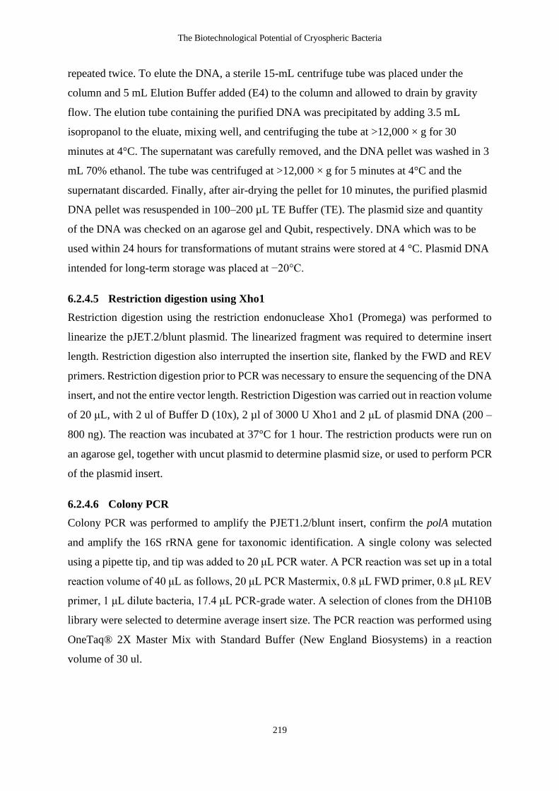
The Biotechnological Potential of Cryospheric Bacteria
219
repeated twice. To elute the DNA, a sterile 15-mL centrifuge tube was placed under the
column and 5 mL Elution Buffer added (E4) to the column and allowed to drain by gravity
flow. The elution tube containing the purified DNA was precipitated by adding 3.5 mL
isopropanol to the eluate, mixing well, and centrifuging the tube at >12,000 × g for 30
minutes at 4°C. The supernatant was carefully removed, and the DNA pellet was washed in 3
mL 70% ethanol. The tube was centrifuged at >12,000 × g for 5 minutes at 4°C and the
supernatant discarded. Finally, after air-drying the pellet for 10 minutes, the purified plasmid
DNA pellet was resuspended in 100–200 µL TE Buffer (TE). The plasmid size and quantity
of the DNA was checked on an agarose gel and Qubit, respectively. DNA which was to be
used within 24 hours for transformations of mutant strains were stored at 4 °C. Plasmid DNA
intended for long-term storage was placed at −20°C.
6.2.4.5 Restriction digestion using Xho1
Restriction digestion using the restriction endonuclease Xho1 (Promega) was performed to
linearize the pJET.2/blunt plasmid. The linearized fragment was required to determine insert
length. Restriction digestion also interrupted the insertion site, flanked by the FWD and REV
primers. Restriction digestion prior to PCR was necessary to ensure the sequencing of the DNA
insert, and not the entire vector length. Restriction Digestion was carried out in reaction volume
of 20 μL, with 2 ul of Buffer D (10x), 2 µl of 3000 U Xho1 and 2 μL of plasmid DNA (200 –
800 ng). The reaction was incubated at 37°C for 1 hour. The restriction products were run on
an agarose gel, together with uncut plasmid to determine plasmid size, or used to perform PCR
of the plasmid insert.
6.2.4.6 Colony PCR
Colony PCR was performed to amplify the PJET1.2/blunt insert, confirm the polA mutation
and amplify the 16S rRNA gene for taxonomic identification. A single colony was selected
using a pipette tip, and tip was added to 20 μL PCR water. A PCR reaction was set up in a total
reaction volume of 40 μL as follows, 20 μL PCR Mastermix, 0.8 μL FWD primer, 0.8 μL REV
primer, 1 μL dilute bacteria, 17.4 μL PCR-grade water. A selection of clones from the DH10B
library were selected to determine average insert size. The PCR reaction was performed using
OneTaq® 2X Master Mix with Standard Buffer (New England Biosystems) in a reaction
volume of 30 ul.

Chapter 6
220
6.2.5 Glycerol stocks
Glycerol stocks were made of strains and clone libraries for long-term storage at -80 °C. To
make stocks of mutant strains, colonies were streaked on LB+Thymine agar and grown
overnight. Five colonies of each strain were picked and added to 10 mL LB broth supplemented
with Thymine, then grown overnight at 37°C in a shaking incubator. The stocks were made by
adding 500 μL of the overnight culture to 500 μL of 50% glycerol in a 2 mL microcentrifuge
tube, resulting in a glycerol concentration of 25%.
6.2.5.1 Clone library stocks
Glycerol stocks of E.coli DH10B, cs2-29 and HCS1 clone libraries were made by washing
colonies of transformants from agar plates using a small amount of LB and diluting the mixture
in fresh LB, supplemented with carbenicillin (and thymine for cs2-29 and HCS1). The stocks
were made by adding 500 μL of the diluted library to 500 μL of 50% glycerol in a 2 mL
microcentrifuge tube, resulting in a glycerol concentration of 25%.
Table 6-7 Table of glycerol stocks of different strains with different supplements
6.2.5.2 DNA extraction from glycerol stocks
Glycerol stocks were revived in overnight culture and then streaked onto LB agar and L-agar
plates supplemented with thymine. For DNA extraction, single colonies were picked from LB
plates and DNA was extracted using the ZymoBIOMICSTM DNA Mini Kit (Zymo Research,
Irvine, CA).
6.2.6 Bioinformatics
Low quality bases were trimmed from the Sanger sequences using Chromas. Sequences were
aligned using ClustalW on Mega. The Sanger sequences of the pJET 2.1/ blunt vector inserts
were submitted to BLAST and aligned using blastx (translated nucleotide sequence against the
non-redundant protein database).
Strain Description Supplements
cs2-29 Strain stock Thymine
HCS1 Strain stock Thymine
DH10B Max Efficiency Clone library Carbenicillin
cs2-29 Clone library Thymine + Carbenicillin
HCS1 Clone library Thymine + Carbenicillin
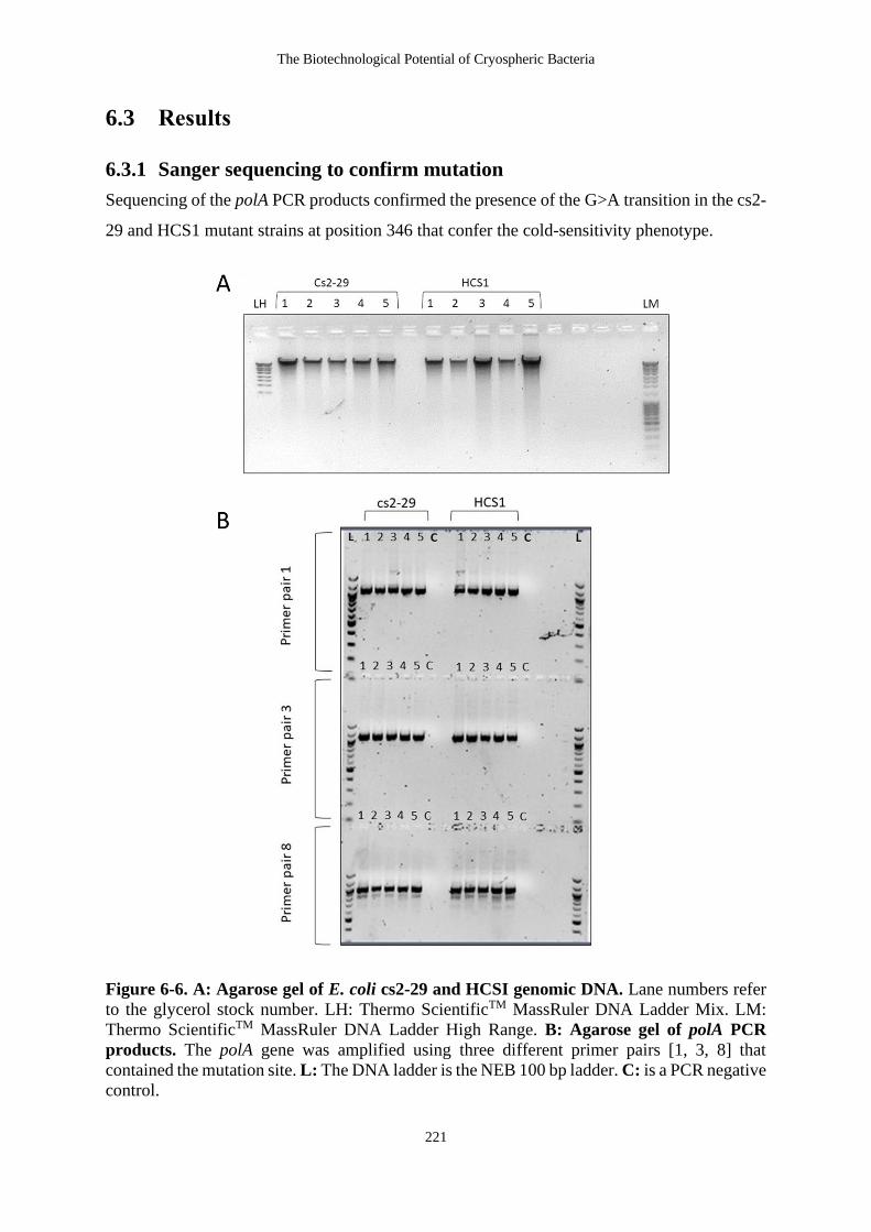
The Biotechnological Potential of Cryospheric Bacteria
221
6.3 Results
6.3.1 Sanger sequencing to confirm mutation
Sequencing of the polA PCR products confirmed the presence of the G>A transition in the cs2-
29 and HCS1 mutant strains at position 346 that confer the cold-sensitivity phenotype.
Figure 6-6. A: Agarose gel of E. coli cs2-29 and HCSI genomic DNA. Lane numbers refer
to the glycerol stock number. LH: Thermo ScientificTM MassRuler DNA Ladder Mix. LM:
Thermo ScientificTM MassRuler DNA Ladder High Range. B: Agarose gel of polA PCR
products. The polA gene was amplified using three different primer pairs [1, 3, 8] that
contained the mutation site. L: The DNA ladder is the NEB 100 bp ladder. C: is a PCR negative
control.

Chapter 6
222
Figure 6-7. Alignment of polA amplicons and polA gene showing the position of the mutation conferring cold sensitivity. There is a G>A
transition in the sc2-29 and HCS1 mutant strains at position 346.
Figure 6-8. Alignment of translated polA gene showing the position of the amino acid change causing cold sensitivity. The G>A transition
in the cs2-29 and HCS1 mutant strains at position results in an amino acid change from D (Aspartic acid) to be changed to a N (Asparagine) at
position 116.
The Biotechnological Potential of Cryospheric Bacteria
223
6.3.2 Transformation of DH10B with soil and cryoconite eDNA
The ligations and transformations were repeated twice. The first transformation resulted in a
library of approximately ~3400 cryoconite clones and ~1800 soil clones. The second
transformation resulted in an improved library size of 5760 cryoconite clones and ~2700 soil
clones. Between both transformation batches, a clone library of 9160 cryoconite clones and
4500 soil clones was created.
Figure 6-9 Examples of clones obtained by transformation into DH10B. A shows clones
derived from soil DNA. B shows clones obtained from cryoconite DNA. C is a PUC19 control
to check transformation efficiency and D is a PCR product control to check ligation efficiency.
Plates are LB, supplemented with carbenicillin.
Several clones were randomly selected from each plate for colony PCR of the pJET2.1/blunt
plasmid insert. The gel (Figure6-10), showing insert sizes, and the BLAST results from Sanger
sequencing of the PCR products are shown in Table 6-8. The size of the inserts was within the
intended range. Clones 1A, 1B and 1D were approximately 5 kb or greater. Although 1A, 1E
and 1H were the largest inserts, the Sanger sequences appeared to be heterozygous or contained
mixed sequences. The ~5 kB sequence from cryoconite clone 1B is related to a hypothetical
protein from Phormidesmis priestleyi ULC0007.

Chapter 6
224
Figure 6-10 Agarose gel of PCR of pJET1.2/blunt inserts from randomly selected DH10B
cryoconite and soil clones.
Table 6-8 Table of blastx hits of randomly selected soil and cryoconite clones in DH10B
cells.
Description Max
Score
Total
Score
Query
Cover
E
value
Per.
Ident Accession
Random selection of inserts from DH10B clones
1B
hypothetical protein
C7B65_04385 [Phormidesmis
priestleyi ULC007]
99.4 99.4 43% 1e-20 73.03% PSB21180.1
1C ketol-acid reductoisomerase
[Isosphaera pallida] 316 316 77% 3e-105 89.70% WP_013563169.1
1D
alpha-D-glucose phosphate-
specific phosphoglucomutase
[Afipia sp. GAS231]
391 391 99% 6e-132 97.18% WP_092511167.1
1F TPA: acetate--CoA ligase
[Ktedonobacter sp.] 191 191 65% 3e-57 67.88% HBE27042.1
1G 30S ribosomal protein S5
[Bdellovibrionales bacterium] 136 136 38% 8e-37 76.19% MSP19036.1

The Biotechnological Potential of Cryospheric Bacteria
225
6.3.3 Size of cryoconite and soil eDNA inserts
As mentioned previously, we were aiming for an insert length of 3kB to 10kB. To check the
size of the clone library, the plasmids were pooled. Colonies from all the plates from a single
ligation mixture were pooled, and then all the ligation mixtures from the same environment
were pooled. The entire transformation was repeated twice (batch 1 and batch 2). In the end
there were two libraries, a cryoconite and soil library. We ran these on a gel to check the size
of the plasmids (Figure 6-11). We expected a smear, which can be interpreted as the size
distribution of the plasmids from each library. An empty pJET2.1/blunt plasmid is 2974 bp in
size, but self-ligated vectors without an insert should be lethal and so we did not expect many
3kB plasmids. Unfortunately, because plasmids are circular, they do not run in the same manner
as linear DNA and therefore the ladder is not a good indicator of library size. To linearize the
library, the plasmids were incubated with Xho1 restriction enzyme. The library is unfortunately
skewed towards shorter sequences, which is due to greater ligation efficiency for shorter DNA
sequences. However, there are some inserts above the desired length of 6kB.

Chapter 6
226
Figure 6-11 A: Example of an agarose gel of undigested plasmids extracted from Batch 2
cryoconite and soil clone libraries. S: soil, C: cryoconite, (n-n) refer to the mixed ligation
batches. B: Restriction digestion of Batch 1 plasmids to check linear size. C Cryoconite
library. S: soil library. P: PCR ligation control. BR: Cleaver Scientific Broad Range Ladder.
+/– reflects whether the library was (+) or was not (-) incubated with Xho1 restriction enzyme.
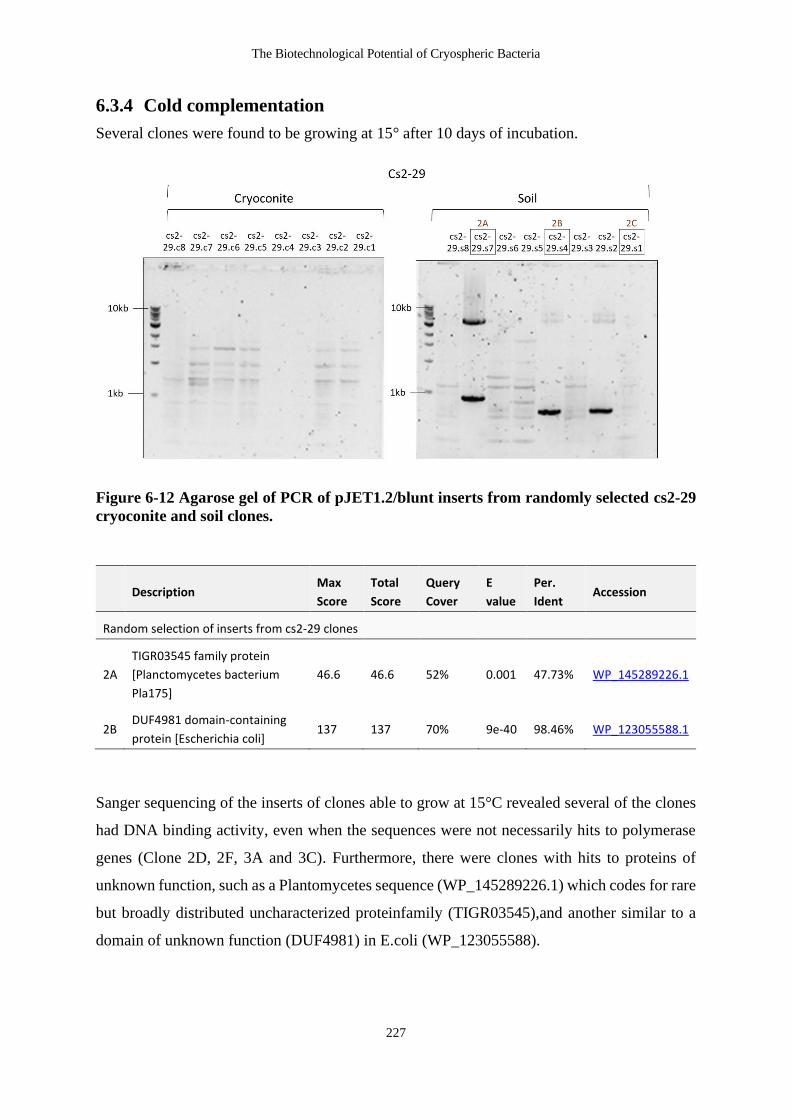
The Biotechnological Potential of Cryospheric Bacteria
227
6.3.4 Cold complementation
Several clones were found to be growing at 15° after 10 days of incubation.
Figure 6-12 Agarose gel of PCR of pJET1.2/blunt inserts from randomly selected cs2-29
cryoconite and soil clones.
Description Max
Score
Total
Score
Query
Cover
E
value
Per.
Ident Accession
Random selection of inserts from cs2-29 clones
2A
TIGR03545 family protein
[Planctomycetes bacterium
Pla175]
46.6 46.6 52% 0.001 47.73% WP_145289226.1
2B DUF4981 domain-containing
protein [Escherichia coli] 137 137 70% 9e-40 98.46% WP_123055588.1
Sanger sequencing of the inserts of clones able to grow at 15°C revealed several of the clones
had DNA binding activity, even when the sequences were not necessarily hits to polymerase
genes (Clone 2D, 2F, 3A and 3C). Furthermore, there were clones with hits to proteins of
unknown function, such as a Plantomycetes sequence (WP_145289226.1) which codes for rare
but broadly distributed uncharacterized proteinfamily (TIGR03545),and another similar to a
domain of unknown function (DUF4981) in E.coli (WP_123055588).
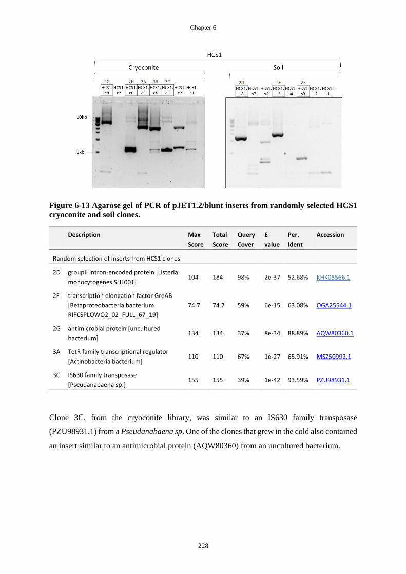
Chapter 6
228
Figure 6-13 Agarose gel of PCR of pJET1.2/blunt inserts from randomly selected HCS1
cryoconite and soil clones.
Description Max
Score
Total
Score
Query
Cover
E
value
Per.
Ident
Accession
Random selection of inserts from HCS1 clones
2D groupII intron-encoded protein [Listeria
monocytogenes SHL001] 104 184 98% 2e-37 52.68% KHK05566.1
2F transcription elongation factor GreAB
[Betaproteobacteria bacterium
RIFCSPLOWO2_02_FULL_67_19]
74.7 74.7 59% 6e-15 63.08% OGA25544.1
2G antimicrobial protein [uncultured
bacterium] 134 134 37% 8e-34 88.89% AQW80360.1
3A TetR family transcriptional regulator
[Actinobacteria bacterium] 110 110 67% 1e-27 65.91% MSZ50992.1
3C IS630 family transposase
[Pseudanabaena sp.] 155 155 39% 1e-42 93.59% PZU98931.1
Clone 3C, from the cryoconite library, was similar to an IS630 family transposase
(PZU98931.1) from a Pseudanabaena sp. One of the clones that grew in the cold also contained
an insert similar to an antimicrobial protein (AQW80360) from an uncultured bacterium.

The Biotechnological Potential of Cryospheric Bacteria
229
6.4 Discussion
Functional screening of metagenomic libraries remains a vital arm of the bioprospecting
enterprise. The use of purely bioinformatic approaches to identify enzymes relies on homology
to known proteins, and therefore misses truly novel sequences that do not already exist in
databases. In this chapter we cloned soil and cryoconite eDNA into E. coli DH10B cells to
create a clone library and then extracted the plasmids and transformed them into cold-sensitive
mutant E. coli strains HCS1 and cs2-29. Clones from the DH10B backup library and HCS1
and cs2-29 clones that grew in the cold were selected and sequenced using Sanger sequencing.
6.4.1 Difficulties encountered
There were several issues encountered in this cloning experiment. The initial experiment was
meant to use the PCCFOS1 cloning vector system, which makes use of fosmids that can take
inserts of 40 kB in size. This was the system previously used with success to identify
polymerases from glacier ice (Simon et al., 2009a). It is also the system of choice in several
other screens of metagenomic libraries (Fu et al., 2013; Jeon et al., 2009; Vester et al., 2014).
Large inserts are ideal in cloning experiments because they capture several genes at once,
which reduces the number of clones that are needed to cover a genome. However, the use of
fosmids, requires both long inserts of around 40 kb and enormous quantities of DNA ranging
in the 10s to 100s of μg. Several months and many DNA extraction kits and methods were
tested to get the DNA length and quantities needed to be packaged into the lambda phage.
Several of these methods are listed in Section 2.2. Unfortunately, to get long DNA fragments,
direct lysis methods like DNA beating are inappropriate and so the focus is to separate the cells
from the environment matrix in which they are embedded and then to perform gentle lysis.
Although we attempted many of these methods, from soil agitation in a blender followed by
filtering through miracloth and filter paper, to a Ludox Density gradient, we were unable to
isolate the quantities of DNA described in the literature (Bakken and Lindahl, 1995; Robe et
al., 2003). In addition, most of the methods for long DNA require indirect lysis, which severely
reduced the taxonomic diversity and the abundance. The diversity loss is likely due to a
combination of factors, such as bacteria forming biofilms and adhering to soil particles with
different affinity, size exclusion where larger bacteria or bacterial aggregates don’t get past
filters or settle out of the density gradient, and different sensitivity to lysis (Section 4.4.7.1).

Chapter 6
230
Although several metagenome studies have used soil in the past, glacial forefield may have
been more tricky than loamy soils because of the high clay content. It is incredibly difficult to
separate the microorganisms from the clay in the first place. DNA also adsorbs to any clay
carry over in subsequent lysis steps, resulting in further DNA loss.
Instead, we decided to use a plasmid system. We had intended to use the TOPO XL (Invitrogen)
which can take inserts of up to 13kb and is ideal for long inserts. However, there was a
worldwide shortage of these plasmids and so the pJET1.2/Blunt system which can take inserts
of up to 10kB was chosen instead. Plasmids are ideally used with cleaned PCR products of a
specific length. In this sample we had sheared metagenomic DNA which ranged in size. To
obtain the ideal length for the plasmids, we performed a gel size selection, followed by clean-
up. This resulted in some loss of DNA, and the purification, which could only be done in 50uL
volumes needed to be reduced via speedivac to the concentrations required for the ligation
reaction. The ligation reaction itself is most efficient for short inserts and efficient at specific
vector: DNA ratios. Unfortunately, based on our midiprep gels and restriction digestions, it
seems that many of the plasmids contained incredibly short inserts, which makes sense as these
have a higher probability of proper ligation and plasmid closure. A 976 bp PCR product was
included with the cloning kit to act as ligation control. The plasmids with the PCR control
repeatedly had much higher transformation efficiencies that the environmental DNA. This
perhaps reflects the fact that ligation of smaller DNA fragments is far more efficient than
ligation of long inserts.
Cloning of environmental DNA into a plasmid vector and transformation of that vector into a
heterologous host was performed multiple times. Initially, electroporation was attempted to
transform plasmids directly into the cold-sensitive mutant HCS1 and cs2-29 E. coli strains
(Appendix Section F-1). However, various difficulties with the electroporation, lead to changes
in strategy to Calcium Chloride chemical transformation. The benefit of the Calcium Chloride
method is that it is relatively inexpensive and can be repeated many times at very low cost. The
initial decision to clone directly into the mutant strains was made to screen the greatest
biodiversity possible, with the understanding that cloning into another competent host strain
first might reduce the diversity in the library that gets cloned into the mutant strain in the
complementation screen. However, the competency of the mutant strains was unknown, and it
was decided instead to clone into a commercial competent strain, like E. coli DH10B to
maximise the efficiency of DNA take up. The successfully transformed DH10B cells would be
amplified and their plasmids extracted to allow massive rescreening of the library. The use of
The Biotechnological Potential of Cryospheric Bacteria
231
Calcium Chloride transformation method and amplified plasmids from a competent cell library,
made unlimited attempts to clone the plasmids into the mutant strains possible.
Cloning into the chemically competent E. coli cells resulted in a much bigger library than
electroporation directly into HCS1 and cs2-29. Using this method, we were able to create a
clone library of approximately 9160 cryoconite clones and 4500 soil clones
6.4.2 The clones reflect the most abundant taxa in cryoconite and soil
The clones we sequenced were from the most abundant taxa in these environments. There was
good correlation between the taxonomy of the clone sequences and what we know to be the
most abundant species in these environments. For example, Phormidesmis priestleyi (1B),
Ktedonobacter sp (1F), Bdellovibrionales (1G), Pseudanabaena sp (3C), Actinobacteria
bacterium.
6.4.3 The clones from the cold-complementation assay tended to have DNA-
binding activity
Sanger sequencing of the clones reflected that many of the clones that grew in the cold had
inserts with genes that had DNA binding activity. Unfortunately, we were limited to Sanger
sequencing of the PCR inserts from the clones, with only several hundred high quality bases
from which to base our BLAST search. Several of the clones had large inserts, and therefore it
is possible that there was a polymerase gene downstream of the short section we sequenced.
The HCSI cryoconite clone (2G) was > 6kB in size. For example, clone 3C from cryoconite
had a sequence similar to a transposase from Pesudoanabaena. This raises the possibility of
mutation correction by the Pseudanabaena transposase. In any community of bacteria, with a
given mutation rate, and sufficient generations, it is possible for point mutations to revert to
their original WT. This may be what happened in the case of the empty inserts we sequenced.
There were also several instances where we cloned the empty vector or where the Sanger PCR
products were clearly mixtures, containing inserts from more than one clone. This was partly
a consequence of time pressure, and generations of sub-culturing could have separated the
mixed clones, although it might have taken PCRs of several colonies to capture both, (or all)
of the clones that were in the mixture.
Although we did not have any clear clones with a polymerase, this is not improbable given
other studies of this nature. The previous study that used the fcsA mutation to screen for
polymerases identified 1 fosmid clone, and 8l plasmid clones, although several were

Chapter 6
232
duplications (Simon et al., 2009a). They calculated a success rate of approximately 1
polymerase clone per 1000 plasmids screened. This is a success rate many times higher than
most metagenomic screens (Ferrer et al., 2016). In this study, we had approximately 9160
cryoconite clones and 4500 soil clones. However, the study by Simon et al, used plasmids with
insert sizes of 14 kB (Simon et al., 2009a). The insert sizes in our library were 10kB maximum,
and occasionally much smaller, which drives down the actual coverage in our clone library as
well as the number that might contain full and functional polymerase sequences.
6.4.4 Future work
The cryoconite and soil clone libraries created in this chapter have been stored as glycerol
stocks and as plasmids. They remain a resource for future investigation. The intention was to
catalogue the entire library by performing a PCR of the pJET2.1/blunt vector insert site,
followed by sequencing of the library on a Nanopore minION. Long-read sequencing by
Nanopore could easily capture the entire insert, with no need for assembly, and allow the
determination of the exact number of clones, together with the taxonomic and functional
classification. The screening of clone libraries can be an exceptionally laborious exercise,
generally requiring hundreds of plates, meticulously poured, marked, and catalogued and then
grown for long periods of time for a relatively low hit rate (Ferrer et al., 2016). A bioinformatic
catalogue of a clone library lends itself to many applications. In this study we employed a
relatively easy complementation assay for polymerases. However, based on a bioinformatic
screen of the library, specific assays could be designed to target specific clones that we know
to be present and complete.
If a clone with a full enzyme sequences is present, the clone can then be analysed for signatures
of cold adaptation. The types of structural adaptations that signify cold-adaption include
decreased core hydrophobicity and increased surface hydrophilicity, alterations in the types,
and proportions of amino acids present, such as less Isoleucine, more histidine and methionine,
a high (Glu + Asp) / (Lys + Arg) ratio, and a low Low Arg/ Lys ratio (Siddiqui and Cavicchioli,
2006). In addition, there is more Gly, less pro in loops, and more proline in a-helices, resulting
in more loops and/ or loops of longer length. Because there are fewer total charged residues,
there tend to be fewer hydrogen bonds, disulphide bridges and salt bridges. There are also fewer
metal-binding sites and/ or lower affinity for metal-binding, less aromatic interactions and
weaker intersubunit/ interdomain contacts (Siddiqui and Cavicchioli, 2006).

The Biotechnological Potential of Cryospheric Bacteria
233
Unfortunately, only part of the inserts from the clones could be sequenced using Sanger
sequencing (~1000 bp). An obvious extension of this work would be to sequence the full-length
inserts using long read technology such as Nanopore, or alternatively, Illumina shotgun
sequencing of the clone library and assembly of the contigs.
6.5 Conclusion
In this chapter, clone libraries of cryoconite and soil environmental DNA were created in
DH10B E. coli for storage, propagation, and future screens, as well as in cold-sensitive mutant
E. coli strains cs2-29 and HCS1. Several clones capable of growth at 15°C, suggesting they
were able to rescue transcription in the mutant strains. The sequenced clones were similar to
proteins that had DNA binding ability and should be investigated in further.

Chapter 7
234
7 A METAGENOMIC ANALYSIS
OF THE FUNCTIONAL
POTENTIAL OF THE
SCĂRIȘOARA ICE CAVE
7.1 Introduction
The Scărișoara Ice Cave is one of the oldest and largest perennial underground ice-blocks in
the world, being older than 3000 years and greater than 100 000 m3 in volume (Perşoiu and
Pazdur, 2011). The cave is located in the Bihor Mountains of North West Romania
(46°29’23”N, 22°48’35”E) at an altitude of 1165m. The Scărișoara ice block differs from
surface glaciers and glacier caves because it is not formed by snow accumulation. Rather, it
grows via the annual freezing of a layer of water that trickles into the cave during summer
months, forming a shallow lake on top of the existing ice block (Holmlund et al., 2005). This
layer, which can be up to 20 cm deep, freezes every winter, trapping at its bottom a layer of
sediment deposited during the summer. The ice block therefore consists of sequential layers of
ice of variable thickness, separated by organic-rich sediment layers. This makes it a fascinating
record of past climactic conditions, as each year remains frozen, like layers of sedimentary
rock. Secondly, the environment is oligotrophic and dark, and many of the deeper layers are
also anaerobic, meaning that bacteria that thrive here will be adapted to extreme conditions.
Although there may be annual injections of nutrients into the cave via the water and sediment
that trickles into the cave each summer, there is likely to be significant recycling of nutrients.
Without photoautotrophy to continuously add organic carbon into the environment, there will
need to be alternative pathways for carbon fixation. To investigate this environment, bacterial
MAGs were constructed from shotgun metagenomes collected from seven sites within the cave.
The abundance of the MAGs at various sites was inferred via read mapping, and the MAGs
were investigated for their biogeochemical cycling potential, which was used in turn to infer
the types of nutrient cycling occurring at each site.

The Biotechnological Potential of Cryospheric Bacteria
235
In addition, the MAGs were also screened for secondary metabolite BGCs. Growing
antimicrobial resistance poses a serious threat to human health and novel antibiotics are
urgently needed (Sabtu et al., 2015; Ventola, 2015). Antimicrobial secondary metabolites are
often synthesised by bacteria as weapons against competitive species (Bérdy, 2005; van
Bergeijk et al., 2020). Low nutrient environments are especially harsh and competitive
environments in which cell death is often required to recycle nutrients for continued growth
(Bérdy, 2005; van Bergeijk et al., 2020). It has been suggested that a resistome is innate in
some cave environments (Bhullar et al., 2012), and since resistance develops in response to the
presence of antimicrobials, this raises the possibility that the microorganisms of cave
microbiomes may synthesise a novel and distinct arsenal of antimicrobial compounds (Ghosh
et al., 2017). Because caves are such isolated habitats, in which organisms predominantly enter
the cave, and do not tend to leave, it possible that that there are distinct and endemic bacterial
communities, with a novel, unknown BGCs. Although several caves have been explored for
potential antimicrobials, from the subterranean Kotumsar cave, India (Rajput et al., 2012), to a
volcanic cave in western Canada (Rule and Cheeptham, 2013) to Magura Cave, Bulgaria
(Tomova et al., 2013), these studies relied on cultured bacteria, and none have investigated a
solid ice block like the one present in the Scărișoara Ice Cave.
7.1.1 Aims and objectives
The aims of this chapter were as follows:
1. Construct high quality metagenome-assembled genomes (MAGs) from seven samples
collected from different sites within the Scărișoara Ice Cave.
2. Classify the MAGs using phylogenomic methods and identify novel species from these
environments.
3. Use read mapping and coverage information to identify:
3.1. distribution of these species across different sample sites.
3.2. co-occurrence of different species at specific locations.
4. Identify the presence of genes involved in biogeochemical cycling of major nutrients at
specific sites:
5. Use antiSMASH to identify the main categories of secondary metabolites synthesized by
Ice Cave Bacteria

Chapter 7
236
7.2 Materials and methods
7.2.1 Site description
Seven metagenomes from the perennial ice block of Scărișoara Ice Cave in Romania were
included in this study (Iţcuş et al., 2016). Ice samples of three different ages were collected
from the cave in 2012. At the time of collection, samples with the prefix 1 were collected in
2012, samples designated 400 were from 385 calendar years before the collection date and
samples with the prefix 900 were 943 calendar years before 2012. The most recent samples
were collected from a sun-exposed site in the immediate vicinity of the entrance (IS), a second
sample was collected from an indirect light exposed area in the centre of the cave (1L). A
description of sample locations and characteristics are in Table 7-1. A table describing the age,
location and characteristics of samples collected in the Scărișoara Ice Cave.
Table 7-1. A table describing the age, location and characteristics of samples collected in
the Scărișoara Ice Cave.
Sample Name Age location description Organic or inorganic
1S (2) Present Great Hall, immediate vicinity of entrance
Sunlight exposed
1L (13) Present Great Hall, centre of cave Light-exposed
400-O (6) -385 Little Reservation, horizontal drilling of ice-wall surface
Organic
900-O (15) -943 Little Reservation, horizontal drilling of ice-wall surface
Organic
900-I (7) -943 Little Reservation horizontal drilling of ice-wall surface
Inorganic, clear ice
1500 (18) ~1200 (?)
2000 (14) ~1500 (?)

The Biotechnological Potential of Cryospheric Bacteria
237
Figure 7-1 A) Schematic diagram of the Scărișoara Ice Cave showing the locations of
sample collection. B) The Great Hall. C) Layers of sediment and water deposited in
annual layers. D) The Church contains stalagmites and is accessed from the Great Hall
(not shown on map). E) Entrance to the Cave (Shaft).

Chapter 7
238
7.2.2 Sequencing and bioinformatics
The metagenomes were sequenced on an Illumina HiSeq and are available from the nanuq
platform at McGill University and Génome Québec Innovation Centre
(https://genomequebec.mcgill.ca/nanuqAdministration). The sequences were uploaded to
KBase and adapters were removed and low quality bases trimmed using Trimmomatic (Bolger
et al., 2014) with a minimum Phred score threshold of 30. The seven ice cave libraries were
assembled together on the KBase server, using three different assembly tools: metaSPAdes
(Nurk et al., 2017), MEGAHIT (D. Li et al., 2015) and IDBA-UD (Peng et al., 2012).
7.2.2.1 Taxonomy
Taxonomy was determined from the trimmed reads for each library individually and for the
combined library using the kaiju (Menzel et al., 2016) module hosted on the KBase server
(Arkin et al., 2018).
7.2.3 Metagenome assembled genomes (MAGs)
Genomes were assembled from metagenomes using Anvi’o (Section 8.2.4). Analysis was
started in Anvi’o v5 “margaret” (https://github.com/merenlab/anvio/releases/tag/v5), which
was then updated to Anvi’o v6.1 "esther" (https://github.com/merenlab/anvio/releases/v6). The
existing profile.db and contigs.db were migrated to the latest versions using anvi-migrate.
Functions were added to the contigs database using anvi-run-hmms and anvi-run-ncbi-cogs -c
contigs.db -T 8. The contigs were also functionally annotated using KEGG annotations and
Eggnog mapper (Chapter 8).
7.2.3.1 Binning and refinement of MAGs
The contigs database of 179753 contigs was too large to run anvi-interactive with hierarchical
clustering and run manual binning. Therefore, the contigs were binned using anvi-cluster-
contigs as part of the anvi’o workflow using CONCOCT, MaxBin2 and MetaBAT2 (Section
8.3.6). The DAS Tool was then run on all three collections, using diamond as a search engine.
The taxonomic classification of the bins, and bin refinement was performed as previously
described in Chapter 4 and detailed in Chapter 8. The dataset was trimmed to contain high
quality MAGs. The genomes had to be larger than 1.8 MB, have greater 70% completion and
less than 10% redundancy (Bowers et al., 2017). The list of medium to low quality bins not
included for further analysis is shown in Appendix Table G-7.

The Biotechnological Potential of Cryospheric Bacteria
239
7.2.3.2 Check genome quality with CheckM and GTDB-Tk
The completeness, redundancy and taxonomic classification of the MAGs was performed using
CheckM (Parks et al., 2015) and the GTDB-Tk module on KBase (Chaumeil et al., 2020) as
previously described (Section 4.2.6). The phylogenomic relationship of the MAGs was
calculated using the HMM hits from a curated collection of single copy core genes for the
GToTree workflow (Lee, 2019) as previously described (Section 4.2.6).
7.2.3.3 Spatial distribution of the MAGs across sample sites
A heatmap of max-normalised ratio (number of reads recruited to a contig divided by the
maximum number of reads recruited to that contig in any sample) was created using the R
package ComplexHeatmap to visualise the spatial distribution of the MAGs
(http://www.bioconductor.org/packages/devel/bioc/html/ComplexHeatmap.html) (Gu et al.,
2016).
7.2.3.4 Biogeochemical cycles
The fasta files from the MAGs were analysed for major metabolic pathways using
MetabolisHMM (https://github.com/elizabethmcd/metabolisHMM).
7.2.3.5 Screening for antimicrobial secondary metabolites
The MAGs were submitted to antiSMASH v 5 to screen for secondary metabolite BGCs (Blin
et al., 2019b).

Chapter 7
240
7.3 Results
Table 7-2 Ice-cave library shotgun library statistics
Read Length Duplicate reads Quality
Environment Sample Reads No Bases mean std dev Number % mean std dev GC%
Ice-cave dataset
Present, sun 1S_2 69,575,748 8,530,226,859 122.60 10.58 29,675 0.04 35.48 3.95 53.19
Present, light 1L_13 72,190,896 8,860,007,146 122.73 10.26 36,821 0.05 35.48 3.94 56.84
-385, organic 400_O_6 76,039,348 9,324,467,510 122.63 10.53 161,544 0.21 35.47 3.97 54.29
-943. Organic 900_O_15 73,462,594 9,019,960,422 122.78 10.20 353,401 0.48 35.51 3.90 54.57
-943, inorganic 900_I_7 75,113,102 9,213,747,381 122.67 10.46 145,477 0.19 35.43 4.03 59.89
~1200 1500_18 75,510,556 9,278,999,040 122.88 9.77 1,286,620 1.70 35.67 3.59 42.33
~1500 2000_14 63,569,516 7,815,266,055 122.94 9.78 84,276 0.13 35.48 3.93 61.72

The Biotechnological Potential of Cryospheric Bacteria
241
7.3.1 Sequencing results
The library size (number of reads), average read length, quality (average Phred score) and GC
content of the seven shotgun metagenome libraries included in the study are described in Table
7-2.
7.3.2 Taxonomy
Figure 7-2 Phylum-level taxonomic profile of individual samples from various locations
in the Scărișoara Ice Cave.
Samples 1L and 1S from the cave Great Hall as well as 400-O and 900-O which were older in
age, but from organic layers, were similar in profile with approximately 50% of reads classified
to Phylum level. The Proteobacteria dominated these samples, with Bacteroidetes and
Actinobacteria comprising the second and third most abundant phyla. The present-day samples
contained a greater diversity of Phyla, with small proportions of Firmicutes, Plantomycetes,
Verrucobacteria, Chlorobi, Chloroflexi and Cyanobacteria also present. The older samples
1500 and 2000 and the inorganic sample 900-I had more reads (~70%) classified to Phylum
level. Sample 900-I from an inorganic layer had fewer Proteobacteria and the largest proportion
of Actinobacteria. Sample 1500 was unique with most reads classified as Bacteroidetes, while
Sample 2000 was dominated by Proteobacteria.

Chapter 7
242
Figure 7-3 Class-level taxonomic profile of individual samples from various locations in
the Scărișoara Ice Cave.
Samples 1L and 1S from the cave Great Hall as well as 400-O and 900-O which were older in
age, but from organic layers, were similar in profile with approximately 50% of reads classified
to Class level. The Beta-, Alpha- and Gammaproteobacterial classes were in high abundance,
with a smaller number of Deltaproteobacteria present. Flavobacteriia from the Bacteroidetes
phylum and Actinobacteria comprised the second and third most abundant non-proteobacterial
classes. The present-day samples contained a greater diversity of Classes. The older samples
1500 and 2000 and the inorganic sample 900-I had more reads (~70%) classified to Class level.
Sample 900-I from an inorganic layer had the largest proportion of Actinobacteria. Sample
1500 was unique with most reads classified as Flavobacteriia from the Bacteroidetes, while
Sample 2000 was dominated by Beta-, Alpha- and Gammaproteobacteria in that order, with
some Actinobacteria and Flavobacteriia also present.

The Biotechnological Potential of Cryospheric Bacteria
243
Table 7-3 Table comparing Ice Cave assemblies
Assembly Longest contig (bp)
Nx (Lx) Length
(bp)
Number of
contigs
Sum Length (bp)
Contig Length Histogram
Contig Length Histogram
Contig Length Histogram
(1bp <= len < 10Kbp) (10Kbp <= len <
100Kbp) (len >= 100Kbp)
MEGAHIT 1388828
N50: 8767 >= 106 2 2540240
L50: (24021) >= 105 547 99933809
N75: 3819 >= 104 19855 522690257
L75: (74910) >= 103 179753 1123284953
N90: 2539 >= 500 179753 1123284953
L90: (129650) >= 1 179753 1123284953
IDBA-UD 1388786
N50: 11935 >= 106 1 1388786
L50: (12589) >= 105 453 81591909
N75: 4631 >= 104 15812 430080664
L75: (40483) >= 103 106360 789866587
N90: 2828 >= 500 106360 789866587
L90: (73683) >= 1 106360 789866587
metaSPAdes 1644450
N50: 9447 >= 106 4 4899394
L50: (21521) >= 105 611 116757355
N75: 3862 >= 104 19998 549270645
L75: (70816) >= 103 175966 1128145066
N90: 2538 >= 500 175966 1128145066
L90: (125621) >= 1 175966 1128145066
Chapter 7
244
7.3.3 Assembly
The combined ice-cave library was assembled using MEGAHIT v1.1.1 and metaSPAdes 1.1.3
and IDBA-UD v1.1.3 on the KBase server. The assembly contig distributions were compared
using Compare Assembled Contig Distributions - v1.1.2. The assemblies were remarkably
similar in size and contig distribution (Table 7-3). MEGAHIT was the assembly used for MAG
construction.
7.3.4 Metagenome assembled genomes
The contigs from the MEGAHIT assembly were clustered into 270 bins using CONCOCT (v
1.1.0) (Appendix Table G-2), 253 bins using MaxBin2 (version 2.2.7) (Appendix Table G-3),
and 401 bins using metaBAT2 (v 2.12.1) (Appendix Table G-4). The bins in each collection
were compared using DAS Tool (v 1.1.2) (Appendix Table G-5) and a refined collection of
145 bins with completion > 50% was created. The taxonomic classification of the bins from
each binning method (collection) were checked using anvi-estimate-scg-taxonomy, using the
contigs database, merged profile, and collection (Appendix Table G-8).
The DAS Tool collection consisted of 145 bins, accounting for 502,443,977 nucleotides, which
represent 44.73% of all nucleotides stored in the contigs and profile databases. This collection
was refined using anvi-refine, resulting in the collection ice-mags, which describes 146 bins
accounting for 472,098,455 nucleotides, representing 42.03% of all nucleotides stored in the
contigs and profile database. The fastas from each of the MAGs in the ice-mags collection were
downloaded and submitted to CheckM on KBase. Based on the KBase completion and
redundancy estimates, the collection was reduced to 121 bins (ice_mags_final) which had
completion above 70% (Appendix Table G-6). Bins excluded from the dataset at this point can
be found in Appendix Table G-7. This final dataset comprises 430,185,758 nucleotides, which
represent 38.30% of all nucleotides stored in the contigs database.

The Biotechnological Potential of Cryospheric Bacteria
245
Figure 7-4 Phylogram of the 121 MAGs in the Ice cave dataset. The Items order: Abundance (D: Euclidean; L: Ward) | Current view: detection.
Bars represent proportion of contigs that have at least 1x coverage.
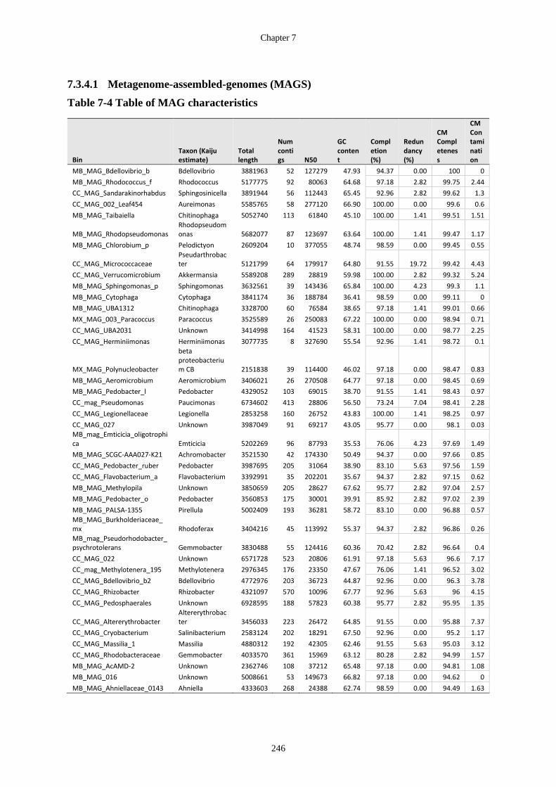
Chapter 7
246
7.3.4.1 Metagenome-assembled-genomes (MAGS)
Table 7-4 Table of MAG characteristics
Bin Taxon (Kaiju estimate)
Total length
Num contigs N50
GC content
Completion (%)
Redundancy (%)
CM Completeness
CM Contamination
MB_MAG_Bdellovibrio_b Bdellovibrio 3881963 52 127279 47.93 94.37 0.00 100 0
MB_MAG_Rhodococcus_f Rhodococcus 5177775 92 80063 64.68 97.18 2.82 99.75 2.44
CC_MAG_Sandarakinorhabdus Sphingosinicella 3891944 56 112443 65.45 92.96 2.82 99.62 1.3
CC_MAG_002_Leaf454 Aureimonas 5585765 58 277120 66.90 100.00 0.00 99.6 0.6
MB_MAG_Taibaiella Chitinophaga 5052740 113 61840 45.10 100.00 1.41 99.51 1.51
MB_MAG_Rhodopseudomonas Rhodopseudomonas 5682077 87 123697 63.64 100.00 1.41 99.47 1.17
MB_MAG_Chlorobium_p Pelodictyon 2609204 10 377055 48.74 98.59 0.00 99.45 0.55
CC_MAG_Micrococcaceae Pseudarthrobacter 5121799 64 179917 64.80 91.55 19.72 99.42 4.43
CC_MAG_Verrucomicrobium Akkermansia 5589208 289 28819 59.98 100.00 2.82 99.32 5.24
MB_MAG_Sphingomonas_p Sphingomonas 3632561 39 143436 65.84 100.00 4.23 99.3 1.1
MB_MAG_Cytophaga Cytophaga 3841174 36 188784 36.41 98.59 0.00 99.11 0
MB_MAG_UBA1312 Chitinophaga 3328700 60 76584 38.65 97.18 1.41 99.01 0.66
MX_MAG_003_Paracoccus Paracoccus 3525589 26 250083 67.22 100.00 0.00 98.94 0.71
CC_MAG_UBA2031 Unknown 3414998 164 41523 58.31 100.00 0.00 98.77 2.25
CC_MAG_Herminiimonas Herminiimonas 3077735 8 327690 55.54 92.96 1.41 98.72 0.1
MX_MAG_Polynucleobacter
beta proteobacterium CB 2151838 39 114400 46.02 97.18 0.00 98.47 0.83
MB_MAG_Aeromicrobium Aeromicrobium 3406021 26 270508 64.77 97.18 0.00 98.45 0.69
MB_MAG_Pedobacter_l Pedobacter 4329052 103 69015 38.70 91.55 1.41 98.43 0.97
CC_mag_Pseudomonas Paucimonas 6734602 413 28806 56.50 73.24 7.04 98.41 2.28
CC_MAG_Legionellaceae Legionella 2853258 160 26752 43.83 100.00 1.41 98.25 0.97
CC_MAG_027 Unknown 3987049 91 69217 43.05 95.77 0.00 98.1 0.03
MB_mag_Emticicia_oligotrophica Emticicia 5202269 96 87793 35.53 76.06 4.23 97.69 1.49
MB_MAG_SCGC-AAA027-K21 Achromobacter 3521530 42 174330 50.49 94.37 0.00 97.66 0.85
CC_MAG_Pedobacter_ruber Pedobacter 3987695 205 31064 38.90 83.10 5.63 97.56 1.59
CC_MAG_Flavobacterium_a Flavobacterium 3392991 35 202201 35.67 94.37 2.82 97.15 0.62
MB_MAG_Methylopila Unknown 3850659 205 28627 67.62 95.77 2.82 97.04 2.57
MB_MAG_Pedobacter_o Pedobacter 3560853 175 30001 39.91 85.92 2.82 97.02 2.39
MB_MAG_PALSA-1355 Pirellula 5002409 193 36281 58.72 83.10 0.00 96.88 0.57
MB_MAG_Burkholderiaceae_mx Rhodoferax 3404216 45 113992 55.37 94.37 2.82 96.86 0.26
MB_mag_Pseudorhodobacter_psychrotolerans Gemmobacter 3830488 55 124416 60.36 70.42 2.82 96.64 0.4
CC_MAG_022 Unknown 6571728 523 20806 61.91 97.18 5.63 96.6 7.17
CC_mag_Methylotenera_195 Methylotenera 2976345 176 23350 47.67 76.06 1.41 96.52 3.02
CC_MAG_Bdellovibrio_b2 Bdellovibrio 4772976 203 36723 44.87 92.96 0.00 96.3 3.78
CC_MAG_Rhizobacter Rhizobacter 4321097 570 10096 67.77 92.96 5.63 96 4.15
CC_MAG_Pedosphaerales Unknown 6928595 188 57823 60.38 95.77 2.82 95.95 1.35
CC_MAG_Altererythrobacter Altererythrobacter 3456033 223 26472 64.85 91.55 0.00 95.88 7.37
CC_MAG_Cryobacterium Salinibacterium 2583124 202 18291 67.50 92.96 0.00 95.2 1.17
CC_MAG_Massilia_1 Massilia 4880312 192 42305 62.46 91.55 5.63 95.03 3.12
CC_MAG_Rhodobacteraceae Gemmobacter 4033570 361 15969 63.12 80.28 2.82 94.99 1.57
MB_MAG_AcAMD-2 Unknown 2362746 108 37212 65.48 97.18 0.00 94.81 1.08
MB_MAG_016 Unknown 5008661 53 149673 66.82 97.18 0.00 94.62 0
MB_MAG_Ahniellaceae_0143 Ahniella 4333603 268 24388 62.74 98.59 0.00 94.49 1.63
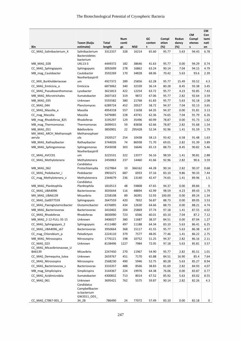
The Biotechnological Potential of Cryospheric Bacteria
247
Bin Taxon (Kaiju estimate)
Total length
Num contigs N50
GC content
Completion (%)
Redundancy (%)
CM Completeness
CM Contamination
CC_MAG_Salinibacterium_X Salinibacterium 3312337 328 16214 65.60 95.77 5.63 94.43 6.78
MB_MAG_028
Bacteroidetes bacterium UKL13-3 4449372 182 38646 41.63 95.77 0.00 94.29 0.74
CC_MAG_Sphingopyxis Sphingopyxis 3092699 278 16862 63.24 90.14 7.04 94.15 4.79
MB_mag_Caulobacter Caulobacter 3592269 170 34828 68.06 70.42 5.63 93.6 2.39
CC_MIX_Burkholderiaceae Noviherbaspirillum 4927372 289 25856 62.28 95.77 15.49 93.52 4.3
CC_MAG_Emticicia_o Emticicia 6873062 340 32339 36.14 80.28 8.45 93.38 3.45
CC_MAG_Pseudoxanthomonas Lysobacter 3621813 422 12254 63.72 95.77 4.23 92.85 7.43
MB_MAG_Microtrichales Ilumatobacter 2607163 319 9872 67.06 95.77 2.82 92.64 3.59
MB_MAG_035 Unknown 5555582 380 21768 61.83 95.77 5.63 92.18 2.08
CC_MAG_044 Planctomyces 6289724 452 20527 58.72 94.37 7.04 92.13 3.65
CC_MAG_Massilia_e Massilia 4954318 557 11658 64.35 94.37 0.00 91.81 3.13
CC_mag_Massilia Massilia 5479085 228 43741 62.36 74.65 7.04 91.79 6.26
MB_mag_Rhodoferax_825 Rhodoferax 3195297 129 35496 60.99 78.87 0.00 91.73 1.62
MB_mag_Thermomonas Thermomonas 2699415 59 83838 62.66 78.87 2.82 91.68 1.54
MB_MAG_051 Bdellovibrio 3850901 22 295428 52.34 92.96 1.41 91.59 1.79
MX_MAG_ARCH_Methanosphaerula
Methanosphaerula 1920527 254 10438 58.13 93.42 6.58 91.48 1.63
MB_MAG_Rathayibacter Rathayibacter 3744026 74 86938 71.70 69.01 2.82 91.39 3.89
MB_MAG_Sphingomonas Sphingomonas 3543038 303 16646 65.13 88.73 8.45 90.82 5.46
CC_MAG_AVCC01 Noviherbaspirillum 3225531 322 13377 56.16 98.59 1.41 90.81 2.88
CC_MAG_Methylotenera Methylotenera 2450063 237 14460 41.66 92.96 2.82 90.6 3.59
MB_MAG_062 Candidatus Protochlamydia 1527864 10 366162 44.28 90.14 2.82 90.37 0.68
CC_MAG_Pedobacter_i Pedobacter 3901671 687 6933 37.16 83.10 9.86 90.33 7.44
CC_mag_Methylotenera_v Methylotenera 2344679 236 13140 42.47 74.65 1.41 89.96 1.5
MB_MAG_Planktophila Candidatus Planktophila 1810513 48 59808 47.65 94.37 0.00 89.84 0
CC_MAG_UBA4096 Bacteriovorax 3035644 116 48894 42.99 98.59 4.23 89.43 1.79
MX_MAG_UBA6139 Micavibrio 2258108 89 36391 52.93 100.00 0.00 89.24 1.34
CC_MAG_Ga0077559 Sphingopyxis 2647559 420 7832 56.87 88.73 0.00 89.05 3.53
CC_MAG_Paeniglutamicibacter Glutamicibacter 4376895 434 12630 64.66 88.73 0.00 88.21 4.74
MB_MAG_Bacteriovorax Bacteriovorax 3410402 204 25869 37.74 97.18 1.41 87.55 4.02
CC_MAG_Rhodoferax Rhodoferax 3830090 723 6566 60.01 83.10 7.04 87.2 7.12
MB_MAG_2-12-FULL-35-15 Unknown 3406027 380 11687 38.37 84.51 0.00 87.04 1.27
CC_MAG_Sphingopyxis_2 Sphingopyxis 4111480 497 11188 64.34 83.10 5.63 86.41 6.25
CC_MAG_UBA4096_s67 Bacteriovorax 3950664 368 15117 41.55 95.77 5.63 86.38 4.37
CC_mag_Chlorobium_p Pelodictyon 2224110 379 7577 48.05 77.46 1.41 86.22 2.75
MB_MAG_Nitrosospira Nitrosospira 1776121 198 10752 51.25 94.37 2.82 86.16 2.11
CC_MAG_023 Unknown 8138496 1227 7984 72.05 97.18 5.63 85.81 3.57
CC_MAG_Micavibrionaceae_UBA6139 Micavibrio 2247450 270 11967 54.90 95.77 2.82 85.51 1.01
CC_MAG_Demequina_lutea Unknown 2659767 451 7170 65.88 84.51 16.90 85.4 7.64
CC_MAG_Nitrosospira Nitrosospira 2568230 490 5946 52.75 80.28 5.63 85.27 8.94
CC_MAG_Bacteriovorax_s Bacteriovorax 3316357 488 8566 38.83 81.69 2.82 84.93 4.07
MB_mag_Simplicispira Simplicispira 3144367 224 19976 64.38 76.06 0.00 83.87 0.77
CC_MAG_Acidimicrobiia Ilumatobacter 4300832 713 8014 67.52 85.92 5.63 83.02 8.55
CC_MAG_061 Unknown 3695421 762 5575 59.87 90.14 2.82 82.26 4.3
CC_MAG_C7867-001_2
Candidatus Campbellbacteria bacterium GW2011_OD1_34_28 786490 24 77072 57.49 83.10 0.00 82.18 0

Chapter 7
248
Bin Taxon (Kaiju estimate)
Total length
Num contigs N50
GC content
Completion (%)
Redundancy (%)
CM Completeness
CM Contamination
MB_MAG_DTU024 Unknown 1792322 223 10828 56.49 88.73 2.82 81.99 2.65
CC_MAG_Anaerolineaceae Brevefilum 2160356 458 5311 51.00 81.69 5.63 81.82 7.56
CC_MAG_Devosia_14 Devosia 2966599 631 5324 62.07 71.83 4.23 81.37 4.41
CC_mag_T78 Brevefilum 2379041 440 6296 49.94 78.87 4.23 81.15 5
CC_MAG_Lacunisphaera_MIX Lacunisphaera 4502698 1132 4180 66.31 90.14 16.90 80.93 8.19
CC_MAG_UBA6139 Micavibrio 2043176 357 6721 55.04 90.14 2.82 80.36 1.88
MB_mag_Burkholderiaceae Rhodoferax 3355550 252 19993 59.58 73.24 5.63 80.16 5.49
MB_mag_Rhodoferax_ferrireducens Rhodoferax 4385890 201 33231 60.95 74.65 4.23 79.74 9.02
MX_mag_Ga0077559 Sphingorhabdus 2002653 365 6284 55.95 78.87 1.41 79.26 3.85
MB_MAG_Microbacterium Microbacterium 3130372 416 8640 68.02 57.75 4.23 78.84 9.51
CC_mag_UBA2259 Unknown 786234 18 100936 33.12 77.46 1.41 78.13 0
CC_mag_Taibaiella_3 Unknown 4191268 1044 4291 43.67 67.61 4.23 78 9.52
CC_MAG_Methylobacter_tundripaludum Methylovulum 2969009 672 4942 47.45 84.51 9.86 77.87 1.07
MX_MAG_Micavibrionales_UBA2020 Micavibrio 2325853 389 6954 49.09 94.37 8.45 77.62 3.57
CC_MAG_092
Candidatus Campbellbacteria bacterium GW2011_OD1_34_28 1016293 9 154946 37.69 80.28 2.82 76.22 0
CC_mag_Taibaiella Unknown 4393797 803 6472 42.34 81.69 2.82 76.07 2.71
MX_MAG_Flavobacterium-6 Flavobacterium 2625055 60 61210 34.33 63.38 0.00 75.98 5.27
MB_MAG_Gemmatimonas Gemmatimonas 3002341 602 5554 65.72 88.73 0.00 75.82 1.1
CC_MAG_Chthoniobacter_f Unknown 4874552 1070 4992 61.41 92.96 4.23 75.72 1.01
MB_mag_110
Candidatus Beckwithbacteria bacterium GW2011_GWC1_49_16 869644 87 12429 33.14 77.46 1.41 75.24 1.72
MB_mag_118
candidate division SR1 bacterium RAAC1_SR1_1 1240642 80 20658 32.17 74.65 4.23 75.13 1.72
CC_mag_Rhodococcus_895_1 Rhodococcus 6901278 838 11143 61.39 52.11 7.04 74.83 3.45
MX_bin_Methanosarcina_MX Methanosarcina 1948321 472 4753 42.03 67.11 2.63 74.46 2.48
CC_MAG_Hydrogenophaga Hydrogenophaga 3735540 933 4183 65.77 81.69 5.63 73.61 9.31
CC_mag_Actinotalea Cellulomonas 2327837 712 3242 71.79 77.46 5.63 73.25 2.29
MX_MAG_JG1575 Unknown 2150409 382 6672 47.76 81.69 1.41 73.01 1.86
CC_bin_Hydrogenophaga Hydrogenophaga 4330368 902 5593 65.50 66.20 8.45 72.94 8.63
Bin_Bin_162_sub Caldisericum 1422177 247 6994 57.25 66.20 5.63 72.81 6.57
Bin_METABAT__213 Unknown 3717713 676 5933 38.35 63.38 0.00 72.31 2.49
Bin_Bin_177_sub_6 Brevefilum 2027050 503 4236 49.78 63.38 7.04 71.99 8.64
MX_MAG_Archangium_g Unknown 6300226 1491 4631 66.26 81.69 8.45 71.36 1.14
CC_bin_UBA4822 Caldisericum 1680086 313 5874 56.60 69.01 8.45 71.17 4.63
CC_bin_Polaromonas Polaromonas 3506572 961 3654 62.60 57.75 15.49 70.69 9.25
CC_mag_Mucilaginibacter Mucilaginibacter 2532027 713 3672 42.44 78.87 2.82 70.19 1.1
MB_MAG_075
Candidatus Campbellbacteria bacterium GW2011_OD1_34_28 883026 10 122784 43.04 85.92 0.00 70.04 1.12

The Biotechnological Potential of Cryospheric Bacteria
249
7.3.5 Phylogenomics
Using GTDB-Tk, the MAGs were classified taxonomically into 13 different bacterial phyla
and one archaeal phylum (Figure 7-5 and Table 7-6). The two archaeal MAGs belonged to the
Halobacterota. The phylum with the largest MAG membership was the Proteobacteria, with 50
MAGs in total, 30 of which belonged to the Gammaproteobacteria, and 20 belonging to the
Alphaproteobacteria. The second largest phylum was the Bacteroidota (20), followed by the
Actinobacteria (15) and the Bdellovibrionota (7). The Verrucomicrobiae and Patesibacteria had
six MAGs each, the Plantomycetota had four, the Chloroflexota had three and the
Myxococcota, Caldisericota, Firmicutes_A each had two MAGs. There was a single MAG in
each of the Gemmatimonadota and Verrucomicrobiota_A. The majority of the MAGs represent
new species, however 10 of the MAGs were identified to species level using FastANI (Table
7-5).
Table 7-5 Table of MAGS classified to species level using FastANI
User Genome FastANI Reference
Fast
AN
I R
efe
ren
ce
Rad
ius FastANI Taxonomy
Fast
AN
I AN
I
Fast
AN
I
Alig
nm
en
t Fr
acti
on
MB_MAG_Sphingomonas_p GCF_000739895.2 95 Sphingomonas paucimobilis 99.89 0.96
MB_mag_Caulobacter GCF_002737765.1 95 Caulobacter sp002737765 97.46 0.9
MX_MAG_003_Paracoccus GCF_000787695.1 95 Paracoccus sp000787695 97.02 0.83
MX_MAG_Polynucleobacter GCF_002206635.1 95 Polynucleobacter aenigmaticus 98.22 0.82
CC_bin_Polaromonas GCF_000709345.1 95 Polaromonas glacialis 95.02 0.8
MB_MAG_Rathayibacter GCF_003044275.1 95 Rathayibacter caricis 98.3 0.92
MB_MAG_Rhodococcus_f GCF_001894785.1 95 Rhodococcus fascians 97.69 0.92
CC_MAG_Pedobacter_ruber GCF_900103545.1 95 Pedobacter_A ruber 97.11 0.9
MX_MAG_Flavobacterium-6 GCA_003312425.1 95 Flavobacterium psychrolimnae 95.01 0.87
MX_bin_Methanosarcina_MX GCA_001714685.2 95 Methanosarcina sp001714685 96.8 0.89
A phylogenomic tree of Ice-Caves MAGS (Figure 7-5) was created by using Fast Tree on a
Muscle alignment of 71 single copy core genes. The clades on the phylogenomic tree agree
with the taxonomic assignment of the MAGs by GTDB-Tk.

Chapter 7
250
Figure 7-5 Phylogenomic tree of Ice-Caves MAGS. Fast Tree of Muscle alignment of 71
single copy core genes.

The Biotechnological Potential of Cryospheric Bacteria
251
Table 7-6 GTDB-Yk classification of Ice Cave MAGS
phylum Class Genus MAG Closest Placement Reference
Closest Placement Taxonomy Closest Placement ANI
Close. Place. AF
Class. Method
Note AA Percent
RED Value
Archaea
Halobacterota Methanomicrobia Methanosphaerula
MX_MAG_ARCH_Methanosphaerula
GCF_000021965.1 Methanosphaerula palustris 86.34 0.87 P N: RED 91.02 0.96
Methanosarcinia Methanosarcina MX_bin_Methanosarcina_MX GCA_001714685.2 Methanosarcina sp001714685 96.8 0.89 ANI/P F: T+ANI
68.77
Bacteria
Actinobacteriota
Acidimicrobiia UBA11034 CC_MAG_Acidimicrobiia P N: RED 77.82 0.88
f_UBA8139 MB_MAG_Microtrichales P N: RED 81.41 0.77
Actinobacteria
Actinotalea CC_mag_Actinotalea GCA_000767215.1 Actinotalea fermentans 80.22 0.46 P C: TOP 66.9 0.92
Demequina CC_MAG_Demequina_lutea GCF_000975075.1 Demequina lutea_B 82.62 0.53 P C: TOP 80.69 0.99
Cryobacterium_A CC_MAG_Cryobacterium GCF_003065485.1 Cryobacterium_A sp003065485 79.83 0.47 P C: TOP 87.3 0.97
Microbacterium MB_MAG_Microbacterium GCF_002024885.1 Microbacterium foliorum_A 91.58 0.87 P C: TOP 64.05 1.00
Rathayibacter MB_MAG_Rathayibacter GCF_003044275.1 Rathayibacter caricis 98.3 0.92 ANI/P F: T+ANI
72.8
Salinibacterium CC_MAG_Salinibacterium_X GCF_900230175.1 Salinibacterium xinjiangense 78.87 0.34 P C: TOP 88.93 0.97
Paeniglutamicibacter CC_MAG_Paeniglutamicibacter GCF_900010755.1 Paeniglutamicibacter antarcticus 83.91 0.61 P C: TOP 76.59 0.98
Pseudarthrobacter_A CC_MAG_Micrococcaceae P C: TOP 95.06 0.99
Rhodococcus CC_mag_Rhodococcus_895_1 GCF_002245895.1 Rhodococcus sp002245895 94.44 0.78 P C: TOP 65.52 1.00
Rhodococcus MB_MAG_Rhodococcus_f GCF_001894785.1 Rhodococcus fascians 97.69 0.92 ANI/P F: T+ANI
97.46
Planktophila MB_MAG_Planktophila P C: TOP 94.66 0.94
f_UBA12327 MB_MAG_AcAMD-2 P N: RED 92.3 0.79
Aeromicrobium MB_MAG_Aeromicrobium P C: TOP 96.87 0.93
Bacteroidota Bacteroidia
o_AKYH767 CC_MAG_027 P N: RED 96.39 0.67
2-12-FULL-35-15 MB_MAG_2-12-FULL-35-15 P C: TOP 81.51 0.93
Ferruginibacter Bin_METABAT__213 P C: TOP 61.09 0.92
Taibaiella_B CC_mag_Taibaiella P C: TOP 71.35 0.92
Taibaiella_B MB_MAG_Taibaiella P C: TOP 97.38 0.92
Taibaiella_B CC_mag_Taibaiella_3 P C: TOP 63.97 0.92
UBA1312 MB_MAG_UBA1312 GCA_002482815.1 UBA1312 sp002482815 78.54 0.25 P C: TOP 97.56 0.97
Cytophaga MB_MAG_Cytophaga GCF_000379725.1 Cytophaga aurantiaca 79.99 0.44 P C: TOP 97.7 0.98
Emticicia CC_MAG_Emticicia_o GCA_000263195.1 Emticicia oligotrophica 78.36 0.37 P C: TOP 80.65 0.96
Emticicia MB_mag_Emticicia_oligotrophica
GCA_000263195.1 Emticicia oligotrophica 77.69 0.33 P C: TOP 83.1 0.96

Chapter 7
252
Phylum Class Genus MAG Closest Placement Reference
Closest Placement Taxonomy Closest Placement ANI
Close. Place. AF
Class. Method
Note AA Percent
RED Value
Bacteroidota
Bacteroidia
Flavobacterium CC_MAG_Flavobacterium_a P C: TOP 95.69 0.95
Flavobacterium MX_MAG_Flavobacterium-6 GCA_003312425.1 Flavobacterium psychrolimnae 95.01 0.87 ANI/P F: T+ANI 64.78
f_UBA8524 MB_MAG_028 P N: RED 96.73 0.83
f_Sphingobacteriaceae CC_mag_Mucilaginibacter P N: RED 71.07 0.80
Pedobacter CC_MAG_Pedobacter_i GCF_900113525.1 Pedobacter insulae 79.41 0.43 P C: TOP 77.14 0.98
Pedobacter_A MB_MAG_Pedobacter_l GCF_900168015.1 Pedobacter_A luteus 78.18 0.22 P C: TOP 96.17 0.95
Pedobacter_A MB_MAG_Pedobacter_o P C: TOP 90.99 0.91
Pedobacter_A CC_MAG_Pedobacter_ruber GCF_900103545.1 Pedobacter_A ruber 97.11 0.9 ANI/P F: T+ANI 90
Chlorobia Chlorobium CC_mag_Chlorobium_p GCF_000020645.1 Chlorobium phaeoclathratiforme 81.26 0.59 P C: TOP 75.75 0.96
Chlorobium MB_MAG_Chlorobium_p GCF_000020645.1 Chlorobium phaeoclathratiforme 82.99 0.65 P C: TOP 98.12 0.97
Bdellovibrionota
Bacteriovoracia
Bacteriovorax MB_MAG_Bacteriovorax P C: TOP 87.7 0.95
Bacteriovorax CC_MAG_Bacteriovorax_s GCA_002428265.1 Bacteriovorax sp002428265 79.08 0.42 P C: TOP 76.41 0.98
UBA4096 CC_MAG_UBA4096 P C: TOP 93.47 0.93
UBA4096 CC_MAG_UBA4096_s67 P C: TOP 86.53 0.95
Bdellovibrionia f_Bdellovibrionaceae MB_MAG_Bdellovibrio_b P N: RED 97.8 0.86
Bdellovibrio CC_MAG_Bdellovibrio_b2 P C: TOP 91.77 0.92
UBA2394 f_UBA2428 MB_MAG_051 P N: RED 89.84 0.79
Caldisericota Caldisericia UBA4822 Bin_Bin_162_sub P C: TOP 65.22 0.98
UBA4822 CC_bin_UBA4822 P C: TOP 65.73 0.97
Chloroflexota Anaerolineae
T78 Bin_Bin_177_sub_6 P C: TOP 66.61 0.91
T78 CC_MAG_Anaerolineaceae P C: TOP 77.92 0.91
T78 CC_mag_T78 P C: TOP 81.65 0.91
Firmicutes_A Clostridia UBA1038 MB_MAG_DTU024 P N: RED 84.48 0.91
JG1575 MX_MAG_JG1575 P N: RED 78.15 0.91
Gemmatimonadota
Gemmatimonadetes
Gemmatimonas MB_MAG_Gemmatimonas GCA_002737115.1 Gemmatimonas sp002737115 84.56 0.49 P C: TOP 70.97 0.99
Myxococcota Myxococcia Archangium_A MX_MAG_Archangium_g GCA_003243425.1 Archangium_A gephyra 79.92 0.53 P N: RED 70.36 0.94
UBA796 o_UBA796 CC_MAG_023 P N: RED 93.45 0.64
Patescibacteria
Dojkabacteria UBA2259 CC_mag_UBA2259 GCA_002419125.1 UBA2259 sp002419125 83.8 0.77 P C: TOP 71.17 0.99
Gracilibacteria f_X112 MB_mag_118 P C: TOP 58.15 0.79
Microgenomatia UBA1435 MB_mag_110 P N: RED 58.04 0.87
Paceibacteria
f_UBA11359 CC_MAG_092 P C: TOP 67.32 0.80
C7867-001 CC_MAG_C7867-001_2 GCA_001189075.1 C7867-001 sp001189075 78.84 0.4 P C: TOP 68.17 0.96
f_UBA9973 MB_MAG_075 P C: TOP 70.02 0.79

The Biotechnological Potential of Cryospheric Bacteria
253
Phylum Class Genus MAG Closest Placement Reference
Closest Placement Taxonomy
Closest Placement ANI
Close. Pl.ace AF
Classification Method
Note AA Percent
RED Value
Planctomycetota
Planctomycetes o_Pirellulales MB_MAG_PALSA-1355 P N: RED 85.14 0.69
Planctomyces_A CC_MAG_044 P N: RED 86.09 0.88
UBA11346 f_UBA11346 CC_MAG_061 P N: RED 78.33 0.84
BOG-1363 MB_MAG_016 GCA_003136555.1 BOG-1363 sp003136555 77.11 0.18 P N: RED 89.48 0.86
Proteobacteria
Alphaproteobacteria
Caulobacter MB_mag_Caulobacter GCF_002737765.1 Caulobacter sp002737765 97.46 0.9 ANI/P F: T+ANI 81.65
f_Micavibrionaceae MX_MAG_UBA6139 P C: TOP 87.68 0.88
UBA6139 CC_MAG_Micavibrionaceae_UBA6139
P N: RED 87.24 0.94
UBA6139 CC_MAG_UBA6139 GCA_002423285.1 UBA6139 sp002423285 78.22 0.46 P N: RED 76.61 0.97 UBA2020 MX_MAG_Micavibrionales_UBA2020 P C: TOP 82.9 0.90 Devosia CC_MAG_Devosia_14 GCF_000971275.1 Devosia psychrophila 84.91 0.75 P C: TOP 61.01 0.99 Methylopila MB_MAG_Methylopila GCF_000384475.1 Methylopila sp000384475 82.5 0.68 P C: TOP 85.24 0.97 Leaf454 CC_MAG_002_Leaf454 P N: RED 97.24 0.95
Rhodopseudomonas MB_MAG_Rhodopseudomonas GCF_000014825.1 Rhodopseudomonas palustris_B
91.74 0.74 P C: TOP 96.94 0.99
Paracoccus MX_MAG_003_Paracoccus GCF_000787695.1 Paracoccus sp000787695 97.02 0.83 ANI/P F: T+ANI 97.86
Pseudorhodobacter_A CC_MAG_Rhodobacteraceae P N: RED 84.42 0.97
Pseudorhodobacter_A MB_mag_Pseudorhodobacter_psychrotolerans
GCF_001294535.1 Pseudorhodobacter_A psychrotolerans
89.46 0.85 P C: TOP 86.19 1.00
Altererythrobacter_B CC_MAG_Altererythrobacter P C: TOP 88.61 0.98 Ga0077559 CC_MAG_Ga0077559 GCA_001464315.1 Ga0077559 sp001464315 79.1 0.43 P C: TOP 84.37 0.99 Ga0077559 MX_mag_Ga0077559 GCA_002299895.1 Ga0077559 sp002299895 80.69 0.65 P C: TOP 75.58 0.99
Sandarakinorhabdus CC_MAG_Sandarakinorhabdus GCA_003241875.1 Sandarakinorhabdus sp003241875
82.13 0.58 P C: TOP 94.25 0.97
Sphingomonas MB_MAG_Sphingomonas GCF_001591025.1 Sphingomonas soli 83.51 0.65 P C: TOP 79.33 0.98 Sphingomonas MB_MAG_Sphingomonas_p GCF_000739895.2 Sphingomonas paucimobilis 99.89 0.96 ANI/P F: T+ANI 95.48
Sphingopyxis CC_MAG_Sphingopyxis P N: RED 83.29 0.94 Sphingopyxis CC_MAG_Sphingopyxis_2 P C: TOP 72.36 0.99
Proteobacteria
Gammaproteobacteria
AVCC01 CC_MAG_AVCC01 GCF_000622895.1 AVCC01 sp000622895 85.02 0.63 P N: RED 91.63 0.97 Herminiimonas CC_MAG_Herminiimonas P C: TOP 92.4 0.98 Herminiimonas CC_MIX_Burkholderiaceae P C: TOP 83.95 0.94 Hydrogenophaga CC_bin_Hydrogenophaga GCF_001571225.1 Hydrogenophaga palleronii 83.11 0.57 P C: TOP 55.73 0.99 Hydrogenophaga CC_MAG_Hydrogenophaga P C: TOP 68.85 0.99 Massilia CC_MAG_Massilia_1 P N: RED 87.84 0.96 Massilia_B CC_mag_Massilia GCF_900129765.1 Massilia_B sp900129765 81.72 0.53 P C: TOP 70.99 0.98 Massilia_B CC_MAG_Massilia_e GCF_002760655.1 Massilia_B eurypsychrophila 88.13 0.79 P C: TOP 88.53 0.99 Polaromonas MB_MAG_Burkholderiaceae_mx P N: RED 90.48 0.95 Polaromonas CC_bin_Polaromonas GCF_000709345.1 Polaromonas glacialis 95.02 0.8 ANI/P F: T+ANI 64.01
Polynucleobacter MX_MAG_Polynucleobacter GCF_002206635.1 Polynucleobacter aenigmaticus
98.22 0.82 ANI/P F: T+ANI 98.77

Chapter 7
254
Phylum Class Genus MAG Closest Placement Reference
Closest Placement Taxonomy
Close. Place. ANI
Close. Place. AF:
Class Method
Note AA Percent
RED Value
Proteobacteria
Gammaproteobacteria
Rhizobacter CC_MAG_Rhizobacter GCF_001425865.1 Rhizobacter sp001425865 86.28 0.77 P C: TOP 87.16 0.98
Rhodoferax CC_MAG_Rhodoferax GCA_001770935.1 Rhodoferax sp001770935 81.19 0.54 P C: TOP 75.38 0.98
Rhodoferax MB_mag_Burkholderiaceae GCA_002413825.1 Rhodoferax sp002413825 80.24 0.49 P C: TOP 66.23 0.98
Rhodoferax MB_mag_Rhodoferax_825 GCA_002422455.1 Rhodoferax sp002422455 83.07 0.65 P C: TOP 83.53 0.98
Rhodoferax MB_mag_Rhodoferax_ferrireducens GCF_000013605.1 Rhodoferax ferrireducens 83.52 0.6 P C: TOP 70.81 0.98
SCGC-AAA027-K21 MB_MAG_SCGC-AAA027-K21 P C: TOP 87.58 0.96
Simplicispira_A MB_mag_Simplicispira GCF_003008595.1 Simplicispira_A suum 87.14 0.84 P C: TOP 67.18 0.99
Methylotenera CC_MAG_Methylotenera GCA_002429455.1 Methylotenera sp002429455 79.2 0.39 P C: TOP 86.25 0.97
Methylotenera CC_mag_Methylotenera_195 GCA_002429455.1 Methylotenera sp002429455 78.1 0.31 P C: TOP 87.66 0.97
Methylotenera CC_mag_Methylotenera_v GCF_000093025.1 Methylotenera versatilis 78.99 0.48 P C: TOP 85.52 0.98
Nitrosospira CC_MAG_Nitrosospira P C: TOP 78.27 0.96
Nitrosospira MB_MAG_Nitrosospira GCF_900102495.1 Nitrosospira sp900102495 79.39 0.65 P C: TOP 89.46 0.92
Legionella_A CC_MAG_Legionellaceae P C: TOP 97.12 0.90
Methylobacter_A CC_MAG_Methylobacter_tundripaludum
GCF_000190755.2 Methylobacter_A tundripaludum
84.34 0.72 P C: TOP 75.73 0.98
f_Moraxellaceae CC_MAG_UBA2031 P N: RED 98.63 0.88
Pseudomonas_E CC_mag_Pseudomonas P C: TOP 88.23 0.98
0-14-3-00-62-12 MB_MAG_Ahniellaceae_0143 GCA_002785585.1 0-14-3-00-62-12 sp002785585
77.37 0.29 P N: RED 92.32 0.92
Pseudoxanthomonas_A CC_MAG_Pseudoxanthomonas GCF_900104085.1 Pseudoxanthomonas_A sp900104085
83.77 0.72 P C: TOP 90.18 0.99
Thermomonas MB_mag_Thermomonas P N: RED 79.19 0.95
Verrucomicrobiota
Verrucomicrobiae
Chthoniobacter CC_MAG_Chthoniobacter_f P N: RED 67.5 0.86
Lacunisphaera CC_MAG_Lacunisphaera_MIX P C: TOP 65.83 0.94
f_Palsa-1400 CC_MAG_Pedosphaerales P N: RED 90.75 0.80
o_Verrucomicrobiales CC_MAG_022 P N: RED 91.01 0.72
o_Verrucomicrobiales MB_MAG_035 P N: RED 85.28 0.72
Verrucomicrobium CC_MAG_Verrucomicrobium P N: RED 91.17 0.89
Verrucomicrobiota_A
Chlamydiia o_Parachlamydiales MB_MAG_062 P C: TOP 83.95 0.60
P: Placement C: TOP: taxonomic classification fully defined by topology N: RED: taxonomic novelty determined using RED F: T+ANI: topological placement and ANI have congruent species assignments
Column Headings: Close. Place. ANI: Closest Placement ANI; Close. Place.AF: Closest Placement Alignment Fraction; Class. Method, Classification Method

The Biotechnological Potential of Cryospheric Bacteria
255
7.3.6 Spatial distribution of MAGs throughout the Ice-Cave
The spatial distribution of the MAGs is plotted using a MAG-centric (Appendix Figure G-2)
and sample-centric views as described in Section 4.2.9. One of the striking observations of this
Ice-Cave metagenome is that many of the community members are predominantly present at a
single site. The cave locations with the fewest number of MAGs and the least coverage were
the two oldest sites, Ice_cave_7_2000_14 (ice deposited approximately 1500 years ago) and
Ice_cave_6_1500_18 (ice deposited approximately 1200 years ago). The oldest site
(Ice_cave_7_2000_14) was dominated by CC_MAG_Hydrogenophaga and
CC_MAG_Massilia_e, while Ice_cave_6_1500_18 was dominated by
MX_MAG_Flavobacterium-6 and CC_MAG_002_Leaf454. Although a MAG may be site-
specific, there are several genera that have MAG representatives at different sites.
Site IL_13 has several phyla that are unique to that site. Both Archaeal MAGs occur at site
1L_13, as do the three Patescibacteria MAGs. Two Chlorobium MAGs are also found solely
at this site. Site 900_I is particularly rich in Actinobacteria compared to other sites.

Chapter 7
256
Figure 7-6 Abundance and spatial distribution of community members in the Scărișoara
Ice Cave.

The Biotechnological Potential of Cryospheric Bacteria
257
7.3.7 Biogeochemical cycles
The Scărișoara ice-cave is an oligotrophic environment. It is freezing, receives very little light
for photosynthesis and so much of its metabolism is chemolithotrophic.
7.3.7.1 Carbon cycling
Out of 122 MAGs, there were only eight that had RubisCO Form 1 genes involved in carbon
fixation, and all of these were Proteobacterial MAGs. The two MAGs belonging to the Phylum
Bacteroidetes, order Chlorobiales, were found in Ice_Cave_2_1L_13 had the genes acetate
citrate lyase genes aclA and aclB, which enables carbon fixation in anaerobic conditions.
7.3.7.2 Nitrogen cycling
There were only four MAGs capable of nitrogen fixation via one or more of nifH/D/K. Three
of these MAGs (MB_MAG_Rhodopseudomonas, MB_MAG_Chlorobium_p and
MX_MAG_ARCH_Methanosphaerula) were found predominantly at site IL. The
Gammaproteobacterial MB_mag_Rhodoferax_ferrireducens from site 400-O also had the
genes for nifD/H. The napA/B and narG/H genes are involved in denitrification and
dissimilatory nitrate reduction. The napA/B and narG/H genes encode genes that reduce nitrate
(NO3-) to nitrite (NO2-). Both napA/B were present in a Planctomycetales MAG
(CC_MAG_044), a single Alphaproteobacterial MAG (MB_MAG_Rhodopseudomonas) and
three Gammaproteobacterial MAGs (CC_MAG_Massilia_1, CC_MAG_Rhodoferax and
MB_mag_Burkholderiaceae). The narG/H genes were far more abundant, and found in four
Actinobacterial MAGs, four Alphaproteobacterial MAGs and 18 Gammaproteobacterial
MAGs. MAGs CC_MAG_Massilia_1 and CC_MAG_Rhodoferax had all four genes for
napA/B and narG/H. NirB/D genes were detected in eight Actinobacterial MAGs, five
Bacteroidota MAGs (including all three Cytophagales MAGs), three Plantomycetes, eight
Alphaproteobacteria and 21 Gammaproteobacterial MAGs. The NorB/C genes encode a
respiratory nitric oxide reductase that reduces NO to N2O.
7.3.7.3 Sulfur
The sdo gene was the most common gene across all the phyla. Sulfur oxidation via the Sulfur
Oxidising (soxBCY) pathways was highly prevalent in the Gammaproteobacteria, and
specifically, within the order Burkholderiales, where 13/23 had at least one sox gene, and 10
had all three of soxBCY. There were two Rhizobiales MAGs in the Alphaproteobacteria with
at least one sox gene and a single sox gene in MB_MAG_Gemmatimonas.

Chapter 7
258
7.3.7.4 Oxygen cycling
The coxAB genes were present in 13 Actinobacterial MAGs, none of the Bacteroidetes and all
but one of the Proteobacteria. The genes for the CcoNOP complex was ubiquitous across
Bacteroidetota (15/16), the Alphaproteobacteria (11/20), Gammaproteobacteria (27/31)
Bdellovibrionota (7/7), Planctomycetota (2/4), Verrucomicrobiota (5/6) the Gemmatimonadota
(1/1), Myxococcota (2/2), but completely absent from the Actinobacteria, Caldisericota,
Chloroflexota, Firmicutes_A, Patescibacteria and Verrucomicrobiota_A. Whilst the
Actinobacteria tend to have all three of cyoE, cydA and cydB, most of the Bacteroidetes only
have cyoE, except for MX_mag_Flavobacterium_6 and the two Chlorobium MAGs which only
have cydA and cydB.
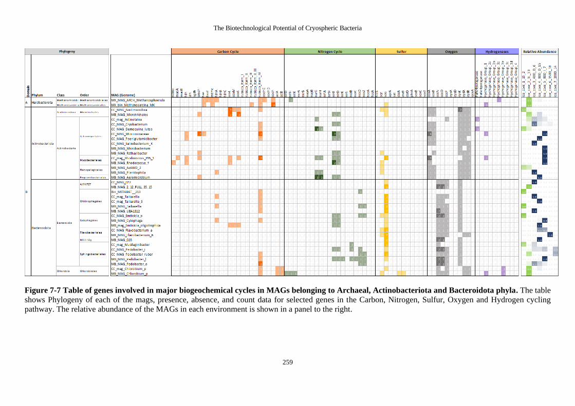
The Biotechnological Potential of Cryospheric Bacteria
259
Figure 7-7 Table of genes involved in major biogeochemical cycles in MAGs belonging to Archaeal, Actinobacteriota and Bacteroidota phyla. The table
shows Phylogeny of each of the mags, presence, absence, and count data for selected genes in the Carbon, Nitrogen, Sulfur, Oxygen and Hydrogen cycling
pathway. The relative abundance of the MAGs in each environment is shown in a panel to the right.

Chapter 7
260
Figure 7-8 Table of genes involved in major biogeochemical cycles in MAGs belonging to Bdellovibrionota, Caldisericota, Chloroflexota, Firmicutes_A,
Gemmatimonadota, Myxococcota, Patescibacteria, Planctomycetota, Verrucomicrobiota, Verrucomicrobiota_Aphyla. The table shows Phylogeny of each
of the mags, presence, absence, and count data for selected genes in the Carbon, Nitrogen, Sulfur, Oxygen and Hydrogen cycling pathway. The relative abundance
of the MAGs in each environment is shown in a panel to the right.

The Biotechnological Potential of Cryospheric Bacteria
261
Figure 7-9 Table of genes involved in major biogeochemical cycles in Proteobacterial MAGs. The table shows Phylogeny of each of the mags, presence,
absence, and count data for selected genes in the Carbon, Nitrogen, Sulfur, Oxygen and Hydrogen cycling pathway. The relative abundance of the MAGs in each
environment is shown in a panel to the right.
Chapter 7
262
7.3.8 Antimicrobial secondary metabolites
The 122 MAGs were submitted to antiSMASH to mine for novel BGCs (Figure 7-10, Figure
7-11, and Figure 7-12). There were 2694 clusters detected in total. Of the cluster types detected,
the most common was saccharide clusters (1597), followed by fatty acids (344) and
halogenated clusters (131). Together, there were more NRPS and NRPS-like clusters
(NRPS=122, NRPS-like=41, combined=163) than there were terpenes (124). The NRPS and
NRPS-like compounds are somewhat distributed throughout several phyla, but they are
especially concentrated in the Actinobacteria. Together, 47/122 of the NRPS clusters and 14
of the 41 NRPS-like clusters occur in just eight Actinobacterial MAGs. Interestingly, all eight
of these MAGs occur in the older and darker ice from sites 400-O (2), 900-O (1) and 900-I (5).
Of note, there was a single Actinobacterial MAG (CC_mag_Rhodococcus_895_1) that had 28
NRPS clusters. This represents 23% of the NRPS clusters in the whole dataset. Of these, only
four are similar to known compounds with described BGCs in the MiBIG database, and the
remainder represent novel NRPS clusters.
The known clusters include one with 45% similarity to heterobactin A and heterobactin S2
(BGC0000371) from Rhodococcus erythropolis PR4, two different clusters with 5 and 7 %
similarity to atratumycin (BGC0001975) from Streptomyces atratus, and a fourth cluster with
similarity to SF2575 (BGC0000269) from Streptomyces sp. SF2575. There were eight
siderophores detected, two of which had 100% similarity to known BGCs in the MIBiG
database.

The Biotechnological Potential of Cryospheric Bacteria
263
Figure 7-10 Secondary metabolites detected by antiSMASH in the Halobacterota, Actinobacteria and Bacteroidota MAGS.

Chapter 7
264
Figure 7-11 Secondary metabolites detected by antiSMASH in the Bdellovibrionota, Caldisericota, Chloroflexota, Firmicutes, Gemmatimonadota,
Myxococcota, Patescibacteria, Planctomycetota and Verrucomicrobiota MAGS.

The Biotechnological Potential of Cryospheric Bacteria
265

Chapter 7
266
Figure 7-12 Secondary metabolites detected by antiSMASH in the Proteobacterial MAGS.

The Biotechnological Potential of Cryospheric Bacteria
267
7.4 Discussion
The Scărișoara Ice Cave has several unique features that make it a fascinating environment for
study. Firstly, it is a perennially cold environment, where the bulk of ice remains frozen year-
round, and only a top liquid layer is added annually, making it a fascinating record of past
climactic conditions (Perşoiu and Pazdur, 2011). Secondly, the ice cave is an extremely unique
and rare environment because of its steady, year-round cold temperatures, variable light
conditions, and oligotrophic conditions. Nonetheless, several studies have shown that bacteria
(Hillebrand-Voiculescu et al., 2015; Itcus et al., 2018; Iţcuş et al., 2016; Paun et al., 2019) and
fungi (Brad et al., 2018; Mondini et al., 2018) can thrive in these systems. The previous
investigations relied on culturing and amplicon sequencing studies, which have two
disadvantages- they can only capture the diversity of cultivable organisms, and secondly, they
only provide information about phylotype, and do not tell us anything about functional
adaptations to this environment. In this study, 121 high-quality MAGs were assembled from
metagenomic DNA collected from seven sites. The spatial distribution of the MAGs (Figure
7-6), their phylogenetic relatedness to each other (Figure 7-5) and to reference species (Table
7-6), their biogeochemical cycling ability (Figure 7-7, Figure 7-8 and Figure 7-9) and their
repertoire of secondary metabolites (Figure 7-10, Figure 7-11 and Figure 7-12) were all
investigated.
7.4.1 Phylogeny and novel species
There were 121 MAGS resolved from the Ice Cave, and they belonged to 14 different phyla.
The phylogenetic classification of these MAGs corroborates recent 16S rRNA amplicon studies
of this same cave environment (Paun et al., 2019). The most abundant phylum by far was the
Proteobacteria, which was in agreement with previous 16S rRNA studies of this environment
(Iţcuş et al., 2016). We also managed to resolve two Archaea from the dataset.
Several MAGs from the Ice Cave were species-level matches to known bacteria and archaea
according to FastANI (Table 7-5). When we looked at the habitats of these close relatives, we
found that they were isolated predominantly in oligotrophic and cold environments. The
Archaea, MX_bin_Methanosarcina_MX, is a close relative of Methanosarcina sp001714685
(GCA_001714685.2), which was assembled from a permafrost metagenome from near Miers
Lake, McMurdo Dry Valleys, Antarctica. MX_MAG_Flavobacterium-6 is like the type strain
Flavobacterium psychrolimnae (GCA_003312425.1) collected from an Antarctic lake.
CC_bin_Polaromonas is similar to Polaromonas glacialis (GCF_000709345.1) which was

Chapter 7
268
collected from glacial foreland till in Norway. MX_MAG_003_Paracoccus is a close relation
of Paracoccus sp000787695 (GCF_000787695.1) collected from a marine sediment near Ny-
Ålesund, Svalbard. There was no geographic information associated with the assembly for
Pedobacter_A ruber (GCF_900103545.1) which was the closest relative of
CC_MAG_Pedobacter_ruber, however, the species Pedobacter_A ruber was first described as
a psychrophilic soil bacteria (Margesin and Zhang, 2013). MB_mag_Caulobacter is similar to
Caulobacter sp002737765 (GCF_002737765.1), an isolate from littorial waters of Lake
Michigan that had been stored at 4 degrees C for one year. MX_MAG_Polynucleobacter,
relative of Polynucleobacter aenigmaticus (GCF_002206635.1) from a freshwater lake, Lake
Krottensee, from the Salzkammergut Area, Austria.
The exceptions to the overwhelming majority of psychrophilic microorganisms was
MB_MAG_Rhodococcus_f, was similar to Rhodococcus fascians (GCF_001894785.1) and
MB_MAG_Rathayibacter, similar to Rathayibacter caricis (GCF_003044275.1) and
MB_MAG_Sphingomonas_p related to Sphingomonas paucimobilis (GCF_000739895.2),
which was isolated from a hospital respirator.
There were many more MAGs that fell short of the 95 radius set by FastANI, but that could be
identified to species level using GTDB-tk. For example, there were three MAGs belonging to
the Massilia, which are known to be psychrophilic.
This ice block has previously been investigated using 16S rRNA sequencing, and the
assembled MAGs bear striking and reassuring similarity to the communities detected using
16S rRNA amplicon studies. Previously, methanogenic species belonging to
Methanosphaerula and Methanosarcina were detected in 2,000- and 5,000-year-old samples
(Paun et al., 2019), however, in this study we found these MAGs predominantly in ice from
site 1L-13 ice from the present day (Figure 7-6).
7.4.2 Spatial distribution of the MAGs
There was significant variation in the ages and environmental properties of the different sites
that were sampled. Some areas of the cave, near the entrance, receive direct light (1S), others
receive indirect light (1L) and still others are in complete darkness. In addition, some layers
have higher organic and inorganic content (due to the settling of sediment within each annual
layer) than others, which appear as clear ice. Apart from site 1S and 1L, sampled layers were
quite old and have remained frozen for hundreds (400-O: 385 years) to thousands of years
(1800: ~1500 years ago). The bacteria within, have therefore been trapped (dead or alive), for
The Biotechnological Potential of Cryospheric Bacteria
269
significant periods of time, and they provide a fascinating insight into the conditions outside of
the cave, during the summer when the water first trickled in and then froze. In a previous study
of these same sites, cell density and number of cultivatable organisms was negatively correlated
to the age of the ice (Iţcuş et al., 2016), which is corroborated in this study as because the cave
locations with the fewest number of MAGs and the least coverage were the two oldest sites.
A striking observation was the strong spatial preference of specific MAGs for a single site
(Figure 7-6). This could be explained by the fact that the Ice Cave remains frozen, and that
community members become trapped within a single layer with each freezing. Nonetheless,
this obvious spatial organisation of the microbial communities suggests that it is a priceless
resource for looking the changing climate conditions over recent millennia.
The spatial distribution of the MAGs also highlights the incredible power of read mapping to
distinguish between closely related strains when the assembly is good. There were three
different Bacteroidete MAGs from the genus Taibaiella_B, however, they could be
distinguished because they occurred in completely different samples. MB_MAG_Taibaiella
occurred at location 1S_2, CC_mag_Taibaiella was found in location 400_O_6 and
CC_mag_Taibaiella_3 occurred at location 900_O_15. There is a Flavobacterium
(MX_MAG_Flavobacterium-6) that occurs exclusively at site 1500_18 and a Flavobacterium
(CC_MAG_Flavobacterium_a) that can be found at sites 400_O_6, 900_O_15 and 900_I_7. It
is evident that the locations of each of the three Massilia MAGs differ. CC_MAG_Massilia_1
is found in location 1500_18, while CC_mag_Massilia (GCF_900129765.1) and
CC_MAG_Massilia_e (GCF_002760655.1) are found mainly in location 2000_14, and to
different extents in nearby locations. The same can be said of Methylotenera MAGs.
The fact that similar MAGs crop up again and again at different sites suggests that the ice cave
community is not particularly diverse. The passage of times between freezing events allows us
to assemble and distinguish different strains of the same species and genera, but the genera and
species making up the core community in the different layers is relatively constant.
7.4.3 Biogeochemical cycling
Analysis of several biogeochemical cycling genes revealed that the Ice Cave is a highly
reducing environment (Figure 7-7, Figure 7-8, and Figure 7-9).
Chapter 7
270
7.4.3.1 Carbon cycling
The Calvin–Benson–Bassham (CBB) cycle assimilates CO2 for the primary production of
organic matter and the key enzyme of this cycle is ribulose-bisphosphate
carboxylase/oxygenase (RubisCO). Of the three carboxylating forms of RubisCO (I, II and III),
form I is the main enzyme responsible for photoautotrophy in bacteria (Tabita et al., 2008).
Given the low levels of light in the cave, we did not expect to find much evidence
photoautotrophy. Indeed, there were only eight MAGs in total with Form 1 RubisCO genes,
three Alphaproteobacterial MAGs, and five Gammaproteobacterial MAGs, all of which belong
to the family Burkholderia. Of these, five came from sites IS and IL which received light. We
also found a form III RubisCO gene in MX_bin_Methanosarcina_MX. Until recently, form III
RubisCO was thought to exist exclusively in archaea where it aided in the utilization of
ribonucleotides and ribonucleosides via the pentose-bisphosphate pathway (Frolov et al.,
2019). However, Form III RubisCO has just recently been implicated in autotrophic CO2
fixation (Frolov et al., 2019).
The two MAGs belonging to the Phylum Chlorobia, order Chlorobiales, found predominantly
at site 1L_13, had acetate citrate lyase genes aclA and aclB, which enable carbon fixation in
anaerobic conditions (Kanao et al., 2001). Chlorobium, which have previously been detected
in the Scărișoara Ice Cave (Itcus et al., 2018; Paun et al., 2019), generally grow
photoautotrophically in strict anaerobic environments and are known to contain acetate citrate
lyase genes (Kanao et al., 2001). These genes encode a key enzyme (ATP‐citrate lyase) in the
reductive tricarboxylic acid (RTCA) cycle because it determines the direction of this cycle
(Kanao et al., 2001). The (RTCA) cycle fixes four molecules of CO2 to generate one molecule
of oxaloacetate in one cycle. Even though these bacteria are exposed to light, they are too
deeply embedded in the ice to photosynthesize aerobically.
7.4.3.2 Nitrogen cycling
There were only four MAGs capable of nitrogen fixation via one or more of nifH/D/K (Fani et
al., 2000). Three of these MAGs were found predominantly at site IL, which receives some
sunlight and represents a ‘present day’ community. The napA/B and narG/H genes are involved
in denitrification and dissimilatory nitrate reduction and encode genes that reduce nitrate
(NO3_) to nitrite (NO2
-) (Sparacino-Watkins et al., 2014). Both napA/B were present in a
Planctomycetales MAG, a single Alphaproteobacterial MAG and three Gammaproteobacterial
MAGs. The narG/H genes were far more abundant, and found in four Actinobacterial MAGs,
four Alphaproteobacterial MAGs and 18 Gammaproteobacterial MAGs. MAGs

The Biotechnological Potential of Cryospheric Bacteria
271
CC_MAG_Massilia_1 and CC_MAG_Rhodoferax had all four genes for napA/B and narG/H.
Nitrite reductase (NirBD) functions during aerobic growth where is reduces nitrite (NO3−) to
ammonium (NH4+) (Harborne et al., 1992). NirB/D genes were detected in eight
Actinobacterial MAGs, five Bacteroidota MAGs (including all three Cytophagales MAGs),
three Plantomycetes, eight Alphaproteobacteria and 21 Gammaproteobacterial MAGs. The
norB/C genes encode a respiratory nitric oxide reductase that reduces NO to N2O (Hendriks et
al., 2000). NorB/C genes were present in several Bdellovibrionota and Alphaproteobacterial
MAGs and in 20 Gammaproteobacterial MAGs. Several of the MAGs with norB/C genes also
had nosD/Z genes, which reduce N2O further to N2 (McGuirl et al., 1998).
7.4.3.3 Sulfur cycling
The sdo (sulfuf dioxygenase) gene was the most common gene across all the phyla. Sulfur
dioxygenases (SDOs) were originally found in the cell extracts of chemolithotrophic bacteria
as glutathione (GSH)-dependent sulfur dioxygenases (Liu et al., 2014). GSH spontaneously
reacts with elemental sulfur to generate glutathione persulfide (GSSH), and SDOs oxidize
GSSH to sulfite and GSH (Liu et al., 2014). Sulfur oxidation via the Sulfur Oxidising
(soxBCY) pathways (Bagchi and Ghosh, 2005; Bagchi and Roy, 2005) was highly prevalent
in the Gammaproteobacteria, and specifically, within the order Burkholderiales, where 13/23
had at least one sox gene, and 10 had all three of soxBCY. There were two Rhizobiales MAGs
in the Alphaproteobacteria with at least one sox gene and a single sox gene in the
Gemmatimonadota MAG (MB_MAG_Gemmatimonas).
7.4.3.4 Oxygen cycling
There are also some striking clade-specific differences in biogeochemical cycling pathways for
oxygen cycling. The coxAB genes encode for a cytochrome c oxidase that couples the oxidation
of reduced cytochrome c with the reduction of molecular oxygen to water (Schmetterer et al.,
1994). These genes are present in 13 Actinobacterial MAGs, none of the Bacteroidetes and all
but one of the Proteobacteria. CcoNOP is a cbb3 cytochrome c oxidase that exhibits oxygen
reductase activity (Swem and Bauer, 2002). The genes for this complex was ubiquitous across
Bacteroidetota (15/16), the Alphaproteobacteria (11/20), Gammaproteobacteria (27/31)
Bdellovibrionota (7/7), Planctomycetota (2/4), Verrucomicrobiota (5/6) the Gemmatimonadota
(1/1), Myxococcota (2/2), but completely absent from the Actinobacteria, Caldisericota,
Chloroflexota, Firmicutes_A, Patescibacteria and Verrucomicrobiota_A. Whilst the
Actinobacteria tend to have all three of cyoE, cydA and cydB, most of the Bacteroidetes only

Chapter 7
272
have cyoE, except for MX_mag_Flavobacterium_6 and the two Chlorobium MAGs which only
have cydA and cydB. The cyoE gene encodes a cytochrome o oxidase complex and cydAB
encodes a cytochrome d oxidase complex, which act as terminal oxidases that catalyse the
oxidation of ubiquinol-8 and the reduction of oxygen to water (Cotter et al., 1990).
7.4.4 Secondary metabolites
Several caves have been explored in the past for novel antimicrobial compounds (Ghosh et al.,
2017). Examples include the subterranean Kotumsar cave, India (Rajput et al., 2012), to a
volcanic cave in western Canada (Rule and Cheeptham, 2013) to Magura Cave, Bulgaria
(Tomova et al., 2013). However, all of these studies have relied on cultivated strains, which
can exceptionally difficult to grow because of complicated cultivation conditions and
exceptionally slow growth (Ghosh et al., 2017).
We submitted the 121 MAGs to antiSMASH, and there was a total of 2694 clusters detected.
Of the cluster types detected, the most common was saccharide clusters (1597), followed by
fatty acids (344) and halogenated clusters (131). Together, there were more NRPS and NRPS-
like clusters (NRPS=122, NRPS-like=41, combined=163) than there were terpenes (124).
Since terpenes are often carotenoids and other photoprotective antioxidants, the low-light cave
environment is not unexpected.
The NRPS and NRPS-like compounds are somewhat distributed throughout several phyla, but
they are especially concentrated in the Actinobacteria. Together, 47/122 of the NRPS clusters
and 14 of the 41 NRPS-like clusters occur in just 8 Actinobacterial MAGs. Of note, there was
a single Actinobacterial MAG (CC_mag_Rhodococcus_895_1) that had 28 NRPS clusters.
This represents 23% of the NRPS clusters in the whole dataset. Of these, only four are similar
to known compounds with described BGCs in the MiBIG database, and the remainder represent
novel NRPS clusters. These clusters and compounds are worth exploring for novel
bioactivities.
7.5 Conclusion
Ice Caves are unusual habitats characterized by extreme conditions for life, and to our
knowledge, this is the first study to study shotgun metagenomes from an ice cave. There were
121 high quality MAGs assembled from this environment, including genomes from 111 novel
species. There were strong spatial patterns amongst the community members and mapping
reads back to contigs enabled the resolution of distinct, yet closely related species. There were

The Biotechnological Potential of Cryospheric Bacteria
273
several biogeochemical pathways suggesting that anaerobic photoautotrophy is possible near
the entrance to the cave, but chemolithotrophy is common at other sites. Cave microbiomes
have been hypothesized to be rich resources for antimicrobial products and this study identified
thousands of clusters for secondary metabolites in the MAGs of this biome.

Chapter 8
274
8 BIOINFORMATICS
WORKFLOW FOR
BIOPROSPECTING FROM
METAGENOMES
8.1 Introduction
Bioprospecting is the search for NPs that provide health, societal or environmental benefits.
Increasingly, with a reduction in the cost of DNA sequencing, it is possible to investigate the
bioprospecting potential of an environment as a precursor to obtaining physiological proof of
function. Recently, there has been a major paradigm shift in microbial ecology to the
construction of genomes from metagenomic datasets (Parks et al., 2018; Pasolli et al., 2019),
which is partly fueled by the increased sequencing depth, and to some extent by new long-read
sequencing methods, like Nanopore (Moss et al., 2020; Overholt et al., 2019; Singleton et al.,
2020). This genome-centric view has several advantages in bioprospecting, such as the
resolution of genomes belonging to novel species that have no cultivable relatives and
additional information about regulatory factors, nutrient requirements and metabolism and
antibiotic resistance that all help inform strategic heterologous expression and cultivation
efforts. However, it also comes with disadvantages, the major of these being that only the most
abundant members of a community can be resolved using this method, which means that a
large portion of a dataset is not explored. However, the benefits of a genome-centric
bioprospecting are great, particularly because of the insights it provides when it comes to
community cooperation and the way it opens possibilities for strategic cultivation efforts. In
addition, the contigs of rarer community members that cannot be binned into MAGs are still a
catalogue of diversity that can be mined in the same way as MAGs. The contigs can be
submitted to numerous databases, specialized to identify genes and gene clusters for specific
NP products and gene functions.
The Biotechnological Potential of Cryospheric Bacteria
275
In this thesis, MAGs were constructed from two very different environments, a Svalbard glacial
system comprising cryoconite, soil and seawater metagenomes (Chapter 4) and the Scărișoara
Ice-cave in Romania (Chapter 7). The bioinformatic approach involved the assembly,
annotation, binning, and comparison of genomes from these metagenomic datasets.
This chapter is a review some of some of the benchmarking, method optimization, and
decision-making employed in the construction of the MAGs. The application of these methods
on two different datasets also provided some insights into the effect of sequencing depth and
community complexity on MAG reconstruction.
8.1.1 Aims and Objectives
The aims of this chapter were as follows:
1. Based on knowledge of environmental stressors, create a list of genes and gene products
that have useful applications.
2. Describe a workflow that goes from raw reads to contigs and metagenome-assembled
genomes using readily available open-access tools.
3. Curate a catalogue of tools that can be used and substituted in this workflow
4. Test and compare tools on different cryospheric datasets to compare:
4.1. The effect of the data: i.e. the effect of sampling depth and environment complexity.
4.2. The use of different tools: i.e. the use of different assembly tools and binning methods.
5. Highlight the advantages and disadvantages of using reads, contigs and MAGs in
bioprospecting.

Chapter 8
276
8.2 Methods
8.2.1 Environmental sample types
In accordance with the project objectives, a range of different environmental sample types was
analysed. There were two datasets analysed in detail for their bioprospecting potential. A
Svalbard dataset consisting of 17 paired-end (PE) libraries from soil (8), cryoconite (6) and
seawater (3) (see Chapter 4). An ice cave dataset consisting of seven libraries from the
perennial ice block of Scărișoara Ice Cave in Romania (see Chapter 7). The libraries for the
different datasets differ in sequencing depth, community heterogeneity and complexity.
8.2.2 Quality control
All libraries form both metagenome datasets were uploaded to KBase (http://kbase.us/)(Arkin
et al., 2018). The quality of the raw libraries was assessed using FastQC (J. Brown et al., 2017).
Adapters were removed and low-quality bases were trimmed using Trimmomatic (Bolger et
al., 2014) with a minimum Phred score threshold of 30. The quality of the read libraries was
then reassessed using FastQC.
8.2.3 Assembly
Assembly is the process by which individual reads are split into predefined segments (k-mers),
which are overlapped into a network, and paths are traversed iteratively to create longer contigs
(van der Walt et al., 2017). Assembly is a very computationally expensive step, and all
downstream analyses depend on the quality of the contigs. There are a range of different
assembly tool available, many of which can be tailored with different parameters such as k-
mer length (Vollmers et al., 2017). Metagenome libraries, consisting of the DNA from a single
site, can either be assembled individually, or co-assembled together, wherein all the libraries
are combined in the assembly step, and reads are mapped to the contigs to determine the
contribution of different libraries to the contigs in the final assembly. In this thesis, the
performance of three different assembly tools: MEGAHIT (D. Li et al., 2015), metaSPAdes
(Nurk et al., 2017) and IDBA-UD (Peng et al., 2012) were tested, as was the effect of co-
assembly vis single-sample assembly. MetaQUAST was used to compared the assemblies
(Gurevich et al., 2013).

The Biotechnological Potential of Cryospheric Bacteria
277
8.2.4 Metagenome-assembled genomes (MAGs) using anvi’o
With large shotgun metagenomic libraries, it is possible to assemble putative genomes or
metagenome-assembled genomes (MAGs). To do this, we used the tool anvi’o (versions 5, 6.1
and 6.2) (Eren et al., 2015) following the Anvi'o User Tutorial for Metagenomic Workflow
(http://merenlab.org/2016/06/22/anvio-tutorial-v2/). An anvi’o contigs databases is created
using anvi-gen-contigs-database, with an assembly fasta file as input. The contigs database is
an essential component of the anvi’o metagenomic workflow because it stores information on
positions of open reading frames (ORFs), identified using Prodigal (Hyatt et al., 2010), and k-
mer frequencies for each contig.
8.2.4.1 Functional Annotation of contigs
The contigs database can be annotated from within the anvi’o workflow using scripts that
access external databases.
8.2.4.1.1 Single copy gene HMMs
To estimate the number of bacterial genomes in the metagenome, anvi’o runs HMMER (Eddy,
2008; Mistry et al., 2013) against a series of single-copy gene (SCG) databases. In anvi’o-6.1,
these include specially curated HMM profiles of SCGs for Archaea (76 genes), Protista (83
genes) and Bacteria (71 genes)(Lee, 2019). There is also a script to detect candidate phyla
radiation (CPR) that relies on the SCG HMM dataset from (Campbell et al., 2013). Therefore,
the Campbell HMMs, together with the three profiles with anvio-6.1 were included in the
HMMER scan.
8.2.4.1.2 NCBI COGs
The genes in the contigs database can be annotated with functions from the NCBI’s Clusters
of Orthologus Groups (COGs) using anvi-setup-ncbi-cogs to download the database
(http://www.ncbi.nlm.nih.gov/COG/) and anvi-run-ncbi-cogs to annotate the contigs database.
Each COG consists of individual orthologous proteins or orthologous sets of paralogs from
several (minimum of three) lineages (Galperin et al., 2015; Tatusov et al., 1997). Orthologs
generally have the same function, which means functional information from one member can
be transferred to an entire COG, allowing functional predictions of poorly characterized
genomes (Galperin et al., 2015; Tatusov et al., 1997).

Chapter 8
278
8.2.4.1.3 KEGG annotations
The Kyoto Encyclopedia of Genes and Genomes (KEGG) (https://www.genome.jp/kegg/)
database integrates functional information, biological pathways, and sequence similarity in
order to infer high level functions of organisms or ecosystems (Kanehisa and Goto, 2000).
GhostKOALA (https://www.kegg.jp/ghostkoala/) is a web-server-based tool that provides
automatic annotation of KEGG Identifiers to metagenomes (Kanehisa et al., 2016). In order to
import KEGG annotations into the anvi’o contigs database(s), a workflow
(http://merenlab.org/2018/01/17/importing-ghostkoala-annotations/) and its associated tools
(https://github.com/edgraham/GhostKoalaParser.git) were used as described. Gene calls were
exported from the contigs database and submitted in batches of an appropriate size.
8.2.4.1.4 Eggnog mapper
Annotations were computed using eggnog-mapper (Huerta-Cepas et al., 2017) based on
eggNOG 4.5 orthology data (Huerta-Cepas et al., 2016) using the eggNOG mapper v.1 web-
server (http://eggnogdb.embl.de/#/app/emapper). Gene calls from the contig database were
exported, and the file split into multiple files of 80 000 sequences (Svalbard) or 100 000
sequences (Ice-cave), and then submitted to the webserver.
8.2.4.2 Taxonomic Assignment
8.2.4.2.1 Assign Taxonomy from kaiju- refseq
Taxonomic information was added to the genes and contigs using Kaiju (Menzel et al., 2016).
Kaiju was installed locally on the CLIMB VM using instructions available on the Kaiju Github
(https://github.com/bioinformatics-centre/kaiju). The Kaiju database was made using the
‘refseq’ database, which contains 63 million sequences from completely assembled and
annotated reference genomes of Archaea, Bacteria, and viruses from the NCBI RefSeq
database (O’Leary et al., 2016). The sequences for the gene-calls in the contigs database were
exported using anvi-get-sequences-for-gene-calls, and Kaiju was run on these gene-calls. The
script addTaxonNames adds taxon information so that is can be parsed back into the contig
database, and finally taxonomy for the gene calls was added by running anvi-import-taxonomy-
for-genes.
8.2.4.2.2 Single-Copy Core Genes (SCGs)
The taxonomy of the MAGs was estimated using the anvi’o scg-taxonomy workflow
described here: http://merenlab.org/scg-taxonomy. The workflow uses the taxonomy
determined by the Genome Taxonomy Database (GTDB) (Parks et al., 2018) and makes use

The Biotechnological Potential of Cryospheric Bacteria
279
of DIAMOND (Buchfink et al., 2015), a fast alternative to the NCBI’s BLAST. The
command anvi-setup-scg-databases downloads the SCGs and the GTDB taxonomy of the
genomes and builds a search database for a subset of 22 SCGs. The script anvi-run-scg-
taxonomy searches the contigs.db for the 22 SCGs, compares them against the corresponding
genes in the GTDB databases and selects the best hit, which it stores in a table in the contigs
database. The anvi-run-scg-taxonomy script can be run on a contigs database to estimate how
many genomes are in the assembly, or on a contigs database + profile database to determine
the coverage or relative proportion of the different genomes in different samples, or it can be
run on a contigs.db, profile.db and a collection to get the taxonomy of each of the bins in a
collection. There were 1,377 SCG Ribosomal genes with taxonomic affiliations in the
Svalbard contigs database. (Appendix: Figure D-2 shows the number of hits per Ribosomal
gene and Appendix Table D-3 shows the probable identity of the genomes, based on the most
abundant SCG, Ribosomal_S11, (n=112). There were 3,025 SCG genes with taxonomic
affiliations in the Ice Cave contig database (Appendix Figure G-1). Appendix Table G-1
shows the probable identity of the genomes in the data set as well as their coverage and
distribution across samples, based on the most abundant SCG, Ribosomal_S2 (n=202).
8.2.4.3 Mapping and creating a sample profile
Mapping of individual trimmed read libraries to co-assemblies was performed within the anvi’o
environment using Bowtie2 (Langmead and Salzberg, 2012)(version 2.3.4.3). Samtools (Li et
al., 2009) was used to convert the .sam file to raw .bam files, and an anvi’o script ‘anvi-init-
bam to get indexed .bam files for each of the samples. Next, anvi-profile creates a single profile
that reports properties for each contig in a single sample based on mapping results. Profiling
includes calculating the mean coverage, standard deviation of coverage, and the average
coverage for the inner quartiles (Q1 and Q3) as well as coverage and single nucleotide variation
at each nucleotide position for a given contig. Once samples have been individually profiled,
all samples sharing a contigs database can be merged using anvi-merge.
8.2.5 Binning and refinement of MAGs
8.2.5.1 Binning
CONCOCT (v.1.1.0) was the built-in binning program in anvi’o until V. 6.1 because it uses
Gaussian mixture models to cluster contigs into genomes based on sequence composition and
coverage across multiple samples (Alneberg et al., 2014). The cross-sample comparison was
especially suited to binning contigs from co-assemblies. However, additional binning tools

Chapter 8
280
such as metaBAT2 (v2.12.1) (Kang et al., 2015) and MaxBin2 (v2.2.7) (Wu et al., 2016) were
installed and then run from within anvi’o using the script anvi-cluster-contigs. The tool DAS
Tool (v1.1.1) (Sieber et al., 2018), which optimises bins based on bins generated by other tools
was then run, using the metaBAT2, MaxBin2 and CONCOCT collections as input for the
refinement. The DAS Tool bins were then manually refined, and DAS Tool run again, to
determine whether refining resulted in better or worse bins. The iteration and refining of DAS
Tool bins were repeated twice: each time, the DAS Tool results were run on all the original
bins, and the newly refined bins. Where DAS Tool reverted previously refined bins to unrefined
bins, those refinements were checked. If the previous refinement could be clearly justified, the
bin was refined again. Where the decision was unclear, the original bin was kept, regardless of
high redundancy values.
8.2.5.2 Comparing binning results and refining bins
After binning, the collections were exported, merged and them re-imported as an additional
layer. The steps were followed as described in http://merenlab.org/tutorials/infant-gut/ Chapter
II: Automatic Binning: Comparing multiple binning approaches, with some modifications. The
results of each collection, including those that had been through refinement steps were exported
as tab-limited (.tsv) files. These files contained information on split-name and bin membership.
In anvi’o, large contigs are divided into ‘splits’ of approximately 20 kB for processing, but all
information about the original contig is kept, and splits have the same contig_id, with a unique
suffix which comprises the split id. To import the bin membership information, the .tsv files
were edited to remove split details from the contig id using (sed)
(https://www.gnu.org/software/sed/manual/), and then were sorted and deduplicated using uniq
(sort | uniq). The collections were then merged using anvi-script-merge-collections to create a
.tsv file where each line represents a contig id, and each column has the bin id for each binning
result. The .tsv was imported to the profile database as an ‘item’ using anvi-import-misc-data,
which allowed visualisation of bin membership of each contig. Therefore, any collection could
be loaded in anvi-interactive or in anvi-refine and the binning results of each tool compared.
Where there was disagreement between bins, contig membership could be compared, and a
‘consensus’ bin visualised (Figure 8-1). The contigs of chimeric bins are more likely to be
grouped different using different binning methods.

The Biotechnological Potential of Cryospheric Bacteria
281
Figure 8-1 Figure showing an example of a ‘good’ bin during refinement. Anvi’o shows contig coverage across samples, GC content, splits, total reads mapped and single nucleotide variants
(SNVs). Bin membership of each contig using different binning tools is export as an additional data
layer. Kaiju contig classification, and various other metadata and statistics such as extraction method,
year and glacier are also displayed. By selecting the bin, a real-time estimate of taxonomy based on
SCG hits to GTDB can be viewed.

Chapter 8
282
8.2.5.3 Visualisation and refinement of MAGs
The MAGS were refined, visualised, and compared using the anvi’o anvi-interactive and anvi-
refine tools. In the view, Kaiju taxonomy is shown in colour of the contigs, the SCG taxonomy
(including the number of GTDB SCGs and their identity) is shown from the bin information,
and the binning tool membership is added as a layer (Figure 8-1). After refinement, the
collection of complete bins could be exported using anvi-summarise. This summary contains
information about contig coverage, GC content, number of contigs, N50, total size, MAG
completion and redundancy based SCG genes from HMM profiles. The fasta files for each
MAG were also separately uploaded to KBase and the completion and redundancy
(heterogeneity or contamination) of the MAGs was assessed using CheckM (Parks et al., 2015),
and the taxonomic classification was checked using GTDB-Tk (Chaumeil et al., 2020).
8.2.6 Screening MAGs and contigs
Finally, the MAGs can be screened for sequences responsible for the synthesis of desired NPs.
In this chapter, the results of screening these datasets for secondary metabolites using
(antiSMASH) and carbohydrate-active enzymes (dbCAN2) is described.
8.2.6.1 dbCAN2 to detect carbohydrate active enzymes
The contigs from the MEGAHIT assemblies of the Ice Cave and Svalbard datasets were
submitted in batches to the dbCAN2 webserver (http://bcb.unl.edu/dbCAN2/index.php)
(Zhang et al., 2018), which queries the Carbohydrate-Active EnZymes database (CAZy)
(Cantarel et al., 2009; Lombard et al., 2014) (http://www.cazy.org/) using DIAMOND
(Buchfink et al., 2015), HMMER (Mistry et al., 2013) and HotPep (Busk et al., 2017).
8.2.6.2 Biosynthetic gene cluster detection
AntiSMASH has algorithms able to detect a vast range of different BGCs, and many different
molecule families. AntiSMASH is developed by several collaborating institutions, that makes
use of a variety of tools such as NCBI BLAST+, HMMer 3, Muscle 3, Glimmer 3, FastTree,
TreeGraph 2, Indigo-depict, PySVG and JQuery SVG. It can be run using a web application
(https://antismash.secondarymetabolites.org) or as a standalone tool. The antiSMASH v5
results from the Svalbard MAGs (Chapter5) and Ice-Cave MAGs (Chapter7, Figure 7-10 to 7-
12.) have been shown in previous chapters. In addition, all of the contigs from three different
Ice-Cave assemblies, and the contigs from Svalbard cryoconite, soil and seawater were also
screened using antiSMASH.

The Biotechnological Potential of Cryospheric Bacteria
283
8.2.7 Workflow steps
A schematic diagram of the bioinformatics workflow is shown in Figure 8-2. A general outline
Figure 8-2: Schematic diagram of the bioinformatics workflow for Bioprospecting.
Analyses can be performed on the trimmed reads or on assembled contigs. The reads and
contigs can also be mapped back to MAGs.
Summary of terms in figure: Quality control: trimming adapters and primers, removing
bases with a low Phred score. Assembly: assembling millions of short reads into longer contigs.
Mapping: aligning reads back to the contigs to calculate contig coverage and assembly quality.
Annotation: processing the data to look for open reading frames (ORFs) and coding sequences.
Alignment: comparing the amino acids in these samples to reference strains and each other.
Binning: grouping contigs into taxonomic groups based on similar coverage, GC content and
tetranucleotide repeats to resolve genomes.

Chapter 8
284
8.3 Results
8.3.1 Identification of bioprospecting targets
One of the aims of this project was to interrogate cryospheric metagenomes for industrially
useful natural products such as enzymes and antimicrobial metabolites using open and freely
available bioinformatics tools. To focus the project, potentially common and useful product-
types were identified based on likely microbial adaptations to known cryospheric
environmental stresses.
Table 8-1 Bioprospecting targets for cryospheric environments
Product Adaptation Application Steps List of product- specific tools
Cold-active enzymes
Amino acid changes that increase enzyme flexibility
Food industry, detergents, molecular biology tools
QC, alignment, assembly, annotation, BGC mining, binning
DIAMOND-blastx, HMMER3, UniRef, Pfam, CAZy, dbCAN2
Polyunsaturated fatty acids
PUFAs increase membrane permeability at low temperatures
Dietary supplements for humans, livestock, and fish
QC, assembly, annotation, BGC mining, binning
antiSMASH
Ice nucleation proteins
Seed small crystals instead of large damaging crystals
Food industry, synthetic snow
QC, alignment DIAMOND-blastx, HMMER3, MEGA, UniRef, Pfam
Antifreeze proteins and solutes
Disrupt orderely arrangement of water molecules from forming ice-crystal structure
Cryoprotectants, food industry
QC, alignment
Antioxidants and UV pigments
Protect microrganisms from seasonally high UV irradiation in snow
Biomedical, pharmaceutical, food technology and cosmetics
QC, assembly, annotation, BGC mining, binning
antiSMASH
Exopolysaccharide Trap liquid water, preventing freezing
Biomedical, pharmaceutical, food technology and cosmetics
QC, assembly, annotation, BGC mining, binning
antiSMASH, dbCAN2 webserver
Antimicrobial compounds
Chemical defenses and weapons against competeing bacteria in low-resource environments
Pharmaceutical industry- antibiotics, antifungals, anti-tumour medications and pesticides
QC, assembly, annotation, BGC mining, binning
antiSMASH, PRISM, BAGEL
The adaptation strategy, application of the natural product, workflow steps involved, and specific tools and databases are listed.
8.3.2 Datasets
The shotgun metagenome libraries from the Svalbard dataset and Scărișoara Ice Cave dataset
are shown in in Table 8-2 and Table 8-3 respectively.
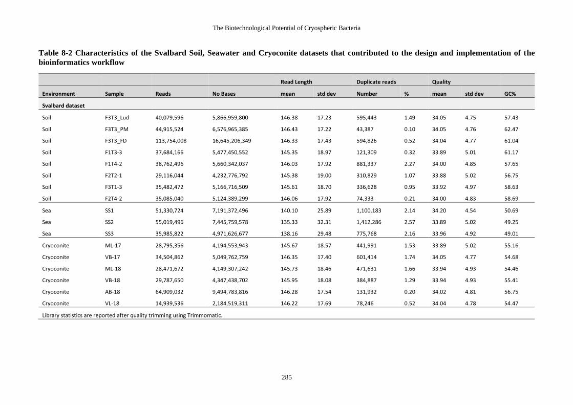
The Biotechnological Potential of Cryospheric Bacteria
285
Table 8-2 Characteristics of the Svalbard Soil, Seawater and Cryoconite datasets that contributed to the design and implementation of the
bioinformatics workflow
Read Length Duplicate reads Quality
Environment Sample Reads No Bases mean std dev Number % mean std dev GC%
Svalbard dataset
Soil F3T3_Lud 40,079,596 5,866,959,800 146.38 17.23 595,443 1.49 34.05 4.75 57.43
Soil F3T3_PM 44,915,524 6,576,965,385 146.43 17.22 43,387 0.10 34.05 4.76 62.47
Soil F3T3_FD 113,754,008 16,645,206,349 146.33 17.43 594,826 0.52 34.04 4.77 61.04
Soil F1T3-3 37,684,166 5,477,450,552 145.35 18.97 121,309 0.32 33.89 5.01 61.17
Soil F1T4-2 38,762,496 5,660,342,037 146.03 17.92 881,337 2.27 34.00 4.85 57.65
Soil F2T2-1 29,116,044 4,232,776,792 145.38 19.00 310,829 1.07 33.88 5.02 56.75
Soil F3T1-3 35,482,472 5,166,716,509 145.61 18.70 336,628 0.95 33.92 4.97 58.63
Soil F2T4-2 35,085,040 5,124,389,299 146.06 17.92 74,333 0.21 34.00 4.83 58.69
Sea SS1 51,330,724 7,191,372,496 140.10 25.89 1,100,183 2.14 34.20 4.54 50.69
Sea SS2 55,019,496 7,445,759,578 135.33 32.31 1,412,286 2.57 33.89 5.02 49.25
Sea SS3 35,985,822 4,971,626,677 138.16 29.48 775,768 2.16 33.96 4.92 49.01
Cryoconite ML-17 28,795,356 4,194,553,943 145.67 18.57 441,991 1.53 33.89 5.02 55.16
Cryoconite VB-17 34,504,862 5,049,762,759 146.35 17.40 601,414 1.74 34.05 4.77 54.68
Cryoconite ML-18 28,471,672 4,149,307,242 145.73 18.46 471,631 1.66 33.94 4.93 54.46
Cryoconite VB-18 29,787,650 4,347,438,702 145.95 18.08 384,887 1.29 33.94 4.93 55.41
Cryoconite AB-18 64,909,032 9,494,783,816 146.28 17.54 131,932 0.20 34.02 4.81 56.75
Cryoconite VL-18 14,939,536 2,184,519,311 146.22 17.69 78,246 0.52 34.04 4.78 54.47
Library statistics are reported after quality trimming using Trimmomatic.

Chapter 8
286
Table 8-3 Characteristics of the Scărișoara Ice-Cave dataset that contributed to the design and implementation of the bioinformatics workflow
Read Length Duplicate reads Quality
Environment Sample Reads No Bases mean std dev Number % mean std dev GC%
Ice-cave dataset
Present, sun 1S_2 69,575,748 8,530,226,859 122.60 10.58 29,675 0.04 35.48 3.95 53.19
Present, light 1L_13 72,190,896 8,860,007,146 122.73 10.26 36,821 0.05 35.48 3.94 56.84
-385, organic 400_O_6 76,039,348 9,324,467,510 122.63 10.53 161,544 0.21 35.47 3.97 54.29
-943. Organic 900_O_15 73,462,594 9,019,960,422 122.78 10.20 353,401 0.48 35.51 3.90 54.57
-943, inorganic 900_I_7 75,113,102 9,213,747,381 122.67 10.46 145,477 0.19 35.43 4.03 59.89
~1200 1500_18 75,510,556 9,278,999,040 122.88 9.77 1,286,620 1.70 35.67 3.59 42.33
~1500 2000_14 63,569,516 7,815,266,055 122.94 9.78 84,276 0.13 35.48 3.93 61.72

The Biotechnological Potential of Cryospheric Bacteria
287
8.3.3 Assembly comparisons
8.3.3.1 Assembly tool: MEGAHIT vs metaSPAdes vs IDBA-UD
MEGAHIT, metaSPAdes and IDBA-UD were used to assemble the Svalbard cryoconite libraries
(n=6, PE reads= 201 408 108 reads) and the Scărișoara Ice cave libraries (n=7, PE reads= 505
461 760) to compare the performance of the tools (Table 8-4, Table 7-3). The cryoconite co-
assembly was tested rather than the combined Svalbard assembly because IDBA-UD and
metaSPAdes were unable to assemble the large combined Svalbard metagenome (n= 17, PE reads
= 718 623 496), or the smaller, but high complexity metagenomes from soil (n=8, PE reads =374
879 346) and seawater (n=3, PE reads =142 336 042). Assembly with metaSPAdes and IDBA-
UD failed despite the large size of these libraries and the large allocation of memory and cores
provided by KBase. Since the allocation by KBase is likely larger than most institutions can
provide themselves, this is essentially a cap on what can be accomplished.
As shown in Figure 8-3, the metaSPAdes and MEGAHIT assemblies provided similar results,
while IDBA-UD differed in both assembly size and contig distribution. Modification of the
default MEGAHIT assembly parameters to parameters optimal for large complex assemblies did
not result in a significant difference. Changing the minimum contig length to include in the
assembly resulted in a considerable inflation of the total assembly size, but negligible difference
in the distribution of contigs. This suggests potential loss of information about less abundant
species occurs when setting a higher contig length cut-off.
However, the most important downstream analyses based on these assemblies includes MAG
assembly via anvi’o and the identification of BGCs with potential antimicrobial activity using
antiSMASH, both of which have minimum contig length cut-offs. Anvi’o does not include
contigs smaller than 2000 bp, and antiSMASH cannot detect large gene clusters from small
contigs. Therefore, the assemblies with a lower contig length cut-off are larger overall, there is
no impacts on the resulting MAGs due to the requirements of anvi’o. The fact that MEGAHIT
provided similar (or superior assemblies) and was faster and more efficient and successful than
the other assembly tools made it the assembler of choice for both datasets.

Chapter 8
288
Figure 8-3 Comparison of Svalbard cryoconite and Scărișoara Ice Cave contigs from
metaSPAdes, IDBA-UD and MEGAHIT assemblies.

The Biotechnological Potential of Cryospheric Bacteria
289
Table 8-4: Comparison of cryoconite metagenome assembly statistics using QUAST
Assembly Longest Contig (bp)
Nx (Lx) Length (bp)
Num Contigs
Sum Length (bp)
Contig Length Histogram (1bp - 10Kbp)
Contig Length Histogram (10Kbp - 100Kbp)
Contig Length Histogram (len >= 100Kbp)
cryoconite_ SPAdes.contigs
210693
N50: 5678 >= 106 0 0
L50: (20919) >= 105 45 5887565
N75: 3090 >= 104 8969 186135969
L75: (54780) >= 103 110819 547654561
N90: 2351 >= 500 110819 547654561
L90: (85495) >= 1 110819 547654561
cryoconite_ IDBA.contigs
176515
N50: 5506 >= 106 0 0
L50: (16320) >= 105 6 780937
N75: 3206 >= 104 5957 102757056
L75: (37936) >= 103 72852 355141001
N90: 2451 >= 500 72852 355141001
L90: (57051) >= 1 72852 355141001
cryoconite-MEGAHIT .contigs
315846
N50: 5126 >= 106 0 0
L50: (24906) >= 105 18 2524410
N75: 2995 >= 104 8246 154707901
L75: (60198) >= 103 115949 538521980
N90: 2329 >= 500 115949 538521980
L90: (90952) >= 1 115949 538521980
large_complex_MEGAHIT_1500.assembly
173759
N50: 3651 >= 106 0 0
L50: (44415) >= 105 5 719522
N75: 2212 >= 104 7588 135209030
L75: (105081) >= 103 198637 673213276
N90: 1736 >= 500 198637 673213276
L90: (156849) >= 1 198637 673213276
cryo_MEGAHIT_1000.assembly
173758
N50: 2616 >= 106 0 0
L50: (78785) >= 105 7 950683
N75: 1533 >= 104 7586 135122332
L75: (191785) >= 103 372891 883628882
N90: 1174 >= 500 372891 883628882
L90: (291143) >= 1 372891 883628882
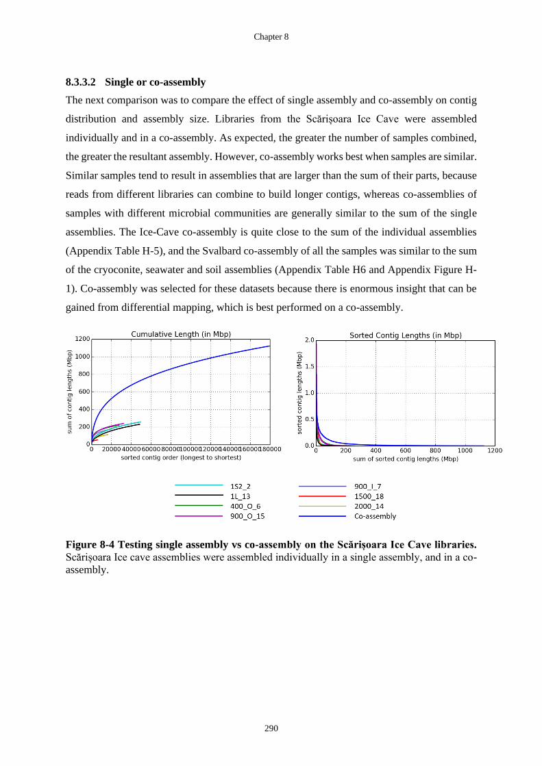
Chapter 8
290
8.3.3.2 Single or co-assembly
The next comparison was to compare the effect of single assembly and co-assembly on contig
distribution and assembly size. Libraries from the Scărișoara Ice Cave were assembled
individually and in a co-assembly. As expected, the greater the number of samples combined,
the greater the resultant assembly. However, co-assembly works best when samples are similar.
Similar samples tend to result in assemblies that are larger than the sum of their parts, because
reads from different libraries can combine to build longer contigs, whereas co-assemblies of
samples with different microbial communities are generally similar to the sum of the single
assemblies. The Ice-Cave co-assembly is quite close to the sum of the individual assemblies
(Appendix Table H-5), and the Svalbard co-assembly of all the samples was similar to the sum
of the cryoconite, seawater and soil assemblies (Appendix Table H6 and Appendix Figure H-
1). Co-assembly was selected for these datasets because there is enormous insight that can be
gained from differential mapping, which is best performed on a co-assembly.
Figure 8-4 Testing single assembly vs co-assembly on the Scărișoara Ice Cave libraries.
Scărișoara Ice cave assemblies were assembled individually in a single assembly, and in a co-
assembly.

The Biotechnological Potential of Cryospheric Bacteria
291
8.3.3.3 Environment complexity
The final test was to compare the effect of environment complexity and heterogeneity on
assembly size. To do this, the libraries for each environment type were co-assembled to create
seawater (n=3), soil (n=8) and cryoconite (n=6) co-assemblies. From previous analysis of these
environments (Chapter 3), the environments differ substantially in heterogeneity and in
community composition. For example, soil was found to be extremely heterogenous, with very
few shared ASVs between sites, and there were many species, all of which made minor
contributions to relative abundance. In comparison, there were many ASVs shared between
cryoconite sites on different glaciers, and there were several species that dominated the
community with extremely high relative abundance. Finally, the seawater samples were
extremely similar and shared many species with each other.
Figure 8-5 Comparison of assembly of different environments. All three assemblies were
performed using MEGAHIT with the default parameters.
The seawater assembly is 26 970 110 bp from 142,336,042 reads, the cryoconite assembly is
538 521 980 bp from 201,408,108 reads and the soil assembly is 208 560 096 bp from
374,879,346 reads (Table 8-5). The cryoconite library is significantly larger than both the soil
and seawater libraries (Figure 8.5), despite being created from fewer reads than the soil
assembly. This comparison reveals the dramatic effect of community heterogeneity and
complexity on the size of the assembly, and subsequently, the number and quality of the MAGs
that can be constructed.

Chapter 8
292
Table 8-5 Table comparing Assembly statistics and contig distribution of sea, soil and cryoconite assemblies.
Assembly
Longest contig (bp)
Nx (Lx) Length
(bp)
Number of
contigs
Sum length (bp)
Contig Length Histogram
Contig Length Histogram
Contig Length Histogram
(1bp <= len < 10Kbp)
(10Kbp <= len < 100Kbp)
(len >= 100Kbp)
sea-MEGAHIT.contigs
115659
N50: 4236 >= 106 0 0
L50: (1450) >= 105 2 221424
N75: 2686 >= 104 321 6766634
L75: (3510) >= 103 6451 26970110
N90: 2225 >= 500 6451 26970110
L90: (5171) >= 1 6451 26970110
soil-MEGAHIT.contigs
300154
N50: 4111 >= 106 0 0
L50: (10133) >= 105 45 6597658
N75: 2616 >= 104 2366 59047038
L75: (26569) >= 103 49641 208560096
N90: 2199 >= 500 49641 208560096
L90: (39681) >= 1 49641 208560096
cryoconite-MEGAHIT.contigs
315846
N50: 5126 >= 106 0 0
L50: (24906) >= 105 18 2524410
N75: 2995 >= 104 8246 154707901
L75: (60198) >= 103 115949 538521980
N90: 2329 >= 500 115949 538521980
L90: (90952) >= 1 115949 538521980

The Biotechnological Potential of Cryospheric Bacteria
293
8.3.3.4 Comparison of functional annotation of contigs from different assemblies
In addition to understanding how the different assembly tools affected contig length, and
assembly size, the assembly tools were compared to see whether there were differences in the
downstream functional analyses from these assemblies. Table 8.6 shows a comparison of three
assemblers, MEGAHIT (Appendix Table H-2), metaSPAdes (Appendix Table H-3) and IDBA-
UD (Appendix Table H-4) on secondary metabolite detection from the Scărișoara Ice Cave
using antiSMASH 4.
Table 8-6 Table comparing BGCs detected from contigs form the MEGAHIT,
metaSPAdes and IDBA-UD assemblies.
MEGAHIT metaSPAdes IDBA-UD
terpene 269 270 181 nrps 195 174 118 T3PKS 131 130 92 bacteriocin 125 133 88 arylpolyene 118 111 89 nrps-like 109 108 69 betalactone 61 62 42 lassopeptide 54 56 39 hserlactone 53 61 44 acyl_amino_acids 45 45 30 siderophore 31 27 22 T1PKS 30 33 13
resorcinol 21 22 14 hglE-KS 14 11 10 lanthipeptide 11 12 7 ectoine 9 7 7 CDPS 7 7 5 phosphonate 7 5 5 indole 5 3 3 linaridin 4 3 3 butyrolactone 4 5 2 other 4 4 3 ladderane 3 5 3 LAP 3 5 3 NAGGN 3 3 3 PKS-like 1 1 0 PUFA 1 1 0 thiopeptide 1 3 1 cyanobactin 1 1 1 sactipeptide 1 1 1 microviridin 1 2 0 nucleoside 1 1 1 phenazine 1 1 0 T2PKS 0 1 0

Chapter 8
294
The similarity between metaSPAdes and MEGAHIT assemblies (Figure 8-2) are reflected in
the antiSMASH results, which are very similar between contigs databases. The greatest
number of BGCs were detected using the MEGAHIT assembly (1374) followed by
metaSPAdes (1368) and then IDBA-UD (934). The most abundant BGCs were the terpenes,
with MEGAHIT and metaSPAdes and IDBA-UD detecting clusters on 269, 270 and 181
contigs respectively. The NRPS were the second most abundant biosynthetic gene cluster
type with MEGAHIT, metaSPAdes and IDBA-UD detecting clusters on 195, 174 and 118
contigs, respectively. The similarity between contig annotations suggest that the tools are
equivalent.
Figure 8-6: Comparison of the choice of assembler on the number and type of secondary
metabolite clusters detected by antismash5.

The Biotechnological Potential of Cryospheric Bacteria
295
8.3.4 Read Mapping
Read mapping is important because it enables the calculation of coverage across the contigs,
(and MAGs) across the different samples. However, it can also be used as a crude indication
of sequencing depth. Reads were mapped back to the assembly using Bowtie2. Mapping tells
us a lot about the complexity of the environments that were sampled, and the extent to which
sampling depth was sufficient to reconstruct the microbial community. The percentage mapped
correlates strongly with the size of the assembly for each sample. This in turn depends on the
complexity and evenness of the environment. Cryoconite recruited the most reads by far,
largely due to skewness in the community structure, with a few key taxa contributing
disproportionately to the overall abundance (Chapter 3). Likewise, many reads from the Ludox
extraction of Soil sample F3T3 contributed to the assembly, likely because the Ludox
extraction method resulted in a lower diversity of organisms (Section 4.4.7.1).
Table 8-7 Alignment rate of reads mapped back to assembly
Sample Trimmed Paired reads Overall alignment rate (%)
Svalbard samples
AB-18 32 454 516 47.48 ML-17 14 397 678 66.29 ML-18 14 235 836 62.62 VB-17 17 252 431 65.56 VB-18 14 893 825 58.97 VL-18 7 469 768 22.32 SS1 25 665 362 5.32 SS2 27 509 748 14.02 SS3 17 992 911 12.79 F3T3_Lud 20 039 798 43.10 F3T3_FD 56 877 004 8.61 F3T3_PM 22 457 762 9.07 F1T3_S4 18 842 083 5.29 F1T4_S5 19 381 248 4.88 F2T2_S6 14 558 022 7.75 F3T1_S7 17 741 236 7.94 F2T4_S8 17 542 420 3.00
Scărișoara Ice Cave
1S_2 69 575 748 21.59 1L_13 72 190 896 9.96 400_O_6 76 039 348 32.94 900_O_15 73 462 594 31.98 900_I_7 75 113 102 45.46 1500_18 75 510 556 46.92 2000_14 63 569 516 41.86

Chapter 8
296
The soil libraries had the lowest proportion of reads mapped back to contigs, ranging from 3%
to 9.07% (Table 8-7, Figure 8-7). The F3T3_Lud library was an exception with a much higher
alignment rate (43.10%), which is reflective of a significant enrichment, caused by diversity
loss in this specific DNA extraction method. The low alignment rate of the soil libraries reflects
the high diversity and heterogeneity of this environment, (also shown in Chapter 3). The
cryoconite libraries had the best alignment rate. Cryoconite is dominated by a core of highly
prevalent and abundant bacteria, and a long tail of rare taxa. The high alignment fraction likely
represents the high coverage of contigs (and MAGs) belonging to this abundant core
community.
Figure 8-7: The percentage of reads aligned to the contigs reflects the complexity of the
communities in each environment type and at each site.

The Biotechnological Potential of Cryospheric Bacteria
297
8.3.5 The performance of different binning tools
Both datasets were binned using four different binding methods: CONCOCT (Alneberg et al.,
2014), MetaBAT2(Kang et al., 2015), MaxBin2 (Wu et al., 2016) and DAS Tool (Sieber et al.,
2018). DAS Tool is designed to score, select, and optimise bins produced using other binning
methods. A summary of the number of bins and the average completion and redundancy
estimates obtained using each binning methods is shown in Table 8-8, and Figure 8-8.
Table 8-8 Binning tool comparison for the Svalbard and Ice-Cave datasets
Ice Cave
Tool CONCOCT MaxBin2 MetaBAT2 DAS Tool
Number of bins 270 253 401 145
No of Nucleotides 1,123,284,953 758,127,487 790,621,951 502,443,977 % Nucleotides 100 67.49 70.38 44.73 Number of contigs 179753 132573 84984 53815 % contigs included 100 73.75 47.28 29.94 Ave completion 57.45 46.06 32.59 85.12 SD completion 36.78 32.21 35.91 11.48 Ave redundancy 28.84 15.62 2.28 5.71 SD redundancy 61.17 19.79 6.95 6.62 Ave size (length) (bp) 4160315 2996551 1971626 3465131 SD length (bp) 3867430 2137964 1758817 1620512
Svalbard
Tool CONCOCT MaxBin2 MetaBAT2 DAS Tool
Number of bins 151 180 226 95
No of Nucleotides 720,998,358 664,863,606 471,439,592 322,990,650 % Nucleotides 100% 92.21 65.39 44.80 Number of contigs 162,105 150,327 73,975 45,400 % contigs included 100% 92.73 45.63 28.01 Ave completion 50.17% 55.05 39.48 83.11 SD completion 36.99% 32.24 36.94 14.09 Ave redundancy 52.78% 20.48 3.25 6.42 SD redundancy 131.14% 21.93 6.28 7.04 Ave size (length) (bp) 4 774 824 3 693 687 2 086 016 3 399 902 SD length (bp) 7 825 034 1 893 821 1 648 078 1 369 520
CONCOCT always binned 100% of the contigs. However, although it retained the largest
portion of the data, it has the highest level of redundancy and largest bin sizes. This is likely a
choice by the anvi’o team, who set the default parameters to err on the size of having bins that
were too large, and could therefore be split in manual refining, rather than bins that had
accidentally been split, which are much harder to detect and combine at a later stage. In both
datasets, MaxBin2 retained the second greatest number of contigs. In the Svalbard dataset,
contigs were split into slightly more bins than CONCOCT, whereas the Ice Cave dataset had
fewer bins.

Chapter 8
298
Figure 8-8: Comparison of different CONCOCT, MaxBin2, MetaBAT2 and DAS Tool
binning methods on the Svalbard and Ice Cave datasets.
The average completion of those bins was higher in the Svalbard dataset, and lower in the Ice
Cave dataset, and the redundancy was greatly reduced, compared to CONCOCT, but still
higher than metaBAT2 and DAS Tool. MetaBAT2 had the largest number of bins in both
datasets. In comparison to CONCOCT, the algorithm seems to have favoured splitting the bins,
which is why this method had both the largest number of bins, but also the lowest redundancy
in both datasets. This aggressive splitting did influence completion, where it had the lowest
percentage completions of all the methods. Finally, DAS Tool, which optimises bins created
using the other tools, had the highest completion, the second lowest redundancy, with a good
average bin size commensurate with expected bacterial genome sizes. However, this quality
came at the expense of data, and this tool resulted in the least number of bins, and the lowest
percentage contigs and nucleotides. The individual bins from the Svalbard and Ice-Cave
datasets are plotted in Figure 8-9 and Figure 8-10 respectively.

The Biotechnological Potential of Cryospheric Bacteria
299
Figure 8-9 Comparison of binning tools for refining MAGs from the Svalbard dataset. Scatterplot showing percent redundancy (x-axis) and
percent completion (y-axis) for the bins resolved using CONCOCT, MaxBin2, MetaBAT2 and DAS Tool, as well as the final MAG collection.
The binning tool is shown represented by colour, and the size of the bin is represented by point size. A horizontal line at 5% and 90% on the x-
and y-axis respectively represent the criteria for high quality MAGs. The grey dashed line at 10% and 70% on the x- and y-axis respectively
represent the criteria for inclusion in this study. Four outlier bins from CONCOCT with redundancy > 350% are not shown.

Chapter 8
300
Figure 8-10 Comparison of binning tools for refining MAGs from the Ice-Cave dataset. Scatterplot showing percent redundancy (x-axis) and
percent completion (y-axis) for the bins resolved using CONCOCT, MaxBin2, MetaBAT2 and DAS Tool, as well as the final MAG collection.
The binning tool is shown represented by colour, and the size of the bin is represented by point size. A horizontal line at 5% and 90% on the x-
and y-axis respectively represent the criteria for high quality MAGs. The grey dashed line at 10% and 70% on the x- and y-axis respectively
represent the criteria for inclusion in this study. Two outlier bins from CONCOCT with redundancy > 350% are not shown.

The Biotechnological Potential of Cryospheric Bacteria
301
8.3.6 Manual refinement in anvi’o
There are several studies, especially when they involve enormous datasets and thousands of
MAGs, that do not go beyond the automatic binning of contigs by binning tools (Parks et al.,
2015; Shaiber and Eren, 2019). However, automatic binning tools can often get contig
membership wrong, and here, anvi’o provides an excellent tool for the manual refinement of
bins (Eren et al., 2015). Every bin in the two datasets was manually refined. Occasionally this
was done in an iterative process, where refined bins were rerun through DAS Tool, together
with unrefined bins to see whether the newly defined bins scored better or worse than the
automatic bins. A comparison between all the different binning methods, which also includes
the final bins is shown in Figures 8-9 and Figure 8-10 for the Svalbard and Ice Cave datasets,
respectively. The effect of the final manual refinement on the DAS Tool bins quality is shown
in Figure 8-14 and Figure 8-15. Manual refinement was greatly assisted by the method
described (Section 8.2.5) where the bin membership of each contig was imported as a data
layer and could be viewed in anvi-refine. This view enabled several easy refinements that could
be performed unambiguously and confidently.
8.3.6.1 High-quality and poor-quality bins
In a complete and uncontaminated bin, one expects coverage to be even across a single sample,
and the relative proportion of reads across samples to be relatively constant. There should be
at least one sample that contains every single contig. Figure 8-11 is a good example of a bin
that contains mis-binned contigs. In Figure 8-11 no samples contain all the contigs. Contigs
from several organisms, from different environments and sites, have erroneously been binned
together. The mis-binning may have occurred because these are related species, with similar
GC content and TNF ratios that resulted in the binning algorithm clustering them together. If
this is a large bin with high redundancy, this bin may still be salvaged by and be maintained in
the dataset as at least one, and possibly more refined bins.
An example of a high-quality bin is shown in Figure 8-12. The coverage is even across a single
sample site and relative coverage cross the sample sites is also even. The different binning
methods all concur on bin membership. In a poor-quality (incomplete, mixed, or chimeric) bin
(Figure 8-13), contigs might have different distribution within and across samples. As a result,
binning methods might disagree about bin membership of different contigs. These aspects of
bin quality do not often come out in summary statistics. However, the visualisation of contigs,
and their bin membership quickly highlights ambiguous contigs and bins.

Chapter 8
302
Figure 8-11 Example A: Bin that is not complete across a single sample, and has varying
levels of coverage in different samples
This is a refined DAS Tool bin based off a MaxBin2 bin. The bin is easy to refine based on
coverage across different samples. Contigs belonging to seawater species, at least two different
cryoconite species and several soil species are easy to discern. This bin is likely not
salvageable, as each ‘refined’ bin from this collection will likely contain too few contigs and
be too incomplete to meet miMAG standards. However, refinement is iterative, and the split
bins can be viewed and assessed in subsequent rounds.

The Biotechnological Potential of Cryospheric Bacteria
303
Figure 8-12: Example B: Bin has high consensus between binning methods and consistent
coverage cross a single site.
This bin has high consensus between all the binning tools and even coverage across all of the
contigs. DAS Tool selected this bin from a metaBAT2 bin.

Chapter 8
304
Figure 8-13: Example C: Bin with low consensus between binning methods, and variable
coverage across contigs and across samples.
This bin is from the CONCOCT collection. There is very little consensus between this bin and
the other binning tools. CONCOCT has accurately binned contigs with high coverage in
cryoconite and low coverage in soil and seawater. However, there is variability in the depth of
coverage in the different contigs, and he GC content is also variable. The Kaiju taxonomy is
mixed.

The Biotechnological Potential of Cryospheric Bacteria
305
Figure 8-14 Scatterplot showing the effect of the manual refinement step on bin quality
(completion and redundancy). A red horizontal line at 5% and 90% on the x- and y-axis
respectively represent the criteria for high quality MAGs. The grey dashed line at 10% and
70% on the x- and y-axis respectively represent the criteria for inclusion in this study.
Figure 8-15 Scatterplot showing the effect of the manual refinement step on bin quality
(completion and redundancy). A red horizontal line at 5% and 90% on the x- and y-axis
respectively represent the criteria for high quality MAGs. The grey dashed line at 10% and
70% on the x- and y-axis respectively represent the criteria for inclusion in this study.
Chapter 8
306
8.3.7 Genome completeness and quality
The completeness and quality of MAGs can be assessed using several tools. Within the anvi’o
workflow, it is possible to estimate completeness and redundancy of the contigs in a bin by
using HMM hits against a curated collection of 70 single copy bacterial genes (Lee, 2019).
This estimate is available during the refinement process and makes it possible to refine bins,
and discard those that fall short of the quality criteria set out by Genomic Standards Consortium
(GSC), in the Minimum information about a metagenome-assembled genome (MIMAG)
standard, one of the most important of which being that completion should be at least 80% and
redundancy or ‘contamination’ less than 10% (Bowers et al., 2017). Although a fantastic
method for refinement and estimates, applying the quality cutoff criteria for the bins at this
stage may ultimately lead to over-fragmentation of bins, or discarding bins that may be
complete. CheckM is another tool that estimates completeness, but it does so by using SCGs
that belong to different lineages of bacteria (Parks et al., 2015). CheckM is arguably a better
tool, since it considers the fact that some clades will contain more than one copy of certain
genes and may be missing others.
The difference between the completion and redundancy estimates of the Ice Cave MAGs using
the 71 Bacterial SCGs and CheckM is shown in Table7-4.
8.3.8 Databases and tools for the annotation of reads, contigs and MAGs
8.3.8.1 BGC detection
There are a number of bioinformatics tools that can be used in NP research (reviewed in
(Chavali and Rhee, 2018; Loureiro et al., 2018; Tracanna et al., 2017; Weber and Kim, 2016).
The various tools and databases can be specialised by class of molecule, by organism or
domain, or by its ability to predict NP product structure and link to external databases. One of
the most commonly used and comprehensive of these tools is antiSMASH (antibiotics and
Secondary Metabolite Analysis SHell) (Blin et al., 2019b; Weber et al., 2015). AntiSMASH
has algorithms able to detect a vast range of different BGCs, and many different molecule
families. These different molecules families have diverse functions such as antimicrobial
compounds, exopolysaccharides, UV pigments, antioxidants, fatty acids.The antiSMASH
results from the Svalbard MAGs (Section 5.3.2), individual cryoconite, soil and seawater
assemblies (Section 5.3.6) and Ice-Cave MAGs (Section 7.3.8), and entire MEGAHIT, IDBA-
UD and metSPAdes assemblies (Section 8.3.3.4) have previously been shown.

The Biotechnological Potential of Cryospheric Bacteria
307
8.3.8.2 Enzyme bioprospecting
The contigs from the megahit assemblies of the Ice Cave and Svalbard datasets were submitted
in batches to the dbCAN2 webserver (http://bcb.unl.edu/dbCAN2/index.php) (Zhang et al.,
2018), which queries the Carbohydrate-Active EnZymes database (CAZy) (Cantarel et
al.,2009; Lombard et al., 2014) (http://www.cazy.org/) using DIAMOND, HMMER and
HotPep (Figure 8-16).
Figure 8-16 Example of a summary of carbohydrate-active enzymes hits in contigs from
the cryoconite MEGAHIT assembly, using each of the tools: HMMER, DIAMOND and
HotPep. A total of 8349 of the detected enzymes were detected by more than one tool, while
4501 of the enzymes were detected using all three tools.
Screening the contigs databases of the different environments is useful to distinguish the range
of different enzyme families present, and the number of variants within each family. In
bioprospecting, an extremely useful enzyme may be found in a rare taxon and cloned into a
model organism. Therefore, the present of the enzyme is more important than the abundance
of the enzyme in the community, as these genes, once identified, can be amplified using specific
primers. Therefore, dbCAN2 screening of contigs rather than MAGs can be used to make
abundance agnostic screening, and the contigs of interest can be identified independent of
taxonomic affiliation and abundance.

Chapter 8
308
Figure 8-17 Relative abundance of carbohydrate active families in seawater, cryoconite,
soil and Ice-Cave contigs.
In total, there were 267 enzymes in the seawater, 13604 in cryoconite, 5053 in soil and 24313
enzymes detected in the Ice Cave. The largest proportion of enzymes belonged to the Glycosyl
Transferases (GTs) class, ranging from 39% in seawater to 47% in soil, which are responsible
for the formation of glycosidic bonds. Enzymes like these would be important during EPS
synthesis. The second most abundant class was the Glycoside Hydrolases (GHs) which are
responsible for the hydrolysis and/or rearrangement of glycosidic bonds. These enzymes had
the highest relative abundance (RA) in seawater (47%), and the lowest RA in soil (31%).
Carbohydrate Esterases (CEs) which perform hydrolysis of carbohydrate esters were the next
most abundant family, followed by the Auxiliary Activities (AAs) family of redox enzymes
that act in conjunction with CAZymes. Several enzymes with carbohydrate-binding modules
(CBM), were also detected. The lowest abundance enzymes were the Polysaccharide Lyases
(PLs) which perform non-hydrolytic cleavage of glycosidic bonds.
A Sunburst plot in Figure 8-18 shows some of the most abundant families within these classes.
These environments seem enriched with enzymes from the GT4, GT2_Glycos_transf_2, GT2
families from the GT class, GH23 and GH3 from the GH class, CE10, CE1 and CE4 from the
CE class, and AA3 from the AA class.

The Biotechnological Potential of Cryospheric Bacteria
309
Figure 8-18 Sunburst plots of the major carbohydrate active enzyme classes and the most
abundant enzyme families within each class.

Chapter 8
310
Table 8-9 Table of tool and databases
Database Full name NP Applications Website Databases accessed
Reference
antiSMASH antibiotics and Secondary Metabolite Analysis SHell
Polyketides, NRPS, bacteriocins, RiPPs, terpenes, saccharides, fatty acids (and many more)
Antimicrobial compounds, EPS, UV screens, pigments, antioxidants, fatty acids.
https://antismash.secondarymetabolites.org/ MIBiG (Blin et al., 2017, 2019b, 2019a)
PRISM PRediction Informatics for Secondary Metabolomes
NRPS, Polyketides Antimicrobial compounds.
http://grid.adapsyn.com/prism/#!/prism (Skinnider et al., 2017, 2015)
BAGEL4 BAGEL Bacteriocins, RiPPs
Antimicrobial compounds.
http://bagel4.molgenrug.nl/index.php (van Heel et al., 2018)
dbCAN2 (database for) automated Carbohydrate-active enzyme ANnotation
Carbohydrate active enzymes
Food, paper, alcohol synthesis, EPS.
http://bcb.unl.edu/dbCAN2/index.php CAZy (H. Zhang et al., 2018)
LED Lipase Engineering Database Lipases and esterases
Detergent, food, bioremediation.
http://www.led.uni-stuttgart.de LED (Fischer and Pleiss, 2003)
LccED Laccase Engineering Database
Laccases Plastic degradation.
https://lcced.biocatnet.de/) LccED (Sirim et al., 2011)
Redoxibase Peroxibase, now Redoxibase Peroxidases, oxido-reductase
Antioxidants. http://peroxibase.toulouse.inra.fr/ Redoxibase (Passardi et al., 2007)

The Biotechnological Potential of Cryospheric Bacteria
311
8.4 Discussion
The number and range of tools available to analyse genetic data has rapidly expanded in recent
years. In this chapter, the bioinformatics workflow that resulted in two MAG collections is
described. In the process of optimizing the workflow, several tools were tested and compared.
In addition, a catalogue of additional tools and databases that can be used to investigate these
datasets for additional products was compiled. In this thesis, the focus was on the assembly of
MAGs as the unit of investigation for bioinformatic bioprospecting. MAGs are useful because
phylogenomic information about the microorganism that harbors the gene for the NP of interest
can be vital in strategic expression and cultivation efforts.
8.4.1 The effect of environment on assembly size
There were several insights from the comparison of the Scărișoara Ice cave and Svalbard
assemblies. The Svalbard library (718 623 496 reads) was larger than the Ice Cave library
(reads= 505 461 760), however the Svalbard assembly (contigs= 162 105, bp = 720 998 358)
was smaller than the Ice Cave assembly (contigs= 179 753, bp= 1 123 284 953) (Table 8 5),
and this was also reflected in the number of high quality MAGs that were resolved from each
assembly (Svalbard=74, Ice Cave = 121). This comparison, together insights from the
comparison of sea, soil and cryoconite libraries (Figure 8-5), highlights the enormous effect
microbial diversity and complexity has on the assembly and resultant MAGs. The greater the
number of bacterial species in a sample, the fewer reads will overlap to form contigs, and this
can be extremely detrimental to downstream analysis. Considering that longer contigs are
needed to obtain good functional annotation of genes, with complete genes and ORFs, this
suggest that it is far better to sequence deeply (few libraries with maximum number of reads)
than widely (many samples with fewer reads). The balance between depth and breadth of
sequencing can be weighed up by considering the heterogeneity of the selected environments.
The use of co-assembly vs single assembly also needs to be considered. A recent study showed
co-assembly recovered a larger genome fraction than a combination of single assemblies
(Hofmeyr et al., 2020). However, single assembly was better at identifying variation between
closely related strains, but the combined single assembly dataset suffered from duplications.
The effect of co-assembly on these datasets appeared to be positive on balance. Microbially
diverse environments are tempting for bioprospecting because greater diversity suggests a
greater probability of genetic novelty. However, in this study of different environments, it is

Chapter 8
312
clear that extremely diverse and heterogenous environments may result in less complete and
robust data for meaningful analysis.
A further consideration when sampling environments include, considering the contribution of
non-bacterial DNA in the environmental DNA. Seawater is known to contain many diverse
bacteria and the marine metagenomes have been explored in several studies. However, Kaiju
revealed many reads had non-bacterial origin, and this substantially reduced the number of
reads that could contribute to the assembly. Although the ability to resolve eukaryotic MAGs
from fungal and algal species will soon be possible (Saary et al., 2020), the size of eukaryotic
genomes, as well as the increased number of repeat regions makes this a formidable challenge.
The number of recovered genomes could be considerably increased via greater sequencing
depth.
8.4.2 The advantages and disadvantages of reads, contigs and metagenome-
assembled genomes
While using the described bioinformatics pipeline, there is information loss at several stages.
For the Svalbard dataset, the initial library was 1.038 x 10¹¹ bases in size. However, read-
mapping back to contigs revealed that only 3% – 9.07% of soil library reads, 22.32% - 66.62%
of cryoconite library reads, and 5.32% - 14.02% of seawater library reads aligned to contigs.
This represents an enormous loss of information, with up to 97% of the reads in the soil library
not being included in the assembly and downstream analysis. Read mapping also confirms the
observation from testing assembly tools, that higher diversity libraries suffer from lack of
incorporation into contigs. During binning and MAG refinement, the information loss
continues, as only 28.01% of the Svalbard contigs and 29.97 % of the Ice-Cave contigs were
included in MAGs (Table 8-8). The use of contigs as a dataset is useful because it detects
diversity in the rarer taxa in environmental samples.
8.4.3 Optimisation and benchmarking are necessary
In this chapter, several tools were compared, from assemblers (Section 8.3.3.1), to binning
tools (Section 8.3.5). Whilst some of these comparisons were reassuring, and gave similar
results, there were sometimes significant differences that are severe enough to potentially
interfere with result interpretation. The use of a consensus approach to select tools and results
assumes that if results converge, despite using different methods to get there, then the
probability of the result being accurate is higher. MetaSPAdes and MEGAHIT gave similar
results in assembly size (Figure 8-3), and in BGC annotation using antiSMASH (Figure 8-6),

The Biotechnological Potential of Cryospheric Bacteria
313
although MEGAHIT got the results more efficiently, which was the justification for using
MEGAHIT. This kind of consensus approach to method selection and optimisation is also
being built into several other tools. For example, dbCAN2 uses several methods to screen
contigs for carbohydrate-active enzymes and suggests that the dataset be trimmed to include
only hits where there is agreement between at least two different tools (Figure 8-16).
The presence or absence of results convergence can be used in several ways. In the comparison
of binning tools there was an alarming lack of overlap between the bins created by metaBAT2,
MaxBin2 and CONCOCT. Parameter tweaking may have resulted in slightly different, and
more similar bins, but nonetheless, the bins were different in size and redundancy (Table 8-8,
Figure 8-9, Figure 8-10). DAS Tool did not particularly favour one tool over the other, with
the final bins coming from all three of the tools. While it is almost impossible to get ‘accurate’
bins, the degree to which results agree or disagree can be used to assign a confidence value.
Where all three tools converge on a similar bin, there is greater confidence in the quality of the
MAG. Where there is a large discrepancy in contig membership between the different binning
tools, it serves as a warning that the data is of poorer quality (Figure 8-13). This method of
consensus seeking can be applied when refining MAGs too. There is growing evidence that
many MAGs in databases are of poor quality, consisting of chimeric bins and even chimeric
contigs (Shaiber and Eren, 2019). The manual refinement of bins is therefore an important step,
however, is made difficult and impractical when there are hundreds to thousands of contigs in
a single bin, and hundreds of bins in a dataset. The visualisation of binning results as a data
layer, used in this thesis, is a way to quickly identify suspect contigs.
During bin-refinement, it is always easier to create large bins, that may contain contaminant
contigs, and the refine the bins, than to accidentally split bins that belong together. Manual
refinement therefore involves a whittling away of contaminant sequences. Figure 8-1 and
Figure 8-11 show how bin refinement can easily be accomplished using differential coverage
across samples, GC content and TNFs. Additional clues can be provided by the taxonomic
classification of MAGs, which can be done in two ways. Kaiju can be used to classify each
gene call and contig taxonomically and viewed on a contig-by contig basis. The HMM scan of
71 bacterial genes is used to estimate the completion and redundancy information for each bin
in real time, and the results from the SCG scan of 22 genes from GTDB can be used to view a
taxonomic prediction in real time. The SCG taxonomy from GTDB can once again be used to
find consensus, where all 22 genes are present have the same closest relative, that is an excellent
indicator of a complete and uncontaminated bin. Occasionally, GTDB SCGs may belong to

Chapter 8
314
several different species from within the same genus, which could indicate contamination, and
chimera or hybrid of closely related species, or a novel species that is related to both, having
diverged from a shared common ancestor. However, the presence of GTDB SCGs from
different orders, classes or phyla are a clear sign that the bin is contaminated or chimeric and
requires further refinement. This approach was very good at identifying bins that were likely
to be chimeric. Chimeras are more likely when there are lots of closely related species or strains
present in a sample. These are may appear as a bin with lots of contigs with uneven coverage
or distribution amongst samples.
Anvi’o is growing and increasing functionality constantly, with several updates annually.
Within the next updates, automatic KEGG functionality is to be included, as well as screening
for tRNAs, which will allow easier fulfilment of the criteria by the miMAG standards (Bowers
et al., 2017).
8.4.4 Long-read technologies will improve MAG quality
The use of long-read sequencing is poised to revolutionise microbial ecology. Currently, bins
are often composed of multiple closely relates species, and these consortia are often very
difficult to separate bioinformatically using the current short-read technology and assembly
methods. However, new long-read technologies such as Nanopore are poised to reinvigorate
genome assembly from metagenomes (Moss et al., 2020; Overholt et al., 2019). The benefit of
long reads is immense, as long reads can act as scaffolds, helping to bridge caps between
contigs and close genomes. Closely related species can also be resolved because deletions/
insertions and rearrangements can highlight differences in strains. It will vastly improve
binning, as long reads that span multiple genes, possible rearrangements and deletion will
address issues of synteny, and help to resolve closely related species within a population (Moss
et al., 2020; Overholt et al., 2019).
8.4.5 Contigs and MAGs are a catalogue of diversity that can be explored
The MAGs and contigs databases are catalogues of diversity that are amenable to a large range
of downstream analysis. In this thesis, the MAGs and contigs were screened for BGCs using
the tool antiSMASH, which also links to several databases and dbCAN2 which links to the
CAZy database. However, multifastas from assemblies can be screened using several databases
using a variety of tools.
The Biotechnological Potential of Cryospheric Bacteria
315
The antiSMASH results are discussed throughout the chapters of this thesis. The dbCAN2 scan
identified abundant carbohydrate active enzymes from the contigs of seawater (267),
cryoconite (13604), soil (5053) and the Ice Cave (24313) (Appendix Table H1). These
environments seem enriched with enzymes from the GT4, GT2_Glycos_transf_2, GT2 from
the GT class, GH23 and GH3 from the GH class, CE10, CE1 and CE4 from the CE class, and
AA3 from the AA class.
Some additional tools, which have been used at various stages (but not included in this thesis)
are listed in Table 8-9 and represent avenues for future work. For example, BAGEL4 (van Heel
et al., 2018) focuses on identifying bacteriocins or ribosomally synthesized and post
translationally modified peptides (RiPPs), which are not commonly covered by other tools.
PRISM (PRediction Informatics for Secondary Metabolomes) is a computational resource that
implements novel algorithms to identify BCGs and predict genetically encoded nonribosomal
peptides and type I and II polyketides (Skinnider et al., 2015). It also uses and bio- and
cheminformatics to detect replication of known natural products, which is a huge advantage
since rediscovery’ of existing molecules has plagued pharmaceutical research.
The Lipase Engineering Database (LED) (http://www.led.uni-stuttgart.de) is a database that
attempts to integrate sequence, structure, and function information of a range of enzymes with
similar catalytic machinery (Fischer and Pleiss, 2003). Within this family, the cutinases are of
interest as enzymes potentially capable of PET and PUR plastic degradation (Fischer and
Pleiss, 2003; Wei and Zimmermann, 2017). Likewise, the non-heme peroxidases, detected
using RedoxiBASE (Passardi et al., 2007; Savelli et al., 2019) may also contain plastic-
degrading enzymes. The Laccase Engineering Database (LccED) (https://lcced.biocatnet.de/)
is a database that contains information about the sequence, structure and function of laccases
and their homologues from the multicopper oxidase (MCO) superfamily (Sirim et al., 2011).
MCOs catalyse the one-electron reduction of substrates concurrent with the four-electron
reduction of molecular oxygen to water. Fungal laccases play a role in lignin degradation,
pigment production and plant pathogenesis, while bacterial laccases play a role in melanin
production, spore coat resistance, morphogenesis, and copper detoxification (Sirim et al.,
2011). In addition to potential plastic-degrading capabilities, laccases are also excellent
candidates for other biotechnological applications, in the textile, pulp and paper, food and
organic synthesis industries as well as in bioremediation (Sirim et al., 2011).

Chapter 8
316
8.4.5.1 Custom databases for specific NP discovery
Finally, it is possible to create custom databases of sequences of specific interest. This was
done for example by downloading sequences and HMM profiles for anti-freeze proteins and
polymerases from Uniprot (data not shown). DIAMOND and HMMER3 can then be used to
query the custom databases and identify products. To ensure good quality data, the use of both
HMMER and DIAMOND can be used, and only hits to both datasets used in analysis (similar
to dbCAN2 recommendations).
8.4.6 MAGs enable strategic bioprospecting
Once the gene or BGC responsible for the synthesis of a NP of interest has been identified,
additional information provided by the entire MAG genome can be used to aid strategic
sampling, cultivation, and heterologous expression efforts.
8.4.6.1 Optimisation of sampling strategy and environmental sites
By their nature, reconstructed genomes represent the most abundant members of a community,
because they are constructed from the longest contigs with the deepest coverage, proportional
to their abundance in the original sample. Because anvi’o maps the reads from individual
libraries, it is possible to see which libraries (i.e. sampling sites, environment types, or
environmental conditions) contribute most to the contig of interest, and therefore, which
environments/ sample sites/ conditions should be favoured in future sampling activities.
8.4.6.2 Host engineering and expression optimisation
Understanding the genomic context overcomes some of the difficulties of BGC expression,
which relies on compatible promoters, ribosome binding sites, substrate metabolites and
secretion machinery for natural products to be correctly expressed (Zhang et al., 2010).
Therefore, locating a BGC inside of a genomic context helps greatly with the genetic
engineering of suitable hosts and the identification of optimal conditions for expression of the
desired natural product.
Traditional cloning methods rely on a random shearing of DNA and insertion of putative BGCs
into cosmids, fosmids and BACs. This approach relies on chance, and fragments are rarely long
enough to capture a BGC in its entirety. However, by conducting a bioinformatic screen and
identifying a BGC of interest, it is possible to target a specific BGC using newer recombinant
DNA technologies. Examples of recombinant DNA technologies that have been successfully
employed to specifically and precisely target and capture BGCs of interest include high

The Biotechnological Potential of Cryospheric Bacteria
317
efficiency linear-linear homologous recombination (LLHR)(Yin et al., 2015), Transformation-
associated recombination (TAR) cloning (Kouprina and Larionov, 2016), serine integrase-
mediated site-specific recombination (SSR)(Du et al., 2015; Olorunniji et al., 2016) and Cas9-
associated targeting of chromosome segments (CATCH) (Jiang et al., 2015). Meanwhile,
advances in synthetic biology, referred to as bottom-up assembly methods, involve assembling
the desired BGCs from several smaller fragments (Li et al., 2017). Examples include
methylation-assisted tailorable ends rational (MASTER) ligation based on the type IIs
endonuclease MspJI (Chen et al., 2013) site-specific recombination-based tandem assembly
(SSTRA) (Zhang et al., 2011), Modified Gibson assembly (L. Li et al., 2015) and DNA
assembler (Shao et al., 2011).
8.5 Conclusion
Two datasets were used in this bioinformatic workflow and tool comparison, a Svalbard
metagenome consisting of cryoconite (6), soil (8) and seawater (3) libraries and an Ice-Cave
dataset (7). The complexity and heterogeneity of the environments played a role in the size
quality of the assembly, which affected all downstream analyses. Nonetheless, using careful
manual refinement, a collection of high-quality MAGs was constructed. These MAGs and
contigs represent catalogues of biodiversity that can be explored for several categories of
products. The insights from MAGS enable strategic sampling, heterologous expression, and
co-cultivation efforts.
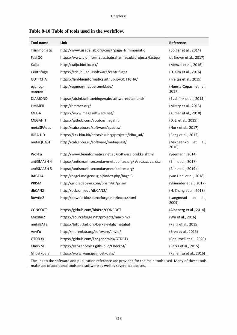
Chapter 8
318
Table 8-10 Table of tools used in the workflow.
Tool name Link Reference
Trimmomatic http://www.usadellab.org/cms/?page=trimmomatic (Bolger et al., 2014)
FastQC https://www.bioinformatics.babraham.ac.uk/projects/fastqc/ (J. Brown et al., 2017)
Kaiju http://kaiju.binf.ku.dk/ (Menzel et al., 2016)
Centrifuge https://ccb.jhu.edu/software/centrifuge/ (D. Kim et al., 2016)
GOTTCHA https://lanl-bioinformatics.github.io/GOTTCHA/ (Freitas et al., 2015)
eggnog-mapper
http://eggnog-mapper.embl.de/ (Huerta-Cepas et al., 2017)
DIAMOND https://ab.inf.uni-tuebingen.de/software/diamond/ (Buchfink et al., 2015)
HMMER http://hmmer.org/ (Mistry et al., 2013)
MEGA https://www.megasoftware.net/ (Kumar et al., 2018)
MEGAHIT https://github.com/voutcn/megahit (D. Li et al., 2015)
metaSPAdes http://cab.spbu.ru/software/spades/ (Nurk et al., 2017)
IDBA-UD https://i.cs.hku.hk/~alse/hkubrg/projects/idba_ud/ (Peng et al., 2012)
metaQUAST http://cab.spbu.ru/software/metaquast/ (Mikheenko et al., 2016)
Prokka http://www.bioinformatics.net.au/software.prokka.shtml (Seemann, 2014)
antiSMASH 4 https://antismash.secondarymetabolites.org/ Previous version (Blin et al., 2017)
antiSMASH 5 https://antismash.secondarymetabolites.org/ (Blin et al., 2019b)
BAGEL4 http://bagel.molgenrug.nl/index.php/bagel3 (van Heel et al., 2018)
PRISM http://grid.adapsyn.com/prism/#!/prism (Skinnider et al., 2017)
dbCAN2 http://bcb.unl.edu/dbCAN2/ (H. Zhang et al., 2018)
Bowtie2 http://bowtie-bio.sourceforge.net/index.shtml (Langmead et al., 2009)
CONCOCT https://github.com/BinPro/CONCOCT (Alneberg et al., 2014)
MaxBin2 https://sourceforge.net/projects/maxbin2/ (Wu et al., 2016)
metaBAT2 https://bitbucket.org/berkeleylab/metabat (Kang et al., 2015)
Anvi’o http://merenlab.org/software/anvio/ (Eren et al., 2015)
GTDB-tk https://github.com/Ecogenomics/GTDBTk (Chaumeil et al., 2020)
CheckM https://ecogenomics.github.io/CheckM/ (Parks et al., 2015)
GhostKoala https://www.kegg.jp/ghostkoala/ (Kanehisa et al., 2016)
The link to the software and publication reference are provided for the main tools used. Many of these tools make use of additional tools and software as well as several databases.

The Biotechnological Potential of Cryospheric Bacteria
319
Table 8-11 List of databases used in the workflow
Database name Link Reference
UniRef100 https://www.uniprot.org/uniref/ (Suzek et al., 2015)
Pfam http://pfam.xfam.org/ (El-Gebali et al., 2019)
CAZy http://www.cazy.org/ (Cantarel et al., 2009)
RefSeq https://www.ncbi.nlm.nih.gov/refseq/ (O’Leary et al., 2016)
NCBI COG https://www.ncbi.nlm.nih.gov/COG/ (Galperin et al., 2015)
GTDB https://gtdb.ecogenomic.org/ (Parks et al., 2018)
NCBI BLAST nr ftp://ftp.ncbi.nlm.nih.gov/blast/db/FASTA/nr.gz (Benson et al., 2013)
KEGG https://www.genome.jp/kegg/ (Kanehisa and Goto, 2000)
antiSMASH-db2 https://antismash-db.secondarymetabolites.org/ (Blin et al., 2019a)
MIBiG https://mibig.secondarymetabolites.org/ (Medema et al., 2015)
Table of most important databases used in the bioinformatics analysis. The link to the software and publication reference are provided for the main tools used. Many databases that are referenced and used by the tools described in Table 8.12 are not mentioned specifically.
Table 8-12: Table of high performance and cloud computing facilities
Tool name Link Reference
Kbase http://kbase.us/ (Arkin et al., 2018)
CLIMB https://www.climb.ac.uk/ (Connor et al., 2016)
IBERS HPC https://bioinformatics.ibers.aber.ac.uk/wiki/index.php/Main_Page

Chapter 9
320
9 DISCUSSION
This thesis sought to explore the biotechnological potential of the cryosphere. The scope for
applications from cryospheric microorganisms is enormous and ranges from novel
antimicrobials to cold-active enzymes to ecosystem services such as soil remediation and
plastic degradation (Chapter 1). In this thesis, Svalbard soil, cryoconite and seawater were
investigated for putative antimicrobials, antioxidants, and EPS (Chapter 5) and cold-active
polymerases (Chapter 6) using mixed sequence-based bioinformatics and functional screening
methods. In addition, shotgun metagenomic data from Svalbard soil, cryoconite and seawater
(Chapter 4), and the Scărișoara ice Cave (Chapter7) were assembled to create contigs databases
and MAGs that can be interrogated for enzymes, secondary metabolites and biodegradation
pathways using bioinformatic tools described in Chapter 8. Crucially, a 16S rRNA amplicon-
based survey of a Svalbard glacial ecosystem showed that the window for undertaking these
bioprospecting activities from these highly specialized cryospheric bacteria is rapidly closing
because of global climate change (Chapter 3).
9.1 Bioprospecting and global climate change
Bioprospecting in the Arctic has the potential to be beneficial for humans and for the
environment. Not only are there multiple products that could benefit human health and
industry, from novel antimicrobials, EPS and antioxidants in the pharmaceutical industry to
enzymes and antifreeze proteins in the food, detergent and molecular biology industries, but
several of these solutions can have positive feedback on the environment (Chapter 1). Cold-
active enzymes can lower energy costs (and carbon footprint) in large scale chemical reactions
(Table 1-5) or degrade persistent organic pollutants (Table 1-11) and plastics (Table 1-12).
Furthermore, the recognition of this environment as having economic value helps to justify its
protection and maintenance.
The importance of these bioprospecting ventures is becoming increasingly urgent because
habitats in the Arctic are rapidly changing as glaciers and sea ice retreat due to global climate
change (Barry, 2017; Fountain, 2012). The potential loss of these extreme environments, and
the unique biodiversity therein, necessitates urgent efforts to understand and uncover the

The Biotechnological Potential of Cryospheric Bacteria
321
potential of these cryospheric microorganisms before the opportunity is lost (Stibal et al.,
2020). Worryingly, the temperatures in the Arctic, (particularly Winter temperatures (Graham
et al., 2017)) are increasing faster than the models predict (Graversen et al., 2008), and sea ice
retreat is also about two decades ahead of predicted rates (Barry, 2017).
To identify how resilient Arctic bacteria are to climate change, several habitats within a glacier
ecosystem, including cryoconite, snow, slush, glacial meltwater, proglacial water, forefield soil
and seawater were investigated to identify a core microbiome for each habitat type and
determine the extent to which bacteria can exist in different environments (Chapter 3). This
helped identify whether Arctic microbial communities consist predominantly of specialists,
able to live only within a narrow ecological niche, or whether they were more cosmopolitan,
able to live across a broad range of environmental parameters. The 16S rRNA gene amplicon
analysis revealed that many of the bacteria inhabiting the High Arctic have strict habitat
preferences (Chapter 3). The survey used ASVs rather than OTUs because it allows the
resolution of exact variants. An UpsetR plot of shared ASVs between environments (Figure 3-
17), and a co-occurrence network (Figure 3-19) revealed that there are very few ASVs able to
occupy several environments. The narrow spatial range suggests significant specialisation, and
therefore a high risk of extinction, should global climate change continue to alter the
environment. Moreover, filtering of the dataset to include only ASVs occurring in more than
two samples resulted in a significant reduction of diversity in the dataset (Figure 3-16), which
suggests that the community is extremely heterogenous, and/or that there is a large and diverse
rare microbiome. The following chapters in this thesis sought to catalogue some of that unique
diversity.
9.2 Genome-centred metagenomics enables strategic bioprospecting
The main contribution of this thesis was the creation of two MAG collections, which form the
foundation for further bioinformatic bioprospecting (Chapter 4,5,7,8). MAGs are reconstructed
genomes from the assembly and then binning of metagenomic DNA. Ideally, a single MAG
represents an exact strain or species from the sampled environment, however MAGs can
represent several closely related species that have assembled together because of their high
level of sequence overlap. MAGs can therefore be thought of as in a similar way to OTUs, as
representing a cluster of highly similar strains or species. MAGs represent a biological
catalogue, with information on phylogenetic relatedness to reference species (Table 4-7, Table
7-6), and metabolic and functional potential (Figure 4-13 to Figure 4-14, Figure 5-2 to Figure
Chapter 9
322
5-3, Figure 7-7 to Figure 7-12). In addition, the use of differential coverage contributes
additional insights, such a map of spatial distribution and abundance across sites (Figure 4-12,
Figure 7-6) and information about co-occurring bacteria and possible symbionts. This
information can then be used in strategic bioprospecting activity, including, but not limited to
the selection of specific habitat types and sites for further work, strategic co-cultivation efforts
and host engineering for heterologous expression of NPs of interest.
In this thesis, 74 high quality MAGs were assembled from cryoconite, soil and seawater from
a glacial ecosystem (Chapter 4) and 121 high quality MAGs were assembled from the
Scărișoara Ice Cave in Romania (Chapter 7). In addition, a bioinformatic workflow was tested
and described, where both the MAG construction process, as well as insights from the
comparison of the two different datasets were compared (Chapter 8).
9.2.1 MAGs vs phylotypes from previous 16S rRNA gene analysis
One of the first observations is that the reconstructed MAGs belonged to the most abundant
species identified using both 16S rRNA analysis, and culturing studies of these environments
(Chapter 3, and (Edwards et al., 2013c; Gokul et al., 2016; Hillebrand-Voiculescu et al., 2015;
Itcus et al., 2018; Paun et al., 2019). The MAG with the highest coverage (a proxy for relative
abundance) in Svalbard cryoconite was classified as Phormidesmis priestleyi, exactly as
expected based on the 16S rRNA analysis (Chapter 3) and previous studies of Svalbard
cryoconite (Gokul et al., 2016; Segawa et al., 2017; Takeuchi et al., 2019). However, several
of the other MAGs belong to members of the cryoconite core community such as
Microbacteriaceae, including Salinibacterium (3), Pseudanabaena (1), Ktedonobacteria (1),
Granulicella (1) and Rhizobacter (2) (Figure 3-6, Figure 4-3, Table 4-4, Appendix Table C-
12). Abundant genera in soil were also present, such as Nostoc (1), Rhizobacter (2),
Phormidium (Microcoleus) (1) and Sphingomonas (1) (Figure 3-12, Figure 4-5, Table 4-4,
Appendix Table C-17). According to the 16S rRNA amplicon analysis, the most abundant
family in the seawater was Nitrincolaceae (39.62%) (Figure 3-14), and a species-level MAG
belonging to the uncultured genus ASP10-02a of within the family Nitrincolaceae was
constructed (Table 4-6).
The same correspondence was observed in the Scărișoara Ice Cave MAGs. Two Archaeal
MAGs were classified as Methanosarcina and Methanosphaerula (Table 7-6), which were the
exact two Archaeal species detected using 16S rRNA amplicon analysis of this same cave
glacier (Paun et al., 2019). Other abundant community members detected using 16S rRNA

The Biotechnological Potential of Cryospheric Bacteria
323
analayis that matched with constructed MAGs, include Cryobacterium (1), Pedobacter (4),
Aeromicrobium (1), Clostridium sensu stricto (2), Pseudomonas (1), and Massilia (3). While
these genus and species-level matches are impressive, there is also overlap in representatives
at the family and order level. Perfect matches are difficult and probably inaccurate, as
sequences in the 16S rRNA and reference genome databases represent only a fraction of the
true diversity in these environments. Nonetheless, taxonomic classification of MAGs to full
reference genomes in the GTDB tended to have been collected in Arctic, Antarctic or other
cryospheric environments (Appendix Table D-11).
Unfortunately, during the bioinformatic processing steps that take place during MAG
construction, there is attrition of reads and contigs at each step, which results in the loss of
information about rare taxa, because these fail to be incorporated into the analysis (Chapter 8).
Of the hundreds of millions of reads that are assembled, the portion that are not incorporated
into contigs are gene fragments of species at too low abundance to overlap into contigs.
Likewise, there are contigs that either fail to meet the length criteria, or that are not incorporated
into bins, which also contributes to a loss of diversity in the data. This loss is unfortunate
because the rare taxa could represent endemic, specialised species with the biological novelty
that is highly desirable in bioprospecting.
The reduction in diversity can be seen from the decrease in the number of taxa identified using
reads-based taxonomic classification with tools like Kaiju (Figure 4-2 to Figure 4-7; Figure 7-
1, Figure 7-2), versus the taxonomic identity of the MAGs (Table 4-5 to Table 4-8, Figure 4-
4; Table 7-4 to Table 7.6, Figure 7-5). However, the MAGs do successfully represent the most
abundant bacterial species detected in these environments. Therefore, there is excellent
correspondence between 16S rRNA amplicon studies (Chapter 3), reads-based taxonomic
classification of shotgun data, and MAGs. The rare taxa are unfortunate casualties of the MAG
approach, but the rare microbiome is often neglected in 16S rRNA amplicon studies too, due
to OTU clustering and rarefaction (Bay et al., 2020; McMurdie and Holmes, 2014).
The construction of MAGs has additional advantages over 16S rRNA amplicon studies,
including the fact that several species, including members of the CPR, which can be 16S rRNA
primer blind, can be reconstructed (Brown et al., 2015). In fact, several of the MAGs from
these environments represented members of the CPR. From the Scărișoara Ice Cave, there were
six MAGs belonging to the CPR phylum Patescibacteria, and they belonged to four classes, the
Paceibacteria (3), Dojkabacteria (1), Gracilibacteria (1) and Microgenomatia (1) (Table 7-6,
Appendix Table G-8). In the Svalbard dataset, there were three CPR MAGs, which belonged

Chapter 9
324
to the Microgenomatia (2) and Saccharimonadia (1) classes (Table 4-8, Appendix Table D-4).
The construction of MAGs is the first, and to date, the only way, that researchers can identify
and describe these CPR species and evaluate their abundance and function in these
environments. This represents an important contribution to glacier and cave biology because
CPR species have been shown to be abundant in oligotrophic environments and may play an
important role in microbial community dynamics (Herrmann et al., 2019).
9.2.2 Environment choice for bioprospecting
Metagenomes were constructed from soil samples because of the high biodiversity in this
environment (Chapter 3). Soil is considered the most biodiverse environment on Earth (Roesch
et al., 2007), and is likely to contain diversity and novelty in enzymes, proteins, and NPs. In
addition, the various environmental influences (like pH, salinity, underlying geology, and
minerals present) are likely to be diverse, and the interaction of these factors are likely to lead
to changes in species composition over even small areas (Bach et al., 2018; Malard et al., 2019;
Malard and Pearce, 2018). This high biodiversity was confirmed by the fact that soil had the
highest species-richness, despite small library sizes (Figure 3-12, Appendix Figure C-22), and
the heterogeneity is reflected by the difficulty in identifying core ASVs present in all 15 glacier
forefield sites (Figure 3-13, Appendix Table C-17 ). Compared to soil, cryoconite is far less
heterogenous, with a core community of highly abundant and prevalent ASVs that were present
on both VB and ML glaciers (Figure 3-6, Figure 4-11, Appendix Table C-12). In addition,
while the species composition in soil is relatively even, with many species contributing a minor
proportion to the community composition, cryoconite is dominated by a single species, with
several members of the core community that contribute moderately to community composition,
and a long tail of rare species.
To construct MAGs, hundreds of millions of pair-end reads are first assembled into contigs,
then binned, annotated, and screened for useful functions (Chapter 8). However, due to current
limitations in sequencing, such as the expense, number and lengths of reads that can be feasibly
sequenced, and limitations in computational resources (memory and cores), and bioinformatics
approaches (efficient algorithms), the high diversity and heterogeneity of environments were
found to have a detrimental effect on the resulting dataset (Chapter 8). The greater the number
of bacterial species in a sample, the fewer reads overlap to form contigs, and this can be
extremely detrimental to downstream analysis. Considering that longer contigs are needed to
obtain good functional annotation of genes, with complete genes and ORFs, this suggest that it
The Biotechnological Potential of Cryospheric Bacteria
325
is far better to sequence deeply (few libraries with maximum number of reads) than widely
(many samples with fewer reads). The balance between depth and breadth of sequencing can
be weighed up by considering the heterogeneity of the selected environments. The cryoconite
and Ice-Cave libraries reflect this relationship, and these environments provided the largest
number of high-quality MAGs.
Differences between the Svalbard glacier system and the Scărișoara Ice Cave environment
extend beyond just the complexity of the environment, but also illustrate how environmental
factors influence the identity and composition of bacteria in different habitats. While both
cryoconite and the Ice Cave metagenomes are frozen freshwater environments, they contain
completely different communities, which is likely due to differences in geology, light regimes,
temperature stability as well as the manner, quantity, regularity and types of nutrients that are
imported and exported from the ice systems. For example, photoautotrophic cyanobacteria
were both diverse (6 MAGs) and abundant in the Svalbard samples where glaciers experience
sunlight for more than six months of the year, whereas there were no Cyanobacteria detected
in the Ice Cave, which experiences perennial dark. This highlights a second vital aspect of
environment selection, which is to seek out environments with environmental pressures that
are likely to favour the synthesis of specific NPs as an adaptation mechanism.
9.3 Environmental pressures select for specific genes and products
Microorganisms synthesise a suite of diverse secondary metabolites, which may or may not be
directly related to their survival (Bérdy, 2005; Calteau et al., 2014; Cimermancic et al., 2014).
These secondary metabolites have been of considerable interest in the food, cosmetic and
pharmaceutical industry, where these metabolites find functions as antioxidants, UV screens,
gums, emollients, nutraceuticals, pigments and antimicrobial compounds (Poli et al., 2010;
Sajjad et al., 2020; Tracanna et al., 2017).
AntiSMASH was used to interrogate the BGCs in the dataset and the most abundant cluster
types reflected adaptation to cryospheric environments but may also have useful
biotechnological applications. There were 2694 BGCs from the 121 MAGs in the Scărișoara
ice Cave dataset (Figures 7-10- 7-12), and 1742 BGCs from the 74 MAGs in the Svalbard
dataset (Figures 5-2, 5-3). The most abundant BGC types detected in the Svalbard MAGs
(Chapter 5) were saccharides (1214), followed by fatty acids (212), and terpenes (122) (Figure
5-2 and Figure 5-3). However, the most abundant clusters detected in the Scărișoara Ice Cave
(Chapter 7) were saccharides (1597), fatty acids (344) and halogenated clusters (131), with

Chapter 9
326
only 124 terpenes. Terpenes therefore represent 4.6% of BGCs in the Ice Cave, but 7.0% of
BGCs in the Svalbard dataset. As many of the terpenes within these MAGs were carotenoid
pigments, which are known to be protective against high UV light, a lower portion of BGCs in
this environment may reflect the low light environment within the Scărișoara Ice Cave,
compared to the Svalbard glacial environment, which will experience high and constant UV
radiation during the summer.
The saccharides clusters detected by antiSMASH comprise several components of the cellular
wall as well as EPS which help to prevent against desiccation, allow the formation of biofilms
and protect against UV stress (Poli et al., 2010). These polysaccharides have diverse functions
as emollients, antioxidants and gums which makes them useful in food technology and
pharmaceutical industries (Poli et al., 2010). In addition, some EPS act as biosurfactants, where
they influence the biodegradation of hydrocarbons, and can be used in bioremediation and
detoxification of petrochemical oil-polluted areas (Gutierrez et al., 2013).
Fatty acids are known to maintain cellular membrane fluidity and permeability at low
temperatures (D’Amico et al., 2006), and terpenes are often pigments and antioxidants capable
of scavenging free radicals and protecting against the damaging effects of UV radiation
(Paduch et al., 2007; Sajjad et al., 2020). However fatty acids and terpenoids have also been
known to play antimicrobial roles (Karpiński and Adamczak, 2019; Yoon et al., 2018).
The potential of some of these compounds to act as antimicrobials is especially attractive,
because increasing antimicrobial resistance to a broad range of antibiotics is a significant threat
to human and animal welfare (Ventola, 2015). To overcome resistance mechanisms, new
classes of antibiotics are urgently needed. Rediscovery and replication of BGCs and their
products is a major problem in bioprospecting, where the same bioactive ingredients are
rediscovered repeatedly in cultured bacteria (Coates et al., 2011; Demain and Sanchez, 2009).
Of the 278 BGCs with hits to MIBiG compounds, only 21 of those had > 85% similarity to the
reference BGC. The remaining 257 clusters with hits to MIBiG compounds ranged from just
1% to 85% similarity, suggesting incredible NP diversity. The low similarity to known BGCs
and compounds in cryospheric bacteria suggests that this is an excellent environment for novel
metabolites, and potential antimicrobials.
9.3.1 Same genes, but with a twist
Sometimes, it is not the gene product that is specific to cold environments, but rather
cryospheric bacteria will have the same genes, with alterations in codon preference or
The Biotechnological Potential of Cryospheric Bacteria
327
regulation that result in differences in protein structure, kinetics, stability or quantity. This was
shown in Chapter 4, where a pangenome of Cyanobacterial genomes consisting of Svalbard
MAGs and their closest temperate relatives revealed that there were no specific genes in the
accessory genome for cold adaptation (Table 4-10). Rather, cryospheric bacteria have a similar
suite of genes, but may have differences in codon preference, that result in differential
regulation or amino acid changes with consequences on protein structure and function in cold
temperatures. Higher activity at lower temperatures is thought to be achieved via amino acid
changes that confer greater conformation flexibility, which has the effect of making the
enzyme-active site able to bind the substrate at a slightly greater range of orientations, as well
as allowing a “tighter fit” (Casanueva et al., 2010).
When dealing with small datasets it is difficult to interpret whether changes in amino acids in
proteins have occurred as an adaptive response to the cold, or whether the changes are purely
the result of evolution and genetic drift. However, the use of very large datasets, such as
genomic, and especially metagenomic data, to compare psychrophilic, mesophilic and
thermophilic organisms from cold, moderate and hot environments respectively, tends to
highlight common trends in cold-adapted organism that are more likely to be due to adaptations
to the extreme environment, as opposed to the random background noise of evolution
(Casanueva et al., 2010; Siddiqui and Cavicchioli, 2006). Previously, the protein sequences of
psychrophilic bacteria were found to have a reduced number of salt-bridge-forming residues,
such as arginine, glutamic acid, and aspartic acid, as well as reduced proline contents, and a
reduction in stabilising hydrophobic clusters (Grzymski et al., 2006). This dataset lends itself
to that type of investigation in future work.
Because of these changes in amino acid preference, there is a high probability that an enzyme
from a cryospheric bacteria will have a lower temperature optimum than an enzyme from a
thermophile. With this is mind, the contigs database was submitted to dbCAN2 to screen for
carbohydrate active enzymes (Figure 8-18). Most studies of carbohydrate- active metabolism
have investigated soils (Jiménez et al., 2015) and ruminant mammals (Stewart et al., 2019),
where the amount of carbohydrate metabolism and breakdown by bacteria is expected to be
high. However, gut microbiomes, and soils with high plant content are likely to be warmer.
The environments investigated in this thesis were extremely low nutrient, and so carbohydrate
metabolism could differ markedly from studies conducted on microbiomes that have
carbohydrate surplus. In total, there were 267 carbohydrate active enzymes in the seawater
contigs, 13604 in cryoconite, 5053 in soil and 24313 enzymes in soil (Figure 8-18). The most

Chapter 9
328
abundant family of enzymes were the Glycosyl Transferases (GTs), which are responsible for
the formation of glycosidic bonds, and important enzymes during EPS synthesis. The second
most abundant class was the Glycoside Hydrolases (GHs) which are responsible for the
hydrolysis and/or rearrangement of glycosidic bonds. Although the trends in enzyme relative
abundance were similar across all environments, the ratio of relative abundance between
enzyme families differed. For example, the ratio of GT:GH was 39%:38% in seawater and
47%:31% in soil.
9.4 The choice of appropriate methods and multiple lines of evidence
The use of 16S rRNA gene based taxonomic surveys may provide insight into taxonomic
diversity, however they will never capture the full metabolic novelty and functional potential
of a community. To do this one needs genotypes not phylotypes. MAGs are a vast improvement
for understanding the functional potential of a microbial community. However, they too, are
limited in their ability to capture the activity of microbes. To truly capitalise on the
biotechnological potential of microbes, the functional predictions based on sequenced-based
genomics, will always need to be ground truthed using functional and physiological data. The
use of transcriptomics and metabolomics will be required to identify the actual activity of the
bacteria, and the novel genes and gene products will need to be purified, expressed, and
characterised to truly gain insights into which bacteria are present, what they are doing, and
how they are doing it.
9.4.1 Functional studies are vital to ground-truth bioinformatics predictions
Bioinformatics is truly entering a golden era, however, reliance on reference databases and
algorithms is not sufficient to make inroads into the truly novel and unknown because new
discoveries are always tethered by what limited knowledge we have. Currently, the number of
hypothetical proteins and proteins of unknown function form the majority of many organisms’
genomes (Vanni et al., 2020). In addition, many of the functions that have been ascribed to
genomes are based on predictions themselves, using homology to known genes (El-Gebali et
al., 2019; Galperin et al., 2015; Huerta-Cepas et al., 2017; Mistry et al., 2013).
The utility of bioinformatics to ascribe functions to hypothetical proteins is severely limited
and would represent guesses at best. The role of traditional wet lab techniques, such as
culturing, cloning and expression experiments is therefore a vital aspect of both bioprospecting
and understanding microbial physiology and ecology. Therefore, in this thesis, a functional
The Biotechnological Potential of Cryospheric Bacteria
329
metagenomics screen was used to identify novel polymerases (Chapter 6). A clone library of
soil and cryoconite eDNA was created in E. coli DH10B for storage, propagation and for future
functional screening, and in two mutant strains, E. coli cs2-29 and HCS1, to screen for cold-
active polymerases. The cs2-29 and HCSI strains harbour a mutation in the PolA gene that is
lethal below 20°C. Several clones grew at 18°C, suggesting that the clone inserts contained
sequences capable of rescuing DNA transcription at low temperatures. Sanger sequencing of
the inserts of clones able to grow at 18°C revealed several of the clones had DNA binding
activity, even when the sequences were not necessarily hits to polymerase genes. Furthermore,
there were clones with hits to proteins of unknown function, such as a Plantomycetes sequence
(WP_145289226.1) which codes for rare but broadly distributed uncharacterized protein
family (TIGR03545), and another similar to a domain of unknown function (DUF4981) in E.
coli (WP_123055588). One of the clones that grew in the cold also contained an insert similar
to an antimicrobial protein (AQW80360) from an uncultured bacterium.
In addition to the clones that grew in the cold, random sequencing of clones from the E. coli
DH10B library reflected inserts belong to highly abundant taxa in these environments, such as
Phormidesmis Priestleyi, a Ktedonobacter species and Bdellovibrionales. The clone libraries
created in this library therefore represent a second resource and ‘catalogue’ of functional
biodiversity from this thesis. Future work is planned to sequence the full inserts of the clones
that grew in the cold in the mutant cs2-29 and HCSI. In addition, the clone library in E. coli in
DH10B can be screened for various enzymes such as lipases, esterases, glucuronidases using
traditional assays.
9.4.2 Non-representative samples
One would like to assume that when DNA is extracted directly from an environmental sample,
it represents the entire community of microbes that are present, in their correct proportions.
However, there are several reasons why this may not be the case. One of the challenges in
sampling from the environment is the heterogeneity of the species in the sample which extends
both to the abundance of different species, and to their resistance to lysis. As a result, there are
multiple steps at which the true structure of the community can be obscured by preferentially
lysing, amplifying or otherwise advantaging some taxa of organisms over others. The method
of lysis can result in unintentional biases (Culligan et al., 2014; Vester et al., 2015). For
example, Gram-positive and Gram-negative cells respond differently to different lysis
methods; gentle lysis is often preferable in order to protect the integrity of the DNA, however

Chapter 9
330
it may lead to under-representation of hard-to-lyse gram-positive cells (Culligan et al., 2014).
In this thesis, three of the shotgun metagenome samples from the same glacier forefield site
(F3T3) were sequenced after using different DNA extraction methods to compare methods
(Chapter 4).
DNA from all samples in this thesis was extracted using direct lysis methods, except for
F3T3_Ludox. F3T3_Ludox DNA was extracted using a custom method that made use of a
Ludox density gradient centrifugation step (Section 2.2.6) to separate bacteria from soil.
Bacteria were then lysed using lysozyme to obtain high molecular weight DNA for cloning.
The DNA obtained using this method was sequenced using shotgun sequencing in Chapter 4,
to determine whether the Ludox microbial DNA was comparable to the microbial DNA
extracted from the same site using PowerSoil and FastDNA methods. Perhaps unsurprisingly,
the Ludox community was significantly altered, with a large reduction in the diversity of
community members.
This observation has several implications for further research. Firstly, it highlights the
importance of using the same DNA extraction techniques when aiming to make comparisons
about community composition. Secondly, indirect lysis approaches are growing in popularity
because of the need for high molecular weight DNA in both cloning experiments, and recently,
in ultra-long read nanopore sequencing (Amarasinghe et al., 2020). However, these results
serve as a warning that these gentler lysis methods may be introducing biases into experiments,
which should be acknowledged, and measured by comparison to direct lysis methods if
possible. Finally, the F3T3_Ludox also confirms the observation from Section 9.2.2, that lower
diversity samples result in superior number and quality of MAGs. The F3T3_Ludox samples
contributed 9 MAGs to the Svalbard metagenome dataset.
9.5 Microbial communities are cooperative
Prior to the metagenomics era, bioprospecting was often performed at a strain or isolate level.
However, zooming out to the ecosystem level and examining how communities cooperate is a
promising strategy. The use of microbial communities has been used in bioremediation and
plastic degradation (Bell et al., 2013; Wei and Zimmermann, 2017; Yergeau et al., 2009).
Several studies of environmental MAGs, many of them without cultured representatives, have
revealed extreme cooperation between different members within a community (Anantharaman
et al., 2016). In fact, most bacteria are symbiotic, working in symphony with other
microorganism to obtain metabolites and energy. The recent discovery of candidate phyla

The Biotechnological Potential of Cryospheric Bacteria
331
radiation (CPR) shows that certain bacteria are wholly dependent on other species for survival
(Brown et al., 2015). The resolution and then annotation of communities of MAGs from
environments can tell us what individual members need in terms of requirements, but also who
they co-occur with. Ecology-level bioprospecting is therefore a promising avenue to describe
community-level solutions, as well as to finally make inroads into the ‘unculturable’ microbial
dark matter by suggesting non-axenic culturing strategies.
9.5.1 Co-cultivation to investigate ‘uncultivatable’ species
Cryoconite emerged as an interesting environment, that may present an ideal system for co-
cultivation efforts. Compared to the highly heterogeneous soil environment, the cryoconite
community was relatively stable across glaciers and years (Chapter 4, Spatial distribution).
Cryoconite in Svalbard is dominated by a single cyanobacterial species, Phormidesmis
priestleyi, although the literature suggests that the dominant cyanobacterial species can vary in
different regions (Segawa et al., 2017). A fascinating observation is the core community or
‘keystone taxa’ that seem to cooccur with the Cyanobacteria, as well as several members of the
CPR. Previous studies show that Cyanobacteria grow more easily in non-axenic culture with
other bacteria (Cornet et al., 2018). In Chapter 3, a strong network of highly prevalent bacteria
was present across many cryoconite samples, and in the MAG reconstruction, the ML, VB, and
AB glacier also shared many similar heterotrophic bacteria. Both Chapter 3, and the MAG
spatial distribution also showed that these species do not necessarily colonise downstream soil
environments. Cryoconite therefore presents an excellent system in which to attempt co-
cultivation of previously uncultivated species from cryoconite, as this ecosystem seems to form
as a symbiotic collaboration between several different species.
9.6 Applications of the results of this thesis
The unique adaptations of bacteria to environmental pressures not only improves our
understanding of general biology and the resilience of life under taxing conditions; but may
also provide us with biotechnological tools that can improve human life in a number of ways
(Cavicchioli et al., 2002).
9.6.1 Strategic cultivation
One of the main reasons for the turn to metagenomics is the realisation that the majority of
microorganism cannot yet be cultured. It is estimated that 99% of bacterial species have not
yet been cultured, and there are entire phyla, classes and orders that have no known cultured

Chapter 9
332
isolates. There are many reasons for this difficulty in culturing bacteria, from a lack of
knowledge of their nutrient, temperature, pH and salinity requirements to obligate dependence
on other species for metabolic substrates, to the regulation of their growth by secondary
metabolites of nearby bacteria. From studies of environmental MAGs, many of them without
cultured representatives, there is growing evidence of extreme cooperation between different
members within a community (Anantharaman et al., 2016). MAGs can be used to inform
strategic cultivation of uncultured species by looking at the genome for information on nutrient
sources and co-occurrence of different species.
9.6.2 Host engineering
Understanding the genomic context overcomes some of the difficulties of BGC expression,
which relies on compatible promoters, ribosome binding sites, substrate metabolites and
secretion machinery for NPs to be correctly expressed. Therefore, locating a BGC inside of a
MAG, assists greatly with the genetic engineering of suitable hosts and the identification of
optimal conditions for expression of the desired NP.
By conducting a bioinformatic screen and identifying a BGC of interest, it is possible to target
a specific BGC using recombinant DNA technologies. Examples of recombinant DNA
technologies that have been successfully employed to specifically and precisely target and
capture BGCs of interest include high efficiency linear-linear homologous recombination
(LLHR)(Yin et al., 2015), Transformation-associated recombination (TAR) cloning (Kouprina
and Larionov, 2016), serine integrase-mediated site-specific recombination (SSR)(Du et al.,
2015; Olorunniji et al., 2016) and Cas9-associated targeting of chromosome segments
(CATCH) (Jiang et al., 2015). Meanwhile, advances in synthetic biology, referred to as bottom-
up assembly methods, involve assembling the desired BGCs from several smaller fragments
(Li et al., 2017). Examples include methylation-assisted tailorable ends rational (MASTER)
ligation based on the type IIs endonuclease MspJI (Chen et al., 2013) site-specific
recombination-based tandem assembly (SSTRA) (Zhang et al., 2011), Modified Gibson
assembly (L. Li et al., 2015) and DNA assembler (Shao et al., 2011).
9.7 Genetic novelty in the cryosphere
Recent surveys of extreme environments reveal that the genetic diversity and novelty of
extreme environments has not even begun to be catalogued by scientists (Duarte et al., 2020).
In this thesis, the enormous depth of phylogenetic and functional diversity in the cryosphere

The Biotechnological Potential of Cryospheric Bacteria
333
was revealed. Firstly, in the 16S rRNA amplicon study of ASVs in a glacial ecosystem, rare
ASVs made up a significant proportion of the samples (Figure 3-16). Secondly, shotgun
analyses of the microbial communities of Svalbard cryoconite, soil and seawater (Chapter 4)
and the Scărișoara Ice Cave in Romania (Chapter 7) resulted in only two MAGs from the
Svalbard dataset (Table 4-7), and ten MAGs from the Scărișoara Ice Cave (Table 7-4) dataset
that could be classified to species level. The remaining MAGs represented novel species within
their genus, or novel genera within their family. Thirdly, when the Svalbard MAGs were
screened for BGCS, there were 1742 BGCs detected, and only 278 of the clusters had hits to
clusters that synthesize known compounds within the MIBiG database (Chapter 5). Of the 278
BGCs with hits to MIBiG compounds, only 21 of those had > 85% similarity to MIBiG
compounds. The remaining 257 clusters with hits to MIBiG compounds ranged from just 1%
to 85% similarity, suggesting incredible NP diversity.
9.8 Conclusion
Bioprospecting in the cryosphere has the potential to provide NPs that benefit human health
and the environment. Although the cryosphere is often considered an extreme environment, it
is an incredibly diverse biome, and most bacteria that inhabit this environment are exquisitely
adapted to their specific ecological niche. These adaptations translate into a range of enzymes
and secondary metabolites that have a wide range of applications in the pharmaceutical,
cosmetics, food, and bioremediation industries. A bioinformatics workflow designed to
assemble MAGs from shotgun data was used to explore the genetic potential of cryoconite, soil
and seawater habitats in Svalbard, and an Ice Cave glacier from Romania. Both settings were
found to have a high level of genetic novelty, with 72 MAGs from the Svalbard data and 111
MAGs from the Scărișoara Ice Cave representing new species. Furthermore, bioinformatics
screens of the MAGs and contigs revealed a wealth of novel BGCs for EPS, carotenoids, and
NRPS secondary metabolites which are useful as emollients, gums, antioxidants, pigments, and
antimicrobial compounds. A clone library of cryoconite and soil eDNA was also created and
can be used in future research to conduct functional screens for novel enzymes. This thesis
therefore represents a contribution to the understanding of cryospheric bacteria, their
adaptations to their environments, and their utility as sources of useful products.

Chapter 10
334
10 REFERENCES
Abedi, E., Sahari, M.A., 2014. Long-chain polyunsaturated fatty acid sources and evaluation
of their nutritional and functional properties. Food Sci. Nutr. 2, 443–463.
https://doi.org/10.1002/fsn3.121
Aislabie, J., Foght, J., Saul, D., 2000. Aromatic hydrocarbon-degrading bacteria from soil
near Scott Base, Antarctica. Polar Biol. 23, 183–188.
https://doi.org/10.1007/s003000050025
Aislabie, J., Saul, D.J., Foght, J.M., 2006. Bioremediation of hydrocarbon-contaminated polar
soils. Extremophiles 10, 171–179. https://doi.org/10.1007/s00792-005-0498-4
Albino, A., Marco, S., Di Maro, A., Chambery, A., Masullo, M., De Vendittis, E., 2012.
Characterization of a cold-adapted glutathione synthetase from the psychrophile
Pseudoalteromonas haloplanktis. Mol. Biosyst. 8, 2405.
https://doi.org/10.1039/c2mb25116g
Alikkunju, A.P., Sainjan, N., Silvester, R., Joseph, A., Rahiman, M., Antony, A.C., Kumaran,
R.C., Hatha, M., 2016. Screening and Characterization of Cold-Active β-
Galactosidase Producing Psychrotrophic Enterobacter ludwigii from the Sediments of
Arctic Fjord. Appl. Biochem. Biotechnol. 180, 477–490.
https://doi.org/10.1007/s12010-016-2111-y
Alikunju, A.P., Joy, S., Salam, J.A., Silvester, R., Antony, A.C., Rahiman, K.M.M.,
Krishnan, K.P., Hatha, A.A.M., 2018. Functional Characterization of a New Cold-
Adapted β-Galactosidase from an Arctic Fjord Sediment Bacteria Enterobacter
ludwigii MCC 3423. Catal. Lett. 148, 3223–3235. https://doi.org/10.1007/s10562-
018-2504-3
Allen, E.E., Bartlett, D.H., 2002. Structure and regulation of the omega-3 polyunsaturated
fatty acid synthase genes from the deep-sea bacterium Photobacterium profundum
strain SS9The GenBank accession numbers for the sequences reported in this paper
are AF409100 and AF467805. Microbiology, 148, 1903–1913.
https://doi.org/10.1099/00221287-148-6-1903
Allison, S.D., Martiny, J.B.H., 2008. Resistance, resilience, and redundancy in microbial
communities. Proc. Natl. Acad. Sci. 105, 11512–11519.
https://doi.org/10.1073/pnas.0801925105
Alneberg, J., Bjarnason, B.S., de Bruijn, I., Schirmer, M., Quick, J., Ijaz, U.Z., Lahti, L.,
Loman, N.J., Andersson, A.F., Quince, C., 2014. Binning metagenomic contigs by
coverage and composition. Nat. Methods 11, 1144–1146.
https://doi.org/10.1038/nmeth.3103
Al-Zereini, W., Schuhmann, I., Laatsch, H., Helmke, E., Anke, H., 2007. New Aromatic
Nitro Compounds from Salegentibacter sp. T436, an Arctic Sea Ice Bacterium:
Taxonomy, Fermentation, Isolation and Biological Activities. J. Antibiot. (Tokyo) 60,
301–308. https://doi.org/10.1038/ja.2007.38
Amarasinghe, S.L., Su, S., Dong, X., Zappia, L., Ritchie, M.E., Gouil, Q., 2020.
Opportunities and challenges in long-read sequencing data analysis. Genome Biol. 21,
30. https://doi.org/10.1186/s13059-020-1935-5
Amato, P., Hennebelle, R., Magand, O., Sancelme, M., Delort, A.-M., Barbante, C., Boutron,
C., Ferrari, C., 2007. Bacterial characterization of the snow cover at Spitzberg,

The Biotechnological Potential of Cryospheric Bacteria
335
Svalbard: Bacterial characterization of an Arctic snow cover. FEMS Microbiol. Ecol.
59, 255–264. https://doi.org/10.1111/j.1574-6941.2006.00198.x
Amoutzias, G.D., Chaliotis, A., Mossialos, D., 2016. Discovery Strategies of Bioactive
Compounds Synthesized by Nonribosomal Peptide Synthetases and Type-I Polyketide
Synthases Derived from Marine Microbiomes. Mar. Drugs 14, 80.
https://doi.org/10.3390/md14040080
Anantharaman, K., Brown, C.T., Hug, L.A., Sharon, I., Castelle, C.J., Probst, A.J., Thomas,
B.C., Singh, A., Wilkins, M.J., Karaoz, U., Brodie, E.L., Williams, K.H., Hubbard,
S.S., Banfield, J.F., 2016. Thousands of microbial genomes shed light on
interconnected biogeochemical processes in an aquifer system. Nat. Commun. 7,
13219. https://doi.org/10.1038/ncomms13219
Anesio, A.M., Hodson, A.J., Fritz, A., Psenner, R., Sattler, B., 2009. High microbial activity
on glaciers: importance to the global carbon cycle. Glob. Change Biol. 15, 955–960.
https://doi.org/10.1111/j.1365-2486.2008.01758.x
Anesio, A.M., Laybourn-Parry, J., 2012. Glaciers and ice sheets as a biome. Trends Ecol.
Evol. 27, 219–225. https://doi.org/10.1016/j.tree.2011.09.012
Anesio, A.M., Lutz, S., Chrismas, N.A.M., Benning, L.G., 2017. The microbiome of glaciers
and ice sheets. Npj Biofilms Microbiomes 3, 1–11. https://doi.org/10.1038/s41522-
017-0019-0
Anesio, A.M., Sattler, B., Foreman, C., Telling, J., Hodson, A., Tranter, M., Psenner, R.,
2010. Carbon fluxes through bacterial communities on glacier surfaces. Ann. Glaciol.
51, 32–40. https://doi.org/10.3189/172756411795932092
Angelaccio, S., Florio, R., Consalvi, V., Festa, G., Pascarella, S., 2012. Serine
Hydroxymethyltransferase from the Cold Adapted Microorganism Psychromonas
ingrahamii: A Low Temperature Active Enzyme with Broad Substrate Specificity.
Int. J. Mol. Sci. 13, 1314–1326. https://doi.org/10.3390/ijms13021314
Arkin, A.P., Cottingham, R.W., Henry, C.S., Harris, N.L., Stevens, R.L., Maslov, S., Dehal,
P., Ware, D., Perez, F., Canon, S., Sneddon, M.W., Henderson, M.L., Riehl, W.J.,
Murphy-Olson, D., Chan, S.Y., Kamimura, R.T., Kumari, S., Drake, M.M., Brettin,
T.S., Glass, E.M., Chivian, D., Gunter, D., Weston, D.J., Allen, B.H., Baumohl, J.,
Best, A.A., Bowen, B., Brenner, S.E., Bun, C.C., Chandonia, J.-M., Chia, J.-M.,
Colasanti, R., Conrad, N., Davis, J.J., Davison, B.H., DeJongh, M., Devoid, S.,
Dietrich, E., Dubchak, I., Edirisinghe, J.N., Fang, G., Faria, J.P., Frybarger, P.M.,
Gerlach, W., Gerstein, M., Greiner, A., Gurtowski, J., Haun, H.L., He, F., Jain, R.,
Joachimiak, M.P., Keegan, K.P., Kondo, S., Kumar, V., Land, M.L., Meyer, F., Mills,
M., Novichkov, P.S., Oh, T., Olsen, G.J., Olson, R., Parrello, B., Pasternak, S.,
Pearson, E., Poon, S.S., Price, G.A., Ramakrishnan, S., Ranjan, P., Ronald, P.C.,
Schatz, M.C., Seaver, S.M.D., Shukla, M., Sutormin, R.A., Syed, M.H., Thomason,
J., Tintle, N.L., Wang, D., Xia, F., Yoo, H., Yoo, S., Yu, D., 2018. KBase: The United
States Department of Energy Systems Biology Knowledgebase. Nat. Biotechnol. 36,
566–569. https://doi.org/10.1038/nbt.4163
Aron, A.T., Gentry, E.C., McPhail, K.L., Nothias, L.-F., Nothias-Esposito, M., Bouslimani,
A., Petras, D., Gauglitz, J.M., Sikora, N., Vargas, F., van der Hooft, J.J.J., Ernst, M.,
Kang, K.B., Aceves, C.M., Caraballo-Rodríguez, A.M., Koester, I., Weldon, K.C.,
Bertrand, S., Roullier, C., Sun, K., Tehan, R.M., P, C.A.B., Christian, M.H.,
Gutiérrez, M., Ulloa, A.M., Tejeda Mora, J.A., Mojica-Flores, R., Lakey-Beitia, J.,
Vásquez-Chaves, V., Zhang, Y., Calderón, A.I., Tayler, N., Keyzers, R.A.,
Tugizimana, F., Ndlovu, N., Aksenov, A.A., Jarmusch, A.K., Schmid, R., Truman,
A.W., Bandeira, N., Wang, M., Dorrestein, P.C., 2020. Reproducible molecular

Chapter 10
336
networking of untargeted mass spectrometry data using GNPS. Nat. Protoc. 15, 1954–
1991. https://doi.org/10.1038/s41596-020-0317-5
Arrigo, K.R., 2014. Sea Ice Ecosystems. Annu. Rev. Mar. Sci. 6, 439–467.
https://doi.org/10.1146/annurev-marine-010213-135103
Asthana, R.K., Deepali, Tripathi, M.K., Srivastava, A., Singh, A.P., Singh, S.P., Nath, G.,
Srivastava, R., Srivastava, B.S., 2009. Isolation and identification of a new
antibacterial entity from the Antarctic cyanobacterium Nostoc CCC 537. J. Appl.
Phycol. 21, 81. https://doi.org/10.1007/s10811-008-9328-2
Bach, E.M., Williams, R.J., Hargreaves, S.K., Yang, F., Hofmockel, K.S., 2018. Greatest soil
microbial diversity found in micro-habitats. Soil Biol. Biochem. 118, 217–226.
https://doi.org/10.1016/j.soilbio.2017.12.018
Bagchi, A., Ghosh, T.C., 2005. A structural study towards the understanding of the
interactions of SoxY, SoxZ, and SoxB, leading to the oxidation of sulfur anions via
the novel global sulfur oxidizing (sox) operon. Biochem. Biophys. Res. Commun.
335, 609–615. https://doi.org/10.1016/j.bbrc.2005.07.115
Bagchi, A., Roy, P., 2005. Structural insight into SoxC and SoxD interaction and their role in
electron transport process in the novel global sulfur cycle in Paracoccus
pantotrophus. Biochem. Biophys. Res. Commun. 331, 1107–1113.
https://doi.org/10.1016/j.bbrc.2005.04.028
Bakken, L.R., Lindahl, V., 1995. Recovery of Bacterial Cells from Soil, in: Trevors, J.T., van
Elsas, J.D. (Eds.), Nucleic Acids in the Environment, Springer Lab Manuals. Springer
Berlin Heidelberg, Berlin, Heidelberg, pp. 9–27. https://doi.org/10.1007/978-3-642-
79050-8_2
Banik, J.J., Craig, J.W., Calle, P.Y., Brady, S.F., 2010. Tailoring Enzyme-Rich
Environmental DNA Clones: A Source of Enzymes for Generating Libraries of
Unnatural Natural Products. J. Am. Chem. Soc. 132, 15661–15670.
https://doi.org/10.1021/ja105825a
Bar Dolev, M., Braslavsky, I., Davies, P.L., 2016. Ice-Binding Proteins and Their Function.
Annu. Rev. Biochem. 85, 515–542. https://doi.org/10.1146/annurev-biochem-060815-
014546
Baraniecki, C.A., Aislabie, J., Foght, J.M., 2002. Characterization of Sphingomonas sp. Ant
17, an Aromatic Hydrocarbon-Degrading Bacterium Isolated from Antarctic Soil.
Microb. Ecol. 43, 44–54. https://doi.org/10.1007/s00248-001-1019-3
Barletta, R.E., Priscu, J.C., Mader, H.M., Jones, W.L., Roe, C.H., 2012. Chemical analysis of
ice vein microenvironments: II. Analysis of glacial samples from Greenland and
Antarctica. J. Glaciol. 58, 1109–1118. https://doi.org/10.3189/2012JoG12J112
Barry, R.G., 2017. The Arctic Cryosphere in the Twenty-First Century. Geogr. Rev. 107, 69–
88. https://doi.org/10.1111/gere.12227
Bastian, M., Heymann, S., Jacomy, M., 2009. Gephi: An Open Source Software for
Exploring and Manipulating Networks, in: International AAAI Conference on Web
and Social Medi. Presented at the International AAAI Conference on Web and Social
Media.
Bauer, J.D., King, R.W., Brady, S.F., 2010. Utahmycins A and B, Azaquinones Produced by
an Environmental DNA Clone. J. Nat. Prod. 73, 976–979.
https://doi.org/10.1021/np900786s
Bay, S.K., McGeoch, M.A., Gillor, O., Wieler, N., Palmer, D.J., Baker, D.J., Chown, S.L.,
Greening, C., 2020. Soil Bacterial Communities Exhibit Strong Biogeographic
Patterns at Fine Taxonomic Resolution. mSystems 5.
https://doi.org/10.1128/mSystems.00540-20

The Biotechnological Potential of Cryospheric Bacteria
337
Bazinet, R.P., Layé, S., 2014. Polyunsaturated fatty acids and their metabolites in brain
function and disease. Nat. Rev. Neurosci. 15, 771–785.
https://doi.org/10.1038/nrn3820
Bej, A.K., Saul, D., Aislabie, J., 2000. Cold-tolerant alkane-degrading Rhodococcus species
from Antarctica. Polar Biol. 23, 100–105. https://doi.org/10.1007/s003000050014
Bell, T.H., Yergeau, E., Maynard, C., Juck, D., Whyte, L.G., Greer, C.W., 2013. Predictable
bacterial composition and hydrocarbon degradation in Arctic soils following diesel
and nutrient disturbance. ISME J. 7, 1200–1210. https://doi.org/10.1038/ismej.2013.1
Benning, L.G., Anesio, A.M., Lutz, S., Tranter, M., 2014. Biological impact on Greenland’s
albedo. Nat. Geosci. 7, 691–691. https://doi.org/10.1038/ngeo2260
Benson, D.A., Cavanaugh, M., Clark, K., Karsch-Mizrachi, I., Lipman, D.J., Ostell, J.,
Sayers, E.W., 2013. GenBank. Nucleic Acids Res. 41, D36-42.
https://doi.org/10.1093/nar/gks1195
Bérdy, J., 2005. Bioactive Microbial Metabolites. J. Antibiot. (Tokyo) 58, 1–26.
https://doi.org/10.1038/ja.2005.1
Bergmann, M., Mützel, S., Primpke, S., Tekman, M.B., Trachsel, J., Gerdts, G., 2019. White
and wonderful? Microplastics prevail in snow from the Alps to the Arctic. Sci. Adv.
5, eaax1157. https://doi.org/10.1126/sciadv.aax1157
Bhullar, K., Waglechner, N., Pawlowski, A., Koteva, K., Banks, E.D., Johnston, M.D.,
Barton, H.A., Wright, G.D., 2012. Antibiotic Resistance Is Prevalent in an Isolated
Cave Microbiome. PLOS ONE 7, e34953.
https://doi.org/10.1371/journal.pone.0034953
Blin, K., Pascal Andreu, V., de los Santos, E.L.C., Del Carratore, F., Lee, S.Y., Medema,
M.H., Weber, T., 2019a. The antiSMASH database version 2: a comprehensive
resource on secondary metabolite biosynthetic gene clusters. Nucleic Acids Res. 47,
D625–D630. https://doi.org/10.1093/nar/gky1060
Blin, K., Shaw, S., Steinke, K., Villebro, R., Ziemert, N., Lee, S.Y., Medema, M.H., Weber,
T., 2019b. antiSMASH 5.0: updates to the secondary metabolite genome mining
pipeline. Nucleic Acids Res. 47, W81–W87. https://doi.org/10.1093/nar/gkz310
Blin, K., Wolf, T., Chevrette, M.G., Lu, X., Schwalen, C.J., Kautsar, S.A., Suarez Duran,
H.G., de Los Santos, E.L.C., Kim, H.U., Nave, M., Dickschat, J.S., Mitchell, D.A.,
Shelest, E., Breitling, R., Takano, E., Lee, S.Y., Weber, T., Medema, M.H., 2017.
antiSMASH 4.0-improvements in chemistry prediction and gene cluster boundary
identification. Nucleic Acids Res. https://doi.org/10.1093/nar/gkx319
Boetius, A., Anesio, A.M., Deming, J.W., Mikucki, J.A., Rapp, J.Z., 2015. Microbial ecology
of the cryosphere: sea ice and glacial habitats. Nat. Rev. Microbiol. 13, 677–690.
https://doi.org/10.1038/nrmicro3522
Bolger, A.M., Lohse, M., Usadel, B., 2014. Trimmomatic: a flexible trimmer for Illumina
sequence data. Bioinformatics 30, 2114–2120.
https://doi.org/10.1093/bioinformatics/btu170
Bowers, R.M., Kyrpides, N.C., Stepanauskas, R., Harmon-Smith, M., Doud, D., Reddy,
T.B.K., Schulz, F., Jarett, J., Rivers, A.R., Eloe-Fadrosh, E.A., Tringe, S.G., Ivanova,
N.N., Copeland, A., Clum, A., Becraft, E.D., Malmstrom, R.R., Birren, B., Podar, M.,
Bork, P., Weinstock, G.M., Garrity, G.M., Dodsworth, J.A., Yooseph, S., Sutton, G.,
Glöckner, F.O., Gilbert, J.A., Nelson, W.C., Hallam, S.J., Jungbluth, S.P., Ettema,
T.J.G., Tighe, S., Konstantinidis, K.T., Liu, W.-T., Baker, B.J., Rattei, T., Eisen, J.A.,
Hedlund, B., McMahon, K.D., Fierer, N., Knight, R., Finn, R., Cochrane, G., Karsch-
Mizrachi, I., Tyson, G.W., Rinke, C., Lapidus, A., Meyer, F., Yilmaz, P., Parks, D.H.,
Eren, A.M., Schriml, L., Banfield, J.F., Hugenholtz, P., Woyke, T., 2017. Minimum
information about a single amplified genome (MISAG) and a metagenome-assembled

Chapter 10
338
genome (MIMAG) of bacteria and archaea. Nat. Biotechnol. 35, 725–731.
https://doi.org/10.1038/nbt.3893
Bowman, J.P., Gosink, J.J., McCammon, S.A., Lewis, T.E., Nichols, D.S., Nichols, P.D.,
Skerratt, J.H., Staley, J.T., McMeekin, T.A., 1998. Colwellia demingiae sp. nov.,
Colwellia hornerae sp. nov., Colwellia rossensis sp. nov. and Colwellia
psychrotropica sp. nov.: psychrophilic Antarctic species with the ability to synthesize
docosahexaenoic acid (22: 63). Int. J. Syst. Bacteriol. 48, 1171–1180.
https://doi.org/10.1099/00207713-48-4-1171
Bowman, J.P., McCammon, S.A., Nichols, D.S., Skerratt, J.H., Rea, S.M., Nichols, P.D.,
McMeekin, T.A., 1997. Shewanella gelidimarina sp. nov. and Shewanella
frigidimarina sp. nov., Novel Antarctic Species with the Ability To Produce
Eicosapentaenoic Acid (20:5 3) and Grow Anaerobically by Dissimilatory Fe(III)
Reduction. Int. J. Syst. Bacteriol. 47, 1040–1047. https://doi.org/10.1099/00207713-
47-4-1040
Box, J.E., Fettweis, X., Stroeve, J.C., Tedesco, M., Hall, D.K., Steffen, K., 2012. Greenland
ice sheet albedo feedback: thermodynamics and atmospheric drivers. The Cryosphere
6, 821–839. https://doi.org/10.5194/tc-6-821-2012
Brad, T., Itcus, C., Pascu, M.-D., Perșoiu, A., Hillebrand-Voiculescu, A., Iancu, L., Purcarea,
C., 2018. Fungi in perennial ice from Scărișoara Ice Cave (Romania). Sci. Rep. 8,
10096. https://doi.org/10.1038/s41598-018-28401-1
Bradley, J.A., Singarayer, J.S., Anesio, A.M., 2014. Microbial community dynamics in the
forefield of glaciers. Proc. R. Soc. B Biol. Sci. 281, 20140882.
https://doi.org/10.1098/rspb.2014.0882
Brown, B.L., Watson, M., Minot, S.S., Rivera, M.C., Franklin, R.B., 2017. MinIONTM
nanopore sequencing of environmental metagenomes: a synthetic approach.
GigaScience 6. https://doi.org/10.1093/gigascience/gix007
Brown, C.T., Hug, L.A., Thomas, B.C., Sharon, I., Castelle, C.J., Singh, A., Wilkins, M.J.,
Wrighton, K.C., Williams, K.H., Banfield, J.F., 2015. Unusual biology across a group
comprising more than 15% of domain Bacteria. Nature 523, 208–211.
https://doi.org/10.1038/nature14486
Brown, J., Pirrung, M., McCue, L.A., 2017. FQC Dashboard: integrates FastQC results into a
web-based, interactive, and extensible FASTQ quality control tool. Bioinformatics 33,
3137–3139. https://doi.org/10.1093/bioinformatics/btx373
Bruntner, C., Binder, T., Pathom-aree, W., Goodfellow, M., Bull, A.T., Potterat, O., Puder,
C., Hörer, S., Schmid, A., Bolek, W., Wagner, K., Mihm, G., Fiedler, H.-P., 2005.
Frigocyclinone, a Novel Angucyclinone Antibiotic Produced by a Streptomyces
griseus Strain from Antarctica†. J. Antibiot. (Tokyo) 58, 346–349.
https://doi.org/10.1038/ja.2005.43
Buchfink, B., Xie, C., Huson, D.H., 2015. Fast and sensitive protein alignment using
DIAMOND. Nat. Methods 12, 59–60. https://doi.org/10.1038/nmeth.3176
Buck, M., Hamilton, C., 2011. The Nagoya Protocol on Access to Genetic Resources and the
Fair and Equitable Sharing of Benefits Arising from their Utilization to the
Convention on Biological Diversity. Rev. Eur. Community Int. Environ. Law 20, 47–
61. https://doi.org/10.1111/j.1467-9388.2011.00703.x
Busi, S.B., Pramateftaki, P., Brandani, J., Fodelianakis, S., Peter, H., Halder, R., Wilmes, P.,
Battin, T., 2020. Optimised biomolecular extraction for metagenomic analysis of
microbial biofilms from high-mountain streams. bioRxiv 2020.04.30.069724.
https://doi.org/10.1101/2020.04.30.069724

The Biotechnological Potential of Cryospheric Bacteria
339
Busk, P.K., Pilgaard, B., Lezyk, M.J., Meyer, A.S., Lange, L., 2017. Homology to peptide
pattern for annotation of carbohydrate-active enzymes and prediction of function.
BMC Bioinformatics 18, 214. https://doi.org/10.1186/s12859-017-1625-9
Butler, M.S., 2004. The Role of Natural Product Chemistry in Drug Discovery †. J. Nat. Prod.
67, 2141–2153. https://doi.org/10.1021/np040106y
Butler, M.S., Blaskovich, M.A., Owen, J.G., Cooper, M.A., 2016. Old dogs and new tricks in
antimicrobial discovery. Curr. Opin. Microbiol. 33, 25–34.
https://doi.org/10.1016/j.mib.2016.05.011
Cai, H., Cui, H., Zeng, Y., An, M., Jiang, H., 2018. Sandarakinorhabdus cyanobacteriorum
sp. nov., a novel bacterium isolated from cyanobacterial aggregates in a eutrophic
lake. Int. J. Syst. Evol. Microbiol. 68, 730–735.
https://doi.org/10.1099/ijsem.0.002571
Callahan, B.J., McMurdie, P.J., Holmes, S.P., 2017. Exact sequence variants should replace
operational taxonomic units in marker-gene data analysis. ISME J. 11, 2639–2643.
https://doi.org/10.1038/ismej.2017.119
Callahan, B.J., McMurdie, P.J., Rosen, M.J., Han, A.W., Johnson, A.J.A., Holmes, S.P.,
2016. DADA2: High-resolution sample inference from Illumina amplicon data. Nat.
Methods 13, 581–583. https://doi.org/10.1038/nmeth.3869
Calteau, A., Fewer, D.P., Latifi, A., Coursin, T., Laurent, T., Jokela, J., Kerfeld, C.A.,
Sivonen, K., Piel, J., Gugger, M., 2014. Phylum-wide comparative genomics unravel
the diversity of secondary metabolism in Cyanobacteria. BMC Genomics 15, 977.
https://doi.org/10.1186/1471-2164-15-977
Cameron, K.A., Hodson, A.J., Osborn, A.M., 2012a. Structure and diversity of bacterial,
eukaryotic and archaeal communities in glacial cryoconite holes from the Arctic and
the Antarctic. FEMS Microbiol. Ecol. 82, 254–267. https://doi.org/10.1111/j.1574-
6941.2011.01277.x
Cameron, K.A., Hodson, A.J., Osborn, A.M., 2012b. Carbon and nitrogen biogeochemical
cycling potentials of supraglacial cryoconite communities. Polar Biol. 35, 1375–1393.
https://doi.org/10.1007/s00300-012-1178-3
Cameron, K.A., Müller, O., Stibal, M., Edwards, A., Jacobsen, C.S., 2020a. Glacial
microbiota are hydrologically connected and temporally variable. Environ. Microbiol.
n/a. https://doi.org/10.1111/1462-2920.15059
Campbell, J.H., O’Donoghue, P., Campbell, A.G., Schwientek, P., Sczyrba, A., Woyke, T.,
Söll, D., Podar, M., 2013. UGA is an additional glycine codon in uncultured SR1
bacteria from the human microbiota. Proc. Natl. Acad. Sci. 110, 5540–5545.
https://doi.org/10.1073/pnas.1303090110
Cantarel, B.L., Coutinho, P.M., Rancurel, C., Bernard, T., Lombard, V., Henrissat, B., 2009.
The Carbohydrate-Active EnZymes database (CAZy): an expert resource for
Glycogenomics. Nucleic Acids Res. 37, D233–D238.
https://doi.org/10.1093/nar/gkn663
Casanueva, A., Tuffin, M., Cary, C., Cowan, D.A., 2010. Molecular adaptations to
psychrophily: the impact of ‘omic’ technologies. Trends Microbiol. 18, 374–381.
https://doi.org/10.1016/j.tim.2010.05.002
Cavicchioli, R., Ripple, W.J., Timmis, K.N., Azam, F., Bakken, L.R., Baylis, M., Behrenfeld,
M.J., Boetius, A., Boyd, P.W., Classen, A.T., Crowther, T.W., Danovaro, R.,
Foreman, C.M., Huisman, J., Hutchins, D.A., Jansson, J.K., Karl, D.M., Koskella, B.,
Mark Welch, D.B., Martiny, J.B.H., Moran, M.A., Orphan, V.J., Reay, D.S., Remais,
J.V., Rich, V.I., Singh, B.K., Stein, L.Y., Stewart, F.J., Sullivan, M.B., van Oppen,
M.J.H., Weaver, S.C., Webb, E.A., Webster, N.S., 2019. Scientists’ warning to

Chapter 10
340
humanity: microorganisms and climate change. Nat. Rev. Microbiol. 17, 569–586.
https://doi.org/10.1038/s41579-019-0222-5
Cavicchioli, R., Siddiqui, K.S., Andrews, D., Sowers, K.R., 2002. Low-temperature
extremophiles and their applications. Curr. Opin. Biotechnol. 13, 253–261.
https://doi.org/10.1016/S0958-1669(02)00317-8
Chang, Z., Flatt, P., Gerwick, W.H., Nguyen, V.-A., Willis, C.L., Sherman, D.H., 2002. The
barbamide biosynthetic gene cluster: a novel marine cyanobacterial system of mixed
polyketide synthase (PKS)-non-ribosomal peptide synthetase (NRPS) origin involving
an unusual trichloroleucyl starter unit. Gene 296, 235–247.
https://doi.org/10.1016/S0378-1119(02)00860-0
Chattopadhyay, M.K., 2006. Mechanism of bacterial adaptation to low temperature. J. Biosci.
31, 157–165.
Chaumeil, P.-A., Mussig, A.J., Hugenholtz, P., Parks, D.H., 2020. GTDB-Tk: a toolkit to
classify genomes with the Genome Taxonomy Database. Bioinformatics 36, 1925–
1927. https://doi.org/10.1093/bioinformatics/btz848
Chavali, A.K., Rhee, S.Y., 2018. Bioinformatics tools for the identification of gene clusters
that biosynthesize specialized metabolites. Brief. Bioinform. 19, 1022–1034.
https://doi.org/10.1093/bib/bbx020
Chen, W.-H., Qin, Z.-J., Wang, J., Zhao, G.-P., 2013. The MASTER (methylation-assisted
tailorable ends rational) ligation method for seamless DNA assembly. Nucleic Acids
Res. 41, e93. https://doi.org/10.1093/nar/gkt122
Chiang, Y.-M., Chang, S.-L., Oakley, B.R., Wang, C.C., 2011. Recent advances in
awakening silent biosynthetic gene clusters and linking orphan clusters to natural
products in microorganisms. Curr. Opin. Chem. Biol., Omics 15, 137–143.
https://doi.org/10.1016/j.cbpa.2010.10.011
Chrapusta, E., Węgrzyn, M., Zabaglo, K., Kaminski, A., Adamski, M., Wietrzyk, P.,
Bialczyk, J., 2015. Microcystins and anatoxin-a in Arctic biocrust cyanobacterial
communities. Toxicon 101, 35–40. https://doi.org/10.1016/j.toxicon.2015.04.016
Chrismas, N.A.M., Barker, G., Anesio, A.M., Sánchez-Baracaldo, P., 2016a. Genomic
mechanisms for cold tolerance and production of exopolysaccharides in the Arctic
cyanobacterium Phormidesmis priestleyi BC1401. BMC Genomics 17, 533.
https://doi.org/10.1186/s12864-016-2846-4
Chrismas, N.A.M., Williamson, C.J., Yallop, M.L., Anesio, A.M., Sánchez‐Baracaldo, P.,
2018. Photoecology of the Antarctic cyanobacterium Leptolyngbya sp. BC1307
brought to light through community analysis, comparative genomics and in vitro
photophysiology. Mol. Ecol. 27, 5279–5293. https://doi.org/10.1111/mec.14953
Cimermancic, P., Medema, M.H., Claesen, J., Kurita, K., Wieland Brown, L.C.,
Mavrommatis, K., Pati, A., Godfrey, P.A., Koehrsen, M., Clardy, J., Birren, B.W.,
Takano, E., Sali, A., Linington, R.G., Fischbach, M.A., 2014. Insights into Secondary
Metabolism from a Global Analysis of Prokaryotic Biosynthetic Gene Clusters. Cell
158, 412–421. https://doi.org/10.1016/j.cell.2014.06.034
Coates, A.R., Halls, G., Hu, Y., 2011. Novel classes of antibiotics or more of the same? Br. J.
Pharmacol. 163, 184–194. https://doi.org/10.1111/j.1476-5381.2011.01250.x
Connor, T.R., Loman, N.J., Thompson, S., Smith, A., Southgate, J., Poplawski, R., Bull,
M.J., Richardson, E., Ismail, M., Thompson, S.E.-, Kitchen, C., Guest, M., Bakke,
M., Sheppard, S.K., Pallen, M.J., 2016. CLIMB (the Cloud Infrastructure for
Microbial Bioinformatics): an online resource for the medical microbiology
community. Microb. Genomics 2. https://doi.org/10.1099/mgen.0.000086
Conte, A., Papale, M., Amalfitano, S., Mikkonen, A., Rizzo, C., De Domenico, E., Michaud,
L., Lo Giudice, A., 2018. Bacterial community structure along the subtidal sandy

The Biotechnological Potential of Cryospheric Bacteria
341
sediment belt of a high Arctic fjord (Kongsfjorden, Svalbard Islands). Sci. Total
Environ. 619–620, 203–211. https://doi.org/10.1016/j.scitotenv.2017.11.077
Conway, J.R., Lex, A., Gehlenborg, N., 2017. UpSetR: an R package for the visualization of
intersecting sets and their properties. Bioinformatics 33, 2938–2940.
https://doi.org/10.1093/bioinformatics/btx364
Cook, J.M., Edwards, A., Bulling, M., Mur, L.A.J., Cook, S., Gokul, J.K., Cameron, K.A.,
Sweet, M., Irvine-Fynn, T.D.L., 2016a. Metabolome-mediated biocryomorphic
evolution promotes carbon fixation in Greenlandic cryoconite holes. Environ.
Microbiol. https://doi.org/10.1111/1462-2920.13349
Cook, J.M., Edwards, A., Takeuchi, N., Irvine-Fynn, T., 2016b. Cryoconite The dark
biological secret of the cryosphere. Prog. Phys. Geogr. 40, 66–111.
https://doi.org/10.1177/0309133315616574
Cook, J.M., Hodson, A., Telling, J., Anesio, A., Irvine-Fynn, T., Bellas, C., 2010. The mass–
area relationship within cryoconite holes and its implications for primary production.
Ann. Glaciol. 51, 106–110. https://doi.org/10.3189/172756411795932038
Cordero, P.R.F., Bayly, K., Man Leung, P., Huang, C., Islam, Z.F., Schittenhelm, R.B., King,
G.M., Greening, C., 2019. Atmospheric carbon monoxide oxidation is a widespread
mechanism supporting microbial survival. ISME J. 13, 2868–2881.
https://doi.org/10.1038/s41396-019-0479-8
Cormack, W.P.M., Fraile, E.R., 1997. Characterization of a hydrocarbon degrading
psychrotrophic Antarctic bacterium. Antarct. Sci. 9.
https://doi.org/10.1017/S0954102097000199
Cornet, L., Bertrand, A.R., Hanikenne, M., Javaux, E.J., Wilmotte, A., Baurain, D., 2018.
Metagenomic assembly of new (sub)polar Cyanobacteria and their associated
microbiome from non-axenic cultures. Microb. Genomics 4.
https://doi.org/10.1099/mgen.0.000212
Cotter, P.A., Chepuri, V., Gennis, R.B., Gunsalus, R.P., 1990. Cytochrome o (cyoABCDE)
and d (cydAB) oxidase gene expression in Escherichia coli is regulated by oxygen,
pH, and the fnr gene product. J. Bacteriol. 172, 6333–6338.
https://doi.org/10.1128/jb.172.11.6333-6338.1990
Craig, J.W., Chang, F.-Y., Kim, J.H., Obiajulu, S.C., Brady, S.F., 2010. Expanding Small-
Molecule Functional Metagenomics through Parallel Screening of Broad-Host-Range
Cosmid Environmental DNA Libraries in Diverse Proteobacteria. Appl. Environ.
Microbiol. 76, 1633–1641. https://doi.org/10.1128/AEM.02169-09
Cuadrat, R., Ionescu, D., Dávila, A., Grossart, H.-P., 2018. Recovering Genomics Clusters of
Secondary Metabolites from Lakes using Genome-Resolved Metagenomics. Front.
Microbiol. 9. https://doi.org/10.3389/fmicb.2018.00251
Culligan, E.P., Sleator, R.D., Marchesi, J.R., Hill, C., 2014. Metagenomics and novel gene
discovery. Virulence 5, 399–412. https://doi.org/10.4161/viru.27208
Cusano, A.M., Parrilli, E., Marino, G., Tutino, M.L., 2006. A novel genetic system for
recombinant protein secretion in the Antarctic Pseudoalteromonas haloplanktis
TAC125. Microb. Cell Factories 5, 40. https://doi.org/10.1186/1475-2859-5-40
Cuthbertson, L., Amores-Arrocha, H., Malard, L.A., Els, N., Sattler, B., Pearce, D.A., 2017.
Characterisation of Arctic Bacterial Communities in the Air above Svalbard. Biology
6. https://doi.org/10.3390/biology6020029
Dai, X.-Z., Kawamoto, J., Sato, S.B., Esaki, N., Kurihara, T., 2012. Eicosapentaenoic acid
facilitates the folding of an outer membrane protein of the psychrotrophic bacterium,
Shewanella livingstonensis Ac10. Biochem. Biophys. Res. Commun. 425, 363–367.
https://doi.org/10.1016/j.bbrc.2012.07.097

Chapter 10
342
D’Amico, S., Collins, T., Marx, J.-C., Feller, G., Gerday, C., 2006. Psychrophilic
microorganisms: challenges for life. EMBO Rep. 7, 385–389.
https://doi.org/10.1038/sj.embor.7400662
Dani, K.G.S., Mader, H.M., Wolff, E.W., Wadham, J.L., 2012. Modelling the liquid-water
vein system within polar ice sheets as a potential microbial habitat. Earth Planet. Sci.
Lett. 333–334, 238–249. https://doi.org/10.1016/j.epsl.2012.04.009
Danso, D., Chow, J., Streit, W.R., 2019. Plastics: Environmental and Biotechnological
Perspectives on Microbial Degradation. Appl. Environ. Microbiol. 85.
https://doi.org/10.1128/AEM.01095-19
Davis, N.M., Proctor, D., Holmes, S.P., Relman, D.A., Callahan, B.J., 2018. Simple
statistical identification and removal of contaminant sequences in marker-gene and
metagenomics data. https://doi.org/10.1101/221499
Davydov, D., Shalygin, S., Vilnet, A., 2020. New cyanobacterium Nodosilinea svalbardensis
sp. nov. (Prochlorotrichaceae, Synechococcales) isolated from alluvium in Mimer
river valley of the Svalbard archipelago. Phytotaxa 442, 61–79.
https://doi.org/10.11646/phytotaxa.442.2.2
de Goffau, M.C., Lager, S., Salter, S.J., Wagner, J., Kronbichler, A., Charnock-Jones, D.S.,
Peacock, S.J., Smith, G.C.S., Parkhill, J., 2018. Recognizing the reagent microbiome.
Nat. Microbiol. 3, 851–853. https://doi.org/10.1038/s41564-018-0202-y
De Santi, C., Leiros, H.-K.S., Di Scala, A., de Pascale, D., Altermark, B., Willassen, N.-P.,
2016. Biochemical characterization and structural analysis of a new cold-active and
salt-tolerant esterase from the marine bacterium Thalassospira sp. Extremophiles 20,
323–336. https://doi.org/10.1007/s00792-016-0824-z
De Santi, C., Tedesco, P., Ambrosino, L., Altermark, B., Willassen, N.-P., de Pascale, D.,
2014. A new alkaliphilic cold-active esterase from the psychrophilic marine
bacterium Rhodococcus sp.: functional and structural studies and biotechnological
potential. Appl. Biochem. Biotechnol. 172, 3054–3068.
https://doi.org/10.1007/s12010-013-0713-1
Debroas, D., Mone, A., Ter Halle, A., 2017. Plastics in the North Atlantic garbage patch: A
boat-microbe for hitchhikers and plastic degraders. Sci. Total Environ. 599–600,
1222–1232. https://doi.org/10.1016/j.scitotenv.2017.05.059
Demain, A.L., Sanchez, S., 2009. Microbial drug discovery: 80 years of progress. J. Antibiot.
(Tokyo) 62, 5–16. https://doi.org/10.1038/ja.2008.16
Deng, R., Chow, T.-J., 2010. Hypolipidemic, Antioxidant and Anti-inflammatory Activities
of Microalgae Spirulina. Cardiovasc. Ther. 28, e33–e45.
https://doi.org/10.1111/j.1755-5922.2010.00200.x
Dineen, S.M., Aranda, R., Anders, D.L., Robertson, J.M., 2010. An evaluation of commercial
DNA extraction kits for the isolation of bacterial spore DNA from soil. J. Appl.
Microbiol. 109, 1886–1896. https://doi.org/10.1111/j.1365-2672.2010.04816.x
Ding, H., Nunes, P., Muso, I., 2006. Is Bioprospecting Contract an Efficient Market based
Policy Instrument for Biodiversity Conservation?, in: BIOECON 2006 Annual
Conference.
Dombrowski, N., Seitz, K.W., Teske, A.P., Baker, B.J., 2017. Genomic insights into potential
interdependencies in microbial hydrocarbon and nutrient cycling in hydrothermal
sediments. Microbiome 5. https://doi.org/10.1186/s40168-017-0322-2
Donia, M.S., Cimermancic, P., Schulze, C.J., Wieland Brown, L.C., Martin, J., Mitreva, M.,
Clardy, J., Linington, R.G., Fischbach, M.A., 2014. A Systematic Analysis of
Biosynthetic Gene Clusters in the Human Microbiome Reveals a Common Family of
Antibiotics. Cell 158, 1402–1414. https://doi.org/10.1016/j.cell.2014.08.032

The Biotechnological Potential of Cryospheric Bacteria
343
Du, D., Wang, L., Tian, Y., Liu, H., Tan, H., Niu, G., 2015. Genome engineering and direct
cloning of antibiotic gene clusters via phage ϕBT1 integrase-mediated site-specific
recombination in Streptomyces. Sci. Rep. 5. https://doi.org/10.1038/srep08740
Duarte, C.M., Ngugi, D.K., Alam, I., Pearman, J., Kamau, A., Eguiluz, V.M., Gojobori, T.,
Acinas, S.G., Gasol, J.M., Bajic, V., Irigoien, X., 2020. Sequencing Effort Dictates
Gene Discovery in Marine Microbial Metagenomes. Environ. Microbiol.
https://doi.org/10.1111/1462-2920.15182
Dubnick, A., Kazemi, S., Sharp, M., Wadham, J., Hawkings, J., Beaton, A., Lanoil, B., 2017.
Hydrological controls on glacially exported microbial assemblages. J. Geophys. Res.
Biogeosciences 122, 1049–1061. https://doi.org/10.1002/2016JG003685
Eckford, R., Cook, F.D., Saul, D., Aislabie, J., Foght, J., 2002. Free-living heterotrophic
nitrogen-fixing bacteria isolated from fuel-contaminated Antarctic soils. Appl.
Environ. Microbiol. 68, 5181–5185.
Eddy, S.R., 2008. A Probabilistic Model of Local Sequence Alignment That Simplifies
Statistical Significance Estimation. PLOS Comput. Biol. 4, e1000069.
https://doi.org/10.1371/journal.pcbi.1000069
Edgar, R.C., 2004. MUSCLE: multiple sequence alignment with high accuracy and high
throughput. Nucleic Acids Res. 32, 1792–1797. https://doi.org/10.1093/nar/gkh340
Edwards, A., Anesio, A.M., Rassner, S.M., Sattler, B., Hubbard, B., Perkins, W.T., Young,
M., Griffith, G.W., 2011. Possible interactions between bacterial diversity, microbial
activity and supraglacial hydrology of cryoconite holes in Svalbard. ISME J. 5, 150–
160. https://doi.org/10.1038/ismej.2010.100
Edwards, A., Cameron, K.A., Cook, J.M., Debbonaire, A.R., Furness, E., Hay, M.C.,
Rassner, S.M.E., 2020. Microbial genomics amidst the Arctic crisis. Microb.
Genomics 6. https://doi.org/10.1099/mgen.0.000375
Edwards, A., Debbonaire, A.R., Sattler, B., Mur, L.A., Hodson, A.J., 2016. Extreme
metagenomics using nanopore DNA sequencing: a field report from Svalbard, 78 N.
bioRxiv 073965. https://doi.org/10.1101/073965
Edwards, A., Mur, L.A.J., Girdwood, S.E., Anesio, A.M., Stibal, M., Rassner, S.M.E., Hell,
K., Pachebat, J.A., Post, B., Bussell, J.S., Cameron, S.J.S., Griffith, G.W., Hodson,
A.J., Sattler, B., 2014. Coupled cryoconite ecosystem structure–function relationships
are revealed by comparing bacterial communities in alpine and Arctic glaciers. FEMS
Microbiol. Ecol. 89, 222–237. https://doi.org/10.1111/1574-6941.12283
Edwards, A., Pachebat, J.A., Swain, M., Hegarty, M., Hodson, A.J., Irvine-Fynn, T.D.L.,
Rassner, S.M.E., Sattler, B., 2013a. A metagenomic snapshot of taxonomic and
functional diversity in an alpine glacier cryoconite ecosystem. Environ. Res. Lett. 8,
035003. https://doi.org/10.1088/1748-9326/8/3/035003
Edwards, A., Rassner, S.M.E., Anesio, A.M., Worgan, H.J., Irvine-Fynn, T.D.L., Wyn
Williams, H., Sattler, B., Wyn Griffith, G., 2013b. Contrasts between the cryoconite
and ice-marginal bacterial communities of Svalbard glaciers. Polar Res. 32.
https://doi.org/10.3402/polar.v32i0.19468
El-Gebali, S., Mistry, J., Bateman, A., Eddy, S.R., Luciani, A., Potter, S.C., Qureshi, M.,
Richardson, L.J., Salazar, G.A., Smart, A., Sonnhammer, E.L.L., Hirsh, L., Paladin,
L., Piovesan, D., Tosatto, S.C.E., Finn, R.D., 2019. The Pfam protein families
database in 2019. Nucleic Acids Res. 47, D427–D432.
https://doi.org/10.1093/nar/gky995
Elleuche, S., Qoura, F.M., Lorenz, U., Rehn, T., Brück, T., Antranikian, G., 2015. Cloning,
expression and characterization of the recombinant cold-active type-I pullulanase
from Shewanella arctica. J. Mol. Catal. B Enzym. 116, 70–77.
https://doi.org/10.1016/j.molcatb.2015.03.001

Chapter 10
344
Enright, A.J., Van Dongen, S., Ouzounis, C.A., 2002. An efficient algorithm for large-scale
detection of protein families. Nucleic Acids Res. 30, 1575–1584.
https://doi.org/10.1093/nar/30.7.1575
Entfellner, E., Frei, M., Christiansen, G., Deng, L., Blom, J., Kurmayer, R., 2017. Evolution
of Anabaenopeptin Peptide Structural Variability in the Cyanobacterium Planktothrix.
Front. Microbiol. 8. https://doi.org/10.3389/fmicb.2017.00219
Erb, T.J., Zarzycki, J., 2018. A short history of RubisCO: the rise and fall (?) of Nature’s
predominant CO2 fixing enzyme. Curr. Opin. Biotechnol., Food biotechnology • Plant
biotechnology 49, 100–107. https://doi.org/10.1016/j.copbio.2017.07.017
Eren, A.M., Esen, Ö.C., Quince, C., Vineis, J.H., Morrison, H.G., Sogin, M.L., Delmont,
T.O., 2015. Anvi’o: an advanced analysis and visualization platform for ‘omics data.
PeerJ 3, e1319. https://doi.org/10.7717/peerj.1319
Eriksson, M., Dalhammar, G., Mohn, W.W., 2002. Bacterial growth and biofilm production
on pyrene. FEMS Microbiol. Ecol. 40, 21–27. https://doi.org/10.1111/j.1574-
6941.2002.tb00932.x
Fani, R., Gallo, R., Liò, P., 2000. Molecular Evolution of Nitrogen Fixation: The
Evolutionary History of the nifD, nifK, nifE, and nifN Genes. J. Mol. Evol. 51, 1–11.
https://doi.org/10.1007/s002390010061
Feng, Z., Chakraborty, D., Dewell, S.B., Reddy, B.V.B., Brady, S.F., 2012. Environmental
DNA-Encoded Antibiotics Fasamycins A and B Inhibit FabF in Type II Fatty Acid
Biosynthesis. J. Am. Chem. Soc. 134, 2981–2987. https://doi.org/10.1021/ja207662w
Feng, Z., Kallifidas, D., Brady, S.F., 2011. Functional analysis of environmental DNA-
derived type II polyketide synthases reveals structurally diverse secondary
metabolites. Proc. Natl. Acad. Sci. U. S. A. 108, 12629–12634.
https://doi.org/10.1073/pnas.1103921108
Ferrer, M., Martínez-Martínez, M., Bargiela, R., Streit, W.R., Golyshina, O.V., Golyshin,
P.N., 2016. Estimating the success of enzyme bioprospecting through metagenomics:
current status and future trends: Enzyme bioprospecting by metagenomics. Microb.
Biotechnol. 9, 22–34. https://doi.org/10.1111/1751-7915.12309
Fischer, M., Pleiss, J., 2003. The Lipase Engineering Database: a navigation and analysis tool
for protein families. Nucleic Acids Res. 31, 319–321.
https://doi.org/10.1093/nar/gkg015
Fountain, A.G., 2012. The Disappearing Cryosphere: Impacts and Ecosystem Responses to
Rapid Cryosphere Loss. BioScience 62, 405–415.
https://doi.org/10.1525/bio.2012.62.4.11
Freitas, T.A.K., Li, P.-E., Scholz, M.B., Chain, P.S.G., 2015. Accurate read-based
metagenome characterization using a hierarchical suite of unique signatures. Nucleic
Acids Res. 43, e69. https://doi.org/10.1093/nar/gkv180
Frioux, C., Singh, D., Korcsmaros, T., Hildebrand, F., 2020. From bag-of-genes to bag-of-
genomes: metabolic modelling of communities in the era of metagenome-assembled
genomes. Comput. Struct. Biotechnol. J. https://doi.org/10.1016/j.csbj.2020.06.028
Frolov, E.N., Kublanov, I.V., Toshchakov, S.V., Lunev, E.A., Pimenov, N.V., Bonch-
Osmolovskaya, E.A., Lebedinsky, A.V., Chernyh, N.A., 2019. Form III RubisCO-
mediated transaldolase variant of the Calvin cycle in a chemolithoautotrophic
bacterium. Proc. Natl. Acad. Sci. 116, 18638–18646.
https://doi.org/10.1073/pnas.1904225116
Fu, J., Leiros, H.-K.S., de Pascale, D., Johnson, K.A., Blencke, H.-M., Landfald, B., 2013.
Functional and structural studies of a novel cold-adapted esterase from an Arctic
intertidal metagenomic library. Appl. Microbiol. Biotechnol. 97, 3965–3978.
https://doi.org/10.1007/s00253-012-4276-9

The Biotechnological Potential of Cryospheric Bacteria
345
Fuentes-Tristan, S., Parra-Saldivar, R., Iqbal, H.M.N., Carrillo-Nieves, D., 2019. Bioinspired
biomolecules: Mycosporine-like amino acids and scytonemin from Lyngbya sp. with
UV-protection potentialities. J. Photochem. Photobiol. B 201, 111684.
https://doi.org/10.1016/j.jphotobiol.2019.111684
Gabor, E.M., Alkema, W.B.L., Janssen, D.B., 2004. Quantifying the accessibility of the
metagenome by random expression cloning techniques. Environ. Microbiol. 6, 879–
886. https://doi.org/10.1111/j.1462-2920.2004.00640.x
Galperin, M.Y., Makarova, K.S., Wolf, Y.I., Koonin, E.V., 2015. Expanded microbial
genome coverage and improved protein family annotation in the COG database.
Nucleic Acids Res. 43, D261-269. https://doi.org/10.1093/nar/gku1223
Ghosh, S., Kuisiene, N., Cheeptham, N., 2017. The cave microbiome as a source for drug
discovery: Reality or pipe dream? Biochem. Pharmacol., Antibiotics - Meeting the
Challenges of 21st Century Health Care: Part II 134, 18–34.
https://doi.org/10.1016/j.bcp.2016.11.018
Gich, F., Overmann, J., 2006. Sandarakinorhabdus limnophila gen. nov., sp. nov., a novel
bacteriochlorophyll a-containing, obligately aerobic bacterium isolated from
freshwater lakes. Int. J. Syst. Evol. Microbiol. 56, 847–854.
https://doi.org/10.1099/ijs.0.63970-0
Gilbert, J.A., Hill, P.J., Dodd, C.E.R., Laybourn-Parry, J., 2004. Demonstration of antifreeze
protein activity in Antarctic lake bacteria. Microbiology, 150, 171–180.
https://doi.org/10.1099/mic.0.26610-0
Giordano, D., Coppola, D., Russo, R., Denaro, R., Giuliano, L., Lauro, F.M., di Prisco, G.,
Verde, C., 2015. Marine Microbial Secondary Metabolites: Pathways, Evolution and
Physiological Roles. Adv. Microb. Physiol. 66, 357–428.
https://doi.org/10.1016/bs.ampbs.2015.04.001
Gokul, J.K., Hodson, A.J., Saetnan, E.R., Irvine-Fynn, T.D.L., Westall, P.J., Detheridge,
A.P., Takeuchi, N., Bussell, J., Mur, L.A.J., Edwards, A., 2016. Taxon interactions
control the distributions of cryoconite bacteria colonizing a High Arctic ice cap. Mol.
Ecol. 25, 3752–3767. https://doi.org/10.1111/mec.13715
Gomez-Escribano, J.P., Bibb, M.J., 2014. Heterologous expression of natural product
biosynthetic gene clusters in Streptomyces coelicolor: from genome mining to
manipulation of biosynthetic pathways. J. Ind. Microbiol. Biotechnol. 41, 425–431.
https://doi.org/10.1007/s10295-013-1348-5
Gowers, G.-O.F., Vince, O., Charles, J.-H., Klarenberg, I., Ellis, T., Edwards, A., 2019.
Entirely Off-Grid and Solar-Powered DNA Sequencing of Microbial Communities
during an Ice Cap Traverse Expedition. Genes 10, 902.
https://doi.org/10.3390/genes10110902
Graham, R.M., Cohen, L., Petty, A.A., Boisvert, L.N., Rinke, A., Hudson, S.R., Nicolaus,
M., Granskog, M.A., 2017. Increasing frequency and duration of Arctic winter
warming events. Geophys. Res. Lett. 44, 6974–6983.
https://doi.org/10.1002/2017GL073395
Grannas, A.M., Bogdal, C., Hageman, K.J., Halsall, C., Harner, T., Hung, H., Kallenborn, R.,
Klán, P., Klánová, J., Macdonald, R.W., Meyer, T., Wania, F., 2013. The role of the
global cryosphere in the fate of organic contaminants. Atmospheric Chem. Phys. 13,
3271–3305. https://doi.org/10.5194/acp-13-3271-2013
Graversen, R.G., Mauritsen, T., Tjernström, M., Källén, E., Svensson, G., 2008. Vertical
structure of recent Arctic warming. Nature 451, 53–56.
https://doi.org/10.1038/nature06502
Grzymski, J.J., Carter, B.J., DeLong, E.F., Feldman, R.A., Ghadiri, A., Murray, A.E., 2006.
Comparative Genomics of DNA Fragments from Six Antarctic Marine Planktonic

Chapter 10
346
Bacteria. Appl. Environ. Microbiol. 72, 1532–1541.
https://doi.org/10.1128/AEM.72.2.1532-1541.2006
Gu, Z., Eils, R., Schlesner, M., 2016. Complex heatmaps reveal patterns and correlations in
multidimensional genomic data. Bioinformatics 32, 2847–2849.
https://doi.org/10.1093/bioinformatics/btw313
Gurevich, A., Saveliev, V., Vyahhi, N., Tesler, G., 2013. QUAST: quality assessment tool for
genome assemblies. Bioinforma. Oxf. Engl. 29, 1072–1075.
https://doi.org/10.1093/bioinformatics/btt086
Gutierrez, T., Berry, D., Yang, T., Mishamandani, S., McKay, L., Teske, A., Aitken, M.D.,
2013. Role of Bacterial Exopolysaccharides (EPS) in the Fate of the Oil Released
during the Deepwater Horizon Oil Spill. PLOS ONE 8, e67717.
https://doi.org/10.1371/journal.pone.0067717
Hamilton, T.L., Peters, J.W., Skidmore, M.L., Boyd, E.S., 2013. Molecular evidence for an
active endogenous microbiome beneath glacial ice. ISME J. 7, 1402–1412.
https://doi.org/10.1038/ismej.2013.31
Harborne, N.R., Griffiths, L., Busby, S.J., Cole, J.A., 1992. Transcriptional control,
translation and function of the products of the five open reading frames of the
Escherichia coli nir operon. Mol. Microbiol. 6, 2805–2813.
https://doi.org/10.1111/j.1365-2958.1992.tb01460.x
Hauksson, J.B., Andrésson, Ó.S., Ásgeirsson, B., 2000. Heat-labile bacterial alkaline
phosphatase from a marine Vibrio sp. Enzyme Microb. Technol. 27, 66–73.
https://doi.org/10.1016/S0141-0229(00)00152-6
Hauptmann, A.L., Sicheritz-Pontén, T., Cameron, K.A., Bælum, J., Plichta, D.R., Marlene
Dalgaard, Stibal, M., 2017. Contamination of the Arctic reflected in microbial
metagenomes from the Greenland ice sheet. Environ. Res. Lett. 12, 074019.
https://doi.org/10.1088/1748-9326/aa7445
Head, I.M., Saunders, J.R., Pickup, R.W., 1998. Microbial Evolution, Diversity, and Ecology:
A Decade of Ribosomal RNA Analysis of Uncultivated Microorganisms. Microb.
Ecol. 35, 1–21. https://doi.org/10.1007/s002489900056
Hell, K., Edwards, A., Zarsky, J., Podmirseg, S.M., Girdwood, S., Pachebat, J.A., Insam, H.,
Sattler, B., 2013. The dynamic bacterial communities of a melting High Arctic glacier
snowpack. ISME J. 7, 1814–1826. https://doi.org/10.1038/ismej.2013.51
Hendriks, J., Oubrie, A., Castresana, J., Urbani, A., Gemeinhardt, S., Saraste, M., 2000.
Nitric oxide reductases in bacteria. Biochim. Biophys. Acta BBA - Bioenerg. 1459,
266–273. https://doi.org/10.1016/S0005-2728(00)00161-4
Herrmann, M., Wegner, C.-E., Taubert, M., Geesink, P., Lehmann, K., Yan, L., Lehmann, R.,
Totsche, K.U., Küsel, K., 2019. Predominance of Cand. Patescibacteria in
Groundwater Is Caused by Their Preferential Mobilization From Soils and
Flourishing Under Oligotrophic Conditions. Front. Microbiol. 10.
https://doi.org/10.3389/fmicb.2019.01407
Hess, M., Sczyrba, A., Egan, R., Kim, T.-W., Chokhawala, H., Schroth, G., Luo, S., Clark,
D.S., Chen, F., Zhang, T., Mackie, R.I., Pennacchio, L.A., Tringe, S.G., Visel, A.,
Woyke, T., Wang, Z., Rubin, E.M., 2011. Metagenomic Discovery of Biomass-
Degrading Genes and Genomes from Cow Rumen. Science 331, 463–467.
https://doi.org/10.1126/science.1200387
Hillebrand-Voiculescu, A., Itcus, C., Ardelean, I., Pascu, D., Persoiu, A., Rusu, A., Brad, T.,
Popa, E., Onac, B.P., Purcarea, C., 2015. Searching for cold-adapted microorganisms
in the underground glacier of Scarisoara Ice Cave, Romania. Acta Carsologica 43.
https://doi.org/10.3986/ac.v43i2-3.604

The Biotechnological Potential of Cryospheric Bacteria
347
Hodson, A., Anesio, A.M., Ng, F., Watson, R., Quirk, J., Irvine-Fynn, T., Dye, A., Clark, C.,
McCloy, P., Kohler, J., Sattler, B., 2007. A glacier respires: Quantifying the
distribution and respiration CO 2 flux of cryoconite across an entire Arctic
supraglacial ecosystem: respiration rates upon an Arctic glacier. J. Geophys. Res.
Biogeosciences 112, n/a-n/a. https://doi.org/10.1029/2007JG000452
Hodson, A., Anesio, A.M., Tranter, M., Fountain, A., Osborn, M., Priscu, J., Laybourn-Parry,
J., Sattler, B., 2008. Glacial Ecosystems. Ecol. Monogr. 78, 41–67.
https://doi.org/10.1890/07-0187.1
Hodson, A., Cameron, K., Bøggild, C., Irvine-Fynn, T., Langford, H., Pearce, D., Banwart,
S., 2010a. The structure, biological activity and biogeochemistry of cryoconite
aggregates upon an Arctic valley glacier: Longyearbreen, Svalbard. J. Glaciol. 56,
349–362. https://doi.org/10.3189/002214310791968403
Hodson, A., Roberts, T.J., Engvall, A.-C., Holmén, K., Mumford, P., 2010b. Glacier
ecosystem response to episodic nitrogen enrichment in Svalbard, European High
Arctic. Biogeochemistry 98, 171–184. https://doi.org/10.1007/s10533-009-9384-y
Hofmeyr, S., Egan, R., Georganas, E., Copeland, A.C., Riley, R., Clum, A., Eloe-Fadrosh, E.,
Roux, S., Goltsman, E., Buluç, A., Rokhsar, D., Oliker, L., Yelick, K., 2020.
Terabase-scale metagenome coassembly with MetaHipMer. Sci. Rep. 10, 10689.
https://doi.org/10.1038/s41598-020-67416-5
Holmlund, P., Onac, B.P., Hansson, M., Holmgren, K., Mörth, M., Nyman, M., Persoiu, A.,
2005. Assessing the Palaeoclimate Potential of Cave Glaciers: The Example of the
Scǎrişoara Ice Cave (romania). Geogr. Ann. Ser. Phys. Geogr. 87, 193–201.
https://doi.org/10.1111/j.0435-3676.2005.00252.x
Honda, D., Yokota, A., Sugiyama, J., 1999. Detection of Seven Major Evolutionary Lineages
in Cyanobacteria Based on the 16S rRNA Gene Sequence Analysis with New
Sequences of Five Marine Synechococcus Strains. J. Mol. Evol. 48, 723–739.
https://doi.org/10.1007/PL00006517
Hooft, J.J.J. van der, Mohimani, H., Bauermeister, A., C. Dorrestein, P., R. Duncan, K.,
H. Medema, M., 2020. Linking genomics and metabolomics to chart specialized
metabolic diversity. Chem. Soc. Rev. 49, 3297–3314.
https://doi.org/10.1039/D0CS00162G
Hu, A., Ju, F., Hou, L., Li, J., Yang, X., Wang, H., Mulla, S.I., Sun, Q., Bürgmann, H., Yu,
C.-P., 2017. Strong impact of anthropogenic contamination on the co-occurrence
patterns of a riverine microbial community. Environ. Microbiol. 19, 4993–5009.
https://doi.org/10.1111/1462-2920.13942
Huerta-Cepas, J., Forslund, K., Coelho, L.P., Szklarczyk, D., Jensen, L.J., von Mering, C.,
Bork, P., 2017. Fast Genome-Wide Functional Annotation through Orthology
Assignment by eggNOG-Mapper. Mol. Biol. Evol. 34, 2115–2122.
https://doi.org/10.1093/molbev/msx148
Huerta-Cepas, J., Szklarczyk, D., Forslund, K., Cook, H., Heller, D., Walter, M.C., Rattei, T.,
Mende, D.R., Sunagawa, S., Kuhn, M., Jensen, L.J., von Mering, C., Bork, P., 2016.
eggNOG 4.5: a hierarchical orthology framework with improved functional
annotations for eukaryotic, prokaryotic and viral sequences. Nucleic Acids Res. 44,
D286–D293. https://doi.org/10.1093/nar/gkv1248
Hyatt, D., Chen, G.-L., LoCascio, P.F., Land, M.L., Larimer, F.W., Hauser, L.J., 2010.
Prodigal: prokaryotic gene recognition and translation initiation site identification.
BMC Bioinformatics 11, 119. https://doi.org/10.1186/1471-2105-11-119
Irvine-Fynn, T.D.L., Edwards, A., 2014. A frozen asset: The potential of flow cytometry in
constraining the glacial biome: Communication to the Editor. Cytometry A 85, 3–7.
https://doi.org/10.1002/cyto.a.22411

Chapter 10
348
Ishino, S., Ishino, Y., 2014. DNA polymerases as useful reagents for biotechnology – the
history of developmental research in the field. Front. Microbiol. 5.
https://doi.org/10.3389/fmicb.2014.00465
Iţcuş, C., Pascu, M.-D., Brad, T., Perşoiu, A., Purcarea, C., 2016. Diversity of cultured
bacteria from the perennial ice block of Scarisoara Ice Cave, Romania. Int. J. Speleol.
45. http://dx.doi.org/10.5038/1827-806X.45.1.1948
Itcus, C., Pascu, M.D., Lavin, P., Perşoiu, A., Iancu, L., Purcarea, C., 2018. Bacterial and
archaeal community structures in perennial cave ice. Sci. Rep. 8.
https://doi.org/10.1038/s41598-018-34106-2
Iulia, L., Bianca, I.M., Octavian, P., 2013. The evidence of contaminant bacterial DNA in
several commercial Taq polymerases. Romanian Biotechnol. Lett. 18, 6.
Jacomy, M., Venturini, T., Heymann, S., Bastian, M., 2014. ForceAtlas2, a Continuous
Graph Layout Algorithm for Handy Network Visualization Designed for the Gephi
Software. PLOS ONE 9, e98679. https://doi.org/10.1371/journal.pone.0098679
Jain, A., Krishnan, K.P., 2017. Differences in free-living and particle-associated bacterial
communities and their spatial variation in Kongsfjorden, Arctic. J. Basic Microbiol.
57, 827–838. https://doi.org/10.1002/jobm.201700216
Jain, C., Rodriguez-R, L.M., Phillippy, A.M., Konstantinidis, K.T., Aluru, S., 2018. High
throughput ANI analysis of 90K prokaryotic genomes reveals clear species
boundaries. Nat. Commun. 9, 5114. https://doi.org/10.1038/s41467-018-07641-9
Jambeck, J.R., Geyer, R., Wilcox, C., Siegler, T.R., Perryman, M., Andrady, A., Narayan, R.,
Law, K.L., 2015. Marine pollution. Plastic waste inputs from land into the ocean.
Science 347, 768–771. https://doi.org/10.1126/science.1260352
Janssen, E.M.-L., 2019. Cyanobacterial peptides beyond microcystins – A review on co-
occurrence, toxicity, and challenges for risk assessment. Water Res. 151, 488–499.
https://doi.org/10.1016/j.watres.2018.12.048
Jeon, H.J., Kim, M.N., 2015. Functional analysis of alkane hydroxylase system derived from
Pseudomonas aeruginosa E7 for low molecular weight polyethylene biodegradation.
Int. Biodeterior. Biodegrad. 103, 141–146.
https://doi.org/10.1016/j.ibiod.2015.04.024
Jeon, J.H., Kim, J.-T., Kang, S.G., Lee, J.-H., Kim, S.-J., 2009. Characterization and its
Potential Application of Two Esterases Derived from the Arctic Sediment
Metagenome. Mar. Biotechnol. 11, 307–316. https://doi.org/10.1007/s10126-008-
9145-2
Ji, M., Greening, C., Vanwonterghem, I., Carere, C.R., Bay, S.K., Steen, J.A., Montgomery,
K., Lines, T., Beardall, J., van Dorst, J., Snape, I., Stott, M.B., Hugenholtz, P., Ferrari,
B.C., 2017. Atmospheric trace gases support primary production in Antarctic desert
surface soil. Nature 552, 400–403. https://doi.org/10.1038/nature25014
Jiang, W., Zhao, X., Gabrieli, T., Lou, C., Ebenstein, Y., Zhu, T.F., 2015. Cas9-Assisted
Targeting of CHromosome segments CATCH enables one-step targeted cloning of
large gene clusters. Nat. Commun. 6, 8101. https://doi.org/10.1038/ncomms9101
Jiménez, D.J., Chaves-Moreno, D., van Elsas, J.D., 2015. Unveiling the metabolic potential
of two soil-derived microbial consortia selected on wheat straw. Sci. Rep. 5, 13845.
https://doi.org/10.1038/srep13845
Jøstensen, J.-P., Landfald, B., 1997. High prevalence of polyunsaturated-fatty-acid producing
bacteria in arctic invertebrates. FEMS Microbiol. Lett. 151, 95–101.
https://doi.org/10.1111/j.1574-6968.1997.tb10400.x
Ju, F., Xia, Y., Guo, F., Wang, Z., Zhang, T., 2014. Taxonomic relatedness shapes bacterial
assembly in activated sludge of globally distributed wastewater treatment plants.
Environ. Microbiol. 16, 2421–2432. https://doi.org/10.1111/1462-2920.12355

The Biotechnological Potential of Cryospheric Bacteria
349
Ju, F., Zhang, T., 2015. Bacterial assembly and temporal dynamics in activated sludge of a
full-scale municipal wastewater treatment plant. ISME J. 9, 683–695.
https://doi.org/10.1038/ismej.2014.162
Kaczmarek, Ł., Jakubowska, N., Celewicz-Gołdyn, S., Zawierucha, K., 2016. The
microorganisms of cryoconite holes (algae, Archaea, bacteria, cyanobacteria, fungi,
and Protista): a review. Polar Rec. 52, 176–203.
https://doi.org/10.1017/S0032247415000637
Kafarski, P., 2019. Phosphonates: Their Natural Occurrence and Physiological Role.
Contemp. Top. Phosphorus Biol. Mater. https://doi.org/10.5772/intechopen.87155
Kallifidas, D., Kang, H.-S., Brady, S.F., 2012. Tetarimycin A, an MRSA-Active Antibiotic
Identified through Induced Expression of Environmental DNA Gene Clusters. J. Am.
Chem. Soc. 134, 19552–19555. https://doi.org/10.1021/ja3093828
Kanao, T., Fukui, T., Atomi, H., Imanaka, T., 2001. ATP-citrate lyase from the green sulfur
bacterium Chlorobium limicola is a heteromeric enzyme composed of two distinct
gene products. Eur. J. Biochem. 268, 1670–1678. https://doi.org/10.1046/j.1432-
1327.2001.02034.x
Kanehisa, M., Goto, S., 2000. KEGG: Kyoto Encyclopedia of Genes and Genomes. Nucleic
Acids Res. 28, 27–30. https://doi.org/10.1093/nar/28.1.27
Kanehisa, M., Sato, Y., Morishima, K., 2016. BlastKOALA and GhostKOALA: KEGG
Tools for Functional Characterization of Genome and Metagenome Sequences. J.
Mol. Biol., Computation Resources for Molecular Biology 428, 726–731.
https://doi.org/10.1016/j.jmb.2015.11.006
Kang, D.D., Froula, J., Egan, R., Wang, Z., 2015. MetaBAT, an efficient tool for accurately
reconstructing single genomes from complex microbial communities. PeerJ 3, e1165.
https://doi.org/10.7717/peerj.1165
Karpiński, T.M., Adamczak, A., 2019. Fucoxanthin—An Antibacterial Carotenoid.
Antioxidants 8. https://doi.org/10.3390/antiox8080239
Kaštovská, K., Elster, J., Stibal, M., Šantrůčková, H., 2005. Microbial Assemblages in Soil
Microbial Succession After Glacial Retreat in Svalbard (High Arctic). Microb. Ecol.
50, 396. https://doi.org/10.1007/s00248-005-0246-4
Kaštovská, K., Stibal, M., Šabacká, M., Černá, B., Šantrůčková, H., Elster, J., 2007.
Microbial community structure and ecology of subglacial sediments in two
polythermal Svalbard glaciers characterized by epifluorescence microscopy and
PLFA. Polar Biol. 30, 277–287. https://doi.org/10.1007/s00300-006-0181-y
Katz, L., Baltz, R.H., 2016. Natural product discovery: past, present, and future. J. Ind.
Microbiol. Biotechnol. 43, 155–176. https://doi.org/10.1007/s10295-015-1723-5
Kellogg, D.E., Rybalkin, I., Chen, S., Mukhamedova, N., Vlasik, T., Siebert, P.D., Chenchik,
A., 1994. TaqStart Antibody: “hot start” PCR facilitated by a neutralizing monoclonal
antibody directed against Taq DNA polymerase. BioTechniques 16, 1134–1137.
Kim, D., Song, L., Breitwieser, F.P., Salzberg, S.L., 2016. Centrifuge: rapid and sensitive
classification of metagenomic sequences. Genome Res.
https://doi.org/10.1101/gr.210641.116
Kim, E.H., Jeong, H.-J., Lee, Y.K., Moon, E.Y., Cho, J.-C., Lee, H.K., Hong, S.G., 2011.
Actimicrobium antarcticum gen. nov., sp. nov., of the family Oxalobacteraceae,
isolated from Antarctic coastal seawater. Curr. Microbiol. 63, 213–217.
https://doi.org/10.1007/s00284-011-9962-9
Kim, M., Kang, O., Zhang, Y., Ren, L., Chang, X., Jiang, F., Fang, C., Zheng, C., Peng, F.,
2016. Sphingoaurantiacus polygranulatus gen. nov., sp. nov., isolated from high-
Arctic tundra soil, and emended descriptions of the genera Sandarakinorhabdus,
Polymorphobacter and Rhizorhabdus and the species Sandarakinorhabdus
Chapter 10
350
limnophila, Rhizorhabdus argentea and Sphingomonas wittichii. Int. J. Syst. Evol.
Microbiol. 66, 91–100. https://doi.org/10.1099/ijsem.0.000677
Kim, M.-K., Park, H., Oh, T.-J., 2014. Antibacterial and antioxidant capacity of polar
microorganisms isolated from Arctic lichen Ochrolechia sp. Pol. J. Microbiol. 63,
317–322.
Kim, S.-J., Yim, J.-H., 2007. Cryoprotective Properties of Exopolysaccharide (P-21653)
Produced by the Antarctic Bacterium, Pseudoalteromonas arctica KOPRI 21653. J.
Microbiol. 45, 510–514.
Kleinteich, J., Puddick, J., Wood, S.A., Hildebrand, F., Laughinghouse IV, H.D., Pearce,
D.A., Dietrich, D.R., Wilmotte, A., 2018. Toxic Cyanobacteria in Svalbard: Chemical
Diversity of Microcystins Detected Using a Liquid Chromatography Mass
Spectrometry Precursor Ion Screening Method. Toxins 10, 147.
https://doi.org/10.3390/toxins10040147
Kleinteich, J., Wood, S.A., Puddick, J., Schleheck, D., Küpper, F.C., Dietrich, D., 2013.
Potent toxins in Arctic environments – Presence of saxitoxins and an unusual
microcystin variant in Arctic freshwater ecosystems. Chem. Biol. Interact. 206, 423–
431. https://doi.org/10.1016/j.cbi.2013.04.011
Klindworth, A., Pruesse, E., Schweer, T., Peplies, J., Quast, C., Horn, M., Glöckner, F.O.,
2013. Evaluation of general 16S ribosomal RNA gene PCR primers for classical and
next-generation sequencing-based diversity studies. Nucleic Acids Res. 41, e1–e1.
https://doi.org/10.1093/nar/gks808
Knight, C.A., Hallett, J., DeVries, A.L., 1988. Solute effects on ice recrystallization: An
assessment technique. Cryobiology 25, 55–60. https://doi.org/10.1016/0011-
2240(88)90020-X
Knight, V., Sanglier, J.-J., DiTullio, D., Braccili, S., Bonner, P., Waters, J., Hughes, D.,
Zhang, L., 2003. Diversifying microbial natural products for drug discovery. Appl.
Microbiol. Biotechnol. 62, 446–458. https://doi.org/10.1007/s00253-003-1381-9
Kohler, T.J., Vinšová, P., Falteisek, L., Žárský, J.D., Yde, J.C., Hatton, J.E., Hawkings, J.R.,
Lamarche-Gagnon, G., Hood, E., Cameron, K.A., Stibal, M., 2020. Patterns in
Microbial Assemblages Exported From the Meltwater of Arctic and Sub-Arctic
Glaciers. Front. Microbiol. 11. https://doi.org/10.3389/fmicb.2020.00669
Komatsu, M., Komatsu, K., Koiwai, H., Yamada, Y., Kozone, I., Izumikawa, M., Hashimoto,
J., Takagi, M., Omura, S., Shin-ya, K., Cane, D.E., Ikeda, H., 2013. Engineered
Streptomyces avermitilis Host for Heterologous Expression of Biosynthetic Gene
Cluster for Secondary Metabolites. ACS Synth. Biol. 2, 384–396.
https://doi.org/10.1021/sb3001003
Kouprina, N., Larionov, V., 2016. Transformation-associated recombination (TAR) cloning
for genomics studies and synthetic biology. Chromosoma 125, 621–632.
https://doi.org/10.1007/s00412-016-0588-3
Kumar, S., Stecher, G., Li, M., Knyaz, C., Tamura, K., 2018. MEGA X: Molecular
Evolutionary Genetics Analysis across Computing Platforms. Mol. Biol. Evol. 35,
1547–1549. https://doi.org/10.1093/molbev/msy096
Langford, H., Hodson, A., Banwart, S., Bøggild, C., 2010. The microstructure and
biogeochemistry of Arctic cryoconite granules. Ann. Glaciol. 51, 87–94.
https://doi.org/10.3189/172756411795932083
Langmead, B., Salzberg, S.L., 2012. Fast gapped-read alignment with Bowtie 2. Nat.
Methods 9, 357–359. https://doi.org/10.1038/nmeth.1923
Langmead, B., Trapnell, C., Pop, M., Salzberg, S.L., 2009. Ultrafast and memory-efficient
alignment of short DNA sequences to the human genome. Genome Biol. 10, R25.
https://doi.org/10.1186/gb-2009-10-3-r25

The Biotechnological Potential of Cryospheric Bacteria
351
Larose, C., Dommergue, A., Vogel, T., 2013a. The Dynamic Arctic Snow Pack: An
Unexplored Environment for Microbial Diversity and Activity. Biology 2, 317–330.
https://doi.org/10.3390/biology2010317
Larose, C., Dommergue, A., Vogel, T.M., 2013b. Microbial nitrogen cycling in Arctic
snowpacks. Environ. Res. Lett. 8, 035004. https://doi.org/10.1088/1748-
9326/8/3/035004
Leary, D., 2008. Bioprospecting in the Arctic. United Nations University Institute of
Advanced Studies.
Lee, J.K., Park, K.S., Park, S., Park, H., Song, Y.H., Kang, S.-H., Kim, H.J., 2010. An
extracellular ice-binding glycoprotein from an Arctic psychrophilic yeast.
Cryobiology 60, 222–228. https://doi.org/10.1016/j.cryobiol.2010.01.002
Lee, Learn-Han, Cheah, Y.-K., Mohd Sidik, S., Ab Mutalib, N.-S., Tang, Y.-L., Lin, H.-P.,
Hong, K., 2012. Molecular characterization of Antarctic actinobacteria and screening
for antimicrobial metabolite production. World J. Microbiol. Biotechnol. 28, 2125–
2137. https://doi.org/10.1007/s11274-012-1018-1
Lee, L.-H., Cheah, Y.-K., Nurul Syakima, A.M., Shiran, M.S., Tang, Y.-L., Lin, H.-P., Hong,
K., 2012. Analysis of Antarctic proteobacteria by PCR fingerprinting and screening
for antimicrobial secondary metabolites. Genet. Mol. Res. GMR 11, 1627–1641.
https://doi.org/10.4238/2012.June.15.12
Lee, M.D., 2019. GToTree: a user-friendly workflow for phylogenomics. Bioinformatics 35,
4162–4164. https://doi.org/10.1093/bioinformatics/btz188
Lee, S.-H., Jang, I., Chae, N., Choi, T., Kang, H., 2013. Organic Layer Serves as a Hotspot of
Microbial Activity and Abundance in Arctic Tundra Soils. Microb. Ecol. 65, 405–
414. https://doi.org/10.1007/s00248-012-0125-8
Lex, A., Gehlenborg, N., Strobelt, H., Vuillemot, R., Pfister, H., 2014. UpSet: Visualization
of Intersecting Sets. IEEE Trans. Vis. Comput. Graph. 20, 1983–1992.
https://doi.org/10.1109/TVCG.2014.2346248
Li, D., Liu, C.-M., Luo, R., Sadakane, K., Lam, T.-W., 2015. MEGAHIT: an ultra-fast single-
node solution for large and complex metagenomics assembly via succinct de Bruijn
graph. Bioinformatics 31, 1674–1676. https://doi.org/10.1093/bioinformatics/btv033
Li, H., Handsaker, B., Wysoker, A., Fennell, T., Ruan, J., Homer, N., Marth, G., Abecasis,
G., Durbin, R., 1000 Genome Project Data Processing Subgroup, 2009. The Sequence
Alignment/Map format and SAMtools. Bioinforma. Oxf. Engl. 25, 2078–2079.
https://doi.org/10.1093/bioinformatics/btp352
Li, L., Jiang, W., Lu, Y., 2017. New strategies and approaches for engineering biosynthetic
gene clusters of microbial natural products. Biotechnol. Adv. 35, 936–949.
https://doi.org/10.1016/j.biotechadv.2017.03.007
Li, L., Zhao, Y., Ruan, L., Yang, S., Ge, M., Jiang, W., Lu, Y., 2015. A stepwise increase in
pristinamycin II biosynthesis by Streptomyces pristinaespiralis through combinatorial
metabolic engineering. Metab. Eng. 29, 12–25.
https://doi.org/10.1016/j.ymben.2015.02.001
Li, W., Xue, Y., Li, J., Yuan, J., Wang, X., Fang, W., Fang, Z., Xiao, Y., 2016. A cold-
adapted and glucose-stimulated type II α-glucosidase from a deep-sea bacterium
Pseudoalteromonas sp. K8. Biotechnol. Lett. 38, 345–349.
https://doi.org/10.1007/s10529-015-1987-x
Linz, A.M., He, S., Stevens, S.L.R., Anantharaman, K., Rohwer, R.R., Malmstrom, R.R.,
Bertilsson, S., McMahon, K.D., 2018. Freshwater carbon and nutrient cycles revealed
through reconstructed population genomes. PeerJ 6, e6075.
https://doi.org/10.7717/peerj.6075

Chapter 10
352
Liu, S.-B., Chen, X.-L., He, H.-L., Zhang, X.-Y., Xie, B.-B., Yu, Y., Chen, B., Zhou, B.-C.,
Zhang, Y.-Z., 2013. Structure and Ecological Roles of a Novel Exopolysaccharide
from the Arctic Sea Ice Bacterium Pseudoalteromonas sp. Strain SM20310. Appl.
Environ. Microbiol. 79, 224–230. https://doi.org/10.1128/AEM.01801-12
Lo Giudice, A., Fani, R., 2016. Antimicrobial Potential of Cold-Adapted Bacteria and Fungi
from Polar Regions, in: Rampelotto, P.H. (Ed.), Biotechnology of Extremophiles:
Advances and Challenges, Grand Challenges in Biology and Biotechnology. Springer
International Publishing, Cham, pp. 83–115. https://doi.org/10.1007/978-3-319-
13521-2_3
Lombard, V., Golaconda Ramulu, H., Drula, E., Coutinho, P.M., Henrissat, B., 2014. The
carbohydrate-active enzymes database (CAZy) in 2013. Nucleic Acids Res. 42, D490-
495. https://doi.org/10.1093/nar/gkt1178
Lorv, J.S.H., Rose, D.R., Glick, B.R., 2014. Bacterial Ice Crystal Controlling Proteins.
Scientifica 2014, 1–20. https://doi.org/10.1155/2014/976895
Loureiro, C., Medema, M.H., van der Oost, J., Sipkema, D., 2018. Exploration and
exploitation of the environment for novel specialized metabolites. Curr. Opin.
Biotechnol., Energy biotechnology • Environmental biotechnology 50, 206–213.
https://doi.org/10.1016/j.copbio.2018.01.017
Lutz, S., Anesio, A.M., Edwards, A., Benning, L.G., 2016. Linking microbial diversity and
functionality of Arctic glacial surface habitats. Environ. Microbiol.
https://doi.org/10.1111/1462-2920.13494
Lutz, S., Anesio, A.M., Jorge Villar, S.E., Benning, L.G., 2014. Variations of algal
communities cause darkening of a Greenland glacier. FEMS Microbiol. Ecol. 89,
402–414. https://doi.org/10.1111/1574-6941.12351
Lyutskanova, D., Ivanova, V., Stoilova-Disheva, M., Kolarova, M., Aleksieva, K.,
Raykovska, V., Peltekova, V., 2009. Isolation, Characterization and Screening for
Antimicrobial Activities of Psychrotolerant Streptomycetes Isolated from Polar
Permafrost Soil. Biotechnol. Biotechnol. Equip. 23, 305–309.
https://doi.org/10.1080/13102818.2009.10818425
Maccario, L., Sanguino, L., Vogel, T.M., Larose, C., 2015. Snow and ice ecosystems: not so
extreme. Res. Microbiol. 166, 782–795. https://doi.org/10.1016/j.resmic.2015.09.002
Macherla, V.R., Liu, J., Bellows, C., Teisan, S., Nicholson, B., Lam, K.S., Potts, B.C.M.,
2005. Glaciapyrroles A, B, and C, Pyrrolosesquiterpenes from a Streptomyces sp.
Isolated from an Alaskan Marine Sediment. J. Nat. Prod. 68, 780–783.
https://doi.org/10.1021/np049597c
Madsen, E.L., 2011. Microorganisms and their roles in fundamental biogeochemical cycles.
Curr. Opin. Biotechnol. 22, 456–464. https://doi.org/10.1016/j.copbio.2011.01.008
Malard, L.A., Anwar, M.Z., Jacobsen, C.S., Pearce, D.A., 2019. Biogeographical patterns in
soil bacterial communities across the Arctic region. FEMS Microbiol. Ecol. 95.
https://doi.org/10.1093/femsec/fiz128
Malard, L.A., Pearce, D.A., 2018. Microbial diversity and biogeography in Arctic soils.
Environ. Microbiol. Rep. 10, 611–625. https://doi.org/10.1111/1758-2229.12680
Mandelli, F., Miranda, V.S., Rodrigues, E., Mercadante, A.Z., 2012. Identification of
carotenoids with high antioxidant capacity produced by extremophile
microorganisms. World J. Microbiol. Biotechnol. 28, 1781–1790.
https://doi.org/10.1007/s11274-011-0993-y
Mangiagalli, M., Brocca, S., Orlando, M., Lotti, M., 2020. The “cold revolution”. Present and
future applications of cold-active enzymes and ice-binding proteins. New Biotechnol.
55, 5–11. https://doi.org/10.1016/j.nbt.2019.09.003

The Biotechnological Potential of Cryospheric Bacteria
353
Margesin, R., Collins, T., 2019. Microbial ecology of the cryosphere (glacial and permafrost
habitats): current knowledge. Appl. Microbiol. Biotechnol. 103, 2537–2549.
https://doi.org/10.1007/s00253-019-09631-3
Margesin, R., Miteva, V., 2011. Diversity and ecology of psychrophilic microorganisms. Res.
Microbiol. 162, 346–361. https://doi.org/10.1016/j.resmic.2010.12.004
Margesin, R., Zhang, D.-C., 2013. Pedobacter ruber sp. nov., a psychrophilic bacterium
isolated from soil. Int. J. Syst. Evol. Microbiol. 63, 339–344.
https://doi.org/10.1099/ijs.0.039107-0
Martin, M., 2011. Cutadapt removes adapter sequences from high-throughput sequencing
reads. EMBnet.journal 17, 10–12. https://doi.org/10.14806/ej.17.1.200
McAlpine, J.B., Bachmann, B.O., Piraee, M., Tremblay, S., Alarco, A.-M., Zazopoulos, E.,
Farnet, C.M., 2005. Microbial Genomics as a Guide to Drug Discovery and Structural
Elucidation: ECO-02301, a Novel Antifungal Agent, as an Example †. J. Nat. Prod.
68, 493–496. https://doi.org/10.1021/np0401664
McClerren, A.L., Cooper, L.E., Quan, C., Thomas, P.M., Kelleher, N.L., van der Donk,
W.A., 2006. Discovery and in vitro biosynthesis of haloduracin, a two-component
lantibiotic. Proc. Natl. Acad. Sci. 103, 17243–17248.
https://doi.org/10.1073/pnas.0606088103
McDaniel, E.A., Anantharaman, K., McMahon, K.D., 2019. metabolisHMM: Phylogenomic
analysis for exploration of microbial phylogenies and metabolic pathways. bioRxiv
2019.12.20.884627. https://doi.org/10.1101/2019.12.20.884627
McGuirl, M.A., K. Nelson, L., Bollinger, J.A., Chan, Y.-K., Dooley, D.M., 1998. The nos
(nitrous oxide reductase) gene cluster from the soil bacterium Achromobacter
cycloclastes: Cloning, sequence analysis, and expression. J. Inorg. Biochem. 70, 155–
169. https://doi.org/10.1016/S0162-0134(98)10001-6
McMahon, M.D., Guan, C., Handelsman, J., Thomas, M.G., 2012. Metagenomic Analysis of
Streptomyces lividans Reveals Host-Dependent Functional Expression. Appl.
Environ. Microbiol. 78, 3622–3629. https://doi.org/10.1128/AEM.00044-12
McMurdie, P.J., Holmes, S., 2014. Waste Not, Want Not: Why Rarefying Microbiome Data
Is Inadmissible. PLOS Comput. Biol. 10, e1003531.
https://doi.org/10.1371/journal.pcbi.1003531
McMurdie, P.J., Holmes, S., 2013. phyloseq: An R Package for Reproducible Interactive
Analysis and Graphics of Microbiome Census Data. PLOS ONE 8, e61217.
https://doi.org/10.1371/journal.pone.0061217
Medema, M.H., Kottmann, R., Yilmaz, P., Cummings, M., Biggins, J.B., Blin, K., de Bruijn,
I., Chooi, Y.H., Claesen, J., Coates, R.C., Cruz-Morales, P., Duddela, S., Düsterhus,
S., Edwards, D.J., Fewer, D.P., Garg, N., Geiger, C., Gomez-Escribano, J.P., Greule,
A., Hadjithomas, M., Haines, A.S., Helfrich, E.J.N., Hillwig, M.L., Ishida, K., Jones,
A.C., Jones, C.S., Jungmann, K., Kegler, C., Kim, H.U., Kötter, P., Krug, D.,
Masschelein, J., Melnik, A.V., Mantovani, S.M., Monroe, E.A., Moore, M., Moss, N.,
Nützmann, H.-W., Pan, G., Pati, A., Petras, D., Reen, F.J., Rosconi, F., Rui, Z., Tian,
Z., Tobias, N.J., Tsunematsu, Y., Wiemann, P., Wyckoff, E., Yan, X., Yim, G., Yu,
F., Xie, Y., Aigle, B., Apel, A.K., Balibar, C.J., Balskus, E.P., Barona-Gómez, F.,
Bechthold, A., Bode, H.B., Borriss, R., Brady, S.F., Brakhage, A.A., Caffrey, P.,
Cheng, Y.-Q., Clardy, J., Cox, R.J., De Mot, R., Donadio, S., Donia, M.S., van der
Donk, W.A., Dorrestein, P.C., Doyle, S., Driessen, A.J.M., Ehling-Schulz, M., Entian,
K.-D., Fischbach, M.A., Gerwick, L., Gerwick, W.H., Gross, H., Gust, B., Hertweck,
C., Höfte, M., Jensen, S.E., Ju, J., Katz, L., Kaysser, L., Klassen, J.L., Keller, N.P.,
Kormanec, J., Kuipers, O.P., Kuzuyama, T., Kyrpides, N.C., Kwon, H.-J., Lautru, S.,
Lavigne, R., Lee, C.Y., Linquan, B., Liu, X., Liu, W., Luzhetskyy, A., Mahmud, T.,

Chapter 10
354
Mast, Y., Méndez, C., Metsä-Ketelä, M., Micklefield, J., Mitchell, D.A., Moore, B.S.,
Moreira, L.M., Müller, R., Neilan, B.A., Nett, M., Nielsen, J., O’Gara, F., Oikawa, H.,
Osbourn, A., Osburne, M.S., Ostash, B., Payne, S.M., Pernodet, J.-L., Petricek, M.,
Piel, J., Ploux, O., Raaijmakers, J.M., Salas, J.A., Schmitt, E.K., Scott, B., Seipke,
R.F., Shen, B., Sherman, D.H., Sivonen, K., Smanski, M.J., Sosio, M., Stegmann, E.,
Süssmuth, R.D., Tahlan, K., Thomas, C.M., Tang, Y., Truman, A.W., Viaud, M.,
Walton, J.D., Walsh, C.T., Weber, T., van Wezel, G.P., Wilkinson, B., Willey, J.M.,
Wohlleben, W., Wright, G.D., Ziemert, N., Zhang, C., Zotchev, S.B., Breitling, R.,
Takano, E., Glöckner, F.O., 2015. Minimum Information about a Biosynthetic Gene
cluster. Nat. Chem. Biol. 11, 625–631. https://doi.org/10.1038/nchembio.1890
Menzel, P., Ng, K.L., Krogh, A., 2016. Fast and sensitive taxonomic classification for
metagenomics with Kaiju. Nat. Commun. 7, 11257.
https://doi.org/10.1038/ncomms11257
Mikheenko, A., Saveliev, V., Gurevich, A., 2016. MetaQUAST: evaluation of metagenome
assemblies. Bioinforma. Oxf. Engl. 32, 1088–1090.
https://doi.org/10.1093/bioinformatics/btv697
Mistry, J., Finn, R.D., Eddy, S.R., Bateman, A., Punta, M., 2013. Challenges in homology
search: HMMER3 and convergent evolution of coiled-coil regions. Nucleic Acids
Res. 41, e121–e121. https://doi.org/10.1093/nar/gkt263
Miteva, V., 2008. Bacteria in Snow and Glacier Ice, in: Margesin, R., Schinner, F., Marx, J.-
C., Gerday, C. (Eds.), Psychrophiles: From Biodiversity to Biotechnology. Springer
Berlin Heidelberg, Berlin, Heidelberg, pp. 31–50.
Mojib, N., Philpott, R., Huang, J.P., Niederweis, M., Bej, A.K., 2010. Antimycobacterial
activity in vitro of pigments isolated from Antarctic bacteria. Antonie Van
Leeuwenhoek 98, 531–540. https://doi.org/10.1007/s10482-010-9470-0
Mondini, A., Donhauser, J., Itcus, C., Marin, C., Perșoiu, A., Lavin, P., Frey, B., Purcarea,
C., 2018. High-throughput sequencing of fungal communities across the perennial ice
block of Scărișoara Ice Cave. Ann. Glaciol. 59, 134–146.
https://doi.org/10.1017/aog.2019.6
Moss, E.L., Maghini, D.G., Bhatt, A.S., 2020. Complete, closed bacterial genomes from
microbiomes using nanopore sequencing. Nat. Biotechnol. 38, 701–707.
https://doi.org/10.1038/s41587-020-0422-6
Mu, D.-S., Ouyang, Y., Chen, G.-J., Du, Z.-J., 2020. Strategies for culturing active/dormant
marine microbes. Mar. Life Sci. Technol. https://doi.org/10.1007/s42995-020-00053-z
Mueller, D.R., Vincent, W.F., Bonilla, S., Laurion, I., 2005. Extremotrophs, extremophiles
and broadband pigmentation strategies in a high arctic ice shelf ecosystem. FEMS
Microbiol. Ecol. 53, 73–87. https://doi.org/10.1016/j.femsec.2004.11.001
Muñoz, P.A., Márquez, S.L., González-Nilo, F.D., Márquez-Miranda, V., Blamey, J.M.,
2017. Structure and application of antifreeze proteins from Antarctic bacteria. Microb.
Cell Factories 16. https://doi.org/10.1186/s12934-017-0737-2
Muryoi, N., Sato, M., Kaneko, S., Kawahara, H., Obata, H., Yaish, M.W.F., Griffith, M.,
Glick, B.R., 2004. Cloning and expression of afpA, a gene encoding an antifreeze
protein from the arctic plant growth-promoting rhizobacterium Pseudomonas putida
GR12-2. J. Bacteriol. 186, 5661–5671. https://doi.org/10.1128/JB.186.17.5661-
5671.2004
Nagano, K., Wachi, M., Takada, A., Takaku, F., Hirasawa, T., Nagai, K., 1999. fcsA29
Mutation is an Allele of polA Gene of Escherichia coli. Biosci. Biotechnol. Biochem.
63, 427–429. https://doi.org/10.1271/bbb.63.427
Navarro-Muñoz, J.C., Selem-Mojica, N., Mullowney, M.W., Kautsar, S.A., Tryon, J.H.,
Parkinson, E.I., De Los Santos, E.L.C., Yeong, M., Cruz-Morales, P., Abubucker, S.,

The Biotechnological Potential of Cryospheric Bacteria
355
Roeters, A., Lokhorst, W., Fernandez-Guerra, A., Cappelini, L.T.D., Goering, A.W.,
Thomson, R.J., Metcalf, W.W., Kelleher, N.L., Barona-Gomez, F., Medema, M.H.,
2020. A computational framework to explore large-scale biosynthetic diversity. Nat.
Chem. Biol. 16, 60–68. https://doi.org/10.1038/s41589-019-0400-9
Nelson, W.C., Maezato, Y., Wu, Y.-W., Romine, M.F., Lindemann, S.R., 2015. Identification
and Resolution of Microdiversity through Metagenomic Sequencing of Parallel
Consortia. Appl. Environ. Microbiol. 82, 255–267.
https://doi.org/10.1128/AEM.02274-15
Nichols, D.S., 2003. Prokaryotes and the input of polyunsaturated fatty acids to the marine
food web. FEMS Microbiol. Lett. 219, 1–7. https://doi.org/10.1016/S0378-
1097(02)01200-4
Nichols, D.S., McMeekin, T.A., 2002. Biomarker techniques to screen for bacteria that
produce polyunsaturated fatty acids. J. Microbiol. Methods 48, 161–170.
https://doi.org/10.1016/S0167-7012(01)00320-7
Novototskaya-Vlasova, K., Petrovskaya, L., Yakimov, S., Gilichinsky, D., 2012. Cloning,
purification, and characterization of a cold-adapted esterase produced by
Psychrobacter cryohalolentis K5 T from Siberian cryopeg. FEMS Microbiol. Ecol.
82, 367–375. https://doi.org/10.1111/j.1574-6941.2012.01385.x
Novototskaya-Vlasova, K.A., Petrovskaya, L.E., Rivkina, E.M., Dolgikh, D.A.,
Kirpichnikov, M.P., 2013. Characterization of a cold-active lipase from
Psychrobacter cryohalolentis K5T and its deletion mutants. Biochem. Mosc. 78, 385–
394. https://doi.org/10.1134/S000629791304007X
Nurk, S., Meleshko, D., Korobeynikov, A., Pevzner, P.A., 2017. metaSPAdes: a new
versatile metagenomic assembler. Genome Res. 27, 824–834.
https://doi.org/10.1101/gr.213959.116
Nwodo, U.U., Green, E., Okoh, A.I., 2012. Bacterial Exopolysaccharides: Functionality and
Prospects. Int. J. Mol. Sci. 13, 14002–14015. https://doi.org/10.3390/ijms131114002
O’Brien, A., Sharp, R., Russell, N.J., Roller, S., 2004. Antarctic bacteria inhibit growth of
food-borne microorganisms at low temperatures. FEMS Microbiol. Ecol. 48, 157–
167. https://doi.org/10.1016/j.femsec.2004.01.001
Ochsenreither, K., Glück, C., Stressler, T., Fischer, L., Syldatk, C., 2016. Production
Strategies and Applications of Microbial Single Cell Oils. Front. Microbiol. 7.
https://doi.org/10.3389/fmicb.2016.01539
Ohhata, N., Yoshida, N., Egami, H., Katsuragi, T., Tani, Y., Takagi, H., 2007. An extremely
oligotrophic bacterium, Rhodococcus erythropolis N9T-4, isolated from crude oil. J.
Bacteriol. 189, 6824–6831. https://doi.org/10.1128/JB.00872-07
O’Leary, N.A., Wright, M.W., Brister, J.R., Ciufo, S., Haddad, D., McVeigh, R., Rajput, B.,
Robbertse, B., Smith-White, B., Ako-Adjei, D., Astashyn, A., Badretdin, A., Bao, Y.,
Blinkova, O., Brover, V., Chetvernin, V., Choi, J., Cox, E., Ermolaeva, O., Farrell,
C.M., Goldfarb, T., Gupta, T., Haft, D., Hatcher, E., Hlavina, W., Joardar, V.S.,
Kodali, V.K., Li, W., Maglott, D., Masterson, P., McGarvey, K.M., Murphy, M.R.,
O’Neill, K., Pujar, S., Rangwala, S.H., Rausch, D., Riddick, L.D., Schoch, C.,
Shkeda, A., Storz, S.S., Sun, H., Thibaud-Nissen, F., Tolstoy, I., Tully, R.E., Vatsan,
A.R., Wallin, C., Webb, D., Wu, W., Landrum, M.J., Kimchi, A., Tatusova, T.,
DiCuccio, M., Kitts, P., Murphy, T.D., Pruitt, K.D., 2016. Reference sequence
(RefSeq) database at NCBI: current status, taxonomic expansion, and functional
annotation. Nucleic Acids Res. 44, D733-745. https://doi.org/10.1093/nar/gkv1189
Olorunniji, F.J., Rosser, S.J., Stark, W.M., 2016. Site-specific recombinases: molecular
machines for the Genetic Revolution. Biochem. J. 473, 673–684.
https://doi.org/10.1042/BJ20151112

Chapter 10
356
Oman, T.J., Lupoli, T.J., Wang, T.-S.A., Kahne, D., Walker, S., van der Donk, W.A., 2011.
Haloduracin α binds the peptidoglycan precursor lipid II with 2:1 stoichiometry. J.
Am. Chem. Soc. 133, 17544–17547. https://doi.org/10.1021/ja206281k
Overholt, W.A., Hölzer, M., Geesink, P., Diezel, C., Marz, M., Küsel, K., 2019. Inclusion of
Oxford Nanopore long reads improves all microbial and phage metagenome-
assembled genomes from a complex aquifer system. bioRxiv 2019.12.18.880807.
https://doi.org/10.1101/2019.12.18.880807
Owen, J.G., Charlop-Powers, Z., Smith, A.G., Ternei, M.A., Calle, P.Y., Reddy, B.V.B.,
Montiel, D., Brady, S.F., 2015. Multiplexed metagenome mining using short DNA
sequence tags facilitates targeted discovery of epoxyketone proteasome inhibitors.
Proc. Natl. Acad. Sci. U. S. A. 112, 4221–4226.
https://doi.org/10.1073/pnas.1501124112
Paduch, R., Kandefer-Szerszeń, M., Trytek, M., Fiedurek, J., 2007. Terpenes: substances
useful in human healthcare. Arch. Immunol. Ther. Exp. (Warsz.) 55, 315.
https://doi.org/10.1007/s00005-007-0039-1
Panicker, G., Aislabie, J., Saul, D., Bej, A., 2002. Cold tolerance of Pseudomonas sp. 30-3
isolated from oil-contaminated soil, Antarctica. Polar Biol. 25, 5–11.
https://doi.org/10.1007/s003000100304
Papale, M., Giannarelli, S., Francesconi, S., Di Marco, G., Mikkonen, A., Conte, A., Rizzo,
C., De Domenico, E., Michaud, L., Giudice, A.L., 2017. Enrichment, isolation and
biodegradation potential of psychrotolerant polychlorinated-biphenyl degrading
bacteria from the Kongsfjorden (Svalbard Islands, High Arctic Norway). Mar. Pollut.
Bull. 114, 849–859. https://doi.org/10.1016/j.marpolbul.2016.11.011
Park, D., Swayambhu, G., Pfeifer, B.A., 2020. Heterologous biosynthesis as a platform for
producing new generation natural products. Curr. Opin. Biotechnol. 66, 123–130.
https://doi.org/10.1016/j.copbio.2020.06.014
Parks, D.H., Chuvochina, M., Waite, D.W., Rinke, C., Skarshewski, A., Chaumeil, P.-A.,
Hugenholtz, P., 2018. A standardized bacterial taxonomy based on genome phylogeny
substantially revises the tree of life. Nat. Biotechnol. 36, 996–1004.
https://doi.org/10.1038/nbt.4229
Parks, D.H., Imelfort, M., Skennerton, C.T., Hugenholtz, P., Tyson, G.W., 2015. CheckM:
assessing the quality of microbial genomes recovered from isolates, single cells, and
metagenomes. Genome Res. 25, 1043–1055. https://doi.org/10.1101/gr.186072.114
Parks, D.H., Rinke, C., Chuvochina, M., Chaumeil, P.-A., Woodcroft, B.J., Evans, P.N.,
Hugenholtz, P., Tyson, G.W., 2017. Recovery of nearly 8,000 metagenome-
assembled genomes substantially expands the tree of life. Nat. Microbiol. 2, 1533–
1542. https://doi.org/10.1038/s41564-017-0012-7
Parrilli, E., De Vizio, D., Cirulli, C., Tutino, M.L., 2008. Development of an improved
Pseudoalteromonas haloplanktis TAC125 strain for recombinant protein secretion at
low temperature. Microb. Cell Factories 7, 2. https://doi.org/10.1186/1475-2859-7-2
Pasolli, E., Asnicar, F., Manara, S., Zolfo, M., Karcher, N., Armanini, F., Beghini, F.,
Manghi, P., Tett, A., Ghensi, P., Collado, M.C., Rice, B.L., DuLong, C., Morgan,
X.C., Golden, C.D., Quince, C., Huttenhower, C., Segata, N., 2019. Extensive
Unexplored Human Microbiome Diversity Revealed by Over 150,000 Genomes from
Metagenomes Spanning Age, Geography, and Lifestyle. Cell 176, 649-662.e20.
https://doi.org/10.1016/j.cell.2019.01.001
Passardi, F., Theiler, G., Zamocky, M., Cosio, C., Rouhier, N., Teixera, F., Margis-Pinheiro,
M., Ioannidis, V., Penel, C., Falquet, L., Dunand, C., 2007. PeroxiBase: the
peroxidase database. Phytochemistry 68, 1605–1611.
https://doi.org/10.1016/j.phytochem.2007.04.005

The Biotechnological Potential of Cryospheric Bacteria
357
Pathak, J., Pandey, A., Maurya, P.K., Rajneesh, R., Sinha, R.P., Singh, S.P., 2020.
Cyanobacterial Secondary Metabolite Scytonemin: A Potential Photoprotective and
Pharmaceutical Compound. Proc. Natl. Acad. Sci. India Sect. B Biol. Sci. 90, 467–
481. https://doi.org/10.1007/s40011-019-01134-5
Paun, V.I., Icaza, G., Lavin, P., Marin, C., Tudorache, A., Perşoiu, A., Dorador, C., Purcarea,
C., 2019. Total and Potentially Active Bacterial Communities Entrapped in a Late
Glacial through Holocene Ice Core from Scarisoara Ice Cave, Romania. Front.
Microbiol. 10. https://doi.org/10.3389/fmicb.2019.01193
Peng, Y., Leung, H.C.M., Yiu, S.M., Chin, F.Y.L., 2012. IDBA-UD: a de novo assembler for
single-cell and metagenomic sequencing data with highly uneven depth. Bioinforma.
Oxf. Engl. 28, 1420–1428. https://doi.org/10.1093/bioinformatics/bts174
Pereira, J.O., de Souza, A.Q.L., de Souza, A.D.L., de Castro França, S., de Oliveira, L.A.,
2017. Overview on Biodiversity, Chemistry, and Biotechnological Potential of
Microorganisms from the Brazilian Amazon, in: de Azevedo, J.L., Quecine, M.C.
(Eds.), Diversity and Benefits of Microorganisms from the Tropics. Springer
International Publishing, Cham, pp. 71–103. https://doi.org/10.1007/978-3-319-
55804-2_5
Pereira, S., Zille, A., Micheletti, E., Moradas-Ferreira, P., De Philippis, R., Tamagnini, P.,
2009. Complexity of cyanobacterial exopolysaccharides: composition, structures,
inducing factors and putative genes involved in their biosynthesis and assembly.
FEMS Microbiol. Rev. 33, 917–941. https://doi.org/10.1111/j.1574-
6976.2009.00183.x
Perşoiu, A., Pazdur, A., 2011. Ice genesis and its long-term mass balance and dynamics in
Scărişoara Ice Cave, Romania. The Cryosphere 5, 45–53. https://doi.org/10.5194/tc-5-
45-2011
Petrovskaya, L.E., Novototskaya-Vlasova, K.A., Kryukova, E.A., Rivkina, E.M., Dolgikh,
D.A., Kirpichnikov, M.P., 2015. Cell surface display of cold-active esterase EstPc
with the use of a new autotransporter from Psychrobacter cryohalolentis K5(T).
Extrem. Life Extreme Cond. 19, 161–170. https://doi.org/10.1007/s00792-014-0695-0
Pham, V.H.T., Kim, J., 2012. Cultivation of unculturable soil bacteria. Trends Biotechnol. 30,
475–484. https://doi.org/10.1016/j.tibtech.2012.05.007
Piel, J., 2011. Approaches to capturing and designing biologically active small molecules
produced by uncultured microbes. Annu. Rev. Microbiol. 65, 431–453.
https://doi.org/10.1146/annurev-micro-090110-102805
Poli, A., Anzelmo, G., Nicolaus, B., 2010. Bacterial Exopolysaccharides from Extreme
Marine Habitats: Production, Characterization and Biological Activities. Mar. Drugs
8, 1779–1802. https://doi.org/10.3390/md8061779
Potapov, V., Ong, J.L., 2017. Examining Sources of Error in PCR by Single-Molecule
Sequencing. PLOS ONE 12, e0169774. https://doi.org/10.1371/journal.pone.0169774
Price, M.N., Dehal, P.S., Arkin, A.P., 2010. FastTree 2 – Approximately Maximum-
Likelihood Trees for Large Alignments. PLOS ONE 5, e9490.
https://doi.org/10.1371/journal.pone.0009490
Pritchard, L., Glover, R.H., Humphris, S., Elphinstone, J.G., Toth, I.K., 2015. Genomics and
taxonomy in diagnostics for food security: soft-rotting enterobacterial plant
pathogens. Anal. Methods 8, 12–24. https://doi.org/10.1039/C5AY02550H
Pruthi, V., Cameotra, S.S., 1997. Production and properties of a biosurfactant synthesized by
Arthrobacter protophormiae — an antarctic strain. World J. Microbiol. Biotechnol.
13, 137–139. https://doi.org/10.1007/BF02770822

Chapter 10
358
Pushkareva, E., Pessi, I.S., Wilmotte, A., Elster, J., 2015. Cyanobacterial community
composition in Arctic soil crusts at different stages of development. FEMS Microbiol.
Ecol. 91. https://doi.org/10.1093/femsec/fiv143
Qoura, F., Kassab, E., Reiße, S., Antranikian, G., Brueck, T., 2015. Characterization of a
new, recombinant thermo-active subtilisin-like serine protease derived from
Shewanella arctica. J. Mol. Catal. B Enzym. Complete, 16–23.
https://doi.org/10.1016/j.molcatb.2015.02.015
Quast, C., Pruesse, E., Yilmaz, P., Gerken, J., Schweer, T., Yarza, P., Peplies, J., Glöckner,
F.O., 2013. The SILVA ribosomal RNA gene database project: improved data
processing and web-based tools. Nucleic Acids Res. 41, D590–D596.
https://doi.org/10.1093/nar/gks1219
Quesada, A., Vincent, W.F., Lean, D.R.S., 1999. Community and pigment structure of Arctic
cyanobacterial assemblages: the occurrence and distribution of UV-absorbing
compounds. FEMS Microbiol. Ecol. 28, 315–323. https://doi.org/10.1111/j.1574-
6941.1999.tb00586.x
Räisänen, O., 2008. English: Topographic map of Svalbard. Suomi: Huippuvuorten
topografinen kartta. Norsk bokmål: Topografisk kart over Svalbard.Polski: Mapa
topograficzna Svalbardu.Русский: Топографическая_карта
Шпицбергена.Українська: Топографічна_карта Свальбарда.
Rajput, Y., Biswas, J., Rai, V., 2012. Potentiality test in antimicrobial activity and antibiotic
sensitivity of subterranean Streptomyces strains isolated from Kotumsar cave of India.
Int. J. Biol. Chem. 6, 53–60.
Rashid, M., Stingl, U., 2015. Contemporary molecular tools in microbial ecology and their
application to advancing biotechnology. Biotechnol. Adv. 33, 1755–1773.
https://doi.org/10.1016/j.biotechadv.2015.09.005
Ratledge, C., 2004. Fatty acid biosynthesis in microorganisms being used for Single Cell Oil
production. Biochimie, Recent advances in lipid metabolism and related disorders 86,
807–815. https://doi.org/10.1016/j.biochi.2004.09.017
Rime, T., Hartmann, M., Brunner, I., Widmer, F., Zeyer, J., Frey, B., 2015. Vertical
distribution of the soil microbiota along a successional gradient in a glacier forefield.
Mol. Ecol. 24, 1091–1108. https://doi.org/10.1111/mec.13051
Rime, T., Hartmann, M., Frey, B., 2016. Potential sources of microbial colonizers in an initial
soil ecosystem after retreat of an alpine glacier. ISME J. 10, 1625–1641.
https://doi.org/10.1038/ismej.2015.238
Robe, P., Nalin, R., Capellano, C., Vogel, T.M., Simonet, P., 2003. Extraction of DNA from
soil. Eur. J. Soil Biol. 39, 183–190. https://doi.org/10.1016/S1164-5563(03)00033-5
Roesch, L.F.W., Fulthorpe, R.R., Riva, A., Casella, G., Hadwin, A.K.M., Kent, A.D.,
Daroub, S.H., Camargo, F.A.O., Farmerie, W.G., Triplett, E.W., 2007.
Pyrosequencing enumerates and contrasts soil microbial diversity. ISME J. 1, 283–
290. https://doi.org/10.1038/ismej.2007.53
Rossi, F., De Philippis, R., 2015. Role of cyanobacterial exopolysaccharides in phototrophic
biofilms and in complex microbial mats. Life Basel Switz. 5, 1218–1238.
https://doi.org/10.3390/life5021218
Rule, D., Cheeptham, N., 2013. The effects of UV light on the antimicrobial activities of cave
actinomycetes. Int. J. Speleol. 42. http://dx.doi.org/10.5038/1827-806X.42.2.7
Saary, P., Mitchell, A.L., Finn, R.D., 2020. Estimating the quality of eukaryotic genomes
recovered from metagenomic analysis. bioRxiv 2019.12.19.882753.
https://doi.org/10.1101/2019.12.19.882753
Sabtu, N., Enoch, D.A., Brown, N.M., 2015. Antibiotic resistance: what, why, where, when
and how? Br. Med. Bull. 116, 105–113. https://doi.org/10.1093/bmb/ldv041
The Biotechnological Potential of Cryospheric Bacteria
359
Sajjad, W., Din, G., Rafiq, M., Iqbal, A., Khan, S., Zada, S., Ali, B., Kang, S., 2020. Pigment
production by cold-adapted bacteria and fungi: colorful tale of cryosphere with wide
range applications. Extremophiles 24, 447–473. https://doi.org/10.1007/s00792-020-
01180-2
Salter, S.J., Cox, M.J., Turek, E.M., Calus, S.T., Cookson, W.O., Moffatt, M.F., Turner, P.,
Parkhill, J., Loman, N.J., Walker, A.W., 2014. Reagent and laboratory contamination
can critically impact sequence-based microbiome analyses. BMC Biol. 12, 87.
https://doi.org/10.1186/s12915-014-0087-z
Santiago, M., Ramírez-Sarmiento, C.A., Zamora, R.A., Parra, L.P., 2016. Discovery,
Molecular Mechanisms, and Industrial Applications of Cold-Active Enzymes. Front.
Microbiol. 7. https://doi.org/10.3389/fmicb.2016.01408
Santo, M., Weitsman, R., Sivan, A., 2013. The role of the copper-binding enzyme – laccase –
in the biodegradation of polyethylene by the actinomycete Rhodococcus ruber. Int.
Biodeterior. Biodegrad. 84, 204–210. https://doi.org/10.1016/j.ibiod.2012.03.001
Sato, S., Kurihara, T., Kawamoto, J., Hosokawa, M., Sato, S.B., Esaki, N., 2008. Cold
adaptation of eicosapentaenoic acid-less mutant of Shewanella livingstonensis Ac10
involving uptake and remodeling of synthetic phospholipids containing various
polyunsaturated fatty acids. Extremophiles 12, 753–761.
https://doi.org/10.1007/s00792-008-0182-6
Saul, D.J., Aislabie, J.M., Brown, C.E., Harris, L., Foght, J.M., 2005. Hydrocarbon
contamination changes the bacterial diversity of soil from around Scott Base,
Antarctica. FEMS Microbiol. Ecol. 53, 141–155.
https://doi.org/10.1016/j.femsec.2004.11.007
Saum, S.H., Pfeiffer, F., Palm, P., Rampp, M., Schuster, S.C., Müller, V., Oesterhelt, D.,
2013. Chloride and organic osmolytes: a hybrid strategy to cope with elevated
salinities by the moderately halophilic, chloride-dependent bacterium Halobacillus
halophilus: Genome of H. halophilus. Environ. Microbiol. 15, 1619–1633.
https://doi.org/10.1111/j.1462-2920.2012.02770.x
Savelli, B., Li, Q., Webber, M., Jemmat, A.M., Robitaille, A., Zamocky, M., Mathé, C.,
Dunand, C., 2019. RedoxiBase: A database for ROS homeostasis regulated proteins.
Redox Biol. 26, 101247. https://doi.org/10.1016/j.redox.2019.101247
Säwström, C., Mumford, P., Marshall, W., Hodson, A., Laybourn-Parry, J., 2002. The
microbial communities and primary productivity of cryoconite holes in an Arctic
glacier (Svalbard 79°N). Polar Biol. 25, 591–596. https://doi.org/10.1007/s00300-
002-0388-5
Schmetterer, G., Alge, D., Gregor, W., 1994. Deletion of cytochrome c oxidase genes from
the cyanobacterium Synechocystis sp. PCC6803: Evidence for alternative respiratory
pathways. Photosynth. Res. 42, 43–50. https://doi.org/10.1007/BF00019057
Schmidt, M., Stougaard, P., 2010. Identification, cloning and expression of a cold‐active β‐
galactosidase from a novel Arctic bacterium, Alkalilactibacillus ikkense. Environ.
Technol. 31, 1107–1114. https://doi.org/10.1080/09593331003677872
Schöner, T.A., Gassel, S., Osawa, A., Tobias, N.J., Okuno, Y., Sakakibara, Y., Shindo, K.,
Sandmann, G., Bode, H.B., 2016. Aryl Polyenes, a Highly Abundant Class of
Bacterial Natural Products, are Functionally Related to Antioxidative Carotenoids.
Chembiochem Eur. J. Chem. Biol. 17, 247–253.
https://doi.org/10.1002/cbic.201500474
Schostag, M., Stibal, M., Jacobsen, C.S., Bælum, J., Taş, N., Elberling, B., Jansson, J.K.,
Semenchuk, P., Priemé, A., 2015. Distinct summer and winter bacterial communities
in the active layer of Svalbard permafrost revealed by DNA- and RNA-based
analyses. Front. Microbiol. 6. https://doi.org/10.3389/fmicb.2015.00399

Chapter 10
360
Schulz, S., Brankatschk, R., Dümig, A., Kögel-Knabner, I., Schloter, M., Zeyer, J., 2013. The
role of microorganisms at different stages of ecosystem development for soil
formation. Biogeosciences 10, 3983–3996. https://doi.org/10.3929/ethz-b-000070776
Seemann, T., 2014. Prokka: rapid prokaryotic genome annotation. Bioinforma. Oxf. Engl. 30,
2068–2069. https://doi.org/10.1093/bioinformatics/btu153
Segawa, T., Yonezawa, T., Edwards, A., Akiyoshi, A., Tanaka, S., Uetake, J., Irvine‐Fynn,
T., Fukui, K., Li, Z., Takeuchi, N., 2017. Biogeography of cryoconite forming
cyanobacteria on polar and Asian glaciers. J. Biogeogr. 44, 2849–2861.
https://doi.org/10.1111/jbi.13089
Seipke, R.F., 2015. Strain-Level Diversity of Secondary Metabolism in Streptomyces albus.
PLOS ONE 10, e0116457. https://doi.org/10.1371/journal.pone.0116457
Seok, Y.J., Song, E.-J., Cha, I.-T., Lee, H., Roh, S.W., Jung, J.Y., Lee, Y.K., Nam, Y.-D.,
Seo, M.-J., 2016. Microbial Community of the Arctic Soil from the Glacier Foreland
of Midtre Lovénbreen in Svalbard by Metagenome Analysis. Microbiol. Biotechnol.
Lett. 44, 171–179. https://doi.org/10.4014/mbl.1601.01003
Setlow, R.B., Swenson, P.A., Carrier, W.L., 1963. Thymine Dimers and Inhibition of DNA
Synthesis by Ultraviolet Irradiation of Cells. Science 142, 1464–1466.
https://doi.org/10.1126/science.142.3598.1464
Shaiber, A., Eren, A.M., 2019. Composite Metagenome-Assembled Genomes Reduce the
Quality of Public Genome Repositories. mBio 10.
https://doi.org/10.1128/mBio.00725-19
Shao, Z., Luo, Y., Zhao, H., 2011. Rapid Characterization and Engineering of Natural
Product Biosynthetic Pathways via DNA Assembler. Mol. Biosyst. 7, 1056–1059.
https://doi.org/10.1039/c0mb00338g
Shi, Y., Wang, Q., Hou, Y., Hong, Y., Han, X., Yi, J., Qu, J., Lu, Y., 2014. Molecular
cloning, expression and enzymatic characterization of glutathione S-transferase from
Antarctic sea-ice bacteria Pseudoalteromonas sp. ANT506. Microbiol. Res. 169, 179–
184. https://doi.org/10.1016/j.micres.2013.06.012
Shvarev, D., Nishi, C.N., Maldener, I., 2019. Glycolipid composition of the heterocyst
envelope of Anabaena sp. PCC 7120 is crucial for diazotrophic growth and relies on
the UDP‐galactose 4‐epimerase HgdA. Microbiology Open 8.
https://doi.org/10.1002/mbo3.811
Siddiqui, K.S., Cavicchioli, R., 2006. Cold-Adapted Enzymes. Annu. Rev. Biochem. 75,
403–433. https://doi.org/10.1146/annurev.biochem.75.103004.142723
Sieber, C.M.K., Probst, A.J., Sharrar, A., Thomas, B.C., Hess, M., Tringe, S.G., Banfield,
J.F., 2018. Recovery of genomes from metagenomes via a dereplication, aggregation
and scoring strategy. Nat. Microbiol. 3, 836–843. https://doi.org/10.1038/s41564-018-
0171-1
Simon, C., Herath, J., Rockstroh, S., Daniel, R., 2009a. Rapid Identification of Genes
Encoding DNA Polymerases by Function-Based Screening of Metagenomic Libraries
Derived from Glacial Ice. Appl. Environ. Microbiol. 75, 2964–2968.
https://doi.org/10.1128/AEM.02644-08
Simon, C., Wiezer, A., Strittmatter, A.W., Daniel, R., 2009b. Phylogenetic Diversity and
Metabolic Potential Revealed in a Glacier Ice Metagenome. Appl. Environ.
Microbiol. 75, 7519–7526. https://doi.org/10.1128/AEM.00946-09
Singh, B., Mal, G., Gautam, S.K., Mukesh, M., 2019. Metagenomics for Utilizing Herbivore
Gut Potential, in: Singh, B., Mal, G., Gautam, S.K., Mukesh, M. (Eds.), Advances in
Animal Biotechnology. Springer International Publishing, Cham, pp. 3–15.
https://doi.org/10.1007/978-3-030-21309-1_1

The Biotechnological Potential of Cryospheric Bacteria
361
Singh, P., Hanada, Y., Singh, S.M., Tsuda, S., 2014a. Antifreeze protein activity in Arctic
cryoconite bacteria. FEMS Microbiol. Lett. 351, 14–22. https://doi.org/10.1111/1574-
6968.12345
Singh, P., Singh, S.M., Dhakephalkar, P., 2014b. Diversity, cold active enzymes and
adaptation strategies of bacteria inhabiting glacier cryoconite holes of High Arctic.
Extremophiles 18, 229–242. https://doi.org/10.1007/s00792-013-0609-6
Singleton, C.M., Petriglieri, F., Kristensen, J.M., Kirkegaard, R.H., Michaelsen, T.Y.,
Andersen, M.H., Kondrotaite, Z., Karst, S.M., Dueholm, M.S., Nielsen, P.H.,
Albertsen, M., 2020. Connecting structure to function with the recovery of over 1000
high-quality activated sludge metagenome-assembled genomes encoding full-length
rRNA genes using long-read sequencing. bioRxiv 2020.05.12.088096.
https://doi.org/10.1101/2020.05.12.088096
Sirim, D., Wagner, F., Wang, L., Schmid, R.D., Pleiss, J., 2011. The Laccase Engineering
Database: a classification and analysis system for laccases and related multicopper
oxidases. Database J. Biol. Databases Curation 2011.
https://doi.org/10.1093/database/bar006
Skinnider, M.A., Dejong, C.A., Rees, P.N., Johnston, C.W., Li, H., Webster, A.L.H., Wyatt,
M.A., Magarvey, N.A., 2015. Genomes to natural products PRediction Informatics for
Secondary Metabolomes (PRISM). Nucleic Acids Res. 43, 9645–9662.
https://doi.org/10.1093/nar/gkv1012
Skinnider, M.A., Merwin, N.J., Johnston, C.W., Magarvey, N.A., 2017. PRISM 3: expanded
prediction of natural product chemical structures from microbial genomes. Nucleic
Acids Res. 45, W49–W54. https://doi.org/10.1093/nar/gkx320
Solheim, B., Endal, A., Vigstad, H., 1996. Nitrogen fixation in Arctic vegetation and soils
from Svalbard, Norway. Polar Biol. 16, 35–40. https://doi.org/10.1007/BF01876827
Sparacino-Watkins, C., Stolz, J.F., Basu, P., 2014. Nitrate and periplasmic nitrate reductases.
Chem. Soc. Rev. 43, 676–706. https://doi.org/10.1039/c3cs60249d
Spoof, L., Błaszczyk, A., Meriluoto, J., Cegłowska, M., Mazur-Marzec, H., 2015. Structures
and Activity of New Anabaenopeptins Produced by Baltic Sea Cyanobacteria. Mar.
Drugs 14. https://doi.org/10.3390/md14010008
Staley, J.T., Konopka, A., 1985. Measurement of in Situ Activities of Nonphotosynthetic
Microorganisms in Aquatic and Terrestrial Habitats. Annu. Rev. Microbiol. 39, 321–
346. https://doi.org/10.1146/annurev.mi.39.100185.001541
Steinrücken, P., Erga, S.R., Mjøs, S.A., Kleivdal, H., Prestegard, S.K., 2017. Bioprospecting
North Atlantic microalgae with fast growth and high polyunsaturated fatty acid
(PUFA) content for microalgae-based technologies. Algal Res. 26, 392–401.
https://doi.org/10.1016/j.algal.2017.07.030
Stewart, E.J., 2012. Growing Unculturable Bacteria. J. Bacteriol. 194, 4151–4160.
https://doi.org/10.1128/JB.00345-12
Stewart, R.D., Auffret, M.D., Warr, A., Walker, A.W., Roehe, R., Watson, M., 2019.
Compendium of 4,941 rumen metagenome-assembled genomes for rumen
microbiome biology and enzyme discovery. Nat. Biotechnol. 37, 953–961.
https://doi.org/10.1038/s41587-019-0202-3
Stibal, M., Bradley, J.A., Edwards, A., Hotaling, S., Zawierucha, K., Rosvold, J., Lutz, S.,
Cameron, K.A., Mikucki, J.A., Kohler, T.J., Šabacká, M., Anesio, A.M., 2020.
Glacial ecosystems are essential to understanding biodiversity responses to glacier
retreat. Nat. Ecol. Evol. https://doi.org/10.1038/s41559-020-1163-0
Stibal, M., Šabacká, M., Kaštovská, K., 2006. Microbial Communities on Glacier Surfaces in
Svalbard: Impact of Physical and Chemical Properties on Abundance and Structure of

Chapter 10
362
Cyanobacteria and Algae. Microb. Ecol. 52, 644–654. https://doi.org/10.1007/s00248-
006-9083-3
Stibal, M., Tranter, M., 2007. Laboratory investigation of inorganic carbon uptake by
cryoconite debris from Werenskioldbreen, Svalbard. J. Geophys. Res. Biogeosciences
112, G04S33. https://doi.org/10.1029/2007JG000429
Stibal, M., Tranter, M., Benning, L.G., Řehák, J., 2008. Microbial primary production on an
Arctic glacier is insignificant in comparison with allochthonous organic carbon input.
Environ. Microbiol. 10, 2172–2178. https://doi.org/10.1111/j.1462-
2920.2008.01620.x
Stibal, M., Wadham, J.L., Lis, G.P., Telling, J., Pancost, R.D., Dubnick, A., Sharp, M.J.,
Lawson, E.C., Butler, C.E.H., Hasan, F., Tranter, M., Anesio, A.M., 2012.
Methanogenic potential of Arctic and Antarctic subglacial environments with
contrasting organic carbon sources. Glob. Change Biol. 18, 3332–3345.
https://doi.org/10.1111/j.1365-2486.2012.02763.x
Stokke, R., Reeves, E.P., Dahle, H., Fedøy, A.-E., Viflot, T., Lie Onstad, S., Vulcano, F.,
Pedersen, R.B., Eijsink, V.G.H., Steen, I.H., 2020. Tailoring Hydrothermal Vent
Biodiversity Toward Improved Biodiscovery Using a Novel in situ Enrichment
Strategy. Front. Microbiol. 11. https://doi.org/10.3389/fmicb.2020.00249
Sun, M.-L., Zhao, F., Shi, M., Zhang, X.-Y., Zhou, B.-C., Zhang, Y.-Z., Chen, X.-L., 2015.
Characterization and Biotechnological Potential Analysis of a New
Exopolysaccharide from the Arctic Marine Bacterium Polaribacter sp. SM1127. Sci.
Rep. 5, 18435. https://doi.org/10.1038/srep18435
Sun, M.-L., Zhao, F., Zhang, X.-K., Zhang, X.-Y., Zhang, Y.-Z., Song, X.-Y., Chen, X.-L.,
2020. Improvement of the production of an Arctic bacterial exopolysaccharide with
protective effect on human skin cells against UV-induced oxidative stress. Appl.
Microbiol. Biotechnol. 104, 4863–4875. https://doi.org/10.1007/s00253-020-10524-z
Suzek, B.E., Wang, Y., Huang, H., McGarvey, P.B., Wu, C.H., 2015. UniRef clusters: a
comprehensive and scalable alternative for improving sequence similarity searches.
Bioinformatics 31, 926–932. https://doi.org/10.1093/bioinformatics/btu739
Swain, S.S., Paidesetty, S.K., Padhy, R.N., 2017. Antibacterial, antifungal and
antimycobacterial compounds from cyanobacteria. Biomed. Pharmacother. 90, 760–
776. https://doi.org/10.1016/j.biopha.2017.04.030
Swem, D.L., Bauer, C.E., 2002. Coordination of Ubiquinol Oxidase and Cytochrome cbb3
Oxidase Expression by Multiple Regulators in Rhodobacter capsulatus. J. Bacteriol.
184, 2815–2820. https://doi.org/10.1128/JB.184.10.2815-2820.2002
Tabita, F.R., Satagopan, S., Hanson, T.E., Kreel, N.E., Scott, S.S., 2008. Distinct form I, II,
III, and IV Rubisco proteins from the three kingdoms of life provide clues about
Rubisco evolution and structure/function relationships. J. Exp. Bot. 59, 1515–1524.
https://doi.org/10.1093/jxb/erm361
Takeuchi, N., 2002. Optical characteristics of cryoconite (surface dust) on glaciers: the
relationship between light absorbency and the property of organic matter contained in
the cryoconite. Ann. Glaciol. 34, 409–414.
https://doi.org/10.3189/172756402781817743
Takeuchi, N., Tanaka, S., Konno, Y., Irvine-Fynn, T.D.L., Rassner, S.M.E., Edwards, A.,
2019. Variations in Phototroph Communities on the Ablating Bare-Ice Surface of
Glaciers on Brøggerhalvøya, Svalbard. Front. Earth Sci. 7.
https://doi.org/10.3389/feart.2019.00004
Tatusov, R.L., Koonin, E.V., Lipman, D.J., 1997. A genomic perspective on protein families.
Science 278, 631–637. https://doi.org/10.1126/science.278.5338.631

The Biotechnological Potential of Cryospheric Bacteria
363
Tedesco, P., Maida, I., Palma Esposito, F., Tortorella, E., Subko, K., Ezeofor, C.C., Zhang,
Y., Tabudravu, J., Jaspars, M., Fani, R., de Pascale, D., 2016. Antimicrobial Activity
of Monoramnholipids Produced by Bacterial Strains Isolated from the Ross Sea
(Antarctica). Mar. Drugs 14, 83. https://doi.org/10.3390/md14050083
Telling, J., Anesio, A.M., Tranter, M., Stibal, M., Hawkings, J., Irvine-Fynn, T., Hodson, A.,
Butler, C., Yallop, M., Wadham, J., 2012. Controls on the autochthonous production
and respiration of organic matter in cryoconite holes on high Arctic glaciers: Carbon
Production on Arctic Glaciers. J. Geophys. Res. Biogeosciences 117, n/a-n/a.
https://doi.org/10.1029/2011JG001828
Terashima, M., Umezawa, K., Mori, S., Kojima, H., Fukui, M., 2017. Microbial Community
Analysis of Colored Snow from an Alpine Snowfield in Northern Japan Reveals the
Prevalence of Betaproteobacteria with Snow Algae. Front. Microbiol. 8.
https://doi.org/10.3389/fmicb.2017.01481
Thomas, F.A., Sinha, R.K., Krishnan, K.P., 2020. Bacterial community structure of a glacio-
marine system in the Arctic (Ny-Ålesund, Svalbard). Sci. Total Environ. 718, 135264.
https://doi.org/10.1016/j.scitotenv.2019.135264
Thomas, T., Gilbert, J., Meyer, F., 2012. Metagenomics - a guide from sampling to data
analysis. Microb. Inform. Exp. 2, 3. https://doi.org/10.1186/2042-5783-2-3
Thomassin-Lacroix, E.J., Yu, Z., Eriksson, M., Reimer, K.J., Mohn, W.W., 2001. DNA-
based and culture-based characterization of a hydrocarbon-degrading consortium
enriched from Arctic soil. Can. J. Microbiol. 47, 1107–1115.
Tomova, I., Lazarkevich, I., Tomova, A., Kambourova, M., Vasileva-Tonkova, E., 2013.
Diversity and biosynthetic potential of culturable aerobic heterotrophic bacteria
isolated from Magura Cave, Bulgaria. Int. J. Speleol. 42, 65–76.
https://doi.org/10.5038/1827-806X.42.1.8
Tracanna, V., de Jong, A., Medema, M.H., Kuipers, O.P., 2017. Mining prokaryotes for
antimicrobial compounds: from diversity to function. FEMS Microbiol. Rev. 41, 417–
429. https://doi.org/10.1093/femsre/fux014
Trevors, J. T., van Elsas, J. D., 1995. Introduction to Nucleic Acids in the Environment:
Methods and Applications, in: Trevors, Jack T., van Elsas, J. Dick (Eds.), Nucleic
Acids in the Environment, Springer Lab Manuals. Springer Berlin Heidelberg, Berlin,
Heidelberg, pp. 1–7. https://doi.org/10.1007/978-3-642-79050-8_1
Trivedi, C.B., Stamps, B.W., Lau, G.E., Grasby, S.E., Templeton, A.S., Spear, J.R., 2020.
Microbial Metabolic Redundancy Is a Key Mechanism in a Sulfur-Rich Glacial
Ecosystem. mSystems 5. https://doi.org/10.1128/mSystems.00504-20
Trout-Haney, J.V., Wood, Z.T., Cottingham, K.L., 2016. Presence of the Cyanotoxin
Microcystin in Arctic Lakes of Southwestern Greenland. Toxins 8, 256.
https://doi.org/10.3390/toxins8090256
Tveit, A., Schwacke, R., Svenning, M.M., Urich, T., 2013. Organic carbon transformations in
high-Arctic peat soils: key functions and microorganisms. ISME J. 7, 299–311.
https://doi.org/10.1038/ismej.2012.99
Uchiyama, T., Miyazaki, K., 2010. Product-Induced Gene Expression, a Product-Responsive
Reporter Assay Used to Screen Metagenomic Libraries for Enzyme-Encoding Genes.
Appl. Environ. Microbiol. 76, 7029–7035. https://doi.org/10.1128/AEM.00464-10
Uchiyama, T., Watanabe, K., 2008. Substrate-induced gene expression (SIGEX) screening of
metagenome libraries. Nat. Protoc. 3, 1202–1212.
https://doi.org/10.1038/nprot.2008.96
Urbanek, A.K., Rymowicz, W., Strzelecki, M.C., Kociuba, W., Franczak, Ł., Mirończuk,
A.M., 2017. Isolation and characterization of Arctic microorganisms decomposing
bioplastics. AMB Express 7, 148. https://doi.org/10.1186/s13568-017-0448-4

Chapter 10
364
van Bergeijk, D.A., Terlouw, B.R., Medema, M.H., van Wezel, G.P., 2020. Ecology and
genomics of Actinobacteria: new concepts for natural product discovery. Nat. Rev.
Microbiol. https://doi.org/10.1038/s41579-020-0379-y
van der Walt, A.J., van Goethem, M.W., Ramond, J.-B., Makhalanyane, T.P., Reva, O.,
Cowan, D.A., 2017. Assembling metagenomes, one community at a time. BMC
Genomics 18, 521. https://doi.org/10.1186/s12864-017-3918-9
van Heel, A.J., de Jong, A., Song, C., Viel, J.H., Kok, J., Kuipers, O.P., 2018. BAGEL4: a
user-friendly web server to thoroughly mine RiPPs and bacteriocins. Nucleic Acids
Res. 46, W278–W281. https://doi.org/10.1093/nar/gky383
Vanni, C., Schechter, M.S., Acinas, S.G., Barberán, A., Buttigieg, P.L., Casamayor, E.O.,
Delmont, T.O., Duarte, C.M., Eren, A.M., Finn, R.D., Kottmann, R., Mitchell, A.,
Sanchez, P., Siren, K., Steinegger, M., Glöckner, F.O., Fernandez-Guerra, A., 2020.
Light into the darkness: Unifying the known and unknown coding sequence space in
microbiome analyses. bioRxiv 2020.06.30.180448.
https://doi.org/10.1101/2020.06.30.180448
Vavourakis, C.D., Ghai, R., Rodriguez-Valera, F., Sorokin, D.Y., Tringe, S.G., Hugenholtz,
P., Muyzer, G., 2016. Metagenomic Insights into the Uncultured Diversity and
Physiology of Microbes in Four Hypersaline Soda Lake Brines. Front. Microbiol. 7.
https://doi.org/10.3389/fmicb.2016.00211
Ventola, C.L., 2015. The Antibiotic Resistance Crisis. Pharm. Ther. 40, 277–283.
Vester, J., Glaring, M., Stougaard, P., 2014. Discovery of novel enzymes with industrial
potential from a cold and alkaline environment by a combination of functional
metagenomics and culturing. Microb. Cell Factories 13, 72.
https://doi.org/10.1186/1475-2859-13-72
Vester, J.K., Glaring, M.A., Stougaard, P., 2015. Improved cultivation and metagenomics as
new tools for bioprospecting in cold environments. Extremophiles 19, 17–29.
https://doi.org/10.1007/s00792-014-0704-3
Vollmers, J., Wiegand, S., Kaster, A.-K., 2017. Comparing and Evaluating Metagenome
Assembly Tools from a Microbiologist’s Perspective - Not Only Size Matters! Plos
One 12, e0169662. https://doi.org/10.1371/journal.pone.0169662
Wang, Q., Hou, Y., Shi, Y., Han, X., Chen, Q., Hu, Z., Liu, Y., Li, Y., 2014. Cloning,
Expression, Purification, and Characterization of Glutaredoxin from Antarctic Sea-Ice
Bacterium Pseudoalteromonas sp. AN178. BioMed Res. Int. 2014, 1–6.
https://doi.org/10.1155/2014/246871
Weber, T., Blin, K., Duddela, S., Krug, D., Kim, H.U., Bruccoleri, R., Lee, S.Y., Fischbach,
M.A., Müller, R., Wohlleben, W., Breitling, R., Takano, E., Medema, M.H., 2015.
antiSMASH 3.0—a comprehensive resource for the genome mining of biosynthetic
gene clusters. Nucleic Acids Res. 43, W237–W243.
https://doi.org/10.1093/nar/gkv437
Weber, T., Kim, H.U., 2016. The secondary metabolite bioinformatics portal: Computational
tools to facilitate synthetic biology of secondary metabolite production. Synth. Syst.
Biotechnol., Special Issue on “Bioinformatic tools and approaches for Synthetic
Biology of natural products” 1, 69–79. https://doi.org/10.1016/j.synbio.2015.12.002
Wei, R., Zimmermann, W., 2017. Microbial enzymes for the recycling of recalcitrant
petroleum-based plastics: how far are we? Microb. Biotechnol. n/a-n/a.
https://doi.org/10.1111/1751-7915.12710
Welker, M., von Döhren, H., 2006. Cyanobacterial peptides - nature’s own combinatorial
biosynthesis. FEMS Microbiol. Rev. 30, 530–563. https://doi.org/10.1111/j.1574-
6976.2006.00022.x

The Biotechnological Potential of Cryospheric Bacteria
365
Wicka, M., Wanarska, M., Krajewska, E., Pawlak-Szukalska, A., Kur, J., Cieśliński, H.,
2016. Cloning, expression, and biochemical characterization of a cold-active GDSL-
esterase of a Pseudomonas sp. S9 isolated from Spitsbergen island soil. Acta
Biochim. Pol. 63, 117–125. https://doi.org/10.18388/abp.2015_1074
Wietz, M., Månsson, M., Bowman, J.S., Blom, N., Ng, Y., Gram, L., 2012. Wide
Distribution of Closely Related, Antibiotic-Producing Arthrobacter Strains
throughout the Arctic Ocean. Appl. Environ. Microbiol. 78, 2039–2042.
https://doi.org/10.1128/AEM.07096-11
Wong, C.M.V.L., Tam, H., Alias, S., González, M., González-Rocha, G., Domínguez-
Yévenes, M., 2011. Pseudomonas and Pedobacter isolates from King George Island
inhibited the growth of foodborne pathogens. https://doi.org/10.2478/V10183-011-
0003-Y
Woodcroft, B.J., Singleton, C.M., Boyd, J.A., Evans, P.N., Emerson, J.B., Zayed, A.A.F.,
Hoelzle, R.D., Lamberton, T.O., McCalley, C.K., Hodgkins, S.B., Wilson, R.M.,
Purvine, S.O., Nicora, C.D., Li, C., Frolking, S., Chanton, J.P., Crill, P.M., Saleska,
S.R., Rich, V.I., Tyson, G.W., 2018. Genome-centric view of carbon processing in
thawing permafrost. Nature 560, 49–54. https://doi.org/10.1038/s41586-018-0338-1
Wu, Y.-W., Simmons, B.A., Singer, S.W., 2016. MaxBin 2.0: an automated binning
algorithm to recover genomes from multiple metagenomic datasets. Bioinforma. Oxf.
Engl. 32, 605–607. https://doi.org/10.1093/bioinformatics/btv638
Xue, Yuan, Braslavsky, I., Quake, S.R., 2020. Kinetics and Fidelity of Psychrophilic DNA
Polymerases. bioRxiv 2020.08.04.236919. https://doi.org/10.1101/2020.08.04.236919
Xue, Yaxin, Jonassen, I., Øvreås, L., Taş, N., 2020. Metagenome-assembled genome
distribution and key functionality highlight importance of aerobic metabolism in
Svalbard permafrost. FEMS Microbiol. Ecol. 96.
https://doi.org/10.1093/femsec/fiaa057
Yabuzaki, J., 2017. Carotenoids Database: structures, chemical fingerprints and distribution
among organisms. Database J. Biol. Databases Curation 2017.
https://doi.org/10.1093/database/bax004
Yamanaka, K., Reynolds, K.A., Kersten, R.D., Ryan, K.S., Gonzalez, D.J., Nizet, V.,
Dorrestein, P.C., Moore, B.S., 2014. Direct cloning and refactoring of a silent
lipopeptide biosynthetic gene cluster yields the antibiotic taromycin A. Proc. Natl.
Acad. Sci. 111, 1957–1962. https://doi.org/10.1073/pnas.1319584111
Yarza, P., Yilmaz, P., Pruesse, E., Glöckner, F.O., Ludwig, W., Schleifer, K.-H., Whitman,
W.B., Euzéby, J., Amann, R., Rosselló-Móra, R., 2014. Uniting the classification of
cultured and uncultured bacteria and archaea using 16S rRNA gene sequences. Nat.
Rev. Microbiol. 12, 635–645. https://doi.org/10.1038/nrmicro3330
Yergeau, E., Arbour, M., Brousseau, R., Juck, D., Lawrence, J.R., Masson, L., Whyte, L.G.,
Greer, C.W., 2009. Microarray and Real-Time PCR Analyses of the Responses of
High-Arctic Soil Bacteria to Hydrocarbon Pollution and Bioremediation Treatments.
Appl. Environ. Microbiol. 75, 6258–6267. https://doi.org/10.1128/AEM.01029-09
Yin, J., Hoffmann, M., Bian, X., Tu, Q., Yan, F., Xia, L., Ding, X., Stewart, A.F., Müller, R.,
Fu, J., Zhang, Y., 2015. Direct cloning and heterologous expression of the
salinomycin biosynthetic gene cluster from Streptomyces albus DSM41398 in
Streptomyces coelicolor A3(2). Sci. Rep. 5, 15081. https://doi.org/10.1038/srep15081
Yoon, B.K., Jackman, J.A., Valle-González, E.R., Cho, N.-J., 2018. Antibacterial Free Fatty
Acids and Monoglycerides: Biological Activities, Experimental Testing, and
Therapeutic Applications. Int. J. Mol. Sci. 19, 1114.
https://doi.org/10.3390/ijms19041114

Chapter 10
366
Yoon, M., Jeon, H., Kim, M., 2012. Biodegradation of polyethylene by a soil bacterium and
alkB cloned recombinant cell. J. Bioremediation Biodegrad. 3.
Yoshitake, S., Uchida, M., Iimura, Y., Ohtsuka, T., Nakatsubo, T., 2018. Soil microbial
succession along a chronosequence on a High Arctic glacier foreland, Ny-Ålesund,
Svalbard: 10 years’ change. Polar Sci. 16, 59–67.
https://doi.org/10.1016/j.polar.2018.03.003
Yu, Z., Stewart, G.R., Mohn, W.W., 2000. Apparent Contradiction: Psychrotolerant Bacteria
from Hydrocarbon-Contaminated Arctic Tundra Soils That Degrade Diterpenoids
Synthesized by Trees. Appl. Environ. Microbiol. 66, 5148–5154.
https://doi.org/10.1128/AEM.66.12.5148-5154.2000
Yuan, M., Yu, Y., Li, H.-R., Dong, N., Zhang, X.-H., 2014. Phylogenetic diversity and
biological activity of actinobacteria isolated from the Chukchi Shelf marine sediments
in the Arctic Ocean. Mar. Drugs 12, 1281–1297. https://doi.org/10.3390/md12031281
Zarsky, J.D., Stibal, M., Hodson, A., Sattler, B., Schostag, M., Hansen, L.H., Jacobsen, C.S.,
Psenner, R., 2013. Large cryoconite aggregates on a Svalbard glacier support a
diverse microbial community including ammonia-oxidizing archaea. Environ. Res.
Lett. 8, 035044. https://doi.org/10.1088/1748-9326/8/3/035044
Zeng, Y.-X., Yu, Y., Li, H.-R., Luo, W., 2017. Prokaryotic Community Composition in
Arctic Kongsfjorden and Sub-Arctic Northern Bering Sea Sediments as Revealed by
454 Pyrosequencing. Front. Microbiol. 8. https://doi.org/10.3389/fmicb.2017.02498
Zhang, D.-C., Liu, H.-C., Xin, Y.-H., Yu, Y., Zhou, P.-J., Zhou, Y.-G., 2008. Salinibacterium
xinjiangense sp. nov., a psychrophilic bacterium isolated from the China No. 1
glacier. Int. J. Syst. Evol. Microbiol. 58, 2739–2742.
https://doi.org/10.1099/ijs.0.65802-0
Zhang, H., Boghigian, B.A., Armando, J., Pfeifer, B.A., 2010. Methods and options for the
heterologous production of complex natural products. Nat. Prod. Rep. 28, 125–151.
https://doi.org/10.1039/C0NP00037J
Zhang, H., Yohe, T., Huang, L., Entwistle, S., Wu, P., Yang, Z., Busk, P.K., Xu, Y., Yin, Y.,
2018. dbCAN2: a meta server for automated carbohydrate-active enzyme annotation.
Nucleic Acids Res. 46, W95–W101. https://doi.org/10.1093/nar/gky418
Zhang, H.L., Hua, H.M., Pei, Y.H., Yao, X.S., 2004. Three New Cytotoxic Cyclic
Acylpeptides from Marine Bacillus sp. Chem. Pharm. Bull. (Tokyo) 52, 1029–1030.
https://doi.org/10.1248/cpb.52.1029
Zhang, L., Demain, A.L., 2005. Natural products: drug discovery and therapeutic medicine.
Humana Press, Totowa, N.J.
Zhang, L., Zhao, G., Ding, X., 2011. Tandem assembly of the epothilone biosynthetic gene
cluster by in vitro site-specific recombination. Sci. Rep. 1.
https://doi.org/10.1038/srep00141
Zhang, S., Hou, S., Qin, X., Du, W., Liang, F., Li, Z., 2015. Preliminary Study on Effects of
Glacial Retreat on the Dominant Glacial Snow Bacteria in Laohugou Glacier No. 12.
Geomicrobiol. J. 32, 113–118. https://doi.org/10.1080/01490451.2014.929761
Zhang, Y., Liu, Z., Sun, J., Xue, C., Mao, X., 2018. Biotechnological production of
zeaxanthin by microorganisms. Trends Food Sci. Technol. 71, 225–234.
https://doi.org/10.1016/j.tifs.2017.11.006
Recommended


