ISeCureThe ISC Int'l Journal ofInformation Security
July 2021, Volume 13, Number 2 (pp. 177–208)
http://www.isecure-journal.org
Better Sampling Method of Enumeration Solution forBKZ-SimulationGholam Reza Moghissi 1,∗ and Ali Payandeh 11Department of ICT, Malek-Ashtar University of Technology, Tehran, Iran.
A R T I C L E I N F O.
Article history:Received: April 8, 2020
Revised: May 8, 2020
Accepted: May 26, 2021
Published Online: June 26, 2021
Keywords:BKZ Simulation, CoefficientVector, GNR Enumeration,Optimal Bounding Function,Sampling Method, Solution Norm
Type: Research Article
doi: 10.22042/isecure.2021.225886.531
dor: 20.1001.1.20082045.2021.13.2.8.3
Abstract
The exact manner of BKZ algorithm for higher block sizes cannot be studiedby practical running, so simulation of BKZ can be used to predict the totalcost and output quality of BKZ algorithm. Sampling method of enumerationsolution vector v is one of the main components of designing BKZ-simulationand can be divided into two phases: sampling norm of solution vector v andsampling corresponding coefficient vectors. This paper introduces a simpleand efficient idea for sampling the norm of enumeration solution v for anysuccess probability of enumeration bounding functions, while to the best ofour knowledge, no such sampling method for norm of enumeration solutionis proposed in former studies. Next, this paper analyzes the structure andprobability distribution of coefficient vectors (corresponding with enumerationsolution v), and consequently introduces the sampling methods for thesecoefficient vectors which are verified by our test results, while no such a deepanalysis for sampling coefficient vectors is considered in design of formerBKZ-simulations. Moreover, this paper proposes an approximation for cost ofenumerations pruned by optimal bounding functions.
© 2020 ISC. All rights reserved.
1 Introduction
Lattice reduction is the determinative phase of mostlattice security attacks, and BKZ reduction is cur-
rently considered as a main practical one [1–4]. Infact, for selecting security parameters in lattice cryp-tographic primitives, the total cost and output qualityof BKZ algorithm should be determined in high blocksizes. For predicting the manner of BKZ in higherblock sizes, practical running is not the way, there-fore BKZ-simulators are introduced. At first, an effi-cient simulation algorithm is introduced by Chen andNguyen [2] based on Gaussian heuristic. The simula-
∗ Corresponding author.Email addresses: [email protected],[email protected]: 2008-2045 © 2020 ISC. All rights reserved.
tion by Shi Bai et al. [3] is focused on head concavityphenomenon in BKZ and Gaussian heuristic. Also,Aono et al. [4] introduces a sharp simulator undergeometric series assumption (GSA). There are manystudies which show the main role of BKZ algorithmand BKZ-simulation in determining the bit-security oflattice-based cryptographic primitives (see [2, 5–10]).
Two main outputs which are expected to be re-turned from a BKZ-simulation over an input basis(often in the form of GSO norms) are the output ba-sis quality (often in form of GSO norms) and totalcost of BKZ. Total cost and output quality of ba-sis depend to each other in many cases, (e.g., thequality of a lattice block affects the enumeration costover that block, in other side, the cost of enumera-tions in optimal progressive-BKZ affects the qualityof lattice blocks). Designing a BKZ-simulation with
ISeCure
178 Better Sampling Method of Enumeration Solution for BKZ-Simulation — Moghissi and Payandeh
GNR-pruned enumeration needs to some necessarybuilding-blocks which includes enumeration radius,generation of bounding function, estimation of suc-cess probability, LLL simulation, estimation of GNRenumeration cost, sampling method for enumerationsolution, simulation of updating GSO.
One of main components in design of BKZ-simulation with GNR-pruned enumeration as SVPsolver are sampling the enumeration solution. Enu-meration solution v is often represented in formerBKZ-simulations by estimating the expected valueof the norm of this solution as ‖v‖. This paper triesto introduce an approximate sampling method forenumeration solution v which samples both normand coefficient vectors of enumeration solution. Infact, the GNR enumeration function in BKZ al-gorithm over a lattice block L[bj ,...,bk] returns thecoefficient vector y, which can be used to computethe solution vector v by linear combination of this
lattice block vectors as v =k∑l=j
ylbl. To the best of
our knowledge, no precise and explicit analysis ofsampling the coefficient vector y is considered informer studies on BKZ-simulations. Also to the bestof our knowledge, no sampling method for norm ofGNR-pruned enumeration solution with any successprobability is introduced, however paper [3] intro-duces a sampling method (see line 14 of Algorithm 4from paper [3]) by using the probability distributionof solution norm which is stated in Chen’s thesis [11]just for full-enumeration (see Theorem 1 in [3]), notfor any GNR-pruning with any success probability.Also, paper [4] uses an efficient way to estimate theexpected value of solution norm, instead of samplingthis norm. Moreover, paper [2] uses only the approxi-mation by Gaussian heuristic expectation of solutionnorm. In other side, not only this paper introduces asampling method for solution norm of GNR-prunedenumeration with any success probability, but alsoit introduces a statistical sampling method for co-efficient vector y (and other coefficient vectors).Also by using our analysis on enumerations solutionnorm and coefficient vectors, this paper proposes anapproximation for cost of enumerations pruned byoptimal bounding functions.
The remainder of this paper is organized as follows.Section 2 is dedicated to essential background forunderstanding our contributions in this paper. Ourcontributions in design of sampling method of GNR-enumeration solution would be introduced in Section3 (Section 3.1 introduces our sampling method ofnorm of enumeration solution and Section 3.2 intro-duces our sampling method of coefficient vectors ofenumeration solution). Also our approximation ofcost for GNR-enumeration by optimal bounding func-
tion is introduced at the end of Section 3. Our testresults for verifying our proposed sampling methodsare introduced in Section 4. Finally, in Section 5, theconclusions and further studies for this work are ex-pressed.
2 BackgroundIn this section, a sufficient background on BKZ algo-rithm is introduced to make this work easy to be un-derstood. Also, some related preliminary discussions,propositions, definitions and notations are proposedwhich help to simply focus on our main contributionsin the next sections. To have most traceability amongrelations, propositions and algorithms, the similar no-tations would be used in this paper (such as the no-tations of n and m for rank and dimension of latticein whole the paper).
2.1 Basic Definitions, Notations andConcepts
Here some basic lattice concepts which are needed inthis paper are defined.
Lattices. A lattice is a set of points in the n-dimensional space with a periodic structure [12].More formally, given n-linearly independent vectorsb1, . . . , bn ∈ Rm, the lattice generated by them is aset of vectors as follows:
L[b1,...,bn] =n∑i=1
xibi : xi ∈ Z (1)
Note: The set of vectors of [b1, . . . , bn] are known asthe basis of lattice, which is usually shown by thecolumn of matrix B.
Note: Since the lattice in paper is discussed for cryp-tographic applications, this is assumed to bi ∈ Zm.
Note: The rank and dimension of lattice L(B) in thispaper are respectively n and m.
Note: The vector of x ∈ Zn in relation (1) is namedas coefficient basis vector.
Euclidean Norm. The length of a lattice vector v =(v1, . . . , vm) is measured by ‖v‖= 2
√v2
1 + · · ·+ v2m.
Note: In this paper, the phrases of “norm” and “length”refer to Euclidean norm.
Fundamental Domain. For a lattice L(B), the funda-mental domain is defined as following set:
F(L) = t1b1 + t2b2 + · · ·+ tnbn : 0 ≤ ti < 1 (2)
Volume of Lattices. The volume of a lattice L(B) isdefined by the volume of the parallelepiped of funda-mental domain F(L) which is computed as follows:
vol (L(B)) = vol (F(L(B))) = |detB| (3)
ISeCure
July 2021, Volume 13, Number 2 (pp. 177–208) 179
There are many hard problems in the lattice theory,where the shortest vector problem (SVP) is one of thebasic ones. For a given lattice basis B, SVP solvers tryto find the shortest nonzero vector in this lattice. Inpractice, SVP is discussed as an approximate variant,which is defined as follows:
Approximate-SVP (SVPγ). For a lattice L, the prob-lem of finding a lattice vector whose length is at mostsome approximation factor γ times the length of theshortest nonzero vector.
Note: The norm of shortest nonzero vector in latticeL is shown by λ1(L) (which is first successive-minimain lattice L).
Since in practical attacks to solve SVPγ , the valueof λ1(L) is not known, so this is common to use theconcept of Hermite-SVPr which is defined as follows:
Hermite-SVPr (HSVPr). For a lattice L(B), the prob-lem of finding a lattice vector whose length is atmost some approximation factor r times the lengthof vol (L(B))1/n (i.e., ‖b1‖≤ r|detB|1/n).
Root-Hermite factor (δr). The common parameter tomeasure the quality of a reduced basis B is definedas follows
δr = r1/n (4)
Another basic concept which is needed in our analysis,is the volume of a n-dimensional ball, which can becomputed as follows (by using sterling approximationfor high dimensional space)
Vn(R) = vol (Balln(R)) = (πn/2/Γ(n/2 + 1))Rn≈ ((2πe/n)n/2/
√nπ)Rn (5)
Note: In this paper, Vl(R) refers to volume of a l-dimensional ball with radius R.
The gamma function Γ(x) is defined for x > 0by Γ(x) =
∫∞0 tx−1e−tdt, where by using sterling
approximation, the gamma function Γ(n/2 + 1) isdefined as Γ(n/2 + 1) ≈
√nπ( n2e )n/2. Also, the beta
function Beta(x, y) which is used later in Lemma 1,is defined as follows
Beta(x, y) =∫ 1
0 tx−1(1− t)y−1
dt = Γ(x)Γ(y)Γ(x+y) (6)
Note: In this paper, the dimension m is assumed tobe equal to rank n (i.e., m = n), however the mainparts of this paper just work on analysis of latticeblocks with rank of β and dimension n.
One of the main heuristic in lattice theory is Gaus-sian heuristic, which estimates the number of pointsin a set S. This heuristic is used massively in ouranalysis and discussion. This heuristic is defined asfollows
Heuristic 1 (Gaussian heuristic). “Given a lattice
L and a set S, the number of points in S⋂L is
approximated by vol (S) /vol (L)” [1];
By using Heuristic 1 (Gaussian heuristic), if the lat-tice L would be limited to a centred ball with radiuslength of R = λ1(L), then this is expected that thereis at least one lattice vector in Balln(R) with radiusR, which is the shortest vector. Therefore, the valueof λ1(L) can be estimated by Gaussian heuristic oflattice gh(L) as follows (by using sterling approxima-tion)
gh(L) =(
vol(L(B))vol(Balln(1))
)1/n≈√
n2πe (detB)1/n. (7)
Also, the concepts of Gram-Schmidt Orthogonaliza-tion and projected sub-lattices are the fundamentaldefinitions in the structure of BKZ reduction, andthey are used massively in our contributions.
Orthogonal projection (πi). For a given lattice basisB = (b1, b2, . . . , bn), the orthogonal projection πi(· · ·)is defined as follows
πi : Rm 7→ span(b1, . . . , bi−1)⊥ for i ∈ 1, . . . , n
Gram-Schmidt Orthogonal basis (GSO basis). For agiven lattice basis B = (b1, b2, . . . , bn), the Gram-Schmidt Orthogonal basis B∗ = (b∗1, b∗2, . . . , b∗n) isdefined as follows
πi(bi) = b∗i = bi −∑i−1j=1 µi,jb
∗j , (8)
where µi,j = (bib∗j )/‖b∗j‖2 and 1 ≤ j < i ≤ n
Note: For an input lattice basis B, volume of thelattice can be computed by norm of GSO vectors asfollows
vol (L(B)) =∏ni=1 ‖b∗i ‖. (9)
In addition to Heuristic 1 (Gaussian heuristic), otherimportant heuristic in Lattice theory is GeometricSeries Assumption (GSA), which is defined as follows
Geometric Series Assumption (GSA). Schnorr’sGSA says that for a BKZ-reduced basis, the geometricseries of ‖b∗i ‖= ri−1‖b1‖ for the GSA constant r ∈[3/4, 1) can be assumed [4].
By using GSA assumption, q-factor can be definedas follows, which measures the quality of basis [13],
q ≈ 1/r = ‖b∗i ‖/‖b∗i+1‖. (10)
Furthermore, following approximation between root-Hermite factor and q-factor can be assumed
δr ≈ q(n−1)/2n ≈ √q. (11)
In other side, some statistical distribution massivelyis used in our analysis and proofs, such as Normal dis-tribution and Gamma distribution (different from theGamma function Γ(x)), and exponential distribution.These distributions are defined as follows.
ISeCure
180 Better Sampling Method of Enumeration Solution for BKZ-Simulation — Moghissi and Payandeh
Normal distribution. The Normal distribution is a bell-shaped, two-parameter and continuous probabilitydistribution which is defined as follows
N (x;µ, σ2) = 1σ√
2π e− 1
2 ( x−µσ )2, where x ∈ R.
(12)
The mean and variance in Normal distribution re-spectively are determined by µ and σ2.
Gamma distribution. The gamma distribution is a two-parameter and continuous probability distributionwhich is defined as follows (for input shape-parameterof k and scale-parameter of θ)
Gamma(x; k, θ) = xk−1e−x/θ
Γ(k)θk , where x > 0. (13)
The mean and variance in gamma distribution respec-tively are determined by kθ and kθ2.
Exponential distribution. The exponential distribu-tion is a one-parameter and continuous probabilitydistribution which is defined as follows (for input pa-rameter of ϑ)
Expo(x;ϑ) = ϑe−ϑx, where x > 0 and ϑ > 0. (14)
The mean and variance in exponential distributionrespectively are determined by 1/ϑ and 1/ϑ2.
Note: In this paper, the expected value and varianceof random variable X respectively are shown by E [X]and V [X].
At the end, some notations which be used in thispaper, are defined as follows. The random functionrand(x,...,y) returns a random real number betweenx and y (except the numbers of x and y). In fact,the notations of (x, . . . , y), (x, . . . , y], [x, . . . , y) and[x, . . . , y] respectively represent the range of x to yexcept x and y, the range of x to y except x, therange of x to y except y and the full range of x to y.Also, the notation of bxe returns the nearest integernumber to x.
2.2 LLL Reduction
The most well-known and widely used lattice reduc-tion algorithm for lattice problems is LLL, which de-veloped by Lenstra (Arjen Klaas), Lenstra (HendrikWillem), and LovÃąsz in 1982 [14]. LLL reductionis a polynomial time algorithm for the approximate-SVP within an approximation factor of γ = 2O(n)
(where n is the dimension of the lattice).
LLL-reduced basis. For a given basis b1, . . . , bn ∈ Zm,and the parameter of δ ∈ [1/4, 1), LLL-reduced basesshould satisfy the following conditions
• Size-reduction: |µi,j |≤ 1/2 for 1 ≤ j < i ≤ n;• Lovasz criterion: ‖b∗i+1‖2≥ (δ− µ2
i+1,i)‖b∗i ‖2 for1 ≤ i ≤ n− 1;
Note: In this paper, the notation of LLL-parameteris shown by δ and notation of root-Hermite factor isshown by δr.
Remark 1. Based on Size-reduction and Lovasz crite-rion, LLL cannot replace the first GSO norm of basis(i.e., ‖b∗1‖) with a bigger GSO norm (in fact, LLLalways decreases or does not modify the first GSOnorm).
2.3 BKZ Algorithm
In 1987, BKZ (Blockwise Korkine-Zolotarev) algo-rithm was proposed by Schnorr as an extension ofLLL algorithm. The main idea behind the design ofBKZ is to replace the blocks of 2× 2 (which are usedin LLL) with the blocks of larger size. Increasing theblock size improves the approximation factor at theexpense of more running time. There are several vari-ants of Schnorr’s BKZ, but all these variants achievenearly the same exponential approximation factor.Here, BKZ and HKZ (Hermite-Korkine-Zolotarev) isformally defined as follows
HKZ-reduced basis. For every block L[bj ,...,bn] of in-put lattice basis L[b1,...,bn] where j = 1 . . . n, thebasis should be size-reduced and satisfies πj(bj) =λ1(πj(L[bj ,...,bn])).
BKZβ-reduced basis. For every block L[bj ,...,bk] of inputlattice basis L[b1,...,bn] where 1 ≤ j < k = min(j +β − 1, n), then this basis should be size-reduced andsatisfies πj(bj) = λ1(πj(L[bj ,...,bk])).
Informally, BKZ algorithm starts with the LLL re-duction of basis; then, it iteratively performs the fol-lowing steps
• For an input parameter R (which is defined asenumeration radius), the solution vector v =∑kl=j ylbl is returned from SVP oracle (e.g., lat-
tice enumeration) applied on projected latticeblock of πj(L[bj ,...,bk]), when ‖πj(v)‖< R; at thenext, v is inserted between the vectors of bj−1and bj . The resulted set of vectors is not a basis(because of the linear dependency between vec-tors), so LLL algorithm is performed on the par-tial set of b1, . . . , bj−1, v, bj , . . . , bh=min(k+1,n).
• Otherwise, LLL algorithm is performed on thepartial set of b1, . . . , bh=min(k+1,n).
The pseudo-code of Schnorr-Euchner’s BKZ algo-rithm is introduced in Appendix A.1. The BKZ algo-rithm can use the lattice enumeration for solving SVPin the projected lattice blocks (however some otherfunctions, such as sieve algorithm can be used too) [1].The norm of first vector of a BKZβ-reduced basis Bis bounded by ‖b1‖≤ (β/(πe))(n−1)/(β−1)λ1(L(B)).
ISeCure
July 2021, Volume 13, Number 2 (pp. 177–208) 181
2.4 Enumeration and Pruning
In this paper, for a lattice block of L[j...k] =L[bj ,bj+1,...,bk], the block size β is assumed sufficientlybig. Also since these lattice blocks are assumed to beused in BKZ algorithms, the notation L[bj ,bj+1,...,bk]refers to the projected form of πj(bj , bj+1, . . . , bk),as a lattice block from the index j to k, whose vec-tors are projected on the vectors of (b1, b2, . . . , bj−1).Furthermore, it is clear that the enumeration cost isaffected by the choice of the initial radius R [2].
Full-enumeration. For initial radius R, the full-enumeration tree enumerates all lattice points inn-dimensional ball of radius R.
The sound pruning technique, or GNR-pruning, whichis introduced by Gama, Nguyen and Regev, usesthe concept of cylinder-intersection in pruning theenumeration tree. The cylinder-intersection, boundingfunction and GNR-pruning formally are defined asfollows.
Cylinder-intersection. The l-dimensional cylinder-intersection with radius (R1, . . . , Rl) is defined asfollowing set [1],
CR1...Rl =(x1, . . . , xl) ∈ Rl|∀1 ≤ i ≤ l : Σit=1x
2t ≤ R2
i . (15)
Bounding function. For initial radius R, the vec-tor of R = [R1, . . . ,Rβ ] with condition of 0 ≤R1 ≤ R2 ≤ · · · ≤ Rβ = 1, defines a boundedcylinder-intersections with radius (R1, . . . , Rl) =(R×R1, . . . , R×Rl) for 1 ≤ l ≤ β, and consequentlycan be used to prune the enumeration trees [1].
GNR-pruning (Sound pruning). For a lattice blockof B[j,k] = (bj , bj+1, . . . , bk) and the coefficientvector x ∈ Zβ , GNR pruning replaces the in-equalities of ‖πk+1−i(xB[j,k])‖≤ R for 1 ≤ i ≤k − j + 1 (as a bounded ball in full-enumeration) by‖πk+1−i(xB[j,k])‖≤ RiR as a cylinder-intersection,where 0 ≤ R1 ≤ . . . ≤ Rk−j+1 = 1 [2].
The pseudo-code of the sound pruned enumerationfunction (GNR-enumeration) can be studied in Ap-pendix B from paper [1]. Based on the definition ofGNR-pruning, this paper uses the concepts of finalsolution vector (usually referred as solution vector)as follows.
Final solution vector. For a lattice block of B[j,k] =(bj , bj+1, . . . , bk) and the coefficient vector x ∈ Zβ ,the projected vector of πj(xB[j,k]) where satisfiesthe condition of ‖πj(xB[j,k])‖≤ Rk−j+1R is a finalsolution vector.
Following fact is a clear proposition on updating
radius in GNR pruned enumeration.
Fact 1. If there are some vectors in cylinder-intersection of a GNR pruned enumeration over Lβ ,the shortest one is never eliminated by updatingradius and finally be returned as the response ofenumeration.
The success probability is one of the main features ofbounding function, which is defined as follows [1].
Success probability of bounding function. For any lat-tice block of [bj , bj+1, . . . , bk], initial enumeration ra-dius R and bounding function R, if there is just onelattice vector v in n-dimensional ball with radius ofR (i.e., ‖v‖≤ R), the probability of finding solutionvector v after GNR pruning by R in enumeration treeis defined as the success probability of R, which isshown by psucc(R).
For analysis of the success probability of GNR bound-ing function, Gama et al. uses following heuristic as-sumptions (in addition to Gaussian heuristic) [1].
Heuristic 2. “The distribution of the coordinates ofthe target vector v, when written in the normalizedGram-Schmidt basis (b∗1/‖b∗1‖, . . . , b∗n/‖b∗n‖) of the in-put basis, look like those of a uniformly distributedvector of norm ‖v‖”.
Heuristic 3. “The distribution of the normalizedGram-Schmidt orthogonalized basis
(b∗1/‖b∗1‖, . . . , b∗n/‖b∗n‖)
of a random reduced basis (b1, . . . , bn) looks like thatof a uniformly distributed orthogonal matrix”.
The coefficient of orthonormal basis vector z =(z1, z2, . . . , zk−j+1=d) in Heuristic 2, which corre-sponds with the target lattice vector of v, can be for-mulated as follows (note that, b∗i /‖b∗i ‖ is the ith vectorof the orthonormal basis of (b∗1/‖b∗1‖, . . . , b∗n/‖b∗n‖) [1],
v = [z1, . . . , zd]
b∗k/‖b∗k‖
...
b∗j/‖b∗j‖
= [v1, . . . , vm]. (16)
The coordinates of the coefficient vector z are re-versed (i.e., zi corresponds to b∗k−i+1/‖b∗k−i+1‖), whilethis is clear that ‖z‖= ‖v‖ [1]. Also, the vectoru = (u1, u2, . . . , uk−j+1=d) = (z1/R, z2/R, . . . , zd/R)is chosen to be uniformly distributed from the d-dimensional ball of the radius 1 (by the notationof u ∼Balld). By using these formulations, successprobability of a GNR bounding function R can beformally defined as follows [1]
psucc(R) = Pru∼Balld
(∀i ∈ [1, d],
∑il=1 u
2l ≤ R2
i /R2d
)
ISeCure
182 Better Sampling Method of Enumeration Solution for BKZ-Simulation — Moghissi and Payandeh
= Pru∼Balld
(∀i ∈ [1, d],
∑il=1 u
2l ≤ R2
i
)(17)
Note: Since in last block of BKZ, the size of blocksbecome less than initial block size of β, so this paperusually uses variable size of d = k−j+1 to emphasizethis fact.
At the end of this subsection, two families of bound-ing function including linear-pruning and piecewise-liner pruning, are defined as follows (here, assumethat the target vectors have the norm of ‖v‖= R) [1].
Linear pruning. The linear bounding functionis defined as R2
i = i/β, for i = 1, . . . , β [1].The uniformly random coefficient vector z =(z1, z2, . . . , zk−j+1=d) with length R in Heuristic 2,has the expected squared norm of its projection onthe first coordinates of i exactly as (i/β)R2 [1]. Also,since for vector u, which is uniformly distributedin the unit sphere Ballβ , paper [1] shows thatPru∼Ballβ
(∀j ∈ [1, β],
∑jl=1 u
2l ≤ j/β
)= 1/β [1].
Piecewise-linear pruning. The piecewise-linear bound-ing function is defined as R2
i = 2ia/β, for i =1, . . . , β/2 and otherwise R2
i = 2a − 1 + 2i(1 −a)/β, where a > 0 [1]. In paper [1], it is shownthat the success probability of R is roughly ≥Ω(β−5/2(4a(1− a))β/4
).
Linear pruning is an instance of piecewise-linear prun-ing for parameter of a = 1/2. In this paper, linearpruning bounding function is represented by Rlinear.By using linear pruning, the function of F(d) (whichis frequently used in this paper) is defined as follows
F(d) ≈ 1psucc(Rlinear) ∈ O(d). (18)
Note: However success probability of linear pruningbounding function can be estimated by Monte-Carlomethod with condition of (25) or by using the efficienttechnique of Chen-Nguyen in Algorithm 7 from [2],the function F(d) can be estimated by our followingapproximation of F(d) ≈ d
3.4+(d−50)/(8d) for 50 < d <300.
2.5 Cost Analysis of GNR-enumeration
The estimation of total nodes in sound pruned enu-meration tree is the same as the full-enumeration(Schnorr-Euchner enumeration), except that, insteadof using balls of radius R, sound pruned enumer-ation employs the cylinder-intersections of radius(R1, . . . , Rl) = (R1R, . . . ,RlR) for 1 ≤ l ≤ β. Theenumeration radius R is defined in [2] as follows (bysome partial modification)
R =
min(√
Υgh(L[j,k]), ‖b∗j‖), if k − j + 1 ≥ 30
‖b∗j‖, otherwise.(19)
where gh(L[j,k]) is defined by relation (7). In reminderof this paper, the enumeration radius is determinedby parameter of rfac, as follows
R = rfacgh(L) (20)
Also by using relation (20) and (19), for block size ofk − j > 30, the value of rfac is defined as follows
rfac = min(√
Υgh(L[j,k]), ‖b∗j‖)/gh(L[j,k]). (21)
By using Heuristic 1 (Gaussian heuristic), the numberof nodes at the level l of the sound pruned enumera-tion tree can be estimated as follows
H′
l = 12
VR1,...,Rl∏k
i=k−l+1‖b∗i‖
= 12
RlVR1,...,Rl∏k
i=k−l+1‖b∗i‖. (22)
The volume of CR1...Rl can be defined as follows
VR1...Rl = Vol(CR1...Rl)= Vl(R) Pru∼Balll
(∀j ∈ [1, l],
∑ji=1 u
2i ≤ R2
j
). (23)
Therefore, the total number of nodes in the soundpruned enumeration tree can be estimated as
N ′(L[j,k],R′, R) ≈∑k−j+1l=1 H
′
l ≈∑βl=1 Pru∼Balll
(∀j ∈ [1, l],
∑ji=1 u
2i ≤ R2
j
)Hl. (24)
The success probability of the bounding functionR can be estimated by Monte-Carlo simulation (seeAlgorithm 8 in paper [2]) which is used in some testsof this paper, but it is not so efficient, since the num-ber of samples required in this estimation is propor-tional to 1/psucc(R) [1]. The Monte-Carlo estimationof success probability is defined by at least 1/psucc(R)sampling of random vector u ∼ Balld, and countingthe times of success of satisfying the bounding func-tion constraint which is defined as follows [2] (notethat R = Rd is the enumeration radius)(
∀i ∈ [1, d],∑il=1 z
2l ≤ R2
iR2d
)≡(∀i ∈ [1, d],
∑il=1 u
2l ≤
R2i
R2d
= R2i
)≡(∀i ∈ [1, d],
∑il=1
ωd−l+1∑d
t=1ωt≤ R2
i
)(25)
where ωi ← Gamma(1/2, 2).
2.6 Static Success Probability & DynamicSuccess Frequency
The original definition of success probability in Sec-tion 2.4, can be applied ideally, when the enumer-ation radius is nearly equal to the shortest vectorlength (i.e., R ≈ λ1). By using relation (20), Roger’stheorem [15] determines the approximate number ofrfac
β/2 solution vector pairs (v,−v) with in the ballof radius R = rfacgh(L) for sufficiently big blocksize β. Roger’s theorem says that, if rfac > 1 thenthe success frequency of bounding function R is morethan it’s success probability, by factor of ≈ rfac
β/2.
ISeCure
July 2021, Volume 13, Number 2 (pp. 177–208) 183
Note: Since Roger’s theorem defines this expectationin average-case, the factor of CRoger is used as anabstract notation (not a real parameter) to emphasizethe variance for different lattice blocks and parameterset, however CRoger is set to be 1 in this paper.
The definition of static success probability is thesame as the original definition of success probability(which comes in Section 2.4 and is defined at first in[1]) when enumeration radius R is set to be λ1 (i.e.,the norm of shortest vector). This definition can bedeclared in following forms.
Static success probability of bounding function. For anylattice block of [bj , bj+1, . . . , bk], initial enumerationradius R = λ1 and bounding function R, the staticsuccess probability of R is defined as the probabilityof finding solution vector v (with length of λ1) afterGNR pruning by bounding functionR in enumerationtree.
By the original definition of success probability (whichcomes in Section 2.4 and at first is defined in [1]),this is clear that, in this definition, there is just onelattice vector v with length of λ1 in n-dimensionalball with radius of R (i.e., ‖v‖≤ R = λ1). The staticsuccess probability is formulated as follows:
pnew0succ (L[1,d],R, R) =
Pru∼Balld
(∀j ∈ [1, d],
∑ji=1 u
2i ≤ R2
j
). (26)
Note: The definition of success probability in Section2.4 and relation (17) corresponds to static successprobability pnew0
succ which is defined in (26).
In other side, by using Roger’s theorem, dynamicsuccess frequency can be defined as follows.
Dynamic success frequency of bounding function.For any lattice block of L = [bj , bj+1, . . . , bk], initialenumeration radius R = rfacgh(L) and boundingfunction R with static success probability psucc(R),there are rfac
β/2 solution vectors in n-dimensionalball with radius of R, consequently the frequencyof solution vectors v in enumeration tree (where‖v‖≤ R) after GNR-pruning by R is estimated bypsucc(R)rfac
β/2.
The dynamic success frequency is formulated as fol-lows (while pnew0
succ is defined in (26))
fnew0succ (L[1,d],R, R) = CRoger
rfacβ2 pnew0
succ (L[1,d],R, R).(27)
Note: However GNR-enumeration uses updating ra-dius, if this is assumed that there is no updatingradius, then the dynamic success frequency of bound-ing function can be assumed as the exact number ofsolutions which be visited in enumeration function,else this dynamic success frequency would be more
than the exact number of solutions visited in GNR-enumeration.
Note: Dynamic success frequency would be any realnumber, even much bigger than 1.
2.7 Norm of Full/Pruned EnumerationSolution
For high dimensional lattice basis, it is assumed thatthe basis tends to be random [2]. In fact, for exactdefinition of random lattices, it can be shown that asthe lattice dimension tends to inanity, the expectedvalue of the best vector of the lattice converges togh(L[j,k]) [11, 15]. Currently, just general boundsfrom a theoretical point of view are known on howsmall λ1(L[j,k]) should be. Chen and Nguyen per-formed some experimental tests which show that forthe sufficiently large block size β, the norm of thebest vector is nearly around gh(L[j,k]) (see Figure 4in [2]). Also Chen and Nguyen [2] performed someexperimental tests to compare the final solution normof enumeration with value of gh(L[j,k]), depending onthe starting index j of a local block for one round ofBKZ, so that for the first indices j, the final norm issignificantly lower than gh(L[j,k]). This behaviour ofsolution norm in running of BKZ is “head concavityphenomenon” in BKZ, which is discussed in [3]. How-ever, for the last indices (tail of GSO norms), the GSOnorms are significantly larger (which can be namedas “tail convexity”). Finally, in the middle indices,which includes the most of the enumeration calls, thesolution norms are mostly bounded as follows [2]
0.95 gh(L[j,k]) ≤ ‖v‖≤ 1.05 gh(L[j,k]). (28)
This third behaviour of BKZ, can be named as “ran-dom manner of middle lattice blocks”. To the bestof our knowledge, this test in paper [2] is performedwith some block sizes ≤ 70. It is believed in this paperthat these experiments correspond to the behaviourof GSA, which is not satisfied exactly in the first andlast indexes [16]. There are several works modifyingthe reduction algorithms so that their outputs satisfythe GSA, but it seems difficult to obtain GSA shapeeasily in practice [4, 13, 16]. Also in the test of Chenand Nguyen (see Figure 3 in [2]), the average normof λ1 in the blocks L[j,k] from the basis B duringthe BKZ reduction, in the middle indices, is almostgh(L[j,k]). Besides the blocks of a basis in running ofBKZ reduction in the experimental test of [2], also thebest norm of solutions for Darmstadt SVP challenges[17, 18] (which are assumed to be close to λ1) roughlyverify the bound of (28) for the random lattice blocks.
Although such experimental results which arepointed at the beginning of this subsection are souseful, some strong theoretical evidence is needed to
ISeCure
184 Better Sampling Method of Enumeration Solution for BKZ-Simulation — Moghissi and Payandeh
define the probability distribution of enumerationsolution norms. In fact, the probability distributionof best solution norm for a lattice basis/block isstated in Chen’s thesis [11], as following theorem [3].
Theorem 1. For random lattice L1 with rank n andunit volume, the distribution of Vn(1)λ1(L1)n con-verges to distribution of Expo(1/2) as n→∞.
By using λ1(L) = X1/ngh(L) which X sampled fromExpo(1/2), the expected value and variance for λ1(L)are computed as follows [3],
E [λ1(L)] = 21/nΓ(1 + 1/n)gh(L), (29)
V [λ1(L)] = 2 2n
(Γ(1 + 2
n )− Γ(1 + 1n )2)
gh(L)2,
(30)
also for lattices with large n [3],
E [λ1(L)] ≈ (1 + 0.116/n+ o(1/n))gh(L),
V [λ1(L)] ≈ π2
6n2 (1 + o(1))gh(L)2.
The random variable of λ1(L) for lattices of rank dcan be sampled by following formula [3],
λ1(L)←(Xvol(L)Vd(1)
)1/d, whereX ← Expo(1/2). (31)
Note: Theorem 1 should be considered for full-enumeration (i.e., a GNR enumeration function in-cluding a bounding function with static success prob-ability 1 or dynamic success frequency of rfac
β/2),not for any pruned enumeration with any successprobability.
Since for high block sizes, pruned enumeration isusually used, so the shortest vector of each latticeblock may not be returned by enumeration function.In paper [4], for the lattice block L[j,k] (with dimen-sion of β), the expected norm of the solution vec-tor of a pruned enumerations is determined by usingLemma 1 of paper [4], which computes the expectedvalue of the shortest length of vectors from origin tothe points uniformly sampled from the β-dimensionalunit ball as follows (see proof in [4])
Lemma 1. For K points x1, x2, . . . , xk which areuniformly sampled from the β-dimensional unit ball,the expected value of the shortest length of vectorsfrom origin to these points can be estimated as follows[4],
E[
mini∈1,...,K‖xi‖≤1
‖xi‖
]= KBeta
(K, β+1
β
)= K
∫ 10 t
1/β(1− t)K−1dt. (32)
In particular, for K = 1, this expected value isβ/(β + 1) [4]. Therefore, for R = rfacgh(Lβ), theexpected norm of the solution vector returned bypruned enumeration with success probability 2/rfac
β
can be computed as follows [4],
E′[‖v‖] = β
β + 1rfacgh(Lβ).
(33)
3 Our Sampling Method ofEnumeration Solution
One of main components in design of BKZ-simulationwith GNR-pruned enumeration as SVP-solver is sam-pling the enumeration solution. Enumeration solutionv is represented in former BKZ-simulation just by es-timating the expected value of the norm of this solu-tion as ‖v‖. This paper tries to introduce an efficientand exact sampling method for enumeration solutionv, in the way that samples both norm and coefficientvectors of enumeration solution. In fact, the GNR enu-meration function over each lattice block L[bj ,...,bk] inBKZ algorithm returns the coefficient vector y, whichcan be used to compute the solution vector v by lin-ear combination of this lattice block vectors as v =k∑l=j
ylbl. To the best of our knowledge, no precise and
explicit analysis of sampling the coefficient vector y isconsidered in former BKZ-simulations. Also, no sam-pling method for norm of GNR-pruned enumerationsolution with any success probability is introduced,however paper [3] introduces a sampling method (seeline 14 of Algorithm 4 from paper [3]) which is statedin Chen’s thesis [11] just for full-enumeration (seeTheorem 1 in Section 2.7), not for any GNR pruningwith any success probability. Also our approximationof cost for GNR-enumeration by optimal boundingfunction is introduced at the end of this section.
3.1 New Sampling Method for SolutionNorm
The expected norm of solution vector returned byGNR-pruned enumeration with success probability2/rfac
β can be estimated by following limit
E [‖v‖] = gh(Lβ)rfacβ
limt→∞∑ti=1(rfac − iω + ω
2)×(
(rfac − iω + ω)β − (rfac − iω)β), (34)
where ω = (rfac − 1)/t.
As mentioned in Section 2.7, the expected value for(34) is equal to E′[‖v‖] in formula (33). Also, themedian for the norm of these solution vectors (for apruned enumeration with success probability 2/rfac
β)can be estimated as follows
Median[‖v‖] = β
√rfacβ+1
2 gh(Lβ). (35)
The condition of E [‖v‖] < Median[‖v‖] can be con-sidered for enumeration solution v. As mentioned,by using formula (33), this is possible to estimate
ISeCure

July 2021, Volume 13, Number 2 (pp. 177–208) 185
the expected norm of the solution vector returned bypruned enumeration with success probability 2/rfac
β ,while sampling the norm of this solution vector forsuccess probability 2/rfac
β can be estimated simplyby our proposed lemma, as follows.
Lemma 2. The norm of solution vector v returnedby a pruned enumeration with radius factor of rfacand success probability 2/rfac
β over lattice block Lβcan be sampled by (36)
‖v‖= β
√1 + rand[0...1](rfacβ − 1)gh(Lβ) (36)
See proof in Appendix B.1.
This lemma can be generalized for other success prob-ability of P ≥ 2/rfac
β , by repeating this samplingmethod and selecting the shortest one, however run-ning time of this technique may be non-tolerable asthe number of solution vectors would be increased.Here we generalize Lemma 2 for any success proba-bility 0 < P ≤ 1 by an efficient and simple techniquein Lemma 3.
Lemma 3. If norm of shortest vector in lattice blockLβ is less than enumeration radius R, the norm ofsolution vector v which is returned by a pruned enu-meration with radius factor of rfac and static successprobability P over lattice block Lβ can be sampled by
‖v‖=
1 : X1/βgh(Lβ), where X ← Expo(1/2), if P ≈ 1
2 : β√
1 + rand[0...1]( 2P− 1)gh(Lβ), if 2
rfacβ≤ P < 1
3 : β√
1 + rand[0...1](rfacβ − 1)gh(Lβ), if P < 2rfacβ
&
rand[0... 2rfacβ
] ≤ P
4 : Un-Successfull, if P < 2rfacβ
&rand[0... 2rfacβ
] > P
(37)
See proof in Appendix B.2.
The pseudo-code of our efficient sampling algorithmby Lemma 3 can be studied in Algorithm 2 from Ap-pendix A.2. Furthermore, our following lemma deter-mines the number of rounds which BKZβ algorithmwith GNR-enumeration and bounding function of Rand any dynamic success frequency of fsucc needs toreach the quality of a basis which is reduced by BKZβalgorithm with full-enumeration.
Lemma 4. For given block size of β, enumerationradius R defined by (21) and initial radius parame-ter rfac =
√Υ = 1 + 1/Cr, the Hermite-factor of a
basis reduced by the rounds number of N ≤ C0/Crfrom BKZβ algorithm including GNR-enumerationwith dynamic success frequency of fsucc1 and the ex-pected norm of 0 < E [‖v‖] = 1
φ(β,fsucc1) × R whereφ(β, fsucc1) = 1 + 1/C0 > 1, is equal to the Hermite-factor of this basis after one round of BKZβ-reduction
with full-enumeration.
See proof in Appendix B.3.
Note: Full-enumeration corresponds with GNR-enumeration including a bounding function R withstatic success probability of psucc(R) = 1 and dy-namic success frequency of fsucc0 = rfac
β/2 (see ourdefinitions in Section 2.6).
Note: By using our definitions in Section 2.6, dy-namic success frequency of fsucc1 = 1 correspondswith static success probability of bounding functionRas psucc(R) = 2/rfac
β and consequently φ(β, fsucc1 =1) = β/(β + 1) (see relation (33) in Section 2.7).
Note: For GNR pruned enumeration including abounding function with dynamic success frequencyof fsucc1 = 1 (i.e., static success probability ofpsucc(R) = 2/rfac
β), initial enumeration radius withrfac =
√Υ = 1.05 and parameters of Cr = 20 and
C0 = β, the rounds number of N in Lemma 4 can beestimated as N ≤ β/20.
Remark 2. Since (to the best of our knowledge) thebest time complexity for heuristically sieving algo-rithm is O(2292β) with exponential space order [19],which by Grover algorithm, this cost would be low-ered to O(2265β) with exponential space, so the op-timal cost SVP-oracles currently have exponentialtime/space order and consequently for high dimen-sional lattices, any high block sizes cannot be usedin BKZ reduction. This means that, as the lattice di-mension tends to in?nity, β ∈ O(1) and consequently,the rounds number of N in Lemma 4, for dynamicsuccess frequency fsucc ≥ 1, asymptotically belongsto O(1).
3.2 Our Sampling Method for CoefficientVectors of Enumeration Solution
In this section, the structure and probability distribu-tion of coefficient vectors corresponding with solutionvector v returned by GNR-enumeration are defined.Consequently the sampling method of them are de-signed, while to the best of our knowledge, no suchdeep discussions for sampling these coefficient vec-tors are considered in former BKZ-simulations. Thissection includes following steps. In Section 3.2.1, thestructure of coefficient vectors of w and y is analyzed.In Section 3.2.2, the estimation of index of last non-zero coefficient in vector of w is introduced (whichis notated by g). In Section 3.2.3, the probabilitydistributions of coefficient vectors of w, z and y areanalysed, and sampling methods of them are intro-duced. Finally some complementary discussions oncoefficient vectors are introduced in Section 3.2.4.
ISeCure
186 Better Sampling Method of Enumeration Solution for BKZ-Simulation — Moghissi and Payandeh
3.2.1 Structure of Coefficient Vector wand y
By using Heuristic 2 and Heuristic 3, the uni-form randomness of the coefficient vector z =(z1, z2, . . . , zd) over the normalized Gram-Schmidtbasis (b∗d/‖b∗d‖, . . . , b∗1/‖b∗1‖) is assumed. Also, for theenumeration radius R, the corresponding vector ofu = (u1, u2, . . . , ud) = (z1/R, z2/R, . . . , zd/R) canbe assumed to be uniformly distributed from the d-dimensional ball with radius 1 (see Section 2.4). Forgiven lattice block L[1,d], the enumeration over thisblock returns the solution vector v, where ‖v‖< ‖b∗1‖.The solution vector v can be written by the coefficientvector w = (zd/‖b∗1‖, . . . , z2/‖b∗d−1‖, z1/‖b∗d‖) on theGSO block basis as follows (corresponding to (16))
v = (v1, . . . , vm) = (w1, . . . , wd)
b∗1...
b∗d
(38)
Note: The solution vector v from enumeration overlattice block L[j,k] is a GSO projected vector which isorthogonal over the previous basis vectors in L[1,j−1](remember that, here the notation of L[1,d] representsL[j,k]).
By inserting the solution vector v at first of thelattice block L[1,d] (which results in the block of(v, b∗1, . . . , b∗d) with d+ 1 vectors), one of the vectorsfrom the GSO block (v, b∗1, . . . , b∗d) should be elimi-nated after updating GSO norms of these d+ 1 vec-tors. Lattice enumeration uses the integer coefficientsyi for enumerating over the projected lattice blockL[1,d], therefore the coefficients wi in vector w de-pend on integer entries in the vector of y, as follows(remember that, here the projection notation of π1(·)represents πj(·)),
Note: The dimension of b∗i and v is m which differsfrom the rank of lattice block (i.e., block size of d).
v = y×
π1(b1)
...
π1(bd)
= y×
b∗1...
b∗d +∑d−1i=1 µd,ib
∗i
(39)
where y = (y1, y2, . . . , yd).
v =(y1 +d∑i=2
yiµi,1)b∗1︸ ︷︷ ︸zd
+ · · ·+ (yg +d∑
i=g+1
yiµi,g)b∗g︸ ︷︷ ︸zd−g+1
+ · · ·+
ydb∗d︸︷︷︸
z1
⇒
w =
y1 +d∑i=2
yiµi,1︸ ︷︷ ︸w1
, . . . , yg +d∑
i=g+1
yiµi,g︸ ︷︷ ︸wg
, . . . , yd︸︷︷︸wd
(40)
Consequently the following main theorem can beintroduced.
Theorem 2. The projected vector b∗g ∈ b∗1, . . . , b∗dwhich is eliminated after inserting the enumerationsolution v, has the GSO norm of ‖b∗g‖≤ ‖v‖, and thecoefficient wg is always the last non-zero coefficientin vector of w in lattice block of L[1,d], as follows
wg = yg = 1. (41)
See proof in Appendix B.4.
Based on (40), a zero coefficient of yi does not alwaysresult in wi = 0, except for indices after the last non-zero coefficient of yg.
3.2.2 Estimation of Last Non-zero Index g
In this section, the last non-zero index for vectors ofw and y (corresponding with first non-zero index forvectors of z and u) would be determined statistically.Lemma 5. After inserting the enumeration solutionv at the first of lattice block L[1,d], the vector of b1 isnever eliminated in updating GSO.
Proof. By using (19), the condition of ‖v‖< ‖b∗1‖ isalways true, while by using the fact of ‖b∗g‖≤ ‖v‖,then ‖b∗g‖6= ‖b∗1‖ and consequently g > 1.
If ‖b∗g‖2> R2R2d−g+1 then the bounding function R
prunes all solution vectors of the lattice block withlast non-zero vector index g, and returns the solutionvectors with other last non-zero vector index, if thereis. Also following lemma motivates us for assumingg = d when radius factor of rfac is not too smallLemma 6. For block size d, the condition of ‖b∗g‖2>R2R2
d−g+1 is never satisfied for a piecewise-linearbounding function R with parameter 2(πe)2
d×rfac4 ≤ a.
See proof in Appendix B.5.
In fact, the concept behind the condition of ‖b∗g‖2≤R2R2
d−g+1, formally can be defined by cut point in-dex, as follows.
Cutting point. The enumeration cut point index isdefined as the last GSO norm index cut ∈ [1, d]where ‖b∗cut‖2≤ R2R2
d−cut+1 and cut ≥ 2.
Remark 3. For an input lattice block L[1,d] and bound-ing function R, the cutting point cut would be non-negligibly smaller than d, just if this lattice block ispreprocessed too much, in the way that the quality ofGSO shape is too well (i.e., q-factor is too small) or
ISeCure
July 2021, Volume 13, Number 2 (pp. 177–208) 187
the basis is formed by some special structures (suchas the one in Darmstadt lattice challenges, which hasexactly ‖b∗i ‖= 1 and consequently q = 1 in many lastGSO vector index i), or/and with an extremely smallsuccess probability of R.
Surprisingly, this is possible to see some GNR enumer-ations with cutting point in first block indices, whichnearly always does not lead to an enumeration solu-tion (such as in Darmstadt lattice challenges)! Thepseudo-code of generating a piecewise-linear boundingfunction with a specific success probability and deter-mining the cutting point of the generated boundingfunction is introduced in Algorithm 3 from AppendixA.3. Following lemma introduces an expectation foreliminated vector bg, in full-enumerations.
Lemma 7. Under assumption of Heuristic 2 for fullenumerations, the statistical expected vector of thelattice block which is eliminated after updating GSOis bg ≈ bd (i.e., g ≈ cut = d).
Proof. The proof is trivial, since Heuristic 2 statesthat, the solution vector v is a uniformly distributedvector of norm ‖v‖ on the normalized Gram-Schmidtbasis (b∗1/‖b∗1‖, . . . , b∗d/‖b∗d‖), so the chance of everyGSO vector of b∗i to be used in linear combination ofv is ≈ 1 (for this end, imagine that a unit vector intwo dimensional circle with unit radius is uniformlydistributed, now the probability of each two perpen-dicular vertices in generating this vector in the unit-radius circle is ≈ 1). At result, the last non-zero entryof y would be yd with probability ≈ 1, thereby theestimation of bg ≈ bd can be concluded.
According to Heuristic 2 and Heuristic 3, for samplingg, only this is needed to determine the probabilityof whether an integer coefficient yi to be zero or not.If the probability of that an integer coefficient yi isnone-zero, is assumed to be p, then
Pr(g = i) = p(1−p)d−i1−(1−p)d ⇒
Pr(g = i) = p(1−p)d−i1−(1−p)d−1 , where i ≥ 2. (42)
If the probability of whether an integer coefficient yito be zero or not, is assumed to be p ≈ 1/2, then byusing (42) and Lemma 5, the vector bi (where 1 ≤ i ≤cut) with probability of Pr(g = i) = 2i−2/(2d−1 −1) is the eliminated vector, also for block size d ≥20, the expected value of index for the eliminatedvector is E [g] =
∑cuti=1(2i−2i)/(2d−1 − 1) ≈ cut− 1.
Accordingly, the index of g can be sampled by
g =⌊log2
((2d − 1)rand[2/(2d−1),...,1]
)⌋+ 1. (43)
There are massive observations in Section 4.1 withuseful statistical results for index g in lattice enumer-ation over random lattice blocks which are reducedby BKZβ=45 in different settings. For determining
PDF (probability distribution function) of g, the ex-periments in Section 4.1 are not sufficient and neededto be applied for sufficiently big block sizes. Insteadof using experimental results for determining thisPDF, by using the Roger’s theorem for sufficientlybig block sizes, the probability distribution of g canbe estimated in Lemma 8.
Lemma 8. For a GNR-enumeration with radius R =rfacgh(L[1,d]) over lattice block of L[1,d] with qualityq, sufficiently big block size d and cut point indexcut, the probability distribution of g for the solutionvectors v which is returned from this enumeration isestimated as follows
Pr(g = i) = rfaci−d(d/i)i/2×
(‖b∗1‖...‖b∗d‖)
id−‖b∗i ‖(‖b
∗1‖...‖b
∗d‖)
i−1d
√ii
(i−1)i−1d rfac2
(‖b∗1‖...‖b∗i ‖)(44)
≈ rfaci−d√
(dqi−d/i)i(1−√
iiqd−2i+1
(i−1)i−1d rfac2 )
for rfac ≥gh(L[1,i])gh(L[1,d]) and i ≤ cut,
else Pr(g = i) = 0.
See proof in Appendix B.6.
For sufficiently big block sizes, the expected value ofg is predicted as E [g] ≈ d and corresponding varianceof V [g] is predicted to be negligible. Our experimen-tal tests in Section 4.1 gives some useful informationon statistical measures of g in enumeration successesof actual running BKZβ=45. Also a simple comparisonof formula (44) in Lemma 8 with formula (42) is intro-duced in Figure 2 from Section 4.1 for dimension 60.
Note: Although the first vectors of block usually areprone to violate the condition of ‖b∗i ‖≤ ‖v‖, for suffi-ciently high block sizes, the probability of these vec-tors to be selected as the eliminated vector would benearly zero, which is consistent with Lemma 8.
Note: The probability distribution of g in Lemma 8,is consistent with Heuristic 2, relation (42), Lemma7, and our massive observations in Section 4.1.
Note: For an input enumeration radius R =rfacgh(L[1,d]), the enumeration radius factor rfac isdecreased for smaller block sizes i in L[1,i], since theGaussian heuristic is increased for this smaller blocksizes, i.e., gh(L[1,d]) < gh(L[1,i]); Consequently, byusing the probability distribution of solution vectornorms in Theorem 1, this is probable that there are nosolutions in these smaller block sizes! Therefore thecondition of rfac > gh(L[1,i])/gh(L[1,d]) keeps theuse of this probability distribution (44) just for thesolutions (with last non-zero index g) whose normsare bigger than gh(L[1,g]). Accordingly, the relation(44) is found to be consistent with Theorem 1 too.
By use of Lemma 8 (and Lemma 7), the followingcorollary can introduce the approximate index of cut
ISeCure
188 Better Sampling Method of Enumeration Solution for BKZ-Simulation — Moghissi and Payandeh
in average-case, if there is an enumeration solution.
Corollary 1 . If GNR enumeration returns a solutionvector, this is expected to g ≈ cut ≈ d in average-case.
Also Corollary 1 is consistent with Remark 3. After de-termining the probability distribution of g in Lemma8, how many times should parameter g be sampleduntil corresponding constraints in this lemma wouldbe satisfied? The number of samples of index g is Kwhich is the number of expected solutions existing inthe polytope of bounding function R (which is esti-mated by dynamic success frequency). Our proposedmethod for sampling the index of g can be studied inAlgorithm 4 from Appendix A.4.
3.2.3 Our Sampling Method of Vector w
In this section, the sampling method for coefficientvector w (and consequently vector z) would be in-troduced. One of the main phase in this step is tosample a uniformly-distributed unit vector on a d-dimensional unit ball, which can be estimated in Re-mark 4 as follows.
Remark 4. For given random variable X =(X1,X2, . . . ,Xd) iid∼ N (0, 1), by assuming the vectorof X/
√X 2
1 + · · ·+ X 2d as a uniformly-distributed
unit vector on the surface of d-dimensional unit-radiussphere, the formula (45) samples the vector of wfor a typical GSO lattice block [b∗1, b∗2, . . . , b∗g, . . . , b∗d]under a full-enumeration
wi ← Xi√
‖v‖2−‖b∗g‖2
‖b∗i‖2∑g−1
t=1X 2t
, (45)
where Xi ∼ N (0, 1). It is clear that, the correspondingvector z can be sampled by Remark 4 as follows
zd−i+1 ← Xi√‖v‖2−‖b∗g‖2∑g−1
t=1X 2t
, (46)
where Xi ∼ N (0, 1). Also by defining the randomvariable of ωi = X 2
i , where ωi ← Gamma(1/2, 2), therelations (45) and (46) can be re-defined as follows
wi ← (−1)brand[0...2)c√
ωi(‖v‖2−‖b∗g‖2)‖b∗i‖2∑g−1
t=1ωt
, (47)
where ωi ← Gamma(1/2, 2),
zd−i+1 ← (−1)brand[0...2)c√
ωi(‖v‖2−‖b∗g‖2)∑g−1t=1
ωt, (48)
where ωi ← Gamma(1/2, 2). The Monte-Carlo es-timation of success probability for bounding func-tion in (25) is consistent with Remark 4 (see [2]).The random vector z under Heuristic 2 and Heuris-tic 3, is a uniformly distributed vector with norm of
√‖v‖2−‖b∗g‖2 over the normalized Gram-Schmidt lat-
tice block (b∗d/‖b∗d‖, . . . , b∗1/‖b∗1‖), and it’s entries asrandom variable of zt are dependent whose expectedvalues are estimated in Lemma 9.
Lemma 9. For a cut point index of cut, also for asolution vector v returned by a full-enumeration overa typical GSO lattice block [b∗1, b∗2, . . . , b∗g, . . . , b∗d], theexpected value for all entries of z2
x is approximatelysimilar to each other as follows,
E[z2x
]≈ ‖v‖
2−‖b∗g‖2
cut , (49)
where x ∈ d− g + 2, . . . , d.
See proof in Appendix B.7.
Corollary 2 . For an enumeration solution vector vreturned by a full-enumeration over a typical GSOlattice block [b∗1, b∗2, . . . , b∗g, . . . , b∗d], the expected valuefor entries of w2
x is approximated with an increasingslope as follows
E[w2x
]≈ ‖v‖
2−‖b∗g‖2
cut‖b∗x‖2 , where x ∈ 1, . . . , g − 1. (50)
The running time of rejection sampling for coefficientvector w (and vector z) with number of ≈ 1/psucc(R)rejections before one success is not tolerable for bound-ing functions with asymptotically small success prob-abilities. Therefore, some efficient techniques for thissampling should be used, however the accuracy ofsampling distribution would be lowered a bit. Ouridea for sampling coefficient vector w originates fromfollowing lemma (note that, ‖v‖ represents the solu-tion norm and R represents the enumeration radius).Lemma 10. Under condition of ‖v‖2/R2 ≈ 1 − εwhere ε ≈ O(1/d) and by assumption of uniform dis-tribution for coefficient vector z on the normalizedorthogonal matrix (b∗d/‖b∗d‖, . . . , b∗1/‖b∗1‖), when ran-dom variable w2
l = z2t /‖b∗l ‖2 would be sampled by
(47) under full-enumeration, the expected value ofXi =
∑it=1 z
2t /R
2 can be closely approximated by en-tries of linear pruned bounding function Rlinear (forl = d− t+ 1).
See proof in Appendix B.8. As mentioned in Section2.4, linear pruning is an instance of piecewise-linearpruning by setting parameter of a = 1/2. Our pro-posed approximate method of sampling vector w canbe generalized for piecewise-linear pruning (insteadof linear pruning), which Claim 1 states the mainidea behind it
Claim 1. Under the condition of ‖v‖2/R2 ≈1 − ε where ε ≈ O(1/d), for a typical GSO block(b∗1, b∗2, . . . , b∗g, . . . , b∗d) and piecewise-linear boundingfunction R′ with parameter a′ , if random variableof w2
j = z2t /‖b∗j‖2 would be sampled by rejection
sampling in relation (47), then the expected value of
ISeCure
July 2021, Volume 13, Number 2 (pp. 177–208) 189
random variable Xi =i∑t=1
z2t /R
2 which is bounded
by R′i2, can be approximated by a piecewise-linear
bounding function R (with parameter a) and staticsuccess probability of psucc(R) = psucc(R′)/F(d),where function psucc is defined in (17) and functionF is defined in (18).
Claim 1 introduces the approximate expected value
for Xi =i∑t=1
z2t /R
2 and consequently for entries of z2t ,
while this is preferred for BKZ-simulations to use astatistical random sampling from (48) bounded by R′ .For this end, a suitable statistical sampling methodwith sufficiently exact PDF should be used insteadof just approximate expected values of z2
t . Note that,by using (49) and (50), the approximate expectedvalues for entries of z2
t can be simply modified intoapproximate expected values for entries of w2
i . Thisis clear that, Claim 1 is proved in Lemma 10 just forpiecewise-linear bounding functionR′ with parametera′ = 1 (corresponding with full-enumeration). Lemma11 introduces a sampling technique for coefficientvector z, based on Claim 1, in the way that thissampling method (Lemma 11) claims to be equivalentwith rejection sampling by using (48) for coefficient
vector z (while random variable Xi =i∑t=1
z2t /R
2 is
bounded by entries of R′i from bounding function R′
in Claim 1). Our sampling method by using Claim1 and Lemma 11 which is referred as “Our samplingmethod 1” would be verified in Section 4.2.1 (alsothis sampling method is generalized to “Our samplingmethod 2” in Section 4.2.2 and Section 4.2.3).
Lemma 11. Under condition of ‖v‖2/R2 ≈1 − ε where ε ≈ O(1/d), for a typical GSO block(b∗1, b∗2, . . . , b∗g, . . . , b∗d), and piecewise-linear boundingfunction R, if the random variable of w2
l = z2t /‖b∗l ‖2
would be sampled by formula (51), then the expected
value for random variable Xi =i∑t=1
z2t /R
2 can be
closely approximated by R2i
w2l =
(1−a) ωl(‖v‖2−‖b∗g‖
2)
‖b∗l‖2
((1−a)
b d2 c∑t=1
ωt+ag−1∑
t=b d2 c+1
ωt
) , for 1 ≤ l ≤ b d2 c
a ωl
(‖v‖2−‖b∗g‖
2)
‖b∗l‖2
((1−a)
b d2 c∑t=1
ωt+ag−1∑
t=b d2 c+1
ωt
) , for b d2 c < l ≤ g − 1
1, for l = g
0, for g < l ≤ d(51)
where l = d − t + 1, R with parameter of a and
ωi ← Gamma(1/2, 2).
See proof in Appendix B.9.
Note: By using (47), the sign of entries of wl in vec-tor w from formula (51), can be set by factor of(−1)brand[0...2)c.
Lemma 11 by using Claim 1 introduces a samplingmethod for coefficient vector w which tries to sam-ples the random variable of Xi =
i∑t=1
z2t /R
2 as the
same as original sampling method of (48) which isbounded by bounding function R′ . Our test resultsin Test 1 from Section 4.2.1 show that our proposedsampling method by Claim 1 and Lemma 11 is nearlyclose to the original sampling method by (48) whichis bounded by bounding function R′ . Note that, thecondition of ‖v‖2/R2 ≈ 1− ε where ε ≈ O(1/d) forour proposed sampling method emphasizes that theenumeration radius should be neared to solution norm.In fact, when the radius factor of rfac is sufficientlyclose to 1 together with any success probability ofbounding function, or when there is any radius fac-tor of rfac with small success probability of currentbounding function, this condition (the condition of‖v‖2/R2 ≈ 1− ε where ε ≈ O(1/d)) can be observed.The pseudo-code of this sampling method can beseen in Algorithm 5 from Appendix A.5 (which imple-ments our sampling method 1; also see Test 1 fromSection 4.2.1).
In fact, our sampling method by Lemma 11 andClaim 1 is just introduced for piecewise-linear bound-ing functions. Algorithm 6 in Appendix A.5, whichis referred as “Our sampling method 2”, tries to gen-eralize Algorithm 5 to work with any type of bound-ing function, any success probability and any radiusfactor rfac. Lines 1-6 in Algorithm 6 do this general-ization by use of a simple transformation. Our testresults in Test 2 and Test 3 from Section 4.2.2 andSection 4.2.3, show that the accuracy of our samplingmethod 2 is not acceptable in all settings and shouldbe revised for better exactness in further studies!
3.2.4 Complementary Discussions onCoefficient Vectors
Another measurement which gives some useful infor-mation about PDF of coefficient vector z (and vector
w) is median of random variable of Xi =i∑t=1
z2t /R
2,
which is defined following lemma.Lemma 12. For a GSO block (b∗1, b∗2, . . . , b∗g, . . . , b∗d)and enumeration radii R, if the random variable ofw2l = z2
t /‖b∗l ‖2 would be sampled by (47), the medianof random variable X which is bounded by bounding
function R′i (where Xi =i∑t=1
z2t /R
2), can be approxi-
ISeCure
190 Better Sampling Method of Enumeration Solution for BKZ-Simulation — Moghissi and Payandeh
mated by set of vectors in (52)
Median[X] ∈ x| for 1 ≤ i ≤ d : xi ≤ R′
i &psucc(x) = 1
2 psucc(R′) (52)
Proof. This proof is trivial and comes from the originaldefinition of median measurement.
Note: There are too many medians for random vari-able X which is bounded by a bounding function R′
(even if R′ is a piecewise-linear bounding function,the shape of entries in one of these medians would bein the form of a piecewise-linear bounding functionwith dimension d).
At the end of this section, note that the coefficientvector w originally is defined in a discrete way, basedon integer vector y. There is no polynomial timemethod to find such integer vector y precisely, un-less there is a polynomial time solver for correspond-ing problem of approximate-SVP! A simple samplingmethod of integer vector of y and corresponding dis-crete vector w can be defined as following remark.
Remark 5. After sampling the continuous vector wby use of (47) for L[1,d], the integer vector of y anddiscrete value of entries of vector w as coefficientvector of w′′ can be redefined as following way (thesequence of operations is important in (53)).
[y, w′′ ] =1 : yt ←
⌊wt −
d∑i=t+1
yiµi,t
⌉, for t = d down to 1
2 : w′′t ← yt −d∑
i=t+1yiµi,t, for t = d down to 1
(53)
Some propositions in this paper which use the con-tinuous vector w in their reasoning and proofs wouldbe affected by discrete version w′′ , such as, Lemma 9,Corollary 2, Lemma 10, Lemma 11 and Claim 1. Thedefinition in Remark 5 introduces non-exact approxi-mations, so the definitions of w and y are introducedin a continuous way in this paper (instead of discreteones) as follows
yt ← wt −d∑
i=t+1yiµi,t, for t = d down to 1 (54)
The pseudo-code of rejection sampling method forcoefficient vector w and vector y can be studied inAlgorithm 5 (referred as “Our sampling method 1”)and its generalized version in Algorithm 6 (referredas “Our sampling method 2”) from Appendix A.5.
3.3 Approximate Cost of Enumeration byOptimal Bounding Function
The estimation of cost for GNR-enumeration by op-timal bounding function can be used to determinethe best running time of attacks which use this SVP-
solver (i.e., GNR-enumeration), such as BKZ algo-rithm, and consequently better approximation forbit-security of lattice-based cryptographic primitivesagainst these attacks. A formal definition of optimalbounding function can be declared as follows.
Optimal bounding function. For input lattice blockL[j,k] and the enumeration radius R ≈ ‖v‖ where vis expected to be the final solution vector of GNR-enumeration with an input success probability P , theoptimal bounding function Ropt with success proba-bility P can be defined formally as following set
Ropt ∈ R| psucc(R) = P & ∀ R′ : N(L[j,k],R, R) ≤N(L[j,k],R
′, R), where R ≈ ‖v‖. (55)
The function of N(L[j,k],R, R) is defined in (24).
Note: This is possible to have many solutions in thecylinder-intersection by bounding functionR, but justone of them which is the shortest one among them isthe final solution and returned by GNR-enumeration(see Fact 1).
Note: In our definition of optimal bounding function,this is assumed that the enumeration radius is nearto final solution norm returned by GNR-enumerationwith an input success probability P , this means that,for using optimal bounding function, the enumerationradius should be forced to be R ≈ ‖v‖!
Following claim introduces an approximation for thecost of GNR-enumeration by optimal bounding func-tion.
Claim 2. For a typical lattice block L[j,k], the costof GNR-enumeration which is pruned by optimalbounding functionRopt with static success probabilityP which is defined in (55), can be approximated bythe cost of GNR-enumeration pruned by a boundingfunction R1 whose entries are defined by expected
value of random variable of Xi =i∑t=1
z2t /R
2 (i.e.,
R1[i] = E [Xi]) corresponding with final solutionvectors returned by a GNR-enumeration pruned byarbitrary bounding function R2 with static successprobability P .
By using Claim 2, the cost of enumeration by optimalbounding function can be approximated by usinga bounding function whose entries are equal to the
expected value of samples of Xi =i∑t=1
z2t /R
2 in Our
sampling method 1 and Our sampling method 2 (andthese expected values of samples Xi refer to Ra3 withpiecewise-linear parameter of a3 in Algorithm 5 andAlgorithm 6). By using following approximations, thereasoning behind Claim 2 would be clear more:
(1) Since Claim 2 is declared based on (55), this
ISeCure
July 2021, Volume 13, Number 2 (pp. 177–208) 191
is forced that R ≈ ‖v‖, and the static successprobability of enumeration as P is nearly equiv-alent to dynamic success frequency f succ.
(2) For a typical lattice block L[j,k], if an enumera-tion by radius R ≈ ‖v‖ and an arbitrary bound-ing function R2 with success probability P isapplied on that block and returns the final so-lution vector v with coefficient vector of z andvalue of Xi =
i∑t=1
z2t /R
2, then the best estima-
tion for optimal bounding functionRopt for thatblock and success probability P can be equalto Ropt = Xi + ε (which returns final solutionvector v again). Unfortunately this is not pos-sible to find the exact final solution of an enu-meration with success probability P simply! Sothis is needed to use the approximate expected
value of E [Xi] = E[i∑t=1
z2t /R
2]for each input
lattice block (in fact, this is assumed that the
variance of Xi =i∑t=1
z2t /R
2 is near to 0 which is
considered as a small approximation gap frombest estimation of optimal bounding functionin this reasoning).
(3) The probability distribution and expected value
of Xi =i∑t=1
z2t /R
2 for different bounding func-
tions R2 (in Claim 2) with same success proba-bility P is not similar in all settings (as shownin Figure 5 for three different bounding func-tions), however this is considered as anothersmall approximation gap from best estimationfor optimal bounding function in this reasoning.
4 Results for Our Sampling MethodsIn this section, sufficient experimental/simulation re-sults are introduced which try to verify our proposedsampling methods of enumeration solution. All thetests in this section are performed on the randominstances of SVP lattice challenges [17, 18] and Darm-stadt lattice challenges [20, 21].
4.1 Results for Probability Distribution of g
To exhibit the statistical features of parameter of g aslast non-zero index in coefficient vectors of w and y,which is defined in Theorem 2, we introduce some ex-perimental tests by actual running of BKZβ=45 oversome random lattice bases with dimension 100 and200, in different enumeration radius. Also, just thesuccessful enumerations are considered in results ofthis test. By using excessive number of enumerationsuccesses in this test, the statistical parameters re-lated to g are shown in Table 1. Table 1 includesfollowing parameters
• The parameter of E [g] represents the meanvalue of parameter of g.• The parameter of SD.[g] represents the standarddeviation of parameter of g;
• The parameter of E [rfac] represents the meanvalue of rfac.• The parameter of E [ZeroCount] represents the
mean value of number of zero entries in integercoefficient vector y.
• The parameter of E [NoneZeroCount] repre-sents the mean value of number of non-zeroentries in integer coefficient vector y.
• The parameter of E [|NonZero_yi|] representsthe mean value for absolute values of non-zeroentries in integer coefficient vector y.
• The parameter of E [|wi|] represents the meanvalue for absolute values of the entries in coeffi-cient vector w.
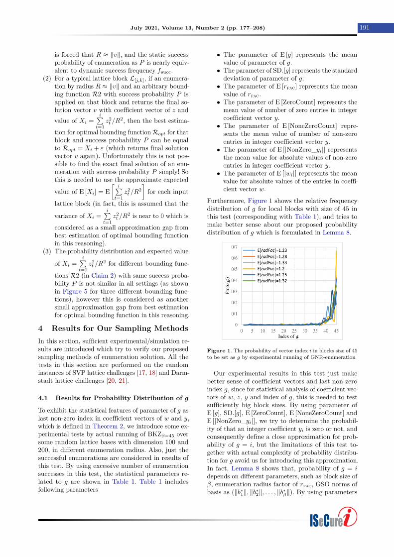
Furthermore, Figure 1 shows the relative frequencydistribution of g for local blocks with size of 45 inthis test (corresponding with Table 1), and tries tomake better sense about our proposed probabilitydistribution of g which is formulated in Lemma 8.
Figure 1. The probability of vector index i in blocks size of 45to be set as g by experimental running of GNR-enumeration
Our experimental results in this test just makebetter sense of coefficient vectors and last non-zeroindex g, since for statistical analysis of coefficient vec-tors of w, z, y and index of g, this is needed to testsufficiently big block sizes. By using parameter ofE [g], SD.[g], E [ZeroCount], E [NoneZeroCount] andE [|NonZero_yi|], we try to determine the probabil-ity of that an integer coefficient yi is zero or not, andconsequently define a close approximation for prob-ability of g = i, but the limitations of this test to-gether with actual complexity of probability distribu-tion for g avoid us for introducing this approximation.In fact, Lemma 8 shows that, probability of g = idepends on different parameters, such as block size ofβ, enumeration radius factor of rfac, GSO norms ofbasis as (‖b∗1‖, ‖b∗2‖, . . . , ‖b∗β‖). By using parameters
ISeCure
192 Better Sampling Method of Enumeration Solution for BKZ-Simulation — Moghissi and Payandeh
Table 1. Experimental results for g in successful enumerations on blocks of BKZβ=45 over random lattices with dim. of 100 and 200
E [rfac] E [g] SD.[g] E [ZeroCount] E [NoneZeroCount] E [|NonZero_yi|] E [|wi|]
1.2 43.23 4.03 16.93 28.07 1.59 0.25
1.23 40.67 7.2 19.48 25.52 1.61 0.27
1.25 40.67 8.39 21.46 23.54 1.51 0.27
1.28 42.03 6.14 19.41 25.59 1.51 0.27
1.32 42.96 4.04 18.38 26.62 1.48 0.28
1.33 43.05 3.92 18.17 26.83 1.5 0.29
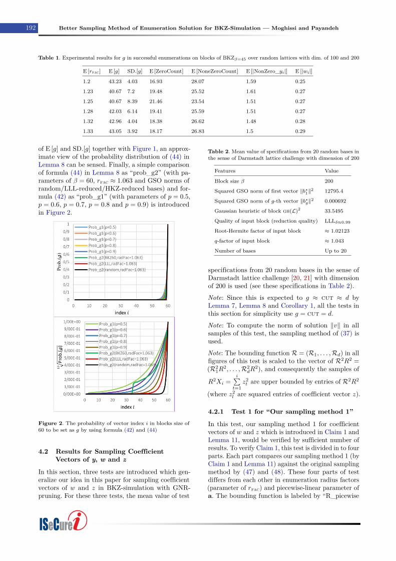
of E [g] and SD.[g] together with Figure 1, an approx-imate view of the probability distribution of (44) inLemma 8 can be sensed. Finally, a simple comparisonof formula (44) in Lemma 8 as “prob_g2” (with pa-rameters of β = 60, rfac ≈ 1.063 and GSO norms ofrandom/LLL-reduced/HKZ-reduced bases) and for-mula (42) as “prob_g1” (with parameters of p = 0.5,p = 0.6, p = 0.7, p = 0.8 and p = 0.9) is introducedin Figure 2.
Figure 2. The probability of vector index i in blocks size of60 to be set as g by using formula (42) and (44)
4.2 Results for Sampling CoefficientVectors of y, w and z
In this section, three tests are introduced which gen-eralize our idea in this paper for sampling coefficientvectors of w and z in BKZ-simulation with GNR-pruning. For these three tests, the mean value of test
Table 2. Mean value of specifications from 20 random bases inthe sense of Darmstadt lattice challenge with dimension of 200
Features Value
Block size β 200
Squared GSO norm of first vector ‖b∗1‖2 12795.4
Squared GSO norm of g-th vector ‖b∗g‖2 0.000692
Gaussian heuristic of block gh(L)2 33.5495
Quality of input block (reduction quality) LLLδ≈0.99
Root-Hermite factor of input block ≈ 1.02123
q-factor of input block ≈ 1.043
Number of bases Up to 20
specifications from 20 random bases in the sense ofDarmstadt lattice challenge [20, 21] with dimensionof 200 is used (see these specifications in Table 2).
Note: Since this is expected to g ≈ cut ≈ d byLemma 7, Lemma 8 and Corollary 1, all the tests inthis section for simplicity use g = cut = d.
Note: To compute the norm of solution ‖v‖ in allsamples of this test, the sampling method of (37) isused.
Note: The bounding function R = (R1, . . . ,Rd) in allfigures of this test is scaled to the vector of R2R2 =(R2
1R2, . . . ,R2
dR2), and consequently the samples of
R2Xi =i∑t=1
z2t are upper bounded by entries of R2R2
(where z2l are squared entries of coefficient vector z).
4.2.1 Test 1 for “Our sampling method 1”
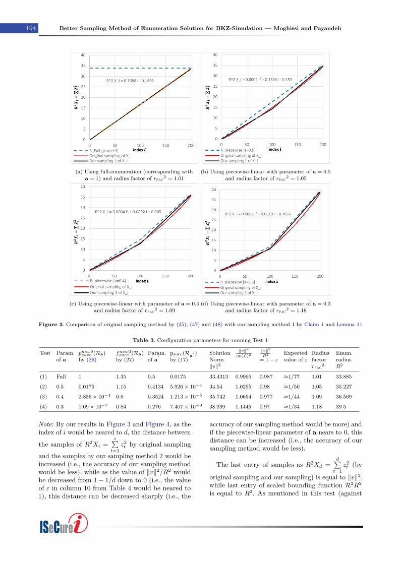
In this test, our sampling method 1 for coefficientvectors of w and z which is introduced in Claim 1 andLemma 11, would be verified by sufficient number ofresults. To verify Claim 1, this test is divided in to fourparts. Each part compares our sampling method 1 (byClaim 1 and Lemma 11) against the original samplingmethod by (47) and (48). These four parts of testdiffers from each other in enumeration radius factors(parameter of rfac) and piecewise-linear parameter ofa. The bounding function is labeled by “R_picewise
ISeCure
July 2021, Volume 13, Number 2 (pp. 177–208) 193
[a = c]” which means a piecewise-linear boundingfunction with parameter a = c, and “R_Full [psucc =1]” which means full-enumeration. This test is donein following way
• The original sampling in this test uses formulaof (48) to sample coefficient vector z or for-mula (47) to sample coefficient vector w, thenit selects just the sampled vector of z satisfyingthe bounding function constraints in (25). Themean value of entries of selected (successful)samples of vector z is used to compute Xi =i∑t=1
z2t /R
2 as “Original sampling of Xi”. Also
the trend line equation for “Original samplingof Xi” is presented for each part of test.
• Our sampling method which is labeled as “Oursampling 1 of Xi”, uses Claim 1 which saysthat for each piecewise-linear bounding func-tion Ra (labeled by “R_picewise [a = c]” or“R_Full [psucc = 1]”), this is only needed to finda piecewise-linear bounding function Ra′ wherepsucc(Ra′ ) = psucc(Ra)
F(d) by function psucc de-fined in (17) and function F defined in (18), andconsequently we use the entries ofRa′ as the ap-proximate expected values of sampling of Xi =i∑t=1
z2t /R
2 while bounded by Ra. The parameter
a′ from bounding function Ra′ can be used byLemma 11 to sample w2
t = z2d−t+1/‖b∗t ‖2 and
consequently to sample the values of R2Xi =i∑t=1
z2t which is bounded by R2
aR2.
Our results for four parts of this test can be observedin Figure 3 and Table 3. Each part uses up to 4× 10⁸
samples.
Note: In Figure 3, Figure 4 and Figure 5, the label ofa typical bounding function R represents the vectorR2R2 = [R2
1R2, . . . ,R2
dR2], also the label of sampled
vector X represents the vector R2X with entries of
R2Xi =i∑t=1
z2t .
As shown in Figure 3, the original sampling and
our sampling method 1 of R2Xi =i∑t=1
z2t are upper-
bounded by bounding function of “R_picewise [a =c]” (see the blue dash line as the bounding function).
The parameter a in Table 3 shows the piecewise-linear parameter of bounding function of Ra. Thestatic success probability and dynamic success fre-quency of Ra by (26) and (27) is shown in column3 and 4. The parameter a′ shows the input param-eter of Lemma 11 which computed by Claim 1 aspsucc(Ra′ ) = psucc(Ra)/F(d) by function psucc de-
fined in (17) and function F defined in (18) (parame-ter a′ in Table 3 corresponds with parameter a3 inAlgorithm 5 from Appendix A.5). The expected num-ber of solutions in the cylinder-intersection of radius(R′1R2, . . . ,R′lR2) which is defined by fnew0
succ (Ra) in(27) is approximated by column 4 in Table 3. In fact,as shown in column 9 and column 10, the conditionof ‖v‖2/R2 ≈ 1− ε where ε ≈ O(1/d) is satisfied inthis test, so Claim 1, Lemma 10 and Lemma 11 canbe applied consistently. As shown in Figure 3, oursampling method 1 by Claim 1 and Lemma 11 canbe used as an approximation of original sampling by(47), (48) and (25), however as the piecewise-linearparameter of a nears to 0, our sampling method 1would be less precise.
Note: As mentioned, the success probability psucc,which is defined in (17), is equal to static successprobability pnew0
succ which is defined in (26).
Note: If the radius factor rfac is sufficiently small to-gether with any static success probability of boundingfunction or the static success probability of currentbounding function is small together with any radiusfactor rfac, then the condition of ‖v‖2/R2 ≈ 1 − εwhere ε ≈ O(1/d) can be observed. So our proposedsampling method 1 (based on Claim 1 and Lemma11) just be applied for small radius factor or smallstatic success probability! In other words, if dynamicsuccess frequency fnew0
succ (Ra) belongs to ≈ O(1), thecondition of ‖v‖2/R2 ≈ 1− ε where ε ≈ O(1/d) canbe observed.
4.2.2 Test 2 for “Our sampling method 2”
As mentioned, Claim 1, Lemma 10 and Lemma 11are introduced under condition of ‖v‖2/R2 ≈ 1 − εwhere ε ≈ O(1/d). This test focuses on the situationsthat ε would be close to ≈ 1, so this is not possibleto use Claim 1 and Lemma 11 directly to samplethe coefficient vector of z. For this case, Algorithm6 in Appendix A.5 generalizes our sampling method1 (in Algorithm 5 from Appendix A.5). Lines 1-6 inAlgorithm 6 do this generalization by use of a simpletransformation. This new sampling method is labeledhere as “Our sampling method 2 of Xi”. Our resultsfor this test would be observed in Figure 4 and Table4. The trend line equation for “Original sampling ofXi” is presented for each part of this test in Figure 4.
As shown in Figure 4, sampling method 2 of Xi (byusing lines 1-6 in Algorithm 6) introduces acceptableapproximation for sampling coefficient vector z. Notethat, by using these observation, sampling method2 can be used for sampling coefficient vector z andpiecewise-linear bounding function with any enumer-ation radius.
ISeCure
194 Better Sampling Method of Enumeration Solution for BKZ-Simulation — Moghissi and Payandeh
(a) Using full-enumeration (corresponding witha = 1) and radius factor of rfac2 = 1.01
(b) Using piecewise-linear with parameter of a = 0.5and radius factor of rfac2 = 1.05
(c) Using piecewise-linear with parameter of a = 0.4and radius factor of rfac2 = 1.09
(d) Using piecewise-linear with parameter of a = 0.3and radius factor of rfac2 = 1.18
Figure 3. Comparison of original sampling method by (25), (47) and (48) with our sampling method 1 by Claim 1 and Lemma 11
Table 3. Configuration parameters for running Test 1
Test Param.of a
pnew0succ (Ra)
by (26)fnew0succ (Ra)
by (27)Param.of a′
psucc(Ra′ )by (17)
SolutionNorm‖v‖2
‖v‖2
gh(L)2‖v‖2
R2= 1− ε
Expectedvalue of ε
Radiusfactorrfac2
Enum.radiusR2
(1) Full 1 1.35 0.5 0.0175 33.4313 0.9965 0.987 ≈1/77 1.01 33.885
(2) 0.5 0.0175 1.15 0.4134 5.926× 10⁻⁴ 34.54 1.0295 0.98 ≈1/50 1.05 35.227
(3) 0.4 2.856× 10⁻⁴ 0.8 0.3524 1.213× 10⁻⁵ 35.742 1.0654 0.977 ≈1/44 1.09 36.569
(4) 0.3 1.09× 10⁻⁷ 0.84 0.276 7.407× 10⁻⁹ 38.399 1.1445 0.97 ≈1/34 1.18 39.5
Note: By our results in Figure 3 and Figure 4, as theindex of i would be neared to d, the distance between
the samples of R2Xi =i∑t=1
z2t by original sampling
and the samples by our sampling method 2 would beincreased (i.e., the accuracy of our sampling methodwould be less), while as the value of ‖v‖2/R2 wouldbe decreased from 1− 1/d down to 0 (i.e., the valueof ε in column 10 from Table 4 would be neared to1), this distance can be decreased sharply (i.e., the
accuracy of our sampling method would be more) andif the piecewise-linear parameter of a nears to 0, thisdistance can be increased (i.e., the accuracy of oursampling method would be less).
The last entry of samples as R2Xd =d∑t=1
z2t (by
original sampling and our sampling) is equal to ‖v‖2,while last entry of scaled bounding function R2R2
is equal to R2. As mentioned in this test (against
ISeCure
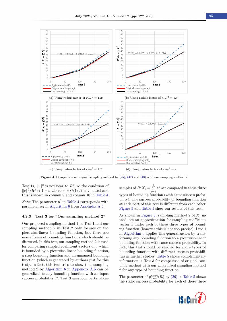
July 2021, Volume 13, Number 2 (pp. 177–208) 195
(a) Using radius factor of rfac2 = 1.25 (b) Using radius factor of rfac2 = 1.5
(c) Using radius factor of rfac2 = 1.75 (d) Using radius factor of rfac2 = 2
Figure 4. Comparison of original sampling method by (25), (47) and (48) with our sampling method 2
Test 1), ‖v‖2 is not near to R2, so the condition of‖v‖2/R2 ≈ 1 − ε where ε ≈ O(1/d) is violated andthis is shown in column 9 and column 10 in Table 4.
Note: The parameter a′ in Table 4 corresponds withparameter a3 in Algorithm 6 from Appendix A.5.
4.2.3 Test 3 for “Our sampling method 2”
Our proposed sampling method 1 in Test 1 and oursampling method 2 in Test 2 only focuses on thepiecewise-linear bounding function, but there aremany forms of bounding functions which should bediscussed. In this test, our sampling method 2 is usedfor comparing sampled coefficient vectors of z whichis bounded by a piecewise-linear bounding function,a step bounding function and an unnamed boundingfunction (which is generated by authors just for thistest). In fact, this test tries to show that samplingmethod 2 by Algorithm 6 in Appendix A.5 can begeneralized to any bounding function with an inputsuccess probability P . Test 3 uses four parts whose
samples of R2Xi =i∑t=1
z2t are compared in these three
types of bounding function (with same success proba-bility). The success probability of bounding functionat each part of this test is different from each other.Figure 5 and Table 5 show our results of this test.
As shown in Figure 5, sampling method 2 of Xi in-troduces an approximation for sampling coefficientvector z under each of these three types of bound-ing function (however this is not too precise). Line 1in Algorithm 6 applies this generalization by trans-forming any bounding function to a piecewise-linearbounding function with same success probability. Infact, this test should be studied for more types ofbounding function with different success probabili-ties in further studies. Table 5 shows complementaryinformation in Test 3 for comparison of original sam-pling method with our generalized sampling method2 for any type of bounding function.
The parameter of pnew0succ (R) by (26) in Table 5 shows
the static success probability for each of these three
ISeCure
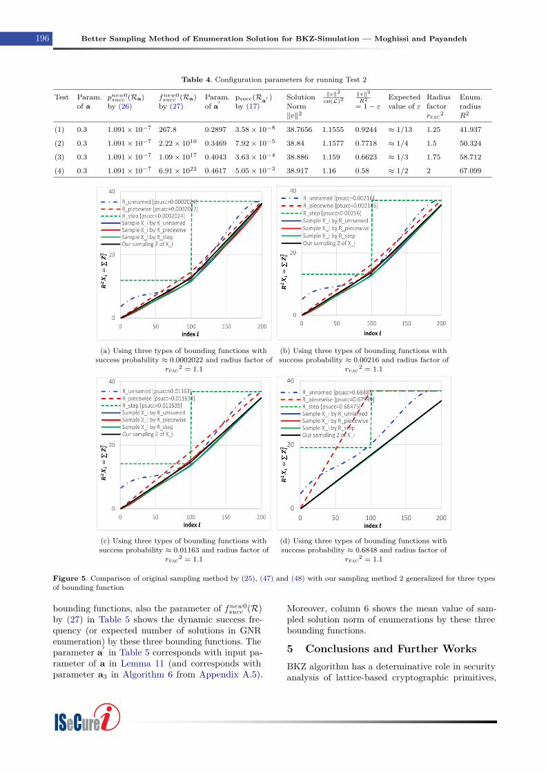
196 Better Sampling Method of Enumeration Solution for BKZ-Simulation — Moghissi and Payandeh
Table 4. Configuration parameters for running Test 2
Test Param.of a
pnew0succ (Ra)
by (26)fnew0succ (Ra)
by (27)Param.of a′
psucc(Ra′ )by (17)
SolutionNorm‖v‖2
‖v‖2
gh(L)2‖v‖2
R2= 1− ε
Expectedvalue of ε
Radiusfactorrfac2
Enum.radiusR2
(1) 0.3 1.091× 10⁻⁷ 267.8 0.2897 3.58× 10⁻⁸ 38.7656 1.1555 0.9244 ≈ 1/13 1.25 41.937
(2) 0.3 1.091× 10⁻⁷ 2.22× 10¹⁰ 0.3469 7.92× 10⁻⁵ 38.84 1.1577 0.7718 ≈ 1/4 1.5 50.324
(3) 0.3 1.091× 10⁻⁷ 1.09× 10¹⁷ 0.4043 3.63× 10⁻⁴ 38.886 1.159 0.6623 ≈ 1/3 1.75 58.712
(4) 0.3 1.091× 10⁻⁷ 6.91× 10²² 0.4617 5.05× 10⁻³ 38.917 1.16 0.58 ≈ 1/2 2 67.099
(a) Using three types of bounding functions withsuccess probability ≈ 0.0002022 and radius factor of
rfac2 = 1.1
(b) Using three types of bounding functions withsuccess probability ≈ 0.00216 and radius factor of
rfac2 = 1.1
(c) Using three types of bounding functions withsuccess probability ≈ 0.01163 and radius factor of
rfac2 = 1.1
(d) Using three types of bounding functions withsuccess probability ≈ 0.6848 and radius factor of
rfac2 = 1.1
Figure 5. Comparison of original sampling method by (25), (47) and (48) with our sampling method 2 generalized for three typesof bounding function
bounding functions, also the parameter of fnew0succ (R)
by (27) in Table 5 shows the dynamic success fre-quency (or expected number of solutions in GNRenumeration) by these three bounding functions. Theparameter a′ in Table 5 corresponds with input pa-rameter of a in Lemma 11 (and corresponds withparameter a3 in Algorithm 6 from Appendix A.5).
Moreover, column 6 shows the mean value of sam-pled solution norm of enumerations by these threebounding functions.
5 Conclusions and Further WorksBKZ algorithm has a determinative role in securityanalysis of lattice-based cryptographic primitives,
ISeCure
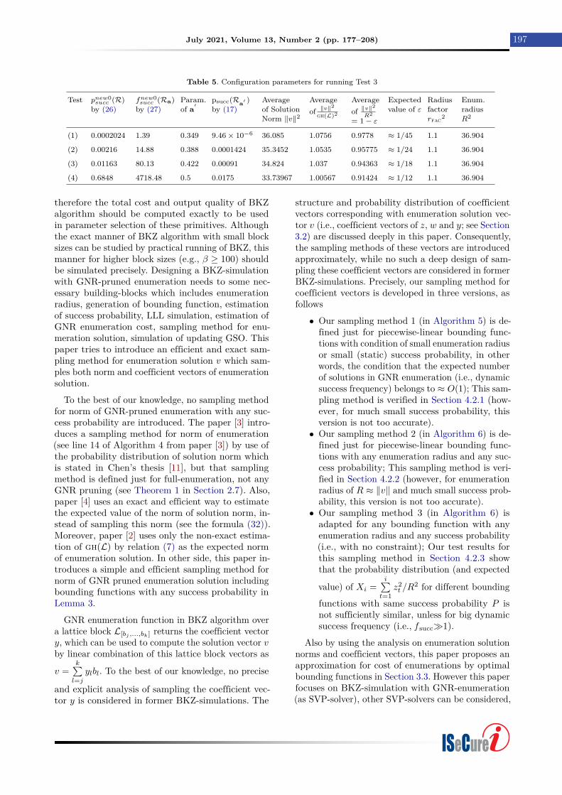
July 2021, Volume 13, Number 2 (pp. 177–208) 197
Table 5. Configuration parameters for running Test 3
Test pnew0succ (R)
by (26)fnew0succ (Ra)
by (27)Param.of a′
psucc(Ra′ )by (17)
Averageof SolutionNorm ‖v‖2
Averageof ‖v‖
2
gh(L)2
Averageof ‖v‖
2
R2= 1− ε
Expectedvalue of ε
Radiusfactorrfac2
Enum.radiusR2
(1) 0.0002024 1.39 0.349 9.46× 10⁻⁶ 36.085 1.0756 0.9778 ≈ 1/45 1.1 36.904
(2) 0.00216 14.88 0.388 0.0001424 35.3452 1.0535 0.95775 ≈ 1/24 1.1 36.904
(3) 0.01163 80.13 0.422 0.00091 34.824 1.037 0.94363 ≈ 1/18 1.1 36.904
(4) 0.6848 4718.48 0.5 0.0175 33.73967 1.00567 0.91424 ≈ 1/12 1.1 36.904
therefore the total cost and output quality of BKZalgorithm should be computed exactly to be usedin parameter selection of these primitives. Althoughthe exact manner of BKZ algorithm with small blocksizes can be studied by practical running of BKZ, thismanner for higher block sizes (e.g., β ≥ 100) shouldbe simulated precisely. Designing a BKZ-simulationwith GNR-pruned enumeration needs to some nec-essary building-blocks which includes enumerationradius, generation of bounding function, estimationof success probability, LLL simulation, estimation ofGNR enumeration cost, sampling method for enu-meration solution, simulation of updating GSO. Thispaper tries to introduce an efficient and exact sam-pling method for enumeration solution v which sam-ples both norm and coefficient vectors of enumerationsolution.
To the best of our knowledge, no sampling methodfor norm of GNR-pruned enumeration with any suc-cess probability are introduced. The paper [3] intro-duces a sampling method for norm of enumeration(see line 14 of Algorithm 4 from paper [3]) by use ofthe probability distribution of solution norm whichis stated in Chen’s thesis [11], but that samplingmethod is defined just for full-enumeration, not anyGNR pruning (see Theorem 1 in Section 2.7). Also,paper [4] uses an exact and efficient way to estimatethe expected value of the norm of solution norm, in-stead of sampling this norm (see the formula (32)).Moreover, paper [2] uses only the non-exact estima-tion of gh(L) by relation (7) as the expected normof enumeration solution. In other side, this paper in-troduces a simple and efficient sampling method fornorm of GNR pruned enumeration solution includingbounding functions with any success probability inLemma 3.
GNR enumeration function in BKZ algorithm overa lattice block L[bj ,...,bk] returns the coefficient vectory, which can be used to compute the solution vector vby linear combination of this lattice block vectors as
v =k∑l=j
ylbl. To the best of our knowledge, no precise
and explicit analysis of sampling the coefficient vec-tor y is considered in former BKZ-simulations. The
structure and probability distribution of coefficientvectors corresponding with enumeration solution vec-tor v (i.e., coefficient vectors of z, w and y; see Section3.2) are discussed deeply in this paper. Consequently,the sampling methods of these vectors are introducedapproximately, while no such a deep design of sam-pling these coefficient vectors are considered in formerBKZ-simulations. Precisely, our sampling method forcoefficient vectors is developed in three versions, asfollows
• Our sampling method 1 (in Algorithm 5) is de-fined just for piecewise-linear bounding func-tions with condition of small enumeration radiusor small (static) success probability, in otherwords, the condition that the expected numberof solutions in GNR enumeration (i.e., dynamicsuccess frequency) belongs to ≈ O(1); This sam-pling method is verified in Section 4.2.1 (how-ever, for much small success probability, thisversion is not too accurate).• Our sampling method 2 (in Algorithm 6) is de-fined just for piecewise-linear bounding func-tions with any enumeration radius and any suc-cess probability; This sampling method is veri-fied in Section 4.2.2 (however, for enumerationradius of R ≈ ‖v‖ and much small success prob-ability, this version is not too accurate).
• Our sampling method 3 (in Algorithm 6) isadapted for any bounding function with anyenumeration radius and any success probability(i.e., with no constraint); Our test results forthis sampling method in Section 4.2.3 showthat the probability distribution (and expected
value) of Xi =i∑t=1
z2t /R
2 for different bounding
functions with same success probability P isnot sufficiently similar, unless for big dynamicsuccess frequency (i.e., f succ1).
Also by using the analysis on enumeration solutionnorms and coefficient vectors, this paper proposes anapproximation for cost of enumerations by optimalbounding functions in Section 3.3. However this paperfocuses on BKZ-simulation with GNR-enumeration(as SVP-solver), other SVP-solvers can be considered,
ISeCure
198 Better Sampling Method of Enumeration Solution for BKZ-Simulation — Moghissi and Payandeh
such as lattice enumeration with discrete pruning [22],sieving algorithm (e.g., the variant in [23]), enumera-tion by integrating sparse orthogonalized integer rep-resentations for shortest vectors [24], or even our evo-lutionary search for solving SVP [25]. Also, althoughTest 3 in Section 4.2.3 tries to show that samplingmethod 2 by Algorithm 6 in Appendix A.5 can begeneralized to any bounding function, new techniquescan be studied in further works to introduce more ac-curate approximation of sampling coefficient vectorsof z, w, and y.
AcknowledgmentThe authors would like to thank the anonymous re-viewers for their much valuable, constructive and in-sightful comments which helped us to improve thepresentation of this work significantly, also thank theeditorial board and editorial staff of the ISeCure jour-nal for their generous help in publishing this study.
References[1] Nicolas Gama, Phong Q Nguyen, and Oded
Regev. Lattice enumeration using extreme prun-ing. In Annual International Conference on theTheory and Applications of Cryptographic Tech-niques, pages 257–278. Springer, 2010.
[2] Yuanmi Chen and Phong Q Nguyen. BKZ 2.0:Better lattice security estimates. In InternationalConference on the Theory and Application ofCryptology and Information Security, pages 1–20.Springer, 2011.
[3] Shi Bai, Damien Stehlé, and Weiqiang Wen. Mea-suring, simulating and exploiting the head con-cavity phenomenon in BKZ. In InternationalConference on the Theory and Application ofCryptology and Information Security, pages 369–404. Springer, 2018.
[4] Yoshinori Aono, Yuntao Wang, Takuya Hayashi,and Tsuyoshi Takagi. Improved progressive BKZalgorithms and their precise cost estimation bysharp simulator. In Annual International Con-ference on the Theory and Applications of Cryp-tographic Techniques, pages 789–819. Springer,2016.
[5] Joop van de Pol and Nigel P Smart. Estimatingkey sizes for high dimensional lattice-based sys-tems. In IMA International Conference on Cryp-tography and Coding, pages 290–303. Springer,2013.
[6] Tancrede Lepoint and Michael Naehrig. A com-parison of the homomorphic encryption schemesFV and YASHE. In International Conference onCryptology in Africa, pages 318–335. Springer,2014.
[7] Mingjie Liu and Phong Q Nguyen. Solving BDD
by enumeration: An update. In Cryptographers’Track at the RSA Conference, pages 293–309.Springer, 2013.
[8] Yoshinori Aono, Xavier Boyen, Lihua Wang, et al.Key-private proxy re-encryption under LWE. InInternational Conference on Cryptology in India,pages 1–18. Springer, 2013.
[9] Martin R Albrecht, Benjamin R Curtis, AmitDeo, Alex Davidson, Rachel Player, Eamonn WPostlethwaite, Fernando Virdia, and ThomasWunderer. Estimate all the LWE, NTRUschemes! In International Conference on Secu-rity and Cryptography for Networks, pages 351–367. Springer, 2018.
[10] Jeff Hoffstein, Jill Pipher, John M Schanck,Joseph H Silverman, and William Whyte. Prac-tical signatures from the partial fourier recoveryproblem. In International Conference on Ap-plied Cryptography and Network Security, pages476–493. Springer, 2014.
[11] Yuanmi Chen. Réduction de réseau et sécuritéconcrete du chiffrement completement homomor-phe. PhD thesis, Paris 7, 2013.
[12] Daniele Micciancio and Oded Regev. Lattice-based cryptography. In Post-quantum cryptogra-phy, pages 147–191. Springer, 2009.
[13] Claus Peter Schnorr. Lattice reduction by ran-dom sampling and birthday methods. In AnnualSymposium on Theoretical Aspects of ComputerScience, pages 145–156. Springer, 2003.
[14] Arjen K Lenstra, Hendrik Willem Lenstra, andLászló Lovász. Factoring polynomials withrational coefficients. Mathematische annalen,261(ARTICLE):515–534, 1982.
[15] CA Rogers. The number of lattice points in a set.Proceedings of the London Mathematical Society,3(2):305–320, 1956.
[16] Johannes Buchmann and Christoph Ludwig.Practical lattice basis sampling reduction. InInternational Algorithmic Number Theory Sym-posium, pages 222–237. Springer, 2006.
[17] SVP Challenge. Available at: https://www.latticechallenge.org/svp-challenge/index.php.
[18] Daniel Goldstein and Andrew Mayer. On theequidistribution of Hecke points. In Forum Math-ematicum, volume 15, 2003.
[19] Yang Yu and Léo Ducas. Second order statisticalbehavior of LLL and BKZ. In InternationalConference on Selected Areas in Cryptography,pages 3–22. Springer, 2017.
[20] Johannes Buchmann, Richard Lindner, andMarkus Rückert. Explicit hard instances of theshortest vector problem. In International Work-shop on Post-Quantum Cryptography, pages 79–94. Springer, 2008.
ISeCure
July 2021, Volume 13, Number 2 (pp. 177–208) 199
[21] TU Darmstadt lattice challenge. Available at:www.latticechallenge.org.
[22] Yoshinori Aono and Phong Q Nguyên. Randomsampling revisited: lattice enumeration with dis-crete pruning. In Annual International Confer-ence on the Theory and Applications of Cryp-tographic Techniques, pages 65–102. Springer,2017.
[23] Léo Ducas. Shortest vector from lattice siev-ing: a few dimensions for free. In Annual Inter-national Conference on the Theory and Appli-cations of Cryptographic Techniques, pages 125–145. Springer, 2018.
[24] Zhongxiang Zheng, Xiaoyun Wang, GuangwuXu, and Yang Yu. Orthogonalized lattice enu-meration for solving SVP. Science China Infor-mation Sciences, 61(3):1–15, 2018.
[25] Gholam Reza Moghissi and Ali Payandeh. A par-allel evolutionary search for shortest vector prob-lem. Int. J. Inf. Technol. Comput. Sci.(IJITCS),11(8):9–19, 2019.
[26] Joop van de Pol. Lattice-based cryptography.Eindhoven University of Technology, Departmentof Mathematics and Computer Science, 2011.
[27] Johan Ludwig William Valdemar Jensen et al.Sur les fonctions convexes et les inégalités entreles valeurs moyennes. Acta mathematica, 30:175–193, 1906.
Gholam Reza Moghissi re-ceived the M.S. degree in de-partment of ICT at Malek-e-Ashtar University of Technology,Tehran, Iran, in 2016. His re-searches focus on information secu-rity.
Ali Payandeh received the M.S. de-gree in electrical engineering fromTarbiat Modares University in 1994,and the Ph.D. degree in electrical en-gineering from K.N. Toosi Universityof Technology (Tehran, Iran) in 2006.He is now an assistant professor in
the department of information and communicationstechnology at Malek-e-Ashtar University of Technol-ogy, Iran. His research interests include informationtheory, coding theory, cryptography, security proto-cols, secure communications, and satellite communi-cations.
Appendices
A. Algorithms Used/Introduced inPaperIn this appendix, the pseudo-codes of essential algo-rithms in this paper are introduced.
A.1 Schnorr-Euchner’s BKZ
Algorithm 1 shows the pseudo-code of original versionof BKZ algorithm [26].
Algorithm 1 Block Korkin-Zolotarev (BKZ)Input: B = (b1, . . . , bn) ∈ Zn×m, GSO Coef Mat µ, 2 ≤ β ≤n, 1/4 ≤ δ < 1.Output: BKZβ reduced basis B.1: LLL(B,µ, δ); //LLL reduce the basis and update µ2: for (z = 0, j = 0; z < n− 1;) do3: j = (j mod (n− 1)) + 1;4: k = min(j + β − 1, n);5: h = min(k + 1, n);6: y ← Enum(‖b∗j‖2, ‖b∗j+1‖
2, . . . , ‖b∗k‖2, µ[j,k]);
7: if y 6= (1, 0, . . . , 0) then
8: LLL([b1, . . . , bj−1,k∑l=j
ylbl, bj , . . . , bh], µ, δ)at stage j;
9: z = 0;10: else11: LLL ([b1, . . . , bh] , µ, δ) at stage h− 1;12: z + +;13: end if14: end for
A.2 Our Sampling Algorithm of SolutionNorm
The pseudo-code of the sampling method of solutionnorm by (37) in Lemma 3 can be studied in Algorithm2. Note that, sampling x from exponential distributionwhere PDF = Expo(x;ϑ) (see relation (14)), for ϑ =0.5 can be done by uniformly random selection of Yfrom corresponding CDF as Y ← CDF = 1− e−0.5x,and computing the corresponding sample of x (seeline 2 in Algorithm 2).
A.3 Generator of Piecewise-Linear BoundingFunc.
Here, we introduce the pseudo-code of generatingpiecewise-linear bounding function in Algorithm 3.The function of PiecewiceLinear(a, d) makes apiecewise-linear bounding function with length of dand piecewise-linear parameter of a. The search ap-proach for suitable parameter of a in this algorithmcan be used for step bounding function too. Alsofunction psucc(R) comes from relation (17) or (26) asthe static success probability which is implementedin Algorithm 6 or Algorithm 7 from Appendix A inpaper [2].
ISeCure
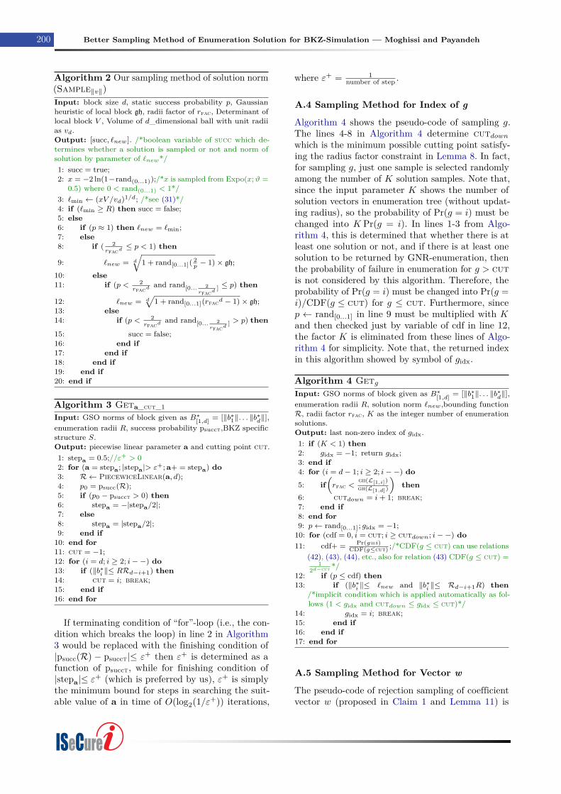
200 Better Sampling Method of Enumeration Solution for BKZ-Simulation — Moghissi and Payandeh
Algorithm 2 Our sampling method of solution norm(Sample‖v‖)Input: block size d, static success probability p, Gaussianheuristic of local block gh, radii factor of rfac, Determinant oflocal block V , Volume of d_dimensional ball with unit radiias vd.Output: [succ, `new]. /*boolean variable of succ which de-termines whether a solution is sampled or not and norm ofsolution by parameter of `new*/1: succ = true;2: x = −2 ln(1−rand(0...1));/*x is sampled from Expo(x;ϑ =
0.5) where 0 < rand(0...1) < 1*/3: `min ← (xV /vd)1/d; /*see (31)*/4: if (`min ≥ R) then succ = false;5: else6: if (p ≈ 1) then `new = `min;7: else8: if ( 2
rfacd≤ p < 1) then
9: `new = d
√1 + rand[0...1]( 2
p− 1)× gh;
10: else11: if (p < 2
rfacdand rand[0... 2
rfacd] ≤ p) then
12: `new = d√
1 + rand[0...1](rfacd − 1)× gh;13: else14: if (p < 2
rfacdand rand[0... 2
rfacd] > p) then
15: succ = false;16: end if17: end if18: end if19: end if20: end if
Algorithm 3 Geta_cut_1Input: GSO norms of block given as B∗[1,d] = [‖b∗1‖. . . ‖b∗d‖],enumeration radii R, success probability psucct,BKZ specificstructure S.Output: piecewise linear parameter a and cutting point cut.1: stepa = 0.5;//ε+ > 02: for (a = stepa; |stepa|> ε+;a+ = stepa) do3: R← PiecewiceLinear(a, d);4: p0 = psucc(R);5: if (p0 − psucct > 0) then6: stepa = −|stepa/2|;7: else8: stepa = |stepa/2|;9: end if
10: end for11: cut = −1;12: for (i = d; i ≥ 2; i−−) do13: if (‖b∗i ‖≤ RRd−i+1) then14: cut = i; break;15: end if16: end for
If terminating condition of “for”-loop (i.e., the con-dition which breaks the loop) in line 2 in Algorithm3 would be replaced with the finishing condition of|psucc(R) − psucct|≤ ε+ then ε+ is determined as afunction of psucct, while for finishing condition of|stepa|≤ ε+ (which is preferred by us), ε+ is simplythe minimum bound for steps in searching the suit-able value of a in time of O(log2(1/ε+)) iterations,
where ε+ = 1number of step .
A.4 Sampling Method for Index of g
Algorithm 4 shows the pseudo-code of sampling g.The lines 4-8 in Algorithm 4 determine cutdownwhich is the minimum possible cutting point satisfy-ing the radius factor constraint in Lemma 8. In fact,for sampling g, just one sample is selected randomlyamong the number of K solution samples. Note that,since the input parameter K shows the number ofsolution vectors in enumeration tree (without updat-ing radius), so the probability of Pr(g = i) must bechanged into K Pr(g = i). In lines 1-3 from Algo-rithm 4, this is determined that whether there is atleast one solution or not, and if there is at least onesolution to be returned by GNR-enumeration, thenthe probability of failure in enumeration for g > cutis not considered by this algorithm. Therefore, theprobability of Pr(g = i) must be changed into Pr(g =i)/CDF(g ≤ cut) for g ≤ cut. Furthermore, sincep ← rand[0...1] in line 9 must be multiplied with Kand then checked just by variable of cdf in line 12,the factor K is eliminated from these lines of Algo-rithm 4 for simplicity. Note that, the returned indexin this algorithm showed by symbol of gidx.
Algorithm 4 GetgInput: GSO norms of block given as B∗[1,d] = [‖b∗1‖. . . ‖b∗d‖],enumeration radii R, solution norm `new,bounding functionR, radii factor rfac, K as the integer number of enumerationsolutions.Output: last non-zero index of gidx.1: if (K < 1) then2: gidx = −1; return gidx;3: end if4: for (i = d− 1; i ≥ 2; i−−) do5: if
(rfac <
gh(L[1,i])gh(L[1,d])
)then
6: cutdown = i+ 1; break;7: end if8: end for9: p← rand[0...1]; gidx = −1;
10: for (cdf = 0, i = cut; i ≥ cutdown; i−−) do11: cdf+ = Pr(g=i)
CDF(g≤cut) ;/*CDF(g ≤ cut) can use relations(42), (43), (44), etc., also for relation (43) CDF(g ≤ cut) =
12d−cut */
12: if (p ≤ cdf) then13: if (‖b∗i ‖≤ `new and ‖b∗i ‖≤ Rd−i+1R) then
/*implicit condition which is applied automatically as fol-lows (1 < gidx and cutdown ≤ gidx ≤ cut)*/
14: gidx = i; break;15: end if16: end if17: end for
A.5 Sampling Method for Vector w
The pseudo-code of rejection sampling of coefficientvector w (proposed in Claim 1 and Lemma 11) is
ISeCure
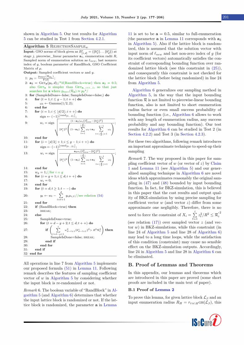
July 2021, Volume 13, Number 2 (pp. 177–208) 201
shown in Algorithm 5. Our test results for Algorithm5 can be studied in Test 1 from Section 4.2.1.
Algorithm 5 RejectionSamplewInput: GSO norms of block given as B∗[1,d] = (‖b∗1‖. . . ‖b∗d‖) atstage j, piecewise_linear parameter a1, enumeration radii R,Sampled norm of enumeration solution as `new, last nonzeroindex of g, boolean parameter of RandBlock, GSO CoefficientMatrix of µ.Output: Sampled coefficient vectors w and y.1: p0 = psucc(Ra1 )
F(d) ;2: a3 = Geta(p0, d);/*if(RandBlock=true) then a3 = 0.5;
also Geta is simpler than Geta_cut_1, so that justsearches for a where psucc(Ra) ≈ p0*/
3: for (SampleIsDone←false; SampleIsDone=false;) do4: for (t = 1; t ≤ g − 1; t+ +) do5: ωt ← Gamma(1/2, 2);6: end for7: for (i = 1; i ≤ bd/2c; i+ +) do8: sign← (−1)brand[0...2)c;
9: wi = sign√√√√√ (1−a3)ωi(`2
new−‖b∗g‖2)
‖b∗i‖2
((1−a3)
b d2 c∑t=1
ωt+a3
g−1∑t=b d2 c+1
ωt
) ;
10: end for11: for (i = bd/2c+ 1; i ≤ g − 1; i+ +) do12: sign← (−1)brand[0...2)c;
13: wi = sign√√√√√ a3ωi(`2
new−‖b∗g‖2)
‖b∗i‖2
((1−a3)
b d2 c∑t=1
ωt+a3
g−1∑t=b d2 c+1
ωt
) ;
14: end for15: wg = 1;//for i = g
16: for (i = g + 1; i ≤ d; i+ +) do17: wi = 0;18: end for19: for (t = d; t ≥ 1; t−−) do
20: yt ← wt −d∑
i=t+1yiµi,t;//see relation (54)
21: end for22: if (RandBlock=true) then23: break;24: else25: SampleIsDone=true;26: for (t = d− g + 2; t ≤ d; t+ +) do
27: if(
t∑l=d−g+1
w2d−l+1‖b
∗d−l+1‖
2> R2R2t
)then
28: SampleIsDone=false; break;29: end if30: end for31: end if32: end for
All operations in line 7 from Algorithm 5 implementsour proposed formula (51) in Lemma 11. Followingremark describes the features of sampling coefficientvector of w in Algorithm 5 by considering whetherthe input block is re-randomized or not.
Remark 6. The boolean variable of “RandBlock” in Al-gorithm 5 (and Algorithm 6) determines that whetherthe input lattice block is randomized or not. If the lat-tice block is randomized, the parameter a in Lemma
11 is set to be a = 0.5, similar to full-enumeration(the parameter a in Lemma 11 corresponds with a3in Algorithm 5). Also if the lattice block is random-ized, this is assumed that the solution vector withinput norm of `new and last non-zero index of g (forits coefficient vectors) automatically satisfies the con-straint of corresponding bounding function over ran-domized lattice block (see this constraint in (25)),and consequently this constraint is not checked forthe lattice block (before being randomized) in line 24from Algorithm 5.
Algorithm 6 generalizes our sampling method inAlgorithm 5, in the way that the input boundingfunction R is not limited to piecewise-linear boundingfunction, also is not limited to short enumerationradius factor or even small success probability ofbounding function (i.e., Algorithm 6 allows to workwith any length of enumeration radius, any successprobability and any bounding function). Our testresults for Algorithm 6 can be studied in Test 2 (inSection 4.2.2) and Test 3 (in Section 4.2.3).
For these two algorithms, following remark introducesan important approximate technique to speed-up theirsampling
Remark 7. The way proposed in this paper for sam-pling coefficient vector of w (or vector of z) by Claim1 and Lemma 11 (see Algorithm 5) and our gener-alized sampling technique in Algorithm 6 are novelideas which approximates reasonably the original sam-pling in (47) and (48) bounded by input boundingfunction. In fact, for BKZ-simulation, this is believedin this paper that the cost results and output qual-ity of BKZ-simulation by using precise sampling forcoefficient vector w (and vector z) differ from someapproximate one negligibly. Therefore, there is no
need to force the constraint of Xi =i∑t=1
z2t /R
2 ≤ R′i2
(see relation (17)) over sampled vector z (and vec-tor w) in BKZ-simulations, while this constraint (inline 24 of Algorithm 5 and line 28 of Algorithm 6)may lead to a long time loops, while the satisfactionof this condition (constraint) may cause no sensibleeffect on the BKZ-simulation outputs. Accordingly,line 24 in Algorithm 5 and line 28 in Algorithm 6 canbe eliminated.
B. Proof of Lemmas and TheoremsIn this appendix, our lemmas and theorems whichare introduced in this paper are proved (some shortproofs are included in the main text of paper).
B.1 Proof of Lemma 2
To prove this lemma, for given lattice block Lβ and aninput enumeration radius RH = rfacHgh(Lβ), this
ISeCure
202 Better Sampling Method of Enumeration Solution for BKZ-Simulation — Moghissi and Payandeh
Algorithm 6 GeneralizedRejectionSamplewInput: GSO norms of block given as B∗[1,d] = (‖b∗1‖. . . ‖b∗d‖) atstage j, any type of bounding function R, enumeration radii R,Sampled norm of enumeration solution as `new, last nonzeroindex of g, boolean parameter of RandBlock, GSO CoefficientMatrix of µ.Output: Sampled coefficient vectors w and y.1: p0 = psucc(R); a0 = Geta(p0, d); /*Geta(p0, d) is sim-
pler than Geta_cut_1 so that just searches for a0 wherepsucc(Ra0 ) ≈ p0 */
2: p1 = p0F(d) ;a1 = Geta(p1, d);
3: A = a1R2−‖b∗g‖
2
d2−(d−g+1)
;a3 = dA2`2new
;4: if (a3 > 0.5) then5: a3 = 0.5;6: end if//if(RandBlock=true) then a3 = 0.5;7: for (SampleIsDone←false; SampleIsDone=false;) do8: for (t = 1; t ≤ g − 1; t+ +) do9: ωt ← Gamma(1/2, 2);
10: end for11: for (i = 1; i ≤ bd/2c; i+ +) do12: sign← (−1)brand[0...2)c;
13: wi = sign√√√√√ (1−a3)ωi(`2
new−‖b∗g‖2)
‖b∗i‖2
((1−a3)
b d2 c∑t=1
ωt+a3
g−1∑t=b d2 c+1
ωt
) ;
14: end for15: for (i = bd/2c+ 1; i ≤ g − 1; i+ +) do16: sign← (−1)brand[0...2)c;
17: wi = sign√√√√√ a3ωi(`2
new−‖b∗g‖2)
‖b∗i‖2
((1−a3)
b d2 c∑t=1
ωt+a3
g−1∑t=b d2 c+1
ωt
) ;
18: end for19: wg = 1;//for i = g20: for (i = g + 1; i ≤ d; i+ +) do21: wi = 0;22: end for23: for (t = d; t ≥ 1; t−−) do
24: yt ← wt −d∑
i=t+1yiµi,t;//see relation (54)
25: end for26: if (RandBlock=true) then27: break;28: else29: SampleIsDone=true;30: for (t = d− g + 2; t ≤ d; t+ +) do
31: if(
t∑l=d−g+1
w2d−l+1‖b
∗d−l+1‖
2> R2R2t
)then
32: SampleIsDone=false; break;33: end if34: end for35: end if36: end for
is needed to show that the probability distributionof the norm of returned solution vector by a prunedenumeration which includes a bounding function withstatic success probability 2/rfac
βH is equal to the
probability distribution of sampled norm by formula(36). This goal for proof can be modified into a well-defined equivalent proposition, as follows.
Goal. For an input enumeration radius RH , the prob-ability of that the returned solution vector from anactual pruned enumeration function belongs to therange of enumeration radius [R1, R2], where R1 ≤R2 ≤ RH , is the same as the probability of that thesampled norm by Lemma 2 belongs to this range.
Note: For input lattice block Lβ with blocksize β: gh(Lβ) ≤ R1 = rfac1gh(Lβ) ≤ R2 =rfac2gh(Lβ) ≤ RH = rfacHgh(Lβ).
For actual enumeration function on lattice block Lβ ,the number of solution vectors in a ball with each enu-meration radius of Ry, where gh(Lβ) ≤ Ry ≤ RH ,is determined simply by using Roger’s theorem asfollows ny = rfac
βy/2. Therefore, the probability of
that the returned solution vector from an actual full-enumeration function belongs to the range of enumer-ation radius [R1, R2], can be determined as follows.
P1 = (n2 − n1)/nH = (rfacβ2 − rfac
β1 )/rfac
βH .
In other side, the probability of whether the samplednorm in this lemma belongs to the range of enumera-tion radius [R1, R2] can be computed by determiningthe corresponding distance of [x1, . . . , x2] from therange of [0, . . . , 1] in random number generation informula (36), as follows
rfac1gh(Lβ) ≤ ‖v‖≤ rfac2gh(Lβ)⇒rfac1gh(Lβ) ≤ β
√1 + rand[x1,...,x2](rfac
βH − 1)gh(Lβ)
≤ rfac2gh(Lβ)⇒rfac
β1 ≤ 1 + rand[x1,...,x2](rfac
βH − 1) ≤ rfac
β2 ⇒
rfacβ1 − 1 ≤ rand[x1,...,x2](rfac
βH − 1) ≤ rfac
β2 − 1⇒
x1 = rfacβ1−1rfacβH−1
and x2 = rfacβ2−1rfacβH−1
⇒
P2 = x2 − x1 = rfacβ2−rfacβ1rfacβH−1
Because of the equality of these two probabilities(i.e., P1 ≈ P2), this proof is completed.
B.2 Proof of Lemma 3
Since Lemma 3 is introduced under the condition thatthe norm of shortest vector of lattice block Lβ is lessthan enumeration radius R, so there is at least onesolution which can be sampled or cannot be success-full in sampling. Under this condition, four parts ofsampling method of (37) can be proved respectivelyas follows.
• If P ≈ 1, then corresponding enumeration isnot pruned (i.e., this full-enumeration), andtherefore relation (31) from Theorem 1 can beused.
• As mentioned in Section 2.6, dynamic successfrequency of bounding function R with staticsuccess probability P = psucc(R) is defined as
ISeCure
July 2021, Volume 13, Number 2 (pp. 177–208) 203
fsucc = P rfacβ2 , therefore if P ≥ 2
rfacβthen
fsucc ≥ 1, and the solution number is nearly≈ bfsucce in average-case; If P = 2
rfacβ, then
the number of solution is only bfsucce = 1 andconsequently the sampling method (37) is thesame as (36) in Lemma 2; If 2
rfacβ< P < 1,
then the number of solution is 1 ≤ bfsucce ≤rfacβ
2 , but for solution number > 1, one solu-tion should be returned finally as the responseof GNR enumeration after updating radius; Byusing Fact 1, the shortest solution vector isnever eliminated by updating radius and finallyis returned by GNR-enumeration. Thereforethe norm of shortest solution only should beestimated. To sample the norm of shortestsolution in this case, the minimum radius forGNR-enumeration with static success probabil-ity P is needed, so that this GNR-enumerationreturns just one solution (i.e., a radius factorr0 is searched to force the success probabilityof corresponding GNR-pruned enumeration toPrβ02 = 1). Since the β-dimensional ball for full-
enumeration with radius R = β√
2/Pgh(Lβ) <rfacgh(Lβ) includes 1/P number of solutions,the cylinder-intersection of correspondingGNR-pruned enumeration with success proba-bility P has one solution in average-case (i.e.,
P ×(β√
2/P)β
2 = 1) which can be sampled byLemma 2:
‖v‖= β
√1 + rand[0...1]
((β√
2/P)β− 1)
gh(Lβ)
= β√
1 + rand[0...1](2/P − 1)gh(Lβ)Note: Other solution vectors v with norms inrange of β
√2/Pgh(Lβ) < ‖v‖≤ rfacgh(Lβ)
are eliminated by updating radii.• For static success probability of P < 2
rfacβand
dynamic success frequency of fsucc = P rfacβ2 <
1 (see the concepts of static success probabil-ity and dynamic success frequency in Section2.6), there is one solution with norm ‖v‖<rfacgh(Lβ) to be returned by enumeration withprobability of fsucc. In this case, the condition of“rand[0... 2
rfacβ] ≤ P” check that whether there
is a solution to be sampled or not, as followsrand[0...1] ≤ fsucc ⇒ rand[0...1] ≤ P rfacβ
2 ⇒rand
[0... rfacβ2 ]≤ P
Therefore if the condition of “rand[0... 2rfacβ
] ≤P ” is true, then there is one solution with norm‖v‖< rfacgh(Lβ), and consequently the normof this solution can be sampled by Lemma 2.
• By using our reasoning in previous item, forstatic success probability of P < 2
rfacβ, if condi-
tion of “rand[0... 2rfacβ
] ≤ P ” is false, then thereis no solution to be sampled.
This proof is completed.
B.3 Proof of Lemma 4
For simplicity in this proof, without losing general-ity, Gaussian heuristic is assumed as the minimumexpected norm of solution (which is approximatelyconsistent with Theorem 1). By this assumption, thecondition of φ(β, fsucc1) ≤ rfac should be satisfied toresult in the condition of C0 ≥ Cr. This proof divideinto two steps. In Step 1, Lemma 4 is proved for β =n. At next, in Step 2, this is proved that for β < n,after less number of rounds than the rounds countin Step 1, the quality of BKZβ-reduced basis withdynamic success frequency of fsucc1 is similar to oneround of BKZβ-reduced basis with full-enumeration.
Note: However this paper defines the concept of cut-ting point in Section 3.2.2, the bounding functions isassumed to be forced in this proof for cutting pointof cut = d (there is some techniques to force this).
Step 1 : In this step, when an enumeration solutionis added at the first of lattice block and consequentlyGSO vectors of b∗i in this block are updated for β = n,the determinant of the first block would be the sameas old one (i.e., Gaussian heuristic of the block is notchanged after each round). The GSO norm of firstvector in block of L[b1,...,bβ=n], after each round ofBKZβ=n with dynamic success frequency of fsucc1, iscomputed by using (19), as follows.
Note: In this proof, the notations of l[i]j , gh[i][j,k] and
R[i][j,k] respectively represent the GSO norm of ‖b∗j‖ in
round i, Gaussian heuristic and enumeration radiusR based on (19) for block L[j,k] in round i, also forsimplicity, the notation of φ(β, fsucc1) is shown by φ.
Round 0: l[0]1 = ‖b∗1‖, with gh[0]
[1,β] =√
β2πe (l[0]
1 ×l[0]2 ×
. . .× l[0]β )1/β where R[0]
[1,β] = rfacgh[0][1,β] by using
(21);Round 1: l[1]
1 = 1φrfacgh[0]
[1,β], with gh[1][1,β] = gh[0]
[1,β]
where R[1][1,β] = 1
φrfacgh[0][1,β] by (21);
Round 2: l[2]1 =
(1φ
)2rfacgh[0]
[1,β], with gh[2][1,β] =
gh[0][1,β] where R
[2][1,β] =
(1φ
)2rfacgh[0]
[1,β] by (21);
...
Round N : l[N ]1 =
(1φ
)Nrfacgh[0]
[1,β], with gh[N ][1,β] =
gh[0][1,β] where R
[N ][1,β] =
(1φ
)Nrfacgh[0]
[1,β].
ISeCure
204 Better Sampling Method of Enumeration Solution for BKZ-Simulation — Moghissi and Payandeh
To reach the solution norm of gh[0][1,β] in this step, the
rounds count of N is computed as follows.1φNrfac = 1⇒ N ln(1 + 1/C0) = ln(1 + 1/Cr)⇒
N = ln(Cr+1Cr
)ln(C0+1C0
) = ln(Cr+1)−ln(Cr)ln(C0+1)−ln(C0) =
1Cr
1C0
= C0Cr
Step 2 : In this step, when an enumeration solutionis added at the first of lattice block with size ofβ < n and consequently GSO norms of vectors inthis block are updated, the determinant of the firstblock is preserved. After updating GSO, when partial-LLL (see line 7 in Algorithm 1) applied on the basis,the determinant of the block and the correspondingGaussian heuristic can be modified.
Note: Since updating GSO just changes the GSOnorm of lattice block vectors (i.e., norms of ‖b∗i ‖),so the determinant of current block is not changedby updating GSO, but the determinant of previousblocks are changed. In other side, partial-LLL (see line7 in Algorithm 1) always can modify the determinantof all lattice blocks in the basis.
By using Remark 1, after each round of BKZβ<n withdynamic success frequency of fsucc1, the first GSOnorm is computed as follows.
Round 0: l[0]1 = ‖b∗1‖, with gh[0]
[1,β] =√
β2πe (l[0]
1 ×l[0]2 × . . .× l
[0]β )1/β where R[0]
[1,β] = rfacgh[0][1,β] ≤√
Υgh[0][1,β], since R
[0][1,β] = min(
√Υgh[0]
[1,β], l[0]1 )
by using (21).Round 1: l[1]
1 = 1φrfacgh[0]
[1,β], where R[1][1,β] ≤
1φrfacgh[0]
[1,β] because of following three states:(1) For gh[1]
[1,β] > gh[0][1,β], then R
[1][1,β] =
min(√
Υgh[1][1,β], l
[1]1 ) = l
[1]1 = 1
φrfacgh[0][1,β],
since l[1]1 <
√Υgh[0]
[1,β] <√
Υgh[1][1,β] and
l[1]1 < l
[0]1 ,
(2) For gh[1][1,β] = gh[0]
[1,β], then R[1][1,β] = l
[1]1 =
1φrfacgh[0]
[1,β] (similar to our reasoning inStep 1),
(3) For gh[1][1,β] < gh[0]
[1,β], then R[1][1,β] =
min(√
Υgh[1][1,β], l
[1]1 ) ≤ l
[1]1 = 1
φrfacgh[0][1,β],
since if√
Υgh[1][1,β] < l
[1]1 then R
[1][1,β] =
√Υgh[1]
[1,β] < l[1]1 else R[1]
[1,β] = l[1]1 .
Note: By using these three states, in averagecase, this can be concluded that R[1]
[1,β] ≤ l[1]1 .
Round 2: l[2]1 = 1
φR[1][1,β] ≤
(1φ
)2rfacgh[0]
[1,β], where
R[2][1,β] ≤
(1φ
)2rfacgh[0]
[1,β] for following states
(1) For gh[2][1,β] > gh[1]
[1,β], then R[2][1,β] =
min(√
Υgh[2][1,β], l
[2]1 ) = l
[2]1 ≤
(1φ
)2rfac
gh[0][1,β], since l
[2]1 <
√Υgh[1]
[1,β] <√
Υgh[2][1,β]
and l[2]1 < l
[1]1 ,
(2) For gh[2][1,β] = gh[1]
[1,β], then R[2][1,β] = l
[2]1 ≤(
1φ
)2rfacgh[0]
[1,β],
(3) For gh[2][1,β] < gh[1]
[1,β], then R[2][1,β] =
min(√
Υgh[2][1,β], l
[2]1 ) ≤ l[2]
1 ≤(
1φ
)2rfac
gh[0][1,β], since if
√Υgh[2]
[1,β] < l[2]1 then
R[2][1,β] =
√Υgh[2]
[1,β] < l[2]1 else R[2]
[1,β] = l[2]1 .
Note: By using these three states, in averagecase, this can be concluded that R[2]
[1,β] ≤ l[2]1 .
Round 3: l[3]1 ≤
(1φ
)3rfacgh[0]
[1,β], where R[3][1,β] ≤(
1φ
)[3]rfacgh[0]
[1,β] with the same reasoning.
...
Round N : l[N ]1 ≤
(1φ
)[N ]rfacgh[0]
[1,β], where R[N ][1,β] ≤(
1φ
)[N ]rfacgh[0]
[1,β] with the same reasoning.
To reach to solution norm of gh[0]1 in this step, the
rounds count of N can be computed as follows1φNrfac ≥ 1⇒ N ln(1 + 1/C0) ≤ ln(1 + 1/Cr)⇒
N ≤ ln(Cr+1Cr
)ln(C0+1
C0)
= ln(Cr+1)−ln(Cr)ln(C0+1)−ln(C0) =
1Cr
1C0
= C0Cr
.
B.4 Proof of Theorem 2
By inserting a vector v at the beginning of the linearindependent GSO vectors of b∗1, b∗2, . . ., b∗d, whilevector v is generated by the linear combination of
these GSO vectors as v =d∑i=1
wib∗i , GSO process just
eliminates the last vector b∗g, where wg 6= 0. Becauseof eliminating one of the solution pairs (v,−v) inthe enumeration tree (because of the symmetry ofenumeration tree), the enumeration algorithms justcan use wg > 0 or wg < 0. The enumeration algorithmusually uses the positive values for wg (however useof negative wg leads to a symmetric solution −v; seeline 29 in Algorithm 2 from paper [1] and line 32in Algorithm 9 from paper [2], which use wg > 0).Therefore
0 < wg = yg +d∑
i=g+1yiµi,g ≤ ‖v‖
‖b∗g‖
(yg+1, yg+2, . . . , yd) = (0, 0, . . . , 0)⇒d∑
i=g+1yiµi,g = 0⇒ 0 < wg = yg ≤ ‖v‖
‖b∗g‖⇒ wg ∈ N.
Now there are two states which can be assumed as
ISeCure
July 2021, Volume 13, Number 2 (pp. 177–208) 205
follows.
State 1: For wg = yg = 1 then ‖v‖= `1.State 2: For wg = yg > 1 then `2 = `1 + (yg −
1)‖b∗g‖⇒ State 1 always leads to shorter solutionof v ⇒
wg = yg = 1. (56)
So this is concluded that ‖b∗g‖≤ ‖v‖. Now by addingv at the first of block, the GSO vector b∗g is updatedas follows (here, the old vector of b∗g is shown by b∗gand the updated vector is shown by b∗gnew):The old orthogonal block of (b∗1, b∗2, . . . , b∗g, . . . , b∗d) isupdated to [π1(v), π2(b1), . . . , πg+1(bg), . . . , πd+1(bd)].Also by using the relation of Span(v, b1, . . . , bg)⊥ =Span(b1, . . . , bg, v)⊥, the updated orthogonal blockcan be represented by L[1,d+1]new = [π1(b1), π2(b2), . . ., πg(v), πg+1(bg), . . . , πd+1(bd)]. Now by usingL[1,d+1]new , the vector of b∗gnew would be computedas follows.
b∗gnew = πg+1(bg) =
b∗g︷ ︸︸ ︷bg −
g−1∑j=1
µg,jb∗j −µg,vπg(v)
= b∗g − µg,vπg(v) (57)
where for 1 ≤ i ≤ g − 1, GSO coefficient of µv,i isdefined as follows.
µv,i = vb∗i‖b∗i‖2 = wi‖b∗i ‖
2
‖b∗i‖2 = wi. (58)
By using (58), (56) and (38)
πg(v) = v −g−1∑j=1
µv,jb∗j = v − (w1b
∗1 + w2b
∗2 + . . . +
wg−1b∗g−1) = b∗g. (59)
Also, by using (38) and (59), the GSO coefficientof µg,v for bg over solution v at index of g can becomputed as
µg,v = bgπg(v)‖πg(v)‖2 = bgb
∗g
‖b∗g‖2 = ‖b∗g‖2
‖b∗g‖2 = 1. (60)
By using (60), (57) and (59) πg+1(bg) = b∗gnew = 0;The proof is completed.
B.5 Proof of Lemma 6
GSA assumption leads to ‖b∗d‖2= ‖b∗1‖2
q2d−2 .By using the definition of piecewise-linear boundingfunction with parameter of a and condition of ‖b∗g‖2≤R2R2
d−g+1 ⇒ ‖b∗d‖2≤ 2ad R
2.By using the worst-case assumption of ‖b∗1‖= R =rfacgh(L[1,d]) in satisfying the condition of ‖b∗g‖2≤R2R2
d−g+1 ⇒ ‖b∗d‖2≤ 2ad ‖b
∗1‖2⇒
d2q2d−2 ≤ a (61)
By using (11) and worst case assumption of ‖b∗1‖= R
(the notation δr shows the root-Hermite factor)
q ≈ δr2 =(
‖b∗1‖det(L[1,d])1/d
)2/d=(rfacgh(L[1,d])det(L[1,d])1/d
)2/d⇒
q ≈(rfac√
d2πe det(L[1,d])1/d
det(L[1,d])1/d
)2/d⇒
q ≈(d rfac2
2πe
)1/d(62)
By using (61) and (62), 2(πe)2
d rfac4 ≤ a.
B.6 Proof of Lemma 8
By using the definition of cutting point in Section3.2.2, Roger’s theorem says that, there are the num-ber of rfaccut
2 solution vector pairs (v,−v) with in theball of radius R = rfacgh(L[1,d]) for the sufficientlybig block size d. Accordingly, the probability distri-bution for last non-zero index of g can be computedas follows,Pr(g = i) ≈ (R/gh(L[1,i] ))i/2− (R/gh(L[1,i−1] ))i−1/2
rfacd/2
.By using (21):Pr(g = i) ≈(
rfacgh(L[1,d])gh(L[1,i])
)i−
(rfac
gh(L[1,d])gh(L[1,i−1])
)i−1
rfacd.
By using (7) and (9),
Pr(g = i) ≈
(rfac√
di
(‖b∗1‖...‖b∗d‖)1/d
(‖b∗1‖...‖b∗i ‖)1/i
)irfacd
−(rfac
√di−1
(‖b∗1‖...‖b∗d‖)1/d
(‖b∗1‖...‖b∗i−1‖)1/(i−1)
)i−1
rfacd.
By using (10) and some simplifications: Pr(g = i) ≈
rfaci−d(d/i)i/2qi(i−d)/2
(1− 1
rfac
√iiqd−2i+1
d (i−1)i−1
).
This is clear that the index of g = i should be lowerthan cutting point (i.e., the condition of i ≤ cut).Also the condition of rfac ≥ gh(L[1,i])/gh(L[1,d]) em-phasizes that whether a solution vector v exists inlattice block L[1,i] to use this formula in estimatingthe probability of index of g = i or not. In this condi-tion, without losing generality, this is assumed thatthe shortest norm of vector in a lattice block is notlower than Gaussian heuristic of that lattice block.
B.7 Proof of Lemma 9
Let 1 < x ≤ g − 1 and Y = z2x
‖v‖2−‖b∗g‖2 = ωxg−1∑t=1
ωt
.
Our goal is computing E [Y] where ωi ← Gamma(1/2, 2).For random variable Y, since Y>0, the function ofφ(Y) = 1/Y is convex, therefore by using Jensen’s in-equality [27], following inequality is proved as follows
Y > 0⇒ 1/E [Y] ≤ E [1/Y];
1/Y =
x−1∑t=1
ωt+g−1∑t=x+1
ωt
ωx+ 1,
ISeCure
206 Better Sampling Method of Enumeration Solution for BKZ-Simulation — Moghissi and Payandeh
where ωi ← Gamma(1/2, 2);
Y1 =x−1∑t=1
ωt +g−1∑t=x+1
ωt and Y2 = ωx;
Fact 2. Let 1/Y = Y1/Y2 + 1, if Y1 is indepen-dent from Y2 then E [Y1/Y2] = E [Y1]E [1/Y2], andby using Jensen’s inequality [27]: E [Y1] /E [Y2] + 1 ≤E [Y1]E [1/Y2] + 1⇒ E [Y1] /E [Y2] + 1 ≤ E [1/Y].
Approximation 1. Following with Fact 2, by using1/E [Y] ≤ E [1/Y] and E [Y1] /E [Y2] + 1 ≤ E [1/Y],this is assumed the approximation of E [Y1] /E [Y2] +1 ≈ 1/E [Y].
By using Fact 2 and Approximation 1:
E [Y1] /E [Y2] + 1 ≈ E[g−1∑t=1
ωt
]/E [ωx] ≈ g − 1 ⇒
E [Y] ≈ 1g−1 .
It is expected to g ≈ cut by using Lemma 7, so it isexpected E [Y] ≈ 1/cut and therefore, it is expectedthat each entries of z approximately are similar toeach other as follows E
[z2x
]≈ ‖v‖
2−‖b∗g‖2
cut .
B.8 Proof of Lemma 10
To prove this lemma (and Lemma 11), the expectedvalue of ‖v‖2/R2 is approximated in Remark 8.
Remark 8. For full-enumeration with successprobability P = 1, by using (19) and (29),this is expected to E
[‖v‖2/R2] = E
[λ2
1/R2] =
22/dΓ2(1+1/d)gh2(L[j,k])min(Υgh2(L[j,k]),‖b∗j ‖2) which can be simplified as22/dΓ2(1+1/d)
Υ ≤ E[‖v‖2/R2] ≤ 1. For other success
probability 0 < P < 1, with number of solution asK ≈ bP rfacβ
2 e, this is expected to E[‖v‖2/R2] =
K2 × Beta2(K, (β + 1)/β), and specially for suc-cess probability of P = 2/rfac
β , this is expectedto E
[‖v‖2/R2] = d/(d + 1). At result, for success
probability 2/rfacβ ≤ P ≤ 1, the expectation of
E[‖v‖2/R2] can be approximated by 1− ε where ε
nearly varied from 1/(d + 1) up to Υ−22/dΓ2(1+1/d)Υ .
For much long enumeration radius, the conditionof ε ≈ 1 may be observed, while if the conditionof ‖v‖2/R2 ≈ 1 − ε where ε ≈ O(1/d) is satisfied,then this is expected to E
[‖v‖2/R2] ≈ 1− ε where
E [ε] ≈ O(1/d), also the enumeration radius R islimited to be near to solution norm ‖v‖.
Note: The cutting point in full-enumeration withbounding function R = [1, 1, . . . , 1] is always cut =d. also by using Lemma 7 for full-enumeration, thisis expected to g ≈ d, therefore this can be assumedto g ≈ cut.
Goal. For linear pruned bounding function R, thisproof tries to show the correctness of following ap-
proximation E[i∑t=1
z2t /R
2]≈ R2
i .
For simplicity, here we introduce Approximation 2without violating the correctness of this proof.
Approximation 2. By using Lemma 7 (also Corol-lary 1), this is assumed to g ≈ cut = d, so the ex-pected value of ‖b∗g‖2 in this lemma can be approx-imated by E
[‖b∗g‖2
]≈ R2R2
d−cut+1 where R is thelinear pruning bounding function, and consequentlyfollowing estimation is used
E[‖b∗g‖2/R2] ≈ R2
d−cut+1 = d−cut+1d ;
Note: The value of ‖b∗g‖2 is smaller than the solutionnorm ‖v‖2 and nearly smaller than other GSO norms‖b∗i ‖2 where 1 ≤ i ≤ g.
Note: For more simplicity in this proof, the varianceof ‖b∗g‖ in Approximation 2 and ‖v‖ in Remark 8 isassumed to be nearly 0, this means that, instead ofE[‖b∗g‖2
]and E
[‖v‖2
], this proof uses the approxi-
mations of ‖b∗g‖2≈ R2R2d−cut+1 and ‖v‖2≈ (1− ε)R2
as invariants.The mentioned approximation in Goal of this proofcan be simplified as follows
E[i∑t=1
z2t /R
2]
?≈ R2
i ⇒ E[
i∑t=d−g+2
z2t
]?≈ R2R2
i −
‖b∗g‖2⇒ E[
i∑t=d−g+2
z2t
‖v‖2−‖b∗g‖2
]?≈ R2R2
i−‖b∗g‖
2
‖v‖2−‖b∗g‖2
For 1 < g ≤ d and 1 ≤ x ≤ g − 1,
X =i∑
t=d−g+2
z2t
‖v‖2−‖b∗g‖2 =
g−1∑t=x
ωt
g−1∑t=1
ωt
,
where ωi ← Gamma(1/2, 2).It should be proved that whether E [X] ?
≈R2R2
d−x+1−‖b∗g‖
2
‖v‖2−‖b∗g‖2 for i = d− x+ 1.Let c0 for linear pruned bounding function Rc0(i) = ‖v‖2−‖b∗g‖
2
R2R2i−‖b∗g‖2 = ‖v‖2/R2−‖b∗g‖
2/R2
R2i−‖b∗g‖2/R2 ≈
cut−εd−1cut+i−d−1 ≈ O
(di −
1i
),
where E [ε] ≈ O(1/d) by Remark 8.In other side, for random variable X, since X > 0,the function φ(X) = 1/X is convex, therefore byusing Jensen’s inequality [27].X > 0⇒ 1/E [X] ≤ E [1/X];
1/X =
x−1∑t=1
ωt
g−1∑t=x
ωt
+ 1. Y1 =x−1∑t=1
ωt and Y2 =g−1∑t=x
ωt are
independent random variables.By using Fact 2, Approximation 1 and Approxima-tion 2:c1(i) = 1/E [X] ≈ E[Y1]
E[Y2] + 1 ≈ d−icut+i−d−1 + 1 ≈
ISeCure
July 2021, Volume 13, Number 2 (pp. 177–208) 207
O(di − 1)⇒To complete the proof, this is needed to checkwhether the value of c0(i) is nearly equal to the valueof c1(i) or not, as followsc1(i) ≈ c0(i)− 1 + err, where err ≈ O(1/i)⇒For 1 ≤ i ≤ d: c1(i) ≈ O(c0(i)) ≈ O(d/i)⇒
Finally, by assuming that the variance of X =
g−1∑t=x
ωt
g−1∑t=1
ωt
is small enough (which can be checked in the sameway that be done for expected value of X), themain approximation in Goal of this proof (i.e.,
E[i∑t=1
z2t /R
2]≈ R2
i ) can be proved as follows
E[i∑t=1
z2t /R
2]≈ E
[(‖v‖2−‖b∗g‖
2)X+‖b∗g‖2
R2
]≈
(‖v‖2−‖b∗g‖2)E[X]
R2 + ‖b∗g‖2
R2 ≈ ‖v‖2−‖b∗g‖2
R2c1(i) + ‖b∗g‖2
R2 ≈‖v‖2−‖b∗g‖
2
R2c0(i) + ‖b∗g‖2
R2 ≈ R2i .
B.9 Proof of Lemma 11
To prove this lemma, the expected value of ‖v‖2/R2
is approximated in Remark 8.
Note: It is expected to g ≈ cut ≈ d by using Lemma7, Lemma 8, Corollary 1.
Goal. For piecewise-linear pruned bounding functionR, this proof tries to show the correctness of following
approximation: E[i∑t=1
z2t /R
2]≈ R2
i .
For simplicity, here we introduce Approximation 3without violating the correctness of this proof.
Approximation 3. By using Corollary 1, this is as-sumed to g ≈ cut ≈ d, so the expected value of ‖b∗g‖2in this lemma can be approximated by E
[‖b∗g‖2
]≈
R2R2d−cut+1 where R is the piecewise-linear bound-
ing function with parameter a, and consequently fol-lowing estimation is used
E[‖b∗g‖2/R2] ≈ R2
d−cut+1 = 2a(d−cut+1)d ;
Note: The value of ‖b∗g‖2 is smaller than the solutionnorm ‖v‖2 and nearly smaller than other GSO norms‖b∗i ‖2 where 1 ≤ i ≤ g.
Note: For more simplicity in this proof (similar toproof of Lemma 10), the variance of ‖b∗g‖ in Ap-proximation 3 and ‖v‖ in Remark 8 is assumed tobe nearly 0, this means that, instead of E
[‖b∗g‖2
]and E
[‖v‖2
], this proof uses the approximations of
‖b∗g‖2≈ R2R2d−cut+1 and ‖v‖2≈ (1 − ε)R2 as invari-
ants.
The mentioned approximation in Goal of this proofcan be simplified as follows
E[i∑t=1
z2t /R
2]
?≈ R2
i ⇒ E[
i∑t=d−g+2
z2t
]?≈ R2R2
i −
‖b∗g‖2⇒ E[
i∑t=d−g+2
z2t
‖v‖2−‖b∗g‖2
]?≈ R2R2
i−‖b∗g‖
2
‖v‖2−‖b∗g‖2 .
Note: The reasonable and effective piecewise-linearparameter a even for extreme-pruning is nearly as-sumed to be a > 0.1 (this note is used in approximat-ing the expressions in this proof).
The reminder of this proof can be proceeded in fol-lowing three steps.
Step 1 : For d/2 < g ≤ d and d/2 < x ≤ g − 1 letFor i = d− x+ 1, following approximation should beproved
X =i∑
t=d−g+2
z2t
‖v‖2−‖b∗g‖2 =ag−1∑t=x
ωt
(1−a)d/2∑t=1
ωt+ag−1∑
t=d/2+1
ωt
,
where ωi ← Gamma(1/2, 2).It should be proved whether E [X] ?
≈ R2R2d−x+1−‖b
∗g‖
2
‖v‖2−‖b∗g‖2 .Let c0 for piecewise-linear bounding function R
c0(i) = ‖v‖2−‖b∗g‖2
R2R2i−‖b∗g‖2 = ‖v‖2/R2−‖b∗g‖
2/R2
R2i−‖b∗g‖2/R2
≈ d−εd−2ad+2acut−2a2ai−2ad+2acut−2a ,
where E [ε] ≈ O(1/d), and consequently by Remark 8,
c0(i) ≈ d−εd−2a2ai−2a ≈ O(di −
1i ) (63)
In other side, for random variable X, since X > 0,the function φ(X) = 1/X is convex, therefore byusing Jensen’s inequality [27]X > 0⇒ 1/E [X] ≤ E [1/X];
1/X =(1−a)
d/2∑t=1
ωt+ax−1∑
t=d/2+1
ωt
ag−1∑t=x
ωt
+ 1;
Y1 = (1 − a)d/2∑t=1
ωt + ax−1∑
t=d/2+1ωt and Y2 = a
g−1∑t=x
ωt
are independent random variables.By using Fact 2, Approximation 1, Approximation 3c1(i) = 1
E[X] ≈E[Y1]E[Y2] + 1 ≈ d−2ai
2ai−2a ≈ O(di − 1)To complete the proof of this step, this is needed tocheck whether the value of c0(i) is nearly equal tothe value of c1(i) or not, as followsc1(i) ≈ c0(i)− 1 + err, where err ≈ O(1/i)⇒For 1 ≤ i < d/2 + 1 in this step c1(i) ≈ O(c0(i)) ≈O(d/i).Finally, by assuming that the variance of X =
ISeCure
208 Better Sampling Method of Enumeration Solution for BKZ-Simulation — Moghissi and Payandeh
ag−1∑t=x
ωt
(1−a)d/2∑t=1
ωt+ag−1∑
t=d/2+1
ωt
is small enough (which can be
checked in the same way that be done for expectedvalue of X), the main approximation in Goal of this
proof, as E[i∑t=1
z2t /R
2]≈ R2
i , for 1 ≤ i < d/2 + 1,
can be proved as follows
E[i∑t=1
z2t /R
2]≈ E
[(‖v‖2−‖b∗g‖
2)X+‖b∗g‖2
R2
]≈
(‖v‖2−‖b∗g‖2)E[X]
R2 + ‖b∗g‖2
R2 ≈ ‖v‖2−‖b∗g‖2
R2c1(i) + ‖b∗g‖2
R2 ≈‖v‖2−‖b∗g‖
2
R2c0(i) + ‖b∗g‖2
R2 ≈ R2i ;
The proof of this step is completed.
Step 2 : For d/2 < g ≤ d and 1 ≤ x ≤ d/2 letFor i = d − x + 1, following approximation
should be proved X′ =
i∑t=d−g+2
z2t
‖v‖2−‖b∗g‖2 =
ag−1∑
t=d/2+1
ωt+(1−a)d/2∑t=x
ωt
(1−a)d/2∑t=1
ωt+ag−1∑
t=d/2+1
ωt
, where ωi ← Gamma(1/2, 2)
It should be proved that whether E[X′] ?≈
R2R2d−x+1−‖b
∗g‖
2
‖v‖2−‖b∗g‖2 or not.
Let c0 for piecewise-linear bounding function R
c0(i) = ‖v‖2−‖b∗g‖2
R2R2i−‖b∗g‖2 = ‖v‖2/R2−‖b∗g‖
2/R2
R2i−‖b∗g‖2/R2
≈ d−εd−2ad+2acut−2a−d+2i−2ia+2acut−2a ,
where E [ε] ≈ O(1/d) by Remark 8.
c0(i) ≈ d−εd−2a−d+2i−2ia+2acut−2a ≈ O( d−εd
−d+2i+2ad ) (64)
In other side, by using Jensen’s inequality [27]
X′> 0⇒ 1/E
[X′]≤ E
[1/X ′
];
1/X ′ =(1−a)
x−1∑t=1
ωt
(1−a)d/2∑t=x
ωt+ag−1∑
t=d/2+1
ωt
+ 1;
Y3 = (1 − a)x−1∑t=1
ωt and Y4 = (1 − a)d/2∑t=x
ωt +
ag−1∑
t=d/2+1ωt are independent random variables.
By using Fact 2, Approximation 1, Approximation 3,
c1(i) = 1/E[X′]≈ E[Y3]
E[Y4] + 1
≈ d−d+2i−2ia+2acut−2a ≈ O( d
−d+2i+2ad )To complete the proof of this step, this is needed tocheck whether the value of c0(i) is nearly equal tothe value of c1(i) or not, as follows.
c1(i) ≈ c0(i) + err, where err ≈ O( 1−d+2i+2ad )⇒
For d/2 + 1 ≤ i ≤ d in this step: c1(i) ≈ O(c0(i)) ≈O( d−d+2i+2ad ).
Finally, by assuming that the variance of X ′ =a
g−1∑t=d/2+1
ωt+(1−a)d/2∑t=x
ωt
(1−a)d/2∑t=1
ωt+ag−1∑
t=d/2+1
ωt
is small enough (which can be
checked in the same way that be done for expectedvalue of X ′), the main approximation in Goal of this
proof, as E[i∑t=1
z2t /R
2]≈ R2
i , for d/2 + 1 ≤ i ≤ d,
can be proved as follows
E[i∑t=1
z2t /R
2]≈ E
[(‖v‖2−‖b∗g‖
2)X′+‖b∗g‖
2
R2
]≈
(‖v‖2−‖b∗g‖2)E[X′]
R2 + ‖b∗g‖2
R2 ≈ ‖v‖2−‖b∗g‖2
R2c1(i) + ‖b∗g‖2
R2 ≈‖v‖2−‖b∗g‖
2
R2c0(i) + ‖b∗g‖2
R2 ≈ R2i ;
The proof of this step is completed.
Step 3 : For 1 < g ≤ d/2 and 1 ≤ x ≤ d/2 let
By using Lemma 8, the probability of the conditionof 1 < g ≤ d/2 is zero! Therefore, this step refers to aspecial case which is rarely expected to be observed(and occurred), and consequently the effect of thisstep can be ignored in checking the accuracy of our
approximation of the random variableXi =i∑t=1
z2t /R
2
in Lemma 11. Therefore this step is not consideredin the proof;
At results, by using these three steps, for 1 ≤ i ≤d, this is proved that the expected value of Xi =i∑t=1
z2t /R
2 is closely approximated by R2i .
ISeCure
Recommended


