�����������������

Citation: Kim, S.; Lee, Y.; Kim, C.;

Choi, S. Analysis of Mechanical

Property Degradation of Outdoor

Weather-Exposed Polymers. Polymers

2022, 14, 357. https://doi.org/

10.3390/polym14020357

Academic Editor: Byoung-Ho Choi

Received: 20 November 2021

Accepted: 13 January 2022

Published: 17 January 2022

Publisher’s Note: MDPI stays neutral

with regard to jurisdictional claims in

published maps and institutional affil-

iations.

Copyright: © 2022 by the authors.

Licensee MDPI, Basel, Switzerland.

This article is an open access article

distributed under the terms and

conditions of the Creative Commons

Attribution (CC BY) license (https://

creativecommons.org/licenses/by/

4.0/).

polymers

Article

Analysis of Mechanical Property Degradation of OutdoorWeather-Exposed PolymersSunwoo Kim 1,2, Youngmin Lee 3, Changhwan Kim 4 and Sunwoong Choi 1,*

1 Department of Polymer Science and Engineering, Hannam University, Daejeon 34054, Korea;swkpado@krict.re.kr

2 Chemical Materials Solutions Center, Korea Research Institute of Chemical Technology, Daejeon 34114, Korea3 Advanced Materials R&D, LG Chem Ltd., Daejeon 34122, Korea; leeyoungmin@lgchem.com4 Climate & Environmental Real-Scale Testing Center, Korea Conformity Laboratories,

Jincheon-gun 27872, Korea; kch@kcl.re.kr* Correspondence: swchoi@hnu.kr; Tel.: +82-10-3426-7938

Abstract: It is well known that many polymers are prone to outdoor weathering degradation.Therefore, to ensure the safety and integrity of the structural parts and components made frompolymers for outdoor use, their weather-affected mechanical behavior needs to be better understood.In this study, the critical mechanical property for degradation was identified and modeled into ausable format for use in the virtual analysis. To achieve this, an extensive 4-year outdoor weatheringtest was carried out on polycarbonate (PC), polypropylene (PP), polybutylene terephthalate (PBT),and high-density polyethylene (HDPE) polymers up to a total UV irradiation of 1020 MJ/m2 at a315~400 nm wavelength. In addition, tensile tests were performed by collecting five specimens foreach material at every 60 MJ/m2 interval. With the identification of fracture strain retention as thekey performance index for mechanical property degradation, a fracture strain retention function wasdeveloped using logistic regression analysis for each polymer. In addition, a method for using fracturestrain retention function to establish a mechanical property degradation dataset was proposed andsuccessfully tested by performing weathering FE analysis on the virtual automotive collision behaviorof a PC part under intermittent UV irradiation doses. This work showed the potential of using fracturestrain retention function to predict the performance of polymeric components undergoing mechanicalproperty degradation upon outdoor weathering.

Keywords: outdoor weathering degradation; mechanical property degradation; performance predic-tion; fracture strain retention ratio; logistic regression analysis; finite element method

1. Introduction

When polymeric materials are applied to structural parts and components for outdooruse, material degradation due to prolonged weather exposure must be considered in thedesign to ensure safe and reliable lifetime performance [1,2]. This requires a method togenerate appropriate mechanical property degradation data and model it into a format fordesign analysis in virtual engineering. The long-term outdoor weather-affected mechanicalproperty data of polymers are often not readily available, which are essential for successfuldesign analysis of parts made from polymers. Studies on weathering-induced photooxida-tive degradation on polymers are extensive [3–10]. Discoloration, loss of gloss, refractiveindex and mechanical property reduction, and peeling of the surface coatings are amongthe changes occurring from photooxidation [11–13]. The mechanism of photooxidativedegradation is well known for many polymers. In particular, molecular weight reductionand crosslinking have been identified as major causes of mechanical property changes [4–9].

Although many photooxidative studies were conducted using films, fewer studies existon using bulk specimens. Films were utilized as their primary intent was to characterize thekinetics of degradative chemical reactions. In contrast, bulk specimens were employed to

Polymers 2022, 14, 357. https://doi.org/10.3390/polym14020357 https://www.mdpi.com/journal/polymers

Polymers 2022, 14, 357 2 of 23

study the deformation and fracture behavior of polymers exposed to UV irradiation [3–5].In bulk specimens, photooxidative degradation is limited to the exposed thin surfacelayer thickness [6,7] that became brittle [3–9]. Although the thickness of the brittle surfacelayer is negligible compared to the total thickness of the specimen, a drastic reductionin deformation and fracture behavior of the specimen occurred [4–10]. In terms of theloading mode, the static tensile [4–10], creep and stress-rupture [14–16], fatigue [17,18], andimpact [19,20] properties were all affected to a large degree. It was shown that when apre-notched specimen and a specimen with a thin, brittle surface layer produced under UVlight were compared under impact loading, the brittle surface layer significantly loweredthe impact fracture energy than the pre-notch in the specimen [20]. This was explained assurface layer cracking is an event that imparts kinetic energy to the crack tip and drives thesharp surface cracks further. At the same time, the pre-notch would first undergo crack tipblunting before the impact fracture and hence caused the difference in fracture energies [20].With regard to the long-term stress-rupture behavior, a drastic reduction in rupture timeobserved was attributed to the lowering of the crack initiation energy due to the formationof a thin, brittle surface layer by photooxidation [16]. In static tensile behavior, unlikefilm specimens, where the modulus of elasticity, tensile yield strength, and fracture strainswere all affected, the former two properties remained constant with the bulk specimen. Incontrast, the fracture strain was significantly reduced [8,10,16,19,21]. This was attributedto the pre-yield surface cracking and post-yield crack growth in ductile polymers, such aspolyethylene [14–16,20] and polycarbonate [21–23]. The same report further determinedthat the onset of such significant fracture strain reduction occurred when the carbonyl indexvalue reached 0.1 for polyethylene [14–16]. It is clear from previous studies that weatherexposure degrades the mechanical properties of bulk plastics and affects their deformationand fracture behavior.

Virtual engineering with finite element (FE) analysis is a crucial step in designingrobust plastic components. Since most plastic parts are assembled with other parts, they areconstantly subjected to internal and external stresses such as clamping force, contact force,internal and external pressures, and thermal stresses. Therefore, virtual stress analysis usinglong-term mechanical property data obtained from the weathering test is needed to designagainst weather-induced premature failures. However, the procurement of long-termmechanical property data is not so straightforward, and not only is this capital intensiveand time-consuming, but expertise in weatherability testing is essential. Acceleratedweathering tests are often used to obtain information about degradation behavior withweather exposure. However, because not all weathering factors can be reproduced inaccelerated laboratory tests, realistic base data sets obtained from actual outdoor tests areessential to validate accelerated test results.

Even after obtaining the necessary mechanical property data, it is another challenge toappropriately tailor the data and utilize it to perform weathering FE analysis. The difficultyarises in creating mechanical property data that account for degradation due to weatherexposure. At present, no such FE-based design exists to address the weathering effect. As aresult, the part designers often try to hedge design risks due to weathering degradationby relying on their design experience as safety factors to the short-term property dataprovided by the resin suppliers.

This paper presents a 4-year outdoor weathering exposure study on four selectedpolymers to procure mechanical property changes. It identifies the most appropriate setof weather-affected mechanical property data and proposes a scheme for transformingthem into material data for weathering FE analysis. Finally, a virtual product FE analysisinvolving an impact analysis of PC double chamber channel undergoing weatheringdegradation was made by applying the material data.

This work is focused on the mechanical property change and its data modeling for FEanalysis of long-term outdoor weathering, as it occurs outdoors. The effect of stabilizers,color, and temperature, as well as changes, such as crystallinity, molecular weight, and

Polymers 2022, 14, 357 3 of 23

cross-linking reactions, and the measurement of relevant chemical changes such as thecarbonyl index would be subjects for the future work.

2. Materials and Methods2.1. Materials

The materials used in this study were polycarbonate (PC), polypropylene (PP), poly-butylene terephthalate (PBT), and high-density polyethylene (HDPE). Table 1 illustratessome of the basic properties of the four polymers received from LG Chem, Ltd. (Seoul,Korea). PC (LUPOY PC1303AH, transparent), an injection-grade resin used for outdoorparts and automobile headlamps. PP (LUPOL HF5157, ivory) contains rubber and talcto make automotive exterior parts (especially bumper fascia). PBT (LUPOX HI1006FA,black) is a blend with PC and is used in electrical components due to flame retardancyand high-impact properties. Finally, HDPE (LUTENE-H ME2500, translucent) is for capsand closures due to enhanced environmental stress crack resistance. PC, PP, and PBT wereUV stabilized to prevent premature failures from photooxidation since their application isoutdoor specific. However, the types of UV stabilizers were not provided as they are themanufacturer’s proprietary information. HDPE is not UV stabilized as its use is not outdoorspecific but requires environmental stress crack resistance. The color of the specimen isknown to contribute to the degradation by providing a thermal effect [23]. While lightcolors tend to cause lower temperature rise, the infrared part of the solar radiation causesa higher temperature rise in the darker color specimen. All specimens were received asinjection-molded tensile specimens according to ISO 527 Type 1A for PC and PP and ASTMD638 Type I for PBT and HDPE.

Table 1. Basic information on four polymers.

Material UV StabilizerTensile

Modulus (MPa)Tensile Yield

Strength (MPa)Fracture

Strain (%)MFR 1

(g/10 min)Density

(g/cc)CTE 2, ×10−5

(mm/mm/◦C)

PC Yes 2340 60 150 15(300 ◦C/1.2 kg) 1.2 6.80

PP Yes 1200 19 30 25(230 ◦C/2.16 kg) 1.03 4.50

PBT Yes 2200 50 >50 15(250 ◦C/5.0 kg) 1.33 8.00

HDPE None 800 28 >600 2(190 ◦C/2.16 kg) 0.952 15.00

1 MFR: Melt Flow Rate, 2 CTE: Coefficient of thermal expansion.

2.2. Experimental Methods2.2.1. Outdoor Weathering

Outdoor weathering tests on four polymers were performed at an outdoor exposuresite of Korea Conformity Laboratories (KCL) in Seosan, Korea (Figure 1a), located at the lat-itude 36◦55′ (north) and longitude 126◦21′ (east). According to the Köppen–Geiger climateclassification, Seosan is a Cfa (warm, fully humid hot summer) region [24]. Outdoor weatherinformation was collected daily over a 4-year exposure period (2014–2017) using KCL’s inte-grated weather station facility. The exposure set up included Kipp & Zonen (Delft, The Nether-lands) CUV 5 UV radiometer (315~400 nm, sensitivity = 300–500 µV/W/m2, non-linearity(0 to 100 W/m2) < 1%, operational temperature range = −40 to +80 ◦C), CMP 10 pyranome-ter (285~2800 nm, sensitivity = 7 to 14 µV/W/m2, Temperature dependence of sensitivity(−10 ◦C to +40 ◦C) < 1%, operational temperature range =−40 ◦C to +80 ◦C), Vaisala (Vantaa,Finland) HMP155 humidity/temperature probe (RH measurement range = 0~100% RH andthe accuracy varies with temperature, but has accuracy within ± (1.4 + 0.032 × reading)%RH, and temperature measurement range = −80~+60 ◦C (−112~+140 ◦F) and the accuracyvaries with temperature, but has± (0.226–0.0028× temperature) ◦C), Texas Electronics (Dallas,TX, USA) TE525MM rain gage (Operating temperature range = 0◦ to 50◦C, accuracy = 1.0%up to 50 mm/h (2 in./h)), coated black panel (BP), and wetness panel, as shown in Figure 1b.

Polymers 2022, 14, 357 4 of 23

All specimens were mounted in a patented specimen holder (Figure 1c) that allowedspecimens free from thermal expansion and contraction stresses caused by the tempera-ture change.

Polymers 2022, 14, x FOR PEER REVIEW 4 of 23

+80 °C), Vaisala (Vantaa, Finland) HMP155 humidity/temperature probe (RH measure-ment range = 0~100% RH and the accuracy varies with temperature, but has accuracy within ± (1.4 + 0.032 × reading) %RH, and temperature measurement range = −80~+60 °C (−112~+140 °F) and the accuracy varies with temperature, but has ± (0.226–0.0028 × tem-perature) °C), Texas Electronics (Dallas, TX, USA) TE525MM rain gage (Operating temper-ature range = 0° to 50°C, accuracy = 1.0% up to 50 mm/h (2 in./h)), coated black panel (BP), and wetness panel, as shown in Figure 1b. All specimens were mounted in a patented specimen holder (Figure 1c) that allowed specimens free from thermal expansion and con-traction stresses caused by the temperature change.

(a) (b) (c)

Figure 1. Outdoor weathering test at Seosan: (a) overall view; (b) integrated station; (c) stress-free tensile specimen mounts facing south at a 37° solar angle.

Illustrated in Figure 2a–e are monthly cumulative solar radiation (305 nm–2800 nm), cumulative UV irradiation (315 mm–400 nm), average monthly temperature, average monthly relative humidity, and average monthly accumulative precipitation, respec-tively. In addition, the variation of black panel temperature (BPT) is also given in Figure 2f, which is taken as the surface temperature of the specimen (see Table 2).

(a) (b) (c)

(d) (e) (f)

Figure 2. Four-year outdoor weathering information at Seosan, Korea: (a) cumulative solar radia-tion; (b) cumulative UV radiation; (c) average monthly temperature; (d) average monthly relative humidity; (e) average monthly cumulative precipitation; and (f) average monthly BPT.

With seasonal variation, the monthly cumulative solar radiation was highest between March and May and lowest during November and January (Figure 2a, maximum = 674.0 MJ/m2, minimum = 286.8 MJ/m2, average = 505.7 MJ/m2). Similarly, the cumulative UV

Figure 1. Outdoor weathering test at Seosan: (a) overall view; (b) integrated station; (c) stress-freetensile specimen mounts facing south at a 37◦ solar angle.

Illustrated in Figure 2a–e are monthly cumulative solar radiation (305 nm–2800 nm),cumulative UV irradiation (315 mm–400 nm), average monthly temperature, averagemonthly relative humidity, and average monthly accumulative precipitation, respectively.In addition, the variation of black panel temperature (BPT) is also given in Figure 2f, whichis taken as the surface temperature of the specimen (see Table 2).

Polymers 2022, 14, x FOR PEER REVIEW 4 of 23

+80 °C), Vaisala (Vantaa, Finland) HMP155 humidity/temperature probe (RH measure-ment range = 0~100% RH and the accuracy varies with temperature, but has accuracy within ± (1.4 + 0.032 × reading) %RH, and temperature measurement range = −80~+60 °C (−112~+140 °F) and the accuracy varies with temperature, but has ± (0.226–0.0028 × tem-perature) °C), Texas Electronics (Dallas, TX, USA) TE525MM rain gage (Operating temper-ature range = 0° to 50°C, accuracy = 1.0% up to 50 mm/h (2 in./h)), coated black panel (BP), and wetness panel, as shown in Figure 1b. All specimens were mounted in a patented specimen holder (Figure 1c) that allowed specimens free from thermal expansion and con-traction stresses caused by the temperature change.

(a) (b) (c)

Figure 1. Outdoor weathering test at Seosan: (a) overall view; (b) integrated station; (c) stress-free tensile specimen mounts facing south at a 37° solar angle.

Illustrated in Figure 2a–e are monthly cumulative solar radiation (305 nm–2800 nm), cumulative UV irradiation (315 mm–400 nm), average monthly temperature, average monthly relative humidity, and average monthly accumulative precipitation, respec-tively. In addition, the variation of black panel temperature (BPT) is also given in Figure 2f, which is taken as the surface temperature of the specimen (see Table 2).

(a) (b) (c)

(d) (e) (f)

Figure 2. Four-year outdoor weathering information at Seosan, Korea: (a) cumulative solar radia-tion; (b) cumulative UV radiation; (c) average monthly temperature; (d) average monthly relative humidity; (e) average monthly cumulative precipitation; and (f) average monthly BPT.

With seasonal variation, the monthly cumulative solar radiation was highest between March and May and lowest during November and January (Figure 2a, maximum = 674.0 MJ/m2, minimum = 286.8 MJ/m2, average = 505.7 MJ/m2). Similarly, the cumulative UV

Figure 2. Four-year outdoor weathering information at Seosan, Korea: (a) cumulative solar radiation;(b) cumulative UV radiation; (c) average monthly temperature; (d) average monthly relative humidity;(e) average monthly cumulative precipitation; and (f) average monthly BPT.

Polymers 2022, 14, 357 5 of 23

Table 2. Four-year monthly average black panel temperatures at solar angle of 37◦, facing south.

Black Panel Temperature @ 37◦Facing South (◦C) December January February March April May June July August September October November

Highest temp. (Tmax) 40.9 35.1 38.6 47.2 50.8 54.1 54.0 62.3 64.9 57.5 55.3 48.2Avg. temp. 3.7 2.5 4.0 8.9 14.6 20.0 24.4 27.1 28.9 25.1 19.0 10.4

Lowest temp. (Tmin) −11.6 −13.3 −11.4 −9.6 −3.9 2.6 8.6 13.7 16.0 0.0 0.2 −5.8∆T 52.5 48.4 50.0 56.8 54.7 51.5 45.4 48.6 48.9 57.5 55.1 54.0

Seasonaltemp.

Tmax 40.9 54.1 64.9 57.5Tmin −13.3 −9.6 8.6 −5.8

Daily temp.cycle

(Tmax + Tmin)/2 13.8 22.3 36.8 25.9(Tmax − Tmin)/2 27.1 31.9 28.2 31.7

Seasonaltemp. cycle

(Tmax + Tmin)/2 25.8 = (64.9 + (−13.3))/2(Tmax − Tmin)/2 39.1 = (64.9 − (−13.3))/2

With seasonal variation, the monthly cumulative solar radiation was highest betweenMarch and May and lowest during November and January (Figure 2a, maximum = 674.0 MJ/m2,minimum = 286.8 MJ/m2, average = 505.7 MJ/m2). Similarly, the cumulative UV light in-tensity passed through maximum values from June to August and continued to decreaseto the lowest values toward December and January (Figure 2b, maximum = 35.1 MJ/m2,minimum = 10.1 MJ/m2, average = 23.2 MJ/m2). Monthly average temperatures were highestfrom June to August and lowest from December to February (Figure 2c, maximum = 26.1 ◦C,minimum = 0.4 ◦C, average = 12.4 ◦C). The average monthly relative humidity was highestin July and maintained a relative humidity range of 50–75% for 4-year periods (Figure 2e,maximum = 83.0%, minimum = 40.0%, average = 63.3%). Rainfall was concentrated be-tween July and August, with significantly higher precipitation in 2016 and 2017 than in2014 and 2015 (Figure 2f, maximum = 379.7 mm, minimum = 1.5 mm, average = 64.63 mm).Therefore, a local dip in solar radiation and UV intensity for July was probably due to theconcentrated rainfall. Weather variations from 2014 through 2016 remained similar, andin 2017 the change was more pronounced (Figure 2). At the time of planning this study,the annual cumulative UV radiation of the Seosan area was estimated to be 240 MJ/m2.However, it was determined to be 283.5 MJ/m2.

Table 2 shows the 4-year monthly average BPT at Seosan. The changes are significantand were the result of daily, monthly and seasonal climate in Seosan. Based on the BPTchange, a daily temperature cycle was produced, and then a quarterly seasonal temperaturecycle was created, as shown in Figure 3.

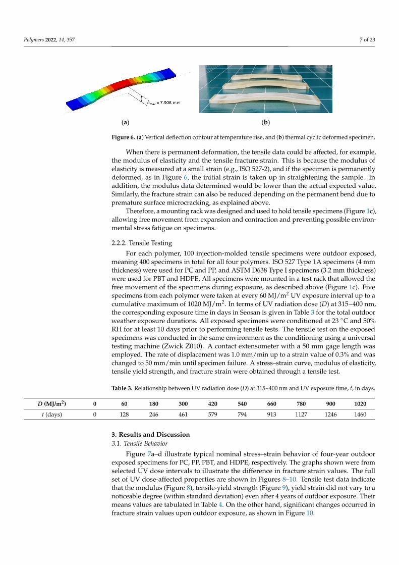
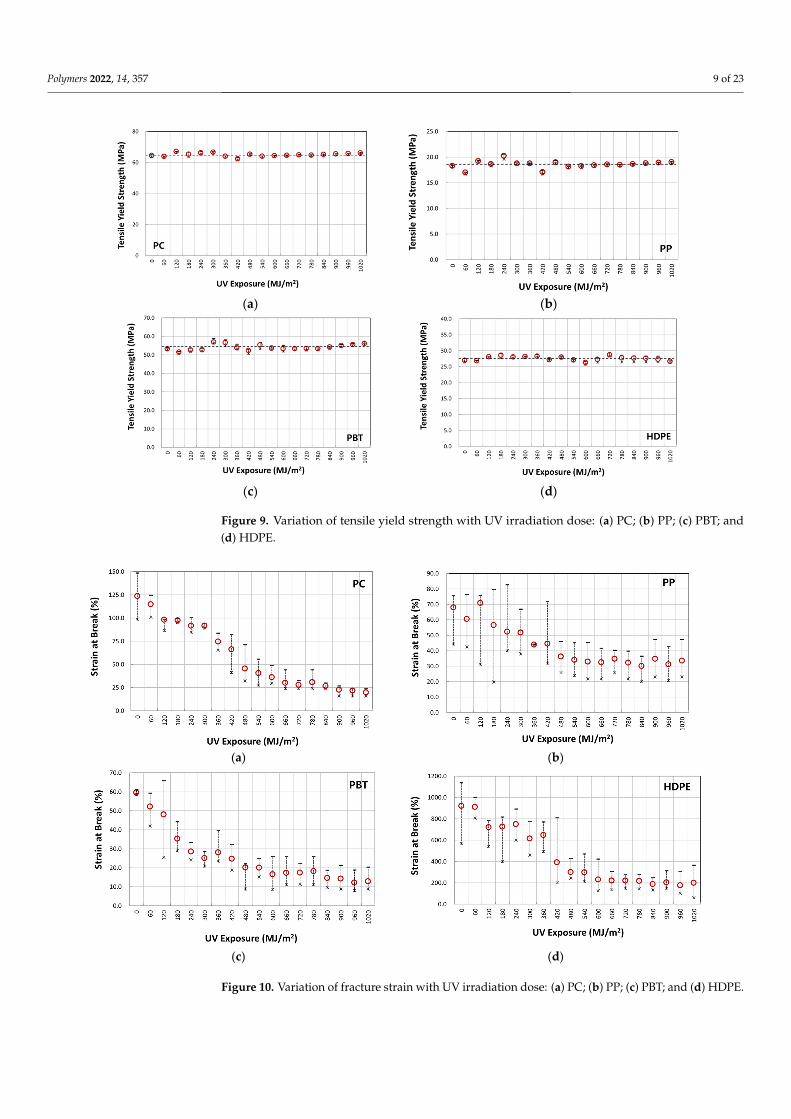
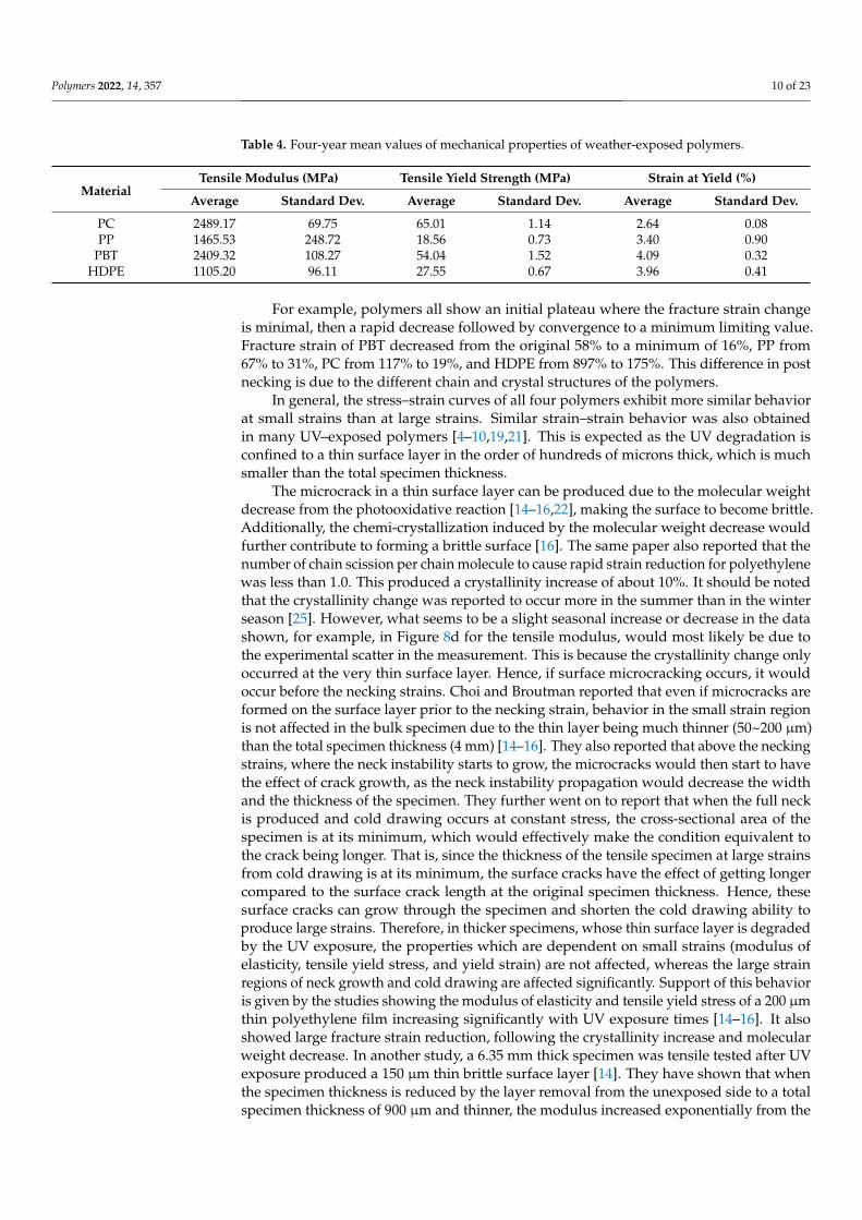
Because of such cyclic climate change, particularly the temperature, thermal cyclicstresses can be imposed on specimens during outdoor exposure if specimens are not prop-erly mounted. For the proper design of the specimen mounting jig, the effect of cyclictemperature variation on the development of thermal cyclic stresses on specimens wasfirst analyzed. Figure 4 shows the principal stress (σ11) development on tensile specimensof four polymers under thermal expansion and contractions from temperature variationwhen specimens were mounted with two ends fixed. For example, the finite element resulthas shown that for a temperature rise from 20 ◦C to 65 ◦C (seasonal highest BPT), thesurface of the outer center portion can attain as high as 6.3 MPa tensile stress for HDPE(Figures 5a and 6a) and the corresponding deflection was almost 8 mm (Figure 6a). Tem-perature decrease to −13 ◦C (seasonal lowest BPT) similarly created tensile stress (4.8 MPa)at the center portion of the specimen (Figure 5b), while recovered the center point deflec-tion to zero. As a result of such weather-induced thermal cyclic stresses occurring daily,simultaneous with UV exposure, surface micro-cracks are caused to form [14–16,20,22],affecting the tensile test result. Moreover, thermal fatigue and creep can cause permanentdeformation in the specimen for longer-exposed specimens, as shown in Figure 6b.

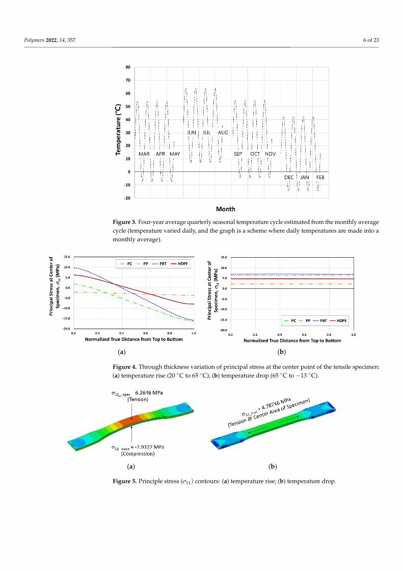
Polymers 2022, 14, 357 6 of 23Polymers 2022, 14, x FOR PEER REVIEW 6 of 23

Figure 3. Four-year average quarterly seasonal temperature cycle estimated from the monthly av-erage cycle (temperature varied daily, and the graph is a scheme where daily temperatures are made into a monthly average).

When there is permanent deformation, the tensile data could be affected, for exam-ple, the modulus of elasticity and the tensile fracture strain. This is because the modulus of elasticity is measured at a small strain (e.g., ISO 527-2), and if the specimen is perma-nently deformed, as in Figure 6, the initial strain is taken up in straightening the sample. In addition, the modulus data determined would be lower than the actual expected value. Similarly, the fracture strain can also be reduced depending on the permanent bend due to premature surface microcracking, as explained above.

Therefore, a mounting rack was designed and used to hold tensile specimens (Figure 1c), allowing free movement from expansion and contraction and preventing possible en-vironmental stress fatigue on specimens.

(a) (b)

Figure 4. Through thickness variation of principal stress at the center point of the tensile specimen: (a) temperature rise (20 °C to 65 °C); (b) temperature drop (65 °C to −13 °C).

Figure 3. Four-year average quarterly seasonal temperature cycle estimated from the monthly averagecycle (temperature varied daily, and the graph is a scheme where daily temperatures are made into amonthly average).

Polymers 2022, 14, x FOR PEER REVIEW 6 of 23

Figure 3. Four-year average quarterly seasonal temperature cycle estimated from the monthly av-erage cycle (temperature varied daily, and the graph is a scheme where daily temperatures are made into a monthly average).

When there is permanent deformation, the tensile data could be affected, for exam-ple, the modulus of elasticity and the tensile fracture strain. This is because the modulus of elasticity is measured at a small strain (e.g., ISO 527-2), and if the specimen is perma-nently deformed, as in Figure 6, the initial strain is taken up in straightening the sample. In addition, the modulus data determined would be lower than the actual expected value. Similarly, the fracture strain can also be reduced depending on the permanent bend due to premature surface microcracking, as explained above.

Therefore, a mounting rack was designed and used to hold tensile specimens (Figure 1c), allowing free movement from expansion and contraction and preventing possible en-vironmental stress fatigue on specimens.

(a) (b)

Figure 4. Through thickness variation of principal stress at the center point of the tensile specimen: (a) temperature rise (20 °C to 65 °C); (b) temperature drop (65 °C to −13 °C). Figure 4. Through thickness variation of principal stress at the center point of the tensile specimen:(a) temperature rise (20 ◦C to 65 ◦C); (b) temperature drop (65 ◦C to −13 ◦C).

Polymers 2022, 14, x FOR PEER REVIEW 7 of 23

(a) (b)

Figure 5. Principle stress (𝜎 ) contours: (a) temperature rise; (b) temperature drop.

(a) (b)

Figure 6. (a) Vertical deflection contour at temperature rise, and (b) thermal cyclic deformed speci-men.

2.2.2. Tensile Testing For each polymer, 100 injection-molded tensile specimens were outdoor exposed,

meaning 400 specimens in total for all four polymers. ISO 527 Type 1A specimens (4 mm thickness) were used for PC and PP, and ASTM D638 Type I specimens (3.2 mm thickness) were used for PBT and HDPE. All specimens were mounted in a test rack that allowed the free movement of the specimens during exposure, as described above (Figure 1c). Five specimens from each polymer were taken at every 60 MJ/m2 UV exposure interval up to a cumulative maximum of 1020 MJ/m2. In terms of UV radiation dose (D) at 315~400 nm, the corresponding exposure time in days in Seosan is given in Table 3 for the total outdoor weather exposure durations. All exposed specimens were conditioned at 23 °C and 50% RH for at least 10 days prior to performing tensile tests. The tensile test on the exposed specimens was conducted in the same environment as the conditioning using a universal testing machine (Zwick Z010). A contact extensometer with a 50 mm gage length was em-ployed. The rate of displacement was 1.0 mm/min up to a strain value of 0.3% and was changed to 50 mm/min until specimen failure. A stress–strain curve, modulus of elasticity, tensile yield strength, and fracture strain were obtained through a tensile test.

Table 3. Relationship between UV radiation dose (D) at 315~400 nm and UV exposure time, t, in days.

D (MJ/m2) 0 60 180 300 420 540 660 780 900 1020 t (days) 0 128 246 461 579 794 913 1127 1246 1460

3. Results and Discussion 3.1. Tensile Behavior

Figure 7a–d illustrate typical nominal stress–strain behavior of four-year outdoor ex-posed specimens for PC, PP, PBT, and HDPE, respectively. The graphs shown were from selected UV dose intervals to illustrate the difference in fracture strain values. The full set of UV dose-affected properties are shown in Figures 8–10. Tensile test data indicate that the modulus (Figure 8), tensile-yield strength (Figure 9), yield strain did not vary to a noticeable degree (within standard deviation) even after 4 years of outdoor exposure.

Figure 5. Principle stress (σ11) contours: (a) temperature rise; (b) temperature drop.

Polymers 2022, 14, 357 7 of 23

Polymers 2022, 14, x FOR PEER REVIEW 7 of 23

(a) (b)

Figure 5. Principle stress (𝜎 ) contours: (a) temperature rise; (b) temperature drop.

(a) (b)

Figure 6. (a) Vertical deflection contour at temperature rise, and (b) thermal cyclic deformed speci-men.

2.2.2. Tensile Testing For each polymer, 100 injection-molded tensile specimens were outdoor exposed,

meaning 400 specimens in total for all four polymers. ISO 527 Type 1A specimens (4 mm thickness) were used for PC and PP, and ASTM D638 Type I specimens (3.2 mm thickness) were used for PBT and HDPE. All specimens were mounted in a test rack that allowed the free movement of the specimens during exposure, as described above (Figure 1c). Five specimens from each polymer were taken at every 60 MJ/m2 UV exposure interval up to a cumulative maximum of 1020 MJ/m2. In terms of UV radiation dose (D) at 315~400 nm, the corresponding exposure time in days in Seosan is given in Table 3 for the total outdoor weather exposure durations. All exposed specimens were conditioned at 23 °C and 50% RH for at least 10 days prior to performing tensile tests. The tensile test on the exposed specimens was conducted in the same environment as the conditioning using a universal testing machine (Zwick Z010). A contact extensometer with a 50 mm gage length was em-ployed. The rate of displacement was 1.0 mm/min up to a strain value of 0.3% and was changed to 50 mm/min until specimen failure. A stress–strain curve, modulus of elasticity, tensile yield strength, and fracture strain were obtained through a tensile test.

Table 3. Relationship between UV radiation dose (D) at 315~400 nm and UV exposure time, t, in days.

D (MJ/m2) 0 60 180 300 420 540 660 780 900 1020 t (days) 0 128 246 461 579 794 913 1127 1246 1460

3. Results and Discussion 3.1. Tensile Behavior

Figure 7a–d illustrate typical nominal stress–strain behavior of four-year outdoor ex-posed specimens for PC, PP, PBT, and HDPE, respectively. The graphs shown were from selected UV dose intervals to illustrate the difference in fracture strain values. The full set of UV dose-affected properties are shown in Figures 8–10. Tensile test data indicate that the modulus (Figure 8), tensile-yield strength (Figure 9), yield strain did not vary to a noticeable degree (within standard deviation) even after 4 years of outdoor exposure.

Figure 6. (a) Vertical deflection contour at temperature rise, and (b) thermal cyclic deformed specimen.

When there is permanent deformation, the tensile data could be affected, for example,the modulus of elasticity and the tensile fracture strain. This is because the modulus ofelasticity is measured at a small strain (e.g., ISO 527-2), and if the specimen is permanentlydeformed, as in Figure 6, the initial strain is taken up in straightening the sample. Inaddition, the modulus data determined would be lower than the actual expected value.Similarly, the fracture strain can also be reduced depending on the permanent bend due topremature surface microcracking, as explained above.

Therefore, a mounting rack was designed and used to hold tensile specimens (Figure 1c),allowing free movement from expansion and contraction and preventing possible environ-mental stress fatigue on specimens.

2.2.2. Tensile Testing

For each polymer, 100 injection-molded tensile specimens were outdoor exposed,meaning 400 specimens in total for all four polymers. ISO 527 Type 1A specimens (4 mmthickness) were used for PC and PP, and ASTM D638 Type I specimens (3.2 mm thickness)were used for PBT and HDPE. All specimens were mounted in a test rack that allowed thefree movement of the specimens during exposure, as described above (Figure 1c). Fivespecimens from each polymer were taken at every 60 MJ/m2 UV exposure interval up to acumulative maximum of 1020 MJ/m2. In terms of UV radiation dose (D) at 315~400 nm,the corresponding exposure time in days in Seosan is given in Table 3 for the total outdoorweather exposure durations. All exposed specimens were conditioned at 23 ◦C and 50%RH for at least 10 days prior to performing tensile tests. The tensile test on the exposedspecimens was conducted in the same environment as the conditioning using a universaltesting machine (Zwick Z010). A contact extensometer with a 50 mm gage length wasemployed. The rate of displacement was 1.0 mm/min up to a strain value of 0.3% and waschanged to 50 mm/min until specimen failure. A stress–strain curve, modulus of elasticity,tensile yield strength, and fracture strain were obtained through a tensile test.

Table 3. Relationship between UV radiation dose (D) at 315~400 nm and UV exposure time, t, in days.

D (MJ/m2) 0 60 180 300 420 540 660 780 900 1020

t (days) 0 128 246 461 579 794 913 1127 1246 1460

3. Results and Discussion3.1. Tensile Behavior

Figure 7a–d illustrate typical nominal stress–strain behavior of four-year outdoorexposed specimens for PC, PP, PBT, and HDPE, respectively. The graphs shown were fromselected UV dose intervals to illustrate the difference in fracture strain values. The fullset of UV dose-affected properties are shown in Figures 8–10. Tensile test data indicatethat the modulus (Figure 8), tensile-yield strength (Figure 9), yield strain did not vary to anoticeable degree (within standard deviation) even after 4 years of outdoor exposure. Theirmeans values are tabulated in Table 4. On the other hand, significant changes occurred infracture strain values upon outdoor exposure, as shown in Figure 10.

Polymers 2022, 14, 357 8 of 23

Polymers 2022, 14, x FOR PEER REVIEW 9 of 23

larger for PBT and HDPE than the PC and PP. Furthermore, HDPE shows the most fluc-tuation (max ± 7.5%) in the strain range between full neck formation and cold drawing to failure, where it occurs at more or less constant stress. These post-necking behaviors be-come more sensitive to the surface layer cracking and growth. Furthermore, this is most likely due to PBT being an aromatic polyester and HDPE not being UV stabilized, making them more prone to surface layer degradation on UV exposure. In turn, this would also make them more sensitive to specimen preparation and deviations in the tensile test (e.g., HDPE in Figure 7d, the post necking stress–strain curve of 0 MJ/m2 and 360 MJ/m2 matches, and 120 MJ/m2and 240 MJ/m2 are in a match). In addition, PBT is known to be-come more sensitive to photo-degradation, particularly when moisture is present, as in outdoor weathering [23]. In addition, the color of PBT being black may also have contrib-uted to the increase in the rate of degradation due to the temperature rise upon radiative heat absorption. Another factor may be that with the high ductility of HDPE (large elon-gation ~1000%), the initial surface microcracks created before necking strain produce dif-ferent surface crack lengths depending on the amount of UV exposure received. These cracks then would have the effect of growing deeper or shorter into the material from the onset of necking. Therefore, depending on the crack growth effect into the bulk specimen from the point of full neck formation, the larger the growth, the lower the stress–strain curve at those affected strain regions, and therefore appearing as fluctuations in the stress–strain curve observed.

From the above, the fracture strain reduction can be identified as the source of me-chanical property degradation occurring during prolonged outdoor weathering. Hence, the generation of material data for weathering FE analysis would involve fracture strain reduction with weather exposure and other mechanical properties maintained at constant values.

(a) (b)

(c) (d)

Figure 7. Nominal tensile stress–strain curves of weather-exposed polymers during a 4-year weath-ering test: (a) PC; (b) PP; (c) PBT; and (d) HDPE. Figure 7. Nominal tensile stress–strain curves of weather-exposed polymers during a 4-year weather-ing test: (a) PC; (b) PP; (c) PBT; and (d) HDPE.

Polymers 2022, 14, x FOR PEER REVIEW 10 of 23

(a) (b)

(c) (d)

Figure 8. Variation of tensile modulus with UV irradiation dose: (a) PC; (b) PP; (c) PBT; and (d) HDPE.

(a) (b)

(c) (d)

Figure 9. Variation of tensile yield strength with UV irradiation dose: (a) PC; (b) PP; (c) PBT; and (d) HDPE.

Figure 8. Variation of tensile modulus with UV irradiation dose: (a) PC; (b) PP; (c) PBT; and (d) HDPE.

Polymers 2022, 14, 357 9 of 23

Polymers 2022, 14, x FOR PEER REVIEW 10 of 23

(a) (b)

(c) (d)

Figure 8. Variation of tensile modulus with UV irradiation dose: (a) PC; (b) PP; (c) PBT; and (d) HDPE.

(a) (b)

(c) (d)

Figure 9. Variation of tensile yield strength with UV irradiation dose: (a) PC; (b) PP; (c) PBT; and (d) HDPE.

Figure 9. Variation of tensile yield strength with UV irradiation dose: (a) PC; (b) PP; (c) PBT; and(d) HDPE.

Polymers 2022, 14, x FOR PEER REVIEW 11 of 23

Table 4. Four-year mean values of mechanical properties of weather-exposed polymers.

Material Tensile Modulus (MPa) Tensile Yield Strength (MPa) Strain at Yield (%) Average Standard Dev. Average Standard Dev. Average Standard Dev.

PC 2489.17 69.75 65.01 1.14 2.64 0.08 PP 1465.53 248.72 18.56 0.73 3.40 0.90

PBT 2409.32 108.27 54.04 1.52 4.09 0.32 HDPE 1105.20 96.11 27.55 0.67 3.96 0.41

(a) (b)

(c) (d)

Figure 10. Variation of fracture strain with UV irradiation dose: (a) PC; (b) PP; (c) PBT; and (d) HDPE.

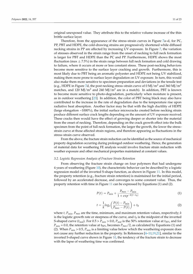
3.2. Logistic Regression Analysis of Fracture Strain Retention From observing the fracture strain change on four polymers that had undergone 4

years of weathering (Figure 10), the characteristic behavior can be described by a logistic regression model of the inverted S-shape function, as shown in Figure 11. In this model, the property retention (e.g., fracture strain retention) is maintained for the initial period, followed by an accelerated decrease, and converges to some constant value. Thus, the property retention with time in Figure 11 can be expressed by Equations (1) and (2).

Figure 10. Variation of fracture strain with UV irradiation dose: (a) PC; (b) PP; (c) PBT; and (d) HDPE.

Polymers 2022, 14, 357 10 of 23

Table 4. Four-year mean values of mechanical properties of weather-exposed polymers.

MaterialTensile Modulus (MPa) Tensile Yield Strength (MPa) Strain at Yield (%)

Average Standard Dev. Average Standard Dev. Average Standard Dev.

PC 2489.17 69.75 65.01 1.14 2.64 0.08PP 1465.53 248.72 18.56 0.73 3.40 0.90

PBT 2409.32 108.27 54.04 1.52 4.09 0.32HDPE 1105.20 96.11 27.55 0.67 3.96 0.41

For example, polymers all show an initial plateau where the fracture strain changeis minimal, then a rapid decrease followed by convergence to a minimum limiting value.Fracture strain of PBT decreased from the original 58% to a minimum of 16%, PP from67% to 31%, PC from 117% to 19%, and HDPE from 897% to 175%. This difference in postnecking is due to the different chain and crystal structures of the polymers.

In general, the stress–strain curves of all four polymers exhibit more similar behaviorat small strains than at large strains. Similar strain–strain behavior was also obtainedin many UV–exposed polymers [4–10,19,21]. This is expected as the UV degradation isconfined to a thin surface layer in the order of hundreds of microns thick, which is muchsmaller than the total specimen thickness.

The microcrack in a thin surface layer can be produced due to the molecular weightdecrease from the photooxidative reaction [14–16,22], making the surface to become brittle.Additionally, the chemi-crystallization induced by the molecular weight decrease wouldfurther contribute to forming a brittle surface [16]. The same paper also reported that thenumber of chain scission per chain molecule to cause rapid strain reduction for polyethylenewas less than 1.0. This produced a crystallinity increase of about 10%. It should be notedthat the crystallinity change was reported to occur more in the summer than in the winterseason [25]. However, what seems to be a slight seasonal increase or decrease in the datashown, for example, in Figure 8d for the tensile modulus, would most likely be due tothe experimental scatter in the measurement. This is because the crystallinity change onlyoccurred at the very thin surface layer. Hence, if surface microcracking occurs, it wouldoccur before the necking strains. Choi and Broutman reported that even if microcracks areformed on the surface layer prior to the necking strain, behavior in the small strain regionis not affected in the bulk specimen due to the thin layer being much thinner (50~200 µm)than the total specimen thickness (4 mm) [14–16]. They also reported that above the neckingstrains, where the neck instability starts to grow, the microcracks would then start to havethe effect of crack growth, as the neck instability propagation would decrease the widthand the thickness of the specimen. They further went on to report that when the full neckis produced and cold drawing occurs at constant stress, the cross-sectional area of thespecimen is at its minimum, which would effectively make the condition equivalent tothe crack being longer. That is, since the thickness of the tensile specimen at large strainsfrom cold drawing is at its minimum, the surface cracks have the effect of getting longercompared to the surface crack length at the original specimen thickness. Hence, thesesurface cracks can grow through the specimen and shorten the cold drawing ability toproduce large strains. Therefore, in thicker specimens, whose thin surface layer is degradedby the UV exposure, the properties which are dependent on small strains (modulus ofelasticity, tensile yield stress, and yield strain) are not affected, whereas the large strainregions of neck growth and cold drawing are affected significantly. Support of this behavioris given by the studies showing the modulus of elasticity and tensile yield stress of a 200 µmthin polyethylene film increasing significantly with UV exposure times [14–16]. It alsoshowed large fracture strain reduction, following the crystallinity increase and molecularweight decrease. In another study, a 6.35 mm thick specimen was tensile tested after UVexposure produced a 150 µm thin brittle surface layer [14]. They have shown that whenthe specimen thickness is reduced by the layer removal from the unexposed side to a totalspecimen thickness of 900 µm and thinner, the modulus increased exponentially from the

Polymers 2022, 14, 357 11 of 23

original unexposed value. They attribute this to the relative volume increase of the thinbrittle surface layer.

Therefore, from the appearance of the stress–strain curves in Figure 7a–d, for PC,PP, PBT and HDPE, the cold-drawing strains are progressively shortened while diffusednecking strains in PP are affected by increasing UV exposure. In Figure 7, the variationof stresses observed in the strain range from the onset of necking to full neck formationis larger for PBT and HDPE than the PC and PP. Furthermore, HDPE shows the mostfluctuation (max ± 7.5%) in the strain range between full neck formation and cold drawingto failure, where it occurs at more or less constant stress. These post-necking behaviorsbecome more sensitive to the surface layer cracking and growth. Furthermore, this ismost likely due to PBT being an aromatic polyester and HDPE not being UV stabilized,making them more prone to surface layer degradation on UV exposure. In turn, this wouldalso make them more sensitive to specimen preparation and deviations in the tensile test(e.g., HDPE in Figure 7d, the post necking stress–strain curve of 0 MJ/m2 and 360 MJ/m2

matches, and 120 MJ/m2 and 240 MJ/m2 are in a match). In addition, PBT is knownto become more sensitive to photo-degradation, particularly when moisture is present,as in outdoor weathering [23]. In addition, the color of PBT being black may also havecontributed to the increase in the rate of degradation due to the temperature rise uponradiative heat absorption. Another factor may be that with the high ductility of HDPE(large elongation ~1000%), the initial surface microcracks created before necking strainproduce different surface crack lengths depending on the amount of UV exposure received.These cracks then would have the effect of growing deeper or shorter into the materialfrom the onset of necking. Therefore, depending on the crack growth effect into the bulkspecimen from the point of full neck formation, the larger the growth, the lower the stress–strain curve at those affected strain regions, and therefore appearing as fluctuations in thestress–strain curve observed.

From the above, the fracture strain reduction can be identified as the source of mechanicalproperty degradation occurring during prolonged outdoor weathering. Hence, the generationof material data for weathering FE analysis would involve fracture strain reduction withweather exposure and other mechanical properties maintained at constant values.

3.2. Logistic Regression Analysis of Fracture Strain Retention

From observing the fracture strain change on four polymers that had undergone4 years of weathering (Figure 10), the characteristic behavior can be described by a logisticregression model of the inverted S-shape function, as shown in Figure 11. In this model,the property retention (e.g., fracture strain retention) is maintained for the initial period,followed by an accelerated decrease, and converges to some constant value. Thus, theproperty retention with time in Figure 11 can be expressed by Equations (1) and (2).

P(t) = Pmin +Pmax − Pmin

1 + exp−k(t−t0)(1)

t =1k

loge

(P(t)− PminPmax − P(t)

)+ t0 (2)

where t, Pmin, Pmax are the time, minimum, and maximum retention values, respectively; kis the logistic growth rate or steepness of the curve, and t0 is the midpoint of the invertedS-shaped curve (tmid). For 0.5 > Pmin > 0.0, Pmid is the 50% retention value at t50% and forPmin = 0.0, the retention value at t50% becomes Pmax/2, as calculated by Equations (1) and(2). When Pmin > 0.5, Pmin is a limiting value below which the weathering exposure doesnot cause any further reduction in the property. In References [4–10,19,21], similar to theinverted S-shaped curve shown in Figure 10, the tendency of the fracture strain to decreasewith the lapse of weathering time was confirmed.

Polymers 2022, 14, 357 12 of 23Polymers 2022, 14, x FOR PEER REVIEW 12 of 23

Figure 11. Schematic representation of the inverted S-shaped property retention model.

𝑃 𝑡) 𝑃 𝑃 𝑃1 𝑒𝑥𝑝 ) (1)

𝑡 1𝑘 𝑙𝑜𝑔 𝑃 𝑡) 𝑃𝑃 𝑃 𝑡) 𝑡 (2)

where t, Pmin, Pmax are the time, minimum, and maximum retention values, respectively; k is the logistic growth rate or steepness of the curve, and t0 is the midpoint of the inverted S-shaped curve (tmid). For 0.5 > Pmin > 0.0, Pmid is the 50% retention value at t50% and for Pmin = 0.0, the retention value at t50% becomes Pmax/2, as calculated by Equations (1) and (2). When Pmin > 0.5, Pmin is a limiting value below which the weathering exposure does not cause any further reduction in the property. In References [4–10,19,21], similar to the in-verted S-shaped curve shown in Figure 10, the tendency of the fracture strain to decrease with the lapse of weathering time was confirmed.

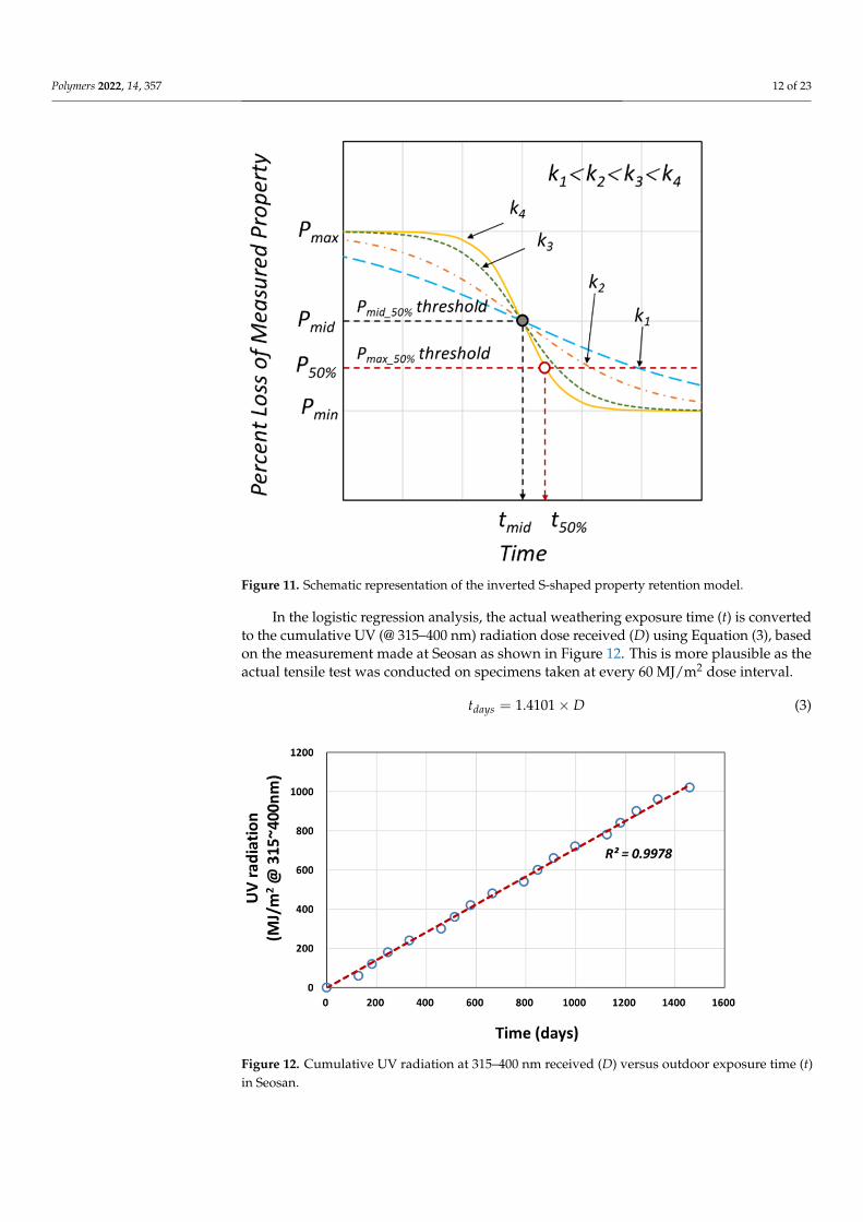
In the logistic regression analysis, the actual weathering exposure time (t) is con-verted to the cumulative UV (@ 315–400 nm) radiation dose received (D) using Equation (3), based on the measurement made at Seosan as shown in Figure 12. This is more plau-sible as the actual tensile test was conducted on specimens taken at every 60 MJ/m2 dose interval.

Figure 11. Schematic representation of the inverted S-shaped property retention model.

In the logistic regression analysis, the actual weathering exposure time (t) is convertedto the cumulative UV (@ 315–400 nm) radiation dose received (D) using Equation (3), basedon the measurement made at Seosan as shown in Figure 12. This is more plausible as theactual tensile test was conducted on specimens taken at every 60 MJ/m2 dose interval.

tdays = 1.4101× D (3)Polymers 2022, 14, x FOR PEER REVIEW 13 of 23

Figure 12. Cumulative UV radiation at 315–400 nm received (D) versus outdoor exposure time (t) in Seosan.

𝑡 1.4101 𝐷 (3)

In terms of UV irradiation dose, D, the nominal fracture strain retention (𝑃 𝐷)𝑒 𝑒⁄ ) is given as the ratio of fracture strain at specific UV exposure dose (𝑒 ) normal-ized by the fracture strain value of the unexposed specimen (𝑒 ) as shown in Equations (4) and (5): 𝑃 𝐷) 𝑒𝑒 𝑃 𝑃 𝑃1 𝑒𝑥𝑝 ) , 𝑃 0) 1, 𝑃 0 (4)

𝐷 % 1𝑘 𝑙𝑜𝑔 𝑃 0.50.5 𝑃 𝐷 (5)

Here, k is the logistic growth rate or steepness of the curve, D0 is the midpoint (Dmid) of the inverted S regression model, and D50% is the corresponding accumulated UV radiation dose when the fracture strain drops to 50% of the initial unexposed value as shown in Equation (5). Hence, if Pmin > 0, D0 ≠ D50% and if Pmin = 0, then D0 = D50%. The four parameters of Pmin, Pmax, k, and D0 in Equation (4) were obtained by implementing the Generalized Reduced Gradient (GRG) nonlinear algorithm in Excel as a Solver function [26,27]. The coefficient of determination of fracture strain, R2, was calculated using the sum of squares regression (SSR-Equation (6)) and the total sum of squares (SST-Equation (8)) in Equation (9). The SST is equal to SSR + SSE as shown in Equation (8), and the sum of squares of error (SSE-Equation (7)) is that least-squares regression selects the line with the lowest total sum of squared prediction errors. 𝑆𝑆𝑅 𝑃 𝑃 (6)

𝑆𝑆𝐸 𝑃 𝑃 (7)

𝑆𝑆𝑇 𝑆𝑆𝑅 𝑆𝑆𝐸 𝑃 𝑃) (8)

where 𝑃 is the mean of 𝑃 and 𝑃 is the estimate of 𝑃 𝑅 𝑆𝑆𝑅𝑆𝑆𝑇 𝑆𝑆𝑅𝑆𝑆𝑅 𝑆𝑆𝐸 1 𝑆𝑆𝐸𝑆𝑆𝑇 (9)

Figure 12. Cumulative UV radiation at 315–400 nm received (D) versus outdoor exposure time (t)in Seosan.

Polymers 2022, 14, 357 13 of 23

In terms of UV irradiation dose, D, the nominal fracture strain retention (Pe f (D) =

e fD /e f0) is given as the ratio of fracture strain at specific UV exposure dose (e fD ) normalizedby the fracture strain value of the unexposed specimen (e f0) as shown in Equations (4) and (5):

Pe f (D) =e fD

e f0

= Pmin +Pmax − Pmin

1 + exp(k(D−D0)), Pe f (0) = 1, Pmin ≥ 0 (4)

D50% =1k

loge

(Pmax − 0.50.5− Pmin

)+ D0 (5)

Here, k is the logistic growth rate or steepness of the curve, D0 is the midpoint (Dmid) ofthe inverted S regression model, and D50% is the corresponding accumulated UV radiationdose when the fracture strain drops to 50% of the initial unexposed value as shown in Equa-tion (5). Hence, if Pmin > 0, D0 6= D50% and if Pmin = 0, then D0 = D50%. The four parametersof Pmin, Pmax, k, and D0 in Equation (4) were obtained by implementing the GeneralizedReduced Gradient (GRG) nonlinear algorithm in Excel as a Solver function [26,27]. Thecoefficient of determination of fracture strain, R2, was calculated using the sum of squaresregression (SSR-Equation (6)) and the total sum of squares (SST-Equation (8)) in Equation (9).The SST is equal to SSR + SSE as shown in Equation (8), and the sum of squares of error(SSE-Equation (7)) is that least-squares regression selects the line with the lowest total sumof squared prediction errors.

SSR = ∑(

P̂− P)2 (6)

SSE = ∑(

P− P̂)2 (7)

SST = SSR + SSE = ∑(

P− P)2 (8)

where P is the mean of P and P̂ is the estimate of P

R2 =SSRSST

=SSR

SSR + SSE= 1− SSE

SST(9)

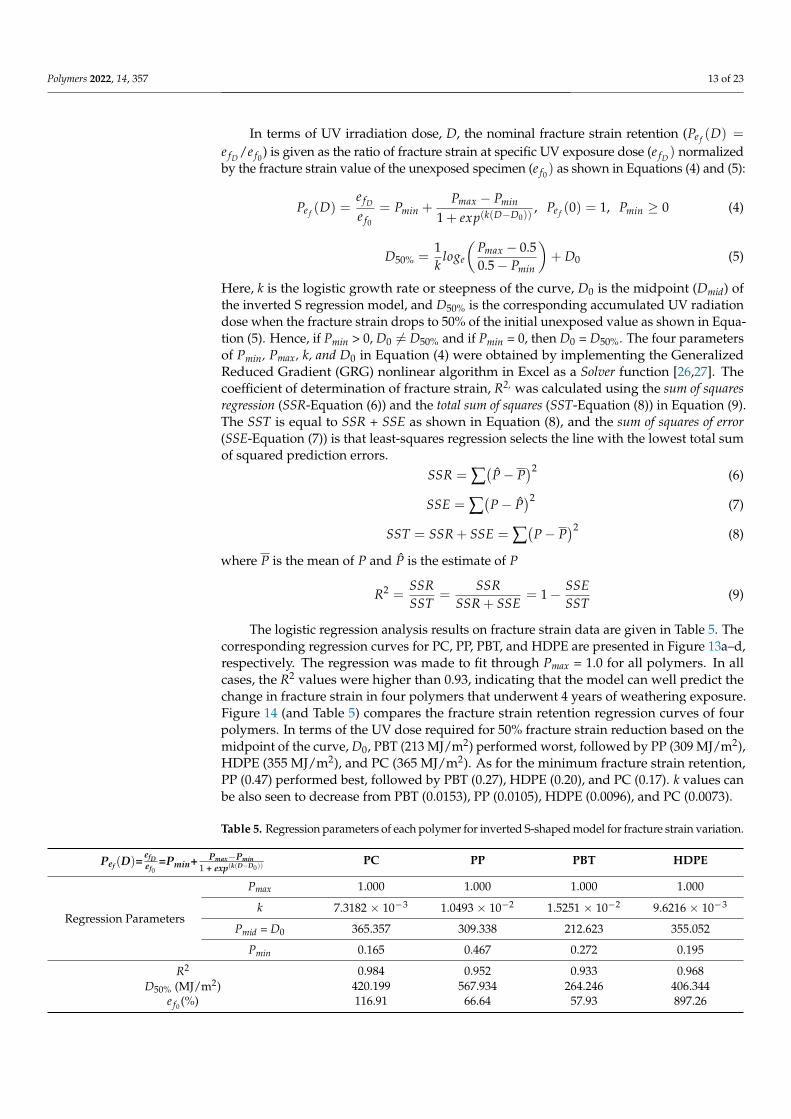
The logistic regression analysis results on fracture strain data are given in Table 5. Thecorresponding regression curves for PC, PP, PBT, and HDPE are presented in Figure 13a–d,respectively. The regression was made to fit through Pmax = 1.0 for all polymers. In allcases, the R2 values were higher than 0.93, indicating that the model can well predict thechange in fracture strain in four polymers that underwent 4 years of weathering exposure.Figure 14 (and Table 5) compares the fracture strain retention regression curves of fourpolymers. In terms of the UV dose required for 50% fracture strain reduction based on themidpoint of the curve, D0, PBT (213 MJ/m2) performed worst, followed by PP (309 MJ/m2),HDPE (355 MJ/m2), and PC (365 MJ/m2). As for the minimum fracture strain retention,PP (0.47) performed best, followed by PBT (0.27), HDPE (0.20), and PC (0.17). k values canbe also seen to decrease from PBT (0.0153), PP (0.0105), HDPE (0.0096), and PC (0.0073).

Table 5. Regression parameters of each polymer for inverted S-shaped model for fracture strain variation.

Pef (D)=efDef0

=Pmin+ Pmax−Pmin1 + exp(k(D−D0))

PC PP PBT HDPE

Regression Parameters

Pmax 1.000 1.000 1.000 1.000

k 7.3182 × 10−3 1.0493 × 10−2 1.5251 × 10−2 9.6216 × 10−3

Pmid = D0 365.357 309.338 212.623 355.052

Pmin 0.165 0.467 0.272 0.195

R2 0.984 0.952 0.933 0.968D50% (MJ/m2) 420.199 567.934 264.246 406.344

e f0 (%) 116.91 66.64 57.93 897.26

Polymers 2022, 14, 357 14 of 23

Polymers 2022, 14, x FOR PEER REVIEW 14 of 23

The logistic regression analysis results on fracture strain data are given in Table 5. The corresponding regression curves for PC, PP, PBT, and HDPE are presented in Figure 13a–d, respectively. The regression was made to fit through Pmax = 1.0 for all polymers. In all cases, the R2 values were higher than 0.93, indicating that the model can well predict the change in fracture strain in four polymers that underwent 4 years of weathering ex-posure. Figure 14 (and Table 5) compares the fracture strain retention regression curves of four polymers. In terms of the UV dose required for 50% fracture strain reduction based on the midpoint of the curve, D0, PBT (213 MJ/m2) performed worst, followed by PP (309 MJ/m2), HDPE (355 MJ/m2), and PC (365 MJ/m2). As for the minimum fracture strain re-tention, PP (0.47) performed best, followed by PBT (0.27), HDPE (0.20), and PC (0.17). k values can be also seen to decrease from PBT (0.0153), PP (0.0105), HDPE (0.0096), and PC (0.0073).

Table 5. Regression parameters of each polymer for inverted S-shaped model for fracture strain variation. 𝑷𝒆𝒇 𝑫) 𝒆𝒇𝑫𝒆𝒇𝟎 𝑷𝒎𝒊𝒏 𝑷𝒎𝒂𝒙 𝑷𝒎𝒊𝒏𝟏 𝒆𝒙𝒑 𝒌 𝑫 𝑫𝟎)) PC PP PBT HDPE

Regression Parameters

Pmax 1.000 1.000 1.000 1.000 k 7.3182 × 10−3 1.0493 × 10−2 1.5251 × 10−2 9.6216 × 10−3

Pmid = D0 365.357 309.338 212.623 355.052 Pmin 0.165 0.467 0.272 0.195 𝑅 0.984 0.952 0.933 0.968

D50% (MJ/m2) 420.199 567.934 264.246 406.344 𝑒 (%) 116.91 66.64 57.93 897.26

(a) (b)

(c) (d)

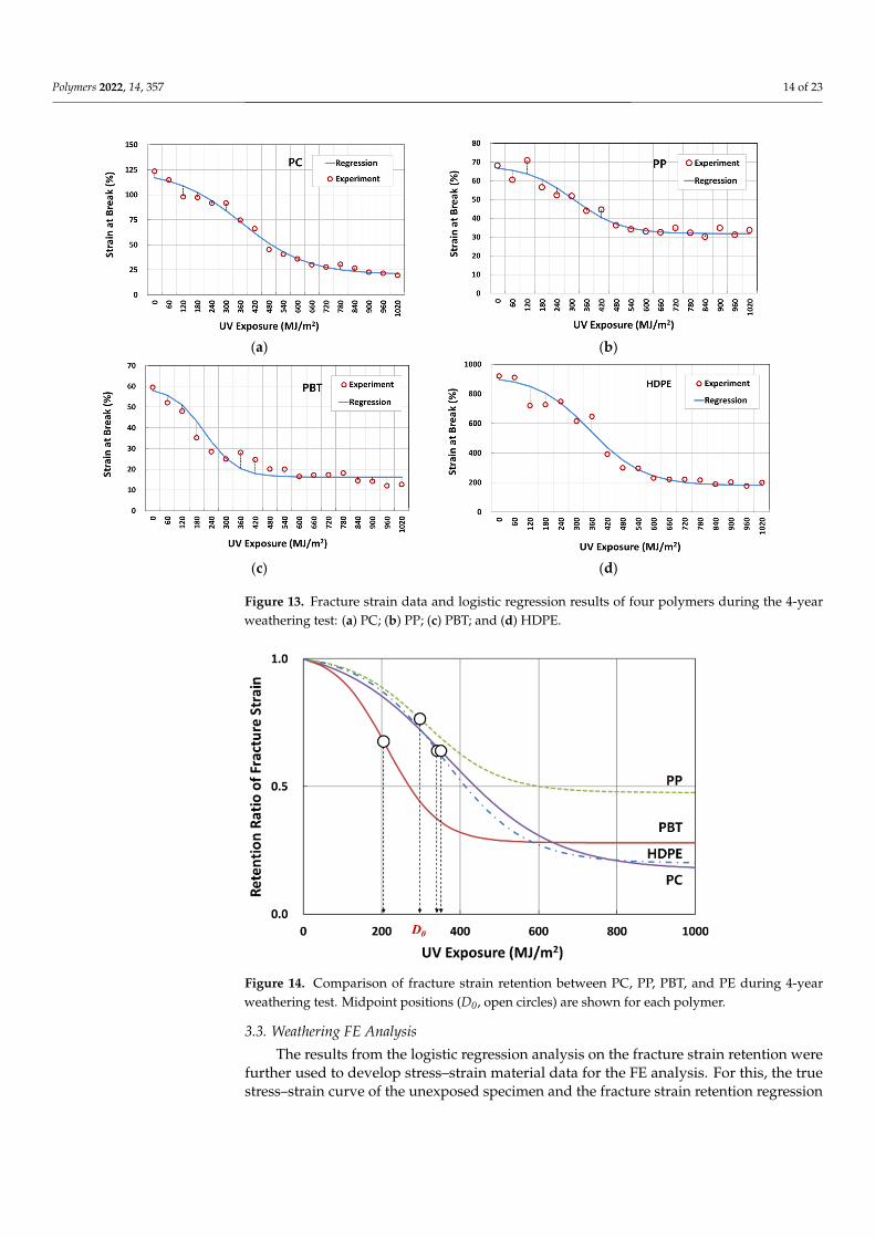
Figure 13. Fracture strain data and logistic regression results of four polymers during the 4-year weathering test: (a) PC; (b) PP; (c) PBT; and (d) HDPE. Figure 13. Fracture strain data and logistic regression results of four polymers during the 4-yearweathering test: (a) PC; (b) PP; (c) PBT; and (d) HDPE.

Polymers 2022, 14, x FOR PEER REVIEW 15 of 23

Figure 14. Comparison of fracture strain retention between PC, PP, PBT, and PE during 4-year weathering test. Midpoint positions (D0, open circles) are shown for each polymer.

3.3. Weathering FE Analysis The results from the logistic regression analysis on the fracture strain retention were

further used to develop stress–strain material data for the FE analysis. For this, the true stress–strain curve of the unexposed specimen and the fracture strain retention regression model were utilized. The true stress and true strain were calculated from the nominal-–stress strain data using Equations (10) and (11), respectively.

𝜎 𝜎 1 𝑒 ), 𝜎 𝜎𝜎 1 𝑒 𝑒 , 𝜎 𝜎 (10)

𝜀 𝑑𝑙 𝑙⁄ 𝑙𝑛 𝑙 𝑙 𝑙𝑛 1 𝑒 ) (11)

where, σnom, enom, σtrue εtrue, σy, εn are the nominal stress and strain, true stress and strain, tensile yield stress and strain (per ISO 527), and strain exponent, respectively. l0 is the original distance between gauge marks, l is the distance between gauge marks at any time t, dl is the incremental elongation when the distance between the gauge marks is l. The true stress–strain curve of PC constructed using n = 1.0 is shown in Figure 15.

Figure 15. True stress–strain curve for PC.

Figure 14. Comparison of fracture strain retention between PC, PP, PBT, and PE during 4-yearweathering test. Midpoint positions (D0, open circles) are shown for each polymer.

3.3. Weathering FE Analysis

The results from the logistic regression analysis on the fracture strain retention werefurther used to develop stress–strain material data for the FE analysis. For this, the truestress–strain curve of the unexposed specimen and the fracture strain retention regression

Polymers 2022, 14, 357 15 of 23

model were utilized. The true stress and true strain were calculated from the nominal—stress strain data using Equations (10) and (11), respectively.

σtrue =

{σnom(1 + enom), σnom ≤ σy

σy

(1 +

(enom − ey

)n)

, σnom > σy(10)

εtrue =∫ l

l0dl/l = ln

(ll0

)= ln(1 + enom) (11)

where, σnom, enom, σtrue εtrue, σy, εn are the nominal stress and strain, true stress and strain,tensile yield stress and strain (per ISO 527), and strain exponent, respectively. l0 is theoriginal distance between gauge marks, l is the distance between gauge marks at any timet, dl is the incremental elongation when the distance between the gauge marks is l. The truestress–strain curve of PC constructed using n = 1.0 is shown in Figure 15.

Polymers 2022, 14, x FOR PEER REVIEW 15 of 23

Figure 14. Comparison of fracture strain retention between PC, PP, PBT, and PE during 4-year weathering test. Midpoint positions (D0, open circles) are shown for each polymer.

3.3. Weathering FE Analysis The results from the logistic regression analysis on the fracture strain retention were

further used to develop stress–strain material data for the FE analysis. For this, the true stress–strain curve of the unexposed specimen and the fracture strain retention regression model were utilized. The true stress and true strain were calculated from the nominal-–stress strain data using Equations (10) and (11), respectively.

𝜎 𝜎 1 𝑒 ), 𝜎 𝜎𝜎 1 𝑒 𝑒 , 𝜎 𝜎 (10)

𝜀 𝑑𝑙 𝑙⁄ 𝑙𝑛 𝑙 𝑙 𝑙𝑛 1 𝑒 ) (11)

where, σnom, enom, σtrue εtrue, σy, εn are the nominal stress and strain, true stress and strain, tensile yield stress and strain (per ISO 527), and strain exponent, respectively. l0 is the original distance between gauge marks, l is the distance between gauge marks at any time t, dl is the incremental elongation when the distance between the gauge marks is l. The true stress–strain curve of PC constructed using n = 1.0 is shown in Figure 15.

Figure 15. True stress–strain curve for PC. Figure 15. True stress–strain curve for PC.

The true stress–strain data of polymers were further converted into appropriate elastic-plastic data for FE analysis using ABAQUS [28]. Most of the plasticity models in ABAQUSare incremental theories, and the mechanical strain is decomposed into an elastic part anda plastic (inelastic) part, as shown in Equations (12) and (13).

εtotal = εe + εp (12)

εp = ln (1 + enom)− ln(1 + σy/E

), enom ≥ ey (13)

where, εe, εp, E are true elastic strain, true plastic strain, and tensile modulus, respectively.The independent elastic constants (tensile modulus, E = 2489.17 MPa, and Poisson’s ra-tio = 0.43 [29,30]) were used to describe the elastic part and the first true plastic strain inputεp = 0, replaces εy = 0.022338 which defines the true yield stress, σy = 56.2 MPa.

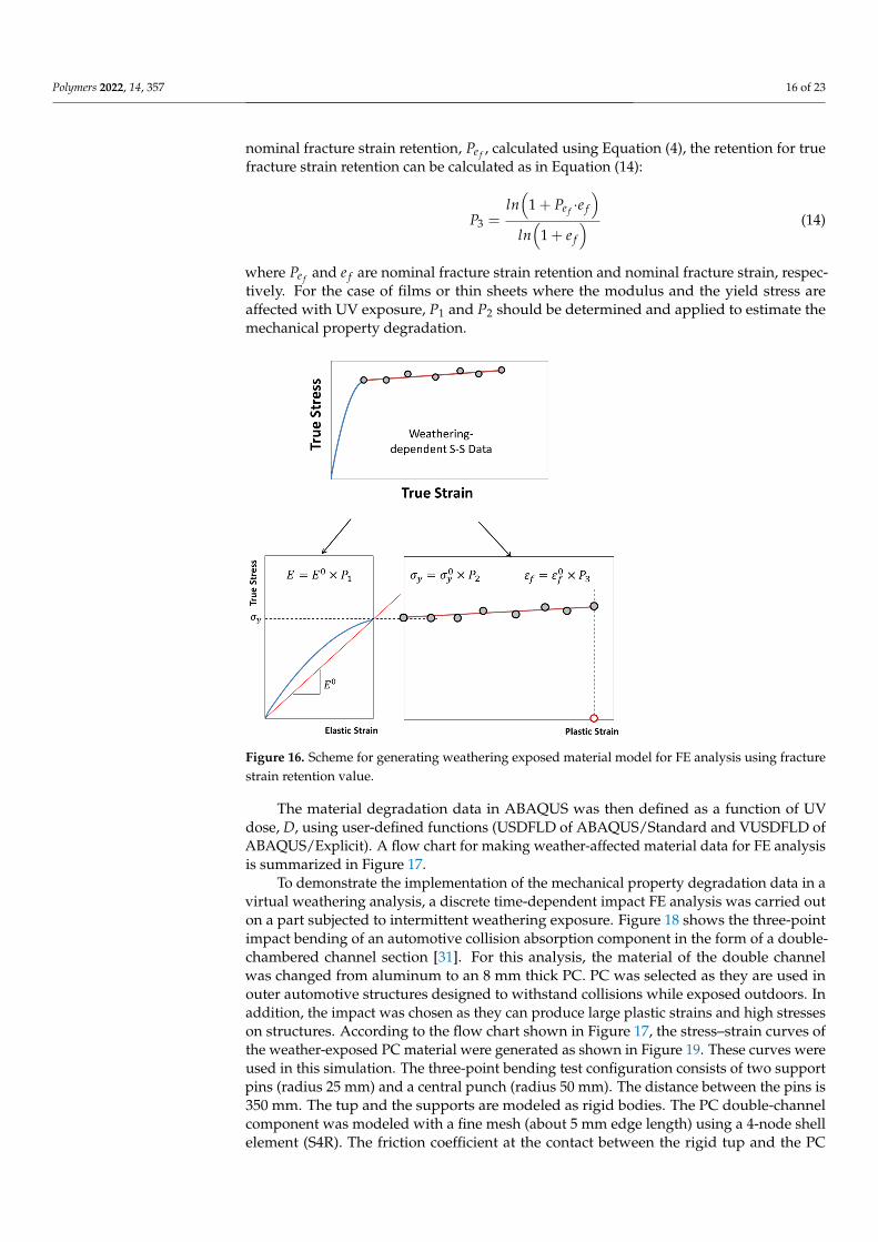
For the material data to accommodate the fracture strain reduction with weatherexposure, the unexposed mechanical property values of elastic modulus (E0), yield strength(σ0

y ), failure strain (ε0f ) and the property retention values (Pi) were utilized. Therefore, the

true stress–strain curves maintained the elastic portion of the unexposed polymers whilethe unexposed fracture strain (ε0

f ) was multiplied by the fracture strain retention values (P3)obtained through the logistic regression analysis (Equation (4) and Table 5) in estimatingthe degradation of the mechanical properties over exposure time (Figure 16). The retentionvalues of elastic modulus (P1) and the tensile yield strength (P2) were set to 1.0, as negligiblechanges were observed during the weathering exposure (Figures 8a and 9a). Based on the

Polymers 2022, 14, 357 16 of 23

nominal fracture strain retention, Pe f , calculated using Equation (4), the retention for truefracture strain retention can be calculated as in Equation (14):

P3 =ln(

1 + Pe f ·e f

)ln(

1 + e f

) (14)

where Pe f and e f are nominal fracture strain retention and nominal fracture strain, respec-tively. For the case of films or thin sheets where the modulus and the yield stress areaffected with UV exposure, P1 and P2 should be determined and applied to estimate themechanical property degradation.

Polymers 2022, 14, x FOR PEER REVIEW 16 of 23

The true stress–strain data of polymers were further converted into appropriate elas-tic-plastic data for FE analysis using ABAQUS [28]. Most of the plasticity models in ABAQUS are incremental theories, and the mechanical strain is decomposed into an elas-tic part and a plastic (inelastic) part, as shown in Equations (12) and (13). ε 𝜀 𝜀 (12)

ε 𝑙𝑛 1 𝑒 ) 𝑙𝑛 1 𝜎 𝐸⁄ , 𝑒 𝑒 (13)

where, εe, εp, E are true elastic strain, true plastic strain, and tensile modulus, respectively. The independent elastic constants (tensile modulus, E = 2489.17 MPa, and Poisson’s ratio = 0.43 [29,30]) were used to describe the elastic part and the first true plastic strain input εp = 0, replaces εy = 0.022338 which defines the true yield stress, σy = 56.2 MPa.

For the material data to accommodate the fracture strain reduction with weather ex-posure, the unexposed mechanical property values of elastic modulus (𝐸 ), yield strength (𝜎 ), failure strain 𝜀 ) and the property retention values (Pi) were utilized. Therefore, the true stress–strain curves maintained the elastic portion of the unexposed polymers while the unexposed fracture strain (𝜀 ) was multiplied by the fracture strain retention values (P3) obtained through the logistic regression analysis (Equation (4) and Table 5) in estimating the degradation of the mechanical properties over exposure time (Figure 16). The retention values of elastic modulus (P1) and the tensile yield strength (P2) were set to 1.0, as negligible changes were observed during the weathering exposure (Figures 8a and 9a). Based on the nominal fracture strain retention, 𝑃 , calculated using Equation (4), the retention for true fracture strain retention can be calculated as in Equation (14):

𝑃 𝑙𝑛 1 𝑃 ∙ 𝑒𝑙𝑛 1 𝑒 (14)

where 𝑃 and 𝑒 are nominal fracture strain retention and nominal fracture strain, re-spectively. For the case of films or thin sheets where the modulus and the yield stress are affected with UV exposure, P1 and P2 should be determined and applied to estimate the mechanical property degradation.

Figure 16. Scheme for generating weathering exposed material model for FE analysis using fracture strain retention value. Figure 16. Scheme for generating weathering exposed material model for FE analysis using fracturestrain retention value.

The material degradation data in ABAQUS was then defined as a function of UVdose, D, using user-defined functions (USDFLD of ABAQUS/Standard and VUSDFLD ofABAQUS/Explicit). A flow chart for making weather-affected material data for FE analysisis summarized in Figure 17.

To demonstrate the implementation of the mechanical property degradation data in avirtual weathering analysis, a discrete time-dependent impact FE analysis was carried outon a part subjected to intermittent weathering exposure. Figure 18 shows the three-pointimpact bending of an automotive collision absorption component in the form of a double-chambered channel section [31]. For this analysis, the material of the double channelwas changed from aluminum to an 8 mm thick PC. PC was selected as they are used inouter automotive structures designed to withstand collisions while exposed outdoors. Inaddition, the impact was chosen as they can produce large plastic strains and high stresseson structures. According to the flow chart shown in Figure 17, the stress–strain curves ofthe weather-exposed PC material were generated as shown in Figure 19. These curves wereused in this simulation. The three-point bending test configuration consists of two supportpins (radius 25 mm) and a central punch (radius 50 mm). The distance between the pins is350 mm. The tup and the supports are modeled as rigid bodies. The PC double-channelcomponent was modeled with a fine mesh (about 5 mm edge length) using a 4-node shellelement (S4R). The friction coefficient at the contact between the rigid tup and the PC

Polymers 2022, 14, 357 17 of 23

component was 0.05. The friction coefficient of 0.15 was used for the contact between PCself parts. The dynamic bending impact tests were conducted using an impact velocityof 2 m/s. ABAQUS/Explicit is used as it is particularly suitable for simulating transientdynamic events as in automotive crashworthiness, where inertia is a variable in calculatingdynamic equilibrium. The FE analysis was carried out to compare the difference in theimpact behavior of the channel section according to the weathering exposure. As used inthe reference [28,31], the same collision condition was utilized for the FE analysis.

Polymers 2022, 14, x FOR PEER REVIEW 17 of 23

The material degradation data in ABAQUS was then defined as a function of UV dose, D, using user-defined functions (USDFLD of ABAQUS/Standard and VUSDFLD of ABAQUS/Explicit). A flow chart for making weather-affected material data for FE analy-sis is summarized in Figure 17.

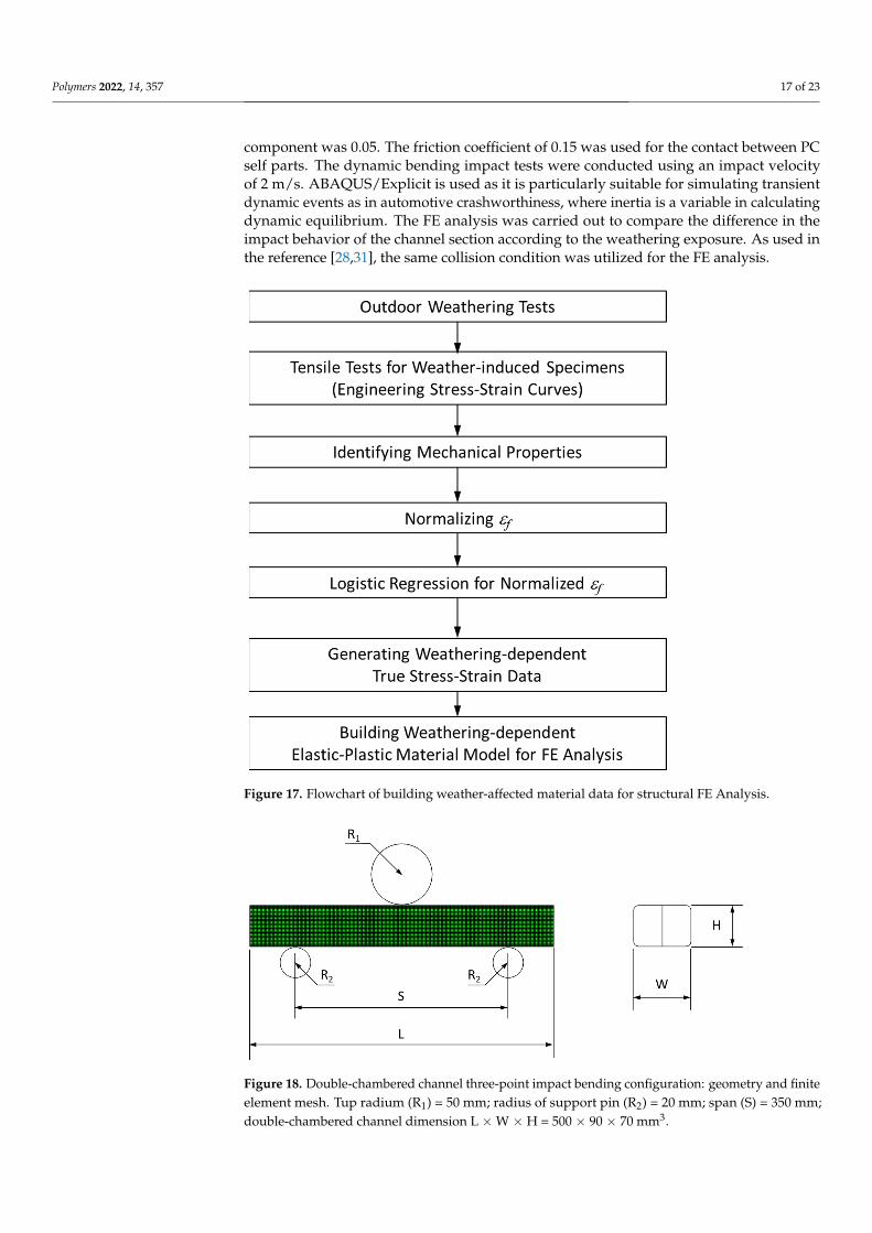
Figure 17. Flowchart of building weather-affected material data for structural FE Analysis.

To demonstrate the implementation of the mechanical property degradation data in a virtual weathering analysis, a discrete time-dependent impact FE analysis was carried out on a part subjected to intermittent weathering exposure. Figure 18 shows the three-point impact bending of an automotive collision absorption component in the form of a double-chambered channel section [31]. For this analysis, the material of the double chan-nel was changed from aluminum to an 8 mm thick PC. PC was selected as they are used in outer automotive structures designed to withstand collisions while exposed outdoors. In addition, the impact was chosen as they can produce large plastic strains and high stresses on structures. According to the flow chart shown in Figure 17, the stress–strain curves of the weather-exposed PC material were generated as shown in Figure 19. These curves were used in this simulation. The three-point bending test configuration consists of two support pins (radius 25 mm) and a central punch (radius 50 mm). The distance between the pins is 350 mm. The tup and the supports are modeled as rigid bodies. The PC double-channel component was modeled with a fine mesh (about 5 mm edge length) using a 4-node shell element (S4R). The friction coefficient at the contact between the rigid tup and the PC component was 0.05. The friction coefficient of 0.15 was used for the con-tact between PC self parts. The dynamic bending impact tests were conducted using an impact velocity of 2 m/s. ABAQUS/Explicit is used as it is particularly suitable for simu-lating transient dynamic events as in automotive crashworthiness, where inertia is a var-iable in calculating dynamic equilibrium. The FE analysis was carried out to compare the

Figure 17. Flowchart of building weather-affected material data for structural FE Analysis.

Polymers 2022, 14, x FOR PEER REVIEW 18 of 23

difference in the impact behavior of the channel section according to the weathering ex-posure. As used in the reference [28,31], the same collision condition was utilized for the FE analysis.

Figure 18. Double-chambered channel three-point impact bending configuration: geometry and finite element mesh. Tup radium (R1) = 50 mm; radius of support pin (R2) = 20 mm; span (S) = 350 mm; double-chambered channel dimension L × W × H = 500 × 90 × 70 mm3.

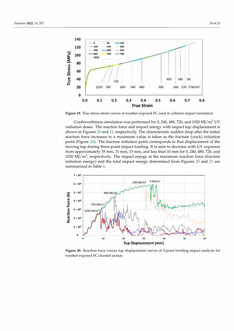
Figure 19. True stress–strain curves of weather-exposed PC used in collision impact simulation.

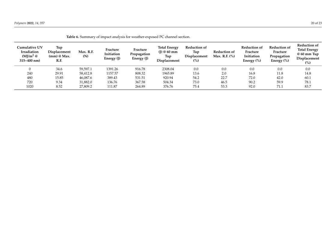
Crashworthiness simulation was performed for 0, 240, 480, 720, and 1020 MJ/m2 UV radiation doses. The reaction force and impact energy with impact tup displacement is shown in Figures 20 and 21, respectively. The characteristic sudden drop after the initial reaction force increases to a maximum value is taken as the fracture (crack) initiation point (Figure 20). The fracture initiation point corresponds to that displacement of the moving tup during three-point impact loading. It is seen to decrease with UV exposure from ap-proximately 35 mm, 31 mm, 15 mm, and less than 10 mm for 0, 240, 480, 720, and 1020 MJ/m2, respectively. The impact energy at the maximum reaction force (fracture initiation energy) and the total impact energy determined from Figures 20 and 21 are summarized in Table 6.

Figure 18. Double-chambered channel three-point impact bending configuration: geometry and finiteelement mesh. Tup radium (R1) = 50 mm; radius of support pin (R2) = 20 mm; span (S) = 350 mm;double-chambered channel dimension L ×W × H = 500 × 90 × 70 mm3.

Polymers 2022, 14, 357 18 of 23

Polymers 2022, 14, x FOR PEER REVIEW 18 of 23

difference in the impact behavior of the channel section according to the weathering ex-posure. As used in the reference [28,31], the same collision condition was utilized for the FE analysis.

Figure 18. Double-chambered channel three-point impact bending configuration: geometry and finite element mesh. Tup radium (R1) = 50 mm; radius of support pin (R2) = 20 mm; span (S) = 350 mm; double-chambered channel dimension L × W × H = 500 × 90 × 70 mm3.

Figure 19. True stress–strain curves of weather-exposed PC used in collision impact simulation.

Crashworthiness simulation was performed for 0, 240, 480, 720, and 1020 MJ/m2 UV radiation doses. The reaction force and impact energy with impact tup displacement is shown in Figures 20 and 21, respectively. The characteristic sudden drop after the initial reaction force increases to a maximum value is taken as the fracture (crack) initiation point (Figure 20). The fracture initiation point corresponds to that displacement of the moving tup during three-point impact loading. It is seen to decrease with UV exposure from ap-proximately 35 mm, 31 mm, 15 mm, and less than 10 mm for 0, 240, 480, 720, and 1020 MJ/m2, respectively. The impact energy at the maximum reaction force (fracture initiation energy) and the total impact energy determined from Figures 20 and 21 are summarized in Table 6.

Figure 19. True stress–strain curves of weather-exposed PC used in collision impact simulation.

Crashworthiness simulation was performed for 0, 240, 480, 720, and 1020 MJ/m2 UVradiation doses. The reaction force and impact energy with impact tup displacement isshown in Figures 20 and 21, respectively. The characteristic sudden drop after the initialreaction force increases to a maximum value is taken as the fracture (crack) initiationpoint (Figure 20). The fracture initiation point corresponds to that displacement of themoving tup during three-point impact loading. It is seen to decrease with UV exposurefrom approximately 35 mm, 31 mm, 15 mm, and less than 10 mm for 0, 240, 480, 720, and1020 MJ/m2, respectively. The impact energy at the maximum reaction force (fractureinitiation energy) and the total impact energy determined from Figures 20 and 21 aresummarized in Table 6.

Polymers 2022, 14, x FOR PEER REVIEW 19 of 23

Figure 20. Reaction force versus tup displacement curves of 3-point bending impact analysis for weather-exposed PC channel section.

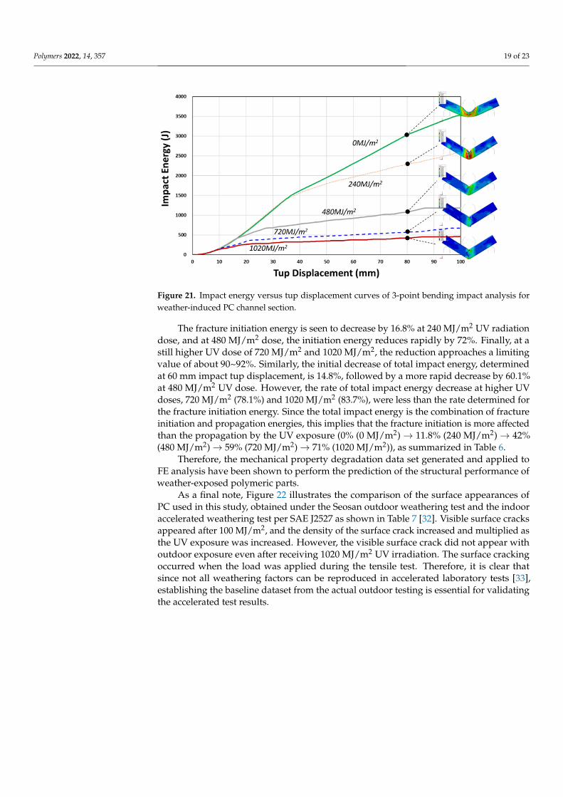
Figure 21. Impact energy versus tup displacement curves of 3-point bending impact analysis for weather-induced PC channel section.

The fracture initiation energy is seen to decrease by 16.8% at 240 MJ/m2 UV radiation dose, and at 480 MJ/m2 dose, the initiation energy reduces rapidly by 72%. Finally, at a still higher UV dose of 720 MJ/m2 and 1020 MJ/m2, the reduction approaches a limiting value of about 90~92%. Similarly, the initial decrease of total impact energy, determined at 60 mm impact tup displacement, is 14.8%, followed by a more rapid decrease by 60.1% at 480 MJ/m2 UV dose. However, the rate of total impact energy decrease at higher UV doses, 720 MJ/m2 (78.1%) and 1020 MJ/m2 (83.7%), were less than the rate determined for the fracture initiation energy. Since the total impact energy is the combination of fracture initiation and propagation energies, this implies that the fracture initiation is more af-fected than the propagation by the UV exposure (0% (0 MJ/m2) → 11.8% (240 MJ/m2) → 42% (480 MJ/m2) → 59% (720 MJ/m2) → 71% (1020 MJ/m2)), as summarized in Table 6.

Therefore, the mechanical property degradation data set generated and applied to FE analysis have been shown to perform the prediction of the structural performance of weather-exposed polymeric parts.

Figure 20. Reaction force versus tup displacement curves of 3-point bending impact analysis forweather-exposed PC channel section.

Polymers 2022, 14, 357 19 of 23

Polymers 2022, 14, x FOR PEER REVIEW 19 of 23

Figure 20. Reaction force versus tup displacement curves of 3-point bending impact analysis for weather-exposed PC channel section.

Figure 21. Impact energy versus tup displacement curves of 3-point bending impact analysis for weather-induced PC channel section.

The fracture initiation energy is seen to decrease by 16.8% at 240 MJ/m2 UV radiation dose, and at 480 MJ/m2 dose, the initiation energy reduces rapidly by 72%. Finally, at a still higher UV dose of 720 MJ/m2 and 1020 MJ/m2, the reduction approaches a limiting value of about 90~92%. Similarly, the initial decrease of total impact energy, determined at 60 mm impact tup displacement, is 14.8%, followed by a more rapid decrease by 60.1% at 480 MJ/m2 UV dose. However, the rate of total impact energy decrease at higher UV doses, 720 MJ/m2 (78.1%) and 1020 MJ/m2 (83.7%), were less than the rate determined for the fracture initiation energy. Since the total impact energy is the combination of fracture initiation and propagation energies, this implies that the fracture initiation is more af-fected than the propagation by the UV exposure (0% (0 MJ/m2) → 11.8% (240 MJ/m2) → 42% (480 MJ/m2) → 59% (720 MJ/m2) → 71% (1020 MJ/m2)), as summarized in Table 6.

Therefore, the mechanical property degradation data set generated and applied to FE analysis have been shown to perform the prediction of the structural performance of weather-exposed polymeric parts.

Figure 21. Impact energy versus tup displacement curves of 3-point bending impact analysis forweather-induced PC channel section.

The fracture initiation energy is seen to decrease by 16.8% at 240 MJ/m2 UV radiationdose, and at 480 MJ/m2 dose, the initiation energy reduces rapidly by 72%. Finally, at astill higher UV dose of 720 MJ/m2 and 1020 MJ/m2, the reduction approaches a limitingvalue of about 90~92%. Similarly, the initial decrease of total impact energy, determinedat 60 mm impact tup displacement, is 14.8%, followed by a more rapid decrease by 60.1%at 480 MJ/m2 UV dose. However, the rate of total impact energy decrease at higher UVdoses, 720 MJ/m2 (78.1%) and 1020 MJ/m2 (83.7%), were less than the rate determined forthe fracture initiation energy. Since the total impact energy is the combination of fractureinitiation and propagation energies, this implies that the fracture initiation is more affectedthan the propagation by the UV exposure (0% (0 MJ/m2)→ 11.8% (240 MJ/m2)→ 42%(480 MJ/m2)→ 59% (720 MJ/m2)→ 71% (1020 MJ/m2)), as summarized in Table 6.

Therefore, the mechanical property degradation data set generated and applied toFE analysis have been shown to perform the prediction of the structural performance ofweather-exposed polymeric parts.

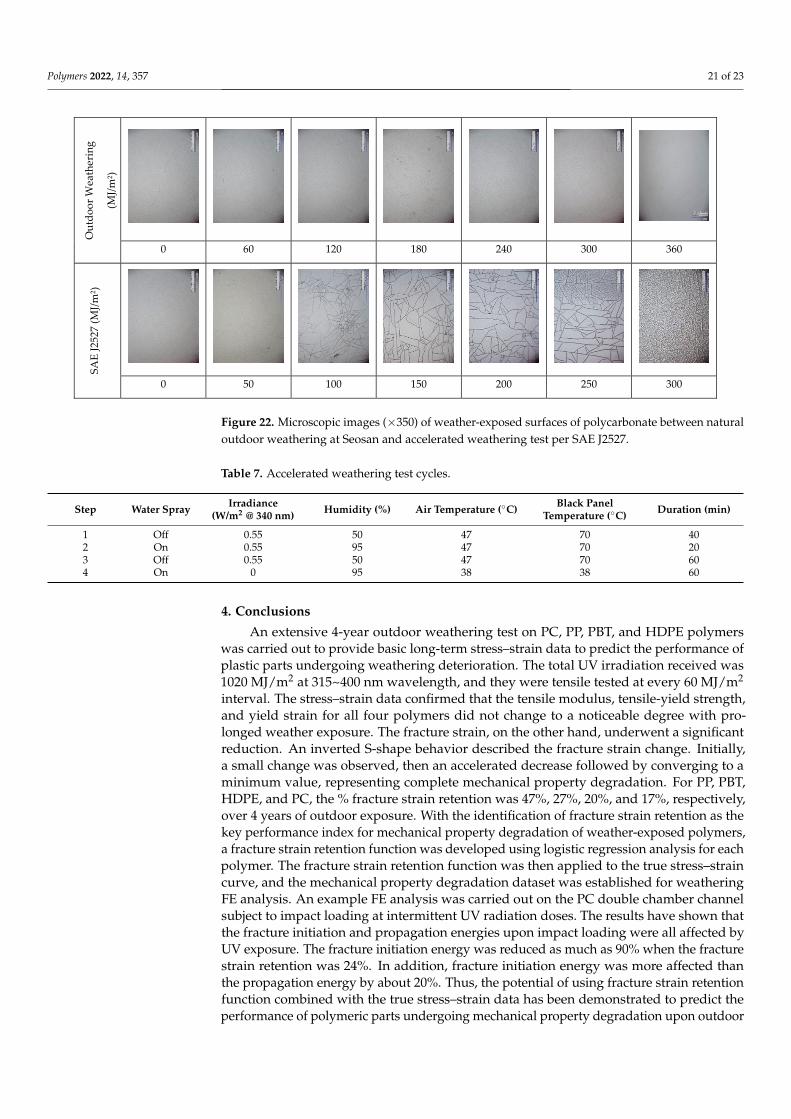
As a final note, Figure 22 illustrates the comparison of the surface appearances ofPC used in this study, obtained under the Seosan outdoor weathering test and the indooraccelerated weathering test per SAE J2527 as shown in Table 7 [32]. Visible surface cracksappeared after 100 MJ/m2, and the density of the surface crack increased and multiplied asthe UV exposure was increased. However, the visible surface crack did not appear withoutdoor exposure even after receiving 1020 MJ/m2 UV irradiation. The surface crackingoccurred when the load was applied during the tensile test. Therefore, it is clear thatsince not all weathering factors can be reproduced in accelerated laboratory tests [33],establishing the baseline dataset from the actual outdoor testing is essential for validatingthe accelerated test results.

Polymers 2022, 14, 357 20 of 23

Table 6. Summary of impact analysis for weather-exposed PC channel section.

Cumulative UVIrradiation(MJ/m2 @

315~400 nm)

TupDisplacement(mm) @ Max.

R.F.

Max. R.F.(N)

FractureInitiationEnergy (J)

FracturePropagation

Energy (J)

Total Energy(J) @ 60 mm

TupDisplacement

Reduction ofTup

Displacement(%)

Reduction ofMax. R.F. (%)

Reduction ofFracture

InitiationEnergy (%)

Reduction ofFracture

PropagationEnergy (%)

Reduction ofTotal Energy@ 60 mm TupDisplacement

(%)

0 34.6 59,597.1 1391.26 916.78 2308.04 0.0 0.0 0.0 0.0 0.0240 29.91 58,412.8 1157.57 808.32 1965.89 13.6 2.0 16.8 11.8 14.8480 15.85 46,087.6 389.43 531.51 920.94 54.2 22.7 72.0 42.0 60.1720 9.34 31,882.0 136.76 367.58 504.34 73.0 46.5 90.2 59.9 78.1

1020 8.52 27,809.2 111.87 264.89 376.76 75.4 53.3 92.0 71.1 83.7

Polymers 2022, 14, 357 21 of 23

Polymers 2022, 14, x FOR PEER REVIEW 20 of 23

Table 6. Summary of impact analysis for weather-exposed PC channel section.

Cumulative UV Irradia-tion (MJ/m2 @ 315~400

nm)

Tup Dis-place-ment

(mm) @ Max. R.F.

Max. R.F. (N)

Fracture In-itiation En-

ergy (J)

Fracture Propaga-

tion Energy (J)

Total En-ergy (J) @

60 mm Tup Displace-

ment

Reduction of Tup Dis-placement

(%)

Reduction of Max. R.F. (%)

Reduction of Fracture Initiation

Energy (%)

Reduction of Fracture Propaga-

tion Energy (%)

Reduction of Total En-

ergy @ 60 mm Tup Displace-ment (%)

0 34.6 59,597.1 1391.26 916.78 2308.04 0.0 0.0 0.0 0.0 0.0 240 29.91 58,412.8 1157.57 808.32 1965.89 13.6 2.0 16.8 11.8 14.8 480 15.85 46,087.6 389.43 531.51 920.94 54.2 22.7 72.0 42.0 60.1 720 9.34 31,882.0 136.76 367.58 504.34 73.0 46.5 90.2 59.9 78.1

1020 8.52 27,809.2 111.87 264.89 376.76 75.4 53.3 92.0 71.1 83.7

As a final note, Figure 22 illustrates the comparison of the surface appearances of PC used in this study, obtained under the Seosan outdoor weathering test and the indoor accelerated weathering test per SAE J2527 as shown in Table 7 [32]. Visible surface cracks appeared after 100 MJ/m2, and the density of the surface crack increased and multiplied as the UV exposure was increased. However, the visible surface crack did not appear with outdoor exposure even after receiving 1020 MJ/m2 UV irradiation. The surface cracking occurred when the load was applied during the tensile test. Therefore, it is clear that since not all weathering factors can be reproduced in accelerated laboratory tests [33], establish-ing the baseline dataset from the actual outdoor testing is essential for validating the ac-celerated test results.

Table 7. Accelerated weathering test cycles for SAE J2527 [32].

Step Water Spray Irradiance (W/m2 @ 340 nm)

Humidity (%)

Air Temperature (°C)

Black Panel Temperature (°C)

Duration (min)

1 Off 0.55 50 47 70 40 2 On 0.55 95 47 70 20 3 Off 0.55 50 47 70 60 4 On 0 95 38 38 60

Out

door

Wea

ther

ing

(MJ/m

2 )

0 60 120 180 240 300 360

SAE

J252

7 (M

J/m2 )

0 50 100 150 200 250 300

Figure 22. Microscopic images (×350) of weather-exposed surfaces of polycarbonate between natural outdoor weathering at Seosan and accelerated weathering test per SAE J2527.

Figure 22. Microscopic images (×350) of weather-exposed surfaces of polycarbonate between naturaloutdoor weathering at Seosan and accelerated weathering test per SAE J2527.

Table 7. Accelerated weathering test cycles.

Step Water Spray Irradiance(W/m2 @ 340 nm) Humidity (%) Air Temperature (◦C) Black Panel

Temperature (◦C) Duration (min)

1 Off 0.55 50 47 70 402 On 0.55 95 47 70 203 Off 0.55 50 47 70 604 On 0 95 38 38 60

4. Conclusions

An extensive 4-year outdoor weathering test on PC, PP, PBT, and HDPE polymerswas carried out to provide basic long-term stress–strain data to predict the performance ofplastic parts undergoing weathering deterioration. The total UV irradiation received was1020 MJ/m2 at 315~400 nm wavelength, and they were tensile tested at every 60 MJ/m2

interval. The stress–strain data confirmed that the tensile modulus, tensile-yield strength,and yield strain for all four polymers did not change to a noticeable degree with pro-longed weather exposure. The fracture strain, on the other hand, underwent a significantreduction. An inverted S-shape behavior described the fracture strain change. Initially,a small change was observed, then an accelerated decrease followed by converging to aminimum value, representing complete mechanical property degradation. For PP, PBT,HDPE, and PC, the % fracture strain retention was 47%, 27%, 20%, and 17%, respectively,over 4 years of outdoor exposure. With the identification of fracture strain retention as thekey performance index for mechanical property degradation of weather-exposed polymers,a fracture strain retention function was developed using logistic regression analysis for eachpolymer. The fracture strain retention function was then applied to the true stress–straincurve, and the mechanical property degradation dataset was established for weatheringFE analysis. An example FE analysis was carried out on the PC double chamber channelsubject to impact loading at intermittent UV radiation doses. The results have shown thatthe fracture initiation and propagation energies upon impact loading were all affected byUV exposure. The fracture initiation energy was reduced as much as 90% when the fracturestrain retention was 24%. In addition, fracture initiation energy was more affected thanthe propagation energy by about 20%. Thus, the potential of using fracture strain retentionfunction combined with the true stress–strain data has been demonstrated to predict theperformance of polymeric parts undergoing mechanical property degradation upon outdoor

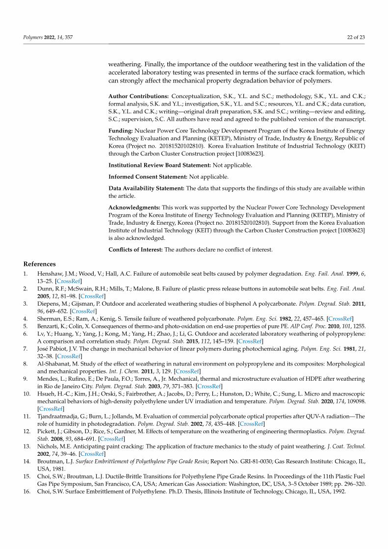
Polymers 2022, 14, 357 22 of 23

weathering. Finally, the importance of the outdoor weathering test in the validation of theaccelerated laboratory testing was presented in terms of the surface crack formation, whichcan strongly affect the mechanical property degradation behavior of polymers.

Author Contributions: Conceptualization, S.K., Y.L. and S.C.; methodology, S.K., Y.L. and C.K.;formal analysis, S.K. and Y.L.; investigation, S.K., Y.L. and S.C.; resources, Y.L. and C.K.; data curation,S.K., Y.L. and C.K.; writing—original draft preparation, S.K. and S.C.; writing—review and editing,S.C.; supervision, S.C. All authors have read and agreed to the published version of the manuscript.

Funding: Nuclear Power Core Technology Development Program of the Korea Institute of EnergyTechnology Evaluation and Planning (KETEP), Ministry of Trade, Industry & Energy, Republic ofKorea (Project no. 20181520102810). Korea Evaluation Institute of Industrial Technology (KEIT)through the Carbon Cluster Construction project [10083623].

Institutional Review Board Statement: Not applicable.

Informed Consent Statement: Not applicable.

Data Availability Statement: The data that supports the findings of this study are available withinthe article.

Acknowledgments: This work was supported by the Nuclear Power Core Technology DevelopmentProgram of the Korea Institute of Energy Technology Evaluation and Planning (KETEP), Ministry ofTrade, Industry & Energy, Korea (Project no. 20181520102810). Support from the Korea EvaluationInstitute of Industrial Technology (KEIT) through the Carbon Cluster Construction project [10083623]is also acknowledged.

Conflicts of Interest: The authors declare no conflict of interest.

References1. Henshaw, J.M.; Wood, V.; Hall, A.C. Failure of automobile seat belts caused by polymer degradation. Eng. Fail. Anal. 1999, 6,

13–25. [CrossRef]2. Dunn, R.F.; McSwain, R.H.; Mills, T.; Malone, B. Failure of plastic press release buttons in automobile seat belts. Eng. Fail. Anal.

2005, 12, 81–98. [CrossRef]3. Diepens, M.; Gijsman, P. Outdoor and accelerated weathering studies of bisphenol A polycarbonate. Polym. Degrad. Stab. 2011,

96, 649–652. [CrossRef]4. Sherman, E.S.; Ram, A.; Kenig, S. Tensile failure of weathered polycarbonate. Polym. Eng. Sci. 1982, 22, 457–465. [CrossRef]5. Benzarti, K.; Colin, X. Consequences of thermo-and photo-oxidation on end-use properties of pure PE. AIP Conf. Proc. 2010, 101, 1255.6. Lv, Y.; Huang, Y.; Yang, J.; Kong, M.; Yang, H.; Zhao, J.; Li, G. Outdoor and accelerated laboratory weathering of polypropylene:

A comparison and correlation study. Polym. Degrad. Stab. 2015, 112, 145–159. [CrossRef]7. José Pabiot, J.V. The change in mechanical behavior of linear polymers during photochemical aging. Polym. Eng. Sci. 1981, 21,

32–38. [CrossRef]8. Al-Shabanat, M. Study of the effect of weathering in natural environment on polypropylene and its composites: Morphological

and mechanical properties. Int. J. Chem. 2011, 3, 129. [CrossRef]9. Mendes, L.; Rufino, E.; De Paula, F.O.; Torres, A., Jr. Mechanical, thermal and microstructure evaluation of HDPE after weathering

in Rio de Janeiro City. Polym. Degrad. Stab. 2003, 79, 371–383. [CrossRef]10. Hsueh, H.-C.; Kim, J.H.; Orski, S.; Fairbrother, A.; Jacobs, D.; Perry, L.; Hunston, D.; White, C.; Sung, L. Micro and macroscopic

mechanical behaviors of high-density polyethylene under UV irradiation and temperature. Polym. Degrad. Stab. 2020, 174, 109098.[CrossRef]

11. Tjandraatmadja, G.; Burn, L.; Jollands, M. Evaluation of commercial polycarbonate optical properties after QUV-A radiation—Therole of humidity in photodegradation. Polym. Degrad. Stab. 2002, 78, 435–448. [CrossRef]

12. Pickett, J.; Gibson, D.; Rice, S.; Gardner, M. Effects of temperature on the weathering of engineering thermoplastics. Polym. Degrad.Stab. 2008, 93, 684–691. [CrossRef]

13. Nichols, M.E. Anticipating paint cracking: The application of fracture mechanics to the study of paint weathering. J. Coat. Technol.2002, 74, 39–46. [CrossRef]

14. Broutman, L.J. Surface Embrittlement of Polyethylene Pipe Grade Resin; Report No. GRI-81-0030; Gas Research Institute: Chicago, IL,USA, 1981.

15. Choi, S.W.; Broutman, L.J. Ductile-Brittle Transitions for Polyethylene Pipe Grade Resins. In Proceedings of the 11th Plastic FuelGas Pipe Symposium, San Francisco, CA, USA; American Gas Association: Washington, DC, USA, 3–5 October 1989; pp. 296–320.

16. Choi, S.W. Surface Embrittlement of Polyethylene. Ph.D. Thesis, Illinois Institute of Technology, Chicago, IL, USA, 1992.

Polymers 2022, 14, 357 23 of 23

17. Lamnii, H.; Abdelaziz, M.N.; Ayoub, G.; Gloaguen, J.-M.; Maschke, U.; Mansoor, B. Effect of UV Ageing on the fatigue life of bulkpolyethylene. In Proceedings of the FATIGUE 2018, Poitiers, France, 27 May–1 June 2018.

18. Lamnii, H.; Abdelaziz, M.N.; Ayoub, G.; Colin, X.; Maschke, U. Experimental investigation and modeling attempt on the effectsof ultraviolet aging on the fatigue behavior of an LDPE semi-crystalline polymer. Int. J. Fatigue 2021, 142, 105952. [CrossRef]

19. Iizuka, T.; Ohtake, Y.; Tanaka, K. A effect of moisture on photo-degradation for polypropylene. Zair./J. Soc. Mater. Sci. Jpn. 2016,65, 812–817. [CrossRef]

20. Erdmann, M.; Niebergall, U.; Wachtendorf, V.; Böhning, M. Evaluation of UV-induced embrittlement of PE-HD by Charpy impacttest. J. Appl. Polym. Sci. 2020, 137, 49069. [CrossRef]

21. Jiang, L.; Zhou, M.; Ding, Y.; Zhou, Y.; Dan, Y. Aging induced ductile-brittle-ductile transition in bisphenol A polycarbonate. J.Polym. Res. 2018, 25, 39. [CrossRef]

22. Blaga, A.; Yamasaki, R. Surface microcracking induced by weathering of polycarbonate sheet. J. Mater. Sci. 1976, 11, 1513–1520.[CrossRef]

23. McKeen, L.W. The Effect of UV Light and Weather on Plastics and Elastomers; William Andrew: Amsterdam, The Netherlands, 2019.24. World Maps of Köppen-Geiger Climate Classification. Available online: http://koeppen-geiger.vu-wien.ac.at/ (accessed on

10 November 2021).25. Rajakumar, K.; Sarasvathy, V.; Chelvan, A.T.; Chitra, R.; Vijayakumar, C. Natural weathering studies of polypropylene. J. Polym.

Environ. 2009, 17, 191–202. [CrossRef]26. Lasdon, L.S.; Waren, A.D.; Jain, A.; Ratner, M.W. Design and Testing of a Generalized Reduced Gradient Code for Nonlinear Optimization;

Case Western Reserve University: Cleveland, OH, USA, 1975.27. Lasdon, L.S.; Waren, A.D.; Jain, A.; Ratner, M. Design and testing of a generalized reduced gradient code for nonlinear

programming. ACM Trans. Math. Softw. (TOMS) 1978, 4, 34–50. [CrossRef]28. ABAQUS Document Manual, Version 6.14; Dassault Systemes: Velizy-Villacoublay, France, 2010.29. Grassia, L.; D’Amore, A.; Simon, S.L. On the viscoelastic Poisson’s ratio in amorphous polymers. J. Rheol. 2010, 54, 1009–1022.

[CrossRef]30. Polymer Properties Database. Available online: http://polymerdatabase.com/polymer%20physics/Poisson%20Table.html

(accessed on 10 November 2021).31. Hooputra, H.; Gese, H.; Dell, H.; Werner, H. A comprehensive failure model for crashworthiness simulation of aluminium

extrusions. Int. J. Crashworthiness 2004, 9, 449–464. [CrossRef]32. Performance Based Standard for Accelerated Exposure of Automotive Exterior Materials Using a Controlled Irradiance Xenon-Arc Apparatus;

Society of Automotive Engineers: Warrendale, PA, USA, 2017; SAE J2527.33. Frigione, M.; Rodríguez-Prieto, A. Can Accelerated Aging Procedures Predict the Long Term Behavior of Polymers Exposed to

Different Environments? Polymers 2021, 13, 2688. [CrossRef] [PubMed]