
arX
iv:1
601.
0358
7v1
[nl
in.C
D]
14
Jan
2016
Accelerated diffusion by chaotic fluctuation in probability in
photoexcitation transfer system
Song-Ju Kim1,∗ Makoto Naruse2, Masashi Aono3, Hirokazu Hori4, and Takuma Akimoto5†
1WPI Center for MANA, National Institute for Materials Science,
Tsukuba, Ibaraki 305–0044, Japan
2PNRI, National Institute of Information and
Communications Technology, Tokyo 184–8795, Japan
3Earth-Life Science Institute, Tokyo Institute of Technology,
Tokyo 152–8550 & PRESTO JST, Japan
4Graduate School of Medicine and Engineering,
University of Yamanashi, Yamanashi 400-8511, Japan and
5Department of Mechanical Engineering, Keio University,
Kohoku-ku, Yokohama 223-8522, Japan
(Dated: January 15, 2016)
1
Abstract
We report a new accelerated diffusion phenomenon that is produced by a one-dimensional ran-
dom walk in which the flight probability to one of the two directions (i.e., bias) oscillates dynam-
ically in periodic, quasiperiodic, and chaotic manners. The probability oscillation dynamics can
be physically observed in nanoscale photoexcitation transfer in a quantum-dot network, where the
existence probability of an exciton at the bottom energy level of a quantum dot fluctuates dif-
ferently with a parameter setting. We evaluate the ensemble average of the time-averaged mean
square displacement (ETMSD) of the time series obtained from the quantum-dot network model
that generates various oscillatory behaviors because the ETMSD exhibits characteristic changes
depending on the fluctuating bias; in the case of normal diffusion, the asymptotic behavior of the
ETMSD is proportional to the time (i.e., a linear growth function), whereas it grows nonlinearly
with an exponent greater than 1 in the case of superdiffusion. We find that the diffusion can
be accelerated significantly when the fluctuating bias is characterized as weak chaos owing to the
transient nonstationarity of its biases, in which the spectrum contains high power at low frequen-
cies. By introducing a simplified model of our random walk, which exhibits superdiffusion as well
as normal diffusion, we explain the mechanism of the accelerated diffusion by analyzing the mean
square displacement.
PACS numbers: 05.40.Fb, 05.45.-a, 42.65.Sf
∗Electronic address: [email protected]†Electronic address: [email protected]
2

I. INTRODUCTION
Previously, the authors theoretically and numerically demonstrated that chaotic oscil-
lation occurs in a nanoscale system consisting of a pair of quantum dots (QDs), between
which energy transfers via optical near-field interactions [1]. The chaotic oscillation occurs
at the values of the existence probability of an exciton in one of the QDs when the QDs are
connected with an external time delay. It is scientifically and technologically important to
elucidate the exact nature of this new oscillatory phenomenon, which we call “nanochaos,”
since it implies that ultrafast random number generators [1], problem solvers [2, 3], and
decision makers [4–6] can be constructed by the nanoscale elements. For simplicity in
modeling the oscillation in the probability of random selection operations, we consider a
one-dimensional random-walk model in this study, in which the flight probability to one of
the two directions, which is called “bias,” fluctuates.
Our random-walk model with a fluctuating bias is different from the previously studied
Langevin equation model that has a fluctuating diffusion coefficient, which was proposed
to investigate the diffusion phenomena of a particle with inner degrees of freedom, e.g., a
cell, the center-of-mass motion in the reptation model, and diffusion in a heterogeneous
environment [7–11]. In fact, the diffusivity in our model does not change, even while the
bias fluctuates. On the other hand, Sinai’s random-walk model uses a bias that fluctuates
depending on the position of a particle [12, 13]. Our model is used to evaluate how the
chaotic dynamics in the time-dependent bias fluctuation contribute to diffusion phenomena,
whereas the Sinai model having the position-dependent bias is not useful for our purposes.
In Section II, we will define our random-walk model with a fluctuating bias by introducing
some time series data taken from numerical simulations of the quantum-dot network model.
In Section III, we will present simulation results obtained by our model, including a new
accelerated diffusion phenomenon. To clarify the mechanism of accelerated diffusion, we will
introduce a simplified model of our random walk and will present theoretical explanations
of the mechanism in Section IV. We will conclude the paper by providing some discussion
of the implications of our results.
3

FIG. 1: Method for treating chaotic time series as probabilities.
II. METHODS
Random walks can be generated by chaotic time series. In previous studies, we usu-
ally obtain coarse-grained (binary) time series of the chaotic times series by using a fixed
threshold of 0.5 [14]. In other words, we use chaotic time series instead of a random number
generator (RNG), where a right flight is generated (X(t) = +1) if a random number r(t)
> 0.5 or a left flight (X(t) = −1) otherwise. The trajectory x(t) = X(1) + · · · + X(t)
represents the position of the random walker at time t.
On the other hand, one can use chaotic time series as threshold time series. In other
words, we treat chaotic time series as the “probabilities” for a left flight, as shown in Fig. 1.
Therefore, the bias fluctuates in this random walk.
First, we prepare a good RNG that generates real values between 0.0 and 1.0. We used
the Mersenne Twister (MT) [15] in this study. Using the RNG, we treat each value of the
time series as a threshold at the time. In other words, if the value of the RNG at time t is
larger than the threshold (the value of the time series), X(t) = +1 (right flight); otherwise,
X(t) = −1 (left flight). To construct a normalized threshold time series within [0.0, 1.0], we
executed the following preprocessing for the time series we use, S(t) (t = 1, · · · , T ):
N(t) =S(t)−m
6σ+ 0.5, (1)
4
0 20000 40000 60000 800000
0.5
1
Threshold
0 20000 40000 60000 800000
0.5
1
Threshold
0 20000 40000 60000 800000
0.5
1
Threshold
0 20000 40000 60000 80000
Time
0
0.5
1
Threshold
a
b
c
d
100000
100000
100000
100000
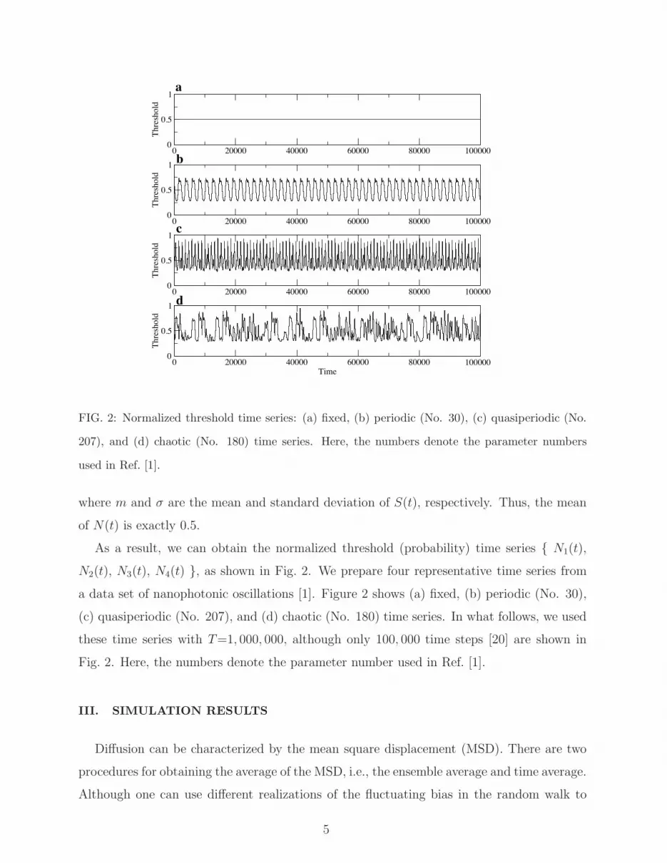
FIG. 2: Normalized threshold time series: (a) fixed, (b) periodic (No. 30), (c) quasiperiodic (No.
207), and (d) chaotic (No. 180) time series. Here, the numbers denote the parameter numbers
used in Ref. [1].
where m and σ are the mean and standard deviation of S(t), respectively. Thus, the mean
of N(t) is exactly 0.5.
As a result, we can obtain the normalized threshold (probability) time series { N1(t),
N2(t), N3(t), N4(t) }, as shown in Fig. 2. We prepare four representative time series from
a data set of nanophotonic oscillations [1]. Figure 2 shows (a) fixed, (b) periodic (No. 30),
(c) quasiperiodic (No. 207), and (d) chaotic (No. 180) time series. In what follows, we used
these time series with T=1, 000, 000, although only 100, 000 time steps [20] are shown in
Fig. 2. Here, the numbers denote the parameter number used in Ref. [1].
III. SIMULATION RESULTS
Diffusion can be characterized by the mean square displacement (MSD). There are two
procedures for obtaining the average of the MSD, i.e., the ensemble average and time average.
Although one can use different realizations of the fluctuating bias in the random walk to
5

calculate the MSD, we take the average for a single time series of the bias generated by
the previous study [1]. It follows that the MSD crucially depends on the time series. To
extract overall diffusion property, we take both averages, i.e., the ensemble average of the
time-averaged mean square displacement (ETMSD), defined as
ETMSD(τ) = 〈 1
T − τ
T−τ∑
t=1
(x(t+ τ)− x(t))2〉, (2)
where x(t) is the position at time t with the initial condition x(0) = 0, 〈· · · 〉 denotes
the ensemble average with respect to the noise (the seed of the RNG), and T is the total
measurement time length (1, 000, 000). We note that the ensemble average is taken under
one realization of the fluctuating bias (the threshold time series is fixed). When there is no
bias, i.e., N(t) = 0.5, the ETMSD exhibits normal diffusion, i.e., ETMSD(τ) = τ .
Figures 3(a) and (b) show the ETMSDs of the time series shown in Fig. 2. We can confirm
that the ETMSDs do not monotonically increase, except in the ordinary one (the case with
a fixed probability of 0.5). In particular, the ETMSD for the chaotic time series undergoes
many large changes in a short time interval owing to the transient nonstationarity of its
biases, although the overall time dependence of the ETMSD is proportional to the time,
which indicates normal diffusion, as shown in Fig. 3(b). We confirmed that the ETMSD at
τ = 106, 2 × 10⁶, · · · increases linearly with the time when we periodically generate N(t)
with a period of 106 (not shown).
This nonstationarity originates from the bias of 0 or 1 in a local time interval, as shown
in Fig. 4(b). This is because the spectrum of the chaotic oscillation (No. 180) contains high
power at low frequencies. It is noted that the ETMSD of a strongly chaotic data such as a
logistic map or the No. 180 chaotic data with a destructive time correlation (surrogate data)
exhibits similar behavior to that of the fixed threshold (monotonically increasing). There
exists a huge bias in a short time interval, although these biases are canceled in the overall
time series owing to the normalization (see Section II), as shown in Fig. 4(a).
Figure 5 shows the sojourn-time distributions of X(t) generated from the threshold time
series shown in Fig. 2. The log-log scale distributions are shown for fixed (black solid line),
periodic (blue dotted line), quasiperiodic (green dashed line), and chaotic (red filled circles)
probabilities. We can confirm that the sojourn-time distributions come close to the power
law distribution as the time series become chaotic. The power law distribution means that
there is no characteristic sojourn-time length. This is one of the properties of superdiffusion
6

Log ( )1e+06
1e+051
1e+06
1e+07
1e+08
Log (
ET
MS
D)
FixedPeriodicQuasiperiodic
Chaotic
1e+04
1e+03
1e+021e+051e+02 1e+03 1e+04
0 2e+05 4e+05 6e+05 8e+05
τ
(a)
(b)
0
5e+05
1e+06
1.5e+06
2e+06
ET
MS
D
FixedPeriodicQuasiperiodic
Chaotic
1e+06
FIG. 3: (a) ETMSDs for fixed (black solid line), periodic (blue dotted line), quasiperiodic (green
dashed line), and chaotic (red filled circles) probabilities. (b) Fig. 3(a) plotted with logarithmic
scales.
shown in the Levy walk [16, 17]. However, the power law distribution is not perfect in the
case of No. 180. The 1-run distribution does not follow a power law, whereas the 0-run
distribution follows a short power law. As a result, the overall property is classified as
normal diffusion.
7

0 2e+05 4e+05 6e+05 8e+05 1e+06Time
0.49
0.5
0.51
Tim
e-av
erag
e of
N(t
) PeriodicQuasiperiodicChaotic
0 2e+05 4e+05 6e+05 8e+05 1e+06Time
-1000
-500
0
500
1000
Bia
s
PeriodicQuasiperiodicChaotic
FIG. 4: (a) The time average of N(t) for periodic (blue dotted line), quasiperiodic (green dashed
line), and chaotic (red solid line) probabilities. (b) The average difference between the number of
occurrences of 1 and the number of occurrences of 0 until time t.
Among the nanochaos data sets, we can observe superdiffusion in our model if we find a
time series of chaotic probability, such as the modified Bernoulli map (Aizawa map [14, 18]),
that generates power law distributions. The Aizawa map is described by following equations:
S(t+ 1) =
S(t) + 2B−1S(t)B (0 ≤ S(t) ≤ 0.5)
S(t)− 2B−1(1− S(t))B (0.5 < S(t) ≤ 1).
(3)
Figure 6 shows the ETMSDs of a random walk using a time series generated by an Aizawa
map with B = 1.7 and B = 2.2. Here, for the purposes of correctly estimating the slope,
we do not use normalization (Eq. (1)) and use 100 samples from different initial conditions.
The time dependences of the MSD (=tβ) for the Aizawa map, which has one parameter
B, are as follows:
• B ≤ 1.5: normal diffusion (β = 1.0),
• 1.5 < B ≤ 2.0: superdiffusion (β = 3− 1
B−1),
• B > 2.0: superdiffusion (β = 2.0).
8

0 1 2 3 4Log (run length)
-20
-15
-10
-5
0
Log
(ra
te o
f fr
eq.)
FixedPeriodicQuasiperiodicChaotic
FIG. 5: The sojourn-time distributions of X(t) generated from the time series of fixed (black solid
line), periodic (blue dotted line), quasiperiodic (green dashed line), and chaotic (red filled circles)
probabilities.
In next section, we show analytical calculations of these MSDs using a simplified stochastic
model. Each of these results corresponds to Eq. (25), Eq. (27), and Eq. (29), respectively,
in the next section. In Fig. 6, we can confirm that the exponent β indicates superdiffusion,
which is very close to the expected value 1.57 or 2.0 from our theory (see section IV).
IV. THEORETICAL RESULTS
In this section, we consider a simple stochastic model related to a random walk with a
fluctuating bias, which can generate a variety of diffusion types, as shown in Fig. 7. The
model is a simple generalization of a Levy walk, in which a random walker performs a
two-state biased random walk with a random persistence time. The probability of going to
the left is given by p± = 0.5 ± ǫ (ǫ = 0.5 corresponds to the ordinary Levy walk), where
the subscript represents the state, i.e., the + or − state. The MSDs can be analytically
calculated for several persistence time distributions. Using the analytical results of the
stochastic model, we can understand that the overall properties in nanochaos data we treat
in this paper are all classified as normal diffusion (see Eq. (25)).
9

1Log(time)
1
1e+08
1e+12
1e+16L
og
(ET
MS
D)
Aizawa Map (B=1.7)
Aizawa Map (B=2.2)
pow (t, 1.57)
pow (t, 2.0)
1e+04
1e+02 1e+04 1e+06
FIG. 6: ETMSDs of a random walk using a time series generated by an Aizawa map with B = 1.7
(black circles) and B = 2.2 (red squares). The slope of each ETMSD indicates superdiffusion,
which is very close to the expected value (1.57 or 2.0) from our theory (see Section IV).
A. Stochastic model
In a Levy walk, a random walker moves to the right or left with a constant velocity for
a continuous random persistence time. After the persistence time, the random walker can
change direction. Instead, a random walker in our model performs a biased random walk
with a probability of going to the left of p± = 0.5 ± ǫ (the probability of going to the right
is q± = 1− p±) for a continuous random persistence time. In what follows, we consider the
continuous version of the random walk. Thus, we use the following propagator during the
biased random walk with the state ±:
P±(x, t) =1√4πDt
e−(x∓ct)2
4Dt . (4)
We note that the diffusion coefficient D and the velocity c are expressed as 2D = 4p±q± =
1− 4ǫ2 and c = p+ − q+ = 2ǫ, respectively. We use ρ(t) as the probability density function
(PDF) of the persistence times.
10

FIG. 7: Simplified stochastic model (deterministic change).
B. Random walk framework
Let Q±(x, t) be the joint PDF of finding a random walker at position x at time t, and
the states changes from ∓ to ± exactly at t. Further, let R±(x, t) be the PDF of finding
a random walker with the state ± at position x at time t. Then, we have the following
Montroll–Weiss equations (deterministic change of state) [16, 19]:
Q±(x, t) = p0±δ(x)δ(t) +
∫ t
0
dt′∫ ∞
−∞
dx′ψ∓(x′, t′)Q∓(x− x′, t− t′) (5)
and
R±(x, t) =
∫ t
0
dt′∫ ∞
−∞
dx′Ψ±(x′, t′)Q±(x− x′, t− t′), (6)
where p0± is the probability of the initial state (±), ψ±(x, t) = P±(x, t)ρ(t), and Ψ±(x, t) =
P±(x, t)∫∞
tdt′ρ(t′). Note that the initial position is x = 0, and we assume that the initial
persistence time distribution is the same as ρ(t). Using the Fourier–Laplace transform of
Q±(x, t) with respect to x and t in Eq. (5), we have Q±(k, s). Then, the substitution of this
into the Fourier–Laplace transform of R±(k, s) in Eq. (6) gives
R±(k, s) =p0± + p0∓ψ∓(k, s)
1− ψ±(k, s)ψ∓(k, s)Ψ±(k, s). (7)
11

When p0± = 1/2, we have
R±(k, s) =1
2
1 + ψ∓(k, s)
1− ψ±(k, s)ψ∓(k, s)Ψ±(k, s), (8)
and R(x, t) ≡ R+(x, t) +R−(x, t) becomes
R(k, s) =Ψ(k, s) + ψΨ(k, s)
1− ψ±(k, s)ψ∓(k, s), (9)
where Ψ(k, s) = {Ψ+(k, s) + Ψ−(k, s)}/2, and ψΨ(k, s) = {ψ+(k, s)Ψ−(k, s) +
ψ−(k, s)Ψ+(k, s)}/2. We note that ψ±(0, s) = ρ(s), Ψ±(0, s) = {1 − ρ(s)}/s, Ψ(0, s) =
{1− ρ(s)}/s, and ψΨ(0, s) = ρ(s){1− ρ(s)}/s.
C. Persistence time distribution
1. Deterministic case (periodic)
Here, we consider that the persistence time of the state is constant (τ0): ρ(t) = δ(t− τ0).
By Eq. (5), we have
Q±(x, τ0) =P∓(x, τ0)
2(10)
and
Q±(x, 2τ0) =
∫ ∞
−∞
dx′ψ∓(x′, τ0)Q∓(x− x′, τ0). (11)
The Fourier transform with respect to x is
Q±(k, 2nτ0 + τ0) ={ψ+(k, τ0)ψ−(k, τ0)}nψ±(k, τ0)
2(12)
and
Q±(k, 2nτ0) ={ψ+(k, τ0)ψ−(k, τ0)}n
2(13)
for n = 0, 1, · · · .
2. Stochastic case
Here, we consider three cases for the PDFs of the persistence times whose Laplace trans-
forms are given by
12

(1) α = 2: ρ(s) = 1− µs+ as2 + o(sα),
(2) 1 < α < 2: ρ(s) = 1− µs+ asα + o(sα),
(3) α < 1: ρ(s) = 1− asα + o(sα),
where µ is the mean persistence time and a is an arbitrary value. The mean persistence
time diverges for case (3), and the second moment of the persistence time diverges for cases
(2) and (3). For example, cases (2) and (3) correspond to
∫ ∞
t
dt′ρ(t′) ∼(c0t
)α
(t→ ∞), (14)
where c0 is a microscopic scale parameter. Because
ψ(k, s) =
∫ ∞
−∞
dx
∫ ∞
0
dte−st−kxψ(x, t), (15)
the derivative with respect to k gives
ψ′(k, s) =
∫ ∞
−∞
dx
∫ ∞
0
dt(−x)e−st−kxψ(x, t), (16)
implying ψ′(0, s) = 0. Moreover,
ψ′′(0, s) =
∫ ∞
0
dte−st(2Dt+ c2t2)ρ(t). (17)
For α < 2,
ψ′′(0, s) ∼ c2∫ ∞
0
dte−stt2ρ(t) (s→ 0). (18)
In a similar manner, we have Ψ′(0, s) = 0 and
Ψ′′(0, s) =
∫ ∞
0
e−st(2Dt+ c2t2)
∫ ∞
t
dt′ρ(t′). (19)
For α < 2,
Ψ′′(0, s) ∼ c2∫ ∞
0
e−stt2∫ ∞
t
dt′ρ(t′) (s→ 0). (20)
13

D. Mean square displacement
1. Deterministic change
The Laplace transform of the mean displacement is given by
L(〈x(t)〉)(s) = ∂R(k, s)
∂k
∣
∣
∣
∣
∣
k=0
= 0. (21)
The Laplace transform of the MSD is given by
L(〈x(t)2〉)(s) =∂2R(k, s)
∂k2
∣
∣
∣
∣
∣
k=0
(22)
=
[
Ψ′′(0, s) + ψΨ′′(0, s)
1− ρ(s)2+
2
s
ψ′′(0, s) + ψ′+(0, s)ψ
′−(0, s)
1− ρ(s)2
]
. (23)
For case (1),
L(〈x(t)2〉)(s) ∼ 2Dµ+ (2a− µ2)c2
µs2. (24)
The inverse transform is
〈x(t)2〉 ∼ 2Dµ+ (2a− µ2)c2
µt. (25)
For case (2),
L(〈x(t)2〉)(s) ∝ 1
s4−α. (26)
The inverse transform is
〈x(t)2〉 ∝ t3−α. (27)
For case (3),
L(〈x(t)2〉)(s) ∝ 1
s3. (28)
The inverse transform is
〈x(t)2〉 ∝ t2. (29)
Therefore, superdiffusion is observed for cases (2) and (3), which is consistent with the Levy
walk.
When the persistence time is periodic, the MSD is given by
〈x(nτ0)2〉 =∂2Q(k, nτ0)
∂k2
∣
∣
∣
∣
∣
k=0
. (30)
14

Because Q′′±(0, 2nτ0) = 4nDτ0 and Q′′
±(0, 2nτ0) = 2D(2n+ 1)τ0 + c2τ 20 , the MSD becomes
〈x(kτ0)2〉 =
2D(2n+ 1)τ0 + c2τ 20 (k = 2n+ 1)
4nDτ0 (k = 2n).
(31)
Because D is related to the bias, i.e., D = 1 − 4ǫ2, the bias decreases the diffusivity at
t = 2nτ0. However, the diffusivity at t = (2n+1)τ0 is greatly enhanced by a large period τ0
and bias c = 2ǫ. This is a mechanism of accelerated diffusion.
V. DISCUSSION
To characterize the “chaotic probability” observed in the nanoscale optical energy trans-
fer between QDs [1], we investigated one-dimensional random walks using fixed, periodic,
quasiperiodic, and chaotic probabilities in this study. The ETMSDs exhibited rich behav-
iors, although the overall time behaviors are classified as normal diffusion. In particular,
the ETMSD undergoes many large changes in weakly chaotic random walks, which we call
“accelerated diffusion,” owing to the transient nonstationarity of its biases.
It is noted that the rapid increase in the ETMSD of No. 180 at the initial stage is
only observed in the situation where we treat the time series as “probabilities (thresholds).”
This rapid increase implies a short-time arrival to some points (± x), as shown in Fig. 3.
In real physical situations, nanophotonic oscillations are the oscillations of the existence
probabilities of the optical energy in QDs but not a probability of the left flight of a particle.
However, we believe that the properties of the nonsymmetricity and nonstationarity of the
chaotic probabilities could generate the short-time arrival as well. This “nonstationary quick
search” property could be used for physically solving demanding computational problems
implemented in QD arrays, such as a maze that consists of QDs [2–4].
This characterization will also provide new applications using nanoscale chaotic proba-
bilities, such as efficient optical energy transfer used for information propagation, efficient
decision-making devices, and high-quality and high-speed physical nanoscale RNGs for in-
formation and communications technologies.
15

Acknowledgement
This work was supported in part by the Core-to-Core Program, A. Advanced Research
Networks from the Japan Society for the Promotion of Science. We thank Prof. Takahisa
Harayama for valuable discussions.
[1] M. Naruse, S.-J. Kim, M. Aono, H. Hori, and M. Ohtsu, Sci. Rep. 4, 6039 (2014).
[2] M. Naruse, M. Aono, S.-J. Kim, T. Kawazoe, W. Nomura, H. Hori, M. Hara, and M. Ohtsu,
Phys. Rev. B 86, 125407 (2012).
[3] M. Aono, M. Naruse, S.-J. Kim, M. Wakabayashi, H. Hori, M. Ohtsu, and M. Hara, Langmuir
29, 7557 (2013).
[4] S.-J. Kim, M. Naruse, M. Aono, M. Ohtsu, and M. Hara, Sci. Rep. 3, 2370 (2013).
[5] M. Naruse, W. Nomura, M. Aono, M. Ohtsu, Y. Sonnefraud, A. Drezet, S. Huant, and S.-
J. Kim, J. Appl. Phys. 116, 154303 (2014).
[6] M. Naruse, M. Berthel, A. Drezet, S. Huant, M. Aono, H. Hori, and S.-J. Kim, Sci. Rep. 5,
13253 (2015).
[7] P. Massignan, C. Manzo, J. A. Torreno-Pina, M. F. Garca-Parajo, M. Lewenstein, and
G. J. Lapeyre, Jr., Phys. Rev. Lett. 112, 150603 (2014).
[8] C. Manzo, J. A. Torreno-Pina, P. Massignan, G. J. Lapeyre, Jr., M. Lewenstein, and
M. F. Garcia Parajo, Phys. Rev. X 5, 011021 (2015).
[9] T. Ueyama, T. Miyaguchi, and T. Akimoto, Phys. Rev. E 92, 032140 (2015).
[10] E. Yamamoto, A. C. Kalli, T. Akimoto, K. Yasuoka, and M. S. P. Sansom, Sci. Rep. 5, 18245
(2015).
[11] T. Akimoto and K. Seki, Phys. Rev. E 92, 022114 (2015).
[12] Y. G. Sinai, Selecta II: Probability Theory, Statistical Mechanics, Mathematical Physics and
Mathematical Fluid Dynamics (Springer-Verlag, New York, 2010).
[13] B. D. Cheliotis and B. Virag, Ann. Probability 41, 1900 (2013).
[14] T. Akimoto and Y. Aizawa, Prog. Theor. Phys. 114, 737 (2005).
[15] M. Matsumoto, Mersenne Twister Home Page,
http://www.math.sci.hiroshima-u.ac.jp/∼m-mat/MT/emt.html.
16

[16] M. F. Shlesinger, J. Klafter, and Y. M. Wong, J. Stat. Phys. 27, 499 (1982).
[17] T. Geisel, J. Nierwetberg, and A. Zacherl, Phys. Rev. Lett. 54, 616 (1985).
[18] Y. Aizawa and T. Kohyama, in Chaos and Statistical Methods, edited by Y. Kuramoto
(Springer-Verlag, Berlin Heidelberg, 1983), p. 109.
[19] E. W. Montroll and G. H. Weiss, J. Math. Phys. 6, 167 (1965).
[20] Actually, owing to the transition period, we used normalized time steps (T ) of (a) 1, 000, 000,
(b) 990, 000, (c) 900, 000, and (d) 900, 000.
17
Recommended


