Embed Size (px)
Citation preview

Introduction to Statistics
(Science of Data)

What is statistics Form Latin word ‘Statis’ means ‘Political
State’. Science of Uncertainty It Deals with what could be, what might be
or what probably is.
The basis to verify theories and laws in every discipline.Overall, it is a method which deals with numerical facts and figures.

Examples The Indian army is going to grow by 9-10%
per annum in coming 5 yrs. The male female ratio in India is 972 as per
2001 census. Indian population is growing by 2% every
year. Attendance of a student should be 75% for
appearing in exams.And many more……

STATISTICS (The Scientific Method) What is Science? Originated form Latin word “Scientia” meaning knowledge.
Knowledge attained through study or practice.
Knowledge covering general truths of the operation of generals laws (esp obtained and tested
through scientific method) and concerned with physical world.

STATISTICS (The Scientific Method) Statistics is not a body of substantive
knowledge, but a body of methods for obtaining knowledge.
It can be accepted as scientific method than a complete science.
Scientific Methods:-Classifies facts, sees their mutual relation through experimentation, observation, logical arguments from accepted postulates

Research Process

Introduction 7
Population. Universe. The entire category under consideration. This is the data which we have not completely examined but to which our conclusions refer. The population size is usually indicated by a capital N.◦ Examples: every user of twitter; all female user of facebook.
Sample. That portion of the population that is available, or to be made available, for analysis. A good sample is representative of the population. We will learn about probability samples and how they provide assurance that a sample is indeed representative. The sample size is shown as lower case n.
◦ If your company manufactures one million laptops, they might take a sample of say, 500, of them to test quality. The population size is N = 1,000,000 and the sample size is n= 500.
Key Terms

Introduction 8
Parameter. A characteristic of a population. The population mean, µ and the population standard deviation, σ, are two examples of population parameters. If you want to determine the population parameters, you have to take a census of the entire population. Taking a census is very costly.
Statistic. A statistic is a measure that is derived from the sample data. For example, the sample mean, , and the sample standard deviation, s, are statistics. They are used to estimate the population parameters.
Key Terms

Introduction 9
ccvccvcvvvv
Key Termsv

Introduction 10
Example of statistical inference from quality control: GE manufactures LED bulbs and wants to know how
many are defective. Suppose one million bulbs a year are produced in its new plant in Staten Island. The company might sample, say, 500 bulbs to estimate the proportion of defectives. ◦ N = 1,000,000 and n = 500◦ If 5 out of 500 bulbs tested are defective, the sample
proportion of defectives will be 1% (5/500). This statistic may be used to estimate the true proportion of defective bulbs (the population proportion).
◦ In this case, the sample proportion is used to make inferences about the population proportion.
Key Terms
Introduction 11
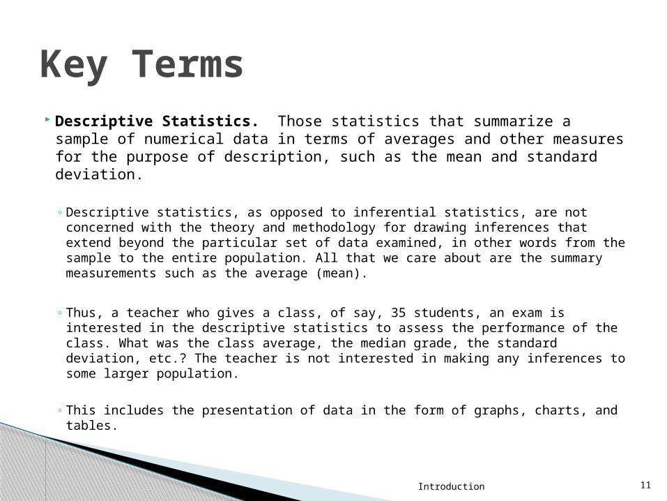
Descriptive Statistics. Those statistics that summarize a sample of numerical data in terms of averages and other measures for the purpose of description, such as the mean and standard deviation.
◦ Descriptive statistics, as opposed to inferential statistics, are not concerned
with the theory and methodology for drawing inferences that extend beyond the particular set of data examined, in other words from the sample to the entire population. All that we care about are the summary measurements such as the average (mean).
◦ Thus, a teacher who gives a class, of say, 35 students, an exam is interested in the descriptive statistics to assess the performance of the class. What was the class average, the median grade, the standard deviation, etc.? The teacher is not interested in making any inferences to some larger population.
◦ This includes the presentation of data in the form of graphs, charts, and tables.
Key Terms

Introduction 12
Primary data. This is data that has been compiled by the researcher using such techniques as surveys, experiments, depth interviews, observation, focus groups.
Types of surveys. A lot of data is obtained using
surveys. Each survey type has advantages and disadvantages.◦ Mail: lowest rate of response; usually the lowest cost◦ Personally administered: can “probe”; most costly;
interviewer effects (the interviewer might influence the response)
◦ Telephone: fastest◦ Web: fast and inexpensive
Primary vs. Secondary Data

Introduction 13
Secondary data. This is data that has been compiled or published elsewhere, e.g., census data.
◦ The trick is to find data that is useful. The data was probably collected for some purpose other than helping to solve the researcher’s problem at hand.
◦ Advantages: It can be gathered quickly and inexpensively. It enables researchers to build on past research.
◦ Problems: Data may be outdated. Variation in definition of terms. Different units of measurement. May not be accurate (e.g., census undercount).
Primary vs. Secondary Data

Introduction 14
Nonprobability Samples – based on convenience or judgment◦ Convenience (or chunk) sample - students in a class, mall
intercept◦ Judgment sample - based on the researcher’s judgment as to
what constitutes “representativeness” e.g., he/she might say these 20 stores are representative of the whole chain.
◦ Quota sample - interviewers are given quotas based on demographics for instance, they may each be told to interview 100 subjects – 50 males and 50 females. Of the 50, say, 10 nonwhite and 40 white.
The problem with a nonprobability sample is that we do not
know how representative our sample is of the population.
Types of Samples

Introduction 15
Probability Sample. A sample collected in such a way that every element in the population has a known chance of being selected.
One type of probability sample is a Simple Random Sample. This is a sample collected in such a way that every element in the population has an equal chance of being selected.
How do we collect a simple random sample?
◦ Use a table of random numbers or a random number generator.
Probability Samples
Introduction 16
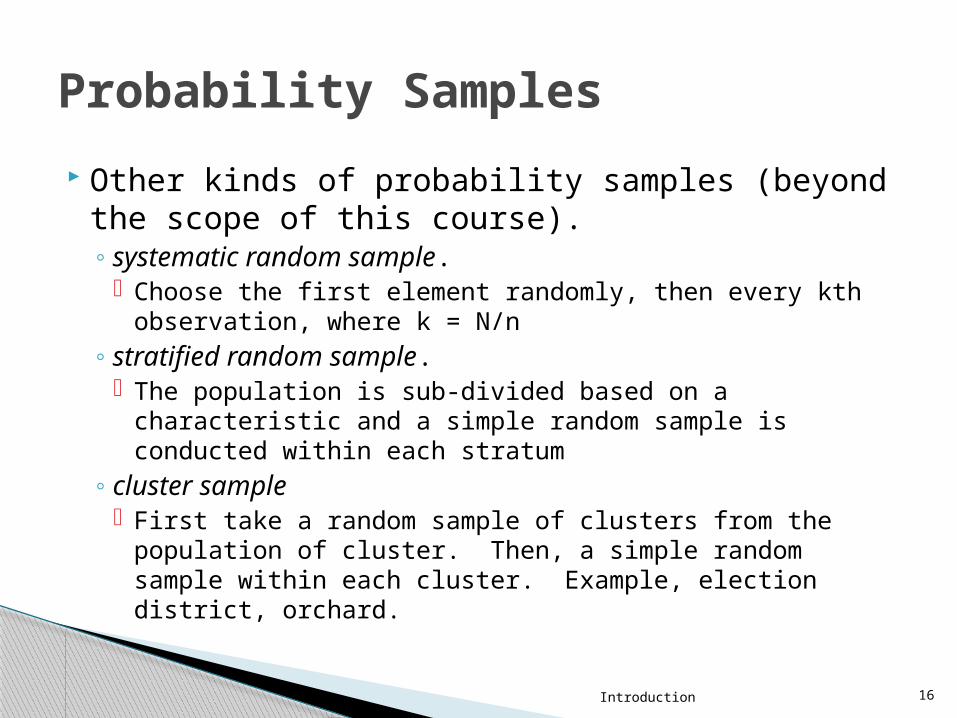
Other kinds of probability samples (beyond the scope of this course).◦ systematic random sample.
Choose the first element randomly, then every kth observation, where k = N/n
◦ stratified random sample. The population is sub-divided based on a characteristic
and a simple random sample is conducted within each stratum
◦ cluster sample First take a random sample of clusters from the
population of cluster. Then, a simple random sample within each cluster. Example, election district, orchard.
Probability Samples

Descriptive Statistics I 17
◦ Measures of Location
Measures of central tendency: Mean; Median; Mode Measures of noncentral tendency - Quantiles
Quartiles; Quintiles; Percentiles
◦ Measures of Dispersion Range Interquartile range Variance Standard Deviation Coefficient of Variation
◦ Measures of Shape◦ Skewness
Descriptive Statistics

Descriptive Statistics I 18
Measures of location place the data set on the scale of real numbers.
Measures of central tendency (i.e., central location) help find the approximate center of the dataset.
These include the mean, the median, and the mode.
Measures of Location

Descriptive Statistics I 19
The sample mean is the sum of all the observations (∑Xi) divided by the number of observations (n):
ΣXi = X1 + X2 + X3 + X4 + … + Xn
Example. 1, 2, 2, 4, 5, 10. Calculate the mean. Note: n = 6 (six observations)
∑Xi = 1 + 2+ 2+ 4 + 5 + 10 = 24
= 24 / 6 = 4.0
The Mean

Descriptive Statistics I 20
The median is the middle value of the ordered data To get the median, we must first rearrange the data
into an ordered array (in ascending or descending order). Generally, we order the data from the lowest value to the highest value.
Therefore, the median is the data value such that half of the observations are larger and half are smaller. It is also the 50th percentile (we will be learning about percentiles in a bit).
If n is odd, the median is the middle observation of the ordered array. If n is even, it is midway between the two central observations.
The Median

Descriptive Statistics I 21
The mode is the value of the data that occurs with the greatest frequency.
Example. 1, 1, 1, 2, 3, 4, 5Answer. The mode is 1 since it occurs three times. The other values each appear only once in the data set.
Example. 5, 5, 5, 6, 8, 10, 10, 10.Answer. The mode is: 5, 10. There are two modes. This is a bi-modal dataset.
The Mode

Descriptive Statistics I 22
Quartiles split a set of ordered data into four parts. ◦ Imagine cutting a chocolate bar into four equal pieces… How
many cuts would you make? (yes, 3!) Q1 is the First Quartile
◦ 25% of the observations are smaller than Q1 and 75% of the observations are larger
Q2 is the Second Quartile◦ 50% of the observations are smaller than Q2 and 50% of the
observations are larger. Same as the Median. It is also the 50th percentile.
Q3 is the Third Quartile ◦ 75% of the observations are smaller than Q3and 25% of the
observations are larger
Quartiles

Descriptive Statistics I 23
Dispersion is the amount of spread, or variability, in a set of data.
Why do we need to look at measures of dispersion?
Consider this example:
A company is about to buy computer chips that must have an average life of 10 years. The company has a choice of two suppliers. Whose chips should they buy? They take a sample of 10 chips from each of the suppliers and test them. See the data on the next slide.
Measures of Dispersion

Descriptive Statistics I 24
We see that supplier B’s chips have a longer average life.
However, what if the company offersa 3-year warranty?
Then, computers manufactured using the chips from supplier A will have no returns while using supplier B will result in4/10 or 40% returns.
Measures of Dispersion
Supplier A chips (life in years)
Supplier B chips (life in years)
11 170
11 1
10 1
10 160
11 2
11 150
11 150
11 170
10 2
12 140
A = 10.8 years = 94.6 years
MedianA = 11 years
MedianB = 145 years
sA = 0.63 years sB = 80.6 years
RangeA = 2 years RangeB = 169 years

Descriptive Statistics I 25
We will study these five measures of dispersion◦ Range◦ Interquartile Range ◦ Standard Deviation ◦ Variance◦ Coefficient of Variation
Measures of Dispersion

Descriptive Statistics I 26
Range = Largest Value – Smallest Value
Example: 1, 2, 3, 4, 5, 8, 9, 21, 25, 30Answer: Range = 30 – 1 = 29.
The range is simple to use and to explain to others.
One problem with the range is that it is influenced by extreme values at either end.
The Range

Descriptive Statistics I 27
IQR = Q3 – Q1
Example (n = 15):0, 0, 2, 3, 4, 7, 9, 12, 17, 18, 20, 22, 45, 56, 98Q1 = 3, Q3 = 22IQR = 22 – 3 = 19 (Range = 98)
This is basically the range of the central 50% of the observations in the distribution.
Problem: The interquartile range does not take into
account the variability of the total data (only the central 50%). We are “throwing out” half of the data.
Inter-Quartile Range (IQR)

Descriptive Statistics I 28
The standard deviation, s, measures a kind of “average” deviation about the mean. It is not really the “average” deviation, even though we may think of it that way.
Why can’t we simply compute the average
deviation about the mean, if that’s what we want?
If you take a simple mean, and then add up the deviations about the mean, as above, this sum will be equal to 0. Therefore, a measure of “average deviation” will not work.
Standard Deviation

Descriptive Statistics I 29
Instead, we use:
This is the “definitional formula” for standard deviation. The standard deviation has lots of nice properties,
including: ◦ By squaring the deviation, we eliminate the problem of the
deviations summing to zero.
◦ In addition, this sum is a minimum. No other value subtracted from X and squared will result in a smaller sum of the deviation squared. This is called the “least squares property.”
Note we divide by (n-1), not n. This will be referred to as a loss of one degree of freedom.
Standard Deviation

Descriptive Statistics I 30
Example. Two data sets, X and Y. Which of the two data sets has greater variability? Calculate the standard deviation for each.
We note that both sets of data have the same mean: = 3 = 3
(continued…)
Standard Deviation
Xi Yi
1 0
2 0
3 0
4 5
5 10

Descriptive Statistics I 31
SX == 1.58
SY == = 4.47
[Check these results with your calculator.]
Standard Deviation
X (X-) (X-)2
1 3 -2 42 3 -1 13 3 0 04 3 1 15 3 2 4 ∑=0 10
Y (Y-) (Y- )2
0 3 -3 90 3 -3 90 3 -3 95 3 2 4
10 3 7 49 ∑=0 80

Descriptive Statistics I 32
The variance, s2, is the standard deviation (s) squared. Conversely, .
Definitional formula: Computational formula:
This is what computer software (e.g., MS Excel or your calculator key) uses.
Variance

Descriptive Statistics I 33
We see that supplier B’s chips have a longer average life.
However, what if the company offersa 3-year warranty?
Then, computers manufactured using the chips from supplier A will have no returns while using supplier B will result in4/10 or 40% returns.
Measures of Dispersion
Supplier A chips (life in years)
Supplier B chips (life in years)
11 170
11 1
10 1
10 160
11 2
11 150
11 150
11 170
10 2
12 140
A = 10.8 years = 94.6 years
MedianA = 11 years
MedianB = 145 years
sA = 0.63 years sB = 80.6 years
RangeA = 2 years RangeB = 169 years

34
A sample space is the set of all possible outcomes of an experiment.
A random variable is a rule for associating a number with each element in a sample space.
Suppose there are 8 balls in a bag. The random variable X is the weight, in kg, of a ball selected at random. Balls 1, 2 and 3 weigh 0.1kg, balls 4 and 5 weigh 0.15kg and balls 6, 7 and 8 weigh 0.2kg
Random Variable

Probability Distributions 35
There are two types of random variables: ◦ A Discrete random variable can take on only
specified, distinct values.◦ A Continuous random variable can take on any
value within an interval. Thus, there are also two types of probability
distributions:◦ Discrete probability distributions◦ Continuous probability distributions
Types of Probability Distributions

Normal Distribution 36
Called a Probability density function. The probability is interpreted as "area under the curve."
1) The random variable takes on an infinite # of
values within a given interval
2) the probability that X = any particular value is 0. Consequently, we talk about intervals. The probability is = to the area under the curve.
3) The area under the whole curve = 1.
Normal Distribution

Normal Distribution 37
Probabilities are obtained by getting the area under the curve inside of a particular interval. The area under the curve = the proportion of times under identical (repeated) conditions that a particular range of values will occur.
3 Characteristics of the Normal distribution:◦ It is symmetric about the mean μ.◦ Mean = median = mode. [“bell-shaped” curve]◦ f(X) decreases as X gets farther and farther away from
the mean. It approaches horizontal axis asymptotically:- ∞ < X < + ∞. This means that there is always some probability (area) for extreme values.
Normal Distribution

Normal Distribution 38
The probability density function for the normal distribution:
X
f(X) the height of the curve, represents the relative frequency at which the corresponding values occur.
Normal Distribution

Normal Distribution 39
Note that the normal distribution is defined by two parameters, μ and σ . You can draw a normal distribution for any μ and σ combination. There is one normal distribution, Z, that is special. It has a μ = 0 and a σ = 1. This is the Z distribution, also called the standard normal distribution. It is one of trillions of normal distributions we could have selected.
Normal Distribution

Normal Distribution 40
Any normal distribution can be converted into a standard normal distribution by transforming the normal random variable into the standard normal random variable:
This is called standardizing the data. It will result in (transformed) data with μ = 0 and σ = 1.
The areas under the curve for the Standard Normal Distribution (Z) has been computed and tabled. See, for example http://www.statsoft.com/textbook/distribution-tables/#z
Please note that you may find different tables for the Z-distribution. The table we use here gives you the area under the curve from 0 to z. Some books provide a slightly different table, one that gives you the area in the tail. If you check the diagram that is usually shown above the table, you can determine which table you have. In the table on the next slide, the area from 0 to z is shaded so you know that you are getting the area from 0 to z. Also, note that table value can never be more than .5000. The area from 0 to infinity is .5000.
Z-Distribution

Estimation 41
Estimation Hypothesis Testing
Both activities use sample statistics (for example, Xc) to make inferences about a population parameter (μ).
Statistical Inference involves:

Estimation 42
Why don’t we just use a single number (a point estimate) like, say, Xc to estimate a population parameter, μ?
The problem with using a single point (or value) is that it
will very probably be wrong. In fact, with a continuous random variable, the probability that the variable is equal to a particular value is zero. So, P(Xc=μ) = 0.
This is why we use an interval estimator.
We can examine the probability that the interval includes the population parameter.
Estimation

Estimation 43
How wide should the interval be? That depends upon how much confidence you want in the estimate.
For instance, say you wanted a confidence interval estimator
for the mean income of a college graduate:
The wider the interval, the greater the confidence you will have in it as containing the true population parameter μ.
Confidence Interval Estimators
You might have That the mean income is between100% confidence $0 and $∞95% confidence $35,000 and $41,00090% confidence $36,000 and $40,00080% confidence $37,500 and $38,500
… …0% confidence $38,000 (a point estimate)

Estimation 44
To construct a confidence interval estimator of μ, we use:
Xc ± Zα σ /√n (1-α) confidence
where we get Zα from the Z table.
When n≥30, we use s as an estimator of σ.
Confidence Interval Estimators

Estimation 45
To be more precise, the α is split in half since we are constructing a two-sided confidence interval. However, for the sake of simplicity, we call the z-value Zα rather than Za/2 .
Confidence Interval Estimators
-Z/2 Z/2
/2 /2

Estimation 46
You work for a company that makes smart TVs, and your boss asks you to determine with certainty the exact life of a smart TV. She tells you to take a random sample of 100 TVs.
What is the exact life of a smart TV made by this company?Sample Evidence:n = 100 Xc = 11.50 years
s = 2.50 years
Question

Estimation 47
Since your boss has asked for 100% confidence, the only answer you can accurately provide is: -∞ to + ∞ years.
After you are fired, perhaps you can get your job back by
explaining to your boss that statisticians cannot work with 100% confidence if they are working with data from a sample. If you want 100% confidence, you must take a census. With a sample, you can never be absolutely certain as to the value of the population parameter.
This is exactly what statistical inference is: Using sample statistics to draw conclusions (e.g., estimates) about population parameters.
Answer – Take 1

Estimation 48
n = 100Xc = 11.50 yearsS = 2.50 years at 95% confidence:11.50 ± 1.96*(2.50/√100)11.50 ± 1.96*(.25) 11.50 ± .49The 95% CIE is: 11.01 years ---- 11.99 years
The Better Answer

Estimation 49
We are 95% certain that the interval from 11.01 years to 11.99 years contains the true population parameter, μ.
Another way to put this is, in 95 out of 100 samples, the population mean would lie in intervals constructed by the same procedure (same n and same α).
Remember – the population parameter (μ ) is fixed, it is not a random variable. Thus, it is incorrect to say that there is a 95% chance that the population mean will “fall” in this interval.
The Better Answer - Interpretation

Estimation 50
The sample:n = 100 Xc = 18 years
s = 4 years
Construct a confidence interval estimator (CIE) of the true population mean life (µ), at each of the following levels of confidence: ◦ (a)100% (b) 99% (c) 95% (d) 90% (e) 68%
EXAMPLE: Life of a Refrigerator

Estimation 51
In this problem we use s as an unbiased estimator of σ: E(s) = σ
σ = s =
95% Confidence Interval Estimator:
EXAMPLE: Life of a Refrigerator

Estimation 52
(a) 100% Confidence [α = 0, Zα = ∞]
100% CIE: −∞ years ↔ +∞ years(b) 99% Confidence α = .01, Zα = 2.575 (from Z table)
18 ± 2.575 (4/√100)18 ± 1.03
99% CIE: 16.97 years ↔ 19.03 years(c) 95% Confidence α = .05, Zα = 1.96 (from Z table)
18 ± 1.96 (4/√100)18 ± 0.78
95% CIE: 17.22 years ↔ 18.78 years
EXAMPLE: Life of a Refrigerator

Estimation 53
(d) 90% Confidence α = .10, Zα = 1.645 (from Z table)
18 ± 1.645 (4/√100)18 ± 0.66
90% CIE: 17.34 years ↔ 18.66 years
(e) 68% Confidence α = .32, Zα =1.0 (from Z table)
18 ± 1.0 (4/√100)18 ± 0.4
68% CIE: 17.60 years ↔ 18.40 years
EXAMPLE: Life of a Refrigerator

Estimation 54
How can we keep the same level of confidence and still construct a narrower CIE?
Let’s look at the formula one more time: Xc ± Zασ/√n The sample mean is in the center. The more confidence
you want, the higher the value of Z, the larger the half-width of the interval.
The larger the sample size, the smaller the half-width, since we divide by √n.
So, what can we do? If you want a narrower interval, take a larger sample.
What about a smaller standard deviation? Of course, this depends on the variability of the population. However, a more efficient sampling procedure (e.g., stratification) may help. That topic is for a more advanced statistics course.
Balancing Confidence and Width in a CIE

Estimation 55
Once you are working with a sample, not the entire population, you cannot be 100% certain of population parameters. If you need to know the value of a parameter certainty, take a census.
The more confidence you want to have in the estimator, the larger the interval is going to be.
Traditionally, statisticians work with 95% confidence. However, you should be able to use the Z-table to construct a CIE at any level of confidence.
Key Points