Embed Size (px)
Citation preview

Pipelining
&
Instruction Level Parallelism
Mr. A. B. Shinde
Assistant Professor,
Electronics Engineering,
P.V.P.I.T., Budhgaon
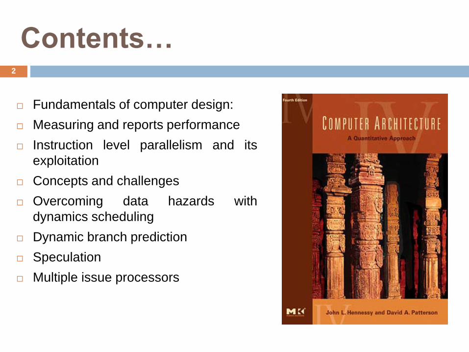
Contents…2
Fundamentals of computer design:
Measuring and reports performance
Instruction level parallelism and its
exploitation
Concepts and challenges
Overcoming data hazards with
dynamics scheduling
Dynamic branch prediction
Speculation
Multiple issue processors
Early Computers3
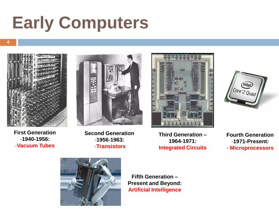
Early Computers
First Generation
-1940-1956:
-Vacuum Tubes
Second Generation
-1956-1963:
-Transistors
Third Generation –
1964-1971:
Integrated Circuits
Fourth Generation
-1971-Present:
- Microprocessors
Fifth Generation –
Present and Beyond:
Artificial Intelligence
4
Fundamentals of Computer
Computer technology has made incredible progress over the last 60
years.
This improvement has come:
From advances in the technology used to build computers and
From innovation in computer design.
During the first 25 years, both forces made a major contribution,
delivering performance improvement of about 25% per year.
The late 1970s (after emergence of the microprocessor):
The higher rate of improvement— roughly 35% growth per year in
performance.
5
Fundamentals of Computer
Two significant changes in the computer made new architecture:
The virtual elimination of assembly language programming
reduced the need for object-code compatibility.
The creation of standardized, vendor-independent operating
systems, such as UNIX, Linux, lowered the cost.
These changes developed a new set of architectures with simpler
instructions, called RISC (Reduced Instruction Set Computer)
architectures, in the early 1980s.
The RISC-based machines focused on instruction level parallelism and
the use of caches.
The RISC-based computers raised the performance.
6
Fundamentals of Computer Design
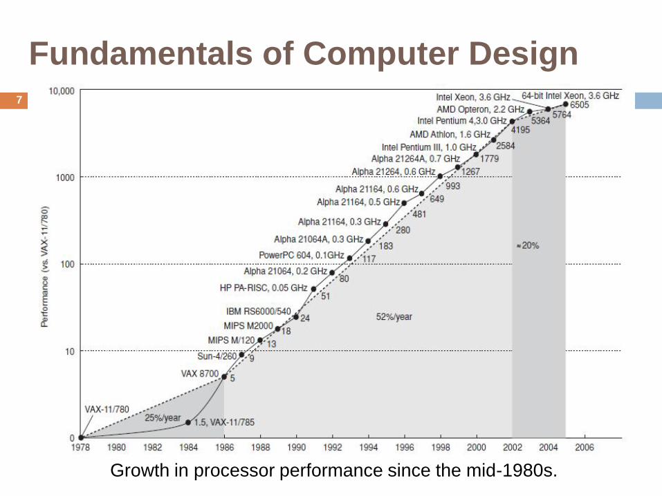
Growth in processor performance since the mid-1980s.
7

Classes of Computers
The 1980s: desktop computer were invented
(based on microprocessors)
Personal computers and workstations
The 1990s: Emergence of the Internet and the World Wide Web
(www).
Cell phones has been introduced in 2000, with rapid improvements in
functions and sales.
More recent applications used embedded computers.
8
Classes of Computers
Desktop Computing:
Desktop computing spans from low-end systems to high-end (heavily
configured workstations)
The desktop market tends to be driven to optimize price
performance.
Desktop computers are widely used for applications and
benchmarking.
9

Classes of Computers
Servers:
Servers are used to provide larger-scale and more reliable file and
computing services.
Consider the servers running Google, taking orders for CISCO, or
running auctions on eBay. Failure of such server systems is far more
catastrophic than failure of a single desktop, since these servers must
operate 24 x 7.
10
Classes of Computers
Servers:
Servers are designed for efficient throughput i.e. in terms of
transactions per minute or Web pages served per second.
Supercomputers are the most expensive computers, emphasize
floating-point performance.
Clusters of desktop computers, have largely overtaken this class of
computer.
11
Classes of Computers
Clusters/Warehouse-Scale Computers
The growth of Software as a Service (SaaS) for applications like
search, social networking, video sharing, multiplayer games, online
shopping, and so on has led to the growth of a class of computers
called clusters.
Clusters are collections of desktop computers or servers
connected by local area networks to act as a single larger computer.
Each node runs its own operating system, and nodes communicate
using a networking protocol.
The largest of the clusters are called warehouse-scale computers
(WSCs), in that they are designed so that tens of thousands of servers
can act as one.
12
Classes of Computers
Embedded Computers
Embedded computers are the fastest growing computer market.
They range from microwaves, washing machines, printers, networking
switches and all cars contain simple embedded microprocessors — to
handheld digital devices, such as cell phones and smart cards to video
games and digital set-top boxes.
Embedded applications: Minimize memory and minimize power.
13
Classes of Parallelism and Parallel Architectures
Parallelism at multiple levels is now the driving force of computer
design across all four classes of computers.
There are basically two kinds of parallelism in applications:
1. Data-Level Parallelism (DLP): Arises because there are many data
items that can be operated on at the same time.
2. Task-Level Parallelism (TLP): Arises because tasks of work are
created that can operate independently and largely in parallel.
14
Classes of Parallelism and Parallel Architectures
Data parallelism:
Consider a 2-processor system (CPUs A and B) in a parallel
environment, and we wish to do a task on some data „d‟.
It is possible to tell CPU A to do that task on one part of „d‟ and CPU
B on another part simultaneously, thereby reducing the duration of the
execution.
The data can be assigned using conditional statements
As a specific example, consider adding two matrices.
In a data parallel implementation, CPU A could add all elements from
the top half of the matrices, while CPU B could add all elements from
the bottom half of the matrices.
15
Classes of Parallelism and Parallel Architectures
Task parallelism:
Task parallelism (function parallelism or control parallelism) is a
form of parallelization of computer code across multiple processors in
parallel computing environments.
Task parallelism focuses on distributing execution processes
(threads) across different parallel computing nodes.
In a multiprocessor system, task parallelism is achieved when each
processor executes a different thread (or process) on the same or
different data.
16
Classes of Parallelism and Parallel Architectures
Task parallelism
As a simple example, if we are running code on a 2- processor system
(CPUs "a" & "b") in a parallel environment and we wish to do
tasks "A" and "B”.
It is possible to tell CPU "a" to do task "A" & CPU "b" to do task 'B"
simultaneously, thereby reducing the runtime of the execution.
The tasks can be assigned using conditional statements.
17
Defining Computer Architecture
The Computer designer faces the problems:
To maximize performance while staying within cost, power, and
availability constraints.
Instruction set design, functional organization, logic design, and
implementation.
The implementation may encompass integrated circuit design,
packaging, power and cooling.
18
Defining Computer Architecture
Instruction Set Architecture:
Class of ISA —
ISAs are classified as general-purpose register architectures, where
the operands are either registers or memory locations.
All recent ISAs have load-store architecture.
Memory addressing —
All desktops and servers uses byte addressing to access memory
operands.
19
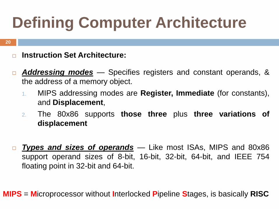
Defining Computer Architecture
Instruction Set Architecture:
Addressing modes — Specifies registers and constant operands, &
the address of a memory object.
1. MIPS addressing modes are Register, Immediate (for constants),
and Displacement,
2. The 80x86 supports those three plus three variations of
displacement
Types and sizes of operands — Like most ISAs, MIPS and 80x86
support operand sizes of 8-bit, 16-bit, 32-bit, 64-bit, and IEEE 754
floating point in 32-bit and 64-bit.
MIPS = Microprocessor without Interlocked Pipeline Stages, is basically RISC
20
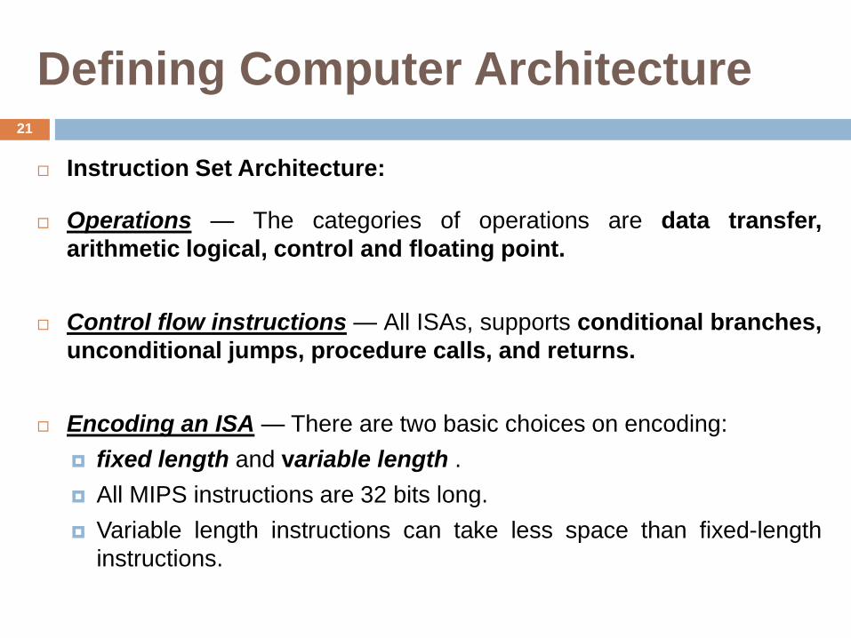
Defining Computer Architecture
Instruction Set Architecture:
Operations — The categories of operations are data transfer,
arithmetic logical, control and floating point.
Control flow instructions — All ISAs, supports conditional branches,
unconditional jumps, procedure calls, and returns.
Encoding an ISA — There are two basic choices on encoding:
fixed length and variable length .
All MIPS instructions are 32 bits long.
Variable length instructions can take less space than fixed-length
instructions.
21
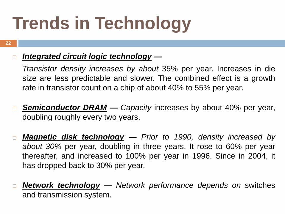
Trends in Technology
Integrated circuit logic technology —
Transistor density increases by about 35% per year. Increases in die
size are less predictable and slower. The combined effect is a growth
rate in transistor count on a chip of about 40% to 55% per year.
Semiconductor DRAM — Capacity increases by about 40% per year,
doubling roughly every two years.
Magnetic disk technology — Prior to 1990, density increased by
about 30% per year, doubling in three years. It rose to 60% per year
thereafter, and increased to 100% per year in 1996. Since in 2004, it
has dropped back to 30% per year.
Network technology — Network performance depends on switches
and transmission system.
22
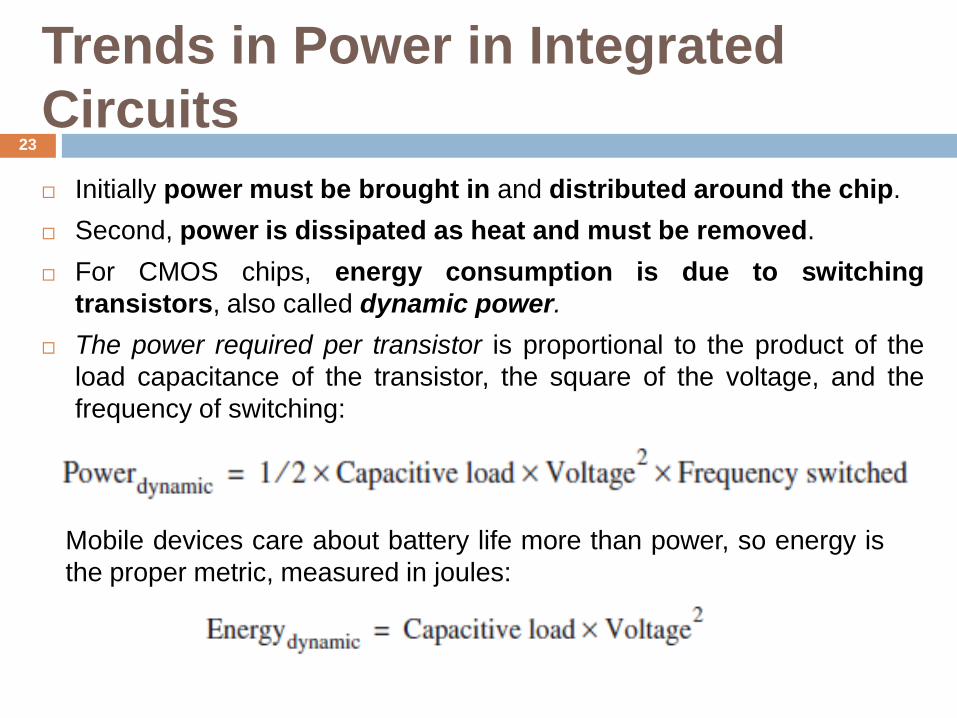
Trends in Power in Integrated
Circuits
Initially power must be brought in and distributed around the chip.
Second, power is dissipated as heat and must be removed.
For CMOS chips, energy consumption is due to switching
transistors, also called dynamic power.
The power required per transistor is proportional to the product of the
load capacitance of the transistor, the square of the voltage, and the
frequency of switching:
Mobile devices care about battery life more than power, so energy is
the proper metric, measured in joules:
23
Trends in Power in Integrated
Circuits
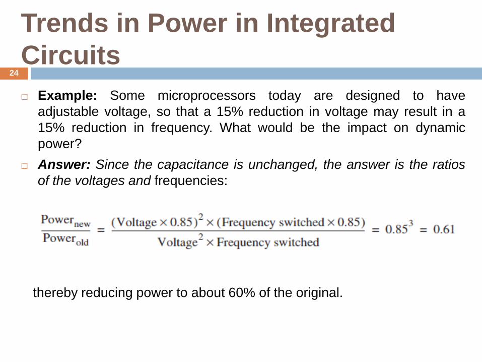
Example: Some microprocessors today are designed to have
adjustable voltage, so that a 15% reduction in voltage may result in a
15% reduction in frequency. What would be the impact on dynamic
power?
Answer: Since the capacitance is unchanged, the answer is the ratios
of the voltages and frequencies:
thereby reducing power to about 60% of the original.
24

Trends in Power in Integrated
Circuits
The increase in the number of transistors switching, and thefrequency of switching, dominates the decrease in load capacitanceand voltage, leading to an overall growth in power consumption andenergy.
Power is now the major limitation, therefore most microprocessorstoday turn off the clock of inactive modules to save energy and dynamicpower e.g. if no floating-point instructions are executing, the clock of thefloating-point unit is disabled.
Although dynamic power is the primary source of power dissipation inCMOS, static power is becoming an important issue because leakagecurrent flows even when a transistor is off:
Static Power is Calculated by:
25
Trends in Cost
Although there are computers where cost tends to be less important—
specifically supercomputers.
In the past 20 years:
The technology improvements to lower cost, increased
performance, was a major theme in the computer industry.
Yet an understanding of cost and its factors is essential for
designers to make intelligent decisions about whether or not a new
feature should be included in designs.
26
Trends in Cost:
The Impact of Time, Volume, and Commodification
Cost of a manufactured computer component decreases over time
even without major improvements in the implementation technology.
One example is that the price per megabyte of DRAM has dropped
over the long term by 40% per year.
Volume is a second key factor in determining cost.
Increasing volumes affects cost in several ways.
First, they decrease the time needed, which is proportional to the
number of systems manufactured.
Second, volume decreases cost, since it increases manufacturing
efficiency.
27

Trends in Cost:
Cost of an Integrated Circuit:
Although the costs of integrated circuits have dropped exponentially, the
basic process of silicon manufacture is unchanged.
The cost of a packaged integrated circuit is
28
Trends in Cost:
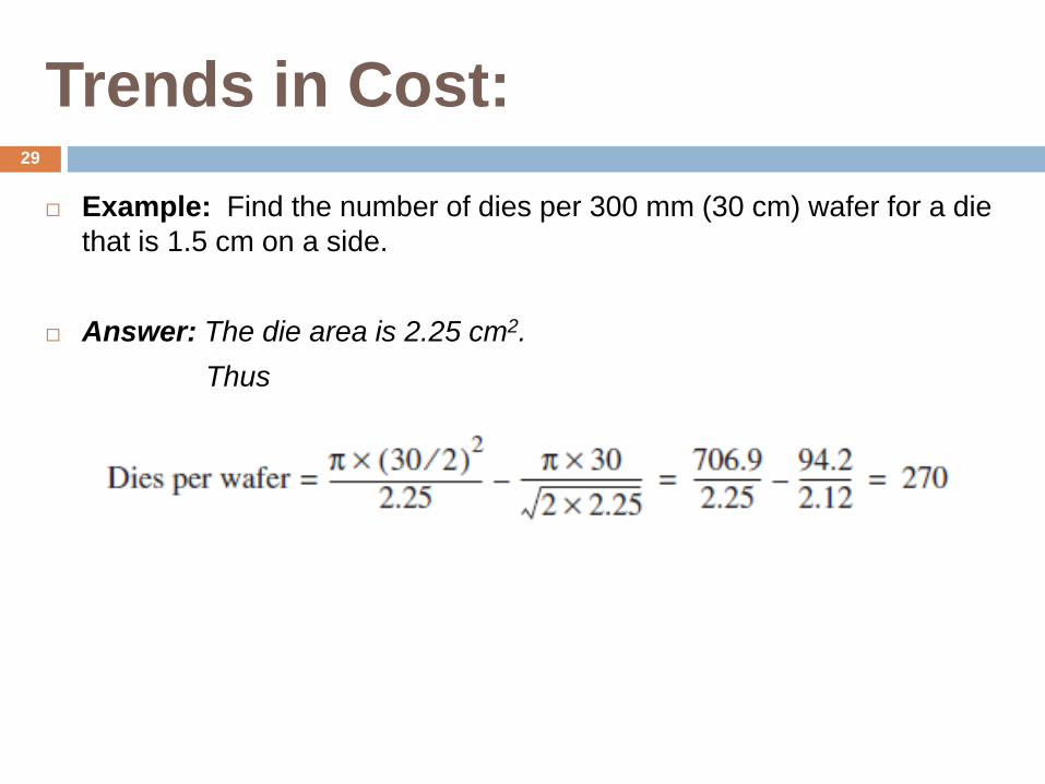
Example: Find the number of dies per 300 mm (30 cm) wafer for a die
that is 1.5 cm on a side.
Answer: The die area is 2.25 cm2.
Thus
29
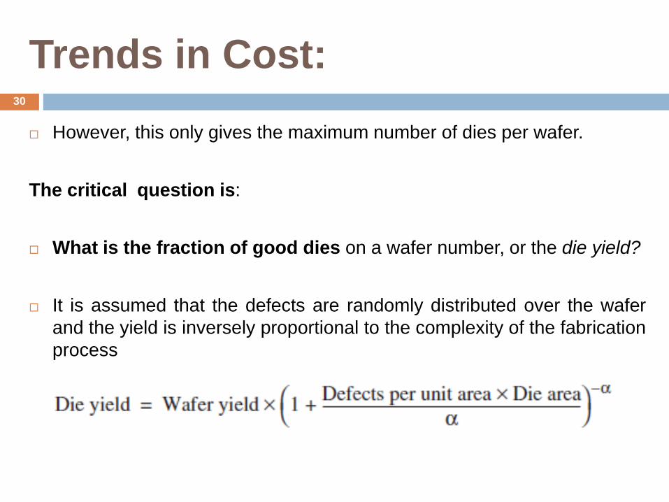
Trends in Cost:
However, this only gives the maximum number of dies per wafer.
The critical question is:
What is the fraction of good dies on a wafer number, or the die yield?
It is assumed that the defects are randomly distributed over the wafer
and the yield is inversely proportional to the complexity of the fabrication
process
30
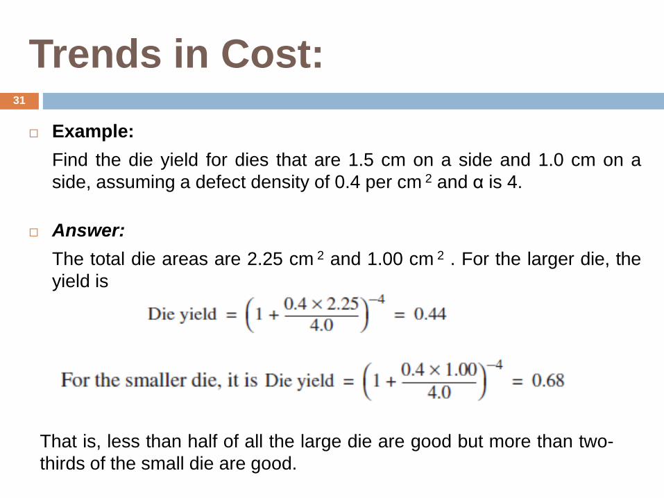
Trends in Cost:
Example:
Find the die yield for dies that are 1.5 cm on a side and 1.0 cm on a
side, assuming a defect density of 0.4 per cm 2 and α is 4.
Answer:
The total die areas are 2.25 cm 2 and 1.00 cm 2 . For the larger die, the
yield is
That is, less than half of all the large die are good but more than two-
thirds of the small die are good.
31

Measuring, Reporting and
Summarizing Performance
32

Measuring Performance
When we say one computer is faster than another, what do we
mean?
The user of a desktop computer may say a computer is faster when a
program runs in less time,
While an amazon.com administrator may say a computer is faster
when it completes more transactions per hour.
The computer user is interested in reducing response time — the
time between the start and the completion of an event (execution time).
The administrator of a large data processing center may be
interested in increasing throughput — the total amount of work done
in a given time.
33
Measuring Performance
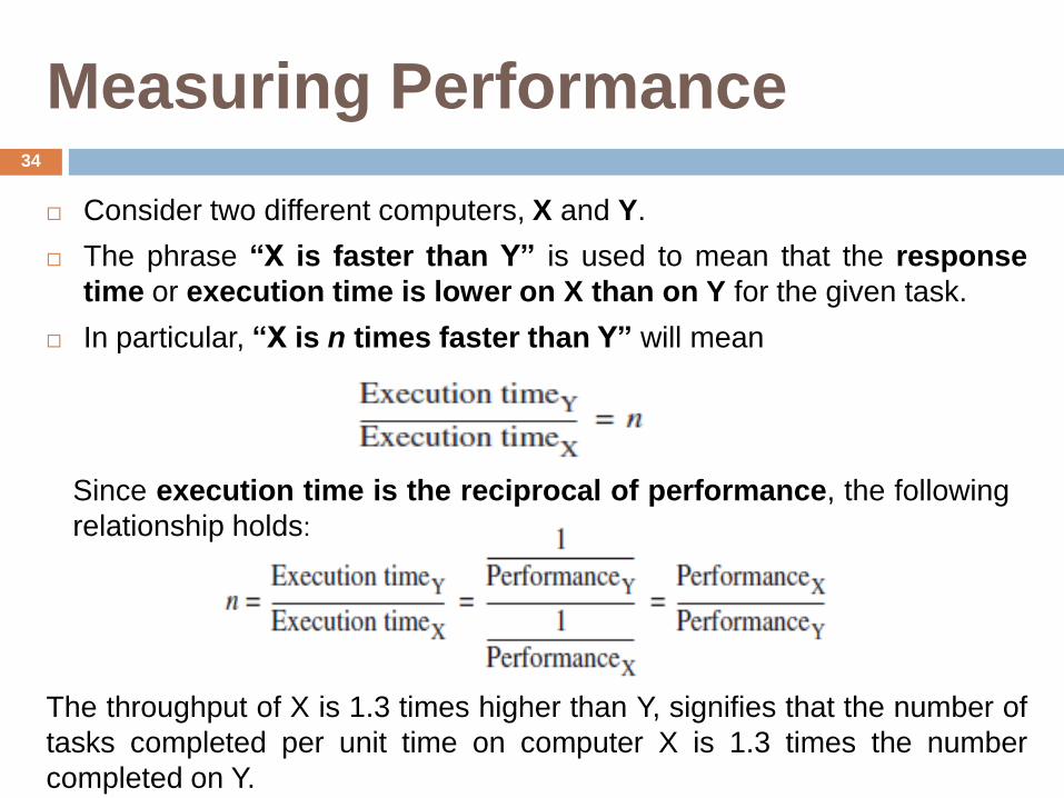
Consider two different computers, X and Y.
The phrase “X is faster than Y” is used to mean that the response
time or execution time is lower on X than on Y for the given task.
In particular, “X is n times faster than Y” will mean
Since execution time is the reciprocal of performance, the following
relationship holds:
The throughput of X is 1.3 times higher than Y, signifies that the number of
tasks completed per unit time on computer X is 1.3 times the number
completed on Y.
34

Measuring Performance
Execution time can be defined in different ways like
wall-clock time,
response time, or
elapsed time,………which is the latency to complete a task.
The response time seen by the user is the elapsed time of the
program, not the CPU time.
To evaluate a new system the users would simply compare the
execution time of their workloads.
35
Reporting Performance
Reporting Performance Results
The reporting performance measurements should be for
reproducibility — list everything another experimenter would need to
duplicate the results.
A SPEC (Standard Performance Evaluation Corporation)
(www.spec.org.) benchmark report requires an extensive description of
the computer and the compiler flags, as well as the publication of both
the baseline and optimized results.
36
Reporting Performance
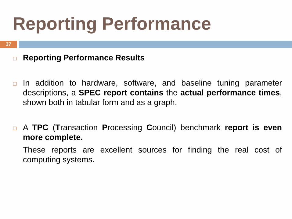
Reporting Performance Results
In addition to hardware, software, and baseline tuning parameter
descriptions, a SPEC report contains the actual performance times,
shown both in tabular form and as a graph.
A TPC (Transaction Processing Council) benchmark report is even
more complete.
These reports are excellent sources for finding the real cost of
computing systems.
37

Summarizing Performance
Summarizing Performance Results
A straightforward approach to computing a summary result would be
to compare the arithmetic means of the execution times of the
programs in the suite.
An alternative would be to add a weighting factor to each benchmark
and use the weighted arithmetic mean as the single number to
summarize performance.
Each company might have their own set of weights.
38
Summarizing Performance
Summarizing Performance Results
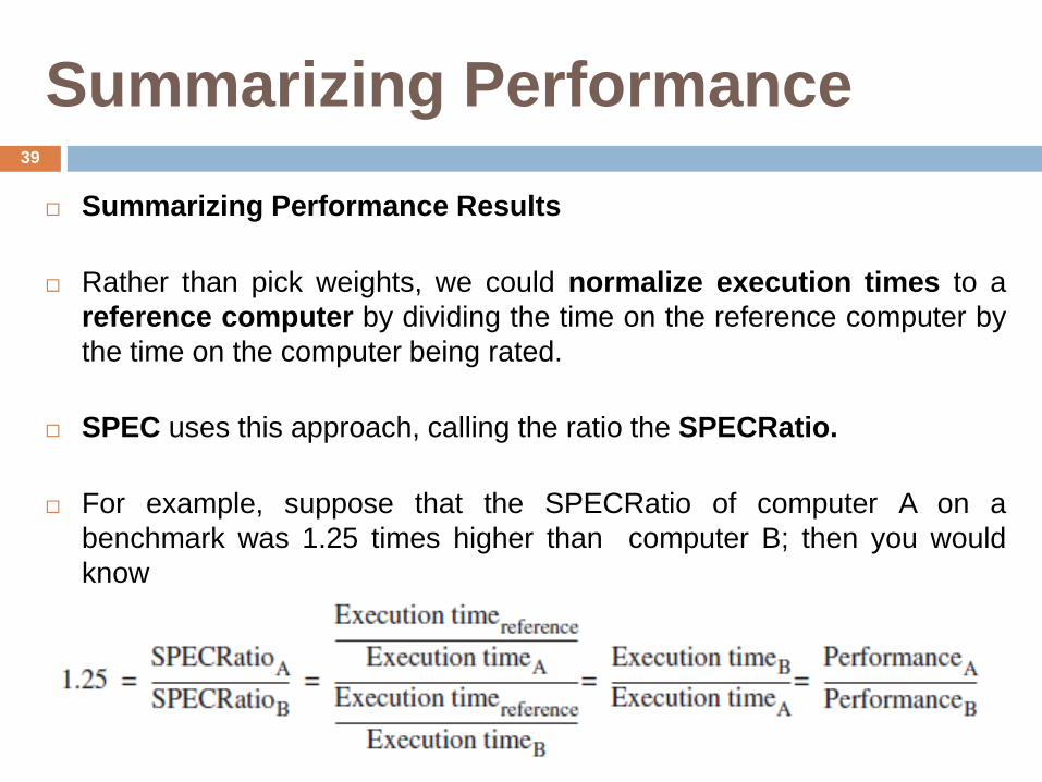
Rather than pick weights, we could normalize execution times to a
reference computer by dividing the time on the reference computer by
the time on the computer being rated.
SPEC uses this approach, calling the ratio the SPECRatio.
For example, suppose that the SPECRatio of computer A on a
benchmark was 1.25 times higher than computer B; then you would
know
39
Summarizing Performance
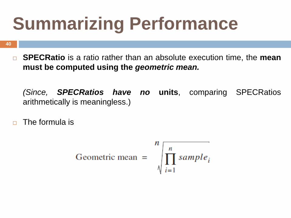
SPECRatio is a ratio rather than an absolute execution time, the mean
must be computed using the geometric mean.
(Since, SPECRatios have no units, comparing SPECRatios
arithmetically is meaningless.)
The formula is
40

Summarizing Performance
Example: Show that the ratio of the geometric means is equal to the
geometric mean of the performance ratios, and that the reference
computer of SPECRatio matters not.
Answer: Assume two computers A and B and a set of SPECRatios for
each.
That is, the ratio of the geometric means of the SPECRatios of A and B is
the geometric mean of the performance ratios of A to B.
41
Pipelining
42
Pipelining (Concept)
Lets, consider the example of washing a car:
Suppose washing, drying & polishing of car requires 30 minutes each.
To wash, dry and polish:
1 car will take 1.5 hrs
4 cars will need (1.5 hrs x 4) 6 hours…
Suppose,
After washing the first car, it is sent for drying at the same time second
car was taken for washing.
Washing of second car and drying of first car was done simultaneously;
and will be done/over at same time.
When washing of second car and drying of first car is over, then first car
was sent for polishing, washed car is sent to drying and third car was
taken for washing.
The total time to complete all three operations for 4 cars is ___.
43
What is Pipelining?
In computing, a pipeline is a set of data processing elements
connected in series, so that the output of one element is the input
of the next one.
Pipelining is an implementation technique whereby multiple
instructions are overlapped in execution;
The elements of a pipeline are often executed in parallel or in time-
sliced fashion.
Today, pipelining is the key implementation technique used to make
fast CPUs
44
Pipelining Types
Buffered, Synchronous pipelines:
Conventional microprocessors are synchronous circuits that use
buffered, synchronous pipelines.
In these pipelines, "pipeline registers" are inserted in-between
pipeline stages, and are clocked synchronously.
Buffered, Asynchronous pipelines:
Asynchronous pipelines are used in asynchronous circuits, and have
their pipeline registers clocked asynchronously.
They use a request/acknowledge system, wherein each stage can
detect when it's finished.
45

Pipelining Types
Unbuffered pipelines:
Unbuffered pipelines, called "wave pipelines", do not have registers in-
between pipeline stages.
Instead, the delays in the pipeline are "balanced" so that, for each
stage, the difference between the first stabilized output data and the last
is minimized.
46
Pipelining
Because all stages proceed at the same time, the length of a processor
cycle is determined by the time required for the slowest pipe stage
In a computer, this processor cycle is usually 1 clock cycle (sometimes
it is 2, rarely more).
The pipeline designer’s goal is to balance the length of each pipeline
stage.
If the stages are perfectly balanced, then the time per instruction on the
pipelined processor is
47
Implementation of a RISC Instruction Set
How RISC instruction set is implemented without pipelining?
RISC instruction takes at most 5 clock cycles.
This basic implementation to a pipelined version, resulting in a much
lower CPI.
Unpipelined implementation is not the most economical or the highest-
performance implementation.
Implementing the instruction set requires the introduction of several
temporary registers that are not part of the architecture
48

Implementation of a RISC Instruction Set
Every instruction in this RISC subset can be implemented in at most 5
clock cycles. The 5 clock cycles are as follows.
1. Instruction fetch cycle (IF):
Send the program counter (PC) to memory and fetch the current
instruction from memory. Update the PC to the next sequential PC by
adding 4 (since each instruction is 4 bytes) to the PC.
2. Instruction decode/register fetch cycle (ID):
Decode the instruction and read the registers corresponding to register
source specifiers from the register file.
Decoding is done in parallel with reading registers, which is possible
because the register specifiers are at a fixed location in a RISC
architecture. This technique is known as fixed-field decoding
49

Implementation of a RISC Instruction Set
Every instruction in this RISC subset can be implemented in at most 5
clock cycles. The 5 clock cycles are as follows.
3. Execution/effective address cycle (EX):
The ALU operates on the operands prepared in the prior cycle,
performing one of three functions.
Memory reference:.
Register-Register ALU instruction:
Register-Immediate ALU instruction:
In a load-store architecture the effective address and execution cycles
can be combined into a single clock cycle.
50
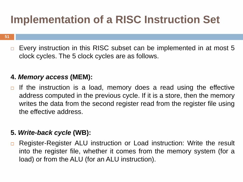
Implementation of a RISC Instruction Set
Every instruction in this RISC subset can be implemented in at most 5
clock cycles. The 5 clock cycles are as follows.
4. Memory access (MEM):
If the instruction is a load, memory does a read using the effective
address computed in the previous cycle. If it is a store, then the memory
writes the data from the second register read from the register file using
the effective address.
5. Write-back cycle (WB):
Register-Register ALU instruction or Load instruction: Write the result
into the register file, whether it comes from the memory system (for a
load) or from the ALU (for an ALU instruction).
51

Simple RISC pipeline
IF = instruction fetch,
ID = instruction decode,
EX = execution,
MEM = memory access, and
WB = write back.
52
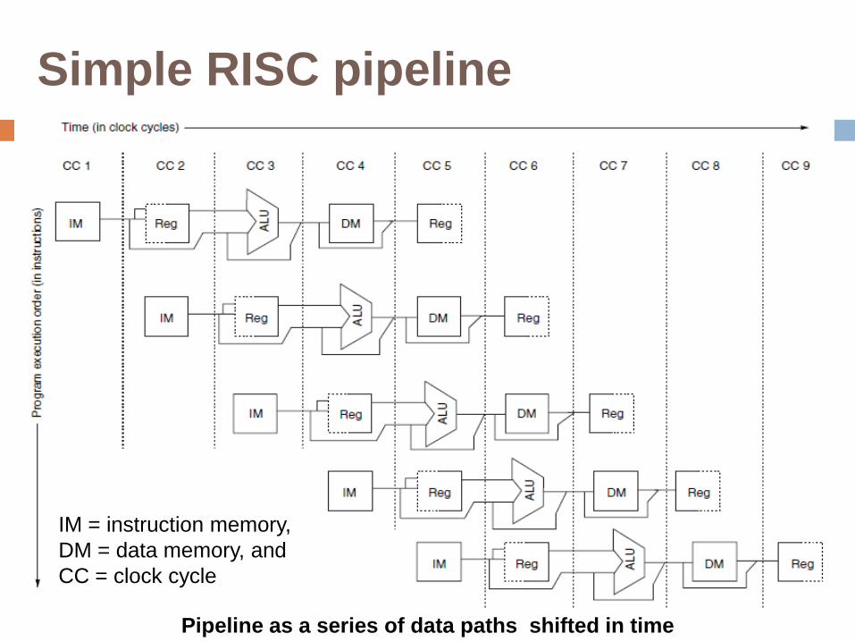
Simple RISC pipeline
Pipeline as a series of data paths shifted in time
IM = instruction memory,
DM = data memory, and
CC = clock cycle
53
Performance Issues in Pipelining
Pipelining increases the CPU instruction throughput — the number
of instructions completed per unit of time — but it does not reduce the
execution time of an individual instruction.
In fact, it usually slightly increases the execution time of each
instruction due to overhead in the control of the pipeline.
The increase in instruction throughput means that a program runs
faster and has lower total execution time, even though no single
instruction runs faster.
54

Performance Issues in Pipelining
Imbalance among the pipeline stages reduces performance.
Pipeline overhead arises from the combination of pipeline register
delay and clock skew.
The pipeline registers add setup time, (time that a register input must
be stable before the clock signal).
Clock skew, also contributes to the lower limit on the clock cycle.
Once the clock cycle is as small as the sum of the clock skew and
latch overhead, no further pipelining is useful.
(there is no time left in the cycle for useful work)
55
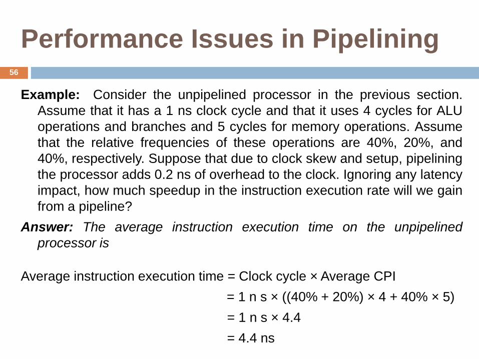
Performance Issues in Pipelining
Example: Consider the unpipelined processor in the previous section.
Assume that it has a 1 ns clock cycle and that it uses 4 cycles for ALU
operations and branches and 5 cycles for memory operations. Assume
that the relative frequencies of these operations are 40%, 20%, and
40%, respectively. Suppose that due to clock skew and setup, pipelining
the processor adds 0.2 ns of overhead to the clock. Ignoring any latency
impact, how much speedup in the instruction execution rate will we gain
from a pipeline?
Answer: The average instruction execution time on the unpipelined
processor is
Average instruction execution time = Clock cycle × Average CPI
= 1 n s × ((40% + 20%) × 4 + 40% × 5)
= 1 n s × 4.4
= 4.4 ns
56
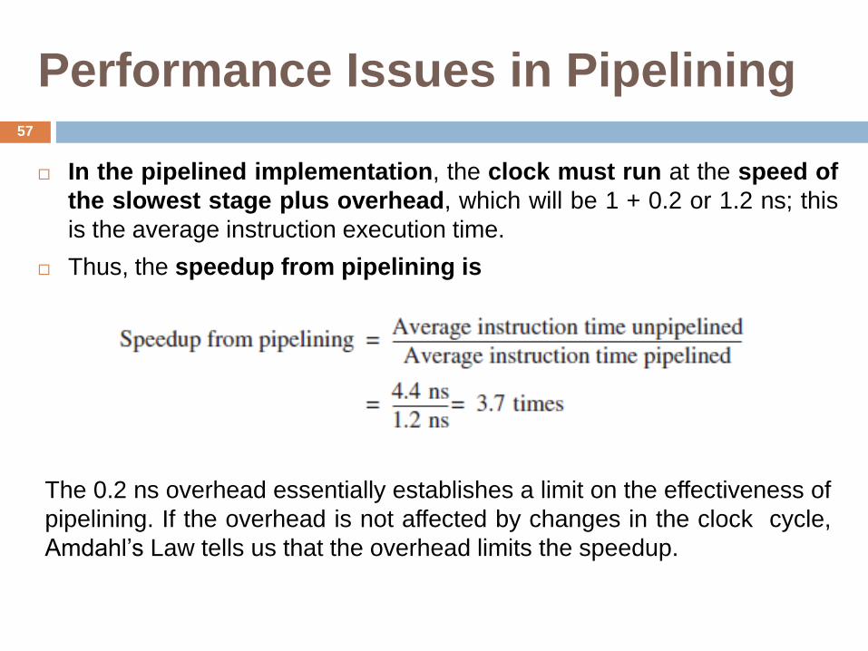
Performance Issues in Pipelining
In the pipelined implementation, the clock must run at the speed of
the slowest stage plus overhead, which will be 1 + 0.2 or 1.2 ns; this
is the average instruction execution time.
Thus, the speedup from pipelining is
The 0.2 ns overhead essentially establishes a limit on the effectiveness of
pipelining. If the overhead is not affected by changes in the clock cycle,
Amdahl’s Law tells us that the overhead limits the speedup.
57
Pipeline Hazards
There are situations, called hazards, that prevents the next
instruction in the instruction stream from executing during its
designated clock cycle.
Hazards reduce the performance gained from pipelining.
There are three classes of hazards:
1. Structural hazards arise from resource conflicts when the hardware
cannot support all possible combinations of instructions simultaneously
in overlapped execution.
2. Data hazards arise when an instruction depends on the results of a
previous instruction, because of overlapping of instructions.
3. Control hazards arise from the pipelining of branches and other
instructions that change the PC.
58
Pipeline Hazards
Hazards in pipelines can make it necessary to stall (stop, halt or pause),
the pipeline.
Avoiding a hazard often requires that some instructions in the pipeline
be allowed to proceed while others are delayed.
When an instruction is stalled, all instructions issued later than the
stalled instruction are also stalled.
Instructions issued earlier than the stalled instruction must continue,
otherwise the hazard will never clear.
59
Pipeline Hazards
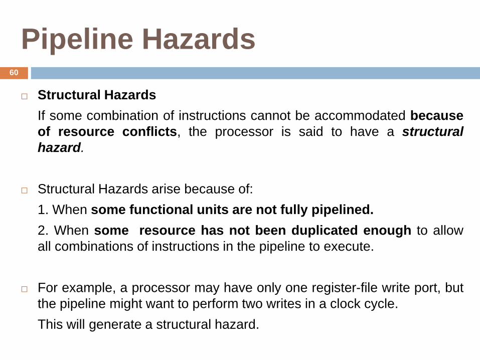
Structural Hazards
If some combination of instructions cannot be accommodated because
of resource conflicts, the processor is said to have a structural
hazard.
Structural Hazards arise because of:
1. When some functional units are not fully pipelined.
2. When some resource has not been duplicated enough to allow
all combinations of instructions in the pipeline to execute.
For example, a processor may have only one register-file write port, but
the pipeline might want to perform two writes in a clock cycle.
This will generate a structural hazard.
60

Pipeline Hazards
Structural Hazards
When a instructions encounters this hazard, the pipeline will stall
one of the instructions until the required unit is available.
Such stalls will increase the CPI from its usual ideal value of 1.
To resolve this hazard, we need to stall the pipeline for 1 clock
cycle. A stall is commonly called a pipeline bubble or just bubble.
The effect of the pipeline bubble is actually to occupy the resources
for that instruction slot as it travels through the pipeline.
61
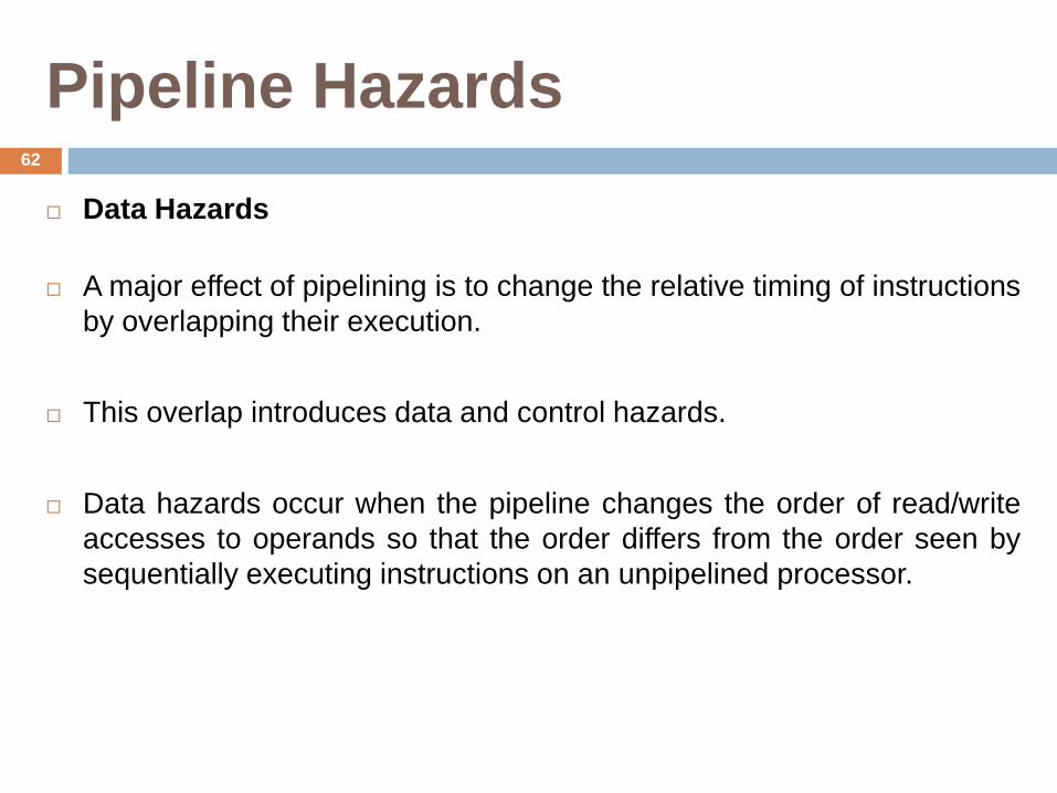
Pipeline Hazards
Data Hazards
A major effect of pipelining is to change the relative timing of instructions
by overlapping their execution.
This overlap introduces data and control hazards.
Data hazards occur when the pipeline changes the order of read/write
accesses to operands so that the order differs from the order seen by
sequentially executing instructions on an unpipelined processor.
62
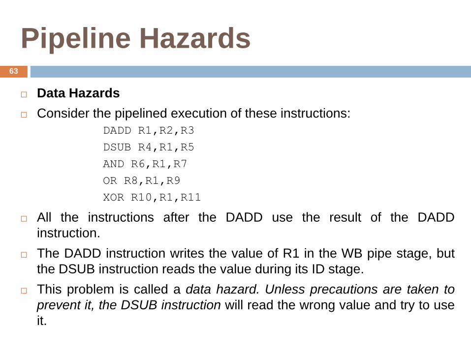
Pipeline Hazards
Data Hazards
Consider the pipelined execution of these instructions:
DADD R1,R2,R3
DSUB R4,R1,R5
AND R6,R1,R7
OR R8,R1,R9
XOR R10,R1,R11
All the instructions after the DADD use the result of the DADD
instruction.
The DADD instruction writes the value of R1 in the WB pipe stage, but
the DSUB instruction reads the value during its ID stage.
This problem is called a data hazard. Unless precautions are taken to
prevent it, the DSUB instruction will read the wrong value and try to use
it.
63

Pipeline Hazards
Data Hazards
If an interrupt occurs between the DADD and DSUB instructions, then
WB stage of the DADD will complete, and the value of R1 at that point
will be the result of the DADD.
The AND instruction is also affected by this hazard. The AND instruction
that reads the registers during clock cycle 4 will receive the wrong
results.
The XOR instruction operates properly because its register read occurs
in clock cycle 6, after the register write.
The OR instruction also operates without incurring a hazard.
64
DADD R1,R2,R3
DSUB R4,R1,R5
AND R6,R1,R7
OR R8,R1,R9
XOR R10,R1,R11

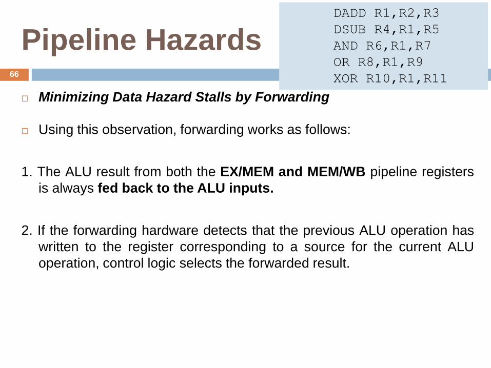
Pipeline Hazards
Minimizing Data Hazard Stalls by Forwarding
The problem of data hazard can be solved with a simple hardware
technique called forwarding (also called bypassing and sometimes
short-circuiting).
The result is not needed by the DSUB until the DADD produces it.
If the result moved from the pipeline register where the DADD stores
it, to where the DSUB needs it, then the need for a stall can be
avoided.
65
DADD R1,R2,R3
DSUB R4,R1,R5
AND R6,R1,R7
OR R8,R1,R9
XOR R10,R1,R11
Pipeline Hazards
Minimizing Data Hazard Stalls by Forwarding
Using this observation, forwarding works as follows:
1. The ALU result from both the EX/MEM and MEM/WB pipeline registers
is always fed back to the ALU inputs.
2. If the forwarding hardware detects that the previous ALU operation has
written to the register corresponding to a source for the current ALU
operation, control logic selects the forwarded result.
66
DADD R1,R2,R3
DSUB R4,R1,R5
AND R6,R1,R7
OR R8,R1,R9
XOR R10,R1,R11
Pipeline Hazards
Branch Hazards
Control hazards can cause a greater performance loss for MIPS
pipeline than data hazards.
When a branch is executed, it may or may not change the PC to
something other than its current value plus 4.
If the branch is not taken, then the repetition of the IF stage is
unnecessary since the correct instruction was fetched.
One stall cycle for every branch will yield a performance loss of
10% to 30% depending on the branch frequency.
67
Pipeline Hazards
Reducing Pipeline Branch Penalties
The software can try to minimize the branch penalty using
knowledge of the hardware scheme and of branch behavior.
The simplest scheme to handle branches is to freeze or flush the
pipeline, holding or deleting any instructions after the branch until
the branch destination is known.
It is simple from both sides hardware and software.
68
Pipeline Hazards
Reducing Pipeline Branch Penalties
Treat every branch as not taken.
(Allow the hardware to continue as if the branch were not
executed).
In the simple five-stage pipeline, this predicted untaken scheme is
implemented by continuing to fetch instructions as if the branch
were a normal instruction.
If the branch is taken, however, we need to turn the fetched
instruction into a no-op and restart the fetch at the target address.
69
Pipeline Hazards
Reducing Pipeline Branch Penalties
An alternative scheme is to treat every branch as taken.
As soon as the branch is decoded and the target address is
computed, we assume the branch to be taken and begin fetching
and executing at the target address (location).
In some processors — powerful (hence slower) branch conditions —
the branch target is known, and a predicted-taken scheme might make
sense.
A another scheme used in some processors is called delayed branch.
This technique was heavily used in early RISC processors.
70
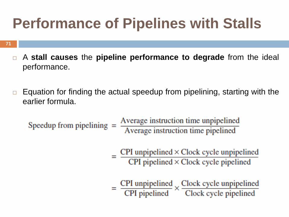
Performance of Pipelines with Stalls
A stall causes the pipeline performance to degrade from the ideal
performance.
Equation for finding the actual speedup from pipelining, starting with the
earlier formula.
71
Performance of Pipelines with Stalls
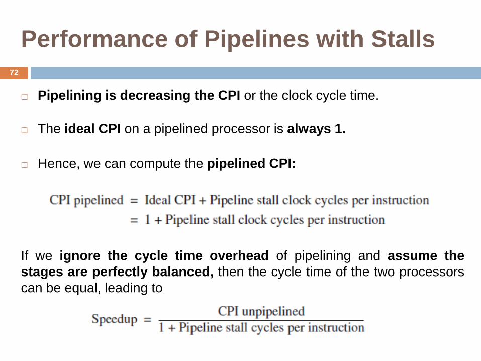
Pipelining is decreasing the CPI or the clock cycle time.
The ideal CPI on a pipelined processor is always 1.
Hence, we can compute the pipelined CPI:
If we ignore the cycle time overhead of pipelining and assume the
stages are perfectly balanced, then the cycle time of the two processors
can be equal, leading to
72
Performance of Pipelines with Stalls
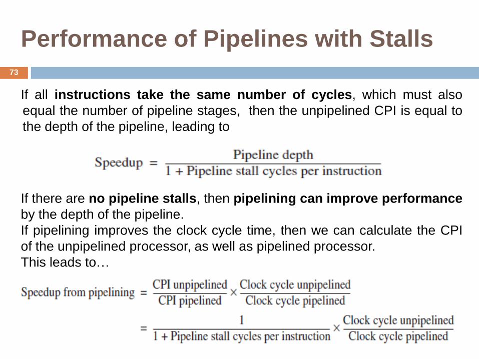
If all instructions take the same number of cycles, which must also
equal the number of pipeline stages, then the unpipelined CPI is equal to
the depth of the pipeline, leading to
If there are no pipeline stalls, then pipelining can improve performance
by the depth of the pipeline.
If pipelining improves the clock cycle time, then we can calculate the CPI
of the unpipelined processor, as well as pipelined processor.
This leads to…
73
Performance of Pipelines with Stalls
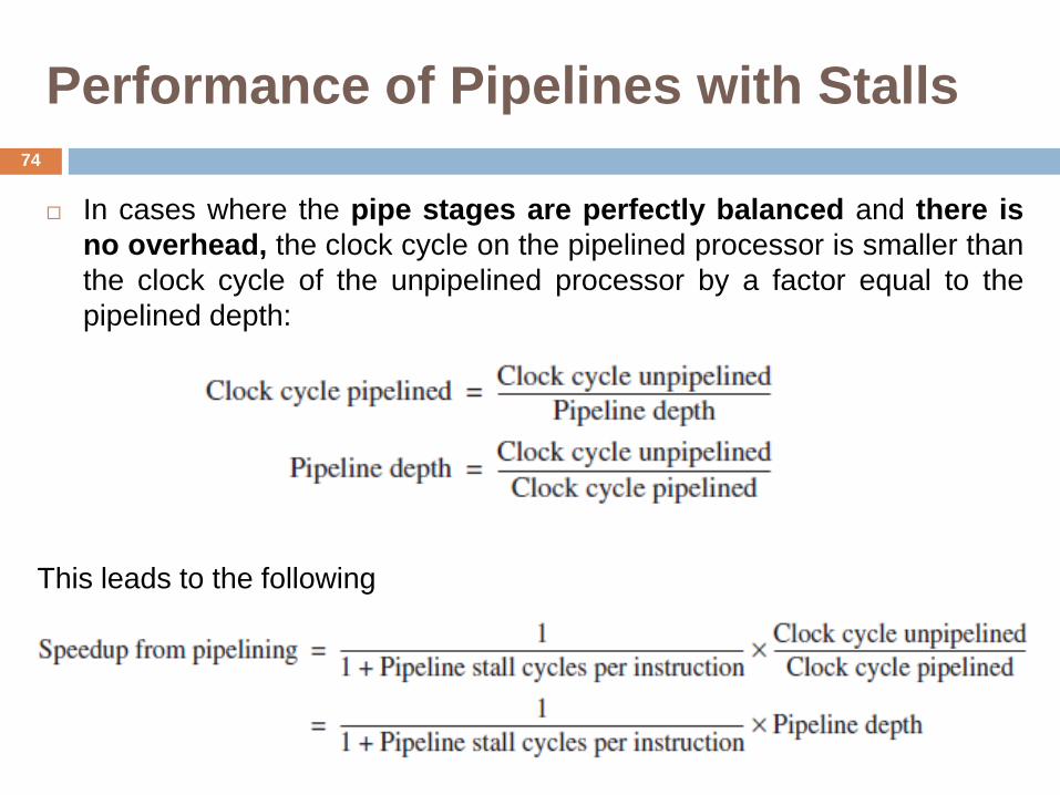
In cases where the pipe stages are perfectly balanced and there is
no overhead, the clock cycle on the pipelined processor is smaller than
the clock cycle of the unpipelined processor by a factor equal to the
pipelined depth:
This leads to the following
74

MIPS Instructions (load and store)
75
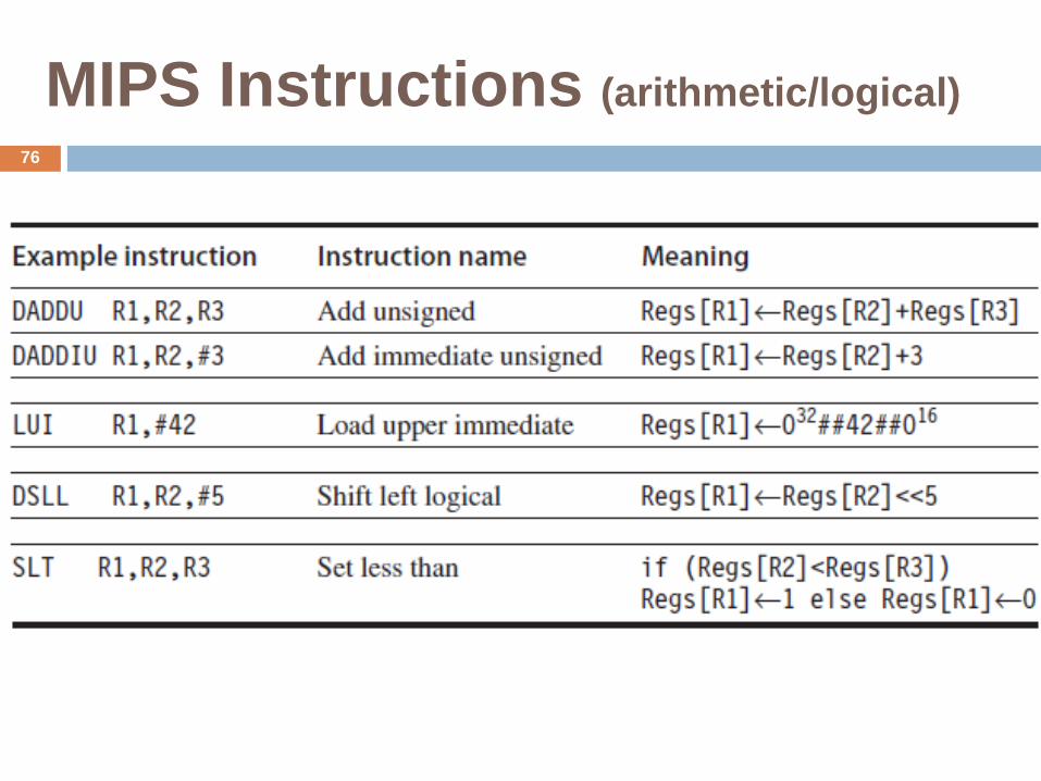
MIPS Instructions (arithmetic/logical)
76
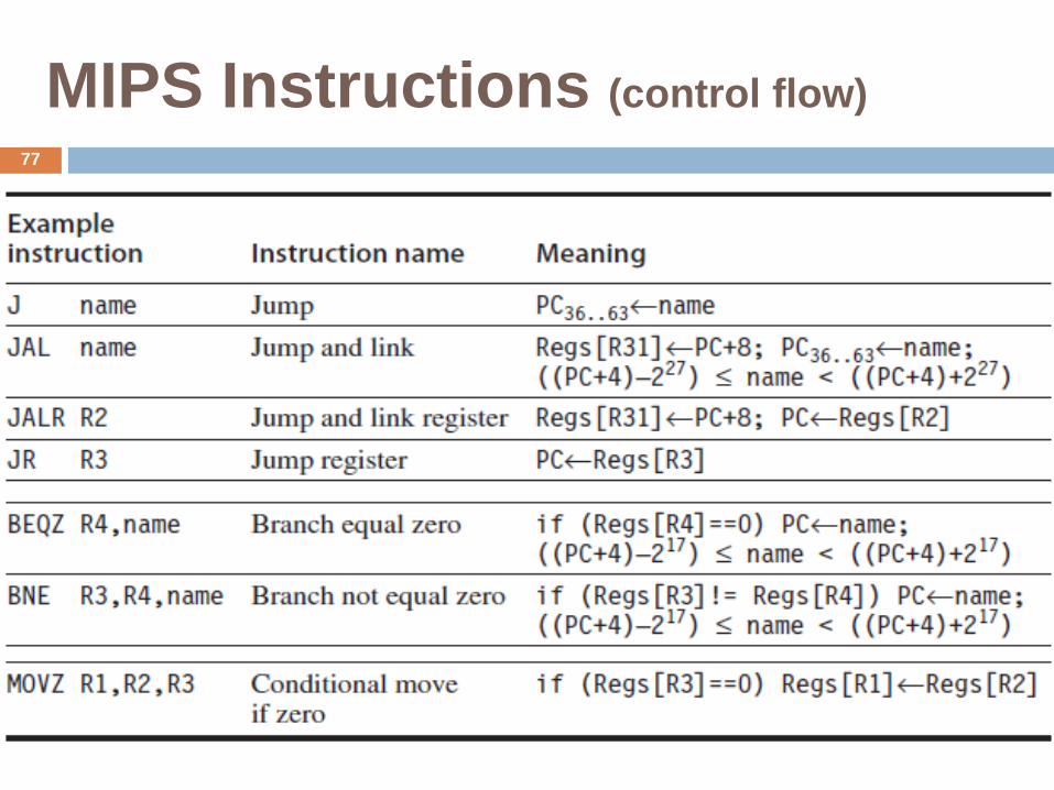
MIPS Instructions (control flow)
77
ILP
(Instruction-Level Parallelism)
78
Instruction-Level Parallelism
All processors since about 1985 use pipelining to overlap the execution
of instructions and improve performance.
This potential overlap among instructions is called instruction-level
parallelism (ILP), since the instructions can be evaluated in parallel.
79
Instruction-Level Parallelism
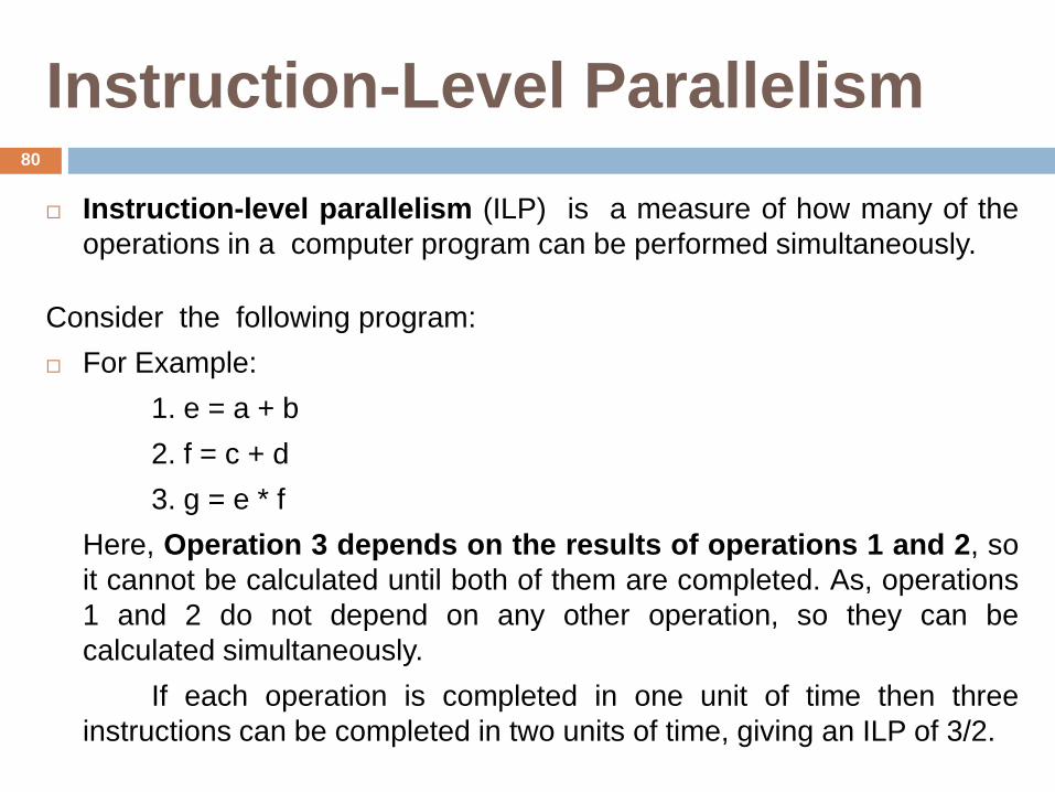
Instruction-level parallelism (ILP) is a measure of how many of the
operations in a computer program can be performed simultaneously.
Consider the following program:
For Example:
1. e = a + b
2. f = c + d
3. g = e * f
Here, Operation 3 depends on the results of operations 1 and 2, so
it cannot be calculated until both of them are completed. As, operations
1 and 2 do not depend on any other operation, so they can be
calculated simultaneously.
If each operation is completed in one unit of time then three
instructions can be completed in two units of time, giving an ILP of 3/2.
80
Instruction-Level Parallelism
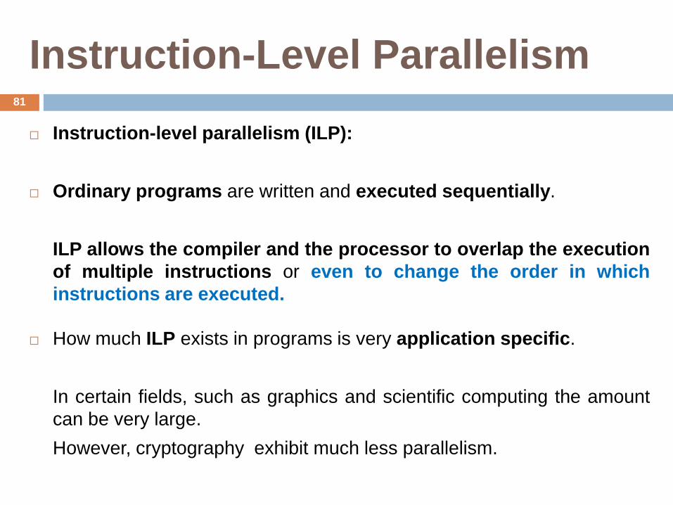
Instruction-level parallelism (ILP):
Ordinary programs are written and executed sequentially.
ILP allows the compiler and the processor to overlap the execution
of multiple instructions or even to change the order in which
instructions are executed.
How much ILP exists in programs is very application specific.
In certain fields, such as graphics and scientific computing the amount
can be very large.
However, cryptography exhibit much less parallelism.
81

Instruction-Level Parallelism
There are two largely separable approaches to exploiting (utilizing) ILP:
(1) an approach that relies on hardware to help discover and exploit
(utilize) the parallelism, and
(2) an approach that relies on software technology to find parallelism
at compile time.
82
Instruction-Level Parallelism
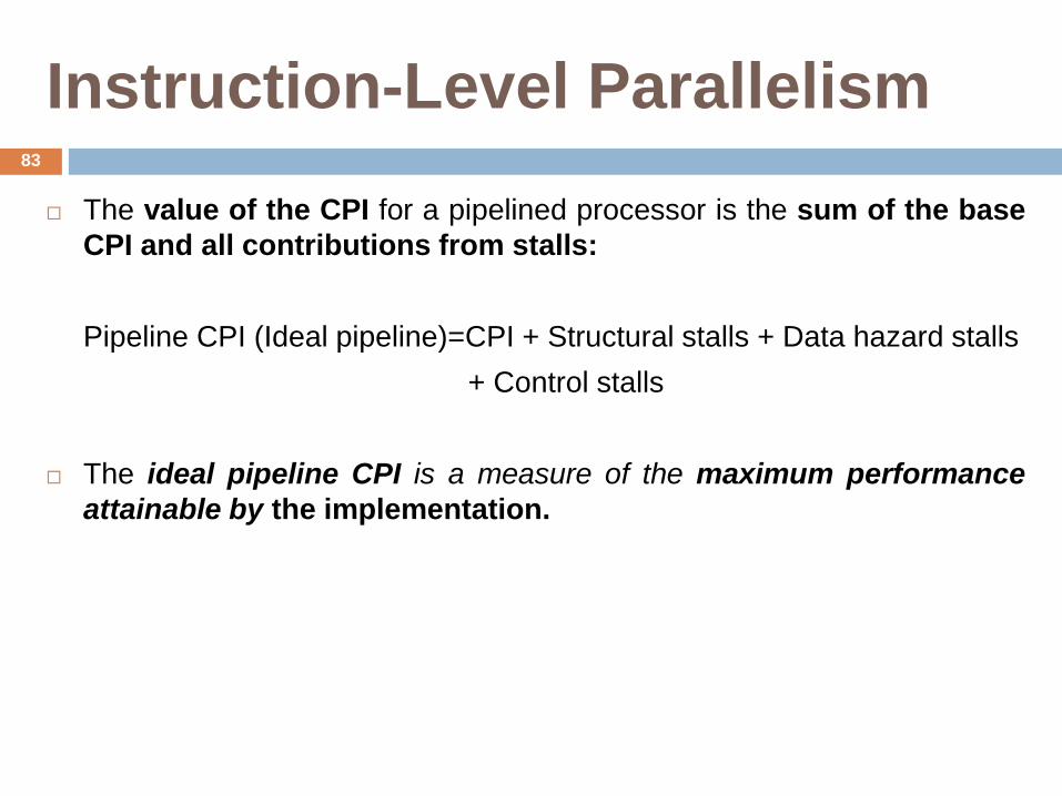
The value of the CPI for a pipelined processor is the sum of the base
CPI and all contributions from stalls:
Pipeline CPI (Ideal pipeline)=CPI + Structural stalls + Data hazard stalls
+ Control stalls
The ideal pipeline CPI is a measure of the maximum performance
attainable by the implementation.
83
Instruction-Level Parallelism
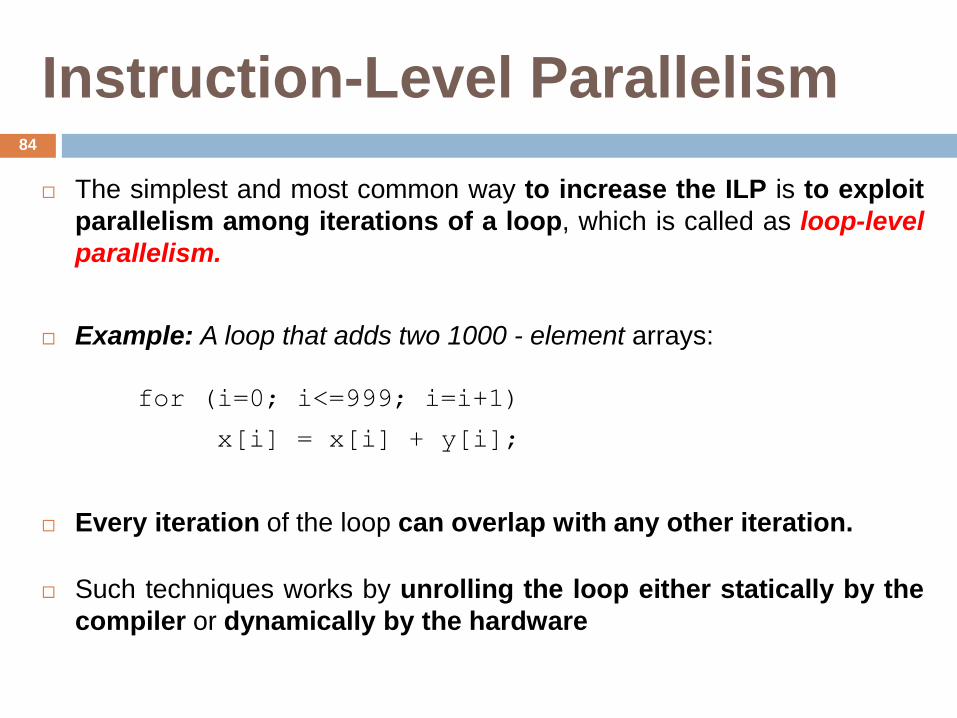
The simplest and most common way to increase the ILP is to exploit
parallelism among iterations of a loop, which is called as loop-level
parallelism.
Example: A loop that adds two 1000 - element arrays:
for (i=0; i<=999; i=i+1)
x[i] = x[i] + y[i];
Every iteration of the loop can overlap with any other iteration.
Such techniques works by unrolling the loop either statically by the
compiler or dynamically by the hardware
84
Instruction-Level Parallelism
An important alternative method for exploiting loop-level parallelism
is the use of SIMD in both vector processors and Graphics Processing
Units (GPUs).
A SIMD instruction exploits data-level parallelism by operating on a
small to moderate number of data items in parallel.
85

SIMD
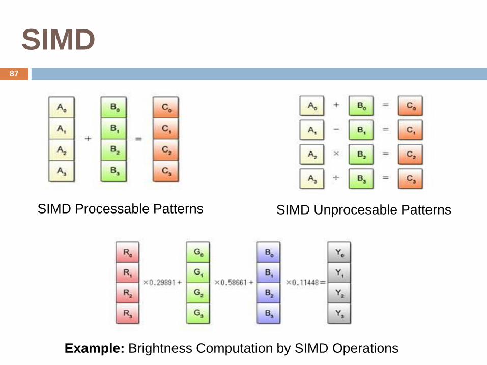
SIMD machines are capable of
applying the exact same
instruction stream to multiple
streams of data simultaneously.
This type of architecture is
perfectly suited to achieving very
high processing rates
86
SIMD
SIMD Processable Patterns SIMD Unprocesable Patterns
Example: Brightness Computation by SIMD Operations
87
ILP Challenges
Determining how one instruction depends on another is critical &
determining how much parallelism exists in a program and how that
parallelism can be exploited is major problem.
If two instructions are independent, they can execute
simultaneously in a pipeline, provided that pipeline has sufficient
resources (and hence no structural hazards exist).
If two instructions are dependent, they are not parallel and must be
executed in predefined order.
88
ILP Challenges
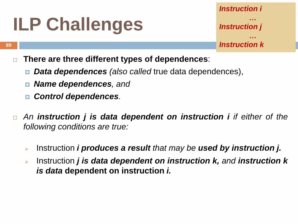
There are three different types of dependences:
Data dependences (also called true data dependences),
Name dependences, and
Control dependences.
An instruction j is data dependent on instruction i if either of the
following conditions are true:
Instruction i produces a result that may be used by instruction j.
Instruction j is data dependent on instruction k, and instruction k
is data dependent on instruction i.
89
Instruction i
…
Instruction j
…
Instruction k
ILP Challenges
Data Dependences
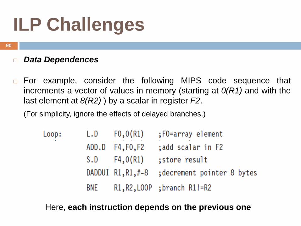
For example, consider the following MIPS code sequence that
increments a vector of values in memory (starting at 0(R1) and with the
last element at 8(R2) ) by a scalar in register F2.
(For simplicity, ignore the effects of delayed branches.)
Here, each instruction depends on the previous one
90
ILP Challenges
Data Dependences
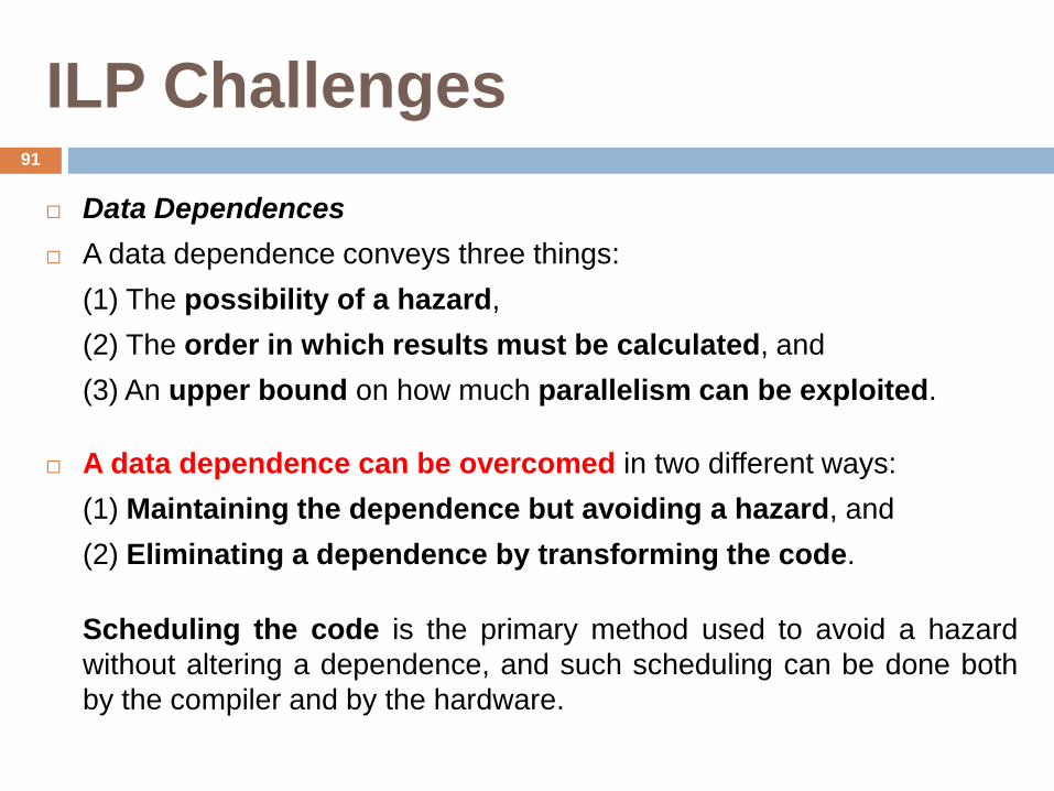
A data dependence conveys three things:
(1) The possibility of a hazard,
(2) The order in which results must be calculated, and
(3) An upper bound on how much parallelism can be exploited.
A data dependence can be overcomed in two different ways:
(1) Maintaining the dependence but avoiding a hazard, and
(2) Eliminating a dependence by transforming the code.
Scheduling the code is the primary method used to avoid a hazard
without altering a dependence, and such scheduling can be done both
by the compiler and by the hardware.
91
ILP Challenges
Name Dependences
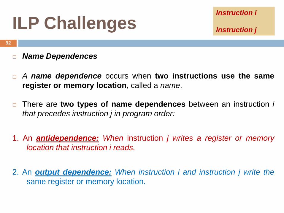
A name dependence occurs when two instructions use the same
register or memory location, called a name.
There are two types of name dependences between an instruction i
that precedes instruction j in program order:
1. An antidependence: When instruction j writes a register or memory
location that instruction i reads.
2. An output dependence: When instruction i and instruction j write the
same register or memory location.
92
Instruction i
Instruction j
ILP Challenges
Name Dependences
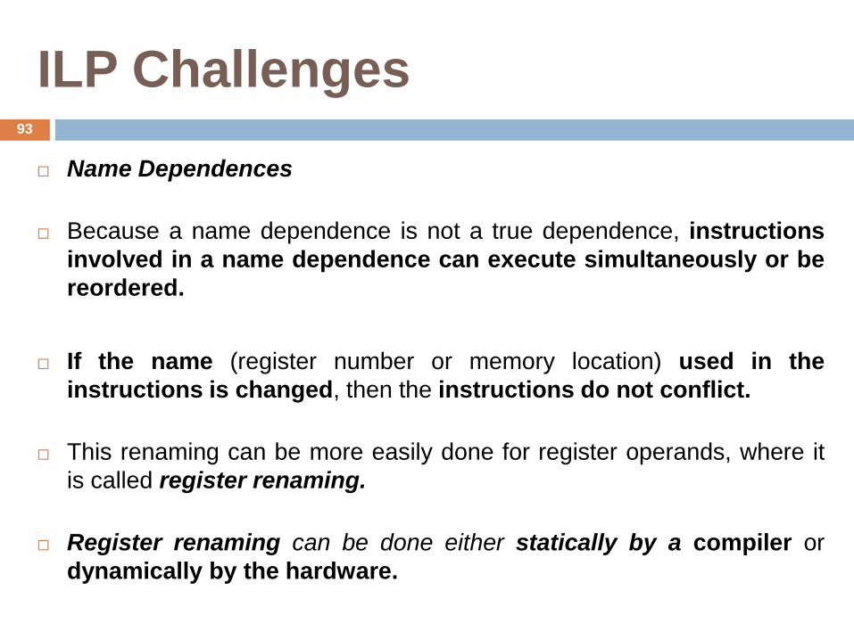
Because a name dependence is not a true dependence, instructions
involved in a name dependence can execute simultaneously or be
reordered.
If the name (register number or memory location) used in the
instructions is changed, then the instructions do not conflict.
This renaming can be more easily done for register operands, where it
is called register renaming.
Register renaming can be done either statically by a compiler or
dynamically by the hardware.
93
ILP Challenges
Data Hazards
A hazard exists whenever there is a name or data dependence
between instructions.
Normally, we must preserve program order
The goal of both software and hardware techniques is to exploit
parallelism by preserving program order.
Data hazards, may be classified as one of three types, depending on
the order of read and write accesses in the instructions.
94
ILP Challenges
Data Hazards
The possible data hazards are
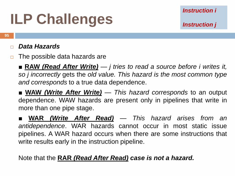
■ RAW (Read After Write) — j tries to read a source before i writes it,
so j incorrectly gets the old value. This hazard is the most common type
and corresponds to a true data dependence.
■ WAW (Write After Write) — This hazard corresponds to an output
dependence. WAW hazards are present only in pipelines that write in
more than one pipe stage.
■ WAR (Write After Read) — This hazard arises from an
antidependence. WAR hazards cannot occur in most static issue
pipelines. A WAR hazard occurs when there are some instructions that
write results early in the instruction pipeline.
Note that the RAR (Read After Read) case is not a hazard.
95
Instruction i
Instruction j
ILP Challenges
Control Dependences
A control dependence determines the ordering of an instruction, i,
with respect to a branch instruction so that instruction i is executed in
correct program order.
Examples of a control dependence is the dependence of the statements
in the “then” part of an “if” statement on the branch.
96
ILP Challenges
Control Dependences
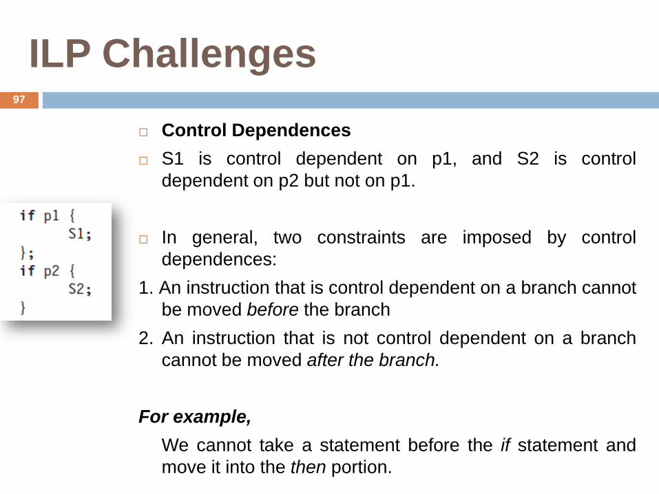
S1 is control dependent on p1, and S2 is control
dependent on p2 but not on p1.
In general, two constraints are imposed by control
dependences:
1. An instruction that is control dependent on a branch cannot
be moved before the branch
2. An instruction that is not control dependent on a branch
cannot be moved after the branch.
For example,
We cannot take a statement before the if statement and
move it into the then portion.
97
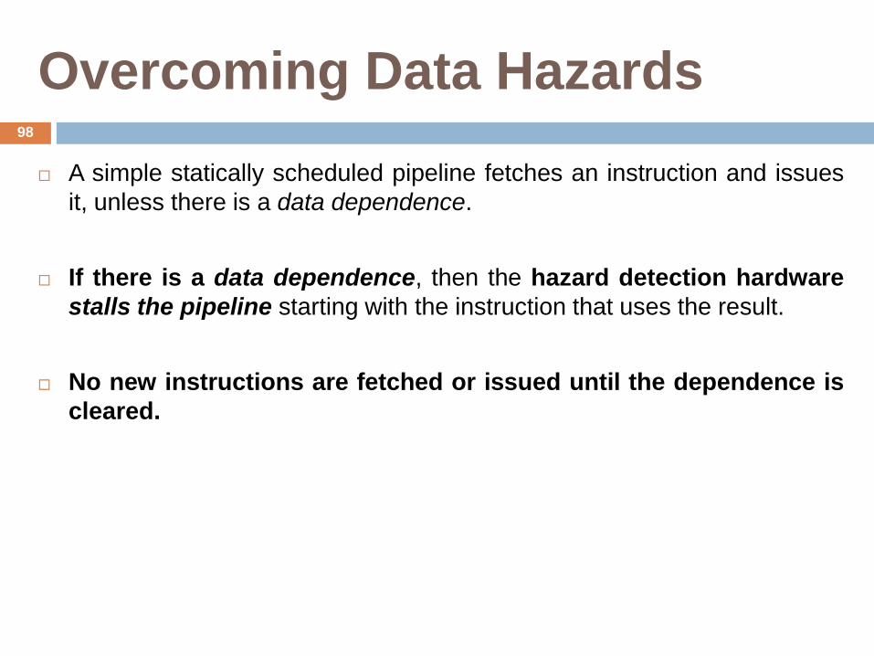
Overcoming Data Hazards
A simple statically scheduled pipeline fetches an instruction and issues
it, unless there is a data dependence.
If there is a data dependence, then the hazard detection hardware
stalls the pipeline starting with the instruction that uses the result.
No new instructions are fetched or issued until the dependence is
cleared.
98
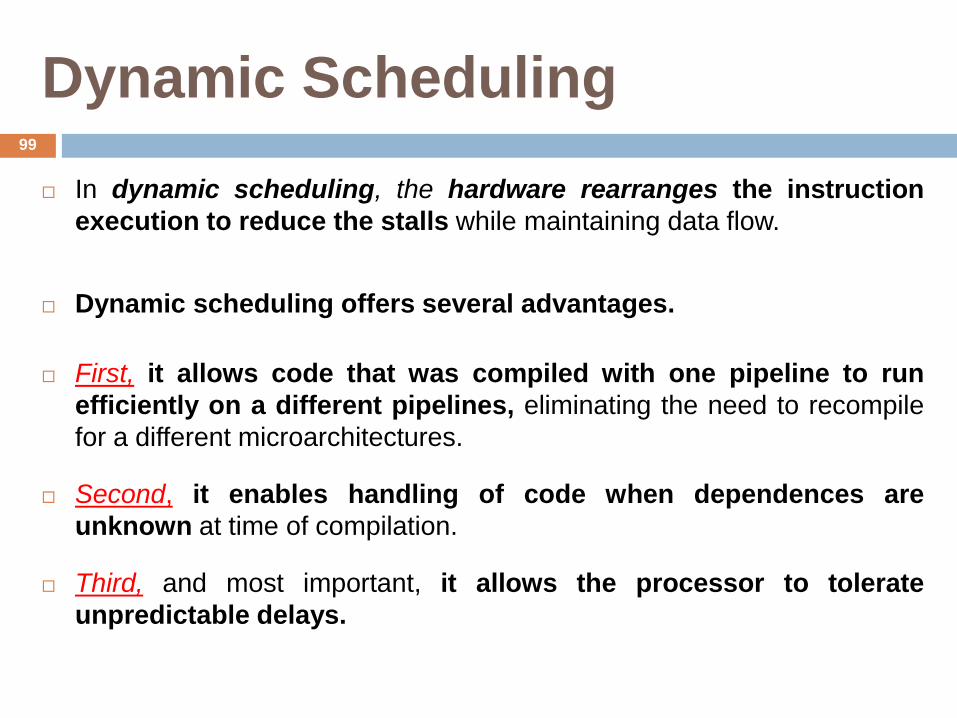
Dynamic Scheduling
In dynamic scheduling, the hardware rearranges the instruction
execution to reduce the stalls while maintaining data flow.
Dynamic scheduling offers several advantages.
First, it allows code that was compiled with one pipeline to run
efficiently on a different pipelines, eliminating the need to recompile
for a different microarchitectures.
Second, it enables handling of code when dependences are
unknown at time of compilation.
Third, and most important, it allows the processor to tolerate
unpredictable delays.
99
Dynamic Scheduling: The Idea
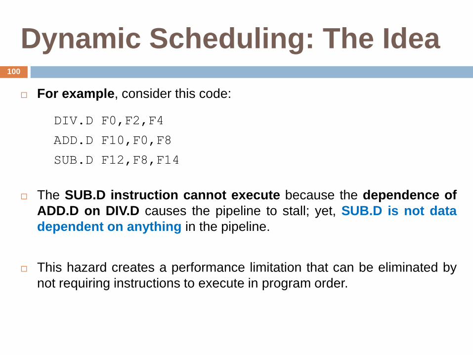
For example, consider this code:
DIV.D F0,F2,F4
ADD.D F10,F0,F8
SUB.D F12,F8,F14
The SUB.D instruction cannot execute because the dependence of
ADD.D on DIV.D causes the pipeline to stall; yet, SUB.D is not data
dependent on anything in the pipeline.
This hazard creates a performance limitation that can be eliminated by
not requiring instructions to execute in program order.
100

Dynamic Scheduling:
The Idea
In the classic five-stage pipeline, both structural and data hazards
could be checked during instruction decode (ID).
To allow us to begin executing the SUB.D in the above example,
We must separate the issue process into two parts:
- checking for any structural hazards and
- waiting for the absence of a data hazard.
Thus, we still use in-order instruction issue, but we want an instruction
to begin execution as soon as its data operands are available.
101
DIV.D F0,F2,F4
ADD.D F10,F0,F8
SUB.D F12,F8,F14

Dynamic Scheduling
To understand how register renaming eliminates WAR and WAW
hazards, consider the following example code sequence:
DIV.D F0,F2,F4
ADD.D F6,F0,F8
S.D F6,0(R1)
SUB.D F8,F10,F14
MUL.D F6,F10,F8
There are two antidependences: between the ADD.D and the SUB.D
and between the S.D and the MUL.D.
There is also an output dependence between the ADD.D and MUL.D.
There are also three true data dependences: between the DIV.D and
the ADD.D, between the SUB.D and the MUL.D, and between the
ADD.D and the S.D.
102
Dynamic Scheduling
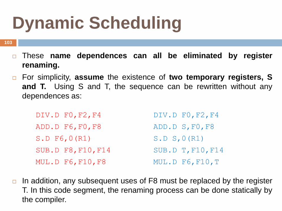
These name dependences can all be eliminated by register
renaming.
For simplicity, assume the existence of two temporary registers, S
and T. Using S and T, the sequence can be rewritten without any
dependences as:
DIV.D F0,F2,F4 DIV.D F0,F2,F4
ADD.D F6,F0,F8 ADD.D S,F0,F8
S.D F6,0(R1) S.D S,0(R1)
SUB.D F8,F10,F14 SUB.D T,F10,F14
MUL.D F6,F10,F8 MUL.D F6,F10,T
In addition, any subsequent uses of F8 must be replaced by the register
T. In this code segment, the renaming process can be done statically by
the compiler.
103

Speculation
Exploiting more parallelism requires that we should overcome the
limitation of control dependence.
Overcoming control dependence is done by speculating
(guessing) on the outcome of branches and executing the program
as if our guesses were correct.
With speculation (guesswork), we can fetch, issue, and execute
instructions, as if our branch predictions were always correct;
dynamic scheduling only fetches and issues such instructions.
Hardware speculation, extends the ideas of dynamic scheduling.
104
Hardware-Based Speculation
Hardware-based speculation combines three key ideas:
(1) Dynamic branch prediction to choose which instructions to execute,
(2) Speculation to allow the execution of instructions before the
control dependences are resolved and
(3) Dynamic scheduling to deal with the scheduling of different
combinations of basic blocks.
Hardware-based speculation follows the predicted flow of data values to
choose when to execute instructions.
105
Hardware-Based Speculation
Speculation allows instructions to execute out of order but to force
them to commit in order execution.
Adding this commit phase to the instruction execution sequence
requires an additional set of hardware buffers.
This hardware buffer (reorder buffer), is also used to pass results
among instructions that may be speculated.
The ROB supplies operands in the interval between completion of
instruction execution and instruction commit.
106
Hardware-Based Speculation
Each entry in the ROB contains four fields:
- the instruction type,
- the destination field,
- the value field, and
- the ready field.
The instruction type field indicates whether the instruction is a branch
(and has no destination), a store (memory address), or a register
operation.
The destination field supplies the register number (for load) or the
memory address (for stores)
The value field is used to hold the value of the instruction result until the
instruction commits.
The ready field indicates that the instruction has completed execution,
and the value is ready.
107
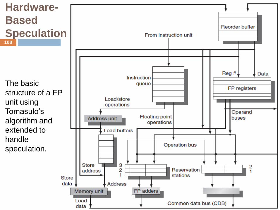
Hardware-
Based
Speculation
The basic
structure of a FP
unit using
Tomasulo’s
algorithm and
extended to
handle
speculation.
108
Hardware-Based Speculation
The hardware structure of the processor including the ROB is shown in
figure.
The ROB includes the store buffers. The renaming function of the
reservation stations is replaced by the ROB.
This tagging requires that the ROB assigned for an instruction must be
tracked in the reservation station.
109

Hardware-Based Speculation
Here are the four steps involved in instruction execution:
1. Issue —
Get an instruction from the instruction queue.
Issue the instruction if there is an empty reservation station and an
empty slot in the ROB.
If either all reservations are full or the ROB is full, then instruction issue
is stalled until both have available entries.
2. Execute —
If one or more of the operands is not yet available, monitor the CDB
(Common Data Bus) while waiting for the register to be computed.
This step checks for RAW hazards. When both operands are available
at a reservation station, execute the operation.
Instructions may take multiple clock cycles in this stage.
110
Hardware-Based Speculation
Here are the four steps involved in instruction execution:
3. Write result—
When the result is available, write it on the CDB (Common Data Bus)
and from the CDB into the ROB, as well as to any reservation stations
waiting for this result.
4. Commit—
This is the final stage of completing an instruction, after which only its
result remains. (Commit phase is also called as “completion” or
“graduation”)
111

Hardware-Based Speculation
There are three different sequences of actions at commit:
The normal commit case occurs when an instruction reaches the head
of the ROB and its result is present in the buffer.
Committing a store is similar except that memory is updated rather
than a result register.
When a branch with incorrect prediction reaches the head of the
ROB, it indicates that the speculation was wrong. The ROB is flushed
and execution is restarted at the correct successor of the branch. If the
branch was correctly predicted, the branch is finished.
112
ILP Using Multiple Issue
To improve performance, we would like to decrease the CPI < 1, but the
CPI cannot be reduced below one if we issue only one instruction every
clock cycle.
The goal of the multiple-issue processors, is to allow multiple
instructions to issue in a clock cycle.
Multiple-issue processors come in three major flavors:
1. Statically scheduled superscalar processors
2. VLIW (very long instruction word) processors
3. Dynamically scheduled superscalar processors
113

Thank You …
(This Presentation is Published Only for Educational Purpose)
114


![Software Pipelining and Superblock Scheduling: Compilation ... · find ILP across successive basic blocks. Two techniques for extracting ILP are software pipelining [6, 7] and superblock](https://img.dokumen.tips/doc/110x75/5f54eb622a4fbd1e48440ede/software-pipelining-and-superblock-scheduling-compilation-find-ilp-across-successive.jpg)